Profitability and Labor Productivity in Indonesian Agriculture

0

Profitability and Labor Productivity in Indonesian Agriculture

Bustanul Arifin

Nunung Nuryartono

Syamsul Hidayat Pasaribu

Fitria Yasmin

Muhammad Amin Rifai

Ravli Kurniadi

Bustanul Arifin is a professor of agricultural economics at the University of Lampung (UNILA) and professorial

fellow in the International Center for Applied Finance and Economics at Bogor Agricultural University

(InterCAFE-IPB) and Team Leader of the study; Nunung Nuryartono is Dean of Faculty of Economics and

Management at IPB; Syamsul Hidayat Pasaribu is Senior Economist and Secretary of InterCAFE-IPB, and Fitria Yasmin, Muhammad Amin Rifai and Ravli Kurniadi are Research Fellow at InterCAFE-IPB.

Pub

lic D

iscl

osur

e A

utho

rized

Pub

lic D

iscl

osur

e A

utho

rized

Pub

lic D

iscl

osur

e A

utho

rized

Pub

lic D

iscl

osur

e A

utho

rized

1

EXECUTIVE SUMMARY

1. Urbanization and income growth are contributing to significant changes in

consumer food demand and expenditures, with aggregate demand for rice levelling

off and with increased consumption of animal products, fruits and vegetables,

processed foods, and a range of beverages. This provides Indonesian farmers with

significant market opportunities if they can competitively supply these foods or food/feed

raw materials. Yet, most attention to farm economics has centered on rice and

comparatively little is known about the productivity and profitability of farmers supplying

this wider range of commodities. Are the returns to family and hired labor (significantly)

higher for these other commodities than for rice despite the predominant attention which

the government has given to supporting rice production? If this is the case, then we would

expect to see market forces driving considerable shifts in agricultural land uses in the

coming years. Yet, if such production systems are not yielding higher returns to farmers,

then adjustments in policies and programs may be needed to better facilitate a competitive

supply response by Indonesian smallholders to changing patterns of demand.

2. This study is a first attempt to address this knowledge gap. Given funding and time

limitations, it is designed as an exploratory study whose insights may stimulate

discussion and demand for further work in this area. The study aims to inform the

discussion on improving productivity and farmer incomes by examining the profitability

and labor productivity of different crops and smallholder farming systems. The study

draws upon existing survey and a supplemental field survey to compare and contrast the

labor productivity and overall profitability in smallholder production for a range of staple

and higher value food crops, animal production systems and mixed farming systems.








this wider range of commodities. This study is a first attempt to address this knowledge

gap. Given funding and time limitations, it is designed as an exploratory study whose

insights may stimulate discussion and demand for further work in this area. The study

aims to inform the discussion on improving productivity and farmer incomes by

examining the profitability and labor productivity of different crops and smallholder

farming systems. The study draws upon existing survey and a supplemental field survey

to compare and contrast the labor productivity and overall profitability in smallholder

production for a range of staple and higher value food crops, animal production systems

and mixed farming systems.

4. In the process of economic structural transformation, countries generally experience

a significant contraction in the share of employment in primary agriculture as

growth rates diverge between agriculture, industry and services, as agricultural

production consolidates into somewhat larger and often more mechanized units, and

2

as surplus underemployed agricultural labor is absorbed in other segments of the

economy. With a lower proportion of the workforce employed in agriculture and with a

growing proportion of agricultural workers coming to be involved with higher value

segments of primary agriculture (i.e. horticulture and animal production) there is a

tendency for wages and productivity levels in agriculture to converge with those in many

segments of industry and services.

5. Middle-income Indonesia has been experiencing a reduction in the share of workers

engaged in primary agriculture, although the pace of this reduction is slower than

the contraction in primary agriculture’s share of national GDP and also slower than

observed patterns in many other peer countries in Asia. For a variety of reasons, other

segments of the economy have been slow to absorb surplus agricultural labor, resulting in

significant levels of seasonal or other underemployment of people in rural areas. Lack of

demographic pressures, small farm sizes, topographical challenges and other factors have

contributed to very low rates of mechanization in Indonesian agriculture. In 2017,

primary agriculture (including fisheries and forestry) remained by far the largest

employer in Indonesia with nearly 36 million people involved.

6. This study has found very large gaps in labor productivity between primary

agriculture and nearly all other segments of the Indonesian economy. While the

estimated growth rate in labor productivity has been quite a bit higher in agriculture than

in some other segments of the economy in the period of 2000 to 2017, the size of the

productivity gap is such that it will take many decades to fully close this gap based upon

the current patterns. The picture for Indonesia is somewhat unusual in that even the

segments of agriculture experiencing somewhat higher rates of labor productivity still lag

or barely approximate the productivity levels experienced in comparatively lower levels

of industry (i.e. construction) and services (i.e. hotel and restaurants).

7. This study utilized three sources of data to estimate agricultural labor productivity,

namely (i) Sakernas household survey data, (ii) prior surveys of smallholder tree crop

producers, and (iii) a small supplemental field survey covering several locations and a

range of staple and specialty food crops and animal or mixed farming systems.

8. The results convey a mixed picture, with some divergence between the Sakernas

results and those based upon surveys focused on specific commodities. The Sakernas

surveys point to patterns which are consistent with observations in other Asian countries

in which labor productivity for (relatively low unit value) food crops is decidedly lower—

by half or more—than is the case for horticulture, animal production, mixed farming

systems, and specialized plantation crops. The surveys that focused on individual crops or

production systems point to a much more complex pattern. As expected, labor

productivity is comparatively higher in poultry and aquaculture production and in some

segments of horticulture which have received government attention (i.e. shallot

production). However, labor productivity is found to be quite a bit lower in several

horticultural crop specialties and in beverage crop production than in rice cultivation.

This pattern contrasts sharply with that found in Vietnam, a country which has

experienced considerable success both in raising rice productivity and in developing large

competitive cash crop industries. There, labor productivity in rice differs among regions

depending upon patterns of mechanization and commercialization, yet even in the best

3

circumstances this labor productivity is no more than one-third that experienced for

coffee or horticulture production.

9. The factors underpinning the observed patterns in Indonesia are not fully clear and

require additional work, including through more extensive field surveys which

would bring out greater variations among locations due to agro-ecological, farmer

organization, rural connectivity and other factors. Restrictions on competitive imports

and various programs of direct support have helped to boost the profitability of rice

production in parts of Indonesia, although this profitability remains modest and given

very small average farm sizes, inadequate to provide a solid living standard for most

producing households. Even among surplus rice growing households an increasing

majority of household income is now coming from other (including non-agricultural)

sources.

10. Perhaps more surprising is the moderate to low level of profitability and/or labor

productivity associated with most horticultural and beverage crops in Indonesia.

This is alarming as one would expect these higher value commodities to provide for more

remunerative employment. Growing demand, both at home and abroad, should be

catalyzing farmers to invest further in these crops and to build up the requisite knowledge

base to improve product quality. More competitive horticultural and beverage crop

industries should then be achieving higher rates of productivity growth and be in a better

position to reward both skilled and unskilled labor. This dynamic does not seem to be

occurring, at least not on a broad scale.

11. This is of concern not only for realizing near term goals related to poverty reduction

and farm incomes, but also in relation to attracting and retaining entrepreneurial

youth to being Indonesia’s farmers of the future. Recent studies and consultative

processes have drawn attention to the challenges of productivity, profitability and

competitiveness in Indonesian horticulture and beverage crop industries. This study’s

findings about low labor productivity in these industries calls for a redoubling of efforts

to strengthen the provision of core public goods and services to such industries and to

better facilitate private investment in production technologies, advisory services, and

downstream logistical and marketing services.

12. There are multiple pathways to raise labor productivity in Indonesian agriculture

and all these should be further explored and re-enforced by appropriate government

policies and programs. For example:

a. One important pathway will be efforts to achieve more economies scale in

smallholder production of staple food crops, by facilitating community-based land

consolidation, a more active market in agricultural land rentals and sales, and the

emergence of a dynamic market for provision of mechanized services covering

different components of the crop cycle. Reforms will be needed in land

administration and in the enabling environment for mechanized services.

b. A second important pathway will be to encourage more diversified farming

systems to make fuller use of available labor and other resources as well as better

mitigate weather, pest and other risks. In place of monocrop systems, higher labor

productivity and remuneration may be possible through the introduction of

4

rotations in lowland rice-based systems (i.e. moving towards rice-vegetable, rice-

aquaculture and other rotations) and mixed agro-forestry systems. Single crop

advisory services may need to be replaced by technical support emphasizing

whole farm management.

c. A third critical pathway is through measures to increase productivity, value

addition, and risk management capabilities in higher value crop and animal

production systems. This may require interventions to improve biosecurity

controls and practices, enable farmers to acquire new knowledge and skills, foster

greater rural entrepreneurship, encourage more collective action in agricultural

marketing, and strengthen the market and other rural infrastructure to carry

perishable and other higher value commodities.

5

Table of Contents

Executive Summary .................................................................................................................................................................. 1

1. Introduction ....................................................................................................................................................................... 7

1.1 Background and Objectives.............................................................................................................................. 7

1.2 Recent Economic Developments ................................................................................................................... 9

2. Labor Productivity in Agriculture ........................................................................................................................ 11

2.1 Case study: Agricultural Labor Productivity in Vietnam ............................................................... 11

2.2 Labor Productivity in Indonesia ................................................................................................................. 13

3. Methods and Framework ......................................................................................................................................... 18

3.1 Literature and Data ........................................................................................................................................... 18

3.2 Methods of Analysis .......................................................................................................................................... 18

Farm Economics Analysis ........................................................................................................................................ 19

Productivity Analysis .................................................................................................................................................. 20

Profit Function Analysis ............................................................................................................................................ 20

Policy Analysis ............................................................................................................................................................... 20

4. Results and Discussion .................................................................................................................................................. 21

4.1 Introduction .......................................................................................................................................................... 21

4.2 Increasing Labor Productivity ..................................................................................................................... 22

4.3 Declining Employment in Agriculture ..................................................................................................... 24

4.4 Source of Growth in Indonesian Agriculture ....................................................................................... 28

4.5 Farm Profitability and Labor Productivity ............................................................................................ 32

Food Crops: Rice, Maize, and Soybean ............................................................................................................. 33

Cash Crops: Coffee and Cocoa ................................................................................................................................ 34

Horticulture: Orange, Tomato, Cabbage, Shallot .......................................................................................... 35

Poultry: Chicken/broilers and Eggs .................................................................................................................... 36

Aquaculture (Fattening and Hatchery) ............................................................................................................. 37

Mixed Farming: Mina-Paddy, Horticulture ..................................................................................................... 38

5. Conclusions ...................................................................................................................................................................... 39

References .................................................................................................................................................................................. 42

Annex 1. Structural Transformation of the Indonesian Economy................................................................. 45

Annex 2. Simulation of Government Intervention ................................................................................................. 47

Annex 3. Determinants of Profitability and Farmer Incomes .......................................................................... 49

6

LIST OF FIGURES

Figure 1: Comparative Trajectories in Agricultural Labor Productivity ....................................................... 7

Figure 2: Labor productivity in agriculture and other sectors, 2000-2017 ....................................................... 24

Figure 3: Number of agricultural workers (and share in agriculture sector) by subsector ......................... 27

Figure 4: Sectoral Employment by Educational Attainment (%) ......................................................................... 28

Figure 5: Indonesia Agriculture Productivity Index................................................................................................... 29

Figure 6: Resource Decomposition of Indonesian Agriculture Growth ............................................................ 30

Figure 7: Agricultural total factor productivity of some Asian countries ......................................................... 31

Figure 8: Profitability and Labor Productivity of Selected Commodities......................................................... 32

LIST OF TABLES

Table 1: Net Returns Per Hectare and Per Person-Day in Major Asian ‘Rice Bowls’ (US$) ................ 8

Table 2: Comparison of annual and per-hour-work adjusted labor productivity, 2014 .............................. 12

Table 3: Labor input and productivity from the field data by commodity, 2016-2017 ............................... 13

Table 4: Table 2.1 Roles of Agriculture in the Indonesian Economy, 1975-2017 ....................................... 14

Table 5: Labor Productivity in Indonesia 2011-17 (‘000 Rp at Constant Price 2010) and index ........... 15

Table 6: Growth of Labor Productivity in Indonesia 2011-2017 (percent per year) .................................... 16

Table 7: The Share of Sectoral GDP and Employment to the Indonesian Economy ................................... 21

Table 8: Average Wage Rate by Sector in 2000, 2010 and 2017 (Rp/worker/month) ................................ 22

Table 9: Labor Productivity by Sector both in Current and Constant Price of 2010 .................................... 23

Table 10: Rate of Growth of Agricultural Productivity in the period of 2000-2017 (%) ................. 23

Table 11: Sectoral Shifting of Employment, 2000, 2010 and 2017..................................................................... 24

Table 12: Growth of Employment by Sector, 2000-2017 (%) ............................................................................... 25

Table 13: Agricultural Labor Productivity (Regular, Per full-time Adjusted) in 2010 ............................... 26

Table 14: Productivity Indicators for Indonesia’s Agriculture (average annual growth rate in percent)

.......................................................................................................................................................................................................... 29

Table 15: Indonesia’s agricultural productivity average annual growth rate in percent ............................. 30

Table 16: Agricultural total factor productivity average annual growth rate of selected Asian countries

(percent) ........................................................................................................................................................................................ 32

Table 17: Profitability of Food Crops (Rice, Maize, and Soybean) –per hectare basis............................... 34

Table 18: Profitability of Cash Crops (Coffee and Cocoa) –per hectare basis ............................................... 35

Table 19: Profitability of Horticulture (Orange, Tomato, Cabbage, Shallot) –per hectare ........................ 36

Table 20: Profitability of Poultry (Chicken and Egg) –per m3 volume ............................................................. 37

Table 21: Profitability of Aquaculture (Fresh water: Fattening and Hatchery) –per m3 ............................ 38

Table 22: Profitability of Mixed Farming (Mina-Paddy and Horticulture) –per hectare............................ 38

Table 23: Removing Fertilizer Subsidies on Food Crops, Horticulture, Mixed Farming ......................... 47

Table 24: Removing Subsidies for Soybean Seed ...................................................................................................... 48

Table 25: Removing Price Support on Rice .................................................................................................................. 48

Table 26: Regression Analysis of Determinant of Profitability of Farming Systems .................................. 49

Table 27: Regression Analysis of Determinant of Farmers’ Income .................................................................. 50

Table 28: Regression Analysis of Determinant of Farmers’ Income .................................................................. 51

Table 29: Regression Analysis of Profit Function ...................................................................................................... 51

7

1. INTRODUCTION

1.1 BACKGROUND AND OBJECTIVES

13. Indonesia’s agricultural strategy aims to expand national output, especially of

‘strategic commodities’, while also raising farm incomes. Given constraints on

available resources, improvements in productivity are needed to realize these twin

goals. National policies have tended to define productivity in narrow terms, centered on

crop yields (i.e. physical output per hectare of land). Investments (i.e. in irrigation

facilities) and programs (i.e. input subsidies) have sought to promote higher yields. But,

agricultural productivity should be understood and promoted from a broader perspective.

Especially when exploring opportunities to improve rural livelihoods and farm incomes it

is also critical to consider the status and patterns of agricultural labor productivity and the

strategies for increasing this. To date, labor productivity has factored little in national

policy considerations.

14. Earlier analytical work pointed to two very different and potentially conflicting

viewpoints on the status and trajectory of agricultural labor productivity in

Indonesia. Based simply upon national aggregates for agricultural GDP and ‘persons

employed in agriculture’, the picture for Indonesia looks highly favorable, at least in

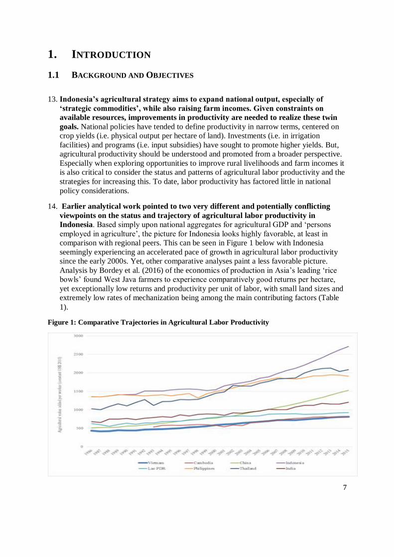
comparison with regional peers. This can be seen in Figure 1 below with Indonesia

seemingly experiencing an accelerated pace of growth in agricultural labor productivity

since the early 2000s. Yet, other comparative analyses paint a less favorable picture.

Analysis by Bordey et al. (2016) of the economics of production in Asia’s leading ‘rice

bowls’ found West Java farmers to experience comparatively good returns per hectare,

yet exceptionally low returns and productivity per unit of labor, with small land sizes and

extremely low rates of mechanization being among the main contributing factors (Table

1).

Figure 1: Comparative Trajectories in Agricultural Labor Productivity

8

15. How could Indonesia be achieving high rates of overall growth in agricultural labor

productivity when labor productivity for its leading crop—accounting for a majority

of agricultural land use—is exceptionally low? Can this be explained by much higher

rates of labor productivity for a range of other crops or in other sub-sectors of agriculture

such as livestock and aquaculture? What are the policy implications of this? Or, has this

divergence been due to a more specific factor? For example, the period of accelerated

growth in agricultural labor productivity overlaps quite closely with a major expansion in

the planted area of oil palm. It is possible that favorable labor dynamics in that industry

have hidden a less favorable pattern elsewhere in Indonesian agriculture? If so, what are

the implications of this for future policy and programs?

Table 1: Net Returns Per Hectare and Per Person-Day in Major Asian ‘Rice Bowls’ (US$)

Source: Bordey et al (2016)








this wider range of commodities. Are the returns to family and hired labor (significantly)

higher for these other commodities than for rice despite the predominant attention which

the government has given to supporting rice production? If this is the case, then we would

expect to see market forces driving considerable shifts in agricultural land uses in the

coming years. Yet, if such production systems are not yielding higher returns to farmers,

then adjustments in policies and programs may be needed to better facilitate a competitive

supply response by Indonesian smallholders to changing patterns of demand.

17. This study is a first attempt to address this knowledge gap. Given funding and time

limitations, it is designed as an exploratory study whose insights may stimulate

discussion and demand for further work in this area. The study aims to inform the

discussion on improving productivity and farmer incomes by examining the profitability

and labor productivity of different crops and smallholder farming systems. The study

draws upon existing survey and a supplemental field survey to compare and contrast the

labor productivity and overall profitability in smallholder production for a range of staple

(rice, maize, soybean) and higher value food crops (shallot, cabbage, tomatoes, oranges),

poultry, aquaculture, and mixed farming systems.

9

1.2 RECENT ECONOMIC DEVELOPMENTS

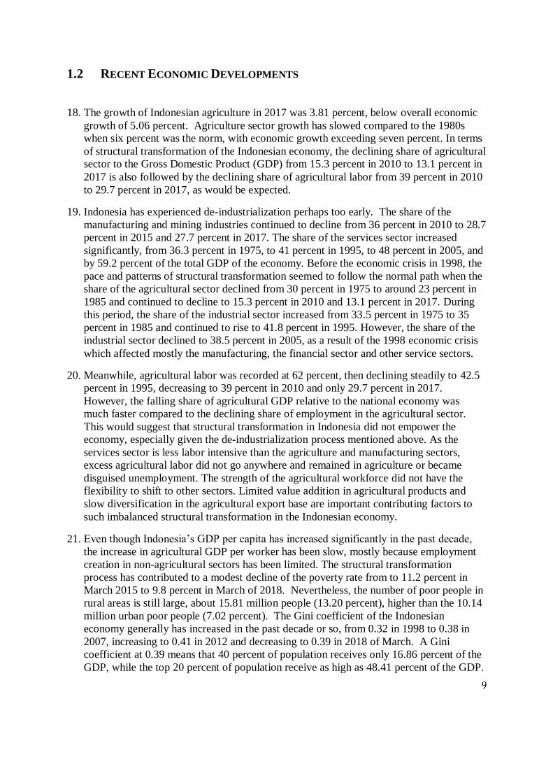
18. The growth of Indonesian agriculture in 2017 was 3.81 percent, below overall economic

growth of 5.06 percent. Agriculture sector growth has slowed compared to the 1980s

when six percent was the norm, with economic growth exceeding seven percent. In terms

of structural transformation of the Indonesian economy, the declining share of agricultural

sector to the Gross Domestic Product (GDP) from 15.3 percent in 2010 to 13.1 percent in

2017 is also followed by the declining share of agricultural labor from 39 percent in 2010

to 29.7 percent in 2017, as would be expected.

19. Indonesia has experienced de-industrialization perhaps too early. The share of the

manufacturing and mining industries continued to decline from 36 percent in 2010 to 28.7

percent in 2015 and 27.7 percent in 2017. The share of the services sector increased

significantly, from 36.3 percent in 1975, to 41 percent in 1995, to 48 percent in 2005, and

by 59.2 percent of the total GDP of the economy. Before the economic crisis in 1998, the

pace and patterns of structural transformation seemed to follow the normal path when the

share of the agricultural sector declined from 30 percent in 1975 to around 23 percent in

1985 and continued to decline to 15.3 percent in 2010 and 13.1 percent in 2017. During

this period, the share of the industrial sector increased from 33.5 percent in 1975 to 35

percent in 1985 and continued to rise to 41.8 percent in 1995. However, the share of the

industrial sector declined to 38.5 percent in 2005, as a result of the 1998 economic crisis

which affected mostly the manufacturing, the financial sector and other service sectors.

20. Meanwhile, agricultural labor was recorded at 62 percent, then declining steadily to 42.5

percent in 1995, decreasing to 39 percent in 2010 and only 29.7 percent in 2017.

However, the falling share of agricultural GDP relative to the national economy was

much faster compared to the declining share of employment in the agricultural sector.

This would suggest that structural transformation in Indonesia did not empower the

economy, especially given the de-industrialization process mentioned above. As the

services sector is less labor intensive than the agriculture and manufacturing sectors,

excess agricultural labor did not go anywhere and remained in agriculture or became

disguised unemployment. The strength of the agricultural workforce did not have the

flexibility to shift to other sectors. Limited value addition in agricultural products and

slow diversification in the agricultural export base are important contributing factors to

such imbalanced structural transformation in the Indonesian economy.

21. Even though Indonesia’s GDP per capita has increased significantly in the past decade,

the increase in agricultural GDP per worker has been slow, mostly because employment

creation in non-agricultural sectors has been limited. The structural transformation

process has contributed to a modest decline of the poverty rate from to 11.2 percent in

March 2015 to 9.8 percent in March of 2018. Nevertheless, the number of poor people in

rural areas is still large, about 15.81 million people (13.20 percent), higher than the 10.14

million urban poor people (7.02 percent). The Gini coefficient of the Indonesian

economy generally has increased in the past decade or so, from 0.32 in 1998 to 0.38 in

2007, increasing to 0.41 in 2012 and decreasing to 0.39 in 2018 of March. A Gini

coefficient at 0.39 means that 40 percent of population receives only 16.86 percent of the

GDP, while the top 20 percent of population receive as high as 48.41 percent of the GDP.

10

This constitutes a serious imbalance that needs to be recognized when designing and

implementing social inclusion policies and programs. More importantly, ineffective

government policies have contributed to Indonesia’s income inequality while poor

infrastructure affects the economic access to the production factors.

22. In the staple food sector, the policy to increase the production of rice, maize and soybean

(Pajale Program) and to stabilize prices has not succeeded to improve the welfare of

farmers and the general public. According to the most recent official estimates of rice

production (October 2018), using the Area Sample Framework (KSA) method, the total

area of 7.10 million hectares of rice fields is a significant reduction compared to 7.75

million hectares in 2013. In the past five years, the conversion of rice fields accounts for

more than 600 thousand hectares, or over 120 thousand hectares each year. This

conversion of rice fields occurred in spite of Law No. 41/2009 on the Protection of

Agricultural Land for Food Production (PLP2B). The Law is supplemented by

Government Regulation (PP) No. 1/2011 on Allocation of Land Protection, PP 12/2012

on Incentives of Land Protection, and PP 25/2012 on Information System of Land

Protection and PP 30/12 on Financing for Land Protection, and other Ministerial

Regulations.

23. The harvested area as measured by the KSA (an agriculture survey that measures area

under production) in 2018 is 10.9 million hectares, far lower than 16 million hectares by

earlier “eye estimates”. The difference of 5.1 million hectares (31.88 percent) is too high

to be statistically tolerable, causing biases in any development planning such as fertilizer

and seed subsidies, agricultural machinery and equipment etc. The new estimate of rice

production by KSA in 2018 is 56.54 million tons of non-husked dry rice (GKG), instead

of 83 million ton, which is a correction of 26.46 million tons (31.88 percent). Until

September 2018, BPS data showed that rice imports reached 2.02 million ton, a

significant increase from 311 thousand tons in 2017. Some rice production centers in

Indonesia experienced a serious drought and crop failures due to pests and diseases, the

rice import in 2018 might exceed 2.5 million ton, which is much higher than the import

after El-Nino year in 2016 of 1.3 million tons.

24. BPS recorded that the retail price of rice in November 2018 was Rp 14,007 per kilogram,

an increase of 4.30 percent compared to the price of rice in June 2017. The price of rice

has now decreased compared to the price of rice in February 2018 of Rp 14,697 per

kilogram, the highest record so far. The high price of rice and other food contributes

specifically to the poverty line in Indonesia. The price of food contributes 73.48 to the

poverty line in March 2018, an increase from the contribution of 73.35 percent in

September 2017. Food commodities that affect the rural poverty line are rice, clove

cigarettes, eggs, chicken meat, instant noodles and sugar. Although the number of poor

people has dropped to 25.95 million people (9.82 percent) in March 2018, from 26.58

million people (10.12 percent) in September 2017, the number of poor people in rural

areas is still large, namely 15.81 million people (13.20 percent), higher than the urban

poor 10.14 million people (7.02 percent).

25. Compared to other major rice producing countries in the region, Vietnam, Thailand,

India, the Philippines, and China, the cost structure of rice production in Indonesia is the

highest. A study by IRRI (2016) suggests that the average production cost of one

11

kilogram of rice in Indonesia is Rp 4,079, which is nearly 2.5 times the cost in Vietnam

(Rp 1,679), nearly 2 times the cost in Thailand (Rp 2,291) and India (2,306), and 1.5

times the cost in the Philippines (Rp 3,224) and China (Rp 3,661). The highest cost

components are land rental (Rp 1,719) and labor costs (Rp 1,115) to produce one

kilogram of non-husked rice. Low labor productivity in Indonesia has contributed to the

low level of competitiveness of the rice farming system and has contributed to poverty

incidence in rural areas. Agricultural labor in Indonesia only receives Rp 86,593 per day,

which is generally lower than that in the Philippines of Rp 86,752, in Vietnam of Rp

121,308, in Thailand of Rp 181,891 and in China of Rp 208,159, but significantly higher

than that in India of Rp 42,492 (IRRI, 2016).

2. LABOR PRODUCTIVITY IN AGRICULTURE

2.1 CASE STUDY: AGRICULTURAL LABOR PRODUCTIVITY IN VIETNAM1

26. The number of people working in Vietnam’s primary agriculture is large, but it is

decreasing over time. In 2000, about 25 million people worked in agriculture, accounting

for 65 percent of total labor force. By 2015, agriculture employed some 23.2 million

people, representing 46 percent of the workforce. The movement of rural people out of

agriculture has largely been a result of rapid economic growth that created many nonfarm

jobs.2 As primary agriculture remains a large employment and income source in many

parts of rural Vietnam, improving the remuneration of this work is an important task for

policy makers. How to do it is strongly related to labor productivity, which is perceived to

be low.

27. When measured in a traditional way, by dividing the sectoral value-added by number of

workers, agricultural labor productivity is indeed low—in 2014 it was 2.5 times smaller

than the average labor productivity in Vietnam’s industry and construction. Yet

agricultural labor productivity is not necessarily lower than other sectors when measured

on per-hour-worked basis. The recent survey evidence from around the world indicates

that on a per-hour-worked basis, rather than simply using national accounts data on the

1 Based on Vietnam’s Future Jobs: Shaping Agriculture to Deliver Jobs. S. Zorya et al (2018) World Bank: Hanoi. 2 Vietnamese households increasingly rely on nonfarm sources of income. Between 2004 and 2014, the share of

rural households relying entirely on nonfarm income and wages increased from 22 percent to 32 percent. At the

same time, the share of rural households relying only on income from agriculture declined from 23 percent to 19

percent. About 90 percent of rural households have multiple sources of income.

12

number of people employed in agriculture, and accounting for differences in human

capital, agricultural labor productivity is not intrinsically lower than other sectors – it is

often similar.

28. Indeed, for Vietnam the labor productivity of some specialized agricultural households

appears to be even higher than that in nonfarm sectors where skill requirements are

comparable to that in primary agriculture (Table 2). The value of the unadjusted

agricultural labor productivity in 2014 was VND 28.6 million per worker; yet the per-

hour-worked adjusted annual productivity is estimated to be almost as twice as large at

VND 53.7 million per worker. Some productivity gap with manufacturing and

construction remains, but it narrowed from more than 200 percent when using national

accounts annual data to only 20 percent for construction and 30 percent for manufacturing

and transport and warehousing when using per-hour-worked data.3

Table 2: Comparison of annual and per-hour-work adjusted labor productivity, 2014

Annual labor productivity

(GDP/worker) (VND)

Per-hour-work adjusted

annual productivity (VND)

Agriculture 28,600,000 53,710,000

Crops 51,000,000

Livestock 57,000,000

Agricultural services 76,000,000

Fisheries 68,750,000

Forestry 39,250,000

Manufacturing and processing industry 70,000,000

Construction 60,700,000

Transport and warehousing 73,200,000

29. Labor productivity varies significantly by commodity, pointing to the ability of different

jobs to provide differentiated income. This analysis suggests that large gains can be

achieved from changes in land use, e.g. by moving land from less labor productive to

more labor productive commodities. Importantly for employment discussions, is also the

fact that the commodities with higher labor productivity in Vietnam also tend to be more

labor intensive, allowing the full use of sector resources for job and income generation.

3 In addition, the labor productivity in agricultural services, provided by cooperatives and other farmer

organizations, was found to be higher than that in nonfarm sectors, and the labor productivity in fisheries was

higher than that in construction, a common off-farm employment alternative to farmers.

13

Table 3: Labor input and productivity from the field data by commodity, 2016-2017

Labor input, days/ha Labor productivity, ‘000 VND/day

Paddy [VHLSS 2014] 46-150 [278] 174-276 [94]

Maize 165-170 [n/a] 95-110 [n/a]

Cassava 185-220 [n/a] 118-135 [n/a]

Oranges 350-415 [300] 600-1,000 [297]

Mango 200-300 [182] 500-900 [484]

Dragon fruit 700 [n/a] 550-650 [n/a]

Pepper 360-500 [329] 520-1,830 [511]

Coffee 115-130 [287] 500-700 [411]

Pork 500-1,500 [n/a] 320-950 [157]

Shrimp 240-335 [261] 1,700-3,300 [403]

Fish 212 [373] 280-980 [329]

Sources: IPSARD’s estimate using field data collected in 2016-2017; Maize and cassava from Keyser et al. (2013) Figures in parentheses are the estimates based on VHLSS 2014

30. This analysis illustrates that labor productivity in primary agriculture is generally higher

than often perceived in Vietnam. This is most evident when one looks beyond paddy

production or production of other low value feed commodities. The latter have dragged

down the aggregated estimate of labor productivity in the entire sector, and this is

especially the case when statistics do not take account of the part-time and highly

seasonal nature of paddy production—especially in the Mekong Delta, which has

accounted for a large majority of Vietnam’s rice production expansion since 2000. When

adjusting labor input by per-hour-worked efforts and differentiating by commodities,

some of which are more labor intensive and higher value than others, a brighter picture

arises for agricultural labor productivity. Significant economic and “better job” gains can

still be achieved in Vietnam’s primary agriculture going forward by facilitating the shift

of labor from less to more productive activities, often requiring a shift of farmland from

paddy and maize to other crops. This would be consistent with the government efforts to

promote high-tech agriculture and would be similarly consistent with a broad

employment agenda.

2.2 LABOR PRODUCTIVITY IN INDONESIA

31. Agriculture has played an important role in the Indonesia national economy, even though

its share of the country’s gross domestic product (GDP) has declined as the economy has

grown. The decline in the share of GDP in agriculture occurs due to both push and pull-

factors. Push factors can have negative effects on poverty, where agriculture cannot

accommodate the growing labor force, so that resources move out from the agricultural

sector to more rapidly growing sectors in the economy. Pull factors are at play where

nonagricultural sectors offer more attractive employment opportunities, primarily because

of differences in factor endowments and capital accumulation.

14

32. Structural transformation in the Indonesian economy has not occurred smoothly,

especially over the past decade. The share of the agricultural sector has declined from 30

percent in 1975 to around 23 percent in 1985 and continues to decline to 15.3 percent in

2010 and 13.1 percent in 2017 (Table 4). The share of the industrial sector has increased

from 33 5 percent in 1975 to 35 percent in 1985 and continued to rise to 41.8 percent in

1995. The share of the industrial sector declined to 38.5 percent in 2005, as a result of the

1998 economic crisis which affects mostly manufacturing sectors in Indonesia and

financial and other service sectors.

Table 4: Roles of Agriculture in the Indonesian Economy, 1975-2017

1975 1985 1995 2005 2010 2015 2017

1. Share of GDP (%)

▪ Agriculture 30.2 22.9 17.1 13.4 15.3 13.5 13.1

▪ Industry (manufacture etc.) 33.5 35.3 41.8 38.5 36.0 28.6 27.7

▪ Services 36.3 42.8 41.1 48.1 48.7 57.9 59.2

2. Share of Employment (%)

▪ Agriculture 62.0 56.0 46.0 42.5 39.0 32.9 29.7

▪ Industry (manufacture etc.) 6.0 9.0 12.8 13.0 14.5 13.3 14.5

▪ Services 32.0 35.0 43.2 44.5 47.5 53.8 55.8

Source: The share is calculated from BPS data, various issues.

33. The literature on the roles of agriculture in economic development and productivity gap

between agriculture and non-agriculture during the structural transformation can be traced

back to the seminal works by Johnston and Mellor (1961), Mellor (1995), Timmer (1988)

and my most recent works by Christiaensen et al. (2011), Dorward (2013), Imai et al.

(2016), Imai et al. (2017) and Mellor (2017). Initially, agriculture has made a net

contribution to the capital required for overhead investment and expansion of secondary

industry. The rising net cash income of the farm population will be important as a

stimulus for an expansion of the non-farm sector. The relationship between agriculture

and non-agriculture developed from the facts that modernization of agriculture would

require the use of chemical fertilizers, pesticides, machine services, processed seeds or

fuels, which would promote non-agricultural production. Increase in agricultural income

will lead to increased demand for non-agricultural products, and vice versa. Finally,

decrease in food prices as a result of agricultural growth will result in better food security

and overall poverty reduction in both rural and urban areas, while the reduction in food

price would lower the real product wage in non-agriculture, thereby raising profitability

and investment in that sector (Christiaensen, et al. 2011).

34. The performance of labor productivity in Indonesia is generally increasing in all sectors,

measured in terms of added value per worker (Rp/worker) (Table 5). The data show that

the overall labor productivity on Indonesian workers were Rp 66.4 million in 2011,

increased to 72.8 million in 2014 and 78.7 million per worker in 2017. The labor

productivity in agriculture also increased significantly in the last decade, from Rp 25.4

million per worker to Rp 30 million and to 35 million per worker. However, the level of

labor productivity in agriculture is relatively lower than that of other sectors, as the total

added value in non-agricultural sectors is generally higher. There has been a tendency of

15

sectoral gap between labor productivity in agriculture and non-agriculture, such as

suggested by Imai et al. (2018).

Table 5: Labor Productivity in Indonesia 2011-17 (‘000 Rp at Constant Price 2010) and index

Sector 2011 2012 2013 2014 2015 2016 2017

1. Agriculture, Livestock, Forestry 25,425 26,254 27,617 28,970 31,031 32,053 34,987

2. Mining and Quarrying 522,355 482,040 555,497 553,659 582,488 526,989 562,352

3. Manufactures 108,359 105,193 113,961 118,706 124,505 127,050 119,774

4. Electricity, Gas, Clean Water 237,832 251,622 251,948 236,080 218,189 214,689 152,770

5. Construction 109,107 106,290 121,700 113,545 107,109 115,943 121,412

6. Trade, Hotel, and Restaurant 53,215 52,899 54,028 55,723 55,523 55,333 54,795

7. Transportation, Communication 107,345 117,234 126,526 137,332 149,272 147,520 154,834

8. Finance, Rental, and Services 224,692 228,680 230,871 234,046 229,320 231,849 233,240

9. Other Services 45,769 45,469 45,225 46,459 50,745 48,947 49,651

Total Sector

66,495

67,199

70,532

72,856

75,767

76,828

78,748

Index of labor productivity

1. Agriculture, Livestock, Forestry 100 103 109 114 122 126 138

2. Mining and Quarrying 2,054 1,896 2,185 2,178 2,291 2,073 2,212

3. Manufactures 426 414 448 467 490 500 471

4. Electricity, Gas, Clean Water 935 990 991 929 858 844 601

5. Construction 429 418 479 447 421 456 478

6. Trade, Hotel, and Restaurant 209 208 212 219 218 218 216

7. Transportation, Communication 422 461 498 540 587 580 609

8. Finance, Rental, and Services 884 899 908 921 902 912 917

9. Other Services 180 179 178 183 200 193 195

Total Sector 262 264 277 287 298 302 310

Source: Calculated from BPS, GDP at 2010 Constant Price and Sakernas Series (various years)

35. Using the data of Asian countries, Imai et al (2018) examine the pattern of (1) the

convergence of labor productivity between agricultural and non-agricultural sectors and

(2) the convergence of agricultural or non-agricultural productivity across different

countries. The studies find that the agricultural labor productivity growth has promoted

the non-agricultural productivity growth. The sectoral gap has widened, while the

between-country disparity of sectoral labor productivity has reduced.

36. However, the growth performance of labor productivity is somewhat different from the

magnitude or the value of labor productivity. The growth performance of each sector has

experienced some fluctuations, but the average growth level of labor productivity in

agriculture is 6.09 percent per year, the second largest, after that of transportation and

communication sector of 8.91 percent per year (Table 6). Sectors that have experienced

negative growth performance, although the added value is quite large, also experienced

negative growth in labor productivity.

16

Table 6: Growth of Labor Productivity in Indonesia 2011-2017 (percent per year)

Sector 2011 2012 2013 2014 2015 2016 2017

Average

1. Agriculture, Livestock, Forestry 9.73 3.26 5.19 4.90 7.12 3.29 9.15 6.09

2. Mining and Quarrying -11.18 -7.72 15.24 -0.33 5.21 -9.53 6.71 -0.23

3. Manufactures 0.90 -2.92 8.33 4.16 4.89 2.04 -5.73 1.67

4. Electricity, Gas, Clean Water 4.58 5.80 0.13 -6.30 -7.58 -1.60 -28.84 -4.83

5. Construction -5.29 -2.58 14.50 -6.70 -5.67 8.25 4.72 1.03

6. Trade, Hotel, and Restaurant 10.19 -0.59 2.14 3.14 -0.36 -0.34 -0.97 1.88

7. Transportation, Communication 24.24 9.21 7.93 8.54 8.69 -1.17 4.96 8.91

8. Finance, Rental, and Services -27.90 1.77 0.96 1.38 -2.02 1.10 0.60 -3.44

9. Other Services 6.70 -0.65 -0.54 2.73 9.22 -3.54 1.44 2.19

Total Sector 7.27 1.06 4.96 3.29 4.00 1.40 2.50 3.50

Source: Calculated from BPS, GDP at 2010 Constant Price and Sakernas Series (various years)

37. Empirical estimates on productivity growth using the concept of total factor productivity

(TFP) and decomposition of the sources of economic growth have been conducted by

Fuglie (2004, 2010, and 2012) and some others (see Arifin, 2015). The studies suggest

that in the period of 1961-2006, Indonesia achieved an annual growth rate in agricultural

production of 3.6%. About half of this growth can be attributed to an expansion of

conventional inputs (land, labor, capital and intermediate inputs) and the rest to

improvement in total factor productivity. Productivity growth accelerated during the

“Green Revolution” period when modern varieties of food crops were widely

disseminated but stagnated during the 1990s. Productivity growth resumed in the early

2000s following the recovery from the Asian Financial Crisis and liberalization of

policies toward agriculture.

38. Commodity diversification, allocating more agricultural resources to the production of

higher-valued commodities as well as crops that make fuller use of farm labor, has been

an important source of TFP growth in recent years. The private sector rather than the state

appears to be the driving force behind the reemergence of growth in the sector. Higher

levels of schooling amongst the farm population account for about 10% of the growth in

labor productivity. Continued improvement in the quality of labor can offset the projected

decline in the size of the farm labor force. Commodity diversification was probably as

important a source of agricultural productivity growth as technological change. Farmers

increased productivity by moving to more intensive production systems involving

perennial tree crops, horticulture, animals and aquaculture. However, the gains from

diversification were preceded by an impressive improvement in productivity of rice and

other food staples. Having secured food security first may well have been a prerequisite

for small-holder farmers to be willing to allocate more resources to producing non-staple

commodities for the market (Fuglie, 2010).

39. The Indonesian economy has been dominated by rice production, although the agriculture

sector has become increasingly diversified, with perennials, horticultural crops, livestock,

and aquaculture growing in relative importance over time. Indonesia has become a

significant global supplier of tropical vegetable oil, rubber, cocoa, coffee, fish, and

shrimp. Although the country continues to rely on imports for a significant share of its

17

cereal grain needs for food and feed, it maintains a positive agricultural trade balance

overall. Resource expansion and productivity improvement have been important sources

of growth in Indonesian agriculture. Agricultural land continues to expand in the sparsely

populated regions of the country where area planted to perennial crops, oil palm

especially, has undergone rapid expansion in recent decades, with serious environmental

consequences. These regions include the islands of Sumatra, Kalimantan, Sulawesi, and

Papua. Both smallholder farms and large estate companies are heavily involved in the

perennial-crop sector. Large estate companies, with access to capital and technology,

often dominate the early stages of perennial crop development, but over time,

smallholders have entered these sub-sectors. Presently, smallholders dominate the

production of rubber, coffee, cocoa, and coconut and are gaining market share in oil palm.

40. Rice farming is barely profitable, according to a recent survey on rice farm cost structures

conducted by BPS in 2017, covering a sample of 165.9 thousand farm households. Farm

profit from lowland paddy is Rp 4.7 million in 2017 per season. For upland paddy this is

Rp 2.4 million per season (Hermanto, 2018). The revenue to cost ratio (R/C ratio) for

lowland paddy is 1.32 and for upland paddy is 1.28, implying that the rice farming system

in Indonesia does not contribute much towards a decent living standard for farm

households. The benefit revenue to cost ratio (B/C ratio) for lowland paddy is 0.34 and

for upland paddy is 0.28, implying that the profit generated from rice farming activities is

too low to allow the farmers to invest in a more productive and profitable crop production

system (the literature generally suggests a bench mark of 1.5 for R/C ratio and 1.25 for

B/C ratio).

41. The economic performance of farm households of rice paddy using a large sample is

comparable to the results of a farm household survey of 403 paddy farmers along the

Lower Sekampung Watershed in the Province of Lampung in 2017. The profitability of

rice farming system is positive, but very low, which prevents the paddy farmers to have a

decent living, and possibly very prone to fall below poverty line. The R/C ratio of rice

farmers in the District of Central Lampung is 2.19 during rainy season and decrease to

1.07 during dry season. The R/C ratio of rice farmers in the District of East Lampung is

1.73 during rainy season and 1.11 during the dry season. The B/C ratios of rice farming

systems in all two districts in study sites of Lower Sekampung Watershed are a way

below 1.00, implying that the farming system is not able to generate an adequate

economic profitability for the farm households (Arifin et al., 2018). The major problems

in rice farming system along the Lower Sekampung Watershed is the lack of water supply

and other availability issues of irrigation water as the problems of operation and

maintenance (O&M), both physical and social-economic issues of irrigation

infrastructures, as well as heavy sedimentation of irrigation infrastructures along the main

canals as well as secondary and tertiary canals. In addition, added value of secondary and

other food crops and could be significantly higher than the economic returns on rice

farming activities.

42. The average land holding size of rice farmers in Indonesia is less than 0.5 hectares,

leaving many in relative poverty and with limited options to diversify and become a more

profitable enterprise. Government efforts to implement land reforms, including land

registration and certification, and land distribution to landless farmers may contribute to

18

enhanced access to land. However, a holistic approach of empowerment is required that

would improve the farmers’ access to markets, information, technology, and finance.

3. METHODS AND FRAMEWORK

3.1 LITERATURE AND DATA

43. The study combines desk analysis, literature studies, field surveys and in-depth interviews

with relevant resource persons from the government, private sector, academia, farmers

associations, stakeholder groups and community organizations. A small field survey was

conducted in four relevant food crop production areas.

44. A desk analysis was carried out to review the available literature and relevant previous

studies on the economics of agricultural labor productivity, both in the context of

macroeconomics and structural transformation, and in a microeconomic context using

data from the national labor survey (Sakernas). The review also covered economic policy

on food and agriculture, labor policy, and other relevant policies in the local and regional

context.

45. The study included a field survey among smallholders farmers in four relevant provinces,

namely North Sumatra, East Nusa Tenggara, Central Java and West Java. These

provinces were purposively selected based on the characteristics of the regions and crop

production performance of food commodities covered in the study. Samples were selected

based on recommendation by local officials of the Ministry of Agriculture in the districts

and/or provinces. Using non-probability sampling, 20-30 households were included in the

sample in each district:

a. North Sumatera: Rice in the districts of Deli Serdang and Serdang Bedagai, and

orange, cabbage, tomatoes in the districts of Karo.

b. East Nusa Tenggara: Maize in the districts of Timor Tengah and Kupang, Poultry

in the districts of Kupang and Kupang City.

c. Central Java: Soybean and maize in the district of Grobogan, and shallot and

garlic in the district of Brebes.

d. West Java: Mixed farming and aquaculture fresh water in the district of Garut and

mixed farming and poultry in the district of Tasikmalaya.

3.2 METHODS OF ANALYSIS

46. The methods of analysis of both primary and secondary data collected for the study can

be summarized as follows:

19

FARM ECONOMICS ANALYSIS

47. Farm economic analysis was employed in the study, by calculating (a) the production

costs of each crop by multiplying the total use of farm inputs and their prices, (b) revenue

of farming system by multiplying the estimated output and farm gate price, and (c)

estimated income by subtracting the total revenue from the total costs. Therefore, the

concept of (d) revenue-cost ratio (R/C ratio) could be easily calculated by dividing the

total revenue from total costs, while (e) benefit-cost ratio (B/C) could also calculated by

dividing the total income from total costs. Here is the brief explanation of the farm

economics and cost.

a) Production Cost (C). This is the total costs of using all inputs for farm production

or simply written as follows:

C = ∑Xi. rXi

where C is production cost (in Rupiah), Xi the i-th production input and rXi the i-

th input price.

b) Revenue (R). This is the total revenue generated from selling the production or the

current value of production or output of farming activities, simply written as

follows:

R= Q x P

where R is total revenue (in Rupiah), Q is total production output and P is the

farm-gate price.

c) Farm Income (π). Farm income is calculated by subtracting total revenue from

total cost.

π = TR – TC

where Y is income, TR is total revenue and TC is total costs, where all is Rupiah.

d) Revenue-Cost Ratio (R/C Ratio). This is usually defined by simply comparing the

total revenue from total costs, or simply written as follows:

R/C ratio = TR/TC

e) Benefit-Cost Ratio (R/C Ratio). This is usually defined by simply comparing the

estimated income from total costs, or simply written as follows:

B/C ratio = π/TC

48. The profitability of crop production and/or farming systems can be assessed based on the

R/C ratio and B/C ratio of each crop and/or farming system. Further profitability analysis

of each crop production can differentiate the use of subsidized inputs (mostly fertilizer

and seed) from the inputs purchased at the market price.

20

PRODUCTIVITY ANALYSIS

49. We performed productivity analysis in a macro context based on published data from the

Central Agency of Statistics (BPS) and other sources, and in a micro context using the

data collected from the field surveys in four provinces as well as previously collected data

by the researchers. Labor productivity in agriculture here is simply defined as “value

added per worker”. In the micro context, we employed a more detailed calculation of

“value added per working hour” from each farming system.

50. We also referred to the findings from Fuglie (2010, 2015) to discuss the Total Factor

Productivity (TFP) of Indonesian agriculture.

PROFIT FUNCTION ANALYSIS

51. This is a standard profit function analysis where the input use and input price are

important determinants of farm income, such as in the following equation.

𝑌𝑖 = 𝛼 + 𝑋𝑖′𝛽 + 𝑍𝑖

′𝛾 + 𝑒𝑖

where 𝑌𝑖 represents farm incomes, 𝑋𝑖′ is a vector of internal households’ variables such as:

household size, farm land size, and level of education, 𝑍𝑖′ denotes a vector of policy variables

such as price supports, subsidies and social assistance for agricultural households.

52. Profit function in Cobb-Douglas model is usually expressed in the production output and

farm-gate price, which is normalized by a certain price, which is usually written as

follows:

ln 𝜋∗ = ln 𝐴∗ + ∑ 𝛼𝑖 ln 𝑞𝑗∗ + ∑ 𝛽𝑗 ln 𝑍𝑗

𝑛

𝑗=1

𝑚

𝑗=1

Where:

𝜋∗ = Normalized profit or farm income by the farm-gate price

𝐴 = Intercept

𝛼𝑖 = Coefficient of input price, also normalized by farm-gate price

𝛽𝑗 = Coefficient of fixed input

𝑞𝑗 = Price of variable inputs, also normalized by farm-gate price

Z j = Fixed input

POLICY ANALYSIS

53. Consequences for the relationship between profitability and labor productivity are

examined and simulated under some conditions, such as changes in prices of outputs

and/or inputs, and changes in other sensitive and non-sensitive factors.

21

4. RESULTS AND DISCUSSION

4.1 INTRODUCTION

54. Results of data analyses are presented, both at macro level using the data from the

Agency of Central Statistics (BPS) on standardized method of Gross Domestic Product

(GDP) accounting and on employment composition and changes from the series of

National Labor Survey (Sakernas). Even though BPS has now published the GDP details

of 17 sectors in the economy, we are using the old classification of 9 sectors as of the

GDP in 2000, simply for the consistency purposes. As mentioned briefly in previous

chapter, the structural transformation of the Indonesian economy has not occurred in the

last two decades (Table 7). The declining share of agricultural sector in the national GDP

from 16.6 percent in 2000 to 13.2 percent in 2017 has been also associated with the

declining share of agricultural employment in total employment of the country from 45.3

percent to 29.7 percent in the same period. However, the GDP share of manufacturing

sector during the same period has not increased, but surprisingly declined from 23.9

percent to 22.1 percent. The phenomena of deindustrialization in the early 2000s have

affected the performance of labor productivity in the country. The employment

contribution of manufacturing sector to the total employment in Indonesia has increased

from 13 percent in 2000 to 14.5 percent in 2017. This should imply that increasing

number of labor force in manufacturing has not been translated into higher contribution to

the national GDP. In other words, there have been serious issues of declining labor

productivity in Indonesia, especially in manufacturing sectors, and most probably in other

economic sectors. The details of increasing labor productivity in the Indonesian economy

will be explained in the following sub-sections.

Table 7: The Share of Sectoral GDP and Employment to the Indonesian Economy

Sectors

PDB Contribution

(%)

Employment

Contribution (%)

2000 2010 2017 2000 2010 2017

1. Agriculture, Livestock, and Forestry 16.62 14.31 13.19 45.28 38.35 29.68

2. Mining and Quarrying 15.73 10.74 8.18 0.50 1.16 1.15

3. Manufactures 23.87 22.63 22.07 12.96 12.78 14.51

4. Electricity, Gas, and Clean Water 0.89 1.17 1.15 0.08 0.22 0.59

5. Construction 7.82 9.38 10.37 3.89 5.17 6.72

6. Trade, Hotel, and Restaurant 15.40 16.82 16.89 20.58 20.79 24.28

7. Transportation and Communication 3.65 7.50 9.56 5.07 5.19 4.86

8. Finance, Rental, and Services 6.86 8.03 9.04 0.98 1.61 3.05

9. Other Services 9.15 9.41 9.55 10.66 14.75 15.15

Total 100.00 100.00 100.00 100.00 100.00 100.00

Source: Calculated from Sakernas 2000, 2010 and 2017.

22

4.2 INCREASING LABOR PRODUCTIVITY

55. The average wage rate in the agricultural sector in 2017 was Rp 1.9 million per month,

the lowest in the economy, in contrast with the wage rate in mining and quarrying sector

which was Rp 4.4 million per month, the highest in the economy. The wage rate in

manufacturing sector has increased from Rp 1.2 million per worker per month in 2000 to

Rp 2.5 million per worker per month in 2017. In general, wage rates have nearly

doubled, which would be driven by the level of economic development and inflation

during the last 17 years.

Table 8: Average Wage Rate by Sector in 2000, 2010 and 2017 (Rp/worker/month)

Sectors

2000 2010 2017

1. Agriculture, Livestock, Forestry 241,724 945,728 1,936,813

2. Mining and Quarrying 699,669 2,387,778 4,374,756

3. Manufacturing 408,509 1,176,612 2,544,264

4. Electricity, Gas, Clean Water 660,115 1,757,994 3,886,441

5. Construction 431,692 1,302,241 2,370,966

6. Trade, Hotel, and Restaurant 418,565 1,067,812 2,142,618

7. Transportation, Communication 532,124 1,438,353 3,005,767

8. Finance, Rental, and Services 732,330 1,957,823 3,722,759

9. Other Services 567,638 1,688,410 3,052,498

Source: Calculated from Sakernas 2000, 2010 and 2017

56. In general, labor productivity in Indonesia has experienced a significant increase during

the period of 2000 to 2017. We calculate labor productivity using the added value of the

sectoral GDP divided by the number of workers in each sector, using current prices and

constant 2010 prices, presented in Table 9 below. For further analysis and comparison,

2010 constant prices are used. Overall, labor productivity in Indonesia has increased

from Rp 45.5 million in 2000 to Rp 78.8 million in 2017. The “usual tradable sectors”

such as agriculture and manufacturing have experienced a significant increase in labor

productivity. Labor productivity in agriculture has increased from a very low Rp 16.7

million in 2000 to Rp 35.0 million, and that in manufacturing sector has increased from

Rp 83.9 million in 2000 to Rp 119.8 million in 2017. However, a decrease in labor

productivity occurred in the mining and quarrying sector, in electricity, gas and clean

water, and in finance, rental and services. Despite the growth trajectory, labor

productivity in agriculture remains the lowest of all sectors in absolute terms (Figure 2).

23

Table 9: Labor Productivity by Sector both in Current and Constant Price of 2010

Sectors

Productivity (Constant Price

in 2010, Rp million)

Productivity (Current

Price, Rp million)

2000 2010 2017 2000 2010 2017

1. Agriculture, Livestock, Forestry 16.72 23.04 34.99 5.33 23.04 49.71

2. Mining and Quarrying 1,423.79 572.44 562.35 371.06 572.44 741.78

3. Manufacturing 83.91 109.43 119.77 33.12 109.43 156.02

4. Electricity, Gas, and Clean Water 516.17 334.93 152.77 118.84 334.93 239.97

5. Construction 91.50 112.09 121.41 21.90 112.09 173.27

6. Trade, Hotel, and Restaurant 34.08 49.98 54.79 12.14 49.98 73.35

7. Transportation Communication 32.84 89.24 154.83 14.28 89.24 212.65

8. Finance, Rental and Services 317.86 308.73 233.24 130.82 308.73 321.95

9. Other Services 39.11 39.40 49.65 13.55 39.40 72.69

Total 45.54 61.77 78.75 15.47 61.77 107.95

Source: Processed from Sakernas 2000, 2010 and 2017.

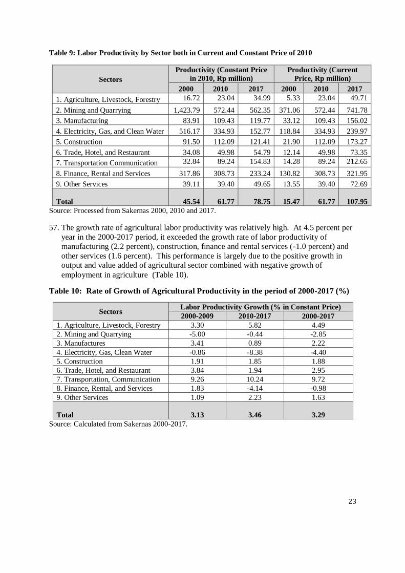
57. The growth rate of agricultural labor productivity was relatively high. At 4.5 percent per

year in the 2000-2017 period, it exceeded the growth rate of labor productivity of

manufacturing (2.2 percent), construction, finance and rental services (-1.0 percent) and

other services (1.6 percent). This performance is largely due to the positive growth in

output and value added of agricultural sector combined with negative growth of

employment in agriculture (Table 10).

Table 10: Rate of Growth of Agricultural Productivity in the period of 2000-2017 (%)

Sectors Labor Productivity Growth (% in Constant Price)

2000-2009 2010-2017 2000-2017

1. Agriculture, Livestock, Forestry 3.30 5.82 4.49

2. Mining and Quarrying -5.00 -0.44 -2.85

3. Manufactures 3.41 0.89 2.22

4. Electricity, Gas, Clean Water -0.86 -8.38 -4.40

5. Construction 1.91 1.85 1.88

6. Trade, Hotel, and Restaurant 3.84 1.94 2.95

7. Transportation, Communication 9.26 10.24 9.72

8. Finance, Rental, and Services 1.83 -4.14 -0.98

9. Other Services 1.09 2.23 1.63

Total 3.13 3.46

3.29

Source: Calculated from Sakernas 2000-2017.

24

Figure 2: Labor productivity in agriculture and other sectors, 2000-2017


4.3 DECLINING EMPLOYMENT IN AGRICULTURE

58. Structural transformation in the Indonesian economy is characterized, among other things,

by a declining share of employment in agricultural sector. Total employment in

agriculture was 40.7 million (45.3 percent of total employment) in 2000 and declining to

35.9 million (29.7 percent of total employment) in Indonesia (Table 11). All other sectors

from mining, manufacture, electricity, trade and other services experienced a significant

increase in employment.

Table 11: Sectoral Shifting of Employment, 2000, 2010 and 2017

Sectors

Employment (thousand)

2000 2010 2017

1. Agriculture, Livestock, and Forestry 40,677 41,495 35,925

2. Mining and Quarrying 452 1,255 1,387

3. Manufactures 11,642 13,824 17,559

4. Electricity, Gas, and Clean Water 71 234 717

5. Construction 3,497 5,593 8,137

6. Trade, Hotel, and Restaurant 18,489 22,492 29,382

7. Transportation and Communication 4,554 5,619 5,883

8. Finance, Rental, and Services 883 1,739 3,694

9. Other Services 9,574 15,956 18,340

Total 89,838 108,208 121,022

Source: Calculated from Sakernas 2000, 2010 and 2017.

0

20,000

40,000

60,000

80,000

100,000

120,000

140,000

2000

2001

2002

2003

2004

2005

2006

2007

2008

2009

2010

2011

2012

2013

2014

2015

2016

2017

Agriculture, Livestock, and Forestry Manufactures Other Services Total

25

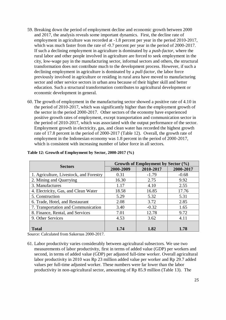
59. Breaking down the period of employment decline and economic growth between 2000

and 2017, the analysis reveals some important dynamics. First, the decline rate of

employment in agriculture was recorded at -1.8 percent per year in the period 2010-2017,

which was much faster from the rate of -0.7 percent per year in the period of 2000-2017.

If such a declining employment in agriculture is dominated by a push-factor, where the

rural labor and other people involved in agriculture are forced to seek employment in the

city, low-wage pay in the manufacturing sector, informal sectors and others, the structural

transformation does not contribute much to the development process. However, if such a

declining employment in agriculture is dominated by a pull-factor, the labor force

previously involved in agriculture or residing in rural area have moved to manufacturing

sector and other service sectors in urban area because of their higher skill and better

education. Such a structural transformation contributes to agricultural development or

economic development in general.

60. The growth of employment in the manufacturing sector showed a positive rate of 4.10 in

the period of 2010-2017, which was significantly higher than the employment growth of

the sector in the period 2000-2017. Other sectors of the economy have experienced

positive growth rates of employment, except transportation and communication sector in

the period of 2010-2017, which was associated with the output performance of the sector.

Employment growth in electricity, gas, and clean water has recorded the highest growth

rate of 17.8 percent in the period of 2000-2017 (Table 12). Overall, the growth rate of

employment in the Indonesian economy was 1.8 percent in the period of 2000-2017,

which is consistent with increasing number of labor force in all sectors.

Table 12: Growth of Employment by Sector, 2000-2017 (%)

Sectors Growth of Employment by Sector (%)

2000-2009 2010-2017 2000-2017

1. Agriculture, Livestock, and Forestry 0.31 -1.79 -0.68

2. Mining and Quarrying 16.30 2.75 9.92

3. Manufactures 1.17 4.10 2.55

4. Electricity, Gas, and Clean Water 18.58 16.85 17.76

5. Construction 5.29 5.32 5.31

6. Trade, Hotel, and Restaurant 2.08 3.72 2.85

7. Transportation and Communication 3.40 -0.32 1.65

8. Finance, Rental, and Services 7.01 12.78 9.72

9. Other Services 4.53 3.62 4.11

Total 1.74 1.82 1.78


61. Labor productivity varies considerably between agricultural subsectors. We use two

measurements of labor productivity, first in terms of added value (GDP) per workers and

second, in terms of added value (GDP) per adjusted full-time worker. Overall agricultural

labor productivity in 2010 was Rp 23 million added value per worker and Rp 29.7 added

values per full-time adjusted worker. These numbers were far lower than the labor

productivity in non-agricultural sector, amounting of Rp 85.9 million (Table 13). The

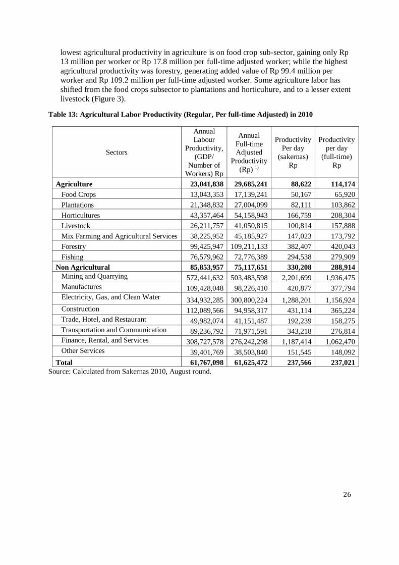
26

lowest agricultural productivity in agriculture is on food crop sub-sector, gaining only Rp

13 million per worker or Rp 17.8 million per full-time adjusted worker; while the highest

agricultural productivity was forestry, generating added value of Rp 99.4 million per

worker and Rp 109.2 million per full-time adjusted worker. Some agriculture labor has

shifted from the food crops subsector to plantations and horticulture, and to a lesser extent

livestock (Figure 3).

Table 13: Agricultural Labor Productivity (Regular, Per full-time Adjusted) in 2010

Sectors

Annual Labour

Productivity,

(GDP/

Number of Workers) Rp

Annual

Full-time Adjusted

Productivity

(Rp) 1)

Productivity

Per day

(sakernas)

Rp

Productivity

per day

(full-time)

Rp

Agriculture 23,041,838 29,685,241 88,622 114,174

Food Crops 13,043,353 17,139,241 50,167 65,920

Plantations 21,348,832 27,004,099 82,111 103,862

Horticultures 43,357,464 54,158,943 166,759 208,304

Livestock 26,211,757 41,050,815 100,814 157,888

Mix Farming and Agricultural Services 38,225,952 45,185,927 147,023 173,792

Forestry 99,425,947 109,211,133 382,407 420,043

Fishing 76,579,962 72,776,389 294,538 279,909

Non Agricultural 85,853,957 75,117,651 330,208 288,914

Mining and Quarrying 572,441,632 503,483,598 2,201,699 1,936,475

Manufactures 109,428,048 98,226,410 420,877 377,794

Electricity, Gas, and Clean Water 334,932,285 300,800,224 1,288,201 1,156,924

Construction 112,089,566 94,958,317 431,114 365,224

Trade, Hotel, and Restaurant 49,982,074 41,151,487 192,239 158,275

Transportation and Communication 89,236,792 71,971,591 343,218 276,814

Finance, Rental, and Services 308,727,578 276,242,298 1,187,414 1,062,470

Other Services 39,401,769 38,503,840 151,545 148,092

Total 61,767,098 61,625,472 237,566 237,021

Source: Calculated from Sakernas 2010, August round.

27

Figure 3: Number of agricultural workers (and share in agriculture sector) by subsector

Source: Processed from SAKERNAS (2017)

62. The level of education among the agriculture labor force is low. In 2000, 94 percent of

the labor force in agriculture had an educational attainment of junior high school or

lower, while the remainder of the labor force was educated above the level of junior high

school (Figure 4). In that same year, 63 percent of non-agriculture workers were educated

at junior high school or lower. While the proportion of post junior high school educated

agricultural workers increased by 2017 to 14%, the education gap between agriculture

and non-agriculture widened, with 51% of the non-agricultural work force being educated

above junior high. However, this may be partly explained by the ageing farmer

population.

14,443,677 , 40%

11,896,716 , 33%

3,180,006 , 9%

3,839,162 , 11%

2,564,325 , 7%

Agriculture Labor in 2017

Food Crops Plantations

Horticultures Livestock

Fishery, Forestry, Others

19,421,893 , 47%

12,563,090 , 30%

2,546,166 , 6%

4,135,545 , 10%

2,828,247 , 7%

Agriculture Labor in 2010

Food Crops Plantations

Horticultures Livestock

Fishery, Forestry, Others

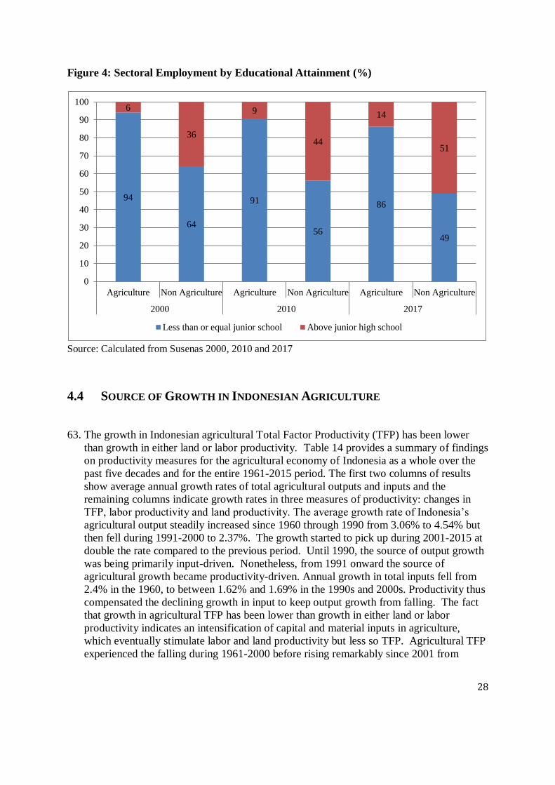
28

Figure 4: Sectoral Employment by Educational Attainment (%)

Source: Calculated from Susenas 2000, 2010 and 2017

4.4 SOURCE OF GROWTH IN INDONESIAN AGRICULTURE

63. The growth in Indonesian agricultural Total Factor Productivity (TFP) has been lower

than growth in either land or labor productivity. Table 14 provides a summary of findings

on productivity measures for the agricultural economy of Indonesia as a whole over the

past five decades and for the entire 1961-2015 period. The first two columns of results

show average annual growth rates of total agricultural outputs and inputs and the

remaining columns indicate growth rates in three measures of productivity: changes in

TFP, labor productivity and land productivity. The average growth rate of Indonesia’s

agricultural output steadily increased since 1960 through 1990 from 3.06% to 4.54% but

then fell during 1991-2000 to 2.37%. The growth started to pick up during 2001-2015 at

double the rate compared to the previous period. Until 1990, the source of output growth

was being primarily input-driven. Nonetheless, from 1991 onward the source of

agricultural growth became productivity-driven. Annual growth in total inputs fell from

2.4% in the 1960, to between 1.62% and 1.69% in the 1990s and 2000s. Productivity thus

compensated the declining growth in input to keep output growth from falling. The fact

that growth in agricultural TFP has been lower than growth in either land or labor

productivity indicates an intensification of capital and material inputs in agriculture,

which eventually stimulate labor and land productivity but less so TFP. Agricultural TFP

experienced the falling during 1961-2000 before rising remarkably since 2001 from

94

64

91

56

86

49

6

36

9

44

14

51

0

10

20

30

40

50

60

70

80

90

100

Agriculture Non Agriculture Agriculture Non Agriculture Agriculture Non Agriculture

2000 2010 2017

Less than or equal junior school Above junior high school

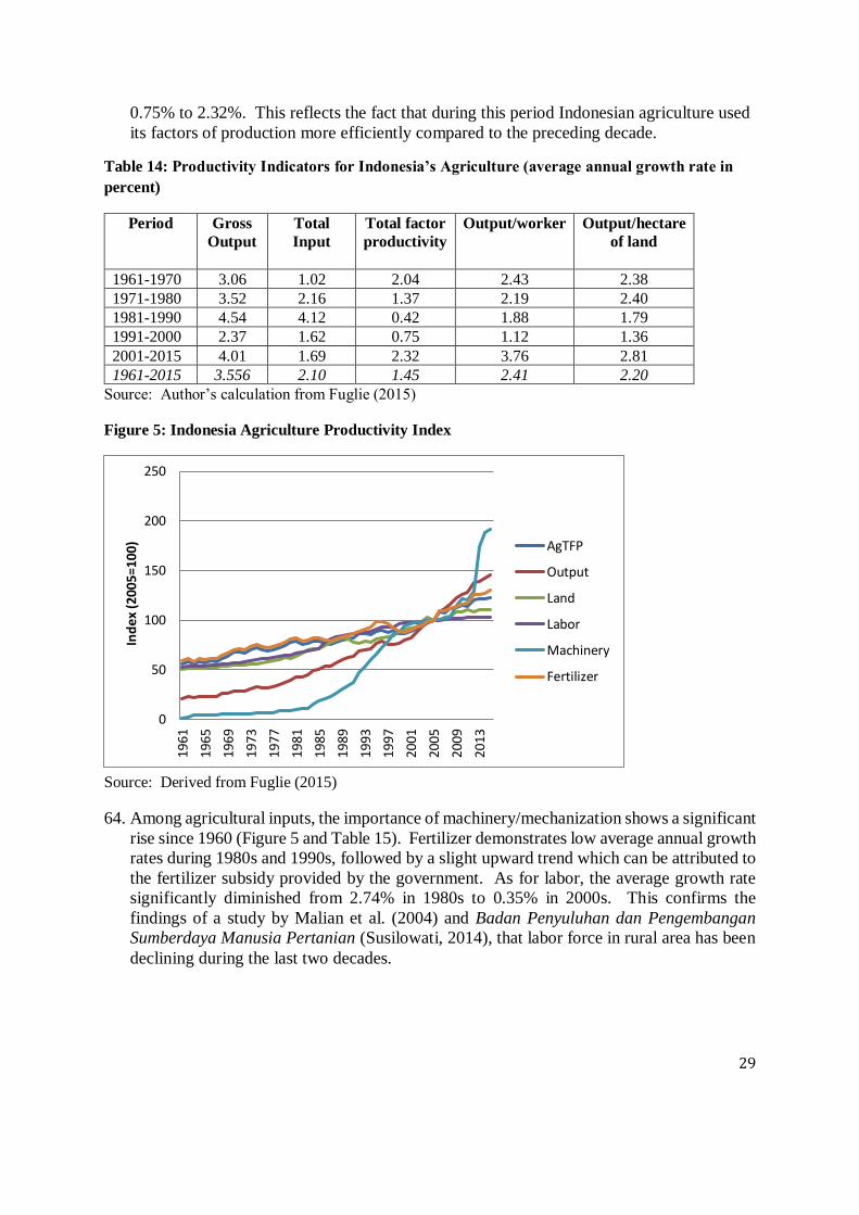
29

0.75% to 2.32%. This reflects the fact that during this period Indonesian agriculture used

its factors of production more efficiently compared to the preceding decade.

Table 14: Productivity Indicators for Indonesia’s Agriculture (average annual growth rate in

percent)

Period Gross

Output

Total

Input

Total factor

productivity

Output/worker Output/hectare

of land

1961-1970 3.06 1.02 2.04 2.43 2.38

1971-1980 3.52 2.16 1.37 2.19 2.40

1981-1990 4.54 4.12 0.42 1.88 1.79

1991-2000 2.37 1.62 0.75 1.12 1.36

2001-2015 4.01 1.69 2.32 3.76 2.81

1961-2015 3.556 2.10 1.45 2.41 2.20

Source: Author’s calculation from Fuglie (2015)

Figure 5: Indonesia Agriculture Productivity Index

Source: Derived from Fuglie (2015)

64. Among agricultural inputs, the importance of machinery/mechanization shows a significant

rise since 1960 (Figure 5 and Table 15). Fertilizer demonstrates low average annual growth

rates during 1980s and 1990s, followed by a slight upward trend which can be attributed to

the fertilizer subsidy provided by the government. As for labor, the average growth rate

significantly diminished from 2.74% in 1980s to 0.35% in 2000s. This confirms the

findings of a study by Malian et al. (2004) and Badan Penyuluhan dan Pengembangan

Sumberdaya Manusia Pertanian (Susilowati, 2014), that labor force in rural area has been

declining during the last two decades.

0

50

100

150

200

250

1961

1965

1969

1973

1977

1981

1985

1989

1993

1997

2001

2005

2009

2013

Ind

ex

(20

05

=10

0) AgTFP

Output

Land

Labor

Machinery

Fertilizer

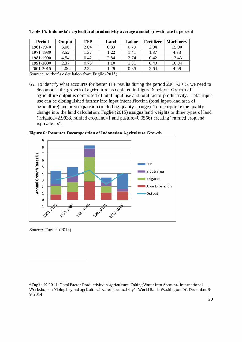
30

Table 15: Indonesia’s agricultural productivity average annual growth rate in percent

Period Output TFP Land Labor Fertilizer Machinery

1961-1970 3.06 2.04 0.83 0.79 2.04 15.00

1971-1980 3.52 1.37 1.22 1.41 1.37 4.33

1981-1990 4.54 0.42 2.84 2.74 0.42 13.43

1991-2000 2.37 0.75 1.10 1.31 0.40 10.34

2001-2015 4.00 2.32 1.29 0.35 2.64 4.69


65. To identify what accounts for better TFP results during the period 2001-2015, we need to

decompose the growth of agriculture as depicted in Figure 6 below. Growth of

agriculture output is composed of total input use and total factor productivity. Total input

use can be distinguished further into input intensification (total input/land area of

agriculture) and area expansion (including quality change). To incorporate the quality

change into the land calculation, Fuglie (2015) assigns land weights to three types of land

(irrigated=2.9933, rainfed cropland=1 and pasture=0.0566) creating “rainfed cropland

equivalents”.

Figure 6: Resource Decomposition of Indonesian Agriculture Growth

Source: Fuglie4 (2014)

4 Fuglie, K. 2014. Total Factor Productivity in Agriculture: Taking Water into Account. International Workshop on “Going beyond agricultural water productivity”. World Bank. Washington DC. December 8-9, 2014.

-1

0

1

2

3

4

5

6

7

8

9

An

nu

al G

row

th R

ate

(%)

TFP

input/area

Irrigation

Area Expansion

Output

31

66. Resource decomposition of agricultural growth shows that TFP became the major source

of agricultural growth in Indonesia in the last decade. Area expansion is the second

driver in agricultural output growth. Based on the land-weight assignment by Fuglie,

rainfed cropland dominates the agriculture land, however the growth in the past few years

has stagnated.

67. China’s and Malaysia’s agriculture TFP grew more rapidly than other countries in the

region, including Indonesia (Figure 7 and Table 16). Except Malaysia, all of these

countries experienced a downfall of TFP growth rate during 1980s, but China

demonstrated its productivity performance by rising at double digit growth rates. It

implies that China’s output growth became increasingly driven by the improvement of

immaterial values such as technology change, knowledge and skills compared to peer

Asian countries. China is also known as one of the largest agricultural producers (China

has by far the largest agricultural sector in the world, accounting for 24% of gross

agricultural output in 2013 according to FAO). Philippines, Thailand and India exhibit a

slightly decrease in TFP growth rate in the past decade.

Figure 7: Agricultural total factor productivity of some Asian countries

Source: Derived from Fuglie (2015)

0

20

40

60

80

100

120

140

160

1961

1964

1967

1970

1973

1976

1979

1982

1985

1988

1991

1994

1997

2000

2003

2006

2009

2012

2015

Agr

icu

ltu

re T

FP

China

Indonesia

Malaysia

Philippines

Thailand

Viet Nam

India

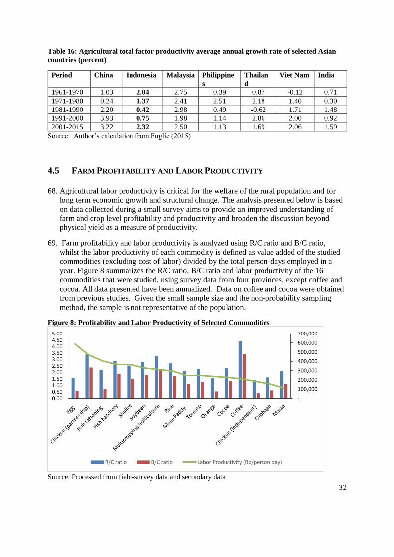
32

Table 16: Agricultural total factor productivity average annual growth rate of selected Asian

countries (percent)

Period China Indonesia Malaysia Philippine

s

Thailan

d

Viet Nam India

1961-1970 1.03 2.04 2.75 0.39 0.87 -0.12 0.71

1971-1980 0.24 1.37 2.41 2.51 2.18 1.40 0.30

1981-1990 2.20 0.42 2.98 0.49 -0.62 1.71 1.48

1991-2000 3.93 0.75 1.98 1.14 2.86 2.00 0.92

2001-2015 3.22 2.32 2.50 1.13 1.69 2.06 1.59


4.5 FARM PROFITABILITY AND LABOR PRODUCTIVITY

68. Agricultural labor productivity is critical for the welfare of the rural population and for

long term economic growth and structural change. The analysis presented below is based

on data collected during a small survey aims to provide an improved understanding of

farm and crop level profitability and productivity and broaden the discussion beyond

physical yield as a measure of productivity.

69. Farm profitability and labor productivity is analyzed using R/C ratio and B/C ratio,

whilst the labor productivity of each commodity is defined as value added of the studied

commodities (excluding cost of labor) divided by the total person-days employed in a

year. Figure 8 summarizes the R/C ratio, B/C ratio and labor productivity of the 16

commodities that were studied, using survey data from four provinces, except coffee and

cocoa. All data presented have been annualized. Data on coffee and cocoa were obtained

from previous studies. Given the small sample size and the non-probability sampling

method, the sample is not representative of the population.

Figure 8: Profitability and Labor Productivity of Selected Commodities

Source: Processed from field-survey data and secondary data

-

100,000

200,000

300,000

400,000

500,000

600,000

700,000

0.000.501.001.502.002.503.003.504.004.505.00

R/C ratio B/C ratio Labor Productivity (Rp/person day)

33

70. Labor productivity does not necessarily converge with the level of profitability of each

commodity. Coffee, for instance, although it exhibits relatively high profitability, its

labor productivity is not as high as expected. From the perspective of profitability, three

commodities appear to stand out: broilers (partnership model), coffee, and multi-cropping

horticulture farming system.

FOOD CROPS: RICE, MAIZE, AND SOYBEAN

71. In general, production of food crops generates profitability, as shown by the R/C ratio

being greater than 2.0 and B/C ratio greater than 1.0 for rice, maize, and soybean. The

average land productivity (yield) of rice in the study sites in North Sumatra is 5.1 ton/ha,

about similar to the national average of 5.2 ton/ha. The land productivity of maize in East

Nusa Tenggara is 2.24 ton/ha, which is much lower than the national average of 4.5

ton/ha. Maize farmers in Nusa Tenggara do not use certified seeds and rarely apply

chemical fertilizer due to the remoteness of the study sites and limited access of poor

maize farmers. Land productivity of soybean in Central Java is 2.31 ton/ha, far higher

than the national average of 1.5 ton/ha. The sample sites of Grobogan District and the

vicinity are the soybean production centers of the Province, where government programs

such as high-yielding seed, farmers’ empowerment for good agricultural practices (GAP)

etc. are frequently allocated to the soybean farmers.5

72. Smallholder farmers in Indonesia use less than one hectare for food crop production.

Survey respondents reported land holding sizes for rice, maize, and soybean of 0.58

hectare, 0.79 hectare, 0.75 hectare respectively. This number is consistent with the

national farmers’ panel survey (Patanas). Rice yields in North Sumatera are 5,000 to

5,750 Kg/Ha. The farm-gate price of rice received by farmers ranges from Rp 4,500 to

Rp 5,000 per kilogram and total revenue received by farmers is about Rp 24.1 million.

The total cost of rice production in the study was reported at Rp 9.3 million, mostly for

labor costs and land rental, so that the estimated profit or farm income is Rp 14.8 million.

The ratio between revenue and costs of rice production results in R/C ratio of 2.7, which

means that every Rp 1 of input will produce an output of Rp 2.7. This shows that rice

farming in North Sumatra is worth cultivating or providing financial benefits. The

estimated profit of 14.8 million per hectare is much higher than the recent estimates of

farm cost structure (SOUT) by BPS, suggesting the profit of Rp 4.95 million per hectare.

5 The government has allocated Rp 15 trillion for the “Special Efforts to Increase the Production of Rice, Maize

and Soybean” (Upsus Pajale), with the goal to achieve self-sufficiency in these commodities. This includes

providing subsidies for fertilizer, seeds, tractors, and other activities to empower smallholder farmers, even

involving military personnel in rural areas (Babinsa) in addition to the regular agricultural extension agents.

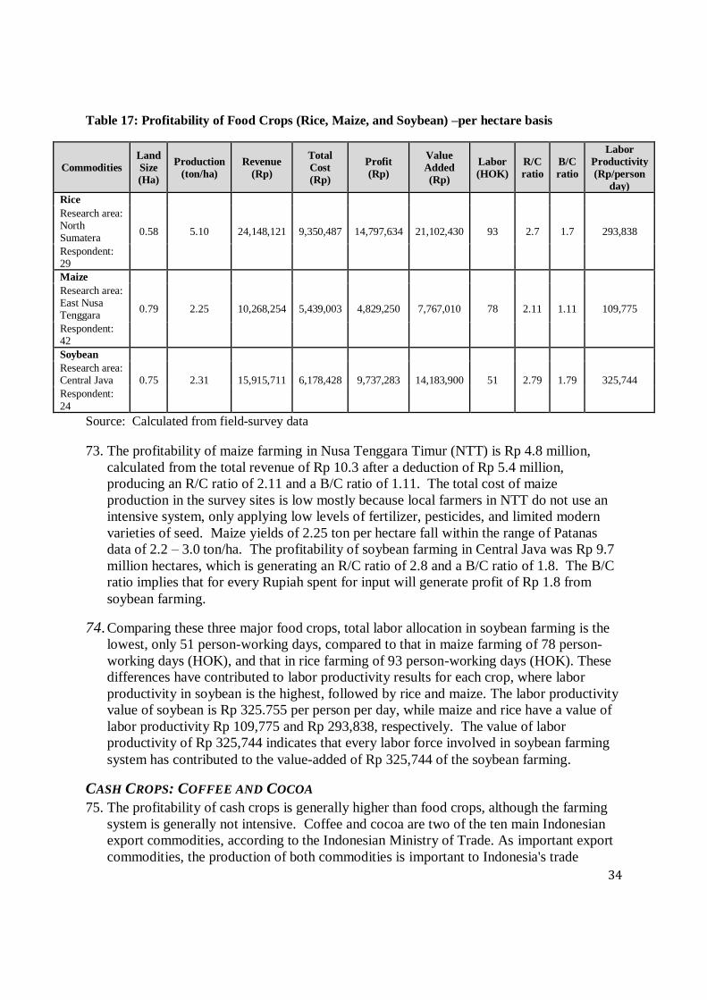
34

Table 17: Profitability of Food Crops (Rice, Maize, and Soybean) –per hectare basis

Commodities

Land

Size

(Ha)

Production

(ton/ha)

Revenue

(Rp)

Total

Cost

(Rp)

Profit

(Rp)

Value

Added

(Rp)

Labor

(HOK)

R/C

ratio

B/C

ratio

Labor

Productivity

(Rp/person

day)

Rice

0.58 5.10 24,148,121 9,350,487 14,797,634 21,102,430 93 2.7 1.7 293,838

Research area: North Sumatera

Respondent: 29

Maize

0.79 2.25 10,268,254 5,439,003 4,829,250 7,767,010 78 2.11 1.11 109,775

Research area: East Nusa Tenggara

Respondent: 42

Soybean

0.75 2.31 15,915,711 6,178,428 9,737,283 14,183,900 51 2.79 1.79 325,744 Research area: Central Java

Respondent:

24

Source: Calculated from field-survey data

73. The profitability of maize farming in Nusa Tenggara Timur (NTT) is Rp 4.8 million,

calculated from the total revenue of Rp 10.3 after a deduction of Rp 5.4 million,

producing an R/C ratio of 2.11 and a B/C ratio of 1.11. The total cost of maize

production in the survey sites is low mostly because local farmers in NTT do not use an

intensive system, only applying low levels of fertilizer, pesticides, and limited modern

varieties of seed. Maize yields of 2.25 ton per hectare fall within the range of Patanas

data of 2.2 – 3.0 ton/ha. The profitability of soybean farming in Central Java was Rp 9.7

million hectares, which is generating an R/C ratio of 2.8 and a B/C ratio of 1.8. The B/C

ratio implies that for every Rupiah spent for input will generate profit of Rp 1.8 from

soybean farming.

74. Comparing these three major food crops, total labor allocation in soybean farming is the

lowest, only 51 person-working days, compared to that in maize farming of 78 person-

working days (HOK), and that in rice farming of 93 person-working days (HOK). These

differences have contributed to labor productivity results for each crop, where labor

productivity in soybean is the highest, followed by rice and maize. The labor productivity

value of soybean is Rp 325.755 per person per day, while maize and rice have a value of

labor productivity Rp 109,775 and Rp 293,838, respectively. The value of labor

productivity of Rp 325,744 indicates that every labor force involved in soybean farming

system has contributed to the value-added of Rp 325,744 of the soybean farming.

CASH CROPS: COFFEE AND COCOA

75. The profitability of cash crops is generally higher than food crops, although the farming

system is generally not intensive. Coffee and cocoa are two of the ten main Indonesian

export commodities, according to the Indonesian Ministry of Trade. As important export

commodities, the production of both commodities is important to Indonesia's trade

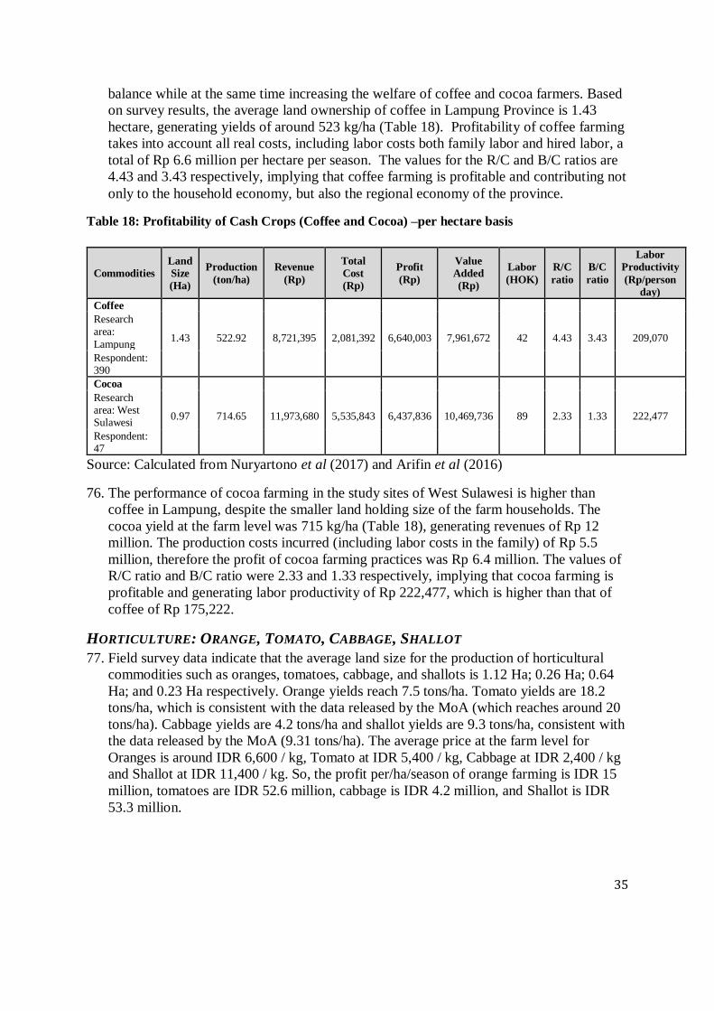
35

balance while at the same time increasing the welfare of coffee and cocoa farmers. Based

on survey results, the average land ownership of coffee in Lampung Province is 1.43

hectare, generating yields of around 523 kg/ha (Table 18). Profitability of coffee farming

takes into account all real costs, including labor costs both family labor and hired labor, a

total of Rp 6.6 million per hectare per season. The values for the R/C and B/C ratios are

4.43 and 3.43 respectively, implying that coffee farming is profitable and contributing not

only to the household economy, but also the regional economy of the province.

Table 18: Profitability of Cash Crops (Coffee and Cocoa) –per hectare basis

Source: Calculated from Nuryartono et al (2017) and Arifin et al (2016)

76. The performance of cocoa farming in the study sites of West Sulawesi is higher than

coffee in Lampung, despite the smaller land holding size of the farm households. The

cocoa yield at the farm level was 715 kg/ha (Table 18), generating revenues of Rp 12

million. The production costs incurred (including labor costs in the family) of Rp 5.5

million, therefore the profit of cocoa farming practices was Rp 6.4 million. The values of

R/C ratio and B/C ratio were 2.33 and 1.33 respectively, implying that cocoa farming is

profitable and generating labor productivity of Rp 222,477, which is higher than that of

coffee of Rp 175,222.

HORTICULTURE: ORANGE, TOMATO, CABBAGE, SHALLOT

77. Field survey data indicate that the average land size for the production of horticultural

commodities such as oranges, tomatoes, cabbage, and shallots is 1.12 Ha; 0.26 Ha; 0.64

Ha; and 0.23 Ha respectively. Orange yields reach 7.5 tons/ha. Tomato yields are 18.2

tons/ha, which is consistent with the data released by the MoA (which reaches around 20

tons/ha). Cabbage yields are 4.2 tons/ha and shallot yields are 9.3 tons/ha, consistent with

the data released by the MoA (9.31 tons/ha). The average price at the farm level for

Oranges is around IDR 6,600 / kg, Tomato at IDR 5,400 / kg, Cabbage at IDR 2,400 / kg

and Shallot at IDR 11,400 / kg. So, the profit per/ha/season of orange farming is IDR 15

million, tomatoes are IDR 52.6 million, cabbage is IDR 4.2 million, and Shallot is IDR

53.3 million.

Commodities

Land

Size

(Ha)

Production

(ton/ha)

Revenue

(Rp)

Total

Cost

(Rp)

Profit

(Rp)

Value

Added

(Rp)

Labor

(HOK)

R/C

ratio

B/C

ratio

Labor

Productivity

(Rp/person

day)

Coffee

1.43 522.92 8,721,395 2,081,392 6,640,003 7,961,672 42 4.43 3.43 209,070

Research area:

Lampung

Respondent: 390

Cocoa

0.97 714.65 11,973,680 5,535,843 6,437,836 10,469,736 89 2.33 1.33 222,477

Research area: West Sulawesi

Respondent: 47

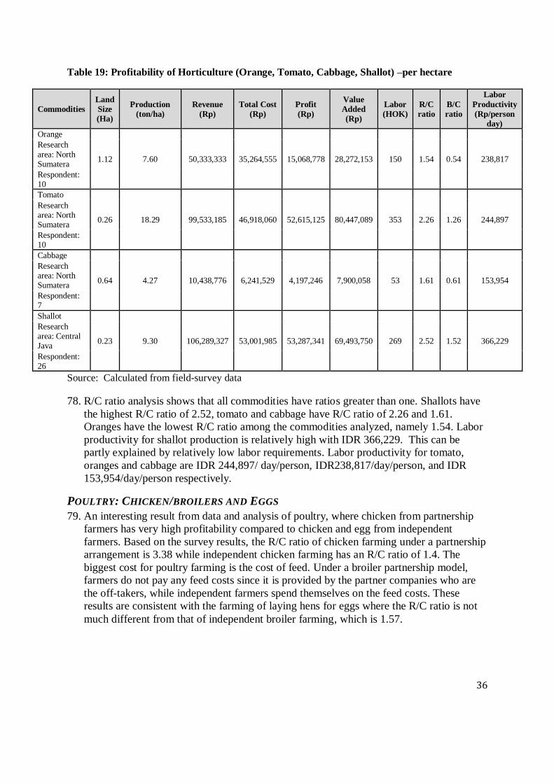
36

Table 19: Profitability of Horticulture (Orange, Tomato, Cabbage, Shallot) –per hectare

Commodities

Land

Size

(Ha)

Production

(ton/ha)

Revenue

(Rp)

Total Cost

(Rp)

Profit

(Rp)

Value

Added

(Rp)

Labor

(HOK)

R/C

ratio

B/C

ratio

Labor

Productivity

(Rp/person

day)

Orange

1.12 7.60 50,333,333 35,264,555 15,068,778 28,272,153 150 1.54 0.54 238,817

Research

area: North Sumatera

Respondent: 10

Tomato

0.26 18.29 99,533,185 46,918,060 52,615,125 80,447,089 353 2.26 1.26 244,897


Respondent: 10

Cabbage

0.64 4.27 10,438,776 6,241,529 4,197,246 7,900,058 53 1.61 0.61 153,954


Respondent: 7

Shallot

0.23 9.30 106,289,327 53,001,985 53,287,341 69,493,750 269 2.52 1.52 366,229

Research area: Central Java

Respondent: 26


78. R/C ratio analysis shows that all commodities have ratios greater than one. Shallots have

the highest R/C ratio of 2.52, tomato and cabbage have R/C ratio of 2.26 and 1.61.

Oranges have the lowest R/C ratio among the commodities analyzed, namely 1.54. Labor

productivity for shallot production is relatively high with IDR 366,229. This can be

partly explained by relatively low labor requirements. Labor productivity for tomato,

oranges and cabbage are IDR 244,897/ day/person, IDR238,817/day/person, and IDR

153,954/day/person respectively.

POULTRY: CHICKEN/BROILERS AND EGGS

79. An interesting result from data and analysis of poultry, where chicken from partnership

farmers has very high profitability compared to chicken and egg from independent

farmers. Based on the survey results, the R/C ratio of chicken farming under a partnership

arrangement is 3.38 while independent chicken farming has an R/C ratio of 1.4. The

biggest cost for poultry farming is the cost of feed. Under a broiler partnership model,

farmers do not pay any feed costs since it is provided by the partner companies who are

the off-takers, while independent farmers spend themselves on the feed costs. These

results are consistent with the farming of laying hens for eggs where the R/C ratio is not

much different from that of independent broiler farming, which is 1.57.

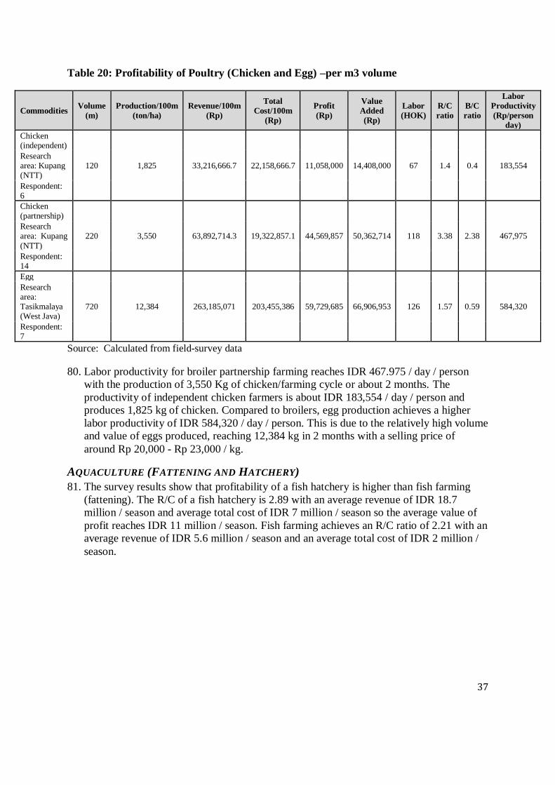
37

Table 20: Profitability of Poultry (Chicken and Egg) –per m3 volume

Commodities Volume

(m)

Production/100m

(ton/ha)

Revenue/100m

(Rp)

Total

Cost/100m

(Rp)

Profit

(Rp)

Value

Added

(Rp)

Labor

(HOK)

R/C

ratio

B/C

ratio

Labor

Productivity

(Rp/person

day)

Chicken (independent)

120 1,825 33,216,666.7 22,158,666.7 11,058,000 14,408,000 67 1.4 0.4 183,554 Research area: Kupang (NTT)

Respondent: 6

Chicken (partnership)

220 3,550 63,892,714.3 19,322,857.1 44,569,857 50,362,714 118 3.38 2.38 467,975 Research area: Kupang

(NTT)

Respondent: 14

Egg

720 12,384 263,185,071 203,455,386 59,729,685 66,906,953 126 1.57 0.59 584,320

Research area: Tasikmalaya (West Java)

Respondent: 7


80. Labor productivity for broiler partnership farming reaches IDR 467.975 / day / person

with the production of 3,550 Kg of chicken/farming cycle or about 2 months. The

productivity of independent chicken farmers is about IDR 183,554 / day / person and

produces 1,825 kg of chicken. Compared to broilers, egg production achieves a higher

labor productivity of IDR 584,320 / day / person. This is due to the relatively high volume

and value of eggs produced, reaching 12,384 kg in 2 months with a selling price of

around Rp 20,000 - Rp 23,000 / kg.

AQUACULTURE (FATTENING AND HATCHERY)

81. The survey results show that profitability of a fish hatchery is higher than fish farming

(fattening). The R/C of a fish hatchery is 2.89 with an average revenue of IDR 18.7

million / season and average total cost of IDR 7 million / season so the average value of

profit reaches IDR 11 million / season. Fish farming achieves an R/C ratio of 2.21 with an

average revenue of IDR 5.6 million / season and an average total cost of IDR 2 million /

season.

38

Table 21: Profitability of Aquaculture (Fresh water: Fattening and Hatchery) –per m3

Commodities Volume

(m)

Production/100

m

Revenue/100m

(Rp)

Total

Cost/100m

(Rp)

Profit Value

Added

Total

HOK

R/C

ratio

B/C

ratio

Labor

Productivity

(Rp/person

day)

Fish fattening

2,338.2 721.77 5,645,011 2,054,391 3,590,620 3,951,594 7 2.21 0.72 405,591

Research

area: West Java

Respondent: 15

Fish hatchery

1,435.7 692.67 18,756,046 7,097,232 11,658,814 12,967,032 36 2.89 1.9 366,468

Research area: West Java

Respondent: 14


82. The results for labor productivity show that fish farming has a slightly higher labor

productivity at IDR 405,591 / day / person compared to IDR 366,468 for the fish

hatchery. The amount of labor on fish farming is 7 mandays/harvest cycle mainly for

feeding and other maintenance. Labor requirements for a fish hatchery are more

demanding, especially during spawning or mating sires. In one harvest cycle the fish

hatchery requires an average of 36 person days.

MIXED FARMING: MINA-PADDY, HORTICULTURE

83. Mina-paddy is a farming system that combines rice and fish in one cultivated land area.

Survey results show that the average land ownership for mina-paddy is 1.6 ha. The

average revenue is IDR 59 million/season with the average cost of IDR 32.5

million/season. The R/C ratio for mina-paddy farming is 2.1, i.e. it appears financially

profitable. Labor productivity of mina-paddy is IDR 247,546 / day / person.

Table 22: Profitability of Mixed Farming (Mina-Paddy and Horticulture) –per hectare

Commodities

Land

Size

(Ha)

Production

(ton/ha)

Revenue

(Rp)

Total Cost

(Rp)

Profit

(Rp)

Value

Added

(Rp)

Labor

(HOK)

R/C

ratio

B/C

ratio

Labor

Productivity

(Rp/person

day)

Mina-Paddy

1.632 9,027 58,902,435 32,568,285 26,334,150 49,067,156 234 2.1 1.1 247,546 Research area:

West Java

Respondent: 8

Multicropping

holticulture

1.09 10,052 57,697,299 18,333,883 39,363,416 48,880,478 168 3.23 2.23 309,922

Potato, Chili,

Cabbage

Research area:

West Java

Respondent:


39

84. In the multi-cropping farming system that was included in the survey, a number of crops

are produced, mainly horticulture crops. Based on the survey data, the average land

ownership is 1.09 ha. Farmers receive an average revenue of IDR 57.6 million/season

with profit of around IDR 39.3 million/season. A multi-cropping system is more

profitable than monoculture, as confirmed by the R/C ratio of 3.23 and a labor

productivity of IDR 309.922 / day / person. The production inputs such as fertilizers,

chemicals, and labor are used simultaneously for various types of plants, which enhances

efficiency.

5. CONCLUSIONS

85. In the process of economic structural transformation, countries generally experience a

significant contraction in the share of employment in primary agriculture as growth rates

diverge between agriculture, industry and services, as agricultural production consolidates

into somewhat larger and often more mechanized units, and as surplus underemployed

agricultural labor is absorbed in other segments of the economy. With a lower proportion

of the workforce employed in agriculture and with a growing proportion of agricultural

workers coming to be involved with higher value segments of primary agriculture (i.e.

horticulture and animal production) there is a tendency for wages and productivity levels

in agriculture to converge with those in many segments of industry and services.

86. Middle-income Indonesia has been experiencing a reduction in the share of workers

engaged in primary agriculture, although the pace of this reduction is slower than the

contraction in primary agriculture’s share of national GDP and also slower than observed

patterns in many other peer countries in Asia. For a variety of reasons, other segments of

the economy have been slow to absorb surplus agricultural labor, resulting in significant

levels of seasonal or other underemployment of people in rural areas. Lack of

demographic pressures, small farm sizes, topographical challenges and other factors have

contributed to very low rates of mechanization in Indonesian agriculture. In 2017,

primary agriculture (including fisheries and forestry) remained by far the largest

employer in Indonesia with nearly 36 million people involved.

87. This study has found very large gaps in labor productivity between primary agriculture

and nearly all other segments of the Indonesian economy. While the estimated growth

rate in labor productivity has been quite a bit higher in agriculture than in some other

segments of the economy in the period of 2000 to 2017, the size of the productivity gap is

such that it will take many decades to fully close this gap based upon the current patterns.

The picture for Indonesia is somewhat unusual in that even the segments of agriculture

experiencing somewhat higher rates of labor productivity still lag or barely approximate

the productivity levels experienced in comparatively lower levels of industry (i.e.

construction) and services (i.e. hotel and restaurants).

88. This study utilized three sources of data to estimate agricultural labor productivity,

namely (i) Sakernas household survey data, (ii) prior surveys of smallholder tree crop

40

producers, and (iii) a small supplemental field survey covering several locations and a

range of staple and specialty food crops and animal or mixed farming systems. The

results convey a mixed picture, with some divergence between the Sakernas results and

those based upon surveys focused on specific commodities.

89. The Sakernas surveys point to patterns which are consistent with observations in other

Asian countries in which labor productivity for (relatively low unit value) food crops is

decidedly lower—by half or more—than is the case for horticulture, animal production,

mixed farming systems, and specialized plantation crops. The surveys focused on

individual crops or production systems point to a much more complex pattern. As

expected, labor productivity is comparatively higher in poultry and aquaculture

production and in some segments of horticulture which have received government

attention (i.e. shallot production). However, labor productivity is found to be quite a bit

lower in several horticultural crop specialties and in beverage crop production than in rice

cultivation. This pattern contrasts sharply with that found in Vietnam, a country which

has experienced considerable success both in raising rice productivity and in developing

large competitive cash crop industries. There, labor productivity in rice differs among

regions depending upon patterns of mechanization and commercialization, yet even in the

best circumstances this labor productivity is no more than one-third that experienced for

coffee or horticulture production.

90. The factors underpinning the observed patterns in Indonesia are not fully clear and

require additional work, including through more extensive field surveys which would

bring out greater variations among locations due to agro-ecological, farmer organization,

rural connectivity and other factors. Restrictions on competitive imports and various

programs of direct support have helped to boost the profitability of rice production in

parts of Indonesia, although this profitability remains modest and given very small

average farm sizes, inadequate to provide a solid living standard for most producing

households. Even among surplus rice growing households an increasing majority of

household income is now coming from other (including non-agricultural) sources.

91. Perhaps more surprising is the moderate to low level of profitability and/or labor

productivity associated with most horticultural and beverage crops in Indonesia. This is

alarming as one would expect these higher value commodities to provide for more

remunerative employment. Growing demand, both at home and abroad, should be

catalyzing farmers to invest further in these crops and to build up the requisite knowledge

base to improve product quality. More competitive horticultural and beverage crop

industries should then be achieving higher rates of productivity growth and be in a better

position to reward both skilled and unskilled labor. This dynamic does not seem to be

occurring, at least not on a broad scale.

92. This is of concern not only for realizing near term goals related to poverty reduction and

farm incomes, but also in relation to attracting and retaining entrepreneurial youth to

being Indonesia’s farmers of the future. Recent studies and consultative processes have

drawn attention to the challenges of productivity, profitability and competitiveness in

Indonesian horticulture and beverage crop industries. This study’s findings about low

labor productivity in these industries calls for a redoubling of efforts to strengthen the

provision of core public goods and services to such industries and to better facilitate

41

private investment in production technologies, advisory services, and downstream

logistical and marketing services.

93. There are multiple pathways to raise labor productivity in Indonesian agriculture and all

these should be further explored and re-enforced by appropriate government policies and

programs. For example:

• One important pathway will be efforts to achieve more economies scale in

smallholder production of staple food crops, by facilitating community-based land

consolidation, a more active market in agricultural land rentals and sales, and the

emergence of a dynamic market for provision of mechanized services covering

different components of the crop cycle. Reforms will be needed in land administration

and in the enabling environment for mechanized services.

• A second important pathway will be to encourage more diversified farming systems to

make fuller use of available labor and other resources as well as better mitigate

weather, pest and other risks. In place of monocrop systems, higher labor productivity

and remuneration may be possible through the introduction of rotations in lowland

rice-based systems (i.e. moving towards rice-vegetable, rice-aquaculture and other

rotations) and mixed agro-forestry systems. Single crop advisory services may need to

be replaced by technical support emphasizing whole farm management.

• A third critical pathway is through measures to increase productivity, value addition,

and risk management capabilities in higher value crop and animal production systems.

This may require interventions to improve biosecurity controls and practices, enable

farmers to acquire new knowledge and skills, foster greater rural entrepreneurship,

encourage more collective action in agricultural marketing, and strengthen the market

and other rural infrastructure to carry perishable and other higher value commodities.

42

REFERENCES

Alston, Julian M., Bruce A. Babcock, and Philip G. Pardey. 2012. "The Shifting Patterns of

Agricultural Production and Productivity Worldwide". Iowa State University. CARD Books.

http://lib.dr.iastate.edu/card_books/2

Arifin, Bustanul. 2014. The Roles of Input Policies in Transforming Agriculture in Indonesia. IFPRI

Working Paper 03, November 2014. Washington, D.C.: International Food Policy Research Institute.

http://www.ifpri.org/publication/roles-input-policies-transforming-agriculture-indonesia

Arifin, Bustanul, Katsuya Tanakan, Ryohei Kada, Hanung Ismono, Slamet Budiyuwono, and Fitri

Meystisari. 2018. “Sustainability of Rice Farming Practices in Lower Sekampung Watershed,

Indonesia”. Presented at Trepsea Conference on August 11-12 of 2018 in Gorontalo.

Arifin, Bustanul, Noer A. Achsani, Drajat Martianto, Linda Karlina Sari, Ahmad H Firdaus. 2018. Modeling the Future of Indonesian Food Consumption. Research Report submitted to the National

Development Planning Agency (Bappenas), World Food Programme (WFP) and Food and

Agricultural Organization of the United Nations (FAO). https://www.wfp.org/content/2018-

modeling-future-indonesia-food-consumption

Arifin, Bustanul. 2015. Ekonomi Pembangunan Pertanian (The Economics of Agricultural

Development). Second Edition. Bogor: IPB Press. 310 pages

Barrett, Christopher. 2011. “The Economics of Agricultural Development: An Overview.” In

Christopher Barrett, ed., Agricultural Development: Critical Concepts in Development Studies.

London: Routledge, 1–23.

Christiaensen, Luc, Lionel Demery and Jesper Kuhl. 2011. “The (evolving) role of agriculture

inpoverty reduction: An empirical perspective”, Journal of Development Economics 96: 239–254.

http://dx.doi.org/10.1016/j.jdeveco.2010.10.006

Doorward, Andrew. 2013. “Agricultural labour productivity, food prices and sustainable

development impacts and indicators”, Food Policy 39: 40-50,

http://dx.doi.org/10.1016/j.foodpol.2012.12.003

Fuglie, Keith O. (2015). "Accounting for Growth in Global Agriculture," Bio-based and Applied

Economics 4(3): 221-54.

Fuglie, Keith O. 2004. “Productivity Growth In Indonesian Agriculture 1961–2000”. Bulletin of

Indonesian Economic Studies, 40 (2): 209–25. http://dx.doi.org/10.1080/0007491042000205286

Fuglie, Keith O. 2008. “Is a slowdown in agricultural productivity growth contributing to the rise in

commodity prices?” Agricultural Economics 39: 431–441. https://dx.doi.org/10.1111/j.1574-

0862.2008.00349.x


http://www.ifpri.org/publication/roles-input-policies-transforming-agriculture-indonesia

https://www.wfp.org/content/2018-modeling-future-indonesia-food-consumption

https://www.wfp.org/content/2018-modeling-future-indonesia-food-consumption

http://dx.doi.org/10.1016/j.jdeveco.2010.10.006


http://dx.doi.org/10.1080/0007491042000205286

https://dx.doi.org/10.1111/j.1574-0862.2008.00349.x

https://dx.doi.org/10.1111/j.1574-0862.2008.00349.x

43

Fuglie, Keith O. 2008. “Indonesia: From Food Security to Market-Led Agricultural Growth” in Julian M Alston, Bruce A. Babcock, and Philip G. Pardey (Eds). 2012. "The Shifting Patterns of

Agricultural Production and Productivity Worldwide". Iowa State University. CARD Books. Pp: 343-

381. http://lib.dr.iastate.edu/card_books/2

Fuglie, Keith O. 2010. “Sources of Growth in Indonesian Agriculture” Journal of Productivity

Analysis 33: 225–240. http://dx.doi.org/10.1007/s11123-009-0150-x

Fuglie, Keith O, V Eldon Ball, and Sun Lin Wang (Eds). 2012. Productivity Growth in Agriculture:

An International Perspective. Washington DC.: USDA and CABI. 378 pages.

Fuglie, Keith O and Sun Lin Wang. 2013. New Evidence Points to Robust but Uneven Productivity

Growth in Global Agriculture. Global Journal of Emerging Market Economies, 5(1): 23–30.

http://dx.doi.org/10.1177/0974910112469266

Gollin, Douglas, Stephen Parente and Richard Rogerson. 2002. "The Role of Agriculture in

Development ." American Economic Review, 92(2):160-164.

Grabowski, Richard. 2015. “Agriculture, Labor Intensive Growth, and Structural Change: East Asia,

Southeast Asia, and Africa”, The Development Journal of the South, 1(1): 43-64.

Yujiro Hayami and Yoshihisa Godo. 2005. Development Economics: From the Poverty to the

Wealth of Nations. New York: Oxford University Press. 450 pages

Hermanto, 2018. “Hasil Survai Struktur Ongkos Usahatani Tanaman Pandi” (Survey Results of Cost

Structure of Paddy Farming), Paper presented at House of Rice on May 4, 2018 in Jakarta.

Imai, Katsushi S. Wenya Cheng and Raghav Gaiha. 2016. “Dynamic and long-term linkages among agricultural and non-agricultural growth, inequality and poverty in developing countries”,

International Review of Applied Economics, http://dx.doi.org/10.1080/02692171.2016.1249833

Imai, Katsushi S., Raghav Gaiha, Raghav and Alessandra Garbero. 2017. “Poverty Reduction during

the Rural-Urban Transformation: Rural development is still more important than Urbanisation”

Journal of Policy Modeling, https://dx.doi.org/10.1016/j.jpolmod.2017.10.002

Imai, Katsushi S., Raghav Gaiha and Fabrizio Bresciani. 2018. The Labour Productivity Gap between

Agricultural and Non-agricultural Sectors and Poverty in Asia. Discussion Paper. Research Institute

for Economics and Business Administration. Kobe University. Japan. https://www.rieb.kobe-

u.ac.jp/academic/ra/dp/English/DP2017-04.pdf

Malian AH, Friyatno S, Dermoredjo SK, Mardiyanto S, Suryadi M, Maulana M. 2004. Analisis

perkembangan aset, kesempatan kerja dan pendapatan rumah tangga di sektor pertanian. Laporan

Akhir Penelitian. Bogor (ID): Pusat Penelitian dan Pengembangan Sosial Ekonomi Pertanian

Organization of Economic Cooperation and Development (OECD). 2012. OECD Review of Agricultural Policies: Indonesia 2012. OECD Publishing. 229 pages.

http://dx.doi.org/10.1787/9789264179011-en


http://dx.doi.org/10.1007/s11123-009-0150-x

http://dx.doi.org/10.1177/0974910112469266

http://dx.doi.org/10.1080/02692171.2016.1249833

https://dx.doi.org/10.1016/j.jpolmod.2017.10.002

https://www.rieb.kobe-u.ac.jp/academic/ra/dp/English/DP2017-04.pdf

https://www.rieb.kobe-u.ac.jp/academic/ra/dp/English/DP2017-04.pdf

http://dx.doi.org/10.1787/9789264179011-en

44

Kim, Tai-Yo, Keshmati, A. and Jihyoun Park. 2014. “Decelerating Agricultural Society: Theoretical and Historical Perspectives” in Tai-Yoo Kim and Almas Heshmati (Eds). Economic Growth: The

New Perspectives for Theory and Policy. New York: Springer. Pp: 21-56

Kim, Tai-Yoo and Almas Heshmati (Eds). 2014. Economic Growth: The New Perspectives for

Theory and Policy. New York: Springer. 323 pages.

McCullough, Ellen B. 2017. “Labor productivity and employment gaps in sub-Saharan Africa”. Food

Policy, 67: 133–152. http://dx.doi.org/10.1016/j.foodpol.2016.09.013

Mellor, John W (Ed.). 1995. Agriculture on the Road to Industrialisation. IFPRI/John Hopkins

Press. 358 pages. http://www.ifpri.org/publication/agriculture-road-industrialization-0

Mellor, John W. 2017. Agricultural Development and Economic Transformation: Promoting Growth

with Poverty Reduction. New York: Palgrave MacMillan. 259 pages.

Mundlak, Yair. 2000. Agriculture and Economic Growth: Theory and Measurement. Cambridge:

Harvard University Press, Cambridge, MA

Naylor, Rosamond. 2011. “Expanding the boundaries of agricultural development”, Food Security 3,

233–251. http://dx.doi.org/10.1007/s12571-011-0123-6

Rosegrant. Mark W, Faisal Kasryno, Nicostrato D. Perez. 1998. “Output response to prices and public investment in agriculture: Indonesian food crops”, Journal of Development Economics, 55:

333-352

Susilowati, SH. 2014. Attracting the young generation to engage in agriculture. FFTC-RDA 2014 International Seminar on Enhanced Entry of Young Generation into Farming; 2014 Oct 20-24; Jeonju,

Korea.

Timmer, C. Peter. 1988. “The Agricultural Transformation.” In H. Chenery and T.N. Srinivasan, eds.,

Handbook of Development Economics, Vol. 1. Amsterdam: North-Holland, 275–331.

Timmer, C. Peter. 1989. “Food Price Policy: The Rationale for Government Intervention.” Food

Policy 14: 17–42.

Timmer, C. Peter. 2009. “A World without Agriculture: The Structural Transformation in Historical

Perspective”, Henry Wendt Lecture, American Enterprise Institute.

Timmer, C. Peter. 2010. “Reflections on food crises past”. Food Policy 35, 1–11.

https://dx.doi.org/10.1016/j.foodpol.2009.09.002

World Bank. 2012. “Indonesia: Agriculture Public Expenditure Review”. Washington DC.: the

World Bank. http://documents.worldbank.org/curated/en/146351468040728696/Public-

expenditure-review-summary


http://www.ifpri.org/publication/agriculture-road-industrialization-0

http://dx.doi.org/10.1007/s12571-011-0123-6

https://dx.doi.org/10.1016/j.foodpol.2009.09.002

http://documents.worldbank.org/curated/en/146351468040728696/Public-expenditure-review-summary

http://documents.worldbank.org/curated/en/146351468040728696/Public-expenditure-review-summary

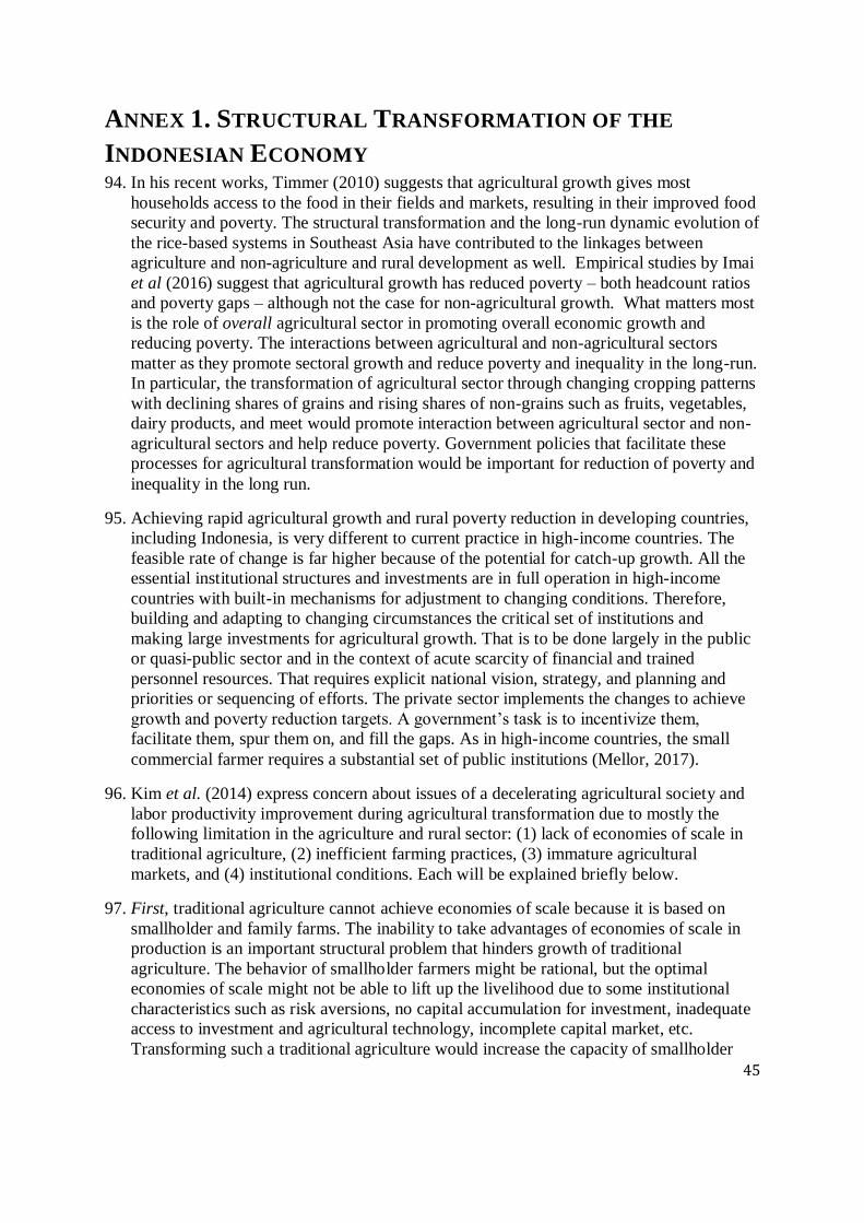
45

ANNEX 1. STRUCTURAL TRANSFORMATION OF THE

INDONESIAN ECONOMY 94. In his recent works, Timmer (2010) suggests that agricultural growth gives most

households access to the food in their fields and markets, resulting in their improved food

security and poverty. The structural transformation and the long-run dynamic evolution of

the rice-based systems in Southeast Asia have contributed to the linkages between

agriculture and non-agriculture and rural development as well. Empirical studies by Imai

et al (2016) suggest that agricultural growth has reduced poverty – both headcount ratios

and poverty gaps – although not the case for non-agricultural growth. What matters most

is the role of overall agricultural sector in promoting overall economic growth and

reducing poverty. The interactions between agricultural and non-agricultural sectors

matter as they promote sectoral growth and reduce poverty and inequality in the long-run.

In particular, the transformation of agricultural sector through changing cropping patterns

with declining shares of grains and rising shares of non-grains such as fruits, vegetables,

dairy products, and meet would promote interaction between agricultural sector and non-

agricultural sectors and help reduce poverty. Government policies that facilitate these

processes for agricultural transformation would be important for reduction of poverty and

inequality in the long run.

95. Achieving rapid agricultural growth and rural poverty reduction in developing countries,

including Indonesia, is very different to current practice in high-income countries. The

feasible rate of change is far higher because of the potential for catch-up growth. All the

essential institutional structures and investments are in full operation in high-income

countries with built-in mechanisms for adjustment to changing conditions. Therefore,

building and adapting to changing circumstances the critical set of institutions and

making large investments for agricultural growth. That is to be done largely in the public

or quasi-public sector and in the context of acute scarcity of financial and trained

personnel resources. That requires explicit national vision, strategy, and planning and

priorities or sequencing of efforts. The private sector implements the changes to achieve

growth and poverty reduction targets. A government’s task is to incentivize them,

facilitate them, spur them on, and fill the gaps. As in high-income countries, the small

commercial farmer requires a substantial set of public institutions (Mellor, 2017).

96. Kim et al. (2014) express concern about issues of a decelerating agricultural society and

labor productivity improvement during agricultural transformation due to mostly the

following limitation in the agriculture and rural sector: (1) lack of economies of scale in

traditional agriculture, (2) inefficient farming practices, (3) immature agricultural

markets, and (4) institutional conditions. Each will be explained briefly below.

97. First, traditional agriculture cannot achieve economies of scale because it is based on

smallholder and family farms. The inability to take advantages of economies of scale in

production is an important structural problem that hinders growth of traditional

agriculture. The behavior of smallholder farmers might be rational, but the optimal

economies of scale might not be able to lift up the livelihood due to some institutional

characteristics such as risk aversions, no capital accumulation for investment, inadequate

access to investment and agricultural technology, incomplete capital market, etc.

Transforming such a traditional agriculture would increase the capacity of smallholder

46

farmers, access to innovation and technological change, supportive public policies to

improve access to financial institution for capital formation.

98. Second, inefficient farming practices might experience low level of growth because of

low productivity from lack of modern technologies. Modern agriculture might also be

inferior to other industries, so that the the transition from an agricultural to an industrial

economy moves the society to a more developed state. Therefore, a significant

improvement in agricultural productivity is necessary to contribute to the development

economic process. The neo-classical theory of economic development suggests that the

movement of productive resources to industry promotes economic growth. In this case,

economic growth is achieved by transferring the input factor from a simple reproduction

sector to an expansive-reproduction sector (Johnston and Mellor (1961), Mellor (1995)

and Mellor (2017). However, Matsuyama (1991) and Hayami (2001) argues that low

productivity in agriculture may promote industrialization of an economy because

relatively low income encourages labor to move into higher productive manufacturing.

There might a situation where high productivity in agriculture hinders the development of

manufacturing, because the surplus of agriculture production may trap people in choosing

a career in agriculture. A self-fulfilling expectation of future job opportunities can play a

key role in the economy’s adjustment processes.

99. Third, smallholder farmers usually have difficulties in responding quickly to changes in

market conditions so that the supply is therefore inelastic in product or price dimensions.

The basic Engel’s law suggests that income elasticity of agricultural products, mostly

food products, is generally less than that of industrial products. Even, the relative

importance of agricultural production decreases as the economy grows due to the

characteristics of income elasticity explained above. Therefore, the improvement rate of

agricultural technology contributes much more to the economic growth than to the

improvement rate of agricultural technology.

100. Fourth, the performance of structural transformation is generally affected by the

levels of agricultural productivity, which comprehensively also reflect the taxation,

regulation, property rights, institutions, and natural environments of each country. Gollin

et al. (2002) suggests that low agricultural productivity can substantially delay

industrialization. Improvements in agricultural productivity can hasten the start of

industrialization and, hence, have large effects on a country’s relative income. In the

short run, such changes will have a larger impact than comparable increases in

nonagricultural productivity. Although in the long run, it is productivity in the

nonagricultural sector that determines a country’s position relative to the leader or other

countries. As the productivity of non-agriculture is higher than that of agriculture, the

capability of the agriculture sector to release resources to non-agricultural sectors

eventually contributes to economic development. Therefore, agricultural development

should be investigated not only within the sector but also in the context of the general

economy (Mundlak, 2000). Policies, particularly those regarding government

expenditure and trade, affect the productivity and human capital resource accumulation in

agriculture. When those policies become unfavorable for the modern agricultural sector,

large amounts of capital and labor migrate from the agricultural sector to other sectors.

This migration is affected by changes in input factor availability and technology as the

economic growth progressed.

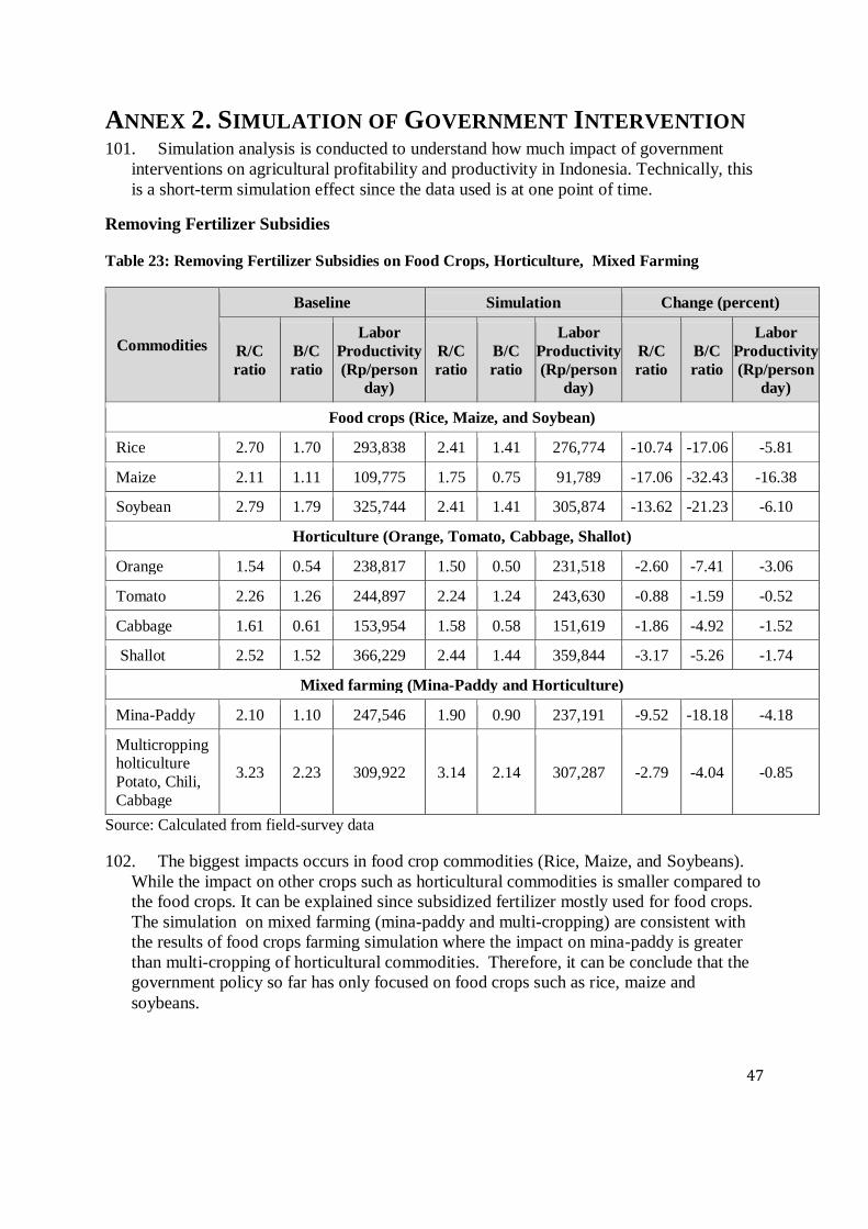
47

ANNEX 2. SIMULATION OF GOVERNMENT INTERVENTION 101. Simulation analysis is conducted to understand how much impact of government

interventions on agricultural profitability and productivity in Indonesia. Technically, this

is a short-term simulation effect since the data used is at one point of time.

Removing Fertilizer Subsidies

Table 23: Removing Fertilizer Subsidies on Food Crops, Horticulture, Mixed Farming


102. The biggest impacts occurs in food crop commodities (Rice, Maize, and Soybeans).

While the impact on other crops such as horticultural commodities is smaller compared to

the food crops. It can be explained since subsidized fertilizer mostly used for food crops.

The simulation on mixed farming (mina-paddy and multi-cropping) are consistent with

the results of food crops farming simulation where the impact on mina-paddy is greater

than multi-cropping of horticultural commodities. Therefore, it can be conclude that the

government policy so far has only focused on food crops such as rice, maize and

soybeans.

Commodities

Baseline Simulation Change (percent)

R/C

ratio

B/C

ratio

Labor

Productivity

(Rp/person

day)

R/C

ratio

B/C

ratio

Labor

Productivity

(Rp/person

day)

R/C

ratio

B/C

ratio

Labor

Productivity

(Rp/person

day)

Food crops (Rice, Maize, and Soybean)

Rice 2.70 1.70 293,838 2.41 1.41 276,774 -10.74 -17.06 -5.81

Maize 2.11 1.11 109,775 1.75 0.75 91,789 -17.06 -32.43 -16.38

Soybean 2.79 1.79 325,744 2.41 1.41 305,874 -13.62 -21.23 -6.10

Horticulture (Orange, Tomato, Cabbage, Shallot)

Orange 1.54 0.54 238,817 1.50 0.50 231,518 -2.60 -7.41 -3.06

Tomato 2.26 1.26 244,897 2.24 1.24 243,630 -0.88 -1.59 -0.52

Cabbage 1.61 0.61 153,954 1.58 0.58 151,619 -1.86 -4.92 -1.52

Shallot 2.52 1.52 366,229 2.44 1.44 359,844 -3.17 -5.26 -1.74

Mixed farming (Mina-Paddy and Horticulture)

Mina-Paddy 2.10 1.10 247,546 1.90 0.90 237,191 -9.52 -18.18 -4.18

Multicropping holticulture

Potato, Chili,

Cabbage

3.23 2.23 309,922 3.14 2.14 307,287 -2.79 -4.04 -0.85

48

Removing Subsidies for Soybean Seed

Table 24: Removing Subsidies for Soybean Seed


103. The Grobogan district government provides subsidized soybean seeds for farmers to

increase the soybean production in the district. This simulation explains that the revokes

the subsidized soybean seed policy will have major impacts on reducing the profitability

and productivity of labor in soybean farming.

Simulation of Government Policy on Agricultural Outputs

Table 25: Removing Price Support on Rice


104. If the government implements purchase price policy on rice grain, it will have an

impact on reducing profitability and productivity in the rice farming. So far, the the farm

level prices for the rice is relatively safe. The purchase price policy is not applied to

horticultural commodities (such as oranges, tomatoes and cabbage) and the analysis found

that profitability and productivity of the farmers will be very dependent on the selling

prices, therefore this intervention will not have any impacts to other commodities.

Commodity


R/C

ratio

B/C

ratio

Labor

Productivity

(Rp/person

day)

R/C

ratio

B/C

ratio

Labor

Productivity

(Rp/person

day)

R/C

ratio

B/C

ratio

Labor

Productivity

Soybean 2.79 1.79 325,744 2.60 1.60 317,483 -6.81 -10.61 -2.54

Commodity


R/C

ratio

B/C

ratio

Labor

Productivity

(Rp/person

day)

R/C

ratio

B/C

ratio

Labor

Productivity

(Rp/person

day)

R/C

ratio

B/C

ratio

Labor

Productivity

Rice 2.70 1.70 293,838 2.12 1.12 216,953 -21.48 -34.12 -26.17

49

ANNEX 3. DETERMINANTS OF PROFITABILITY AND

FARMER INCOMES

Determinants of Profitability

105. The relationship between profitability and labor productivity in this study was carried

out by conducting a simple regression with profitability as the dependent variable and

labor productivity as an independent variable. The equation of model as below:

𝐿𝑛𝑃𝑟𝑜𝑓𝑖𝑡𝑎𝑏𝑙𝑖𝑡𝑦𝑖 = 𝛼 + 𝐿𝑛𝐿𝑎𝑏𝑜𝑟𝑃𝑟𝑜𝑑𝑢𝑐𝑡𝑖𝑣𝑖𝑡𝑦𝑖𝛽 + 𝑒𝑖

The regression results show that labor productivity is significant to the profitability of farmers.

Coefficient values show the value of elasticity of profitability to changes in labor productivity.

Table 26: Regression Analysis of Determinant of Profitability of Farming Systems

Sector Coefficient T stat (P

Value)

Obs R-Squared

All Crops 0.457 15.20 (0.000) 228 0.299

Food Crops 0.383 10.04 (0.000) 95 0.515

Horticulture 0.551 9.60 (0.000) 51 0.646

Aquaculture 0.404 4.10 (0.000) 29 0.360

Poultry 0.662 3.59 (0.001) 27 0.314

Mixed Farming 0.720 8.81 (0.000) 26 0.754

Source: field survey data are processed

106. The regression result for “all crops” yields a coefficient of 0.457, meaning that if

labor productivity increases by 1 percent, the profitability of farmers will increase by

0.457 percent, ceteris paribus. The lowest elasticity value is produced by food crops with

a coefficient of 0.383. While the highest elasticity value is produced by mixed farming

with a coefficient of 0.72.

Determinants of Farmers’ Income

107. Factors that influence farmers' income in this study were carried out by regression. a

standard linear econometric model of farmers’ incomes can be applied. econometric

model for analyze farmers’ income can be modeled as follows:

𝑌𝑖 = 𝛼 + 𝑋𝑖′𝛽 + 𝑍𝑖

′𝛾 + 𝑒𝑖

where: 𝑌𝑖 represents farmers’ income, 𝑋𝑖′ is a vector of main variable of input such as: labor

cost, agriculture input cost, and farm land size. 𝑍𝑖′ denotes control variables of household

such as Age, education level, household size, and farmers’ experience.

50

Table 27: Regression Analysis of Determinant of Farmers’ Income

Independent

Variables

Dependent Variable : ln_Income

Model 1

(all crops)

Model 2

(without poultry

and aquaculture)

Model 3

(poultry and

aquaculture)

Model 4

(Mixed Farming)

Ln_laborcost 0.601*** 0.567*** 0.816*** 0.622***

Ln_agriinputcost 0.423*** 0.420*** 0.293*** 0.473**

Land_size 0.164** 0.079 0.191

Age 0.012 -0.046 0.002 -0.182

Education 0.092** 0.003 0.130 0.150

Experience 0.003 0.063 0.006

Hhsize 0.055*** 0.040* 0.036 0.141

Constanta 0.859** 1.514** 0.010 -0.735

Adj R-Squared 0.870 0.889 0.887 0.835


Noted: *significant at α = 10%, ** significant at α = 5%, *** significant at α = 1%.

108. Based on the regression results of model 1 (all crops), significant factors affecting

farmers’ income are labor costs, agricultural input costs, education level, and household

size. Model 2 in this analysis excludes aquaculture and poultry. Variable that significantly

influence farmers’ income are labor cost, agricultural input costs, farm land size, and

household size. Results from model 3 (poultry and aquaculture) and model 4 (mixed

farming) suggest that farmer income influenced by labor cost and the cost of agricultural

inputs.

109. In addition to the above model, alternative models can be constructed to examine the

effect of farming type on farmer income. Based on the results, it can be concluded that

food crops cultivation will have a significant negative effect on farmer income. In

contrast, horticulture, poultry, and mixed farming have a significantly positive effect on

farmer income. As a control variable, land ownership, education, and household size have

a positive effect on farmer income. And in general, the age variable of the farmer and

farming experience does not have a significant effect on farmer income, except in

horticulture farming where the age of the farmer has a negative effect on farmer income.

51

Table 28: Regression Analysis of Determinant of Farmers’ Income

Independent

Variables

Dependent Variable : ln_income

Model 1

Food crops

Model 2

Horticulture

Model 3

poultry

Model 4

Aquaculture

Model 5

Mixed Farming

D_FoodCrops -1.850*** - - - -

D_Horticulture - 0.967*** - - -

D_Poultry - - 1.932*** - -

D_Aquaculture - - - -0.130 -

D_Mixedfarming - - - - 1.031***

Land size 1.005*** 0.909*** 0.996*** 0.785*** 0.576***

Age -0.010 0.006 -0.011 0.003 0.003

Education 0.042* 0.085*** 0.030 0.068** 0.062**

Experience 0.007 -0.018* 0.001 -0.015 -0.011

Hhsize 0.103** 0.067 0.001 0.058 0.087

Constanta 16.712*** 13.315*** 16.425*** 15.896*** 15.689***

Adj R-Squared 0.431 0.176 0.241 0.107 0.146


Note: *significant at α = 10%, ** significant at α = 5%, *** significant at α = 1%.

Profit Function Analysis

110. A profit function analysis is carried out to determine the effect of input prices on

farmers' income in Indonesia. To analyze these relationships we use a simple regression

and the Cobb-Douglas profit function model.

Table 29: Regression Analysis of Profit Function

Independent

Variables

Dependent Variable : ln_profit Model 1

(all crops)

Model 2

(Food crops)

Model 3

(Horticulture)

Model 4

(Poultry)

Model 5

(Aquaculture)

Model 6 (Mixed

Farming)

ln_inputprice -

0.238***

-0.467 -0.014 0.029 0.462** 0.121

ln_laborprice 0.872*** 1.117*** 0.216 4.286*** 1.044*** 0.267 Land 0.784*** 1.061*** 1.076 1.662** 1.150* 1.056***

Constant 4.884*** 3.466*** 6.713*** 4.760*** 5.029*** 6.358***

Adj R-Squared 0.255 0.310 0.142 0.739 0.747 0.727

Noted: *significant at α = 10%, ** significant at α = 5%, *** significant at α = 1%.

111. There are 6 different models for analyzing all crops, including poultry and

aquaculture. In general, prices of agricultural inputs, labor wages, and land ownership

have a significant effect on farmers' profits. The price of agricultural inputs has a negative

influence on farmers' profits. Labor wages have a positive influence on farmers' profits,

indicating positive labor productivity of hired labor. Based on the previous analysis, an

52

increase in productivity will have a positive effect on farmer profitability. Land

ownership as a fixed input also has a positive influence on farmers' profits, where the

addition of land will increase production capacity and profits.

112. The results of the analysis on the agricultural sector of food crops and poultry,

farmers’ profits are positively influenced by labor wages, and land ownership. There is no

variable in the horticulture sector that has a significant effect on farmer profits. In the

aquaculture sector, all variables have a positive effect on farmer profits. And in the mixed

farming sector, only land ownership influences farmers' profits.

Profitability and Labor Productivity in Indonesian Agriculture

Documents

Transcript of Profitability and Labor Productivity in Indonesian Agriculture