The Profitability of Momentum Investing

Testing a Practical Momentum Strategy

by

Ekkehard Arne Friedrich

Dissertation presented in fulfilment of the requirements for the degree

MSc (EngineeringManagement) at the

University of Stellenbosch

Supervisor: Mr. Konrad von Leipzig

Department of Industrial Engineering

March 2010

i | P a g e

Acknowledgements

I would like to extend a hearty word of thanks to the following persons:

My mentor and the originator of this project, Tom de Lange for sharing his knowledge around

feasible momentum investing strategies and their practical implementation. Tom also supplied most

of the software and the JSE data and offered some financial support.

My study leader, Konrad von Leipzig for his guidance and for accommodating this rather unusual

project.

My parents for financial and psychological support.

My office colleagues for their wit and their friendship.

ii | P a g e

Declaration

By submitting this dissertation electronically, I declare that the entirety of the work contained therein is

my own, original work, that I am the owner of the copyright thereof (unless to the extent explicitly

otherwise stated) and that I have not previously in its entirety or in part submitted it for obtaining any

qualification.

March 2010

Copyright © 2010 Stellenbosch University

All rights reserved

iii | P a g e

Abstract

Several studies have shown that abnormal returns can be generated simply by buying past winning

stocks and selling past losing stocks. Being able to predict future price behaviour by past price

movements represents a direct challenge to the Efficient Market Hypothesis, a centrepiece of

contemporary finance.

Fund managers have attempted to exploit this effect, but reliable footage of the performance of such

funds is very limited. Several academic studies have documented the presence of the momentum effect

across different markets and between different periods. These studies employ trading rules that might

be helpful to establish whether the momentum effect is present in a market or not, but have limited

practical value as they ignore several practical constraints.

The number of shares in the portfolios formed by academic studies is often impractical. Some studies

(e.g. Conrad & Kaul, 1998) require holding a certain percentage of every share in the selection universe,

resulting in an extremely large number of shares in the portfolios. Others create portfolios with as little

as three shares (e.g. Rey & Schmid, 2005) resulting in portfolios that are insufficiently diversified. All

academic studies implicitly require extremely high portfolio turnover rates that could cause transaction

costs to dissipate momentum profits and lead the returns of such strategies to be taxed at an investor’s

income tax rate rather than her capital gains tax rate. Depending on the tax jurisdiction within which the

investor resides these tax ramifications could represent a tax difference of more than 10 percent, an

amount that is unlikely to be recovered by any investment strategy.

Critics of studies documenting positive alpha argue that momentum returns may be due to statistical

biases such as data mining or due to risk factors not effectively captured by the standard CAPM. The

empirical tests conducted in this study were therefore carefully designed to avoid every factor that

could compromise the results and hinder a meaningful interpretation of the results. For example, small-

caps were excluded to avoid the small firm effect from influencing the results and the tests were

conducted on two different samples to avoid data mining from being a possible driver. Previous

momentum studies generally used long/short strategies. It was found, however, that momentum

iv | P a g e

strategies generally picked short positions in volatile and illiquid stocks, making it difficult to effectively

estimate the transaction costs involved with holding such positions. For this reason it was chosen to test

a long-only strategy.

Three different strategies were tested on a sample of JSE mid-and large-caps on a replicated S&P500

index between January 2000 and September 2009. All strategies yielded positive abnormal returns and

the null hypothesis that feasible momentum strategies cannot generate statistically significant abnormal

returns could be rejected at the 5 percent level of significance for all three strategies on the JSE sample.

However, further analysis showed that the momentum profits were far more pronounced in “up”

markets than in “down” markets, leaving macroeconomic risk as a possible explanation for the vast

returns generated by the strategy. There was ample evidence for the January anomaly being a possible

driver behind the momentum returns derived from the S&P500 sample.

v | P a g e

Opsomming

Verskillende studies het gewys dat abnormale winste geskep kan word deur eenvoudig voormalige

wenner aandele te koop en voormalige verloorder aandele te verkoop. Die moontlikheid om

toekomstige prysgedrag te voorspel deur na prysbewegings uit die verlede te kyk is ‘n direkte uitdaging

teen die “Efficient Market Hypothesis”, wat ’n kernstuk van hedendaagse finansies is.

Fondsbestuurders het gepoog om hierdie effek te benut, maar akademiese ondersteuning vir die gedrag

van sulke fondse is uiters beperk. Verskeie akademiese studies het die teenwoordigheid van die

momentum effek in verskillende markte en oor verskillende periodes uitgewys.

Hierdie akademiese studies benut handelsreëls wat gebruik kan word om te bepaal of die momentum

effek wel in die mark teenwordig is al dan nie, maar is van beperkte waarde aangesien hulle verskeie

praktiese beperkings ignoreer. Sommige studies (Conrad & Kaul, 1998) vereis dat 'n sekere persentasie

van elke aandeel in die seleksie-universum gehou moet word, wat in oormatige groot aantal aandele in

die portefeulle tot gevolg het. Ander skep portefeuljes met so min as drie aandele (Rey & Schmid, 2005),

wat resulteer in onvoldoende gediversifiseerde portefeuljes. Die hooftekortkoming van alle akademiese

studies is dat hulle portefeulleomsetverhoudings van hoër as 100% vereis wat daartoe sal lei dat winste

uit sulke strategieë teen die belegger se inkomstebelastingskoers belas sal word in plaas van haar

kapitaalaanwinskoers. Afhangende van die belastingsjurisdiksie waaronder die belegger val, kan hierdie

belastingseffek meer as 10% beloop, wat nie maklik deur enige belegginsstrategie herwin kan word nie.

Kritici van studies wat abnormale winste dokumenteer beweer dat sulke winste ‘n gevolg kan wees van

statistiese bevooroordeling soos die myn van data, of as gevolg van risikofaktore wat nie effektief deur

die standaard CAPM bepaal word nie. Die empiriese toetse is dus sorgvuldig ontwerp om enige faktor uit

te skakel wat die resultate van hierdie studie sal kan bevraagteken en ‘n betekenisvolle interpretasie van

die resultate kan verhinder. Die toetse sluit byvoorbeeld sogenaamde “small-caps” uit om die klein

firma effek uit te skakel, en die toetse is verder op twee verskillende monsters uitgevoer om myn van

data as ‘n moontlke dryfveer vir die resultate uit te skakel. Normaalweg toets akademiese studies lang/

kort nulkostestrategieë. Dit is gevind dat momentum strategieë oor die algemeen kort posisies kies in

vi | P a g e

vlugtige en nie-likiede aandele, wat dit moeilik maak om die geassosieerde transaksiekoste effektief te

bepaal. Daar is dus besluit om ’n “lang-alleenlik” strategie te toets.

Drie verskillende strategieë is getoets op ‘n steekproef van JSE “mid-caps” en “large-caps” en op ‘n

gerepliseerde S&P500 index tussen Januarie 2000 en September 2009. Alle strategieë het positiewe

abnormale winste opgelewer, en die nul hipotese dat momentum strategieë geen statisties beduidende

abnormale winste kan oplewer kon op die 5% vlak van beduidendheid vir al drie strategieë van die JSE

monster verwerp word.

Verdere analiese het wel getoon dat momentumwinste baie meer opvallend vertoon het in opwaartse

markte as in afwaartse markte, wat tot die gevolgtrekking kan lei dat makro-ekonomiese risiko ‘n

moontlike verklaring kan wees. Daar was genoegsaam bewyse vir die Januarie effek as ‘n moontlike

dryfveer agter die momentum-winste in die S&P500 monster.

vii | P a g e

Index

CHAPTER 1: INTRODUCTION ............................................................................................................................ 1

1.1 BACKGROUND .................................................................................................................................................. 1

1.2 PURPOSE OF THE STUDY ..................................................................................................................................... 3

1.3 RESEARCH QUESTIONS AND HYPHOTHESES ............................................................................................................. 3

1.4 SCOPE OF THE STUDY ......................................................................................................................................... 4

1.5 RESEARCH METHODOLOGY ................................................................................................................................. 6

CHAPTER 2: KEY CONCEPTS .............................................................................................................................. 9

2.1 EFFICIENT MARKET HYPOTHESIS (EMH) ................................................................................................................ 9

2.1.1 History of EMH ......................................................................................................................................... 9

2.1.2 Rationale of the EMH ............................................................................................................................. 10

2.1.3 Levels of Efficiency ................................................................................................................................. 10

2.2 PORTFOLIO THEORY ......................................................................................................................................... 11

2.2.1 Diversification and Portfolio Risk ........................................................................................................... 11

2.2.2 Risk vs. Returns ...................................................................................................................................... 12

2.2.3 Diversification ........................................................................................................................................ 13

2.2.4 The optimal Number of Shares in a Portfolio ......................................................................................... 14

2.2.5 The Capital Asset Pricing Model (CAPM) ............................................................................................... 14

2.2.6 The Market Model ................................................................................................................................. 17

2.2.7 Market Model Coefficient Estimation .................................................................................................... 19

Regression Issues ............................................................................................................................................................. 20

The Market Index ............................................................................................................................................................. 20

Length of Estimation Period ............................................................................................................................................. 20

Beta Instability.................................................................................................................................................................. 20

Adjustments for Thin Trading ........................................................................................................................................... 20

2.3 EQUITY INVESTMENT STYLES.............................................................................................................................. 21

2.3.1 Value Investing....................................................................................................................................... 21

2.3.2 Growth Investing .................................................................................................................................... 22

2.4 FUNDAMENTAL ANALYSIS ................................................................................................................................. 22

2.5 TECHNICAL ANALYSIS ....................................................................................................................................... 23

2.6 MOMENTUM INDICATORS ................................................................................................................................ 25

viii | P a g e

2.7 TECHNICAL TRADING RULES .............................................................................................................................. 25

2.8 CONCLUSIONS ................................................................................................................................................ 25

CHAPTER 3: LITERATURE REVIEW ................................................................................................................... 27

3.1 US STUDIES ................................................................................................................................................... 27

Jegadeesh & Titman (1993) ................................................................................................................................ 27

Jegadeesh & Titman (1996) ................................................................................................................................ 29

Conrad & Kaul (1998) .......................................................................................................................................... 29

3.2 INTERNATIONAL STUDIES ON DEVELOPED MARKETS ............................................................................................... 30

Rouwenhorst (1998) ............................................................................................................................................ 30

Schiereck, De Bondt and Weber (1999)............................................................................................................... 31

Ryan and Obermeyer (2004) ............................................................................................................................... 32

Rey and Schmid (2005) ........................................................................................................................................ 32

3.3 STUDIES ON DEVELOPING MARKETS .................................................................................................................... 34

Rouwenhorst (1999) ............................................................................................................................................ 34

Hameed & Kusnandi (2002) ................................................................................................................................ 34

3.4 SOUTH AFRICAN STUDIES.................................................................................................................................. 34

Fraser and Page (2000) ....................................................................................................................................... 34

Van Rensburg (2001)........................................................................................................................................... 34

Boshoff (2009) ..................................................................................................................................................... 35

3.5 CONCLUSIONS ................................................................................................................................................ 35

CHAPTER 4: PRACTICAL MOMENTUM INVESTING .......................................................................................... 36

4.1 VEGA EQUITY – A PRACTICAL MOMENTUM STRATEGY............................................................................................ 37

4.1.1 Methodology .......................................................................................................................................... 37

4.1.2 Portfolio Characteristics and Rebalancing Procedure ............................................................................ 40

4.1.3 Cash Position .......................................................................................................................................... 41

4.1.4 Updating Frequency ............................................................................................................................... 41

4.1.5 Research by De Lange ............................................................................................................................ 42

4.2 COMPARISON OF METHODOLOGIES IN TERMS OF PRACTICABILITY ............................................................................ 43

4.2.1 Systematic Risk and Number of Shares in Portfolio ............................................................................... 43

4.2.2 Other Practical Implementation Issues .................................................................................................. 43

4.2.3 Trading Frequency and Portfolio Turnover ............................................................................................ 44

4.2 CONCLUSIONS ................................................................................................................................................ 45

ix | P a g e

CHAPTER 5: EXPLANATIONS OF THE MOMENTUM EFFECT ............................................................................. 47

5.1 STATISTICAL ISSUES WITH TESTS FOR ABNORMAL RETURNS ..................................................................................... 48

5.1.1 Data Mining Bias.................................................................................................................................... 48

5.1.2 Survivorship Bias .................................................................................................................................... 48

5.1.3 Small Sample Bias .................................................................................................................................. 49

5.1.4 Time Period Bias..................................................................................................................................... 49

5.1.5 Non-synchronous Trading ...................................................................................................................... 49

5.2 RISK- BASED EXPLANATIONS .............................................................................................................................. 50

5.2.1 Systematic Risk in terms of Standard CAPM .......................................................................................... 50

5.2.2 Macroeconomic/ Strategy Risk .............................................................................................................. 50

5.3 IMPACT OF REPORTED MARKET ANOMALIES ......................................................................................................... 52

5.3.1 The Fama & French Three Factor Model ................................................................................................ 52

5.3.2 Book Value/ Market Value (BV/MV) ...................................................................................................... 53

5.3.3 Price-Earnings Ratio (P/E) ...................................................................................................................... 53

5.3.4 Small Firm Effect .................................................................................................................................... 54

5.3.5 The Neglected Firms Effect .................................................................................................................... 55

5.3.6 Earnings Surprises to Predict Returns .................................................................................................... 55

5.3.7 Calendar Studies .................................................................................................................................... 56

5.4 BEHAVIORAL EXPLANATIONS ............................................................................................................................. 56

5.5 MARKET MICROSTRUCTURE EFFECTS .................................................................................................................. 57

5.5.1 Liquidity.................................................................................................................................................. 57

5.5.2 Explicit vs. Implicit Trading Costs ........................................................................................................... 59

5.5.3 Unconditional Trading Costs .................................................................................................................. 59

5.5.4 Conditional Trading Costs ...................................................................................................................... 61

Market Capitalization ....................................................................................................................................................... 62

Investment Style ............................................................................................................................................................... 64

Portfolio Turnover ............................................................................................................................................................ 65

Long vs. Short positions .................................................................................................................................................... 68

Exchange Characteristics .................................................................................................................................................. 68

Passage of Time and Innovation ....................................................................................................................................... 69

5.6 TAXATION ...................................................................................................................................................... 69

5.7 CONCLUSIONS ................................................................................................................................................ 70

CHAPTER 6: RESEARCH DESIGN AND METHODOLOGY .................................................................................... 72

x | P a g e

6.1 RESEARCH HYPOTHESES.................................................................................................................................... 72

6.2 DATA COLLECTION AND PREPROCESSING ............................................................................................................. 73

6.2.1 JSE Test Data .......................................................................................................................................... 73

6.3 METHODOLOGY .............................................................................................................................................. 76

6.3.1 Tests ....................................................................................................................................................... 77

6.3.2 Indicators ............................................................................................................................................... 77

Momentum (MOM) .......................................................................................................................................................... 77

MACDX ............................................................................................................................................................................. 78

RSMOM ............................................................................................................................................................................ 79

6.3.3 Rebalancing Criteria ............................................................................................................................... 80

6.3.4 Transaction Costs ................................................................................................................................... 80

6.3.5 Number of Shares in Portfolio ................................................................................................................ 81

6.3.6 Updating Frequency ............................................................................................................................... 81

6.3.7 Taxation ................................................................................................................................................. 81

6.4 MEASUREMENT OF KEY VARIABLES ..................................................................................................................... 82

6.4.1 Market Model Parameter Estimation .................................................................................................... 82

6.4.2 Additional Performance and Risk Measures .......................................................................................... 83

The Information Ratio ...................................................................................................................................................... 84

Kurtosis and Skewness ..................................................................................................................................................... 84

Portfolio Turnover ............................................................................................................................................................ 84

6.5 LIMITATIONS .................................................................................................................................................. 85

6.6 EXPECTED OUTCOMES...................................................................................................................................... 86

6.7 CONCLUSIONS ................................................................................................................................................ 86

CHAPTER 7: ANALYSIS AND FINDINGS ............................................................................................................ 87

7.1 PRESENTATION OF RESULTS OVER COMPLETE PERIOD (2000-2009) ......................................................................... 87

7.1.1 Performance Measures .......................................................................................................................... 88

7.1.2 Risk Measures ........................................................................................................................................ 88

7.1.3 Portfolio Turnover .................................................................................................................................. 90

7.2 PRESENTATION OF RESULTS OVER 5-YEAR SUB-SAMPLES ........................................................................................ 91

7.3 GRAPHICAL REPRESENTATION OF RESULTS ........................................................................................................... 94

7.4 JANUARY EFFECT AND SEASONALITY .................................................................................................................... 98

7.5 CONCLUSION .................................................................................................................................................. 99

CHAPTER 8: CONCLUSIONS AND RECOMMENDATIONS ................................................................................ 101

xi | P a g e

8.1 MAIN FINDINGS ............................................................................................................................................ 101

8.2 ANOMALIES OR SURPRISING RESULTS ................................................................................................................ 103

8.3 LARGER RELEVANCE ....................................................................................................................................... 103

8.4 RECOMMENDATIONS FOR FUTURE RESEARCH...................................................................................................... 103

APPENDIX A: DATA FLOW DIAGRAM ELEMENTS ............................................................................................ 105

APPENDIX B: WORKING PROCESS OF SOFTWARE .......................................................................................... 106

APPENDIX C: HISTORICAL S&P 500 CONSTITUENTS ........................................................................................ 108

APPENDIX D: REGRESSION ESTIMATION EXAMPLES ....................................................................................... 109

BIBLIOGRAPHY ................................................................................................................................................... 111

xii | P a g e

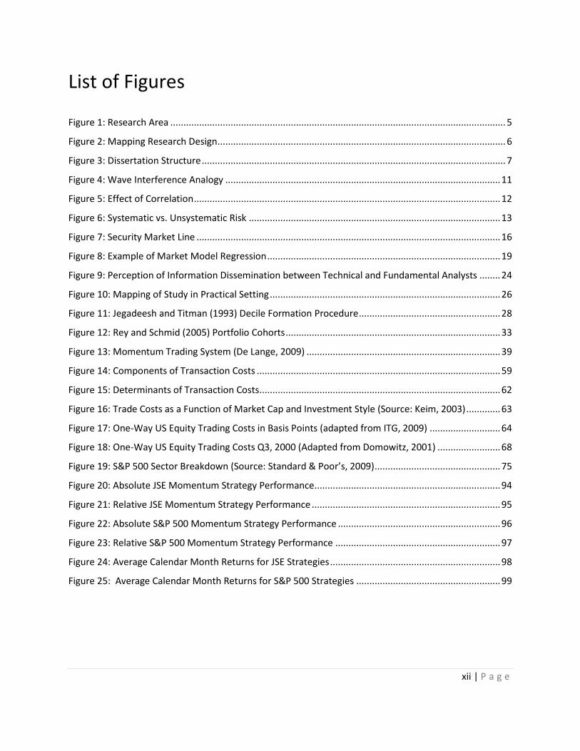
List of Figures

Figure 1: Research Area ................................................................................................................................ 5

Figure 2: Mapping Research Design .............................................................................................................. 6

Figure 3: Dissertation Structure .................................................................................................................... 7

Figure 4: Wave Interference Analogy ......................................................................................................... 11

Figure 5: Effect of Correlation ..................................................................................................................... 12

Figure 6: Systematic vs. Unsystematic Risk ................................................................................................ 13

Figure 7: Security Market Line .................................................................................................................... 16

Figure 8: Example of Market Model Regression ......................................................................................... 19

Figure 9: Perception of Information Dissemination between Technical and Fundamental Analysts ........ 24

Figure 10: Mapping of Study in Practical Setting ........................................................................................ 26

Figure 11: Jegadeesh and Titman (1993) Decile Formation Procedure ...................................................... 28

Figure 12: Rey and Schmid (2005) Portfolio Cohorts .................................................................................. 33

Figure 13: Momentum Trading System (De Lange, 2009) .......................................................................... 39

Figure 14: Components of Transaction Costs ............................................................................................. 59

Figure 15: Determinants of Transaction Costs ............................................................................................ 62

Figure 16: Trade Costs as a Function of Market Cap and Investment Style (Source: Keim, 2003) ............. 63

Figure 17: One-Way US Equity Trading Costs in Basis Points (adapted from ITG, 2009) ........................... 64

Figure 18: One-Way US Equity Trading Costs Q3, 2000 (Adapted from Domowitz, 2001) ........................ 68

Figure 19: S&P 500 Sector Breakdown (Source: Standard & Poor’s, 2009) ................................................ 75

Figure 20: Absolute JSE Momentum Strategy Performance....................................................................... 94

Figure 21: Relative JSE Momentum Strategy Performance ........................................................................ 95

Figure 22: Absolute S&P 500 Momentum Strategy Performance .............................................................. 96

Figure 23: Relative S&P 500 Momentum Strategy Performance ............................................................... 97

Figure 24: Average Calendar Month Returns for JSE Strategies ................................................................. 98

Figure 25: Average Calendar Month Returns for S&P 500 Strategies ....................................................... 99

xiii | P a g e

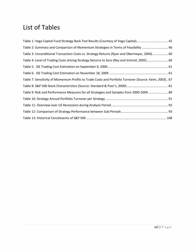
List of Tables

Table 1: Vega Capital Fund Strategy Back Test Results (Courtesy of Vega Capital).................................... 42

Table 2: Summary and Comparison of Momentum Strategies in Terms of Feasibility .............................. 46

Table 3: Unconditional Transaction Costs vs. Strategy Returns (Ryan and Obermeyer, 2004) .................. 60

Table 4: Level of Trading Costs driving Strategy Returns to Zero (Rey and Schmid, 2005) ........................ 60

Table 5: JSE Trading Cost Estimation on September 9, 2000 ..................................................................... 61

Table 6: JSE Trading Cost Estimation on November 18, 2009 ................................................................... 61

Table 7: Sensitivity of Momentum Profits to Trade Costs and Portfolio Turnover (Source: Keim, 2003) .. 67

Table 8: S&P 500 Stock Characteristics (Source: Standard & Poor’s, 2009) ............................................... 81

Table 9: Risk and Performance Measures for all Strategies and Samples from 2000-2009 ....................... 89

Table 10: Strategy Annual Portfolio Turnover per Strategy ....................................................................... 91

Table 11: Overview over US Recessions during Analysis Period ................................................................. 92

Table 12: Comparison of Strategy Performance between Sub-Periods ..................................................... 93

Table 13: Historical Constituents of S&P 500 ........................................................................................... 108

xiv | P a g e

“The boundaries of my language are the boundaries of my world.”

– Ludwig von Wittgenstein

Glossary and Abbreviations

active management: Holding portfolios that differ from their benchmark portfolios in an attempt to

produce positive risk adjusted returns

AMEX: American Stock Exchange

anomalies: Security price relationships that contradict the Efficient Market Hypothesis

alpha: The return on an asset in excess of the asset’s required rate of return; the risk-adjusted return

autocorrelation: The correlation of a time series with its own past values

autoregressive (AR) model: A time series regressed on its own past values, in which the independent

variable is a lagged value of the dependent variable

autoregressive conditional heteroskedacity (ARCH): ARCH describes the condition where the variance

of the residuals in one time series is dependent on the variance of the residuals in another

period. When this condition exists, the standard errors of the regression coefficients in AR

models and the hypothesis tests of these coefficients are invalid

basis point: One basis point equals 0.1 percent

xv | P a g e

beta: A standardized measure of systematic risk based on an asset’s covariance with the market

portfolio

Capital Asset Pricing Model (CAPM): An equation describing the expected return on any asset (or

portfolio) as a linear function of its beta relative to the market portfolio

cointegration: Cointegration means that two time series are economically linked or follow the same

trend. If two time series are cointegrated, the error term from regressing one on the other

is covariate stationary and the t-tests are reliable

contrarian investing: Investing contrary to general market sentiment

conditional trading costs: Trading costs that are adjusted for certain factors such as market conditions,

buying or selling positions, immediacy of trades, etc.

covariance stationary: Statistical inferences based on a lagged time series model may be invalid unless

it can be assumed that the time series is covariance stationary. A time series is covariance

stationary if it has a constant and finite expected value, a constant and finite variance and if

it exhibits a constant and finite variance with regards to leading or lagged values

decile: One-tenth of a portfolio in terms of its net asset value (NAV)

data snooping bias: Concern that studies on historical (ex-post) data do not create a good fit for

technical trading strategies that will work for forecasted (ex-ante)returns

earnings momentum: Phenomenon that stocks with high earnings in one period exhibit higher earnings

in the following period

ex-ante returns: Expected or future returns

ex-post returns: Past or historical returns

formation period: The time in months of previous price series information before the current date used

to make investment decisions for the upcoming holding period

xvi | P a g e

firm-specific risk: See “unsystematic” risk

holding period: The time in months a security is held in a portfolio, or the time in months a portfolio of

securities is held as a whole

industry: Group of companies that are related in terms of their primary business activities. Industry

average ratios and returns etc. are often used as a benchmark for comparison between

different companies in a certain industry

industry effects: Concept that stipulates that the overall performance or behaviour of an industry will

explain a significant amount of the performance or behaviour of individual stocks located

within that industry

J: Formation period in months

JSE: Johannesburg Stock Exchange

K: Holding period in months

large-cap: A company with large market capitalization (over $5 billion on US markets)

liquidity: The ability to trade a stock quickly and at quoted prices. For example, small illiquid stock

positions can often not be converted to cash right away, leading to opportunity costs of

imperfect execution. Liquid stock positions will not exhibit these problems

long position: The buying or holding of a security such as stock. The holder of a long position owns the

underlying security and will profit if it appreciates in price

market capitalization: The market price of an entire company, computed by multiplying the number of

shares outstanding by the market price of these shares

mid-cap: A company with medium capitalization ($1 billion to $5 billion on US markets)

market microstructure: Branch of finance concerned with the details of how exchange occurs in

markets. Microstructure research examines the ways in which the working processes of a

xvii | P a g e

market affects determinants of transaction costs, prices, quotes and volume (for example

bid-ask bounce and liquidity effects)

momentum effect: The tendency of stocks that have performed well in one period to continue to

perform well in subsequent periods

momentum indicators: Valuation indicators that relate either price or a fundamental (such as earnings)

to the time series of their own past values

NASDAQ: National Association of Securities and Dealers Automated Quotation. It is the largest

electronic screen-based over-the-counter equity securities trading market in the United

States

Net Asset Value (NAV): The combined asset value of all share and cash positions of a portfolio

NYSE: New York Stock Exchange

passive management: An investment strategy such as a buy-and-hold strategy, usually investing in an

index

portfolio turnover: The rate of trading activity in a fund’s portfolio of investments, equal to the lesser of

purchases or sales, for a year, divided by average total assets during that year

price reversals: A sudden change in the price direction of a stock

price momentum: Phenomenon that stocks exhibiting high price appreciation over previous periods are

likely continue this trend over subsequent periods.

risk-free rate: The maximum return that can be earned in a market without taking on any risk. Usually

the rate on Treasury securities.

robustness: A robust statistical technique is one that performs well even if the assumptions for the

model used to analyse are somewhat violated

xviii | P a g e

securities: Financial assets. These can be broadly classified as debt securities (e.g. bonds, Treasury

Securities and debentures), equity securities (e.g. common stocks) and derivative contracts

(e.g. futures and options). In this paper the term securities is used interchangeably for

equity securities, shares or stocks

short position: Short selling is investing in the downside of the market. A stock is borrowed at a nominal

fee and immediately sold in the market. The short seller gets the proceeds and repurchases

the stock in the market at a later stage for a (hopefully) lower price and gives it back to the

lender. He/she keeps the difference between the original price and the lower repurchase

price

small-cap: A company with small capitalization (less than $250000 on US markets)

systematic risk: The variability of an asset’s return that is due to macroeconomic factors that affect all

risky assets. It is the portion of risk that cannot be eliminated by diversification

tax loss selling: Selling off securities that had undergone losses to reduce taxable income and therefore

the amount of tax to be paid

technical analysis: A security analysis discipline for forecasting the future direction of prices through

the study of past market data, primarily price and volume

unconditional trading costs: Trading costs that are fixed to a certain percentage of the trade’s value

underreaction: An investor’s delayed price reaction to the release of new information on the market

unsystematic risk (or non-diversifiable risk): The portion of risk that is unique to an asset and is due to

individual characteristics. It can be eliminated by diversification

volatility: The total risk of a stock or a portfolio. It is measured in standard deviation ( )

zero-cost strategy: Portfolios formed in a way that the long positions are financed by short positions

equal in value

1 | P a g e

“Scientists investigate that which already is; Engineers create that which never has been.”

-Albert Einstein

1.1 BACKGROUND

Various studies, predominantly on U.S. markets, document predictability in equity returns, in other

words, stocks that have outperformed in the past continue to do so in the near future (For example, De

Bondt and Thaler, 1987; Jegadeesh and Titman, 1993; Chan, Jegadeesh, & Lakonishok, 1996). These

studies have found that an investment strategy based on buying past “winners” and selling past “losers”

can generate statistically significant abnormal returns over holding periods of 3 to 12 months.

A heated academic debate started when Jegadeesh and Titman (1993) first documented the profitability

of simple, trading rule-based momentum investing strategies on US equity markets. A myriad of studies

followed, on US markets and internationally, most them confirming the findings of Jegadeesh and

Titman (1993) (For example, Jegadeesh and Titman, 1996; Rouwenhorst, 1998; Schiereck et al., 1999).

For example, Moskowitz and Grinblatt (1999) state: “The ability to outperform buy-and-hold strategies

by acquiring past winning stocks and selling past losing stocks, commonly referred to as individual stock

momentum, remains one of the most puzzling of these anomalies, both because of its magnitude ~up to

12 percent abnormal return per dollar long on a self-financing strategy per year.”

Chapter 1: Introduction

2 | P a g e

The main critic of momentum investing is the Efficient Market Hypothesis (EMH), a fundamental

theorem in contemporary finance. The EMH claims that past price information cannot be used to predict

future price patterns, one of the core principles upon which momentum investing relies. Jegadeesh and

Titman (2001) remark that “the momentum effect represents perhaps the strongest evidence against

the Efficient Market Hypothesis”. It is safe to say that momentum investing is one of the most disputed

topics in investment finance academia today.

Momentum investing was used by investors and fund managers long before the academic debate even

started. One of the most prominent examples is Gerald Tsai, who used a momentum approach to

manage Fidelity’s Capital Fund with great success throughout the bullish “Go-Go” years on Wall Street

from 1958 to 1965 (Ellis & Vertin, 2001). Today momentum investing is utilized by many mutual fund

managers and private investors. Momentum investing is a widespread investment style in the US and

other equity markets (Taffler, 1999). Jeff Saunders, fund manager of the UK Growth Fund and the

winner of the 1997 and 1999 Standard and Poor's Micropal award for the best UK mutual fund, publicly

attributes his investment success to the principle of running the winners and cutting the losers

(Saunders, 2004).

Tom de Lange1 outperformed the FTSE/JSE All Share index over most of the past decade using a unique

momentum investing strategy. He also conducted several back tests for different periods on JSE stock

price data and found that he could earn abnormal returns in almost every randomly selected period in

the history of the JSE, even when taking trading costs into account.

Momentum research to date investigates hypothetical trading strategies that are far from being

implementable in practice. There exists sufficient evidence of successful practical implementations of

1 De Lange is the CIO of Vega Capital, a South African boutique asset management firm based in Centurion, Pretoria.

3 | P a g e

size and value strategies2; but a similar practical implementation of a momentum strategy has never

been formally documented (Keim, 2003).

1.2 PURPOSE OF THE STUDY

While the methodologies used by momentum researchers (e.g. Jegadeesh and Titman, 1993; Conrad

and Kaul, 1998) to date were found to be able to earn abnormal returns it is questionable whether such

strategies can be readily implemented in practice. On the other hand, it is likewise questionable

whether practical strategies similar to the one used by De Lange (2009) yield abnormal returns when

tested in an academic setting.

This paper will seek to test the practical approach followed by De Lange (2009) which relies on technical

indicators and reflects the restrictions imposed by practical portfolio management and taxation

considerations within a formal academic framework to establish whether momentum strategies are

viable in practice.

While De Lange’s results could be explained by factors such as data mining bias, this paper will seek to

design and conduct a robust statistical test of De Lange’s method. This will entail simulating De Lange’s

approach on two different sets of historical data and recording returns and risk measures.

This study is very relevant as little or no academic research has taken on such a perspective. Most

published momentum studies focus on proving the existence of the momentum anomaly or

investigating the sources of momentum profits, rather than testing the performance of realistic and

implementable investment strategies based on the momentum effect (Rey & Schmid, 2005).

1.3 RESEARCH QUESTIONS AND HYPHOTHESES

2 For example, Dimensional Fund Advisors and LSV Asset Management have successfully implemented strategies based on academic research on the size and value effect.

4 | P a g e

The research questions and hypotheses of the study deal with the profitability of feasible momentum

strategies.

Hypotheses:

H0: Feasible momentum strategies do not yield statistically significant abnormal returns.

Ha: Feasible momentum strategies yield statistically significant abnormal returns.

Rejection of the null hypothesis would lead to accepting the alternative hypothesis.

More general research questions pertaining to the subject area include:

Are feasible momentum strategies profitable across different markets?

Do the optimized technical momentum indicators used in practice deliver superior portfolio

performance as opposed to simply ranking stocks in terms of past performance as done in most

academic studies?

Do the momentum returns persist through time and through different macroeconomic states?

Are momentum profits robust with regard to trading costs?

The hypotheses and research questions will be refined in Section 6.1 and form the core focus of this

dissertation.

1.4 SCOPE OF THE STUDY

This study is conducted in fulfilment of an MSc (Engineering Management) degree, which requires a

relatively narrow focus on a subject area. It does not necessitate the creation of new theory. However,

a formal framework for testing feasible momentum strategies such as the one used by De Lange (2009)

has never been devised before, in essence requiring the creation of new knowledge and a new testing

framework.

As this report is compiled from the perspective of engineering management, basic financial concepts

terminology will be discussed in more detail than in the case of conventional papers stemming from this

context.

5 | P a g e

Engineering can be defined as: “The application of scientific and mathematical principles to practical

ends such as the design, manufacture, and operation of efficient and economical structures, machines,

processes, and systems.” Engineering management involves managing engineered solutions. In other

words, engineering is concerned with applying theoretical knowledge to a practical problem. Managing

portfolios is similar to managing any other complex system. Establishing whether feasible momentum

strategies can earn abnormal returns is a practical problem that requires to be substantiated by

academic theory in order to arrive at a result that can be used by practitioners.

This dissertation fuses the academic theory around momentum investing with a practical investment

strategy and its results have practical and academic implications.

Figure 1: Research Area

The research area of this study is mapped in Figure 1 above. The field of technical analysis serves as a

basis to the existing, practical momentum strategy used by De Lange (2009) that serves as the basis for

Portfolio Theory

Existing Strategy

Market Anomalies

Momentum Research

Statistical Issues

Technical Analysis

Hypothesis Tests

Transaction Costs

RiskMarket

Efficiency

Technical Indicators

Trading Rules

6 | P a g e

the hypothesis tests. Previous literature on momentum investing, market efficiency and previously

documented market anomalies represent the academic setting of the study. Practical issues pertaining

to the field of portfolio management such as the number of shares in a portfolio and the diversification

of risk, alongside with statistical issues generally encountered with tests for abnormal returns and

transaction costs guide the design of the empirical tests.

The scope of the study is to investigate whether a momentum strategy such as the one developed by De

Lange (2009) will yield statistically significant returns on the JSE and when applied in another market.

1.5 RESEARCH METHODOLOGY

The research method design chosen for this study is mapped in Figure 2 below.

Figure 2: Mapping Research Design

Primary Data

Non-EmpiricalEmpirical

Existing Data

Secondary data analysis, modelling and simulation studies, historical studies, content analysis, textual

studies

Ethnographic designs, participatory research,

surveys, experiments, field experiments, comparative

studies, evaluation research

Methodological studies

Discourse analysis, conversational analysis, life history methodology

Conceptional studies, philosophical analyses,

theory and model building

7 | P a g e

Figure 2 above categorizes different types of research approaches as to the degree that they are

empirical in nature and as to whether they employ primary (new) or existing data. This dissertation is

empirical in nature and entails simulating feasible momentums strategies on historical data. It therefore

falls into the lower left quadrant of Figure 2.

The dissertation is structured as follows:

Figure 3: Dissertation Structure

The area of research, the aim and scope of the study are outlined in Chapter 1. In Chapter 2the study

will be mapped from an academic as well as from an investment industry perspective. Key concepts that

form the basis of the discussion throughout the study will also be introduced.

In Chapter 3 previous academic studies pertaining to momentum investing are discussed. In Chapter 4

the practical momentum strategy followed by De Lange (2009) is described and the latter is compared to

the academic studies discussed in Chapter 3. In Chapter 5 possible explanations of the momentum effect

are discussed and a set of guidelines for a robust empirical test is set forth.

6. Metho-dology

1. Introduction

2. Key Concepts

3. Literature Review

4. Feasible Momentum Strategies

5. Momentum

Effect Explanations

7. Findings & Analysis

8. Conclusions Recommen-

dations

8 | P a g e

In Chapter 6 the data and methodology used is discussed. It is shown how the data set and the

methodology were chosen according to the guidelines in Chapter 5, the academic studies of Chapter 3

and the practical momentum strategy introduced in Chapter 4. The empirical results are presented and

analysed in Chapter 7. The dissertation is concluded in Chapter 8 and suggests future research is

suggested.

9 | P a g e

“A successful man is one who can lay a firm foundation with the bricks others have thrown at him.”

- David Brinkley

In this chapter the financial concepts necessary to facilitate the discussion throughout the study will be

explained. The Efficient Market Hypothesis is formally introduced and a basic understanding of risk vs.

returns is established. Finally differences between the two active investment strategies, fundamental

and technical analysis, will be discussed.

2.1 EFFICIENT MARKET HYPOTHESIS (EMH)

The Efficient Market Hypothesis (EMH) is a central concept to this study. The EMH was devised by

Eugene Fama in 1965 based on the articles by Kendall (1953) and Roberts (1959) and is still regarded as

one of the most important concepts in contemporary finance.

2.1.1 History of EMH

Kendall (1953) analysed a sample of 22 UK commodity stock price series. He found that there were no

predictable patterns in the price series and that they behaved in a truly random manner. The prices at

any point were equally likely to increase, decrease or remain the same. In statistical terms this means

that there is no autocorrelation between the stock’s current prices and their previous prices. Roberts

(1959) conducted similar tests on US stocks confirming the findings of Kendall (1953).

Chapter 2: Key Concepts

10 | P a g e

2.1.2 Rationale of the EMH

The EMH stipulates that only the arrival of new information can influence stock prices. Since information

arrives randomly on the market, stock prices are also bound to behave in a random manner. If there was

any way to develop a model that predicts future price movements it would be fully discounted in the

market. If more returns could be generated by an investment at the same level of risk, all investors

would allocate their funds to exploit this opportunity. The increased demand would increase the price to

the equilibrium level.

2.1.3 Levels of Efficiency

The EMH suggests three levels of market efficiency.

1. Strong form market efficiency is the highest attainable level of market efficiency. All information,

including insider’s information is reflected by the security prices.

2. Semi-strong form market efficiency stipulates that all publicly available information is incorporated

into asset prices. New information on assets is disseminated correctly and instantly. It is impossible

to earn abnormal returns as all publicly available information is already discounted in the market.

Earning abnormal returns is only possible by holding inside information.

3. Weak form market efficiency exists when all information contained in historical price series is

correctly represented in asset prices. Consequently no abnormal returns can be earned by technical

analysis that uses past price and volume information to predict future price movements. However

insiders and fundamental analysts can earn abnormal returns.

The EMH represents the basis of a vigorous academic debate. Proponents of the EMH reject the claims

of researchers of market anomalies and technical analysts suggesting that abnormal returns can be

derived from analysing past price behaviour.

Basic portfolio theory will be discussed next, leading to the market model that will be used to measure

abnormal returns.

11 | P a g e

2.2 PORTFOLIO THEORY

The fundamentals of modern portfolio theory were established by Professor Harry Markowitz in 1952.

Markowitz (1953) proposed that all investors are risk averse and want to be compensated for taking on

additional risk. He defined risk in terms of volatility, i.e. if an investor is faced with the choice between

two assets that are expected to yield the same return but the one is more volatile than the other, the

investor would opt for the less volatile asset as he can be more certain of the returns of the latter.

2.2.1 Diversification and Portfolio Risk

Markowitz (1953) introduced the concept of reducing portfolio risk by diversification. Every asset is

characterized by its volatility and its correlation with other assets. This concept can best be explained by

a simple analogy to wave theory:

If Wave 1 and Wave 2 are 90 degrees out of phase they will cancel each other out, a phenomenon

known as destructive interference.

Figure 4: Wave Interference Analogy

However, if the two waves are in phase, constructive interference will occur and the amplitude of the

fluctuations of the two waves will be superimposed.

According to Markowitz’ portfolio theory assets behave in much the same manner. The wave amplitude

can be compared to an asset’s volatility and the phase angle can be compared to the asset’s correlation

with another asset or market return. The more out of phase the two waves are, the less the amplitude

12 | P a g e

of the superimposed wave. Similarly, the less correlated two assets are - the less their combined

volatility. For example, the stocks of two companies might be differently related to changes in oil price.

Should the oil price increase the one stock (say a green energy company stock) will increase and the

stock of the other company (say a plastic manufacturer) will decrease. Combined, the one stock

functions as “insurance” for the other, reducing their combined volatility.

2.2.2 Risk vs. Returns

In this section the concepts of diversification and expected returns will be combined in to create a basic

understanding of how securities are priced in the marketplace. Investors will expect to be compensated

for taking on more risk. A hypothetical portfolio consisting of asset A and asset B is illustrated in Figure

5 below.

Figure 5: Effect of Correlation

Asset A has lower risk (measured by standard deviation) and has therefore a lower expected return

compared to asset B which has higher expected returns at the expense of higher risk. The lines and

curves in the figure represent the portfolio risk for different weights of asset A and asset B and different

levels of correlation between the two. If the two assets are perfectly correlated (ρ=1), adding a higher

percentage of asset B to a portfolio consisting mainly of asset A will result in an increase in portfolio

E(R)

σ

р = 1р = 0.3р = 0р = -1

0

A

B

D C

13 | P a g e

variance (moving along the line connecting A and B). Conversely, if the assets are perfectly negatively

correlated (ρ=-1) a combination of A and B will be able to yield a return with no risk at all. If assets A

and B are less than perfectly correlated (ρ=0.3), increasing the component of asset B in the portfolio will

decrease portfolio variance up to a certain point (C) after which overall volatility will start to increase

again.

2.2.3 Diversification

In the previous paragraph the unlikely case of a portfolio comprised of only two assets was discussed.

When an increasing number of less than perfectly correlated assets are added to a portfolio, the overall

portfolio standard deviation will decrease (See Figure 6). It seems intuitive that overall volatility will

eventually decrease to zero if an infinite number of assets is added. It has been found, however, that

volatility decreases logarithmically to a certain level (Evans & Archer, 1968).

Figure 6: Systematic vs. Unsystematic Risk

This remaining level of risk is referred to as systematic risk or non-diversifiable risk. Systematic risk

cannot be diversified away as it affects all assets in an economy equally; thus it is sometimes referred to

as market risk.

no. of Assets

Volatility [ ]

Unsystematic Risk

Systematic Risk

14 | P a g e

2.2.4 The optimal Number of Shares in a Portfolio

Various studies investigate the optimum number of shares needed in a portfolio to be adequately

diversified.

Evans and Archer (1968) regard 10 shares to be enough. They state that their results "raise doubts

concerning the economic justification of increasing portfolio sizes beyond 10 or so securities".

Stevenson and Jennings (1984) indicate that a portfolio of 8 to 16 randomly selected shares will

closely resemble the market portfolio (a portfolio consisting of all assets in the market) in terms of

fluctuations and returns.

Reilly (1985) finds that systematic risk is satisfactorily reduced between 8 and 12 shares.

Gup (1983) indicates that proper diversification does not require investing in a large number of

securities and industries. He concludes that almost all diversifiable risk is eliminated when the

number of securities in a portfolio is increased to 9.

Under guidance from the literature quoted above, we can be reasonably assured that systematic risk

will have been eliminated in portfolios consisting of 10 to 15 shares.

2.2.5 The Capital Asset Pricing Model (CAPM)

Although the CAPM will not be formally used in this study in its raw form, the beta measure set forth in

this model will be used to assess the riskiness of the simulated portfolios.

The Capital Asset Pricing Model (CAPM) developed by William Sharpe in 1964 is regarded by many as

the centrepiece of modern finance. Essentially the CAPM is a model that relates a stock’s (or a

portfolio’s) systematic risk to the returns of a “market portfolio”. It is important to note that only the

systematic risk that remains after diversification is priced by the model as opposed to other models that

price total volatility represented by standard deviation ( ).The rationale behind using systematic risk as

a proxy for risk is that unsystematic risk can be diversified away at no cost and that it should therefore

not be priced in the market.

The expected CAPM return of an asset or a portfolio of assets is governed by the equation:

15 | P a g e

𝐸 𝑅𝑖 = 𝑅𝑓𝑟 + 𝛽𝑖 (𝑅𝑚 − 𝑅𝑓𝑟)

Where:

𝐸 𝑅𝑖 = Expected return of asset i or portfolio i

𝑅𝑓𝑟 = Risk-free rate

𝑅𝑚 = The return on the market portfolio

𝛽𝑖 = 𝐶𝑜𝑣(𝑅𝑖 ,𝑅𝑚)

𝜎𝑚2

Where:

𝐶𝑜𝑣(𝑅𝑖 ,𝑅𝑚) = The covariance of the asset or portfolio’s returns with the returns of the market

portfolio.

𝜎𝑚2 = The variance of the market portfolio3.

The expected return on individual assets or portfolios is proportional to the returns of the market

portfolio in excess of the risk-free rate. The beta coefficient measures to which extent the security

moves together with the market.

The beta measure of an individual security or a portfolio is a measure of how risky the security or

portfolio is relative to the market portfolio and is in essence a correlation coefficient (the covariance

between the asset or the portfolio standardized by the market’s variance). The market portfolio will, per

definition, have a beta of 1. Portfolios and securities with betas larger than one are regarded riskier

than the market portfolio and portfolios and securities with betas less than one exhibit less systematic

risk than the market portfolio.

3 The market portfolio is defined as a portfolio holding direct proportions of all assets in the market.

16 | P a g e

The SML is the graphic representation of the CAPM (See Figure 7 below). It is very useful in providing a

benchmark for evaluating investment performance and is often used in practice. All “fairly priced” assets

in an efficient market should plot on the SML, that is, their returns can be explained by systematic risk.

Point M represents the risk and return of the market portfolio. The market portfolio has a beta of 1.

Riskier “fairly priced” assets have higher beta measures plot to the right of the market portfolio on the

SML and have higher expected returns. Assets that are less risky have lower betas and therefore lower

expected returns and plot to the left of the market portfolio.

Figure 7: Security Market Line

If an asset plots above/below the SML, it is underpriced/ overpriced in term of systematic risk (Figure 7).

An underpriced stock will plot above the SML, since it is expected to generate higher returns than an

equal “fairly priced” asset at the same level of systematic risk. These expected excess returns are

referred to as ex-ante (expected) alpha (α). The same concept holds for underperforming assets. If an

asset plots below the SML, it is expected to generate too little returns for its level of systematic risk and

is regarded to be overpriced.

βM = 1.0β

E(R)

0

Rfr

SML

E(RM)

α

M

Stock

βi

E(Ri)

17 | P a g e

Investors pursuing an active investment style typically seek to capture alpha, while passive investors

invest in fairly priced assets and seek to receive market returns.

2.2.6 The Market Model

The CAPM is impractical as it requires the estimation of a host of different parameters that will not be

discussed here. William Sharpe (1963) proposed a simplified model that is easier to estimate and

therefore more commonly used in practice.

The Market Model uses ordinary least squares to regress the returns of a market-wide index against the

returns of a security or a portfolio of securities according to the equation:

𝑅𝑖 = 𝛼𝑖 + 𝛽𝑖 𝑅𝑀 + 𝜀𝑖

Where:

𝑅𝑖 = return of asset i

𝛼𝑖 = intercept (the value of 𝑅𝑖 when 𝑅𝑀 equals zero)

𝛽𝑖 = slope (estimate of the systematic risk for asset i)

𝑅𝑀 = return on the market portfolio

𝜀𝑖 = regression error with expected value equal to zero (firm specific surprises)

The market model regression essentially yields the historical (ex-post) beta and alpha coefficients of the

returns series used as an input to the regression. Beta is a measure of how much an individual security

or portfolio is correlated to movements of the market and is interpreted in the same manner as the

CAPM beta explained earlier.

Alpha represents the returns of a security or portfolio if market return equals zero. If the

asset’s/portfolio’s alpha were zero, the regression line intercept would pass through zero and the asset

18 | P a g e

would generate an equal amount of returns as the benchmark4 and therefore earn zero abnormal

returns. Positive alphas represent risk-adjusted outperformance relative to the benchmark, while

negative alphas indicate underperformance in terms of risk-adjusted returns.

It should be noted that the Market Model does not rely on any assumptions about investor behaviour

as, for example, the CAPM. It simply reflects the linear relationship that exists between the returns of

the market versus that of an individual security or a portfolio. This relationship is illustrated for a

hypothetical “Momentum Portfolio” in Figure 8 below. Looking at the equation of the regression line it

can be seen that the portfolio has a beta of 1.15 and an alpha of 1.61. If the market (S&P 500) moves by

1 percent the portfolio is expected to respond with a 1.15 percent movement. Consequently the

portfolio is deemed to be more risky than the average share or portfolio in the market. If the market has

zero returns, the portfolio will still return 1.61 percent (alpha) at zero systematic risk relative to the

market index. The portfolio is said to be outperforming the market on a risk-adjusted basis or that it is

earning abnormal returns. On the other hand, an alpha smaller than one means the portfolio will be

underperforming the market on a risk-adjusted basis. A beta smaller than unity means the portfolio is

less risky than the average portfolio or security in the market.

4 The benchmark is usually chosen to be a market-wide index

19 | P a g e

Figure 8: Example of Market Model Regression

The market model will be used to estimate risk-adjusted returns of momentum portfolios in later

chapters. The beta measure will give an indication of the riskiness of the portfolios and alpha will be

used to determine whether the strategies can earn abnormal returns. However, there are a few

difficulties with the implementation of the market model that will be discussed next.

2.2.7 Market Model Coefficient Estimation

The market model regression can be conducted with relative ease. However, there are a few practical

issues with estimating beta in this manner that could influence the results of a study using beta as a risk

measure and alpha as a measure for abnormal returns.

y = 1.65 + 1.15x

-30

-20

-10

0

10

20

30

40

-15 -10 -5 0 5 10 15

Mo

me

ntu

m P

ort

folio

Re

turn

s [%

]

S&P 500 Reurns [%]

20 | P a g e

REGRESSION ISSUES

The market model regression relies on three assumptions:

1. The expected value of the error term is zero.

2. The error terms are uncorrelated with the market returns.

3. The firm-specific surprises are uncorrelated across assets.

Failing to meet any of the above criteria would lead to unreliable alpha and beta estimates.

THE MARKET INDEX

In contrast to the assumptions made by the CAPM, the Market model does not assume a market

portfolio containing all possible assets. Practical considerations dictate that an investable proxy such as

a stock index be used as a benchmark for portfolio performance. Often all share indices are used, but if

markets appear to be segmented, sector indices can be used (Bradfield, 2003).

LENGTH OF ESTIMATION PERIOD

Estimates that are generated using long periods of historical data can be irrelevant because the

economic conditions and/or the markets and therefore the business risks may have changed

significantly. Extensive research was conducted on the behaviour of beta with varying time periods. It

was concluded that 5-year betas generated by monthly returns are the most stable (Bradfield, 2003).

This translates into a regression with 60 data points (5 years of monthly returns).

BETA INSTABILITY

Research has shown that ex-post betas derived from market model regression are imperfect estimates

for predicting future returns. Due to the mean reverting characteristics of the beta measure, extremely

high negative or positive betas are likely to be overestimates (Kaplan Schweser, 2009) and need to be

adjusted.

ADJUSTMENTS FOR THIN TRADING

Beta estimates need to be adjusted for thin trading should liquidity be an issue (Bradfield, 2003).

21 | P a g e

This section has dealt with pricing assets and measuring returns in terms of risk, leading up to the

market model and a discussion of practical implementation issues. The next section will seek to map the

intended study from a practical, investment industry perspective. A later chapter on literature review

will map the study from an academic viewpoint.

2.3 EQUITY INVESTMENT STYLES

This section will seek to map momentum investing in the investment industry.

There are three main categories of investment styles:

Value

Growth

Market-oriented

Value and growth investing are active investment strategies, that is, they seek to derive abnormal

returns and therefore disregard the EMH.

Market-oriented investors are said to follow a passive investment strategy. They aim to mimic the

behaviour of the market and therefore do not challenge the EMH.

2.3.1 Value Investing

Value investors focus on the numerator in the P/E or P/BV ratio, desiring a low stock price relative to

earnings or book value of assets. The two main justifications for a value strategy are: (1) although a

firm’s earnings are depressed now, the earnings will rise in the future as they revert to the mean; and

(2) value investors argue that growth investors expose themselves to the risk that earnings and price

multiples will contract for high-priced growth stocks. The philosophy of value investing is consistent with

behavioural finance, where investors overreact to the value stock’s low earnings and price them too

cheaply.

22 | P a g e

2.3.2 Growth Investing

Growth investors focus on the denominator of the P/E ratio, searching for firms and industries where

high expected earnings growth will drive the stock price up even higher.

There are two main substyles of growth investing: consistent earnings growth and momentum. A

consistent earnings growth firm has a historical record of earnings growth that is expected to continue

into the future. Momentum stocks have had a record of high past earnings and/or stock price growth,

but their record is likely less sustainable than that of the consistent earnings growth firms. The manager

holds the stock as long as the momentum (i.e. the trend) continues, and then sells the stock when the

momentum breaks.

Next, fundamental and technical analysis, two analysis styles often followed by active investors in

practice, will be discussed and compared.

2.4 FUNDAMENTAL ANALYSIS

Fundamental analysis is a top-down scrutinizing process that usually consists of three levels, namely

economic analysis, industry analysis and company analysis.

Economic analysis involves determining whether the overall economic conditions are suitable for

investing in a certain asset class. In order to determine the state of the economy, macroeconomic

variables such as interest rates, inflation, consumer spending, balance of payments, money supply etc.

are analysed.

Industry analysis investigates the health of specific industries within an economy. If the industry as a

whole is struggling, it is relatively more difficult for a stock within that industry to perform well than it is

for a stock within a thriving industry.

Company analysis: After establishing the state of the economy and the industry, specific companies are

analysed to determine their financial condition. This is done by analysing the companies’ financial

23 | P a g e

statements and computing ratios that are compared to other companies’ ratios within the same

industry. There are five main categories of ratios: profitability, price, liquidity, leverage, and efficiency.

The main objective of fundamental analysis is determining the theoretical “fundamental” value of a

security through financial statement analysis and applying dividend discount models and risk models. If

a security’s market price is less than its fundamental value, it is regarded “undervalued” and is

recommended for purchase. Conversely, if the security turns out to be above its fundamental value it is

“overvalued” and should be sold short.

As mentioned previously, the semi-strong version of the EMH prohibits fundamental analysis to

outperform the market. However, a number of asset managers and mutual funds have managed to

consistently outperform the market in which is a direct violation of the EMH. Examples of such funds

include Fidelity’s Magellan fund (formerly managed by Peter Lynch) and Vanguard’s Windsor fund

(managed by John Neff). This is confirmed by a number of semi-strong efficiency tests. It was found that

across the world a small number of mutual funds were in fact able to consistently outperform the

market over significant periods of time.

2.5 TECHNICAL ANALYSIS

This section will explore the field of technical analysis, which forms a core element of the methodology

used in the study.

Technical analysts predict the behaviour of individual securities and the market as a whole by analysing

trading volume, past prices and market activity (Achelis, 2000). Contrary to fundamental analysis

technical analysis refrains from establishing the intrinsic value of a security, but rather relies on trends

and reversals to give an indication of future performance. Basing investment decisions on past volume

and price data is a direct violation of the weak-form of the EMH. Most, but not all weak form tests of the

EMH indicate that markets are in fact weak form efficient (Bodie, Kane, & Marcus, 2008).

The key difference between technical and fundamental analysis lies in the way how information

dissemination within markets is interpreted. Fundamental analysts believe that prices react quickly and

accurately to reflect the arrival of new information in the market. Technicians, to the contrary, believe

24 | P a g e

that information enters the market gradually over a period of time because market participants receive

or interpret information about fundamental changes differently and at different periods of time. They

surmise that as various groups of investors such as insiders, investment professionals and private

investors receive information and buy and sell a security accordingly, its price gradually moves to a new

equilibrium.

Figure 9: Perception of Information Dissemination between Technical and Fundamental Analysts

As illustrated in Figure 9, technicians look for the beginning of a shift in a trend (1), so they can get on

the “bandwagon” early and benefit from the shift to the new equilibrium price (2) by buying the trend

when it is up and selling it when it is down. If the shift was short (1), as believed by proponents of the

EMH, deriving profits from shifts in trends would not be viable.

There are different approaches towards technical analysis, which can be broadly divided into four main

groups, namely contrary opinion rules, follow the smart money rules, momentum indicators, and stock

price and volume indicators.

Old Equilibrium Price

New Information Enters Market

New Equilibrium Price

Technical Analyst Identifies New Trend and Takes Action

Fundamental Analyst Takes Position in Market

Price

Time

(1) (2)

25 | P a g e

Contrarian investors typically assume that the majority of the market participants are wrong. So, for

example, if the general market sentiment is highly optimistic the contrarian would regard this as a

bearish sign and would be bullish when the market sentiment is pessimistic.

Follow the smart money investors believe that there are a few superior investors that lead the pack

and try to match their behaviour while there is still time.

Momentum investors use trend-following indicators that are supposed to identify persistent market

trends.

Stock price and volume techniques are aimed at timing the market and are aimed at profiting from

the irrational behaviour of other market participants.

2.6 MOMENTUM INDICATORS

An indicator is a mathematical formula that can be applied to a security’s price, volume or even to

another indicator (Equis, 2006). The resulting value is used to anticipate future changes in prices. Such

indicators guide the trading decisions of momentum investors.

The specific indicators and their formulae used in this study are discussed under “methodology” in

Chapter 6 to avoid repetition.

2.7 TECHNICAL TRADING RULES

Technical trading rules typically rely on indicator values. Some technical analysts apply indicators to

charts and base their trading decisions upon visual inspection of the charts (hence technical analysts are

often referred to as “Chartists”).

The trading system developed by de Lange (2009) specifies threshold values for indicators which are

used to trigger investment decisions. Specific “buy” and “sell” rules are defined which together establish

a mechanized trading system that cannot be influenced by human emotion. A trading system similar to

that of De Lange (2009) will be used in this study. This system will be discussed in more detail in Chapter

4.

2.8 CONCLUSIONS

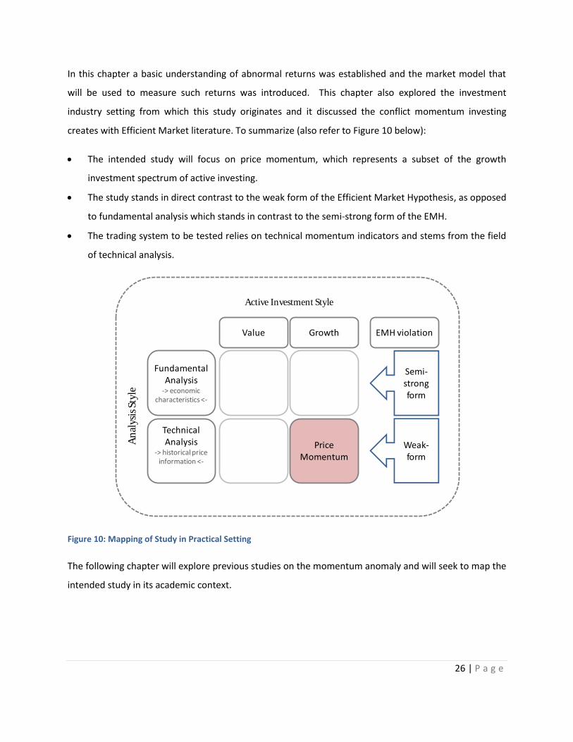
26 | P a g e

In this chapter a basic understanding of abnormal returns was established and the market model that

will be used to measure such returns was introduced. This chapter also explored the investment

industry setting from which this study originates and it discussed the conflict momentum investing

creates with Efficient Market literature. To summarize (also refer to Figure 10 below):

The intended study will focus on price momentum, which represents a subset of the growth

investment spectrum of active investing.

The study stands in direct contrast to the weak form of the Efficient Market Hypothesis, as opposed

to fundamental analysis which stands in contrast to the semi-strong form of the EMH.

The trading system to be tested relies on technical momentum indicators and stems from the field

of technical analysis.

Figure 10: Mapping of Study in Practical Setting

The following chapter will explore previous studies on the momentum anomaly and will seek to map the

intended study in its academic context.

Fundamental Analysis

-> economic characteristics <-

GrowthValue

Technical Analysis

-> historical price information <-

PriceMomentum

Active Investment Style

An

alys

is S

tyle

EMH violation

Weak-form

Semi-strong form

27 | P a g e

“He who loves practice without theory is like the sailor who boards the ship without a rudder and

compass and never knows where he may cast.”

- Leonardo da Vinci

The aim of this chapter is to map this study within the field of academia. A general overview will be

given over relevant US, international and South African studies on momentum investing. The most

authoritative studies and those closely related to the content of this dissertation are discussed. Note

that this chapter focuses more on the methodologies followed in previous academic studies. Studies

relating to the explanation of the momentum effect will be discussed in Chapter 5.

3.1 US STUDIES

Most in-depth studies on the momentum anomaly were conducted on US markets using AMEX and

NYSE stocks as samples. In this section the most authoritative studies on momentum investing will be

discussed. Most attention is given to the methodologies set forth by Jegadeesh and Titman (1993) and

Conrad and Kaul (1998) because these studies form the basis of most other studies researching the

momentum effect.

Jegadeesh & Titman (1993) conduct the first comprehensive study on the momentum effect and create

a framework that is employed and referenced by numerous consequent studies. This study is regarded

by many as the most authoritative piece of literature on the momentum anomaly.

Chapter 3: Literature Review

28 | P a g e

Jegadeesh and Titman (1993) use a sample of NYSE and AMEX stocks covering the period from 1965 to

1989. The methodology used will be explained next: The stocks in the sample are ranked according to

their returns over the past J months and are held for the following K months. J and K refer to the

formation period and to the holding period in months, respectively. A set of 16 strategies were tested;

for each J = 3, 6, 9 and 12 with K = 3, 6, 9 and 12.

The Jegadeesh and Titman (1993) methodology is illustrated in Figure 11 below. At the beginning of

each month all stocks in the test sample are divided into ten equally weighted decile portfolios. The

decile portfolios are formed according to the returns during the past J months and are ranked in

ascending order.

Figure 11: Jegadeesh and Titman (1993) Decile Formation Procedure

The top decile is referred to as the “winner” portfolio and the decile with the lowest returns is referred

to as the “loser” portfolio. The “loser” portfolio is sold short and the “winner” portfolio is bought. All

long and short positions entered K months ago are closed out at the end of every month and are

replaced by the new “winner” and “loser” decile. In any given month t there are K different overlapping

Decile 1

Decile 2

Decile 3

Decile 4

Decile 5

Decile 6

Decile 7

Decile 8

Decile 9

Decile 10

Ran

ked

ac

cord

ing

to p

rice

app

reci

atio

n o

ver

pas

t J

mo

nth

s

Buy

Sell short

Each decile represents 1/10th of the total sample

Month t

Decile 10

Decile 1

Hold for K months

29 | P a g e

portfolios, each created from buying “winner” deciles and short selling “loser” deciles formed in each

month between month t and month t-(K-1). The returns of the short position are subtracted from the

returns of the long position (the short position is profitable if loser decile returns are negative) to yield

the returns of the overall long/short strategy.

In the Jegadeesh and Titman (1993) study all 32 zero-cost portfolio selection strategies yield positive

returns. The most significant returns are generated by the K=3 and J= 12 strategy, which yields average

monthly risk adjusted returns of 1.31 percent. All other strategies yield returns between 0 % and 1%.

Jegadeesh and Titman (1993) conclude that momentum was present on the NYSE and the AMEX in the

period from 1965 to 1989 and suggest investor underreaction to firm specific information as a possible

explanation.

Jegadeesh & Titman (1996) conduct an out-of-sample test for their 1993 study using a similar sample,

but over the period from 1990 to1998. They find that the relative strength momentum strategies

continued to be profitable in the same order as in the Jegadeesh and Titman (1993) study. This is a

remarkable result at that time, as this study suggests that the Jegadeesh and Titman (1993) results were

unlikely to be the result of data mining.

Conrad & Kaul (1998) investigate the profitability of 120 different rule-based trading strategies on the

NYSE and the AMEX during 1926 to 1989. They find that merely 55 of these strategies have returns

statistically significant different from zero, including eight basic momentum strategies. The

methodology and findings pertaining to their momentum strategies will be briefly discussed here.

Conrad and Kaul (1998) use a weighting scheme and methodology that differs from the one used by

Jegadeesh and Titman (1993) in several aspects. They include every of the N shares contained in their

test sample in their portfolios, as opposed to Jegadeesh and Titman (1993) who select only one

“winner” and one “loser” decile from the whole sample. They assign each share a weighting according to

its relative performance to the “market portfolio”. The market portfolio in this case comprises all stocks

contained in the test sample. If a share performs better than the market portfolio it receives a long

weight scaled upwards by how much the share outperforms the market portfolio. In other words, the

30 | P a g e

greater the outperformance of a stock is relative to the market portfolio, the greater will be the position

in that specific stock. The opposite applies for the short position. If a share significantly underperforms

the market portfolio, it is assigned a relatively large percentage of the total short positions. The overall

stock position weights are confined in such a manner that the sum of all long position is equal to all

short positions, in effect creating a zero-cost strategy.

Conrad and Kaul (1998) test momentum strategies with holding and formation periods (K and J) of 1 to

36 months and they merely implement strategies with equal holding and formation periods. They split

their sample into two parts, one ranging from 1926 to 1946 and the other from 1947 to 1989. Both sub-

samples yield positive returns for holding/formation periods of 6, 9 and 12 months. The 1962-1989

sample is found to be profitable for holding periods of 6, 9, 12, and 18 months, which confirms the

results of Jegadeesh & Titman (1993). The magnitude of the returns is also in the same order as in the

original Jegadeesh & Titman (1993) study.

3.2 INTERNATIONAL STUDIES ON DEVELOPED MARKETS

Four studies will be discussed in this section. The study conducted by Rouwenhorst (1998) is considered

an authoritative study on foreign markets. Schiereck et al. (1999) provide another well-regarded study

on international equities. Ryan and Obermeyer (2004) conduct their test on Germany’s top 100 shares

only, which differs from other studies that do not differentiate stock according to market capitalization.

The Rey and Schmid (2005) study is the only available study that focuses on the profitability of feasible

momentum investing strategies optimized to reduce trading costs, also focusing on large caps only.

Consequently the Rey and Schmid (2005) study is very relevant to this dissertation and will be discussed

in some detail.

Rouwenhorst (1998) studies momentum profits across 12 European markets, namely: Austria, Belgium,

Denmark, France, Germany, Italy, The Netherlands, and the UK using 2190 shares over the period 1978

to 1999. He intends to investigate whether the momentum anomaly documented by Jegadeesh and

Titman (1993) was merely the result of data mining processes and therefore focuses on international

returns continuation in and across markets at the individual share level. The method used to construct

the portfolios is identical to the one used by Jegadeesh & Titman (1993). Since the sample spans across

31 | P a g e

multiple countries, all currencies were converted to Deutsche Marks. Rouwenhorst (1998) considers

bid-ask bounce by constructing an additional set of portfolios delayed by one month relative to the

ranking period. Rouwenhorst (1998) finds that all portfolios yield positive returns, varying from 0.64

percent to 1.35 percent per month. Confirming the results previously obtained by Jegadeesh and Titman

(1993), the J=12, K=3 strategy is the most profitable.

Rouwenhorst (1998) conducts another test, in which he uses country specific samples instead of the

combined sample of all 2190 international stocks using a J=6, K=6 strategy. All 12 countries except

Sweden show profits that are significantly different from zero. He finds that the momentum effect is the

most prominent in Spain, Netherlands, Belgium and Denmark in descending order. These results lead

Rouwenhorst (1998) to the conclusion that the continuation of momentum can be explained by country

effects.

Schiereck, De Bondt and Weber (1999) conduct their experiments in a similar fashion to Rouwenhorst

(1998) but use a larger sample of stocks and use a slightly different ranking method. The study involves

a sample of 375 companies listed in the Prime5 segment of the Frankfurt stock exchange over a period

between 1961 and 1991. Schiereck et al. (1999) rank the stocks in the sample according to their returns

in excess of a market index over the past J months. They use formation periods of 1, 3, 6, and 12 months

and measure formation period returns in two different ways. For the one, they record cumulative

strategy returns in excess of the index returns. For the other they calculate the monthly compounded

geometric returns of the respective strategy from which they subtract the monthly compounded index

returns over the same period.

Schiereck et al. (1999) form winner and loser portfolios with 10, 20 or 40 shares containing the top and

bottom 10, 20 or 40 ranked shares in terms of cumulative excess returns. Again a zero cost strategy is

created by buying the winner portfolio and selling the loser portfolio short.

5 Prime Standard is a market segment of the German Stock Exchange that lists German companies which comply with international transparency standards.

32 | P a g e

Schiereck et al. find that all their momentum strategies were profitable. Progressively increasing the

ranking period from 3 to 6 months increased the returns, but increasing the ranking period further to 12

months decreased the returns. This is in contrast to the findings of Jegadeesh and Titman (1993) for US

markets. The two different methods of calculating returns did not influence the results and it was

concluded that momentum was present in the Frankfurt Stock Exchange.

Ryan and Obermeyer (2004) use an approach similar to Jegadeesh and Titman (1993) on a sample of a

replicated DAX 100 index, Germany’s 100 largest and most liquid stocks during the period between 1990

and 1999. They find that the momentum profits generated are statistically significant even after

transaction costs (For example, their J=6, K=6 strategy generates 4.21% annualized returns after

allowing 1% transaction costs).

Rey and Schmid (2005) focus on the profitability of momentum investing and, in an attempt to

maximize momentum profits, employ a trading strategy that differs slightly from the traditional

approach used by Jegadeesh and Titman (1993). They restrict their sample to the shares contained in

the Swiss Market Index (SMI), Switzerland’s largest blue chips (between January 1994 and December

2004) and by limiting their trades to buying and short selling merely one share per month. In other

words, Instead of buying the entire top decile and short selling the bottom decile every month, they

merely buy the highest ranked momentum share, short sell the lowest momentum ranked share and

close out the positions from t-K months ago.

Rey and Schmid (2005) form portfolios from strategies with formation periods of J = 3, 6 and 12 months

and holding periods of K = 3, 6 and 12 months respectively. The NAV of these portfolios are divided into

1/K cohorts according to their holding period (K). A strategy with a three-month holding period will thus

be divided into three cohorts. The idea behind the cohorts is creating a portfolio with sub-portfolios

each staggered by one month, similar to Jegadeesh & Titman (1993).

Let us consider the K=3 strategy. For a strategy with a 3-month holding period, the share that has been

in the portfolio for three months already will be sold and replaced by the current top-ranked share in

terms of momentum. The share with the lowest momentum ranking will be sold short against the same

33 | P a g e

amount as the new long position and both are kept in the portfolio for the following three months after

which both are closed out. Consequently three investment cohorts are created, each holding one long

and one short position. In the K = 3 case this would result in three long and three short positions (3 zero

cost strategies staggered by one month; 6 strategies in total) being held in a portfolio at any time (See

Figure 12).

Figure 12: Rey and Schmid (2005) Portfolio Cohorts

The K = 6 strategy results in 12 positions and the K = 12 strategy into a portfolio with 24 positions at all

times.

Rey and Schmid (2005) use a sample of 17 to 26 stocks during the period from January 1994 to

December 2004. Their portfolios generate annual returns between 9% and 44%, depending on the

strategy used. The most successful strategy is the J=6, K=3 strategy which outperforms the benchmark

81.82% of the time. The momentum returns seem to be stable over the eleven-year evaluation period

and are not explained by a few years of exceptional performance.

t-1

t-2

t-3

K=3

t-1

t-2

t-3t-4

t-5

t-6

K=6

t-1

t-2

t-3

t-4

t-5

t-6t-7

t-8

t-9

t-10

t-11

t-12

K=12

34 | P a g e

3.3 STUDIES ON DEVELOPING MARKETS

Rouwenhorst (1999) conducts a similar study to Rouwenhorst (1998), but uses a sample of 1705 shares

from 20 emerging countries during 1975-1997 and a J=6, K=6 strategy. He ranks the shares according to

past performance and allocates the top third to the “winner” portfolio and the bottom third to the

“loser” portfolio. Even while countries such as Brazil and Zimbabwe have insignificantly positive returns

and Indonesia even has negative momentum returns over the period, monthly cross-sectional average

returns amongst all countries amount to 0.58% and prove to be statistically significant.

Hameed & Kusnandi (2002) investigate the profitability of momentum strategies in Asian markets,

namely Hong Kong, Malaysia, Singapore, South Korea, Taiwan and Thailand over the period 1979-1994.

Their methodology is similar to Rouwenhorst (1998). All momentum portfolios yield profitable returns,

while the J=12, K=6 strategy on Taiwanese stocks yields the highest monthly returns of 0.6% and

Malaysia the lowest with 0.19%. Not all of the returns are statistically significant. While controlling for

the size and country effects, cross-sectional returns across all Asian markets were 0.19% and proved to

be statistically insignificant.

The studies on developing markets (which exclude South Africa) highlight the fact that momentum

strategies are not profitable on Asian markets.

3.4 SOUTH AFRICAN STUDIES

Momentum research on South African markets is very limited. Only three relevant studies were

published to date.

Fraser and Page (2000) analyse momentum strategies on industrial shares of the JSE during the period

of 1973 to 1997. They use a similar approach to Jegadeesh and Titman (1993), but use quintile (5 equally

weighted portfolios) rather than decile portfolios. The only test a K=1, J=1 strategy and find it to be

profitable, producing average returns of 1.5% per month.

Van Rensburg (2001) also uses a method similar to Jegadeesh and Titman (1993), but forms three

equally-weighted portfolios instead of forming decile portfolios. He tests strategies with K=1 and J=1, 3,

35 | P a g e

6 and 12 and finds the 3, 6, and 12-month strategies to produce monthly returns between 0.85% and

1.52%.

Boshoff (2009) uses a sample of 1686 JSE shares between January 1980 and October 2007. He uses the

Conrad and Kaul (1998) method to form portfolios and finds that momentum strategies cannot earn

statistically significant abnormal returns, on average, over the analysis period. He also finds that adding

a liquidity constraint significantly improves the results and that only one of his strategies yields

statistically significant positive returns if no liquidity constraints are added.

The findings of the South African studies are contradictory and were not conducted up to the standard

of the other US and international studies cited. Furthermore, all of these studies focus on the existence

of the momentum effect rather than the profitability of momentum strategies.

3.5 CONCLUSIONS

This chapter gave an overview over the most authoritative literature relating to the field of research

stipulated for this dissertation.

The momentum effect is found across multiple international markets and is persistent throughout

different time periods. Only very limited research has been conducted on South African markets and

none of the studies conducted to date focused on the profitability of momentum investing.

Very little literature exists of feasible momentum strategies that are practically implementable and are

designed to reduce trading costs. Rey and Schmid (2005) is the only available study that focuses on

measuring the performance of feasible momentum strategies and find such strategies to be very

profitable. This fact highlights the relevance of this study to both academia and practicing investors.

36 | P a g e

“In theory, there is no difference between theory and practice. But, in practice, there is.”

- Jan van de Snepscheut

This chapter discusses the momentum-based investment strategy that was developed by Tom De

Lange6. The chapter is divided into two major sections. In the first section, De Lange’s trading system7

will be discussed in some detail. The major workings of his investment approach and the rationale

behind it will be described.

In the second part, the methodologies followed by the previous academic studies on the momentum

effect will be evaluated and contrasted with the practical implementation of De Lange (2009) to

highlight the differences in practical feasibility of the different momentum investing strategies.

6 De Lange has been an active fund manager from 2005 and is focused on technical analysis. 7 The information regarding De Lange’s approach was gathered in a series of informal meetings and telephone calls and will hereafter be referenced as De Lange (2009). For queries on the approach contact Tom De Lange via email at tom@vegacapital.co.za

Chapter 4: Practical Momentum Investing

37 | P a g e

4.1 VEGA EQUITY – A PRACTICAL MOMENTUM STRATEGY

This section will discuss the practical long-only momentum strategy used by De Lange (2009).

4.1.1 Methodology

De Lange (2009) developed a unique trading system based on technical momentum indicators that are

closely related to price momentum (The indicators used will be discussed in detail in Section 6.3). A

long-only strategy is the heart of this system, although De Lange (2009) manages some long/short hedge

funds that typically involve gearing. For reasons that will be discussed in the next chapter, it was chosen

to focus on the long-only strategy. Therefore only this strategy will be discussed here.

De Lange (2009) exploits the momentum effect in a rather innovative manner. He bases his investment

decisions solely on quantitative figures to avoid being influenced by greed and fear (Shefrin, 2007). The

simplified workings of the trading system will now be discussed by breaking up the iterations pertaining

to one updating interval into several steps. In order to aid the explanation, the flow of information

through a typical iteration is illustrated by the data flow diagram (DFD)8 in Figure 13. The following

discussion related to Figure 13:

Process 1: Calculate Indicator Values

At the end of every 3 months (quarterly) indicator values are calculated for all shares in the selection

sample using the shares’ historical closing price series over the specified formation period. This step is

similar to all other academic studies discussed in the previous chapter, except that technical momentum

indicators are used instead of merely price appreciation.

8 Should the reader not be acquainted with data flow diagrams he/she can refer to Appendix A for a brief description

38 | P a g e

Process 2: Rank Stocks

The indicator values from Process 1 are used to rank all stocks in the selection universe in ascending

order according to their specific indicator values (price momentum). Each stock is assigned to a specific

percentile ranking. This step is identical to other academic studies. For example, Jegadeesh and Titman

(1993) rank all stocks in ascending order to form decile portfolios.

Process 3: Sell Stocks below Cut-off Ranking

This step is somewhat different to what is done in other academic studies. Whereas studies such as

Jegadeesh and Titman (1993) close out all (long and short) positions of all stocks that have reached the

end of their predefined holding period, De Lange (2009) only sells off stocks that fall through a certain

percentile ranking threshold.

Process 4: Buy High Momentum Stocks

The highest ranking momentum stocks are bought from the proceeds from the sale of the stocks in

process 3. In this step Jegadeesh & Titman (1993) would buy equal proportions of the stocks contained

in the top decile in terms of momentum ranking and sell a portfolio comprised of the stocks in the

lowest decile equal in value as the long portfolio short, creating a zero cost strategy. Note again that the

strategy discussed here is a long-only strategy, so shares will only be bought and not sold short.

Therefore an initial cash position needs to be introduced and the net asset value (NAV) of the portfolio

needs to be tracked.

This concludes the description of the basic working of the De Lange (2009) portfolio formation

procedure. Next some practical considerations pertaining to this momentum strategy will be discussed.

39 | P a g e

Figure 13: Momentum Trading System (De Lange, 2009)

Calculate Indicator Values

Rank StocksSell Stocks

below Cut-off Ranking

Historical Price SeriesD1

Ranking D3

1. 2. 3.

Buy High Momentum

Stocks

4.

Indicators Stock RanksEOQ

Stock Ranks

Proceeds

PortfolioD5

Portfolio Compo-sition

StockRanks

40 | P a g e

4.1.2 Portfolio Characteristics and Rebalancing Procedure

As mentioned before, strategies followed by academic researchers such as Jegadeesh & Titman (1993)

close all positions out at the end of a specified holding period. As De Lange (2009) only closes out

positions in shares that fall below a cut-off ranking, his portfolios have to be rebalanced from time to

time.

De Lange’s portfolios contain between 10 and 15 shares. A specific number of shares between 10 and 15

is chosen and this number remains fixed for each portfolio. As all shares in the portfolio will perform

differently over the quarterly horizon, certain shares in the portfolio will become overweight relative to

others, increasing overall portfolio risk and lowering the benefits of portfolio diversification (See Section

2.2.1). If a share’s weight becomes significantly more than 10% of the total portfolio NAV, De Lange

(2009) suggests the portfolio to be rebalanced within the context of the situation in order to save

trading costs. Some guidance to this process is given in the following paragraph.

The sell signal for a security is given when the respective momentum rating drops below the specified

ranking percentile, e.g. 25%. By definition high momentum stocks are the ones with the highest past

performance and low momentum stocks are the ones with the lowest past performance. Accordingly,

the stocks sold are often those which showed little or even negative returns and are therefore relatively

low in value relative to the shares remaining in the portfolio. The proceeds from selling loser stocks are

used to purchase new positions, which should preferably be of the same size as the other stocks in the

portfolio. However, the stocks remaining in the portfolio are per definition highly priced “winners” and

the amount of money required to make up the new position in the new stocks will almost never match

the amount obtained from the selling the “loser” stocks. The initial position size is defined by the

number of shares in the portfolio. A 10-share portfolio will have 10 positions of 10% (in terms of NAV) in

10 different stocks. The replacement position size will have to be somewhat smaller, usually around 8%.

De Lange (2009) resolves this issue by purchasing a constant, but lower percentage of the NAV for the

new positions. For example, consider a 10-stock portfolio with initial stock positions of 10% per share. If

in this 10-stock portfolio 4 stocks fall below the threshold indicator ranking, these 4 stocks will be

41 | P a g e

replaced by 4 stocks that each have a position size of 8% of the portfolios’ total NAV. If the total value

of the intended new stock positions exceeds the proceeds from selling the loser stocks, the outstanding

amount is financed by selling a part of the highest overweight stock position, reducing it to it its initial

size, and then selling off part of the second-biggest position and so forth until the positions balance out.

This saves on trading costs because the overweight positions are rebalanced naturally. In order to

mechanize the investment decisions, the replacement position size is predefined as a percentage of the

total net asset value (NAV) of the portfolio. All stocks below the 25th percentile are sold off and are each

replaced by a position of 8% (in a 10 stock portfolio) and 6.67% (in a 15 stock portfolio).

The above considerations should keep the portfolio within reasonable bounds, but there are always

exceptions. Sometimes, especially in strong bull-runs, positions become overweight and need to be

rebalanced leaving vast amounts of cash in the portfolio. In such cases the replacement positions can be

made bigger (e.g. 10% instead of 8% for a 10 stock portfolio). If some cash remains after this measure,

all positions can be topped up by an equal amount until all cash is invested. The cash position will be

discussed in more detail in the following paragraph.

4.1.3 Cash Position

Initially a cash amount is deposited into the portfolio. This amount is used to purchase the first set of

shares according to their respective momentum ranking. It is difficult to maintain a zero cash balance, as

some shares have very high prices and consequently a cash balance will remain as no exact multiple of

the share can be found. However this cash balance is kept below 5% of the portfolios NAV at all times.

4.1.4 Updating Frequency

De Lange (2009) updates his portfolios on a quarterly basis. Theoretically, quarterly updates should

reduce trading and therefore trading costs and taxes; however, De Lange (2009) finds that the returns

and the trading frequency are not significantly affected if the portfolios are updated in monthly or

quarterly intervals.

42 | P a g e

This concludes the discussion of the methodology used by De Lange (2009). The author could not locate

any literature on similar strategies, but some of De Lange’s own research findings will be displayed

below.

4.1.5 Research by De Lange

De Lange conducted some back tests for various momentum-based fund strategies during the period

from 2000 to 2006. His results are summarized in Table 1 below.

Table 1: Vega Capital Fund Strategy Back Test Results (Courtesy of Vega Capital)

The back-tested performance of De Lange’s funds is phenomenal and, according to De Lange (2009)

confirm some of his actual portfolios over the same interval. The first three columns in Table 1

represent various long/short geared hedge fund strategies and the last column represents the standard

long-only Vega Equity strategy that is similar to the strategy that forms the basis of the simulations run

in this study. All strategies yield significant outperformance in absolute terms and in terms of market

model alpha. The long-only strategy’s alpha (2%) is much higher than the alphas found with academic

conventional strategies, while the beta figure is also very low at 0.87. The long/short strategies

displayed in Table 1 all involve gearing and are therefore not comparable to the zero-cost strategies

used by previous studies.

43 | P a g e

This concludes the discussion of the working and the performance of De Lange’s momentum investing

strategy. Next, De Lange’s strategy and the strategies used by previous studies will be compared in

terms of practical feasibility.

4.2 COMPARISON OF METHODOLOGIES IN TERMS OF PRACTICABILITY

The aim of this study is to investigate the performance of practical momentum investing strategies. This

section will evaluate the long-only strategy proposed by De Lange (2009) along with previous academic

studies in terms of their feasibility when actually implemented. Several factors such as implied holding

periods and portfolio turnover, the number of shares and rebalancing strategies, will be discussed.

4.2.1 Systematic Risk and Number of Shares in Portfolio

The number of shares in De Lange’s portfolios is fixed to between 10 to 15 shares. This allows the

portfolio to be reasonably diversified in terms of unsystematic risk (See Section 2.2) and limits excessive

trading. In terms of portfolio management theory and in the light of practical implementation, the

number of shares contained in portfolios of Conrad and Kaul (1998), Jegadeesh and Titman (1993) and

even Rey and Schmid (2005) seem rather inadequate. Rey and Schmid hold between 3 and 12 long

positions. A portfolio with only three shares is definitely not sufficiently diversified and will be subject to

excessive levels of firm-specific risk (See Section 2.2.4). Jegadeesh and Titman (1993) hold long positions

in an entire decile (one tenth) of the stocks in terms of value of the sample population. Depending on

the size of the sample, this can be a considerable amount of shares and results in a greater amount of

trading effort and trading costs. The Conrad and Kaul (1998) portfolio selection procedure is completely

inadequate for practical applications as it requires a position in every single share of the selection

universe specified by a certain weighting formula (See Section 3.1).

4.2.2 Other Practical Implementation Issues

Another complication that would occur when implementing the strategies followed by Jegadeesh and

Titman (1993) and Conrad and Kaul (1998) is that they implicitly assume that shares are infinitesimally

divisible. It is unlikely that 10 deciles equal in value can be formed as some shares are traded at

relatively high prices.

44 | P a g e

4.2.3 Trading Frequency and Portfolio Turnover

The standard academic studies employ strategies that explicitly define holding periods. Researchers

such as Jegadeesh and Titman (1993) use holding periods of 3 to 12 months, which translates into

portfolio turnovers equal or in excess of 100% per annum. Such high levels of portfolio turnover are very

undesirable in terms of transaction costs and from a taxation perspective.9

De Lange (2009) merely sells stocks that fall below a certain indicator percentile ranking threshold (See

Section 4.1). If, in a certain ranking period, there are no shares that fall below the threshold ranking, no

shares will be sold at all. This is the single, most significant difference between the De Lange (2009) and

the Rey and Schmid (2005) procedures. The strategies used by Rey and Schmid (2005) and all other

previous momentum studies for that matter are limited by the fact that they adhere to predefined fixed

formation holding periods that require extensive portfolio turnover. Even if Rey and Schmid (2005) enter

and exit only one long and one short position per holding period (which they argue should reduce

trading costs), the holding periods are always less or equal to one year, resulting in higher than desirable

portfolio turnover rates. The holding periods implied by the De Lange (2009) methodology are variable

and solely dependent on when the exit signal is triggered for an individual share. This could result in

more or less portfolio turnover than the standard academic strategies and will need to be confirmed.

According to De Lange (2009) his long-only strategies produce portfolio turnover rates that are

significantly less than 100% per year.

Another issue relating to the practical implementation of the academic momentum trading rule-based

strategies occurs because of the fact that all stock positions are closed out at the end of every holding

period per default. Consequently, in the same period, stocks may be sold simply because they reached

the end of their pre-defined holding period and be re-bought because they are still ranked highest in

terms of momentum. This would result in completely unnecessary trading costs.

9 A more detailed discussion of impact of portfolio turnover and taxation on momentum profits will follow in Chapter 5.

45 | P a g e

4.2 CONCLUSIONS

Momentums investing strategies such as those suggested by Jegadeesh & Titman (1993) and Conrad &

Kaul (1998) have little practical value because of inadequate numbers of shares in the portfolios, issues

with implementing the method such as the assumption that shares are infinitely divisible and high

portfolio turnovers.

The approaches of Jegadeesh and Titman (1993), Rey and Schmid (2005) and De Lange (2009) are

summarized and contrasted in terms of their practical feasibility in Table 2 below. The study by Conrad

and Kaul (1998) is not represented in this table because of its apparent impracticalities (it requires

holding a portion of every stock of the selection universe).

The next chapter will outline some general considerations that need to be kept in mind when

conducting a study such as the one proposed.

46 | P a g e

Table 2: Summary and Comparison of Momentum Strategies in Terms of Feasibility

Aspect Jegadeesh & Titman (1993) Rey & Schmid (2005) De Lange (2009)

Ranking Criteria

Formation Period

Holding Period

Strategy Type

Long Position Top momentum decile

Exit Signal

No. of Shares in Portfolio

Portion of portfolio closed out and

replaced over updating interval

Portfolio turnover (p.a.)

Bottom momentum decile

Pre-defined holding period of 3, 6, 9

or 12 months

Top and bottom decile of sample

All share positions at the end of their

holding period (1/K of NAV)

Short Position

Price Momentum Technical Momentum Indicators

3, 6, 9 or 12 months

3, 6, 9 or 12 months

Long/short (zero cost)

Price Momentum

3, 6, or 12 months

3, 6, or 12 months

Long/short (zero cost)

Top momentum decile

Bottom momentum decile

< Cut-off ranking percentile

10-15 long positions

Variable – Sold when shares fall

below cut-off ranking

> 1

Academia >>

Pre-defined holding period of 3, 6 or

12 months

Between 3-12 long and 3-12 short

positions

All share positions at the end of their

holding period (1/K of NAV)

45 weeks

Variable

Long only (initial cash position)

Top momentum shares

n.a..

Variable – aim is <= 1

>> Practice

Rebalancing Frequency n.a. n.a. Variable – if share weight is > 15%

bring down to 10%

>= 1

>>Application

47 | P a g e

“ Fool you are, to say you learn by your experience.

I prefer to profit by others’ mistakes and avoid the price of my own”

– Otto von Bismarck

Even though momentum profits are well documented, the sources of these anomalous returns remain a

mystery. Researchers have taken various attempts to explain the sources of momentum.

This chapter discusses general issues that have evolved from studies on market anomalies that could

render the results of such studies questionable. It is often argued by proponents of the EMH that the

results of studies documenting abnormal returns emanating from trading rule based strategies might be

subject to several statistical biases. These biases need to be avoided if a meaningful test is to be

constructed.

Another issue faced by momentum researchers is the possibility that the momentum effect might be

explainable by another well-documented anomaly. It is desirable to circumvent the abovementioned

issues by designing an experiment that is robust to these factors.

Furthermore, momentum returns might be explainable simply by risk or perhaps by market

inefficiencies manifested in the irrational behaviour of market participants. However, the primary goal is

Chapter 5: Explanations of the Momentum Effect

48 | P a g e

not to find explanations for the momentum effect, but to investigate the profitability of feasible

momentum investing strategies. Therefore the majority of this chapter will be concerned with an in-

depth discussion of the possible effects of liquidity and transaction costs on momentum profits. These

factors have a direct impact on the profitability of momentum strategies which represents the focus of

this dissertation.

5.1 STATISTICAL ISSUES WITH TESTS FOR ABNORMAL RETURNS

The following biases are described in the CFA Level I Curriculum (Kaplan Schweser, 2008):

5.1.1 Data Mining Bias

Data mining results when researchers repeatedly use the same data until they discover a trading rule

that “works”. Trading rules found in this manner are prone to be tailored to the specific data set, and it

is doubtful whether such trading rules can be used to generate profits in the future.

Some early studies conducted in the field of momentum investing argued that the profits derived by

momentum strategies may be due to data mining. It is fairly obvious from the out of sample tests and

the international studies discussed in the previous chapter that data mining cannot be used as an

explanation for momentum profits.

The best way to avoid data mining bias is to test a profitable trading rule on a data set different from the

one used to develop the rule ( i.e. use out of sample data).

5.1.2 Survivorship Bias

Survivorship bias is often present in mutual fund performance reporting. Funds that have previously

underperformed are often discontinued or rolled over into better-performing funds. Only surviving

mutual funds are reported. A sample of mutual funds with a 10-year track record or price/dividend data

will typically have an upward performance bias as only “survivors” are included in the sample.

In the context of the intended experiment the price series need to be adjusted for delisted stocks, share

splits and dividends.

49 | P a g e

5.1.3 Small Sample Bias

Choosing the appropriate sample size is imperative for the success of a statistical experiment. A small

sample might not adequately represent the characteristics of the underlying population from which it is

drawn.

In terms of choosing the sample for the study, one must be wary to use a sample that properly reflects

the characteristics of the market it is drawn from. One way of circumventing this problem is to use a

sample containing all stocks of a specific segment of the market and drawing conclusions only about this

specific segment of the market.

5.1.4 Time Period Bias

One type of small sample bias can occur when we use either a too short or a too long time period for

analysis. What is true over a short time period is not necessarily true over longer periods and vice versa.

If the time period for analysis is too short, there exists a risk that the effects captured only hold for that

specific short period and that they do not have explanatory power over future results. On the other

hand, if the period is chosen too long, the fundamental economic behaviour underlying the results may

have changed, equally resulting in time period bias. A period of five years is generally regarded to be a

reasonable period to establish the performance of an investment strategy.

In our case, a time period dating back 10 years from now seems to be reasonable to capture

fundamental economic relationships underlying stock returns and generate enough data points to

conduct statistical tests. It is however difficult to be completely certain as to whether markets have

significantly changed or not over the past ten years. The choice of the time period also depends a great

deal on whether the market under scrutiny has undergone significant changes.

5.1.5 Non-synchronous Trading

When back-testing infrequently traded stocks there is often a mismatch between closing price data and

the actual prices that the stocks are traded at because prices might be recorded earlier in the day.

50 | P a g e

Prices of frequently traded large-cap stocks tend to more closely match the closing prices recorded in

the price series. Thus a test based on large-cap samples can be expected to be more reliable.

5.2 RISK- BASED EXPLANATIONS

Several studies investigate the possibility that risk is the true driver behind momentum returns. The

discussion around risk explaining momentum returns can be sub-categorized into two main divisions,

namely studies that express risk in terms of standard models such as the CAPM and studies that relate

to risk factors that depend on the state of the economy.

5.2.1 Systematic Risk in terms of Standard CAPM

Several studies investigate the riskiness of momentum strategies of standard CAPM, most of which find

that beta cannot sufficiently explain the abnormal returns derived from momentum strategies (e.g.

Jegadeesh and Titman, 1993; Rouwenhorst, 1998; Liu et al., 1999; Ryan & Obermeyer, 2004 and Rey &

Schmid, 2004). The only study with results to the contrary is Conrad and Kaul (1998) who find that

stocks with high realized returns are generally the ones with high expected returns in terms of the

standard CAPM. In other words, they claim that momentum strategies pick more risky stocks, so higher

returns are expected in any case. However, Jegadeesh and Titman (2001) reject the results of Conrad

and Kaul (1998) on the grounds that they find reversals in the price of momentum stocks in the post-

holding period. Hence, they argue, the stocks could not have been effectively priced and that the results

of Conrad and Kaul (1998) were subject to errors.

In conclusion, there is ample evidence that momentum returns cannot be explained by the standard

CAPM and are therefore not due systematic risk captured by CAPM beta.

5.2.2 Macroeconomic/ Strategy Risk

Proponents of the EMH often argue that an investment strategy based on exploiting market anomalies

might bear risks that are inherent in such strategies. Examples of such risks could be that a trading-rule

based investment strategy could be generating abnormal returns only in certain phases of the business

cycle or that it might yield negative returns for a few consecutive periods. The anomalous returns might

51 | P a g e

not persist in future or might be significantly reduced by new investors pursuing similar or identical

strategies (Kaplan Schweser, 2008).

The following studies relate to the macroeconomic risk of momentum returns.

Conrad and Kaul (1998) find that only the 9-month holding period strategy is profitable during the

period 1926-1946 (the period of the great depression and World War 2).

Schiereck et al. (2002) use the macro-economic state of the economy as a proxy for systematic risk.

They set out certain criteria according to which they classify the state of the economy as either “good”,

“neutral” and “bad”. These criteria include the level of interest rates, unemployment rates, the growth

rate of industrial production, the interest rate term structure and overall share market performance.

They compare momentum strategy returns between the economic states and find that momentum

profits are not affected by the state of the economy. As their set of lagged macroeconomic variables

cannot explain their momentum strategy returns, Schiereck et al. (1999) conclude that momentum

returns are not a result of systematic risk.

Chordia and Shivakumar (2002) find that AMEX momentum returns can be explained by a set of lagged

macroeconomic variables (T-Bill yield, dividend yield and credit default spread). In other words, Chordia

and Shivakumar (2002) find that macroeconomic variables can be used to predict the returns of

momentum strategies. They also find that their momentum strategies yield positive returns only in

expansionary periods and are negative (though not statistically significantly so) in recessionary periods.

Huang (2006) uses the Jegadeesh and Titman (1993) procedure in a study on momentum returns on a

sample of 17 international country indices. He employs industrial production as a the sole measure for

the economic states classified by Chordia and Shivakumar (2002) and concludes that momentum profits

are generally more pronounced in “up” markets rather than “down” markets, deducing that momentum

profits are driven by macroeconomic risk.

Rey and Schmid (2004) confirm the findings of Chordia and Shivakumar (2002) on their sample of Swiss

blue chips. They find that their strategies’ returns are positively correlated with the volatility of the Swiss

52 | P a g e

Market index (SMI). However, they find their long/short strategies to be more profitable in volatile

down markets than in stable up markets. This aspect of the Rey and Schmid (2004) study differs from

the results of Chordia and Shivakumar (2002), who claim that momentum strategies are only profitable

in “up” markets.

According to the literature quoted above, there is a good possibility that momentum returns can be

explained by macroeconomic risk. It is therefore necessary to compare the performance of the

momentum strategies between different macroeconomic states.

5.3 IMPACT OF REPORTED MARKET ANOMALIES

Anomalies are defined as: “Security price relationships that appear to contradict a well-regarded

hypothesis; in this case, the Efficient Market Hypothesis.” (Kaplan Schweser, 2008).

The following market anomalies are documented in the 2008 Level 1 CFA Curriculum and are used fairly

often to explain abnormal returns; that is, they are used to depict situations where abnormal returns

can be earned in otherwise efficient markets. Ultimately, the influences of these documented anomalies

should be removed when conducting an experiment on abnormal returns to ensure that they do not

possess explanatory power over the results of the study. When they cannot be adequately avoided we

must take cognisance of their possible influence on the results.

Each anomaly will be discussed briefly and is placed in context with relevant momentum studies in order

to evaluate its possible impact on the results of this study. Note that the BV/MV effect, P/E ratios and

the small firm effect are factors that are priced by the Fama & French Three Factor Model.

5.3.1 The Fama & French Three Factor Model

Many researchers argue that some apparent mispricings in stock markets can be explained by risk

factors not effectively captured by the Capital Asset Pricing Model (CAPM).

53 | P a g e

The biggest criticism of studies that document anomalous returns based on firm characteristics is that

the model used to compute returns may be flawed. It is argued that the CAPM may be ignoring certain

risk components (Kaplan Schweser, 2008).

Being aware of apparent mispricings Fama and French (1993) developed a three-factor model that

compensates the returns estimates for price-earnings, book-value to market-value and small firm

effects. A host of researchers have, depending on the objectives of their studies, adopted this updated

model to estimate returns. The viability of using the Fama and French (1993) model to measure

momentum returns will be evaluated by discussing each of its three factors in the context of momentum

strategies.

5.3.2 Book Value/ Market Value (BV/MV)

Fama and French (1993) find that book-to-market values are a strong predictor of future returns. They

find that high BV/MV stocks yielded abnormal returns, even after adjusting for beta whereas low BV/MV

stocks generally underperformed. When adjusting for firm size and BV/MV effects Fama and French

(1993) found that beta has only limited explanatory power, challenging the validity of the standard

CAPM.

However, all momentum studies find that the model devised by Fama and French (1993) has limited or

no explanatory power over momentum profits (e.g. Fama & French, 1996; Ryan & Obermeyer, 2004; Rey

& Schmid, 2005). Therefore momentum does not seem to be driven by BV/MV effects and we can

divert our attention from this factor.

5.3.3 Price-Earnings Ratio (P/E)

The P/E ratio is a stock’s market price divided by earnings per share. It was found that, in general,

portfolios with low P/E ratios exhibit superior returns, while high P/E stocks significantly underperform

the market. This phenomenon persists even after controlling for beta (Bodie, Kane, & Marcus, 2008).

Fama and French (1996) find that their Three Factor Model cannot satisfactorily explain momentum

profits and a recent study conducted on European stock markets indicates that stocks selected by

54 | P a g e

momentum criteria and those selected by low P/E or high P/E criteria are not correlated (Bird &

Whitaker, 2004). Grinblatt and Moskowitz (2002) find that the momentum effect is more pronounced

amongst growth stocks than value stocks.

Hence we can be reasonably assured that momentum profits are not driven by P/E effects.

5.3.4 Small Firm Effect

The small firm anomaly was first discovered by Banz (1981) who found that abnormal returns could be

generated simply by investing in small-cap stocks. A possible explanation for this phenomenon is that

standard risk models such as the capital asset-pricing model (CAPM) fail to capture all risk components

that are inherent in investing in small firm stocks.

Hong et al. (1999) show that small firms with low analyst coverage exhibit more momentum than their

larger counterparts. Grinblatt and Moskowitz (2002) confirm that momentum increases for firms with

few institutional owners. However Rouwenhorst (1998) finds that the momentum effect cannot be

explained by the small firm effect, but is more prominent amongst small firms. To the contrary, Ryan

and Obermeyer (2004) find that the average firm size of the stocks in their winner portfolios was larger

than the firm size of the stocks contained in their loser portfolios.

Although there is no conclusive evidence for the small firm effect driving momentum returns, the small

firm effect can be ruled out by following a similar approach to Rey & Schmid (2005) who use a sample of

the stocks contained in a replicated large-cap index.

This concludes the separate discussion of each of the three anomalies that are priced by the Fama &

French Three Factor Model. It is fairly obvious, also from other literature, that the P/E and BV/MV

effects cannot explain the momentum effect (e.g. Grundy & Martin, 2001; Rey & Schmid, 2004).

Therefore using the Fama French Three Factor Model as a proxy for risk does not seem viable. When

using a sample of large and/or mid caps, the small firm effect can be ruled out and therefore all three of

the Fama & French (1993) factors. Three other relevant market anomalies not explicitly covered by any

standard risk model will be explained next.

55 | P a g e

5.3.5 The Neglected Firms Effect

Firms that have only a small number of analysts following them tend to produce abnormally high

returns. These excess returns appear to be caused by the lack of institutional interest in the firms, which

causes that less information is available about those firms, making them riskier investments. Contrary to

the small firm anomaly, the neglected firm effect applies to all sizes of firms (Bodie, Kane, & Marcus,

2008).

However, studies investigating the impact of trading volume on momentum profits find that momentum

returns are more prominent amongst high turnover stocks (Glaser & Weber, 2003).

The neglected firm effect does not seem to have explanatory power over momentum returns; however,

it can be removed by restricting the sample to the most liquid and most prominent stocks such as those

contained in a large-cap index.

5.3.6 Earnings Surprises to Predict Returns

Ball and Brown (1968) were the first to discover that even a while after earnings announcements,

cumulative earnings continued to drift upwards for “good news” and downwards for “bad news”. This is

contrary to the expected behaviour of efficient markets. Foster et al. (1984) found that when investing

in stocks with earnings surprises, investors can reap average abnormal returns of 25% in the 60 days

following the earnings announcement. In other words, markets do not adjust as fast to quarterly

earnings surprises as would be expected by the EMH. Consequently, earnings surprises could be used to

identify stocks that will produce abnormal returns.

Jegadeesh and Titman (1993) find that earnings surprises can explain a part, but not all of the

momentum profits. Chan et al. (1996) document that price momentum is more persistent than earnings

momentum and therefore conclude that earnings surprises cannot be the driver behind momentum

returns.

56 | P a g e

5.3.7 Calendar Studies

It is found that stocks generally have exceptionally high returns in January. This phenomenon is very

prominent among small capitalization stocks. In other words, Investors can reap profits by buying stocks

during December and selling them off during the first week in January. This is also a direct challenge to

the EMH and to the CAPM. De Bondt and Thaler (1987) and Ritter (1988) hypothesize that tax-loss

selling at the year-end might be a possible driver behind the January effect.

Literature is contradictory on this matter. Grinblatt and Moskowitz (2002) find that January and

December are the most profitable months on average for their simulated momentum strategies on a US

sample, whereas Rey and Schmid (2004) find no such evidence on their sample of Swiss blue chips.

The impact of the January effect needs to be assessed by determining whether exceptionally high

returns occur in the month January relative to the other months.

5.4 BEHAVIORAL EXPLANATIONS

The lack of conclusive evidence that momentum returns can be explained by risk factors has led

researchers to pursue behavioural explanations for the momentum effect who seek to find evidence

that markets are in fact inefficient and that irrational investors drive prices to non-effective levels.

Although it is beyond the scope of this dissertation to find behavioural explanations for momentum

results, the main concepts relating to this field will be briefly explained.

Behavioural theories imply that the consequence of irrational investors participating in financial markets

is that rational investors who are aware of the behavioural biases of their irrational counterparts can

exploit this behaviour generating higher returns at lower levels of risk (Shefrin, 2007). The academic

school of thought associated with such phenomena is referred to as behavioural finance. A host of

behavioural models have been generated, attempting to explain momentum returns, some with

reasonable success. Behavioural finance deals with a variety of psychological phenomena found in

financial markets.

57 | P a g e

The “underreaction” bias, the “overreaction and subsequent price reversals” bias, the “anchor-and-

adjust” bias and the “representativeness” biases have been used in attempts to explain the momentum

effect. The underreaction and the overreaction with subsequent reversal are the most common

behavioural models used to explain the momentum effect. For example, Jegadeesh and Titman (1993)

attribute the momentum effect to investor underreaction to the announcement of firm-specific

information. Daniel, Hirshleifer and Subramanyam (1998) find that momentum returns are driven by

investor overreaction to the release of firm-specific information and subsequent reversion to efficient

levels.

Not dwelling on behavioural finance too long, the focus will return to factors affecting the profitability of

feasible momentum strategies, how such factors can compromise the accuracy of momentums studies

and which measures can be employed to prevent a loss of accuracy in the proposed study. The

remainder of this chapter will discuss the impact of market microstructure effects on momentum

studies.

5.5 MARKET MICROSTRUCTURE EFFECTS

This section of the chapter is the most voluminous one and it will discuss issues related to market

microstructure effects pertaining to momentum studies. This is an important domain for this

dissertation as market microstructure effects are closely related to the profitability of momentum

strategies and incorrectly accounting for such factors could severely skew the results of the study. First

general issues relating to the liquidity of momentum stocks will be discussed, followed by a short

description of the components of transaction costs, and finally a discussion of studies relating to

unconditional trading costs and the sub-components of conditional trading costs.

5.5.1 Liquidity

The illiquidity of shares is a primary concern in low market capitalisation and emerging markets

(Rouwenhorst K. G., 1999). Liquidity problems with momentum strategies arise when the positions need

to be liquidated and be replaced by new positions. When testing momentum strategies it is important to

consider the liquidity of the selection universe, as the opportunity costs of not being able to trade

quickly and at the prevailing market prices might substantially skew the results as the trades.

58 | P a g e

Jegadeesh and Titman (2001) resolve this issue by restricting their sample to shares that trade above $5

and excluding the shares constituting the bottom decile of NYSE stocks in terms of market capitalization.

They find that their adjustments to restrict illiquid stocks do not have a significant effect on the results,

but that the stocks chosen by their strategies were in any case only those with high market capitalization

and high trading volume (i.e. liquid stocks).

De Lange (2009) applies a certain liquidity ranking to screen shares for inclusion into the selection

universe. The details of this screening process remain the property of Vega Capital10, but it involves

excluding shares below a certain weighted threshold in terms of trading volume and market

capitalization.

Lee and Swaminathan (2000) find that for US stocks price momentum is more prominent among large

capitalization stocks than among small capitalization stocks and Glaser and Weber (2003) find that on

the German stock markets momentum strategies perform better among high-turnover stocks.

Consequently, it seems unnecessary to make any adjustments for illiquidity or thin trading in the case of

testing momentum strategies.

However, Lesmond et al. (2000) and Moskowitz and Grinblatt (2004) find that momentum strategies

following the Jegadeesh and Titman (1993) procedure tend to pick illiquid and volatile stocks for their

loser portfolios (short positions). This fact complicates matters for momentum strategies employing

long/short strategies. A solution to this problem will be proposed in the discussion of the transaction

costs relating to long and short positions.

The remainder of this section deals with the impact of transaction costs (trading costs) on momentum

profits and consequently on momentum studies.

10 For enquiries, contact Tom De Lange via email at tom@vegacapital.co.za

59 | P a g e

5.5.2 Explicit vs. Implicit Trading Costs

Total transaction costs can be subdivided into explicit and implicit trading costs (See Figure 14 below).

Taxes and brokerage involved with trading are referred to as explicit trading costs. Implicit costs refer to

bid-ask spreads, the impact of the trade itself on the price of the security and the opportunity cost of

untimely execution of the trade.

Figure 14: Components of Transaction Costs

Implicit costs such as price impacts and opportunity costs are very hard to measure, making the

interpretation of such costs extremely difficult. Consequently, most momentum studies completely

disregard trading costs or deduct a certain fixed percentage of the value of each trade referred to as

“unconditional” trading.

5.5.3 Unconditional Trading Costs

The results of and the methodologies followed by some studies employing unconditional trading costs

will be discussed briefly below in order to establish a general overview of the treatment and

interpretation of transaction costs by previous momentum studies.

Jegadeesh and Titman (1993) use unconditional transaction costs of 0.5 percent. Their K=6, J=6 strategy

produces returns that are reliably different from zero at 9.29% per year.

Brokerage

Opportunity Costs

Bid-Ask Spreads

Price Impact of Trade

Taxes

Implicit CostsExplicit Costs

Total Transaction Costs

60 | P a g e

Grundy and Martin (2001) find that the returns of their J=6, K=6 strategy becomes statistically

insignificant at the 5% level of significance for round-trip11 transaction costs of 1.5%. At round trip

transaction costs of 1.77% these profits are driven to zero.

Ryan and Obermeyer (2004) report the annualized returns generated by their J=6, K=6 zero-cost

strategy at different levels of transaction costs. These (annualized) returns are summarized in Table 4

below.

Table 3: Unconditional Transaction Costs vs. Strategy Returns (Ryan and Obermeyer, 2004)

Rey and Schmid (2005) argue that the momentum profits generated by their strategies applied to Swiss

blue chips are robust to transaction costs. They compute the level of trading costs at which the returns

of their strategies become statistically insignificant at a 10% level of significance. They also establish the

level of trading costs where the respective strategy returns are driven to zero.

Table 4: Level of Trading Costs driving Strategy Returns to Zero (Rey and Schmid, 2005)

De Lange (2009) uses unconditional one-way trading costs of 0.5% for his back tests. He derives this

amount as follows: He uses the average bid-ask spread on the JSE top 40 and adds this percentage to

the 0.25% brokerage charged per transaction by Vega Capital unit trusts (De Lange, 2009). The reason

De Lange (2009) used the JSE top 40 spreads is that he only includes the most liquid shares in his

selection universe. The author reconstructed the calculation on September 9, 2009 calculating the bid-

11 Round-trip costs refer to selling a stock position and replacing it with (a) long position(s) equal in value.

Transaction Costs 1% 0.5% 0.3% 0.1%

Winner minus loser returns (%) 4.21 8.53 10.3 10.54

Strategy J=6, K=3 J=6, K=6 J=6, K=12

Level of trading costs (%) causingreturns to drop below statisticalsignificance.

1,38 1,22 1,56

Level of trading costs (%) at which returns are driven to zero. 1,94 2,06 2,01

61 | P a g e

ask spreads from the JSE Top 40 prices quoted by Standard Bank Online Trading12 and adding the 0.25%

brokerage:

Table 5: JSE Trading Cost Estimation on September 9, 2000

The same calculation on November 18, 2009 yielded:

Table 6: JSE Trading Cost Estimation on November 18, 2009

Following from the calculations above, allowing for 0.5% - 0.6% unconditional average transaction costs

can be regarded to be conservative from a South African perspective when the selection sample is

restricted to liquid stocks only.

This concludes the discussion on unconditional trading costs. The next section will deal with conditional

trading costs and will discuss every driving force of transaction costs in context of momentum studies.

5.5.4 Conditional Trading Costs

Transaction costs that are dependent on specific situations or strategies are referred to as conditional

trading costs. Studies on conditional transaction costs investigate the sources and the drivers of

transaction costs. This section discusses impact of several factors that influence the level of transaction

costs possibly encountered when following momentum investment strategies.

12 Source: https://securities.standardbank.co.za/ost/

Trading Cost Component Costs [%] per Trade

Average JSE Top40 Spread 0.17

Vega Unit Trust brokerage 0.25

Total 0.42

Trading Cost Component Costs [%] per Trade

Average JSE Top40 Spread 0.12

Vega Unit Trust brokerage 0.25

Total 0.37

62 | P a g e

Unconditional transaction costs are driven by a variety of factors, each of which will be addressed

briefly. An overview over these factors is given in Figure 14 below. Many of these factors are

interrelated and several are related to the liquidity of a stock. If the liquidity of a stock is influenced by a

trade in any way, implicit trading costs will most likely be affected.

Figure 15: Determinants of Transaction Costs

A short discussion of each of these factors itself and its relation to momentum investing follows below.

MARKET CAPITALIZATION

The market capitalization of a stock is often regarded as a direct proxy for the liquidity of a stock. As the

large cap stocks are usually traded at high volumes it is unlikely that an individual trade affects the

liquidity and therefore the price of the stock. Bid-ask spreads are generally lower for large-cap shares

and they also tend to trade more efficiently.

Keim & Madhavan (1998) set out the relationship between trading costs and market capitalization (see

Figure 16 below). Trading costs increase exponentially for smaller stocks, while average total one-way

transaction costs for technical traders drop to about 0.6% for large-cap stocks on US markets. Although

Total Transaction

Costs

Market Capitalization /

Liquidity

Investment Style

Portfolio Turnover

Long vs. Short Positions

Exchange Characteristics

Type of Investor

Time & Innovations

63 | P a g e

indicated in Figure 16, note that the differentiation of trading costs between value, index and technical

strategies will be discussed later in this section.

Figure 16: Trade Costs as a Function of Market Cap and Investment Style (Source: Keim, 2003)

The study by Keim was conducted in 2003. The latest available estimates for total (implicit and explicit)

trading costs available for US large-caps at the date of print of this document are displayed in Figure 17

below. Apart from giving an indication of the latest large-cap trading costs on US markets, Figure 17 also

illustrates how trading costs vary through market cycle stages and through the passage of time.

2.5

1.0

0.5

1.5

2.0

0 0.5 1.0 1.5 2.0 2.5

0

Est

imat

ed T

rad

ing

Cost

s [%

]

Market Capitalization [$ Billions]

Technical Traders

Value TradersIndex Traders

64 | P a g e

Figure 17: One-Way US Equity Trading Costs in Basis Points (adapted from ITG, 2009)

The maximum total trading costs for US large-caps over the period between Q4, 2004 and Q2, 2009

were recorded in Q4, 2008 and amount to just above 60 basis points (0.6%) per trade. For the remainder

of the period the total trading costs actually stay well-below 60 basis points.

INVESTMENT STYLE

Keim (2003) conducts an in-depth analysis of conditional trading costs related to different investment

styles. He argues that total trading costs differ for momentum, value and index strategies. He derives

trading costs as a function of the market cycle stage and investment style.

He estimates the trading costs of momentum, value and index strategies from the trades of 33 active

fund managers in the US and in 36 other countries in both developed and emerging countries over the

period from 1997 to 2000. He notes that momentum buys occur predominantly in rising markets and

that momentum sells occur mostly in declining markets. This is contrary to the timing of buys and sells

of value and index strategies. Value buys generally occur when prices decline or in “down” markets’ and

value sells are usually executed when the market is “up”. Index buys and sells are unrelated to the

prevailing market conditions. As most market participants buy when the market rises and sell when the

market is falling, the costs associated with momentum trades are expected to be higher than the

unconditional average as the general demand for liquidity in those times is higher (See Figure 16).

0

10

20

30

40

50

60

70

20

04

/Q4

20

05

/Q1

20

05

/Q2

20

05

/Q3

20

05

/Q4

20

06

/Q1

20

06

/Q2

20

06

/Q3

20

06

/Q4

20

07

/Q1

20

07

/Q2

20

07

/Q3

20

07

/Q4

20

08

/Q1

20

08

/Q2

20

08

/Q3

20

08

/Q4

20

09

/Q1

20

09

/Q2

US Large Cap Trading Costs (bpe)

implicit

explicit

total

65 | P a g e

Furthermore it is of utmost importance for momentum traders (who generally trade over short-term to

medium–term horizons) that the trades occur in a timely manner. If a trade takes too long to clear,

much of the underlying price movement might not be captured and opportunity costs will rise. This is in

contrast to value or index strategies which are not critically dependent on fast execution since they

generally take on long-term horizons.

Although the interpretation of the opportunity costs is somewhat ambiguous, Keim (2003) derives a

model to quantify these costs and concludes that the implicit trading costs for momentum strategies are

much higher than those associated with value or index strategies. According to his results, monthly total

trading costs (explicit and implicit) amount to 1.13% to 1.31% on average for momentum strategies,

which will dissipate the abnormal returns generated by most academic momentum strategies (Please

refer to Chapter 3).

PORTFOLIO TURNOVER

It is intuitive that investment strategies exhibiting high portfolio turnover will have higher total trading

costs. This can be a very limiting factor for momentum strategies, as standard academic momentum

strategies rely on frequent trading. For example, Jegadeesh and Titman (1993) find that the average

turnover of their K=6, J=6 strategy is 84.8% semi-annually. Lesmond et al. (2004) find that the trading

frequency required to execute standard momentum strategies prohibits momentum profits.

Keim (2003) sets forth a table that displays the profitability of a typical academic momentum strategy in

terms of monthly portfolio turnover and the corresponding trading costs. A copy of the abovementioned

table is displayed below (See Table 7). The table maps momentum profits in terms of trading costs per

trade and monthly portfolio turnover. Keim (2003) uses the average monthly profits of 1.11% derived by

Moskowitz and Grinblatt (2002) and subtracts trading costs as a function of portfolio turnover.

66 | P a g e

The monthly portfolio turnover13 implied by the Grinblatt and Moskowitz (2002) strategy is 110% and

the average total transaction costs for this representative momentum strategy are estimated to lie

between 1.7% to 3.4% of trade value (Keim D. , 2003). Using these criteria as inputs and scanning

through Table 7, a momentum strategy such as the one used by Grinblatt and Moskowitz (2002) yields

profits that are already deep in the loss region of the matrix in Table 7.

In conclusion, it is absolutely vital for momentum strategies to focus on lowering portfolio turnover.

13 Keim (2003) interprets turnover as follows: When 50 percent of the value of the holdings in the portfolio is sold at a certain time and is immediately replaced by a new position equal in value, portfolio turnover amounts to 100 percent.

67 | P a g e

Table 7: Sensitivity of Momentum Profits to Trade Costs and Portfolio Turnover (Source: Keim, 2003)

68 | P a g e

LONG VS. SHORT POSITIONS

As discussed previously under the impact of liquidity on momentum returns, it was found that standard

academic momentum strategies tend to pick volatile short positions. In essence, this finding implies that

short positions are more costly than long positions. Total costs of such positions are difficult to assess as

opportunity costs can be expected to be involved when entering and exiting such positions.

In order to maintain the accuracy of momentum strategies and to save on trading costs it might be

advisable to focus on the long side of momentum investing strategies. Moskowitz and Grinblatt (2004),

for example, restrict their analysis to long positions only to avoid positions in small and illiquid stocks.

EXCHANGE CHARACTERISTICS

Keim & Madhavan (1998) find that the type of the exchange on which the trades occur also has a

profound impact on the both explicit and implicit trading costs. On average trades conducted on the

NYSE were cheaper than those on the NASDAQ. The NYSE operates as a specialist auction market where

immediacy is supplied by the public limit order. Bid-ask spreads are very low on the NYSE (Keim &

Madhavan, 1998).

Figure 18: One-Way US Equity Trading Costs Q3, 2000 (Adapted from Domowitz, 2001)

Consequently, the impact of trading costs can be significantly reduced by choosing to conduct all trading

activity via specified exchanges such as the NYSE and the AMEX on US markets.

0

10

20

30

40

50

60

70

80

NYSE AMEX NASDAQ World

US Equity Trading Costs Q3 2000 (bpe)

explicit

implicit

total

69 | P a g e

PASSAGE OF TIME AND INNOVATION

Domowitz, Glen and Madhavan (2001) find that average US explicit trading costs exhibit a declining

trend. They also remark that, in general, implicit costs decrease at a much faster rate than explicit costs,

leading to rapidly decreasing total trading costs. Domowitz et al. (2001) reason that this decline might

be due to the increased presence of institutional investors resulting in more pressure on suppliers of

trading services because institutions tend to be able to negotiate lower commissions. Innovations such

as the low-cost Electronic Crossing Networks used by institutional traders might also have played a

significant role. Furthermore soft dollar practices payments by which brokers return a portion of the

stated commission to their clients have become increasing popular, reducing the actual quoted trading

costs.

These developments may speak in favour of momentum strategies in future and reduce the impact of

transaction costs on momentum studies using recent samples.

5.6 TAXATION

Taxation is a subject area that the author deems very important in the context of investigating the

profitability of momentum investing strategies. However, the author was not able to source any

meaningful study relating to the impact of taxation on momentum returns.

In most tax regimes around the world, long-term investments are favoured over short term trading.

Short-term investment returns are taxed at the investor’s marginal income tax rate, while longer-term

investments are generally taxed at the investor’s capital gains tax rate which is usually significantly

lower.

US federal tax legislation differentiates between short-term capital gains and long-term capital gains.

Profits that are derived from selling assets that have been in the investor’s possession for less than one

year are taxed as short-term capital gains at the income tax rate which is typically around 25% or even

more. Profits on Investments that are held for one year or more are classified as long-term capital gains

and are taxed at the investor’s capital gains tax rate. If the investor is in the 25% income tax bracket or

70 | P a g e

higher, the investor will pay the maximum capital gains tax of 15%. Investors in lower income tax

brackets may pay as little as 5% (Stock Market Investors, 2009).

Although the specific tax rates will vary from country to country and between the different types of

investors such as institutions, corporate investors and individual investors, all investors will likely be

faced by the differences in tax treatment between long-term and short-term profits. As discussed above,

the differences in tax rates between the two types of classification are substantial and cannot be

ignored.

These tax implications (at least 10% per year in US markets) are so profound that maintaining portfolios

with turnover rates14 greater than 1 per year is simply not viable from an after-tax perspective as it is

highly unlikely that the difference in tax rates can be recovered by a trading strategy focusing on shorter

horizons.

A sensible parameter to evaluate an investment strategy’s practical feasibility is thus to assess the

portfolio turnover rate. Should the portfolio turnover rate be in excess of 100 percent it is unlikely that

the portfolio is feasible from a tax or transaction cost perspective.

5.7 CONCLUSIONS

This chapter discussed factors that could influence studies on the profitability of momentum strategies

and how these factors can be mitigated. The most important findings and their implications for the

selection of the stock sample for the study and guidelines for the methodology to be used are

summarized below.

The price series to be used for the simulations should:

Be out of sample to prevent data mining bias;

14 The author uses the SEC definition for portfolio turnover (refer to Glossary)

71 | P a g e

Date back not more than 10 years to capture the prevailing economic relationships;

Include delisted securities to prevent survivorship bias;

Exclude illiquid stocks to avoid market microstructure-related issues such as the difficulties with

estimating opportunity costs for imperfect execution of trades;

Exclude small-cap stocks to avoid the small firm effect from having explanatory power over the

results;

Preferably be comprised of stocks that receive sufficient analyst scrutiny such as those contained in

large-cap indices

The following guidelines were established for the empirical testing procedure:

The January returns of momentum strategies should be compared to the returns in other months in

order to assess whether the January effect can explain momentum returns.

The performance of momentum strategies should be assessed between different macroeconomic

states and in different periods. Momentum profits seem to be not explainable by systematic risk as

defined by standard risk models such as the CAPM and the Fama & French Three Factor model, but

there is ample evidence of momentum strategies being subject to macroeconomic risk.

Portfolio turnover should be computed. It is important for momentum strategies to limit portfolio

turnover. Apart from trading costs being higher for momentum strategies than for value or index

strategies, taxation has a profound impact on trading intensive strategies such as momentum

investing. US Portfolios with turnover rates in excess 100% per year are taxed at the individual

investor’s marginal tax rate as opposed to the capital gains tax rate that is charged for portfolios

that have turnover rates below 100% per year.

The strategy should focus on a long-only strategy since momentum strategies tend to pick volatile

and illiquid stocks for their short positions.

The next chapter will discuss the methodology used to conduct the empirical tests. The methodology is

based on the guidance of this chapter.

72 | P a g e

“New ideas require new structures.”

– Leroy Hood

The author decided to test a long-only trading system similar to the one used by De Lange (2009) on the

JSE and to conduct an out of sample test on the S&P 500. This chapter will discuss the empirical testing

methodology used to establish whether such an investment approach can be used to generate abnormal

returns. The tests have a slightly different focus compared to previous studies. While risk-adjusted

returns will be measured, some practical measures such as portfolio turnover will also be included in the

analysis in order to assess the practicability of the trading system.

6.1 RESEARCH HYPOTHESES

The aim of this study is to determine whether feasible momentum investing strategies similar to those

used by De Lange (2009) are able to consistently outperform benchmark returns. Emanating from the

research objectives stated in Chapter 1 and the discussion leading up to this chapter, the following

specific hypotheses can be formulated:

The null hypothesis for both the baseline and the out of sample test holds that feasible momentum

strategies cannot, on average, generate abnormal returns.

Chapter 6: Research Design and Methodology

73 | P a g e

H0: 𝛼𝑀𝑜𝑚𝑒𝑛𝑡𝑢𝑚 = 0

The null hypothesis will be rejected if the alpha is statistically significant.

Algebraically, for the baseline test and the out of sample test, respectively:

H1: 𝛼𝐽𝑆𝐸 ≥ 0

H2: 𝛼𝑆&𝑃500 ≥ 0

Both the baseline test and the out of sample test are comprised of three different portfolio simulations,

one for every indicator used. Therefore each hypothesis test involves three separate sub-hypotheses in

terms of the indicators used.

The selection of the data set will be discussed next.

6.2 DATA COLLECTION AND PREPROCESSING

The tests were conducted on two data samples, namely JSE large- and mid-caps and the stocks

constituting a replicated S&P500 index. Both samples span across the same time period from January

2000 to September 2009 and will be described in this section.

The reason for choosing a sample period of the past ten years for both samples is to ensure that the

fundamental economic relationships are more or less consistent with the situation pertaining in

contemporary markets.

6.2.1 JSE Test Data

The baseline sample includes all listed and delisted closing price series of mid- and large-cap stocks on

the JSE between January 2000 and September 2009.

74 | P a g e

A period of around 60 months (5 years) can generate enough data points for tests for statistical

significance using monthly returns. Using a sample period of 10 years sub-divided into two equal 5-

year periods allows an evaluation of whether momentum returns are robust across different time

periods and market states.

Small-cap stocks are excluded to prevent small firm bias and liquidity-related issues from influencing

the results. The benchmark chosen is the JSE All Share index, as market model estimation requires

the use of a market wide index.

The relevant database was provided by Vega Capital, who in turn sourced their data from I-Net Bridge15.

The data is fully adjusted for stock splits, reverse splits, stock dividends, special dividends and spin-offs.

In other words, all dilutive effects are removed from the data so that the price series reflects an

accurate pure capital return, which represents the source of momentum returns. The data is not

adjusted for ordinary or normal cash dividends, meaning that the ordinary value weighted index can be

used as a benchmark instead of a total return index.

Although the samples were carefully chosen to avoid most factors that could compromise the results,

the JSE baseline sample may still have several problems:

The availability of historical price series for delisted JSE stocks is limited. Accurate and complete

price series of delisted securities are hardly available.

Liquidity issues may affect the results of mid-cap JSE stocks even though small-caps are excluded.

The results might be influenced by risk factors uniquely associated with developing markets.

The JSE is overweight in mining companies; making it an inadequate benchmark as investing in such

a benchmark would require the portfolio to be excessively risky.

The US out of sample data was specifically chosen to avoid the problems associated with the JSE

baseline test and to enable an isolated analysis of the momentum effect.

15 http://www.inetbridge.co.za/

75 | P a g e

The out of sample test was conducted on the constituents of the S&P 500 over the same period as the

JSE test. Following the reasoning of Ryan and Obermeyer (2004) and Rey and Schmid (2005), the out of

sample tests were conducted on a replicated large-cap index over a period of 10 years.

The S&P500 index contains the 500 largest US-based stocks in terms of market capitalization and

turnover from leading US industries. To be included in the S&P500 index stocks need to fulfil several

requirements. They must, amongst other criteria, have a market capitalization in excess of $3 billion and

a public float of at least 50% and the ratio of annual dollar value traded to market capitalization must be

higher than 0.3. Due to their large market capitalization and their high liquidity, S&P 500 stocks exhibit

some of the lowest transaction costs globally.

The S&P 500 is widely regarded as the best gauge of US equity and the overall US market as it covers

about 75% of all equity. It is designed to be easily replicable and cost efficient and it is relatively

diversified across industries, as illustrated in Figure 19 below. The S&P500 thus represents a very good

benchmark as opposed to the JSE All Share.

Figure 19: S&P 500 Sector Breakdown (Source: Standard & Poor’s, 2009)

76 | P a g e

Further issues and criteria that led to the choice of the replicated S&P 500 constituents sample:

By using a replicated large-cap index as a sample, the small firm effect and market microstructure

effects that might compromise the integrity of the results can be eliminated.

Implicit trading costs, even if incorrectly estimated, would be small and therefore not significantly

influence the results.

S&P 500 historical price data is readily available at reasonable cost.

Delisted share price series are available at reasonable cost.

A comprehensive list of S&P 500 index listings and de-listings necessary to create a database of the

stocks contained in a replicated index is available from Standard and Poor’s (See Appendix C: ).

The historical price data series were purchased from Premiumdata16, an Australian data vendor. The

data is fully adjusted for stock splits, reverse splits, stock dividends, special dividends and spin-offs. The

data is also adjusted for inter-exchange movements. For example, a share that used to trade on the

NYSE and now trades over the counter on the NASAQ will still have its complete historical price series.

Most delisted companies’ historical price series is included. The data is not adjusted for cash dividends,

so the standard index (not the total return index) will be used as the benchmark price series.

This concludes the discussion of the data samples used. The remainder of this chapter will focus on the

methodology used in this study.

6.3 METHODOLOGY

The emphasis of this study lies in assessing the performance feasible momentum strategies. Therefore

the scope is confined to testing only one set of parameters for three different indicators on two sets of

data rather than using different ranking periods, resulting in a total of three strategies to be tested on

each data set.

16 http://www.premiumdata.net/

77 | P a g e

Portfolios are formed using the De Lange (2009) methodology with the MOM, RSMOM and MACDX

indicators on the South African and US markets. It should be noted that long-only strategies will be

tested as opposed to the long/short strategies tested in typical momentum studies such as Jegadeesh

and Titman (1993).

The rationale behind using a long-only strategy is that implicit transaction costs related to volatile short

momentum positions are likely to be high and are difficult to measure. Therefore, confining the study to

testing merely long strategies will eliminate the possibility that the results are biased by inaccurately

accounting for transaction costs.

6.3.1 Tests

As mentioned above, the empirical testing procedure will encompass two main parts, namely the

baseline test on JSE mid- and large-caps and the out of sample test on the constituents of the replicated

S&P500 index. First the baseline test is conducted on the JSE in order to assess whether the strategies

adapted from De Lange (2009) are, in fact, profitable over the sampling period. Following the baseline

test, an exact replica of the baseline test is performed out of sample, on the S&P500.

In order to assess whether the strategies are robust over different periods of time and across market

states the 10-year sample will be split in two equal parts. The impact of the January effect will be

evaluated by comparing the momentum strategy January returns to annual aggregate returns.

6.3.2 Indicators

For ranking purposes, the standard price momentum with a formation period of 12 months will be used

additionally to De Lange’s MACDX and RSMOM indicators. A short description and the calculation of all

indicators to be used are given below.

MOMENTUM (MOM)

The momentum indicator (hereafter referred to as “MOM”) is the basic measure of price momentum

used in most academic momentum studies (For example Jegadeesh & Titman (1993), Conrad & Kaul

78 | P a g e

(1998) etc. The MOM indicator computes the percentage price change of a security over a certain

period of time, referred to as the formation period. Mathematically:

𝑀𝑂𝑀𝑡 =(𝑃𝑟𝑖𝑐𝑒𝑡 − 𝑃𝑟𝑖𝑐𝑒𝑡−𝑗 )

𝑃𝑟𝑖𝑐𝑒𝑡−𝑗∗ 100

Where:

𝑃𝑟𝑖𝑐𝑒𝑡 = Price of the security at time t

𝑃𝑟𝑖𝑐𝑒𝑡−𝑗 = Price of the security j periods ago

Jegadeesh and Titman (1993) use strategies with 3, 6, 9 and 12 month formation periods for their study.

The formation period in months corresponds to “j” in the MOM formula above. The reason for using the

J=12 indicator is that it was the best-performing indicator in the Jegadeesh and Titman (1993) study on a

sample of US stocks. Should the optimized technical indicators add significant value to the security

selection process, it can be expected that the portfolios formed by these indicators will perform better

than the expected best-performing pure momentum indicator on US samples.

MACDX

The Moving Average Convergence-Divergence (MACD) indicator was developed by Gerald Appel, the

publisher of Systems and Forecasts and is well-regarded amongst technical analysts. The MACDX

indicator used by De Lange (2009) is simply a normalized version of the MACD indicator.

The MACD indicator is calculated by subtracting a long-term (slow) exponential moving average from a

short-term (fast) exponential moving average of previous closing prices.

𝑀𝐴𝐶𝐷𝑡 = 𝑆𝑀𝐴𝑡 − 𝐿𝑀𝐴𝑡

Where:

𝑆𝑀𝐴𝑡 = Short Term Exponential Moving Average at time t

𝐿𝑀𝐴𝑡 = Long Term Exponential Moving Average at time 𝑡

79 | P a g e

The MACDX (MACD Index) indicator is the MACD divided by the long-term moving average:

𝑀𝐴𝐶𝐷𝑋𝑡 = (𝑆𝑀𝐴𝑡 − 𝐿𝑀𝐴𝑡)/𝐿𝑀𝐴𝑡

This refinement of the MACD serves to standardize the MACD measure, which in its raw form is an

absolute measure and thus not suitable for comparison between different stocks, hindering the ranking

process. The parameters used for the MACDX indicator are as follows:

The fast moving average usually ranges from 6 to 19 units (hours, days, weeks etc.) Following the

guidance of De Lange (2009), a 15-week fast moving average will be used.

The slow moving average is normally two or three times as long as the fast moving average. For

example, if the short moving average is 12 units, the long moving average is between 24 and 36

units. De Lange (2009) suggests a 45-week slow moving average.

RSMOM

The third indicator to be used in this study is the RSMOM (Relative Strength Momentum) indicator.

Again the various components that comprise the indicator will be discussed.

First, the relative strength (RS) measure is calculated by dividing the closing price of the security by the

index value.

𝑅𝑆𝑡 = 𝐶𝑙𝑡

𝐼𝑛𝑑𝑒𝑥 𝑉𝑎𝑙𝑢𝑒t

Where:

𝑅𝑆𝑡 = The relative strength of a stock at time t

𝐼𝑛𝑑𝑒𝑥 𝑉𝑎𝑙𝑢𝑒t = The price of the corresponding benchmark index at time t

The RSMOM indicator is simply the momentum of the of the RS measure, smoothed by a 45-week

exponential moving average.

𝑅𝑆𝑀𝑂𝑀 =(𝑅𝑆𝑠𝑡 − 𝑅𝑆𝑠𝑡−15)

𝑅𝑆𝑠𝑡−15∗ 100

Where:

80 | P a g e

𝑅𝑆𝑠𝑡 = The 45-week exponential moving average of the RS figure at time 𝑡

𝑅𝑆𝑠𝑡−15 = The 45-week exponential moving average of the RS figure at time 𝑡-15

The MACDX and the RSMOM indicators are both closely related to ordinary price momentum (which is

in essence expressed by the MOM indicator discussed above), but are both expected to be more reliable

than standard price momentum as they use moving averages to smooth out the returns used as signals.

6.3.3 Rebalancing Criteria

The sell-off threshold is set at the 45th percentile (i.e. securities in the portfolio will be sold off if their

momentum rating drops below the 45th percentile ranking in terms of indicator ranking of all securities

in the sample. Furthermore no share is allowed to constitute more than 10 percent of the portfolio

when bought and the portfolio will be rebalanced if a share constitutes more than 15% of the portfolio.

The same rules regarding position sizes as discussed in Section 4.1.4 will be employed.

6.3.4 Transaction Costs

Unconditional trading costs of 0.6% will be used in both the baseline test and the out of sample test due

to the ambiguity of the interpretation of implicit trading costs. This figure is considered to be

conservative for both the baseline test according to De Lange (2009) and the sample of S&P500

constituents according to Keim (2003).

Referring to Figure 16 in Section 5.5.4 showing total transaction costs as a function of the investment

style and market capitalization and to Table 8 below, transaction costs can be expected to be lower than

0.6% as the median market capitalization for S&P 500 companies is almost $8-billion and momentum

strategies on large-caps are already expected to have trading costs as low as 0.6% and decrease more

for larger capitalization.

81 | P a g e

Table 8: S&P 500 Stock Characteristics (Source: Standard & Poor’s, 2009)

6.3.5 Number of Shares in Portfolio

The number of securities in every simulated portfolio is set to strictly 15 to eliminate most firm-specific

risk without holding an excessive amount of securities in the portfolio (See Section 2.2.4).

6.3.6 Updating Frequency

As suggested by De Lange (2009), the portfolios will be updated quarterly. If a stock delists between two

analysis periods, the stock is sold and the proceeds are kept as a cash balance until the next analysis

period.

6.3.7 Taxation

The study views taxation effects from the perspective of fund managers who manage individual

portfolios for clients. The effect of taxation will be measured in a qualitative rather than in a quantitative

manner. Portfolio turnover will be calculated for each of the tested strategies. If it is more than 100%

per annum, then the strategy will be rendered impractical due to tax implications. Note that while the

100% turnover rule applies only to the US sample. The South African investor is subjected to a much

more vague tax legislation based on the intent stated at inception by the investor to hold the securities

in his/her portfolio for more than three years. However, for South African portfolios with turnover rates

in excess of 100% it is very unlikely that the investor will be able to substantiate the intent of

maintaining a holding period of more than three years. Due to the reasoning above the 100% portfolio

82 | P a g e

turnover rule will be applied to evaluate both, US and South African portfolio performance in terms of

taxation.

6.4 MEASUREMENT OF KEY VARIABLES

The key input variables to the analysis are the monthly benchmark and portfolio returns series over the

analysis period. Monthly portfolio returns are measured as the percentage change of the NAV of the

portfolio

Monthly returns are calculated as follows:

𝑟𝑡 = 𝑁𝐴𝑉1− 𝑁𝐴𝑉0

𝑁𝐴𝑉0

Where:

𝑁𝐴𝑉1= Market value of the portfolio at the end of the evaluation period (current market value)

𝑁𝐴𝑉0= Market value at the beginning of the evaluation period (market value one month ago)

Benchmark returns are computed by the same simple calculation. Note that cash dividends are excluded

from the analysis; consequently no cash flows except the initial cash deposit have to be considered.

6.4.1 Market Model Parameter Estimation

Abnormal returns are measured by ex-post alpha and systematic risk is assessed in terms of historical

beta. The market model parameters are estimated by regressing monthly portfolio returns against

market index returns using ordinary least squares as described in Section 2.2.7. As this study is

concerned with measuring ex-post returns and entails no forward-looking application and is not

concerned with illiquid stocks, betas are not adjusted for instability or thin trading.

A basic t-test is used to determine whether alpha is statistically significant at the 5 percent level of

significance for each strategy on both samples. As mentioned before, the market model regression relies

on the assumption that the error terms are not correlated and that they are normally distributed with

an expected value of zero. As this cannot simply be assumed the following steps were followed to

establish statistically reliable model parameters.

83 | P a g e

A regression analysis was conducted according to the guidelines of the CFA Institute (Kaplan Schweser,

2009):

1. Run trend analysis and compute the residuals. Test for serial correlation using the Durbin Watson

test.

If no serial correlation is detected, the standard market model OLS is used.

If serial correlation is detected another model is fitted (e.g. AR)

2. If the returns series exhibit serial correlation, the series are re-examined for stationarity before

applying an AR model.

If the series (portfolio returns and benchmark returns) are cointegrated the linear model is

used.

If the data is not cointegrated or stationary, first differencing is applied to convert the data

to stationary data.

3. After the series is covariance stationary, an autoregressive model with one lagged value of the

variable (i.e. and AR (1) model) is applied and again tested for serial correlation and seasonality.

If no serial correlation remains the model is used.

If serial correlation is still present, more lagged values of the beta variable are introduced

until all serial correlation is removed.

4. After an appropriate model has been specified, the residuals are tested for autoregressive

conditional hetereoskedacity (ARCH). The square of the residuals are regressed on the squared

lagged values of the residuals.

If the coefficient is not significantly different from zero, the model is used.

If the coefficient is significantly different from zero ARCH is present and is corrected by using

generalized least squares.

The regressions were conducted using the program E-views. For sample outputs refer to Appendix D.

6.4.2 Additional Performance and Risk Measures

Supplementary performance and risk measures used will be discussed briefly.

84 | P a g e

THE INFORMATION RATIO

The information will be used to evaluate the strategies’ performance in terms of active return per unit of

active risk. The information ratio over certain period is defined as the average active return divided by

active risk.

𝐼𝑛𝑓𝑜𝑟𝑚𝑎𝑡𝑖𝑜𝑛 𝑅𝑎𝑡𝑖𝑜 =𝐴𝑐𝑡𝑖𝑣𝑒 𝑅𝑒𝑡𝑢𝑟𝑛

𝐴𝑐𝑡𝑖𝑣𝑒 𝑅𝑖𝑠𝑘

Active return (also known as outperformance or tracking error) is computed by subtracting benchmark

returns from the returns of an actively managed portfolio.

𝑎𝑐𝑡𝑖𝑣𝑒 𝑟𝑒𝑡𝑢𝑟𝑛 = 𝑅𝑃 − 𝑅𝐵

Active risk (also known as tracking risk) is defined as the standard deviation of active return.

𝑎𝑐𝑡𝑖𝑣𝑒 𝑟𝑖𝑠𝑘 = 𝑠(𝑅𝑃−𝑅𝐵 )

The information ratio penalizes portfolios that have a high standard deviation of active returns (active

risk) relative to portfolios that outperform the benchmark in a more predictable and less volatile

manner. It can thus be stated that the higher the information ratio the better the portfolio’s

performance.

KURTOSIS AND SKEWNESS

Additional risk measures employed include kurtosis and skewness of the portfolio. Returns distributions

with significant negative skew and excess kurtosis are deemed more risky as a distribution of returns

exhibiting such characteristics has “fat tails” that are skewed to the negative side, indicating that

extremely negative returns are likely to be incurred.

PORTFOLIO TURNOVER

85 | P a g e

In addition to the academic performance measures, portfolio turnover will be computed for the various

strategies tested to determine the strategies’ viability in term of tax treatment.

In accordance with the US Security Exchange Commission (SEC) definition17, portfolio turnover is

calculated by dividing the lesser of purchases or sales of portfolio securities by the monthly average

total value of the portfolio during the reporting period.

6.5 LIMITATIONS

The data used in this study ignored dividend information and the strategy returns will be measured

against a capital gains benchmark instead of a total returns benchmark. Previous studies such as Rey and

Schmid (2005) have found that excluding dividends from the analysis causes only minor differences in

the results. This and the fact the momentum strategies under scrutiny focus on price appreciation rather

than total returns and issues related to data availability led the author to the choice of a set data that is

adjusted for cash dividends. However, the reader needs to consider the possible effects of such

simplifying adjustments. First, the dividend yield between momentum stocks and the index chosen

might differ, possibly compromising a realistic representation of the results. Secondly, the price drop of

the stock price on the ex-dividend date might influence the trading-rule based stock selection process.

As mentioned before, previous studies have found that dividends do not significantly impact the results

of momentum strategies. De Lange (2009) confirms these findings with his own research and practical

experience. De Lange (2009) also finds that the average price drop in momentum stocks instilled by

dividends is relatively small compared to the average price of stocks leaving the strategies relatively

unaffected by the dividend characteristics of stocks.

As mentioned before, the approach to taxation is not accurate for the South African case. Although

there tax classification is directly dependent on portfolio turnover in the US, South African tax legislation

is somewhat vague in this respect. Currently, to be classified as a trader one must prove the intent of

holding securities for less than three years and vice versa for being an investor.

17 http://www.sec.gov/rules/ic/2008/ic-28442.pdf

86 | P a g e

Due to the lack of proper research published on transaction costs in South Africa, the author took a

rather intuitive approach to for determining the level of unconditional transaction costs which may be

subject to error.

6.6 EXPECTED OUTCOMES

The author hopes to confirm the findings of De Lange (2009) that abnormal returns can be derived by

employing a feasible long-only momentum strategy on a sample of JSE stocks. Since the presence of the

momentum effect has been widely documented on US equity markets by various studies (e.g. Jegadeesh

and Titman, 1993; Grundy and Martin, 2001), a momentum-based strategy is expected to be profitable

on US markets. It would be interesting to see how the technical indicators perform relative to standard

price momentum. The author expects the strategies based on technical indicators to outperform the

strategies employing standard price momentum.

6.7 CONCLUSIONS

This chapter discussed the data and the methodology to be used to execute the proposed hypothesis

tests and to investigate the research questions. The following chapter is concerned with presenting the

research results.

87 | P a g e

“A careful analysis of the process of observation in atomic physics has shown that the subatomic

particles have no meaning as isolated entities, but can only be understood as interconnections between

the preparation of an experiment and the subsequent measurement.”

- Erwin Schrodinger

This chapter is organized around presenting the findings with regards to the hypotheses and the

research questions. The results are displayed either in tabulated format or graphically and are

categorized according to the sample from which they were derived.

7.1 PRESENTATION OF RESULTS OVER COMPLETE PERIOD (2000-2009)

This section is concerned with analyzing the performance and risk of the JSE and S&P 500 strategies over

the complete period from period from January 2000 to September 2009.

Various performance and risk measures that pertain to the three different strategies (MOM, RSMOM

and MACDX) applied to the two samples (JSE large- and mid-caps and the constituent stocks of the

S&P500) are displayed in Table 9 below. Performance measures are displayed under Panel A and

include geometric mean monthly returns, arithmetic mean monthly returns, monthly market model

alpha and finally, information ratios. Risk measures including market model beta as a proxy for

systematic risk and volatility (standard deviation) as a measure of total risk are displayed under Panel B.

The combined interpretation of skewness and the kurtosis of the distribution of monthly strategy

returns give an indication towards the likelihood of extremely negative or positive returns for that

strategy.

Chapter 7: Analysis and Findings

88 | P a g e

The results presented in Table 8 will now be discussed.

7.1.1 Performance Measures

All strategies outperform their respective benchmark on an absolute basis (all strategies have positive

average active returns) and also on a risk-adjusted basis (all strategies have positive alphas).

The best-performing strategy is the plain momentum strategy applied on the JSE (JSE MOM) with a

significant monthly market model alpha of 1%. This is a surprising finding as one would expect the

strategies based on technical indicators such as MACDC and RSMOM which were optimized on the JSE,

to yield superior returns. However, the MACDX strategy performs best on the US sample. The worst-

performing strategies are RSMOM on the JSE sample with an alpha of 0.77 and MOM with an alpha of

0.3 on the JSE and S&P500 samples, respectively. Overall the JSE strategies yield statistically significant

alphas, whereas the alphas on the S&P 500 are positive but not statistically significantly so at the 5%

level of significance.

The information ratio (IR) is highest overall for the JSE MOM strategy with a value of 0.23.The IRs of the

MACDX and RSMOM strategies on this sample are of the same order of magnitude with values of 0.2

and 0.17, respectively. The S&P500 portfolios exhibit information ratios that are orders smaller and

range from 0.06 to 0.17, indicating that the reward for taking on active risk is less on the sample of US

large-caps.

7.1.2 Risk Measures

The market model betas of the JSE strategies are slightly above the market average of 1, indicating that

these portfolios are slightly more risky than the index in terms of systematic risk. The betas relating to

the SP&500 sample revolve closely around 1, with MACDX and MOM strategy betas being slightly below

1 and RSMOM being slightly above 1, indicating systematic risk levels that are more or less comparable

to the benchmark itself.

89 | P a g e

Table 9: Risk and Performance Measures for all Strategies and Samples from 2000-2009

Sample INDEX INDEX

Strategy JSE ALSI MACDX RSMOM MOM S&P 500 MACDX RSMOM MOM

Panel A: Performance Measures

Geometric mean return (monthly, %) 1.01 1.77 1.60 1.86 -0.30 -0.30 0.13 -0.11

Arithmetic mean return (monthly, %) 1.09 2.07 1.90 2.15 -0.14 0.83 0.45 0.17

Market model alpha (monthly, %)* – 0.92 0.77 1.00 – 0.96 0.60 0.30

Alpha p-values (dec.) –0.035 0.004 0.016

–0.08 0.23 0.54

Mean outperformance (monthly, %) – 0.98 0.81 1.06 – 0.97 0.59 0.31

Information ratio – 0.20 0.17 0.23 – 0.17 0.11 0.06

Panel B: Risk Measures

Beta – 1.05 1.04 1.06 – 0.98 1.04 0.92

Volatitilty (montly, %) 5.89 7.70 7.64 7.57 5.67 8.04 7.96 7.35

Skewness ** 0.10 -0.47 -0.63 -0.25 0.11 -0.26 -0.24 -0.32

Kurtosis *** 0.03 1.02 2.65 0.93 2.74 2.76 1.02 1.39

* Alphas that are statistically significant at the 5% level of significance appear in bold font

** Skewness levels exceeding an absolute level of 0.5 are considered to be significant and appear in bold font

*** Kurtosis levels exceeding an absolule value of 1 are considered to be significant and appear in bold font

JSE S&P 500

90 | P a g e

It is apparent that the momentum strategies are generally more volatile than their benchmarks. The JSE

ALSI and the S&P500 have average annual standard deviations of 5.89 percent and 5.67 percent,

respectively, while the momentum strategies have standard deviations ranging from 7.35 percent to

8.04 percent.

The monthly JSE ALSI benchmark returns exhibit reasonable measures of kurtosis and skewness and

therefore follow a relatively standard bell-shaped normal distribution. The S&P 500 returns, while

exhibiting a reasonable level of skewness do exhibit positive excess kurtosis of 2.74, indicating a

benchmark distribution with “fat tails”.

All momentum strategies have slightly negative skews, indicating that there is a greater than normal

chance for extremely negative returns. However, the negative skew is only significant for the JSE

RSMOM strategy while the skew levels of the other strategies exhibit reasonable levels of negative

skew. Every one of the six momentum strategies tested also exhibits excess kurtosis and therefore has a

fat-tailed returns distribution. This finding, combined with the finding that all momentum strategies

exhibit some negative skew, leads to the conclusion that the momentum strategies are prone to have

large outlying negative returns.

7.1.3 Portfolio Turnover

In order to assess whether the momentum strategies under scrutiny are viable from a tax perspective,

the annual portfolio turnover was computed for each strategy (Refer to Table 12 below). The reason for

not including an aggregate measure of portfolio turnover in Table 9 below is that it could be misleading,

because the aggregate could be below the 100 percent threshold while some years may exhibit

turnovers in excess of 100%, which would have lead to a re-classification to short-term capital gains by

tax authorities.

The annual portfolio turnover of every momentum portfolio is below 100%, indicating that the

strategies are in fact feasible in terms of the tax implications discussed in Section 5.6. The worst-

performing strategy in terms of portfolio turnover is S&P500 RSMOM strategy. Although the aggregate

annual strategy portfolio turnover is 44 percent, the 2001 figure amounts to 99 percent, almost

91 | P a g e

exceeding the classification threshold. Note that the 2009 portfolio turnover was not computed as the

samples only reached up to September 2009, which would have biased the results which are expressed

in annual terms.

Table 10: Strategy Annual Portfolio Turnover per Strategy

This concludes the discussion of the tests that pertain to the three samples over the complete period

from 2002 to 2009. Next, the effects of seasonality and macroeconomic states will be discussed by

analysing Table 12.

7.2 PRESENTATION OF RESULTS OVER 5-YEAR SUB-SAMPLES

In the previous section the performance of the momentum strategies was analysed over a near 10-year

horizon. In order to assess whether the robustness of the strategies’ performance is consistent between

different time periods the 10-year sample period was sub-divided into two equal near 5-year periods of

58 months each. The first sub-period spans from January 2000 to the end of September 2004 and the

second from October 2004 to September 2009.

Referring to the results presented in Table 12, all strategies are strikingly more profitable over the first

sub-period (hereafter referred to as S1). All strategies exhibit positive alphas and information ratios over

S1. This period encompasses the collapse of the dot-com bubble in 2001 and the beginning of a long

bull-run that lasted until the beginning of the sub-prime crisis (see Table 11 below). Although the South

African stock market took some hardship during the dot-com bubble, the South African economy

Sample

Year MACDX RSMOM MOM MACDX RSMOM MOM

2000 0.07 0.19 0.17 0.00 0.70 0.02

2001 0.33 0.29 0.32 0.83 0.99 0.62

2002 0.14 0.24 0.22 0.24 0.38 0.40

2003 0.74 0.57 0.87 0.26 0.44 0.36

2004 0.07 0.34 0.16 0.42 0.30 0.26

2005 0.32 0.32 0.20 0.35 0.15 0.48

2006 0.57 0.50 0.35 0.31 0.35 0.28

2007 0.13 0.05 0.12 0.23 0.34 0.27

2008 0.45 0.30 0.24 0.45 0.30 0.57

Average* 0.31 0.31 0.30 0.34 0.44 0.36

* Average annual portfolio turnover turnover

JSE S&P 500

92 | P a g e

experienced a period of uninterrupted growth from 1999 to September 2008 and therefore throughout

the JSE sample period of S1.

Table 11: Overview over US Recessions during Analysis Period

The second sub-period (hereafter referred to as S2) is characterised by the major bull-run from 2003 to

2007 and the bursting of the sub-prime bubble at the end of 2007/ the beginning of 2008. Apart from

the aggregate arithmetic and geometric returns being lower for S2, alphas and information ratios also

differ significantly between S1 and S2, indicating that the momentum strategies perform badly in

“down” markets. The JSE MACDX and RSMOM strategies even underperform the market having

aggregate alphas of -0.25 percent and -0.33 percent over S2. Nevertheless the JSE MOM strategy and all

S&P 500 strategies are able to generate positive alphas.

An interesting observation is that the betas (systematic risk) and standard deviations (total risk) increase

from S1 to S2 for the JSE sample but decrease from S1 to S2 on the S&P 500 sample.

All strategy returns exhibit significant positive skew during S1 and significant negative skew during S2.

All strategies except the RSMOM strategies exhibit positive levels of kurtosis. While the S&P 500 MACDX

strategy has the most favourable kurtosis and skewness characteristics during S1, it also has the worst

kurtosis and skewness characteristics during S2. Therefore it has great upside potential during S1, but

also great downside potential during S2.

In conclusion, the profitability of the long-only momentum strategies differs widely between periods,

suggesting high levels of macroeconomic and strategy risk.

Dot-Com

bubble

March – Nov

2001

One of the longest growth periods of the American economy

came to an end with the collapse of the dot-com bubble and the

9/11 terrorist attacks. Despite the length of the preceding period

of growth (nearly 10 years) this recession was brief and shallow.

Subprime

Crisis

Dec 2007-

present

The sub-prime mortgage crisis was the trigger for the collapse of

the US housing bubble and a global financial crisis. Major sufferers

were the financialand automobile industries.

93 | P a g e

Table 12: Comparison of Strategy Performance between Sub-Periods

Sample

Strategy

Sub-Period* S1 S2 S1 S2 S1 S2 S1 S2 S1 S2 S1 S2

Geo. return (monthly, %) 2.49 1.02 2.24 0.95 2.22 1.50 -0.32 -0.28 0.38 -0.28 -0.24 0.03

Arithm. return (monthly, %) 2.07 1.02 2.46 1.32 2.50 1.78 1.45 0.18 0.74 0.15 0.11 0.23

Alpha (monthly, %)** 1.98 -0.25 1.73 -0.33 1.70 0.23 1.67 0.25 0.97 0.23 0.32 0.29

Alpha p-values (dec.)0.003 0.785 0.004 0.743 0.016 0.506 0.08 0.61 0.26 0.63 0.68 0.55

Outperf. (monthly, %) 1.97 -0.05 1.67 -0.08 1.71 0.39 1.64 0.27 0.93 0.24 0.30 0.31

Information ratio 0.42 -0.06 0.42 -0.07 0.35 0.06 0.25 0.05 0.16 0.05 0.05 0.07

Beta 0.98 1.14 0.92 1.18 1.01 1.11 1.15 0.86 1.17 0.95 1.13 0.78

Volatitilty (monthly, %) 7.46 7.93 6.82 8.43 7.74 7.45 8.89 7.07 8.89 7.30 8.40 6.15

Skewness*** 0.62 -0.83 0.91 -0.98 0.82 -0.84 1.86 -1.13 1.22 -0.84 1.06 -0.95

Kurtosis**** 0.23 1.54 -0.18 3.54 0.46 1.47 2.44 2.79 -0.25 3.37 1.02 1.50

* S1 refers to the period from January 2000 to September 2004 and S2 refers to the period from October 2004 to September 2009

** Alphas that are statistically significant at the 5% level of significance appear in bold font

*** Skewness levels exceeding an absolute level of 0.5 are considered to be significant and appear in bold font

**** Kurtosis levels exceeding an absolule value of 1 are considered to be significant and appear in bold font

JSE SP500

Panel B: Risk Measures

MACDX RSMOM MOM

Panel A: Performance Measures

MACDX RSMOM MOM

94 | P a g e

7.3 GRAPHICAL REPRESENTATION OF RESULTS

The performance of the momentum strategies over the entire sample periods is graphically represented

in Figure 20 and Figure 21 for the JSE sample and Figure 22 and Figure 23 for the S&P 500 sample. The

figures confirm the findings regarding the performance of the strategies during different macro-

economic states discussed previously. Note that periods in which economy growth stagnates or is

negative are indicated by light shading in the graphs.

As illustrated in Figure 20 for the JSE sample and in Figure 22 for the S&P 500 sample, the momentum

strategies tend to outperform the benchmark in “up” markets and underperform the benchmark in

”down” markets. For example, the JSE MACDX portfolio value appreciates by a phenomenal 1200

percent between January 2000 and May 2007 and plummets by an excruciating 57 percent between

May 2009 and September 2009.

Figure 20: Absolute JSE Momentum Strategy Performance

0%

200%

400%

600%

800%

1000%

1200%

1400%

1600%

2000 2001 2002 2003 2004 2005 2006 2007 2008 2009

Po

rtfo

lio V

alu

e

Months

JSE Momentum Portfolios

MOM

MACDX

RSMOM

JSE ALSI

95 | P a g e

A more meaningful insight about the performance of the JSE momentum strategies can be gained from

analysing Figure 21 for the JSE sample, showing the cumulative outperformance of each strategy over

the benchmark. Until March 2000 all strategies outperform the benchmark, however, in the aftermath

of the bursting US dot-com bubble between March 2000 and mid-2001, the MACDX and RSMOM

strategies perform significantly better than the MOM strategy, which actually underperforms the

market. From there on all three strategies continue to outperform the JSE ALSI, with the MACDX yielding

the best results until 2006. In mid-2006, the MACDX and the RSMOM strategies take a near 40 percent

dip relative to the benchmark while the MOM strategy only loses 10% of its cumulative outperformance

over the benchmark.

Figure 21: Relative JSE Momentum Strategy Performance

During the financial crisis of 2008/2009, the same pattern occurs. The MACDX and RSMOM portfolios

plummet, shedding 40 percent and 30 percent of their relative outperformance relative to the

benchmark, respectively, while the MOM strategy only falls by 14 percent. Overall, the JSE MACDX

strategy performs best of all in up markets and worst of all in down markets. The MOM strategy,

-50%

0%

50%

100%

150%

200%

250%

300%

350%

2000 2001 2002 2003 2004 2005 2006 2007 2008 2009

Cu

mm

ula

tive

Ou

tpe

rfo

rma

nce

Months

Cumulative Momentum Strategy Outperformance over JSE ALSI

MACDX

RSMOM

MOM

96 | P a g e

because of its limited downside, performed best overall, but underperformed the JSE MACDX and JSE

RSMOM strategy for most of the interval 2000-2001.

The momentum strategies behave similarly on the S&P 500, however, the performance between the

strategies differs more significantly. The US market is characterised by two severe bear runs, the dot

com bubble and its aftermath from March 2000 to September 2003 and the sub-prime/financial crisis

from December 2007 till the publishing date of this dissertation.

Figure 22: Absolute S&P 500 Momentum Strategy Performance

The MACDX strategy gains heavily on a few rocketing software and semiconductor stocks from March to

September 2000, justifying the extreme outperformance of the strategy (See Figure 23 below). The

same stocks plummet again until sold in beginning 2001 causing relative underperformance. The

MACDX strategy is able to maintain positive levels of outperformance at all times, whereas the other

strategies’ underperformance from March 2000 to mid 2001 causes their previous accumulated

outperformance to be dissipated.

0%

50%

100%

150%

200%

250%

300%

350%

400%

450%

2000 2001 2002 2003 2004 2005 2006 2007 2008 2009

Po

rtfo

lio V

alu

e

Months

S&P 500 Momentum Portfolios

MACDX

RSMOM

MOM

S&P 500

97 | P a g e

All strategies yield significant outperformance in the bull-run from 2002 to 2008. Two important aspects

should be noted when comparing the performance between the S&P500 and the JSE samples. First, the

outperformance (active returns) of the JSE strategies over the JSE ALSI, on average, is much greater than

the outperformance of the S&P500 strategies over the S&P500, suggesting either a difference in the

effectiveness of the strategies between US and South African markets or a difference in effectiveness of

the strategies between large- and mid-cap samples and the largest large-caps. Second, the difference in

performance between the strategies is more pronounced on the S&P 500 sample than on the JSE

sample. The S&P MACDX performs far better than the S&P RSMOM strategy and the S&P RSMOM

strategy, in turn, outperforms the S&P MOM strategy by far (See Figure 23).

Figure 23: Relative S&P 500 Momentum Strategy Performance

When comparing Figure 21 to Figure 23 it is obvious that the JSE strategies’ performance is much closer

to each other.

This concludes the discussion of the performance of the momentum strategies on the JSE and on the

constituents of the S&P500. Next the possible influence of the January effect on momentum returns will

be discussed.

-50%

0%

50%

100%

150%

200%

250%

300%

350%

2000 2001 2002 2003 2004 2005 2006 2007 2008 2009

Cu

mu

lati

ve O

utp

erfo

rman

ce (%

)

Months

Cumulative Strategy Outperformance over S&P 500

MACDX

RSMOM

MOM

98 | P a g e

7.4 JANUARY EFFECT AND SEASONALITY

As mentioned in the previous chapter, it is necessary to evaluate the possible influences of the January

effect on the results obtained. Should momentum returns be explainable by the January effect one

would expect the momentum strategies to have extremely high returns in January, on average.

In order to assess the impact of the January effect on the JSE and the S&P500 samples, the average

calendar month returns of each strategy are plotted alongside index returns in Figure 24 and Figure 25,

respectively.

Figure 24: Average Calendar Month Returns for JSE Strategies

Clearly there is no convincing evidence for the January anomaly on the JSE sample as the

outperformance over the index is much greater in October and the highest returns in absolute terms

actually occur in December.

-4%

-3%

-2%

-1%

0%

1%

2%

3%

4%

5%

6%

7%

Jan Feb Mar Apr May Jun Jul Aug Sep Oct Nov Dec

Ave

rage

Mo

nth

ly R

etu

rns

Average JSE Strategy Calender Month Returns

JSE ALSI

MACDX

RSMOM

MOM

99 | P a g e

The evidence on the S&P500 presented in Figure 25 is somewhat different. All three momentum

strategies significantly outperform the benchmark in January, more than in any other month. Thus there

is a possibility that tax-loss selling may have some explanatory power with regard to the results.

Furthermore, both samples exhibit significant evidence for the seasonality of returns. The old Wall

Street saying “Sell in May and go away” seems to be applicable for both the JSE and the S&P 500 stocks

as there is a significant drop in performance in June. May, August and October generally yield high

positive returns, while February, June and September are associated with negative returns.

Figure 25: Average Calendar Month Returns for S&P 500 Strategies

In conclusion, there is ample evidence for seasonality of momentum returns on both samples and some

evidence for the January effect explaining some of the momentum returns on the S&P 500 sample.

7.5 CONCLUSION

In this chapter the empirical results pertaining to the hypothesis test and the research questions were

presented. The null hypothesis that the long-only momentum strategy proposed cannot, on average

outperform the market-wide index could be rejected at a 5 percent level of significance for the sample

-4%

-3%

-2%

-1%

0%

1%

2%

3%

4%

Jan Feb Mar Apr May Jun Jul Aug Sep Oct Nov Dec

Ave

rage

Mo

nth

ly R

etu

rns

Average S&P 500 Strategy Calender Month Returns

S&P 500

MACDX

RSMOM

MOM

100 | P a g e

of JSE large and mid-caps. Although positive alphas were recorded for the strategies simulated on the

S&P500, the null hypothesis could not be rejected at the 5 percent level of significance and the January

effect may have some explanatory power with regard to the results. Nevertheless, the strategies

generated positive active returns on both samples on average, which remains a remarkable result.

It was found that the momentum strategies underperform their passive benchmarks in “down” markets

and outperform their benchmarks in “up” markets and exhibit clear signs of seasonality. Hence the

momentum strategies are subject to macroeconomic risk and strategy risk. The January effect seems to

be possible driver behind the momentum returns for the S&P500 sample but not for the JSE sample.

The following chapter concludes this study and is aimed at tying together the results, findings and

conclusions of all other chapters and re-iterate the complete line of argument.

101 | P a g e

“You get recessions, you have stock market declines. If you don't understand that's going to happen,

then you're not ready, you won't do well in the markets.”

- Peter Lynch

This chapter gives an overview over the study discusses the findings in the context of previous literature

and suggests further future research.

8.1 MAIN FINDINGS

By reviewing previous academic studies on momentum investing, the author found that most academic

studies employ methodologies that are unlikely to be used in practice because of impractical numbers of

shares in the portfolios, inefficient rebalancing procedures, and most prominently, annual portfolio

turnovers in excess of 100 percent. Such high turnover rates could result in the profits that are derived

from momentum strategies, to be subjected to short-term capital gains taxation (or taxation at the

investor’s marginal income tax rate, depending on the tax jurisdiction of the investor’s country of

residence) rather than the long-term capital gains tax rate. This would render momentum portfolios

ineffective as the profound difference in taxation is unlikely to be recovered by investment

performance. The strategies investigated and tested by this study, are applied in practice and are aimed

at keeping transaction costs and portfolio turnover to a minimum.

Chapter 8: Conclusions and Recommendations

102 | P a g e

Efficient market literature suggests that momentum returns could be explainable by statistical biases, by

inaccurate experiments and by means of other anomalies or risk factors. Amongst other considerations,

small-cap stocks were excluded from the study to avoid the small firm effect from influencing the results

and to avoid inaccuracies due to the difficulties in estimating indirect transaction costs pertaining to

illiquid small-cap stocks. Furthermore it was decided to test a long-only strategy to avoid the difficulties

with estimating the indirect transaction costs pertaining to illiquid short momentum positions

documented by previous studies.

All feasible long-only momentum strategies were found to be profitable over the period from January

2001 to September 2009, on the JSE large- and mid-cap sample, as well as on the sample of the

replicated S&P500 constituents. All momentum strategies also proved to be feasible in terms of

portfolio turnover, which was found to be below 100 percent in every year for each strategy. The null

hypothesis that feasible momentum strategies cannot produce statistically significant abnormal returns

could be rejected for all JSE strategies at the 5 percent level of significance. Although the S&P500

sample also yields positive market model alphas, the null hypothesis cannot be rejected at the 5 percent

level of significance.

A different picture manifests itself when the sample 116-month sample is split into two 58-month sub-

samples. In terms of abnormal returns, information ratios and active returns, all momentum strategies

perform significantly better over the first sub-period from January 2000 to September 2004 than over

the second sub-period from October 2004 to September 2009. This led to the conclusion that

momentum strategies similar to the ones tested are subject to strategy risk. Furthermore, the

momentum strategies produced high abnormal returns in “up” markets or periods of economic

expansion, and low or negative abnormal returns in “down” markets or periods of economic hardship,

suggesting that the strategies are subject to macroeconomic risk.

All momentum strategies exhibit seasonality in their returns and the January effect seems to be partly

responsible for the abnormal returns derived on the S&P500 sample.

103 | P a g e

8.2 ANOMALIES OR SURPRISING RESULTS

It was expected that the portfolios selected on the basis of the technical indicators that were developed

and optimized by De Lange (2009) on South African markets would outperform standard price

momentum. However, standard price momentum yields the best results over the period from 2000 to

2009 on the sample of JSE large- and mid-caps. On the other hand, on the sample of replicated S&P 500

constituents, both technical indicators perform far better than standard price momentum.

8.3 LARGER RELEVANCE

This dissertation establishes a bridge between the academic field of momentum effect research and the

practical application of such strategies to manage actual portfolios.

While most academic studies use hypothetical trading rule-based momentum strategies to prove the

existence of the momentum effect or develop models to find explanations for the momentum effect,

very little research exists that investigates the profitability of practically feasible momentum strategies.

For instance, previous academic studies ignore the relationship between portfolio turnover and the tax

treatment; they hold excessively large or extremely small numbers of shares in the simulated

momentum portfolios, and often assume that shares are infinitely divisible. All these factors can have a

profound impact on the performance of momentum strategies, causing most academic research to be

far removed from the practice of active portfolio management.

This study tests an investment strategy that is as a matter of fact practicable and therefore gives a much

better understanding as to whether abnormal returns can be derived from momentum strategies.

8.4 RECOMMENDATIONS FOR FUTURE RESEARCH

While conducting some supplemental tests, the author noticed that portfolios with 10 shares performed

worse than portfolios with 15 shares. Contrary to the findings of De Lange (2009) the author found that

the S&P 500 MACDX strategy performed orders better when monthly updating was used rather than

quarterly updating. The impact of changing such portfolio parameters should be further researched.

104 | P a g e

Rey and Schmid (2005) find that their long/short momentum strategy performs best in volatile “down”

markets, whereas the long-only strategy tested in this dissertation performed significantly worse in

“down” markets. It should be investigated how the addition of short position affects portfolio

performance overall and especially in times of economic hardship. However such a study will have to

investigate implicit transaction costs encountered with short momentum positions in much more detail

than could be done in this study.

105 | P a g e

The IDEF® data flow diagram consists of three types of elements: data stores, processes and time

triggers.

IDEF Symbol Description

Data stores are represented by horizontal rectangular boxes with caption and index number, e.g. “Data Store” (D1). Data stores are static

Processes are indicated by vertical rectangular boxes with rounded corners and sequence index number, e.g. “Process” (1.). Processes perform calculations on data fed from data stores and can change the format of data and input data into other data stores.

Time triggers: Square box with clock hands triggering a process at certain predetermined time intervals, e.g. at the end of every quarter of a year (EOQ).

Data StoreD1

Process

1.

Appendix A: Data Flow Diagram Elements

106 | P a g e

The software used for the simulation process consists of three parts, namely a MS Access database, a

program called Ariel and a separate Excel macro-enabled worksheet. Ariel is a program developed and

used by De Lange (2009) in day-to-day fund management and for back testing. Its stock ranking and

indicator building functionality is very similar to Equis’ Metastock®, a commercially available technical

analysis package that was initially intended to be used for ranking stocks for this study. Ariel differs from

Metastock® and most other commercially available programs in that it contains portfolio tracking

functionality.

The software functionality needed for this study:

Historical Price Series Database

Share Scanner

Share Ranking Functionality

Portfolio Tracker

Historical Price Series Database:

An MS Access database containing the historical closing price series of the JSE large- and mid-cap stocks

and the replicated constituents of the S&P 500 was created. The S&P 500 constituents’ price series were

truncated according to the exact periods they were listed in the index.

Share Scanner:

The scanning functionality is contained within Ariel and is used to calculate the indicator values for all

shares in the selection sample at a specific point in time.

Share Ranking Functionality:

Appendix B: Working Process of Software

107 | P a g e

The indicator values are copied to the macro-enabled Excel sheet and ranked according to their

indicator values. All shares falling below the cut-off ranking percentile are displayed and are

subsequently sold and replaced with the highest ranking stocks.

Portfolio tracker

It is necessary in this study to keep track of the positions that are not closed out and are carried over to

the next period. Cash and equity positions can be entered and withdrawn and trading costs are

subtracted as a percentage of each trade. The program computes the daily closing balance of the overall

portfolio. For back testing, the date is simply changed to the desired date in history. The program

updates all portfolio holdings when the date is shifted one period ahead. Functionality such as the

portfolio manager requires extensive programming or purchasing expensive institutional software. The

author believes that this might be a reason for the rather simplistic approach to portfolio formation

formed in previous studies.

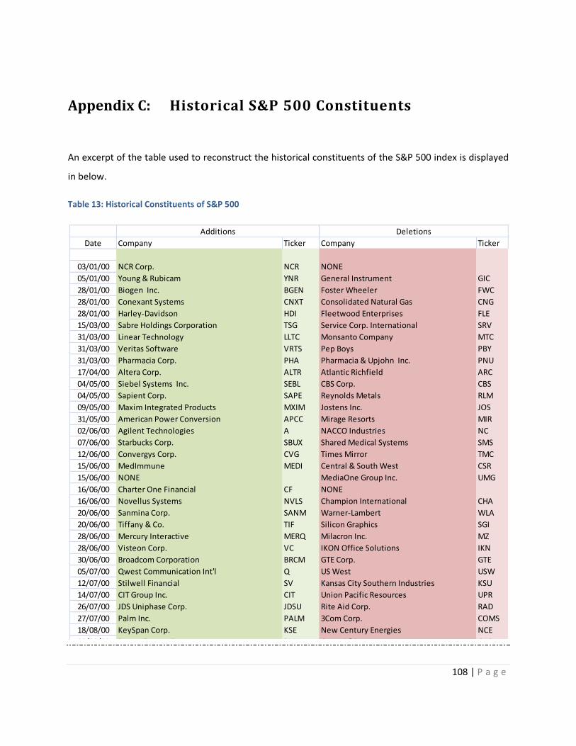
108 | P a g e

An excerpt of the table used to reconstruct the historical constituents of the S&P 500 index is displayed

in below.

Table 13: Historical Constituents of S&P 500

Date Company Ticker Company Ticker

03/01/00 NCR Corp. NCR NONE

05/01/00 Young & Rubicam YNR General Instrument GIC

28/01/00 Biogen Inc. BGEN Foster Wheeler FWC

28/01/00 Conexant Systems CNXT Consolidated Natural Gas CNG

28/01/00 Harley-Davidson HDI Fleetwood Enterprises FLE

15/03/00 Sabre Holdings Corporation TSG Service Corp. International SRV

31/03/00 Linear Technology LLTC Monsanto Company MTC

31/03/00 Veritas Software VRTS Pep Boys PBY

31/03/00 Pharmacia Corp. PHA Pharmacia & Upjohn Inc. PNU

17/04/00 Altera Corp. ALTR Atlantic Richfield ARC

04/05/00 Siebel Systems Inc. SEBL CBS Corp. CBS

04/05/00 Sapient Corp. SAPE Reynolds Metals RLM

09/05/00 Maxim Integrated Products MXIM Jostens Inc. JOS

31/05/00 American Power Conversion APCC Mirage Resorts MIR

02/06/00 Agilent Technologies A NACCO Industries NC

07/06/00 Starbucks Corp. SBUX Shared Medical Systems SMS

12/06/00 Convergys Corp. CVG Times Mirror TMC

15/06/00 MedImmune MEDI Central & South West CSR

15/06/00 NONE MediaOne Group Inc. UMG

16/06/00 Charter One Financial CF NONE

16/06/00 Novellus Systems NVLS Champion International CHA

20/06/00 Sanmina Corp. SANM Warner-Lambert WLA

20/06/00 Tiffany & Co. TIF Silicon Graphics SGI

28/06/00 Mercury Interactive MERQ Milacron Inc. MZ

28/06/00 Visteon Corp. VC IKON Office Solutions IKN

30/06/00 Broadcom Corporation BRCM GTE Corp. GTE

05/07/00 Qwest Communication Int'l Q US West USW

12/07/00 Stilwell Financial SV Kansas City Southern Industries KSU

14/07/00 CIT Group Inc. CIT Union Pacific Resources UPR

26/07/00 JDS Uniphase Corp. JDSU Rite Aid Corp. RAD

27/07/00 Palm Inc. PALM 3Com Corp. COMS

18/08/00 KeySpan Corp. KSE New Century Energies NCE

29/08/00 Devon Energy Corp. DVN Great A&P GAP

29/09/00 Avaya Inc. AV Owens Corning OWC

02/10/00 King Pharmaceuticals KG Young & Rubicam YNR

02/10/00 Moody's Corp. MCO Dun & Bradstreet DNB

02/10/00 Dynegy Inc. DYN BestFoods BFO

17/10/00 Nabors Industries NBR Mallinckrodt Inc. MKG

20/10/00 Power-One Inc. PWER Unicom Corp. UCM

01/11/00 NiSource Inc. NI Columbia Energy Group CG

01/11/00 EOG Resources EOG Eastern Enterprises EFU

03/11/00 BroadVision Inc. BVSN PainWebber Group PWJ

16/11/00 Starwood Hotels & Resorts HOT Armstrong Holdings Inc. ACK

21/11/00 Forest Laboratories FRX Seagate Technology SEG

22/11/00 Chiron Corp. CHIR Fort James Corp. FJ

30/11/00 Calpine Corp. CPN Florida Progress FPC

01/12/00 NONE Associates First Capital AFS

04/12/00 Robert Half International RHI NONE

08/12/00 Allegheny Energy Inc. AYE Bethlehem Steel BS

DeletionsAdditions

Appendix C: Historical S&P 500 Constituents

109 | P a g e

The regression results for the MACDX indicator on both the JSE and S&P500 strategies are displayed

below.

JSE MACDX 2009 DATA

Dependent Variable: JSEMACDX

Method: Least Squares

Date: 11/26/09 Time: 15:10

Sample (adjusted): 1 116

Included observations: 116 after adjustments Coefficient Std. Error t-Statistic Prob.

C 0.919113 0.431282 2.131117 0.0352

JSE 1.053486 0.072262 14.57874 0.0000

R-squared 0.650885 Mean dependent var 2.066321

Adjusted R-squared 0.647822 S.D. dependent var 7.695862

S.E. of regression 4.567077 Akaike info criterion 5.892715

Sum squared resid 2377.833 Schwarz criterion 5.940190

Log likelihood -339.7775 Hannan-Quinn criter. 5.911987

F-statistic 212.5396 Durbin-Watson stat 1.805426

Prob(F-statistic) 0.000000

Residuals and squared residuals are identified as white noise. This is the best regression model.

SPMACDX 2009 DATA

Dependent Variable: SPMACDX

Method: Least Squares

Date: 11/26/09 Time: 14:48

Sample: 1 116

Included observations: 116 Coefficient Std. Error t-Statistic Prob.

C 0.964311 0.543383 1.774645 0.0786

SP500 0.978109 0.096252 10.16194 0.0000

Appendix D: Regression Estimation Examples

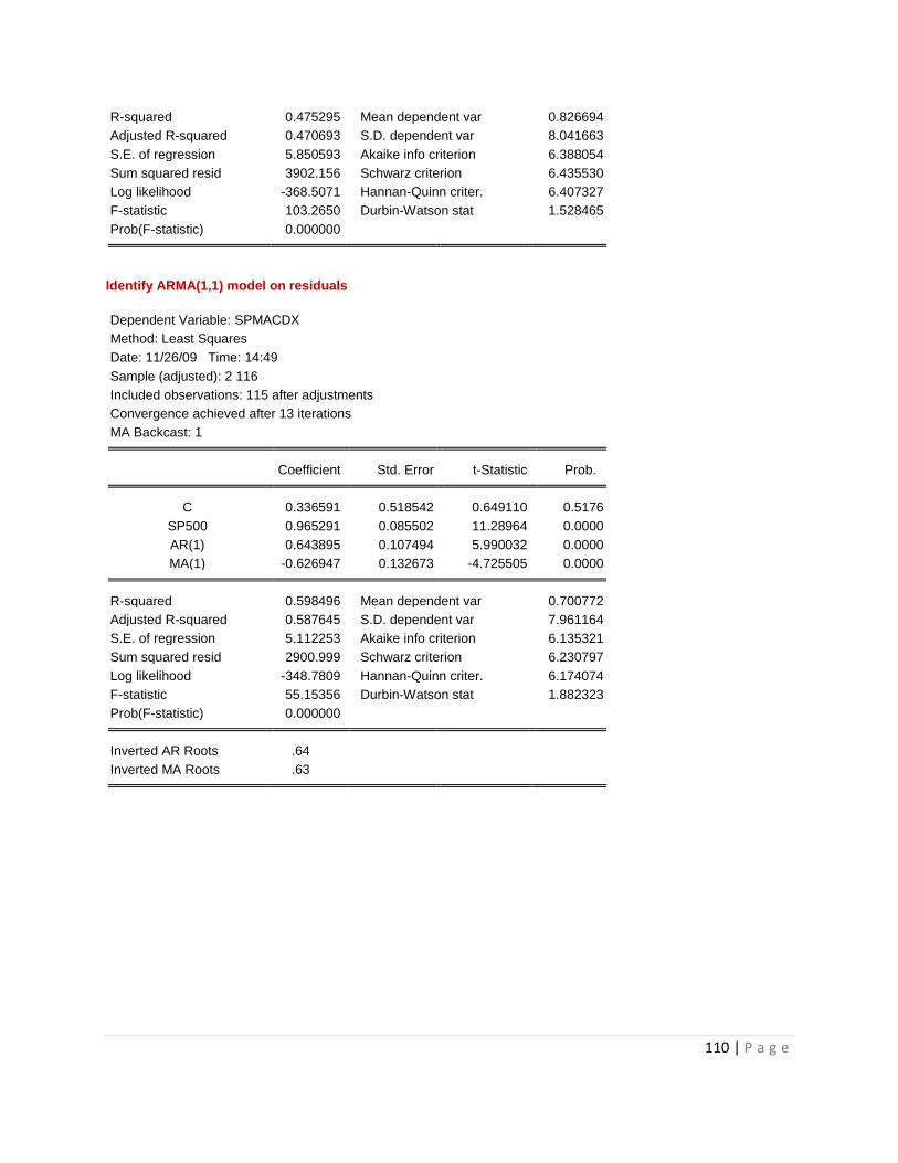
110 | P a g e

R-squared 0.475295 Mean dependent var 0.826694

Adjusted R-squared 0.470693 S.D. dependent var 8.041663

S.E. of regression 5.850593 Akaike info criterion 6.388054

Sum squared resid 3902.156 Schwarz criterion 6.435530

Log likelihood -368.5071 Hannan-Quinn criter. 6.407327

F-statistic 103.2650 Durbin-Watson stat 1.528465

Prob(F-statistic) 0.000000

Identify ARMA(1,1) model on residuals

Dependent Variable: SPMACDX

Method: Least Squares

Date: 11/26/09 Time: 14:49

Sample (adjusted): 2 116

Included observations: 115 after adjustments

Convergence achieved after 13 iterations

MA Backcast: 1 Coefficient Std. Error t-Statistic Prob.

C 0.336591 0.518542 0.649110 0.5176

SP500 0.965291 0.085502 11.28964 0.0000

AR(1) 0.643895 0.107494 5.990032 0.0000

MA(1) -0.626947 0.132673 -4.725505 0.0000

R-squared 0.598496 Mean dependent var 0.700772

Adjusted R-squared 0.587645 S.D. dependent var 7.961164

S.E. of regression 5.112253 Akaike info criterion 6.135321

Sum squared resid 2900.999 Schwarz criterion 6.230797

Log likelihood -348.7809 Hannan-Quinn criter. 6.174074

F-statistic 55.15356 Durbin-Watson stat 1.882323

Prob(F-statistic) 0.000000

Inverted AR Roots .64

Inverted MA Roots .63

111 | P a g e

Achelis, S. (2000). Technical Analysis A-Z. McGraw-Hill.

Ball, R., & Brown, P. (1968). A Emperical Evaluation of Accounting Income Numbers. Journal of

Accounting Research , Vol. 6, No.2, pp. 159-78.

Banz, R. (1982). The Relationship between Return and Market Value of Common Stocks. Journal of

Financial Economics , Vol. 9, No.1, pp 3-18.

Barberis, N., Shleifer, A., & Vishny, R. (1998). A Model for Investor Sentiment. Journal of Financial

Economics , Vol. 49, pp. 307-343.

Bird, R., & Whitaker, J. (2004). The Performance of Value and Momentum Investment Portfolios: Recent

Experience in the Major European Markets Part 2. Journal of Asset Management Vol. 5, No. 3 , pp. 157-

175.

Bodie, Kane, & Marcus. (2008). Investments. McGraw-Hill.

Bondt, W. D., & Thaler, R. (1987). Further Evidence on Investor Overreaction and Stock Market

Seasonality. Journal of Finance , Vol. 42, No.3, pp. 557-581.

Bradfield, D. (2003). Investment Basics . Investment Analysts Journal , Vol.57, pp. 47-53.

Carhart, M. (1997). On Persistence in Mutual Fund Performance . The Journal of Finance , Vol. 52, No.1,

pp. 57-82.

Chan, K., Jegadeesh, N., & Lakonishok, J. (1999). The Profitability of Momentum Strategies. Fanancial

Analysts Journal , Vol. 55, No. 6, pp. 80-90.

Chan, L., Jegadeesh, N., & Lakonishok, J. (1996). Momentum Strategies. Journal of Finance , Vol.2, No. 5,

pp. 1681-1713.

Chordia, T., & Shivakumar, L. (2002). Momentum, Business Cycle, and Time-varing Expected Returns.

The Journal of Finance , Vol. 57, No.2, pp. 985-1019.

Conrad, J., & Kaul, G. (1998). An Anatomy of Trading Strategies. The Review of Financial Studies , Vol.11,

No. 3, pp. 489-519.

Daniel, K., Hirshleifer, D., & Subrahmanyam, A. (1998). Investor Psychology and Security Market Under-

and Overreactions. The Journal of Finance , Vol. 53, pp. 1839-1886.

De Lange, T. (2009, 6 2009). CIO, Vega Capital. (E. Friedrich, Interviewer)

Bibliography

112 | P a g e

Domowitz, I., Glen, J., & Madhavan, A. (2001, 5 8). Investment Technology Group. Retrieved 11 5, 2009,

from ITG: http://www.plexusgroup.com/category/news-research-events/itg-research-trends

Du, D. (2008). The 52-week High and Momentum Investing in International Stock Indexes. The Quartlerly

Review of Economics and Finance 48 , 61-77.

Ellis, C., & Vertin, J. (2001). Wall Street People: True Stories of Today's Masters and Moguls. John Wiley

& Sons, ISBN 0471238090 .

Equis. (2006). MetaStock User Manual. Salt Lake City, UT, USA 84101: Equis.

Evans, J., & Archer, S. (1968). Diversification and Reduction of Dispersion: An Empirical Analysis. The

Journal of Finance , Vol. 23, No. 5, pp. 761-767.

Fama, E., & French, K. (1996). Multifactor Explanations of Asset Pricing Anomalies. The Journal of

Finance , Vol. 51, No.1, pp. 55-84.

Fama, E., & French, K. (1993). The Cross-Section of Expected Stock Returns. The Journal of Finance , Vol.

47, No. 2, pp. 427-65.

Foster, G., Olsen, C., & Shevlin, T. (1984). Earnings Surprise Research: Synthesis and Perspectives.

Financial Analysts Journal , 574-603.

Glaser, M., & Weber, M. (2003). Momentum and Turnover: Evidence from the German Stock Market.

Schmalenbach Business Review , Vol. 55, pp. 108-135.

Griffin, J., Xi, X., & Martin, S. (2003). Momentum Investing and Business Cycle Risk: Evidence from Pole

to Pole. The Journal of Finance , Vo. 58, No. 6, pp. 2515-2547.

Grinblatt, M., & Moskowitz, T. (2002). What Do We Really Know About the Cross-Sectional Relation

Between Past and Expected Returns? Yale ICF Working Paper , No. 00-72. Available at SSRN:

http://ssrn.com/abstract=296643 or DOI: 10.2139/ss.

Grundy, B., & Martin, J. (2001). Understanding the Nature of the Risks and the Source of the Rewards to

Momentum Investing. Review of Finacial Studies , Vol. 14, pp. 29-78.

Gup, B. (1983). The Basics of Investing. New York: John Wiley & Sons.

Hong, H., & Stein, J. (1999). A Unified Theory of Underreaction, Momentum Trading and Overreation in

Asset Markets. The Journal of Finance, Vol. 59, No. 6.

Hong, H., Lim, T., & Stein, J. (2000). Bad News Travels Slowly: Size, Analyst Coverage, and the Profitability

of Momentum Strategies. The Journal of Finance, Vol. 55, No.1.

Huang, D. (2006). Market States and International Momentum Strategies. The Quarterly Review of

Economics and Finance , Vol. 46, pp. 437-446.

113 | P a g e

Investment Technology Group. (2009, 10 9). Retrieved 11 5, 2009, from ITG:

http://www.itg.com/category/news-research-events/itg-research-trends/

Jegadeesh. (1990). Evidence of Predictable Behavior of Security Returns. The Journal of Finance , Vol. 45,

No.3, pp. 881-898.

Jegadeesh, N., & Titman, S. (2001). Profitability of Momentum Strategies: An Evaluation of Alternative

Explanations . The Journal fo Finance , Vol. 51, No. 2, pp. 699-720.

Jegadeesh, N., & Titman, S. (1993). Returns to buying Winners and selling Losers: Implications for Stock

Market Efficiency. Journal of Finance Vol. 48 , pp. 65-91.

Kaplan Schweser. (2008). CFA Level 1 Study Notes. Kaplan Schweser.

Kaplan Schweser. (2009). CFA Level 2 Study Notes. Kaplan Schweser.

Keim, D. (2003, May 28). The Cost of Trend Chasing and the Illusion of Momentum Profits. Finance

Department, The Warton School of Financial Research, 2300 Steiberg/Dietrich Hall, Philadelphia.

Keim, D., & Madhavan, A. (1998). The Cost of Institutional Equity Trades. Financial Analysts Journal , Vol.

54, No. 4, pp. 50-69 .

Keim, D., & Madhavan, A. (1997). Transaction Costs and Investment Syle: An Inter-Exchange Analysis of

Equity Trades. Journal of Financial Economics , Vol. 46, No.3, pp.265-292.

Kendall, M. (1953). The Analysis of Economic Time-Series-Part I: Prices. Journal of the Royal Statistical

Society , Vol. 116, No. 1, pp. 11-34 .

Korajczyk, R. A., & Sadka, R. (2004). Are Momentum Profits Robust to Trading Costs? The Journal of

Finance , Vol. 59, No. 3, pp. 1039-1082.

Lee, C., & Swaminathan, B. (2000). Price Momentum and Trading Volume. The Journal of Finance , Vol.

55, pp. 2017-2069.

Lesmond, D., Schill, M., & Zhou, C. (2004). The Illusory Nature of Momentum Profits. Journal of Financial

Economics , Vol. 71, No. 2, pp. 349-380.

Markowitz, H. (1952). Portfolio Selection. The Journal of Finance , Vol. 7, No. 1, pp. 77-91 .

Moskowitz, T. J., & Grinblatt, M. (1999). Do Industries Explain Momentum? Journal of Finance , Vol. 54,

No.4, pp. 1249-1290.

Moskowitz, T., & Grinblatt, M. (2004). Predicting Stock Price Movements from past Returns: The Role of

Consistency and Tax-loss Selling. Journal of Financial Economics , Vol. 71, No.3, pp. 541-579.

Reilly, F. (1985). Investment Analysis and Portfolio Management, 2nd ed. San Fransisco: Dryden Press.

114 | P a g e

Rey, D., & Schmid, M. (2005). Feasible Momentum Strategies -Evidence from the Swiss Stock Market.

Base: Department of Finance, University of Basel.

Ritter, J. (1988). The Buying and Selling Behaviour of Individual Investors at the Turn of the Year. The

Journal of Finance , Vol. 43, No. 3, pp. 701-717.

Roberts, H. (1959). Stock Market "Patterns" and Financial Analysis: Methodological Suggestions . The

Journal of Finance , Vol. 14, No.1, pp. 1-10.

Rouwenhorst, K. G. (1998). International Momentum Strategies. Journal of Finance 53 , Vol.54, No.4, pp.

267-284.

Rouwenhorst, K. G. (1999). Local Return Factors and Turnovers in Emerging Stock Markets. The Journal

of Finance , Vol. 54, No. 4, pp. 1439-1464.

Ryan, P., & Obermeyer, I. (2004). Profitability of Price Momentum Strategies: The Dax 100 Evidence. The

Journal of Investing , pp. 55-61.

Saunders, J. (2004). Investor Behavioural Psychology. Practical Investors Journal , No. 1.

Schiereck, D., Bondt, W. D., & Weber, M. (1999). Contrarian and Momentum Strategies in Germany .

Financial Analysts Journal , Vol. 55, No. 6, pp. 104-116.

Sharpe, W. (1963). A Simplified Model for Portfolio Analysis. Management Science , Vol. 9, No.2, pp.

277-293.

Shefrin, H. (2007). Beyond the Greed and Fear. Oxford University Press.

Standard and Poor's. (2009, 09 18). S&P 500 Fact Sheet. Retrieved 09 18, 2009, from Standard and

Poor's: http://www2.standardandpoors.com/spf/pdf/index/500factsheet.pdf

Stevenson, R., & Jennings, E. (1984). Fundamentals of Investments, 3rd ed. San Fransico: West Publ. Co.

Stock Market Investors. (2009, 10 8). Stock Market Investors. Retrieved 10 8, 2009, from

http://www.stock-market-investors.com/stock-tax-issues/stock-tax-implications.html

Swinkels, L. (2004). Momentum Investing: A Survey. Journal of Asset Management , Vol. 5, No. 2, pp.

120-143.

Taffler, R. (1999). Discussion of the Profitability of Momentum Investing. Journal of Business Finance and

Accounting , Vol. 26, No. 9, pp. 1093-1102.

Weinstein, S. (1988). Secrets for Profiting in Bull and Bear Markets. McGraw-Hill, ISBN 1-55623-079-6.

115 | P a g e