The Foundations of Factor Investing

Hanken Finance Day (Hanken School of Economics,

September 2020)

Paulo Maio

Hanken School of Economics

Asset Pricing Background

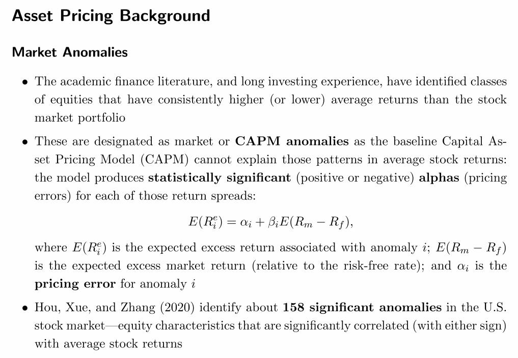
Market Anomalies

• The academic finance literature, and long investing experience, have identified classes

of equities that have consistently higher (or lower) average returns than the stock

market portfolio

• These are designated as market or CAPM anomalies as the baseline Capital As-

set Pricing Model (CAPM) cannot explain those patterns in average stock returns:

the model produces statistically significant (positive or negative) alphas (pricing

errors) for each of those return spreads:

E(Rei ) = αi + βiE(Rm −Rf ),

where E(Rei ) is the expected excess return associated with anomaly i; E(Rm − Rf )

is the expected excess market return (relative to the risk-free rate); and αi is the

pricing error for anomaly i

• Hou, Xue, and Zhang (2020) identify about 158 significant anomalies in the U.S.

stock market—equity characteristics that are significantly correlated (with either sign)

with average stock returns

• There are strong correlations among several anomalies⇒ Hou, Xue, and Zhang (2020)

aggregate those 158 anomalies into 6 major categories:

– Momentum: Stocks with high returns/earnings in the previous year tend to

subsequently outperform stocks with low returns/earnings

– Value-growth: Value stocks (high fundamentals-to-price ratios), low-duration

stocks, stocks with low returns in the previous 3 to 5 years subsequently outperform

growth stocks (low fundamentals-to-price ratios), high-duration stocks, and past

long-term winners, respectively

– Investment: Stocks of firms that invest less subsequently outperform stocks of

firms that invest more

– Profitability: Stocks of more profitable firms subsequently outperform less prof-

itable firms

– Trading frictions: Stocks with low volatility/beta subsequently outperform stocks

with high volatility/beta; but there are other unrelated anomalies

– Intangibles: All other anomalies (lots of heterogeneity inside this group)

• There are several competing theories for many of these anomalies

• For example, Fama and French (2015) rely on the present-value model of Miller

and Modigliani (1961) for the market-to-book ratio:

Mt

Bt=

∑∞τ=1E(Yt+τ − dBt+τ )/(1 + r)τ

Bt

– Ceteris paribus, lower market value (M), or equivalently a higher book-to-

market ratio (Bt/Mt), implies a higher expected return (r)

– Ceteris paribus, higher expected earnings (Y ) implies a higher expected

return

– Ceteris paribus, higher expected growth in book equity (db, investment) implies

a lower expected return

• Alternatively, Hou, Xue, and Zhang (2015) rely on the q-theory of corporate invest-

ment to justify the investment and (net) profitability anomalies

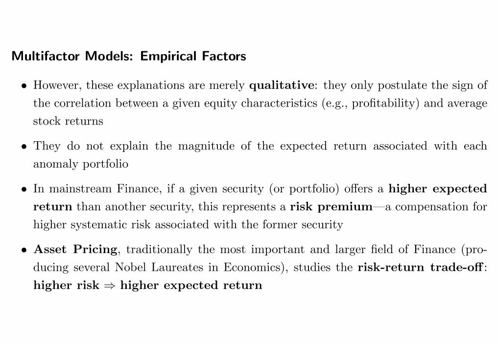
Multifactor Models: Empirical Factors

• However, these explanations are merely qualitative: they only postulate the sign of

the correlation between a given equity characteristics (e.g., profitability) and average

stock returns

• They do not explain the magnitude of the expected return associated with each

anomaly portfolio

• In mainstream Finance, if a given security (or portfolio) offers a higher expected

return than another security, this represents a risk premium—a compensation for

higher systematic risk associated with the former security

• Asset Pricing, traditionally the most important and larger field of Finance (pro-

ducing several Nobel Laureates in Economics), studies the risk-return trade-off :

higher risk ⇒ higher expected return

• Systematic risk:

– A risk factor is a variable that affects the returns of all assets (only the exposure

varies from asset to asset)

– Cannot be diversified away (eliminated) by forming large portfolios

– There is a reward (in the form of higher expected returns)

• Idiosyncratic risk:

– It is specific to each asset

– Can be diversified away (eliminated) by forming large portfolios

– There is no reward (no higher expected returns)

• The risk-return trade-off is often postulated in the form of a linear multifactor

model, with the following expected return-beta representation:

E(Rei ) = βi,1λ1 + ...+ βi,KλK + αi

– E(Rei ): risk premium for asset i or expected return of asset i in excess of another

asset (often the risk-free rate)

– βi,j quantity of risk of factor j, j = 1, ...,K; it measures the exposure of each

asset to each risk factor (source of systematic risk); it varies from stock to stock

(some stocks are riskier than others)

– λj price of risk of factor j, j = 1, ...,K; It is constant across stocks; it represents

the premium for one unit of risk for a given factor

– The total risk premium of a stock (or a portfolio), E(Rei ), represents the sum of

factor risk premiums

– αi is the pricing error for asset i: component of expected return that, according

to this model, should not exist

– αi represents a failure of the model: if the model is true⇒ αi = 0 from a statistical

viewpoint

• We do not observe expected returns: A common approach is to use the sample

average of realized returns over a relatively long period

• More importantly, we do not observe risk, or more specifically, we do not know

how many and the identity of the “true” risk factors

• Asset pricing researchers derive and test linear asset pricing models—selection

and identification of risk factors

• The average investor in the economy is risk averse ⇒ he/she requires a positive

risk premium to be exposed to riskier assets

• Riskier assets are assets that tend to perform poorly when factor realizations (re-

turns) are adverse (“bad”)

• Each factor has its own definition of “bad times”

• Assume that the factor carries a positive risk price (λj > 0) (this does not have to be

always the case)

• When a stock covaries more with that factor (high factor beta) ⇒ unattractive

stock to hold because it tends to have low payoffs (realized returns) during the bad

times defined by that factor’s negative realizations ⇒ this stock has to offer high

returns on average (expected returns) to compensate risk-averse investors (for the

higher risk)

• Exposure to factor risk over the long run yields a positive risk premium, but the

premium does not come for free: it represents a compensation for bearing losses

during bad times (high risk)

• Historically, the first asset pricing model was the Sharpe-Lintner CAPM:

E(Rei ) = βiE(Rm −Rf )

• The sole factor is the market risk premium (expected market return in excess of

the risk-free rate)

• The sole measure (quantity) of risk is the market beta (βi)

• The factor is traded (it represents an excess return) ⇒ the risk price (λ) estimate

is exactly equal to the mean of the factor, E(Rm −Rf )

• Under the CAPM, the definition of “bad times” are periods with low (negative)

realized market returns

• Due to the tremendous empirical failure of the CAPM (e.g., Fama and French, 1992),

Fama and French (1993, 1996, FF3) proposed the following 3-factor extension of

the CAPM:

E(Rei ) = βiE(Rm −Rf ) + siE(SMB) + hiE(HML)

– Similarly to the market factor, both SMB and HML are traded factors (excess

stock returns); hence, they represent zero-cost portfolios

– SMB (small-minus-big): return on a portfolio of small caps minus the return on

a portfolio of large caps

– HML (high-minus-low): return on a portfolio of value stocks minus the return on

a portfolio of growth stocks

– SMB captures the size anomaly (Banz, 1981); HML captures the book-to-

market (BM, value-growth) anomaly (Rosenberg, Reid, and Lanstein, 1985)

• This multifactor model can be seen as the academic foundation for factor investing:

all factors are traded ⇒ enables to conduct performance evaluation (see below)

• The FF3 model explains well the average returns on portfolios sorted on both size

(market capitalization) and BM

• However, this represents nearly a tautological exercise: it just informs us that the

relationship between average stock returns and BM is approximately monotonic—

stocks in the second decile of BM behave closer to stocks in the first decile (extreme

value stocks) relative to stocks in the upper deciles (growth stocks)

• A model with traded factors (empirical model) is only useful to the extent that it

helps explaining anomalies that are not mechanically related (by construction) to its

factors

• A good example is the 4-factor model of Hou, Xue, and Zhang (2015, HXZ4),

E(Rei ) = βiE(Rm −Rf ) + aiE(ME) + biE(ROE) + ciE(IA),

which does a relatively good job in explaining the momentum (broadly defined)

anomaly

• Such pricing performance comes from their profitability (high-minus-low ROE)

factor⇒ these two anomalies (momentum and net profitability) are connected (some-

thing that is not obvious a priori)

• Fama and French (2015, 2016, FF5) proposed the following 5-factor extension of their

3-factor model:

E(Rei ) = βiE(Rm −Rf ) + siE(SMB) + hiE(HML) + riE(RMW ) + ciE(CMA)

– CMA (conservative-minus-aggressive) represents an investment factor (quite

similar to the IA factor in HXZ4)

– RMW (robust-minus-weak) represents an operating profitability factor

– The differences between ROE and RMW explain the differences in the em-

pirical performance among the HXZ4 and FF5 models (e.g., Cooper and

Maio, 2019a, 2019b; Hou, Mo, Xue, and Zhang, 2019, 2020)

• However, FF5 is not able to explain momentum-based anomalies (just like FF3)

• In response to that failure, Fama and French (2018, FF6) add the momentum factor

(UMD, up-minus-down) of Carhart (1997):

E(Rei ) = βiE(Rm−Rf )+siE(SMB)+hiE(HML)+riE(RMW )+ciE(CMA)+uiE(UMD)

• Barillas and Shanken (2018) propose a 6-factor model, which combines some of the

factors in FF6 and HXZ4:

E(Rei ) = βiE(Rm−Rf )+siE(SMB)+hiE(HML)+riE(ROE)+ciE(IA)+uiE(UMD)

• Hou, Mo, Xue, and Zhang (2019, 2010, HMXZ5) add an expected growth factor

(EG) to HXZ4:

E(Rei ) = βiE(Rm −Rf ) + aiE(ME) + biE(ROE) + ciE(IA) + diE(EG)

• We have also seen the emergence of other empirical multifactor models: Novy-Marx

(2013); Asness and Frazzini (2013); Stambaugh and Yuan (2017); Daniel, Hirshleifer,

and Sun (2020); Asness, Frazzini, and Pedersen (2019)

• Similarly to the factors in HMXZ5 and FF6, the factors in those models are traded:

excess returns on portfolios associated with different anomalies (i.e., other stock char-

acteristics correlated with average stock returns)

• The hurdle in the empirical asset pricing literature has increased substantially in

recent years: A newly proposed asset pricing model should explain risk premia in a

broad cross-section of all equity portfolios (associated with a large number of CAPM

anomalies)

• This is especially relevant in the case of empirical models, which have a weaker theo-

retical background

• Hou, Xue, and Zhang (2015) test their model on 35 anomalies

• Hou, Mo, Xue, and Zhang (2020) employ 150 anomalies to test their 5-factor model

• Cooper, Ma, Maio, and Philip (2020) conduct a horse race of several multifactor

models in terms of pricing jointly 42 anomalies

• In principle, the traded multifactor models can be rationalized as empirical applica-

tions of the Arbitrage Pricing Theory (APT) of Ross (1976)

• Under the APT framework, factors that do a good job in summarizing the common

time-series variation in realized excess returns of a large number of portfolios ⇒candidate risk factors to explain the risk premia (expected returns) associated with

those same portfolios: Statistical factors are pricing risk factors

• However, Cooper, Ma, Maio, and Philip (2020) show that most empirical multifactor

models are not good empirical proxies for the APT: These models underperform

by a large degree a benchmark statistical model designed (by construction) to

price a cross-section associated with 42 anomalies

• HMXZ5 is the sole model that is not dominated (in statistical terms) by the bench-

mark statistical model

Multifactor Models: Fundamental/Macro Factors

• All empirical models contain the standard market factor despite the failure of the

CAPM in explaining the market anomalies

• The job of the market factor is to act as a “level” factor: to explain the average risk

premium in the cross-section

• Since all empirical multifactor models contain the market factor plus other equity fac-

tors, they are candidates to being empirical applications of the Intertemporal CAPM

(ICAPM) from Merton (1973):

E(Rei ) = βi,MλM + βi,zλz

• Under the ICAPM, the non-market factors (z) are called “hedging factors”—innovations

in state variables that predict changes in the investment opportunity set

• In practical terms, this means variables that help to forecast the excess market return

and/or aggregate stock volatility

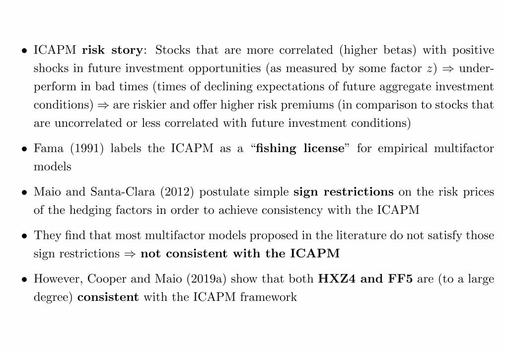
• ICAPM risk story: Stocks that are more correlated (higher betas) with positive

shocks in future investment opportunities (as measured by some factor z) ⇒ under-

perform in bad times (times of declining expectations of future aggregate investment

conditions)⇒ are riskier and offer higher risk premiums (in comparison to stocks that

are uncorrelated or less correlated with future investment conditions)

• Fama (1991) labels the ICAPM as a “fishing license” for empirical multifactor

models

• Maio and Santa-Clara (2012) postulate simple sign restrictions on the risk prices

of the hedging factors in order to achieve consistency with the ICAPM

• They find that most multifactor models proposed in the literature do not satisfy those

sign restrictions ⇒ not consistent with the ICAPM

• However, Cooper and Maio (2019a) show that both HXZ4 and FF5 are (to a large

degree) consistent with the ICAPM framework

• Nonetheless, the empirical factor models cannot represent the ultimate explanation of

a given risk premium; these models represent relative asset pricing: explaining one

equity risk premium (anomaly) by a collection of other equity risk premiums (factors)

• In most cases, we do not know why the factor risk premium exists in the first place

(absolute asset pricing)

• Both CAPM/ICAPM refer to absolute asset pricing while APT refers to relative

asset pricing ⇒ the ICAPM is more demanding and imposes more structure

(assumptions) than the APT

• Ideally, at least some of the major sources of systematic risk (factors) must originate

from outside the equity market

• The traditional 3 major classes of fundamental asset pricing models are the Lucas–

Breeden Consumption-CAPM (CCAPM), the ICAPM, and the Conditional CAPM

• In the CCAPM, the only risk factor is the growth in aggregate consumption

(non-durable goods plus services):

E(Rei ) = βiλC ,

where λC is the risk price for the consumption factor

• In the case of CCAPM (and other fundamental models), the factor is not traded

⇒ the risk price estimates are obtained by running a cross-sectional regression (of

average excess return onto betas)

• Under the Consumption-CAPM, the definition of “bad times” are periods with low

(negative) growth in aggregate consumption

• CCAPM risk story: stocks that are more correlated with aggregate consumption

tend to underperform in bad times (times in which aggregate consumption is declin-

ing) ⇒ these stocks are riskier and offer higher risk premiums (compared to stocks

that are less correlated or uncorrelated with the consumption factor)

• Empirically, the CCAPM performs poorly due to the small correlations between stock

returns and aggregate consumption

• Multifactor extensions of the CCAPM: Other macro factors in addition to aggregate

consumption

• Yogo (2006) proposes the following 3-factor macro model,

E(Rei ) = βi,MλM + βi,CλC + βi,DλD,

in which λM , λC , and λD denote the risk prices associated with the excess market

return, non-durable consumption growth, and durable consumption growth, respec-

tively

• The superior empirical performance of the model (relative to CCAPM) is mainly

driven by the presence of the durable-consumption factor

• The traditional hedging factors in the ICAPM are innovations in state variables that

forecast the excess market return

• Typically, these factors are not traded (not excess stock returns)

• The most popular predictors of the aggregate equity premium are the dividend

yield (DY ), term spread (TERM), default spread (DEF ), and T-bill rate

(RF ) (Fama and French, 1988, 1989)

• Empirically, the ICAPM has had some success in explaining several CAPM anomalies

(e.g., value-growth)

• Petkova (2006) proposes the following 5-factor ICAPM:

E(Rei ) = βi,MλM + βi,TERMλTERM + βi,DEFλDEF + βi,DY λDY + βi,RFλRF

in which the hedging factors are the innovations in TERM , DEF , DY , and RF

• The innovations are obtained from a vector autoregression (VAR) model

• Campbell and Vuolteenaho (2004) and Maio (2013) estimate different versions of the

Campbell (1993)’s variant of the ICAPM: The (composite) factors represent linear

functions of the VAR innovations in the state variables

• Often, the factor risk prices in fundamental models are connected to structural pa-

rameters (e.g., risk aversion coefficient)⇒ constraint in both the sign and magnitudes

of the risk price estimates

• In empirical models, there is no connection between the factor risk price estimates

and structural parameters

• The main advantage of fundamental models (macro/ICAPM) is to provide an eco-

nomic foundation (other than the law of one price, as in the APT) for the risk premium

associated with a given anomaly

• The pattern in factor loadings associated with a given group of portfolios (anomaly)

puts an additional constraint in the factor model: Does such cross-sectional pattern

in factor loadings make sense?

• For example, Maio and Santa-Clara (2017) shows that several value-growth and in-

vestment anomalies can be explained by an interest-rate factor in a two-factor ICAPM

• Value and low-investment stocks are more negatively correlated with short-term in-

terest rates (in comparison to growth and high-investment stocks, respectively): the

former type of equities are near financial distress after a sequence of negative shocks to

their cash-flows ⇒ more sensitive to rises in short-term interest rates, which increase

their financial costs (Fama and French, 1992; Bernanke and Gertler, 1989, 1990)

• Because the interest-rate factor has a negative price of risk⇒ value and low-investment

stocks offer higher risk premia (expected returns) than growth and high-investment

stocks, respectively

Implications for Factor Investing

• A disadvantage of fundamental multifactor models is that these cannot be used for

performance evaluation: (some of) the factors are not traded

• For this reason, factor investing focuses on empirical factor models: all factors

are traded (excess stock returns)

• Traded (also labelled as dynamic) factors represent long-short or zero-cost portfolios:

taking long position in securities with similar characteristics (e.g., value stocks), which

tend to comove with each other, and offsetting short positions in securities with the

opposite characteristics (e.g., growth stocks)

• The factors are dynamic because they need to be rebalanced: the stock characteris-

tics change over time

• Consider the case of the FF3 model

• The average return on Fund i is equal to the average return on the replicating (or

benchmark) portfolio plus the average active return (αi):

E(Ri)−Rf = αi + βiE(Rm −Rf ) + siE(SMB) + hiE(HML)⇔

E(Ri) = αi + βiE(Rm) + (1− βi)Rf + siE(SMB) + hiE(HML)⇔

E(Ri) = αi + E(Rb)

• The alpha (αi) is the “risk-adjusted return” or active return of the fund: Unique

average return generated by the manager in excess of what could be done mechanically

through passive exposures to the factors (average return on the benchmark portfolio,

E(Rb))

• The composition of the benchmark portfolio is as follows:

– βi on the stock market portfolio

– 1− βi on the risk-free asset (T-bill)

– si on a portfolio of small caps

– −si on a portfolio of large caps

– hi on a portfolio of value stocks

– −hi on a portfolio of growth stocks

• The benchmark portfolio is indeed a portfolio, as the weights sum up to 1:

βi + 1− βi + si − si + hi − hi = 1

• Dynamic factors assume the investor (owner of funds) can short: If not, the factors (in

the benchmark portfolio) should represent long-only equity portfolio (e.g., a diversified

portfolio of value stocks) in excess of the risk-free rate

• Duality between asset pricing and factor investing:

– In asset pricing, the factor loadings represent the measure of systematic risk asso-

ciated with each factor

– In factor investing, the factor loadings represent the weights (for each factor) in

the benchmark portfolio

– In asset pricing, the objective is to obtain low alphas (pricing errors)

– In factor investing, the objective is to obtain large alphas (high active performance)

• The reward of the portfolio manager (active management fee) is based exclusively on

the alpha, not Rb ⇒ possible moral hazard in the form of taking excessive risks

(large factor exposures)

• To minimize this problem, the investor (owner of funds) might specify ex-ante, not

only the factors, but also the corresponding weights in the benchmark portfolio

• The return on the benchmark portfolio represents the return that the investor

would obtain by investing on its own on the desired factors: The benchmark model

should be specific to each investor (owner of funds)

• Unsophisticated investor that wants to invest in a well diversified equity portfolio

that does not deviate a lot from the market portfolio ⇒ the appropriate benchmark

portfolio should be the market portfolio (combined with the risk-free asset)

• Sophisticated investor that wants to exploit the value-growth, investment, and

profitability groups of anomalies; the investor can short on its own⇒ the appropri-

ate benchmark portfolio should correspond to either FF5 or HXZ4

• Another sophisticated investor that wants to exploit the value-growth, in-

vestment, profitability, and momentum groups of anomalies; the investor can

also short ⇒ the indicated benchmark portfolio should correspond to either FF6 or

HXZ4

• In principle, more factors in the benchmark portfolio ⇒ harder job of the portfolio

manager in terms of generating significant positive alpha: Over a long period of time,

it should be substantially easier to generate positive alpha against the market model

than against the HXZ4 model

• Tension between the investor (owner of funds) and the portfolio manager in the

definition of the benchmark portfolio

• Even if two investors want to have exposure to the same factors, the portfolio

weights can differ: One investor might want to have a larger exposure to mo-

mentum risk premium, whereas the other investor might want to be more exposed to

the value-growth or investment risk premia

• Therefore, factor investing (when properly implemented) is more about “tailor-

made” investment products than about “commoditized” investment products

• Factor investing is more appropriate for sophisticated (can short), long-horizon,

and large (wealthier) investors in comparison to unsophisticated, short-horizon,

and small investors

• The average investor in the stock market holds the market portfolio (market

capitalization weights) ⇒ does not practice dynamic factor investing!

• Factor investing is similar in spirit to selling insurance

• One group of investors (less risk averse who sell insurance) are happy to have a

larger exposure to riskier stocks (e.g., value stocks) in their portfolio, which is financed

by a lower exposure to less risky stocks (e.g., growth stocks)⇒ In the long run, these

investors collect a positive risk premium (insurance premium) associated with the

higher risk exposure of their portfolio

• Another group of investors (more risk averse who buy insurance) want to have

a lower exposure to riskier stocks (e.g., value stocks) in their portfolio, which is offset

by a higher exposure to less risky stocks (e.g., growth stocks) ⇒ In the long run,

these investors are willing to accept a negative risk premium as a result of the lower

(hedged) risk exposure of their portfolio

• The staring point for both groups of investors is the market portfolio (combined with

the risk-free asset):

– The first group will overweight (underweight) value (growth) stocks in their

desired portfolio (positive loading on the HML factor)

– The second group will overweight (underweight) growth (value) stocks in their

desired portfolio (negative loading on the HML factor)

• Each investor chooses the risks (factors) he/she wants to take (positive exposure)

and the risks (factors) that he/she wants to hedge (negative exposure)

• If the investor does not want to invest in a given anomaly (e.g., momentum)⇒ his/her

benchmark portfolio will have a zero exposure to UMD (winner and loser stocks are

held at market weights)

• Factor investing represents a transfer of risks from more risk-averse and short-

horizon investors to less risk-averse and long-horizon investors

• Factor risk premiums do not come for free: episodic large negative returns

• The long-run positive expected return (risk premium) on a given factor represents

a compensation for negative realized returns over some periods—the “bad times”

according to the factor

• Consider the case of the price momentum anomaly (captured by UMD)

– UMD has an average monthly return of 0.70% (8.40% per year!) over the 1973–

2013 period

– However, there are substantial episodic losses: The maximum drawdown (MDD,

maximum cumulative loss) is −57.61%

– The betting-against-beta factor (BAB, low-risk anomaly) from Frazzini and Ped-

ersen (2014) produces an average monthly return of 0.88% (10.56% per year!) and

a MDD of −52.03% over the same period

– How many investors are willing to accept those losses (in more than half of their

portfolio value)? Probably, not the majority of the investors in the stock market

• This finding has implications for the candidate theories explaining asset (factor) risk

premia

• Behavioral theories: high expected returns result from investors’ under- or over-

reaction to news and/or the inefficient updating of beliefs; behavioral biases persist

because there are barriers to the entry of capital (which prevent arbitrage op-

portunities, associated with psychological biases, to be eliminated)

• In particular, the finding above precludes behavioral theories from representing a

consistent explanation of factor risk premia: market imperfections and frictions

are difficult to sustain in the long-run!

• The rational paradigm in Finance (risk-return tradeoff) seems like a more plausible

explanation!

• Looking forward to your questions and comments!

Readings

• Asness, C., and A. Frazzini, 2013, The devil in HML’s details, Journal of Portfolio

Management 39, 49–68.

• Asness, C., A. Frazzini, and L. Pedersen, 2019, Quality minus junk, Review of Ac-

counting Studies 24, 34–112.

• Banz, R.W., 1981, The relationship between return and market value of common

stocks, Journal of Financial Economics 9, 3–18.

• Barillas, F., and J. Shanken, 2018, Comparing asset pricing models, Journal of Fi-

nance 73, 715–754.

• Bernanke, B.S., and M. Gertler, 1989, Agency costs, net worth, and business fluctu-

ations, American Economic Review 79, 14–31.

• Bernanke, B.S., and M. Gertler, 1990, Financial fragility and economic performance,

Quarterly Journal of Economics 105, 87–114.

• Campbell, J.Y., 1993, Intertemporal asset pricing without consumption data, Amer-

ican Economic Review 83, 487–512.

• Campbell, J.Y., and T. Vuolteenaho, 2004, Bad beta, good beta, American Economic

Review 94, 1249–1275.

• Carhart, M., 1997, On persistence in mutual fund performance, Journal of Finance

52, 57–82.

• Cooper, I., L. Ma, P. Maio, and D. Philip, 2020, Multifactor models and their consis-

tency with the APT, SSRN Working Paper.

• Cooper, I., and P. Maio, 2019a, Asset Growth, Profitability, and Investment Oppor-

tunities, Management Science 65, 3988–4010.

• Cooper, I., and P. Maio, 2019b, New Evidence on Conditional Factor Models, Journal

of Financial and Quantitative Analysis 54, 1975–2016.

• Daniel, K., D. Hirshleifer, and L. Sun, 2020, Short- and Long-horizon behavioral

factors, Review of Financial Studies 33, 1673–1736.

• Fama, E.F., 1991, Efficient capital markets: II, Journal of Finance 46, 1575–1617.

• Fama, E.F., and K.R. French, 1988, Dividend yields and expected stock returns,

Journal of Financial Economics 22, 3–25.

• Fama, E.F., and K.R. French, 1989, Business conditions and expected returns on

stock and bonds, Journal of Financial Economics 25, 23–49.

• Fama, E.F., and K.R. French, 1992, The cross-section of expected stock returns,

Journal of Finance 47, 427–465.

• Fama, E., and K. French, 1993, Common risk factors in the returns on stocks and

bonds, Journal of Financial Economics 33, 3–56.

• Fama, E.F., and K.R. French, 1996, Multifactor explanations of asset pricing anoma-

lies, Journal of Finance 51, 55–84.

• Fama, E., and K. French, 2015, A five-factor asset pricing model, Journal of Financial

Economics 116, 1–22.

• Fama, E., and K. French, 2016, Dissecting anomalies with a five-factor model, Review

of Financial Studies 29, 69–103.

• Fama, E., and K. French, 2018, Choosing factors, Journal of Financial Economics

128, 234–252.

• Frazzini, A., and L. Pedersen, 2014, Betting against beta, Journal of Financial Eco-

nomics 111, 1–25.

• Hou, K., H. Mo, C. Xue, and L. Zhang, 2019, Which factors? Review of Finance 23,

1–35.

• Hou, K., H. Mo, C. Xue, and L. Zhang, 2020, An augmented q-factor model with

expected growth, Review of Finance, forthcoming.

• Hou, K., C. Xue, and L. Zhang, 2015, Digesting anomalies: an investment approach,

Review of Financial Studies 28, 650–705.

• Hou, K., C. Xue, and L. Zhang, 2020, Replicating anomalies, Review of Financial

Studies 33, 2019–2133.

• Maio, P., 2013, Intertemporal CAPM with conditioning variables, Management Sci-

ence 59, 122–141.

• Maio, P., and P. Santa-Clara, 2012, Multifactor models and their consistency with

the ICAPM, Journal of Financial Economics 106, 586–613.

• Maio, P., and P. Santa-Clara, 2017, Short-term interest rates and stock market anoma-

lies, Journal of Financial and Quantitative Analysis 52, 927–961.

• Merton, R.C., 1973, An intertemporal capital asset pricing model, Econometrica 41,

867–887.

• Miller, M.H., and F. Modigliani, 1961, Dividend policy, growth, and the valuation of

shares, Journal of Business 34, 411–433.

• Novy-Marx, R., 2013, The other side of value: The gross profitability premium, Jour-

nal of Financial Economics 108, 1–28.

• Petkova, R., 2006, Do the Fama-French factors proxy for innovations in predictive

variables? Journal of Finance 61, 581–612.

• Rosenberg, B., K. Reid, and R. Lanstein, 1985, Persuasive evidence of market ineffi-

ciency, Journal of Portfolio Management 11, 9–17.

• Ross, S. A. 1976, The arbitrage theory of capital asset pricing, Journal of Economic

Theory 13, 341–360.

• Stambaugh, R., and Y. Yuan, 2017, Mispricing factors, Review of Financial Studies

30, 1270–1315.

• Yogo, M., 2006, A consumption-based explanation of expected stock returns, Journal

of Finance 61, 539–580.