What's Driving U.S. Broiler Farm Profitability?1

2015 International Food and Agribusiness Management Association (IFAMA). All rights reserved. 59

International Food and Agribusiness Management Review Volume 18 Special Issue A, 2015

What’s Driving U.S. Broiler Farm Profitability?1

Richard Nehringa, Jeffrey Gillespieb, Ani L. Katchovac, Charlie Hallahand,

J. Michael Harrise, and Ken Ericksonf

aEconomist, dOperations Research Analyst, f Economist, U.S. Department of Agriculture, Economic Research Service, 1400 Independence Ave. SW, Mail Stop 1800, Washington, DC, 20250-0002, USA

bMartin D. Woodin Endowed Professor, Dept. of Agricultural Economics & Agribusiness, Louisiana State University Agricultural Center 101 Martin D. Woodin Hall, Louisiana State University, Baton Rouge, Louisiana, 70803, USA

cAssociate Professor, Farm Income Enhancement Chair, and Director of the Center for Cooperatives, Department of Agricultural, Environmental, and Development Economics, 220 Ag Admin Building,

2120 Fyffe Road, Columbus, Ohio, 43210, USA.

Abstract Using USDA’s ARMS data for 2003-2011 and the DuPont expansion financial model, we determine the extent and location of U.S. broiler farms and estimate the drivers of farm profitability, asset turnover, solvency, and return on equity. We find that farm size, diversification, and broiler housing vintage are the major drivers of farm financial performance, so these factors will likely have the greatest impact on U.S. broiler production in an increasingly competitive broiler trade market. Furthermore, region, farmer age, and off-farm employment are additional farm financial performance drivers that have implications for international competitiveness. Keywords: DuPont model, profitability, solvency, asset efficiency, broilers

Corresponding author: Tel: + 1.225.578.2759

Email: R. Nehring: [email protected] J. Gillespie: [email protected] A. Katchova: [email protected] C. Hallahan: [email protected] J. Harris: [email protected] K. Erickson: [email protected]

1 The views expressed are those of the authors and do not necessarily represent the views or policies of the USDA.

Nehring et al. Volume18 Special Issue A, 2015

2015 International Food and Agribusiness Management Association (IFAMA). All rights reserved.

60

Introduction

The broiler industry plays a significant role in the economy of a number of states in the U.S., particularly those located in the South. In 2012, almost 33,000 U.S. farms sold nearly 8.5 billion broilers and other meat-type chickens (USDA Census of Agriculture 2014). This resulted in nearly 37 billion pounds of product being produced on a ready-to-cook basis, of which approximately 20% was exported and the remainder consumed in the U.S. at a consumption rate of 95 pounds per capita (USDA-NASS 2013). Over 2004-2013, total broiler and other chicken meat produced increased from 34.2 billion pounds to 37.9 billion pounds, of which exports increased from 5.0 billion pounds to 7.5 billion pounds, and domestic consumption remained relatively stable, moving from 29.1 billion pounds to 30.5 billion pounds (USDA-NASS 2013). These figures suggest that the export market has been responsible for the marketing of the majority of the increased production. The importance of trade in U.S. broiler production suggests that the industry must continue to remain competitive in the world broiler market, with cost of production and farm financial performance continuing to be of importance domestically. This paper addresses the drivers of financial performance of U.S. broiler farms, with implications for broiler trade. Broiler production is concentrated in a group of states in the U.S. (Figure 1) primarily in the South, but also including significant production in California, Delaware and Pennsylvania. The top broiler states are Georgia, Arkansas, Alabama, Mississippi, and North Carolina.

Nearly all U.S. broiler growers operate under production contracts with large, quasi-vertically integrated firms that produce feed and handle bird processing (Knoeber 1989; Rogers 2002; MacDonald 2008). Figure 2 shows the organization of the U.S. broiler industry. A significant open cash market for broilers has not existed since the 1950s. Under production contracts, broiler growers do not own the birds; rather they provide the broiler grow-out house, labor, and utilities required to raise the chicks. The grow-out house and associated equipment can require a significant investment of $300,000 or more. The house is equipped, by agreement with the contractor (or integrator), with all necessary heating, cooling, feeding, and watering systems. The grower provides the labor and clean litter needed for growing the birds and disposes of the used litter. The contractor supplies the chicks, feed, veterinary services, and transportation to the processing plant when the broilers are fully grown. The birds and feed are owned by the contractor who contracts with the grower to feed the birds to market weight. A typical broiler production contract involves a tournament in which growers are paid by the contractor on the basis of their productivity relative to the productivity of the other growers in the same group (Knoeber 1989). Taylor (2004) provides a critical review of the “fairness” of production contracts. The integrator generally owns the hatchery, feed mills, and slaughter and further processing plants. The breeding segment is generally either owned by the integrator or contracted with breeding companies (MacDonald 2008).

The structure of this industry has led to relatively low costs per pound of broiler meat produced, making the U.S. market particularly competitive on the world broiler market. The resultant high productivity led to greater exports (MacDonald 2008). However, low-cost countries that have emerged as broiler producers in recent years, such as Brazil, China, and Thailand, are potential threats to the U.S. broiler export market (Constance 2008). The U.S. broiler model has been



61

exported to a number of countries throughout the world. Various U.S. companies such as Tyson Foods, Cargill, Inc., and Pilgrim’s Pride have invested in countries in Asia, South America, and Mexico with operations there (Constance 2008). The U.S. broiler industry is currently undergoing retrenchment. While the industry’s organization contributed to commercial success for most of the last two decades, the industry today faces challenges in the form of volatile feed costs, now in a profitable range with a broiler to feed ratio of over 5 after almost two years below 5 (Day 2015). Moreover, smaller farms tend to have significantly older broiler houses, leading to lower operator returns per broiler and greater reliance on off-farm income. Hence, the industry is shifting toward larger operations where household income is more closely tied to the broiler enterprise. In addition, two recent major bankruptcies of integrators (Day 2015) have resulted in a more global business model for integrators. (See Feedstuffs July, 2014, on the divestiture of Tyson holdings in Mexico and Feedstuffs, September, 2014, for the trade outlook for broiler meat). At the same time, per capita domestic consumption appears to be strengthening in recent years with projected 2015 consumption close to the historic high of about 86 pounds per capita in 2006 (The National Chicken Council 2015). Figure 1. Broiler production by state number produced, thousand, 2010. Source. USDA, National Agricultural Statistics Service, Washington DC, 2011. Factors influencing trade for broiler meat have generally been similar to drivers for other products. Davis et al. (2014) show that broiler trade was affected by several drivers: exporter and



62

importer GDPs and population, distance between countries, whether countries have common borders and/or languages, whether countries are part of the North American Free Trade Agreement or the European Union, and exchange rate volatility. Another trade determinant has been cost of production. Golz and Woo (1991) estimated, for example, that if Canada and Mexico reduced their production costs by 10%, they would import less broiler meat from the U.S., and if they reduced their production costs by 20%, they would become net exporters to the U.S. Clearly, production costs and hence profitability are significant trade flow determinants and relatively small changes in the cost structure can alter broiler trade. Factors that can alter competitiveness and thus trade in the relative short run but with potential long-term impacts can include feed costs, labor costs, demand, disease outbreaks such as avian influenza, others. Determination of the drivers of financial success (profitability, solvency, and asset efficiency) in U.S. broiler production is useful in determining competitiveness in broiler trade.

Figure 2. Structure of the U.S. Broiler Industry Source. Poultry Science and Technology Guide Extension Poultry Science, North Carolina State University, Raleigh, North Carolina, 2011.

A country’s agricultural competitiveness in the global market can depend on a number of factors, which are considered in this study. For example, farm size can impact competitiveness. MacDonald (2008) shows the cost advantages that are associated with large-scale broiler

Raw Ingredient

Further ProcessingDistribution

Feed Manufacturing Equipment, Supplies

Breeder Chicks or Poults

Breeder Growout

Parent Breeders

Hatching Eggs

Equipment, Supplies Processing

Storage

Hatchery

Chicks or Poults

Growout

Live Haul

Primary Breeder



63

production. Furthermore, production technology is hypothesized to impact competitiveness. Broiler houses built since 1996 have the capacity for greater control over the environment (climate controls), and therefore may further impact the financial performance of the broiler operation. Other issues such as farm diversification, off-farm work, and management may also impact farm financial performance and, thus, global competitiveness and trade. The objective of this study is to examine the drivers of financial success in U.S. broiler production. Specifically, we examine factors influencing broiler farm profitability, decomposing it into four components including net return on assets, asset efficiency, solvency, and net return on equity. We analyze the USDA’s Agricultural Resource Management Survey (ARMS) 2003-2011 Phase III data for broiler farms to estimate a DuPont expansion model. We discuss the implications of this analysis for U.S. broiler trade.

The DuPont Expansion Model We use the DuPont expansion model to analyze the economic and financial performance of U.S. broiler farms. The DuPont Expansion (also commonly known as the DuPont identity, DuPont equation, DuPont model, or the DuPont method) is a method that breaks return on equity into three parts: profitability, operating efficiency, and financial leverage. Mishra et al. (2012) attribute the original DuPont model to F. Donaldson Brown in 1918, who showed that return on assets was the product of two common financial ratios, one for profitability and the other for efficiency. This later evolved into the three-part equation used today. The name originated from the DuPont Corporation, which started using this formula in the 1920s. Based on these three performance measures, a farm can increase its return on equity by maintaining a high profit margin, increasing asset turnover, or leveraging assets more efficiently. This approach helps simplify the farm financial performance analysis and improve decision making concerning operations and finance (Moss 2013). The DuPont expansion model has been widely used for firm analysis in corporate finance as well as by university extension personnel for farm business analysis. The DuPont expansion focuses primarily on the return on owner’s equity, R/E, where R is net return and, for farm analysis, E is farm equity. Net return is defined as R = S – C, where S represents agricultural sales and C represents production costs. Collins (1985) introduced a variant of the DuPont formulation which has been used in agricultural finance applications (Melvin et al. 2004, Mishra et al. 2012, Moss 2013). The DuPont identity decomposes return on equity into profitability, asset turnover, and leveraging decisions as: Return on Equity = Operating Profit Margin × Asset Turnover × Solvency. The equation used to analyze the relationship between the rate of return on equity, asset efficiency, profitability, and solvency, is shown as (Mishra et al. 2009):

(1) RE

= S-CS

* SA

* AERE

= S-CS

* SA

* AE

,

where A is the value of farm assets. Thus, with the DuPont expansion, return on equity is the product of farm profitability using the operating profit margin ratio �R

S� �R

S�, farm asset efficiency



64

using the asset turnover ratio �SA� �S

A�, and farm solvency (or in our case inverse solvency) using

the inverse of the equity/asset ratio �AE� �A

E�.

In cases where the farm is debt-free, the rate of return on equity equals the farm’s rate of return on assets �R

A� �R

A�. However, if there is interest to be paid on debt, it must be subtracted from net

farm income R. Furthermore, in these cases when the farm has debt, assets > equity. As measures of profitability, higher rates of return on equity and higher operating profit margin ratios are preferred. Asset efficiency measures how quickly the farm’s gross revenue covers the capital invested in farm assets. In other words, with a farm asset ratio of 0.25, it would take four years for the farm to realize gross revenue that would cover the investment in assets. A higher asset turnover ratio is desirable since this indicates shorter time to cover investment costs. Solvency provides a measure of whether farm liabilities can be covered by selling farm assets. The equity/asset ratio is a measure of solvency that indicates owner equity capital as a portion of total farm assets. In the DuPont expansion as we present, a measure of inverse solvency is analyzed. More information regarding these measures of profitability, asset efficiency, and solvency can be found in the literature (Kay et al. 2012). Previous authors (Mishra et al. 2009) show that the DuPont expansion is linear in logs, as in (2):

(2) ln �R

E� = ln �R

S� + ln �S

A� + ln �A

E� ln �R

E� = ln �R

S� + ln �S

A� + ln �A

E�

In accordance with this relationship, determinants of farm financial performance can be analyzed using seemingly unrelated regression (SUR) where a separate equation is estimated for the farm’s return on equity, operating profit margin ratio, asset turnover ratio, and equity/asset ratio. These measures, thus, serve as the dependent variables in a system that takes into consideration the correlation of the error terms. SUR was also deemed appropriate since the Breusch-Pagan test showed correlation of the cross-equation error terms. Because ln �R

E� ln �R

E� is the sum of

ln �RS� , ln �S

A� , ln �R

S� , ln �S

A�, and ln �A

E� ln �A

E� , the former may be dropped from the system due to

summing-up conditions, as in Mishra et al. (2012). Data To analyze farm financial performance in U.S. broiler production, we use 2003-2011 Phase III ARMS and 2006 and 2011 ARMS broiler cost of production survey data. The ARMS is conducted annually by the USDA’s National Agricultural Statistics Service and Economic Research Service. The Phase III data include whole-farm costs and returns for a sample of U.S. farms along with information on farm size, type, structure, and farm and household characteristics. Only a limited number of farms in the Phase III data produce broilers. Every year, several farm enterprises are selected for more in-depth surveying, with questions addressing costs and returns specifically for the enterprise of interest, the use of technologies and management practices for that enterprise, and other questions of interest specifically for the enterprise. Broiler cost of production surveys were conducted in 2006 and 2011, resulting in



65

1,561 and 1,444 usable responses in each year, respectively. For the Phase III ARMS surveys conducted during 2003-2011, a total of 8,892 observations included broilers. Because the ARMS is a design-based survey that uses stratified sampling, weights or expansion factors are included for each observation to extend the results to the U.S. farm population. In the case of the broiler cost of production surveys, the data can be expanded to represent the largest U.S. broiler states, representing 90% of U.S. broiler production. We use the 2006 and 2011 ARMS broiler surveys to examine the impact of farm and farmer characteristics on the use of new versus old broiler housing technology and the 2003-2011 ARMS Phase III data to provide a longer-term view of the drivers of broiler farm financial performance.

Equations to Be Estimated The three equations estimated using SUR include the following:

(3) ln �RS� ln �R

S�=f

(Appalachia, Corn Belt, Delta, Northeast, Southern Plains, Age, Spouse Off-Farm, Operator Off-Farm, Acres Operated, Chicks Sold, Proportion Broilers, New Technology, THI)

(4) ln �SA� ln �S

A�=f

(Appalachia, Corn Belt, Delta, Northeast, Southern Plains, Age, Spouse Off-Farm, Operator Off-Farm, Acres Operated, Chicks Sold, Proportion Broilers, New Technology, THI)

(5) ln �A

E� ln �A

E�=f

(Appalachia, Corn Belt, Delta, Northeast, Southern Plains, Age, Spouse Off-Farm, Operator Off-Farm, Acres Operated, Chicks Sold, Proportion Broilers, New Technology, Heat Index, Region × THI, Region × Chicks Sold) These factors are hypothesized to impact U.S. broiler farm asset efficiency, profitability, and solvency, and thus the competitiveness of U.S. broiler production within the world market. In our model, we control for the impact of region on broiler farm asset efficiency, profitability, and solvency by including six regions: Appalachia including Kentucky, North Carolina, Tennessee, and Virginia; Corn Belt including Missouri; Delta including Arkansas, Louisiana, and Mississippi; Northeast including Delaware, Maryland, and Pennsylvania; Southeast including Alabama, Georgia, and South Carolina; and Southern Plains including Oklahoma and Texas. There were relatively few California firms in the data; they were included with the Southern Plains farms. These 17 states, representing 90% of the value of U.S. broiler production, were included in the 2006 and 2011 ARMS broiler cost of production survey and are the only states we include in our DuPont SUR model. Operator demographic variables included in each of the three equations include operator Age, predicted spouse hours per year working off the farm (Spouse Off-Farm), and predicted operator



66

hours per year working off the farm (Operator Off-Farm). Previous studies have shown that operator age significantly influences farm financial performance. For instance, asset efficiency was lower among older U.S. farmers (Mishra et al. 2012) and older dairy farmers operated less profitable farms than younger ones (Gillespie et al. 2009). Spouse Off-Farm and Operator Off-Farm are included to examine the impacts of off-farm work on broiler farm financial performance. Appendix Table 1 shows that operators and their spouses worked off farm on average 283 and 361 hours per year, respectively, over the period. Since off-farm employment can be endogenously determined with farm financial variables, the Hausman (1978) test was used to test for endogeneity in each of the three SUR equations. Endogeneity was found, so instrumental variables were substituted into the model for these two variables. Ordinary least squares estimates of the predicted values for these variables were then included in the SUR model (Appendix Table 3). Independent variables included in the Spouse Off-Farm model were farm net worth, government payments received by the farm, household size, accrued interest, off-farm interest income, population accessibility of the farm, value of livestock production under contract, farm operator household assets, adjusted wage rates in the area where the farm is located, and owned acres operated. Thus, these variables served as instruments for Spouse Off-Farm. Independent variables for Operator Off-Farm were the same as for Spouse Off-Farm except that Age, a household well-being dummy variable indicating that the household was above the median value of well-being, and total animal units on the farm were also included, while adjusted wage rates in the area and owned acres operated were not included. Thus, these variables, with the exception of Age, which is also included in the DuPont SUR equations, served as instruments for the Operator Off-Farm variable. For the Spouse Off-Farm regression equation, all but three coefficients were significant at P < 0.10. For the Operator Off-Farm regression equation, all but two variables were significant at P < 0.10. With many significant drivers, it was determined that the predicted values could be used in the SUR model. Specification of these equations was heavily influenced by previous work (Gillespie and Mishra 2011; Nehring et al. 2014), who used similar specifications for instrumental variables for Spouse Off-Farm and Operator Off-Farm. It is expected that off-farm work increases financial resources available to the farm, thus potentially increasing solvency, but it may also divert management resources from the farm, which could negatively impact farm financial performance. Variables used for farm size include Acres Operated and Broilers Sold. Both were specified as their natural logs, so their interpretation is similar to that of an elasticity. Acres Operated measures the total number of operated acres, serving as a measure of the size of the total farm operation, including acres in crops, pasture, and woodland. Broilers Sold serves as a measure of the size of the broiler enterprise. Farm size was found to increase the asset efficiency of U.S. cow-calf farms (Nehring et al. 2014) and to impact both profitability and asset efficiency of U.S. farms (Mishra et al. 2012). Appendix Table 1 shows that Acres Operated averaged 199 for U.S. broiler farms, ranging from 161 in the Northeast to 284 in the Corn Belt. The number of Broilers Sold averaged 467,400 for the U.S., ranging from 297,386 in the Northeast to 634,259 in the Corn Belt.



67

Proportion Broilers, defined as the value of broiler production divided by the value of total farm production, is a measure of specialization in broiler farming. Earlier studies have found that farm diversification (the opposite of specialization) impacted farm asset efficiency, profitability, and solvency (Mishra et al. 2012). Specialization in beef production was found to reduce the asset efficiency of U.S. cow-calf farms (Nehring et al. 2014). The expected impact of specialization would depend upon whether managerial gains can be expected from specialization or whether significant scope economies exist in the production of broilers along with other farm enterprises. Appendix Table 1 shows that the Proportion Broilers averaged 95% and ranged from 88% in the Northeast to 98% in the Southeast, showing a relatively large specialization in broilers. The impact of technology on farm financial performance has been extensively addressed in the agricultural economics literature. Technology that improves productivity can be expected to improve long-run farm profitability and asset efficiency. It can also impact solvency if debt financing is used to purchase the technology. Technology is an important productivity driver, and increased productivity is a major factor that has influenced the increase in U.S. broiler exports (MacDonald 2008). We define new technology housing as housing that was built after 1996. New broiler housing technologies that have become more common since the mid-1990s include tunnel ventilation and evaporative cooling cells (MacDonald 2008). MacDonald states that houses constructed prior to 1995 (about 40% of housing capacity) are less likely to include these technologies and other modern technologies such as computer warning systems. Tunnel ventilation systems consist of large fans at one end of a broiler house and air inlets at the other end. Fans pull air through the house, removing heat and creating a wind chill for cooling. Evaporative cooling systems located near the air inlets can be activated for further cooling in a tunnel-ventilated house. Cooling pads, moistened by fogging nozzles, lower the air temperature as it is pulled through the pads and the house. About 75% of broiler houses had cooling cells and tunnel ventilation in 2006 (MacDonald 2008). While some houses built prior to 1996 have been retrofitted with new technology, those houses tend to be smaller and often do not include other new technologies. As discussed earlier, we used the 2003-2011 ARMS Phase III data for the DuPont SUR. However, those surveys did not query broiler farmers as to the vintage of their houses. The 2006 and 2011 Phase III broiler cost of production surveys, however, did query growers as to housing vintage. Thus, we used the 2006 and 2011 Phase III broiler cost of production survey data to estimate a probit model to determine the probability that a broiler farmer owned broiler houses constructed after 1996. This probit model includes as independent variables dummy variables for the regions, the total number of chicks placed, total cash wages paid to labor, total reported depreciation for machinery, Age, whether the operator worked off-farm, the operator’s education level, the debt-asset ratio, whether the household’s well-being index was higher than the median value for all broiler farms, and a trend variable that was coded as 2006=0 and 2011=5. We then used the predicted values of the probit model to estimate the probability that an operation of specific characteristics used old or new technology and included these predicted values in the DuPont model. Since we expect that from 2003 to 2011, the adoption rate would have increased, a trend variable is used to adjust probabilities of adoption in the DuPont model year, with 2003 coded as -3, 2004 as -2, …, to 2011 as 5. As seen in Appendix Table 4, 10 of the 14 independent variables were significant at P ≤ 0.10 and the percentage correctly predicted was 68.1%. Furthermore, because growers self-select into a technology, i.e. more productive growers are



68

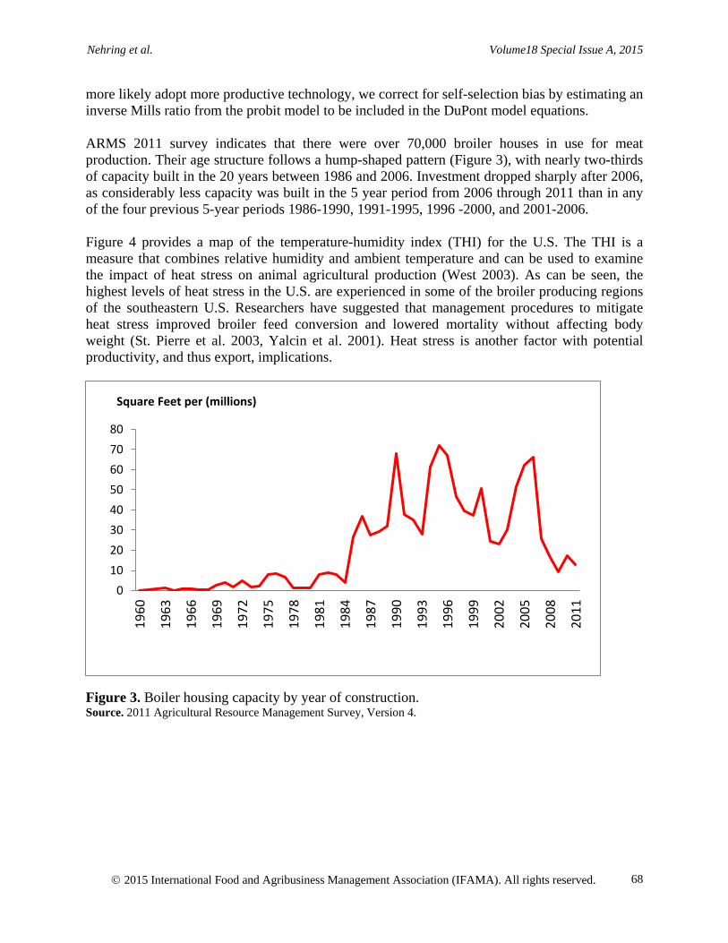
more likely adopt more productive technology, we correct for self-selection bias by estimating an inverse Mills ratio from the probit model to be included in the DuPont model equations. ARMS 2011 survey indicates that there were over 70,000 broiler houses in use for meat production. Their age structure follows a hump-shaped pattern (Figure 3), with nearly two-thirds of capacity built in the 20 years between 1986 and 2006. Investment dropped sharply after 2006, as considerably less capacity was built in the 5 year period from 2006 through 2011 than in any of the four previous 5-year periods 1986-1990, 1991-1995, 1996 -2000, and 2001-2006. Figure 4 provides a map of the temperature-humidity index (THI) for the U.S. The THI is a measure that combines relative humidity and ambient temperature and can be used to examine the impact of heat stress on animal agricultural production (West 2003). As can be seen, the highest levels of heat stress in the U.S. are experienced in some of the broiler producing regions of the southeastern U.S. Researchers have suggested that management procedures to mitigate heat stress improved broiler feed conversion and lowered mortality without affecting body weight (St. Pierre et al. 2003, Yalcin et al. 2001). Heat stress is another factor with potential productivity, and thus export, implications.

Figure 3. Boiler housing capacity by year of construction. Source. 2011 Agricultural Resource Management Survey, Version 4.

01020304050607080

1960

1963

1966

1969

1972

1975

1978

1981

1984

1987

1990

1993

1996

1999

2002

2005

2008

2011

Square Feet per (millions)



69

Figure 4. Heat Index Map, U.S. Source. Prism data group and GIS/ERS calculations. In the SUR models, independent variables were crossed with regional variables to determine whether an interaction would impact financial performance. If any one of the β estimates was substantively larger than its standard error for any of the regional crosses, all of the regional crosses for that variable were included in the model. This is similar to the method Nehring et al. (2014) used to select regional crosses for their DuPont cow-calf model. As a result, regional cross effects with THI and Broilers Sold were included in the solvency equation. The regional cross effects with THI could be important if managerial and technological response to a higher THI differed by region, impacting financial performance. Furthermore, differential farm size impacts on farm financial performance by region are investigated with the Broilers Sold regional crosses. Results

Table 1 (see Appendix) shows the means for variables used in this study by region and for the whole U.S. The results indicate that inverse solvency averaged 1.26, ranging from 1.15 in the Northeast to 1.41 in the Southern Plains. This suggests that, on average for U.S. broiler farms, the value of total assets was 26% higher than the equity, or conversely the more commonly-used measure for solvency using the equity/asset ratio would be the inverse, 0.79. Profitability



70

measured as net return over sales averaged 32.4%, ranging from 22.3% in the Corn Belt to 37.1% in the Southeast. Asset efficiency measured as sales over assets averaged 22.3%, ranging from 18.5% in the Northeast to 25.4% in the Corn Belt. Finally, return on equity averaged 9.1%, ranging from 6.2% in the Northeast to 10.5% in the Appalachia and Delta regions. Note that there are many reasons why these whole-farm measures of financial performance may vary by region including production conditions, average farm size, diversification and the other enterprises into which the farms are diversified, and others. The regional main effects shown in Table 2 (see Appendix) are generally consistent with the Appendix Table 1 results. Relative to the Southeast, farms in the Southern Plains, Delta, and Corn Belt regions were less solvent and farms in Appalachia were more solvent. These results are consistent with the debt-asset ratios by region reported in Appendix Table 1. Relative to the Southeast, Delta and Southern Plains farms were more profitable and Corn Belt farms were less profitable. Regional variables will be further discussed as we discuss results of the other independent variables in the model. Overall, while important, region did not appear to be the most important driver in this analysis, as opposed to results for cow-calf operations (Nehring et al. 2014), where regional main effects showed significance and many of the regional crosses were also significant. We believe this reflects the more homogeneous general nature of broiler farms relative to cow-calf farms by region, where broiler housing has enabled producers to more effectively control the production environment of broilers. Also, broiler farms have a more homogeneous farm structure by region in terms of (1) enterprise specialization (note Proportion Broilers in Appendix Table 1), (2) farm size (note Broilers Sold and Acres Operated, both of which do not differ greatly by region), and (3) the impact of a limited number of integrators who have partial control over the grow-out phase. Age was significant in two of the equations. Similar to results for cow-calf operations (Nehring et al. 2014), farms with older producers were more profitable, which can likely be attributed to greater experience. On the other hand, contrary to expectations, older producers were less solvent, suggesting that as they aged they took on more debt relative to equity. Though unexpected, it is not uncommon for older producers to take on additional debt to retrofit older housing or to expand their operations, particularly if there is a younger family member who is also involved in the operation. On farms where the spouse worked off-farm, both profitability and asset efficiency were lower. Spouses likely provide significant unpaid labor and management to the operation that is not included in the operational costs. When the spouse works off-farm, that contribution is lost, explaining the lower levels of profitability and efficiency. The asset efficiency result differs from previous studies of U.S. farms (Mishra et al. 2012) and for cow-calf farms (Nehring et al. 2014). Operator off-farm work positively impacted farm profitability, suggesting that as with cow-calf farming (Nehring et al. 2014), operator off-farm work is complementary with broiler production. This is supported by results from a previous study which found that farmers who worked more hours off the farm were more likely to choose broilers as a farm enterprise (Gillespie and Mishra 2011). On the other hand, operators who worked more hours off the farm were more likely to experience lower asset efficiency, similar to the spousal off-farm work result. It appears that while there are differential impacts of spousal and operator off-farm work on farm profitability, off-farm employment among broiler households is consistently associated with lower farm asset efficiency.



71

Farm size was measured in two ways, first as Acres Operated, with farms operating more acres having lower asset efficiency and higher solvency. Producers with greater acreage tended to hold less debt relative to equity, but also sold less relative to their asset base. On the other hand, producers who sold more broilers experienced greater profitability, had higher asset efficiency, and were more solvent, suggesting that, as expected, significant economies of size exist in the broiler industry. Furthermore, since the coefficient on Broilers Sold was significant in all three equations, we can calculate the impact of broilers sold on return on equity by summing its three parameter estimates in the SUR equation: 0.5427. This suggests that larger-scale broiler operators had higher return on equity than smaller ones. From a trade perspective, these results suggest that as broiler production continues to expand internationally, the larger-scale U.S. broiler operations will be those that drive U.S. competitiveness. Though regional crosses on Broilers Sold were included in the asset efficiency equation because the Northeastern cross was “close” to significant, none of the crosses were significant at P ≤ 0.10. Proportion Broilers was significant in all three equations, suggesting that farms that are more specialized in broiler production were less profitable, had lower asset efficiency, and were less solvent. This suggests that though broiler farms tend to be highly specialized – regional averages in Appendix Table 1 show that Proportion Broilers ranges from 0.88 to 0.98 – more diversified farms tended to experience better financial performance. Since Proportion Broilers was significant in all three equations, we calculate its impact on return on equity by summing its three SUR parameter estimates: -2.7239. This suggests that more specialized broiler farms had lower return on equity than more diversified ones. From a trade perspective, these results do not suggest a need for U.S. farms to further specialize in broiler production in order to remain competitive in the global market. The result for asset efficiency is consistent with that found for cow-calf production (Nehring et al. 2014). Farms with newer broiler houses tended to experience lower profitability, lower asset efficiency, and lower solvency. The solvency result is not surprising given the greater debt most farms with newer housing would be expected to hold. Furthermore, the profitability result is plausible considering that farms with new equipment are likely to continue to depreciate their assets on their tax returns, thus reducing net farm income. If newer housing, however, is expected to improve production efficiency, then we would initially expect asset efficiency to be higher for operations with new housing. However, it is likely that the value of the older assets is lower than that of the new assets. Therefore, having older buildings reduces the denominator of the asset efficiency measure at a greater amount than the sales numerator is reduced. Since the coefficient on New Technology was significant in all three equations, we calculate its impact on return on equity by summing its three SUR parameter estimates: -2.3660. This suggests that new technology operations had lower return on equity than older technology operations. We urge caution in reading too much into these results, as newer housing using the older technology would also have likely led to similar signs, with higher debt, higher-valued assets, and greater depreciation. These results may tell us more about the impact of holding new assets in general than about a specific technology. Note that the inverse Mills ratios were significant at P ≤ 0.01 for both the profitability and efficiency equations, indicating that self-selection bias was present in the adoption of new technology and it was corrected for in the analysis. Higher Temperature-Humidity Indexes were associated with greater asset efficiency and solvency, indicating that producers have adapted to heat stress through improved management. It would be of interest to examine the impact of heat stress on broilers from an international



72

perspective to gain understanding of the interactions between technology use, heat stress, and global competitiveness. Of further interest would be to examine the impact of temperature and humidity on enterprises where the environment is less controlled than with broilers, such as cattle. Key and Sneeringer (2014) analyzed the impact of heat stress on dairy farm productivity. The lower asset efficiency of farms experiencing greater heat stress in the Delta region relative to the Southeast suggests differential impacts of heat stress by region. Conclusions

Results of this study suggest the main drivers of higher return on equity in U.S. broiler production to be farm size, diversification, and housing vintage, where larger, more diversified farms using older housing experienced greater profitability, asset efficiency, solvency, and return on equity. Regional differences were found among farms, with the DuPont model comparing farm financial performance of the five ERS regions with the Southeast, the largest broiler production region. Some significant differences were found, most notably with solvency and followed by profitability, with Corn Belt and Southern Plains farms having lower profit and being less solvent than Southeast farms. Overall, however, the differences are not large, with the exception of the lower profitability and solvency measures in the Corn Belt. We believe that bigger differences in financial performance would have been found in agricultural industries that do not control the production environment to the extent of that in broilers, with climate controlled housing. The fact that the THI had the opposite-than-expected impact on financial performance is indicative of the role of management and control of the production environment in broiler production. Another characteristic of broiler farms that has impacted farm financial performance has been off-farm income. The percentage of income from off-farm sources ranged from 11% in the Corn Belt to 27% in the Southern Plains, with many operators and spouses working significant numbers of hours off the farm. The negative impacts of Spouse Off-Farm on both profitability and asset efficiency likely tell us something about the opportunity cost of spousal labor off the farm. Specifically, for spousal off-farm work to lead to greater household income, the additional income from off-farm employment must exceed the reduced farm income associated with the loss of unpaid spousal labor and management on the farm. On the other hand, operator off-farm work appears to be complementary with broiler production. This result is consistent with previous work on cow-calf operations (Nehring et al. 2014). Further work on the reasons for this complementarity in production would be of interest. A significant contribution of this study is that it provides industry benchmark information that producers and agricultural lenders can use as baseline information from which to compare their farms. From an agricultural trade perspective, industry production competitiveness is of primary importance. The U.S. has long been competitive in the world broiler market]. Continued attention to production competitiveness will be important as broiler production becomes more competitive in other countries. Results of our study suggest that the most competitive broiler farms in the U.S. are larger-scale and, interestingly, more diversified into other farm enterprises. Production region impacts competitiveness and the southeastern portion of the U.S. appears to have held the competitive edge during the 2003-2011 period. These are factors that will need to be considered as the broiler industry continues to strive to remain competitive in a global broiler



73

market. From a trade perspective, our results suggest that as low-cost, vertically integrated broiler production continues to expand globally into developing countries (as discussed by Constance, 2008), larger-scale, diversified farms in the U.S. Southeast will have the advantage in competing in the global market. References Collins, R.A. 1985. Expected utility, debt-equity structure, and risk balancing. American Journal

of Agricultural Economics 67(3):627-29. Constance, D.H. 2008. The southern model of broiler production and its global implications.

Culture and Agriculture 30(1&2): 17-31. Davis, C.G., A. Muhammad, D. Karemera, and D. Harvey. 2014. The impact of exchange rate

volatility on world broiler trade. Agribusiness 30(1):46-55. Day, C. 2015. Exceptional first quarter sales posted by Tyson Foods. Feedstuffs January 30.

feedstuffs.com/story-exceptional-first-quarter-sales-posted-tyson-foods-45- 123389. Feedstuffs 2014. Tyson Foods to sell Mexico, Brazil Poultry Businesses. Editorial. Minnetonka,

Minnesota, July 28. http://feedstuffs.com/story-tyson-foods-sell-mexico-brazil-poultry-businesses-45-115658.

Feedstuffs 2014. USDA adjusts trade outlook lower, Feedstuffs Editorial, Minnetonka,

Minnesota, September 1. http://feedstuffs.com/story-usda-adjusts-trade-outlook-lower-45-117070.

Gillespie, J. and A. Mishra. 2011. Off-farm employment and reasons for entering farming as

determinants of production enterprise selection in U.S. agriculture. Australian Journal of Agricultural and Resource Economics 55(3):411-428.

Gillespie, J., R. Nehring, C. Hallahan, and C. Sandretto. 2009. Pasture-based dairy

systems: Who are the producers and are their operations more profitable than conventional dairies? Journal of Agricultural and Resource Economics 43(3):412-427.

Golz, J.T. and W.W. Koo. 1991. Competitiveness of broiler producers in North America

under alternative free trade scenarios. Agricultural Economics Report No. 277, Dept. of Agricultural Economics, North Dakota State University, Fargo, December.

Hausman, J.A. 1978. Specification tests in econometrics. Econometrica 46(6):1751-

1271. Kay, R.D., W.M. Edwards, and P.A. Duffy. 2012. Farm Management, 7th Edition.

New York: McGraw-Hill.



74

Key, N., and S. Sneeringer. 2014. Potential effects of climate change on the productivity of U.S. dairies. American Journal of Agricultural Economics 96(4):1136-1156.

Knoeber, C.R. 1989. A real game of chicken: contracts, tournaments, and the production of

broilers. Journal of Law, Economics, and Organization 5:271-92. MacDonald, J. 2008. The Economic Organization of U.S. Broiler Production. USDA-Economic

Research Service, EIB 38. Melvin, J., M. Boehlje, C. Dobbins, and A. Gray 2004. The DuPont profitability analysis model:

an application and evaluation of an e-learning tool. Agricultural Finance Review 64(1): 75-89.

Mishra, A.K., J.M. Harris, K.W. Erickson, C. Hallahan and J.D. Detre. 2012. Drivers of

agricultural profitability in the USA: An application of the DuPont expansion method. Agricultural Finance Review 72(3):325-340.

Mishra, A.K., C.B. Moss, and K.W. Erickson. 2009. Regional differences in agricultural

profitability, government payments, and farmland values: Implications of DuPont expansion. Agricultural Finance Review 69(1):49-66.

Moss, Charles B., Agricultural Finance, Routledge, New York, 2013. Nehring, R., J. Gillespie, J.M. Harris, and K. Erickson. 2014. What’s driving economic

and financial success of U.S. cow-calf operations? Agricultural Finance Review 74(3):311-325.

PRISM Group. 2008. Gridded climate data time series for the conterminous United States,

1895-2008. Oregon State University. http://prism.oregonstate.edu. St. Pierre, N.R. , B. Cobanov, and G. Schnitkey. 2003. Economic loss from heat stress by U.S.

livestock industries. Journal of Dairy Science 86(E Suppl.):E52-E77. Taylor, C. Robert. Auburn University. The Many Faces of Power in the Food System.

[presentation, DoJ/FTC Workshop on Merger Enforcement, Auburn, AL, February 17, 2004.]

The National Chicken Council, Washington, D. C. http://www.nationalchickencouncil.org

[accessed January 12, 2015]. Rogers, R.T. 2002. Broilers: differentiating a commodity. In Industry Studies, 3rd Ed., edited by

Larry L. Duetsch. Armonk, NY: M.E. Sharpe, Inc. U.S. Department of Agriculture, National Agricultural Statistics Service. 2015. Agricultural

Prices. Agricultural Statistics. U.S. Government Printing Office, Washington, DC.

http://www.nationalchickencouncil.org/



75

U.S. Department of Agriculture, National Agricultural Statistics Service. 2013. Agricultural Statistics. U.S. Government Printing Office, Washington, DC.

U.S. Department of Agriculture. 2012 Census of Agriculture United States Summary and State

Data, volume 1, part 51 (2014): AC-12-A-51. West, J.W. 2003. Effects of heat-stress on production in dairy cattle. Journal of Dairy Science

86:2131–2144. Yalcin, S., S. Ozkan, L. Turkmut, and P. B. Siegel. 2001. Responses to heat stress in commercial

and local broiler stock. Broiler Poultry Science 42:149-162.



76

Appendix Table 1. Means of Variables of Interest by Region and Whole U.S.

Tab

le 1

. Mea

ns o

f Var

iabl

es o

f Int

eres

t by

Reg

ion

and

Who

le U

.S.

It

em

Nor

thea

st

Cor

n B

elt

App

alac

hia

So

uthe

ast

Del

ta

Sout

hern

Pla

ins

Who

le U

.S.

G

ener

al S

tatis

tics b

y Re

gion

Num

ber o

f Obs

erva

tions

50

4 30

5 1,

857

2,86

3 2,

483

880

8,89

2

% o

f U.S

. Bro

iler F

arm

s 10

.9

2.2

21.1

31

.5

26.4

7.

9 10

0.0

%

of V

alue

of U

.S. B

roile

r Pro

duct

ion

7.6

2.8

21.9

33

.6

24.4

9.

7 10

0.0

M

eans

of D

uPon

t Ind

epen

dent

Var

iabl

es b

y Re

gion

Age

54

.6

50.3

52

.7

54.2

53

.3

53.3

53

.5

O

pera

tor O

ff-f

arm

Hou

rs

413

276

247

296

245

272

283

Sp

ouse

Off

-far

m H

ours

32

1 20

6 32

1 36

2 40

7 40

4 36

1

Acr

es O

pera

ted

161

284

209

183

202

256

199

B

roile

rs so

ld

297,

386

634,

259

460,

386

519,

078

457,

951

615,

065

476,

400

Pr

opor

tion

Bro

ilers

88

94

91

97

98

96

95

THI I

ndex

79

28

5 16

9 33

5 55

3 82

3 37

0

Mea

ns o

f Oth

er V

aria

bles

of I

nter

est b

y Re

gion

Hou

seho

ld N

et R

et o

n A

sset

s 7.

0 7.

0 9.

5 8.

7 7.

8 10

.2

8.5

Fa

rm N

et R

etur

n on

Ass

ets

4.0

4.4

6.7

6.5

4.8

5.8

5.7

H

arve

sted

Acr

es

135

115

124

54

52

45

78

%

Hou

seho

ld In

com

e O

ff-F

arm

25

.8

11.4

18

.0

20.7

21

.3

27.4

21

.2

La

nd P

rice

($/a

cre)

8,

995

2,02

3 3,

494

3,73

8 1,

982

1,63

8 3,

413

D

ebt-A

sset

Rat

io

16.4

27

.8

22.8

23

.1

34.5

35

.0

25.7

Mea

ns o

f DuP

ont F

arm

Fin

anci

al P

erfo

rman

ce M

easu

res b

y Re

gion

DuP

ont I

nver

se S

olve

ncy

(A/E

) 1.

15

1.29

1.

23

1.23

1.

39

1.41

1.

26

D

uPon

t Pro

fitab

ility

(R/S

) 29

.2

22.3

33

.9

37.1

27

.4

30.0

32

.4

D

uPon

t Eff

icie

ncy

(S/A

) 18

.5

25.4

25

.1

21.7

21

.9

24.7

22

.3

D

uPon

t Ret

urn

on E

quity

(S/E

) 6.

2 7.

3 10

.5

9.9

10.5

10

.4

9.1



77

Table 2. Results of the DuPont Seemingly Unrelated Regression Model

Inde

pend

ent V

aria

bles

Pr

ofita

bilit

y (R

/S)

Eff

icie

ncy

(S/A

) In

vers

e So

lven

cy (A

/E)

β St

anda

rd

Err

or

β St

anda

rd

Err

or

β St

anda

rd

Err

or

Con

stan

t -3

.043

7 *

1.63

80

-1.2

418

**

0.52

98

-0.0

406

0.

2475

A

ppal

achi

a -0

.028

1

0.10

52

0.13

48

0.

6671

-0

.068

2 **

* 0.

0206

C

orn

Bel

t -0

.398

8 **

0.

1982

0.

4074

0.82

17

0.45

99

***

0.04

55

Del

ta

0.16

90

* 0.

0969

0.

4921

0.53

22

0.09

73

***

0.01

91

Nor

thea

st

-0.0

803

0.

1552

-0

.991

7

0.76

40

0.01

20

0.

0360

So

uthe

rn P

lain

s -0

.374

4 **

0.

1557

0.

3692

0.92

53

0.18

17

***

0.04

74

Age

0.

0559

**

* 0.

0131

0.

0032

0.00

24

0.01

18

***

0.00

17

Pred

icte

d Sp

ouse

Off

-Far

m

-0.0

012

***

0.00

02

-0.0

004

***

0.00

02

0.00

01

0.

0001

Pr

edic

ted

Ope

rato

r Off

-Far

m

0.00

64

***

0.00

12

-0.0

004

***

8.5E

-5

0.00

01

0.

0001

A

cres

Ope

rate

d -0

.031

0

0.03

57

-0.1

548

***

0.01

42

-0.0

431

***

0.00

80

Bro

ilers

Sol

d 0.

3868

**

* 0.

0829

0.

2654

**

* 0.

0372

-0

.109

5 **

* 0.

0275

Pr

opor

tion

Bro

ilers

-0

.992

5 **

0.

4031

-1

.976

5 **

* 0.

1612

0.

2451

**

* 0.

0853

N

ew T

echn

olog

y -3

.628

9 **

* 0.

3754

-1

.147

2 **

* 0.

1476

2.

4101

**

* 0.

1499

TH

I 0.

0002

0.00

02

0.00

03

**

0.00

01

-0.0

001

* 4.

3E-5

In

vers

e M

ills R

atio

-1

.165

5 **

* 0.

1755

-1

.000

71

***

0.07

57

0.04

09

0.

0341

A

ppal

achi

a ×

THI

0.

0001

0.00

03

C

orn

Bel

t × T

HI

-0

.000

1

0.00

03

D

elta

× T

HI

-0

.000

4 **

* 0.

0002

Nor

thea

st ×

TH

I

0.00

07

0.

0015

Sout

hern

Pla

ins ×

TH

I

-0.0

001

0.

0002

App

alac

hia

× C

hick

s Sol

d

0.00

04

0.

0503

Cor

n B

elt ×

Chi

cks S

old

0.

0111

0.06

28

D

elta

× C

hick

s Sol

d

-0.0

105

0.

0403

Nor

thea

st ×

Chi

cks S

old

0.

0734

0.06

23

So

uthe

rn P

lain

s × C

hick

s Sol

d

0.02

11

0.

0698

Adj

uste

d R

-Squ

are

0.17

51

0.25

47

0.51

04

Tab

le 2

. Res

ults

of t

he D

uPon

t see

min

gly

Unr

elat

ed R

egre

ssio

n M

odel



78

Table 3. Results of Probit Model, 1=Housing Constructed Since 1996; 0=Housing Constructed Before 1996 Independent Variables β Standard Error Constant 0.3494 0.2322 Appalachia -0.0276 0.0553 Corn Belt -0.3896 *** 0.1513 Delta -0.1060 0.0736 Northeast -0.0309 0.1319 Southern Plains -0.1233 0.1585 Chicks Placed 0.0024 *** 0.0006 Cash Wages -0.0018 *** 0.0005 Depreciation on Machinery 0.0006 *** 0.0002 Age -0.0219 *** 0.0033 Operator Holds Off-Farm Job -0.0014 *** 0.0007 Operator Education -0.0288 0.0239 Debt-Asset Ratio 0.9042 *** 0.1916 Household Well-Being Above Median Level

0.0714 ** 0.0342

Trend 0.0726 *** 0.0109

Table 4. Results from the Operator and Spouse Off-Farm Employment Hours Regressions Independent Variables Spouse Off-Farm Operator Off-Farm

β Standard Error β Standard Error Constant -136.03 166.54 1116.72 *** 159.08 Farm Net Worth -2.21 2.60 2.52 2.30 Government Payments 0.46 0.96 -2.58 *** 0.87 Household Size 64.52 *** 5.23 14.95 *** 5.15 Accrued Interest 2.07 ** 0.92 1.56 * 0.87 Off-Farm Interest Income 2.90 *** 0.85 2.75 *** 0.77 Population Accessibility -60.60 *** 11.60 29.67 *** 10.46 Value Livestock Production under Contract

-18.73 *** 6.18 -42.11 *** 5.84

Household Assets 58.61 *** 12.45 -10.37 11.47 Adjusted Wage Rates in Area 15.23 *** 0.71 Acres Operated -2.99 4.19 Age -9.77 *** 0.69 Household Well-Being Above Median

50.51 *** 7.18

Total Animal Units 3.90 *** 1.13

What's Driving U.S. Broiler Farm Profitability?1

Documents

Transcript of What's Driving U.S. Broiler Farm Profitability?1