
Robust model predictive control for deployment and ...
257
HAL Id: tel-02976812 https://tel.archives-ouvertes.fr/tel-02976812 Submitted on 23 Oct 2020 HAL is a multi-disciplinary open access archive for the deposit and dissemination of sci- entific research documents, whether they are pub- lished or not. The documents may come from teaching and research institutions in France or abroad, or from public or private research centers. L’archive ouverte pluridisciplinaire HAL, est destinée au dépôt et à la diffusion de documents scientifiques de niveau recherche, publiés ou non, émanant des établissements d’enseignement et de recherche français ou étrangers, des laboratoires publics ou privés. Robust model predictive control for deployment and reconfiguration of multi-agent systems Thomas Chevet To cite this version: Thomas Chevet. Robust model predictive control for deployment and reconfiguration of multi-agent systems. Automatic. Université Paris-Saclay, 2020. English. NNT: 2020UPASG007. tel-02976812
-
Upload
khangminh22 -
Category
Documents
-
view
1 -
download
0
Transcript of Robust model predictive control for deployment and ...
HAL Id: tel-02976812https://tel.archives-ouvertes.fr/tel-02976812
Submitted on 23 Oct 2020
HAL is a multi-disciplinary open accessarchive for the deposit and dissemination of sci-entific research documents, whether they are pub-lished or not. The documents may come fromteaching and research institutions in France orabroad, or from public or private research centers.
L’archive ouverte pluridisciplinaire HAL, estdestinée au dépôt et à la diffusion de documentsscientifiques de niveau recherche, publiés ou non,émanant des établissements d’enseignement et derecherche français ou étrangers, des laboratoirespublics ou privés.
Robust model predictive control for deployment andreconfiguration of multi-agent systems
Thomas Chevet
To cite this version:Thomas Chevet. Robust model predictive control for deployment and reconfiguration of multi-agentsystems. Automatic. Université Paris-Saclay, 2020. English. NNT : 2020UPASG007. tel-02976812

Thèsede
doctorat
NNT:2020UPASG007
Robust model predictive control
for deployment and
reconfiguration of multi-agent
systems
Thèse de doctorat de l’Université Paris-Saclay
École doctorale n 580, Sciences et Technologies de l’Information et
de la Communication (STIC)
Spécialité de doctorat : Automatique
Unité de recherche : Université Paris-Saclay, CNRS, CentraleSupélec, Laboratoire
des signaux et systèmes, 91190, Gif-sur-Yvette, France
Référent : Faculté des sciences d’Orsay
Thèse présentée et soutenue à Gif-sur-Yvette, le 25septembre 2020, par
Thomas CHEVETComposition du jury :
Saïd MAMMAR Président
Professeur, Université d’Évry Val-d’Essonne/IBISC
Pedro CASTILLO Rapporteur & Examinateur
Chargé de recherche, HDR, Université de Technologie deCompiègne/Heudiasyc
Nicolas LANGLOIS Rapporteur & Examinateur
Professeur, ESIGELEC/IRSEEM
Mirko FIACCHINI Examinateur
Chargé de recherche, HDR, Université Grenoble-Alpes/GIPSA-lab
Didier THEILLIOL Examinateur
Professeur, Université de Lorraine/CRAN
Cristina STOICA MANIU Directrice de thèse
Professeur, CentraleSupélec/L2S
Cristina VLAD Coencadrante & Examinatrice
Maître de conférences, CentraleSupélec/L2S
Youmin ZHANG Coencadrant & Examinateur
Professeur, Université Concordia
Eduardo F. CAMACHO Invité
Professeur, Université de Séville
José M. MAESTRE Invité
Professeur associé, Université de Séville

NNT : 2020UPASG007
Robust model predictive control fordeployment and reconfiguration of
multi-agent systems
Thèse de doctorat de l’Université Paris-Saclay
École doctorale n580 STICSciences et Technologies de l’Information et de la Communication
Spécialité de doctoratAutomatique
Unité de rechercheUniversité Paris-Saclay, CNRS, CentraleSupélec, Laboratoire des signaux et systèmes, 91190,
Gif-sur-Yvette, FranceRéférent
Faculté des sciences d’Orsay
Thèse présentée et soutenue à Gif-sur-Yvette, le 25 septembre 2020, par
Thomas Chevet
Composition du jury :Saïd Mammar PrésidentProfesseur, Université d’Évry Val-d’Essonne/IBISCPedro Castillo Rapporteur & ExaminateurChargé de recherche, HDR, Université de Technologie de Com-piègne/HeudiasycNicolas Langlois Rapporteur & ExaminateurProfesseur, ESIGELEC/IRSEEMMirko Fiacchini ExaminateurChargé de recherche, HDR, Université Grenoble-Alpes/GIPSA-labDidier Theilliol ExaminateurProfesseur, Université de Lorraine/CRAN
Cristina Stoica Maniu Directrice de thèseProfesseur, CentraleSupélec/L2SCristina Vlad Coencadrante & ExaminatriceMaître de conférences, CentraleSupélec/L2SYoumin Zhang Coencadrant & ExaminateurProfesseur, Université ConcordiaEduardo F. Camacho InvitéProfesseur, Université de SévilleJosé M. Maestre InvitéProfesseur associé, Université de Séville


Tomorrow soon turns into yesterday.Everything we see just fades away.
There’s sky and sand where mountains used to be.Time drops by a second to eternity.
It doesn’t matter if we turn to dust;Turn and turn and turn we must!
I guess I’ll see you dancin’ in the ruins tonight!
Dancin’ in the Ruins, Blue Öyster Cult


Acknowledgements
The preparation of this thesis was a long and exciting journey. This journey, whichwould not have been possible without the help of many great people, was marked bythe meeting of many others. The following few words are an attempt to thank themfor their time, help and support.
I would like to start by expressing my deepest gratitude to my supervising team.I thank Cristina Stoica Maniu and Cristina Vlad for their kindness, their trust, sinceeven before the beginning of my thesis, their insightful advice, their constant supportof my work, and for always encouraging me in moments when I needed it. Thanksto them, I was also able to participate in many other academic and administrativeactivities that reinforced the idea that I wanted to continue working in academia.I also thank Professor Youmin Zhang for his constant support of my work and hisprecious advice to further it, both on theoretical and practical aspects, as well as forwelcoming me in his lab in Montréal to start working on the real-time implementationof the algorithms presented in this thesis. To be able to work under their guidancehas been a great privilege and no words could ever express how thankful I am for allthe work they have done to help me. I look forward to working with them again.
I am also grateful to the members of my thesis committee. I would like tothank Pedro Castillo, Chargé de Recherches CNRS at Université Technologiquede Compiègne, and Nicolas Langlois, Professor at ESIGELEC, for accepting toreview my manuscript. I also thank Mirko Fiacchini, Chargé de Recherches CNRS atGIPSA-lab, and Didier Theilliol, Professor at Université de Lorraine, for acceptingto be part of my committee and Saïd Mammar, Professor at Université d’ÉvryVal-d’Essonne, for presiding it. The questions and remarks they had during thereviewing phase and the defense are a valuable contribution to further the workpresented in this thesis.
It has been an honor being able to work with José Maestre and Eduardo Camachoat Universidad de Sevilla. I thank them both for welcoming me in their team, fortheir kindness and for the time they took to discuss new ideas and improvements ofmy work. Their scientific insight and excellence has been of the greatest importanceto help me see the relevance and potential of my work. I really hope we will be ableto continue our collaboration in the future.
A special acknowledgment has to go to Alain Théron, Professor of IndustrialSciences at Lycée Pierre de Fermat in Toulouse, who, with his classes, convinced methat Automatic control was what I wanted to work with when he “brought us to theDark Side of the Force” by introducing the Laplace transform.
This feeling became even stronger during the seven years I spent at Centrale-Supélec (which was still Supélec when I entered the school in 2013). For that, I thankall the members of the Automatic Control Department of the school, Didier Dumur,
v

vi
Emmanuel Godoy, Gilles Duc, Dominique Beauvois, Guillaume Sandou, Sorin Olaru,Pedro Rodriguez, Stéphane Font, Maria Makarov, Houria Siguerdidjane, GiorgioValmorbida, Sihem Tebbani, Antoine Chaillet and, of course, my two supervisorsCristina Stoica Maniu and Cristina Vlad, for the high quality teaching and super-vision they provide to engineering students and that I could receive myself. I alsothank them for the many teaching opportunities that were given to me as a teachingassistant for the Automatic course, for all the lunch break tarot games and for allthe discussions, scientific or not, that we had. I would also like to extend my thanksto Israel Hinostroza, researcher at the SONDRA laboratory, for his support duringthe supervision, with Maria Makarov and Cristina Stoica Maniu, of my graduationproject, a project that launched me into the world of research with my first scientificpublication. Finally, I would like to thank Léon Marquet and Caroline Charles fortheir prompt and excellent technical support in all circumstances and for all thediscussions we had about electronics and informatics.
I am grateful to the Laboratoire des Signaux et Systèmes and its LIA on In-formation, Learning and Control for the funding of my stay in Professor Zhang’slaboratory in Montréal. I would also like to thank the STIC Doctoral School for theinternational mobility grant that allowed me to go to work in Seville.
This doctoral journey would not have been possible without the support of myfriends. I would like to thank all my friends from Supélec who were there to supportme during the last three years, and mainly Gwendoline, Mony, Thomas and Yaël forthe board game afternoons that we had, as well as Matthias and Marine, that I havenot seen as much as I would have liked. I also have to thank Brice, one of the bestfriend I had through our time in prépa, Supélec and beyond, who has always beenthere to help and encourage me when I needed it. This journey also allowed me tomeet many companions who made the trip more pleasant with all the discussions, thelunch break Mölkky and tarot games or the board games and theater evenings thatwe had. I would then like to thank Vincent for our never ending discussions on anytrivial subject that arose, Maxime for our philosophical debates on Automatic controland research in general, Gauthier for all our discussions on music and drones, Doryfor all the work and jokes we did together and his deadly aim at Mölkky, Geoffrayand Martin for their encyclopedic knowledge of history and philosophy, Dario for hisunconditional defense of Genoa, Joy for her constant and communicative good moodand positivity, Matthieu for his unfortunately unsuccessful attempts to keep us in arighteous path, Fetra for his calm and serenity, Kodjo for his exuberance and thedebates only he is able to provoke, Antonello for his attempts to channel Vincent,Andreea for her kindness, Nicolò for his craziness, as well as the others, Jérémy, Ugo,Baptiste, Jean, Mert, Daniel, Benjamin and Merouane, with whom I spent less timebut were always there to participate in any of the discussions, debates or activitiesthat I mentioned.
Last but not least, my thanks and love go to my family, my mother, my father,my sister, my stepfather and my grandparents who have always been there to adviseand support me in my decisions.

Table of Contents
List of Figures xi
List of Definitions xv
List of Assumptions xvii
List of Acronyms xix
List of Symbols xxi
Résumé en français xxvContexte . . . . . . . . . . . . . . . . . . . . . . . . . . . . . . . . . . . . xxv
Qu’est-ce qu’un système multi-agents ? . . . . . . . . . . . . . . . . xxvAperçu des stratégies de commande des systèmes multi-agents . . . xxviiCommande pour le déploiement . . . . . . . . . . . . . . . . . . . . xxix
Contributions . . . . . . . . . . . . . . . . . . . . . . . . . . . . . . . . . xxxDéploiement dans le cas nominal . . . . . . . . . . . . . . . . . . . xxxDéploiement sous perturbations déterministes bornées . . . . . . . . xxxiDéploiement sous perturbations stochastiques non bornées . . . . . xxxiReconfiguration dans le cas d’un système multi-véhicules variant dans
le temps . . . . . . . . . . . . . . . . . . . . . . . . . . . . . xxxii
Chapter 1 Introduction 11.1 Context and motivations . . . . . . . . . . . . . . . . . . . . . . . . 1
1.1.1 What is a multi-agent system? . . . . . . . . . . . . . . . . 11.1.2 An overview of multi-agent system control strategies . . . . 3
1.1.2.1 Communication topologies . . . . . . . . . . . . . 31.1.2.2 Classification of the approaches for MAS control . 6
1.1.3 Deployment control . . . . . . . . . . . . . . . . . . . . . . . 91.1.4 Main motivations and thesis orientation: Model Predictive
Control for the deployment of multi-vehicle systems . . . . . 121.2 Contributions of the thesis . . . . . . . . . . . . . . . . . . . . . . . 13
1.2.1 Deployment in the nominal case . . . . . . . . . . . . . . . . 131.2.2 Deployment under bounded deterministic perturbations . . 141.2.3 Deployment under unbounded stochastic perturbations . . . 141.2.4 Reconfiguration in the case of a time-varying multi-vehicle
system . . . . . . . . . . . . . . . . . . . . . . . . . . . . . . 151.2.5 Publications . . . . . . . . . . . . . . . . . . . . . . . . . . . 16
vii

viii Table of Contents
1.3 Thesis outline . . . . . . . . . . . . . . . . . . . . . . . . . . . . . . 17
Chapter 2 Mathematical tools and set-theoretic elements 192.1 Definitions and useful properties of matrices . . . . . . . . . . . . . 192.2 Set-theoretic elements for control . . . . . . . . . . . . . . . . . . . 22
2.2.1 Ellipsoidal sets . . . . . . . . . . . . . . . . . . . . . . . . . 232.2.2 Polyhedral sets . . . . . . . . . . . . . . . . . . . . . . . . . 242.2.3 Set operations . . . . . . . . . . . . . . . . . . . . . . . . . 292.2.4 Sets in control theory . . . . . . . . . . . . . . . . . . . . . 34
2.3 Multi-vehicle system description . . . . . . . . . . . . . . . . . . . . 382.4 Voronoi tessellation and formation configuration . . . . . . . . . . . 41
2.4.1 Conventional Voronoi tessellation . . . . . . . . . . . . . . . 412.4.2 Generalized Voronoi tessellations . . . . . . . . . . . . . . . 44
2.4.2.1 Box-based guaranteed Voronoi tessellation . . . . . 442.4.2.2 Pseudo-Voronoi tessellation . . . . . . . . . . . . . 50
2.4.3 Chebyshev configuration of a multi-vehicle system . . . . . . 532.5 Continuous random variables and stochastic processes . . . . . . . . 562.6 Conclusion . . . . . . . . . . . . . . . . . . . . . . . . . . . . . . . . 59
Chapter 3 Decentralized control for the deployment of a multi-vehicle system 61
3.1 Overview of the existing deployment algorithms in the nominal case 613.2 Problem formulation and first results . . . . . . . . . . . . . . . . . 64
3.2.1 Centralized MPC approach . . . . . . . . . . . . . . . . . . 643.2.2 Decentralized algorithm . . . . . . . . . . . . . . . . . . . . 683.2.3 Discussion on the convergence of the decentralized algorithm 693.2.4 Deployment results in the case of single integrator dynamics 74
3.3 Deployment of a quadrotor UAV fleet . . . . . . . . . . . . . . . . . 783.3.1 Agent model . . . . . . . . . . . . . . . . . . . . . . . . . . 78
3.3.1.1 Continuous-time nonlinear dynamics . . . . . . . . 783.3.1.2 Discrete-time linear dynamics . . . . . . . . . . . . 80
3.3.2 Global control strategy . . . . . . . . . . . . . . . . . . . . . 813.3.2.1 Overall architecture . . . . . . . . . . . . . . . . . 813.3.2.2 Inner-loop control . . . . . . . . . . . . . . . . . . 833.3.2.3 Outer-loop control . . . . . . . . . . . . . . . . . . 85
3.3.3 Deployment results . . . . . . . . . . . . . . . . . . . . . . . 873.4 Discussion on the stability of the deployment of UAVs . . . . . . . 923.5 Conclusion . . . . . . . . . . . . . . . . . . . . . . . . . . . . . . . . 94
Chapter 4 Deployment of a multi-vehicle system subject to pertur-bations 95
4.1 Bounded perturbations . . . . . . . . . . . . . . . . . . . . . . . . . 964.1.1 System model . . . . . . . . . . . . . . . . . . . . . . . . . . 964.1.2 Overview of robust tube-based MPC for systems with bounded
perturbations . . . . . . . . . . . . . . . . . . . . . . . . . . 984.1.3 Deployment algorithm . . . . . . . . . . . . . . . . . . . . . 99
4.1.3.1 Deployment objective in the perturbed case . . . . 994.1.3.2 Optimization problem for the tube-based MPC . . 1004.1.3.3 Tube envelope . . . . . . . . . . . . . . . . . . . . 101

Table of Contents ix
4.1.4 Proposed deployment results for MAS with bounded pertur-bations . . . . . . . . . . . . . . . . . . . . . . . . . . . . . 1074.1.4.1 Single integrator dynamics . . . . . . . . . . . . . 1074.1.4.2 UAV dynamics . . . . . . . . . . . . . . . . . . . . 113
4.2 Unbounded stochastic perturbations . . . . . . . . . . . . . . . . . 1194.2.1 System model . . . . . . . . . . . . . . . . . . . . . . . . . . 1204.2.2 Overview of chance-constrained MPC for systems with stochas-
tic perturbations . . . . . . . . . . . . . . . . . . . . . . . . 1234.2.3 Deployment algorithm . . . . . . . . . . . . . . . . . . . . . 124
4.2.3.1 Deployment objective and chance-constrained opti-mization problem . . . . . . . . . . . . . . . . . . 124
4.2.3.2 Relaxation of the probabilistic constraints into alge-braic constraints . . . . . . . . . . . . . . . . . . . 128
4.2.4 Proposed deployment results for MAS with stochastic pertur-bations . . . . . . . . . . . . . . . . . . . . . . . . . . . . . 1354.2.4.1 Single integrator dynamics . . . . . . . . . . . . . 1354.2.4.2 UAV dynamics . . . . . . . . . . . . . . . . . . . . 140
4.3 Conclusion . . . . . . . . . . . . . . . . . . . . . . . . . . . . . . . . 144
Chapter 5 Extension to the deployment of a time-varying multi-vehicle system 147
5.1 A first approach to reconfiguration . . . . . . . . . . . . . . . . . . 1485.1.1 Motivation . . . . . . . . . . . . . . . . . . . . . . . . . . . 1485.1.2 Problem formulation . . . . . . . . . . . . . . . . . . . . . . 150
5.1.2.1 Agent dynamics . . . . . . . . . . . . . . . . . . . 1505.1.2.2 Incoming agents . . . . . . . . . . . . . . . . . . . 1515.1.2.3 Outgoing agents . . . . . . . . . . . . . . . . . . . 153
5.1.3 Deployment results . . . . . . . . . . . . . . . . . . . . . . . 1595.1.3.1 Incoming agents . . . . . . . . . . . . . . . . . . . 1595.1.3.2 Outgoing agents . . . . . . . . . . . . . . . . . . . 162
5.2 A safer way to deal with outgoing vehicles . . . . . . . . . . . . . . 1655.2.1 Limitation of the first reconfiguration algorithm . . . . . . . 1655.2.2 Improved reconfiguration algorithm . . . . . . . . . . . . . . 169
5.2.2.1 A new transient objective . . . . . . . . . . . . . . 1695.2.2.2 A new reconfiguration algorithm . . . . . . . . . . 174
5.3 Reconfiguration in the case of outgoing agents . . . . . . . . . . . . 1785.3.1 Comparison of the two algorithms in the case of one outgoing
agent . . . . . . . . . . . . . . . . . . . . . . . . . . . . . . 1785.3.2 Reconfiguration in the case of multiple outgoing agents . . . 181
5.3.2.1 Reconfiguration for single integrator dynamics . . 1815.3.2.2 Reconfiguration for UAV dynamics . . . . . . . . . 187
5.4 Conclusion . . . . . . . . . . . . . . . . . . . . . . . . . . . . . . . . 191
Chapter 6 Concluding remarks and future work 1936.1 Conclusion . . . . . . . . . . . . . . . . . . . . . . . . . . . . . . . . 1936.2 Future directions . . . . . . . . . . . . . . . . . . . . . . . . . . . . 195
Bibliography 197

List of Figures
Chapter 1 IntroductionFigure 1.1: Centralized control architecture . . . . . . . . . . . . . . . . 4Figure 1.2: Decentralized control architecture . . . . . . . . . . . . . . . 5Figure 1.3: Distributed control architecture . . . . . . . . . . . . . . . . 6Figure 1.4: Voronoi tessellation of a square for 5 generators with the
Euclidean norm (a) and the Manhattan norm (b). . . . . . . 10Figure 1.5: Illustration of Lloyd’s algorithm at initialization, after the first
iteration and after the last iteration. . . . . . . . . . . . . . 11
Chapter 2 Mathematical tools and set-theoretic elementsFigure 2.1: An example of ellipsoidal set in R2. . . . . . . . . . . . . . . 24Figure 2.2: An example of polyhedral set in R2. . . . . . . . . . . . . . . 26Figure 2.3: An example of polytopic set in R2. . . . . . . . . . . . . . . 26Figure 2.4: Equivalence between V-representation and H-representation
for a polytope in R2. . . . . . . . . . . . . . . . . . . . . . . 28Figure 2.5: Intersection of two polytopes in R2. . . . . . . . . . . . . . . 30Figure 2.6: Minkowski sum of two polytopes in R2. . . . . . . . . . . . . 32Figure 2.7: Pontryagin difference of two polytopes in R2. . . . . . . . . . 33Figure 2.8: Different scalings of a polytope in R2. . . . . . . . . . . . . . 34Figure 2.9: Comparison of two approximations of the mRPI set of a system
in R2. . . . . . . . . . . . . . . . . . . . . . . . . . . . . . . 38Figure 2.10: Construction of the Voronoi cell V3. . . . . . . . . . . . . . . 43Figure 2.11: An example of Voronoi tessellation in R2. . . . . . . . . . . . 43Figure 2.12: Maximum distance of a point to a box in R2. . . . . . . . . 45Figure 2.13: Minimum distance of a point to a box in R2. . . . . . . . . . 46Figure 2.14: Example of guaranteed Voronoi cell border generated by two
sets in R2. . . . . . . . . . . . . . . . . . . . . . . . . . . . . 48Figure 2.15: Box-based guaranteed Voronoi cell borders generated by two
rectangles in R2. . . . . . . . . . . . . . . . . . . . . . . . . 49Figure 2.16: Linear approximation of a guaranteed cell border generated
by two sets in R2. . . . . . . . . . . . . . . . . . . . . . . . . 50Figure 2.17: Box-based guaranteed Voronoi tessellation of five generator
sets in R2. . . . . . . . . . . . . . . . . . . . . . . . . . . . . 51Figure 2.18: An example of Delaunay triangulation in R2. . . . . . . . . . 52Figure 2.19: An example of pseudo-Voronoi tessellation in R2. . . . . . . 53Figure 2.20: Chebyshev center and Chebyshev ball of a polytope in R2. . 55Figure 2.21: An example of Chebyshev configuration for 5 agents in a
classical Voronoi tessellation in R2. . . . . . . . . . . . . . . 56
xi

xii List of Figures
Chapter 3 Decentralized control for the deployment of a multi-vehicle system
Figure 3.1: Initial position of the agents of Σ in X . . . . . . . . . . . . . 75Figure 3.2: Configuration of Σ at different time instants. . . . . . . . . . 76Figure 3.3: Trajectories of the agents of Σ and their associated Chebyshev
centers. . . . . . . . . . . . . . . . . . . . . . . . . . . . . . 77Figure 3.4: Distance of each agent of Σ to its Chebyshev center over time. 78Figure 3.5: Schematic representation of a quadrotor UAV. . . . . . . . . 79Figure 3.6: Overall control architecture for a quadrotor UAV. . . . . . . 82Figure 3.7: Structure of the position controller for a quadrotor UAV. . . 86Figure 3.8: Initial position of the agents of Σ in Y . . . . . . . . . . . . . 88Figure 3.9: Configuration of Σ at different time instants. . . . . . . . . . 89Figure 3.10: Trajectories of the agents of Σ and their associated Chebyshev
centers. . . . . . . . . . . . . . . . . . . . . . . . . . . . . . 90Figure 3.11: Distance of each agent of Σ to its Chebyshev center over time. 91Figure 3.12: Norm of the error between the measured position and the
observed position of all agents of Σ. . . . . . . . . . . . . . . 91
Chapter 4 Deployment of a multi-vehicle system subject to pertur-bations
Figure 4.1: Invariant sets for the tube-based MPC controller in the singleintegrator dynamics case. . . . . . . . . . . . . . . . . . . . 108
Figure 4.2: Initial position of the MVS Σ in the output space. . . . . . . 109Figure 4.3: Final position of the MVS Σ in the output space at t = 50 s. 110Figure 4.4: Nominal trajectories of the agents of Σ and their associated
Chebyshev centers. . . . . . . . . . . . . . . . . . . . . . . . 111Figure 4.5: Distance of the nominal position of each agent of Σ to its
Chebyshev center over time. . . . . . . . . . . . . . . . . . . 111Figure 4.6: Norm of the estimation error of each agent of Σ. . . . . . . . 112Figure 4.7: Norm of the deviation error of each agent of Σ. . . . . . . . 112Figure 4.8: Invariant sets for the tube-based MPC controller in the UAV
case. . . . . . . . . . . . . . . . . . . . . . . . . . . . . . . . 114Figure 4.9: Structure of the position controller for a quadrotor UAV sub-
ject to perturbations. . . . . . . . . . . . . . . . . . . . . . . 115Figure 4.10: Initial position of the MVS Σ in the output space. . . . . . . 116Figure 4.11: Position of the MVS Σ in the output space at t = 1 s. . . . . 117Figure 4.12: Final position of the MVS Σ in the output space at t = 50 s. 118Figure 4.13: Distance of the nominal position of each agent of Σ to its
Chebyshev center over time. . . . . . . . . . . . . . . . . . . 118Figure 4.14: Norm of the estimation error of each agent of Σ. . . . . . . . 119Figure 4.15: Norm of the deviation error of each agent of Σ. . . . . . . . 119Figure 4.16: Initial position of the MVS Σ in the output space. . . . . . . 137Figure 4.17: Final position of the MVS Σ in the output space. . . . . . . 137Figure 4.18: Distance of the estimated position of each agent of Σ to its
Chebyshev center over time. . . . . . . . . . . . . . . . . . . 138Figure 4.19: Norm of the estimation error for each agent of Σ. . . . . . . 138Figure 4.20: Structure of the position controller for a quadrotor UAV sub-
ject to perturbations. . . . . . . . . . . . . . . . . . . . . . . 142Figure 4.21: Initial position of the MVS Σ in the output space. . . . . . . 142

List of Figures xiii
Figure 4.22: Final position of the MVS Σ in the output space. . . . . . . 143Figure 4.23: Distance of the estimated position of each agent of Σ to its
Chebyshev center over time. . . . . . . . . . . . . . . . . . . 144Figure 4.24: Norm of the estimation error for each agent of Σ. . . . . . . 144
Chapter 5 Extension to the deployment of a time-varying multi-vehicle system
Figure 5.1: Example of construction of a neighbors’ barycenter for MASreconfiguration when one agent leaves the workspace. . . . . 158
Figure 5.2: Trajectories of the agents of Σ, the agents joining Σ and theirassociated objectives. . . . . . . . . . . . . . . . . . . . . . . 161
Figure 5.3: Distance of each agent of Σ to its Chebyshev center over time. 162Figure 5.4: Trajectories of the agents of Σ during the first phase of the
deployment. . . . . . . . . . . . . . . . . . . . . . . . . . . . 163Figure 5.5: Trajectories of the agents of Σ and agent 7 during the recon-
figuration phase of the deployment. . . . . . . . . . . . . . . 164Figure 5.6: Trajectories of the agents of Σ during the third phase of the
deployment. . . . . . . . . . . . . . . . . . . . . . . . . . . . 165Figure 5.7: Distance of each agent of Σ to its Chebyshev center or neigh-
bors’ barycenter over time. . . . . . . . . . . . . . . . . . . . 166Figure 5.8: Distance of agent 7 to its objective over time. . . . . . . . . 166Figure 5.9: Limit case of the barycentric approach for the MAS reconfigu-
ration when several agents leave the workspace. . . . . . . . 168Figure 5.10: Construction of the contracted working regions. . . . . . . . 171Figure 5.11: Attribution of weights to the neighbors of the agents of the
MAS Σ. . . . . . . . . . . . . . . . . . . . . . . . . . . . . . 173Figure 5.12: Construction of the sets Oi(k) for the agents of the MAS Σ. 176Figure 5.13: Position of the MAS Σ and of agent 7 at time t = 5.2 s. . . . 178Figure 5.14: Construction of the safe objective of agent 6 at t = 5.2 s. . . 179Figure 5.15: Position of the MAS Σ and of agent 7 at time t = 6.8 s. . . . 180Figure 5.16: Distance of each agent of Σ to its Chebyshev center or safe
objective over time. . . . . . . . . . . . . . . . . . . . . . . . 181Figure 5.17: Trajectories of the agents of Σ during the first phase of the
deployment. . . . . . . . . . . . . . . . . . . . . . . . . . . . 182Figure 5.18: Construction of the safe objective of agent 2 at t = 4 s. . . . 183Figure 5.19: Construction of the safe objectives of agents 2 and 5 at t = 5.2 s. 184Figure 5.20: Final configuration of the MAS Σ at t = 40 s. . . . . . . . . 185Figure 5.21: Distance of each agent of Σ to its Chebyshev center or safe
objective over time. . . . . . . . . . . . . . . . . . . . . . . . 186Figure 5.22: Distance of the agents leaving Σ to their objectives over time. 186Figure 5.23: Initial configuration of the MAS Σ at t = 0 s. . . . . . . . . . 188Figure 5.24: Configuration of the MAS Σ at t = 5.4 s. . . . . . . . . . . . 189Figure 5.25: Final configuration of the MAS Σ at t = 40 s. . . . . . . . . 190Figure 5.26: Distance of each agent of Σ to its Chebyshev center or safe
objective over time. . . . . . . . . . . . . . . . . . . . . . . . 190Figure 5.27: Norm of the difference between the estimation position and
the real position of each agent of Σ over time. . . . . . . . . 191


List of Definitions
Résumé en françaisDéfinition Fr.1: Agent . . . . . . . . . . . . . . . . . . . . . . . . . . . . xxvDéfinition Fr.2: Système multi-agents . . . . . . . . . . . . . . . . . . . . xxvi
Chapter 1 IntroductionDefinition 1.1: Agent . . . . . . . . . . . . . . . . . . . . . . . . . . . . 2Definition 1.2: Multi-agent system . . . . . . . . . . . . . . . . . . . . . 2
Chapter 2 Mathematical tools and set-theoretic elementsDefinition 2.1: Positive definite matrix . . . . . . . . . . . . . . . . . . . 19Definition 2.2: Weighted quadratic norm . . . . . . . . . . . . . . . . . . 20Definition 2.3: Linear Matrix Inequality . . . . . . . . . . . . . . . . . . 20Definition 2.4: Bilinear Matrix Inequality . . . . . . . . . . . . . . . . . 21Definition 2.5: Convex set . . . . . . . . . . . . . . . . . . . . . . . . . . 23Definition 2.6: Convex hull . . . . . . . . . . . . . . . . . . . . . . . . . 23Definition 2.7: Ellipsoidal set . . . . . . . . . . . . . . . . . . . . . . . . 23Definition 2.8: Normalized ellipsoidal set . . . . . . . . . . . . . . . . . 24Definition 2.9: Half-space or H-representation . . . . . . . . . . . . . . . 25Definition 2.10: Polytope . . . . . . . . . . . . . . . . . . . . . . . . . . . 25Definition 2.11: Vertex or V-representation . . . . . . . . . . . . . . . . . 27Definition 2.12: Box . . . . . . . . . . . . . . . . . . . . . . . . . . . . . . 29Definition 2.13: Unitary box . . . . . . . . . . . . . . . . . . . . . . . . . 29Definition 2.14: Cartesian product of two sets . . . . . . . . . . . . . . . 29Definition 2.15: Intersection of two sets . . . . . . . . . . . . . . . . . . . 29Definition 2.16: Translation of a set . . . . . . . . . . . . . . . . . . . . . 31Definition 2.17: Minkwoski sum of two sets . . . . . . . . . . . . . . . . . 31Definition 2.18: Pontryagin difference of two sets . . . . . . . . . . . . . . 32Definition 2.19: Scaling of a set . . . . . . . . . . . . . . . . . . . . . . . 33Definition 2.20: Positive invariant set . . . . . . . . . . . . . . . . . . . . 35Definition 2.21: Minimal positive invariant set . . . . . . . . . . . . . . . 35Definition 2.22: Robustly positive invariant set . . . . . . . . . . . . . . . 35Definition 2.23: Minimal robustly positive invariant set . . . . . . . . . . 35Definition 2.24: Controlled invariant set . . . . . . . . . . . . . . . . . . . 35Definition 2.25: Controlled λ-contractive set . . . . . . . . . . . . . . . . 36Definition 2.26: Voronoi cell . . . . . . . . . . . . . . . . . . . . . . . . . 41Definition 2.27: Guaranteed Voronoi cell . . . . . . . . . . . . . . . . . . 44Definition 2.28: Chebyshev center of a polytope . . . . . . . . . . . . . . 54Definition 2.29: Chebyshev configuration . . . . . . . . . . . . . . . . . . 55
xv

xvi List of Definitions
Definition 2.30: Probability density function . . . . . . . . . . . . . . . . 57Definition 2.31: Mathematical expectation . . . . . . . . . . . . . . . . . 57Definition 2.32: Expectation of a multivariate random variable . . . . . . 57Definition 2.33: Variance matrix . . . . . . . . . . . . . . . . . . . . . . . 57Definition 2.34: Covariance of two random variables . . . . . . . . . . . . 58Definition 2.35: Independence of two random variables . . . . . . . . . . 58Definition 2.36: Multivariate normal distribution . . . . . . . . . . . . . . 58Definition 2.37: Normally distributed white noise . . . . . . . . . . . . . 59
Chapter 3 Decentralized control for the deployment of a multi-vehicle system
Definition 3.1: Generalized controlled λ-contractive set . . . . . . . . . . 70Definition 3.2: N -step controlled λ-contractiveness . . . . . . . . . . . . 86
Chapter 5 Extension to the deployment of a time-varying multi-vehicle system
Definition 5.1: Neighbor of an agent . . . . . . . . . . . . . . . . . . . . 155

List of Assumptions
Chapter 2 Mathematical tools and set-theoretic elementsAssumption 2.1: Controllability . . . . . . . . . . . . . . . . . . . . . . 39Assumption 2.2: Observability . . . . . . . . . . . . . . . . . . . . . . . 39Assumption 2.3: Output space . . . . . . . . . . . . . . . . . . . . . . . 39Assumption 2.4: Structure of the state vector . . . . . . . . . . . . . . . 39Assumption 2.5: Knowledge of environment . . . . . . . . . . . . . . . . 40Assumption 2.6: Homogeneity . . . . . . . . . . . . . . . . . . . . . . . 40
Chapter 3 Decentralized control for the deployment of a multi-vehicle system
Assumption 3.1: Workspace . . . . . . . . . . . . . . . . . . . . . . . . . 64Assumption 3.2: Equilibrium points . . . . . . . . . . . . . . . . . . . . 64Assumption 3.3: λ-contractiveness of the Voronoi cells . . . . . . . . . . 70Assumption 3.4: Shape of the input constraints . . . . . . . . . . . . . . 71Assumption 3.5: Terminal constraint . . . . . . . . . . . . . . . . . . . . 71Assumption 3.6: Output of the position subsytem . . . . . . . . . . . . 81Assumption 3.7: Small angles . . . . . . . . . . . . . . . . . . . . . . . . 83Assumption 3.8: Availability of measurements . . . . . . . . . . . . . . . 85
Chapter 4 Deployment of a multi-vehicle system subject to pertur-bations
Assumption 4.1: Knowledge of environment in the perturbed case . . . . 99Assumption 4.2: Process noise matrix . . . . . . . . . . . . . . . . . . . 120Assumption 4.3: Normally distributed noises . . . . . . . . . . . . . . . 120Assumption 4.4: Positive definite initialization . . . . . . . . . . . . . . 122Assumption 4.5: Knowledge of environment under unbounded stochastic
perturbations . . . . . . . . . . . . . . . . . . . . . . . 125Assumption 4.6: Invariance of the stochastic properties over the prediction
horizon . . . . . . . . . . . . . . . . . . . . . . . . . . 128
Chapter 5 Extension to the deployment of a time-varying multi-vehicle system
Assumption 5.1: Knowledge of the outgoing agent . . . . . . . . . . . . 155
xvii


List of Acronyms
BMI Bilinear Matrix Inequality
CC Chebyshev configurationCCMPC Chance Constrained Model Predictive Control
FTC Fault-Tolerant ControlFTFC Fault-Tolerant Formation Control
GV Guaranteed VoronoiGVC Guaranteed Voronoi Cell
LMI Linear Matrix InequalityLTI Linear Time Invariant
MAS Multi-Agent SystemMPC Model Predictive ControlmPI Minimal Positive InvariantmRPI Minimal Robust Positive InvariantMVS Multi-Vehicle System
RPI Robust Positive Invariant
UAV Unmanned Aerial VehicleUGV Unmanned Ground Vehicle
ZOH Zero Order Hold
xix


List of Symbols
Sets
N Set of the nonnegative integers
n,m Set of all integers i such that n ≤ i ≤ m, with n,m ∈ N
R, R∗, R+ Set of the real numbers, of the non-zero real numbers andof the positive real numbers
Rn Set of n-dimensional real vectors
Bn Unitary box in Rn
Bn(α), α ∈ Rn Box in Rn
Rn×m Set of all real n-by-m matrices
x Singleton set, i.e. a set which only contains one element(here vector x)
∅ Empty set
∂A Boundary of set A
A ⊆ B (resp. A ⊂ B) A is a subset (resp. strict subset) of B
A \ B Set difference of A and B, the elements of A that are notin B
A× B Cartesian product of sets A and B
A ∩ B Intersection of sets A and B
A ∪ B Union of sets A and B
A⊕ B Minkowski sum of sets A and B
A B Pontryagin difference of sets A and B
|A| Cardinality of set A, i.e. the number of elements in A
Algebra
a ∈ R A real scalar
x ∈ Rn A real vector of n elements
xxi

xxii List of Symbols
A ∈ Rn×m A real matrix of n rows and m columns
In Identity matrix of size n-by-n
1n×m, 1n Matrices filled with ones of size n-by-m and n-by-n
0n×m, 0n Matrices filled with zeros of size n-by-m and n-by-n
A> Transpose of matrix A
A−1 Inverse of matrix A
A 0 (resp. A 0) Matrix A is positive definite (resp. semidefinite)
x > 0 (resp. x ≥ 0) Element-wise positivity (resp. nonnegativity) of vector x
|x|, x ∈ Rn Element-wise absolute value of vector x
‖x‖2 Euclidean norm of vector x such that ‖x‖2 =√x>x
‖x‖Q Weighted norm of vector x such that ‖x‖Q =√x>Qx
A⊗B Kronecker product of matrices A and B
det(x,y), x,y ∈ R2 Determinant of the matrix[x y
]∈ R2×2
Probabilities
P(X ≤ x) Probability that the continuous random variable X ∈ R isless than or equal to x ∈ R
P(X ∈ A) Probability that the continuous multivariate random vari-able X ∈ Rn belongs to the set A ⊂ Rn
E(X) Mathematical expectation of the continuous random vari-able X ∈ R
µX Mean of the continuous random variable X ∈ R, alternativenotation for E(X)
E(X) Mathematical expectation of the continuous multivariaterandom variable X ∈ Rn
µX Mean of the continuous multivariate random variable X ∈Rn, alternative notation for E(X)
ΣX Variance matrix of the continuous multivariate randomvariable X ∈ Rn
Multi-agent system
Σ Multi-agent system
Vi(k) Voronoi cell of agent i at time k
Vgi (k) Guaranteed Voronoi cell of the set Wi at time k

List of Symbols xxiii
∂Vgi j(k) Border of the guaranteed Voronoi cell of the setWi inducedby generator set Wj at time k
Vpi (k) Pseudo-Voronoi cell of agent i at time k
∂Vpi j(k) Border of the pseudo-Voronoi cell of agent i induced by thegenerator j at time k
ci(k) Chebyshev center of a set at time k
Robust control
xi State of agent i subject to perturbations
qxi Nominal state of agent i
xi Estimated state of agent i
xi Estimation error xi − xi of agent i
xi Deviation error xi − qxi of agent i
Sx Approximation of the mRPI set for the dynamics of x

Résumé en français
Sommaire
Contexte . . . . . . . . . . . . . . . . . . . . . . . . . . . . . . . . . . . . xxvQu’est-ce qu’un système multi-agents ? . . . . . . . . . . . . . . . . xxvAperçu des stratégies de commande des systèmes multi-agents . . . xxviiCommande pour le déploiement . . . . . . . . . . . . . . . . . . . . xxix
Contributions . . . . . . . . . . . . . . . . . . . . . . . . . . . . . . . . . xxxDéploiement dans le cas nominal . . . . . . . . . . . . . . . . . . . xxxDéploiement sous perturbations déterministes bornées . . . . . . . . xxxiDéploiement sous perturbations stochastiques non bornées . . . . . xxxiReconfiguration dans le cas d’un système multi-véhicules variant dans
le temps . . . . . . . . . . . . . . . . . . . . . . . . . . . . . xxxii
Contexte
Qu’est-ce qu’un système multi-agents ?La notion de système multi-agents trouve ses origines dans le domaine de l’informa-tique. Aujourd’hui, le concept de système multi-agents est utilisé dans de nombreusesdisciplines. Toutefois, comme présenté par Wooldridge and Jennings (1995), il n’estpas facile de répondre à la question « qu’est-ce qu’un agent ? » En effet, la notiond’agent n’a pas de définition transcendant le domaine dans lequel elle est utilisée.C’est pour cela que Wooldridge (2009) propose, sur la base d’une liste de caractéris-tiques présentée dans Wooldridge and Jennings (1995), une définition qui sera celleutilisée tout au long de la présente thèse.
Définition Fr.1 : Agent (Wooldridge, 2009)
Un agent est un système informatique se trouvant dans un environnement donné,capable de réaliser des actions de façon autonome dans cet environnement afind’atteindre l’objectif pour lequel il a été conçu.
La liste de caractéristiques associées à cette définition dans Wooldridge andJennings (1995) est :
(i) l’autonomie : agir sans l’intervention d’un opérateur humain ;
(ii) la perception : percevoir les changements dans son environnement par le biaisde capteurs ;
xxv
xxvi Résumé en français
(iii) l’interaction : communiquer avec les autres agents présents dans l’environne-ment ;
(iv) la réactivité : répondre aux changements de son environnement ;
(v) la proactivité : prendre des initiatives afin de remplir sa mission.
Ces caractéristiques sont rendues possibles en pratique du fait des grandes tendancesde la recherche en informatique des soixante dernières années. Ainsi, un systèmemulti-agents peut être défini comme suit.
Définition Fr.2 : Système multi-agents
Un système multi-agents est un ensemble d’agents possédant les caractéristiques(i)–(v).
Depuis leur introduction dans les années cinquante, les systèmes multi-agentsont été utilisés dans de nombreux domaines tels que l’économie (Čech et al., 2013,Malakhov et al., 2017, Herzog et al., 2017, Han et al., 2017, Gao et al., 2018), lasociologie (Davidsson, 2002, Li et al., 2008, Serrano and Iglesias, 2016, Ramírezet al., 2020), la biologie (Couzin et al., 2005, Roche et al., 2008, Ren et al., 2008,Colosimo, 2018), l’informatique (Ferber and Gutknecht, 1998, DeLoach et al., 2001,Bellifemine et al., 2007, Calvaresi et al., 2019) ou encore, l’automatique (Hespanhaet al., 2007, Bullo et al., 2009, Dimarogonas et al., 2011, Maestre and Negenborn,2014). C’est dans le cadre de cette dernière discipline que s’inscrit le travail présentédans cette thèse. En effet, dans de nombreuses applications, un système complexepeut se décomposer en sous-systèmes possédant les caractéristiques (i)–(v) évoquéesprécédemment. Chaque sous-système peut alors être appelé agent tandis que lesystème complexe est appelé système multi-agents au sens de la Définition Fr.2. Ladifférence principale avec l’informatique vient du fait que l’évolution de chaque agentest régie par un système d’équations différentielles (pour un système à temps continu)ou aux différences (pour un système à temps discret). Les agents sont alors ditsdynamiques. Dans la suite, la dénomination « système multi-agents » est alors utiliséepour désigner un système composé de plusieurs agents dynamiques en interaction.
Une grande variété de systèmes multi-agents sont étudiés en automatique commeles smart grids (Logenthiran et al., 2012, Radhakrishnan and Srinivasan, 2016, Singhet al., 2017) et les microgrids (Dimeas and Hatziargyriou, 2005, Minchala-Avila et al.,2015), les réseaux de distribution d’eau (Wang et al., 2017, Shahdany et al., 2019),de circulation (Lin et al., 2012, Chanfreut et al., 2020), de fret (Negenborn et al.,2008, Larsen et al., 2020) ou de capteurs mobiles (Cortés et al., 2004) ou bien encoreles formations multi-robots et multi-véhicules tant dans leur mouvement général(D’Andrea and Dullerud, 2003, Wurman et al., 2008, Bullo et al., 2009, Prodan et al.,2011, Alonso-Mora et al., 2015, Kamel et al., 2020) que pour leur groupement enpelotons (Ploeg et al., 2013, Turri et al., 2016, Van De Hoef et al., 2017) ou leurdéploiement (Schwager et al., 2011, Nguyen and Stoica Maniu, 2016, Papatheodorouet al., 2017). Pour toutes ces applications, l’automatique va se concentrer sur l’étudedes interactions entre les agents, ainsi que sur le développement de lois de commandepour permettre aux agents d’atteindre un but commun.
Toutefois, une telle diversité d’applications mène à différentes voies de rechercheliées aux caractéristiques du système multi-agent étudié. En effet, la définition d’unsystème comme celui-ci dispose de plusieurs degrés de liberté comme la nature

Résumé en français xxvii
de sa dynamique (linéaire variant dans le temps, par exemple), la nature de lacommunication entre les agents ou les contraintes physiques s’appliquant sur lesystème. Ainsi, la suite de ce résumé présente quelques exemples de stratégies decommande liées à certains des critères susmentionnés.
Aperçu des stratégies de commande des systèmesmulti-agentsAfin d’asservir un système multi-agents, il est nécessaire de concevoir un algorithmede commande fournissant un signal d’entrée à chacun des agents pour atteindreun objectif commun. Comme cela a été évoqué précédemment, il existe différentesclasses d’algorithmes de commande pour des systèmes multi-agents. De nombreusesclassifications existent sur la base de paramètres divers mais ici sont seulementprésentées des stratégies différenciées en fonction d’abord de la topologie de commu-nication entre les agents, puis de la façon dont le signal d’entrée est calculé. Cettedifférenciation permet de donner un aperçu des techniques de commande existantpour les systèmes multi-agents.
Topologies de communication
La communication entre les agents est un élément essentiel de la commande dessystèmes multi-agents. À partir de la définition du réseau de communication entreles agents, les stratégies de commande peuvent être séparées en trois catégories :les stratégies centralisées, décentralisées et distribuées (Tanenbaum and Van Steen,2007).
Lorsque la commande est dite centralisée, chaque agent a connaissance de l’étatet du signal de commande des autres agents pour calculer son propre signal d’entrée.Pour ce faire, un correcteur central collecte les informations utiles relatives à tousles agents du système et calcule le signal de commande de chaque agent avant de lelui envoyer. Les algorithmes de commande centralisés ont été abondamment étudiésau cours des dernières décennies (Xu and Hespanha, 2006, Olfati-Saber et al., 2007,Prodan et al., 2011, Changuel et al., 2014, Wang et al., 2015, Sujil et al., 2018). Ilssont efficaces en ce sens que la commande de chaque agent est calculée à partir de laconnaissance du comportement de l’ensemble du système multi-agents. Cependant,ils sont entièrement dépendants de la robustesse du réseau de communication devantsupporter de nombreux échanges entre les agents et le correcteur central. Le correcteurdoit lui-même être suffisamment puissant pour calculer les signaux de commandedésirés, la complexité du problème pouvant augmenter très rapidement avec le nombred’agents composant le système. Du fait des limitations des stratégies centralisées,des stratégies décentralisées et distribuées ont vu le jour.
Dans le cas d’un algorithme de commande décentralisé, chaque agent calcule sonpropre signal de commande à partir de la connaissance de son état et d’informationspartielles sur l’état du système multi-agents obtenues auprès d’une entité centralecommuniquant avec tous les agents. Ces stratégies sont utilisées pour de nombreusesapplications telles que la commande de microgrids (Liu et al., 2014), de smartgrids (Lu et al., 2011, Ayar et al., 2017), le suivi de trajectoire pour des robotsmobiles (Prodan, 2012, Angelini et al., 2018) ou l’évitement de collisions (Verginisand Dimarogonas, 2019), cette liste n’étant évidemment pas exhaustive. Ce type destratégie fournit des lois de commande relativement extensible permettant d’asservir

xxviii Résumé en français
de nombreux agents. Toutefois, du fait des échanges limités entre les agents, atteindreun objectif coopératif se trouve être plus complexe qu’avec une solution centralisée.
Un algorithme de commande distribué est similaire à un algorithme décentraliséen ce sens que chaque agent calcule son propre signal de commande. Toutefois, unalgorithme distribué verra les agents échanger des informations entre eux, participantau calcul du signal d’entrée, sans passer par une entité centrale. Une telle stratégiede commande se trouve à mi-chemin entre une stratégie de commande centraliséeet une stratégie décentralisée. En effet, la charge de travail (en termes de calcul)de chaque agent se trouve augmentée par rapport à une architecture décentralisée,mais toujours inférieure à la charge de travail du correcteur central dans le casd’une architecture centralisée. De plus, chaque agent dispose de plus d’informationssur l’état du système multi-agents que dans le cas décentralisé, lui permettantd’atteindre plus facilement un objectif coopératif. En revanche, il n’a toujours pasla connaissance complète du système que l’on peut atteindre avec une architecturecentralisée. Enfin, les stratégies décentralisées sont plus robustes que les deux autresà la perte d’une partie des communications. Plusieurs productions scientifiques de ladernière décennie proposent un état de l’art des stratégies de commande distribuéeexistantes (Scattolini, 2009, Cao et al., 2012, Maestre and Negenborn, 2014, Rossiet al., 2018).
Mode de calcul du signal de commande
Une autre façon de classifier les méthodes de commande de systèmes multi-agentsse fonde sur le type de problème résolu pour obtenir le signal d’entrée appliqué ausystème. Les classes obtenues sont nombreuses et l’objectif ici n’est pas d’en produireune liste exhaustive mais seulement de présenter quelques grandes catégories utiliséespour la commande de systèmes multi-agents.
L’une des typologies de méthodes de commande les plus communes pour lesapplications multi-agents est le consensus (Olfati-Saber and Murray, 2004, Ren andBeard, 2008), fondé sur la théorie des graphes. En effet, le réseau de communicationinter-agents peut être vu comme un graphe dont les agents sont les sommets. Lesignal de commande de chaque agent sera alors calculé sur la base des connexions lereliant au reste du réseau (Sorensen and Ren, 2006, Flores-Palmeros et al., 2019).
En ce qui concerne les problèmes de navigation, une approche trouvée fréquem-ment dans la littérature (Hagelbäck and Johansson, 2008, Prodan, 2012, Ivić et al.,2016, Baillard et al., 2018) utilise des champs de potentiel. L’objectif du systèmemulti-agents sera alors représenté par un potentiel attractif alors que les obstaclesseront représentés par des potentiels répulsifs. Ainsi, les agents se déplaceront endirection de leur objectif tout en évitant les obstacles.
Pour des applications telles que les réseaux de circulation (Chanfreut et al.,2020), les réseaux d’irrigation (Fele et al., 2014) ou les systèmes de grande échelleplus généraux (Fele et al., 2018), la stratégie de commande peut être fondée sur lathéorie des jeux. Dans ce cas, les agents sont des joueurs, soit des entités prenant desdécisions intelligentes et rationnelles, évoluant dans un système de règles régissantleur comportement (Osborne and Rubinstein, 1994). L’ensemble des règles correspondalors aux contraintes s’appliquant sur le système et chaque joueur cherche à maximiserses gains par les décisions qu’il prend.
Enfin, l’une des classes de stratégies de commande les plus populaires des deuxdernières décennies est fondée sur l’optimisation. Le signal de commande est obtenu en

Résumé en français xxix
résolvant un problème d’optimisation, sous contraintes ou non. Ce type de stratégiespeut prendre plusieurs formes telle que la commande optimale (Ji et al., 2006, Movricand Lewis, 2013, Yuan et al., 2018), la commande par réseaux de neurones (Houet al., 2009, Wen et al., 2016, Yu et al., 2020) ou la commande prédictive qui aconnu un essor considérable au cours des vingt dernières années. La popularité de lacommande prédictive vient de sa capacité à résoudre des problèmes de commandesous contraintes (Mayne et al., 2000). Les propriétés de cette stratégie de commandeont été abondamment étudiées et documentées dans la littérature (Maciejowski, 2002,Camacho and Bordons, 2007, Rawlings and Mayne, 2009, Kouvaritakis and Cannon,2016) et appliquées dans de nombreuses applications multi-agents (Maestre andNegenborn, 2014, Olaru et al., 2015). De plus, les stratégies de commande prédictiveclassiques présentées par Maciejowski (2002) ou Rawlings and Mayne (2009) ontété étendues pour traiter des problèmes complexes. Ces extensions ont par exempledonné naissance à la commande prédictive explicite (Bemporad et al., 2002, Tøndelet al., 2003) ou à la commande prédictive robuste lorsque le système est soumis àdes perturbations déterministes bornées (Mayne et al., 2005, 2006, Kouvaritakisand Cannon, 2016) ou à des perturbations stochastiques (Cannon et al., 2010, 2012,Kouvaritakis and Cannon, 2016).
Commande pour le déploiementLorsqu’un système multi-agents sera composé de véhicules autonomes (drones, robotsmobiles, véhicules de surface autonomes, etc.), le système est dit multi-véhicules. Cetype de système multi-agents est utilisé pour de nombreuses applications telles quele contrôle de feux de forêt (Merino et al., 2012, Yuan et al., 2019) ou de ressources(Laliberte and Rango, 2009, Jin and Tang, 2010, d’Oleire Oltmanns et al., 2012),la cartographie (Nex and Remondino, 2014, Han and Chen, 2014, Torres et al.,2016) ou la surveillance (Li et al., 2019, Trujillo et al., 2019). Dans la plupart de cesapplications, le système multi-véhicules a pour objectif de maximiser la couvertured’une zone donnée en étant potentiellement soumis à des contraintes opérationnelles.Afin d’obtenir une telle couverture, une solution pour le système est de permettreaux véhicules de se répartir en une configuration fixe rendant possible leur missiondans l’environnement à l’intérieur duquel ils évoluent (Schwager et al., 2011).
Au cours des deux dernières décennies, plusieurs algorithmes pour le déploiementautonome d’un système multi-véhicules ont été proposés en se fondant sur desalgorithmes de planification de mouvement (Choset, 2001), à base de champs depotentiel (Howard et al., 2002) ou à base de partitions de Voronoï (Cortés et al., 2004,Nguyen, 2016, Hatleskog, 2018). La partition de Voronoï est un objet mathématiqueintroduit par Dirichlet (1850) et approfondi par Voronoï (1908). Il permet de découperun espace métrique muni d’une distance en un ensemble de cellules ne se chevauchantpas et appelées cellules de Voronoï. Les cellules sont générées à partir d’un ensemblede points de l’espace, appelés germes, et une cellule est obtenue comme la portionde l’espace se trouvant plus près d’un germe que de tous les autres. La partition deVoronoï classique est obtenue en utilisant la norme euclidienne comme distance, lesgermes étant des points de l’espace de travail, mais d’autres distances (Aurenhammer,1991) ainsi que des germes non ponctuels (Sugihara, 1993, Choset and Burdick, 1995)peuvent être utilisés pour générer une partition de Voronoï.
Dans le cas du déploiement d’un système multi-véhicules, à un instant donné, lesgermes sont les positions des véhicules. L’objectif du système est alors de se déployer

xxx Résumé en français
en une configuration statique où la position de chaque véhicule est confondue avecun point remarquable de la cellule de Voronoï dont le véhicule est le germe. L’une desprincipales difficultés vient du fait que la partition de Voronoï varie dans le temps,les germes étant mobiles, et que la configuration finale n’est pas connue a priori.En se basant sur les travaux de Lloyd (1982), Cortés et al. (2004) proposent unalgorithme de commande optimale décentralisé pour le déploiement d’agents ayantune dynamique simple intégrateur. Dans ces travaux, les agents cherchent à rejoindrele centre de masse de leur cellule de Voronoï. Plusieurs algorithmes proposés dans lalittérature (Schwager et al., 2011, Song et al., 2013, Moarref and Rodrigues, 2014)se fondent également sur une configuration où les agents reposent sur le centre demasse de leur cellule de Voronoï. Toutefois, ces dernières années, des travaux sefondant sur un autre point remarquable de la cellule, le centre de Tchebychev, ontémergé (Nguyen, 2016, Hatleskog, 2018). L’avantage du centre de Tchebychev estqu’il est en général plus simple à obtenir que le centre de masse puisqu’il est solutiond’un problème d’optimisation linéaire, là où le centre de masse est obtenu commeun rapport d’intégrales de surface ou de volume. Enfin, Papatheodorou et al. (2016,2017), Tzes et al. (2018) et Turanli and Temeltas (2020) étudient des algorithmes pourle déploiement de systèmes multi-véhicules lorsque la position de chaque véhicule estincertaine.
ContributionsSur la base de ce qui a été introduit plus haut, la présente thèse propose différentsalgorithmes de commande prédictive décentralisés pour le déploiement d’un systèmemulti-agents dans une zone convexe et bornée du plan. Ces algorithmes se basent surune partition de Voronoï de la zone à couvrir et utilisent le centre de Tchebychev deces cellules comme objectif de déploiement pour les agents. Les paragraphes ci-dessousdétaillent les contributions de la thèse pour chacun des algorithmes proposés.
Déploiement dans le cas nominalNguyen (2016) introduit un correcteur prédictif décentralisé pour le déploiementd’un système multi-agents dans une zone convexe et bornée du plan dans le casnominal (c’est-à-dire lorsque les agents ne sont sujet à aucun défaut, incertitude ouperturbation) avec lequel chaque agent est conduit vers le centre de Tchebychev de sacellule de Voronoï. Hatleskog (2018), quant à lui, donne une preuve de convergenced’un algorithme de déploiement similaire pour des agents obéissant à une dynamiquesimple intégrateur, les agents étant asservis par un correcteur par retour d’état sanscontraintes.
Suite à ces travaux, la présente thèse propose un correcteur prédictif centraliséà base de cellules de Voronoï pour le déploiement d’un système multi-agents dansune zone convexe et bornée du plan, chaque agent se dirigeant vers le centre deTchebychev de sa cellule. Après avoir formulé le pendant décentralisé de l’algorithmede déploiement susmentionné, une preuve de faisabilité du problème d’optimisationutilisé par le correcteur prédictif dans le cas où les agents obéissent à une dynamiquesimple intégrateur est détaillée. La preuve de faisabilité mène à une discussion sur laconvergence de l’algorithme de déploiement décentralisé. Pour montrer l’efficacitédudit algorithme, le correcteur prédictif est utilisé comme correcteur de position pour

Résumé en français xxxi
une flotte de drones quadrirotors, pour lesquels un modèle d’évolution non linéaireest utilisé. Des pistes pour la preuve de convergence de l’algorithme de déploiementpour une flotte de drones quadrirotors sont ensuite introduites.
Ces contributions ont mené à la publication des articles Chevet et al. (2018) etChevet et al. (2020b).
Déploiement sous perturbations déterministes bornéesPapatheodorou et al. (2016) et Papatheodorou et al. (2017) étudient le déploiementd’un système où les agents sont soumis à une incertitude bornée sur la mesure deposition. Ces travaux se fondent sur la définition d’une partition de Voronoï garantieà base d’ellipsoïdes pour laquelle les germes ne sont plus des points mais des disques.
Dans la même idée, la présente thèse introduit une nouvelle partition de Voronoïgarantie à base de boîtes où les germes de la partition de Voronoï ne sont plusdes points mais des boîtes (ou des rectangles lorsque l’espace est ramené au plan).Une telle partition garantie est utilisée dans le cas où les agents sont soumis à desperturbations bornées sur leur mesure de position.
Pour traiter le cas de perturbations déterministes bornées agissant sur un système,une stratégie de commande prédictive à base de tubes (Mayne et al., 2005) peut êtreutilisée. L’idée régissant un tel algorithme de commande est la séparation du signald’entrée appliqué au système en deux parties : l’une obtenue par résolution d’unproblème d’optimisation sur la dynamique nominale et l’autre par multiplicationde l’écart entre l’état réel et l’état nominal du système par un gain matriciel. Il estalors garanti que l’état du système appartient à un ensemble, positivement invariantde manière robuste pour la dynamique de l’écart évoqué précédemment, centré surl’état nominal du système. Alvarado (2007) propose un problème d’optimisation souscontraintes d’inégalités matricielles linéaires pour obtenir la matrice de gain utiliséepour un correcteur prédictif à base de tubes classique (Mayne et al., 2005).
Ainsi, la présente thèse propose un correcteur prédictif décentralisé à base de tubesavec observateur pour le déploiement d’un système où les agents sont soumis à desperturbations d’entrée et de sortie déterministes et bornées. Une nouvelle procédured’optimisation sous contraintes d’inégalités matricielles linéaires/bilinéaires est conçuepour obtenir les gains matriciels du retour d’état et de l’observateur nécessairespour la stratégie de commande à base de tubes avec observateur. Cette procédureminimise la taille des ensembles positivement invariants de manière robuste pourles dynamiques d’erreur auxquels l’état du système appartient. Cela permet delaisser suffisamment de degrés de liberté au correcteur prédictif pour optimiserla performance du système. L’algorithme de déploiement décentralisé est ensuiteappliqué, dans un premier temps, à un système composé d’agents obéissant à unedynamique simple intégrateur, puis pour la commande en position d’une flotte dedrones quadrirotors.
Ces contributions ont mené à la publication de l’article Chevet et al. (2019).
Déploiement sous perturbations stochastiques non bornéesLorsqu’un système est soumis à des perturbations stochastiques, bornées ou non, descontraintes probabilistes apparaissent dans le problème d’optimisation résolu parle correcteur prédictif. Gavilan et al. (2012) proposent un correcteur prédictif souscontraintes probabilistes pour un système pour lequel les contraintes doivent être
xxxii Résumé en français
satisfaites avec une probabilité égale à 1. À partir des propriétés stochastiques de laperturbation, Gavilan et al. (2012) introduisent une méthode pour transformer lescontraintes probabilistes en contraintes algébriques.
Ainsi, la présente thèse introduit un nouveau correcteur prédictif décentralisésous contraintes probabilistes avec observateur pour le déploiement d’un systèmeoù les agents sont soumis à des perturbations d’entrée et de sortie stochastiques etnon bornées. Toutefois, la perturbation stochastique, dont l’évolution est inconnuesur l’horizon de prédiction, apparaît dans les contraintes du correcteur prédictif. Cescontraintes doivent être respectées avec une probabilité égale à 1. Une procédure pourtransformer ces contraintes probabilistes en contraintes algébriques, pour pouvoirrésoudre le problème d’optimisation du correcteur, est conçue, accompagnée d’unepreuve de faisabilité. Cette procédure se fonde sur les propriétés stochastiques dessignaux de perturbation et cherche à trouver une borne permettant aux contraintesd’être respectées pour presque toutes les perturbations agissant sur le système.L’algorithme de déploiement décentralisé est ensuite appliqué, dans un premiertemps, à un système composé d’agents obéissant à une dynamique simple intégrateur,puis, pour la commande en position d’une flotte de drones quadrirotors.
Ces contributions ont mené à la publication de l’article Chevet et al. (2020a).
Reconfiguration dans le cas d’un système multi-véhiculesvariant dans le tempsUne autre contribution de cette thèse porte sur la reconfiguration d’un systèmemulti-agents se déployant pendant que des agents rejoignent ou quittent la zone dedéploiement. Ce problème se rapproche du domaine de la commande de formationtolérante aux défauts étant donné que, bien souvent, les agents devant quitter lazone de déploiement le font parce qu’ils sont défectueux.
Dans le cas d’agents rejoignant la zone de déploiement, l’algorithme proposé danscette thèse est une extension naturelle de l’algorithme de déploiement dans le casnominal. En effet, cet algorithme étant décentralisé, il est aisément extensible etpermet, par construction, d’ajouter de nouveaux agents à l’objectif de déploiement.
Dans le cas d’agents quittant la zone de déploiement, la présente thèse introduitdeux nouvelles stratégies se fondant sur un objectif transitoire, différent du centrede Tchebychev de la cellule de Voronoï, pour les agents restant dans la zone dedéploiement, leur permettant d’éviter la trajectoire des agents quittant la zone. Dansla première stratégie, l’objectif transitoire d’un agent est le barycentre des positionspondérées de ses voisins. Avec la seconde stratégie, l’objectif transitoire est obtenupar résolution d’un problème d’optimisation contraignant cet objectif à l’intérieurd’une région de la zone de déploiement dans laquelle l’agent peut évoluer de manièresûre, sans risquer de collisions avec les agents quittant l’espace de travail. Cettestratégie a pour avantage de permettre une reconfiguration du système multi-agentslorsque plusieurs agents quittent la zone de déploiement en même temps.
Pour le cas où des agents intègrent la zone de déploiement, des résultats desimulation sont présentés pour un système où les agents obéissent à une dynamiquesimple intégrateur. Pour le cas d’agents quittant la zone de déploiement, les deuxstratégies de reconfiguration sont comparées à l’aide d’un système composé d’agentsobéissant à une dynamique simple intégrateur, un agent quittant la zone au cours dudéploiement. Enfin, des résultats de simulation sont présentés pour la reconfiguration

Résumé en français xxxiii
d’un système multi-agents lorsque deux agents quittent la zone de déploiement,d’abord avec un système composé d’agents obéissant à une dynamique simpleintégrateur, puis avec une flotte de drones quadrirotors.
Ces contributions ont mené à la publication des articles Chevet et al. (2018) etChevet et al. (2020b).


Chapter 1Introduction
Table of Contents
1.1 Context and motivations . . . . . . . . . . . . . . . . . . . . . . . . 11.1.1 What is a multi-agent system? . . . . . . . . . . . . . . . . 11.1.2 An overview of multi-agent system control strategies . . . . 3
1.1.2.1 Communication topologies . . . . . . . . . . . . . 31.1.2.2 Classification of the approaches for MAS control . 6
1.1.3 Deployment control . . . . . . . . . . . . . . . . . . . . . . . 91.1.4 Main motivations and thesis orientation: Model Predictive
Control for the deployment of multi-vehicle systems . . . . . 121.2 Contributions of the thesis . . . . . . . . . . . . . . . . . . . . . . . 13
1.2.1 Deployment in the nominal case . . . . . . . . . . . . . . . . 131.2.2 Deployment under bounded deterministic perturbations . . 141.2.3 Deployment under unbounded stochastic perturbations . . . 141.2.4 Reconfiguration in the case of a time-varying multi-vehicle
system . . . . . . . . . . . . . . . . . . . . . . . . . . . . . . 151.2.5 Publications . . . . . . . . . . . . . . . . . . . . . . . . . . . 16
1.3 Thesis outline . . . . . . . . . . . . . . . . . . . . . . . . . . . . . . 17
1.1 Context and motivations
1.1.1 What is a multi-agent system?The notion of Multi-Agent System (MAS) takes its roots in the computer sciencecommunity. In the introduction of his book, Wooldridge (2009) gives five maintrends that lead the research and development in computing:
• Ubiquity: the capability to introduce processing power into devices where it wasonce thought to be impossible due to both technical and economic restrictions;
• Interconnection: the networking of devices empowered with processing capa-bilities to interact and communicate in a complex topology;
• Intelligence: the ability of computing devices to perform increasingly complextasks;
• Delegation: the possibility to trust and have confidence in the computingdevices when performing safety critical tasks;
1

2 Chapter 1. Introduction
• Human-orientation: the interaction between humans and computing devicesrendered more natural, as it would be between two humans, by using conceptsand metaphors instead of machine code.
These trends have led to the emergence of MAS. However, as stated by Wooldridgeand Jennings (1995), the question “what is an agent?” is not easy to answer. Indeed,despite the concept being used nowadays in a wide spectrum of topics, there is nounified definition of the concept of agent. This is why, based on a list of propertiesthat an agent has to possess, Wooldridge and Jennings (1995) propose a definitionfurther improved in Wooldridge (2009) and that is the one accepted throughout thepresent thesis.
Definition 1.1: Agent (Wooldridge, 2009)
An agent is a computer system that is situated in some environment, and thatis capable of autonomous actions in this environment in order to meet its designobjectives.
In their work, Wooldridge and Jennings (1995) present four properties associatedwith Definition 1.1 that an agent has to obey. However, these properties can bereorganized into five intertwined requirements:
(i) Autonomy: an agent is able to evolve without the direct intervention of ahuman operator;
(ii) Perception: an agent is able, through sensors of very different natures, toperceive the changes in its environment;
(iii) Interaction: an agent is able to communicate with other agents present in theenvironment;
(iv) Reactivity: an agent is able to respond to changes in its environment whennecessary;
(v) Pro-activeness: an agent is able to take the initiative to fulfill its mission.
These requirements are made possible thanks to the main trends that have ledresearch and developments in computer science since its birth. Then, it is possibleto formulate a definition of a MAS.
Definition 1.2: Multi-agent system
A multi-agent system is a set of agents meeting the requirements (i)-(v).
Apart from computer science and artificial intelligence (Weiss, 1999, Wooldridge,2009, Wang et al., 2016b, Grzonka et al., 2018), the notion of MAS is of interestfor several other scientific fields. MAS are used for example in economy (Čechet al., 2013, Malakhov et al., 2017, Herzog et al., 2017, Han et al., 2017, Gao et al.,2018), social sciences (Davidsson, 2002, Li et al., 2008, Serrano and Iglesias, 2016,Ramírez et al., 2020), biology (Couzin et al., 2005, Roche et al., 2008, Ren et al.,2008, Colosimo, 2018), computer science (Ferber and Gutknecht, 1998, DeLoachet al., 2001, Bellifemine et al., 2007, Calvaresi et al., 2019) or control engineering(Hespanha et al., 2007, Bullo et al., 2009, Dimarogonas et al., 2011, Maestre and

1.1. Context and motivations 3
Negenborn, 2014). This field of engineering is of interest for the remainder of thisthesis. In the last two decades, an increasing number of control applications wherethe system can be decomposed into several subsystems, each of them meeting therequirements (i)-(v), have appeared. The systems studied in such control applicationsare thus covered by the scope of Definition 1.2 and are then dubbed MAS whileeach subsystem is an individual agent. The main difference with computer science isthat in control applications, each agent obeys a given dynamical equation in additionto the five previous requirements. This is why, in control engineering literature,multi-agent systems are sometimes referred to as dynamical MAS. Then, in thisthesis, MAS designates a dynamical multi-agent system where each agent meets therequirements (i)-(v) and obeys a dynamical equation.
Plenty of multi-agent systems are actively studied in control engineering such assmart grids (Logenthiran et al., 2012, Radhakrishnan and Srinivasan, 2016, Singhet al., 2017) and microgrids (Dimeas and Hatziargyriou, 2005, Minchala-Avila et al.,2015), water distribution networks (Wang et al., 2017, Shahdany et al., 2019), traffic(Lin et al., 2012, Chanfreut et al., 2020) and transportation networks (Negenbornet al., 2008, Larsen et al., 2020), mobile sensor networks (Cortés et al., 2004), multi-robot or multi-vehicle formation (D’Andrea and Dullerud, 2003, Wurman et al., 2008,Bullo et al., 2009, Prodan et al., 2011, Alonso-Mora et al., 2015, Kamel et al., 2020),vehicle platooning (Ploeg et al., 2013, Turri et al., 2016, Van De Hoef et al., 2017)and deployment control (Schwager et al., 2011, Nguyen and Stoica Maniu, 2016,Papatheodorou et al., 2017). For all these kinds of MAS, the control engineeringapproach consists in the supervision of the interactions between the agents as wellas the development of a control strategy to lead the agents towards a common goal.
As always in control engineering, as pointed out by Nguyen (2016), each applica-tion has its own characteristics that lead to different research directions. Indeed, thedefinition of a MAS has several degrees of freedom such as the nature of the dynamics(e.g. linearity, time-invariance, etc.), the nature of the communications betweenthe agents or the physical constraints on the system such as actuator limitations orsafety constraints. Then, the following paragraphs give several examples of MAScontrol strategies based on different criteria.
1.1.2 An overview of multi-agent system control strategiesIn order to control the agents of the MAS, it is necessary to design control algorithmsto obtain the input signal of each agent in order to achieve a common goal. Thereexist different classes of control algorithms for multi-agent systems. These classesdepend on various parameters such as the communication topology between theagents or the way the control input is computed. In the following are described twoways to classify the control algorithms to give an overview of the existing controltechniques used for MAS.
1.1.2.1 Communication topologies
As discussed at the end of Section 1.1.1, communications are one of the criticalissues when dealing with MAS. Based on the communication topology between theagents, the MAS control strategies are often divided in three classes: centralized,decentralized and distributed strategies (Tanenbaum and Van Steen, 2007).
4 Chapter 1. Introduction
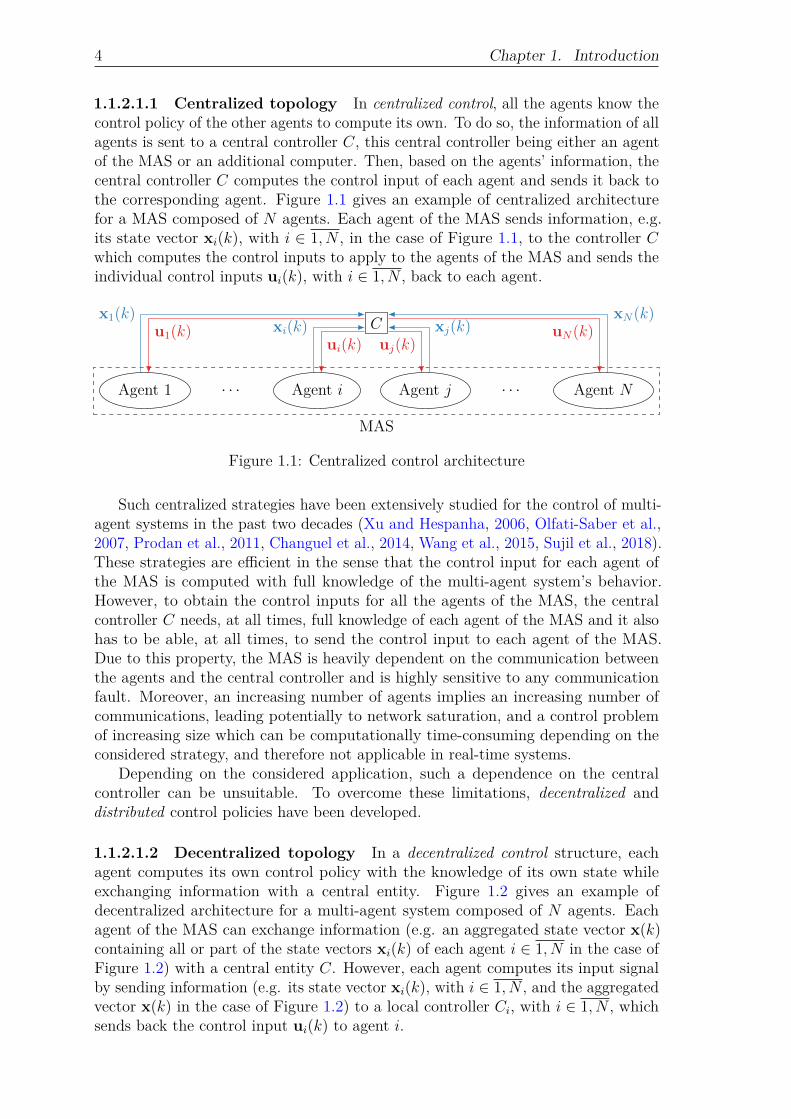
1.1.2.1.1 Centralized topology In centralized control, all the agents know thecontrol policy of the other agents to compute its own. To do so, the information of allagents is sent to a central controller C, this central controller being either an agentof the MAS or an additional computer. Then, based on the agents’ information, thecentral controller C computes the control input of each agent and sends it back tothe corresponding agent. Figure 1.1 gives an example of centralized architecturefor a MAS composed of N agents. Each agent of the MAS sends information, e.g.its state vector xi(k), with i ∈ 1, N , in the case of Figure 1.1, to the controller Cwhich computes the control inputs to apply to the agents of the MAS and sends theindividual control inputs ui(k), with i ∈ 1, N , back to each agent.
C
Agent 1 · · · Agent i Agent j · · · Agent N
MAS
x1(k)u1(k) xi(k)
ui(k)xj(k)
uj(k)
xN(k)uN(k)
Figure 1.1: Centralized control architecture
Such centralized strategies have been extensively studied for the control of multi-agent systems in the past two decades (Xu and Hespanha, 2006, Olfati-Saber et al.,2007, Prodan et al., 2011, Changuel et al., 2014, Wang et al., 2015, Sujil et al., 2018).These strategies are efficient in the sense that the control input for each agent ofthe MAS is computed with full knowledge of the multi-agent system’s behavior.However, to obtain the control inputs for all the agents of the MAS, the centralcontroller C needs, at all times, full knowledge of each agent of the MAS and it alsohas to be able, at all times, to send the control input to each agent of the MAS.Due to this property, the MAS is heavily dependent on the communication betweenthe agents and the central controller and is highly sensitive to any communicationfault. Moreover, an increasing number of agents implies an increasing number ofcommunications, leading potentially to network saturation, and a control problemof increasing size which can be computationally time-consuming depending on theconsidered strategy, and therefore not applicable in real-time systems.
Depending on the considered application, such a dependence on the centralcontroller can be unsuitable. To overcome these limitations, decentralized anddistributed control policies have been developed.
1.1.2.1.2 Decentralized topology In a decentralized control structure, eachagent computes its own control policy with the knowledge of its own state whileexchanging information with a central entity. Figure 1.2 gives an example ofdecentralized architecture for a multi-agent system composed of N agents. Eachagent of the MAS can exchange information (e.g. an aggregated state vector x(k)containing all or part of the state vectors xi(k) of each agent i ∈ 1, N in the case ofFigure 1.2) with a central entity C. However, each agent computes its input signalby sending information (e.g. its state vector xi(k), with i ∈ 1, N , and the aggregatedvector x(k) in the case of Figure 1.2) to a local controller Ci, with i ∈ 1, N , whichsends back the control input ui(k) to agent i.

1.1. Context and motivations 5
Centralentity
Agent 1 · · · Agent i Agent j · · · Agent N
MAS
x1(k)
x(k) xi(k)
x(k)
xj(k)
x(k)
xN(k)
x(k)
C1· · ·Ci Cj
· · · CN
x1(k)x(k)
u1(k)xi(k)x(k)
ui(k)xj(k)x(k)
uj(k)xN(k)x(k)
uN(k)
Figure 1.2: Decentralized control architecture
One of the most used decentralized strategy in control of multi-vehicle systems isthe leader-follower approach where the central entity is another agent and severalstructures of the kind presented in Figure 1.2 can be cascaded. This approach ismainly used in formation control (Consolini et al., 2008, Liu et al., 2016, Wang et al.,2019) of MAS where the agents are mobile robots or vehicles. In a more generalframework, decentralized control strategies have been developed for numerous controlapplications such as microgrids (Liu et al., 2014), smart grids (Lu et al., 2011, Ayaret al., 2017), trajectory tracking for mobile robots (Prodan, 2012, Angelini et al.,2018) or collision avoidance (Verginis and Dimarogonas, 2019).
A decentralized control strategy is easily scalable compared to a centralizedstrategy since the addition of new agents to the MAS does not increase the complexityof a central controller, each agent obtaining its own input with a local controller. Adecentralized structure is also resilient to the loss of the central entity since eachagent is able to either continue its mission by itself or reach a safe state by using itslocal controller.
However, this comes with a drawback linked to the limited communicationsbetween the agents since such communications have to be done through the centralentity. Indeed, the control input of an agent being computed solely from theinformation of this agent, cooperative objectives can be more difficult to carryout. The example of a fleet of several vehicles following a given trajectory whilemaintaining a given formation is considered to illustrate this element. A commonstrategy is for each vehicle to follow a trajectory provided by the formation leadersuch that if every vehicle follows its trajectory, the formation is maintained. Ifa perturbation or a fault occurs on one or several vehicles, their trajectory canbe modified. However, due to the absence of communications, a vehicle does notknow its relative position to another vehicle. Then, without additional strategies tomitigate the perturbation or the fault, there is a potential risk of collision betweentwo or more vehicles which is a hindrance to cooperation. Some strategies in theliterature seek to guarantee a certain level of interaction between the agents to attainglobal coordination of the MAS such as the one proposed by Morărescu and Fiacchini(2016).
1.1.2.1.3 Distributed topology With a distributed control strategy, similarlyto the decentralized case, each agent computes its own control policy with the

6 Chapter 1. Introduction
knowledge of its own state. However, the agents are able to exchange informationwith all or part of the agents belonging to the MAS to obtain its control input.Figure 1.3 gives an example of distributed architecture for a MAS composed of Nagents. Each agent computes its control input ui(k), with i ∈ 1, N , with a localcontroller Ci. However, contrary to the decentralized case, each controller Ci is ableto exchange information with the controllers Cj of the other agents. In the exampleof Figure 1.3, each controller exchanges information with its neighbors, the nature ofthe information not being reported here. It can be noticed that such a structure isan example among others and more connections between the local controllers couldbe added.
Agent 1 · · · Agent i Agent j · · · Agent N
MAS
C1· · ·Ci Cj
· · · CN
x1(k)
u1(k)
xi(k)
ui(k)
xj(k)
uj(k)
xN(k)
uN(k)
Figure 1.3: Distributed control architecture
The distributed strategies bridge the gap between centralized and decentralizedstrategies. Indeed, they involve more communications than a decentralized controlstrategy but less than a centralized one. The computational load delegated toeach agent is heavier than with a decentralized strategy but the complexity ofthe control problem solved by each local controller is reduced compared to thecomplexity of the problem solved by the central controller of a centralized architecture.Moreover, a distributed strategy, as a decentralized strategy, is resilient to the lossof communication with one or several local controllers and it allows to improve thecooperation capabilities of the agents with respect to a decentralized strategy.
Due to these elements and the ubiquity trend presented in Section 1.1.1, dis-tributed strategies are attracting increasing attention. Some examples includeOlfati-Saber (2006), Ren and Beard (2008) or Cao and Ren (2011) who use dis-tributed consensus strategies or Viel (2017) who studies event-triggered control forMAS. In their book, Maestre and Negenborn (2014) give a in-depth overview of exist-ing distributed model predictive control algorithms. A state of the art of distributedcontrol techniques can be found in either Scattolini (2009), Cao et al. (2012) or Rossiet al. (2018). Such strategies can also be applied to different types of multi-agentsystems such as microgrids (Khan et al., 2016, Cominesi et al., 2017), traffic networks(Chanfreut et al., 2020), power grids (Bidram et al., 2014) or multi-vehicle systems(Turri et al., 2016, Li et al., 2017b, Belkadi et al., 2017, 2019).
1.1.2.2 Classification of the approaches for MAS control
An element that goes with the choice of a communication topology for the multi-agent system control structure is the nature of the controller itself, either central orlocal. Indeed, the control problem solved to obtain the control input of the agents isas important and dependent on the nature of the problem as the communication
1.1. Context and motivations 7
topology. Then, the following paragraph does not aim to be exhaustive but topresent some of the most widely used methods of the last twenty years to computethe control input in the central or local controllers.
1.1.2.2.1 Graph theory The communication topology used by the agents ofa MAS to exchange information can be seen as a graph where the agents are thenodes of the graph and the communication between two agents is a link, directed ornot, between the two nodes. Results from algebraic graph theory (Godsil and Royle,2001) are therefore considered in combination with the dynamics of the agents tocompute the control inputs.
The main graph-theoretic strategy that has been extensively applied in multi-agent system control application is the consensus (Olfati-Saber and Murray, 2004,Ren and Beard, 2008), also called agreement (Mesbahi and Egerstedt, 2010). Thename consensus is self-descriptive. Indeed, in the case of consensus problems, theagents aim to synchronize to a common value. Consensus strategies are often usedto address issues related to multi-vehicle systems such as rendezvous (Sorensen andRen, 2006) or formation control (Fax and Murray, 2004, Olfati-Saber, 2006, Flores-Palmeros et al., 2019) and are related to synchronization problems (Ahmadizadehet al., 2016, Panteley and Loría, 2017).
1.1.2.2.2 Potential field As stated in Cheng et al. (2004), the idea of potentialfield approaches is based on a physical analogy. Indeed, an electrically charged bodyproduces an electrical vector field that either attracts or repulses other electricallycharged bodies. This vector field is the gradient of a scalar function f of a vectorvariable x. In most physics applications, this vector variable x is a vector of spacecoordinates (e.g. Cartesian or spherical coordinates). A potential field approach incontrol is then based on the construction of an artificial scalar function f which isthe sum of an attractive and a repulsive potential. The attractive potential is meantto attract the system towards its desired objective while the repulsive potential takesthe system away from a given area of the state space in which it evolves. Then, thenegative gradient −∇f(x) indicates the most promising direction in the state spaceto drive the system towards its objective.
Potential field approaches are often used in navigation problems (Hagelbäck andJohansson, 2008, Prodan, 2012, Ivić et al., 2016, Baillard et al., 2018) where theattractive potential is minimal on the objectives that the agents have to reach andmaximal on the obstacles such that the agents go towards their objectives whileavoiding obstacles. One of the main drawbacks of this approach is that it can drivethe system into a configuration corresponding to a local minimum of the potentialfunction. Rimon and Koditschek (1992) provide methods to compute artificialpotential functions free of local minima.
1.1.2.2.3 Game theory Game theory (Osborne and Rubinstein, 1994) is amathematical framework used to describe the behavior of interacting players. In sucha framework, a player is an intelligent and rational decision maker, i.e. an entity thattakes decisions from reasoning, which has to evolve within a set of rules guiding itsbehavior. Game theory is often used in social sciences to represent human interactionand social phenomena. Moreover, given its characteristics, such a framework is anobvious tool to study MAS control problems. Indeed, the agents are players which

8 Chapter 1. Introduction
have to reach an objective where they maximize their gain in the game, the rules ofthe game being the constraints applied on the problem.
Game theoretic methods for MAS control have been increasingly studied inthe last decade. For example, Fele et al. (2017) present a game theoretic controlframework called coalitional control to deal with various problems. This frameworkis based on the theory of coalitional games (Myerson, 1991), in which it is assumedthat cooperation always brings benefits to the players, but with the limitation thatforming new coalitions of agents might provide a lower gain than doing tasks with alarger number of coalitions. Coalitional control has been used in the last years todeal with irrigation canals (Fele et al., 2014), traffic networks (Chanfreut et al., 2020)or more general large-scale systems (Fele et al., 2018). However, coalitional controlis just one of the many aspects of game theoretic control for multi-agent systemsand numerous other works deal with different game theoretic strategies (Quijanoet al., 2017). Such works are for example Semsar-Kazerooni and Khorasani (2009)and Zhang et al. (2014) which mix respectively cooperative and differential gametheory with consensus problems or Khan et al. (2016) that use non-cooperative gametheory for the control of microgrid systems.
1.1.2.2.4 Optimization Optimization-based control methods compute the con-trol input of a system as the solution of an optimization problem minimizing a givencriterion under constraints. Then, using efficient tools such as linear, quadratic,mixed-integer or even semi-definite programming solvers, it is possible to obtain theoptimal input driving the agents of a MAS towards their objective. Optimization-based control have been applied to multi-agent systems in different forms suchas optimal control (Ji et al., 2006, Movric and Lewis, 2013, Yuan et al., 2018) orneural-network based control (Hou et al., 2009, Wen et al., 2016, Yu et al., 2020),which have been attracting a lot of attention for the past ten years. One of the mostwidely used optimization-based control method is model predictive control (MPC)thanks to its effectiveness with constraint handling due to the receding horizon policyit adopts (Mayne et al., 2000). The properties of MPC have been extensively studiedand are well documented in the literature (Maciejowski, 2002, Camacho and Bordons,2007, Rawlings and Mayne, 2009, Kouvaritakis and Cannon, 2016). In the case ofmulti-agent systems, Maestre and Negenborn (2014) and Olaru et al. (2015) presenta detailed overview of current uses and applications of MPC strategies.
In addition to the classical MPC as presented in Maciejowski (2002) or Rawlingsand Mayne (2009), several different flavors have been developed over the years todeal with increasingly complex situations. For example, an explicit solution to theMPC optimization problem can be found as a piecewise affine function (Bemporadet al., 2002, Tøndel et al., 2003) obtained by exploiting the Karush-Kuhn-Tuckerconditions (Boyd and Vandenberghe, 2009). Moreover, robust versions have beendeveloped for the case of a perturbed system (Kouvaritakis and Cannon, 2016),either when the perturbations are deterministic and bounded (Mayne et al., 2005,2006) or have a stochastic nature (Cannon et al., 2010, 2012), both having beenapplied on multi-agent systems (Prodan et al., 2011, Trodden and Richards, 2014,Nikou and Dimarogonas, 2019, Lyons et al., 2012, Dai et al., 2016).

1.1. Context and motivations 9
1.1.3 Deployment controlMulti-vehicle systems (MVS) are a type of MAS where each agent is an autonomousvehicle. They are used for a wide spectrum of real world missions such as forest firemonitoring (Merino et al., 2012, Yuan et al., 2019), ground and resource monitoring(Laliberte and Rango, 2009, Jin and Tang, 2010, d’Oleire Oltmanns et al., 2012),mapping and modeling (Nex and Remondino, 2014, Han and Chen, 2014, Torreset al., 2016) or even surveillance missions (Li et al., 2019, Trujillo et al., 2019). Formost of these applications, a MVS seeks to maximize the coverage of a given spatialarea under potential operating constraints. A way to achieve such a coverage is forthe MVS to self-deploy within the area it seeks to cover. The works cited abovehave different ways to define what is a deployment for coverage. The definition thatis used for this thesis is the one from Schwager et al. (2011), which considers thedeployment of a multi-vehicle system as a strategically appropriate spreading of theMVS in a given environment in order to reach a fixed configuration, the environmentbeing the spatial area that the vehicles aim to cover.
In the last twenty years, several works have studied the self-deployment of aMVS problem such as Choset (2001), Howard et al. (2002), Cortés et al. (2004),Li and Cassandras (2005), Murray (2007), Moarref and Rodrigues (2014), Nguyen(2016), Papatheodorou et al. (2017) or Hatleskog (2018). The deployment of a MASis meant to ensure the maximal coverage of an environment with respect to a givencriterion. In that sense, several techniques have been proposed to deal with thisproblem such as motion planning (Choset, 2001), potential field (Howard et al., 2002),probabilistic (Li and Cassandras, 2005) or Voronoi-based techniques (Cortés et al.,2004). Schwager et al. (2011) show that the last three approaches can be unifiedthrough the use of a mixing function encoding the coverage criteria to be maximized.Many of the works cited are based on the use of a time-varying Voronoi tessellationof the deployment area. The Voronoi tessellation is a tool that has been introducedby Dirichlet (1850) and further developed by Voronoï (1908). It is a way to partitiona metric space, equipped with a distance function, into a set of non-overlappingregions called Voronoi cells. These cells are generated from a finite set of elementsbelonging to the metric space, these elements being called generators. Each cell isassociated uniquely with one of the generators. The classical Voronoi tessellation isobtained by using the Euclidean norm but Voronoi diagrams can also be obtainedfrom other types of distances (Aurenhammer, 1991) and for generators that are notpoints but sets (Sugihara, 1993, Choset and Burdick, 1995). Figure 1.4 presents forexample the Voronoi tessellation of a square with five generators. The plot on theleft is obtained using the Euclidean distance and the one on the right is obtainedusing the Manhattan distance where, if x =
[x1 · · · xn
]> is a vector of Rn, theEuclidean and the Manhattan norm are defined as:
‖x‖2 =
√√√√ n∑i=1
x2i and ‖x‖1 =n∑i=1
|xi|,
respectively. Moreover, when the generators are not points but circles or ellipses, theVoronoi tessellation is often called power Voronoi diagram (Aurenhammer, 1991).
For the deployment over an area, the positions of the vehicles of the MVS are thegenerators of the Voronoi tessellation. The goal of the MVS is then to reach a staticconfiguration in which each vehicle lies on a remarkable point of the Voronoi cell

10 Chapter 1. Introduction
−5 0 5
−5
0
5
x
y
Generator
−5 0 5
−5
0
5
x
y
Generator
(a) (b)
Figure 1.4: Voronoi tessellation of a square for 5 generators with the Euclidean norm(a) and the Manhattan norm (b).
generated by this vehicle. It can be noticed that the main difficulties in achieving thedeployment are, first, that, since the generators of the Voronoi tessellation move overtime, the Voronoi tessellation is time varying and, second, that the final configurationis not known a priori due to the dynamics of the Voronoi tessellation. One of the firstapproaches to define a Voronoi-based coverage of a given area is the Lloyd’s algorithm(Lloyd, 1982), derived from the k-means clustering algorithm (MacQueen, 1967),where the goal is to obtain a maximum coverage from a set of agents without anydynamics. With Lloyd’s algorithm, the considered remarkable point of a cell is thecenter of mass of the cell. Then, if pi(k) denotes the position of the agent i at timek and ci(k) the center of mass of its Voronoi cell at time k, Lloyd’s algorithm runsas presented in Algorithm 1.1. Figure 1.5 presents the result of Lloyd’s algorithmfor five agents inside a square. The circles represent the positions of the agentsat iteration k and the stars represent the centers of mass at iteration k. The firstdiagram presented in Figure 1.5 is obtained from the initial positions, the second isthe one obtained after the first iteration of Lloyd’s algorithm and the third one isthe final result obtained after 26 iterations.
Algorithm 1.1: Lloyd’s algorithm.Input: The initial positions of the agents pi(0), with i ∈ 1, N
1 while ci(k + 1) 6= ci(k) for all i do2 Compute the Voronoi tessellation of the area from the positions pi(k);3 Compute the center of mass ci(k) of each Voronoi cell;4 Set pi(k + 1) = ci(k);5 end
Output: The static configuration of the MAS
Recent work on the deployment of a MAS starts with the deployment of amulti-sensor network in a convex two-dimensional area. In their paper, Cortés

1.1. Context and motivations 11
−5 0 5
−5
0
5
x
y Position pi(0)
Center of mass ci(0)
−5 0 5
−5
0
5
x
y Position pi(1)
Center of mass ci(1)
−5 0 5
−5
0
5
x
y Position pi(26)
Center of mass ci(26)
(a) (b) (c)
Figure 1.5: Illustration of Lloyd’s algorithm at initialization, after the first iterationand after the last iteration.
et al. (2004) propose a decentralized optimal control algorithm for agents obeyingsingle integrator dynamics such that the MAS reaches a static centroidal Voronoiconfiguration1. Based on this work, Sharifi et al. (2014) propose a distributed controlalgorithm based on feedback linearization for the deployment into a centroidalconfiguration in a so-called weighted Voronoi tessellation, where the distance betweentwo points is the Euclidean norm of the difference between their coordinates dividedby a given positive weight. Several other works propose control algorithms to drivea MAS into a static configuration under constraints such as maximization of thecoverage (Schwager et al., 2011) or energy efficiency constraints (Song et al., 2013,Moarref and Rodrigues, 2014) and even control strategies for MAS subject to drifts(Bakolas and Tsiotras, 2013). In the last years, Nguyen (2016) proposed a newdeployment strategy where the remarkable point considered for the Voronoi cells isnot the center of mass of the cell, but the Chebyshev center (Boyd and Vandenberghe,2009), i.e. the center of the largest ball contained in the Voronoi cell. This pointis obtained as the solution of a linear optimization problem and is often easier tocompute than the center of mass. Nguyen (2016) proposes state-feedback strategies,including model predictive control, for the Voronoi-based deployment of a MASusing the Chebyshev center of the Voronoi cells. This work has been further studiedin Hatleskog (2018) who provides a proof of convergence of the deployment strategyin the one dimensional case and in the two dimensional case when the agents obeysingle integrator dynamics and are controlled with an unconstrained state-feedbackcontroller. In addition, the problem of optimal coverage of an area when the locationof the agent is uncertain has been recently studied. Papatheodorou et al. (2016)propose for example a distributed optimal control strategy for the deployment of amulti-sensor network for which the position of the agent is uncertain and containedinside a circle. These results have been further extended in Papatheodorou et al.(2017), Tzes et al. (2018) or Turanli and Temeltas (2020).
1Centroidal configuration means that the agents lie on the center of mass of their Voronoi cells.

12 Chapter 1. Introduction
1.1.4 Main motivations and thesis orientation: ModelPredictive Control for the deployment ofmulti-vehicle systems
From the literature overview of Sections 1.1.1 and 1.1.2, it appears that the controlof multi-agent systems is a wide and active research topic. Thus, the present thesis islimited to a given area that is overviewed in Section 1.1.3. Indeed, deployment controlof a multi-vehicle system is a task that is relevant for a wide range of applications asdetailed previously.
As presented in Section 1.1.3, several control strategies exist for the deploymentof a MAS using a Voronoi tessellation of the area in which the MAS is deployed.However, the majority of these works are based on the center of mass of the Voronoicells to drive the agents towards a static configuration. Then, building on the resultsof Nguyen and Stoica Maniu (2016) and Nguyen et al. (2017), the present thesisdeals with the deployment and reconfiguration of a multi-vehicle system inside abounded convex two-dimensional area.
The goal of the present work is to develop model predictive control algorithms forthe Voronoi-based deployment of a multi-vehicle system in a bounded convex two-dimensional area and to apply the proposed control algorithms for the deploymentof a fleet of quadrotor unmanned aerial vehicles (UAVs). The first step for suchwork is to adapt the decentralized model predictive controller proposed in Nguyen(2016) for the deployment of agents obeying simple dynamics such as single or doubleintegrator dynamics. Thus, a decentralized deployment algorithm is proposed andapplied to a fleet of quadrotor UAVs obeying continuous-time nonlinear dynamics.To this end, a cascaded control architecture is considered, where the decentralizedMPC algorithm is used for the position control of the vehicles, the position controldesign being performed based on simplified models of the agents having doubleintegrator dynamics. The goal of the multi-vehicle system is then to deploy into astatic configuration in which each agent lies on the Chebyshev center of its associatedVoronoi cell. The use of MPC is justified in this context since it allows to considerconstraints on the future evolution of the system, limiting it to evolve inside itsVoronoi cell, used as a safety region to avoid collision with the other vehicles, andrestraining the speed and attitude of the system due to physical limitations. Moreover,such a framework is favorable towards the use of a decentralized control algorithm.Indeed, with just the knowledge of the other agents’ positions by measurements orcommunication with a central entity, an agent is able to build its own Voronoi cell,allowing it to then carry the burden of control input computation.
Nguyen (2016) or Hatleskog (2018) study the deployment of a MAS in thenominal case. Papatheodorou et al. (2016), for example, opens the door on thedeployment of MAS subject to position uncertainty. Further investigations haveto be led in this direction to allow a system subject to more general perturbationsto be deployed over a given area. Robust MPC techniques have been developedto account for bounded perturbations on a single system, for example in Mayneet al. (2005) and Mayne et al. (2006). Then, based on these works, the presentthesis studies the deployment of a MAS when the agents are subject to boundeddeterministic perturbations and proposes a decentralized tube-based MPC algorithmfor the Voronoi-based deployment of a fleet of UAVs which drives the MAS into astatic configuration, guaranteeing that the distance between the agents and their

1.2. Contributions of the thesis 13
Chebyshev center is bounded.Nevertheless, perturbations are not always bounded and, in addition, they can
be of stochastic nature, as modeling errors or measurement noises. Such signalsacting on a system lead to the appearance of so-called chance constraints in theoptimization problem solved by the model predictive controller for single (Cannonet al., 2012, Farina et al., 2016) or multi-agent systems (Dai et al., 2015, 2018). Then,this thesis also investigates chance-constrained MPC techniques for the deploymentof MAS subject to unbounded stochastic perturbations.
Finally, based on the collision avoidance requirement, a question arises: whathappens if one or several agents have to leave or join the area in which the deploymentoccurs? MPC algorithms can be used in this case, where the deploying multi-agentsystem needs to be reconfigured to deal with the modification in the number ofagents. Indeed, it is possible to construct regions for the safe evolution of the agentsduring the reconfiguration phase using set-theoretic tools (Blanchini and Miani,2015), translated into constraints to obtain a safe transient objective. For eachagent, the elements needed for its safety require only the knowledge of the otheragents’ position, allowing for a decentralized algorithm to drive the MAS. Suchproblems often arise in fault-tolerant formation control and are relevant for variousmulti-vehicle system applications.
1.2 Contributions of the thesisThe present thesis proposes several flavors of decentralized MPC algorithms forthe deployment of a MAS over a convex bounded two dimensional area. Thesealgorithms are based on a Voronoi tessellation of the area to cover as well as onthe Chebyshev center of the Voronoi cells as an objective point for the agents to bedeployed. Then, the following paragraphs detail the contribution of this thesis foreach of the proposed MPC techniques.
1.2.1 Deployment in the nominal caseNguyen (2016) introduces a decentralized model predictive controller for the de-ployment of a nominal multi-agent system (i.e. no uncertainties, no fault) in aconvex bounded area, where each agent is driven towards the Chebyshev center ofits associated Voronoi cell. For its part, Hatleskog (2018) gives a proof of conver-gence of the Voronoi and Chebyshev-based deployment algorithm for the case ofsingle integrator dynamics when the agents are driven with an unconstrained fullstate-feedback controller.
The present thesis proposes a Voronoi-based centralized MPC for the deploymentof a MAS in a convex bounded area, each agent being driven towards the Chebyshevcenter of its Voronoi cell. After formulating the decentralized version of this deploy-ment algorithm, it provides a proof of feasibility of the MPC optimization problemwhen the agents obey single integrator dynamics. This feasibility proof leads to adiscussion on the convergence of the decentralized deployment algorithm. To showits efficiency, the proposed decentralized model predictive controller is used as theposition controller for quadrotor unmanned aerial vehicles, modeled as nonlinearsystems. Directions to prove the convergence of the deployment algorithm for a fleetof quadrotor UAVs are then discussed.

14 Chapter 1. Introduction
These contributions have led to the publication of the papers Chevet et al. (2018)and Chevet et al. (2020b).
1.2.2 Deployment under bounded deterministicperturbations
Papatheodorou et al. (2016) and Papatheodorou et al. (2017) study the deploymentof a MAS over an area when the agents are subject to bounded position uncertainty.These works are based on the definition of an ellipsoidal-based so-called guaranteedVoronoi tessellation taking into account the fact that the generators of the cells arenot points anymore but discs.
The present thesis introduces a new box-based guaranteed Voronoi tessellationwhere the generators of the Voronoi tessellation are not points but boxes (i.e.rectangles in a two-dimensional space). Such a guaranteed Voronoi tessellation isused to cope with the bounded output perturbations acting on the system.
To deal with the case of bounded perturbations acting on a system, a tube-basedMPC strategy (Mayne et al., 2005) can be used. The idea behind such a controlalgorithm is to decompose the control input applied to a system into two parts, oneobtained via optimization on the nominal dynamics and the other one by multiplyingthe error between the real state and the nominal state of the system by a gain matrix.The state of the system is then guaranteed to belong to a robust positively invariantset for the error dynamics centered on the nominal state of the system. Alvarado(2007) proposes a linear matrix inequality constrained optimization problem toobtain the gain matrix used in classical state-feedback tube-based MPC (Mayneet al., 2005).
This thesis then proposes a decentralized output-feedback tube-based MPCstrategy for the deployment of a multi-agent system subject to bounded deterministicinput and output perturbations. A novel linear/bilinear matrix inequality constrainedoptimization-based procedure is designed to obtain the gain matrices of the state-feedback part of the tube-based controller and of the observer introduced in theoutput-feedback strategy. This procedure aims to minimize the size of the robustpositively invariant sets to which the state belongs such that the optimization part ofthe tube-based controller has enough degrees of freedom to optimize the performanceof the system. The decentralized output-feedback tube-based MPC is firstly appliedfor the deployment of a MAS composed of agents obeying single integrator dynamics,and secondly for the position control of a fleet of quadrotor UAVs.
These contributions have led to the publication of the paper Chevet et al. (2019).
1.2.3 Deployment under unbounded stochasticperturbations
When a system is subject to unbounded stochastic perturbations, probabilisticconstraints, also called chance constraints, appear on the optimization problemsolved by the model predictive controller. Gavilan et al. (2012) propose a state-feedback chance-constrained model predictive controller for a single system wherethe chance constraints have to be satisfied with a probability equal to 1. Basedon the stochastic properties of the perturbation, Gavilan et al. (2012) introduces amethod to relax probabilistic constraints into algebraic constraints.

1.2. Contributions of the thesis 15
The present thesis introduces a new decentralized output-feedback chance-constrained MPC algorithm for the deployment of a MAS when the agents aresubject to unbounded stochastic perturbations. However, the stochastic perturbationsignal, which is unknown over the prediction horizon of the MPC, appears in theconstraints of the MPC optimization problem. These constraints have to be satisfiedwith a probability equal to 1. A relaxation procedure of the probabilistic constraintsinto algebraic constraints in order to solve the MPC optimization problem is proposedalong with a proof of feasibility. This relaxation uses the stochastic properties ofthe perturbations to find a bound allowing the constraints to be satisfied for almostall perturbations acting on the system. The decentralized output-feedback chance-constrained MPC is applied to the deployment of two MAS composed, respectively, ofagents obeying single integrator dynamics and of agents obeying nonlinear quadrotorUAV dynamics.
These contributions have led to the publication of the paper Chevet et al. (2020a).
1.2.4 Reconfiguration in the case of a time-varyingmulti-vehicle system
Another contribution of the present thesis deals with the reconfiguration of a deployingmulti-agent system when agents join or leave the area in which the deployment isoccurring. This problem is related to fault-tolerant formation control since the mainreasons leading an agent to leave the deployment area are related to faulty situations.
In the case of incoming agents, the proposed technique is a natural extension of thenominal deployment strategy. Indeed, the deployment algorithm being decentralized,it is easily scalable and allows intrinsically to consider additional agents.
To deal with the case of outgoing agents, the present work proposes two originalstrategies based on a transient objective, different from the Chebyshev center of theVoronoi cells, for the agents remaining in the deployment area allowing them to avoidthe trajectory of the outgoing agents. For the first strategy, the transient objective ofan agent is defined as the weighted barycenter of the agent’s neighbors. For the secondstrategy, the transient objective of an agent is obtained by solving an optimizationproblem constraining the objective to belong to a region of the deployment area inwhich it is safe for this agent to evolve in order to avoid collisions with the outgoingagents. The second strategy has the advantage of allowing a reconfiguration of theMAS when several agents leave the deployment area simultaneously, increasing thefault-related capabilities.
For the case of agents joining the deployment area, simulation results are presentedfor a MAS with agents obeying single integrator dynamics. For the case of outgoingagents, the two reconfiguration strategies are compared on a MAS composed ofagents obeying single integrator dynamics when one agent leaves the deploymentarea. Finally, simulation results are presented for the second reconfiguration strategywhen two agents leave the deployment area with two MAS, the first one composedof agents obeying single integrator dynamics and the second composed of agentsobeying nonlinear UAV dynamics.
These contributions have led to the publication of the papers Chevet et al. (2018)and Chevet et al. (2020b).

16 Chapter 1. Introduction
1.2.5 PublicationsThe work done during the preparation of this thesis has led to the submission andpublication of several conference and journal papers.Peer-reviewed journal paper
• T. Chevet, C. Vlad, C. Stoica Maniu, and Y.M. Zhang. Decentralized MPCfor UAVs formation deployment and reconfiguration with multiple outgoingagents. Journal of Intelligent & Robotic Systems, 97(1):155-170, 2020.
Peer-reviewed conference papers
• T. Chevet, C. Stoica Maniu, C. Vlad, Y.M. Zhang, and E.F. Camacho.Chance-constrained MPC for Voronoi-based multi-agent system deployment.In 21st IFAC World Congress. Berlin, Germany, July 12–17, 2020.
• T. Chevet, C. Stoica Maniu, C. Vlad, and Y.M. Zhang. Guaranteed Voronoi-based deployment for multi-agent systems under uncertain measurements. In18th European Control Conference, pages 4016–4021. Naples, Italy, June 25–28,2019.
• T. Chevet, C. Stoica Maniu, C. Vlad, and Y.M. Zhang. Voronoi-basedUAVs formation deployment and reconfiguration using MPC techniques. InInternational Conference on Unmanned Aircraft Systems, pages 9–14. Dallas,TX, United States, June 12–15, 2018.
Other publicationsHandouts
• T. Chevet, M.A. Lefebvre, V. Letort-Le Chevalier, D. Madhavan Brochier,C. Maniu, G. Sandou, and C. Vlad. Model Representations and Analysis.CentraleSupélec Handouts. 210 pages. 2020.
• T. Chevet, M.A. Lefebvre, V. Letort-Le Chevalier, C. Maniu, G. Sandou,and C. Vlad. Modélisation. Représentations et analyse des modèles. Centrale-Supélec Handouts (in French). 210 pages. 2020.
Peer-reviewed journal paper
• D. Merhy, C. Stoica Maniu, T. Alamo, E.F. Camacho, S. Ben Chabane,T. Chevet, M. Makarov, and I. Hinostroza. Guaranteed set-membershipestimation of an octorotor’s position for radar applications. InternationalJournal of Control. In press.
Peer-reviewed conference papers
• C. Stoica Maniu, C. Vlad, T. Chevet, S. Bertrand, A. Venturino, G. Rousseau,and S. Olaru. Control systems engineering made easy: Motivating studentsthrough experimentation on UAVs. In 21st IFAC World Congress, Demonstra-tor session. Berlin, Germany, July 12–17, 2020.

1.3. Thesis outline 17
• D. Merhy, C. Stoica Maniu, T. Alamo, E.F. Camacho, T. Chevet, M. Makarov,and I. Hinostroza. Zonotopic set-membership state estimation applied to anoctorotor model. In 12th Summer Workshop on Interval Methods. Palaiseau,France, July 23–26, 2019.
• C. Stoica Maniu, C. Vlad, T. Chevet, G. Rousseau, S. Bertrand, and S. Olaru.Modernizing teaching through experimentation on UAVs formations. 12th IFACSymposium on Advances in Control Education, Invited Demonstration Session.Philadelphia, PA, United States, July 7–9, 2019. In IFAC-PapersOnLine,52(9):144–146, 2019.
Oral presentations
• T. Chevet, C. Stoica Maniu, C. Vlad, Y.M. Zhang, and E.F. Camacho.Voronoi-based deployment of multi-vehicle systems. Seminar at Departamentode Ingeniería de Sistemas y Automática, University of Seville, Spain, December17, 2019.
• T. Chevet, M. Makarov, C. Stoica Maniu, I. Hinostroza, and P. Tarascon.State estimation of an octorotor with unknown inputs. Application to radarimaging. Seminar at Networked Autonomous Vehicles Lab, Concordia Univer-sity, Montréal, Canada, October 31, 2017.
1.3 Thesis outlineThe remainder of the present thesis is organized as follows.
Chapter 2: Mathematical tools and set-theoretic elements This chap-ter provides the different mathematical results necessary for the development of thedecentralized model predictive control algorithms presented in this thesis. It startsby recalling some properties on matrices and linear/bilinear matrix inequalities. Itthen introduces necessary set-theoretic elements before presenting the notion of setinvariance in control theory. The general state-space representation of a MAS isdescribed along with the necessary assumptions for the development of the MPCalgorithms. Then, the construction of several types of Voronoi tessellation is detailed.The construction of the classical Voronoi tessellation is given before introducingtwo contributions of this thesis, i.e. the box-based guaranteed Voronoi tessellationand the so-called pseudo-Voronoi tessellation, along with a formal definition ofa Chebyshev configuration. Finally, Chapter 2 presents some classical results oncontinuous univariate and multivariate random variables.
Chapter 3: Decentralized control for the deployment of a multi-vehiclesystem This chapter starts by giving a centralized and a decentralized formulationof the Voronoi-based deployment algorithm. It then gives a proof of feasibility of theMPC optimization problem when the agents obey single integrator dynamics anddiscusses the convergence of the deployment algorithm. After, simulation results arepresented for the deployment of a MAS composed of agents obeying single integratordynamics. The nonlinear dynamics of quadrotor unmanned aerial vehicles areintroduced, as well as a cascaded control structure to allow the use of a decentralized

18 Chapter 1. Introduction
output-feedback MPC strategy for position control. Simulation results are exposedfor the deployment of a MAS composed of agents obeying nonlinear quadrotor UAVdynamics. Chapter 3 ends on a discussion of possible directions for the convergenceproof of the deployment algorithm when agents obey double integrator dynamics ormore complex dynamics.
Chapter 4: Deployment of a multi-vehicle system subject to perturba-tions This chapter is twofold in the sense that it presents two robust decentralizedMPC algorithms for the deployment of a MAS: the first one for agents subject tobounded deterministic perturbations, and the second one for agents subject to un-bounded stochastic perturbations. In the first part, a decentralized output-feedbacktube-based model predictive controller is introduced along with two linear/bilinearmatrix inequality constrained optimization problems to obtain the observer andstate-feedback gain matrices necessary for the tube-based strategy. In the second part,a decentralized output-feedback chance-constrained model predictive controller is ex-posed along with a method allowing probabilistic constraints relaxation into algebraicconstraints. In both cases, simulation results are presented for the Voronoi-baseddeployment of a MAS firstly composed of agents obeying single integrator dynamicsand secondly composed of agents obeying nonlinear quadrotor UAV dynamics.
Chapter 5: Extension to the deployment of a time-varying multi-vehicle system This chapter aims to present reconfiguration algorithms for a MASin the case of agents joining or leaving the MAS during the deployment. It starts bypresenting the decentralized MPC strategy for the incoming agents. Then, a firstreconfiguration strategy to deal with the case of one agent leaving the deploymentarea is introduced. This reconfiguration strategy is based on a transient objectivecomputed as an agent’s neighbors’ barycenter. Simulation results are presented inboth situations for a MAS composed of agents obeying single integrator dynamics.Then, Chapter 5 introduces a new decentralized reconfiguration strategy to drive theremaining agents safely away from the outgoing agents when several agents leavethe MAS simultaneously. This second strategy is based on a new transient objectiveobtained by solving an optimization problem constraining it to belong to a regionin which it is safe for the remaining agent to evolve. This new algorithm is thencompared in simulation with the first reconfiguration strategy. Finally, simulationresults are presented for the deployment and reconfiguration of two MAS when twoagents leave the deployment area using the improved reconfiguration algorithm. Thefirst MAS is composed of agents obeying single integrator dynamics and the secondone of agents obeying nonlinear quadrotor UAV dynamics.
Chapter 6: Concluding remarks and future work This chapter completesthe present thesis by means of concluding remarks and gathers several open directionsof this work.

Chapter 2Mathematical tools and set-theoretic
elements
Table of Contents
2.1 Definitions and useful properties of matrices . . . . . . . . . . . . . 192.2 Set-theoretic elements for control . . . . . . . . . . . . . . . . . . . 22
2.2.1 Ellipsoidal sets . . . . . . . . . . . . . . . . . . . . . . . . . 232.2.2 Polyhedral sets . . . . . . . . . . . . . . . . . . . . . . . . . 242.2.3 Set operations . . . . . . . . . . . . . . . . . . . . . . . . . 292.2.4 Sets in control theory . . . . . . . . . . . . . . . . . . . . . 34
2.3 Multi-vehicle system description . . . . . . . . . . . . . . . . . . . . 382.4 Voronoi tessellation and formation configuration . . . . . . . . . . . 41
2.4.1 Conventional Voronoi tessellation . . . . . . . . . . . . . . . 412.4.2 Generalized Voronoi tessellations . . . . . . . . . . . . . . . 44
2.4.2.1 Box-based guaranteed Voronoi tessellation . . . . . 442.4.2.2 Pseudo-Voronoi tessellation . . . . . . . . . . . . . 50
2.4.3 Chebyshev configuration of a multi-vehicle system . . . . . . 532.5 Continuous random variables and stochastic processes . . . . . . . . 562.6 Conclusion . . . . . . . . . . . . . . . . . . . . . . . . . . . . . . . . 59
2.1 Definitions and useful properties of matricesAs stated by Blanchini and Miani (2015) in the preface of their book, sets willnaturally appear with three aspects of control theory: constraints, uncertaintiesand design specifications. In this context, this chapter focuses on the main setproperties necessary for the comprehension of the results elaborated in the presentthesis. Before introducing elements about sets, it is necessary to present some usefuldefinitions about matrices.
Definition 2.1: Positive definite matrix
A symmetric matrix P = P> ∈ Rn×n is called positive definite (respectively positivesemidefinite), denoted by P 0 (respectively by P 0), if x>Px > 0 (respectivelyx>Px ≥ 0) for all x ∈ Rn \ 0n×1.
19
20 Chapter 2. Mathematical tools and set-theoretic elements
Definition 2.2: Weighted quadratic norm
Let P ∈ Rn×n be a positive semidefinite matrix and x ∈ Rn be a vector. Thequadratic norm of x weighted by P is the quantity ‖x‖P =
√x>Px.
The two following properties of special matrices related to positive definitenessare important for the results presented in this thesis.
Property 2.1: Exponential of a matrix (Hall, 2015)
Let A ∈ Rn×n be a matrix. Then, the exponential of matrix A:
exp(A) =+∞∑i=0
Ai
i!(2.1)
is positive definite, denoted by exp(A) 0.
Property 2.2: Product of matrices (Horn and Johnson, 2013)
Let A ∈ Rn×n be a positive semidefinite matrix and B ∈ Rn×m be a matrix withm ≤ n. Then, the product B>AB is positive semidefinite. It is positive definite ifand only if A is positive definite and B has rank m.
The concept of positive definite matrices is also used to introduce Linear MatrixInequalities in control theory.
Definition 2.3: Linear Matrix Inequality (Boyd et al., 1994)
A Linear Matrix Inequality (LMI) is an expression of the following form:
F (x) = F0 +n∑i=1
xiFi 0 (2.2)
where x =[x1 · · · xn
]> ∈ Rn is the vector of decision variables and the matricesFi ∈ Rm×m, with i ∈ 0, n, are symmetric.
♦
Remark 2.1: Non strict LMIDefinition 2.3 can be extended to the case where the inequality is not strict. In thiscase, F (x) is considered to be positive semidefinite, denoted by F (x) 0.
♦
Remark 2.2: Affine matrixA matrix F (x) ∈ Rm×m is called affine in x ∈ Rn if it can be written as:
F (x) = F0 +n∑i=1
xiFi. (2.3)
If F0 = 0m, the the matrix F (x) is linear with respect to x.
LMI problems often arise in several domains of control engineering, such as robustcontrol (Scherer and Weiland, 2015) or state-estimation (Le et al., 2013) for example.These problems often consist in minimizing a linear objective c>x, with c ∈ Rn

2.1. Definitions and useful properties of matrices 21
under strict or nonstrict LMI constraints such as:
minimizex
c>x
subject to
F (x) 0.(2.4)
These problems can be solved numerically with appropriate solvers. For example,the Robust Control Toolbox of Matlab® provides a solver to solve the problems ofthe form (2.4) called mincx. Other openly distributed toolboxes for Matlab® suchas CVX (Grant and Boyd, 2014, 2008) or YALMIP (Löfberg, 2004, 2020) allow tosolve problems of the form (2.2) but also more general problems where the LMIs arenonstrict.
Property 2.3: Schur complement (Boyd et al., 1994)
Let Q(x) ∈ Rn×n and R(x) ∈ Rm×m be symmetric matrices affine in x and S(x) ∈Rn×m a matrix affine in x. Then the LMI:[
Q(x) S(x)S>(x) R(x)
] 0 (2.5)
is equivalent to: Q(x) 0
R(x)− S>(x)Q−1(x)S(x) 0(2.6)
or: R(x) 0
Q(x)− S(x)R−1(x)S>(x) 0.(2.7)
The concept of LMI can be extended to the more general case of Bilinear MatrixInequalities.
Definition 2.4: Bilinear Matrix Inequality
A Bilinear Matrix Inequality (BMI) is an inequality of the form:
F (x) = F0 +n∑i=1
xiFi +n∑i=1
n∑j=1
xixjFij 0 (2.8)
where x =[x1 · · · xn
]> ∈ Rn is the vector of decision variables and F0,Fi,Fij ∈Rm×m, with i ∈ 1, n and j ∈ 1, n, are symmetric matrices.
BMI problems can sometimes be reduced to LMI problems using for instanceProperty 2.3. When they cannot, specific optimization solvers exist such as PENBMI(Henrion et al., 2005) or its open source counterpart PENLAB (Fiala et al., 2013)that can solve optimization problems under BMI constraints. Such BMI constraintsoften appear in control with one specific procedure presented hereafter.
22 Chapter 2. Mathematical tools and set-theoretic elements
Theorem 2.1: S-procedure (Boyd et al., 1994)
Let Fi ∈ R, with i ∈ 0,m be quadratic functions of a variable x ∈ Rn:
Fi(x) = x>Qix+ 2f>i x+ ri (2.9)
where Qi ∈ Rn×n is a symmetric matrix, fi ∈ Rn and ri ∈ R, with i ∈ 0,m. If∃τi ≥ 0, with i ∈ 1,m, such that:
F0(x)−m∑i=1
τiFi(x) ≥ 0 (2.10)
then F0(x) ≥ 0 for all x such that Fi(x) ≥ 0 for all i ∈ 1,m.
The link between the S-procedure defined in Theorem 2.1 and LMIs and BMIs isnot immediate from what is presented in Theorem 2.1. Using (2.9), the left handside of inequality (2.10) can be rewritten as:
F0(x)−m∑i=1
τiFi(x) = x>
(Q0 −
m∑i=1
τiQi
)x+ 2
(f0 −
m∑i=1
τifi
)>
x
+
(r0 −
m∑i=1
τiri
)
=
[x1
]> Q0 −
m∑i=1
τiQi f0 −m∑i=1
τifi
f>0 −m∑i=1
τif>i r0 −
m∑i=1
τiri
[x1
].
Then, with the notation:
F =
Q0 −
m∑i=1
τiQi f0 −m∑i=1
τifi
f>0 −m∑i=1
τif>i r0 −
m∑i=1
τiri
,
inequality (2.10) is equivalent to the nonstrict matrix inequality:
F 0. (2.11)
If the matrices Qi, the vectors fi and the scalars ri, with i ∈ 0,m, are known, then(2.11) is a LMI where the vector of decision variables is τ =
[τ1 · · · τm
]>. However,if the terms Qi, fi and ri are also decision variables, then the expression (2.11) is aBMI. The S-procedure is used in Chapter 4 to design tube-based model predictivecontrol policies.
2.2 Set-theoretic elements for controlGiven their importance in control theory, this part of the present chapter focuses ondefinitions relative to sets and operations on sets. One of the most common class

2.2. Set-theoretic elements for control 23
of sets used in control is the class of convex sets (Boyd and Vandenberghe, 2009)and all the results presented in this thesis are based on such convex sets, hence thenecessity of the following definition.
Definition 2.5: Convex set
A set S ∈ Rn is called convex if for all x1, . . . ,xk ∈ S, with k ≥ 2:
k∑i=1
αixi ∈ S, with α1, . . . , αk ∈ R such thatk∑i=1
αi = 1.
Another general definition which is of use in Sections 2.2.2 and 2.2.3 is that ofthe convex hull of a finite set of points.
Definition 2.6: Convex hull
The convex hull of a finite set of points V = v1, . . . ,vk, with v1, . . . ,vk ∈ Rn andk ≥ 2, is the set:
conv(V) =
x ∈ Rn
∣∣∣∣∣ x =k∑i=1
λivi, λi ∈ R+,k∑i=1
λi = 1
The remainder of this section is organized as follows: two types of sets, namelyellipsoidal and polyhedral sets are defined in Sections 2.2.1 and 2.2.2 respectively.Section 2.2.3 presents some classical operations on sets and Section 2.2.4 introducesthe concept of set invariance.
2.2.1 Ellipsoidal setsEllipsoids are one of the most widespread family of convex sets in control theory(Kurzhanski and Vályi, 1997, Blanchini and Miani, 2015). They are used in numerousareas such as identification (Polyak et al., 2004), state estimation (Schweppe, 1968,Merhy, 2019) and, what is mainly relevant for this thesis, robust control (Boyd et al.,1994, Poznyak et al., 2014). Due to their relevance in such fields, some definitionsare further detailed.
Definition 2.7: Ellipsoidal set
Given a symmetric positive definite matrix P = P> 0 with P ∈ Rn×n, a vectorc ∈ Rn and a real scalar ρ > 0, the ellipsoid E (P , c, ρ) is the set:
E (P , c, ρ) =x ∈ Rn
∣∣∣ (x− c)>P (x− c) ≤ ρ
(2.12)
where P is called the shape matrix, c the center and ρ the so called radius ofE (P , c, ρ).
Example 2.1: An ellipsoidal set in R2
Let P =
[2 −1−1 4
], c =
[21
]and ρ = 6. Then, Figure 2.1 shows, in red, the set

24 Chapter 2. Mathematical tools and set-theoretic elements
E (P , c, 6). Moreover, the border of E (P , c, 6) is the set:
∂E (P , c, 6) =x ∈ R2
∣∣∣ (x− c)>P (x− c) = 6
which is an ellipse.
x
y
−1−1
0
0
1
1
2
2
3
3
4
4
c
∂E (P , c, 6)
E (P , c, 6)
Figure 2.1: An example of ellipsoidal set in R2.
Definition 2.8: Normalized ellipsoidal set
A normalized ellipsoidal set is an ellipsoidal set with ρ = 1, leading to:
E (Q, c, 1) = E (Q, c) =x ∈ Rn
∣∣∣ (x− c)>Q(x− c) ≤ 1.
Note that such a normalized set can be obtained from an ellipsoidal set by takingQ = P /ρ.
Example 2.2: A normalized ellipsoidal set in R2
By taking the same numerical values as in Example 2.1, if Q = P /6, one has thatE (Q, c) = E (P , c, 6). This way, Figure 2.1 also represents the normalized ellipsoidalset E (Q, c) in red and its border in black.
The attentive reader will have noticed that, for a normalized ellipsoidal setE (Q, c), since the radius ρ is unitary, it can be omitted from the notation. Thesame way, if c = 0n, the center is omitted from the notation, giving E (P , ρ) for acentered ellipsoidal set or E (Q) for a centered normalized ellipsoidal set.
However, while simple to use and of reduced complexity, an ellipsoidal set can bemore conservative than other sets such as polyhedral sets introduced in Section 2.2.2.
2.2.2 Polyhedral setsThe family of polyhedral sets is another widespread family of convex sets appearingin control theory (Blanchini and Miani, 2015). They appear in particular when linearconstraints are applied to a system. Polyhedral sets have two types of representationeither based on half spaces (Definition 2.9) or on vertices (Definition 2.11), making
2.2. Set-theoretic elements for control 25
them very flexible and allowing them to be a good approximation of any convexset (Bronstein, 2008). Another advantage of using polyhedral sets is that they areinvariant by the operations presented in Section 2.2.3, i.e. the result of an operationbetween two polyhedral sets is a polyhedral set. Polyhedral sets are less conservativethan ellipsoidal sets. However, their complexity do not depend on the dimension ofthe space but on the number of vertices, which can quickly increase.
Definition 2.9: Half-space or H-representation (Schrijver, 1998)
A polyhedral set or polyhedron P ⊂ Rn is the combination of finitely many linearinequalities:
P = x ∈ Rn |Hx ≤ θ, (2.13)
with H ∈ Rm×n and θ ∈ Rm, where m is the number of inequalities defining P .
From a geometrical point of view, each row of H and the associated element ofθ in (2.13) define a closed half-space Pi, with i ∈ 1,m, such that:
Pi = x ∈ Rn | hix ≤ θi
where hi and θi are the i-th rows of H and θ, hence the name half-space representationor H-representation. The border ∂Pi of Pi, is the hyperplane in Rn:
∂Pi = x ∈ Rn | hix = θi.
This way, the rows hi of H can be interpreted as the transpose of the normal vectorsto the hyperplanes ∂Pi and the elements θi of θ as the algebraic distances of thesehyperplanes to the origin 0n×1, if
∥∥h>i
∥∥2= 1. Indeed, since the distance between
∂Pi and a vector x ∈ Rn is:
d(x, ∂Pi) =|hix− θi|∥∥h>
i
∥∥2
,
if∥∥h>
i
∥∥2= 1, d(0n×1, ∂Hi) = |θi|.
Example 2.3: A polyhedron in R2
Let H =
[3 20 1
]and θ =
[82
]. Then, H and θ induce a polyhedron P in R2 (as per
Definition 2.9) represented in Figure 2.2. This figure also shows the hyperplanes ∂P1
and ∂P2 defined respectively by the first and second rows of H and θ, as well as thenormal vectors h>
1 and h>2 .
However, as it can be seen in Example 2.3, a polyhedral set can be unbounded.In control theory, a specific class of polyhedral sets is used, namely the class ofbounded polyhedral sets.
Definition 2.10: Polytope
A bounded polyhedron is called a polytope.
♦Remark 2.3: H-polytopeA polytope defined by a H-representation is called a H-polytope.

26 Chapter 2. Mathematical tools and set-theoretic elements
x
y
−2 0 2 4−2
0
2
4
P∂P1
∂P2
h>1h>
2
−2 0 2 4−2
0
2
4
x
y
Figure 2.2: An example of polyhedral set in R2.
Example 2.4: A polytope in R2
Let H =
[3 0 −1 −1 22 1 2 −1 −1
]>and θ =
[8 2 3 5 4
]>. Then H and θ induce
a polyhedron P in R2 (as per Definition 2.9) represented in Figure 2.3. It is obviousfrom the representation in Figure 2.3 that P is a polytope since it is bounded.
x
y
−5−5
−4
−4
−3
−3
−2
−2
−1
−1
0
0
1
1
2
2
3
3
4
4
5
5
P
∂P1
∂P2
∂P3
∂P4
∂P5
Figure 2.3: An example of polytopic set in R2.
Before going further in the definitions about polyhedrons and polytopes, a wayto test if a polytope is empty or not is presented below.

2.2. Set-theoretic elements for control 27
Theorem 2.2: Farkas’ lemma (Matoušek and Gärtner, 2007)
Let H ∈ Rm×n and θ ∈ Rm. Then exactly one of the two following statements istrue:
1. There exists a vector x ∈ Rn such that Hx ≤ θ;
2. There exists a vector y ∈ Rm such that y ≥ 0, H>y = 0n×1 and θ>y < 0.
With Theorem 2.2, it is then possible to test if a polytope is empty or not givenits H-representation.
Now that the half-space representation of a polyhedron has been introduced, itis time to introduce its dual representation, the vertex representation. However, thisdefinition is limited to the V-representation of a polytope, the general definition fora polyhedron being out of the scope of this thesis.
Definition 2.11: Vertex or V-representation
A polytopic set or polytope P ⊂ Rn is the linear combination of finitely many pointscalled vertices v1, . . . ,vk ∈ Rn, with k ≥ 2:
P =
x ∈ Rn
∣∣∣∣∣ x =k∑i=1
λivi, λi ∈ R+,k∑i=1
λi = 1
. (2.14)
♦Remark 2.4: V-polytopeA polytope defined by a V-representation is called a V-polytope.
♦
Remark 2.5: Polytope and convex hull of verticesConsider a set of points V = v1, . . . ,vk, where vi ∈ Rn, with i ∈ 1, k, k ≥ 2. If Vis the set of the vertices of a polytope P ⊂ Rn, then:
P = conv(V),
i.e. a polytope is the convex hull of its vertices.
Two ways to represent polytopes have been introduced. However, these tworepresentations are formally different, since one needs a set of hyperplanes and theother requires a set of vertices to induce a polytope. Intuitively, seeking all theintersection points of the hyperplanes, one can find the vertices or define hyperplanesfrom the vertices. While its proof is not trivial, the following theorem formalizesthis idea.
Theorem 2.3: Main theorem for polytopes (Ziegler, 2007)
A subset P ∈ Rn is the convex hull of a finite set of points if and only if it is abounded intersection of half-spaces.
Corollary 2.4: Equivalence of H- and V-representation of polytopes
A polytope P ∈ Rn admits a V-representation if and only if it admits a H-represen-tation.

28 Chapter 2. Mathematical tools and set-theoretic elements
Example 2.5: Equivalence between H and V-representation of polytopesLet V be a family of vectors of R2:
V =
v1 =
[31
],v2 =
[13
],v3 =
[−22
],v4 =
[−2−2
],v5 =
[1−2
].
The polytope P = conv(V) is presented in Figure 2.4 as well as the points vi, withi ∈ 1, 5.
With this basic example in two dimensions, it is easy to extract the H-representa-tion of P by finding the equations of the lines joining two consecutive vertices. Thisway:
P =
x ∈ Rn
∣∣∣∣∣∣∣∣∣∣
1 1−1 3−1 00 −13 −2
x ≤
48227
.
x
y
−3−3
−2
−2
−1
−1
0
0
1
1
2
2
3
3
4
4
P
v1
v2
v3
v4 v5
∂P1
∂P2
∂P3
∂P4
∂P5
Figure 2.4: Equivalence between V-representation and H-representation for a polytopein R2.
Example 2.5 illustrates the equivalence between H-representation and V-represen-tation of a polytope given in Corollary 2.4. The construction of the H-representationfrom a V-representation, presented in the case of a polytope in R2 in Example 2.5,is known as the facet enumeration problem. The construction of the V-representa-tion from a H-representation is known as the vertex enumeration problem. Severalalgorithms exist to solve these problems (Fukuda and Prodon, 1995, Bremner et al.,1998) but their runtime increases greatly with the number of vertices.
Finally, a special kind of polytope that is used to define perturbation sets inParagraph 2.4.2.1 or Section 4.1 or even to define constraint sets in the modelpredictive controllers of Chapters 3 to 5 is introduced.

2.2. Set-theoretic elements for control 29
Definition 2.12: Box
A box Bn(α) ⊂ Rn, with α =[α1 · · · αn
]> ∈ Rn, with αi ≥ 0 for all i ∈ 1, n, iscomposed by n intervals:
Bn(α) = x ∈ Rn | |x| ≤ α. (2.15)
When α ∈ Rn in Definition 2.12 is reduced to 1n×1, the box Bn(α) is called aunitary box.
Definition 2.13: Unitary box
A unitary box Bn ⊂ Rn is composed by n unitary intervals:
Bn = x ∈ Rn | |x| ≤ 1n×1. (2.16)
2.2.3 Set operationsTwo types of convex sets, ellipsoidal and polytopic sets, have been introduced in theprevious paragraphs. This paragraph then introduces some useful operations on sets,mainly on polytopic sets since, as mentioned in Section 2.2.2, the set of polytopes isinvariant by the operations that are presented in the following. Thus, the followingdefinitions are given for general sets X ,Y ⊂ Rn, but some useful properties onpolytopes coming from these definitions are introduced.
Definition 2.14: Cartesian product of two sets
The Cartesian product of two sets X ⊂ Rn and Y ⊂ Rm is the set:
X × Y = (x,y) | x ∈ X and y ∈ Y. (2.17)
Property 2.4: Cartesian product of two polytopes
Let P ⊂ Rn, Q ⊂ Rm be two polytopes for which a H-representation is known:
P = x ∈ Rn |HPx ≤ θP and Q = x ∈ Rm |HQx ≤ θQ.
The Cartesian product of P and Q is the set:
P ×Q =
x ∈ Rn+m
∣∣∣∣ diag(HP ,HQ)x ≤[θPθQ
]. (2.18)
Definition 2.15: Intersection of two sets
The intersection of two sets X ,Y ⊂ Rn is the set:
X ∩ Y = x ∈ Rn | x ∈ X and x ∈ Y. (2.19)

30 Chapter 2. Mathematical tools and set-theoretic elements
Property 2.5: Intersection of two polytopes
Let P ,Q ⊂ Rn be two polytopes for which a H-representation is known:
P = x ∈ Rn |HPx ≤ θP and Q = x ∈ Rn |HQx ≤ θQ.
The intersection of P and Q is the set:
P ∩Q =
x ∈ Rn
∣∣∣∣ [HPHQ
]x ≤
[θPθQ
]. (2.20)
♦
Remark 2.6: Redundant inequalitiesIn the H-representation (2.20) of the intersection of two polytopes, some inequalitiesare redundant as shown in Example 2.6. However, algorithms exists, such as theFourier-Motzkin elimination method (Dantzig, 1972), to remove them.
Example 2.6: Intersection of two polytopesLet P be the polytope introduced in Example 2.5 and Q a polytope induced by
HQ =
[−11 −1 77 −3 1
]>and θQ =
[6 6 18
]>. Figure 2.5 presents the two polytopes
P and Q as well as their intersection P ∩Q.
x
y
−3−3
−2
−2
−1
−1
0
0
1
1
2
2
3
3
4
4
P
QP ∩Q
∂P2
∂P3
Figure 2.5: Intersection of two polytopes in R2.
As per Remark 2.6, it is obvious from Figure 2.5 that two inequalities areredundant. These inequalities are the ones associated with the hyperplanes ∂P2
and ∂P3. Thus, the second and third rows of HP and θP can be omitted from the

2.2. Set-theoretic elements for control 31
H-representation of P ∩Q such that:
P ∩Q =
x ∈ R2
∣∣∣∣∣∣∣∣∣∣∣∣
1 10 −13 −2−11 7−1 −37 1
x ≤
4276618
.
In general, the elimination of redundant constraints is not as simple as inExample 2.6 (a plot was still needed to see which constraints were redundant) andthe complexity of the problem increases greatly with the number of inequalities andthe dimension of the vector space Rn.
Definition 2.16: Translation of a set
The translation of a set X ⊂ Rn by a vector t ∈ Rn is the set:
T(X , t) = x+ t | x ∈ X. (2.21)
Property 2.6: Translation of a V-polytope
Let P ⊂ Rn be a polytope for which a V-representation is known. Let v1, . . . ,vk ∈ Rn,with k ≥ 2, be the vertices of P and consider t ∈ Rn. Then:
T(P , t) = conv(v1 + t, . . . ,vk + t). (2.22)
Proof. The proof is immediate from Definition 2.11 and Definition 2.16.
Property 2.7: Translation of a H-polytope
Let P ⊂ Rn be a polytope for which a H-representation is known. Let H ∈ Rm×n
and θ ∈ Rm the matrices inducing P and t ∈ Rn. Then:
T(P , t) = x ∈ Rn |Hx ≤ θ +Ht. (2.23)
Proof. Let P = x ∈ Rn |Hx ≤ θ be a polytope with H ∈ Rm×n and θ ∈ Rm.Let pi ∈ ∂Pi, with i ∈ 1,m a point on the i-th border of P , thus verifying hipi = θiwhere hi and θi are the i-th rows of H and θ, respectively. The translation of thepoint pi by the vector t ∈ Rn verifies:
hi(pi + t) = θi + hit. (2.24)
Thus, if x ∈ Rn is such that x ∈ T(∂Pi, t), it has the form x = pi + t and verifies(2.24). This way, T(∂Pi, t) = x ∈ Rn | hix = θi + hit, ∀i ∈ 1,m. Then, T(P , t) isgiven by (2.23).
Definition 2.17: Minkwoski sum of two sets
The Minkowski sum of two sets X ,Y ⊂ Rn is the set:
X ⊕ Y = x+ y | x ∈ X ,y ∈ Y. (2.25)

32 Chapter 2. Mathematical tools and set-theoretic elements
♦
Remark 2.7: Minkowski sum of two V-polytopes (Ziegler, 2007)If X ,Y ⊂ Rn are two polytopes for which a V-representation is known, theirMinkowski sum can be computed easily. Let x1, . . . ,xk,y1, . . . ,yl ∈ Rn, withk, l ≥ 2, such that X = conv(x1, . . . ,xk) and Y = conv(y1, . . . ,yl). Then,X ⊕ Y = conv(V) where:
V =xi + yj,∀i ∈ 1, k, ∀j ∈ 1, l
.
Definition 2.18: Pontryagin difference of two sets
The Pontryagin difference of two sets X ,Y ⊂ Rn is the set:
X Y = x ∈ X | x+ y ∈ X ,∀y ∈ Y. (2.26)
Example 2.7: Minkowski sum and Pontryagin difference of V-polytopesLet P ⊂ R2 be the polytope introduced in Example 2.5. Let Q ⊂ R2 be the polytope:
Q = conv
(q1 =
[−1−1
],q2 =
[01
],q3 =
[1−1
]).
Figure 2.6 presents the Minkowski sum P ⊕Q of P and Q. As per Remark 2.7, it isobtained by adding all the vertices of Q to the vertices of P and by taking the convexhull of all the obtained points. It can be done graphically by centering the set Q onall the vertices of P and by joining the maximum points.
x
y
−3
−3
−2
−2
−1
−1
0
0
1
1
2
2
3
3
4
4
QP
P ⊕Q
v1
v2
v3
v4 v5
q1
q2
q3
Figure 2.6: Minkowski sum of two polytopes in R2.
Figure 2.7 presents the Pontryagin difference P Q of P and Q. In this figure,the set Q is centered on all the vertices of P Q to show that the sum of an elementfrom P Q and one from Q is an element of P.
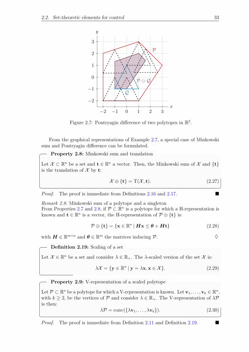
2.2. Set-theoretic elements for control 33
x
y
−2
−2
−1
−1
0
0
1
1
2
2
3
3
Q
P
P Q
Figure 2.7: Pontryagin difference of two polytopes in R2.
From the graphical representations of Example 2.7, a special case of Minkowskisum and Pontryagin difference can be formulated.
Property 2.8: Minkowski sum and translation
Let X ⊂ Rn be a set and t ∈ Rn a vector. Then, the Minkowski sum of X and tis the translation of X by t:
X ⊕ t = T(X , t). (2.27)
Proof. The proof is immediate from Definitions 2.16 and 2.17.
♦
Remark 2.8: Minkowski sum of a polytope and a singletonFrom Properties 2.7 and 2.8, if P ⊂ Rn is a polytope for which a H-representation isknown and t ∈ Rn is a vector, the H-representation of P ⊕ t is:
P ⊕ t = x ∈ Rn |Hx ≤ θ +Ht (2.28)
with H ∈ Rm×n and θ ∈ Rm the matrices inducing P .
Definition 2.19: Scaling of a set
Let X ∈ Rn be a set and consider λ ∈ R+. The λ-scaled version of the set X is:
λX = y ∈ Rn | y = λx,x ∈ X. (2.29)
Property 2.9: V-representation of a scaled polytope
Let P ⊂ Rn be a polytope for which a V-representation is known. Let v1, . . . ,vk ∈ Rn,with k ≥ 2, be the vertices of P and consider λ ∈ R+. The V-representation of λPis then:
λP = conv(λv1, . . . , λvk). (2.30)
Proof. The proof is immediate from Definition 2.11 and Definition 2.19.
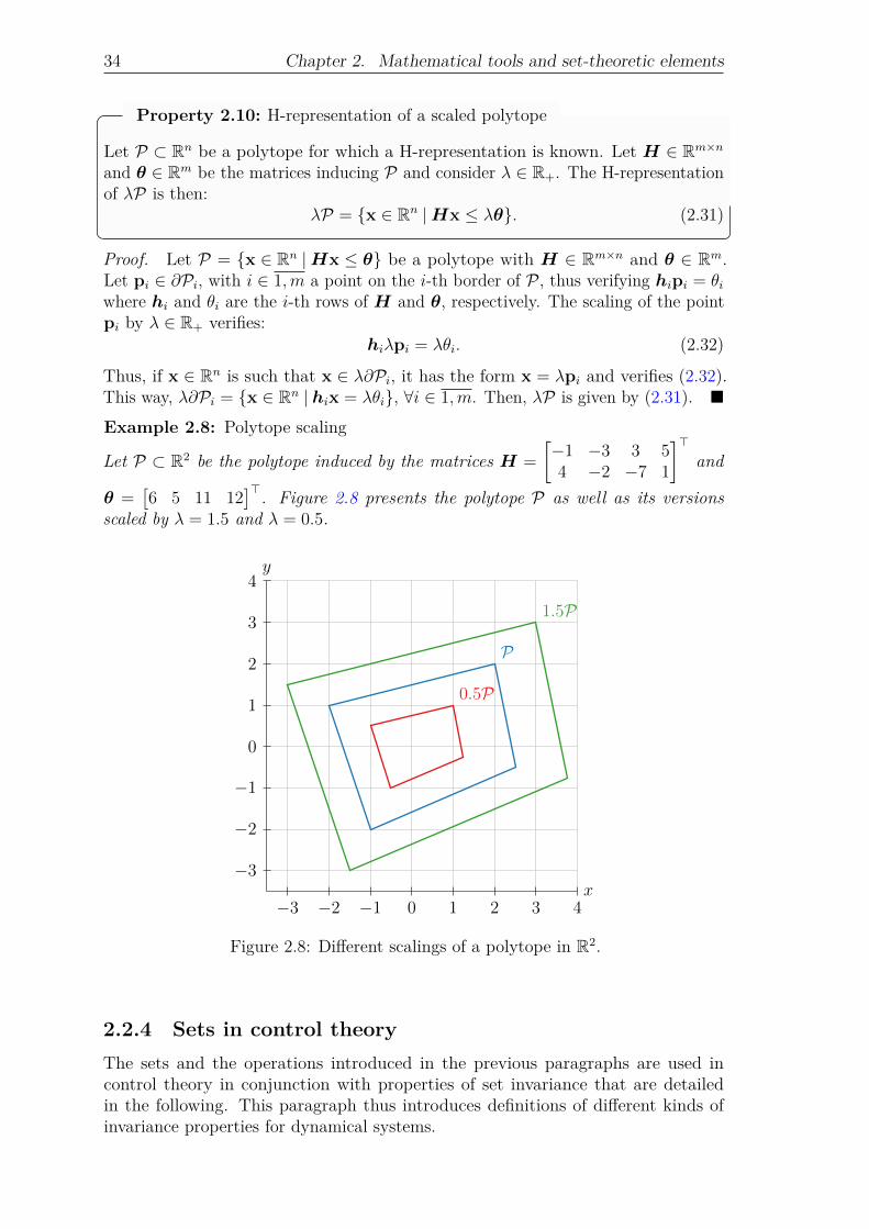
34 Chapter 2. Mathematical tools and set-theoretic elements
Property 2.10: H-representation of a scaled polytope
Let P ⊂ Rn be a polytope for which a H-representation is known. Let H ∈ Rm×n
and θ ∈ Rm be the matrices inducing P and consider λ ∈ R+. The H-representationof λP is then:
λP = x ∈ Rn |Hx ≤ λθ. (2.31)
Proof. Let P = x ∈ Rn |Hx ≤ θ be a polytope with H ∈ Rm×n and θ ∈ Rm.Let pi ∈ ∂Pi, with i ∈ 1,m a point on the i-th border of P , thus verifying hipi = θiwhere hi and θi are the i-th rows of H and θ, respectively. The scaling of the pointpi by λ ∈ R+ verifies:
hiλpi = λθi. (2.32)
Thus, if x ∈ Rn is such that x ∈ λ∂Pi, it has the form x = λpi and verifies (2.32).This way, λ∂Pi = x ∈ Rn | hix = λθi, ∀i ∈ 1,m. Then, λP is given by (2.31).
Example 2.8: Polytope scaling
Let P ⊂ R2 be the polytope induced by the matrices H =
[−1 −3 3 54 −2 −7 1
]>and
θ =[6 5 11 12
]>. Figure 2.8 presents the polytope P as well as its versionsscaled by λ = 1.5 and λ = 0.5.
x
y
−3
−3
−2
−2
−1
−1
0
0
1
1
2
2
3
3
4
4
1.5P
P
0.5P
Figure 2.8: Different scalings of a polytope in R2.
2.2.4 Sets in control theoryThe sets and the operations introduced in the previous paragraphs are used incontrol theory in conjunction with properties of set invariance that are detailedin the following. This paragraph thus introduces definitions of different kinds ofinvariance properties for dynamical systems.

2.2. Set-theoretic elements for control 35
The first two definitions are given for an autonomous discrete-time linear timeinvariant (LTI) system. They are related to positive invariance of a set which is oneof the most important invariance property in control theory.
Definition 2.20: Positive invariant set (Blanchini and Miani, 2015)
Consider an autonomous discrete-time linear time invariant system with the dynam-ics:
x(k + 1) = Ax(k) (2.33)
where A ∈ Rn×n is a Schur matrix and x(k) ∈ Rn for all k ∈ N. A set X ⊂ Rn iscalled positive invariant for the dynamics (2.33) if x(k + 1) ∈ X for all x(k) ∈ X orif:
AX ⊆ X . (2.34)
Definition 2.21: Minimal positive invariant set (Blanchini and Miani, 2015)
The set X ⊂ Rn is called minimal positive invariant (mPI) for the dynamics (2.33)if it is the intersection of all the positive invariant sets for the dynamics (2.33).
Definition 2.22: Robustly positive invariant set (Blanchini and Miani, 2015)
Consider a perturbed autonomous discrete-time linear time-invariant system withthe dynamics:
x(k + 1) = Ax(k) +w(k) (2.35)
where A ∈ Rn×n is a Schur matrix, x(k) ∈ Rn for all k ∈ N and w(k) ∈ W ⊂ Rn aperturbation signal. A set X ⊂ Rn is called robustly positive invariant (RPI) for thedynamics (2.35) if x(k + 1) ∈ X for all x(k) ∈ X and w(k) ∈ W or if:
AX ⊕W ⊆ X . (2.36)
Definition 2.23: Minimal RPI set (Blanchini and Miani, 2015)
The set X ⊂ Rn is called minimal robustly positive invariant (mRPI) for the dynamics(2.35) if it is the intersection of all the RPI sets for the dynamics (2.35).
Other works, such as Basile and Marro (1969), have presented the concept of setinvariance when the dynamics are not autonomous.
Definition 2.24: Controlled invariant set (Basile and Marro, 1969)
Consider a discrete-time linear time-invariant system with the dynamics:
x(k + 1) = Ax(k) +Bu(k) (2.37)
where A ∈ Rn×n, B ∈ Rn×m, x(k) ∈ Rn and u(k) ∈ Rm for all k ∈ N. The pair(A,B) is assumed to be controllable. A set X ⊂ Rn is called controlled invariant forthe dynamics (2.37) if for all x(k) ∈ X , there exists a control law u(k) ∈ U ⊂ Rm
such that x(k + 1) ∈ X .
Finally, the scaling of sets can be used to define a last kind of invariance property.

36 Chapter 2. Mathematical tools and set-theoretic elements
Definition 2.25: Controlled λ-contractive set (Blanchini and Miani, 2015)
A set X ⊂ Rn is called controlled λ-contractive, with λ ∈ [0, 1), for the dynamics(2.37) if for all x(k) ∈ X , there exists a control law u(k) ∈ U ⊂ Rm such thatx(k + 1) ∈ λX .If λ = 1, X is controlled invariant.
The last important element of this section is related to the construction of suchinvariant sets. Several algorithms exist to compute RPI and mRPI sets (Rakovićet al., 2005, Kofman et al., 2007, Olaru et al., 2010, Trodden, 2016) or even controlledinvariant sets (Fiacchini and Alamir, 2017). Most of these algorithms are based on H-polytopes, leading to one of their main drawbacks, i.e. its complexity. Indeed, thesealgorithms are iterative, which can make the number of vertices of the consideredpolytopes quickly increase. This is why it is often better to compute invariantsets offline and use the result online. In order to reduce the complexity of theinvariant set computation, ellipsoidal sets could be used. However, such sets wouldinduce quadratic constraints in the optimization problems of the model predictivecontrollers of Section 4.1, while the constraints remain linear with H-polytopes.Then, while the computation of invariant sets is simplified with the use of ellipsoidalsets, the computation of the input signal with a model predictive controller is morecomplicated if an ellipsoidal set is used instead of a polytopic set.
A method to compute polytopic invariant sets is based on Kofman et al. (2007)followed by a procedure coming from Olaru et al. (2010). Indeed, Kofman et al.(2007) provides a useful theorem to build an initial RPI set from the dynamicsof a perturbed autonomous discrete-time linear time invariant system when theperturbation is bounded.
Theorem 2.5: Initial RPI set (Kofman et al., 2007)
Consider the system:x(k + 1) = Ax(k) +w(k)
together with the notations from Definition 2.22. The perturbation vector is assumedto be such that ‖w(k)‖∞ ≤ w for all k ∈ N, where w ∈ R+. Let A = V JV −1, withV ,J ∈ Rn×n, be the Jordan decomposition of A. Then the set:
S =
x ∈ Rn
∣∣∣∣ [ V −1
−V −1
]x ≤ 12×1 ⊗ (In − |J |)−1
∣∣V −1w1n×1
∣∣ (2.38)
is invariant for the dynamics (2.35).
From this initial shape, Olaru et al. (2010) propose an iterative algorithm tobuild an ε-approximation of the mRPI set, where ε ∈ R∗
+, recalled in Algorithm 2.1.In this algorithm, E (In, ε) ⊂ Rn is a centered ellipsoid and Bn is a unitary box of Rn
as defined in Definition 2.13. For a complete version, the reader can refer to Olaruet al. (2010).
Algorithm 2.1 provides an approximation of the mRPI set depending on thechosen value of the parameter ε. However, this method can end up being timeconsuming depending on the dimension of the state space n and on the matrix A.
Trodden (2016) provides a faster method, while more conservative, than the oneproposed above. However, this method being based on the maximization of a cost

2.2. Set-theoretic elements for control 37
Algorithm 2.1: ε-approximation of the mRPI setInput: The matrix A, the disturbance bound w, the scalar ε ∈ R∗
+
1 Compute the Jordan decomposition of A;2 Build the initial RPI set S with (2.38);3 Initialize Sε = S;4 Initialize l = 0;5 while Al+1Sε 6⊂ E (In, ε) do6 l = l + 1;7 Sε = ASε ⊕ wBn;8 end
Output: The ε-approximation Sε of the mRPI set
function under constraints, if the cost function is unbounded, there is no guaranteeto get a result. To present the optimization problem proposed by Trodden (2016),it is necessary to introduce notations for some elements of the problem. First, theH-representation of Bn as used in Algorithm 2.1 is:
Bn = x ∈ Rn |Bx ≤ θBn
and second, the set S from (2.38) has for simplified H-representation:
S = x ∈ Rn | Sx ≤ θS.
Then, the approximation of the mRPI set S∗ have for H-representation:
S∗ = x ∈ Rn | Sx ≤ θ∗
with θ∗ = c∗ + d∗ such that (Trodden, 2016):
(c∗,d∗) = maximizeci,di,ξi,ωi
∀i∈1,2n
2n∑i=1
ci + di (2.39a)
subject to
ci ≤ siAξi, ∀i ∈ 1, 2n, (2.39b)Sξi ≤ c+ d, ∀i ∈ 1, 2n, (2.39c)di ≤ siωi, ∀i ∈ 1, 2n, (2.39d)
Bωi ≤ wθBn , ∀i ∈ 1, 2n (2.39e)
where si, ci and di, with i ∈ 1, 2n, are the rows of S, c and d, respectively, andξi ∈ Rn and ωi ∈ Rn, with i ∈ 1, 2n, are optimization variables. Thus, as mentionedearlier, if the problem is bounded, (2.39) provides an approximation of the mRPIset which can be more conservative than the one provided by Olaru et al. (2010),but is obtained faster. Example 2.9 provides an academic example of construction ofthe mRPI set with the two methods.
Example 2.9: Comparison of two approximation of the mRPI set of a system
Consider the system x(k+1) = Ax(k)+w(k), with A =
[0.8 0.10.3 0.5
]and ‖w(k)‖∞ ≤
w = 0.1 for k ∈ N. The Jordan decomposition of A is:
A = V JV −1, with V =
[−0.2638 1.2638
1 1
]and J =
[0.4209 0
0 0.8791
].

38 Chapter 2. Mathematical tools and set-theoretic elements
Using Theorem 2.5, the initial RPI set is:
S =
x ∈ R2
∣∣∣∣∣∣∣∣−0.6547 0.82730.6547 0.17270.6547 −0.8273−0.6547 −0.1727
x ≤
0.02980.68450.02980.6845
.
−1 −0.5 0 0.5 1
−1
−0.5
0
0.5
1
S = S∗
x1
x2
(b)
−1 −0.5 0 0.5 1
−1
−0.5
0
0.5
1
Sε
S
x1
x2
(a)
Figure 2.9: Comparison of two approximations of the mRPI set of a system in R2.
Figure 2.9 presents in red the initial RPI set defined above. The left plot (a)shows the ε-approximation of the mRPI set Sε with ε = 10−5 in blue obtained withAlgorithm 2.1. On the right plot (b) is drawn the approximation of the mRPI set S∗
in blue obtained by solving (2.39).The fact that S∗ is more conservative than Sε is obvious from Figure 2.9 since
Sε ⊂ S, while S∗ = S. However, it is not obvious from the plot that the V-representation of Sε contains 149 vertices, its H-representation is composed of 79inequalities and s = 88 iterations are needed to compute Sε. The approximationS∗ has the same V-representation and H-representation as S, i.e. 4 vertices and 4inequalities.
Finally, a trade-off between conservativeness and complexity can be made bycombining the methods from Olaru et al. (2010) and Trodden (2016). For this, thewhile loop in Algorithm 2.1 can be modified to run for a limited number of iterationsarbitrarily chosen or until a maximal number of vertices or inequalities is reached.Then, the H-representation of the obtained set can be used as input to (2.39).
2.3 Multi-vehicle system descriptionThe elements introduced in the previous sections are used in the development ofcontrol algorithms for multi-agent systems (MAS). For this, the dynamics of theagents composing the MAS are introduced in the present section as well as theassumptions necessary for the development of the control algorithms proposed inthis thesis.
2.3. Multi-vehicle system description 39
Let Σ be a multi-agent system composed of N agents. Each agent obeys discrete-time LTI dynamics:
xi(k + 1) = Aixi(k) +Biui(k) (2.40a)yi(k) = Cixi(k) (2.40b)
where xi ∈ Rni , ui ∈ Rmi , yi ∈ Rpi , Ai ∈ Rni×ni , Bi ∈ Rni×mi and Ci ∈ Rpi×ni ,with i ∈ 1, N . For an agent i ∈ 1, N , the vector xi is called the state vector, uiis called the input vector and yi is called the output vector. The output set Yi isa subset of the state space Xi and is of lower or equal dimension, i.e. pi ≤ ni. Inthe literature, several types of multi-vehicle systems (MVS) are considered. Someexamples include MVS composed of several unmanned aerial vehicles (Chevet et al.,2020b), unmanned ground vehicles (Kamel et al., 2020) or even both unmannedground and aerial vehicles (Sharifi et al., 2014).
Assumption 2.1: ControllabilityThe pair (Ai,Bi) is controllable for all i ∈ 1, N .
Assumption 2.2: ObservabilityThe pair (Ai,Ci) is observable for all i ∈ 1, N .
The goal of the control algorithms that are presented in the following chapters ofthis thesis is to control the position of vehicles in a two-dimensional space. Hence,each agent of Σ is a vehicle which evolves in an output space subset of R2, i.e.pi = p = 2 ∀i ∈ 1, N . The output of an agent i ∈ 1, N is then the Cartesian positionyi(k) =
[xi(k) yi(k)
]> of agent i in the plane R2.
Assumption 2.3: Output spaceAll agents of Σ share the same output space, i.e. Yi = Yj = Y ⊂ R2 for all i, j ∈ 1, N ,i 6= j.
Assumption 2.4: Structure of the state vectorThe state vector xi(k) of an agent i ∈ 1, N of Σ is composed of the Cartesian positionyi(k) =
[xi(k) yi(k)
]> of agent i in the plane R2 and additional states (e.g. thespeed of the agent) such that:
xi(k) =
xi(k)x1,i(k)yi(k)x2,i(k)
where x1,i ∈ Rn1,i and x2,i ∈ Rn2,i, with n1,i + n2,i + 2 = ni, n1,i, n2,i ≥ 0.
♦
Remark 2.9: Additional statesThe additional states x1,i and x2,i appearing in Assumption 2.4 could refer to thespeed of the agents, their acceleration, etc.
Remark 2.10: Output matrixGiven the structure of the state vector xi(k) of agent i ∈ 1, N given in Assumption 2.4,

40 Chapter 2. Mathematical tools and set-theoretic elements
♦
the output matrix Ci is:
Ci =
[1 01×n1,i
0 01×n2,i
0 01×n1,i1 01×n2,i
]for all i ∈ 1, N . The case n1,i = 0 and/or n2,i = 0 is handled by removing thecorresponding column in Ci.
The evolution of each agent of Σ is conditioned by the position of the otheragents in Y .Assumption 2.5: Knowledge of environmentEach agent of Σ knows, at all time, the position of the other agents of Σ.
To make the notations more compact, the dynamics of each agent can be aggre-gated in one single state-space model:
x(k + 1) = AΣx(k) +BΣu(k) (2.41a)y(k) = CΣx(k) (2.41b)
where x =[x>1 · · · x>
N
]> ∈ R∑
i∈1,N ni , u =[u>1 · · · u>
N
]> ∈ R∑
i∈1,N mi , y =[y>1 · · · y>
N
]> ∈ R2N , AΣ = diag(A1, . . . ,AN), BΣ = diag(B1, . . . ,BN) andCΣ = diag(C1, . . . ,CN).
In the formulation given by (2.41), the shape of AΣ, BΣ and CΣ show nodependence between the state of the agents. However, as mentioned earlier, somedependency appears from constraints given later in Chapters 3 to 5 since the evolutionof each agent of Σ are conditioned by the position of the other agents in Y .
Thus, the individual control input of an agent of Σ depends on the position ofthe agents of Σ and it is:
ui(k) = ui(y1(k), . . . ,yN(k)) (2.42)
and the aggregated control input is u(k) = u(y(k)). In other words, despite theabsence of coupling between the agents in open-loop, the closed-loop strategy inducesa coupling between the agents, hence the necessity of the development of centralized,distributed or decentralized multi-agent system control strategies.
It can be noted that, depending on the considered control strategy, the controlsignal ui(k) of agent i ∈ 1, N can depend only on a part of the agents denoted byNi(k) ⊆ 1, N . Thus, (2.42) is modified to:
ui(k) = ui
(yν1(k), . . . ,yν∣∣Ni(k)
∣∣(k))
whereν1, . . . , ν|Ni(k)|
= Ni(k).
♦
Remark 2.11: Set of neighborsThe notation Ni(k) designates the set of neighbors of the agent i, with i ∈ 1, N , inthe subsequent chapters.
Assumption 2.6: HomogeneityThe dynamics of all agents are the same, i.e. Ai = Aj, Bi = Bj and Ci = Cj forall i, j ∈ 1, N .
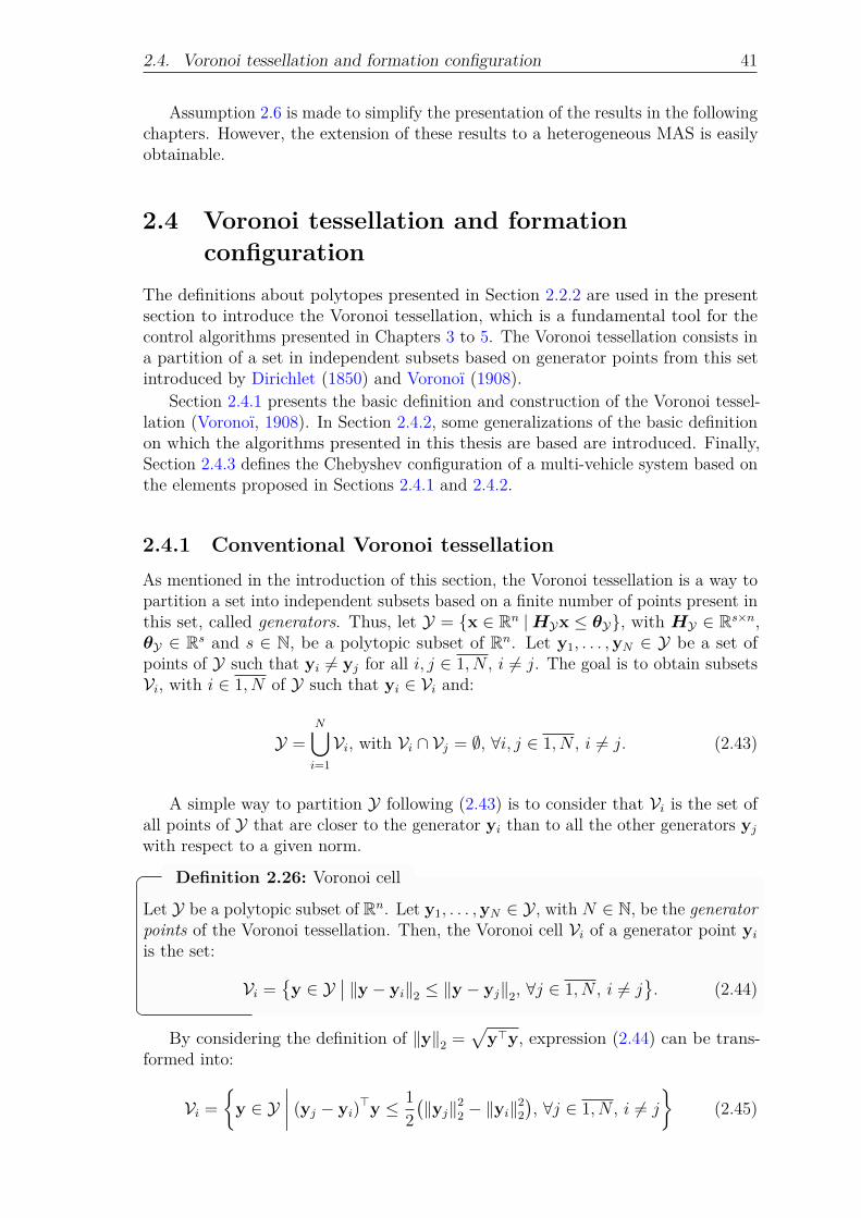
2.4. Voronoi tessellation and formation configuration 41
Assumption 2.6 is made to simplify the presentation of the results in the followingchapters. However, the extension of these results to a heterogeneous MAS is easilyobtainable.
2.4 Voronoi tessellation and formationconfiguration
The definitions about polytopes presented in Section 2.2.2 are used in the presentsection to introduce the Voronoi tessellation, which is a fundamental tool for thecontrol algorithms presented in Chapters 3 to 5. The Voronoi tessellation consists ina partition of a set in independent subsets based on generator points from this setintroduced by Dirichlet (1850) and Voronoï (1908).
Section 2.4.1 presents the basic definition and construction of the Voronoi tessel-lation (Voronoï, 1908). In Section 2.4.2, some generalizations of the basic definitionon which the algorithms presented in this thesis are based are introduced. Finally,Section 2.4.3 defines the Chebyshev configuration of a multi-vehicle system based onthe elements proposed in Sections 2.4.1 and 2.4.2.
2.4.1 Conventional Voronoi tessellationAs mentioned in the introduction of this section, the Voronoi tessellation is a way topartition a set into independent subsets based on a finite number of points present inthis set, called generators. Thus, let Y = x ∈ Rn |HYx ≤ θY, with HY ∈ Rs×n,θY ∈ Rs and s ∈ N, be a polytopic subset of Rn. Let y1, . . . ,yN ∈ Y be a set ofpoints of Y such that yi 6= yj for all i, j ∈ 1, N , i 6= j. The goal is to obtain subsetsVi, with i ∈ 1, N of Y such that yi ∈ Vi and:
Y =N⋃i=1
Vi, with Vi ∩ Vj = ∅, ∀i, j ∈ 1, N , i 6= j. (2.43)
A simple way to partition Y following (2.43) is to consider that Vi is the set ofall points of Y that are closer to the generator yi than to all the other generators yjwith respect to a given norm.
Definition 2.26: Voronoi cell
Let Y be a polytopic subset of Rn. Let y1, . . . ,yN ∈ Y , with N ∈ N, be the generatorpoints of the Voronoi tessellation. Then, the Voronoi cell Vi of a generator point yiis the set:
Vi =y ∈ Y
∣∣ ‖y − yi‖2 ≤ ‖y − yj‖2, ∀j ∈ 1, N , i 6= j
. (2.44)
By considering the definition of ‖y‖2 =√y>y, expression (2.44) can be trans-
formed into:
Vi =y ∈ Y
∣∣∣∣ (yj − yi)>y ≤ 1
2
(‖yj‖22 − ‖yi‖
22
), ∀j ∈ 1, N , i 6= j
(2.45)

42 Chapter 2. Mathematical tools and set-theoretic elements
which is the H-representation of a polytope. Hence, to take the notations fromDefinition 2.9:
HVi=
(y1 − yi)>
...(yi−1 − yi)
>
(yi+1 − yi)>
...(yN − yi)
>
HY
θVi
=1
2
‖y1‖22 − ‖yi‖22...
‖yi−1‖22 − ‖yi‖22
‖yi+1‖22 − ‖yi‖22...
‖yN‖22 − ‖yi‖22
θY
the matrices HY and θY inducing Y being necessary to keep the property thatVi ⊂ Y. As per Remark 2.6, some of the lines of HVi
and θViare redundant and
can be omitted.By going back to the geometrical interpretation of a H-representation introduced
in Section 2.2.2, this can be seen as the collection of inequalities defining half-spaces.Let ∂Vij denote the border of Vi induced by the point yj . This border is a hyperplane:
∂Vij =y ∈ Rn
∣∣∣∣ (yj − yi)>y =
1
2
(‖yj‖22 − ‖yi‖
22
)(2.46)
Such a hyperplane is defined by a normal vector and a point it passes by. The generalrepresentation of a hyperplane H is:
H =x ∈ Rn
∣∣ n>x = n>p
where n ∈ Rn is the normal vector and p ∈ Rn is a point known to belong to H.From (2.46), it is obvious that the normal vector to ∂Vij is yj − yi. Then, from(2.46) and the definition of the Voronoi cell (2.45), it is easy to deduce a point bywhich ∂Vij passes. This point is the point located at half the distance between yiand yj, i.e. (yi + yj)/2.
This geometric interpretation leads to an easy way to graphically represent aVoronoi tessellation in R2 or R3. A border ∂Vij of a cell Vi induced by a point yj isthen the bisecting line (in R2) or bisecting plane (in R3) of the line segment betweenyi and yj.
Example 2.10: Construction of a Voronoi tessellation in R2
Let Y ⊂ R2 be a polytope such that Y = 5B2. Let y1 =[4 4
]>, y2 =[3 −4
]>,y3 =
[1 0
]>, y4 =[−2 2
]> and y5 =[−3 −2
]> be 5 points of Y.Figure 2.10 presents the construction of the Voronoi cell V3. The points p31,
p32, p34 and p35 are the middle points of the line segments joining y3 to y1, y2, y4
and y5, respectively. The normal vectors are also drawn. Finally, all the borders∂V31, ∂V32, ∂V34 and ∂V35 are constructed as described above with the geometricalelements previously introduced.
The cell V3 is then constructed as the intersection of all the half-spaces definedby the hyperplanes ∂V31, ∂V32, ∂V34 and ∂V35. It is also limited on the right by thefact that V3 ⊂ Y.
The other cells are obtained the same way as V3. However, it can be seen onthe figure that the construction of several borders can be avoided. For example, theborder ∂V51 is redundant with the border ∂V53 which is more restrictive. The resultingVoronoi tessellation of Y is presented in Figure 2.11.

2.4. Voronoi tessellation and formation configuration 43
−4 −2 0 2 4
−4
−2
0
2
4y1
y2
y3
y4
y5
p31
p32
p34
p35
∂V31
∂V32
∂V34
∂V35
Y V3
x
y
Figure 2.10: Construction of the Voronoi cell V3.
−4 −2 0 2 4
−4
−2
0
2
4y1
y2
y3
y4
y5
V1
V2
V3
V4
V5
Yx
y
Figure 2.11: An example of Voronoi tessellation in R2.

44 Chapter 2. Mathematical tools and set-theoretic elements
2.4.2 Generalized Voronoi tessellationsFrom the definition of the Voronoi tessellation given in the previous paragraph,generalizations have been proposed such as the ones in Sugihara (1993) or Chosetand Burdick (1995). In Choset and Burdick (1995), the generators of the Voronoitessellation are not defined as points as in Section 2.4.1 but as given subsets of theset being tessellated. Evans and Sember (2008) and Tzes et al. (2018) give resultson the shape of a tessellation when the generating subsets are discs (the tessellationis then often called power Voronoi diagram). Moreover, Evans and Sember (2008)gives a preliminary result on the complexity of the tessellation when the generatingsubsets are polytopes. From this, Chevet et al. (2019) introduces the shape of aso-called box-based guaranteed Voronoi tessellation when the generating subsets areboxes. The results introduced in Chevet et al. (2019) are recalled and a method toexplicitly compute the expression of the borders of the guaranteed cells as well as alinear approximation of these borders is contributed in Paragraph 2.4.2.1. Finally,Paragraph 2.4.2.2 presents a new generalization of the Voronoi tessellation namedhereafter pseudo-Voronoi tessellation.
2.4.2.1 Box-based guaranteed Voronoi tessellation
A kind of generalization of Voronoi tessellations has been used for some time incontrol theory (Rowat, 1979, Choset and Burdick, 1995) and has recently been calledguaranteed Voronoi (GV) tessellation (Evans and Sember, 2008, Tzes et al., 2018,Chevet et al., 2019) since its use arises from uncertainty on the position of agents dueto a perturbation on their measurement signal. The name guaranteed thus impliesthat all the elements in a guaranteed Voronoi cell (GVC) are guaranteed to be closerto all the possible positions of an agent than to all the possible positions of anotheragent.
Definition 2.27: Guaranteed Voronoi cell
Let Y be a polytopic subset of Rn. Let W1, . . . ,WN ⊂ Y, with N ∈ N, be thegenerator sets of the guaranteed Voronoi (GV) tessellation, assuming thatWi∩Wj =∅, ∀i, j ∈ 1, N , i 6= j. Then, the guaranteed1 Voronoi cell Vgi of a generator set Wi isthe set:
Vgi =y ∈ Y
∣∣ ‖y − zi‖2 ≤ ‖y − zj‖2,∀zi ∈ Wi, zj ∈ Wj, j ∈ 1, N, i 6= j
. (2.47)
With such a definition, in the general case, it is not guaranteed that the tessellationcovers the whole original polytope, i.e.:⋃
i∈1,N
Vgi ⊆ Y ,
while it is still guaranteed that for given i, j ∈ 1, N , i 6= j, Vgi ∩ Vgj 6= ∅.
In the present thesis, the generator sets are considered to be boxes as definedin Definition 2.12 centered on a point yi ∈ Y, with i ∈ 1, N . Thus, the subsetsW1, . . . ,WN of Y can be defined as:
Wi = Bn(αi)⊕ yi (2.48)1In the notation Vg
i , the superscript g is used to designate a guaranteed Voronoi cell.

2.4. Voronoi tessellation and formation configuration 45
where αi ∈ Rn and yi ∈ Y Bn(αi), such that Wi ⊂ Y , with i ∈ 1, N . It is obviousfrom Definition 2.27 that a H-representation of the cell is not immediate from (2.47).The first step consists in looking at the border of the guaranteed cell of Wi inducedby Wj:
∂Vgi j =y ∈ Y
∣∣∣∣ maxzi∈Wi
‖y − zi‖2 = minzj∈Wj
‖y − zj‖2
. (2.49)
In the general case, i.e. when the sets Wi do not have a particular shape, thesemaximum and minimum would be difficult to compute. However, in the case of boxesas defined in (2.48), they can be explicitly formulated. To find these expressions, itcan be useful to look at what happens in two dimensions.
The maximum distance of a point to a box in R2 is reached for the vertex of thebox which is farthest from the point. Figure 2.12 presents an example for a givenset Wi = B2
([1 2
]>)⊕ yi, with yi =[0 1
]>, and two points y1,y2 ∈ Y . Sincethe objective of this example is to find the expression of the maximum distance froma point to the set Wi, the shape of Y is irrelevant and Y = R2 such that Wi ⊂ Yand yi ∈ Y B2
([1 2
]>). It can be seen in the figure that maxzi∈Wi
‖y1 − zi‖2, the
maximum distance from y1 ∈ Y to Wi, i.e. the box B2([
1 2]>) centered on yi, is
reached for zi = v1 and maxzi∈Wi
‖y2 − zi‖2 is reached for zi = v2.
x
y
−4 −3 −2 −1 0 1 2 3 4−2
−1
0
1
2
3
4
yi
B2([
1 2]>)⊕ yi
y1
y2
v2
v1
Figure 2.12: Maximum distance of a point to a box in R2.
From the example of Figure 2.12, an expression for the maximum distance of apoint to a box in R2 can be formulated:
maxzi∈Wi
‖y − zi‖2 =√
(|x− xi|+ αi,x)2 + (|y − yi|+ αi,y)
2
where Wi is defined as in (2.48), with n = 2, αi =[αi,x αi,y
]>, yi =[xi yi
]> andy =
[x y
]>.This expression can be generalized in Rn, giving:
maxzi∈Wi
‖y − zi‖2 = ‖|y − yi|+αi‖2. (2.50)

46 Chapter 2. Mathematical tools and set-theoretic elements
The expression of the minimum distance of a point to a box is less straightforward.It depends on the relative position of the point to the box and it is reached eitheron a facet of the box or on a vertex or be zero if the point is inside the box. In theexample of Figure 2.13, the set Wj is Wj = B2
([2 1
]>)⊕ yj with yj =[0 1
]>.Then, R2 can be divided into nine areas of four types as shown in Figure 2.13.In areas of type 1, the minimum distance from a point to Wj is the distance tothe point that has the same ordinate and is on the closest border of Wj (e.g. theminimal distance from y1 to Wj is the distance from y1 to p1). In areas of type 2,the minimum distance is the same as in areas of type 1 while replacing ordinate byabscissa (e.g. the minimal distance from y2 to Wj is the distance from y2 to p2).In areas of type 3, the minimum distance from a point to Wj is the distance to thecloser vertex of Wj (e.g. the minimal distance from y3 to Wj is the distance fromy3 to p3). Finally, in areas of type 4, the minimum distance from all points to Wj is0 since the points are already in Wi.
−4 −3 −2 −1 0 1 2 3 4−2
−1
0
1
2
3
4
x
y
yj1 1
2
2
3 3
3 3
4
B2([
2 1]>)⊕ yj
y1
y2
y3
p1
p2
p3
αj,x
αj,y
Figure 2.13: Minimum distance of a point to a box in R2.
From the example of Figure 2.13, an expression for the minimum distance of apoint to a box in R2 can be formulated:
minzj∈Wj
‖y − zj‖2 =√
(max|x− xj| − αj,x, 0)2 + (max|y − yj| − αj,y, 0)2
where Wj is defined as in (2.48), with αj =[αj,x αj,y
]>, zj =[xj yj
]> andy =
[x y
]>.This expression can be generalized in Rn, giving:
minzj∈Wj
‖y − zj‖2 =
√√√√ n∑k=1
(max|yk − yj,k| − αj,k, 0)2 (2.51)
where Wj = Bn(αj) ⊕ yj, with αj =[αj,1 · · · αj,n
]> ∈ Rn, the center of thebox yj =
[yj,1 · · · yj,n
]> ∈ Y Bn(αj) ⊂ Rn and y =[y1 · · · yn
]> ∈ Y ⊂ Rn.

2.4. Voronoi tessellation and formation configuration 47
With the expressions given in (2.50) and (2.51), the shape of ∂Vgi j in R2 can bededuced and generalized to higher dimensions (which is not treated in the presentthesis).
Given (2.50) and (2.51), the equation defining ∂Vgi j is piecewise and continuous.Each piece is defined over an area corresponding to a type of area defined inFigure 2.13. It is easy to verify that the intersection of ∂Vgi j and an area of type 1or 2 defined for Wj is a parabolic arc. Indeed, if y ∈ ∂Vgi j is in an area of type 1:
(|x− xi|+ αi,x)2 + (|y − yi|+ αi,y)
2 = (|x− xj| − αj,x)2
or, by developing and gathering the terms depending on x:
(|y − yi|+ αi,y)2
= 2x(xi − xj)− 2αj,x|x− xj| − 2αi,x|x− xi|+ α2j,x − α2
i,x + x2j − x2i (2.52)
which is the equation of a parabola.If y is in an area of type 2 for Wj, the role of x and y are inverted in equation
(2.52).The intersection of ∂Vgi j and an area of type 3 for Wj is a line segment since:
(|x− xi|+ αi,x)2 + (|y − yi|+ αi,y)
2 = (|x− xj| − αj,x)2 + (|y − yj| − αj,y)2
or, equivalently:
2y(yj − yi) + 2αi,y|y − yi|+ 2αj,y|y − yj|+ α2i,y − α2
j,y + y2i − y2j= 2x(xi − xj)− 2αj,x|x− xj| − 2αi,x|x− xi|+ α2
j,x − α2i,x + x2j − x2i
which is the equation of a line.Finally, the intersection of ∂Vgi j with an area of type 4 for Wj is an elliptic arc
since:(|x− xi|+ αi,x)
2 + (|y − yi|+ αi,y)2 = 0
which is the equation of an ellipse.
Example 2.11: Construction of guaranteed bordersLet Wi = B2
([2 1
]>) ⊕ yi, where yi =[−6 −7
]>, and Wj = B2([
1 2]>) ⊕
yj, where yj =[5 4
]> be two sets of R2. These two sets are drawn in Figure 2.14,Wi in black and Wj in gray, as well as dashed lines delimiting the same areas as inFigure 2.13 for the set Wi. For Wi, the red hatched area A1 is an area of type 1, thegreen hatched area A2 is an area of type 2 and the blue hatched area is an area oftype 3. To build ∂Vgj i, it is necessary to find all the y ∈ R2 such that:
minzi∈Wi
‖y − zi‖2 = maxzj∈Wj
‖y − zj‖2.
If a point of A1 is part of ∂Vgj i, it has to satisfy:
(|x− 5|+ 1)2 + (|y − 4|+ 2)2 = (|x+ 6| − 2)2
which is the equation of of a piecewise continuous parabola. This part of ∂Vgj i isdrawn as a dashdotted blue line in Figure 2.14.

48 Chapter 2. Mathematical tools and set-theoretic elements
If a point of A2 is part of ∂Vgj i, it has to satisfy:
(|x− 5|+ 1)2 + (|y − 4|+ 2)2 = (|x+ 7| − 1)2
which is again the equation of a piecewise continuous parabola. This part of ∂Vgj i isalso drawn in a dashdotted blue line in Figure 2.14.
Finally, if a point of A3 is part of ∂Vgj i, it has to satisfy:
(|x− 5|+ 1)2 + (|y − 4|+ 2)2 = (|x+ 6| − 2)2 + (|x+ 7| − 1)2
which is, as discussed before, the equation of a piecewise continuous line. This partof ∂Vgj i is drawn as a plain blue line in Figure 2.14.
In addition, ∂Vgj i also extends to the left and to the right of the part that ispresented in Figure 2.14. Indeed, to the left of A2, the border ∂Vgj i intersects anarea of type 3 for Wi and it is then composed of a piecewise continuous line. Thesame way, below A1, the border ∂Vgj i intersects another area of type 3 for Wi and itis composed of a piecewise continuous line.
−10 −8 −6 −4 −2 0 2 4 6 8 10−10
−8
−6
−4
−2
0
2
4
6
8
10
A3
A1
A2
yi
Wi
yj
Wj
∂Vgj i
x
y
Figure 2.14: Example of guaranteed Voronoi cell border generated by two sets in R2.
The same way as for ∂Vgj i, the border ∂Vgi j is obtained by finding all the y ∈ R2
such that:maxzi∈Wi
‖y − zi‖2 = minzj∈Wj
‖y − zj‖2.
Figure 2.15 then presents the resulting borders ∂Vgi j in red and ∂Vgj i in blue for thesets Wi and Wj.
From the equalities defining ∂Vgi j , inequalities defining Vgi can be deduced. How-ever, because of the presence of parabolic or elliptic arcs, some of those inequalities are

2.4. Voronoi tessellation and formation configuration 49
−10 −8 −6 −4 −2 0 2 4 6 8 10−10
−8
−6
−4
−2
0
2
4
6
8
10
yi
Wi
yj
Wj
∂Vgi j
∂Vgj i
x
y
Figure 2.15: Box-based guaranteed Voronoi cell borders generated by two rectanglesin R2.
not linear which could pose a problem for the control algorithms that are developedin the following chapters.
Due to the convexity of these arcs, a linear approximation of the parabolic andelliptic arcs, albeit conservative, is easy to obtain. This approximation consists inreplacing the quadratic arcs by a line joining their intersection with the borders ofthe area in which they are defined. Figure 2.16 gives the linear approximation of theborders ∂Vgi j and ∂Vgj i from Example 2.11 where the original borders are the dashedlines and the approximated borders are the plain light red and light blue lines. Inthe remainder of this thesis, the linear approximation of the box-based guaranteedVoronoi cells is always used.
From all the developments presented above, a H-representation of the guaranteedVoronoi cells Vgi , with i ∈ 1, N , generated by sets Wi having the form (2.48) canbe constructed. The matrices of the H-representation of Vgi are then obtained byappending all the linear inequalities induced by the borders ∂Vgi j from (2.49) andthe linear inequalities defining the polytopic set Y being tessellated.
Example 2.12: Box-based guaranteed Voronoi tessellation in R2
Let H =
[3 0 −1 −1 22 1 2 −1 −1
]>and θ =
[24 6 9 15 12
]> inducing a polytope
Y in R2. Let:
y1 =
[42
]y2 =
[−1−10
]y3 =
[0−4
]y4 =
[−8−4
]y5 =
[−20
]α1 =
[10.5
]α2 =
[11
]α3 =
[11
]α4 =
[0.51
]α5 =
[0.51
]

50 Chapter 2. Mathematical tools and set-theoretic elements
−10 −8 −6 −4 −2 0 2 4 6 8 10−10
−8
−6
−4
−2
0
2
4
6
8
10
yi
Wi
yj
Wj
∂Vgi j
∂Vgj i
x
y
Figure 2.16: Linear approximation of a guaranteed cell border generated by two setsin R2.
inducing the sets Wi = B2(αi)⊕ yi, with i ∈ 1, 5.The guaranteed Voronoi tessellation of the boxes Wi, with i ∈ 1, 5 is presented in
Figure 2.17. It can be seen thatWi is not always totally included inside its guaranteedcell Vgi , e.g. W3 6⊂ Vg3 .
2.4.2.2 Pseudo-Voronoi tessellation
Further generalization of the classical Voronoi tessellation introduced in Section 2.4.1can be formulated. However, this generalization is presented only in R2, an extensionto higher dimensions being possible but of increased complexity.
Let Y ∈ R2 be a polytope in R2. Let y1, . . . ,yN ∈ Y be N points of Y suchthat yi 6= yj for all i, j ∈ 1, N , i 6= j. This paragraph introduces a pseudo-Voronoitessellation2 of W generated by the points yi, with i ∈ 1, N such that:
Y =N⋃i=1
Vpi , with Vpi ∩ Vpj = ∅, ∀i, j ∈ 1, N , i 6= j. (2.53)
In (2.46), the border ∂Vij of the Voronoi cell generated by the two points yiand yj has been characterized as the hyperplane passing by (yi + yj)/2 with thenormal vector yj − yi. The border ∂Vpi j of the pseudo-Voronoi cell generated by twopoints yi and yj is defined as the hyperplane passing by αijyj + (1− αij)yi, whereαij ∈ (0, 1), with the normal vector yj − yi, i.e.:
∂Vpi j =y ∈ Y
∣∣∣ (yj − yi)>y = (yj − yi)
>(αijyj + (1− αij)yi)
. (2.54)2In the notation Vp
i , the superscript p is used to designate a pseudo-Voronoi cell.

2.4. Voronoi tessellation and formation configuration 51
−14 −12 −10 −8 −6 −4 −2 0 2 4 6 8−16
−14
−12
−10
−8
−6
−4
−2
0
2
4
6
8
Vg1
Vg2
Vg3
Vg4
Vg5
y1
y2
y3y4
y5
W1
W2
W3W4
W5
Y
x
y
Figure 2.17: Box-based guaranteed Voronoi tessellation of five generator sets in R2.
In order to have Vpj ∩ Vpi = ∅, it is necessary that αij ≤ 1− αji. Moreover, in order
to have:
Y =N⋃i=1
Vpi ,
it is also necessary that αij = 1− αji. However, this condition is not enough.A necessary tool for further comprehension is the Delaunay triangulation, which
has been introduced in Delaunay (1934) as the dual graph of the Voronoi tessellation.Several algorithms have been proposed to compute it (Delaunay, 1934, Preparata andShamos, 1985) but is not investigated here. The Delaunay triangulation associatesthe generators of a Voronoi tessellation by group of three generators. In this thesis,only a graphical method to understand how to build a Delaunay triangulation ofa set of generators T (y1, . . . ,yN) is presented, the reader can refer to Preparataand Shamos (1985) for explicit algorithms to build it. Graphically, if a triangle ofgenerators is part of the Delaunay triangulation, the Voronoi cells of each of thesegenerators share one vertex. This vertex is the center of the circumscribed circle tothe triangle formed by the three generators (it can be noticed that this fact is the

52 Chapter 2. Mathematical tools and set-theoretic elements
basis of the algorithm to build the Delaunay triangulation).
Example 2.13: Construction of a Delaunay triangulationIt is now possible to build the Delaunay triangulation T (y1,y2,y3,y4,y5) as the dualgraph of the Voronoi tessellation presented in Example 2.10. From Figure 2.11,the obvious triangles of generators are T1 = y1,y3,y4, T2 = y2,y3,y5, T3 =y3,y4,y5. However, a fourth triangle exists in T (y1,y2,y3,y4,y5). Indeed, ifY was wider, the border ∂V12 would appear and intersect ∂V13 and ∂V23. Then,the Voronoi cells V1, V2 and V3 would also share a vertex thus T4 = y1,y2,y3 ∈T (y1,y2,y3,y4,y5). These triangles are presented in Figure 2.18.
−4 −2 0 2 4
−4
−2
0
2
4y1
y2
y3
y4
y5
V1
V2
V3
V4
V5
Yx
y
Figure 2.18: An example of Delaunay triangulation in R2.
A way to ensure that the constraint (2.53) is satisfied with the Delaunay trian-gulation T (y1, . . . ,yN) is to guarantee that for a triangle Tm ∈ T (y1, . . . ,yN), withm ∈ 1, |T (y1, . . . ,yN)|, such that Tm = yi,yj,yk, with i, j, k ∈ 1, N , i 6= j 6= k,the borders ∂Vpi j = ∂Vpj i, ∂V
pi k = ∂Vpk i and ∂Vpj k = ∂Vpk j are concurrent at a single
point as in the classical Voronoi case. If this condition is not respected, there mightbe parts of Y not covered by a cell Vpi .
Consider the vectors nij = yj − yi, nik = yk − yi, njk = yk − yj in R2 andthe scalars θij = n>
ij(αijyj + (1− αij)yi), θik = n>ik(αikyk + (1− αik)yi) and θjk =
n>jk(αjkyk + (1− αjk)yj). Then, the borders ∂Vpi j , ∂V
pi k and ∂Vpj k are concurrent at
a single point if and only if:det(nij,njk)θik − det(nik,njk)θij − det(nij,nik)θjk = 0. (2.55)
If a tessellation satisfies the conditions that have been presented in this paragraph,it is called a pseudo-Voronoi tessellation because of its similarity with the classicalVoronoi tessellation. However, since the basic definition of a Voronoi cell (2.44) ismodified, the word “pseudo” is added.
2.4. Voronoi tessellation and formation configuration 53
Example 2.14: Construction of a pseudo-Voronoi tessellation in R2
Let Y ⊂ R2 be a polytope such that Y = 5B2. Let y1 =[4 4
]>, y2 =[3 −4
]>,y3 =
[1 0
]>, y4 =[−2 2
]> and y5 =[−3 −2
]> be 5 points of Y. The Delaunaytriangulation of these points T (y1,y2,y3,y4,y5) has been presented in Example 2.13.
Consider the initial values α12 = 0.3 and α23 = 0.7 chosen arbitrarily. Despitethe fact that Vp1 and Vp2 do not visibly share a border, y1 and y2 belong to a triangleas shown in Example 2.13, thus the need to chose a value for α12. Equation (2.55)results in α13 = 0.14. Let α14 = 0.4, giving α34 = 23/26. Let α35 = 0.7, givingα45 = 15/34. Finally, the previous values lead to α25 = 0.7.
Figure 2.19 presents the pseudo-Voronoi tessellation with the values given above.The pseudo-Voronoi cells Vpi , with i ∈ 1, 5, have the same shape as the cells Vi ofthe classical Voronoi tessellation in Example 2.10. Indeed, the normal vectors of theborders of Vpi are the same as the normal vectors of the borders of Vi. However, thedimension of the pseudo-Voronoi cells Vpi and of the Voronoi cells Vi are different.
−4 −2 0 2 4
−4
−2
0
2
4 y1
y2
y3
y4
y5
Vp1
Vp2
Vp3
Vp4
Vp5
Yx
y
Figure 2.19: An example of pseudo-Voronoi tessellation in R2.
2.4.3 Chebyshev configuration of a multi-vehicle systemThe Voronoi tessellation (either classical or generalized) defined in Sections 2.4.1and 2.4.2 is used in the following chapter to constrain the movement of a multi-vehiclesystem as defined in Section 2.3. However, a goal for such a multi-vehicle has alsoto be introduced, which is the purpose of the present paragraph. To do so, theChebyshev center (Boyd and Vandenberghe, 2009) of a polytope is presented as wellas the definition of a Chebyshev configuration of a multi-vehicle system. The waysuch objects are used for control purposes is out of the scope of this paragraph andis further introduced in the following chapters.
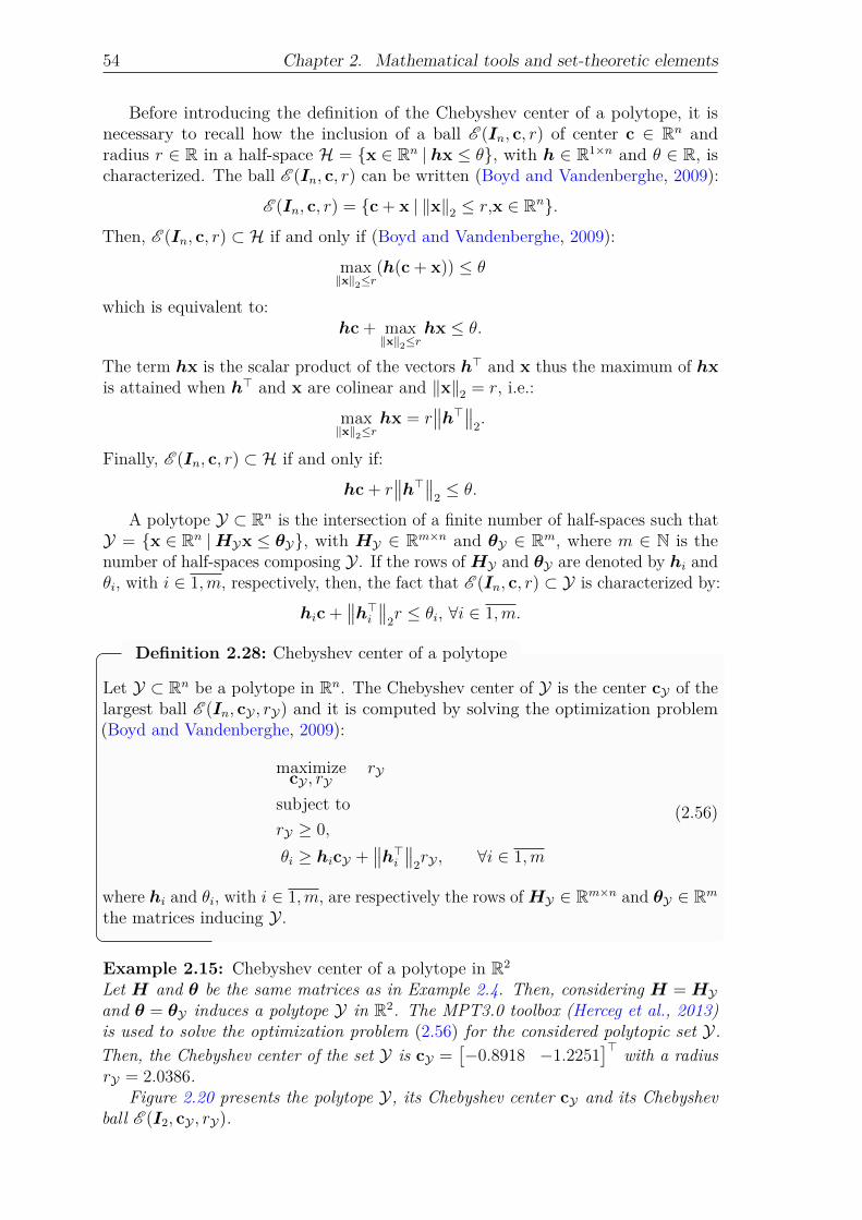
54 Chapter 2. Mathematical tools and set-theoretic elements
Before introducing the definition of the Chebyshev center of a polytope, it isnecessary to recall how the inclusion of a ball E (In, c, r) of center c ∈ Rn andradius r ∈ R in a half-space H = x ∈ Rn | hx ≤ θ, with h ∈ R1×n and θ ∈ R, ischaracterized. The ball E (In, c, r) can be written (Boyd and Vandenberghe, 2009):
E (In, c, r) = c+ x | ‖x‖2 ≤ r,x ∈ Rn.
Then, E (In, c, r) ⊂ H if and only if (Boyd and Vandenberghe, 2009):
max‖x‖2≤r
(h(c+ x)) ≤ θ
which is equivalent to:hc+ max
‖x‖2≤rhx ≤ θ.
The term hx is the scalar product of the vectors h> and x thus the maximum of hxis attained when h> and x are colinear and ‖x‖2 = r, i.e.:
max‖x‖2≤r
hx = r∥∥h>∥∥
2.
Finally, E (In, c, r) ⊂ H if and only if:
hc+ r∥∥h>∥∥
2≤ θ.
A polytope Y ⊂ Rn is the intersection of a finite number of half-spaces such thatY = x ∈ Rn |HYx ≤ θY, with HY ∈ Rm×n and θY ∈ Rm, where m ∈ N is thenumber of half-spaces composing Y . If the rows of HY and θY are denoted by hi andθi, with i ∈ 1,m, respectively, then, the fact that E (In, c, r) ⊂ Y is characterized by:
hic+∥∥h>
i
∥∥2r ≤ θi, ∀i ∈ 1,m.
Definition 2.28: Chebyshev center of a polytope
Let Y ⊂ Rn be a polytope in Rn. The Chebyshev center of Y is the center cY of thelargest ball E (In, cY , rY) and it is computed by solving the optimization problem(Boyd and Vandenberghe, 2009):
maximizecY , rY
rY
subject to
rY ≥ 0,
θi ≥ hicY +∥∥h>
i
∥∥2rY , ∀i ∈ 1,m
(2.56)
where hi and θi, with i ∈ 1,m, are respectively the rows of HY ∈ Rm×n and θY ∈ Rm
the matrices inducing Y .
Example 2.15: Chebyshev center of a polytope in R2
Let H and θ be the same matrices as in Example 2.4. Then, considering H = HYand θ = θY induces a polytope Y in R2. The MPT3.0 toolbox (Herceg et al., 2013)is used to solve the optimization problem (2.56) for the considered polytopic set Y.Then, the Chebyshev center of the set Y is cY =
[−0.8918 −1.2251
]> with a radiusrY = 2.0386.
Figure 2.20 presents the polytope Y, its Chebyshev center cY and its Chebyshevball E (I2, cY , rY).

2.4. Voronoi tessellation and formation configuration 55
x
y
−5−5
−4
−4
−3
−3
−2
−2
−1
−1
0
0
1
1
2
2
3
3
Y
cY
E (I2, cY , rY)
rY
Figure 2.20: Chebyshev center and Chebyshev ball of a polytope in R2.
With the elements introduced in Section 2.4.1 and Definition 2.28, it is nowpossible to introduce the Chebyshev configuration of a multi-vehicle system.
Definition 2.29: Chebyshev configuration (Nguyen, 2016)
A Chebyshev configuration (CC) of a multi-vehicle system Σ (2.41a)-(2.41b) is theconfiguration where the output yi, with i ∈ 1, |Σ|, of each vehicle coincides with theChebyshev center of its Voronoi cell Vi, i.e. yi = cVi
for all i ∈ 1, |Σ|.
Property 2.11: Non-uniqueness of the Chebyshev configuration
A Chebyshev configuration of a multi-vehicle system Σ is not unique and dependson the initial position of the vehicles.
Example 2.16: Chebyshev configuration of a multi-vehicle system in R2
Let Σ be a multi-vehicle system composed of 5 agents. These agents evolve insidea polytope Y = 5B2 ⊂ R2. Figure 2.21 presents a Chebyshev configuration for Σ.In this configuration, each vehicle output coincides with the Chebyshev center of itsVoronoi cell.
It can be noticed that while Definition 2.29 has been given for a classical Voronoitessellation as defined in Section 2.4.1, using a guaranteed or a pseudo-Voronoi tessel-lation as defined in Section 2.4.2 does not change the definition. Such configurationsdefined on different Voronoi tessellation are used in the remainder of this thesis.

56 Chapter 2. Mathematical tools and set-theoretic elements
−4 −2 0 2 4
−4
−2
0
2
4
y1
y2
y3
y4
y5
V1
V2
V3
V4
V5
Yx
y
Figure 2.21: An example of Chebyshev configuration for 5 agents in a classicalVoronoi tessellation in R2.
2.5 Continuous random variables and stochasticprocesses
In numerous real life applications, dynamical systems are subject to stochasticperturbations as presented in Chapter 4. Such perturbations are often modeled asGaussian white noises which are stochastic processes. Thus, in order to developcontrol algorithms for such systems, some results on multivariate continuous randomvariables and stochastic processes have to be introduced. However, these resultsare limited to what is useful for the development of the algorithm of Section 4.2.Indeed, these results are based on measure theory (Halmos, 1950) and real analysis(DiBenedetto, 2016) which are out of the scope of this thesis. Complements onprobability theory and stochastic processes can be found for example to Loève (1977,1978) and Rosenblatt (1974).
A continuous random variable3 X is an application that maps an element of asample space Ω to an element of R. The same way, a multivariate continuous randomvariable4 X is an application that maps an element of a sample space Ω to an elementof Rn, with n ∈ N. The definition of the sample space Ω is out of the scope ofthis thesis and X ∈ R (respectively X ∈ Rn) is used abusively to denote X(ω) ∈ R(respectively X(ω) ∈ Rn), the image of an element ω ∈ Ω by X (respectively X).
Then, specifying the probability law P of a random variable X ∈ R (respec-tively X ∈ Rn) consists in finding the probability that X ∈ (−∞, a], with a ∈ R
3A continuous random variable is also called a univariate random variable.4A multivariate random variable X is a vector of Rn where each component X1, . . . , Xn ∈ R of
X =[X1 · · · Xn
]> is a univariate continuous random variable.

2.5. Continuous random variables and stochastic processes 57
(respectively X ∈ P ⊂ Rn), denoted by P(X ≤ a) (respectively P(X ∈ P)).The following definition of a probability density function is given in the multivariate
case but can be obtained in the univariate case by taking n = 1 and P = (−∞, a],with a ∈ R.
Definition 2.30: Probability density function
Let X ∈ Rn be a multivariate continuous random variable. The probability densityfunction fX of X is the non-negative function such that:
P(X ∈ P) =∫PfX(x)dx ∀P ⊂ Rn and
∫Rn
fX(x)dx = 1.
From the existence of a probability density function, it is possible to define themoments of a random variable. Only two moments are used and presented in thisthesis, namely the moment of order 1, or mathematical expectation, and the centeredmoment of order 2, or variance.
Definition 2.31: Mathematical expectation
Let X ∈ R be a continuous random variable admitting a probability density functionfX . The mathematical expectation of X is defined as:
E(X) =
∫ +∞
−∞xfX(x)dx.
Definition 2.32: Expectation of a multivariate random variable
Let X =[X1 · · · Xn
]> ∈ Rn be a multivariate continuous random variable, whereX1, . . . , Xn ∈ R are univariate random variables. The mathematical expectation ofX is the vector composed of the mathematical expectations of its components, i.e.:
E(X) =[E(X1) · · · E(Xn)
]> .
♦
Remark 2.12: Alternative notation for the expectationThe mathematical expectation of a random variable X ∈ R or X ∈ Rn is also calledthe mean of X or X. In Chapter 4, the mathematical expectation of a multivariaterandom variable X ∈ Rn is then denoted by:
E(X) = µX.
The definition of the variance is given only in the multivariate case since onlythe variance of multivariate continuous random variables is used in this thesis. Inthis case, the variance of a random variable is often referred as the variance matrixof this random variable.
Definition 2.33: Variance matrix
Let X ∈ Rn be a multivariate continuous random variable. The variance matrix ofX is defined as:
ΣX = E((X− E(X))(X− E(X))>
).
58 Chapter 2. Mathematical tools and set-theoretic elements
Definition 2.34: Covariance of two random variables
Let X,Y ∈ Rn be two multivariate continuous random variables. The covariancematrix of X and Y is defined as:
cov(X,Y) = cov(Y,X)> = E((X− E(X))(Y − E(Y))>
).
Before introducing the probability distributions that are used in this thesis, it isnecessary to present the concept of independence of two random variables.
Definition 2.35: Independence of two random variables (Flury, 1997)
Two multivariate continuous random variables X,Y ∈ Rn are called independent if:
P((X,Y) ∈ P ×Q) = P(X ∈ P)P(Y ∈ Q)
where P ,Q ⊂ Rn.
The following property, useful for Chapter 4, is then given without proof.
Property 2.12: Covariance of independent variables
Let X,Y ∈ Rn be two independent multivariate continuous random variables. Then,the covariance of X and Y is the null matrix:
cov(X,Y) = 0n.
Now that general definitions and properties have been given for continuousrandom variables, it is necessary to introduce the multivariate normal distribution,which is one of the probability distributions used in control theory.
Definition 2.36: Multivariate normal distribution
Let X ∈ Rn be a multivariate continuous random variable. Then, X has a multivariatenormal distribution with mean µX and variance matrix ΣX 0 if X admits theprobability density function:
fX(x) =1√
(2π)ndet(ΣX)exp
(−1
2(x− µX)
>Σ−1X (x− µX)
).
♦
Remark 2.13: Normally distributed variableA multivariate continuous random variable X ∈ Rn having a multivariate normaldistribution is called normally distributed.
The chi-squared with n degrees of freedom, denoted by χ2n is another probability
distribution that often appears in various scientific fields, mainly when statisticaltests are involved. A univariate continuous random variable having a chi-squareddistribution with n degrees of freedom is obtained as the sum of n squared normallydistributed univariate random variables. Then, Flury (1997) builds a univariaterandom variable having a chi-squared distribution with n degrees of freedom from anormally distributed multivariate continuous random variable X ∈ Rn.

2.6. Conclusion 59
Property 2.13: Chi-squared distribution (Flury, 1997)
Let X ∈ Rn be a normally distributed multivariate continuous random variable withmean µX and variance matrix ΣX 0. Then, the univariate continuous randomvariable:
Y = (X− µX)>Σ−1
X (X− µX)
has a chi-squared distribution with n degrees of freedom.
The probability density function of a random variable having a chi-squareddistribution is not presented in this thesis. However, if X ∈ R is a univariatecontinuous random variable with a chi-squared distribution with n degrees of freedom,tables exist in the literature (Elderton, 1902) to obtain the solution α of the equation:
P(X ≤ α) = P
where P ∈ (0, 1).Finally, the notion of normally distributed white noise is defined. Indeed, this
kind of noise appears in numerous real world applications as a perturbation ondynamical systems. A white noise is the realization of a stochastic process. For thisthesis, even though it is an abuse of notation, a stochastic process is considered tobe a continuous random variable which depends on time. Then, a continuous-timestochastic process is denoted by X(t) ∈ Rn and a discrete-time stochastic process isdenoted by X(k) ∈ Rn.
Definition 2.37: Normally distributed white noise
The continuous-time multivariate continuous random variable X(t) ∈ Rn is a normallydistributed white noise if:
• X(t) is normally distributed with mean µX(t) = 0n and variance matrixΣX(t) 0 for all t ∈ R∗
+;
• X(t1) and X(t2) are independent for all t1, t2 ∈ R∗+ such that t1 6= t2.
The above definition can be obtained in the discrete-time case by replacingt ∈ R∗
+ by k ∈ N∗.
2.6 ConclusionThis chapter introduces the main mathematical tools necessary for the comprehensionof the results proposed in the remainder of this thesis. Thus, basic operations onellipsoids and polytopic sets are presented, together with the conventional andgeneralized (box-based guaranteed and pseudo-) Voronoi tessellation of a polytopicspace in R2. Elements on the Chebyshev configuration for a classical tessellation arealso provided to the aim of using them in the context of multi-agent vehicles. Finally,in order to develop control algorithms for systems subject to stochastic perturbations,basic notions on continuous random variables and stochastic processes are recalled.


Chapter 3Decentralized control for the
deployment of a multi-vehicle system
Table of Contents
3.1 Overview of the existing deployment algorithms in the nominal case 613.2 Problem formulation and first results . . . . . . . . . . . . . . . . . 64
3.2.1 Centralized MPC approach . . . . . . . . . . . . . . . . . . 643.2.2 Decentralized algorithm . . . . . . . . . . . . . . . . . . . . 683.2.3 Discussion on the convergence of the decentralized algorithm 693.2.4 Deployment results in the case of single integrator dynamics 74
3.3 Deployment of a quadrotor UAV fleet . . . . . . . . . . . . . . . . . 783.3.1 Agent model . . . . . . . . . . . . . . . . . . . . . . . . . . 78
3.3.1.1 Continuous-time nonlinear dynamics . . . . . . . . 783.3.1.2 Discrete-time linear dynamics . . . . . . . . . . . . 80
3.3.2 Global control strategy . . . . . . . . . . . . . . . . . . . . . 813.3.2.1 Overall architecture . . . . . . . . . . . . . . . . . 813.3.2.2 Inner-loop control . . . . . . . . . . . . . . . . . . 833.3.2.3 Outer-loop control . . . . . . . . . . . . . . . . . . 85
3.3.3 Deployment results . . . . . . . . . . . . . . . . . . . . . . . 873.4 Discussion on the stability of the deployment of UAVs . . . . . . . 923.5 Conclusion . . . . . . . . . . . . . . . . . . . . . . . . . . . . . . . . 94
3.1 Overview of the existing deploymentalgorithms in the nominal case
A fundamental problem in control of autonomous multi-vehicle systems (MVS) is thedeployment over a given environment to carry out a certain mission. Autonomousvehicles missions cover a wide spectrum of real world applications such as forest firemonitoring (Merino et al., 2012, Yuan et al., 2019), ground and resource monitoring(Laliberte and Rango, 2009, Jin and Tang, 2010, d’Oleire Oltmanns et al., 2012),mapping and modeling (Nex and Remondino, 2014, Han and Chen, 2014, Torreset al., 2016) or even surveillance missions (Li et al., 2019, Trujillo et al., 2019).Several of these applications have been tested with one unmanned ground or aerialvehicle (UGV or UAV) or multi-agent systems composed of either UGV, UAV orboth. For all these tasks, the word deployment is used in a broader sense than inSchwager et al. (2011) to denote the fact that vehicles move over a given environmentto complete their mission.
61

62 Chapter 3. Decentralized control for the deployment of a multi-vehicle system
For the results presented in this thesis, the primary sense of deployment given bySchwager et al. (2011), which considers the deployment of a multi-vehicle system asa strategically appropriate spreading of the MVS in a given environment in order toreach a fixed configuration, is used. The environment and the fixed configurationremain to be characterized. A classical way to approach this problem is to considerthe deployment of the multi-vehicle system inside a convex bounded area. This areais considered as the environment mentioned in the definition of Schwager et al. (2011).Several approaches exist to deal with the deployment problem. Choset (2001) givesan overview of methods used when the problem is seen as a motion planning problem.Other techniques have been subsequently proposed such as potential field (Howardet al., 2002), probabilistic (Li and Cassandras, 2005) or Voronoi-based (Cortés et al.,2004). When the deployment of a MAS is meant to ensure a maximal coverage of anenvironment according to a given criterion, Schwager et al. (2011) show that the lastthree approaches can be unified through the use of a mixing function encoding theassociated criteria.
In the following, methods based on the tessellation of the environment areconsidered. It is then partitioned into regions depending on the position of thevehicles. An easy way to get such regions is to consider the Voronoi tessellation ofthe environment where the position of each vehicle in the environment is a generatorpoint. Since the vehicles can move inside the environment, the resulting Voronoi cellsare time-varying. The overall problem is then known as a Voronoi-based deploymentof a multi-vehicle system. The deployment is then handled by driving the vehiclestowards a given point defined over their Voronoi cells.
One of the most widely used types of Voronoi-based deployment strategies is thecentroidal Voronoi configuration. The vehicles are then driven towards the center ofmass cMVi
of their Voronoi cell Vi computed as:
cMVi=
∫Vi
φ(y)ydy∫Vi
φ(y)dy
where i is an identifier of the vehicle and φ is a mass density function defined overthe environment. The center of mass is computed each time the Voronoi tessellationchanges, i.e. at each time sample where the position of the vehicles is observed.Such a strategy has been applied over the years to different types of multi-agentsystems (MAS): mobile sensor networks (Cortés et al., 2004), multi-robot systems(Schwager et al., 2011) or autonomous vehicle systems (Sharifi et al., 2014, Moarrefand Rodrigues, 2014). The simplest way to reach the centroidal Voronoi configurationis to steer each agent individually towards the center of mass of its associated Voronoicell, this center of mass being regularly updated given the configuration of the Voronoitessellation. The MAS then eventually reaches a static configuration where eachagent lies on its center of mass. This decentralized control algorithm is known in theliterature as Lloyd’s method (Lloyd, 1982).
However, depending on the complexity of the mass density function, the centerof mass defined above can end up being difficult to compute. Nguyen (2016) thenproposes a simpler approach based on the Chebyshev center (Boyd and Vandenberghe,2009) of the Voronoi cells of the agents. Such a center is the solution of an optimizationproblem which is reduced to the linear optimization problem (2.56) due to the

3.1. Overview of the existing deployment algorithms in the nominal case 63
polytopic nature of the Voronoi cell. The Chebyshev center is then often simpler toobtain than the center of mass. Therefore, in this thesis, the objective point for eachagent is the Chebyshev center of its Voronoi cell.
Several control methods can be applied to the Voronoi-based deployment problem.Cortés et al. (2004) propose a decentralized state feedback approach for both contin-uous and discrete-time single integrator dynamics, as well as Hatleskog (2018) andNguyen et al. (2017) who consider a decentralized discrete-time state feedback, atleast as a first approach. Schwager et al. (2011) propose distributed continuous-timeconsensus-like (Ren and Beard, 2008) controller. In Moarref and Rodrigues (2014)or Nguyen and Stoica Maniu (2016), a decentralized optimal control approach isconsidered to drive the agents towards a centroidal Voronoi configuration. Finally,Sharifi et al. (2014) consider distributed continuous-time feedback linearization forthe MAS to be deployed in a generalized Voronoi tessellation. For purposes otherthan Voronoi-based deployment, e.g. for formation control, other types of controllaw can be used such as consensus-based control (Olfati-Saber and Murray, 2004,Ren and Beard, 2008) or sliding mode control (Galzi and Shtessel, 2006, Hu et al.,2015, Li et al., 2017a).
Despite the results obtained with all the control strategies mentioned above,systems are often subject to constraints, either due to limitations in their sensorsor actuators or to limitations imposed by the user or the specific application. Thecontrol strategies presented in the previous paragraph cannot take such constraintsinto consideration and assume that the values of the control input remain withinacceptable physical limits or impose saturations on the inputs to force the systemto remain in a feasible area. One of the control methods that allows to take suchconstraints into account is model predictive control (MPC). Such a control methodhas been introduced in Nguyen and Stoica Maniu (2016) and Nguyen (2016) to drivea MAS towards a Chebyshev configuration (i.e. a configuration in which all theagents output coincides with the Chebyshev center of its Voronoi cell as defined inDefinition 2.29).
This chapter is then focused on the study of MPC to drive a multi-vehiclesystem towards a Chebyshev configuration in a convex bounded region. First ofall, Section 3.2 formally presents the problem of the deployment of a multi-vehiclesystem in a polytopic region of R2. Two model predictive control strategies arethen proposed for this deployment, a centralized approach in Section 3.2.1 and adecentralized approach in Section 3.2.2, in the continuity of the work of Nguyen(2016). The convergence and the performance of the proposed decentralized MPCalgorithm is analyzed for a MVS where all vehicles have single integrator dynamics.In a second stage, Section 3.3 introduces the dynamics of a quadrotor unmannedaerial vehicle (UAV) and applies the decentralized control algorithm of Section 3.2 toa MVS composed of quadrotor UAVs. Finally, Section 3.4 discusses the convergenceand stability of the control strategy applied to a fleet of quadrotor UAVs. In theremainder of this thesis, the multi-vehicle system is called indifferently multi-vehiclesystem (MVS) or multi-agent system (MAS). In the latter case, it is implied that allagents in the system are vehicles.

64 Chapter 3. Decentralized control for the deployment of a multi-vehicle system
3.2 Problem formulation and first resultsThis section is organized as follows. Section 3.2.1 formulates the control strategy forthe Voronoi-based deployment problem of a multi-vehicle system as a centralizedMPC optimization problem. The assumptions allowing the control algorithm tobe decentralized over all vehicles in the MVS are presented in Section 3.2.2 and adiscussion on the convergence of this algorithm is drawn in Section 3.2.3. Finally,simulation results on single integrator dynamics systems are given in Section 3.2.4.
3.2.1 Centralized MPC approachLet Σ be a multi-agent system composed on N agents. Each agent obeys thedynamics (2.40). Since the MAS is homogeneous according to Assumption 2.6, allthe agents have the same dynamics and the dependency on the agent identifieri ∈ 1, N can be dropped in the matrices such that:
xi(k + 1) = Axi(k) +Bui(k) (3.1a)yi(k) = Cxi(k) (3.1b)
where xi ∈ Xi ⊂ Rn, ui ∈ Ui ⊂ Rm, yi ∈ Yi ⊂ R2, A ∈ Rn×n, B ∈ Rn×m andC ∈ R2×n, with i ∈ 1, N . From Assumption 2.3, all the agents share the same outputspace, then it is possible to also drop the dependency on the agent identifier suchthat Yi = Y for all i ∈ 1, N . For the sake of simplicity, it can be assumed that, inthe nominal case, the state spaces and the input spaces satisfy Xi = X and Ui = Ufor all i ∈ 1, N . The output yi of agent i ∈ 1, N is the Cartesian position of agent iin the plane R2.Assumption 3.1: WorkspaceThe output space Y of the MAS is a convex bounded polytope of R2. This polytope isalso called the workspace of the MAS.
The objective of the control algorithm that is presented in this chapter is to drivethe agents of the MAS towards a static configuration belonging to Y by controllingtheir positions in a two-dimensional space. For the configuration to be static, thepoints of Y that the agents reach have to be equilibrium points.
Assumption 3.2: Equilibrium pointsThe system dynamics (3.1) are such that for all y0 ∈ Y, there exist a state x0 ∈ Xand an input u0 ∈ U such that:
x0 = Ax0 +Bu0
y0 = Cx0.(3.2)
♦
Remark 3.1Assumption 3.2 is satisfied if the matrix:[
A− In BC 02×m
]is invertible. This is trivially the case for systems with integrator dynamics.

3.2. Problem formulation and first results 65
The objective of the control algorithm then follows the same idea as the oneintroduced in Nguyen (2016). The MAS is deployed inside a convex bounded polytopeY as defined in Assumption 3.1. A discrete-time control law is applied to the MASto drive it towards a static final configuration. From the knowledge of the positionof each agent, it is possible to compute the Voronoi tessellation of Y by defining theVoronoi cell Vi(k), with i ∈ 1, N , of each agent. In addition to its initial definitionin Section 2.4.1, a time dependency is added to the Voronoi cell. Indeed, since theagents move inside the workspace Y , the Voronoi tessellation is time-varying. Fromthe knowledge of the Voronoi tessellation, the Chebyshev center can be obtainedfrom (2.56) with a slight modification in the centralized case which is presentedbelow in (3.6). A control input for the MAS is then computed to drive each agenttowards the Chebyshev center of its time-varying cell while constrained to remaininside it.
As in Section 2.3, the dynamics of the agents can be gathered in one generalstate-space representation of the MAS:
x(k + 1) = AΣx(k) +BΣu(k) (3.3a)y(k) = CΣx(k) (3.3b)
where x, u and y are defined as in Section 2.3 with x(k) =[x1(k)
> · · · x>N(k)
]> ∈RNn, u(k) =
[u1(k)
> · · · u>N(k)
]> ∈ RNm and y(k) =[y1(k)
> · · · y>N(k)
]> ∈R2N , and the matrices expressions can be simplified with respect to the ones given inSection 2.3 since now AΣ = IN ⊗A, BΣ = IN ⊗B and CΣ = IN ⊗C, the matrixC being defined as in Remark 2.10.
From the output vector yi, with i ∈ 1, N , of each agent, the Voronoi tessellationis computed as presented in (2.45) such that:
Vi(k) =y ∈ Y
∣∣∣∣ (yj(k)− yi(k))>y ≤ 1
2
(‖yj(k)‖22 − ‖yi(k)‖
22
), ∀j ∈ 1, N , i 6= j
with i ∈ 1, N which is reduced to the more compact H-representation:
Vi(k) = y ∈ Y |Hi(k)y ≤ θi(k) (3.4)
where Hi(k) ∈ Rmi(k)×2 and θi(k) ∈ Rmi(k), with mi(k) the number of sides ofthe cell Vi(k). For the detailed construction of such a cell, the reader can refer toSection 2.4.1.
The next step rests on the computation of the Chebyshev center of each Voronoicell. For a centralized control algorithm, all the computations are run on a singlemachine and the result is sent to each agent. They then have to implement thecontrol input that has been found for them by the central machine. Thus, dependingon the computing capabilities of this machine, the Chebyshev center can be computedby solving sequentially or in parallel the N linear problems (2.56):
maximizeci(k), ri(k)
ri(k)
subject to
ri(k) ≥ 0,
θi,j(k) ≥ hi,j(k)ci(k) +∥∥h>
i,j(k)∥∥2ri(k), ∀j ∈ 1,mi(k)
(3.5)

66 Chapter 3. Decentralized control for the deployment of a multi-vehicle system
where θi,j(k) and hi,j(k), with j ∈ 1,mi(k) and i ∈ 1, N , are the rows of θi(k) andHi(k) introduced in (3.4) and ci(k) and ri(k), which are a shortened form of cVi(k)
and rVi(k), are the Chebyshev center and Chebyshev radius of Vi(k).Since the control algorithm is meant here to be centralized, the computation of
the Chebyshev centers can also be centralized. This centralization leads to a slightlymodified version of the previous optimization problem:
maximizeci(k),ri(k),
∀i∈1,N
N∑i=1
ri(k)
subject to
ri(k) ≥ 0, ∀i ∈ 1, N,
θi,j(k) ≥ hi,j(k)ci(k) +∥∥h>
i,j(k)∥∥2ri(k), ∀j ∈ 1,mi(k), ∀i ∈ 1, N
(3.6)
It is immediate that running N problems of type (3.5) is equivalent to running oneproblem (3.6) since (3.6) maximizes the sum of N independent real positive variables.In the following, c(k) denotes the aggregated vector of Chebyshev centers such thatc(k) =
[c1(k)
> · · · cN(k)>]> ∈ R2N . The objective of each agent i ∈ 1, N is to
track the movement of the Chebyshev center ci(k) of its Voronoi cell Vi(k) to obtainyi(k) = ci(k) for all i ∈ 1, N or, in a centralized fashion, y(k) = c(k). This is doneby imposing that at all time instant k, the Chebyshev center ci(k) is an equilibriumpoint for agent i ∈ 1, N obeying the dynamics (3.1). With Assumption 3.2, it ispossible to obtain the couple (xci(k),uci(k)) associated with the equilibrium pointci(k) for all i ∈ 1, N , this couple being used as elements of the reference trajectoriesfor the state and input of agent i. The Chebyshev center tracking continues untilthe MAS reaches a static configuration, i.e. until there is no further evolution of theVoronoi cells Vi(k) and thus of the Chebyshev centers ci(k). From Assumption 3.2,it is possible to define the couple (xc(k),uc(k)) for the MAS obeying the dynamics(3.3) such that:
xc(k) = AΣxc(k) +BΣuc(k)
c(k) = CΣxc.(3.7)
With all the elements computed above, the input u(k) from (3.3a) is computedby finding the solution of the MPC optimization problem:
minimizeu(k+l),
∀l∈0,Np−1
Np−1∑l=0
`(x(k + l),u(k + l),xc(k),uc(k)) + V (x(k +Np),xc(k)) (3.8a)
subject to
x(k + l + 1) = AΣx(k + l) +BΣu(k + l), ∀l ∈ 0, Np − 1, (3.8b)x(k + l) ∈ XN , ∀l ∈ 0, Np − 1, (3.8c)u(k + l) ∈ UN , ∀l ∈ 0, Np − 1, (3.8d)
CΣx(k + l) ∈ V1(k)× · · · × VN(k), ∀l ∈ 0, Np − 1, (3.8e)x(k +Np) ∈ Ω(k) (3.8f)

3.2. Problem formulation and first results 67
where `(x(k + l),u(k + l),xc(k),uc(k)), with l ∈ 0, Np − 1, is the stage cost:
`(x(k + l),u(k + l),xc(k),uc(k))
= ‖x(k + l)− xc(k)‖2Q + ‖u(k + l)− uc(k)‖2R (3.9)
and V (x(k +Np),xc(k)) is the terminal cost:
V (x(k +Np),xc(k)) = ‖x(k +Np)− xc(k)‖2P . (3.10)
The weighting matrices Q,P ∈ RNn×Nn and R ∈ RNm×Nm in (3.9) and (3.10)are chosen such that Q = Q> 0, P = P> 0 and R = R> 0. The predictionhorizon Np is a positive integer.
The constraint (3.8b) is used to predict the future state x(k + l + 1) for alll ∈ 0, Np − 1 of the MAS given the value of the input sequence u(k + l) for alll ∈ 0, Np − 1. The other constraints are meant to restrict the movement of the agentsof the MAS.
Constraint (3.8e) is meant to ensure that, over the prediction horizon Np, theoutput of each agent lies inside the agent’s Voronoi cell Vi(k), with i ∈ 1, N , computedat time k.
The constraint (3.8c) constrains the state vector of the MAS inside a convexpolytope XN over the prediction horizon, where X is the state space of the agents.However, the constraint (3.8e) is more restrictive than CΣx(k + l) ∈ CΣXN for alll ∈ 0, Np − 1. Indeed, CΣXN = YN which means, at the level of an agent, that(3.8c) imposes that the position of each agent over the prediction horizon evolvesinside the workspace Y , i.e. Cxi(k+ l) ∈ Y for all l ∈ 0, Np − 1. Since, by definition,Vi(k) ⊂ Y for all i ∈ 1, N , the constraint (3.8e) is more restrictive on CΣx(k + l)than (3.8c). Then, given the structure of the state vector given in Assumption 2.4,constraint (3.8c) constrains the other states than those participating in the output.
Constraint (3.8d), ensures that the input signal of the MAS remains inside aconvex polytope UN , where U is the input space of the agents.
Finally, (3.8f) is a terminal constraint, with Ω(k) the terminal set, added forstability. The expression of the terminal set is discussed in Section 3.2.3 in thedecentralized case that is presented in Section 3.2.2 with an extension to the presentcentralized case.
With standard MPC policy, the first element u(k) obtained from (3.8) is appliedto the MAS. As mentioned in Section 2.3, although the agents in the MAS appearto be decoupled in the open-loop equations (3.3), the closed-loop control policy(3.8) induces a coupling between the agents by means of the constraint (3.8e) andthe objective point (xc(k),uc(k), c(k)), which depends itself on the Voronoi cells bymeans of equation (3.6). The whole procedure can be summarized by Algorithm 3.1,this algorithm being applied at each time instant.
♦
Remark 3.2: Output constraintThe Voronoi cells Vi(k) for all i ∈ 1, N are considered constant over the predictionhorizon Np for the optimization problem (3.8) at time k.
♦
Remark 3.3: Different stage costThe stage cost function (3.9) can be modified to take into account additional elementsto be minimized. For example, Chevet et al. (2018) or Chevet et al. (2020b) add a termof the form ‖u(k + l + 1)− u(k + l)‖2S, where S ∈ RNm×Nm such that S = S> 0,to smooth the evolution of the control input.

68 Chapter 3. Decentralized control for the deployment of a multi-vehicle system
Algorithm 3.1: Centralized nominal MPC algorithm.Input: The current state x(k) of the MAS
1 for i ∈ 1, N do2 Compute the Voronoi cell Vi(k) of agent i with (2.45);3 end4 Compute the aggregated vector of Chebyshev centers c(k) with (3.6);5 Compute the couple (xc(k),uc(k)) with (3.7) such that (xc(k),uc(k), c(k))
is an equilibrium point of (3.3);6 Solve the optimization problem (3.8);
Output: The input signal u(k)
3.2.2 Decentralized algorithmOften, centralized policies for control of MAS are not the most suitable control policies.Indeed, when the goal is to drive a group of agents towards a given configuration, acentralized control algorithm can be limited by several factors covering for examplethe heavy computational load for the central computing unit or the delays or lossof communication between this central unit and one or several agents. This is whydistributed or decentralized policies are preferred since they can, in some instances,reduce the communication time between the machines while increasing the robustnessof the global MAS and the tolerance to faults. Here, due to Assumption 2.5, adecentralized policy is chosen: each agent knows the position of the other agents ofthe MAS, thus each agent is able to independently compute its Voronoi cell and itsassociated Chebyshev center and can then solve its own MPC optimization problem.
Let i ∈ 1, N be an agent of the MAS. Then the computation of its Voronoi cellVi(k) and its Chebyshev center ci(k) have already been covered in Section 3.2.1, theagent computing ci(k) by solving (3.5).
With Assumption 3.2, it is possible to find the couple (xci(k),uci(k)) such that(xci(k),uci(k), ci(k)) is an equilibrium point of the dynamics (3.1):
xci(k) = Axci(k) +Buci(k)
ci(k) = Cxci(k).(3.11)
With all the elements computed above, the input ui(k) for agent i ∈ 1, N from(3.1) is computed by finding the solution of the optimization problem:
minimizeui(k+l),
∀l∈0,Np−1
Np−1∑l=0
`(xi(k + l),ui(k + l),xci(k),uci(k)) + V (xi(k +Np),xci(k))
(3.12a)subject to
xi(k + l + 1) = Axi(k + l) +Bui(k + l), ∀l ∈ 0, Np − 1, (3.12b)xi(k + l) ∈ X , ∀l ∈ 0, Np − 1, (3.12c)ui(k + l) ∈ U , ∀l ∈ 0, Np − 1, (3.12d)
Cxi(k + l) ∈ Vi(k), ∀l ∈ 0, Np − 1, (3.12e)xi(k +Np) ∈ Ωi(k) (3.12f)

3.2. Problem formulation and first results 69
where `(xi(k + l),ui(k + l),xci(k),uci(k)), with l ∈ 0, Np − 1, is the stage cost:
`(xi(k + l),ui(k + l),xci(k),uci(k))
= ‖xi(k + l)− xci(k)‖2Qi
+ ‖ui(k + l)− uci(k)‖2Ri
(3.13)
and V (xi(k +Np),xci(k)) is the terminal cost:
V (xi(k +Np),xci(k)) = ‖xi(k +Np)− xci(k)‖2Pi
. (3.14)
The weighting matrices Qi,Pi ∈ Rn×n and Ri ∈ Rm×m in (3.13) and (3.14) arechosen such that Qi = Q>
i 0, Pi = P>i 0 and Ri = R>
i 0. The predictionhorizon Np is a positive integer.
Given the shape of the optimization problem (3.12), it is immediate that the goalof the cost function (3.12a) and the constraints (3.12b)-(3.12f) in the decentralizedcase (3.12) is identical to the goal of the same elements in the centralized case (3.8).The difference between (3.8) and (3.12) lies in the fact that the constraints of (3.8)are applied to the state, input and output vectors of the entire MAS Σ, while theconstraints of (3.12) only restrain the state, input and output vectors of one agenti ∈ 1, N of Σ. Then, since problem (3.12) is reduced to only one agent, the controlalgorithm can be embedded into each agent, thus reducing the computational burdenand communication time.
For all l ∈ 0, Np − 1, the constraint (3.12b) predicts the future state xi(k+ l+1)of the agent i given the value of the input sequence ui(k + l).
Constraint (3.12e) is meant to ensure that, over the prediction horizon Np, theoutput of agent i belongs to the agent’s Voronoi cell Vi(k) computed at time k.
The constraint (3.12c) restricts the state of agent i to remain inside a convexpolytope X over the prediction horizon. However, as discussed in Section 3.2.1,(3.12e) is more restrictive on Cxi(k+ l) for all l ∈ 0, Np − 1 than (3.12c). Then, theconstraint (3.12c) constrains the other states than those participating in the output.
Constraint (3.12d) ensures that the input signal of the agent remains inside aconvex polytope U , the input space of the agent.
Finally, the terminal constraint (3.12f) is added for stability purposes. Thisconstraint is discussed in Section 3.2.3.
♦
Remark 3.4: Weighting matricesPer Assumption 2.6, all the agents of Σ share the same dynamics, hence, withoutloss of generality, it is simpler to consider, Qi = Q, Ri = R and Pi = P for alli ∈ 1, N .
♦
Remark 3.5: Output constraintAs in the centralized case, the Voronoi cells Vi(k), ∀i ∈ 1, N , are considered constantover the prediction horizon Np for the optimization problem (3.12) at time k.
Then, Algorithm 3.2 summarizes the entire control procedure for an agent. Thisprocedure is applied for each agent at each time instant (it is assumed that theagents’ clocks are synchronized).
3.2.3 Discussion on the convergence of the decentralizedalgorithm
The contribution of the following paragraph is to provide a framework for the proofof convergence of the decentralized algorithm of Section 3.2.2 (though it can be easily

70 Chapter 3. Decentralized control for the deployment of a multi-vehicle system
Algorithm 3.2: Decentralized nominal MPC algorithm for one agent.Input: The current state xi(k) of agent i
1 Acquire the position of the other agents yj(k), with j ∈ 1, N , j 6= 1;2 Compute the Voronoi cell Vi(k) of agent i with (2.45);3 Compute the Chebyshev center ci(k) of agent i with (3.5);4 Compute the couple (xci(k),uci(k)) with (3.11) such that
(xci(k),uci(k), ci(k)) is an equilibrium point of (3.1);5 Solve the optimization problem (3.12);
Output: The input signal ui(k) of agent i
modified to be extended to the centralized algorithm of Section 3.2.1) for a specificdynamics: the single integrator dynamics. This framework stems from the works ofNguyen (2016) and Hatleskog (2018), the latter providing a proof of convergence forthe deployment of a MAS when a linear state-feedback controller is used instead ofMPC.
Before starting the convergence analysis of the proposed algorithm, it is necessaryto introduce an existing result on a generalization of the definition of the controlledλ-contractiveness of a set given in Definition 2.25.
Definition 3.1: Generalized controlled λ-contractive set (Nguyen, 2016)
A convex set Y ⊂ Rp is said to be controlled λ-contractive, with λ ∈ [0, 1), forthe dynamics (3.1) if for any y0 ∈ Y and any x(k) ∈ X ⊂ Rn such that Cx(k) =y(k) ∈ Y , there exists a control law u(k) ∈ U ⊂ Rm such that y(k + 1) ∈ y0 ⊕λ(Y ⊕ −y0).
In his work, Hatleskog (2018) considers that the control input for an agenti ∈ 1, N obeying the dynamics (3.1) is given by ui(k) = K(xi(k),Vi(k)), where Kis a continuous function. Then, to prove the convergence of the MAS to a staticChebyshev configuration, Hatleskog (2018) assumes four regularity conditions. Threeof these conditions have already been provided:
• the system (3.1) is controllable according to Assumption 2.1;
• the system (3.1) is observable according to Assumption 2.2;
• the system (3.1) admits equilibrium points according to Assumption 3.2.
The last regularity condition is based on the generalization of the notion of controlledλ-contractiveness of a set given in Definition 3.1.Assumption 3.3: λ-contractiveness of the Voronoi cellsFor any agent i ∈ 1, N of the MAS, its Voronoi cell Vi(k) is controlled λ-contractivewith respect to the dynamics (3.1).
One of the few dynamics that verifies such restrictive conditions is the singleintegrator dynamics of the type:
xi(k + 1) = xi(k) + Tsui(k) (3.15a)yi(k) = xi(k) (3.15b)

3.2. Problem formulation and first results 71
where Ts is the sampling rate. In this case, the state vector xi(k) ∈ R2, with i ∈ 1, N ,is also the output yi(k) of the system, i.e. the position of agent i in the plane R2,while the input vector ui(k) ∈ R2 is the horizontal velocity of agent i. While thesedynamics might seem simplistic, numerous vehicle dynamics can be reduced to singleintegrator dynamics of type (3.15) (Ren and Beard, 2008). In the following, all theagents are assumed to obey the single integrator dynamics (3.15).
In Hatleskog (2018), the chosen control law ui(k) = K(xi(k),Vi(k)) is an uncon-strained state-feedback such that ui(k) = K(xi(k)− ci(k)), with ci(k) the Cheby-shev center of the Voronoi cell Vi(k). The gain matrix K ∈ R2×2 can be chosen byany method as long as the closed-loop dynamics is stable (Hatleskog, 2018). Sincethe control law proposed in the present thesis is subject to constraints, additionalassumptions have to be made.
Assumption 3.4: Shape of the input constraintsThe input constraints set U used in (3.12d) is a box B2(αu), where αu ∈ R2.
♦
Remark 3.6: Shape of the state constraintsFrom the dynamics (3.15), the state space X and the output space Y are equal.Then, in the case of single integrator dynamics, the constraint (3.12c) is redundantwith (3.12e) and it is dropped.
Assumption 3.5: Terminal constraintThe set Ωi, with i ∈ 1, N , in the terminal constraint (3.12f) is chosen to be:
Ωi(k) = ci(k) ⊕ λi(Vi(k)⊕ −ci(k)), (3.16)
with λi ∈ [0, 1), where ci(k) is the Chebyshev center of agent i’s Voronoi cell Vi(k).
Given Assumption 3.3, it is guaranteed that there exists a real λi ∈ [0, 1) suchthat (3.12f) is feasible.
♦
Remark 3.7: Choice of the value of the contraction factorThe contraction factor λi ∈ [0, 1), with i ∈ 1, N , can be chosen in different ways. Afirst approach would be to chose λi such that Ωi(k) is reachable in Np steps by thesystem. Another approach would be to add λi(k) as a decision variable in (3.12) byadding λi(k) to the cost function (3.12a) to be minimized and adding:
0 ≤ λi(k) < 1 (3.17)
as a constraint.
Theorem 3.1: Feasibility of the decentralized MPC optimization problem
If the agents in the MAS obey the dynamics (3.15) and Assumptions 3.3 to 3.5 areverified, then the optimization problem (3.12) is always feasible.
Proof. For the optimization problem (3.12) to be feasible, the set of constraints(3.12c)-(3.12f) has to be satisfied. The claim that problem (3.12) is always feasibleis mathematically translated to the claim that the constraint set is never empty. Forthe remainder of this proof, xi, with i ∈ 1, N , is used instead of yi since the systemobeys the dynamics (3.15), where yi = xi.

72 Chapter 3. Decentralized control for the deployment of a multi-vehicle system
The first step of the proof is to obtain the H-representation of the sets Vi(k) andΩi(k) appearing in constraints (3.12e) and (3.12f) to formulate those two constraintsas linear inequalities. To do so, the expression of the Voronoi cell Vi(k) given in(2.45) is used. From this equation the rows of the matrices Hi(k) and θi(k) inducingthe Voronoi cell Vi(k) of agent i are written:
hi,j(k) = (xj(k)− xi(k))> (3.18)
θi,j(k) =1
2
(‖xj(k)‖22 − ‖xi(k)‖
22
), (3.19)
with j ∈ 1, N \ i. However, (3.19) can be written:
θi,j(k) =1
2
(‖xj(k)‖22 − ‖xi(k)‖
22
)=
1
2(xj(k)− xi(k))
>(xj(k) + xi(k))
= (xj(k)− xi(k))>(1
2xj(k) +
(1− 1
2
)xi(k)
)=
1
2(xj(k)− xi(k))
>︸ ︷︷ ︸hi,j(k)
(xj(k)− xi(k)) + (xj(k)− xi(k))>xi(k)
=1
2
∥∥hi,j(k)>∥∥22 + hi,j(k)xi(k)
giving, according to Remark 2.8:
Vi(k) = xi(k) ⊕ Ci(k) (3.20)
where:Ci(k) =
x ∈ R2
∣∣Hi(k)x ≤ κi(k)
with the elements of κi(k) ∈ RN−1 being the κi,j(k) = 12
∥∥hi,j(k)>∥∥22 ≥ 0 for allj ∈ 1, N \ i. Using Remark 2.8, Vi(k) can be rewritten such that:
Vi(k) =x ∈ R2
∣∣Hi(k)x ≤ κi(k) +Hi(k)xi(k)
.
Moreover, given the definition of Ωi(k) in Assumption 3.5, it can be verified withRemark 2.8 and Property 2.10 that:
Ωi(k) = x ∈ Rn |Hi(k)x ≤ λiκi(k) + λiHi(k)xi(k) + (1− λi)Hi(k)ci(k)
or, equivalently:
Ωi(k) = λixi(k) + (1− λi)ci(k) ⊕ λiCi(k).
These results will come in handy later in this proof.For the next part of the proof, the feasibility of the constraints (3.12e) and (3.12f)
is studied separately. Indeed, while the constraint on the input vector (3.12d) is aconstraint on ui(k + l) for all l ∈ 0, Np − 1, the constraint on the output (or statevector in the present case) (3.12e) is a constraint on ui(k + l) for all l ∈ 0, Np − 2and the terminal constraint (3.12f) is a constraint on ui(k+Np− 1). Then, as a firststep, the constraints (3.12b), (3.12e) and (3.12d) are aggregated over the horizon0, Np − 2 before studying (3.12f) along with (3.12b) and (3.12d) for l = Np − 1.

3.2. Problem formulation and first results 73
Consider:
Xi(k) =
xi(k + 1)...
xi(k +Np − 1)
Ui(k) =
ui(k)...
ui(k +Np − 2)
F = 1Np−1×1 ⊗ I2 G = Ts ·
1 0 · · · 0... . . . . . . ...... . . . 01 · · · · · · 1
⊗ I2
such that the constraint (3.12b) can be rewritten, for all l ∈ 0, Np − 2:
Xi(k) = Fxi(k) +GUi(k). (3.21)
Thus, since xi = yi, the constraints (3.12d)-(3.12e) can be aggregated as:
Hhi (k)Xi(k) ≤ κhi (k) +Hh
i (k)(1(Np−1)×1 ⊗ xi(k)
)(3.22a)
HhU(k)Ui(k) ≤ θhU(k) (3.22b)
where Hhi (k) = INp−1⊗Hi(k), κhi (k) = 1(Np−1)×1⊗κi(k), Hh
U(k) = INp−1⊗HU(k)and θhU(k) = 1(Np−1)×1 ⊗ θU(k), with HU(k) and θU(k) the matrices inducing Uin R2. It can be noticed that, with dynamics (3.15), 1(Np−1)×1 ⊗ xi(k) = Fxi(k).Injecting (3.21) into (3.22a), the inequalities (3.22) become:
Hhi (k)GUi(k) ≤ κhi (k)
HhU(k)Ui(k) ≤ θhU(k).
Given its definition, κhi (k) ≥ 0 and, since U is a box, θhU(k) ≥ 0, by Definition 2.12.Then, there exists no vector y ≥ 0 such that
[κhi (k)
> θhU(k)>]y < 0 and, by
Theorem 2.2, the set of constraints:U ∈ R2(Np−1)
∣∣∣∣ [Hhi (k)G
HhU(k)
]U ≤
[κhi (k)θhU(k)
]is not empty.
Finally, given Assumption 3.5 and the associated Remark 3.7, the terminalconstraint is built such that the terminal sets Ωi(k) is reachable in Np steps withthe constraint u(k + l) ∈ U for all l ∈ 0, Np − 1.
Thus, the set of constraints of problem (3.12) is never empty, guaranteeing thefeasibility of problem (3.12).
The feasibility of the decentralized MPC algorithm has been proven. With theproposed control algorithm, the regularity assumptions of Hatleskog (2018) areverified, hence, for a proof of convergence of the overall decentralized algorithm, thereader can refer to Hatleskog (2018).
♦
Remark 3.8: Different dynamicsTheorem 3.1 is valid for the case of agents obeying single integrator dynamics. InSection 3.3, the agents are assumed to obey double integrator dynamics. Then, adiscussion on the convergence of the deployment algorithm in this case is drawn inSection 3.4.
74 Chapter 3. Decentralized control for the deployment of a multi-vehicle system
♦
Remark 3.9: Feasibility of (3.8)By following the same steps as in the proof of Theorem 3.1, it can be proven that thecentralized problem (3.8) is feasible. In the centralized case, the terminal constraintfor optimization problem (3.8) would be chosen such that:
Ω(k) = Ω1(k)× · · · × ΩN(k)
where Ωi(k), with i ∈ 1, N , is defined in (3.16).
3.2.4 Deployment results in the case of single integratordynamics
Let Σ be a system composed of N agents. The agents are vehicles obeying thesingle integrator dynamics presented in (3.15). This is a reasonable assumption oftenmade for vehicles such as unmanned ground vehicles (UGV) (Ren and Beard, 2008,Pickem et al., 2017). In the case of UGV, the agent’s state vector xi, with i ∈ 1, N ,is the position of this agent in the plane R2 denoted by xi(k) =
[xi(k) yi(k)
]>,while the input vector ui is the horizontal velocity of the vehicle denoted by ui(k) =[vx,i(k) vy,i(k)
]>. The output vector yi being identical to the state vector xi, it isnot used in the following.
Let the state space be:
X =
x ∈ R2
∣∣∣∣∣∣∣∣∣∣
3 20 1−1 2−1 −12 −1
x ≤
24691512
(3.23)
and the input space be:
U = B2(12×1) =
x ∈ R2
∣∣∣∣∣∣∣∣−1 01 00 −10 1
x ≤ 14×1
. (3.24)
The sets X = Y and U satisfy Assumptions 3.1 and 3.4.For a first example, consider N = 10 agents in Σ. The agents use the decentralized
MPC strategy of Algorithm 3.2. The sampling period used in (3.15) is Ts = 0.2 s andthe prediction horizon is Np = 10. In this problem, given the size of the workspaceX and the constraints on the control input, the contraction factor λi is chosen suchthat λi = 0.9 for all i ∈ 1, N . With such a value, an agent located on a vertex of Xcan reach λiX in less than Np steps. The weighting matrices are chosen such thatQ = R = I2 and P is the solution of the algebraic Riccati equation:
A>PA− P −A>PB(B>PB +R
)−1B>PA+Q = 02
with A = I2 and B = TsI2. The solver for the optimization problem (3.12) isgenerated with CVXGEN (Mattingley and Boyd, 2012, 2013).
The vehicles start from random positions inside the polytopic set X and startmoving towards their Chebyshev centers. The initial configuration is displayed in

3.2. Problem formulation and first results 75
Figure 3.1. The agents are represented by circles and the Chebyshev center of theirVoronoi cells by stars. The Voronoi cell of each agent is also presented. It can benoticed that in the present example, some agents start from very close positions suchas agents 2, 4, 5, 7 and 10. It would not be possible for a real system since eachvehicle would have a given size prohibiting them to be too close from each other.However, in the case of the present simulation, punctiform systems are considered.It has to be noted that it is possible to bias the randomness of the starting positionby ensuring that two agents cannot be closer than a given distance.
−10 −5 0 5−15
−10
−5
0
5
1
2
3
4
56
7
8
9 10
X
x
y
Agent’s initial position xi(0) Initial Chebyshev center ci(0)
Figure 3.1: Initial position of the agents of Σ in X .
The agents of Σ then evolve inside X by following their Chebyshev center. Somesnapshots of the deployment are presented in Figure 3.2. These snapshots show thedeployment of the agents (represented as in Figure 3.1 by circles) and the Chebyshevcenters of their Voronoi cells (represented as in Figure 3.1 by stars) as well as theVoronoi tessellation at different time instants.
Figure 3.2 can be analyzed along with Figure 3.3. Indeed, Figure 3.3 presents thecomplete trajectory of all agents as well as the trajectory of the Chebyshev centers.In this figure, it is possible to see that the Chebyshev center trajectory (dashed line)can undergo abrupt changes such as the trajectories of c3, c5, c6 or c7. These abruptchanges can be explained by the fact that the shape of a Voronoi cell changes fromone time sample to the other due to the global movement of the MAS. For example,agents 1, 2, 4 and 10 have a tendency to move to the left of X , liberating space for

76 Chapter 3. Decentralized control for the deployment of a multi-vehicle system
−10 −5 0 5−15
−10
−5
0
5
x
y
(a) Deployment at t = 0 s.
−10 −5 0 5−15
−10
−5
0
5
x
y
(b) Deployment at t = 6 s.
−10 −5 0 5−15
−10
−5
0
5
x
y
(c) Deployment at t = 10 s.
−10 −5 0 5−15
−10
−5
0
5
x
y
(d) Deployment at t = 15 s.
−10 −5 0 5−15
−10
−5
0
5
x
y
(e) Deployment at t = 20 s.
−10 −5 0 5−15
−10
−5
0
5
x
y
(f) Deployment at t = 50 s.
Figure 3.2: Configuration of Σ at different time instants.

3.2. Problem formulation and first results 77
agents 5, 6 and 7, making their Chebyshev centers coming back to the left of X aftera first movement to the right. However, these changes do not affect the convergenceof the overall algorithm since it is obvious from Figure 3.3 that each agent reachesits Chebyshev center and the MAS reaches a static Chebyshev configuration.
−10 −5 0 5−15
−10
−5
0
5
1
2
3
4
56
7
8
910
x
y
Agent’s initial position xi(0) Initial Chebyshev center ci(0)
Agent’s final position xi(250) Final Chebyshev center ci(250)
Figure 3.3: Trajectories of the agents of Σ and their associated Chebyshev centers.
This convergence is even more obvious when analyzing Figure 3.4, which showsthe distance of each agent to its Chebyshev center over time, denoted by di(k),with i ∈ 1, N . Pikes appear on the distance between agent 1 and 9 and theirrespective Chebyshev centers. This sudden increase in the distance can be observedin Figure 3.2. Around t = 14 s, the position of the Chebyshev center of agent 1greatly changes, as well as the position of the Chebyshev center of agent 9 aroundt = 6 s, causing the pikes in Figure 3.4.
Overall, the system reaches the objective described previously, i.e. it deploys toa static Chebyshev configuration as defined in Definition 2.29: each agent lies onthe Chebyshev center of its Voronoi cell. As expected, the optimization problem isalways feasible with the choice of λi, with i ∈ 1, N , made earlier, knowing that thefeasibility of the terminal constraint (3.12f) can be guaranteed by adding λi as adecision variable in (3.12) as mentioned in Remark 3.7.

78 Chapter 3. Decentralized control for the deployment of a multi-vehicle system
0 5 10 15 20 25 30 35 40 45 500
1
2
3
4
5
t (s)
d (m)
d1(k)d2(k)d3(k)d4(k)d5(k)d6(k)d7(k)d8(k)d9(k)d10(k)
Figure 3.4: Distance of each agent of Σ to its Chebyshev center over time.
3.3 Deployment of a quadrotor UAV fleetAs specified in Section 3.2.3, the assumptions made for the convergence of theproblem reduce the possible dynamics of the agents to a very strict class. The aim ofthis section is to apply the decentralized control algorithm (i.e. Algorithm 3.2) to afleet of quadrotor unmanned aerial vehicles (UAV). The model of a quadrotor UAVis continuous-time nonlinear with twelve states and not observable with the outputmatrix described in Remark 2.10. Thus, the model of the UAV has to be linearized,discretized and decomposed into several subsystems. With such a decomposition, theposition subsystem of a quadrotor UAV is modeled as double integrator dynamics onwhich it is possible to apply the decentralized MPC strategy of Algorithm 3.2. Then,the present section shows in simulation that the convergence is also ensured in thecase of double integrator dynamics which are also widely used to represent vehicles(Ren and Beard, 2008). The first paragraph of this section, Section 3.3.1, presentsthe continuous-time nonlinear model of a quadrotor UAV that is used to test thedecentralized deployment algorithm Algorithm 3.2. Then, Section 3.3.2 presents thecontrol architecture allowing to consider only double integrator dynamics for theposition control of such a vehicle. Finally, Section 3.3.3 shows simulation results ofthe deployment algorithm applied on a UAV fleet.
3.3.1 Agent model3.3.1.1 Continuous-time nonlinear dynamics
The dynamics of a quadrotor UAV has been extensively studied. It can be derivedfrom Lagrangian mechanics (Bouabdallah et al., 2004, Castillo et al., 2005, Sabatino,2015) however, such a derivation is out of the scope of the present thesis.
The continuous-time nonlinear dynamics of a quadrotor UAV can be expressedas a function of the state vector:
x =[x y z φ θ ψ vx vy vz ωx ωy ωz
]> (3.25)

3.3. Deployment of a quadrotor UAV fleet 79
Table 3.1: State variables of a quadrotor UAV.
x, y, z Cartesian coordinates of the UAV in Earth’s frameφ, θ, ψ Roll, pitch and yaw angles of the UAVvx, vy, vz Linear speed of the UAV is Earth’s frameωx, ωy, ωz Angular speed of the UAVft Total upward thrust of the UAVτx, τy, τz Torques on the axes of the UAV
and the input vector:
u =[ft τx τy τz
]> (3.26)
such that:x = f(x,u). (3.27)
The physical meaning of all variables presented in (3.25) and (3.26) are gathered inTable 3.1. In (3.25), (3.26) and (3.27), as well as for the remainder of this paragraph,the time dependence is dropped to simplify the notations.
L
f4
f3
f1
f2
φ θ
ψ
xUAV yUAV
zUAV
xEarthyEarth
zEarth
Figure 3.5: Schematic representation of a quadrotor UAV.
Figure 3.5 gathers some elements necessary to understand the model consideredin this thesis. The vectors xUAV, yUAV and zUAV are attached to the UAV’s framewhile xEarth, yEarth and zEarth are attached to the Earth’s frame. The total upwardthrust ft is such that:
ft =
(4∑i=1
fi
)>
zUAV.
The torques τx, τy and τz are such that a positive value of the torque induces avariation of φ, θ and ψ respectively in the direction indicated in Figure 3.5. Thelength L denotes the length of an arm of the quadrotor, from the center of inertia toone rotor’s rotation axis. This length is not used here but influences some controlstrategies (Wang et al., 2016a, Chevet et al., 2020b).

80 Chapter 3. Decentralized control for the deployment of a multi-vehicle system
Table 3.2: Values of UAV model’s parameters (Chevet et al., 2020b).
Mass m = 1.4 kgInertia components Ix = Iy = 0.03 kg ·m2
Iz = 0.04 kg ·m2
Arm’s length L = 0.2mGravitational acceleration g = 9.81m · s−2
With these elements, the continuous-time nonlinear state space model can bewritten (Chevet et al., 2020b):
x = vx (3.28a)y = vy (3.28b)z = vz (3.28c)φ = ωx + (ωy sinφ+ ωz cosφ) tan θ (3.28d)θ = ωy cosφ− ωz sinφ (3.28e)
ψ = ωysinφ
cos θ+ ωz
cosφ
cos θ(3.28f)
vx =ftm
(cosφ sin θ cosψ + sinφ sinψ) (3.28g)
vy =ftm
(cosφ sin θ sinψ − sinφ cosψ) (3.28h)
vz =ftm
cosφ cos θ − g (3.28i)
ωx =Iy − IzIx
ωyωz +τxIx
(3.28j)
ωy =Iz − IxIy
ωxωz +τyIy
(3.28k)
ωz =Ix − IyIz
ωxωy +τzIz
(3.28l)
where m is the mass of the quadrotor UAV, Ix, Iy and Iz the moments of inertiaaround each axis of the UAV and g is the gravitational acceleration. The numericalvalues of these parameters are gathered in Table 3.2.
3.3.1.2 Discrete-time linear dynamics
The state vectors of the form x =[x y z 01×2 ψ 06×1
]> associated with aninput vector of the form u =
[mg 01×3
]> are the only admissible type of equilibriumpoints for the system described by equations (3.28). The nonlinear system can thusbe linearized around an equilibrium point (x,u) as:
x =
03 03 I3 03
03 03 03 I303 M 03 03
03 03 03 03
(x− x) +
08×1 08×1 08×1 08×1
m−1 0 0 00 I−1
x 0 00 0 I−1
y 00 0 0 I−1
z
(u− u) (3.29)

3.3. Deployment of a quadrotor UAV fleet 81
where:
M = g
sinψ cosψ 0
− cosψ sinψ 00 0 0
.
♦
Remark 3.10: NotationIn the following, to simplify the notations, x and u designate the variations of thestate and input of the position subsystem around the equilibrium point.
Since it is quite sparse, the system (3.29) can be separated into a position and anattitude subsystem. However, only one is of interest for the deployment objective thatis presented later in this section: the horizontal position subsystem. This subsystemis written:
x =
xvxyvy
=
0 1 0 00 0 0 00 0 0 10 0 0 0
x− xvx
y − yvy
+
0 0
0 g cosψ0 0
−g cosψ 0
[φθ]
. (3.30)
To simplify and without loss of generality, it can be assumed that the consideredequilibrium point of (3.28) is x =
[01×2 z 01×9
]>. With this value for the equi-librium state vector, it is possible to discretize the dynamics (3.30) with the Eulermethod with the sampling period Ts:
x(k+1) =
x(k + 1)vx(k + 1)y(k + 1)vy(k + 1)
=
1 Ts 0 00 1 0 00 0 1 Ts0 0 0 1
x(k)vx(k)y(k)vy(k)
+ 1
2gTs
0 Ts0 2−Ts 0−2 0
[φθ]
. (3.31)
Assumption 3.6: Output of the position subsytem
The output of the horizontal position subsystem (3.31) is[x(k) y(k)
]>.
It is not necessary to describe the other subsystems since the control strategyfor the variables other than x, y, vx and vy is based on feedback linearization asdescribed in Paragraph 3.3.2.2.
3.3.2 Global control strategyIn order to apply the decentralized MPC strategy of Algorithm 3.2 to the positionsubsystem (3.31), a control architecture for the quadrotor UAV (3.28) has to bedesigned. Paragraph 3.3.2.1 introduces the overall control architecture for a UAV,while Paragraph 3.3.2.2 and Paragraph 3.3.2.3 present the control strategies for theinner and outer loops that appear in the architecture of Paragraph 3.3.2.1.
3.3.2.1 Overall architecture
Given the model of the position subsystem given in (3.31) and the full state-spacemodel (3.28) of a quadrotor UAV, a cascaded control scheme seems to be a solutionfor the control of the system. From the models in Section 3.3.1, the outer loop ismeant to control the horizontal position of the vehicle, while the inner loop is meantto control the attitude of the vehicle, i.e. the pitch and roll angles φ and θ. However,

82 Chapter 3. Decentralized control for the deployment of a multi-vehicle system
with such a structure, some variables present in (3.28) do not appear in this controlstructure, i.e. the altitude z and the yaw angle ψ. However, it is also necessaryto control the altitude and yaw angle of the quadrotor UAV. Then, the altitude iscontrolled with a subsidiary loop, while the control of the yaw angle is integrated tothe inner loop described before.
Positioncontroller
Attitudecontroller
Altitudecontroller
UAV
Thrust ft
Torques[τx τy τz
]>Position reference[
xr yr]>
Altitudereference zr
Angle reference[φr θr
]>
Angles[φ θ ψ
]>Angular speeds
[ωx ωy ωz
]>Horizontal position
[x y
]>
Altitude z, Vertical speed vzAngles
[φ θ ψ
]>
Figure 3.6: Overall control architecture for a quadrotor UAV.
Figure 3.6 provides a schematic view of the overall control structure for a UAV:
• The altitude controller is used for take-off and landing (which is out of thescope of this thesis) and for maintaining altitude of the quadrotor UAV duringthe flight. It receives measurements of attitude, altitude and vertical speedas well as a constant reference zr = z (the equilibrium value z described inParagraph 3.3.1.2) to compute a value of total thrust provided to the UAV.
• The attitude controller is used to follow the angle reference necessary to movethe quadrotor UAV from a given position in the plane to a given objective.It receives measurements of attitude and angular speeds as well as a pitchand roll reference from the position controller (the yaw reference ψr beingψr = ψ = 0° as described in Paragraph 3.3.1.2) to compute torque values thatare provided to the UAV.
• The position controller receives a position reference, namely the Chebyshevcenter of the Voronoi cell associated to the UAV, as well as position measure-ments from the UAV itself that enable the deployment algorithm to be carriedout.
• The total thrust and torques are then converted by the UAV to a rotor speedvalue for each of the four rotors. Such a conversion is not treated in this thesis.
Both the attitude and altitude controller are described in Paragraph 3.3.2.2.However, this description is only presented for reproducibility of the results described

3.3. Deployment of a quadrotor UAV fleet 83
in Section 3.3.3, a complete study of such controllers being out of the scope of thisthesis. The position controller is extensively described in Paragraph 3.3.2.3.
3.3.2.2 Inner-loop control
In this paragraph, the altitude and the attitude controller are briefly described.As mentioned in Paragraph 3.3.1.2, these controllers are obtained via feedbacklinearization (Isidori, 1995) and a full procedure for the overall control of a quadrotorUAV can be found in Voos (2009).
In order to derive the attitude controller, it is first necessary to make an assump-tion on the angles.
Assumption 3.7: Small angles
The roll, pitch and yaw angles are sufficiently small so that φ = ωx, θ = ωy andψ = ωz. Such a behavior is obtained when |φ|, |θ|, |ψ| < 30°.
♦
Remark 3.11: Limit value of the anglesIn the literature (Abdolhosseini et al., 2013), the limit value of |φ|, |θ|, |ψ| < 15° canbe found. In this case, a linear MPC strategy is used to control the position andattitude hence the need to constrain the angles tightly for the linearized model to bevalid over the entire control space. The control structure proposed here being morerobust, it is possible to relax the limit value of the angles to the one proposed inAssumption 3.7.
With Assumption 3.7, it is possible to derive the attitude controller. The angularspeed dynamics are described in (3.28j)-(3.28l) as:
ωx =Iy − IzIx
ωyωz +τxIx
(3.32a)
ωy =Iz − IxIy
ωxωz +τyIy
(3.32b)
ωz =Ix − IyIz
ωxωy +τzIz
. (3.32c)
By following the procedure of Voos (2009), the control inputs are of the form:
τx = fx(ωx, ωy, ωz) + τ ∗x (3.33a)τy = fy(ωx, ωy, ωz) + τ ∗y (3.33b)τz = fz(ωx, ωy, ωz) + τ ∗z (3.33c)
where τ ∗x , τ ∗y and τ ∗z are new input variables. In order to maintain the linearity in ωxand τ ∗x , it is then necessary that:
ωx =Iy − IzIx
ωyωz +1
Ixfx(ωx, ωy, ωz) +
τ ∗xIx
= Kxωx +τ ∗xIx

84 Chapter 3. Decentralized control for the deployment of a multi-vehicle system
or, by doing the same thing for ωy and ωz:
Iy − IzIx
ωyωz +1
Ixfx(ωx, ωy, ωz) = Kxωx (3.34a)
Iz − IxIy
ωxωz +1
Iyfy(ωx, ωy, ωz) = Kyωy (3.34b)
Ix − IyIz
ωxωy +1
Izfz(ωx, ωy, ωz) = Kzωz (3.34c)
where Kx, Ky and Kz are gains. Obtaining fx, fy and fz from (3.34) and using themin (3.33), the control inputs are:
τx = KxIxωx − (Iy − Iz)ωyωz + τ ∗x (3.35a)τy = KyIyωy − (Iz − Ix)ωxωz + τ ∗y (3.35b)τz = KzIzωz − (Ix − Iy)ωxωy + τ ∗z . (3.35c)
Using the inputs defined in (3.35) in (3.32) and Assumption 3.7:
φ = Kxφ+τ ∗xIx
θ = Kyθ +τ ∗yIy
ψ = Kzψ +τ ∗zIz
.
By choosing τ ∗x = Kφ(φr − φ), τ ∗y = Kθ(θr − θ) and τ ∗z = Kψ(ψr − ψ), it is thenpossible to tune the values of Kx, Kφ, Ky, Kθ, Kz and Kψ to obtain the desiredbehavior for the attitude controller with classical closed-loop second order tuning.
Thus, the attitude controller is such that:
τx = KxIxωx − (Iy − Iz)ωyωz +Kφ(φr − φ) (3.36a)τy = KyIyωy − (Iz − Ix)ωxωz +Kθ(θr − θ) (3.36b)τz = KzIzωz − (Ix − Iy)ωxωy +Kψ(ψr − ψ) (3.36c)
where the values of Ix, Iy and Iz are given in Table 3.2 and Kx = Ky = Kz =−72 kg−1 ·m−2, Kφ = Kθ = 48N · kg ·m3 and Kψ = 64N · kg ·m3, assuming thatthe yaw reference ψr is always 0°. With such values, there is no overshoot in thestep response of the attitude loop and a 5% response time of 0.1 s.
The same procedure can be applied for the altitude controller. The dynamics ofthe vertical speed is given by (3.28i):
vz =ftm
cosφ cos θ − g
thus, the input guaranteeing the linearity in f ∗t is:
ft = fv(vz, φ, θ) +m
cosφ cos θf ∗t . (3.37)
Injecting (3.37) into (3.28i) gives the expression of fv guaranteeing linearity in vz:
fv(vz, φ, θ) =m
cosφ cos θ(g +Kvvz)
3.3. Deployment of a quadrotor UAV fleet 85
where Kv is a gain. Again, by choosing f ∗t = Kw(zr − z), where zr is the altitude
reference to be followed, the altitude controller is such that:
ft =m
cosφ cos θ(g +Kvvz +Kw(zr − z)) (3.38)
where Kv = 36 s−1 and Kw = 400 s−2 to have no overshoot in the step response ofthe altitude loop and a 5% response time of 0.2 s.
3.3.2.3 Outer-loop control
With the inner loop and the subsidiary control loop of the overall control structureof Figure 3.6, it is now possible to focus on the position controller. This controllerfollows Algorithm 3.2 for one UAV agent. An additional step of state estimationis considered. Indeed, in Section 3.2.2, the assumptions that the system (3.1) isobservable (Assumption 2.2) and that equilibrium points exist for the dynamics (3.1)(Assumption 3.2) are made. It is implicit in Section 3.2.2 that the full state vector isknown for the control strategy to work.
Here, the considered system for the control design is the linearized discrete-time position subsystem defined in (3.31). To simplify the discussion, the followingnotations are valid until the end of Section 3.3:
xi(k) =
xi(k)vx,i(k)yi(k)vy,i(k)
A =
1 Ts 0 00 1 0 00 0 1 Ts0 0 0 1
ui(k) =
[φi(k)θi(k)
]B =
1
2gTs
0 Ts0 2−Ts 0−2 0
yi(k) =
[xi(k)yi(k)
]C =
[1 0 0 00 0 1 0
](3.39)
where the index i is appended to the notations introduced in Section 3.3.1 to denotethat the variable is related to the UAV agent i of Σ, where i ∈ 1, N , with N = |Σ|.The assumptions of controllability (Assumption 2.1) and observability of the system(Assumption 2.2) as well as the existence of equilibrium points (Assumption 3.2) areverified by the dynamics:
xi(k + 1) = Axi(k) +Bui(k)
yi(k) = Cxi(k)(3.40)
with the matrices A, B and C defined in (3.39). However, it is also easy to verify thatthe Voronoi cells are not controlled λ-contractive in this case, thus Assumption 3.3does not hold. This is overlooked for the time being and a discussion on this matteris lead in Section 3.4.Assumption 3.8: Availability of measurementsOnly the position measurements yi(k) coming from the continuous-time nonlinearUAV are available to the position controller.

86 Chapter 3. Decentralized control for the deployment of a multi-vehicle system
Due to Assumption 3.8, it is necessary to introduce an observer to retrieve thefull state vector xi(k) from the value of yi(k), with i ∈ 1, N . Since the system isnominal and with quite simple dynamics, a Luenberger observer (Luenberger, 1964)is adequate. This observer is designed such that:
xi(k + 1) = Axi(k) +Bui(k) +L(yi(k)− yi(k)) (3.41)
where yi, with i ∈ 1, N , is the measured output from the UAV agent, xi is the stateobtained from the observer, yi = Cxi is the estimated output and L ∈ R4×2 is thegain of the Luenberger observer.
The structure of the position controller for an agent i ∈ 1, N is then presentedin Figure 3.7. Algorithm 3.2 runs the MPC optimization problem (3.12) with thedifference that the observed state xi(k) is used instead of the state xi(k) to computethe input signal ui(k). This input signal then passes through a zero order hold(ZOH) running at the sampling rate of the outer loop Ts to send the reference to theinner-loop controller. The measurement yi(k) comes back from the UAV agent, isprocessed by the Luenberger observer (3.41) and the observed state is sent to theMPC algorithm.
MPC ZOH
Observer
ui(k) Angle reference[φr θr
]>xi(k)
Ts
Position measurementyi(k)
Other agent positionsyj(k), j ∈ 1, N , j 6= i
Figure 3.7: Structure of the position controller for a quadrotor UAV.
Another issue that has to be addressed here is the terminal constraint (3.12f).It has been mentioned that Assumption 3.3 does not hold anymore with doubleintegrator dynamics such as (3.40) with the matrices A, B and C given in (3.39).However, the terminal constraint can be built on the same concept of λ-contractivecontrolled invariant set described in Definition 3.1. In his thesis, Nguyen (2016)introduces a concept that is interesting for a constraint such as the one used inAssumption 3.5, the N -step controlled λ-contractiveness.
Definition 3.2: N -step controlled λ-contractiveness (Nguyen, 2016)
A convex set Y ∈ Rp is said to be N -step controlled λ-contractive, with λ ∈ [0, 1),for the dynamics (3.1) if for any y0 ∈ Y and any x(k) ∈ X ⊂ Rn such thatCx(k) = y(k) ∈ Y, there exists a control sequence u(k), . . . ,u(k +N − 1) suchthat y(k +N) ∈ y0 ⊕ λ(Y ⊕ −y0).
With the concept exposed in Definition 3.2, a useful result arises.Theorem 3.2: Controlled λ-contractiveness of a polytope (Nguyen, 2016)
Let a system following the dynamics (3.1) satisfy Assumptions 2.1, 2.2 and 3.2 withX bounded. Then, for all λ ∈ [0, 1), there exists a finite integer N(λ) such that any

3.3. Deployment of a quadrotor UAV fleet 87
convex set Y ⊂ Rp is N(λ)-step controlled λ-contractive.
Then, with Theorem 3.2, it is always possible, taking a long enough predictionhorizon Np, to consider a terminal constraint of the form given in Assumption 3.5.Thus, the terminal constraint (3.12f) is modified to be such that:
Cxi(k +Np) ∈ ci(k) ⊕ λi(k)(Vi(k)⊕ −ci(k)). (3.42)
3.3.3 Deployment resultsLet Σ be a system composed of N agents. These agents are UAVs obeying thedynamics (3.28). Each agent uses the control structure presented in Section 3.3.2 tomove inside a polytopic set. Let the output space be the same as in Section 3.2.4:
Y =
x ∈ R2
∣∣∣∣∣∣∣∣∣∣
3 20 1−1 2−1 −12 −1
x ≤
24691512
(3.43)
and the input space for the MPC algorithm be, according to Assumption 3.7 andAssumption 3.4:
U = B2(π6· 12×1
)=
x ∈ R2
∣∣∣∣∣∣∣∣−1 01 00 −10 1
x ≤ π
6· 14×1
. (3.44)
Since the MPC algorithm concerns the position subsystem (3.40) with the matricesfrom (3.39), it is also necessary to give a constraint for the other state variables, i.e.vx,i and vy,i, with i ∈ 1, N , that are controlled via the MPC. Thus, the state space is:
X =
x ∈ R4
∣∣∣∣∣∣∣∣Cx ∈ Y and
0 −1 0 00 1 0 00 0 0 −10 0 0 1
x ≤ 2 · 14×1
(3.45)
which constrains the speed to be such that |vx,i|, |vy,i| ≤ 2m · s−1, with i ∈ 1, N .The example presented here follows the same idea as the one presented in
Section 3.2.4. Consider N = 10 agents in Σ and the prediction horizon Np = 10steps for all agents with a contraction factor for the terminal constraint λi = 0.9,with i ∈ 1, N . The sampling rate used in (3.31) is Ts = 0.2 s. The weighting matricesare chosen such that Q = I4, R = I2 and P is the solution of the algebraic Riccatiequation:
A>PA− P −A>PB(B>PB +R
)−1B>PA+Q = 04
with A and B defined in (3.39). The observer gain is obtained as a linear quadraticregulator with weighting matrices Qobs = 10I4 and Robs = I2, giving:
L =
1.0971 00.8303 0
0 1.09710 0.8303
.

88 Chapter 3. Decentralized control for the deployment of a multi-vehicle system
Finally, the solver for the optimization problem (3.12) is generated with CVXGEN(Mattingley and Boyd, 2012, 2013).
The UAVs start from random positions inside the polytopic set Y. The initialvalue of the other variables is 0 except the altitude zi(0) = zr = 5m, with i ∈ 1, N .Each vehicle then starts moving towards its Chebyshev center. The behavior isglobally the same as the one obtained for single integrator dynamics in Section 3.2.4.In each of the figures referenced until the end of this paragraph, the position of theUAV agents is the “real” position yi, with i ∈ 1, N , the output of the continuous-timenonlinear dynamics (3.28), and not the observed position yi.
The initial configuration of Σ in Y is displayed in Figure 3.8. The UAV agentsare represented by circles and the Chebyshev center of their associated cell by stars.The initial Voronoi cell of each agent is also presented. Contrary to the example inSection 3.2.4, the UAVs are placed sufficiently far from one another so that they arenot superposed (since their diameter is of 2L = 40 cm according to Table 3.2).
−10 −5 0 5−15
−10
−5
0
5
1
23
45
67
8
910
Y
x
y
Agent’s initial position yi(0) Initial Chebyshev center ci(0)
Figure 3.8: Initial position of the agents of Σ in Y .
The agents of Σ follow their Chebyshev centers inside Y . Some snapshots of thedeployment are presented in Figure 3.9. These snapshots show the position of theUAV agents, represented by circles, and the Chebyshev centers they are tracking,represented by stars, inside their Voronoi cells.
By examining Figure 3.9 along with Figure 3.10, it is immediate that the behaviorof the MAS is close, if not identical, to the behavior observed for single integrator

3.3. Deployment of a quadrotor UAV fleet 89
−10 −5 0 5−15
−10
−5
0
5
x
y
(a) Deployment at t = 0 s.
−10 −5 0 5−15
−10
−5
0
5
x
y
(b) Deployment at t = 10 s.
−10 −5 0 5−15
−10
−5
0
5
x
y
(c) Deployment at t = 15 s.
−10 −5 0 5−15
−10
−5
0
5
x
y
(d) Deployment at t = 20 s.
−10 −5 0 5−15
−10
−5
0
5
x
y
(e) Deployment at t = 25 s.
−10 −5 0 5−15
−10
−5
0
5
x
y
(f) Deployment at t = 50 s.
Figure 3.9: Configuration of Σ at different time instants.

90 Chapter 3. Decentralized control for the deployment of a multi-vehicle system
dynamics in Section 3.2.4. As in the last case, the Chebyshev center position canundergo an abrupt change such as what can be seen between Figure 3.9(b) andFigure 3.9(c) where the position of c6 (in the red Voronoi cell) changes greatly dueto the overall movement of the MAS. As in the single integrator case, such changesdo not affect the convergence of the algorithm as can be seen in Figure 3.10.
−10 −5 0 5−15
−10
−5
0
5
1
23
4
56
7
8
9
10
x
y
Agent’s initial position yi(0) Initial Chebyshev center ci(0)
Agent’s final position yi(250) Final Chebyshev center ci(250)
Figure 3.10: Trajectories of the agents of Σ and their associated Chebyshev centers.
As well as for the single integrator case, a measure of the convergence of thesystem to a static Chebyshev configuration is the distance from the agents’ positionto their Chebyshev center over time. This distance is displayed in Figure 3.11 foreach agent. All distances are calculated as:
di(k) = ‖yi(k)− ci(k)‖2for all i ∈ 1, N . The distances converge to 0 with some occasional pikes due to thesudden change of the Chebyshev center position.
Finally, one of the differences with the single integrator case is the presence of anobserver in the control loop. Even though the “real” value of the yi was used for theprevious plots, it would be interesting to see the difference between the measuredposition yi and the observed position yi over time. In Figure 3.12 are presented thevalue of the norm of the aforementioned difference:
εi(k) = ‖yi(k)− yi(k)‖2

3.3. Deployment of a quadrotor UAV fleet 91
0 5 10 15 20 25 30 35 40 45 500
0.5
1
1.5
2
2.5
3
3.5
t (s)
d (m)
d1(k)d2(k)d3(k)d4(k)d5(k)d6(k)d7(k)d8(k)d9(k)d10(k)
Figure 3.11: Distance of each agent of Σ to its Chebyshev center over time.
for all i ∈ 1, N over time. Given that for all agents, εi is always less than 0.04m, it isthen reasonable to use the proposed observer in the control loop since the deviationbetween the measured output and the observed output is negligible.
0 5 10 15 20 25 30 35 40 45 500
0.01
0.02
0.03
0.04
t (s)
ε (m)
ε1(k)ε2(k)ε3(k)ε4(k)ε5(k)ε6(k)ε7(k)ε8(k)ε9(k)ε10(k)
Figure 3.12: Norm of the error between the measured position and the observedposition of all agents of Σ.

92 Chapter 3. Decentralized control for the deployment of a multi-vehicle system
3.4 Discussion on the stability of the deploymentof UAVs
In Section 3.2, a control algorithm based on MPC has been introduced as well as aproof of feasibility of the problem for agents with single integrator dynamics. Theconvergence proof is not treated since the proposed controller for agents with singleintegrator dynamics (classical dynamics when dealing with autonomous vehicles)satisfies the assumptions made by Hatleskog (2018) to show convergence of thedecentralized deployment problem proposed in Section 3.2. Thus, combining thefeasibility result of Theorem 3.1 with the proof of Hatleskog (2018), it is immediatethat the proposed algorithm converges.
However, Section 3.3 introduces the idea of using the decentralized algorithmpresented in Section 3.2.2 for a different type of dynamics, i.e. double integratordynamics. While still quite simple and classical in autonomous vehicle modeling,one of the essential assumption of Hatleskog (2018) is not satisfied anymore. Indeed,Assumption 3.3 leads to the fact that the depth, i.e. the minimal distance of theposition of an agent yi(k) to the border of its Voronoi cell ∂Vi(k), increases withthe applied control input, or that min(d(yi(k), ∂Vi(k))) < min(d(yi(k + 1), ∂Vi(k))).This assumption is essential for the convergence proof in Hatleskog (2018) to hold.
With double integrator dynamics, Assumption 3.3 is not guaranteed anymore.Thus, the convergence is not a priori guaranteed. Meanwhile, simulations showthat the system still converges towards a static Chebyshev configuration. Whileonly one simulation has been shown in Section 3.3.3, Monte-Carlo simulations withrandom starting points and random convex shape for the output space Y still leadto convergence. Thus, it seems that Assumption 3.3 can be relaxed, potentiallyunder some conditions. However, the proof of this statement is difficult to formulate.Such a proof is twofold: first, the fact that the decentralized MPC controller isstable has to be exhibited before dealing with the convergence to a static Chebyshevconfiguration of the MAS, where each agent obeys double integrator dynamics.
A fundamental ingredient for the stability of MPC is recursive feasibility (Löf-berg, 2012), i.e. the fact that finding a feasible solution at time k for the MPCoptimization problem implies that a feasible solution exists at time k + 1 for thissame optimization problem. In the literature (Limón et al., 2018, Köhler et al.,2018), proofs of recursive feasibility often (if not always) assume the existence ofa feasible sequence of input signals to the MPC optimization problem at time k,e.g. u(k), . . . ,u(k +Np − 1), and show that this same sequence shifted by oneelement, e.g. u(k + 1), . . . ,u(k +Np − 1),u(k +Np), is still feasible at time k+1.The last element u(k +Np) of the shifted sequence is constructed from the fact thatthe state of the system is supposed to be inside an invariant set at time k +Np − 1,leading to the existence of the element u(k +Np).
The deployment problem studied in this chapter is closely related to another kindof control application that can be found in the literature: the MPC tracking problem(Dughman and Rossiter, 2015). Indeed, the objective for each agent is to track atime-varying objective in order to finally reach a static and stable configuration.The main complication that arises in such a problem, causing recursive feasibilityissues, is the time-varying terminal constraint (3.12f) of the MPC optimizationproblem (3.12). Indeed, the objective appearing in the cost function (3.12a) hasto belong to the set that is used as a terminal constraint. Often, the choice of a

3.4. Discussion on the stability of the deployment of UAVs 93
terminal constraint centered on the objective point is made. With the deploymentproblem, as seen in the simulations of Section 3.2.4 or Section 3.3.3, this objectivepoint can change abruptly from one time step to the other, these changes beingimpossible to predict with the strategy proposed here. Such a behavior can lead torecursive feasibility issues for the MPC as explained in Dughman and Rossiter (2015).Several strategies exist to deal with time-varying terminal constraints. For example,Limón et al. (2008) and Limón et al. (2018) introduce a new decision variable inthe optimization problem used for the MPC that is used as a virtual reference thatguarantees recursive feasibility of the controller. Another example can be found inSimon et al. (2014), which resembles the algorithm proposed in Section 3.2. Indeed,it uses a scaled and translated version of an invariant set for the dynamics of theconsidered system (here, the UAV agents), where the scaling factor is a decisionvariable as well as the translation vector which is close to the concept of virtualreference introduced by Limón et al. (2008).
Another element that can make the proof of recursive feasibility difficult is thepresence of the time-varying constraints (3.12e) on the output of an agent. Indeed,since the constraint on the output of each agent changes at each time step, it isa priori difficult to guarantee that a sequence feasible at time k is still feasible attime k + 1. In the literature, in order to deal with time-varying constraints, it isoften assumed that the evolution of the sets involved in such constraints is knowna priori as in Köhler et al. (2018). With the problem at hand, constraint (3.12e)would then be replaced by yi(k + l) ∈ Vi(k + l), with i ∈ 1, N , for all l ∈ 0, Np − 1.The initial constraints Vi(l) for all l ∈ 0, Np − 1 would be obtained by finding aninitial trajectory for all the agents and constructing all the Voronoi cells along theprediction horizon. The constraints would then be updated by shifting the trajectoryof Voronoi cells by one element and constructing the last one with the knowledgeof the last element of the trajectory of each agent. With such constraints, theoptimization problem would be recursively feasible if used in combination with themethod from Limón et al. (2018) or Simon et al. (2014) which allows to deal withthe terminal constraint. However, such a strategy would only work in a centralizedor distributed framework, the latter requiring too many communications betweenthe agents. The main advantage of the control algorithm proposed in Section 3.2is that it is based only on the current position of the other agents to compute thecontrol input of a given agent, thus limiting the need for communications and thecomplexity of the overall problem.
A proof of stability of the decentralized control algorithm Algorithm 3.2 couldstart with a strategy similar to the one proposed in Köhler et al. (2018) combinedwith the virtual reference of Limón et al. (2018) or the terminal sets of Simon et al.(2014). The constraints on the output would then be modified to what was describedabove by computing a so-called trajectory of Voronoi cells for each agent. Then, aproof of stability of the centralized algorithm of Section 3.2.1 would be formulated. Itshould then be adapted for the decentralized approach of Section 3.2.2 with modifiedoutput constraints. The last step of the proof would be to prove that a suboptimalyet stable controller is obtained by restricting the problem introduced above to theone presented in Section 3.2.2. Another possibility would be to find a condition underwhich the time-varying constraints present in the proposed problem are recursivelyfeasible. Work on recursive feasibility of time-varying constraints has been done byLiu and Stursberg (2019), but this is limited to polyhedral constraints of the formHx ≤ θ, where only θ is time-varying. In the problem considered in this chapter,
94 Chapter 3. Decentralized control for the deployment of a multi-vehicle system
both H and θ are time-varying, which complicates the problem.Once the stability of the decentralized MPC algorithm is proven, the convergence
of the deployment algorithm is studied. The proof of convergence would then beadapted from the proof of Hatleskog (2018).
However, it can be verified with Monte-Carlo simulations that any initial con-figuration in any convex set (wide enough for the agents to fit and move inside)converges towards a static Chebyshev configuration when the agents obey quadrotorUAV dynamics. It then must be possible to relax Assumption 3.3 and still obtainconvergence of the deployment algorithm.
3.5 ConclusionThis chapter presents a novel model predictive control algorithm to perform aVoronoi-based deployment of a multi-agent system where each agent is trackingthe Chebyshev center of the Voronoi cell it belongs to. This algorithm, derivedfrom the one introduced in Nguyen (2016), is presented in both centralized anddecentralized forms. A proof of feasibility is proposed in the case of single integratordynamics which, combined with the proof of convergence of Hatleskog (2018), provesconvergence of the deployment algorithm in the case of single integrator dynamics.Simulations then show an example of deployment of a MAS composed of vehicleshaving single integrator dynamics. Using the decentralized deployment algorithm,the MAS converges to a static Chebyshev configuration.
In a second part, the decentralized deployment algorithm is applied to a fleet ofUAVs. The position dynamics used for the MPC are reduced to double integratorand the other dynamics are controlled with a controller obtained from feedbacklinearization. Simulations performed using nonlinear models for all agents show thatthe system deploys and converges to a static Chebyshev configuration. The chapterends on a discussion about said convergence. Indeed, one essential assumption for theproof of converge given in Hatleskog (2018) is not satisfied in the case of dynamicsmore complex than single integrator. Moreover, time-varying constraints appearingin the MPC algorithm are another drawback. Future work on such a deploymentalgorithm should tackle the problem of proving convergence for a wider variety ofdynamics than single integrator dynamics.
While Chapter 3 deals with a Voronoi-based deployment of a multi-agent systemin the nominal case, Chapter 4 considers perturbation and measurement noise onthe agent dynamics. Then, it presents robust algorithms to allow the agents totrack the Chebyshev center of their Voronoi cell when they are subject to boundeddeterministic perturbations as well as when they are subject to unbounded stochasticperturbations.

Chapter 4Deployment of a multi-vehicle system
subject to perturbations
Table of Contents
4.1 Bounded perturbations . . . . . . . . . . . . . . . . . . . . . . . . . 964.1.1 System model . . . . . . . . . . . . . . . . . . . . . . . . . . 964.1.2 Overview of robust tube-based MPC for systems with bounded
perturbations . . . . . . . . . . . . . . . . . . . . . . . . . . 984.1.3 Deployment algorithm . . . . . . . . . . . . . . . . . . . . . 99
4.1.3.1 Deployment objective in the perturbed case . . . . 994.1.3.2 Optimization problem for the tube-based MPC . . 1004.1.3.3 Tube envelope . . . . . . . . . . . . . . . . . . . . 101
4.1.4 Proposed deployment results for MAS with bounded pertur-bations . . . . . . . . . . . . . . . . . . . . . . . . . . . . . 1074.1.4.1 Single integrator dynamics . . . . . . . . . . . . . 1074.1.4.2 UAV dynamics . . . . . . . . . . . . . . . . . . . . 113
4.2 Unbounded stochastic perturbations . . . . . . . . . . . . . . . . . 1194.2.1 System model . . . . . . . . . . . . . . . . . . . . . . . . . . 1204.2.2 Overview of chance-constrained MPC for systems with stochas-
tic perturbations . . . . . . . . . . . . . . . . . . . . . . . . 1234.2.3 Deployment algorithm . . . . . . . . . . . . . . . . . . . . . 124
4.2.3.1 Deployment objective and chance-constrained opti-mization problem . . . . . . . . . . . . . . . . . . 124
4.2.3.2 Relaxation of the probabilistic constraints into alge-braic constraints . . . . . . . . . . . . . . . . . . . 128
4.2.4 Proposed deployment results for MAS with stochastic pertur-bations . . . . . . . . . . . . . . . . . . . . . . . . . . . . . 1354.2.4.1 Single integrator dynamics . . . . . . . . . . . . . 1354.2.4.2 UAV dynamics . . . . . . . . . . . . . . . . . . . . 140
4.3 Conclusion . . . . . . . . . . . . . . . . . . . . . . . . . . . . . . . . 144
The deployment problem for a multi-vehicle system (MVS) has been introducedin Chapter 3. However, it has only been approached in the case where the vehicledynamics are nominal, i.e. their dynamics are of the form (2.40) and the vehiclesare not subject to any form of perturbation. This situation is not realistic since thiskind of system is meant to operate in real conditions, where the vehicles are affectedby noises from the sensors or external perturbations from the environment.
The contribution of this chapter is the deployment of a MVS subject to boundedperturbations in Section 4.1 and then investigates control strategies when the agents in
95

96 Chapter 4. Deployment of a multi-vehicle system subject to perturbations
the MVS are affected by stochastic noises and external perturbations in Section 4.2.In both cases, the model considered for a vehicle is presented along with otherdynamics (prediction model, state observer) that are necessary to formulate themodel predictive control problem for the Voronoi-based deployment of a MVS. Inaddition, an overview of existing control methods for systems subject to bounded andunbounded perturbations is developed according to the considered case. Then, ineach case, the deployment algorithm is presented. Finally, the deployment algorithmis tested on multi-vehicle systems where each vehicle obeys single integrator andquadrotor unmanned aerial vehicle (UAV) dynamics. As in Chapter 3, the namesmulti-agent system (MAS) and multi-vehicle system (MVS) are used indifferentlysince here, the agents are all vehicles.
4.1 Bounded perturbationsIn the following section, bounded perturbations are considered on the system model.To this end, Section 4.1.1 introduces the necessary modifications on the dynamics ofan agent part of a larger MAS as well as the essential dynamics for the development ofa control algorithm. Section 4.1.2 presents an overview of existing methods for controlof systems subject to bounded perturbations. The decentralized model predictivecontrol algorithm for Voronoi-based deployment of a MAS presented in Section 3.2.2is modified using a tube-based MPC approach with guaranteed Voronoi cells to copewith bounded perturbations in Section 4.1.3 before finally being applied in simulationto a MAS composed of agents obeying single integrator or UAV dynamics.
4.1.1 System modelLet Σ be a multi-agent system composed of N agents. Each agent obeys discrete-timelinear time-invariant dynamics as in the previous chapter. In addition to (3.1), eachagent is now considered to be subject to bounded input and output perturbations.The dynamics of an agent is then:
xi(k + 1) = Axi(k) +Bui(k) + di(k) (4.1a)yi(k) = Cxi(k) +wi(k) (4.1b)
where xi ∈ X ⊂ Rn, ui ∈ U ⊂ Rm, yi ∈ Y ⊂ R2, with i ∈ 1, N , A ∈ Rn×n,B ∈ Rn×m and C ∈ R2×n. With Assumption 2.6, all the agents share the samedynamics and, with Assumption 3.1, all the agents share the same output space.Then the dependency in i ∈ 1, N is dropped for A, B and C as well as for the outputspace Y which is a part of the plane R2. The dependency in i ∈ 1, N for X and U isalso dropped for the sake of simplicity. The signals di ∈ D ⊂ Rn and wi ∈ W ⊂ R2,with i ∈ 1, N , are the input and output perturbations, respectively. The sets D andW are boxes such that D = Bn(αd) and W = B2(αw), where αd ∈ Rn and αw ∈ R2.
In order to apply control strategies to such a system, it is necessary to define thenominal dynamics associated to (4.1):
qxi(k + 1) = Aqxi(k) +Bqui(k) (4.2a)qyi(k) = Cqxi(k) (4.2b)
where qxi ∈ Rn, qui ∈ Rm and qyi ∈ R2. The matrices A, B and C are the same asin (4.1). This is the dynamics that the system would follow if it was not subject to

4.1. Bounded perturbations 97
any perturbation and is identical to the dynamics used in Chapter 3. It is assumedthat Assumption 3.2 holds for the system defined by (4.2) and that the nominaldynamics (4.2) then admits equilibrium points. The dynamics (4.2) is the one usedin the model predictive controller presented in Section 4.1.3.
Since, in the general case, there are more states than measured outputs, i.e.n ≥ 2, the state of system (4.2) is estimated with a Luenberger observer (Luenberger,1964). The dynamics of the state observer is then:
xi(k + 1) = Axi(k) +Bui(k) +L(yi(k)− yi(k)) (4.3a)yi(k) = Cxi(k) (4.3b)
where L ∈ Rn×2 is the observer gain, xi(k) ∈ Rn is the estimated state vector andyi(k) ∈ R2 is the estimated output vector.
From the dynamics of the estimated state, it is possible to derive the estimationerror xi, i.e. the difference between the real state xi and the estimated state xi,obeying the dynamics:
xi(k + 1) = xi(k + 1)− xi(k + 1)
= Axi(k) +Bui(k) + di(k)−Axi(k)−Bui(k)−L(yi(k)− yi(k))
= (A−LC)(xi(k)− xi(k))−Lwi(k) + di(k)
that can be summarized as:
xi(k + 1) = (A−LC)xi(k)−Lwi(k) + di(k). (4.4)
Another necessary dynamics for the remainder of this section is the deviation errorxi, i.e. the difference between the estimated state xi and the nominal state qxi,obeying the dynamics:
xi(k + 1) = xi(k + 1)− qxi(k + 1)
= Axi(k) +Bui(k) +L(yi(k)− yi(k))−Aqxi(k)−Bqui(k)
= Axi(k) +B(ui(k)− qui(k)) +LCxi(k) +Lwi(k).
Since the control algorithm that is presented in Section 4.1.3 is based on classicalrobust tube-based MPC (Mayne et al., 2006), the control input is chosen such that:
ui(k) = qui(k) +K(xi(k)− qxi(k)) (4.5)
where qui is obtained by solving a MPC optimization problem and K ∈ Rm×n is again. Then, the deviation error dynamics can be summarized as:
xi(k + 1) = (A+BK)xi(k) +LCxi(k) +Lwi(k). (4.6)
Given the dynamics (4.4) and (4.6), the gain matrices L and K have to bechosen such that A−LC and A+BK have their poles with module lower thanone. Moreover, based on the definition of the estimation and deviation error, it isalso immediate that:
xi(k) = qxi(k) + xi(k) + xi(k). (4.7)
98 Chapter 4. Deployment of a multi-vehicle system subject to perturbations
4.1.2 Overview of robust tube-based MPC for systemswith bounded perturbations
When systems are subject to perturbations, existing control methods have to beadapted to cope with the different behavior that could arise from the action ofendogenous or exogenous signals. One of the most widely studied case is when theseperturbations are contained in a compact set as for the dynamics (4.1). One of themost famous approaches to deal with perturbations belonging to such a set is basedon H∞ optimization methods (Zames, 1981, Green and Limebeer, 2012). Anotherwidespread approach is based on sliding mode (Drakunov and Utkin, 1992).
However, when dealing with dynamical systems subject to operating constraints,the most popular control technique is tube-based model predictive control (Langsonet al., 2004, Mayne et al., 2005, 2006, Kouvaritakis and Cannon, 2016) which hasbeen first studied in the state-feedback case (Langson et al., 2004, Mayne et al.,2005) where only the state equation (4.1a) is used, and later on the output-feedbackcase (Mayne et al., 2006), where both the state and the output are affected byperturbations.
The tube-based MPC strategy is based on the combination of a model predictivecontroller and a state-feedback controller such that the control input is given by(4.5). In the state-feedback case, the estimated state xi is replaced by the state xiitself in (4.5) since there is no need for state estimation. In this case, such a controlstrategy ensures that the system’s state remains inside a robust positively invariant(RPI) set for the dynamics xi(k + 1) = (A+BK)xi(k) + di(k) centered on thenominal state qxi(k). The goal is then to find the minimal RPI (mRPI) (Blanchiniand Miani, 2015), or an approximation of it, for the aforementioned dynamics. Then,it is guaranteed (Mayne et al., 2005) that if xi(0) ∈ qxi(0) ⊕ Sd, where Sd is anapproximation of the mRPI set for the dynamics of xi(k) − qxi(k), then one hasxi(k) ∈ qxi(k) ⊕ Sd for all k > 0. The way this control strategy works in theoutput feedback case is quite similar. The controller ensures that the system’s stateremains inside the sum of the approximation Sx of the mRPI set for the estimationerror dynamics (4.4) and of the approximation Sx of the mRPI set for the deviationerror dynamics (4.6) centered on the nominal state. Then, it is guaranteed (Mayneet al., 2006) that if xi(0) ∈ qxi(0) ⊕ Sx ⊕ Sx, then, the following expression holdsxi(k) ∈ qxi(k) ⊕ Sx ⊕ Sx for all k > 0.
Subsequent work on tube-based MPC has tried to improve its capabilities. Forexample Alvarado et al. (2007) and Limón et al. (2010) adapted the control strategyfrom Mayne et al. (2005) for trajectory tracking. Cannon et al. (2012) developeda tube-based MPC when the bounded perturbations have a stochastic nature1.Moreover, tube-based strategies have been applied on single vehicles such as groundvehicles (González et al., 2011, Gao et al., 2014, Kayacan et al., 2015, Sun et al.,2018), aerial vehicles (Santos et al., 2018, Chevet et al., 2019, Michel et al., 2019) oreven spacecrafts (Mirshams and Khosrojerdi, 2016, Mammarella et al., 2018).
When it comes to multi-agent systems, several schemes of tube-based MPC havebeen developed. For example, Prodan et al. (2011) use tube-based MPC to driveseveral agents along a given trajectory, while using RPI sets for their dynamicsto derive a safe configuration avoiding collision. Nikou and Dimarogonas (2019)present a decentralized tube-based MPC algorithm for navigation of a multi-agent
1In this thesis, the case of unbounded stocahstic perturbations is further investigated inSection 4.2.

4.1. Bounded perturbations 99
system, while Trodden and Richards (2014) propose a distributed scheme for linearagents, the agents being coupled by constraints in both cases. The case of boundedstochastic perturbations has also been studied and it is addressed in Section 4.2.
The deployment problem when the agents are subject to bounded perturbationshas been addressed in Chevet et al. (2019). It is based on the work on optimalcoverage by systems with uncertain location (Papatheodorou et al., 2016, 2017, Tzeset al., 2018). It starts by considering that the uncertainty on the location of anagent is represented by a perturbation on the output equation (4.1b) and derives atube-based MPC scheme to drive the agents into a static Chebyshev configuration.Then, in the case of Chevet et al. (2019), the perturbation di(k) appearing in (4.1a)is such that di(k) = 0n×1 and wi(k) ∈ W for all i ∈ 1, N , k ≥ 0. The remainder ofthis section builds upon Chevet et al. (2019) to also consider bounded perturbationson the state equation which is a generalization of the strategy already exposed.
4.1.3 Deployment algorithmAs in Chapter 3, the objective of the deployment algorithm that is presented in thisparagraph is to drive the MAS defined in Section 4.1.1 into a static configurationin Y . The set Y is a convex bounded polytope of R2 as defined in Assumption 3.1.However, an important difference with the algorithm for the nominal case presentedin Chapter 3 appears due to the bounded perturbations on the dynamics (4.1).Indeed, the deployment algorithm in the nominal case is based on the Voronoitessellation of Y, where the positions yi ∈ Y, with i ∈ 1, N , are the generators ofthe said tessellation. Here, a bounded additive perturbation exists on the positionyi of each agent i ∈ 1, N and it is not reliable enough for each agent to compute itsVoronoi cell.
4.1.3.1 Deployment objective in the perturbed case
Based on Assumption 2.5, a first assumption is made to deal with the case of boundedperturbations.Assumption 4.1: Knowledge of environment in the perturbed caseEach agent of Σ knows, at all time, the nominal output of the other agents of Σ.
With Assumption 4.1 and the knowledge of the output perturbation set W , it ispossible for each agent to compute its guaranteed Voronoi cell (GVC) as defined inParagraph 2.4.2.1.
♦
Remark 4.1: Inhomogeneous perturbationsIn the case of inhomogeneous perturbations on the agents of Σ, i.e. in the casewhere each agent is affected by a different perturbation belonging to a set W(i),with i ∈ 1, N , Assumption 4.1 is modified to include the knowledge of all W(i).
The deployment objective is modified to cope with the perturbations. At eachtime instant, each agent i ∈ 1, N computes its guaranteed Voronoi cell Vgi (k) withthe knowledge of qyj(k), with j ∈ 1, N , j 6= i. The generator sets of such GVC arethe boxes W centered on the nominal position of each agent Wi(k) = qyi(k) ⊕W .The construction of the guaranteed Voronoi tessellation generated by rectangles hasbeen extensively presented in Paragraph 2.4.2.1 and the reader can refer to it formore information.
100 Chapter 4. Deployment of a multi-vehicle system subject to perturbations
With the knowledge of its guaranteed Voronoi cell Vgi (k), each agent is ableto compute the Chebyshev center ci(k) of Vgi (k) by solving the problem (3.5).The objective of the controller is then to drive the agent towards the Chebyshevcenter ci(k) of Vgi (k) using a tube-based MPC algorithm. However, while in thenominal case, each agent had to reach the Chebyshev center of its Voronoi cell, i.e.limk→∞
yi(k) = limk→∞
ci(k), here, the nominal position of each agent has to reach theChebyshev center of its GVC, i.e. lim
k→∞qyi(k) = lim
k→∞ci(k), while the position yi(k)
of the agent belongs to a RPI set centered on qyi(k). To do so, the input signalis as presented in (4.5), where qui(k) is obtained by solving a MPC optimizationproblem and K is a gain matrix that has to be computed2. The following paragraphintroduces the optimization problem solved to obtain qui(k) as well as the associatedconstraints.
4.1.3.2 Optimization problem for the tube-based MPC
Let i ∈ 1, N be an agent of the MAS. The computation of its guaranteed Voronoicell Vgi (k) and its Chebyshev center ci(k) have been covered in Paragraph 4.1.3.1.With Assumption 3.2, it is possible to find a couple (qxci(k), quci(k)) such that(qxci(k), quci(k), ci(k)) is an equilibrium point of (4.2) satisfying:
qxci(k) = Aqxci(k) +Bquci(k)
ci(k) = Cqxci(k).(4.8)
With all the elements computed above, the nominal input qui(k) for agent i ∈ 1, Nis computed by finding the solution of the optimization problem:
minimizequi(k+l),
∀l∈0,Np−1
Np−1∑l=0
`(qxi(k + l), qui(k + l), qxci(k), quci(k)) + V (qxi(k +Np), qxci(k))
(4.9a)subject to
qxi(k + l + 1) = Aqxi(k + l) +Bqui(k + l), ∀l ∈ 0, Np − 1, (4.9b)qxi(k + l) ∈ qX , ∀l ∈ 0, Np − 1, (4.9c)qui(k + l) ∈ qU , ∀l ∈ 0, Np − 1, (4.9d)
Cqxi(k + l) ∈ qVgi (k), ∀l ∈ 0, Np − 1, (4.9e)Cqxi(k +Np) ∈ qΩi(k) (4.9f)
where `(qxi(k + l), qui(k + l), qxci(k), quci(k)), with l ∈ 0, Np − 1, is the stage cost:
`(qxi(k + l), qui(k + l), qxci(k), quci(k))
= ‖qxi(k + l)− qxci(k)‖2Qi
+ ‖qui(k + l)− quci(k)‖2Ri
(4.10)
and V (qxi(k +Np), qxci(k)) is the terminal cost:
V (qxi(k +Np), qxci(k)) = ‖qxi(k +Np)− qxci(k)‖2Pi
. (4.11)2The computation of the gain matrix K is detailed in Paragraph 4.1.3.3.
4.1. Bounded perturbations 101
The weighting matrices Qi,Pi ∈ Rn×n and Ri ∈ Rm×m in (4.10) and (4.11) arechosen such that Qi = Q>
i 0, Pi = P>i 0 and Ri = R>
i 0. The predictionhorizon Np is a positive integer.
The decentralized optimization problem (4.9) is similar to the decentralizedproblem (3.12) used in the nominal case. However, contrary to the nominal case, aswas explained in the previous paragraphs, the model predictive controller runs forthe nominal system (4.2), hence the presence of the nominal state and nominal inputin the cost function as well as in the constraints of (4.9). Moreover, the constraintshave to be heavily modified with respect to their nominal counterpart to be adaptedto the tube-based control law that is applied in the case of bounded perturbations.
The constraint (4.9b) predicts the future value of the nominal state qxi(k + l + 1)for all l ∈ 0, Np − 1 of the agent i given the value of the decision variables, i.e. thenominal input sequence qui(k + l) for all l ∈ 0, Np − 1.
In constraints (4.9c)-(4.9f), the notation q· over a set denotes a set to which aninvariant set has been “subtracted”. For example, the constraint (4.9c) ensures that,over the prediction horizon Np, the nominal state of agent i lies inside the statespace X , a convex polytope, to which the mRPI set for the estimation error Sx andthe mRPI set for the deviation error Sx are subtracted. Then, the nominal state isconstrained inside qX = X SxSx. Indeed, the final objective of the control law isto have xi ∈ X and the expression of qX is obtained from the relation (4.7).
The constraint (4.9d) ensures that the nominal input of agent i lies inside theinput set qU = UKSx over the prediction horizon Np, where U is a convex polytope.This relation comes from the expression of the full control input (4.5) and the factthat, as for the state, the goal is to have ui ∈ U .
The constraint (4.9e) constrains the agent’s nominal output to belong to arestricted version of the agent’s guaranteed Voronoi cell qVgi (k) = V
gi (k)CSxCSx
over the prediction horizon. The expression of qVgi (k) has the same origin as theexpression of qX . For the same reason as in Section 3.2.2, this constraint is morerestrictive on the states participating in the output than the state constraint (4.9e).
Finally, the terminal set appearing in the constraint (4.9f) is defined as qΩi(k) =
Ωi(k) C(Sx ⊕ Sx) where Ωi(k) is defined in Assumption 3.5. Indeed, if qΩi(k) =
ci(k)⊕λi(k)(Vgi (k)⊕ −ci(k))C(Sx ⊕ Sx), it is ensured that qΩi(k) is controlledinvariant by Theorem 3.2 for the nominal dynamics (4.2).
By solving the optimization problem (4.9), the first element qui(k) of the controlinput (4.5) to be applied to the system (4.3) is obtained. However, for the second partof the control input as well as for solving the optimization problem, it is necessaryto find a gain matrix K for the state-feedback part of the input and invariant setsSx and Sx for the error dynamics (4.4) and (4.6), respectively. The proposed tuningprocedure to obtain the state-feedback and observer gain matrices K and L and themethod proposed to compute the invariant sets Sx and Sx are presented in the nextparagraph.
4.1.3.3 Tube envelope
♦Remark 4.2: IndexFor this entire paragraph, the index i ∈ 1, N is used to designate an agent of Σ.
When designing a tube-based MPC scheme, the gain matrix K appearing inthe control input (4.5) has an important role as well as the observer gain matrix

102 Chapter 4. Deployment of a multi-vehicle system subject to perturbations
L appearing in the estimation error dynamics (4.4). The design method for bothgain matrices K and L is based on the method proposed by Limón et al. (2010).However, in Limón et al. (2010), the tuning is proposed in the state-feedback case(i.e. only the gain matrix K is obtained). Given the dynamics of the estimation anddeviation error (4.4) and (4.6), both gain matrices K and L are linked and could beobtained from one single optimization problem. However, such a procedure would becomplex and lead to polynomial matrix inequalities while the procedures proposed inthe following lead to bilinear matrix inequalities (BMI) that can be simplified, andeven relaxed into linear matrix inequalities (LMI). Then, the procedures proposed inthis thesis consider that the gains are independent and are tuned sequentially. Adiscussion on the robustification of such a procedure is held in Section 4.3.
The tuning procedure for the control gain matrix K in Limón et al. (2010) is basedon three elements. For the present problem, i.e. input and output perturbations onthe system, these elements are:
(i) the existence of a RPI set S (respectively S) for the dynamics (4.6) (respectively(4.4));
(ii) the RPI set is such that the sets X S and U KS (respectively X S) arenot empty and large enough for the MPC to have enough degrees of freedomto optimize the performance of the system ;
(iii) the size of the RPI set S (respectively S) is minimal to reduce the impact ofperturbations on the closed-loop system.
For this procedure, the RPI sets are considered to be centered and normalizedellipsoidal sets S = E (P ) and S = E (P ), with P , P ∈ Rn×n such that P = P> 0
and P = P> 0. In (ii), the sets X S and X S are preferred to the setX S S since the use of the latter would lead, as mentioned earlier, to polynomialmatrix inequalities in the tuning procedure.
♦
Remark 4.3: Invariant sets for the tuning proceduresThe RPI sets S and S defined for the tuning procedures are not the same sets as Sxand Sx used for control. Indeed, the sets S and S are outer ellipsoidal approximationsof the mRPI sets Sx and Sx for the dynamics (4.4) and (4.6), respectively.
The elements (i)-(iii) can be translated mathematically for both procedures. Thefact that S is RPI for (4.4) can be translated into:
xi(k + 1)>P xi(k + 1) ≤ 1, ∀xi(k) ∈ S, ∀di(k) ∈ D, ∀wi(k) ∈ W .
Taking into account that xi(k + 1) is convex with respect to di(k) and wi(k), byapplying the S-procedure (Theorem 2.1), the previous equation is satisfied if thereexists a real τ ≥ 0 such that:
((A−LC)xi(k)−Lw + d)>P ((A−LC)xi(k)−Lw + d)
+ τ(1− xi(k)
>P xi(k))≤ 1, ∀d ∈ vert(D), ∀w ∈ vert(W)
where vert(D) and vert(W) are the sets of all vertices of the sets D and W , respec-tively. Such an inequality can be rewritten:[
xi(k)1
]> [τ P −A>
LPAL A>LP (Lw − d)
(Lw − d)>PAL 1− τ − (Lw − d)>P (Lw − d)
] [xi(k)1
]≥ 0 (4.12)

4.1. Bounded perturbations 103
for all d ∈ vert(D) and w ∈ vert(W), where AL = A−LC. The matrix appearingin (4.12) can be rewritten ∀xi(k) ∈ S, ∀d ∈ vert(D), ∀w ∈ vert(W), as the BMI:[
τ P −A>LPAL A>
LP (Lw − d)
(Lw − d)>PAL 1− τ − (Lw − d)>P (Lw − d)
] 0
which can be separated into:[τ P 0n×1
01×n 1− τ
]−[
A>L
(d−Lw)>
]P[AL d−Lw
] 0,
∀d ∈ vert(D), ∀w ∈ vert(W), or, equivalently, into:
[τ P 0n×1
01×n 1− τ
]−
[A>
LP
(d−Lw)>P
]P−1
[PAL P (d−Lw)
] 0, (4.13)
∀d ∈ vert(D), ∀w ∈ vert(W). By using the Schur complement (2.7), (4.13) isequivalent to: τ P 0n×1 A>
LP
01×n 1− τ (d−Lw)>P
PAL P (d−Lw) P
0, ∀d ∈ vert(D), ∀w ∈ vert(W).
Thus, the inequality (4.12) is equivalent to the BMI:
τ P ? ?01×n 1− τ ?
PA− Y C Pd− Y w P
0, ∀d ∈ vert(D), ∀w ∈ vert(W) (4.14)
with the decision variables τ ∈ R+, P ∈ Rn×n and Y = PL ∈ Rn×2. The placeholder? designates symmetrical terms. The attentive reader notices that in (4.14), the onlybilinear term is the product between the scalar τ and the matrix P . Then, the BMI(4.14) can be relaxed into a LMI if τ is fixed arbitrarily.
To ensure that S is of minimal size as per (iii), the measure of the size of theRPI set chosen in Limón et al. (2010) is also chosen here. It consists in a parameterη such that S ⊆
√ηX . Thus, minimizing the size of S can be transformed into the
problem of the minimization of the value of the parameter η subject to the constraintS ⊆
√ηX . Considering that X is a polytope induced by HX ∈ Rrx×n and θX ∈ Rrx ,
the constraint S ⊆√ηX can be rewritten as a LMI (Boyd et al., 1994):
[ηθ2X ,j hX ,j
h>X ,j P
] 0, ∀j ∈ 1, rx (4.15)
where h>X ,j and θX ,j are the j-th rows of HX and θX , with j ∈ 1, rx.
104 Chapter 4. Deployment of a multi-vehicle system subject to perturbations
With all these elements, the BMI constrained optimization problem to be solvedto find the observer gain matrix L while minimizing the size of the set S is:
minimizeτ, η, P , Y
η
subject to τ P ? ?01×n 1− τ ?
PA− Y C Pd− Y w P
0, ∀d ∈ vert(D), ∀w ∈ vert(W),
[ηθ2X ,j ?
h>X ,j P
] 0, ∀j ∈ 1, rx,
τ ≥ 0,
η ∈ [0, 1).
(4.16)
This problem has n2/2+5n/2+2 scalar decision variables and |vert(D)| · |vert(W)|+rx + 3 constraints.
By solving (4.16), it is then possible to obtain L = P−1Y . Then, using L and theperturbation set D ⊕ (−LW), Algorithm 2.1 is used to obtain an approximation ofthe mRPI set Sx for the dynamics (4.4). However, since this set is used in the tuningprocedure for the control gain matrix K as well as to obtain an approximation of themRPI set Sx for the dynamics (4.6), the combination of Algorithm 2.1 and (2.39)can be used to keep a reasonable number of vertices for Sx. For another objectivethan the deployment or to keep a reasonable complexity, other methods can be usedto compute the approximation of the mRPI set such as the ones proposed in Rakovićet al. (2005) or Alvarado (2007).
When the observer gain matrix L and the approximation of the mRPI set Sx forthe dynamics (4.4) are obtained, the tuning procedure for the control gain matrixK is run. This procedure is quite similar to the tuning procedure to obtain theobserver gain matrix L. The set S is RPI for (4.6) if:
xi(k + 1)>P xi(k + 1) ≤ 1, ∀xi(k) ∈ S, ∀xi(k) ∈ Sx, ∀wi(k) ∈ W .
Taking into account that xi(k + 1) is convex with respect to xi(k) and wi(k), byapplying the S-procedure (Theorem 2.1), the previous equation is satisfied if thereexists a real scalar τ ≥ 0 such that:
((A+BK)xi(k) +LCx+Lw)>P ((A+BK)xi(k) +LCx+Lw)
+ τ(1− xi(k)
>P xi(k))≤ 1, ∀x ∈ vert(Sx), ∀w ∈ vert(W)
where vert(Sx) and vert(W) are the sets of all vertices of the sets Sx and W,respectively. Such an inequality can be rewritten:[xi(k)1
]> [τ P −A>
KPAK −A>KPL(Cx+w)
−(Cx+w)>L>PAK 1− τ − (Cx+w)>L>PL(Cx+w)
] [xi(k)1
]≥ 0
(4.17)for all x ∈ vert(Sx) and w ∈ vert(W), where AK = A+BK. The matrix appearingin (4.17) can be rewritten ∀xi(k) ∈ S, ∀x ∈ vert(Sx), ∀w ∈ vert(W), as the BMI:[
τ P −A>KPAK −A>
KPL(Cx+w)
−(Cx+w)>L>PAK 1− τ − (Cx+w)>L>PL(Cx+w)
] 0
4.1. Bounded perturbations 105
which is equivalent, by using the Schur complement (2.7), to: τ P 0n×1 A>K
01×n 1− τ (Cx+w)>L>
AK L(Cx+w) P−1
0, ∀x ∈ vert(Sx), ∀w ∈ vert(W)
which can be decomposed, using the Schur complement (2.6) ∀x ∈ vert(Sx), ∀w ∈vert(W), into:[
1− τ (Cx+w)>L>
L(Cx+w) P−1
]−[
01×n
AKP−1
]1
τP[0n×1 P−1A>
K
] 0
which is equivalent, by using the Schur complement (2.6), to: τ P−1 0n×1 P−1A>K
01×n 1− τ (Cx+w)>L>
AKP−1 L(Cx+w) P−1
0, ∀x ∈ vert(Sx), ∀w ∈ vert(W).
Thus, the inequality (4.17) is equivalent to the BMI: τZ ? ?01×n 1− τ ?
AZ +BY L(Cx+w) Z
0, ∀x ∈ vert(Sx), ∀w ∈ vert(W) (4.18)
with the decision variables τ ∈ R+, Z = P−1 ∈ Rn×n and Y = KZ ∈ Rm×n. Asfor (4.14), the attentive reader notices that in (4.18), the only bilinear term is theproduct between the scalar τ and the matrix Z. Then, the BMI (4.18) can be relaxedinto a LMI if τ is fixed arbitrarily.
Using the same measure of the size of S as for S, minimizing the size of S consistsin minimizing the value of a parameter η subject to the constraint S ⊆
√ηX that
can be written, by applying the Schur complement (2.7), as the LMI:[ηθ2X ,j hX ,jP
−1
P−1h>X ,j P−1
] 0, ∀j ∈ 1, rx (4.19)
or: [ηθ2X ,j ?
Zh>X ,j Z
] 0, ∀j ∈ 1, rx (4.20)
where Z is defined as for (4.18).For the tuning of the control gain matrix K, Limón et al. (2010) proposes a last
constraint. Indeed, this gain K has an impact on the size of the input constraintset qU = U KSx in the MPC problem (4.9). Thus, a constraint to restrict thesize of the set KSx of admissible control inputs for the state-feedback part of thecontroller would be useful to increase the control range of its MPC part. By denotingHU ∈ Rru×m and θU ∈ Rru the matrices inducing U in Rm and hU ,j and θU ,j, withj ∈ 1, ru, their rows, such a constraint would have the form:
hU ,jKx ≤ √ρjθU ,j, ∀j ∈ 1, ru, ∀x ∈ S
106 Chapter 4. Deployment of a multi-vehicle system subject to perturbations
where ρj ∈ (0, 1] for all j ∈ 1, ru, which can be rewritten as the LMI:[ρjθ
2U ,j hU ,jK
K>h>U ,j P
] 0, ∀j ∈ 1, ru (4.21)
By applying the Schur complement (2.7), the LMI (4.21) is equivalent to the LMI:[ρjθ
2U ,j ?
Y >h>U ,j Z
] 0, ∀j ∈ 1, ru (4.22)
where Z and Y are defined as for (4.18).With all these elements, the BMI constrained optimization problem to be solved
to find the controller gain matrix K is:
minimizeτ,η,Z,Y ,ρj ,∀j∈1,ru
αη + β
r∑j=1
ρj
subject to τZ ? ?01×n 1− τ ?
AZ +BY L(Cx+w) Z
0, ∀x ∈ vert(Sx), ∀w ∈ vert(W),
[ηθ2X ,j ?
Zh>X ,j Z
] 0, ∀j ∈ 1, rx,[
ρjθ2U ,j ?
Y >h>U ,j Z
] 0, ∀j ∈ 1, ru,
ρj ∈ (0, 1], ∀j ∈ 1, ru,
τ ≥ 0,
η ∈ [0, 1)
(4.23)
with α, β ∈ R+ two weights. This problem has n2/2 + (2m+ 1)n/2 + ru + 2 scalardecision variables and |vert(Sx)| · |vert(W)|+ 3ru + rx + 3.
As for (4.16), the only bilinear term is the product between the scalar τ andthe matrix Z. Then, the problem (4.23) can be relaxed into a LMI constrainedproblem if τ is fixed arbitrarily. Moreover, the values of the decision variables ρj,with j ∈ 1, ru, can be chosen beforehand to impose a given behavior as in Limónet al. (2010). In this last case, the cost function of (4.23) is changed simply into η.
By solving (4.23), it is then possible to obtain K = Y Z−1. Then, using K andthe set L(CSx ⊕W) containing the signal L(Cxi(k) +wi(k)), the same procedureused to obtain Sx is used for Sx.
For both tuning procedures, no constraint relative to the output set has beenformulated. This is due to the fact that such constraints would be linked to thetime varying guaranteed Voronoi cells that are not available a priori. The tuningprocedures presented above are meant to be run before using the gains and theinvariant sets in the MPC problem (4.9). Thus, constraints on the output cannot beformulated to tune the observer and controller gain matrices L and K.

4.1. Bounded perturbations 107
As mentioned in Section 4.1.2, Mayne et al. (2006) show that, with the controlinput defined in (4.5), as long as xi(0) ∈ Sx and xi(0) ∈ Sx, it is guaranteed thatxi(k) ∈ qxi(k)⊕Sx⊕Sx for all k ≥ 0. Then, the set Sx⊕Sx defines the envelope ofa tube centered on the trajectory qxi(k) in which the state xi(k) of the agent i ∈ 1, Nevolves.
4.1.4 Proposed deployment results for MAS with boundedperturbations
In this paragraph the tube-based MPC strategy proposed in Section 4.1.3 is appliedto two multi-vehicle systems. These two MVS are composed of vehicles obeyingsingle integrator dynamics for the first case and of quadrotor UAVs as described inSection 3.3 for the second case.
4.1.4.1 Single integrator dynamics
Let Σ be a multi-vehicle system composed of N = 6 agents deployed into the outputspace:
Y = X =
x ∈ R2
∣∣∣∣∣∣∣∣−1 4−3 −23 −75 1
x ≤
24204448
. (4.24)
Each agent i ∈ 1, N obeys the discrete-time single integrator dynamics:
xi(k + 1) = xi(k) + Tsui(k) + di(k)
yi(k) = xi(k) +wi(k)(4.25)
where xi(k) ∈ R2, ui(k) ∈ U with the input set U = B2(2 · 12×1), di(k) ∈ D withthe input perturbation set D = B2(0.05 · 12×1) and wi(k) ∈ W with the outputperturbation setW = B2(0.1 · 12×1). A value of Ts = 0.2 s is chosen for the samplingperiod.
Using the notations from (4.1), in (4.25), A = C = I2 and B = TsI2. As statedin Raković et al. (2005), the mRPI set for the dynamics (4.4) is defined as:
S∞ =+∞⊕j=0
(A−LC)j(D ⊕ (−LW)).
Given the simplicity of A and C, it is immediate that S∞ is finitely determined andas small as possible if L = I2. Moreover, with L = I2, the dynamics (4.4) is stable.Using L = I2 for the observer gain as in Chevet et al. (2019), (A−LC)j = 02 forall j > 0 and (A−LC)0 = I2, thus:
Sx = S∞ = D ⊕ (−I2W). (4.26)
♦
Remark 4.4: Value of the observer gain matrixWith the tuning procedure described in Paragraph 4.1.3.3 for the dynamics (4.25),the optimization problem (4.16) also gives L = I2.

108 Chapter 4. Deployment of a multi-vehicle system subject to perturbations
Solving the BMI constrained optimization problem (4.23), it is then possible toobtain the control gain matrix K. With the weights α = β = 1, the control gainmatrix obtained with the optimization problem (4.23) is then:
K = −5I2.
♦
Remark 4.5: Value of the control gain matrixThe arguments used to chose the value of L could have been used here to choseK = −5I2 such that A+BK = 02 to have a finitely determined mRPI set S∞.
As for the dynamics (4.4), the mRPI set for the dynamics (4.6) is defined as:
S∞ =+∞⊕j=0
(A+BK)jL(CSx ⊕W)
Since the gain matrix K obtained via the tuning procedure is such that A+BK = 02,the mRPI set Sx for the dynamics (4.6) is:
Sx = S∞ = Sx ⊕W . (4.27)
The sets Sx, Sx and KSx are presented in Figure 4.1.
−0.2 0 0.2
−0.2
0
0.2 Sx
x
y
−0.4−0.2 0 0.2 0.4−0.4
−0.2
0
0.2
0.4 Sx
x
y
−2 −1 0 1 2−2
−1
0
1
2KSx
vx
vy
Figure 4.1: Invariant sets for the tube-based MPC controller in the single integratordynamics case.
The nominal input qui(k) from (4.5) is computed by solving the optimizationproblem (4.9). As in Section 3.2.4, the weighting matrices are chosen such thatQ = R = I2 and P is the solution of the algebraic Riccati equation:
A>PA− P −A>PB(B>PB +R
)−1B>PA+Q = 02
with A = I2 and B = TsI2. The prediction horizon is chosen to be Np = 10. Thescaling factor used in the terminal constraint is chosen to be λi = 0.9, with i ∈ 1, N .
The initial value of qxi(0) for all i ∈ 1, N is chosen randomly such that the setsqxi(0)⊕W do not overlap. The initial value of the estimated state xi for all i ∈ 1, Nis initialized such that xi(0) = qxi(0) and the state xi is initialized to a random valuein qxi(0) ⊕ Sx. During the entire simulation, the input and output perturbationsignals di(k) and wi(k) take random values in D and W for all i ∈ 1, N , this valuechanging every 10 s.
The initial configuration of the MAS Σ in Y is displayed in Figure 4.2. Theinitial nominal position qxi(0), with i ∈ 1, N , of the agents is represented by circles,
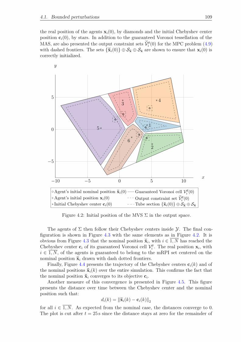
4.1. Bounded perturbations 109
the real position of the agents xi(0), by diamonds and the initial Chebyshev centerposition ci(0), by stars. In addition to the guaranteed Voronoi tessellation of theMAS, are also presented the output constraint sets qVgi (0) for the MPC problem (4.9)with dashed frontiers. The sets qxi(0) ⊕ Sx ⊕ Sx are shown to ensure that xi(0) iscorrectly initialized.
−10 −5 0 5 10
−5
0
5
1
2
34
5
6
x
y
Agent’s initial nominal position qxi(0) Guaranteed Voronoi cell Vgi (0)
Agent’s initial position xi(0) Output constraint set qVgi (0)
Initial Chebyshev center ci(0) Tube section qxi(0) ⊕ Sx ⊕ Sx
Figure 4.2: Initial position of the MVS Σ in the output space.
The agents of Σ then follow their Chebyshev centers inside Y. The final con-figuration is shown in Figure 4.3 with the same elements as in Figure 4.2. It isobvious from Figure 4.3 that the nominal position qxi, with i ∈ 1, N has reached theChebyshev center ci of its guaranteed Voronoi cell Vgi . The real position xi, withi ∈ 1, N , of the agents is guaranteed to belong to the mRPI set centered on thenominal position qxi drawn with dash dotted frontiers.
Finally, Figure 4.4 presents the trajectory of the Chebyshev centers ci(k) and ofthe nominal positions qxi(k) over the entire simulation. This confirms the fact thatthe nominal position qxi converges to its objective ci.
Another measure of this convergence is presented in Figure 4.5. This figurepresents the distance over time between the Chebyshev center and the nominalposition such that:
di(k) = ‖qxi(k)− ci(k)‖2for all i ∈ 1, N . As expected from the nominal case, the distances converge to 0.The plot is cut after t = 25 s since the distance stays at zero for the remainder of

110 Chapter 4. Deployment of a multi-vehicle system subject to perturbations
−10 −5 0 5 10
−5
0
5
x
y
Agent’s final nominal position qxi(250) Guaranteed Voronoi cell Vgi (250)
Agent’s final position xi(250) Output constraint set qVgi (250)
Final Chebyshev center ci(250) Tube section qxi(250) ⊕ Sx ⊕ Sx
Figure 4.3: Final position of the MVS Σ in the output space at t = 50 s.
the simulation.An interesting measure of the efficiency of the proposed control algorithm is the
norm of the estimation error xi as well as the norm of the deviation error xi. Indeed,these two quantities quantify the fact that the state of the agent i ∈ 1, N remainsinside the invariant set centered on qxi(k) and bounded by Sx ⊕ Sx. Figure 4.6 andFigure 4.7 show the evolution of these two norms over time. While the signals inFigure 4.6 might be difficult to understand, one element is of importance. Indeed, thenorm remains bounded by the maximum norm of the vectors of Sx, i.e. ‖xmax‖2 =maxx∈Sx
‖x‖2. Given the shape of Sx, the maximum norm is ‖xmax‖2 = 0.21m. Everyplot in Figure 4.6 is below the value of ‖xmax‖2. The shape of the plots comes fromthe fact that, given (4.4), the estimation error converges quickly to di(k)−Lwi(k).Since the perturbation signals di(k) and wi(k) take random values every 10 s, thenorm of the estimation error ‖xi(k)‖2 converges to the norm ‖di(k)−Lwi(k)‖2.The same remark concerns Figure 4.7: every plot remains below the maximumnorm of the vectors of Sx, i.e. ‖xmax‖2 = max
x∈Sx
‖x‖2. Given the shape of Sx, themaximum norm is ‖xmax‖2 = 0.35m, which is indeed an upper bound of the plotsin Figure 4.7. The pikes that appear in this figure occur for every change of theperturbation signals di(k) and wi(k). After every change, the norm of the deviationerror ‖xi(k)‖2 converges to ‖LCxi(k) +Lwi(k)‖2 since the control gain matrix Kis chosen such that the dynamics (4.6) is stable.

4.1. Bounded perturbations 111
−10 −5 0 5 10
−5
0
5
1
2
3
4
5
6
x
y
Agent’s initial nominal position qxi(0) Initial Chebyshev center ci(0)
Agent’s final nominal position qxi(250) Final Chebyshev center ci(250)Nominal trajctory of the agent Trajectory of the Chebyshev center
Figure 4.4: Nominal trajectories of the agents of Σ and their associated Chebyshevcenters.
0 2 4 6 8 10 12 14 16 18 20 22 240
1
2
3
4
t (s)
d (m)
d1(k)d2(k)d3(k)d4(k)d5(k)d6(k)
Figure 4.5: Distance of the nominal position of each agent of Σ to its Chebyshevcenter over time.

112 Chapter 4. Deployment of a multi-vehicle system subject to perturbations
0 5 10 15 20 25 30 35 40 45 500
0.05
0.1
0.15
t (s)
‖x‖2 (m)
‖x1(k)‖2‖x2(k)‖2‖x3(k)‖2‖x4(k)‖2‖x5(k)‖2‖x6(k)‖2
Figure 4.6: Norm of the estimation error of each agent of Σ.
0 5 10 15 20 25 30 35 40 45 500
0.1
0.2
0.3
t (s)
‖x‖2 (m)
‖x1(k)‖2‖x2(k)‖2‖x3(k)‖2‖x4(k)‖2‖x5(k)‖2‖x6(k)‖2
Figure 4.7: Norm of the deviation error of each agent of Σ.
Since there is no offset cancellation strategy (Limón et al., 2010), the estimationand deviation errors never go back to zero. Indeed, the goal of the presented controlstrategy is to drive the MVS to a static Chebyshev configuration without collisionsdespite the presence of bounded perturbations on the agents’ dynamics. Then,the control strategy proves to be efficient since the MVS is deployed into a staticChebyshev configuration. Moreover, the state of the agents, despite the perturbations,is guaranteed to remain in a given set known beforehand which, coupled with theguaranteed Voronoi tessellation, guarantees, by construction, that no collision canoccur between two vehicles.

4.1. Bounded perturbations 113
4.1.4.2 UAV dynamics
Let Σ be a multi-vehicle system composed of N = 6 agents deployed in the outputspace:
Y = B2(10 · 12×1). (4.28)Each agent i ∈ 1, N is a quadrotor UAV obeying the dynamics and the controlstrategy presented in Section 3.3. The predictive controller used for the outer loopin Paragraph 3.3.2.3 is replaced by the tube-based MPC described in Section 4.1.3.
The dynamics (3.31) is replaced by:
xi(k + 1) = Axi(k) +Bui(k) + di(k)
yi(k) = Cxi(k) +wi(k)(4.29)
where A, B and C are defined in (3.39), ui(k) ∈ U = B2(π6· 12×1
), di(k) ∈
D = B4(10−2 ·
[0.5 2 0.5 2
]>), wi(k) ∈ W = B2(0.01 · 12×1) and xi(k) ∈ X =
B4([
10 3 10 3]>). The definition of the sets D and W is based on Michel et al.
(2019).The tuning procedures for the observer and controller gain matrices L and K
are computationally heavy if the four state dynamics (4.29) is used. Given the statematrices (3.39), the position subsystem (4.29) can be separated into two independentsubsystems on which the tuning procedures are applied. These two subsystems are:[
xi(k + 1)vx,i(k + 1)
]=
[1 Ts0 1
] [xi(k)vx,i(k)
]+
1
2gTs
[Ts2
]θi(k) +
[1 0 0 00 1 0 0
]di(k)
xi(k) =[1 0
] [ xi(k)vx,i(k)
]+[1 0
]wi(k)
(4.30)
and:[yi(k + 1)vy,i(k + 1)
]=
[1 Ts0 1
] [yi(k)vy,i(k)
]− 1
2gTs
[Ts2
]φi(k) +
[0 0 1 00 0 0 1
]di(k)
yi(k) =[1 0
] [ yi(k)vy,i(k)
]+[0 1
]wi(k)
(4.31)
with g = 9.81m · s−2 and Ts = 0.2 s. With the decomposition given in (4.30) and(4.31), the tuning procedures are run two times to obtain the gain matrices Lx andKx for (4.30) and Ly, Ky for (4.31) such that:
L =
[Lx 02×1
02×1 Ly
]and K =
[01×2 Ky
Kx 01×2
].
Then, using these gains, it is possible to obtain the sets Sx,x and Sx,x, approximationsof the mRPI sets for the estimation error and deviation error of the subsystem (4.30)and the sets Sx,y and Sx,y, approximations of the mRPI sets for the estimationerror and deviation error of the subsystem (4.31) such that Sx = Sx,x × Sx,y andSx = Sx,x × Sx,y.
Solving the BMI constrained problem (4.16) for (4.30) and (4.31) by consideringτ as a decision variable yields:
Lx = Ly =
[0.99011.0482
].

114 Chapter 4. Deployment of a multi-vehicle system subject to perturbations
Then, Algorithm 2.1 is run to obtain Sx,x and Sx,y which are such that Sx,x = Sx,y.Let Hx and θx be the matrices inducing Sx,x and Sx,y in R2. Then:
Sx =x ∈ R2
∣∣ (I2 ⊗Hx)x ≤ 12×1 ⊗ θx
.
The values of Hx and θx are not reported here since Sx,x is composed of 43 inequalities.However, it is shown in Figure 4.8.
Solving the BMI constrained problem (4.23) for (4.30) and (4.31) by consideringτ as a decision variable gives, with the weights α = 10 and β = 0.1:
Kx = −Ky =[−0.3628 −0.4986
].
Then, Algorithm 2.1 is run to obtain Sx,x and Sx,y which are such that Sx,x = Sx,y.From the definition of these two sets, Sx is obtained the same way as Sx. Again, sinceSx,x is composed of 29 inequalities, the values of the matrices inducing it are notreported here. However, it is shown in Figure 4.8. Along with the sets Sx,x = Sx,yand Sx,x = Sx,y, Figure 4.8 also displays the set KSx.
−0.1 0 0.1
−0.2
0
0.2
Sx,x
x
vx
−0.5 0 0.5
−0.5
0
0.5 Sx,x
x
vx
−0.2 0 0.2
−0.2
0
0.2 KSx
φ
θ
Figure 4.8: Invariant sets for the tube-based MPC controller in the UAV case.
According to Section 3.3.2, a cascaded control structure is considered to controleach UAV. For the inner loop, a continuous-time controller based on feedbacklinearization is used for attitude control. For the outer loop, the discrete-timetube-based MPC of Section 4.1.3 is used for position control. However, for simulationpurpose, the controller of the inner loop is run in discrete-time with a samplingperiod of 1ms. This sampling period is 200 times shorter than the sampling periodof the outer loop. It is not a problem in the nominal case described in Section 3.3.3but in the perturbed case, this might cause a larger estimation error and evenlead to instability. Then the outer loop needs a modified version of the positioncontroller described in Figure 3.7. This structure is based on the ones used inChevet et al. (2020a) and Rousseau et al. (2018). The MPC part of the tube-basedMPC controller runs at the sampling period Ts. However, the control input appliedto the agent i ∈ 1, N is changed to ui(kin) = qui(k) + K(xi(kin)− qxi(k)) for all
kin ∈TsT ins
k,TsT ins
(k + 1)− 1 where T ins = 1ms is the sampling period of the inner loop.
The gain matrix Lin of the observer is obtained by pole placement. The poles placedto obtain Lin are the eigenvalues of A− LC. The matrix A used to get the gainmatrix Lin is the matrix A of (4.30) and (4.31) obtained by replacing Ts by T in
s .With such a structure, the estimated state xi(kin) used for the tube-based controlleris more accurate and guarantees that the estimation and deviation errors remain
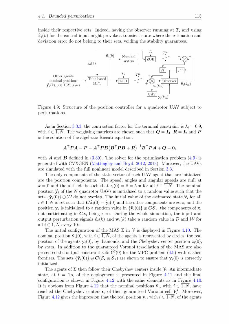
4.1. Bounded perturbations 115
inside their respective sets. Indeed, having the observer running at Ts and usingxi(k) for the control input might provoke a transient state where the estimation anddeviation error do not belong to their sets, voiding the stability guarantees.
Tube-basedMPC ZOH
T ins
+Observer
xi(kin)
+
K
+
z−1
Nominalsystem
qui(k)
qxi(k)
TsOther agentsnominal positions
qyj(k), j ∈ 1, N , j 6= i
ZOH−
UAVyi(kin)
ui(kin)
Ts T ins
Figure 4.9: Structure of the position controller for a quadrotor UAV subject toperturbations.
As in Section 3.3.3, the contraction factor for the terminal constraint is λi = 0.9,with i ∈ 1, N . The weighting matrices are chosen such that Q = I4, R = I2 and Pis the solution of the algebraic Riccati equation:
A>PA− P −A>PB(B>PB +R
)−1B>PA+Q = 04
with A and B defined in (3.39). The solver for the optimization problem (4.9) isgenerated with CVXGEN (Mattingley and Boyd, 2012, 2013). Moreover, the UAVsare simulated with the full nonlinear model described in Section 3.3.
The only components of the state vector of each UAV agent that are initializedare the position components. The speed, angles and angular speeds are null atk = 0 and the altitude is such that zi(0) = z = 5m for all i ∈ 1, N . The nominalposition qyi of the N quadrotor UAVs is initialized to a random value such that thesets qyi(0) ⊕W do not overlap. The initial value of the estimated state xi for alli ∈ 1, N is set such that Cxi(0) = qyi(0) and the other components are zero, and theposition yi is initialized to a random value in qyi(0) ⊕CSx, the components of xinot participating in Cxi being zero. During the whole simulation, the input andoutput perturbation signals di(k) and wi(k) take a random value in D and W forall i ∈ 1, N every 10 s.
The initial configuration of the MAS Σ in Y is displayed in Figure 4.10. Thenominal position qyi(0), with i ∈ 1, N , of the agents is represented by circles, the realposition of the agents yi(0), by diamonds, and the Chebyshev center position ci(0),by stars. In addition to the guaranteed Voronoi tessellation of the MAS are alsopresented the output constraint sets qVgi (0) for the MPC problem (4.9) with dashedfrontiers. The sets qyi(0) ⊕C(Sx ⊕ Sx) are shown to ensure that yi(0) is correctlyinitialized.
The agents of Σ then follow their Chebyshev centers inside Y . An intermediatestate, at t = 1 s, of the deployment is presented in Figure 4.11 and the finalconfiguration is shown in Figure 4.12 with the same elements as in Figure 4.10.It is obvious from Figure 4.12 that the nominal positions qyi, with i ∈ 1, N , havereached the Chebyshev centers ci of their guaranteed Voronoi cell Vgi . Moreover,Figure 4.12 gives the impression that the real position yi, with i ∈ 1, N , of the agents
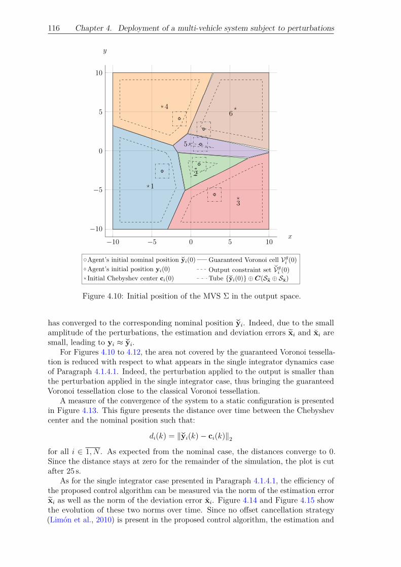
116 Chapter 4. Deployment of a multi-vehicle system subject to perturbations
−10 −5 0 5 10
−10
−5
0
5
10
1
2
3
4
5
6
x
y
Agent’s initial nominal position qyi(0) Guaranteed Voronoi cell Vgi (0)
Agent’s initial position yi(0) Output constraint set qVgi (0)
Initial Chebyshev center ci(0) Tube qyi(0) ⊕C(Sx ⊕ Sx)
Figure 4.10: Initial position of the MVS Σ in the output space.
has converged to the corresponding nominal position qyi. Indeed, due to the smallamplitude of the perturbations, the estimation and deviation errors xi and xi aresmall, leading to yi ≈ qyi.
For Figures 4.10 to 4.12, the area not covered by the guaranteed Voronoi tessella-tion is reduced with respect to what appears in the single integrator dynamics caseof Paragraph 4.1.4.1. Indeed, the perturbation applied to the output is smaller thanthe perturbation applied in the single integrator case, thus bringing the guaranteedVoronoi tessellation close to the classical Voronoi tessellation.
A measure of the convergence of the system to a static configuration is presentedin Figure 4.13. This figure presents the distance over time between the Chebyshevcenter and the nominal position such that:
di(k) = ‖qyi(k)− ci(k)‖2for all i ∈ 1, N . As expected from the nominal case, the distances converge to 0.Since the distance stays at zero for the remainder of the simulation, the plot is cutafter 25 s.
As for the single integrator case presented in Paragraph 4.1.4.1, the efficiency ofthe proposed control algorithm can be measured via the norm of the estimation errorxi as well as the norm of the deviation error xi. Figure 4.14 and Figure 4.15 showthe evolution of these two norms over time. Since no offset cancellation strategy(Limón et al., 2010) is present in the proposed control algorithm, the estimation and
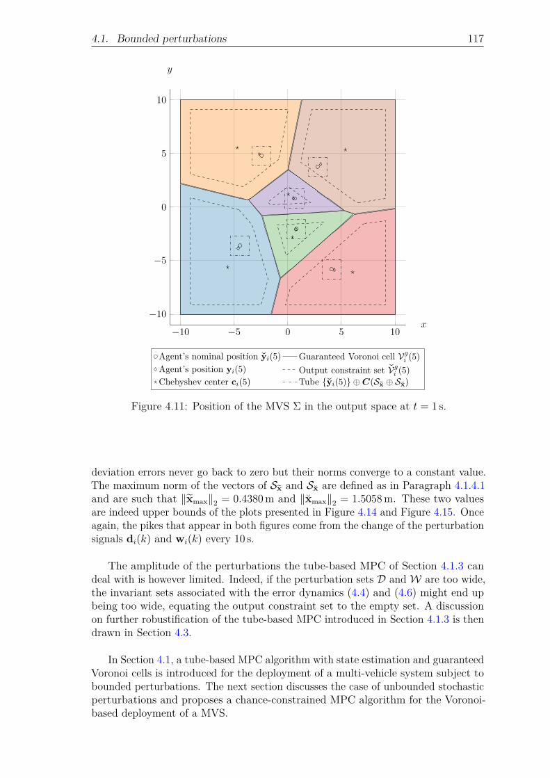
4.1. Bounded perturbations 117
−10 −5 0 5 10
−10
−5
0
5
10
x
y
Agent’s nominal position qyi(5) Guaranteed Voronoi cell Vgi (5)
Agent’s position yi(5) Output constraint set qVgi (5)
Chebyshev center ci(5) Tube qyi(5) ⊕C(Sx ⊕ Sx)
Figure 4.11: Position of the MVS Σ in the output space at t = 1 s.
deviation errors never go back to zero but their norms converge to a constant value.The maximum norm of the vectors of Sx and Sx are defined as in Paragraph 4.1.4.1and are such that ‖xmax‖2 = 0.4380m and ‖xmax‖2 = 1.5058m. These two valuesare indeed upper bounds of the plots presented in Figure 4.14 and Figure 4.15. Onceagain, the pikes that appear in both figures come from the change of the perturbationsignals di(k) and wi(k) every 10 s.
The amplitude of the perturbations the tube-based MPC of Section 4.1.3 candeal with is however limited. Indeed, if the perturbation sets D and W are too wide,the invariant sets associated with the error dynamics (4.4) and (4.6) might end upbeing too wide, equating the output constraint set to the empty set. A discussionon further robustification of the tube-based MPC introduced in Section 4.1.3 is thendrawn in Section 4.3.
In Section 4.1, a tube-based MPC algorithm with state estimation and guaranteedVoronoi cells is introduced for the deployment of a multi-vehicle system subject tobounded perturbations. The next section discusses the case of unbounded stochasticperturbations and proposes a chance-constrained MPC algorithm for the Voronoi-based deployment of a MVS.

118 Chapter 4. Deployment of a multi-vehicle system subject to perturbations
−10 −5 0 5 10
−10
−5
0
5
10
x
y
Agent’s final nominal position qyi(250) Guaranteed Voronoi cell Vgi (250)
Agent’s final position yi(250) Output constraint set qVgi (250)
Final Chebyshev center ci(250) Tube qyi(250) ⊕C(Sx ⊕ Sx)
Figure 4.12: Final position of the MVS Σ in the output space at t = 50 s.
0 2 4 6 8 10 12 14 16 18 20 22 240
1
2
3
4
5
t (s)
d (m)
d1(k)d2(k)d3(k)d4(k)d5(k)d6(k)
Figure 4.13: Distance of the nominal position of each agent of Σ to its Chebyshevcenter over time.

4.2. Unbounded stochastic perturbations 119
0 5 10 15 20 25 30 35 40 45 500
1
2
3
4
5
·10−2
t (s)
‖x‖2 (m)
‖x1(k)‖2‖x2(k)‖2‖x3(k)‖2‖x4(k)‖2‖x5(k)‖2‖x6(k)‖2
Figure 4.14: Norm of the estimation error of each agent of Σ.
0 5 10 15 20 25 30 35 40 45 500
0.2
0.4
0.6
t (s)
‖x‖2 (m)
‖x1(k)‖2‖x2(k)‖2‖x3(k)‖2‖x4(k)‖2‖x5(k)‖2‖x6(k)‖2
Figure 4.15: Norm of the deviation error of each agent of Σ.
4.2 Unbounded stochastic perturbations
In the following section, unbounded stochastic perturbations will be considered on thesystem model. To this end, Section 4.2.1 introduces the necessary modifications onthe model of an agent part of a larger MAS before presenting an overview of existingmethods for control of systems subject to unbounded stochastic perturbations inSection 4.2.2. The decentralized model predictive control algorithm presented inSection 3.2.2 is reformulated to cope with agents which dynamics is subject toprocess and measurement noises. The proposed chance-constrained MPC algorithmis then exposed in Section 4.2.3 before finally being applied in simulation to a MAScomposed of vehicle agents following single integrator or UAV dynamics.

120 Chapter 4. Deployment of a multi-vehicle system subject to perturbations
4.2.1 System modelLet Σ be a multi-agent system composed of N agents. Each agent obeys discrete-timelinear time-invariant dynamics as in the previous chapter. However, while it wasnot relevant for the cases presented in Chapter 3 and Section 4.1, it is important tonote that such discrete-time dynamics often, if not always, arise from discretizedcontinuous-time dynamics. The continuous-time linear time-invariant dynamics ofan agent subject to process and measurement noise is written:
xi(t) = ACxi(t) +BCui(t) +Mdi(t)
yi(t) = Cxi(t) +wi(t)(4.32)
where xi ∈ X ⊂ Rn, ui ∈ U ⊂ Rm, yi ∈ Y ⊂ R2, with i ∈ 1, N , AC ∈ Rn×n,BC ∈ Rn×m, C ∈ R2×n and M ∈ Rn×q, q ≤ n. Since the agents share the samedynamics and the same output space by Assumptions 2.6 and 3.1, the dependency ini ∈ 1, N is dropped for AC , BC and C and for Y. The dependency in i ∈ 1, N forX and U is also dropped for the sake of simplicity. The signals di ∈ Rq and wi ∈ R2,with i ∈ 1, N , are the process and measurement noises.Assumption 4.2: Process noise matrixThe matrix M ∈ Rn×q has rank q, with q ≤ n.
The process noise signal di(t) present in the dynamics (4.32) is in fact twofold.It is the sum di(t) = pi(t) +ws
i (t) of a deterministic exogenous perturbation signaldenoted by pi(t) ∈ Rq and a normally distributed white noise signal ws
i ∈ Rq (asdefined in Definition 2.37) representing the modeling errors. As such, the mean andvariance matrix of di(t) are such that µdi
(t) = pi(t) and Σdi(t) = Σws
i(t). For its
part, the measurement noise signal wi(t) is such that µwi(t) = 02×1 and a variance
matrix given in the following assumption.Assumption 4.3: Normally distributed noisesThe signal ws
i (t) and the measurement noise wi, with i ∈ 1, N , are independent andnormally distributed white noises as defined in Definition 2.37. The means of ws
i (t)and wi(t) are then µws
i(t) = 0q×1 and µwi
(t) = 02×1 and their variance matrices arethe positive definite matrices Σws
i(t) 0 and Σwi
(t) 0.
The discrete-time linear time-invariant dynamics used later for control purposesis obtained by discretizing (4.32):
xi(k + 1) = Axi(k) +Bui(k) + δi(k)
yi(k) = Cxi(k) + γi(k)(4.33)
where A ∈ Rn×n, B ∈ Rn×m and C ∈ Rp×n. The signals δi ∈ Rn and γi ∈ R2, withi ∈ 1, N , are the discrete-time process and measurement noises. The matrices in(4.33) are obtained as (Franklin et al., 1997):
A = exp(AC · Ts) and B =
∫ Ts
0
exp(AC · τ)Bdτ
where Ts is the sampling period and exp is the exponential function. The matrix Cis not modified by the discretization process.

4.2. Unbounded stochastic perturbations 121
The discretization of the random signals is not as straightforward as the dis-cretization of the state-space matrices. Indeed, the discrete-time process noise is(Franklin et al., 1997):
δi(k) =
∫ Ts
0
exp(AC · τ)Mdi((k + 1)Ts − τ)dτ
while the discrete-time measurement noise is γi(k) = wi(kTs). However, for controlpurposes, it is important to characterize random signals such as the discrete-timeprocess and measurement noises δi(k) and γi(k) with their mean and variance. Theycan be obtained from the value of the mean and variance matrix of their continuous-time counterparts di(k) and wi(k). For the following mathematical developments,let hk(t) = (k + 1)Ts − t.
By definition of the mathematical expectation, it is immediate that:
µγi(k) = E(γi(k)) = E(wi(kTs)) = µwi
(kTs) (4.34)
and, by linearity of the mathematical expectation:
µδi(k) = E(δi(k)) =∫ Ts
0
exp(AC · τ)ME(di(hk(τ)))dτ
=
∫ Ts
0
exp(AC · τ)Mµdi(hk(τ))dτ . (4.35)
Moreover, it is a well known result (Kamen and Su, 1999) that:
Σγi(k) =
1
TsΣwi
(kTs) (4.36)
for all k ≥ 0 such that Σγi(k) 0. The variance matrix of δi(k) is:
Σδi(k) = E((δi(k)− µδi(k))(δi(k)− µδi(k))
>)
= E
(∫ Ts
0
exp(AC · τ)M (di(hk(τ))− µdi(hk(τ)))dτ
·∫ Ts
0
(di(hk(ν))− µdi(hk(ν)))
>M> exp(A>C · ν
)dν
)which, by Fubini’s theorem (DiBenedetto, 2016), gives:
Σδi(k) = E
(∫ Ts
0
∫ Ts
0
exp(AC · τ)M(di(hk(τ))− µdi(hk(τ)))·
(di(hk(ν))− µdi(hk(ν)))
>M> exp(A>C · ν
)dτdν
).
By definition:
E((di(hk(τ))− µdi
(hk(τ)))(di(hk(ν))− µdi(hk(ν)))
>)= Σdi
(τ)δ(τ − ν)
where δ is the Dirac delta function such that δ(τ − ν) 6= 0 when τ = ν. Thus, bylinearity of the mathematical expectation:
Σδi(k) =
∫ Ts
0
exp(AC · τ)MΣdi(τ)M> exp
(A>C · τ
)dτ . (4.37)
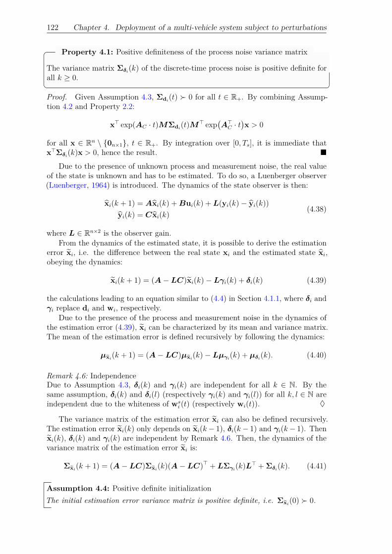
122 Chapter 4. Deployment of a multi-vehicle system subject to perturbations
Property 4.1: Positive definiteness of the process noise variance matrix
The variance matrix Σδi(k) of the discrete-time process noise is positive definite forall k ≥ 0.
Proof. Given Assumption 4.3, Σdi(t) 0 for all t ∈ R+. By combining Assump-
tion 4.2 and Property 2.2:
x> exp(AC · t)MΣdi(t)M> exp
(A>C · t
)x > 0
for all x ∈ Rn \ 0n×1, t ∈ R+. By integration over [0, Ts], it is immediate thatx>Σδi(k)x > 0, hence the result.
Due to the presence of unknown process and measurement noise, the real valueof the state is unknown and has to be estimated. To do so, a Luenberger observer(Luenberger, 1964) is introduced. The dynamics of the state observer is then:
xi(k + 1) = Axi(k) +Bui(k) +L(yi(k)− yi(k))
yi(k) = Cxi(k)(4.38)
where L ∈ Rn×2 is the observer gain.From the dynamics of the estimated state, it is possible to derive the estimation
error xi, i.e. the difference between the real state xi and the estimated state xi,obeying the dynamics:
xi(k + 1) = (A−LC)xi(k)−Lγi(k) + δi(k) (4.39)
the calculations leading to an equation similar to (4.4) in Section 4.1.1, where δi andγi replace di and wi, respectively.
Due to the presence of the process and measurement noise in the dynamics ofthe estimation error (4.39), xi can be characterized by its mean and variance matrix.The mean of the estimation error is defined recursively by following the dynamics:
µxi(k + 1) = (A−LC)µxi
(k)−Lµγi(k) + µδi(k). (4.40)
♦
Remark 4.6: IndependenceDue to Assumption 4.3, δi(k) and γi(k) are independent for all k ∈ N. By thesame assumption, δi(k) and δi(l) (respectively γi(k) and γi(l)) for all k, l ∈ N areindependent due to the whiteness of ws
i (t) (respectively wi(t)).
The variance matrix of the estimation error xi can also be defined recursively.The estimation error xi(k) only depends on xi(k− 1), δi(k− 1) and γi(k− 1). Thenxi(k), δi(k) and γi(k) are independent by Remark 4.6. Then, the dynamics of thevariance matrix of the estimation error xi is:
Σxi(k + 1) = (A−LC)Σxi
(k)(A−LC)> +LΣγi(k)L> +Σδi(k). (4.41)
Assumption 4.4: Positive definite initializationThe initial estimation error variance matrix is positive definite, i.e. Σxi
(0) 0.

4.2. Unbounded stochastic perturbations 123
Property 4.2: Positive definiteness of the estimation error variance
The variance matrix Σxi(k) of the estimation error xi, with i ∈ 1, N , is positive
definite for all k > 0.
Proof. Consider the dynamics (4.41). Since Σδi(k) 0 and Σγi(k) 0 for all
k ≥ 0 and Σxi(0) 0 by Assumption 4.4, by recursion, it leads to Σxi
(k) 0 for allk > 0. Indeed, (A−LC)Σxi
(k)(A−LC)> 0 and LΣγi(k)L> 0 according to
Property 2.2 and Σδi(k) 0 for all k ≥ 0 by Property 4.1 thus their sum is positivedefinite.
4.2.2 Overview of chance-constrained MPC for systemswith stochastic perturbations
As in Section 4.1, perturbations are added to the system model (4.33). However,these perturbations now have a stochastic nature and the control methods have tobe adapted to cope with this new kind of endogenous or exogenous signals. As inthe classical bounded perturbations case presented in 4.1, several control strategieshave been studied and applied when the perturbations on a system are stochastic.For example, as in the deterministic perturbations case, H∞ optimization methodscan be used (Ugrinovskii, 1998) as well as sliding mode control (Niu et al., 2005).
However, as stated previously, when dealing with dynamical systems subject tooperating constraints, one of the most popular technique is model predictive control,and most particularly, stochastic, or chance-constrained, MPC (Farina et al., 2016),when the system is subject to perturbations having a stochastic nature. In this case,the system follows the dynamics presented in (4.33), leading to the definition ofconstraints of the form P(x ∈ X ) ≥ P denoting the fact that the probability of thevector x belonging to the set X has to be greater or equal to an arbitrary value P .Such constraints can be defined on any of the decision variables of the problem (e.g.the input vector sequence).
Farina et al. (2016) reviewed several existing methods of chance-constrainedmodel predictive control (CCMPC) and they found three main CCMPC categoriesfor linear systems. To define their categories, they use the superposition principleto separate the state equation of (4.33) into a stochastic part depending only onthe stochastic variable (e.g. δi and/or γi in (4.33)) and a deterministic part whichcan be assimilated to the nominal system defined in (4.2). They can then make adistinction between what they call “open-loop” control methods and “disturbancefeedback” or “state-feedback” control. The “open-loop” control methods can befound for example in Blackmore et al. (2011), Gavilan et al. (2012), Hashimoto(2013) or Chevet et al. (2020a). Such methods are called “open-loop” since thecontroller only acts on the deterministic part while the stochastic part evolves inan uncontrolled open-loop fashion. Such an evolution is opposed to the feedbackmethods, where the control signal acts on both the deterministic and stochastic partof the system. For disturbance feedback (Prandini et al., 2012, Zhang et al., 2013,Korda et al., 2014), the control input is an affine function of the disturbance over theprediction horizon and the optimization problem is meant to find the value of theparameters of this function. In the case of state feedback (Primbs and Sung, 2009,Cannon et al., 2010, 2012, Kouvaritakis and Cannon, 2016), the formulation of theproblem is similar, if not identical, to the tube-based MPC approach presented in

124 Chapter 4. Deployment of a multi-vehicle system subject to perturbations
Section 4.1.2, the main difference being that a stochastic RPI set has to be definedfor the control strategy to work. Both feedback methods have the advantage ofenlarging the feasibility region of the MPC optimization problem.
Regardless of the category defined in Farina et al. (2016) the controller falls into,the main problem that will appear is the presence of unknown terms in the constraints.This is due to the probabilistic nature of said constraints and the fact that stochasticsignals are taken into account when expressing them. To overcome this difficulty,the probabilistic constraints are reformulated into algebraic constraints by using theproperties of the stochastic process used to represent the perturbation. This oftenamounts to tighten the constraints by finding a bound on the perturbation signalensuring that the probabilistic constraint is respected with the required probability.
CCMPC approaches have been used for the control of different types of vehicles(Blackmore et al., 2011) such as ground vehicles (Carvalho et al., 2014, Wan et al.,2017), spacecrafts (Gavilan et al., 2012, Zhu et al., 2018) or unmanned aerial vehicles(Chevet et al., 2020a). Chance-constrained approaches have also been developed formulti-agent systems (Lyons et al., 2012, Dai et al., 2015, 2016, 2018) and applied onvehicles such as UAVs (Chevet et al., 2020a) or multi-robot frameworks (Zhu andAlonso-Mora, 2019).
This section focuses on the work presented in Chevet et al. (2020a). The CCMPCalgorithm presented is derived from the work of Gavilan et al. (2012) which describesan “open-loop” (as per Farina et al. (2016) naming) scheme to control a spacecraft.The controller proposed in Gavilan et al. (2012) is improved to work in the casewhere full state information is not known and state estimation is necessary. It isthen applied in a decentralized fashion to a multi-agent system composed first ofagents obeying single integrator dynamics before being applied to a MAS composedof quadrotor UAVs.
4.2.3 Deployment algorithmAs in Chapter 3, the objective of the deployment algorithm that is presented in thisparagraph is to drive the MAS defined in Section 4.2.1 into a static configuration in Y .The set Y is a convex bounded polytope as defined in Assumption 3.1. However, animportant difference with the algorithm for the nominal case presented in Chapter 3appears due to the unbounded stochastic perturbation on the dynamics (4.33).Indeed, such perturbations induce the presence of probabilistic constraints in theMPC problem. As described in Section 4.2.2, such constraints have to be relaxedinto algebraic constraints for the optimization problem on which the MPC is basedto be solvable. This section then describe how such a relaxation can be done.
4.2.3.1 Deployment objective and chance-constrained optimizationproblem
In the nominal case of Chapter 3, the MPC algorithm uses as input the current stateof the system xi(k) for all i ∈ 1, N . In the case of systems subject to perturbationsand/or with an output yi(k) such that yi(k) 6= xi(k), the characterization of thesystem is done via the estimated state xi(k) obtained through a state observer. Then,in this case, the MPC uses this estimated state of the system xi(k) to obtain thecontrol input ui(k) to be applied to the system. As for the bounded perturbations

4.2. Unbounded stochastic perturbations 125
case, a first assumption is made, based on Assumption 2.5, to deal with the case ofstochastic perturbations.Assumption 4.5: Knowledge of environment under unbounded stochastic pertur-
bationsEach agent of Σ knows, at all time, the estimated position of the other agents of Σ.
The deployment objective is the same as the one presented in Section 3.2. At eachtime instant, each agent i ∈ 1, N computes its Voronoi cell Vi(k) with the knowledgeof yj(k), with j ∈ 1, N , j 6= i, by Assumption 4.5. Then, with the knowledgeof its Voronoi cell, each agent is able to compute the Chebyshev center ci(k) ofVi(k) by solving the problem (3.5). The objective of the controller is then to driveeach agent towards the Chebyshev center ci(k) of Vi(k) using a chance-constrainedMPC algorithm. However, while in the nominal case, each agent had to reachthe Chebyshev center of its Voronoi cell, i.e. lim
k→+∞yi(k) = lim
k→+∞ci(k), here, the
estimated position of each agent has to reach the Chebyshev center of its Voronoicell, i.e. lim
k→+∞yi(k) = lim
k→+∞ci(k).
In order to introduce the optimization problem on which the MPC is based, it isnecessary to formulate the evolution of the estimated state vector over the predictionhorizon Np ∈ N. Since the dynamics (4.38) are defined recursively, it is possible towrite:
xi(k + l) = Axi(k + l − 1) +Bui(k + l − 1) +LCxi(k + l − 1) +Lγi(k + l − 1)
= Alxi(k) +l−1∑j=0
Al−j−1(Bui(k + j) +L(Cxi(k + j) + γi(k + j))).
Then, defining the following vectors and matrices:
Xi(k) =
xi(k + 1)...
xi(k +Np)
F =
A...
ANp
Ui(k) =
ui(k)...
ui(k +Np − 1)
G =
B 0n×m · · · 0n×m
AB B. . . ...
... . . . 0n×mANp−1B · · · AB B
Xi(k) =
xi(k)...
xi(k +Np − 1)
Gx =
LC 0n×n · · · 0n×n
ALC LC. . . ...
... . . . 0n×nANp−1LC · · · ALC LC
Γi(k) =
γi(k)...
γi(k +Np − 1)
Gγ =
L 0n×2 · · · 0n×2
AL L. . . ...
... . . . 0n×2
ANp−1L · · · AL L
the estimated state over the prediction horizon is:
Xi(k) = F xi(k) +GUi(k) +GxXi(k) +GγΓi(k). (4.42)
126 Chapter 4. Deployment of a multi-vehicle system subject to perturbations
However, the estimation error xi is also defined recursively and can be expressedover the prediction horizon. Defining:
∆i(k) =
δi(k)...
δi(k +Np − 1)
Gδ =
In 0n×n · · · 0n×n
A−LC In. . . ...
... . . . 0n×n(A−LC)Np−1 · · · A−LC In
F =
A−LC...
(A−LC)Np
Gγ =
L 0n×2 · · · 0n×2
(A−LC)L L. . . ...
... . . . 0n×2
(A−LC)Np−1L · · · (A−LC)L L
the estimation error over the prediction horizon is:
Xi(k + 1) = F xi(k)− GγΓi(k) + Gδ∆i(k). (4.43)
The system (4.38) satisfies Assumption 3.2, i.e. there exists a couple (xci(k),uci(k))such that (xci(k),uci(k), ci(k)) is an equilibrium point of the nominal dynamics (3.1)satisfying:
xci(k) = Axci(k) +Buci(k)
ci(k) = Cxci(k).(4.44)
Since the equilibrium point is the constant objective point over the entire predictionhorizon, it is possible to define Xci(k) = 1Np×1⊗ xci(k) and Uci(k) = 1Np×1⊗uci(k).
With all these elements, based on Gavilan et al. (2012) and Chevet et al. (2020a),a decentralized chance-constrained model predictive controller for an agent i ∈ 1, Nobeying the dynamics (4.33) is formulated as:
minimizeUi(k)
J(Xi(k),Ui(k), Xci(k),Uci(k)
)(4.45a)
subject to
P(Xi(k) ∈ X
)≥ Px, (4.45b)
Ui(k) ∈ U , (4.45c)
P((
INp ⊗C)Xi(k) ∈ V i(k)
)≥ Py (4.45d)
where the cost function (4.45a) is:
J(Xi(k),Ui(k), Xci(k),Uci(k)
)= E
(∥∥∥Xi(k)− Xci(k)∥∥∥2Qi
+ ‖Ui(k)−Uci(k)‖2Ri
). (4.46)
The weighting matrices Qi ∈ RNpn×Npn and Ri ∈ RNpm×Npm are block diagonalmatrices composed of Np individual positive definite matrices Qi,Pi ∈ Rn×n andRi ∈ Rm×m such that Q>
i = Qi 0, P>i = Pi 0, R>
i = Ri 0, Qi =diag
(INp−1 ⊗Qi,Pi
)and Ri = INp ⊗Ri.

4.2. Unbounded stochastic perturbations 127
♦
Remark 4.7: Terminal cost and terminal constraintBy construction of the matrix Qi, the terminal cost is embedded in the term∥∥∥Xi(k)− Xci(k)
∥∥∥2Qi
of the cost function (4.46). The same way, by construction of
the set V i(k) described below, the terminal constraint is embedded in the constraint(4.45d).
Let HX ∈ Rrx×n and θX ∈ Rrx (respectively HU ∈ Rru×m and θU ∈ Rru)be the matrices inducing X (respectively U). Then, the set X (respectively U)used in the constraint (4.45b) (respectively (4.45c)) is induced by the matricesHX = INp ⊗ HX ∈ RrxNp×nNp and θX = 1Np×1 ⊗ θX ∈ RrxNp×1 (respectivelyHU = INp ⊗HU ∈ RruNp×mNp and θU = 1Np×1 ⊗ θU ∈ RruNp×1). The set V i(k) isconstructed based on the Voronoi cell Vi(k) and the invariant set Ωi(k) is defined asin Assumption 3.5. If Hi(k) ∈ Rry(k)×2 and θi(k) ∈ Rry(k) are the matrices inducingVi(k) in R2, H i(k) = INp ⊗Hi(k) ∈ Rry(k)Np×2Np and:
θi(k) =
[1(Np−1)×1 ⊗ θi(k)
θi(k) + (1− λi(k))Hi(k)ci(k)
]∈ Rry(k)Np×1,
with λi(k) ∈ [0, 1), are the matrices inducing V i(k). The last line of θi(k) is obtainedfrom the definition of Ωi(k) = ci(k) ⊕ λi(k)(Vi(k)⊕ −ci(k)) with Property 2.7and Property 2.10.
With these parameters, the constraint (4.45b) is meant to ensure that theestimated state over the prediction horizon Xi(k) remains inside X with a probabilitygreater than or equal to Px ∈ [0, 1]. The constraint (4.45c) is meant to ensure thatthe control input over the prediction horizon Ui(k) remains inside the input set U .Finally, the constraint (4.45d) ensures that the estimated position over the predictionhorizon Yi(k) =
(INp ⊗C
)Xi(k) of the agent i ∈ 1, N remains inside the set V i(k)
induced by H i(k) and θi(k) given above with a probability greater than or equalto Py ∈ [0, 1]. It can be noticed that if Px = 1, the constraint (4.45b) is an equalityconstraint. The same way, if Py = 1, the constraint (4.45d) is an equality constraint.
Before investigating further the constraints appearing in problem (4.45), the costfunction (4.46) is expressed as a function of the control sequence Ui(k) and theavailable information at time k, i.e. Xi(k), µxi
(k), µγi(k), Xci(k) and Uci(k). Indeed,
the norms can be expanded in order to calculate the mathematical expectation. Using(4.42), the expansion of the norms is:∥∥∥Xi(k)− Xci(k)
∥∥∥2Qi
=(Xi(k)− Xci(k)
)>Qi
(Xi(k)− Xci(k)
)= Ui(k)
>G>QiGUi(k)
+ 2(F xi(k) +GxXi(k) +GγΓi(k)− Xci(k)
)>QiGUi(k)
+ fx
(xi(k), Xi(k),Γi(k), Xci(k)
)‖Ui(k)−Uci(k)‖
2Ri
= (Ui(k)−Uci(k))>Ri(Ui(k)−Uci(k))
= U>i (k)RiUi(k)− 2Uci(k)
>RiUi(k) + fu(Uci(k)))
where fx and fu are functions of terms that will not be relevant for the optimizationprocess since they are terms that do not depend on the decision variable Ui(k).
128 Chapter 4. Deployment of a multi-vehicle system subject to perturbations
Assumption 4.6: Invariance of the stochastic properties over the prediction horizonThe mean and variance matrix of the noise signals δi and γi are constant over theprediction horizon.
Taking the expectation of the previous norms considering Assumption 4.6, thecost function (4.46) is then reduced to:
J(Xi(k),Ui(k), Xci(k),Uci(k)
)= Ui(k)
>(G>QiG+Ri
)Ui(k)− 2Uci(k)
>RiUi(k)
+ 2(F xi(k) +GxµXi
(k) +GγµΓi(k)− Xci(k)
)>QiGUi(k)
+ fx
(xi(k),µXi
(k),µΓi(k), Xci(k)
)+ fu(Uci(k))
(4.47)
where µΓi(k) = 1Np×1 ⊗ µγi
(k) is the mean of the discrete-time measurement noiseover the prediction horizon and:
µXi(k) =
µxi(k)...
µxi(k +Np − 1)
is the mean of the state estimation error over the prediction horizon. In the vectorµXi
(k), each individual mean µxi(k + l + 1) for all l ∈ 0, Np − 1 is calculated recur-
sively with (4.40) from µxi(k). Indeed, µxi
(k) is known and, with Assumption 4.6,µδi(k + l) = µδi(k) and µγi
(k + l) = µγi(k) for all l ∈ 0, Np − 1, µδi(k) and µγi
(k)being known.
Finally, since the functions fx and fu in (4.47) are fixed by the system properties,they are constant and are not minimized. They can then be removed from theexpression of the cost function. Thus, the cost function to be minimized is:
J(Xi(k),Ui(k), Xci(k),Uci(k)
)= Ui(k)
>(G>QiG+Ri
)Ui(k)− 2Uci(k)
>RiUi(k)
+ 2(F xi(k) +GxµXi
(k) +GγµΓi(k)− Xci(k)
)>QiGUi(k).
(4.48)
With (4.48), the cost function that is minimized by the optimization problem(4.45) do not contain any unknown stochastic term. However, the probabilisticconstraints (4.45b) and (4.45d) prevent the problem to be easily solvable. Asexplained before, such constraints have to be relaxed into algebraic constraints toend up with a classical optimization problem that can be solved with a quadraticprogramming solver. Such a relaxation is the purpose of Paragraph 4.2.3.2.
4.2.3.2 Relaxation of the probabilistic constraints into algebraicconstraints
In order to be able to formulate the constraints (4.45b) and (4.45d) as algebraicconstraints, it is first necessary to express them as a function of the different signalsacting on the system (4.38).
With the notations introduced in Paragraph 4.2.3.1, it is possible to rewrite theconstraint (4.45b) as a function of the different signals acting on the system. The

4.2. Unbounded stochastic perturbations 129
event which probability is studied is the event Xi(k) ∈ X . Such an event can berewritten, with (4.42), as the inequality:
HX Xi(k) ≤ θX
⇔HXGUi(k) ≤ θX −HX
(F xi(k) +GxXi(k) +GγΓi(k)
). (4.49)
The same way, the event which probability is studied in (4.45d) is the event(INp ⊗C
)Xi(k) ∈ V i(k) which can be rewritten as the inequality:
H i(k)CXi(k) ≤ θi(k)
⇔H i(k)CGUi(k) ≤ θi(k)−H i(k)C(F xi(k) +GxXi(k) +GγΓi(k)
)(4.50)
where C = INp ⊗ C. In both inequalities (4.49) and (4.50), a stochastic term
Ξi(k) =[Xi(k)
> Γi(k)>]>∈ R(2+n)Np appears.
Theorem 4.1: Satisfaction of the constraints (Cannon et al., 2012)
At time k, the constraints (4.45b) and (4.45d) are satisfied if and only if Ui(k)satisfies:
HXGUi(k) ≤ θX −HXF xi(k)− bx(k) (4.51)H i(k)CGUi(k) ≤ θi(k)−H i(k)CF xi(k)− by(k) (4.52)
where bx(k) ∈ RrxNp and by(k) ∈ Rry(k)Np are defined as the minimum values suchthat, respectively:
P(HX
[Gx Gγ
]Ξi(k) ≤ bx(k)
)= Px (4.53)
P(H i(k)C
[Gx Gγ
]Ξi(k) ≤ by(k)
)= Py. (4.54)
In the general case, the bounds bx and by satisfying (4.53) and (4.54) are noteasy to compute. However, here, given Assumption 4.3, the stochastic term Ξi(k) isdefined from normally distributed signals. Thus, Ξi(k) is normally distributed. Withsuch a property, it would be possible to find the bound bx =
[bx,1 · · · bx,rxNp
]> bysolving:
minimizebx(k)
f(bx(k)) (4.55a)
subject to
P(HX
[Gx Gγ
]Ξi(k) ≤ bx(k)
)= Px (4.55b)
where:
P(HX
[Gx Gγ
]Ξi(k) ≤ bx(k)
)=
∫ bx,rxNp (k)
−∞· · ·∫ bx,1(k)
−∞fΞ,x(x1, . . . , xrxNp)dx1 · · · dxrxNp

130 Chapter 4. Deployment of a multi-vehicle system subject to perturbations
where fΞ,x is the probability density function of the random variable HXGΞΞi(k),with GΞ =
[Gx Gγ
]. The bound by(k) can be found by solving a problem similar
to (4.55), replacing bx(k) by by(k), HX[Gx Gγ
]by H iC
[Gx Gγ
]and Px by
Py.However, a problem such as (4.55) is difficult to solve. Usually (Farina et al.,
2016), the probabilistic constraints are separated such that (4.53) (the same can besaid for (4.54)) would rather be:
P(ejHXGΞΞi(k) ≤ ejbx(k)) = Px
where ej ∈ R1×rxNp , with j ∈ 1, rxNp, is a vector of the canonical basis of RrxNp suchthat:
e1 =[1 0 · · · 0
]· · · erxNp =
[0 · · · 0 1
].
♦
Remark 4.8: IndexIn the following it is implicitly assumed that when ej is used, j is in the range 1, rxNp
unless stated otherwise.A way to avoid the complexity of solving the previous optimization problem
(4.55), albeit conservative, is found in Gavilan et al. (2012) or Chevet et al. (2020a).It consists in setting Px = Py = 1 such that the constraint is satisfied for allperturbations. The constraints (4.45b) and (4.45d) are then equality constraintssince a probability cannot be higher than 1. Then, the constraint (4.45b) can berelaxed by taking:
− ejbx(k) = minΞi(k)∈DΞ
−ejHXGΞΞi(k) (4.56)
with j ∈ 1, rxNp, where DΞ is the support of the distribution of the random variableΞi. The same can be done to relax (4.45d). For the minimum (4.56) to exist,the support DΞ has to be bounded. Here, since Ξi follows a multivariate normaldistribution, the support is unbounded. Thus, to obtain the bounds bx(k) and by(k),the problem (4.56) has to be modified.
Since Ξi(k) is normally distributed with mean µΞi(k) and variance matrix ΣΞi
(k),the random variable:
ξi(k) = (Ξi(k)− µΞi(k))>Σ−1
Ξi(k)(Ξi(k)− µΞi
(k)) (4.57)
follows a chi-squared law with (n+ 2)Np degrees of freedom according to Prop-erty 2.13, denoted by χ2
(n+2)Np, since Ξi(k) ∈ R(n+2)Np .
Since the chi-squared distribution is often used in statistical testing, tables exist(Elderton, 1902) to find the value of the parameter α such that:
P(ξi(k) ≤ α) = Pχ (4.58)
with Pχ ∈ [0, 1]. With this parameter α, it is then guaranteed with probability Pχthat all the random vectors Ξi(k) are inside the ellipsoid E (ΣΞi
(k)−1,µΞi(k), α). To
ensure that most of the perturbations are covered by the bounds bx(k) and by(k), itis preferable to chose Pχ as close to 1 as possible. In the following, only the procedureto find bx(k) is treated, this procedure being immediately transposable to by(k).
4.2. Unbounded stochastic perturbations 131
With the knowledge of the bounding ellipsoid E (ΣΞi(k)−1,µΞi
(k), α), the prob-lem (4.56) is changed into:
−ejbx(k) = minimizeΞi(k)
− ejHXGΞΞi(k) (4.59a)
subject to
(Ξi(k)− µΞi(k))>Σ−1
Ξi(k)(Ξi(k)− µΞi
(k)) ≤ α. (4.59b)
Despite the problem (4.59) being formulated, the positive definiteness of ΣΞi(k)
has been implicitly assumed since the definition of ξi(k). A formal proof of such aproperty has to be drawn.
Property 4.3: Positive definiteness of the variance matrix of Ξi
The variance matrix ΣΞi(k) is positive definite for all k > 0.
Proof. By definition:
ΣΞi(k) = E
(Ξi(k)Ξi(k)
>)− E(Ξi(k))E(Ξi(k))>.
Considering Ξi(k) =[Xi(k)
> Γi(k)>]>
, with Xi(k) and Γi(k) the estimation errorand the measurement noise, respectively, which are random variables, over theprediction horizon:
ΣΞi(k) =
ΣXi(k) cov
(Xi(k),Γi(k)
)cov(Xi(k),Γi(k)
)>ΣΓi
(k)
where ΣXi
(k) ∈ R(n+2)Np×(n+2)Np is described below in (4.60), ΣΓi(k) = INp ⊗
Σγi(k) ∈ R2Np×2Np and:
cov(Xi(k),Γi(k)
)= E
(Xi(k)Γi(k)
>)− E
(Xi(k)
)E(Γi(k))>.
The expression of the covariance matrix of Xi(k) can be deduced from (4.43).Remark 4.6 states that xi(k− 1), Γi(k− 1) and ∆i(k− 1) are independent, yieldingnull covariances. Thus the variance matrix ΣXi
(k) is such that:
ΣXi(k) = FΣxi
(k − 1)F> + GγΣΓi(k − 1)G>
γ + GδΣ∆i(k − 1)G>
δ , (4.60)
where:Σ∆i
(k − 1) = diag(Σδi(k − 1), INp−1 ⊗Σδi(k)
)∈ RnNp×nNp (4.61)
and:ΣΓi
(k − 1) = diag(Σγi
(k − 1), INp−1 ⊗Σγi(k))∈ R2Np×2Np . (4.62)
Indeed, ∆i(k − 1) =[δi(k − 1)> δi(k)
> · · · δi(k +Np − 2)>]>. Then, from As-
sumption 4.3, the δi(k − 1 + l) are independent for all l ∈ 0, Np − 1. The variancematrix of ∆i(k − 1) is then:
Σ∆i(k − 1) = diag(Σδi(k − 1),Σδi(k), . . . ,Σδi(k +Np − 2)).

132 Chapter 4. Deployment of a multi-vehicle system subject to perturbations
However, with Assumption 4.6, the variance matrix of δi(k+ l) is considered constantfor all l ∈ 0, Np − 1. Then, Σδi(k) = Σδi(k + 1) = · · · = Σδi(k +Np − 1), hence theexpression given in (4.61). By replacing δi by γi, the same reasoning leads to theexpression of ΣΓi
(k − 1) given in (4.62).The only term that remains to be calculated in the variance matrix ΣΞi
(k) iscov(Xi(k),Γi(k)
). In the expression of Xi(k) given in (4.43), all the terms are
independent of Γi(k), leading to null covariances, except the one term depending onΓi(k − 1). Then, the covariance appearing in ΣΞi
(k) is such that:
cov(Xi(k),Γi(k)
)= cov
(−GγΓi(k − 1),Γi(k)
)= −Gγcov(Γi(k − 1),Γi(k))
= −GγE
γi(k − 1)
...γi(k +Np − 2)
[γi(k)> · · · γi(k +Np − 1)>].
From Assumption 4.3, E(γi(k + a)γi(k + b)>
)= Σγi
(k)δ(a−b), where δ is the Diracdelta function. Then, it leads to:
cov(Xi(k),Γi(k)
)= −GγΣΓi,L(k)
where:
ΣΓi,L(k) =
02 · · · · · · · · · 02
Σγi(k)
. . . ...02
. . . . . . ...... . . . . . . . . . ...02 · · · 02 Σγi
(k) 02
∈ R2Np×2Np .
The variance matrix of Ξi(k) is then finally:
ΣΞi(k) =
[ΣXi
(k) −GγΣΓi,L(k)
−ΣΓi,L(k)>G>
γ ΣΓi(k)
]. (4.63)
Consider the matrix:
S(k) = ΣXi(k)− GγΣΓi,L(k)Σ
−1Γi(k)ΣΓi,L(k)
>G>γ (4.64)
obtained by using the Schur complement (2.7) on the matrix ΣΞi(k) in (4.63). The
variance matrix ΣΞi(k) is positive definite if and only if ΣΓi
(k) 0 and S(k) 0by Property 2.3. It then remains to prove that ΣΓi
(k) 0 and S(k) 0.The variance matrix ΣΓi
(k) given by (4.62) is positive definite (thus invertible)since Σγi
(k) 0 for all k > 0. Moreover, since Σγi(k) is diagonal, its inverse is the
diagonal matrix Σ−1γi(k), and Σ−1
Γi(k) = INp ⊗Σ−1
γi(k). Then:
ΣΓi,L(k)Σ−1Γi(k)ΣΓi,L(k)
> =
02 02 · · · · · · 02
02 Σγi(k)
. . . ...... . . . . . . . . . ...... . . . . . . 02
02 · · · · · · 02 Σγi(k)

4.2. Unbounded stochastic perturbations 133
since Σγi(k)> = Σγi
(k), and, by injecting this result and (4.60) into (4.64):
S(k) = FΣxi(k − 1)F> + Gγi
ΣΓi,1(k − 1)G>γ + GδΣ∆i
(k − 1)G>δ
where:
ΣΓi,1(k − 1) = ΣΓi(k − 1)−ΣΓi,L(k)Σ
−1Γi(k)ΣΓi,L(k)
>
= diag(Σγi
(k − 1),02(Np−1)×2(Np−1)
).
Property 4.2 gives Σxi(k − 1) 0, thus FΣxi
(k − 1)F> 0 according toProperty 2.2. By definition, ΣΓi,1(k − 1) 0 thus, with Property 2.2, it leadsto GγΣΓi,1(k − 1)G>
γ 0. To prove that S(k) 0, it remains to prove thatGδΣ∆i
(k − 1)G>δ 0.
By definition, Gδ = InNp + T , where T is the strictly lower block triangularmatrix:
T =
0n · · · · · · 0n
A−LC. . . ...
... . . . . . . ...(A−LC)Np−1 · · · A−LC 0n
and:
GδiΣ∆i(k − 1)G>
δi=(InNp + T
)Σ∆i
(k − 1)(InNp + T
)>= Σ∆i
(k − 1) + TΣ∆i(k − 1)
+Σ∆i(k − 1)T> + TΣ∆i
(k − 1)T>.
Since Σδi(k − 1) 0 and Σδi(k) 0, the variance matrix Σ∆i(k − 1) is positive
definite. The products TΣ∆i(k− 1) and Σ∆i
(k− 1)T> are strictly lower and upperblock triangular matrices, respectively, their eigenvalues are then their diagonalelements. Then, the matrices TΣ∆i
(k−1) and Σ∆i(k−1)T> are positive semidefinite.
By Property 2.2, TΣ∆i(k − 1)T> 0.
Finally, it is proven that S(k) is positive definite as the sum of positive semidefinitematrices and at least one positive definite matrix. Moreover, ΣΓi
(k) is positivedefinite by definition since Σγi
(k) is positive definite. Then, it is proven fromProperty 2.3 that the variance matrix ΣΞi
(k) of Ξi(k) is positive definite for allk > 0.
Under the assumptions of this section, the problem (4.59) is feasible. Based onthe method from Gavilan et al. (2012), an explicit solution to (4.59) is proposed.
Let Σ = ΣΞi(k)−1/α and zi(k) = Σ1/2(Ξi(k)− µΞi
(k)). Since Σ is symmetricby definition, Σ1/2 is symmetric and Σ−1/2 is also symmetric. Then, the optimizationproblem (4.59) can be rewritten:
−ejbx(k) = minimizezi(k)
− ejHXGΞ
(Σ−1/2zi(k) + µΞi
(k))
subject to
zi(k)>zi(k) ≤ 1.
(4.65)

134 Chapter 4. Deployment of a multi-vehicle system subject to perturbations
Using the notations aj = −ejHXGΞ, fz(zi(k)) = aj(Σ−1/2zi(k) + µΞi
(k))
andgz(zi(k)) = zi(k)
>zi(k)− 1, the following expressions hold:
∇fz(zi(k)) =(Σ−1/2
)>a>j (4.66a)
∇gz(zi(k)) = 2zi(k) (4.66b)
where ∇ is the gradient operator. The optimal value of zi(k), denoted by z∗i (k), canthen be found by using the Karush-Kuhn-Tucker conditions (Boyd and Vandenberghe,2009).
The Karush-Kuhn-Tucker conditions gather a stationarity condition:
∇fz(z∗i (k)) + ζ∇gz(z∗i (k)) = 0(n+2)Np×1, (4.67)
a primal feasibility condition:gz(z
∗i (k)) ≤ 0, (4.68)
a dual feasibility condition:ζ ≥ 0, (4.69)
and a complementary slackness condition:
ζgz(z∗i (k)) = 0. (4.70)
Using (4.66), the stationarity condition (4.67) can be rewritten:
z∗i (k) = −1
2ζΣ−1/2a>
j . (4.71)
The value of z∗i (k) can be injected into the complementary slackness condition (4.70),knowing that gz(z∗i (k)) = z∗i (k)
>z∗i (k)− 1:
ζ2 =1
4ajΣ
−1a>j . (4.72)
The multiplier ζ satisfies the dual feasibility condition (4.69) when taking the positivesquare root of (4.72). Finally, combining (4.71) and (4.72), the expression of z∗i (k)is:
z∗i (k) = −Σ−1/2a>
j√ajΣ−1a>
j
(4.73)
The vector z∗i (k) satisfies the primal feasibility condition (4.68) since gz(z∗i (k)) = 0.Injecting (4.73) into (4.65), the value of the bound is:
ejbx(k) = ejHXGΞ
(Σ−1/2z∗i (k) + µΞi
(k))
= ejHXGΞ
Σ−1/2Σ−1/2G>
ΞH>X e
>j√
ejHXGΞΣ−1G>ΞH
>X e
>j
+ µΞi(k)
such that, remembering that Σ = ΣΞi
(k)−1/α, the bound for the robust satisfactionof the constraint (4.45b) is:
ejbx(k) =√αejHXGΞΣΞi
(k)G>ΞH
>X e
>j + ejHXGΞµΞi
(k) (4.74)

4.2. Unbounded stochastic perturbations 135
for all j ∈ 1, rxNp. Equation (4.74) is used to find by(k), the bound for the robustsatisfaction of the constraint (4.45d), by replacing HX by H i(k)C.
With the bounds bx(k) and by(k), the chance-constrained MPC optimizationproblem (4.45) is reformulated into the classical MPC optimization problem:
minimizeUi(k)
J(Xi(k),Ui(k), Xci(k),Uci(k)
)(4.75a)
subject to
HXGUi(k) ≤ θX −HXF xi(k)− bx(k), (4.75b)Ui(k) ∈ U , (4.75c)
H i(k)CGUi(k) ≤ θi(k)−H iCF xi(k)− by(k) (4.75d)
where J(Xi(k),Ui(k), Xci(k),Uci(k)
)is given by (4.48), the matrices in (4.75b)
and (4.75d) have been extensively described in Paragraph 4.2.3.1 and the boundsbx(k) and by(k) are found with (4.74).
However, despite the will for the chance constraints (4.45b) and (4.45d) to besatisfied for all perturbations, expressed by choosing Px = Py = 1, the ellipsoidE (ΣΞi
(k)−1,µΞi(k), α) contains almost all the perturbations and there is probability
1− Pχ that the constraints are not satisfied. Indeed, the fraction Pχ can be as closeto 1 as possible but not exactly equal to 1 due to the properties of the chi-squareddistribution. The control strategy presented in this paragraph can then allow theconstraints to not be satisfied with a probability 1 − Pχ. This concludes on thealgebraic relaxation of the proposed probabilistic constraints.
4.2.4 Proposed deployment results for MAS withstochastic perturbations
In this paragraph the chance-constrained MPC strategy proposed above is appliedto two multi-vehicle systems. These two MVSs are composed of vehicles obeyingsingle integrator dynamics for the first system and quadrotor UAVs dynamics asdescribed in Section 3.3 for the second system. Then, Paragraph 4.2.4.1 presentsthe deployment of a MAS composed of vehicles obeying single integrator dynamicssubject to unbounded stochastic perturbations, while Paragraph 4.2.4.1 shows thedeployment of a MAS composed of quadrotor UAVs subject to the same kind ofperturbations.
4.2.4.1 Single integrator dynamics
Let Σ be a multi-agent system composed of N = 6 vehicles obeying the continuous-time dynamics:
xi(t) = ui(k) + di(t)
yi(t) = xi(t) +wi(t)(4.76)
with xi,ui,yi,di,wi ∈ R2, which is discretized as:
xi(k + 1) = xi(k) + Tsui(k) + δi(k)
yi(k) = xi(k) + γi(k)(4.77)

136 Chapter 4. Deployment of a multi-vehicle system subject to perturbations
where Ts = 0.2 s is the sampling period. The variance matrices of di(t) and wi(t) areconstant over time and are, respectively, Σdi
(t) = 0.01·I2 and Σwi(t) = 10−4·I2 for all
i ∈ 1, N . Then, from (4.36) and (4.37), Σγi(k) = 5 ·10−3 ·I2 and Σδi(k) = 2 ·10−3 ·I2
for all i ∈ 1, N and for all k ≥ 0. For all agents, the variance matrix of the estimationerror is initialized as Σxi
(0) = 0.1 · I2, while its initial mean is µxi(0) = 02×1. The
mean of the measurement noise wi is always zero for all i ∈ 1, N , i.e. µwi(t) = 02×1.
A discussion on the value of the mean of the process noise di is held later in thisparagraph. For now, it is considered to be also zero, i.e. µdi
(t) = 02×1 for alli ∈ 1, N . The values of the mean vectors µδi(k) and µγi
(k) are then immediately02×1 from (4.34) and (4.35).
The MVS is deployed inside the output space:
Y = X =
x ∈ R2
∣∣∣∣∣∣∣∣−1 4−3 −23 −75 1
x ≤
24204448
with an input space U = B2(2 · 12×1). The goal for the MVS is then to deploy in Yinto a static Chebyshev configuration, where the estimated state of each agent lieson the Chebyshev center of its Voronoi cell.
As for the tube-based MPC case of Paragraph 4.1.4.1, the weighting matricesare chosen such that Q = R = I2 and P is the solution of the algebraic Riccatiequation:
A>PA− P −A>PB(B>PB +R
)−1B>PA+Q = 02
with A = I2 and B = TsI2. The prediction horizon is chosen to be Np = 10. Thescaling factor used in the terminal constraint is chosen to be λi = 0.9, with i ∈ 1, N .The parameter Pχ is chosen to be Pχ = 0.99 such that, according to chi-squaredtables (Elderton, 1902), the parameter α appearing in (4.58) is α = 63.691 since therandom variable ξi(k) of (4.57) follows a chi-squared law with 40 degrees of freedom.Finally, the observer gain matrix L is chosen such that it is the solution of a LQRdesign problem with the weighting matrices QL = 10 · I2 and RL = I2.
The estimated state xi, with i ∈ 1, N , is initialized to a random position in Ysuch that the optimization problem (4.45) is feasible. The real state xi, with i ∈ 1, N ,is initialized with xi(0) = xi(0).
The initial and final configuration of the multi-agent system Σ in Y are displayedin Figures 4.16 and 4.17. The estimated states xi(0) and xi(250), with i ∈ 1, N , arerepresented by circles while the Chebyshev centers ci(0) and ci(250) are representedby stars. It is obvious from Figure 4.17 that the estimated position xi, with i ∈ 1, N ,has reached the Chebyshev center ci of its Voronoi cell Vi.
As for the tube-based case, a measure of the convergence of Σ to a staticconfiguration is given by the distance between the estimated states and the Chebyshevcenters:
di(k) = ‖xi(k)− ci(k)‖2 (4.78)with i ∈ 1, N . As shown by Figure 4.18, all these distances converge to 0. Moreover,Figure 4.19 shows that the norm of the estimation error xi, with i ∈ 1, N , denotedby ‖xi(k)‖2, remains bounded with ‖xi(k)‖2 ≤ 0.008m.
To show that the estimation error xi(k) and the distance di(k) remain boundedwhen the mean of the process noise µdi
is not null, simulations are run to compare

4.2. Unbounded stochastic perturbations 137
−10 −5 0 5 10
−5
0
5
12
3 4
5
6
x
y
Agent’s initial estimated position xi(0) Initial Chebyshev center ci(0)
Initial Voronoi cell Vi(0)
Figure 4.16: Initial position of the MVS Σ in the output space.
−10 −5 0 5 10
−5
0
5
x
y
Agent’s final estimated position xi(250) Final Chebyshev center ci(250)
Final Voronoi cell Vi(250)
Figure 4.17: Final position of the MVS Σ in the output space.

138 Chapter 4. Deployment of a multi-vehicle system subject to perturbations
0 2 4 6 8 10 12 14 16 18 20 22 240
1
2
3
4
t (s)
d (m)
d1(k)d2(k)d3(k)d4(k)d5(k)d6(k)
Figure 4.18: Distance of the estimated position of each agent of Σ to its Chebyshevcenter over time.
0 5 10 15 20 25 30 35 40 45 500
2
4
6
8·10−3
t (s)
‖x‖2 (m)
‖x1(k)‖2‖x2(k)‖2‖x3(k)‖2‖x4(k)‖2‖x5(k)‖2‖x6(k)‖2
Figure 4.19: Norm of the estimation error for each agent of Σ.
the efficiency of the chance-constrained MPC (4.75) with that of the nominal MPC(3.12) similarly to Gavilan et al. (2012). Three batches of 2000 simulations are runfor a total of 6000 simulations. Half of these simulations, i.e. 3000 simulations, arerun with the CCMPC of Section 4.2.3, while the other half are run with the nominalMPC of Section 3.2.2. In all the simulations, the mean of the process noise di(t) ismodified such that:
µdi(t) =
02×1 if t < 2 sµdi
else
where µdi∈ R2 is a vector which components are chosen randomly in one of three
given intervals I. Thus, for each interval I, there are 1000 simulations of Σ whereeach agent is subject to a given perturbation di(k) and driven with the chance-

4.2. Unbounded stochastic perturbations 139
constrained MPC (4.75). Then, 3000 more simulations (1000 simulations for a giveninterval I) are run with the exact same scenario, where each agent is driven withthe decentralized nominal MPC (3.12). In this last case, the agents are simulatedusing the dynamics (4.77) and the control input is obtained by replacing the statexi by the estimated state xi in the optimization problem (3.12).
For each of the three batches, the interval I is such that I = [−1, 1], I =[−1.5, 1.5] and I = [−2, 2], respectively. When running the simulation, wheneveran agent does not satisfy a constraint, the whole simulation is stopped and itsresults are not counted in the following. The results on the deployment success rateare gathered in Table 4.1. For each batch of simulations, 100% of the simulationswith the chance-constrained MPC result in the deployment of the MAS in a staticconfiguration. With the nominal MPC for the first batch, i.e. for I = [−1, 1],24.2% of the simulations result in at least one agent not satisfying a constraint. Thispercentage goes up to 84.8% for the second batch, i.e. for I = [−1.5, 1.5], and 98.5%for the third one, i.e. for I = [−2, 2]. Since the number of successful simulations forthe second and third batch is not representative, a comparative analysis is performedbetween the performances of the CCMPC and of the nominal MPC for the firstbatch only.
The mean value of di(k), with i ∈ 1, N , as defined in (4.78) for k ∈ 30, 150, wherek = 150 is the end of the simulation, is computed. The value of k = 30 for thebeginning of the interval is chosen such that the MAS has converged into a staticChebyshev configuration based on the results presented in Figure 4.18. The use ofthe mean value of di(k) allows to remove the potential sudden variations that canappear on di(k) due to a sudden change in the position of the Chebyshev centerci(k) as was observed in the nominal case in Section 3.2.4. Let mdi denote theaforementioned mean, i.e.:
mdi =1
121
150∑k=30
di(k).
The mean mdi is studied for each agent and the results are gathered in Table 4.2.For each simulation, six agents are deployed in the workspace Y. This means that6000 values for mdi are retrieved in the chance-constrained case and 4548 values areretrieved in the nominal case since only 758 simulations ran successfully, the other242 ending up in at least one agent not satisfying the constraints. With the use of theCCMPC, the maximum value of mdi is maxmdi = 25.38 cm and 100% of the 6000simulated agents are such that mdi ≤ maxmdi . With the use of the nominal MPC,the maximum value of mdi is maxmdi = 154.41 cm. To compare with the CCMPCcase, only 3.03% of the 6000 simulated agents are able to maintain mdi ≤ 25.38 cmwhile 72.77% of these 6000 agents are such that 25.38 cm < mdi ≤ 154.41 cm. Forthe other 24.2% of the simulated agents no value is obtained for mdi since thesimulations were interrupted.
Since for all simulations, µγi(t) = 02×1, there is no significant difference in the
values of the norm of the estimation error ‖xi(k)− xi(k)‖2. However, the Monte-Carlo simulations could be repeated to measure the impact of a non null mean forthe measurement noise, caused potentially by a bias on the sensors. These resultshighlight the necessity of the robust chance-constrained model predictive controllerproposed in this section for the deployment of a MAS subject to unbounded stochasticperturbations.

140 Chapter 4. Deployment of a multi-vehicle system subject to perturbations
Table 4.1: Comparison of the deployment success rate with the CCMPC scheme andthe nominal MPC scheme.
I = [−1, 1] I = [−1.5, 1.5] I = [−2, 2]Nominal
MPC CCMPC NominalMPC CCMPC Nominal
MPC CCMPC
Number ofsimulations 1000 1000 1000 1000 1000 1000
Simulationsuccess rate 75.8% 100% 15.2% 100% 1.5% 100%
Table 4.2: Comparison of the mean value of the distance mdi for the agents in thecase I = [−1, 1].
mdi ≤ 25.38 cm 25.38 cm < mdi ≤ 154.41 cmNumber of
simulated agentsNumber of
agentsPercentageof agents
Number ofagents
Percentageof agents
Nominal MPC 6000 182 3.03% 4366 72.77%CCMPC 6000 6000 100% 0 0%
4.2.4.2 UAV dynamics
Let Σ be a multi-agent system composed of N = 6 vehicles. Each agent i ∈ 1, Nis a quadrotor UAV obeying the dynamics and the control structure presented inSection 3.3. The predictive controller used for the outer loop in Paragraph 3.3.2.3 isreplaced by the chance-constrained MPC described in Paragraph 4.2.3.2.
The linearized continuous-time dynamics of the outer loop are:
xi(t) =
0 1 0 00 0 0 00 0 0 10 0 0 0
xi(t) +
0 00 g0 0−g 0
ui(t) +
0 01 00 00 1
︸ ︷︷ ︸
M
di(t)
yi(t) =
[1 0 0 00 0 1 0
]xi(t) +wi(t)
(4.79)
where xi ∈ R4, ui,yi,di,wi ∈ R2. Assumption 4.2 is satisfied since M has full rank.In the dynamics of (4.79), the perturbation di(t) only acts on the horizontal speed ofthe UAVs. Indeed, the perturbations considered are potential wind gusts. Moreover,the main source of modeling error when linearizing the position subsystem is on thehorizontal speed dynamics.
Then, the dynamics (4.79) is discretized as:
xi(k + 1) = Axi(k) +Bui(k) + δi(k)
yi(k) = Cxi(k) + γi(k)(4.80)
where A, B and C are the matrices defined in (3.39), with the sampling periodTs = 0.2 s. The variance matrices of di and wi are Σdi
(t) = 10−3 · I2 and Σwi(t) =

4.2. Unbounded stochastic perturbations 141
10−5 · I2 for all i ∈ 1, N . With (4.37) and (4.36), Σγi(k) = 5 · 10−5 · I2 and:
Σδi(k) = 10−4 ·
0.027 0.2 0 00.2 2 0 00 0 0.027 0.20 0 0.2 2
.
The variance matrix of the estimation error is initialized as Σx(0) = 10−3 · I4 whileits mean is initialized as µxi
(0) = 04×1. The mean of the measurement and processnoises wi and di are always zero for all i ∈ 1, N , i.e. µwi
(t) = µdi(t) = 02×1. The
values of the mean vectors µδi(k) and µγi(k) are then immediately 04×1 and 02×1,
respectively, from (4.35) and (4.34).The MVS is deployed inside the output space:
Y =
x ∈ R2
∣∣∣∣∣∣∣∣−1 4−3 −23 −75 1
x ≤
24204448
and the state space is such that CX = Y and the horizontal speeds vx,i(k) andvyi(k), with i ∈ 1, N , belong to B2(2 · 12×1) with an input space U = B2
(π6· I2).
As discussed in Paragraph 4.1.4.2, the outer loop controller has to be modifiedwith respect to Paragraph 3.3.2.3. Indeed, according to Section 3.3.2, a cascadedcontrol structure is considered to control each UAV. For the inner loop, a continuous-time controller based on feedback linearization is used for attitude control. For theouter loop, the discrete-time CCMPC of Section 4.2.3 is used for position control.However, for simulation purpose, the controller of the inner loop is run in discrete-time with a sampling period of 1ms. This sampling period is 200 times shorterthan the sampling period of the outer loop. Indeed, the control input applied to
the agent i ∈ 1, N is changed to ui(kin) = ui(k) for all kin ∈TsT ins
k,TsT ins
(k + 1)− 1,
where T ins = 1ms is the sampling period of the inner loop. The gain matrix Lin of
the observer shown in Figure 4.20 is obtained by solving a LQR design problem withthe weighting matrices QLin = 10 · I4 and RLin = I2 for the dynamics (4.80), wherethe sampling period is replaced by T in
s = 1ms. The resulting control structure ispresented in Figure 4.20.
As in Section 3.3.3, the contraction factor for the terminal constraints is λi = 0.9,with i ∈ 1, N . The weighting matrices are chosen such that Q = I4, R = I2 and Pis the solution of the algebraic Riccati equation:
A>PA− P −A>PB(B>PB +R
)−1B>PA+Q = 04
with A and B defined in (3.39). The observer gain matrix L of the outer loop usedin the CCMPC block is obtained as the solution of a LQR design problem withthe weighting matrices QL = 10 · I4 and RL = I2 for the dynamics (4.80). Theprediction horizon is chosen such that Np = 10. The solver for optimization problem(4.45) is generated with CVXGEN (Mattingley and Boyd, 2012, 2013). The evolutionmodel for the quadrotor UAV agents in the simulation is then the nonlinear modelof (3.28).
The position yi of each UAV agent is initialized to a random value of Y suchthat the optimization problem (4.59) is feasible. The altitude zi of each agent is
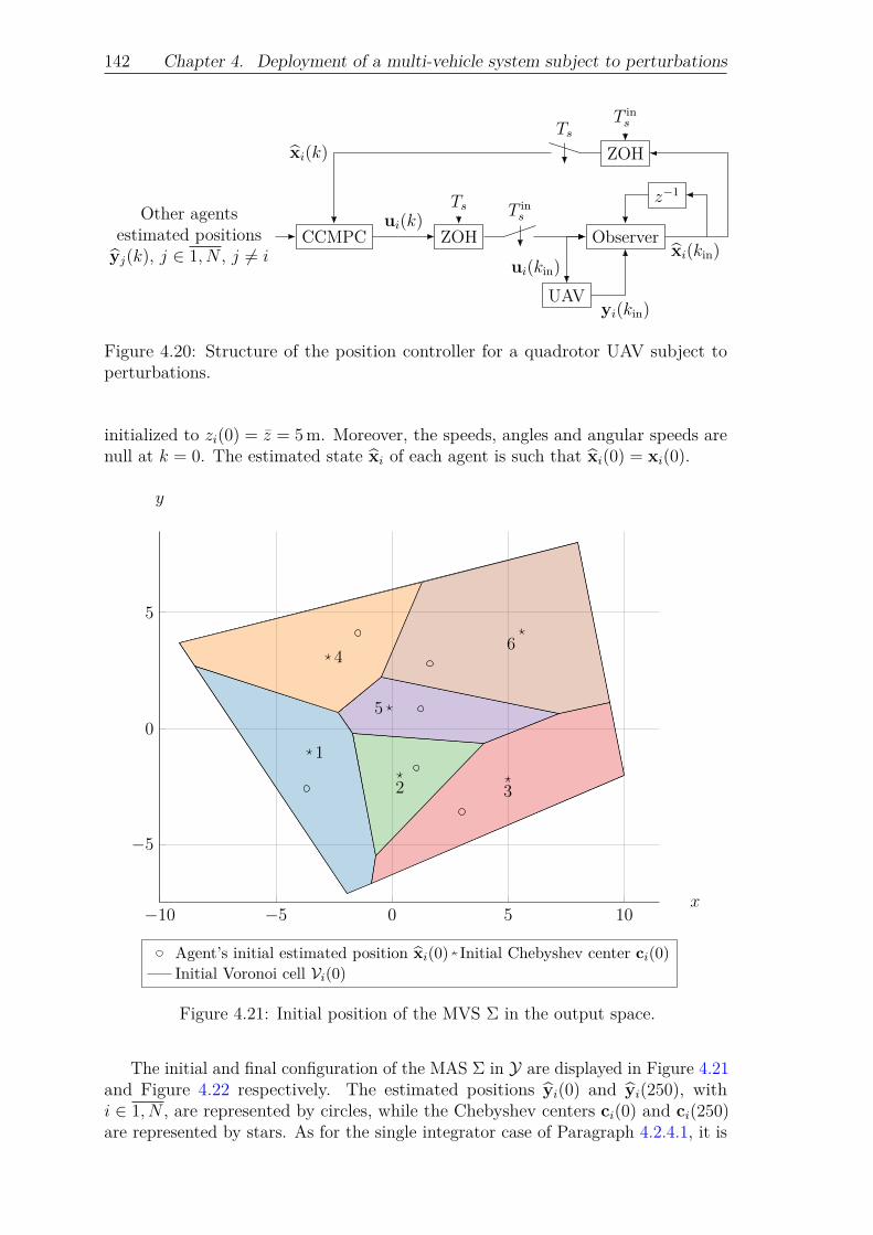
142 Chapter 4. Deployment of a multi-vehicle system subject to perturbations
CCMPC ZOH Observer
ZOH
UAV
z−1
T ins
xi(k)
ui(k)TsOther agents
estimated positionsyj(k), j ∈ 1, N , j 6= i
yi(kin)
T insTs
ui(kin)xi(kin)
Figure 4.20: Structure of the position controller for a quadrotor UAV subject toperturbations.
initialized to zi(0) = z = 5m. Moreover, the speeds, angles and angular speeds arenull at k = 0. The estimated state xi of each agent is such that xi(0) = xi(0).
−10 −5 0 5 10
−5
0
5
1
2 3
4
5
6
x
y
Agent’s initial estimated position xi(0) Initial Chebyshev center ci(0)
Initial Voronoi cell Vi(0)
Figure 4.21: Initial position of the MVS Σ in the output space.
The initial and final configuration of the MAS Σ in Y are displayed in Figure 4.21and Figure 4.22 respectively. The estimated positions yi(0) and yi(250), withi ∈ 1, N , are represented by circles, while the Chebyshev centers ci(0) and ci(250)are represented by stars. As for the single integrator case of Paragraph 4.2.4.1, it is

4.2. Unbounded stochastic perturbations 143
−10 −5 0 5 10
−5
0
5
x
y
Agent’s final estimated position xi(250) Final Chebyshev center ci(250)
Final Voronoi cell Vi(250)
Figure 4.22: Final position of the MVS Σ in the output space.
obvious from Figure 4.22 that the estimated position yi, with i ∈ 1, N , has reachedthe Chebyshev center ci of its Voronoi cell Vi. The real positions of the agents are notshown since, given the noise variances, they are close to the estimated position. Thisassertion is supported by the norm of the estimation errors shown in Figure 4.24.
As for the tube-based case, a measure of the convergence of Σ to a staticconfiguration is given by the distance between the estimated positions and theChebyshev centers:
di(k) = ‖yi(k)− ci(k)‖2
with i ∈ 1, N . As shown by Figure 4.23, all these distances converge to 0. However,the convergence is slower than in the bounded perturbations case of Paragraph 4.1.4.2due to the high level of noise. Indeed, a static configuration is reached in around 15 sfor the unbounded stochastic perturbations case, while it is reached in around 8 s forthe bounded deterministic perturbations case. Moreover, Figure 4.24 shows, as inthe single integrator case, that the norm of the estimation error remains boundedwith ‖xi(k)− xi(k)‖2 ≤ 42 cm. Due to the modified control strategy and the morecomplex dynamics, the norm of the estimation error is larger than the one obtainedin the single integrator case of Paragraph 4.2.4.1, where ‖xi(k)− xi(k)‖2 ≤ 0.8 cm.A similar approach than the one developed in Paragraph 4.2.4.1 could be developedhere to show that the error remains bounded when the mean of the process noise,i.e. the external disturbance, is not null.

144 Chapter 4. Deployment of a multi-vehicle system subject to perturbations
0 2 4 6 8 10 12 14 16 18 20 22 240
1
2
3
4
t (s)
d (m)
d1(k)d2(k)d3(k)d4(k)d5(k)d6(k)
Figure 4.23: Distance of the estimated position of each agent of Σ to its Chebyshevcenter over time.
0 5 10 15 20 25 30 35 40 45 500
0.1
0.2
0.3
0.4
t (s)
‖x‖2 (m)
‖x1(k)‖2‖x2(k)‖2‖x3(k)‖2‖x4(k)‖2‖x5(k)‖2‖x6(k)‖2
Figure 4.24: Norm of the estimation error for each agent of Σ.
4.3 ConclusionThis chapter presents two control strategies to perform the robust Voronoi-baseddeployment of a multi-agent system (MAS) where each agent is tracking the Cheby-shev center of the Voronoi cell or guaranteed Voronoi cell it belongs to. The vehiclescomposing the MAS are subject to perturbations either bounded deterministic orunbounded stochastic. In both cases, a solution based on model predictive control(MPC) has been proposed to adapt the deployment algorithm presented in Chapter 3to the perturbed case.
As a first step, the input and output perturbations are considered deterministicand bounded. Thus, a decentralized model predictive controller is derived fromexisting robust output feedback tube-based MPC (Mayne et al., 2006) and adapted for

4.3. Conclusion 145
the deployment control of a MAS. Such a control strategy is based on the knowledgeof invariant sets for error dynamics. In order for the optimization problem to remainfeasible, these invariant sets have to be of minimal size. Since their size depends onthe value of the observer and state feedback controller gain matrices appearing in theoutput feedback tube-based MPC strategy, tuning procedures derived from the onegiven by Alvarado (2007) are introduced. These procedures are used to obtain theobserver and state feedback gain matrices guaranteeing that the robust positivelyinvariant sets for the associated stable dynamics are of minimal size. Simulations arerun on both single integrator and nonlinear UAV dynamics to show that the MASdeploys in a static Chebyshev configuration with guarantees that the state of thesystem remains bounded inside a set such that, despite the perturbations, collisionsbetween the agents are avoided.
However, despite being efficient, such a strategy is limited in the case of realsystems, which opens the way to interesting future research directions. Indeed, inthe double integrator case, i.e. for the position control of a quadrotor unmannedaerial vehicles fleet, the strategy depends on the availability of measurements at animportant rate which is not realistic. This is due to the properties of the Luenbergerobserver which might not be adapted to such an application. Then, a more robustobserver should be used such as Kalman filter (Chui and Chen, 2017, Chevet et al.,2017) or even set-membership state estimation techniques (Le et al., 2013) on whichtube-based MPC techniques have already been studied (Le, 2012) in the case ofa single system. This last possibility could be coupled with the tuning procedureproposed in the present thesis since both are based on bilinear matrix inequalities.Indeed, one of the main point arising in the deployment problem is the appearanceof time-varying constraints, discussed in Chapter 3, in the optimization problem. Anonline computation of the invariant sets based on set-membership state estimationwould then allow to take such time-varying constraints into account, which is notthe case for the method proposed in the present thesis. However, an analysis of thecomputation time is necessary.
Then, in a second stage, stochastic and unbounded perturbations are considered.Such perturbations are then characterized by a mean and a variance matrix. Themean represents an external deterministic disturbance for the input perturbation ora sensor bias for the output perturbation while the variance matrix is related to theprocess or measurement noise to which the system is subject. To perform the robustdeployment of the MAS, a novel output feedback decentralized model predictivecontroller is derived from the state feedback chance-constrained MPC strategyintroduced in Gavilan et al. (2012). Indeed, Gavilan et al. (2012) proposes a state-feedback chance-constrained model predictive controller applied to a single system. Inthe present thesis, the control strategy is improved to obtain a decentralized output-feedback chance-constrained model predictive controller applied to a MAS. Thisstrategy consists in using the stochastic properties of the perturbations to computea probabilistic bound to the perturbation signal, relaxing the chance constraints ofthe optimization problem into algebraic constraints. Finally, simulations on a MAScomposed of agents obeying single integrator dynamics or nonlinear quadrotor UAVsdynamics show that the MAS deploys in a static Chebyshev configuration. Monte-Carlo simulations in the single integrator dynamics case show that the behavior ofsuch a control strategy is analogous to the robust tube-based MPC case in the sensethat, with the proposed chance-constrained MPC, the errors remain bounded.
As for the tube-based MPC case, such a strategy can be limited in the case of real

146 Chapter 4. Deployment of a multi-vehicle system subject to perturbations
systems. The same problem linked to the observer arises. Moreover, this strategy,with the formulation given in the present thesis, works for stochastic processescharacterized by their mean and variance matrix, i.e. the Gaussian processes. Alogical next step of the work presented in this thesis would be to adapt it to differentprobability distributions. Another possibility would be to study tube-based chance-constrained techniques as developed in Cannon et al. (2012) adapted to the caseof the deployment of a MAS. Indeed, the work of Cannon et al. (2012) and thesubsequent improvements of their algorithm as presented in Dai et al. (2015) or Daiet al. (2018), for example, are based on the assumption that the constraints areconstant over time while in the deployment case, the constraints are time-varying. Atube-based strategy could then be coupled with a set-membership state estimationtechnique or a tuning procedure similar to the one used for the tube-based MPCcase.

Chapter 5Extension to the deployment of atime-varying multi-vehicle system
Table of Contents
5.1 A first approach to reconfiguration . . . . . . . . . . . . . . . . . . 1485.1.1 Motivation . . . . . . . . . . . . . . . . . . . . . . . . . . . 1485.1.2 Problem formulation . . . . . . . . . . . . . . . . . . . . . . 150
5.1.2.1 Agent dynamics . . . . . . . . . . . . . . . . . . . 1505.1.2.2 Incoming agents . . . . . . . . . . . . . . . . . . . 1515.1.2.3 Outgoing agents . . . . . . . . . . . . . . . . . . . 153
5.1.3 Deployment results . . . . . . . . . . . . . . . . . . . . . . . 1595.1.3.1 Incoming agents . . . . . . . . . . . . . . . . . . . 1595.1.3.2 Outgoing agents . . . . . . . . . . . . . . . . . . . 162
5.2 A safer way to deal with outgoing vehicles . . . . . . . . . . . . . . 1655.2.1 Limitation of the first reconfiguration algorithm . . . . . . . 1655.2.2 Improved reconfiguration algorithm . . . . . . . . . . . . . . 169
5.2.2.1 A new transient objective . . . . . . . . . . . . . . 1695.2.2.2 A new reconfiguration algorithm . . . . . . . . . . 174
5.3 Reconfiguration in the case of outgoing agents . . . . . . . . . . . . 1785.3.1 Comparison of the two algorithms in the case of one outgoing
agent . . . . . . . . . . . . . . . . . . . . . . . . . . . . . . 1785.3.2 Reconfiguration in the case of multiple outgoing agents . . . 181
5.3.2.1 Reconfiguration for single integrator dynamics . . 1815.3.2.2 Reconfiguration for UAV dynamics . . . . . . . . . 187
5.4 Conclusion . . . . . . . . . . . . . . . . . . . . . . . . . . . . . . . . 191
Chapter 3 introduces the deployment problem of a multi-agent system over aconvex bounded area in the nominal case. For its part, Chapter 4 discusses the sameproblem when the agents are subject to input and output perturbations. In boththese chapters, the multi-agent system is constant over time, i.e. the number ofagents in the system does not evolve during the deployment. The present chapterdeals with the case where the number of agents is time varying. A first Voronoi-basedreconfiguration algorithm using a decentralized MPC approach is proposed for atime-varying multi-agent system (MAS). The considered dynamics for the agentsand the reconfiguration strategy when either agents join or one agent leaves theMAS are detailed. Finally results on the case of incoming agents and one outgoingagent during the deployment are presented.
After analyzing the possible limitations of the previous reconfiguration algorithmfor the case of several agents leaving the MAS, a robustified algorithm is proposed
147

148 Chapter 5. Extension to the deployment problem
to deal with the case of several simultaneous outgoing agents. A comparison isthen made between the two algorithms for the case of one outgoing agent beforepresenting reconfiguration results in simulation for the case of multiple outgoingagents with the robustified algorithm.
The algorithm for the case of agents joining the multi-agent system has beenintroduced in Chevet et al. (2018). For the case of agents leaving the system, Chevetet al. (2018) presents a novel decentralized MPC-based reconfiguration algorithm.For its part, Chevet et al. (2020b) robustifies the algorithm of Chevet et al. (2018)by designing a novel safe objective along with a safety region in which the remainingagents of the MAS evolve to avoid potential collisions with the outgoing agents.
5.1 A first approach to reconfigurationSection 5.1.1 inscribes the problem of the present chapter in the context of faulttolerant formation control. Then, Section 5.1.2 starts by introducing the generalagent dynamics used throughout this chapter, before presenting two reconfigurationalgorithms, one for the case of agents joining the multi-agent system, and one forthe case of agents leaving this system. Finally, Section 5.1.3 presents reconfigurationresults for both single integrator and nonlinear quadrotor unmanned aerial vehicledynamics.
5.1.1 MotivationThis thesis presents several control algorithms for the deployment of a multi-agentsystem (MAS). Despite being subject to perturbations, bias or noise, each agentis always considered healthy, that is, it is not subject to any fault. Varga (2017)defines a fault as an unexpected variation of one or several physical parameters of aplant leading it to evolve outside its normal operation mode. A fault can occur oneither an actuator, a sensor or an internal component (Blanke et al., 2000, Varga,2017). A fault can be characterized by a modification of the input or output signal(e.g. in this sense, the output perturbation considered in Section 4.1.1 can resultfrom a sensor fault) or a modification of the dynamics (e.g. a modification of the A,B and/or C matrices from the dynamics (2.40)). When a system can be subjectto a fault, a fault detection and isolation scheme has to be used to know when thesystem is faulty and on which part the fault acts exactly. When a system is faulty, afault-tolerant control scheme (Zhang and Jiang, 2008, Amin and Hasan, 2019) canbe used to mitigate the fault and allow the system to continue working despite thefault or reach a state in which it is possible to stop or repair it safely. Robust controlor adaptive control fall into the category of fault-tolerant control (Blanke et al.,2000) and, in this sense, the tube-based model predictive control scheme presented inSection 4.1.3 can be deemed as fault-tolerant since, as mentioned earlier, the outputperturbation can result from a sensor fault.
In the present chapter, the focus is not on a fault appearing on individual agentsbut rather on the multi-agent system itself. Such a fault consists in the addition orthe removal of one or several agents from the MAS in the case of MAS deployment.The removal of agents can result from faults occurring on these agents, from thechange in the mission objective resulting in the need of less agents in the MAS oreven from the need for these agents to recharge. The addition of agents results

5.1. A first approach to reconfiguration 149
mainly from the need of more agents in the MAS to carry out its mission. Forexample, in a search and rescue mission after an avalanche, more agents could beneeded to better cover the area around a victim after it was found. Then, the controlalgorithms presented in the following are part of a specific branch of fault-tolerantcontrol (FTC), i.e. fault-tolerant formation control (FTFC).
FTFC strategies often rely on a predefined formation (Kamel et al., 2020). Whenone or several agents taking part in this formation are faulty, based on the severityof the fault, a modification on the control algorithm is made. Then, Kamel et al.(2020) define three categories of FTFC (also called fault-tolerant cooperative control)strategies in the case of unmanned ground vehicles that are immediately transposableto the case of any vehicle.
The first two are strategies that can be used to mitigate mild to moderate faults,i.e. faults that do not incapacitate the agent, namely individual FTFC and motionre-coordination. Individual FTFC consists in using a FTC strategy (Blanke et al.,2016) directly on the faulty agent to mitigate the fault effect while the other agentscontinue their mission as if nothing happened. In this case, used for example in Zhouet al. (2014), Xu et al. (2014), Hua et al. (2017) or Khalili et al. (2019), the formationbehavior is not taken into account for the mitigation strategy and each faulty agentadapts its control law to be able to continue the mission of the MAS. For its part,motion re-coordination consists in adapting the control algorithm of both healthyand faulty agents. It takes into account the capabilities of the faulty agents suchthat the healthy ones limit their movement to maintain the formation’s integrityor carry out a larger part of the mission to lighten the faulty agents’ task. Forexample, when the mission involves path following, a re-planning of the trajectoryis performed so that, even with limited physical capabilities, each agent is able tofollow the new trajectory. This kind of method is find for example in Chamseddineet al. (2012), Wang et al. (2014) or Yu et al. (2016). In the case of consensus-basedalgorithms, such as in Saboori and Khorasani (2015), the motion re-coordinationstrategy involves the decrease of the importance of the faulty agents to carry outthe mission.
Finally, the third category is the one to which the algorithms of this chapterbelong to: the category of task assignment strategies. However, while Kamel et al.(2020) limit it to the case of severe fault occurring on one or several agents, here,only moderate faults (or even no faults) are considered. Nevertheless, such strategiescome from the need for a faulty (or not) agent to leave the formation or, in thepresent case, for a healthy agent to join the formation. Then, the healthy agentsremaining in the formation have to reconfigure themselves to adopt a new formationeither without the outgoing agents (faulty or not) or with the incoming healthyagents. In the case of path following for a formation of vehicles, a natural strategy,used for example in Kamel et al. (2015) or Hafez and Kamel (2016), is to “abandon”the faulty agent along the way. Then, the healthy agents adopt a new formationshape while avoiding collision with the agent left behind. Strategies of the same kindcan be found in Ghamry and Zhang (2016) or Huang et al. (2019).
In the present work, no path following or any global movement of the formationis involved. Thus, task assignment strategies as presented in the cited publicationsare not easily applicable. Indeed, these methods, proposed for MAS composed ofvarious kinds of vehicles, involve leaving faulty agents where they are, while theothers continue their movement. For the deployment problem, it is not possible forthe faulty agent to be abandoned where it is since it would become an obstacle to

150 Chapter 5. Extension to the deployment problem
the deployment of the MAS. In this chapter, task assignment methods are tingedwith motion re-coordination. Indeed, the idea is to have the healthy agents makingroom for the faulty ones to leave the workspace without colliding with other agents.The collision avoidance concern is then left to the healthy agents with respect to thelimited physical capabilities of the faulty agents, hence the motion re-coordinationidea. However, since the main objective is to remove (or integrate) agents fromthe formation, the algorithms of this chapter indeed belong to the task assignmentfamily.
The proposed methods are meant to be applied on any type of multi-vehiclesystem. Then, since they can be applied to unmanned ground or surface vehicles,they are developed for a deployment and reconfiguration mission in a two-dimensionalplanar area. It could be argued that for vehicles able to move in the three spatialdirections, such as unmanned aerial vehicles, the agents leaving the workspace inwhich the MAS is deployed could change their altitude and then move away fromthe workspace. However, if such a vehicle is faulty, it could be impossible for it toincrease its altitude, and in missions such as forest fire monitoring, decreasing thealtitude might be dangerous for the vehicle, leading potentially to its total loss. Forthese reasons, the methods presented in the following are developed for a planarmovement, despite the potential three-dimensional movement capabilities of somevehicles.
In the case of outgoing agents, the control algorithms presented in this chapterare based on a novel transient objective for the healthy agents ensuring collisionavoidance with the faulty agents by construction. These algorithms are based on thework of Chevet et al. (2018) and Chevet et al. (2020b). The control algorithm forthe case of incoming agents incorporates the new vehicles in a natural extension ofthe deployment algorithm presented in Chapter 3. It is based on the work of Chevetet al. (2018).
5.1.2 Problem formulation5.1.2.1 Agent dynamics
Let Σ be a multi-agent system composed of N agents. Each agent obeys discrete-timelinear time-invariant dynamics as in Chapter 3. The general dynamics are the sameas the one used in Chapter 3, i.e.:
xi(k + 1) = Axi(k) +Bui(k) (5.1a)yi(k) = Cxi(k) (5.1b)
where xi ∈ X ⊂ Rn, ui ∈ U ⊂ Rm, yi ∈ Y ⊂ R2, A ∈ Rn×n, B ∈ Rn×m andC ∈ R2×n, with i ∈ 1, N . As in the previous chapters, the multi-agent systemis homogeneous by Assumption 2.6, the dependency in the identifier i is droppedfor the matrices A, B and C as well as for the state, input and output spacesX , U and Y. All the agents share the same two-dimensional output space (orworkspace) by Assumption 2.3 and the system (5.1) admits equilibrium points asper Assumption 3.2.
When the multi-agent system operates normally, each agent follows the deploy-ment algorithm presented in Section 3.2.2. The properties of the model predictivecontroller are the same as the one described in Section 3.2.2. In this case, thealgorithm followed by the MAS presents no difference with Algorithm 3.2.

5.1. A first approach to reconfiguration 151
However, this chapter aims to improve this algorithm to make it resilient to theaddition or removal of one or several agents to the MAS. Thus, in the nominal case,i.e. when the system operates without modification in the number of agents, it isclear that the MAS is simply deployed in the workspace Y and the algorithm needsnot be modified. Nevertheless, Paragraph 5.1.2.2 introduces the modification of thealgorithm to make it able to integrate agents in the MAS. Moreover, Paragraph 5.1.2.3presents a new algorithm to make the MAS able to be deployed in Y while agentsleave Y without causing collisions with the remaining agents.
5.1.2.2 Incoming agents
Let E be a set of agents present in R2 \ Y . The objective for the incoming agents ofE (which can also be called entering agents) is to join Σ, while Σ is deployed insideY. Thus, the goal for E is to enter Y. After entering Y, the set E is part of Σ andparticipates in the deployment of the multi-agent system Σ. With this in mind, thefollowing paragraph is a natural extension of the decentralized deployment algorithmpresented in Section 3.2.2 to allow the agents outside the workspace to participatein the deployment of Σ.
The objective of the present control algorithm is then to drive the agents of Einside the workspace Y with a decentralized model predictive controller. To do so,an objective point yE
i (k) for each agent i ∈ 1, |E| of E is defined as the point in theinterior of Y, i.e. the point of Y \ ∂Y, where ∂Y is the border of Y, closer to theposition yi(k) of agent i than any other point of Y \ ∂Y . This property is translatedmathematically as:
yEi (k) = argmin
y∈Y\∂Y‖yi(k)− y‖2, ∀i ∈ 1, |E|. (5.2)
This point yEi (k) is chosen since it is computationally easy to obtain and, given the
deployment strategy followed by the agents of Σ, the incoming agents of E enter theworkspace Y at a point relatively far from the position of the deploying agents of Σ.
Then, since yEi (k) ∈ Y, it is possible, according to Assumption 3.2, to find a
couple(xEi (k),u
Ei (k)
)such that
(xEi (k),u
Ei (k),y
Ei (k)
)is an equilibrium point of the
dynamics (5.1):
xEi (k) = AxE
i (k) +BuEi (k)
yEi (k) = CxE
i (k).(5.3)
The couple(xEi (k),u
Ei (k)
)is then used as a reference point for the decentralized
MPC algorithm driving agent i of E. When agent i enters Y , it switches from E toΣ and starts participating in the deployment of Σ by following Algorithm 3.2.
While the agents of Σ follow Algorithm 3.2, the agents of E compute their input

152 Chapter 5. Extension to the deployment problem
ui(k), with i ∈ 1, |E|, by finding the solution to the optimization problem:
minimizeui(k+l),
∀l∈0,Np−1
Np−1∑l=0
`(xi(k + l),ui(k + l),xE
i (k),uEi (k)
)+ V
(xi(k +Np),x
Ei (k)
)(5.4a)
subject to
xi(k + l + 1) = Axi(k + l) +Bui(k + l), ∀l ∈ 0, Np − 1, (5.4b)xi(k + l) ∈ XE, ∀l ∈ 0, Np − 1, (5.4c)ui(k + l) ∈ U , ∀l ∈ 0, Np − 1 (5.4d)
where `(xi(k + l),ui(k + l),xE
i (k),uEi (k)
), with l ∈ 0, Np − 1, is the stage cost:
`(xi(k + l),ui(k + l),xE
i (k),uEi (k)
)=∥∥xi(k + l)− xE
i (k)∥∥2QE
i+∥∥ui(k + l)− uE
i (k)∥∥2RE
i(5.5)
and V(xi(k +Np),x
Ei (k)
)is the terminal cost:
V(xi(k +Np),x
Ei (k)
)=∥∥xi(k +Np)− xE
i (k)∥∥2PE
i. (5.6)
The weighting matrices QEi ,P
Ei ∈ Rn×n and RE
i ∈ Rm×m in (5.5) and (5.6) arechosen such that QE
i = QEi> 0, P E
i = P Ei
> 0 and REi = RE
i> 0. The
prediction horizon Np is a positive integer.The constraint (5.4b) is used to predict the future state xi(k + l + 1) for all
l ∈ 0, Np − 1 of the agent i ∈ 1, |E| given the value of the input sequence ui(k+ l) forall l ∈ 0, Np − 1. The other two constraints are meant to restrict the movement ofagent i of E. Constraint (5.4d) is meant to ensure that, over the prediction horizonNp, the input signal of the agent remains inside a convex polytope U , the input spaceof the agent, obtained from limitations on the actuators (e.g. physical limitations)or from the considered application. Moreover, constraint (5.4c) ensures that, overthe prediction horizon, the state remains inside a convex polyhedron XE obtainedfrom the potential physical limitations of the system.
♦
Remark 5.1: Output constraintsContrary to the MPC optimization problem (3.12), XE does not impose constraintson the position of the agent since it is not restricted to evolve in Y but can moveinside R2.
For the reason invoked in Remark 5.1, contrary to the deployment algorithm ofSection 3.2.2, no constraint on the output appears in problem (5.4). Indeed, for theagents of E, the objective is to rally Σ. Then, it is unnecessary to enforce the factthat the outputs of the agents belong to a given area.
Agent i ∈ 1, |E| uses (5.4) to compute its input signal until it reaches Y . Whenthis agent is such that yi(k) ∈ Y , it leaves E and joins Σ. As soon as it joins Σ, itstarts participating in the deployment of Σ in Y by following Algorithm 3.2. Thisprocedure is summarized by Algorithm 5.1.
Such a procedure does not impact the agents already present in Y . Indeed, thedecentralized algorithm used for the deployment of the MAS, i.e. Algorithm 3.2,makes the agents dependent only on the knowledge of the position of the other
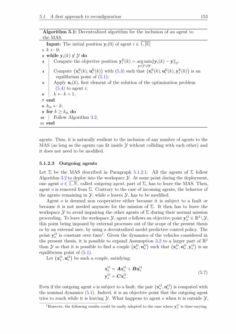
5.1. A first approach to reconfiguration 153
Algorithm 5.1: Decentralized algorithm for the inclusion of an agent tothe MAS.
Input: The initial position yi(0) of agent i ∈ 1, |E|1 k ← 0;2 while yi(k) 6∈ Y do3 Compute the objective position yE
i (k) = argminy∈Y\∂Y
‖yi(k)− y‖2;
4 Compute(xEi (k),u
Ei (k)
)with (5.3) such that
(xEi (k),u
Ei (k),y
Ei (k)
)is an
equilibrium point of (5.1);5 Apply ui(k), first element of the solution of the optimization problem
(5.4) to agent i;6 k ← k + 1;7 end8 kin ← k;9 for k ≥ kin do
10 Follow Algorithm 3.2;11 end
agents. Thus, it is naturally resilient to the inclusion of any number of agents to theMAS (as long as the agents can fit inside Y without colliding with each other) andit does not need to be modified.
5.1.2.3 Outgoing agents
Let Σ be the MAS described in Paragraph 5.1.2.1. All the agents of Σ followAlgorithm 3.2 to deploy into the workspace Y . At some point during the deployment,one agent o ∈ 1, N , called outgoing agent, part of Σ, has to leave the MAS. Then,agent o is removed from Σ. Contrary to the case of incoming agents, the behavior ofthe agents remaining in Y , while o leaves Y , has to be modified.
Agent o is deemed non cooperative either because it is subject to a fault orbecause it is not needed anymore for the mission of Σ. It then has to leave theworkspace Y to avoid impairing the other agents of Σ during their normal missionproceeding. To leave the workspace Y , agent o follows an objective point yO
o ∈ R2\Y ,this point being imposed by external processes out of the scope of the present thesisor by an external user, by using a decentralized model predictive control policy. Thepoint yO
o is constant over time1. Given the dynamics of the vehicles considered inthe present thesis, it is possible to expand Assumption 3.2 to a larger part of R2
than Y so that it is possible to find a couple(xOo ,u
Oo
)such that
(xOo ,u
Oo ,y
Oo
)is an
equilibrium point of (5.1).Let
(xOo ,u
Oo
)be such a couple, satisfying:
xOo = AxO
o +BuOo
yOo = CxO
o .(5.7)
Even if the outgoing agent o is subject to a fault, the pair(xOo ,u
Oo
)is computed with
the nominal dynamics (5.1). Indeed, it is an objective point that the outgoing agenttries to reach while it is leaving Y. What happens to agent o when it is outside Y,
1However, the following results could be easily adapted to the case where yOo is time-varying.
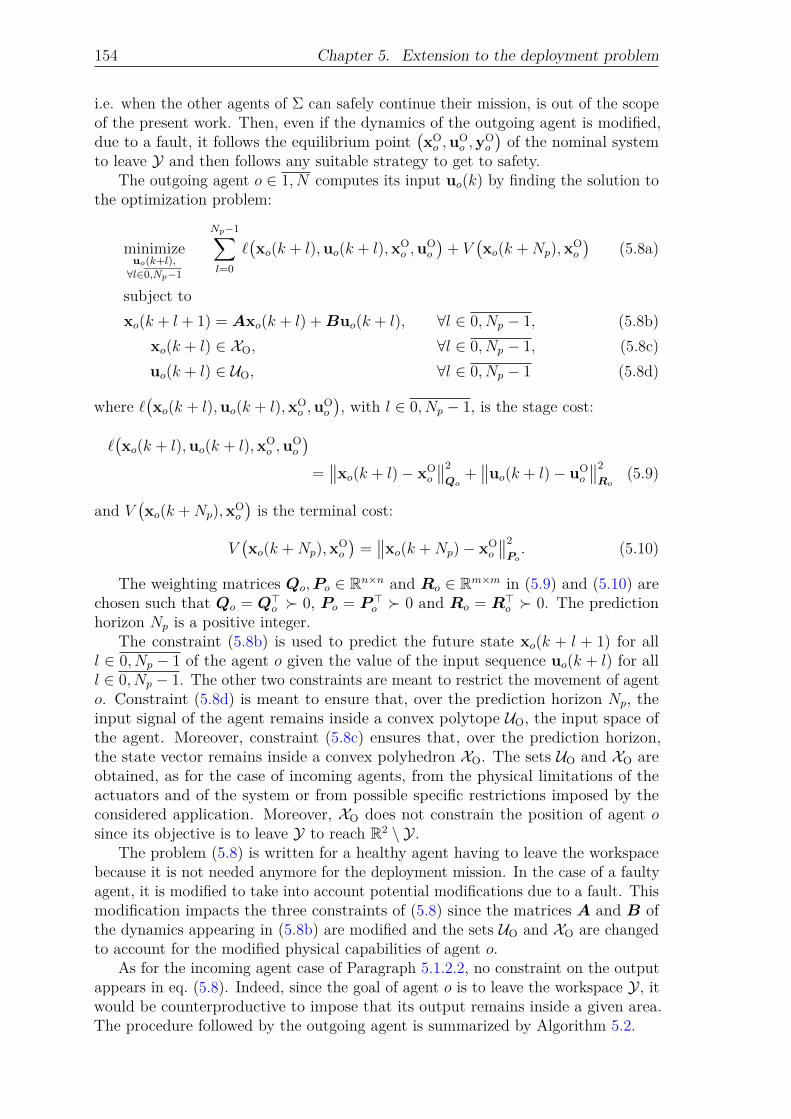
154 Chapter 5. Extension to the deployment problem
i.e. when the other agents of Σ can safely continue their mission, is out of the scopeof the present work. Then, even if the dynamics of the outgoing agent is modified,due to a fault, it follows the equilibrium point
(xOo ,u
Oo ,y
Oo
)of the nominal system
to leave Y and then follows any suitable strategy to get to safety.The outgoing agent o ∈ 1, N computes its input uo(k) by finding the solution to
the optimization problem:
minimizeuo(k+l),
∀l∈0,Np−1
Np−1∑l=0
`(xo(k + l),uo(k + l),xO
o ,uOo
)+ V
(xo(k +Np),x
Oo
)(5.8a)
subject to
xo(k + l + 1) = Axo(k + l) +Buo(k + l), ∀l ∈ 0, Np − 1, (5.8b)xo(k + l) ∈ XO, ∀l ∈ 0, Np − 1, (5.8c)uo(k + l) ∈ UO, ∀l ∈ 0, Np − 1 (5.8d)
where `(xo(k + l),uo(k + l),xO
o ,uOo
), with l ∈ 0, Np − 1, is the stage cost:
`(xo(k + l),uo(k + l),xO
o ,uOo
)=∥∥xo(k + l)− xO
o
∥∥2Qo
+∥∥uo(k + l)− uO
o
∥∥2Ro
(5.9)
and V(xo(k +Np),x
Oo
)is the terminal cost:
V(xo(k +Np),x
Oo
)=∥∥xo(k +Np)− xO
o
∥∥2Po
. (5.10)
The weighting matrices Qo,Po ∈ Rn×n and Ro ∈ Rm×m in (5.9) and (5.10) arechosen such that Qo = Q>
o 0, Po = P>o 0 and Ro = R>
o 0. The predictionhorizon Np is a positive integer.
The constraint (5.8b) is used to predict the future state xo(k + l + 1) for alll ∈ 0, Np − 1 of the agent o given the value of the input sequence uo(k + l) for alll ∈ 0, Np − 1. The other two constraints are meant to restrict the movement of agento. Constraint (5.8d) is meant to ensure that, over the prediction horizon Np, theinput signal of the agent remains inside a convex polytope UO, the input space ofthe agent. Moreover, constraint (5.8c) ensures that, over the prediction horizon,the state vector remains inside a convex polyhedron XO. The sets UO and XO areobtained, as for the case of incoming agents, from the physical limitations of theactuators and of the system or from possible specific restrictions imposed by theconsidered application. Moreover, XO does not constrain the position of agent osince its objective is to leave Y to reach R2 \ Y .
The problem (5.8) is written for a healthy agent having to leave the workspacebecause it is not needed anymore for the deployment mission. In the case of a faultyagent, it is modified to take into account potential modifications due to a fault. Thismodification impacts the three constraints of (5.8) since the matrices A and B ofthe dynamics appearing in (5.8b) are modified and the sets UO and XO are changedto account for the modified physical capabilities of agent o.
As for the incoming agent case of Paragraph 5.1.2.2, no constraint on the outputappears in eq. (5.8). Indeed, since the goal of agent o is to leave the workspace Y , itwould be counterproductive to impose that its output remains inside a given area.The procedure followed by the outgoing agent is summarized by Algorithm 5.2.

5.1. A first approach to reconfiguration 155
Algorithm 5.2: Decentralized algorithm for the removal of the agent ofrom the MAS.1 for k ≥ 0 do2 if agent o leaves Σ then3 kout ← k;4 Go to 9;5 else6 Follow Algorithm 3.2;7 end8 end9 Acquire the objective point yO
o ;10 Compute the couple
(xOo ,u
Oo
)with (5.7) such that
(xOo ,u
Oo ,y
Oo
)is an
equilibrium point of (5.1);11 for k ≥ kout do12 Solve the optimization problem (5.8) to obtain the input signal uo(k);13 Apply uo(k) to the agent;14 end
However, contrary to the case of Paragraph 5.1.2.2, the other agents of Σ whichdo not leave the workspace Y do not follow Algorithm 3.2. As mentioned earlier,their behavior is modified to avoid collisions with the outgoing agent o. This firstapproach has been introduced in Chevet et al. (2018).
Assumption 5.1: Knowledge of the outgoing agentThe agents of Σ know the position yo(k) and the objective yO
o of the outgoing agent o.
Definition 5.1: Neighbor of an agent
For an agent i ∈ 1, N \ o of Σ, a neighbor ν of agent i is one of the following:
• another agent of Σ having a Voronoi cell contiguous to Vi(k);
• the outgoing agent o if its Voronoi cell is contiguous to Vi(k);
• a vertex of Vi(k) lying on ∂Y .
The set of all neighbors of agent i at time k is denoted by Ni(k).
The position yo(k) ∈ R2 and the objective yOo of the outgoing agent o define
a hyperplane ∂Ho(k) = x ∈ R2 | ho(k)x = θo(k) in R2, where ho(k) ∈ R1×2 andθo(k) ∈ R, which is known by each agent of Σ as per Assumption 5.1. Then, a newobjective point, different from the Chebyshev center ci(k) of the Voronoi cell Vi(k),is computed for each agent i ∈ 1, N \ o. This new objective point is the barycenterybi (k) ∈ R2 of the neighbors of agent i as defined in Definition 5.1:
ybi (k) =
∑ν∈Ni(k)
ων,i(k)yν(k)∑ν∈Ni(k)
ων,i(k)(5.11)

156 Chapter 5. Extension to the deployment problem
where ων,i(k) is a weight attributed to the neighbor ν ∈ Ni(k) of agent i ∈ 1, N \ odepending on its relative position to ∂Ho(k) and yν(k) ∈ R2 is the position of theneighbor ν ∈ Ni(k). A procedure has then to be designed to attribute the weightsων,i(k) to the neighbors.
Let d(yi(k), ∂Ho(k)) denote the distance of agent i ∈ 1, N \o to the hyperplane∂Ho(k) defined as:
d(yi(k), ∂Ho(k)) = miny∈∂Ho(k)
‖yi(k)− y‖2.
If the conditions:
• d(yν(k), ∂Ho(k)) ≥ d(yi(k), ∂Ho(k)), with ν ∈ Ni(k), i.e. the neighbor ν ∈Ni(k) is farther from ∂Ho(k) than agent i;
• ho(k)(yν(k)− yo(k)) · ho(k)(yi(k)− yo(k)) ≥ 0, with ν ∈ Ni(k), i.e. theneighbor ν and agent i belong to the same half-space delimited by ∂Ho(k)
are met, then ων,i(k) = κ, where κ ∈ R, with κ > 1. Else, ων,i(k) = 1. With such achoice of weights, the barycenter ends up driving the remaining agent i away fromthe trajectory of the outgoing agent, thus leaving room for the outgoing agent toleave Y safely. This procedure is summarized in Algorithm 5.3.
Algorithm 5.3: Computation of the neighbors’ barycenter of a remainingagent of Σ.
Input: The list of neighbors Ni(k) of agent i ∈ 1, N \ o, the position ofthe neighbors yν(k), ∀ν ∈ Ni(k), the position of the outgoing agentyo(k), the hyperplane ∂Ho(k) = x ∈ R2 | ho(k)x ≤ θo(k)
1 for ν ∈ Ni(k) do2 if ho(k)(yν(k)− yo(k)) · ho(k)(yi(k)− yo(k)) ≥ 0 then3 if d(yν(k), ∂Ho(k)) > d(yi(k), ∂Ho(k)) then4 ων,i(k)← κ;5 else6 ων,i(k)← 1;7 end8 else9 ων,i(k)← 1;
10 end11 end12 Compute the neighbors’ barycenter of agent i with (5.11);
Output: The neighbors’ barycenter ybi (k) of agent i
Example 5.1: Construction of a neighbor’s barycenterLet Σ be a MAS composed of 10 agents deployed in Y = B2(10 · 12×1) as presentedin Figure 5.1. At a given time k, agent 3 has to leave Σ and the workspace Y.It has for objective yO
3 =[−9 −12
]> ∈ R2 \ Y, chosen arbitrarily and depictedby asterisks in Figure 5.1, which defines with y3(k) the hyperplane ∂H3(k) =x ∈ R2 | h3(k)x = θ3(k), represented as a solid line in Figure 5.1.
This example then presents how the neighbors’ barycenters of the agents 2 and 5are obtained. The hyperplanes ∂D2(k) and ∂D5(k), represented with dashed lines,

5.1. A first approach to reconfiguration 157
are the sets of all the points of R2 at the same distance of the hyperplane ∂H3(k) asagents 2 and 5, respectively, defined as:
∂Di(k) =x ∈ R2
∣∣ d(x, ∂H3(k)) = d(yi(k), ∂H3(k))
where i ∈ 2, 5. They are presented in Figure 5.1 to graphically compare thedistances but are not necessary for the real procedure.
Agents 4, 5, 8, 9 and 10 have a Voronoi cell contiguous to V2(k), the Voronoi cellV3(k) of the outgoing agent 3 is also contiguous to V2(k) and 11 and 12 are verticesof V2(k) lying on ∂Y. Then, by Definition 5.1, the set of neighbors of agent 2 isN2(k) = 3, 4, 5, 8, 9, 10, 11, 12. Agents 2, 6 and 9 have a Voronoi cell contiguousto V5(k) and the Voronoi cell V3(k) of the outgoing agent 3 is contiguous to V5(k).Then, by Definition 5.1, the set of neighbors of agent 5 is N5(k) = 2, 3, 6, 9.
It can be seen in Figure 5.1 that d(yν(k), ∂H3(k)) ≥ d(y2(k), ∂H3(k)) andh3(k)(yν(k)− y3(k)) · h3(k)(y2(k)− y3(k)) ≥ 0 for all ν ∈ 8, 10, 11, 12. Then,ων,2(k) = κ for all ν ∈ 8, 10, 11, 12, while ων,2(k) = 1 for all ν ∈ 3, 4, 5, 9.Again, it can be seen in Figure 5.1 that only neighbor 2 is located further from∂H3(k) than agent 5 among the neighbors that are on the same side of ∂H3(k)as agent 5, thus d(y2(k), ∂H3(k)) ≥ d(y5(k), ∂H3(k)) and h3(k)(y2(k)− y3(k)) ·h3(k)(y5(k)− y3(k)) ≥ 0. Then ω2,5(k) = κ, while ων,5(k) = 1 for all ν ∈ 3, 6, 9.
From (5.11), the barycenters are:
yb2(k) =
κ(y8(k) + y10(k) + y11(k) + y12(k)) + y3(k) + y4(k) + y5(k) + y9(k)
4(κ+ 1)
yb5(k) =
κy2(k) + y3(k) + y6(k) + y9(k)
κ+ 3
where y11(k) and y12(k) are the coordinates in R2 of the vertices of V2(k) lying on∂Y.
When κ = 3, the neighbors’ barycenter of agents 2 and 5 are presented inFigure 5.1 with squares. The other neighbors’ barycenter of agents 1, 4, 6, 7, 8, 9and 10 can then be obtained the same way.
♦
Remark 5.2: Heterogeneous MASIn the case of heterogeneous MAS, different weights κi could be considered fordifferent type of vehicles.
While the outgoing agent o is inside Y , i.e. while yo(k) ∈ Y , the objective pointof the agents of Σ is changed from the Chebyshev center ci(k) of the Voronoi cellVi(k), with i ∈ 1, N \o, to the neighbors’ barycenter yb
i (k). With such an objectivepoint, the agents of Σ are driven away from the trajectory of the outgoing agent orepresented by the hyperplane ∂Ho(k).
According to Assumption 3.2, there exists a couple(xbi (k),u
bi (k)
), with i ∈
1, N \ o, such that(xbi (k),u
bi (k),y
bi (k)
)is an equilibrium point of (5.1) satisfying:
xbi (k) = Axb
i (k) +Bubi (k)
ybi (k) = Cxb
i (k).(5.12)

158 Chapter 5. Extension to the deployment problem
−10 −5 0 5 10
−10
−5
0
5
10
Y∂H3(k)
∂D5(k)∂D2(k)
1
2 3
4
5
6
7
8
9
10
1112
yO3
yb2(k)
yb5(k)
x
y
Agent’s position yi(k) Neighbors’ barycenter ybi (k), i ∈ 2, 5
Vertices of V2(k) lying on ∂Y
Figure 5.1: Example of construction of a neighbors’ barycenter for MAS reconfigura-tion when one agent leaves the workspace.
Then, the agents of Σ compute their input ui(k), with i ∈ 1, N \ o, by finding thesolution of the optimization problem:
minimizeui(k+l),
∀l∈0,Np−1
Np−1∑l=0
`(xi(k + l),ui(k + l),xb
i (k),ubi (k)
)+ V
(xi(k +Np),x
bi (k)
)(5.13a)
subject to
xi(k + l + 1) = Axi(k + l) +Bui(k + l), ∀l ∈ 0, Np − 1, (5.13b)xi(k + l) ∈ X , ∀l ∈ 0, Np − 1, (5.13c)ui(k + l) ∈ U , ∀l ∈ 0, Np − 1, (5.13d)
Cxi(k + l) ∈ Vi(k), ∀l ∈ 0, Np − 1, (5.13e)xi(k +Np) ∈ Ωi(k) (5.13f)
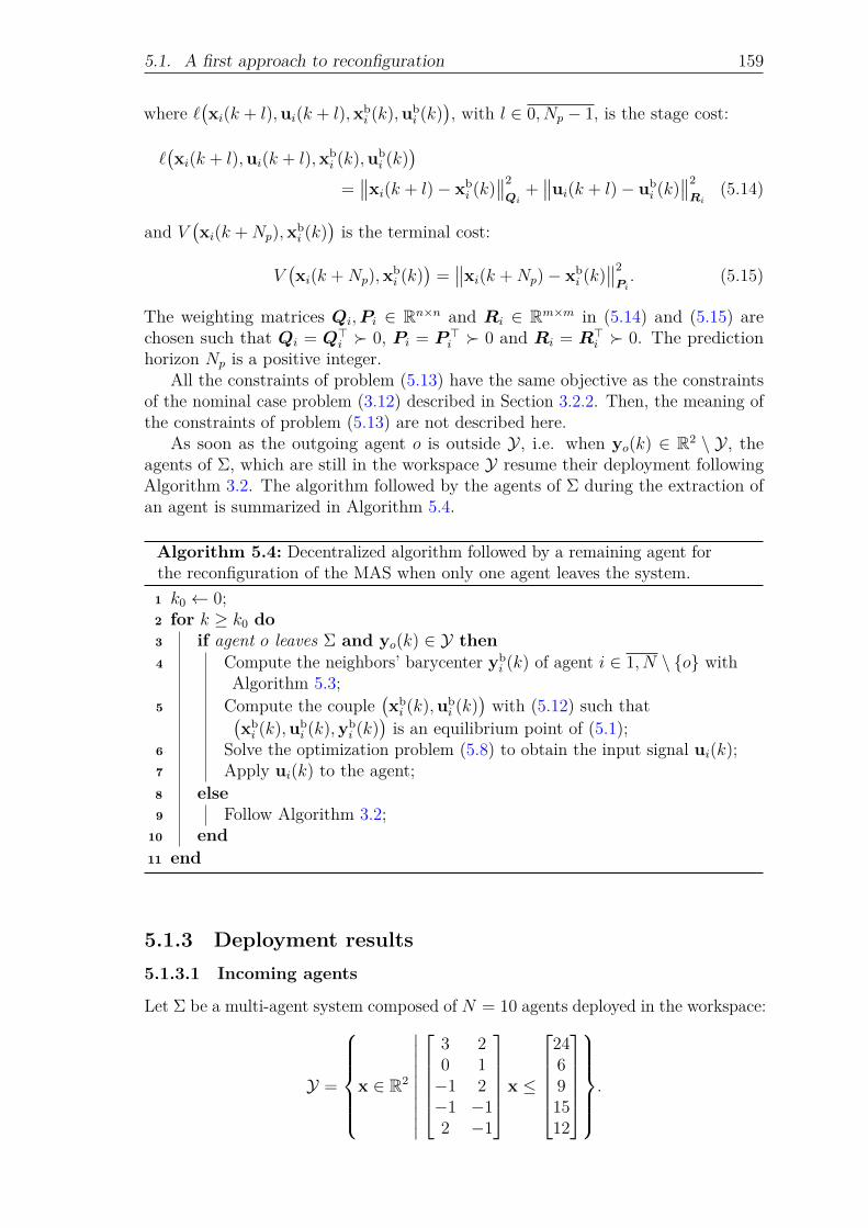
5.1. A first approach to reconfiguration 159
where `(xi(k + l),ui(k + l),xb
i (k),ubi (k)
), with l ∈ 0, Np − 1, is the stage cost:
`(xi(k + l),ui(k + l),xb
i (k),ubi (k)
)=∥∥xi(k + l)− xb
i (k)∥∥2Qi
+∥∥ui(k + l)− ub
i (k)∥∥2Ri
(5.14)
and V(xi(k +Np),x
bi (k)
)is the terminal cost:
V(xi(k +Np),x
bi (k)
)=∥∥xi(k +Np)− xb
i (k)∥∥2Pi
. (5.15)
The weighting matrices Qi,Pi ∈ Rn×n and Ri ∈ Rm×m in (5.14) and (5.15) arechosen such that Qi = Q>
i 0, Pi = P>i 0 and Ri = R>
i 0. The predictionhorizon Np is a positive integer.
All the constraints of problem (5.13) have the same objective as the constraintsof the nominal case problem (3.12) described in Section 3.2.2. Then, the meaning ofthe constraints of problem (5.13) are not described here.
As soon as the outgoing agent o is outside Y, i.e. when yo(k) ∈ R2 \ Y, theagents of Σ, which are still in the workspace Y resume their deployment followingAlgorithm 3.2. The algorithm followed by the agents of Σ during the extraction ofan agent is summarized in Algorithm 5.4.
Algorithm 5.4: Decentralized algorithm followed by a remaining agent forthe reconfiguration of the MAS when only one agent leaves the system.1 k0 ← 0;2 for k ≥ k0 do3 if agent o leaves Σ and yo(k) ∈ Y then4 Compute the neighbors’ barycenter yb
i (k) of agent i ∈ 1, N \ o withAlgorithm 5.3;
5 Compute the couple(xbi (k),u
bi (k)
)with (5.12) such that(
xbi (k),u
bi (k),y
bi (k)
)is an equilibrium point of (5.1);
6 Solve the optimization problem (5.8) to obtain the input signal ui(k);7 Apply ui(k) to the agent;8 else9 Follow Algorithm 3.2;
10 end11 end
5.1.3 Deployment results5.1.3.1 Incoming agents
Let Σ be a multi-agent system composed of N = 10 agents deployed in the workspace:
Y =
x ∈ R2
∣∣∣∣∣∣∣∣∣∣
3 20 1−1 2−1 −12 −1
x ≤
24691512
.

160 Chapter 5. Extension to the deployment problem
Three agents 11, 12 and 13 start respectively from:
y11(0) =
[−10−10
]y12(0) =
[−105
]y13(0) =
[5−10
]while the other agents start from random positions yi(0) ∈ Y , with i ∈ 1, N . All theagents obey the single integrator dynamics (3.15) and the reconfiguration algorithmin the case of incoming agents is tested only with agents obeying this dynamics since,as for the nominal deployment case of Chapter 3, the results are quite similar in theUAV dynamics case.
The objective of the agents of Σ is to deploy into a Chebyshev configuration asin Chapter 3 while agents 11, 12 and 13 aim to join Y to integrate Σ and participatein the deployment. Their initial objectives to enter the workspace are, respectively:
yE11(0) =
[−7.125−7.125
]yE12(0) =
[−7.710.42
]yE13(0) =
[1.56−8.28
]as obtained from (5.2). Then, from (5.3), since A = I2, B = TsI2, where Tsis the sampling period, and C = I2, xE
i (0) = yEi (0) and uE
i (0) = 02×1 for alli ∈ 11, 12, 13.
The sampling period used is Ts = 0.2 s and the contraction factor for the terminalconstraint is λi = 0.9 with a prediction horizon Np = 10. The results exposed hereare more succinct than those presented in the previous paragraphs since they areclose to what happens in the nominal case in Section 3.2.4.
The considered dynamics is the same as the one presented in Section 3.2.4. Theinput set is then still U = B2(2 · 12×1), while the weighting matrices are chosen suchthat Qi = Ri = I2 and Pi is the solution of the algebraic Riccati equation for alli ∈ 1, N . These tuning parameters are used for the deploying agents of Σ driven withthe MPC (3.12). Meanwhile, for the incoming agents driven with the MPC (5.4),UE = U , QE
i = REi = I2 and P E
i is the solution of the algebraic Riccati equation forall i ∈ 11, 13. Since the state vector of the incoming agents is exactly the position ofthese agents, as discussed in Paragraph 5.1.2.2, XE = R2 and (5.4c) can be dropped.The solvers for optimization problems (3.12) and (5.4) are generated with CVXGEN(Mattingley and Boyd, 2012, 2013).
Then, Figure 5.2 presents the trajectory of the agents of Σ as well as thetrajectory of the three incoming agents that are integrated to Σ when they enterthe workspace Y . These trajectories are presented in the final Voronoi configurationat k = 150. The trajectories of the agents are displayed as solid lines while thetrajectory of the Chebyshev center of their Voronoi cell is presented as a dashedline. The initial position of the 10 agents of Σ and of the three incoming agentsare represented by circles. The 10 agents of Σ begin to deploy by following theChebyshev center of their cell, the initial centers being represented with stars. Eachincoming agent follows its objective point yE
i (k), with i ∈ 11, 13, the initial objectivesyEi (0) being represented with diamonds. When an incoming agent reaches Y, it
joins the MAS Σ. The incoming agents integrate Σ at different time instants. Then,with Assumption 2.5, all 13 agents of Σ are able to compute their Voronoi cell andthe associated Chebyshev center. The initial Chebyshev centers of the incomingagents 11, 12 and 13 are represented with a triangle. Then, these agents naturallyparticipate in the deployment of Σ over Y until the MAS reaches a static Chebyshevconfiguration.
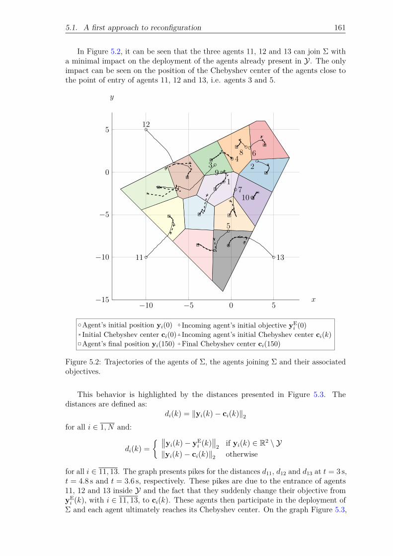
5.1. A first approach to reconfiguration 161
In Figure 5.2, it can be seen that the three agents 11, 12 and 13 can join Σ witha minimal impact on the deployment of the agents already present in Y. The onlyimpact can be seen on the position of the Chebyshev center of the agents close tothe point of entry of agents 11, 12 and 13, i.e. agents 3 and 5.
−10 −5 0 5−15
−10
−5
0
5
1
234
5
6
7
8
9
10
11
12
13
x
y
Agent’s initial position yi(0) Incoming agent’s initial objective yEi (0)
Initial Chebyshev center ci(0) Incoming agent’s initial Chebyshev center ci(k)
Agent’s final position yi(150) Final Chebyshev center ci(150)
Figure 5.2: Trajectories of the agents of Σ, the agents joining Σ and their associatedobjectives.
This behavior is highlighted by the distances presented in Figure 5.3. Thedistances are defined as:
di(k) = ‖yi(k)− ci(k)‖2for all i ∈ 1, N and:
di(k) =
∥∥yi(k)− yEi (k)
∥∥2
if yi(k) ∈ R2 \ Y‖yi(k)− ci(k)‖2 otherwise
for all i ∈ 11, 13. The graph presents pikes for the distances d11, d12 and d13 at t = 3 s,t = 4.8 s and t = 3.6 s, respectively. These pikes are due to the entrance of agents11, 12 and 13 inside Y and the fact that they suddenly change their objective fromyEi (k), with i ∈ 11, 13, to ci(k). These agents then participate in the deployment of
Σ and each agent ultimately reaches its Chebyshev center. On the graph Figure 5.3,
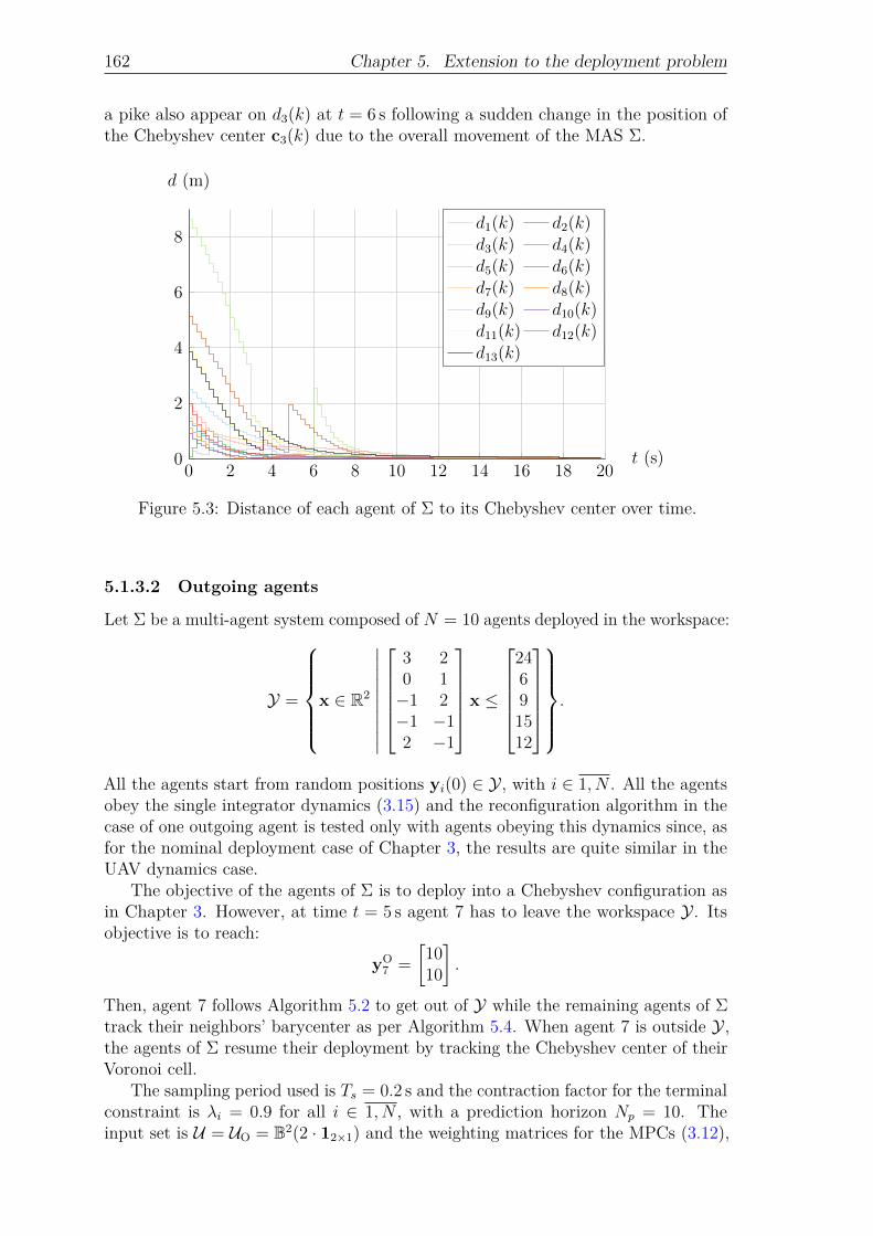
162 Chapter 5. Extension to the deployment problem
a pike also appear on d3(k) at t = 6 s following a sudden change in the position ofthe Chebyshev center c3(k) due to the overall movement of the MAS Σ.
0 2 4 6 8 10 12 14 16 18 200
2
4
6
8
t (s)
d (m)
d1(k) d2(k)d3(k) d4(k)d5(k) d6(k)d7(k) d8(k)d9(k) d10(k)d11(k) d12(k)d13(k)
Figure 5.3: Distance of each agent of Σ to its Chebyshev center over time.
5.1.3.2 Outgoing agents
Let Σ be a multi-agent system composed of N = 10 agents deployed in the workspace:
Y =
x ∈ R2
∣∣∣∣∣∣∣∣∣∣
3 20 1−1 2−1 −12 −1
x ≤
24691512
.
All the agents start from random positions yi(0) ∈ Y , with i ∈ 1, N . All the agentsobey the single integrator dynamics (3.15) and the reconfiguration algorithm in thecase of one outgoing agent is tested only with agents obeying this dynamics since, asfor the nominal deployment case of Chapter 3, the results are quite similar in theUAV dynamics case.
The objective of the agents of Σ is to deploy into a Chebyshev configuration asin Chapter 3. However, at time t = 5 s agent 7 has to leave the workspace Y. Itsobjective is to reach:
yO7 =
[1010
].
Then, agent 7 follows Algorithm 5.2 to get out of Y while the remaining agents of Σtrack their neighbors’ barycenter as per Algorithm 5.4. When agent 7 is outside Y ,the agents of Σ resume their deployment by tracking the Chebyshev center of theirVoronoi cell.
The sampling period used is Ts = 0.2 s and the contraction factor for the terminalconstraint is λi = 0.9 for all i ∈ 1, N , with a prediction horizon Np = 10. Theinput set is U = UO = B2(2 · 12×1) and the weighting matrices for the MPCs (3.12),
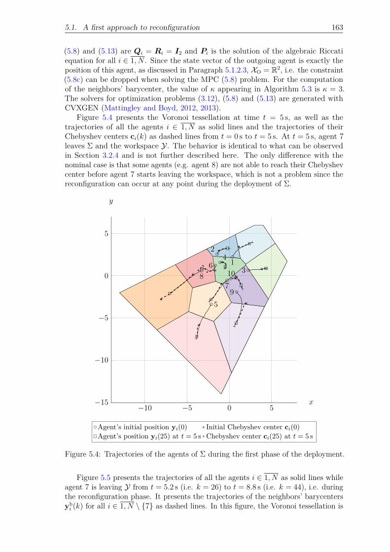
5.1. A first approach to reconfiguration 163
(5.8) and (5.13) are Qi = Ri = I2 and Pi is the solution of the algebraic Riccatiequation for all i ∈ 1, N . Since the state vector of the outgoing agent is exactly theposition of this agent, as discussed in Paragraph 5.1.2.3, XO = R2, i.e. the constraint(5.8c) can be dropped when solving the MPC (5.8) problem. For the computationof the neighbors’ barycenter, the value of κ appearing in Algorithm 5.3 is κ = 3.The solvers for optimization problems (3.12), (5.8) and (5.13) are generated withCVXGEN (Mattingley and Boyd, 2012, 2013).
Figure 5.4 presents the Voronoi tessellation at time t = 5 s, as well as thetrajectories of all the agents i ∈ 1, N as solid lines and the trajectories of theirChebyshev centers ci(k) as dashed lines from t = 0 s to t = 5 s. At t = 5 s, agent 7leaves Σ and the workspace Y. The behavior is identical to what can be observedin Section 3.2.4 and is not further described here. The only difference with thenominal case is that some agents (e.g. agent 8) are not able to reach their Chebyshevcenter before agent 7 starts leaving the workspace, which is not a problem since thereconfiguration can occur at any point during the deployment of Σ.
−10 −5 0 5−15
−10
−5
0
5
1
2
3
4
5
6
78
9
10
x
y
Agent’s initial position yi(0) Initial Chebyshev center ci(0)
Agent’s position yi(25) at t = 5 s Chebyshev center ci(25) at t = 5 s
Figure 5.4: Trajectories of the agents of Σ during the first phase of the deployment.
Figure 5.5 presents the trajectories of all the agents i ∈ 1, N as solid lines whileagent 7 is leaving Y from t = 5.2 s (i.e. k = 26) to t = 8.8 s (i.e. k = 44), i.e. duringthe reconfiguration phase. It presents the trajectories of the neighbors’ barycentersybi (k) for all i ∈ 1, N \ 7 as dashed lines. In this figure, the Voronoi tessellation is

164 Chapter 5. Extension to the deployment problem
not presented for readability reasons. It can be seen in Figure 5.5 that the positionsof the neighbors’ barycenters vary greatly at each time instant in a reduced timeframe which is still acceptable since this time frame is short. The agents are globallyable to track their neighbors’ barycenter while agent 7 leaves the workspace. Theobjective of the outgoing agent 7 is not presented in the figure for readability reasons.
−10 −5 0 5−15
−10
−5
0
5
12
34
5
6
78
9
10
x
y
Agent’s position yi(26) Neighbors’ barycenter ybi (26)
Agent’s position yi(44) Neighbors’ barycenter ybi (44)
Figure 5.5: Trajectories of the agents of Σ and agent 7 during the reconfigurationphase of the deployment.
Finally, Figure 5.6 is similar to Figure 5.4 since it presents the same elements forthe agents of Σ when agent 7 is out of Y . The trajectories are presented from t = 9 s(i.e. k = 45) to t = 40 s (i.e. k = 200) inside the Voronoi tessellation at t = 40 s.
As for the other cases presented in this thesis, it is interesting to look at thedistances between the agents and their objectives. This distance is defined as:
di(k) =
∥∥yi(k)− ybi (k)
∥∥2
if y7(k) ∈ Y‖yi(k)− ci(k)‖2 otherwise
for all i ∈ 1, N \ 7 and:
d7(k) =
‖y7(k)− c7(k)‖2 if k < 25∥∥y7(k)− yO7 (k)
∥∥2
otherwise.

5.2. A safer way to deal with outgoing vehicles 165
−10 −5 0 5−15
−10
−5
0
5
12
3
4
5
6
8
9
10
x
y
Agent’s position yi(45) Chebyshev center ci(45)
Final Agent’s position yi(200) Final Chebyshev center ci(200)
Figure 5.6: Trajectories of the agents of Σ during the third phase of the deployment.
Figure 5.7 presents the distances di(k) for all i ∈ 1, N \ 7. The behavior previouslyobserved appears clearly on the value of the distances. Indeed, at t = 5.2 s, animportant change on the distance to the objective point appears since each agentstarts tracking its neighbors’ barycenter instead of the Chebyshev center of itsVoronoi cell. Then, at t = 8.8 s, a new important change occurs since the agents goback to the deployment objective instead of tracking their neighbors’ barycenter. Theagents then converge towards their Chebyshev center. During the time frame whereagent 7 leaves the workspace Y , it is obvious from Figure 5.7 and Figure 5.5 that themovement of the entire multi-agent system is not negligible. This is something thatthe algorithm provided in Section 5.2.2 aims to improve. Finally, Figure 5.8 presentsthe distance d7(k) which exhibits the fact that it is able to rally its objective pointoutside the workspace.
5.2 A safer way to deal with outgoing vehicles
5.2.1 Limitation of the first reconfiguration algorithmIn the following, Σ is the multi-agent system described in Paragraph 5.1.2.1. WhileAlgorithm 5.4 and Algorithm 5.2 are effective to deal with the case of one agent
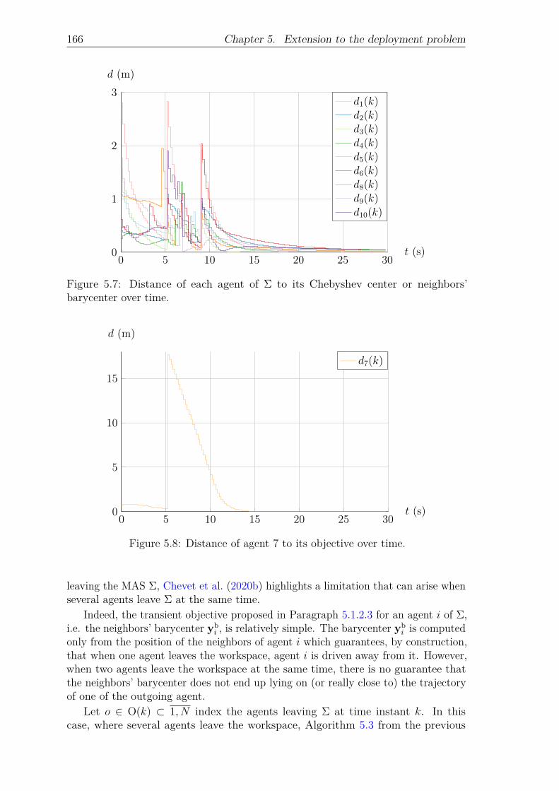
166 Chapter 5. Extension to the deployment problem
0 5 10 15 20 25 300
1
2
3
t (s)
d (m)
d1(k)d2(k)d3(k)d4(k)d5(k)d6(k)d8(k)d9(k)d10(k)
Figure 5.7: Distance of each agent of Σ to its Chebyshev center or neighbors’barycenter over time.
0 5 10 15 20 25 300
5
10
15
t (s)
d (m)
d7(k)
Figure 5.8: Distance of agent 7 to its objective over time.
leaving the MAS Σ, Chevet et al. (2020b) highlights a limitation that can arise whenseveral agents leave Σ at the same time.
Indeed, the transient objective proposed in Paragraph 5.1.2.3 for an agent i of Σ,i.e. the neighbors’ barycenter yb
i , is relatively simple. The barycenter ybi is computed
only from the position of the neighbors of agent i which guarantees, by construction,that when one agent leaves the workspace, agent i is driven away from it. However,when two agents leave the workspace at the same time, there is no guarantee thatthe neighbors’ barycenter does not end up lying on (or really close to) the trajectoryof one of the outgoing agent.
Let o ∈ O(k) ⊂ 1, N index the agents leaving Σ at time instant k. In thiscase, where several agents leave the workspace, Algorithm 5.3 from the previous

5.2. A safer way to deal with outgoing vehicles 167
section is naturally modified into Algorithm 5.5 described below. Let ∂Ho(k), witho ∈ O(k), be the hyperplane described by the position yo(k) of the outgoing agento and its target point yO
o . For an agent i ∈ 1, N \ O(k), if the neighbor ν ∈ Ni(k)is on the same side of all the hyperplanes ∂Ho(k) as agent i and farther from allthese hyperplanes than agent i, then it is assigned the weight ων,i(k) = κ, otherwiseων,i(k) = 1. A limitation related to this objective point arises when at least twoagents leave Σ. Indeed, if a remaining agent is located between the trajectories ofthese two outgoing agents, the neighbors’ barycenter might not guarantee anymorethat the remaining agent is driven away from the outgoing agents, leading to acollision risk. Example 5.2 then illustrates the limitation of the barycentric approach.
Algorithm 5.5: Computation of the neighbors’ barycenter of a remainingagent of Σ when several agents leave the workspace.
Input: The list of neighbors Ni(k) of agent i ∈ 1, N \O(k), the positions ofthe neighbors yν(k), ∀ν ∈ Ni(k), the positions of the outgoingagents yo(k), ∀o ∈ O(k), the hyperplanes∂Ho(k) = x ∈ R2 | ho(k)x = θo(k), ∀o ∈ O(k)
1 for ν ∈ Ni(k) do2 for o ∈ O(k) do3 if ho(k)(yν(k)− yo(k)) · ho(k)(yi(k)− yo(k)) ≥ 0 then4 if d(yν(k), ∂Ho(k)) > d(yi(k), ∂Ho(k)) then5 ων,i(k)← κ;6 else7 ων,i(k)← 1;8 Go to 1;9 end
10 else11 ων,i(k)← 1;12 Go to 1;13 end14 end15 end16 Compute the neighbors’ barycenter of agent i with (5.11);
Output: The neighbors’ barycenter ybi (k) of agent i
Example 5.2: Limit case of the reconfiguration algorithm in the case of severaloutgoing agentsThe conditions are exactly the same as for Example 5.1. However, now, at a giventime k, agents 2 and 3 leave Σ and the workspace Y as illustrated in Figure 5.9. Theyhave for objectives yO
2 =[−12 −6.2
]> ∈ R2 \ Y and yO3 =
[−9 −12
]> ∈ R2 \ Ywhich define the hyperplanes ∂H2(k) and ∂H3(k), with y2(k) and y3(k), respectively.
Since there is no difference in the configuration with respect to Example 5.1,the neighbor set of agent 5 is still N5(k) = 2, 3, 6, 9. However, here, ∂H2(k) and∂H3(k) are parallel. It is thus impossible for any neighbor of agent 5 to be fartherfrom both ∂H2(k) and ∂H3(k) than agent 5. Then, from Algorithm 5.5, all theneighbors of agent 5 receive the weight ων,5(k) = 1 for all ν ∈ N5(k).
The neighbors’ barycenter yb5(k) of agent 5 is then presented in Figure 5.9 as a
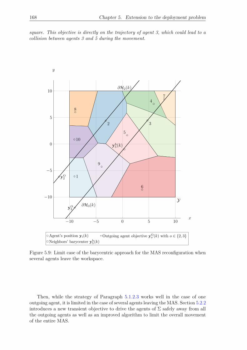
168 Chapter 5. Extension to the deployment problem
square. This objective is directly on the trajectory of agent 3, which could lead to acollision between agents 3 and 5 during the movement.
−10 −5 0 5 10
−10
−5
0
5
10
Y∂H3(k)
∂H2(k)
1
2 3
4
5
6
7
8
9
10
yO3
yO2
yb5(k)
x
y
Agent’s position yi(k) Outgoing agent objective yOo (k) with o ∈ 2, 3
Neighbors’ barycenter yb5(k)
Figure 5.9: Limit case of the barycentric approach for the MAS reconfiguration whenseveral agents leave the workspace.
Then, while the strategy of Paragraph 5.1.2.3 works well in the case of oneoutgoing agent, it is limited in the case of several agents leaving the MAS. Section 5.2.2introduces a new transient objective to drive the agents of Σ safely away from allthe outgoing agents as well as an improved algorithm to limit the overall movementof the entire MAS.

5.2. A safer way to deal with outgoing vehicles 169
5.2.2 Improved reconfiguration algorithm5.2.2.1 A new transient objective
Using the notations of the previous paragraph, the neighbors’ barycenter of agent iof Σ, with i ∈ 1, N \O(k), satisfies:∑
ν∈Ni(k)
ων,i(k)(ybi (k)− yν(k)
)= 02×1.
Based on this relation, a new safe objective ysi(k) is designed. Indeed, the neighbors’
barycenter is the unconstrained minimum:
ybi (k) = argmin
y∈R2
∥∥∥∥∥∥∑
ν∈Ni(k)
ων,i(k)(y − yν(k))
∥∥∥∥∥∥2
2
. (5.16)
Due to the lack of constraints in the previous minimization problem, there is noguarantee, as illustrated in Section 5.2.1, that the objective of the agents remaininginside the workspace Y allow them to be driven to safety and to avoid collision withthe outgoing agents. Then, the new objective ys
i(k) is the solution of:
ysi(k) = arg min
y ∈ R2
∑ν∈Ni(k)
ων,i(k)2‖y − yν(k)‖22
subject to
y ∈ Ri(k)
(5.17)
where Ri(k) is a region where it is safe for agent i to evolve. In problem (5.17),the cost function is equivalent to the cost function of (5.16) since by the triangularinequality:∥∥∥∥∥∥
∑ν∈Ni(k)
ων,i(k)(y − yν(k))
∥∥∥∥∥∥2
2
≤
∑ν∈Ni(k)
ων,i(k)‖y − yν(k)‖2
2
and by the Cauchy-Schwarz inequality: ∑ν∈Ni(k)
ων,i(k)‖y − yν(k)‖2
2
≤ |Ni(k)|∑
ν∈Ni(k)
ων,i(k)2‖y − yν(k)‖22.
In addition, |Ni(k)| acting as a scaling factor, it can be omitted in the minimizationproblem (5.17).
The region Ri(k) is defined as the intersection of two sets:
• the contracted Voronoi cell Vi(k, λVi) of agent i defined as:
Vi(k, λVi) = ci(k)⊕ λVi
(Vi(k)⊕ −ci(k))
where ci(k) is the Chebyshev center of the Voronoi cell Vi(k) and λVi∈ [0, 1)
is a scaling factor;

170 Chapter 5. Extension to the deployment problem
• the contracted working region Wi(k, λWi) defined from the hyperplanes ∂Ho(k),
with o ∈ O(k), where λWi∈ [0, 1) is a scaling factor.
The contracted working region has been introduced in Chevet et al. (2020b). Letyo(k), with o ∈ O(k), be the positions of the outgoing agents and yO
o their objectivesin R2\Y . These vectors define |O(k)| hyperplanes ∂Ho(k) = x ∈ R2 | ho(k)x = θo(k)in R2. The working region of agent i ∈ 1, N \O(k) is then defined as:
Wi(k) =y ∈ R2
∣∣ ho(k)(yi(k)− yo(k)) · ho(k)(y − yo(k)) ≥ 0, ∀o ∈ O(k)
(5.18)or as the set of all points on the same side of all the hyperplanes ∂Ho(k) as yi(k).The definition of Wi(k) of (5.18) is that of a polyhedron. Then, in the following, theworking region of agent i is represented equivalently as:
Wi(k) =x ∈ R2
∣∣HWi(k)x ≤ θWi
(k)
(5.19)
with HWi(k) ∈ Rsi(k)×2 and θWi
(k) ∈ Rsi(k), where si(k) ∈ 1, |O(k)|. The workingregion as defined in (5.19) is convex but can be unbounded.
Let cWi(k) be the Chebyshev center of the intersection Wi(k)∩Y of the working
regionWi(k) and the workspace Y . The intersectionWi(k)∩Y is necessary to ensurethat the Chebyshev center cWi
(k) exists, since Wi(k) is generally unbounded. Then,the contracted working region is defined as:
Wi(k, λWi) = cWi
(k)⊕ λWi(Wi(k)⊕ −cWi
(k)). (5.20)
It can be noticed that the Chebyshev center cWi(k) is used only for the definition of
Wi(k, λWi) and is not used per se in the following control algorithms.
♦
Remark 5.3: Shared working regionGiven the definition of the working region Wi(k) of agent i ∈ 1, N \ O(k), severalagents can share the same working region (and as such, the same contracted workingregion) such that Wi(k) =Wj(k) for two agents i, j ∈ 1, N \O(k).
Example 5.3: Construction of a contracted working regionLet Σ be the MAS of Example 5.2. Agents 2 and 3 leave the workspace Y towardsthe objectives yO
2 =[−12 −8
]> and yO3 =
[−9 −12
]> depicted by squares inFigure 5.10. At a given time k, the positions y2(k) and y3(k) of agents 2 and 3combined with their objectives define two hyperplanes ∂H2(k) and ∂H3(k) representedas solid lines in Figure 5.10.
By expression (5.18), the working regions of agents 1, 4, 5, 7 and 9 are containedin-between ∂H2(k) and ∂H3(k) and, as per Remark 5.3, W1(k) =W4(k) =W5(k) =W7(k) =W9(k). The working regionW1(k), i.e. the area between the two hyperplanes∂H2(k) and ∂H3(k), is displayed in light blue in Figure 5.10. Moreover, the workingregion W6(k) of agent 6 is the half-space below ∂H3(k), which is displayed in lightred in Figure 5.10. The working regions of agents 8 and 10 are the half-space above∂H2(k) such that W8(k) =W10(k), which is displayed in light green in Figure 5.10.
The Chebyshev centers cWi(k), with i ∈ 1, 10 \ 2, 3, of the intersection of the
working regions Wi(k) with the workspace Y are displayed with stars in Figure 5.10.Then, choosing λWi
= 0.8 for all i ∈ 1, 4, 5, 7, 9, λW6 = 0.5 and λWi= 0.7 for all
i ∈ 8, 10, the contracted working regions Wi(k, λWi) for all i ∈ 1, 4, 5, 7, 9 are
displayed in dark blue, the region W6(k, λW6) is displayed in dark red and the regionsWi(k, λWi
) for all i ∈ 8, 10 are displayed in dark green.

5.2. A safer way to deal with outgoing vehicles 171
−10 −5 0 5 10
−10
−5
0
5
10
Y∂H3(k)
∂H2(k)
1
2 3
4
5
6
7
8
9
10
yO3
yO2
cW5(k)
cW6(k)
cW8(k)
x
y
Agent’s position yi(k)Objective of the outgoingagent yO
o with o ∈ 2, 3Chebyshev center of theworking region cWi(k)
Working region W5(k) Working region W6(k) Working region W8(k)
Contracted workingregion W5(k, 0.8)
Contracted workingregion W6(k, 0.5)
Contracted workingregion W8(k, 0.7)
Figure 5.10: Construction of the contracted working regions.
With these definitions, the safe objective ysi(k) is then the solution of (5.17) such
that ysi(k) ∈ Vi(k, λVi
) ∩Wi(k, λWi). Then, due to the fact that ys
i(k) ∈ Wi(k, λWi),
it is guaranteed that agent i is driven away from the trajectories of all the outgoingagents o ∈ O(k).
In the following, the neighbors are defined as in Definition 5.1. As for the case ofParagraph 5.1.2.3, the weights ων,i(k), with ν ∈ Ni(k), have to be attributed giventhe relative position of the neighbors of agent i ∈ 1, N \O(k) to agent i and to theoutgoing agents o ∈ O(k). The way these weights are attributed is close to what ispresented in Algorithm 5.5. Let ωh, ωl and ωe be three positive weights such thatωh > ωl > ωe ≥ 0. The weight ωh is attributed to so-called “heavy” neighbors, theweight ωl to “light” neighbors and the weight ωe to outgoing (or exiting) neighbors.
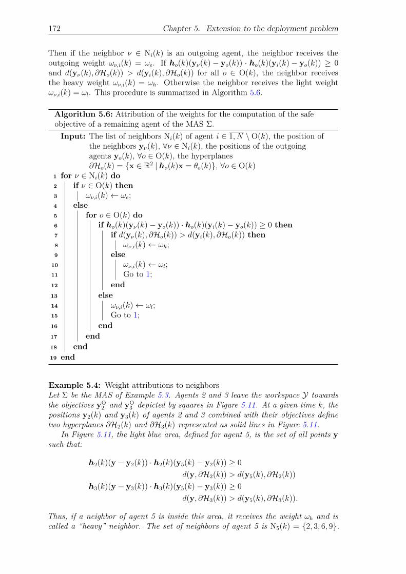
172 Chapter 5. Extension to the deployment problem
Then if the neighbor ν ∈ Ni(k) is an outgoing agent, the neighbor receives theoutgoing weight ων,i(k) = ωe. If ho(k)(yν(k)− yo(k)) · ho(k)(yi(k)− yo(k)) ≥ 0and d(yν(k), ∂Ho(k)) > d(yi(k), ∂Ho(k)) for all o ∈ O(k), the neighbor receivesthe heavy weight ων,i(k) = ωh. Otherwise the neighbor receives the light weightων,i(k) = ωl. This procedure is summarized in Algorithm 5.6.
Algorithm 5.6: Attribution of the weights for the computation of the safeobjective of a remaining agent of the MAS Σ.
Input: The list of neighbors Ni(k) of agent i ∈ 1, N \O(k), the position ofthe neighbors yν(k), ∀ν ∈ Ni(k), the positions of the outgoingagents yo(k), ∀o ∈ O(k), the hyperplanes∂Ho(k) = x ∈ R2 | ho(k)x = θo(k), ∀o ∈ O(k)
1 for ν ∈ Ni(k) do2 if ν ∈ O(k) then3 ων,i(k)← ωe;4 else5 for o ∈ O(k) do6 if ho(k)(yν(k)− yo(k)) · ho(k)(yi(k)− yo(k)) ≥ 0 then7 if d(yν(k), ∂Ho(k)) > d(yi(k), ∂Ho(k)) then8 ων,i(k)← ωh;9 else
10 ων,i(k)← ωl;11 Go to 1;12 end13 else14 ων,i(k)← ωl;15 Go to 1;16 end17 end18 end19 end
Example 5.4: Weight attributions to neighborsLet Σ be the MAS of Example 5.3. Agents 2 and 3 leave the workspace Y towardsthe objectives yO
2 and yO3 depicted by squares in Figure 5.11. At a given time k, the
positions y2(k) and y3(k) of agents 2 and 3 combined with their objectives definetwo hyperplanes ∂H2(k) and ∂H3(k) represented as solid lines in Figure 5.11.
In Figure 5.11, the light blue area, defined for agent 5, is the set of all points ysuch that:
h2(k)(y − y2(k)) · h2(k)(y5(k)− y2(k)) ≥ 0
d(y, ∂H2(k)) > d(y5(k), ∂H2(k))
h3(k)(y − y3(k)) · h3(k)(y5(k)− y3(k)) ≥ 0
d(y, ∂H3(k)) > d(y5(k), ∂H3(k)).
Thus, if a neighbor of agent 5 is inside this area, it receives the weight ωh and iscalled a “heavy” neighbor. The set of neighbors of agent 5 is N5(k) = 2, 3, 6, 9.

5.2. A safer way to deal with outgoing vehicles 173
There are no elements of N5(k) in the area described before thus no neighbors ofagent 5 receive the weight ωh. Agents 2 and 3 are outgoing agents and thus receivethe weight ω2,5(k) = ω3,5(k) = ωe. Finally, agents 6 and 9 receive the weightω6,5(k) = ω9,5(k) = ωl and are called “light” agents.
−10 −5 0 5 10
−10
−5
0
5
10
Y∂H3(k)
∂H2(k)
1ωl
2ωe
ωe3ωe
ωe
4ωl
5ωl
6ωl
7
8ωh
9 ωl
ωlωl
10
yO3
yO2
11
ωl
12
ωh
13ωh14
ωl
15 ωh
x
y
Outgoing agent’s objective yOo , o ∈ 2, 3 Agent’s position yi(k)
Vertex of the Voronoi cell Vi(k) lying on ∂Y
Figure 5.11: Attribution of weights to the neighbors of the agents of the MAS Σ.
The light red area of Figure 5.11, defined for agent 6, is the set of all points ysuch that:
h2(k)(y − y2(k)) · h2(k)(y6(k)− y2(k)) ≥ 0
d(y, ∂H2(k)) > d(y6(k), ∂H2(k))
h3(k)(y − y3(k)) · h3(k)(y6(k)− y3(k)) ≥ 0
d(y, ∂H3(k)) > d(y6(k), ∂H3(k)).

174 Chapter 5. Extension to the deployment problem
Thus, if a neighbor of agent 6 is inside this area, it receives the “heavy” weightωh. The set of neighbors of agent 6 is N6(k) = 3, 5, 9, 11, 12, 13, where 11, 12and 13 are not agents but vertices of the Voronoi cell V6(k) of agent 6 lying on ∂Y.Vertices 12 and 13 are the only neighbors of agent 6 in the area described before,thus ω12,6(k) = ω13,6(k) = ωh. Agent 3 is an outgoing agent and thus receives theweight ω3,6(k) = ωe. Finally, agents 5 and 9 as well as vertex 11 receive the weightω5,6(k) = ω9,6(k) = ω11,6(k) = ωl.
Finally, in Figure 5.11, the light green area, defined for agent 10, is the set of allpoints y such that:
h2(k)(y − y2(k)) · h2(k)(y10(k)− y2(k)) ≥ 0
d(y, ∂H2(k)) > d(y10(k), ∂H2(k))
h3(k)(y − y3(k)) · h3(k)(y10(k)− y3(k)) ≥ 0
d(y, ∂H3(k)) > d(y10(k), ∂H3(k)).
Thus, if a neighbor of agent 10 is inside this area, it receives the weight ωh. Theset of neighbors of agent 10 is N10(k) = 1, 2, 8, 9, 14, 15 where 14 and 15 are notagents but vertices of the Voronoi cell V10(k) of agent 10 lying on ∂Y. Vertex 15and agent 8 are the only neighbors of agent 10 in the area described before, thereforeω8,10(k) = ω15,10(k) = ωh. Agent 2 is an outgoing agent and thus receives the weightω2,10(k) = ωe. Finally, agents 1 and 9 as well as vertex 14 receive the weightω1,10(k) = ω9,10(k) = ω14,10(k) = ωl.
The weights attributed for the computation of ys5(k), ys
6(k) and ys10(k) are pre-
sented in Figure 5.11 in blue, red and green, respectively.The same procedure can be applied to the other agents of Σ but is not be presented
here. However, the construction of the safe objective ysi(k), with i ∈ 1, 10 \ 2, 3 is
not presented in this example since an additional layer to the reconfiguration algorithmconcerning the computation of this objective point is presented in Paragraph 5.2.2.2.
5.2.2.2 A new reconfiguration algorithm
In Paragraph 5.1.2.3, a reconfiguration algorithm where the remaining agents of themulti-agent system Σ follow a transient objective to avoid the trajectory of agentsleaving the workspace Y is proposed. With the new safe objective allowing theagents to evolve inside a safe region proposed in Paragraph 5.2.2.1, this algorithmis efficient in allowing the agents of Σ remaining in the workspace Y to avoid thetrajectory of the outgoing agents, it can be improved on some aspects. Indeed, withsuch a strategy, all the agents of Σ remaining in the workspace Y move until all theoutgoing agents leave Y before resuming their deployment objective. The presentparagraph then proposes an improved way to deal with MAS reconfiguration in thecase of outgoing agents.
In order to avoid too much movement from the MAS, only the agents risking acollision with an outgoing agent follow the new transient safe objective ys
i(k), withi ∈ 1, N \O(k), defined in the previous paragraph, while the other agents continuetheir deployment objective by following the Chebyshev center ci(k) of their Voronoicell Vi(k). To do so, each agent of Σ has to discriminate which outgoing agents areharmless to it and which are not.

5.2. A safer way to deal with outgoing vehicles 175
Let Oi(k), with i ∈ 1, N\O(k), denote the set of all the outgoing agents consideredpotentially harmful by agent i of Σ. For all outgoing agents o ∈ O(k), let:
∂Oo(k) =x ∈ R2
∣∣∣ (yOo − yo(k)
)>(x− yo(k)) = 0
(5.21)
which separates the plane R2 into two parts. An outgoing agent o ∈ O(k) isthen considered harmful by agent i ∈ 1, N \ O(k) if yi(k) and yO
o lie on the sameside of ∂Oo(k), i.e. if
(yOo − yo(k)
)>(yi(k)− yo(k)) ≥ 0. In this case, if o 6∈
Oi(k), the outgoing agent o is added to Oi(k), otherwise, Oi(k) does not change.However, as soon as yi(k) and yO
o lie on different sides of ∂Oo(k), i.e. when(yOo − yo(k)
)>(yi(k)− yo(k)) < 0, the outgoing agent o is removed from Oi(k).
This procedure is summarized in Algorithm 5.7.
Algorithm 5.7: Construction of the set Oi(k) of the outgoing agentsconsidered by the agent i.
Input: The positions yo(k) and objectives yOo , ∀o ∈ O(k), of the outgoing
agents, the position yi(k) of agent i and the set Oi(k − 1)1 for o ∈ O(k) do2 if
(yOo − yo(k)
)>(yi(k)− yo(k)) ≥ 0 and o /∈ Oi(k − 1) then
3 Oi(k)← Oi(k − 1) ∪ o;4 else if
(yOo − yo(k)
)>(yi(k)− yo(k)) < 0 and o ∈ Oi(k − 1) then
5 Oi(k)← Oi(k − 1) \ o;6 end7 end
Output: The updated set Oi(k) of the agent i ∈ 1, N \O(k)
♦
Remark 5.4: Behind and in frontIn the following, an agent satisfying
(yOo − yo(k)
)>(yi(k)− yo(k)) ≥ 0 is said to be
in front of the outgoing agent o ∈ O(k).An agent satisfying
(yOo − yo(k)
)>(yi(k)− yo(k)) < 0 is said to be behind the
outgoing agent o ∈ O(k).
Based on the set Oi(k) constructed with Algorithm 5.7, agent i of Σ thencomputes its safe objective ys
i(k) by solving (5.17). However, a slight modificationto Algorithm 5.6 is done. Indeed, the line 5 is changed from “for o ∈ O(k) do” to“for o ∈ Oi(k) do” to take into account the new way of dealing with outgoing agents.The same procedure is done for the construction of the contracted working region.Indeed, the definition of the working region given in (5.18) is replaced with:
Wi(k) =y ∈ R2
∣∣ ho(k)(yi(k)− yo(k)) · ho(k)(y − yo(k)) ≥ 0, ∀o ∈ Oi(k)
.(5.22)
Example 5.5: Construction of the sets Oi(k)Let Σ be the multi-agent system of Example 5.4 in the exact same conditions. Theagents 2 and 3 leave the workspace to join the points yO
2 and yO3 depicted as squares
in Figure 5.12. In Figure 5.12 both hyperplanes ∂O2(k) and ∂O3(k) are presentedas solid lines. Then, if an agent i of Σ remaining inside Y belongs to the areacolored in light blue, the set Oi(k) of the outgoing agents it considers is such that

176 Chapter 5. Extension to the deployment problem
Oi(k) = 2, 3, which is verified for agents 1, 6, 8, 9 and 10. Indeed, these agentsare in front of both agents 2 and 3 with respect to their objectives. On the other hand,if an agent i of Σ remaining inside Y belongs to the area colored in light red, its setOi(k) is such that Oi(k) = 3, which is verified only for agent 5. Indeed, agent 5 is infront of agent 3 but behind agent 2. Finally, if an agent i of Σ remaining inside Ybelongs to the white area, its set Oi(k) is empty since the agent is behind both agents2 and 3. This is verified for agents 4 and 7 such that O4(k) = O7(k) = ∅.
−10 −5 0 5 10
−10
−5
0
5
10
Y
∂H2(k)
∂H3(k)
∂O2(k) ∂O3(k)
1
2 3
4
5
6
7
8
9
10
yO3
yO2
x
y
Agent’s position yi(k) Outgoing agent’s objective yOo , o ∈ 2, 3
Figure 5.12: Construction of the sets Oi(k) for the agents of the MAS Σ.
Contrary to Example 5.4, the weight attributions for the neighbors of agent 5is then slightly modified given the considered modification of Algorithm 5.6. Indeed,d(yν(k), ∂H2(k)), with ν ∈ N5(k), is not considered anymore for the weight attributionprocedure. However, this does not change the result given the configuration of thesystem.

5.2. A safer way to deal with outgoing vehicles 177
In addition, since the definition of the working region of an agent has beenmodified from (5.18) to (5.22), some conclusions of Example 5.3 are modified. Indeed,given the configuration of the MAS at time k, W4(k) and W7(k) are not definedsince O4(k) = O7(k) = ∅. Moreover, since O5(k) = 3 6= O9(k), it is immediatethat W5(k) 6=W9(k).
There is no modification in the behavior of the outgoing agents with respectto what was presented in Paragraph 5.1.2.3, i.e. the outgoing agents then stillfollow the decentralized MPC algorithm of Algorithm 5.2 to leave the workspace Y .However, for the remaining agents, Algorithm 5.4 is modified to incorporate all theimprovements presented in this section.
If an agent i, with i ∈ 1, N \ O(k), remaining in the workspace Y is such thatOi(k) = ∅, it follows Algorithm 3.2 without modification. However, if Oi(k) 6= ∅,agent i follows the safe objective ys
i(k) with a decentralized MPC algorithm.According to Assumption 3.2, let (xs
i(k),usi(k)), with i ∈ 1, N \O(k), be a couple
such that (xsi(k),u
si(k),y
si(k)) is an equilibrium point of (5.1), i.e.:
xsi(k) = Axs
i(k) +Busi(k)
ysi(k) = Cxs
i(k).(5.23)
Then, the agents of Σ such that Oi(k) 6= ∅ compute their input ui(k), with i ∈1, N \ O(k), by finding the solution of problem (5.13), while replacing xb
i (k) andubi (k) by xs
i(k) and usi(k), respectively. The procedure for the reconfiguration of the
MAS Σ in the case of outgoing agents is then summarized in Algorithm 5.8.
Algorithm 5.8: Decentralized algorithm followed by a remaining agent forthe reconfiguration of the MAS when several agents leave the system.1 for k ≥ 0 do2 if O 6= ∅ then3 Compute Oi(k) of agent i ∈ 1, N \O with Algorithm 5.7;4 if Oi(k) = ∅ then5 Follow Algorithm 3.2;6 else7 Attribute weights to agent i’s neighbors with Algorithm 5.6
(modified with Oi(k) instead of O at line 5);8 Compute the safe objective ys
i(k) of agent i by solving (5.17);9 Compute the couple (xs
i(k),usi(k)) with (5.12) such that
(xsi(k),u
si(k),y
si(k)) is an equilibrium point of (5.1);
10 Solve the optimization problem (5.13) (by replacing xbi (k) and
ubi (k) by xs
i(k) and usi(k)) to obtain the input signal ui(k);
11 Apply ui(k) to agent i;12 end13 else14 Follow Algorithm 3.2;15 end16 end

178 Chapter 5. Extension to the deployment problem
5.3 Reconfiguration in the case of outgoingagents
5.3.1 Comparison of the two algorithms in the case of oneoutgoing agent
In order to exhibit the improvement of the algorithm described in Section 5.2 withrespect to the one presented in Paragraph 5.1.2.3, the exact same scenario as theone described in Paragraph 5.1.3.2 is considered. However, instead of followingAlgorithm 5.4 used when only one agent leaves the workspace, the remaining agentsof Σ follow Algorithm 5.8 used when one or several agents leave the workspace.Agent 7 still follows Algorithm 5.2 and leaves Σ at t = 5 s.
The first phase of the deployment is identical to the one presented in Figure 5.4since it only consists in the deployment of the MAS and is then not reported here.
−10 −5 0 5−15
−10
−5
0
5
∂H7(26)
∂O7(26)1
2
34
5
6
7
8
9
10
x
y
Agent’s position yi(26) Chebyshev center ci(26) Safe objective ysi(26)
Figure 5.13: Position of the MAS Σ and of agent 7 at time t = 5.2 s.
Figure 5.13 presents the position of Σ and agent 7 at time t = 5.2 s (i.e. k = 26).In this figure are presented the hyperplanes ∂H7(26) and ∂O7(26) described inSection 5.2. Since agent 7 moves towards the point yO
7 =[10 10
]>, agents 5 and 8are behind agent 7 and, per Algorithm 5.7, O5(26) = O8(26) = ∅ since they are notin the same half-space delimited by ∂O7(26) as yO
7 . Agents 5 and 8 then continue to

5.3. Reconfiguration in the case of outgoing agents 179
track their Chebyshev center c5(k) and c8(k), represented as stars in Figure 5.13,according to Algorithm 5.8. However, though agent 9 is in the limit case as itlies on ∂O7(26), it is considered to be in front of agent 7 and Oi(26) = 7 for alli ∈ 1, N \ 5, 7, 8 since they are in front of agents 7. They then start tracking thesafe objective ys
i(26), with i ∈ 1, N \5, 7, 8, represented as diamonds in Figure 5.13,according to Algorithm 5.8.
−10 −5 0 5−15
−10
−5
0
5
∂H7(26)
∂D6(26)
12
34
5
6
7
8
9
10
12
11
x
y
Agent’s position yi(26) Vertices of V6(26) on the border ∂YChebyshev center ci(26) Contracted Voronoi cell V6(26, λV6)Safe objective ys
i(26) Contracted working region W6(26, λW6)
Figure 5.14: Construction of the safe objective of agent 6 at t = 5.2 s.
For the computation of the safe objectives ysi(k), with i ∈ 1, N \ 5, 7, 8, the
weights λViand λWi
described in Paragraph 5.2.2.1 are chosen to be 0.5 and 0.8,respectively, for all the agents. Figure 5.14 details the construction of the safeobjective ys
6(26), the procedure being the same for all the other agents. The line∂D6(26) is used to graphically see which neighbors of agent 6 receive a heavyweight ωh and which neighbors receive a light weight ωl. Indeed, all the pointsy ∈ R2 above ∂D6(26) are such that d(y, ∂H7(26)) ≥ d(y6(26), ∂H7(26)). The setof neighbors of agent 6 N6(26) is N6(26) = 2, 4, 7, 8, 11, 12, where 11 and 12 arevertices of the Voronoi cell V6(26) lying on the border ∂Y of the workspace Y.Then, per Algorithm 5.6, ων,6(26) = ωh for all ν ∈ 8, 11, 12, ων,6(26) = ωl for allν ∈ 2, 4 and ω7,6(26) = ωe. The contracted Voronoi cell V6(26, λV6) of agent 6 isthe area delimited by the dashed line in Figure 5.14. The contracted working region

180 Chapter 5. Extension to the deployment problem
W6(26, λW6) of agent 6 is the area colored in red in Figure 5.14. It can be noted that,as explained in Paragraph 5.2.2.1, W6(26, λW6) = Wi(26, λWi
) for all i ∈ 1, 2, 4.Then, by choosing ωh = 5, ωl = 1 and ωe = 0, the safe objective ys
6(26) of agent 6 isobtained by solving (5.17).
−10 −5 0 5−15
−10
−5
0
5
∂H7(34)
∂O7(34)
12
3
4
5
67
8
9
10
x
y
Agent’s position yi(34) Chebyshev center ci(34) Safe objective ysi(34)
Figure 5.15: Position of the MAS Σ and of agent 7 at time t = 6.8 s.
As agent 7 moves towards its objective yO7 as shown in Figure 5.14, the agents
tracking their safe objective ysi(k), with i ∈ 1, N \ 5, 7, 8, resume tracking their
Chebyshev centers when they pass on the other side of ∂O7(k), i.e. as soon as theyare behind agent 7. For example, at time t = 6.8 s (k = 34), agents 4, 6, 9 and10 resumed tracking the Chebyshev center of their Voronoi cell as illustrated inFigure 5.15. The only agents still tracking their safe objective are agents 1, 2 and 3.
It is difficult to show the trajectories of the agents and of their objectives over timeas it is done in Paragraph 5.1.3.2, since the movement cannot be decomposed intodistinct phases. Indeed, all the agents change their objective asynchronously, contraryto the case of Paragraph 5.1.2.3, where they track their neighbors’ barycenter assoon as agent 7 leaves Σ and starts leaving Y and resume tracking their Chebyshevcenter when agent 7 is out of Y . Then, only the distances:
di(k) =
‖yi(k)− ys
i(k)‖2 if Oi(k) 6= ∅‖yi(k)− ci(k)‖2 otherwise
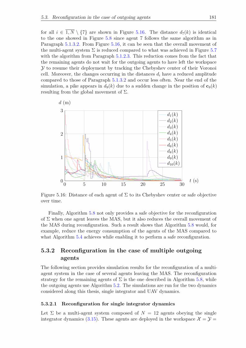
5.3. Reconfiguration in the case of outgoing agents 181
for all i ∈ 1, N \ 7 are shown in Figure 5.16. The distance d7(k) is identicalto the one showed in Figure 5.8 since agent 7 follows the same algorithm as inParagraph 5.1.3.2. From Figure 5.16, it can be seen that the overall movement ofthe multi-agent system Σ is reduced compared to what was achieved in Figure 5.7with the algorithm from Paragraph 5.1.2.3. This reduction comes from the fact thatthe remaining agents do not wait for the outgoing agents to have left the workspaceY to resume their deployment by tracking the Chebyshev center of their Voronoicell. Moreover, the changes occurring in the distances di have a reduced amplitudecompared to those of Paragraph 5.1.3.2 and occur less often. Near the end of thesimulation, a pike appears in d9(k) due to a sudden change in the position of c9(k)resulting from the global movement of Σ.
0 5 10 15 20 25 300
1
2
3
t (s)
d (m)
d1(k)d2(k)d3(k)d4(k)d5(k)d6(k)d8(k)d9(k)d10(k)
Figure 5.16: Distance of each agent of Σ to its Chebyshev center or safe objectiveover time.
Finally, Algorithm 5.8 not only provides a safe objective for the reconfigurationof Σ when one agent leaves the MAS, but it also reduces the overall movement ofthe MAS during reconfiguration. Such a result shows that Algorithm 5.8 would, forexample, reduce the energy consumption of the agents of the MAS compared towhat Algorithm 5.4 achieves while enabling it to perform a safe reconfiguration.
5.3.2 Reconfiguration in the case of multiple outgoingagents
The following section provides simulation results for the reconfiguration of a multi-agent system in the case of several agents leaving the MAS. The reconfigurationstrategy for the remaining agents of Σ is the one described in Algorithm 5.8, whilethe outgoing agents use Algorithm 5.2. The simulations are run for the two dynamicsconsidered along this thesis, single integrator and UAV dynamics.
5.3.2.1 Reconfiguration for single integrator dynamics
Let Σ be a multi-agent system composed of N = 12 agents obeying the singleintegrator dynamics (3.15). These agents are deployed in the workspace X = Y =

182 Chapter 5. Extension to the deployment problem
B2(7.5 · 12×1) with an input space U = B2(2 · 12×1). The sampling rate used in(3.15) is Ts = 0.2 s. The prediction horizon for the model predictive controllers ofAlgorithm 5.2 and Algorithm 5.8 is Np = 10 and the contraction factor for theterminal constraint is λi = 0.9 for all i ∈ 1, N . The weighting matrices for the MPCare Q = R = I2 and P is the solution of the algebraic Riccati equation.
For this simulation scenario, the agents of Σ start deploying inside Y from randompositions yi(0) ∈ Y , with i ∈ 1, N represented by circles in Figure 5.17. At t = 4 s,agent 7 leaves Σ to join yO
7 =[0 10
]>. Then, while agent 7 is leaving Y, agent 9also leaves Σ at t = 5.2 s to join yO
9 =[10 0
]>. Thus, during the deployment, theset O(k) of the outgoing agents is:
O(k) =
∅ for k < 207 for 20 ≤ k < 26.7, 9 for 26 ≤ k
−5 0 5
−5
0
5
1
2
345
67
89
1011
12
x
y
Agent’s initial position yi(0) Initial Chebyshev center ci(0)Agent’s position yi(19) Chebyshev center ci(19)
Figure 5.17: Trajectories of the agents of Σ during the first phase of the deployment.
While agents 7 and 9 leave the workspace, the other agents are in a reconfigurationphase before resuming their deployment to reach a Chebyshev configuration aspresented in Algorithm 5.8. For the reconfiguration phase, the weights ωh, ωl and ωeused to compute the safe objective ys
i(k) for all i ∈ 1, N \O(k) are chosen to be 5, 1and 0 respectively. The contraction factor to compute the contracted Voronoi cellsVi(k, λVi
) is λVi= 0.5 for all i ∈ 1, N \O(k) and the contraction factor to compute
the contracted working region Wi(k, λWi) is λWi
= 0.8 for all i ∈ 1, N \O(k).
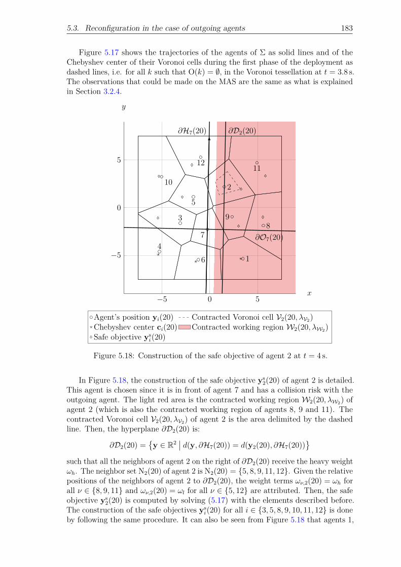
5.3. Reconfiguration in the case of outgoing agents 183
Figure 5.17 shows the trajectories of the agents of Σ as solid lines and of theChebyshev center of their Voronoi cells during the first phase of the deployment asdashed lines, i.e. for all k such that O(k) = ∅, in the Voronoi tessellation at t = 3.8 s.The observations that could be made on the MAS are the same as what is explainedin Section 3.2.4.
−5 0 5
−5
0
5
∂H7(20) ∂D2(20)
∂O7(20)
1
2
3
4
5
6
78
9
10
1112
−5 0 5
−5
0
5
x
y
Agent’s position yi(20) Contracted Voronoi cell V2(20, λV2)Chebyshev center ci(20) Contracted working region W2(20, λW2)Safe objective ys
i(20)
Figure 5.18: Construction of the safe objective of agent 2 at t = 4 s.
In Figure 5.18, the construction of the safe objective ys2(20) of agent 2 is detailed.
This agent is chosen since it is in front of agent 7 and has a collision risk with theoutgoing agent. The light red area is the contracted working region W2(20, λW2) ofagent 2 (which is also the contracted working region of agents 8, 9 and 11). Thecontracted Voronoi cell V2(20, λV2) of agent 2 is the area delimited by the dashedline. Then, the hyperplane ∂D2(20) is:
∂D2(20) =y ∈ R2
∣∣ d(y, ∂H7(20)) = d(y2(20), ∂H7(20))
such that all the neighbors of agent 2 on the right of ∂D2(20) receive the heavy weightωh. The neighbor set N2(20) of agent 2 is N2(20) = 5, 8, 9, 11, 12. Given the relativepositions of the neighbors of agent 2 to ∂D2(20), the weight terms ων,2(20) = ωh forall ν ∈ 8, 9, 11 and ων,2(20) = ωl for all ν ∈ 5, 12 are attributed. Then, the safeobjective ys
2(20) is computed by solving (5.17) with the elements described before.The construction of the safe objectives ys
i(20) for all i ∈ 3, 5, 8, 9, 10, 11, 12 is doneby following the same procedure. It can also be seen from Figure 5.18 that agents 1,

184 Chapter 5. Extension to the deployment problem
4 and 6 continue tracking their Chebyshev center according to Algorithm 5.7 sincethey are behind the outgoing agent 7.
−5 0 5
−5
0
5
∂H7(26)
∂O7(26)
∂H9(26)
∂O9(26)
1
2
3
4
5
6
789
10
1112
−5 0 5
−5
0
5
x
y
Agent’s position yi(26) Contracted Voronoi cell Vi(26, λVi)
Chebyshev center ci(26) Contracted working region W2(26, λW2)Safe objective ys
i(26) Contracted working region W5(26, λW5)
Figure 5.19: Construction of the safe objectives of agents 2 and 5 at t = 5.2 s.
While agent 7 is leaving Y, agent 9 decides to leave Σ at t = 5.2 s. Then,Figure 5.19 presents the position of the agents at t = 5.2 s and details the constructionof the safe objectives of agents 2 and 5. According to Algorithm 5.7, at time t = 5.2 s,Oi(26) = ∅ for i ∈ 1, 3, 4, 6 since these agents are behind both outgoing agents,thus, agents 1, 3, 4 and 6 follow the Chebyshev center of their Voronoi cells. Attime t = 5.2 s the sets of the outgoing agents considered by agents 2 and 5 are,respectively, O2(26) = 7, 9 and O5(26) = 7 since agent 2 is in front of bothoutgoing agents, while agent 5 is in front of agent 7 and behind of agent 9. Theneighbor sets N2(26) and N5(26) of agents 2 and 5 are N2(26) = 7, 8, 9, 11, 12and N5(26) = 3, 7, 10, 12. Agent 11 is the only neighbor of agent 2 farther from∂H7(26) and ∂H9(26) than agent 2 and on the same side of these hyperplanes asagent 2. Then, according to Algorithm 5.6, agent 11 receives the weight ωh suchthat ω11,2(26) = ωh. Agents 8 and 12 are not on the same side of both ∂H7(26) and∂H9(26) as agent 2, thus they receive the light weight ωl such that ων,2(26) = ωlfor ν ∈ 8, 12. Finally, since agents 7 and 9 are outgoing agents, they receive theweight ωe such that ων,2(26) = ωe for ν ∈ 7, 9. The same way, ων,5(26) = ωh forν ∈ 3, 10, ω12,5(26) = ωl and ω7,5(26) = ωe. The areas inside the dashed linesare the contracted Voronoi cells V2(26, λV2) and V5(26, λV5). From the definition of

5.3. Reconfiguration in the case of outgoing agents 185
the contracted working region given in Paragraph 5.2.2.2 in (5.22), the contractedworking region W5(26, λW5) of agent 5 is obtained by considering only the half-spacedefined by ∂H7(26). This contracted working region is colored in blue in Figure 5.19.For its part, the contracted working region W2(26, λW2) of agent 2 is obtained byconsidering the half-spaces defined by both ∂H7(26) and ∂H9(26). This region iscolored in red in Figure 5.19. Then, solving (5.17), the safe objectives ys
2(26) andys5(26) of agents 2 and 5 are found. The other safe objectives are found by following
the same procedure.
−5 0 5
−5
0
5
1
2
3
4
5
6
7
8
9
10
1112
−5 0 5
−5
0
5
x
y
Agent’s final position yi(200) Final Chebyshev center ci(200)
Figure 5.20: Final configuration of the MAS Σ at t = 40 s.
Agents 7 and 9 continue tracking their objectives yO7 and yO
9 and leave Y att = 9 s and t = 7.6 s. In between the time the agents 7 and 9 leave Σ and the timethey are outside Y , the remaining agents of Σ avoid the trajectories of agents 7 and9 by following their safe objectives ys
i(k), with i ∈ 1, N \O(k). Moreover, as soonas they are behind both outgoing agents, the remaining agents resume tracking theChebyshev center of their Voronoi cells ci(k). The final Voronoi configuration att = 40 s is presented in Figure 5.20.
Finally, Figure 5.21 presents the distances:
di(k) =
‖yi(k)− ys
i(k)‖2 if Oi(k) 6= ∅‖yi(k)− ci(k)‖2 otherwise
for all i ∈ 1, N \ 7, 9, while Figure 5.22 presents the distances:
di(k) =
∥∥yi(k)− yOi (k)
∥∥2
if i ∈ O(k)
‖yi(k)− ci(k)‖2 otherwise

186 Chapter 5. Extension to the deployment problem
0 5 10 15 20 25 300
1
2
3
4
t (s)
d (m)
d1(k)d2(k)d3(k)d4(k)d5(k)d6(k)d8(k)d10(k)d11(k)d12(k)
Figure 5.21: Distance of each agent of Σ to its Chebyshev center or safe objectiveover time.
0 5 10 15 20 25 300
2
4
6
8
10
12
t (s)
d (m)
d7(k)d9(k)
Figure 5.22: Distance of the agents leaving Σ to their objectives over time.
for i ∈ 7, 9. From Figure 5.21, it can be seen that the reconfiguration strategyallows the agents to have a limited number of changes in their objectives during thereconfiguration phase. It also allows the system to return quickly to a reconfigurationstrategy such that the MAS reaches a static Chebyshev configuration quickly afterthe last outgoing agent has left the workspace Y. The main changes occur on thedistances of the agents of Σ to their objectives at t = 4 s and t = 5.2 s, i.e. whenagents 7 and 9 leave Σ and when the agents of Σ resume tracking the Chebyshevcenter of their Voronoi cells. Figure 5.22 shows that the outgoing agents 7 and 9 areable to reach their objectives yO
7 and yO9 .

5.3. Reconfiguration in the case of outgoing agents 187
5.3.2.2 Reconfiguration for UAV dynamics
Let Σ be a multi-agent system composed of N = 12 agents obeying the UAV dynamicspresented in Section 3.3. Then, for position control, the linearized dynamics of (3.30)are used, while the simulation is run with the nonlinear model of a quadrotor UAV(3.28). The MAS is deployed in the workspace Y = B2(7.5 · 12×1) with the inputspace U = B2
(π6· 12×1
). In addition to the output and input space, the state space
is defined as:
X =
x ∈ R4
∣∣∣∣∣∣∣∣Cx ∈ Y and
0 −1 0 00 1 0 00 0 0 −10 0 0 1
x ≤ 2 · 14×1
thus constraining the horizontal speed of each agent i ∈ 1, N to |vx,i|, |vy,i| ≤2m · s−1. The sampling rate used in the position subsystem of (3.30) is Ts = 0.2 s.The prediction horizon for the model predictive controllers of Algorithm 5.2 andAlgorithm 5.8 is Np = 10 and the contraction factor for the terminal constraint isλi = 0.9 for all i ∈ 1, N . The weighting matrices for the MPC are Q = I4, R = I2and P is the solution of the algebraic Riccati equation. As in Section 3.3.3, it isnecessary to introduce a Luenberger observer to estimate the state of the positionsubsystem. The observer gain is obtained as a linear quadratic regulator withweighting matrices Qobs = 10I4 and Robs = I2, giving:
L =
1.0971 00.8303 0
0 1.09710 0.8303
.
The example presented here follows the same idea as the one presented inParagraph 5.3.2.1. The agents of Σ start deploying inside Y from random positionsyi(0) ∈ Y , while the other states have a null initial value except the altitude whichis such that zi(0) = 5m for all i ∈ 1, N . The estimated states xi of all the agentsi ∈ 1, N are initialized such that xi(0) = xi(0). At t = 4 s, agent 4 leaves Σ to joinyO4 =
[5 10
]>. Then, while agent 4 is leaving Y, agent 10 leaves Σ at t = 5.2 s torally yO
10 =[10 10
]>. Thus, during the deployment, the set O(k) of the outgoingagents is:
O(k) =
∅ for k < 204 for 20 ≤ k < 26.4, 10 for 26 ≤ k
While agents 4 and 10 leave the workspace, the remaining agents of Σ enter areconfiguration phase before resuming their deployment in a Chebyshev configurationfollowing Algorithm 5.8. For the reconfiguration, the weights to compute the safeobjective ys
i(k) for all i ∈ 1, N \O(k) are chosen such that ωh = 5, ωl = 1 and ωe = 0.The contraction factors for the computation of the contracted Voronoi cells Vi(k, λVi
)is λVi
= 0.5 and the contraction factor for the computation of the contracted workingregions Wi(k, λWi
) is λWi= 0.8 for all i ∈ 1, N \O(k). The way the safe objectives
are computed is not described here since it is not different from what is presented inParagraph 5.3.2.1.

188 Chapter 5. Extension to the deployment problem
−5 0 5
−5
0
5
1
2
3
4
5
6
7
8
9
10
11
12
−5 0 5
−5
0
5
x
y
Agent’s initial position yi(0) Initial Chebyshev center ci(0)
Figure 5.23: Initial configuration of the MAS Σ at t = 0 s.
Figure 5.23, Figure 5.24 and Figure 5.25 show the configuration of Σ at differenttime instants. The initial configuration at t = 0 s is displayed in Figure 5.23, whilethe final configuration at t = 40 s is presented in Figure 5.25. Then, Figure 5.24illustrates the configuration at time t = 5.4 s, while agents 4 and 10 are leaving theworkspace Y . In these three figures, the position yi(k), with i ∈ 1, N , of the agentsis represented by a circle while the Chebyshev centers ci are represented by starsand the safe objectives ys
i by diamonds. Moreover, in Figure 5.24 are shown as solidlines the hyperplanes ∂H4(27) and ∂H10(27) defined by the outgoing agents 4 and10 and their objectives yO
4 and yO10 as well as the hyperplanes ∂O4(27) and ∂O10(27),
respectively orthogonal to ∂H4(27) and ∂H10(27), allowing to obtain graphicallythe sets Oi(27) for all i ∈ 1, N \O(27). Since the construction of these hyperplanesis based on the estimated position yi(k), with i ∈ O(k), of the outgoing agents,the estimated positions of all the agents are shown in Figure 5.24 with squares.The estimated positions are not presented in Figure 5.23 and Figure 5.25 sinceyi(0) = yi(0) for all i ∈ 1, N and, according to Figure 5.27, yi(200) ≈ yi(200).From Figure 5.24, it can be seen that the agents i ∈ 2, 3, 11 are in front of theoutgoing agents 4 and 10, that the agents i ∈ 1, 6, 9 are in front of agent 10 butbehind agent 4 while agents i ∈ 5, 7, 8, 12 are behind both outgoing agents. ThenOi(27) = 4, 10 for i ∈ 2, 3, 11, Oi(27) = 10 for i ∈ 1, 6, 9 and Oi(27) = ∅for i ∈ 5, 7, 8, 12. These sets are used to compute the safe objectives ys
i(27) ofagents 1, 2, 3, 6, 9 and 11 as presented extensively before.
In Figure 5.24, it can be seen that at t = 5.4 s, agent 2 and agent 4 are close.

5.3. Reconfiguration in the case of outgoing agents 189
−5 0 5
−5
0
5
∂H4(27)
∂O4(27)
∂H10(27)
∂O10(27)
1
2
3
4
5
6
7
8
9
10
11
12
−5 0 5
−5
0
5
x
y
Agent’s position yi(27) Chebyshev center ci(27)Estimated agent’s position yi(27) Safe objective ys
i(27)
Figure 5.24: Configuration of the MAS Σ at t = 5.4 s.
This is due to the fact that the contracted working region W2(27, λW2) is too wide,allowing for the safe objective to be too close to the trajectory of the outgoing agents.Indeed, this region is obtained by contracting the region in between the hyperplanes∂H4(27) and ∂H10(27) which is tight. Then, a contraction factor λW2 = 0.8 is notreally effective in reducing the size of the area in which the safe objective ys
2(27)can be found. To obtain a safe objective ys
2(27) farther from ∂H4(27) that what isobtained in Figure 5.24, a smaller contraction factor λW2 has to be chosen.
Finally, Figure 5.26 presents the distances:
di(k) =
‖yi(k)− ys
i(k)‖2 if Oi(k) 6= ∅‖yi(k)− ci(k)‖2 otherwise
for all i ∈ 1, N \ 4, 10. The distances of agents 4 and 10 to their objective pointsare not shown since the behavior of the agents is similar to what is achieved forthe deployment of a multi-UAV system as shown in Section 3.3.3. For its part,Figure 5.27, shows the norm of the estimation error:
εi(k) = ‖yi(k)− yi(k)‖2
for all i ∈ 1, N .A behavior similar to the one seen in the single integrator dynamics case is
observed. When agent 4 leaves Σ at t = 4 s, the change of objective for all the agents

190 Chapter 5. Extension to the deployment problem
−5 0 5
−5
0
5
1
2
3
4
5
6
7
8
9
10
11
12
−5 0 5
−5
0
5
x
y
Agent’s final position yi(200) Final Chebyshev center ci(200)
Figure 5.25: Final configuration of the MAS Σ at t = 40 s.
0 5 10 15 20 25 30 35 400
1
2
3
t (s)
d (m)
d1(k)d2(k)d3(k)d5(k)d6(k)d7(k)d8(k)d9(k)d11(k)d12(k)
Figure 5.26: Distance of each agent of Σ to its Chebyshev center or safe objectiveover time.
of Σ, except the ones behind agent 4, is seen in Figure 5.26 with a sudden change inthe distance between the agents and their objectives. Then, the agents start rallyingtheir safe objectives until agent 10 leaves Σ at t = 5.2 s. While agents 4 and 10leave the workspace Y, the agents of Σ either track their safe objective or resume

5.4. Conclusion 191
tracking the Chebyshev center of their Voronoi cell. When both the outgoing agentsare outside Y , all the agents have resumed deploying into a Chebyshev configurationwhich they are able to reach since the distance of the agents to their Chebyshevcenters converges to 0m. The norm εi(k), with i ∈ 1, N , displayed in Figure 5.27shows that the estimation error remains small except for the two outgoing agentswhen they start rallying their objectives yO
4 and yO10. While the values of ε4(k) and
ε10(k) remain reasonably small, the sudden change is due to the attitude and speedof the outgoing agents which make the approximation of the nonlinear model of aUAV (3.27) by a linear model approaching its limits.
0 5 10 15 20 25 30 35 400
5 · 10−2
0.1
0.15
0.2
t (s)
ε (m)
ε1(k) ε2(k)ε3(k) ε4(k)ε5(k) ε6(k)ε7(k) ε8(k)ε9(k) ε10(k)ε11(k) ε12(k)
Figure 5.27: Norm of the difference between the estimation position and the realposition of each agent of Σ over time.
5.4 ConclusionThis chapter deals with the reconfiguration of a multi-agent system (MAS) performinga Voronoi-based deployment in a two-dimensional convex bounded area when thenumber of agents in the MAS changes. Two reconfiguration strategies are presented,one when the number of agents increases because agents join the MAS, and the otherwhen the number of agents decreases because agents need to leave the MAS.
The reconfiguration strategy in the case of incoming agents is a natural extensionof the deployment strategy of Chapter 3 and allows to integrate agents seamlesslyto the MAS. The agents that integrate the MAS then participate in its deploymentinto a static Chebyshev configuration. This strategy can be further improved bycombining it with the robust deployment strategies of Chapter 4.
For its part, the reconfiguration strategy in the case of outgoing agents is morecomplex. It stems from problems arising in fault-tolerant formation control and ismeant to allow agents to leave safely the workspace in which the MAS is deployedwithout colliding with the agents remaining in the workspace. The strategiespresented in this chapter are based on the use of an objective different from theChebyshev center for the agents remaining in the workspace, and allowing them

192 Chapter 5. Extension to the deployment problem
to avoid the trajectories of the outgoing agents. This objective is calculated as aweighted barycenter of the remaining agents. A first strategy able to deal with thecase of a single outgoing agent is introduced. However, this strategy is limited inthe case of multiple outgoing agents. Another reconfiguration algorithm is thenproposed. It is based on a new transient objective, again computed as a weightedbarycenter, but constrained to remain inside a region obtained as the intersectionof a contracted version of the Voronoi cell of the agent and a contracted versionof the area contained between the trajectories of the outgoing agents, called hereworking region. When there is no risk of collision, the remaining agents of the MASresume tracking their Chebyshev center in order to deploy into a static Chebyshevconfiguration.
Despite being only mentioned in this thesis, the strategy is easily adaptable in thecase of a fault occurring on one of the agents. An example of use of this reconfigurationwhen the outgoing agents are faulty can be found in Chevet et al. (2020b). To covera wider spectrum of faults on the agents, the reconfiguration strategy proposed inthis chapter could be combined with the robust deployment strategies proposed inChapter 4. Moreover, the examples presented in this thesis always assume contractionfactors for the construction of the reconfiguration objectives to be identical for all theagents. This can lead to dangerous situations, as presented in the UAV reconfigurationexample of Paragraph 5.3.2.2, where the region to which the reconfiguration objectivebelongs to is not tight enough and allows for an objective to be too close to thetrajectory of an outgoing agent. This kind of situation could be avoided by developingan efficient strategy to adapt the value of the contraction factors depending on therelative position of the agents remaining in the workspace to the trajectories of theoutgoing agents.

Chapter 6Concluding remarks and future work
6.1 ConclusionThe present thesis introduces several deployment and reconfiguration strategiesfor a multi-agent system (MAS). The proposed control strategies are based ondecentralized model predictive control (MPC) laws and lead the MAS into a staticconfiguration over a convex bounded two-dimensional area. The configuration issuch that each agent lies on the Chebyshev center of a Voronoi cell of which it isthe generator. Then, the contributions of this thesis are threefold. It first studiesthe deployment of a MAS in the nominal case and applies it to a fleet of quadrotorunmanned aerial vehicles (UAVs). It secondly studies the deployment of a MAS whenthe agents are subject to perturbations, either bounded deterministic or unboundedstochastic perturbations. Finally, reconfiguration strategies are proposed to dealwith the case of agents joining or leaving the MAS.
Based on the work of Nguyen (2016), a centralized and a decentralized MPCalgorithms are proposed in Chapter 3 to allow a MAS to deploy into a two-dimensionalconvex bounded area. Each agent is constrained in the MPC optimization problemto remain inside a Voronoi cell, of which it is the generator, and tracks the Chebyshevcenter of this Voronoi cell. For the case of agents obeying single integrator dynamics,a proof of feasibility of the decentralized MPC optimization problem is proposed,together with the convergence of the MAS deployment into a static Chebyshevconfiguration.
To deal with the case of a fleet of quadrotor UAVs, a cascaded control structurewhere the decentralized MPC is used to control the position of the UAVs is proposed.Simulations results showing the efficiency of the deployment when the UAVs aremodeled as nonlinear systems are presented.
However, in real world applications, the agents are often subject to perturbations,either external (caused by the environment they evolve in), or internal (caused byfaults or noises). With this in mind, a decentralized output-feedback tube-basedMPC algorithm is designed for the deployment of a MAS subject to input and outputbounded deterministic perturbations. In this framework, the position of the agentsis not punctiform anymore but contained inside a box. Thus, a new box-basedguaranteed Voronoi tessellation is then proposed in Chapter 2 to ensure that theagents are constrained to evolve inside an area in which there is no risk of collisionwith the other agents. To drive the agents in the guaranteed Voronoi tessellation, theproposed tube-based MPC strategy decomposes the computation of the control inputinto two parts. The first one is obtained by solving a nominal MPC optimizationproblem that neglects the bounded perturbations. The second one is obtained bymultiplying the difference between the estimated state and the unperturbed nominalstate of the system by a gain matrix. The state-feedback is designed to keep the
193

194 Chapter 6. Concluding remarks and future work
actual state within a tube envelope around the nominal state and ensures thatthe actual state deviation is bounded in the presence of uncertain dynamics withbounded deterministic perturbations. In addition, to obtain the estimated state,an observer is introduced in the control loop. For these reasons, in Chapter 4, twolinear/bilinear matrix inequality constrained optimization problems are proposed inorder to obtain the gains of a Luenberger observer and of the state-feedback part ofthe tube-based MPC controller.
In some cases (i.e. systems subject to process and measurement noises), the per-turbations acting on a system can be unbounded and have a stochastic nature. Thus,Chapter 4 introduces an output-feedback chance-constrained MPC algorithm for theVoronoi-based deployment of a MAS subject to unbounded stochastic perturbations.Indeed, in this context, it is necessary to enforce that the constraints appearing in theMPC optimization problem are satisfied with a given probability. Then, using thestochastic properties of these signals, an optimization-based procedure is proposed torelax the probabilistic constraints into algebraic constraints. A proof of feasibility ofthis procedure is provided as well as an explicit solution to the optimization problem,allowing the online relaxation of constraints. With the proposed procedure, thecontroller is able to deal with time-varying stochastic properties of the perturbationsignals.
For both the bounded deterministic and unbounded stochastic perturbationscases, the efficiency of the deployment strategies are illustrated on two types ofmulti-agent systems. To do so, two MAS are considered for each strategy. A firstmulti-agent system is composed of agents obeying single integrator dynamics, whilethe other is composed of quadrotor UAVs modeled with nonlinear dynamics. In thecase of a fleet of quadrotor UAVs, the robust model predictive controller is used asthe position controller of the agents.
For operational reasons, the MAS may need to incorporate new agents to par-ticipate in its deployment. Then, Chapter 5 proposes a natural extension of thedecentralized deployment algorithm of Chapter 3 to allow new agents to join theMAS and to deploy over the convex bounded two-dimensional area. However, whilethe MAS may need to include new agents, the converse is also true, and a reconfigu-ration strategy is needed to allow agents to leave the multi-agent system and thedeployment area while the remaining agents avoid colliding with them.
A first reconfiguration strategy is introduced to deal with the case of a singleoutgoing agent. While this agent leaves the deployment area using a decentralizedmodel predictive controller, the remaining agents track a transient objective allowingthem to be driven away from the trajectory of the outgoing agent. This transientobjective is the weighted barycenter of the neighbors of an agent. If a neighbor ofa remaining agent is farther away from the outgoing agent’s trajectory than theremaining agent, it receives a higher weight than the other neighbors. A secondreconfiguration strategy is then presented to deal with the case of several agentsleaving the MAS simultaneously. With this new strategy, each remaining agentdecides if it continues tracking the Chebyshev center of its Voronoi cell or if it tracksa new transient objective depending on its relative position to both the outgoingagents and their objectives outside the deployment area. The new transient objectiveis then obtained by solving an optimization problem, constraining it to belong toan area in which it is ensured that no risk of collision with the outgoing agentsexists for the remaining agents. These two reconfiguration strategies are compared insimulation for the case of one agent leaving a MAS composed of agents obeying single

6.2. Future directions 195
integrator dynamics. Then, the efficiency of the second reconfiguration strategy inthe case of several agents leaving the deployment area simultaneously is illustrated.
6.2 Future directionsAll along this thesis, directions opened by the proposed work have been discussed.A synthetic view of these perspectives is presented here.
The Voronoi-based deployment and reconfiguration strategies introduced through-out this thesis are two-dimensional since they are meant to be applied in any kindof multi-agent system composed of vehicles, some of them, as unmanned groundor surface vehicles, which cannot move in more than two dimensions. However,unmanned aerial or underwater vehicles are able to move in the three directions ofspace. Then, a generalization of the proposed control strategies for the Voronoi-based deployment and reconfiguration of multi-agent systems in a convex boundedthree-dimensional area could be studied. Such a generalization would cover both thenominal and perturbed case. Moreover, an extension of the reconfiguration strategiesin the case of outgoing agents introduced in Chapter 5 would be needed. Indeed, theworking regions of the remaining agents are based on the trajectories of the outgoingagents. However, in three dimensions, an infinite number of hyperplanes contain thistrajectory. Thus, an efficient scheme should be introduced to select the appropriatehyperplanes to define the remaining agents’ working regions.
To generalize the deployment strategy in the nominal case, following the discussionat the end of Chapter 3, the recursive feasibility and stability of model predictivecontrol under time-varying constraints has to be further investigated. To do so, itmay be necessary to adopt a centralized or distributed control strategy instead of adecentralized one. Then, to provide more degrees of freedom to the optimizationproblem on which the model predictive controller is based, the pseudo-Voronoitessellation proposed in Chapter 2 could be used. With this new tessellation, theborder of a cell generated by two agents passes by a point located on the line segmentjoining these two agents. This location would be added as a decision variable to theproblem.
When dealing with systems subject to bounded deterministic perturbations,robust control strategies are used. In the present thesis, a Luenberger observer isused to estimate the state of the agents of the MAS. Future work on the deploymentof a multi-agent system subject to bounded deterministic perturbations should studythe use of a more robust observer such as Kalman filters or set-membership stateestimation techniques. The latter method could be combined with the linear/bilinearmatrix inequality constrained gain tuning procedure proposed in Chapter 4 tocompute the gains necessary for the decentralized output-feedback tube-based MPCas well as the associated invariant sets online. Indeed, the MPC optimizationproblems are subject to time-varying constraints which influence the shape and sizeof the invariant sets. Thus, computing them online would allow to take this timedependence into account. An analysis of the computation time of such a strategy isnecessary.
The aforementioned gain tuning procedure for the output-feedback tube-basedmodel predictive controller consists in solving two linear/bilinear matrix inequalityconstrained optimization problems sequentially. Further studies of a common tuning

196 Chapter 6. Concluding remarks and future work
procedure, where both gains are obtained from a single polynomial matrix inequalityconstrained optimization problem, should be carried out.
Since the output-feedback decentralized chance-constrained MPC strategy intro-duced in Chapter 4 is based, as the tube-based MPC strategy, on the estimationof the state with a Luenberger observer, the same future direction concerning theuse of more robust observers holds. Moreover, the unbounded stochastic perturba-tions considered in this case are normally distributed. Thus, the adaptation of thechance-constrained strategy to other probability distributions should be investigated.Such investigations would study the possibility to use the stochastic propertiesof the distributions to relax the probabilistic constraints appearing in the MPCoptimization problem into algebraic constraints.
Another direction for the deployment of a MAS subject to unbounded stochasticperturbations is to use tube-based chance-constrained MPC techniques. Indeed,the algebraic relaxation procedure of Chapter 4 is meant to find a probabilisticbound to the perturbations. Then, a bounded set containing a fraction (ideallyclose to 1) of the unbounded stochastic perturbations could be defined. Thus, thetube-based MPC strategy introduced for bounded perturbations could be used forthe deployment of a MAS subject to unbounded stochastic perturbations.
The reconfiguration strategies of Chapter 5 have been introduced for nominalagents. Then, considering perturbations, either bounded deterministic or unboundedstochastic, the robust control strategies of Chapter 4 could be used for the re-configuration of a MAS subject to perturbations. Moreover, the deployment andreconfiguration strategy in the case of multiple outgoing agents is based on thedefinition of safe operating regions for the remaining agents. These safe regions areobtained by contracting areas to which a remaining agent belongs. However, in thestrategy proposed in Chapter 5, the contraction factors are chosen arbitrarily by theuser. Thus, further improvements of this algorithm should include an efficient schemeto adapt the value of the contraction factors depending on the relative position ofthe remaining agents to the outgoing agents.
In the present thesis, the proposed deployment and reconfiguration strategies aretested in simulation. Thus, future work should focus on the implementation of thecontrol algorithms on real multi-vehicle systems.

Bibliography
Mahyar Abdolhosseini, Youmin Zhang, and Camille Alain Rabbath. An efficientmodel predictive control scheme for an unmanned quadrotor helicopter. Journalof Intelligent & Robotic Systems, 70(1-4):27–38, 2013. 83
Saeed Ahmadizadeh, Dragan Nešić, Dean R. Freestone, and David B. Grayden.On synchronization of networks of Wilson–Cowan oscillators with diffusive coupling.Automatica, 71:169–178, 2016. 7
Javier Alonso Mora, Tobias Nägeli, Roland Siegwart, and Paul Beardsley.Collision avoidance for aerial vehicles in multi-agent scenarios. Autonomous Robots,39(1):101–121, 2015. xxvi, 3
Ignacio Alvarado. Model predictive control for tracking constrained linear systems.Ph.D. thesis, Universidad de Sevilla, 2007. xxxi, 14, 104, 145
Ignacio Alvarado, Daniel Limón, Teodoro Álamo, Mirko Fiacchini, and Ed-uardo F. Camacho. Robust tube based MPC for tracking of piece-wise constantreferences. In 46th IEEE Conference on Decision and Control, pages 1820–1825.IEEE, 2007. 98
Arslan Ahmed Amin and Khalid Mahmood Hasan. A review of fault tolerantcontrol systems: advancements and applications. Measurement, 143:58–68, 2019.148
Franco Angelini, Cosimo Della Santina, Manolo Garabini, Matteo Bianchi,Gian Maria Gasparri, Giorgio Grioli, Manuel Giuseppe Catalano, and Anto-nio Bicchi. Decentralized trajectory tracking control for soft robots interactingwith the environment. IEEE Transactions on Robotics, 34(4):924–935, 2018. xxvii,5
Franz Aurenhammer. Voronoi diagrams–a survey of a fundamental geometric datastructure. ACM Computing Surveys, 23(3):345–405, 1991. xxix, 9
Muharrem Ayar, Rodrigo D. Trevizan, Arturo S. Bretas, Haniph Latchman,and Serhat Obuz. A robust decentralized control framework for enhancing smartgrid transient stability. In 2017 IEEE Power & Energy Society General Meeting,pages 1–5. IEEE, 2017. xxvii, 5
Valentin Baillard, Alexandre Goy, Nicolas Vasselin, and Cristina StoicaManiu. Potential field based optimization of a prey-predator multi-agent system.In 9th Vienna Conference on Mathematical Modelling, 2018. xxviii, 7
197
198 Bibliography
Efstathios Bakolas and Panagiotis Tsiotras. Optimal partitioning for spatiotem-poral coverage in a drift field. Automatica, 49(7):2064–2073, 2013. 11
Giuseppe Basile and Giovanni Marro. Controlled and conditioned invariantsubspaces in linear system theory. Journal of Optimization Theory and Applications,3(5):306–315, 1969. 35
Adel Belkadi, Hernan Abaunza, Laurent Ciarletta, Pedro Castillo, andDidier Theilliol. Distributed path planning for controlling a fleet of UAVs:Application to a team of quadrotors. IFAC-PapersOnLine, 50(1):15983–15989,2017. 6
Adel Belkadi, Hernan Abaunza, Laurent Ciarletta, Pedro Castillo, andDidier Theilliol. Design and implementation of distributed path planningalgorithm for a fleet of UAVs. IEEE Transactions on Aerospace and ElectronicSystems, 55(6):2647–2657, 2019. 6
Fabio L. Bellifemine, Giovanni Caire, and Dominic P.A. Greenwood. Develop-ing Multi-Agent Systems with JADE, volume of Wiley Series in Agent Technology.John Wiley & Sons, 2007. xxvi, 2
Alberto Bemporad, Manfred Morari, Vivek Dua, and Efstratios N. Pistikopou-los. The explicit linear quadratic regulator for constrained systems. Automatica,38(1):3–20, 2002. xxix, 8
Ali Bidram, Frank L. Lewis, and Ali Davoudi. Distributed control systems forsmall-scale power networks: Using multiagent cooperative control theory. IEEEControl Systems Magazine, 34(6):56–77, 2014. 6
Lars Blackmore, Masahiro Ono, and Brian C. Williams. Chance-constrainedoptimal path planning with obstacles. IEEE Transactions on Robotics, 27(6):1080–1094, 2011. 123, 124
Franco Blanchini and Stefano Miani. Set-Theoretic Methods in Control, volumeof Systems & Control: Foundations & Applications. Birkhäuser, 2nd edition, 2015.13, 19, 23, 24, 35, 36, 98
Mogens Blanke, Christian W. Frei, Franta Kraus, Ron J. Patton, and MarcelStaroswiecki. What is fault-tolerant control? IFAC Proceedings Volumes, 33(11):41–52, 2000. 148
Mogens Blanke, Michel Kinnaert, Jan Lunze, Marcel Staroswiecki, andJochen Schröder. Diagnosis and Fault-Tolerant Control. Springer, 3rd edition,2016. 149
Samir Bouabdallah, Pierpaolo Murrieri, and Roland Siegwart. Design andcontrol of an indoor micro quadrotor. In IEEE International Conference onRobotics and Automation, volume 5, pages 4393–4398. IEEE, 2004. 78
Stephen Boyd and Lieven Vandenberghe. Convex Optimization. CambridgeUniversity Press, 7th edition, 2009. 8, 11, 23, 53, 54, 62, 134

Bibliography 199
Stephen Boyd, Laurent El Ghaoui, Eric Feron, and Venkataramanan Balakr-ishnan. Linear Matrix Inequalities in System and Control Theory, volume 15 ofSIAM Studies in Applied Mathematics. SIAM, 1994. 20, 21, 22, 23, 103
David Bremner, Komei Fukuda, and Ambros Marzetta. Primal-dual methodsfor vertex and facet enumeration. Discrete & Computational Geometry, 20(3):333–357, 1998. 28
Efim M. Bronstein. Approximation of convex sets by polytopes. Journal ofMathematical Sciences, 153(6):727–762, 2008. 25
Francesco Bullo, Jorge Cortés, and Sonia Martínez. Distributed Control ofRobotic Networks: A Mathematical Approach to Motion Coordination Algorithms,volume 27 of Princeton Series in Applied Mathematics. Princeton University Press,2009. xxvi, 2, 3
Davide Calvaresi, Amro Najjar, Michael Schumacher, and Kary Främling.Explainable, Transparent Autonomous Agents and Multi-Agent Systems, volume11763 of Lecture Notes in Computer Science. Springer, 2019. xxvi, 2
Eduardo F. Camacho and Carlos Bordons. Model Predictive Control, volume ofAdvanced Textbooks in Control and Signal Processing. Springer, 2nd edition, 2007.xxix, 8
Mark Cannon, Basil Kouvaritakis, Saša V. Raković, and Qifeng Cheng.Stochastic tubes in model predictive control with probabilistic constraints. IEEETransactions on Automatic Control, 56(1):194–200, 2010. xxix, 8, 123
Mark Cannon, Qifeng Cheng, Basil Kouvaritakis, and Saša V. Raković.Stochastic tube MPC with state estimation. Automatica, 48(3):536–541, 2012.xxix, 8, 13, 98, 123, 129, 146
Yongcan Cao and Wei Ren. Distributed coordinated tracking with reduced interac-tion via a variable structure approach. IEEE Transactions on Automatic Control,57(1):33–48, 2011. 6
Yongcan Cao, Wenwu Yu, Wei Ren, and Guanrong Chen. An overview of recentprogress in the study of distributed multi-agent coordination. IEEE Transactionson Industrial informatics, 9(1):427–438, 2012. xxviii, 6
Ashwin Carvalho, Yiqi Gao, Stéphanie Lefèvre, and Francesco Borrelli.Stochastic predictive control of autonomous vehicles in uncertain environments.In 12th International Symposium on Advanced Vehicle Control, pages 712–719,2014. 124
Pedro Castillo, Rogelio Lozano, and Alejandro E. Dzul. Modelling and Controlof Mini-Flying Machines, volume of Advances in Industrial Control. Springer, 2005.78
Pavel Čech, Petr Tučník, Vladimír Bureš, and Martina Husráková. Modellingcomplexity of economic system with multi-agent systems. In 5th InternationalConference on Knowledge Management and Information Sharing, pages 464–469,2013. xxvi, 2
200 Bibliography
Abbas Chamseddine, Youmin Zhang, and Camille Alain Rabbath. Trajectoryplanning and re-planning for fault tolerant formation flight control of quadrotorunmanned aerial vehicles. In American Control Conference, pages 3291–3296.IEEE, 2012. 149
Paula Chanfreut, José M. Maestre, and Eduardo F. Camacho. Coalitionalmodel predictive control on freeways traffic networks. IEEE Transactions onIntelligent Transportation Systems, 2020. xxvi, xxviii, 3, 6, 8
Nesrine Changuel, Bessem Sayadi, and Michel Kieffer. Control of multipleremote servers for quality-fair delivery of multimedia contents. IEEE Journal onSelected Areas in Communications, 32(4):746–759, 2014. xxvii, 4
Gong Cheng, Jason Gu, Tao Bai, and Osama Majdalawieh. A new efficientcontrol algorithm using potential field: extension to robot path tracking. InCanadian Conference on Electrical and Computer Engineering, volume 4, pages2035–2040. IEEE, 2004. 7
Thomas Chevet, Maria Makarov, Cristina Stoica Maniu, Israel Hinostroza,and Pierre Tarascon. State estimation of an octorotor with unknown inputs.Application to radar imaging. In 21st International Conference on System Theory,Control and Computing, pages 723–728. IEEE, 2017. 145
Thomas Chevet, Cristina Stoica Maniu, Cristina Vlad, and Youmin Zhang.Voronoi-based UAVs formation deployment and reconfiguration using MPC tech-niques. In International Conference on Unmanned Aircraft Systems, pages 9–14.IEEE, 2018. xxxi, xxxiii, 14, 15, 67, 148, 150, 155
Thomas Chevet, Cristina Stoica Maniu, Cristina Vlad, and Youmin Zhang.Guaranteed Voronoi-based deployment for multi-agent systems under uncertainmeasurements. In 18th European Control Conference, pages 4016–4021. IEEE,2019. xxxi, 14, 44, 98, 99, 107
Thomas Chevet, Cristina Stoica Maniu, Cristina Vlad, Youmin Zhang, andEduardo F. Camacho. Chance-constrained MPC for Voronoi-based multi-agentsystem deployment. In IFAC World Congress, pages 7051–7056. IFAC, 2020a.xxxii, 15, 114, 123, 124, 126, 130
Thomas Chevet, Cristina Vlad, Cristina Stoica Maniu, and Youmin Zhang.Decentralized MPC for UAVs formation deployment and reconfiguration withmultiple outgoing agents. Journal of Intelligent & Robotic Systems, 97(1):155–170,2020b. xxxi, xxxiii, 14, 15, 39, 67, 79, 80, 148, 150, 166, 170, 192
Howie Choset. Coverage for robotics – A survey of recent results. Annals ofMathematics and Artificial Intelligence, 31(1-4):113–126, 2001. xxix, 9, 62
Howie Choset and Joel Burdick. Sensor based planning, Part I: The generalizedVoronoi graph. In IEEE International Conference on Robotics and Automation,pages 1649–1655. IEEE, 1995. xxix, 9, 44
Charles K. Chui and Guanrong Chen. Kalman Filtering. Springer, 5th edition,2017. 145

Bibliography 201
Alfredo Colosimo. Multi-agent simulations of population behavior: A promisingtool for systems biology. In Mariano Bizzarri, editor, Systems Biology, volume1702 of Methods in Molecular Biology, pages 307–326. Springer, 2018. xxvi, 2
Stefano R. Cominesi, Marcello Farina, Luca Giulioni, Bruno Picasso, andRiccardo Scattolini. A two-layer stochastic model predictive control scheme formicrogrids. IEEE Transactions on Control Systems Technology, 26(1):1–13, 2017.6
Luca Consolini, Fabio Morbidi, Domenico Prattichizzo, and Mario Tosques.Leader–follower formation control of nonholonomic mobile robots with inputconstraints. Automatica, 44(5):1343–1349, 2008. 5
Jorge Cortés, Sonia Martínez, Timur Karatas, and Francesco Bullo. Cov-erage control for mobile sensing networks. IEEE Transactions on Robotics andAutomation, 20(2):243–255, 2004. xxvi, xxix, xxx, 3, 9, 10, 62, 63
Iain D. Couzin, Jens Krause, Nigel R. Franks, and Simon A. Levin. Effectiveleadership and decision-making in animal groups on the move. Nature, 433(7025):513–516, 2005. xxvi, 2
Li Dai, Yuanqing Xia, Yulong Gao, Basil Kouvaritakis, and Mark Cannon.Cooperative distributed stochastic MPC for systems with state estimation andcoupled probabilistic constraints. Automatica, 61:89–96, 2015. 13, 124, 146
Li Dai, Yuanqing Xia, Yulong Gao, and Mark Cannon. Distributed stochastic MPCof linear systems with additive uncertainty and coupled probabilistic constraints.IEEE Transactions on Automatic Control, 62(7):3474–3481, 2016. 8, 124
Li Dai, Yuanqing Xia, Yulong Gao, and Mark Cannon. Distributed stochasticMPC for systems with parameter uncertainty and disturbances. InternationalJournal of Robust and Nonlinear Control, 28(6):2424–2441, 2018. 13, 124, 146
Raffaello D’Andrea and Geir E. Dullerud. Distributed control design for spa-tially interconnected systems. IEEE Transactions on Automatic Control, 48(9):1478–1495, 2003. xxvi, 3
George B. Dantzig. Fourier-motzkin elimination and its dual. Technical report,Stanford University, 1972. 30
Paul Davidsson. Agent based social simulation: A computer science view. Journalof artificial societies and social simulation, 5(1), 2002. xxvi, 2
Boris Delaunay. Sur la sphère vide. Bulletin de l’Académie des sciences de l’URSS,6:793–800, 1934. 51
Scott A. DeLoach, Mark F. Wood, and Clint H. Sparkman. Multiagent sys-tems engineering. International Journal of Software Engineering and KnowledgeEngineering, 11(03):231–258, 2001. xxvi, 2
Emmanuele DiBenedetto. Real Analysis, volume of Birkhäuser Advanced TextsBasler Lehrbücher. Springer, 2nd edition, 2016. 56, 121

202 Bibliography
Dimos V. Dimarogonas, Emilio Frazzoli, and Karl H. Johansson. Distributedevent-triggered control for multi-agent systems. IEEE Transactions on AutomaticControl, 57(5):1291–1297, 2011. xxvi, 2
Aris L. Dimeas and Nikos D. Hatziargyriou. Operation of a multiagent systemfor microgrid control. IEEE Transactions on Power Systems, 20(3):1447–1455,2005. xxvi, 3
G. Lejeune Dirichlet. Über die Reduction der positiven quadratischen Formenmit drei unbestimmten ganzen Zahlen. Journal für die reine und angewandteMathematik, 40:209–227, 1850. xxix, 9, 41
Sebastian d’Oleire Oltmanns, Irene Marzolff, Klaus Daniel Peter, andJohannes B. Ries. Unmanned aerial vehicle (UAV) for monitoring soil erosion inMorocco. Remote Sensing, 4(11):3390–3416, 2012. xxix, 9, 61
Sergey V. Drakunov and Vadim I. Utkin. Sliding mode control in dynamicsystems. International Journal of Control, 55(4):1029–1037, 1992. 98
S.S. Dughman and John Anthony Rossiter. A survey of guaranteeing feasibilityand stability in MPC during target changes. IFAC-PapersOnLine, 48(8):813–818,2015. 92, 93
W. Palin Elderton. Tables for testing the goodness of fit of theory to observation.Biometrika, 1(2):155–163, 1902. 59, 130, 136
William Evans and Jeff Sember. Guaranteed Voronoi diagrams of uncertain sites.In 20th Canadian Conference on Computational Geometry, pages 207–210, 2008.44
Marcello Farina, Luca Giulioni, and Riccardo Scattolini. Stochastic linearModel Predictive Control with chance constraints – A review. Journal of ProcessControl, 44:53–67, 2016. 13, 123, 124, 130
J. Alexander Fax and Richard M. Murray. Information flow and cooperativecontrol of vehicle formations. IEEE Transactions on Automatic Control, 49(9):1465–1476, 2004. 7
Filiberto Fele, José M. Maestre, S. Mehdy Hashemy, David Muñoz de la Peña,and Eduardo F. Camacho. Coalitional model predictive control of an irrigationcanal. Journal of Process Control, 24(4):314–325, 2014. xxviii, 8
Filiberto Fele, José M. Maestre, and Eduardo F. Camacho. Coalitional control:Cooperative game theory and control. IEEE Control Systems Magazine, 37(1):53–69, 2017. 8
Filiberto Fele, Ezequiel Debada, José M. Maestre, and Eduardo F. Camacho.Coalitional control for self-organizing agents. IEEE Transactions on AutomaticControl, 63(9):2883–2897, 2018. xxviii, 8
Jacques Ferber and Olivier Gutknecht. A meta-model for the analysis anddesign of organizations in multi-agent systems. In International Conference onMulti Agent Systems, pages 128–135. IEEE, 1998. xxvi, 2
Bibliography 203
Mirko Fiacchini and Mazen Alamir. Computing control invariant sets is easy.arXiv e-prints, art. arXiv:1708.04797, 2017. 36
Jan Fiala, Michal Kočvara, and Michael Stingl. PENLAB: A MATLAB solverfor nonlinear semidefinite optimization. arXiv e-prints, art. arXiv:1311.5240, 2013.21
Pedro Flores Palmeros, Pedro Castillo, and Fernando Castanos.Backstepping-based controller for flight formation. In International Conference onUnmanned Aircraft Systems, pages 263–269. IEEE, 2019. xxviii, 7
Bernard Flury. A First Course in Multivariate Statistics, volume of Springer Textsin Statistics. Springer, 1st edition, 1997. 58, 59
Gene F. Franklin, J. David Powell, and Michael L. Workman. Digital Controlof Dynamic Systems. Addison-Wesley, 3rd edition, 1997. 120, 121
Komei Fukuda and Alain Prodon. Double description method revisited. InFranco-Japanese and Franco-Chinese Conference on Combinatorics and ComputerScience, pages 91–111. Springer, 1995. 28
Damien Galzi and Yuri Shtessel. UAV formations control using high order slidingmodes. In American Control Conference, pages 4249–4254. IEEE, 2006. 63
Yan Gao, Gengyuan Liu, Marco Casazza, Yan Hao, Yan Zhang, and Biagio F.Giannetti. Economy-pollution nexus model of cities at river basin scale basedon multi-agent simulation: A conceptual framework. Ecological Modelling, 379:22–38, 2018. xxvi, 2
Yiqi Gao, Andrew Gray, H. Eric Tseng, and Francesco Borrelli. A tube-basedrobust nonlinear predictive control approach to semiautonomous ground vehicles.Vehicle System Dynamics, 52(6):802–823, 2014. 98
Francisco Gavilan, Rafael Vazquez, and Eduardo F. Camacho. Chance-constrained model predictive control for spacecraft rendezvous with disturbanceestimation. Control Engineering Practice, 20(2):111–122, 2012. xxxi, xxxii, 14,123, 124, 126, 130, 133, 138, 145
Khaled A. Ghamry and Youmin Zhang. Fault-tolerant cooperative control ofmultiple UAVs for forest fire detection and tracking mission. In 3rd Conference onControl and Fault-Tolerant Systems, pages 133–138. IEEE, 2016. 149
Chris Godsil and Gordon F. Royle. Algebraic Graph Theory, volume 207 ofGraduate Texts in Mathematics. Springer, 1st edition, 2001. 7
Ramón González, Mirko Fiacchini, José Luis Guzmán, Teodoro Álamo, andFrancisco Rodríguez. Robust tube-based predictive control for mobile robots inoff-road conditions. Robotics and Autonomous Systems, 59(10):711–726, 2011. 98
Michael Grant and Stephen Boyd. Graph implementations for nonsmooth convexprograms. In Vincent D. Blondel, Stephen Boyd, and Hidenori Kimura, editors,Recent Advances in Learning and Control, volume 371 of Lecture Notes in Controland Information Sciences, pages 95–110. Springer, 2008. 21

204 Bibliography
Michael Grant and Stephen Boyd. CVX: Matlab software for disciplined convexprogramming, version 2.1. http://cvxr.com/cvx, mar 2014. 21
Michael Green and David J.N. Limebeer. Linear Robust Control. Courier Corpo-ration, 2012. 98
Daniel Grzonka, Agnieszka Jakobik, Joanna Kołodziej, and Sabri Pllana.Using a multi-agent system and artificial intelligence for monitoring and improvingthe cloud performance and security. Future Generation Computer Systems, 86:1106–1117, 2018. 2
Ahmed Taimour Hafez and Mohamed A. Kamel. Fault-tolerant control forcooperative unmanned aerial vehicles formation via fuzzy logic. In InternationalConference on Unmanned Aircraft Systems, pages 1261–1266. IEEE, 2016. 149
Johan Hagelbäck and Stefan J. Johansson. Using multi-agent potential fields inreal-time strategy games. In Seventh International Conference on AutonomousAgents and Multi-agent Systems, pages 631–638, 2008. xxviii, 7
Brian C. Hall. Lie Groups, Lie Algebras, and Representations: An ElementaryIntroduction, volume 222 of Graduate Texts in Mathematics. Springer, 2nd edition,2015. 20
Paul R. Halmos. Measure Theory, volume 18 of Graduate Texts in Mathematics.Springer, 1st edition, 1950. 56
Jinlu Han and YangQuan Chen. Multiple UAV formations for cooperative sourceseeking and contour mapping of a radiative signal field. Journal of Intelligent &Robotic Systems, 74(1-2):323–332, 2014. xxix, 9, 61
Tianfang Han, Chuntao Zhang, Yan Sun, and Xiaomin Hu. Study on environment-economy-society relationship model of liaohe river basin based on multi-agentsimulation. Ecological modelling, 359:135–145, 2017. xxvi, 2
Tomoaki Hashimoto. Probabilistic constrained model predictive control for lineardiscrete-time systems with additive stochastic disturbances. In 52nd Conferenceon Decision and Control, pages 6434–6439. IEEE, 2013. 123
Johan Hatleskog. Voronoi-based deployment for multi-agent systems. Master’sthesis, Norwegian University of Science and Technology (NTNU), 2018. xxix, xxx,9, 11, 12, 13, 63, 70, 71, 73, 92, 94
Didier Henrion, Johan Löfberg, Michal Kočvara, and Michael Stingl. Solv-ing polynomial static output feedback problems with PENBMI. In 44th IEEEConference on Decision and Control, pages 7581–7586. IEEE, 2005. 21
Martin Herceg, Michal Kvasnica, Colin N. Jones, and Manfred Morari. Multi-Parametric Toolbox 3.0. In 12th European Control Conference, pages 502–510.IEEE, 2013. 54
Christina Herzog, Jean-Marc Pierson, and Laurent Lefèvre. Modelling tech-nology transfer in green IT with multi-agent system. In Rachid Benlamri andMichael Sparer, editors, Leadership, Innovation and Entrepreneurship as Driving

Bibliography 205
Forces of the Global Economy, volume of Springer Proceedings in Business andEconomics, pages 3–16. Springer, 2017. xxvi, 2
João P. Hespanha, Payam Naghshtabrizi, and Yonggang Xu. A survey of recentresults in networked control systems. Proceedings of the IEEE, 95(1):138–162,2007. xxvi, 2
Roger A. Horn and Charles R. Johnson. Matrix Analysis. Cambridge UniversityPress, 2nd edition, 2013. 20
Zeng-Guang Hou, Long Cheng, and Min Tan. Decentralized robust adaptivecontrol for the multiagent system consensus problem using neural networks. IEEETransactions on Systems, Man, and Cybernetics, Part B (Cybernetics), 39(3):636–647, 2009. xxix, 8
Andrew Howard, Maja J. Matarić, and Gaurav S. Sukhatme. Mobile sensornetwork deployment using potential fields: A distributed, scalable solution to thearea coverage problem. In Hajime Asama, Tamio Arai, Toshio Fukuda, andTsutomu Hasegawa, editors, Distributed Autonomous Robotic Systems 5, pages299–308. Springer, 2002. xxix, 9, 62
Qinglei Hu, Hongyang Dong, Youmin Zhang, and Guangfu Ma. Tracking controlof spacecraft formation flying with collision avoidance. Aerospace Science andTechnology, 42:353–364, 2015. 63
Yongzhao Hua, Xiwang Dong, Qingdong Li, and Zhang Ren. Distributed fault-tolerant time-varying formation control for second-order multi-agent systems withactuator failures and directed topologies. IEEE Transactions on Circuits andSystems II: Express Briefs, 65(6):774–778, 2017. 149
Sunan Huang, Rodney Swee Huat Teo, Jennifer Lai Pheng Kwan, Wenqi Liu,and Siarhei Michailovich Dymkou. Distributed UAV loss detection and auto-replacement protocol with guaranteed properties. Journal of Intelligent & RoboticSystems, 93(1-2):303–316, 2019. 149
Alberto Isidori. Nonlinear Control Systems, volume of Communications and ControlEngineering. Springer, 3rd edition, 1995. 83
Stefan Ivić, Bojan Crnković, and Igor Mezić. Ergodicity-based cooperativemultiagent area coverage via a potential field. IEEE Transactions on Cybernetics,47(8):1983–1993, 2016. xxviii, 7
Meng Ji, Abubakr Muhammad, and Magnus Egerstedt. Leader-based multi-agent coordination: Controllability and optimal control. In American ControlConference, pages 1358–1363. IEEE, 2006. xxix, 8
Jian Jin and Lie Tang. Optimal coverage path planning for arable farming on 2Dsurfaces. Transactions of the ASABE, 53(1):283–295, 2010. xxix, 9, 61
Mohamed A. Kamel, Youmin Zhang, and Xiang Yu. Fault-tolerant cooperative con-trol of multiple wheeled mobile robots under actuator faults. IFAC-PapersOnLine,48(21):1152–1157, 2015. 149

206 Bibliography
Mohamed A. Kamel, Xiang Yu, and Youmin Zhang. Formation control andcoordination of multiple unmanned ground vehicles in normal and faulty situations:A review. Annual Reviews in Control, 2020. xxvi, 3, 39, 149
Edward W. Kamen and Jonathan K. Su. Introduction to Optimal Estimation,volume of Advanced Textbooks in Control and Signal Processing. Springer, 1999.121
Erkan Kayacan, Herman Ramon, and Wouter Saeys. Robust trajectory trackingerror model-based predictive control for unmanned ground vehicles. IEEE/ASMETransactions on Mechatronics, 21(2):806–814, 2015. 98
Mohsen Khalili, Xiaodong Zhang, Yongcan Cao, Marios M. Polycarpou, andThomas Parisini. Distributed fault-tolerant control of multiagent systems: Anadaptive learning approach. IEEE Transactions on Neural Networks and LearningSystems, 2019. 149
M. Reyasudin Basir Khan, Razali Jidin, and Jagadeesh Pasupuleti. Multi-agentbased distributed control architecture for microgrid energy management andoptimization. Energy Conversion and Management, 112:288–307, 2016. 6, 8
Ernesto Kofman, Hernan Haimovich, and María M. Seron. A systematic methodto obtain ultimate bounds for perturbed systems. International Journal of Control,80(2):167–178, 2007. 36
Philipp N. Köhler, Matthias A. Müller, and Frank Allgöwer. A distributedeconomic MPC framework for cooperative control under conflicting objectives.Automatica, 96:368–379, 2018. 92, 93
Milan Korda, Ravi Gondhalekar, Frauke Oldewurtel, and Colin N. Jones.Stochastic MPC framework for controlling the average constraint violation. IEEETransactions on Automatic Control, 59(7):1706–1721, 2014. 123
Basil Kouvaritakis and Mark Cannon. Model Predictive Control, volume ofAdvanced Textbooks in Control and Signal Processing. Springer, 2016. xxix, 8, 98,123
Alexander B. Kurzhanski and István Vályi. Ellipsoidal Calculus for Estimation andControl, volume of Systems & Control: Foundations & Applications. Birkhäuser,1997. 23
Andrea S. Laliberte and Albert Rango. Texture and scale in object-basedanalysis of subdecimeter resolution unmanned aerial vehicle (UAV) imagery. IEEETransactions on Geoscience and Remote Sensing, 47(3):761–770, 2009. xxix, 9, 61
Wilbur Langson, Ioannis Chryssochoos, Saša V. Raković, and David Q. Mayne.Robust model predictive control using tubes. Automatica, 40(1):125–133, 2004. 98
Rie B. Larsen, Bilge Atasoy, and Rudy R. Negenborn. Model predictive controlfor simultaneous planning of container and vehicle routes. European Journal ofControl, 2020. xxvi, 3
Vu Tuan Hieu Le. Robust predictive control by zonotopic set-membership estimation.Ph.D. thesis, Supélec, 2012. 145

Bibliography 207
Vu Tuan Hieu Le, Cristina Stoica, Teodoro Álamo, Eduardo F. Camacho, andDidier Dumur. Zonotopes: From Guaranteed State-Estimation to Control, volumeof Automation, control and industrial engineering. John Wiley & Sons, 2013. 20,145
Jing Li, Shuo Chen, Fangbing Zhang, Erkang Li, Tao Yang, and Zhaoyang Lu.An adaptive framework for multi-vehicle ground speed estimation in airbornevideos. Remote Sensing, 11(10):1241, 2019. xxix, 9, 61
Peng Li, Xiang Yu, Xiaoyan Peng, Zhiqiang Zheng, and Youmin Zhang. Fault-tolerant cooperative control for multiple UAVs based on sliding mode techniques.Science China Information Sciences, 60(7), 2017a. 63
Shengbo Eben Li, Yang Zheng, Keqiang Li, Yujia Wu, J. Karl Hedrick, FengGao, and Hongwei Zhang. Dynamical modeling and distributed control ofconnected and automated vehicles: Challenges and opportunities. IEEE IntelligentTransportation Systems Magazine, 9(3):46–58, 2017b. 6
Wei Li and Christos G. Cassandras. Distributed cooperative coverage control ofsensor networks. In 44th Conference on Decision and Control, pages 2542–2547.IEEE, 2005. 9, 62
Xiaochen Li, Wenji Mao, Daniel Zeng, and Fei-Yue Wang. Agent-based socialsimulation and modeling in social computing. In International Conference onIntelligence and Security Informatics, pages 401–412. Springer, 2008. xxvi, 2
Daniel Limón, Ignacio Alvarado, Teodoro Álamo, and Eduardo F. Camacho.MPC for tracking piecewise constant references for constrained linear systems.Automatica, 44(9):2382–2387, 2008. 93
Daniel Limón, Ignacio Alvarado, Teodoro Álamo, and Eduardo F. Camacho.Robust tube-based MPC for tracking of constrained linear systems with additivedisturbances. Journal of Process Control, 20(3):248–260, 2010. 98, 102, 103, 105,106, 112, 116
Daniel Limón, Antonio Ferramosca, Ignacio Alvarado, and Teodoro Álamo.Nonlinear MPC for tracking piece-wise constant reference signals. IEEE Transac-tions on Automatic Control, 63(11):3735–3750, 2018. 92, 93
Shu Lin, Bart De Schutter, Yugeng Xi, and Hans Hellendoorn. Efficientnetwork-wide model-based predictive control for urban traffic networks. Trans-portation Research Part C: Emerging Technologies, 24:122–140, 2012. xxvi, 3
Wei Liu, Wei Gu, Wanxing Sheng, Xiaoli Meng, Zaijun Wu, and Wu Chen. De-centralized multi-agent system-based cooperative frequency control for autonomousmicrogrids with communication constraints. IEEE Transactions on SustainableEnergy, 5(2):446–456, 2014. xxvii, 5
Zhixiang Liu, Chi Yuan, Xiang Yu, and Youmin Zhang. Leader-follower formationcontrol of unmanned aerial vehicles in the presence of obstacles and actuator faults.Unmanned Systems, 4(3):197–211, 2016. 5
208 Bibliography
Zonglin Liu and Olaf Stursberg. Recursive feasibility and stability of MPC withtime-varying and uncertain state constraints. In 18th European Control Conference,pages 1766–1771. IEEE, 2019. 93
Stuart Lloyd. Least squares quantization in PCM. IEEE Transactions on Informa-tion Theory, 28(2):129–137, 1982. xxx, 10, 62
Michel Loève. Probability Theory I, volume 45 of Graduate Texts in Mathematics.Springer, 4th edition, 1977. 56
Michel Loève. Probability Theory II, volume 46 of Graduate Texts in Mathematics.Springer, 4th edition, 1978. 56
Johan Löfberg. YALMIP: A toolbox for modeling and optimization in MATLAB.In IEEE International Conference on Robotics and Automation, pages 284–289.IEEE, 2004. 21
Johan Löfberg. Oops! I cannot do it again: Testing for recursive feasibility inMPC. Automatica, 48(3):550–555, 2012. 92
Johan Löfberg. YALMIP. https://yalmip.github.io/download/, jan 2020. 21
Thillainathan Logenthiran, Dipti Srinivasan, Ashwin M. Khambadkone, andHtay Nwe Aung. Multiagent system for real-time operation of a microgrid inreal-time digital simulator. IEEE Transactions on Smart Grid, 3(2):925–933, 2012.xxvi, 3
Shuai Lu, Nader Samaan, Ruisheng Diao, Marcelo Elizondo, Chunlian Jin, EbonyMayhorn, Yu Zhang, and Harold Kirkham. Centralized and decentralizedcontrol for demand response. In Innovative Smart Grid Technology, pages 1–8.IEEE, 2011. xxvii, 5
David G. Luenberger. Observing the state of a linear system. IEEE Transactionson Military Electronics, 8(2):74–80, 1964. 86, 97, 122
Daniel Lyons, Jan-Peter Calliess, and Uwe D. Hanebeck. Chance constrainedmodel predictive control for multi-agent systems with coupling constraints. InAmerican Control Conference, pages 1223–1230. IEEE, 2012. 8, 124
Jan M. Maciejowski. Predictive Control: with Constraints. Pearson Education,2002. xxix, 8
James MacQueen. Some methods for classification and analysis of multivariateobservations. In Proceedings of the fifth Berkeley symposium on mathematicalstatistics and probability, volume 1, pages 281–297, 1967. 10
José M. Maestre and Rudy R. Negenborn. Distributed Model Predictive ControlMade Easy, volume 69 of Intelligent Systems, Control and Automation: Scienceand Engineering. Springer, 2014. xxvi, xxviii, xxix, 2, 6, 8
Vladimir Malakhov, Kirill Nesytykh, and Tatiana Dubynina. A multi-agentapproach for the intersectoral modeling of the Russian economy. In Tenth Inter-national Conference Management of Large-Scale System Development, pages 1–5.IEEE, 2017. xxvi, 2
Bibliography 209
Martina Mammarella, Elisa Capello, Hyeongjun Park, Giorgio Guglieri, andMarcello Romano. Tube-based robust model predictive control for spacecraftproximity operations in the presence of persistent disturbance. Aerospace Scienceand Technology, 77:585–594, 2018. 98
Jiři Matoušek and Bernd Gärtner. Understanding and Using Linear Programming,volume of Universitext. Springer, 2007. 27
Jacob Mattingley and Stephen Boyd. CVXGEN: A code generator for embeddedconvex optimization. Optimization and Engineering, 13(1):1–27, 2012. 74, 88, 115,141, 160, 163
Jacob Mattingley and Stephen Boyd. CVXGEN: Code generation for convexoptimization. http://www.cvxgen.com/docs/index.html, dec 2013. 74, 88, 115,141, 160, 163
David Q. Mayne, James B. Rawlings, Christopher V. Rao, and Pierre O.M.Scokaert. Constrained model predictive control: Stability and optimality.Automatica, 36(6):789–814, 2000. xxix, 8
David Q. Mayne, María M. Seron, and Saša V. Raković. Robust model predictivecontrol of constrained linear systems with bounded disturbances. Automatica, 41(2):219–224, 2005. xxix, xxxi, 8, 12, 14, 98
David Q. Mayne, Saša V. Raković, Rolf Findeisen, and Frank Allgöwer.Robust output feedback model predictive control of constrained linear systems.Automatica, 42(7):1217–1222, 2006. xxix, 8, 12, 97, 98, 107, 144
Dory Merhy. Contribution to ellipsoidal and zonotopic set-membership stateestimation. Ph.D. thesis, Université Paris-Saclay, 2019. 23
Luis Merino, Fernando Caballero, J. Ramiro Martínez de Dios, Iván Maza,and Aníbal Ollero. An unmanned aircraft system for automatic forest firemonitoring and measurement. Journal of Intelligent & Robotic Systems, 65(1-4):533–548, 2012. xxix, 9, 61
Mehran Mesbahi and Magnus Egerstedt. Graph Theoretic Methods in MultiagentNetworks, volume 33. Princeton University Press, 2010. 7
Nathan Michel, Sylvain Bertrand, Sorin Olaru, Giorgio Valmorbida, andDidier Dumur. Design and flight experiments of a tube-based model predictivecontroller for the AR.Drone 2.0 quadrotor. IFAC-PapersOnLine, 52(22):112–117,2019. 98, 113
Luis I. Minchala Avila, Luis E. Garza Castañón, Adriana Vargas Martínez,and Youmin Zhang. A review of optimal control techniques applied to the energymanagement and control of microgrids. Procedia Computer Science, 52:780–787,2015. xxvi, 3
Mehran Mirshams and Mohsen Khosrojerdi. Attitude control of an underactuatedspacecraft using tube-based MPC approach. Aerospace Science and Technology,48:140–145, 2016. 98

210 Bibliography
Miad Moarref and Luis Rodrigues. An optimal control approach to decentralizedenergy-efficient coverage problems. IFAC Proceedings Volumes, 47(3):6038–6043,2014. xxx, 9, 11, 62, 63
Irinel-Constantin Morărescu and Mirko Fiacchini. Topology preservation formulti-agent networks: design and implementation. In Alexandre Seuret, Lau-rentiu Hetel, Jamal Daafouz, and Karl H. Johansson, editors, Delays andNetworked Control Systems, volume 6 of Advances in Delays and Dynamics, pages253–269. Springer, 2016. 5
Kristian Hengster Movric and Frank L. Lewis. Cooperative optimal controlfor multi-agent systems on directed graph topologies. IEEE Transactions onAutomatic Control, 59(3):769–774, 2013. xxix, 8
Richard M. Murray. Recent research in cooperative control of multivehicle systems.Journal of Dynamic Systems, Measurement, and Control, 129(5):571–583, 2007. 9
Roger B. Myerson. Game Theory, Analysis of Conflict. Harvard University Press,1991. 8
Rudy R. Negenborn, Bart De Schutter, and Johannes Hellendoorn. Multi-agent model predictive control for transportation networks: Serial versus parallelschemes. Engineering Applications of Artificial Intelligence, 21(3):353–366, 2008.xxvi, 3
Francesco Nex and Fabio Remondino. UAV for 3D mapping applications: a review.Applied Geomatics, 6(1):1–15, 2014. xxix, 9, 61
Minh Tri Nguyen. Commande prédictive sous contraintes de sécurité pour dessystèmes dynamiques Multi-Agents. Ph.D. thesis, Université Paris-Saclay, 2016.xxix, xxx, 3, 9, 11, 12, 13, 55, 62, 63, 65, 70, 86, 94, 193
Minh Tri Nguyen and Cristina Stoica Maniu. Voronoi based decentralizedcoverage problem: From optimal control to model predictive control. In 24thMediterranean Conference on Control and Automation, pages 1307–1312. IEEE,2016. xxvi, 3, 12, 63
Minh Tri Nguyen, Cristina Stoica Maniu, and Sorin Olaru. Optimization-based control for multi-agent deployment via dynamic Voronoi partition. IFAC-PapersOnLine, 50(1):1828–1833, 2017. 12, 63
Alexandros Nikou and Dimos V. Dimarogonas. Decentralized tube-based modelpredictive control of uncertain nonlinear multiagent systems. International Journalof Robust and Nonlinear Control, 29(10):2799–2818, 2019. 8, 98
Yugang Niu, Daniel W.C. Ho, and James Lam. Robust integral sliding modecontrol for uncertain stochastic systems with time-varying delay. Automatica, 41(5):873–880, 2005. 123
Sorin Olaru, José A. De Doná, María M. Seron, and Florin Stoican. Positiveinvariant sets for fault tolerant multisensor control schemes. International Journalof Control, 83(12):2622–2640, 2010. 36, 37, 38

Bibliography 211
Sorin Olaru, Alexandra Grancharova, and Fernando Lobo Pereira. Develop-ments in Model-Based Optimization and Control, volume 464 of Lecture Notes inControl and Information Sciences. Springer, 2015. xxix, 8
Reza Olfati Saber. Flocking for multi-agent dynamic systems: Algorithms andtheory. IEEE Transactions on Automatic Control, 51(3):401–420, 2006. 6, 7
Reza Olfati Saber and Richard M. Murray. Consensus problems in networks ofagents with switching topology and time-delays. IEEE Transactions on AutomaticControl, 49(9):1520–1533, 2004. xxviii, 7, 63
Reza Olfati Saber, J. Alex Fax, and Richard M. Murray. Consensus andcooperation in networked multi-agent systems. Proceedings of the IEEE, 95(1):215–233, 2007. xxvii, 4
Martin J. Osborne and Ariel Rubinstein. A Course in Game Theory. MIT press,1994. xxviii, 7
Elena Panteley and Antonio Loría. Synchronization and dynamic consensus ofheterogeneous networked systems. IEEE Transactions on Automatic Control, 62(8):3758–3773, 2017. 7
Sotiris Papatheodorou, Yiannis Stergiopoulos, and Anthony Tzes. Distributedarea coverage control with imprecise robot localization. In 24th MediterraneanConference on Control and Automation, pages 214–219. IEEE, 2016. xxx, xxxi,11, 12, 14, 99
Sotiris Papatheodorou, Anthony Tzes, and Yiannis Stergiopoulos. Collabora-tive visual area coverage. Robotics and Autonomous Systems, 92:126–138, 2017.xxvi, xxx, xxxi, 3, 9, 11, 14, 99
Daniel Pickem, Paul Glotfelter, Li Wang, Mark Mote, Aaron Ames, EricFeron, and Magnus Egerstedt. The robotarium: A remotely accessible swarmrobotics research testbed. In IEEE International Conference on Robotics andAutomation, pages 1699–1706. IEEE, 2017. 74
Jeroen Ploeg, Nathan Van De Wouw, and Henk Nijmeijer. Lp string stabilityof cascaded systems: Application to vehicle platooning. IEEE Transactions onControl Systems Technology, 22(2):786–793, 2013. xxvi, 3
Boris T. Polyak, Sergey A. Nazin, Cécile Durieu, and Eric Walter. Ellip-soidal parameter or state estimation under model uncertainty. Automatica, 40(7):1171–1179, 2004. 23
Alexander Poznyak, Andrey Polyakov, and Vadim Azhmyakov. AttractiveEllipsoids in Robust Control, volume of Systems & Control: Foundations &Applications. Birkhäuser, 2014. 23
Maria Prandini, Simone Garatti, and John Lygeros. A randomized approach tostochastic model predictive control. In 51st Conference on Decision and Control,pages 7315–7320. IEEE, 2012. 123

212 Bibliography
Franco P. Preparata and Michael Ian Shamos. Computational Geometry: AnIntroduction, volume of Texts and Monographs in Computer Science. Springer,1985. 51
James A. Primbs and Chang Hwan Sung. Stochastic receding horizon controlof constrained linear systems with state and control multiplicative noise. IEEETransactions on Automatic Control, 54(2):221–230, 2009. 123
Ionela Prodan. Constrained control of dynamical Multi-Agent systems. Ph.D. thesis,Supélec, 2012. xxvii, xxviii, 5, 7
Ionela Prodan, Sorin Olaru, Cristina Stoica, and Silviu-Iulian Niculescu. Pre-dictive control for tight group formation of multi-agent systems. IFAC ProceedingsVolumes, 44(1):138–143, 2011. xxvi, xxvii, 3, 4, 8, 98
Nicanor Quijano, Carlos Ocampo Martinez, Julian Barreiro Gomez, GermanObando, Andres Pantoja, and Eduardo Mojica Nava. The role of populationgames and evolutionary dynamics in distributed control systems: The advantagesof evolutionary game theory. IEEE Control Systems Magazine, 37(1):70–97, 2017.8
Bharat Menon Radhakrishnan and Dipti Srinivasan. A multi-agent baseddistributed energy management scheme for smart grid applications. Energy, 103:192–204, 2016. xxvi, 3
Saša V. Raković, Eric C. Kerrigan, Konstantinos I. Kouramas, and David Q.Mayne. Invariant approximations of the minimal robust positively invariant set.IEEE Transactions on Automatic Control, 50(3):406–410, 2005. 36, 104, 107
Margarita Ramírez Ramírez, Felipe Lara Rosano, Ricardo Fernando RosalesCisneros, Esperanza Manrique Rojas, Hilda Beatriz Ramírez Moreno, andGonzalo Maldonado Guzmán. Multi-agent complex system for identificationof characteristics and personality types and their relationship in the process ofmotivation of students. In Agents and Multi-agent Systems: Technologies andApplications 2019, pages 143–151. Springer, 2020. xxvi, 2
James B. Rawlings and David Q. Mayne. Model Predictive Control: Theory andDesign. Nob Hill Pub., 2009. xxix, 8
Li-Hong Ren, Yong-Sheng Ding, Yi-Zhen Shen, and Xiang-Feng Zhang. Multi-agent-based bio-network for systems biology: protein–protein interaction networkas an example. Amino Acids, 35(3):565–572, 2008. xxvi, 2
Wei Ren and Randal W. Beard. Distributed Consensus in Multi-Vehicle CooperativeControl, volume of Communications & Control Engineering. Springer, 2008. xxviii,6, 7, 63, 71, 74, 78
Elon Rimon and Daniel E. Koditschek. Exact robot navigation using artificialpotential functions. IEEE Transactions on Robotics and Automation, 8(5):501–518,1992. 7
Benjamin Roche, Jean-François Guégan, and François Bousquet. Multi-agentsystems in epidemiology: a first step for computational biology in the study ofvector-borne disease transmission. BMC Bioinformatics, 9(1):435, 2008. xxvi, 2

Bibliography 213
Murray Rosenblatt. Random Processes, volume 17 of Graduate Texts in Mathe-matics. Springer, 2nd edition, 1974. 56
Federico Rossi, Saptarshi Bandyopadhyay, Michael Wolf, and Marco Pavone.Review of multi-agent algorithms for collective behavior: a structural taxonomy.IFAC-PapersOnLine, 51(12):112–117, 2018. xxviii, 6
Gauthier Rousseau, Cristina Stoica Maniu, Sihem Tebbani, Mathieu Babel,and Nicolas Martin. Quadcopter-performed cinematographic flight plans usingminimum jerk trajectories and predictive camera control. In 17th European ControlConference, pages 2897–2903. IEEE, 2018. 114
Peter Forbes Rowat. Representing spatial experience and solving spatial problemsin a simulated robot environment. Ph.D. thesis, University of British Columbia,1979. 44
Francesco Sabatino. Quadrotor control: modeling, nonlinear control design, andsimulation. Master’s thesis, KTH Royal Institute of Technology, 2015. 78
Iman Saboori and Khashayar Khorasani. Actuator fault accommodation strategyfor a team of multi-agent systems subject to switching topology. Automatica, 62:200–207, 2015. 149
Marcelo A. Santos, Antonio Ferramosca, and Guilherme V. Raffo. Tube-basedMPC with Nonlinear Control for Load Transportation using a UAV. IFAC-PapersOnLine, 51(25):459–465, 2018. 98
Riccardo Scattolini. Architectures for distributed and hierarchical model predictivecontrol–a review. Journal of Process Control, 19(5):723–731, 2009. xxviii, 6
Carsten Scherer and Siep Weiland. Linear Matrix Inequalities in Control. DutchInstitute for Systems and Control, 2015. 20
Alexander Schrijver. Theory of Linear and Integer Programming, volume of WileySeries in Discrete Mathematics & Optimization. John Wiley & Sons, 1998. 25
Mac Schwager, Daniela Rus, and Jean-Jacques Slotine. Unifying geometric,probabilistic, and potential field approaches to multi-robot deployment. TheInternational Journal of Robotics Research, 30(3):371–383, 2011. xxvi, xxix, xxx,3, 9, 11, 61, 62, 63
Fred Schweppe. Recursive state estimation: Unknown but bounded errors andsystem inputs. IEEE Transactions on Automatic Control, 13(1):22–28, 1968. 23
Elham Semsar Kazerooni and Khashayar Khorasani. Multi-agent team cooper-ation: A game theory approach. Automatica, 45(10):2205–2213, 2009. 8
Emilio Serrano and Carlos A. Iglesias. Validating viral marketing strategies inTwitter via agent-based social simulation. Expert Systems with Applications, 50:140–150, 2016. xxvi, 2
S.M. Hashemy Shahdany, Saleh Taghvaeian, José M. Maestre, and A.R.Firoozfar. Developing a centralized automatic control system to increase flex-ibility of water delivery within predictable and unpredictable irrigation waterdemands. Computers and Electronics in Agriculture, 163:104862, 2019. xxvi, 3

214 Bibliography
Farid Sharifi, Abbas Chamseddine, Hamid Mahboubi, Youmin Zhang, andAmir G. Aghdam. A distributed deployment strategy for a network of cooperativeautonomous vehicles. IEEE Transactions on Control Systems Technology, 23(2):737–745, 2014. 11, 39, 62, 63
Daniel Simon, Johan Löfberg, and Torkel Glad. Reference tracking MPC usingdynamic terminal set transformation. IEEE Transactions on Automatic Control,59(10):2790–2795, 2014. 93
Vijay Pratap Singh, Nand Kishor, and Paulson Samuel. Distributed multi-agentsystem-based load frequency control for multi-area power system in smart grid.IEEE Transactions on Industrial Electronics, 64(6):5151–5160, 2017. xxvi, 3
Yuan Song, Bing Wang, Zhijie Shi, Krishna R. Pattipati, and Shalabh Gupta.Distributed algorithms for energy-efficient even self-deployment in mobile sensornetworks. IEEE Transactions on Mobile Computing, 13(5):1035–1047, 2013. xxx,11
Nathan Sorensen and Wei Ren. Rendezvous problem in multi-vehicle systems:Information relay and local information based strategies. In IEEE MountainWorkshop on Adaptive and Learning Systems, pages 183–188. IEEE, 2006. xxviii, 7
Kokichi Sugihara. Approximation of generalized Voronoi diagrams by ordinaryVoronoi diagrams. CVGIP: Graphical Models and Image Processing, 55(6):522–531,1993. xxix, 9, 44
A. Sujil, Jatin Verma, and Rajesh Kumar. Multi agent system: concepts,platforms and applications in power systems. Artificial Intelligence Review, 49(2):153–182, 2018. xxvii, 4
Zhongqi Sun, Li Dai, Kun Liu, Yuanqing Xia, and Karl H. Johansson. Ro-bust MPC for tracking constrained unicycle robots with additive disturbances.Automatica, 90:172–184, 2018. 98
Andrew S. Tanenbaum and Maarten Van Steen. Distributed Systems: Principlesand Paradigms. Prentice-Hall, 2007. xxvii, 3
Petter Tøndel, Tor Arne Johansen, and Alberto Bemporad. An algorithm formulti-parametric quadratic programming and explicit MPC solutions. Automatica,39(3):489–497, 2003. xxix, 8
Marina Torres, David A. Pelta, José L. Verdegay, and Juan C. Torres. Cov-erage path planning with unmanned aerial vehicles for 3D terrain reconstruction.Expert Systems with Applications, 55:441–451, 2016. xxix, 9, 61
Paul A. Trodden. A one-step approach to computing a polytopic robust positivelyinvariant set. IEEE Transactions on Automatic Control, 61(12):4100–4105, 2016.36, 37, 38
Paul A. Trodden and Arthur G. Richards. Cooperative tube-based distributedMPC for linear uncertain systems coupled via constraints. In José M. Maestreand Rudy R. Negenborn, editors, Distributed Model Predictive Control MadeEasy, volume 69 of Intelligent Systems, Control and Automation: Science andEngineering, pages 57–72. Springer, 2014. 8, 99

Bibliography 215
Juan Carlos Trujillo, Rodrigo Munguía, Eduardo Ruiz Velázquez, andBernardino Castillo Toledo. A cooperative aerial robotic approach for trackingand estimating the 3D position of a moving object by using pseudo-stereo vision.Journal of Intelligent & Robotic Systems, 96(2):297–313, 2019. xxix, 9, 61
Mert Turanli and Hakan Temeltas. Multi-robot workspace allocation withHopfield networks and imprecise localization. Acta Polytechnica Hungarica, 17(5):169–188, 2020. xxx, 11
Valerio Turri, Bart Besselink, and Karl H. Johansson. Cooperative look-aheadcontrol for fuel-efficient and safe heavy-duty vehicle platooning. IEEE Transactionson Control Systems Technology, 25(1):12–28, 2016. xxvi, 3, 6
Mariliza Tzes, Sotiris Papatheodorou, and Anthony Tzes. Visual area coverageby heterogeneous aerial agents under imprecise localization. IEEE Control SystemsLetters, 2(4):623–628, 2018. xxx, 11, 44, 99
Valery A. Ugrinovskii. Robust H∞ control in the presence of stochastic uncertainty.International Journal of Control, 71(2):219–237, 1998. 123
Sebastian Van De Hoef, Karl H. Johansson, and Dimos V. Dimarogonas. Fuel-efficient en route formation of truck platoons. IEEE Transactions on IntelligentTransportation Systems, 19(1):102–112, 2017. xxvi, 3
Andreas Varga. Solving Fault Diagnosis Problems, volume 84 of Studies in Systems,Decision and Control. Springer, 1st edition, 2017. 148
Christos K. Verginis and Dimos V. Dimarogonas. Closed-form barrier functionsfor multi-agent ellipsoidal systems with uncertain lagrangian dynamics. IEEEControl Systems Letters, 3(3):727–732, 2019. xxvii, 5
Christophe Viel. Control law and state estimators design for multi-agent system withreduction of communications by event-triggered approach. Ph.D. thesis, UniversitéParis-Saclay, 2017. 6
Holger Voos. Nonlinear control of a quadrotor micro-UAV using feedback-linearization. In IEEE International Conference on Mechatronics, pages 1–6.IEEE, 2009. 83
Georges Voronoï. Nouvelles applications des paramètres continus à la théoriedes formes quadratiques. Premier Mémoire. Sur quelques propriétés des formesquadratiques positives parfaites. Journal für die reine und angewandte Mathematik,133:97–178, 1908. xxix, 9, 41
Nianfeng Wan, Chen Zhang, and Ardalan Vahidi. Probabilistic anticipation andcontrol in autonomous car following. IEEE Transactions on Control SystemsTechnology, 27(1):30–38, 2017. 124
Ban Wang, Khaled A. Ghamry, and Youmin Zhang. Trajectory tracking and atti-tude control of an unmanned quadrotor helicopter considering actuator dynamics.In 35th Chinese Control Conference, pages 10795–10800. IEEE, 2016a. 79

216 Bibliography
Dong Wang, Zehua Wang, Wei Wang, and Jie Lian. Event-triggered basedcontainment control of multi-agent systems with general linear dynamics. In IEEEInternational Conference on Information and Automation, pages 1064–1069. IEEE,2015. xxvii, 4
Qiang Wang, Jie Chen, and Hao Fang. Fault-tolerant topology control algorithmfor mobile robotic networks. International Journal of Control, Automation andSystems, 12(3):582–589, 2014. 149
Shiyong Wang, Jiafu Wan, Daqiang Zhang, Di Li, and Chunhua Zhang. Towardssmart factory for industry 4.0: a self-organized multi-agent system with big databased feedback and coordination. Computer Networks, 101:158–168, 2016b. 2
Ye Wang, Vicenç Puig, and Gabriela Cembrano. Non-linear economic modelpredictive control of water distribution networks. Journal of Process Control, 56:23–34, 2017. xxvi, 3
Yuanzhe Wang, Mao Shan, Yufeng Yue, and Danwei Wang. Vision-based flexibleleader–follower formation tracking of multiple nonholonomic mobile robots in un-known obstacle environments. IEEE Transactions on Control Systems Technology,28(3):1025–1033, 2019. 5
Gerhard Weiss. Multiagent Systems: A Modern Approach to Distributed ArtificialIntelligence. MIT press, 1999. 2
Guoxing Wen, C.L. Philip Chen, Yan-Jun Liu, and Zhi Liu. Neural network-basedadaptive leader-following consensus control for a class of nonlinear multiagentstate-delay systems. IEEE Transactions on Cybernetics, 47(8):2151–2160, 2016.xxix, 8
Michael J. Wooldridge. An Introduction to MultiAgent Systems. John Wiley &Sons, 2nd edition, 2009. xxv, 1, 2
Michael J. Wooldridge and Nicholas R. Jennings. Intelligent agents: Theoryand practice. The Knowledge Engineering Review, 10(2):115–152, 1995. xxv, 2
Peter R. Wurman, Raffaello D’Andrea, and Mick Mountz. Coordinating hun-dreds of cooperative, autonomous vehicles in warehouses. AI magazine, 29(1):9–9,2008. xxvi, 3
Qing Xu, Hao Yang, Bin Jiang, Donghua Zhou, and Youmin Zhang. Faulttolerant formations control of UAVs subject to permanent and intermittent faults.Journal of Intelligent & Robotic Systems, 73(1-4):589–602, 2014. 149
Yonggang Xu and João P. Hespanha. Communication logic design and analysis fornetworked control systems. In Laura Menini, Luca Zaccarian, and Chaouki T.Abdallah, editors, Current trends in nonlinear systems and control, volume ofSystems and Control: Foundations & Applications, pages 495–514. Birkhäuser,2006. xxvii, 4
Xiang Yu, Zhixiang Liu, and Youmin Zhang. Fault-tolerant formation control ofmultiple UAVs in the presence of actuator faults. International Journal of Robustand Nonlinear Control, 26(12):2668–2685, 2016. 149

Bibliography 217
Ziquan Yu, Zhixiang Liu, Youmin Zhang, Yaohong Qu, and Chun-Yi Su. Dis-tributed finite-time fault-tolerant containment control for multiple unmannedaerial vehicles. IEEE Transactions on Neural Networks and Learning Systems, 31(6):2077–2091, 2020. xxix, 8
Chi Yuan, Zhixiang Liu, and Youmin Zhang. Learning-based smoke detection forunmanned aerial vehicles applied to forest fire surveillance. Journal of Intelligent& Robotic Systems, 93(1-2):337–349, 2019. xxix, 9, 61
Yuan Yuan, Zidong Wang, Peng Zhang, and Hongli Dong. Nonfragile near-optimal control of stochastic time-varying multiagent systems with control-andstate-dependent noises. IEEE Transactions on Cybernetics, 49(7):2605–2617, 2018.xxix, 8
George Zames. Feedback and optimal sensitivity: Model reference transformations,multiplicative seminorms, and approximate inverses. IEEE Transactions onAutomatic Control, 26(2):301–320, 1981. 98
Huaguang Zhang, Jilie Zhang, Guang-Hong Yang, and Yanhong Luo. Leader-based optimal coordination control for the consensus problem of multiagent differ-ential games via fuzzy adaptive dynamic programming. IEEE Transactions onFuzzy Systems, 23(1):152–163, 2014. 8
Xiaojing Zhang, Kostas Margellos, Paul Goulart, and John Lygeros. Stochas-tic model predictive control using a combination of randomized and robust opti-mization. In 52nd Conference on Decision and Control, pages 7740–7745. IEEE,2013. 123
Youmin Zhang and Jin Jiang. Bibliographical review on reconfigurable fault-tolerant control systems. Annual Reviews in Control, 32(2):229–252, 2008. 148
Bo Zhou, Wei Wang, and Hao Ye. Cooperative control for consensus of multi-agent systems with actuator faults. Computers & Electrical Engineering, 40(7):2154–2166, 2014. 149
Hai Zhu and Javier Alonso Mora. Chance-constrained collision avoidance formavs in dynamic environments. IEEE Robotics and Automation Letters, 4(2):776–783, 2019. 124
Shuyi Zhu, Ran Sun, Jiaolong Wang, Jihe Wang, and Xiaowei Shao. Robustmodel predictive control for multi-step short range spacecraft rendezvous. Advancesin Space Research, 62(1):111–126, 2018. 124
Günter M. Ziegler. Lectures on Polytopes, volume 152 of Graduate Texts inMathematics. Springer, 2007. 27, 32


Titre : Commande prédictive robuste pour le déploiement et la reconfiguration de systèmesmulti-agents
Mots clés : Systèmes multi-agents, Commande prédictive, Commande robuste, Déploiement,Partition de Voronoï, Méthodes ensemblistes
Résumé : Cette thèse porte sur le développe-ment de techniques de commande prédictivepour le déploiement et la reconfiguration d’unsystème multi-agents dans une zone convexeet bornée en deux dimensions. Un nouvelalgorithme de commande prédictive décentral-isé, fondé sur une partition de Voronoï de l’es-pace pour le déploiement d’une flotte de dronesquadrirotor, est construit. La loi de commandeprédictive décentralisée est d’abord rendue plusrobuste pour supporter des perturbations déter-ministes bornées s’appliquant sur les agents, in-troduisant une nouvelle partition de Voronoïgarantie fondée sur des boîtes pour assurer lasécurité du déploiement. Dans ce cas, un nou-veau correcteur prédictif fondé sur des tubesavec observateur est conçu en résolvant des
problèmes d’optimisation sous contraintes d’in-égalités matricielles linéaires/bilinéaires. En-suite, pour supporter des perturbations stochas-tiques non bornées, un nouvel algorithme decommande prédictive sous contraintes proba-bilistes est proposé, rendu résoluble par la trans-formation des contraintes probabilistes appa-raissant dans le problème d’optimisation en con-traintes algébriques. Enfin, une stratégie de re-configuration fondée sur un correcteur prédictifdécentralisé est conçue pour permettre à desagents de rejoindre ou de quitter le systèmemulti-agents durant son déploiement. Des ré-sultats de simulation sur une flotte de dronesquadrirotor valident l’efficacité des stratégies decommande proposées.
Title: Robust model predictive control for deployment and reconfiguration of multi-agent sys-tems
Keywords: Multi-agent systems, Model predictive control, Robust control, Deployment control,Voronoi tessellation, Set-theoretic methods
Abstract: This thesis presents Model Predic-tive Control (MPC) techniques for the deploy-ment and the reconfiguration of a dynamicalMulti-Agent System (MAS) in a bounded con-vex two-dimensional area. A novel decentral-ized predictive control law for the Voronoi-based deployment of a fleet of quadrotor Un-manned Aerial Vehicles (UAVs) is derived. Theproposed decentralized MPC is firstly robusti-fied to deal with bounded deterministic per-turbations acting on the agents, introducing anew box-based guaranteed Voronoi tessellationto ensure a safe deployment. In this case, a newoutput-feedback tube-based MPC is designed
by solving constrained optimization proceduresrelying on linear/bilinear matrix inequalities.Secondly, to deal with unbounded stochasticperturbations, a new output-feedback chance-constrained MPC algorithm is proposed, solvedby mean of a relaxation of the considered prob-abilistic constraints into algebraic constraints.Finally, a decentralized MPC-based reconfigura-tion strategy is designed to deal with the case ofagents joining or leaving the multi-agent systemduring the deployment. Illustrative simulationresults on a fleet of quadrotor UAVs validate theeffectiveness of the proposed control strategies.
Université Paris-SaclayEspace Technologique / Immeuble DiscoveryRoute de l’Orme aux Merisiers RD 128 / 91190 Saint-Aubin, France