Application of Model Predictive Control to Robust Management of Multiechelon Demand Networks in...

http://sim.sagepub.com

SIMULATION

DOI: 10.1177/0037549703255637 2003; 79; 139 SIMULATION

Martin W. Braun, Daniel E. Rivera, W. Matthew Carlyle and Karl G. Kempf Semiconductor Manufacturing

Application of Model Predictive Control to Robust Management of Multiechelon Demand Networks in

http://sim.sagepub.com/cgi/content/abstract/79/3/139 The online version of this article can be found at:

Published by:

http://www.sagepublications.com

On behalf of:

Society for Modeling and Simulation International (SCS)

can be found at:SIMULATION Additional services and information for

http://sim.sagepub.com/cgi/alerts Email Alerts:

http://sim.sagepub.com/subscriptions Subscriptions:

http://www.sagepub.com/journalsReprints.navReprints:

http://www.sagepub.com/journalsPermissions.navPermissions:

© 2003 Simulation Councils Inc.. All rights reserved. Not for commercial use or unauthorized distribution. at PENNSYLVANIA STATE UNIV on April 17, 2008 http://sim.sagepub.comDownloaded from

http://www.scs.org/

http://sim.sagepub.com/cgi/alerts

http://sim.sagepub.com/subscriptions

http://www.sagepub.com/journalsReprints.nav

http://www.sagepub.com/journalsPermissions.nav


Application of Model Predictive Control toRobust Management of Multiechelon DemandNetworks in Semiconductor ManufacturingMartin W. Braun∗

Daniel E. Rivera†

Department of Chemical and Materials EngineeringControl Systems Engineering LaboratoryArizona State UniversityTempe, AZ [email protected]

W. Matthew Carlyle‡

Department of Industrial EngineeringArizona State UniversityTempe, AZ 85287-5906

Karl G. KempfDecision TechnologiesIntel Corporation5000 W. Chandler BoulevardChandler, AZ 85226-3699

Model predictive control (MPC) is presented as a robust, flexible decision framework for dynamicallymanaging inventories and satisfying customer demand in demand networks. In this paper, a formu-lation and the benefits of an MPC-based, control-oriented tactical inventory management systemmeaningful to the semiconductor industry are presented via two significant examples. The transla-tion of available information in the supply chain problem into MPC variables is demonstrated with asingle-product, two-node supply chain example. Simulations demonstrating the ability of a properlytuned MPC control system to maintain performance and robustness despite plant-model mismatchare shown. Insights gained from these simulations are used to formulate a partially decentralizedMPC implementation for a six-node, two-product, three-echelon demand network problem devel-oped by Intel Corporation. These simulations show that the demand network is well managed underconditions that involve simultaneous demand forecast inaccuracies and plant-model mismatch.

Keywords: Supply chain management, model predictive control, inventory control

1. Introduction

A supply chain (a.k.a. demand network or value web)consists of the interconnected components required totransform ideas and raw materials into delivered productsand services. The entire structure is organized and man-aged with the goal of maintaining a high level of customerservice while minimizing costs and maximizing revenues.

||||||

∗ Currently with Texas Instruments, Inc., 13570 N. Central Express-way, MS 3701, Dallas, TX 75243.†To whom all correspondence should be addressed.‡Currently with the Operations Research Department, Naval Post-graduate School, Monterey, CA 93943.

SIMULATION, Vol. 79, Issue 3, March 2003 139-156©2003 The Society for Modeling and Simulation International

DOI: 10.1177/0037549703255637

Companies no longer compete against other companies. In-stead, supply chains compete against other supply chains.The supply chain that gains market share does so by pro-viding customers the right product, in the right amount,at the right time, for the right price, and at the right place[1, 2].

Among the most difficult of supply chains to optimizeare those in the semiconductor industry. The combinationof features that make semiconductor supply chains espe-cially challenging includes long production lead times andlarge demand forecast errors combined with short productlife cycles. Traditional planning methods applied in thesecircumstances lead to safety stock levels that cover as muchas a year’s worth of demand [3]. Recent literature suggeststhat billions of dollars can be achieved through improvedmanagement of semiconductor supply chains [2, 4].



Braun, Rivera, Carlyle, and Kempf

In this paper, an approach using model predictive con-trol (MPC) is proposed as a means to manage supply chainsin general and those in the semiconductor industry in par-ticular. It is proposed that the long and variable lead timesand error-prone demand forecasts encountered in semi-conductor supply chains can be robustly controlled usingMPC. Since the semiconductor industry generates enor-mous wealth, direct experimentation involves untenablefinancial risk, and simulation is required. The MPC frame-work is shown to control qualitatively realistic simulationsof semiconductor supply chains with safety stock levelswell below levels suggested by industry heuristics. Con-trol is demonstrated on a simple one-product, two-echelon,two-node problem, then scaled up for a more realistictwo-product, three-echelon, six-node problem. Further up-scaling is needed for larger semiconductor problems, butthe initial results are very encouraging. In addition, MPCis regularly used in large-scale plantwide control applica-tions in the petroleum refining and chemical manufacturingindustries [5].

Recently, work using MPC has been found to providean attractive alternative for inventory control [6] and sup-ply chain management [7, 8]. These approaches are con-ceptually different and require less detailed knowledge incomparison with cost-optimal stochastic programming so-lutions that require many “what-if” cases to be run andexamined by highly skilled professionals [9]. Yet MPCoffers the same flexibility in terms of the information shar-ing, network topology, and constraints that can be han-dled. The appeal of MPC for dynamic inventory manage-ment in supply chains can be summarized as follows: asan optimizer, MPC can minimize or maximize an objec-tive function that represents a suitable measure for supplychain performance. As a controller, MPC can be tuned toachieve stability, robustness, and performance in the pres-ence of plant-model mismatch, failures, and disturbancesthat affect the system.

The paper is organized as follows. Section 2 providesan overview of MPC. Section 3 presents a two-node de-mand network problem consisting of a factory and re-tailer to describe, simulate, and evaluate the fundamentalsof the MPC-based inventory management decision tool.The translation of the available information in a supplychain setting to process control variables and the selec-tion of proper tuning parameters are demonstrated to re-sult in well-behaved management of a two-node supplychain. These insights are used in Section 4 to manage asix-node, two-product, three-echelon network that mimicsthe “back-end” configuration of a semiconductor chain.The network is robustly managed using MPC under realis-tic information and modeling inaccuracies. Details of thesimulation development and implementation environmentare presented in Section 5. The paper concludes with asummary of the ideas presented and some extensions forfuture research (Section 6).

2. Model Predictive Control Decision Framework

MPC has long been the preferred algorithm for robust,multivariable control in the process industries, with imple-mentations numbering in the thousands. The popularity ofMPC stems from the relative ease with which it can beunderstood and its ability to handle input and output con-straints [5]. The objective function of an MPC controllercan be written as

J =p∑

�=1

Qe(�)(y(k + �|k) − r(k + �))2 (1)

+m∑

�=1

Q∆u(�)(∆u(k + � − 1|k))2

+m∑

�=1

Qu(�)(u(k + � − 1|k) − utarget (k + � − 1|k))2,

where Qe(�), Q∆u(�), and Qu(�) represent penalty

weights on the control error, control move size, and controlsignal, respectively. The move suppression weight Q∆u

(�)plays a particularly important role in providing robustnessto the MPC control system, as will become evident in theexamples and case studies presented in Sections 3 and 4. pand m represent the controller prediction and move hori-zons, respectively, while k represents time. r representsthe setpoint trajectory, u is the control signal/manipulatedvariable, and y is the estimated output; the relationship ofthese variables to demand network information is summa-rized in Table 1 and further discussed in Section 3. Thethree terms in the MPC cost function penalize predictedsetpoint tracking error, excess movement of the manipu-lated variable, and deviation of the manipulated variablefrom a target value, respectively.

The MPC optimization problem can be written

min∆u(k|k)...∆u(k+m−1|k)

J (2)

s.t.

umin ≤ u(k + � − 1|k) ≤ umax,

∆umin ≤ ∆u(k + � − 1|k) ≤ ∆umin,

ymin ≤ y(k + � − 1|k) ≤ ymax.

The optimization problem is readily solved by stan-dard quadratic programming (QP) algorithms. Only thefirst control element of the solution is implemented. At thenext time step, the optimization problem is solved againwith updated information from the system. This is referredto as the receding-horizon property of MPC, as illustratedin Figure 1. Note that the MPC controller explicitly usesa model relating the inputs and measured disturbances tothe outputs.

140 SIMULATION Volume 79, Number 3



https://www.researchgate.net/publication/222850504_Model-based_predictive_control_for_generalized_production_planning_problems?el=1_x_8&enrichId=rgreq-ad1211b3f3e4f389c4eb45a4cdcac7df-XXX&enrichSource=Y292ZXJQYWdlOzIyMDE2NDU0NjtBUzoxMDY0ODQ1MjAxOTQwNTFAMTQwMjM5OTI5NjI4OA==

https://www.researchgate.net/publication/288358759_Maximize_competitive_advantage_with_a_supply_chain_vision?el=1_x_8&enrichId=rgreq-ad1211b3f3e4f389c4eb45a4cdcac7df-XXX&enrichSource=Y292ZXJQYWdlOzIyMDE2NDU0NjtBUzoxMDY0ODQ1MjAxOTQwNTFAMTQwMjM5OTI5NjI4OA==

MODEL PREDICTIVE CONTROL OF MULTIECHELON DEMAND NETWORKS

Table 1. Variable mapping for model predictive control (MPC) controllers

Process DemandControl Variable Network Information

Setpoints r Inventory targetsof species A

Outputs y Inventories of speciesA minus cumulative

outstanding backorders

Estimated outputs y Forecasted inventoriesof species A

Measured disturbances ud Demand or orders for speciesA being placed at the node

Estimated future measured Forecasted demand ordisturbances ud orders for species A

being placed at the node

Estimated inputs u Forecasted orders forspecies A being placedat the upstream node

Inputs u Orders for species A beingplaced at the upstream node

Pastinput

k k+m k+pPast Future

Setpoint

Predicted controlmoves

Predicted output

Upper control constraint

Upper output constraint

Lower output constraint

Lower control constraint

y

r

ymax

ymin

umax

u

umin

y

Pastoutput

u

∆

Figure 1. Model predictive control (MPC) receding-horizon philosophy

3. Single-Product, Two-Echelon, Two-NodeProblem Analysis

In this section, a single-product, two-node demand networkrepresenting a factory and a retailer is used to establish thelinkages between the inventory management problem andthe process control one. The assignment of demand net-work variables to process control variables is summarizedin Table 1. Figure 2 illustrates the material flows from thefactory to the retailer and on to the customer. The dynam-ics of each node are simulated with a difference equationarising from the conservation of total mass

IA(k + 1) = PA(k) − S2A(k) + IA(k), (3)

where

PA(k) = S1A(k − Θp). (4)

IA is the inventory ofA,S1A is the incoming stream ofA,S2A

is the outgoing stream of A, Θp represents the processingdelay, and PA(k) is the material that has completed pro-cessing at time k of species A. Figure 3 provides a graphi-

Volume 79, Number 3 SIMULATION 141




Factory Retailer Customer

Figure 2. Two-node network material flows

Figure 3. Two-node network model predictive control (MPC) information flows

cal representation of the information transfer between theMPC controllers and nodes of the two-node system.

Current customer demand is fed directly to the retailer,and the retailer can immediately fill that demand that day.It is assumed that a demand forecast is known, althoughit may have bias or random error as dictated by the sim-ulation conditions. The demand (measured disturbance)and demand forecasts (estimated future measured distur-bances) are fed to the first echelon MPC controller. Usingthe current inventory (outputs) information from the re-tailer, the first echelon MPC controller decides what orders(inputs) for product A should be placed with the factoryand what the order forecast (estimated inputs) will looklike. This order forecast is shared with the second echelonMPC controller.

The second echelon MPC controller uses the order fore-cast (now an estimated future measured disturbance) fromthe first echelon MPC controller and the inventory infor-mation (outputs) from the factory to decide on productionstarts (inputs) for the day. Both MPC controllers containmodels that determine the effect that orders (measured dis-turbances) from downstream entities have on the futureinventories (estimated outputs) in their node. This modelalso relates orders to the factory (inputs for the first echelonMPC controller) and production starts (inputs for the sec-ond echelon controller) to the inventory levels (outputs).The inventory targets (setpoint trajectories) are a forwardtime-shifted version of the estimated future measured dis-

turbances (plus safety stock) for the first echelon controller.For the factory, the inventory targets are an exact replica-tion (plus safety stock) of the estimated measured distur-bances for the factory since there is no direct feed-through(i.e., orders placed today are only on backorder if not filledtomorrow).

From Figure 3, it is clear that each node entity has itsown MPC controller to manage inventory levels. Both con-trollers are developed with a slight modification of the in-terpretation of inventory. Namely, the net stock [10] is usedas the measured output of the system. Net stock is the mea-sured inventory at time k less the cumulative outstandingbackorders at time k. Relying on net stock improves theperformance of the network since the effect of backorderson the controlled variable is now recognized by the MPCcontrollers.

Figures 4 and 5 show the responses of the proposedMPC structure to a scenario in which the production lead-time in the factory and the shipping delay to the retailerare 2 and 0 time units, respectively. With no plant-modelmismatch and in the absence of constraints on productionand shipping quantities, there is no need to use move sup-pression. As shown in Figures 4 and 5, demand is perfectlysatisfied with no backorders; inventory levels are system-atically built up or diminished to meet demand.

The MPC control approach is then evaluated under con-ditions of plant-model mismatch. The production leadtimein the factory is actually 3 time units, while the factory




https://www.researchgate.net/publication/239386432_Inventory_Management_and_Production_Planning_and_Scheduling_Third_Edition?el=1_x_8&enrichId=rgreq-ad1211b3f3e4f389c4eb45a4cdcac7df-XXX&enrichSource=Y292ZXJQYWdlOzIyMDE2NDU0NjtBUzoxMDY0ODQ1MjAxOTQwNTFAMTQwMjM5OTI5NjI4OA==


50 100 150 200 2500.9

1

1.1

1.2

1.3

1.4x 10

4 Inventory levels A

Time

Uni

ts

50 100 150 200 2500.9

0.95

1

1.05

1.1

1.15

1.2x 10

4 In Stream

Time

Uni

ts

50 100 150 200 2500.9

0.95

1

1.05

1.1

1.15

1.2x 10

4 Out Stream

Time

Uni

ts

50 100 150 200 2500.9

0.95

1

1.05

1.1

1.15

1.2x 10

4 Demand

Time

Uni

ts

50 100 150 200 2500

0.2

0.4

0.6

0.8

1

Order Status

Order Date

0-un

met

, 1-m

et

50 100 150 200 2500

0.05

0.1

0.15

0.2Lead Times

Order Date

Tim

e to

rec

eive

ord

er

50 100 150 200 2500

0.05

0.1

0.15

0.2Backorder Amounts

Time

Uni

ts

Figure 4. Retailer responses and metrics, two-node example, no move suppression, no plant-model mismatch





50 100 150 200 2500.9

1

1.1

1.2

1.3

1.4x 10


Time

Uni

ts

50 100 150 200 2500.9

0.95

1

1.05

1.1

1.15

1.2x 10

4 In Stream

Time

Uni

ts

50 100 150 200 2500.9

0.95

1

1.05

1.1

1.15

1.2x 10

4 Out Stream

Time

Uni

ts

50 100 150 200 2500.9

0.95

1

1.05

1.1

1.15

1.2x 10

4 Demand

Time

Uni

ts

50 100 150 200 2500

0.2

0.4

0.6

0.8

1

Order Status

Order Date

0-un

met

, 1-m

et

50 100 150 200 2500

0.2

0.4

0.6

0.8

1

Lead Times

Order Date

Tim

e to

rec

eive

ord

er

50 100 150 200 2500

0.05

0.1

0.15


Order Date

Uni

ts

Figure 5. Factory responses and metrics, two-node example, no move suppression, no plant-model mismatch





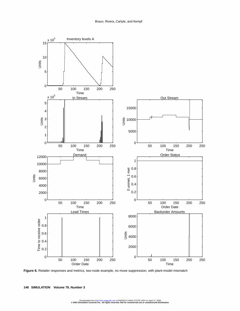
MPC controller makes use of a model that assumes a pro-duction leadtime of 2 time units. The retailer MPC con-troller is implemented as if there exists no shipping delaybetween the factory and the retailer, but in the simulation,there is 1 time unit of delay. There is no production de-lay in the retailer for either simulation or controller. First,the controllers are implemented with no move suppression.The time series and metrics for the retailer and factory areshown in Figures 6 and 7, respectively. Inventory levelsshow wild fluctuations and increase to exorbitant levels;customer service could be better. Using move suppressionvalues of 150 for both controllers, the system is stabilized,and the 1500 units of safety stock are sufficient to eliminatebackorders, as shown in Figures 8 and 9.

4. Two-Product, Three-Echelon, Six-NodeProblem Analysis

The performance and robustness of the MPC control sys-tem are now demonstrated on a six-node network simulatedusing realistic plant-model mismatch, biased forecast er-ror, and a realistic demand profile. These conditions wererecommended for evaluation by Intel Corporation on a six-node, two-product, three-echelon simulation. The simula-tion mimics the packaging, distribution, and retail sale ofsemiconductor products in each of the three echelons.

Figure 10 illustrates the interconnections of the mate-rial flows for the six-node Intel problem [11]. As noted inthe diagram, transportation delays range from 2 to 4 days.The direct shipment routes each require 2 days. The cross-shipment routes require 3 days between assembly/test andwarehouse echelons. The cross-shipment routes require 4days between warehouse and retailer echelons. In the ware-house and retailer nodes, material that enters the receivingdock does not show up in the inventory until the followingday. The assembly/test nodes require an additional 10 daysfor processing.

For this demand network pattern, the transportation de-lays can be modeled in the same way as was done withthe two-node supply chain. There are three new modelingentities to consider: factories, geographic warehouses, andretailers. Each has a different configuration of input andoutput flows. For the single-inflow, two-outflow factory, asshown in Figure 12, the material balances for each speciescan be written

IA(k + 1) = PA(k) − S2A(k) − S3A(k) + IA(k), (5)

IB(k + 1) = PB(k) − S2B(k) − S3B(k) + IB(k), (6)

with the constitutive relationships

PA(k) = S1A(k − Θp), (7)

PB(k) = S1B(k − Θp). (8)

As with the two-node problem, I represents inventory, Srepresents in and out stream values, Θp represents process-ing delays, and PA(k) and PB(k) represent material that has

completed processing at time k of species A and B, respec-tively. These material balances are subject to the followingconstraints:

IA(k + 1) + IB(k + 1) ≤ CI , (9)

S1A(k) + S1B(k) ≤ C1, (10)

S2A(k) + S3A(k) + S2B(k) + S3B(k) ≤ C23, (11)

S2A(k) + S2B(k) ≤ C2, (12)

S3A(k) + S3B(k) ≤ C3. (13)

These constraints represent capacity limitations on inven-tory, shipping for stream 1, release rate from the fac-tory, shipping for stream 2, and shipping for stream 3,respectively.

The next entity to consider is the two-inflow, two-outflow warehouse, as represented in Figure 13. The ma-terial balances of this system are a natural extension of thesingle-inflow, two-outflow material balance equations:

IA(k + 1) = S1A(k) + S2A(k) − S3A(k)

−S4A(k) + IA(k), (14)

IB(k + 1) = S1B(k) + S2B(k) − S3B(k)

−S4B(k) + IB(k). (15)

These material balances are subject to the followingconstraints:

IA(k + 1) + IB(k + 1) ≤ CI , (16)

S1A(k) + S1B(k) ≤ C1, (17)

S2A(k) + S2B(k) ≤ C2, (18)

S1A(k) + S2A(k) + S1B(k) + S2B(k) ≤ C12, (19)

S3A(k) + S3B(k) ≤ C3, (20)

S4A(k) + S4B(k) ≤ C4, (21)

S3A(k) + S4A(k) + S3B(k) + S4B(k) ≤ C34. (22)

These constraints represent capacity limitations on inven-tory, shipping for stream 1, shipping for stream 2, totalinflow rate, shipping for stream 3, shipping for stream 4,and release rate from the warehouse, respectively.

For the two-inflow, single-outflow retailer (Fig. 14), thematerial balances are written

IA(k + 1) = S1A(k) + S2A(k) − S3A(k) + IA(k), (23)

IB(k + 1) = S1B(k) + S2B(k) − S3B(k) + IB(k). (24)

These material balances are subject to the followingconstraints:

IA(k + 1) + IB(k + 1) ≤ CI , (25)

S1A(k) + S1B(k) ≤ C1, (26)

S2A(k) + S2B(k) ≤ C2, (27)

S1A(k) + S2A(k) + S1B(k) + S2B(k) ≤ C12, (28)

S3A(k) + S3B(k) ≤ C3. (29)





50 100 150 200 2500

5

10

15x 10


Time

Uni

ts

50 100 150 200 2500

1

2

3

4

5

x 105

In Stream

Time

Uni

ts

50 100 150 200 2500

5000

10000

15000

Out Stream

Time

Uni

ts

50 100 150 200 2500

2000

4000

6000

8000

10000

12000 Demand

Time

Uni

ts

50 100 150 200 2500

0.2

0.4

0.6

0.8

1

Order Status

Order Date

0un

met

, 1m

et

50 100 150 200 2500

0.2

0.4

0.6

0.8

1

Lead Times

Order Date

Tim

e to

rec

eive

ord

er

50 100 150 200 2500

2000

4000

6000

8000Backorder Amounts

Time

Uni

ts

Figure 6. Retailer responses and metrics, two-node example, no move suppression, with plant-model mismatch





50 100 150 200 250

1

2

3

4x 10


Time

Uni

ts

50 100 150 200 250

2

4

6

8

10x 10

5 In Stream

Time

Uni

ts

50 100 150 200 250

1

2

3

4

5x 10

5 Out Stream

Time

Uni

ts

50 100 150 200 250

1

2

3

4

5x 10

5 Demand

Time

Uni

ts

50 100 150 200 2500

0.2

0.4

0.6

0.8

1

Order Status

Order Date

0-un

met

, 1-m

et

50 100 150 200 2500

0.5

1

1.5

2

2.5

3

Lead Times

Order Date

Tim

e to

rec

eive

ord

er

50 100 150 200 2500

1

2

3

4

x 105 Backorder Amounts

Order Date

Uni

ts

Figure 7. Factory responses and metrics, two-node example, no move suppression, with plant-model mismatch





50 100 150 200 2500.9

1

1.1

1.2

1.3

1.4

1.5x 10


Time

Uni

ts

50 100 150 200 2500.9

1

1.1

1.2

1.3

1.4

1.5x 10

4 In Stream

Time

Uni

ts

50 100 150 200 2500.9

1

1.1

1.2

1.3

1.4

1.5x 10

4 Out Stream

Time

Uni

ts

50 100 150 200 2500.9

1

1.1

1.2

1.3

1.4

1.5x 10

4 Demand

Time

Uni

ts

50 100 150 200 2500

0.2

0.4

0.6

0.8

1

Order Status

Order Date

0un

met

, 1m

et

50 100 150 200 2500

0.05

0.1

0.15

0.2Lead Times

Order Date

Tim

e to

rec

eive

ord

er

50 100 150 200 2500

0.05

0.1

0.15


Time

Uni

ts

Figure 8. Retailer responses and metrics, two-node example, with move suppression and plant-model mismatch





50 100 150 200 2500.9

1

1.1

1.2

1.3

1.4

1.5x 10


Time

Uni

ts

50 100 150 200 2500.9

1

1.1

1.2

1.3

1.4

1.5x 10

4 In Stream

Time

Uni

ts

50 100 150 200 2500.9

1

1.1

1.2

1.3

1.4

1.5x 10

4 Out Stream

Time

Uni

ts

50 100 150 200 2500.9

1

1.1

1.2

1.3

1.4

1.5x 10

4 Demand

Time

Uni

ts

50 100 150 200 2500

0.2

0.4

0.6

0.8

1

Order Status

Order Date

0un

met

, 1m

et

50 100 150 200 2500

0.2

0.4

0.6

0.8

1

Lead Times

Order Date

Tim

e to

rec

eive

ord

er

50 100 150 200 2500

0.05

0.1

0.15


Order Date

Uni

ts

Figure 9. Factory responses and metrics, two-node example, with move suppression and plant-model mismatch





A, B

A, BF1

F2

W1

W2

R1

R2

C1

C2

2 days

3 days

2 days

2 days

4 days

2 days

Assembly/Test Warehouse Retailer

Figure 10. Six-node Intel network material flow

F1

F2

W1

W2

R1

R2

C1

C2


MPC MPCMPCForecasterProduction,

Shipping

Orders, Shipping

Inventory level

Inventorylevel

Inventorylevel

Orders, ShippingOrders, Shipping

Orders, Shipping

Inventorylevel

Inventorylevel

OrderForecasts

OrderForecasts Order

Forecasts

Orders

Orders

F1

F2

W1

W2

R1

R2

C1

C2


MPC MPCMPCForecasterProduction,

Shipping

Orders, Shipping

Inventory level

Inventorylevel

Inventorylevel

Orders, ShippingOrders, Shipping

Orders, Shipping

Inventorylevel

Inventorylevel

OrderForecasts

OrderForecasts Order

Forecasts

Orders

Orders

Inventory levelInventory level

Figure 11. Six-node Intel network information flow





Fi

S1S2

S3Fi

S1S2

S3

Figure 12. Single-inflow, two-outflow factory material streams

Wi

S1 S3

S4S2 Wi

Figure 13. Two-inflow, two-outflow warehouse material streams

Ri

S1 S3

S2RiRi

Figure 14. Two-inflow, single-outflow retailer material streams

These constraints represent capacity limitations on inven-tory, shipping for stream 1, shipping for stream 2, totalinflow rate, and shipping/release for stream 3 from the re-tailer, respectively.

Having investigated different facets of the demand net-work management problem with the two-node network,this insight can be applied to the six-node problem. Fig-ure 11 illustrates the information flow between the threeMPC controllers and the six nodes of the demand network.For this problem, one monolithic MPC controller wouldbecome computationally prohibitive. A fully decentralizedstructure (one controller for each node) would require in-tervention by an outer layer to manage the constraints dueto the interconnections of the nodes, the release rate ca-pacities, and the shipping capacities. Due to the nature of

the constraints, a compromise can be made between thetwo strategies. Three controllers are used. Each controllerhandles the flow and composition decisions for each ech-elon, passing forecasted information to the upstream nodeand receiving forecasted information from the downstreamnode. By resolving the information flows in this manner,the solution is scalable yet still feasible for managing theconstraints.

The MPC controllers for the warehouse and retailerechelons of the network have to be modified slightly toaccount for the cross-shipment routes that can occur be-tween echelons. The problem inputs now number eightsince there are two shipping lanes from each node, andeach lane can transport either or both products. To handlethe extra degrees of freedom this brings to the problem, the





penalties Qu for the cross-shipment routes are purposefullyset high, so these routes are not favored in the cost func-tion. This penalty also allows for a unique solution to theMPC problem.

Experience with the actual performance of assembly/test nodes and the estimated lead times by facility person-nel suggest that the facility personnel traditionally providethemselves a lead time buffer of 1 day. So, for example, ifin reality the process takes 9 days to complete, a 10-daylead time estimate will be quoted to others in the organi-zation. Thus, a 9-day actual/10-day estimate plant-modelmismatch is adopted for both assembly/test facilities.

The sales and marketing personnel have been generallyknown to determine forecasts that are biased in an opti-mistic manner. As an example, the sales forecast for thenext time period might be 11,000 units, when in fact theactual sales will be 10,000 units. To mimic this type of fore-cast bias, all demand forecasts passed to the retailer-levelMPC controller are biased by +1000 units.

Last, products have been observed to follow demandpatterns that may be correlated at times and uncorrelatedat other times. To mimic this type of behavior, the demandpatterns for product A and product B follow correlated,deterministic steps up until time 110. The remainder ofthe time, the demand patterns remain uncorrelated. Thisbehavior can be observed in Figure 15.

The experiment is run with a value of 300 for all movesuppression parameters Q∆u

, 0 for all penalties for valuesother than zero for direct shipment Qu, and a penalty of100 for all penalties for values other than zero for cross-shipmentsQu. Table 2 holds the prediction horizonsNp andcontrol horizons Nu for all three MPC controllers. Safetystock is set at 5000 units per product, per node. All inven-tory control error weights Qe are left at 1. All entities usea “pecking order” dispatch rule. The orders of warehouse1, retailer 1, and customer 1 take precedence over the or-ders of the corresponding counterparts. Secondarily, ordersfor product A take precedence over orders for product B.Figures 16 and 17 demonstrate the performance of this ap-proach with plots of inventories, demands, shipments, andfactory starts.

At time 1, the retailer MPC controller adjusts ordersand order forecasts to the upstream nodes to start bring-ing in more product since the demand forecast is now11,000, even though the actual amounts being demandedare 10,000. Because of the move suppression, the increasesin order amounts are less than 1000. The increase in ordersis evident in the increase in direct shipments and cross-shipments from the warehouse echelon. Soon the retailerMPC echelon realizes that the actual amount supplied tocustomers is not increasing, as suggested by the forecast,and the retailer MPC adjusts to account for the forecasterror and reduce inventory.

In the first few time units, inventories in the factory ech-elon and warehouse echelon are drained below their targetlevels. The factory echelon MPC controller now observes

the effects of the plant-model mismatch since the effectsof changes in the starts show up sooner than expected.The inventory levels of the assembly/test nodes fluctuate,but the fluctuation remains at reasonable levels. No back-orders take place throughout the entire experiment. This israther impressive since the general rule of thumb practicedfor this network requires a safety stock level equivalent tobetween two and four times the expected demand for thenext time period (e.g., if tomorrow’s demand is expectedto be 10,000 units, safety stock held today may range from20,000 to 40,000 units).

Note that the cross-shipments in this example are usedwhenever there are rapid changes in the order/demandforecasts. The MPC controllers make use of the cross-shipments since the costs associated with the move sup-pression weightings of the direct shipments become com-paratively large at these times. This may make sense notonly from an optimization standpoint, but in a realistic set-ting, it may also allow nodes to hedge against uncertaintiesor disturbances in transportation links or nodes connectedby the direct shipment lanes.

5. Simulation Details

All simulation runs reported were performed on a PentiumIV 1.33-GHz processor with 128 MB of memory. The runswere on the order of minutes for the two-node network and14 hours for the six-node network for typical runs.

The simulations were constructed and run in a MAT-LAB 5.3/Simulink 3.0 environment. The work began bycreating a library of Simulink blocks and accompanyingS-functions for each of the representative types of nodesthat might be used in the construction of a supply-demandnetwork: factory, warehouse, retailer. Each library blockwas designed so that multiple blocks could be placed inthe same Simulink model file with the material and infor-mation flows readily connected to form the network. Eachnode was designed with a Graphical User Interface (GUI)mask to allow for custom configuration of each node. De-mand source blocks are constructed to read in deterministicor create stochastic demands. Blocks to determine fore-casts from the stochastic demand source blocks and deter-ministic demand source blocks were included in the library.Finally, the MPC management blocks were constructed toallow for scalar and vector forecast inputs to accommo-date real-time orders or real-time and future order fore-casts. These blocks make use of the Optimization toolboxfor MATLAB, and the accompanying GUI masks allow theuser to readily modify all relevant optimization, constraint,and horizon length parameters. Every block constructedincludes options for generating high-quality plots of the fi-nal results, as well as diagnostic plots at intermediate timesteps in the simulation.

The MATLAB/Simulink simulation environment andthe model library constructed allow for rapid redesign andconfiguration in a visual, object-oriented manner. The GUI





0 50 100 150 200 2500.8

0.9

1

1.1

1.2x 10

4

Time

Uni

ts

Product AProduct B

Figure 15. Demand profiles for products A and B, six-node Intel network

Table 2. Prediction and control horizons used in six-node controllers

Parameter Echelon #1 Echelon #2 Echelon #3

Np 49 41 33Nu 42 34 12

masks not only serve for quick configuration, but vari-ables can be directly put in place of static values to allowfor scripting. Since MATLAB readily allows for a masterscript document to control the Simulink model file, a setof runs for a given design of experiments (DOE) can bereadily scripted and executed with little need for user in-tervention. The myriad of subroutine toolboxes availablefor MATLAB allow for quick implementation of ideas togenerate proof-of-concept results. Moreover, the powerfulgraphical tools of MATLAB can readily be accessed forplotting results from intermediate time steps in a simulationrun, the summary results from a given run, or full-responsesurfaces from a given DOE.

Some of the drawbacks to the approach include the factthat MATLAB is commercial software and additional tool-boxes are added at additional cost. The MATLAB languageis interpretive, which slows down the performance com-pared to compiled language environments, but the Com-piler toolbox can be used with modifications to the customcode. The Optimization toolbox routines are not stream-lined and robust for MPC application; additional work toimprove constraint handling and indeterminant solutions

would be beneficial. Last, the simulation time could benefitsubstantially from a parallel processing approach, whichcould solve the MPC blocks in parallel, rather than in asequential manner. This is not an existing feature of theMATLAB/Simulink environment.

6. Conclusions

As demonstrated throughout this paper, MPC offers theability to develop decision policies that stabilize inventoryin supply chains despite imperfect information regardingthe system dynamics and inaccurate demand forecasts. Themove suppression term in the MPC cost function representsa penalty on order changes; incorporating this term in theMPC optimization problem leads to increased robustness,which may not result from optimization schemes based onstrictly cost-optimal approaches. This was demonstratedthrough simulations performed with the two-node sup-ply chain. An MPC approach was shown to be flexibleenough to manage a system approaching industrial size andconfiguration—the six-node demand network proposed byIntel Corporation.





Warehouse 1 Product A Q

50 100 150 200 250

1

1.5

2x 10

4 Factory 1 Product A Q∆u3=300U

nits

50 100 150 200 250

1

1.5

2x 10

4 Factory 2 Product A Q∆u3=300

Uni

ts

50 100 150 200 250

1

1.5

2x 10

4 Factory 1 Product B Q∆u3=300

Uni

ts

50 100 150 200 250

1

1.5

2x 10

4 Factory 2 Product B Q∆u3=300

Uni

ts

50 100 150 200 250

1

1.5

2∆u2=300

Uni

ts

50 100 150 200 250

1

1.5

2x 10

4 Warehouse 2 Product A Q∆u2=300

Uni

ts

50 100 150 200 250

1

1.5

2x 10

4 Warehouse 1 Product B Q∆u2=300

Uni

ts

50 100 150 200 250

1

1.5

2x 10

4 Warehouse 2 Product B Q∆u2=300

Uni

ts

50 100 150 200 250

1

1.5

2x 10

4 Retailer 1 Product A Q∆u1=300

Uni

ts

50 100 150 200 250

1

1.5

2x 10

4 Retailer 2 Product A Q∆u1=300

Uni

ts

50 100 150 200 250

1

1.5

2x 10

4 Retailer 1 Product B Q∆u1=300

Time

Uni

ts

50 100 150 200 250

1

1.5

2x 10

4 Retailer 2 Product B Q∆u1=300

Time

Uni

ts

x 104

Figure 16. Inventories (solid) and demand (dashed) by facility and product. Assembly/test plots include starts (dash-dot).





50 100 150 200 2500.5

1

1.5x 10

4 Factory 1 Starts Q∆u3=300U

nits

50 100 150 200 2500.5

1

1.5x 10

4 Factory 2 Starts Q∆u3=300

Uni

ts

50 100 150 200 2500.5

1

1.5x 10

4 Warehouse 1 Direct Received Q∆u2=300

Uni

ts

50 100 150 200 2500.5

1

1.5x10

4 Warehouse 2 Direct Received Q∆u2=300

Uni

ts

50 100 150 200 2500

50

100

Warehouse 1 Cross Received Q∆u2=300

Uni

ts

50 100 150 200 2500

50

100

Warehouse 2 Cross Received Q∆u2=300

Uni

ts

50 100 150 200 2500.5

1

1.5x 10

4 Retailer 1 Direct Received Q∆u1=300

Uni

ts

50 100 150 200 2500.5

1

1.5x 10

4 Retailer 2 Direct Received Q∆u1=300

Uni

ts

50 100 150 200 2500

50

100

Retailer 1 Cross Received Q∆u1=300

Uni

ts

50 100 150 200 2500

50

100

Retailer 2 Cross Received Q∆u1=300

Uni

ts

50 100 150 200 2500.5

1

1.5x 10

4 Retailer 1 Demand Q∆u1=300

Time

Uni

ts

50 100 150 200 2500.5

1

1.5x 10

4 Retailer 2 Demand Q∆u1=300

Time

Uni

ts

Figure 17. Material flows product A (dashed) and product B (solid). Demand: product A (dotted) and product B (dash-dot) andcorresponding customer receipts product A (dashed) and product B (solid).





A natural extension of this work is to incorporate thedemand management side of the organization. Sales andmarketing functions serve to manipulate and predict de-mand forecasts, which may also be used to further max-imize profits or minimize costs for the organization. Byincorporating advertising and marketing models to predictsales volume as a function of advertising dollars spent, thesupply chain management function and sales and market-ing function may be better integrated.

7. Acknowledgment

Financial support from the National Science Foundation(NSF-DMI Award 0075682) and the Intel Research Coun-cil is gratefully acknowledged.

8. References

[1] Bodington, C. E., and D. E. Shobrys. 1999. Optimize the supply chain.In Advanced process control and information systems for the pro-cess industries, edited by L. A. Kane, 236-40. Houston, TX: Gulf.

[2] Kempf, K., K. Knutson, B. Armbruster, P. Babu, and B. Duarte. 2001.Fast accurate simulation of physical flows in demand networks.In Advanced simulation technologies conference, 111-16. Seattle,WA: Society for Computer Simulation International.

[3] Lee, H. L., V. Padmanabhan, and S. Whang. 1997. The bullwhip effectin supply chains. Sloan Management Review 93-102.

[4] PriceWaterhouseCoopers. 2000. Silicon 2000: Millennium semi-conductor survey on supply chain management. Retrievedfrom http://www.ebusiness.pwcglobal.com/external/gen-reg.nsf/semi?OpenForm&Seq=1

[5] García, C. E., D. M. Prett, and M. Morari. 1989. Model predictivecontrol: Theory and practice—a survey. Automatica 25 (3): 335-48.

[6] Tzafestas, S., G. Kapsiotis, and E. Kyriannakis. 1997. Model-based

predictive control for generalized production planning problems.Computers in Industry 34 (2): 201-20.

[7] Flores, M. E., D. E. Rivera, and V. Smith- Daniels. 2000. Managingsupply chains using model predictive control. Paper presented atthe AIChE 2000 annual meeting, November, Los Angeles.

[8] Perea-Lopez, E., I. E. Grossman, and B. E. Ydstie. 2000. Applicationof mpc to decentralized dynamic models for supply chain man-agement. Paper presented at the AIChE 2000 Annual Meeting,November, Los Angeles.

[9] Kafoglis,C. C. 1999. Maximize competitive advantage with a supplychain vision. Hydrocarbon Processing 47-50.

[10] Silver, E. A., D. F. Pyke, and R. Peterson. 1998. Inventory manage-ment and production planning and scheduling. New York: JohnWiley.

[11] Armbruster, D., R. Chidambaram, G. Godding, K. G. Kempf, and I.Katzorke. 2001. Modeling and analysis of decision flows in com-plex supply networks. In Proceedings of IV SIMPOI/POMS 2001,Guaruja, Brazil, pp. 1106-14.

Martin W. Braun is a member of the technical staff at the KilbyCenter of Texas Instruments, Inc., Dallas, Texas.

Daniel E. Rivera is an associate professor in the Departmentof Chemical and Materials Engineering, Control Systems Engi-neering Laboratory, Arizona State University, Tempe. He is alsothe program director for the ASU Control Systems EngineeringLaboratory.

W. Matthew Carlyle is an associate professor in the Opera-tions Research Department, Naval Postgraduate School, Mon-terey, California.

Karl G. Kempf is director of decision technologies at the In-tel Corporation and an adjunct professor at Arizona StateUniversity.












Application of Model Predictive Control to Robust Management of Multiechelon Demand Networks in...

Documents

Transcript of Application of Model Predictive Control to Robust Management of Multiechelon Demand Networks in...