Robust backstepping and neural network control of a low

International Journal of Machine Tools & Manufacture 39 (1999) 1117–1134

Robust backstepping and neural network control of a low-quality nonholonomic mobile robot

Qiuju Zhanga, James Shippenb,*, Barrie Jonesc

aSchool of Manufacturing Engineering, Nanjing University of Science and Technology, Nanjing 210014, P.R. ChinabSchool of Manufacturing and Mechanical Engineering, The University of Birmingham, Birmingham B15 2TT, UK

cSchool of Engineering, The University of Aston, Birmingham B4 2A, UK

Received 26 August 1998

Abstract

A robust motion controller based on neural network and backstepping technique is proposed for a two-DOF low-quality mobile robot (MR). There are two main components in the motion controller. One is thetracking controller, which guarantees the MR follows the reference trajectory; the other one is the wheel-level inverse NN controller, which compensates the dynamics of the MR. Simulation results are providedto validate the proposed controllers. Experiments with a real low-quality MR, which were built from cheapdrivelines, have been used to verify the effectiveness and robustness of the motion controller. 1999Elsevier Science Ltd. All rights reserved.

Keywords:Neural network control; Nonholonomic mobile robot

1. Introduction

In the last decade there has been enormous activity in the study of nonholonomic mechanicalsystems. The characteristic of the nonholonomic system is that the constraints, which are imposedon the motion, are not integratable, i.e., the constraints cannot be written as time derivatives ofsome functions of the generalised co-ordinates. The typical examples of nonholonomic controlsystems are: mobile robots, robot manipulators, wheeled vehicles and space robotics. Researchcontinues on models of nonholonomic control systems, and on control design for motion planningand stabilisation [1,6]. Modelling and controlling such nonholonomic systems is a nontrivial prob-

* Corresponding author. Tel.: 0121-414-4153; fax: 0121-414-3958; e-mail: [email protected]

0890-6955/99/$ - see front matter 1999 Elsevier Science Ltd. All rights reserved.PII: S0890-6955(98)00080-7

1118 Q. Zhang et al. / International Journal of Machine Tools & Manufacture 39 (1999) 1117–1134

lem. Even in the simplest case, a two-DOF mobile robot which we shall study here, the trackingcontrol and pose (position and orientation) stabilisation require a sophisticated controller [1–3,6].The relative difficulty of the control problem depends not only on the nonholonomic nature ofthe system but also on the control objective. Furthermore, any efforts at controlling the nonholon-omic system with non-linear dynamics, uncertainties and disturbances will lead to more complex-structured controllers. For the tracking control problem of the MR, using smooth static timeinvariant state feedback for a velocity-controlled MR with one nonholonomic constraint wasdeveloped by Kanayama et al. [8] and later improved by Oelen and van Amerongen [7] with theeffect that the performance of the controller depends only on the geometry of the reference tra-jectory rather than the reference linear velocity. Applications of the backstepping technique tothe adaptive and robust control of the nonholonomic system were considered in Jiang and Nijme-ijer [3], Kolmanovsky and McClamroch [4], and Wan and Lewis [5]. The design technique toobtain a suitable time-varying state feedback was based on an integrator backstepping procedure.Fierro and Lewis [2] also used the backstepping control approach to take into account the specificdynamics to convert a steering system command into control inputs for the actual vehicle. Neuralnetwork and fuzzy logic control approaches were used to deal with the disturbances and dynamicuncertainties in the MR [2,5,9].

Although significant progress has been made, some important research problems remainunsolved, such as the problem of robustness and control of nonholonomic systems when thereare model uncertainties, as arises from parameter variations or from neglected dynamics, andmodel perturbations that destroy the “nonholonomic assumption”, e.g., the no-slip condition mayonly hold approximately. General methods for the design of robust controllers for nonholonomicsystems are still unavailable [1]. Most researchers demonstrate their theoretical approaches bycomputer stimulations. However, simulation studies usually neglect practically important aspects,such as non-linear dynamics, rolling friction, compliance of the mechanical structure and unmod-eled disturbances, therefore, the value of these approaches is limited.

Most mobile robots built for research use expensive precision motors to drive the wheels. Ifthe MR is to become an inexpensive mass-produced item, then it must use inexpensive compo-nents. The control of a low-quality MR is more difficult than that of a high-quality one becausethe non-linearities and uncertainties of the MR are more significant and the measured feedbacksignals are rather noisy. Reports on the study of the control of low-quality mobile robots areunknown, but it is (from an engineering perspective) a very interesting problem and may providepotential practical applications.

The purpose of this paper is to use the backstepping technique and neural networks in thetracking problem for the two-DOF mobile robot. In particular, under our proposed controllers, alow-quality experimental MR, which was constructed from cheap drivelines, can follow a refer-ence trajectory such as straight lines and circles. Special attention is paid to the controllerimplementations. The motion controller is comprised of two main components: one is the trackingcontroller, which is based on the backstepping technique and designed for a system with velocityinput. Another one is the wheel-level controller, which controls the motion of the driven wheels.Two inverse dynamic controllers based on the neural networks were developed to control thevelocity of the wheels. Between these two components, there were the decoupling and couplinginterfaces which were used to decompose the linear velocity and angular velocity of the MR intothe rotation speed of the two driven motors, and vice versa to synthesise the individual measure-ment signals from each wheel into the position and velocity of the MR.

1119Q. Zhang et al. / International Journal of Machine Tools & Manufacture 39 (1999) 1117–1134

The remainder of the article is organised as follows: Section 2 provides the theoretical back-ground of a nonholonomic MR and tracking problem formulation. In Section 3, the trackingmodel and tracking control structure are presented. The simulation results of the proposed trackingcontroller are given in Section 4. Section 5 describes the experimental low-quality MR systemand control implementation. In Section 6, the design of the inverse neural network controlleris explained. In Section 7, experimental results are given. Finally, conclusions are presented inSection 8.

2. Problem formulation

2.1. Preliminary definitions

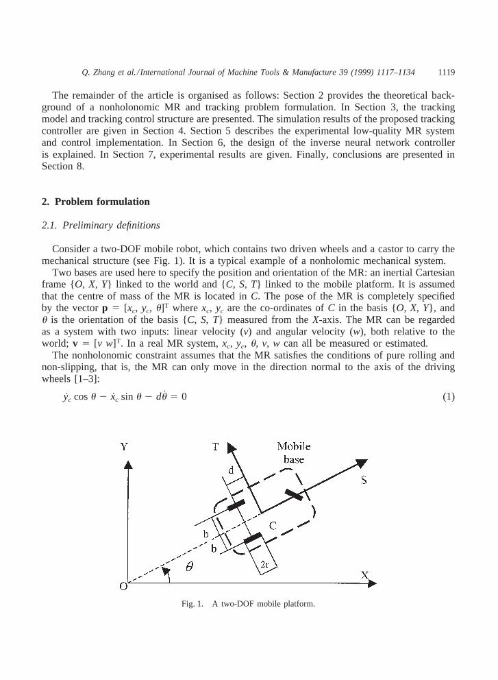
Consider a two-DOF mobile robot, which contains two driven wheels and a castor to carry themechanical structure (see Fig. 1). It is a typical example of a nonholomic mechanical system.

Two bases are used here to specify the position and orientation of the MR: an inertial Cartesianframe {O, X, Y} linked to the world and {C, S, T} linked to the mobile platform. It is assumedthat the centre of mass of the MR is located inC. The pose of the MR is completely specifiedby the vectorp 5 [xc, yc, u]T wherexc, yc are the co-ordinates ofC in the basis {O, X, Y}, andu is the orientation of the basis {C, S, T} measured from theX-axis. The MR can be regardedas a system with two inputs: linear velocity (v) and angular velocity (w), both relative to theworld; v 5 [v w]T. In a real MR system,xc, yc, u, v, w can all be measured or estimated.

The nonholonomic constraint assumes that the MR satisfies the conditions of pure rolling andnon-slipping, that is, the MR can only move in the direction normal to the axis of the drivingwheels [1–3]:

yc cosu 2 xc sin u 2 du 5 0 (1)

Fig. 1. A two-DOF mobile platform.


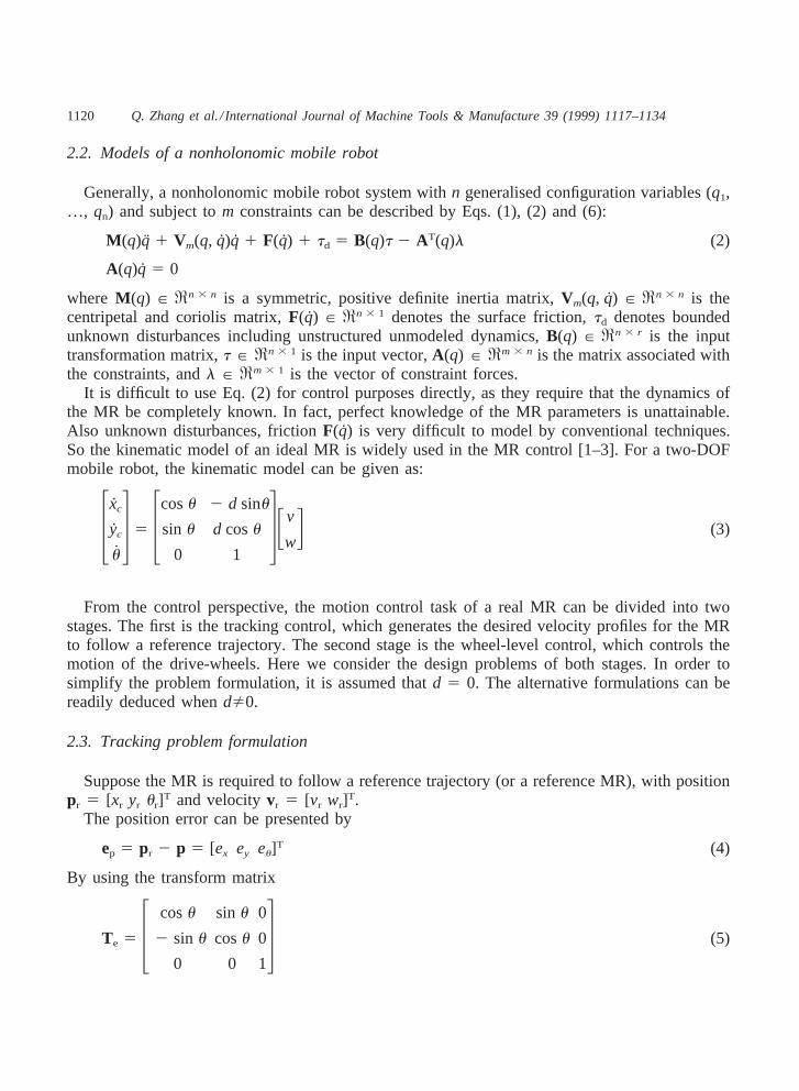
2.2. Models of a nonholonomic mobile robot

Generally, a nonholonomic mobile robot system withn generalised configuration variables (q1,…, qn) and subject tom constraints can be described by Eqs. (1), (2) and (6):

M (q)q 1 Vm(q, q)q 1 F(q) 1 td 5 B(q)t 2 AT(q)l (2)

A(q)q 5 0

where M (q) P Rn 3 n is a symmetric, positive definite inertia matrix,Vm(q, q) P Rn 3 n is thecentripetal and coriolis matrix,F(q) P Rn 3 1 denotes the surface friction,td denotes boundedunknown disturbances including unstructured unmodeled dynamics,B(q) P Rn 3 r is the inputtransformation matrix,t P Rn 3 1 is the input vector,A(q) P Rm 3 n is the matrix associated withthe constraints, andl P Rm 3 1 is the vector of constraint forces.

It is difficult to use Eq. (2) for control purposes directly, as they require that the dynamics ofthe MR be completely known. In fact, perfect knowledge of the MR parameters is unattainable.Also unknown disturbances, frictionF(q) is very difficult to model by conventional techniques.So the kinematic model of an ideal MR is widely used in the MR control [1–3]. For a two-DOFmobile robot, the kinematic model can be given as:

3xc

yc

u4 5 3cosu 2 d sinu

sin u d cosu

0 14Fv

wG (3)

From the control perspective, the motion control task of a real MR can be divided into twostages. The first is the tracking control, which generates the desired velocity profiles for the MRto follow a reference trajectory. The second stage is the wheel-level control, which controls themotion of the drive-wheels. Here we consider the design problems of both stages. In order tosimplify the problem formulation, it is assumed thatd 5 0. The alternative formulations can bereadily deduced whendÞ0.

2.3. Tracking problem formulation

Suppose the MR is required to follow a reference trajectory (or a reference MR), with positionpr 5 [xr yr ur]T and velocityvr 5 [vr wr]T.

The position error can be presented by

ep 5 pr 2 p 5 [ex ey eu]T (4)

By using the transform matrix

Te 5 3 cosu sin u 0

2 sin u cosu 0

0 0 14 (5)


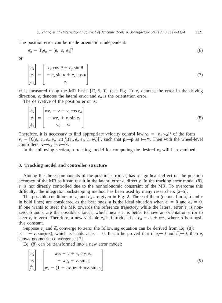
The position error can be made orientation-independent:

ecp 5 Teep 5 [es et eu]T (6)

or

3es

et

eu

4 5 3 ex cosu 1 ey sin u

2 ex sin u 1 ey cosu

eu

4 (7)

ecp is measured using the MR basis {C, S, T} (see Fig. 1).es denotes the error in the driving

direction,et denotes the lateral error andeu is the orientation error.The derivative of the position error is:

3es

et

eu

4 5 3wet 2 v 1 vr coseu

2 wes 1 vr sineu

wr 2 w4 (8)

Therefore, it is necessary to find appropriate velocity control lawvd 5 [vd wd]T of the formvd 5 [fv(es, et, eu, vr, wr) fw(es, et, eu, vr, wr)]T, such thatpr→p as t→`. Then with the wheel-levelcontrollers,v→vd as t→`.

In the following section, a tracking model for computing the desiredvd will be examined.

3. Tracking model and controller structure

Among the three components of the position error,eu has a significant effect on the positionaccuracy of the MR as it can result in the lateral erroret directly. In the tracking error model (8),et is not directly controlled due to the nonholonomic constraint of the MR. To overcome thisdifficulty, the integrator backstepping method has been used by many researchers [2–5].

The possible conditions ofet andeu are given in Fig. 2. Three of them (denoted in a, b and cin bold lines) are considered as the best ones. a is the ideal situation whenet 5 0 andeu 5 0.If one wants to steer the MR towards the reference trajectory while the lateral erroret is non-zero, b and c are the possible choices, which means it is better to have an orientation error tosteeret to zero. Therefore, a new variableeu is introduced aseu 5 eu 1 aet, wherea is a posi-tive constant.

Supposees and eu converge to zero, the following equation can be derived from Eq. (8):et 5 2 vr sin(aet), which is stable atet 5 0. It can be proved that ifes→0 and eu→0, thenet

shows geometric convergence [7].Eq. (8) can be transformed into a new error model:

3es

et

e1u

4 5 3 wet 2 v 1 vr coseu

2 wes 1 vr sin eu

wr 2 (1 1 aes)w 1 avr sin eu

4 (9)


Fig. 2. Possible error situations.

The backstepping technique [3,4] is used here to construct a feedback control law for Eq. (9).Consider the candidate Lyapunov function

V(t, es, et, eu) 512

es2 1

12

et2 1

12g

eu2 (10)

with g > 0. From Eqs. (9) and (10), the time derivative ofV is:

V(t, es, et, eu) 5 es( 2 v 1 vr coseu) 1 etvr sineu 11g

eu[wr 2 (1 1 aes)w (11)

1 avr sineu]

A smooth time-periodic feedback law can be chosen as [4]:

Fvd

wdG 5 F k1es 1 vr coseu

(1 1 aes)−1(wr 1 k2eu 1 avr sin eu)G (12)

where,k1, k2, anda are positive constants.Eq. (12) is the same as the local tracking controller proposed by Jiang and Nijmeijer [3] replac-

ing w(vret) by aet.However, the control law (12) is thatw may not be defined for everyt; consider the case when


a 5 1 andes 5 2 1. So a modification of Eq. (12) is required resulting in the tracking controllaw implemented:

Fvd

wdG 5 F k1es 1 vr coseu

wr 1 k2eu 1 avr sineu

G (13)

Note that Eq. (13) is similar to the control laws used by Fierro and Lewis [2]:

Fvd

wdG 5 F c1es 1 vr coseu

wr 1 c2vret 1 c3vr sineu

G (14)

where,c1, c2, c3 are positive constants.The simulation results, which will be provided later, show that the controller (13) has a better

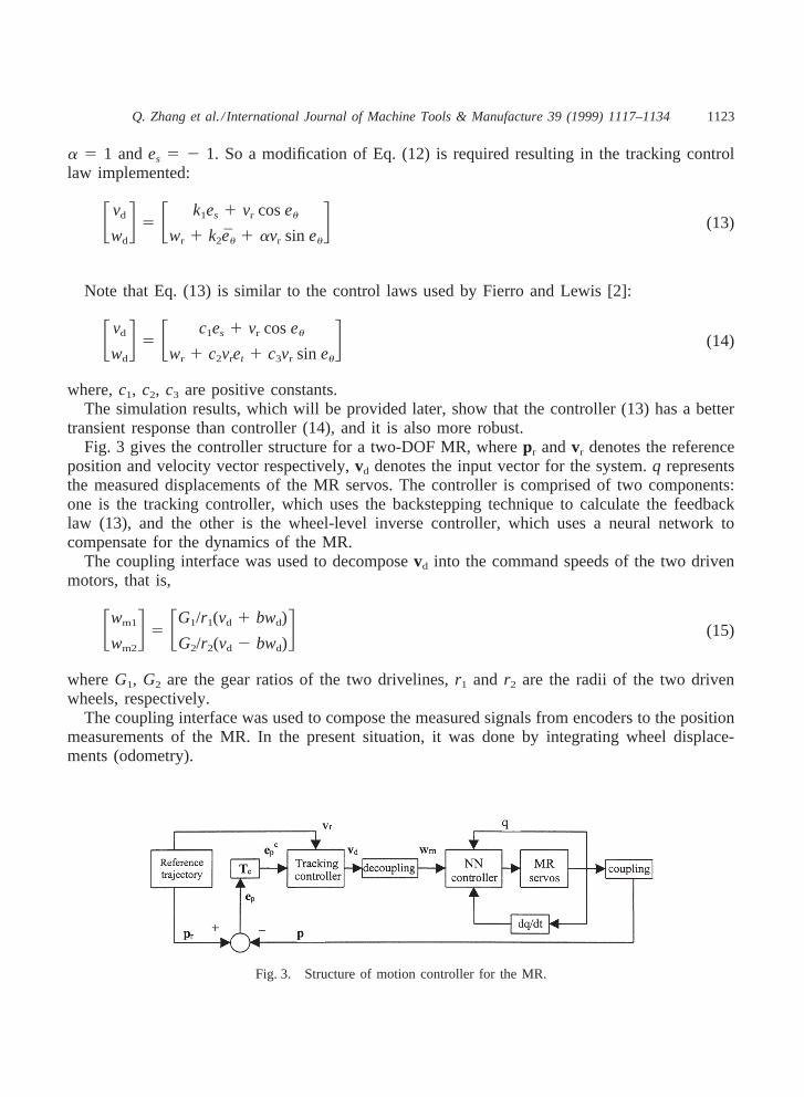
transient response than controller (14), and it is also more robust.Fig. 3 gives the controller structure for a two-DOF MR, wherepr andvr denotes the reference

position and velocity vector respectively,vd denotes the input vector for the system.q representsthe measured displacements of the MR servos. The controller is comprised of two components:one is the tracking controller, which uses the backstepping technique to calculate the feedbacklaw (13), and the other is the wheel-level inverse controller, which uses a neural network tocompensate for the dynamics of the MR.

The coupling interface was used to decomposevd into the command speeds of the two drivenmotors, that is,

Fwm1

wm2G 5 FG1/r1(vd 1 bwd)

G2/r2(vd 2 bwd)G (15)

whereG1, G2 are the gear ratios of the two drivelines,r1 and r2 are the radii of the two drivenwheels, respectively.

The coupling interface was used to compose the measured signals from encoders to the positionmeasurements of the MR. In the present situation, it was done by integrating wheel displace-ments (odometry).

Fig. 3. Structure of motion controller for the MR.


Fig. 4. Simulation model.

4. Simulation results

The model for the simulations is shown in Fig. 4, together with the linear and angular velocityperturbationsjv and jw. For the real MR, the perturbations are primarily caused by mechanicaldisturbances, such as stick-and-slip, gear backlash, misalignment of the drive wheels, vibrationsof the motors, noisy measurement signals, etc. All simulations were carried out using MATLAB.

Firstly the comparison of control law (13) and (14) was made by two sets of simulation results.

1. Ideal MR:jv 5 0, jw 5 0. The controller parameters for (13) were chosen by try-and-trial forbest response:k1 5 10, k2 5 2, a 5 4; the parameters for controller (16) were the same asin [2]: c1 5 10, c2 5 5, c3 5 4. The reference trajectory was a line with orientation angleu5 45°; vr is shown in Fig. 5,Cv 5 2 m/s;wr ; 0. The initial errors were:ex 5 2 0.6, ey 50, eu 5 2 p/4.

2. As (1), but the reference trajectory is a circle with radiusvr/wr, vr ; 1, wr ; 1, xr(t) 5 1 1sin(wrt), yr(t) 5 1 2 cos(wrt). Initial errors:ex 5 1, ey 5 0.6, eu 5 0. The simulation resultsare given in Figs. 6 and 7. It shows that controller (13) has a faster convergence speed andsmaller position errors than controller (14). In order to illustrate the robustness of the trackingcontroller (15), another three sets of simulations were considered:

3. As (1), but with different initial errors: (a) initial error (ex, ey, eu) 5 ( 2 0.06, 0,2 p/4); (b)initial error (ex, ey, eu) 5 ( 2 10, 2, 2 p/4); (c) initial error (ex, ey, eu) 5 (0, 2 5, p/2).

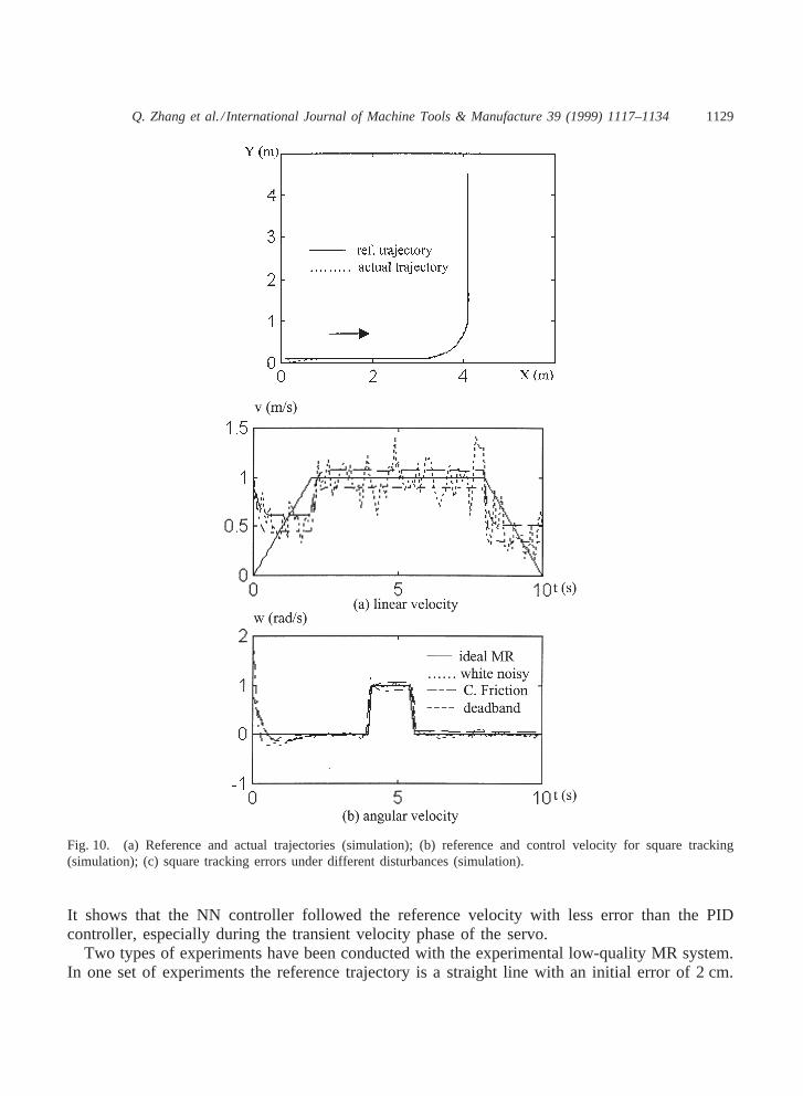
4. As (1), but with differentvr, that is, differentCv: (a) Cv 5 2; (b) Cv 5 3; (c) Cv 5 1.5. Controller parameters: same as (1). Reference trajectory: a square comprised of line and circle

(see Fig. 10(a)); reference velocityvr andwr (see Fig. 10(b)); initial tracking error: (ex, ey, eu)5 (0.1, 0.1, 0). Different signals were chosen as the perturbations: white noise, Coulombicfriction and deadband as may exist in the control of a real MR.

Fig. 5. Reference linear velocity profile (simulation).


Fig. 6. Straight line tracking errors (simulation).

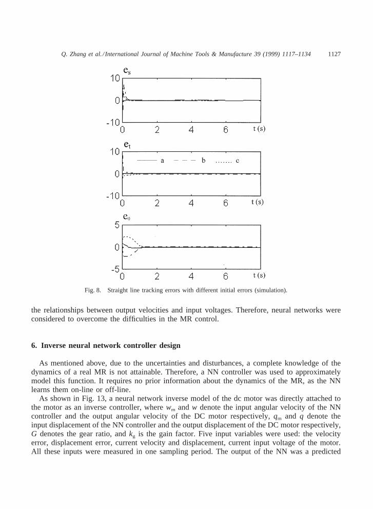
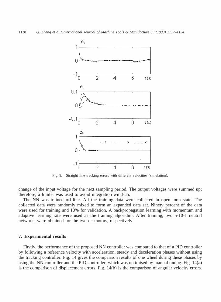
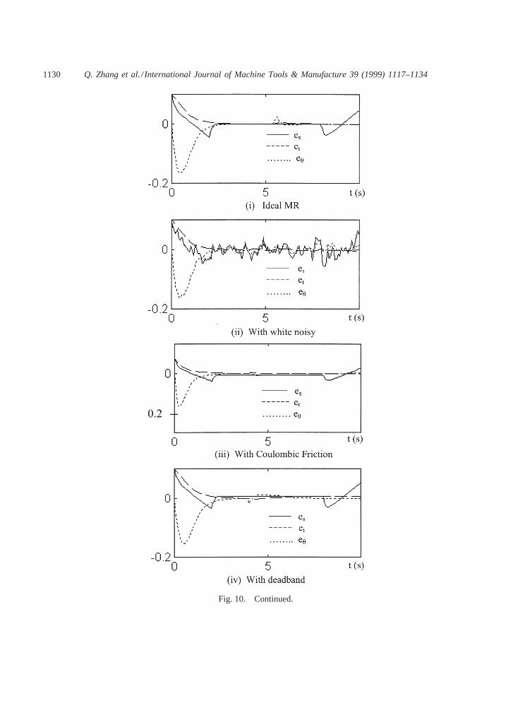
The simulation results are given in Figs. 8–10. Fig. 8 shows that for small (a) and large (b, c)initial errors, the tracking controller performs well. With large initial orientation erroreu, the MRexhibits oscillations whilst tracking the reference trajectory. Therefore, the lateral error decreasesquickly while the orientation error remains. Fig. 9 shows the influence of different linear velocitieson the tracking performance. For lowerCv, the convergence of the lateral erroret becomes slowerand exhibits smaller overshoot. Fig. 10(a) gives the reference square and the actual path of theMR. The MR follows the reference square accurately except in the beginning and the middle arcpart. Fig. 10(b) gives the control linear and angular velocities in different situations. It shows thatthe influence of perturbations on the linear velocity is more significant than on the angular velo-city. Fig. 10(c) shows that the white noise causes noise-like errors, and Coulumbic friction anddeadband generate steady-state errors in driving direction, but no lateral and orientation errorsare introduced.

It is known that the most important performance criteria for tracking control of the MR arelateral and orientation errors. The simulation results in Figs. 8–10 show that the proposed trackingcontroller behaves well and has a good robustness.


Fig. 7. Circle tracking trajectories (simulation).

5. A low quality experimental MR system

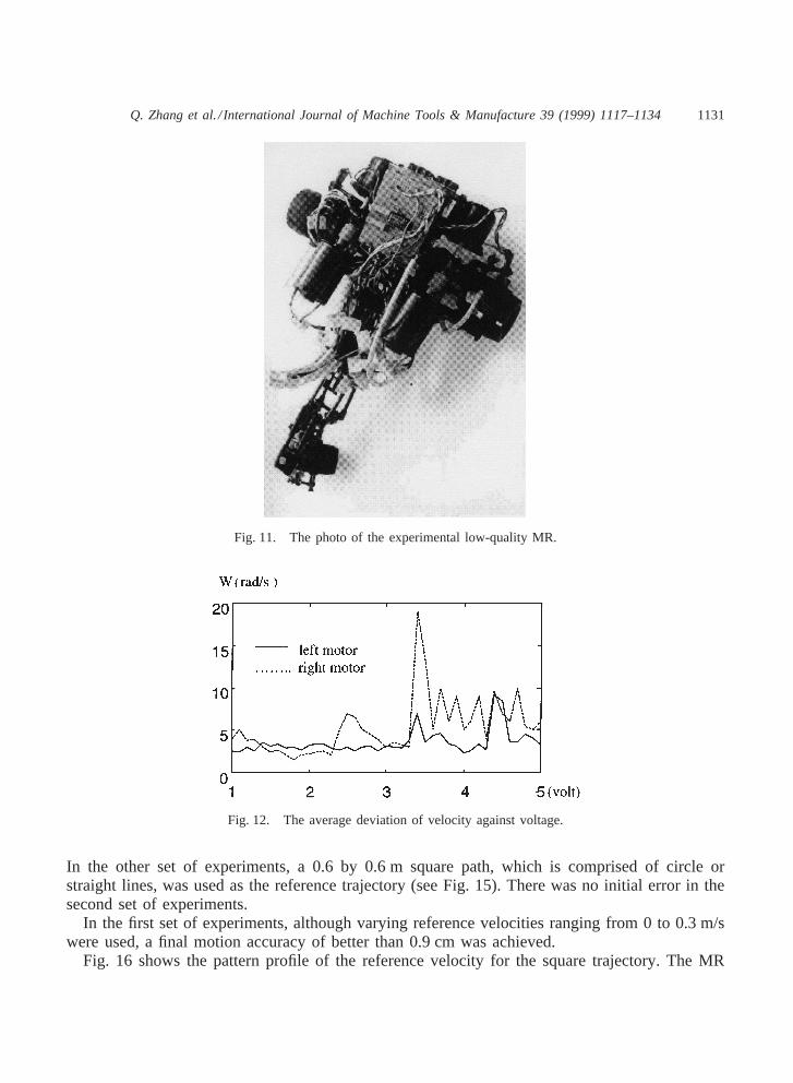
The experimental mobile robot system used in this paper is shown in Fig. 11. It consists of avehicle with two driving front wheels mounted on the same axis; a rear castor wheel preventsthe robot from tipping over as it moves on a plane. The motion and orientation are achieved byindependent actuators, e.g., each front wheel is driven by a dc motor. The dc motor and drivelinewere built from low quality materials. The motor is a three-pole permanent magnetic dc motor.The driveline consists of a set of low-precision polythene worm-pinion gears. The gear ratio is54:1. Both motor and driveline systems suffered from a lot of disturbances and uncertaintiescaused by the vibration of the motor, gear backlash and stick-and-slip problem. The displacementoutput of each motor was measured by a crude incremental encoder on the motor shaft (four-lineencoder). No pre-filtering was used to filter the noisy feedback signals. Velocity signals of theservo were obtained by differentiating the displacement outputs. The error bound of the displace-ment output of the wheel was6 0.03 rad (2p*gear radio/4) and the velocity output was60.3 rad/s with a sampling period of 0.1 s. The tracking controller was implemented in a PC 486-33. A 12-bit resolution D/A card and a 16-bit encoder card were used to transfer the control andfeedback signals.

Fig. 12 gives the average deviations of the left and right motors’ velocities against input volt-ages on the motors from 10 trials. The input voltages varied from 1 to 5 V in steps of 0.1 V. Thesteady velocities of the motors were measured over a period of 5 s with a sampling period of0.1 s. It shows that the velocity outputs were exceptionally noisy and non-linearities existed in


Fig. 8. Straight line tracking errors with different initial errors (simulation).

the relationships between output velocities and input voltages. Therefore, neural networks wereconsidered to overcome the difficulties in the MR control.

6. Inverse neural network controller design

As mentioned above, due to the uncertainties and disturbances, a complete knowledge of thedynamics of a real MR is not attainable. Therefore, a NN controller was used to approximatelymodel this function. It requires no prior information about the dynamics of the MR, as the NNlearns them on-line or off-line.

As shown in Fig. 13, a neural network inverse model of the dc motor was directly attached tothe motor as an inverse controller, wherewm andw denote the input angular velocity of the NNcontroller and the output angular velocity of the DC motor respectively,qm and q denote theinput displacement of the NN controller and the output displacement of the DC motor respectively,G denotes the gear ratio, andkg is the gain factor. Five input variables were used: the velocityerror, displacement error, current velocity and displacement, current input voltage of the motor.All these inputs were measured in one sampling period. The output of the NN was a predicted


Fig. 9. Straight line tracking errors with different velocities (simulation).

change of the input voltage for the next sampling period. The output voltages were summed up;therefore, a limiter was used to avoid integration wind-up.

The NN was trained off-line. All the training data were collected in open loop state. Thecollected data were randomly mixed to form an expanded data set. Ninety percent of the datawere used for training and 10% for validation. A backpropagation learning with momentum andadaptive learning rate were used as the training algorithm. After training, two 5-10-1 neutralnetworks were obtained for the two dc motors, respectively.

7. Experimental results

Firstly, the performance of the proposed NN controller was compared to that of a PID controllerby following a reference velocity with acceleration, steady and deceleration phases without usingthe tracking controller. Fig. 14 gives the comparison results of one wheel during these phases byusing the NN controller and the PID controller, which was optimised by manual tuning. Fig. 14(a)is the comparison of displacement errors. Fig. 14(b) is the comparison of angular velocity errors.


Fig. 10. (a) Reference and actual trajectories (simulation); (b) reference and control velocity for square tracking(simulation); (c) square tracking errors under different disturbances (simulation).

It shows that the NN controller followed the reference velocity with less error than the PIDcontroller, especially during the transient velocity phase of the servo.

Two types of experiments have been conducted with the experimental low-quality MR system.In one set of experiments the reference trajectory is a straight line with an initial error of 2 cm.


Fig. 10. Continued.


Fig. 11. The photo of the experimental low-quality MR.

Fig. 12. The average deviation of velocity against voltage.

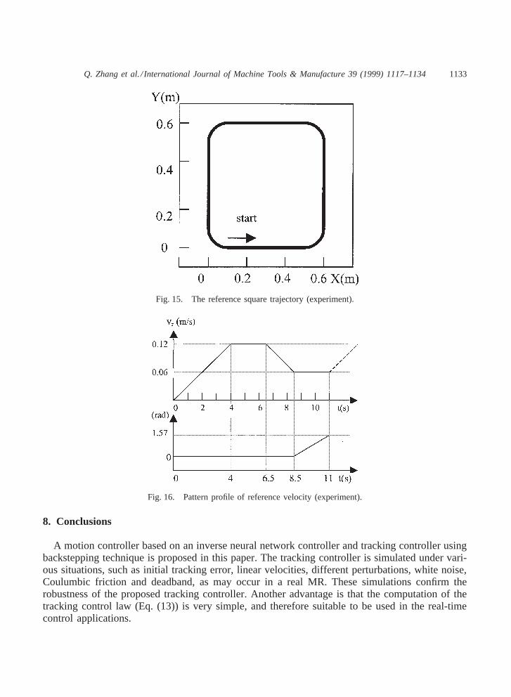
In the other set of experiments, a 0.6 by 0.6 m square path, which is comprised of circle orstraight lines, was used as the reference trajectory (see Fig. 15). There was no initial error in thesecond set of experiments.

In the first set of experiments, although varying reference velocities ranging from 0 to 0.3 m/swere used, a final motion accuracy of better than 0.9 cm was achieved.

Fig. 16 shows the pattern profile of the reference velocity for the square trajectory. The MR


Fig. 13. Inverse NN control structure.

Fig. 14. Comparison between the NN and PID controller (experiment).

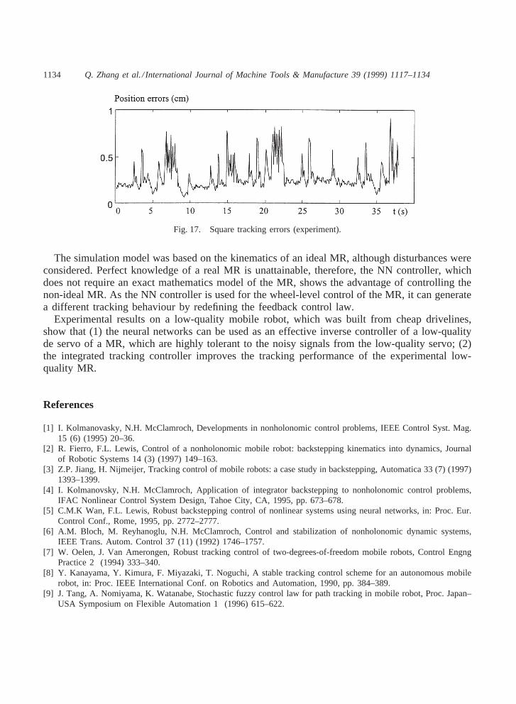
was decelerated from the maximum speed of 0.12 m/s to 0.06 m/s before turning a corner, andit was again accelerated to 0.12 m/s after turning the corner. The tracking controller parameterswere set to:k1 5 10, k2 5 2, a 5 4. The total time taken for the trajectory was 38 s. The vehicledid not stop exactly at the start point, but a certain error remained. Fig. 17 gives the absoluteposition error as a function of time. It shows that during the entire trajectory the tracking positionerror remained below 1 cm.


Fig. 15. The reference square trajectory (experiment).

Fig. 16. Pattern profile of reference velocity (experiment).

8. Conclusions

A motion controller based on an inverse neural network controller and tracking controller usingbackstepping technique is proposed in this paper. The tracking controller is simulated under vari-ous situations, such as initial tracking error, linear velocities, different perturbations, white noise,Coulumbic friction and deadband, as may occur in a real MR. These simulations confirm therobustness of the proposed tracking controller. Another advantage is that the computation of thetracking control law (Eq. (13)) is very simple, and therefore suitable to be used in the real-timecontrol applications.


Fig. 17. Square tracking errors (experiment).

The simulation model was based on the kinematics of an ideal MR, although disturbances wereconsidered. Perfect knowledge of a real MR is unattainable, therefore, the NN controller, whichdoes not require an exact mathematics model of the MR, shows the advantage of controlling thenon-ideal MR. As the NN controller is used for the wheel-level control of the MR, it can generatea different tracking behaviour by redefining the feedback control law.

Experimental results on a low-quality mobile robot, which was built from cheap drivelines,show that (1) the neural networks can be used as an effective inverse controller of a low-qualityde servo of a MR, which are highly tolerant to the noisy signals from the low-quality servo; (2)the integrated tracking controller improves the tracking performance of the experimental low-quality MR.

References

[1] I. Kolmanovasky, N.H. McClamroch, Developments in nonholonomic control problems, IEEE Control Syst. Mag.15 (6) (1995) 20–36.

[2] R. Fierro, F.L. Lewis, Control of a nonholonomic mobile robot: backstepping kinematics into dynamics, Journalof Robotic Systems 14 (3) (1997) 149–163.

[3] Z.P. Jiang, H. Nijmeijer, Tracking control of mobile robots: a case study in backstepping, Automatica 33 (7) (1997)1393–1399.

[4] I. Kolmanovsky, N.H. McClamroch, Application of integrator backstepping to nonholonomic control problems,IFAC Nonlinear Control System Design, Tahoe City, CA, 1995, pp. 673–678.

[5] C.M.K Wan, F.L. Lewis, Robust backstepping control of nonlinear systems using neural networks, in: Proc. Eur.Control Conf., Rome, 1995, pp. 2772–2777.

[6] A.M. Bloch, M. Reyhanoglu, N.H. McClamroch, Control and stabilization of nonholonomic dynamic systems,IEEE Trans. Autom. Control 37 (11) (1992) 1746–1757.

[7] W. Oelen, J. Van Amerongen, Robust tracking control of two-degrees-of-freedom mobile robots, Control EngngPractice 2 (1994) 333–340.

[8] Y. Kanayama, Y. Kimura, F. Miyazaki, T. Noguchi, A stable tracking control scheme for an autonomous mobilerobot, in: Proc. IEEE International Conf. on Robotics and Automation, 1990, pp. 384–389.

[9] J. Tang, A. Nomiyama, K. Watanabe, Stochastic fuzzy control law for path tracking in mobile robot, Proc. Japan–USA Symposium on Flexible Automation 1 (1996) 615–622.

Robust backstepping and neural network control of a low

Documents

Transcript of Robust backstepping and neural network control of a low