Perceptron & Neural Networks

Perceptron & Neural Networks

1

Matt Gormley Lecture 12

October 17, 2016

School of Computer Science

Readings: Bishop Ch. 4.1.7, Ch. 5 Murphy Ch. 16.5, Ch. 28 Mitchell Ch. 4

10-‐701 Introduction to Machine Learning

Reminders

•  Homework 3: – due 10/24/16

2

Outline

•  Discriminative vs. Generative •  Perceptron •  Neural Networks •  Backpropagation

3

DISCRIMINATIVE AND GENERATIVE CLASSIFIERS

4

Generative vs. Discriminative •  Generative Classifiers:

–  Example: Naïve Bayes – Define a joint model of the observations x and the labels y:

–  Learning maximizes (joint) likelihood – Use Bayes’ Rule to classify based on the posterior:

•  Discriminative Classifiers: –  Example: Logistic Regression – Directly model the conditional: –  Learning maximizes conditional likelihood

5

p(x, y)

p(y|x)

p(y|x) = p(x|y)p(y)/p(x)

Generative vs. Discriminative

Finite Sample Analysis (Ng & Jordan, 2002) [Assume that we are learning from a finite training dataset]

6

If model assumptions are correct: Naive Bayes is a more efficient learner (requires fewer samples) than Logistic Regression

If model assumptions are incorrect: Logistic Regression has lower asymtotic error, and does better than Naïve Bayes

solid: NB dashed: LR

7 Slide courtesy of William Cohen

Naïve Bayes makes stronger assumptions about the data but needs fewer examples to estimate the parameters “On Discriminative vs Generative Classifiers: ….” Andrew Ng and Michael Jordan, NIPS 2001.

8

solid: NB dashed: LR

Slide courtesy of William Cohen

Generative vs. Discriminative

9

Learning (Parameter Estimation)

Naïve Bayes: Parameters are decoupled à Closed form solution for MLE

Logistic Regression: Parameters are coupled à No closed form solution – must use iterative optimization techniques instead

Naïve Bayes vs. Logistic Reg.

10

Learning (MAP Estimation of Parameters)

Bernoulli Naïve Bayes: Parameters are probabilities à Beta prior (usually) pushes probabilities away from zero / one extremes

Logistic Regression: Parameters are not probabilities à Gaussian prior encourages parameters to be close to zero (effectively pushes the probabilities away from zero / one extremes)

Naïve Bayes vs. Logistic Reg.

11

Features

Naïve Bayes: Features x are assumed to be conditionally independent given y. (i.e. Naïve Bayes Assumption)

Logistic Regression: No assumptions are made about the form of the features x. They can be dependent and correlated in any fashion.

THE PERCEPTRON ALGORITHM

12

Why don’t we drop the generative model and

try to learn this hyperplane directly?

Background: Hyperplanes Recall…

Background: Hyperplanes

H = {x : wT x = b}Hyperplane (Definition 1):

w

Half-‐spaces: H+ = {x : wT x > 0 and x1 = 1}H� = {x : wT x < 0 and x1 = 1}

Hyperplane (Definition 2):

H = {x : wT x = 0

and x1 = 1}

Recall…

Why don’t we drop the generative model and

try to learn this hyperplane directly?

Background: Hyperplanes Recall… Directly modeling the

hyperplane would use a decision function: for:

h( ) = sign(�T )

y � {�1, +1}

Online Learning Model

Setup: •  We receive an example (x, y) •  Make a prediction h(x) •  Check for correctness h(x) = y?

Goal: •  Minimize the number of mistakes

16

Margins

17

+ + +

+ -

- -

- -

𝛾 𝛾

+

- -

- -

w

Definition: The margin 𝛾 of a set of examples 𝑆 is the maximum 𝛾𝑤 over all linear separators 𝑤.

Geometric Margin

Definition: The margin 𝛾𝑤 of a set of examples 𝑆 wrt a linear separator 𝑤 is the smallest margin over points 𝑥 ∈ 𝑆.

Definition: The margin of example 𝑥 w.r.t. a linear sep. 𝑤 is the distance from 𝑥 to the plane 𝑤 ⋅ 𝑥 = 0 (or the negative if on wrong side)

Slide from Nina Balcan

Recall…

Perceptron Algorithm

18

Learning: Iterative procedure: •  while not converged

•  receive next example (x, y) •  predict y’ = h(x) •  if positive mistake: add x to parameters •  if negative mistake: subtract x from parameters

Data: Inputs are continuous vectors of length K. Outputs are discrete.

D = { (i), y(i)}Ni=1 where � RK and y � {+1, �1}

Prediction: Output determined by hyperplane.

y = h�(x) = sign(�T x) sign(a) =

�1, if a � 0

�1, otherwise

Perceptron Algorithm

19

Learning:

Algorithm 1 Perceptron Learning Algorithm (Batch)

1: procedure P (D = {( (1), y(1)), . . . , ( (N), y(N))})2: � � 0 � Initialize parameters3: while not converged do4: for i � {1, 2, . . . , N} do � For each example5: y � sign(�T (i)) � Predict6: if y �= y(i) then � If mistake7: � � � + y(i) (i) � Update parameters8: return �

Analysis: Perceptron

20 Slide from Nina Balcan

(Normalized margin: multiplying all points by 100, or dividing all points by 100, doesn’t change the number of mistakes; algo is invariant to scaling.)

Perceptron Mistake Bound Guarantee: If data has margin � and all points inside a ball ofradius R, then Perceptron makes � (R/�)2 mistakes.

+ +

+ +

+ +

+

-

- -

-

-

γ γ

- - - -

+

R

��


21 Figure from Nina Balcan

Perceptron Mistake Bound

+ +

+ +

+ +

+

-

--

-

-

γ γ

- -

-

-

+

R

��

Theorem 0.1 (Block (1962), Novikoff (1962)).Given dataset: D = {( (i), y(i))}N

i=1.Suppose:

1. Finite size inputs: ||x(i)|| � R2. Linearly separable data: �� s.t. ||��|| = 1 and

y(i)(�� · (i)) � �, �iThen: The number of mistakes made by the Perceptronalgorithm on this dataset is

k � (R/�)2


22

Proof of Perceptron Mistake Bound: We will show that there exist constants A and B s.t.

Ak � ||�(k+1)|| � B�

k

Ak � ||�(k+1)|| � B�

k

Ak � ||�(k+1)|| � B�

k

Ak � ||�(k+1)|| � B�

k

Ak � ||�(k+1)|| � B�

k


23

+ +

+ +

+ +

+

-

--

-

-

γ γ

- -

-

-

+

R

��

Theorem 0.1 (Block (1962), Novikoff (1962)).Given dataset: D = {( (i), y(i))}N

i=1.Suppose:

1. Finite size inputs: ||x(i)|| � R2. Linearly separable data: �� s.t. ||��|| = 1 and

y(i)(�� · (i)) � �, �iThen: The number of mistakes made by the Perceptronalgorithm on this dataset is

k � (R/�)2

Algorithm 1 Perceptron Learning Algorithm (Online)

1: procedure P (D = {( (1), y(1)), ( (2), y(2)), . . .})2: � � 0, k = 1 � Initialize parameters3: for i � {1, 2, . . .} do � For each example4: if y(i)(�(k) · (i)) � 0 then � If mistake5: �(k+1) � �(k) + y(i) (i) � Update parameters6: k � k + 17: return �


Whiteboard: Proof of Perceptron Mistake Bound

24


25

Proof of Perceptron Mistake Bound: Part 1: for some A, Ak � ||�(k+1)|| � B

�k

�(k+1) · �� = (�(k) + y(i) (i))��

by Perceptron algorithm update

= �(k) · �� + y(i)(�� · (i))

� �(k) · �� + �

by assumption

� �(k+1) · �� k�

by induction on k since �(1) = 0

� ||�(k+1)|| � k�

since || || � || || � · and ||��|| = 1

Cauchy-‐Schwartz inequality


26

Proof of Perceptron Mistake Bound: Part 2: for some B, Ak � ||�(k+1)|| � B

�k

||�(k+1)||2 = ||�(k) + y(i) (i)||2

by Perceptron algorithm update

= ||�(k)||2 + (y(i))2|| (i)||2 + 2y(i)(�(k) · (i))

� ||�(k)||2 + (y(i))2|| (i)||2

since kth mistake � y(i)(�(k) · (i)) � 0

= ||�(k)||2 + R2

since (y(i))2|| (i)||2 = || (i)||2 = R2 by assumption and (y(i))2 = 1

� ||�(k+1)||2 � kR2

by induction on k since (�(1))2 = 0

� ||�(k+1)|| ��

kR


27

Proof of Perceptron Mistake Bound: Part 3: Combining the bounds finishes the proof.

k� � ||�(k+1)|| ��

kR

�k � (R/�)2

The total number of mistakes must be less than this

Extensions of Perceptron

•  Kernel Perceptron – Choose a kernel K(x’, x) – Apply the kernel trick to Perceptron – Resulting algorithm is still very simple

•  Structured Perceptron – Basic idea can also be applied when y ranges over an exponentially large set

– Mistake bound does not depend on the size of that set

28

Summary: Perceptron

•  Perceptron is a simple linear classifier •  Simple learning algorithm: when a mistake is made, add / subtract the features

•  For linearly separable and inseparable data, we can bound the number of mistakes (geometric argument)

•  Extensions support nonlinear separators and structured prediction

29

RECALL: LOGISTIC REGRESSION

30

Using gradient ascent for linear classifiers

Key idea behind today’s lecture: 1.  Define a linear classifier (logistic regression) 2.  Define an objective function (likelihood) 3.  Optimize it with gradient descent to learn

parameters 4.  Predict the class with highest probability under

the model

31

Recall…


32

Use a differentiable function instead:

logistic(u) ≡ 11+ e−u

p�(y = 1| ) =1

1 + (��T )

This decision function isn’t differentiable:

sign(x)

h( ) = sign(�T )

Recall…


33

Use a differentiable function instead:


p�(y = 1| ) =1

1 + (��T )

This decision function isn’t differentiable:

sign(x)

h( ) = sign(�T )

Recall…

Logistic Regression

34

Learning: finds the parameters that minimize some objective function. �� = argmin

�J(�)

Data: Inputs are continuous vectors of length K. Outputs are discrete.

D = { (i), y(i)}Ni=1 where � RK and y � {0, 1}

Prediction: Output is the most probable class. y =

y�{0,1}p�(y| )

Model: Logistic function applied to dot product of parameters with input vector.

p�(y = 1| ) =1

1 + (��T )

Recall…

NEURAL NETWORKS

35

Learning highly non-linear functions

f: X à Y l  f might be non-linear function l  X (vector of) continuous and/or discrete vars l  Y (vector of) continuous and/or discrete vars

© Eric Xing @ CMU, 2006-2011 36

The XOR gate Speech recognition

Perceptron and Neural Nets l  From biological neuron to artificial neuron (perceptron)

l  Activation function

l  Artificial neuron networks l  supervised learning l  gradient descent

© Eric Xing @ CMU, 2006-2011 37

Soma Soma

Synapse

Synapse

Dendrites

Axon

Synapse

DendritesAxon

Threshold

Inputs

x1

x2

OutputY∑

HardLimiter

w2

w1

LinearCombiner

θ

∑=

=n

iiiwxX

1 ⎩⎨⎧

ω<−

ω≥+=

0

0

XX

Y if , if ,

11

Input Layer Output Layer

Middle Layer

I n p

u t

S i

g n

a l s

O u

t p

u t

S i

g n

a l s

Connectionist Models l  Consider humans:

l  Neuron switching time ~ 0.001 second

l  Number of neurons ~ 1010

l  Connections per neuron ~ 104-5

l  Scene recognition time ~ 0.1 second

l  100 inference steps doesn't seem like enough à much parallel computation

l  Properties of artificial neural nets (ANN) l  Many neuron-like threshold switching units l  Many weighted interconnections among units l  Highly parallel, distributed processes

© Eric Xing @ CMU, 2006-2011 38

Why is everyone talking about Deep Learning?

•  Because a lot of money is invested in it… – DeepMind: Acquired by Google for $400 million

– DNNResearch: Three person startup (including Geoff Hinton) acquired by Google for unknown price tag

–  Enlitic, Ersatz, MetaMind, Nervana, Skylab: Deep Learning startups commanding millions of VC dollars

•  Because it made the front page of the New York Times

39

Motivation

Why is everyone talking about Deep Learning?

Deep learning: – Has won numerous pattern recognition competitions

– Does so with minimal feature engineering

40

Motivation

1960s

1980s

1990s

2006

2016

This wasn’t always the case! Since 1980s: Form of models hasn’t changed much, but lots of new tricks…

–  More hidden units –  Better (online) optimization –  New nonlinear functions (ReLUs) –  Faster computers (CPUs and GPUs)

A Recipe for Machine Learning

1. Given training data:

41

Background

2. Choose each of these: –  Decision function

–  Loss function

Face Face Not a face

Examples: Linear regression, Logistic regression, Neural Network

Examples: Mean-‐squared error, Cross Entropy


1. Given training data: 3. Define goal:

42

Background



4. Train with SGD: (take small steps opposite the gradient)



43

Background




Gradients

Backpropagation can compute this gradient! And it’s a special case of a more general algorithm called reverse-‐mode automatic differentiation that can compute the gradient of any differentiable function efficiently!



44

Background




Goals for Today’s Lecture

1.  Explore a new class of decision functions (Neural Networks)

2.  Consider variants of this recipe for training

Linear Regression

45

Decision Functions

…

Output

Input

θ1 θ2 θ3 θM

y = h�(x) = �(�T x)

where �(a) = a

Logistic Regression

46

Decision Functions

…

Output

Input

θ1 θ2 θ3 θM

y = h�(x) = �(�T x)

where �(a) =1

1 + (�a)

y = h�(x) = �(�T x)

where �(a) =1

1 + (�a)

Logistic Regression

47

Decision Functions

…

Output

Input

θ1 θ2 θ3 θM

Face Face Not a face

y = h�(x) = �(�T x)

where �(a) =1

1 + (�a)

Logistic Regression

48

Decision Functions

…

Output

Input

θ1 θ2 θ3 θM

1 1 0

x1

x2

y

Logistic Regression

49

Decision Functions

…

Output

Input

θ1 θ2 θ3 θM

y = h�(x) = �(�T x)

where �(a) =1

1 + (�a)

Inputs

Weights

Output

Independent variables

Dependent variable

Prediction

Age 34

2 Gender

Stage 4

.6

.5

.8

.2

.1

.3 .7

.2

Weights HiddenLayer

“Probability of beingAlive”

0.6 Σ

Σ

.4

.2 Σ

Neural Network Model

© Eric Xing @ CMU, 2006-2011 50

Inputs

Weights

Output


Dependent variable

Prediction

Age 34

2 Gender

Stage 4

.6

.5

.8

.1

.7

Weights HiddenLayer


0.6 Σ

“Combined logistic models”

© Eric Xing @ CMU, 2006-2011 51

Inputs

Weights

Output


Dependent variable

Prediction

Age 34

2 Gender

Stage 4

.5

.8

.2

.3

.2

Weights HiddenLayer


0.6 Σ

© Eric Xing @ CMU, 2006-2011 52

© Eric Xing @ CMU, 2006-2011 53

Inputs

Weights

Output


Dependent variable

Prediction

Age 34

1 Gender

Stage 4

.6

.5

.8

.2

.1

.3 .7

.2

Weights HiddenLayer


0.6 Σ

Weights Independent variables

Dependent variable

Prediction

Age 34

2 Gender

Stage 4

.6

.5

.8

.2

.1

.3 .7

.2

Weights HiddenLayer


0.6 Σ

Σ

.4

.2 Σ

Not really, no target for hidden units...

© Eric Xing @ CMU, 2006-2011 54

Jargon Pseudo-Correspondence l  Independent variable = input variable l  Dependent variable = output variable l  Coefficients = “weights” l  Estimates = “targets”

Logistic Regression Model (the sigmoid unit)

© Eric Xing @ CMU, 2006-2011 55

Inputs Output

Age 34

1 Gender Stage 4


5

8

4 0.6

Σ

Coefficients

a, b, c


x1, x2, x3 Dependent variable

p Prediction

Neural Network

56

Decision Functions

…

…

Output

Input

Hidden Layer

Neural Network

57

Decision Functions

…

…

Output

Input

Hidden Layer

(F) LossJ = 1

2 (y � y(d))2

(E) Output (sigmoid)y = 1

1+ (�b)

(D) Output (linear)b =

�Dj=0 �jzj

(C) Hidden (sigmoid)zj = 1

1+ (�aj), �j

(B) Hidden (linear)aj =

�Mi=0 �jixi, �j

(A) InputGiven xi, �i

Building a Neural Net

58

…

Output

Features


59

…

…

Output

Input

Hidden Layer D = M

1 1 1


60

…

…

Output

Input

Hidden Layer D = M


61

…

…

Output

Input

Hidden Layer D = M


62

…

…

Output

Input

Hidden Layer D < M

Decision Boundary

•  0 hidden layers: linear classifier – Hyperplanes

63

y

1x 2x

Example from to Eric Postma via Jason Eisner

Decision Boundary

•  1 hidden layer – Boundary of convex region (open or closed)

64

y

1x 2x

Example from to Eric Postma via Jason Eisner

Decision Boundary

•  2 hidden layers – Combinations of convex regions

65 Example from to Eric Postma via Jason Eisner

y

1x 2x

Multi-‐Class Output

66

Decision Functions

…

…

Output

Input

Hidden Layer

…

Deeper Networks

Next lecture:

67

Decision Functions

…

…

Output

Input

Hidden Layer 1

Deeper Networks

Next lecture:

68

Decision Functions

…

…Input

Hidden Layer 1

…

Output

Hidden Layer 2

Deeper Networks

Next lecture: Making the neural networks deeper

69

Decision Functions

…

…Input

Hidden Layer 1

…Hidden Layer 2

…

Output

Hidden Layer 3

Different Levels of Abstraction

•  We don’t know the “right” levels of abstraction

•  So let the model figure it out!

70

Decision Functions

Example from Honglak Lee (NIPS 2010)


Face Recognition: – Deep Network can build up increasingly higher levels of abstraction

– Lines, parts, regions

71

Decision Functions



72

Decision Functions


…

…Input

Hidden Layer 1

…Hidden Layer 2

…

Output

Hidden Layer 3

ARCHITECTURES

73

Neural Network Architectures

Even for a basic Neural Network, there are many design decisions to make:

1.  # of hidden layers (depth) 2.  # of units per hidden layer (width) 3.  Type of activation function (nonlinearity) 4.  Form of objective function

74

Activation Functions

75

…

…

Output

Input

Hidden Layer

Neural Network with sigmoid activation functions

(F) LossJ = 1

2 (y � y�)2


1+ (�b)


�Dj=0 �jzj


1+ (�aj), �j





76

…

…

Output

Input

Hidden Layer

Neural Network with arbitrary nonlinear activation functions

(F) LossJ = 1

2 (y � y�)2

(E) Output (nonlinear)y = �(b)


�Dj=0 �jzj

(C) Hidden (nonlinear)zj = �(aj), �j





So far, we’ve assumed that the activation function (nonlinearity) is always the sigmoid function…

77

Sigmoid / Logistic Function



•  A new change: modifying the nonlinearity – The logistic is not widely used in modern ANNs

Alternate 1: tanh

Like logistic function but shifted to range [-‐1, +1]

Slide from William Cohen

AI Stats 2010

sigmoid vs. tanh

depth 4?

Figure from Glorot & Bentio (2010)


•  A new change: modifying the nonlinearity –  reLU often used in vision tasks

Alternate 2: rectified linear unit

Linear with a cutoff at zero (Implementation: clip the gradient when you pass zero)



•  A new change: modifying the nonlinearity –  reLU often used in vision tasks

Alternate 2: rectified linear unit

Soft version: log(exp(x)+1) Doesn’t saturate (at one end) Sparsifies outputs Helps with vanishing gradient


Objective Functions for NNs •  Regression:

–  Use the same objective as Linear Regression –  Quadratic loss (i.e. mean squared error)

•  Classification: –  Use the same objective as Logistic Regression –  Cross-‐entropy (i.e. negative log likelihood) –  This requires probabilities, so we add an additional

“softmax” layer at the end of our network

82

Forward Backward

Quadratic J =1

2(y � y�)2

dJ

dy= y � y�

Cross Entropy J = y� (y) + (1 � y�) (1 � y)dJ

dy= y� 1

y+ (1 � y�)

1

y � 1


83

…

…

Output

Input

Hidden Layer

…


84

…

…

Output

Input

Hidden Layer

…

yk =(bk)

�Kl=1 (bl)

Softmax: (F) LossJ =

�Kk=1 y�

k (yk)

(E) Output (softmax)yk = (bk)�K

l=1 (bl)

(D) Output (linear)bk =

�Dj=0 �kjzj �k

(C) Hidden (nonlinear)zj = �(aj), �j




Cross-‐entropy vs. Quadratic loss

Figure from Glorot & Bentio (2010)



86

Background




Objective Functions Matching Quiz: Suppose you are given a neural net with a single output, y, and one hidden layer.

87

1) Minimizing sum of squared errors…

2) Minimizing sum of squared errors plus squared Euclidean norm of weights…

3) Minimizing cross-‐entropy…

4) Minimizing hinge loss…

5) …MLE estimates of weights assuming target follows a Bernoulli with parameter given by the output value

6) …MAP estimates of weights assuming weight priors are zero mean Gaussian

7) …estimates with a large margin on the training data

8) …MLE estimates of weights assuming zero mean Gaussian noise on the output value

…gives…

A.  1=5, 2=7, 3=6, 4=8 B.  1=5, 2=7, 3=8, 4=6 C.  1=7, 2=5, 3=5, 4=7

D.  1=7, 2=5, 3=6, 4=8 E.  1=8, 2=6, 3=5, 4=7 F.  1=8, 2=6, 3=8, 4=6

BACKPROPAGATION

88



89

Background




Backpropagation

•  Question 1: When can we compute the gradients of the parameters of an arbitrary neural network?

•  Question 2: When can we make the gradient computation efficient?

90

Training

Chain Rule

91

Training

2.2. NEURAL NETWORKS AND BACKPROPAGATION

x to J , but also a manner of carrying out that computation in terms of the intermediatequantities a, z, b, y. Which intermediate quantities to use is a design decision. In thisway, the arithmetic circuit diagram of Figure 2.1 is differentiated from the standard neuralnetwork diagram in two ways. A standard diagram for a neural network does not show thischoice of intermediate quantities nor the form of the computations.

The topologies presented in this section are very simple. However, we will later (Chap-ter 5) how an entire algorithm can define an arithmetic circuit.

2.2.2 BackpropagationThe backpropagation algorithm (Rumelhart et al., 1986) is a general method for computingthe gradient of a neural network. Here we generalize the concept of a neural network toinclude any arithmetic circuit. Applying the backpropagation algorithm on these circuitsamounts to repeated application of the chain rule. This general algorithm goes under manyother names: automatic differentiation (AD) in the reverse mode (Griewank and Corliss,1991), analytic differentiation, module-based AD, autodiff, etc. Below we define a forwardpass, which computes the output bottom-up, and a backward pass, which computes thederivatives of all intermediate quantities top-down.

Chain Rule At the core of the backpropagation algorithm is the chain rule. The chainrule allows us to differentiate a function f defined as the composition of two functions gand h such that f = (g �h). If the inputs and outputs of g and h are vector-valued variablesthen f is as well: h : RK

! RJ and g : RJ! RI

) f : RK! RI . Given an input

vector x = {x1

, x2

, . . . , xK}, we compute the output y = {y1

, y2

, . . . , yI}, in terms of anintermediate vector u = {u

1

, u2

, . . . , uJ}. That is, the computation y = f(x) = g(h(x))can be described in a feed-forward manner: y = g(u) and u = h(x). Then the chain rulemust sum over all the intermediate quantities.

dyi

dxk=

JX

j=1

dyi

duj

duj

dxk, 8i, k (2.3)

If the inputs and outputs of f , g, and h are all scalars, then we obtain the familiar formof the chain rule:

dy

dx=

dy

du

du

dx(2.4)

Binary Logistic Regression Binary logistic regression can be interpreted as a arithmeticcircuit. To compute the derivative of some loss function (below we use regression) withrespect to the model parameters ✓, we can repeatedly apply the chain rule (i.e. backprop-agation). Note that the output q below is the probability that the output label takes on thevalue 1. y⇤ is the true output label. The forward pass computes the following:

J = y⇤log q + (1 � y⇤

) log(1 � q) (2.5)

where q = P✓

(Yi = 1|x) =

1

1 + exp(�

PDj=0

✓jxj)(2.6)

13






! RJ and g : RJ! RI


vector x = {x1

, x2


, y2


1

, u2


dyi

dxk=

JX

j=1

dyi

duj

duj

dxk, 8i, k (2.3)


dy

dx=

dy

du

du

dx(2.4)


J = y⇤log q + (1 � y⇤

) log(1 � q) (2.5)

where q = P✓

(Yi = 1|x) =

1

1 + exp(�

PDj=0

✓jxj)(2.6)

13

Chain Rule: Given:

…

Chain Rule

92

Training






! RJ and g : RJ! RI


vector x = {x1

, x2


, y2


1

, u2


dyi

dxk=

JX

j=1

dyi

duj

duj

dxk, 8i, k (2.3)


dy

dx=

dy

du

du

dx(2.4)


J = y⇤log q + (1 � y⇤

) log(1 � q) (2.5)

where q = P✓

(Yi = 1|x) =

1

1 + exp(�

PDj=0

✓jxj)(2.6)

13






! RJ and g : RJ! RI


vector x = {x1

, x2


, y2


1

, u2


dyi

dxk=

JX

j=1

dyi

duj

duj

dxk, 8i, k (2.3)


dy

dx=

dy

du

du

dx(2.4)


J = y⇤log q + (1 � y⇤

) log(1 � q) (2.5)

where q = P✓

(Yi = 1|x) =

1

1 + exp(�

PDj=0

✓jxj)(2.6)

13

Chain Rule: Given:

…Backpropagation is just repeated application of the chain rule from Calculus 101.

Chain Rule

93

Training






! RJ and g : RJ! RI


vector x = {x1

, x2


, y2


1

, u2


dyi

dxk=

JX

j=1

dyi

duj

duj

dxk, 8i, k (2.3)


dy

dx=

dy

du

du

dx(2.4)


J = y⇤log q + (1 � y⇤

) log(1 � q) (2.5)

where q = P✓

(Yi = 1|x) =

1

1 + exp(�

PDj=0

✓jxj)(2.6)

13






! RJ and g : RJ! RI


vector x = {x1

, x2


, y2


1

, u2


dyi

dxk=

JX

j=1

dyi

duj

duj

dxk, 8i, k (2.3)


dy

dx=

dy

du

du

dx(2.4)


J = y⇤log q + (1 � y⇤

) log(1 � q) (2.5)

where q = P✓

(Yi = 1|x) =

1

1 + exp(�

PDj=0

✓jxj)(2.6)

13

Chain Rule:

Given:

…

Backpropagation: 1.  Instantiate the computation as a directed acyclic graph, where each

intermediate quantity is a node 2.  At each node, store (a) the quantity computed in the forward pass

and (b) the partial derivative of the goal with respect to that node’s intermediate quantity.

3.  Initialize all partial derivatives to 0. 4.  Visit each node in reverse topological order. At each node, add its

contribution to the partial derivatives of its parents This algorithm is also called automatic differentiation in the reverse-‐mode

Backpropagation

94

Training

Forward Backward

J = cos(u)dJ

du= �sin(u)

u = u1 + u2dJ

du1=

dJ

du

du

du1,

du

du1= 1

dJ

du2=

dJ

du

du

du2,

du

du2= 1

u1 = sin(t)dJ

dt=

dJ

du1

du1

dt,

du1

dt= (t)

u2 = 3tdJ

dt=

dJ

du2

du2

dt,

du2

dt= 3

t = x2 dJ

dx=

dJ

dt

dt

dx,

dt

dx= 2x

Simple Example: The goal is to compute J = ( (x2) + 3x2)on the forward pass and the derivative dJ

dx on the backward pass.

Backpropagation

95

Training

Forward Backward

J = cos(u)dJ

du= �sin(u)

u = u1 + u2dJ

du1=

dJ

du

du

du1,

du

du1= 1

dJ

du2=

dJ

du

du

du2,

du

du2= 1

u1 = sin(t)dJ

dt=

dJ

du1

du1

dt,

du1

dt= (t)

u2 = 3tdJ

dt=

dJ

du2

du2

dt,

du2

dt= 3

t = x2 dJ

dx=

dJ

dt

dt

dx,

dt

dx= 2x

Simple Example: The goal is to compute J = ( (x2) + 3x2)on the forward pass and the derivative dJ

dx on the backward pass.

Backpropagation

96

Training

…

Output

Input

θ1 θ2 θ3 θM

Case 1: Logistic Regression

Forward Backward

J = y� y + (1 � y�) (1 � y)dJ

dy=

y�

y+

(1 � y�)

y � 1

y =1

1 + (�a)

dJ

da=

dJ

dy

dy

da,

dy

da=

(�a)

( (�a) + 1)2

a =D�

j=0

�jxjdJ

d�j=

dJ

da

da

d�j,

da

d�j= xj

dJ

dxj=

dJ

da

da

dxj,

da

dxj= �j

Backpropagation

97

Training

…

…

Output

Input

Hidden Layer

(F) LossJ = 1

2 (y � y(d))2


1+ (�b)


�Dj=0 �jzj


1+ (�aj), �j




Backpropagation

98

Training

…

…

Output

Input

Hidden Layer

(F) LossJ = 1

2 (y � y�)2


1+ (�b)


�Dj=0 �jzj


1+ (�aj), �j




Backpropagation

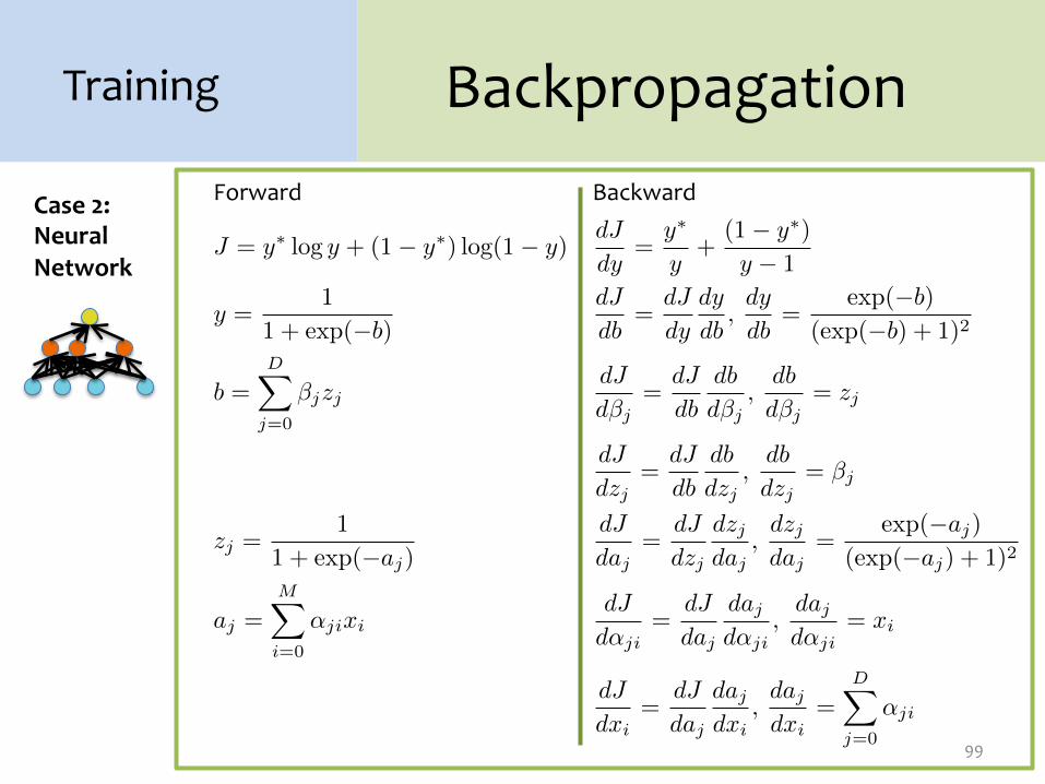
99

Training

Case 2: Neural Network

…

…

Forward Backward

J = y� y + (1 � y�) (1 � y)dJ

dy=

y�

y+

(1 � y�)

y � 1

y =1

1 + (�b)

dJ

db=

dJ

dy

dy

db,

dy

db=

(�b)

( (�b) + 1)2

b =D�

j=0

�jzjdJ

d�j=

dJ

db

db

d�j,

db

d�j= zj

dJ

dzj=

dJ

db

db

dzj,

db

dzj= �j

zj =1

1 + (�aj)

dJ

daj=

dJ

dzj

dzj

daj,

dzj

daj=

(�aj)

( (�aj) + 1)2

aj =M�

i=0

�jixidJ

d�ji=

dJ

daj

daj

d�ji,

daj

d�ji= xi

dJ

dxi=

dJ

daj

daj

dxi,

daj

dxi=

D�

j=0

�ji

Chain Rule

100

Training






! RJ and g : RJ! RI


vector x = {x1

, x2


, y2


1

, u2


dyi

dxk=

JX

j=1

dyi

duj

duj

dxk, 8i, k (2.3)


dy

dx=

dy

du

du

dx(2.4)


J = y⇤log q + (1 � y⇤

) log(1 � q) (2.5)

where q = P✓

(Yi = 1|x) =

1

1 + exp(�

PDj=0

✓jxj)(2.6)

13






! RJ and g : RJ! RI


vector x = {x1

, x2


, y2


1

, u2


dyi

dxk=

JX

j=1

dyi

duj

duj

dxk, 8i, k (2.3)


dy

dx=

dy

du

du

dx(2.4)


J = y⇤log q + (1 � y⇤

) log(1 � q) (2.5)

where q = P✓

(Yi = 1|x) =

1

1 + exp(�

PDj=0

✓jxj)(2.6)

13

Chain Rule:

Given:

…


intermediate quantity is a node 2.  At each node, store (a) the quantity computed in the forward pass

and (b) the partial derivative of the goal with respect to that node’s intermediate quantity.



Chain Rule

101

Training






! RJ and g : RJ! RI


vector x = {x1

, x2


, y2


1

, u2


dyi

dxk=

JX

j=1

dyi

duj

duj

dxk, 8i, k (2.3)


dy

dx=

dy

du

du

dx(2.4)


J = y⇤log q + (1 � y⇤

) log(1 � q) (2.5)

where q = P✓

(Yi = 1|x) =

1

1 + exp(�

PDj=0

✓jxj)(2.6)

13






! RJ and g : RJ! RI


vector x = {x1

, x2


, y2


1

, u2


dyi

dxk=

JX

j=1

dyi

duj

duj

dxk, 8i, k (2.3)


dy

dx=

dy

du

du

dx(2.4)


J = y⇤log q + (1 � y⇤

) log(1 � q) (2.5)

where q = P✓

(Yi = 1|x) =

1

1 + exp(�

PDj=0

✓jxj)(2.6)

13

Chain Rule:

Given:

…


node represents a Tensor. 2.  At each node, store (a) the quantity computed in the forward pass

and (b) the partial derivatives of the goal with respect to that node’s Tensor.



Case 2: Neural Network

…

…

Module 1

Module 2

Module 3

Module 4

Module 5

Backpropagation

102

Training

Forward Backward

J = y� y + (1 � y�) (1 � y)dJ

dy=

y�

y+

(1 � y�)

y � 1

y =1

1 + (�b)

dJ

db=

dJ

dy

dy

db,

dy

db=

(�b)

( (�b) + 1)2

b =D�

j=0

�jzjdJ

d�j=

dJ

db

db

d�j,

db

d�j= zj

dJ

dzj=

dJ

db

db

dzj,

db

dzj= �j

zj =1

1 + (�aj)

dJ

daj=

dJ

dzj

dzj

daj,

dzj

daj=

(�aj)

( (�aj) + 1)2

aj =M�

i=0

�jixidJ

d�ji=

dJ

daj

daj

d�ji,

daj

d�ji= xi

dJ

dxi=

dJ

daj

daj

dxi,

daj

dxi=

D�

j=0

�ji



103

Background




Gradients

Backpropagation can compute this gradient! And it’s a special case of a more general algorithm called reverse-‐mode automatic differentiation that can compute the gradient of any differentiable function efficiently!

Summary 1.  Neural Networks…

–  provide a way of learning features –  are highly nonlinear prediction functions –  (can be) a highly parallel network of logistic

regression classifiers –  discover useful hidden representations of the

input 2.  Backpropagation…

–  provides an efficient way to compute gradients –  is a special case of reverse-‐mode automatic

differentiation 104

Perceptron & Neural Networks

Documents

Transcript of Perceptron & Neural Networks