Rethinking Calibration of Deep Neural Networks:Do Not Be Afraid of Overconfidence

Deng-Bao Wang,1,2 Lei Feng,3 Min-Ling Zhang1,2∗1School of Computer Science and Engineering, Southeast University, Nanjing 210096, China2Key Laboratory of Computer Network and Information Integration (Southeast University),

Ministry of Education, China3College of Computer Science, Chongqing University, Chongqing, 400044, China

wangdb@seu.edu.cn, lfeng@cqu.edu.cn, zhangml@seu.edu.cn

AbstractCapturing accurate uncertainty quantification of the predictions from deep neuralnetworks is important in many real-world decision-making applications. A reliablepredictor is expected to be accurate when it is confident about its predictions andindicate high uncertainty when it is likely to be inaccurate. However, modernneural networks have been found to be poorly calibrated, primarily in the directionof overconfidence. In recent years, there is a surge of research on model calibrationby leveraging implicit or explicit regularization techniques during training, whichachieve well calibration performance by avoiding overconfident outputs. In ourstudy, we empirically found that despite the predictions obtained from these regular-ized models are better calibrated, they suffer from not being as calibratable, namely,it is harder to further calibrate these predictions with post-hoc calibration methodslike temperature scaling and histogram binning. We conduct a series of empiricalstudies showing that overconfidence may not hurt final calibration performanceif post-hoc calibration is allowed, rather, the penalty of confident outputs willcompress the room of potential improvement in post-hoc calibration phase. Ourexperimental findings point out a new direction to improve calibration of DNNs byconsidering main training and post-hoc calibration as a unified framework.

1 Introduction

Modern over-parameterized deep neural networks (DNNs) have been shown to be very powerfulmodeling tools for many prediction tasks involving complex input patterns [37]. In addition toobtaining accurate predictions, it is also important to capture accurate quantification of predictionuncertainty from deep neural networks in many real-world decision-making applications. A reliablepredictive model should be accurate when it is confident about its predictions and indicate highuncertainty when it is likely to be inaccurate. However, modern DNNs trained with cross-entropy(CE) loss, despite being highly accurate, have been recently found to predict poorly calibratedprobabilities, unlike traditional models trained with the same objective [4]. The overconfidentpredictions of DNNs could cause undesired consequences in safety-critical applications such asmedical diagnosis and autonomous driving. Bayesian DNNs, which indirectly infer predictionuncertainty through weight uncertainties, have innate abilities to represent the model uncertainty[2, 16]. But training and inferring those bayesian models are computationally more expensive andconceptually more complicated than non-bayesian models, and their performance depends on theform of approximation made due to computational constraints. Therefore, the study on uncertaintycalibration of deterministic DNNs is important for both development practice and the perspective ofunderstanding DNNs.

Post-hoc calibration addresses the miscalibration problem by equipping a given neural network withan additional parameterized calibration component, which can be tuned with a hold-out validation

∗Corresponding author

35th Conference on Neural Information Processing Systems (NeurIPS 2021), Sydney, Australia.

dataset. Guo et al. [4] experimented with several classical calibration fixes and found that simplepost-hoc methods like Temperature Scaling (TS) [25] and Histogram Binning (HB) [33] are signif-icantly effective for DNNs. The authors of [10] and [27] proposed to learn linear and non-lineartransformation functions to rescale the original output logits respectively. Gupta et al. [5] proposedto obtain a calibration function by approximating the empirical cumulative distribution of outputprobabilities via splines. Kumar et al. [11] proposed to integrate TS with HB to achieve more stablecalibration performance. Patel et al. [24] proposed a mutual information maximization-based binningstrategy to solve the severe sample-inefficiency issue in HB.

Recently, there is another line of research which presents a possibility of improving the calibrationquality of deterministic DNNs via regularization during training. Guo et al. [4] found that trainingDNNs with strong weight decay, which used to be the predominant regularization mechanismfor training neural networks, has a positive impact on calibration. Müller et al. [19] showedthat training models using the standard CE loss with label smoothing [28], instead of one-hotlabels, has a very favourable effect on model calibration. Mukhoti et al. [18] proposed to improveuncertainty calibration by replacing the conventionally used CE loss with the focal loss proposed in[14] when training DNNs. It is important to note that CE loss with label smoothing and focal losscan be considered as standard CE with an additional maximum-entropy regularizer, which meansminimizing these losses is equivalent to minimizing CE loss and maximizing the entropy of thepredicted distribution simultaneously [18, 17]. Following these studies, a recent work [7] exploredseveral explicit regularization techniques for improving the predictive uncertainty calibration directly.

In this paper, we conduct an empirical study showing that despite the predictions obtained fromthe regularized models are well calibrated, they suffer from worse calibratable, namely, it is harderto further improve the calibrate performance with post-hoc calibration methods like temperaturescaling and histogram binning. We found that the regularization works by simply aligning the averageconfidence of the whole dataset to the accuracy with some specific regularization strengths, and cannotachieve fine-grained calibration. The comparison results show that when post-hoc calibration methodsare allowed, the standard CE loss yields better calibration performance than those regularizationmethods. The extended experiments demonstrate that regularization will make DNNs lose theimportant information about the hardness of samples, which results in compressing the room ofpotential improvement by post-hoc calibration. Based on the experimental findings, we raise a naturalquestion: can we design new loss functions in the opposite direction of these regularization methodsto further improve the calibration performance? To this end, we propose inverse focal loss, andempirically found that it can learn more calibratable models in some cases compared with the CEloss, though it causes severer overconfidence problem without post-hoc calibration. Most importantly,our findings show that overconfidence of DNNs is not the nightmare in uncertainty qualificationand point out a new direction to improve the calibration of DNNs by considering main training andpost-hoc calibration as a unified framework.

2 Preliminaries

Let Y = {1, ...,K} denote the label space and X = Rd denote the feature space. Given a sample(x, y) ∈ X × Y sampled from an unknown distribution, a learned neural network classifier fθ :X →∆K can produce a probability distribution for x on K classes, where ∆K denotes the K − 1dimensional unit simplex. Here we assume fθ as a composition of a non-probabilistic K-wayclassifier gθ and a softmax function σ, i.e. fθ = gθ ◦ σ. For a query instance x, fθ gives itsprobability of assigning it to label i as exp(gθi (x))∑K

k=1 exp(gθk(x)), where gθi (x) denotes the i-th element of the

logit vector produced by gθ. Then, y := arg maxi fθi (x) can be returned as the predicted label and

p := maxi fθi (x) can be treated as the associated confidence score.

Expected Calibration Error (ECE) For a well-calibrated model, p is expected to represent the trueprobability of correctness. Formally, a perfectly calibrated model satisfies P(y = y|p = p) = p forany p ∈ [0, 1]. In practice, ECE [20] is a commonly used calibration metric from finite samples. Itworks by firstly grouping all samples (let n denote the number of samples) into M equally intervalbins {Bm}Mm=1 with respect to their confidence scores, then calculating the expected differencebetween the accuracy and average confidence: ECE =

∑Mm=1

|Bm|n |acc(Bm)− avgConf(Bm)|.

Temperature Scaling By scaling the logits produced by gθ with a temperature T , the sharpness

2

of output probabilities can be changed. Formally, after adding TS, the new prediction confidencecan be expressed as: p = maxi

exp(gθi (x)/T )∑Kk=1 exp(gθk(x)/T )

. The temperature softens the output probabilitywith T > 1 and sharpens the probability with T < 1. As T → 0, the output probability collapsesto one-hot vector. As T → ∞, the output probability approaches to a uniform distribution. Aftertraining of the model, T can be tuned on a hold-out validation set by optimization methods.

Histogram Binning is a non-parametric calibration approach. Given an uncalibrated model, allthe prediction confidences of validation samples can be divided into mutually exclusive N bins{Bn}Nn=1 according to a set of intervals {In}N+1

n=1 which partitions [0, 1]. Each bin is assigned aconfidence score η, which can be simply set to the corresponding accuracy of samples in each bin. Ifthe uncalibrated confidence p of a query instance falls into bin Bn, then the calibrated confidenceis ηn. The bins can be chosen by two simple schemes: equal size binning (uniformly partitioningthe probability interval in [0, 1]) and equal mass binning (uniformly distributing samples over bins).Note that although the HB scheme is simple to implement and was demonstrated to achieve goodcalibration results in some datasets, it makes the predictor only produce very sparse confidencedistribution, and compromises the many legitimately confident predictions.

3 Regularization in Neural Networks for Calibration

In recent years, there is a surge of research on model calibration by leveraging implicit or explicitregularization techniques during training of DNNs, which makes better calibrated predictions byavoiding the overconfident outputs. In this section, we firstly review three representative regularizationmethods and then empirically show their improvements on ECE compared with the baseline.

Label Smoothing is widely used as a means to reduce overfitting of DNNs. The mechanism of LSis simple: when training with CE loss, the one-hot label vector y is replaced with soft label vectory, whose elements can be formally denoted as yi = (1− ε)yi + ε/K,∀i ∈ {1, ...,K}, where ε > 0is a strength coefficient. Müller et al. [19] demonstrated that label smoothing implicitly calibratesDNNs by preventing the networks from becoming overconfident. Let Lce denote the CE loss, thenthe following equation holds:

Lce(y,fθ) = (1− ε)Lce(y,fθ) + εLce(u,fθ) (1)

This can be simply proved. Therefore, minimizing CE loss between smoothed labels and the modeloutputs is equivalent to adding a confidence penalty term, i.e., a weighted CE loss between theuniform distribution u and the model outputs, to the original CE loss.

Lp Norm in the Function Space is one of the explicit regularization methods for calibration investi-gated by the recent work [7]. For a real number p ≥ 1, the Lp Norm of a vector z with dimensionn can be expressed as: ‖z‖p = (

∑ni=1 |zi|p)1/p. By adding Lp Norm of logits gθ with a weighting

coefficient α into final objective function, i.e. LLp(y,fθ) = Lce(y,fθ) + α∥∥gθ∥∥

p, the function

complexity of neural networks can be directly penalized during training.

Focal Loss is originally proposed to address the class imbalance problem in object detection. Byreshaping the standard CE loss through weighting loss components of all samples according to howwell the model fits them, focal loss focuses on fitting hard samples and prevents the easy samples fromoverwhelming the training procedure. Formally, for classification tasks where the target distributionis one-hot encoding, it is defined as: Lf = −(1− fθy )γ log fθy , where γ is a predefined coefficient.Mukhoti et al. [18] found that the models learned by focal loss produce output probabilities whichare already very well calibrated. Interestingly, they also showed that focal loss is an upper bound ofthe regularized KL-divergence, which can be expressed formally as follows:

Lf ≥ KL(y||fθ)− γH(fθ) (2)

where H(p) denotes the entropy of distribution p. This upper bound property shows that replacingthe CE loss with focal loss has the effect of adding a maximum-entropy regularizer.

3.1 Empirical Comparison

We conduct a comparison study of the above regularization methods on four commonly used datasets.We train ResNet-32 [6] models on SVHN [21], CIFAR-10/100 [9] and train a 8-layer 1D-CNN

3

Table 1: Comparison results (mean±std) of ECE (%) with M = 15 and predictive accuracy (%)over 5 random runs. The values with underline in first row represent the chosen coefficients of eachregularization method on four datasets according to the ECE on test data.

Cross-Entropy Label Smoothing L1 Norm Focal Loss0.01/0.05/0.09/0.09 0.01/0.05/0.01/0.01 1/3/5/5

SVHNECE 3.03±0.16 1.84±0.19 1.85±0.04 1.01±0.21

Accuracy 95.00±0.27 95.21±0.23 95.29±0.13 94.77±0.19

CIFAR-10ECE 6.43±0.22 2.72±0.32 2.93±0.39 3.00±0.26

Accuracy 90.46±0.23 90.09±0.41 90.06±0.59 87.84±0.17

CIFAR-100ECE 19.53±0.36 2.27±0.48 8.07±0.44 2.34±0.35

Accuracy 64.64±0.43 63.73±0.67 63.07±0.29 60.36±0.44

20 NewsgroupsECE 20.82±0.93 5.85±0.64 13.31±0.56 3.82±0.51

Accuracy 72.85±0.89 72.81±0.26 73.61±0.80 59.17±1.81

model on 20Newsgroups [13], using the standard CE loss and the above regularized losses respec-tively, with state-of-the-art learning policy settings (see implementation details in Appendix). ForNorm regularization, we use L1 Norm, which has been shown effective for calibration despiteits simple form [7]. Table 1 shows the comparison of these methods. Note that for each of theabove three regularization methods, there is a coefficient, i.e., ε, α and γ, controlling the strengthof regularization. We conduct experiments using these methods with the following coefficient set-tings: {0.01, 0.03, 0.05, 0.07, 0.09} for label smoothing, {0.001, 0.005, 0.01, 0.05, 0.1} for L1 Normand {1, 3, 5, 7, 9} for focal loss. And we choose the best coefficient for each method and dataset,according to their ECE directly on test data.

From the results of Table 1, it is obvious that the regularization methods significantly decreasethe ECE on all datasets, compared with the standard CE loss. The prediction accuracy results arealso reported. When the strength coefficients of L1 Norm and focal loss are large, their predictiveperformances are harmed. Especially, L1 Norm fails on CIFAR-100 and 20Newsgroups whenα ≥ 0.05, thus α is chosen from {0.001,0.005,0.01} on these two datasets.

4 Does Regularization Really Help Calibration?

As shown by the above empirical results, the regularization methods do help the calibration of DNNsduring training, especially alleviate the overconfidence issue caused by the standard CE loss. In thissection, we empirically investigate their calibration performance when integrating them with post-hoccalibration. After training, we use the post-hoc methods TS and HB to further calibrate the outputprobabilities. For TS, we simply search the best temperature in the temperature pool {0.01,0.02...,10}on the validation set (see data splits in Appendix). For HB, we use equal size binning scheme onthe top-1 prediction of all classes with bin number set as 15. The experimental details used in thissection are the same with those in Section 3.

Comparison Results Table 2 shows the comparison results of ECE with the help of TS and HB.We can see that: (1) The standard CE loss achieves the best calibration performance on most cases.(2) The searched temperatures of models trained with the CE loss are significantly higher thanthose of other losses, which indicates that CE loss causes higher predictive confidences. Theseresults demonstrate that despite the regularized models can produce better calibrated predictions, itis harder to further improve them with post-hoc calibration methods after main training. In otherwords, the penalty of confident predictions will compress the room of potential improvement bypost-hoc methods. We also conduct experiments on CIFAR-10 and CIFAR-100 using a deeper modelResNet-110 and similar comparison results are obtained (see Appendix Table A).

Coefficient Sensitivity Figure 1(a), 1(b) and 1(c) illustrate the ECEs of these three regularizationmethods with varied coefficient strengths. As we can see, since the complexity of the used datasets aredifferent, the best coefficients of these methods markedly vary across the datasets, and a small changeon these coefficients may cause large ECE increase. This means that we need to carefully choose thecoefficient of each method when employing them on new datasets, to achieve good calibration. We canalso observe that for SVHN, on which the accuracy is highest among four datasets, the regularizationmethods obtain lowest ECE with small coefficients. For CIFAR-100 and 20Newsgroups, on which the

4

Table 2: Comparison results (mean±std) of ECE (%) with M = 15 over 5 random runs. Thecoefficients of the regularization methods on each dataset are same with those in Table 1. N/N andH/H indicate that the average ECE of regularization methods are higher and lower than standard CE,where N and H are based on two-sample t-test at 0.05 significance level.

Cross-Entropy Label Smoothing L1 Norm Focal Loss0.01/0.05/0.09/0.09 0.01/0.05/0.01/0.01 1/3/5/5

SVHN

with TS 0.72±0.26H 1.35±0.11N 1.22±0.08N 0.80±0.22NTemperature 1.82 H 1.11H 1.12H 1.10with HB 0.68±0.22H 0.70±0.21N 0.73±0.20N 0.96±0.14N

CIFAR-10

with TS 0.95±0.19H 2.54±0.11N 2.71±0.36N 1.39±0.28NTemperature 2.51 H 0.96H 0.95H 0.76with HB 0.74±0.15H 0.94±0.21N 1.16±0.54N 1.65±0.31N

CIFAR-100

with TS 1.35±0.19H 1.37±0.27N 3.92±0.21N 2.14±0.42NTemperature 2.19 H 1.04H 1.24H 0.97with HB 1.27±0.27H 2.01±0.22N 1.56±0.44N 1.83±0.30N

20 Newsgroups

with TS 3.11±0.33H 5.22±0.60N 2.71±0.25H 3.77±0.41NTemperature 4.18 H 1.06H 1.48H 0.89with HB 2.52±0.47H 2.67±0.82N 2.61±0.95N 3.16±0.97N

0.01 0.03 0.05 0.07 0.09LS with varied ε

02468

1012141618

ECE

SVHNCIFAR-10CIFAR-10020Newgropus

(a) LS with varied ε

0.001 0.005 0.01 0.05 0.1L1 with varied α

2468

10121416

ECE

SVHNCIFAR-10CIFAR-10020Newgropus

(b) L1 with varied α

1 3 5 7 9

Focal with varied γ0

5

10

15

20

25

30

ECE

SVHNCIFAR-10CIFAR-10020Newgropus

(c) FL with varied γ

3k 4k 5k 10k 15k 20k 25k 30k 35k 40kBest coefficient with varied data size

5

10

15

20

25

Coef

ficie

nt st

reng

th

LS ε× 100

L1 Norm α× 100

Focal γ

(d) Best coefficients

Figure 1: (a-c): ECE (%) with M = 15 of regularization methods with controlled regularizationstrength. (d): Best coefficients of regularization methods with respect to ECE with controlled trainingdata size.

accuracy is relatively lower, the regularization methods need larger coefficients for better calibration.Based on this observation, we conduct another experiment for investigating the correlation betweenthe regularization coefficients and accuracy. We learn networks on CIFAR-10 by controlling trainingdata size, which leads to varied predictive accuracies, and choose the best coefficient for eachcase. Here, ε, α and γ are chosen from {0.01, 0.02, ..., 0.25}, {0.01, 0.02, ..., 0.1} and {1, 3, 5, 7, 9}respectively. Figure 2(d) shows that with the increase of training data size, which results in increaseof predictive accuracy, the best coefficients of the regularization methods keep decreasing.

Reliability Diagram We use reliability diagram to visually represent the gap between predictiveconfidence and accuracy of each method. Due to the space limitation, here we only present thediagrams of CIFAR-10, and the rest figures are presented in Appendix. We can see that these visualresults are similar with the comparison results of ECE reported in Table 2. Although the gap betweenconfidence and accuracy is large when using the standard CE loss, it can be significantly diminishedafter using TS. However, the improvements of TS for the regularization methods are not obvious.Most importantly, no matter whether TS is used or not, the regularization methods suffer fromoverconfidence on samples which have high predictive uncertainty, especially on label smoothing andL1 Norm, which contradicts the traditional view. Combining with the observation in Figure 2(d), it isindicated that the regularization methods work by simply aligning the average predictive confidenceof the whole dataset to the accuracy with some specific regularization strengths, and does not producefine-grained calibration with respect to the difference of samples.

Impact of Validation Size We also wonder how does the validation data size impact the post-hoccalibration. Figure 3 shows the ECE results with controlled validation data size. We can see thatquite low ECE can be obtained with only a small size of validation data when using TS, which offershigh efficiency for practice development. Relatively, HB needs more validation samples to obtainbetter calibration performance. Nevertheless, the standard CE loss stably achieves better calibrationacross varied validation data size with both TS and HB.

5

0.0 0.2 0.4 0.6 0.8 1.0Confidence

0.0

0.2

0.4

0.6

0.8

1.0

Acc

urac

y

ECE=0.89

T=2.58GapAccuracy

(a) CE

0.0 0.2 0.4 0.6 0.8 1.0Confidence

0.0

0.2

0.4

0.6

0.8

1.0

Acc

urac

y

ECE=2.69

T=0.94GapAccuracy

Overconfidence

(b) LS, ε=0.05

0.0 0.2 0.4 0.6 0.8 1.0Confidence

0.0

0.2

0.4

0.6

0.8

1.0

Acc

urac

y

ECE=2.47

T=0.94GapAccuracy

Overconfidence

(c) L1 Norm, α=0.05

0.0 0.2 0.4 0.6 0.8 1.0Confidence

0.0

0.2

0.4

0.6

0.8

1.0

Acc

urac

y

ECE=1.40

T=0.78GapAccuracy

Overconfidence

(d) FL, γ=3

Figure 2: Reliability diagrams of each methods (after TS calibration) on CIFAR-10. The results arechosen from one of the 5 random runs of Table 1. Darker color of bars indicates that more samplesare assigned with the corresponding confidence intervals.

1000 2000 3000 4000 5000Size of Validation set

0.5

1.0

1.5

2.0

2.5

3.0

ECE

Focal Loss 1L1 Norm 0.01LS 0.01CE

(a) SVHN, TS

1000 2000 3000 4000 5000Size of Validation set

0.5

1.0

1.5

2.0

2.5

3.0

3.5

4.0

4.5

5.0

ECE

Focal Loss 3L1 Norm 0.05LS 0.05CE

(b) CIFAR-10, TS

1000 2000 3000 4000 5000Size of Validation set

1

2

3

4

5

6

7

ECE

Focal Loss 5L1 Norm 0.01LS 0.09CE

(c) CIFAR-100, TS

200 400 600 800 1000Size of Validation set

2

3

4

5

6

7

8

9

10

ECE

Focal Loss 5L1 Norm 0.05LS 0.09CE

(d) 20Newsgroups, TS

1000 2000 3000 4000 5000Size of Validation set

0.5

1.0

1.5

2.0

2.5

3.0

ECE

Focal Loss 1L1 Norm 0.01LS 0.01CE

(e) SVHN, HB

1000 2000 3000 4000 5000Size of Validation set

0.5

1.0

1.5

2.0

2.5

3.0

3.5

4.0

4.5

5.0

ECE

Focal Loss 3L1 Norm 0.05LS 0.05CE

(f) CIFAR-10, HB

1000 2000 3000 4000 5000Size of Validation set

1

2

3

4

5

6

7

ECE

Focal Loss 5L1 Norm 0.01LS 0.09CE

(g) CIFAR-100, HB

200 400 600 800 1000Size of Validation set

2

4

6

8

10

12

14

ECE

Focal Loss 5L1 Norm 0.05LS 0.09CE

(h) 20Newsgroups, HB

Figure 3: ECE (%) (after post-hoc calibration) with of regularization methods with controlledvalidation data size.

5 From Calibrated to Calibratable: A Closer Look

The results reported in above section show the degradation of regularization methods when integratingthem with post-hoc calibration methods, which indicates that though regularization helps DNNsobtain well-calibrated predictions, it makes these predictions worse calibratable. In this Section, wefurther investigate this phenomenon by a series of illustrative experiments. We firstly attempt toempirically understand the reason of the calibration degradation from the view of information loss.Then, we propose an inverse form of focal loss to give a closer look at the correlation between theloss functions used in training and the calibration performance. The implementation details used inthis section are also the same with those in Section 3.

5.1 Information Loss of Regularized Models

ECE among Epochs We start by investigating the ECEs of temperature-scaled outputs over epochsduring model training. To avoid the impact of the bias of validation data, we directly search thebest temperature on test data in each training epoch. We denote the corresponding ECE with thissearched temperature as optimal ECE, which is the lower bound of ECE with temperatures searchedon validation data. Figure 4 shows the curves of optimal ECE during epochs using label smoothingwith different smoothing coefficients. We can observe that the optimal ECE rises after some learningepochs: On SVHN and CIFAR-10, it starts to significantly rise around the 10th epoch, and onCIFAR-100 and 20Newsgroups, it tends to rise after 100 and 50 epochs, where the learning rate dropsby a factor of 10. Another observation is that larger smoothing strength ε results in worse calibrationperformance and more remarkable (also earlier) ECE rising. According to the memorization effect[35], DNNs usually learn easy samples at the early stage of training and tend to fit the hard ones later.

6

0 25 50 75 100 125 150 175 200Epoch

0.5

1.0

1.5

2.0

2.5

ECE

LS 0.09LS 0.07LS 0.05LS 0.03LS 0.01CE

(a) SVHN

0 25 50 75 100 125 150 175 200Epoch

0.5

1.0

1.5

2.0

2.5

3.0

3.5

4.0

ECE

LS 0.09LS 0.07LS 0.05LS 0.03LS 0.01CE

(b) CIFAR-10

0 25 50 75 100 125 150 175 200Epoch

0.5

1.0

1.5

2.0

2.5

3.0

ECE

LS 0.09LS 0.07LS 0.05LS 0.03LS 0.01CE

(c) CIFAR-100

0 20 40 60 80 100Epoch

1

2

3

4

5

6

7

8

ECE

LS 0.09LS 0.07LS 0.05LS 0.03LS 0.01CE

(d) 20Newsgroups

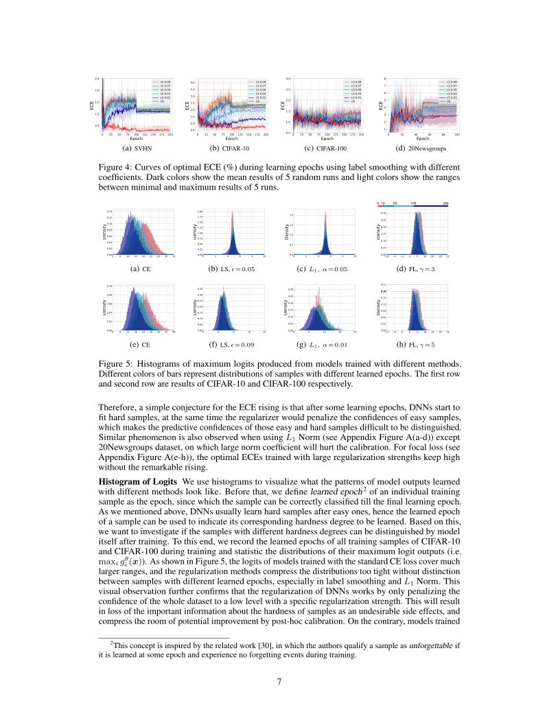
Figure 4: Curves of optimal ECE (%) during learning epochs using label smoothing with differentcoefficients. Dark colors show the mean results of 5 random runs and light colors show the rangesbetween minimal and maximum results of 5 runs.

10 50 100 2000

2 6 10 14 18 22 26 30 340.00

0.02

0.04

0.06

0.08

0.10

0.12

0.14

Dens

ity

(a) CE

0 2 4 6 8 100.00

0.25

0.50

0.75

1.00

1.25

1.50

1.75

2.00

Dens

ity

(b) LS, ε=0.05

0 2 4 6 8 100.0

0.5

1.0

1.5

2.0

Dens

ity

(c) L1, α=0.05

10 6 2 2 6 10 14 18 220.00

0.05

0.10

0.15

0.20

0.25

0.30

Dens

ity

(d) FL, γ=3

0 6 12 18 24 30 36 42 480.00

0.02

0.04

0.06

0.08

0.10

Dens

ity

(e) CE

0 6 12 18 240.00

0.05

0.10

0.15

0.20

0.25

0.30

0.35

Dens

ity

(f) LS, ε=0.09

0 6 12 18 240.00

0.05

0.10

0.15

0.20

0.25

0.30De

nsity

(g) L1, α=0.01

12 6 0 6 12 18 24 30 360.00

0.03

0.06

0.09

0.12

0.15

0.180.18

0.21

Dens

ity

(h) FL, γ=5

Figure 5: Histograms of maximum logits produced from models trained with different methods.Different colors of bars represent distributions of samples with different learned epochs. The first rowand second row are results of CIFAR-10 and CIFAR-100 respectively.

Therefore, a simple conjecture for the ECE rising is that after some learning epochs, DNNs start tofit hard samples, at the same time the regularizer would penalize the confidences of easy samples,which makes the predictive confidences of those easy and hard samples difficult to be distinguished.Similar phenomenon is also observed when using L1 Norm (see Appendix Figure A(a-d)) except20Newsgroups dataset, on which large norm coefficient will hurt the calibration. For focal loss (seeAppendix Figure A(e-h)), the optimal ECEs trained with large regularization strengths keep highwithout the remarkable rising.

Histogram of Logits We use histograms to visualize what the patterns of model outputs learnedwith different methods look like. Before that, we define learned epoch 2 of an individual trainingsample as the epoch, since which the sample can be correctly classified till the final learning epoch.As we mentioned above, DNNs usually learn hard samples after easy ones, hence the learned epochof a sample can be used to indicate its corresponding hardness degree to be learned. Based on this,we want to investigate if the samples with different hardness degrees can be distinguished by modelitself after training. To this end, we record the learned epochs of all training samples of CIFAR-10and CIFAR-100 during training and statistic the distributions of their maximum logit outputs (i.e.maxi g

θi (x)). As shown in Figure 5, the logits of models trained with the standard CE loss cover much

larger ranges, and the regularization methods compress the distributions too tight without distinctionbetween samples with different learned epochs, especially in label smoothing and L1 Norm. Thisvisual observation further confirms that the regularization of DNNs works by only penalizing theconfidence of the whole dataset to a low level with a specific regularization strength. This will resultin loss of the important information about the hardness of samples as an undesirable side effects, andcompress the room of potential improvement by post-hoc calibration. On the contrary, models trained

2This concept is inspired by the related work [30], in which the authors qualify a sample as unforgettable ifit is learned at some epoch and experience no forgetting events during training.

7

0.0 0.2 0.4 0.6 0.8 1.0Confidence

0

1

2

3

4

5

Loss

Inverse Focal γ=3Inverse Focal γ=2Inverse Focal γ=1CEFocal γ=1Focal γ=3Focal γ=5

(a) Loss functionsSVHN CIFAR-10 CIFAR-100 20Newgroups

50

60

70

80

90

100

Accu

racy

Focal γ= 3

Focal γ= 1

CEInverse Focal γ= 0.3

Inverse Focal γ= 1

Inverse Focal ¯γ= 2

Inverse Focal γ= 3

(b) Predictive accuracySVHN CIFAR-10 CIFAR-100 20Newgroups0

5

10

15

20

25

ECE

Focal γ= 3

Focal γ= 1

CEInverse Focal γ= 0.3

Inverse Focal γ= 1

Inverse Focal ¯γ= 2

Inverse Focal γ= 3

(c) ECE without post-hoc calibration

γ= 3 γ= 1 CE γ= 0.3 γ= 1 γ= 2 γ= 3

1

2

3

4

5

Tem

pera

ture

SVHNCIFAR-10CIFAR-10020Newgroups

(d) Best temperaturesSVHN CIFAR-10 CIFAR-100 20Newgroups0

1

2

3

4

ECE

Focal γ= 3

Focal γ= 1

CEInverse Focal γ= 0.3

Inverse Focal γ= 1

Inverse Focal ¯γ= 2

Inverse Focal γ= 3

(e) ECE after TSSVHN CIFAR-10 CIFAR-100 20Newgroups0.0

0.5

1.0

1.5

2.0

2.5

3.0

ECE

Focal γ= 3

Focal γ= 1

CEInverse Focal γ= 0.3

Inverse Focal γ= 1

Inverse Focal ¯γ= 2

Inverse Focal γ= 3

(f) ECE after HB

Figure 6: (a): Visual representation of focal loss, CE loss and inverse focal loss. (b): Predictiveaccuracies (%) of different methods. (c): ECEs (%) with M = 15 of different methods withoutpost-hoc calibration. (d): Searched temperatures on validation data. (e-f): ECEs (%) with M = 15 ofdifferent methods with the help of post-hoc calibration.

with the standard CE loss manage to preserve this information to a certain extent during training,hence achieve better results after post-hoc calibration.

5.2 Is Cross-Entropy the Best for Calibration?

Based on our experimental findings, one natural question is that can we design some loss functionsin the opposite direction of these regularization methods to further improve the calibration? Forlabel smoothing and Lp Norm, we can simply set the regularization coefficients of these methods asnegative values. However, we empirically found this will cause extremely low predictive accuracieseven failures of training using only very small weighting coefficients. Fortunately, we can design aninverse version of focal loss without prediction degradation by mimicking the original focal loss3.Recall the form of focal loss, we see that it works by assigning larger weights to the samples withsmaller confidences. This makes the optimizer pay more attention to those hard samples whenupdating model parameters. Actually, this weighting scheme also implicitly exists in the standard CEloss, and this can be expressed by the gradients of CE loss function w.r.t. model parameters θ:

∂Lce(y,fθ(x))

∂θ= − 1

fθy (x)∇θfθy (x) (3)

where the factor term 1fθy (x)

indicates that samples with smaller confidences are weighted larger ingradient calculation. Opposite to the principle of focal loss, we propose inverse focal loss as follows:

Lf = −(1 + fθy )γ log fθy (4)

By a simple modification on the weighting term of original focal loss, the inverse focal loss assignslarger weights to the samples with larger output confidences. Similar with original focal loss, thechoice of coefficient γ has a huge impact on the property of this loss. In Figure 6(a), we plot thecurves of inverse focal loss with varied γ and also plot the standard CE loss and focal loss forcomparison. We can see that different from the original focal loss, the curves of inverse focal loss aresteeper when confidence is large, and larger γ gives steeper curves.

We conduct another experiment to evaluate the inverse focal loss, and also investigate what willhappen when we increase its coefficient γ. Figure 6(c) shows the ECE results without post-hoccalibration. The ECEs of inverse focal loss are larger than CE and focal loss in most cases. This isconsistent to our expectation since inverse focal loss aggravates the overconfidence issue of DNNs byweighting larger on the easy samples. Figure 6(e) and 6(f) show the ECE results with the help of

3As the reviewer suggested, there already exists an "inverse focal loss" in the literature, which was introducedin a totally different context and using a different mathematical expression, but similar motivation [15].

8

post-hoc calibration. When using HB, the ECEs of inverse focal loss are worse than CE on SVHNand CIFAR-10, while better than CE on CIFAR-100. Generally speaking, there is no clear trend whenwe increase γ. More interesting results appear when using TS: (1) On CIFAR-10 and CIFAR-100,the ECE results of inverse focal loss are better than that of the standard CE loss; and (2) there isa descend-then-ascend trend from focal loss with γ = 3 to inverse focal loss with γ = 3. Fromthese observations, we may say that the best loss function for calibration is varied across differenttasks according to the characteristics of datasets. On SVHN, which is a relatively easy dataset,standard CE loss yields pretty good results; on CIFAR-10 and CIFAR-100, which is more complexand difficult, the best results are obtained using inverse focal loss; on 20Newsgroups, which hasfewest training samples among four datasets, the best result is obtained when using focal loss withγ = 1. The searched temperatures when using TS are presented in Figure 6(d). The increasing ofbest temperatures indicates that the overconfidence problem is severer when using inverse focal losswith larger γ. The predictive accuracies are presented in Figure 6(a). As is shown that inverse focalloss yields highly competitive results compared with the standard CE loss on SVHN, CIFAR-10 andCIFAR-100. On 20Newsgroups, when using large γ, the predictive performance of inverse focal lossis worse than the CE loss.

6 Related Work

In machine learning, calibration has long been studied [25, 33, 34, 22], and many classical methods,like Platt Scaling [25] and Histogram Binning [33], have been proposed in the literature. In recentyears, deep neural networks trained with commonly used CE loss, have been empirically foundto predict poorly calibrated probabilities. The early researches for this problem focus on bayesianmodels [2, 16, 3, 1], which indirectly infer prediction uncertainty through weight uncertainties. Buttraining and inferring the bayesian DNNs are computationally more expensive and conceptuallymore complicated than deterministic DNNs. Therefore, the uncertainty qualification of the non-bayesian models has always been an important topic, which also attracts a lot of researchers from theperspective of understanding DNNs.

Guo et al. [4] systematically investigated the miscalibration problem of the deterministic DNNsand empirically compared several conventional post-hoc calibration fixes. Two key findings aresuggested in their paper: (1) Increasing model capacity and regularization strength negatively affectthe calibration. (2) Simple post-hoc methods like TS [25] and HB [33] can reduce the calibrationerror to a quite low level. Following their work, there is a surge of research that proposed newpost-hoc calibration methods [10, 27, 5, 11, 24, 36, 26]. Different from post-hoc calibration methods,another line of research aims to learn calibrated networks during training by modifying the trainingprocess [29, 12, 8]. Thulasidasan et al. [29] found that DNNs trained with mixup are significantlybetter calibrated than DNNs trained in the regular fashion. Kumar et al. [12] proposed a RKHSkernel based measure of calibration that is efficiently trainable alongside the standard CE loss, whichcan minimize an explicit calibration error during training. Krishnan and Tichoo [8] introduced adifferentiable accuracy versus uncertainty calibration loss function that allows a model to learn toprovide well-calibrated uncertainties, in addition to improved accuracy. Recently, inspired by thefindings in [4], several studies were proposed to leverage the regularization of DNNs to improvecalibration performance during training [19, 18, 7]. As we described in Section 3, these implicit orexplicit regularization techniques can improve calibration by penalizing the predictive confidences ofDNNs. It is worth nothing that besides the studies on improving calibration performance, there arealso several studies that focus on the measure of calibration performance [23, 31, 32, 5].

7 Conclusion

In this work, we investigate the uncertainty calibration problem of DNNs by a series of experiments.The empirical study shows that despite the predictions obtained from the regularized models arebetter calibrated, worse results would be obtained if we employ post-hoc calibration methods onthese regularized models. Extended experiments demonstrate that the regularized DNNs will losethe important information about the hardness of samples, which results in the harm of post-hoccalibration. Based on the experimental observations, we design a new loss function in the oppositedirection of previous regularization methods, and empirically show the superiority of this loss incalibration with the help of post-hoc methods, even though it causes severer overconfidence issue in

9

the main training phase. Our findings suggest that overconfidence of DNNs is not the nightmare inmodel calibration and point out a new direction to improve the calibration performance of DNNs byconsidering main training and post-hoc calibration as a unified framework. Moreover, the study ofthe phenomena of deep learning uncertainty under distribution shift is very interesting as one of thefuture work, since the behaviour with distribution shifts might be most important in practice.

8 Acknowledgments

The authors wish to thank the anonymous reviewers for their helpful comments and suggestions.This work was supported by the National Science Foundation of China (62176055), the PostgraduateResearch & Practice Innovation Program of Jiangsu Province (KYCX21_0151) and the ChinaUniversity S&T Innovation Plan Guided by the Ministry of Education. We thank the Big Data Centerof Southeast University for providing the facility support on the numerical calculations in this paper.

References[1] Charles Blundell, Julien Cornebise, Koray Kavukcuoglu, and Daan Wierstra. Weight uncertainty

in neural network. In International Conference on Machine Learning, pages 1613–1622, 2015.

[2] Yarin Gal and Zoubin Ghahramani. Dropout as a bayesian approximation: Representingmodel uncertainty in deep learning. In International Conference on Machine Learning, pages1050–1059, 2016.

[3] Alex Graves. Practical variational inference for neural networks. In Advances in NeuralInformation Processing Systems, pages 2348–2356, 2011.

[4] Chuan Guo, Geoff Pleiss, Yu Sun, and Kilian Q Weinberger. On calibration of modern neuralnetworks. In International Conference on Machine Learning, pages 1321–1330, 2017.

[5] Kartik Gupta, Amir Rahimi, Thalaiyasingam Ajanthan, Thomas Mensink, Cristian Sminchis-escu, and Richard Hartley. Calibration of neural networks using splines. In InternationalConference on Representation Learning, 2021.

[6] Kaiming He, Xiangyu Zhang, Shaoqing Ren, and Jian Sun. Deep residual learning for imagerecognition. In IEEE Conference on Computer Vision and Pattern Recognition, pages 770–778,2016.

[7] Taejong Joo and Uijung Chung. Revisiting explicit regularization in neural networks forwell-calibrated predictive uncertainty. arXiv:2006.06399, 2021.

[8] Ranganath Krishnan and Omesh Tickoo. Improving model calibration with accuracy versusuncertainty optimization. In Advances in Neural Information Processing Systems, pages 18237–18248, 2020.

[9] Alex Krizhevsky. Learning multiple layers of features from tiny images. In Tech Report, 2009.

[10] Meelis Kull, Miquel Perello Nieto, Markus Kängsepp, Telmo Silva Filho, Hao Song, andPeter Flach. Beyond temperature scaling: Obtaining well-calibrated multi-class probabilitieswith dirichlet calibration. In Advances in Neural Information Processing Systems, pages12295–12305, 2019.

[11] Ananya Kumar, Percy S Liang, and Tengyu Ma. Verified uncertainty calibration. In Advancesin Neural Information Processing Systems, pages 3787–3798, 2019.

[12] Aviral Kumar, Sunita Sarawagi, and Ujjwal Jain. Trainable calibration measures for neuralnetworks from kernel mean embeddings. In International Conference on Machine Learning,pages 2805–2814, 2018.

[13] Ken Lang. Newsweeder: Learning to filter netnews. In International Conference on MachineLearning, pages 331–339, 1995.

10

[14] Tsung-Yi Lin, Priya Goyal, Ross Girshick, Kaiming He, and Piotr Dollár. Focal loss for denseobject detection. In IEEE International Conference on Computer Vision, pages 2980–2988,2017.

[15] Mingsheng Long, Zhangjie Cao, Jianmin Wang, and Michael I Jordan. Conditional adversarialdomain adaptation. In International Conference on Neural Information Processing Systems,pages 1647–1657, 2018.

[16] Wesley J Maddox, Pavel Izmailov, Timur Garipov, Dmitry P Vetrov, and Andrew GordonWilson. A simple baseline for bayesian uncertainty in deep learning. In Advances in NeuralInformation Processing Systems, pages 13153–13164, 2019.

[17] Clara Meister, Elizabeth Salesky, and Ryan Cotterell. Generalized entropy regularization or:There’s nothing special about label smoothing. In Annual Meeting of the Association forComputational Linguistics, pages 6870–6886, 2020.

[18] Jishnu Mukhoti, Viveka Kulharia, Amartya Sanyal, Stuart Golodetz, Philip Torr, and PuneetDokania. Calibrating deep neural networks using focal loss. In Advances in Neural InformationProcessing Systems, pages 15288–15299, 2020.

[19] Rafael Müller, Simon Kornblith, and Geoffrey E Hinton. When does label smoothing help? InAdvances in Neural Information Processing Systems, pages 4696–4705, 2019.

[20] Mahdi Pakdaman Naeini, Gregory Cooper, and Milos Hauskrecht. Obtaining well calibratedprobabilities using bayesian binning. In AAAI Conference on Artificial Intelligence, pages2901–2907, 2015.

[21] Yuval Netzer, Tao Wang, Adam Coates, Alessandro Bissacco, Bo Wu, and Andrew Y. Ng.Reading digits in natural images with unsupervised feature learning. In Advances in NeuralInformation Processing Systems Workshops, 2011.

[22] Alexandru Niculescu-Mizil and Rich Caruana. Predicting good probabilities with supervisedlearning. In International Conference on Machine learning, pages 625–632, 2005.

[23] Jeremy Nixon, Michael W. Dusenberry, Linchuan Zhang, Ghassen Jerfel, and Dustin Tran.Measuring calibration in deep learning. In IEEE Conference on Computer Vision and PatternRecognition Workshops, pages 38–41, 2019.

[24] Kanil Patel, William Beluch, Bin Yang, Michael Pfeiffer, and Dan Zhang. Multi-class uncertaintycalibration via mutual information maximization-based binning. In International Conferenceon Representation Learning, 2021.

[25] John Platt et al. Probabilistic outputs for support vector machines and comparisons to regularizedlikelihood methods. Advances in Large Margin Classifiers, 10(3):61–74, 1999.

[26] Amir Rahimi, Kartik Gupta, Thalaiyasingam Ajanthan, Thomas Mensink, Cristian Sminchis-escu, and Richard Hartley. Post-hoc calibration of neural networks. arXiv:2006.12807, 2020.

[27] Amir Rahimi, Amirreza Shaban, Ching-An Cheng, Richard Hartley, and Byron Boots. Intraorder-preserving functions for calibration of multi-class neural networks. In Advances in NeuralInformation Processing Systems, 2020.

[28] Christian Szegedy, Vincent Vanhoucke, Sergey Ioffe, Jon Shlens, and Zbigniew Wojna. Rethink-ing the inception architecture for computer vision. In IEEE Conference on Computer Visionand Pattern Recognition, pages 2818–2826, 2016.

[29] Sunil Thulasidasan, Gopinath Chennupati, Jeff A. Bilmes, Tanmoy Bhattacharya, and SarahMichalak. On mixup training: Improved calibration and predictive uncertainty for deep neuralnetworks. In Advances in Neural Information Processing Systems, pages 13888–13899, 2019.

[30] Mariya Toneva, Alessandro Sordoni, Remi Tachet des Combes, Adam Trischler, Yoshua Bengio,and Geoffrey J. Gordon. An empirical study of example forgetting during deep neural networklearning. In International Conference on Representation Learning, 2019.

11

[31] Juozas Vaicenavicius, David Widmann, Carl R. Andersson, Fredrik Lindsten, Jacob Roll, andThomas B. Schön. Evaluating model calibration in classification. In International Conferenceon Artificial Intelligence and Statistics, pages 3459–3467, 2019.

[32] David Widmann, Fredrik Lindsten, and Dave Zachariah. Calibration tests in multi-classclassification: A unifying framework. In Advances in Neural Information Processing Systems,pages 12236–12246, 2019.

[33] Bianca Zadrozny and Charles Elkan. Obtaining calibrated probability estimates from decisiontrees and naive bayesian classifiers. In International Conference on Machine Learning, pages609–616, 2001.

[34] Bianca Zadrozny and Charles Elkan. Transforming classifier scores into accurate multiclassprobability estimates. In ACM SIGKDD International Conference on Knowledge Discoveryand Data Mining, pages 694–699, 2002.

[35] Chiyuan Zhang, Samy Bengio, Moritz Hardt, Benjamin Recht, and Oriol Vinyals. Understandingdeep learning requires rethinking generalization. In International Conference on RepresentationLearning, 2017.

[36] Jize Zhang, Bhavya Kailkhura, and T Yong-Jin Han. Mix-n-match: Ensemble and compositionalmethods for uncertainty calibration in deep learning. In International Conference on MachineLearning, pages 11117–11128, 2020.

[37] Zhi-Hua Zhou. Why over-parameterization of deep neural networks does not overfit? ScienceChina Information Sciences, 64(1):1–3, 2021.

12