arX

iv:1

205.

3900

v2 [

cond

-mat

.dis

-nn]

8 J

un 2

012 How glassy are neural networks?

Adriano Barra∗, Giuseppe Genovese†, Francesco Guerra‡, Daniele Tantari§

December 22, 2013

Abstract

In this paper we continue our investigation on the high storageregime of a neural network with Gaussian patterns. Through an exactmapping between its partition function and one of a bipartite spinglass (whose parties consist of Ising and Gaussian spins respectively),we give a complete control of the whole annealed region. The strategyexplored is based on an interpolation between the bipartite systemand two independent spin glasses built respectively by dichotomic andGaussian spins: Critical line, behavior of the principal thermodynamicobservables and their fluctuations as well as overlap fluctuations areobtained and discussed. Then, we move further, extending such anequivalence beyond the critical line, to explore the broken ergodicityphase under the assumption of replica symmetry and we show thatthe quenched free energy of this (analogical) Hopfield model can bedescribed as a linear combination of the two quenched spin-glass freeenergies even in the replica symmetric framework.

Introduction

Neural networks, thought of as the harmonic oscillators of artificial intelli-gence, are nowadays being used in a huge number of different fields of science,ranging from practical application in data mining [13, 39] to theoretical spec-ulation in systems biology [2, 22], crossing fields as disparate as computerscience [34], quantitative sociology [8] or economics [19].As a consequence, as applications develop, the need for mathematical meth-ods (bringing them under rigorous control) and a simple mathematical frame-work (acting as a benchmark for future speculation) increases and motivates

∗Dipartimento di Fisica, Sapienza Università di Roma and GNFM, Sezione di Roma.†Dipartimento di Matematica, Sapienza Università di Roma.‡Dipartimento di Fisica, Sapienza Università di Roma and INFN, Sezione di Roma.§Dipartimento di Matematica, Sapienza Università di Roma.

1

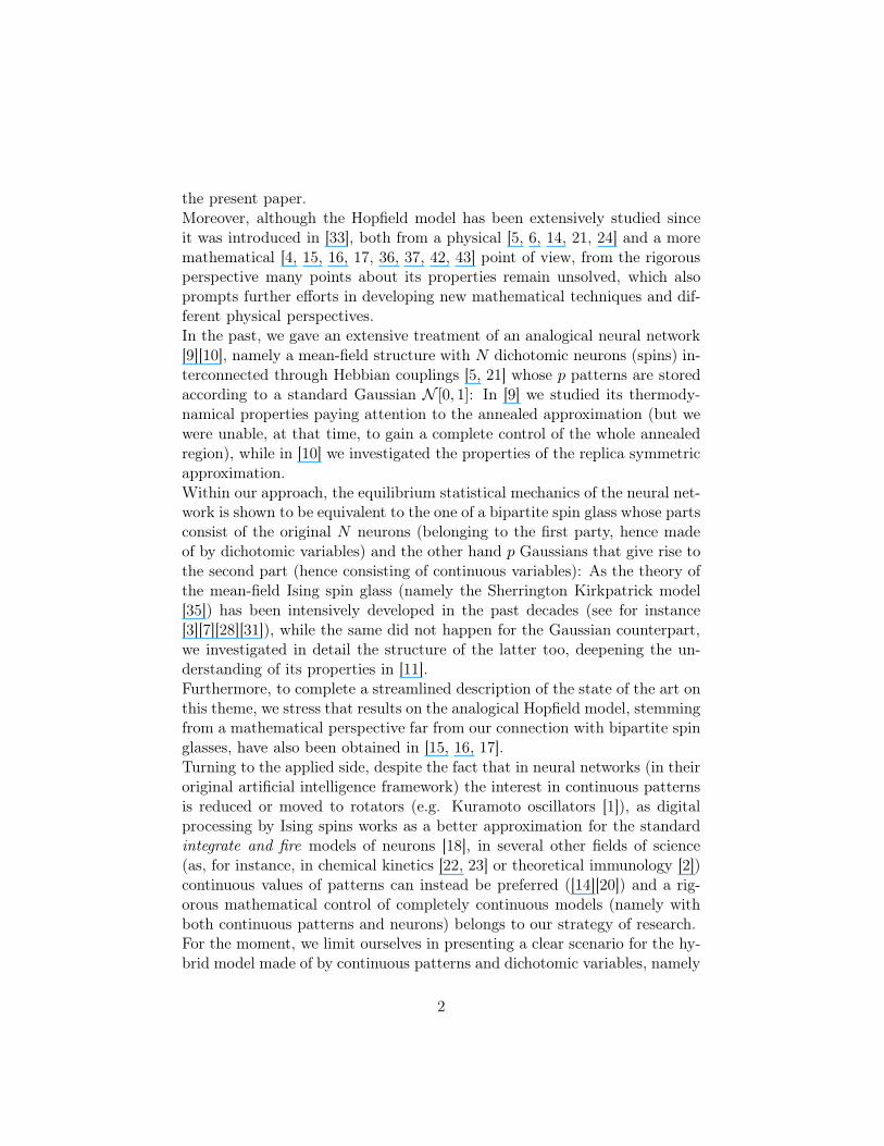
the present paper.Moreover, although the Hopfield model has been extensively studied sinceit was introduced in [33], both from a physical [5, 6, 14, 21, 24] and a moremathematical [4, 15, 16, 17, 36, 37, 42, 43] point of view, from the rigorousperspective many points about its properties remain unsolved, which alsoprompts further efforts in developing new mathematical techniques and dif-ferent physical perspectives.In the past, we gave an extensive treatment of an analogical neural network[9][10], namely a mean-field structure with N dichotomic neurons (spins) in-terconnected through Hebbian couplings [5, 21] whose p patterns are storedaccording to a standard Gaussian N [0, 1]: In [9] we studied its thermody-namical properties paying attention to the annealed approximation (but wewere unable, at that time, to gain a complete control of the whole annealedregion), while in [10] we investigated the properties of the replica symmetricapproximation.Within our approach, the equilibrium statistical mechanics of the neural net-work is shown to be equivalent to the one of a bipartite spin glass whose partsconsist of the original N neurons (belonging to the first party, hence madeof by dichotomic variables) and the other hand p Gaussians that give rise tothe second part (hence consisting of continuous variables): As the theory ofthe mean-field Ising spin glass (namely the Sherrington Kirkpatrick model[35]) has been intensively developed in the past decades (see for instance[3][7][28][31]), while the same did not happen for the Gaussian counterpart,we investigated in detail the structure of the latter too, deepening the un-derstanding of its properties in [11].Furthermore, to complete a streamlined description of the state of the art onthis theme, we stress that results on the analogical Hopfield model, stemmingfrom a mathematical perspective far from our connection with bipartite spinglasses, have also been obtained in [15, 16, 17].Turning to the applied side, despite the fact that in neural networks (in theiroriginal artificial intelligence framework) the interest in continuous patternsis reduced or moved to rotators (e.g. Kuramoto oscillators [1]), as digitalprocessing by Ising spins works as a better approximation for the standardintegrate and fire models of neurons [18], in several other fields of science(as, for instance, in chemical kinetics [22, 23] or theoretical immunology [2])continuous values of patterns can instead be preferred ([14][20]) and a rig-orous mathematical control of completely continuous models (namely withboth continuous patterns and neurons) belongs to our strategy of research.For the moment, we limit ourselves in presenting a clear scenario for the hy-brid model made of by continuous patterns and dichotomic variables, namely

2

the analogical neural network: In Section One we introduce the model andall the statistical-mechanics-related concepts. Then in Section Two we ex-pose our new strategy of interpolation which allows a complete control bothof the ergodic region (confirming the annealed approximation, which is in-vestigated in great detail), and of the replica symmetric scenario, which isthen deepened in Section Three.The last section contains our conclusions.Furthermore, an appendix is added: there the fluctuation theory of the orderparameters of the model is discussed, and it is shown that the critical linefound in this work characterizes a second order phase transition.

1 The model, basic definitions and properties

1.1 The analogical Hopfield model

We introduce a large network of N two-state neurons (1, .., N) ∋ i → σi =±1, which are thought of as quiescent when their value is −1 or spiking whentheir value is +1. They interact throughout a synaptic matrix Jij definedaccording to the Hebb rule for learning [32, 33]

Jij =

p∑

µ=1

ξµi ξµj . (1)

Each random variable ξµ = ξµ1 , .., ξµN represents a learned pattern: While

in the standard literature these patterns are usually chosen at random inde-pendently with values ±1 taken with equal probability 1/2, we chose themas taking real values with a unit Gaussian probability distribution, i.e.

dµ(ξµi ) =1√2π

e−(ξµi )2/2. (2)

The analysis of the network assumes that the system has already stored ppatterns (no learning is investigated here), and we will be interested in thecase in which this number asymptotically increases linearly with respect tothe system size (high storage level), so that p/N → α as N → ∞, whereα ≥ 0 is a parameter of the theory denoting the storage level.The Hamiltonian of the model has a mean-field structure and involves inter-actions between any pair of sites according to the definition

HN(σ; ξ) = − 1

N

p∑

µ=1

N∑

i<j

ξµi ξµj σiσj . (3)

3

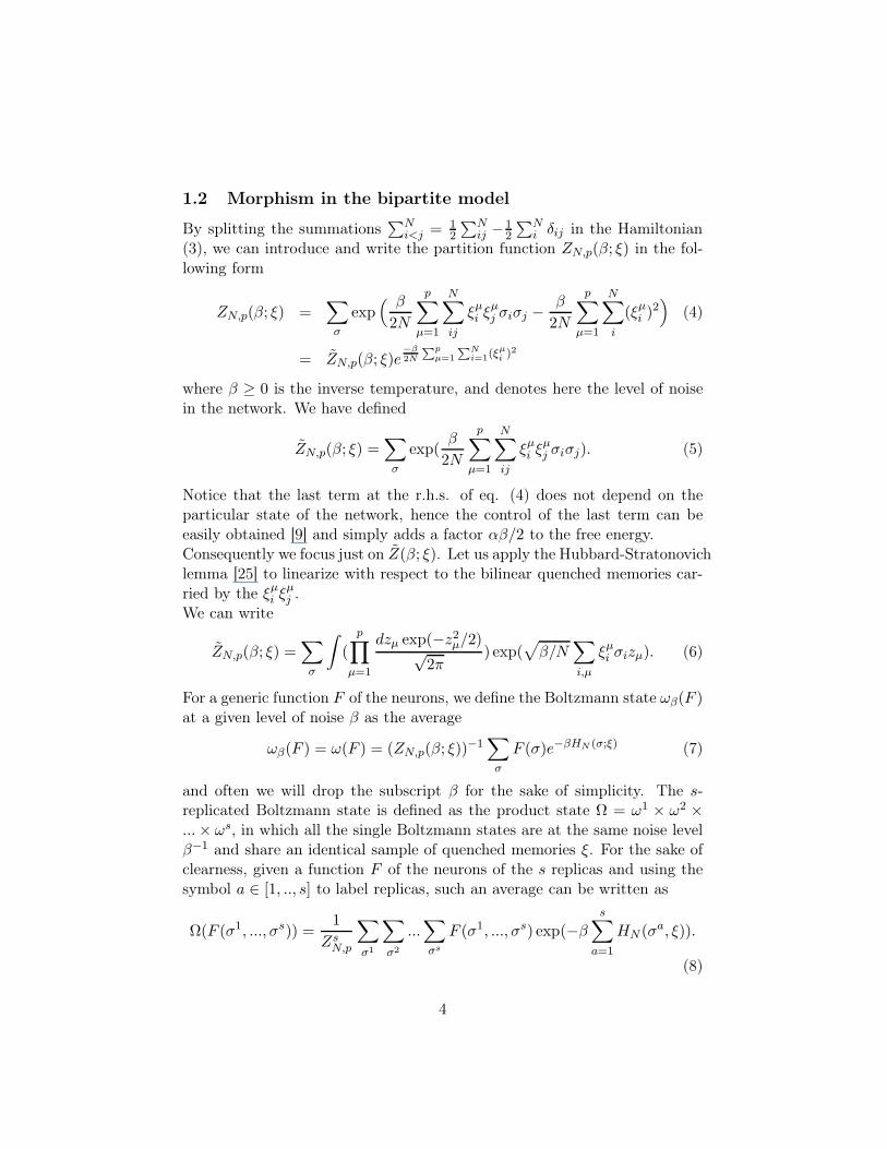
1.2 Morphism in the bipartite model

By splitting the summations∑N

i<j = 12

∑Nij −1

2

∑Ni δij in the Hamiltonian

(3), we can introduce and write the partition function ZN,p(β; ξ) in the fol-lowing form

ZN,p(β; ξ) =∑

σ

exp( β

2N

p∑

µ=1

N∑

ij

ξµi ξµj σiσj −

β

2N

p∑

µ=1

N∑

i

(ξµi )2)

(4)

= ZN,p(β; ξ)e−β2N

∑pµ=1

∑Ni=1(ξ

µi )

2

where β ≥ 0 is the inverse temperature, and denotes here the level of noisein the network. We have defined

ZN,p(β; ξ) =∑

σ

exp(β

2N

p∑

µ=1

N∑

ij

ξµi ξµj σiσj). (5)

Notice that the last term at the r.h.s. of eq. (4) does not depend on theparticular state of the network, hence the control of the last term can beeasily obtained [9] and simply adds a factor αβ/2 to the free energy.Consequently we focus just on Z(β; ξ). Let us apply the Hubbard-Stratonovichlemma [25] to linearize with respect to the bilinear quenched memories car-ried by the ξµi ξ

µj .

We can write

ZN,p(β; ξ) =∑

σ

∫

(

p∏

µ=1

dzµ exp(−z2µ/2)√2π

) exp(√

β/N∑

i,µ

ξµi σizµ). (6)

For a generic function F of the neurons, we define the Boltzmann state ωβ(F )at a given level of noise β as the average

ωβ(F ) = ω(F ) = (ZN,p(β; ξ))−1

∑

σ

F (σ)e−βHN (σ;ξ) (7)

and often we will drop the subscript β for the sake of simplicity. The s-replicated Boltzmann state is defined as the product state Ω = ω1 × ω2 ×...× ωs, in which all the single Boltzmann states are at the same noise levelβ−1 and share an identical sample of quenched memories ξ. For the sake ofclearness, given a function F of the neurons of the s replicas and using thesymbol a ∈ [1, .., s] to label replicas, such an average can be written as

Ω(F (σ1, ..., σs)) =1

ZsN,p

∑

σ1

∑

σ2

...∑

σs

F (σ1, ..., σs) exp(−β

s∑

a=1

HN (σa, ξ)).

(8)

4

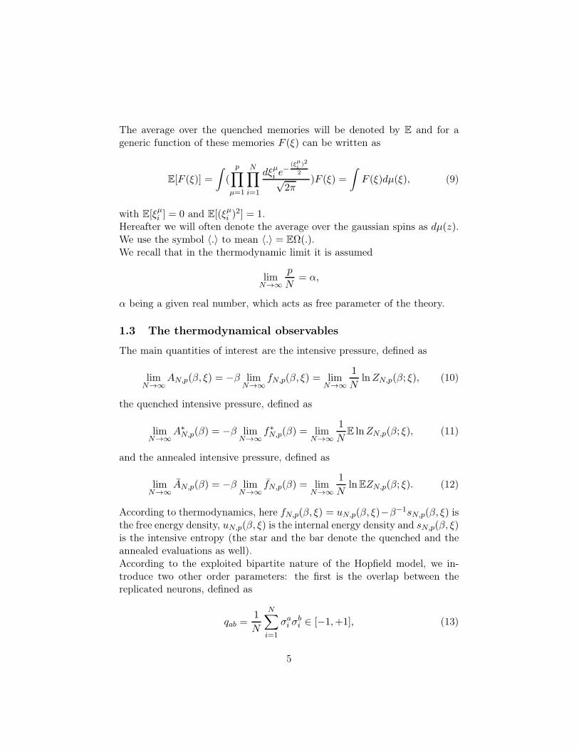
The average over the quenched memories will be denoted by E and for ageneric function of these memories F (ξ) can be written as

E[F (ξ)] =

∫

(

p∏

µ=1

N∏

i=1

dξµi e−

(ξµi)2

2√2π

)F (ξ) =

∫

F (ξ)dµ(ξ), (9)

with E[ξµi ] = 0 and E[(ξµi )2] = 1.

Hereafter we will often denote the average over the gaussian spins as dµ(z).We use the symbol 〈.〉 to mean 〈.〉 = EΩ(.).We recall that in the thermodynamic limit it is assumed

limN→∞

p

N= α,

α being a given real number, which acts as free parameter of the theory.

1.3 The thermodynamical observables

The main quantities of interest are the intensive pressure, defined as

limN→∞

AN,p(β, ξ) = −β limN→∞

fN,p(β, ξ) = limN→∞

1

NlnZN,p(β; ξ), (10)

the quenched intensive pressure, defined as

limN→∞

A∗N,p(β) = −β lim

N→∞f∗N,p(β) = lim

N→∞

1

NE lnZN,p(β; ξ), (11)

and the annealed intensive pressure, defined as

limN→∞

AN,p(β) = −β limN→∞

fN,p(β) = limN→∞

1

NlnEZN,p(β; ξ). (12)

According to thermodynamics, here fN,p(β, ξ) = uN,p(β, ξ)−β−1sN,p(β, ξ) isthe free energy density, uN,p(β, ξ) is the internal energy density and sN,p(β, ξ)is the intensive entropy (the star and the bar denote the quenched and theannealed evaluations as well).According to the exploited bipartite nature of the Hopfield model, we in-troduce two other order parameters: the first is the overlap between thereplicated neurons, defined as

qab =1

N

N∑

i=1

σai σ

bi ∈ [−1,+1], (13)

5

and the second the overlap between the replicated Gaussian variables z,defined as

pab =1

p

p∑

µ=1

zaµzbµ ∈ (−∞,+∞). (14)

These overlaps play a considerable role in the theory as they can expressthermodynamical quantities.

2 A detailed description of the annealed region

2.1 The interpolation scheme for the annealing

In this section we present the main idea of the work, used here to get acomplete control of the high-temperature region: We interpolate between theneural network (described in terms of a bipartite spin glass) and a systemconsisting of two separate spin glasses, one dichotomic and one Gaussian.Note that, by the Jensen inequality, namely

E lnZN,p(β) ≤ lnEZN,p(β),

we can write

A∗N,p ≤

1

NlnE

∑

σ

∫ p∏

µ=1

dµ(zµ)e

√

βN

∑

iµ ξµi σizµ = ln 2− p

2Nlog(1−β), (15)

where we emphasize that the integral inside eq. (15) exists only for β < 1.The N → ∞ limit then offers immediately limN→∞A∗

N,p(β) ≤ ln 2−α ln(1−β)/2. The next step is to use interpolation to prove the validity of theJensen bound in the whole region defined by the line βc = 1/(1 +

√α),

which defines the boundary of the validity of the annealed approximation,in complete agreement with the well known picture of Amit, Gutfreund andSompolinsky [5][6].To understand which is the proper interpolating structure, let us note thatthe exponent of the Boltzmann factor yields a family of random variablesindexed by the configurations (σ, z). For a given realization of the noise,

H(σ, z|ξ) =√

βN

∑

iµ ξi,µσizµ is a randomly centered variable with variance

E(H(σ, z|ξ)H(σ′, z′|ξ)) = β

N

∑

iµ

σiσ′izµz

′µ = βpqσσ′pzz′ .

6

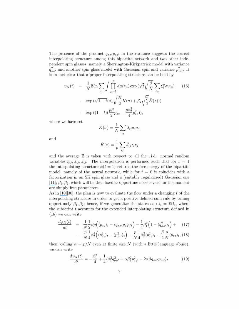
The presence of the product qσσ′pzz′ in the variance suggests the correctinterpolating structure among this bipartite network and two other inde-pendent spin glasses, namely a Sherrington-Kirkpatrick model with varianceq2σσ′ and another spin glass model with Gaussian spin and variance p2zz′ . Itis in fact clear that a proper interpolating structure can be held by

ϕN (t) =1

NE ln

∑

σ

∫ p∏

µ=1

dµ(zµ) exp (√t

√

β

N

∑

iµ

ξµi σizµ) (16)

· exp (√1− t(β1

√

N

2K(σ) + β2

√

p

2K(z)))

· exp ((1− t)(pβ

2pzz −

pβ22

4p2zz)),

where we have set

K(σ) =1

N

∑

ij

Jijσiσj

and

K(z) =1

p

∑

ij

Jijzizj

and the average E is taken with respect to all the i.i.d. normal randomvariables ξij , Jij , Jij . The interpolation is performed such that for t = 1the interpolating structure ϕ(t = 1) returns the free energy of the bipartitemodel, namely of the neural network, while for t = 0 it coincides with afactorization in an SK spin glass and a (suitably regularized) Gaussian one[11]; β1, β2, which will be then fixed as opportune noise levels, for the momentare simply free parameters.As in [10][30], the plan is now to evaluate the flow under a changing t of theinterpolating structure in order to get a positive defined sum rule by tuningopportunely β1, β2; hence, if we generalize the states as 〈.〉t = EΩt, wherethe subscript t accounts for the extended interpolating structure defined in(16) we can write

dϕN (t)

dt=

1

N

1

2βp

(

〈pzz〉t − 〈qσσ′pzz′〉t)

− 1

4β21

(

1− 〈q2σσ′〉t)

+ (17)

− p

N

1

4β22

(

〈p2zz〉t − 〈p2zz′〉t)

+p

N

1

4β22〈p2zz〉t −

β

2

p

N〈pzz〉t, (18)

then, calling α = p/N even at finite size N (with a little language abuse),we can write

dϕN (t)

dt= −β2

1

4+

1

4〈β2

1q2σσ′ + αβ2

2p2zz′ − 2αβqσσ′pzz′〉t. (19)

7

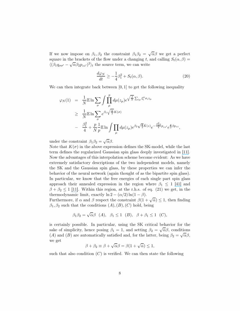
If we now impose on β1, β2 the constraint β1β2 =√αβ we get a perfect

square in the brackets of the flow under a changing t, and calling St(α, β) =〈(β1qσσ′ −√

αβ2pzz′)2〉t the source term, we can write

dϕN

dt≥ −1

4β21 + St(α, β). (20)

We can then integrate back between [0, 1] to get the following inequality

ϕN (1) =1

NE ln

∑

σ

∫ p∏

µ

dµ(zµ)e

√

βN

∑

iµ ξµi σizµ

≥ 1

NE ln

∑

σ

eβ1

√

N2K(σ)

− β21

4+

p

N

1

pE ln

∫

∏

µ

dµ(zµ)eβ2

√p2K(z)e−

β22p

4pzz′e

p2βpzz ,

under the constraint β1β2 =√αβ.

Note that K(σ) in the above expression defines the SK-model, while the lastterm defines the regularized Gaussian spin glass deeply investigated in [11].Now the advantages of this interpolation scheme become evident: As we haveextremely satisfactory descriptions of the two independent models, namelythe SK and the Gaussian spin glass, by these properties we can infer thebehavior of the neural network (again thought of as the bipartite spin glass).In particular, we know that the free energies of each single part spin glassapproach their annealed expression in the region where β1 ≤ 1 [41] andβ + β2 ≤ 1 [11]. Within this region, at the r.h.s. of eq. (21) we get, in thethermodynamic limit, exactly ln 2− (α/2) ln(1− β).Furthermore, if α and β respect the constraint β(1 +

√α) ≤ 1, then finding

β1, β2 such that the conditions (A), (B), (C) hold, being

β1β2 =√αβ (A), β1 ≤ 1 (B), β + β1 ≤ 1 (C),

is certainly possible. In particular, using the SK critical behavior for thesake of simplicity, hence posing β1 = 1, and setting β2 =

√αβ, conditions

(A) and (B) are automatically satisfied and, for the latter, being β2 =√αβ,

we getβ + β2 ≡ β +

√αβ = β(1 +

√α) ≤ 1,

such that also condition (C) is verified. We can then state the following

8

Theorem 1. In the α, β plane there exist a critical line, defined by

βc(α) =1

1 +√α, (21)

such that for β ≤ βc(α) the annealed approximation of the free energy holds

limN→∞

1

NE ln

∑

σ

∫

∏

µ

dµ(zµ)e

(

√

βN

∑

iµ ξµi σizµ

)

= ln 2− α

2ln(1− β). (22)

Remark 1. We stress that the Borel-Cantelli lemma allows straightforwardlyto determine the correct annealed regions for the SK model [41] and, througha careful check of convergence of the integral defining the partition function,the same holds for the Gaussian case too [11]; however, the direct applicationof the Borel-Cantelli argument on the neural network gives a weaker resultas shown for instance in [9]. The interpolation scheme allows to exploit andtransfer the results for the SK and Gaussian models to the neural network,and enlarges the area of validity of the annealed expression for the free energyto the whole expected region, obtained e.g. via the replica method [5].

2.2 The control of the annealed region

As a consequence, we can now extend the previous results exposed in [9] tothe whole annealed region: Summarizing, we get the following

Theorem 2. There exists βc(α), defined by eq. (21), such that for β < βc(α)we have the following limits for the intensive free energy, internal energy andentropy, as N → ∞ and p/N → α > 0:

− β limN→∞

fN,p(β; ξ) = limN→∞

N−1 lnZN,p(β; ξ) (23)

= ln 2− (α/2) ln(1− β)− (αβ/2),

limN→∞

uN,p(β; ξ) = − limN→∞

N−1∂β lnZN,p(β; ξ) (24)

= −αβ/(2(1 − β)),

limN→∞

sN,p(β; ξ) = limN→∞

N−1(lnZN,p(β; ξ)− β∂β lnZN,p(β; ξ)) (25)

= ln 2− (α/2) ln(1− β)− (αβ2)/(2(1 − β))− (αβ/2),

ξ-almost surely. The same limits hold for the quenched averages, so that inparticular

limN→∞

N−1E lnZN,p(β; ξ) = ln 2− α

2ln(1− β)− αβ

2,

9

where, in all these formulas, the last term, namely −αβ/2, arises due to thediagonal contribution of the complete partition function (4).

Theorem 3. There exists βc(α), defined by eq. (21), such that for β < βc(α)we have the following convergence in distribution

ln ZN,p(β; ξ) − lnEZN,p(β; ξ) → C(β) + χS(β) (26)

where χ is a unit Gaussian in N [0, 1] and

C(β) = −1

2ln

√

1/(1 − σ2β2α) (27)

S(β) =(

ln√

1/(1 − σ2β2α))

12, (28)

with σ = (1− β)−1.

3 Extension to the replica symmetric solution

Once the correct interpolating structure is understood, and spurred by theobservation that the replica symmetric expression for the quenched free en-ergy of the three models, namely the analogical neural network, the SK spinglass and the Gaussian one, are well known and investigated (for instancein [30][7][26][9][11]) we want to push further the equivalence among neuralnetwork and spin glasses, giving a complete picture also of the replica sym-metric approximation.To this task, let us recall that the replica symmetric approximation of thequenched free energy of the analogical neural network ARS

NN (α, β) is given bythe following expression [9]

ARSNN (α, β) = ln 2 +

∫

dµ(z) ln cosh(z√

αβp) +α

2ln(

1

1− β(1− q)) +

+αβ

2

q

1− β(1− q)− αβ

2p(1− q), (29)

where the order parameters denoted with a bar (to mean their RS approxi-mation) are given by

q =

∫

dµ(z) tanh2(

z√

αβp)

, (30)

p = βq/(

1− β(1− q))2

. (31)

10

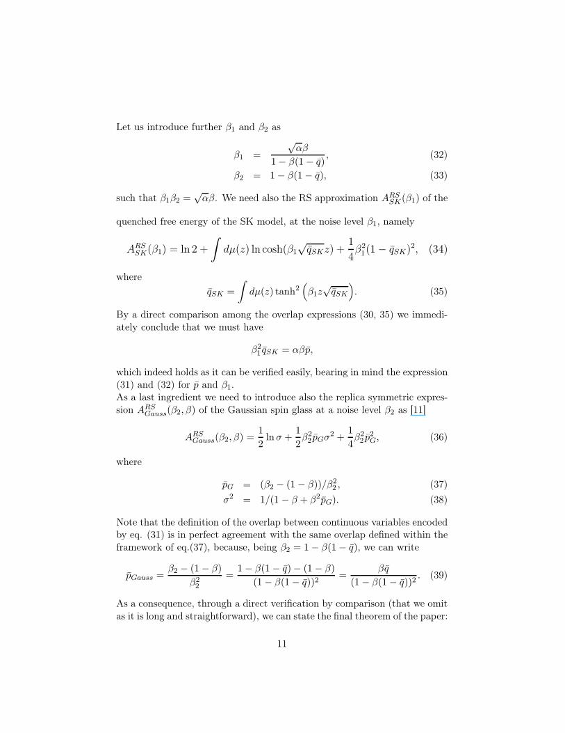
Let us introduce further β1 and β2 as

β1 =

√αβ

1− β(1− q), (32)

β2 = 1− β(1− q), (33)

such that β1β2 =√αβ. We need also the RS approximation ARS

SK(β1) of the

quenched free energy of the SK model, at the noise level β1, namely

ARSSK(β1) = ln 2 +

∫

dµ(z) ln cosh(β1

√qSKz) +

1

4β21(1− qSK)

2, (34)

where

qSK =

∫

dµ(z) tanh2(

β1z√qSK

)

. (35)

By a direct comparison among the overlap expressions (30, 35) we immedi-ately conclude that we must have

β21 qSK = αβp,

which indeed holds as it can be verified easily, bearing in mind the expression(31) and (32) for p and β1.As a last ingredient we need to introduce also the replica symmetric expres-sion ARS

Gauss(β2, β) of the Gaussian spin glass at a noise level β2 as [11]

ARSGauss(β2, β) =

1

2lnσ +

1

2β22 pGσ

2 +1

4β22 p

2G, (36)

where

pG = (β2 − (1− β))/β22 , (37)

σ2 = 1/(1 − β + β2pG). (38)

Note that the definition of the overlap between continuous variables encodedby eq. (31) is in perfect agreement with the same overlap defined within theframework of eq.(37), because, being β2 = 1− β(1− q), we can write

pGauss =β2 − (1− β)

β22

=1− β(1− q)− (1− β)

(1− β(1− q))2=

βq

(1− β(1− q))2. (39)

As a consequence, through a direct verification by comparison (that we omitas it is long and straightforward), we can state the final theorem of the paper:

11

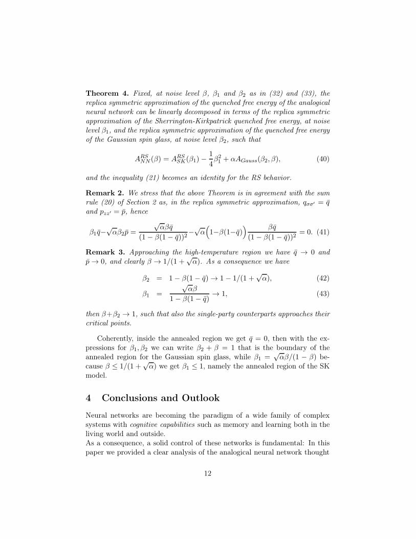
Theorem 4. Fixed, at noise level β, β1 and β2 as in (32) and (33), thereplica symmetric approximation of the quenched free energy of the analogicalneural network can be linearly decomposed in terms of the replica symmetricapproximation of the Sherrington-Kirkpatrick quenched free energy, at noiselevel β1, and the replica symmetric approximation of the quenched free energyof the Gaussian spin glass, at noise level β2, such that

ARSNN (β) = ARS

SK(β1)−1

4β21 + αAGauss(β2, β), (40)

and the inequality (21) becomes an identity for the RS behavior.

Remark 2. We stress that the above Theorem is in agreement with the sumrule (20) of Section 2 as, in the replica symmetric approximation, qσσ′ = qand pzz′ = p, hence

β1q−√αβ2p =

√αβq

(1− β(1− q))2−√

α(

1−β(1−q)) βq

(1− β(1− q))2= 0. (41)

Remark 3. Approaching the high-temperature region we have q → 0 andp → 0, and clearly β → 1/(1 +

√α). As a consequence we have

β2 = 1− β(1− q) → 1− 1/(1 +√α), (42)

β1 =

√αβ

1− β(1− q)→ 1, (43)

then β+β2 → 1, such that also the single-party counterparts approaches theircritical points.

Coherently, inside the annealed region we get q = 0, then with the ex-pressions for β1, β2 we can write β2 + β = 1 that is the boundary of theannealed region for the Gaussian spin glass, while β1 =

√αβ/(1 − β) be-

cause β ≤ 1/(1 +√α) we get β1 ≤ 1, namely the annealed region of the SK

model.

4 Conclusions and Outlook

Neural networks are becoming the paradigm of a wide family of complexsystems with cognitive capabilities such as memory and learning both in theliving world and outside.As a consequence, a solid control of these networks is fundamental: In thispaper we provided a clear analysis of the analogical neural network thought

12

of as a bipartite spin glass, made of by two different type of spins: one en-semble of dichotomic variables, as in the celebrated Sherrington-Kirkpatrickmodel, and one ensemble made of by Gaussian distributed variables.Exploiting this analogy, we developed a new interpolation scheme amongthe bipartite spin glass that mirrors the neural network and two indepen-dent glassy systems. Through this novel technique, we have then shown howto get a complete control of the annealed region of the neural network: Thecritical line has been obtained, together with an explicit behavior of all themain thermodynamical quantities: free energy, internal energy, entropy andoverlaps (namely the order parameters of the theory).One step forward we extended our interpolation scheme beyond the ergodicregion, under the assumption of replica symmetry: We showed that thereplica symmetric approximation of the quenched free energy of the ana-logical Hopfield model (at noise level β) can be expressed in terms of thereplica symmetric expressions of the quenched free energies of the SK model(at noise level β1) and of the Gaussian model (at noise level β2), and weobtained the equations linking β, β1, β2 obtaining then a complete controlalso within this framework.All that opens very interesting perspectives. The structure of the neuralnetwork as a linear combination of spin glasses is very rich: in fact we knowthat, as the SK model presents a very glassy full RSB structure [28], in theGaussian one this is absent, since the true solution is in fact RS even with noexternal field [11]. Thus one could aspect in our analogical neural network acompetition of these two effects: rather a new feature in the complex systemsscenario, that has to be deeply investigated.Clearly we would deepen this topic, for example within a fully broken replicasymmetry scenario on which we plan to report soon.Furthermore, the analogical model shares many features with the originalHopfield model (which is even harder from a mathematical point of view)for which one could study in what measure this structure is preserved.Future outlooks should cover also the completely analogical model in orderto develop mathematical techniques beyond the standard ones required inartificial intelligence and closer to system biology.

Acknowledgements

The strategy of this work is founded by the MIUR trough the FIRB grantRBFR08EKEV which is acknowledged, together with Sapienza Universitàdi Roma for partial financial support. Partial support from INFN is alsoacknowledged.

13

Appendix.

Fluctuation Theory for the Order Parameters

We develop in this appendix a fluctuation theory of the order parametersto see that the ergodicity breaking is accomplished through a second orderphase transition (i.e. the overlap fluctuations, properly rescaled over thevolume, do diverge on the line βc(α) hence defining a critical phenomenon).To satisfy this task we proceed as follows: at first we introduce a differentinterpolating structure with respect to the one discussed above (developedand discussed in [10]) to bridge the neural network with two single partyone-body models where spins are subjected to random fields in a way closeto stochastic stability [40] or cavity perspective [29]. Then we evaluate theflow with respect to the interpolating parameter so to be able to calculatevariations of generic observable as overlap correlation functions.Then we define the centered and rescaled overlaps and introduce their cor-relation matrix. Each element of this matrix then is evaluated at t = 0 andthen propagated thought t = 1 via its flow: This procedure encodes naturallyfor a system of coupled linear differential equations that, once solved, givesthe expressions of the overlap fluctuations. The latter are found to divergeon the critical line βc(α) already outlined and this will close our inspectionof the annealed regime.Let us start the plan by introducing the next interpolating structure:In a pure stochastic stability fashion [10], we need to introduce also twoclasses of i.i.d. N [0, 1] variables, namely N variables ηi and p variables ηµ,whose average is still encoded into the E operator and by which we definethe following interpolating quenched pressure ϕN,p(β, t)

ϕN,p(β, t) =1

NE log

∑

σ

∫ p∏

µ

dµ(zµ) exp(√t

√

β

N

∑

i,µ

ξµi σizµ) (44)

· exp(a√1− t

∑

i

ηiσi) exp(b√1− t

∑

µ

ηµzµ) exp(c(1 − t)

2

∑

µ

z2µ),

wherea =

√

αβp, b =√

βq c = β(1− q).

We stress that t ∈ [0, 1] interpolates between t = 0 where the interpolatingquenched pressure becomes made of by non-interacting systems (a series ofone-body problem) whose integration is straightforward (as well as the evalu-ation of the overlap correlation functions it produces) and the opposite limit,t = 1, that recovers the correct quenched free energy. Then we can evaluate

14

the flow with respect to the Boltzman factor encoded in the structure (44)as stated in the next

Proposition A. Given O as a smooth function of s replica overlaps (q1, ..., qs)and (p1, ..., ps), the following streaming equation holds:

d

dt〈O〉t = β

√α(

s∑

a,b

〈O · ξa,bηa,b〉t (45)

− s

s∑

a=1

〈O · ξa,s+1ηa,s+1〉t +s(s+ 1)

2〈O · ξs+1,s+2ηs+1,s+2〉t

)

.

We skip the proof as it is long but simple and works by a direct evaluationwhich is pretty standard in the disordered system literature (see for example[30, 7]).

The rescaled overlap ξ12 and η12 are defined accordingly to

ξ12 =√N(

q12 − q)

, (46)

η12 =√K(

p12 − p)

. (47)

In order to control the overlap fluctuations, namely 〈ξ212〉t=1, 〈ξ12η12〉t=1,〈η212〉t=1, ..., noting that the streaming equation pastes two replicas to theones already involved (s = 2 so far), we need to study nine correlationfunctions. It is then useful to introduce them and link them to capitalletters so to simplify their visualization:

〈ξ212〉t = A(t), 〈ξ12ξ13〉t = B(t), 〈ξ12ξ34〉t = C(t), (48)

〈ξ12η12〉t = D(t), 〈ξ12η13〉t = E(t), 〈ξ12η34〉t = F (t), (49)

〈η12η12〉t = G(t), 〈η12η13〉t = H(t), 〈η12η34〉t = I(t). (50)

If we introduce the operator dot as

O =1

β√α

dO

dt,

which simplifies calculations and shifts the propagation of the flow from t = 1to t = β

√α. Assuming a Gaussian behavior, as in the strategy outlined in

15

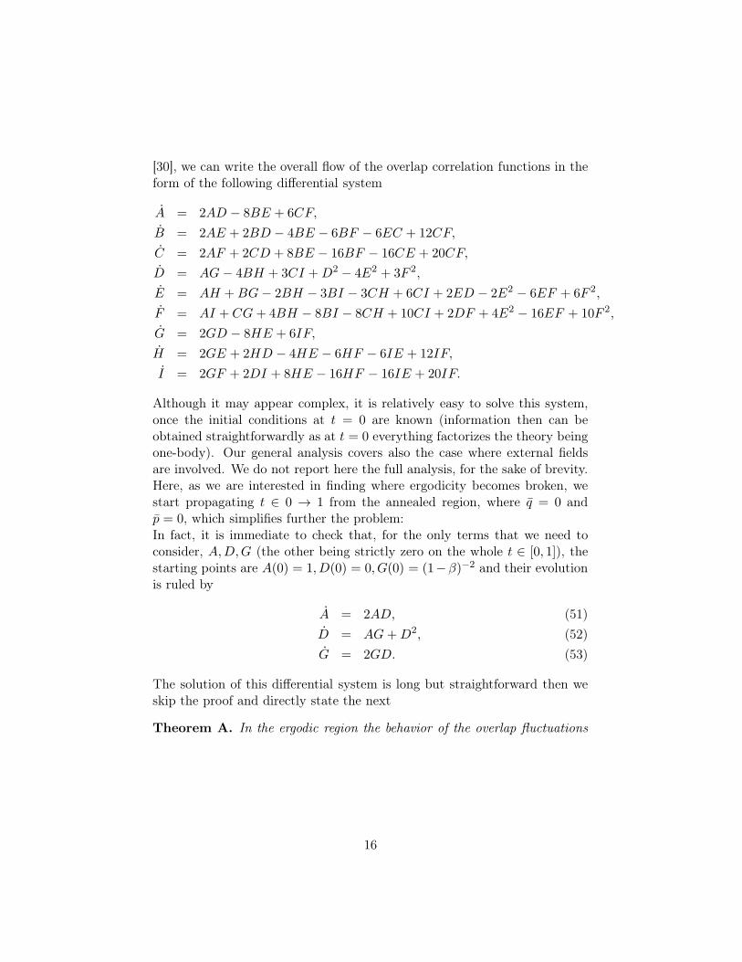
[30], we can write the overall flow of the overlap correlation functions in theform of the following differential system

A = 2AD − 8BE + 6CF,

B = 2AE + 2BD − 4BE − 6BF − 6EC + 12CF,

C = 2AF + 2CD + 8BE − 16BF − 16CE + 20CF,

D = AG− 4BH + 3CI +D2 − 4E2 + 3F 2,

E = AH +BG− 2BH − 3BI − 3CH + 6CI + 2ED − 2E2 − 6EF + 6F 2,

F = AI +CG+ 4BH − 8BI − 8CH + 10CI + 2DF + 4E2 − 16EF + 10F 2,

G = 2GD − 8HE + 6IF,

H = 2GE + 2HD − 4HE − 6HF − 6IE + 12IF,

I = 2GF + 2DI + 8HE − 16HF − 16IE + 20IF.

Although it may appear complex, it is relatively easy to solve this system,once the initial conditions at t = 0 are known (information then can beobtained straightforwardly as at t = 0 everything factorizes the theory beingone-body). Our general analysis covers also the case where external fieldsare involved. We do not report here the full analysis, for the sake of brevity.Here, as we are interested in finding where ergodicity becomes broken, westart propagating t ∈ 0 → 1 from the annealed region, where q = 0 andp = 0, which simplifies further the problem:In fact, it is immediate to check that, for the only terms that we need toconsider, A,D,G (the other being strictly zero on the whole t ∈ [0, 1]), thestarting points are A(0) = 1,D(0) = 0, G(0) = (1−β)−2 and their evolutionis ruled by

A = 2AD, (51)

D = AG+D2, (52)

G = 2GD. (53)

The solution of this differential system is long but straightforward then weskip the proof and directly state the next

Theorem A. In the ergodic region the behavior of the overlap fluctuations

16

is regular and described by the following equations

〈ξ212〉 =(1− β)2

(1− β)2 − β2α, (54)

〈ξ12η12〉 =β√α

(1− β)2 − β2α, (55)

〈η212〉 =1

(1− β)2 − β2α, (56)

diverging on the critical line βc(α), defined by eq. (21), hence defining asecond order phase transition.

References

[1] J.A. Acebron, L. Bonilla, C. Perez-Vicente, Prez; F. Ritort, R. Spigler,The Kuramoto model: a simple paradigm for synchronization phenomena,Rev. Mod. Phys. 77, 137, (2005).

[2] E. Agliari, A. Barra, F. Guerra, F. Moauro, A thermodynamical perspec-tive of immune capabilities, J. Theor. Biol. 287, 48, 2011.

[3] M. Aizenman, J. Lebowitz, D. Ruelle, Some Rigorous Results on theSherrington-Kirkpatrick Model of Spin Glasses, Commun. Math. Phys.,112 3-20 (1987).

[4] S. Albeverio, B. Tirozzi, B. Zegarlinski Rigorous results for the free energyin the Hopfield model, Comm. Math. Phys. 150, 337 (1992).

[5] D.J. Amit, Modeling brain function: The world of attractor neural net-work, Cambridge University Press, (1992).

[6] D.J. Amit, H. Gutfreund, H. Sompolinsky Storing infinite numbers ofpatterns in a spin glass model of neural networks, Phys. Rev. Lett. 55,1530-1533, (1985).

[7] A. Barra, Irreducible free energy expansion and overlap locking in meanfield spin glasses, J. Stat. Phys. 123, 601-614 (2006).

[8] A. Barra, P. Contucci, Toward a quantitative approach to migrants inte-gration, Europhys. Lett. 89, 68001, (2010).

[9] A. Barra, F. Guerra, About the ergodic regime in the analogical Hopfieldneural networks. Moments of the partition function, J. Math. Phys. 49,125217 (2008).

17

[10] A. Barra, G. Genovese, F. Guerra, The replica symmetric behavior ofthe analogical neural network, J. Stat. Phys. 140, 784, (2010).

[11] A. Barra, G. Genovese, F. Guerra, D. Tantari, A solvable mean fieldmodel of a Gaussian spin glass, submitted, available at arXiv:1109.4069.

[12] A.Barra, G.Genovese, F.Guerra, Equilibrium statistical mechanics ofbipartite spin systems, J. Phys. A: Math. and Theor. 44, 245002, (2011).

[13] J. P. Bigus, Data Mining With Neural Networks: Solving Business Prob-lems from Application Development to Decision Support, McGraw-Hill(2006).

[14] D. Bollé, T. M. Nieuwenhuizen, I. Perez-Castillo, T . Verbeiren, A spher-ical Hopfield model, J. Phys. A 36, 10269, (2003).

[15] A. Bovier, A.C.D. van Enter and B. Niederhauser, Stochastic symmetry-breaking in a Gaussian Hopfield-model, J. Stat. Phys. 95, 181-213 (1999).

[16] A. Bovier, V. Gayrard An almost sure central limit theorem for theHopfield model, Markov Proc. Rel. Fields 3, 151-173 (1997).

[17] A. Bovier Self-averaging in a class of generalized Hopfield models, J.Phys. A 27, 7069-7077 (1994).

[18] A. N. Burkitt, A review of the integrate-and-fire neuron model, BiolCybern 95, 1, (2006).

[19] A.C.C. Coolen, The mathematical theory of minority games: Statisticalmechanics of interacting agents, Oxford University Press, (2005).

[20] A.C.C. Coolen, A.J. Noest, G.B. de Vries, Modelling Chemical Modula-tion of Neural Processes, Network 4, 101, (1993).

[21] A.C.C. Coolen, R. Kuehn, P. Sollich, Theory of Neural InformationProcessing Systems, Oxford University Press, 2005.

[22] D. De Martino, M. Figliuzzi, A. De Martino, E. Marinari, Computingfluxes and chemical potential distributions in biochemical networks: en-ergy balance analysis of the human red blood cell, submitted. Available atarXiv:1107.2330 (2012).

[23] A. Di Biasio, E. Agliari, A. Barra, R. Burioni, Cooperativity in chemicalkinetics, Theor. Chem. Acc. 131, 1104, (2012).

18

[24] R. Dietrich, M. Opper, and H. Sompolinsky. Statistical mechanics ofsupport vector networks, Phys. rev. lett. 82, 2975, (1999).

[25] R.S. Ellis, Large deviations and statistical mechanics, Springer, NewYork, 1985.

[26] G. Genovese, A. Barra, A mechanical approach to mean field spin mod-els, J. Math. Phys. 50, 365234 (2009).

[27] F. Guerra, An introduction to mean field spin glass theory: methodsand results, In: Mathematical Statistical Physics, A. Bovier et al. eds,243 − 271, Elsevier, Oxford, Amsterdam, 2006.

[28] F. Guerra, Broken Replica Symmetry Bounds in the Mean Field SpinGlass Model, Commun, Math. Phys. 233:1, 1-12 (2003).

[29] F. Guerra, About the overlap distribution in mean field spin glass models,Int. Jou. Mod. Phys. B 10, 1675-1684 (1996).

[30] F. Guerra, Sum rules for the free energy in the mean field spin glassmodel, in Mathematical Physics in Mathematics and Physics: Quantumand Operator Algebraic Aspects, Fields Institute Communications 30,American Mathematical Society (2001).

[31] F. Guerra, F. L. Toninelli, The Thermodynamic Limit in Mean FieldSpin Glass Models, Commun. Math. Phys. 230:1, 71-79 (2002).

[32] D.O. Hebb, Organization of Behaviour, Wiley, New York, 1949.

[33] J.J. Hopfield, Neural networks and physical systems with emergent col-lective computational abilities, Proc. Ntl. Acad. Sci. USA 79, 2554-2558(1982).

[34] M. Mézard, A. Montanari, Information, Physics and Computation, Ox-ford University press, 2009.

[35] M. Mézard, G. Parisi and M. A. Virasoro, Spin glass theory and beyond,World Scientific, Singapore, 1987.

[36] L. Pastur, M. Scherbina, B. Tirozzi, The replica symmetric solutionof the Hopfield model without replica trick J. Stat. Phys. 74, 1161-1183(1994).

[37] L.Pastur, M. Scherbina, B. Tirozzi, On the replica symmetric equationsfor the Hopfield model J. Math. Phys. 40, 3930-3947 (1999).

19

[38] I. Perez-Castillo, B. Wemmenhove, J.P.L. Hatchett, A.C.C. Coolen, N.S.Skantzos and T. Nikoletopoulos, Analytic solution of attractor neuralnetworks on scale-free graphs, J. Phys. A 37, 8789, (2004).

[39] Y. Singh, A.S. Chauhan, Neural networks in data mining, J. Theor. andAppl. Inform. Techn. 5, 1, (2009).

[40] P. Sollich, A. Barra, Notes on the polynomial identities in random over-lap structures, J. Stat. Phys. 147, 351, (2012).

[41] M. Talagrand, Spin glasses: a challenge for mathematicians. Cavity andmean field models, Springer-Verlag, (2003).

[42] M. Talagrand, Rigourous results for the Hopfield model with many pat-terns, Probab. Th. Relat. Fields 110, 177-276 (1998).

[43] M. Talagrand, Exponential inequalities and convergence of moments inthe replica-symmetric regime of the Hopfield model, Ann. Probab. 38,1393-1469 (2000).

[44] B. Wemmenhove, A.C.C. Coolen, Finite connectivity attractor neuralnetworks, J. Phys. A: Math. and Gen. 36, 9617, (2003).

20