Identification of Recurrent Neural Networks by Bayesian ...

Journal of Machine Learning Research 10 (2009) 515-554 Submitted 12/07; Revised 8/08; Published 2/09

Identification of Recurrent Neural Networks by BayesianInterrogation Techniques

Barnabás Póczos∗ [email protected] .CA

András Lorincz [email protected]

Department of Information Systems, Eötvös Loránd UniversityPázmány P. sétány 1/C, Budapest H-1117, Hungary

Editor: Zoubin Ghahramani

AbstractWe introduce novel online Bayesian methods for the identification of a family of noisy recurrentneural networks (RNNs). We present Bayesian active learning techniques for stimulus selectiongiven past experiences. In particular, we consider the unknown parameters as stochastic variablesand use A-optimality and D-optimality principles to chooseoptimal stimuli. We derive myopic costfunctions in order to maximize the information gain concerning network parameters at each timestep. We also derive the A-optimal and D-optimal estimations of the additive noise that perturbs thedynamical system of the RNN. Here we investigate myopic as well as non-myopic estimations, andstudy the problem of simultaneous estimation of both the system parameters and the noise. Em-ploying conjugate priors our derivations remain approximation-free and give rise to simple updaterules for the online learning of the parameters. The efficiency of our method is demonstrated for anumber of selected cases, including the task of controlled independent component analysis.

Keywords: active learning, system identification, online Bayesian learning, A-optimality, D-optimality, infomax control, optimal design

1. Introduction

When studying systems ininteractiveandonline fashion, it is of high relevance to facilitate fastinformation gain during the interaction (Fedorov, 1972; Cohn, 1994). Asan example, considerexperiments aiming at the description of the receptive field of different neurons. These experi-ments look for those stimuli that maximize the response of the given neuron (deCharms et al., 1998;Földiák, 2001). Neurons, however, might change due to the investigation, so the minimization ofinteraction is highly desired. Different techniques have been developedto speed up the identifica-tion procedure. One approach searches for stimulus distribution that maximizes mutual informationbetween stimulus and response (Machens et al., 2005). A recent technique assumes that the un-known system belongs to the family of generalized linear models (Lewi et al., 2007) and treats theparameters as probabilistic variables. Then the goal is to find the optimal stimuli by maximizingmutual information between the parameter set and the system’s response.

This example motivates our interest in active learning (MacKay, 1992; Cohnet al., 1996; Fuku-mizu, 1996; Sugiyama, 2006) of noisy recurrent artificial neural networks (RNNs), when we havethe freedom to interrogate the network and to measure its responses.

∗. Present address: Department of Computing Science, University ofAlberta, Athabasca Hall, Edmonton, Canada, T6G2E8

c©2009 Barnabás Póczos and András Lorincz.

PÓCZOS ANDL ORINCZ

In active learning, the training set may be modified by the learning process itself based on theprogress experienced so far. The goal of this modification is to maximize the expected improvementof the precision of the estimation. This idea can for example be used to improve generalizationcapability in regression and classification tasks or to better estimate hidden parameters. Theoreticalconcepts have been formulated in the fields of Optimal Experimental Design, or Optimal BayesianDesign (Kiefer, 1959; Fedorov, 1972; Steinberg and Hunter, 1984;Toman and Gastwirth, 1993;Pukelsheim, 1993).

Although active learning is in the focus of current research interest, some relevant theoreticalissues are still unresolved. While there are promising studies showing that active learning mayoutperform uniform sampling under certain conditions (Freund et al., 1997; Seung et al., 1992), inother cases it has been proven that active learning has no advantage over non-adaptive algorithms.For example, this is the case in compressed sensing (Castro et al., 2006a) and also for certainfunction classes in the area of function approximation (Castro et al., 2006b). Even more problematicis the observation that active learning heuristics may be less efficient than uniform sampling in somesituations (Schein, 2005).

There are several forms of active learning. The most relevant difference is in the definition of thevalue of information. One of the simplest heuristics is the Uncertainty Sampling (US): US suggeststhat in regression or in classification tasks one should choose those training examples, which havethe largest uncertainty in the value of the function or in the label of the class,respectively (Lewisand Catlett, 1994; Lewis and Gale, 1994; Cohn et al., 1996). Although several US versions existwith different measure of the uncertainty itself, they all lack robustness. The Query by Committeemethod improves upon robustness (Seung et al., 1992; Freund et al., 1997): the committee of a fewmodels are trained on the existing training set and the next query points are selected to reduce thedisagreement among these models. The method of Roy and McCallum (2001) minimizes the directerror, that is, it tries to choose training points to minimize the expected classification error directly.

In the literature there are other approaches, including decision theory based methods. The orig-inal ideas were worked out in Raiffa and Schlaifer (1961) and Lindley (1971). The objective inthis method family is to choose the design such that the predicted value of a given utility functionbecome maximal. Numerous utility functions have been proposed. For example,if we aim to esti-mate the unknown parameterθ, then one possible direction is the minimization of, for example, theentropy or the standard deviation of the posterior distribution. If we minimize theentropy then wearrive at the D-optimality principle (Bernardo, 1979; Stone, 1959). Thisprinciple is equivalent tothe information maximization method (also known as infomax principle) of Lewi et al. (2007). Ifwe intend to minimize the standard deviation then the result is the A-optimality principle (Duncanand DeGroot, 1976). A special case is called the c-optimality principle (Chaloner, 1984) when thegoal is to estimate a linear projection of parameterθ (cTθ). There exist a number of other methods,called alphabetical optimality and utility functions. For a review see, for example, Chaloner andVerdinelli (1995). Although the original ideas belong to the field of optimal experimental design,they have appeared also in active learning recently (MacKay, 1992; Tong and Koller, 2000; Scheinand Ungar, 2007).

Today, active learning is present almost in all fields of machine learning and there are manypopular applications on diverse areas, including Gaussian Processes(Krause and Guestrin, 2007),Artificial Neural Networks (Fukumizu, 2000), Support Vector Machines (Tong and Koller, 2001b),Generalized Linear Models (Bach, 2007; Lewi et al., 2007), Logistic Regression (Schein, 2005),

516

BAYESIAN INTERROGATION FORPARAMETER AND NOISE IDENTIFICATION

learning the parameters and structure of Bayes nets (Tong and Koller, 2000, 2001a) and HiddenMarkov Models (Anderson and Moore, 2005).

Our framework is similar to the generalized linear model (GLM) approach used by Lewi et al.(2007): we would like to choose interrogating, or ‘control’ inputs in order to (i) identify the pa-rameters of the network and (ii) estimate the additive noise efficiently. From now on, we use thetermscontrol and interrogation interchangeably; control is the conventional expression, whereasthe word interrogation expresses our aims better. We apply online Bayesianlearning (Opper andWinther, 1999; Solla and Winther, 1999; Honkela and Valpola, 2003; Ghahramani, 2000). ForBayesian methods, prior updates often lead to intractable posterior distributions such as a mixtureof exponentially numerous distributions. Here, we show that, for the model studied in this paper,computations are both tractable and approximation-free. Further, the emerging learning rules aresimple. We also show that different stimuli are needed for the same RNN modeldepending onwhether the goal is to estimate the weights of the RNN or the additive perturbation(referred to as‘driving noise’).

In this article we investigate the D-optimality, as well as the A-optimality principles. Tothe bestof our knowledge, neither of them has been applied to the typical non-spiking stochastic artificialrecurrent neural network model that we treat here.

The contribution of this paper can be summarized as follows: We use A-optimalityand D-optimality principles and derive cost functions and algorithms for (i) the learning of parameters ofthe stochastic RNN and (ii) the estimation of its driving noise. We show that, (iii) using the D-optimality interrogation technique, these two tasks are incoherent in the myopic (i.e., single steplook-ahead) control scheme: signals derived from this principle for parameter estimation are sub-optimal (basically the worst possible) for the estimation of the driving noise and vice versa. (iv)We show that for the case of noise estimation task the two principles, that is, A-and D-optimalityprinciples result in the same cost function. (v) For the A-optimality case, we derive equations forthe joined estimation of the noise and the parameters. On the contrary, we showalso that (vi)D-optimality cannot be applied on the same joined task. For the case of noise estimation, (vii) anon-myopic multiple step look-ahead heuristics is introduced and we demonstrate its applicabilitythrough numerical experiments.

The paper is structured as follows: In Section 2 we introduce our model. Section 3 concernsthe Bayesian equations of the RNN model. In Section 4 optimal control for parameter identificationis derived from the D-optimality principle. Section 5 is about the same task, butusing the A-optimality principle instead. Section 6 deals with our second task, when the goalis the estimationof the driving noise of the RNN. Here we treat the D-optimality principle. Section 7 is about thesame problem, but for the A-optimality principle. We combine the two tasks for bothoptimalityprinciples in Section 8 and consider the cost functions for the joined estimationof the parametersand the driving noise. All of these considerations concern myopic algorithms. In Section 9 a non-myopic heuristics is introduced for the noise estimation task. Section 10 containsour numericalexperiments for a number of cases, including independent component analysis. The paper endswith a short discussion and some conclusions (Section 11). Technical details of the derivations canbe found in the Appendix.

517

PÓCZOS ANDL ORINCZ

2. The Model

Let P(e) = Ne(m,V) denote the probability density of a normally distributed stochastic variableewith meanm and covariance matrixV. Let us assume that we haved simple computational unitscalled ‘neurons’ in a recurrent neural network:

r t+1 = g

(

I

∑i=0

Fir t−i +J

∑j=0

B jut+1− j +et+1

)

, (1)

where{et}, the driving noise of the RNN, denotes temporally independent and identically dis-tributed (i.i.d.) stochastic variables andP(et) =Net (0,V), r t ∈R

d represents the observed activitiesof the neurons at timet. Let ut ∈ R

c denote the control signal at timet. The neural network isformed by the weighted delays represented by matricesFi (i = 0, . . . , I ) andB j ( j = 0, . . . ,J), whichconnect neurons to each other and also the control components to the neurons, respectively. Controlcan also be seen as the means of interrogation, or the stimulus to the network (Lewi et al., 2007).We assume that functiong : R

d → Rd in (1) is known and invertible. The computational units, the

neurons, sum up weighted previous neural activities as well as weightedcontrol inputs. These sumsare then passed through identical non-linearities according to Eq. (1). Our goal is to estimate theparametersFi ∈ R

d×d (i = 0, . . . , I ), B j ∈ Rd×c ( j = 0, . . . ,J) and the covariance matrixV, as well

as the driving noiseet by means of the control signals.In artificial neural network terms, (1) is in the form ofrate code models. This is the typical

form for RNNs, but there are methods to approximate rate code descriptionwith spike codes andvice versa. For the case of RNNs, the best is to compare Liquid State Machine, a spike code modelof Maass et al. (2002) with the Echo State Network, the corresponding rate code model of Jaeger(2001). Rate code, very crudely, is the low pass filtered spike code, whereas spike code can be seenas the response of integrate-and-fire neurons. We show that analytic cost functions emerge for therate code RNN model. Due to the applied conjugate priors, we can calculate thehigh dimensionalintegrals involved in our derivations, and hence these derivations remainapproximation-free andgive rise to simple update rules.

3. Bayesian Approach

Here we embed the estimation task into the Bayesian framework. First, we introduce the follow-ing notations:xt+1 = [r t−I ; . . . ; r t ;ut−J+1; . . . ;ut+1], yt+1 = g−1(r t+1), A = [FI , . . . ,F0,BJ, . . . ,B0]∈R

d×m. With these notations, model (1) reduces to a linear equation

yt = Axt +et . (2)

In order to estimate the unknown quantities (parameter matrixA, noiseet and its covariance matrixV) in an online fashion, we rely on Bayes’ method. We assume that prior knowledge is availableand we update our posteriori knowledge on the basis of the observations. Control will be chosenat each instant to provide maximal expected information concerning the quantities we have to esti-mate. Starting from an arbitrary prior distribution of the parameters the posterior distribution needsto be computed. This latter distribution, however, can be highly complex, so approximations areapplied. For example, assumed density filtering, when the computed posterioris projected to sim-pler distributions, has been suggested (Boyen and Koller, 1998; Minka,2001; Opper and Winther,

518


1999). In order to avoid approximations, we apply the method of conjugatedpriors (Gelman et al.,2003). For matrixA we assume a matrix valued normal distribution prior.

For the case of D-optimality principle, we shall use the inverted Wishart (IW)distribution asour prior for covariance matrixV. This is the most general known conjugate prior distributionfor the covariance matrix of a normal distribution at present. For A-optimality,however, we keepthe derivations simple and assume that the covariance matrix has diagonal structure. In turn, wereplaced the IW assumption on the prior with the distribution of the Product of Inverted Gammas(PIG).

We define the normally distributed matrix valued stochastic variableA ∈ Rd×m by using the

following quantities:M ∈ Rd×m is the expected value ofA. V ∈ R

d×d is the covariance matrixof the rows, andK ∈ R

m×m is the so-called precision parameter matrix that we shall modify inaccordance with the Bayesian update. MatrixK contains the estimations of the ‘Bayesian trainer’about the precision of parameters inA. Informally, matrixK behaves as the inverse of a covariancematrix. Upon each observation, matrixK is updated. The larger the eigenvalues of this matrix, thesmaller the variance ellipsoids of the posteriori estimations are.

BothK andV are positive semi-definite matrices. The density function of the stochastic variableA is defined as:

NA(M ,V,K) =|K |d/2

|2πV|m/2exp(−1

2tr((A−M)TV−1(A−M)K)),

where tr, | · |, and superscriptT denote the trace operation, the determinant, and transposition,respectively (see, e.g., Gupta and Nagar, 1999; Minka, 2000). We assume thatQ∈R

d×d is a positivedefinite matrix andn> 0. Using these notations, the density of the Inverted Wishart distribution withparametersQ andn is as follows (Gupta and Nagar, 1999):

IW V(Q,n) =1

Zn,d

1

|V|(d+1)/2

∣

∣

∣

∣

V−1Q2

∣

∣

∣

∣

n/2

exp(−12

tr(V−1Q)),

whereZn,d = πd(d−1)/4d∏i=1

Γ((n+1− i)/2) andΓ(.) denotes the gamma function.

Similarly, letV = diag(v) ∈ Rd×d diagonal covariance matrix with 0< v ∈ R

d diagonal values.With the slight abuse of notation we will use later thev = diag(V) ∈ R

d term, too. Then the densityof PIG is defined as

PIGV(α,β) =d

∏i=1

βαii

Γ(αi)v−αi−1

i exp(−βi

vi),

whereαi > 0 andβi > 0 are the shape and scale parameters respectively.Now, one can rewrite model (2) as follows:

P(A|V) = NA(M ,V,K), (3)

P(et |V) = Net (0,V), (4)

P(yt |A,xt ,V) = Nyt (Axt ,V), (5)

andP(V) = PIGV(α,β) or P(V) = IW V(Q,n) depending on whether we want to use A- or D-optimality.

519

PÓCZOS ANDL ORINCZ

4. D-Optimality Approach for Parameter Learning

Let us compute the D-optimal parameter estimation strategy for our RNN given by (1) and rewritteninto (3)-(5). Let us introduce two shorthands;θ = {A,V}, and{x} j

i = {xi , . . . ,x j}. We choosethe control value in (1) at each instant to provide maximal expected information concerning theunknown parameters. Assuming that{x}t

1, {y}t1 are given, according to the infomax principle our

goal is to compute

argmaxut+1

I(θ,yt+1;{x}t+11 ,{y}t

1), (6)

whereI(a,b;c) denotes the mutual information of stochastic variablesa andb for fixed parametersc. Let H(a|b;c) denote the conditional entropy of variablea conditioned on variableb and for fixedparameterc. Note that

I(θ,yt+1;{x}t+11 ,{y}t

1) = H(θ;{x}t+11 ,{y}t

1)−H(θ|yt+1;{x}t+11 ,{y}t

1),

holds (Cover and Thomas, 1991) andH(θ;{x}t+11 ,{y}t

1) = H(θ;{x}t1,{y}t

1) is independent fromut+1, hence our task is reduced to the evaluation of the following quantity:

argminut+1

H(θ|yt+1;{x}t+11 ,{y}t

1) = (7)

= argminut+1

−Z

dyt+1P(yt+1|{x}t+11 ,{y}t

1)Z

dθP(θ|{x}t+11 ,{y}t+1

1 ) logP(θ|{x}t+11 ,{y}t+1

1 ).

In order to solve this minimization problem we need to evaluateP(yt+1|{x}t+11 ,{y}t

1), the posteriorP(θ|{x}t+1

1 ,{y}t+11 ), and the entropy of the posterior, that is

R

dθP(θ|{x}t+11 ,{y}t+1

1 )logP(θ|{x}t+1

1 ,{y}t+11 ), whereP(a|b) denotes the conditional probability of variablea given con-

dition b. The main steps of these computations are presented below.Assume that the a priori distributions P(A|V,{x}t

1,{y}t1) = N (A|M t ,V,K t) and

P(V|{x}t1,{y}t

1) = IW V(Qt ,nt) are known. Then the posterior distribution ofθ is:

P(A,V|{x}t+11 ,{y}t+1

1 ) =P(yt+1|A,V,xt+1)P(A|V,{x}t

1,{y}t1)P(V|{x}t

1,{y}t1)

P(yt+1|{x}t+11 ,{y}t

1),

=Nyt+1(Axt+1,V)NA(M t ,V,K t)IW V(Qt ,nt)

R

AR

V Nyt+1(Axt+1,V)NA(M t ,V,K t)IW V(Qt ,nt).

This expression can be rewritten in a more useful form: letK ∈ Rm×m andQ ∈ R

d×d be positivedefinite matrices. LetA ∈ R

d×m, and let us introduce the density function of the matrix valuedStudent-t distribution (Kotz and Nadarajah, 2004; Minka, 2000) as follows:

TA(Q,n,M ,K) =|K |d/2

πdm/2

Zn+m,d

Zn,d

|Q|n/2

|Q+(A−M)K(A−M)T |(m+n)/2.

Now, we need the following lemma:

Lemma 4.1

Ny(Ax,V)NA(M ,V,K)IW V(Q,n) =NA((MK +yxT)(xxT +K)−1,V,xxT +K)××IW V

(

Q+(y−Mx)(1−xT(xxT +K)−1x)(y−Mx)T ,n+1)

×

×Ty(

Q,n,Mx ,1−xT(xxT +K)−1x)

.

520


The proof can be found in the Appendix.Using this lemma, we can compute the posterior probabilities. We introduce the following

quantities:

γt+1 = 1−xTt+1(xt+1xT

t+1 +K t)−1xt+1, (8)

nt+1 = nt +1,

M t+1 = (M tK t +yt+1xTt+1)(xt+1xT

t+1 +K t)−1, (9)

Qt+1 = Qt +(yt+1−M txt+1)γt+1(yt+1−M txt+1)T . (10)

For the posterior probabilities we have determined that

P(A|V,{x}t+11 ,{y}t+1

1 ) = NA(M t+1,V,xt+1xTt+1 +K t), (11)

P(V|{x}t+11 ,{y}t+1

1 ) = IW V (Qt+1,nt+1) , (12)

P(yt+1|{x}t+11 ,{y}t

1) = Tyt+1 (Qt ,nt ,M txt+1,γt+1) .

Now we are in the position to compute the entropy of the posterior distribution ofθ = {A,V} usingthe following lemma:

Lemma 4.2 The entropy of a stochastic variable with density function P(A,V) =NA(M ,V,K)IW V(Q,n) assumes the form−d

2 ln |K |+(m+d+12 ) ln |Q|+ f1,1(d,n), where f1,1(d,n)

depends only on d and n.

The proof can be found in the Appendix.Lemmas 4.1 and 4.2 lead to the following corollary:

Corollary 4.3 For the entropy of a stochastic variable with posterior distribution P(A,V|x,y) itholds that

H(A,V;x,y) = −d2

ln |xxT +K |+ f1,1(d,n)+(m+d+1

2) ln |Q+(y−Mx)γ(y−Mx)T |.

We note that the following lemma also holds:

Lemma 4.4Z

Ty (Q,n,µ,γ) ln |Q+(y−µ)γ(y−µ)T |dy

is independent from bothµ andγ,

and thus we can compute the conditional entropy expressed in (7):

Lemma 4.5

H(A,V|y;x) =Z

p(y|x)H(A,V;x,y)dy = −d2

ln |xxT +K |+ f1,2(Q,n,m),

where f1,2(Q,n,m) depends only onQ, n and m.

521

PÓCZOS ANDL ORINCZ

Collecting all the terms, we arrive at the followingintriguingly simpleexpression

uoptt+1 = argmin

ut+1

Z

p(

yt+1|{x}t+11 ,{y}t

1

)

H(A,V|{x}t+11 ,{y}t

1,yt+1)dyt+1,

= argminut+1

−d2

ln |xt+1xTt+1 +K t | = argmax

ut+1xT

t+1K−1t xt+1, (13)

where

xt+1.= [r t−I ; . . . ; r t ;ut−J+1; . . . ;ut+1],

and we used that|xxT +K | = |K |(1+xTK−1x) according to the Matrix Determinant Lemma(Harville, 1997). We assume a bounded domainU for the control, which is necessary to keepthe maximization procedure of (13) finite. This is, however, a reasonable condition for all practicalapplications. So,

uoptt+1 = arg max

ut+1∈UxT

t+1K−1t xt+1, (14)

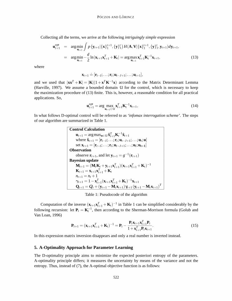
In what follows D-optimal control will be referred to as‘infomax interrogation scheme’. The stepsof our algorithm are summarized in Table 1.

Control Calculationut+1 = argmaxu∈U xT

t+1K−1t xt+1

wherext+1 = [r t−I ; . . . ; r t ;ut−J+1; . . . ;ut ;u]setxt+1 = [r t−I ; . . . ; r t ;ut−J+1; . . . ;ut ;ut+1]

Observationobserver t+1, and letyt+1 = g−1(r t+1)

Bayesian updateM t+1 = (M tK t +yt+1xT

t+1)(xt+1xTt+1 +K t)

−1

K t+1 = xt+1xTt+1 +K t

nt+1 = nt +1γt+1 = 1−xT

t+1(xt+1xTt+1 +K t)

−1xt+1

Qt+1 = Qt +(yt+1−M txt+1)γt+1(yt+1−M txt+1)T

Table 1: Pseudocode of the algorithm

Computation of the inverse(xt+1xTt+1 +K t)

−1 in Table 1 can be simplified considerably by thefollowing recursion: letPt = K−1

t , then according to the Sherman-Morrison formula (Golub andVan Loan, 1996)

Pt+1 = (xt+1xTt+1 +K t)

−1 = Pt −Ptxt+1xT

t+1Pt

1+xTt+1Ptxt+1

. (15)

In this expression matrix inversion disappears and only a real number is inverted instead.

5. A-Optimality Approach for Parameter Learning

The D-optimality principle aims to minimize the expected posteriori entropy of the parameters.A-optimality principle differs; it measures the uncertainty by means of the variance and not theentropy. Thus, instead of (7), the A-optimal objective function is as follows:

522


uoptt+1 = argmin

ut+1

Z


1)trVar[θ|{x}t+11 ,{y}t+1

1 ]. (16)

whereVar[θ|F ] denotes the conditional covariance matrix ofθ given the conditionF .To keep the calculations simple, in this case we usePIGV(αt ,βt) prior distribution for the co-

variance matrix instead ofIW V(Qt ,nt). Using the notations of (8)-(10), the posterior distributionsassume the following forms:

Lemma 5.1

P(A|V,{x}t+11 ,{y}t+1

1 ) = NA(M t+1,V,xt+1xTt+1 +K t), (17)

P(V|{x}t+11 ,{y}t+1

1 ) = PIGV (αt+1,βt+1) ,

P(yt+1|{x}t+11 ,{y}t

1) =d

∏i=1

T(yt+1)i

(

(βt)i ,2(αt)i ,(M txt+1)i ,γt+1

2

)

, (18)

where we used the shorthands

(αt+1)i = (αt)i +1/2,

(βt+1)i = (βt)i +((yt+1)i − (M txt+1)i)2 γt+1

2. (19)

The proof can be found in the Appendix.Given thatP(V|{x}t+1

1 ,{y}t+11 ) belongs to thePIG family we can calculate the quantity

Var(V|{x}t+11 ,{y}t+1

1 ) (Gelman et al., 2003):

tr(

Var[V|{x}t+11 ,{y}t+1

1 ])

=d

∑i=1

(βt+1)i

((αt+1)i −1)2((αt+1)i −2).

We will need the following lemma:

Lemma 5.2

tr(

Var[A|{x}t+11 ,{y}t+1

1 ])

= tr(

(

K t +xt+1xTt+1

)−1)

E[trV|{x}t+11 ,{y}t+1

1 ],

= tr(

(

K t +xt+1xTt+1

)−1) d

∑i=1

(βt+1)i

(αt+1)i −1.

The proof can be found in the Appendix.Now we can elaborate on the A-optimal cost function for parameter estimation (16):

Z


1)trVar[θ|{x}t+11 ,{y}t+1

1 ] = (20)

=Z

dyt+1

d

∏i=1

T(yt+1)i

(


2

)

×

×(

tr(

(

K t +xt+1xTt+1

)−1) d

∑i=1

(βt+1)i

(αt+1)i −1+

d

∑i=1

(βt+1)i

((αt+1)i −1)2((αt+1)i −2)

)

,

= tr(

(

K t +xt+1xTt+1

)−1)

f2,1(αt+1,βt)+ f2,2(αt+1,βt),

523

PÓCZOS ANDL ORINCZ

where f2,1 and f2,2 depend only onαt+1, andβt . Here we used (18), (19) and Lemma 4.4.Applying again the Sherman-Morrison formula (15) and the fact thattr[K−1

t xt+1xTt+1K−1

t ] =

tr[xTt+1K−1

t K−1t xt+1], we arrive at the following expression for A-optimal parameter estimation:

uoptt+1 = arg max

ut+1∈U

xTt+1K−1

t K−1t xt+1

1+xTt+1K−1

t xt+1, (21)

which is a hyperbolic programming task.We can conclude that while in the D-optimality case the task is to minimize expression|(K t +

xt+1xTt+1)

−1|, the A-optimality principle is concerned with the minimization oftr[(K t +xt+1xTt+1)

−1].

6. D-Optimality Approach for Noise Estimation

One might wish to compute the optimal control for estimating noiseet in (1), instead of the identi-fication problem above. Based on (1) and because

et+1 = yt+1−I

∑i=0

Fir t−i −J

∑j=0

B jut+1− j , (22)

one might think that the best strategy is to use the optimal infomax control of Table 1, since itprovides good estimations for parametersA = [FI , . . . ,F0,BJ, . . . ,B0] and so for noiseet .

Another—and different—thought is the following. At timet +1, let the estimation of the noisebe et+1 = yt+1 −∑I

i=0 Fti r t−i −∑J

j=0 Btjut+1− j , whereFt

i (i=0,. . . ,I), andBtj (j=0,. . . ,J) denote the

estimations ofF andB respectively.Using (22), we have that

et+1− et+1 =I

∑i=0

(Fi − Fti )r t−i +

J

∑j=0

(B j − Btj)ut+1− j . (23)

This hints that the control should beut = 0 for all times in order to get rid of the error contributionof matrixB j in (23).

Straightforward D-optimality considerations oppose the utilization of objective(6) for the presenttask. One can optimize, instead, the following quantity:

argmaxut+1

I(et+1,yt+1;{x}t+11 ,{y}t

1).

In other words, for the estimation of the noise we want to design a control signal ut+1 such that thenext output is the best from the point of view of greedy optimization of mutual information betweenthe next outputyt+1 and the noiseet+1. It is easy to show that this task is equivalent to the followingoptimization problem:

argminut+1

Z


1)H(et+1;{x}t+11 ,{y}t+1

1 ), (24)

whereH(et+1;{x}t+11 ,{y}t+1

1 ) = H(Axt+1;{x}t+11 ,{y}t+1

1 ), becauseet+1 = yt+1−Axt+1.In practice, we perform this optimization in an appropriate domainU. After some mathematical

calculation we can prove that the D-optimal interrogation scheme for noise estimation gives rise tothe following control:

524


Lemma 6.1

uoptt+1 = arg min

ut+1∈UxT

t+1K−1t xt+1. (25)

The proof of this lemma can be found in the Appendix.It is worth noting that this D-optimal cost function for noise estimation and the D-optimal cost

function derived for parameter estimation in (13) are not compatible with eachother. Estimatingone of them quickly will necessarily delay the estimation of the other.

We shall show later (Section 9) that for larget values, expression (25) gives rise to control valuesclose tout = 0.

7. A-Optimality Approach for Noise Estimation

Instead of (24), our task is to compute the following quantity:

argminut+1

Z


1) tr(

Var[et+1|{x}t+11 ,{y}t+1

1 ])

. (26)

We will apply the identity

NAxt+1

(

M t+1xt+1,V,(

xTt+1K−1

t+1xt+1)−1)

PIGV (αt+1,βt+1) =

=d

∏i=1

T(Axt+1)i

(βt+1)i ,2(αt+1)i ,(M t+1xt+1)i ,

(

xTt+1

K−1t+1

2xt+1

)−1

×

×PIGV

(

αt+1 +1,βt+1 +diag[(yt+1−M txt+1)γt+1

2(yt+1−M txt+1)

T ])

,

which can be proven by using Lemma A.1. We can simplify (26) by noting that

tr(

Var[et+1|{x}t+11 ,{y}t+1

1 ])

= tr(

Var[Axt+1|{x}t+11 ,{y}t+1

1 ])

.

We also take advantage of the fact that

VarV [E[Axt+1|V,{x}t+11 ,{y}t+1

1 ]] = VarV [M t+1xt+1] = 0,

and proceed as

EV [trVar(Axt+1|V,{x}t+11 ,{y}t+1

1 )] = EV [tr(V⊗xTt+1K−1

t+1xt+1|{x}t+11 ,{y}t+1

1 ],

= tr(E[V|{x}t+11 ,{y}t+1

1 ])xTt+1K−1

t+1xt+1,

= xTt+1K−1

t+1xt+1

d

∑i=1

(βt+1)i

(αt+1)i −1,

where⊗ denotes the Kronecker product. The law of total variance says that

Var[Ax] = Var[E[Ax|V]]+E[Var[Ax|V]],

and hence

trVar[Axt+1|{x}t+11 ,{y}t+1

1 ] = xTt+1K−1

t+1xt+1

d

∑i=1

(βt+1)i

(αt+1)i −1.

525

PÓCZOS ANDL ORINCZ

There is another way to arrive at the same result. One can apply (37) with Lemma A.1 and use

the fact that the covariance matrix of aTx(β,α,µ,K) distributed variable isβK−1

α−2 (Gelman et al.,2003). That is, we have

trVar[Axt+1|{x}t+11 ,{y}t+1

1 ] =d

∑i=1

(βt+1)i

(

xTt+1

K−1t+12 xt+1

)

2(αt+1)i −2

.

Now, we can proceed asZ


1)tr(

Var[et+1|{x}t+11 ,{y}t+1

1 ])

= (27)Z


1)tr(E[V|{x}t+11 ,{y}t+1

1 ])xTt+1K−1

t+1xt+1 =

xTt+1K−1

t+1xt+1

Z


1)d

∑i=1

(βt+1)i

(αt+1)i −1=

xTt+1K−1

t+1xt+1

d

∑i=1

f4((αt+1)i ,(βt)i),

where we used (18), (19) and Lemma 4.4 again. Applying the Sherman-Morrison formula one cansee that the task is the same as in (25).

8. Joint Parameter and Noise Estimation

So far we wanted to optimize the control in order to speed-up learning of either the parameters ofthe dynamics or the noise. In this section we investigate the A- and D-optimality principles for thejoint parameter and noise estimation task.

8.1 A-optimality

According to the A-optimality principle, the joined objective for parameter and noise estimation isgiven as:

Z


1) trVar[vec(A),diag(V),et+1|{x}t+11 ,{y}t+1

1 ].

By means of (20), (27) and Lemma 5.2, it is equivalent to:Z


1)E[trV|xt+11 ,yt+1

1 ] tr(

(

K t +xt+1xTt+1

)−1+xT

t+1K−1t+1xt+1

)

.

From here, one can prove the following lemma in a few steps:

Lemma 8.1 The A-optimality principle in the joined parameter and noise estimation task givesriseto the following choice for control:

uoptt+1 = arg max

ut+1∈U

1+xTt+1K−1

t K−1t xt+1

1+xTt+1K−1

t xt+1. (28)

The proof can be found in the Appendix.Thus, the task is a hyperbolic programming task, similar to (21).

526


8.2 D-optimality

One of the most salient differences between A-optimality and D-optimality is that for D-optimalitywe have

H(X,Y) = H(X|Y)+H(Y),

however, for A-optimality the corresponding equation does not hold in general, because:

trVar(X,Y) 6= EY[trVar(X|Y)]+ trVar(Y).

An implication—as we shall see below—is that we cannot use the D-optimality principle for thejoint parameter and noise estimation task. For D-optimality our cost function would be

argminut+1

Z


1)H(A,V,et+1|{x}t+11 ,{y}t+1

1 ),

but the following equality holds:

H(A,V,et+1|{x}t+11 ,{y}t+1

1 ) = H(A,V|{x}t+11 ,{y}t+1

1 )+H(et+1|A,V{x}t+11 ,{y}t+1

1 ),

and sinceet+1 = yt+1−Axt+1, therefore the last termH(et+1|A,V{x}t+11 ,{y}t+1

1 ) = −∞. The firstterm is a finite real number, thus we can conclude that the D-optimality cost function is constant−∞, and therefore the D-optimality principle does not suit the joint parameter andnoise estimationtask.

9. Non-myopic Optimization

Until now, we considered myopic methods for the optimization of control, that is,we aimed todetermine the optimum of the objective only for the next step. In this section, weshow a non-myopic heuristics for the noise estimation task (25).

The optimization of the derived objective function,xTt+1K−1

t xt+1, is simple, provided thatK t isfixed during the optimization ofut+1. If so, then the optimization task is quadratic. To see this, letus partition matrixK t as follows:

K t =

(

K11t K12

tK21

t K22t

)

,

whereK11t ∈ R

d×d,K21t ∈ R

m−d×d, K22t ∈ R

m−d×m−d. It is easy to see that if domainU in (25) islarge enough then

uoptt+1 = (K22

t )−1K21t r t . (29)

It occurs, however, that the objectivexTt+1K−1

t xt+1 may be improved by considering multiple-step lookaheads. In this case matrixK t can be subject to changes inxT

t+1K−1t xt+1, because it depends

on previous control inputsu1, . . . ,ut derived from previous optimization steps.We propose a two-step heuristics for the long-term minimization of expressionxT

t+1K−1t xt+1.

During the firstτ-step long stage, we focus only on the minimization of the quantity|K−1t |. Then,

if this quantity |K−1t | becomes small, we start the second stage: we considerK−1

t as given andsearch for control that minimizes quantityxT

t+1K−1t xt+1, so we now apply the rule of (29). Thus,

527

PÓCZOS ANDL ORINCZ

this method ‘sacrifices’ the firstτ steps in order to achieve smaller costs later; this heuristic opti-mization is non-myopic. More formally, we use the strategy of Table 1 in the firstτ steps in order todecrease quantity|K−1

t | fast. Then after thisτ-steps, we switch to the control method of (29). Thiswill decrease the cost function (25) further. We will call this non-greedy interrogation heuristicsintroduced for noise estimation‘τ-infomax noise interrogation’. This non-myopic heuristics admitsthat parameter estimation of the dynamics is the prerequisite of noise estimation, because improperparameter estimation makes apparent noise, and thus the heuristics sacrifices τ steps for parameterestimation.

In Section 10 we will empirically show that using this non-myopic strategy, afterτ steps we canachieve smaller cost values in (25)—as well as better performance in parameter estimation—thanusing the greedy competitors. The compromise is that in the firstτ steps the performance of thenon-myopic control can be worse than that of the other control methods.

We note that in theτ-infomax noise interrogation, for large switching timeτ and for largetvalues,|K22

t | will be large, and hence—according to (29)—the optimalut for interrogation willbe close to0. (In Section 10 we will show this empirically.) A reasonable approximation of the‘τ-infomax noise interrogation’ is to use the control given in Table 1 forτ steps and to switch tozero-interrogationonwards. This scheme will be called the‘τ-zero interrogation’scheme.

10. Numerical Illustrations

We illustrate by numerical simulations the power of A- and D-optimizations.

10.1 Generated Data

This section provides numerical experiments for parameter and noise estimations on artificiallygenerated toy problems.

10.1.1 PARAMETER ESTIMATION

We investigated the parameter estimation capability of the D- and A-optimal interrogation. MatrixF∈R

d×d has been generated as a random orthogonal matrix multiplied by 0.9 so that themagnitudesof its eigenvalues remained below 1. Random matrixB∈R

d×c was generated from standard normaldistribution. Elements of the diagonal covariance matrixV of noiseet were generated from theuniform distribution over[0,1]. The process is stable under these conditions.

To study whether or not the D- and A-optimal interrogations are able to estimatethe true pa-rameters we measured the averages of the squared deviations of the true matricesF andB and themeans of their posterior estimations, respectively. The square roots of these estimations are themean squared errors (MSE). One might use other options to measure performance. For example,L2

norm could be replaced by theL1 norm and the variance of the posterior estimations could also beadded as the complementary information for the bias.

We examined the following strategies: (i) D-optimal control of Table 1 withU = [−δ,δ]c, whichdefines ac-dimensional hypercube. The value ofδ was set to 50. (ii) A-optimal control of (21) withthe sameU, (iii) zero control:ut = 0∈R

c ∀t, (iv) random control:ut ∈ [−δ,δ]c generated randomlyfrom the uniform distribution in thec-dimensional hypercube, (v) control defined by (25) for noiseestimation, called ‘noise control’, (vi) 25-zero control and (vii) 75-zerocontrol defined in Section 9.

528


For solving the quadratic problem of (14) and (25) we used a subspacetrust-region procedure,which is based on the interior-reflective Newton method described by Coleman and Li (1996). Itsimplementation is available in the Matlab Optimization toolbox. However, the optimization task in(21) is more involved: Generally, the optimization of a constrained hyperbolicprogramming task isquite difficult. We tried the gradient ascent method, but its convergence appeared to be very slowand we got poor results. In this case, it was more efficient to apply a simplexmethod as follows:we know that the optimal solution of (21) lies at the boundary ofU. Thus, we chose one cornerof hypercubeU randomly with uniform distribution and moved greedily to the neighboring cornerswith the best improvement in the objective. This procedure was iterated until convergence. Themethod was efficient for our special simple optimization domain.

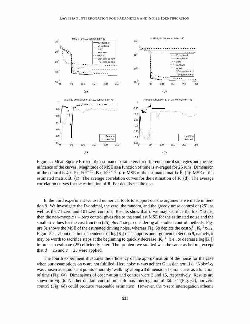
We investigated two distinct cases. In the first case we setd = 10< c = 40; the dimension ofthe observations is smaller than the dimension of the control. By contrast, in the other case we setd = 40> c= 10. Results are shown in Fig. 1 (a-b) and in Fig. 2 (a-b). We separated the MSE valuesof matricesB andF. According to the figure, zero control may give rise to early and suddendropsin the MSE values of matrixF. Not surprisingly, however, zero control is unable to estimate matrixB. For both types of matrices as well as ford < c and ford > c, the D-optimal procedure producedthe smallest MSE after about 50 online estimations, but the A-optimal method reached very similarlevels only a few iterations later. As can be expected,τ-zero control, which is identical to D-optimalcontrol in the firstτ steps fell behind D-optimal control afterτ since it changes the objective andestimates the noise and not the parameters afterwards.

For statistical significance studies, we introduced the concept of average correlation curves. Weuse Fig. 1 to explain this concept. There are 7 curves in Fig. 1 each representing the averages of25 computer runs. Error bars make the curves incomprehensible and theyhide the correlationsthat may be present between the errors. We note that the relative order of the curves is of interestfor us. However, it is possible that in each run the relative order of the curves was the same andthe overlap of the error bars—which originates from the large differences between the individualruns—hides this important piece of information. We treat this problem as follows. In each timeinstant 1≤ t ≤ 250 and for all 1≤ i < j ≤ 25 we compute the empirical (linear, or rank) correlationof the 7 curves of theith and j th experiment and take the average of the 25×24/2 = 300 values.The most significant case gives rise to 1 for each of the 300 correlations, that is, the 25 experimentsagree in the height of the curves at that time instant, or in their relative orderings for the caseof rank correlation. If there is any single experiment out of 25 that produces different heightsor orders then the average correlation becomes smaller than 1. For randomly chosen curves theaverage correlation is 0. Results can be seen in Fig. 1 (c-d) and Fig. 2 (c-d) for linear Pearson andfor Kendal rank correlations, respectively. The curves demonstratethat after about 50 steps, thecorrelations, in particular the linear correlation is almost 1. This means that thecurves behavedsimilarly in a considerable portion of the experiments. The slightly different picture shown by thelinear correlation and the rank correlation could be due to the fact that the performance of the A andD-optimal control is very similar after some time, and their ordering may change often, thus givingrise to changes in the ranks in different experiments.

10.1.2 NOISE ESTIMATIONS

In Section 7 we showed that A- and D-optimality principles result in the same cost function.

529

PÓCZOS ANDL ORINCZ

0 50 100 150 200 25010

−2

100

102

104

MSE F, d= 40, control dim= 10

D−optimalA−optimalzerorandomnoise25−zero control75−zero control

(a)

0 50 100 150 200 25010

−2

100

102

104

MSE B, d= 40, control dim= 10


(b)

0 50 100 150 200 2500.2

0.4

0.6

0.8

1Average correlation F, d= 40, control dim= 10

PearsonKendall

(c)

0 50 100 150 200 2500.5

0.6

0.7

0.8

0.9

1Average correlation B, d= 40, control dim= 10

PearsonKendall

(d)

Figure 1: Mean Square Error of the estimated parameters for different control strategies and the sig-nificance of the curves. Magnitude of MSE as a function of time is averagedfor 25 runs. Dimensionof the control is 10.F ∈ R

40×40, B ∈ R40×10. (a): MSE of the estimated matrixF. (b): MSE of the

estimated matrixB. (c): The average correlation curves for the estimation ofF. (d): The averagecorrelation curves for the estimation ofB. For details see the text.

We investigated the noise estimation capability of the interrogation in (25) for four cases. Thefirst set of experiments illustrates that the estimation of driving noiseet for largeτ values barelydiffers if we replace theτ-infomax noise interrogationwith the τ-zero interrogationscheme. Pa-rameters were the same as above and the MSE of the noise estimation was computed. Results areshown in Fig. 3: for the case ofτ = 21, cost function (25) of theτ-zero interrogation is higher thanthat of τ-infomax interrogation. However, for valuesτ = 51 and 81 the performances of the twoschemes are approximately identical. Given thatτ-zero andτ-infomax noise interrogation behavesimilarly for largeτ values, we compare theτ-zero interrogation scheme with other schemes in ournumerical experiments.

In the second experiment we investigated the problem of noise estimation on a toy problem.Parameters were set as in Section 10.1.1, and the following strategies were compared: zero control,infomax control, random control andτ-zero control for differentτ values. Results are shown inFig. 4. It is clear from the figure that neither the zero control, nor the infomax (D-optimal) controlof Table 1 work for this case. If we want to have minimal MSE in approximatelyτ steps then thebest strategy is to apply theτ-zero strategy, that is, the strategy of Table 1 up toτ steps and thento switch to zero control. Note, however, that parameter estimation requires tokeep control valuesnon-negligible forever (Table 1).

530


0 50 100 150 200 25010

−4

10−2

100

102

104

MSE F, d= 10, control dim= 40


(a)

0 50 100 150 200 25010

−2

100

102

104

MSE B, d= 10, control dim= 40


(b)

0 50 100 150 200 2500.4

0.5

0.6

0.7

0.8

0.9

1Average correlation F, d= 10, control dim= 40

PearsonKendall

(c)

0 50 100 150 200 2500.65

0.7

0.75

0.8

0.85

0.9

0.95

1Average correlation B, d= 10, control dim= 40

PearsonKendall

(d)

Figure 2: Mean Square Error of the estimated parameters for different control strategies and the sig-nificance of the curves. Magnitude of MSE as a function of time is averagedfor 25 runs. Dimensionof the control is 40.F ∈ R

10×10, B ∈ R10×40. (a): MSE of the estimated matrixF. (b): MSE of the

estimated matrixB. (c): The average correlation curves for the estimation ofF. (d): The averagecorrelation curves for the estimation ofB. For details see the text.

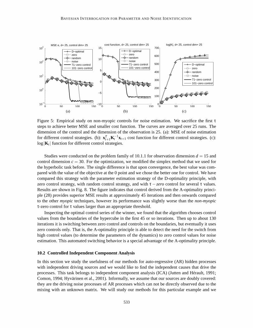
In the third experiment we used numerical tools to support our the argumentswe made in Sec-tion 9. We investigate the D-optimal, the zero, the random, and the greedy noisecontrol of (25), aswell as the 71-zero and 101-zero controls. Results show that if we may sacrifice the firstτ steps,then the non-myopicτ−zerocontrol gives rise to the smallest MSE for the estimated noise and thesmallest values for the cost function (25)after τ steps considering all studied control methods. Fig-ure 5a shows the MSE of the estimated driving noise, whereas Fig. 5b depicts the costxT

t+1K−1t xt+1.

Figure 5c is about the time dependence of log|K t | that supports our argument in Section 9, namely, itmay be worth to sacrifice steps at the beginning to quickly decrease|K−1

t | (i.e., to decrease log|K t |)in order to estimate (25) efficiently later. The problem we studied was the same as before, exceptthatd = 25 andc = 25 were applied.

The fourth experiment illustrates the efficiency of the approximation of the noise for the casewhen our assumptions onet are not fulfilled. Here noiseet was neither Gaussian nor i.i.d. ‘Noise’et

was chosen as equidistant points smoothly ‘walking’ along a 3 dimensional spiral curve as a functionof time (Fig. 6a). Dimensions of observation and control were 3 and 15, respectively. Results areshown in Fig. 6. Neither random control, nor infomax interrogation of Table1 (Fig. 6c), nor zerocontrol (Fig. 6d) could produce reasonable estimation. However, theτ-zero interrogation scheme

531

PÓCZOS ANDL ORINCZ

0 50 100 150 20010

−4

10−2

100

102

104

106

MSE e, d= 10, control dim= 15

a

b

c

d e

f

a, 21−zero controlb, 51− zero controlc, 81− zero controld, 21−infomax noisee, 51−infomax noisef, 81−infomax noise

(a)

0 50 100 150 200−15

−10

−5

0cost fun, d= 10, control dim= 15

a

b c d e f

a, 21−zero controlb, 51−zero controlc, 81−zero controld, 21−infomax noisee, 51−infomax noisef, 81−infomax noise

(b)

Figure 3: Comparingτ-infomax noise andτ-zero interrogations. The curves are averaged for 50runs. Dimension of the control is 15 and the dimension of the observation is 10. (a): MSE of theestimated noise (b): Cost function as given in (25). ‘τ-infomax noise’ (τ-zero) means that up to stepnumberτ strategy of Table 1 applies and then the control of Eq. (29) is followed.

0 50 100 150 20010

−4

10−2

100

102

104

106


a

f g h

e d

c

b

a, zero controlb, infomax controlc, random controld, 11−zero controle, 31−zero controlf, 51−zero controlg, 71−zero controlh, 91−zero control

(a)

0 50 100 150 20010

−1

100

101

102

103


a b

c

d

e f

g h

a, zero controlb, infomax controlc, random controld, 11−zero controle, 31−zero controlf, 51−zero controlg, 71−zero controlh, 91−zero control

(b)

Figure 4: Mean Square Error of the estimated noise for different control strategies. Magnitude ofMSE as a function of time is averaged for 20 runs. (a): Dimension of the control is 40.F ∈ R

40×40,B ∈ R

40×10. (b): Dimension of the control is 10.F ∈ R10×10, B ∈ R

10×40. ‘τ-zero’ means that up tostep numberτ the strategy illustrated in Table 1 was applied and then zero control followed.

produced a good approximation for large enoughτ values (Fig. 6e). Details of this illustration areshown in Fig. 6f.

10.1.3 JOINT PARAMETER AND NOISE ESTIMATIONS

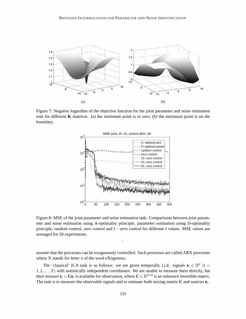
In Section 8 we showed that the objective of the D-optimality principle is constant for the joinedparameter and noise estimation task. However, A-optimality principle provides sensible cost func-tion (Eq. (28)). Unfortunately, it leads to a hyperbolic programming task. This optimization is hardin most cases. One can estimate the complexity of the objective by inspecting lower dimensionalcases. We show the negative logarithm of (28) for the 2 dimensional casefor differentK matrices(Fig. 7). In one of the cases the null vector corresponds to the minimum, whereas in the other casethe minimum is at a boundary point of the optimization domain. Also, the cost functions appear tobe flat in a large part of their domains, rendering gradient based methodsineffective.

532


0 50 100 15010

−1

100

101

102

103


D−optimalzerorandomnoise71−zero control101−zero control

(a)0 50 100 150

−10

−5

0

5

10

15cost function, d= 25, control dim= 25


(b)0 50 100 150

0

100

200

300

400

500

600

700log|K|, d= 25, control dim= 25


(c)

Figure 5: Empirical study on non-myopic controls for noise estimation. We sacrifice the firstτsteps to achieve better MSE and smaller cost function. The curves are averaged over 25 runs. Thedimension of the control and the dimension of the observation is 25. (a): MSEof noise estimationfor different control strategies. (b):xT

t+1K−1t xt+1 cost function for different control strategies. (c):

log|K t | function for different control strategies.

Studies were conducted on the problem family of 10.1.1 for observation dimensiond = 15 andcontrol dimensionc = 30. For the optimization, we modified the simplex method that we used forthe hyperbolic task before. The single difference is that upon convergence, the best value was com-pared with the value of the objective at the 0 point and we chose the better one for control. We havecompared this strategy with the parameter estimation strategy of the D-optimality principle, withzero control strategy, with random control strategy, and withτ− zerocontrol for severalτ values.Results are shown in Fig. 8. The figure indicates that control derived from the A-optimality princi-ple (28) provides superior MSE results at approximately 45 iterations and then onwards comparedto the othermyopictechniques, however its performance was slightly worse than thenon-myopicτ-zero control forτ values larger than an appropriate threshold.

Inspecting the optimal control series of the winner, we found that the algorithm chooses controlvalues from the boundaries of the hypercube in the first 45 or so iterations. Then up to about 130iterations it is switching between zero control and controls on the boundaries, but eventually it useszero controls only. That is, the A-optimality principle is able to detect the need for the switch fromhigh control values (to determine the parameters of the dynamics) to zero control values for noiseestimation. This automated switching behavior is a special advantage of the A-optimality principle.

10.2 Controlled Independent Component Analysis

In this section we study the usefulness of our methods for auto-regressive (AR) hidden processeswith independent driving sources and we would like to find the independent causes that drive theprocesses. This task belongs to independent component analysis (ICA) (Jutten and Hérault, 1991;Comon, 1994; Hyvärinen et al., 2001). Informally, we assume that our sources are doubly covered:they are the driving noise processes of AR processes which can not be directly observed due to themixing with an unknown matrix. We will study our methods for this particular exampleand we

533

PÓCZOS ANDL ORINCZ

−1

0

1

−1

0

10

0.05

0.1

0.15

0.2

original noise

(a)

−1

0

1

−1

0

10

0.05

0.1

0.15

0.2

random control

(b)

−1

0

1

−1

0

10

0.05

0.1

0.15

0.2

infomax

(c)

−50

510

x 10−3

0.04

0.06

0.08

0.10.02

0.04

0.06

0.08

zero control

(d)

−1

0

1

−1

0

10

0.05

0.1

0.15

0.2

51−zero

(e)

0 50 100 150 20010

−4

10−2

100

102

104

106


zero controlinfomax controlrandom control21−zero control51−zero control81−zero control

(f)

Figure 6: Different control strategies for non i.i.d. noise. (a): originalnoise. (b-e): estimatednoise using random, infomax, zero, 51-zero strategy, respectively. (f): MSE for different controlstrategies. In (b-e), estimations of the first 51 time steps are not shown.

534


(a) (b)

Figure 7: Negative logarithm of the objective function for the joint parameter and noise estimationtask for differentK matrices. (a) the minimum point is in zero, (b) the minimum point is on theboundary.

0 50 100 150 200 250 300 350 40010

1

102

103

104

105

MSE joint, d= 15, control dim= 30

A−optimal jointD−optimal paramrandom controlzero control21−zero control51−zero control81−zero control

Figure 8: MSE of the joint parameter and noise estimation task. Comparisons between joint param-eter and noise estimation using A-optimality principle, parameter estimation using D-optimalityprinciple, random control, zero control andτ−zerocontrol for differentτ values. MSE values areaveraged for 20 experiments.

.

assume that the processes can be exogenously controlled. Such processes are called ARX processeswhere X stands for letter x of the word eXogenous.

The ‘classical’ ICA task is as follows: we are given temporally i.i.d. signalset ∈ Rd (t =

1,2, . . . ,T) with statistically independent coordinates. We are unable to measure them directly, buttheir mixturer t = Cet is available for observation, whereC∈R

d×d is an unknown invertible matrix.The task is to measure the observable signals and to estimate both mixing matrixC and sourceset .

535

PÓCZOS ANDL ORINCZ

There are several generalizations of this problem. Hyvärinen (1998) has introduced an algorithmto solve the ICA task even if the hidden sources are AR processes, whereas Szabó and Lorincz(2008) generalized this problem for ARX processes in the following way:Processeset ∈ R

d aregiven and they are statistically independent for the different coordinates and are temporally i.i.dsignals. They generate ARX processst by means of parametersF ∈ R

d×d, B ∈ Rd×c:

st+1 =I

∑i=0

Fist−i +J

∑j=0

B jut+1− j + et+1. (30)

We assume that ARX processst can not be observed directly, but its mixture

r t = Cst (31)

is observable, where mixing matrixC ∈ Rd×d is invertible,but unknown. Our task is to estimate the

original independent processes also called sources, noises or ‘causes’, that is,et , the hidden processst and mixing matrixC from observationsr t . It is easy to see that (30) and (31) can be rewritteninto the following form

r t+1 =I

∑i=0

CFiC−1r t−i +J

∑j=0

CBut+1− j +Cet+1. (32)

Using notationsFi = CFiC−1, B j = CB j , et+1 = Cet+1, (32) takes the form of the model (1) that weare studying with functiong being the identity matrix. The only difference is that in ICA taskset isassumed to be non-Gaussian, whereas in our derivations we always used the Gaussian assumption.In our studies, however, we found that the different control methods can be useful for non-Gaussiannoise, too. Furthermore, the Central Limit Theorem says that the mixture of the variableset , thatis, Cet approximates Gaussian distributions, provided that the number of mixed variables is largeenough.

In our numerical experiments we studied the following special case:

r t+1 = Fr t +But+1 +Cet+1,

where the dimension of the noise was 3, the dimension of the control was 15. MatricesF andBwere generated the same way as before, matrixC was a randomly chosen orthogonal mixing, noisesourceset+1 were chosen from the benchmark tasks of the fastICA toolbox1 (Hyvärinen, 1999).We compared 5 different control methods (zero control, D-optimal control developed for parameterestimation, random control, A-optimal control developed for joint estimation ofparameters andnoise, as well as theτ-zero control withτ=81 that we developed for noise estimation). Comparisonsare executed by first estimating the noise (Cet+1) for timesT = 1, . . . ,1000 and then applying theJADE ICA algorithm (Cardoso, 1999) for the estimation of the noise components (et+1). Estimationwas executed in each fiftieth steps, but only for the preceding 300 elementsof the time series.

The quality of separation is evaluated by means of the Amari-error (Amari etal., 1996) asfollows. Let W ∈ R

d×d be the estimated demixing matrix, and letG := WC ∈ Rd×d. In case

1. Found athttp://www.cis.hut.fi/projects/ica/fastica/.

536


of perfect separation the matrixG is a scaled permutation matrix. The Amari-error evaluates thequality of the separation by measuring the ‘distance’ of matrixG from permutation matrices:

r (G) =1

2d(d−1)

d

∑i=1

(

∑dj=1

∣

∣Gi j∣

∣

maxj∣

∣Gi j∣

∣

−1

)

+1

2d(d−1)

d

∑j=1

(

∑di=1

∣

∣Gi j∣

∣

maxi∣

∣Gi j∣

∣

−1

)

.

The Amari-errorr(G) has the property that 0≤ r(G) ≤ 1, andr(G) = 0 if and only if G is apermutation matrix.

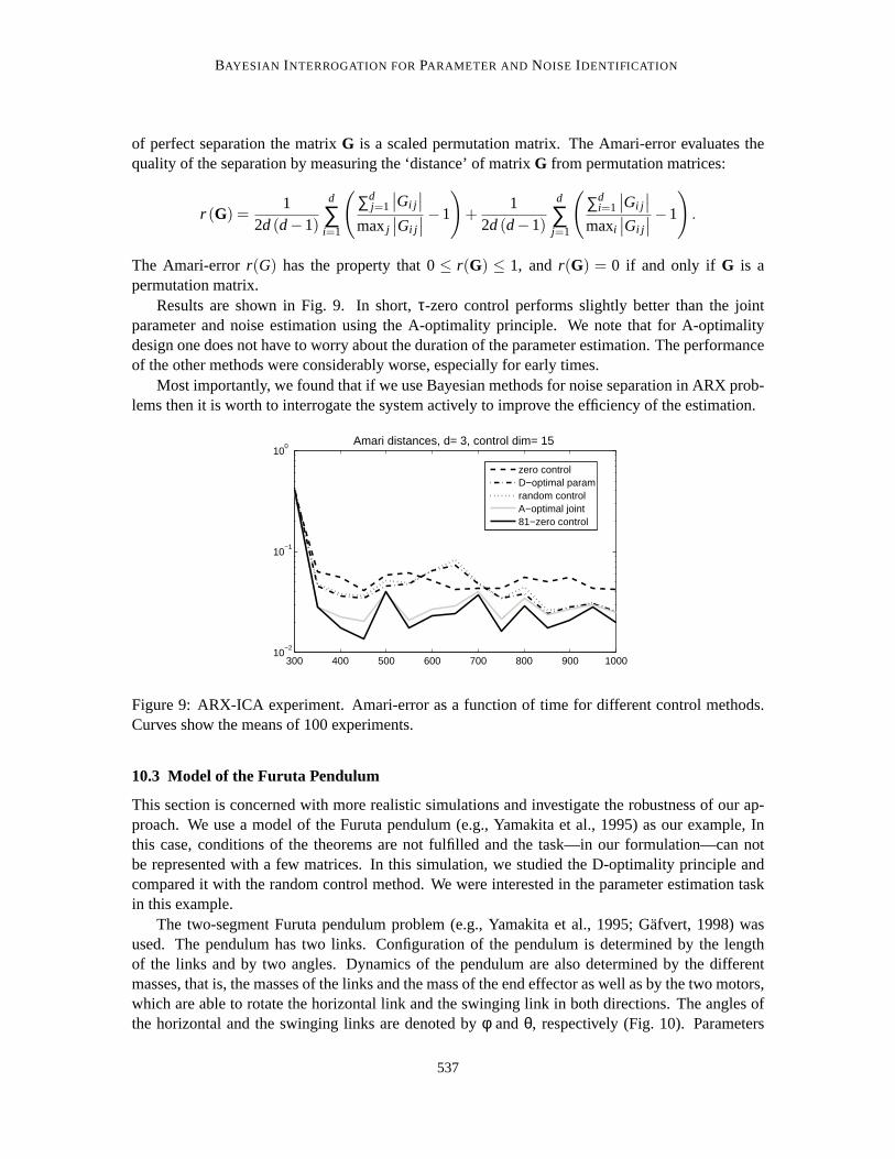
Results are shown in Fig. 9. In short,τ-zero control performs slightly better than the jointparameter and noise estimation using the A-optimality principle. We note that for A-optimalitydesign one does not have to worry about the duration of the parameter estimation. The performanceof the other methods were considerably worse, especially for early times.

Most importantly, we found that if we use Bayesian methods for noise separation in ARX prob-lems then it is worth to interrogate the system actively to improve the efficiency ofthe estimation.

300 400 500 600 700 800 900 100010

−2

10−1

100 Amari distances, d= 3, control dim= 15

zero controlD−optimal paramrandom controlA−optimal joint81−zero control

Figure 9: ARX-ICA experiment. Amari-error as a function of time for different control methods.Curves show the means of 100 experiments.

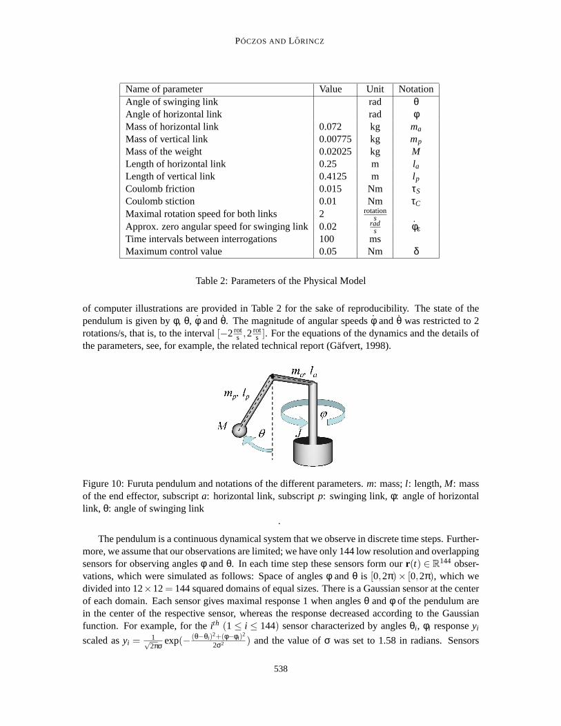
10.3 Model of the Furuta Pendulum

This section is concerned with more realistic simulations and investigate the robustness of our ap-proach. We use a model of the Furuta pendulum (e.g., Yamakita et al., 1995)as our example, Inthis case, conditions of the theorems are not fulfilled and the task—in our formulation—can notbe represented with a few matrices. In this simulation, we studied the D-optimality principle andcompared it with the random control method. We were interested in the parameter estimation taskin this example.

The two-segment Furuta pendulum problem (e.g., Yamakita et al., 1995; Gäfvert, 1998) wasused. The pendulum has two links. Configuration of the pendulum is determined by the lengthof the links and by two angles. Dynamics of the pendulum are also determined by the differentmasses, that is, the masses of the links and the mass of the end effector as well as by the two motors,which are able to rotate the horizontal link and the swinging link in both directions. The angles ofthe horizontal and the swinging links are denoted byφ andθ, respectively (Fig. 10). Parameters

537

PÓCZOS ANDL ORINCZ

Name of parameter Value Unit NotationAngle of swinging link rad θAngle of horizontal link rad φMass of horizontal link 0.072 kg ma

Mass of vertical link 0.00775 kg mp

Mass of the weight 0.02025 kg MLength of horizontal link 0.25 m laLength of vertical link 0.4125 m lp

Coulomb friction 0.015 Nm τS

Coulomb stiction 0.01 Nm τC

Maximal rotation speed for both links 2 rotations

Approx. zero angular speed for swinging link0.02 rads φε

Time intervals between interrogations 100 msMaximum control value 0.05 Nm δ

Table 2: Parameters of the Physical Model

of computer illustrations are provided in Table 2 for the sake of reproducibility. The state of thependulum is given byφ, θ, φ andθ. The magnitude of angular speedsφ andθ was restricted to 2rotations/s, that is, to the interval[−2rot

s ,2rots ]. For the equations of the dynamics and the details of

the parameters, see, for example, the related technical report (Gäfvert, 1998).

Figure 10: Furuta pendulum and notations of the different parameters.m: mass;l : length,M: massof the end effector, subscripta: horizontal link, subscriptp: swinging link,φ: angle of horizontallink, θ: angle of swinging link

.

The pendulum is a continuous dynamical system that we observe in discretetime steps. Further-more, we assume that our observations are limited; we have only 144 low resolution and overlappingsensors for observing anglesφ andθ. In each time step these sensors form ourr(t) ∈ R

144 obser-vations, which were simulated as follows: Space of anglesφ andθ is [0,2π)× [0,2π), which wedivided into 12×12= 144 squared domains of equal sizes. There is a Gaussian sensor at thecenterof each domain. Each sensor gives maximal response 1 when anglesθ andφ of the pendulum arein the center of the respective sensor, whereas the response decreased according to the Gaussianfunction. For example, for theith (1 ≤ i ≤ 144) sensor characterized by anglesθi , φi responseyi

scaled asyi = 1√2πσ exp(− (θ−θi)

2+(φ−φi)2

2σ2 ) and the value ofσ was set to 1.58 in radians. Sensors

538


were crude but noise-free; no noise was added to the sensory outputs. The inset at label 4 of Fig. 11shows the outputs of the sensors in a typical case. Sensors satisfied periodic boundary conditions; ifsensorSwas centered around zero degree in any of the directions, then it sensed both small (around0 radian) and large (around 2π radian) angles. We note that the outputs of the 144 domains arearranged for purposes of visualization; the underlying geometry of the sensors is hidden for thelearning algorithm.

We observed theser t ∈ R144 quantities and then calculated theut+1 ∈ R

2 D-optimal controlusing the algorithm of Table 1, where we approximated the pendulum with the model r t+1 = Fr t +But+1, F ∈ R

144×144, B ∈ R144×2. Components of vectorut+1 controlled the 2 actuators of the

angles separately. Maximal magnitude of each control signal was set to 0.05 Nm. Clearly we donot know the best parameters forF andB in this case, so we studied the prediction error and thenumber of visited domains instead. This procedure is detailed below.

First, we note that the angle of the swinging link and the angular speeds are important fromthe point of view of the prediction of the dynamics, whereas the angle of the horizontal link canbe neglected. Thus, for the investigation of the learning process, we used the 3D space determinedby φ,θ andθ. As was mentioned above, angular speeds were restricted to the[−2rot

s ,2rots ] domain.

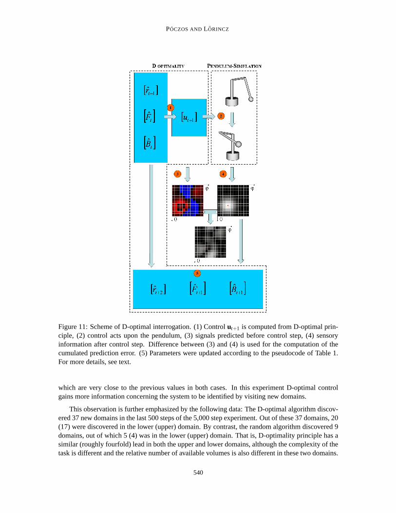
We divided each angular speed domain into 12 equal regions. We also used the 12-fold division ofangleθ. Counting the domains, we had 12×12×12= 1,728 rectangular block shaped domains.Our algorithm provides estimations forFt andBt in each instant. We can use them to compute thepredicted observation vectorr t+1 = Ftr t +Btut+1. An example is shown in inset at label 4 of Fig. 11.We investigated the‖r t+1− r t+1‖ prediction error (see Fig. 11)cumulated over these domainsasfollows. For each of the 1,728 domain, we set the initial error value at 30, avalue somewhat largerthan the maximal error we found in the computer runs. Therefore the cumulated error at start was1,728×30= 51,840.

The D-optimal algorithm does two things simultaneously: (i) it explores new domains, and (ii)it decreases the errors in the domains already visited. Thus, we measuredthe cumulated predictionerrors during learning and corrected the estimation at each step. So, if our cumulated error estima-tion at timet wase(t) = ∑1,728

k=1 ek(t) and the pendulum entered theith domain at timet +1, then wesetek(t +1) = ek(t) for all k 6= i andei(t +1) at ei(t +1) = ‖r t+1− r t+1‖. Then we computed thenew cumulated prediction error, that is,e(t +1) = ∑1,728

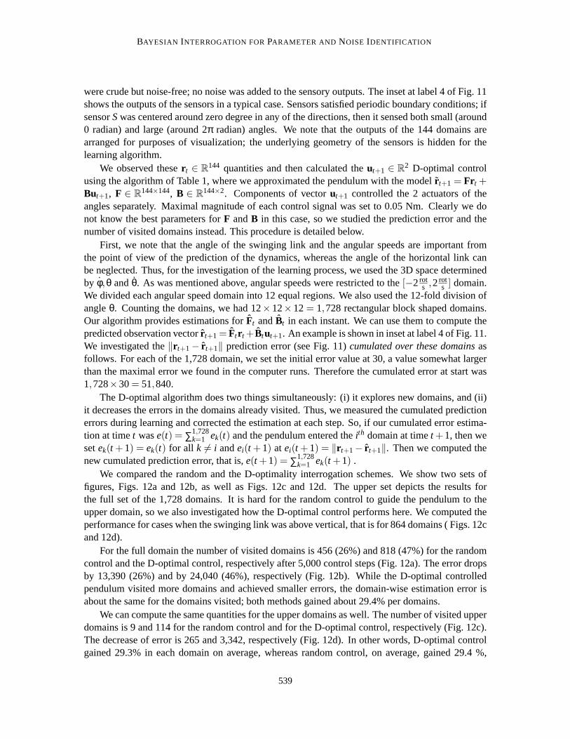
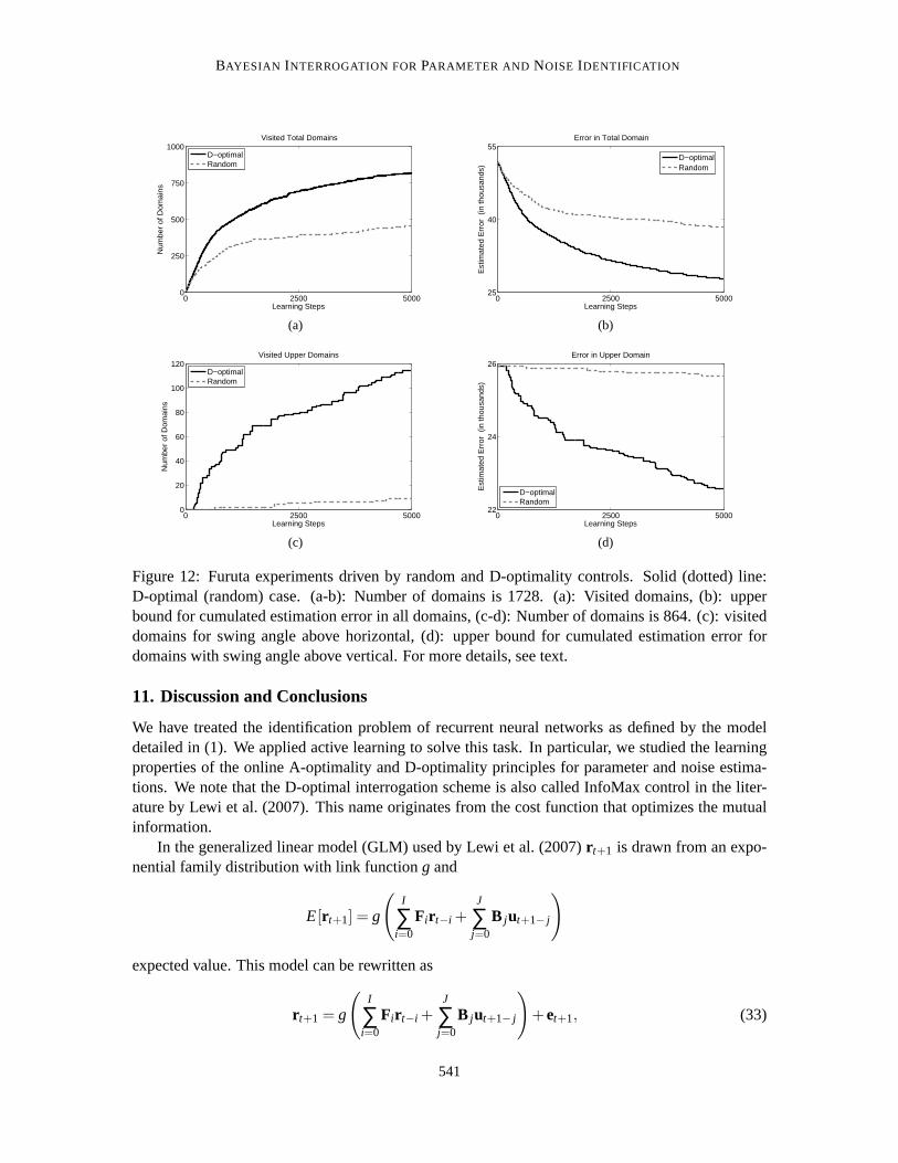
k=1 ek(t +1) .We compared the random and the D-optimality interrogation schemes. We show two sets of

figures, Figs. 12a and 12b, as well as Figs. 12c and 12d. The upper set depicts the results forthe full set of the 1,728 domains. It is hard for the random control to guidethe pendulum to theupper domain, so we also investigated how the D-optimal control performs here. We computed theperformance for cases when the swinging link was above vertical, that is for 864 domains ( Figs. 12cand 12d).

For the full domain the number of visited domains is 456 (26%) and 818 (47%) for the randomcontrol and the D-optimal control, respectively after 5,000 control steps(Fig. 12a). The error dropsby 13,390 (26%) and by 24,040 (46%), respectively (Fig. 12b). While the D-optimal controlledpendulum visited more domains and achieved smaller errors, the domain-wise estimation error isabout the same for the domains visited; both methods gained about 29.4% per domains.

We can compute the same quantities for the upper domains as well. The number ofvisited upperdomains is 9 and 114 for the random control and for the D-optimal control, respectively (Fig. 12c).The decrease of error is 265 and 3,342, respectively (Fig. 12d). Inother words, D-optimal controlgained 29.3% in each domain on average, whereas random control, on average, gained 29.4 %,

539

PÓCZOS ANDL ORINCZ

Figure 11: Scheme of D-optimal interrogation. (1) Controlut+1 is computed from D-optimal prin-ciple, (2) control acts upon the pendulum, (3) signals predicted before control step, (4) sensoryinformation after control step. Difference between (3) and (4) is used for the computation of thecumulated prediction error. (5) Parameters were updated according to thepseudocode of Table 1.For more details, see text.

which are very close to the previous values in both cases. In this experiment D-optimal controlgains more information concerning the system to be identified by visiting new domains.

This observation is further emphasized by the following data: The D-optimal algorithm discov-ered 37 new domains in the last 500 steps of the 5,000 step experiment. Out ofthese 37 domains, 20(17) were discovered in the lower (upper) domain. By contrast, the random algorithm discovered 9domains, out of which 5 (4) was in the lower (upper) domain. That is, D-optimality principle has asimilar (roughly fourfold) lead in both the upper and lower domains, although the complexity of thetask is different and the relative number of available volumes is also different in these two domains.

540


0 2500 50000

250

500

750

1000Visited Total Domains

Learning Steps

Num

ber

of D

omai

ns

D−optimalRandom

(a)

0 2500 500025

40

55Error in Total Domain

Learning Steps

Est

imat

ed E

rror

(in

thou

sand

s)

D−optimalRandom

(b)

0 2500 50000

20

40

60

80

100

120Visited Upper Domains

Learning Steps

Num

ber

of D

omai

ns

D−optimalRandom

(c)

0 2500 500022

24

26Error in Upper Domain

Learning Steps

Est

imat

ed E

rror

(in

thou

sand

s)

D−optimalRandom

(d)

Figure 12: Furuta experiments driven by random and D-optimality controls.Solid (dotted) line:D-optimal (random) case. (a-b): Number of domains is 1728. (a): Visited domains, (b): upperbound for cumulated estimation error in all domains, (c-d): Number of domainsis 864. (c): visiteddomains for swing angle above horizontal, (d): upper bound for cumulated estimation error fordomains with swing angle above vertical. For more details, see text.

11. Discussion and Conclusions

We have treated the identification problem of recurrent neural networksas defined by the modeldetailed in (1). We applied active learning to solve this task. In particular, westudied the learningproperties of the online A-optimality and D-optimality principles for parameter andnoise estima-tions. We note that the D-optimal interrogation scheme is also called InfoMax control in the liter-ature by Lewi et al. (2007). This name originates from the cost function that optimizes the mutualinformation.

In the generalized linear model (GLM) used by Lewi et al. (2007)r t+1 is drawn from an expo-nential family distribution with link functiong and

E[r t+1] = g

(

I

∑i=0

Fir t−i +J

∑j=0

B jut+1− j

)

expected value. This model can be rewritten as

r t+1 = g

(

I

∑i=0

Fir t−i +J

∑j=0

B jut+1− j

)

+et+1, (33)

541

PÓCZOS ANDL ORINCZ

where{et} is a special noise process with0 ∈ Rd mean. The elements of this error series are

independent of each other, but usually they arenot identically distributed. The authors modeledspiking neurons and assumed that the main source of the noise is this spiking,which appears at theoutput of the neurons and adds linearly to the neural activity. They investigated the case in whichthe observed quantityr t had a Poisson distribution. Unfortunately, in this model Bayesian equationsbecome intractable and the estimation of the posterior may be corrupted, because the distribution isprojected to the family of normal distributions at each instant. A serious problem with this approachis that the extent of the information loss caused by this approximation is not known. Our stochasticRNN model

r t+1 = g

(

I

∑i=0

Fir t−i +J

∑j=0

B jut+1− j +et+1

)

,

differs only slightly from the GLM model of (33), but it has considerable advantages, as we discussit later. Note that the two models assume the same form if functiong is the identity matrix and ifthe noise distribution is normal.

Our model is very similar to the well-studied non-linear Wiener (Celka et al., 2001) and Ham-merstein (Pearson and Pottmann, 2000; Abonyi et al., 2000) systems. TheHammerstein modeldevelops according to the following dynamics

r t+1 =I

∑i=0

Fir t−i +J

∑j=0

B jg(ut+1− j)+et+1.

The dynamics of the Wiener system is

r t+1 = g

(

I

∑i=0

Fig−1(r t−i)+

J

∑j=0

B jut+1− j +et+1

)

,

where we assumed that functiong is invertible.The Wiener and the Hammerstein systems have found applications in a broad range of areas,

including financial predictions to the modeling of chemical processes. These models are specialcases of non-linear ARX (NARX) models (Billings and Leontaritis, 1981). They are popular, be-cause they belong to the simplest non-linear systems. Using block representation, they are simplythe compositions of a static non-linear function and a dynamic ARX system. As a result, their prop-erties can be investigated in a relatively simple manner and they are still able to model a large classof sophisticated non-linear phenomena.

Interesting comparisons between Wiener and Hammerstein systems can be found in Bai (2002),Aguirre et al. (2005), and Haber and Unbehauen (1990). We note that our Bayesian interrogationmethods can be easily transferred to both the Wiener and to the Hammerstein systems.

Bayesian designs of different kinds were derived for the linear regression problem by Verdinelli(2000):

y = Xθ +e, (34)

P(e) =Ne(0,σ2I).

This problem is similar to ours ((3)-(5)), but while the goal of Verdinelli (2000) was to find anoptimal design for the explanatory variablesθ, we were concerned with the parameter (X in 34) and

542


Parameter Noise Joint

D-optimal maxut+1∈U

xTt+1K−1

t xt+1 minut+1∈U

xTt+1K−1

t xt+1 N/A

A-optimal maxut+1∈U

xTt+1K−1

t K−1t xt+1

1+xTt+1K−1

t xt+1min

ut+1∈UxT

t+1K−1t xt+1 max

ut+1∈U1+xT

t+1K−1t K−1

t xt+1

1+xTt+1K−1

t xt+1

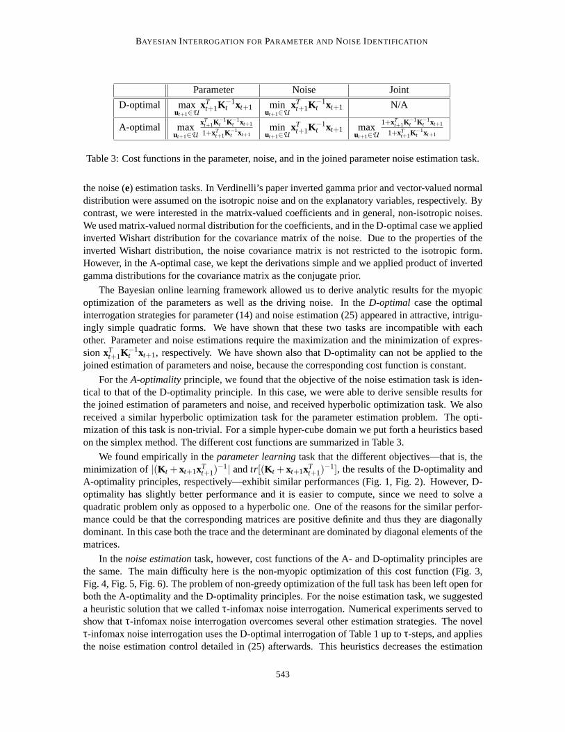
Table 3: Cost functions in the parameter, noise, and in the joined parameter noise estimation task.

the noise (e) estimation tasks. In Verdinelli’s paper inverted gamma prior and vector-valued normaldistribution were assumed on the isotropic noise and on the explanatory variables, respectively. Bycontrast, we were interested in the matrix-valued coefficients and in general, non-isotropic noises.We used matrix-valued normal distribution for the coefficients, and in the D-optimal case we appliedinverted Wishart distribution for the covariance matrix of the noise. Due to theproperties of theinverted Wishart distribution, the noise covariance matrix is not restricted to the isotropic form.However, in the A-optimal case, we kept the derivations simple and we applied product of invertedgamma distributions for the covariance matrix as the conjugate prior.

The Bayesian online learning framework allowed us to derive analytic results for the myopicoptimization of the parameters as well as the driving noise. In theD-optimal case the optimalinterrogation strategies for parameter (14) and noise estimation (25) appeared in attractive, intrigu-ingly simple quadratic forms. We have shown that these two tasks are incompatible with eachother. Parameter and noise estimations require the maximization and the minimization ofexpres-sion xT

t+1K−1t xt+1, respectively. We have shown also that D-optimality can not be applied to the

joined estimation of parameters and noise, because the corresponding cost function is constant.

For theA-optimalityprinciple, we found that the objective of the noise estimation task is iden-tical to that of the D-optimality principle. In this case, we were able to derive sensible results forthe joined estimation of parameters and noise, and received hyperbolic optimization task. We alsoreceived a similar hyperbolic optimization task for the parameter estimation problem. The opti-mization of this task is non-trivial. For a simple hyper-cube domain we put fortha heuristics basedon the simplex method. The different cost functions are summarized in Table 3.

We found empirically in theparameter learningtask that the different objectives—that is, theminimization of|(K t +xt+1xT

t+1)−1| andtr[(K t +xt+1xT

t+1)−1], the results of the D-optimality and

A-optimality principles, respectively—exhibit similar performances (Fig. 1, Fig. 2). However, D-optimality has slightly better performance and it is easier to compute, since we need to solve aquadratic problem only as opposed to a hyperbolic one. One of the reasons for the similar perfor-mance could be that the corresponding matrices are positive definite and thus they are diagonallydominant. In this case both the trace and the determinant are dominated by diagonal elements of thematrices.

In thenoise estimationtask, however, cost functions of the A- and D-optimality principles arethe same. The main difficulty here is the non-myopic optimization of this cost function (Fig. 3,Fig. 4, Fig. 5, Fig. 6). The problem of non-greedy optimization of the full task has been left open forboth the A-optimality and the D-optimality principles. For the noise estimation task, we suggesteda heuristic solution that we calledτ-infomax noise interrogation. Numerical experiments served toshow thatτ-infomax noise interrogation overcomes several other estimation strategies.The novelτ-infomax noise interrogation uses the D-optimal interrogation of Table 1 up toτ-steps, and appliesthe noise estimation control detailed in (25) afterwards. This heuristics decreases the estimation

543

PÓCZOS ANDL ORINCZ

error of the coefficients of matricesF andB up to timeτ and thus—upon turning off the explorativeD-optimization—tries to minimize the estimation error of the value of the noise at timeτ +1. Weintroduced theτ-zero interrogation scheme and showed that it is a good approximation of theτ-infomax noise scheme for largeτ values.

In thejoint noise parameter estimationtask the D-optimal principle leads to a meaningless con-stant valued cost function. The A-optimal objective is a hyperbolic programming task, which isdifficult to optimize. Still, its myopic optimization gave us better results than the myopic D-optimalobjective derived for parameter estimation only. Interestingly, myopic A-optimal interrogations be-haved similarly to the non-myopicτ-zero control (D-optimal parameter estimation up toτ steps,then zero control) with emergent automaticτ selection. However, these myopic results were some-what worse than the non-myopic results from theτ-zero interrogation, whenτ was larger than anappropriate threshold (Fig. 8).

In the field of active-learning, non myopic optimization is one of the most challenging tasks somost studies are concerned with greedy optimization only. Still, greedy optimization has producedvaluable results in many cases. A few studies are concerned with non-greedy optimization of activelearning, but only for certain special cases (Krause and Guestrin, 2007; Rangarajan et al., 2007).This field is in a rather early stage at the moment.

We illustrated the working of the algorithm on artificial databases both for the parameter estima-tion problem and for the noise estimation task. In the first set of experiments the database satisfiedthe conditions of our theorems. We studied the robustness of the algorithm and studied the noise es-timation problem for a situation in which the conditions of our theorems were not satisfied, namelywhen the noise was neither Gaussian nor i.i.d. In particular, we studied the ARX problem family,when the hidden driving sources are non-Gaussian and statistically independent i.i.d. processes. Wefound that active control can speed-up the learning process. Function g was the identity function inthese experiments.

We have also started to characterize the algorithm for a problem closer to reality. We chose thetwo-link Furuta pendulum task in these studies. We used a crude discretization for the pendulum,where the underlying dynamics and the low-dimensional nature of the problem are both hidden.Clearly we could express neither the ideal parameters for this case nor thenoise that arose as aresult of the disctretization. Thus we have studied the volume explored by theD-optimality methodas well as the magnitude of the prediction errors.

The pendulum problem demonstrated that D-optimality maximizes mutual information by ex-ploring new areas without significant compromise in the precision of estimation inthe visited do-mains. The discovery rate is in favor of the D-optimality algorithm, which has a significant leadin both the frequently visited and the rarely visited domains, although the task is different and therelative number of available volumes is also different in these domains.

Our method treats the identification problem of non-linear ARX systems. We planto generalizethe method to NARMAX systems in the future. Such systems have several application fields, includ-ing financial modeling and the modeling of gas turbines (Chiras et al., 2001).One may try to applythese principles in a broad variety of fields, including selective laser chemistry Rabitz (2003), orthe analysis of brain signals ‘controlled’ by visual inputs, for example, in brain-computer interfacesVaughan et al. (2003).

Finally, it seems desirable to determine the conditions under which the algorithms derived fromthe optimality principles are both consistent and efficient. The tractable form of our approximation-free results is promising in this respect.

544


Acknowledgments

We thank the anonymous reviewers for their valuable comments. We are grateful to György Flóreaand László A. Jeni for running the pendulum simulations, and to Gábor Szirtes for his valuable com-ments. This research has been supported by the EC NEST ‘Perceptual Consciousness: Explicationand Testing’ grant under contract 043261. Opinions and errors in thismanuscript are the author’sresponsibility, they do not necessarily reflect the opinions of the EC or other project members.

Appendix A.

In this section we provide the technical details of our derivations.

A.1 Proof of Lemma 4.1

It is easy to show that the following equations hold:

Ny(Ax,V)NA(M ,V,K) = NA(M+,V,xxT +K)Ny(Mx ,V,γ),NA(M ,V,K)IW V(Q,n) = IW V (Q+H,n+m)TA(Q,n,M ,K),

whereM+ = (MK +yxT)(xxT +K)−1, γ = 1−xT(xxT +K)−1x, H = (A−M)K(A−M)T for thesake of brevity. Then we have

Ny(Mx ,V,γ)IW V(Q,n) = IW V(Q+(y−Mx)γ(y−Mx)T ,n+1)Ty (Q,n,Mx ,γ) ,

and the statement of the lemma follows.


Let vec(A) denote a vector ofdm dimensions where the(d(i − 1) + 1)th, . . . ,(id)th (1 ≤ i ≤ m)elements of this vector are equal to the elements of theith column of matrixA ∈ R

d×m in the ap-propriate order. Let⊗ denote the Kronecker-product. It is known that forP(A) = NA(M ,V,K),P(vec(A)) =Nvec(A)(vec(M),V⊗K−1) holds (Minka, 2000). Using the well-known formula forthe entropy of a multivariate and normally distributed variable (Cover and Thomas, 1991) and ap-plying the relation|V⊗K−1| = |V|m/|K |d, we have that

H(A;V) =12

ln |V⊗K−1|+ dm2

ln(2πe) =m2

ln |V|− d2

ln |K |+ dm2

ln(2πe).

By exploiting certain properties of the Wishart distribution, we can compute theentropy of distri-butionIW V(Q,n). The density of the Wishart distribution is defined by

WV(Q,n) =1

Zn,d|V|(n−d−1)/2

∣

∣

∣

∣

Q−1

2

∣

∣

∣

∣

n/2

exp

(

−12

tr(VQ−1)

)

.

Let Ψ denote the digamma function, and letf1,3(d,n) = −∑di=1 Ψ(n+1−i

2 ))−d ln2. ReplacingV−1

with S, we have for the Jacobian that|dVdS |= |dS−1

dS |= |S|−(d+1) (Gupta and Nagar, 1999). To proceed

545

PÓCZOS ANDL ORINCZ

we use thatEWS(Q,n)S = nQ, andEWS(Q,n) ln |S| = ln |Q| − f1,3(d,n), (Beal, 2003) and substitutethem intoEIW V(Q,n) ln |V|, andEIW V(Q,n)tr(QV−1):

EIW V(Q,n) ln |V| =Z

1Zn,d

1

|V|(d+1)/2

∣

∣

∣

∣

V−1Q2

∣

∣

∣

∣

n/2

exp

(

−12

tr(V−1Q)

)

ln |V|dV,

= −Z

1Zn,d

|S|(d+1)/2

∣

∣

∣

∣

SQ2

∣

∣

∣

∣

n/2

exp

(

−12

tr(SQ)

)

ln |S||S|−d−1dS,

= −Z

1Zn,d

|S|(n−d−1)/2

∣

∣

∣

∣

Q2

∣

∣

∣

∣

n/2

exp

(

−12

tr(SQ)

)

ln |S|dS,

= −EWS(Q−1,n) ln |S|,= ln |Q|+ f1,3(d,n). (35)

One can also show that

EIW V(Q,n)tr(QV−1) =Z

1Zn,d

1

|V|(d+1)/2

∣

∣

∣

∣

V−1Q2

∣

∣

∣

∣

n/2

exp

(

−12

tr(V−1Q)

)

tr(QV−1)dV,

=Z

1Zn,d

|S|(d+1)/2

∣

∣

∣

∣

SQ2

∣

∣

∣

∣

n/2

exp

(

−12

tr(SQ)

)

tr(QS)|S|−d−1dS,

=Z

1Zn,d

|S|(n−d−1)/2

∣

∣

∣

∣

Q2

∣

∣

∣

∣

n/2

exp

(

−12

tr(SQ)

)

tr(QS)dS,

= EWS(Q−1,n)tr(QS),

= tr(QQ−1n) = nd. (36)

We calculate the entropy of stochastic variableV with distribution IW V(Q,n). It follows fromEq. (35) and Eq. (36) that

H(V) = −EIW V(Q,n)

[

− ln(Zn,d)+n2

ln

∣

∣

∣

∣

Q2

∣

∣

∣

∣

− n+d+12

ln |V|− 12

tr(V−1Q)

]

,

= ln(Zn,d)−n2

ln

∣

∣

∣

∣

Q2

∣

∣

∣

∣

+n+d+1

2

[

ln |Q|−d

∑i=1

Ψ(n+1− i

2))−d ln2

]

+nd2

,

=d+1

2ln |Q|+ f1,4(d,n),

where f1,4(d,n) depends only ond andn.Given the results above, we complete the computation of entropyH(A,V) as follows:

H (A,V) = H(A|V)+H(V) = H(V)+Z

dVIW V(Q,n)H(A;V),

=Z

dVIW V(Q,n)

(

m2

ln |V|− d2

ln |K |+ dm2

ln(2πe)

)

+H(V),

= −d2

ln |K |+ dm2

ln(2πe)+m2

[ln |Q|+ f1,3(d,n)]+d+1

2ln |Q|+ f1,4(d,n),

= −d2

ln |K |+(m+d+1

2) ln |Q|+ f1,1(d,n).

This is exactly what was claimed in Lemma 4.2.

546



The proof is analogous to the D-optimality case. We need the following lemma:

Lemma A.1 Let V diagonal positive definite matrix. LetX(i,:) denote the ith row of matrixX. Letηi = (A(i,:)−M (i,:))K(A(i,:)−M (i,:))

T , ∀i = 1, . . . ,d. η ∈ Rd. Then the following statement holds:

NA(M ,V,K)PIGV(α,β) = PIGV(α+m/2,β +η/2)d

∏i=1

TA(i,:)(βi ,2αi ,M (i,:),

K2

).

Proof:

NA(M ,V,K)PIGV(α,β) =

=|K |d/2

|2πV|m/2exp(−1

2tr(V−1(A−M)K(A−M)T))

d

∏i=1

βαii

Γ(αi)v−αi−1

i exp(−βi

vi),

=|K |d/2

∏di=1(2π)m/2vm/2

i

exp(−12

d

∑i=1

1vi

ηi)d

∏i=1

βαii

Γ(αi)v−αi−1

i exp(−βi

vi),

=|K |d/2

∏di=1(2π)m/2

d

∏i=1

βαii

Γ(αi)v−αi−m/2−1

i exp(−βi +ηi/2vi

),

=|K |d/2

∏di=1(2π)m/2

d

∏i=1

βαii

Γ(αi)

(βi +ηi/2)αi+m/2

(βi +ηi/2)αi+m/2

Γ(αi +m/2)

Γ(αi +m/2),v−αi−m/2−1


),

=|K |d/2

∏di=1(2π)m/2

d

∏i=1

βαii Γ(αi +m/2)/Γ(αi)

(βi +ηi/2)αi+m/2

d

∏i=1

(βi +ηi/2)αi+m/2

Γ(αi +m/2)v−αi−m/2−1


),

=d

∏i=1

|K |1/2

(2π)m/2

Γ(αi +m/2)

Γ(αi)

βαii

(βi +ηi/2)αi+m/2PIGv(α+m/2,β +η/2),

=d

∏i=1

|K2 |1/2

πm/2

Γ(αi +m/2)βαii

Γ(αi)(βi +(A(i,:)−M (i,:))K2 (A(i,:)−M (i,:))T)αi+m/2

PIGv(α+m/2,β +η/2),

= PIGv(α+m/2,β +η/2)d

∏i=1

TA(i,:)(βi ,2αi ,M (i,:),

K2

).

Lemma A.2

Ny(Ax,V)NA(M ,V,K)PIGV(α,β) =NA((MK +yxT)(xxT +K)−1,V,xxT +K)×

×PIGV

(

α+1/2,β +diag(y−Mx)(1−xT(xxT +K)−1x)

2(y−Mx)T

)

×

×d

∏i=1

Tyi

(

βi ,2αi ,(Mx)i ,1−xT(xxT +K)−1x

2

)

.

Proof:

Ny(Ax,V)NA(M ,V,K)PIGV(α,β) =NA((MK +yxT)(xxT +K)−1,V,xxT +K)×Ny((Mx ,V,1−xT(xxT +K)−1x)×

PIGV(α,β).

547

PÓCZOS ANDL ORINCZ


We can see thatVarV [E[A|V,{x}t+11 ,{y}t+1

1 ]] = VarV [M t+1] = 0, and

EV [trVar(A|V,{x}t+11 ,{y}t+1

1 )] = EV [tr(V⊗ (K t +xt+1xTt+1)

−1)|{x}t+11 ,{y}t+1

1 ],

= tr(E[V|{x}t+11 ,{y}t+1

1 ])tr[(K t +xt+1xTt+1)

−1],

= tr[(K t +xt+1xTt+1)

−1]d

∑i=1

(βt+1)i

(αt+1)i −1,

where we used thatP(V|{x}t+11 ,{y}t+1

1 ) = PIGV(αt+1,βt+1).The law of total variance says thatVar[A] = Var[E[A|V]]+E[Var[A|V]], hence

trVar[A|{x}t+11 ,{y}t+1

1 ] = tr(K t +xt+1xTt+1)

−1d

∑i=1

(βt+1)i

(αt+1)i −1.


To compute (24) we need the following lemma (Minka, 2000):

Lemma A.3 If P(A) =NA(M ,V,K), then P(Ax) =NAx

(

Mx ,V,(

xTK−1x)−1)

.

Applying this lemma and using (11) we have that

P(Axt+1|V,{x}t+11 ,{y}t+1

1 ) =NAxt+1

(

M t+1xt+1,V,(

xTt+1K−1

t+1xt+1)−1)

. (37)

We introduce the notations

Kt+1 =(

xTt+1K−1

t+1xt+1)−1 ∈ R, (38)

λt+1 = 1+(Axt+1−M t+1xt+1)T(Kt+1Q−1

t+1)(Axt+1−M t+1xt+1) ∈ R.

Exploit the fact that

NA(M ,V,K)IW V(Q,n) = IW V (Q+H,n+m)TA(Q,n,M ,K),

and use (12) for the posterior distribution (37) and get

P(Axt+1|{x}t+11 ,{y}t+1

1 ) = TAxt+1

(

Qt+1,nt+1,M t+1xt+1, Kt+1)

,

= π−d/2|K−1t+1Qt+1|−1/2 Γ(nt+1+1

2 )

Γ(nt+1+1−d2 )

λnt+1+1

2t+1 .

The Shannon-entropy of this distribution according to Zografos and Nadarajah (2005) can be writtenas:

H(Axt+1;{x}t+11 ,{y}t+1

1 ) = f3,1(d,nt+1)+d2

log|K−1t+1|+ log|Qt+1|,

where

f3,1(d,nt+1) = − logΓ(nt+1+1

2 )

πd/2Γ(nt+1+1−d2 )

+nt+1 +1

2

(

Ψ(

nt+1 +12

)

−Ψ(

nt+1 +1−d2

))

.

548


Using the notations introduced in (10) and in (38), the above expressionscan be transcribed asfollows:

H(Axt+1;{x}t+11 ,{y}t+1

1 ) = f3,1(d,nt+1)−d2

log|Kt+1|+ log|Qt+1|,

= f3,1(d,nt+1)+d2

log|xTt+1(K t +xt+1xT

t+1)−1xt+1|+ log|Qt+1|,

= f3,1(d,nt+1)+d2


t+1)−1xt+1|+

+ log|Qt +(yt+1−M txt+1)γt+1(yt+1−M txt+1)T |.

Now, we are in a position to calculate (24) by applying Lemma 4.4 as before. Weget that

Z


1)H(et+1;{x}t+11 ,{y}t+1

1 ) =

= f3,2(Qt ,nt+1)+d2


t+1)−1xt+1|,

where f3,2(Qt ,nt+1) depends only onQt , andnt+1. We can proceed as follows

argmaxut+1

I(et+1,yt+1;{x}t+11 ,{y}t

1) = argminut+1


t+1)−1xt+1|,

= argminut+1

log

∣

∣

∣

∣

∣

xTt+1

(

K−1t − K−1

t xt+1xTt+1K−1

t

1+xTt+1K−1

t xt+1

)

xt+1

∣

∣

∣

∣

∣

,

= argminut+1

log

∣

∣

∣

∣

∣

xTt+1K−1

t xt+1

1+xTt+1K−1

t xt+1

∣

∣

∣

∣

∣

,

= argminut+1

xTt+1K−1

t xt+1.

This is exactly what we were to prove.


One needs to compute the value of the integral

Z


1)E[trV|xt+11 ,yt+1

1 ]tr(

(

K t +xt+1xTt+1

)−1+xT

t+1K−1t+1xt+1

)

.

However,

Z


1)E[trV|xt+11 ,yt+1

1 ]

=Z

dyt+1

d

∏i=1

T(yt+1)i

(


2

) d

∑i=1

(βt+1)i

(αt+1)i −1,

549

PÓCZOS ANDL ORINCZ

and depends only on the values ofαt+1 andβt as a result of (19) and Lemma 4.4, and is independentof the value ofxt+1. Thus, we arrive at the minimization of the following expression:

tr

[(

K−1t − K−1

t xt+1xTt+1K−1

t

1+xTt+1K−1

t xt+1

)

+xTt+1

(

K−1t − K−1

t xt+1xTt+1K−1

t

1+xTt+1K−1

t xt+1

)

xt+1

]

=

[

tr(K−1t )− tr

K−1t xt+1xT

t+1K−1t

1+xTt+1K−1

t xt+1+

xTt+1K−1

t xt+1

1+xTt+1K−1

t xt+1

]

,

=

[

tr(K−1t )− xT

t+1K−1t K−1

t xt+1

1+xTt+1K−1

t xt+1+

xTt+1K−1

t xt+1

1+xTt+1K−1

t xt+1

]

,

=1+xT

t+1K−1t K−1

t xt+1

1+xTt+1K−1

t xt+1.

References

J. Abonyi, R. Babuska, A. Ayala-Botto, A. Szeifert, and L. Nagy. Identification and control ofnonlienar systems using Hammerstein-models.Ind. Eng. Chem. Res, 39:4302–4314, 2000.

L. A. Aguirre, M. C. S. Coelho, and M. V. Correa. On the interpretation and practice of dynamicaldifferences between Hammerstein and Wiener models. InIEE. Proc. of Control Theory Applica-tion, volume 152, pages 349–354, 2005.

S. Amari, A. Cichocki, and H. H. Yang. A new learning algorithm for blind signal separation. InAdvances in Neural Information Processing Systems, volume 8, pages 757–763, Cambridge, MA,1996. MIT Press.

B. Anderson and A. Moore. Active learning for hidden Markov models:objective functions andalgorithms. InICML ’05: Proceedings of the 22nd international conference on Machine learning,pages 9–16, New York, NY, USA, 2005. ACM.

F. R. Bach. Active learning for misspecified generalized linear models. InB. Schölkopf, J. Platt,and T. Hoffman, editors,Advances in Neural Information Processing Systems, volume 19, pages65–72, Cambridge, MA, 2007. MIT Press.

E. W. Bai. A blind approach to the Hammerstein-Wiener model identification.Automatica, 38:967–979, 2002.

M. J. Beal.Variational Algorithms for Approximate Bayesian Inference. PhD thesis, Gatsby Com-putational Neuroscience Unit, University College London, 2003.

J. M. Bernardo. Expected information as expected utility.The Annals of Statistics, 7(3):686–690,1979.

S. A. Billings and I. J. Leontaritis. Identifiaction of nonlinear systems using parametric estimationtechniques. InIEE. Proc. of Control and its Applications, pages 183–187, 1981.

X. Boyen and D. Koller. Tractable inference for complex stochastic processes. InFourteenthConference on Uncertainty in Artificial Intelligence, pages 33–42, 1998.

550


J. F. Cardoso. High-order contrasts for independent component analysis. Neural Computation, 11(1):157–192, 1999.

R. Castro, J. Jaupt, and R. Nowak. Compressed sensing vs. active learning. In ICASSP 2006, IEEEInternational Conference on Acoustics, Speech and Signal Processing, volume 3, 2006a.

R. Castro, R. Willett, and R. Nowak. Faster rates in regression via active learning. In Y. Weiss,B. Schölkopf, and J. Platt, editors,Advances in Neural Information Processing Systems 18, pages179–186. MIT Press, Cambridge, MA, 2006b.

P. Celka, N. J. Bershad, and J. Vesin. Stochastic gradient identificationof polynomial Wienersystems: Analysis and application.IEEE Trans. Signal Process., 49(2):301–313, 2001.

K. Chaloner. Optimal bayesian experimental design for linear models.The Annals of Statistics, 12(1):283–300, 1984.

K. Chaloner and I. Verdinelli. Bayesian experimental design: A review.Statist. Sci., 10:273–304,1995.

N. Chiras, C. Evans, and D. Rees. Nonlinear gas turibne modeling using NARMAX structures.IEEE Trans. Instrum. Meas., 50(4):893–898, 2001.

D. A. Cohn. Neural network exploration using optimal experiment design.In Advances in NeuralInformation Processing Systems, volume 6, pages 679–686, 1994.

D. A. Cohn, Z. Ghahramani, and M. I. Jordan. Active learning with statistical models.Journal ofArtificial Intelligence Research, 4:129–145, 1996.

T. F. Coleman and Y. Li. A reflective newton method for minimizing a quadratic function subject tobounds on some of the variables.SIAM Journal on Optimization, 6(4):1040–1058, 1996.

P. Comon. Independent component analysis, a new concept?Signal Processing, 36(3):287–314,1994.

T. M. Cover and J. A. Thomas.Elements of Information Theory. Wiley-Interscience, 1991.

R. C. deCharms, D. T. Blake, and M. M. Merzenich. Optimizing sound features for cortical neurons.Science, 280:1439–1444, 1998.

G. Duncan and M. H. DeGroot. A mean squared error approach to optimaldesign theory. InProceedings of the 1976 Conference on Information: Sciences and Systems, pages 217–221. TheJohns Hopkins University, 1976.

V. V. Fedorov.Theory of Optimal Experiments. Academic Press, New York, 1972.

P. Földiák. Stimulus optimization in primary visual cortex.Neurocomputing, 38–40:1217–1222,2001.

Y. Freund, H. S. Seung, E. Shamir, and N. Tishby. Selective sampling using the query by committeealgorithm.Machine Learning, 28:133–168, 1997.

551

PÓCZOS ANDL ORINCZ

K. Fukumizu. Active learning in multilayer perceptrons. In David S. Touretzky, Michael C. Mozer,and Michael E. Hasselmo, editors,Advances in Neural Information Processing Systems, vol-ume 8, pages 295–301. The MIT Press, 1996.

K. Fukumizu. Statistical active learning in multilayer perceptrons.IEEE Transactions on NeuralNetworks, 11(1):17–26, 2000.

M. Gäfvert. Modelling the Furuta pendulum. Technical report ISRN LUTFD2/TFRT–7574–SE,Department of Automatic Control, Lund University, Sweden, April 1998.

A. Gelman, J. B. Carlin, H. S. Stern, and D. B. Rubin.Bayesian Data Analysis. CRC Press, 2nderdition, 2003.

Z. Ghahramani. Online variational Bayesian learning, 2000. Slides from talk presented at NIPS2000 workshop on Online Learning.

G. H. Golub and C. F. Van Loan.Matrix Computations. Johns Hopkins, Baltimore, MD, 3rd ed.edition, 1996.

A. K. Gupta and D. K. Nagar.Matrix Variate Distributions, volume 104 ofMonographs and Surveysin Pure and Applied Mathematics. Chapman and Hall/CRC, 1999.

R. Haber and H. Unbehauen. Structure identification of nonlinear dynamicsystems– a survey oninput/output approaches.Automatica, 26(4):651–677, 1990.

D. A. Harville. Matrix Algebra From a Statistician’s Perspective. Springer-Verlag, 1997.

A. Honkela and H. Valpola. On-line variational Bayesian learning. In4th International Symposiumon Independent Component Analysis and Blind Signal Separation, pages 803–808, 2003.

A. Hyvärinen. Fast and robust fixed-point algorithms for independent component analysis.IEEETrans. on Neural Networks, (10):626–634, 1999.

A. Hyvärinen, J. Karhunen, and E. Oja.Independent Component Analysis. John Wiley, New York,2001. URLhttp://www.cis.hut.fi/projects/ica/book/.

A. Hyvärinen. Independent component analysis for time-dependent stochastic processes. InProc.of ICANN’98, International Conference on Artificial Neural Networks, Skövde, Sweden, pages541–546, 1998.

H. Jaeger. Short term memory in echo state networks. GMD Report, 152, Fraunhofer AIS, 2001.http://publica.fraunhofer.de/starweb/pub08/en/index.htm.

C. Jutten and J. Hérault. Blind separation of sources: An adaptive algorithm based on neuromimeticarchitecture.Signal Processing, 24:1–10, 1991.

J. Kiefer. Optimum experimental designs.Journal of the Royal Statistical Society, Series B, 21:272–304, 1959.

S. Kotz and S. Nadarajah.Multivariate T-Distributions and Their Applications. Cambridge Univer-sity Press, 2004.

552


A. Krause and C. Guestrin. Nonmyopic active learning of gaussian processes: an exploration-exploitation approach. InICML ’07: Proceedings of the 24th international conference on Ma-chine learning, pages 449–456, New York, NY, USA, 2007. ACM.

J. Lewi, R. Butera, and L. Paninski. Real-time adaptive information-theoretic optimization of neu-rophysiology experiments. InAdvances in Neural Information Processing Systems, volume 19,2007.

D. D. Lewis and J. Catlett. Heterogeneous uncertainty sampling for supervised learning. InWilliam W. Cohen and Haym Hirsh, editors,Proceedings of ICML-94, 11th International Con-ference on Machine Learning, pages 148–156, New Brunswick, US, 1994. Morgan KaufmannPublishers, San Francisco, US.

D. D. Lewis and W. A. Gale. A sequential algorithm for training text classifiers. In Proceedingsof SIGIR-94, 17th ACM International Conference on Research and Development in InformationRetrieval, pages 3–12, Dublin, IE, 1994. Springer Verlag, Heidelberg, DE.

D. V. Lindley. Bayesian Statistics: A Review. SIAM, 1971.

W. Maass, T. Natschläger, and H. Markram. Real-time computing without stablestates: A newframework for neural computation based on perturbations.Neural Computation, 14:2531–2560,2002.

C. K. Machens, T. Gollisch, O. Kolesnikova, and A. V. M. Herz. Testingthe efficiency of sensorycoding with optimal stimulus ensembles.Neuron, 47:447–456, 2005.

D. J. C. MacKay. Information-based objective functions for active data selection.Neural Compu-tation, 4(4):590–604, 1992.

T. Minka. Bayesian linear regression, 2000. MIT Media Lab note.

T. Minka. A Family of Algorithms for Approximate Bayesian Inference. PhD thesis, MIT MediaLab, MIT, 2001.

M. Opper and O. Winther. A Bayesian approach to online learning. InOnline Learning in NeuralNetworks. Cambridge University Press, 1999.

R. K. Pearson and M. Pottmann. Gray-box identification of block-orientednonlnear models.Journalof Process Control, 10:301–315, 2000.

F. Pukelsheim.Optimal Design of Experiments. John Wiley & Sons, 1993.

H. Rabitz. Shaped laser pulses as reagents.Science, 299:525–527, 2003.

H. Raiffa and R. Schlaifer.Applied Statistical Decision Theory. Boston, MIT Press, 1961.

R. Rangarajan, R. Raich, and A. O. Hero. Optimal sequential energy allocation for inverse problems.IEEE Journal of Selected Topics in Signal Processing, 1:67–78, 2007.

N. Roy and A. McCallum. Toward optimal active learning through sampling estimation of errorreduction. InProc. 18th International Conference on Machine Learning, pages 441–448. MorganKaufmann, San Francisco, CA, 2001.

553

PÓCZOS ANDL ORINCZ

A. I. Schein. Active Learning for Logistic Regression. PhD thesis, University of Pennsylvania,2005.

A. I. Schein and L. H. Ungar. Active learning for logistic regression: an evaluation. MachineLearning, 68(3):235–265, 2007.

H. S. Seung, M. Opper, and H. Sompolinsky. Query by committee. InComputational LearningTheory, 1992.

S. Solla and O. Winther. Optimal perceptron learning: An online Bayesian approach. InOnlineLearning in Neural Networks. Cambridge University Press, 1999.

D. M. Steinberg and W.G. Hunter. Experimental design: review and comment.Technometrixs, 26:71–97, 1984.

M. Stone. Application of a measure of information to the design and comparisonof regressionexperiments.Ann. Math. Statist, 30(1):55–70, 1959.

M. Sugiyama. Active learning in approximately linear regression based on conditional expectationof generalization error.The Journal of Machine Learning Research, 7:141–166, 2006.

Z. Szabó and A. Lorincz. Towards independent subspace analysis in controlled dynamical systems.ICA Research Network International Workshop, 2008.

B. Toman and J. L. Gastwirth. Robust Bayesian experimental design and estimation for analysis ofvariance models using a class of normal mixtures.Journal of statistical planning and inference,35(3):383–398, 1993.

S. Tong and D. Koller. Active learning for parameter estimation in Bayesian networks. InAdvancesin Neural Information Processing Systems, pages 647–653, 2000.

S. Tong and D. Koller. Active learning for structure in Bayesian networks. In Proceedings of theInternational Joint Conference on Artificial Intelligence, 2001a.

S. Tong and D. Koller. Support vector machine active learning with applications to text classifica-tion. Journal of Machine Learning Research, pages 45–66, 2001b.

T. M. Vaughan, W. J. Heetderks, L. J. Trejo, W. Z. Rymer, M. Weinrich, M. M. Moore, A. Kübler,B. H. Dobkin, N. Birbaumer, E. Donchin, E. W. Wolpaw, and J. R. Wolpaw. Brain-computerinterface technology: a review of the Second International Meeting.IEEE Transactions on NeuralSystems and Rehabilitation Engineering, 11:94–109, 2003.

I. Verdinelli. A note on Bayesian design for the normal linear model with unknown error variance.Biometrika, 87:222–227, 2000.

M. Yamakita, M. Iwashiro, Y. Sugahara, and K. Furuta. Robust swing-up control of double pendu-lum. In American Control Conference, volume 1, pages 290–295, 1995.

K. Zografos and S. Nadarajah. Expressions for Rényi and Shannon entropies for multivariate dis-tributions.Statistics and Probability Letters, 71(1):71–84, 2005.

554

Identification of Recurrent Neural Networks by Bayesian ...

Documents

Transcript of Identification of Recurrent Neural Networks by Bayesian ...