Auto claim fraud detection using Bayesian learning neural networks

Auto claim fraud detection using Bayesian learning neural networks

S. Viaenea,b,*, G. Dedeneb,c, R.A. Derrigd

aApplied Economic Sciences, K. V. Leuvei, Naamsestraat 69, B-3000 Leuven, BelgiumbVlerick Leuven Gent Management School, Reep1, B-9000 Gent, Belgium

cEconomics and Econometrics, University of Amsterdam, Roetersstract 11, 1018 WB Amsterdam, The NetherlandsdAutomobile Insurers Bureau of Massachusetts & Insurance Fraud Bureau of Massachusetts, 101 Arch Street, Boston MA 02110, USA

Abstract

This article explores the explicative capabilities of neural network classifiers with automatic relevance determination weight

regularization, and reports the findings from applying these networks for personal injury protection automobile insurance claim fraud

detection. The automatic relevance determination objective function scheme provides us with a way to determine which inputs are most

informative to the trained neural network model. An implementation of MacKay’s, (1992a,b) evidence framework approach to Bayesian

learning is proposed as a practical way of training such networks. The empirical evaluation is based on a data set of closed claims from

accidents that occurred in Massachusetts, USA during 1993.

q 2005 Elsevier Ltd. All rights reserved.

JEL classification: C45

Keywords: Automobile insurance; Claim fraud; Neural network; Bayesian learning; Evidence framework

SIBC: IB40

1. Introduction

In recent years, the detection of fraudulent claims has

blossomed into a high-priority and technology-laden

problem for insurers (Viaene, 2002). Several sources

speak of the increasing prevalence of insurance fraud and

the sizeable proportions it has taken on (see, for example,

Canadian Coalition Against Insurance Fraud, 2002;

Coalition Against Insurance Fraud, 2002; Comite Europeen

des Assurances, 1996; 1997). September 2002, a special

issue of the Journal of Risk and Insurance (Derrig, 2002)

was devoted to insurance fraud topics. It scopes a significant

part of previous and current technical research directions

regarding insurance (claim) fraud prevention, detection and

diagnosis.

More systematic electronic collection and organization

of and company-wide access to coherent insurance data

0957-4174/$ - see front matter q 2005 Elsevier Ltd. All rights reserved.

doi:10.1016/j.eswa.2005.04.030

* Corresponding author. Tel.: C32 16 32 68 91; fax: C32 16 32 67 32.

E-mail address: [email protected] (S. Viaene).

have stimulated data-driven initiatives aimed at analyzing

and modeling the formal relations between fraud indicator

combinations and claim suspiciousness to upgrade fraud

detection with (semi-)automatic, intelligible, accountable

tools. Machine learning and artificial intelligence solutions

are increasingly explored for the purpose of fraud prediction

and diagnosis in the insurance domain. Still, all in all, little

work has been published on the latter. Most of the state-of-

the-art practice and methodology on fraud detection remains

well-protected behind the thick walls of insurance compa-

nies. The reasons are legion.

Viaene, et al. (2002) reported on the results of a

predictive performance benchmarking study. The study

involved the task of learning to predict expert suspicion of

personal injury protection (PIP) (no-fault) automobile

insurance claim fraud. The data that was used consisted of

closed real-life PIP claims from accidents that occurred in

Massachusetts, USA during 1993, and that were previously

investigated for suspicion of fraud by domain experts. The

study contrasted several instantiations of a spectrum of

state-of-the-art supervised classification techniques, that is,

techniques aimed at algorithmically learning to allocate data

objects, that is, input or feature vectors, to a priori defined

Expert Systems with Applications 29 (2005) 653–666

www.elsevier.com/locate/eswa

http://www.elsevier.com/locate/eswa

S. Viaene et al. / Expert Systems with Applications 29 (2005) 653–666654

object classes, based on a training set of data objects with

known class or target labels. Among the considered

techniques were neural network classifiers trained according

to MacKay’s (1992a) evidence framework approach to

Bayesian learning. These neural networks were shown to

consistently score among the best for all evaluated

scenarios.

Statistical modeling techniques such as logistic

regression, linear and quadratic discriminant analysis are

widely used for modeling and prediction purposes. How-

ever, their predetermined functional form and restrictive

(often unfounded) model assumptions limit their usefulness.

The role of neural networks is to provide general and

efficiently scalable parameterized nonlinear mappings

between a set of input variables and a set of output variables

(Bishop, 1995). Neural networks have shown to be very

promising alternatives for modeling complex nonlinear

relationships (see, for example, Desai et al. 1996;

Lacher et al. 1995; Lee et al. 1996; Mobley et al. 2000;

Piramuthu, 1999; Salchenberger et al. 1997; Sharda &

Wilson, 1996). This is especially true in situations where

one is confronted with a lack of domain knowledge which

prevents any valid argumentation to be made concerning an

appropriate model selection bias on the basis of prior

domain knowledge.

Even though the modeling flexibility of neural

networks makes them a very attractive and interesting

alternative for pattern learning purposes, unfortunately,

many practical problems still remain when implementing

neural networks, such as What is the impact of the initial

weight choice? How to set the weight decay parameter?

How to avoid the neural network from fitting the noise in

the training data? These and other issues are often dealt

with in ad hoc ways. Nevertheless, they are crucial to the

success of any neural network implementation. Another

major objection to the use of neural networks for

practical purposes remains their widely proclaimed lack

of explanatory power. Neural networks are black boxes,

it says. In this article Bayesian learning (Bishop, 1995;

Neal, 1996) is suggested as a way to deal with these

issues during neural network training in a principled,

rather than an ad hoc fashion.

We set out to explore and demonstrate the explicative

capabilities of neural network classifiers trained using an

implementation of MacKay’s (1992a) evidence framework

approach to Bayesian learning for optimizing an automatic

relevance determination (ARD) regularized objective func-

tion (MacKay, 1992; 1994; Neal, 1998). The ARD objective

function scheme allows us to determine the relative

importance of inputs to the trained model. The empirical

evaluation in this article is based on the modeling work

performed in the context of the baseline benchmarking

study of Viaene et al. (2002).

The importance of input relevance assessment needs no

underlining. It is not uncommon for domain experts to ask

which inputs are relatively more important. Specifically,

Which inputs contribute most to the detection of insurance

claim fraud? This is a very reasonable question. As such,

methods for input selection are not only capable of

improving the human understanding of the problem domain,

in casu the diagnosis of insurance claim fraud, but also

allow for more efficient and lower-cost solutions. In

addition, penalization or elimination of (partially) redundant

or irrelevant inputs may also effectively counter the curse of

dimensionality (Bellman, 1961). In practice, adding inputs

(even relevant ones) beyond a certain point can actually lead

to a reduction in the performance of a predictive model. This

is because, faced with limited data availability, as we are in

practice, increasing the dimensionality of the input space

will eventually lead to a situation where this space is so

sparsely populated that it very poorly represents the true

model in the data. This phenomenon has been termed the

curse of dimensionality. The ultimate objective of input

selection is, therefore, to select a minimum number of inputs

required to capture the structure in the data.

This article is organized as follows. Section 2 revisits

some basic theory on multilayer neural networks for

classification. Section 3 elaborates on input relevance

determination. The evidence framework approach to

Bayesian learning for neural network classifiers is discussed

in Section 4. The theoretical exposition in the first three

sections is followed by an empirical evaluation. Section 5

describes the characteristics of the 1993 Massachusetts,

USA PIP closed claims data that were used. Section 6

describes the setup of the empirical evaluation and reports

its results. Section 7 concludes this article.

2. Neural networks for classification

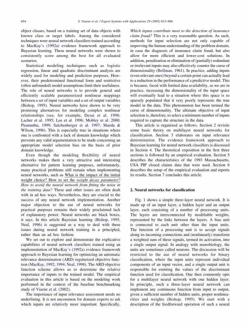
Fig. 1 shows a simple three-layer neural network. It is

made up of an input layer, a hidden layer and an output

layer, each consisting of a number of processing units.

The layers are interconnected by modifiable weights,

represented by the links between the layers. A bias unit

is connected to each unit other than the input units.

The function of a processing unit is to accept signals

along its incoming connections and (nonlinearly) transform

a weighted sum of these signals, termed its activation, into

a single output signal. In analogy with neurobiology, the

units are sometimes called neurons. The discussion will be

restricted to the use of neural networks for binary

classification, where the input units represent individual

components of an input vector, and a single output unit is

responsible for emitting the values of the discriminant

function used for classification. One then commonly opts

for a multilayer neural network with one hidden layer.

In principle, such a three-layer neural network can

implement any continuous function from input to output,

given a sufficient number of hidden units, proper nonlinea-

rities and weights (Bishop, 1995). We start with a

description of the feedforward operation of such a neural

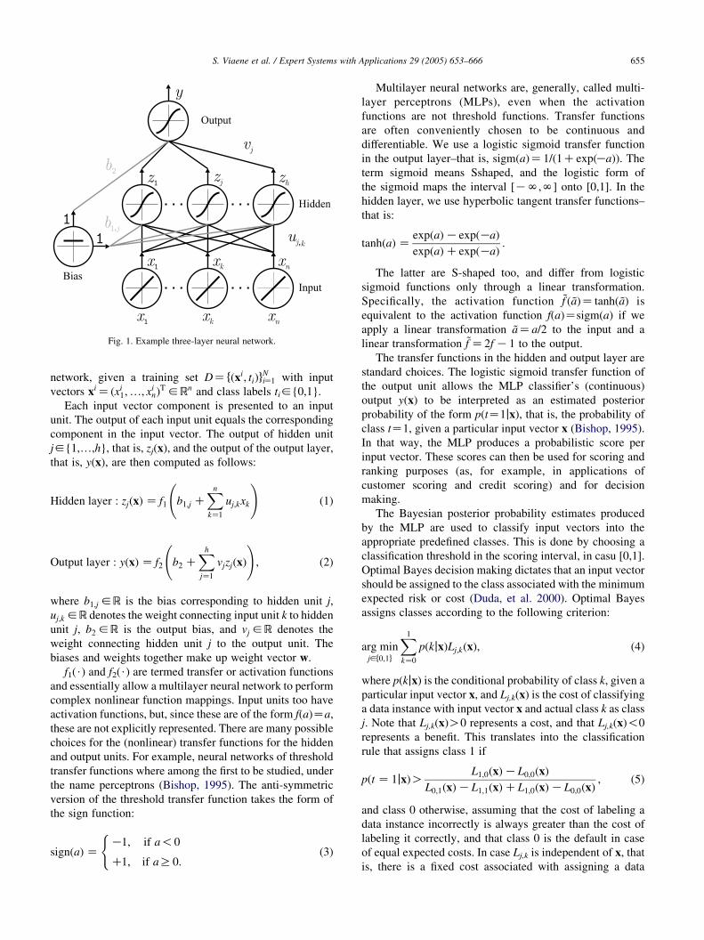
Fig. 1. Example three-layer neural network.

S. Viaene et al. / Expert Systems with Applications 29 (2005) 653–666 655

network, given a training set DZ fðxi; tiÞgNiZ1 with input

vectors xiZ ðxi1;.; xi

nÞT 2R

n and class labels ti2{0,1}.

Each input vector component is presented to an input

unit. The output of each input unit equals the corresponding

component in the input vector. The output of hidden unit

j2{1,.,h}, that is, zj(x), and the output of the output layer,

that is, y(x), are then computed as follows:

Hidden layer : zjðxÞ Z f1 b1;j CXn

kZ1

uj;kxk

!(1)

Output layer : yðxÞ Z f2 b2 CXh

jZ1

vjzjðxÞ

!; (2)

where b1;j 2R is the bias corresponding to hidden unit j,

uj;k 2R denotes the weight connecting input unit k to hidden

unit j, b2 2R is the output bias, and vj 2R denotes the

weight connecting hidden unit j to the output unit. The

biases and weights together make up weight vector w.

f1($) and f2($) are termed transfer or activation functions

and essentially allow a multilayer neural network to perform

complex nonlinear function mappings. Input units too have

activation functions, but, since these are of the form f(a)Za,

these are not explicitly represented. There are many possible

choices for the (nonlinear) transfer functions for the hidden

and output units. For example, neural networks of threshold

transfer functions where among the first to be studied, under

the name perceptrons (Bishop, 1995). The anti-symmetric

version of the threshold transfer function takes the form of

the sign function:

signðaÞ ZK1; if a!0

C1; if aR0:

((3)

Multilayer neural networks are, generally, called multi-

layer perceptrons (MLPs), even when the activation

functions are not threshold functions. Transfer functions

are often conveniently chosen to be continuous and

differentiable. We use a logistic sigmoid transfer function

in the output layer–that is, sigmðaÞZ1=ð1CexpðKaÞÞ. The

term sigmoid means Sshaped, and the logistic form of

the sigmoid maps the interval [KN,N] onto [0,1]. In the

hidden layer, we use hyperbolic tangent transfer functions–

that is:

tanhðaÞ ZexpðaÞKexpðKaÞ

expðaÞCexpðKaÞ:

The latter are S-shaped too, and differ from logistic

sigmoid functions only through a linear transformation.

Specifically, the activation function ~f ð ~aÞZ tanhð ~aÞ is

equivalent to the activation function f(a)Zsigm(a) if we

apply a linear transformation ~aZa=2 to the input and a

linear transformation ~f Z2f K1 to the output.

The transfer functions in the hidden and output layer are

standard choices. The logistic sigmoid transfer function of

the output unit allows the MLP classifier’s (continuous)

output y(x) to be interpreted as an estimated posterior

probability of the form p(tZ1jx), that is, the probability of

class tZ1, given a particular input vector x (Bishop, 1995).

In that way, the MLP produces a probabilistic score per

input vector. These scores can then be used for scoring and

ranking purposes (as, for example, in applications of

customer scoring and credit scoring) and for decision

making.

The Bayesian posterior probability estimates produced

by the MLP are used to classify input vectors into the

appropriate predefined classes. This is done by choosing a

classification threshold in the scoring interval, in casu [0,1].

Optimal Bayes decision making dictates that an input vector

should be assigned to the class associated with the minimum

expected risk or cost (Duda, et al. 2000). Optimal Bayes

assigns classes according to the following criterion:

arg minj2f0;1g

X1

kZ0

pðkjxÞLj;kðxÞ; (4)

where p(kjx) is the conditional probability of class k, given a

particular input vector x, and Lj,k(x) is the cost of classifying

a data instance with input vector x and actual class k as class

j. Note that Lj,k(x)O0 represents a cost, and that Lj,k(x)!0

represents a benefit. This translates into the classification

rule that assigns class 1 if

pðt Z 1jxÞOL1;0ðxÞKL0;0ðxÞ

L0;1ðxÞKL1;1ðxÞCL1;0ðxÞKL0;0ðxÞ; (5)

and class 0 otherwise, assuming that the cost of labeling a

data instance incorrectly is always greater than the cost of

labeling it correctly, and that class 0 is the default in case

of equal expected costs. In case Lj,k is independent of x, that

is, there is a fixed cost associated with assigning a data

Fig. 2. Schematic illustration of the data partitioning for k-fold cross-

validation.


instance to class j when it in fact belongs to class k, Eq. (5)

defines a fixed classification threshold in the scoring

interval [0,1].

Weight vector w needs to be estimated using the training

data DZ fðxi; tiÞgNiZ1. Learning works by randomly initializ-

ing and then iteratively adjusting w so as to optimize an

objective function ED, typically a sum of squared errors that

is:

ED Z1

2

XN

iZ1

ðti KyiÞ2; (6)

where yi stands for y(xi). The backpropagation algorithm,

based on gradient descent, is one of the most popular

methods for supervised learning of MLPs. During training,

the weights of the network are successively adjusted based

on a set of input vectors and their desired outputs in a

direction that reduces the error function, in casu ED. Each

iteration consists of a feedforward operation followed by a

backward propagation of errors to change the weights. Basic

backpropagation computes the change in the weight of a

network link at iteration t as follows:

DwðtÞ ZKhdED

dwðtÞ; (7)

where h is called the learning parameter, which is

proportional to the relative size of the change in the weight.

Learning stops when convergence is reached (which is

guaranteed, except for pathological cases). While basic

backpropagation is simple, flexible and general, a number of

heuristic modifications to gradient descent have been

proposed to improve its performance. For example, one

improvement is to add a momentum term mDw(tK1) to the

gradient descent formula in Eq. (7), where m is called the

momentum parameter. Adding this type of inertia to

the motion through weight space aims at speeding up the

convergence by smoothing out oscillations in weight

updates. For an overview of alternative training schemes,

see Bishop (1995).

The sum of squared errors criterion is derived from the

maximum likelihood principle by assuming target data

generated from a smooth deterministic function with added

Gaussian noise. This is clearly not a sensible starting point

for binary classification problems, where the targets are

categorical and the Gaussian noise model does not provide a

good description of their probability density. The cross-

entropy objective function is more suitable (Bishop, 1995).

At base, cross-entropy optimization maximizes the like-

lihood of the training data by minimizing its negative

logarithm. Given training data DZ fðxi; tiÞgNiZ1 and assuming

the training data instances are drawn independently from a

Bernouilli distribution, the likelihood of observing D is

given by:

YNiZ1

ðyiÞtið1 KyiÞ

1Kti ; (8)

where we have used the fact that we would like the value of

the MLP’s output y(x) to represent the posterior probability

p(tZ1jx).

Maximizing Eq. (8) is equivalent to minimizing its

negative logarithm, which leads to the cross-entropy error

function of the form:

ED ZKXN

iZ1

ðti lnðyiÞC ð1 K tiÞlnð1 KyiÞÞ: (9)

The ultimate goal of learning is to produce a model

that performs well on new data objects. If this is the

case, we say that the model generalizes well. Perform-

ance evaluation aims at estimating how well a model is

expected to perform on data objects beyond those in the

training set, but from the same underlying population and

representative of the same operating conditions. This is

not a trivial task, given the fact that, typically, we are to

design and evaluate models from a finite sample of data.

For one, looking at a model’s performance on the actual

training data that underlie its construction is likely to

overestimate its likely future performance. A common

option is to assess its performance on a separate test set

of previously unseen data. This way we may, however,

loose precious data for training.

Cross-validation (see, for example, Hand, 1997) provides

an alternative. k-Fold cross-validation is a resampling

technique that randomly splits the data into k disjoint sets

of approximately equal size, termed folds. The partitioning

of the data set is illustrated in Fig. 2. Then, k classifiers are

trained, each time with a different fold held out (shown

shaded in Fig. 2) for performance assessment. This way all

data instances are used for training, and each one is used

exactly once for testing. Finally, performance estimates are

averaged to obtain an estimate of the true generalization

performance.

Two popular measures for gauging classification

performance are the percentage correctly classified (PCC)

and the area under the receiver operating characteristic

curve (AUROC).

The PCC on (test) data DZ fðxi; tiÞgNiZ1, an estimate of

a classifier’s probability of a correct response, is

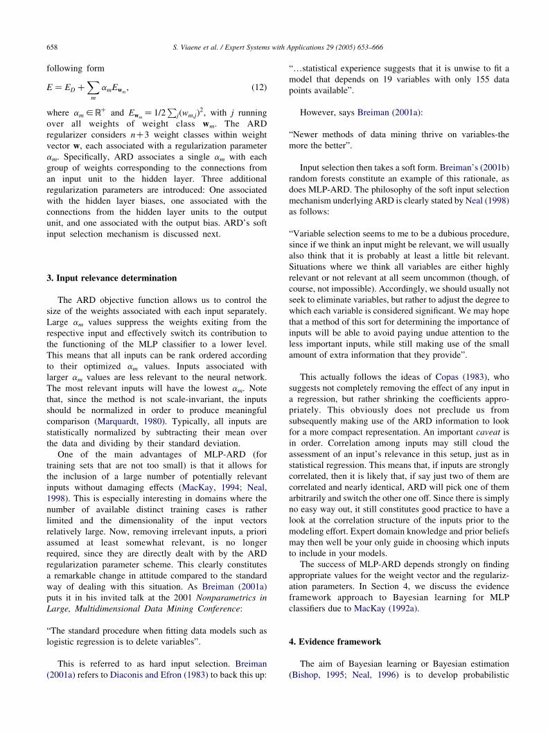
Fig. 3. Example ROCs.


the proportion of data instances that are correctly classified:

PCC Z1

N

XN

iZ1

dðHðxiÞ; tiÞ; (10)

where H(xi) is the predicted class label for xi, and d(.,.) has

value 1 if both arguments match, 0 otherwise. It is,

undoubtedly, the most commonly used classifier perform-

ance evaluation and comparison basis.

The receiver operating characteristic curve (ROC) is a

two-dimensional visualization of the false alarm rate

(N1,0)/N0,0CN1,0)) versus the true alarm rate (N1,1/(N1,1CN0,1)) for various values of the classification threshold

imposed on the value range of a scoring rule or continuous-

output classifier, where Nj,k is the number of data instances

with actual class k that were classified as class j.1 The ROC

illustrates the decision making behavior of the scoring rule

for alternative operating conditions (for example, misclassi-

fication costs), in casu summarized in the classification

threshold. The ROC essentially allows us to evaluate and

visualize the quality of the rankings produced by a scoring

rule.

Fig. 3 provides an example of several ROCs. Informally,

the more the ROC approaches the (0,1) point, the better

the classifier will discriminate under various operating

conditions (for example, curve D dominates curves A, B and

C). A specific operating condition coincides with a point on

the ROC. For known operating conditions scoring rules can

be compared by contrasting the appropriate points on their

ROCs (or convex hulls) (Provost Fawcett, 2001). ROC

analysis is not applicable for more than two classes.

However, Hand and Till (2001) present a simple general-

ization of the area under the ROC for multiple class

classification problems.

1 Drummond and Holte (2000) elaborate on a dual representation termed

cost curve.

ROCs from different classifiers may intersect, making

a general performance comparison less obvious (see, for

example, curves B and C in Fig. 3). To overcome this

problem, one often calculates and compares the area

under the ROCs. The AUROC (also known as c-index) is

a single-figure summary measure associated with ROC

performance assessment. It is only appropriate as a

performance measure in the case of unknown or vague

operating conditions, and when more general comparison

or evaluation of scoring rules over a range of operating

conditions is in order. The AUROC provides a simple

figure of merit for the expected performance of a scoring

rule across a wide range of operating conditions. It is

equivalent to the nonparametric Wilcoxon–Mann–Whit-

ney statistic, which estimates the probability that a

randomly chosen positive data instance is correctly

ranked higher than a randomly selected nonpositive

data instance (Hand, 1997; Hanley & McNeil, 1982).

The best generalization performance is achieved by a

model whose complexity is neither too small nor too

large. Besides our choosing an MLP architecture or

functional form that offers the necessary complexity to

capture the true structure in the data, during optimization

we have to avoid it from fitting the noise or

idiosyncrasies of the training data. The latter is known

as overfitting. Countering overfitting is often realized by

monitoring the predictive performance of the neural

network on a separate validation set during training.

When the performance measure evaluated on the latter

starts to deteriorate, training is stopped, therefore

preventing the neural network from fitting the noise in

the training data. An alternative, eliminating the need for

a separate validation set, is to add a regularization or

penalty term to the objective function as follows (Bishop,

1995):

E Z ED CaEw; (11)

where the regularization parameter a2RC and, typically,

the regularizer Ew Z1=2P

j w2j , with j running over all

elements of the weight vector w. This simple regularizer

is known as weight decay (or ridge regression in

conventional curve fitting), as it penalizes large weights.

The latter encourages smoother network mappings and

thereby decreases the risk of overfitting. The parameter a

controls the extent to which Ew influences the solution

and, therefore, controls the complexity of the model.

Several more sophisticated regularization schemes

have been proposed in which weights are penalized

individually or pooled and penalized as groups (see, for

example, Bengio, 2000; Grandvalet, 1998; Tibshirani,

1996). If weights are pooled by incoming and outgoing

connections of a unit, unit-based penalization is

performed. ARD (MacKay, 1994; Neal, 1998) is such a

scheme. The goal here is to penalize inputs according to

their relevance. The objective function then takes the


following form

E ¼ ED þX

m

amEwm; (12)

where am 2RC and Ewm

Z1=2P

jðwm;jÞ2, with j running

over all weights of weight class wm. The ARD

regularizer considers nC3 weight classes within weight

vector w, each associated with a regularization parameter

am. Specifically, ARD associates a single am with each

group of weights corresponding to the connections from

an input unit to the hidden layer. Three additional

regularization parameters are introduced: One associated

with the hidden layer biases, one associated with the

connections from the hidden layer units to the output

unit, and one associated with the output bias. ARD’s soft

input selection mechanism is discussed next.

3. Input relevance determination

The ARD objective function allows us to control the

size of the weights associated with each input separately.

Large am values suppress the weights exiting from the

respective input and effectively switch its contribution to

the functioning of the MLP classifier to a lower level.

This means that all inputs can be rank ordered according

to their optimized am values. Inputs associated with

larger am values are less relevant to the neural network.

The most relevant inputs will have the lowest am. Note

that, since the method is not scale-invariant, the inputs

should be normalized in order to produce meaningful

comparison (Marquardt, 1980). Typically, all inputs are

statistically normalized by subtracting their mean over

the data and dividing by their standard deviation.

One of the main advantages of MLP-ARD (for

training sets that are not too small) is that it allows for

the inclusion of a large number of potentially relevant

inputs without damaging effects (MacKay, 1994; Neal,

1998). This is especially interesting in domains where the

number of available distinct training cases is rather

limited and the dimensionality of the input vectors

relatively large. Now, removing irrelevant inputs, a priori

assumed at least somewhat relevant, is no longer

required, since they are directly dealt with by the ARD

regularization parameter scheme. This clearly constitutes

a remarkable change in attitude compared to the standard

way of dealing with this situation. As Breiman (2001a)

puts it in his invited talk at the 2001 Nonparametrics in

Large, Multidimensional Data Mining Conference:

“The standard procedure when fitting data models such as

logistic regression is to delete variables”.

This is referred to as hard input selection. Breiman

(2001a) refers to Diaconis and Efron (1983) to back this up:

“.statistical experience suggests that it is unwise to fit a

model that depends on 19 variables with only 155 data

points available”.

However, says Breiman (2001a):

“Newer methods of data mining thrive on variables-the

more the better”.

Input selection then takes a soft form. Breiman’s (2001b)

random forests constitute an example of this rationale, as

does MLP-ARD. The philosophy of the soft input selection

mechanism underlying ARD is clearly stated by Neal (1998)

as follows:

“Variable selection seems to me to be a dubious procedure,

since if we think an input might be relevant, we will usually

also think that it is probably at least a little bit relevant.

Situations where we think all variables are either highly

relevant or not relevant at all seem uncommon (though, of

course, not impossible). Accordingly, we should usually not

seek to eliminate variables, but rather to adjust the degree to

which each variable is considered significant. We may hope

that a method of this sort for determining the importance of

inputs will be able to avoid paying undue attention to the

less important inputs, while still making use of the small

amount of extra information that they provide”.

This actually follows the ideas of Copas (1983), who

suggests not completely removing the effect of any input in

a regression, but rather shrinking the coefficients appro-

priately. This obviously does not preclude us from

subsequently making use of the ARD information to look

for a more compact representation. An important caveat is

in order. Correlation among inputs may still cloud the

assessment of an input’s relevance in this setup, just as in

statistical regression. This means that, if inputs are strongly

correlated, then it is likely that, if say just two of them are

correlated and nearly identical, ARD will pick one of them

arbitrarily and switch the other one off. Since there is simply

no easy way out, it still constitutes good practice to have a

look at the correlation structure of the inputs prior to the

modeling effort. Expert domain knowledge and prior beliefs

may then well be your only guide in choosing which inputs

to include in your models.

The success of MLP-ARD depends strongly on finding

appropriate values for the weight vector and the regulariz-

ation parameters. In Section 4, we discuss the evidence

framework approach to Bayesian learning for MLP

classifiers due to MacKay (1992a).

4. Evidence framework

The aim of Bayesian learning or Bayesian estimation

(Bishop, 1995; Neal, 1996) is to develop probabilistic


models that fit the data, and make optimal predictions using

those models. The conceptual difference between Bayesian

estimation and maximum likelihood estimation is that we no

longer view model parameters as fixed, but rather treat them

as random variables that are characterized by a joint

probability model. This stresses the importance of capturing

and accommodating for the inherent uncertainty about the

true function mapping being learned from a finite training

sample. Prior knowledge, that is, our belief of the model

parameters before the data are observed, is encoded in the

form of a prior probability density. Once the data are

observed, the prior knowledge can be converted into a

posterior probability density using Bayes’ theorem. This

posterior knowledge can then be used to make predictions.

There are two practical approaches to Bayesian learning

for MLPs (Bishop, 1995; Neal, 1996). The first, known as

the evidence framework, involves a local Gaussian

approximation to the posterior probability density in weight

space. The second is based on Monte Carlo methods. Only

the former will be discussed here.

Suppose we are given a set of training data

DZ fðxi; tiÞgNiZ1. In the Bayesian framework a trained MLP

model is described in terms of the posterior probability

density over the weights p(wjD). Given the posterior,

inference is made by integrating over it. For example, to

make a classification prediction at a given input vector x, we

need the probability that x belongs to class tZ1, which is

obtained as follows:

pðt Z 1jx;DÞ ZÐ

pðt Z 1jx;wÞpðwjDÞdw; (13)

where p(tZ1jx, w) is given by the neural network function

y(x). To compute the integral in Eq. (13) MacKay (1992a)

introduces some simplifying approximations. We start by

concentrating on the posterior weight density under the

assumption of given regularization parameters.

Let p(wja) be the prior probability density over the

weights w, given the regularization parameter vector a, that

is, the vector of all ARD regularization parameters am (see

Eq. (12)). Typically, this will be a rather broad probability

density, reflecting the fact that we only have a vague belief

in a range of possible parameter values before the data

arrives. Once the training data D are observed, we can adjust

the prior probability density to a posterior probability

density p(wjD,a) using Bayes’ theorem. The posterior will

be more compact, reflecting the fact that we have learned

something about the extent to which different weight values

are consistent with the observed data. The prior to posterior

conversion works as follows:

pðwjD;aÞ ZpðDjwÞpðwjaÞ

pðDjaÞ: (14)

In the above expression, p(Djw) is the likelihood

function, that is, the probability of the data D occurring,

given the weights w. Note that p(Djw)Zp(Djw,a), for the

probability of the data D occurring is independent of a,

given w. The term p(Dja) is called the evidence for a, that

guarantees that the righthand side of the equation integrates

to one over the weight space. Note that, since the MLP’s

architecture or functional form A is assumed to be known,

it should, strictly speaking, always be included as a

conditioning variable in Eq. (14). We have, however,

omitted it, and shall continue to do so, to simplify notation.

With reference to Eq. (8), the first term in the numerator

of the righthand side of Eq. (14) can be written as follows:

pðDjwÞ ZYNiZ1

ðyiÞtið1 KyiÞ

1Kti Z expðKEDÞ; (15)

which introduces the cross-entropy objective function ED.

By carefully choosing the prior p(wja), more specifically,

by making Gaussian assumptions, MacKay (1994) is able to

introduce ARD. Specifically, the concept of input relevance is

implemented by assuming that all weights of weight class wm

(see Eq. (12)) are distributed according to a Gaussian prior

with zero mean and variance s2m Z1=am. Besides introducing

the requirement for small weights, this prior states that the

input-dependent am is inversely proportional to the variance of

the corresponding Gaussian. Since the parameter am itself

controls the probability density of other parameters, it is called

a hyperparameter. The design rationale underlying this choice

of prior is that a weight channeling an irrelevant input to the

output should have a much tighter probability density around

zero than a weight connecting a highly correlated input to the

output. In other words, a small hyperparameter value means

that large weights are allowed, so we conclude that the input is

important. A large hyperparameter constrains the weights near

zero, and hence the corresponding input is less important.

Then, with reference to Eq. (12), the second term in the

numerator of the righthand side of Eq. (14) can be written as

follows:

pðwjaÞ Z1

ZW

exp KX

m

amEwm

!; (16)

which introduces the ARD regularizer, and yields the

following expression for the posterior weight density:

pðwjD;aÞ Z1

ZM

exp KED KX

m

amEwm

!Z

1

ZM

expðKEÞ;

(17)

where 1/ZW and 1/ZM are appropriate normalizing constants.

Hence, we note that the most probable weight values wMP are

found by minimizing the objective function E in Eq. (12).

Standard optimization methods can be used to perform this

task. We used a scaled conjugate gradient method (Bishop,

1995). This concludes the first level of Bayesian inference in

the evidence framework, which involved learning the most

probable weights wMP, given a setting of a.

At the first level of Bayesian inference, we have assumed

hyperparameter vector a to be known. So, we have not yet

2 The source code can be obtained at http://www.ncrg.aston.ac.uk/netlab/.


addressed the question of how the hyperparameters should

be chosen in light of the training data D. A true Bayesian

would take care of any unknown parameters, in casu a, by

integrating them out of the joint posterior probability

density p(w,ajD) to make predictions, yielding:

pðwjDÞ ZÐ

pðw;ajDÞda ZÐ

pðwjD;aÞpðajDÞda: (18)

The approximation made in the evidence framework is to

assume that the posterior probability density p(ajD) is

sharply peaked around the most probable values aMP. With

this assumption, the integral in Eq. (18) reduces to:

pðwjDÞzpðwjD;aMPÞÐ

pðajDÞdazpðwjD;aMPÞ; (19)

which means that we should first try to find the most

probable hyperparameter values aMP and then perform the

remaining calculations involving p(wjD) using the opti-

mized hyperparameter values.

The second level of Bayesian inference in the evidence

framework is aimed at calculating aMP from the posterior

probability density p(ajD). We, again, make use of Bayes’

theorem:

pðajDÞ ZpðDjaÞpðaÞ

pðDÞ: (20)

Starting from Eq. (20) and assuming a uniform prior

p(a), representing the fact that we have very little idea of

suitable values for the hyperparameters, we obtain aMP by

maximizing p(Dja). Optimization is discussed in detail in

MacKay (1992b). This involves approximating E by a

second-order Taylor series expansion around wMP, which

comes down to making a local Gaussian approximation to

the posterior weight density centered at wMP.

A practical implementation involving both levels of

Bayesian learning starts by choosing appropriate initial

values for the hyperparameter vector a and the weight

vector w, and then trains the MLP using standard

optimization to minimize E, with the novelty that training

is periodically halted for the regularization parameters to be

updated.

Now we have trained the neural network to find the most

probable weights wMP and hyperparameters aMP, we return

to Eq. (13) for making predictions. By introducing some

additional simplifying approximations (such as assuming

that the MLP’s output unit activation is locally a linear

function of the weights), MacKay (1992a) ends up

suggesting the following approximation:

pðt Z 1jx;DÞzsigmðkðsÞaMPÞ; (21)

where aMP is the activation of the MLP’s logistic sigmoid

output unit calculated using the optimized neural network

parameters, and

kðsÞ Z 1 Cps2

8

� K1=2

; (22)

where s2 is the variance of a local Gaussian approximation

to p(ajx,D) centered at aMP, which is proportional to the

error bars around wMP.

We observe that MacKay (1992a) argues in favor of

moderating the output of the trained MLP in relation to

the error bars around the most probable weights, so that

these point estimates may better represent posterior

probabilities of class membership. The moderated output

is similar to the most probable output in regions where the

data are dense. Where the data are more sparse, moderation

smoothes the most probable output towards a less extreme

value, reflecting the uncertainty in sparse data regions. In

casu, smoothing is done toward 0.5. Although, from a

Bayesian point of view, it is better to smooth the estimates

toward the corresponding prior, the approximation proposed

by MacKay (1992a) is not readily adaptable to this

requirement.

For further details on the exact implementation of

MacKay’s (1992a,b) evidence framework, we refer to the

source code of the Netlab2 toolbox for Matlab and the

accompanying documentation provided by Bishop (1995)

and Nabney (2001).

5. PIP claims data

The empirical evaluation in Section 6 is based on a data

set of 1,399 closed PIP automobile insurance claim files

from accidents that occurred in Massachusetts, USA during

1993, and for which information was meticulously collected

by the Automobile Insurers Bureau (AIB) of Massachusetts,

USA. For all the claims the AIB tracked information on 25

binary fraud indicators (also known as red flags) and 12

nonindicator inputs, specifically, discretized continuous

inputs, that are all supposed to make sense to claims

adjusters and fraud investigators. Details on the exact

composition and semantics of the data set and the data

collection process can be found in Weisberg and Derrig

(1991, 1995, 1998).

Guided by the analysis of the timing of claim information

in Derrig and Weisberg (1998), we retained the binary fraud

indicators listed in Table 1 as inputs for the development of

our first-stage claims screening models. The listed fraud

indicators may all be qualified as typically available

relatively early in the life of a claim. The timing of the

arrival of the information on claims is crucial to its

usefulness for the development of an early claims screening

facility. The information pertains to characteristics of the

accident (ACC), the claimant (CLT), the injury (INJ), the

insured driver (INS), and lost wages (LW). The indicator

names are identical to the ones used in previous work.

Notice that no indicators related to the medical treatment are

included in the data set. None of these fraud indicators are

http://www.ncrg.aston.ac.uk/netlab/

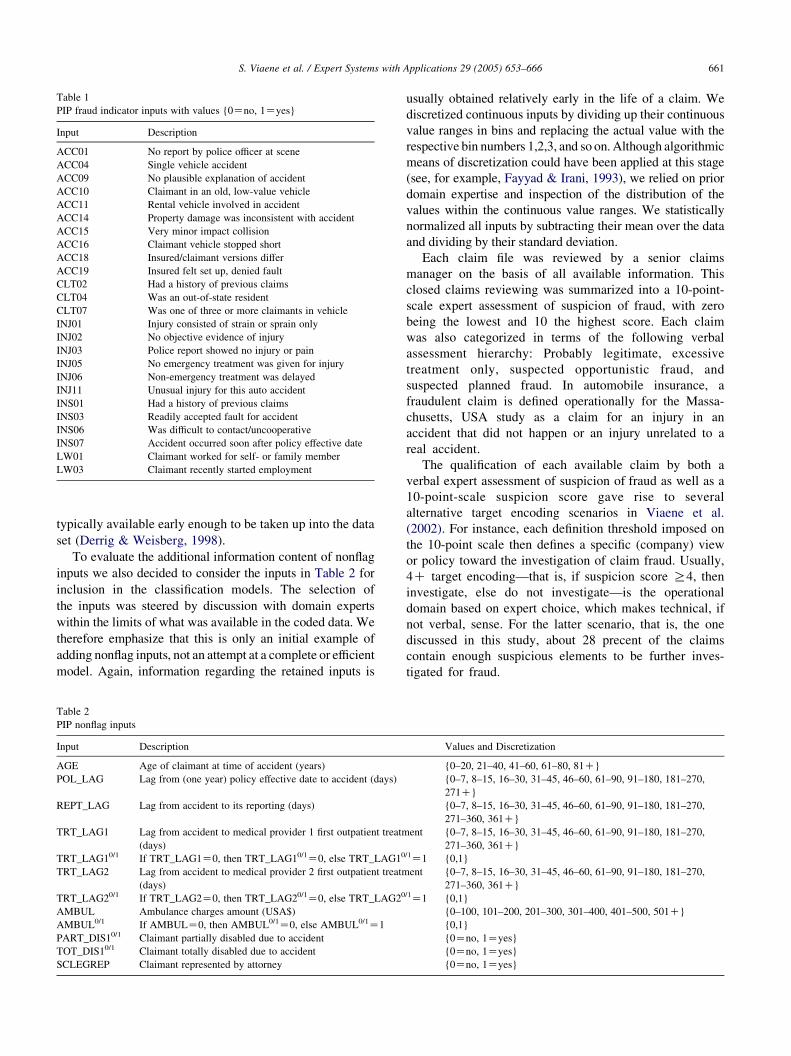
Table 1

PIP fraud indicator inputs with values {0Zno, 1Zyes}

Input Description

ACC01 No report by police officer at scene

ACC04 Single vehicle accident

ACC09 No plausible explanation of accident

ACC10 Claimant in an old, low-value vehicle

ACC11 Rental vehicle involved in accident

ACC14 Property damage was inconsistent with accident

ACC15 Very minor impact collision

ACC16 Claimant vehicle stopped short

ACC18 Insured/claimant versions differ

ACC19 Insured felt set up, denied fault

CLT02 Had a history of previous claims

CLT04 Was an out-of-state resident

CLT07 Was one of three or more claimants in vehicle

INJ01 Injury consisted of strain or sprain only

INJ02 No objective evidence of injury

INJ03 Police report showed no injury or pain

INJ05 No emergency treatment was given for injury

INJ06 Non-emergency treatment was delayed

INJ11 Unusual injury for this auto accident

INS01 Had a history of previous claims

INS03 Readily accepted fault for accident

INS06 Was difficult to contact/uncooperative

INS07 Accident occurred soon after policy effective date

LW01 Claimant worked for self- or family member

LW03 Claimant recently started employment


typically available early enough to be taken up into the data

set (Derrig & Weisberg, 1998).

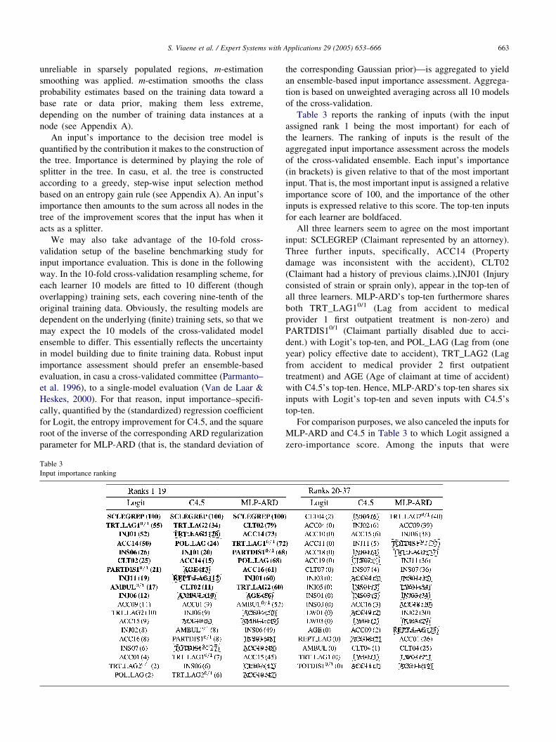
To evaluate the additional information content of nonflag

inputs we also decided to consider the inputs in Table 2 for

inclusion in the classification models. The selection of

the inputs was steered by discussion with domain experts

within the limits of what was available in the coded data. We

therefore emphasize that this is only an initial example of

adding nonflag inputs, not an attempt at a complete or efficient

model. Again, information regarding the retained inputs is

Table 2

PIP nonflag inputs

Input Description

AGE Age of claimant at time of accident (years)

POL_LAG Lag from (one year) policy effective date to accident (days)

REPT_LAG Lag from accident to its reporting (days)

TRT_LAG1 Lag from accident to medical provider 1 first outpatient treatm

(days)

TRT_LAG10/1 If TRT_LAG1Z0, then TRT_LAG10/1Z0, else TRT_LAG10

TRT_LAG2 Lag from accident to medical provider 2 first outpatient treatm

(days)

TRT_LAG20/1 If TRT_LAG2Z0, then TRT_LAG20/1Z0, else TRT_LAG20

AMBUL Ambulance charges amount (USA$)

AMBUL0/1 If AMBULZ0, then AMBUL0/1Z0, else AMBUL0/1Z1

PART_DIS10/1 Claimant partially disabled due to accident

TOT_DIS10/1 Claimant totally disabled due to accident

SCLEGREP Claimant represented by attorney

usually obtained relatively early in the life of a claim. We

discretized continuous inputs by dividing up their continuous

value ranges in bins and replacing the actual value with the

respective bin numbers 1,2,3, and so on. Although algorithmic

means of discretization could have been applied at this stage

(see, for example, Fayyad & Irani, 1993), we relied on prior

domain expertise and inspection of the distribution of the

values within the continuous value ranges. We statistically

normalized all inputs by subtracting their mean over the data

and dividing by their standard deviation.

Each claim file was reviewed by a senior claims

manager on the basis of all available information. This

closed claims reviewing was summarized into a 10-point-

scale expert assessment of suspicion of fraud, with zero

being the lowest and 10 the highest score. Each claim

was also categorized in terms of the following verbal

assessment hierarchy: Probably legitimate, excessive

treatment only, suspected opportunistic fraud, and

suspected planned fraud. In automobile insurance, a

fraudulent claim is defined operationally for the Massa-

chusetts, USA study as a claim for an injury in an

accident that did not happen or an injury unrelated to a

real accident.

The qualification of each available claim by both a

verbal expert assessment of suspicion of fraud as well as a

10-point-scale suspicion score gave rise to several

alternative target encoding scenarios in Viaene et al.

(2002). For instance, each definition threshold imposed on

the 10-point scale then defines a specific (company) view

or policy toward the investigation of claim fraud. Usually,

4C target encoding—that is, if suspicion score R4, then

investigate, else do not investigate—is the operational

domain based on expert choice, which makes technical, if

not verbal, sense. For the latter scenario, that is, the one

discussed in this study, about 28 precent of the claims

contain enough suspicious elements to be further inves-

tigated for fraud.

Values and Discretization

{0–20, 21–40, 41–60, 61–80, 81C}

{0–7, 8–15, 16–30, 31–45, 46–60, 61–90, 91–180, 181–270,

271C}

{0–7, 8–15, 16–30, 31–45, 46–60, 61–90, 91–180, 181–270,

271–360, 361C}

ent {0–7, 8–15, 16–30, 31–45, 46–60, 61–90, 91–180, 181–270,

271–360, 361C}/1Z1 {0,1}

ent {0–7, 8–15, 16–30, 31–45, 46–60, 61–90, 91–180, 181–270,

271–360, 361C}/1Z1 {0,1}

{0–100, 101–200, 201–300, 301–400, 401–500, 501C}

{0,1}

{0Zno, 1Zyes}

{0Zno, 1Zyes}

{0Zno, 1Zyes}


Most insurance companies use lists of fraud indicators

(most often per insurance business line) representing a

summary of the detection expertise as a standard aid to

claims adjusters for assessing suspicion of fraud. These

lists form the basis for systematic, consistent and

swift identification of suspicious claims. Operationally,

company claims adjustment units identify those claims

needing attention by noting the presence or absence of red

flags in the inflow of information during the life of a

claim. This has become the default modus operandi for

most insurers.

Claims adjusters are trained to recognize (still often

on an informal, judgmental basis) those claims that have

combinations of red flags that experience has shown are

typically associated with suspicious claims. This assess-

ment is embedded in the standard claims handling

process that roughly is organized as follows. In a first

stage, a claim is judged by a front-line adjuster, whose

main task is to assess the exposure of the insurance

company to payment of the claim. In the same effort, the

claim is scanned for claim amount padding and fraud.

Claims that are modest or appear to be legitimate are

then settled in a routine fashion. Claims that raise serious

questions and involve a substantial payment are sched-

uled to pass a second reviewing phase. In case fraud is

suspected, this might lead to a referral of the claim to a

special investigation unit.

3 Since the inputs are statistically normalized by subtracting their mean

over the data and dividing by their standard deviation, the logistic

regression yields standardized effect coefficients that may be used for

comparing the individual strength of the inputs.

6. Empirical evaluation

In this section, we demonstrate the intelligible soft

input selection capabilities of MLP-ARD using the

1993 Massachusetts, USA PIP automobile insurance

closed claims data. The produced input importance

ranking will be compared with the results from popular

logistic regression and decision tree learning. For this

study, we have used the models that were fitted to the

data for the baseline benchmarking study of Viaene

et al. (2002).

In the baseline benchmarking study, we contrasted the

predictive power of logistic regression, decision tree,

nearest neighbor, MLP-ARD, least squares support vector

machine, naive Bayes and tree-augmented naive Bayes

classification on the data described in Section 5. For most of

these techniques or algorithm types, we reported on several

operationalizations using alternative, a priori sensible

design choices. The algorithms were then compared in

terms of mean PCC and mean AUROC using a 10-fold

cross-validation experiment. We also contrasted algorithm

type performance visually by means of the convex hull of

the ROCs (Provost & Fawcett, 2001) associated with the

alternative operationalizations per algorithm type. MLP-

ARD consistently scored among the best for all evaluated

scenarios. The results we report in this section for MLP-

ARD are based on MLPs with one hidden layer of three

neurons.

In light of the overall excellent performance of logistic

regression reported in the baseline benchmarking study and

its widespread availability and use in practice, an assess-

ment of the relative importance of the inputs based on

inspection of the (standardized)3 regression coefficients is

taken as a point of reference for comparison. The model

specification for the logistic regression approach to

classification is as follows:

pðt Z 1jxÞ Z1

1 CexpðKðb0 CbTxÞÞ; (23)

where b2Rn represents the coefficient vector, and b0 2R

n

is the intercept. Maximum likelihood estimation of the

unknown parameters can be performed in most statistical

packages. To test for multicollinearity, variance inflation

factors (VIFs), specifically, calculated as in Allison (1999),

were checked. The VIFs were all well below the heuristic

acceptance limit of 10 (Joos, 1998). We report on the

(standardized) coefficients of logistic regression fitted with

SAS for Windows V8 PROC LOGISTIC with the default

model options at TECHNIQUEZFISHER and RID-

GINGZRELATIVE using hard, stepwise input selection,

that is, SELECTIONZSTEPWISE. The latter is termed

Logit in the rest of this article.

Decision trees are taken as a second point of reference.

They are among the most popular data mining methods and

are available in customizable form in most commercial

off-the-shelf data mining software. C4.5 (Quinlan, 1993)

(for details, see Appendix A) is among the most popular

decision tree induction algorithms. The implementation

reported on in this study is the m-estimation smoothed and

curtailed C4.5 variant due to Zadrozny and Elkan (2001).

The latter tended to outperform standard (smoothed) C4.5 in

the baseline benchmarking study, although its reported

performance was clearly inferior to that of logistic

regression and MLP-ARD. It is conceived as follows.

First, a full, that is, unpruned, C4.5 decision tree is

grown. Then, instead of estimating class membership for

decision making purposes from the leaf nodes of the

unpruned tree, we backtrack through the parents of the

leaf until we find a subtree that contains k or more

training data instances. That is, the estimation neighbor-

hood of a data instance is enlarged until we find a subtree

that classifies k or more training data instances. The

optimal k in terms of generalization ability of the tree’s

predictions and reliability of the probability estimates is

determined using cross-validation. Since probability

estimates based on raw training data frequencies may be


unreliable in sparsely populated regions, m-estimation

smoothing was applied. m-estimation smooths the class

probability estimates based on the training data toward a

base rate or data prior, making them less extreme,

depending on the number of training data instances at a

node (see Appendix A).

An input’s importance to the decision tree model is

quantified by the contribution it makes to the construction of

the tree. Importance is determined by playing the role of

splitter in the tree. In casu, et al. the tree is constructed

according to a greedy, step-wise input selection method

based on an entropy gain rule (see Appendix A). An input’s

importance then amounts to the sum across all nodes in the

tree of the improvement scores that the input has when it

acts as a splitter.

We may also take advantage of the 10-fold cross-

validation setup of the baseline benchmarking study for

input importance evaluation. This is done in the following

way. In the 10-fold cross-validation resampling scheme, for

each learner 10 models are fitted to 10 different (though

overlapping) training sets, each covering nine-tenth of the

original training data. Obviously, the resulting models are

dependent on the underlying (finite) training sets, so that we

may expect the 10 models of the cross-validated model

ensemble to differ. This essentially reflects the uncertainty

in model building due to finite training data. Robust input

importance assessment should prefer an ensemble-based

evaluation, in casu a cross-validated committee (Parmanto–

et al. 1996), to a single-model evaluation (Van de Laar &

Heskes, 2000). For that reason, input importance–specifi-

cally, quantified by the (standardized) regression coefficient

for Logit, the entropy improvement for C4.5, and the square

root of the inverse of the corresponding ARD regularization

parameter for MLP-ARD (that is, the standard deviation of

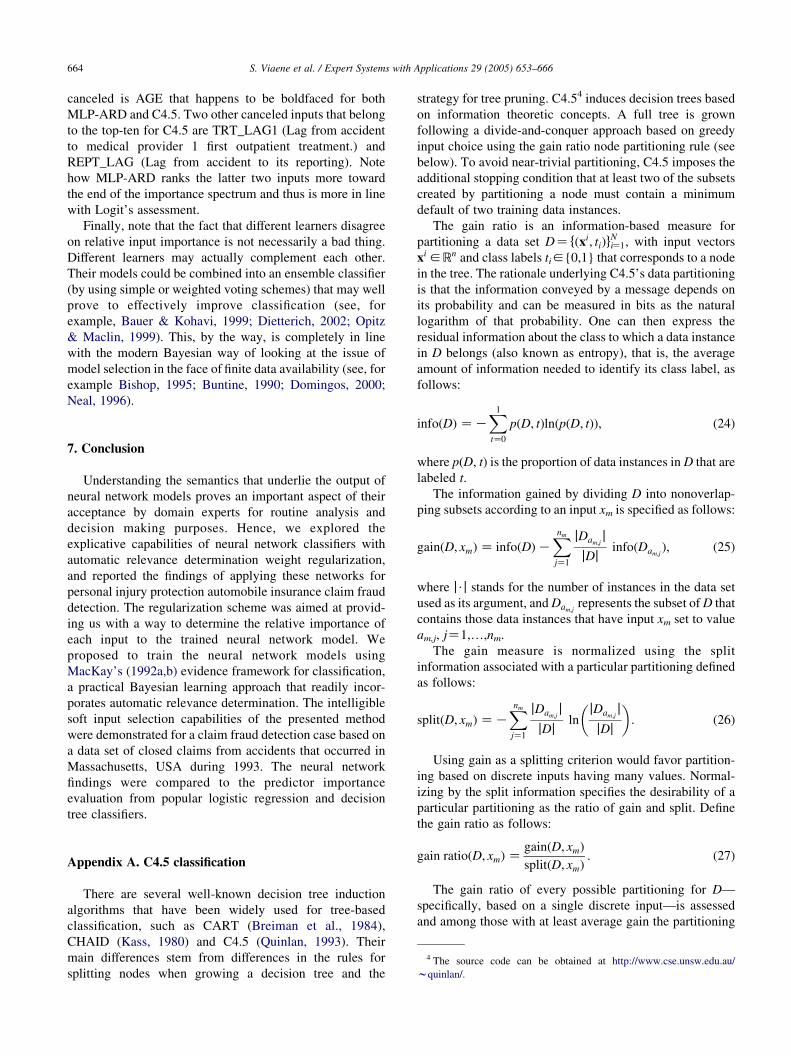
Table 3

Input importance ranking

the corresponding Gaussian prior)—is aggregated to yield

an ensemble-based input importance assessment. Aggrega-

tion is based on unweighted averaging across all 10 models

of the cross-validation.

Table 3 reports the ranking of inputs (with the input

assigned rank 1 being the most important) for each of

the learners. The ranking of inputs is the result of the

aggregated input importance assessment across the models

of the cross-validated ensemble. Each input’s importance

(in brackets) is given relative to that of the most important

input. That is, the most important input is assigned a relative

importance score of 100, and the importance of the other

inputs is expressed relative to this score. The top-ten inputs

for each learner are boldfaced.

All three learners seem to agree on the most important

input: SCLEGREP (Claimant represented by an attorney).

Three further inputs, specifically, ACC14 (Property

damage was inconsistent with the accident), CLT02

(Claimant had a history of previous claims.),INJ01 (Injury

consisted of strain or sprain only), appear in the top-ten of

all three learners. MLP-ARD’s top-ten furthermore shares

both TRT_LAG10/1 (Lag from accident to medical

provider 1 first outpatient treatment is non-zero) and

PARTDIS10/1 (Claimant partially disabled due to acci-

dent.) with Logit’s top-ten, and POL_LAG (Lag from (one

year) policy effective date to accident), TRT_LAG2 (Lag

from accident to medical provider 2 first outpatient

treatment) and AGE (Age of claimant at time of accident)

with C4.5’s top-ten. Hence, MLP-ARD’s top-ten shares six

inputs with Logit’s top-ten and seven inputs with C4.5’s

top-ten.

For comparison purposes, we also canceled the inputs for

MLP-ARD and C4.5 in Table 3 to which Logit assigned a

zero-importance score. Among the inputs that were


canceled is AGE that happens to be boldfaced for both

MLP-ARD and C4.5. Two other canceled inputs that belong

to the top-ten for C4.5 are TRT_LAG1 (Lag from accident

to medical provider 1 first outpatient treatment.) and

REPT_LAG (Lag from accident to its reporting). Note

how MLP-ARD ranks the latter two inputs more toward

the end of the importance spectrum and thus is more in line

with Logit’s assessment.

Finally, note that the fact that different learners disagree

on relative input importance is not necessarily a bad thing.

Different learners may actually complement each other.

Their models could be combined into an ensemble classifier

(by using simple or weighted voting schemes) that may well

prove to effectively improve classification (see, for

example, Bauer & Kohavi, 1999; Dietterich, 2002; Opitz

& Maclin, 1999). This, by the way, is completely in line

with the modern Bayesian way of looking at the issue of

model selection in the face of finite data availability (see, for

example Bishop, 1995; Buntine, 1990; Domingos, 2000;

Neal, 1996).

7. Conclusion

Understanding the semantics that underlie the output of

neural network models proves an important aspect of their

acceptance by domain experts for routine analysis and

decision making purposes. Hence, we explored the

explicative capabilities of neural network classifiers with

automatic relevance determination weight regularization,

and reported the findings of applying these networks for

personal injury protection automobile insurance claim fraud

detection. The regularization scheme was aimed at provid-

ing us with a way to determine the relative importance of

each input to the trained neural network model. We

proposed to train the neural network models using

MacKay’s (1992a,b) evidence framework for classification,

a practical Bayesian learning approach that readily incor-

porates automatic relevance determination. The intelligible

soft input selection capabilities of the presented method

were demonstrated for a claim fraud detection case based on

a data set of closed claims from accidents that occurred in

Massachusetts, USA during 1993. The neural network

findings were compared to the predictor importance

evaluation from popular logistic regression and decision

tree classifiers.

4 The source code can be obtained at http://www.cse.unsw.edu.au/

wquinlan/.

Appendix A. C4.5 classification

There are several well-known decision tree induction

algorithms that have been widely used for tree-based

classification, such as CART (Breiman et al., 1984),

CHAID (Kass, 1980) and C4.5 (Quinlan, 1993). Their

main differences stem from differences in the rules for

splitting nodes when growing a decision tree and the

strategy for tree pruning. C4.54 induces decision trees based

on information theoretic concepts. A full tree is grown

following a divide-and-conquer approach based on greedy

input choice using the gain ratio node partitioning rule (see

below). To avoid near-trivial partitioning, C4.5 imposes the

additional stopping condition that at least two of the subsets

created by partitioning a node must contain a minimum

default of two training data instances.

The gain ratio is an information-based measure for

partitioning a data set DZ fðxi; tiÞgNiZ1, with input vectors

xi 2Rn and class labels ti2{0,1} that corresponds to a node

in the tree. The rationale underlying C4.5’s data partitioning

is that the information conveyed by a message depends on

its probability and can be measured in bits as the natural

logarithm of that probability. One can then express the

residual information about the class to which a data instance

in D belongs (also known as entropy), that is, the average

amount of information needed to identify its class label, as

follows:

infoðDÞ ZKX1

tZ0

pðD; tÞlnðpðD; tÞÞ; (24)

where p(D, t) is the proportion of data instances in D that are

labeled t.

The information gained by dividing D into nonoverlap-

ping subsets according to an input xm is specified as follows:

gainðD; xmÞ Z infoðDÞKXnm

jZ1

jDam;jj

jDjinfoðDam;j

Þ; (25)

where j$j stands for the number of instances in the data set

used as its argument, and Dam;jrepresents the subset of D that

contains those data instances that have input xm set to value

am,j, jZ1,.,nm.

The gain measure is normalized using the split

information associated with a particular partitioning defined

as follows:

splitðD; xmÞ ZKXnm

jZ1

jDam;jj

jDjln

jDam;jj

jDj

� : (26)

Using gain as a splitting criterion would favor partition-

ing based on discrete inputs having many values. Normal-

izing by the split information specifies the desirability of a

particular partitioning as the ratio of gain and split. Define

the gain ratio as follows:

gain ratioðD; xmÞ ZgainðD; xmÞ

splitðD; xmÞ: (27)

The gain ratio of every possible partitioning for D—

specifically, based on a single discrete input—is assessed

and among those with at least average gain the partitioning

http://www.cse.unsw.edu.au/~quinlan/

http://www.cse.unsw.edu.au/~quinlan/


with the maximum gain ratio is chosen. By recursively

partitioning the training data at the leaf nodes until the

stopping conditions are fulfilled, a full tree is grown.

To avoid the tree from overfitting the training data, that

is, to avoid fitting the idiosyncrasies of the training data that

are not representative of the population, the full tree is

pruned using C4.5’s error-based pruning (see below) with

the default confidence factor aZ25%.

Pruning is performed by identifying subtrees that

contribute little to the predictive accuracy and replacing

each by a leaf or one of the branches. Of course, training

error at a node, that is, estimating the true error by the

number of wrongly classified training data instances at the

node, is not an appropriate error estimate for making that

evaluation. Since the tree is biased toward the training data

that underly its construction, training error is usually too

optimistic an estimate of the true error. Instead, C4.5 goes

for a more pessimistic estimate. Suppose a leaf covers N

training data instances, e of which are misclassified. Then

C4.5 equates the predicted error rate at a node with the

upper bound of an a percent confidence interval assuming a

binomial (N,e/N) distribution. This is known as C4.5’s

pessimistic error rate estimation. A subtree will then be

pruned if the predicted error rate times the number of

training data instances covered by the subtree’s root node

exceeds the weighted sum of error estimates for all its direct

descendants. For details, see Quinlan (1993).

One can use decision trees to estimate probabilities of the

form p(tZ1jx). These can then be used for scoring and

ranking input vectors, constructing the ROC and calculating

the AUROC. Such trees have been called class probability

trees (Breiman et al., 1984) or probability estimation trees

(PETs) (Provost & Domingos, 2003).

The simplest method that has been proposed to obtain

these estimates uses the training data instance frequencies at

the leaves—that is, a test data instance gets assigned the raw

frequency ratio k/l at the leaf node to which it belongs,

where k and l stand for the number of training data instances

with actual class tZ1 at the leaf and the total number of

training data instances at the leaf, respectively. However,

since the tree was built to separate the classes and to make

the leaves as homogeneous as possible, these raw estimates

systematically tend to be too extreme, that is, they are

systematically shifted towards 0 or 1. Furthermore, when

the number of training data instances associated with the

leaf is small, frequency counts provide unreliable prob-

ability estimates.5

Several methods have been proposed to overcome this,

including applying simple Laplace correction and

m-estimation smoothing. For two-class problems simple

Laplace correction (Good, 1965) replaces k/l by (kC)1/(lC2). This smooths the data instance score toward 0.5, making

5 In principle, pruning and stopping conditions requiring a minimum

number of training data instances at the tree leaves counter this.

it less extreme depending on the number of training data

instances at the leaf. This approach has been applied

successfully (see, for example, Kohavi et al., 1997; Provost

& Domingos, 2003). However, from a Bayesian perspec-

tive, conditional probability estimates should be smoothed

toward the corresponding unconditional probabilities.

This can be done using m-estimation smoothing (Cestnik,

1990) instead of Laplace correction. m-estimation replaces

k/l by (kCbm)/(lCm), where b is the data prior––assuming

that the class proportions in the data are representative of the

true class priors––and m is a parameter that controls how

much the raw score is shifted toward b. Given a base rate

estimate b, one can use cross-validation to specify m (see,

for example, Cussens, 1993) or, alternatively, follow the

suggestion by Zadrozny and Elkan (2001) and specify m

such that bmZ5, approximately. This heuristic is motivated

by its similarity to the rule of thumb that says that a c2

goodness-of-fit test is reliable if the number of data

instances in each cell of the contingency table is at least five.

References

Allison, P. D. (1999). Logistic regression using the SAS system: Theory and

application. Cary: SAS Institute.

Bauer, E., & Kohavi, R. (1999). An empirical comparison of voting

classification algorithms: Bagging, boosting and variants. Machine

Learning, 36(1/2), 105–139.

Bellman, R. E. (1961). Adaptive control processes. Princeton: Princeton

University Press.

Bengio, Y. (2000). Gradient-based optimization of hyper-parameters.

Neural Computation, 12(8), 1889–1900.

Bishop, C. M. (1995). Neural networks for pattern recognition. Oxford:

Oxford University Press.

Breiman, L. (2001a). Understanding complex predictors. Invited talk at the

nonparametrics in large, multidimensional data mining conference,

Dallas, http://www.smu.edu/statistics/NonparaConf/Breiman-dallas-

2000.pdf.

Breiman, L. (2001b). Random forests. Machine Learning, 45, (1), 5–32.

Breiman, L., Friedman, J. H., Olshen, R. A., & Stone, C. J. (1984).

Classification and regression trees (CART). Belmont: Wadsworth

International Group.

Buntine, W.L. (1990). A theory of learning classification rules. PhD Thesis.

School of Computing Science, University of Technology Sydney.

Canadian Coalition Against Insurance fraud. (2002). Insurance fraud,

http://www.fraudcoalition.org/.

Cestnik, B. (1990). Estimating probabilities: A crucial task in machine

learning Proceedings of the ninth European conference on artificial

intelligence, Stockholm (pp. 147–149).

Coalition Against Insurance Fraud (2002). Insurance fraud: The crime you

pay for, http://www.insurancefraud.org/fraud_backgrounder.htm.

Comite Europeen des Assurances. (1996). The European insurance anti-

fraud guide. CEA info special issue 4. Paris: Euro Publishing System.

Comite Europeen des Assurances. (1997). The European insurance anti-

fraud guide 1997 update. CEA info special issue 5 Paris: Euro

Publishing System.

Copas, J. B. (1983). Regression, prediction and shrinkage (with discussion).

Journal of the Royal Statistical Society: Methodological 45, (3),

311–354.

http://www.smu.edu/statistics/NonparaConf/Breiman-dallas-2000.pdf

http://www.smu.edu/statistics/NonparaConf/Breiman-dallas-2000.pdf

http://www.fraudcoalition.org/

http://www.insurancefraud.org/fraud_backgrounder.htm


Cussens, J. (1993). Bayes and pseudo-Bayes estimates of conditional

probabilities and their reliability. Proceedings of the sixth European

conference on machine learning, Vienna (pp. 136–152).

Derrig, R. A. (Ed.) (2002), Special issue on insurance fraud. Journal of Risk

and Insurance 69 (3).

Derrig, R. A., & Weisberg, H. (1998). AIB PIP screening experiment final

report—Understanding and improving the claim investigation process.

AIB Cost Containment/Fraud Filing DOI Docket R98-41 (IFRR-267).

Boston: Automobile insurers Bureau of Massachusetts.

Desai, V. S., Crook, J. N., & Overstreet Jr.,, G. A. (1996). A comparison of

neural networks and linear scoring models in the credit union environment.

European Journal of Operational Research, 95(1), 24–37.

Diaconis, P., & Efron, B. (1983). Computer-intensive methods in statistics.

Scientific American, 248(5), 116–130.

Dietterich, T. G. (2002). Ensemble learning. In M.A. Arbib (Ed.), The

hanbook of brain theory and neural networks (2nd ed.) (PP.405–408).

Cambridge: MIT Press

Domingos, P. (2000). Bayesian averaging of classifiers and the overfitting

problem. Proceedings of the seventeenth international conference on

machine learning, Stanford (pp. 223–230).

Drummond, C., & Holte, R. C. (2000). Explicitly representing expected

cost: An alternative to ROC representation. Proceedings of the sixth

ACM SIGKDD international conference on knowledge discovery and

data mining, Boston (pp. 198–207).

Duda, R. O., Hart, P. E., & Stork, D. G. (2000). Pattern classification (2nd

ed.). New York: Wiley.

Fayyad, U. M., & Irani, K. B. (1993). Multi-interval discretization of

continuous-valued attributes for classification learning. Proceedings of

the thirteenth international joint conference on artificial intelligence,

Chambery (pp. 1022–1027).

Good, I. J. (1965). The estimation of probabilities: An essay on modern

Bayesian methods. Cambridge: MIT Press.

Grandvalet, Y. (1998). Lasso is equivalent to quadratic penalization.

Proceedings of the international conference on artificial neural

networks, Skovde (pp. 201–206).

Hand, D. J. (1997). Construction and assessment of classification rules.

Chichester: Wiley.

Hand, D. J., & Till, R. J. (2001). A simple generalisation of the area under

the ROC curve for multiple class classification problems. Machine

Learning, 45(2), 171–186.

Hanley, J. A., & McNeil, B. J. (1982). The meaning and use of the area

under a receiver operating characteristic (ROC) curve. Radiology,

143(1), 29–36.

Joos, P., Vanhoof, K., Sierens, N., & Ooghe, H. (1998). Credit

classification: A comparison of logit models and decision trees.

Proceedings of the tenth European conference on machine learning,

workshop on the application of machine learning and data mining in

finance, Chemnitz (pp. 59–73).

Kass, G. V. (1980). An exploratory technique for investigating quantities of

categorical data. Applied Statistics, 29(2), 119–127.

Kohavi, R., Becker, B., & Sommerfield, D. (1997). Improving simple

Bayes. Proceedings of the ninth European conference on machine

learning, Prague, http://robotics.stanford.edu/wronnyk/impSBC.ps.Z.

Lacher, R. C., Coats, P. K., Shanker, S. C., & Fant, L. F. (1995). A neural

network for classifying the financial health of a firm. European Journal

of Operational Research, 85(1), 53–65.

Lee, K. C., Han, I., & Kwon, Y. (1996). Hybrid neural network models for

bankruptcy predictions. Decision Support Systems, 18(1), 63–72.

MacKay, D. J. C. (1992a). The evidence framework applied to

classification networks. Neural Computation, 4(5), 720–736.

MacKay, D. J. C. (1992b). A practical Bayesian framework for back-

propagation networks. Neural Computation, 4(3), 448–472.

MacKay, D. J. C. (1994). Bayesian non-linear modelling for the energy

prediction competition. ASHRAE Transactions, 100(2), 1053–1062.

Marquardt, D. W. (1980). Comment on Smith and Campbell: You should

standardize the predictor variables in your regression models. Journal

of the American Statistical Association, 75(369), 87–91.

Mobley, B. A., Schechter, E., Moore, W. E., McKee, P. A., & Eichner, J. E.

(2000). Predictions of coronary artery stenosis by artificial neural

network. Artificial Intelligence in Medicine, 18(3), 187–203.

Nabney, I. T. (2001). Netlab: Algorithms for pattern recognition. New

York: Springer.

Neal, R. M. (1996). Bayesian learning for neural networks. New York:

Springer.

Neal, R. M. (1998). Assessing relevance determination methods using

Delve. In C. M. Bishop (Ed.), Neural networks and machine learning.

New York: Springer.

Opitz, D., & Maclin, R. (1999). Popular ensemble methods: An empirical

study. Journal of Artificial Intelligence Research, 11, 169–198.

Parmanto, B., Munro, P. W., & Doyle, H. R. (1996). Reducing variance of

committee prediction with resampling techniques. Connection Science,

8(3/4), 405–426.

Piramuthu, S. (1999). Financial credit-risk evaluation with neural and

neurofuzzy systems. European Journal of Operational Research,

112(2), 310–321.

Provost, F. J., & Domingos, P. (2003). Tree induction for probability-based

ranking. Machine Learning, 52(3), 199–215.

Provost, F. J., & Fawcett, T. (2001). Robust classification for imprecise

environments. Machine Learning, 42(3), 203–231.

Quinlan, J. (1993). C4.5: Programs for machine learning. San Mateo:

Morgan Kaufmann.

Salchenberger, L. M., Venta, E. R., & Venta, L. A. (1997). Using neural

networks to aid the diagnosis of breast implant rupture. Computers and

Operations Research, 24(5), 435–444.

Sharda, R., & Wilson, R. (1996). Neural network experiments in business

failures prediction: A review of predictive performance issues.

International Journal of Computational Intelligence and Organiz-

ations, 1(2), 107–117.

Tibshirani, R. J. (1996). Regression shrinkage and selection via the lasso.

Journal of the Royal Statistical Association: Methodological, 58(1),

267–288.

Van de Laar, P., & Heskes, T. (2000). Input selection based on an ensemble,

http:/citeseer.nj.nec.com/vandelaar00input.html.

Viaene, S. (2002). Learning to detect fraud from enriched insurance claims

data: Context, theory and applications. PhD Thesis, Department of

Applied Economics, K.U. Leuven.

Viaene, S., Derrig, R. A., Baesens, B., & Dedene, G. (2002). A comparison

of state-of-the-art classification techniques for expert automobile

insurance claim fraud detection. Journal of Risk and Insurance,

69(3), 373–421.

Weisberg, H. I., & Derrig, R. A. (1991). Fraud and automobile insurance: A

report on the baseline study of bodily injury claims in Massachusetts.

Journal of Insurance Regulation, 9(4), 497–541.

Weisberg, H. I., & Derrig, R. A. (1995). Identification and investigation of

suspicious claims. AIB Cost Containment/Fraud Filing DOI Docket

R95-12 (IFFR-170). Boston: Automobile Insurers Bureau of

Massachusetts.

Weisberg, H. I., & Derrig, R. A. (1998). Quantitative methods for detecting

fraudulent automobile bodily injury claims. Risques, 35, 75–101.

Zadrozny, B., & Elkan, C. (2001). Obtaining calibrated probability

estimates from decision trees and naive Bayesian classifiers. Proceed-

ings of the eighteenth international conference on machine learning,

Williams College (pp. 609–616).

http://robotics.stanford.edu/~ronnyk/impSBC.ps.Z

http://http:/citeseer.nj.nec.com/vandelaar00input.html

Auto claim fraud detection using Bayesian learning neural networks

Documents

Transcript of Auto claim fraud detection using Bayesian learning neural networks