Analysis Fraud
127
A A i i i g g g l l l i i i R R R i i z z o o o u u u SUPERVISORS PROF. J. SOLDATOS PROF. I. CHRISTOU MASTER OF ASTER OF ASTER OF ASTER OF SCIENCE IN CIENCE IN CIENCE IN CIENCE IN INFORMATION NFORMATION NFORMATION NFORMATION & TELECOMMUNICATIONS ELECOMMUNICATIONS ELECOMMUNICATIONS ELECOMMUNICATIONS TECHNOLOGIES ECHNOLOGIES ECHNOLOGIES ECHNOLOGIES ATHENS ATHENS ATHENS ATHENS , OCTOBER OCTOBER OCTOBER OCTOBER 2010 2010 2010 2010
-
Upload
independent -
Category
Documents
-
view
4 -
download
0
Transcript of Analysis Fraud
AAAAAAAAAAAA iiiiiiiiiiii gggggggggggg llllllllllll iiiiiiiiiiii RRRRRRRRRRRR iiiiiiiiiiii zzzzzzzzzzzz oooooooooooo uuuuuuuuuuuu
SSSSSSSSUUUUUUUUPPPPPPPPEEEEEEEERRRRRRRRVVVVVVVVIIIIIIIISSSSSSSSOOOOOOOORRRRRRRRSSSSSSSS
PPPPPPPPRRRRRRRROOOOOOOOFFFFFFFF........ JJJJJJJJ ........ SSSSSSSSOOOOOOOOLLLLLLLLDDDDDDDDAAAAAAAATTTTTTTTOOOOOOOOSSSSSSSS
PPPPPPPPRRRRRRRROOOOOOOOFFFFFFFF........ IIIIIIII ........ CCCCCCCCHHHHHHHHRRRRRRRRIIIIIIIISSSSSSSSTTTTTTTTOOOOOOOOUUUUUUUU
MMMMAS TE R O F A S T E R O F A S T E R O F A S T E R O F SSSS C I ENC E I N C I ENC E I N C I ENC E I N C I ENC E I N IIII N FORMAT I ON N FORMAT I ON N FORMAT I ON N FORMAT I ON
&&&& TTTT E L E COMMUN ICA T I ON S E L E COMMUN ICA T I ON S E L E COMMUN ICA T I ON S E L E COMMUN ICA T I ON S TTTT E CHNO LOG I E SE CHNO LOG I E SE CHNO LOG I E SE CHNO LOG I E S
ATHENSATHENSATHENSATHENS ,,,, OCTOBER OCTOBER OCTOBER OCTOBER 2010201020102010
Analysis of Fraud Detection
Aigli Rizou – MSITT 2010 2
ABSTRACTABSTRACTABSTRACTABSTRACT
Fraud plays a leading role in most aspects of social and economical life
worldwide. The expansion of modern technology resulted in the facilitation of
our daily activities, but rendered our lives more vulnerable to fraud attacks.
Intense financial pressure during the economic crisis has, also, led to a bulge
in fraud and increasing number of victims. Banking, telecommunications
insurance, internet and enterprises are the sectors which suffer significant
losses and they are the basic parts the current thesis disserts. The
economical impact of fraud made fraud prevention and detection a dire
necessity. Fraud detection theoretical background stems from scientific fields,
such as data mining, machine learning, artificial intelligence and statistics.
Supervised and unsupervised learning algorithms have contributed to the
evolvement of fraud detection. Moreover, several academic studies have
indulged in the research of various promising fraud techniques, with a view to
encounter the evolving nature of fraud. The presentation of a real-life fraud
detection system of a Greek Bank aims at giving a more practical view of the
problem. A short description of the system reveals the way the Bank deals
with fraud cases. Based on a real data set labeled by the system, another
machine learning tool is used in order to check the reliability of the running
supervised algorithms. Finally, the proposed fraud detection solution aims at
offering a robust fraud detection system with improved performance,
constituting a subject for future work.
Keywords: fraud detection, fraud losses, classification, clustering, confusion
matrix, false alarm rate, classifier ensembles, class label

Analysis of Fraud Detection
Aigli Rizou – MSITT 2010 3
ACKNOWLEDGMENTSACKNOWLEDGMENTSACKNOWLEDGMENTSACKNOWLEDGMENTS
I w o u l d l i ke t o e x p r e s s m y g r a t i t u d e a n d a p p r e c i a t i o n t o
m y s u p e r v i s o r s , P r o f . J . S o l d a t o s a n d P r o f . I . C h r i s t o u ,
w h o s e v a l u a b l e g u i d a n c e a n d h a r mo n i o u s c o l l a b o r a t i o n
e n c o u r a g e d m e t o d i s c o v e r u n kn o w n a s p e c t s o f t h e
s u b j e c t .

Analysis of Fraud Detection
Aigli Rizou – MSITT 2010 4
DECLARATIONDECLARATIONDECLARATIONDECLARATIONSSSS
I , A i g l i R i z o u , d e c l a r e t h a t t h e w o r k p r e s e n t e d i n t h i s
t h e s i s w a s c a r r i e d o u t i n a c c o r d a n c e w i t h t h e r e g u l a t i o n s
o f t h e A t h e n s I n f o r m a t i o n T e c h n o l o g y I n s t i t u t e . A n y
v i e w s e x p r e s s e d i n t h i s d i s s e r t a t i o n a r e t h o s e o f t h e
a u t h o r a n d i n n o w a y r e p r e s e n t t h o s e o f t h e A t h e n s
In f o r m a t i o n Te c h n o l o g y ( A I T ) I n s t i t u t e .
Aigli Rizou
22/10/2010
Th e w o r k c o n t a i n e d i n t h i s t h e s i s “ A n a l ys i s o f F r a u d
D e t e c t i o n ” b y A i g l i R i z o u h a s b e e n c a r r i e d o u t u n d e r m y
s u p e r v i s i o n .
J. Soldatos I. Christou
22/10/2010 22 /10/2010
Athens Information Technology Athens Information Technology
Analysis of Fraud Detection
Aigli Rizou – MSITT 2010 5
TABLE OF CONTENTSTABLE OF CONTENTSTABLE OF CONTENTSTABLE OF CONTENTS
1 . I N T R O D UC T I O N .............................................................................11
1 . 1 . H i s t o r y ............................................................................................11
1 . 2 . O b j e c t i v e .......................................................................................12
1 . 3 . S t r u c tu r e .......................................................................................13
2 FRAUD DETECTION (FD) OVERVIEW .................................................15
22 .. 11 .. FF rr aa uu dd DD ee ff ii nn ii tt ii oo nn .......................................................................15
2 . 2 . F r a u d D e t e c t i o n & P r e v e n t i o n .........................................15
2 . 3 . F r a u d T y p e s ................................................................................16
2 . 3 . 1 . B a n k i n g ...............................................................................16
2 . 3 . 2 . In s u r a n c e ...........................................................................18
2 . 3 . 3 . In t e r n e t ................................................................................18
2 . 3 . 4 . T e l e c o m m u n i c a t i o n s ...................................................19
2 . 3 . 5 . E n t e r p r i s e s .......................................................................19
2 . 3 . 6 . G e n e r a l ................................................................................19
2 . 4 . F r a u d T e c h n i q u e s ....................................................................20
2 . 4 . 1 . B a n k i n g ...............................................................................20
2 . 4 . 2 . In s u r a n c e ...........................................................................22
2 . 4 . 3 . In t e r n e t ................................................................................23
2 . 4 . 4 . T e l e c o m m u n i c a t i o n s ...................................................24
2 . 4 . 5 . E n t e r p r i s e s .......................................................................25
2 . 5 . F r a u d s t e r s T y p e ........................................................................26
2 . 6 . E c o n o m i c a l I m p a c t o f F r a u d .............................................27
2 . 6 . 1 . G e n e r a l ................................................................................28
2 . 6 . 2 . B a n k i n g ...............................................................................30
2 . 6 . 2 . 1 . C r e d i t / D e b i t c a r d s ...................................................30
2 . 6 . 2 . 2 . I d e n t i t y T h e f t ..............................................................34
2 . 6 . 3 . E n t e r p r i s e s .......................................................................34
2 . 6 . 4 . In s u r a n c e ...........................................................................36
2 . 6 . 5 . In t e r n e t ................................................................................36
2 . 6 . 5 . 1 . A d v a n c e F e e F r a u d – 4 1 9 S c a m ......................37
Analysis of Fraud Detection
Aigli Rizou – MSITT 2010 6
2 . 6 . 6 . T e l e c o m m u n i c a t i o n s ...................................................38
2 . 7 . D i f f i c u l t i e s i n F D .....................................................................39
2 . 8 . F D S y s t e m R e q u i r e m e n t s ....................................................41
2 . 8 . 1 . B u s i n e s s R e q u i r e m e n t s ............................................41
2 . 8 . 2 . T e c h n i c a l R e q u i r e m e n t s ...........................................41
2 . 8 . 3 . F u n c t i o n a l R e q u i r e m e n t s .........................................42
2.9. P e r f o r m a n c e M e t r i c s ..............................................................42
2 . 9 . 1 . R e c e i v e r O p e r a t i n g C h a r a c t e r i s t i c ( R O C ) .....44
3 THEORETICAL PERSPECTIVE ............................................................46
3.1. F D M e t h o d s ..................................................................................46
3 . 2 . S u p e r v i s e d & U n s u p e r v i s e d L e a r n i n g M e t h o d s ....46
3 . 2 . 1 . C l a s s i f i c a t i o n ..................................................................47
3 . 2 . 1 . 1 . D e c i s i o n T r e e ( D T ) ..................................................48
3 . 2 . 1 . 1 . 1 . C 4 . 5 ( J 4 8 ) ..............................................................49
3 . 2 . 1 . 2 . A r t i f i c i a l N e u r a l N e t w o r k s ( A N N ) ...................50
3 . 2 . 1 . 3 . F u z z y L o g i c ( F L ) .......................................................53
3 . 2 . 1 . 4 . F u z z y N e u r a l Ne t w o r k ( F N N) .............................54
3 . 2 . 1 . 5 . N a ï v e B a y e s ( N B ) .....................................................55
3 . 2 . 1 . 6 . S u p p o r t V e c t o r M a c h i n e s ( S V M ) .....................55
3 . 2 . 2 . L i n e a r a n d L o g i s t i c R e g r e s s i o n ..........................57
3 . 2 . 3 . C l u s t e r i n g ..........................................................................57
3 . 2 . 3 . 1 . O u t l i e r D e t e c t i o n ......................................................57
3 . 2 . 4 . Me t a - l e a r n i n g ..................................................................58
3 . 2 . 4 . 1 . B a g g i n g ( B o o t s t r a p A g g r e g a t i n g ) ..................59
3 . 2 . 4 . 2 . S t a c k i n g ( S t a c k e d G e n e r a l i z a t i o n ) ...............60
3 . 2 . 4 . 3 . B o o s t i n g .......................................................................60
4 ACADEMIC PERSPECTIVE ..................................................................61
4 . 1 . S c i e n t i f i c R e s e a r c h ................................................................61
4 . 1 . 1 . C a r d F D ...............................................................................61
4 . 1 . 1 . 1 . E x p e r i m e n t 1 - D e s c r i p t i o n ................................61
4 . 1 . 1 . 2 . E x p e r i m e n t 1 – R e s u l t s ........................................63
4 . 1 . 2 . In s u r a n c e F D ....................................................................66
4 . 1 . 2 . 1 . E x p e r i m e n t 1 - D e s c r i p t i o n ................................66

Analysis of Fraud Detection
Aigli Rizou – MSITT 2010 7
4 . 1 . 2 . 2 . E x p e r i m e n t 1 - R e s u l t s .........................................68
4 . 1 . 3 . T e l e c o m m u n i c a t i o n s F D ............................................69
4 . 1 . 3 . 1 . E x p e r i m e n t 1 - D e s c r i p t i o n ................................69
4 . 1 . 3 . 2 . E x p e r i m e n t 1 - R e s u l t s .........................................72
5 PRACTICAL PERSPECTIVE .................................................................76
5 . 1 . B a n k An t i - F r a u d S y s t e m ......................................................76
5 . 1 . 1 . T h e S o f t w a r e ....................................................................78
5 . 1 . 1 . 1 . S e r v i c e C o n s u m e r T i e r .........................................78
5 . 1 . 1 . 2 . S e r v i c e P r o v i d e r T i e r ............................................79
5 . 1 . 1 . 3 . C l i e n t T i e r .....................................................................79
5 . 1 . 1 . 4 . C o m m u n i c a t i o n ..........................................................79
5 . 1 . 2 . F L S o f t w a r e ......................................................................80
5 . 1 . 2 . 1 . R i s k S h i e l d P r o j e c t ..................................................82
5 . 1 . 2 . 1 . 1 . I n p u t V a r i a b l e s ...................................................82
5 . 1 . 2 . 1 . 2 . F i n g e r p r i n t s .........................................................83
5 . 1 . 2 . 1 . 3 . C a l c u l a t i o n U n i t s ..............................................85
5 . 1 . 2 . 1 . 4 . O u t p u t V a r i a b l e s ...............................................85
5 . 1 . 2 . 1 . 5 . D e c i s i o n V a r i a b l e .............................................85
5 . 1 . 2 . 1 . 6 . C a s e Ma n a g e m e n t .............................................86
5 . 2 . W a i k a t o E n vi r o n m e n t f o r K n o w l e d g e An a l y s i s ( W E K A) ......................................................................................................86
5 . 2 . 1 . P r e p r o c e s s ........................................................................87
5 . 2 . 1 . 1 . D a t a s e t ..........................................................................88
5 . 2 . 2 . C l a s s i f i c a t i o n ..................................................................89
5 . 2 . 2 . 1 . P e r f o r m a n c e M e t r i c s ..............................................90
5 . 2 . 3 . E x p e r i m e n t s .....................................................................93
5 . 3 . R e s u l t s ...........................................................................................94
5 . 4 . C o n c l u s i o n s & F u t u r e W o r k ..............................................99
R E F E R E N C E S ......................................................................................103
A P P E N D I X A .........................................................................................109
A P P E N D I X B .........................................................................................124
Analysis of Fraud Detection
Aigli Rizou – MSITT 2010 8
LIST OF FIGURESLIST OF FIGURESLIST OF FIGURESLIST OF FIGURES
Figure 1: Bar chart of fraud types from 51 unique and published FD papers [76].................................................................................................................20
Figure 2: Hierarchy chart of white-collar crime perpetrators from both firm-level and community-level perspectives [76]..................................................26
Figure 3: Breakdown of fraud losses in UK for 2008 according to NFA [48] ..30
Figure 4: Breakdown of card losses in UK during 2008 according to FFA [48].......................................................................................................................31
Figure 5: UK Fraud loss ratios by card type according to Visa estimates for 2008 [16]. .......................................................................................................31
Figure 6: Comparative overview of European countries based on Visa estimates in 2008 [16]....................................................................................32
Figure 7: Fraud loss ratios of 2008 according to Visa [16]. ............................33
Figure 8: Card fraud losses in the US for 2006..............................................33
Figure 9: Distribution of occupational fraud losses worldwide according to ACFE [25]. .....................................................................................................34
Figure 10: Proportion analysis per fraud category according to ACFE [25]....35
Figure 11: Median occupational fraud losses by category for 106 nations according to ACFE [25]..................................................................................35
Figure 12: Annual dollar loss of referred complaints according to IC3 (in millions) [46]...................................................................................................36
Figure 13:Advance fee fraud losses for Greece (419 Unit of Ultrascan AGI) [54].................................................................................................................37
Figure 14: Advance fee fraud losses worldwide in 2009 in million $ (Ultrascan AGI) [54].........................................................................................................38
Figure 15: Receiver Operating Characteristic curve & the Area Under the Curve [84]. .....................................................................................................45
Figure 16: A Simple Linear Classification Boundary for the Loan Data Set, where the shaped region denotes class no loan [85]. ....................................48
Figure 17: An indicative DT example [61]. .....................................................49
Figure 18: A human neuron forming a chemical synapse [66]. .....................50
Figure 19: Artificial Neuron (Perceptron) [66].................................................51
Figure 20: Three-Layer feedforward ANN......................................................52
Figure 21: A multilayer perceptron .................................................................53
Analysis of Fraud Detection
Aigli Rizou – MSITT 2010 9
Figure 22: Membership function of the linguistic variable “amount” in FL ......54
Figure 23: Margins and Support Vectors in a two-dimensional example [65].56
Figure 24: Example of clustering [85].............................................................58
Figure 25: Graphical representation of bagging. ............................................59
Figure 26: System architecture of combined discriminant analysis and ANN approach [41]. ................................................................................................67
Figure 27: The vector of comparison [30].......................................................70
Figure 28: An example of similarity vectors of 3 user profile – test sets (Group 1) [30].............................................................................................................72
Figure 29: Plot of similarity probability between accounts against the data used in the test set [30]..................................................................................74
Figure 30: RiskShield architecture [79]. .........................................................78
Figure 31: A simplified FL environment – fuzzyTECH software .....................81
Figure 32: RiskShield-Client project...............................................................83
Figure 33: Fingerprint.....................................................................................84
Figure 34: Preprocess tab of WEKA ..............................................................87
Figure 35: arff file ...........................................................................................88
Figure 36: Classify tab of WEKA – The results of the application ZeroR classifier are shown on the right part .............................................................90
Figure 37: LOF proposed solution [84].........................................................100
Figure 38: The general framework for combining outlier detection techniques [84]...............................................................................................................101
LIS T O F TABLES
Table 1: Annual Fraud losses per fraud sector and country...........................29
Table 2: Cost model assuming a fixed overhead [17]. ...................................63
Table 3:Cost and savings in the credit card fraud domain using class-combiner (cost ± 95% confidence interval) [17]. ............................................64
Table 4: Results on knowledge sharing and pruning [17]...............................65
Table 5: Confusion matrix for binary problems...............................................91

Analysis of Fraud Detection
Aigli Rizou – MSITT 2010 10
Analysis of Fraud Detection
Aigli Rizou – MSITT 2010 11
1.1.1.1. INTRODUCTIONINTRODUCTIONINTRODUCTIONINTRODUCTION
1 .1.1.1.1.1.1.1. H is toryHis toryHis toryHis tory
The phenomenon of fraud dates back centuries ago and it’s believed that its
presence coincides with the dawn of commerce. A true history of fraud has
been recorded in 300 B.C. in Greece, when a merchant named Hegestratus
took out a large insurance policy known as bottomry. In essence, the
merchant borrowed money and agreed to pay back with interest as soon as
the cargo (i.e. corn) was delivered. If the loan was not paid back, then the
lender had the right to acquire the boat and the cargo as well. Hegestratus
decided to sink his empty boat, keep the loan and sell the corn. However, he
didn’t manage to deceive the lender, as he drowned when trying to escape his
crew passengers when they caught him in the act. This is regarded as the first
recorded incident of insurance fraud worldwide [9].
Fraud, undoubtedly, keeps up with the social, economical and technological
evolution and thus it appears with different intensity and form, depending on
the epoch. The expansion of modern technology and the global
superhighways of communications in combination with the fraudsters’
“professionalism” have led to a dramatic increase on fraud incidents and fraud
losses.
The modern trend is the appearance of new fraud forms on the scene, as an
attempt to establish the financial crime as a part of the organized crime.
Financial crime is a global phenomenon and poses a threat not only to
organizations and businesses, but also to individuals, through international
organized bands of criminals, who take advantage of the sophisticated means
of technology and of course worldwide web. As a result, fraudsters are no
INTRODUCTION
Analysis of Fraud Detection
Aigli Rizou – MSITT 2010 12
more naïve and entrepreneurs but more cautious and intelligent, developing
new adaptive ways to deceive the potential victims.
The fraud loss of billion of dollars worldwide each year has sparked a search
for effective countermeasures to those who exploit security vulnerabilities to
commit any kind of fraud. Under this scope, fraud prevention and detection
technologies have become an imperative need. However, the effectiveness of
these techniques is based on their flexibility towards fraudsters’ evolving
behavior.
1.2.1.2.1.2.1.2. Object iveObject iveObject iveObject ive
The present study addresses the fraud detection issue, focusing in particular
fraud sectors, such as banking, insurance, internet and telecommunications.
The citation of some statistical figures worldwide indicates the recent aspect
of the problem. Irrespective of the fraud type and the obstacles during fraud
detection, the requirements of each fraud detection system are common.
Various scientific areas offer the means for developing a number of fraud
detection methods, which are applicable in real life scenarios. In addition,
some indicative scientific experiments are presented in order to provide the
results of the utilization of the previous methods and to give motivations for
further research.
The final part of the thesis includes the analysis of a real life fraud detection
scenario of application fraud and the description of the implemented software
in order to explain the operation and the requirements of a real fraud detection
system. In the context of this thesis, a number of algorithms have been
applied as part of another kind of open source machine learning tool.
Providing that the real fraud detection system exhibits a high degree of
accuracy, a comparative evaluation of the algorithms’ performance is
accomplished. The ultimate goal is to propose an optimized solution, which
will yield improved results in real life fraud detection systems.

Analysis of Fraud Detection
Aigli Rizou – MSITT 2010 13
1.3 .1.3 .1.3 .1.3 . S t ruc tureSt ruc tureSt ruc tureSt ruc ture
The present thesis has been organized in the following way.
Chapter 2 introduces the fraud concept through various definitions. Banking,
telecommunications, insurance, internet and enterprises are the sectors under
consideration. Depending on fraud type, different techniques have been
developed so far by the perpetrators. This chapter, also, describes the typical
characteristics of fraudsters’ profile. In order to highlight the magnitude of the
problem, figures concerning fraud losses of Europe and the U.S. for the last
years are quoted. In addition, chapter 2 refers to the obstacles during FD so
that it brings out the complexity of the problem. The last part includes the
requirements of a reliable FD system as well as the metrics used for the
evaluation of its performance.
Chapter 3 provides a theoretical background of FD, introducing fundamental
concepts, necessary for the next chapters. The existing FD methods, used in
modern FD tools, proceed from various scientific fields and they are divided
into two categories, supervised and unsupervised methods. A special
reference to metalearning algorithms is given, since they have proven to be
very effective means of FD.
Chapter 4 contains a number of experiments carried out in the scientific field,
divided per fraud sector as in chapter 2. The experiments exploit the
algorithms of chapter 3, providing useful results for future considerations.
Chapter 5 constitutes the practical part of the thesis and describes a real FD
system, implemented by a Greek bank, which detects fraud behaviors among
loan applications. In the first place, the real application fraud data, provided by
the bank, are loaded in the system and the results are recorded. Next, the
same data set is loaded in an open source machine learning tool in order to
record the results of the running algorithms. The comparison of both result
sets helps to draw conclusions for the effectiveness of the algorithms as a

Analysis of Fraud Detection
Aigli Rizou – MSITT 2010 14
standalone tool. Finally, a potential ideal FD solution is proposed as an object
for future work.

Analysis of Fraud Detection
Aigli Rizou – MSITT 2010 15
2222 FRAUD DFRAUD DFRAUD DFRAUD DETECTION OVERVIEWETECTION OVERVIEWETECTION OVERVIEWETECTION OVERVIEW
22222222 ........ 11111111 ........ FFFFFFFF rrrrrrrr aaaaaaaa uuuuuuuu dddddddd DDDDDDDD eeeeeeee ffffffff iiiiiiii nnnnnnnn iiiiiiii tttttttt iiiiiiii oooooooo nnnnnnnn
Fraud is the crime of obtaining money by deceiving people (Cambridge
Advanced Learner’s Dictionary).
Fraud is a criminal deception; the use of false representations to gain an
unjust advantage (Concise Oxford Dictionary).
Fraud is an intentional deception made for personal gain or to damage
another individual and undoubtedly it’s considered to be a crime and a civil
law violation [2].
Fraud is an intentional act meant to induce another person to part with
something of value, or to surrender a legal right. It is a deliberate
misrepresentation or concealment of information in order to deceive or
mislead [31].
Fraud occurs in most of the areas of human endeavour, causing significant
financial losses not only to the individuals but also to various enterprises. No
matter in which domain fraudsters commit fraud, their primary motivation is
money and secondarily power, peer regard, appreciation and greed.
2.2.2.2.2.2.2.2. Fraud Detect ionFraud Detect ionFraud Detect ionFraud Detect ion & Prevent ion& Prevent ion& Prevent ion& Prevent ion
As fraud increases dramatically with the expansion of modern technologies,
there is an urgent need that sophisticated technologies and fraud experts’
knowledge should be combined in order to ensure against fraud attacks.
FRAUD
DETECTION (FD)
OVERVIEW
Analysis of Fraud Detection
Aigli Rizou – MSITT 2010 16
Nowadays, individuals, organizations or companies apply various fraud
prevention and detection methods, aiming at minimizing their losses as soon
as possible.
In particular, fraud prevention involves measures to inhibit fraud at an early
stage, such as personal identification number for bank cards, chip-based EMV
payment cards, Internet security systems for credit card transactions,
Subscriber Identity Module (SIM) cards for mobile phones, laminated metal
strips and holographs on banknotes etc. However, none of these measures
acts as panacea in practice. What is more, there should be a trade-off
between expense and inconvenience (e.g. to a customer) on the one hand
and effectiveness on the other.
Unlike prevention, fraud detection implies identifying fraud as soon as
possible once it has been perpetrated. FD comes into effect, after fraud
prevention has failed. Hence, FD must be applied constantly, since failure of
fraud prevention is not always verified. For example, although individuals
guard their cards against fraudsters very meticulously, card’s data can be
stolen and then it’s crucial to be able to detect as fast as possible that fraud is
being committed.
2.3.2.3.2.3.2.3. Fraud TypesFraud TypesFraud TypesFraud Types
There are at least as many types of fraud as there are types of people who
commit it, but in every case the deception is their common denominator. The
common fraud types per sector are the following.
2 .3 .1 .2 .3 .1 .2 .3 .1 .2 .3 .1 . Bank ing Bank ing Bank ing Bank ing
Bank fraud is an attempt to deceptively earn money, assets or property owned
or held by a financial institution [2]. In this case, not only banks but also
millions of people fall victim to monetary damages caused by bank fraud.
There are countless ways that bank fraud can occur, but only two main
Analysis of Fraud Detection
Aigli Rizou – MSITT 2010 17
categories can be distinguished, insider and outsider bank fraud.
Insider Bank Fraud is perpetrated by people who work inside or have access
to restricted areas of information inside of the financial institution [4]. This type
of fraud is difficult for banks to combat, since the number of people who hold
positions with responsibilities for handling large amount of money is
significantly high. Hence, there is an urgent need for banks to constantly
update security measures. Here are some of the common forms of insider
fraud.
Illegal Insider Trading: When someone has the authority to make
investments on behalf of the bank without the bank being aware of it. This
type of fraud may lead to an irreparable damage for the bank.
Identity theft: It is often the case that a bank employee uses customers’
personal information with a view to selling this information or making
fraudulent purchases.
Fraudulent loans: When a loan officer within a bank forges documents,
creates false entities or lies about the ability of the applicant to repay in order
to “borrow” a sum of money from the bank that they never intend to repay.
Wire Fraud: There are cases where insiders attempt to use fraudulent or
forged documents which claim to request a bank depositor’s money be wired
to another bank often an offshore account in some distant foreign country. It
may take a bank months or even longer to notice the missing funds.
Outsider bank fraud or fraud perpetrated by outside parties is not limited to
persons working inside the financial institutions. Some of the common ways to
accomplish this form of fraud are the following [4].
Debit/Credit card fraud: It’s described as the unauthorized use of a
debit/credit card to obtain goods of value. It includes counterfeiting cards,
using lost or stolen cards and fraudulently acquiring credit cards through the
mail. In all of these cases, the fraudster uses a physical card, but physical
Analysis of Fraud Detection
Aigli Rizou – MSITT 2010 18
possession is not essential to perpetrate credit card fraud. Typical case is the
“cardholder-not- present” fraud, where only the card’s details are given (e.g.
over the phone) [44]. Apart from internet, card fraud occurs in ATM and POS
transactions.
Identity theft: It’s considered to be one of the most popular schemes today
and occurs when someone steals the identity of another person to perform an
illegal action. Fraudsters obtain useful information from a variety of sources,
such as the victim’s wallet, trash, fake websites of internet, fake documents
etc [6]. Identity theft is strongly connected with other types of fraud, such as
application fraud, which is described subsequently.
Application fraud: It refers to the theft of an individual’s personal data such
as name, address, telephone and mobile numbers, id number, passports,
social security number and their use in financial credit products applications in
someone’s name. Credit cards, bank accounts, loans are examples of such
applications which are recorded fraudulently in victim’s name, leaving her/him
liable for any resulting charges and fees [5].
Money Laundering: It involves the investment or transfer of money from
racketeering, drug transactions or other embezzlement schemes so that the
original source either is concealed or it appears to be legitimate [6].
Purchasing and selling securities, using the funds as collateral on the loans,
and even writing off the money as business expenses are all common forms
of money laundering.
2 .3 .2 .2 .3 .2 .2 .3 .2 .2 .3 .2 . I ns ur anceIns ur anceIns ur anceIns ur ance
It’s any act perpetrated with the fraudulent intent to obtain payment from an
insurer agent. Although insurance fraud is not a highly visible crime, it costs
insurance companies great deal of money annually [2, 3].
2 .3 .3 .2 .3 .3 .2 .3 .3 .2 .3 .3 . I n t er ne tIn t er ne tIn t er ne tIn t er ne t
This type of fraud varies and it’s intended to intercept, view or redirect

Analysis of Fraud Detection
Aigli Rizou – MSITT 2010 19
confidential information about the client and the client’s financial information in
order to compromise accounts and commit fraud. A common practice is to
create fake websites which deceive clients, extorting them great amounts of
money [6].
2 .3 .4 .2 .3 .4 .2 .3 .4 .2 .3 .4 . Te l ecommun ica t i onsTe l ecommun ica t i onsTe l ecommun ica t i onsTe l ecommun ica t i ons
Fraudsters steal or use telecommunication service (telephones, cell, phones,
computers etc.) to commit other types of fraud, deceiving consumers,
businesses and communication service providers. This type of fraud can only
be detected once it has occurred [7, 30].
2 .3 .5 .2 .3 .5 .2 .3 .5 .2 .3 .5 . Ente rpr i sesEn te r pr i sesEn te r pr i sesEn te r pr i ses
The occupational fraud is described as the abuse of one’s occupation for
personal enrichment through the deliberate misuse of the employing
enterprises’s resources or assets [24].
2 .3 .6 .2 .3 .6 .2 .3 .6 .2 .3 .6 . GeneralGener alGener alGener al
Referring to the above fraud types, Figure 1 [76] displays the most popular
subgroups of occupational, insurance, credit card and telecommunications
fraud, studied in published FD papers. Occupational FD is concerned with
determining fraudulent financial reporting by management and abnormal retail
transactions by employees. Referring to insurance fraud, four groups exist: a)
home insurance, b) crop insurance, c) automobile insurance and d) medical
insurance. Credit FD involves screening credit applications and/or logged
credit card transactions. In telecommunications fraud, subscription data and/or
wire-line and wireless phone calls are monitored [76].

Analysis of Fraud Detection
Aigli Rizou – MSITT 2010 20
Figure 1: Bar chart of fraud types from 51 unique and published FD papers [76].
2.4.2.4.2.4.2.4. Fraud TechnFraud TechnFraud TechnFraud Techn iquesiquesiquesiques
Depending on the sector and the type, fraud is committed in various ways
which are described in the following paragraphs. Note that there are also
combinations of these types.
2 .4 .1 .2 .4 .1 .2 .4 .1 .2 .4 .1 . Bank ingBank ingBank ingBank ing
There are numerous ways to impose credit or debit card fraud is committed
and the following are the most typical.
- Phishing: Phishing attacks are considered to be one of the fastest growing
fraud trends and potential victims are customers of both large and small
financial institutions. It is a criminal scam whereby Internet perpetrators try to
steal cardholder’s pertinent and sensitive data through e-mail. This will result
in committing identity theft fraud and possible account hijacking. The e-mails
appear to come from a well-known organization –with which victim does not
even have an account- and ask for victims’ personal information, such as card
number, social security number, account number or password. The fraudster
leads cardholders to a website so that he/she will be able to “phish” their
personal information. Phishing e-mails almost always urge victims to click a
link, which results in a site for entering their personal information. However,
legitimate organizations would never request personal information of
Analysis of Fraud Detection
Aigli Rizou – MSITT 2010 21
cardholders via email.
- Skimming: Card skimming is the most traditional method for defrauding
cardholders, which takes place in public areas with internet access, such as
airports, gas stations, supermarkets, gas stations and Internet cafes. It, also,
takes place in ATMs and POS and involves illegal copying of information from
the magnetic strip of a credit or debit card. It is a more direct version of a
phishing scam. Scammers use a “wedge”, that is a device that captures and
stores the full magnetic stripe tract data, to steal the account number
information. Some wedges can store large volumes of track information
versus some that are wireless and send data to the scammer in the parking lot
or outside the merchant establishment. Once criminals have skimmed the
card, they are able to create a fake or ‘cloned’ card with victim’s details on it.
Then, they run up charges on victim’s account.
Card skimming is an alternative way for fraudsters to steal cardholder’s
identity and use it to commit identity fraud, i.e. to borrow money or take out
loans in victim’s name [19, 21].
Money Laundering: Main precondition is the physical disposal of cash. The
next step is known as layering and involves carrying out complex layers of
financial transactions to separate the illicit proceeds from their source and
disguise the audit trail. Finally, the perpetrator makes the wealth derived from
the illicit proceeds appear legitimate.
Identity theft is strongly connected with other types of fraud, such as credit
card or application fraud, and the common techniques used are the following
[2, 37].
- Shoulder surfing: Perpetrators observe directly victims from a nearby
location, such as looking over someone’s shoulder to extract valuable
information. It is especially effective in crowded places and it’s relatively easy
for fraudsters to observe victims as they fill out a form, enter their PIN at an
ATM or a POS terminal, enter passwords at an internet café, public and

Analysis of Fraud Detection
Aigli Rizou – MSITT 2010 22
university libraries or airport kiosks or use a calling card a public pay phone.
Shoulder surfing is accomplished at a distance using binoculars or other
vision-enhancing devices. Inexpensive, miniature closed-circuit television
cameras can be concealed in ceilings, walls or fixtures to observe data entry.
- Dumpster diving: When criminals go through victims’ garbage cans or a
communal dumpster or trash bin to obtain copies of their checks, credit card
or bank statements or other records that typically bear their name, address,
and even their telephone number. These types of records make it easier for
criminals to get control over accounts in victim's name and assume his/her
identity.
The way to commit application fraud is divided into 2 categories: a) when the
fraudster assumes another person’s identity, solely for the purpose of
receiving another individual’ s credit cards or loans and b) when the fraudster
applies for a loan or a credit card, but gives false personal details on purpose.
2 .4 .2 .2 .4 .2 .2 .4 .2 .2 .4 .2 . I ns ur anceIns ur anceIns ur anceIns ur ance
Fraudsters use four kinds of techniques in order to perpetrate insurance fraud
[22]:
- Exploited accidents: They refer to actual accidents which did occur and
they’re exploited in order to get reimbursed for pre-existing damage or the
damage increased on purpose at fraudster’s interest.
- Fabricated accidents: In this case, an accident either did not take place or
at least not as stated and fraudster merely pretends it did occur in order to
proceed to a legitimate claim.
- Provoked accidents: One driver intentionally involves another innocent
driver in an accident, which is crafted cleverly to make the latter appear as the
one at fault. A typical case is when the fraudster accelerates before a yellow
traffic light and brakes hard or perhaps reverse in front of a red light. Potential
locations for these accidents are blind corners, where accomplices are always
Analysis of Fraud Detection
Aigli Rizou – MSITT 2010 23
on hand to coordinate the accident and act as witnesses.
- Staged accidents: An accident did occur but, if one strictly applies the laws
of coincidence, an accident did not really take place. It’s common practice that
rental vehicles are involved and sometimes more than once. The damage
incurred is either not repaired or only to the extent absolutely necessary.
2 .4 .3 .2 .4 .3 .2 .4 .3 .2 .4 .3 . I n ter ne t I n ter ne t I n ter ne t I n ter ne t
Apart from the Phishing, Skimming, techniques already mentioned, internet
fraud can be committed through the following ways as well [26]:
- Trojan horse: It appears to be a useful, legitimate software program or file,
but once installed, it causes havoc with a computer by damaging or deleting
files. Such scam may claim to have pornographic element or to have a
program which removes computer viruses. When the unsuspecting user
opens the file or downloads the software, then the damage has happened.
Unlike viruses or worms, Trojan horse is not designed to replicate itself. Some
Trojan horse programs open a backdoor into the computer, allowing
unscrupulous users to steal sensitive financial and identity information [19,
20].
- Advance Fee: An incident involving communications that would have people
believe that to receive something, they must first pay money to cover some
sort of incidental cost or expense. Among the variations on this type of scam
is the Nigerian letter or 419 scam [46].
- Nigerian Letter or 419 scam: The fraudster sends spam e-mails to
numerous recipients and narrates a fake story about a money transfer which
is not able to make. Usually, these e-mails contain the famous subject line
“Your assistance is needed”. The potential victim answers this e-mail and the
perpetrator either steals money from his/her bank account or steals sensitive
card data [28]. The majority of Nigerian Advance fee fraud is still organized by
Nigerians, but no longer initially from Nigeria [46].

Analysis of Fraud Detection
Aigli Rizou – MSITT 2010 24
- Lottery scam: Scammers send e-mails/letters/faxes which claim that the
potential victim has already won a great deal of money in an international
lottery, even though he/she has never taken part in. They also claim that
victim’s address has been randomly chosen out of a large pool of addresses
as a ‘winning entry’. In some cases, the emails claim to be endorsed by well-
known companies such as Microsoft or include links to legitimate lottery
organization websites. Any relationships implied by these endorsements and
links will be completely bogus.
2 .4 .4 .2 .4 .4 .2 .4 .4 .2 .4 .4 . Te l ecommun ica t i onsTe l ecommun ica t i onsTe l ecommun ica t i onsTe l ecommun ica t i ons
Methods of telecommunications fraud are grouped into four categories [44]:
- Contractual fraud: In this case, perpetrators generate revenue through the
normal use of a service, whilst having no intention of paying for use.
Subscription and Premium Rate fraud are some of the examples of
contractual fraud. In Subscription fraud, the fraudster subscribes to the mobile
network using a false identity and then sells the use of his phone to
unscrupulous customers (typically for international calls to distant foreign
countries) at a rate lower than the regular tariff. A large number of expensive
calls is accumulated, but the fraudster disappears before the bill can be
collected [40].
- Technical fraud: It is connected with attacks against weaknesses in the
technology of the mobile system. The perpetrator should have technical skills
and abilities, but once a weakness is discovered then this information is often
quickly distributed in a form that non-technical people can use.
- Hacking fraud: The fraudster generates revenue by breaking into insecure
systems and exploiting or selling on any available functionality.
- Procedural fraud: It involves attacks against the procedures followed to
minimize the exposure to fraud. The perpetrator often attacks the weaknesses
in the business procedures used to grant access to the system.
Analysis of Fraud Detection
Aigli Rizou – MSITT 2010 25
Apart from the above, there are combinations of these techniques. For
example, there are cases where fraudsters obtain the ability to place
international and mobile calls, by gaining a legitimate PIN to use with the
private PABX1 of an organization as employees of the organization, but have
no intention of paying for these services (contractual fraud). Additionally,
fraudsters give the PIN to others (hacking fraud) who also used the service,
without paying. There is often the case where an employee of the
organization with special technical knowledge manages to deceive the system
and obtain a PIN that belongs to another person. The fraudster then starts
using this PIN, pretending to be the legitimate user and burdens the legitimate
user’s account [30].
2 .4 .5 .2 .4 .5 .2 .4 .5 .2 .4 .5 . Ente rpr i sesEn te r pr i sesEn te r pr i sesEn te r pr i ses
According to the Association of Certified Fraud Examiners (ACFE),
occupational fraud is committed mainly through the following ways [23]:
- Asset misappropriation: In this case, the perpetrator steals or misuses an
organization’s resources, like false invoicing, payroll fraud and skimming.
- Corruption: Fraudsters use the influence in business transactions so that
their duty to their employer is violated aiming at obtaining for themselves.
Employees might receive or offer bribes, extort funds from third parties or
engage in conflicts of interest.
- Financial statement fraud: It involves the intentional misstatement or
omission of material information from the organization’s financial reports.
These are the cases of “cooking the books” that often make front page
headlines. Financial statement fraud cases often involve the reporting of
fictitious revenues or the concealment of expenses or liabilities in order to
make an organization appear more profitable than it really is.
1 Private Automated Branch Exchange (PABX), this telephone network is commonly used
by call centres and other organizations. PABX allows a single access number to offer multiple lines to outside callers while providing a range of external lines to internal callers or staff [75]

Analysis of Fraud Detection
Aigli Rizou – MSITT 2010 26
2.5.2.5.2.5.2.5. FFFFrauds tersrauds tersrauds tersrauds ters T T T Typeypeypeype
Figure 2 illustrates the types of profit-motivated fraudsters and affected
industries [76]. It stands to reason that, each business is susceptible to
internal fraud or corruption not only from the high level employees
(managers), but also the low level employees.
Fraudsters can be an external party (or parties) or can perpetrate fraud in the
form of prospective/existing customer or supplier. The external fraudster has
three basic profiles: the average offender, the criminal offender and the
organized crime offender.
Figure 2: Hierarchy chart of white-collar crime perpetrators from both firm-level and
community-level perspectives [76]
Average offenders display random and/or occasional dishonest behaviour
when there is opportunity, sudden temptation, or when suffering from financial
problems. In contrast, the more risky external fraudsters are individual criminal
offenders and organised/group crime offenders (professional/career
fraudsters) because they repeatedly disguise their true identities and/or evolve
their modus operandi over time to approximate legal forms and to counter FD
systems. Hence, it’s very important that business should take effective
countermeasure concerning their FD systems and algorithms according to
professional fraudsters’ modus operandi. Occupational and insurance fraud is
mainly committed by average offenders, while credit and telecommunications

Analysis of Fraud Detection
Aigli Rizou – MSITT 2010 27
fraud is more vulnerable to professional fraudsters.
2.6.2.6.2.6.2.6. Economical Impac t o f F raudEconomical Impac t o f F raudEconomical Impac t o f F raudEconomical Impac t o f F raud
Fraud is a considerable and increasing financial risk which threatens the
profitability and status of enterprises and causes great inconvenience to
individuals and merchants worldwide. The financial and economic result of
fraud is obviously the worst aspect of the problem.
In contrast with fraud costs, business costs, such as utility, accommodation,
salaries or procurement costs are usually known and predictable. The attitude
of denying the existence of fraud or reacting after the losses have been
occurred, surely, doesn’t help to mitigate the problem. It’s often the case that
the necessary protection measures against fraud are taken after the fraud
losses have occurred or after the resources have been diverted from where
they were intended and of course after the economic damage has happened.
Furthermore, fraud losses affect individuals not only in a direct but also in an
indirect way. For instance, when banks lose money because of credit card
fraud, cardholders pay for all of that loss through higher interest rates, higher
fees, and reduced benefits. In case of insurance companies, policyholders
pay fraud losses through high premiums.
The key to successful loss reduction is measurement methodologies, which
have been developed and implemented over the last decade by various
associations and organizations. Measuring fraud costs contributes to draw
useful conclusions about the investment to be made in moderating them and
the financial benefits from their reduction [89].
Of course, fraud scientific observation or measurement is not an easy task
because of its complicated nature. However, in the cost of fraud the following
parameters should be taken into account [11]:
− immediate direct loss due to fraud
Analysis of Fraud Detection
Aigli Rizou – MSITT 2010 28
− cost of fraud prevention and detection
− cost of lost business (when replacing card)
− opportunity cost of fraud prevention/detection
− deterrent effect on spread of e-commerce
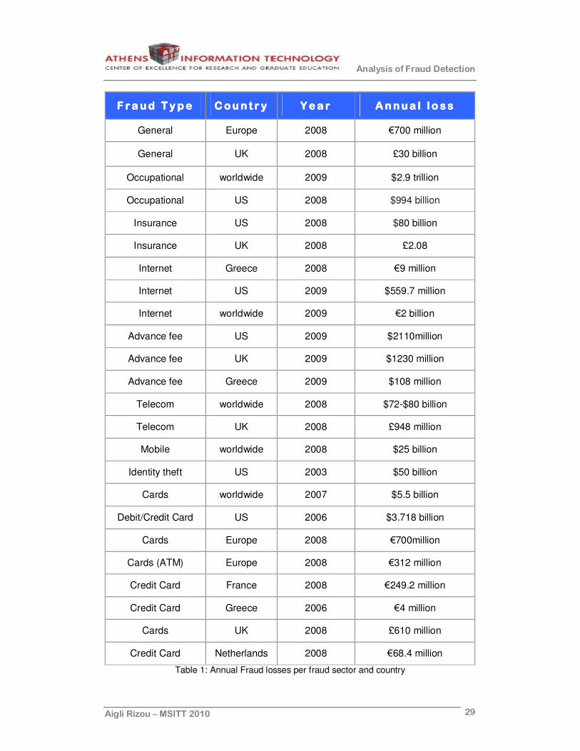
Table 1 contains the size of annual fraud losses of various countries and time
periods based on fraud sector, interpreted in actual figures. Some comments
on the losses are given in the following paragraphs.
It’s important to mention that if detected fraud losses increase, this doesn’t
necessarily mean that there is more fraud or the FD systems improved;
similarly, if detected fraud losses drop, this doesn’t mean that there is less
fraud or worse detection [89].
2 .6 .1 .2 .6 .1 .2 .6 .1 .2 .6 .1 . Genera lGenera lGenera lGenera l
Using fraud figures that are currently available, the National Fraud Authority
(NFA) estimates that fraud cost the UK economy £30.5 billion during 2008
[48]. However, these estimations suggest that public sector losses accounted
for 58% of all fraud loss, with estimated fraud losses of £17.6 billion for the
public sector alone (Figure 3). Next, the private sector losses, which
accounted for 30% of, total loss or £9.3 billion. The individual and charity
sector represents the rest 12% of the total loss, which is translated to £3.5
billion and £32 million respectively.
Analysis of Fraud Detection
Aigli Rizou – MSITT 2010 29
F raud T y peF raud T y peF raud T y peF raud T y pe C oun t r yCoun t r yCoun t r yCoun t r y Y e a rYea rYea rYea r A nnua l l o s sAnnua l l o s sAnnua l l o s sAnnua l l o s s
General Europe 2008 €700 million
General UK 2008 £30 billion
Occupational worldwide 2009 $2.9 trillion
Occupational US 2008 $994 billion
Insurance US 2008 $80 billion
Insurance UK 2008 £2.08
Internet Greece 2008 €9 million
Internet US 2009 $559.7 million
Internet worldwide 2009 €2 billion
Advance fee US 2009 $2110million
Advance fee UK 2009 $1230 million
Advance fee Greece 2009 $108 million
Telecom worldwide 2008 $72-$80 billion
Telecom UK 2008 £948 million
Mobile worldwide 2008 $25 billion
Identity theft US 2003 $50 billion
Cards worldwide 2007 $5.5 billion
Debit/Credit Card US 2006 $3.718 billion
Cards Europe 2008 €700million
Cards (ATM) Europe 2008 €312 million
Credit Card France 2008 €249.2 million
Credit Card Greece 2006 €4 million
Cards UK 2008 £610 million
Credit Card Netherlands 2008 €68.4 million
Table 1: Annual Fraud losses per fraud sector and country

Analysis of Fraud Detection
Aigli Rizou – MSITT 2010 30
Figure 3: Breakdown of fraud losses in UK for 2008 according to NFA [48]
2 .6 .2 .2 .6 .2 .2 .6 .2 .2 .6 .2 . Bank ingBank ingBank ingBank ing
2 .6 .2 .1 .2 .6 .2 .1 .2 .6 .2 .1 .2 .6 .2 .1 . Cred i t /Deb i t ca rdsC red i t /Deb i t ca rdsC red i t /Deb i t ca rdsC red i t /Deb i t ca rds
In 2007, card fraud globally took in an estimated $5.5 billion, based on a
worldwide survey conducted by Kroll Consulting Services in collaboration with
the Economist Intelligence Unit [51].
Concerning Europe figures, the European ATM Security Team (EAST)
estimates that losses of card fraud referring to ATM transactions fell from
€485 million to €312 million during 2008, despite a rise in attacks [15]. Based
on EAST’s estimates international losses due to skimming attacks fell by 43%
from €393 million to €226 million, continuing a downward trend from 2007
[15]. Furthermore, according to Visa, 0.055% of the cards transactions is
considered to be fraudulent and the card fraud turnover is estimated at
€700million [53].

Analysis of Fraud Detection
Aigli Rizou – MSITT 2010 31
Figure 4: Breakdown of card losses in UK during 2008 according to FFA [48]
Figure 5: UK Fraud loss ratios by card type according to Visa estimates for 2008 [16].
Financial Fraud Action (FFA) has reported that over 10.5 billion UK card
transactions have taken place in 2008, with spending amount £397 billion and
card fraud loss up to £610 million, up 14% from 2007 [48]. The majority of
card losses resulted from card-not-present scheme and accounted for over a
Analysis of Fraud Detection
Aigli Rizou – MSITT 2010 32
half of all card losses. However, this should be considered along with changes
in card usage, i.e. many more transactions are made online, by phone or
through mail order than 5 years ago. Figure 4 illustrates that card-not-present
fraud appears the highest losses (£328.4 million) whilst the application fraud
appears the lowest losses (£11 million) [48]. Additionally, Figure 5 shows the
UK fraud loss ratios by type of card, where credit cards stand out significantly
[16].
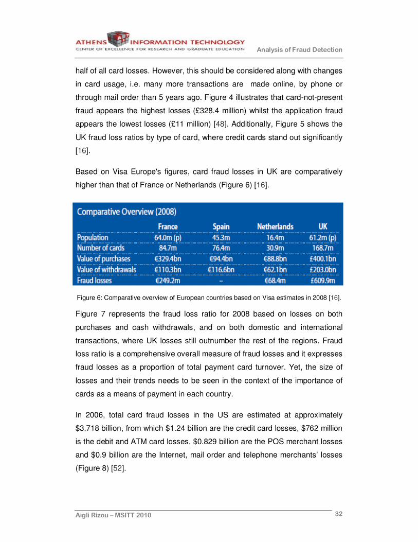
Based on Visa Europe's figures, card fraud losses in UK are comparatively
higher than that of France or Netherlands (Figure 6) [16].
Figure 6: Comparative overview of European countries based on Visa estimates in 2008 [16].
Figure 7 represents the fraud loss ratio for 2008 based on losses on both
purchases and cash withdrawals, and on both domestic and international
transactions, where UK losses still outnumber the rest of the regions. Fraud
loss ratio is a comprehensive overall measure of fraud losses and it expresses
fraud losses as a proportion of total payment card turnover. Yet, the size of
losses and their trends needs to be seen in the context of the importance of
cards as a means of payment in each country.
In 2006, total card fraud losses in the US are estimated at approximately
$3.718 billion, from which $1.24 billion are the credit card losses, $762 million
is the debit and ATM card losses, $0.829 billion are the POS merchant losses
and $0.9 billion are the Internet, mail order and telephone merchants’ losses
(Figure 8) [52].

Analysis of Fraud Detection
Aigli Rizou – MSITT 2010 33
Figure 7: Fraud loss ratios of 2008 according to Visa [16].
Greek banks and financial institutions as well as Visa and MasterCard
estimate that card fraud loss in Greece is half than the corresponding
European losses. For every, €1000 transaction, €0.35 is the result of fraud,
while in Europe the corresponding amount is €0.75 and the total turnover is
estimated to €1,2-€1,5 billion. This implies that debit and credit card fraud
turnover is calculated around €4 million and concerns 2.500 cardholders, with
average loss €110 each. The most frequent fraud types in Greece are: 23%
counterfeiting, 24% stolen cards, 26% lost cards and 27% other types. The
corresponding percentages in Europe are 35%, 19%, 17% and 29% [28].
Card fraud losses in billions $ (US, 2006)
0,7620,829
0,9
1,24
0
0,2
0,4
0,6
0,8
1
1,2
1,4
credit card debit and ATM POS merchant losses Internet, mail order and telephone merchants’
Figure 8: Card fraud losses in the US for 2006
Analysis of Fraud Detection
Aigli Rizou – MSITT 2010 34
2 .6 .2 .2 .2 .6 .2 .2 .2 .6 .2 .2 .2 .6 .2 .2 . I d en t i t y TI den t i t y TI den t i t y TI den t i t y T he f the f th e f th e f t
During 2007, nearly 10 million victims of identity theft fraud in the US have
been recorded and the total loss to individuals and businesses has risen to
$50 billion, according to Federal Trade Commission survey. In addition, the
average loss to a business is $4.800. Total business losses from identity theft
exceeded $47 billion during 2008 [5, 11].
2 .6 .3 .2 .6 .3 .2 .6 .3 .2 .6 .3 . Ente rpr i sesEn te r pr i sesEn te r pr i sesEn te r pr i ses
According to survey of the Association of Certified Fraud Experts (ACFE),
including more than 106 nations – with more than 40% of the cases occurring
in countries outside the US – total global occupation fraud loss is estimated
more than $2.9 trillion between January 2008 and December 2009 [25].
Furthermore, the US companies lose 7% of their annual revenues due to
occupational fraud, which is translated to $994 billion.
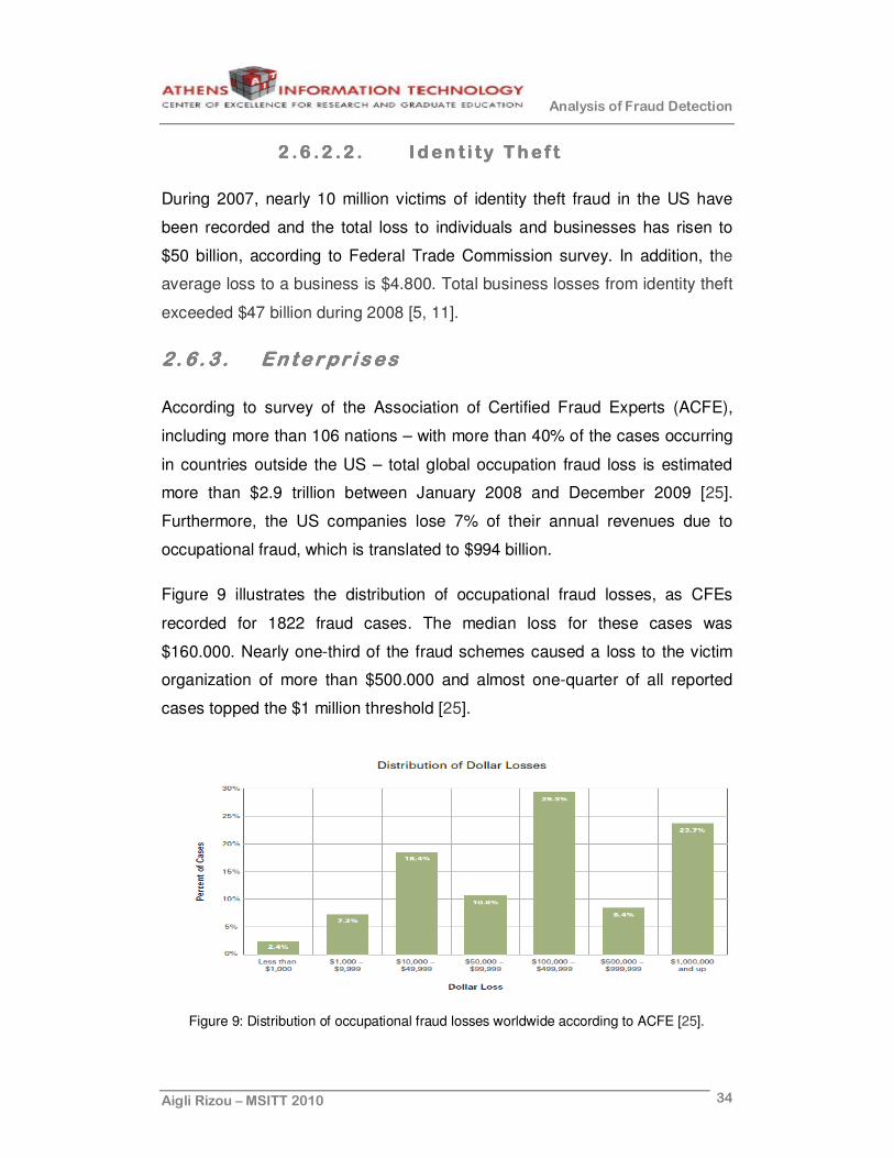
Figure 9 illustrates the distribution of occupational fraud losses, as CFEs
recorded for 1822 fraud cases. The median loss for these cases was
$160.000. Nearly one-third of the fraud schemes caused a loss to the victim
organization of more than $500.000 and almost one-quarter of all reported
cases topped the $1 million threshold [25].
Figure 9: Distribution of occupational fraud losses worldwide according to ACFE [25].

Analysis of Fraud Detection
Aigli Rizou – MSITT 2010 35
In addition, Figure 10 shows the proportion of the total losses based on fraud
category. Referring to cases which cost more than $18 billion, 21% were
caused by asset misappropriation, 11% by corruption and 68% by fraudulent
financial statements.
Figure 10: Proportion analysis per fraud category according to ACFE
[25].
Analyzing the median losses of occupational fraud per scheme worldwide
(Figure 11), the asset misappropriation appears to be the least costly, despite
its high frequency. In contrast, financial statement fraud caused a loss of more
than $4 million and corruption schemes fell in the middle category, creating a
median loss of $250.000.
Figure 11: Median occupational fraud losses by category for 106 nations according to ACFE [25].

Analysis of Fraud Detection
Aigli Rizou – MSITT 2010 36
2 .6 .4 .2 .6 .4 .2 .6 .4 .2 .6 .4 . I ns ur anceIns ur anceIns ur anceIns ur ance
The annual losses of fraudulent insurance claims are calculated nearly $80
billion in the US, according to the estimates of the Coalition Against Insurance
Fraud. This figure includes all lines of insurance. It’s also a conservative figure
because much insurance fraud goes undetected and unreported. As it’s
mentioned in §2.6, fraud contributes to higher insurance premiums because
insurance companies generally must pass the costs of bogus claims — and of
fighting fraud — onto policyholders [48].
According to Association of British Insurers (ABI), losses occurred by both
detected and undetected insurance fraud in the UK during 2008 reach £2.08
billion. It’s worth mentioning that the UK insurance industry is the largest in
Europe and the third largest in the world accounting for 11% of total worldwide
premium income [47].
2 .6 .5 .2 .6 .5 .2 .6 .5 .2 .6 .5 . I n t er ne tIn t er ne tIn t er ne tIn t er ne t
Internet fraud losses in the USA referred to law enforcement amounts to
$559.7 million in 2009 according to the Internet Crime Complaint Center (IC3)
[46]. Figure 12 shows the increasing internet fraud losses of referred
complaints from 2001 until 2009 for the US.
Figure 12: Annual dollar loss of referred complaints according to IC3 (in millions) [46].
On the other hand, the total turnover per year in Greece reached from €3,2
million in 2007 to €9 million in 2008. At the same time, the global turnover is
Analysis of Fraud Detection
Aigli Rizou – MSITT 2010 37
estimated more than €2 billion.
2 .6 .5 .1 .2 .6 .5 .1 .2 .6 .5 .1 .2 .6 .5 .1 . Advance Advance Advance Advance Fe e F raud Fe e F raud Fe e F raud Fe e F raud –––– 41 9 S 41 9 S 41 9 S 41 9 S camcamcamcam
According to Ultrascan Advanced Global Investigations (AGI), currently there
is no country even actively encourages the reporting of these criminal
attempts to defraud to the authorities [54]. Reporting is only limited only to
cases in which there has been a financial loss. There are, of course, only a
very small percentage of the total criminal attempts to defraud by the 419ers
(though the number of loss cases is still huge both in numbers of victims and
amounts lost). When only these loss cases are considered in statistics on 419,
the true massive magnitude of 419 Advance fee fraud criminal activities is
obscured- as only the tip of the iceberg of the actual numbers of 419 crimes is
being included in the statistics [54].
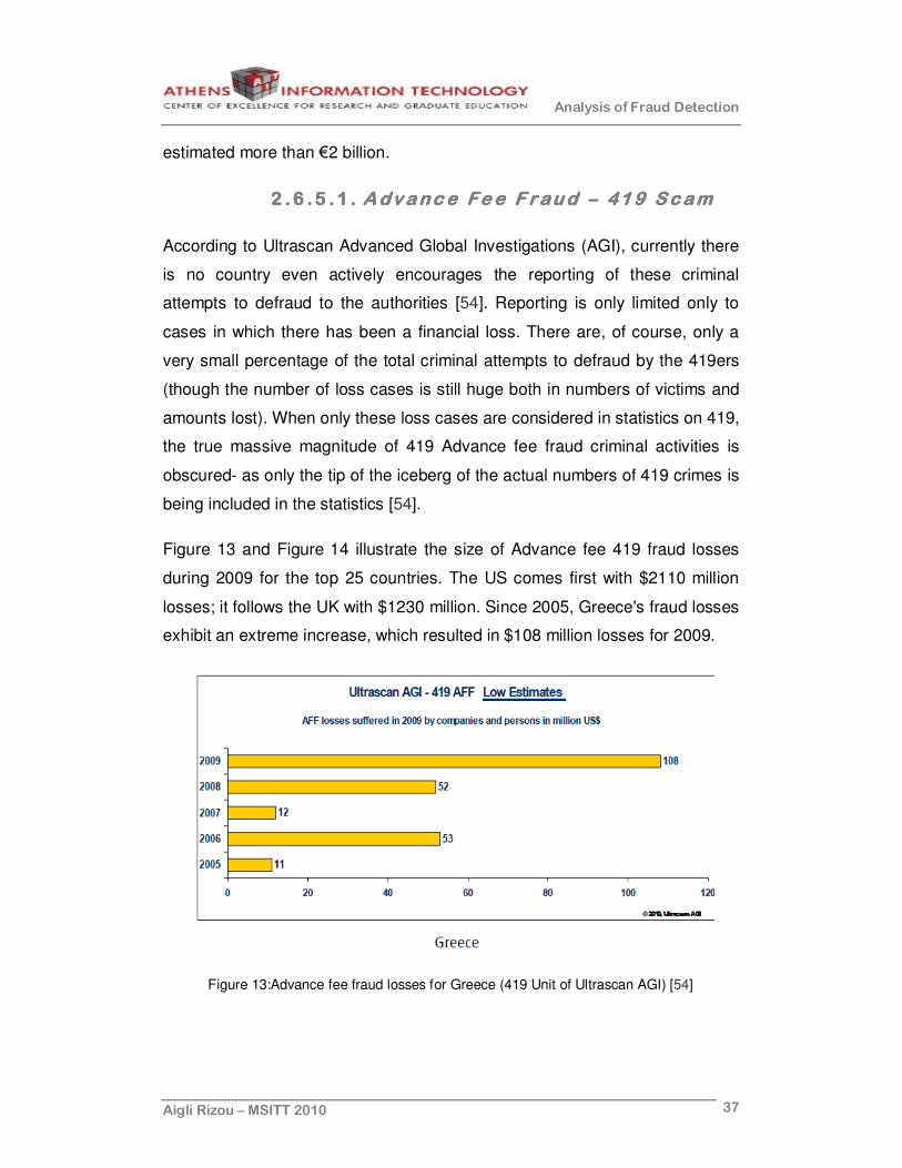
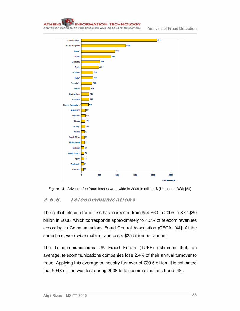
Figure 13 and Figure 14 illustrate the size of Advance fee 419 fraud losses
during 2009 for the top 25 countries. The US comes first with $2110 million
losses; it follows the UK with $1230 million. Since 2005, Greece's fraud losses
exhibit an extreme increase, which resulted in $108 million losses for 2009.
Figure 13:Advance fee fraud losses for Greece (419 Unit of Ultrascan AGI) [54]
Analysis of Fraud Detection
Aigli Rizou – MSITT 2010 38
Figure 14: Advance fee fraud losses worldwide in 2009 in million $ (Ultrascan AGI) [54]
2 .6 .6 .2 .6 .6 .2 .6 .6 .2 .6 .6 . Te l ecommun ica t i onTe l ecommun ica t i onTe l ecommun ica t i onTe l ecommun ica t i on ssss
The global telecom fraud loss has increased from $54-$60 in 2005 to $72-$80
billion in 2008, which corresponds approximately to 4.3% of telecom revenues
according to Communications Fraud Control Association (CFCA) [44]. At the
same time, worldwide mobile fraud costs $25 billion per annum.
The Telecommunications UK Fraud Forum (TUFF) estimates that, on
average, telecommunications companies lose 2.4% of their annual turnover to
fraud. Applying this average to industry turnover of £39.5 billion, it is estimated
that £948 million was lost during 2008 to telecommunications fraud [48].

Analysis of Fraud Detection
Aigli Rizou – MSITT 2010 39
2.7.2.7.2.7.2.7. D i f f i cu l t ies in FDD i f f i cu l t ies in FDD i f f i cu l t ies in FDD i f f i cu l t ies in FD
Fraud is a constantly evolving discipline and a hard task to deal with, so it’s
not surprising that many FD systems exhibit serious limitations. Depending on
the fraud type, different systems with different parameters, database
interfaces, procedures and case management tools should be developed.
Hence, nowadays FD is considered to be a great challenge for numerous
reasons.
Whenever it becomes known that FD method is in place, criminals adapt their
strategies rapidly. To avoid information leaks to fraudsters, FD methods must
be kept secret. New criminals that will enter the field may not be aware of
these FD methods and adopt strategies which lead to identifiable frauds [32].
It’s often the case that there is a subtle distinction between a fraudulent and a
legitimate behaviour, since legitimate account users may gradually change
their behaviour over a long period of time and it’s important to avoid spurious
alarms [32].
Another fundamental problem of FD is the unwillingness of financial
institutions, organizations or companies to admit being defrauded in order to
preserve a good reputation in the market. Due to the severely limited
exchange of ideas in FD, data sets do not become available and the results
are often censored, encumbering the measurement of fraud losses [32].
Beyond these limitations, FD requires the analysis of massive amounts of
transactions data. For example, the credit card company Barclaycard carries
approximately 350 million transactions a year in the United Kingdom alone
(Hand, Blunt, Kelly and Adams, 2000), the Royal Bank of Scotland - which
has the largest credit card merchant acquiring business in Europe - carries
over a billion transactions a year and AT&T carries around 275 million calls
each weekday (Cortes and Pregibon, 1998) [32]. As a consequence,
assuming that the fraudulent transaction represent the 0,1% out of 100 million
transactions and for each fraud case the company loses €10, this implies that

Analysis of Fraud Detection
Aigli Rizou – MSITT 2010 40
the fraud cost or alternatively the potential value of FD amounts to €1 million.
Processing huge data sets in a search for fraudulent transactions in a timely
manner is an important problem [32]. Experienced and well-trained employees
are capable of effective manual classification of transactions, comparing with
historical data. Yet, time and cost requirements render this aspect prohibitive
[18].
High dimensionality of the input, i.e. the number of attributes, is another point
to be considered. This implies that the search space also increases in an
exponential manner and thus the processing time is affected [57].
There is no doubt that the correct choice of data attributes is often a tricky
task. The existence of both irrelative variables and mixed attribute data-sets
(i.e. data-sets containing both nominal and continuous attributes) or even
complex data types such as text, signals, images is a crucial factor during FD
[11].
Moreover, the FD task exhibits technical problems because the available
training data are highly skewed, i.e. legitimate transactions outnumber
fraudulent ones [11, 17]. It's estimated that 1 out of 1000 transactions is
fraudulent. This percentage is lower in case of debit card fraud and even
lower in case of web-based banking transactions and money laundering [18].
An additional difficulty in FD procedure lies in the typical validity of
transactions for classification. In particular, almost all transactions concerning
electronic payments are typical valid, since fraudsters do not commit fraud
with an expired card [18].
Because of this the typical validity, it is possible that some transaction records
contain original and fake subsets at the same time (class overlapping).
Consequently, the finding of suitable business rules for the discrimination
between original and fraud cases becomes a hard task [18].
Finally, it's noteworthy that the variable misclassification cost per error type

Analysis of Fraud Detection
Aigli Rizou – MSITT 2010 41
burdens significantly the FD process. For example, credit card transactions
may be labelled incorrectly: a fraudulent transaction may remain unobserved
and thus be labelled legitimate (and the extent of this may remain unknown)
or a legitimate transaction may be misreported as fraudulent [32].
2.8.2.8.2.8.2.8. FD SFD SFD SFD Sys temys temys temys tem Requi rements Requi rements Requi rements Requi rements
All the aforementioned difficulties generate the need of a number of business,
technical and functional requirements for the development of a robust FD
system.
2 .8 .1 .2 .8 .1 .2 .8 .1 .2 .8 .1 . Bus iness Bus iness Bus iness Bus iness RRRRequ i r emen tsequ i r emen tsequ i r emen tsequ i r emen ts
As it’s already mentioned, fraud losses may imperil the good name and the
profitability of the businesses. In this case, there is a dual impact, which
involves not only the lost amounts but also the internal cost, generated due to
the settlement of the fraud case. So, the reference point for money saving is
the following: spare as less money as possible for fraud cases and their
settlement [18].
Obviously, every time a fraud case appears, the relationship between
customer and the particular organization is put on a risk. So, the point is that a
reliable FD system should produce a minimum number of false alarms for
preserving the customer’s satisfaction [18].
Another key issue in FD is the interception of authorization request in real
time, since fraudsters constitute a serious threat as long as they act
inconspicuously [18], especially in cases such as card fraud.
2 .8 .2 .2 .8 .2 .2 .8 .2 .2 .8 .2 . Techn ica l Techn ica l Techn ica l Techn ica l RRRRequi r emen tsequi r emen tsequi r emen tsequi r emen ts
The connection and the integration of new FD solutions in an existent
business environment cause many problems due to the high cost. Hence, the
FD solution should be flexible and available for the majority of technological

Analysis of Fraud Detection
Aigli Rizou – MSITT 2010 42
platforms and should allow the easy integration and interconnection. Thus, the
implementation and maintenance cost remains low [18].
2 .8 .3 .2 .8 .3 .2 .8 .3 .2 .8 .3 . Funct ional Requi rements
The percentage of false alarms is slightly connected with the percentage of
response. This means that when there is high percentage of responses, then
several false alarms are produced, which leads to customers’ inconvenience.
Consequently, the number of the accepted false alarms helps to define how
many cases will be investigated. This suggests that there should be a
balance between the number of false alarms and responses [18].
Usually, each service provider knows better the fraud issues that encounters.
For this reason, the internal design of an FD system is a secure approach. In
addition, fraud experts should be very precise and studious during the system
design and the goal is to create an FD system totally transparent to them [18].
Some fraud types are global and other appear in specific areas or in specific
service providers. These are the rarest ones, but they can cause great losses.
Given the rampant change of fraud types, it’s very important to use FD safety
measures as fast as possible. Hence, the system processor should be
capable of preserving the decision logic in an independent way [18].
Last but not least, fraud systems should not be awkward to use. The goal is to
facilitate fraud experts during FD, so as to avoid wasting time on simple tasks,
such as retrieving the necessary analytical data of the transaction from
several disparate databases.
2.9.2.9.2.9.2.9. PerformanPerformanPerformanPerformance Mce Mce Mce Metr icsetr icsetr icsetr ics
The performance of a FD system is a subtle matter with many pitfalls and
ambiguous opinions. The performance is usually defined by each service
provider’s needs and requirements and it’s strongly connected with the losses
a service provider is able to prevent. Because measuring averted losses is not
Analysis of Fraud Detection
Aigli Rizou – MSITT 2010 43
a feasible task, service providers use metrics as detection rate and false
alarm rate [39]. Additional information for classifiers’ performance metrics is
given in §5.2.2.1.
An ideal FD system would have 0% false alarms and 100% hits with
instantaneous detection. Though, the successful detection of all fraud cases
as soon as fraud starts implies that many legitimate cases will be mislabelled
as fraudulent at least once. In fact, in a real FD system there is a trade-off of
the above performance criteria.
False alarm rate refers to the percentage of legitimate instances mislabelled
as fraud. In case of 1000000 legitimate instances in the total population out of
which 100 cases are mislabelled as fraud, this gives a false alarm rate of
0.01%. This measure is considered to be important especially in the flagging
phase, where fraud experts aim at reducing the number of cases that have to
be investigated for fraud to just those that involve actual fraud [39].
As it is mentioned in §5.1, when there is no clear evidence of fraud, there
should be a further analysis by the fraud analysts, before the interception of a
transaction, the restriction of an account or the denial of an insurance claim. In
this case, the flagged instances with the highest priority in the queue are
investigated first, whenever a fraud analyst is available. A queue may
prioritize instances by the number of fraudulent minutes accumulated to date
or by the time of the most recent high scoring call, for example. Performance
can then be evaluated after flagging or after prioritization. For example, the
flagging detection rate is the fraction of compromised accounts in the
population that are flagged. In addition, the system detection rate is the
fraction of compromised accounts in the population that are investigated by a
fraud analyst. The system and flagging detection rates are equal only when
fraud analysts or investigators investigate all flagged instances. Otherwise,
the system detection rate is smaller than the flagging detection rate because
both detection rates are computed relative to the number of accounts with
fraud in the population [39].
Analysis of Fraud Detection
Aigli Rizou – MSITT 2010 44
Another key issue is that investigators should focus on fraud cases and not
spend time on investigating legitimate instances. This implies that there
should be a precise definition of the percentage of investigated cases that
involve potential fraud. The flagging hit rate is the fraction of flagged instances
that have fraud, and the system hit rate is the fraction of investigated cases
that have fraud. The (1- system hit rate) is often a good measure of the
service provider's perception of the “real false alarm rate”, especially since
this is the only error rate that the service provider can evaluate easily from
experience. That is, only the cases that are investigated may be of service
provider’s concern and not the legitimate cases in the population that were
never classified as suspicious. If 20 cases of fraud are investigated and only 8
turn out to be fraud, then a service provider may feel that the “real false alarm
rate" is 60%, even if only .01% of the legitimate accounts in the population are
flagged as fraud [39].
Moreover, the difference between the fraction of fraud in the population and
the fraction of fraud in flagged instances is used as a measure of the
efficiency of the FD algorithm. Similarly, the system hit rate should be larger
than the flagging hit rate, or else the analyst can find as much fraud by
randomly selecting one of the flagged accounts to investigate [39].
Despite the aforementioned metrics, a key point during FD performance
measurement is the uncertain misclassification costs which are equal to false
positive and false negative error costs. These costs differ from example to
example and may change over time. A common practice is that a false
negative error costs more than a false positive error.
The following paragraph includes an additional performance measure of FD,
which is a result of the aforementioned detection and false alarm rate.
2 .9 .1 .2 .9 .1 .2 .9 .1 .2 .9 .1 . Rece iv er Oper a t i ng Char ac ter i s t i c Rece iv er Oper a t i ng Char ac ter i s t i c Rece iv er Oper a t i ng Char ac ter i s t i c Rece iv er Oper a t i ng Char ac ter i s t i c
(ROC)(ROC)(ROC)(ROC)
The striking feature of FD is finding the right balance between detection of

Analysis of Fraud Detection
Aigli Rizou – MSITT 2010 45
actual fraudulent users and the production of false alarms. For instance,
telecommunications service providers are very cautious about unnecessary
bothering of good customers. This implies that false alarm rate are not
common for all FD applications, since the number of users and thus the size
or processed record varies significantly [40].
The Receiver Operating Characteristic plots the percentage of correct
detection fraud cases versus the percentage of false alarms for non-fraudulent
users for varying values of the threshold. In other words, ROC curve is a
graphical plot of the sensitivity (true positive rate) versus the (1-specificity) or
false positive rate for a binary classification problem as the discrimination
threshold is varied [2]. The ROC curve is typically shown on a 2-D graph,
where false alarm rate and detection rate are plotted on x-axis and y-axis
respectively (Figure 15).
The ideal ROC curve has 0% false alarm rate and 100% detection rate, but
this is not a real case scenario. Hence, researchers compute detection rate for
different false alarm rates and present the results on ROC curves [84].
Figure 15: Receiver Operating Characteristic curve & the Area Under the Curve [84].
Furthermore, the Area Under the Curve (AUC) is often used to gauge the
classification performance of a FD system. The AUC is defined as the surface
area under the ROC curve (Figure 15 – shaded area) and it’s set to be 1 for
the case of ideal scenario. In practice, the AUC is the index of performance
needs to be maximized.

Analysis of Fraud Detection
Aigli Rizou – MSITT 2010 46
3333 THEORETICAL PERSPECTIVETHEORETICAL PERSPECTIVETHEORETICAL PERSPECTIVETHEORETICAL PERSPECTIVE
3.1.3.1.3.1.3.1. FD MethodsFD MethodsFD MethodsFD Methods
Fraud is an adaptive crime, so it requires special methods of intelligent data
analysis to detect and prevent it. FD techniques aim at the automation of the
procedure of pattern recognition and come from the fields of Knowledge
Discovery in Databases (KDD), Data Mining, Machine Learning and Statistics,
which offer applicable and successful solutions in different areas of fraud
crimes [2].
KDD is viewed as the overall process of discovering useful knowledge from
data, while data mining is the application of specific algorithms for extracting
patterns (models) from data. Sometimes, KDD and data mining are used
interchangeably [56].
Machine learning is a scientific discipline refers to the design and
development of algorithms that allow computers to evolve behaviours based
on empirical data, such as from sensor data or databases. A major focus of
machine learning research is to automatically learn to recognize complex
patterns and make intelligent decisions based on data.
3.2.3.2.3.2.3.2. Supervi sed Supervi sed Supervi sed Supervi sed &&&& Unsuperv ised Unsuperv ised Unsuperv ised Unsuperv ised LLLLearningearningearningearning
MMMMethodsethodsethodsethods
Supervised learning methods attempt to discover the relationships between
input attributes (independent variables) and a target attribute (dependent
variable) [57]. The relationship discovered is represented in a structure
THEORETICAL
PERSPECTIVE
Analysis of Fraud Detection
Aigli Rizou – MSITT 2010 47
referred to as a Model, used to describe and explain phenomena, which are
hidden in the dataset. It can be, also, used for predicting the value of the
target attribute knowing the values of the input attributes.
In supervised methods, samples of both fraudulent and non-fraudulent
records are necessary to construct models which allow one to assign new
observations into one of the two classes. Of course, this requires one to be
confident about the true classes of the original data used to build the models.
It, also, requires that one has examples of both classes. Furthermore, it can
only be used to detect frauds of a type which have previously occurred [32].
The supervised models are distinguished into two main categories: a)
Classification models known as classifiers (§3.2.1) and b) Regression models
(§3.2.2)
In contrast, the unsupervised learning refers to modelling the distribution of
instances in a typical, high-dimensional input space. According to [Kohavi and
Provost (1998)] the term "Unsupervised learning" refers to “learning
techniques that group instances without a pre-specified dependent attribute"
[57].
Unsupervised methods simply seek those accounts, customers, transactions
and so forth which are most dissimilar from the norm. Typical characteristic of
unsupervised methods is the fact that there are no prior set of legitimate and
fraudulent observations. Fraud experts model a baseline distribution that
represents normal behaviour and then attempt to detect observations that
show the greatest departure from this norm [32].
3 .2 .1 .3 .2 .1 .3 .2 .1 .3 .2 .1 . Cl ass i f i ca t i onC l ass i f i ca t i onC l ass i f i ca t i onC l ass i f i ca t i on
Classification is learning a function that maps (classifies) a data item into one
of several predefined classes (Weiss and Kulikowski 1991; Hand 1981).
Figure 16 shows a simple partitioning of loan data into two class regions. The
bank may use the classification regions to automatically decide whether future

Analysis of Fraud Detection
Aigli Rizou – MSITT 2010 48
loan applicants will be given a loan or not [85]. The most widely known
classifiers are analyzed in the next paragraphs.
Figure 16: A Simple Linear Classification Boundary for the Loan Data Set, where the shaped region denotes class no loan [85].
3 .2 .1 .1 .3 .2 .1 .1 .3 .2 .1 .1 .3 .2 .1 .1 . Dec is i on T re eDec is i on T re eDec is i on T re eDec is i on T re e (DT ) (DT ) (DT ) (DT )
DTs are decision making prediction models with a simple representational
form. They generate rules to classify a data set, where each tree represents a
set of decisions. DT is based on “divide and conquer” technique, which means
that the problem is broken down into two or more sub-problems of the same
(or related) type, until these become simple enough to be solved directly. The
solutions to the sub-problems are then combined to give a solution to the
original problem.
To be more specific, a DT is a classifier expressed as a recursive partition of
the instance space. It consists of nodes that form a rooted tree, meaning that
it is a directed tree with a node called root that has no incoming edges. All
other nodes have exactly one incoming edge. A node with outgoing edges is
called internal node or test nodes and all other nodes are called leaves [57].
In a DT, each internal node splits the instance space into two or more
subspaces according to a certain discrete function of the input attributes
values. In the simplest and most frequent case, each test considers a single
attribute, such that the instance space is partitioned according to the
attribute's value. In the case of numeric attributes -with continuous values- the

Analysis of Fraud Detection
Aigli Rizou – MSITT 2010 49
condition refers to a range and it refers to regression (§3.2.2) [57].
Figure 17 represents a DT example, where given this classifier all transactions
with a probability of >=0.70 (defined threshold) will be indicated and alerted as
fraud [61].
Figure 17: An indicative DT example [61].
3 .2 .1 .1 . 1 .3 .2 .1 .1 . 1 .3 .2 .1 .1 . 1 .3 .2 .1 .1 . 1 . C4. 5 ( J48 )C4. 5 ( J48 )C4. 5 ( J48 )C4. 5 ( J48 )
The DTs generated by C4.5 algorithm as following: Initially, the most
characteristic attribute is selected in order to become a tree root. This
appropriate selection constitutes the key to successful DT, due to the effective
division of problem space. For each different value, a root descendant is
generated and all the training instances which bear this value are mapped
with the descendant. The whole process is repeated retrospectively for each
descendant of the DT root, limiting the examined trained subset to the
instances that have been mapped to this node. The termination of this
process happens when one of the following conditions are satisfied: a) all the
instances of the current node belong to the same class and b) all the
attributes have been used.
One of the most popular mechanisms for instance space partitioning is that of

Analysis of Fraud Detection
Aigli Rizou – MSITT 2010 50
Information Entropy, which selects that independent variable that leads to the
most compact tree. Let S be the training set at the point of partitioning (node),
the entropy measures the existent incongruity in S, referring to the dependent
variable under consideration. In practice, the Information Gain represents the
reduction in entropy of a training set S, as a result of the usage of a specific
attribute, let A. In other words, it is a measure for the attribute evaluation.
3 .2 .1 .2 .3 .2 .1 .2 .3 .2 .1 .2 .3 .2 .1 .2 . AAAA r t i f i c i a l Neu ra l Ne two rks (ANN )r t i f i c i a l Neu ra l Ne two rks (ANN )r t i f i c i a l Neu ra l Ne two rks (ANN )r t i f i c i a l Neu ra l Ne two rks (ANN )
ANNs resemble the central processing unit (CPU) of a biological neural
network, the human brain, in the following two ways: a) an ANN acquires
knowledge through learning and b) an ANN's knowledge is stored within inter-
neuron connection strengths known as synaptic weights [66].
A human brain is highly complex, nonlinear, and parallel computer, made up
of about 100 billion tiny units called neurons (Figure 18) and has the capability
of organizing neurons so as to perform certain computations many times
faster than the fastest digital computer in existence today [19].
Each neuron is connected to thousands of other neurons and communicates
with them via electrochemical signals. Signals coming into the neuron are
received via junctions called synapses; these in turn are located at the end of
branches of the neuron cell called dendrites.
Figure 18: A human neuron forming a chemical synapse [66].
The neuron continuously receives signals from these inputs and sums up

Analysis of Fraud Detection
Aigli Rizou – MSITT 2010 51
them to itself in some way and then, if the end result is greater than some
threshold value, the neuron fires. It generates a voltage and outputs a signal
along something called an axon.
Each input into the neuron has its own weight, which is adjusted for the
network training (Figure 19). When each input enters the nucleus (blue circle),
it's multiplied by its weight. The nucleus, then, sums all these new input
values which gives us the activation. If the activation is greater than a
threshold value the neuron outputs a signal; otherwise the neuron outputs
zero.
Figure 19: Artificial Neuron (Perceptron) [66].
Given that a neuron has n number of inputs, x1 ,x2, x3… xn and their
corresponding weights (synaptic strength) are w1, w2, w3… wn, then the
weighted sum becomes:
a = x1w1+x2w2+x3w3... +xnwn or
To express a background activation level of the neuron, an offset (bias) Θ is
added to the weighted sum and this becomes the propagation function. The
bias is a constant term that doesn't depend on any input value (Figure 19).
The activation function computes the output signal Y of the neuron from the
activation level f and it’s of sigmoid type as plotted in the same figure.
There are many different ways of connecting artificial neurons together to
create a neural network but the most common is called a feedforward network
+ Θ

Analysis of Fraud Detection
Aigli Rizou – MSITT 2010 52
(Figure 19). It gets its name from the way the neurons in each layer feed their
output forward to the next layer until we get the final output from the neural
network. The simplest kind of a feedforward network is the perceptron (Figure
20), which is a single layer neural network whose weights and biases could be
trained to produce a correct target output when presented with the
corresponding input [67].
Once the ANN has been created, it needs to be trained. One way of doing this
is initialize the neural net with random weights and then feed it a training set.
There are many different ways of adjusting the weights of ANN, but the most
common is called backpropagation (BP). This method efficiently propagates
values of the evaluation function backward from the output of the network,
which then allows the network to be adapted so as to obtain a better
evaluation score. In other words, a BP network learns by example, which
implies that it needs as feedback some input examples and the known-correct
output for each case and this will result in network adaptation.
Figure 20: Three-Layer feedforward ANN
The most common feedforward ANN model is the multilayer perceptron
(MLP), which consists of multiple layers of nodes in a directed graph. The goal
of this type of network is to create a model that correctly maps the input to the
output using historical data so that the model can then be used to produce the
output when the desired output is unknown. MLP utilizes BP technique for
training the network. A graphical representation of an MLP is shown Figure
21.
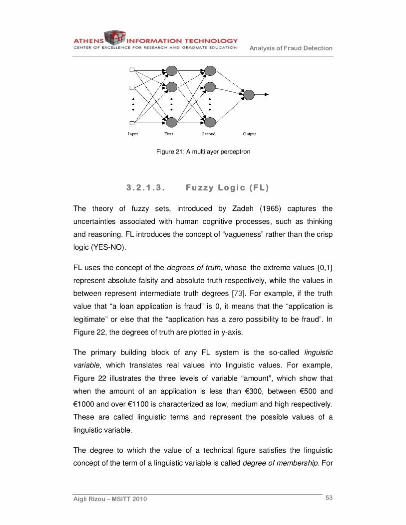
Analysis of Fraud Detection
Aigli Rizou – MSITT 2010 53
Figure 21: A multilayer perceptron
3 .2 .1 .3 .3 .2 .1 .3 .3 .2 .1 .3 .3 .2 .1 .3 . Fu zzy Log i c (F L )Fu zzy Log i c (F L )Fu zzy Log i c (F L )Fu zzy Log i c (F L )
The theory of fuzzy sets, introduced by Zadeh (1965) captures the
uncertainties associated with human cognitive processes, such as thinking
and reasoning. FL introduces the concept of “vagueness” rather than the crisp
logic (YES-NO).
FL uses the concept of the degrees of truth, whose the extreme values {0,1}
represent absolute falsity and absolute truth respectively, while the values in
between represent intermediate truth degrees [73]. For example, if the truth
value that “a loan application is fraud” is 0, it means that the “application is
legitimate” or else that the “application has a zero possibility to be fraud”. In
Figure 22, the degrees of truth are plotted in y-axis.
The primary building block of any FL system is the so-called linguistic
variable, which translates real values into linguistic values. For example,
Figure 22 illustrates the three levels of variable “amount”, which show that
when the amount of an application is less than €300, between €500 and
€1000 and over €1100 is characterized as low, medium and high respectively.
These are called linguistic terms and represent the possible values of a
linguistic variable.
The degree to which the value of a technical figure satisfies the linguistic
concept of the term of a linguistic variable is called degree of membership. For

Analysis of Fraud Detection
Aigli Rizou – MSITT 2010 54
a continuous attribute, this degree is expressed by a function called
membership function. The membership functions map each value of the
technical figure to the membership degree to the linguistic terms. Figure 22
plots the membership functions of all terms of the linguistic variable “amount”
into the same graph.
Figure 22: Membership function of the linguistic variable “amount” in FL
FL models consist of a number of conditional "IF-THEN" rules [74]. Fuzzy
systems often glean their rules from experts. These rules are a transparent
way of imitating human decision processes and they are basically made up of
linguistic variables, associated linguistic terms, and connecting FL operators,
allowing more direct modeling [19].
3 .2 .1 .4 .3 .2 .1 .4 .3 .2 .1 .4 .3 .2 .1 .4 . Fu zzy Neu ra l Netwo rk ( FNN )Fu zzy Neu ra l Netwo rk ( FNN )Fu zzy Neu ra l Netwo rk ( FNN )Fu zzy Neu ra l Netwo rk ( FNN )
The fusion of ANN and FL in neuro-fuzzy models provides learning as well as
readability. FNN systems combine the human-like reasoning style of FL
systems with the learning and connectionist structure of ANN [2].
However, the simplicity of an FL system constitutes an important
disadvantage, since the “IF-THEN” rules must derive from the huge data sets,
which is not an easy task. At this point, ANNs play a significant role due to
their power of training a system with the available data sets. ANN can learn
from data sets while FL solutions are easy to verify and optimize [19].

Analysis of Fraud Detection
Aigli Rizou – MSITT 2010 55
3 .2 .1 .5 .3 .2 .1 .5 .3 .2 .1 .5 .3 .2 .1 .5 . Naï v e BayeNaï v e BayeNaï v e BayeNaï v e Baye s (NB )s (NB )s (NB )s (NB )
The NB classifier algorithm is based on the so-called Bayes theorem and is
particularly suited when the dimensionality of the inputs is high [55].
Suppose the given data consist of card transactions, described by their time
and amount. Bayesian classifiers operate by saying "If a transaction of €1000
that took place at night, in which of the two classes (legitimate or fraud) is it
likely to belong, based on the observed data sample? In future, classify these
transactions as that type."
A difficulty arises when there are more than a few variables and classes,
because it’s required that there should be an estimation of these probabilities
for an enormous number of observations (records).
NB classification gets around this problem by not requiring that there are lots
of observations for each possible combination of the variables. Rather, the
variables are assumed to be independent of one another. Therefore the
probability that a transaction of €1000, took place at night, with 123 as a
Processing code with cardholder’s name Smith etc. will be fraud can be
calculated from the independent probabilities that a transaction had the
following characteristics: amount= €1000, time=night, Processing code=123
and cardholder’s name= Smith, etc.
In other words, NB classifiers assume that the effect of a variable value on a
given class is independent of the values of other variable. This assumption is
called class conditional independence and is often not applicable. It is made
to simplify the computation and in this sense considered to be naïve.
However, it is the order of the probabilities, not their exact values that
determine the classifications [64].
3 .2 .1 .6 .3 .2 .1 .6 .3 .2 .1 .6 .3 .2 .1 .6 . Suppo r t Vec to r MacSuppo r t Vec to r MacSuppo r t Vec to r MacSuppo r t Vec to r Mach i nes ( SVM)h i nes ( SVM)h i nes ( SVM)h i nes ( SVM)
A SVM performs classification by constructing an N-dimensional hyperplane
that optimally separates the data into two categories. The goal of SVM

Analysis of Fraud Detection
Aigli Rizou – MSITT 2010 56
modelling is to find the optimal hyperplane that separates clusters of vector in
such a way that cases with one category of the target variable are on one side
of the plane and cases with the other category are on the other size of the
plane. The vectors near the hyperplane are the support vectors [65].
Figure 23 shows a simple two-dimensional example. In this case, the data has
a categorical target variable with two categories. One category of the target
variable is represented by rectangles while the other category is represented
by ovals and they are completely separated. The SVM analysis attempts to
find a one-dimensional hyperplane (i.e. a line) that separates the cases based
on their target categories. There are an infinite number of possible lines and
two candidate lines are shown in Figure 23. The question is which line is
better, and how do we define the optimal line.
The dashed lines drawn parallel to the separating line mark the distance
between the dividing line and the closest vectors to the line. The distance
between the dashed lines is called the margin. The vectors (points) that
constrain the width of the margin are the support vectors (Figure 23).
However, in real life scenarios SVM deals with: (a) more than two predictor
variables, (b) separating the points with non-linear curves, (c) handling the
cases where clusters cannot be completely separated, and (d) handling
classifications with more than two categories.
Figure 23: Margins and Support Vectors in a two-dimensional example [65]

Analysis of Fraud Detection
Aigli Rizou – MSITT 2010 57
3 .2 .2 .3 .2 .2 .3 .2 .2 .3 .2 .2 . L inear and Logi s t i c Regr ess i onL inear and Logi s t i c Regr ess i onL inear and Logi s t i c Regr ess i onL inear and Logi s t i c Regr ess i on
Regression is learning a function that maps a data item to a real-valued
prediction variable [85].
Linear regression models the relationship between a dependent variable y
and one or more independent variables X, using linear functions. It can be
used to fit a predictive model to an observed data set of y and X values. After
developing such model, if an additional value of X is then given without its
accompanying value of y, the fitted model can be used to make a prediction of
the value y [2].
On the contrary, logistic regression is a variation of ordinary regression which
is used when the dependent (output) variable is a dichotomous variable (i. e. it
takes only two values, which usually represent the occurrence or non-
occurrence of some outcome event, usually coded as 0 or 1) and the
independent (input) variables are continuous, categorical, or both [64]. Unlike
ordinary linear regression, logistic regression does not assume that the
relationship between the independent variables and the dependent variable is
a linear one.
3 .2 .3 .3 .2 .3 .3 .2 .3 .3 .2 .3 . Clus ter i ngC lus ter i ngC lus ter i ngC lus ter i ng
Clustering is a common descriptive task where one seeks to identify a finite
set of categories or clusters to describe the data (Jain and Dubes 1988;
Titterington, Smith, and Makov 1985). Figure 24 shows a possible clustering
of the loan data set into three clusters, where the clusters overlap, and
allowing data points to belong to more than one cluster. The original class
labels (denoted by x’s and o’s in the previous figures) have been replaced by
a '+' to indicate that the class membership is no longer assumed known.
3 .2 .3 .1 .3 .2 .3 .1 .3 .2 .3 .1 .3 .2 .3 .1 . Ou t l i e r Ou t l i e r Ou t l i e r Ou t l i e r DDDDe tec t i o ne tec t i o ne tec t i o ne tec t i o n
An outlier is an observation of the data that deviates from other observations
so much that it arouses suspicions that it was generated by a different

Analysis of Fraud Detection
Aigli Rizou – MSITT 2010 58
mechanism from the most part of data [68]. In FD, outlier detection helps to
recognize fraudulent behaviour through an exception in the amount of money
spent, type of items purchased, time and location.
Outliers may be erroneous or real in the following sense. Real outliers are
observations whose actual values are very different than those observed for
the rest of the data and violate plausible relationships among variables.
Erroneous outliers are observations that are distorted during data collection.
Many data-mining algorithms find outliers as a side-product of clustering
algorithms. However, these techniques define outliers as points, which do not
lie in clusters. Thus, the techniques implicitly define outliers as the
background noise in which the clusters are embedded. Another class of
techniques defines outliers as points, which are neither a part of a cluster nor
a part of the background noise; rather they are specifically points which
behave very differently from the norm.
Figure 24: Example of clustering [85].
3 .2 .4 .3 .2 .4 .3 .2 .4 .3 .2 .4 . MetaMe taMe taMe ta ---- l e arn inglearn inglearn inglearn ing
The efficiency of a model generated by machine learning algorithms is based
not only on the size and the quality of training set, but also on the
appropriateness of the selected algorithm. There is often the case to utilize
the experience of more than one model-expert, whose combination leads to
the final output for a specific data set. At this point, the various classifiers stem
from the training of a single algorithm applied on different subsets of the

Analysis of Fraud Detection
Aigli Rizou – MSITT 2010 59
available data set.
Meta-learning methods take advantage of the lack of stability of some learning
algorithms or else the oversensitivity towards the small changes of input data.
The aim is the successive creation of models, capable of complementing each
other. This implies that one model will outperform others in a specific subset
of the training set, where the others will have disadvantages. As it is expected,
meta-learning methods show better results for unstable algorithms, i.e.
algorithms which generate classifiers quite different for only a small change of
the training set.
3 .2 .4 .1 .3 .2 .4 .1 .3 .2 .4 .1 .3 .2 .4 .1 . Bagg i ng (Boo ts t rap Agg rega t i ng )Bagg i ng (Boo ts t rap Agg rega t i ng )Bagg i ng (Boo ts t rap Agg rega t i ng )Bagg i ng (Boo ts t rap Agg rega t i ng )
Bagging involves having each model in the ensemble2 vote with equal weight.
It’s the simplest meta-learning method and it is based on the production of a
number of models (sub-classifiers), which come from a common learning
algorithm. The point is that in each case the sampling of the training set
differentiates. Decision is taken following the voting method, which means that
the final decision of the system coincides with the decision of the majority. In
the case of cross-validated committees the subsets of the training data are
defined through the cross-validation (§5.2.3) method [2].
Figure 25: Graphical representation of bagging.
In Figure 25, D represents the training set, D1,..., Dt represent the various data 2 Ensemble methods use multiple models to obtain better predictive performance that could
be obtained from any of the constituent models [2]. These methods centre around producing classifiers that disagree as much as possible on their predictions [70].
Analysis of Fraud Detection
Aigli Rizou – MSITT 2010 60
sets (1st step), C1,...,Ct represent the various classifiers per data set (2nd step)
and C represent the final classifier as a result of the combination of C1,...,Ct
(3rd step).
3 .2 .4 .2 .3 .2 .4 .2 .3 .2 .4 .2 .3 .2 .4 .2 . S tack ing ( S t acked Gen era l i z a tS t ack ing ( S t acked Gen era l i z a tS t ack ing ( S t acked Gen era l i z a tS t ack ing ( S t acked Gen era l i z a t io n )io n )io n )io n )
It is a type of ensemble learning, where the set of the models used come from
different learning algorithms, in contrast with most of the approaches.
Additionally, the final decision-making doesn't presuppose the majority voting
or the weighted estimation of individual decisions. Conversely, stacking uses
a model-leader that judges which of the set of the competitors learning
algorithms are the best [2]. The choice among a set of models is done with
cross-validation (§5.2.3) as well.
3 .2 .4 .3 .3 .2 .4 .3 .3 .2 .4 .3 .3 .2 .4 .3 . Boos t i ngBoos t i ngBoos t i ngBoos t i ng
Boosting involves incrementally building an ensemble by training each new
model instance to emphasize the training instances that previous models
misclassified. It is a general method which attempts to boost the accuracy of
any given learning algorithm. The focus of boosting methods is to produce
iteratively learning weak classifiers3 with respect to a distribution and then
adding them to produce a more powerful combination or else a strong
classifier. Thus, boosting attempts to produce new classifiers that are better
able to predict examples for which the current ensemble's performance is
poor [2, 88].
When the weak classifiers are added, they are typically weighted in a way that
is usually related to the weak learner's accuracy. Next, the data is reweighed,
which implies that misclassified examples gain weight and examples correctly
classified lose weight. Unlike bagging (§3.2.4.1), future weak classifiers focus
mostly on the examples that previous weak learners misclassified.
3 A weak classifier is a learner that has misclassification error rate only slightly better than
random guessing.
Analysis of Fraud Detection
Aigli Rizou – MSITT 2010 61
4444 ACADEMIC PERSPECTIVEACADEMIC PERSPECTIVEACADEMIC PERSPECTIVEACADEMIC PERSPECTIVE 4 .1.4.1.4.1.4.1. Sc ien t i f ic Sc ien t i f ic Sc ien t i f ic Sc ien t i f ic RRRResearchesearchesearchesearch
FD has been widely studied in terms of scientific research for the last 10
years. The following paragraphs describe experiments carried out in the
academic field. These experiments utilize the aforementioned data mining and
machine learning methods (§3) and draw conclusions for future consideration.
The following material is based on scientific publications and it’s grouped
according to fraud types. Within the present thesis research, it has been
noticed that credit card FD has received the most attention from academic
point of view.
4 .1 .1 .4 .1 .1 .4 .1 .1 .4 .1 .1 . Card Card Card Card FDFDFDFD
The following experiment addresses the desirable data distribution, the
pruning4 effects, the use of cost models and the meta-learning advantages.
The research was conducted by Philip K. Chan from Florida Institute of
Technology and Wei Fan, Andreas L. Prodromidis and Salvatore J. Stolfo
from Columbia University [17].
4 .1 .1 .1 .4 .1 .1 .1 .4 .1 .1 .1 .4 .1 .1 .1 . Expe r iment 1Expe r imen t 1Expe r imen t 1Expe r imen t 1 ---- Desc r i p t i on Desc r i p t i on Desc r i p t i on Desc r i p t i on
The proposed methods of combining various learned fraud detectors under a
cost model using distributed data mining appear to be useful for reducing card
fraud losses. For the experiment’s purposes, two American banks, the Chase
Manhattan Bank and the First Union Bank, provided 500.000 real and labeled
4 Pruning a DT leads to the reduction of classification errors, caused by specialization in the
training set. The tree becomes more general, by removing those sections that provide limited power to classify instances. The result is low complexity and better predictive accuracy.
ACADEMIC
PERSPECTIVE
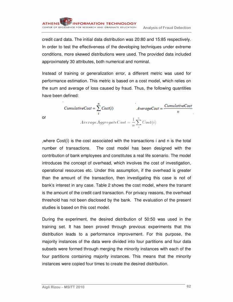
Analysis of Fraud Detection
Aigli Rizou – MSITT 2010 62
credit card data. The initial data distribution was 20:80 and 15:85 respectively.
In order to test the effectiveness of the developing techniques under extreme
conditions, more skewed distributions were used. The provided data included
approximately 30 attributes, both numerical and nominal.
Instead of training or generalization error, a different metric was used for
performance estimation. This metric is based on a cost model, which relies on
the sum and average of loss caused by fraud. Thus, the following quantities
have been defined:
or
,where Cost(i) is the cost associated with the transactions i and n is the total
number of transactions. The cost model has been designed with the
contribution of bank employees and constitutes a real life scenario. The model
introduces the concept of overhead, which involves the cost of investigation,
operational resources etc. Under this assumption, if the overhead is greater
than the amount of the transaction, then investigating this case is not of
bank’s interest in any case. Table 2 shows the cost model, where the tranamt
is the amount of the credit card transaction. For privacy reasons, the overhead
threshold has not been disclosed by the bank. The evaluation of the present
studies is based on this cost model.
During the experiment, the desired distribution of 50:50 was used in the
training set. It has been proved through previous experiments that this
distribution leads to a performance improvement. For this purpose, the
majority instances of the data were divided into four partitions and four data
subsets were formed through merging the minority instances with each of the
four partitions containing majority instances. This means that the minority
instances were copied four times to create the desired distribution.

Analysis of Fraud Detection
Aigli Rizou – MSITT 2010 63
Table 2: Cost model assuming a fixed overhead [17].
The training, validation and test data set contained transactions from first eight
months (10/95–5/96), the ninth month (6/96) and the twelfth month (9/96)
respectively. To each subset of the training set, a learning algorithm(s) was
applied (C4.5, CART, Ripper and Bayes) and thus 128 classifiers were
produced. This process was made in parallel processors in order to save time.
After the creation of the classifiers, they are combined by meta-learning
through stacking (§3.2.4.2). Results are shown in the following paragraph
(Table 3).
Another important issue is that of bridging different database schemata. In
particular, banks often need to exchange their classifiers with specific data
attributes. Though, there is often the case of attributes incompatibility, which
renders the exchanged classifiers useless. Hence, two methods have been
proposed, referring to features with different semantics as well as missing
values.
Furthermore, pretraining and posttraining pruning has been applied in order to
improve system’s accuracy and efficiency. Pretraining pruning filters the
classifiers before they are combined. Finally, based on predefined metrics, the
most competent classifiers are selected for the final meta-classifier. Through,
posttraining pruning, the evaluation and pruning of the initial base classifiers is
performed, after the construction of a complete meta-classifier.
4 .1 .1 .2 .4 .1 .1 .2 .4 .1 .1 .2 .4 .1 .1 .2 . Expe r iment 1 E xpe r imen t 1 E xpe r imen t 1 E xpe r imen t 1 –––– Resu l ts Resu l ts Resu l ts Resu l ts
Table 3 contains the cost and savings from stacking algorithm using 50:50
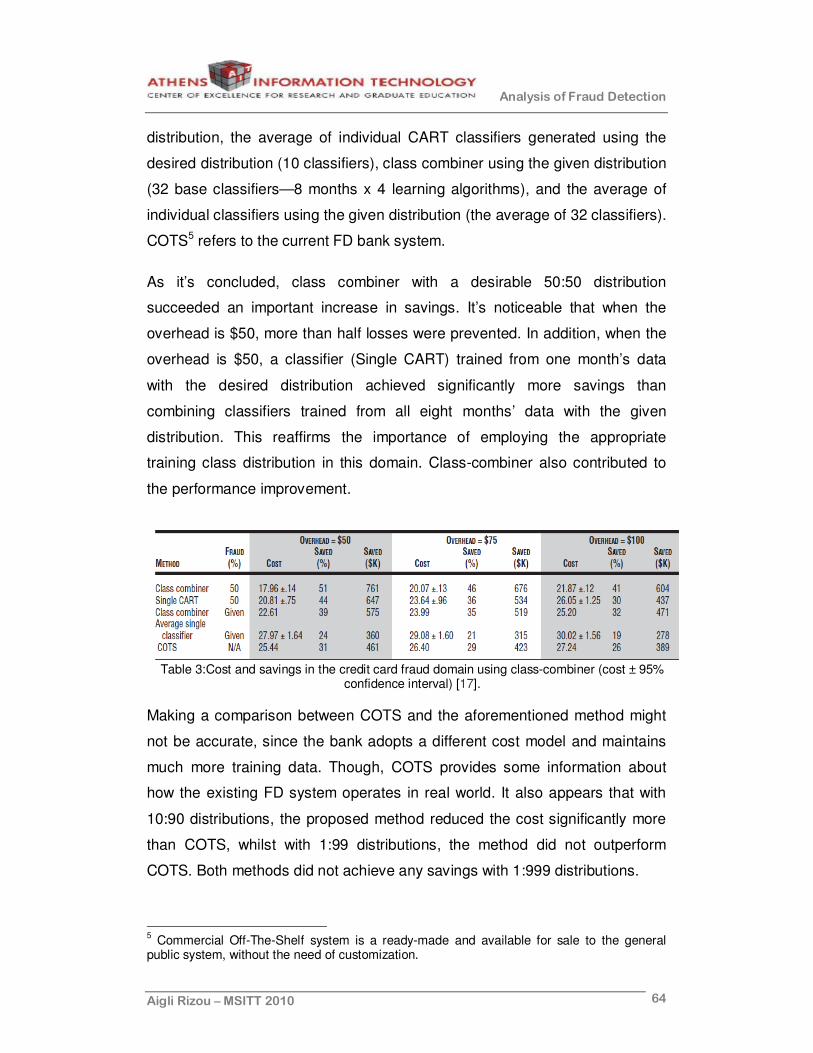
Analysis of Fraud Detection
Aigli Rizou – MSITT 2010 64
distribution, the average of individual CART classifiers generated using the
desired distribution (10 classifiers), class combiner using the given distribution
(32 base classifiers—8 months x 4 learning algorithms), and the average of
individual classifiers using the given distribution (the average of 32 classifiers).
COTS5 refers to the current FD bank system.
As it’s concluded, class combiner with a desirable 50:50 distribution
succeeded an important increase in savings. It’s noticeable that when the
overhead is $50, more than half losses were prevented. In addition, when the
overhead is $50, a classifier (Single CART) trained from one month’s data
with the desired distribution achieved significantly more savings than
combining classifiers trained from all eight months’ data with the given
distribution. This reaffirms the importance of employing the appropriate
training class distribution in this domain. Class-combiner also contributed to
the performance improvement.
Table 3:Cost and savings in the credit card fraud domain using class-combiner (cost ± 95%
confidence interval) [17].
Making a comparison between COTS and the aforementioned method might
not be accurate, since the bank adopts a different cost model and maintains
much more training data. Though, COTS provides some information about
how the existing FD system operates in real world. It also appears that with
10:90 distributions, the proposed method reduced the cost significantly more
than COTS, whilst with 1:99 distributions, the method did not outperform
COTS. Both methods did not achieve any savings with 1:999 distributions.
5 Commercial Off-The-Shelf system is a ready-made and available for sale to the general
public system, without the need of customization.
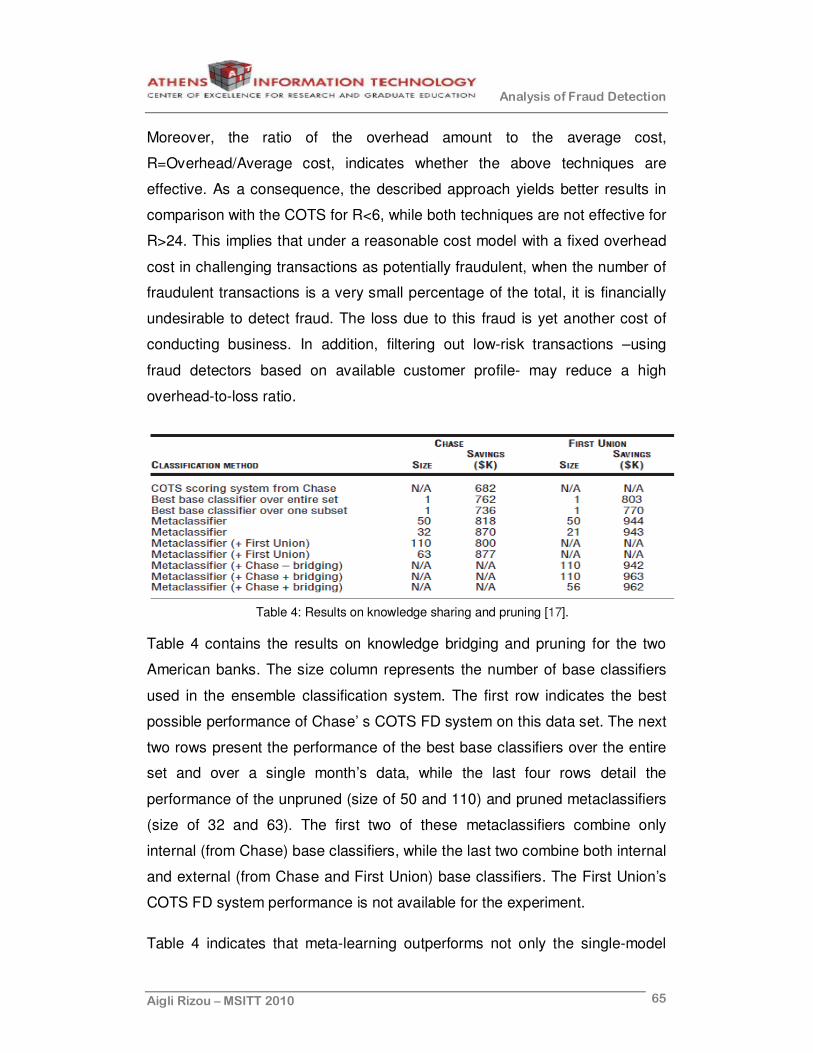
Analysis of Fraud Detection
Aigli Rizou – MSITT 2010 65
Moreover, the ratio of the overhead amount to the average cost,
R=Overhead/Average cost, indicates whether the above techniques are
effective. As a consequence, the described approach yields better results in
comparison with the COTS for R<6, while both techniques are not effective for
R>24. This implies that under a reasonable cost model with a fixed overhead
cost in challenging transactions as potentially fraudulent, when the number of
fraudulent transactions is a very small percentage of the total, it is financially
undesirable to detect fraud. The loss due to this fraud is yet another cost of
conducting business. In addition, filtering out low-risk transactions –using
fraud detectors based on available customer profile- may reduce a high
overhead-to-loss ratio.
Table 4: Results on knowledge sharing and pruning [17].
Table 4 contains the results on knowledge bridging and pruning for the two
American banks. The size column represents the number of base classifiers
used in the ensemble classification system. The first row indicates the best
possible performance of Chase’ s COTS FD system on this data set. The next
two rows present the performance of the best base classifiers over the entire
set and over a single month’s data, while the last four rows detail the
performance of the unpruned (size of 50 and 110) and pruned metaclassifiers
(size of 32 and 63). The first two of these metaclassifiers combine only
internal (from Chase) base classifiers, while the last two combine both internal
and external (from Chase and First Union) base classifiers. The First Union’s
COTS FD system performance is not available for the experiment.
Table 4 indicates that meta-learning outperforms not only the single-model

Analysis of Fraud Detection
Aigli Rizou – MSITT 2010 66
approaches, but also the traditional FD systems, at least for the given data
sets. One step further, it appears that the database bridging led to the
improvement of metalearning system performance. What is more, pruning
achieved satisfactory results in computing meta-classifiers.
As a conclusion, this survey indicates that distributed data mining techniques
that combine multiple models result in effective FD. An additional advantage
of the present approach is that these multi-classifiers allow adaptation over
time and out-of-date knowledge is removed. Nevertheless, an important
disadvantage of this experiment is the definition of the desired distribution
according to the cost model, which presupposes the running of laborious
preliminary experiments.
4 .1 .2 .4 .1 .2 .4 .1 .2 .4 .1 .2 . I ns ur ance FDIns ur ance FDIns ur ance FDIns ur ance FD
The particular experiment in insurance domain concerns a Complex Event
Processing (CEP) engine (Figure 26), which applies a combination of ANN
(§3.2.1.2) and discriminant analysis6 techniques. CEP is an advanced
technology for detecting already seen patterns of events and aggregating
them as complex events at a higher level of analysis in real time. Taking into
account that the common practice of insurance fraud experts is the manual
FD, it’s clear that the automation of FD techniques will contribute significantly
to the saving costs.
The following description is based on two scientific papers published by A.
Widder, R. v. Ammon, G. Hagemann, D. Scoenfeld, P. Scaeffer and C. Wolff
[22, 41].
4 .1 .2 .1 .4 .1 .2 .1 .4 .1 .2 .1 .4 .1 .2 .1 . Expe r iment 1 E xpe r imen t 1 E xpe r imen t 1 E xpe r imen t 1 ---- Desc Desc Desc Desc r i p t i onr i p t i onr i p t i onr i p t i on
In insurance companies, fraud experts investigate the various insurance
6 It is a technique for classifying a set of observations (training set) into predefined classes, based on a set of predictors (input variables). It constructs a set of linear functions of the predictors, known as discriminant functions, such that L = b1x1 + b2x2 + .. + bnxn + c , where the b's are discriminant coefficients, the x's are the input variables or predictors & c is a constant. These discriminant functions are used to predict the class of a new observation with unknown class [64].
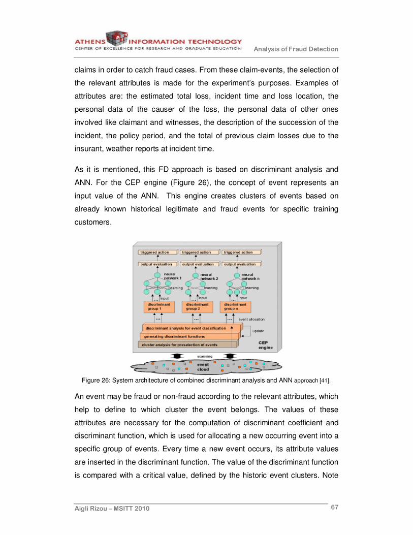
Analysis of Fraud Detection
Aigli Rizou – MSITT 2010 67
claims in order to catch fraud cases. From these claim-events, the selection of
the relevant attributes is made for the experiment’s purposes. Examples of
attributes are: the estimated total loss, incident time and loss location, the
personal data of the causer of the loss, the personal data of other ones
involved like claimant and witnesses, the description of the succession of the
incident, the policy period, and the total of previous claim losses due to the
insurant, weather reports at incident time.
As it is mentioned, this FD approach is based on discriminant analysis and
ANN. For the CEP engine (Figure 26), the concept of event represents an
input value of the ANN. This engine creates clusters of events based on
already known historical legitimate and fraud events for specific training
customers.
Figure 26: System architecture of combined discriminant analysis and ANN approach [41].
An event may be fraud or non-fraud according to the relevant attributes, which
help to define to which cluster the event belongs. The values of these
attributes are necessary for the computation of discriminant coefficient and
discriminant function, which is used for allocating a new occurring event into a
specific group of events. Every time a new event occurs, its attribute values
are inserted in the discriminant function. The value of the discriminant function
is compared with a critical value, defined by the historic event clusters. Note
Analysis of Fraud Detection
Aigli Rizou – MSITT 2010 68
that, the discriminant function is updated every time new discriminant groups
are created and, thus, it has a dynamic form.
At the beginning of the experiment, the CEP engine scans the global event of
clouds of an organization. After the insertion of attribute values into the
discriminant function and the comparison with the critical discriminant value,
the events are allocated into a specific cluster. For every discriminant cluster,
an ANN is produced, where the weights are defined through training with
discriminant values of known legitimate and fraud event patterns. Finally, the
ANN classifies the events to fraud and non-fraud.
The ANN runs for an occurring combination of event discriminant values and
the output is evaluated for distinguishing whether the input events are fraud or
not. During network training with BP algorithm (§3.2.1.2), the known fraud
and non-fraud combinations have the output values 1 and 0 respectively. For
the unknown combinations, a threshold is determined through the training
results. This means that when the output value of an input combination is
greater than the threshold, the system classifies it as fraud and reacts with a
predefined action, e.g. sends an alert. Then, the values of the detected fraud
pattern are used to retrain the ANN, after the expiration of predefined time
interval, depending on the system performance.
4 .1 .2 .2 .4 .1 .2 .2 .4 .1 .2 .2 .4 .1 .2 .2 . Expe r iment 1 E xpe r imen t 1 E xpe r imen t 1 E xpe r imen t 1 ---- R esu l Resu l Resu l Resu l t st st st s
The combination of discriminant analysis and ANN appears to run
successfully for a small set of events with two relevant attributes. In this
experiment, the ANN consists of two input nodes, two hidden nodes and one
output node, which is a rather simple structure. Future experiments should be
carried out involving a more complicated environment in order to confirm the
proper operation of this system based on real time requirements. So, the next
step is the use of a higher number of test and training data sets and historic
events as well as the use of a more advanced ANN environment.

Analysis of Fraud Detection
Aigli Rizou – MSITT 2010 69
4 .1 .3 .4 .1 .3 .4 .1 .3 .4 .1 .3 . Te l ecommun ica t i onTe l ecommun ica t i onTe l ecommun ica t i onTe l ecommun ica t i on ssss FD FD FD FD
The current experiment addresses fraud cases, which are a combination of
contractual, hacking, technical and procedural fraud (§2.4.4). The applied
technique is the user profiling, where the past behavior of a user is
accumulated in order to create a profile. If future behavior deviates from this
profile, this may imply the existence of fraud and may trigger an alarm to the
Network Operations Centre (NOC).
More than five thousand users for one year are collected through the Call
Detail Record (CDR) of a University PBX. In addition, only outgoing calls and
periods users are not on a leave are taken into account during the experiment.
The caller id, the date and the time of the call, the chargeable duration of the
call, the called party id are some indicative attributes of the experiment. The
accumulated user behavior per day is used as a differentiator measure,
because it doesn’t disclose any private information of the user, such as the
caller id.
The scientific research was performed by Constantinos S. Hilas from
Technological Educational Institute of Serres and John N. Sahalos from
Aristotle University of Thessaloniki [30].
4 .1 .3 .1 .4 .1 .3 .1 .4 .1 .3 .1 .4 .1 .3 .1 . Expe r iment 1 E xpe r imen t 1 E xpe r imen t 1 E xpe r imen t 1 ---- Desc r i p t i on Desc r i p t i on Desc r i p t i on Desc r i p t i on
The precondition of the experiment is to construct a reliable user profile that
will represent the normal behavior. The assumption is that any behavior that
doesn’t exist in historical data is at least suspicious or another user. In order
to compare the user profile with a different or fraudulent user, experts use a
similarity measure. They create an eight-element vector , which contains the
following data: number of calls made to local destinations (loc), the duration of
local calls (locd), the number of calls to mobile destinations (mob), the
duration of mobile calls (mobd), the number of calls to national (nat) and
international (int) destination and their corresponding durations (natd, intd)
(Figure 27). Sequence of more than one vector can be used, but the length of

Analysis of Fraud Detection
Aigli Rizou – MSITT 2010 70
the sequence must be the same for a single run.
For the similarity measure, the rule of “r-contiguous bits” is used. For example,
if a seq1 has k equal points with two other sequences seq2 and seq3, but the
common points with seq2 are in neighbouring positions then the similarity
(seq1, seq2) is greater than the similarity (seq1, seq3).
Figure 27: The vector of comparison [30].
There are two levels of comparison within the experiment: a) the equality of
the number of the calls of the same category and b) the total call duration per
category.
The first level of similarity can give a score from 0 to m*4, where m is the
number of vector sequences. The second level of similarity exists only if the
corresponding number of calls yields equality and, thus, has possible values
from 0 to m*8. The disadvantage of this measure is that there is often the
case where users make no international calls (nat=0 and natd=0 of the
vector), which increases unduly the similarity measure. For this reason, the
zero number calls were excluded from the computation of similarity.
Furthermore, it’s very rare that the call duration will be equal during
comparison. Hence, according to “equality interval”, two call durations are
considered the same only if the first differs by a ±X percentage with the
second. This practice indicates the fuzziness of the system. Here is the
algorithm followed:
1. Start with k profiles and k test sets,
2. Select the length m of the sequence (seq)
(seq = m*unit vector)
3. For each profile - test pair
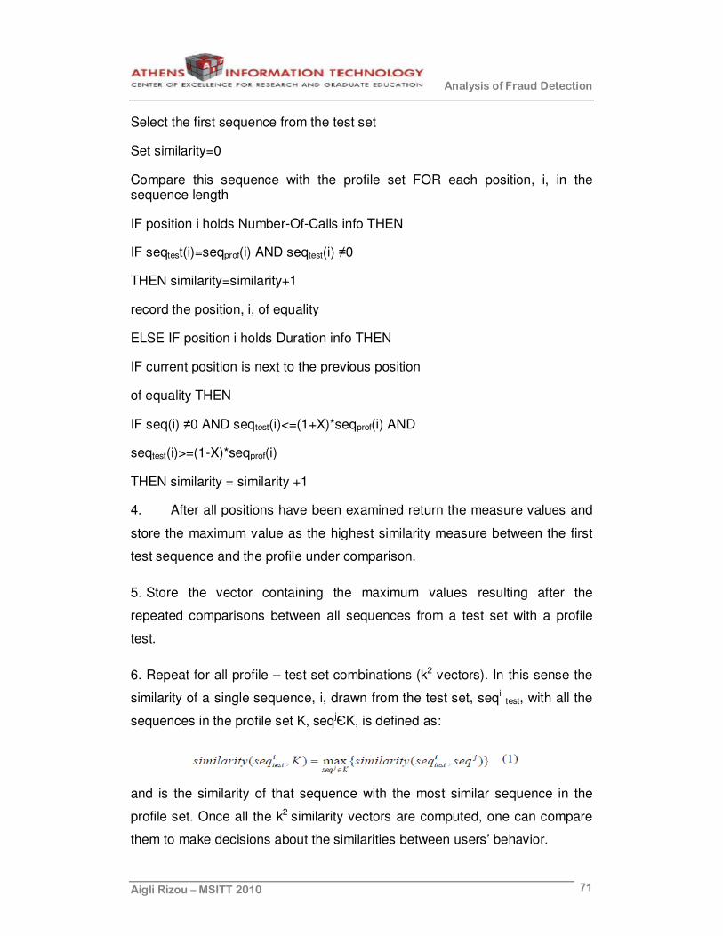
Analysis of Fraud Detection
Aigli Rizou – MSITT 2010 71
Select the first sequence from the test set
Set similarity=0
Compare this sequence with the profile set FOR each position, i, in the sequence length
IF position i holds Number-Of-Calls info THEN
IF seqtest(i)=seqprof(i) AND seqtest(i) ≠0
THEN similarity=similarity+1
record the position, i, of equality
ELSE IF position i holds Duration info THEN
IF current position is next to the previous position
of equality THEN
IF seq(i) ≠0 AND seqtest(i)<=(1+X)*seqprof(i) AND
seqtest(i)>=(1-X)*seqprof(i)
THEN similarity = similarity +1
4. After all positions have been examined return the measure values and
store the maximum value as the highest similarity measure between the first
test sequence and the profile under comparison.
5. Store the vector containing the maximum values resulting after the
repeated comparisons between all sequences from a test set with a profile
test.
6. Repeat for all profile – test set combinations (k2 vectors). In this sense the
similarity of a single sequence, i, drawn from the test set, seqi test, with all the
sequences in the profile set K, seqjЄK, is defined as:
and is the similarity of that sequence with the most similar sequence in the
profile set. Once all the k2 similarity vectors are computed, one can compare
them to make decisions about the similarities between users’ behavior.

Analysis of Fraud Detection
Aigli Rizou – MSITT 2010 72
4 .1 .3 .2 .4 .1 .3 .2 .4 .1 .3 .2 .4 .1 .3 .2 . Expe r iment 1 E xpe r imen t 1 E xpe r imen t 1 E xpe r imen t 1 ---- R esu l t s Resu l t s Resu l t s Resu l t s
During the experiment, twelve telephone terminals were used and four groups
were formed with three terminals each. For each terminal, a similarity vector
for the last year was created. The terminal’s activity was divided into a training
set (user profile) and a test set at split 2/3 and 1/3 respectively. Finally, each
group of terminals had their similarity vectors computed (Figure 28).
It’s observed that when a user profile is compared with the same user then it
appears to be the same, but when it is compared with different users, it differs
significantly. For the comparison of means of each vector, the Analysis of
Variance (ANOVA)7 test was used. The mean of each vector and the
probability that the corresponding mean value is equal to the mean similarity
of the same user is given in the tables III, IV, V, VI.
Figure 28: An example of similarity vectors of 3 user profile – test sets (Group 1) [30].
7 In statistics, ANOVA is a collection of statistical models and their associated procedures, in
which the observed variance in a particular variable is partitioned into components due to different sources of variation. ANOVAs are useful in comparing three or more means [2].

Analysis of Fraud Detection
Aigli Rizou – MSITT 2010 73
It is apparent, that the diagonal values of the tables III, IV are the maximum
values of the rows (red rectangles). For the table III, this means that e.g.
comparing user profile 1 with test set 1 gives that both sets refer to the same
user. In contrast, the comparison between tests set 1 and user profile 2
results in lower values of mean similarity vectors, indicating a case of different
users.
As a consequence, this is reflected to the respective probability of equality
between means in table IV, where the diagonal values are 1. This implies that
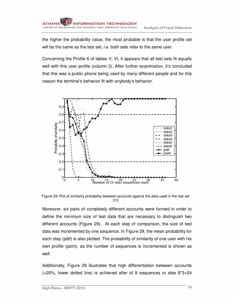
Analysis of Fraud Detection
Aigli Rizou – MSITT 2010 74
the higher the probability value, the most probable is that the user profile set
will be the same as the test set, i.e. both sets refer to the same user.
Concerning the Profile 6 of tables V, VI, it appears that all test sets fit equally
well with this user profile (column 3). After further examination, it’s concluded
that this was a public phone being used by many different people and for this
reason the terminal’s behavior fit with anybody’s behavior.
Figure 29: Plot of similarity probability between accounts against the data used in the test set [30]
Moreover, six pairs of completely different accounts were formed in order to
define the minimum size of test data that are necessary to distinguish two
different accounts (Figure 29). At each step of comparison, the size of test
data was incremented by one sequence. In Figure 29, the mean probability for
each step (pdif) is also plotted. The probability of similarity of one user with his
own profile (psim), as the number of sequences is incremented is shown as
well.
Additionally, Figure 29 illustrates that high differentiation between accounts
(<20%, lower dotted line) is achieved after of 8 sequences or else 8*3=24
Analysis of Fraud Detection
Aigli Rizou – MSITT 2010 75
days. One step further, it appears that 13 sequences (13*3=39 days) are
necessary for identifying on one user, where similarity probability is greater
than 80% (upper dotted line).
Among the advantages of the aforementioned approach is the simplicity, the
protection of private data, the application in different and various fields
(cellular phones, web usage, and intrusion detection) and the transferability to
an ANN (§3.2.1.2) of fuzzy network (§3.2.1.3) implementation. Also, the
differentiation measure between accounts gives a motivation for further
research. However, the approach can be used only for midterm decisions and
not for an online account comparison.

Analysis of Fraud Detection
Aigli Rizou – MSITT 2010 76
5555 PRACTICAL PERSPECTIVEPRACTICAL PERSPECTIVEPRACTICAL PERSPECTIVEPRACTICAL PERSPECTIVE
The aim of the final chapter is to examine a real FD scenario, using a real
anti-fraud system and an open source machine learning tool as well. After the
analysis of the results, a potential FD solution is suggested as a final
conclusion.
The first section of the present chapter describes the anti-fraud system
operating in a Greek Bank. An available labeled data set based on real data is
given by the Bank in order to perform a number of tests for the thesis
purposes. The second section of this chapter describes a machine learning
tool which applies a number of supervised algorithms to the same labeled
data set. The results of the machine learning tool are compared with the
results of the existing anti-fraud system, given that the latter constitutes a fool-
proof mechanism, which provides a reliable classification. In the end, the aim
is to propose a viable FD, combining the existing FD system of the Bank and
an effective method proceeded from the scientific field.
The type of fraud under consideration is the application fraud (§2.3.1, §2.4.1).
The application fraud refers to loan applications, which contain fake data,
such as identity card number, tax identification number, employer name,
telephone numbers etc. Fraudsters use these data in order to achieve a loan
approval quickly, without having the intention of paying back the installments.
5.1.5.1.5.1.5.1. BankBankBankBank Ant i Ant i Ant i Ant i ---- Fraud SystemFraud SystemFraud SystemFraud System
The Bank has implemented an integrated solution, implemented by a Greek
Company. This anti-fraud solution comprises a German software (§5.1.1),
PRACTICAL
PERSPECTIVE

Analysis of Fraud Detection
Aigli Rizou – MSITT 2010 77
which is parameterized to each customer, and a web-based case investigation
tool suitable for monitoring and managing the produced alarms in real time,
developed by the Greek company.
Before the description of the system operation, it’s important to analyze the
two basic roles of the Bank, i.e. fraud analysts and investigators. Fraud
analysts belong to the Fraud Department of Bank and their experience in
fraud qualifies them to undertake the decision making issues. They are
responsible for rule analysis, rule design and system maintenance. After the
system configuration and fine-tuning by the Company, analysts perform all the
necessary tasks, such as data analysis and decision model optimization, in
order to adapt to new emerging fraud patterns and to improve system
performance. Fraud analysts are authorized to make final decisions about
whether an application will be rejected or not. Conversely, fraud investigators
monitor and investigate the incoming loan applications, and they are not
allowed to decide about the loan disbursement.
However, during investigation there are two possible scenarios: a) the loan
application contains wrong data due to users' errors and b) the loan
application contains actual fraud data. In the first case, fraud investigators
notify the corresponding user, who corrects the application data and proceeds
with the typical procedures. Finally, the loan application is filed in the bank
system as legitimate. In the second case, after the completion of initial
investigation, fraud investigators ask for analysts' contribution, only if they
have concluded high probability of fraud. Fraud analysts investigate further
the application and they decide about the final outcome.
The anti-fraud solution has been incorporated in the Bank’s system and gives
a real-time indication of fraud. According to the Bank’s demand, it acts at an
early stage of the workflow, even if the application contains missing data. Yet,
authorized users (fraud analysts and investigators) may call the system at any
time they need an updated fraud indication throughout the workflow.
The route followed by an incoming loan application in the Bank system is

Analysis of Fraud Detection
Aigli Rizou – MSITT 2010 78
described hereupon. A loan application is inserted into the Bank’s workflow
and then the anti-fraud system evaluates the data and sends a real-time
indication to the investigators about whether the application involves fraud or
not. If the evaluation indicates fraud, then the investigator investigates the
case and if necessary, he/she contacts fraud analysts, who take the final
decision. Otherwise, the application is forwarded for approval automatically by
the Bank's workflow. However, in both cases the Bank’s system is updated
with the final result.
The following paragraphs contain an overview of the fraud prevention and
detection logic, implemented by the Greek Company, using the German
software.
5 .1 .1 .5 .1 .1 .5 .1 .1 .5 .1 .1 . The The The The SSSSo f twareo f twareo f twareo f tware
RiskShield is a product family for automated decision-making in financial
engineering and it follows client-server architecture.
Figure 30: RiskShield architecture [79].
The RiskShield Server is usually used as the middle ("service provider") tier of
a multi-tiered architecture [79]. In many RiskShield applications, the following
three tiers are used (Figure 30).
5 .1 .1 .1 .5 .1 .1 .1 .5 .1 .1 .1 .5 .1 .1 .1 . Serv i ce Consumer T i e rSe rv i ce Consumer T i e rSe rv i ce Consumer T i e rSe rv i ce Consumer T i e r
This is where the "consumers" of the decision "service" resides. For payment
systems, the service consumers are the authorisation and card management

Analysis of Fraud Detection
Aigli Rizou – MSITT 2010 79
systems. For insurance claim processing systems, this is the claims
processing system itself. There can be multiple service consumers in a
RiskShield installation. Communication between the service provider and the
service consumer is provided in XML or CSV format using IP or other
transport layers.
5 .1 .1 .2 .5 .1 .1 .2 .5 .1 .1 .2 .5 .1 .1 .2 . Serv i ce Se rv i ce Se rv i ce Se rv i ce P ro v i de rP rov i de rP rov i de rP rov i de r T i e r T i e r T i e r T i e r
The RiskShield Server has two interfaces. The one to the left is the real time
interface for the actual decisions. The one to the right is a maintenance
interface (non real time) for the RiskShield Client. The maintenance interface
is used only during the maintenance. Connection between the RiskShield
Server and the RiskShield Client is not necessary during operation.
The RiskShield-Server is coded in Java. This allows operating it on virtually
any commercial computer platform, such as IBM-AIX, SUN-Solaris, Linux and
Microsoft Windows Server based environments.
5 .1 .1 .3 .5 .1 .1 .3 .5 .1 .1 .3 .5 .1 .1 .3 . Cl i en tC l i en tC l i en tC l i en t T ie r T ie r T ie r T ie r
The RiskShield Client is a Microsoft Foundation Class based software product
that runs on a MS Windows PC computer. It is used by decision project
designers and analysts to create and adapt decision projects, and to verify the
performance of an operational decision making system. The RiskShield Client
can be used both as a stand-alone software tool and as client tier within a
multi-tiered architecture. The RiskShield Client connects to the RiskShield
Server via IP over the Bank’s Intranet.
The RiskShield Client employs FL (§3.2.1.3, §5.1.2) that allows for the
transparent implementation of complex decision patterns. Furthermore, FL
facilitates a rapid reaction on new fraud schemes and allows the exact
addressing of specific fraud patterns as no complete retraining is necessary.
5 .1 .1 .4 .5 .1 .1 .4 .5 .1 .1 .4 .5 .1 .1 .4 . Commun i ca t io nCommun i ca t io nCommun i ca t io nCommun i ca t io n

Analysis of Fraud Detection
Aigli Rizou – MSITT 2010 80
The RiskShield Client produces a decision project (§5.1.2.1), which is
uploaded to the Server in order to become operational. The RiskShield Server
then loads the decision project and provides it to service consumers. To
obtain analysis data, the RiskShield-Server can be configured to capture
production data within csv8 files and/or within its embedded database. The
analysis data is downloaded by the RiskShield Client where the actual
analyses are performed offline [80].
During operational usage, the RiskShield-Server is independent of the
RiskShield Client. When started on the Server computer, the RiskShield
Server behaves very much like typical server programs, e.g. an http daemon.
It reads its initialisation file with its configuration, then it loads the decision
projects to be served, initializes the IP ports it shall provide its services at, and
writes its actions into a log file. Once initialized, other software systems, either
located on the same computer or on other computers, can access the
decision computation services via XML messages.
5 .1 .2 .5 .1 .2 .5 .1 .2 .5 .1 .2 . FLFLFLFL So f tware So f tware So f tware So f tware
FL technology (§3.2.1.4) has proven to be a very effective means of modelling
human expertise and is thus an important part of the RiskShield Client. The
actual development of a FL system itself involves a number of design and
verification steps. Hence, this development is not performed within the
RiskShield Client, but uses the separate fuzzyTECH software package, which
is a product of the same German company as well [80].
fuzzyTECH software allows the design of rules providing a user-friendly
interface. It applies all the fundamental concepts of FL, such as linguistics
variables, fuzzification and defuzzification, etc. A simplified FL environment is
given in Figure 31, where an indicative rule block and a variable’s
membership function is given.
8 csv stands for character separated values

Analysis of Fraud Detection
Aigli Rizou – MSITT 2010 81
The development of a completed fuzzyTECH project presupposes the
creation of the input and output linguistic variables (red rectangles), including
their membership functions, and the creation of rule blocks (blue rectangle),
which contain the “IF-THEN” rules and their weights.
Figure 31: A simplified FL environment – fuzzyTECH software
The Bank’s fuzzyTECH project consists of 327 numerical and categorical
(input and output) variables, which are used in order to build 540 rules totally.
The output variables include, apart from the final decision (§5.1.2.1.5), a
number of intermediate scores for the application FD purposes.
Each fuzzyTECH project is incorporated in the RiskShield Client project
(§5.1.2.1) and the cooperation of both softwares results in an alarm for each
Input Linguistic Variables
Output Linguistic Variables
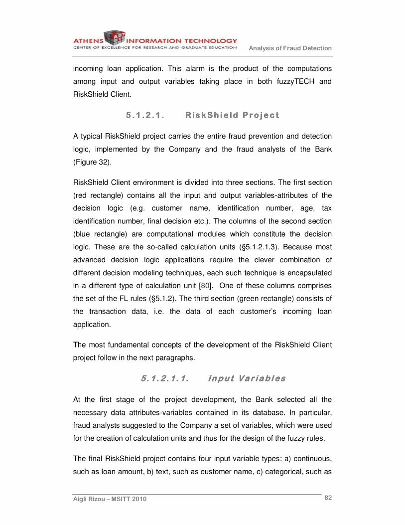
Analysis of Fraud Detection
Aigli Rizou – MSITT 2010 82
incoming loan application. This alarm is the product of the computations
among input and output variables taking place in both fuzzyTECH and
RiskShield Client.
5 .1 .2 .1 .5 .1 .2 .1 .5 .1 .2 .1 .5 .1 .2 .1 . Ris kSh i e ld P ro j ec tR is kSh i e ld P ro j ec tR is kSh i e ld P ro j ec tR is kSh i e ld P ro j ec t
A typical RiskShield project carries the entire fraud prevention and detection
logic, implemented by the Company and the fraud analysts of the Bank
(Figure 32).
RiskShield Client environment is divided into three sections. The first section
(red rectangle) contains all the input and output variables-attributes of the
decision logic (e.g. customer name, identification number, age, tax
identification number, final decision etc.). The columns of the second section
(blue rectangle) are computational modules which constitute the decision
logic. These are the so-called calculation units (§5.1.2.1.3). Because most
advanced decision logic applications require the clever combination of
different decision modeling techniques, each such technique is encapsulated
in a different type of calculation unit [80]. One of these columns comprises
the set of the FL rules (§5.1.2). The third section (green rectangle) consists of
the transaction data, i.e. the data of each customer’s incoming loan
application.
The most fundamental concepts of the development of the RiskShield Client
project follow in the next paragraphs.
5 . 1 . 2 . 1 . 1 .5 . 1 . 2 . 1 . 1 .5 . 1 . 2 . 1 . 1 .5 . 1 . 2 . 1 . 1 . I n pu t Va r i ab l esIn pu t Va r i ab l esIn pu t Va r i ab l esIn pu t Va r i ab l es
At the first stage of the project development, the Bank selected all the
necessary data attributes-variables contained in its database. In particular,
fraud analysts suggested to the Company a set of variables, which were used
for the creation of calculation units and thus for the design of the fuzzy rules.
The final RiskShield project contains four input variable types: a) continuous,
such as loan amount, b) text, such as customer name, c) categorical, such as

Analysis of Fraud Detection
Aigli Rizou – MSITT 2010 83
old or current types of identification card numbers and d) fingerprints.
Fingerprint plays an important role in the decision logic and thus is described
in more detail.
5 . 1 . 2 . 1 . 2 .5 . 1 . 2 . 1 . 2 .5 . 1 . 2 . 1 . 2 .5 . 1 . 2 . 1 . 2 . F i ng e rp r i n tsF i ng e rp r i n tsF i ng e rp r i n tsF i ng e rp r i n ts
Fingerprint is a special variable type that the RiskShield Server stores in-
between requests representing for instance sequences of previous
transactions of the same entity, events or profiles (Figure 33). Each fingerprint
has a single (or a combination of) key variable(s), which declare the specific
entity. RiskShield Server stores these fingerprints in its embedded database
[79].
Figure 32: RiskShield-Client project
The concept of fingerprint becomes more clear with the following example:
Assuming that FingerprintTAXid has the tax identification number as a key
variable and that on day 1, customer A with tax identification number
123123123 makes a loan application in the Bank. This application is stored in
Variables Calculation Units Loan Application Data

Analysis of Fraud Detection
Aigli Rizou – MSITT 2010 84
the FingerprintTAXid. Afterwards, on day 2, customer B makes another
application and uses the same tax identification number (123123132).
Similarly, the second application will be stored in the FingerprintTAXid, which
already contains the first application of customer A. This will lead to a conflict
between data and will probably indicate fraud.
Of course, there are as many fingerprints as the numbers of the specific
entities, e.g. Tax identification numbers. It's important to mention, that the
choice of the fingerprint and thus its keys is not made at random. Instead,
fraud experts choose attributes which characterize uniquely each customer.
As a consequence, a fingerprint holds the historical data of a transaction and
creates a more complete behavioral profile of each customer as time goes by.
In a simplified point of view, the comparison of the aforementioned
accumulated history with the current transaction data leads to the final
decision for the incoming loan application.
Figure 33 shows a typical fingerprint which contains two past loan applications
(with application code 44091 and 29916), bearing the same tax identification
number.
Figure 33: Fingerprint

Analysis of Fraud Detection
Aigli Rizou – MSITT 2010 85
5 . 1 . 2 . 1 . 3 .5 . 1 . 2 . 1 . 3 .5 . 1 . 2 . 1 . 3 .5 . 1 . 2 . 1 . 3 . Cal cu l a t i o n Un i tsCa l cu l a t i o n Un i tsCa l cu l a t i o n Un i tsCa l cu l a t i o n Un i ts
Consequently, RiskShield Client renders decision logics as sequences of so-
called calculation units. Within this sequence, each calculation unit constitutes
a “universe of its own”. Each calculation unit contains its own definition of
variables and variable types, and its own configuration of settings [80].
In other words, calculation units are independent “plug-ins” that compute new
data (output variables) from the existing data (input variables). Most of the
RiskShield Client projects use multiple and different types of calculation units
[80].
In the RiskShield project spreadsheet, each calculation unit is visualized as a
column, which shows the input and output variables of the calculation unit,
and how they are connected to the RiskShield Client variables and the other
calculation unit’s variables. fuzzyTECH project constitutes one of these
columns.
The processing order is strict from left to right in the project spreadsheet. This
means that a pre-processing calculation unit must be arranged left to a post-
processing calculation unit [80].
5 . 1 . 2 . 1 . 4 .5 . 1 . 2 . 1 . 4 .5 . 1 . 2 . 1 . 4 .5 . 1 . 2 . 1 . 4 . Ou tpu t V a r i ab l esOu tpu t V a r i ab l esOu tpu t V a r i ab l esOu tpu t V a r i ab l es
The output variables constitute the result of each calculation unit. Apart from
the Decision variable (§5.1.2.1.5), there is a number of continuous, text,
categorical or fingerprint as in the case of output variables. A special case of
output variables is the variables which are used for the rule design in the
fuzzyTECH, i.e. rule variables.
5 . 1 . 2 . 1 . 5 .5 . 1 . 2 . 1 . 5 .5 . 1 . 2 . 1 . 5 .5 . 1 . 2 . 1 . 5 . Dec is i on Va r i ab l eDec is i on Va r i ab l eDec is i on Va r i ab l eDec is i on Va r i ab l e
This is the final output variable of the RiskShield project and it’s the outcome
of the combination of both RiskShield project and fuzzyTECH project (Figure
32 – yellow rectangle). According to the Bank's indications, the Decision of the

Analysis of Fraud Detection
Aigli Rizou – MSITT 2010 86
project is not a crispy variable (fraud-legitimate), but instead it is separated in
different levels of alerts, such as: accepted, suspicious, low risky and
extremely risky.
The Decision is a numeric variable and its possible values are 0, 1, 2, 3 for
‘accepted’, ‘low_risky’, ‘suspicious’, and ‘extr_risky’ respectively. Note that the
Decision values are discrete and characterize each loan application
individually.
5 . 1 . 2 . 1 . 6 .5 . 1 . 2 . 1 . 6 .5 . 1 . 2 . 1 . 6 .5 . 1 . 2 . 1 . 6 . Case Managemen tCase Managemen tCase Managemen tCase Managemen t
Depending on the different levels of alerts, the Bank can manage each
application in multiple ways. As it’s mentioned in the beginning of this chapter,
the case management is performed through a case investigation tool,
developed by the Company. In specific, loan applications with the ‘accepted’
flag are forwarded for approval by the Bank’s workflow. Applications with the
'suspicious' or ‘low-risky’ flag are examined by the investigators and if there is
a need, they are forwarded for further examination to the Fraud Department.
Applications with the ‘extr_risky’ flag are rejected by the fraud analysts after
thorough investigation. Next, the approval authority evaluates the application
and the usual approval process can be resumed right after fraud investigator's
declassification.
The next paragraph introduces a machine learning tool used for the thesis
experiments.
5.2.5.2.5.2.5.2. WWWWaikato a ikato a ikato a ikato EEEEnv ironment for nv ironment for nv ironment for nv ironment for KKKKnowledge nowledge nowledge nowledge
AAAAnalysis (WEKA)nalysis (WEKA)nalysis (WEKA)nalysis (WEKA)
WEKA is a popular suite of machine learning free software written in Java,
developed at University of Waikato in New Zealand. Its advantages include
the great variety of machine learning algorithms and the user-friendly
environment.

Analysis of Fraud Detection
Aigli Rizou – MSITT 2010 87
In the following paragraphs, only the tools of WEKA used for the thesis
experiments are described. These tools are comprised in the “Explorer”
selection of WEKA GUI Chooser. The experiments were carried out with the
version 3.6.2 of WEKA.
5 .2 .1 .5 .2 .1 .5 .2 .1 .5 .2 .1 . PreprocessPreprocessPreprocessPreprocess
This is the first tab of the “Explorer” environment. The Preprocess tool is
necessary for loading the available data sets in order to run the appropriate
algorithms. There are, also, filters which are algorithms to transform the
datasets, by removing or adding attributes, resampling the dataset, removing
examples and so on [81].
Figure 34: Preprocess tab of WEKA
As it’s shown from Figure 34, the “Current relation” box is the currently loaded
data, which can be interpreted as a single relational table in database

Analysis of Fraud Detection
Aigli Rizou – MSITT 2010 88
terminology. The name of the loaded file, the total number of records and the
total number of attributes (variables or features) in the data is given by the
Relation, Instances and Attributes entries respectively. The “Attributes” box
lists all the attributes of the loaded data sample. There is also the choice of
removing them through the Remove button. Finally, the “Selected attribute”
box contains the aggregate results for every selected data attribute of
“Attributes” section. In addition, the user must choose the variable which will
be the class label for the supervised algorithms, i.e. Decision, which histogram
is given in the following figure. With Visualize all button, the histograms of all
attributes appear.
5 .2 .1 .1 .5 .2 .1 .1 .5 .2 .1 .1 .5 .2 .1 .1 . Da ta s e tDa ta s e tDa ta s e tDa ta s e t
The data set is a very basic concept of the current machine learning tool. A
dataset is roughly equivalent to a two-dimensional spreadsheet or database
table, which consists of a number of numerical (a real or integer number),
nominal (one of a predefined list of values) or string (an arbitrary long list of
characters) attributes. Date/time attributes types are also supported.
Figure 35: arff file
WEKA data sets have a special structure, which is shown in Figure 35. This is
a typical Attribute-Relation File Format (arff file). Apart from arff files, WEKA
accepts alternative formats such as csv, c4.5, binary or data from databases

Analysis of Fraud Detection
Aigli Rizou – MSITT 2010 89
through JDBC.
The arff files consist of two parts: the first part is the header and the second
part is the actual data. The header part contains information about the name
of the dataset (@relation application_fraud), as well as a list of data attributes
and their data types (e.g. @attribute tax_id numeric). The data part has the
form {<class label>,<value1>,…<value n>} and {<value1>,…,<value n>} for
supervised and unsupervised machine learning respectively. So, the
sequence {suspicious, LPR013470, DU0093840, 7327Α∆ΠΑΡΑ, 1257320, 26,
60172089} indicates a data record or a loan application which is labeled as
‘suspicious’ and has ‘LPR013470’ as application code, ‘DU0093840’ as
customer number, ‘7327Α∆ΠΑΡΑ’ as identification card number, ‘1257320’ as
tax_id, ‘26’ as customer age and ‘60172089’ as customer phone number.
5 .2 .2 .5 .2 .2 .5 .2 .2 .5 .2 .2 . C l ass i f i ca t io nC l ass i f i ca t io nC l ass i f i ca t io nC l ass i f i ca t io n
The “Classify” tab of the “Explorer” selection is used for the training of a
machine learning algorithm (classifier), based on the available data sets, so
that it can be used for the classification of additional data samples.
As it’s shown from Figure 36, the “Classifier” box contains the name of the
currently selected classifier and its options. The result of running the selected
classifier will be tested according to the options that are set in the “Test
Options” box. Furthermore, the classifiers in WEKA are designed to be trained
to predict a single ‘class’ attribute, which is the target for prediction. Some
classifiers can only learn nominal classes; others can only learn numeric
classes (regression problems); still others can learn both. The “Classifier
output” box comprises all the aggregate results of a specific classifier
application. The “Result list” box contains several entries, after the training of
various classifiers.
Some of the WEKA classifiers are the: DT (§3.2.1.1), NB networks (§3.2.1.5),
logistic regression (§3.2.2), C4.5 (§3.2.1.1.1), SVM (§3.2.1.6) etc. Apart from
these, WEKA implements some classifiers ensembles such as Bagging
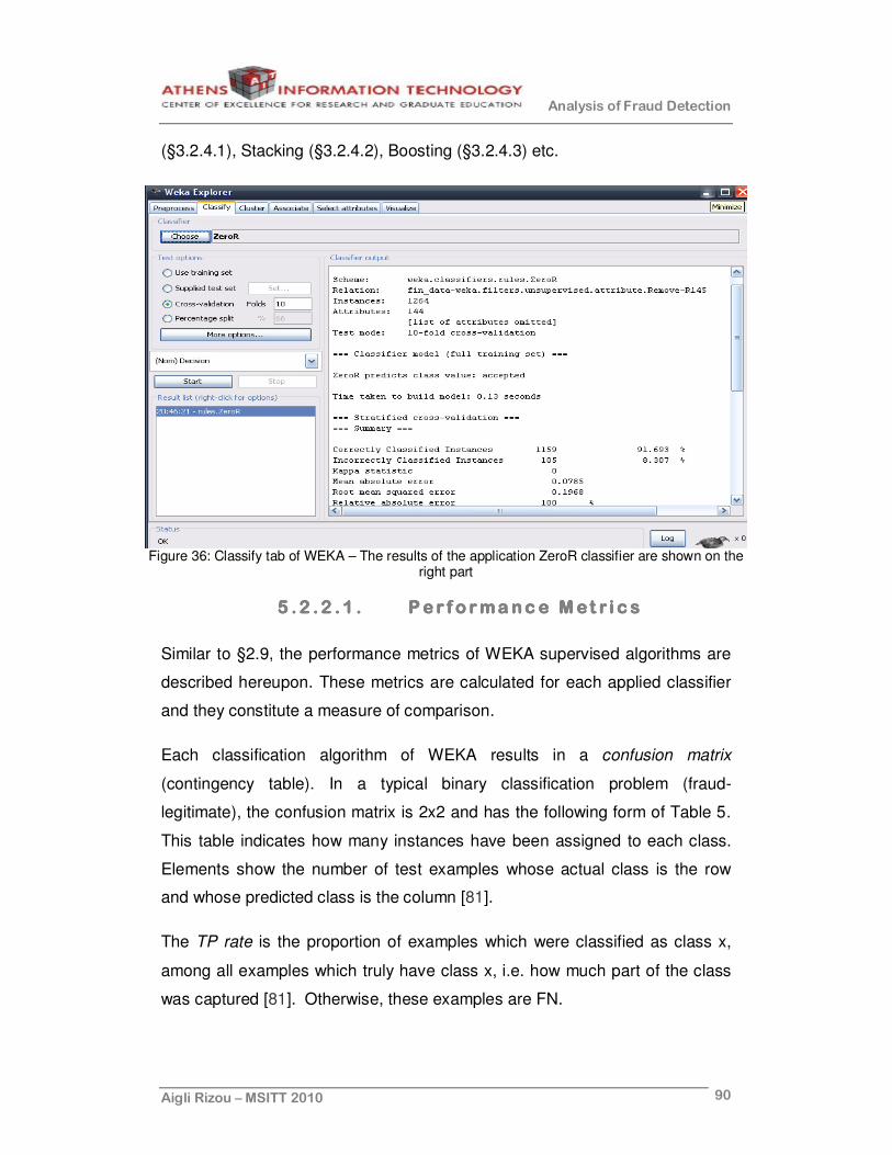
Analysis of Fraud Detection
Aigli Rizou – MSITT 2010 90
(§3.2.4.1), Stacking (§3.2.4.2), Boosting (§3.2.4.3) etc.
Figure 36: Classify tab of WEKA – The results of the application ZeroR classifier are shown on the
right part
5 .2 .2 .1 .5 .2 .2 .1 .5 .2 .2 .1 .5 .2 .2 .1 . Per f o rmance Pe r f o rmance Pe r f o rmance Pe r f o rmance MMMMet r i c set r i c set r i c set r i c s
Similar to §2.9, the performance metrics of WEKA supervised algorithms are
described hereupon. These metrics are calculated for each applied classifier
and they constitute a measure of comparison.
Each classification algorithm of WEKA results in a confusion matrix
(contingency table). In a typical binary classification problem (fraud-
legitimate), the confusion matrix is 2x2 and has the following form of Table 5.
This table indicates how many instances have been assigned to each class.
Elements show the number of test examples whose actual class is the row
and whose predicted class is the column [81].
The TP rate is the proportion of examples which were classified as class x,
among all examples which truly have class x, i.e. how much part of the class
was captured [81]. Otherwise, these examples are FN.

Analysis of Fraud Detection
Aigli Rizou – MSITT 2010 91
Fraud Legitimate
# class fraud True Positive (TP) False Negative (FN)
# class legitimate False Positive (FP) True Negative (TN)
Table 5: Confusion matrix for binary problems
The FP rate is the proportion of examples which were classified as class x,
but belong to a different class, among all examples which are not of class x. In
the matrix, this is the column sum of class x minus the diagonal element,
divided by the rows sums of all other classes [81]. Otherwise, these examples
are TN.
Nevertheless, samples A, B, C, D of the experiments (§5.2.3) contain a four-
level class label, which implies that the produced matrices will be 4x4 for each
of the algorithm.
Based on the aforementioned concepts, after the implementation of the
classifiers for the thesis purposes, the following metrics are recorded
(Appendix A):
� Precision=TP/(TP+FP): It is the proportion of the examples which truly have
class x among all those which were classified as class x.
� Recall=TP/(TP+FN): In the confusion matrix, this is the diagonal element
divided by the sum over the relevant row.
� Accuracy=(TP+TN)/(TP+FN+TN+FP): It represents the percentage of
correctly classified instances.
� Error=100%-Accuracy
� F-Measure=2*Precision*Recall/(Precision+Recall): It is a combined
measure for precision and recall.
Prediction values
Actual values

Analysis of Fraud Detection
Aigli Rizou – MSITT 2010 92
� ROC area: This measure (§2.9.1) can be interpreted as the probability
that when we randomly pick one positive and one negative example, the
classifier will assign a higher score to the positive example than to the
negative [2].
� Correlation coefficient: It is a measure of the interdependence of two
random variables that ranges in value from −1 to +1, indicating perfect
negative correlation at −1, absence of correlation at zero, and perfect
positive correlation at +1.
� Mean absolute error: It is a quantity used to measure how close
predictions are to the eventual outcomes. As the name suggests, the
mean absolute error is an average of the absolute errors ei = fi − yi,
where fi is the prediction and yi the true value [2].
� Root mean squared error: It is a good measure of precision and reflects
the differences between values predicted by a model and the values
actually observed from the thing being modelled or estimated. The root
mean squared error Ei of an individual program i is evaluated by the
equation where P(ij) is the value predicted by
the individual program i for sample case j (out of n sample cases); and Tj
is the target value for sample case j. For a perfect fit, P(ij) = Tj and Ei = 0.
So, the Ei index ranges from 0 to infinity, with 0 corresponding to the ideal
[82].
� Root relative squared error: It is relative to what it would have been if a
simple predictor had been used. This simple predictor is just the average
of the actual values. Thus, the relative squared error takes the total
squared error and normalizes it by dividing by the total squared error of
the simple predictor. By taking the square root of the relative squared
error one reduces the error to the same dimensions as the quantity being
predicted [82].
� Relative absoluter error: The relative absolute error Ei of an individual
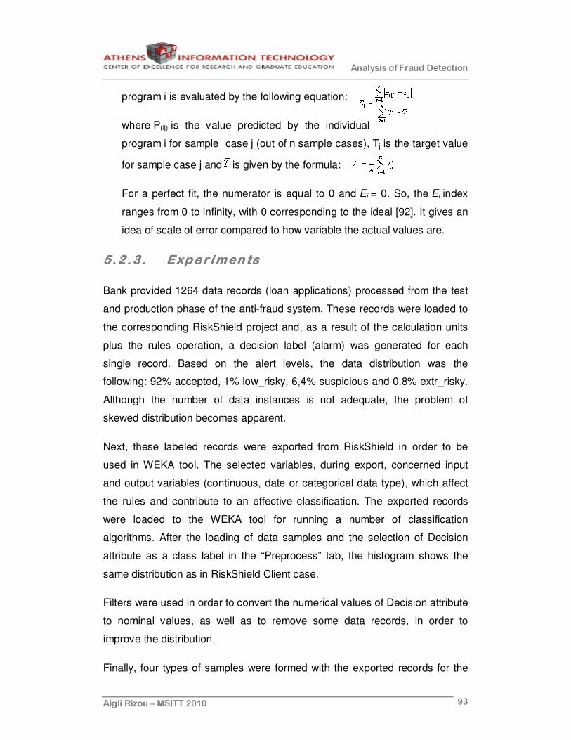
Analysis of Fraud Detection
Aigli Rizou – MSITT 2010 93
program i is evaluated by the following equation:
where P(ij) is the value predicted by the individual
program i for sample case j (out of n sample cases), Tj is the target value
for sample case j and is given by the formula:
For a perfect fit, the numerator is equal to 0 and Ei = 0. So, the Ei index
ranges from 0 to infinity, with 0 corresponding to the ideal [92]. It gives an
idea of scale of error compared to how variable the actual values are.
5 .2 .3 .5 .2 .3 .5 .2 .3 .5 .2 .3 . Exper imen tsExper imen tsExper imen tsExper imen ts
Bank provided 1264 data records (loan applications) processed from the test
and production phase of the anti-fraud system. These records were loaded to
the corresponding RiskShield project and, as a result of the calculation units
plus the rules operation, a decision label (alarm) was generated for each
single record. Based on the alert levels, the data distribution was the
following: 92% accepted, 1% low_risky, 6,4% suspicious and 0.8% extr_risky.
Although the number of data instances is not adequate, the problem of
skewed distribution becomes apparent.
Next, these labeled records were exported from RiskShield in order to be
used in WEKA tool. The selected variables, during export, concerned input
and output variables (continuous, date or categorical data type), which affect
the rules and contribute to an effective classification. The exported records
were loaded to the WEKA tool for running a number of classification
algorithms. After the loading of data samples and the selection of Decision
attribute as a class label in the “Preprocess” tab, the histogram shows the
same distribution as in RiskShield Client case.
Filters were used in order to convert the numerical values of Decision attribute
to nominal values, as well as to remove some data records, in order to
improve the distribution.
Finally, four types of samples were formed with the exported records for the

Analysis of Fraud Detection
Aigli Rizou – MSITT 2010 94
experiments’ purposes:
Sample A contains 1264 data records with 145 attributes (input variables of
RiskShield project) with nominal class label, i.e. Decision values are
‘accepted’, ‘low_risky’, ‘suspicious’, ‘extr_risky’.
Sample B contains 1264 data records with 145 attributes (input variables of
RiskShield project) with numeric class label, i.e. Decision values are 0, 1, 2, 3.
Sample C contains 1264 data records with 439 attributes (input variables plus
the rule variables of RiskShield project) with nominal class label.
Sample D contains 1264 data records with 439 attributes (input variables plus
the rule variables of RiskShield project) with numeric class label.
For each of the above sample, a stratified cross-validation of 10 folds is
selected for the training, in the “Classify” tool. This means, that data are
randomly broken into 10 record sets of size 1264/10, then the training is
performed on 9 sets and the test on 1 set and this procedure is repeated 10
times. At the end, an average performance from the individual experiments
was calculated. Thus, every record took part once in the test set and nine
times in the training set. The reason for choosing 10 partitions is that this
yields the same error rate as if the entire data set had been used for training.
5.3.5.3.5.3.5.3. Resul tsResul tsResul tsResul ts
Upon the completion of the previous settings, a set of supervised algorithms
was applied to each of the samples A, B, C and D. The aforementioned
metrics (§5.2.2.1) of indicative algorithms are given in detail in Appendix A.
Moreover, the tables of Appendix B contain the aggregate results for all
samples. They show the running time, accuracy and relative absolute error for
samples A, B, C and D for 10-fold cross validation for all classification
algorithms, which run during the thesis experiments.
Additionally, the following comparative diagrams illustrate the accuracy and

Analysis of Fraud Detection
Aigli Rizou – MSITT 2010 95
relative absolute error of some indicative algorithms, such as J48, SMO,
AdaBoostM1, Naïve Bayes, Decision Tables, EnsembleSelection and Bagging
algorithm for samples A,B,C and D. In the end of this paragraph, the overall
comparative diagram includes the accuracies of the previous algorithms. As
it’s shown, only the EnsembleSelection, Bagging and DecisionTable run for all
samples, since they accept both nominal and numerical class label.
According to the results of Appendix A, it’s apparent that the increase in
feature space from sample A (or B) to sample C (or D) affects significantly the
time taken to build the model for the same number of instances. The
comparative diagram indicates that the LogitBoost and DecisionTable, which
exhibit a better accuracy in comparison with the rest of the algorithms, show
also a normal running time.
SMO proved to be very time-consuming algorithm and for this reason the data
records reduced to 764 for both samples. Yet, the time taken to build the
model was still long and the accuracy low in comparison with the rest of the
algorithms for both samples. Conversely, NaiveBayes run in a very short time,
but it resulted in very low accuracy for both samples as well.
In case of EnsembleSelection, Bagging and J48, it’s concluded that there is
no difference in accuracy between samples A and C for the same number of
instances.
Furthermore, taking the confusion matrices of the aforementioned algorithms
(Appendix A) into consideration, it seems that all algorithms have the
tendency to classify almost all instances as ‘accepted’, which is not a safe
practice in real-life anti-fraud systems. Referring to the Bank’s strategy and
the confusion matrix of J48 algorithm, all 1264 loan applications would be
approved, which would pose a serious threat for the institution. However, the
classifiers’ behaviour was presumable, given the limited number of available
instances (only 1264) and the skewed distribution of all data samples.
The following paragraph describes an alternative solution which would lead to

Analysis of Fraud Detection
Aigli Rizou – MSITT 2010 96
a more reliable FD, as a final conclusion for the present paper.
91,693% 91,693%
98,6723% 98,6723%
80%
83%
86%
89%
92%
95%
98%
Accu
racy/E
rro
r (%
)
Accuracy (%) Relative Absolute Error (%)
J48J48J48J48
sample A
sample C
86,6317% 87,156%
213,8027%
214,5457%
80%
83%
86%
89%
92%
95%
98%
Ac
cu
rac
y/E
rro
r (%
)
Accuracy (%) Relative Absolute Error (%)
SMOSMOSMOSMO
sample A
sample C
91,693%92,959%
97,5671%
104%
80%
83%
86%
89%
92%
95%
98%
Accu
racy/E
rro
r (%
)
Accuracy (%) Relative Absolute Error
(%)
AdaBoostM1AdaBoostM1AdaBoostM1AdaBoostM1
sample A
sample C

Analysis of Fraud Detection
Aigli Rizou – MSITT 2010 97
91,5348%
98,0222%
89,3212%
25,685%
80%
83%
86%
89%
92%
95%
98%
Accu
racy/E
rro
r (%
)
Accuracy (%) Relative Absolute Error (%)
LogitBoostLogitBoostLogitBoostLogitBoost
sample A
sample C
84,8892%
87,1835%
97,5098%
82,6355%
80%
83%
86%
89%
92%
95%
98%
Accura
cy/E
rror (%
)
Accuracy (%) Relative Absolute Error (%)
NaiveBayesNaiveBayesNaiveBayesNaiveBayes
sample A
sample C
91,6139%
97,3892%
112,4373%
32,7%
93,5832%
9,7337%
80%
83%
86%
89%
92%
95%
98%
Accura
cy/E
rror
(%)
Accuracy (%) Relative Absolute Error (%)
DecisionTableDecisionTableDecisionTableDecisionTable
sample A
sample C
sample B
sample D

Analysis of Fraud Detection
Aigli Rizou – MSITT 2010 98
91,93%91,93%
95,6%95,6%
93,5%
93,5%
80%
83%
86%
89%
92%
95%
98%A
ccura
cy/E
rror
(%)
Accuracy (%) Relative Absolute Error (%)
EnsembleSelectionEnsembleSelectionEnsembleSelectionEnsembleSelection
sample A
sample C
sample B
sample D
92,17%92,17%92,7%92,7%
92,464%
92,464%
80%
83%
86%
89%
92%
95%
98%
Accura
cy/E
rror
(%)
Accuracy (%) Relative Absolute Error (%)
BaggingBaggingBaggingBagging
sample A
sample C
sample B
sample D
91,69%
SMO LogitBoost NaiveBayes Bagging
80%
83%
86%
89%
92%
95%
98%
Ac
cu
rac
y(%
)
J48 AdaBoostM1 DecisionTable EnsembleSelection
Comparative DiagramComparative DiagramComparative DiagramComparative Diagram
sample A sample C
91,69%
86,63% 87,16%
91,69%92,96%
91,69% 91,535%
98,02%97,39%
84,89%87,18%
91,93% 91,93%92,17% 92,17%

Analysis of Fraud Detection
Aigli Rizou – MSITT 2010 99
5.4.5.4.5.4.5.4. ConclusionsConc lusionsConc lusionsConc lusions & Future Work & Future Work & Future Work & Future Work
As it is mentioned, the above results indicate that there is no classification
algorithm with the sufficient accuracy, which can be used independently in the
case of FD of the Bank. Moreover, WEKA treats all types of classification
errors equally, which is not a desirable approach for the real application fraud
scenario. Classifying a loan application incorrectly as ‘accepted’ may damage
the Bank’s credibility; especially when this application involves a high amount
of money.
Hence, using WEKA as a stand-alone tool is not an effective solution for the
for the loan application scenario of the Bank. Instead, cost-sensitive classifiers
in combination with the existing anti-fraud system should be employed in
order to detect fraud effectively.
At this point, a novel and promising technique for combining outlier detection
algorithms is presented. This feature bagging (§3.2.4.1) approach is
developed by Aleksandar Lazarevic and Vipin Kumar from University of
Minnesota [84].
The outlier detection algorithms used for these experiments are based on
computing the full dimensional distances of the points from one another as
well as on computing the densities of local neighborhoods. The Density Based
Local Outlier Factor Detection has been finally used, due to its satisfactory
prediction performance.
In this method, each data example acquires a degree of being outlier
(§3.2.3.1), which is called Local Outlier Factor (LOF). Thus, data with high
LOF are more possible to be outliers. Referring to Figure 37, despite the
different densities of clusters C1 and C2, LOF approach recognizes both p2
and p3 as outliers, because it considers the density around the points.

Analysis of Fraud Detection
Aigli Rizou – MSITT 2010 100
Figure 37: LOF proposed solution [84].
The procedure for combining different outlier detection algorithm takes place
in a series of T rounds. The outlier detection algorithm runs in every round t
with different set of features Ft, used for distance computation. The number of
selected features (Nt) is randomly chosen and ranges from d/2 to d-1, where d
is the number of features in original data set. When the number of features Nt
in Ft is selected, Nt features are randomly selected without replacement from
the original feature set.
Thus, various outlier score vectors ASt are produced by each outlier detection
algorithm. These vectors indicate the probability of each data record from the
data set S being an outlier. Finally, the outcome of T rounds is the generation
of T outlier score vectors for each outlier detection algorithm. Using the
COMBINE function, the various outlier score vectors are combined into a
uniquely anomaly score vector ASfinal. This vector assigns a final probability of
being an outlier to every data records of the original data set. Figure 38
displays this general framework of combining the outlier detection algorithms.
The experiments have been carried out on synthetic and real life data sets
with different percentage of outliers, different sizes and different number of
features for providing a diverse test bed. Throughout the experiments, the
single LOF compared with the method of combining outlier detection
algorithms.

Analysis of Fraud Detection
Aigli Rizou – MSITT 2010 101
Figure 38: The general framework for combining outlier detection techniques [84].
Feature bagging methods in real life data sets outperformed single LOF outlier
detection. In case of synthetic data, these combining methods are able to
alleviate the effect of noisy features and outperform the single LOF as well,
but only till a certain level. Generally, these methods decrease the influence of
irrelevant features in the data sets and thus improve the detection
performance. This decrease is rather small if the number of irrelevant features
is much greater than the number of relevant features in the data set. When all
features are relevant, the detection performance of combining methods
deteriorates.
The main advantage of the proposed feature bagging methods is that they
exploit benefits from combining multiple outputs of separate individual
predictions through focusing on smaller feature projections. In addition, the
proposed framework allows various combinations of any outlier detection
algorithms and this indicates its usefulness in real-life scenarios. However,
future work should be done in order to experiment with high dimensional
databases, new combining algorithms and not only distance-based outlier

Analysis of Fraud Detection
Aigli Rizou – MSITT 2010 102
detection approaches.
However, in real life scenarios there is no ideal FD system, which produces
zero false alarm rates. Problems such as skewed distributions, noisy data,
inadequate training, non-uniform cost per error, evolving fraud patterns and
unknown misclassification costs are encountered on a daily basis.
The current paper can be further extended to propose a novel FD system, as
a product of fusion of the Bank anti-fraud software (§5.1.1) or similar
commercial product and the aforementioned technique for combining outlier
detection algorithms, which would operate in parallel for improved
performance. As no modern FD method is panacea, the proposed system
aims at combining the strengths and alleviating the weaknesses of each
individual method, resulting in a viable FD solution and reinforcing the prestige
of the particular institution.

Analysis of Fraud Detection
Aigli Rizou – MSITT 2010 103
REFERENCES
1] National Check Fraud Center
2] Wikipedia, the Free Encyclopedia
3] Spamlaws community
4] BustThief.com, “Protecting you and your finances”
5] Identity theft detection
6]J.P. Morgan's Treasury Services
7]http://www.wantagh.li/spin/telecommunications_fraud.pdf
8] Veridian Credit Union
9] Investopedia, “The Pioneers of financial fraud”
10] Parilman & Associates, A national law firm, resource4quitam.com
11] David J. Hand, “Statistical techniques for fraud detection, prevention and evaluation”, Imperial College London, September 2007
12]Bank Systems and Technology
13]SC magazine for IT security professionals
14] Subex global provider of Operations Support Systems,”GlobalFraud Loss Survey”, December 2009
15] Finextra, “European ATM fraud losses tumble – East“, April 2010,
16]Payments Cards and Mobiles magazine, “Inside Fraud-Sponsored by VISA”
17]Philip K. Chan, Florida Institute of Technology, Wei Fan, Andreas L. Prodromidis, and Salvatore J. Stolfo, Columbia University, “Distributed Data Mining in Credit Card Fraud Detection”, November/December 1999
18]Panos Sarafidis, DIENEKIS S.A., “Εισαγωγή στο ΙRIS - Πρόληψη της απάτης στα συστήµατα επεξεργασίας ηλεκτρονικών πληρωµών INFORM GZS “, 2004
Analysis of Fraud Detection
Aigli Rizou – MSITT 2010 104
19] Panos Sarafidis, DIENEKIS SA, “Exploring the NEURO-FUZZY from Theory to Practice”, January 2009
20]Online Cyber Safety website
21]Australian Competition & Consumer Commission, Scam Watch
22] Alexander Widder, Rainer v. Ammon, Gerit Hagemann, Dirk Schönfeld, “An Approach for Automatic Fraud Detection in the Insurance Domain”, Association for the Advancement of Artificial Intelligence, 2009
23] Association of Certified Fraud Examiners (ACFE), “2008 Report to the Nation on Occupational Fraud & Abuse”, 2008
24]Association of Certified Fraud Examiners, “2006 Report to the Nation on Occupational Fraud & Abuse“, 2006
25] Association of Certified Fraud Examiners, “Report to the Nation on Occupational Fraud & Abuse”, 2010 Global Fraud Study
26]Hoax Slayer website
27] Oliver Sylvester, University of Exeter, “Transactional Credit Card Fraud”
28]“Kathimerini” newspaper, “Η τεχνη της απάτης και ο τζίρος της”, 2006 http://portal.kathimerini.gr
29]CNN Money.com, “Health care: A 'goldmine' for fraudsters”, January 2010
30]Constantinos S. Hilas, John N. Sahalos, “User Profiling for Fraud Detection in Telecommunication Networks”, 5th International Conference of Technology and Autmation (ICTA) 2005
31] Thomas J. Winn Jr., State Auditor’s Office, Austin, Texas, “Fraud Detection – A Primer for SAS Programmers”, http://www.sas.com/
32]Richard J. Bolton, David J. Hand, “Statistical Fraud Detection: A Review”, Statistical Science 2002, Vol. 17, No. 3, 235–255
33] Philip K. Chan, Salvatore J. Stolfo, “Toward Scalable Learning with Non-Uniform Class and Cost Distributions: A Case Study in Credit Card Fraud Detection”, March 1998
34]Parilman & Assiciates website, Phillips National Injury Group
35]Fraud Aid, Fraud Victim Advocacy website
36]Jörn Dinkla, Dipl.-Inform., “Artificial Intelligence and Fraud Detection/ Fraud Management”

Analysis of Fraud Detection
Aigli Rizou – MSITT 2010 105
37]The United States Department of Justice website
38]V.Dheepa1, Dr. R.Dhanapal, “Analysis of Credit Card Fraud Detection Methods”, International Journal of Recent Trends in Engineering, Vol 2, No. 3, November 2009
39] Michael H. Cahill, Diane Lambert, Jose C. Pinheiro, Don X. Sun, “Detecting Fraud in the Real World”, Computational Cybersecurity in Compromised Environments C3E
40] Herman Verrelst, Ellen Lerouge, Yves Moreau, Joos Vandewalle, Christof Störmann, Peter Burge, “A rule based and neural network system for fraud detection in mobile communications”, Advanced Security for Personal Communications Technologies (ASPeCT)
41]Alexander Widder, Rainer v. Ammon, Philippe Schaeffer, Christian Wolff, “Combining Discriminant Analysis and Neural Networks for Fraud Detection on the Base of Complex Event Processing”, The second International Conference on Distributed Event-Based Systems, Rome-Italy, July 1st-4th 2008
42]Noara Foiatto, Christine Tessele Nodari, João Miguel Lac Roehe, Marcus Vinicius Viegas Pinto, “AUTOMATIZATION OF TAMPERING IDENTIFICATION IN INDUCTION ELECTRICAL POWER METERS”, XIX IMEKO World Congress Fundamental and Applied Metrology, Lisbon, Portugal, September 6−11, 2009
43] C. Muniz, M. Vellasco, R. Tanscheit, K. Figueiredo, “A Neuro-fuzzy System for Fraud Detection in Electricity Distribution”, Computational Intelligence Lab., Department of Electrical Engineering, Pontifical Catholic University of Rio de Janeiro Rio de Janeiro, Brazil, IFSA-EUSFLAT, 2009
44] Phil Gosset, Mark Hyland, “Classification, Detection and Prosecution of Fraud on Mobile Networks”, Katholikie Universiteit Leuven
45] Nathan Kurtz, “Securing A Mobile Telecommunications Network From Internal Fraud”, SANS Institute InfoSec Reading Room, 2002
46] Internet Crime Complaint Center (IC3), “2009 Internet Crime Report”,
47] Coalition Against Insurance Fraud website
48] National Fraud Authority (NFA), “Annual fraud indicator”, January 2010
49] Identity Theft Protection, “Identity Theft Statistics”, 2009
50] “Simerini” newspaper, “Έξαρση στις απάτες στα ΑΤΜ και στο διαδίκτυο”, 2009
51] Kroll consulting company, “Global Fraud Report”, Annual Edition

Analysis of Fraud Detection
Aigli Rizou – MSITT 2010 106
2009/2010,
52] Richard J. Sullivan, “THE CHANGING NATURE OF U.S. CARD PAYMENT FRAUD: ISSUES FOR INDUSTRY AND PUBLIC POLICY”, Presentation for Workshop on the Economics of Information Security Harvard University. May 21, 2010
53] “The New INKA” website
54] 419 Unit of Ultrascan Advanced Global Investigations (AGI), “419 Advance Fee Fraud The World’s Most Successful Scam”, January 2007
55]Statsoft, Electronic Statistics Textbook, website
56] Usama Fayyad, Gregory Piatetsky – Shapiro, Padhraic Smyth “The KDD Process for Extracting Useful Knowledge from Volumes of Data”, COMMUNICATIONS OF THE ACM November 1996, Vol. 39, No. 11 27
57] World Scientific Books, “Knowledge Discovery and Data Mining: Concepts and Fundamental Aspects”,Book: “Decomposition Methodology for Knowledge Discovery and Data Mining: -Chapter 1
58] www.kddnuggets.com
59] Nikos Pelekis, Yannis Theothoridis, “Data Warehousing & Data Mining”, University of Peraeus, Information Systems Lab
60] Frank Keller, “Evaluation Connectionist and Statistical Language Processing”, Computerlinguistik Universitat des Saarlandes
61] SmartSoft, Banking Risk Solutions, website
62] University of Regina, Department of Computer Science website
63] Thales Sehn Korting, “C4.5 algorithm and Multivariate Decision Trees”, Image Processing Division, National Institute for Space Research – INPE S˜ao Jos´e dos Campos – SP, Brazil
64] Resampling Stats website
65]DTREG Software For Predictive Modeling and Forecasting
66] NeuroDimension company website
67] Computer Science Ben Gurion University of Negev website
68] Svetlana Cherednichenko, “Outlier Detection in Clustering”, University of Joensuu Department of Computer Science Master’s Thesis
69] Christophe Giraud-Carrier, “Metalearning - A Tutorial”, The Seventh

Analysis of Fraud Detection
Aigli Rizou – MSITT 2010 107
International Conference on Machine Learning and Applications (ICMLA'08), December 2008
70] School of Computer Science Carnegie Mellon website, “Classifier Ensembles”
71] Online Guards, Identity Protection Company website
72] Universite Libre de Bruxelles, Department d' Informatique, Presentation: “Boosting Methods”
73]Toby Ord, “Degrees of Truth, Degrees of Falsity”, British Academy Postdoctoral Fellow, Department of Philosophy, University of Oxford
74] “FUZZY LOGIC and ITS USES, ARTICLE 2 Fuzzy Logic Introduction”, Imperial College of London
75] The free online dictionary for words, Webopedia
76] Clifton Phua, Vincent Lee, Kate Smith, Ross Gayler, “A Comprehensive Survey of Data Mining-based Fraud Detection Research”
77] Artificial Intelligence Junkie website
78] Risk Shield website
79] RiskShield-Server Manual, “RiskShield-Turn Risk into Profit”, Server Version 3.73b, Manual Revision of 2010-06-15
80] RiskShield-Client Manual, “RiskShield-Turn Risk into Profit”, RiskShield-Client Software Release 1.44, Manual Release of 2009-11-30
81]Remco R. Bouckaert, Eibe Frank, Mark Hall, Richard Kirkby, Peter Reutemann, Alex Seewald, David Scuse, “WEKA Manual for Version 3-6-2“, January 11, 2010
82]GeneXproTools company website
83] WEKA documents website
84] Aleksandar Lazarevic, Vipin Kumar, “Feature Bagging for Outlier Detection”, Research Track Paper
85] Usama Fayyad, Gregory Piatetsky-Shapiro, and Padhraic Smyth, “From Data Mining to Knowledge Discovery in Databases”, American Association for Artificial Intelligence, FALL 1996
86] Pete McCollum, “An Introduction to Back-Propagation Neural Networks”, Encoder, The Newsletter of the Seattle Robotics Society

Analysis of Fraud Detection
Aigli Rizou – MSITT 2010 108
87] Robert Fuller, “Neural Fuzzy Systems”, Donner Visiting professor Abo Akademi University, 1995
88] Pasquale Malacaria & Fabrizio Smeraldi, “A Simplification of Adaboost and its Relation to Betting Strategies”, Queen Mary University of London, January 2007
89] Report of Maclntyre Hudson LLP & Center for Counter Fraud Studies, University of Portsmouth, “Counter Fraud - The financial cost of Healthcare fraud”, 2006

Analysis of Fraud Detection
Aigli Rizou – MSITT 2010 109
APPENDIX A
The following tables refer to §5 and include the results of the application of
some indicative running supervised machine learning algorithms, grouped by
data samples. The uploaded real data sample contains 1264 records.
SAMPLE A
CONFUSION MATRIX – Bayes - BayesNet
accepted low_risky suspicious extr_risky
accepted 929 7 217 6
low_risky 12 0 2 0
suspicious 55 1 25 0
extr_risky 6 2 2 0
Time taken to build the model: 0.23 seconds
Correctly Classified Instances: 75.4747 % (954)
TP Rate
FP Rate
Precision Recall F-measure ROC Area
accepted 0.802 0.695 0.927 0.802 0.86 0.627
low_risky 0 0.008 0 0 0 0.56
suspicious 0.309 0.187 0.102 0.309 0.153 0.638
extr_risky 0 0.005 0 0 0 0.721
CONFUSION MATRIX – Bayes - NaiveBayes
accepted low_risky suspicious extr_risky
accepted 1058 3 78 20
low_risky 12 0 1 1
suspicious 67 1 12 1
extr_risky 6 0 1 3
Time taken to build the model: 0.13 seconds
Correctly Classified Instances: 84.8892 % (1073)
Predicted values Target
values
Predicted values
Target values
Measures
Class
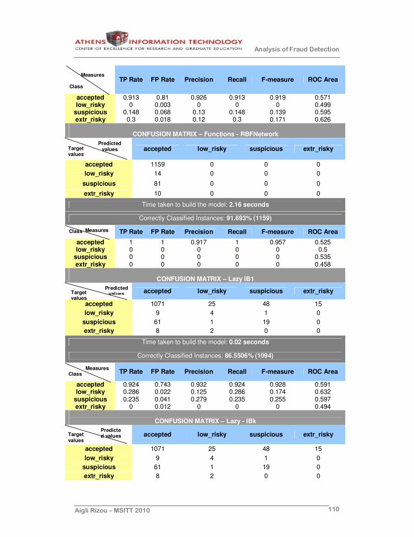
Analysis of Fraud Detection
Aigli Rizou – MSITT 2010 110
TP Rate FP Rate Precision Recall F-measure ROC Area
accepted 0.913 0.81 0.926 0.913 0.919 0.571 low_risky 0 0.003 0 0 0 0.499
suspicious 0.148 0.068 0.13 0.148 0.139 0.595 extr_risky 0.3 0.018 0.12 0.3 0.171 0.626
CONFUSION MATRIX – Functions - RBFNetwork
accepted low_risky suspicious extr_risky
accepted 1159 0 0 0
low_risky 14 0 0 0
suspicious 81 0 0 0
extr_risky 10 0 0 0
Time taken to build the model: 2.16 seconds
Correctly Classified Instances: 91.693% (1159)
TP Rate FP Rate Precision Recall F-measure ROC Area
accepted 1 1 0.917 1 0.957 0.525 low_risky 0 0 0 0 0 0.5
suspicious 0 0 0 0 0 0.535 extr_risky 0 0 0 0 0 0.458
CONFUSION MATRIX – Lazy IB1
accepted low_risky suspicious extr_risky
accepted 1071 25 48 15
low_risky 9 4 1 0
suspicious 61 1 19 0
extr_risky 8 2 0 0
Time taken to build the model: 0.02 seconds
Correctly Classified Instances: 86.5506% (1094)
TP Rate FP Rate Precision Recall F-measure ROC Area
accepted 0.924 0.743 0.932 0.924 0.928 0.591 low_risky 0.286 0.022 0.125 0.286 0.174 0.632
suspicious 0.235 0.041 0.279 0.235 0.255 0.597 extr_risky 0 0.012 0 0 0 0.494
CONFUSION MATRIX – Lazy - IBk
accepted low_risky suspicious extr_risky
accepted 1071 25 48 15
low_risky 9 4 1 0
suspicious 61 1 19 0
extr_risky 8 2 0 0
Measures
Class
Predicted values Target
values
Measures Class
Predicted values Target
values
Measures Class
Predicted values Target
values

Analysis of Fraud Detection
Aigli Rizou – MSITT 2010 111
Time taken to build the model: 0 seconds
Correctly Classified Instances: 86.5506% (1094)
TP Rate FP Rate Precision Recall F-measure ROC Area
accepted 0.924 0.743 0.932 0.924 0.928 0.569 low_risky 0.286 0.022 0.125 0.286 0.174 0.671
suspicious 0.235 0.041 0.279 0.235 0.255 0.568 extr_risky 0 0.012 0 0 0 0.499
CONFUSION MATRIX – Meta – AdaBoostM1
accepted low_risky suspicious extr_risky
accepted 1159 0 0 0
low_risky 14 0 0 0
suspicious 81 0 0 0
extr_risky 10 0 0 0
Time taken to build the model: 0.3 seconds
Correctly Classified Instances: 91.693% (1159)
TP Rate FP Rate Precision Recall F-measure ROC Area
accepted 1 1 0.917 1 0.957 0.53 low_risky 0 0 0 0 0 0.559
suspicious 0 0 0 0 0 0.529 extr_risky 0 0 0 0 0 0.668
CONFUSION MATRIX – Meta - LogitBoost
accepted low_risky suspicious extr_risky
accepted 1155 1 3 0
low_risky 14 0 0 0
suspicious 79 0 2 0
extr_risky 10 0 0 0
Time taken to build the model: 4.3 seconds
Correctly Classified Instances: 91.5348% (1157)
TP Rate FP Rate Precision Recall F-measure ROC Area
accepted 0.997 0.981 0.918 0.997 0.956 0.663 low_risky 0 0.001 0 0 0 0.772
suspicious 0.025 0.003 0.4 0.025 0.047 0.65 extr_risky 0 0 0 0 0 0.81
CONFUSION MATRIX – Meta - Bagging
accepted low_risky suspicious extr_risky
accepted 1155 0 4 0
low_risky 10 4 0 0
Measures Class
Predicted values Target
values
Measures Class
Predicted values Target
values
Predicted values Target
values
Measures Class

Analysis of Fraud Detection
Aigli Rizou – MSITT 2010 112
suspicious 75 0 6 0
extr_risky 10 0 0 0
Time taken to build the model: 41.02 seconds
Correctly Classified Instances: 92.1677% (1165)
TP Rate FP Rate Precision Recall F-measure ROC Area
accepted 0.997 0.905 0.924 0.997 0.959 0.637 low_risky 0.286 0 1 0.286 0.444 0.704
suspicious 0.074 0.003 0.6 0.074 0.132 0.595 extr_risky 0 0 0 0 0 0.674
CONFUSION MATRIX – Meta - EnsembleSelection
accepted low_risky suspicious extr_risky
accepted 1155 0 4 0
low_risky 12 2 0 0
suspicious 76 0 5 0
extr_risky 10 0 0 0
Time taken to build the model: 49.75 seconds
Correctly Classified Instances: 91.9304% (1162)
TP Rate FP Rate Precision Recall F-measure ROC Area
accepted 0.997 0.933 0.922 0.997 0.958 0.573 low_risky 0.143 0 1 0.143 0.25 0.635
suspicious 0.062 0.003 0.556 0.062 0.111 0.554 extr_risky 0 0 0 0 0 0.58
CONFUSION MATRIX – Meta - Stacking
accepted low_risky suspicious extr_risky
accepted 1159 0 0 0
low_risky 14 0 0 0
suspicious 81 0 0 0
extr_risky 10 0 0 0
Time taken to build the model: 0 seconds
Correctly Classified Instances: 91.693 % (1159)
TP Rate FP Rate Precision Recall F-measure ROC Area
accepted 1 1 0.917 1 0.957 0.488 low_risky 0 0 0 0 0 0.414
suspicious 0 0 0 0 0 0.493 extr_risky 0 0 0 0 0 0.499
CONFUSION MATRIX – Rules - DecisionTable
accepted low_risky suspicious extr_risky
accepted 1158 0 0 1
Measures Class
Predicted values Target
values
Measures Class
Predicted values Target
values
Measures Class
Predicted values Target
values

Analysis of Fraud Detection
Aigli Rizou – MSITT 2010 113
low_risky 14 0 0 0
suspicious 81 0 0 0
extr_risky 10 0 0 0
Time taken to build the model: 13.77 seconds
Correctly Classified Instances: 91.6139 % (1158)
TP Rate FP Rate Precision Recall F-measure ROC Area
accepted 0.999 1 0.917 0.999 0.956 0.494 low_risky 0 0 0 0 0 0.494
suspicious 0 0 0 0 0 0.443 extr_risky 0 0 0 0 0 0.494
CONFUSION MATRIX – Rules - JRip
accepted low_risky suspicious extr_risky
accepted 1159 0 0 0
low_risky 14 0 0 0
suspicious 81 0 0 0
extr_risky 10 0 0 0
Time taken to build the model: 7 seconds
Correctly Classified Instances: 91.693% (1159)
TP Rate FP Rate Precision Recall F-measure ROC Area
accepted 1 1 0.917 1 0.957 0.501 low_risky 0 0 0 0 0 0.5
suspicious 0 0 0 0 0 0.494 extr_risky 0 0 0 0 0 0.499
CONFUSION MATRIX – Trees - DecisionStump
accepted low_risky suspicious extr_risky
accepted 1159 0 0 0
low_risky 14 0 0 0
suspicious 81 0 0 0
extr_risky 10 0 0 0
Time taken to build the model: 0.11 seconds
Correctly Classified Instances: 91.693% (1159)
TP Rate FP Rate Precision Recall F-measure ROC Area
accepted 1 1 0.917 1 0.957 0.53 low_risky 0 0 0 0 0 0.559
suspicious 0 0 0 0 0 0.529 extr_risky 0 0 0 0 0 0.668
CONFUSION MATRIX – Trees – J48
accepted low_risky suspicious extr_risky
accepted 1159 0 0 0
low_risky 14 0 0 0
suspicious 81 0 0 0
Measures Class
Predicted values Target
values
Measures
Class
Predicted values Target
values
Measures
Class
Predicted values Target
values

Analysis of Fraud Detection
Aigli Rizou – MSITT 2010 114
extr_risky 10 0 0 0
Time taken to build the model: 0.38 seconds
Correctly Classified Instances: 91.693% (1159)
TP Rate FP Rate Precision Recall F-measure ROC Area
accepted 1 1 0.917 1 0.957 0.488 low_risky 0 0 0 0 0 0.414
suspicious 0 0 0 0 0 0.493 extr_risky 0 0 0 0 0 0.499
CONFUSION MATRIX – Trees - RandomForest
accepted low_risky suspicious extr_risky
accepted 1156 0 3 0
low_risky 10 4 0 0
suspicious 71 0 10 0
extr_risky 10 0 0 0
Time taken to build the model: 0.56 seconds
Correctly Classified Instances: 92.5633% (1170)
TP Rate FP Rate Precision Recall F-measure ROC Area
accepted 0.997 0.867 0.927 0.997 0.961 0.61 low_risky 0.286 0 1 0.286 0.444 0.74
suspicious 0.123 0.03 0.769 0.123 0.213 0.621 extr_risky 0 0 0 0 0 0.775
CONFUSION MATRIX – Functions - SMO
accepted low_risky suspicious extr_risky
accepted 646 1 10 1
low_risky 10 4 0 0
suspicious 70 0 11 0
extr_risky 10 0 0 0
Time taken to build the model: 263.89seconds
Correctly Classified Instances: 86.6317 % (661 out of 764)
TP Rate FP Rate Precision Recall F-measure ROC Area
accepted 0.982 0.857 0.878 0.982 0.927 0.562 low_risky 0.286 0.001 0.8 0.286 0.421 0.64
suspicious 0.136 0.015 0.524 0.136 0.216 0.563 extr_risky 0 0.001 0 0 0 0.694
Measures Class
Predicted values Target
values
Measures
Class
Predicted values Target
values
Measures
Class

Analysis of Fraud Detection
Aigli Rizou – MSITT 2010 115
SAMPLE B
Functions – RBFNetwork - Time taken to build the model: 1.33 seconds
Correlation coefficient -0.0468
Mean absolute error 0.202
Root mean squared error 0.4108
Relative absolute error 100.1464%
Root relative squared error 100.3364 %
Lazy – IBk - Time taken to build the model: 0 seconds
Correlation coefficient 0.1084
Mean absolute error 0.2023
Root mean squared error 0.6081
Relative absolute error 100.2708 %
Root relative squared error 148.5255 %
Lazy – KStar - Time taken to build the model: 0 seconds
Correlation coefficient 0.1812
Mean absolute error 0.1068
Root mean squared error 0.4162
Relative absolute error 101.662 %
Root relative squared error 148.5255 %
Lazy – LWL - Time taken to build the model: 0 seconds
Correlation coefficient 0.0658
Mean absolute error 0.1923
Root mean squared error 0.4145
Relative absolute error 95.3114 %
Root relative squared error 101.2442 %
Meta – Bagging - Time taken to build the model: 22.66 seconds
Correlation coefficient 0.2693
Mean absolute error 0.1865
Root mean squared error 0.3951
Relative absolute error 92.464 %
Root relative squared error 96.5 %
Meta – Stacking - Time taken to build the model: 0.02 seconds
Correlation coefficient -0.0609
Mean absolute error 0.2017
Root mean squared error 0.4094
Relative absolute error 100 %
Root relative squared error 100%

Analysis of Fraud Detection
Aigli Rizou – MSITT 2010 116
Meta – EnsmbleSelection -Time taken to build the model: 43.95 seconds
Correlation coefficient 0.2142
Mean absolute error 0.1886
Root mean squared error 0.3998
Relative absolute error 93.5038 %
Root relative squared error 97.6461 %
Rules – ConjunctiveRule - Time taken to build the model: 0.28 seconds
Correlation coefficient -0.0144
Mean absolute error 0.1982
Root mean squared error 0.4219
Relative absolute error 98.2663 %
Root relative squared error 103.0476 %
Rules – DecisionTable - Time taken to build the model: 25.2 seconds
Correlation coefficient 0.1379
Mean absolute error 0.1888
Root mean squared error 0.407
Relative absolute error 93.5832 %
Root relative squared error 99.3922 %
Trees – DecisionStump - Time taken to build the model: 0.39 seconds
Correlation coefficient -0.0101
Mean absolute error 0.1989
Root mean squared error 0.4133
Relative absolute error 98.5768 %
Root relative squared error 100.9369 %

Analysis of Fraud Detection
Aigli Rizou – MSITT 2010 117
SAMPLE C
CONFUSION MATRIX – Bayes - BayesNet
accepted low_risky suspicious extr_risky
accepted 932 4 219 4
low_risky 10 3 1 0
suspicious 55 0 25 1
extr_risky 5 2 3 0
Time taken to build the model: 0.67 seconds
Correctly Classified Instances: 75.9494% (1170)
TP Rate FP Rate Precision Recall F-measure ROC Area
accepted 0.804 0.667 0.93 0.804 0.863 0.663 low_risky 0.214 0.005 0.333 0.214 0.261 0.613
suspicious 0.309 0.189 0.101 0.309 0.152 0.667 extr_risky 0 0.004 0 0 0 0.755
CONFUSION MATRIX – Bayes - NaiveBayes
accepted low_risky suspicious extr_risky
accepted 1060 4 73 22
low_risky 1 3 9 1
suspicious 43 0 37 1
extr_risky 5 7 1 2
Time taken to build the model: 0.31 seconds
Correctly Classified Instances: 87.1835% (1102)
TP Rate FP Rate Precision Recall F-measure ROC Area
accepted 0.915 0.419 0.96 0.915 0.937 0.818 low_risky 0.214 0.009 0.214 0.214 0.214 0.573
suspicious 0.457 0.07 0.308 0.457 0.368 0.791 extr_risky 0.2 0.019 0.077 0.2 0.111 0.622
CONFUSION MATRIX – Functions - RBFNetwork
accepted low_risky suspicious extr_risky
accepted 1159 0 0 0
low_risky 14 0 0 1
suspicious 81 0 0 0
extr_risky 10 0 0 0
Time taken to build the model: 6.77 seconds
Correctly Classified Instances: 91.693 % (1159)
TP Rate FP Rate Precision Recall F-measure ROC Area
accepted 1 1 0.917 1 0.957 0.5 low_risky 0 0 0 0 0 0.413
Predicted values Target
values
Measures Class
Predicted values Target
values
Measures Class
Predicted values Target
values
Measures
Class

Analysis of Fraud Detection
Aigli Rizou – MSITT 2010 118
suspicious 0 0 0 0 0 0.445 extr_risky 0 0 0 00 0 0.555
CONFUSION MATRIX – Lazy – IB1
accepted low_risky suspicious extr_risky
accepted 1071 6 78 4
low_risky 10 4 0 0
suspicious 53 1 27 0
extr_risky 6 2 0 2
Time taken to build the model: 0.03 seconds
Correctly Classified Instances: 87.3418 % (1104)
TP Rate FP Rate Precision Recall F-measure ROC Area
accepted 0.924 0.657 0.939 0.924 0.932 0.633 low_risky 0.286 0.007 0.308 0.286 0.296 0.639
suspicious 0.333 0.066 0.257 0.333 0.29 0.634 extr_risky 0.2 0.003 0.333 0.2 0.25 0.598
CONFUSION MATRIX – Meta – AdaBoostM1
accepted low_risky suspicious extr_risky
accepted 1159 0 0 0
low_risky 10 0 1 3
suspicious 67 0 14 0
extr_risky 6 2 0 2
Time taken to build the model: 2.05 seconds
Correctly Classified Instances: 92.9589% (1175)
TP Rate FP Rate Precision Recall F-measure ROC Area
accepted 1 0.79 0.933 1 0.965 0.792 low_risky 0 0.002 0 0 0 0.833
suspicious 0.173 0.001 0.933 0.173 0.292 0.753 extr_risky 0.2 0.002 0.4 0.2 0.267 0.859
CONFUSION MATRIX – Meta - Bagging
accepted low_risky suspicious extr_risky
accepted 1155 0 4 0
low_risky 10 4 0 0
suspicious 75 0 6 0
extr_risky 10 0 0 0
Time taken to build the model: 99.72 seconds
Correctly Classified Instances: 92.1677% (1165)
TP Rate FP Rate Precision Recall F-measure ROC Area
accepted 0.997 0.905 0.924 0.997 0.959 0.637 low_risky 0.286 0 1 0.286 0.444 0.704
Predicted values Target
values
Measures Class
Predicted values Target
values
Measures
Class
Predicted values Target
values
Measures
Class

Analysis of Fraud Detection
Aigli Rizou – MSITT 2010 119
suspicious 0.074 0.003 0.6 0.074 0.132 0.595 extr_risky 0 0 0.4 0 0 0.674
CONFUSION MATRIX – Meta - LogitBoost
accepted low_risky suspicious extr_risky
accepted 1159 0 0 0
low_risky 5 8 1 0
suspicious 18 0 63 0
extr_risky 0 1 0 9
Time taken to build the model: 16.17 seconds
Correctly Classified Instances: 98.0222% (1239)
TP Rate FP Rate Precision Recall F-measure ROC Area
accepted 1 0.219 0.981 1 0.99 0.945 low_risky 0.571 0.001 0.889 0.571 0.696 0.912
suspicious 0.778 0.001 0.984 0.778 0.869 0.949 extr_risky 0.9 0 1 0.9 0.947 0.998
CONFUSION MATRIX – Rules - DecisionTable
accepted low_risky suspicious extr_risky
accepted 1159 0 0 0
low_risky 6 6 2 0
suspicious 20 0 61 0
extr_risky 5 0 0 5
Time taken to build the model: 62.78 seconds
Correctly Classified Instances: 97.3892% (1231)
TP Rate FP Rate Precision Recall F-measure ROC Area
accepted 1 0.295 0.974 1 0.987 0.926 low_risky 0.429 0 1 0.429 0.6 0.988
suspicious 0.753 0.002 0.968 0.753 0.847 0.903 extr_risky 0.5 0 1 0.5 0.667 0.898
CONFUSION MATRIX – Rules - ConjunctiveRule
accepted low_risky suspicious extr_risky
accepted 1159 0 0 0
low_risky 6 6 2 0
suspicious 20 0 61 0
extr_risky 5 0 0 5
Time taken to build the model: 0.95 seconds
Correctly Classified Instances: 92.6424% (1171)
TP Rate FP Rate Precision Recall F-measure ROC Area
accepted 1 0.876 0.926 1 0.962 0.552 low_risky 0 0 0 0 0 0.38
suspicious 0.148 0.001 0.923 0.148 0.255 0.568 extr_risky 0 0 0 0 0 0.504
Predicted values
Target values
Measures Class
Predicted values Target
values
Measures Class
Predicted values Target
values
Measures
Class
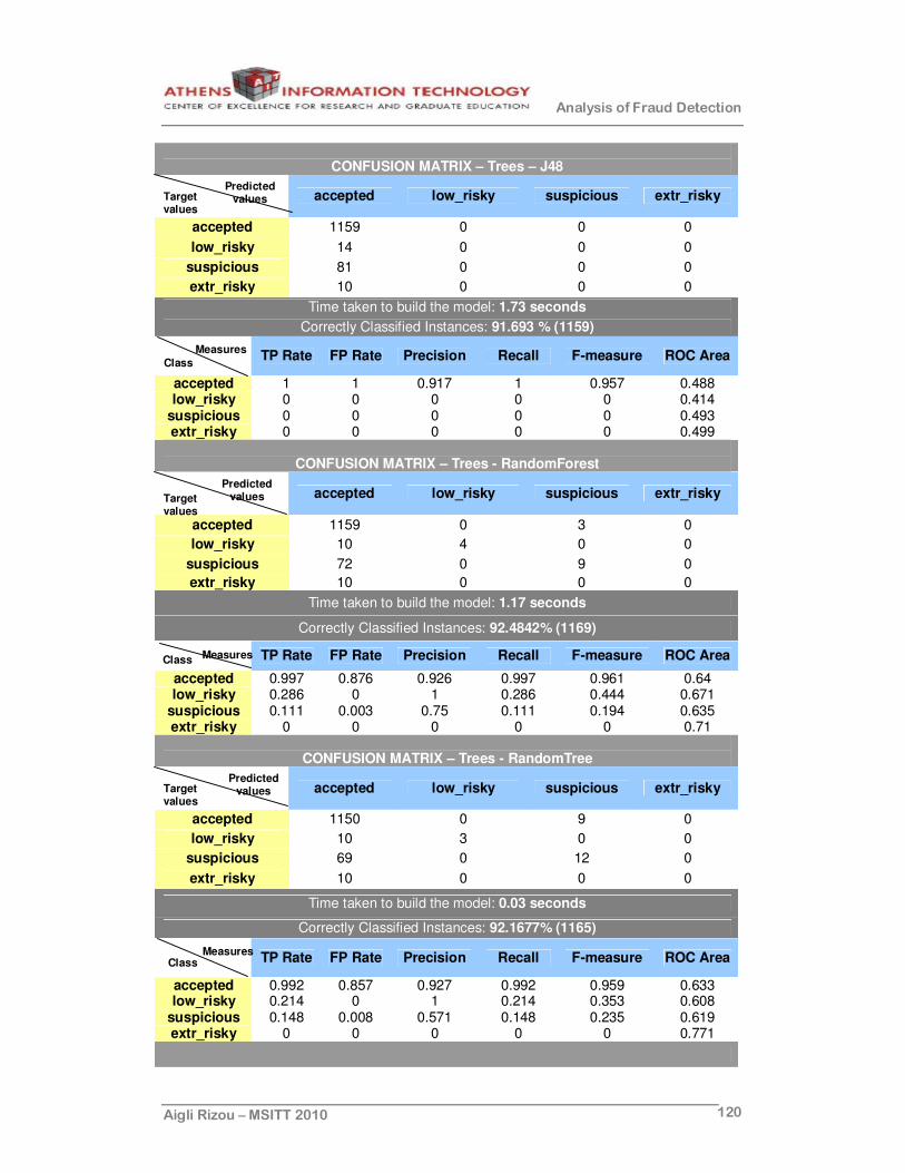
Analysis of Fraud Detection
Aigli Rizou – MSITT 2010 120
CONFUSION MATRIX – Trees – J48
accepted low_risky suspicious extr_risky
accepted 1159 0 0 0
low_risky 14 0 0 0
suspicious 81 0 0 0
extr_risky 10 0 0 0
Time taken to build the model: 1.73 seconds
Correctly Classified Instances: 91.693 % (1159)
TP Rate FP Rate Precision Recall F-measure ROC Area
accepted 1 1 0.917 1 0.957 0.488 low_risky 0 0 0 0 0 0.414
suspicious 0 0 0 0 0 0.493 extr_risky 0 0 0 0 0 0.499
CONFUSION MATRIX – Trees - RandomForest
accepted low_risky suspicious extr_risky
accepted 1159 0 3 0
low_risky 10 4 0 0
suspicious 72 0 9 0
extr_risky 10 0 0 0
Time taken to build the model: 1.17 seconds
Correctly Classified Instances: 92.4842% (1169)
TP Rate FP Rate Precision Recall F-measure ROC Area
accepted 0.997 0.876 0.926 0.997 0.961 0.64 low_risky 0.286 0 1 0.286 0.444 0.671
suspicious 0.111 0.003 0.75 0.111 0.194 0.635 extr_risky 0 0 0 0 0 0.71
CONFUSION MATRIX – Trees - RandomTree
accepted low_risky suspicious extr_risky
accepted 1150 0 9 0
low_risky 10 3 0 0
suspicious 69 0 12 0
extr_risky 10 0 0 0
Time taken to build the model: 0.03 seconds
Correctly Classified Instances: 92.1677% (1165)
TP Rate FP Rate Precision Recall F-measure ROC Area
accepted 0.992 0.857 0.927 0.992 0.959 0.633 low_risky 0.214 0 1 0.214 0.353 0.608
suspicious 0.148 0.008 0.571 0.148 0.235 0.619 extr_risky 0 0 0 0 0 0.771
Predicted values
Target values
Measures Class
Predicted values Target
values
Measures Class
Predicted values Target
values
Measures Class

Analysis of Fraud Detection
Aigli Rizou – MSITT 2010 121
CONFUSION MATRIX – Functions - SMO
accepted low_risky suspicious extr_risky
accepted 4 0 10 0
low_risky 0 10 70 0
suspicious 0 7 651 1
extr_risky 0 0 10 0
Time taken to build the model: 278.38seconds
Correctly Classified Instances: 87.156% (665 out of 764)
TP Rate FP Rate Precision Recall F-measure ROC Area
accepted 0.286 0 1 0.286 0.444 0.666 low_risky 0.125 0.01 0.588 0.125 0.206 0.557
suspicious 0.988 0.865 0.879 0.988 0.93 0.561 extr_risky 0 0.001 0 0 0 0.781
Predicted values Target
values
measures Class
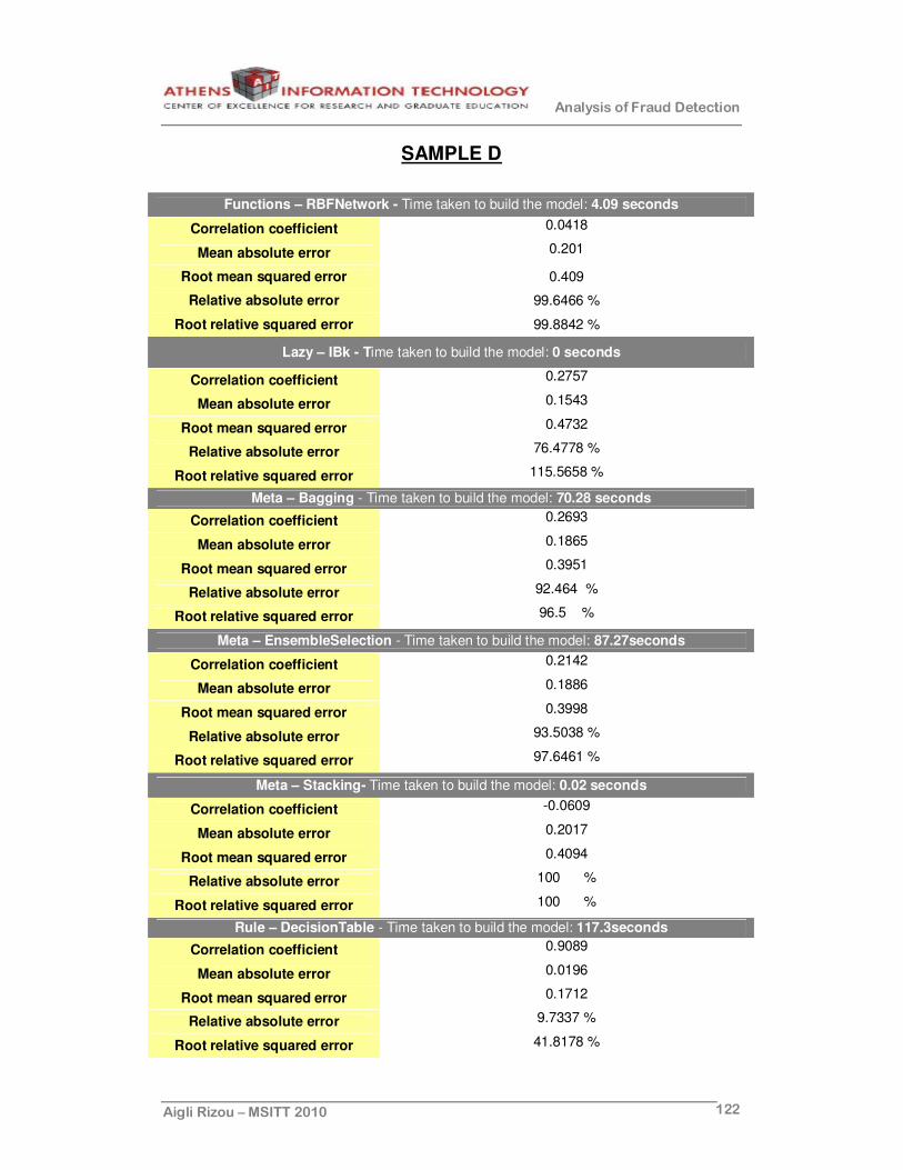
Analysis of Fraud Detection
Aigli Rizou – MSITT 2010 122
SAMPLE D
Functions – RBFNetwork - Time taken to build the model: 4.09 seconds
Correlation coefficient 0.0418
Mean absolute error 0.201
Root mean squared error 0.409
Relative absolute error 99.6466 %
Root relative squared error 99.8842 %
Lazy – IBk - Time taken to build the model: 0 seconds
Correlation coefficient 0.2757
Mean absolute error 0.1543
Root mean squared error 0.4732
Relative absolute error 76.4778 %
Root relative squared error 115.5658 %
Meta – Bagging - Time taken to build the model: 70.28 seconds
Correlation coefficient 0.2693
Mean absolute error 0.1865
Root mean squared error 0.3951
Relative absolute error 92.464 %
Root relative squared error 96.5 %
Meta – EnsembleSelection - Time taken to build the model: 87.27seconds
Correlation coefficient 0.2142
Mean absolute error 0.1886
Root mean squared error 0.3998
Relative absolute error 93.5038 %
Root relative squared error 97.6461 %
Meta – Stacking- Time taken to build the model: 0.02 seconds
Correlation coefficient -0.0609
Mean absolute error 0.2017
Root mean squared error 0.4094
Relative absolute error 100 %
Root relative squared error 100 %
Rule – DecisionTable - Time taken to build the model: 117.3seconds
Correlation coefficient 0.9089
Mean absolute error 0.0196
Root mean squared error 0.1712
Relative absolute error 9.7337 %
Root relative squared error 41.8178 %

Analysis of Fraud Detection
Aigli Rizou – MSITT 2010 123
Rule – ConjunctiveRule - Time taken to build the model: 0.56 seconds
Correlation coefficient 0.5537
Mean absolute error 0.1639
Root mean squared error 0.3408
Relative absolute error 81.2696 %
Root relative squared error 83.2461 %
Trees – DecisionStump - Time taken to build the model: 0.36 seconds
Correlation coefficient 0.6055
Mean absolute error 0.1471
Root mean squared error 0.3257
Relative absolute error 72.9155 %
Root relative squared error 79.5479 %

Analysis of Fraud Detection
Aigli Rizou – MSITT 2010 124
APPENDIX B
The following tables include the WEKA results in an aggregated form after the
application of all supervised algorithms in samples A and B and samples C
and D.
SAMPLES A & B
Algorithm Type
Algorithm Running
Time (sec) Accuracy
(%)
Relative Absolute Error (%)
Class Label
#Records
ConjunctiveRule 0,31 92 99 Nominal 1264
ConjunctiveRule 0,28 98 Numerical 1264
DecisionTable 13,77 91,6139 112,4373 Nominal 1264
DecisionTable 25,2 93,5832 Numerical 1264
Jrip 7 91,693 96,5272 Nominal 1264
OneR 0,08 92 Nominal 1264
PART 0,49 91,693 98,7697 Nominal 1264
Ridor 1,55 89,1614 69,0206 Nominal 1264
ZeroR 0,02 92 100 Nominal 1264
RULES
ZeroR 0 100 Numerical 1264
DecisionStump 0,11 92 98 Nominal 1264
DecisionStump 0,39 99 Numerical 1264
J48 0,38 91,693 98,6723 Nominal 1264
J48graft 1,16 91,693 98,6723 Nominal 1264
REPTree 1,98 92,0886 93,3101 Nominal 1264
REPTree 2,02 90,2275 Numerical 1264
M5P 35,23 119,7694 Numerical 764
RandomForest 0,56 92,5633 89,4978 Nominal 1264
RandomTree 0,06 91,7722 89,0786 Nominal 1264
REES
UserClassifier 58,08 100 Numerical 1264
HyperPipes 0,02 92,4051 465 Nominal 1264 MISC
VFI 0,08 85,9177 88,5161 Nominal 1264
AdaBoostM1 0,3 91,693 98 Nominal 1264
AttributeSelectedClassifier 9,66 91,693 98,6723 Nominal 1264
AdditiveRegression 1,38 86,5033 Numerical 1264 ClassificationViaClustering 1,56 64,6361 225,1986 Nominal 1264
CVParameterSelection 0,02 91,693 100 Nominal 1264
CVParameterSelection 0 100 Numerical 1264
Bagging 41,02 92,1677 92,6654 Nominal 1264
Bagging 22,66 92,464 Numerical 1264
Decorate 15,11 91,693 108,9727 Nominal 1264
END 5,19 91,693 98,6833 Nominal 1264
FilteredClassifier 0,22 91,693 986.723 Nominal 1264
META
Grading 0,03 91,693 52,899 Nominal 1264
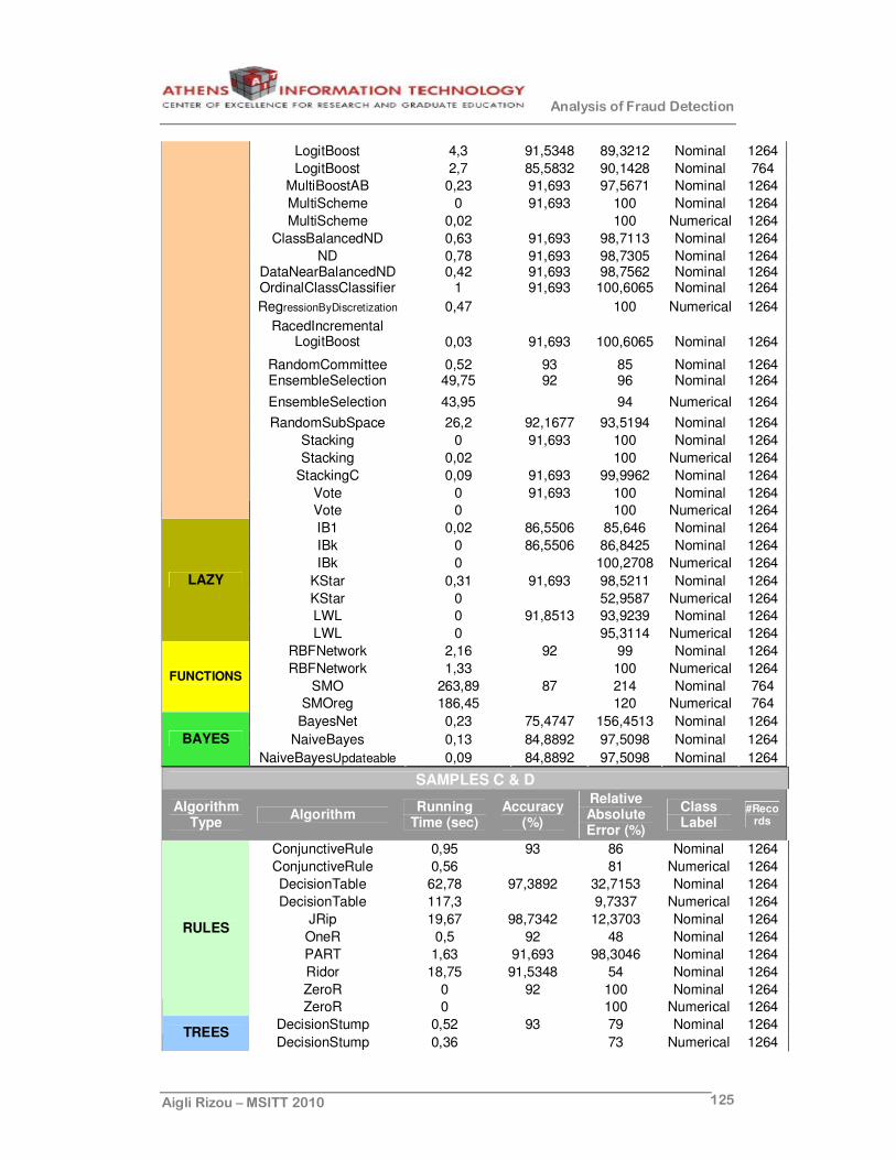
Analysis of Fraud Detection
Aigli Rizou – MSITT 2010 125
LogitBoost 4,3 91,5348 89,3212 Nominal 1264
LogitBoost 2,7 85,5832 90,1428 Nominal 764
MultiBoostAB 0,23 91,693 97,5671 Nominal 1264
MultiScheme 0 91,693 100 Nominal 1264
MultiScheme 0,02 100 Numerical 1264
ClassBalancedND 0,63 91,693 98,7113 Nominal 1264
ND 0,78 91,693 98,7305 Nominal 1264 DataNearBalancedND 0,42 91,693 98,7562 Nominal 1264 OrdinalClassClassifier 1 91,693 100,6065 Nominal 1264
RegressionByDiscretization 0,47 100 Numerical 1264
RacedIncremental LogitBoost 0,03 91,693 100,6065 Nominal 1264
RandomCommittee 0,52 93 85 Nominal 1264 EnsembleSelection 49,75 92 96 Nominal 1264
EnsembleSelection 43,95 94 Numerical 1264
RandomSubSpace 26,2 92,1677 93,5194 Nominal 1264
Stacking 0 91,693 100 Nominal 1264
Stacking 0,02 100 Numerical 1264
StackingC 0,09 91,693 99,9962 Nominal 1264
Vote 0 91,693 100 Nominal 1264
Vote 0 100 Numerical 1264
IB1 0,02 86,5506 85,646 Nominal 1264
IBk 0 86,5506 86,8425 Nominal 1264
IBk 0 100,2708 Numerical 1264
KStar 0,31 91,693 98,5211 Nominal 1264
KStar 0 52,9587 Numerical 1264
LWL 0 91,8513 93,9239 Nominal 1264
LAZY
LWL 0 95,3114 Numerical 1264
RBFNetwork 2,16 92 99 Nominal 1264
RBFNetwork 1,33 100 Numerical 1264
SMO 263,89 87 214 Nominal 764 FUNCTIONS
SMOreg 186,45 120 Numerical 764
BayesNet 0,23 75,4747 156,4513 Nominal 1264
NaiveBayes 0,13 84,8892 97,5098 Nominal 1264 BAYES
NaiveBayesUpdateable 0,09 84,8892 97,5098 Nominal 1264 SAMPLES C & D
Algorithm Type
Algorithm Running
Time (sec) Accuracy
(%)
Relative Absolute Error (%)
Class Label
#Records
ConjunctiveRule 0,95 93 86 Nominal 1264
ConjunctiveRule 0,56 81 Numerical 1264
DecisionTable 62,78 97,3892 32,7153 Nominal 1264
DecisionTable 117,3 9,7337 Numerical 1264
JRip 19,67 98,7342 12,3703 Nominal 1264
OneR 0,5 92 48 Nominal 1264
PART 1,63 91,693 98,3046 Nominal 1264
Ridor 18,75 91,5348 54 Nominal 1264
ZeroR 0 92 100 Nominal 1264
RULES
ZeroR 0 100 Numerical 1264
DecisionStump 0,52 93 79 Nominal 1264 TREES
DecisionStump 0,36 73 Numerical 1264

Analysis of Fraud Detection
Aigli Rizou – MSITT 2010 126
J48 1,73 91,693 98,6723 Nominal 1264
J48 1 86 99 Nominal 764
J48graft 3,73 91,693 98,6723 Nominal 1264
REPTree 8,5 92,0886 93,3101 Nominal 1264
REPTree 7,75 90 Numerical 1264
M5P 38,39 158,0417 Numerical 764
RandomForest 1,17 92,4842 90,1185 Nominal 1264
RandomTree 0,03 92,1677 84,5656 Nominal 1264
UserClassifier 17,42 100 Numerical 1264
HyperPipes 0,05 92,7215 473,1011 Nominal 1264 MISC
VFI 0,14 86,6297 82,1092 Nominal 1264
AdaBoostM1 2,05 93 104 Nominal 1264 AttributeSelectedCla
ssifier 7,69 92 99 Nominal 1264
AdditiveRegression 4,31 24,6164 Numerical 1264 ClassificationViaCluster
ing 7,05 59,4146 258,4494 Nominal 1264
CVParameterSelection 0 92 100 Nominal 1264
CVParameterSelection 0 100 Numerical 1264
Bagging 99,72 92,1677 92,6654 Nominal 1264
Bagging 70,28 92,464 Numerical 1264
Decorate 77,63 91,693 107,7443 Nominal 1264
END 22,41 91,693 98,5855 Nominal 1264
FilteredClassifier 0,7 92,0095 94,147 Nominal 1264
Grading 0,03 92 53 Nominal 1264
LogitBoost 16,17 98,0222 25,685 Nominal 1264
LogitBoost 8,09 96,9856 26,9984 Nominal 764
MultiBoostAB 3,53 92,8797 45,3391 Nominal 1264
MultiScheme 0,02 91,693 100 Nominal 1264
MultiScheme 0,03 100 Numerical 1264
ClassBalancedND 4,92 91,693 98,573 Nominal 1264 ND 1,8 91,693 98,5283 Nominal 1264
DataNearBalancedND 4,88 91,693 98,4153 Nominal 1264
OrdinalClassClassifier 4,36 91,693 98,6723 Nominal 1264 RegressionByDiscret
ization 1,74 99,6557 Numerical 1264
RacedIncrementalLogitBoost
0,02 91,693 100,6065 Nominal 1264
RandomCommittee 0,75 93 88 Nominal 1264
EnsembleSelection 86,39 92 96 Nominal 1264
EnsembleSelection 87,27 94 Numerical 1264
RandomSubSpace 35,06 91,9304 93,4288 Nominal 1264
RandomSubSpace 32,84 92,3796 Numerical 1264
Stacking 0,02 91,693 100 Nominal 1264
Stacking 0,02 100 Numerical 1264
StackingC 0,17 91,693 99,9962 Nominal 1264
Vote 0,02 92 100 Nominal 1264
META
Vote 0 100 Numerical 1264
IB1 0,03 87,3418 80,608 Nominal 1264
Ibk 0 87,3418 81,9896 Nominal 1264
IBk 0 76,4778 Numerical 1264
LAZY
KStar 0 91,693 477,6024 Nominal 1264

Analysis of Fraud Detection
Aigli Rizou – MSITT 2010 127
KStar 0 54,5149 Numerical 1264
LWL 0 94,3829 69,2469 Nominal 1264
LWL 0 70,1878 Numerical 1264
RBFNetwork 6,77 92 99 Nominal 1264
RBFNetwork 4,09 100 Numerical 1264
SMO 278,38 87 215 Nominal 764 FUNCTION
S
SMOreg 195,31 97 Numerical 764
BayesNet 0,67 75,9494 152,8978 Nominal 1264
NaiveBayes 0,31 87,1835 82,6355 Nominal 1264 BAYES
NaiveBayesUpdateable
0,31 87,1835 82,6355 Nominal 1264