Fn

Ta

b

a

ARRAA

KWS(RA

1

oeTicmbas

dh[omppt

(

1d

Applied Soft Computing 11 (2011) 2510–2525

Contents lists available at ScienceDirect

Applied Soft Computing

journa l homepage: www.e lsev ier .com/ locate /asoc

orecasting stock markets using wavelet transforms and recurrent neuraletworks: An integrated system based on artificial bee colony algorithm

sung-Jung Hsieha,∗, Hsiao-Fen Hsiaob,∗∗, Wei-Chang Yeha

Department of Industrial Engineering and Engineering Management, National Tsing Hua University, P.O. Box 24-60, Hsinchu 30013, Taiwan, ROCDepartment of Finance, Mingdao University, 369 Wen-Hua Rd., Peetow, Changhua 52345, Taiwan, ROC

r t i c l e i n f o

rticle history:eceived 6 February 2010eceived in revised form 10 June 2010ccepted 1 September 2010vailable online 30 October 2010

a b s t r a c t

This study presents an integrated system where wavelet transforms and recurrent neural network (RNN)based on artificial bee colony (abc) algorithm (called ABC-RNN) are combined for stock price forecasting.The system comprises three stages. First, the wavelet transform using the Haar wavelet is applied todecompose the stock price time series and thus eliminate noise. Second, the RNN, which has a simplearchitecture and uses numerous fundamental and technical indicators, is applied to construct the input

eywords:avelet transform

tepwise regression-correlation selectionSRCS)ecurrent neural network (RNN)rtificial bee colony algorithm (ABC)

features chosen via Stepwise Regression-Correlation Selection (SRCS). Third, the Artificial Bee Colonyalgorithm (ABC) is utilized to optimize the RNN weights and biases under a parameter space design.For illustration and evaluation purposes, this study refers to the simulation results of several interna-tional stock markets, including the Dow Jones Industrial Average Index (DJIA), London FTSE-100 Index(FTSE), Tokyo Nikkei-225 Index (Nikkei), and Taiwan Stock Exchange Capitalization Weighted Stock Index(TAIEX). As these simulation results demonstrate, the proposed system is highly promising and can be

e tra

implemented in a real-tim

. Introduction

Mining stock market tendencies is a challenging task. Numer-us factors influence stock market performance, including politicalvents, general economic conditions, and trader expectations.hough stock and futures traders rely heavily on various types ofntelligent systems to make trading decisions, to date their suc-ess has been limited [1]. Even financial experts find it difficult toake accurate predictions, because stock market trends tend to

e nonlinear, uncertain, and non-stationary. No consensus existsmong experts as to the effectiveness of forecasting a financial timeeries.

One model that may be more efficient than others in stock pre-iction is the artificial neural network (ANN) [8]. Several studiesave shown that the ANN outperforms statistical regression models2] and discriminant analysis [3]. Generally, two different method-logies exist for stock price prediction using ANNs [4]. The first

ethodology considers stock price variations as a time series and

redicts future prices using past data. This approach uses ANNs asredictors [5–7]. These prediction models suffer limitations owingo the enormous noise and high dimensionality of stock price data.

∗ Corresponding author.∗∗ Corresponding author.

E-mail addresses: tsungjung.hsieh@gmail.com (T.-J. Hsieh), fen@mdu.edu.twH.-F. Hsiao).

568-4946/$ – see front matter. Crown Copyright © 2010 Published by Elsevier B.V. All rioi:10.1016/j.asoc.2010.09.007

ding system for forecasting stock prices and maximizing profits.Crown Copyright © 2010 Published by Elsevier B.V. All rights reserved.

Consequently, none of the existing prediction models has satisfac-tory performance, as Zadeh [8] and Marmer [9] have observed. Asecond approach for stock price prediction has been proposed thatconsiders technical indices and qualitative factors, such as politi-cal effects in stock market forecasting and trend analysis. The ideahere is that merging technical indicators permits the exploitation oftolerance for imprecision, uncertainty, and partial truth to achievetractability, robustness, and low-cost solutions.

Other attempts have been made to forecast financial marketsthat range from traditional time series approaches to artificial intel-ligence techniques, including, ARCH-GARCH models [32], ANNs[8], and evolutionary computation methods [28–31]. However, themain disadvantage of both ANNs and these other black-box tech-niques is the enormous difficulty of interpreting the results. Thisstudy diverges from previous attempts at forecasting stock pricesby proposing a method that uses the Artificial Bee Colony (ABC)algorithm combined with the ANN optimization process to cre-ate a transparent architecture. The operators of the ABC algorithmprovide diverse initial weights and biases for the network under aparameter matrix design, where parameters contain the biases andweight connected neurons.

The ABC algorithm is a new meta-heuristic approach, proposed

by Basturk and Karaboga [10]. Because it has the advantages ofmemory, multi-characters, local search, and a solution improve-ment mechanism, it can be used to identify a high quality optimalsolution and offer a balance between complexity and performance,thus optimizing forecasting effectiveness. In this study, the param-

ghts reserved.

T.-J. Hsieh et al. / Applied Soft Computing 11 (2011) 2510–2525 2511

Data preprocessing by wavelet transform

Fundamental factors and technical index data (X1, X2, . . ., Xn ,Y)

Choosing the most influential factor by stepwise regression-

correlation selection (SRCS)

Performance evaluation

Stock price forecasting by different Methods

RNN Optimization by ABC algorithm

Training Phase

Testing Phase

work

ea

aecl[vlfdiosdau

nitpt[Cssatram

iaedi

Fig. 1. Frame

ter matrix is optimized via the powerful heuristic method, the ABClgorithm.

First, however, wavelet analysis is applied. Wavelet analysis isrelatively new field in signal processing [11]. Wavelets are math-matical functions that decompose data into different frequencyomponents, after which each component is studied with a reso-ution matched to its scale, where a scale denotes a time horizon12]. Wavelet filtering is closely related to the volatile and time-arying characteristics of the real-world time series and is notimited by the stationarity assumption [13]. The wavelet trans-orm decomposes a process into different scales, making it useful inistinguishing seasonality, revealing structural breaks and volatil-

ty clusters, and identifying local and global dynamic propertiesf a process at specific timescales [14]. Wavelet analysis has beenhown to be particularly useful in analyzing, modeling, and pre-icting the behavior of financial instruments as diverse as stocksnd exchange rates [15,16]. This study applies wavelet transformsing the Haar wavelet to decompose the time series.

Numerous practical problems involve a possible quite largeumber of input variables that can be quite large. Moreover, these

nput variables may contain considerable redundancy. Because ofhis redundancy, eliminating redundant variables may improverediction performance. Besides, the interpretability of the predic-ive model can be enhanced by reducing the data dimensionality17]. Consequently, this study employs Stepwise Regression-orrelation Selection (SRCS) to choose the input features that mosttrongly influence the response variable. The framework combineseveral statistical methods and soft computing techniques suchs RNN, wavelet transform, ABC algorithm, and SRCS to extracthe input feature subset. Besides applying wavelet-based data rep-esentation, SRCS to data processing before generating the RNN,nd the parameter matrix was optimized via a powerful heuristicethod—Artificial Bee Colony algorithm.We tested our method on the Taiwan Stock Exchange Capital-

zation Weighted Stock Index (TAIEX) for the period 1997–2003,nd found that it was more predictable than other methods. Tonsure our work was sufficiently robust and workable, we con-ucted simulation studies on other international stock markets,

ncluding the Dow Jones Industrial Average Index (DJIA), London

of ABC-RNN.

FTSE-100 Index (FTSE), and Tokyo Nikkei-225 Index (Nikkei), fortwo periods: 1997–2003 and 2002–2008. The results indicate thatthe proposed integrated system is viable and useful, and it may alsoresult in large profits.

The remainder of this paper is organized as follows: Section 2describes the stock price prediction approach used in this study.Section 3 presents the results and compares the proposed methodto previous approaches. Section 4 summarizes the findings andprovides suggestions for further research.

2. Methodology

Previous studies have used statistics, technical analysis, funda-mental analysis, and linear regression to predict market direction[4]. However, price forecasting is generally conducted usingtechnical analysis or fundamental analysis. Technical analysisconcentrates on market action, while fundamental analysis con-centrates on the forces of supply and demand that drive pricemovements. The basic assumption of this study is supported bystudies of the financial time series, which indicate that price move-ments are closely related to market returns during periods ofvolatility, but also to fundamental factors. The output of these fac-tors is stock price.

To study the relations among the financial time-series variables,this work presents a hybrid method that integrates a wavelet andthe ABC-RNN-based forecasting scheme. Fig. 1 shows the main pro-cedures of this approach. The inputs and outputs of each block arefurther detailed in the material that follows.

2.1. Data preprocessing using wavelet transform

Wavelet theory is applied for data preprocessing, since the rep-resentation of a wavelet can deal with the non-stationarity involvedin the economic and financial time series [15]. The key propertyof wavelets for economic analysis is decomposition by time scale.

Economic and financial systems contain variables that operate onvarious time scales simultaneously; thus, the relations betweenvariables may differ across time scales. One of the benefits of thewavelet approach is that it is flexible in handling highly irregulardata series [13].

2512 T.-J. Hsieh et al. / Applied Soft Computing 11 (2011) 2510–2525

Table 1All variables considered.

ID Feature description Computational formula or statement

1 Moving average (6) (MA (6)) MA (m)t = (∑n

i=n−mxi)/m, m = 6

2 Demand index (DI) DIt = (Ht + Lt + 2Ct)/4

3 Exponential moving average (12) (EMA (12)) EMA(m)i = (1/m) ×∑n

i=t−mDIi , m = 12

4. Exponential moving average (26) (EMA (26)) EMA(m)i = (1/m) ×∑n

i=t−mDIi , m = 26

5 RSI (6) RS(6)i = UP(6)avgDOWN(6)avg

, RSI(6)i = 100 −(

1001+RS(6)i

)UPavg: The average closed price of those arising days in a period 6.DOWNavg: The average closed price of those dropping days in a period 6.

6 RSV (9) RSV (9) = 100(C(9) − L (9))/(H (9) − L(9))C (9): The closed price on the 9th day.L (9): The lowest closed price in 9 days.H (9): The highest closed price in 9 days.

7 K (9) K(9)i = 23K(9)t−1 + 1

3 RSV(9)t8 D (9) D(9)i = 2

3D(9)t−1 + 13K(9)t

9 MACD MACD(9)i = 19

i∑t=i−9

(EMA(12)t − EMA(26)t ),

10 PSY (13) PSY (13) = [(The days of those closed prices arising in a period 13)/13]×100

faLu

a

11 The close price one day ago (C)12 The open price one day ago (O)13 The highest price one day ago (H)14 The lowest price one day ago (L)

This study applies the Haar wavelet as the main wavelet trans-orm tool. A wavelet not only decomposes the data in terms of timesnd frequency, but also significantly reduces the processing time.

et n denote the time series size, then the wavelet decompositionsed in this study can be determined in O(n) time [18].

Wavelets theory is based on Fourier analysis, which representsny function as the sum of the sine and cosine functions. A wavelet(t) is simply a function of time t that obeys a basic rule, known as

Input: Candidate input features.

Output: The features that are strongly influence the dependent variable (Y).

BEGIN

1. Load input features (X1, X2, . . ., Xn)2. Determine the correlation coefficient (r) of each feature and Y3. Derive a correlation matrix

4. Repeat

5. FOR (i=1 to n) DO {

Rank each input feature according to its absolute value of r that is larger

than 0.4 from the correlation matrix (suppose Xi has the largest value of |r| in

the current stage)

Check the significance of the influence of this variable on the output

data; i.e., derive a regression model with the form Y = f(Xi).Apply the p-value to consider the significance of each input variable}.

6. Select the statistically significant variables from Step 5 for further

verification and assume that they are (X1, X2, . . ., Xk).7. FOR (i=1 to k) DO {

Calculate the partial F value for those statistically significant variables,

as shown in equation (8).

If the partial F value of a number (which is assumed to have a value of

Xj ) is below a user defined threshold, it is removed from the model because

Xj is not statistically significant for the output.}

8. If the partial F value of every input number is greater than the user

defined threshold, stop.

END

Fig. 2. Algorithm 1—SRCS.

Cxt

Oxt

Hxt

Lxt

the wavelet admissibility condition [19]:

C =∫ ∞

0

∣∣ (f )∣∣

fdf <∞ (1)

where (f)is the Fourier transform and a function of frequency f, of (t).

The wavelet transform (WT) is a mathematical tool that can beapplied to numerous applications, such as image analysis and sig-nal processing. It was introduced to solve problems associated withthe Fourier transform as they occur. This occurrence can take placewhen dealing with non-stationary signals, or when dealing withsignals that are localized in time, space, or frequency. Dependingon the normalization rules, there are two types of wavelets withina given function/family. Father wavelets describe the smooth andlow-frequency parts of a signal, and mother wavelets describe thedetailed and high-frequency components. In the following equa-tions, (2a) represents the father wavelet and (2b) represents themother wavelet, with j = 1,. . .,J in the J-level wavelet decomposi-tion: [20]

�j,k = 2−j/2�(t − 2jk/2j) (2a)

j,k = 2−j/2 (t − 2jk/2j) (2b)

where J denotes the maximum scale sustainable by the number ofdata points and the two types of wavelets stated above, namelyfather wavelets and mother wavelets, and satisfies:

∫�(t)dt = 1 and

∫ (t)dt = 0 (3)

Time series data, i.e., function f(t), is an input represented bywavelet analysis, and can be built up as a sequence of projec-

tions onto father and mother wavelets indexed by both {k}, k = {0,1, 2,. . .} and by {s}= 2j, {j = 1, 2, 3,. . .J}. Analyzing real discretelysampled data requires creating a lattice for making calculations.Mathematically, it is convenient to use a dyadic expansion, asshown in equation (3). The expansion coefficients are given by the

T.-J. Hsieh et al. / Applied Soft Computing 11 (2011) 2510–2525 2513

Does p-value decline to user

defined significance level

threshold (0.001)?

Keep this variable

NO

Choose the largest value of the square of

correlation coefficient between Xi and Y

Construct correlation matrix between input

variables and dependent variable and

choose that value is larger than 0.4

Derive a regression model as Y = f(Xi) and

get the p-value Discard this variable

YES, but NOT

try out of all input

variables

NO, and NOT try

out of all input

variables

Calculate partial F-value from other input

data X1 …Xk as shown in equation (8).

YES, and try out of all input variable.

Remain X1 …Xk

If every input variable’s partial F-value is

greater than 4, stop.

diagr

p

b

f

a

extent. The WT maps the vector f = (f1, f2,. . .,fn) to a vector of nwavelet coefficients w = (w1, w2,. . .,wn), which contains both thesmoothing coefficient sJ,k and the detail coefficients dj,k, j = 1,2,. . .,J.The symbol sj,k describes the underlying smooth behavior of the sig-

6 7

9

9,8w

7,7w6b 7b

6,7w

9b

8

6,6w

8b

7,1w7,2w 7,3w 7,4w 7,5w

8,8w7,6w6,8w 7,8w

8,6w8,7w

9,7w9,6w

Fig. 3. Flow

rojections:

sJ,k =∫�J,kf (t)dt

dj,k =∫ j,kf (t)dt (j = 1,2, ..., J)

(4)

The orthogonal wavelet series approximation to f(t) is definedy:

(t) =∑k

sJ,k�J,k(t) +∑k

dJ,k J,k(t) +∑k

dJ−1,k J−1,k(t)

+ · · · +∑k

d1,k 1,k(t) (5)

Another brief form can also be represented:

f (t) = SJ(t) + DJ(t) + DJ−1(t) + · · · + D1(t)

SJ(t) =∑k

sJ,k�J,k(t)(6)

DJ(t) =∑k

dJ,k J,k(t)

The WT is used to calculate the coefficient of the wavelet seriespproximation in Eq. (5) for a discrete signal f1, f2,. . .,fn with finite

am of SRCS.

1 2 3 4

6,1w

5

6,2w 6,3w 6,4w 6,5w8,1w 8,2w 8,3w 8,4w 8,5w

Fig. 4. RNN architecture with parameter space design.

2514 T.-J. Hsieh et al. / Applied Soft Computing 11 (2011) 2510–2525

Input: Training data set.

Output: The parameter set of the RNN.

BEGIN

1. Load training samples

2. Generate the initial population Xh randomly, h=1, 2,…, SN.

3. Evaluate the fitness (fith) , h=1, 2,…, SN.

4. Cycle=1

5. Repeat

6. FOR (The employed phase){

Produce a new solution Vi by (6)

Calculate fiti for Vi

Apply greedy selection process}

7. Calculate the probability Ph for Xh by (7)

8. FOR (The onlooker phase){

Apply Roulette Wheel to select a solution Xh depending on Ph

Produce a new solution Vi by (6)

Calculate fiti for Vi

Apply greedy selection process}

9. IF (The scout phase)

There is an abandoned solution for the scout depending on (11)

THEN

10. Repeat it with a new one which will by randomly produced by

(12)Memorize the best solution so far

11. Cycle=Cycle+1

12. Stop if Cycle=MCN

nffi

fisw

n

tmcSfsD

olr

rRarmws

tva

riab

les

for

stoc

ks.

TAIE

XD

JIA

Nik

kei

FTSE

Mov

ing

aver

age

(6)

(MA

(6))

Mov

ing

aver

age

(6)

(MA

(6))

Mov

ing

aver

age

(6)

(MA

(6))

Mov

ing

aver

age

(6)

(MA

(6))

Dem

and

ind

ex(D

I)D

eman

din

dex

(DI)

Exp

onen

tial

mov

ing

aver

age

(12)

(EM

A(1

2))

Dem

and

ind

ex(D

I)Ex

pon

enti

alm

ovin

gav

erag

e(1

2)(E

MA

(12)

)Ex

pon

enti

alm

ovin

gav

erag

e(1

2)(E

MA

(12)

)Ex

pon

enti

alm

ovin

gav

erag

e(2

6)(E

MA

(26)

)Ex

pon

enti

alm

ovin

gav

erag

e(1

2)(E

MA

(12)

)Ex

pon

enti

alm

ovin

gav

erag

e(2

6)(E

MA

(26)

)Ex

pon

enti

alm

ovin

gav

erag

e(2

6)(E

MA

(26)

)K

(9)

Exp

onen

tial

mov

ing

aver

age

(26)

(EM

A(2

6))

The

clos

ep

rice

one

day

ago

(C)

MA

CD

D(9

)M

AC

DTh

eop

enp

rice

one

day

ago

(O)

The

clos

ep

rice

one

day

ago

(C)

The

clos

ep

rice

one

day

ago

(C)

PSY

(13)

The

hig

hes

tp

rice

one

day

ago

(H)

The

open

pri

ceon

ed

ayag

o(O

)Th

eop

enp

rice

one

day

ago

(O)

The

clos

ep

rice

one

day

ago

(C)

The

low

est

pri

ceon

ed

ayag

o(L

)Th

eh

igh

est

pri

ceon

ed

ayag

o(H

)Th

eh

igh

est

pri

ceon

ed

ayag

o(H

)Th

eop

enp

rice

one

day

ago

(O)

–Th

elo

wes

tp

rice

one

day

ago

(L)

The

low

est

pri

ceon

ed

ayag

o(L

)Th

eh

igh

est

pri

ceon

ed

ayag

o(H

)–

––

The

low

est

pri

ceon

ed

ayag

o(L

)

END

Fig. 5. Algorithm 2—ABC.

al at coarse scale 2J, while dj,k describes the coarse scale deviationsrom the smooth behavior, and dj−1,k,. . .,d1,k provides progressivelyner scale deviations from the smooth behavior [21].

When n is divisible by 2J, d1,k contains n/2 observations at thenest scale 21 = 2, and n/4 observations in d2,k at the second finestcale, 21 = 2. Likewise, each of dj,k and sj,k contain n/2Jobservations,here

= n/2 + n/4 + · · · + n/2J−1 + n/2J (7)

Let f(t) denote the original data, S1, represents an approxima-ion signal, and D1 is a detailed signal. This study defines the

ulti-resolution decomposition of a signal by specifying: SJ is theoarsest scale and SJ−1 = SJ + DJ. Generally, Sj−1 = Sj + Dj where {SJ,J−1,. . .,S1} is a sequence of multi-resolution approximations of theunction f(t), with ever increasing levels of refinement. The corre-ponding multi-resolution decomposition of f(t) is given by {SJ, DJ,J−1,. . .Dj,. . .,D1}.

The sequence of terms SJ, DJ, DJ−1,. . .Dj,. . .,D1 represents a setf orthogonal signal components that represent the signal at reso-utions 1 to J. Each DJ−k provides the orthogonal increment to theepresentation of the function f(t) at the scale (or resolution) 2J−k.

When the data pattern is very rough, the wavelet process isepeatedly applied. The aim of preprocessing is to minimize theoot Mean Squared Error (RMSE) between the signal before andfter transformation. The noise in the original data can thus be

emoved. Importantly, the adaptive noise in the training patternay reduce the risk of overfitting in training phase [33]. Thus,e adopt WT twice for the preprocessing of training data in this

tudy. Tab

le2

Sele

cted

inp

u

ID 1 2 3 4. 5 6 7 8 9 10

T.-J. Hsieh et al. / Applied Soft Computing 11 (2011) 2510–2525 2515

Table 3RNN architecture setting.

Architecture TAIEXInput layer 8 The ahead closed price, the ahead open price, the ahead highest price, the ahead lowest

price, DemandIndex, Moving average (6), Exponential moving average (12), Exponential moving average(26)

Hidden layer 3 (by try and error)Output layer 1 (close price)Architecture DJIAInput layer 9 The ahead closed price, the ahead open price, the ahead highest price, the ahead lowest

price, DemandIndex moving average (6), Exponential moving average (12), Exponential moving average(26), MACD

Hidden layer 3 (by try and error)Output layer 1 (close price)Architecture NikkeiInput layer 9 The ahead closed price, the ahead open price, the ahead highest price, the ahead lowest

price, Moving Average(6), Exponential moving average (12), Exponential moving average (26), K, D values

Hidden layer 4 (by try and error)Output layer 1 (close price)Architecture FTSEInput layer 10 The ahead closed price, the ahead open price, the ahead highest price, the ahead lowest

price and DemandIndex, Moving average (6), Exponential moving average (12), Exponential moving average(26), MACD, PSY (13)

Hidden layer 4 (by try and error)Output layer 1 (close price)

2

tsC

pvt

F

F

tec

filroto

tXosadsn

According to the outcome of SRCS, every input value shouldsignificantly influence the output value. This study sets the signif-icance level threshold to 0.001. If the p-value of a specific variableis below the user defined threshold, that variable is added to the

0

0.1

0.2

0.3

0.4

0.5

0.6a

b

6001500140013001200110011

Cycles

Aver

age

RM

SE

0.05

0.1

0.15

0.2

Aver

age

RM

SE

Transformation function Input neurons to hidden neurons:sigmoid function

Hidden neurons recur to hiddenneurons: linear function

Hidden neurons to output neurons:linear function

.2. Input selection using SRCS

Table 1 lists a set of important input variables, includingechnical indexes and fundamental factors. This study furtherelects these important input variables via Stepwise Regression-orrelation Selection (SRCS).

The method of SRCS is applied to determine the set of inde-endent variables that most strongly influences the dependentariable. This is accomplished by the repetition of a variable selec-ion. The SRCS procedure (called algorithm 1) is detailed in Fig. 2.

j =MSR(Xj

∣∣X1, ..., Xj−1, Xj+1, ..., Xk )

MSE(X1, ..., Xk)(8)

∗j = Max(Fj)

1≤j≤k(9)

Fig. 3 shows the flow diagram of SRCS. All candidate input fea-ures are considered at the outset. The correlation coefficient (r) ofach feature is determined, and also Y. We subsequently derive aorrelation matrix.

There are two procedures involved in applying SRCS. Each inputeature must first be ranked according to its absolute value of r thats larger than 0.4 from the correlation matrix. (Suppose Xi has theargest value of |r| in the current stage.) Then, the following steps areequired: (1) Check the significance of the influence of this variablen the output data. This means deriving a regression model withhe form Y = f(Xi); (2) Apply the p-value to consider the significancef each input variable; (3) Try out all input features.

And then, select the statistically significant variables fromhe first procedure for further verification (assume they are X1,2,. . .,Xk). Three further steps follow, which are included in the sec-nd procedure. (1) Calculate the partial F value for the statistically

ignificant variables, as shown in Eq. (8); (2) If the partial F value ofnumber (which is assumed to have a value of Xj) is below the userefined threshold, remove it from the model, as it is not statisticallyignificant for the output; (3) If the partial F value of every inputumber is greater than the user defined threshold, stop SRCS.

0

500140013001200110011

Cycles

Fig. 6. Average RMSE for ABC-RNN training process: (a) 1997–2003; (b) 2002–2008.

2516 T.-J. Hsieh et al. / Applied Soft Computing 11 (2011) 2510–2525

Table 4.1Convergence training value for ABC-RNN in period 1997–2003.

1997 1998 1999 2000 2001 2002 2003 Average

RMSE 0.017654 0.016329 0.014195 0.015052 0.016757 0.012934 0.007022 0.014277

Table 4.2Convergence training value for ABC-RNN in period 2002–2008.

5094

mettembmei

2

iinpehEhbi

trimcGtAoora

aotbs“swtfthtwts

2002 2003 2004 2005

RMSE 0.00907 0.008361 0.010372 0.00

odel as a significant factor. If the p-value of a specific variablexceeds the user defined threshold, that variable is removed fromhe model. Following previous studies [8,22], this study always setshe partial F value threshold to 4. If the F value of a specific variablexceeds the user defined threshold, that variable is added to theodel as a significant factor. If the F value of a specific variable is

elow a user defined threshold, that variable is removed from theodel. The statistical software Statistical Package for Social Sci-

nces (SPSS) version 15.0 for Windows was used to support SRCSn this study.

.3. Artificial Bee Colony algorithm (ABC) for optimization

This work presents an enhanced ANN architecture, RNN, whichs a variant of Elman’s network [23]. The reason for adopting RNNs that it can form more complex computations that static feedfordetworks. Furthermore, some RNNs are capable of learning tem-oral pattern sequences that are context or time dependent, forxample, time series. The presented RNN comprises an input layer,idden layer, collection layer, and output layer, as shown in Fig. 4.ach hidden neuron is connected to itself and also to all the otheridden neurons. The ABC optimization process is further explainedelow. The main process involved in the RNN construction design

s explained in the next subsection.The reason for selecting the ABC algorithm as the optimized

ool is that it possesses the ability to find optimal solutions withelatively modest computational requirements. In previous stud-es [24–26], the ABC algorithm has been used for optimizing

ulti-dimensional numeric problems, and the results have beenompared to several famous heuristic algorithms, including theenetic Algorithm (GA), Particle Swarm Algorithm (PSO), evolu-

ionary algorithm (EA), and Particle Swarm Inspired Evolutionarylgorithm (PS-EA). The results show that ABC outperforms thether algorithms. Fig. 4 presents the application of ABC for RNNptimization. The pseudo-code of the ABC algorithm (called algo-ithm 2) is described in Fig. 5. The following statement presents thepplication of ABC for RNN optimization.

The ABC algorithm is a new population-based meta-heuristicpproach proposed by Basturk and Karaboga [10] and further devel-ped by Karaboga et al. [24–26]. The ABC algorithm is inspired byhe intelligent foraging behavior of honeybee swarms. The foragingees are classified into three categories—employed, onlookers andcouts. All bees currently exploiting a food source are classified asemployed”. The employed bees bring loads of nectar from the foodource to the hive and may share information on the food sourceith onlooker bees. “Onlookers” wait in the hive for employed bees

o share information about their food sources, while “scouts” searchor new food sources near the hive. Employed bees share informa-ion regarding food sources by dancing in a common area of the

ive called the dance area. The duration of a dance is proportionalo the nectar content of the identified food source. Onlooker bees,hich watch numerous dances before choosing a food source, tend

o choose a source that appears to be of high quality; thus good foodources attract more bees than bad ones. Whenever a bee, whether

2006 2007 2008 Average

0.008350 0.007173 0.014953 0.009053

a scout or an onlooker, finds a food source, it becomes employed.Moreover, once a food source has been fully exploited, the associ-ated employed bees abandon it and may return to being scouts oronlookers. Scout bees perform exploration, whereas employed andonlooker bees perform exploitation.

2.3.1. Solution representationIn the ABC algorithm, each food source represents a possible

solution (i.e., the weight space and the corresponding biases forRNN optimization in this study) to the considered problem and thesize of a food source represents the quality of the solution.

The RNN architecture presented in this study is shown in Fig. 4,where the element wj,i represents the weight connected fromneuron i to neuron j, and the element bk represents the bias inneuron k. When the ABC algorithm is utilized in the training pro-cess of the neural network, the parameters (linked weights andbiases) between input, hidden, and output layers are representedby two parameter matrices, s1 = [wj,i,wj,j,wk,j] and s2 = [bj,bk] of sizep[n + p + q]and (p + q), respectively. Element wj,i is the weight of theconnection from input neuron i to hidden neuron j, wj,j is the weightthat hidden j connects itself, and wk,j is the weight of the connec-tion from hidden neuron j to output neuron k. Elements bj and bkare the biases for the hidden neuron j and output neuron k, respec-tively (i = 1,2,. . .,n; j = 1,2,. . .,p; k = 1,2,.,q. n, p and q are the numberof input, hidden, and output neurons, respectively). Thus, the cur-rent solution for each food source will be represented by st(t) = [s1,s2], where st(t) updates with a better food source (solution).

2.3.2. Solution designThis algorithm represents a colony of artificial bees (referred to

here simply as bees) comprising three types—employed, onlook-ers and scouts. The first half of the bee colony comprises employedbees, while the second half comprises onlookers. The ABC algo-rithm assumes only one employed bee per food source—namely,the number of food sources equals the number of employed bees.When a food source is abandoned, employed bees working on thatfood source become scouts until they find a new food source, atwhich point they once again become employed.

Initially, the ABC generates a randomly distributed initial popu-lation of SN solutions (food source positions), where SN denotesthe number of employed or onlooker bees. Each solution Xh(h = 1,2,. . .,SN) is a d-dimensional vector. Here, d represents thenumber of optimization parameters. The population of the posi-tions (solutions) is subject to repeated cycles, C = 1,2. . .,MaximumCycle Number (MCN), of the search processes of the employed bees,onlooker bees and scout bees.

The ABC algorithm is an iterative algorithm, and first associatesall employed bees with randomly generated food sources (solu-tions). Next, during iteration, every employed bee determines a

food source near its currently associated food source and evaluatesits nectar amount (fitness). If the nectar amount of a food sourceis larger than the food source it is currently working with the beeabandons the current food source in favor of the new ones; oth-erwise it remains at the original food sources. Once all employed

T.-J. Hsieh et al. / Applied Soft Computing 11 (2011) 2510–2525 2517

6800

7000

7200

7400

7600

7800

8000

8200

8400

8600

11/3

/199

7

11/6

/199

7

11/1

0/19

97

11/1

4/19

97

11/1

8/19

97

11/2

1/19

97

11/2

5/19

97

11/2

8/19

97

12/3

/199

7

12/6

/199

7

12/1

0/19

97

12/1

3/19

97

12/1

7/19

97

12/2

0/19

97

12/2

4/19

97

12/2

9/19

97

5000

5500

6000

6500

7000

7500

8000

11/2

/199

8

11/7

/199

8

11/1

6/19

98

11/2

1/19

98

11/2

7/19

98

12/4

/199

8

12/1

1/19

98

12/1

8/19

98

12/2

4/19

98

7000

7200

7400

7600

7800

8000

8200

8400

11/2

/199

9

11/5

/199

9

11/9

/199

9

11/1

3/19

99

11/1

8/19

99

11/2

1/19

99

11/2

5/19

99

11/3

0/19

99

12/3

/199

9

12/8

/199

9

12/1

1/19

99

12/1

6/19

99

12/1

9/19

99

12/2

3/19

99

12/2

9/19

99

0

1000

2000

3000

4000

5000

6000

7000

11/1

/200

0

11/4

/200

0

11/8

/200

0

11/1

3/20

00

11/1

6/20

00

11/2

0/20

00

11/2

3/20

00

11/2

8/20

00

12/1

/200

0

12/5

/200

0

12/8

/200

0

12/1

3/20

00

12/1

6/20

00

12/2

0/20

00

12/2

6/20

00

12/3

0/20

00

0

1000

2000

3000

4000

5000

6000

11/1

/200

1

11/6

/200

1

11/1

1/20

01

11/1

4/20

01

11/1

9/20

01

11/2

2/20

01

11/2

7/20

01

12/2

/200

1

12/5

/200

1

12/1

0/20

01

12/1

3/20

01

12/1

8/20

01

12/2

3/20

01

12/2

6/20

01

4200

4300

4400

4500

4600

4700

4800

4900

11/1

/200

2

11/6

/200

2

11/1

1/20

02

11/1

4/20

02

11/1

9/20

02

11/2

2/20

02

11/2

7/20

02

12/2

/200

2

12/5

/200

2

12/1

0/20

02

12/1

3/20

02

12/1

8/20

02

12/2

3/20

02

12/2

6/20

02

12/3

1/20

02

close

forecast

close

forecast

5500

5600

5700

5800

5900

6000

6100

6200

11/3

/200

3

11/8/2

003

11/13/

2003

11/18/

2003

11/23/

2003

11/28/

2003

12/3

/200

3

12/8

/200

3

12/1

3/20

03

12/18/

2003

12/23/

2003

12/28/

2003

close

forecast

close

forecast

close

forecast

close

forecast

close

forecast

Fig. 7. Testing results of ABC-RNN for TAIEX for period 1997–2003.

7000

7200

7400

7600

7800

8000

8200

8400

11/3

/199

7

11/8

/199

7

11/1

3/19

97

11/1

8/19

97

11/2

3/19

97

11/2

8/19

97

12/3

/199

7

12/8

/199

7

12/1

3/19

97

12/1

8/19

97

12/2

3/19

97

12/2

8/19

97

close

forecast

8200

8400

8600

8800

9000

9200

9400

9600

11/2

/199

8

11/7

/199

8

11/1

2/19

98

11/1

7/19

98

11/2

2/1998

11/2

7/19

98

12/2

/1998

12/7/

1998

12/1

2 /1998

12/1

7/19

98

12/22

/1998

12/2

7 /1998

close

forecast

10000

10200

10400

10600

10800

11000

11200

11400

11600

11800

11/1

/199

9

11/6

/199

9

11/1

1/19

99

11/1

6/19

99

11/2

1/19

99

11/2

6/19

99

12/1

/199

9

12/6

/199

9

12/1

1/19

99

12/1

6/19

99

12/2

1/19

99

12/2

6/19

99

close

forecast

9800

10000

10200

10400

10600

10800

11000

11200

11/1

/ 200

0

11/6

/2000

11/1

1/2000

11/1

6/2000

11/2

1/2000

11/2

6/2000

12/1

/ 200

0

12/6

/2000

12/1

1/2000

12/1

6/2000

12/2

1/2000

12/2

6/2000

close

forecast

8800

9000

9200

9400

9600

9800

10000

10200

11/1

/200

1

11/6

/200

1

11/1

1 /200

1

11/1

6 /200

1

11/2

1/20

01

11/2

6/200

1

12/1

/200

1

12/6

/200

1

12/1

1/20

01

12/1

6 /200

1

12/2

1/20

01

12/2

6/20

01

12/3

1/200

1

close

forecast

7800

8000

8200

8400

8600

8800

9000

9200

11/1

/200

2

11/6

/200

2

11/1

1/20

02

11/1

6/20

02

11/2

1/20

02

11/2

6/200

2

12/1

/ 200

2

12/6

/200

2

12/1

1/20

02

12/1

6/200

2

12/2

1/20

02

12/2

6/20

02

close

forecast

9200

9400

9600

9800

10000

10200

10400

10600

11/ 3

/ 200

3

11/8/2

003

11/1

3/20

03

11/18/2

003

11/2

3/20

03

11/28/2

003

12/3/2

003

12/8/2

003

12/1

3/20

03

12/18/2

003

12/2

3/20

03

12/28/

2003

close

forecast

Fig. 8. Testing results of ABC-RNN for DJIA for period 1997–2003.

2518 T.-J. Hsieh et al. / Applied Soft Computing 11 (2011) 2510–2525

13500

14000

14500

15000

15500

16000

16500

17000

17500

11/4

/199

7

11/9

/199

7

11/1

4/19

97

11/1

9/19

97

11/2

4/19

97

11/2

9/19

97

12/4

/1997

12/9

/199

7

12/1

4/19

97

12/1

9/199

7

12/2

4/19

97

12/2

9/19

97

close

forecast

12000

12500

13000

13500

14000

14500

15000

15500

11/2

/199

8

11/7

/199

8

11/12/

1998

11/1

7/19

98

11/22

/199

8

11/2

7/19

98

12/2

/199

8

12/7

/199

8

12/1

2/19

98

12/1

7/19

98

12/2

2/19

98

12/2

7/19

98

close

forecast

1720017400176001780018000182001840018600188001900019200

11/1

/199

9

11/6/

1999

11/1

1/19

99

11/1

6/19

99

11/2

1/199

9

11/2

6/19

99

12/1

/199

9

12/6

/1999

12/1

1/199

9

12/1

6/199

9

12/2

1/199

9

12/2

6/199

9

close

forecast

12000

12500

13000

13500

14000

14500

15000

15500

16000

11/1

/200

0

11/6

/2000

11/1

1/20

00

11/16

/200

0

11/2

1/20

00

11/2

6/20

00

12/1/

2000

12/6

/2000

12/1

1/20

00

12/16

/200

0

12/2

1/20

00

12/2

6/200

0

close

forecast

9400

9600

9800

10000

10200

10400

10600

10800

11000

11200

11/1

/200

1

11/6

/200

1

11/1

1/20

01

11/1

6/20

01

11/2

1/20

01

11/2

6/20

01

12/1

/200

1

12/6

/200

1

12/1

1/20

01

12/1

6/20

01

12/2

1/20

01

12/2

6/20

01

close

forecast

7600

7800

8000

8200

8400

8600

8800

9000

9200

9400

11/1

/200

2

11/6

/200

2

11/1

1/20

02

11/1

6/20

02

11/2

1/20

02

11/2

6/20

02

12/1

/200

2

12/6

/200

2

12/1

1/20

02

12/1

6/20

02

12/2

1/20

02

12/2

6/20

02

close

forecast

9000

9200

9400

9600

9800

10000

10200

10400

10600

10800

11000

11/4

/200

3

11/9

/200

3

11/1

4/20

03

11/1

9/20

03

11/2

4/20

03

11/2

9/20

03

12/4

/200

3

12/9

/200

3

12/1

4/20

03

12/1

9/20

03

12/2

4/20

03

12/2

9/20

03

close

forecast

Fig. 9. Testing results of ABC-RNN for Nikkei for period 1997–2003.

43004400450046004700480049005000510052005300

11/3

/199

7

11/8

/199

7

11/1

3/199

7

11/1

8/19

97

11/2

3/19

97

11/2

8/19

97

12/3

/199

7

12/8

/199

7

12/1

3/19

97

12/1

8/19

97

12/2

3/19

97

12/2

8/19

97

close

forecast

5100

5200

5300

5400

5500

5600

5700

5800

5900

6000

11/2

/199

8

11/7

/199

8

11/1

2/19

98

11/1

7/19

98

11/2

2/19

98

11/2

7/19

98

12/2

/199

8

12/7

/199

8

12/1

2/19

98

12/1

7/19

98

12/2

2/19

98

12/2

7/19

98

close

forecast

5800

6000

6200

6400

6600

6800

7000

11/1

/199

9

11/6/1

999

11/1

1/19

99

11/1

6/19

99

11/2

1/19

99

11/26/

1999

12/1/1

999

12/6

/199

9

12/1

1/19

99

12/16/

1999

12/21/

1999

12/2

6/19

99

close

forecast

5900

6000

6100

6200

6300

6400

6500

6600

11/1

/200

0

11/6

/200

0

11/1

1/20

00

11/1

6/20

00

11/2

1/20

00

11/2

6/20

00

12/1

/200

0

12/6

/200

0

12/1

1/20

00

12/1

6/20

00

12/2

1/20

00

12/2

6/20

00

close

forecast

4900

4950

5000

5050

5100

5150

5200

5250

5300

5350

5400

11/1

/200

1

11/6

/200

1

11/1

1/20

01

11/1

6/20

01

11/2

1/20

01

11/2

6/20

01

12/1/2

001

12/6

/200

1

12/1

1/20

01

12/1

6/20

01

12/2

1/20

01

12/2

6/20

01

12/3

1/20

01

close

forecast

3600

3700

3800

3900

4000

4100

4200

4300

11/1

/200

2

11/6

/200

2

11/1

1/20

02

11/1

6/20

02

11/2

1/20

02

11/2

6/20

02

12/1

/200

2

12/6

/200

2

12/1

1/20

02

12/1

6/20

02

12/2

1/20

02

12/2

6/20

02

12/3

1/20

02

close

forecast

4150

4200

4250

4300

4350

4400

4450

4500

4550

11/3

/200

3

11/8

/200

3

11/1

3/20

03

11/1

8/20

03

11/2

3/20

03

11/2

8/20

03

12/3/2

003

12/8/2

003

12/1

3/20

03

12/1

8/20

03

12/2

3/20

03

12/2

8/20

03

close

forecast

Fig. 10. Testing results of ABC-RNN for FTSE for period 1997–2003.

T.-J. Hsieh et al. / Applied Soft Computing 11 (2011) 2510–2525 2519

3500

4000

4500

5000

5500

6000

7/1/

2002

7/15

/200

2

7/29

/200

2

8/12

/200

2

8/26

/200

2

9/9/

2002

9/23

/200

2

10/7/2

002

10/2

1/20

02

11/4

/200

2

11/1

8/20

02

12/2/2

002

12/1

6/20

02

12/30/

2002

close

forecast

3000

3500

4000

4500

5000

5500

6000

6500

7/1/

2003

7/15

/200

3

7/29

/200

3

8/12

/200

3

8/26

/200

3

9/9/

2003

9/23

/200

3

10/7

/200

3

10/2

1/20

03

11/4

/200

3

11/1

8/20

03

12/2

/200

3

12/1

6/20

03

12/3

0/20

03

close

forecast

4800

5000

5200

5400

5600

5800

6000

6200

6400

7/1/

2004

7/15

/200

4

7/29

/2004

8/12

/2004

8/26

/200

4

9/9/

2004

9/23

/200

4

10/7

/2004

10/2

1/200

4

11/4

/200

4

11/1

8/20

04

12/2

/200

4

12/1

6/20

04

12/3

0/200

4

close

forecast

5000

5200

5400

5600

5800

6000

6200

6400

6600

6800

7/1/

2005

7/15

/200

5

7/29

/200

5

8/12

/200

5

8/26

/200

5

9/9/

2005

9/23

/200

5

10/7

/200

5

10/2

1/20

05

11/4

/200

5

11/1

8/20

05

12/2

/200

5

12/1

6/20

05

12/3

0/20

05

close

forecast

5500

6000

6500

7000

7500

8000

8500

7/3/

2006

7/17

/200

6

7/31

/200

6

8/14

/200

6

8/28

/200

6

9/11

/200

6

9/25

/200

6

10/9/2

006

10/2

3/20

06

11/6/2

006

11/20/

2006

12/4

/200

6

12/1

8/20

06

close

forecast

6500

7200

7900

8600

9300

10000

10700

7/2/

2007

7/16

/200

7

7/30

/200

7

8/13

/200

7

8/27

/200

7

9/10

/200

7

9/24

/200

7

10/8

/200

7

10/2

2/20

07

11/5

/200

7

11/19/

2007

12/3

/200

7

12/17/

2007

12/3

1/20

07

close

forecast

2500

3200

3900

4600

5300

6000

6700

7400

8100

7/1/

2008

7/15

/200

8

7/29

/200

8

8/12

/200

8

8/26

/200

8

9/9/

2008

9/23

/200

8

10/7

/200

8

10/2

1/20

08

11/4

/200

8

11/1

8/20

08

12/2

/200

8

12/1

6/20

08

12/3

0/20

08

close

forecast

Fig. 11. Testing results of ABC-RNN for TAIEX for period 2002–2008.

6000

6500

7000

7500

8000

8500

9000

9500

10000

7/1/

2002

7/15

/200

2

7/29

/200

2

8/12

/200

2

8/26

/200

2

9/9/

2002

9/23

/200

2

10/7

/200

2

10/2

1/20

02

11/4

/200

2

11/1

8/200

2

12/2

/200

2

12/1

6/20

02

12/3

0/200

2

close

forecast

8000

8500

9000

9500

10000

10500

11000

7/1/

2003

7/15

/200

3

7/29

/200

3

8/12

/200

3

8/26

/200

3

9/9/

2003

9/23

/200

3

10/7

/200

3

10/2

1/20

03

11/4

/200

3

11/1

8/20

03

12/2

/200

3

12/1

6/20

03

12/3

0/20

03

close

forecast

90009200

94009600

980010000

1020010400

1060010800

11000

7/1/

2004

7/15

/200

4

7/29

/200

4

8/12

/200

4

8/26

/200

4

9/9/

2004

9/23

/200

4

10/7

/200

4

10/2

1/20

04

11/4

/200

4

11/1

8/20

04

12/2

/200

4

12/1

6/20

04

12/3

0/20

04

close

forecast

9800

10000

10200

10400

10600

10800

11000

11200

7/1/

2005

7/15

/200

5

7/29

/200

5

8/12

/2005

8/26

/200

5

9/9/

2005

9/23

/200

5

10/7

/200

5

10/2

1/20

05

11/4

/200

5

11/1

8/20

05

12/2

/200

5

12/1

6/200

5

12/3

0/20

05

close

forecast

9500

10000

10500

11000

11500

12000

12500

13000

7/3/

2006

7/17

/2006

7/31

/200

6

8/14

/2006

8/28

/200

6

9/11

/2006

9/25

/200

6

10/9

/2006

10/2

3/20

06

11/6

/2006

11/2

0/20

06

12/4

/2006

12/1

8/20

06

close

forecast

11500

12000

12500

13000

13500

14000

14500

7/2/

2007

7/16

/200

7

7/30

/200

7

8/13

/200

7

8/27

/200

7

9/10

/200

7

9/24

/200

7

10/8

/200

7

10/2

2/20

07

11/5

/200

7

11/1

9/20

07

12/3

/200

7

12/1

7/20

07

12/3

1/20

07

close

forecast

5500

6500

7500

8500

9500

10500

11500

12500

7/1/2

008

7/15/2

008

7/29

/200

8

8/12/2

008

8/26

/200

8

9/9/

2008

9/23

/200

8

10/7

/200

8

10/21

/200

8

11/4/2

008

11/1

8/20

08

12/2/2

008

12/1

6/20

08

12/3

0/20

08

close

forecas t

Fig. 12. Testing results of ABC-RNN for DJIA for period 2002–2008.

2520 T.-J. Hsieh et al. / Applied Soft Computing 11 (2011) 2510–2525

0

2000

4000

6000

8000

10000

12000

7/1/

2002

7/15

/200

2

7/29

/200

2

8/12

/200

2

8/26

/200

2

9/9/

2002

9/23

/200

2

10/7

/200

2

10/2

1/20

02

11/4

/200

2

11/1

8/20

02

12/2

/200

2

12/1

6/20

02

12/3

0/20

02

close

forecast

6000

7000

8000

9000

10000

11000

12000

7/1/

2003

7/15

/200

3

7/29

/200

3

8/12

/200

3

8/26

/200

3

9/9/

2003

9/23

/200

3

10/7

/200

3

10/2

1/20

03

11/4

/200

3

11/1

8/20

03

12/2

/200

3

12/1

6/20

03

12/3

0/20

03

close

forecast

7000

8000

9000

10000

11000

12000

13000

7/1/

2004

7/15

/200

4

7/29

/200

4

8/12

/200

4

8/26

/200

4

9/9/

2004

9/23

/200

4

10/7

/200

4

10/2

1/20

04

11/4

/200

4

11/1

8/20

04

12/2

/200

4

12/1

6/20

04

12/3

0/20

04

close

forecast

6500

8500

10500

12500

14500

16500

18500

20500

7/1/

2005

7/15

/200

5

7/29

/200

5

8/12

/200

5

8/26

/200

5

9/9/

2005

9/23

/200

5

10/7

/200

5

10/2

1/20

05

11/4

/200

5

11/1

8/20

05

12/2

/200

5

12/1

6/20

05

12/3

0/20

05

close

forecast

12000

13000

14000

15000

16000

17000

18000

7/3/

2006

7/17

/200

6

7/31

/200

6

8/14

/200

6

8/28

/200

6

9/11

/200

6

9/25

/200

6

10/9

/200

6

10/2

3/20

06

11/6

/200

6

11/2

0/20

06

12/4

/200

6

12/1

8/20

06

close

forecast

8500

10500

12500

14500

16500

18500

20500

7/2/

2007

7/16

/200

7

7/30

/200

7

8/13

/200

7

8/27

/200

7

9/10

/200

7

9/24

/200

7

10/8

/200

7

10/2

2/20

07

11/5

/200

7

11/1

9/20

07

12/3

/200

7

12/1

7/20

07

close

forecast

0

2000

4000

6000

8000

10000

12000

14000

16000

7/2/

2008

7/16

/200

8

7/30

/200

8

8/13

/200

8

8/27

/200

8

9/10

/200

8

9/24

/200

8

10/8

/200

8

10/2

2/20

08

11/5

/200

8

11/1

9/20

08

12/3

/200

8

12/1

7/20

08

close

forecast

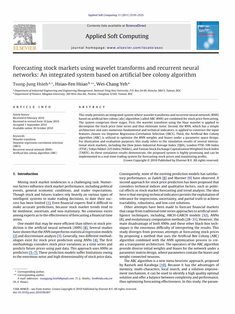
Fig. 13. Testing results of ABC-RNN for Nikkei for period 2002–2008.

2000

2500

3000

3500

4000

4500

5000

7/1/

2002

7/15

/200

2

7/29

/200

2

8/12

/200

2

8/26

/200

2

9/9/

2002

9/23

/200

2

10/7

/200

2

10/2

1/20

02

11/4

/200

2

11/1

8/20

02

12/2

/200

2

12/1

6/20

02

12/3

0/20

02

3400

3600

3800

4000

4200

4400

4600

4800

7/1/

2003

7/15

/200

3

7/29

/200

3

8/12

/200

3

8/26

/200

3

9/9/

2003

9/23

/200

3

10/7

/200

3

10/2

1/20

03

11/4

/200

3

11/1

8/20

03

12/2

/200

3

12/1

6/20

03

12/3

0/20

03

390040004100420043004400450046004700480049005000

7/1/

2004

7/15

/200

4

7/29

/200

4

8/12

/200

4

8/26

/200

4

9/9/

2004

9/23

/200

4

10/7

/200

4

10/2

1/20

04

11/4

/200

4

11/1

8/20

04

12/2

/200

4

12/1

6/20

04

12/3

0/20

04

close

forecast

close

forecast

close

forecast

48004900500051005200530054005500560057005800

7/1/

2005

7/15

/200

5

7/29

/200

5

8/12

/200

5

8/26

/200

5

9/9/

2005

9/23

/200

5

10/7

/200

5

10/2

1/20

05

11/4

/200

5

11/1

8/20

05

12/2

/200

5

12/1

6/20

05

12/3

0/20

05

close

forecast

5200

5400

5600

5800

6000

6200

6400

6600

7/3/

2006

7/17

/200

6

7/31

/200

6

8/14

/200

6

8/28

/200

6

9/11

/200

6

9/25

/200

6

10/9

/200

6

10/2

3/20

06

11/6

/200

6

11/2

0/20

06

12/4

/200

6

12/1

8/20

06

5400

5600

5800

6000

6200

6400

6600

6800

7/2/

2007

7/16

/200

7

7/30

/200

7

8/13

/200

7

8/27

/200

7

9/10

/200

7

9/24

/200

7

10/8

/200

7

10/2

2/20

07

11/5

/200

7

11/1

9/20

07

12/3

/200

7

12/1

7/20

07

12/3

1/20

07

close

forecast

close

forecast

close

forecast

1500

2000

2500

3000

3500

4000

4500

5000

5500

6000

7/2/

2008

7/16

/200

8

7/30

/200

8

8/13

/200

8

8/27

/200

8

9/10

/200

8

9/24

/200

8

10/8

/200

8

10/2

2/20

08

11/5

/200

8

11/1

9/20

08

12/3

/200

8

12/1

7/20

08

12/3

1/20

08

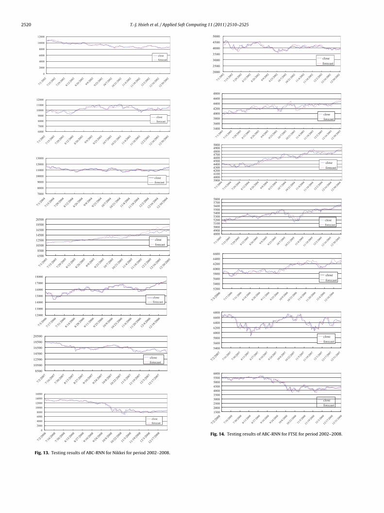
Fig. 14. Testing results of ABC-RNN for FTSE for period 2002–2008.

Comp

btsitEX

P

wsCofcnaf

2

sedtaopf

XXjEvVi

V

wfc

2

iibsgso

fitaoaAso

l

X

T.-J. Hsieh et al. / Applied Soft

ees have completed this process, they share the information onhe size of the food sources with the onlookers, each of whom thenelects a food source, with the probability of them selecting anyndividual source being proportional to the amount of nectar con-ained in that food source; that is, the probabilities established byq. (10) and the probability Ph of selecting a food source (solution)h is determined.

h = fith∑SNh=1fith

(10)

here fith denotes the fitness of the solution represented by foodource h and SN represents the total number of food sources.learly, this scheme leads to good food sources attracting morenlookers than bad ones. After all onlookers have selected theirood sources, each onlooker determines a food source near hishosen food source and calculates its fitness. The best among theeighboring food sources as determined by the onlookers associ-ted with a particular food source h, is selected as the next locationor food source h.

.3.3. Local search for improvement in solutionAfter a solution is generated, that solution is improved via a local

earch process called greedy selection, carried out by onlooker andmployed bees; according to this process, if size (fitness) of the can-idate source is better than the present source, the bee abandonshe present source in favor of the candidate one. This is achieved bydding to the current value of the selected parameter the productf a uniform variable in [−1,1] and the difference in values of thisarameter for this food source and some other randomly selectedood source.

Formally, suppose each solution comprises d parameters and leth = (Xh1, Xh2,. . ., Xhd) denote a solution with parameter values Xh1,h2,. . ., Xhd. To determine a solution Vh near Xh, a solution parameterand another solution Xk = (Xk1, Xk2,. . ., Xkd) are selected randomly.xcept for the value of the selected parameter j, all other parameteralues of Vh are the same as Xh, namely, Vh = (Xh1, Xh2,. . ., Xh(j−1),hj, Xh(j+1),. . ., Xhd). The value Vhj of the selected parameter j in Vh

s determined using the following formula:

hj = Xhj + u(Ahj + Xkj) (11)

here u denotes an uniform variable in [−1,1]. If the resulting valuealls outside the acceptable range for parameter j, it is set to theorresponding extreme value in that range.

.3.4. Solution intensity updateIf a solution represented by a particular food source does not

mprove for a predetermined number of iterations, that food sources abandoned by its associated employed bee and the employed beeecomes a scout; namely, the bee randomly searches for a new foodource. This arrangement is tantamount to assigning a randomlyenerated food source (solution) to the scout and again changing itstatus from scout to employed. After determining the new locationf each food source, another iteration of the ABC algorithm begins.

The process is repeated until the termination condition is satis-ed. In ABC algorithm, if a position cannot be further improvedhrough a predetermined number of cycles, the food source isssumed to be abandoned. The value of the predetermined numberf cycles is an important control parameter of the ABC algorithm,nd is called the “limit” for abandonment and defined using Eq. (12).ssuming the abandoned source is Xh, and j ∈ {1,2,. . .,d}, then the

cout discovers a new food source to be replaced with Xh, and theperation is defined as Eq. (13)

imit = SN × d (12)jh

= Xjmin + rand [0,1](Xjmax − Xjmin) (13)

uting 11 (2011) 2510–2525 2521

3. Illustration results

In this section of the study, we evaluate the model accuracyand compare it with other models. We also perform profit eval-uations and comparisons. To evaluate the forecasting quality andperformance of the ABC-RNN model, our work is applied to fourstock markets. To ensure that the application is sufficiently robust,we have chosen the Dow Jones Industrial Average Index (DJIA),London FTSE-100 Index (FTSE), Tokyo Nikkei-225 Index (Nikkei),and Taiwan Stock Exchange Capitalization Weighted Stock Index(TAIEX) for two periods, 1997–2003 and 2002–2008 (7 sub-datasetsfor each period). For the purpose of variety, we have ensured thateach period possesses a different proportion of training/test data.For the 1997–2003 period, the sub-datasets for the first ten-monthperiod are used for training (83%), while those from November toDecember are selected for testing; for 2002–2008, the first six-month period (50%) is used for training and the next six-monthperiod for testing.

3.1. RNN

Before training the RNN, a wavelet transformation is applied fordata preprocessing. The RMSE is thus used to perform two-levelwavelet preprocessing. This process can remove the noise in theoriginal data.

According to algorithm 1 detailed in Section 2.2, more importantinput variables are finally selected as inputs for predicting stockprices. Table 2 lists the selection results, where the correlation of allinput variables exceeds 0.4, reaching at least a medium correlation.Furthermore, all the p-values are below 0.001.

Table 3 lists the RNN architecture setting for algorithm 2, whichis implemented in C programming language on an Intel PentiumIV, 2.8 GHz PC with 512 MB memory. The explanation presentedin Section 2.3 specifies that algorithm 2 includes three controlparameters, including the number of food sources, which equals thenumber of employed or onlooker bees (SN), the value of limit, andthe maximum cycle number (MCN). The values of these parametersare set as follows: number of food sources = 100, MCN = 6000. Thenumber of limit is specified in Eq. (12). The average convergencediagram and the RMSE values of the seven training sub-datasetsfor each of the two periods using algorithm 2 are shown in Fig. 6and Table 4, respectively. The MSE of the forecasting model gradu-ally converges to around 0.0002 and 0.00008 in average for the firstperiod and the second period, respectively. The satisfactory trainingresults can be approved in testing data, and the forecasting figuresare presented in Figs. 7–14. They are also presented numericallyusing criteria found in Tables 6 and 7.

Statistics about the mean and standard deviation of resid-ual errors, i.e., R2 and Jarque-Bera, could be helpful to checkthe goodness of fit and the fluctuation of the predicted results,respectively. Table 5 reveal some interesting information. The R2

is almost 80% above for all stock markets and periods, thus, theABC-RNN might be an adaptive model for stock market predic-tion, despite the marginally unsatisfactory results for Nikkei in theperiod 1997–2003. Jarque-Bera reveals that the residuals under the0.05 confidence level almost confirm to normal distribution, withmost fluctuations and a few large variations centering around zero.

3.2. Forecasting performance

In this section of the study, we compare the performances of the

integrated system, ABC-RNN, with the conventional back propaga-tion ANN (BP-ANN), the conventional ANN optimized by the ABCalgorithm (called BNN for short) [27], and the conventional fuzzytime-series model of Chen [28] and Yu [29]. Furthermore, to exam-ine whether the ABC-RNN surpasses the latest time series model,

2522T.-J.H

siehet

al./Applied

SoftCom

puting11

(2011)2510–2525

Table 5.1Residual test for model fitness and fluctuation of the predicted results in period 1997–2003.

1997 1998 1999 2000 2001 2002 2003 Average

DJIAR2 0.818750903 0.851544324 0.873366359 0.804428666 0.808705321 0.85875372 0.940875328 0.850917803Jarque-Bera 0.737008 0.396817 4.322374 0.116939 0.269504 2.360649 0.747284

NIKKEIR2 0.878783264 0.795306627 0.812997726 0.88071331 0.806156058 0.796600217 0.87598882 0.83522086Jarque-Bera 0.513177 0.055465 0.731174 1.687246 0.499714 0.75503 2.001095

TAIEXR2 0.877964629 0.815346285 0.889835518 0.88427118 0.95170098 0.891851189 0.850667198 0.880233854Jarque-Bera 1.477803 1.300384 1.08014 0.850524 3.08012 1.423721 2.342792

FTSER2 0.958694205 0.842927546 0.897444581 0.928405662 0.953063238 0.890902158 0.870148573 0.905940852Jarque-Bera 0.429243 3.136172 0.103648 1.77944 0.098763 1.404064 4.138295

Table 5.2Residual test for model fitness and fluctuation of the predicted results in period 2002–2008.

2002 2003 2004 2005 2006 2007 2008 average

DJIAR2 0.86706460 0.941876108 0.898008891 0.86742077 0.96882726 0.851805619 0.93602594 0.9044327Jarque-Bera 0.889075 1.540462 0.694557 1.36684 36.64152 0.911256 3.752844

NIKKEIR2 0.90034167 0.803766751 0.935529888 0.85649055 0.927779066 0.937324729 0.96423915 0.9036388Jarque-Bera 0.614899 2.739275 1.325992 16.2705 3.228279 9.971908 10.17862

TAIEXR2 0.91229723 0.870389456 0.867092373 0.92214703 0.925190477 0.878941135 0.97836235 0.9077742Jarque-Bera 6.369567* 2.684154 2.424592 0.294907 25.11419 11.88336 0.537918

FTSER2 0.92238005 0.879822393 0.944973105 0.88027223 0.843765956 0.874952445 0.93776644 0.8977046Jarque-Bera 13.79405 1.274335 0.358074 16.39358 5.489475* 0.875331 15.99833

* Significant under 0.05.

T.-J. Hsieh et al. / Applied Soft Computing 11 (2011) 2510–2525 2523

Tab

le6

The

per

form

ance

com

par

ison

sof

dif

fere

nt

mod

els—

TAIE

X[3

0].

RM

SE/M

AE/

MA

PE/

Thei

lUY

ear

Met

hod

s19

9719

9819

9920

0020

0120

0220

03

BP-

AN

N17

2/15

2/0.

0190

/0.0

162

186/

166/

0.01

85/0

.017

2913

8/11

1/0.

0154

/0.0

0824

187/

167/

0.02

13/0

.017

7112

9/10

5/0.

0125

/0.0

0797

813

3/10

8/0.

0120

/0.0

0800

677

/69/

0.01

02/0

.007

55B

NN

[27]

146/

112/

0.01

68/0

.009

6412

1/10

2/0.

0127

/0.0

0774

122/

102/

0.01

24/0

.007

918

149/

114/

0.01

64/0

.010

3611

1/98

/0.0

117/

0.00

7826

80/7

0/0.

0100

/0.0

0771

964

/52/

0.01

01/0

.007

0028

Ch

en[2

8]15

4/12

9/0.

0171

/0.0

118

134/

109/

0.01

37/0

.008

1612

0/10

2/0.

0121

/0.0

0790

317

6/15

3/0.

0172

/0.0

1712

148/

113/

0.01

33/0

.010

442

101/

92/0

.012

0/0.

0078

8474

/67/

0.01

05/0

.007

609

Yu

[29]

165/

137/

0.01

83/0

.012

716

4/13

7/0.

0182

/0.0

125

145/

112/

0.01

59/0

.008

8314

5/11

2/0.

0160

/0.0

0879

119

1/17

2/0.

0181

/0.0

1829

75/6

8/0.

0113

/0.0

0746

66/5

4/0.

0098

/0.0

0698

Ch

eng

etal

.[30

]13

0/10

7/0.

0129

/0.0

0798

113/

99/0

.012

0/0.

0078

310

3/94

/0.0

117/

0.00

776

138/

111/

0.01

56/0

.008

3111

8/10

0/0.

0124

/0.0

0784

167

/54/

0.01

04/0

.007

017

50* /

31* /

0.00

57* /

0.00

6803

*

AB

C-R

NN

126* /

105* /

0.01

31* /

0.00

7922

*83

* /72

* /0.

0115

* /0.

0077

15*

86* /

78* /

0.00

89* /

0.00

7148

*13

5* /11

6* /0.

0164

* /0.

0082

*93

* /87

* /0.

0124

* /0.

0077

72*

62* /

48* /

0.00

95* /

0.00

6942

*59

/37/

0.00

71/0

.006

810

*Th

ebe

stp

erfo

rman

ceam

ong

met

hod

s.

Table 7.1aABC-RNN for DJIA, Nikkei and FTSE in period 1997–2003—RMSE.

RMSE 1997 1998 1999 2000 2001 2002 2003

DJIA 92 90 94 137 104 132 89Nikkei 246 203 187 230 181 141 177FTSE 103 79 48 79 56 57 31

Table 7.1bABC-RNN for DJIA, Nikkei and FTSE in period 1997–2003—MAE.

MAE 1997 1998 1999 2000 2001 2002 2003

DJIA 75 70 72 116 85 109 49Nikkei 214 157 144 174 142 117 143FTSE 69 65 37 63 45 49 25

Table 7.1cABC-RNN for DJIA, Nikkei and FTSE in period 1997–2003—MAPE.

MAPE 1997 1998 1999 2000 2001 2002 2003

DJIA 0.0096 0.0078 0.0065 0.00903 0.0086 0.012 0.0051Nikkei 0.0107 0.00912 0.00782 0.0115 0.0108 0.0099 0.0074FTSE 0.01108 0.01013 0.0056 0.00991 0.0087 0.0061 0.0057

the performance of the Cheng et al. model [30] is compared to thatof our model. The forecasting performances of TAIEX (1997–2003)are listed in Table 6.

Numerous measures of prediction accuracy are used to compareforecasting methods out of sample. This study focuses on out-of-sample performance, since the precise purpose of stock predictionis to simultaneously achieve profits and accurately predict futureprices. Evaluated methods are used to measure performance suchas root mean squared error (RMSE), mean absolute error (MAE),mean absolute percentage error (MAPE), and Theil’s inequalitycoefficient (Theil U). The calculations for the above-mentioned cri-teria are shown in Eqs. (14)–(17).

RMSE =

√√√√ 1N

N∑t=1

(Xt − Ft)2 (14)

MAE = 1N

N∑t=1

∣∣Xt − Ft∣∣ (15)

MAPE = 1N

N∑t=1

∣∣∣Xt − FtXt

∣∣∣ (16)

TheilU =

√1N

∑Nt=1(Xt − Ft)2

√1N

∑Nt=1(Xt)

2 +√

1N

∑Nt=1(Ft)

2(17)

Table 7.2aABC-RNN for TAIEX, DJIA, Nikkei and FTSE in period 2002–2008—RMSE.

RMSE 2002 2003 2004 2005 2006 2007 2008

TAIEX 95 92 81 60 116 108 91DJIA 107 84 91 68 84 112 93Nikkei 211 205 116 124 161 242 203FTSE 119 71 40 42 41 88 114

Table 7.2bABC-RNN for TAIEX, DJIA, Nikkei and FTSE in period 2002–2008—MAE.

MAE 2002 2003 2004 2005 2006 2007 2008

TAIEX 72 78 66 45 85 92 79DJIA 82 68 69 55 65 83 76Nikkei 171 165 95 97 127 182 168FTSE 85 53 30 32 37 70 91

2524 T.-J. Hsieh et al. / Applied Soft Computing 11 (2011) 2510–2525

Table 7.2cABC-RNN for TAIEX, DJIA, Nikkei and FTSE in period 2002–2008—MAPE.

MAPE 2002 2003 2004 2005 2006 2007 2008

TAIEX 0.0156 0.0138 0.0116 0.0075 0.012 0.0146 0.0142DJIA 0.0083 0.0071 0.0068 0.0052 0.0056 0.0098 0.01091Nikkei 0.0081 0.01088 0.0085 0.00772 0.00705 0.00949 0.00827FTSE 0.00899 0.00907 0.0066 0.00614 0.00841 0.00873 0.00910

Table 8The profits comparisons of different models (no transaction costs)—TAIEX [30].

Year ˛ Methods

BP-ANN BNN [27] Chen [28] Yu [29] Cheng et al. [30] ABC-RNN

1997 0.02 12 263 −127 −107 935 1491*

1998 0.03 −729 866 661 −864 878 1244*

1999 0.03 −97 109 −702 −756 124 168*

2000 0.01 −54 228 −106 −200 −154 246*

2001 0.02 204 135 −340 450 91 1753*

2002 0.005 −85 −15 −17 −96 466* 40

wvcm

mTIItD

3

o(

tp

P

TT

2003 0.005 −195 201Cumulated profits −944 1787

* The best profits among methods.

here Xt denotes the true value and Ft represents the predictedalue at time t. Table 6 lists the comparison results of the aboveriteria, and clearly shows that our model is superior to the listingethods.Furthermore, we also challenge our approach to other stock

arkets in two predicted periods: 1997–2003 and 2002–2008.hese stock markets include the Dow Jones Industrial Averagendex (DJIA), London FTSE-100 Index (FTSE), and Tokyo Nikkei-225ndex (Nikkei). Table 7 and Tables 7.2a–7.2c show the results forhe criteria RMSE, MAE and MAPE. ABC-RNN is also applicable toIJA, Nikkei and FTSE.

.3. Profit evaluation

Cheng et al. [30] identify two trading rules for calculating profitsn simulated trades, where profits are calculated in units of one. Eq.18) thus defines the profit formula, as follows:

Rule 1: SellIf |Ft−Xt |

Xt≤ ˛ and Ft+1 − Xt > 0 then sell.

Rule 2: BuyIf |Ft−Xt |

Xt≤ ˛ and Ft+1 − Xt < 0 then buy.

Where ˛ denotes the threshold parameter (0 <˛≤ 0.07, and thehreshold parameter depends on daily fluctuation of TAIEX). Next,rofit is defined, as follows:

rofit =p∑ts=1

(Xt+1 − Xt) +q∑

tb=1

(Xt − Xt+1) (18)

able 9he profits comparisons of different models (with transaction costs)—TAIEX.

Year ˛ Methods

BP-ANN BNN [27]

1997 0.02 3 2081998 0.03 −922 6951999 0.03 −131 922000 0.01 −93 1822001 0.02 190 1132002 0.005 −127 −492003 0.005 −253 183Cumulated profits −1333 1424

* The best profits among methods.

−238 −190 481* 260−869 −1763 2821 5202*

where p denotes the total number of days for selling, q representsthe total number of days for buying, ts represents the t-th day forselling and tb represents the t-th day for buying.

The optimal threshold parameter ˛ is obtained when the fore-casting performance maximizes the profits in the training dataset[30]. The optimal threshold parameter ˛ and Eq. (18) are used tocalculate the profits for different models, and Table 8 lists the cal-culation results. Table 8 shows that the ABC-RNN achieves higherprofits than the listing models (excluding 2002 and 2003) for TAIEX.More importantly, it accumulates the most profits.

For further discussion of profit evaluation, we consider the influ-ence of transaction costs on profit. The transaction cost in theTaiwan Stock Exchange (TSE) is 0.1425% for buying and selling,which is a fixed commission fee. Selling a stock involves an addi-tional transaction tax of 0.3%. Thus, the transaction cost is 0.1425%for buying and 0.4425% for selling, and Eq. (18) could be writtenas Eq. (19). Since the investor may use day trading strategies, thetransaction cost will likely have a big impact on profits. Table 9reports the performance in Table 8 when transaction costs are takeninto consideration.

Profit =p∑ts=1

[(Xt+1 − Xt) − |Xt+1 − Xt | × 0.1425%]

q∑

+tb=1

[(Xt − Xt+1) − |Xt − Xt+1| × 0.4425%] (19)

When transaction costs are taken into account, all methods havereduced profits compared to those shown in Table 8. This is due

Chen [28] Yu [29] Cheng et al. [30] ABC-RNN

−318 −384 791 1217*

520 −1369 577 983*

−967 −992 58 132*

−304 −367 −497 197*

−492 352 61 1592*

−46 −299 387* 15−533 −501 341* 163−2140 −3560 1718 4299*

Comp

thtsta

4

pa(a(stvuR

irpctaANfMDp2

dtsiolapmf

A

eh

R

[

[

[

[

[

[

[

[

[

[

[

[

[

[[

[

[

[

[

[

[

[31] S.H. Chen, Genetic Algorithms and Genetic Programming in Computational

T.-J. Hsieh et al. / Applied Soft

o heavy daily trading: the buy and sell strategies suffer from theeavy transaction costs. Table 9 shows that there will be more losshan the negative profits shown in Table 8. Furthermore, Table 9hows that the ABC-RNN model also achieves higher profits thanhe listing models, and gets closer to [30] in 2002 and 2003. It alsoccumulates the most profits.

. Conclusions and discussion

This paper proposes an integrated system, ABC-RNN, for stockrice prediction, and one that combines several statistical methodsnd soft computing techniques. The system involves three stages:1) data preprocessing using the Wavelet Transform (WT), which ispplied to decompose the stock price time series to eliminate noise;2) application of the Recurrent Neural Network (RNN), which has aimpler architecture than the traditional ANN and uses fundamen-al and technical indicators to construct the input features chosenia Stepwise Regression-Correlation Selection (SRCS); and (3) these of the Artificial Bee Colony Algorithm (ABC) to optimize theNN weights and biases under a parameter space design.

The proposed approach is compared to other methods presentedn the literature [27–30] for stock price prediction. Simulationesults show that the proposed model with wavelet-based pre-rocessing greatly outperforms the other methods in TAIEX. Forreating further comparative benchmark problems and to showhat the ABC-RNN is sufficiently robust, we have also applied ourpproach to other stock markets, including the Dow Jones Industrialverage Index (DJIA), London FTSE-100 Index (FTSE), and Tokyoikkei-225 Index (Nikkei), and we extend the predicted period

rom 2002 to 2008. The results for the criteria RMSE, MAE andAPE show that the ABC-RNN model is also applicable to theIJA, Nikkei and FTSE without respect to the training set pro-ortions (50% or 83%) or the predicted periods (1997–2003 or002–2008).

Although the proposed integrated system has a satisfactory pre-ictive performance, it still has some insufficiencies, which meanshe system might be enhanced. For example, it would be better toimplify the system organization, possibly by finding a scheme thatncludes functions of feature selection and an information supplyf addictive parameters. Therefore, in the future, a different intel-igent integrated method, such as a nonlinear model using SVMss a consequence, might be applied to a more complex time seriesroblem. In addition, a more advanced pattern selection schemeight be embedded in the system to retrieve significant patterns

rom the data.

cknowledgement

The authors wish to thank the editor and three anonymous refer-es for their constructive comments and recommendations, whichave significantly improved the presentation of this paper.

eferences

[1] Y.S. Abu-Mostafa, A.F. Atiya, Introduction to financial forecasting, Applied Intel-ligence (1996) 205–213.

[2] A.N. Refenes, A. Zapranis, G. Francis, Stock performance modeling using neu-ral networks: a comparative study with regression models, Neural Networks(1994) 375–388.

[

[

uting 11 (2011) 2510–2525 2525

[3] Yoo, Y. n, G. Swales, T.M. Margavio, A comparison of discriminate analysisversus artificial neural networks, Journal of the Operations Research Society(1993) 51–60.

[4] Y.Q. Zhang, S. Akkaladevi, G. Vachtsevanos, T.Y. Lin, Granular neural Web agentsfor stock prediction, Soft Computing Journal (2002) 406–413.

[5] P.C. Chang, Y.W. Wang, W.N. Yang, An investigation of the hybrid forecastingmodels for stock price variation in Taiwan, Journal of the Chinese Institute ofIndustrial Engineers (2004) 358–368.

[6] A.S. Chen, M.T. Leung, H. Daouk, Application of neural networks to an emergingfinancial market: forecasting and trading the Taiwan stock index, Computersand Operations Research (2003) 901–923.

[7] K. Parasuraman, A. Elshorbagy, Wavelet networks: an alternative to classi-cal neural networks, IEEE International Joint Conference on Neural Networks(2005) 2674–2679.

[8] L.A. Zadeh, The role of fuzzy logic in modeling, identification and control, Mod-eling Identification and Control (1994) 191–203.

[9] V Marmer, Nonlinearity, nonstationarity, and spurious forecasts, Journal ofEconometrics (2008) 1–27.

10] B. Basturk, D. Karaboga, An artificial bee colony (abc) algorithm for numericfunction optimization, in: IEEE Swarm Intelligence Symposium, Indianapolis,Indiana, USA, May, 2006.

11] A. Cohen, I. Daubechies, P. Vial, Wavelets on the interval and fast wavelettransform, Applied and Computational Harmonic (1993) 54–81.

12] J.B. Ramsey, Z. Zhang, The analysis of foreign exchange data using waveformdictionaries, Journal of Empirical Finance (1997) 341–372.

13] A. Popoola, K. Ahmad, Testing the suitability of wavelet preprocessing for TSKfuzzy models, in: Proceeding of FUZZ-IEEE: International Conference FuzzySystem Networks, 2006, pp. 1305–1309.

14] R. Gencay, F. Selcuk, B. Whitcher, Differentiating intraday seasonalities throughwavelet multi-scaling, Physica A (2001) 543–556.

15] J.B. Ramsey, The contribution of wavelets to the analysis of economicand financial data, Philosophical Transactions of the Royal Society of Lon-don Series A-Mathematical Physical and Engineering Sciences (1999) 2593–2606.

16] K. Papagiannaki, N. Taft, Z.-L. Zhang, C. Diot, Long-term forecasting of inter-net backbone traffic, IEEE Transactions on Neural Networks (2005) 1110–1124.

17] Y. Kim, W.N. Street, An intelligent system for customer targeting: a data miningapproach, Decision Support System (2004) 215–228.

18] F. Abramovich, P. Besbeas, T. Sapatinas, Empirical, Bayes approach to blockwavelet function estimation, Computational Statistics and Data Analysis (2002)435–451.

19] R. Gencay, F. Selcuk, B. Whitcher, An Introduction to Wavelets and Other Fil-tering Methods in Finance and Economics, Academic Press, New York, 2002.

20] J.B. Ramsey, C. Lampart, The decomposition of economic relationships by timescale using wavelets: expenditure and income, Nonlinear Dynamics and Econo-metrics (1998) 23–42.

21] S. Adel, C. Martin, J.R. Heather, A.M. Jose, The reaction of stock markets tocrashes and events: a comparison study between emerging and mature mar-kets using wavelet transforms, Physica A (2006) 511–521.

22] P.C. Chang, C.H. Liu, Y.W. Wang, A hybrid model by clustering and evolving fuzzyrules for sale forecasting in printed circuit board industry, Decision SupportSystem (2006) 1715–1729.

23] J.L. Elman, Finding structure in time, Cognitive Science 14 (1990) 179–211.24] D. Karaboga, B. Basturk, A powerful and efficient algorithm for numerical

function optimization: artificial bee colony (abc) algorithm, Journal of GlobalOptimization (2007) 459–471.

25] D. Karaboga, B. Basturk, On the performance of artificial bee colony (abc) algo-rithm, Applied Soft Computing (2008) 687–697.

26] D. Karaboga, B. Akay, A comparative study of artificial bee colony algorithm,Applied Mathematics and Computation (2009) 108–132.

27] D. Karaboga, C. Ozturk, Neural networks training by artificial bee colony algo-rithm on pattern classification, Neural Network World (2009) 279–292.

28] S.M. Chen, Forecasting enrollments based on fuzzy time-series, Fuzzy Sets Sys-tems (1996) 11–319.

29] H.K. Yu, Weighted fuzzy time-series models for TAIEX forecasting, Physica A(2005) 609–624.

30] C.H. Cheng, L.Y. Wei, Y.S. Chen, Fusion ANFIS models based on multi-stockvolatility causality for TAIEX forecasting, Neurocomputing (2009) 3462–3468.

Finance, Kluwer Academic Publishers, Dordrecht, 2002.32] R. Engle, GARCH 101: the use of ARCH/GARCH models in applied econometrics,

The Journal of Economic Perspectives (2001) 157–168.33] D.W. Patterson, Artificial Neural Networks: Theory and Applications, Prentice

Hall, 1996.