Analysis of background variability of honey bee colony size
79
TECHNICAL REPORT APPROVED: 15 March 2021 doi:10.2903/sp.efsa.2021.EN-6518 www.efsa.europa.eu/publications EFSA Supporting publication 2021:EN-6518 Analysis of background variability of honey bee colony size European Food Safety Authority (EFSA), Alessio Ippolito, Andreas Focks, Maj Rundlöf, Andres Arce, Marco Marchesi, Franco Maria Neri, Agnès Rortais, Csaba Szentes and Domenica Auteri Abstract In the context of the definition of specific protection goals for bees, risk managers asked EFSA to provide scientific background to support them in their decision-making process about what needs to be protected and to what extent. The risk managers indicated that the derivation of a threshold of acceptable effects on colony size based on their variability was the preferred option for honey bees. This approach assumes that when evaluating a pesticide, the magnitude of acceptable effects should be set within the range of the background variability of colonies not exposed to pesticides. In this report EFSA used the BEEHAVE model to assess background variability of colony size in 19 EU environmental scenarios covering a range of geographical, climatic and beekeeping conditions. A comparison was made between the model outcome and the measurements performed on control groups of experimental field studies. The analysis of the background variability presented in this document should support risk managers in defining a threshold for colony size reduction that is considered acceptable. © European Food Safety Authority, 2021 Key words: honey bees; background variability; colony dynamics; specific protection goals Requestor: European Commission Question number: EFSA-Q-2020-00530 Correspondence: [email protected]
-
Upload
khangminh22 -
Category
Documents
-
view
1 -
download
0
Transcript of Analysis of background variability of honey bee colony size

TECHNICAL REPORT
APPROVED: 15 March 2021
doi:10.2903/sp.efsa.2021.EN-6518
www.efsa.europa.eu/publications EFSA Supporting publication 2021:EN-6518
Analysis of background variability of honey bee colony size European Food Safety Authority (EFSA), Alessio Ippolito, Andreas Focks, Maj Rundlöf, Andres Arce, Marco Marchesi, Franco Maria Neri, Agnès Rortais, Csaba Szentes and Domenica Auteri
Abstract In the context of the definition of specific protection goals for bees, risk managers asked EFSA to provide scientific background to support them in their decision-making process about what needs to be protected and to what extent. The risk managers indicated that the derivation of a threshold of acceptable effects on colony size based on their variability was the preferred option for honey bees. This approach assumes that when evaluating a pesticide, the magnitude of acceptable effects should be set within the range of the background variability of colonies not exposed to pesticides. In this report EFSA used the BEEHAVE model to assess background variability of colony size in 19 EU environmental scenarios covering a range of geographical, climatic and beekeeping conditions. A comparison was made between the model outcome and the measurements performed on control groups of experimental field studies. The analysis of the background variability presented in this document should support risk managers in defining a threshold for colony size reduction that is considered acceptable.
© European Food Safety Authority, 2021
Key words: honey bees; background variability; colony dynamics; specific protection goals
Requestor: European Commission
Question number: EFSA-Q-2020-00530 Correspondence: [email protected]

Background variability of honey bee colony size
www.efsa.europa.eu/publications 2 EFSA Supporting publication 2021:EN-6518
Acknowledgements: EFSA wishes to thank the following for the support provided to this scientific output: Brecht Ingels, Jacoba Wassenberg, Paulien Adriaanse, Sébastien Lambin, Daniela Jölli, Dirk Süßenbach. EFSA wishes to acknowledge Fani Hatjina, Noa Simon-Delso and Elena Alonso Prados for submitting relevant data and information. EFSA also wishes to acknowledge all European competent institutions, Member State bodies and other organisations that provided feedback for this scientific output. Suggested citation: EFSA (European Food Safety Authority), Ippolito A, Focks A, Rundlöf M, Arce A, Marchesi M, Neri FM, Szentes Cs, Rortais A and Auteri D, 2021. Analysis of background variability of honey bee colony size. EFSA supporting publication 2021:EN-6518. 79 pp. doi:10.2903/sp.efsa.2021.EN-6518
ISSN: 2397-8325 © European Food Safety Authority, 2021
Reproduction is authorised provided the source is acknowledged.
Background variability of honey bee colony size
www.efsa.europa.eu/publications 3 EFSA Supporting publication 2021:EN-6518
Summary Risk managers agreed that background variability in colony size can be used for defining specific protection goals for honey bees This document describes a method for defining specific protection goals (SPGs) for honey bees by deriving the SPGs from the background variability of colony sizes. It allows risk managers to set SPGs which contain the impact of pesticides on the number of bees within the range of the background variability of the colony sizes.
In the context of the definition of SPGs for bees, risk managers asked EFSA to provide scientific background to support them in their decision-making process about what needs to be protected and to what extent. Among the four approaches that EFSA developed, the risk managers indicated that the derivation of a threshold of acceptable effects on colony size based on their variability (i.e. approach #2) was the preferred option for honey bees. This approach assumes that when evaluating a pesticide, the magnitude of acceptable effects should be set within the range of the background variability of colonies not exposed to pesticides. In this way, it is assumed that any impact on the provision of the ecosystem services depending on honey bees would also remain within the background variability.
EFSA used BEEHAVE to assess background variability of colony size in multiple scenarios The analysis was performed with the BEEHAVE computer model in 19 EU environmental scenarios covering a range of geographical, climatic and beekeeping conditions. For each scenario, 500 replicate simulations were run under equal conditions. Each replicate showed the dynamics of a honey bee colony over one year, in situations where the bees were not exposed to any pesticide. The outcome of the simulations for each scenario is conceptually comparable to the observations of replicate hives in the control group of effect field studies, which are the reference for the risk assessment for bees. The background variability allows risk managers to set the level of protection for colonies exposed to pesticides
Plotting the modelled development of the colony sizes over time gives a picture of their background variability. From the variability distribution two elements are of interest: the mean colony size and the lower end of the distribution. The difference between these two values defines the extent to which the size of a colony can be reduced because of background variation. In practice, the knowledge of the shape of the distribution curve allows limits to be set for the reduction in colony size caused by exposure to pesticides. Variations within the limited range would be considered as acceptable. The results of the analysis are presented for the whole year as well as for each season and for each regulatory zone. A summary for the scenarios is also presented, leading to percentage ranges that can inform on colony size reduction. These percentages were calculated for the full variability distribution and for several restricted variability distributions. With a more restricted variability range, the threshold of acceptable effects is more conservative. The analysis of the simulated background variability distribution shows that a large fraction of the total variability is caused by a limited number of colonies.
Additional elements may support the decision of the risk managers: uncertainties, comparison with experimental data and practical implementation in field studies The model combines fixed input parameters and stochastic elements. For some elements belonging to both categories, uncertainties were identified, but could not be fully evaluated and quantified within the present work. However, a comparison was made between the model outcome and the measurements performed on control groups of experimental field studies. Such comparison shows that the model predictions were in the range of the experimental values, but there was a general underestimation of the median variability. A further analysis showed that the variability increases with increasing landscape complexity. The simulated 19 scenarios are all characterised by a simple landscape, thus confirming that variability is likely underestimated compared to the real world. In the present context, an underestimation of the variability leads to a more conservative threshold of acceptable effects. The analysis of the background variability presented in this document should support risk managers in defining a threshold equivalent to a certain percentage reduction in colony size that is considered acceptable, in a similar way as was proposed by EFSA (2013). This threshold represents the largest acceptable mean colony size reduction that exposed colonies can suffer when compared to the
Background variability of honey bee colony size
www.efsa.europa.eu/publications 4 EFSA Supporting publication 2021:EN-6518
unexposed colonies in the control. The threshold will be used to evaluate the field studies; therefore, it should be implementable and measurable. The selected threshold of acceptable effects will determine the requirements for the design of field studies. This document makes explicit the link between the threshold and the complexity of the study design, along with a benchmarking of recent state-of-the-art field studies described in the scientific literature.
Background variability of honey bee colony size
www.efsa.europa.eu/publications 5 EFSA Supporting publication 2021:EN-6518
Table of contents
Abstract .........................................................................................................................................1 Summary .......................................................................................................................................3 1. Introduction ........................................................................................................................7 1.1. Background and Terms of Reference as provided by the requestor ........................................7 2. Scope of the document .......................................................................................................7 3. General framework for the review of the SPG for honey bees ................................................8 3.1. Defining SPGs based on the EFSA method ............................................................................8 3.2. Implementation of the SPG in the risk assessment ................................................................9 3.2.1. Reference tier .....................................................................................................................9 3.2.2. Tiered approach and trigger values .................................................................................... 11 3.3. SPG dimensions with Approach #2 ..................................................................................... 11 3.3.1. Informing the definition of the ‘magnitude’ dimension using the concept of operating range
(OR) ................................................................................................................................. 13 4. Data and methodologies .................................................................................................... 15 4.1. The use of the BEEHAVE model ......................................................................................... 15 4.2. Environmental scenarios and model calibration ................................................................... 17 4.2.1. Scenarios location ............................................................................................................. 17 4.2.2. Overview of scenario development ..................................................................................... 18 4.2.3. Landscape structure .......................................................................................................... 19 4.2.4. Temporal pattern: daily foraging period .............................................................................. 19 4.2.5. Temporal pattern: food availability ..................................................................................... 22 4.2.6. Temporal pattern: egg laying rate ...................................................................................... 25 4.2.7. Background mortality ........................................................................................................ 26 4.2.7.1.Forager mortality .............................................................................................................. 26 4.2.7.2.Winter/in-hive mortality ..................................................................................................... 28 4.2.7.3.Drone mortality ................................................................................................................. 28 4.2.7.4.Brood mortality ................................................................................................................. 28 4.2.8. Energy balance ................................................................................................................. 28 4.2.9. Pollen levels in the landscape ............................................................................................ 33 4.2.10. Initial colony size .............................................................................................................. 34 4.3. Plausibility of the model simulations ................................................................................... 35 5. Results ............................................................................................................................. 40 5.1. Summary statistics of the simulations ................................................................................. 40 5.2. Colony size dynamics ........................................................................................................ 41 5.3. Analysis of the operating range .......................................................................................... 44 5.3.1. Average variability over the entire year .............................................................................. 44 5.3.2. Average variability over spring ........................................................................................... 45 5.3.3. Average variability over summer ........................................................................................ 46 5.3.4. Average variability over autumn ......................................................................................... 47 5.3.5. Comparison between seasons ............................................................................................ 48 5.4. Interpretation of the results ............................................................................................... 50 5.4.1. Recommendations on how to interpret the results ............................................................... 50 5.5. Plausibility of the model simulations ................................................................................... 51 6. Uncertainties and potential future developments ................................................................. 53 6.1. Limitations of BEEHAVE identified in EFSA PPR Panel (2015)................................................ 54 6.2. Limitations of BEEHAVE identified in the present analysis .................................................... 54 6.3. Relevance of input values for the present analysis .............................................................. 55 6.4. Uncertainties in the scenario definition ............................................................................... 55 6.5. Outlook ............................................................................................................................ 57 7. Reference tier (field studies) design in relation to the magnitude of acceptable effect ........... 57 7.1. Preliminary estimation of the requirement for higher tier studies .......................................... 57 7.2. Example from available higher tier studies .......................................................................... 58 7.3. Considerations of the requirements of field studies in the EFSA bee guidance document ....... 60 8. Concluding remarks for decision making process for risk managers ...................................... 60

Background variability of honey bee colony size
www.efsa.europa.eu/publications 6 EFSA Supporting publication 2021:EN-6518
References ................................................................................................................................... 62 Appendix A – Overview of honey bee models in the literature .................................................... 69 Appendix B – Analysis of landscape complexity ......................................................................... 70 Appendix C – Detailed results of the simulations ....................................................................... 77 Appendix D – Variability in risk assessment ............................................................................... 78
Background variability of honey bee colony size
www.efsa.europa.eu/publications 7 EFSA Supporting publication 2021:EN-6518
1. Introduction
1.1. Background and Terms of Reference as provided by the requestor In the context of the definition of specific protection goals (SPGs) for bees, risk managers asked EFSA to provide scientific background to support them in their decision-making about what needs to be protected and to which extent. In the first supporting document1, published at the end of July 2020, EFSA described a set of four possible approaches developed to respond to the request. The four approaches are possible scientific processes which risk managers could choose to determine SPGs. These approaches were developed by considering the request of the European Commission mandate to:
‘take into account planned and ongoing discussions initiated by the Commission on defining specific environmental protection goals and review the risk assessment guidance based on the specific protection goals agreed during this process (ToR6).’
EFSA took into consideration the preliminary outcome of the action initiated in 2019 by the European Commission towards defining SPGs involving Member States (MSs) and stakeholders; in particular, the use of the EFSA framework for identifying SPGs (EFSA PPR Panel, 2010; EFSA Scientific Committee, 2016). Based on the preliminary outcome of this initiative, EFSA deemed that a full review of the SPG defined in the EFSA bee guidance document (EFSA, 2013), involving all steps of the EFSA method (EFSA PPR Panel, 2010; EFSA Scientific Committee, 2016), may not be necessary and was considered outside of the scope of this mandate. In fact, the EFSA method for defining SPGs was already implemented in the EFSA bee guidance document (EFSA, 2013). Nevertheless, EFSA has elaborated the four approaches, along the lines of this preliminary outcome, to address the feedback from MSs on the SPGs as defined in the EFSA bee guidance document (EFSA, 2013) and to support the risk managers on the revision of some of the five dimensions, i.e. Step 3 of the EFSA method. The four approaches were presented on 30 June 2020 to the representatives of the MSs in a workshop organised by the European Commission. They are summarised below:
• Approach 1 – to establish acceptable effect based on long-term colony survival.
• Approach 2 – to derive a threshold of acceptable effect on colony size based on background variability.
• Approach 3 – to establish acceptable effect, based on pre-defined levels, on colony/population size.
• Approach 4 – to establish acceptable effect on colony/population size based on levels of acceptable impact on the provision of ecosystem services.
The scientific concepts underlying each approach, reported in the first supporting document1, were explained to risk managers and discussed during the workshop in June 2020. The pros and cons were also described along with the analysis of the feasibility of their implementation within the timeline of the current mandate. As a result of the discussion, a large majority of the MSs expressed a preference for approach #2 for honey bees. This choice was confirmed at the meeting of the Standing Committee on Plants, Animals, Food and Feed, Section Phytopharmaceuticals – Legislation (SCoPAFF) on 16 July 2020. EFSA presented the four approaches to the stakeholder ad hoc group in an information session organised on the 23 September 2020.
2. Scope of the document In the present document, approach #2 and its implementation are presented. It is important to bear in mind that the outcome of the implementation of approach #2 presented in this report focuses on honey bees, and cannot be used for defining SPGs for bumble bees and solitary bees, due to their different biology and ecology e.g. smaller colony size for bumble bees, solitary nesting in contrast to colony
1 https://www.efsa.europa.eu/sites/default/files/topic/EFSA-Supporting-document-for-RMs-in-defining-SPGs.pdf
Background variability of honey bee colony size
www.efsa.europa.eu/publications 8 EFSA Supporting publication 2021:EN-6518
formation for solitary bees, shorter nesting periods, feeding and breeding behaviour (EFSA PPR Panel, 2012).
The implementation of the principles of approach #2 for bumble bees might be considered at a later stage after suitable models e.g. the Bumble-BEEHAVE model (Becher et al., 2018) have been evaluated according to the EFSA good modelling practices opinion (EFSA PPR Panel, 2014). On the basis of current knowledge, approach #2 cannot be used for the bumble bee and solitary bee groups. As explained in the first supporting document1, due to the lack of knowledge and data, EFSA cannot provide further scientific grounds in this document for supporting the risk managers’ decision on SPGs for bumble bees and solitary bees. Therefore, in the context of the review of the SPGs, risk managers could consider adopting a pragmatic approach for solitary bees and for bumble bees. EFSA PPR Panel (2012) suggested the application of uncertainty factors to the effect percentages identified for honey bees as a pragmatic solution.
Summary box 1 Non-Apis bees The analysis presented in this document is not suitable for defining the SPG for bumble bees and solitary bees.
3. General framework for the review of the SPG for honey bees
3.1. Defining SPGs based on the EFSA method In 2019, the Commission initiated actions towards defining SPGs involving MSs and stakeholders on the basis of the EFSA method (EFSA PPR Panel, 2010; EFSA Scientific Committee, 2016) for defining SPGs. The EFSA method includes several steps:
Step 1 – identification of the relevant ecosystem services (ES) potentially impaired by a stressor; Step 2 – identification of the relevant Service Providing Units (SPU); Step 3 – specification of the level/parameters of protection of the SPUs based on five interrelated dimensions: 1) Ecological entity; 2) Attribute; 3) Magnitude of the effect; 4) Temporal scale; 5) Spatial scale.
So far, the Commission has organised three workshops: two in 2019 with MSs and stakeholders separately, and one in February 2020, with both stakeholders and MSs. In the workshop in February 2020 step 1 of the EFSA method was discussed for different pesticide use scenarios. The provision of pollination was widely recognised as a key ecosystem service.
Already in the EFSA bee guidance document (EFSA, 2013) and in the preceding Scientific Opinion (EFSA PPR Panel, 2012), ecosystem services and SPGs were identified and discussed with risk managers, according to the methodology proposed by the EFSA opinion for SPGs (EFSA PPR Panel, 2010). Therefore, the methodology and the process implemented in the EFSA bee guidance document (EFSA, 2013) can be considered in line with the EFSA method (EFSA PPR Panel, 2010; EFSA Scientific Committee, 2016) for defining SPGs and therefore with the action initiated by the European Commission. The ecosystem services identified for the EFSA bee guidance document (EFSA, 2013) were pollination, food and genetic resources provisioning, and cultural services. These are in line with step 1 of the EFSA method as discussed at the workshop held with stakeholders and MSs in February 2020. Furthermore, the EFSA bee guidance document (EFSA, 2013) includes, beyond honey bees covered in the current data requirements2, bumble bees and solitary bees. This means that the second step of the EFSA method – identifying the SPU for the above ecosystem services – can already be considered as partially addressed. As a general remark, additional SPU may be added, i.e. other pollinators that are not covered by the EFSA bee guidance document if identified as being important to be covered by future guidance. The EFSA opinion (EFSA PPR Panel, 2012) suggested a specification of five interrelated dimensions of the SPG (i.e. Ecological Entities, Attribute, Magnitude, Temporal and Spatial scale) in line with the third step of the EFSA method (see Table 1 for details). These were discussed with risk managers and
2 Regulation 283/2013 and 284/2013.

Background variability of honey bee colony size
www.efsa.europa.eu/publications 9 EFSA Supporting publication 2021:EN-6518
implemented in the EFSA bee guidance document. Some of these dimensions may need to be discussed again by risk managers.
Table 1: Overview of the SPGs as implemented in the EFSA bee guidance document (EFSA, 2013) and defined in the preceding Scientific Opinion (EFSA PPR Panel, 2012) in light of the steps described in the EFSA framework for defining SPGs (EFSA Scientific Committee, 2016)
EFSA Scientific Committee (2016)
EFSA PPR Panel (2012) EFSA (2013)
Step 1 Definition of ecosystem services
Pollination, food and genetic resources provisioning, and cultural service.
Step 2 SPU
Honey bees, bumble bees and solitary bees
Step 3 Specification of the level/parameters of protection of the SPUs based on five interrelated dimensions
Dimensions Honey bees Bumble bees Solitary bees Ecological Entities
colony colony population
Attribute Colony strength(a)
Colony strength(a)
Population abundance
Magnitude Negligible effect(b)
Negligible effect(b)
Negligible effect(b)
Temporal scale(c)
Not relevant i.e. any time
Not relevant i.e. any time
Not relevant i.e. any time
Spatial scale edge of field edge of field edge of field (a): Colony strength is defined operationally as the number of adult bees in a
colony (= colony size). (b): Negligible in the EFSA (2013) is such if statistically distinguishable from
‘small effects’. The effect was considered negligible when the magnitude is below 7%.
Note: It is important to note that the above SPGs and in particular, the Magnitude of the effect (i.e. effect sizes) have been defined principally by reference to honey bees. In the case of other bees, the same magnitude has been used as a surrogate to colony-level impacts (for other social bees, such as bumble bees) or to population abundance (solitary bees).
(c): Based on EFSA PPR Panel (2010) and EFSA Scientific Committee (2016), no temporal scale is relevant if the selected magnitude is ‘negligible’.
3.2. Implementation of the SPG in the risk assessment 3.2.1. Reference tier
The EFSA method (EFSA PPR Panel, 2010; EFSA Scientific Committee, 2016) for deriving the SPGs, and in particular EFSA PPR Panel (2010), suggests identifying for each SPU a reference tier for developing the risk assessment scheme. The reference tier is represented by the most sophisticated experimental or modelling risk assessment method that addresses the specific protection goal, and is then used to calibrate lower tiers which are based on simpler methods that are practical for routine use. In a routine risk assessment, the reference tier would only be used when the results of the lower tiers do not demonstrate a low risk for a specific use. In the case of honey bees, the reference tier is represented by field studies. These are experiments with a high level of realism, characterised by complex set-up and interpretation of the results. In general, these studies aim to compare at least two groups of honey bee colonies:
a) The treated group, which is exposed to the pesticide under investigation. Field studies are performed with the aim of mimicking realistic conditions. This implies that the pesticide under investigation is applied to a crop that the honey bees have access to for collecting pollen and/or nectar. The pesticide application rate, frequency and timing should be in line with the use for which authorisation is sought.
Background variability of honey bee colony size
www.efsa.europa.eu/publications 10 EFSA Supporting publication 2021:EN-6518
b) The control group, which is set up in the same way as the treated group with the exception that it is not exposed to the pesticide under investigation. The control group should have access to the same cropping system / field characteristics as the treatment group, but these do not receive the treatment of the pesticide being investigated.
While more complex designs are possible (e.g. combining investigations in several regions at the same time, etc.) the underlying basic principle remains a comparison between the treatment and the control group.
The reference tier should be able to address the defined SPG – in all its dimensions – by performing targeted measurement. All five dimensions of the SPG contribute significantly to the design of field studies. The ecological entity identifies the object of the experimental observation. For honey bees, these are the colonies. The attribute identifies the main variable to be measured. This is not necessarily the only measured variable, but it is the one driving the overall risk assessment. In the EFSA bee guidance document, this was colony strength, which was operationally defined as the number of adult bees in a colony (= colony size). The magnitude of the effect is pivotal both in the design of the study and in the interpretation of the results. The most straightforward way to check whether the exposure to a certain pesticide caused an effect on the colony strength is to compare the arithmetic mean value of this variable in the control and in the treatment groups. A difference larger than the agreed magnitude is an indication that the SPG may not be met in the study. Furthermore, the definition of a certain magnitude influences the number of replicates needed to satisfy statistical requirements, i.e. the number of colonies and fields used in the treatment and control groups.
Statistical considerations linked to the magnitude dimension Comparing the arithmetic mean value of the colony strength in the control and in the treatment groups is not sufficient per se, as this difference may be due to chance (type I error). To tackle this, statistical tests with a pre-defined level of confidence are often used. The comparison of mean values is also the basis of the most common statistical tools used to evaluate these studies. The concept underlying these statistical tests is to check whether the difference between the means of the treatment and control groups is larger than the difference observed within each of the two groups. If so, then the difference is ‘flagged’ as statistically significant, meaning that the observed difference between the groups is unlikely to be due to chance, with a probability reflected by the confidence level. However, lack of significance alone does not tell much about whether the magnitude dimension of the SPG is met. The probability that a specific study will detect as significant a pre-defined difference between the mean values of the treatment and the control (i.e. the SPG magnitude) is defined as ‘power’. If the power is low, then there is a high probability that a difference larger than the defined (SPG) magnitude will not be marked as significant (type II error). The power increases with larger magnitudes of the SPG and with higher replication (i.e. higher numbers of colonies and fields used in the treatment and control groups) in field studies. It follows that the selection of a certain magnitude will also drive the number of replicates needed in field studies in order to have a satisfactory power. This aspect is further discussed in Section 7.
The spatial scale determines mainly the spatial distribution of the hives in the area used for the field study. In the EFSA bee guidance document, the identified spatial scale is the ‘edge of the field’, which implies that all hives in a field study should be placed in the proximity of fields where the same crop is grown for both the treatment and the control group. In the treatment, the pesticide for which authorisation is sought is applied to the crop, while in the control group the crop remains untreated. The temporal scale is the maximum time over which single or repeated exposure events are expected to exceed the acceptable effect level that can be tolerated. In principle, this includes the duration and the frequency of the effects, along with the interval between them. The temporal scale influences the frequency of the measurements and the length of the study. In particular, the EFSA bee guidance document (EFSA, 2013) specified that field studies should last at least two brood cycles (about 42 days) as this was considered the minimum time to appropriately assess any potential adverse effect of pesticide. The EFSA bee guidance document (EFSA, 2013) did not include any ‘recovery option’, but the entire SPG was based on a ‘threshold option’, thus a temporal scale for acceptable effects was not considered. For field studies, this means that the difference between the mean colony size in the
Background variability of honey bee colony size
www.efsa.europa.eu/publications 11 EFSA Supporting publication 2021:EN-6518
treatment and the control should not exceed the magnitude threshold at any time. This presents practical limitations as the colony size cannot yet be measured continuously, as discussed in Section 3.3.
The ‘recovery option’ and the ‘threshold option’ These two options were first introduced for the pesticide risk assessment of aquatic organisms in EFSA PPR Panel (2013). The ‘recovery option’ implies that transient effects above the threshold defined for the magnitude dimension may still be acceptable, if ecological recovery takes place within a defined time period. The ‘threshold option’ implies that effects above the threshold defined for the magnitude dimension should not occur at any time.
3.2.2. Tiered approach and trigger values
Risk assessment does not uniquely rely on the reference tier (i.e. field studies) as this kind of experiment is complex and resource-intensive for all parties involved, including applicants and risk assessors. Risk assessment follows a tiered approach, starting from lower tiers that are typically based on simpler, more standardised laboratory studies and relatively simple approaches for estimating exposure. Lower tiers are routinely used as a basis for screening substances in relation to particular concerns. In such lower tier laboratory studies, effects on bees are observed and recorded on an individual basis and not on colonies as in field studies. Once the SPG dimensions are defined and it has been verified that these can be addressed in the reference tier, all different tiers of the risk assessment need to be calibrated accordingly. Such a calibration exercise entails several steps, which allow linking standard endpoints such as L(D)D503 to a reduction in colony size (SPG attribute of the identified ecological entity) equivalent to the acceptable effect (SPG magnitude) for a temporal scale defined on the basis of the exposure length in the laboratory study (i.e. acute and chronic). The calibration, performed once all the SPG dimensions are defined, results in the definition of trigger values. For the actual lower tier risk assessment, a risk quotient is calculated from the ratio between the dose equivalent to the standard laboratory endpoint (e.g. L(D)D50) and the exposure predicted for the specific use of the substance, which accounts for the spatial scale of interest. The risk quotient is then compared to the trigger values described above. Hence, trigger values can be considered as thresholds that, if not exceeded by the risk quotient, guarantee the respect of the SPG. If trigger values in lower tiers are not exceeded, no further investigation is necessary, whereas if they are exceeded, higher tier risk assessments may be needed to further investigate whether the SPG is met.
3.3. SPG dimensions with Approach #2 As described in the first supporting document1, approach #2 is based on the analysis of the background variability of honey bee colony size. The analysis aims to define an operating range (OR), i.e. the range of honey bee colony size given by their background variability4. The term ‘background’ reflects that the analysis does not consider exposure to pesticides (e.g. like ‘controls’ in experimental field studies). Approach #2 does not require a complete revision of the SPG, i.e. a revision of all five dimensions (i.e. ecological entity, attribute, magnitude of the effects, spatial scale, temporal scale) implemented in the EFSA (2013). By selecting this approach, the MSs implicitly confirmed that the ecological entity is the colony and that the attribute is the colony strength. The spatial scale implemented in EFSA (2013) is the edge of field. This means that the exposure estimation considered uniquely the colonies that are located at the edge of treated fields, i.e. those colonies that are likely to be most exposed among the ones in the area of use of a certain pesticide. The colonies living in the remaining hives (farther away from fields) are thus automatically protected.
3 Lethal (daily) dose for 50% of the tested individual bees. Typical endpoint from laboratory studies with bees. 4 The object of the analysis was initially referred to as ‘natural variability’. Following some relevant comments from MSs, EFSA
changed the terminology to ‘background variability’. This was done to clarify that the focus is not on colonies living in wild conditions. On the contrary, the focus is on managed honey bee colonies, like those that are likely to be used in field studies.
Background variability of honey bee colony size
www.efsa.europa.eu/publications 12 EFSA Supporting publication 2021:EN-6518
While in principle the exposure estimation could explicitly include all colonies (also the ones far from the treated fields), this has severe limitations in its practical implementation in the risk assessment. The level of exposure is likely to be influenced, among other things, by the distance between the hives and the treated field(s). Since the actual location of all bee colonies in Europe relative to agricultural crops is unknown (and likely not constant in time), implementing this approach in the risk assessment is unlikely to be feasible. The edge of field is the common spatial scale in the risk assessment for non-target organisms. This was also explained in Appendix A of the first supporting document1.
By selecting approach #2, the risk managers implicitly agreed to revise mainly the definition of the current magnitude of effect and to implement a suitable temporal scale for the higher tier studies. As reported in Table 1, in the EFSA bee guidance document (EFSA, 2013), the magnitude of effect was agreed as ‘negligible’ and it was defined based on experts’ judgement as colony size reduction < 7%, more specifically in the range of 3.5–7%. The EFSA Scientific Committee (2016) suggests avoiding using the terms ‘negligible’, ‘small’, ‘medium’, ‘large’ as descriptors of the magnitude of effects because these terms can be considered vague and qualitative. The experts in the Working Group (WG) drafting the EFSA bee guidance document (EFSA, 2013) unanimously agreed that:
‘a proportional reduction in colony size of greater than one-third would be likely to compromise the viability, pollinating capability and yield of any colony; this consideration was used to define an effect as large.’
This definition is generally accepted and not questioned, as it is rooted in a clear biological threshold (i.e. colony viability). The current quantitative definition of ‘negligible effects’ is also based on valuable experts’ judgement. However, in contrast to the definition of ‘large’ effects, assigning boundaries to this qualitative effect class may be disputable, as it is not rooted in any clear biological threshold. Therefore, any attempt to quantitatively define ‘negligible’ may lead to a controversial outcome, as demonstrated by the debate that occurred regarding the implementation of the EFSA bee guidance document (EFSA, 2013). The quantitative definition of the intermediate classes for ‘medium’ and ‘small’ effects were arbitrarily set at even intervals in the range between ‘large’ and ‘negligible’, but cannot be substantiated further. The term ‘threshold of acceptable effects’ was introduced with approach #2 because it is difficult to establish consensus on an undisputable scientific definition of qualitative class effects such as ‘negligible’, ‘small’, and ‘medium’. Furthermore, the term ‘acceptable’ is also in accordance with Annex II, point 3.8.3 of Regulation (EC) 1107/2009. Therefore, the concept of ‘acceptable effect’ is considered as more suited in this context than any qualitative definition of effect class. With approach #2, the magnitude of the effect on colony size is informed by the expected background variability (see Section 3.3.1).
With approach #2, no explicit consideration is given to the temporal scale of the assessment, as the operating range is quantified in a continuous manner. In principle, this can be interpreted as an indication that the temporal scale of acceptable effects is not relevant, since any possible effect following the exposure to a pesticide should remain at a level indicated as acceptable at any time. In practice, a temporal scale may be defined on the basis of practical limitations in the field studies (i.e. the reference tier). A continuous measurement of the colony size is not practically feasible yet, nor is it advisable to inspect the colonies too frequently, as this creates stress for the bees which would affect the results of the experiments. Until less invasive techniques become available, it is good practice to inspect the hive no more often than every week (see EPPO, 2010). Hence, in the time between two monitoring points, possible transient effects greater than the defined threshold could occur without being measured; however, the SPG can be considered met if the threshold of acceptable effects is not breached at the two monitoring time points.
An alternative possibility, based on the biology of bees, could be to set the relevant temporal scale of acceptable effects as equal to one honey bee worker brood cycle (21 days). This is because it may be considered acceptable to have transient effects if these are compensated by the new generation of

Background variability of honey bee colony size
www.efsa.europa.eu/publications 13 EFSA Supporting publication 2021:EN-6518
worker bees. However, this possibility should be carefully considered because if, for example, the transient effect over the 21 day occurs during the flowering period of the treated crop, pollination of the crop may be affected. Even if temporal scale may, in practice, be part of the SPG definition, it will not have an impact on the calculation of the trigger values.
3.3.1. Informing the definition of the ‘magnitude’ dimension using the concept of operating range (OR)
As explained in Section 3.2, the SPG dimension related to the magnitude of acceptable effect can be directly measured in the reference tier (i.e. field studies) by comparing the mean colony sizes of the treatment and control groups. Effects are considered acceptable only if the mean colony size of the treatment group is not decreased by more than the magnitude dimension of the SPG, which is calculated relative to the mean colony size of the control group. Thus, the mean colony size in the control group should be taken as the reference. The OR estimated with approach #2 considers uniquely colonies in the control group. The relative difference between the mean colony size and the lower limit of the OR informs on the maximum difference that can be caused by background variability. As such, the relative difference between the mean and the minimum, or any value between these, can be used to inform the definition of the magnitude of the acceptable effect of pesticides on colony size. In summary, the following aspects should be considered:
• In the present analysis, honey bee colony dynamics are simulated over 1 year using the BEEHAVE model (see more about the use of this model under Section 4.1).
• Simulations were carried out for 500 replicate control colonies in each of the considered scenarios (see more about the scenarios under Section 4.2) allowing for assessing variability in size.
• The OR may consider the full variability range (hereafter ‘full operating range’ or FOR), or it could be ‘restricted’, by selecting a narrower range (hereafter ‘restricted operating range’ or ROR), which excludes the colonies with lower size. The narrower the ROR, the smaller is the difference between the mean and the lower limit of the OR. Hence, the narrower the range, the smaller the magnitude of the acceptable effect.
• The part of the OR relevant for approach #2 is only the one below the mean, i.e. colonies that present a lower size compared to the mean. The part of the range above the mean is never considered in this approach, because there is no interest in imposing a limit on a beneficial effect, i.e. increase in colony size.
• The results are presented in terms of average variability over the entire simulated year, along with average variability over each season (spring: March–May; summer: June-August; autumn: September-November). The variability over winter was not considered in isolation, as measurements of colony size during this season are generally not performed.
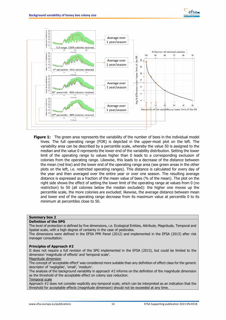
Within this report, different operating ranges are defined by either the percentage fractions of colonies retained in the operating range or, which is equivalent, by the percentiles of the variability used as lower limit. For instance, when a fraction of 95% of colonies are retained in the restricted range, the lower limit would correspond to the 5th percentile of the full operating range. The resulting difference between the mean of the colony size and the lower limit of the OR – irrespective of this being a FOR or a ROR – is always referred to as a percentage difference. The concept is graphically illustrated in Figure 1.
Background variability of honey bee colony size
www.efsa.europa.eu/publications 14 EFSA Supporting publication 2021:EN-6518
Figure 1: The green area represents the variability of the number of bees in the individual model hives. The full operating range (FOR) is depicted in the upper-most plot on the left. The variability area can be described by a percentile scale, whereby the value 50 is assigned to the median and the value 0 represents the lower end of the variability distribution. Setting the lower limit of the operating range to values higher than 0 leads to a corresponding exclusion of colonies from the operating range. Likewise, this leads to a decrease of the distance between the mean (red line) and the lower end of the operating range area (see green areas in the other plots on the left, i.e. restricted operating ranges). This distance is calculated for every day of the year and then averaged over the entire year or over one season. The resulting average distance is expressed as a fraction of the mean value of bees (% of the mean). The plot on the right side shows the effect of setting the lower limit of the operating range at values from 0 (no restriction) to 50 (all colonies below the median excluded): the higher one moves up the percentile scale, the more colonies are excluded; likewise, the average distance between mean and lower end of the operating range decrease from its maximum value at percentile 0 to its minimum at percentiles close to 50.
Summary box 2 Definition of the SPG The level of protection is defined by five dimensions, i.e. Ecological Entities, Attribute, Magnitude, Temporal and Spatial scale, with a high degree of certainty in the case of pesticides. The dimensions were defined in the EFSA PPR Panel (2012) and implemented in the EFSA (2013) after risk manager consultation. Principles of Approach #2 It does not require a full revision of the SPG implemented in the EFSA (2013), but could be limited to the dimension ‘magnitude of effects’ and ‘temporal scale’. Magnitude dimension The concept of ‘acceptable effect’ was considered more suitable than any definition of effect class for the generic descriptor of ‘negligible’, ‘small’, ‘medium’. The analysis of the background variability in approach #2 informs on the definition of the magnitude dimension as the threshold of the acceptable effect on colony size reduction. Temporal scale Approach #2 does not consider explicitly any temporal scale, which can be interpreted as an indication that the threshold for acceptable effects (magnitude dimension) should not be exceeded at any time.
Background variability of honey bee colony size
www.efsa.europa.eu/publications 15 EFSA Supporting publication 2021:EN-6518
Practical limitation in the reference tier (i.e. field studies) suggests that more practical temporal scales can be based on either:
• The minimum interval between colony inspections (1 week) • The length of a honey bee brood cycle (21 days)
Consequences for risk assessment 1) In principle, when effects of a pesticide observed in higher tier studies are above that threshold, the
SPG is considered not met. 2) Since the lower tier risk assessment is calibrated to be compliant with the SPG, when the trigger values
are breached, the SPG is not met.
4. Data and methodologies The analysis makes use of both modelling approaches and experimental data from literature and pesticide dossiers. For the modelling part, the BEEHAVE model (Becher et al., 2014) has been used. The experimental data from literature and pesticide dossiers are hereafter referred to as ‘external data’, to highlight that these were produced independently of the model simulations. Exploring the background variability of honey bee colony size using experimental data is in principle possible, but studies carried out with this scope are not readily available. In addition, experimental studies have other practical limitations:
1) colonies cannot be continuously monitored, and increasing the frequency of measurements also increases the level of stress to bees, altering the measured outcome;
2) the number of replicates that can be monitored is limited by the budget and other practical constraints of the study set-up;
3) similarly, the possibility to analyse variability in different settings is subject to a big experimental effort, which requires significant investment in terms of time and economic resources.
In view of the limitations of the experimental approaches in isolation, EFSA considered that the task could be performed with the support of modelling. External data were used for calibration of the model and to check the plausibility of the final model predictions.
4.1. The use of the BEEHAVE model The BEEHAVE model (Becher et al., 2014) simulates hive population dynamics by considering environmental factors, such as weather conditions, distance to flower patches and food availability. The model can also simulate the effects of infectious agents, like the Varroa mite and two associated viruses. The model was evaluated by the EFSA PPR Panel (2015). The EFSA PPR Panel considered the conceptual model of BEEHAVE and the links between processes and variables logical and concluded that:
‘the validation of the BEEHAVE model for the original use fits quite well with the criteria required in the good modelling practice opinion (EFSA PPR Panel, 2014)’. The overall conclusion of the evaluation was that ‘BEEHAVE performs well in modelling honeybee colony dynamics.’
Further models were considered for the present exercise. Since a comprehensive review of honey bee models was already performed by Becher et al. (2013), the focus was put mainly on models that were published after such review. An exception was made for BEEPOP (DeGrandi-Hoffmann et al., 1989), HoPoMo (Schmickl and Crailsheim, 2007) and the model from Khoury et al. (2011), all published before 2013, but further considered because of their status as reference for many other models developed afterwards. The review considered more than 40 models, some of which were similar to pre-existing ones, but with some elements of novelty worth investigating. The review was carried out in a rather schematic way, mostly by considering whether a pre-defined list of processes and attributes found explicit consideration in each model or not. The outcome is a matrix with the process/attribute in the rows and the different models in the columns. This is available in Appendix A. It must be highlighted that the list of processes and attributes is not necessarily exhaustive, but it certainly encompasses most of the aspects that models published so far tackled in an explicit way. Processes and attributes considered in this scheme do not have necessarily the same weight in all contexts. Furthermore, such

Background variability of honey bee colony size
www.efsa.europa.eu/publications 16 EFSA Supporting publication 2021:EN-6518
schematic assessment of the different models could not account for more subtle/or overarching aspects such as e.g. the overall complexity of the modelling approach. Nevertheless, it allows to make some general considerations. Most of the available models are completely deterministic, and thus any assessment of the colony size variability would need to be caused by variability ‘imposed’ by the user, e.g. by setting different resource levels or different mortality rates or different egg-laying rate at every run. While this would be a possibility if there were specific knowledge of parameter variability in each environmental context, this was not the case for the present analysis. Furthermore, this ‘imposed’ variability would, in some cases, challenge the idea to have multiple runs as perfect replicates (e.g. if different resource levels are set in the landscape). Some of the available models would instead present stochastic elements that allow an assessment of the variability among replicate runs. Apart from BEEHAVE, these include: HoPoMo (Schmickl and Crailsheim, 2007), SimBeeBop (Devillers et al., 2014), Bee++ (Betti et al., 2017), Rivière et al. (2018), VARROAPOP + Pesticide (Kuan et al., 2018), and Alves et al. (2020). However, among these, only the one from Kuan et al. (2018) has a publicly available computer implementation. Becher et al. (2013) classified models on the basis of their ability to describe honey bee colony dynamics (C), foraging behaviour (F) or honeybee–Varroa mite–virus interactions (V). In the present review, we have attempted the use of the same classification, extending the third category beyond Varroa as more recent models account for other pathogens as well. Nevertheless, distinguishing the presence of a proper foraging module was often problematic and thus it was decided not to apply a rigid classification. Indeed, in many models foraging is only simulated as an input of food resources, with limited or even no influence from the environment outside the hive. Food collection by foragers is in some models constant in time (e.g. Khoury et al., 2013; Perry et al., 2015; Myerscough et al., 2017; Schmickl and Karsai, 2017). Other models simulate changes during the year, either just by accounting for a stop of foraging during winter (Betti et al., 2014, 2016), or by accounting for seasonal fluctuations of food availability in the environment (e.g. Schmickl and Crailsheim, 2007; Russell et al., 2013; Paiva et al., 2016; Bagheri and Mirzaie, 2019; Comper and Eberl, 2020) and/or of foraging rates (e.g. Torres et al., 2015). For the present analysis, it was considered pivotal that the model should at least describe: 1) the ‘internal’ structure and dynamics of honey bee colonies;2) the foraging behaviour driven by some dynamic landscape/environmental characteristics. Out of more than 40 considered models, only two would satisfy this requirement: BEEHAVE (Becher et al., 2014) and Bee++ (Betti et al., 2017). Among these two, the level of detail reported for the model parametrisation and implementation is considerably greater for BEEHAVE than for Bee++. Furthermore, as mentioned, there does not seem to be a publicly available computer implementation of Bee++. All in all, BEEHAVE presented an explicit consideration for the largest share of relevant processes and attributes. On this basis, the EFSA WG has considered BEEHAVE the most appropriate model available for investigating the background variability of honey bee colonies in different environmental scenarios. Nevertheless, the EFSA WG acknowledged and carefully considered the shortcomings identified by the PPR Panel (EFSA PPR Panel, 2015). The main limitation, i.e. that BEEHAVE is unsuitable for regulatory risk assessment, was deemed not relevant for the purpose of approach #2. This is because, in the analysis of the background variability of colonies, exposure to pesticides is not simulated, as risk from pesticides as a stressor is not evaluated.
Other limitations identified, which were considered relevant for the present exercise, have been fixed or mitigated (see Section 6.1). However, some other aspects could not be addressed within the scope and the timeframe of the current work. Possible sources of uncertainties related to those aspects are reflected in this document in Section 6. It is important to note that, following the evaluation of BEEHAVE in 2015, EFSA outsourced the development and validation of a mechanistic agent-based model (ApisRAM project), to assess risks to honey bee colonies from exposure to pesticides under different scenarios of combined stressors and factors (EFSA, 2016). Among the aims of ApisRAM there is an explicit willingness to overcome the limitations identified for BEEHAVE, particularly the lack of a pesticide module.
Background variability of honey bee colony size
www.efsa.europa.eu/publications 17 EFSA Supporting publication 2021:EN-6518
Considering the possibility for simulating combined stressors in different environmental scenarios, the use of ApisRAM would provide benefits also for investigating the background colony variability as proposed in approach #2. However, ApisRAM is still under development, therefore it was not possible to propose it for the present exercise (see Section 6.5 for more details on the use of ApisRAM). Overall, the EFSA WG concluded that the use of BEEHAVE represented the best option currently available for the scope proposed with approach #2.
Summary box 3 Why analyse the background variability with the support of modelling?
• The practical limitations of field studies prevent a comprehensive analysis of the colony background variability, while this can be performed with the support of models simulating the colony dynamics (e.g. in-hive processes, feeding behaviours etc.).
• The BEEHAVE model was evaluated in 2015 by the EFSA PPR Panel, who considered it suitable for simulating colony dynamics and therefore this model was selected for this analysis as the best available option.
4.2. Environmental scenarios and model calibration Honey bee colonies behave in different ways depending on the environmental context they are part of. Consequently, the background variability in colony sizes can also vary, resulting in different operating ranges for different environmental contexts.
4.2.1. Scenarios location
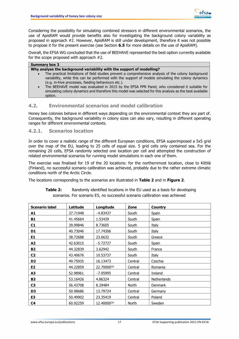
In order to cover a realistic range of the different European conditions, EFSA superimposed a 5x5 grid over the map of the EU, leading to 25 cells of equal size. 5 grid cells only contained sea. For the remaining 20 cells, EFSA randomly selected one location per cell and attempted the construction of related environmental scenarios for running model simulations in each one of them. The exercise was finalised for 19 of the 20 locations: for the northernmost location, close to Kittilä (Finland), no successful scenario calibration was achieved, probably due to the rather extreme climatic conditions north of the Arctic Circle.
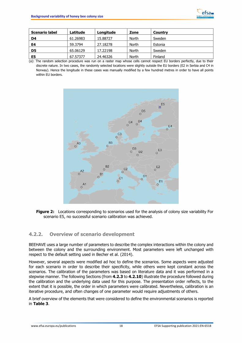
The locations corresponding to the scenarios are illustrated in Table 2 and in Figure 2.
Table 2: Randomly identified locations in the EU used as a basis for developing scenarios. For scenario E5, no successful scenario calibration was achieved
Scenario label Latitude Longitude Zone Country A1 37.71948 −4.83437 South Spain B1 41.45664 1.53439 South Spain C1 39.99846 8.73605 South Italy D1 40.73046 17.74306 South Italy E1 38.72688 23.6632 South Greece A2 42.63015 −5.72727 South Spain B2 44.32839 3.62942 South France C2 43.40676 10.53737 South Italy D2 49.75935 16.13473 Central Czechia E2 44.22859 22.70000(a) Central Romania A3 52.98961 −7.05995 Central Ireland B3 53.16426 4.86324 Central Netherlands C3 56.43708 8.29484 North Denmark D3 50.98686 13.79724 Central Germany E3 50.49902 23.35419 Central Poland C4 60.92259 12.40000(a) North Sweden
Background variability of honey bee colony size
www.efsa.europa.eu/publications 18 EFSA Supporting publication 2021:EN-6518
Scenario label Latitude Longitude Zone Country D4 61.26983 15.88727 North Sweden E4 59.3794 27.18278 North Estonia D5 65.06129 17.22198 North Sweden E5 67.57377 24.46326 North Finland
(a): The random selection procedure was run on a raster map whose cells cannot respect EU borders perfectly, due to their discrete nature. In two cases, the randomly selected locations were slightly outside the EU borders (E2 in Serbia and C4 in Norway). Hence the longitude in these cases was manually modified by a few hundred metres in order to have all points within EU borders.
Figure 2: Locations corresponding to scenarios used for the analysis of colony size variability For scenario E5, no successful scenario calibration was achieved.
4.2.2. Overview of scenario development
BEEHAVE uses a large number of parameters to describe the complex interactions within the colony and between the colony and the surrounding environment. Most parameters were left unchanged with respect to the default setting used in Becher et al. (2014).
However, several aspects were modified ad hoc to define the scenarios. Some aspects were adjusted for each scenario in order to describe their specificity, while others were kept constant across the scenarios. The calibration of the parameters was based on literature data and it was performed in a stepwise manner. The following Sections (from 4.2.3 to 4.2.10) illustrate the procedure followed during the calibration and the underlying data used for this purpose. The presentation order reflects, to the extent that it is possible, the order in which parameters were calibrated. Nevertheless, calibration is an iterative procedure, and often changes of one parameter would require adjustments of others. A brief overview of the elements that were considered to define the environmental scenarios is reported in Table 3.
Background variability of honey bee colony size
www.efsa.europa.eu/publications 19 EFSA Supporting publication 2021:EN-6518
Table 3: Overview of the elements describing the environmental scenarios used in the BEEHAVE simulations
Main area Item Scenario-specific Description Foraging Foraging hours per
day Yes Adjusted for each scenario based on
temperature and solar irradiance. See Section 4.2.4.
Landscape structure
Number of patches No A simplified landscape with two food patches has been used in all scenarios. This is the same landscape used in the original implementation of BEEHAVE(a). See Section 4.2.3.
Distance of the patches to the hive
Yes Parameter calibrated for each scenario in consideration of the energy balance. See Section 4.2.8.
Resource availability
Max availability of pollen and nectar
Yes Parameter calibrated for each scenario in consideration of the energy balance and of pollen/nectar ratios. See Sections 4.2.8 and 4.2.9.
Availability of pollen and nectar in time
Yes Adjusted to the foraging period. See Section 4.2.5.
Bee biology Maximal egg-laying rate of the queen over time
Yes Adjusted to the foraging period. See Section 4.2.6.
Mortality rate No The mortality rate was calibrated on the basis of values retrieved from the literature. See Section 4.2.7.
Beekeeping practices
Amount of added fondant
Yes Model outcome, different in each scenario. See Section 4.2.8.
Honey harvesting period
Yes Adjusted to the foraging window. See Section 4.2.8.
Initial colony size No The starting bee population in the simulated colonies was 10,000 honey bees (±1000). See Section 4.2.10.
(a): Due to limited data availability, a more realistic definition of landscape scenarios based on data was not possible. However, since the EFSA WG considered that the adopted simplification of the landscape was a crucial point, a separate analysis has been set up to explore the effect of landscape complexity on the final outcome i.e. variability in colony size as simulated by the model. The results of this analysis are presented in Appendix A.
4.2.3. Landscape structure
It was not possible to retrieve detailed information about the actual landscape structure for the identified locations in the time frame of this project. In addition, locations were selected randomly, so there has been no consideration of the representativeness of these locations for typical agricultural settings in the EU. In order to overcome this issue, it was chosen to use a simplified landscape, based on the default BEEHAVE implementation (Becher et al., 2014) whose main characteristics are common across scenarios. The default BEEHAVE scenario consists of two floral patches (‘green’ and ‘red’), which are located at different distances from the hive, and have shifted phenology, but are in all other aspects identical. The detection probability for both was fixed at 0.2. It was assumed that the size of both patches was 10 ha, but this choice has no influence since the foraging module in BEEHAVE is spatially implicit, i.e. it accounts for some effects of space (e.g. distance from the hive), but without using actual spatial positions. However, since the EFSA WG considered that the adopted simplification of the landscape was a crucial point, a separate dedicated analysis has been set up to explore the effect of landscape complexity on the variability in colony size as simulated by the model. The methodology and the results of this analysis are presented in Appendix A.
4.2.4. Temporal pattern: daily foraging period
Background variability of honey bee colony size
www.efsa.europa.eu/publications 20 EFSA Supporting publication 2021:EN-6518
The daily foraging period is quantified as the number of hours for each day of the year during which bees can leave the hive to forage in the surrounding environment.
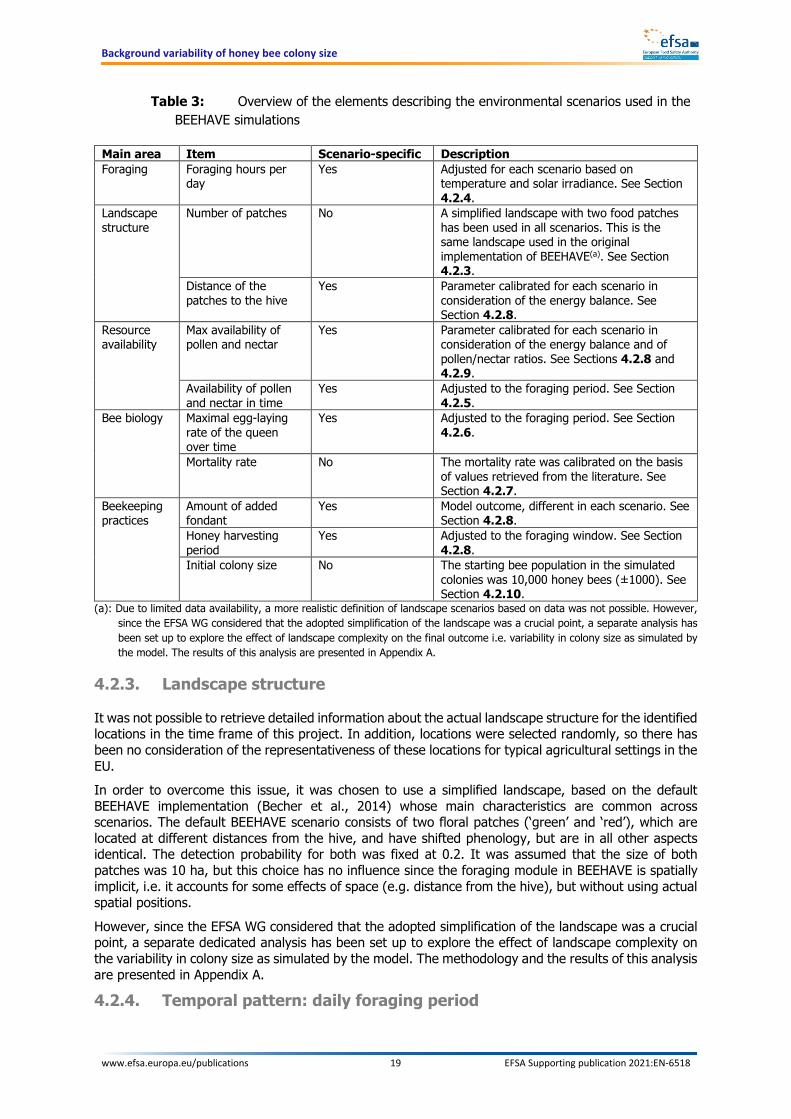
In the original BEEHAVE publication (Becher et al., 2014), and particularly in the ODD (Overview, Design concepts, and Details) protocol, the authors reported that ‘We used the hours of sunshine on days with a maximum temperature above 15°C from those weather data as an approximation to the hours of suitable weather for foraging’. However, the ‘hours of sunshine’ is not necessarily a straightforward concept, due to its dichotomic nature and a lack of a clear threshold. The degree of cloudiness that marks the difference between ‘sunshine’ and ‘not sunshine’ is debatable and, if not further rooted in biological consideration, arbitrary. A more useful way to express the same concepts is given by the measurement of global (direct and indirect) irradiance. Hains and Gamper (2017) report that ‘bees forage at temperatures above 12–19°C and solar irradiance greater than 400 W/m2’, even though they do not provide empirical data to underpin this. Burrill and Dietz (1981) reported a positive correlation between foraging activity and irradiance up to 0.66 Langleys (probably Langleys/min ≈460 W/m2, but there is some uncertainty on the actual unit), while at higher level of irradiance, the foraging activity starts decreasing slowly. In this work, based on the available plots, foraging starts increasing significantly at around 0.2 Langleys (probably Langleys/min ≈140 W/m2). Clarke and Robert (2018) showed how both temperature and irradiance are able to explain most of the foraging activity (in terms of outgoing bees) by using simple linear models. While triggers of activity are not explicitly reported, the analysis of an example day of data reported in a plot, showed that the bee activity took off when solar irradiation increased above 200 W/m2. Similarly, Vicens and Bosch (2000) provided approximate temperature-radiation thresholds for honey bees and Osmia cornuta. Honey bee foraging took place at minimum 329 W/m2 when temperature was 12.2°C, at 233 W/m2 when temperature was at 13.2°C, and at 151 W/m2 when temperature was at 15.8°C. All these publications highlight that it is not possible to identify clear thresholds for irradiance and temperature in isolation, but rather that these two variables should be considered together. Particularly the last-mentioned publication by Vicens and Bosch (2000) offered the possibility to work out an empirical relationship between the two variables, so that the threshold for temperature is dynamically driven by irradiance and vice versa.
Figure 3: Empirical relationship derived from Vicens and Bosch (2000) between temperature and irradiance marking conditions for honey bee foraging flight
Spatially explicit data on solar irradiance and temperature are available from the JRC photovoltaic Geographical Information System (PVGIS)5. The data behind the platform are based on ground
5 https://ec.europa.eu/jrc/en/pvgis
Background variability of honey bee colony size
www.efsa.europa.eu/publications 21 EFSA Supporting publication 2021:EN-6518
measurements and estimations using satellite images. The solar radiation tool, in particular, allows accessing hourly time-series of data for any point of Europe (and more) from 2005 to 2016.
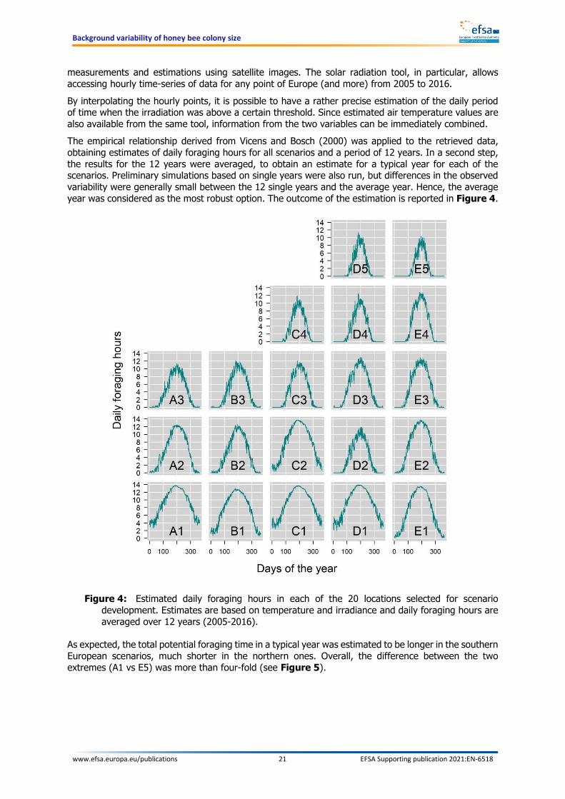
By interpolating the hourly points, it is possible to have a rather precise estimation of the daily period of time when the irradiation was above a certain threshold. Since estimated air temperature values are also available from the same tool, information from the two variables can be immediately combined. The empirical relationship derived from Vicens and Bosch (2000) was applied to the retrieved data, obtaining estimates of daily foraging hours for all scenarios and a period of 12 years. In a second step, the results for the 12 years were averaged, to obtain an estimate for a typical year for each of the scenarios. Preliminary simulations based on single years were also run, but differences in the observed variability were generally small between the 12 single years and the average year. Hence, the average year was considered as the most robust option. The outcome of the estimation is reported in Figure 4.
Figure 4: Estimated daily foraging hours in each of the 20 locations selected for scenario development. Estimates are based on temperature and irradiance and daily foraging hours are averaged over 12 years (2005-2016).
As expected, the total potential foraging time in a typical year was estimated to be longer in the southern European scenarios, much shorter in the northern ones. Overall, the difference between the two extremes (A1 vs E5) was more than four-fold (see Figure 5).

Background variability of honey bee colony size
www.efsa.europa.eu/publications 22 EFSA Supporting publication 2021:EN-6518
Figure 5: Estimated cumulative foraging hours in each of the 20 locations selected for scenario development
4.2.5. Temporal pattern: food availability
The temporal pattern of floral resources (i.e. pollen and nectar) depends on the phenology and on the diversity of the plants that are present in the landscape. These, in turn, are largely determined by climatic variables (e.g. temperature, light intensity and photoperiod, soil characteristics such as nutrient levels, moisture, etc.).
In view of the simplified landscape structure adopted for the scenario development, a species-specific analysis of plant phenology in different European locations was considered out of scope. However, a consideration of the temporal dynamics of food resources at the landscape level was performed for the different scenarios. As a first step, an attempt to find ‘first-hand’ data on the availability of (generic) flowers during the year at different latitudes was made. Beekeepers’ calendars (e.g. Leida et al., 2004; Matey Valderrama; Mathis and Buchanan, 2006) are a useful source of qualitative information as they report, for a specific area, how many attractive (melliferous) plant species flower each month/week. This provided confirmation on two aspects:
• The availability of floral resources – at least in terms of diversity – often presents multiple peaks during the year, generally at least one in spring and one in summer.
• Floral resources are available for longer periods in warmer climates (i.e. southern Europe) than in colder ones.
On the other hand, beekeepers’ calendars are not readily available for all parts of Europe and they do not provide quantitative information on the actual pollen and nectar temporal pattern in terms of amount. Some literature studies provide more quantitative information, especially on nectar production. For example, Timberlake et al. (2019) quantified the daily sugar production per square kilometre in four different farms in UK. The analysis was extremely detailed: the authors performed 137 field visits to the four farms over 2 years and counted nearly half a million individual floral units from 176 flowering plant species. The outcome identified fluctuations in the temporal dynamic of nectar, with the two main peaks

Background variability of honey bee colony size
www.efsa.europa.eu/publications 23 EFSA Supporting publication 2021:EN-6518
identified in spring (April/May) and summer (July). A later period of slight increase in nectar availability was found between September and October. Meikle et al. (2008) identified five periods of nectar flows from September 2004 to June 2006 in southern France, confirming that two or three peaks of nectar availability per year are likely the norm. Similarly, Requier et al. (2015) found that the mass of pollen and nectar collected by honey bees in intensive farmland in France followed a bimodal seasonal trend, marked by a two-month period of low food supply between two mass-flowerings (one ending in May and another ending in July).
However, other studies indicate more unimodal temporal distributions. Baude et al. (2016) modelled monthly nectar productivity in a spatially explicit way over Great Britain, identifying a single peak in summer (July/August). However, this may be due to their assumption that the flowering season for each species has only one peak, for both flower density and nectar productivity. Similarly, Hicks et al. (2016), while monitoring nectar production in urban meadows in the UK, also found predominantly unimodal patterns, with peaks generally occurring during summer. Many studies focus on seasonal shifts of pollen collected by honey bees in terms of quality and/or diversity (Bilisik et al., 2008; Wood et al., 2018; Lau et al., 2019), while comprehensive evaluations of the temporal trends of the total amount collected during the year are less abundant. Among these, the fluctuating nature of available resources seems to be confirmed by some studies. Apart from the already mentioned paper by Requier et al. (2015), also Taha et al. (2017), in northern Egypt, found peaks in pollen collection in early and late spring (March and May) and later during mid-summer (July). While the study was carried out outside Europe, the experimental area is characterised by a Mediterranean climate, which makes these findings relevant for southern European countries. Similarly to nectar, Hicks et al. (2016) found more unimodal temporal pattern also for pollen. For the present work, a shifted phenology in the two flower patches was used, each one characterised by a bell-shaped trend, in order to mimic the pattern observed in the aforementioned studies at the landscape level. In addition, it was assumed that the available flowers would provide pollen and nectar with the same temporal pattern.
The flowering length was maintained equal for the two flower patches and all scenarios, i.e. 150 days between the two points in which the curve hit 50% of the maximum productivity, the first time while increasing, and the second time while decreasing. Scenarios differed in the shift between the phenology of the two floral patches. As already mentioned, food tends to be available for longer time in southern Europe, and for shorter time in northern Europe. To reproduce this finding, the phenology of the two patches was more overlapping in the north, and less in the south. This was achieved by indirectly linking the plant phenology to the temperature and the sunlight (i.e. irradiance), i.e. climatic factors that play a major role in determining the development of the plants. The link between these two climatic variables and the floral temporal pattern was mediated by the daily foraging period, which was entirely determined on the basis of the same climatic variables (Section 4.2.4). In practice, this link was achieved by fixing the interval between the curve describing the daily foraging period and the curves describing the availability of the floral resources in the two patches. Such distance was derived from the ‘Rothamsted’ scenario, presented in the original BEEHAVE implementation (Becher et al., 2014). The procedure is graphically illustrated in Figure 6.
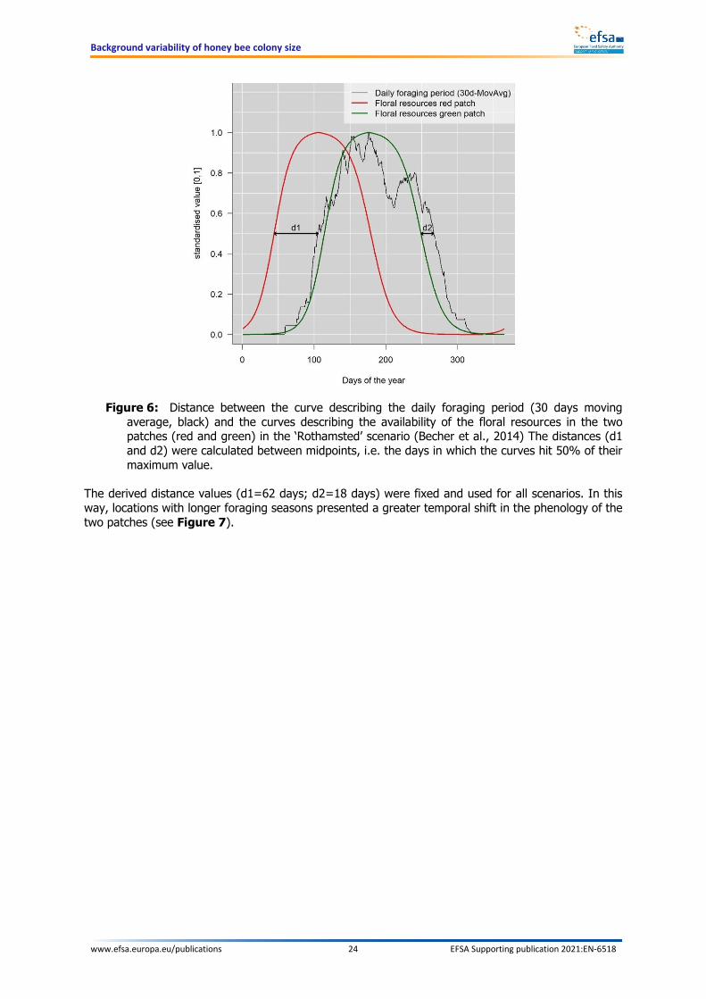
Background variability of honey bee colony size
www.efsa.europa.eu/publications 24 EFSA Supporting publication 2021:EN-6518
Figure 6: Distance between the curve describing the daily foraging period (30 days moving average, black) and the curves describing the availability of the floral resources in the two patches (red and green) in the ‘Rothamsted’ scenario (Becher et al., 2014) The distances (d1 and d2) were calculated between midpoints, i.e. the days in which the curves hit 50% of their maximum value.
The derived distance values (d1=62 days; d2=18 days) were fixed and used for all scenarios. In this way, locations with longer foraging seasons presented a greater temporal shift in the phenology of the two patches (see Figure 7).

Background variability of honey bee colony size
www.efsa.europa.eu/publications 25 EFSA Supporting publication 2021:EN-6518
Figure 7: Temporal pattern of the floral resources of the two patches (red and green) for each of the scenarios
4.2.6. Temporal pattern: egg-laying rate
The temporal pattern of the queen’s egg laying in the BEEHAVE model is based on Schmickl and Crailsheim's (2007) bell-shaped curve. This curve should represent the seasonal variability in egg laying which is observed from experimental data. In fact, Schmickl and Crailsheim's (2007) derived their pattern from figure 1 in Bodenheimer (1937), which in turn depicted data from Ebert (1922). While reflecting such seasonal trend, Schmickl and Crailsheim's (2007) did not explain in detail how their egg-laying curve can be manipulated in order to link it to a specific climate. On the contrary, DeGrandi-Hoffman et al. (1989) in their BEEPOP model, modelled the daily number of eggs laid as explicitly dependent from several other parameters, including temperature (in degree days) and sunlight (as day length). Nevertheless, the origin of such mathematical relationship is not explained nor justified.
The influence of temperature on the egg laying has been well known for long time (see Dunham, 1930). The joint influence of temperature and light has also been widely acknowledged in the literature, particularly on the onset of egg laying (Nürnberger et al., 2018). In order to maintain the structure of the BEEHAVE model, but still be able to link this to the climatic features of the different scenarios, the temporal pattern of the egg-laying rate was adjusted to the daily foraging period, similarly to what was done for the temporal pattern of food availability (see Section 4.2.5). By doing this, the egg laying was longer in warmer scenarios, and shorter in colder ones (see Figure 8).

Background variability of honey bee colony size
www.efsa.europa.eu/publications 26 EFSA Supporting publication 2021:EN-6518
The seasonal bell-shaped curve represents the maximum egg laying for any given day. However, the model can reduce egg laying comparing to this curve when the number of adult bees available for brood care is not enough. The yearly peak of egg laying was fixed at 1,600 egg/day for all scenarios.
Figure 8: Temporal pattern of the maximum daily egg-laying rate for each of the scenarios
4.2.7. Background mortality
In the context of the revision of the EFSA Bee Guidance Document, the first deliverable produced by EFSA was a review of the evidence of bee background mortality (EFSA et al., 2020b). This report integrated the outcome of a systematic literature review and of a survey involving beekeepers in several EU countries, focusing on background mortality of adult bees.
4.2.7.1. Forager mortality Within EFSA et al. (2020b), information on forager background mortality was initially collected in terms of forager lifespan, i.e. from age of first forage to death. Reliable forager lifespan estimates were collected from 15 different references. Within BEEHAVE, forager mortality is implemented as a mortality probability per second spent foraging outside the hive. As such, the data collected in EFSA et al. (2020b) could not be used directly as input value for the simulations. Thus, a calibration exercise was performed.
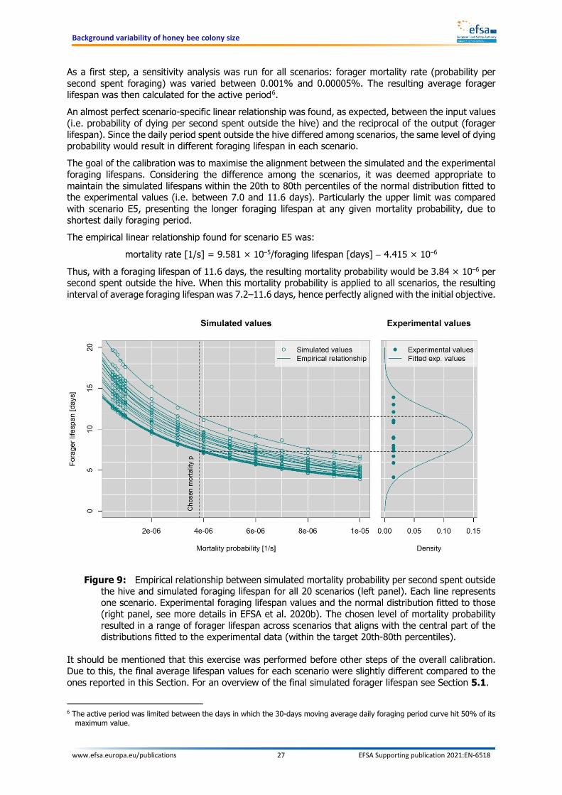
Background variability of honey bee colony size
www.efsa.europa.eu/publications 27 EFSA Supporting publication 2021:EN-6518
As a first step, a sensitivity analysis was run for all scenarios: forager mortality rate (probability per second spent foraging) was varied between 0.001% and 0.00005%. The resulting average forager lifespan was then calculated for the active period6. An almost perfect scenario-specific linear relationship was found, as expected, between the input values (i.e. probability of dying per second spent outside the hive) and the reciprocal of the output (forager lifespan). Since the daily period spent outside the hive differed among scenarios, the same level of dying probability would result in different foraging lifespan in each scenario.
The goal of the calibration was to maximise the alignment between the simulated and the experimental foraging lifespans. Considering the difference among the scenarios, it was deemed appropriate to maintain the simulated lifespans within the 20th to 80th percentiles of the normal distribution fitted to the experimental values (i.e. between 7.0 and 11.6 days). Particularly the upper limit was compared with scenario E5, presenting the longer foraging lifespan at any given mortality probability, due to shortest daily foraging period. The empirical linear relationship found for scenario E5 was:
mortality rate [1/s] = 9.581 × 10⁻⁵/foraging lifespan [days] − 4.415 × 10⁻⁶
Thus, with a foraging lifespan of 11.6 days, the resulting mortality probability would be 3.84 × 10⁻⁶ per second spent outside the hive. When this mortality probability is applied to all scenarios, the resulting interval of average foraging lifespan was 7.2–11.6 days, hence perfectly aligned with the initial objective.
Figure 9: Empirical relationship between simulated mortality probability per second spent outside the hive and simulated foraging lifespan for all 20 scenarios (left panel). Each line represents one scenario. Experimental foraging lifespan values and the normal distribution fitted to those (right panel, see more details in EFSA et al. 2020b). The chosen level of mortality probability resulted in a range of forager lifespan across scenarios that aligns with the central part of the distributions fitted to the experimental data (within the target 20th-80th percentiles).
It should be mentioned that this exercise was performed before other steps of the overall calibration. Due to this, the final average lifespan values for each scenario were slightly different compared to the ones reported in this Section. For an overview of the final simulated forager lifespan see Section 5.1.
6 The active period was limited between the days in which the 30-days moving average daily foraging period curve hit 50% of its
maximum value.
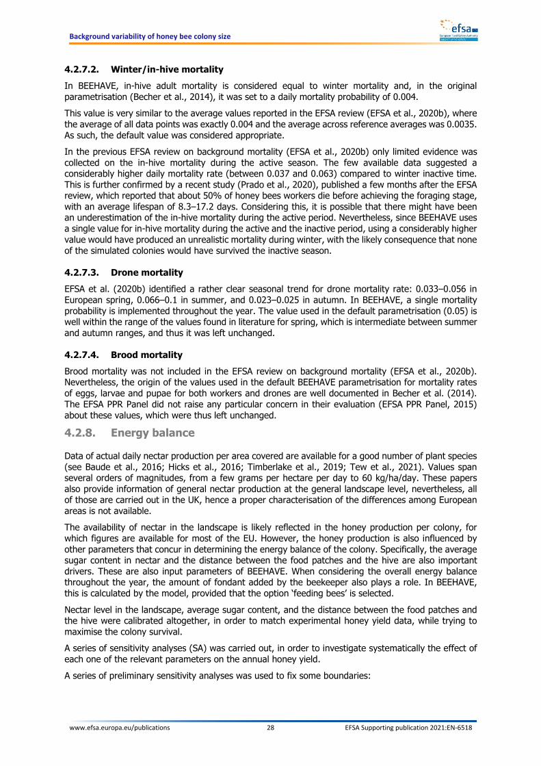
Background variability of honey bee colony size
www.efsa.europa.eu/publications 28 EFSA Supporting publication 2021:EN-6518
4.2.7.2. Winter/in-hive mortality In BEEHAVE, in-hive adult mortality is considered equal to winter mortality and, in the original parametrisation (Becher et al., 2014), it was set to a daily mortality probability of 0.004. This value is very similar to the average values reported in the EFSA review (EFSA et al., 2020b), where the average of all data points was exactly 0.004 and the average across reference averages was 0.0035. As such, the default value was considered appropriate. In the previous EFSA review on background mortality (EFSA et al., 2020b) only limited evidence was collected on the in-hive mortality during the active season. The few available data suggested a considerably higher daily mortality rate (between 0.037 and 0.063) compared to winter inactive time. This is further confirmed by a recent study (Prado et al., 2020), published a few months after the EFSA review, which reported that about 50% of honey bees workers die before achieving the foraging stage, with an average lifespan of 8.3–17.2 days. Considering this, it is possible that there might have been an underestimation of the in-hive mortality during the active period. Nevertheless, since BEEHAVE uses a single value for in-hive mortality during the active and the inactive period, using a considerably higher value would have produced an unrealistic mortality during winter, with the likely consequence that none of the simulated colonies would have survived the inactive season.
4.2.7.3. Drone mortality EFSA et al. (2020b) identified a rather clear seasonal trend for drone mortality rate: 0.033–0.056 in European spring, 0.066–0.1 in summer, and 0.023–0.025 in autumn. In BEEHAVE, a single mortality probability is implemented throughout the year. The value used in the default parametrisation (0.05) is well within the range of the values found in literature for spring, which is intermediate between summer and autumn ranges, and thus it was left unchanged.
4.2.7.4. Brood mortality Brood mortality was not included in the EFSA review on background mortality (EFSA et al., 2020b). Nevertheless, the origin of the values used in the default BEEHAVE parametrisation for mortality rates of eggs, larvae and pupae for both workers and drones are well documented in Becher et al. (2014). The EFSA PPR Panel did not raise any particular concern in their evaluation (EFSA PPR Panel, 2015) about these values, which were thus left unchanged.
4.2.8. Energy balance
Data of actual daily nectar production per area covered are available for a good number of plant species (see Baude et al., 2016; Hicks et al., 2016; Timberlake et al., 2019; Tew et al., 2021). Values span several orders of magnitudes, from a few grams per hectare per day to 60 kg/ha/day. These papers also provide information of general nectar production at the general landscape level, nevertheless, all of those are carried out in the UK, hence a proper characterisation of the differences among European areas is not available. The availability of nectar in the landscape is likely reflected in the honey production per colony, for which figures are available for most of the EU. However, the honey production is also influenced by other parameters that concur in determining the energy balance of the colony. Specifically, the average sugar content in nectar and the distance between the food patches and the hive are also important drivers. These are also input parameters of BEEHAVE. When considering the overall energy balance throughout the year, the amount of fondant added by the beekeeper also plays a role. In BEEHAVE, this is calculated by the model, provided that the option ‘feeding bees’ is selected.
Nectar level in the landscape, average sugar content, and the distance between the food patches and the hive were calibrated altogether, in order to match experimental honey yield data, while trying to maximise the colony survival. A series of sensitivity analyses (SA) was carried out, in order to investigate systematically the effect of each one of the relevant parameters on the annual honey yield.
A series of preliminary sensitivity analyses was used to fix some boundaries:
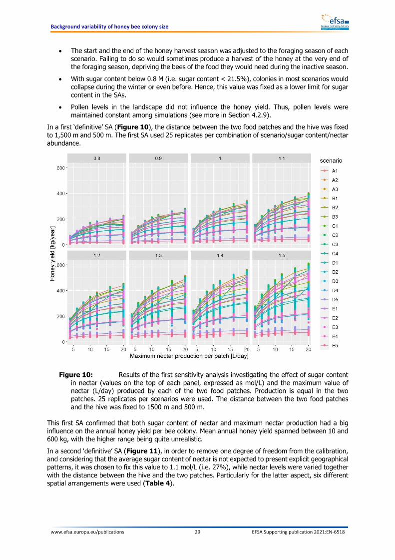
Background variability of honey bee colony size
www.efsa.europa.eu/publications 29 EFSA Supporting publication 2021:EN-6518
• The start and the end of the honey harvest season was adjusted to the foraging season of each scenario. Failing to do so would sometimes produce a harvest of the honey at the very end of the foraging season, depriving the bees of the food they would need during the inactive season.
• With sugar content below 0.8 M (i.e. sugar content < 21.5%), colonies in most scenarios would collapse during the winter or even before. Hence, this value was fixed as a lower limit for sugar content in the SAs.
• Pollen levels in the landscape did not influence the honey yield. Thus, pollen levels were maintained constant among simulations (see more in Section 4.2.9).
In a first ‘definitive’ SA (Figure 10), the distance between the two food patches and the hive was fixed to 1,500 m and 500 m. The first SA used 25 replicates per combination of scenario/sugar content/nectar abundance.
Figure 10: Results of the first sensitivity analysis investigating the effect of sugar content in nectar (values on the top of each panel, expressed as mol/L) and the maximum value of nectar (L/day) produced by each of the two food patches. Production is equal in the two patches. 25 replicates per scenarios were used. The distance between the two food patches and the hive was fixed to 1500 m and 500 m.
This first SA confirmed that both sugar content of nectar and maximum nectar production had a big influence on the annual honey yield per bee colony. Mean annual honey yield spanned between 10 and 600 kg, with the higher range being quite unrealistic. In a second ‘definitive’ SA (Figure 11), in order to remove one degree of freedom from the calibration, and considering that the average sugar content of nectar is not expected to present explicit geographical patterns, it was chosen to fix this value to 1.1 mol/L (i.e. 27%), while nectar levels were varied together with the distance between the hive and the two patches. Particularly for the latter aspect, six different spatial arrangements were used (Table 4).

Background variability of honey bee colony size
www.efsa.europa.eu/publications 30 EFSA Supporting publication 2021:EN-6518
Table 4: Different spatial arrangements of the food patches used in a second sensitivity analysis
Nr Distance patch-hive [m] Green patch Red patch
1 100 300 2 200 600 3 300 900 4 300 100 5 600 200 6 900 300
A
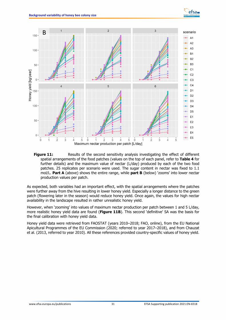
Background variability of honey bee colony size
www.efsa.europa.eu/publications 31 EFSA Supporting publication 2021:EN-6518
Figure 11: Results of the second sensitivity analysis investigating the effect of different spatial arrangements of the food patches (values on the top of each panel, refer to Table 4 for further details) and the maximum value of nectar (L/day) produced by each of the two food patches. 25 replicates per scenario were used. The sugar content in nectar was fixed to 1.1 mol/L. Part A (above) shows the entire range, while part B (below) ‘zooms’ into lower nectar production values per patch.
As expected, both variables had an important effect, with the spatial arrangements where the patches were further away from the hive resulting in lower honey yield. Especially a longer distance to the green patch (flowering later in the season) would reduce honey yield. Once again, the values for high nectar availability in the landscape resulted in rather unrealistic honey yield. However, when ‘zooming’ into values of maximum nectar production per patch between 1 and 5 L/day, more realistic honey yield data are found (Figure 11B). This second ‘definitive’ SA was the basis for the final calibration with honey yield data. Honey yield data were retrieved from FAOSTAT (years 2010–2018; FAO, online), from the EU National Apicultural Programmes of the EU Commission (2020; referred to year 2017–2018), and from Chauzat et al. (2013, referred to year 2010). All these references provided country-specific values of honey yield.
B
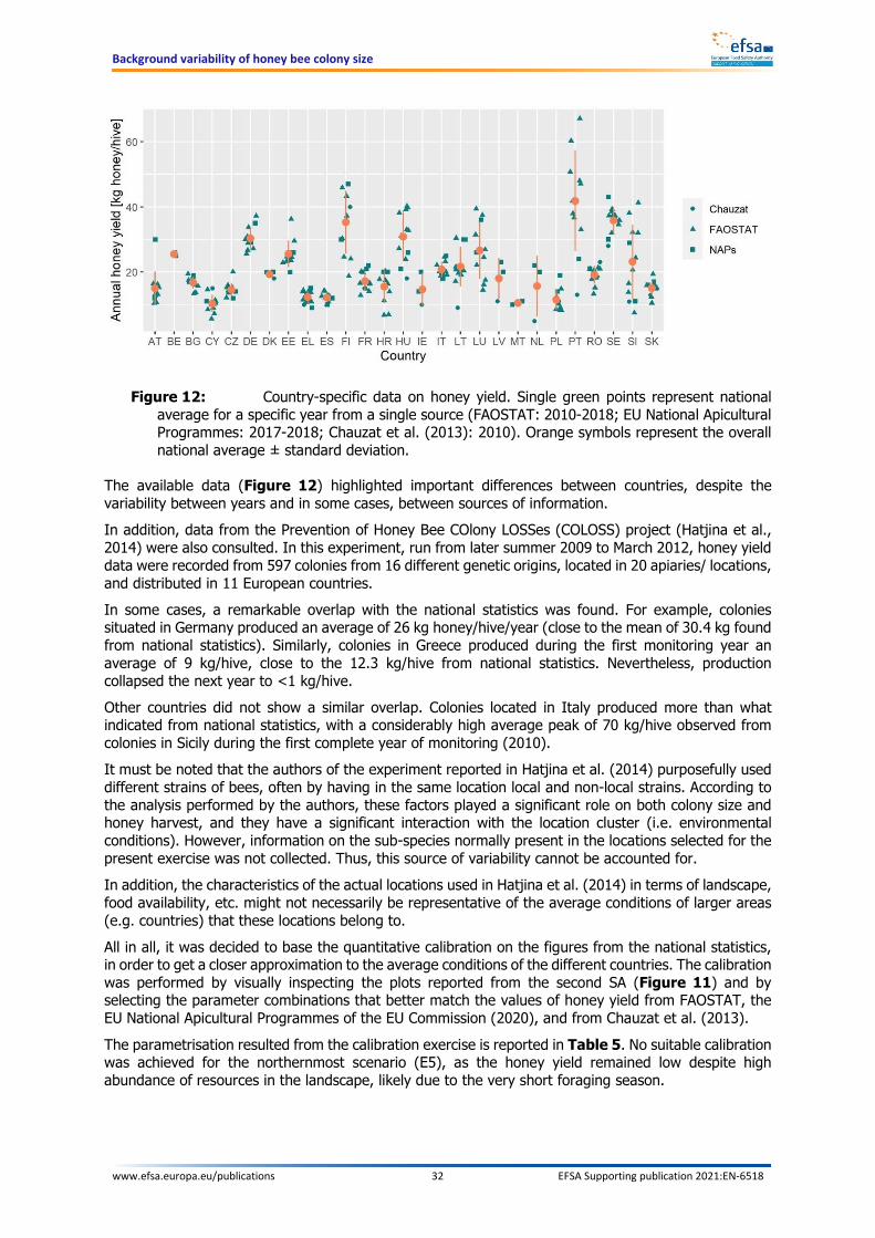
Background variability of honey bee colony size
www.efsa.europa.eu/publications 32 EFSA Supporting publication 2021:EN-6518
Figure 12: Country-specific data on honey yield. Single green points represent national average for a specific year from a single source (FAOSTAT: 2010-2018; EU National Apicultural Programmes: 2017-2018; Chauzat et al. (2013): 2010). Orange symbols represent the overall national average ± standard deviation.
The available data (Figure 12) highlighted important differences between countries, despite the variability between years and in some cases, between sources of information. In addition, data from the Prevention of Honey Bee COlony LOSSes (COLOSS) project (Hatjina et al., 2014) were also consulted. In this experiment, run from later summer 2009 to March 2012, honey yield data were recorded from 597 colonies from 16 different genetic origins, located in 20 apiaries/ locations, and distributed in 11 European countries. In some cases, a remarkable overlap with the national statistics was found. For example, colonies situated in Germany produced an average of 26 kg honey/hive/year (close to the mean of 30.4 kg found from national statistics). Similarly, colonies in Greece produced during the first monitoring year an average of 9 kg/hive, close to the 12.3 kg/hive from national statistics. Nevertheless, production collapsed the next year to <1 kg/hive. Other countries did not show a similar overlap. Colonies located in Italy produced more than what indicated from national statistics, with a considerably high average peak of 70 kg/hive observed from colonies in Sicily during the first complete year of monitoring (2010). It must be noted that the authors of the experiment reported in Hatjina et al. (2014) purposefully used different strains of bees, often by having in the same location local and non-local strains. According to the analysis performed by the authors, these factors played a significant role on both colony size and honey harvest, and they have a significant interaction with the location cluster (i.e. environmental conditions). However, information on the sub-species normally present in the locations selected for the present exercise was not collected. Thus, this source of variability cannot be accounted for. In addition, the characteristics of the actual locations used in Hatjina et al. (2014) in terms of landscape, food availability, etc. might not necessarily be representative of the average conditions of larger areas (e.g. countries) that these locations belong to. All in all, it was decided to base the quantitative calibration on the figures from the national statistics, in order to get a closer approximation to the average conditions of the different countries. The calibration was performed by visually inspecting the plots reported from the second SA (Figure 11) and by selecting the parameter combinations that better match the values of honey yield from FAOSTAT, the EU National Apicultural Programmes of the EU Commission (2020), and from Chauzat et al. (2013).
The parametrisation resulted from the calibration exercise is reported in Table 5. No suitable calibration was achieved for the northernmost scenario (E5), as the honey yield remained low despite high abundance of resources in the landscape, likely due to the very short foraging season.

Background variability of honey bee colony size
www.efsa.europa.eu/publications 33 EFSA Supporting publication 2021:EN-6518
Table 5: Final parametrisation used to define the energy balance of the simulated colonies
Scenario Max nectar level [L/patch/day] Sucrose [mol/L] Distance scenario(a) A1 1.8 1.1 3 B1 1.6 1.1 2 C1 2 1.1 6 D1 2 1.1 6 E1 1.6 1.1 3 A2 1.6 1.1 2 B2 1.6 1.1 5 C2 1.8 1.1 1 D2 1.6 1.1 3 E2 1.6 1.1 1 A3 1.6 1.1 3 B3 1.6 1.1 5 C3 1.6 1.1 4 D3 2 1.1 6 E3 1.6 1.1 4 C4 2 1.1 2 D4 2 1.1 2 E4 2 1.1 5 D5 6 1.1 5 E5 No suitable combination
(a): See Table 4 for further details on the different distance scenarios.
4.2.9. Pollen levels in the landscape
For maximum pollen levels in the landscape, data are perhaps even more limited than for nectar, also because there is no possibility to link this aspect to a quantified output as it was for nectar and honey yield. However, some information exists at least for comparing production ratios between pollen and nectar. Particularly, useful information from the literature was compiled by Becher et al. (2016) and Agatz et al. (2019) (Table 6). Hicks et al. (2016) also reports information on multiple plant species, but pollen production is only expressed as volume per day. Without information on its density, it is not possible to work out daily production values in terms of weight per area.
Table 6: Sugar/pollen production ratios for several plants as retrieved from the literature
Ref. Plant Nectar production [mL/m2/d]
Sucrose conc. [mol/L]
Sucrose production [g/m2/d]
Pollen production [g/m2/d]
Ratio sugar/ pollen
Becher et al. (2016)
Oilseed rape 0.30 1.50 0.15 0.13 1.18 Maize 0.00 0.00 0.00 0.75 0.00 Sunflower 0.003 1.25 0.001 0.11 0.01 Field bean 0.09 1.275 0.04 0.06 0.63 White clover 0.05 1.495 0.03 0.01 2.67 Willow 1.84 1.08 0.68 8.52 0.08

Background variability of honey bee colony size
www.efsa.europa.eu/publications 34 EFSA Supporting publication 2021:EN-6518
Agatz et al. (2019)
Sloe 0.43 0.58 0.09 0.30 0.28 Maple 3.41 1.75 2.04 20.44 0.10 Oilseed rape 0.30 1.30 0.13 0.13 1.03 Dandelion 0.37 0.41 0.05 10.64 0.005 White clover 0.05 1.08 0.02 0.01 1.93 Ivy 0.01 1.43 0.01 0.44 0.02
Calculated ratios span from 0 to 2.67. Considering the maximum values of nectar production selected for the final simulations (Table 5), and excluding crops which have no or very small nectar production (such as maize and sunflower), the expected plausible values of maximum pollen production spans from 0.22 kg/patch/day to 435 kg/patch/day. This is obviously a very large range, influenced by the specific characteristics of the single plants. At the landscape level, such large differences in mass are probably not the rule. Another preliminary SA was carried out to understand the input of pollen on several model output, such as: maximal colony size (Figure 13 A), colony size at the end of the year (31 December, Figure 13 B), average forager lifespan and honey yield. Values between 0.3 kg/patch/day and 2 kg/patch/day were used in this SA. For none of the investigated outcomes, pollen was found to be a limiting factor at the selected levels, which are on the lower end of the plausible range identified above. As such, all final simulations were carried out with a fixed pollen level of 1 kg/patch/day.
Figure 13: Effect of maximum pollen availability in the food patches on the maximum and on the final colony size In the simulations reported in this figure, maximum nectar production was 3 L/patch/day (but similar results were obtained with other nectar levels) and distances from the hive were 1,500 m and 500 m.
4.2.10. Initial colony size
The possibility to include colony size in the calibration phase was initially considered. This would in principle be possible by modifying the initial colony size and then analysing the temporal trends under variable conditions in terms of energy balance and pollen availability. However, specific data on typical colony size for several parts of the EU are scarce.

Background variability of honey bee colony size
www.efsa.europa.eu/publications 35 EFSA Supporting publication 2021:EN-6518
Some information was retrieved from a survey sent to beekeepers in the context of the review of the evidence on bee background mortality (EFSA et al., 2020b). Within this survey, beekeepers were asked to provide average colony size for their apiaries at the beginning of spring, at the top of the hive development, and before winter. A general trend, maintained throughout the season, suggested bigger colony size in central zone, with the smaller values recorded for the southern zone. Nevertheless, the outcome of the survey presented important limitations in terms of both representativeness and reliability. For example, for southern Europe, only some responses from Greece were obtained. In addition, beekeepers reported on occasions unrealistic high values of colony size (often above 250,000 bees per hive, up to 2,500,000). Values of colony size were also available from the experiment carried out within the COLOSS project (Hatjina et al., 2014). Within this study, important differences were identified between the different years of monitoring. By inspecting the data, one could hypothesise a certain latitudinal gradient: during summer, colonies had larger size in the southern zone. Such latitudinal gradient was instead partially reversed in autumn. However, these trends were not sufficiently clear to be used quantitatively in the calibration exercise. Thus, colony size recorded in this study were just used qualitatively to check the plausibility of the first preliminary simulations during the calibration phase. In the final simulations, colonies would start the year with 10,000 (±1,000) bees, which is a rather standard number for field studies, but also for new colonies set up by beekeepers. Considering that annual colony mortality is frequently above 15–20% in several Member States (see Chauzat et al., 2013;Jacques et al., 2017; Gray et al., 2019), a significant share of colonies is likely to start each year with this size. In addition, Harbo (1986) tested the performance of colonies of different size (from 2,300 to 35,000 bees) and concluded that a starting population size of 9,000 bees – i.e. very close to our starting number – was optimal for balancing brood and honey production efficiency.
4.3. Plausibility of the model simulations Data on colony size have been extracted from control colonies of 33 field studies. In particular, the data set assembled for the review of the neonicotinoids (EFSA, 2018) through an open call for data and systematic literature search, in addition to other pesticide dossier studies, were used for the present analysis. About 90 studies had been initially considered, but many were excluded due to either lack of details or reliability issues, e.g. application of insecticides also in the area of the control colonies, evidence of control contamination, etc. In addition, two studies from public literature (Hernando et al., 2018; Flores et al., 2021) were submitted during the process by one Member State and were thus considered as well. Sufficiently detailed information was available for one of them, which was hence included in the analysis. Overall, about 2,000 colony size values have been extracted from more than 300 time points. The variability among replicates (i.e. colonies in the same field) in these control colonies was used as a reference to check the plausibility of the model simulations.
Table 7: Field studies considered for the plausibility check, their location and for those that have been excluded, the reason for the decision. For field studies from the review of the neonicotinoids, the code corresponds to the one used in EFSA (2018). For the others, the original study code or the bibliographic reference is reported
Code Zone Country Region/State Included Reason for excluding C.1061 C Germany Lower Saxony No Plot with mean and standard
deviation, only for two dates, 9 days apart
C.1062 C Germany Lower Saxony Yes
C.1063 C Germany Lower Saxony Yes
C.1064 C Germany Lower Saxony No No available data C.1065 C Germany Lower Saxony No Only two time points; no info on
variability
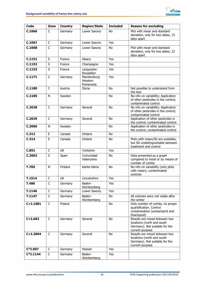
Background variability of honey bee colony size
www.efsa.europa.eu/publications 36 EFSA Supporting publication 2021:EN-6518
Code Zone Country Region/State Included Reason for excluding C.1066 C Germany Lower Saxony No Plot with mean and standard
deviation, only for two dates, 15 days apart
C.1067 C Germany Lower Saxony Yes
C.1068 C Germany Lower Saxony No Plot with mean and standard deviation, only for two dates, 22 days apart
C.1151 S France Alsace Yes
C.1152 S France Champagne Yes
C.1153 S France Languedoc-Roussillon
Yes
C.1171 C Germany Mecklenburg-Western Pomerania
Yes
C.1180 C Austria Styria No Not possible to understand from the text
C.1185 N Sweden
No No info on variability; Application of other pesticides in the control; contaminated control
C.2028 C Germany Several No No info on variability; Application of other pesticides in the control; contaminated control
C.2029 C Germany Several No Application of other pesticides in the control; contaminated control
C.2066 N Sweden
No Application of other pesticides in the control; contaminated control
C.312 E Canada Ontario No
C.314 E Canada Ontario No Plots with mean/SD are available, but SD undistinguishable between treatment and control
C.851 C UK Yorkshire Yes
C.2002 S Spain Comunidad Valenciana
No Data presented as a graph compared to initial or by means of number of combs
T.705 N Finland Kanta-Häme No No info on variability (only plots with mean); contaminated controls
T.1514 C UK Lincolnshire Yes
T.486 C Germany Baden-Württemberg
Yes
T.1146 C Germany Lower Saxony Yes
T.1147 C Germany Baden-Württemberg
No All colonies were not viable after the winter
C+I.1081 C Poland
No Only number of combs, no proper quantification. Control contamination (acetamiprid and thiacloprid)
C+I.602 C Germany Several No Results are mixed between two locations (north and south Germany). Not suitable for the current purpose
C+I.2004 C Germany Several No Results are mixed between two locations (north and south Germany). Not suitable for the current purpose
C*I.607 C Germany Hessen Yes
C*I.1144 C Germany Baden-Württemberg
Yes
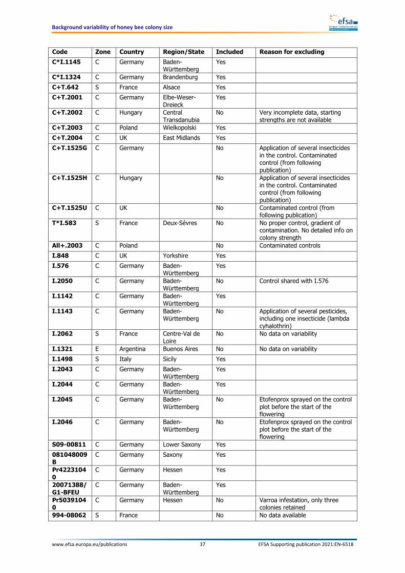
Background variability of honey bee colony size
www.efsa.europa.eu/publications 37 EFSA Supporting publication 2021:EN-6518
Code Zone Country Region/State Included Reason for excluding C*I.1145 C Germany Baden-
Württemberg Yes
C*I.1324 C Germany Brandenburg Yes
C+T.642 S France Alsace Yes
C+T.2001 C Germany Elbe-Weser-Dreieck
Yes
C+T.2002 C Hungary Central Transdanubia
No Very incomplete data, starting strengths are not available
C+T.2003 C Poland Wielkopolski Yes
C+T.2004 C UK East Midlands Yes
C+T.1525G C Germany
No Application of several insecticides in the control. Contaminated control (from following publication)
C+T.1525H C Hungary
No Application of several insecticides in the control. Contaminated control (from following publication)
C+T.1525U C UK
No Contaminated control (from following publication)
T*I.583 S France Deux-Sévres No No proper control, gradient of contamination. No detailed info on colony strength
All+.2003 C Poland
No Contaminated controls I.848 C UK Yorkshire Yes
I.576 C Germany Baden-Württemberg
Yes
I.2050 C Germany Baden-Württemberg
No Control shared with I.576
I.1142 C Germany Baden-Württemberg
Yes
I.1143 C Germany Baden-Württemberg
No Application of several pesticides, including one insecticide (lambda cyhalothrin)
I.2062 S France Centre-Val de Loire
No No data on variability
I.1321 E Argentina Buenos Aires No No data on variability I.1498 S Italy Sicily Yes
I.2043 C Germany Baden-Württemberg
Yes
I.2044 C Germany Baden-Württemberg
Yes
I.2045 C Germany Baden-Württemberg
No Etofenprox sprayed on the control plot before the start of the flowering
I.2046 C Germany Baden-Württemberg
No Etofenprox sprayed on the control plot before the start of the flowering
S09-00811 C Germany Lower Saxony Yes
081048009B
C Germany Saxony Yes
Pr42231040
C Germany Hessen Yes
20071388/G1-BFEU
C Germany Baden-Württemberg
Yes
Pr50391040
C Germany Hessen No Varroa infestation, only three colonies retained
994-08062 S France No No data available
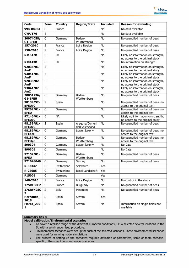
Background variability of honey bee colony size
www.efsa.europa.eu/publications 38 EFSA Supporting publication 2021:EN-6518
Code Zone Country Region/State Included Reason for excluding 994-08063 S France No No data available CYP/T76 E
No No data available
20074058/G1-BFEU
C Germany Baden-Württemberg
No No quantified number of bees
157-2010 S France Loire Region No No quantified number of bees 158-2010 S France Loire Region No No quantified number of bees RJ1547B C UK
No Likely no information on strength,
no access to the original study RJ0413B C UK
No No information on strength
92038/01-AmF
E
No Likely no information on strength, no access to the original study
93041/01 AmF
E
No Likely no information on strength, no access to the original study
92038/02 AmF
E
No Likely no information on strength, no access to the original study
93041/02 AmZ
E
No Likely no information on strength, no access to the original study
20051236/G1-BFEU
C Germany Baden-Württemberg
No No quantified number of bees
98139/S2-BFEU/C
S Spain
No No quantified number of bees, no access to the original test
99202/01-BFEU
C Germany
No No quantified number of bees, no access to the original test
97146/01-BFEU/C
E NA
No Likely no information on strength, no access to the original study
98139/S1-BFEU/C
S Spain Aragona/Comunidad valenciana
No No quantified number of bees
98189/01-BFCe/C
C Germany Lower Saxony No No quantified number of bees, no access to the original test
98189/01-BFEU/C
C Germany Baden-Württemberg
No No quantified number of bees, no access to the original test
890304 C Germany Lower Saxony No No Data 890305 C Germany No No Data 97152/01-BFEU
C Germany Baden-Württemberg
No No quantified number of bees
971048049 C Germany Saxony No No quantified number of bees R-33347 C Switzerland Solothurn Yes
R-28685 C Switzerland Basel-Landschaft Yes
P15005 C Germany
Yes
148-2010 S France Loire Region No No control in the study 17SRF08C2 S France Burgundy No No quantified number of bees 17SRFX08C3
S Italy Piedmont No No quantified number of bees
Hernando_2018
S Spain Several Yes
Flores_2021
S Spain Several No Information on single fields not available
Summary box 4 Model calibration/Environmental scenarios
• To cover a realistic range of the different European conditions, EFSA selected several locations in the EU with a semi-randomised procedure.
• Environmental scenarios were set up for each of the selected locations. These environmental scenarios were used for running model simulations.
• The process of setting up the scenarios required definition of parameters, some of them scenario-specific, others kept constant across scenarios.

Background variability of honey bee colony size
www.efsa.europa.eu/publications 39 EFSA Supporting publication 2021:EN-6518
• The definition of these parameters was performed via a calibration of the model for each scenario. • The calibration made use of literature data of different sorts. • Other model input parameters were left unchanged with respect to the default setting used by the
model’s authors. • Data from pesticide dossiers and from literature have been used to check the plausibility of the model
simulations.
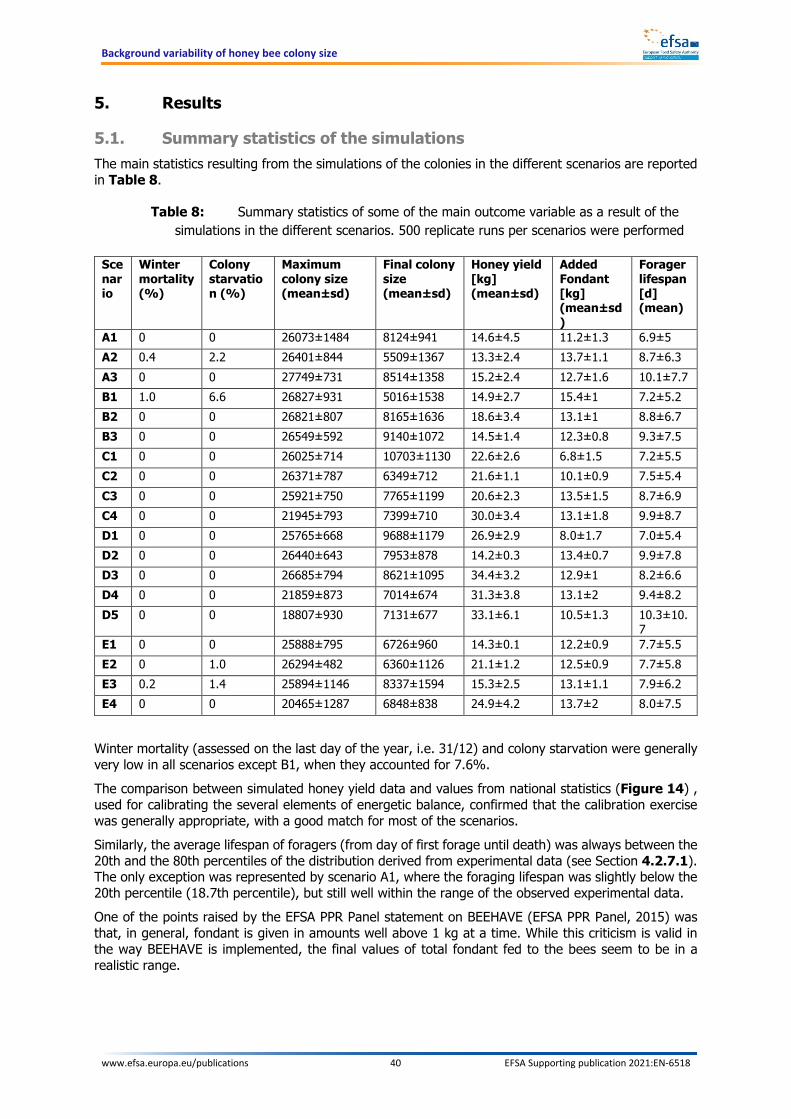
Background variability of honey bee colony size
www.efsa.europa.eu/publications 40 EFSA Supporting publication 2021:EN-6518
5. Results
5.1. Summary statistics of the simulations The main statistics resulting from the simulations of the colonies in the different scenarios are reported in Table 8.
Table 8: Summary statistics of some of the main outcome variable as a result of the simulations in the different scenarios. 500 replicate runs per scenarios were performed
Scenario
Winter mortality (%)
Colony starvation (%)
Maximum colony size (mean±sd)
Final colony size (mean±sd)
Honey yield [kg] (mean±sd)
Added Fondant [kg] (mean±sd)
Forager lifespan [d] (mean)
A1 0 0 26073±1484 8124±941 14.6±4.5 11.2±1.3 6.9±5 A2 0.4 2.2 26401±844 5509±1367 13.3±2.4 13.7±1.1 8.7±6.3 A3 0 0 27749±731 8514±1358 15.2±2.4 12.7±1.6 10.1±7.7 B1 1.0 6.6 26827±931 5016±1538 14.9±2.7 15.4±1 7.2±5.2 B2 0 0 26821±807 8165±1636 18.6±3.4 13.1±1 8.8±6.7 B3 0 0 26549±592 9140±1072 14.5±1.4 12.3±0.8 9.3±7.5 C1 0 0 26025±714 10703±1130 22.6±2.6 6.8±1.5 7.2±5.5 C2 0 0 26371±787 6349±712 21.6±1.1 10.1±0.9 7.5±5.4 C3 0 0 25921±750 7765±1199 20.6±2.3 13.5±1.5 8.7±6.9 C4 0 0 21945±793 7399±710 30.0±3.4 13.1±1.8 9.9±8.7 D1 0 0 25765±668 9688±1179 26.9±2.9 8.0±1.7 7.0±5.4 D2 0 0 26440±643 7953±878 14.2±0.3 13.4±0.7 9.9±7.8 D3 0 0 26685±794 8621±1095 34.4±3.2 12.9±1 8.2±6.6 D4 0 0 21859±873 7014±674 31.3±3.8 13.1±2 9.4±8.2 D5 0 0 18807±930 7131±677 33.1±6.1 10.5±1.3 10.3±10.
7 E1 0 0 25888±795 6726±960 14.3±0.1 12.2±0.9 7.7±5.5 E2 0 1.0 26294±482 6360±1126 21.1±1.2 12.5±0.9 7.7±5.8 E3 0.2 1.4 25894±1146 8337±1594 15.3±2.5 13.1±1.1 7.9±6.2 E4 0 0 20465±1287 6848±838 24.9±4.2 13.7±2 8.0±7.5
Winter mortality (assessed on the last day of the year, i.e. 31/12) and colony starvation were generally very low in all scenarios except B1, when they accounted for 7.6%. The comparison between simulated honey yield data and values from national statistics (Figure 14) , used for calibrating the several elements of energetic balance, confirmed that the calibration exercise was generally appropriate, with a good match for most of the scenarios. Similarly, the average lifespan of foragers (from day of first forage until death) was always between the 20th and the 80th percentiles of the distribution derived from experimental data (see Section 4.2.7.1). The only exception was represented by scenario A1, where the foraging lifespan was slightly below the 20th percentile (18.7th percentile), but still well within the range of the observed experimental data. One of the points raised by the EFSA PPR Panel statement on BEEHAVE (EFSA PPR Panel, 2015) was that, in general, fondant is given in amounts well above 1 kg at a time. While this criticism is valid in the way BEEHAVE is implemented, the final values of total fondant fed to the bees seem to be in a realistic range.
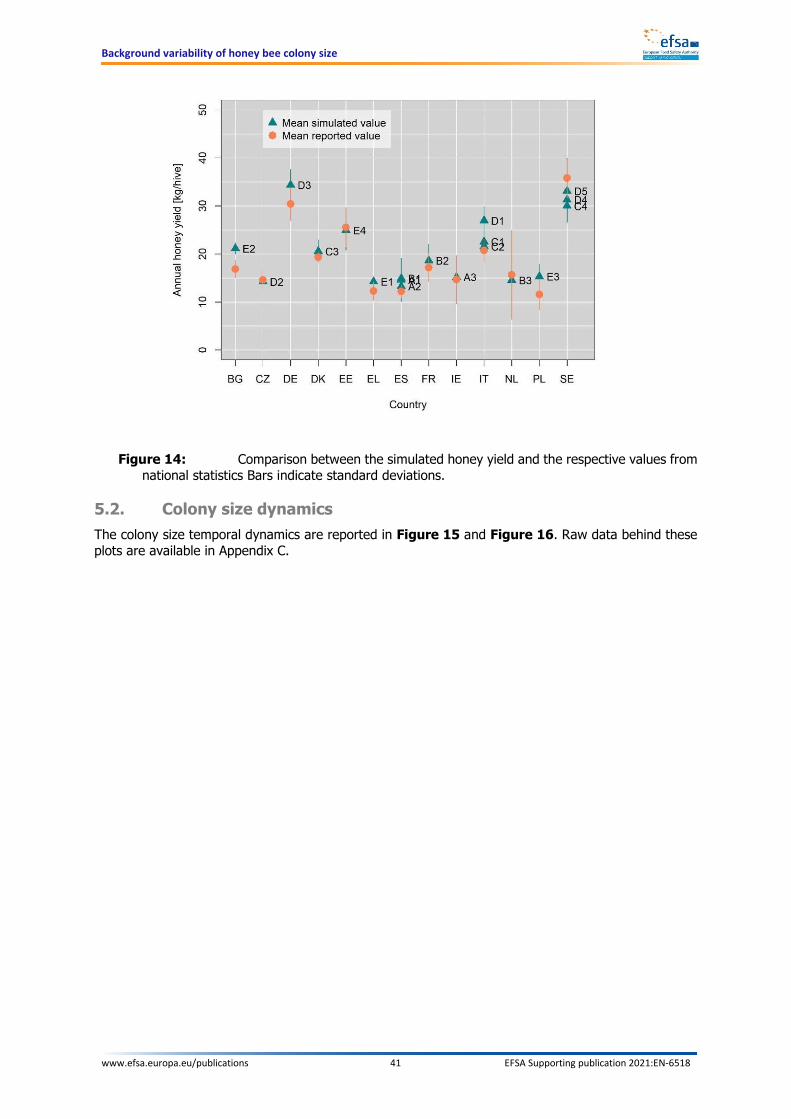
Background variability of honey bee colony size
www.efsa.europa.eu/publications 41 EFSA Supporting publication 2021:EN-6518
Figure 14: Comparison between the simulated honey yield and the respective values from national statistics Bars indicate standard deviations.
5.2. Colony size dynamics The colony size temporal dynamics are reported in Figure 15 and Figure 16. Raw data behind these plots are available in Appendix C.
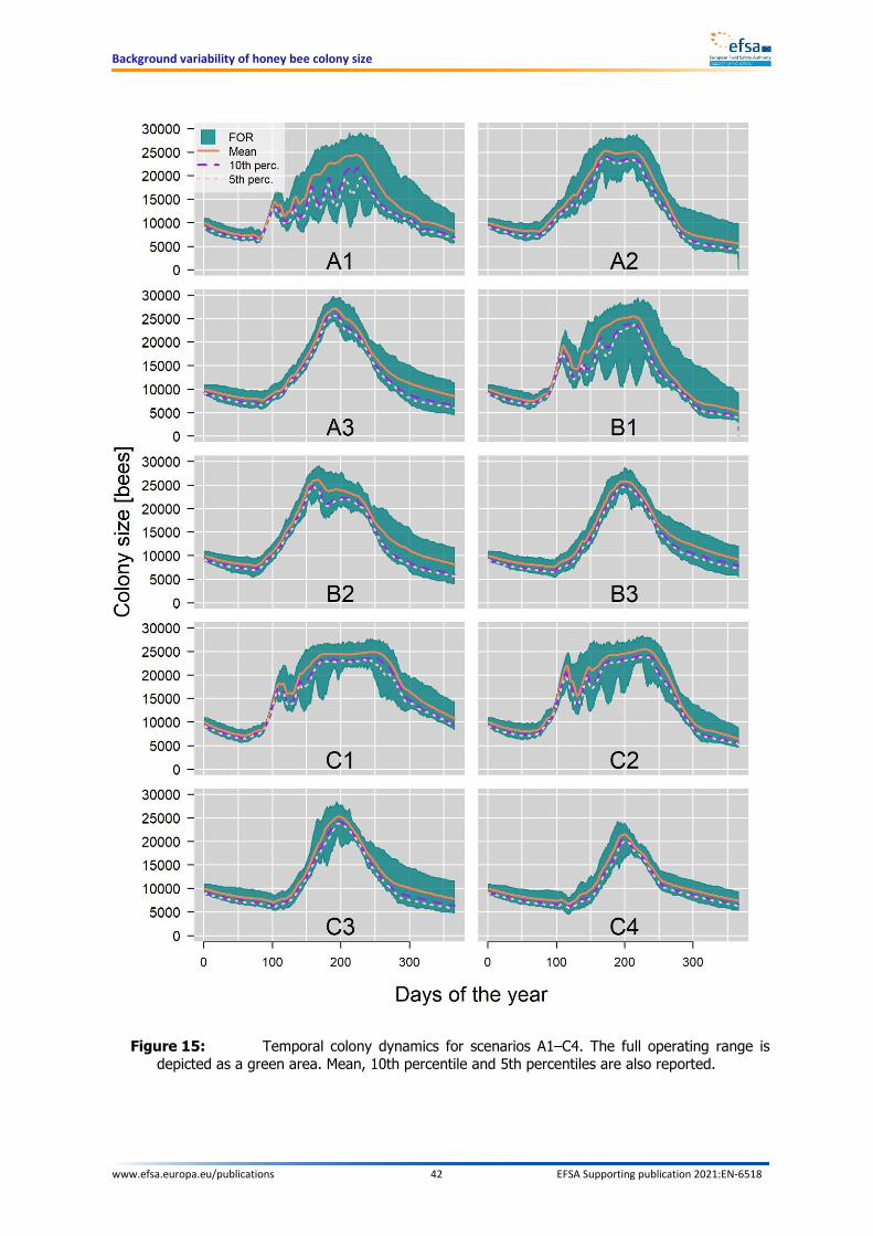
Background variability of honey bee colony size
www.efsa.europa.eu/publications 42 EFSA Supporting publication 2021:EN-6518
Figure 15: Temporal colony dynamics for scenarios A1–C4. The full operating range is depicted as a green area. Mean, 10th percentile and 5th percentiles are also reported.
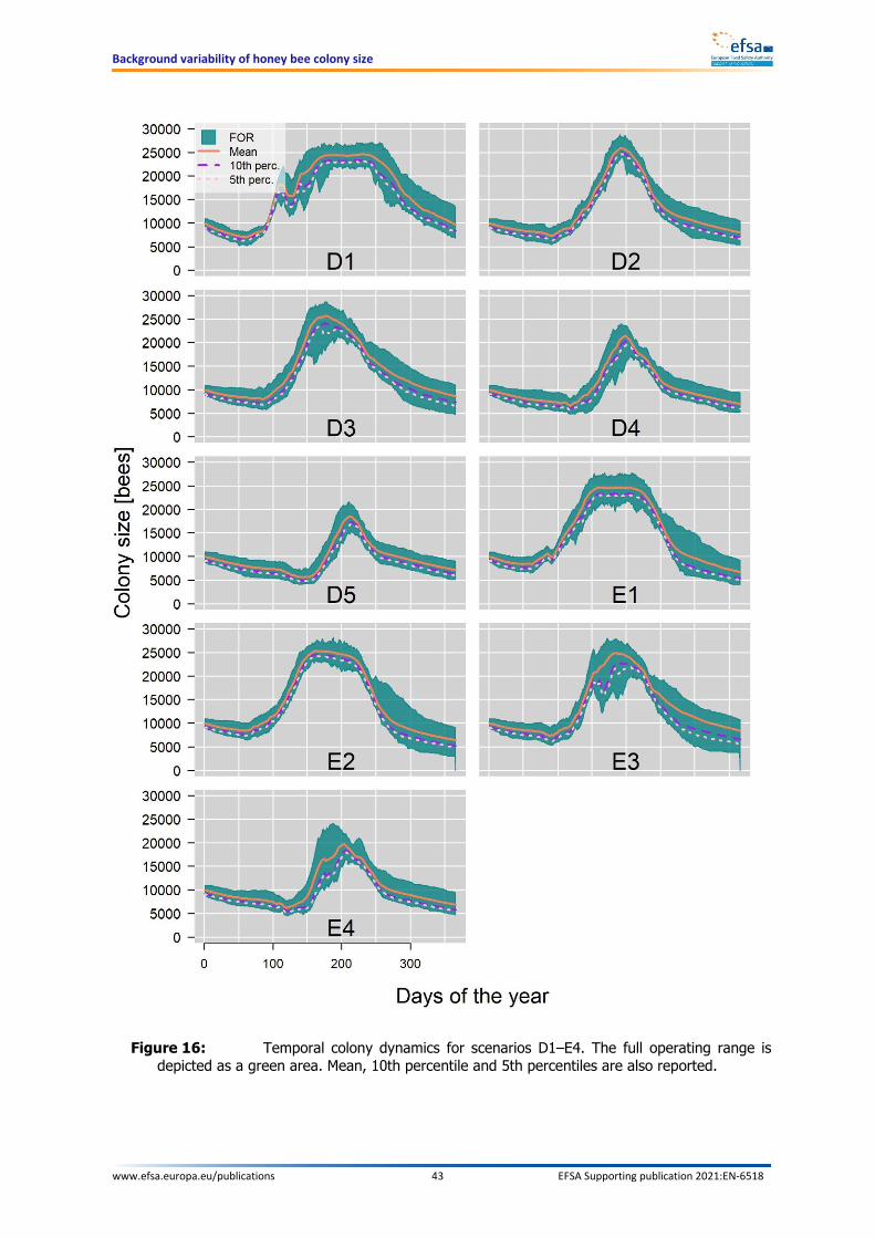
Background variability of honey bee colony size
www.efsa.europa.eu/publications 43 EFSA Supporting publication 2021:EN-6518
Figure 16: Temporal colony dynamics for scenarios D1–E4. The full operating range is depicted as a green area. Mean, 10th percentile and 5th percentiles are also reported.
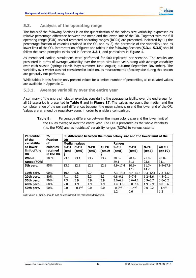
Background variability of honey bee colony size
www.efsa.europa.eu/publications 44 EFSA Supporting publication 2021:EN-6518
5.3. Analysis of the operating range The focus of the following Sections is on the quantification of the colony size variability, expressed as relative percentage difference between the mean and the lower limit of the OR. Together with the full operating range (FOR) several restricted operating ranges (RORs) are presented, indicated by: 1) the percentage fraction of colonies retained in the OR and by 2) the percentile of the variability used as lower limit of the OR. Interpretation of figures and tables in the following Sections (5.3.1–5.3.5) should follow the same principles explained in Section 3.3.1, and particularly in Figure 1.
As mentioned earlier, simulations were performed for 500 replicates per scenario. The results are presented in terms of average variability over the entire simulated year, along with average variability over each season (spring: March–May; summer: June–August; autumn: September–November). The variability over winter was not considered in isolation, as measurements of colony size during this season are generally not performed.
While tables in this Section only present values for a limited number of percentiles, all calculated values are available in Appendix C.
5.3.1. Average variability over the entire year
A summary of the entire simulation exercise, considering the average variability over the entire year for all 19 scenarios is presented in Table 9 and in Figure 17. The values represent the median and the complete range of the per cent differences between the mean colony size and the lower end of the OR. Values are arranged by regulatory zone, in order to enable a comparison.
Table 9: Percentage difference between the mean colony size and the lower limit of the OR as averaged over the entire year. The OR is presented as the whole variability (i.e. the FOR) and as ‘restricted’ variability ranges (RORs) to various extents
Percentile of the variability as lower limit of the OR
% fraction of colonies retained in the OR
% difference between the mean colony size and the lower limit of the OR Median values Ranges S-EU (n=8)
C-EU (n=6)
N-EU (n=5)
All EU (n=19)
S-EU (n=8)
C-EU (n=6)
N-EU (n=5)
All EU (n=19)
Whole range (FOR)
100% 23.6 23.1 23.2 23.2 20.0–29.1
20.4–31.1
21.0–23.6
20.0–31.1
5th perc. 95% 13.2 12.9 12.8 12.8 9.9–17.4 10.8–17.9
11.7–14.7
9.9–17.9
10th perc. 90% 10.6 9.6 9.7 9.7 7.3–13.3 8.7–13.2 9.3–12.1 7.3–13.3 20th perc. 80% 7.1 6.3 6.3 6.3 4.8–9.1 6–7.6 6.2–8.6 4.8–9.1 30th perc. 70% 4.3 3.9 3.9 3.9 3.0–6.2 3.6–4.1 3.9–5.7 3.0–6.2 40th perc. 60% 2.0 1.9 1.9 1.9 1.4–3.6 0.8–2.4 1.9–2.9 0.8–3.6 50th perc. 50% 0.0 −0.1(a) 0.0 0.0 −0.2(a)–
1.2 −1.4(a)–0.6
0.0–0.2 −1.4(a)–1.2
(a): Value > mean, should not be considered for threshold derivation.

Background variability of honey bee colony size
www.efsa.europa.eu/publications 45 EFSA Supporting publication 2021:EN-6518
Figure 17: Relationship between the difference mean colony size – lower limit of the OR and the percentile selected as lower limit of the OR. Reported values are averages over the entire simulated year (1st January-31st December). Median (lines) and ranges (areas) for each regulatory zone are illustrated.
5.3.2. Average variability over spring
A summary of the entire simulation exercise, considering the average variability over spring for all 19 scenarios is presented in Table 10 and in Figure 18. The values represent the median and the complete range of the per cent differences between the mean colony size and the lower end of the OR. Values are arranged by regulatory zone, in order to enable a comparison.
Table 10: Percentage difference between the mean colony size and the lower limit of the OR as averaged over spring. The OR is presented as the whole variability (i.e. the FOR) and as ‘restricted’ variability ranges (RORs) to various extents
Percentile of the variability as lower limit of the OR
% fraction of colonies retained in the OR
% difference between the mean colony size and the lower limit of the OR Median values Ranges S-EU (n=8)
C-EU (n=6)
N-EU (n=5)
All EU (n=19)
S-EU (n=8)
C-EU (n=6)
N-EU (n=5)
All EU (n=19)
Whole range (FOR)
100% 20.2 21.6 25.4 20.9 17.4–21.7
17.9–24.9
22.1–28.2
17.4–28.2
5th perc. 95% 9.8 11.8 14.3 11.5 9.1–12.4 9.2–14.1 12.6–14.8
9.1–14.8
10th perc. 90% 7.4 9.3 11.0 9.0 7.0–9.7 7.1–11.1 9.9–12.0 7.0–12 20th perc. 80% 4.8 6.1 7.1 5.9 4.4–6.1 4.7–7.3 6.2–8.4 4.4–8.4

Background variability of honey bee colony size
www.efsa.europa.eu/publications 46 EFSA Supporting publication 2021:EN-6518
30th perc. 70% 2.9 3.8 4.4 3.6 2.6–3.7 2.8–4.4 3.6–5.4 2.6–5.4 40th perc. 60% 1.3 1.8 2.1 1.6 1.1–1.8 1.3–2.0 1.5–2.6 1.1–2.6 50th perc. 50% −0.2(a) −0.1(a) −0.2(a) −0.2(a) −0.4(a)–
0.1 −0.3(a)–0.0
−0.3(a)–0.1
−0.4(a)–0.1
(a): Value > mean, should not be considered for threshold derivation.
Figure 18: Relationship between the difference mean colony size – lower limit of the OR and the percentile selected as lower limit of the OR. Reported values are averages over spring (March-May). Median (lines) and ranges (areas) for each regulatory zone are illustrated.
5.3.3. Average variability over summer
A summary of the entire simulation exercise, considering the average variability over summer for all 19 scenarios is presented in Table 11 and in Figure 19. The values represent the median and the complete range of the per cent differences between the mean colony size and the lower end of the OR. Values are arranged by regulatory zone, in order to enable a comparison.
Table 11: Percentage difference between the mean colony size and the lower limit of the OR as averaged over summer. The OR is presented as the whole variability (i.e. the FOR) and as ‘restricted’ variability ranges (RORs) to various extents
Percentile of the variability as lower limit of the OR
% fraction of colonies retained in the OR
% difference between the mean colony size and the lower limit of the OR Median values Ranges S-EU (n=8)
C-EU (n=6)
N-EU (n=5)
All EU (n=19)
S-EU (n=8)
C-EU (n=6)
N-EU (n=5)
All EU (n=19)
Whole range (FOR)
100% 20.3 13.2 22.1 18.6 14.5–47.1
10.4–24.2
18.4–24.7
10.4–47.1
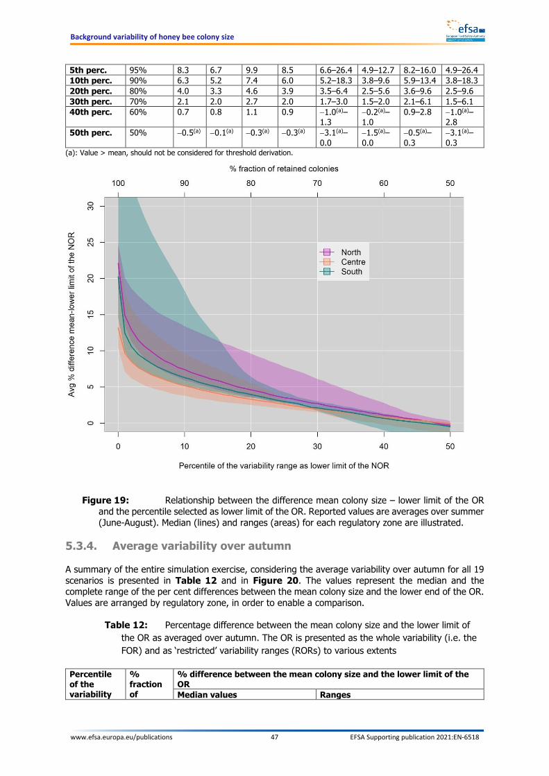
Background variability of honey bee colony size
www.efsa.europa.eu/publications 47 EFSA Supporting publication 2021:EN-6518
5th perc. 95% 8.3 6.7 9.9 8.5 6.6–26.4 4.9–12.7 8.2–16.0 4.9–26.4 10th perc. 90% 6.3 5.2 7.4 6.0 5.2–18.3 3.8–9.6 5.9–13.4 3.8–18.3 20th perc. 80% 4.0 3.3 4.6 3.9 3.5–6.4 2.5–5.6 3.6–9.6 2.5–9.6 30th perc. 70% 2.1 2.0 2.7 2.0 1.7–3.0 1.5–2.0 2.1–6.1 1.5–6.1 40th perc. 60% 0.7 0.8 1.1 0.9 −1.0(a)–
1.3 −0.2(a)–1.0
0.9–2.8 −1.0(a)–2.8
50th perc. 50% −0.5(a) −0.1(a) −0.3(a) −0.3(a) −3.1(a)–0.0
−1.5(a)–0.0
−0.5(a)–0.3
−3.1(a)–0.3
(a): Value > mean, should not be considered for threshold derivation.
Figure 19: Relationship between the difference mean colony size – lower limit of the OR and the percentile selected as lower limit of the OR. Reported values are averages over summer (June-August). Median (lines) and ranges (areas) for each regulatory zone are illustrated.
5.3.4. Average variability over autumn
A summary of the entire simulation exercise, considering the average variability over autumn for all 19 scenarios is presented in Table 12 and in Figure 20. The values represent the median and the complete range of the per cent differences between the mean colony size and the lower end of the OR. Values are arranged by regulatory zone, in order to enable a comparison.
Table 12: Percentage difference between the mean colony size and the lower limit of the OR as averaged over autumn. The OR is presented as the whole variability (i.e. the FOR) and as ‘restricted’ variability ranges (RORs) to various extents
Percentile of the variability
% fraction of
% difference between the mean colony size and the lower limit of the OR Median values Ranges

Background variability of honey bee colony size
www.efsa.europa.eu/publications 48 EFSA Supporting publication 2021:EN-6518
as lower limit of the OR
colonies retained in the OR
S-EU (n=8)
C-EU (n=6)
N-EU (n=5)
All EU (n=19)
S-EU (n=8)
C-EU (n=6)
N-EU (n=5)
All EU (n=19)
Whole range (FOR)
100% 27.7 31.3 22.1 28.6 24.2–33.6
26.2–44.5
19.1–30.2
19.1–44.5
5th perc. 95% 17.9 17.6 12.1 16.6 12.6–23.8
13.8–27.2
11–20.2 11–27.2
10th perc. 90% 15.0 13.4 9.3 12.3 8.2–20.8 11.2–19.4
9.1–14.1 8.2–20.8
20th perc. 80% 10.5 9.0 6.4 8.9 5.2–16.9 7.4–10.3 5.7–9.3 5.2–16.9 30th perc. 70% 7.0 5.1 4.4 5.3 3.3–12.7 4.4–7.1 3.4–6.2 3.3–12.7 40th perc. 60% 3.9 2.5 2.5 2.9 1.5–8.1 0.3–4.6 1.5–3.7 0.3–8.1 50th perc. 50% 0.8 0.2 0.5 0.5 −0.2(a)–
3.1 −2.8(a)–2.1
−0.1(a)–1.1
−2.8(a)–3.1
(a): Value > mean, should not be considered for threshold derivation.
Figure 20: Relationship between the difference mean colony size – lower limit of the OR and the percentile selected as lower limit of the OR. Reported values are averages over autumn (September-November). Median (lines) and ranges (areas) for each regulatory zone are illustrated.
5.3.5. Comparison between seasons
Since variability changed in the course of the simulated year, this Section enables a comparison between the variability averaged over the entire simulated year and over each single season (i.e. spring, summer, autumn). Values reported in Table 13 and in Figure 21 refer to median and ranges for the whole EU (based on all 19 simulated scenarios).
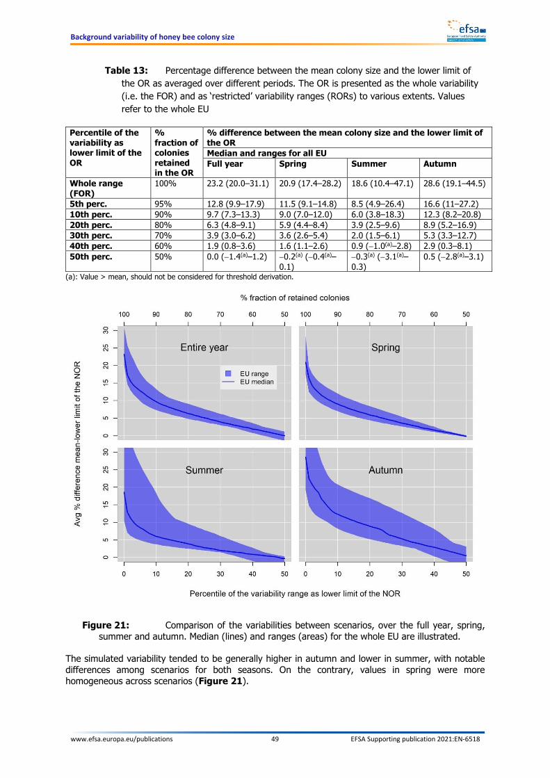
Background variability of honey bee colony size
www.efsa.europa.eu/publications 49 EFSA Supporting publication 2021:EN-6518
Table 13: Percentage difference between the mean colony size and the lower limit of the OR as averaged over different periods. The OR is presented as the whole variability (i.e. the FOR) and as ‘restricted’ variability ranges (RORs) to various extents. Values refer to the whole EU
Percentile of the variability as lower limit of the OR
% fraction of colonies retained in the OR
% difference between the mean colony size and the lower limit of the OR Median and ranges for all EU Full year Spring Summer Autumn
Whole range (FOR)
100% 23.2 (20.0–31.1) 20.9 (17.4–28.2) 18.6 (10.4–47.1) 28.6 (19.1–44.5)
5th perc. 95% 12.8 (9.9–17.9) 11.5 (9.1–14.8) 8.5 (4.9–26.4) 16.6 (11–27.2) 10th perc. 90% 9.7 (7.3–13.3) 9.0 (7.0–12.0) 6.0 (3.8–18.3) 12.3 (8.2–20.8) 20th perc. 80% 6.3 (4.8–9.1) 5.9 (4.4–8.4) 3.9 (2.5–9.6) 8.9 (5.2–16.9) 30th perc. 70% 3.9 (3.0–6.2) 3.6 (2.6–5.4) 2.0 (1.5–6.1) 5.3 (3.3–12.7) 40th perc. 60% 1.9 (0.8–3.6) 1.6 (1.1–2.6) 0.9 (−1.0(a)–2.8) 2.9 (0.3–8.1) 50th perc. 50% 0.0 (−1.4(a)–1.2) −0.2(a) (−0.4(a)–
0.1) −0.3(a) (−3.1(a)–0.3)
0.5 (−2.8(a)–3.1)
(a): Value > mean, should not be considered for threshold derivation.
Figure 21: Comparison of the variabilities between scenarios, over the full year, spring, summer and autumn. Median (lines) and ranges (areas) for the whole EU are illustrated.
The simulated variability tended to be generally higher in autumn and lower in summer, with notable differences among scenarios for both seasons. On the contrary, values in spring were more homogeneous across scenarios (Figure 21).
Background variability of honey bee colony size
www.efsa.europa.eu/publications 50 EFSA Supporting publication 2021:EN-6518
While the simulations revealed no striking differences between the three regulatory zones, generally the variability tended to be slightly higher in the northern scenarios during spring (see Figure 18). In summer the variability was rather high in some of the southern scenarios (mainly B1), but not in the others (Figure 19). A similar pattern was observed for the central zone in autumn (Figure 20). The variability peaked in spring in the northern scenarios, in autumn in the central scenarios, while it was more heterogenous in the southern scenarios.
5.4. Interpretation of the results The results presented in Section 5.3 cover the simulated variabilities of 500 ‘control’ colony replicates for the whole year and in spring, summer and autumn. The whole range of the simulated variabilities (FOR) includes the ‘stronger’ control colonies i.e. the colonies at the top of the range and the ‘weaker’ ones, i.e. colonies at the bottom of the range. The mean of the range represents the mean size of the 500 ‘control’ colony replicates.
The colonies showing sizes lower than the mean are the relevant ones for approach #2. This is because the attribute to protect is the colony strength (=colony size). Detrimental effects in the reference tier (i.e. field studies) are expected to cause the mean size of the treated colonies to be reduced compared to the mean size of the controls. Hence, the part of the range which is below the mean is relevant for defining the magnitude of the effect. Identifying a threshold for the magnitude of acceptable effects in the range above the mean would mean that the effect is acceptable only if it causes the mean colony size in the treatment to be higher than the mean colony size in the control, which is nonsensical in a risk assessment context. The explicit consideration of the honey bee colony size background variability clarifies the extent to which colonies unexposed to pesticides can deviate from each other, and, most importantly, how much they can deviate from their mean size. The results presented in all tables and figures in Section 5.3 show the percentage of colony size ‘reduction’ which correspond to a fraction of colonies retained in the OR. These percentages of size ‘reduction’ are calculated as difference between the mean colony size and the lower limit of the OR. The results can also be read as selecting a ROR by defining a given percentile of the colony size variability distribution as the lower limit of the ROR. Retaining in the ROR 95% of the total colony size variability (lower limit at the 5th percentile of the FOR) or the 90% (lower limit at the 10th percentile) is equivalent to excluding, for the definition of the magnitude of acceptable effect, the 5% or the 10% weakest colonies. If these restrictions are selected to determine the threshold of acceptable effects when this threshold is used to evaluate a pesticide, it means that the mean colony size of the exposed colonies in the treatment group should always be larger than all the 5% or 10% most vulnerable colonies in the control. In other words, the treatment colonies must, on average, perform better than the 5–10 % weakest control colonies, in order to meet the SPG.
It has to be noted that the exclusion of only 5% of the colonies would significantly reduce the range of the background variability, and thus the threshold for acceptable effect on colony size reduction. By taking as example the lowest variability figures over the entire year for the whole EU (see Table 9 and Figure 17), the threshold would be 9.9%, instead of 20.0% without restriction. When 10% of the colonies are excluded, the range of the variability is less reduced, and the threshold would be 7.3% and so on. It is clear that, the narrower the range, the smaller – and thus more conservative – is the magnitude of the acceptable effect.
Summary box 5 Percentages of colony size reduction Threshold(s) of acceptable effects represent percentage(s) of mean colony size reduction. A threshold of X% (for example 20.0%, or 9.9%, or 7.3%, or 4.8% etc.) indicates that the mean size of colonies exposed to a pesticide (i.e. the treatment) should not be lower by more than X% (for example 20.0%, or 9.9% or 7.3%, 4.8% etc.) compared to the mean size of the colony in the control.
5.4.1. Recommendations on how to interpret the results
Background variability of honey bee colony size
www.efsa.europa.eu/publications 51 EFSA Supporting publication 2021:EN-6518
The background variability and the analysis of its distribution should support the selection of a threshold of acceptable effects. Further considerations are necessary on how to use this analysis for determining the threshold of acceptable effect. In particular, the following is recommended:
• Colony size reductions of one-third were already identified (see Section 3.3) as a threshold potentially leading to the impairment of the colony viability. The results of the simulations show that, in some circumstances (see Table 13), the distance between the mean size and the lower limit of the OR (either FOR or ROR) is close to or even higher than one-third (i.e.33%).
• By using a more restricted OR the weaker colonies are left out, and therefore the threshold of acceptable effects is more conservative. The results of the simulations show that only a few colonies are substantially weaker than the average colony size, even when no exposure to a pesticide is considered. By restricting the OR for threshold derivation, these weaker colonies will not be used as a reference for acceptable effects, resulting in a general higher protection level.
• A restriction to the 50th percentile of the variability should not be considered for the threshold derivation, since this would mean that, in many cases, only beneficial effects of pesticides are considered acceptable i.e. increase in colony size compared to the control. This is nonsensical from a risk assessment point of view, as pesticide exposure is not expected to produce beneficial effects.
• The threshold of acceptable effect should be implementable in the reference tier; since, currently, the reference tier is represented by the field studies, it should be realistically measurable in those studies (see Section 7).
More considerations about variability distributions in risk assessment and selection of relevant thresholds can be found in Appendix D. Additional considerations for selecting the OR restrictions/or the threshold of acceptable effect can be found in Section 8.
5.5. Plausibility of the model simulations As previously mentioned (Section 4.3), colony size data have been extracted from control colonies of 33 field studies. These data were not used in the calibration phase, so they are fully independent from the model simulations. Almost all field studies were conducted in the central zone. Six studies were formally conducted in the southern zone, but the location of three of them (Alsace and Champagne) is probably more representative of central European conditions. None of the studies was carried out in the northern zone. Starting from those, the variability in size between replicate colonies at every measurement time point has been quantified as coefficient of variation (CV), i.e. the standard deviation divided by the mean.
Overall, these experimental data show two very clear trends: 1) The variability of the CV among studies is extremely high. This can be considered as the
‘variability of the variabilities’ and shows that, while in some studies the colony size was relatively similar among replicates, in some other studies this was not the case.
2) Overall, the CV tends to increase with time (see Figure 22). This is likely to happen because, at the beginning of field studies, colony sizes are often purposefully equalised, in order to have more meaningful comparisons.
The present modelling analysis simulates colony dynamics for one year. Hence, only data related to the first year of each study were retained. Furthermore, studies presenting a CV > 0.3 at the start of the test period were excluded, as this rather high variability was already there before the colonies were placed in a common environment. Having too high variability (i.e. CV > 0.3) would have resulted in a non-plausible comparison with the model results which started with a CV ≈ 0.1 at the beginning of the simulation. This led to the exclusion of 91 data points, while 230 were kept for the analysis. The comparison of the variability from field studies and from the simulated scenarios is presented in Figure 22. The variability across all the available control replicates from the 33 field studies is
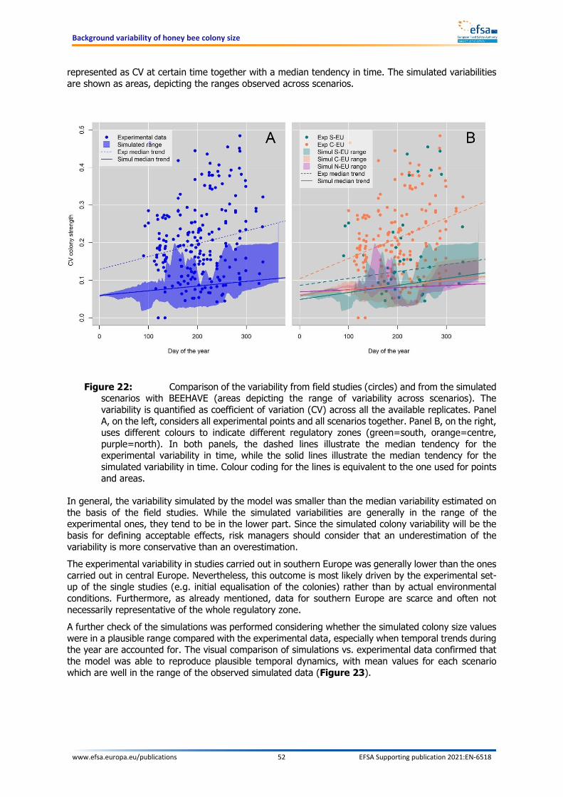
Background variability of honey bee colony size
www.efsa.europa.eu/publications 52 EFSA Supporting publication 2021:EN-6518
represented as CV at certain time together with a median tendency in time. The simulated variabilities are shown as areas, depicting the ranges observed across scenarios.
Figure 22: Comparison of the variability from field studies (circles) and from the simulated scenarios with BEEHAVE (areas depicting the range of variability across scenarios). The variability is quantified as coefficient of variation (CV) across all the available replicates. Panel A, on the left, considers all experimental points and all scenarios together. Panel B, on the right, uses different colours to indicate different regulatory zones (green=south, orange=centre, purple=north). In both panels, the dashed lines illustrate the median tendency for the experimental variability in time, while the solid lines illustrate the median tendency for the simulated variability in time. Colour coding for the lines is equivalent to the one used for points and areas.
In general, the variability simulated by the model was smaller than the median variability estimated on the basis of the field studies. While the simulated variabilities are generally in the range of the experimental ones, they tend to be in the lower part. Since the simulated colony variability will be the basis for defining acceptable effects, risk managers should consider that an underestimation of the variability is more conservative than an overestimation. The experimental variability in studies carried out in southern Europe was generally lower than the ones carried out in central Europe. Nevertheless, this outcome is most likely driven by the experimental set-up of the single studies (e.g. initial equalisation of the colonies) rather than by actual environmental conditions. Furthermore, as already mentioned, data for southern Europe are scarce and often not necessarily representative of the whole regulatory zone. A further check of the simulations was performed considering whether the simulated colony size values were in a plausible range compared with the experimental data, especially when temporal trends during the year are accounted for. The visual comparison of simulations vs. experimental data confirmed that the model was able to reproduce plausible temporal dynamics, with mean values for each scenario which are well in the range of the observed simulated data (Figure 23).
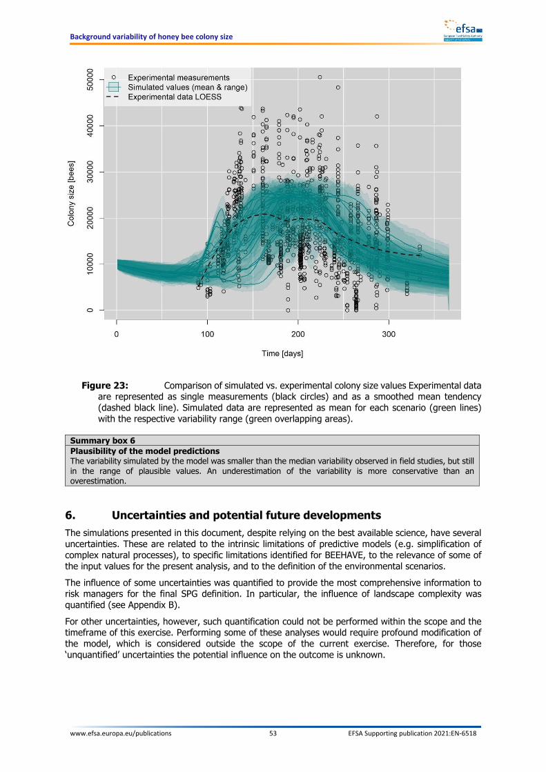
Background variability of honey bee colony size
www.efsa.europa.eu/publications 53 EFSA Supporting publication 2021:EN-6518
Figure 23: Comparison of simulated vs. experimental colony size values Experimental data are represented as single measurements (black circles) and as a smoothed mean tendency (dashed black line). Simulated data are represented as mean for each scenario (green lines) with the respective variability range (green overlapping areas).
Summary box 6 Plausibility of the model predictions The variability simulated by the model was smaller than the median variability observed in field studies, but still in the range of plausible values. An underestimation of the variability is more conservative than an overestimation.
6. Uncertainties and potential future developments The simulations presented in this document, despite relying on the best available science, have several uncertainties. These are related to the intrinsic limitations of predictive models (e.g. simplification of complex natural processes), to specific limitations identified for BEEHAVE, to the relevance of some of the input values for the present analysis, and to the definition of the environmental scenarios. The influence of some uncertainties was quantified to provide the most comprehensive information to risk managers for the final SPG definition. In particular, the influence of landscape complexity was quantified (see Appendix B).
For other uncertainties, however, such quantification could not be performed within the scope and the timeframe of this exercise. Performing some of these analyses would require profound modification of the model, which is considered outside the scope of the current exercise. Therefore, for those ‘unquantified’ uncertainties the potential influence on the outcome is unknown.
Background variability of honey bee colony size
www.efsa.europa.eu/publications 54 EFSA Supporting publication 2021:EN-6518
6.1. Limitations of BEEHAVE identified in EFSA PPR Panel (2015) Among the limitations identified in EFSA PPR Panel (2015), the main one relates to the use of BEEHAVE in the regulatory risk assessment of pesticides. Considering the use of BEEHAVE (see also Section 4.1) in the present document, this limitation is deemed neither relevant nor applicable for this analysis. For example, the lack of a pesticide module is unimportant when the simulations are run to address colony dynamics where pesticide exposure is absent. Some drawbacks identified by the EFSA PPR Panel (2015) were either fixed or at least mitigated in the present analysis. Primarily, the lack of a sufficient number of environmental scenarios able to represent conditions in the three EU regulatory zones was tackled by developing 19 scenarios distributed across the entire EU. Some parameters considered not validated by the PPR Panel were calibrated by using relevant experimental data. For example, the amount of nectar in the food patches was calibrated in the different scenarios to match official figures of honey yield per colony in the different EU countries. Forager mortality rate was calibrated by making use of the outcome of a systematic literature review on the topic. However, other limitations identified by the EFSA PPR Panel (2015) are still relevant and have the potential to influence the outcome of the analysis presented in Section 5. Specifically, some of the default parameters (e.g. food consumption, flight velocity, maximum egg laying, etc.) used in the model are not fully supported by empirical data.
6.2. Limitations of BEEHAVE identified in the present analysis Additional limitations intrinsic to BEEHAVE for the specific purpose of the simulations have been identified while performing this analysis. The first aspect regards how foraging intensity is simulated. In the real world, food needs and environmental conditions are both important drivers for the number of bees leaving the hive to forage (i.e. foraging intensity). However, in BEEHAVE, environmental conditions (i.e. temperature and sunlight hours/irradiance) do not determine foraging intensity but are used only to quantify the daily foraging time-window. The influence of this on colony size variability is, at the moment, not quantifiable without introducing significant modifications to BEEHAVE. Perhaps the most relevant aspect is that the variability between replicate runs in BEEHAVE is determined by stochastic (=random) processes described by probability distributions. Stochastic is defined as an event determined by random processes. This means that some of the parameters of the model are not fixed, but assume different values at every run, under equal conditions, on the basis of probability distributions. The variation in the value(s) of these parameters determines the variability in the model output. In BEEHAVE, stochasticity concerns two main processes – mortality and forager activity:
• Mortality of single bees is random in BEEHAVE. However, this occurs with different pre-defined probabilities. In-hive bees die with different daily probabilities for each life stage (eggs, larvae, pupae, adult, all different for drones and workers). Scarcity of nurse bees or lack of pollen may influence brood mortality as well, but these aspects are not random and they are added on top of the stochastic mortality. Foragers have a certain probability of dying for every second spent foraging, so that longer foraging times entail higher mortality probability.
• Forager activities have several random aspects: the choice of a bee to start or stop its foraging activity, the choice to forage pollen and/or nectar are all determined by probabilities, which are in turn driven by the hive needs. The detection of a flower patch occurs with a certain probability, driven in our landscape complexity analysis (see Appendix B) by the patch size and its distance from the hive.
• Other stochastic parameters exist for the Varroa module of BEEHAVE, which was not used in the present simulations (see Section 6.4).
While the stochastic approach per se can be considered reasonable, there seems to be a lack of explicit justification for the probability distributions chosen in the model. Also in this case, the influence of this aspect on the colony size variability was not quantified.

Background variability of honey bee colony size
www.efsa.europa.eu/publications 55 EFSA Supporting publication 2021:EN-6518
6.3. Relevance of input values for the present analysis The objective of the present work is to illustrate an analysis of colony strength background variability for a perfect control in the reference tier of the risk assessment (i.e. a field study). This entails two main aspects:
• The conditions surrounding the simulated colonies should resemble the typical habitat for honey bees in agricultural areas, where field studies are carried out.
• A complete lack of exposure to pesticides, since this should serve as a benchmark for effects of pesticides.
In the real world, agricultural areas are unlikely to be completely pesticide-free, while this could be the case for some non-agricultural areas (e.g. mountains, forests). However, habitats in these areas are completely different in terms of structure, food availability, competition and predation compared to agricultural areas. Some aspects related to the habitat structures (i.e. food availability etc.) can be dealt with directly in the model by adjusting some of the scenario parameters. Limitations in the simulated habitat structure, also in terms of food availability, are discussed in detail in the next Section. BEEHAVE makes use of input values, i.e. not calculated by the model but imposed by the user, describing the biology of bees. These encompass aspects related to reproduction and development (e.g. max egg laying, length of each life stage, etc.), foraging (e.g. flight velocity, maximum amount of pollen and nectar carried by one bee, time needed for food collection and unloading, etc.), food consumption, mortality (probability of death for in-hive for adult and brood, foraging mortality etc.), and brood care (e.g. maximum amount of brood nurse bees can care for).
Some of these input values are known to be robustly estimated: for example, the developmental time of eggs, larvae and pupae are known to be the same in agricultural areas and in the laboratory. However, at least in principle, each one of the aforementioned biology-related input values can be influenced by both the habitat type and exposure to pesticides (or to any other hazardous chemical). Hence, the conditions of the experimental studies used to derive these input values are relevant.
For mortality of adult bees, the input values were calibrated on the basis of the data included in the recent review of the evidence of bee background mortality (EFSA et al., 2020b). For that review, data from both agricultural and non-agricultural areas were considered, but studies presenting evidence that bees were exposed to insecticides were excluded. The maximum egg-laying rate over time was adjusted for each scenario considering daily temperature and sunlight hours. However, the starting point was the egg-laying rate used by Becher et al. (2014), which was based on a previous model (Schmickl and Crailsheim, 2007). This model made use of observations from Ebert (1922). While it was not possible to ascertain whether these observations were performed in agricultural areas, considering the time of publication it is safe to assume that bees were not exposed to synthetic pesticides in the original study. The origin of all other input values had not been investigated in depth, but many were derived from rather old studies, whose level of detail does not allow to ascertain whether they were carried out in agricultural areas or not.
6.4. Uncertainties in the scenario definition The main limitations of the definition of the scenarios is related to the lack of suitable ready-to-use data. While some aspects were satisfactorily addressed (i.e. climatic conditions, average mortality rate of foragers) by using available data, others relied on indirect estimations, which entailed relevant uncertainties in the final outcome. The main source of uncertainty in this sense is related to food (i.e. pollen and nectar) availability. While some data are available in the literature (Baude et al., 2016; Becher et al., 2016; Agatz et al., 2019; Timberlake et al., 2019) these are too scattered to establish reliable food levels in all the scenarios. Hence, nectar levels in the landscape were indirectly calibrated by aligning as much as possible the simulated amount of harvested honey with available data on average honey yield (Chauzat et al., 2013; FAOSTAT, online; European Commission, 2020 online). However, these available data are averages at

Background variability of honey bee colony size
www.efsa.europa.eu/publications 56 EFSA Supporting publication 2021:EN-6518
country level and might not be representative for the specific selected locations. Hatjina et al. (2014) reported site-specific data for 2 years and several European locations, but: 1) these locations did not overlap with the scenario locations used in this report, and 2) extrapolation was hampered by the lack of a clear geographical pattern. Realistic pollen levels were also indirectly estimated by using experimental nectar:pollen ratios available in the literature (Becher et al., 2016; Agatz et al., 2019). The scenario calibration exercise also considered data on maximum colony size. Hatjina et al. (2014) reported information for a larger area, but no consistent geographical pattern could be identified in the 2 years of the study. Finally, the results from the beekeeper survey proved to be of limited reliability (as already noted in EFSA et al., 2020b) with a very limited coverage of southern countries and several unrealistically high values indicated (e.g. >1 million bees per hive). Overall, the available information on average colony size could only be used qualitatively to check that plausible values were simulated, but not to calibrate differences between scenarios. The influence of adopting a simplified landscape description was analysed systematically (see Appendix B). The results of this analysis show that landscape complexity has the potential to increase colony strength variability, mainly via increasing food inflow variability. Consequently, the use of a simplified landscape context, as in the model standard settings, may have resulted in an underestimation of the variability. BEEHAVE offers the possibility to simulate the effects of Varroa mite and two associated viruses: deformed wing virus (DWV) and acute paralysis virus (APV). However, in the present analysis, it was decided not to include a simulation of pathogen infections related to Varroa. This decision was taken mainly for two reasons:
• Several concerns were raised by the EFSA PPR Panel in their 2015 statement about this module. The PPR Panel concluded that the impact of Varroa/viruses on colony survival was underestimated, and that the simulated treatment against Varroa might be too effective to be realistic.
• The activation of the Varroa module in BEEHAVE entails the selection of many additional parameters (e.g. number of initial mites, initial infection rate, choice between different mite reproductive models, choice between the simulated viruses, etc.), which could be different for each scenario. In the absence of relevant data on these parameters, it was considered that the uncertainty introduced by simulating Varroa/viruses may potentially exceed the uncertainty of simulations that explicitly ignore this aspect.
Exploratory simulations were nevertheless performed. They revealed that the activation of the Varroa module is likely to increase the colony size variability between replicates. Hence, risk managers should be aware that the choice of not including Varroa/virus in the simulation may have resulted in an underestimation of the variability. An underestimation of the variability is more conservative than an overestimation.
Summary box 7 Uncertainties/limitation of BEEHAVE
• Any model entails a simplification of complex natural processes.
• The lack of a pesticide module is unimportant when the simulations are run to address colony dynamics where pesticide exposure is absent.
• Some of the default parameters (e.g. food consumption, flight velocity, maximum egg laying, etc.) used in the model are not fully supported by experimental data.
• The source of variability between replicate runs in BEEHAVE is determined by stochastic (=random) processes described by probability distributions.
• Landscape complexity has the potential to increase colony strength variability, mainly via increasing food inflow variability. Consequently, the use of a simplified landscape context, as in the model standard settings, may have resulted in an underestimation of the variability.
• The choice of not including Varroa/virus in the simulation may have resulted in an underestimation of the variability.
Background variability of honey bee colony size
www.efsa.europa.eu/publications 57 EFSA Supporting publication 2021:EN-6518
6.5. Outlook As mentioned in Section 6.4, many of the uncertainties are related to lack of reliable data with sufficient coverage of different European conditions. Several ongoing research projects have the potential to fill some of the identified data gaps. For example, B-GOOD and PoshBee (due in May 2023) will collect information on multiple aspects connected to the health of bees (honey bees under B-GOOD and honey bees, bumble bees and solitary bees under PoshBee). While the focus is mainly on the effects on bee health caused by multiple stressors, it is likely that relevant data about the landscape and other elements related to bee nutrition will also be collected. Finally, as previously mentioned, EFSA outsourced the development and validation of a mechanistic agent-based model (ApisRAM project). In the context of the development of ApisRAM, data are being collected as input for modelling environmental scenarios (i.e. Denmark, Portugal) at a very high spatiotemporal resolution. This should include the farming activities and phenology of the vegetation.
With the support of the B-GOOD project, additional data will be made available for ApisRAM from eight other countries (by 2023) which can be used to evaluate the model’s performance. The EFSA procurement for the development of ApisRAM corresponding to version 1.0 (i.e. calibrated with data collected in Denmark/Poland) is expected early 2022, but it will take about 2–3 more years before the next versions, enabling the model to be used with confidence, are developed. An important step to be performed is to show that the population dynamics, the colony structure and behaviour in the model is a good proxy for the real world. Then, further steps need to be taken before it can be used to predict pesticide effects (e.g. further harmonised data collection/generation). Finalisation of the key research projects mentioned above is crucial for supporting further ApisRAM calibration. It is noted that the analysis presented in this document could be performed with new data and the bee models when they become available. A proper consideration of using ApisRAM (and any other bee models under development) can be fully performed once the models are finalised.
7. Reference tier (field studies) design in relation to the magnitude of acceptable effect
7.1. Preliminary estimation of the requirement for higher tier studies The definition of the SPG, and particularly the selected ‘magnitude’ of effect, has a direct impact on the requirements and feasibility of the reference tier testing (i.e. field studies). To help risk managers make an informed decision, this Section aims to provide a preliminary estimation of the higher tier requirements depending on the selected ‘magnitude’ of acceptable effects. These requirements are expressed in terms of number of hives and field replication necessary.
These estimations are based on the power of a t-test, where two groups (i.e. one control and one treatment) are compared to each other. The total variability in colony size within each group is assumed to proceed from two components: a variability within one field and a variability between several fields. The parameters used for these estimations are summarised in Table 14.
Table 14: Parameters used for the estimation of the higher tier requirements depending on the selected ‘magnitude’ of acceptable effects
Parameter Assumed value CV within one field 0.15 CV between several fields 0.05 Alpha 0.9 Beta 0.2 Effect size (threshold of acceptable effect) Variable (1–25%) Hives per field Variable (5–8)
The estimated figures (reported in Table 15) need to be considered as preliminary, as some parameters used in this estimation (reported in Table 14) still need to be discussed and agreed by the WG dealing

Background variability of honey bee colony size
www.efsa.europa.eu/publications 58 EFSA Supporting publication 2021:EN-6518
with the review of the EFSA bee guidance document. In addition, these estimations do not consider the increase in variability in time that colonies are likely to experience in field studies. The preliminary estimations in Table 15 show the number of fields and hives that would be needed to detect a certain threshold of acceptable effects. These preliminary estimations assume that five to eight hives are deployed per field, which represents a good coverage of the most common setups used in field studies.
Table 15: Estimated total number of fields (i.e. treated + control fields) and bee hives needed in higher tier studies in order to detect different percentages of colony size reduction (i.e. magnitude of acceptable effect) with sufficient statistical power. This table assumes that 5 to 8 hives are monitored per field as an example
Thresholds of acceptable effect (i.e.% of colony size reduction) – SPG magnitude 1% 2% 3% 4% 5% 6% 7% 8% 9% 10% 12% 15% 20% 25% 8 hives/field Fields 944 234 104 58 38 26 20 14 12 10 6 4 2 2 Hives 7552 1872 832 464 304 208 160 112 96 80 48 24 16 16 7 hives/field Fields 1014 252 112 62 40 28 20 16 12 10 8 4 4 2 Hives 7098 1764 784 434 280 196 140 112 84 70 56 24 28 14 6 hives/field Fields 1108 276 122 68 44 30 22 18 14 12 8 6 4 2 Hives 6648 1656 732 408 264 180 132 108 84 72 48 36 24 12 5 hives/field Fields 1242 308 136 76 48 34 24 20 16 12 8 6 4 2 Hives 6210 1540 680 380 240 170 120 100 80 60 40 30 20 10
7.2. Example from available higher tier studies EPPO (2010) offered recommendations for several types of experiments investigating pesticide effects on bees, including field studies. For these, it was specified that field replication is desirable, but ‘often not feasible because of the requirements for separation’, which leads to a minimum requirement of one field for the treated group and one field for the control group. A minimum of four hives per field was also recommended. With this level of replication, and by using the same preliminary parametrisation used in the previous Section, the minimum effect that can be detected as significant is around 25%, that is, when the mean colony size of the treatment group is at least 25% lower than that of the control group. The most complex field studies ever evaluated by EFSA were considered in the context of the last review of the risk assessment for neonicotinoids (EFSA, 2018) applied as seed treatment and granules. Two newer field studies investigating the effects of the same substances are also summarised below. Jaekel (2015) performed a study with one control and two treatment groups (two different substances applied), with one field per group and six hives per field. The experiment was replicated in five different countries (France, Germany, Hungary, UK and Poland). Overall, 90 hives were deployed. In that case, the results were presented separately for each country. Using this numbers with the parameterisation reported in Section 7.1 reveals that a similar set-up could be able to detect as significant effects close to 10%. However, distributing the replicates on such a wide area is likely to increase considerably the variability, thus decreasing the actual power.
Rolke et al. (2014) used 12 fields (six for treatment and six for control) with eight hives per field, with a total of 96 hives deployed for the experiment. Nevertheless, the study design presented some issues, as all treatment fields were clustered in one area and all control fields were clustered in another area, thus essentially reducing the replication to one treatment area and one control area. The post-hoc power analysis, i.e. using the variability observed in the study, carried out within the same project (with a
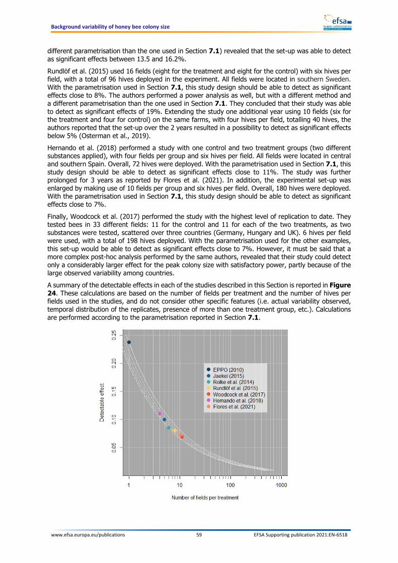
Background variability of honey bee colony size
www.efsa.europa.eu/publications 59 EFSA Supporting publication 2021:EN-6518
different parametrisation than the one used in Section 7.1) revealed that the set-up was able to detect as significant effects between 13.5 and 16.2%.
Rundlöf et al. (2015) used 16 fields (eight for the treatment and eight for the control) with six hives per field, with a total of 96 hives deployed in the experiment. All fields were located in southern Sweden. With the parametrisation used in Section 7.1, this study design should be able to detect as significant effects close to 8%. The authors performed a power analysis as well, but with a different method and a different parametrisation than the one used in Section 7.1. They concluded that their study was able to detect as significant effects of 19%. Extending the study one additional year using 10 fields (six for the treatment and four for control) on the same farms, with four hives per field, totalling 40 hives, the authors reported that the set-up over the 2 years resulted in a possibility to detect as significant effects below 5% (Osterman et al., 2019). Hernando et al. (2018) performed a study with one control and two treatment groups (two different substances applied), with four fields per group and six hives per field. All fields were located in central and southern Spain. Overall, 72 hives were deployed. With the parametrisation used in Section 7.1, this study design should be able to detect as significant effects close to 11%. The study was further prolonged for 3 years as reported by Flores et al. (2021). In addition, the experimental set-up was enlarged by making use of 10 fields per group and six hives per field. Overall, 180 hives were deployed. With the parametrisation used in Section 7.1, this study design should be able to detect as significant effects close to 7%.
Finally, Woodcock et al. (2017) performed the study with the highest level of replication to date. They tested bees in 33 different fields: 11 for the control and 11 for each of the two treatments, as two substances were tested, scattered over three countries (Germany, Hungary and UK). 6 hives per field were used, with a total of 198 hives deployed. With the parametrisation used for the other examples, this set-up would be able to detect as significant effects close to 7%. However, it must be said that a more complex post-hoc analysis performed by the same authors, revealed that their study could detect only a considerably larger effect for the peak colony size with satisfactory power, partly because of the large observed variability among countries. A summary of the detectable effects in each of the studies described in this Section is reported in Figure 24. These calculations are based on the number of fields per treatment and the number of hives per fields used in the studies, and do not consider other specific features (i.e. actual variability observed, temporal distribution of the replicates, presence of more than one treatment group, etc.). Calculations are performed according to the parametrisation reported in Section 7.1.

Background variability of honey bee colony size
www.efsa.europa.eu/publications 60 EFSA Supporting publication 2021:EN-6518
Figure 24: Relationship between the estimated detectable effect on colony size and number of fields per treatment used in field studies. The different reported curves correspond to the number of hives per field (from 4, i.e. the upper curve, to 8, i.e. the lower curve) and are calculated using the method report in Section 7.1. Coloured dots report the estimated detectable effects for the studies described in this Section, calculated from the number of fields per treatment and the number of hives per fields used in the respective studies.
7.3. Considerations of the requirements of field studies in the EFSA bee guidance document
In the consultations held during the revision process of the bee guidance document, some stakeholders and MSs expressed concerns regarding the link between the SPG implemented in EFSA (2013) and its practical implementation in the risk assessment, particularly for the field studies. These concerns were related to the practicality and feasibility of detecting a magnitude of effects <7% of colony size reduction with a sufficient statistical power. In addition, concerns were also expressed in relation to the SPG consideration when evaluating field studies. In particular, some MSs and stakeholders deemed the replication of field studies for addressing this requirement difficult to obtain considering that the foraging area of honeybees around the hive is large and the variation in vegetation and exposure to other pesticides may influence the results. It is difficult to ensure sufficiently controlled conditions for example to prevent cross-contamination. Some MSs pointed out that to get 200 standardised colonies there is a need to start from 500 colonies (by leaving the weakest and strongest out) and only two or three apiculturists in MSs have such a number of colonies. Furthermore, standardisation will disappear in a hive after six weeks. Overall, the statistical power and the requirements for field studies determined by EFSA (2013) for detecting the magnitude of 7% (e.g. number of replicates, field sites) was considered not feasible in realistic environments.
8. Concluding remarks for decision-making process for risk managers
The present analysis provides scientific grounds to risk managers for the review of the SPG for honey bees, according to Step 3 of the EFSA method (EFSA PPR Panel, 2010; EFSA Scientific Committee, 2016) and in particular as regards the quantification of the magnitude of the effects. Feedback from risk managers is also required for the definition of an appropriate temporal scale. In practice, the analysis of the background variability presented in this document should support risk managers in defining a threshold (or a set of thresholds based on geographical or seasonal variabilities) equivalent to a certain % reduction in colony size in a similar way as proposed by EFSA (2013).
When defining the threshold(s) of acceptable effects, risk managers should consider the following: • Colony size reductions of one-third were already identified (see Section 3.3) as a
threshold potentially leading to the impairment of the colony viability. The results of the simulations show that, in some circumstances (see Table 9), the distance between the mean size and the lower limit of the OR (either FOR or ROR) is close to or even higher than one-third (i.e. 33%).
• By using a more restricted OR the weaker colonies are left out, and therefore the threshold of acceptable effects is more conservative. The results of the simulations show that only a few colonies are substantially weaker than the average colony size, even when no exposure to pesticide is present. By restricting the OR for threshold derivation, these weaker colonies will not be used as a reference for acceptable effects, resulting in a general higher protection level.
• A restriction to the 50th percentile of the variability should not be considered for the threshold derivation, since this would mean that, in many cases, only beneficial effects of pesticides are considered acceptable i.e. increase in colony size compared to the control.
Background variability of honey bee colony size
www.efsa.europa.eu/publications 61 EFSA Supporting publication 2021:EN-6518
• The threshold of acceptable effect should be implementable in the reference tier; since, currently, the reference tier is represented by the field studies, it should be realistically measurable in those studies (see Section 7).
Additional considerations: 1) Why background variability can inform on the definition of the threshold(s) of acceptable effects? With approach #2, the magnitude dimension of the SPG will be based on a threshold of acceptable effect on colony size reduction identified within the range of the background variability, i.e. variability comparable to control replicates in experimental studies. Using the background variability means that, when evaluating a pesticide, the acceptable effect should not be larger than the variability of colonies not exposed to pesticides.
2) How reliable are the simulated variabilities? • The variabilities simulated by the model were smaller than the median variability observed in
the field studies, but still in the range of plausible values.
• The uncertainty of using simple landscape vs. complex landscape was quantified. The analysis indicated that the variability in simple landscapes, such as the ones used in the current simulations, may be underestimated.
• The exclusion of Varroa from the simulations indicated that simulated variability may be underestimated.
• The impact of other uncertainties is unknown. An underestimation of the variability should be regarded as more conservative than an overestimation for the purpose of establishing an acceptable effect within the simulated background variability of colony size. 3) What are the consequences for risk assessment of the OR restrictions?
The narrower the range, the smaller the magnitude of the acceptable effect.
This means that there is a: • higher level of conservativism;
• lower impact on the provision of the ecosystem services;
• lower trigger values for the tier risk assessment, thus higher number of substances that will not pass the risk assessment at the lower tiers;
• higher requirements of field experiments (higher replication, higher costs, etc.) to reliably test whether the protection goal is met; therefore, practical limitations of the field studies should be considered.
4) What are the consequences for risk assessment if multiple thresholds are selected? If risk managers select multiple thresholds of acceptable effects depending on the season/geographic variability, their implementation will require different risk assessments and the development and application of different criteria for the higher tier requirements. The consequence for the approval of the substance may be a highly demanding and non-harmonised risk assessment. This would also make it difficult to extrapolate a field study from one area/season to another. 5) What threshold should be selected in order to be implementable and measurable in field studies? The selection of the threshold influences the required complexity of the experimental set-up for field studies. EFSA is not in the position to express a definitive judgement of feasibility of different experimental setups, which mainly concerns costs and resources availability from the study sponsor. However, the examples of some of the most extensive studies that were recently evaluated (Section 7), could be used as a benchmark. It is also important to note that the evaluation of complex field studies would require a high expertise and it is time- and resource-demanding.

Background variability of honey bee colony size
www.efsa.europa.eu/publications 62 EFSA Supporting publication 2021:EN-6518
References Agatz A, Kuhl R, Miles M, Schad T and Preuss TG, 2019. An evaluation of the BEEHAVE model using
honey bee field study data: insights and recommendations. Environmental Toxicology and Chemistry, 38, 2535–2545. doi: 10.1002/etc.4547
Akman Yıldız T, 2018. A fractional dynamical model for honeybee colony population. International Journal of Biomathematics, 11, 1850063. doi: 10.1142/s1793524518500638
Alves T, Rivière J, Alaux C, Le Conte Y, Singhoff F, Duval T and Rodin V, 2020. An interruptible task allocation model: application to a honey bee colony simulation. 18th International Conference on Practical Applications of Agents and Multi-Agent Systems (PAAMS 2020), October 2020, L'Aquila, Italy. pp. 3–15.
Bagheri S and Mirzaie M, 2019. A mathematical model of honey bee colony dynamics to predict the effect of pollen on colony failure. PLoS One, 14, e0225632. doi: 10.1371/journal.pone.0225632
Bastiaansen R, Doelman A, van Langevelde F and Rottschäfer V, 2020. Modeling honey bee colonies in winter using a Keller–Segel model with a sign-changing chemotactic coefficient. SIAM Journal on Applied Mathematics, 80, 839–863. doi: 10.1137/19m1246067
Baude M, Kunin WE, Boatman ND, Conyers S, Davies N, Gillespie MA, Morton RD, Smart SM and Memmott J, 2016. Historical nectar assessment reveals the fall and rise of floral resources in Britain. Nature, 530, 85–88. doi: 10.1038/nature16532
Baveco J, Focks A, Belgers D, Van der Steen J, Boesten J and Roessink I, 2016. An energetics-based honeybee nectar-foraging model used to assess the potential for landscape-level pesticide exposure dilution. PeerJ, 4, e2293. doi: 10.7717/peerj.2293
Becher MA, Osborne JL, Thorbek P, Kennedy PJ and Grimm V, 2013. Towards a systems approach for understanding honeybee decline: a stocktaking and synthesis of existing models. Journal of Applied Ecology, 50, 868–880. doi: 10.1111/1365-2664.12112
Becher MA, Grimm V, Thorbek P, Horn J, Kennedy PJ and Osborne JL, 2014. BEEHAVE: a systems model of honeybee colony dynamics and foraging to explore multifactorial causes of colony failure. Journal of Applied Ecology, 51, 470–482. doi: 10.1111/1365-2664.12222
Becher MA, Grimm V, Knapp J, Horn J, Twiston-Davies G and Osborne JL, 2016. BEESCOUT: A model of bee scouting behaviour and a software tool for characterizing nectar/pollen landscapes for BEEHAVE. Ecological Modelling, 340, 126–133. doi: https://doi.org/10.1016/j.ecolmodel.2016.09.013
Becher MA, Twiston-Davies G, Penny TD, Goulson D, Rotheray EL and Osborne JL, 2018. Bumble-BEEHAVE: a systems model for exploring multifactorial causes of bumblebee decline at individual, colony, population and community level. Journal of Applied Ecology, 55, 2790–2801. doi: https://doi.org/10.1111/1365-2664.13165
Betti M, LeClair J, Wahl LM and Zamir M, 2017. Bee++: an object-oriented, agent-based simulator for honey bee colonies. Insects, 8, 31. doi: 10.3390/insects8010031
Betti MI, Wahl LM and Zamir M, 2014. Effects of infection on honey bee population dynamics: a model. PLoS One, 9, e110237. doi: 10.1371/journal.pone.0110237
Betti MI, Wahl LM and Zamir M, 2016. Age structure is critical to the population dynamics and survival of honeybee colonies. Royal Society Open Science, 3, 160444. doi: 10.1098/rsos.160444
Bilisik A, Cakmak I, Bicakci A and Malyer H, 2008. Seasonal variation of collected pollen loads of honeybees (Apis mellifera L. anatoliaca). Grana, 47, 70–77. doi: 10.1080/00173130801923976
Bodenheimer FS, 1937. Studies in animal populations II. Seasonal population-trends in the honey-bee. The Quarterly Review of Biology, 12, 406–425.
Booton RD, Iwasa Y, Marshall JAR and Childs DZ, 2017. Stress-mediated Allee effects can cause the sudden collapse of honey bee colonies. Journal of Theoretical Biology, 420, 213–219. doi: 10.1016/j.jtbi.2017.03.009
Background variability of honey bee colony size
www.efsa.europa.eu/publications 63 EFSA Supporting publication 2021:EN-6518
Bukovinszky T, Verheijen J, Zwerver S, Klop E, Biesmeijer JC, Wäckers FL, Prins HHT and Kleijn D, 2017. Exploring the relationships between landscape complexity, wild bee species richness and reproduction, and pollination services along a complexity gradient in the Netherlands. Biological Conservation, 214, 312–319. doi: https://doi.org/10.1016/j.biocon.2017.08.027
Burrill RM and Dietz A, 1981. The response of honey bees to variations in solar radiation and temperature. Apidologie, 12, 319–328.
Chauzat M-P, Cauquil L, Roy L, Franco S, Hendrikx P and Ribière-Chabert M, 2013. Demographics of the European Apicultural Industry. PLoS One, 8, e79018. doi: 10.1371/journal.pone.0079018
Chen J, Messan K, Rodriguez Messan M, Degrandi-Hoffman G, Bai D and Kang Y, 2020. How to model honeybee population dynamics: stage structure and seasonality. Mathematics in Applied Sciences and Engineering, 1, 91–206. doi: https://doi.org/10.5206/mase/10559
Clarke D and Robert D, 2018. Predictive modelling of honey bee foraging activity using local weather conditions. Apidologie, 49, 386–396. doi: 10.1007/s13592-018-0565-3
Comper JR and Eberl HJ, 2020. Mathematical modelling of population and food storage dynamics in a honey bee colony infected with Nosema ceranae. Heliyon, 6, e04599. doi: 10.1016/j.heliyon.2020.e04599
Cormont A, Siepel H, Clement J, Melman TCP, WallisDeVries MF, van Turnhout CAM, Sparrius LB, Reemer M, Biesmeijer JC, Berendse F and de Snoo GR, 2016. Landscape complexity and farmland biodiversity: Evaluating the CAP target on natural elements. Journal for Nature Conservation, 30, 19–26. doi: https://doi.org/10.1016/j.jnc.2015.12.006
Croft S, Brown M, Wilkins S, Hart A and Smith G, 2018. Evaluating EFSA protection goals for honey bees (Apis mellifera): what do they mean for pollination? Integrated Environmental Assessment and Management, 14. doi: 10.1002/ieam.4078
DeGrandi-Hoffman G, Roth SA, Loper GL and Erickson EH, 1989. BEEPOP: a honeybee population dynamics simulation model. Ecological Modelling, 45, 133–150. doi: https://doi.org/10.1016/0304-3800(89)90088-4
DeGrandi-Hoffman G, Ahumada F and Graham H, 2017. Are dispersal mechanisms changing the host–parasite relationship and increasing the virulence of Varroa destructor (Mesostigmata: Varroidae) in managed honey bee (Hymenoptera: Apidae) Colonies? Environmental Entomology, 46, 737–746. doi: 10.1093/ee/nvx077
Dénes A and Ibrahim MA, 2019. Global dynamics of a mathematical model for a honeybee colony infested by virus-carrying Varroa mites. Journal of Applied Mathematics and Computing, 61, 349–371. doi: 10.1007/s12190-019-01250-5
Dennis B and Kemp WP, 2016. How hives collapse: Allee effects, ecological resilience, and the honey bee. PLoS One, 11, e0150055. doi: 10.1371/journal.pone.0150055
Devillers J, Devillers H, Decourtye A, Fourrier J, Aupinel P and Fortini D, 2014. Agent-based modeling of the long-term effects of pyriproxyfen on honey bee population. In: Devillers J (ed.). In Silico Bees. Boca Raton, CRC Press. pp. 179–208.
Dunham WE, 1930. Temperature gradient in the egg-laying activities of the queen bee. The Ohio Journal of Science, 30, 403–410.
Eberl H, Kevan P and Ratti V, 2014. Infectious Disease Modeling for Honey Bee Colonies. In: Devillers J (ed.). In Silico Bees. Boca Raton, CRC Press. pp. 87–108.
Ebert GV, 1922. Zur Massenentwicklung der Bienenvoelker. Archiv für Biertenkunde, 4, 1–26.
EFSA (European Food Safety Authority), 2013. Guidance on the risk assessment of plant protection products on bees (Apis mellifera, Bombus spp. and solitary bees). EFSA Journal 2013;11(7):3295, 268 pp. doi: https://doi.org/10.2903/j.efsa.2013.3295
Background variability of honey bee colony size
www.efsa.europa.eu/publications 64 EFSA Supporting publication 2021:EN-6518
EFSA (European Food Safety Authority), 2016. A mechanistic model to assess risks to honeybee colonies from exposure to pesticides under different scenarios of combined stressors and factors. EFSA supporting publication 2016:EN-1069, 116 pp. Available online: https://doi.org/10.2903/sp.efsa.2016.EN-1069
EFSA (European Food Safety Authority), 2017. EFSA Guidance Document for predicting environmental concentrations of active substances of plant protection products and transformation products of these active substances in soil. EFSA Journal 2017;15(10):4982, 115 pp., doi:10.2903/j.efsa.2017.4982
EFSA (European Food Safety Authority), 2018. Evaluation of the data on clothianidin, imidacloprid and thiamethoxam for the updated risk assessment to bees for seed treatments and granules in the EU. EFSA supporting publication 2018:EN-1378, 31 pp. Available online: https://doi.org/10.2903/sp.efsa.2018.EN-1378
EFSA (European Food Safety Authority), Adriaanse P, Boivin A, Klein M, Jarvis N, Stemmer M, Fait G and Egsmose M, 2020a. Scientific report of EFSA on the 'repair action' of the FOCUS surface water scenarios. EFSA Journal 2020;18(6):6119, 301 pp. Available online: https://doi.org10.2903/j.efsa.2020.6119
EFSA (European Food Safety Authority), Ippolito A, del Aguila M, Aiassa E, Guajardo IM, Neri FM, Alvarez F, Mosbach‐Schulz O and Szentes C, 2020b. Review of the evidence on bee background mortality. EFSA supporting publications 2020:EN-1880 76 pp. Available online: https://doi.org/10.2903/sp.efsa.2020.EN-1880
EFSA PPR Panel (EFSA Panel on Plant Protection Products and their Residues), 2010. Scientific Opinion on the development of specific protection goal options for environmental risk assessment of pesticides, in particular in relation to the revision of the Guidance Documents on Aquatic and Terrestrial Ecotoxicology (SANCO/3268/2001 and SANCO/10329/2002). EFSA Journal 2010;8(10):1821, 55 pp. Available online: https://doi.org/10.2903/j.efsa.2010.1821
EFSA PPR Panel (EFSA Panel on Plant Protection Products and their Residues), 2012. Scientific Opinion on the science behind the development of a risk assessment of Plant Protection Products on bees (Apis mellifera, Bombus spp. and solitary bees). EFSA Journal 2012;10(5):2668, 275 pp. doi: 10.2903/j.efsa.2012.2668
EFSA PPR Panel (EFSA Panel on Plant Protection Products and their Residues), 2013. Guidance on tiered risk assessment for plant protection products for aquatic organisms in edge‐of‐field surface waters. EFSA Journal 2013, 11(7):3290, 268 pp. doi: 10.2903/j.efsa.2013.3290
EFSA PPR Panel (EFSA Panel on Plant Protection Products and their Residues), 2014. Scientific Opinion on good modelling practice in the context of mechanistic effect models for risk assessment of plant protection products. EFSA Journal 2014;12(3):3589, 92 pp. https://doi.org/10.2903/j.efsa.2014.3589
EFSA PPR Panel (EFSA Panel on Plant Protection Products and their Residues), 2015. Statement on the suitability of the BEEHAVE model for its potential use in a regulatory context and for the risk assessment of multiple stressors in honeybees at the landscape level. EFSA Journal 2015;13(6):4125, 92 pp. https://doi.org/10.2903/j.efsa.2015.4125
EFSA Scientific Committee, 2016. Guidance to develop specific protection goals options for environmental risk assessment at EFSA, in relation to biodiversity and ecosystem services. EFSA Journal 2016;14(6):e04499, 50 pp. https://doi.org/10.2903/j.efsa.2016.4499
EPPO, 2010. PP1/170(4) – Side-effects on honeybees. OEPP/EPPO Bulletin, 40, 313–319. European Commission, online. Honey market overview (Spring 2020). Available online:
https://ec.europa.eu/info/food-farming-fisheries/animals-and-animal-products/animal-products/honey_en [Accessed: 20 July 2020].
FAO, online. FAOSTAT. Available online: http://www.fao.org/faostat/en/ [Accessed: 18 June 2020].
Fijen TPM, Scheper JA, Boekelo B, Raemakers I and Kleijn D, 2019. Effects of landscape complexity on pollinators are moderated by pollinators' association with mass-flowering crops. Proceedings of the Royal Society B: Biological Sciences, 286, 20190387. doi: 10.1098/rspb.2019.0387
Background variability of honey bee colony size
www.efsa.europa.eu/publications 65 EFSA Supporting publication 2021:EN-6518
Flores JM, Gámiz V, Gil-Lebrero S, Rodríguez I, Navas FJ, García-Valcárcel AI, Cutillas V, Fernández-Alba AR and Hernando MD, 2021. A three-year large scale study on the risk of honey bee colony exposure to blooming sunflowers grown from seeds treated with thiamethoxam and clothianidin neonicotinoids. Chemosphere, 262, 127735. doi: https://doi.org/10.1016/j.chemosphere.2020.127735
FOCUS, 2000. FOCUS groundwater scenarios in the EU review of active substances. Report of the FOCUS Groundwater Scenarios Workgroup, EC Document Reference Sanco/321/2000 rev.2. 202 pp.
FOCUS, 2001. FOCUS Surface Water Scenarios in the EU Evaluation Process under 91/414/EEC. Report of the FOCUS Working Group on Surface Water Scenarios, EC Document Reference SANCO/4802/2001-rev.2. 245 pp.
Gray A, Brodschneider R, Adjlane N, Ballis A, Brusbardis V, Charrière J-D, Chlebo R, Coffey MF, Cornelissen B, Amaro da Costa C, Csáki T, Dahle B, Danihlík J, Dražić MM, Evans G, Fedoriak M, Forsythe I, de Graaf D, Gregorc A, Johannesen J, Kauko L, Kristiansen P, Martikkala M, Martín-Hernández R, Medina-Flores CA, Mutinelli F, Patalano S, Petrov P, Raudmets A, Ryzhikov VA, Simon-Delso N, Stevanovic J, Topolska G, Uzunov A, Vejsnaes F, Williams A, Zammit-Mangion M and Soroker V, 2019. Loss rates of honey bee colonies during winter 2017/2018 in 36 countries participating in the COLOSS survey, including effects of forage sources. Journal of Apicultural Research, 58, 479–485. doi: 10.1080/00218839.2019.1615661
Hains BC and Gamper H, 2017. Disruption in honey bee (Apis mellifera) foraging flight activity during a partial solar eclipse shown by individual flight path tracking. Bulletin of Insectology, 70, 315–320.
Harbo JR, 1986. Effect of population size on brood production, worker survival and honey gain in colonies of honeybees. Journal of Apicultural Research, 25, 22–29. doi: 10.1080/00218839.1986.11100687
Hatjina F, Costa C, Büchler R, Uzunov A, Drazic M, Filipi J, Charistos L, Ruottinen L, Andonov S, Meixner MD, Bienkowska M, Dariusz G, Panasiuk B, Conte YL, Wilde J, Berg S, Bouga M, Dyrba W, Kiprijanovska H, Korpela S, Kryger P, Lodesani M, Pechhacker H, Petrov P and Kezic N, 2014. Population dynamics of European honey bee genotypes under different environmental conditions. Journal of Apicultural Research, 53, 233–247. doi: 10.3896/IBRA.1.53.2.05
Hernando MD, Gámiz V, Gil-Lebrero S, Rodríguez I, García-Valcárcel AI, Cutillas V, Fernández-Alba AR and Flores JM, 2018. Viability of honeybee colonies exposed to sunflowers grown from seeds treated with the neonicotinoids thiamethoxam and clothianidin. Chemosphere, 202, 609–617. doi: https://doi.org/10.1016/j.chemosphere.2018.03.115
Hicks DM, Ouvrard P, Baldock KCR, Baude M, Goddard MA, Kunin WE, Mitschunas N, Memmott J, Morse H, Nikolitsi M, Osgathorpe LM, Potts SG, Robertson KM, Scott AV, Sinclair F, Westbury DB and Stone GN, 2016. Food for pollinators: quantifying the nectar and pollen resources of urban flower meadows. PLoS One, 11, e0158117. doi: 10.1371/journal.pone.0158117
Hörig K, Maus C, Nikolakis A, Ratte H-T, Roß-Nickoll M, Schmitt W and Preuss T, 2014. The advantage of a toxicokinetic model of the honey bee colony in the context of the risk assessment of plant protection products. Proceedings of the Hazards of pesticides to bees – 12th International Symposium of the ICP-PR Bee Protection Group, Ghent (Belgium), 51–55 pp.
Jacques A, Laurent M, Consortium E, Ribière-Chabert M, Saussac M, Bougeard S, Budge GE, Hendrikx P and Chauzat M-P, 2017. A pan-European epidemiological study reveals honey bee colony survival depends on beekeeper education and disease control. PLoS One, 12, e0172591. doi: 10.1371/journal.pone.0172591
Jaekel KM, 2015. Demonstration Farm Network – an approach to monitor health of honey bee colonies exposed to neonicotinoid seed-treated oilseed rape fields at pre-selected locations in France, Ger-many, Hungary, Poland and the United Kingdom 2014/2015. Study. Unpublished document.
Jatulan EO, Rabajante JF, Banaay CG, Fajardo AC, Jr and Jose EC, 2015. A mathematical model of intra-colony spread of American foulbrood in european honeybees (Apis mellifera L.). PLoS One, 10, e0143805. doi: 10.1371/journal.pone.0143805Kang Y, Blanco K, Davis T, Wang Y and DeGrandi-Hoffman G, 2016. Disease dynamics of honeybees with Varroa destructor as parasite and virus vector. Mathematical Biosciences, 275, 71–92. doi: 10.1016/j.mbs.2016.02.012
Background variability of honey bee colony size
www.efsa.europa.eu/publications 66 EFSA Supporting publication 2021:EN-6518
Kang Y, Blanco K, Davis T, Wang Y and DeGrandi-Hoffman G, 2016. Disease dynamics of honeybees with Varroa destructor as parasite and virus vector. Mathematical Biosciences, 275, 71–92. doi: 10.1016/j.mbs.2016.02.012
Khoury DS, Myerscough MR and Barron AB, 2011. A quantitative model of honey bee colony population dynamics. PLoS One, 6, e18491. doi: 10.1371/journal.pone.0018491
Khoury DS, Barron AB and Myerscough MR, 2013. Modelling food and population dynamics in honey bee colonies. PLoS One, 8, e59084. doi: 10.1371/journal.pone.0059084
Kribs-Zaleta CM and Mitchell C, 2014. Modeling colony collapse disorder in honeybees as a contagion. Mathematical Biosciences and Engineering, 11, 1275–1294. doi: 10.3934/mbe.2014.11.1275
Kuan AC, DeGrandi-Hoffman G, Curry RJ, Garber KV, Kanarek AR, Snyder MN, Wolfe KL and Purucker ST, 2018. Sensitivity analyses for simulating pesticide impacts on honey bee colonies. Ecological Modelling, 376, 15–27. doi: 10.1016/j.ecolmodel.2018.02.010
Lau P, Bryant V, Ellis JD, Huang ZY, Sullivan J, Schmehl DR, Cabrera AR and Rangel J, 2019. Seasonal variation of pollen collected by honey bees (Apis mellifera) in developed areas across four regions in the United States. PLoS One, 14, e0217294. doi: 10.1371/journal.pone.0217294
Leida B, Della Valle G and Piana L, 2004. I quaderni dell’apicoltore, 4. Flora Apistica. In: MIPAF UNAA (ed.).
Magal P, Webb GF and Wu Y, 2019. An Environmental Model of Honey Bee Colony Collapse Due to Pesticide Contamination. Bulletin of Mathematical Biology, 81:4908-4931. doi: 10.1007/s11538-019-00662-5
Magal P, Webb GF and Wu Y, 2020. A spatial model of honey bee colony collapse due to pesticide contamination of foraging bees. Journal of Mathematical Biology, 80, 2363–2393. doi: 10.1007/s00285-020-01498-7
Matey Valderrama J, Principal flora apícola del Alto Oja – La Rioja (Ezcaray-Ojacastro-Valgañón-Zorraquín): sucesión floral.
Mathis C and Buchanan E, 2006. Typical flowering seasons for Western North Carolina honey and pollen sources: approximately 2500 feet elevation.
Meikle WG, Rector BG, Mercadier G and Holst N, 2008. Within-day variation in continuous hive weight data as a measure of honey bee colony activity. Apidologie, 39, 694–707. doi: 10.1051/apido:2008055
Messan K, DeGrandi-Hoffman G, Castillo-Chavez C and Kang Y, 2017. Migration effects on population dynamics of the honeybee–mite interactions. Mathematical Modelling of Natural Phenomena, 12, 84–115. doi: 10.1051/mmnp/201712206
Messan K, Rodriguez Messan M, Chen J, DeGrandi-Hoffman G and Kang Y, 2021. Population dynamics of Varroa mite and honeybee: effects of parasitism with age structure and seasonality. Ecological Modelling, 440, 109359. doi: https://doi.org/10.1016/j.ecolmodel.2020.109359
Muhammad N and Eberl HJ, 2020. Two routes of transmission for Nosema infections in a honeybee population model with polyethism and time-periodic parameters can lead to drastically different qualitative model behavior. Communications in Nonlinear Science and Numerical Simulation, 84, 105207. doi: 10.1016/j.cnsns.2020.105207
Myerscough M, Khoury D, Ronzani S and Barron A, 2017. Why Do Hives Die? Using Mathematics to Solve the Problem of Honey Bee Colony Collapse. In: Osogami T (ed.). The Role and Importance of Mathematics in Innovation. Proceedings of the Forum “Math-for-Industry”. Springer, Singapore, pp. 35–50.
Nowosad J and Stepinski TF, 2019. Information theory as a consistent framework for quantification and classification of landscape patterns. Landscape Ecology, 34, 2091–2101. doi: 10.1007/s10980-019-00830-x
Background variability of honey bee colony size
www.efsa.europa.eu/publications 67 EFSA Supporting publication 2021:EN-6518
Nürnberger F, Härtel S and Steffan-Dewenter I, 2018. The influence of temperature and photoperiod on the timing of brood onset in hibernating honey bee colonies. PeerJ, 6, e4801–e4801. doi: 10.7717/peerj.4801
Ode Å, Hagerhall CM and Sang N, 2010. Analysing visual landscape complexity: theory and application. Landscape Research, 35, 111–131. doi: 10.1080/01426390903414935
Okosun K, 2014. Dynamics of a Varroa-infested honey bee colonies model. International Symposium on Mathematical and Computational Biology, 158–175. doi: 10.1142/9789814602228_0009
Osterman J, Wintermantel D, Locke B, Jonsson O, Semberg E, Onorati P, Forsgren E, Rosenkranz P, Rahbek-Pedersen T, Bommarco R, Smith HG, Rundlöf M and de Miranda JR, 2019. Clothianidin seed-treatment has no detectable negative impact on honeybee colonies and their pathogens. Nature Communications, 10, 692. doi: 10.1038/s41467-019-08523-4
Paiva JP, Paiva HM, Esposito E and Morais MM, 2016. On the effects of artificial feeding on bee colony dynamics: a mathematical model. PLoS One, 11, e0167054. doi: 10.1371/journal.pone.0167054
Perry CJ, Søvik E, Myerscough MR and Barron AB, 2015. Rapid behavioral maturation accelerates failure of stressed honey bee colonies. Proceedings of the National Academy of Sciences, 112, 3427. doi: 10.1073/pnas.1422089112
Persson AS, Olsson O, Rundlöf M and Smith HG, 2010. Land use intensity and landscape complexity—Analysis of landscape characteristics in an agricultural region in Southern Sweden. Agriculture, Ecosystems & Environment, 136, 169–176. doi: https://doi.org/10.1016/j.agee.2009.12.018
Petric A, Guzman-Novoa E and Eberl HJ, 2017. A mathematical model for the interplay of Nosema infection and forager losses in honey bee colonies. Journal of Biological Dynamics, 11, 348–378. doi: 10.1080/17513758.2016.1237682
Prado A, Requier F, Crauser D, Le Conte Y, Bretagnolle V and Alaux C, 2020. Honeybee lifespan: the critical role of pre-foraging stage. Royal Society Open Science, 7, 200998. doi: 10.1098/rsos.200998
Ratti V, Kevan P and Eberl H, 2013. A mathematical model for population dynamics in honeybee colonies infested with Varroa destructor and the acute bee paralysis virus. Canadian Applied Mathematics Quarterly, 21, 63–93. doi: 10.1007/s11538-017-0281-6
Ratti V, Kevan PG and Eberl HJ, 2017. A mathematical model of forager loss in honeybee colonies infested with Varroa destructor and the acute bee paralysis virus. Bulletin of Mathematical Biology, 79, 1218–1253. doi: 10.1007/s11538-017-0281-6
Requier F, Odoux J-F, Tamic T, Moreau N, Henry M, Decourtye A and Bretagnolle V, 2015. Honey bee diet in intensive farmland habitats reveals an unexpectedly high flower richness and a major role of weeds. Ecological Applications, 25, 881–890. doi: 10.1890/14-1011.1
Rivière J, Alaux C, Le Conte Y, Layec Y, Lozac'h A, Rodin V and Singhoff F, 2018. Toward a Complete agent-based model of a honeybee colony. Proceedings of the Highlights of Practical Applications of Agents, Multi-Agent Systems, and Complexity: The PAAMS Collection, Toledo, Spain, 2018-06-20. Available online: https://hal.archives-ouvertes.fr/hal-01826153
Rodriguez Messan M, Page RE and Kang Y, 2018. Effects of vitellogenin in age polyethism and population dynamics of honeybees. Ecological Modelling, 388, 88–107. doi: 10.1016/j.ecolmodel.2018.09.011
Rolke D, Persigehl M, Gruenewald B and Blenau W, 2014. Large-scale monitoring of long-term effects of Elado (10 g clothianidin & 2 g beta-cyfluthrin/kg seed) dressed oilseed rape on pollinating insects in Mecklenburg-Vorpommern, Germany: VII effects on honeybees (Apis mellifera). Study. Unpublished document.
Rundlöf M, Andersson GKS, Bommarco R, Fries I, Hederström V, Herbertsson L, Jonsson O, Klatt BK, Pedersen TR, Yourstone J and Smith HG, 2015. Seed coating with a neonicotinoid insecticide negatively affects wild bees. Nature, 521, 77–80. doi: 10.1038/nature14420
Russell S, Barron AB and Harris D, 2013. Dynamic modelling of honey bee (Apis mellifera) colony growth and failure. Ecological Modelling, 265, 158–169. doi: 10.1016/j.ecolmodel.2013.06.005
Background variability of honey bee colony size
www.efsa.europa.eu/publications 68 EFSA Supporting publication 2021:EN-6518
Schmickl T and Crailsheim K, 2007. HoPoMo: a model of honeybee intracolonial population dynamics and resource management. Ecological Modelling, 204, 219–245. doi: 10.1016/j.ecolmodel.2007.01.001
Schmickl T and Karsai I, 2017. Resilience of honeybee colonies via common stomach: a model of self-regulation of foraging. PLoS One, 12, e0188004. doi: 10.1371/journal.pone.0188004
Taha E-K, Taha R and Al-Kahtani S, 2019. Nectar and pollen sources for honeybees in Kafrelsheikh of northern Egypt. Saudi Journal of Biological Sciences, 26, 890–896. doi: 10.1016/j.sjbs.2017.12.010
Tew NE, Memmott J, Vaughan IP, Bird S, Stone GN, Potts SG and Baldock KCR, 2021. Quantifying nectar production by flowering plants in urban and rural landscapes. Journal of Ecology, doi: https://doi.org/10.1111/1365-2745.13598
Timberlake TP, Vaughan IP and Memmott J, 2019. Phenology of farmland floral resources reveals seasonal gaps in nectar availability for bumblebees. Journal of Applied Ecology, 56, 1585–1596. doi: https://doi.org/10.1111/1365-2664.13403
Torres DJ and Torres NA, 2020. Modeling the influence of mites on honey bee populations. Veterinary Sciences, 7, 139. doi: 10.3390/vetsci7030139
Torres DJ, Ricoy UM and Roybal S, 2015. Modeling honey bee populations. PLoS One, 10, e0130966. doi: 10.1371/journal.pone.0130966
vanEngelsdorp D and Meixner MD, 2010. A historical review of managed honey bee populations in Europe and the United States and the factors that may affect them. Journal of Invertebrate Pathology, 103, S80–S95. doi: https://doi.org/10.1016/j.jip.2009.06.011
Vicens N and Bosch J, 2000. Weather-dependent pollinator activity in an apple orchard, with special reference to Osmia cornuta and Apis mellifera (Hymenoptera: Megachilidae and Apidae). Environmental Entomology, 29, 413–420. doi: 10.1603/0046-225X-29.3.413
Wang B, Tian C and Sun J, 2019. Effects of landscape complexity and stand factors on arthropod communities in poplar forests. Ecology and Evolution, 9, 7143–7156. doi: https://doi.org/10.1002/ece3.5285
Wood TJ, Kaplan I and Szendrei Z, 2018. Wild bee pollen diets reveal patterns of seasonal foraging resources for honey bees. Frontiers in Ecology and Evolution, 6, 210. doi: 10.3389/fevo.2018.00210
Woodcock BA, Bullock JM, Shore RF, Heard MS, Pereira MG, Redhead J, Ridding L, Dean H, Sleep D, Henrys P, Peyton J, Hulmes S, Hulmes L, Sárospataki M, Saure C, Edwards M, Genersch E, Knäbe S and Pywell RF, 2017. Country-specific effects of neonicotinoid pesticides on honey bees and wild bees. Science, 356, 1393. doi: 10.1126/science.aaa1190

Background variability of honey bee colony size
www.efsa.europa.eu/publications 69 EFSA Supporting publication 2021:EN-6518
Appendix A – Overview of honey bee models in the literature See Excel file ‘Appendix-A_model_overview.xlsx’. The excel file presents an overview of honey bee models published after the review from Becher et al. (2013). An exception was made for BEEPOP (DeGrandi-Hoffmann et al., 1988), HoPoMo (Schmickl and Crailsheim, 2007) and the model from Khoury et al. (2011), all published before 2013, but further considered because of their status as reference for many other models developed afterwards. For each model, it was checked whether explicit consideration was given to a pre-defined list of processes and attributes. The outcome is a matrix with the process/attribute in the rows and the different models in the columns.
Background variability of honey bee colony size
www.efsa.europa.eu/publications 70 EFSA Supporting publication 2021:EN-6518
Appendix B – Analysis of landscape complexity
B.1. Background of the issue The default BEEHAVE landscape used in the analysis described in the main document consists of two flower patches, which are located at different distances from the hive, and have shifted phenology, but are in all other aspects (size, nectar provision, pollen provision, detection probability) identical. Due to current limitation of data availability, a more realistic definition of landscape scenarios based on data was not possible. However, since the EFSA WG considered that the adopted simplification of the landscape was a crucial point, a separate analysis has been set up in order to explore the effect of landscape complexity on the final outcome (i.e. variability in colony size as simulated by the model). Landscape complexity is defined in many ways in the literature, and even more operative ways for quantifying this concept are available. Nowosad and Stepinski (2019) highlighted that ‘complexity is a concept defying a precise definition’ and they claim that ‘there is no bona fide metric of landscape overall complexity’. Some authors have quantified landscape complexity by using the amount of natural and semi-natural habitats (see for example Cormont et al., 2016; Bukovinszky et al., 2017; Fijen et al., 2019). More structural attempts to identify the components of landscape complexity focused on the spatial arrangement of the landscape elements (see for example Ode et al., 2010; Wang et al., 2019). Persson et al. (2010) analysed the relationship between landscape complexity and agricultural land use intensity, finding that they are separate factors, at least at smaller spatial scales. In this Appendix it is investigated how changing various landscape parameters influences the output of BEEHAVE simulations, with a specific focus on the variability between equal replicate runs.
B.2. Dimensions of landscape complexity Within the present work, EFSA have identified four dimensions which have the potential to regulate the foraging of the simulated bee hives. These are:
• Size heterogeneity of flower patches, i.e. the difference in size of food areas
• Patch fragmentation, i.e. the degree of scattering in the landscape of the different food patches
• Asynchrony of flowering, i.e. the degree of (lack of) overlap in the flowering period between patches
• Food level heterogeneity, i.e. the difference in food level provided by the different patches
The first two dimensions contribute to describe the spatial aspect of landscape complexity. The third concerns the temporal aspect, while the fourth captures flower source heterogeneity. For each of the four dimension, three different levels (low, medium, high) have been defined. All possible combinations of the three levels and four dimensions have been used for building 81 (=34) different landscapes (see Figure B1 and Figure B2). The overall size of the landscape (i.e. 3,000 m × 3,000 m) and the overall area of food patches in the landscape were kept constant, to avoid that food availability and not spatial or temporal aspects determine responses in the scenario simulations. In all landscapes, the food is provided by nine ‘building block’ patches (see Figure B1), which were changed in size and combined in space. A description of the implementation of the different dimension is reported below, with the three levels always presented from the simplest to the most complex.
Size heterogeneity of flower patches • Low: all patches have the same size (total food patch area/9).
• Medium: Patch size vary between 50 and 150%. The total food patch area is still the same.
• Large: Patch size vary between 10 and 200%. The total food patch area is still the same.
Patch fragmentation
• Low: all patches are directly neighboured to each other, building up one ‘field’.

Background variability of honey bee colony size
www.efsa.europa.eu/publications 71 EFSA Supporting publication 2021:EN-6518
• Medium: patches are directly neighboured in group of three. The resulting three ‘fields’ are located in the upper, middle and lower part of the landscape.
• High: all patches are separated from each other, the nine ‘fields’ are distributed in the nine quadrants of the landscape.
Asynchrony of flowering
• High synchronisation: all patches provide pollen and nectar exactly at the same time.
• Medium synchronisation: groups of three patches provide pollen and nectar at the same time, but each group has a shifted phenology compared to the others.
• Low synchronisation: each patch provides pollen and nectar at a different time.
Food level heterogeneity
• Low: all patches provide the same maximum level of pollen and nectar per square metre.
• Medium: the maximum level of pollen and nectar varies between each patch by a small extent (3 patches at 70%, 3 at 100%, 3 at 130%).
• Large: the maximum level of pollen and nectar varies between each patch by a large extent (between 25 and 300%).
Figure B1: Spatial arrangement of the nine food patches used in the analysis of landscape complexity. Size heterogeneity increases from left to right, while patch fragmentation increases

Background variability of honey bee colony size
www.efsa.europa.eu/publications 72 EFSA Supporting publication 2021:EN-6518
from top to bottom. The hive is represented by the small square with the lower-left angle at the origin of the two axes (0,0).
Figure B2: Temporal dynamics of food availability (pollen and nectar) in the nine food patches used in the analysis of landscape complexity. The heterogeneity related to the maximum food level increases from left to right, while the asynchrony of flowering increases from top to bottom. When less than nine curves are visible, this is because they are overlapping.
The detection probability of food patches was calculated on the basis of their distance from the hive and their size according to the following equation:
p = Exp(−0.307312 × distance/log10(size))
This was empirically derived from the ‘RRes food inflow’ scenario file from the default BEEHAVE implementation (Becher et al., 2014). In addition, in order to explore the influence of landscape complexity under different climatic conditions, an entire latitudinal transect identified from the initially selected 20 locations was considered. Specifically, scenarios D1, D2, D3, D4 and D5 were used (see Figure 2 in the main text). These locations span from Euboea (Greece) to Lapland (Finland).
The total flowering window in each landscape was adjusted on the basis of the foraging window (following the same approach used in the default 2-patches landscapes).
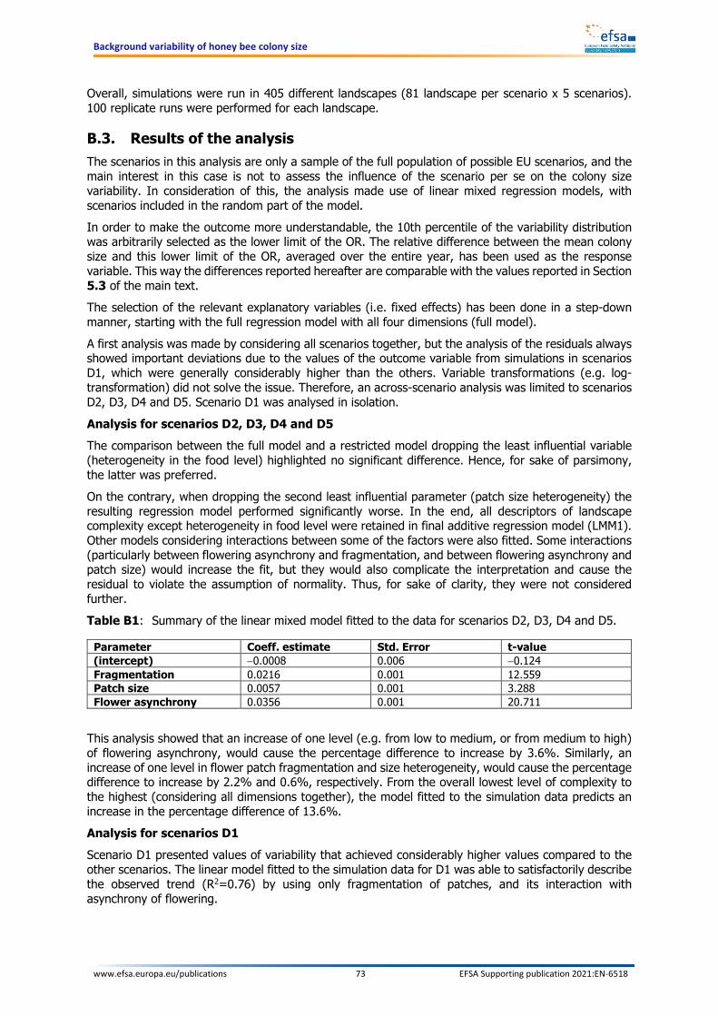
Background variability of honey bee colony size
www.efsa.europa.eu/publications 73 EFSA Supporting publication 2021:EN-6518
Overall, simulations were run in 405 different landscapes (81 landscape per scenario x 5 scenarios). 100 replicate runs were performed for each landscape.
B.3. Results of the analysis The scenarios in this analysis are only a sample of the full population of possible EU scenarios, and the main interest in this case is not to assess the influence of the scenario per se on the colony size variability. In consideration of this, the analysis made use of linear mixed regression models, with scenarios included in the random part of the model. In order to make the outcome more understandable, the 10th percentile of the variability distribution was arbitrarily selected as the lower limit of the OR. The relative difference between the mean colony size and this lower limit of the OR, averaged over the entire year, has been used as the response variable. This way the differences reported hereafter are comparable with the values reported in Section 5.3 of the main text. The selection of the relevant explanatory variables (i.e. fixed effects) has been done in a step-down manner, starting with the full regression model with all four dimensions (full model). A first analysis was made by considering all scenarios together, but the analysis of the residuals always showed important deviations due to the values of the outcome variable from simulations in scenarios D1, which were generally considerably higher than the others. Variable transformations (e.g. log-transformation) did not solve the issue. Therefore, an across-scenario analysis was limited to scenarios D2, D3, D4 and D5. Scenario D1 was analysed in isolation. Analysis for scenarios D2, D3, D4 and D5 The comparison between the full model and a restricted model dropping the least influential variable (heterogeneity in the food level) highlighted no significant difference. Hence, for sake of parsimony, the latter was preferred. On the contrary, when dropping the second least influential parameter (patch size heterogeneity) the resulting regression model performed significantly worse. In the end, all descriptors of landscape complexity except heterogeneity in food level were retained in final additive regression model (LMM1). Other models considering interactions between some of the factors were also fitted. Some interactions (particularly between flowering asynchrony and fragmentation, and between flowering asynchrony and patch size) would increase the fit, but they would also complicate the interpretation and cause the residual to violate the assumption of normality. Thus, for sake of clarity, they were not considered further. Table B1: Summary of the linear mixed model fitted to the data for scenarios D2, D3, D4 and D5.
Parameter Coeff. estimate Std. Error t-value (intercept) −0.0008 0.006 −0.124 Fragmentation 0.0216 0.001 12.559 Patch size 0.0057 0.001 3.288 Flower asynchrony 0.0356 0.001 20.711
This analysis showed that an increase of one level (e.g. from low to medium, or from medium to high) of flowering asynchrony, would cause the percentage difference to increase by 3.6%. Similarly, an increase of one level in flower patch fragmentation and size heterogeneity, would cause the percentage difference to increase by 2.2% and 0.6%, respectively. From the overall lowest level of complexity to the highest (considering all dimensions together), the model fitted to the simulation data predicts an increase in the percentage difference of 13.6%. Analysis for scenarios D1 Scenario D1 presented values of variability that achieved considerably higher values compared to the other scenarios. The linear model fitted to the simulation data for D1 was able to satisfactorily describe the observed trend (R2=0.76) by using only fragmentation of patches, and its interaction with asynchrony of flowering.
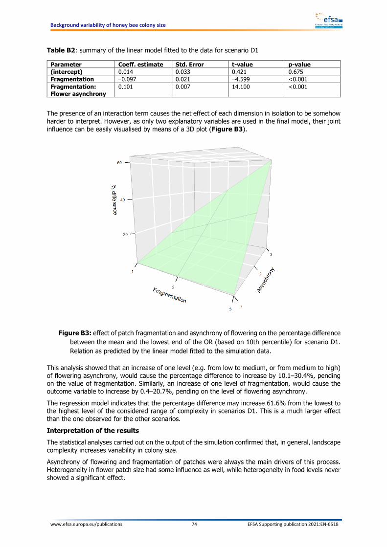
Background variability of honey bee colony size
www.efsa.europa.eu/publications 74 EFSA Supporting publication 2021:EN-6518
Table B2: summary of the linear model fitted to the data for scenario D1
Parameter Coeff. estimate Std. Error t-value p-value (intercept) 0.014 0.033 0.421 0.675 Fragmentation −0.097 0.021 −4.599 <0.001 Fragmentation: Flower asynchrony
0.101 0.007 14.100 <0.001
The presence of an interaction term causes the net effect of each dimension in isolation to be somehow harder to interpret. However, as only two explanatory variables are used in the final model, their joint influence can be easily visualised by means of a 3D plot (Figure B3).
Figure B3: effect of patch fragmentation and asynchrony of flowering on the percentage difference between the mean and the lowest end of the OR (based on 10th percentile) for scenario D1. Relation as predicted by the linear model fitted to the simulation data.
This analysis showed that an increase of one level (e.g. from low to medium, or from medium to high) of flowering asynchrony, would cause the percentage difference to increase by 10.1–30.4%, pending on the value of fragmentation. Similarly, an increase of one level of fragmentation, would cause the outcome variable to increase by 0.4–20.7%, pending on the level of flowering asynchrony.
The regression model indicates that the percentage difference may increase 61.6% from the lowest to the highest level of the considered range of complexity in scenarios D1. This is a much larger effect than the one observed for the other scenarios.
Interpretation of the results The statistical analyses carried out on the output of the simulation confirmed that, in general, landscape complexity increases variability in colony size. Asynchrony of flowering and fragmentation of patches were always the main drivers of this process. Heterogeneity in flower patch size had some influence as well, while heterogeneity in food levels never showed a significant effect.
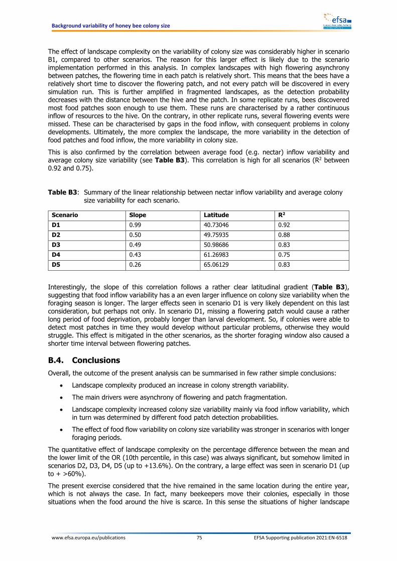
Background variability of honey bee colony size
www.efsa.europa.eu/publications 75 EFSA Supporting publication 2021:EN-6518
The effect of landscape complexity on the variability of colony size was considerably higher in scenario B1, compared to other scenarios. The reason for this larger effect is likely due to the scenario implementation performed in this analysis. In complex landscapes with high flowering asynchrony between patches, the flowering time in each patch is relatively short. This means that the bees have a relatively short time to discover the flowering patch, and not every patch will be discovered in every simulation run. This is further amplified in fragmented landscapes, as the detection probability decreases with the distance between the hive and the patch. In some replicate runs, bees discovered most food patches soon enough to use them. These runs are characterised by a rather continuous inflow of resources to the hive. On the contrary, in other replicate runs, several flowering events were missed. These can be characterised by gaps in the food inflow, with consequent problems in colony developments. Ultimately, the more complex the landscape, the more variability in the detection of food patches and food inflow, the more variability in colony size.
This is also confirmed by the correlation between average food (e.g. nectar) inflow variability and average colony size variability (see Table B3). This correlation is high for all scenarios (R2 between 0.92 and 0.75).
Table B3: Summary of the linear relationship between nectar inflow variability and average colony
size variability for each scenario.
Scenario Slope Latitude R2 D1 0.99 40.73046 0.92 D2 0.50 49.75935 0.88 D3 0.49 50.98686 0.83 D4 0.43 61.26983 0.75 D5 0.26 65.06129 0.83
Interestingly, the slope of this correlation follows a rather clear latitudinal gradient (Table B3), suggesting that food inflow variability has a an even larger influence on colony size variability when the foraging season is longer. The larger effects seen in scenario D1 is very likely dependent on this last consideration, but perhaps not only. In scenario D1, missing a flowering patch would cause a rather long period of food deprivation, probably longer than larval development. So, if colonies were able to detect most patches in time they would develop without particular problems, otherwise they would struggle. This effect is mitigated in the other scenarios, as the shorter foraging window also caused a shorter time interval between flowering patches.
B.4. Conclusions Overall, the outcome of the present analysis can be summarised in few rather simple conclusions:
• Landscape complexity produced an increase in colony strength variability.
• The main drivers were asynchrony of flowering and patch fragmentation.
• Landscape complexity increased colony size variability mainly via food inflow variability, which in turn was determined by different food patch detection probabilities.
• The effect of food flow variability on colony size variability was stronger in scenarios with longer foraging periods.
The quantitative effect of landscape complexity on the percentage difference between the mean and the lower limit of the OR (10th percentile, in this case) was always significant, but somehow limited in scenarios D2, D3, D4, D5 (up to +13.6%). On the contrary, a large effect was seen in scenario D1 (up to + >60%). The present exercise considered that the hive remained in the same location during the entire year, which is not always the case. In fact, many beekeepers move their colonies, especially in those situations when the food around the hive is scarce. In this sense the situations of higher landscape
Background variability of honey bee colony size
www.efsa.europa.eu/publications 76 EFSA Supporting publication 2021:EN-6518
complexity used in this exercise may not be very frequent for many hives. However, this should be further checked by means of more in-depth analysis, which is not available for the time being.

www.efsa.europa.eu/publications 77 EFSA Supporting publication 2021:EN-6518
Appendix C – Detailed results of the simulations See zip file ‘Appendix-C_simulation_results.xlsx’. The zip file includes an excel file ‘variability analysis.xlsx’ where a more detailed analysis of the variability analysis is presented (all percentiles from full range to 50th percentile) for all scenarios and all averaging period (full year, spring, summer and autumn). The zip file also includes 19 text files (one per scenario) where simulated colony sizes for every day of the simulation are reported. The text files are matrices of 366 rows (=days) and 500 columns (=replicate simulation runs).
www.efsa.europa.eu/publications 78 EFSA Supporting publication 2021:EN-6518
Appendix D – Variability in risk assessment In this Appendix a brief overview of the use of probability in the current environmental risk assessment of pesticides is presented. In the past, risk managers have been asked several times to select thresholds within variability ranges and/or probability distributions (i.e. percentiles) for tuning the risk assessment procedures to the desired level of protection. So, in this respect, the current exercise does not represent a novelty. Within the domain of the environmental risk assessment, examples of such selections are particularly abundant in the field of the exposure assessment, i.e. selecting the level of exposure to be used in the risk assessment. The definition and related parameterisation of the FOCUS surface water scenarios aimed to cover at least:
‘a 90th percentile worst-case for surface water exposures resulting from agricultural pesticide use within the European Union’ (FOCUS, 2001).
In other words, the estimated surface water concentrations used for the risk assessment should be higher than 90% of possible situations occurring in time and space (EFSA et al., 2020a). Similarly, weather and soil characteristics used in the FOCUS ground water scenarios are combined to result in an overall 90th percentile vulnerability in terms of leaching (FOCUS, 2000). The same 90th percentile goal is also recommended for soil, although this will be applied specifically for each regulatory zone (EFSA, 2017).
The risk assessment for bees in EFSA (2013) is based on an exposure estimation that should cover the 90% (i.e. the 90th percentile) of the hives placed in the vicinity of the treated fields. The use of probability and/or variability thresholds in risk assessment is however not limited to exposure. Species sensitivity distributions (SSD) are often used to derive HC5 (hazardous concentration for 5% of the species, i.e. the 5th percentile), or analogous hazard estimates (e.g. HR5, HP5). This means that the selected toxicological threshold is protective for 95% of the species. For example, the current risk assessment for non-target plants (European Commission, 2002) considers the SSD as a tool to identify an application rate that would protect (i.e. causing <50% effect) 95% of the species being potentially exposed, leaving out 5% of those. Since no assessment factor is used in such risk assessment, this percentage could immediately be interpreted as the current protection goal, although this was never explicitly agreed. SSD-derived hazard estimates are also used for assessing risk to aquatic organisms (EFSA PPR Panel, 2013). However, the presence of assessment factors complicates the relations between the threshold (5%, i.e. the 5th percentile) of the sensitivity distribution used in the risk assessment and the final object of protection. All previous examples deal with situations when one of the two main dimensions of the risk assessment (i.e. either the exposure or the hazard) is known to be variable: across space and time, across species, etc. In order to make the risk assessment operational, several times in the past there has been an explicit decision to neglect part of the variability distribution, generally the most ‘extreme’ part. In this respect, the present task for the risk managers does not represent a novelty. Nevertheless, the present task presents two fundamental differences compared to similar decisions made in the past:
1) The selection of the percentile, unlike all other situations, has an upper bound at the mean of the variability distribution (see Figure 1) i.e. often close to the 50th percentile7. Selecting a percentile higher than the mean as lower limit of the OR would indeed be nonsensical, as any treatment would need to produce a positive effect on the mean colony size to be considered acceptable.
2) Second, in all examples presented in this Section, ‘pushing’ the threshold towards most extreme values (in particular very high percentiles for the exposure assessment goals and very low
7 Most variability distributions are not heavily skewed (i.e. more or less symmetric), thus the mean and the median are not too
dissimilar.

www.efsa.europa.eu/publications 79 EFSA Supporting publication 2021:EN-6518
percentiles for the SSD) would translate into a more conservative risk assessment. On the contrary, in the present task, the selection of very low percentiles as lower limit of the OR would translate in less conservative risk assessments as this would allow for a higher acceptable effect.
By putting together the two points above it derives that the conservativeness of risk assessment will increase with percentiles that get closer to the mean (i.e. likely closer to 50th percentile).