Western University Western University

Scholarship@Western Scholarship@Western

Electronic Thesis and Dissertation Repository

8-8-2017 2:00 PM

On Honey Bee Colony Dynamics and Disease Transmission On Honey Bee Colony Dynamics and Disease Transmission

Matthew I. Betti, The University of Western Ontario

Supervisor: Lindi Wahl, The University of Western Ontario

Co-Supervisor: Mair Zamir, The University of Western Ontario

A thesis submitted in partial fulfillment of the requirements for the Doctor of Philosophy degree

in Applied Mathematics

© Matthew I. Betti 2017

Follow this and additional works at: https://ir.lib.uwo.ca/etd

Part of the Dynamic Systems Commons, Ordinary Differential Equations and Applied Dynamics

Commons, Other Applied Mathematics Commons, Other Ecology and Evolutionary Biology Commons,

Partial Differential Equations Commons, and the Population Biology Commons

Recommended Citation Recommended Citation Betti, Matthew I., "On Honey Bee Colony Dynamics and Disease Transmission" (2017). Electronic Thesis and Dissertation Repository. 4803. https://ir.lib.uwo.ca/etd/4803

This Dissertation/Thesis is brought to you for free and open access by Scholarship@Western. It has been accepted for inclusion in Electronic Thesis and Dissertation Repository by an authorized administrator of Scholarship@Western. For more information, please contact wlswadmin@uwo.ca.

AbstractThe work herein falls under the umbrella of mathematical modeling of disease transmission.

The majority of this document focuses on the extent to which infection undermines the strengthof a honey bee colony. These studies extend from simple mass-action ordinary differentialequations models, to continuous age-structured partial differential equation models and finallya detailed agent-based model which accounts for vector transmission of infection betweenbees as well as a host of other influences and stressors on honey bee colony dynamics. Thesemodels offer a series of predictions relevant to the fate of honey bee colonies in the presenceof disease and the nonlinear effects of disease, seasonality and the complicated dynamics ofhoney bee colonies. We are also able to extract from these models metrics that preempt colonyfailure. The analysis of disease dynamics in age-structured honey bee colony models requiredthe study of next generation operators (NGO) and the basic reproduction number, R0, for partialdifferential equations. This led us to the development of a coherent path from the NGO to itsdiscrete compartmental counterpart, the next generation matrix (NGM) as well as the derivationof new closed-form formulae for the NGO for specific classes of disease models.

Keywords: Honey Bee Dynamics, Colony Collapse, Basic Reproduction Number, NextGeneration Operator

ii

Co-Authorship Statement

The thesis herein has been written by Matthew Ilario Betti under the supervision of Dr. LindiM. Wahl and Dr. Mair Zamir. Chapter 2 has been published in PLOS ONE with co-authorsL.M. Wahl and M. Zamir. Chapter 3 is in press, to be published in Bulletin of MathematicalBiology with co-authors L.M. Wahl and M. Zamir. Chapter 4 has been published in Royal So-ciety Open Science with co-authors L.M. Wahl and M. Zamir. Chapter 5 has been published inthe journal Insects with co-authors J. LeClair, L.M. Wahl and M. Zamir. Chapter 6 is under re-view for publication in SIAM Journal of Applied Mathematics with co-authors J. LeClair, L.M.Wahl and M. Zamir. The aforementioned chapters contain models and analysis developed andcarried out by M.I. Betti. The model and corresponding simulation package in Chapter 5 wasco-developed with J. LeClair. The limit arguments in Chapter 6.2.1 were carried out by L.M.Wahl. All authors contributed to the writing of the respective manuscripts.

iii

Acknowledgements

I first and foremost must thank my incredible supervisors Lindi Wahl and Mair Zamir fortheir continued support, insights and infinite patience. They have allowed me the freedom totravel down paths of research which did nothing more than piqued my curiosity and have beensupportive the entire way. None of this would be possible without them. There are not enoughwords in enough languages to truly describe their influence.

I would also like to thank the Applied Mathematics department at Western University forfour years of invaluable instruction, guidance and insightful discussions. In particular, I wouldlike to thank David Dick and Josh LeClair for many thoughtful discussions.

Finally, I would like to thank Geoff Wild whose course on mathematical biology was thecatalyst for everything herein.

iv

For my parents, Elvi and Silena Betti

v

Handle a book as a bee does a flower, extract its sweetness but do not damage it.- John Muir

OH, NO! NOT THE BEES! NOT THE BEES! AAAAAHHHHH! OH, THEY’RE IN MY EYES!MY EYES! AAAAHHHHH! AAAAAGGHHH!

- Nicolas Cage

vi

Contents

Co-Authorship Statement ii

Acknowledgements iii

Abstract vi

List of Figures ix

List of Tables xi

List of Appendices xii

1 Introduction 11.1 Honey Bees . . . . . . . . . . . . . . . . . . . . . . . . . . . . . . . . . . . . 1

1.1.1 Honey Bee Colony Dynamics . . . . . . . . . . . . . . . . . . . . . . 21.1.2 Honey Bee Diseases . . . . . . . . . . . . . . . . . . . . . . . . . . . 31.1.3 Mathematical Models of Honey Bees . . . . . . . . . . . . . . . . . . 4

1.2 Basic Reproduction Number . . . . . . . . . . . . . . . . . . . . . . . . . . . 7

2 Effects of Infection on Honey Bee Population Dynamics: A Model 222.1 Introduction . . . . . . . . . . . . . . . . . . . . . . . . . . . . . . . . . . . . 222.2 Background . . . . . . . . . . . . . . . . . . . . . . . . . . . . . . . . . . . . 24

2.2.1 Normal Demographics of a Honey Bee Colony . . . . . . . . . . . . . 242.2.2 Nosema Infection . . . . . . . . . . . . . . . . . . . . . . . . . . . . . 24

2.3 Mathematical Model . . . . . . . . . . . . . . . . . . . . . . . . . . . . . . . 252.3.1 Governing Equations: Active Season . . . . . . . . . . . . . . . . . . . 252.3.2 Governing Equations: Winter . . . . . . . . . . . . . . . . . . . . . . . 272.3.3 Parameter Values . . . . . . . . . . . . . . . . . . . . . . . . . . . . . 28

2.4 Results . . . . . . . . . . . . . . . . . . . . . . . . . . . . . . . . . . . . . . . 292.5 Discussions and Conclusions . . . . . . . . . . . . . . . . . . . . . . . . . . . 41

3 Honey Bee Reproduction Number 463.1 Introduction . . . . . . . . . . . . . . . . . . . . . . . . . . . . . . . . . . . . 463.2 Model . . . . . . . . . . . . . . . . . . . . . . . . . . . . . . . . . . . . . . . 483.3 Results . . . . . . . . . . . . . . . . . . . . . . . . . . . . . . . . . . . . . . . 51

3.3.1 Existence . . . . . . . . . . . . . . . . . . . . . . . . . . . . . . . . . 513.3.2 Disease-free Equilibria (DFE) . . . . . . . . . . . . . . . . . . . . . . 53

vii

3.3.3 Stability of DFE . . . . . . . . . . . . . . . . . . . . . . . . . . . . . . 563.3.4 Basic Reproduction NumberR0 . . . . . . . . . . . . . . . . . . . . . 59

3.4 Discussion . . . . . . . . . . . . . . . . . . . . . . . . . . . . . . . . . . . . . 633.5 Appendix . . . . . . . . . . . . . . . . . . . . . . . . . . . . . . . . . . . . . 65

4 Age Structure in Honey Bee Colonies 734.1 Introduction . . . . . . . . . . . . . . . . . . . . . . . . . . . . . . . . . . . . 734.2 Model . . . . . . . . . . . . . . . . . . . . . . . . . . . . . . . . . . . . . . . 74

4.2.1 Age Structure . . . . . . . . . . . . . . . . . . . . . . . . . . . . . . . 754.2.2 Winter . . . . . . . . . . . . . . . . . . . . . . . . . . . . . . . . . . . 77

4.3 Results . . . . . . . . . . . . . . . . . . . . . . . . . . . . . . . . . . . . . . . 794.4 Discussion . . . . . . . . . . . . . . . . . . . . . . . . . . . . . . . . . . . . . 85

5 Bee++ 905.1 Introduction . . . . . . . . . . . . . . . . . . . . . . . . . . . . . . . . . . . . 905.2 Model . . . . . . . . . . . . . . . . . . . . . . . . . . . . . . . . . . . . . . . 91

5.2.1 Bees . . . . . . . . . . . . . . . . . . . . . . . . . . . . . . . . . . . . 925.2.2 Food Stores . . . . . . . . . . . . . . . . . . . . . . . . . . . . . . . . 975.2.3 Environment . . . . . . . . . . . . . . . . . . . . . . . . . . . . . . . 985.2.4 Pathogens . . . . . . . . . . . . . . . . . . . . . . . . . . . . . . . . . 99

5.3 Results . . . . . . . . . . . . . . . . . . . . . . . . . . . . . . . . . . . . . . . 995.4 Discussion . . . . . . . . . . . . . . . . . . . . . . . . . . . . . . . . . . . . . 114

6 The Next Generation Operator 1256.1 Introduction . . . . . . . . . . . . . . . . . . . . . . . . . . . . . . . . . . . . 1256.2 The limit of the Next Generation Matrix . . . . . . . . . . . . . . . . . . . . . 127

6.2.1 Separable Interaction Term . . . . . . . . . . . . . . . . . . . . . . . . 1286.2.2 Non-separable Interaction Term . . . . . . . . . . . . . . . . . . . . . 131

6.3 Reaction-Diffusion System . . . . . . . . . . . . . . . . . . . . . . . . . . . . 1316.3.1 Inversion Formula: the expected infectious occupation time . . . . . . . 1346.3.2 Conjecture . . . . . . . . . . . . . . . . . . . . . . . . . . . . . . . . . 136

6.4 Levy Flight . . . . . . . . . . . . . . . . . . . . . . . . . . . . . . . . . . . . 1366.5 Approximating the Spectral Radius of the Next Generation Operator . . . . . . 1376.6 Discussion . . . . . . . . . . . . . . . . . . . . . . . . . . . . . . . . . . . . . 138

7 Discussion & Conclusions 147

A Chapter 4 Supplementary Material 152

Curriculum Vitae 166

viii

List of Figures

1.1 The hierarchy of a colony . . . . . . . . . . . . . . . . . . . . . . . . . . . . . 21.2 Waggle dance . . . . . . . . . . . . . . . . . . . . . . . . . . . . . . . . . . . 31.3 Varroa mites . . . . . . . . . . . . . . . . . . . . . . . . . . . . . . . . . . . . 41.4 Basic Reproduction Number . . . . . . . . . . . . . . . . . . . . . . . . . . . 71.5 Infection interaction . . . . . . . . . . . . . . . . . . . . . . . . . . . . . . . . 9

2.1 Compartmental diagram of model . . . . . . . . . . . . . . . . . . . . . . . . 272.2 Baseline demographic dynamics of the honey bee colony in the absence of

disease. . . . . . . . . . . . . . . . . . . . . . . . . . . . . . . . . . . . . . . 302.3 Scenario 1 . . . . . . . . . . . . . . . . . . . . . . . . . . . . . . . . . . . . . 312.4 Scenario 2 . . . . . . . . . . . . . . . . . . . . . . . . . . . . . . . . . . . . . 322.5 Scenario 3 . . . . . . . . . . . . . . . . . . . . . . . . . . . . . . . . . . . . . 332.6 Average Age of Recruitment . . . . . . . . . . . . . . . . . . . . . . . . . . . 342.7 Disease-induced death vs AARF . . . . . . . . . . . . . . . . . . . . . . . . . 352.8 Scenario 4 . . . . . . . . . . . . . . . . . . . . . . . . . . . . . . . . . . . . . 362.9 The expected size of the bee population at the end of winter as influenced by

the severity of the disease . . . . . . . . . . . . . . . . . . . . . . . . . . . . . 372.10 The expected size of the bee population at the end of winter as influenced by

the time interval between the onset of infection and the beginning of winter . . 382.11 Effects of environmental hazard – equal death rate . . . . . . . . . . . . . . . . 392.12 Effects of environmental hazard – equal average lifespan . . . . . . . . . . . . 40

3.1 The disease-free equilibrium distributions H∗S and F∗S . . . . . . . . . . . . . . . 543.2 Total infected population after 100 days vs. R0 . . . . . . . . . . . . . . . . . . 623.3 Age-dependent R0 vs age-independent R0 . . . . . . . . . . . . . . . . . . . . 63

4.1 Death rate distribution which match experimental results . . . . . . . . . . . . 784.2 Example death rates . . . . . . . . . . . . . . . . . . . . . . . . . . . . . . . . 794.3 Time course of total bee population in a disease-free colony. . . . . . . . . . . 814.4 Effect of age distribution on the dynamics of disease within the bee colony. . . . 814.5 Time course of a diseased bee population over four years. . . . . . . . . . . . . 824.6 Sensitivity of honey bee popluations to seasonality and disease onset . . . . . . 834.7 Most vulnerable times for the onset of disease. . . . . . . . . . . . . . . . . . . 84

5.1 Flow diagram of the main program loop. . . . . . . . . . . . . . . . . . . . . 935.2 Flow diagram of honey bee life . . . . . . . . . . . . . . . . . . . . . . . . . . 1015.3 Daily temperature highs for London, Ontario, Canada . . . . . . . . . . . . . . 102

ix

5.4 Sensitivity analysis; total colony size . . . . . . . . . . . . . . . . . . . . . . . 1055.5 Sensitivity analysis; brood size . . . . . . . . . . . . . . . . . . . . . . . . . . 1065.6 Sensitivity analysis; AARF . . . . . . . . . . . . . . . . . . . . . . . . . . . . 1075.7 Total bee population from early spring to late summer . . . . . . . . . . . . . . 1085.8 Total brood population from early spring to late summer . . . . . . . . . . . . 1095.9 Average Age of Recruitment in summer . . . . . . . . . . . . . . . . . . . . . 1105.10 Average Age of Recruitment in summer . . . . . . . . . . . . . . . . . . . . . 1115.11 Intoxication of foragers and its effect on navigation over time. . . . . . . . . . . 1125.12 Map of spatial distribution of dead bees . . . . . . . . . . . . . . . . . . . . . 113

6.1 R0 in real space and Fourier space . . . . . . . . . . . . . . . . . . . . . . . . 1406.2 Comparison of operator and NGM . . . . . . . . . . . . . . . . . . . . . . . . 1416.3 Test functions illustrating inverse operator . . . . . . . . . . . . . . . . . . . . 1426.4 Test functions illustrating conjecture . . . . . . . . . . . . . . . . . . . . . . . 143

A.1 Time course of total bee population in a disease-free colony . . . . . . . . . . . 153A.2 Age distribution of a healthy colony at equilibrium during the active season . . 154A.3 Population dynamics with increasing effects of age-dependent parameters . . . 155A.4 Sensitivity analysis: example Gaussian death rate . . . . . . . . . . . . . . . . 156A.5 Sensitivity analysis: age distribution . . . . . . . . . . . . . . . . . . . . . . . 157A.6 Sensitivity analysis: time course of uninfected colony . . . . . . . . . . . . . . 158A.7 Sensitivity analysis: time course of infected colony . . . . . . . . . . . . . . . 159A.8 Sensitivity analysis: time course of infected population . . . . . . . . . . . . . 160A.9 Sensitivity analysis: example linear death rate . . . . . . . . . . . . . . . . . . 161A.10 Sensitivity analysis: equilibrium age distribution . . . . . . . . . . . . . . . . . 162A.11 Sensitivity analysis: time course of uninfected colony . . . . . . . . . . . . . . 163A.12 Sensitivity analysis: time course of infected colony . . . . . . . . . . . . . . . 164

x

List of Tables

2.1 Parameter values and references. . . . . . . . . . . . . . . . . . . . . . . . . . 292.2 Tabulated results from the model scenarios and experimental data . . . . . . . . 41

3.1 Parameter values and source references. . . . . . . . . . . . . . . . . . . . . . 55

4.1 Comparison of experimental results with model results . . . . . . . . . . . . . 80

5.1 Parameter values and source references. . . . . . . . . . . . . . . . . . . . . . 1035.2 Parameters used in sensitivity analysis . . . . . . . . . . . . . . . . . . . . . . 104

A.1 Parameter values and source references. . . . . . . . . . . . . . . . . . . . . . 152

xi

List of Appendices

Appendix A Chapter 4 Supplementary Material . . . . . . . . . . . . . . . . . . . . . . 152

xii

Chapter 1

Introduction

1.1 Honey Bees

True honey bees, distinguished from other bees by their ability to produce honey, are any ofthe seven species within the genus Apis [45]. The most common honey bee is the Western, orEuropean, honey bee, Apis mellifera [45].

Honey and wax from honey bees have been harvested by humans for at least 8, 000 years[28]. There is also evidence that honey from bees provided a nutritionally dense [119] sup-plement for early members of the genus Homo [29]. While for much of human history honeybees have been cultivated and farmed for their honey and wax production [28], more recentlyhoney bees have been used largely for their ability to pollinate commercial crops [79]. Nearly80 years ago, the USDA recognized the need for an increase in pollinators to keep up with theincreasing production of insect pollinated crops [129]. From this observation came researchleading to honey bees bred specifically as pollinators for commercial crops [129].

The economic impact of insect pollinators in the U.S. in 2009 is estimated to be $15 billionUSD, with $11.6 billion attributed to honey bees. It is worthwhile to note that these figures donot include the value of honey and wax produced by the honey bee colonies.

Due to their economic [24, 121] and ecological [35] importance, the fact that honey beelosses are increasing on a global scale [10] is of great concern. In North America alone, honeybee populations had been declining steadily since the 1960’s [44].

While there are many wild pollinators who aid in the reproductive success of plants (e.g.bats, butterflies, birds, beetles, etc.) [31], it is estimated that bees pollinate roughly 70% ofglobal crops [31, 110]. In the U.S., honey bees are estimated to pollinate 15 − 30% of com-mercial crops [77]. Again, the pollination of these crops is often enhanced by visitation fromlocal, wild insect populations [52] but managed honey bee colonies remain the most economi-cally valuable pollinator for monoculture crops [78]. While there are many pollinators who arebetter suited to specific crops [52, 71, 79], there are certain fruit, nut and seed plants which seea 90% decrease in crop production without honey bee pollination [121].

In [52], it is observed that managed honey bee are responsible for the majority of pollendeposition in plants yet, counter-intuitively, wild insect pollinators create higher fruit yield inthe studied crops. Despite this, honey bees continue to be the most widely used commercialpollinator due to their economic viability as well as their ability to produce honey, wax, and

1

2 Chapter 1. Introduction

offer pollination services [78]. Moreover, Gaines-Day and Gratton show that in low woodlandareas, there is a positive correlation between honey bee presence and crop yield [51]. In anycase, a synergistic effect has been observed on crop yield when both honey bees and wildpollinators are present [21].

Of more recent concern, is the mysterious disappearance of colonies due to so-calledColony Collapse Disorder (CCD) [139]. The disorder is characterized by three symptoms:(1) the presence of brood and excessive food stores, but no adult bees, (2) the lack of deadworker bees in or surrounding the hive, and (3) delayed invasion of the abandoned hive (i.e.scavengers do not immediately pillage the hive) [132].

The current consensus is that colony collapse disorder, and in general the continual increasein number of lost colonies [80], is due to a number of factors including disease and parasites[41, 67, 101, 125], predation from competing hives [111], and environmental hazards such aspesticide exposure [64] and lack of biodiversity of plants in the local ecosystem [55]. Recently,studies have been more focused on the interactions between different combinations of stressorsand their aggregate effects on honey bee colony dynamics [1, 7, 55, 95, 120, 134].

1.1.1 Honey Bee Colony DynamicsThe honey bee is a highly eusocial insect [91]. They live in female-dominated colonies [91],and are divided into castes based on sex, morphology and age [113, 116]. The major castesof honey bees are: queen, worker and drone [140]. Within the worker caste, the bees arefurther divided into juveniles, hive bees, and foragers [140]. Sex differentiates the queen

Figure 1.1: A honey beecolony functions throughcaste divisions based onboth genetics and age.

and workers from the drones [140], morphology differentiatesthe queen bee from the worker bees [140], and age differentiatesthe subtypes of workers [108].

At the center of a honey bee colony is the queen. She isresponsible for all reproduction within a hive [91]. Drones areborn of unfertilized eggs, making them genetic clones of thequeen [54], and workers and new queens are born of fertilizedeggs [140]. The sole purpose of drones in honey bee colonies isto leave the hive to fertilize virgin queens [91].

Even though queens and workers originate from the sameeggs, the care they received during their larval stages cre-ates bees of differing morphology [116]. Worker bees are fedbee bread (a concoction of pollen and honey [133]) as larvae[140] whereas those destined to become queens are fed copiousamounts of so-called royal jelly (a glandular secretion producedby worker bees) [85]. This difference in diet leads to workerbees being born functionally sterile (although a small percent-age of workers can and will lay drone eggs) and smaller than aqueen [46, 96, 115, 117].

The worker caste is indispensable to a functioning honey bee colony. From emergence asadults until three days of age, the workers are known as juveniles and spend most of their timeeating and cleaning cells within the hive [113]. After this phase, they continue cleaning cellsbut take on the additional responsibility of caring for the brood [113]. After approximately

1.1. Honey Bees 3

sixteen days, the bees will move on to other hive duties (such as maintenance, security, repairsetc.) or be recruited to foraging duties [140].

Hive bees are recruited to foraging duties through the waggle dance [140]. When foragersreturn to the hive with food, they will pass on information such as quality of food source,distance from the hive, and direction of the source to the hive bees who will then be recruitedto join the foragers [107]. There are a number of conditions surrounding this recruitment

Figure 1.2: Foragers willdance upon returning to thehive if they have found a vi-able food source. The danceencourages other workers tobegin foraging duties, aswell as offers directions tothe food source in question.

such as the age of the bee [47] (regulated by Juvenile HormoneIII [108]) or the needs of the hive [69]. In order to help con-trol the forager population within a hive, the foragers produce apheromone ethyl oleate, which inhibits the desire to begin forag-ing [81]. This latter process is known as ‘social inhibition’ andreduces recruitment when the foraging population is high [81].

The foragers are responsible for exploring the nearby en-vironment and extracting pollen and nectar from nearby flow-ers [140]. The flight range of a honey bee is roughly three kilo-meters, but has been observed up to six kilometers [43]. Thenectar brought back to the hive is stored within particular cells– specifically made to hold nectar – of the hive and the wa-ter content is evaporated out through the flapping of the bees’wings [8], producing honey.

These dynamics are confined to the spring and summer, ashoney bees are dormant in the winter. As temperatures drop andfood becomes scarce, honey bees halt all foraging and returnto the hive [73]. Within the hive, given they are warm enough,honey bees can survive up to 6 months [116]. The egg-layingrate of the queen is also greatly reduced in the winter monthsand, in harsh climates, ceases completely [73]. The harsh con-ditions in the winter, including the lack of new bees to replace

the older members of the hive and the lack of incoming food, cause considerable stress on thehive.

Honey bees are also susceptible to certain parasites, which have been found to play a rolein the failure of colonies and high honey bee losses [139]. There are three major pathogens thataffect honey bee colonies: Varroa destructor, Nosema ceranae, and Nosema apis.

1.1.2 Honey Bee DiseasesNosema ceranae is a microsporidian introduced into the European honey bee, Apis mellifera,from Asia where it is a common parasite of the Asian honey bee, Apis ceranae. Infectionsby Nosema ceranae are thought to contribute to colony collapse [66, 67]. Nosema ceranae istransmitted via fecal-oral. The two major routes of transmission are through susceptible beeseating food contaminated by infected bees, or through bees ridding the hive of infected fecalmatter [26, 50]. There is evidence that N. ceranae can also be transmitted through oral-oraltransmission during feeding [120]. In 2013, it was observed that colonies that suffer fromNosema infection also exhibit many of the symptoms of colony collapse [122].

Nosema apis is a relative of N. ceranae, and is a common parasite of the European honey

4 Chapter 1. Introduction

bee [42]. A comparative study between N. apis and N. ceranae showed that neither has acompetitive advantage at the level of individual bees [49], but N. apis has been observed tobe less virulant than N. ceranae [66]. Nosema apis has also been observed to be less welladapted to high temperatures than its Asian counterpart [48, 90]. Furthermore, the severity ofN. ceranae may be linked to increased energy consumption in honey bees [89]. Complicatingthe issue is the fact that the treatment for N. apis infection may suppress a bee’s immuneresponse and allows N. ceranae to thrive [68].

The final major parasite of honey bee colonies is Varroa destructor. These mites were firstfound in 1904, and spread globally [6]. The parasite is found in all honey bee populationsexcept for those in Australia [5]. Varroa is a danger to honey bees as it acts as a vector formany viruses, including Israeli Acute Paralysis Virus [36] and Deformed Wing Virus [53].Varroa mites enter brood cells before they are capped, and reproduce alongside the bee larvae[86]. A female varroa mite will lay up to six eggs (the majority of which are female [125])which will then hatch and mate within the sealed brood cell and emerge with the bee [86, 87].

Figure 1.3: Varroa mites at-tach themselves to bees andfeed off their blood for 4-5days before inserting them-selves into brood cells for re-production.

The female mites will then attach themselves to nearby bees andfeed off of the bee for four to five days [114], between reproduc-tive cycles [58, 86].The mites will then insert themselves into abrood cell [114]. In addition to the viruses which are vectoredby the mites, the mites themselves create wounds within theexoskeleton of the bees, which in turn increase mortality [58].The mites themselves also lead to lower body weight of adultbees [18]. These conditions lead to reduced productivity [92]and longevity [58] at the colony level.

1.1.3 Mathematical Models of Honey BeesDue to the complexity of honey bee colony dynamics – espe-cially in the context of changing environments, pathogens, andpesticides – mathematical models have become an indispens-able tool for exploring the underlying mechanics of these inter-actions. They are also powerful predictive tools that can aid inbest practice decisions for colony management and protectionefforts.

Early mathematical models focusing on honey bees involvedbroad population dynamics. Rowland and McLellan used a sim-ple set of differential equations to model brood production inhoney bee colonies [112]. Harris’ model took into account only classes of adults, pupae, lar-vae, and eggs and was based on empirical data [61]. The foragers in this model were notdistinguished from the hive bees [61]. Omholt developed a simple ordinary differential equa-tion (ODE) model for the population size of a honey bee colony, taking into account some ofthe intracolonial mechanics [97]. Not long after that, DeGrandi-Hoffman et al. built one ofthe first computer simulations for honey bee colony dynamics [32], that was able to simulateclasses of drones, workers, brood and queen in a healthy colony. Other early models, such asthat by Camazine and Sneyd, investigated the decision-making processes of the foragers whensearching for nectar [25].

1.1. Honey Bees 5

As the global decline in honey bee populations gained notoriety in the late 20th and early21st century [4, 16, 62, 138], new mathematical models were developed to aid in explain-ing these dwindling populations and to develop strategies counter-acting the observed de-clines. Sumpter and Martin developed models to investigate the interactions between honeybee colonies and the parasite V. destructor, as well as the role this parasite – and the virusesthat it vectored – played in the collapse of honey bee colonies [88, 125]. In 2011, Khoury etal. developed and analyzed a simple compartmental ODE model to quantitatively predict thedifferent sub-populations of workers in a honey bee colony: nursing bees and foragers [76].This model was extended by the same authors in 2014 to include food stores and brood dy-namics [75].

Khoury et al. developed a quantitative model for honey bee colony dynamics which focuseson the worker bees: the driving force behind a honey bee colony [76]. The ordinary differentialequation model itself consists of two compartments: the hive bees (those bees that perform du-ties around the hive, mainly maintaining the brood), and the foragers (those that leave the hiveto gather resources such as nectar and pollen). This model also quantifies the main interactionsbetween the hive bees and foragers, mainly the effect of social inhibition [76].

A number of key insights came from the analysis of the model by Khoury et al. The authorswere able to successfully determine a steady-state equilibrium of the model, as well as stabilitycriteria for this equilibrium [76]. Also extracted from the model is a critical forager death rateabove which a colony cannot survive. This insight provides evidence that foragers are integralto the success of a hive, even in the presence of sufficient food (one of the assumptions ofthe model) [76]. The model also proves its robustness in that, despite being a very simplerepresentation of honey bee colony dynamics, model predictions agree well with experimentaldata for the Average Age of Onset of Foraging (AAOF) [76].

The same authors later extended this model to include brood dynamics and explicit foodstores [75]. The extended model (building on the last) allows brood survival and recruitmentto be explicitly dependent on food stores. Again, the authors derive non-zero equilibria ofthe model and determine the conditions for stability. Numerical analysis of the model showsthe effects of a sudden increase in forager death on the colony dynamics [75]. These resultssuggest potential reasons for one of the symptoms of colony collapse: namely that under certainconditions colonies may go extinct while leaving behind residual food stores [75]. The authorsalso compare results of the model to experimental data in [60] and find good agreement withmedium to large colonies [75].

In 2014, I extended the model of Khoury et al. to include the effects of infection [14]. Theproposed model continued to account for basic honey bee colony dynamics (such as recruit-ment based on food and regulatory mechanisms, brood survival explicitly dependent on foodand number of hive bees, etc.) but also included the dynamics of infection motivated by theprevalence of N. ceranae. The novel aspect of this model was the introduction of seasonalityinto the mathematical model, which allowed analysis of the interplay between infection andwintering [14]. This model is described in depth in Chapter 2, and led to seasonality beingincorporated into later models.

Concurrently, many other mathematical treatments of honey bee colonies were developed.One such model, developed in 2013 by Ratti et al. and later extended in 2015 by the samegroup, focused on honey bee dynamics and the interactions with the parasite V. destructor[105, 106] that can transmit Acute Paralysis Virus (APV).

6 Chapter 1. Introduction

The first paper [105] introduces the four-dimensional system of ordinary differential equa-tions which account for healthy bees, infected bees, virus-free mites, and mites who are carriersof APV. Most notably, the authors develop threshold conditions which determine the survivalof a colony infested with mites [105].

The second study in this series builds upon the first and investigates the long-term behaviourof a colony that is infested with varroa mites and treated with a varroacide [106]. The effectsof over-wintering are also considered, and the time to collapse is estimated based on the initialinfection [106].

Other mathematical models were developed at the time that were not related to infection orpesticide exposure. The focus of these models is to generate more realistic dynamics of wildand farmed honey bee colonies. A model developed by Pereira et al. in 2016 [99] was used toshow the effects of artificial feeding on honey bee colony dynamics. The model is an extensionof that developed in [75], and is consistent with both the results in [75] and validated againstexperimental data from the literature [99].

A model developed by Dennis & Kemp describes the interplay between a strong Alleeeffect – a critical population size, below which the population growth rate is negative [27]–and environmental hazards on honey bee colony dynamics [34]. The results of this study

show that there is a minimum critical population size as well as a stable population size in theneighbourhood of the carrying capacity of the hive [34]. One major result from this paper isthe observation that environmental stresses can intensify the Allee effect leading to an increasein both the stable population size as well as the critical minimum population size, thus creatingan environment in which a honey bee colony cannot survive [34].

In 2016, we extended our generalized disease model to include the age-structure of honeybee colonies [13, 15]. The worker castes (Juvenile, Nurse, Maintenance, and Forager) aredivided mainly based on age [108]. Aside from determining the duties of a worker bee, the agepolyethism inherent in the hive contributes to two major factors relating to honey bee colonydynamics: the death of honey bees and the recruitment of honey bees away from nursing dutiesand to foraging duties [108]. In [15], we develop a threshold condition (particularly the basicreproduction number, R0) for an epidemic outbreak in a honey bee colony. We also show thatin the absence of a disease, our model predicts an asymptotically stable colony, given sufficientnurse bees to seed the population [15]. A secondary study shows the long-term effects ofseasonality and infection on a honey bee colony [13]. The major results of this study are thepeaks of infection seen in early spring, as well as the ability of the model to capture, and offer anexplanation for, ‘spring dwindle’ [141], a phenomenon in which a colony suffers major lossesin early spring. The model also predicts times of disease onset during the year which wouldresult in quantifiably significant long-term colony losses [13]. This model and its implicationsare discussed in Chapters 3 & 4.

While all the models described above focus on particular aspects of colony dynamics, greatstrides were also made to develop computational models that capture realistic colony dynamicsin heterogeneous environments. Of note is the simulation package BEEHAVE developed byBecher et al. which uses an Agent-Based Model (ABM) to simulate the interactions betweenV. destrcutor and a honey bee colony in an environment that incorporates both spatial andtemperature heterogeneity [9]. Each agent within BEEHAVE represents a group of 100 bees[9]. The model is implemented in NetLogo, and shows good agreement with experimentalresults from the literature [9]. The simulation package was used by Thorbek et al. to explore

1.2. Basic Reproduction Number 7

the effects of pesticide exposure on a honey bee colony [128] in the context of protection goalsset out by the European Food Safety Authority (EFSA) [128]. In this study, pesticide exposureis simulated via an increase in forager mortality [128].

Seeing a need for a comprehensive, robust simulation package for honey bee colony dynam-ics, we set out to develop Bee++ [12]. This model is implemented in C++, is object-orientedin nature, and freely available to use and modify. One of the novel features of this ABM isits ability to model and track pesticide exposure for individual bees within a colony. Eachbee is able to ingest and metabolize toxins according to mechanisms derived from observa-tions in the primary literature such as [123, 124]. Known interactions between toxins [72] arealso accounted for in Bee++. The model, its components and implementation are discussed inChapter 5.

1.2 Basic Reproduction Number

Mathematical treatments of disease progression in human populations has its beginnings inthe latter half of the 18th century as Bernoulli used mathematics to model the effectiveness ofinoculation against smallpox [11]. It was another 150 years before Hamer developed a discreteepidemiological model for measles epidemics [59]. This is the first evidence of the use of massaction – the idea that the number of new infections is dependent on the product of infectedindividuals and susceptible individuals [65]. Five years later, the first vector-borne infectionmodel was developed for malaria in which disease transmission between humans occured viamosquitoes [109]. Throughout the 20th century and into the present, the body of literature onepidemiological modeling has continued to grow steadily.

Central to these concepts are threshold values for epidemic outbreaks. An epidemic is saidto occur when an infected population, I(t), grows from its initial condition [19]. In other words,

an epidemic occurs when I′(t)∣∣∣∣∣t=t0

> 0. In 1927, Kermack and McKendrick developed the first

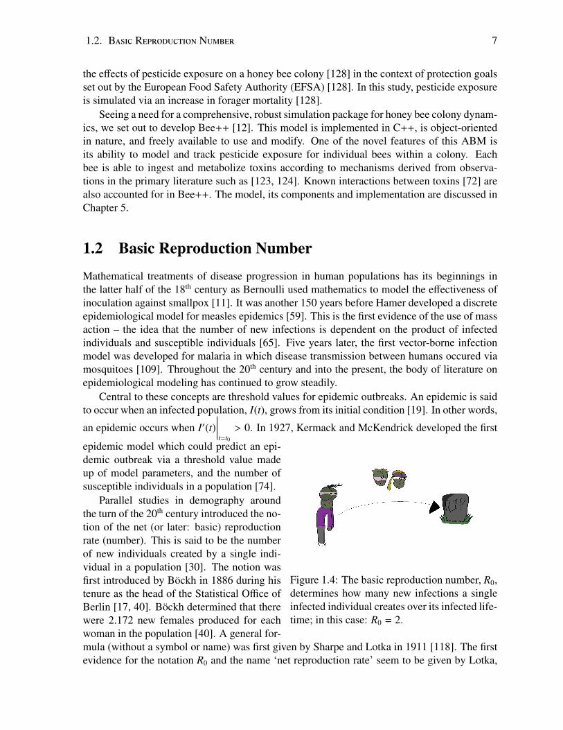
Figure 1.4: The basic reproduction number, R0,determines how many new infections a singleinfected individual creates over its infected life-time; in this case: R0 = 2.

epidemic model which could predict an epi-demic outbreak via a threshold value madeup of model parameters, and the number ofsusceptible individuals in a population [74].

Parallel studies in demography aroundthe turn of the 20th century introduced the no-tion of the net (or later: basic) reproductionrate (number). This is said to be the numberof new individuals created by a single indi-vidual in a population [30]. The notion wasfirst introduced by Bockh in 1886 during histenure as the head of the Statistical Office ofBerlin [17, 40]. Bockh determined that therewere 2.172 new females produced for eachwoman in the population [40]. A general for-mula (without a symbol or name) was first given by Sharpe and Lotka in 1911 [118]. The firstevidence for the notation R0 and the name ‘net reproduction rate’ seem to be given by Lotka,

8 Chapter 1. Introduction

in French (la reproductivite nette), in 1939 [83].The modern usage of R0 – the number of secondary infections created by a single infected

individual over its lifetime – was coined in 1952 by MacDonald as he analyzed malaria out-breaks in the tropics [84]. In this context, R0 can predict an epidemic outbreak as well as allowfor quantitative predictions on effective control measures [63, 94].

The next generation matrix (NGM) is a technique which offers both an intuitive biologi-cal basis and algorithmic mathematical framework for deriving R0 for compartmental diseasemodels [38, 130]. The method of the next generation matrix applies to a system of N ordinarydifferential equations of which M define infected classes. The equations for the infected classesare then linearized about the disease-free equilibrium and divided into two matrix components:the terms which define the influx into the infected classes from uninfected classes are put intoa matrix F. The remaining terms (all other influx terms, say, between infected classes and out-flux from each class) are used to generate a separate matrix, −V . The next generation matrix isthen given by NGM = FV−1. We offer the following clarifying example1 of this process.

A Clarifying ExampleConsider a standard SEIR model in which susceptible members, S , of a population become

exposed2 to an infection, E, who after a period of time then become infectious, I, and finallyeither die or recover from the disease and join the removed class, R. Exposed in this sensemeans that the individual has the disease, but is not contagious. A more apt name for thisclass would be incubator (but I is already being used, alas...). This situation is modeled by thesystem

dSdt

= B − βS I − µS (1.1)

dEdt

= βS I − κE − µE (1.2)

dIdt

= pκE − (d + µ)I (1.3)

dRdt

= (1 − p)κE + dI + µ(S + E + I) (1.4)

where B is a constant birth rate, µ is a natural death rate of the population, β is the contactrate of individuals, 1/κ is the average period of incubation before the individual either becomesinfectious or clears the infection, p is the probability the individual becomes infectious, and dis the death rate of an infectious individual due to disease.

The disease-free equilibrium, (S , E, I,R) = (S ∗, 0, 0, 0), is found using the equationdSdt

= 0. (1.5)

The linearized equations for the infected classes are then written asdEdt

= βS ∗I − (κ + µ)E (1.6)

dIdt

= pκE − (d + µ)I. (1.7)

1This model is based on those appearing in [3, 131].2Exposed in the sense that the disease is incubating and non-infectious

1.2. Basic Reproduction Number 9

From these equations we can generate the two necessary matrices F and −V . The only influxinto the infected classes from non-infected classes is the term βS ∗I. Therefore,

F =

[0 βS ∗

0 0

]. (1.8)

The matrix −V consists of all other terms in the equations for the infected classes. Note thatthe negative sign in front of V causes a sign change in all the terms (i.e. outflux is positive).The matrix −V for this example is

−V =

[κ + µ 0−pκ d + µ

]. (1.9)

The next generation matrix is then given as

FV−1 =

[0 βS ∗

0 0

] (κ + µ)−1 0

pκ(κ + µ) (d + µ)

(d + µ)−1

(1.10)

=

βS ∗pκ

(κ + µ) (d + µ)βS ∗

d + µ

0 0

. (1.11)

As stated above, the primary function of the next generation matrix is to provide the basic

Figure 1.5: The term β ap-pearing in equations (1.1)and (1.2) (and later equation(1.12)) determines the rate atwhich infectious individualsinteract with susceptible in-dividuals

reproduction number for a population model [63]. The basicreproduction number is given by the largest eigenvalue of theNGM, R0 = ρ

(FV−1

)[130]. In the above example, we find that

R0 =βS ∗pκ

(κ + µ) (d + µ).

The number of studies that rely on this method (see [63] forreview) for stability analysis of epidemic models substantiatethe importance of the NGM.

In 2009, Diekmann et al. developed a method for derivingthe NGM directly from model parameters in an intuitive, bio-logically relevant way [37]. This contribution to the scientificliterature also aims to validate different definitions of the NGMnamely, the decomposition described above, and the originalformulation developed by Diekmann in 1990 [39]. A discrep-ancy often arises because the NGM can be constructed so thatan infection moving from, say, a latent phase to infectious phaseis considered a “new infection” [37]. This obviously can lead todiscrepancies with the more biologically relevant formulationsand definitions. Therefore, Diekmann et al. consolidate the ap-proaches and prove conditions under which R0 approximationsare the same.

As biological processes are often multi-layered and com-plex, the systems which model them are often highly nonlinear and as a consequence, using

10 Chapter 1. Introduction

systems of ordinary differential equations is often desired. The theory of ordinary differentialsystems and dynamical systems is rich with tools for approximating and analyzing nonlinearsystems [102–104, 126]. Population structures, when using ODE models are often broken intodiscrete classes or compartments. Often times, a continuum is a more natural structure fora population model. For example, spatial spread and migration are easily modeled by a sec-ond and first derivative respectively [93]; nonlocal infection in either space and/or time canbe modeled by a convolution [137]; and a Levy flight [33] can be modeled by a fractionalderivative.

Such models – whether partial differential equations, integro-differential equations, or both– are infinite dimensional and the theory of the framework provided by the next generationmatrix does not directly apply when attempting to find the basic reproduction number, R0, forthese systems. Instead a continuous operator is required.

Such an operator was first proposed in 1987 by Greenhalgh [56, 57]. Greenhalgh proposedan integral operator and conjectured that its spectral radius would act as a threshold conditionfor stability for an infinite-dimensional population model [56]. This result was then confirmedby Inaba two years later [70]. Contemporaneously, Diekmann defined the next generationoperator (NGO) [39] for populations on a continuum.

Brauer also proposed a method for finding both a next generation operator and basic re-production number for continuous age-structured models [20]. We may extend β in equations(1.1) and (1.2) to a continuous age structure. One susceptible of age a may then be infectedby an infected individual of age a′ at rate β(a, a′). Accounting for infected individuals of allpossible ages leads to the interaction terms

F = S (a)∫ ∞

0β(a, a′)I(a′) da′. (1.12)

For a separable interaction term – one of the form

F = S (a, t)∫ ∞

0β(a, a′)I(a′) da′ (1.13)

= S (a, t)α(a)∫ ∞

0γ(a′)I(a′) da′ (1.14)

– Brauer is able to derive an expression for the basic reproduction number explicitly [20]. Fora general interaction term, the same methods allow for the construction of a next generationoperator [20]. However, this method does not use the FV−1 factorization commonly associatedwith the equivalent discretized, compartmental model.

In 2009, Thieme proved that R0 is the spectral radius of the next generation operator FB−1

for certain classes of infinite dimensional systems (e.g. systems of partial differential equa-tions) [127]. The operators Theime defines are analogous to F and −V in the case of the nextgeneration matrix for finite dimensional compartmental models. Another monumental con-clusion in this work is Thieme’s result on the difference between the spectral radius and thegrowth parameter. Thieme shows that in infinite dimensional models, the exponential growthparameter of infected classes and the spectral radius of the next generation operator will havethe same threshold characteristics, but may be quantitatively different [127].

Thieme’s work was extended by Wang and Zhao in 2012 to include reaction-diffusion mod-els [136]. Aside from proving that the spectral radius of the next generation operator FB−1 is

1.2. Basic Reproduction Number 11

indeed R0 for reaction-diffusion systems, they offer an illustrative example for computing R0

for an SEIR model with diffusion [136].Based on this previous work, the operator factorization for the next generation operator is

guaranteed to exist and provide the basic reproduction number for specific classes of infinite-dimensional systems [127, 136]. The importance of this cannot be understated as infinite-dimensional systems – especially reaction-diffusion systems – are ubiquitous in mathematicalbiology. This is ratified by the fact that such systems are covered in many introductory textsin mathematical biology [2, 22, 23, 82, 93, 98] (see [100, 135] for review). Yet, a closed-formnext generation operator has yet to be determined.

While clearly analogs of one another, a direct connection between the NGM and NGO hasremained elusive. Many formulations of the NGO are constructed ‘intuitively’, using the ideathat the operator should provide the number of secondary infections created by one infectedindividual in its lifetime [38], or by developing an operator with the necessary threshold prop-erties [127]. In Chapter 6, we discuss this connection and show that the NGO can be recoveredas the limit of the NGM. Furthermore, we use this technique to find a closed-form operator forthe NGO for a simple reaction-diffusion system and offer a conjecture which can extend thisoperator to a broader class of models.

Bibliography

[1] Alaux, C., Brunet, J.-L., Dussaubat, C., Mondet, F., Tchamitchan, S., Cousin, M.,Brillard, J., Baldy, A., Belzunces, L. P., and Le Conte, Y. Interactions between Nosemamicrospores and a neonicotinoid weaken honeybees (Apis mellifera). Environmentalmicrobiology 12, 3 (2010), 774–782.

[2] Allen, L. J. Introduction to mathematical biology. Pearson/Prentice Hall, 2007.

[3] Allen, L. J., and Van Den Driessche, P. The basic reproduction number in some discrete-time epidemic models. Journal of Difference Equations and Applications 14, 10-11(2008), 1127–1147.

[4] Allen-Wardell, G., Bernhardt, P., Bitner, R., Burquez, A., Buchmann, S., Cane, J.,Cox, P. A., Dalton, V., Feinsinger, P., Ingram, M., et al. The potential consequences ofpollinator declines on the conservation of biodiversity and stability of food crop yields.Conservation Biology (1998), 8–17.

[5] Anderson, D., and East, I. J. The latest buzz about colony collapse disorder. Science319, 5864 (2008), 724–725.

[6] Anderson, D., and Trueman, J. Varroa jacobsoni (Acari: Varroidae) is more than onespecies. Experimental and Applied Acarology 24, 3 (2000), 165–189.

[7] Aufauvre, J., Biron, D. G., Vidau, C., Fontbonne, R., Roudel, M., Diogon, M., Vigues,B., Belzunces, L. P., Delbac, F., and Blot, N. Parasite-insecticide interactions: a casestudy of Nosema ceranae and fipronil synergy on honeybee. Scientific reports 2 (2012).

[8] Ball, D. W. The chemical composition of honey. J. Chem. Educ 84, 10 (2007), 1643.

[9] Becher, M. A., Grimm, V., Thorbek, P., Horn, J., Kennedy, P. J., and Osborne, J. L.BEEHAVE: a systems model of honeybee colony dynamics and foraging to exploremultifactorial causes of colony failure. Journal of Applied Ecology 51, 2 (2014), 470–482.

[10] Becher, M. A., Osborne, J. L., Thorbek, P., Kennedy, P. J., and Grimm, V. Review:Towards a systems approach for understanding honeybee decline: a stocktaking andsynthesis of existing models. Journal of Applied Ecology 50, 4 (2013), 868–880.

12

BIBLIOGRAPHY 13

[11] Bernoulli, D. Essai dune nouvelle analyse de la mortalite causee par la petite verole etdes avantages de linoculation pour la prevenir. Histoire de l’Acad. Roy. Sci.(Paris) avecMem. des Math. et Phys. and Mem (1760), 1–45.

[12] Betti, M., LeClair, J., Wahl, L. M., and Zamir, M. Bee++: An object-oriented, agent-based simulator for honey bee colonies. Insects 8, 1 (2017), 31.

[13] Betti, M., Wahl, L. M., and Zamir, M. Age structure is critical to the populationdynamics and survival of honeybee colonies. Royal Society Open Science 3, 11 (2016),160444.

[14] Betti, M. I., Wahl, L. M., and Zamir, M. Effects of infection on honey bee populationdynamics: A model. PLOS ONE 9, 10 (2014), e110237.

[15] Betti, M. I., Wahl, L. M., and Zamir, M. Reproduction number and asymptotic stabil-ity for a model with continuous age structure: An application to honey bee dynamics.Bulletin of Mathematical Biology (2016). submitted.

[16] Biesmeijer, J. C., Roberts, S., Reemer, M., Ohlemuller, R., Edwards, M., Peeters, T.,Schaffers, A., Potts, S., Kleukers, R., Thomas, C., et al. Parallel declines in pollinatorsand insect-pollinated plants in Britain and the Netherlands. Science 313, 5785 (2006),351–354.

[17] Bockh, R. Statistisches Jahrbuch der Stadt Berlin, Zwolfter Jahrgang, Statistik desJahres 1884. P Stankiewicz, 1886.

[18] Bowen-Walker, P. L., and Gunn, A. The effect of the ectoparasitic mite, Varroa de-structor on adult worker honeybee (Apis mellifera) emergence weights, water, protein,carbohydrate, and lipid levels. Entomologia Experimentalis et Applicata 101, 3 (2001),207–217.

[19] Brauer, F. The Kermack–McKendrick epidemic model revisited. Mathematical Bio-sciences 198, 2 (2005), 119–131.

[20] Brauer, F., and Castillo-Chavez, C. Mathematical models in population biology andepidemiology, vol. 1. Springer, 2001.

[21] Brittain, C., Williams, N., Kremen, C., and Klein, A.-M. Synergistic effects of non-Apis bees and honey bees for pollination services. Proceedings of the Royal Society ofLondon B: Biological Sciences 280, 1754 (2013), 20122767.

[22] Britton, N. Essential mathematical biology. Springer Science & Business Media, 2012.

[23] Britton, N. F., et al. Reaction-diffusion equations and their applications to biology.Academic Press, 1986.

[24] Calderone, N. W. Insect pollinated crops, insect pollinators and US agriculture: Trendanalysis of aggregate data for the period 1992-2009. PLOS ONE 7, 5 (05 2012), e37235.

14 BIBLIOGRAPHY

[25] Camazine, S., and Sneyd, J. A model of collective nectar source selection by honey bees:self-organization through simple rules. Journal of theoretical Biology 149, 4 (1991),547–571.

[26] Chen, Y., Evans, J. D., Smith, I. B., and Pettis, J. S. Nosema ceranae is a long-presentand wide-spread microsporidian infection of the European honey bee (Apis mellifera) inthe United States. Journal of Invertebrate Pathology 97, 2 (2008), 186–188.

[27] Courchamp, F., Berec, L., and Gascoigne, J. Allee effects in ecology and conservation.Oxford University Press, Oxford, 2008.

[28] Crane, E. The archaeology of beekeeping. Cornell University Press, New York, 1983.

[29] Crittenden, A. N. The importance of honey consumption in human evolution. Foodand Foodways 19, 4 (2011), 257–273.

[30] Cushing, J., and Diekmann, O. The many guises of R0 (a didactic note). Journal ofTheoretical Biology 404 (2016), 295–302.

[31] Daily, G. C. Natures services. Island Press, Washington, DC, 1997.

[32] DeGrandi-Hoffman, G., Roth, S. A., Loper, G., and Erickson, E. H. BEEPOP: a hon-eybee population dynamics simulation model. Ecological modelling 45, 2 (1989), 133–150.

[33] del Castillo-Negrete, D., Carreras, B., and Lynch, V. Front dynamics in reaction-diffusion systems with Levy flights: a fractional diffusion approach. Physical ReviewLetters 91, 1 (2003), 018302.

[34] Dennis, B., and Kemp, W. P. How hives collapse: Allee effects, ecological resilience, andthe honey bee. PLOS ONE 11, 2 (2016), e0150055.

[35] Devillers, J. The ecological importance of honey bees and their relevance to ecotoxi-cology. In Honey Bees: Estimating the Environmental Impact of Chemicals, J. Devillersand M. Pham-Delegue, Eds. Taylor and Francis London, London, 2002, pp. 1–11.

[36] Di Prisco, G., Pennacchio, F., Caprio, E., Boncristiani Jr, H. F., Evans, J. D., and

Chen, Y. Varroa destructor is an effective vector of Israeli acute paralysis virus in thehoneybee, Apis mellifera. Journal of General Virology 92, 1 (2011), 151–155.

[37] Diekmann, O., Heesterbeek, J., and Roberts, M. The construction of next-generationmatrices for compartmental epidemic models. Journal of the Royal Society Interface(2009), rsif20090386.

[38] Diekmann, O., and Heesterbeek, J. A. P. Mathematical epidemiology of infectious dis-eases: model building, analysis and interpretation, vol. 5. John Wiley & Sons, 2000.

[39] Diekmann, O., Heesterbeek, J. A. P., and Metz, J. A. On the definition and the computa-tion of the basic reproduction ratio R0 in models for infectious diseases in heterogeneouspopulations. Journal of mathematical biology 28, 4 (1990), 365–382.

BIBLIOGRAPHY 15

[40] Dietz, K. The estimation of the basic reproduction number for infectious diseases.Statistical methods in medical research 2, 1 (1993), 23–41.

[41] Eberl, H. J., Frederick, M. R., and Kevan, P. G. Importance of brood maintenanceterms in simple models of the honeybee - Varroa destructor - Acute Bee Paralysis Viruscomplex. Electronic Journal of Differential Equations (EJDE) [electronic only] 2010(2010), 85–98.

[42] Eckert, J., Friedhoff, K. T., and Zahner, H. Lehrbuch der Parasitologie fur die Tier-medizin. Georg Thieme Verlag, 2008.

[43] Eckert, J. E. The flight range of the honeybee. Journal of Agricultural Research (1933).

[44] Ellis, J. D., Evans, J. D., and Pettis, J. Colony losses, managed colony population de-cline, and colony collapse disorder in the United States. Journal of Apicultural Research49, 1 (2010), 134–136.

[45] Engel, M. S. The taxonomy of recent and fossil honey bees (Hymenoptera: Apidae;Apis). Journal of Hymenoptera Research 8, 2 (1999), 165–196.

[46] Evans, J. D., and Wheeler, D. E. Differential gene expression between developingqueens and workers in the honey bee, apis mellifera. Proceedings of the NationalAcademy of Sciences 96, 10 (1999), 5575–5580.

[47] Fahrbach, S., and Robinson, G. Juvenile hormone, behavioral maturation and brainstructure in the honey bee. Developmental Neuroscience 18 (1996), 102–114.

[48] Fenoy, S., Rueda, C., Higes, M., Martın-Hernandez, R., and Del Aguila, C. High-levelresistance of Nosema ceranae, a parasite of the honeybee, to temperature and desicca-tion. Applied and environmental microbiology 75, 21 (2009), 6886–6889.

[49] Forsgren, E., and Fries, I. Comparative virulence of Nosema ceranae and Nosema apisin individual European honey bees. Veterinary parasitology 170, 3 (2010), 212–217.

[50] Fries, I. Nosema apisa parasite in the honey bee colony. Bee World 74, 1 (1993), 5–19.

[51] Gaines-Day, H. R., and Gratton, C. Crop yield is correlated with honey bee hive den-sity but not in high-woodland landscapes. Agriculture, Ecosystems & Environment 218(2016), 53–57.

[52] Garibaldi, L. A., Steffan-Dewenter, I., Winfree, R., Aizen, M. A., Bommarco, R.,Cunningham, S. A., Kremen, C., Carvalheiro, L. G., Harder, L. D., Afik, O., et al.Wild pollinators enhance fruit set of crops regardless of honey bee abundance. Science339, 6127 (2013), 1608–1611.

[53] Gisder, S., Aumeier, P., and Genersch, E. Deformed wing virus: replication and viralload in mites (Varroa destructor). Journal of General Virology 90, 2 (2009), 463–467.

[54] Gould, J. L., Gould, C. G., et al. The honey bee. Scientific American Library, 1988.

16 BIBLIOGRAPHY

[55] Goulson, D., Nicholls, E., Botıas, C., and Rotheray, E. L. Bee declines driven by com-bined stress from parasites, pesticides, and lack of flowers. Science 347, 6229 (2015),1255957.

[56] Greenhalgh, D. Analytical results on the stability of age-structured recurrent epidemicmodels. Mathematical Medicine and Biology 4, 2 (1987), 109–144.

[57] Greenhalgh, D. Threshold and stability results for an epidemic model with an age-structured meeting rate. Mathematical Medicine and Biology 5, 2 (1988), 81–100.

[58] Gregory, P. G., Evans, J. D., Rinderer, T., and De Guzman, L. Conditional immune-gene suppression of honeybees parasitized by Varroa mites. Journal of Insect Science5, 7 (2005), 1–5.

[59] Hamer, W. H. Epidemic disease in England. Lancet 1 (1906), 733–739.

[60] Harbo, J. R. Effect of population size on brood production, worker survival and honeygain in colonies of honeybees. Journal of Apicultural Research 25, 1 (1986), 22–29.

[61] Harris, J. A model of honeybee colony population dynamics. Journal of ApiculturalResearch 24, 4 (1985), 228–236.

[62] Hauk, G. Toward Saving the Honeybee. Steiner Books, Oregon, 2002.

[63] Heffernan, J., Smith, R., and Wahl, L. M. Perspectives on the basic reproductive ratio.Journal of the Royal Society Interface 2, 4 (2005), 281–293.

[64] Henry, M., Beguin, M., Requier, F., Rollin, O., Odoux, J.-F., Aupinel, P., Aptel, J.,Tchamitchian, S., and Decourtye, A. A common pesticide decreases foraging successand survival in honey bees. Science 336, 6079 (2012), 348–350.

[65] Hethcote, H. W. The mathematics of infectious diseases. SIAM review 42, 4 (2000),599–653.

[66] Higes, M., Martin-Hernandez, R., Botias, C., Bailon, E. G., Gonzalez-Porto, A. V.,and Barrios, L. How natural infection by Nosema ceranae causes honeybee colonycollapse. Environmental microbiology 10, 10 (2008), 2659–2669.

[67] Higes, M., Martin-Hernandez, R., Garrido-Bailon, E., Gonzalez-Porto, A. V., Garcia-Palencia, P., and Meana, A. Honeybee colony collapse due to Nosema ceranae in pro-fessional apiaries. Environmental Microbiology Reports 1, 2 (2009), 110–113.

[68] Huang, W.-F., Solter, L. F., Yau, P. M., and Imai, B. S. Nosema ceranae escapes fumag-illin control in honey bees. PLOS Pathog 9, 3 (2013), e1003185.

[69] Huang, Z.-Y., and Robinson, G. E. Regulation of honey bee division of labor by colonyage demography. Behavioral Ecology and Sociobiology 39 (1996), 147–158.

[70] Inaba, H. Threshold and stability results for an age-structured epidemic model. Journalof mathematical biology 28, 4 (1990), 411–434.

BIBLIOGRAPHY 17

[71] Javorek, S., Mackenzie, K., and Vander Kloet, S. Comparative pollination effectivenessamong bees (Hymenoptera: Apoidea) on lowbush blueberry (Ericaceae: Vacciniumangustifolium). Annals of the Entomological Society of America 95, 3 (2002), 345–351.

[72] Johnson, R. M., Dahlgren, L., Siegfried, B. D., and Ellis, M. D. Acaricide, fungicideand drug interactions in honey bees (Apis mellifera). PLOS ONE 8, 1 (2013), e54092.

[73] Kauffeld, N. M. Beekeeping in the United States Agriculture Handbook Number 335.U.S. Department of Agriculture, 1980.

[74] Kermack, W. O., and McKendrick, A. G. A contribution to the mathematical theory ofepidemics. Proceedings of the Royal Society of London A: mathematical, physical andengineering sciences 115, 772 (1927), 700–721.

[75] Khoury, D. S., Barron, A. B., and Myerscough, M. R. Modelling food and populationdynamics in honey bee colonies. PLOS ONE 8, 5 (05 2013), e59084.

[76] Khoury, D. S., Myerscough, M. R., and Barron, A. B. A quantitative model of honeybee colony population dynamics. PLOS ONE 6, 4 (04 2011), e18491.

[77] Klatt, B. K., Holzschuh, A., Westphal, C., Clough, Y., Smit, I., Pawelzik, E., and

Tscharntke, T. Bee pollination improves crop quality, shelf life and commercial value.Proc. R. Soc. B 281, 1775 (2014), 20132440.

[78] Klein, A.-M., Vaissiere, B. E., Cane, J. H., Steffan-Dewenter, I., Cunningham, S. A.,Kremen, C., and Tscharntke, T. Importance of pollinators in changing landscapes forworld crops. Proceedings of the Royal Society of London B: Biological Sciences 274,1608 (2007), 303–313.

[79] Kremen, C., Williams, N. M., and Thorp, R. W. Crop pollination from native bees atrisk from agricultural intensification. Proceedings of the National Academy of Sciences99, 26 (2002), 16812–16816.

[80] Kulhanek, K., Steinhauer, N., Rennich, K., Caron, D. M., Sagili, R. R., Pettis, J. S.,Ellis, J. D., Wilson, M. E., Wilkes, J. T., Tarpy, D. R., et al. A national survey ofmanaged honey bee 2015–2016 annual colony losses in the usa. Journal of ApiculturalResearch (2017), 1–13.

[81] Leoncini, I., Le Conte, Y., Costagliola, G., Plettner, E., Toth, A. L., and Wang, M.Regulation of behavioral maturation by a primer pheromone produced by adult workerhoney bees. Proceedings of the National Academy of Sciences of the United States ofAmerica 101, 50 (2004), 17559–17564.

[82] Li, J., and Brauer, F. Continuous-time age-structured models in population dynamicsand epidemiology. In Mathematical Epidemiology, F. Brauer, P. van den Driessche, andJ. Wu, Eds. Springer, 2008, pp. 205–227.

[83] Lotka, A. J. Theorie analytique des associations biologiques: analyse demographiqueavec application particuliere a l’espece humaine. Hermann, 1939.

18 BIBLIOGRAPHY

[84] Macdonald, G. The analysis of equilibrium in malaria. Tropical diseases bulletin 49, 9(1952), 813–829.

[85] Maleszka, R. Epigenetic integration of environmental and genomic signals in honeybees: the critical interplay of nutritional, brain and reproductive networks. Epigenetics3, 4 (2008), 188–192.

[86] Martin, S. Hygienic behaviour: an alternative view. Bee Improvement 7 (2000), 6–7.

[87] Martin, S. Biology and life-history of Varroa mites. Mites of the honey bee. Dadant &

Sons, Hamilton, IL (2001), 131–148.

[88] Martin, S. J. The role of Varroa and viral pathogens in the collapse of honeybeecolonies: a modelling approach. Journal of Applied Ecology 38, 5 (2001), 1082–1093.

[89] Martın-Hernandez, R., Botıas, C., Barrios, L., Martınez-Salvador, A., Meana, A.,Mayack, C., and Higes, M. Comparison of the energetic stress associated with experi-mental Nosema ceranae and Nosema apis infection of honeybees (Apis mellifera). Par-asitology research 109, 3 (2011), 605–612.

[90] Martın-Hernandez, R., Meana, A., Garcıa-Palencia, P., Marın, P., Botıas, C., Garrido-Bailon, E., Barrios, L., and Higes, M. Effect of temperature on the biotic potential ofhoneybee microsporidia. Applied and Environmental Microbiology 75, 8 (2009), 2554–2557.

[91] Michener, C. D. The bees of the world. JHU press, Maryland, 2000.

[92] Murilhas, A. M., et al. Varroa destructor infestation impact on Apis mellifera carnicacapped worker brood production, bee population and honey storage in a Mediterraneanclimate. Apidologie 33, 3 (2002), 271–282.

[93] Murray, J. D. Mathematical Biology II: Spatial Models and Biomedical Applications.Springer-Verlag New York Incorporated, 2001.

[94] Murray, J. D. Mathematical Biology I: An Introduction. Springer, New York, NY, USA,,2002.

[95] Nazzi, F., Brown, S. P., Annoscia, D., Del Piccolo, F., Di Prisco, G., Varricchio, P.,Della Vedova, G., Cattonaro, F., Caprio, E., and Pennacchio, F. Synergistic parasite-pathogen interactions mediated by host immunity can drive the collapse of honeybeecolonies. PLOS Pathog 8, 6 (2012), e1002735.

[96] Oldroyd, B. P., and Ratnieks, F. L. Evolution of worker sterility in honey-bees (apismellifera): how anarchistic workers evade policing by laying eggs that have low removalrates. Behavioral Ecology and Sociobiology 47, 4 (2000), 268–273.

[97] Omholt, S. W. A model for intracolonial population dynamics of the honeybee in tem-perate zones. Journal of Apicultural Research 25, 1 (1986), 9–21.

BIBLIOGRAPHY 19

[98] Otto, S. P., and Day, T. A biologist’s guide to mathematical modeling in ecology andevolution, vol. 13. Princeton University Press, 2007.

[99] Paiva, J. P. L. M., Paiva, H. M., Esposito, E., and Morais, M. M. On the effects ofartificial feeding on bee colony dynamics: A mathematical model. PLOS ONE 11, 11(2016), e0167054.

[100] Pastor-Satorras, R., Castellano, C., Van Mieghem, P., and Vespignani, A. Epidemicprocesses in complex networks. Reviews of modern physics 87, 3 (2015), 925.

[101] Paxton, R. J., Klee, J., Korpela, S., and Fries, I. Nosema ceranae has infected Apismellifera in Europe since at least 1998 and may be more virulent than Nosema apis.Apidologie 38, 6 (2007), 558–565.

[102] Perko, L. Differential equations and dynamical systems, vol. 7. Springer Science &Business Media, 2013.

[103] Polyanin, A. D., and Zaitsev, V. F. Exact solutions for ordinary differential equations.Campman and Hall/CRC 2 (1995).

[104] Protter, P. Stochastic differential equations. In Stochastic Integration and DifferentialEquations. Springer, 1990, pp. 187–284.

[105] Ratti, V., Kevan, P. G., and Eberl, H. J. A mathematical model for population dynamicsin honeybee colonies infested with Varroa destructor and the Acute Bee Paralysis Virus.Canadian Applied Mathematics Quarterly 21, 1 (2013), 63–93.

[106] Ratti, V., Kevan, P. G., and Eberl, H. J. A mathematical model of the honeybee-Varroadestructor-Acute Bee Paralysis Virus complex with seasonal effects. Bulletin of Math-ematical Biology (2015).

[107] Riley, J. R., Greggers, U., Smith, A. D., Reynolds, D. R., and Menzel, R. The flightpaths of honeybees recruited by the waggle dance. Nature 435, 7039 (2005), 205–207.

[108] Robinson, G. E., Page, R. E., Strambi, C., and Strambi, A. Colony integration in honeybees: mechanisms of behavioral reversion. Ethology 90, 4 (1992), 336–348.

[109] Ross, R. The prevention of malaria. Dutton, 1910.

[110] Roubik, D. W. Pollination of cultivated plants in the tropics. No. 118. Food & Agricul-ture Org., 1995.

[111] Roubik, D. W., and Wolda, H. Do competing honey bees matter? dynamics and abun-dance of native bees before and after honey bee invasion. Population Ecology 43, 1(2001), 53–62.

[112] Rowland, C., and McLellan, A. A simple mathematical model of brood production inhoneybee colonies. Journal of Apicultural Research 21, 3 (1982), 157–160.

20 BIBLIOGRAPHY

[113] Sakagami, S., and Fukuda, H. Life tables for worker honeybees. Researches on Popu-lation Ecology 10, 2 (1968), 127–139.

[114] Sammataro, D., Gerson, U., and Needham, G. Parasitic mites of honey bees: life history,implications, and impact. Annual review of entomology 45, 1 (2000), 519–548.

[115] Seehuus, S.-C., Norberg, K., Gimsa, U., Krekling, T., and Amdam, G. V. Reproductiveprotein protects functionally sterile honey bee workers from oxidative stress. Proceed-ings of the National Academy of Sciences of the United States of America 103, 4 (2006),962–967.

[116] Seeley, T. D. Honeybee Democracy. Princeton University Press, 2010.

[117] Seeley, T. D., and Visscher, P. K. Survival of honeybees in cold climates: the criticaltiming of colony growth and reproduction. Ecological Entomology 10, 1 (1985), 81–88.

[118] Sharpe, F. R., and Lotka, A. J. A problem in age-distribution. The London, Edinburgh,and Dublin Philosophical Magazine and Journal of Science 21, 124 (1911), 435–438.

[119] Skinner, M. Bee brood consumption: an alternative explanation for hypervitaminosis Ain KNM-ER 1808 (Homo erectus) from Koobi Fora, Kenya. Journal of Human Evolu-tion 20, 6 (1991), 493–503.

[120] Smith, M. L. The honey bee parasite Nosema ceranae: Transmissible via food ex-change? PLOS ONE 7, 8 (08 2012), e43319.

[121] Southwick, E. E., and Southwick Jr, L. Estimating the economic value of honey bees(Hymenoptera: Apidae) as agricultural pollinators in the United States. Journal of Eco-nomic Entomology 85, 3 (1992), 621–633.

[122] Stevanovic, J., Simeunovic, P., Gajic, B., Lakic, N., Radovic, D., Fries, I., and Stan-imirovic, Z. Characteristics of Nosema ceranae infection in Serbian honey bee colonies.Apidologie 44, 5 (2013), 522–536.

[123] Suchail, S., De Sousa, G., Rahmani, R., and Belzunces, L. P. In vivo distribution andmetabolisation of 14C-imidacloprid in different compartments of Apis mellifera L. Pestmanagement science 60, 11 (2004), 1056–1062.

[124] Suchail, S., Debrauwer, L., and Belzunces, L. P. Metabolism of imidacloprid in Apismellifera. Pest management science 60, 3 (2004), 291–296.

[125] Sumpter, D. J. T., and Martin, S. J. The dynamics of virus epidemics in Varroa-infestedhoney bee colonies. Journal of Animal Ecology 73, 1 (2004), 51–63.

[126] Teschl, G. Ordinary differential equations and dynamical systems, vol. 140. AmericanMathematical Society Providence, 2012.

[127] Thieme, H. R. Spectral bound and reproduction number for infinite-dimensional pop-ulation structure and time heterogeneity. SIAM Journal on Applied Mathematics 70, 1(2009), 188–211.

BIBLIOGRAPHY 21

[128] Thorbek, P., Campbell, P. J., Sweeney, P. J., and Thompson, H. M. Using BEEHAVEto explore pesticide protection goals for European honeybee (Apis melifera L.) workerlosses at different forage qualities. Environmental Toxicology and Chemistry (2016).

[129] Torchio, P. F. Diversification of pollination strategies for US crops. EnvironmentalEntomology 19, 6 (1990), 1649–1656.

[130] Van den Driessche, P., and Watmough, J. Reproduction numbers and sub-thresholdendemic equilibria for compartmental models of disease transmission. Mathematicalbiosciences 180, 1 (2002), 29–48.

[131] Van den Driessche, P., and Watmough, J. Further notes on the basic reproduction num-ber. In Mathematical Epidemiology. Springer, 2008, pp. 159–178.

[132] van Engelsdorp, D., Evans, J. D., Saegerman, C., Mullin, C., Haubruge, E., Nguyen,B. K., Frazier, M., Frazier, J., Cox-Foster, D., Chen, Y., Underwood, R., Tarpy, D. R.,and Pettis, J. S. Colony collapse disorder: A descriptive study. PLOS ONE 4, 8 (082009), e6481.

[133] Vasquez, A., and Olofsson, T. C. The lactic acid bacteria involved in the production ofbee pollen and bee bread. Journal of apicultural research 48, 3 (2009), 189–195.

[134] Vidau, C., Diogon, M., Aufauvre, J., Fontbonne, R., Vigues, B., Brunet, J.-L., Texier,C., Biron, D. G., Blot, N., El Alaoui, H., et al. Exposure to sublethal doses of fiproniland thiacloprid highly increases mortality of honeybees previously infected by Nosemaceranae. PLOS ONE 6, 6 (2011), e21550.

[135] Volpert, V., and Petrovskii, S. Reaction–diffusion waves in biology. Physics of lifereviews 6, 4 (2009), 267–310.

[136] Wang, W., and Zhao, X.-Q. Basic reproduction numbers for reaction-diffusion epidemicmodels. SIAM Journal on Applied Dynamical Systems 11, 4 (2012), 1652–1673.

[137] Wang, Z.-C., and Wu, J. Travelling waves of a diffusive Kermack–McKendrick epi-demic model with non-local delayed transmission. In Proceedings of the Royal Societyof London A: Mathematical, Physical and Engineering Sciences (2009), The Royal So-ciety, p. rspa20090377.

[138] Watanabe, M. E. Pollination worries rise as honey bees decline. Science 265, 5176(1994), 1170–1171.

[139] Watanabe, M. E. Colony collapse disorder: Many suspects, no smoking gun. BioScience58, 5 (2008), 384–388.

[140] Winston, M. The biology of the honey bee. Harvard University Press, 1987.

[141] Yamada, T., et al. Honeybee colony collapse disorder. Emerging Biological Threats: AReference Guide 13 (2009), 141.

Chapter 2

Effects of Infection on Honey BeePopulation Dynamics: A Model

Abstract

We propose a model which combines the dynamics of the spread of disease within a beecolony with the underlying demographic dynamics of the colony to determine the ulti-mate fate of the colony under different scenarios. The model suggests that key factorsin the survival or collapse of a honey bee colony in the face of an infection are the rateof transmission of the infection and the disease-induced death rate. An increase in thedisease-induced death rate, which can be thought of as an increase in the severity of thedisease, may actually help the colony overcome the disease and survive through winter.By contrast, an increase in the transmission rate, which means that bees are being infectedat an earlier age, has a drastic deleterious effect. Another important finding relates to thetiming of infection in relation to the onset of winter, indicating that in a time interval ofapproximately 20 days before the onset of winter the colony is most affected by the onsetof infection. The results suggest further that the age of recruitment of hive bees to forag-ing duties is a good early marker for the survival or collapse of a honey bee colony in theface of infection, which is consistent with experimental evidence but the model providesinsight into the underlying mechanisms. The most important result of the study is a cleardistinction between an exposure of the honey bee colony to an environmental hazard suchas pesticides or insecticides, or an exposure to an infectious disease. The results indicateunequivocally that in the scenarios which we have examined, and perhaps more gener-ally, an infectious disease is far more hazardous to the survival of a bee colony than anenvironmental hazard which causes an equal death rate in foraging bees.

2.1 IntroductionThe widespread collapse of honey bee colonies has been the subject of much discussion andresearch in recent years [15, 34, 35]. Aside from their ecological importance [5], honey beepopulations have a large economical impact on agriculture in North America, Europe, theMiddle East, and Japan [2, 23, 31].

The focus of research has been largely on environmental factors outside the hive, such aspesticides or insecticides, which may cause death or injury to foraging bees and jeopardize

22

2.1. Introduction 23

their return to the hive. The reduced number of foraging bees then leads to younger hive beesbeing recruited prematurely to perform foraging duties and this chain reaction ultimately leadsto a disruption in the dynamics of the colony as a whole. Examples of this scenario would beproduced by the effects of various pesticides to which foraging bees are exposed in the courseof their duties [12, 35]. Other factors in the same category include possible disruptions to thebees’ navigation system by mobile phones or other electronic devices, again to the effect ofjeopardizing their return to the hive and thereby reducing their numbers [8].

A key element in this category of disruption to honey bee population dynamics is the un-timely death of a certain proportion of foraging bees outside the hive and the consequences ofthis on the colony as a whole. An important question here concerns the threshold in the deathrate of foraging bees that would determine the survival or collapse of the bee colony. This wasexamined recently in two papers by Khoury et al. [20, 21].

In the present paper we consider a different category of disruption to the healthy dynamicsof a bee colony, namely one in which the key hazard is an infection by a communicable diseaseacquired by foraging bees outside the hive. The key difference here is that foraging bees thathave been infected would then transport the disease into the hive and go on to infect othermembers of the colony within the hive. Here too the affected bees will ultimately suffer anuntimely death, but the effects on the dynamics of the colony are clearly more complex becausethe infection in this case may now involve all members of the colony. We sought a model thatwould allow a comparison between the effects of these two categories of hazards (pesticideversus infection) on the ultimate fate of the bee colony.

Disease in honey bee colonies has been studied previously by Sumpter et al. [33] whomodeled the effects of Varroa mites on the brood and on the adult worker bees. The focus ofthe model was on the relationship between the mite population within a hive and its role invirus transmission within the hive. A study by Ratti et al. [24] examined the transmission ofviruses via Varroa mites, using an SIR-framework with the mites as vectors for transmission.

In the present paper we propose a more general model which combines the normal dy-namics of a honey bee colony with the dynamics of an infectious disease which is acquiredoutside the hive but ultimately spreads to the rest of the colony. As a working example, we usea disease known as Nosema which is a common disease affecting both hive bees and foragingbees [9]. Nosema is caused by a microsporidian with two common species: Nosema ceranaeand Nosema apis. The former was first discovered in Asian honey bees (Apis ceranae) and thelatter is common among European honey bees (Apis mellifera). A key factor in the collapse ofhoney bee colonies in recent years is thought to be the introduction of Nosema ceranae to Apismellifera [14].

The main aim of the model is to provide a general tool for determining the ultimate fate ofa honey bee colony under this fairly common hazard. In particular, we identify key variablesthat determine the collapse or survival of the bee colony, namely the severity of the disease andthe rate of transmission, and examine different scenarios using different combinations of thesevariables. Winter is an important phase in the normal demographic dynamics of a bee colony;the queen lays fewer eggs and foraging bees return to and remain within the hive [19, 29].Therefore, the time interval between the onset of disease and the onset of winter may play acritical role in the ultimate survival or collapse of the colony in the face of an infection. Weshow that the model can be used to explore potential markers of the presence of the diseasewithin the bee colony and of the ultimate fate of the colony under different scenarios.

24 Chapter 2. Effects of Infection on Honey Bee Population Dynamics: A Model

2.2 Background

2.2.1 Normal Demographics of a Honey Bee Colony

Honey bee colonies are complex societies in which different members of the colony have spe-cialized functions that serve the entire colony, thus making members of the colony highlydependent on each other.

The queen can live up to three years, is responsible for laying eggs, and during peak seasonmay lay up to 2000 eggs per day [4]. In this function the queen is dependent on workerbees [36]. The worker bees emerge from fertilized eggs of the queen and consist of femaleswho maintain the hive and gather resources, and males who mate with the queen to producemore eggs [28]. Drones are born from unfertilized eggs of the queen [28] and typically makingup less than 5% of the hive population [17, 28]. Because they do not contribute to the colonywork force, and because of their small numbers, they are generally neglected when consideringthe dynamics of the colony as a whole.

Female hive bees, following a transition period, leave the hive to start foraging duties andusually forage until their death. The age at which they start foraging duties is variable, de-pending on the state of the colony and its needs. If the number of forager bees is lower thanis required for meeting the colony needs, hive bees will begin foraging duties at a youngerage [16]. If the number of forager bees is higher than required, behavioural maturation of hivebees will be regulated by a pheromone, ethyl oleate, produced by the foragers. This process isusually referred to as “social inhibition” [22]. Similarly, if the number of hive bees is too low,it is possible for foragers to revert back to hive bee duties [16].

As the temperature drops outside the hive, foraging becomes less frequent, the queen beginsto lay fewer eggs [36], and drones are expelled from the hive to save hive resources [28]. Whenthe temperature drops below a certain threshold, the colony enters a winter phase in whichthe queen will cease to lay eggs [19] and any remaining foraging bees will return to the hive.During winter the entire hive population surrounds the queen in order to maintain a temperatureof 34 − 36◦C within the hive [28].

2.2.2 Nosema Infection

Nosema, also known as “Nosemosis”, is an infection affecting honey bees that is spread by themicrosporidian parasites in the Nosema family. Nosema ceranae is of particular interest, as itis thought to be linked to colony collapse incidents [13, 14]. We use this disease only as anexample to illustrate the utility of the model. The choice was motivated by the availability ofparameter values which allowed us to examine some realistic scenarios of the dynamics of thebee colony in the presence of infection.

Within the bee colony, Nosema is typically spread via fecal-oral transmission. Adult beeswill contract Nosema either from eating food contaminated by infected bees, or while riddingthe hive of infected fecal matter [3]. There is also evidence that Nosema can be spread viaoral-oral transmission, through feeding [30].

While it is typically asymptomatic at the level of individual bees, Nosema has some symp-toms that can be observed at the colony level [9, 32]. Stevanovic et al. [32] observed in 2013

2.3. Mathematical Model 25

that colonies infected by the parasite Nosema ceranae exhibited many of the classic signs thatprecede colony collapse.

Much of the experimental research linking Nosema infection to colony collapse is based oncorrelated observations, but direct cause and effect evidence is lacking [9]. Our model aims toprovide a possible mechanism for this linkage in terms of the interplay between the dynamicsof the infection and the normal dynamics of the honey bee colony.

2.3 Mathematical ModelIn what follows we present a mathematical model that combines the normal demographic dy-namics of a honey bee colony with the dynamics of an infection affecting foraging bees outsidethe hive at first and then spreading to the rest of the colony. We follow a model for the basicdynamics of a bee colony in the absence of disease presented recently by Khoury et al. [20, 21],in which the adult bee population is divided into a number of hive bees H, and a number offoraging bees F. In the model to be described below we extend this division into four cate-gories, namely susceptible hive bees HS , infected hive bees HI , susceptible foraging bees FS ,and infected foraging bees FI . Equations governing each of these four populations during theactive and winter seasons are presented in the following section.

2.3.1 Governing Equations: Active SeasonThe rate of change in time t (days) of the susceptible hive bee population HS during the activeseason is assumed to be governed by

dHS

dt= LS − HS R − (βHHHI + βHF FI) HS . (2.1)

In the first term on the right L is the queen’s egg laying rate per day and S is the proportion ofthose eggs that survive both larval and pupal stages to yield mature bees. This proportion is afunction of the total number of hive bees and of the amount of food f available within the hivebecause the brood requires food as well as a sufficient number of supporting hive bees in orderto survive [18]. Following [20] we take

S =

(HS + HI

w + HS + HI

) (f

b + f

). (2.2)

This function is constructed such that the value of S saturates at 1.0 in the limiting case whenthe amount of food f and the total number of hive bees HS + HI are sufficiently large to ensurethe survival of 100% of the eggs laid by the queen. The parameters b and w determine at whatvalues of f and HS + HI this saturation occurs and they will be discussed later.

In the second term on the right of Eq. 2.1, R is the proportion of maturing hive bees HS thatare being recruited to foraging duties. As discussed earlier, and following [20], we assume thatrecruitment is increased when either food stores or forager populations are low and recruitmentis reduced when food stores and forager populations are in excess. Note that in an overabun-dance of foragers, R may become negative, which implies that foragers are reverting to hive

26 Chapter 2. Effects of Infection on Honey Bee Population Dynamics: A Model

duties.

R = Rb + α f

(b

b + f

)− αF

(FI + FS

N

)(2.3)

where Rb is the baseline recruitment rate in the absence of foragers but sufficient food stores,α f is a weighting of the effect of low food, αF is a weighting of the effect of excess foragers onrecruitment, and N = FI + FS + HS + HI is the colony adult population size. The Average Ageof Recruitment to Foraging (AARF) at any point in time is equal to 1/R.

The last term in Eq. 2.1 determines the rate at which susceptible hive bees become infected.The transmission rate per day per susceptible hive bee is given by (βHHHI + βHF FI), where βHH

is the contact rate between hive bees and βHF is that between hive bees and foraging bees.Hive bees are safe within the hive environment under normal circumstances, surviving up

to 6 months over winter [21, 28]. It is therefore assumed that the natural death rate of hive beesis negligible compared to their recruitment rate to foraging duties.

For the rate of change of the infected hive bee population, we take

dHI

dt= (βHHHI + βHF FI) HS − HIR − dHHI . (2.4)

Infected hive bees continue to be recruited to foraging duties but, unlike their healthy counter-parts, they are at risk of dying from the disease before they do so; dH is the rate at which thisoccurs.

Susceptible foragers are recruited from susceptible hive bees and may subsequently suffernatural death, at a rate m, or become infected. Their rate of change is therefore governed by

dFS

dt= HS R − mFS − (βHF HI + βFF FI) FS . (2.5)

Infected foragers are recruited from infected hive bees or are susceptible foragers that havebecome infected. If the death rate from the infection is assumed to be dF then their rate ofchange is governed by

dFI

dt= HIR + (βHF HI + βFF FI) FS − (m + dF) FI . (2.6)

Food is brought into the hive by foragers, either healthy or infected. Although infected for-agers may forage less efficiently, for simplicity we assume the same foraging rate, c (gm/day)per forager. The collected food is then consumed by both foragers and hive bees and forsimplicity again we assume the same consumption rate, γA (gm/day). The amount of foodconsumed by the larvae is substantial. We assume that the number of larvae is proportional tothe number of surviving eggs and that the larvae consume food at a rate of γL (gm/day). Theamount of food available at time t is thus given by

d fdt

= c(FS + FI) − γAN − γLLS . (2.7)

The full dynamics of the bee colony are thus governed by Eqs. 2.1, 2.4, 2.5, 2.6 and 2.7to be solved simultaneously. A compartmental diagram of these dynamics is shown in Figure2.3.1.

2.3. Mathematical Model 27

HS

HI

FS

FI

dH dF

m

m

Figure 2.1: A compartmental diagram of the dynamics of the honey bee colony combined withthe dynamics of an infectious disease. The susceptible and infected hive bees, HS and HI livewithin the hive. New susceptible hive bees are generated by surviving brood through the sur-vival function, S . New infected hive bees are generated through interactions of susceptiblehive bees with infected hive bees and infected foragers at rates βHH and βHF . Hive bees arerecruited to foraging duties through the recruitment function R, which also allows for the re-versal of duties, from foraging to hive duties. Foragers move into the infected compartmentvia interactions with infected hive bees and infected foragers at rates βHF and βFF . All infectedbees die at rates dH or dF , and foragers die naturally at rate m.

2.3.2 Governing Equations: Winter

During winter the rate of egg laying by the queen is considerably diminished, and in harshclimates the queen may cease laying eggs completely [19]. For simplicity, in our model simu-lations therefore we take L = 0 for the winter season.

Foraging resources become scarce in winter and foraging bees return to the hive to join hivebees in their effort to keep the hive warm [19]. The two groups thus perform the same dutiesin winter and there is no longer any recruitment from hive to foraging duties. We therefore setR = 0, although we maintain the separate identities of the two groups in the model in order totrack the behaviors of bees that were foraging before winter against those that were hive bees.

Since there is no foraging in winter, food production halts and we set c = 0. Also, beesare able to survive longer in winter than they do outside the hive during the active season [26].Thus the new natural death rate for both hive bees and foraging bees during the winter season

28 Chapter 2. Effects of Infection on Honey Bee Population Dynamics: A Model

is set to be mW .Introducing these changes into the equations governing the dynamics of the colony (Eqs.

2.1, 2.4, 2.5, 2.6, 2.7) we obtain the corresponding equations for the winter season:

dHS

dt= −mW HS − (βHHHI + βHF FI) HS (2.8)

dFS

dt= −mW FS − (βHF HI + βFF FI) FS (2.9)

dHI

dt= (βHHHI + βHF FI) HS − (mW + dH)HI (2.10)

dFI

dt= (βHF HI + βFF FI) FS − (mW + dF)FI (2.11)

d fdt

= −γAN − γLLS (2.12)

2.3.3 Parameter ValuesThe model presented in Section 2.3 contains a total of 13 parameters. Of these, 10 parametersrelate to the baseline demographic dynamics of a honey bee colony, in the absence of disease,for which empirical estimates are available in the literature. In particular, we consider a beecolony in which the maximum rate (L in Eq. 4.10) of egg laying by the queen is 2000 eggs/dayand take w = 5000 [21]. Hive bees spend, on average, a minimum of 4 days in the hive beforebeing recruited to foraging duties [7], and foragers will not revert to hive duties unless one-third of the bee population is foraging [21]. Based on these values, and following [21], wetake Rb = 0.25 and α f = 0.75. In the complete absence of food, recruitment of foragers willdouble [27], thus we take αF = 0.25. Foraging bees are estimated to live approximately 6.76days outside the hive [6], thus we set m = 0.14 deaths per bee per day.

The parameter b in Eq. 4.10 is the amount of food required to ensure the survival of halfof the eggs to maturation. Based on the observation that the effects of low food stores becomeevident when there is less than 1 kg of stored food [21], we take b = 500. It is estimatedthat as long as the hive is in an environment that provides sufficient food resources, a foragerwill return with c = 0.1 g of food per day [11, 25]. It is also estimated that the daily foodrequirement of each member of the brood is γL = 0.018 g and that of an adult hive or foragingbee is γA = 0.007 g [11, 20, 21].

We assume that both the rate of food consumption and the transmission rate of the diseaseremain the same during the active and winter seasons. However, empirical evidence indicatesthat bees live longer in winter, surviving up to six months [26], and on that basis we take thenatural death rate in winter, mW = 1/180 deaths per bee per day.

The remaining parameters relate to the dynamics of the disease and, as stated earlier, wehave chosen Nosema ceranae particularly because of the availability of parameter values. Theeffect of Nosema ceranae infection is estimated to double the mortality rate of adult for-agers [10]. On that basis we take dH = dF = m = 0.14 deaths per bee per day. For therates of transmission at first we considered different values of βHH, βHF , βFF . Following somepreliminary simulations, however, we found these different values have only a marginal qual-itative effect on the overall dynamics of the disease. Accordingly, and in the absence of anyfield values on which to base a meaningful examination of this issue, the simulations which we

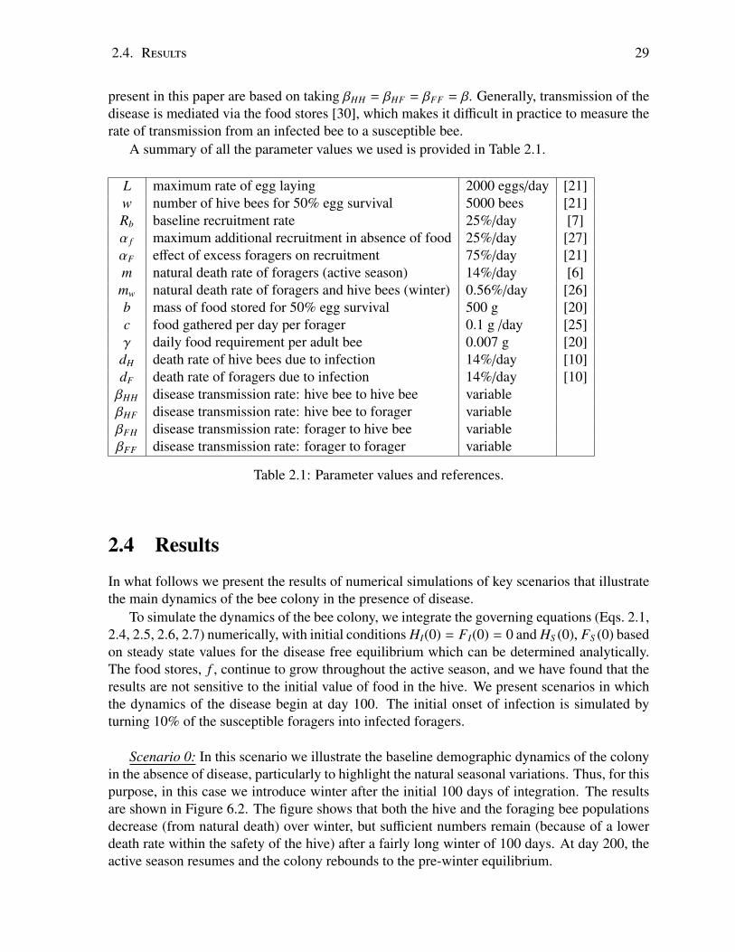
2.4. Results 29

present in this paper are based on taking βHH = βHF = βFF = β. Generally, transmission of thedisease is mediated via the food stores [30], which makes it difficult in practice to measure therate of transmission from an infected bee to a susceptible bee.

A summary of all the parameter values we used is provided in Table 2.1.

L maximum rate of egg laying 2000 eggs/day [21]w number of hive bees for 50% egg survival 5000 bees [21]Rb baseline recruitment rate 25%/day [7]α f maximum additional recruitment in absence of food 25%/day [27]αF effect of excess foragers on recruitment 75%/day [21]m natural death rate of foragers (active season) 14%/day [6]mw natural death rate of foragers and hive bees (winter) 0.56%/day [26]b mass of food stored for 50% egg survival 500 g [20]c food gathered per day per forager 0.1 g /day [25]γ daily food requirement per adult bee 0.007 g [20]

dH death rate of hive bees due to infection 14%/day [10]dF death rate of foragers due to infection 14%/day [10]βHH disease transmission rate: hive bee to hive bee variableβHF disease transmission rate: hive bee to forager variableβFH disease transmission rate: forager to hive bee variableβFF disease transmission rate: forager to forager variable

Table 2.1: Parameter values and references.

2.4 Results

In what follows we present the results of numerical simulations of key scenarios that illustratethe main dynamics of the bee colony in the presence of disease.

To simulate the dynamics of the bee colony, we integrate the governing equations (Eqs. 2.1,2.4, 2.5, 2.6, 2.7) numerically, with initial conditions HI(0) = FI(0) = 0 and HS (0), FS (0) basedon steady state values for the disease free equilibrium which can be determined analytically.The food stores, f , continue to grow throughout the active season, and we have found that theresults are not sensitive to the initial value of food in the hive. We present scenarios in whichthe dynamics of the disease begin at day 100. The initial onset of infection is simulated byturning 10% of the susceptible foragers into infected foragers.

Scenario 0: In this scenario we illustrate the baseline demographic dynamics of the colonyin the absence of disease, particularly to highlight the natural seasonal variations. Thus, for thispurpose, in this case we introduce winter after the initial 100 days of integration. The resultsare shown in Figure 6.2. The figure shows that both the hive and the foraging bee populationsdecrease (from natural death) over winter, but sufficient numbers remain (because of a lowerdeath rate within the safety of the hive) after a fairly long winter of 100 days. At day 200, theactive season resumes and the colony rebounds to the pre-winter equilibrium.

30 Chapter 2. Effects of Infection on Honey Bee Population Dynamics: A Model

50 100 150 200 250 300 3500

0.5

1

1.5

2

2.5

3

3.5

4

4.5x 10

4

time (days)

num

ber

of b

ees

hive beesforaging bees

Winter

Figure 2.2: Baseline demographic dynamics of the honey bee colony in the absence of disease.

Scenario 1: In this scenario, after the initial 100 days we introduce infected foragers intothe system, followed by winter 100 days later. The results are shown in Figure 2.3 based onβ = 5×10−5 and dH = dF = m = 0.14. The figure shows that within about 5 days the susceptiblebee population suffers a drastic drop and the majority of the hive bees have become infected.The infection greatly reduces the overall size of the colony but a new equilibrium is reached,with about 65% of the total population sustaining the infection. At the onset of winter, the sizeof the colony is not sustainable and within 50 days of winter the colony has collapsed.

Scenario 2: In this scenario we examine the effect of a more severe infection in whichthe transmission rate is unchanged but the mortality rates from the disease are increased todH = dF = 4m = 0.56. The results, in Figure 2.4, show that after an initial drastic drop, thepopulation of susceptible bees begins to recover approximately 10 days after the onset of theinfection. The small numbers of infected hive and forager bees lead to their quick demise soonafter the onset of winter, and the disease is eradicated from the hive within 25 days of the onsetof winter. Thus, in this case while the colony has sustained heavy losses from the infection, itsurvives winter with a viable number of bees and no disease. A more severe infection, in thesense that it kills faster, can therefore lead to the survival of the colony as a whole.

Scenario 3: In this scenario we examine the effect of an increased rate of transmission,setting β = 5 × 10−3 and dH = dF = 2m = 0.28. The results are shown in Figure 2.5. Theinfection spreads quickly through the colony, the susceptible population is almost immediately

2.4. Results 31

50 100 150 200 2500

0.5

1

1.5

2

2.5

3

3.5

4x 10

4

time (days)

num

ber

of b

ees

susceptible hive beessusceptible foraging beesinfected hive beesinfected foraging bees

Figure 2.3: Scenario 1: Colony dynamics in the presence of disease with β = 5 × 10−5, dH =

dF = 0.14. Red arrow = onset of infection, grey shading = winter.

eradicated, and within 30 days the colony drops drastically to < 10% of its size before infection.Thereafter, the colony population continues to dwindle slowly, and at the onset of winter itcollapses within 10 days. For comparison, with the same natural death rate but in the absenceof infection, the colony survives through winter and rebounds to its pre-winter level at the onsetof the next active season as seen in Figure 2.2.

Age of Recruitment to Foraging Duties: The average age at which hive bees are recruitedto foraging duties (AARF) under the three scenarios is shown in Figure 2.6. The figure showsthat AARF is an important marker of the health of the colony in the sense that a colony with ayounger workforce can be taken as a sign of disease within the colony. In Scenario 1, AARF isreduced from 19.6 days before the onset of infection to 13.16 after the infection. In Scenario 2,with a more severe infection, AARF is reduced to about 14.6 days, though fluctuating between10 days and 16 days at first. In Scenario 3, with a higher rate of transmission of the infection,AARF is reduced drastically to 9.7 days. This value is determined from the inverse of therecruitment function, R.

Figure 2.7 shows the complex relationship between the rate of transmission β and disease-induced the death rates dH, dF in their effects on the AARF. The figure shows that a combinationof small β and large dH is favorable in that it leads to higher value of the AARF. At higher valuesof β, however, the AARF becomes less sensitive to the value of β (as indicated by the clumpingof the curves in that region. The position of the three scenarios in this relationship as shownin the figure, and their ultimate fate as described earlier, shows again that AARF is an earlymarker of colony collapse, which has been supported by experimental evidence [1].

32 Chapter 2. Effects of Infection on Honey Bee Population Dynamics: A Model

50 100 150 200 2500

0.5

1

1.5

2

2.5

3

3.5

4x 10

4

time (days)

num

ber

of b

ees

susceptible hive beessusceptible foraging beesinfected hive beesinfected foraging bees

Figure 2.4: Scenario 2: Colony dynamics under a more severe infection represented by a higherdeath rates from the disease, with β = 5×10−5, dH = dF = 0.56. Red arrow = onset of infection,grey shading = winter.

Scenario 4: In this scenario, finally, we examine the effect of the timing of the infection inrelation to the onset of winter. Figure 2.8 shows the effect of infection occurring only 10 daysbefore the onset of winter, compared with 100 days in earlier scenarios. The results, comparedwith those in Scenario 2, show that the disease is eradicated sooner by early winter. This isclearly because healthy bees live longer in the safety of the hive in winter, while the death ratefrom infection is unchanged.

Another important indicator of the ultimate fate of the bee colony is the size of the beepopulation at the end of winter. While under all scenarios winter is taken to last 100 days,the size of the bee population at the end of winter is influenced by the severity of the disease(dH, dF), the transmission rate (β), and the time interval between the onset of infection andthe beginning of winter which we shall denote ∆t. This complex relationship is shown firstin Figure 2.9 for Scenarios 1, 2, 3 where ∆t = 100 days in all three cases. Again, we see adecrease in sensitivity to β aat higher values of β. Furthermore, an increases in the value ofdH initially has an unfavorable effect on the colony size at end of winter, but at high valuesof dH this effect is reversed. The region of fractional values is included in Figure 2.9 only for(mathematical) completeness of the figure. Biologically, the region represents colonies that donot survive. By comparison, in Scenario 4 where ∆t = 10 the size of the bee population atend of winter is reduced by 38% from that in Scenario 2 where the values of other parametersare the same. A more general indication of the dependence of the size of the bee population

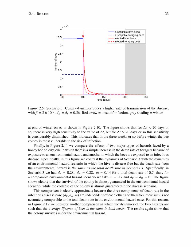
2.4. Results 33

50 100 150 200 2500

0.5

1

1.5

2

2.5

3

3.5

4x 10

4

time (days)

num

ber

of b

ees

susceptible hive beessusceptible foraging beesinfected hive beesinfected foraging bees

Figure 2.5: Scenario 3: Colony dynamics under a higher rate of transmission of the disease,with β = 5 × 10−3, dH = dF = 0.56. Red arrow = onset of infection, grey shading = winter.

at end of winter on ∆t is shown in Figure 2.10. The figure shows that for ∆t < 20 days orso, there is very high sensitivity to the value of ∆t, but for ∆t > 20 days or so this sensitivityis considerably diminished. This indicates that in the three weeks or so before winter the beecolony is most vulnerable to the risk of infection.

Finally, in Figure 2.11 we compare the effects of two major types of hazards faced by ahoney bee colony, one in which there is a simple increase in the death rate of foragers because ofexposure to an environmental hazard and another in which the bees are exposed to an infectiousdisease. Specifically, in this figure we contrast the dynamics of Scenario 3 with the dynamicsof an environmental hazard scenario in which the hive is disease-free but the death rate fromthe environmental hazard is the same as the total death rate in Scenario 3. Specifically, inScenario 3 we had dF = 0.28, dH = 0.28, m = 0.14 for a total death rate of 0.7, thus, fora comparable environmental hazard scenario we take m = 0.7 and dF = dH = 0. The figureshows clearly that the survival of the colony is almost guaranteed in the environmental hazardscenario, while the collapse of the colony is almost guaranteed in the disease scenario.

This comparison is clearly approximate because the three components of death rate in theinfectious disease case (dF , dH,m) are independent of each other and therefore their sum is notaccurately comparable to the total death rate in the environmental hazard case. For this reason,in Figure 2.12 we consider another comparison in which the dynamics of the two hazards aresuch that the average lifespan of bees is the same in both cases. The results again show thatthe colony survives under the environmental hazard.

34 Chapter 2. Effects of Infection on Honey Bee Population Dynamics: A Model

50 100 150 200

8

10

12

14

16

18

20

22

time (days)

AA

RF

(da

ys)

Scenario 1Scenario 2Scenario 3

Figure 2.6: Average age of recruitment to foraging duties (AARF) under the three scenarios inFigures 2.3, 2.4, 2.5. Red arrow = onset of infection.

2.4. Results 35

Figure 2.7: Relationship between the rate of transmission β and disease-induced death ratesdH = dF in their effects on the Average Age of Recruitment to Foraging (AARF). The figureshows the effects of an increase of β and dH on the AARF. Note that the AARF becomes lesssensitive to changes in β as β is increased. Meanwhile, for small β, an increase in dH can havea favourable effect on the AARF.

36 Chapter 2. Effects of Infection on Honey Bee Population Dynamics: A Model

50 100 150 2000

0.5

1

1.5

2

2.5

3

3.5

4x 10

4

time (days)

num

ber

of b

ees

susceptible hive beessusceptible foraging beesinfected hive beesinfected foraging bees

Figure 2.8: Scenario 4: β = 5 × 10−5, dH = dF = 0.56. Effect of the proximity of the onset ofinfection to the onset of winter. Red arrow = onset of infection, grey shading = winter.

2.4. Results 37

0 1 2 3 4 5 610

−8

10−6

10−4

10−2

100

102

104

106

Exp

ecte

d N

umbe

r of

Bee

s at

End

of W

inte

r

β = 5e−05

β=0.005

1

2

3

disease free: 26,119

β=5Ε−05β=0.00075β=0.00145β=0.00215β=0.00285β=0.00355 β=0.005

Figure 2.9: The expected size of the bee population at the end of winter as influenced by theseverity of the disease (dH = dF) and the transmission rate of the disease (β). For comparison,the black arrow indicates the population size at end of winter in the absence of disease (Figure2.2). The figure illustrates the different sensitivity to β and dH. Note that dH has a favourableeffect for small β and dH large enough.

38 Chapter 2. Effects of Infection on Honey Bee Population Dynamics: A Model

0 20 40 60 80 100 12010

−1

100

101

102

103

104

105

∆ t

expe

cted

num

ber

of b

ees

at e

nd o

f win

ter

1

2

disease free: 26,119

4

dH

/m=1

dH

/m=2

dH

/m=4

Figure 2.10: The expected size of the bee population at the end of winter as influenced by thetime interval between the onset of infection and the beginning of winter (∆t), with β = 5×10−5.For comparison, the black arrow indicates the population size at end of winter in the absenceof disease (Figure 6.2).

2.4. Results 39

50 100 150 200 250 300 3500

0.5

1

1.5

2

2.5

3

3.5

4x 10

4

time (days)

num

ber

of b

ees

susceptible hive beessusceptible foraging beesinfected hive beesinfected foraging beesenvironmental−hazard hive beesenvironmental−hazard foraging bees

Figure 2.11: The stark difference between the dynamics of Scenario 3 with an environmentalhazard scenario in which the death rate is increased (by the effects of pesticides, for example)to equal the total death rate in Scenario 3. The survival of the colony is almost guaranteed inthe environmental hazard scenario while the collapse of the colony is almost guaranteed in thedisease scenario.

40 Chapter 2. Effects of Infection on Honey Bee Population Dynamics: A Model

Figure 2.12: An alternative comparison of the dynamics of Scenario 3 with an environmentalhazard scenario in which the comparison between the two hazards is based not on the totaldeath rate as in Figure 2.11 but on the average lifespan of bees being the same in both cases.

2.5. Discussions and Conclusions 41

2.5 Discussions and ConclusionsThe main aim of this study was to construct a model for examining the way in which thedynamics of a honey bee colony are affected by an infection. We present this model in termsof a set of governing equations representing the interplay between the dynamics of the spreadof the disease and the demographic dynamics of the bee colony. Up to this point the model isfairly general in regard to the specific characteristics of the colony or the disease and can thus beadapted to a variety of specific cases by an appropriate choice of parameter values. To illustratethe utility of the model, we chose parameter values associated with Nosema ceranae which hasbeen well studied experimentally. Our findings, compared with those found experimentally aresummarized in Table 2.2.

Exp. 1 2 3AARF- Healthy 14-21 19.6 19.6 19.6AARF- Infected 7-16 13.1 14.6 9.7

(HI + FI)/N 45% 64% 12.2% 92%

Table 2.2: Tabulated results from the model scenarios 1, 2, and 3 and experimental data from [1] and [10]. Thelast row shows the percentage of the population infected at the endemic equilibrium, and the experimental valueis the threshold value which leads to over-winter colony collapse.

The model suggests that key factors in the survival or collapse of a honey bee colony inthe face of an infection are the rate of transmission of the infection β and the disease-induceddeath rates, dH and dF . An increase in the disease-induced death rates, which can be thought ofas an increase in the severity of the disease, may actually help the colony overcome the diseaseand survive through winter (Scenario 2), which is consistent with SIR models of epidemics.By contrast, an increase in the transmission rate, which means that bees are being infected atan earlier age, has a drastic deleterious effect (Scenario 3).

Another important finding relates to the timing of infection in relation to the onset of winter.The results (Figure 2.10) suggest that in a time interval of approximately 20 days before theonset of winter the colony is most affected by the onset of infection. An infection duringthis “dangerous” time period is more likely to lead to colony collapse because the numberof bees surviving through winter becomes unviable for a rebound of the colony in the newactive season. Outside this dangerous time period, i.e. for ∆t > 20 days, the survival of thecolony is no longer critically affected by the timing of infection. It must be emphasized thatthe numerical value of 20 days for this dangerous time period is likely not a “universal” valuebut one that is specific to the choice of parameter values we used both for the colony and thedisease. With other combinations of colony and disease parameters, the model can be used tofind the corresponding critical time period.

Our results (Figures 2.6 and 2.7) suggest that AARF is a good early marker for the survivalor collapse of a honey bee colony in the face of infection. This is consistent with experimentalevidence in [1] but the model and the results in Figures 2.6 and 2.7 provide an insight into theunderlying mechanisms for this.

Finally, an important result of this study is the clear distinction between two major typesof hazards faced by a honey bee colony, namely, one in which there is a simple increase in

42 Chapter 2. Effects of Infection on Honey Bee Population Dynamics: A Model

the death rate of bees because of exposure to an environmental hazard such as pesticides orinsecticides, and another in which the bees are exposed to an infectious disease. The resultsin Figure 2.11 show that an exposure to an infectious disease is almost guaranteed to lead tocolony collapse while under an environmental hazard the colony has a good chance of survival.This conclusion is confirmed by the results of Figure 2.12 in which the comparison betweenthe two hazards is based not on the total death rate but on the average lifespan of bees being thesame in both cases. Since an environmental hazard in the first place affects only forager bees,the comparison in this case is equivalent to considering a more severe environmental hazardthan that in Figure 2.11, or to considering the long term consequences of an environmentalhazard as it affects the demographics of the colony. Together, the two comparisons lead us tosuspect that, under comparable death rates and the range of disease transmission rates whichwe have considered, an infectious disease may typically be more hazardous to the survival of abee colony than an exposure to pesticide or insecticide.

AcknowledgmentThis work was supported by the Natural Sciences and Engineering Research Council of Canada.We thank Mary Myerscough and Gloria DeGrandi-Hoffman for insightful comments.

Bibliography

[1] Botias, C., Martin-Hernandez, R., Barrios, L., Meana, A., and Higes, M. Nosema spp.infection and its negative effects on honey bees (Apis mellifera iberiensis) at the colonylevel. Veterinary research 44, 1 (2013), 1–15.

[2] Calderone, N. W. Insect pollinated crops, insect pollinators and US agriculture: Trendanalysis of aggregate data for the period 1992-2009. PLOS ONE 7, 5 (05 2012), e37235.

[3] Chen, Y., Evans, J. D., Smith, I. B., and Pettis, J. S. Nosema ceranae is a long-presentand wide-spread microsporidian infection of the European honey bee (Apis mellifera) inthe United States. Journal of Invertebrate Pathology 97, 2 (2008), 186–188.

[4] Cramp, D. A Practical Manual of Beekeeping. How To Books, London, 2008.

[5] Devillers, J. The ecological importance of honey bees and their relevance to ecotoxicol-ogy. In Honey Bees: Estimating the Environmental Impact of Chemicals, J. Devillers andM. Pham-Delegue, Eds. Taylor and Francis London, London, 2002, pp. 1–11.

[6] Dukas, R. Mortality rates of honey bees in the wild. Insectes Sociaux 55, 3 (2008),252–255.

[7] Fahrbach, S., and Robinson, G. Juvenile hormone, behavioral maturation and brain struc-ture in the honey bee. Developmental Neuroscience 18 (1996), 102–114.

[8] Favre, D. Mobile phone-induced honeybee worker piping. Apidologie 42, 3 (2011),270–279.

[9] Fries, I. Nosema ceranae in European honey bees (Apis mellifera). Journal of inverte-brate pathology 103 (2010), S73–S79.

[10] Goblirsch, M., Huang, Z. Y., and Spivak, M. Physiological and behavioral changes inhoney bees (Apis mellifera) induced by Nosema ceranae infection. PLOS ONE 8, 3 (032013), e58165.

[11] Harbo, J. R. Effect of brood rearing on honey consumption and the survival of the workerhoney bees. Journal of Apicultural Research 32, 1 (1993), 11–17.

[12] Henry, M., Beguin, M., Requier, F., Rollin, O., Odoux, J.-F., Aupinel, P., Aptel, J.,Tchamitchian, S., and Decourtye, A. A common pesticide decreases foraging successand survival in honey bees. Science 336, 6079 (2012), 348–350.

43

44 BIBLIOGRAPHY

[13] Higes, M., Martin-Hernandez, R., Botias, C., Bailon, E. G., Gonzalez-Porto, A. V., and

Barrios, L. How natural infection by Nosema ceranae causes honeybee colony collapse.Environmental microbiology 10, 10 (2008), 2659–2669.

[14] Higes, M., Martin-Hernandez, R., Garrido-Bailon, E., Gonzalez-Porto, A. V., Garcia-Palencia, P., and Meana, A. Honeybee colony collapse due to Nosema ceranae in profes-sional apiaries. Environmental Microbiology Reports 1, 2 (2009), 110–113.

[15] Ho, M.-W., and Cummins, J. Mystery of disappearing honeybees. Science in Society 34(2007), 35–36.

[16] Huang, Z.-Y., and Robinson, G. E. Regulation of honey bee division of labor by colonyage demography. Behavioral Ecology and Sociobiology 39 (1996), 147–158.

[17] Jay, S. Seasonal development of honeybee colonies started from package bees. Journalof Apicultural Research 13 (1974), 149–152.

[18] Jones, J. C., Helliwell, P., Beekman, M., Maleszka, R., and Oldroyd, B. The effectsof rearing temperature on developmental stability and learning and memory in the honeybee, Apis mellifera. Journal of Comparative Physiology A 191, 12 (2005), 1121–1129.

[19] Kauffeld, N. M. Beekeeping in the United States Agriculture Handbook Number 335.U.S. Department of Agriculture, 1980.

[20] Khoury, D. S., Barron, A. B., and Myerscough, M. R. Modelling food and populationdynamics in honey bee colonies. PLOS ONE 8, 5 (05 2013), e59084.

[21] Khoury, D. S., Myerscough, M. R., and Barron, A. B. A quantitative model of honeybee colony population dynamics. PLOS ONE 6, 4 (04 2011), e18491.

[22] Leoncini, I., Le Conte, Y., Costagliola, G., Plettner, E., Toth, A. L., and Wang, M.Regulation of behavioral maturation by a primer pheromone produced by adult workerhoney bees. Proceedings of the National Academy of Sciences of the United States ofAmerica 101, 50 (2004), 17559–17564.

[23] Neumann, P., and Carreck, N. L. Honey bee colony losses. Journal of ApiculturalResearch 49, 1 (2010), 1–6.

[24] Ratti, V., Kevan, P. G., and Eberl, H. J. A mathematical model for population dynamicsin honeybee colonies infested with Varroa destructor and the Acute Bee Paralysis Virus.Canadian Applied Mathematics Quarterly 21, 1 (2013), 63–93.

[25] Russell, S., Barron, A. B., and Harris, D. Dynamic modelling of honey bee (Apismellifera) colony growth and failure. Ecological Modelling 265, 0 (2013), 158 – 169.

[26] Sakagami, S., and Fukuda, H. Life tables for worker honeybees. Researches on Popula-tion Ecology 10, 2 (1968), 127–139.

BIBLIOGRAPHY 45

[27] Schulz, D. J., Huang, Z.-Y., and Robinson, G. E. Effects of colony food shortage on be-havioral development in honey bees. Behavioral Ecology and Sociobiology 42, 5 (1998),295–303.

[28] Seeley, T. D. Honeybee Democracy. Princeton University Press, 2010.

[29] Seeley, T. D., and Visscher, P. K. Survival of honeybees in cold climates: the criticaltiming of colony growth and reproduction. Ecological Entomology 10, 1 (1985), 81–88.

[30] Smith, M. L. The honey bee parasite Nosema ceranae: Transmissible via food exchange?PLOS ONE 7, 8 (08 2012), e43319.

[31] Southwick, E. E., and Southwick Jr, L. Estimating the economic value of honey bees(Hymenoptera: Apidae) as agricultural pollinators in the United States. Journal of Eco-nomic Entomology 85, 3 (1992), 621–633.

[32] Stevanovic, J., Simeunovic, P., Gajic, B., Lakic, N., Radovic, D., Fries, I., and Stan-imirovic, Z. Characteristics of Nosema ceranae infection in Serbian honey bee colonies.Apidologie 44, 5 (2013), 522–536.

[33] Sumpter, D. J. T., and Martin, S. J. The dynamics of virus epidemics in Varroa-infestedhoney bee colonies. Journal of Animal Ecology 73, 1 (2004), 51–63.

[34] vanEngelsdorp, D., Evans, J. D., Saegerman, C., Mullin, C., Haubruge, E., Nguyen,B. K., Frazier, M., Frazier, J., Cox-Foster, D., Chen, Y., Underwood, R., Tarpy, D. R.,and Pettis, J. S. Colony collapse disorder: A descriptive study. PLOS ONE 4, 8 (082009), e6481.

[35] Watanabe, M. E. Colony collapse disorder: Many suspects, no smoking gun. BioScience58, 5 (2008), 384–388.

[36] Winston, M. The biology of the honey bee. Harvard University Press, 1987.

Chapter 3

Reproduction Number And AsymptoticStability For The Dynamics of a HoneyBee Colony with Continuous AgeStructure

AbstractA system of partial differential equations is derived as a model for the dynamics of a

honey bee colony with a continuous age distribution, and the system is then extended to in-clude the effects of a simplified infectious disease. In the disease-free case we analyticallyderive the equilibrium age distribution within the colony and propose a novel approach fordetermining the global asymptotic stability of a reduced model. Furthermore, we presenta method for determining the basic reproduction number R0 of the infection; the methodcan be applied to other age-structured disease models with interacting susceptible classes.The results of asymptotic stability indicate that a honey bee colony suffering losses willrecover naturally so long as the cause of the losses is removed before the colony collapses.Our expression for R0 has potential uses in the tracking and control of an infectious diseasewithin a bee colony.

3.1 IntroductionHoney bee populations continue to decline on a global scale [3], and as research efforts toidentify the underlying cause or causes continue [23, 63, 65], there is as yet no clear resolutionof the problem. While the consequences of the decline are usually discussed in the context ofagriculture and economics [9, 37, 54], the key question clearly hinges on the stability of a honeybee colony as a population dynamical system. Mathematical models thus provide criticallyimportant tools for studying honey bee populations as they can both simulate many differentenvironments as well as suggest potential sensitivities a colony may have to environmentalhazards such as pesticides and climate change, or microbial hazards such as parasites anddisease.

Mathematical models have been used in recent years to shed light on the effects of pesti-cides on the lifespan of foraging bees [29, 30]. Other models have focused on the changing

46

3.1. Introduction 47

dynamics of a colony under changing environmental conditions [58], or the interactions be-tween colonies [49]. Recent work has also investigated the effects of infection on honey beecolony dynamics, including Varroa mites [17, 44, 45] and nosema [5], the latter approximatinginfection through mass action. An approach from systems biology has been used to explore themultifactorial causes of colony failure [2].

One of the complicating factors in the dynamics of a honey bee colony is the age distri-bution (structure) within the colony since age groups may differ in their expected lifespans,foraging behaviour or susceptibility to a given hazard. While age-independent models haveprovided a number of key insights into the properties of colony dynamics [5, 30, 44], the ulti-mate conditions for the survival or collapse of a honey bee colony must take into account thisadded dimension of the problem.

From a mathematical standpoint, incorporating the age structure of a honey bee colony intothe equations governing the population dynamics leads to a set of partial differential equationsinstead of the ordinary differential equations obtained when age structure is not included. Theproblem of finding stability and equilibrium conditions for the dynamics of the colony becomescorrespondingly more complex. When considering disease dynamics, the problem of findingthe basic reproduction number (R0) at which the fate of the colony is at a bifurcation becomesparticularly difficult.

We propose a method of resolving these mathematical difficulties by transforming the prob-lem from the real space (age, time) into the Laplace space such that the governing equationsbecome ordinary differential equations, and from the solution of these equations it is then possi-ble to deduce the asymptotic behavior of the dynamical system in the real space. In particular,in the absence of disease we show that the system has an asymptotically stable equilibrium,which implies that the bee population will rebound from losses when hazards are removed,provided they are removed before the complete demise of the colony. In the presence of dis-ease we use a linearized form of the system to obtain a closed form expression for the basicreproduction number R0. The expression thus provides a measurable threshold for whether thedisease will decay or persist.

Determining R0 for age-structured models has been previously studied for general diseasemodels with one infected class [25, 32, 59]. Our model has the added complexity of having twointeracting infected classes, namely infected hive bees (HI) and infected foragers (FI), that can-not be transformed into a single infected class for analysis. Moreover, work on the asymptoticstability of disease models with age structure is sparse. Several studies use Lyapunov functionsand semi-group analysis to prove persistence of solutions [21, 33], while perturbation analysishas also proved useful [26]. Other work has made use of properties of the particular model athand to show stability [11].

In the present study, we take advantage of detailed experimental work elucidating the dis-tinct roles that honey bees of different ages play within a honey bee colony, and use this infor-mation to develop a model of honey bee demographics with continuous age structure (Section3.2). This model is then extended to include the dynamics of an infectious disease withinthe colony. In particular, we find a stability threshold criterion which corresponds to the ba-sic reproduction number R0. In Section 3.3.1, we use a steady-state approximation to derivethe equilibrium age distribution of the disease-free hive. In 3.3.2, we develop a novel Laplacetransform approach to prove global stability of this disease-free distribution in a reduced model,implying local stability in the full model. In 3.3.3, we again develop a novel approach to find a

48 Chapter 3. Honey Bee Reproduction Number

threshold criterion at which this equilibrium state becomes unstable, and an infection will in-vade; this threshold corresponds to the basic reproductive number, R0. In Section 4, we discussthe implications of these results and suggest possible applications of the new approaches wehave developed to other problems in population dynamics.

3.2 ModelThe proposed model combines the normal demographics of a honey bee colony with a diseasethat at first infects foragers and then spreads to the rest of the colony. As in previous studies,to keep the problem tractable, we focus on hive bees, H, which are primarily responsible formaintenance of the brood, and foragers, F, which are responsible for bringing food, f , intothe hive. Although hive bees can take on other duties such as guarding or hive maintenance,for simplicity we do not model these roles explicitly, but assume all hive bees contribute eitherdirectly or indirectly to the survival of the brood. Male honey bees, known as drones, do notcontribute to the maintenance of the hive, so this population is not included in the model.

Generally, bees emerge from the brood as hive bees and are later recruited to foragingduties. These two classes are further divided, in the presence of disease, into susceptible pop-ulations, HS and FS , and infected populations, HI and FI . The following sections presentthe governing equations for each of these sub-populations. The total size of the colony to bemodeled in age, a (days), and time, t (days), is thus,

N(t) =

∫ ∞

0(HS (a, t) + HI(a, t) + FS (a, t) + FI(a, t))da, (3.1)

while the total infected population of the hive, denoted I, is

I(t) =

∫ ∞

0(HI(a, t) + FI(a, t))da. (3.2)

Susceptible Hive Bees: For the susceptible hive bee population HS (a, t), incorporating ageusing the standard approach of McKendrick [36] into our earlier formulation of the problem [5],the governing equation becomes

∂HS (a, t)∂t

+∂HS (a, t)

∂a= −u(a, t)HS (a, t) − βI(t)HS (a, t). (3.3)

Here, the first term on the right-hand side represents the recruitment of hive bees to foragingduties, as described below, where u(a, t) denotes the age-dependent rate of recruitment. Thesecond term on the right governs the disease dynamics within the colony, as described in thenext subsection. It is assumed that the hive provides sufficient safety for bees that remain withinit [30, 51] such that the natural death rate of healthy hive bees is negligible compared to therate of recruitment to foraging.

Research has shown that juvenile hormone III regulates the age at which honey bees beginforaging [46], and there is a minimum age, aR, at which hive bees are normally recruited toforaging duties [18]. If the foraging needs of the colony are not being met, however, hive

3.2. Model 49

bees will be recruited to foraging duties at a younger age [24]. Conversely, if the foraging beepopulation exceeds the needs of the colony, foragers produce a pheromone, ethyl oleate, toreduce recruitment [31]. We incorporate these regulatory mechanisms by taking

u(a, t) = α( aa + k

)2(1 −

σ

N(t)

∫ ∞

0(FS + FI)da

)Hv(a − aR) (3.4)

where α is a free parameter representing the base rate of recruitment, Hv(a−aR) is the Heavisidefunction, and 1/σ is the maximum allowable fraction of foragers in the colony size. Thusrecruitment begins at age aR and increases sigmoidally with age thereafter where k is the ageat which recruitment is at a quarter of its maximal rate. The form of this sigmoidal function,(a/(a+k))2, was chosen as it yielded the best fit to available data describing the age distributionof a healthy honey bee colony [4].

Disease dynamics: To retain analytical tractability when both age- and caste-structure havebeen added to the model, we use the simplest possible approximation for disease dynamics. Inparticular, we assume the infection is transmitted via mass action at a constant rate β, and in-fection can be transferred from hive bees to foragers or vice versa. While mass action kinetics,with no time delay, are unlikely to be the best possible model for any particular disease ofhoney bees, this model allows us to gain analytical insight into key broad features of infectionin the colony. Mass action kinetics provide a reasonable approximation for certain modes oftransmission; for example, in the case of nosema, fecal-oral transmission [55], and contami-nation of food stores [53] can be modeled by mass action under the assumptions that food iswell-mixed and infected food is proportional to infected foragers. Of course, nosema infectsfood stores and bees via the microsporidian Nosema ceranae [6, 53]. The microsporidian pop-ulation within the hive fluctuates seasonally and adds a further complexity to nosema infectionin colonies. The simple transmission terms we assume will clearly not capture the completepathogenesis of nosema infections [42].

Three important simplifying assumptions underpin disease transmission in the model. Thefirst is that hive bees and foragers are both infected (and infect) at the same rate, while thesecond is that the disease affects both equally (i.e. same disease-induced death rate for bothclasses). Both of these assumptions have been chosen to allow for a simple, general model.The methods described here, however, remain valid if the second assumption is relaxed, that is,the approach can also be used to describe a disease which affects the lifespan of hive bees andforagers differently. Lastly, we assume infected bees are recruited to foraging at the same rateas healthy bees. We have previously demonstrated that despite this simplifying assumption, arelated model [5] is able to capture reductions caused by infection in the average age at whichbees are recruited to foraging.

Infected Hive Bees: Infected hive bees are at risk of dying due to disease at an age-dependent rate d(a). The equation governing their dynamics is then

∂HI(a, t)∂t

+∂HI(a, t)∂a

= βI(t)HS (a, t) − [u(a, t) + d(a)]HI(a, t). (3.5)

Susceptible Foragers: Susceptible foragers are recruited from susceptible hive bees andare subject to age-dependent natural death at rate µ(a). The equation governing their dynamics

50 Chapter 3. Honey Bee Reproduction Number

is thus given by

∂FS (a, t)∂t

+∂FS (a, t)

∂a= u(a, t)HS (a, t) − [µ(a) + βI(t)]FS (a, t). (3.6)

In all of the analytical work to follow (Sections 3.3.1, 3.3.2, 3.3.3 and 3.3.4), the functionµ(a) is completely general. For illustrative purposes (in the figures only), a quadratic functionhas been used to match qualitative observations of forager mortality. In particular, precociousforaging has been shown to have deleterious effects on forager lifespan [27, 62], while mortalityhas been observed to increase with chronological age [16]. Given these two observations, thesimplest smooth function that agrees qualitatively would be a quadratic with a central age atwhich mortality is at a minimum. The function used for numerical illustrations in this study isprovided in Table A.1.

Infected Foragers: Infected foragers can be either (i) infected hive bees that have beenrecruited to foraging duties or (ii) susceptible foragers that have become infected by eitherinfected foragers or infected hive bees. They are subject to a disease-related death rate, d(a),and their dynamics are governed by

∂FI(a, t)∂t

+∂FI(a, t)∂a

= u(a, t)HI(a, t) + βI(t)FS (a, t) − [µ(a) + d(a)]FI(a, t). (3.7)

Food stores: Food, f , is brought into the hive by both susceptible and infected foragers.For simplicity, we assume that all foragers bring in food at the same rate c (g/day), although itis likely that infected foragers would be less efficient at the task. Food is consumed by foragersand hive bees at, again for simplicity, the same rate, γ. The amount of food available at time tis therefore given by

d fdt

= c∫ ∞

0(FS + FI) da − γN . (3.8)

Boundary Conditions: The system of equations (3.3),(3.5),(3.6),(3.7) is subject to the fol-lowing boundary conditions: {

HS (0, t) = LV(t)HI(0, t) = FS (0, t) = FI(0, t) = 0 .

(3.9)

The first condition represents the birth of new bees where L is the daily egg laying rate by thequeen and V is a survivability function which determines how many of the brood survive tobecome viable hive bees. The brood needs both sufficient food and sufficient care from thehive bees in order to survive [28]. Moreover, it has been shown that there is a range of ageswithin which hive bees will care for the brood. Field data suggest that hive bees take on nursingduties at a minimum age amn and complete these duties at a maximum age amx. After this age,hive bees tend to either transition to foraging duties or take on hive security or maintenanceduties [66]. On this basis, we define the survivability function V(t) as

V(t) =W

(f

b + f

) ∫ amx

amnHS (a, t)da

w +∫ amx

amnHS (a, t)da

, (3.10)

3.3. Results 51

where b is the amount of food required for half the brood to survive to adulthood in the presenceof sufficient care from hive bees, and w is the number of nursing hive bees necessary to ensuresurvival of half the brood in the presence of sufficient food stores. The term W provides a‘conversion’ of eggs to bees with a fixed value ofW = 1 bee per egg, and can be interpretedas the maximum number of bees produced by a single egg. The number of new hive beescreated from L eggs is dependent on the amount of food available as well as the amount of careavailable. The boundary conditions for the infected classes assume that bees cannot emergeinfected.

Equations (3.3), (3.5), (3.6), (3.7), (3.8) form a system of integro-partial differential equa-tions to be solved simultaneously subject to the boundary conditions (3.9).

Numerical Treatment: For illustrative purposes (the figures only), the full system wassolved numerically using a finite difference scheme [20], using parameter values provided inTable 3.1. Age was divided into N classes, each of size ∆a, and the first derivative was approx-imated by using a backward difference [52]. Time integration used Forward Euler [12] froman initial condition of H(a, 0) = 104e−a, F(a, 0) = 0 with step size of ∆t= 10−3. The limit asa → ∞ was approximated by using a maximum value Amax � ∆a. Solutions were consideredto be at steady state when ||(FS (a, tn) + HS (a, tn)) − (FS (a, tn−1) + HS (a, tn−1))||2 < 10−10∆t.

3.3 Results

3.3.1 Existence

We use the method of characteristics [39], with characteristics given by

dada

= 1, a(0) = 0 (3.11)

dtda

= 1, t(0) = t0. (3.12)

The latter equations lead to parallel characteristics of the form t(a) = a + t0. Along thesecharacteristics, the populations HS (a, t(a)), FS (a, t(a)),HI(a, t(a)), and FI(a, t(a)) satisfy the

52 Chapter 3. Honey Bee Reproduction Number

equations

dHS

da= −u(a, t(a))HS (a, t(a)) (3.13)

− βHS (a, t(a))∫ ∞

0HI(a∗, t(a∗)) + FI(a∗, t(a∗))da∗

dFS

da= u(a, t(a))HS (a, t(a)) − µ(t(a))FS (a, t(a)) (3.14)

− βFS (a, t(a))∫ ∞

0HI(a∗, t(a∗)) + FI(a∗, t(a∗))da∗

dHI

da= −(u(a, t(a)) − d(t(a)))HI(a, t(a)) (3.15)

+ βHS (a, t(a))∫ ∞

0HI(a∗, t(a∗)) + FI(a∗, t(a∗))da∗

dFI

da= u(a, t(a))HI(a, t(a)) − (µ(t(a)) + d(t(a)))FI(a, t(a)) (3.16)

+ βFS (a, t(a))∫ ∞

0HI(a∗, t(a∗)) + FI(a∗, t(a∗))da∗

with initial values

HS (a, t0) = LV(t0)e−a (3.17)FS (a, t0) = HI(a,t0) = FI(a, t0) = 0. (3.18)

Due to the discontinuity in u(a, t), we cannot find a unique differentiable solution to equations(13), (14), (15), and (16). We can however split the problem at the discontinuity and solve thesystem in two parts. Patching together these two solutions allows us to infer the existence of acontinuous, but not differentiable, weak solution to the governing PDEs.

The first-order integro-differential equations (13), (14), (15), and (16) – which define thesteady-state distribution of bees – can be reduced to a finite set of ordinary differential equationsthrough methods developed in [14, 15, 19]. The approach described therein creates a mapbetween a system of integro-differential equations with a degenerate kernel (i.e. K(x, y) =

K1(x)K2(y)), and an equivalent system of ordinary differential equations which are guaranteedto have a unique solution on a ∈ (0, aR) [7]. We denote these solutions as H jS (a, t), F jS (a, t),H jI(a, t), and F jI(a, t) ( j for ‘juvenile’). As well, we appeal to the same theoretical frameworkto guarantee a solution in the interval a ∈ (aR,∞), denoted HmS (a, t), FmS (a, t), HmI(a, t), andFmI(a, t) (m for ‘mature’), provided HmI(a, t) and FmI(a, t) are bounded and decay as a→ ∞.The full solution is continuous on a ∈ (0,∞) under the conditions

HmS (aR, aR + t0) = H jS (aR, aR + t0) (3.19)FmS (aR, aR + t0) = F jS (aR, aR + t0) (3.20)HmI(aR, aR + t0) = H jI(aR, aR + t0) (3.21)FmI(aR, aR + t0) = F jI(aR, aR + t0). (3.22)

These conditions act as initial conditions for equations (13), (14), (15), and (16) on the intervala ∈ (aR,∞). As the characteristics are parallel, the solution is unique in the entirety of at-space.

3.3. Results 53

3.3.2 Disease-free Equilibria (DFE)One equilibrium for the disease-free system is the trivial equilibrium

HS (a) = FS (a) = f (t) = 0. (3.23)

A second equilibrium exists, and is the solution to the ODE system,

dH∗∗Sda

= −u(a)H∗∗S (a) (3.24)

dF∗∗Sda

= u(a)H∗∗S (a) − µ(a)F∗∗S (a) (3.25)

γN(t) = c∫ ∞

0F∗∗S (a)da (3.26)

where H∗∗S and F∗∗S denote the steady state solutions. We may relax condition (3.26) by settingd fdt≥ 0 as opposed to

d fdt

= 0, and instead seek a quasi-steady state under which food may bebounded, or may grow unbounded. Note that the quasi-steady state conditions include the trueequilibrium as well.

Equations (3.3) and (3.6) are non-linear, and coupled in such a way as to make an analyticalexpression for their equilibrium evasive. The nonlinearities for the system all appear in the termu(a), given by equation (3.4), which also depends on HS and FS in the disease-free case throughthe integrals

∫FS da/N. At equilibrium, this term will reduce to a constant. In other words, we

can rewrite the term ∫FS da

N= K1

at equilibrium. In the case of bounded food stores, as in equation (3.26),

K1 =γ

cbut in the case of unbounded food stores,

K1 ≥γ

c.

We write the recruitment function at equilibrium, ueq(a) as

ueq(a) = α( ak + a

)2(1 − σK1) Hv

(a − aR

K

)(3.27)

= K( ak + a

)2Hv

(a − aR

K

)(3.28)

where K = α (1 − σK1). We may then rescale the time variables of the system (t = Kt anda = Ka) to obtain the scaled system,

KdH∗Sda

= −K(

a/K

a/K + k/K

)2

Hv

(a − aR

K

)H∗S (a) (3.29)

KdF∗Sda

= K(

a/K

a/K + k/K

)2

Hv

(a − aR

K

)H∗S (a) − µ(a)F∗S (a) (3.30)

54 Chapter 3. Honey Bee Reproduction Number

We can then simplify the system to

dH∗Sda

= −

(a

a + k

)2

Hv

(a − aR

K

)H∗S (a) (3.31)

dF∗Sda

=

(a

a + k

)2

Hv

(a − aR

K

)H∗S (a) − µ(a)F∗S (a) (3.32)

where µ(a) = µ(a)/K. The solutions of equations (3.31) and (3.32) in scaled variables are inde-pendent of K (shown below).

Figure 3.1: The disease-free equilibrium distributions H∗S and F∗S . The equilibrium plottedhere is found by running the full, time dependent equations (3.3), (3.6), (3.8) and (3.9) until thepointwise solution was no longer changing (below threshold O(10−13)), as well as by plottingequations (3.33) and (3.34). The two are indistinguishable. All parameter values used in thissimulation, with references to the literature, are found in Table 1. Total hive bee population is∫ ∞

0HS (a)da = 44839 bees and the total forager population is

∫ ∞0

FS (a)da = 18312 bees.

Equation (3.31) is decoupled from equation (3.32) and is linear. It can be integrated directly.Using the results, equation (3.32) can then be solved by variation of parameters, as it is a linear,non-homogeneous equation. The full solution to equations (3.31) and (3.32) is finally given by

H∗S (a) =

HS 0, if a < aR

HS 0

(a + k

)2 kexp

(−

a2 + ak − k2

a + k

)((

aR + k)2 k

)exp

− a2R + aRk − k2

aR + k

, if a ≥ aR(3.33)

3.3. Results 55

Table 3.1: Parameter values and source references.L maximum rate of egg laying 2000 eggs/day [30]w number of hive bees for 50% egg survival 5000 bees [30]b mass of food stored for 50% egg survival 500g [29]

amn age at which hive bees begin brood care 3 days [24]amx age at which hive bees end brood care 16 days [24]aR minimum recruitment age 4 days [18]k age at which rate of recruitment is 25% of max. 10 daysα maximum rate of recruitment 1 /day1σ

maximum fraction of colony that can be foraging 1/3 [30]µ(a) natural death rate of foragers (summer) (a−20)2/400 [16, 27, 62]

c food gathered per day per forager 0.1 g /day /bee [47]γ daily food requirement per adult bee 0.007 g /day /bee [29]

and

F∗S (a) =

FS 0 exp

(∫ a

0−µ

(a∗

)da∗

), if a < aR

(A(a) + FS 0) exp(∫ a

aR

−µ(a∗

)da∗

), if a ≥ aR

(3.34)

where {HS 0 = H∗S (0)FS 0 = F∗S (0)

, (3.35)

A(a) =

∫ a

aR

(a∗

a∗ + k

)2

H∗S (a∗)e∫ a∗

aRµ(s) ds da∗ (3.36)

The conditions on variable a stem from the Heaviside term in the definition of u(a) inequation (3.4). The age distributions of susceptible hive and foraging bees in equations (3.33)and (3.34) are shown in Figure 3.1.

In order to recover the equilibrium for unscaled variables, one is required to solve theimplicit, nonlinear equation for K,

K = α

1 − σ∫ ∞

0F∗S (Ka) da∫ ∞

0H∗S (Ka) + F∗S (Ka) da

(3.37)

which can then be used to recover the equilibrium distributions in unscaled time, H∗∗S (a) =

H∗S (Ka) and F∗∗S (a) = F∗S (Ka).Using equations (4.9) and (3.31), this steady-state exists so long as∫ amx

amn

H∗(a) da >w

LW ( f/f +b). (3.38)

56 Chapter 3. Honey Bee Reproduction Number

3.3.3 Stability of DFEIf the Laplace transform of H(a, t) is denoted by L {H(a, t)} = H (a, s) and lim

t→∞H(a, t) is finite,

then by the Final Value Theorem [40],

limt→∞

H(a, t) = lims→0

sH (a, s) (3.39)

under two conditions [10]:

i) There is at most one simple pole at the origin in s-space.

ii) Any roots of the denominator of H (a, s) are negative.

In what follows we use this theorem to analyze the asymptotic behaviour of the PDE systemgiven by equations (3.3), (3.5), (3.6), (3.7) and (3.8) expressed in scaled variables a and t, andultimately show that the disease-free equilibrium is locally asymptotically stable.

To begin, we approximate the recruitment function u(a, t) as

u(a, t) = ueq(a) + ε(a, t) (3.40)

where ueq(a) is defined as in equation (3.28) as the rate of recruitment at equilibrium and ε(a, t)is a small perturbation in this function near the equilibrium.

We then take the Laplace Transform in t of equation (3.3) near the disease-free equilibrium,ignoring the term βIHS since here we are interested in the disease-free case, which yields

sH (a, s) − HS (a, 0) +∂H (a, s)

∂a= −ueq(a)H (a, s) +

∫ s

0ε(a, r − s)H (a, r)dr (3.41)

where

H (a, s) = L {HS (a, t)} (3.42)ε(a, s) = L {ε(a, t)}. (3.43)

The corresponding boundary condition is then given by taking the Laplace transform ofcondition (4.9) but this is not easy because of the time dependence of that boundary condition.We simplify this problem by noting that when food stores are unbounded and we are interestedin the behaviour as t → ∞, the term involving food will saturate. On this basis we use theapproximation

limt→∞

fb + f

≈ 1. (3.44)

As well, the second factor in the function V (equation (3.10)) can be expressed at equilibriumas

0 ≤ κ =

∫ amx

amnH∗S (a)da

w +∫ amx

amnH∗S (a)da

≤ 1. (3.45)

3.3. Results 57

We can linearize about the equilibrium,∫

H∗S (a)da (note we have suppressed the limits ofintegration for readability) using the Taylor series

HS (0, t) ≈ Lκ + LdV

d∫

HS da

∣∣∣∣∣HS =H∗S

(∫HS (a, t)da −

∫H∗S (a)da

)(3.46)

wheredV

d∫

HS (a, t)dais the derivative of V with respect to

∫HS (a, t)da here defined as

dV

d∫

HS (a, t)da=

w(w +

∫HS (a, t)da

)2 . (3.47)

Using these approximations, the boundary condition for H becomes

H (0, s) =Lκs

+L

w(w +

∫ amx

amnH∗S (a)da

)2

∫ H (a, s)da −

∫H∗S (a)da

s

=

Lκ2

s+ L

dV

d∫ amx

amnHS da

∫ amx

amn

H (a, s)da (3.48)

and the limit of sH (0, s) becomes

lims→0

sH (0, s) = Lκ2 (3.49)

which we note is constant.Solving the ODE (3.41) with initial condition HS (a, 0) = g(a) ≥ 0 (bounded, analytic, and

satisfying the two aforementioned conditions) yields,

H (a, s) =

(∫ a

0g (a) esada + H (0, s)

)e−sa a < aR

(x(a, s) + C(s)) y(a, s) a ≥ aR

(3.50)

where

y(a, s) =(a + k

)2 kexp

(−

sa2 + sak + a2 + ak − k2

a + k

)(3.51)

x(a, s) =

∫ a

aR

(g (a) +

∫ s

0ε(a, s − r)H (a, r)dr

)1

y(a)da (3.52)

and

C(s) = H (0, s)((

aR + k)2 k

)−1 exp− sa2

R + saRk + a2R + aRk − k2

aR + k

−1

. (3.53)

The tilde sign signifies dummy variables.We examine this result in two parts:(i) a > aR : Here we observe that

s y(a)x(a) ≥ 0 (3.54)

58 Chapter 3. Honey Bee Reproduction Number

and note that

lims→0

s∫ s

0ε(a, s − r)H (a, r)dr = 0. (3.55)

Since g(a) is bounded, and

0 ≤exp

(−

k2

a + k

)(a + k)2k

≤ 1

we find

s y(a)x(a) ≤ s y(a)(

maxa∈[0,∞)

g(a)) ∫ a

aR

e−a(s+1)da (3.56)

= s y(a)(

maxa∈[0,∞)

g(a))

e−(s+1)aR − e−(s+1)a

s + 1.

We also note that

lims→0

s y(a)(

maxa∈[0,∞)

g(a))

e−(s+1)aR − e−(s+1)a

s + 1= 0. (3.57)

Using conditions (3.54), (3.56), (3.57) and the Squeeze Theorem [56] we conclude that

lims→0

s y(a)x(a) = 0 (3.58)

As well,

lims→0

s C = lims→0

{sH (0, s)

((aR + k

)2 k)−1

•exp− sa2

R + saRk + a2R + aRk − k2

aR + k

−1= Lκ2

((aR + k

)2 k)−1

exp a2

R + aRk − k2

aR + k

(3.59)

Using the above, we find

lims→0

sH (a, s) = Lκ2(a + k

)2 kexp

(−

sa2 + sak + a2 + ak − k2

a + k

)(3.60)

= H∗S (a), (3.61)

and applying the Final Value Theorem we find

limt→∞

HS (a, t) = H∗S (a), a ≥ aR (3.62)

(ii) a < aR : Here we note simply that

lims→0

s(∫ a

0g (a) esada + H (0, s)

)e−sa (3.63)

=

(∫ a

0lims→0

sg (a) esada + lims→0

Lκ2)

e−sa (3.64)

= Lκ2 = H∗S (a). (3.65)

3.3. Results 59

This completes the stability analysis of the DFE for HS . Similar analysis applies to theDFE for FS , though with considerably more tedious algebra, therefore we omit the details.

The above analysis determines the global stability of the linearized model in which we havesufficient food stores, brood care and time-independent recruitment. This linearized model isin fact an approximation to the full model governed by equations (3.3), (3.5), (3.6), (3.7) and(3.8) near the quasi-steady state distribution given by equations (3.33) and (3.34). Note that,rather than linearizing the full system by using first order approximations (the Jacobian) inthe neighbourhood of the equilibrium, here we need only consider the functional forms of therecruitment and survival terms. At any equilibrium, factors in these terms that vary with thepopulation size of a certain class will be constant. Imposing only this assumption, along withequation 3.44, produces a linearized model that is valid in some neighbourhood of the disease-free equilibrium. Therefore, the global stability of the linearized model implies local stabilityof the full model.

The significance of these results is that starting from any initial age distribution g(a) suchthat equation (3.38) is satisfied, given sufficient food stores and brood care, a colony will re-bound toward the distributions in equations (3.33) and (3.34), shown numerically in Figure 3.1.While the analysis does not provide a time frame in which the rebound will occur, numericalexperiments suggest that the rebound is relatively fast. More specifically, within months of anenvironmental hazard being removed, the colony returns to its quasi-steady state distribution.Of course, this applies only to the active season, when temperatures are amenable to optimalcolony function. The effects of seasonal changes with age structure are explored separatelyelsewhere [4], while an exploration of the effects of seasonal changes with an age-independentmodel have been previously studied [45, 47].

3.3.4 Basic Reproduction NumberR0

The basic reproduction number, R0, for a system of partial differential equations has beenexplored previously in [25, 32, 59]. The main difficulty in finding an expression for R0 is that asystem of partial differential equations has infinite dimensions and is therefore not amenable tostandard methods such as the next generation matrix [13, 60]. In the present case the situationis further compounded because there are two susceptible classes, namely HS and FS , and theyinteract with each other. In what follows we propose techniques similar to those introducedby [32] and [25] to determine the basic reproduction number in the face of these complications.

We begin by linearizing the system (equations (3.3),(3.5),(3.6),(3.7),(3.8)) about the DFEgiven by equations (3.33) and (3.34). Again, since we are near the disease free equilibrium, weuse ueq(a) to approximate the recruitment function, and rescale time as described previously.For the basic reproduction number, we are concerned with the growth of only the infectedclasses, governed by the following linearized equations in scaled variables:

∂HI

∂t+∂HI

∂a= −

( a

a + k

)2

Hv(a − aR) + d(a) HI (3.66)

+ βH∗S

∫(HI + FI) da

60 Chapter 3. Honey Bee Reproduction Number

∂FI

∂t+∂FI

∂a=

(a

a + k

)2

Hv(a − aR)HI − (d(a) + µ(a))FI(a) (3.67)

+ βF∗S

∫(HI + FI) da

where H∗S and F∗S are the distributions of the disease-free equilibrium found in Section 3.1.We then use the ansatz that at least for a short time after the infection begins, the two infectedpopulations have fixed age distributions that grow or decay exponentially in time [8, 64], thatis

HI(a, t) = hI(a)eρt (3.68)FI(a, t) = fI(a)eρt. (3.69)

The set of all values of the exponent ρ is thus viewed as the growth parameters of the linearizedsystem, equations (3.66),(3.67). For ρ < 0 the solutions will decay to zero, and the DFE willbe asymptotically stable. For ρ > 0 the solutions will lead to an epidemic outbreak, and wenow proceed to determine conditions under which this occurs.

Substituting (3.68) and (3.69) into (3.66) and (3.67) gives a system of integro-differentialequations:

dhI

da= −

( a

a + k

)2

Hv(a − aR) + d(a) + ρ

hI + b(a)W (3.70)

d fI

da=

(a

a + k

)2

Hv(a − aR)hI −[(d(a) + µ(a) + ρ

]fI + B(a)W (3.71)

whereW =

∫(hI + fI) da, (3.72)

b(a) = βH∗S (a) (3.73)

andB(a) = βF∗S (a). (3.74)

The above system has the solution,

hI(a) = We−ρae−Γ1(a)∫ a

0eρsb (s) eΓ1(s)ds (3.75)

fI(a) = We−ρae−Γ2(a)∫ a

0eρseΓ2(s)

(B (s) + u (s) hW

I (s))

ds (3.76)

where

u(a) =

( aa + k

)2Hv(a − aR) (3.77)

Γ1(a) =

∫ a

0u (a) + d (a) da (3.78)

Γ2(a) =

∫ a

0d (a) + µ (a) da (3.79)

hWI (a) = e−ρae−Γ1(a)

∫ a

0eρsb (s) eΓ1(s)ds. (3.80)

3.3. Results 61

Substituting equations (3.75) and (3.76) into equation (6.73), we find

W = WR(ρ) (3.81)

where

R(ρ) =

∫ ∞

0e−ρa

{e−Γ1(a)

∫ a

0eρsb (s) eΓ1(s)ds (3.82)

+e−Γ2(a)∫ a

0eρseΓ2(s)

(B (s) + u (s) hW

I (s))

ds}

da.

To determine if a non-zero solution of equation (6.75) exists, we seek a ρc such that

R(ρc) = 1. (3.83)

We use the Mean Value Theorem to simplify equation (3.82) and rewrite equation (3.82) as

R(ρ) =∫ ∞

0eρ(c1−a)e−Γ1(a)

∫ a

0b (s) eΓ1(s)ds (3.84)

+ eρ(c2−a)e−Γ2(a)∫ a

0eΓ2(s)B (s) ds

+ eρ(c3−c4−a)e−Γ2(a)∫ a

0u(s)hW

I (s)eΓ2(s)dsda

where{c1, c2, c3, c4} ∈ [0, a] (3.85)

and, as a consequence,ci − a ≤ 0 for i = 1, 2, 3, 4. (3.86)

Taking the derivative of equation (3.84) with respect to ρ yields

R′(ρ) = − ρ

∫ ∞

0

{|c1 − a|eρ(c1−a)e−Γ1(a)

∫ a

0b (s) eΓ1(s)ds (3.87)

+ |c2 − a|eρ(c2−a)e−Γ2(a)∫ a

0eΓ2(s)B (s) ds

+ |c3 − c4 − a|eρ(c3−c4−a)e−Γ2(a)∫ a

0u(s)hW

I (s)eΓ2(s)ds}

da.

Recall that for a disease to persist, a value of ρc > 0 is required such that R(ρc) = 1. Sinceeach integral in equation (3.87) is positive (because each integrand is positive), then R(ρ) is anon-increasing function of ρ. Therefore, if R(0) < 1 then R(ρ) , 1 for any ρ > 0. On the otherhand, if R(0) > 1 then by continuity of R(ρ), there must exist a ρc such that R(ρc) = 1. Thisthen implies there is a solution to equation (6.75) such that W , 0 which then in turn impliesthat hI and fI are nonzero. Under these conditions an infection will persist.

The above analysis provides the basis for taking R(0) as our basic reproductionnumber, that is for setting R(0) = R0. For R0 < 1 the infection will decay, whereasfor R0 > 1 the infection will grow.

62 Chapter 3. Honey Bee Reproduction Number

The basic reproduction number for this model is thus given by

R0 = β

∫ ∞

0

{e−Γ1(a)

∫ a

0H∗S (s)eΓ1(s)ds (3.88)

+e−Γ2(a)∫ a

0

(F∗S (s) + u(s)

∫ s

0H∗S (s)eΓ1(s)ds

)eΓ2(s)ds

}da.

Transforming back to the unscaled variables, R0 can be written:

R0 =β

∫ ∞

0

{∫ a

0H∗∗S (s)e−(Γ1(a)−Γ1(s))ds

}da (3.89)

+ β

∫ ∞

0

{∫ a

0F∗∗S (s)e−(Γ2(a)−Γ2(s))ds

}da

+ β

∫ ∞

0

{ueq(s)e−Γ2(a)

∫ s

0H∗∗S (s)e−(Γ2(s)−Γ1(s))dsds

}da ,

recalling that H∗∗S (a) and F∗∗S (a) are the disease-free equilibrium distributions in unscaled time.This value of R0 defines a bifurcation point at which the disease-free equilibrium loses stabilityand gives rise to an epidemic. The appendix relates this expression for R0 to the expression inthe age independent case, R0.

Figure 3.2: The total infected population in the hive after integrating equations (3.3),(3.5),(3.6)and (3.7) for 100 days vs. R0 computed by numerical integration of equation (3.89). We seethat the infection cannot infiltrate the colony for R0 < 1.

Figure 6.1 shows the total infected population, computed numerically and plotted againstvalues of the basic reproduction number R0. The figure confirms numerically the bifurcation

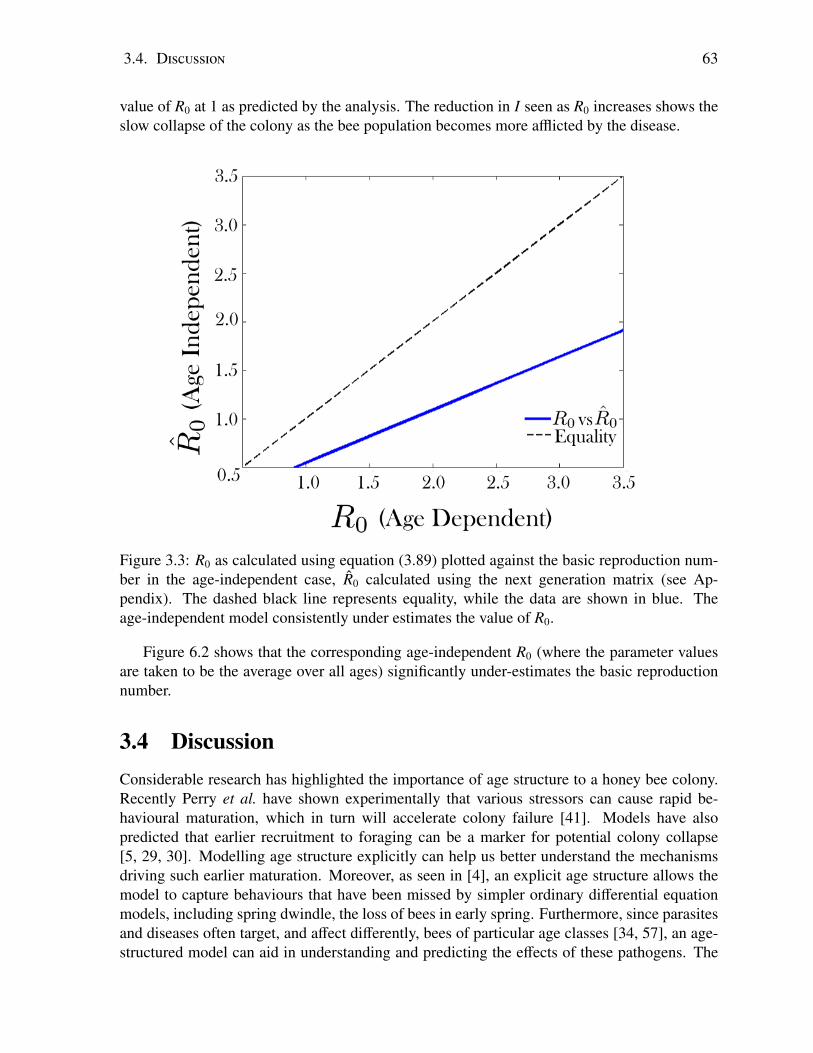
3.4. Discussion 63

value of R0 at 1 as predicted by the analysis. The reduction in I seen as R0 increases shows theslow collapse of the colony as the bee population becomes more afflicted by the disease.

Figure 3.3: R0 as calculated using equation (3.89) plotted against the basic reproduction num-ber in the age-independent case, R0 calculated using the next generation matrix (see Ap-pendix). The dashed black line represents equality, while the data are shown in blue. Theage-independent model consistently under estimates the value of R0.

Figure 6.2 shows that the corresponding age-independent R0 (where the parameter valuesare taken to be the average over all ages) significantly under-estimates the basic reproductionnumber.

3.4 DiscussionConsiderable research has highlighted the importance of age structure to a honey bee colony.Recently Perry et al. have shown experimentally that various stressors can cause rapid be-havioural maturation, which in turn will accelerate colony failure [41]. Models have alsopredicted that earlier recruitment to foraging can be a marker for potential colony collapse[5, 29, 30]. Modelling age structure explicitly can help us better understand the mechanismsdriving such earlier maturation. Moreover, as seen in [4], an explicit age structure allows themodel to capture behaviours that have been missed by simpler ordinary differential equationmodels, including spring dwindle, the loss of bees in early spring. Furthermore, since parasitesand diseases often target, and affect differently, bees of particular age classes [34, 57], an age-structured model can aid in understanding and predicting the effects of these pathogens. The

64 Chapter 3. Honey Bee Reproduction Number

differences between an age-structured model and age-independent model are explored furtherin [4], where we found that the age-structured model provides much richer dynamics, whichsometimes contrast the predictions of simpler models.

Equation (3.38) implies that the less food available, the more care is required in order foran acceptable fraction of the brood to survive. Moreover, if the hive bees begin nursing dutiessubstantially late, or leave nursing duties early, the equilibrium may disappear, leaving onlythe trivial equilibrium (i.e. extinction). This gives insights into the sensitivity of a honey beecolony to the age polyethism inherent in their social structure.

An important prediction of this study is that if a hazard (environmental, parasitic, etc.)causes a bee colony to decline, the colony can recover if the hazard is removed in a timelyfashion (given there are still sufficient food stores and brood care). This prediction is furtherexamined in the sister study [4], where we explore the same model in the context of changingseasons. This general stability result for honey bee dynamics is consistent with the fact thathoney bee colonies experience annual cycles in population size. Colonies typically suffer greatlosses in the late fall and early winter [66], and recover to peak colony population size by latespring to mid-summer [1, 38]. In this context, winter itself can be seen as a stressor on thecolony, and its end allows the colony to once again reach equilibrium. Moreover, consistentagain with experimental results, this is only possible if there are sufficient bees at the end ofwinter (Becher et al. estimate this number to be approximately 4000 bees [3]) and sufficientfood stores (honey bees typically require at least 20kg of stored honey to survive winter [50]).This of course depends on the length of winter.

Given the parameter set in Table A.1, we are able to predict an age distribution for thepopulation of a healthy colony. The total colony size predicted here is consistent within rangesreported by [3, 30, 43]. The age distribution is also consistent with the demography reportedby [48, 49, 61]. This agreement suggests that the simple death rate used in this model is areasonable approximation.

In [5, 29, 30, 44], the average age of recruitment to foraging (AARF) is found to be agood indicator of colony health. Lack of food [29], pesticide exposure [30, 41] and disease[5, 44] have all been predicted to lower the average age of recruitment to foraging. In ourage-dependent model, this average age can be further refined as we can keep track of the ageof bees explicitly. In particular, at any time, we have an age-dependent recruitment function,u(a, t), which (in the full model) depends on the populations of hive bees and foragers. Thusthe age-dependent model can recover a full distribution of the age at which bees are recruitedto foraging, not simply the average value. This distribution is an interesting focus for futurework. For example, a reduction in the AARF could be caused by a reduction in the number ofolder bees becoming foragers, or potentially an increase in the number of young bees becomingforagers. While [41] shows that pesticides would cause the latter situation, our model allowsfor differentiation between these two scenarios; exploring the possible causes underlying eachcase could be of interest.

The work we present here also provides some interesting mathematical techniques, whichcan be adapted to other PDE models. The results of this study determine the necessary con-ditions under which the introduction of an infection will lead to an epidemic outbreak withina bee colony by determining the basic reproduction number, R0. In theory, the formulationof R0 can be verified using an infinite dimensional analog of the next generation matrix [59].We confirm our derived expression of R0 numerically and via reduction to an age-independent

3.5. Appendix 65

model, analyzed using the next generation matrix. Although many models have been proposedfor disease dynamics within a honey bee colony [5, 35, 44, 57] and several provide stabilitycriteria for the disease-free equilibrium, none have provided an expression for R0. Here, weprovide a closed-form expression for R0, admittedly for a simplified disease model, in boththe age-independent case and for the continuous age-structured model. In theory, this shouldprovide an upper and lower bound for R0 for a model of N age classes.

Moreover, R0, although complicated in its formulation, can be used to determine whether adisease will be detrimental to a colony’s health if the transmission rate and death rate associatedwith that disease are known. In practice, it is often easier to obtain an estimate of R0 itself, inwhich case our formula can be used to determine the rate of transmission between bees or thedistribution of the death rate. This knowledge may help in determining strategies for saving thecolony or estimating death rates to be used to more accurately simulate disease transmission ina colony.

As we demonstrated, the basic reproduction number scales linearly with a constant trans-mission rate β, as expected. With similar analysis this result can be generalized to an age-dependent β(a). Also, the rate of recruitment plays a role in the spread of infection to theextent that a change in rate of recruitment may have the potential to either increase or decreaseR0. In the case of the linearized, age-independent expression, R0, we find that an increase inrecruitment lowers R0 (see appendix). We also observe that by omitting age-structure from amodel of honey bee colony dynamics, R0 is under-estimated.

Finally, we note that using the Laplace transform to determine asymptotic stability may beapplied more generally to time-dependent systems of partial differential equations, when theboundary conditions are constant. Also, the computation of R0 is applicable to many biologi-cal models with interacting susceptible classes. For example, age-dependent models of manysexually transmitted diseases may have interacting susceptible classes and could benefit fromthe approach we develop here. Future plans involve describing the methods more rigorously todetermine exactly when they can be applied to a more general class of PDE systems.

3.5 Appendix

Test: Uniform age distribution. We test the validity of this bifurcation parameter by reducingequations (3.70) and (3.71) to a system in which all parameters are constant with respect toage. In doing so, we find from equation (3.89) that

R0 = βH∗S

u + d+ β

uH∗S(µ + d)(u + d)

+ βF∗Sµ + d

. (3.90)

66 Chapter 3. Honey Bee Reproduction Number

This can be verified by using the next generation matrix on the infected classes of the followingreduced model

dHS

dt= −uHS + β(HI + FI)HS (3.91)

dFS

dt= uHS + β(HI + FI)FS − µFS (3.92)

dHI

dt= −uHI + β(HI + FI)HS − dHI (3.93)

dFI

dt= uHI + β(HI + FI)FS − (d + µ)FI (3.94)

which are a reduced form of equations (4.5) and (4.7). The ratio of the disease-free equilibriumvalues of FS ,HS will always be such that

H∗SF∗S

=µ

u. (3.95)

This ratio is found by setting HI = FI =dHS

dt=

dFS

dt= 0 in equations (3.91), (3.92), (3.93)

and (3.94).From these reduced equations we find the matrices,

F =

[βH∗S βH∗SβF∗S βF∗S

](3.96)

V =

[d + u 0−u d + µ

](3.97)

which yield the next generation matrix

FV−1 =

βH∗Su + d

+βuH∗S

(u + d)(µ + d)βH∗Sµ + d

βF∗Su + d

+βuF∗S

(u + d)(µ + d)βF∗Sµ + d

(3.98)

Each term in this matrix has a biological interpretation which is the expected number ofinfections in each class (H or F) caused by a single infected individual in each class. Forexample, the term

βH∗Su + d

(3.99)

gives the expected number of susceptible hive bees that an infected hive bee will infect whileit is still a hive bee. The term

βuH∗S(u + d)(µ + d)

(3.100)

3.5. Appendix 67

represents the probability that an infected hive bee will be recruited to foraging duties during itslife time, multiplied by the expected number of susceptible hive bees that would then becomeinfected. The expected number of susceptible hive bees infected by a single forager is given by

βH∗Sµ + d

(3.101)

The interpretations for the second row of matrix (3.98) are similar, but give the expectednumbers of susceptible foragers that will become infected.

The basic reproduction number for this uniform age distribution model is then determinedby the largest eigenvalue of the matrix FV−1. Since we have the relation (3.95), matrix (3.98)is rank 1. Therefore, one of its eigenvalues is zero and the other is given by its trace. We cansee that the trace of matrix (3.98) gives the same expression for the basic reproduction numberas (3.90).

The three terms that appear in (3.89) are analogous to the three terms that appear in equa-tion (3.90). This suggests that (3.89) correctly determines not only the threshold for diseasepersistence but also correctly estimates the number of secondary infections subsequent to oneprimary infection [22].

Bibliography

[1] Ball, B., and Allen, M. The prevalence of pathogens in honey bee (Apis mellifera)colonies infested with the parasitic mite Varroa jacobsoni. Annals of applied biology113, 2 (1988), 237–244.

[2] Becher, M. A., Grimm, V., Thorbek, P., Horn, J., Kennedy, P. J., and Osborne, J. L.BEEHAVE: a systems model of honeybee colony dynamics and foraging to explore mul-tifactorial causes of colony failure. Journal of applied ecology 51, 2 (2014), 470–482.

[3] Becher, M. A., Osborne, J. L., Thorbek, P., Kennedy, P. J., and Grimm, V. Review:Towards a systems approach for understanding honeybee decline: a stocktaking and syn-thesis of existing models. Journal of Applied Ecology 50, 4 (2013), 868–880.

[4] Betti, M., Wahl, L. M., and Zamir, M. Age structure is critical to the population dy-namics and survival of honeybee colonies. Royal Society Open Science 3, 11 (2016),160444.

[5] Betti, M. I., Wahl, L. M., and Zamir, M. Effects of infection on honey bee populationdynamics: A model. PLOS ONE 9, 10 (2014), e110237.

[6] Botias, C., Martin-Hernandez, R., Barrios, L., Meana, A., and Higes, M. Nosema spp.infection and its negative effects on honey bees (Apis mellifera iberiensis) at the colonylevel. Veterinary research 44, 1 (2013), 1–15.

[7] Boyce, W., and DiPrima, R. Differential Equations and Boundary Value Problems. WileyNew York, 2008.

[8] Brauer, F., Castillo-Chavez, C., and Castillo-Chavez, C. Mathematical models in pop-ulation biology and epidemiology, vol. 1. Springer, 2001.

[9] Calderone, N. W. Insect pollinated crops, insect pollinators and US agriculture: Trendanalysis of aggregate data for the period 1992-2009. PLOS ONE 7, 5 (05 2012), e37235.

[10] Cannon, R. H. Dynamics of physical systems. Courier Corporation, 2003.

[11] Castillo-Chavez, C., and Feng, Z. Global stability of an age-structure model for TBand its applications to optimal vaccination strategies. Mathematical biosciences 151, 2(1998), 135–154.

68

BIBLIOGRAPHY 69

[12] Corless, R. M., and Fillion, N. A graduate introduction to numerical methods. AMC 10(2013), 12.

[13] Diekmann, O., Heesterbeek, J., and Metz, J. A. On the definition and the computation ofthe basic reproduction ratio R0 in models for infectious diseases in heterogeneous popu-lations. Journal of mathematical biology 28, 4 (1990), 365–382.

[14] Domoshnitsky, A. Exponential stability of convolution integro-differential equations.Functional Differential Equations 5, 3-4 (2004), p–297.

[15] Domoshnitsky, A., and Goltser, Y. One approach to study of stability of integro-differential equations. Nonlinear Analysis: Theory, Methods & Applications 47, 6 (2001),3885–3896.

[16] Dukas, R. Mortality rates of honey bees in the wild. Insectes Sociaux 55, 3 (2008),252–255.

[17] Eberl, H. J., Frederick, M. R., and Kevan, P. G. Importance of brood maintenanceterms in simple models of the honeybee - Varroa destructor - Acute Bee Paralysis Viruscomplex. Electronic Journal of Differential Equations (EJDE) [electronic only] 2010(2010), 85–98.

[18] Fahrbach, S., and Robinson, G. Juvenile hormone, behavioral maturation and brain struc-ture in the honey bee. Developmental Neuroscience 18 (1996), 102–114.

[19] Goltser, Y., and Litsyn, E. Volterra integro-differential equations and infinite systems ofordinary differential equations. Mathematical and computer Modelling 42, 1-2 (2005),221–233.

[20] Grossmann, C., Roos, H.-G., and Stynes, M. Numerical treatment of partial differentialequations. Springer, 2007.

[21] Hale, J. K., and Waltman, P. Persistence in infinite-dimensional systems. SIAM Journalon Mathematical Analysis 20, 2 (1989), 388–395.

[22] Heffernan, J., Smith, R., and Wahl, L. M. Perspectives on the basic reproductive ratio.Journal of the Royal Society Interface 2, 4 (2005), 281–293.

[23] Ho, M.-W., and Cummins, J. Mystery of disappearing honeybees. Science in Society 34(2007), 35–36.

[24] Huang, Z.-Y., and Robinson, G. E. Regulation of honey bee division of labor by colonyage demography. Behavioral Ecology and Sociobiology 39 (1996), 147–158.

[25] Hyman, J. M., and Li, J. An intuitive formulation for the reproductive number for thespread of diseases in heterogeneous populations. Mathematical biosciences 167, 1 (2000),65–86.

[26] Inaba, H. Threshold and stability results for an age-structured epidemic model. Journalof mathematical biology 28, 4 (1990), 411–434.

70 BIBLIOGRAPHY

[27] Jaycox, E. R., Skowronek, W., and Guynn, G. Behavioral changes in worker honeybees (apis mellifera) induced by injections of a juvenile hormone mimic. Annals of theEntomological Society of America 67, 4 (1974), 529–534.

[28] Jones, J. C., Helliwell, P., Beekman, M., Maleszka, R., and Oldroyd, B. The effectsof rearing temperature on developmental stability and learning and memory in the honeybee, Apis mellifera. Journal of Comparative Physiology A 191, 12 (2005), 1121–1129.

[29] Khoury, D. S., Barron, A. B., and Myerscough, M. R. Modelling food and populationdynamics in honey bee colonies. PLOS ONE 8, 5 (05 2013), e59084.

[30] Khoury, D. S., Myerscough, M. R., and Barron, A. B. A quantitative model of honeybee colony population dynamics. PLOS ONE 6, 4 (04 2011), e18491.

[31] Leoncini, I., Le Conte, Y., Costagliola, G., Plettner, E., Toth, A. L., and Wang, M.Regulation of behavioral maturation by a primer pheromone produced by adult workerhoney bees. Proceedings of the National Academy of Sciences of the United States ofAmerica 101, 50 (2004), 17559–17564.

[32] Li, J., and Brauer, F. Continuous-time age-structured models in population dynamicsand epidemiology. In Mathematical Epidemiology, F. Brauer, P. van den Driessche, andJ. Wu, Eds. Springer, 2008, pp. 205–227.

[33] Magal, P., McCluskey, C., and Webb, G. Lyapunov functional and global asymptoticstability for an infection-age model. Applicable Analysis 89, 7 (2010), 1109–1140.

[34] Martin, S. Hygienic behaviour: an alternative view. Bee Improvement 7 (2000), 6–7.

[35] Martin, S. J. The role of Varroa and viral pathogens in the collapse of honeybee colonies:a modelling approach. Journal of Applied Ecology 38, 5 (2001), 1082–1093.

[36] McKendrick, A., and Pai, M. K. The rate of multiplication of microorganisms: a mathe-matical study. vol. 31, pp. 649–655.

[37] Neumann, P., and Carreck, N. L. Honey bee colony losses. Journal of ApiculturalResearch 49, 1 (2010), 1–6.

[38] Odoux, J.-F., Aupinel, P., Gateff, S., Requier, F., Henry, M., and Bretagnolle, V.ECOBEE: a tool for long-term honey bee colony monitoring at the landscape scale inWest European intensive agroecosystems. Journal of Apicultural Research 53, 1 (2014),57–66.

[39] Olver, P. J. Introduction to partial differential equations. Springer, 2014.

[40] Parker, S. McGraw-Hill dictionary of scientific and technical terms. McGraw-Hill, 2003.

[41] Perry, C. J., Søvik, E., Myerscough, M. R., and Barron, A. B. Rapid behavioral mat-uration accelerates failure of stressed honey bee colonies. Proceedings of the NationalAcademy of Sciences 112, 11 (2015), 3427–3432.

BIBLIOGRAPHY 71

[42] Petric, A. T. A Mathematical Model for a N. ceranae Infection in an A. mellifera Colony.PhD thesis, 2016.

[43] Ratnieks, F. L., and Keller, L. Queen control of egg fertilization in the honey bee.Behavioral Ecology and Sociobiology 44, 1 (1998), 57–61.

[44] Ratti, V., Kevan, P. G., and Eberl, H. J. A mathematical model for population dynamicsin honeybee colonies infested with Varroa destructor and the Acute Bee Paralysis Virus.Canadian Applied Mathematics Quarterly 21, 1 (2013), 63–93.

[45] Ratti, V., Kevan, P. G., and Eberl, H. J. A mathematical model of the honeybee-Varroadestructor-Acute Bee Paralysis Virus complex with seasonal effects. Bulletin of Mathe-matical Biology (2015).

[46] Robinson, G. E., Page, R. E., Strambi, C., and Strambi, A. Colony integration in honeybees: mechanisms of behavioral reversion. Ethology 90, 4 (1992), 336–348.

[47] Russell, S., Barron, A. B., and Harris, D. Dynamic modelling of honey bee (Apismellifera) colony growth and failure. Ecological Modelling 265, 0 (2013), 158 – 169.

[48] Sakagami, S., and Fukuda, H. Life tables for worker honeybees. Researches on Popula-tion Ecology 10, 2 (1968), 127–139.

[49] Schmickl, T., and Crailsheim, K. Hopomo: A model of honeybee intracolonial populationdynamics and resource management. Ecological modelling 204, 1 (2007), 219–245.

[50] Seeley, T. D. The wisdom of the hive: the social physiology of honey bee colonies.Harvard University Press, 2009.

[51] Seeley, T. D. Honeybee Democracy. Princeton University Press, 2010.

[52] Smith, G. D. Numerical solution of partial differential equations: finite difference meth-ods. Oxford University press, 1985.

[53] Smith, M. L. The honey bee parasite Nosema ceranae: Transmissible via food exchange?PLOS ONE 7, 8 (08 2012), e43319.

[54] Southwick, E. E., and Southwick Jr, L. Estimating the economic value of honey bees(Hymenoptera: Apidae) as agricultural pollinators in the United States. Journal of Eco-nomic Entomology 85, 3 (1992), 621–633.

[55] Stevanovic, J., Simeunovic, P., Gajic, B., Lakic, N., Radovic, D., Fries, I., and Stan-imirovic, Z. Characteristics of Nosema ceranae infection in Serbian honey bee colonies.Apidologie 44, 5 (2013), 522–536.

[56] Stewart, J. Multivariable calculus. Cengage Learning, 2011.

[57] Sumpter, D. J. T., and Martin, S. J. The dynamics of virus epidemics in Varroa-infestedhoney bee colonies. Journal of Animal Ecology 73, 1 (2004), 51–63.

72 BIBLIOGRAPHY

[58] Tereshko, V., and Loengarov, A. Collective decision-making in honey bee foraging dy-namics. Computing and Information Systems 9, 3 (2005), 1.

[59] Thieme, H. R. Spectral bound and reproduction number for infinite-dimensional pop-ulation structure and time heterogeneity. SIAM Journal on Applied Mathematics 70, 1(2009), 188–211.

[60] Van den Driessche, P., and Watmough, J. Reproduction numbers and sub-threshold en-demic equilibria for compartmental models of disease transmission. Mathematical bio-sciences 180, 1 (2002), 29–48.

[61] van der Steen, J. J., Cornelissen, B., Donders, J., Blacquiere, T., and van Dooremalen,C. How honey bees of successive age classes are distributed over a one storey, ten frameshive. Journal of Apicultural Research 51, 2 (2012), 174–178.

[62] Vance, J. T., Williams, J. B., Elekonich, M. M., and Roberts, S. P. The effects of ageand behavioral development on honey bee (Apis mellifera) flight performance. Journal ofExperimental Biology 212, 16 (2009), 2604–2611.

[63] vanEngelsdorp, D., Evans, J. D., Saegerman, C., Mullin, C., Haubruge, E., Nguyen,B. K., Frazier, M., Frazier, J., Cox-Foster, D., Chen, Y., Underwood, R., Tarpy, D. R.,and Pettis, J. S. Colony collapse disorder: A descriptive study. PLOS ONE 4, 8 (082009), e6481.

[64] Wang, W., and Zhao, X.-Q. Basic reproduction numbers for reaction-diffusion epidemicmodels. SIAM Journal on Applied Dynamical Systems 11, 4 (2012), 1652–1673.

[65] Watanabe, M. E. Colony collapse disorder: Many suspects, no smoking gun. BioScience58, 5 (2008), 384–388.

[66] Winston, M. The biology of the honey bee. Harvard University Press, 1987.

Chapter 4

Age structure is Critical to the PopulationDynamics and Survival of Honey BeeColonies

Abstract

Age-structure is an important feature of the division of labour within honey bee colonies,but its effects on colony dynamics have rarely been explored. We present a model of ahoney bee colony that incorporates this key feature, and use this model to explore theeffects of both winter and disease on the fate of the colony. The model offers a novel ex-planation for the frequently observed phenomenon of “spring dwindle”, which emerges asa natural consequence of the age-structured dynamics. Furthermore, the results indicatethat a model taking age structure into account markedly affects the predicted timing andseverity of disease within a bee colony. The timing of the onset of disease with respect tothe changing seasons may also have a substantial impact on the fate of a honey bee colony.Finally, simulations predict that an infection may persist in a honey bee colony over sev-eral years, with effects that compound over time. Thus the ultimate collapse of the colonymay be the result of events several years past.

4.1 Introduction

As honey bee populations continue to decline on a global scale [5], research efforts have beendirected at identifying the underlying causes [12, 20, 43, 45]. These efforts are necessitated bythe ecological [13] and economical importance of honey bee colonies worldwide [9, 29, 40].

To date, much of this research has been focused on the effects of pesticide and insec-ticideexposure on honey bee health and ultimately colony fitness [18, 45]. Such hazardsmay cause injury or death to foraging bees, forcing surviving bees to begin foraging pre-maturely which will then disrupt the dynamics of the colony, ultimately leading to colonycollapse [18, 23, 24]. Further research has focused on the effects of parasitism and dis-ease [6, 7, 14, 32, 33, 41], for example, the effects of Varroa destructor on honey bee colonydynamics [14, 32, 33, 41], the effects of the microsporidian parasite Nosema ceranae [19], andthe effects of communicable infections more generally [6].

73

74 Chapter 4. Age Structure in Honey Bee Colonies

Recent work has also explored the combined effects of two stressors such as disease, limitedbiodiversity, and/or exposure to pesticides, which may create conditions detrimental to honeybee colony survival [1, 2, 17, 28, 39, 44]. Simulation packages have been developed to modelthese effects using realistic parameter values [4, 36]. For example, Pettis et al. explored theinterplay between environmental hazards and the subsequent susceptibility to Nosema ceranae[31]. In previous work [6], we showed that the fate of a honey bee colony in the presence ofdisease is dependent on seasonality, particularly the onset of winter.

Previous mathematical models of honey bee dynamics have not considered the effects ofage-structure within the hive, yet the duties of female bees, which constitute the main workforce of the hive, are determined primarily by their age [34]. Specifically, the hierarchy of acolony hinges on both bee morphology and age [10, 35, 37]: caste polyethism differentiates aqueen bee from a female worker bee [46], while age polyethism determines the functions ofthe worker bees [34].

The age distribution within a honey bee colony is an intrinsic property and this property istherefore important to colony survival because it affects two key components in the dynamicsof the colony, namely ongoing recruitment and death. In the present paper, we examine howthe disease-free age distribution within a colony is altered in the face of a hazard, and howthese changes affect previous predictions of colony survival.

We identify periods of increased vulnerability of the colony to the effects of winter, disease,or a combination of the two, during which the colony would benefit from remedial actions (e.g.higher anti-microbial treatments, increased observation and management etc.). In addition, weuse the added dimension of age-structure to explore the long standing phenomenon of “springdwindle” whereby a drop in the number of bees within a colony occurs immediately afterthe end of winter [47]. While the phenomenon is generally suspected to be due to variousstressors [15, 30, 38], the specific colony dynamics that lead to this phenomenon have not beenestablished. The question of why the dwindle occurs after rather than during winter remainsunanswered. The resolution of this puzzle is of particular value in the ongoing research effortsto understand and ultimately avert honey bee colony collapse, since spring dwindle leaves thecolony in a particularly vulnerable state. Finally, we simulate colony dynamics in the presenceof disease for multiple years to demonstrate the compounding effects of infection.

4.2 ModelWe present a mathematical model that combines the disease-free demographics of a honey beecolony with the effects of seasonal changes and a disease that at first infects foragers, and thenspreads to the rest of the colony. Earlier versions of this model were introduced by Khouryet al. in 2011 and 2013 [23, 24] and were developed further in 2015 [6]. Analytical detailsof the model, including local and global stability of the disease free equilibrium as well as aderivation of the basic reproduction number, R0, are presented in [7].

Briefly, the effects of the brood, guarding bees, as well as bees that work to repair the hiveare neglected. The focus is solely on the hive bees, H, which are responsible for ensuring thesurvival of the brood, and the foragers, F, which are responsible for bringing food, f , into thehive. The male honey bees, known as drones, are also neglected since they contribute only toreproduction [46]. In the presence of disease, the two classes of bees are further divided into

4.2. Model 75

the susceptible populations, HS and FS , and the infected populations, HI and FI .

4.2.1 Age StructureWe incorporate an age structure into the age-independent equations [6], using the standardapproach of McKendrick [27] by writing

∂HS

∂t+∂HS

∂a= −u(a)HS − βN HS , (4.1)

where HS (a, t) is the number of susceptible hive bees of age a at time t and u(a) is the age-dependent rate of recruitment to foraging. Juvenile hormone III regulates the age at whichhoney bees begin foraging [34], making older bees more likely to be recruited to foraging du-ties. As well, it has been observed that there is a minimum age, aR, before which bees cannotbe recruited [16]. Behavioural maturation of hive bees is further regulated by a pheromone,ethyl oleate, that is produced by foragers [26] and has the effect of delaying the age at whichbees are recruited to foraging duties. This so-called “social inhibition” process reduces recruit-ment when the number of foragers in the colony is high [26]. We account for these biologicalprocesses by defining u(a) as

u(a) = α( aa + k

)2(1 −

σ

N

∫(FS + FI)da

)Hv(a − aR) (4.2)

where α is the maximum rate of recruitment and Hv(a − aR) is the Heaviside function suchthat recruitment cannot begin before age aR. Thereafter, the recruitment rate we are usingincreases sigmoidally with age. At age k, recruitment will be one quarter the maximum rate ofrecruitment. 1/σ is the maximum proportion of bees that are foraging at any given time and Nis the total number of bees given by

N =

∫(HS + HI + FS + FI)da. (4.3)

The emergence of new hive bees is modeled as the left boundary condition to Equation (4.1).This, along with other boundary conditions are described at the end of this section.

The second term on the right-hand side of equation (4.1) governs the disease dynamicswithin the hive. We approximate the transmission of disease as a mass action process andassume that, on average, hive bees and foragers transmit infection between or within classes atrate β. The total number of infected bees is given by

N =

∫(HI + FI)da. (4.4)

The hive provides substantial safety for bees that are confined to it [24, 37]. We thereforeassume that the natural death rate of healthy hive bees is negligible compared to the rate ofrecruitment.

The equation governing the dynamics of infected hive bees is given by

∂HI

∂t+∂HI

∂a= βN HS − u(a)HI − dH(a)HI . (4.5)

76 Chapter 4. Age Structure in Honey Bee Colonies

In contrast with their healthy peers, infected hive bees are at risk of dying due to disease at anage-dependent rate dH(a).

Susceptible foragers are recruited from susceptible hive bees, and suffer age-dependentnatural death at rate µ(a). Their dynamics are therefore governed by

∂FS

∂t+∂FS

∂a= u(a)HS − µ(a)FS − βN FS (4.6)

Infected foragers can either be recruited from infected hive bees, or from susceptible for-agers that have become infected. If we assume this class is subject to a disease-related deathrate of dF(a), then their dynamics are governed by

∂FI

∂t+∂FI

∂a= u(a)HI + βN FS − (µ(a) + dF(a)) FI . (4.7)

Food, f , is brought into the hive by both susceptible and infected foragers. Although it islikely that infected foragers would be less efficient at this task [25], for simplicity, we take anaverage rate of food intake, c (g/day/forager). Food is consumed by foragers and hive bees atan average rate γ. Therefore, the amount of food available at time t changes according to

d fdt

= c∫

(FS + FI) da − γN. (4.8)

The above system of equations governing the dynamics of the colony is subject to thefollowing boundary conditions:HS (0, t) = LS

HI(0, t) = FS (0, t) = FI(0, t) = 0. (4.9)

The first condition represents the emergence of new adult bees, where L is the daily egglaying rate of the queen and S is a survivability function, which determines how many eggssurvive to adulthood. The brood needs both sufficient food and sufficient care from the hivebees in order to survive [22]. Moreover, it has been shown that there is a range of ages withinwhich hive bees will take on this care for the brood, a minimum age, am, and a maximum age,aT between 11 and 16 days old [35]. After this age, hive bees tend to transition to foragingduties, or possibly security or hive maintenance [46]. Therefore, we define the survivabilityfunction S as

S =

(f

b + f

) ∫ aT

amH(a, t)da

w +∫ aT

amH(a, t)da

. (4.10)

Here b is the amount of food required for half the eggs to survive to adulthood provided thebrood has sufficient care, w is the number of care providers required for half the eggs to surviveprovided the brood has sufficient food, and H(a, t) = HS (a, t) + HI(a, t).

The dynamics described in this section relate to the main active season of the bee colony,which is defined as the time interval between the end of one winter and the beginning of thenext.

4.2. Model 77

4.2.2 WinterThe winter season is assumed to last 155 days or roughly 5 months, roughly corresponding toa humid continental climate [3]. Over winter, no new hive bees emerge (although some eggsare still being laid by the queen) and foragers return to the hive [46]. Accordingly, in boundaryconditions 4.9 we set L = 0 and in equations 4.1, 4.5, 4.6, 4.7 and 4.8 we set u(a) = 0 andc = 0. Due to an extended lifespan of bees over winter [46], the death rate of hive bees is nolonger negligible and is set to an average rate of

µw =1

180, (4.11)

corresponding to an average lifespan over winter of 6 months [46]. All bees are performing thesame function over winter (keeping the hive warm [21]), therefore we set the natural death rateof foragers equal to that of the hive bees, µ(a) = µw.

As winter ends, bees resume their normal age-related duties, and bees that were foragingbefore winter resume their roles as foragers. We assume that a 21-day transition takes placeduring which parameter values change linearly from end-of-winter to new active season valuesas follows:

µtrans(a) =(1 − t

21

)µw(a) +

(t

21

)µ(a)

Ltrans =(

t21

)L

S trans =(

t21

)S +

(1 − t

21

)S ∗

0 ≤ t ≤ 21 (4.12)

where

S ∗ =

(f

b + f

) ∫ ∞

amHS (a, t)da

w +∫ ∞

amHS (a, t)da

, (4.13)

that is, during winter hive bees of all ages may contribute to brood care. Note that new hivebees that emerge during the early spring come from eggs that were laid over the winter months,after completing phases of development to adulthood.

Equations (4.1), (4.5), (4.6), (4.7), and (4.8) form a system of integro-partial differentialequations which we solved simultaneously to predict the population dynamics of a honey beecolony. The parameter values used in the solution are given in Table A.1 in the supplementarymaterial.

In [42], the authors found that the age distribution in a colony is as follows: 41% of beeswere one week old, 23% were two weeks old, 17% were three weeks old, 11% were fourweeks old, and 8% were five weeks old. Accordingly, the death rate µex(a) in our model wasconstructed to approximately match the experimental findings. In order to account for thewhole range of ages and remain consistent with the five weeks of study in [42], we break theage range into five cohorts of ten days each. The comparison between experimental data andour model is summarized in Table 4.1. The death rate that best matched the observed data isdefined by

µex(a) =

1 − e

(a−20)210 a ≤ 20

Cex

(a − 20

20

)4

a > 20. (4.14)

78 Chapter 4. Age Structure in Honey Bee Colonies

where parameter values were set such that the percentage of bees in their first week of lifematches the experimental data. This death rate is relatively high for very young (≈< 10 days)or very old bees (≈> 40 days), as shown in Figure 6.2. We see that the drop in populationdensity after week 1, as observed in [42], can be explained by the high death rate of youngforagers.

Figure 4.1: Death rate distribution which provides the best fit to experimental results observedin [42]; parameter Cex = 0.42.

We performed sensitivity analysis (see Supplementary Material Figure A.1) and found thatour results are insensitive to the details of the death rate distribution. We therefore use a sim-plified version of the natural death rate distribution,

µ(a) = C(a − 20)2

400, (4.15)

to make the mathematics more tractable. This death rate is plotted in Figure 4.2, and alsocompared with the experimental results in Table 4.1, showing good agreement.

The disease-related death rate,

d(a) = −K1

πtan−1(a − 10) + K2, (4.16)

is motivated by deformed wing virus [11] that disproportionately affects young bees. Theconstants C, K1 and K2 are chosen such that both the natural and disease-related death ratesare non-negative and have an average of 0.14 per day as in [6]. In other cases, we assume thedisease affects all bees uniformly, i.e. d(a) = d. The effects of different death rate distributionsare shown in the supplementary material (Figures A.4–A.12). The results are qualitatively thesame.

4.3. Results 79

Figure 4.2: The natural death rate, µ(a), and an example of disease-related death rate, d(a),motivated by deformed wing virus, which predominantly affects young bees [11]. During theactive season, honey bees live an average of five to seven weeks [46], thus we define our deathrates until the age of 60 days. Beyond this age few, if any, bees are still alive and we set theirnatural death rate as µ(a > 60) = max(µ(a)).

Figure A.1 in the supplementary material shows the age distribution within a disease-freecolony under the natural death rate µ(a) shown in Figure 4.2. This is used as a baseline distri-bution for all simulations that begin from equilibrium. We predict from this distribution thatthe mean forager age of a healthy colony is approximately 25 days [8, 46].

4.3 ResultsFigure 4.3 shows the effects of changing seasons on the number of bees in a colony in theabsence of disease. The seasonal shift back to normal operating conditions is seen to bringwith it a drop in the bee population as the colony emerges from winter. It is obvious thata longer winter may have a fatal effect on the colony, due to winter only having deleteriouseffects on a colony. This is because the surviving bees are now much older and are subjectto a higher natural death rate, while a new generation of younger bees has not yet emerged toreplace them. This seasonal drop in the bee population, which has been referred to as “springdwindle” [15, 30, 38, 47], is discussed further in the next section. The population dynamics thatproduce the phenomenon have not been fully understood in the past because these dynamicsemerge only when the age distribution within the colony is considered.

80 Chapter 4. Age Structure in Honey Bee Colonies

Cohort Experimental Values [42] Model Values, µex(a) Model Values, µ(a)1 41± 6.4% 41% (0) 41% (0)2 23± 5.1% 25% (0.39) 30% (1.37)3 17± 3.7% 18% (0.27) 16% (0.27)4 11± 2.2% 11% (0) 7% (1.81)5 8± 1.3% 5% (2.31) 6% (1.54)

Table 4.1: Comparison of experimental results with model results. Standard deviation forexperimental results are given; z-scores computed from experimental mean and standard devi-ations are given in parentheses next to model values.

Our next objective is to compare the dynamics of the age-structured honey bee colonymodel with the dynamics of the age-independent model such as that presented in [6]. To givethe comparison a measure of equivalency, the same value of the basic reproduction number isused in both cases, namely R0 = 1.43, calculated using the formulas derived in [7]. Figure 5.7shows that an age-independent model makes significantly different predictions about the timingand the severity of disease within a bee colony. This is further explored in the supplementarymaterial (Figure A.3) where we demonstrate that an age-dependent recruitment function bothlowers the severity of a disease and delays the timing of an epidemic, while age-dependentdeath rates, µ(a) and d(a), trade-off the two effects.

The vulnerability of a bee colony in early spring is explored further in Figure 4.5 whichillustrates that an infection which is endemic in a colony during one active season and onewinter may pose the greatest risk to the colony during the small window in which the hive isrecovering from the winter months. Moreover, the colony may suffer much greater losses afterits second, third and fourth winters with disease (figure inset).

The time interval between the beginning of an infection and the onset of winter is an im-portant determinant of the health of the colony at the end of winter, as illustrated in Figure4.6. The figure shows that the number of bees surviving to the end of winter, NW , depends onwhen the infection begins relative to winter. In the figure the infection begins from a singleinfected forager ∆t days before winter. The time interval between the end of one winter and thebeginning of the next is taken to be approximately 200 days (≈ 7 months). The timing of theinfection is seen to produce a point of highest vulnerability (local minimum in population size)which depends on the severity of the disease as represented by the basic reproduction number.

The timing and depth of the points of highest vulnerability seen in Figure 4.6 are tightlycoupled to the time at which an infection peaks within the colony, which in turn is related toR0. Figure 4.7 shows this relationship, estimating the time of greatest risk to the colony, ∆t∗,with respect to the onset of winter, based on the basic reproduction number. Of course, for highvalues of R0 the colony is likely to suffer substantial losses regardless of when a disease occurs.In Figure 4.6, we see for example that for R0 = 2.0, ∆t∗ is unique, but when R0 = 2.2 thereare two ∆t∗ values producing the observed bifurcation in Figure 4.7. To measure the relativesignificance of these minima, we use the metric max(NW) −min(NW) where the maximum andminimum are computed for each value of R0, over the range of possible ∆t. The larger thevalue of this metric, the greater the significance of the time of onset of disease, ∆t.

4.3. Results 81

Figure 4.3: Time course of total bee population in a disease-free colony. Shaded area denoteswinter, during which no brood is produced. We see that the aged bees that restart the colonypost-winter create an added risk to the colony, because of their relatively high death rate, untilnew brood is able to hatch and contribute to population rebound. The post-winter dip seen inthe figure has been referred to in the literature as “spring dwindle” but its dynamics have notbeen previously described.

Figure 4.4: Effect of age distribution on the dynamics of disease within the bee colony. Theblue line represents the total number of susceptible bees and the green dashed line representsthe total infected bees. The shaded area denotes winter. Disease begins with a single infectedforager at t = 112. We use the death rates given in Figure 4.2. The two time courses showthat the two models have significant differences in their predictions when simulating diseasedynamics in the colony.

82 Chapter 4. Age Structure in Honey Bee Colonies

Figure 4.5: Time course of the bee population over four years. The top panel shows the totalnumber of susceptible bees, HS + FS , and the bottom panel shows the total number of infectedbees, HI + FI . An infection is introduced into a colony at equilibrium through a single infectedforager at time t = 0. The inset shows the minimum population size of susceptible bees duringthe spring dwindle following each winter. There is a clear decrease in this minimum year afteryear, thus the risk of colony collapse increases year after year. The ultimate collapse of a beecolony may therefore be the consequence of events long past.

4.3. Results 83

Figure 4.6: Number of bees at the end of winter as a function of the time interval, ∆t betweenthe onset of disease and the beginning of winter, based on various values of the basic repro-duction number, R0. The minima show times during which the colony is most vulnerable dueto the combined effects of winter and disease. The colony is started from the equilibrium agedistribution shown in Figure A.1. Infection is introduced at time t = 200 − ∆t via one infectedforager. The total number of bees is calculated at the end of winter. R0 values are calculatedusing the expression derived in [7].

84 Chapter 4. Age Structure in Honey Bee Colonies

Figure 4.7: The timing and depth of points of highest vulnerability as a function of the basicreproduction number, R0. The colour bar reflects the depth of the minima seen in Figure 4.6(see text for details). Red indicates the most severe combinations of R0 and ∆t∗, where ∆t∗ isthe value of ∆t in Figure 4.6 at which a local minimum occurs.

4.4. Discussion 85

4.4 DiscussionOur results demonstrate that the age structure that is inherent to all honey bee colonies hascritical effects on colony survival that are not captured by previously explored age-independentmodels. Most notably, an age-dependent recruitment rate has a profound impact on the dy-namics, severity, and spread of an infection in a bee colony. In fact, our results predict that agepolyethism in a honey bee colony has the beneficial effect of impeding the spread of infectionwithin the colony. Thus, in practice, any disturbance in the natural age structure of a bee colonymay also increase the severity of an infection within the hive. Results in the supplementarymaterial (Figure A.3) indicate that the natural age distribution within a colony creates a delay inthe speed of spread of an infection. Again, this suggests that any intervention that would alterthe natural age distribution may have the adverse effect of increasing the spread of infectionwithin a hive.

Our explicit treatment of the colony age distribution also revealed the dynamics underlyingthe frequently observed phenomenon of “spring dwindle” in which the total number of beeswithin a colony weakens rapidly immediately after the end of winter. While the phenomenonis generally suspected to be due to various stressors that occurs during winter [15, 30, 38],our results suggest that declining spring populations are a natural consequence of honey beecolony dynamics, leading to seasonal vulnerability during which the colony may be particularlysusceptible to other hazards. This post-winter dip is not captured by age-independent modelsbecause the phenomenon is due predominantly to the aging of the bees over the winter monthsand the time required to replace them by younger bees in the early spring.

Simulations of colony dynamics over multiple winter seasons demonstrated that endemicdiseases may weaken the colony year after year, increasing the risk of colony collapse duringspring. Thus the eventual collapse of a bee colony may be due to the compounded effects of aninfection over several years.

The time interval between the onset of an infection and the beginning of an approachingwinter is a critical determinant of the ultimate course and consequence of the disease withina bee colony. As illustrated in Figures 4.6 and 4.7, this effect is most important for infectionswith a basic reproduction number close to 2. In this case, the colony is particularly vulnerablein the early spring, approximately 5 months before the onset of winter.

In conclusion, age structure is an inherent property of honey bee colonies, determining thedivision of labour and defining how age-related events such as disease and death unfold withinthe colony. Our results suggest that age structure should be a key consideration in future studiesof honey bee population dynamics, and that accurate models of age structure will be necessaryif we are to understand, and ultimately reverse, the increases in colony collapse observed inrecent years.

Bibliography

[1] Alaux, C., Brunet, J.-L., Dussaubat, C., Mondet, F., Tchamitchan, S., Cousin, M., Bril-lard, J., Baldy, A., Belzunces, L. P., and Le Conte, Y. Interactions between Nosemamicrospores and a neonicotinoid weaken honeybees (Apis mellifera). Environmental mi-crobiology 12, 3 (2010), 774–782.

[2] Aufauvre, J., Biron, D. G., Vidau, C., Fontbonne, R., Roudel, M., Diogon, M., Vigues,B., Belzunces, L. P., Delbac, F., and Blot, N. Parasite-insecticide interactions: a casestudy of Nosema ceranae and fipronil synergy on honeybee. Scientific reports 2 (2012).

[3] Baldwin, D. J., Desloges, J. R., and Band, L. E. Physical geography of ontario. Ecology ofa managed terrestrial landscape: patterns and processes of forest landscapes in Ontario(2011), 12.

[4] Becher, M. A., Grimm, V., Thorbek, P., Horn, J., Kennedy, P. J., and Osborne, J. L.BEEHAVE: a systems model of honeybee colony dynamics and foraging to explore mul-tifactorial causes of colony failure. Journal of applied ecology 51, 2 (2014), 470–482.

[5] Becher, M. A., Osborne, J. L., Thorbek, P., Kennedy, P. J., and Grimm, V. Review:Towards a systems approach for understanding honeybee decline: a stocktaking and syn-thesis of existing models. Journal of Applied Ecology 50, 4 (2013), 868–880.

[6] Betti, M. I., Wahl, L. M., and Zamir, M. Effects of infection on honey bee populationdynamics: A model. PLOS ONE 9, 10 (2014), e110237.

[7] Betti, M. I., Wahl, L. M., and Zamir, M. Reproduction number and asymptotic stabil-ity for a model with continuous age structure: An application to honey bee dynamics.Bulletin of Mathematical Biology (2016). submitted.

[8] Botias, C., Martin-Hernandez, R., Barrios, L., Meana, A., and Higes, M. Nosema spp.infection and its negative effects on honey bees (Apis mellifera iberiensis) at the colonylevel. Veterinary research 44, 1 (2013), 1–15.

[9] Calderone, N. W. Insect pollinated crops, insect pollinators and US agriculture: Trendanalysis of aggregate data for the period 1992-2009. PLOS ONE 7, 5 (05 2012), e37235.

[10] Cramp, D. A Practical Manual of Beekeeping. How To Books, London, 2008.

[11] De Miranda, J. R., and Genersch, E. Deformed wing virus. Journal of InvertebratePathology 103 (2010), S48–S61.

86

BIBLIOGRAPHY 87

[12] Dennis, B., and Kemp, W. P. How hives collapse: Allee effects, ecological resilience, andthe honey bee. PLOS ONE 11, 2 (2016), e0150055.

[13] Devillers, J. The ecological importance of honey bees and their relevance to ecotoxicol-ogy. In Honey Bees: Estimating the Environmental Impact of Chemicals, J. Devillers andM. Pham-Delegue, Eds. Taylor and Francis London, London, 2002, pp. 1–11.

[14] Eberl, H. J., Frederick, M. R., and Kevan, P. G. Importance of brood maintenanceterms in simple models of the honeybee - Varroa destructor - Acute Bee Paralysis Viruscomplex. Electronic Journal of Differential Equations (EJDE) [electronic only] 2010(2010), 85–98.

[15] Evans, J. D., and Schwarz, R. S. Bees brought to their knees: microbes affecting honeybee health. Trends in microbiology 19, 12 (2011), 614–620.

[16] Fahrbach, S., and Robinson, G. Juvenile hormone, behavioral maturation and brain struc-ture in the honey bee. Developmental Neuroscience 18 (1996), 102–114.

[17] Goulson, D., Nicholls, E., Botıas, C., and Rotheray, E. L. Bee declines driven bycombined stress from parasites, pesticides, and lack of flowers. Science 347, 6229 (2015),1255957.

[18] Henry, M., Beguin, M., Requier, F., Rollin, O., Odoux, J.-F., Aupinel, P., Aptel, J.,Tchamitchian, S., and Decourtye, A. A common pesticide decreases foraging successand survival in honey bees. Science 336, 6079 (2012), 348–350.

[19] Higes, M., Martin-Hernandez, R., Garrido-Bailon, E., Gonzalez-Porto, A. V., Garcia-Palencia, P., and Meana, A. Honeybee colony collapse due to Nosema ceranae in profes-sional apiaries. Environmental Microbiology Reports 1, 2 (2009), 110–113.

[20] Ho, M.-W., and Cummins, J. Mystery of disappearing honeybees. Science in Society 34(2007), 35–36.

[21] Jay, S. Seasonal development of honeybee colonies started from package bees. Journalof Apicultural Research 13 (1974), 149–152.

[22] Jones, J. C., Helliwell, P., Beekman, M., Maleszka, R., and Oldroyd, B. The effectsof rearing temperature on developmental stability and learning and memory in the honeybee, Apis mellifera. Journal of Comparative Physiology A 191, 12 (2005), 1121–1129.

[23] Khoury, D. S., Barron, A. B., and Myerscough, M. R. Modelling food and populationdynamics in honey bee colonies. PLOS ONE 8, 5 (05 2013), e59084.

[24] Khoury, D. S., Myerscough, M. R., and Barron, A. B. A quantitative model of honeybee colony population dynamics. PLOS ONE 6, 4 (04 2011), e18491.

[25] Kralj, J., and Fuchs, S. Nosema sp. influences flight behavior of infected honey bee (Apismellifera) foragers. Apidologie 41, 1 (2010), 21–28.

88 BIBLIOGRAPHY

[26] Leoncini, I., Le Conte, Y., Costagliola, G., Plettner, E., Toth, A. L., and Wang, M.Regulation of behavioral maturation by a primer pheromone produced by adult workerhoney bees. Proceedings of the National Academy of Sciences of the United States ofAmerica 101, 50 (2004), 17559–17564.

[27] McKendrick, A., and Pai, M. K. The rate of multiplication of microorganisms: a mathe-matical study. vol. 31, pp. 649–655.

[28] Nazzi, F., Brown, S. P., Annoscia, D., Del Piccolo, F., Di Prisco, G., Varricchio, P.,Della Vedova, G., Cattonaro, F., Caprio, E., and Pennacchio, F. Synergistic parasite-pathogen interactions mediated by host immunity can drive the collapse of honeybeecolonies. PLOS Pathog 8, 6 (2012), e1002735.

[29] Neumann, P., and Carreck, N. L. Honey bee colony losses. Journal of ApiculturalResearch 49, 1 (2010), 1–6.

[30] Oldroyd, B. P. What’s killing American honey bees. PLOS Biol 5, 6 (2007), e168.

[31] Pettis, J. S., Lichtenberg, E. M., Andree, M., Stitzinger, J., Rose, R., Vanengelsdorp, D.,et al. Crop pollination exposes honey bees to pesticides which alters their susceptibilityto the gut pathogen Nosema ceranae. PLOS ONE 8, 7 (2013), e70182.

[32] Ratti, V., Kevan, P. G., and Eberl, H. J. A mathematical model for population dynamicsin honeybee colonies infested with Varroa destructor and the Acute Bee Paralysis Virus.Canadian Applied Mathematics Quarterly 21, 1 (2013), 63–93.

[33] Ratti, V., Kevan, P. G., and Eberl, H. J. A mathematical model of the honeybee-Varroadestructor-Acute Bee Paralysis Virus complex with seasonal effects. Bulletin of Mathe-matical Biology (2015).

[34] Robinson, G. E., Page, R. E., Strambi, C., and Strambi, A. Colony integration in honeybees: mechanisms of behavioral reversion. Ethology 90, 4 (1992), 336–348.

[35] Sakagami, S., and Fukuda, H. Life tables for worker honeybees. Researches on Popula-tion Ecology 10, 2 (1968), 127–139.

[36] Schmickl, T., and Crailsheim, K. Hopomo: A model of honeybee intracolonial populationdynamics and resource management. Ecological modelling 204, 1 (2007), 219–245.

[37] Seeley, T. D. Honeybee Democracy. Princeton University Press, 2010.

[38] Smart, M. D., and Sheppard, W. S. Nosema ceranae in age cohorts of the western honeybee (Apis mellifera). Journal of invertebrate pathology 109, 1 (2012), 148–151.

[39] Smith, M. L. The honey bee parasite Nosema ceranae: Transmissible via food exchange?PLOS ONE 7, 8 (08 2012), e43319.

[40] Southwick, E. E., and Southwick Jr, L. Estimating the economic value of honey bees(Hymenoptera: Apidae) as agricultural pollinators in the United States. Journal of Eco-nomic Entomology 85, 3 (1992), 621–633.

BIBLIOGRAPHY 89

[41] Sumpter, D. J. T., and Martin, S. J. The dynamics of virus epidemics in Varroa-infestedhoney bee colonies. Journal of Animal Ecology 73, 1 (2004), 51–63.

[42] van der Steen, J. J., Cornelissen, B., Donders, J., Blacquiere, T., and van Dooremalen,C. How honey bees of successive age classes are distributed over a one storey, ten frameshive. Journal of Apicultural Research 51, 2 (2012), 174–178.

[43] vanEngelsdorp, D., Evans, J. D., Saegerman, C., Mullin, C., Haubruge, E., Nguyen,B. K., Frazier, M., Frazier, J., Cox-Foster, D., Chen, Y., Underwood, R., Tarpy, D. R.,and Pettis, J. S. Colony collapse disorder: A descriptive study. PLOS ONE 4, 8 (082009), e6481.

[44] Vidau, C., Diogon, M., Aufauvre, J., Fontbonne, R., Vigues, B., Brunet, J.-L., Texier,C., Biron, D. G., Blot, N., El Alaoui, H., et al. Exposure to sublethal doses of fiproniland thiacloprid highly increases mortality of honeybees previously infected by Nosemaceranae. PLOS ONE 6, 6 (2011), e21550.

[45] Watanabe, M. E. Colony collapse disorder: Many suspects, no smoking gun. BioScience58, 5 (2008), 384–388.

[46] Winston, M. The biology of the honey bee. Harvard University Press, 1987.

[47] Yamada, T., et al. Honeybee colony collapse disorder. Emerging Biological Threats: AReference Guide: A Reference Guide 13 (2009), 141.

Chapter 5

Bee++: An Object-Oriented, Agent-BasedSimulator for Honey Bee Colonies

Abstract

We present a model and associated simulation package (www.beeplusplus.ca) to cap-ture the natural dynamics of a honey bee colony in a spatially-explicit landscape, withtemporally-variable, weather-dependent parameters. The simulation tracks bees of dif-ferent ages and castes, food stores within the colony, pollen and nectar sources and thespatial position of individual foragers outside the hive. We track explicitly the intake ofpesticides in individual bees and their ability to metabolize these toxins, such that the im-pact of sub-lethal doses of pesticides can be explored. Moreover, pathogen populations(in particular, Nosema apis, Nosema cerenae and Varroa mites) have been included in themodel and may be introduced at any time or location. The ability to study interactionsamong pesticides, climate, biodiversity and pathogens in this predictive framework shouldprove useful to a wide range of researchers studying honey bee populations. To this end,the simulation package is written in open source, object-oriented code (C++) and can beeasily modified by the user. Here, we demonstrate the use of the model by exploring theeffects of sub-lethal pesticide exposure on the flight behaviour of foragers.

5.1 IntroductionDue to the importance of honey bees, both ecologically and agriculturally [14, 19, 51, 74],and because of their decreasing populations on a global scale, honey bees have been thefocus of a large body of research [7, 24, 26, 34, 36, 43, 60, 80, 85]. The recent problem ofcolony collapse has led to a surge in research efforts into honey bee colony dynamics andthe stresses they face. Efforts to understand the causes underlying honey bee decline areimpeded by complex colony dynamics, along with the numerous interactions bees havewith their local ecosystem; these factors create a system with multiple entwined variables,often confounding causality [19]. In order to gain insight into the problem of colonycollapse and into the impact of honey bees as key players in their local ecosystem moregenerally, the suspected causes of colony collapse are often studied in isolation. In thelast fifteen years, both experimental and theoretical studies have looked into the effectsof factors such as competing hives [65], parasites [22, 35, 55, 80], food stores [42], and

90

5.2. Model 91

pesticides [34]. More recently, the combined effects of parasites and pesticides have beenaddressed experimentally [84].

Due to the complexity of the problem, mathematical modelling has emerged as a valu-able tool for exploring the dynamics of honey bee colonies; in particular, modelling ap-proaches are well-suited for understanding the combined effects of multiple stressors onthe colony. Several mathematical studies have addressed the compounding effects of pes-ticides and parasites on a honey bee colony [2, 22, 57, 61, 82]. In [22, 61], the effectsof acute bee paralysis (vectored by the Varroa destructor) are studied in combination withpesticides and seasonality respectively. Pettis et al. predicted that an exposure to pesticideswill increase the susceptibility of Nosema ceranae [57], which was shown experimentallyby [2]. The effects of pesticide use in the local environment in the context of honey beeprotection policy is studied, through models, in [82]. Others have further broadened thescope to account for the combined effects of pesticides and parasites, as well as a lackof biodiversity in the local environment [30]. Our previous studies have focused on thecombined effects of temperature, seasonality and disease [7, 8].

These combined effects have also been synthesized into software simulation packages,studying in silico honey bee colonies in a wide range of environmental scenarios [5, 69];this individual-based approach has proven useful for many ecological models [76]. Thehoney bee software packages are agent-based and include temperature data, stochasticbehaviour, and seasonality. Also included in [5] is Varroa transmission, as well as possiblehuman intervention in the context of care, or honey harvesting. Pesticide exposure ismodelled as an increase in the death rate of foraging bees. In [69], the basic dynamics ofa honey bee colony are modelled in depth.

We have developed a software package, Bee++, that can accurately model a honeybee colony in a spatially-explicit landscape, in which individual foragers can be trackedfor the entirety of their trips away from the hive. Building on previous approaches, ourmodel includes age, caste, food stores, temperature data and pathogens. In addition, ourproposed model relaxes the typical simplification that pesticides can only affect the deathrate of bees and allows for explicit tracking of toxin levels within individual bees. As aconsequence, our model also allows individual bees to detoxify over time by modellingknown mechanisms [39, 40]. This allows Bee++ to be used to simulate and study thelong-term effects of pesticide exposure at non-lethal doses, as well as to simulate the com-pounding effects of different pesticides or prolonged exposure on honey bee physiology.The software package is highly configurable and developed on an open source platform.The individual parameters within the model may be varied by the user, and moreover,the functional form of the processes involved (e.g., recruitment to foraging, detoxificationrate) can be modified. In what follows, we describe the algorithms underlying Bee++, withparticular attention to functions and parameters that are configurable by the user. Our aimis to provide a platform that can be modified and extended to address a number of researchquestions. In what follows, we examine the effects of long-term pesticide exposure on thenavigation abilities of foragers, primarily to illustrate the use of Bee++.

5.2 ModelBee++ (http:\\www.beeplusplus.ca) consists of a stochastic, agent-based model for ahoney bee colony and the surrounding environment. The model includes three classesof bees: hive bees, whose sub-classes consist of juveniles, nurses and maintenance work-

92 Chapter 5. Bee++

ers; foragers, whose sub-classes consist of scouts, nectar carriers and pollen carriers; anddrones. The egg-laying function of the queen is modelled but, since Bee++ currently sim-ulates the dynamics of a single colony, subsequent new queens produced in the hive areomitted.

Bee++ keeps track of the age of each bee, its current role, as well as any diseases itcarries and its level of toxin exposure at any time. The simulation also monitors the stateof the brood, the food stores in the hive (both pollen and honey, separately) and their levelsof contamination by pesticides, fungicides or pathogens.

The environment external to the hive is modelled by the user as a spatial grid, inwhich some elements may contain nectar or pollen sources, and/or sources of pesticides orpathogens. These sources may be constant or may vary with the season as defined by theuser. Within this grid, the position of each bee at each time step is tracked and updated asdescribed in the sections to follow.

As a brief overview of the algorithm, at each time step the time-dependent parame-ters (e.g., environmental temperature) are updated, and then the decisions of each bee areconsidered. The number of brood is only updated once per day for simplicity and compu-tational consideration. The number of brood that survive is dependent on the current foodstores and amount of care available. The decisions of the hive bees depend on a numberof parameters, namely temperature, infection, food stores, age and intoxication. The hivebees are able to transition between juveniles, nursing duties, maintenance duties and for-aging based on the aforementioned parameters. Once recruited to foraging, the bees beginexploring the environment looking for food. In this way, they are able to transmit infectionand pesticides from the environment back to the hive. They are also able to recruit newbees to particular patches of food that they have found. The navigational abilities of theforagers, along with their ability to survive, recruit and carry food are dependent mainlyon the parameters mentioned above. Flow diagrams for the main program loop and for thethree main classes of bees are provided in Figures 5.1 and 5.2, respectively. Details for thevarious processes follow.

5.2.1 BeesHive bees: Hive bees are modelled as agents, which, at each time step, make probabilisticdecisions based on their age, the current demography of the colony and the state of thesurrounding environment. The most important of these decisions is whether or not to berecruited to foraging duties. The recruitment rate increases with the age of the bee and isreduced if the temperature is not appropriate for foraging or if the fraction of bees alreadyforaging is optimal. Specifically, a hive bee of age a begins watching a waggle dance (withthe possibility of being recruited to also forage from that patch) at rate

pW = α

(4 (T − T1) (T2 − T )

(T1 + T2)2

) ( ak + a

) (1 − σ

FT

N

)(5.1)

where α is the base rate of recruitment, k denotes the age at which a hive bee has a 50%chance of being recruited, FT is the total number of bees currently foraging and N is thetotal working population in the colony. The factor 1/σ thus represents the fraction offoragers required to halt recruitment through social inhibition [17, 46, 72]. T1 and T2 arethreshold temperatures such that foraging stops if the environmental temperature T < T1or T > T2, and foraging peaks at T = (T1 + T2)/2. This is consistent with experimental

5.2. Model 93

Figure 5.1: Flow diagram of the main program loop.

findings that there is a peak foraging temperature [81] and that foraging decreases awayfrom this optimal temperature [10, 41]. Note that Equation (5.1) represents the defaultrecruitment function in Bee++; not only can each parameter be set by the user, but the formof the function itself can be reconfigured as needed through straight-forward modificationsto the open source code.

At some point a hive bee foregoes other duties and waits to watch a forager as it returnsto the hive and begins a dance. The hive bee then inherits the target coordinates and carriertype (pollen or nectar) of the forager. If there is more than one forager dancing during thetime that the hive bee is watching, the hive bee has equal chance of following any of thecurrent dances, or becoming a scout.

Foragers: Foragers are divided into subclasses: scouts, recruits (working foragers), restingforagers and dancers [18]. Each forager follows the directions of a waggle dance to the

94 Chapter 5. Bee++

target food patch, but does not follow these directions perfectly; thus, movement is dictatedby a biased random walk toward the destination.

We acknowledge that many strategies may be used by honey bees when foraging, anda number of movement models have been proposed in the literature [13, 18, 62]. Dueto the resolution of the spatial grid in our model, however, we found a biased randomwalk sufficient. A finer grid, in which individual plants could be resolved, would be bettermodelled by a Levy flight [63].

In the biased random walk, the inherent error in following directions is given by pa-rameter ε. The probability of travelling in the correct vertical direction is given by

pV =

(dV

dV + dH

)(1 − ε) +

ε

4(5.2)

where dV is the vertical distance between the forager and its target, and dH is the horizontaldistance between the forager and its target. In other words, if the forager is at coordinates(xF , yF) and the target food patch is at coordinates (xT , yT ), then

dV = |yT − yF | (5.3)

dH = |xT − xF |. (5.4)

Similarly, the forager travels in the correct horizontal direction with probability

pH =

(dH

dV + dH

)(1 − ε) +

ε

4. (5.5)

This leaves a probability ε4 of travelling in each of the two wrong cardinal directions. Note

that the error parameter, ε, is set by the user and can be a function of the intoxicationlevel in an individual bee, such that pesticides that may interfere with navigation can besimulated. The parameter ε may be affected by pesticides ingested by the forager, and thisis modelled explicitly as

ε = εbase + ϕX (5.6)

where X is the intoxication level of the bee, ϕ is a configurable parameter and εbase is thenatural error in a honey bee’s navigation.

In addition, this randomness in movement is necessary to allow foragers to find newsources of food. In fact, our simulation is set up in such a way that if a forager comesacross a viable food source before reaching its target, it will update its target to the patchit has just found.

Foragers will eventually give up on their target if they are looking for too long withoutsuccessfully finding the target food source [9]; this search time limit in our model is givenby tS . Furthermore, bees who have been out of the hive for time tH will attempt to returnhome before death from exhaustion. Foragers are considered lost if they die a distance dL

from the hive or from any food patches.The duty of a scout is solely to find new sources of pollen or nectar [1]. Therefore,

they do not have a target, and thus, by setting dV = dH = 0, we are able to allow scoutsto diffuse through the environment until they reach a viable food source. Put simply, ascout’s movement is governed by a random walk. Once a food source is found, the scoutwill use a biased random walk to navigate back to the hive and back to the food source inthe future.

5.2. Model 95

We assume that a forager always carries a full load of either nectar or pollen back to thehive and that the time it takes to extract the nectar/pollen from the source depends solelyon the properties of the source. When they get back to the hive, food stores are updatedfor both nectar, pollen and any contaminants carried, as described further in Section 2.2.Upon their return, foragers also decide to dance with (currently) fixed probability, pDance.

Drones: Our model also accounts for drones in the hive. The details of drone dynamicscan be found in Appendix A.1.

The brood: The queen has substantial, if not full, control over the number of fertilizedeggs she lays [59, 86]. In general, the number of eggs laid is seasonally dependent [50]. Inaddition, the queen’s health depends on food availability, and thus we assume the numberof eggs she may lay per day depends on the food available to her. Therefore, we model thenumber of eggs laid per day as

L = LB min(

fP

fP + be−E1(t−t)2

, 1), (5.7)

where t is the day of the year on which the queen lays the most eggs, and E1 is a constantdetermining the egg laying season of the queen. The variable fP is the amount of pollenavailable in the hive, while b is a shape parameter (amount of pollen at which the number ofeggs laid is half maximum). LB is a randomly generated number to simulate the decision-making of the queen. Specifically, LB is Poisson-distributed with a mean value set by theuser, which is the mean number of eggs laid per day at the peak of the season, if pollenstores are plentiful. After L is computed, the number of fertilized eggs is determined by abinomial random variable; the probability that an egg is fertilized is set by the user.

For computational considerations, the brood is not considered on an individual level.Instead, the number of brood cells that survive in one day is dependent on the amountof pollen available for consumption and the amount of care that can be provided by thenursing bees [43]. This fraction is denoted the survivability function, S , and is defined as

S =

(fP

fP + b

) (NN

NN + w

)(5.8)

where NN is the number of bees currently nursing and w is a shape parameter (number ofnurses for which half the brood survives). As before, we note that the functional formsof both L and S are configurable; we describe here the default functions currently imple-mented.

The worker brood are capped at eight days by default, a parameter value motivatedby [32]. Between this day and when the pupae emerge, they survive off the food pro-vided during their larval stage and are considered well protected. Surviving worker beepupae emerge 21 days after egg laying [15], and surviving drone pupae after 24 days ofdevelopment [54]. Three days after emerging, the workers begin their nursing duties [67].We emphasize that we choose these values as defaults as they correspond with parametervalues in the literature. All parameters can be modified to simulate different scenarios.

Intoxication: Each bee is assumed to have a level of intoxication. Intoxication increaseswhen toxins (such as pesticides) are ingested, and decreases naturally through detoxifi-cation mechanisms. These mechanisms are poorly understood [23], but it is known that

96 Chapter 5. Bee++

certain fungicides hinder certain mechanisms (namely P450 detoxification) [39]. In orderto simulate these particular interactions, Bee++ is configured to account for one type ofpesticide, P, and one type of fungicide, F , which interact in their effects on bee intoxica-tion, such that:

dXdt

= γNCP − xDX

γNCF + X + 1. (5.9)

Here, X is the intoxication level of the bee; γN is the amount of food ingested in onetime step; CP is the concentration of pesticide in the food stores; xD is the base rate ofdetoxification in a honey bee; and CF is the concentration of fungicide in the food stores.Thus, the detoxification rate is reduced by high levels of fungicide in the food stores. Ofcourse, as more information becomes available this can be modified to incorporate manytypes of interactions between a multitude of different toxins. The concentrations CP andCF depend on the influx of contaminated food from different sources. Each source, i,may have a different concentration of toxin present, denoted by CP,i and CF,i; these areagain configurable. The parameter xD is generally difficult to measure, but recent studieshave been able to measure the half life of pesticides within a honey bee [78, 79], t1/2,and from this value, we can calculate a metabolization rate, xD, through the conversionxD = ln(2)/t1/2.

Unlike previous agent-based models, or even general mathematical models for honeybee colony dynamics, the above method of tracking pesticides allows for exploration of theeffects of toxins on the colony in both a spatially explicit and toxicologically explicit way.Previous models have simulated the effects of pesticides only by increasing the naturaldeath rate of the foragers [6, 7, 22, 42, 43, 60, 61, 82]. Bee++ allows us, in addition, totrack the effects of pesticides on, for example, a bee’s ability to navigate its environmentor potentially the effects on recruitment by modifying Equations (5.1), (5.2), or (5.5), orparameter α.

Death rates: The death of bees is also handled stochastically. The probability of death atany given time is dependent on many factors, and in this model we simulate death as afunction of temperature, disease, intoxication, food availability and natural causes.

Bees outside the hive are subject to death rate dO = dn + dd + dT + dTox, where eachterm is defined below. The natural death rate, dn, is given by

dn = C(1 +

KK + fN

) (a − aopt

)2

a2opt

(5.10)

where aopt is the optimal age of a forager (when it is the strongest), fN is the amount ofnectar available in the colony, and C and K are scaling parameters. Thus, the natural deathrate increases quadratically for young or old bees and can be increased by a factor of twoif insufficient nectar is available.

The death rate is also sensitive to the environmental temperature, T , such that:

dT =

(1 − Ae−J(T−TI )2) dT > 0

0 otherwise.(5.11)

Here, TI is the ideal environmental temperature for honey bees; A and J are scaling pa-rameters.

5.2. Model 97

The death rate due to intoxication depends on the toxin (or combination of toxins)within the bee and is proportional to a user-defined combination of toxins

dTox = KT X (5.12)

where KT is a scaling parameter that would depend on the specific toxin being studied andits associated LD50 value and X is the intoxication of the individual.

The disease-related death rate is disease dependent and configurable. If a bee suffersfrom multiple inflictions, we assume the effects are additive. For example, nosemosisinduced by N. cerenae has been shown to double the death rate of honey bees [11], andthus, for this particular disease, we have

dd = dn. (5.13)

Bees inside the hive suffer from the same natural death rate (Equation (5.10)), with adifferent scaling parameter C due to the safety the hive provides. They are also subjectto death due to differences in temperature, although temperature affects these bees in adifferent way.

Specifically, bees work to keep the temperature inside the hive constant at 35 ◦C byeither fanning their wings to cool, or expending metabolic heat to warm the hive [71].With this information, we posit that the effects of temperature within the hive are tied tothe number of bees within the hive [45]. The number of bees needed to maintain a constanttemperature within the hive is thus modelled to be proportional to the difference betweenthe ambient temperature and the target temperature. In other words, the farther away theambient temperature is from the ideal, the more bees are required to produce the necessarymetabolic heat to maintain a constant temperature. Therefore, inside the hive, we definetemperature-related death as

dT H =C1|T − TI |

C2 + C3NH(5.14)

where C1, C2 and C3 are constants that can be adjusted and NH is the total number of beeswithin the hive.

When the temperature outside the hive drops below the threshold, TW , all bees attemptto return to the hive and begin over-wintering behaviour (i.e. all bees act to maintain broodand control the temperature of the hive). Drones are cast out of the hive, as during winterthey are a detriment to survival [88].

5.2.2 Food StoresBee++ keeps track of the amount of pollen, fP, and honey (derived from nectar), fN , attime t in the hive. The average concentrations of pesticides and fungicides, CP and CF , inthese food stores are also tracked.

For simplicity, food stores are assumed to be consumed at a constant rate by bees thatare present in the hive at any given time. This means that individual bees do not makea decision to eat, but are assumed to find time within each time step to eat, based on theconsumption rate for their caste γ j. Therefore, the amount of pollen is reduced by ∆tγBBU ,while the amount of honey is reduced by ∆t(γHH + γF FR) in each time step ∆t, where BU

is the total population of uncapped brood, FR is the number of resting foragers and H is thetotal hive bee population. The amount of pesticide removed from the food stores per bee,

98 Chapter 5. Bee++

as the bees consume pesticides with the food, is given by CPγ j∆t, where j represents theparticular caste of the bee eating; fungicides are treated analogously. In its present form,Bee++ assumes that pesticides do not decay within the food stores, or in the environment.

When a forager returns to the hive from the environment, it will add its load, cP orcN , to the pollen or honey stores, respectively. The amount of pesticide added to the foodstores from source i is cPCP,i; again, fungicides are treated analogously.

The average water content of honey is approximately 20% [4], whereas the water con-tent of nectar can vary anywhere between 20% and 95%, depending on the plant of ori-gin [4]. This gives a median value of 57.5% water content for nectar, which is in closeagreement with the water content given for alfalfa and clover (55% water concentration)given by Wilson et al. [87]. With these numbers, we can deduce that the sugar concentra-tion of nectar is approximately 45%, and the sugar concentration of honey is approximately80%. Using these numbers, we can convert the weight of nectar in grams to the weight ofhoney in grams via

Wh = 0.54Wn (5.15)

where Wh is the amount of honey by weight and Wn is the amount of nectar by weight.This is necessary, as foragers collect nectar, which is then converted to honey in the hive.

5.2.3 EnvironmentThe environment is represented by an N×N grid of space with which the bees can interact.Each element of the grid is either empty (meaning a bee may fly through it without anyinteractions), a pollen source, a nectar source, or a mating patch as defined by the user.One cell (typically the centre) is designated as the hive. The pollen and nectar sourceshave the ability to be time-dependent to model seasonality, and may be depleted as theresource is consumed by the bees. The cells may also harbour pesticides or fungicides,which are transferred to foragers who interact with the patch, who in turn contaminate thehive food stores when returning to the hive with pollen or nectar. Again, for computationaltractability, we assume that the pesticides are well mixed in both the sources of food, andin the food stores in the hive.

In terms of the effects of pollination on the flowers, we track how many bees return tothe same plant type for two (or more) consecutive trips. With each consecutive trip, weassume the bee is able to pollinate more flowers and thus increase the potential fruit yieldfor the patch. In this way, Bee++ is able to simulate not only honey bee dynamics, butalso the effects of honey bee colonies on a surrounding environment.

The environmental patches are also able to harbour pathogens and pesticides, whichcan then be transmitted to forager bees and brought back to the hive. Moreover, in thecase of certain pathogens, infected foragers may leave parasites on a plant, resulting ininfection of subsequent visitors. The amount of pollen and/or nectar available at a givenpatch is seasonally dynamic, allowing for studies of biodiversity as a potential stressor.

The default time step of Bee++ is on the order of minutes. This gives Bee++ theability to track the foraging trips of individuals, which, on average, last 6–7 minutes forhealthy bees [1, 44]. The default spatial scale is on the order of square meters per spatialelement of the grid. Because of the fixed flight speed of the bees, the spatial scale andtime step are linked. Large areas can be modelled by scaling back the resolution of themap (i.e. allowing for larger cells), and in this case the time step should be adjusted to

5.3. Results 99

days or weeks, such that bees travel one spatial step per time step. Clearly, scaling up theresolution comes at the cost of being able to accurately track the behaviour of individualbees.

5.2.4 PathogensThree types of pathogens are currently included in Bee++: Varroa mites, Nosema apis andNosema cerenae. These are arguably the three most common pathogens affecting honeybee colonies [73]. They are also the three pathogens most likely to be factors in colonycollapse [85]. Again, for computational reasons, it is not feasible to track these pathogensindividually, but detailed pathogen-specific behaviour is feasible as described in AppendixA.2. The behaviour of these pathogens is described in detail in Appendix A.2.

5.3 ResultsWe illustrate the use of Bee++ by simulating a single hive, with several nectar and pollensources, over the course of one spring/summer season. Temperature data were obtainedfor 2015 from London CS Station at London International Airport (YXU) in London, On-tario, Canada, as shown in Figure 5.3. Simulations were run with constant availability ofpesticide-free food so as to highlight the dynamics of the bees themselves without potentialenvironmental pressures.

Table A.1 shows the key parameter values used in the simulations. A comprehen-sive list of all parameter choices are given as the default values in Bee++ in the fileParameters.cpp.

Sensitivity analysis was performed on a subset of 17 parameters, which we believe arecrucial to the function of a healthy colony. We varied these parameters by ±20% aroundthe mean values given in Table A.1. The parameters used are denoted in bold in Table A.1.Given the large parameter space this creates, we use Latin hypercube sampling [49] with10 divisions in order to obtain an illustrative sample of the parameter space. The samplesets used are represented in Table 5.2. The results of the sensitivity analysis on the totalcolony size, brood size, and Average Age of Recruitment to Foraging (AARF) are shownin Figures 5.4–5.6, respectively.

100 Chapter 5. Bee++

Figures 5.7 and 5.8 show the results of the simulation for comparison to other datafrom the literature, namely [6, 12, 52, 53, 69]. The data from [52] are fitted using a seriesof measurements related to colony size; [6] is simulated data; [53] is model data; and [12]is measured data. Given that the climate in London, Ontario, is different from that of, say,northern France in the case of [52] or Hertfordshire in the case of [6], we would like tohighlight the qualitative similarities between these results and extant data.

In addition, note that Bee++ is able to capture the decreasing spring population asseen in [8]. The results suggest that this drop is caused by a combination of the increasedaverage age of the population within the colony at the end of winter, and the tempera-ture oscillations around the threshold temperature. The addition of time-dependent foodavailability would surely further exacerbate this effect.

Figures 5.9 and 5.10 show the Average Age of Recruitment to Foraging (AARF). Thismetric is highly variable when the temperature is close to the threshold in early spring(Figure 5.10), but stabilizes as the temperature remains above the threshold temperature,and increases steadily as the colony becomes stronger in numbers (Figure 5.9), eventuallyleading to a situation in which foraging is an ‘end of life’ activity. The two lines in theplot compare the AARF for a colony that is not exposed to pesticides, with one that isconsistently exposed to pesticides through the local plant life. In this example, we removeall effects of pesticides except the pesticide’s ability to disrupt the navigation abilities ofthe foraging bees. We see that the AARF is robust against this particular effect of pesticideson a colony.

Tracking intoxication levels in bees individually allows Bee++ to explore and confirmthe effects of pesticides on a colony. Figure 5.11 shows a time course of the averagepesticide concentration in the foraging population as well as the number of bees who havebecome lost in the last 20 days as a result. As a liberal estimate, we assume that bees onlydie of pesticide exposure if they consume their body weight in pesticide. In Panels (b) and(c) of Figure 5.12, we introduce pesticides in the local environment which have the effectof interfering with honey bee navigation. In the third panel we note that a far more uniformdistribution of honey bee deaths outside the hive results, indicating that navigation even atthese short distances has been affected by consistent exposure to pesticides, even thoughthe doses remain sub-lethal. In the case illustrated in Panel (c), parameters were set suchthat bees that are highly intoxication can lose any semblance of navigational ability (i.e.,max(ε) = 1). In this situation, food stores become depleted as many bees cannot find theirway back to the hive, and the colony goes extinct in late spring. Figure 5.12b shows amore realistic case in which max(ε) = 0.3. Here, the dead bees are contained within the‘boundary’ of the food sources, but they are more evenly distributed.

The spatial distribution of bee deaths can be easily tracked in an agent-based simula-tion; this distribution is of interest since a lack of dead bees around the hive is a symptomof Colony Collapse Disorder [83, 89]. Figure 5.12a shows the spatial distribution of beesthat have died, while away from the hive, between February and September of the simu-lated year. We see that the highest concentration of dead bees is near the food sources asthis is where foragers spend the majority of their time outside the hive. Note that bees tendto find their way back to the hive fairly well; although not visible in the colour resolutionof the figure, fewer than 10 bees have died in each spatial cell beyond the food sources,over the course of the season.

5.3. Results 101

Figure 5.2: Flow diagram of the three main bee classes and their possible decisions in one time step.This diagram is not exhaustive, but intended to be illustrative of the main decision tree for each of thethree main classes: drones, hive bees, and foragers. These classes of bees are further divided intodifferent states, which changes the behaviours and parameters associated with each bee. The greenarrow begins the cycle for one bee agent. The queen lays an egg, which then gets added to the Brood.The Brood are either fertilized (female) or not (male). After 21 days, the fertilized brood will emergeand become juveniles. Hive bee: The juveniles are responsible for cleaning cells. After three days, thehive bee juvenile will become a nurse. The nurses are responsible for caring for the brood, ensuringtheir survival. At each time point, the nurse will decide to become a maintenance bee, remain a nurseor become a forager. The maintenance bees are responsible for hive repair, security and other dutiesaround the hive that are specifically not caring for brood. Maintenance bees can also revert to nurse beesif there is a need, or be recruited (red arrow) to the forager class. The probability of the bee choosingone of these three states is dependent on the needs of the hive, the bee’s age and many other factors(pesticide exposure, disease, weather etc.). The forager class is typically an ‘end of life’ class. Beesrecruited to forager will leave the hive. If they have a target, the bee will search out the target. If thebee does not have a target or loses its target, it will explore. A bee who is tired (i.e., runs out of energy)will return to the hive. If a bee has found food, it will begin to forage in that patch. When the bee isfull, it will return to the hive. In the hive, the bee may decide to dance to relay the location of a foodsource to other bees. Whether or not a bee dances, she will always rest. Once rested, the forager willagain leave the hive to forage. Drones: After 24 days, an unfertilized egg will develop into a drone.Currently, drones in Bee++ stay in the hive and consume resources until they die or are ejected by thefemales. At each state, the bee has a probability of death, which has been omitted from the diagram forclarity.

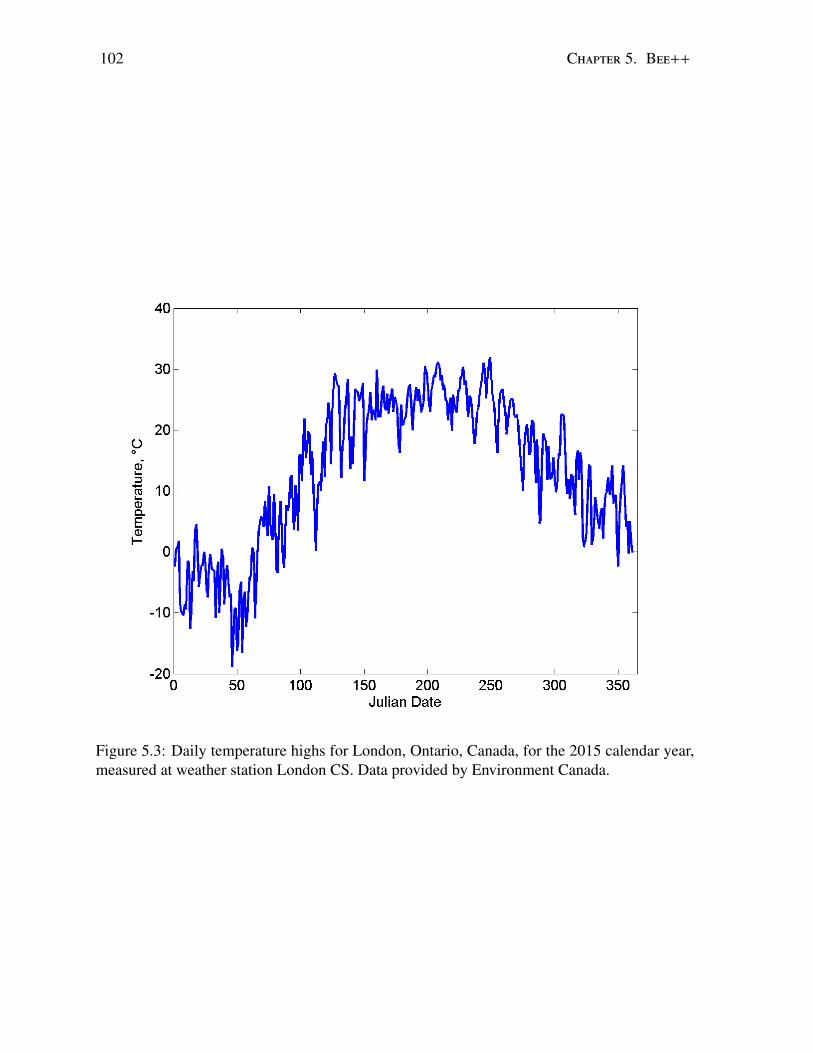
102 Chapter 5. Bee++

Figure 5.3: Daily temperature highs for London, Ontario, Canada, for the 2015 calendar year,measured at weather station London CS. Data provided by Environment Canada.

5.3. Results 103

Table 5.1: Parameter values and source references.L maximum rate of egg laying 1500 eggs/day [28]w number of hive bees for 50% egg survival 1000 beesb mass of food stored for 50% egg survival 500 g/day [42]

am age at which hive bees begin brood care 4 days [67]aT age at which hive bees end brood care 16 days [67]aR minimum age of recruitment to foraging 4 days [25]k age at which rate of recruitment is 50% of max. 10 daysα maximum rate of recruitment 1 /day1σ

maximum fraction of colony that can be foraging 13 [43]

dn natural death rate of foragers outside the hive equation (5.10) [21]cn nectar gathered per day per forager 0.03 g/day/bee [66]cp pollen gathered per day per forager 0.016 g/day/bee [66]γH daily food requirement per hive bee 0.08 g/bee [33, 64]γF daily food requirement per forager 0.13 g/bee [33, 64]γD daily food requirement per drone 0.1 g/bee [33, 64]γBp daily pollen requirement per uncapped brood cell 0.067 g/bee [33, 64]γBn daily nectar requirement per uncapped brood cell 0.018 g/bee [33, 64]K Shape parameter for exit probability of forager 30 mintR Minimum time in hive 1 htE Time forager spends searching for target 15 mintH Maximum flight time 45 minTW Temperature at which foraging begins 10 ◦C [41, 81]TI Ideal ambient temperature * 25 ◦C [41, 71, 81]T1 Minimum foraging temperature 10 ◦C [41, 71, 81]T2 Maximum foraging temperature 40 ◦C [10]xD Rate at which pesticides are metabolised 3.33 /day [78, 79]CP Concentration of pesticide in nectar 1.9 ng/g [75, 77]εbase Error in forager navigation 0.1ϕ Scaling of pesticide effect on navigation 10

* Bee++ assumes there is always some metabolic heat being generated by the bees; therefore, we set the idealtemperature lower than the measured ideal hive temperature in [71]. Bold indicates parameters for which

sensitivity analysis was performed.

104 Chapter 5. Bee++

Table5.2:

Parameters

usedin

10sim

ulationsforsensitivity

analysis.E

achcolum

nrepresents

onesim

ulation.M

eanvalues

providedin

TableA

.1.%

Change

fromM

eank

1.152−

5.951613.53

11.145−

10.583−

1.5224−

12.4156.49

−17.051

19.035w

−14.492

−18.092

2.347215.129

16.566−

11.4446.8644

−2.4616

−7.118

8.1808b

12.322−

17.5397.3496

−15.187

−4.4552

−8.6352

10.57716.609

−2.3312

1.6552K

16.29713.7

7.96−

11.2389.5648

−17.92

−5.0736

−13.032

−1.924

3.0908a

R19.806

−12.677

−5.0336

7.20841.5772

−11.295

8.757612.791

−18.832

−3.4376

am−

19.1243.1848

−3.9732

15.626−

14.6027.1392

−4.9756

18.64111.208

−10.027

tH−

3.8032−

9.578417.662

−6.426

-14.8582.394

12.5658.318

4.9968−

17.142γ

F−

7.187215.429

−10.018

1.5572−

14.815−

17.533−

2.91484.4508

19.77711.447

γH−

19.452−

1.6868−

9.6452−

7.836416.999

0.0767.066

11.615−

13.53813.999

γD−

18.28112.094

10.0286.3964

−15.98

−9.044

−6.6612

−3.8572

17.3152.8032

γB

p13.876

−0.006

16.465−

17.6182.7952

−11.802

−5.8424

10.85−

12.3385.6712

γB

n7.3876

15.708−

10.322−

13.14818.552

−2.8992

−7.4332

2.6084−

19.8478.1856

tE−

4.82412.927

9.5380.3244

−14.41

-2.808417.025

−9.5404

−17.006

7.8528tH

−5.8884

−10.58

6.88413.928

11.017−

17.19−

14.602−

3.565616.556

3.1604c

N10.404

12.448−

5.026−

19.8671.5232

7.3388−

11.305−

2.6228−

14.18618.995

cP−

0.16083.0664

−5.4444

−14.534

−19.944

15.1718.9716

−11.545

18.1117.3644

L8.7564

18.094−

16.465−

7.5028−

2.54087.6108

−11.634

15.86−

12.1590.0456

5.3. Results 105

Figure 5.4: Results of sensitivity analysis on total colony size: mean (red line) ± one standarddeviation (error bars). Parameter sets were sampled using Latin hypercube sampling [49] with10 divisions from the mean values provided in Table A.1, ranging ±20%. The parameters onwhich sensitivity analysis was performed appear in bold in Table A.1.

106 Chapter 5. Bee++

Figure 5.5: Results of sensitivity analysis on brood size: mean (red line) ± one standard de-viation (error bars). Parameter sets were sampled using Latin hypercube sampling [49] with10 divisions from the mean values provided in Table A.1, ranging ±20%. The parameters onwhich sensitivity analysis was performed appear in bold in Table A.1.

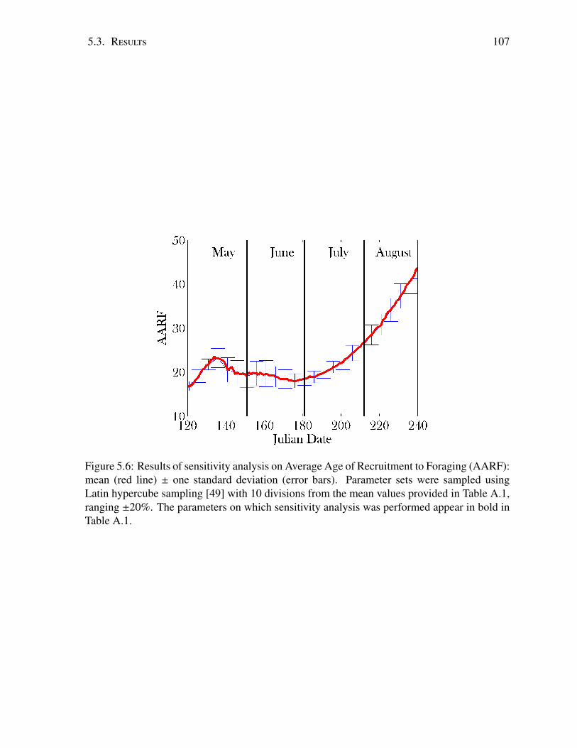
5.3. Results 107

Figure 5.6: Results of sensitivity analysis on Average Age of Recruitment to Foraging (AARF):mean (red line) ± one standard deviation (error bars). Parameter sets were sampled usingLatin hypercube sampling [49] with 10 divisions from the mean values provided in Table A.1,ranging ±20%. The parameters on which sensitivity analysis was performed appear in bold inTable A.1.

108 Chapter 5. Bee++

Figure 5.7: Total bee population from early spring to late summer using data from 10 simula-tions with the same parameter set (mean in black circles, grey error bars show ± one standarddeviation). These 10 simulations begin after the model has simulated 12 years of data, therebyrepresenting the colony size and distribution of a well established colony. Results from themodel are compared with those of other studies [6, 12, 52, 53]. The simulation agrees qual-itatively with previous models (Omholt) [53], observation (Buhlmann) [12], and simulation(Beehave) [6]. Data from Odoux [52] were obtained by model fitting, using measurementsfrom many colonies. In the Bee++ example we have assumed constant availability of food inthe environment and therefore we see a larger peak population.

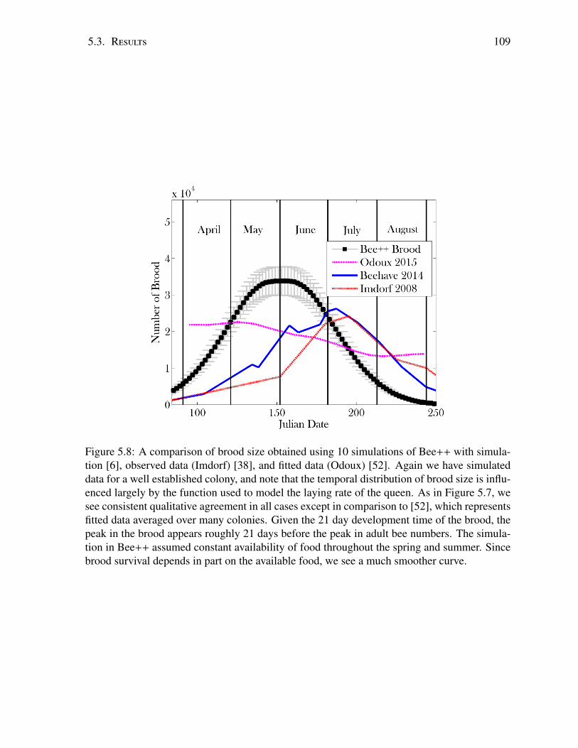
5.3. Results 109

Figure 5.8: A comparison of brood size obtained using 10 simulations of Bee++ with simula-tion [6], observed data (Imdorf) [38], and fitted data (Odoux) [52]. Again we have simulateddata for a well established colony, and note that the temporal distribution of brood size is influ-enced largely by the function used to model the laying rate of the queen. As in Figure 5.7, wesee consistent qualitative agreement in all cases except in comparison to [52], which representsfitted data averaged over many colonies. Given the 21 day development time of the brood, thepeak in the brood appears roughly 21 days before the peak in adult bee numbers. The simula-tion in Bee++ assumed constant availability of food throughout the spring and summer. Sincebrood survival depends in part on the available food, we see a much smoother curve.

110 Chapter 5. Bee++

Figure 5.9: The average age of recruitment to foraging calculated in 7 simulations withoutpesticides (red line) and a simulation with pesticide treated plants (magenta line) through thesummer months. Error bars represent one standard deviation. As mentioned in the text, pesti-cide exposure in this example affects the navigation abilities of the foragers but does not affecttheir lifespan, or the age at which they are recruited, thus it may be studied independently fromother confounding effects. We see that the AARF is robust against pesticide exposure. We alsosee that an age of recruitment between 20–30 days corresponds to a healthy colony. An AARFthat is above this range could indicate a lack of new brood or problem in the brood, as theincrease in the AARF corresponds to the decrease in the brood population in Figure 5.8. AnAARF below this range (as seen in [7, 43, 56]) can indicate an external stressor (in this casethe added stress of early spring on the colony).

5.3. Results 111

Figure 5.10: The average age of recruitment to foraging calculated in 7 simulations with-out pesticides (red line) and a simulation with pesticide treated plants (magenta line) throughspring. Error bars, blue and pink respectively, represent one standard deviation. Comparedwith the results in Figure 5.9, the value of AARF is here seen to be generally higher and highlyvolatile in April. This is caused by large swings in the ambient temperature during this time,the ageing of bees and the absence of new bees during winter. Thus AARF is not a usefulmetric of the health of the colony during early spring.

112 Chapter 5. Bee++

Figure 5.11: Intoxication of foragers and its effect on navigation over time. Seven simulationswere used. Error bars represent one standard deviation. The top plot shows the metabolicefforts of the bees are not enough to completely flush the pesticides from their system. We seethat once pesticide concentration in a bee is high enough to force higher metabolic effort, thereis a decrease to a more stable concentration. The bottom plot shows the correlation betweenpesticide exposure and its effects on navigation. Plotted is the current date versus the numberof bees lost in the previous 20 days. Bees are considered lost if they die outside a radius of ninepatches from the hive (food is at most nine patches away). This plot highlights the functionalityof Bee++ as well as how pesticide exposure may explain one possible symptom of CCD.

5.3. Results 113

Figure 5.12: Number of dead foragers found in each patch of a 25×25 grid of 4m× 4m patchestotalled between February and September. The total number of dead foragers in this time is55,283, 55,592 and 56,426 in (a,b,c) respectively. The pollen and nectar sources (in patcheslabelled P and N, respectively) are assumed to be constant throughout the year. The hive itselfis labelled H. The colour resolution is roughly 100 bees in Panels (a,b) and 10 bees in Panel(c). Panel (a) shows a simulation with no pesticide exposure but with normal navigation errorε = 0.1. In Panels (b,c). this navigation error is increased because of pesticide exposure to amaximum of 0.35 and 1.0, respectively. In Panel (a), there are fewer than 10 bees in each bluecell, and in Panel (b), there are between 10 and 30 bees in each blue cell. The effect of pesticideon the bees is cumulative. In early spring, there is less build up of toxins within individual beesand thus their navigation is better than it is in late summer.

114 Chapter 5. Bee++

5.4 DiscussionWe present a detailed, agent-based simulation package for honey bee colony dynamics,which is broadly configurable and can be adapted to address a wide range of investigations.In the Results, we demonstrate the behaviour of the model at default parameter values,predicting colony dynamics that are comparable to those predicted by other models andsimulations [6, 43, 69]. The larger peak population size obtained in our simulations is dueto the idealized condition that food is plentiful and constant, allowing bees to successfullyforage from early spring through late fall; this is configurable in the model. Moreover,the peak population predicted by Bee++ is well within the range of realistic managedcolonies [58]. In the simulated data, this peak appears in mid-summer, consistent withobserved bee behaviour [16]. Field observations indicate that variation in the timing of thispeak is quite large, with some honey bee populations peaking as early as late spring [29],depending on the local climate.

Sensitivity analysis shows that the model behaves as expected under a range of bio-logically reasonable conditions. Parameters not tested here, such as those associated withintoxication and the transmission rates for different parasites, will clearly also affect thedynamics of the colony. Sensitivity analyses for these can be carried out by individual re-searchers after their default environmental and colony parameters have been chosen. Theframework for sensitivity analysis is built into the source code and can easily be modifiedto accommodate a detailed sensitivity study for each research question.

The flight patterns of honey bees, and the factors impacting their navigation are com-plex and quite involved [31]. The navigation used for the bees in Bee++ is macro scalenavigation, given the size of the patches intended for use (≥ 1m2). This means that thebees are moving toward a general target, and their individual movements between flowersis not modelled here. Models of movement between individual flowers have been wellstudied [13]. Future work entails optimizing the model so that navigation between indi-vidual flowers can be included. Moreover, displaced or lost honey bees have been shownto use a number of mechanisms to search for the hive, which can be modelled as a Levyflight [62]. These mechanisms could also be considered in future extensions of the flightmechanisms in Bee++.

Figure 5.8 shows that the brood population of a healthy colony peaks in early June,consistent again with experimental findings [3]. Qualitatively, we see the same brood-rearing dynamics as predicted by other models. The measurements provided by [52] differqualitatively from the other data presented in Figure 5.8. One potential explanation forthis discrepancy is that the results of [52] are calculated using 208 different colonies, overfour years. Different weather patterns over the 4 years and across the different locales mayforce the colonies to peak at different times of the year, potentially obfuscating the peakexperienced by any one colony.

Figure 5.9 predicts that, when the pesticide-free colony population is at its strongest,the average age of recruitment to foraging is between approximately 20 and 30 days old.This is in full agreement with previous results [11, 42, 43, 56]. Furthermore, in earlyspring, when the colony is under increased stress, we see a lower AARF, consistent withthe predictions of [43], which correlate the AARF and colony health. Our simulationsalso show that as the number of eggs laid by the queen diminishes in late summer, theAARF increases substantially. This behaviour seems to benefit the colony, as the younger,stronger bees are left in the hive for the incoming winter.

The results shown in Figure 5.9 indicate that while the AARF can be used to determine

5.4. Discussion 115

certain aspects of colony health (i.e. a high AARF in the fall corresponds to dwindlingnumbers of the brood, or as an indication of infection [7]), the AARF is not a strong met-ric for the effects of pesticides on the navigational abilities of the worker bees. Results suchas those in [56] (accelerated maturation of bees) can also be added to Bee++, further com-pounding the effects of pesticides on the age of foragers, with likely detrimental results.While the AARF has been previously proposed as a measure of colony health [7, 42, 43],the source of any change to the AARF is hard to extract from this metric, as many stresseswill change its value. Therefore, it is important to know what will and will not effect thismetric as some stresses (such as degrading navigational ability) can be detrimental to thecolony, but asymptomatic without invasive tests on the bees (such as determining intoxi-cation levels within the bees). In future work, we would like to study the compoundingeffects of pesticides, and also investigate the use of time-dependent AARF and other met-rics to potentially identify which source of stress is causing the most harm to the bees. Onepreliminary hypothesis is that high AARF may indicate a problem in the brood, as AARFindeed increases in our model as the brood population decreases.

One of the key benefits of Bee++ is the ability to explicitly track toxins within individ-ual bees, a feature that has not been included in previous studies. With this mechanism, weare able to explore explicit effects of sub-lethal doses of pesticides on honey bees withoutapproximating these effects as an increased death rate. In particular, our model explicitlyallows for pesticide exposure to interfere with foragers’ navigational abilities, as has beendemonstrated experimentally [34]. When comparing the panels of Figure 5.12, we see thatas pesticides affect navigation more strongly, more bees die at distances further from thehive. Importantly, a lack of dead bees around the hive is one of the symptoms of ColonyCollapse Disorder (CCD) [83, 89]; our model predicts that an encumbrance on foragers’navigation ability can help explain this phenomenon. In other words, a loss of navigationability is one potential explanation for the lack of bee corpses reported in CCD. This in-ability to navigate in turn causes a reduction in the amount of food in the hive, and thus anincreased death rate as the bees are generally weaker.

Given the recent proposal by the U.S. Fish and Wildlife service to declare the rusty-patched bumble bee as an endangered species [90], an accurate, parameter-rich model ofbumble bee dynamics may be crucial in developing policies to protect this species. Thesource code of Bee++ can be modified to perform such a task, as bumble bee populationsshare a very similar social structure to honey bees. We hope to do so in the near future.

As well, our future work includes plans to modify the model to run on parallel pro-cessing architectures. With the exception of the waggle dances, each bee makes a decisionat each time step independent of other bees, thus it should be possible to create a moreefficient code by allowing (ideally) all bees to make decisions simultaneously.

Overall, Bee++ has the ability to create realistic simulations of honey bee colonies byincorporating a wide range of parameters and potential interactions. The object-orientednature of the model implementation in C++ allows for easy modification of the sourcecode so that the model can easily be improved and expanded as more experimental databecome available. The simulations of Bee++ can be used to study the potential underlyingcauses of honey bee colony decline such as the effects of biodiversity, disease, predationand intoxication on colony dynamics. The effects of preventive measures (such as optimalplant diversity, crop density or anti-viral treatments) or recovery plans (such as manualfeeding or colony transplant) can thus be studied before costly implementation.

Appendix 5.A.

116 Chapter 5. Bee++

Appendix 5.A.1. Drone Dynamics

Drones are born of the unfertilized eggs laid by the queen [88]. Their main duty in lifeis procreation with a queen of another hive. Upon success, the drone dies [88]. The dronesmake two decisions in their lifetime. With probability

pL = max(et−t∗ , 1

)(5.16)

the drones will leave the hive in search of a mate. Here, t∗ represents the optimal time ofyear for mating. The drones then move in much the same fashion as foragers, with theirtarget being the mating area. Those that become lost will return to the hive, and those thatreach the mating area will successfully mate with a queen with probability

pM = min(

NQ

ND, 1

)(5.17)

where NQ is the number of queens present in the mating area and ND is the number ofdrones present. The drones do not mate with their own queen (as they are genetic clonesof the queen). The mating process is built into Bee++ so that realistic numbers of dronescan be modelled (since mating is followed by death of the drone). As well, having thisfunctionality is the first step to creating a model and simulation package with interactingcolonies. At present, multiple colonies are not implemented in the model and thereforethe position of any mating sites and the number of queens present at any given time mustbe set manually by the user. Nonetheless the drones are an important part of a honey beecolony, as they can be a source of pathogens as well as a drain on the food stores and canaccount for up to 15% of the total population [70].

Appendix 5.A.2. Pathogen Dynamics

Both sub-types of the microsporidian Nosema reproduce within the epithelial cells oflive bees, which in turn causes dysentery, forcing bees to expel waste within hive cellswhere spores will be picked up by bees, which clean contaminated cells [27]. Nosemaceranae is reported to affect foragers disproportionately, killing them away from the hiveat an unsustainable rate [35]. There is also evidence that spores can be transmitted to beesthrough food stores [73]. With this in mind, we posit that bees that clean cells (i.e., nurses)are most likely to be infected, while secondary mechanisms may exist through direct beeto bee transmission and food stores. Therefore, we constrain the rates of transmission ofeither type of Nosema spore to foragers, drones, maintenance bees and nurses (βF , βD, βM

and βN respectively) through the condition

βF ≈ βD ≈ βM < βN . (5.18)

Since hive cells are often soiled during the winter, when honey bees cannot leave thehive to defecate, the transmission of Nosema spores is temperature dependent. PresentlyBee++ does not consider a spatially explicit interior to the hive, therefore we cannot trackindividual brood/food cells and instead treat the pathogen populations and bee populationsas well mixed.

Each infection rate will then depend on the number of spores in the environment (whichin turn depends on the number of infected bees), as well as susceptibility of a particular

5.4. Discussion 117

bee to infection (pesticide exposure may increase susceptibility [84]). In other words, wedefine the time-dependent infection rates, pI , as

pI,i, j = βi(P, ~I, i)S j

s + S j(5.19)

where βi is a function dependent on the intoxication level P of the bee, the number ofinfections I it has acquired that may be compromising its immune system, and the casteof the bee, i. S j is the number of free Nosema spores of type j (apis or cerenae) and s isa shape parameter. This infection through free spores is the main transmission method forboth types of Nosema, and the one that our model currently considers. Of course, futurework can expand the model to include secondary transmission routes.

The population of free spores of type j, S j, is governed by the differential equation,

dS j

dt=

∑i

BS ,i, jIi −CNN . (5.20)

where BS ,i, j is the shedding rate of Nosema spores of type j by one infected bee of type iand Ii is the number of infected bees of type i, C is the rate at which nurses can clean thecells, and NN is once again the total number of nurses.

There is evidence that the fungicide, which prevents Nosema apis infection withinhoney bee colonies, may actually allow Nosema ceranae to thrive [37]. Therefore wethought it imperative to include both possible infections in our model, as well as the N.apis treatment, fumagillin, as a toxin. In this way, our model allows one to explore thetrade-offs between these three very important, and evidently lethal stressors.

Varroa mites on the other hand, reproduce in the sealed brood cells [47]. Within thecell, the mite will lay female and male eggs (usually one male and five female [80]. Themites mate within the sealed brood cell [48], and the female mites emerge with the larvae,and attach themselves to nearby adult worker bees [47]. The mites feed on the blood ofthe adult worker bees, and use them as a means to disperse to new brood cells where theymay reproduce [68].

Varroa has been observed to act as a vector for viruses such as Deformed Wing Virus(DWV) and Acute Paralysis Virus (APV) [20, 48]. Therefore, our Varroa mites are mod-elled as three types, Vi, depending on whether they do not carry any virus, are carriers ofDWV, or carriers of APV.

Varroa mites feed on adult bees for approximately 4 to 5 days [68] before entering abrood cell that is about to be capped. Therefore, we keep track of the number of days a beehas had a mite attached. When a mite has reached reproductive maturity, with probabilitypE(t) the mite will enter a viable brood cell. Once the mite enters a brood cell, the adultbee is no longer considered infested with a mite. The number of mites that leave theiradult bee hosts are exactly the number of brood cells that end up inhabited by a Varroamite. We recognize that this assumes that more than one mite cannot occupy the samebrood cell. We use this assumption first on the basis of empirical data [68] and, second,in order to make the problem tractable without explicitly tracking the spatial movement ofthe bees within the hive. We further assume that all mites either enter a brood cell or dieafter 5 days of attaching to a host.

The number of new Varroa mites created by one infected brood cell as the new beeemerges is

Vnew = rV BI (5.21)

118 Chapter 5. Bee++

where rV is the average number of female mites produced by one foundress (i.e., an egg-laying mite), and BI is the number of infected brood cells. We further assume that uponhatching, the new female mites find a host bee or die. Therefore the number of infectedbees is directly proportional to the number of surviving emerging mites.

Bibliography

[1] Abou-Shaara, H., et al. The foraging behaviour of honey bees, Apis mellifera: areview. Vet Med (Praha) 59, 1 (2014), 1–10.

[2] Aufauvre, J., Biron, D. G., Vidau, C., Fontbonne, R., Roudel, M., Diogon, M.,Vigues, B., Belzunces, L. P., Delbac, F., and Blot, N. Parasite-insecticide interac-tions: a case study of Nosema ceranae and fipronil synergy on honeybee. Scientificreports 2 (2012).

[3] Ball, B., and Allen, M. The prevalence of pathogens in honey bee (Apis mellifera)colonies infested with the parasitic mite Varroa jacobsoni. Annals of applied biology113, 2 (1988), 237–244.

[4] Ball, D. W. The chemical composition of honey. J. Chem. Educ 84, 10 (2007), 1643.

[5] Becher, M. A., Grimm, V., Thorbek, P., Horn, J., Kennedy, P. J., and Osborne, J. L.BEEHAVE: a systems model of honeybee colony dynamics and foraging to exploremultifactorial causes of colony failure. Journal of applied ecology 51, 2 (2014),470–482.

[6] Becher, M. A., Osborne, J. L., Thorbek, P., Kennedy, P. J., and Grimm, V. Review:Towards a systems approach for understanding honeybee decline: a stocktaking andsynthesis of existing models. Journal of Applied Ecology 50, 4 (2013), 868–880.

[7] Betti, M. I., Wahl, L. M., and Zamir, M. Effects of infection on honey bee populationdynamics: A model. PLOS ONE 9, 10 (2014), e110237.

[8] Betti, M. I., Wahl, L. M., and Zamir, M. Age structure is critical to the populationdynamics and survival of honeybee colonies. Royal Society Open Science 3, 11(2016), 160444.

[9] Biesmeijer, J. C., and de Vries, H. Exploration and exploitation of food sources bysocial insect colonies: a revision of the scout-recruit concept. Behavioral Ecologyand Sociobiology 49, 2-3 (2001), 89–99.

[10] Blazyte-Cereskiene, L., Vaitkeviciene, G., Venskutonyte, S., and Buda, V. Honeybee foraging in spring oilseed rape crops under high ambient temperature conditions.Zemdirbyste Agriculture 97, 1 (2010), 61–70.

[11] Botias, C., Martin-Hernandez, R., Barrios, L., Meana, A., and Higes, M. Nosemaspp. infection and its negative effects on honey bees (Apis mellifera iberiensis) at thecolony level. Veterinary research 44, 1 (2013), 1–15.

[12] Buhlmann, G. Assessing population dynamics in a honeybee colony. Mitteilun-gen der Deutschen Gesellschaft fuer Allgemeine und Angewandte Entomologie (Ger-many, FR) (1985).

119

120 BIBLIOGRAPHY

[13] Bukovac, Z., Dorin, A., and Dyer, A. A-bees see: a simulation to assess social beevisual attention during complex search tasks. In Proceedings of the 12th EuropeanConference on Artificial Life (ECAL 2013) (2013), MIT Press Taormina, pp. 276–283.

[14] Calderone, N. W. Insect pollinated crops, insect pollinators and US agriculture:Trend analysis of aggregate data for the period 1992-2009. PLOS ONE 7, 5 (052012), e37235.

[15] Camazine, S. Self-organizing pattern formation on the combs of honey bee colonies.Behavioral ecology and sociobiology 28, 1 (1991), 61–76.

[16] Capinera, J. L. Encyclopedia of entomology, vol. 4. Springer Science & BusinessMedia, 2008.

[17] Castillo, C., Chen, H., Graves, C., Maisonnasse, A., Le Conte, Y., and Plettner, E.Biosynthesis of ethyl oleate, a primer pheromone, in the honey bee (Apis melliferaL.). Insect biochemistry and molecular biology 42, 6 (2012), 404–416.

[18] de Vries, H., and Biesmeijer, J. C. Modelling collective foraging by means of indi-vidual behaviour rules in honey-bees. Behavioral Ecology and Sociobiology 44, 2(1998), 109–124.

[19] Devillers, J. The ecological importance of honey bees and their relevance to eco-toxicology. In Honey Bees: Estimating the Environmental Impact of Chemicals,J. Devillers and M. Pham-Delegue, Eds. Taylor and Francis London, London, 2002,pp. 1–11.

[20] Di Prisco, G., Pennacchio, F., Caprio, E., Boncristiani Jr, H. F., Evans, J. D., and

Chen, Y. Varroa destructor is an effective vector of Israeli acute paralysis virus inthe honeybee, Apis mellifera. Journal of General Virology 92, 1 (2011), 151–155.

[21] Dukas, R. Mortality rates of honey bees in the wild. Insectes Sociaux 55, 3 (2008),252–255.

[22] Eberl, H. J., Frederick, M. R., and Kevan, P. G. Importance of brood maintenanceterms in simple models of the honeybee - Varroa destructor - Acute Bee Paraly-sis Virus complex. Electronic Journal of Differential Equations (EJDE) [electroniconly] 2010 (2010), 85–98.

[23] Esther, E., Smit, S., Beukes, M., Apostolides, Z., Pirk, C. W., and Nicolson, S. W.Detoxification mechanisms of honey bees (Apis mellifera) resulting in tolerance ofdietary nicotine. Scientific reports 5 (2015).

[24] Evans, J. D., and Schwarz, R. S. Bees brought to their knees: microbes affectinghoney bee health. Trends in microbiology 19, 12 (2011), 614–620.

[25] Fahrbach, S., and Robinson, G. Juvenile hormone, behavioral maturation and brainstructure in the honey bee. Developmental Neuroscience 18 (1996), 102–114.

[26] Favre, D. Mobile phone-induced honeybee worker piping. Apidologie 42, 3 (2011),270–279.

[27] Fries, I. Nosema apisa parasite in the honey bee colony. Bee World 74, 1 (1993),5–19.

[28] Gary, N. E. Activities and behavior of honey bees. The hive and the honey bee(1992), 269–373.

BIBLIOGRAPHY 121

[29] Ginsberg, H. S. Foraging ecology of bees in an old field. Ecology 64, 1 (1983),165–175.

[30] Goulson, D., Nicholls, E., Botıas, C., and Rotheray, E. L. Bee declines driven bycombined stress from parasites, pesticides, and lack of flowers. Science 347, 6229(2015), 1255957.

[31] Grimm, V., Revilla, E., Berger, U., Jeltsch, F., Mooij, W. M., Railsback, S. F.,Thulke, H.-H., Weiner, J., Wiegand, T., and DeAngelis, D. L. Pattern-orientedmodeling of agent-based complex systems: lessons from ecology. science 310, 5750(2005), 987–991.

[32] Harbo, J. R. Effect of population size on brood production, worker survival andhoney gain in colonies of honeybees. Journal of Apicultural Research 25, 1 (1986),22–29.

[33] Haydak, M. H. Honey bee nutrition. Annual review of entomology 15, 1 (1970),143–156.

[34] Henry, M., Beguin, M., Requier, F., Rollin, O., Odoux, J.-F., Aupinel, P., Aptel,J., Tchamitchian, S., and Decourtye, A. A common pesticide decreases foragingsuccess and survival in honey bees. Science 336, 6079 (2012), 348–350.

[35] Higes, M., Martin-Hernandez, R., Garrido-Bailon, E., Gonzalez-Porto, A. V.,Garcia-Palencia, P., and Meana, A. Honeybee colony collapse due to Nosema cer-anae in professional apiaries. Environmental Microbiology Reports 1, 2 (2009), 110–113.

[36] Ho, M.-W., and Cummins, J. Mystery of disappearing honeybees. Science in Society34 (2007), 35–36.

[37] Huang, W.-F., Solter, L. F., Yau, P. M., and Imai, B. S. Nosema ceranae escapesfumagillin control in honey bees. PLOS Pathog 9, 3 (2013), e1003185.

[38] Imdorf, A., Ruoff, K., and Fluri, P. Volksentwicklung bei der honigbiene. In ALPforum (2008), vol. 68, pp. 1–88.

[39] Johnson, R. M., Dahlgren, L., Siegfried, B. D., and Ellis, M. D. Acaricide, fungi-cide and drug interactions in honey bees (Apis mellifera). PLOS ONE 8, 1 (2013),e54092.

[40] Johnson, R. M., Wen, Z., Schuler, M. A., and Berenbaum, M. R. Mediation ofpyrethroid insecticide toxicity to honey bees (Hymenoptera: Apidae) by cytochromep450 monooxygenases. Journal of economic entomology 99, 4 (2006), 1046–1050.

[41] Joshi, N. C., and Joshi, P. Foraging behaviour of Apis spp. on apple flowers in asubtropical environment. New York Science Journal 3, 3 (2010), 71–76.

[42] Khoury, D. S., Barron, A. B., and Myerscough, M. R. Modelling food and popula-tion dynamics in honey bee colonies. PLOS ONE 8, 5 (05 2013), e59084.

[43] Khoury, D. S., Myerscough, M. R., and Barron, A. B. A quantitative model ofhoney bee colony population dynamics. PLOS ONE 6, 4 (04 2011), e18491.

[44] Kralj, J., and Fuchs, S. Parasitic Varroa destructor mites influence flight durationand homing ability of infested Apis mellifera foragers. Apidologie 37, 5 (2006), 577.

[45] Kronenbergf, F. Colonial thermoregulation in honey bees. Journal of ComparitivePhysiology B 148 (1979), 65–78.

122 BIBLIOGRAPHY

[46] Leoncini, I., Le Conte, Y., Costagliola, G., Plettner, E., Toth, A. L., and Wang,M. Regulation of behavioral maturation by a primer pheromone produced by adultworker honey bees. Proceedings of the National Academy of Sciences of the UnitedStates of America 101, 50 (2004), 17559–17564.

[47] Martin, S. Hygienic behaviour: an alternative view. Bee Improvement 7 (2000), 6–7.

[48] Martin, S. Biology and life-history of Varroa mites. Mites of the honey bee. Dadant& Sons, Hamilton, IL (2001), 131–148.

[49] McKay, M. D., Beckman, R. J., and Conover, W. J. A comparison of three methodsfor selecting values of input variables in the analysis of output from a computer code.Technometrics 42, 1 (2000), 55–61.

[50] McLellan, A. Growth and decline of honeybee colonies and inter-relationships ofadult bees, brood, honey and pollen. Journal of Applied Ecology (1978), 155–161.

[51] Neumann, P., and Carreck, N. L. Honey bee colony losses. Journal of ApiculturalResearch 49, 1 (2010), 1–6.

[52] Odoux, J.-F., Aupinel, P., Gateff, S., Requier, F., Henry, M., and Bretagnolle, V.ECOBEE: a tool for long-term honey bee colony monitoring at the landscape scalein West European intensive agroecosystems. Journal of Apicultural Research 53, 1(2014), 57–66.

[53] Omholt, S. W. A model for intracolonial population dynamics of the honeybee intemperate zones. Journal of Apicultural Research 25, 1 (1986), 9–21.

[54] Page, R. E., and Peng, C. Y.-S. Aging and development in social insects with em-phasis on the honey bee, apis mellifera l. Experimental gerontology 36, 4 (2001),695–711.

[55] Paxton, R. J., Klee, J., Korpela, S., and Fries, I. Nosema ceranae has infected Apismellifera in Europe since at least 1998 and may be more virulent than Nosema apis.Apidologie 38, 6 (2007), 558–565.

[56] Perry, C. J., Søvik, E., Myerscough, M. R., and Barron, A. B. Rapid behavioralmaturation accelerates failure of stressed honey bee colonies. Proceedings of theNational Academy of Sciences 112, 11 (2015), 3427–3432.

[57] Pettis, J. S., Lichtenberg, E. M., Andree, M., Stitzinger, J., Rose, R., Vanengels-dorp, D., et al. Crop pollination exposes honey bees to pesticides which alters theirsusceptibility to the gut pathogen Nosema ceranae. PLOS ONE 8, 7 (2013), e70182.

[58] Ratnieks, F. L. Egg-laying, egg-removal, and ovary development by workers inqueenright honey bee colonies. Behavioral Ecology and Sociobiology 32, 3 (1993),191–198.

[59] Ratnieks, F. L., and Keller, L. Queen control of egg fertilization in the honey bee.Behavioral Ecology and Sociobiology 44, 1 (1998), 57–61.

[60] Ratti, V., Kevan, P. G., and Eberl, H. J. A mathematical model for populationdynamics in honeybee colonies infested with Varroa destructor and the Acute BeeParalysis Virus. Canadian Applied Mathematics Quarterly 21, 1 (2013), 63–93.

[61] Ratti, V., Kevan, P. G., and Eberl, H. J. A mathematical model of the honeybee-Varroa destructor-Acute Bee Paralysis Virus complex with seasonal effects. Bulletinof Mathematical Biology (2015).

BIBLIOGRAPHY 123

[62] Reynolds, A. M., Smith, A. D., Menzel, R., Greggers, U., Reynolds, D. R., and

Riley, J. R. Displaced honey bees perform optimal scale-free search flights. Ecology88, 8 (2007), 1955–1961.

[63] Reynolds, A. M., Smith, A. D., Reynolds, D. R., Carreck, N. L., and Osborne, J. L.Honeybees perform optimal scale-free searching flights when attempting to locate afood source. Journal of Experimental Biology 210, 21 (2007), 3763–3770.

[64] Rortais, A., Arnold, G., Halm, M.-P., and Touffet-Briens, F. Modes of honeybeesexposure to systemic insecticides: estimated amounts of contaminated pollen andnectar consumed by different categories of bees. Apidologie 36, 1 (2005), 71–83.

[65] Roubik, D. W., and Wolda, H. Do competing honey bees matter? Dynamics andabundance of native bees before and after honey bee invasion. Population Ecology43, 1 (2001), 53–62.

[66] Russell, S., Barron, A. B., and Harris, D. Dynamic modelling of honey bee (Apismellifera) colony growth and failure. Ecological Modelling 265, 0 (2013), 158 – 169.

[67] Sakagami, S., and Fukuda, H. Life tables for worker honeybees. Researches onPopulation Ecology 10, 2 (1968), 127–139.

[68] Sammataro, D., Gerson, U., and Needham, G. Parasitic mites of honey bees: lifehistory, implications, and impact. Annual review of entomology 45, 1 (2000), 519–548.

[69] Schmickl, T., and Crailsheim, K. Hopomo: A model of honeybee intracolonial pop-ulation dynamics and resource management. Ecological modelling 204, 1 (2007),219–245.

[70] Seeley, T. D. The wisdom of the hive: the social physiology of honey bee colonies.Harvard University Press, 2009.

[71] Seeley, T. D. Honeybee ecology: a study of adaptation in social life. PrincetonUniversity Press, 2014.

[72] Slessor, K. N., Winston, M. L., and Le Conte, Y. Pheromone communication in thehoneybee (Apis mellifera L.). Journal of chemical ecology 31, 11 (2005), 2731–2745.

[73] Smith, M. L. The honey bee parasite Nosema ceranae: Transmissible via food ex-change? PLOS ONE 7, 8 (08 2012), e43319.

[74] Southwick, E. E., and Southwick Jr, L. Estimating the economic value of honeybees (Hymenoptera: Apidae) as agricultural pollinators in the United States. Journalof Economic Entomology 85, 3 (1992), 621–633.

[75] Stanley, J., and Preetha, G. Pesticide Toxicity to Non-target Organisms: Exposure,Toxicity and Risk Assessment Methodologies. Springer, 2016.

[76] Stillman, R. A., Railsback, S. F., Giske, J., Berger, U., and Grimm, V. Makingpredictions in a changing world: the benefits of individual-based ecology. BioScience65, 2 (2015), 140–150.

[77] Stoner, K. A., and Eitzer, B. D. Movement of soil-applied imidacloprid and thi-amethoxam into nectar and pollen of squash (Cucurbita pepo). PLOS ONE 7, 6(2012), e39114.

124 BIBLIOGRAPHY

[78] Suchail, S., De Sousa, G., Rahmani, R., and Belzunces, L. P. In vivo distributionand metabolisation of 14C-imidacloprid in different compartments of Apis melliferaL. Pest management science 60, 11 (2004), 1056–1062.

[79] Suchail, S., Debrauwer, L., and Belzunces, L. P. Metabolism of imidacloprid inApis mellifera. Pest management science 60, 3 (2004), 291–296.

[80] Sumpter, D. J. T., and Martin, S. J. The dynamics of virus epidemics in Varroa-infested honey bee colonies. Journal of Animal Ecology 73, 1 (2004), 51–63.

[81] Tan, K., Yang, S., Wang, Z.-W., Radloff, S. E., and Oldroyd, B. P. Differences inforaging and broodnest temperature in the honey bees Apis cerana and A. mellifera.Apidologie 43, 6 (2012), 618–623.

[82] Thorbek, P., Campbell, P. J., Sweeney, P. J., and Thompson, H. M. Using BEE-HAVE to explore pesticide protection goals for European honeybee (Apis meliferaL.) worker losses at different forage qualities. Environmental Toxicology and Chem-istry (2016).

[83] vanEngelsdorp, D., Evans, J. D., Saegerman, C., Mullin, C., Haubruge, E., Nguyen,B. K., Frazier, M., Frazier, J., Cox-Foster, D., Chen, Y., Underwood, R., Tarpy,D. R., and Pettis, J. S. Colony collapse disorder: A descriptive study. PLOS ONE 4,8 (08 2009), e6481.

[84] Vidau, C., Diogon, M., Aufauvre, J., Fontbonne, R., Vigues, B., Brunet, J.-L., Tex-ier, C., Biron, D. G., Blot, N., El Alaoui, H., et al. Exposure to sublethal doses offipronil and thiacloprid highly increases mortality of honeybees previously infectedby Nosema ceranae. PLOS ONE 6, 6 (2011), e21550.

[85] Watanabe, M. E. Colony collapse disorder: Many suspects, no smoking gun. Bio-Science 58, 5 (2008), 384–388.

[86] Wharton, K. E., Dyer, F. C., Huang, Z. Y., and Getty, T. The honeybee queen influ-ences the regulation of colony drone production. Behavioral Ecology 18, 6 (2007),1092–1099.

[87] Wilson, W. T., Moffett, J. O., Harrington, H. D., et al. Nectar and pollen plants ofColorado. Colorado State University, Experiment Station Bulletin (1958), 503–S.

[88] Winston, M. The biology of the honey bee. Harvard University Press, 1987.

[89] Yamada, T., et al. Honeybee colony collapse disorder. Emerging Biological Threats:A Reference Guide 13 (2009), 141.

[90] Zuckerman, L. Rusty patched bumble bee proposed for U.S. endangered speciesstatus.

Chapter 6

Discrete and continuum operatorsfor the spread of disease: Aclosed-form next generationoperator for reaction-diffusionsystems

Abstract

The next generation operator (NGO) is a clear analog to the next genera-tion matrix (NGM) for disease models. However, the NGO has been derivedindependently of the NGM and the quantifiable connection between the twoapproaches remains an open question. Here, we demonstrate that the NGO canbe directly obtained as the limit of the NGM, as the number of discrete classesapproaches infinity. In the case of continuous age-structured disease models,this approach recovers the NGO as previously defined for both separable andnon-separable interaction terms. For reaction-diffusion systems, we present anew, closed-form formulation for the NGO for disease spread. The Fouriermethods illustrated here present a new approach for formulating a closed-formnext generation operator, which can then be used to provide a reproductionnumber for more complex models, including the fractional derivatives used todescribe Levy flight.

6.1 IntroductionAt the core of modeling the progression of disease within a population is thebasic reproduction number, R0. This key parameter determines whether a dis-ease will spread in a population, and allows for quantitative estimates of thestrength of control measures required to contain this spread [20, 27].

The next generation matrix (NGM) [35] offers an intuitively elegant andwell-studied method for calculating R0 for a disease affecting a populationof N discrete classes, that is, for disease dynamics described by a system of

125

126 Chapter 6. The Next Generation Operator

ordinary differential equations. The NGM is arguably the most widely usedapproach for estimating the basic reproduction number in either discrete orcontinuous time (as evidenced by the number of studies that rely on the method[20]), equating the basic reproduction number to the spectral radius of a closed-form matrix with a clear biological meaning. In recent work, Diekmann et al.proposed a method of deriving the NGM directly from model parameters forgeneral epidemic models in discrete compartments [16]. A still more recentstudy by Roberts and Heesterbeek characterizes the next generation matrixand basic reproduction number, R0, for a variety of ecological models [32],while Cushing and Diekmann explore how different physical interpretations ofthe same model can result in different formulations of the NGM, by essentiallycounting infections in different units [11]. Throughout this paper, for modelswith discrete classes we will adopt the definition of the basic reproductionnumber as the dominant positive eigenvalue with non-negative eigenvector ofthe NGM [11, 34, 35].

In recent years, a number of extensions and alternatives to the NGM havebeen proposed. For example, in discrete time models, Li and Schneider takethe novel approach of defining the projection matrix as a matrix sum [25],which can then be used to calculate R0. In [31], Roberts et al. extend the ideaof the next generation matrix to develop new estimates of control efforts forinfectious disease. These estimates have the same threshold behaviour as R0,but each estimate is applicable to one host type. Roberts et al. have also re-cently proposed methods of extending and relating ecological dynamics to R0in predator-prey systems [32]. In [22], Hyman and Li derive an explicit expres-sion for R0 for an HIV model, demonstrating an equivalence between the nextgeneration matrix and the Jacobian of the system. R0 can also be calculatedin randomly fluctuating environments, for discrete population classes in eitherdiscrete or continuous time [4].

In many model formulations, however, it is more intuitive to assume thatpopulations are structured along a continuum, as opposed to having discreteclasses. In the case of periodic infectibility, that is, assuming an interactionterm that depends both on continuous infection age and time, an expressionfor R0 has also been obtained as the spectral radius of a matrix closely relatedto the NGM [3, 12]. Other examples include models with continuous agestructure or spatially heterogeneous populations, that is, models described bysystems of partial differential equations. The basic reproduction number hasbeen determined for such infinite-dimensional models in a number of disease-specific cases, as for example in dengue [10], nosocomial infections [9] andinfections in honey bee colonies [5]. Wang and Zhao [38] developed an elegantmethod for determining the spectral radius of the next generation operator forthe special case of a reaction-diffusion system.

More generally, Greenhalgh first conjectured that the spectral radius of anintegral operator would provide a threshold criterion, R0, in the case of infinite-dimensional population structure [17, 18]. This conjecture was confirmed byInaba [23], and in parallel work, the Next Generation Operator (NGO) wasdefined by Diekmann et al. [15]. The connection between R0, defined as thespectral radius of a positive bounded linear operator, and the spectral bound

6.2. The limit of the Next Generation Matrix 127

of a related linear operator, has also been elucidated in some detail by Thieme[34].

Although the NGO is clearly the continuous analog of the NGM, the deriva-tion of the NGO has typically proceeded either by defining the contribution ofinfectious individuals to the “next generation” of infectious individuals [14],or by deriving an operator whose spectral radius has the necessary thresholdbehaviour [34]. Here, we take a different approach, explicitly demonstratingthe connection between the NGO and the NGM by taking the limit of the NGMas the number of discrete classes approaches infinity. This approach allows usto derive the NGO for a class of well-studied reaction-diffusion disease mod-els. Specifically, we derive a new, closed-form expression for the NGO inthe case of a diffusing infected population with constant death rate, as well asconjecture an operator for a diffusing population with general death rate.

The importance of reaction-diffusion models in mathematical biology can-not be overstated. The construction and analysis of reaction-diffusion systemsare central to modelling and understanding the complex interactions of mobileindividuals, as elucidated in standard reference texts in mathematical biology( [1, 2, 7, 8, 26, 29], see [30, 36] for review). In 2012, Wang and Zhao provedthat the next-generation operator exists for reaction-diffusion systems [38].These authors also proved that the spectral radius of the operator does in-deed yield the basic reproduction number. In an illustrative example, Wangand Zhao consider an SEIR model with diffusion [38]. While a frameworkto determine R0 is provided in this example, the exact closed-form expressionfor the next generation operator, both generally and in the illustrative exam-ple, remains open. The difficulty in determining such an operator lies in theinversion of the non-infection related terms. These terms often involve explicitspatial dependence as well as second derivative terms which complicate inver-sion. The derivation of a closed-form solution, as we illustrate below, couldlead to a richer understanding of the dynamics and stability of this central classof disease models.

In Section 2, we extend the next generation matrix into the continuum fora general age-structured disease model, first with a separable interaction termand then in a more general case. In Section 3, we consider a spatial reaction-diffusion model, and present a closed form next generation operator in thecase of constant diffusion and constant disease-related death. We conjecture anextension of this operator to models with spatially-dependent death. Section 4applies these methods to a broader set of equations which include the fractionalderivative operators used to model Levy flights. In Section 5 we extend themethods used in [6] to derive an upper bound for R0 in the case of a generalinteraction term for age-structured models.

6.2 The limit of the Next Generation Matrix

Consider an outbreak of infection in an age-structured population in which thesusceptible class, S (a, t), and infected class, I(a, t), both functions of age, a,

128 Chapter 6. The Next Generation Operator

and time, t, are governed by

∂S (a, t)∂a

+∂S (a, t)∂t

= − fS (a)S (a, t) − S (a, t)∫ ∞

0β(a, a′)I(a′, t)da′ (6.1)

∂I(a, t)∂a

+∂I(a, t)∂t

= − fI(a)I(a, t) + S (a, t)∫ ∞

0β(a, a′)I(a′, t)da′ (6.2)

S (0, t) = BS (6.3)

I(0, t) = 0 (6.4)

The function β(a, a′) is the infection term, allowing for localized or distantinteractions in age space, while the terms fS (a) and fI(a) are the flux througheach age class (assumed to be bounded and eventually positive, i.e. there existsan A ∈ R+ such that f (a) > 0 for all a > A), and BS is the constant birth rateof new individuals into the population. This simple model assumes that noindividuals are born infected.

6.2.1 Separable Interaction TermIn many cases, the term β(a, a′) creates difficulties in analyzing equations (6.1),(6.2), (6.3), and (6.4). If a disease can be modeled via a separable interactionterm, i.e. β(a, a′) = α(a)γ(a′), the governing equations can be simplified to

∂S (a, t)∂a

+∂S (a, t)∂t

= − fS (a)S (a, t) − α(a)S (a, t)∫ ∞

0γ(a′)I(a′, t)da′ (6.5)

∂I(a, t)∂a

+∂I(a, t)∂t

= − fI(a)I(a, t) + α(a)S (a, t)∫ ∞

0γ(a′)I(a′, t)da′ (6.6)

S (0, t) = B (6.7)

I(0, t) = 0 (6.8)

where γ(a′) represents the infectiousness of an infected individual of age a′,while α(a) is proportional to the susceptibility of susceptible individuals of agea to infection.

The disease-free equilibrium for equations (6.5), (6.6), (6.7), and (6.8) isgiven as the solution to the simple ordinary differential equation

dS (a)da

= − fS (a)S (a) (6.9)

with initial condition

S (0) = BS . (6.10)

(6.11)

The equilibrium (obtained as a solution to equation (6.9) by separation of vari-ables) is

S ∗(a) = BS exp(−

∫ a

0fS (a)da

). (6.12)

6.2. The limit of the Next Generation Matrix 129

Brauer derives an expression for R0 in [6] for equations (6.6) and (6.8):

R0 =

∫ ∞

0γ(a)e−Γ(a)

{∫ a

0α(s)S ∗(s)eΓ(s)ds

}da (6.13)

where

Γ(a) =

∫ a

0fI(a)da. (6.14)

However, the method developed in [6] does not elucidate the relationship be-tween this expression and the next generation matrix. Here, we will discretizeequations (6.5), (6.6) and (6.8) into N distinct age classes so that we may usethe next generation matrix to find R0. We will then show that the limit of thisexpression is indeed equation (6.13).

Consider an age-structured ODE model with N age classes, each of size∆a:

dS 1

dt= BS − α1S 1

N∑j=1

γ jI j −S 1

∆a

dS i

dt= − fS ,iS i − αiS i

N∑j=1

γ jI j +S i−1 − S i

∆a2 ≤ i ≤ N (6.15)

dI1

dt= − fI,iI1 + αiS 1

N∑j=1

γ jI j +−I1

∆a

dIi

dt= − fI,iIi + αiS i

N∑j=1

γ jI j +Ii−1 − Ii

∆a2 ≤ i ≤ N

where BS is some birth rate, and, as above, fi is the total rate of flux through aparticular age class. The last term in each equation specifically represents theaging process. The number of classes, N, is directly related to the discretiza-tion, ∆a, through

N =amax

∆a. (6.16)

Therefore, the limit ∆a→ 0 implies N → ∞.The disease-free equilibrium for System (6.15) is given by

S ∗1 = ∆aBS , (6.17)

S ∗i =S i−1

∆a

(1

∆a− fS ,i

)−1

, i ∈ [2,N]. (6.18)

Note here, as it will come into play when taking the limit as ∆a→ 0, that ∆a isimplicit in the S ∗i terms. This means that in order to transition smoothly fromthe discrete to the continuous disease free equilibrium, we take the limit as

lim∆a→0

S ∗i = S ∗i = S (a). (6.19)

130 Chapter 6. The Next Generation Operator

We can use the above to find the next generation matrix, FV−1, where thecomponents of F are given by

Fi j = αiγ jS ∗i 1 ≤ i, j ≤ N (6.20)

and those of V are given by

Vi j =

fI,i +

1∆a

if i = j

−1

∆aif i = j + 1

0 otherwise

. (6.21)

We note here that F is of rank 1 since the columns are all multiples of oneanother, therefore the product FV−1 must also be of rank 1 [28]. This meansthe eigenvalues of the next generation matrix are λ1 = 0 with multiplicity N−1and λ2 = Trace(FV−1). It follows immediately that R0 = λ2. The expressionfor R0 is then

R0 =

N∑i=1

∆aγi

i∏k=1

1fI,k∆a + 1

i∑j=1

α jS ∗j

j−1∏l=1

( fI,l∆a + 1). (6.22)

We can recover equation (6.13) by taking the limit of equation (6.22) as∆a→ 0. In doing so, we use a result from product integration [33]:

lim∆x→0

b∏i=a

(1 + fi∆x) =

b∏i=a

(1 + f (x)dx) = e∫ b

a f (x)dx. (6.23)

In the limit as ∆a approaches 0, the sums in equation (6.22) become inte-grals, and using equation (6.23) yields

lim∆a→0

R0 =

∫ ∞

0γ(a)e−Γ(a)

{∫ a

0α(s)S ∗(s)eΓ(s)ds

}da = R0. (6.24)

The trace of the FV−1 can equivalently be written as

R0 =

N∑i=1

αiS ∗i ∆a

i−1∏k=1

fk∆a + 1

N∑j=i

γ j

j∏l=1

1fl∆a + 1

(6.25)

and again, taking the limit we find that

lim∆a→0

R0 =

∫ ∞

0S ∗(a)eΓ(a)

{∫ ∞

aγ(s)e−Γ(s)ds

}da = R0. (6.26)

We thus directly recover Brauer’s expression for R0 in a continuous age-structured disease model [6], as the limit of the NGM as the number of ageclasses approaches infinity.

6.3. Reaction-Diffusion System 131

6.2.2 Non-separable Interaction TermThe next generation operator can also be recovered from the next generationmatrix in the more general case of an arbitrary interaction function β(a, a′). Inthis case, we find that in the next generation matrix for a model with N ageclasses, each of size ∆a, the components of F and V are given by

Fi j = βi jS ∗i i, j ∈ [1,N] (6.27)

and those of V are as in equation (6.21).We seek a vector, ~I, with components Ii, where i ∈ [1,N] such that

λ~I = FV−1~I (6.28)

and λ = ρ(FV−1). As is, (6.28) gives us N equations. If we sum these equa-tions, the result is one equation of the form

λ

N∑i=1

Ii =

N∑i=1

CiIi (6.29)

where

Ci = ∆ai∏

l=1

( fi∆a + 1)N∑

j=1

S ∗j

N∑k=i

β jk∏km=1( fm∆a + 1)

. (6.30)

Multiplying both sides of (6.29) by ∆a and, as in Section 2.1, letting ∆a → 0and making use of equation (6.23) allows us to rewrite equation (6.29) in thelimit as

λ

∫ ∞

0I(a)da =

∫ ∞

0S ∗(a)

∫ ∞

0I(a′)eΓ(a′)

∫ ∞

a′β(a, s)e−Γ(s)dsda′da. (6.31)

This makes it possible to extract the next generation operator

Na{I(a)} = S ∗(a)∫ ∞

0I(a′)eΓ(a′)

∫ ∞

a′β(a, s)e−Γ(s)dsda′ (6.32)

thus we recover the operator proposed in [15] and [18]. The method demon-strated here, however, offers the additional insight that the NGO is the contin-uous limit of the NGM. We note that iterative methods for recovering the valueof R0 from such integral operators are well known [24].

6.3 Reaction-Diffusion SystemConsider a spatial reaction-diffusion system:

∂S∂t

+ LxS (x, t) = −S (x, t)∫ ∞

−∞

β(x, y)I(y, t)dy (6.33)

∂I∂t

=ddx

(D(x)

dIdx

)− fI(x)I(x, t) + S (x, t)

∫ ∞

−∞

β(x, y)I(y, t)dy (6.34)

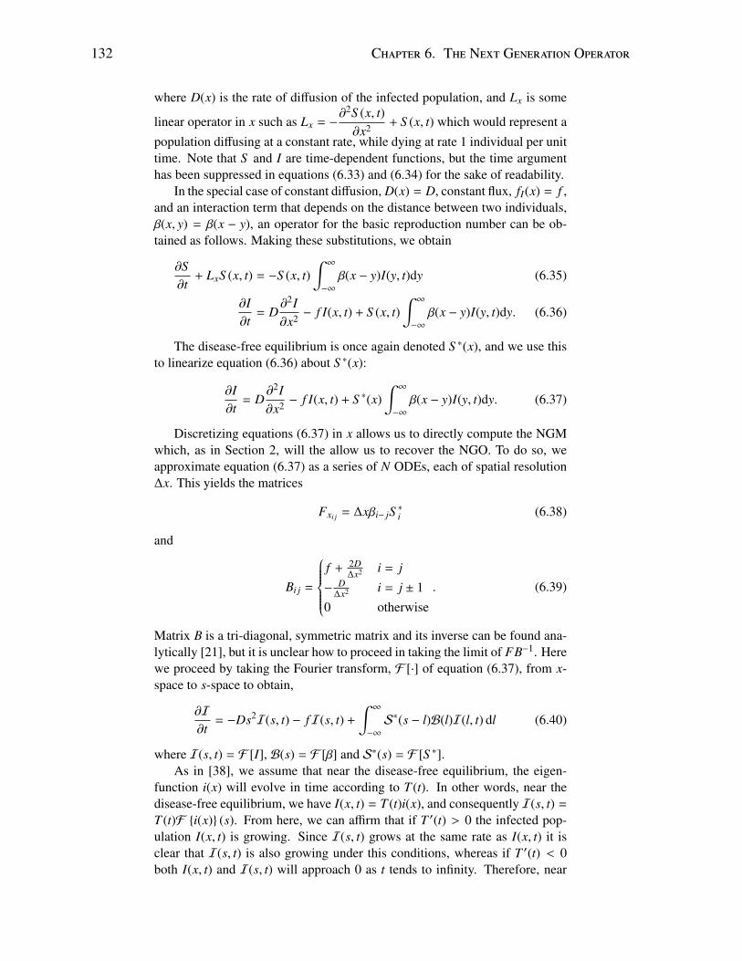
132 Chapter 6. The Next Generation Operator

where D(x) is the rate of diffusion of the infected population, and Lx is some

linear operator in x such as Lx = −∂2S (x, t)∂x2 + S (x, t) which would represent a

population diffusing at a constant rate, while dying at rate 1 individual per unittime. Note that S and I are time-dependent functions, but the time argumenthas been suppressed in equations (6.33) and (6.34) for the sake of readability.

In the special case of constant diffusion, D(x) = D, constant flux, fI(x) = f ,and an interaction term that depends on the distance between two individuals,β(x, y) = β(x − y), an operator for the basic reproduction number can be ob-tained as follows. Making these substitutions, we obtain

∂S∂t

+ LxS (x, t) = −S (x, t)∫ ∞

−∞

β(x − y)I(y, t)dy (6.35)

∂I∂t

= D∂2I∂x2 − f I(x, t) + S (x, t)

∫ ∞

−∞

β(x − y)I(y, t)dy. (6.36)

The disease-free equilibrium is once again denoted S ∗(x), and we use thisto linearize equation (6.36) about S ∗(x):

∂I∂t

= D∂2I∂x2 − f I(x, t) + S ∗(x)

∫ ∞

−∞

β(x − y)I(y, t)dy. (6.37)

Discretizing equations (6.37) in x allows us to directly compute the NGMwhich, as in Section 2, will the allow us to recover the NGO. To do so, weapproximate equation (6.37) as a series of N ODEs, each of spatial resolution∆x. This yields the matrices

Fxi j = ∆xβi− jS ∗i (6.38)

and

Bi j =

f + 2D

∆x2 i = j− D

∆x2 i = j ± 10 otherwise

. (6.39)

Matrix B is a tri-diagonal, symmetric matrix and its inverse can be found ana-lytically [21], but it is unclear how to proceed in taking the limit of FB−1. Herewe proceed by taking the Fourier transform, F [·] of equation (6.37), from x-space to s-space to obtain,

∂I

∂t= −Ds2I(s, t) − fI(s, t) +

∫ ∞

−∞

S∗(s − l)B(l)I(l, t) dl (6.40)

where I(s, t) = F [I], B(s) = F [β] and S∗(s) = F [S ∗].As in [38], we assume that near the disease-free equilibrium, the eigen-

function i(x) will evolve in time according to T (t). In other words, near thedisease-free equilibrium, we have I(x, t) = T (t)i(x), and consequently I(s, t) =

T (t)F {i(x)} (s). From here, we can affirm that if T ′(t) > 0 the infected pop-ulation I(x, t) is growing. Since I(s, t) grows at the same rate as I(x, t) it isclear that I(s, t) is also growing under this conditions, whereas if T ′(t) < 0both I(x, t) and I(s, t) will approach 0 as t tends to infinity. Therefore, near

6.3. Reaction-Diffusion System 133

the disease-free equilibrium, the exponential growth parameter of the infectedpopulation is preserved under the Fourier transform. This will allow us to de-termine a reproduction number in Fourier space which has the same thresholdbehaviour as R0.

From Theorem 3.1 in [38], if we define σ(•) as the spectral radius of anoperator and define operators Fx and B as

Fx[I] = S ∗(x)∫ ∞

−∞

β(x − y)I(y)dy (6.41)

and

B[I] = D∂2I∂x2 − f I(x) (6.42)

then σ(−FxB−1) − 1 and σ(A = B + Fx), and the exponential growth bound ofthe eigenfunction I(x) all have the same sign.

Accordingly, in Fourier space, we define V[I] = −Ds2I − fI, F [I] =∫ ∞−∞S∗(s − l)B(l)I(l)dl and A = F + V, and appeal to Theorems 2.3 and

3.14 in [34] to conclude that σ(A), σ(−FV−1)−1 and the exponential growthbound of I(s) all have the same sign. Since we have already shown that theexponential growth bound is preserved under Fourier transform, it follows thatboth systems will have the same threshold value R0 = 1, such that the disease-free equilibrium is asymptotically stable for R0 < 1.

Discretizing equation (6.40) into N equations of the form,

dIi

dt= −Ds2

i Ii − fIi +

N∑j=0

S∗i− jB jI j∆l (6.43)

permits the use of the next generation matrix where

Fi j = S∗i− jB j∆l (6.44)

and

Vi j =

f + Ds2i , i = j

0, i , j(6.45)

for i, j ∈ [0,N].Using the same techniques as described in Section 2.2, in the limit as ∆s→

0 we obtain the operator

Ns[I] =

∫ ∞

−∞

S∗(s − l)B(l)

f + Dl2I(l) dl. (6.46)

Since this equation is the limit of the next generation matrix as the numberof classes approaches infinity, the spectral radius of operator Ns can be inter-preted as the basic reproduction number, R0 for equations (6.35) and (6.40).Given the above arguments, R0 has the same threshold behaviour as the basicreproduction number, R0, for equations (6.35) and (6.36). Figure 6.1 showsnumerically that not only are the threshold values the same for the spectral

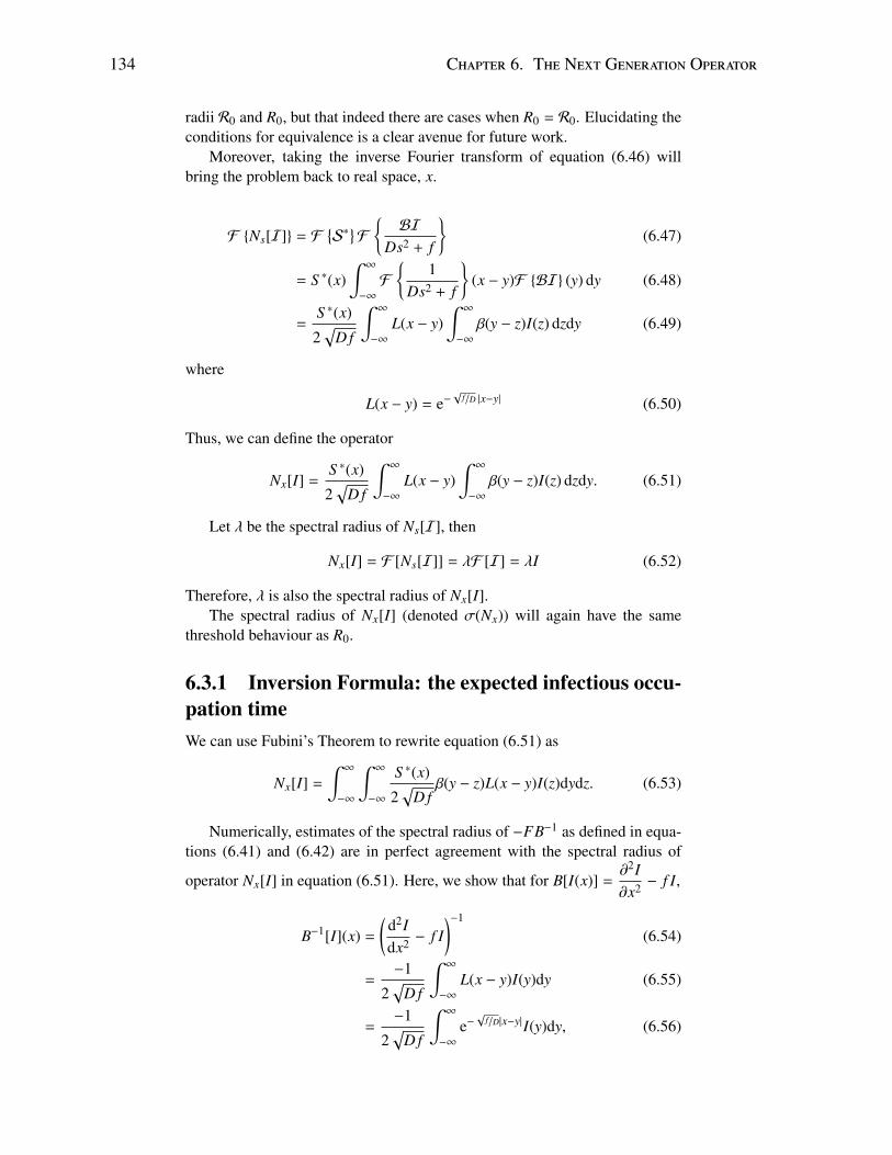
134 Chapter 6. The Next Generation Operator

radii R0 and R0, but that indeed there are cases when R0 = R0. Elucidating theconditions for equivalence is a clear avenue for future work.

Moreover, taking the inverse Fourier transform of equation (6.46) willbring the problem back to real space, x.

F {Ns[I]} = F{S∗

}F

{BI

Ds2 + f

}(6.47)

= S ∗(x)∫ ∞

−∞

F

{1

Ds2 + f

}(x − y)F {BI} (y) dy (6.48)

=S ∗(x)

2√

D f

∫ ∞

−∞

L(x − y)∫ ∞

−∞

β(y − z)I(z) dzdy (6.49)

where

L(x − y) = e−√

f/D |x−y| (6.50)

Thus, we can define the operator

Nx[I] =S ∗(x)

2√

D f

∫ ∞

−∞

L(x − y)∫ ∞

−∞

β(y − z)I(z) dzdy. (6.51)

Let λ be the spectral radius of Ns[I], then

Nx[I] = F [Ns[I]] = λF [I] = λI (6.52)

Therefore, λ is also the spectral radius of Nx[I].The spectral radius of Nx[I] (denoted σ(Nx)) will again have the same

threshold behaviour as R0.

6.3.1 Inversion Formula: the expected infectious occu-pation timeWe can use Fubini’s Theorem to rewrite equation (6.51) as

Nx[I] =

∫ ∞

−∞

∫ ∞

−∞

S ∗(x)

2√

D fβ(y − z)L(x − y)I(z)dydz. (6.53)

Numerically, estimates of the spectral radius of −FB−1 as defined in equa-tions (6.41) and (6.42) are in perfect agreement with the spectral radius of

operator Nx[I] in equation (6.51). Here, we show that for B[I(x)] =∂2I∂x2 − f I,

B−1[I](x) =

(d2Idx2 − f I

)−1

(6.54)

=−1

2√

D f

∫ ∞

−∞

L(x − y)I(y)dy (6.55)

=−1

2√

D f

∫ ∞

−∞

e−√

f/D|x−y|I(y)dy, (6.56)

6.3. Reaction-Diffusion System 135

provided the integral exists.This can be shown in a straightforward manner by considering the expres-

sion

−1

2√

D f

∫ ∞

−∞

e−√

f/D|x−y| (Dw′′(y) − f w(y))

dy (6.57)

where w(y) is any smooth function for which∫ ∞

−∞

L(x − y)w(y) dy

exists. We split this into two integrals, which we can compute:

−1

2√

D f

∫ ∞

−∞

e−√

f/D|x−y| (Dw′′(y) − f w(y))

dy = IL + IR (6.58)

where

IL = −1

2√

D f

∫ x

−∞

e−√

f/D(x−y) (Dw′′(y) − f w(y))

dy (6.59)

and

IR = −1

2√

D f

∫ ∞

xe−√

f/D(y−x) (Dw′′(y) − f w(y))

dy. (6.60)

The result

−1

2√

D f

∫ ∞

−∞

e−√

f/D|x−y| (Dw′′(y) − f w(y))

dy = w(x) (6.61)

comes from integrating by parts. When working with integrals of the form

−1

2√

D f

∫e±√

f/D(x−y)Dw′′(y) dy

we choose u = exp(±√

f/D(x − y)) and dv = w′′(y) and for integrals of theform

−1

2√

D f

∫e±√

f/D(x−y)(− f w(y)) dy

we choose u = f w(y) and dv = exp(±√

f/D(x − y)). From here, equation (6.61)follows easily.

Figure 6.3 shows some test functions which illustrate this inversion for-mula. The functions are chosen to highlight three possible classes of functions:those that decay as x → ±∞, those that are periodic and measurable, and fi-nally those that are not integrable on (−∞,∞), but are less than exponentialorder. In analogy with the previous sections, we interpret B−1[I](x) as the ex-pected length of time an individual will be at position x before either dying ormoving to a new position.

136 Chapter 6. The Next Generation Operator

6.3.2 ConjectureWe conjecture that equation (6.56) can be extended to the case of a spatiallyvariable death rate. In this case, we have

B−1[I](x) =

(d2Idx2 − f (x)I

)−1

(6.62)

=−1

2√

D f (x)

∫ ∞

−∞

M(x − y)I(y)dy (6.63)

where

M(x − y) = e−√

f (x)/D|x−y|. (6.64)

Of course, this requires f (x) , 0.Figure 6.4 shows some test functions that support this conjecture. Numer-

ical exploration suggests that equation (6.63) may hold for periodic functions,monotonically increasing functions that are less than exponential order, andthose that are bounded but not integrable; we show one example of each case.

6.4 Levy FlightThe above methods can be generalized to other movement patterns includingLevy flights [13]. The generalized system makes use of fractional derivatives:

∂S∂t

+ LxS (x, t) = −S (x, t)∫ ∞

−∞

β(x, y)I(y, t)dy (6.65)

∂I∂t

= γ∂αI∂xα− fI(x)I(x, t) + S (x, t)

∫ ∞

−∞

β(x, y)I(y, t)dy (6.66)

where 0 < α ≤ 2, γ is a movement constant and the fractional derivative isdefined through the Fourier transform, F as

F

[∂αI∂xα

]= −|s|αF [I(x)]. (6.67)

Using the same methods and arguments as Section 3, we assume the disease-free equilibrium exists and is denoted by S ∗(x), and that we may linearizearound S ∗(x), and apply a Fourier transform to equation (6.66). Doing soallows us to write out a generalized next generation operator in Fourier space:

NL[I] =

∫ ∞

−∞

S∗(s − l)B(l)

fI + |γl|αI(l)dl (6.68)

where B, S∗ and I are defined as in Section 3 (below equation (6.40)).The largest eigenvalue of this operator will have the same threshold be-

haviour as R0. Reverting to real space, x, is difficult and needs further investi-gation.

6.5. Approximating the Spectral Radius of the Next Generation Operator 137

6.5 Approximating the Spectral Radius of theNext Generation OperatorIn order to obtain the basic reproduction number for a continuously age-structuredpopulation, it is required to solve

R0I(a) = S ∗(a)∫ ∞

0I(a′)eΓ(a′)

∫ ∞

a′β(a, s)e−Γ(s)dsda′ (6.69)

such that I(a) > 0 for all a. This problem may be intractable because ofthe arbitrary nature of both β and Γ. Therefore, in the following section, weattempt to find a closed-form approximation to R0.

We begin by adapting Brauer’s method [6] for the case of a separable in-teraction term to a general interaction term. To do so, we linearize equation(6.2) about S ∗(x),

∂I∂a

+∂I∂t

= S ∗(a)∫ ∞

0β(a, a′)I(a′, t)da′ − ( fI(a)) I(a, t) (6.70)

and again use the ansatz that near the disease-free equilibrium, the infectedpopulation, I(a, t) grows exponentially in time, proportional to the eigenfunc-tion i(a) [6], that is

I(a, t) = eρti(a) . (6.71)

This yields

dida

= S ∗(a)W(a) − ( fI(a) + ρ)i(a) (6.72)

where

W(a) =

∫ ∞

0β(a, a′)i(a)da′. (6.73)

Solving equation (6.72) gives

i(a) = e−ρa−Γ(a)∫ a

0S ∗(s)W(s)eΓ(s)+ρsds. (6.74)

Substituting (6.74) into (6.73) gives

W(a) =

∫ ∞

0β(a, a′)e−ρa′−Γ(a′)

∫ a′

0S ∗(s)W(s)eΓ(s)+ρsds

da′ (6.75)

and rewriting the integral yields

W(a) =

∫ ∞

0S ∗(a′)eΓ(a′)+ρa′

{∫ ∞

a′β(a, s)e−ρs−Γ(s)ds

}W(a′)da′. (6.76)

This is a homogeneous Fredholm equation of the second kind for the func-tion W(a) [39]. A non-trivial solution to equation (6.76) exists if W(a) is aneigenfunction of the kernel, that is

K(a, a′, ρ) = S ∗(a′)eΓ(a′)+ρa′{∫ ∞

a′β(a, s)e−ρs−Γ(s)ds

}(6.77)

138 Chapter 6. The Next Generation Operator

with associated eigenvalue λ = 1 [39].Following the proof in [39], squaring equation (6.76) yields

W(a)2 =

[∫ ∞

0K(a, a′, ρ)W(a′)da′

]2

(6.78)

and we may then use the Cauchy-Schwarz inequality to write

W(a)2 ≤

∫ ∞

0K(a, a′, ρ)2da′

∫ ∞

0W(a′)2da′. (6.79)

Integrating both sides of equation (6.79) with respect to variable a, we find:∫ ∞

0W(a)2da ≤

∫ ∞

0K(a, a′, ρ)2da′

∫ ∞

0W(a′)2da′. (6.80)

Therefore, a non-trivial solution to equation (6.76) exists only if the value ofthe growth parameter ρ is such that

||K||2 ≥ 1. (6.81)

Since K(a, a′, ρ) is a decreasing function of ρ, we know that if ||K(a, a′, 0)||2 <1 then the only ρ values which satisfy equation (6.81) must be negative. There-fore near the disease-free equilibrium, I(a, t) is a decreasing function of t as perequation (6.71). In contrast, if ||K(a, a′, 0)||2 > 1 then by continuity there mustexist a ρ∗ > 0 such that ||K(a, a′, ρ∗)||2 = 1. In this case, every ρ < ρ∗ willalso satisfy condition (6.81). Therefore, the actual growth parameter ρ may bepositive or negative. Thus ||K(a, a′, 0)||2 is only an upper bound on the basicreproduction number, R0. This differs from the case of a separable interactionterm in which the analogous condition is ||K(a, a′, ρ)||1 = 1 (see [6] for details),and a unique ρ satisfies this condition, hence ||K(a, a′, 0||1 = R0.

6.6 DiscussionArguably among the most well-studied tools in disease modelling are the nextgeneration matrix of discrete systems [2, 3, 16, 32, 35] and the next generationoperators used in continuum models [3, 15, 17, 18, 22, 34, 37, 38]. Whilethe two formulations are clear analogs of one another, in this study we showthat the NGO can be directly obtained as the limit of the NGM, as the numberof classes approaches infinity. This approach allows us to extend these limitarguments to disease models described by reaction-diffusion equations, and toderive a closed-form next generation operator for these well-known systems.

The relationship between the next generation matrix of discrete dynam-ics and the next generation operator of continuum dynamics is critical to thebiological interpretation of these operators. The next generation matrix is un-derstood easily as the force of infection, F, multiplied by the expected lifetimein each compartment of an infected individual, V−1 [11]. When moving to thecontinuum, these interpretations can be confounded by either the techniquesused to determine the operator [6] or by the more complicated nature of the

6.6. Discussion 139

mathematics involved (such as the convolution and exponential terms appear-ing in equation (6.32)).

This equivalence between the discrete and continuum approaches makesit possible to manipulate a simple reaction-diffusion model with non-local in-fectibility to determine a closed-form next generation operator whose spectralradius can be guaranteed to have the same threshold dynamics as R0, by con-necting theorems found in [34, 38] and taking advantage of the linear prop-erties of the Fourier transform. While the existence of such an operator haspreviously been proven [34, 38], and while similar results have been applied tovarious systems such as a dengue fever model [37] and a general model withfixed latent period and nonlocal infection [19], a closed-form operator for R0has remained elusive. Since in the present study the next generation operatoris derived as the limit of a discrete operator, this derivation provides an avenuetoward a threshold parameter in both the discrete and continuum models.

Our study also suggests that the Fourier transform may be a more naturalsetting for computation of R0. We see that a closed-form integral operatorwith the same threshold characteristics as the next generation operator canbe derived for both diffusion and Levy flight equations, and can be triviallyextended to higher dimensions. A next step would be to generalize this methodto work with spatially-dependent death rates, in such a way that the validity ofthe operator can be proven. Here, we provide such an operator as a conjecture.

Moreover, we offer a novel, closed-form expression for inversion of the

operator B[I] =d2Idx2 − f I. The ubiquity of reaction-diffusion operators in

mathematical biology indicates both the need for, and potential importance of,such a closed-form inversion. The inversion operator gives the expected timean individual will occupy position x before either dying or moving to a new po-sition. Biologically this is relevant to many spatial models in ecology, and canpotentially be extended to an inversion formula for the expected ‘occupationtime’ of migrating populations. Mathematically, this formula makes it possibleto turn a reaction-diffusion equation into an eigenvalue problem, which allowsa wide range of techniques for solving a reaction-diffusion system analyticallyand numerically.

We conclude with a technique to find a closed-form upper bound for thebasic reproduction number using the operators derived herein. This expressionmay be useful for understanding the spread of disease in the context of contin-uous age or space, and for deriving quantitative estimates of control measures.While we show the approximation for the age-structured model, the methodcan also be applied to equation (6.46) to determine a closed-form approxima-tion for the upper bound of R0 for a spatially-explicit model.

140 Chapter 6. The Next Generation Operator

Figure 6.1: R0 and σ(A) calculated in both real space, x, (blue solid line) using FB−1 (asdefined in equations (6.38) and (6.39), with ∆x = 0.1001 and N = 2000). and Fourier spaces (magenta points) using equation (6.46) with ∆s = 0.1001. The interaction term used here isβ(x − y) = Cexp

(−k(x − y)2

), C ∈ [0.01, 0.5], and Lx[S ∗] = xS ∗

′′

(x) + S ∗′

(x) + 4x3S ∗(x). Thediffusion rate is set to D = 1 and the infected death rate, f = 1. We see that not only does thesystem in Fourier space have the same threshold behaviour as the system in real space, but infact the values for R0 are identical.

6.6. Discussion 141

Figure 6.2: σ(−FxB−1) vs. σ(Nx). σ(−FxB−1) is calculated using equations (6.38) and (6.39),with ∆x = 0.1001 and N = 2000. σ(Nx) is calculated using equation (6.51) with ∆x = 0.1001.

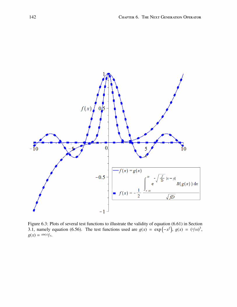
142 Chapter 6. The Next Generation Operator

Figure 6.3: Plots of several test functions to illustrate the validity of equation (6.61) in Section3.1, namely equation (6.56). The test functions used are g(x) = exp

(−x2

), g(x) = (x/10)3,

g(x) = sin(x)/x.

6.6. Discussion 143

Figure 6.4: Plots of several test functions to illustrate the accuracy of equation (6.63) in Section3.2, with f (x) = x2 + 1 to ensure smoothness everywhere. The test functions used are w(x) =2π

arctan(x), w(x) = x3/103, w(x) = sin(x).

Bibliography

[1] Allen, L. J. Introduction to mathematical biology. Pearson/Prentice Hall,2007.

[2] Allen, L. J., and Van Den Driessche, P. The basic reproduction numberin some discrete-time epidemic models. Journal of Difference Equationsand Applications 14, 10-11 (2008), 1127–1147.

[3] Bacaer, N. Approximation of the basic reproduction number R0 forvector-borne diseases with a periodic vector population. Bulletin of math-ematical biology 69, 3 (2007), 1067–1091.

[4] Bacaer, N., and Khaladi, M. On the basic reproduction number in arandom environment. Journal of mathematical biology 67, 6-7 (2013),1729–1739.

[5] Betti, M. I., Wahl, L. M., and Zamir, M. Reproduction number andasymptotic stability for a model with continuous age structure: An appli-cation to honey bee dynamics. Bulletin of Mathematical Biology (2016).submitted.

[6] Brauer, F., and Castillo-Chavez, C. Mathematical models in populationbiology and epidemiology, vol. 1. Springer, 2001.

[7] Britton, N. Essential mathematical biology. Springer Science & Busi-ness Media, 2012.

[8] Britton, N. F. Reaction-diffusion equations and their applications tobiology. Academic Press, 1986.

[9] Browne, C., and Webb, G. F. A nosocomial epidemic model with infec-tion of patients due to contaminated rooms. Mathematical Biosciencesand Engineering 12, 4 (2015), 761–787.

[10] Chowell, G., Fuentes, R., Olea, A., Aguilera, X., Nesse, H., and Hy-man, J. The basic reproduction number R0 and effectiveness of reactiveinterventions during dengue epidemics: The 2002 dengue outbreak inEaster Island, Chile. Mathematical biosciences and engineering: MBE10 (2013), 1455.

[11] Cushing, J., and Diekmann, O. The many guises of R0 (a didactic note).Journal of Theoretical Biology 404 (2016), 295–302.

[12] Cushing, J. M., and Ackleh, A. A net reproductive number for periodicmatrix models. Journal of biological dynamics 6, 2 (2012), 166–188.

[13] del Castillo-Negrete, D., Carreras, B., and Lynch, V. Front dynam-ics in reaction-diffusion systems with Levy flights: a fractional diffusionapproach. Physical Review Letters 91, 1 (2003), 018302.

144

BIBLIOGRAPHY 145

[14] Diekmann, O., and Heesterbeek, J. Mathematical epidemiology of infec-tious diseases: model building, analysis and interpretation, vol. 5. JohnWiley & Sons, 2000.

[15] Diekmann, O., Heesterbeek, J., and Metz, J. A. On the definition and thecomputation of the basic reproduction ratio R0 in models for infectiousdiseases in heterogeneous populations. Journal of mathematical biology28, 4 (1990), 365–382.

[16] Diekmann, O., Heesterbeek, J., and Roberts, M. The construction ofnext-generation matrices for compartmental epidemic models. Journalof the Royal Society Interface (2009), rsif20090386.

[17] Greenhalgh, D. Analytical results on the stability of age-structuredrecurrent epidemic models. Mathematical Medicine and Biology 4, 2(1987), 109–144.

[18] Greenhalgh, D. Threshold and stability results for an epidemic modelwith an age-structured meeting rate. Mathematical Medicine and Biology5, 2 (1988), 81–100.

[19] Guo, Z., Wang, F.-B., and Zou, X. Threshold dynamics of an infectivedisease model with a fixed latent period and non-local infections. Journalof mathematical biology 65, 6-7 (2012), 1387–1410.

[20] Heffernan, J., Smith, R., and Wahl, L. M. Perspectives on the basicreproductive ratio. Journal of the Royal Society Interface 2, 4 (2005),281–293.

[21] Hu, G., and O’Connell, R. F. Analytical inversion of symmetric tridi-agonal matrices. Journal of Physics A: Mathematical and General 29, 7(1996), 1511.

[22] Hyman, J. M., and Li, J. The reproductive number for an HIV modelwith differential infectivity and staged progression. Linear algebra andits applications 398 (2005), 101–116.

[23] Inaba, H. Threshold and stability results for an age-structured epidemicmodel. Journal of mathematical biology 28, 4 (1990), 411–434.

[24] Lanczos, C. An iteration method for the solution of the eigenvalue prob-lem of linear differential and integral operators. Journal of Research orthe National Bureau of Standards 45, 4 (1950), 255–282.

[25] Li, C.-K., and Schneider, H. Applications of Perron–Frobenius theoryto population dynamics. Journal of Mathematical Biology 44, 5 (2002),450–462.

[26] Murray, J. D. Mathematical Biology. II Spatial Models and BiomedicalApplications {Interdisciplinary Applied Mathematics V. 18}. Springer-Verlag New York Incorporated, 2001.

[27] Murray, J. D. Mathematical Biology: I An Introduction{Interdisciplinary Applied Mathematics V. 17}. Springer, New York, NY,USA, 2002.

[28] Noble, B., and Daniel, J. W. Applied linear algebra, vol. 3. Prentice-HallNew Jersey, 1988.

[29] Otto, S. P., and Day, T. A biologist’s guide to mathematical modeling inecology and evolution, vol. 13. Princeton University Press, 2007.

146 BIBLIOGRAPHY

[30] Pastor-Satorras, R., Castellano, C., Van Mieghem, P., and Vespignani,A. Epidemic processes in complex networks. Reviews of modern physics87, 3 (2015), 925.

[31] Roberts, M., and Heesterbeek, J. A new method for estimating the ef-fort required to control an infectious disease. Proceedings of the RoyalSociety of London B: Biological Sciences 270, 1522 (2003), 1359–1364.

[32] Roberts, M. G., and Heesterbeek, J. Characterizing the next-generationmatrix and basic reproduction number in ecological epidemiology. Jour-nal of mathematical biology 66, 4-5 (2013), 1045–1064.

[33] Slavık, A. Product integration, its history and applications. MatfyzpressPrague, 2007.

[34] Thieme, H. R. Spectral bound and reproduction number for infinite-dimensional population structure and time heterogeneity. SIAM Journalon Applied Mathematics 70, 1 (2009), 188–211.

[35] Van den Driessche, P., and Watmough, J. Reproduction numbers andsub-threshold endemic equilibria for compartmental models of diseasetransmission. Mathematical biosciences 180, 1 (2002), 29–48.

[36] Volpert, V., and Petrovskii, S. Reaction–diffusion waves in biology.Physics of life reviews 6, 4 (2009), 267–310.

[37] Wang, W., and Zhao, X.-Q. A nonlocal and time-delayed reaction-diffusion model of dengue transmission. SIAM Journal on Applied Math-ematics 71, 1 (2011), 147–168.

[38] Wang, W., and Zhao, X.-Q. Basic reproduction numbers for reaction-diffusion epidemic models. SIAM Journal on Applied Dynamical Systems11, 4 (2012), 1652–1673.

[39] Zemyan, S. M. Fredholm integral equations of the second kind (generalkernel). In The Classical Theory of Integral Equations. Springer, 2012,pp. 31–84.

Chapter 7

Discussion & Conclusions

The aim of this dissertation was to study models of honey bee colony dynam-ics. Building upon the work of others, [10, 11, 15], I have developed andanalyzed three separate models of honey bee colony dynamics. Each exten-sion to the model has allowed for new predictions or captured new behaviourswhich were not within the scope of other models.

The first such model, as discussed in Chapter 2, was developed to incorpo-rate high-level seasonality and disease dynamics into honey bee models. Twokey predictions came from this model. The first is the use of the Average Ageof Recruitment to Foraging (AARF) as an indicator of a diseased colony and,ultimately, as a herald of colony extinction. The second is the role of the onsetof winter in the severity of disease. The model shows that diseases that occurin late fall are predicted to have more severe long term effects on colony healththan an infection that is introduced in, say, early summer. This model, as a firstpass, was developed to be very general. The main aim was to highlight pre-dictors and nonlinear dynamics that arise from the interplay between infectionand seasonality, and how a diseased colony can exhibit symptoms of colonycollapse.

Age structure was later added to the model and the dynamics were quitedifferent. In Chapter 3, we show the age demography of a healthy colony, con-ditions for stability of the disease-free equilibrium as well as derive the basicreproduction number, R0, for an age-structured model of honey bee colony dy-namics. This expression for R0 is consistent with the expression derived in anage-independent model, and is found to differ significantly from the latter asthe number of age classes is increased toward a continuum. Analysis of themodel also gives insights into the sensitivity of honey bee colonies to the in-herent age polyethism in their societies. The time spent nursing is critical tothe survival of honey bee colonies.

In Chapter 4, we perform numerical simulations on the age-structuredmodel to extract more biological insights from the model. It is found that anage-structured model successfully captures the phenomenon known as ‘springdwindle’ without explicitly building it into the model. The age-structuredmodel also refines the predictions of critical times for onset of infection ina honey bee colony. The introduction of age structure into the model showsthat early spring and late fall are especially vulnerable times for honey bee

147

148 Chapter 7. Discussion & Conclusions

colonies. Moreover, the model predicts that there is a compounding effectwhen disease and seasonality are both considered. The model shows that anendemic disease in a honey bee colony may cause destruction of the colonymany years later. This implies that the causes of honey bee declines, at leastlocally on a colony-by-colony basis, may not be immediate.

The agent-based model in Chapter 5 further builds upon the previous mod-els to incorporate environmental hazards and explicit space dependence. Theaim here was to develop an accurate model of honey bee dynamics which couldbe used in order to help guide policy and conservation efforts. The model isin good agreement with experimental data from the literature [4, 6, 14] andbehaves as expected in a range of biologically reasonable parameters. In par-ticular, the AARF extracted from simulations is consistent with previous re-sults [2, 10, 11, 13]. The model does show that sub-lethal pesticides are hid-den from the AARF, even though the mortality of bees is increased indirectlythrough, for example, hindered navigation. This particular example of a sub-lethal pesticide effects is simulated and shows that this alone may contribute toColony Collapse Disorder, as many bees will die quite far away from the hive.

Currently, there is much work being done on honey bee genomics and se-lectively breeding queens that are able to thrive in the current ecological land-scape [7, 9, 12, 16]. With all the new data coming from these studies, and thefact that honey bees are haploid-diploid, a model for the persistence of benefi-cial mutations in honey bee colonies can help guide efforts to create coloniesthat thrive, without disrupting the genetic diversity of managed honey bees.It is in this direction that I will continue my work on models of honey bees.Insights can be gained through dynamical systems models and through agent-based simulations. The groundwork has been laid herein to then later study thephenotypical responses at the colony level to genomic changes.

Of course, there is also much much to be done in the way of modelinghoney bee colony dynamics. The models herein take a simplified approachto modeling the effect of temperature on forager dynamics. Honey bees arenot able generate enough heat in their muscles at low temperatures in order toachieve flight [5]. As well, temperature of the brood has been shown to influ-ence the behaviour of an adult honey bee [18]. Moreover, higher temperatureswill evaporate some of the water content in nectar, thus making it more diffi-cult to extract [8]. Also, higher temperatures correlate to increases in flowervisiting speed and simultaneous decreases in the number of flowers visited [1].These observed phenomena will greatly influence not only the dynamics of ahoney bee colony, but as well the bee-plant interactions within the ecosystem.The importance of these temperature effects on the longterm health of honeybees is particularly pertinent in the face of global warming [17].

Chapter 6 investigates the connections between the basic reproduction num-ber for compartmental models and partial differential equation models. Thiswork was motivated by the similarities and differences found in the analysis ofR0 in Chapter 3. For general models, R0 is often difficult – if not impossible– to write down analytically and so we focus on the connection between thenext generation matrix (NGM) and its continuous counterpart: the next gener-ation operator (NGO). The basic reproduction number, R0, is then the spectral

149

radius of the defined matrix/operator. We show that for age-structured models,while other techniques exist for defining the NGO [3], one can also recoverthe NGO as the limit of the NGM. This allows for an algorithmic way to deter-mine the next generation operators for a wide class of advection models as wellas allows the techniques and tools developed in the context of compartmentalmodels to be used on models for which one parameter exists on a continuum.

In the case of reaction-diffusion models, we use the above technique todevelop a closed-form next generation operator which can be used to extractR0. Some implications here are that R0 has the same threshold behaviour inFourier space as in real space, and often the NGO is easier to derive in Fourier

space. We are also able to recover an inverse for the operator∂2

∂x2 − f and

conjecture that this inverse can be extended to operators of the form D(x)∂2

∂x2 −

f (x).The proof of the conjecture is open, and I believe can be of great value

both mathematically and biologically if proved. Moreover, there are manyways to modify the simple exploratory models for which the NGOs above havebeen derived. Future work would entail either developing the NGO for morecomplex models using the above framework, or showing how perturbations tothe simple models will change the NGO.

Bibliography

[1] Benedek, P., and Prenner, J. Effect of temperature on the behaviour andpollinating efficiency of honeybees on winter rape flowers. Journal ofApplied Entomology 71, 1-4 (1972), 120–124.

[2] Botias, C., Martin-Hernandez, R., Barrios, L., Meana, A., and Higes,M. Nosema spp. infection and its negative effects on honey bees (Apismellifera iberiensis) at the colony level. Veterinary research 44, 1 (2013),1–15.

[3] Brauer, F., and Castillo-Chavez, C. Mathematical models in populationbiology and epidemiology, vol. 1. Springer, 2001.

[4] Capinera, J. L. Encyclopedia of entomology, vol. 4. Springer Science &Business Media, 2008.

[5] Esch, H. Body temperature and flight performance of honey bees ina servo-mechanically controlled wind tunnel. Journal of comparativephysiology 109, 3 (1976), 265–277.

[6] Ginsberg, H. S. Foraging ecology of bees in an old field. Ecology 64, 1(1983), 165–175.

[7] Harpur, B. A., Kent, C. F., Molodtsova, D., Lebon, J. M., Alqarni,A. S., Owayss, A. A., and Zayed, A. Population genomics of the honeybee reveals strong signatures of positive selection on worker traits. Pro-ceedings of the National Academy of Sciences 111, 7 (2014), 2614–2619.

[8] Haydak, M. H. Honey bee nutrition. Annual review of entomology 15, 1(1970), 143–156.

[9] Ibrahim, A., Reuter, G. S., and Spivak, M. Field trial of honey beecolonies bred for mechanisms of resistance against Varroa destructor.Apidologie 38, 1 (2007), 67–76.

[10] Khoury, D. S., Barron, A. B., and Myerscough, M. R. Modelling foodand population dynamics in honey bee colonies. PLOS ONE 8, 5 (052013), e59084.

[11] Khoury, D. S., Myerscough, M. R., and Barron, A. B. A quantitativemodel of honey bee colony population dynamics. PLOS ONE 6, 4 (042011), e18491.

[12] Meixner, M. D., Costa, C., Kryger, P., Hatjina, F., Bouga, M., Ivanova,E., and Buchler, R. Conserving diversity and vitality for honey beebreeding. Journal of Apicultural Research 49, 1 (2010), 85–92.

[13] Perry, C. J., Søvik, E., Myerscough, M. R., and Barron, A. B. Rapidbehavioral maturation accelerates failure of stressed honey bee colonies.

150

BIBLIOGRAPHY 151

Proceedings of the National Academy of Sciences 112, 11 (2015), 3427–3432.

[14] Ratnieks, F. L. Egg-laying, egg-removal, and ovary development byworkers in queenright honey bee colonies. Behavioral Ecology and So-ciobiology 32, 3 (1993), 191–198.

[15] Ratti, V., Kevan, P. G., and Eberl, H. J. A mathematical model of thehoneybee-Varroa destructor-Acute Bee Paralysis Virus complex withseasonal effects. Bulletin of Mathematical Biology (2015).

[16] Rinderer, T. E., Guzman, L. I. D., Frake, A. M., Tarver, M. R., and

Khongphinitbunjong, K. An evaluation of the associations of parametersrelated to the fall of Varroa destructor (Acari: Varroidae) from com-mercial honey bee (Hymenoptera: Apidae) colonies as tools for selectivebreeding for mite resistance. Journal of economic entomology 107, 2(2014), 516–522.

[17] Stocker, T. Climate change 2013: the physical science basis: WorkingGroup I contribution to the Fifth assessment report of the Intergovern-mental Panel on Climate Change. Cambridge University Press, 2014.

[18] Tautz, J., Maier, S., Groh, C., Rossler, W., and Brockmann, A. Behav-ioral performance in adult honey bees is influenced by the temperatureexperienced during their pupal development. Proceedings of the NationalAcademy of Sciences 100, 12 (2003), 7343–7347.

Appendix A

Age structure is Critical to thePopulation Dynamics andSurvival of Honey Bee Colonies– Supplementary Material

Table A.1: Parameter values and source references.L maximum rate of egg laying 2000 eggs/day [5]w number of hive bees for 50% egg survival 5000 bees [5]am age at which hive bees begin brood care 3 days [7]aT age at which hive bees end brood care 11 days [7]aR minimum recruitment age 4 days [2]k age at which rate of recruitment is 25% of max. 10 daysα maximum rate of recruitment 1 /day1σ

maximum fraction of colony that can be foraging 13 [5]

µ(a) natural death rate of foragers (summer) Figure 1 [1]µw natural death rate of foragers and hive bees (winter) 1/180 /day [7]b mass of food stored for 50% egg survival 500 g [4]c food gathered per day per forager 0.1 g /day / bee [6]γ daily food requirement per adult bee 0.007 g /bee [4]

dH(a) death rate of hive bees due to infection 0.14 /day or Figure 1 [3]dF(a) death rate of hive bees due to infection 0.14 /day or Figure 1 [3]β disease transmission rate variable

152

153

Figure A.1: Time course of total bee population in a disease-free colony. Shaded area denoteswinter, during which no new hive bees are produced. Here we use more realistic food intakec = 0.5 and consumption rates, γ = 0.07 [37]. We see that the dynamics of the colony are notsensitive to the food intake and consumption rates.

154 Chapter A. Chapter 4 Supplementary Material

Figure A.2: Age distribution of a healthy colony at equilibrium during the active season, basedon the natural death rate, µ(a) presented in Figure 1.

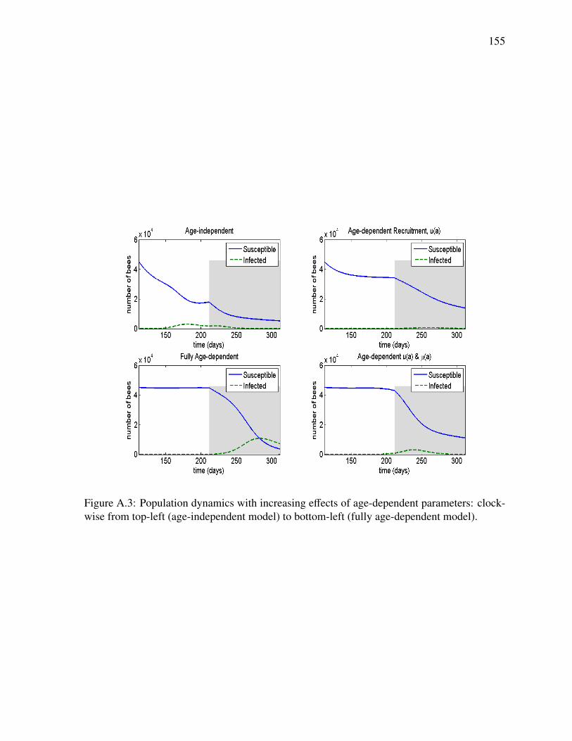
155

Figure A.3: Population dynamics with increasing effects of age-dependent parameters: clock-wise from top-left (age-independent model) to bottom-left (fully age-dependent model).

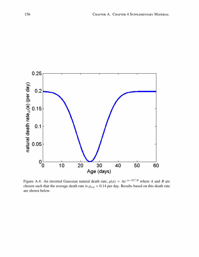
156 Chapter A. Chapter 4 Supplementary Material

Figure A.4: An inverted Gaussian natural death rate, µ(a) = Ae−(a−25)2/B where A and B arechosen such that the average death rate is µavg = 0.14 per day. Results based on this death rateare shown below.

157

Figure A.5: Equilibrium age distribution of healthy colony under the natural death rate shownin Figure A.4.

158 Chapter A. Chapter 4 Supplementary Material

Figure A.6: Time course of disease-free colony based on natural death rate µ(a) shown inFigure A.4.

159

Figure A.7: Time course of infected colony based on natural death rate µ(a) shown in FigureA.4 and a constant disease death rate d(a) = d = 0.14 per day.

160 Chapter A. Chapter 4 Supplementary Material

Figure A.8: Time course of infected colony based on natural death rate µ(a) shown in FigureA.4 and a disease death rate d(a) = µ(a).

161

Figure A.9: An admittedly unrealistic linear natural death rate µ(a) = Aa where A is chosen soonce again the average is 0.14 per day. We show this death rate to illustrate that the qualitativeresults of our model hold in even with drastically different parameter choices.

162 Chapter A. Chapter 4 Supplementary Material

Figure A.10: Equilibrium age distribution of healthy colony under the natural death rate shownin Figure A.9. Note that the linear death rate leads to an unrealistically long lifespan.

163

Figure A.11: Time course of disease-free colony based on natural death rate µ(a) shown inFigure A.9. Despite the unrealistically large colony size and absurdly long lifetime of a bee,we still observe the spring dwindle as a natural phenomena.

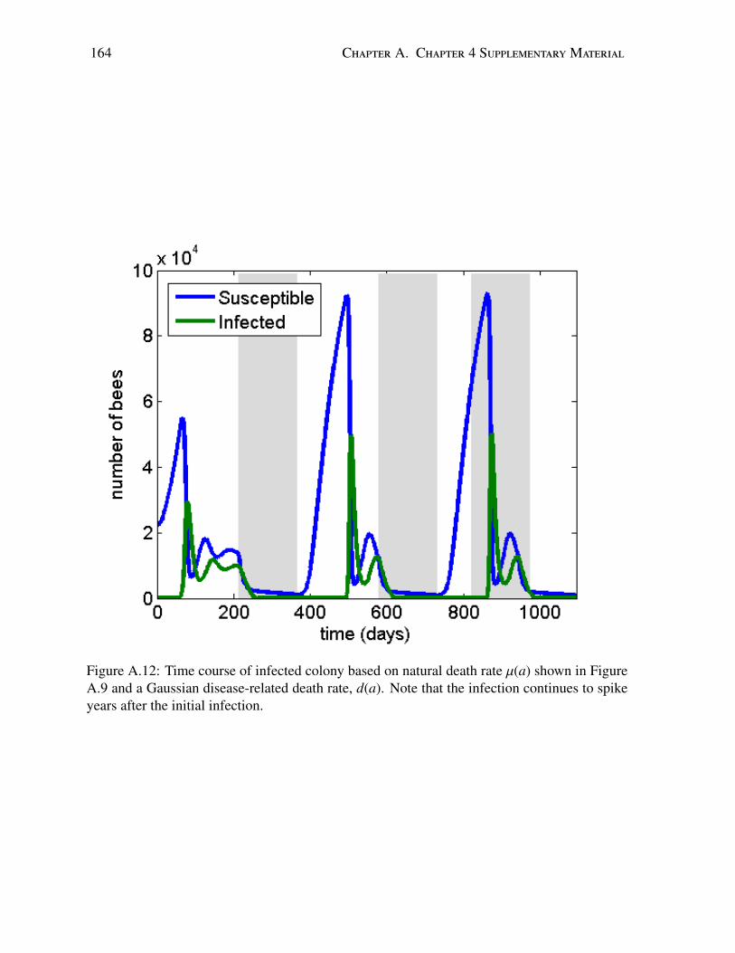
164 Chapter A. Chapter 4 Supplementary Material

Figure A.12: Time course of infected colony based on natural death rate µ(a) shown in FigureA.9 and a Gaussian disease-related death rate, d(a). Note that the infection continues to spikeyears after the initial infection.

Bibliography

[1] R. Dukas, Mortality rates of honey bees in the wild, Insectes Sociaux, 55(2008), pp. 252–255.

[2] S. Fahrbach and G. Robinson, Juvenile hormone, behavioral maturationand brain structure in the honey bee, Developmental Neuroscience, 18(1996), pp. 102–114.

[3] M. Goblirsch, Z. Y. Huang, and M. Spivak, Physiological and behavioralchanges in honey bees (Apis mellifera) induced by Nosema ceranae infec-tion, PLOS ONE, 8 (2013), p. e58165.

[4] D. S. Khoury, A. B. Barron, and M. R. Myerscough, Modelling foodand population dynamics in honey bee colonies, PLOS ONE, 8 (2013),p. e59084.

[5] D. S. Khoury, M. R. Myerscough, and A. B. Barron, A quantitativemodel of honey bee colony population dynamics, PLOS ONE, 6 (2011),p. e18491.

[6] S. Russell, A. B. Barron, and D. Harris, Dynamic modelling of honeybee (Apis mellifera) colony growth and failure, Ecological Modelling, 265(2013), pp. 158 – 169.

[7] S. Sakagami and H. Fukuda, Life tables for worker honeybees, Researcheson Population Ecology, 10 (1968), pp. 127–139.

165

Matthew Betti, Ph.D.

Areas of specializationMathematical Biology, Epidemiology, Population Dynamics, Partial DifferentialEquations.

Education2006–2010 BSc in Mathematics and Physics, McMaster University, Hamilton, ON2010–2012 MSc in Mathematics, McMaster University, Hamilton, ON2013–2017 PhD in Applied Mathematics, Western University, London, ON

Grants, Honors and Awards2014–2017 NSERC PGS, NSERC2016–2017 Doctoral Research Excellence Research Award, Western University2016 Best Graduate Talk, Ontario Ecology, Evolution and Ethology Conference

University of Toronto2015 Fallona Family Interdisciplinary Poster Session - First Place, Western University2015 Graduate Student Teaching Award, Faculty of Science, Western University2015 Graduate Student Teaching Award, School of Graduate and Postdoctoral Studies,

Western University2009 Dr. Harry Lyman Hooker Scholarship, McMaster University2006–2010 Entrance Scholarship, McMaster University

1

Curriculum Vitae

166

PublicationsRefereed journal articles

2009 Wilson, Patrick R, Roschuk, Tyler, Dunn, Kayne, Betti, Matthew, Wojcik, Jacekand Mascher, P (2009), “The Influence of Structural Ordering on Luminescencefrom Nitride-and Oxynitride-Passivated Silicon Nanoclusters”, ECS Transactions19:8 19–28

2013 Sprung, DWL, Betti, MI and van Dijk, W(2013), “Finite Fourier transforms com-puted by a modified Filon–Euler–Maclaurin method” Computer Physics Communi-cations, 184:3 607-616

2013b Betti, Matthew and Pelinovsky, Dmitry E (2013), “Periodic traveling waves in di-atomic granular chains”, Journal of Nonlinear Science 23:5 689–730.

2014 Betti, Matt I, Wahl, Lindi M and Zamir, Mair (2014), “Effects of infection on honeybee population dynamics: a model”, PloS one 9:10 e110237.

2016 Betti, Matt I, Wahl, Lindi M and Zamir, Mair (2016), “Reproduction Number AndAsymptotic Stability For The Dynamics of a Honey Bee Colony with ContinuousAge Structure”, Bull. of Math. Bio. 79(7) 1586-1611.

2016 Betti, Matt I, Wahl, Lindi M and Zamir, Mair (2016), “Age structure is Critical tothe Population Dynamics and Survival of Honey Bee Colonies”, Royal Society OpenScience 3:11 160444.

2017 Betti, Matt I, LeClair, Josh, Wahl, Lindi M and Zamir, Mair (2016), “Bee++: AnObject-Oriented, Agent-Based Simulator for Honey Bee Colonies”, Insects 8(1):31;doi:10.3390/insects8010031

2017 Betti, Matt I, LeClair, Josh, Wahl, Lindi M and Zamir, Mair (2016), “ A closed formnext generation operator for reaction-diffusion systems and the connection betweendiscrete and continuum disease models”, In review

Talks and Posters

2012 Betti, Matthew and Pelinovsky, Dmitry E (2012), “Periodic Travelling Waves inDiatomic Granular Chains”, SIAM Annual Meeting, Seattle

2015 Betti, Matthew I, Wahl, Lindi M and Zamir, Mair (2015), “Population Dyamics andInfections in Honey Bees”, CAIMS Annual Meeting, Waterloo

2015 Betti, Matthew I, Wahl, Lindi M and Zamir, Mair (2015), “Age Before Bee-auty:An Age-structured Honey Bee model”, ICMA-V, London

2015 Betti, Matthew I, Wahl, Lindi M and Zamir, Mair (2015), “Temperature, Diseaseand the Death of Honey Bees”, Fallona Family Interdisciplinary Symposium, Lon-don

2016 Betti, Matthew I, Wahl, Lindi M and Zamir, Mair (2016), “Effects of Infection onHoney Bee Population Dynamics”, Ontario Ecology, Evolution and Ethology Con-ference, Toronto

2016 Betti, Matthew I, Wahl, Lindi M and Zamir, Mair (2016), “Population Dyamics andInfections in Honey Bees”, CAIMS Annual Meeting, Edmonton

2017 Betti, Matthew I, Wahl, LeClair, Josh, Lindi M and Zamir, Mair (2017), “Honey

2

Curriculum Vitae 167

bees in Silica”, Fallona Family Interdisciplinary Symposium, London2017 Betti, Matthew I, LeClair, Josh, Wahl, Lindi M and Zamir, Mair (2017),“ A Novel

Closed-Form Next Generation Operator for Reaction-Diffusion Systems and A Nat-ural Environment For Modeling Movement” AMMCS International Meeting, Wa-terloo

Invited Talks

2015 Betti, Matthew I, Wahl, Lindi M and Zamir, Mair (2015), “Honey Bee PopulationDynamics in the Presence of Infection”, Southern Ontario Bee Conference, Toronto

2015 Betti, Matthew I, Wahl, Lindi M and Zamir, Mair(2015), “Effects of Infection onHoney Bee Population Dynamics”, Ontario Ecology, Evolution and Ethology Con-ference, Toronto

2016 Betti, Matthew I (2016), “The Calculus of Honey Bees”, Western Biology Under-graduate Soceity Seminar, London

2017 Betti, Matthew I, LeClair, Josh, Wahl, Lindi M and Zamir, Mair (2017), “Modelinghoney bee-plant symbiosis in the presence of environmental toxins”, AAAS AnnualMeeting, Boston

2017 Betti, Matthew I, LeClair, Josh, Wahl, Lindi M and Zamir, Mair (2017), “ TheSymbiotic Relationship of Mathematics and Biology”, Undergraduate Conference ofMathematical Sciences, London (Plenary Speaker)

2017 Betti, Matthew I, LeClair, Josh, Wahl, Lindi M and Zamir, Mair (2017), “Math-ematical Biology: Why Math Can Be Useful”, SHAD Western, Summer Program,London

2017 Betti, Matthew I, LeClair, Josh, Wahl, Lindi M and Zamir, Mair (2017), “Honeybee dynamics in an ever-changing environment”, SMB Annual Meeting, Salt LakeCity

Press

2015 Wain, Jennifer (April 2, 2015), “Calculating a new version of pi(e)” Western News2015 (April 22, 2015), “Can Math Save the Honeybees?”, Toronto/Vancouver Metro2015 (April 23, 2015), “Afternoon Drive”, CBC Radio One2015 Montanini, Chris (April 30, 2015), “How math can help us understand bee colony

collapse”, The Londoner.2017 Buck, Genna ( March 16, 2017), “Canadian mathematicians create Sims-like pro-

gram to save bees”, Toronto Metro News.

Teaching2008-2010 Teaching Assistant, Introduction to Electrostatics, Department of Physics, McMas-

ter University.2010 Teaching Assistant, Multivariate Calculus, Department of Mathematics � Statistics,

McMaster University

3

168 Curriculum Vitae

2011 Teaching Assistant, Advanced Mathematics for Engineers (PDEs and Probability),Department of Mathematics � Statistics, McMaster University

2011 Teaching Assistant,Multivariate Calculus, Department of Mathematics � Statistics,McMaster University

2012 Teaching Assistant,Multivariate Calculus, Department of Mathematics � Statistics,McMaster University

2012 Instructor,Mathematics, Department of Mathematics, Humber College2013 Teaching Assistant,Partial Differential Equations for Engineers, Department of Ap-

plied Mathematics, Western University2014 Teaching Assistant,Advanced Partial Differential Equations, Department of Applied

Mathematics, Western University2014 Teaching Assistant,Ordinary Differential Equations, Department of Applied Math-

ematics, Western University2015 Teaching Assistant,Differential Equations � Probability for Life Sciences, Depart-

ment of Applied Mathematics, Western University2015 Teaching Assistant,Ordinary Differential Equations for Engineers, Department of

Applied Mathematics, Western University2016 Teaching Assistant,Differential Equations � Probability for Life Sciences, Depart-

ment of Applied Mathematics, Western University2016 Teaching Assistant,Ordinary Differential Equations for Engineers, Department of

Applied Mathematics, Western University2017 Instructor,Vector Calculus for Engineers, Department of Applied Mathematics, West-

ern University

Software Packages2016 Bee++: A comprehensive, open source simulator for honey bee dynamics over spa-

tially explicit landscapes.

4

Curriculum Vitae 169