ORIGINAL PAPER

Neural networks with artificial bee colony algorithmfor modeling daily reference evapotranspiration

Coskun Ozkan • Ozgur Kisi • Bahriye Akay

Received: 12 August 2010 / Accepted: 2 December 2010 / Published online: 17 December 2010

� Springer-Verlag 2010

Abstract The study investigates the ability of artificial

neural networks (ANN) with artificial bee colony (ABC)

algorithm in daily reference evapotranspiration (ET0)

modeling. The daily climatic data, solar radiation, air

temperature, relative humidity, and wind speed from two

stations, Pomona and Santa Monica, in Los Angeles, USA,

are used as inputs to the ANN–ABC model so as to esti-

mate ET0 obtained using the FAO-56 Penman–Monteith

(PM) equation. In the first part of the study, the accuracy of

ANN–ABC models is compared with those of the ANN

models trained with Levenberg–Marquardt (LM) and

standard back-propagation (SBP) algorithms and those of

the following empirical models: The California Irrigation

Management System (CIMIS) Penman, Hargreaves, and

Ritchie methods. The mean square error (MSE), mean

absolute error (MAE) and determination coefficient (R2)

statistics are used for evaluating the accuracy of the mod-

els. Based on the comparison results, the ANN–ABC and

ANN–LM models are found to be superior alternative to

the ANN–SBP models. In the second part of the study, the

potential of the ANN–ABC, ANN–LM, and ANN–SBP

models in estimation ET0 using nearby station data is

investigated.

Introduction

Accurate estimation of evapotranspiration (ET) is needed to

compute irrigation water requirement and to determine the

water budget, especially under arid conditions where water

resources are scarce and fresh water is a limited resource. As

described by Brutsaert (1982) and Jensen et al. (1990),

various methods have been proposed for estimating ET. The

energy balance/aerodynamic combination equations gener-

ally ‘‘provides the most accurate results as a result of their

foundation in physics and basis on rational relationships’’

(Jensen et al. 1990). The Food and Agricultural Organiza-

tion of the United Nations (FAO) accepted the FAO

Penman–Monteith as the standard equation for estimation of

ET (Allen et al. 1998; Naoum and Tsanis 2003).

A number of researchers have attempted to model ET0

using artificial neural network (Kumar et al. 2002; Sudheer

et al. 2003; Trajkovic 2005, 2009, 2010; Kisi and Yildirim

2005a, b; Kisi 2006a, b, 2007; Kisi 2008; Kim and Kim

2008; Jain et al. 2008; Khoob 2008a, b; Landeras et al.

2009; Kumar et al. 2009; Marti et al. 2010; Kumar et al.

2010). Kumar et al. (2002) used a artificial neural network

(ANN) for estimation of ET0. They tried various ANN

architectures and obtained accurate ET0 estimates. Sudheer

et al. (2003) established radial basis ANN in modeling ET0

using limited climatic data. Trajkovic et al. (2003) fore-

casted ET0 by a radial basis type ANN. Trajkovic (2005)

used temperature-based radial basis neural network

(RBNN) for modeling FAO-56 PM ET0. He compared the

RBNN results with empirical methods and reported that the

RBNN generally performed better than the other models in

Communicated by A. Kassam.

C. Ozkan

Engineering Faculty, Geomatics Department,

Erciyes University, Kayseri, Turkey

O. Kisi (&)

Engineering Faculty, Civil Engineering Department,

Erciyes University, Kayseri, Turkey

e-mail: kisi@erciyes.edu.tr

B. Akay

Engineering Faculty, Computer Science Department,

Erciyes University, Kayseri, Turkey

123

Irrig Sci (2011) 29:431–441

DOI 10.1007/s00271-010-0254-0

estimation of ET0. Kisi (2006a) estimated ET0 using ANN

method, and he compared the ANN estimates with those of

the Penman and Hargreaves empirical models. He con-

cluded that the ANN model performed better than the

empirical models. Kisi (2006b) developed generalized

regression neural network (GRNN) models for estimating

ET0. Kisi (2008) investigated the accuracy of feed-forward

neural network, radial basis neural network, and GRNN

techniques in modeling ET0. Kim and Kim (2008) esti-

mated the alfalfa ET0 using GRNN model with genetic

algorithm. Jain et al. (2008) modeled the ET0 using ANN

and gave a procedure to evaluate the effects of input

variables on the output variable using the weight connec-

tions of ANN models. Khoob (2008a) used ANN for esti-

mating ET0 from pan evaporation in a semi-arid

environment. Khoob (2008b) compared the accuracy of

ANN models with Hargreaves method in a semi-arid

environment and found that the ANN method predicted the

ET0 better than the Hargreaves method. Landeras et al.

(2009) compared ANN and ARIMA models in forecasting

weekly evapotranspirations. Kumar et al. (2009) evaluated

the ANN models in prediction of ET0 under the arid con-

ditions. They compared the ANN estimates with those of

the FAO-24 Radiation, Turc, and FAO-24 Blaney-Criddle

empirical methods and found that the ANN model per-

formed better than the other models. Marti et al. (2010)

proposed a data scanning procedures for the ANN model-

ing of ET0. Kumar et al. (2010) have reviewed and dis-

cussed the ANN studies related to application of ANN in

estimation ET0. All these studies used conventional ANN

models with Levenberg–Marquardt (LM) and/or standard

back-propagation (SBP) algorithms for modeling ET0. In

this study, an ANN model with a novel algorithm, that is

the artificial bee colony (ABC) algorithm, is used for

modeling ET0. To the best knowledge of the authors, there

is no published work indicating the input–output mapping

capability of ANN–ABC technique in modeling of ET0.

This study is concerned with the application of ANN–ABC

technique for modeling daily ET0. The ability of ANN–ABC

is compared with those of the ANN–LM and the ANN–SBP,

CIMIS Penman, Hargreaves, and Ritchie methods employed

in the previous work of Kisi and Ozturk (2007). For this aim,

two stations in Los Angeles, USA, are used as case studies. In

the hydrological context, the presented study is the first study

that investigates the accuracy of ANN–ABC in modeling.

Artificial neural networks (ANN)

Artificial neural networks (ANNs) are based on the present

understanding of biological nervous system, though

neglecting much of the biological details. ANNs are par-

allel systems composed of many processing elements

connected by weights. Of the many ANN paradigms, the

back-propagation network is by far the most popular

(Haykin 1998). The network composed of layers of parallel

processing elements, called neurons. Each layer is fully

connected to the next layer by interconnection weights.

Initial weight values are corrected during a training

(learning) process that compares estimated outputs to

known outputs and back propagates any errors to obtain the

appropriate weight adjustments necessary to minimize the

errors. Detailed information about ANN can be found in

the study of Kisi and Ozturk (2007).

In the present study, novel algorithms, that is the arti-

ficial bee colony (ABC) algorithm and Levenberg–Mar-

quardt (LM), were used for the ANN training. The standard

back-propagation (SBP) algorithm was used by Kisi and

Ozturk (2007) before. Next, the ABC, LM, and SBP

algorithms are introduced.

Artificial bee colony (ABC) algorithm

In nature, there are some species living as social groups

without supervision in order to defense themselves,

enhance foraging success, find a mate etc., which corre-

spond to collective intelligence. One of these species,

honey bees, lives as big colonies and manifests several

collective intelligent behaviors such as communicating,

task selection nest site selection, foraging. In all of tasks

performed by honey bees, foraging is one of the most

crucial tasks to keep the colony alive. Forager bees perform

foraging behavior to meet the requirements of the colony.

Foraging behavior includes finding profitable food sources

around the hive, recruiting the other bees in the hive to the

rich sources by dancing, and abandoning the exhausted

sources and finding the new potentially rich ones. There-

fore, there are three kinds of bees allocated for the foraging

task: employed bees search the neighborhood of the sour-

ces discovered by them; onlooker bees recruited by the

employed bees depending on the dances of employed for-

agers; and scout bees search the environment randomly

depending on some internal motivation external clues.

When an employed bee finds a rich source, she commu-

nicates onlooker bees in the hive to share information about

the profitability, distance, and direction of the source from

the nest by dancing. The richness of a source depends on

several factors including its proximity to the nest, amount

or concentration of nectar, and the ease of extracting this

nectar. Employed bee of an exhausted source becomes a

scout and tries to find a new source.

Artificial bee colony (ABC) algorithm introduced by

Karaboga (2005) is a recent optimization algorithm that

mimics the foraging behavior of honey bees. In the ABC

algorithm, each food source corresponds to a solution in the

space and ABC tries to find the position of the most

432 Irrig Sci (2011) 29:431–441

123

profitable source by searching the food source space, which

is conducted by employed bees, onlooker bees, and scout

bees. The schematic diagram of the ABC algorithm is

given in Fig. 1.

The main steps of the algorithm are given below:

Initialize.

REPEAT.

(a) Employed bees are sent to find food source sites in the

neighborhood of their sources

(b) Employed bees share information about their sources

to recruit the other bees

(c) Onlooker bees are sent to find food source sites in the

neighborhood of the sources they choose depending

on the information shared by employed bees

(d) Memorize the best source achieved so far

(e) Send the scouts to the search area for discovering new

food sources.

UNTIL (requirements are met).

In the initialization phase of the algorithm, a food source

population is generated and then the ABC algorithm starts

to optimize the predefined cost function. Initial solutions

that correspond to food source positions are produced

randomly by Eq. (1)

xij ¼ xminj þ randð0; 1Þðxmax

j � xminj Þ ð1Þ

where i = 1.SN, j = 1.D, SN is the number of food sour-

ces, D is the number of variables to be optimized. xminj and

xmaxj are Llower and upper bounds of the jth parameter,

respectively.

In the employed bee phase, neighborhood of each food

source is searched by an employed bee. The neighbor solution

(t~i) of the current solution (x~i) is produced by Eq. (2)

tij ¼ xij þ uijðxkj � xijÞ ð2Þ

where i ¼ f 1, 2, :::SNg , j is a randomly chosen

parameter index in the range [1, D], k 2 f 1, 2, :::SNg is

a randomly chosen solution different from i, and uijis a

uniform random real number in the range [-1,1]. After a

neighbor solution is produced, its fitness is calculated by

substituting the solution in the cost function. If the neigh-

bor is better, it is inserted to the population by removing

the old one. If the current solution cannot be improved by

the neighbor solution, current solution is kept in the pop-

ulation and the trial number of current solution x~i is

incremented by one in order to be used in abandonment

process.

After all the food sources are exploited by employed

bees, the information about these sources is shared in the

hive to recruit the onlooker bees to potentially rich sources

probabilistically. In order to make the profitable sources

favorable to onlookers and give chance to less profitable

sources to be selected, a roulette wheel selection mecha-

nism is used in ABC algorithm. Probabilities of the solu-

tions to be selected by an onlooker bee to make a local

search are calculated by Eq. (3)

Initialize food source positions

Employed bee finds a new food source in the neighbourhood of i. solution

Employed bee evaluates the nectar amount of new source

i=1

Better solution is kept in the memory

i++

i=SN

Onlooker bee probabilistically chooses a source and finds a new food source in the neighbourhood of the chosen solution

Onlooker bee evaluates the nectar amount of new source

t=1

Better solution is kept in the memory

t++

t=SN

Memorize the best food source achieved so far

Determine the exhausted food source based on "limit" value

Scout bee finds a new random food source position to replace with the exhausted source

Terminate

Best SourceYes No

Yes No

Yes

Fig. 1 The schematic diagram

of the ABC algorithm

Irrig Sci (2011) 29:431–441 433

123

pi ¼fitnessiPnj¼1 fitnessj

ð3Þ

If a uniform random number is less than the probability

value (pi) associated with the source, x~i, an onlooker bee

finds a food source site in the neighborhood of the

source, x~i, by Eq. (2). As in employed bee phase, if the

neighbor is better, it is inserted to the population;

otherwise, the current solution is kept in the population

and the trial number of current solution x~i is incremented

by one.

After onlookers and employed bees search the food

source sites, the exhausted sources are determined by

checking their trial numbers. If the trial number of a source

exceeds the predefined control parameter of ABC algo-

rithm, called ‘‘limit’’, it is assumed to be exhausted or not

worth to exploiting. In each cycle, one of the exhausted

sources is removed from population and a scout bee gen-

erates a new solution for it by (Eq. 1).

Levenberg–Marquardt algorithm

Levenberg–Marquardt (LM) algorithm (Levenberg 1944;

Marquardt 1963) incorporates the advantages of gradient

descent and the Gauss–Newton method and iteratively

optimizes a cost function (Eq. 4) that is sum of squares of

nonlinear functions.

FðxÞ ¼ 1

2

Xm

i¼1

½fiðxÞ�2: ð4Þ

LM algorithm is initialized at a starting point (x~0) and

produces a new solution by Eq. (5)

x~iþ1 ¼ x~i � ðH þ kIÞ�1rf ðx~iÞ ð5Þ

where I is identity matrix, H is the Hessian matrix evalu-

ated at x~i, and k determines the behavior of the algorithm

between steepest descent and the Gauss–Newton method.

If k is large, LM algorithm behaves as steepest descent

method; if k gets small, the LM algorithm behaves as

Gauss–Newton method.

If the error value increases by the modification by Eq.

(5), x~iþ1 is copied from x~i and k is increased. Otherwise, if

the error values decreases by the modification by Eq. (5),

x~iþ1 is taken and k is decreased, and so on.

Standard back-propagation algorithm

Standard back-propagation (SBP) algorithm (Rumelhart

et al. 1986) is used to train neural networks and has

two phases: propagation and weight update. In propa-

gation phase, first network output is calculated by feed-

forward computation and the error values are back-

propagated to the neurons. In the second phase, weights

are updated by the back-propagation of error values

(Rojas 1996).

Assuming the back-propagated error at the j-th node is

dj, the partial derivative of Edefined by Eq. (6) with respect

to w is given by Eq. (7):

E ¼ 1

2

Xp

i¼1

oi � dik k2 ð6Þ

where E is the error calculated based on weight values, di is

the desired output, oi is the actual output, and p is the

number of patterns.

oE

owij¼ oidj ð7Þ

.

The weights in the network are updated by the amount

of Dwij given by Eq. (8):

Dwij ¼ �coidj ð8Þ

Empirical methods

CIMIS Penman method

The CIMIS Penman equation employs the modified Pen-

man equation (Pruitt and Doorenbos 1977) with a wind

function that was developed at the University of California,

Davis. The method uses hourly average weather data as an

input to calculate hourly ET0. The 24 h ET0 values for the

day (midnight–midnight) are then summed to produce

estimates of daily ET0. The hourly PM equation that

CIMIS uses to estimate hourly PM ET0 is the Food and

Agricultural Organization’s version that is described in

Irrigation and Drainage Paper No. 56 (Allen et al. 1998).

The CIMIS Penman equation is also described in detail

in Hidalgo et al. (2005), (see CIMIS website: http://

wwwcimis.water.ca.gov/cimis/infoEtoCimisEquation.jsp);

ET0 ¼D

Dþ c

� �

Rn þ 1� DDþ c

� �

ea � edð ÞfU ð9Þ

where ET0 = mean hourly reference evapotranspiration

(mm day-1); D = slope of the saturation vapor pressure

function (kPa�C-1); Rn = mean hourly net radiation

(Wm-2); c = psychometric constant (kPa �C-1); ea is the

saturation vapor pressure (kPa); ed is the actual vapor

pressure (kPa); and the fU = wind function (m s-1). Daily

ET0 equals to the sum of 24 h ET0 (mm).

434 Irrig Sci (2011) 29:431–441

123

Hargreaves method

The Hargreaves empirical formula is one of the simplest

equations used to estimate ET0. It is expressed as (Har-

greaves and Samani 1985):

ET0 ¼ 0:0023RaTmax þ Tmin

2þ 17:8

� �ffiffiffiffiffiffiffiffiffiffiffiffiffiffiffiffiffiffiffiffiffiffiffiTmax � Tmin

p

ð10Þ

where ET0 = reference evapotranspiration (mm day-1);

Tmax and Tmin = maximum and minimum temperature (�C)

and Ra = extraterrestrial radiation (mm day-1).

Ritchie method

The Ritchie method, as described by Jones and Ritchie

(1990)

ET0 ¼ a1: 3:87� 10�3:Rs: 0:6Tmax þ 0:4Tmin þ 29ð Þ� �

ð11Þ

where ET0 = reference evapotranspiration (mm day-1);

Tmax and Tmin = maximum and minimum temperature (�C)

and Rs = solar radiation (MJ m-2 day-1). When

5\Tmax� 35�C a1 ¼ 1:1Tmax [ 35�C a1 ¼ 1:1þ 0:05 Tmax � 35ð ÞTmax\5�C a1 ¼ 0:01: exp 0:18 Tmax þ 20ð Þ½ �

9=

;:

ð12Þ

Data

The daily climatic data from two automated weather sta-

tions, Pomona Station (Latitude 34� 030N, Longitude

117�480W) and Santa Monica Station (Latitude 34�020N,

Longitude 118�280W) operated by the California Irrigation

Management Information System (CIMIS) are used in the

current study. The elevations are 222 and 104 m for the

Pomona and Santa Monica stations, respectively. The loca-

tion of the stations was illustrated by Kisi and Ozturk (2007).

The Santa Monica Station is located in a coastal area. The

data sample consists of daily records of 4 years (2001–2004)

of solar radiation, air temperature, relative humidity, and

wind speed. For each station, the first 3 years (2001–2003)

data were used to train the ANN models, and the remaining

data were used for testing. The detailed information about

the climatic data of Pomona and Santa Monica stations can

be obtained from the study of Kisi and Ozturk (2007).

Application and results

Kisi and Ozturk (2007) developed two different ANN–SBP

models for the estimation of ET0 of Pomona and Santa

Monica stations before. They compared four-parameter

ANN1 model comprising Rs, T, RH, and U2 inputs and two-

parameter ANN2 model whose inputs are the Rs and T with

the four-parameter CIMIS Penman and two-parameter

Hargreaves and Ritchie empirical methods, respectively.

They used mean square error (MSE), mean absolute error

(MAE), and determination coefficient (R2) statistics for the

evaluation of ANN–SBP models in test period, and they

found that the ANN–SBP models performed better than the

empirical methods. In this study, four- and two-parameter

ANN–ABC and ANN–LM models were developed using

the same data, and the results were compared with those of

the ANN–SBP, CIMIS Penman, Hargreaves, and Ritchie

models employed in Kisi and Ozturk (2007). The MSE and

MAE statistics can be given as

MSE ¼PN

i¼1 ðETFAO�56PM;i � ETestimated;iÞ2

Nð13Þ

MAE ¼XN

i¼1

ETFAO�56PM;i � ETestimated;i

ETFAO�56PM;i

����

����

!

=N ð14Þ

where ETFAO-56 PM, i is the ET0 values obtained by FAO-56

PM method, ETestimated,i is the estimated ET0 values, N is

the data number.

Next, the accuracy of the ANN–ABC and ANN–LM

techniques is tested for two different applications. In the

first application, the ET0 data of two stations are estimated,

separately, and the ANN–ABC and ANN–LM estimates

are compared with those of the ANN–SBP and empirical

models employed in the study of Kisi and Ozturk (2007). In

the second application, the ET0 data of one station are

estimated using the climatic data from the other station,

and the test results of the ANN–ABC and ANN–LM

models are compared with those of the ANN–SBP and

multi-linear regression (MLR) models.

Estimation of ET0 data of Pomona Station

For the Pomona Station, the ANN–ABC1, ANN–ABC2,

ANN–LM1, ANN–LM2, ANN–SBP1, ANN–SBP2, and

the empirical models are compared in Table 1. In this table,

ANN–ABC1 (4,5,1) denotes an ANN model comprising 4

inputs, 5 hidden nodes, and 1 output node. As seen from

this table that the ANN–ABC, ANN–LM, and ANN–SBP

models have the same structure. The input variables used

for each model are also given in Table 1. The temperature-

based methods mostly underestimate or overestimate ET0

obtained by the FAO-56 PM method. In those cases, Allen

et al. (1994) recommended that empirical methods be

calibrated using the standard PM method. ET0 is calculated

as

ET0 ¼ aþ bETeq ð15Þ

Irrig Sci (2011) 29:431–441 435

123

where ET0 = grass reference ET defined by the FAO-56

PM equation; ETeq = ET estimated by the temperature-

based methods; and a and b = calibration factors, respec-

tively. The data used for the training of ANN models were

used for calibration of temperature-based methods. The

CIMIS Penman method was also calibrated. C_CIMIS

Penman denotes the calibrated version of CIMIS Penman

model. It is clear from Table 1 that the ANN–ABC2,

ANN–LM2, ANN–SBP2, Hargreaves, and Ritchie models

use the same input variables. It can be seen from the table

that the ANN–ABC1 and ANN–LM models give almost

similar estimates and they perform better than the four-

parameter ANN–SBP1 and CIMIS Penman models.

Among the two-parameter models, the ANN–ABC2 seems

to be superior to the others. The ANN–LM models are

slightly worse than the ANN–ABC models. The ET0 esti-

mates of each model for the Pomona Station are shown in

Fig. 2 in the form of scatter plot. It is seen from the scatter

plots that the ANN–ABC1 and ANN–LM1 estimates are

closer to the corresponding FAO-56 PM ET0 values than

those of the other models. Among the two-parameter

models, the ANN–ABC2 and ANN–LM2 are similar to the

each other, and they perform better than the ANN–SBP2,

Hargreaves, Ritchie, C_Hargreaves, and C_Ritchie models.

As seen from the fit line equations (assume that the equa-

tion is y = aox ? a1) in the scatter plots, the ao and a1

coefficients for the ANN–ABC1 and ANN–LM1 model are

closer to the 1 and 0 with a higher R2 value than those of

the other models. This is also confirmed by the MSE,

MAE, and R2 values in Table 1. The total ET0 estimates of

the ANN–ABC and ANN–LM models were compared with

those of the ANN–SBP, CIMIS Penman, Hargreaves, and

Ritchie because it is important for irrigation management.

The total ET0 values were calculated by integrating the

ET0 estimates of each model in the test period. The

ANN–ABC2, ANN–LM2, ANN–SBP2, C_Hargreaves,

and C_Ritchie computed the total FAO-56 PM ET0 of

1,288.8 mm as 1,271, 1,274, 1,272, 1,273, and 1,283 mm

with underestimations of 1.4, 1.2, 1.3, 1.2, and 0.4%, while

the ANN–ABC1, ANN–LM1, ANN–SBP1, CIMIS Pen-

man, Hargreaves, Ritchie, and C_CIMIS Penman methods

resulted in 1,303, 1,305, 1,291, 1,411, 1,405, 1,377, and

1,295 mm, with overestimations of 1.1, 1.3, 0.2, 9.5, 9, 6.8,

and 0.5, respectively. Among the four-parameter models,

the ANN–SBP1 had the closest estimate. However, cali-

brated Ritchie model gave better estimate than the other

two-parameter models. For the Pomona Station, while four-

parameter models overestimates the ET0, two-parameter

models underestimates. This implies that the relative

humidity (RH) and wind speed (U2) data lead the four-

parameter models to overestimate the total ET0 value.

Estimation of ET0 data of Santa Monica Station

For the Santa Monica Station, the estimates of the ANN–

ABC, ANN–LM, ANN–SBP, and the empirical models

are compared in Table 2. Here, the ANN–ABC1 and

ANN–LM1 models give almost similar estimates, and

these two models perform much better than the others. The

ANN–ABC2 and ANN–LM2 seem to be better than the

two-parameter ANN–SBP2, Hargreaves, C_Hargreaves,

Ritchie, and C_Ritchie models. The superiority of ABC

and LM algorithms to the SBP algorithm can be obviously

seen from the Table 2. The ET0 estimates of each model

are illustrated in Fig. 3 in the form of scatter plot. The R2

coefficients of the ANN–ABC1 and ANN–LM1 equal to

each other, and they are higher than those of the other

models. The ao and a1 coefficients of the ANN–ABC1

model are closer to the 1 and 0 than those of the other ANN

and empirical models. Out of the two-parameter models,

Table 1 The performance

statistics of the models in test

period—Pomona Station

* The test results of the model

were obtained from the previous

study, Kisi and Ozturk (2007)

Models Model inputs MSE

(mm2 day-2)

MAE

(mm day-1)

R2

ANN–ABC1(4,5,1) Rs, T, RH and U2 0.035 0.137 0.991

ANN–LM1(4,5,1) Rs, T, RH and U2 0.036 0.141 0.991

ANN–SBP1(4,5,1)* Rs, T, RH and U2 0.098 0.225 0.976

CIMIS Penman* Rs, T, RH and U2 0.439 0.361 0.970

C_CIMIS Penman* Rs, T, RH and U2 0.109 0.253 0.970

ANN–ABC2(2,4,1) Rs and T 0.066 0.192 0.984

ANN–LM2(2,4,1) Rs and T 0.067 0.194 0.983

ANN–SBP2(2,4,1)* Rs and T 0.124 0.255 0.970

Hargreaves Rs and T 0.296 0.405 0.978

Ritchie* Rs and T 1.381 0.756 0.985

C_Hargreaves Rs and T 0.078 0.215 0.978

C_Ritchie* Rs and T 0.071 0.205 0.985

436 Irrig Sci (2011) 29:431–441

123

y = 0.9964x + 0.0503R² = 0.9911

0

2

4

6

8

10

AN

N-A

BC

1 E

T 0

(mm

)

FAO-56 PM ET0 (mm)

y = 1.0022x + 0.0366R² = 0.9911

0

2

4

6

8

10

AN

N-L

M1

ET

0(m

m)

FAO-56 PM ET0 (mm)

y = 0.927x + 0.264R2 = 0.976

0

2

4

6

8

10

AN

N-S

BP

1 E

T0(m

m)

FAO-56 PM ET0 (mm)

y = 1.017x + 0.2753R2 = 0.970

0

2

4

6

8

10C

IMIS

Pen

man

ET

0(m

m)

FAO-56 PM ET0 (mm)

y = 0.988x + 0.056R2 = 0.970

0

2

4

6

8

10

C_C

IMIS

Pen

man

ET

0(m

m)

FAO-56 PM ET0 (mm)

y = 0.9621x + 0.0847R² = 0.9836

0

2

4

6

8

10

AN

N-A

BC

2 E

T 0

(mm

)

FAO-56 PM ET0 (mm)

y = 0.959x + 0.1035R² = 0.9832

0

2

4

6

8

10

AN

N-L

M2

ET

0(m

m)

FAO-56 PM ET0 (mm)

y = 0.921x + 0.232R2 = 0.970

0

2

4

6

8

10

AN

N-S

BP

2 E

T 0

(mm

)

FAO-56 PM ET0 (mm)

y = 0.992x + 0.3452R2 = 0.9805

0

2

4

6

8

10

FAO-56 PM ET0 (mm)

Har

gre

aves

ET

0 (m

m)

y = 0.940x + 0.451R2 = 0.985

0

2

4

6

8

10

Rit

chie

ET

0(m

m)

FAO-56 PM ET0 (mm)

y = 0.9487x + 0.138R2 = 0.9805

0

2

4

6

8

10

FAO-56 PM ET0 (mm)

C_H

arg

reav

es E

T0

(mm

)

y = 0.923x + 0.257R2 = 0.985

0

2

4

6

8

10

0 2 4 6 8 10 0 2 4 6 8 10 0 2 4 6 8 10

0 2 4 6 8 10 0 2 4 6 8 10 0 2 4 6 8 10

0 2 4 6 8 10 0 2 4 6 8 10 0 2 4 6 8 10

0 2 4 6 8 10 0 2 4 6 8 10 0 2 4 6 8 10

C_R

itch

ie E

T0 (m

m)

FAO-56 PM ET0 (mm)

Fig. 2 The FAO-56 PM and

estimated ET0 values of the

Pomona Station in test period

Table 2 The performance

statistics of the models in test

period—Santa Monica Station

* The test results of the model

were obtained from the previous

study, Kisi and Ozturk (2007)

Models Model inputs MSE

(mm2 day-2)

MAE

(mm day-1)

R2

ANN–ABC1(4,5,1) Rs, T, RH and U2 0.005 0.053 0.997

ANN–LM1(4,5,1) Rs, T, RH and U2 0.005 0.048 0.997

ANN–SBP1(4,5,1)* Rs, T, RH and U2 0.066 0.179 0.969

CIMIS Penman* Rs, T, RH and U2 0.410 0.392 0.830

C_CIMIS Penman* Rs, T, RH and U2 0.371 0.415 0.830

ANN–ABC2(2,4,1) Rs and T 0.297 0.399 0.856

ANN–LM2(2,4,1) Rs and T 0.291 0.385 0.859

ANN–SBP2(2,4,1)* Rs and T 0.400 0.432 0.814

Hargreaves Rs and T 0.399 0.414 0.818

Ritchie* Rs and T 0.641 0.650 0.780

C_Hargreaves Rs and T 0.381 0.471 0.818

C_Ritchie* Rs and T 0.456 0.474 0.780

Irrig Sci (2011) 29:431–441 437

123

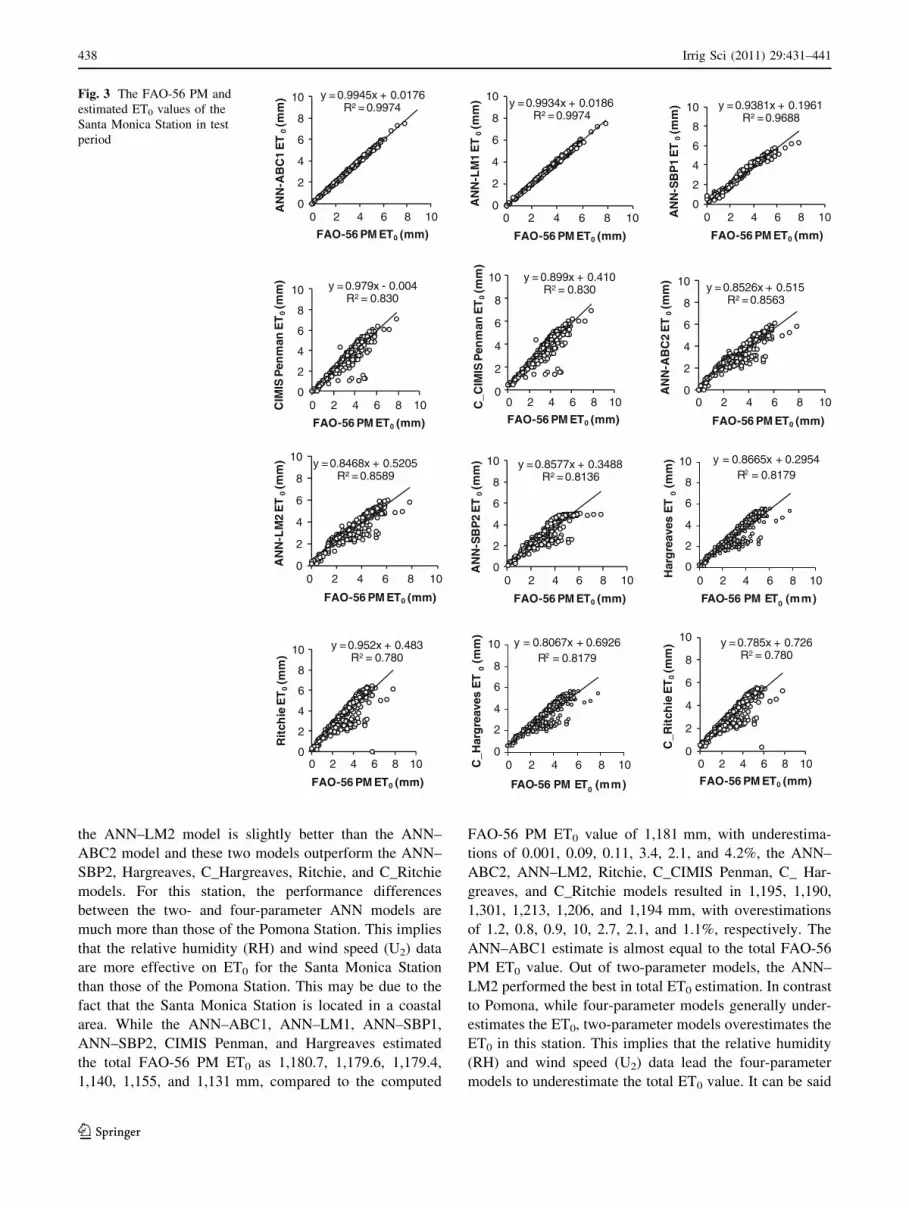
the ANN–LM2 model is slightly better than the ANN–

ABC2 model and these two models outperform the ANN–

SBP2, Hargreaves, C_Hargreaves, Ritchie, and C_Ritchie

models. For this station, the performance differences

between the two- and four-parameter ANN models are

much more than those of the Pomona Station. This implies

that the relative humidity (RH) and wind speed (U2) data

are more effective on ET0 for the Santa Monica Station

than those of the Pomona Station. This may be due to the

fact that the Santa Monica Station is located in a coastal

area. While the ANN–ABC1, ANN–LM1, ANN–SBP1,

ANN–SBP2, CIMIS Penman, and Hargreaves estimated

the total FAO-56 PM ET0 as 1,180.7, 1,179.6, 1,179.4,

1,140, 1,155, and 1,131 mm, compared to the computed

FAO-56 PM ET0 value of 1,181 mm, with underestima-

tions of 0.001, 0.09, 0.11, 3.4, 2.1, and 4.2%, the ANN–

ABC2, ANN–LM2, Ritchie, C_CIMIS Penman, C_ Har-

greaves, and C_Ritchie models resulted in 1,195, 1,190,

1,301, 1,213, 1,206, and 1,194 mm, with overestimations

of 1.2, 0.8, 0.9, 10, 2.7, 2.1, and 1.1%, respectively. The

ANN–ABC1 estimate is almost equal to the total FAO-56

PM ET0 value. Out of two-parameter models, the ANN–

LM2 performed the best in total ET0 estimation. In contrast

to Pomona, while four-parameter models generally under-

estimates the ET0, two-parameter models overestimates the

ET0 in this station. This implies that the relative humidity

(RH) and wind speed (U2) data lead the four-parameter

models to underestimate the total ET0 value. It can be said

y = 0.9945x + 0.0176R² = 0.9974

0

2

4

6

8

10

AN

N-A

BC

1 E

T 0

(mm

)

FAO-56 PM ET0 (mm)

y = 0.9934x + 0.0186R² = 0.9974

0

2

4

6

8

10

AN

N-L

M1

ET

0(m

m)

FAO-56 PM ET0 (mm)

y = 0.9381x + 0.1961R² = 0.9688

0

2

4

6

8

10

AN

N-S

BP

1 E

T0(m

m)

FAO-56 PM ET0 (mm)

y = 0.979x - 0.004R2 = 0.830

0

2

4

6

8

10C

IMIS

Pen

man

ET

0(m

m)

FAO-56 PM ET0 (mm)

y = 0.899x + 0.410R2 = 0.830

0

2

4

6

8

10

C_C

IMIS

Pen

man

ET

0(m

m)

FAO-56 PM ET0 (mm)

y = 0.8526x + 0.515R² = 0.8563

0

2

4

6

8

10

AN

N-A

BC

2 E

T 0

(mm

)

FAO-56 PM ET0 (mm)

y = 0.8468x + 0.5205R² = 0.8589

0

2

4

6

8

10

AN

N-L

M2

ET

0(m

m)

FAO-56 PM ET0 (mm)

y = 0.8577x + 0.3488R² = 0.8136

0

2

4

6

8

10A

NN

-SB

P2

ET

0(m

m)

FAO-56 PM ET0 (mm)

y = 0.8665x + 0.2954R2 = 0.8179

0

2

4

6

8

10

FAO-56 PM ET0 (mm)

Har

gre

aves

ET

0 (m

m)

y = 0.952x + 0.483R2 = 0.780

0

2

4

6

8

10

Rit

chie

ET

0(m

m)

FAO-56 PM ET0 (mm)

y = 0.8067x + 0.6926R2 = 0.8179

0

2

4

6

8

10

FAO-56 PM ET0 (mm)

C_H

arg

reav

es E

T0

(mm

)

y = 0.785x + 0.726R2 = 0.780

0

2

4

6

8

10

0 2 4 6 8 10 0 2 4 6 8 10 0 2 4 6 8 10

0 2 4 6 8 10 0 2 4 6 8 10 0 2 4 6 8 10

0 2 4 6 8 10 0 2 4 6 8 10 0 2 4 6 8 10

0 2 4 6 8 10 0 2 4 6 8 10 0 2 4 6 8 10

C_R

itch

ie E

T0 (m

m)

FAO-56 PM ET0 (mm)

Fig. 3 The FAO-56 PM and

estimated ET0 values of the

Santa Monica Station in test

period

438 Irrig Sci (2011) 29:431–441

123

that the Pomona and Santa Monica stations have different

climatic conditions.

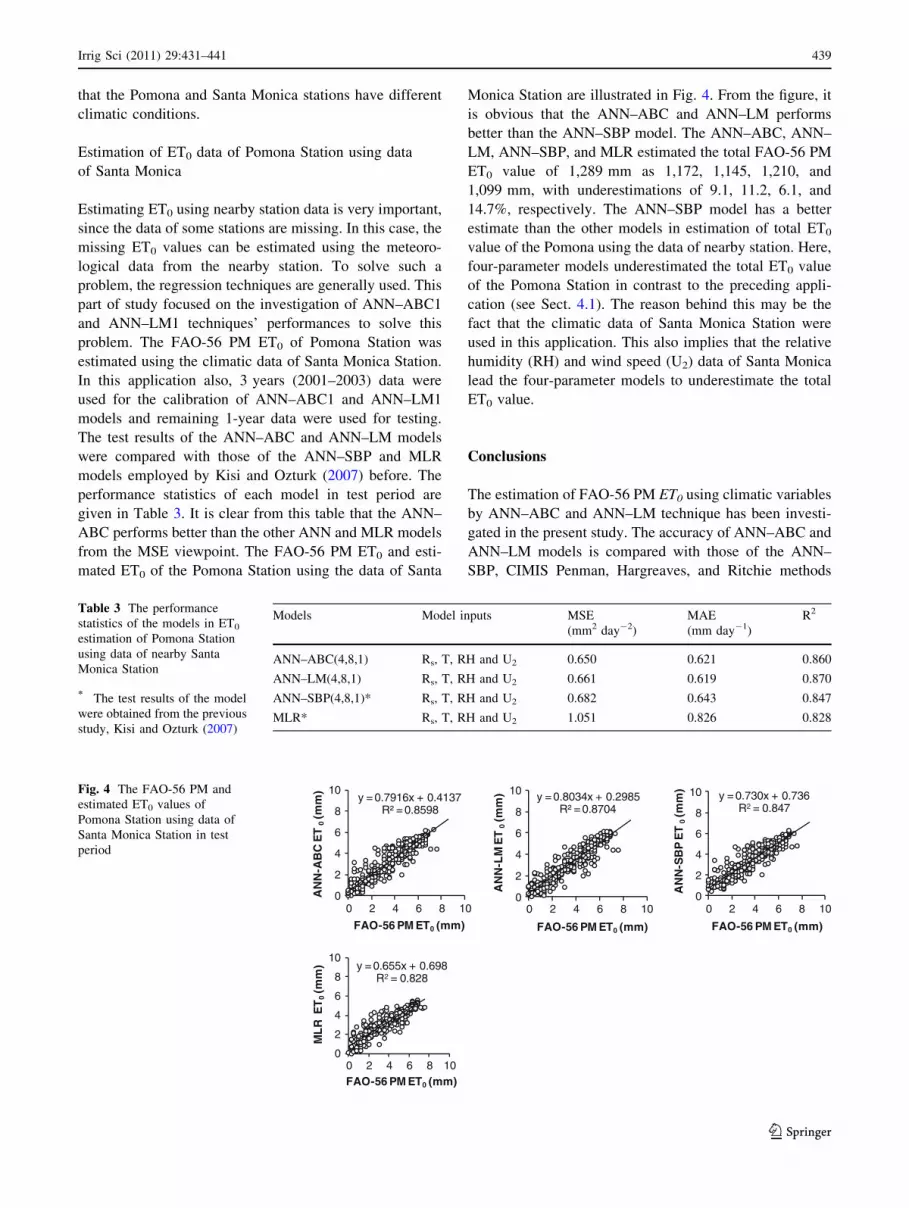
Estimation of ET0 data of Pomona Station using data

of Santa Monica

Estimating ET0 using nearby station data is very important,

since the data of some stations are missing. In this case, the

missing ET0 values can be estimated using the meteoro-

logical data from the nearby station. To solve such a

problem, the regression techniques are generally used. This

part of study focused on the investigation of ANN–ABC1

and ANN–LM1 techniques’ performances to solve this

problem. The FAO-56 PM ET0 of Pomona Station was

estimated using the climatic data of Santa Monica Station.

In this application also, 3 years (2001–2003) data were

used for the calibration of ANN–ABC1 and ANN–LM1

models and remaining 1-year data were used for testing.

The test results of the ANN–ABC and ANN–LM models

were compared with those of the ANN–SBP and MLR

models employed by Kisi and Ozturk (2007) before. The

performance statistics of each model in test period are

given in Table 3. It is clear from this table that the ANN–

ABC performs better than the other ANN and MLR models

from the MSE viewpoint. The FAO-56 PM ET0 and esti-

mated ET0 of the Pomona Station using the data of Santa

Monica Station are illustrated in Fig. 4. From the figure, it

is obvious that the ANN–ABC and ANN–LM performs

better than the ANN–SBP model. The ANN–ABC, ANN–

LM, ANN–SBP, and MLR estimated the total FAO-56 PM

ET0 value of 1,289 mm as 1,172, 1,145, 1,210, and

1,099 mm, with underestimations of 9.1, 11.2, 6.1, and

14.7%, respectively. The ANN–SBP model has a better

estimate than the other models in estimation of total ET0

value of the Pomona using the data of nearby station. Here,

four-parameter models underestimated the total ET0 value

of the Pomona Station in contrast to the preceding appli-

cation (see Sect. 4.1). The reason behind this may be the

fact that the climatic data of Santa Monica Station were

used in this application. This also implies that the relative

humidity (RH) and wind speed (U2) data of Santa Monica

lead the four-parameter models to underestimate the total

ET0 value.

Conclusions

The estimation of FAO-56 PM ET0 using climatic variables

by ANN–ABC and ANN–LM technique has been investi-

gated in the present study. The accuracy of ANN–ABC and

ANN–LM models is compared with those of the ANN–

SBP, CIMIS Penman, Hargreaves, and Ritchie methods

y = 0.7916x + 0.4137R² = 0.8598

0

2

4

6

8

10

AN

N-A

BC

ET

0(m

m)

FAO-56 PM ET0 (mm)

y = 0.8034x + 0.2985R² = 0.8704

0

2

4

6

8

10

AN

N-L

M E

T 0

(mm

)

FAO-56 PM ET0 (mm)

y = 0.730x + 0.736R2 = 0.847

0

2

4

6

8

10

AN

N-S

BP

ET

0(m

m)

FAO-56 PM ET0 (mm)

y = 0.655x + 0.698R2 = 0.828

0

2

4

6

8

10

0 2 4 6 8 10 0 2 4 6 8 10 0 2 4 6 8 10

0 2 4 6 8 10

ML

R E

T0(m

m)

FAO-56 PM ET0 (mm)

Fig. 4 The FAO-56 PM and

estimated ET0 values of

Pomona Station using data of

Santa Monica Station in test

period

Table 3 The performance

statistics of the models in ET0

estimation of Pomona Station

using data of nearby Santa

Monica Station

* The test results of the model

were obtained from the previous

study, Kisi and Ozturk (2007)

Models Model inputs MSE

(mm2 day-2)

MAE

(mm day-1)

R2

ANN–ABC(4,8,1) Rs, T, RH and U2 0.650 0.621 0.860

ANN–LM(4,8,1) Rs, T, RH and U2 0.661 0.619 0.870

ANN–SBP(4,8,1)* Rs, T, RH and U2 0.682 0.643 0.847

MLR* Rs, T, RH and U2 1.051 0.826 0.828

Irrig Sci (2011) 29:431–441 439

123

obtained from the previous study (Kisi and Ozturk 2007).

In the first part of the study, the accuracy of ANN–ABC

models was compared with those of the ANN models

trained with Levenberg–Marquardt (LM) and standard

back-propagation (SBP) algorithms and CIMIS Penman,

Hargreaves, and Ritchie empirical methods. The daily

climatic data of two stations, Pomona and Santa Monica, in

Los Angeles, USA, were used for the model simulations.

The comparison results indicated that the ANN–ABC1 and

ANN–LM1 models whose inputs are the Rs, T, RH, and U2

gave similar results to each other, and they performed

better than the ANN–SBP and empirical models in esti-

mation of FAO-56 PM ET0. Out of the two-parameter

models, the ANN–ABC2 and ANN–LM2 models were

found to be better than the ANN–SBP2, Hargreaves,

Ritchie, C_Hargreaves, and C_Ritchie models. This part of

study indicated that the ANN–ABC2 models can be suc-

cessfully used in estimation of FAO-56 PM ET0 where

there exist only the Rs and T data. The total ET0 estimate of

the ANN–ABC and ANN–LM models were compared with

those of the ANN–SBP, CIMIS Penman, Hargreaves, and

Ritchie. The comparison results showed that the ANN–

ABC and ANN–SBP models generally performed better

than the ANN–LM models in estimation of total ET0. The

estimates obtained using ANN–ABC model were found to

be almost equal to the total FAO-56 PM ET0 value in one

station. In the second part of the study, the accuracy of the

ANN–ABC, ANN–LM, and ANN–SBP models in esti-

mation ET0 using nearby station data was investigated. The

results of the cross-station applications indicated that the

ANN–ABC and ANN–LM could be more adequate than

the ANN–SBP and MLR models in estimation of ET0 using

nearby station data.

References

Allen RG, Smith M, Perrier A, Pereira LS (1994) An update for the

calculation of reference evapotranspiration. ICID Bull

43(2):35–92

Allen RG, Pereira LS, Raes D, Smith M (1998) Crop evapotranspi-

ration guidelines for computing crop water requirements, FAO

Irrigation and Drainage, Paper No. 56, Food and Agriculture

Organization of the United Nations, Rome

Brutsaert WH (1982) Evaporation into the atmosphere. D. Reidel

Publishing Company, Holland

Hargreaves GH, Samani ZA (1985) Reference crop evapotranspira-

tion from temperature. Appl Eng Agric 1(2):96–99

Haykin S (1998) Neural networks: a comprehensive foundation (2nd.

ed.). Prentice-Hall, NJ, pp 26–32

Hidalgo HG, Cayan DR, Dettinger MD (2005) Sources of variability

of evapotranspiration in California. J Hydrometrol 6:3–19

Jain SK, Nayak PC, Sudheer KP (2008) Models for estimating

evapotranspiration using artificial neural networks, and their

physical interpretation. Hydrol Process 22:2225–2234

Jensen ME, Burman RD, Allen RG (1990) Evapotranspiration and

irrigation water requirements. ASCE manuals and reports on

engineering practices no. 70., ASCE, New York, p 360

Jones JW, Ritchie JT (1990) Crop growth models. In: Hoffman GJ,

Howel TA, Solomon KH (eds) Management of farm irrigation

system, ASAE Monograph No.9, ASAE, St. Joseph, pp 63–89

Karaboga D (2005) An Idea based on honey bee swarm for numerical

optimization, technical report TR06. Erciyes University, Engi-

neering Faculty, Computer Engineering Department, Turkey

Khoob AR (2008a) Artificial neural network estimation of reference

evapotranspiration from pan evaporation in a semi-arid environ-

ment. Irrig Sci 27:35–39

Khoob AR (2008b) Comparative study of Hargreaves’s and artificial

neural network’s methodologies in estimating reference evapo-

transpiration in a semiarid environment. Irrig Sci 26:253–259

Kim S, Kim HS (2008) Neural networks and genetic algorithm

approach for nonlinear evaporation and evapotranspiration

modelling. J Hydrol 351:299–317

Kisi O (2006a) Evapotranspiration estimation using feed forward

neurol networks. Nord Hydrol 37(3):247–260

Kisi O (2006b) Generalized regression neural networks for evapo-

transpiration modeling. Hydrol Process 51(6):1092–1105

Kisi O (2007) Evapotranspiration modeling from climatic data using a

neural computing technique. Hydrol Process 21(6):1925–1934

Kisi O (2008) The potential of different ANN techniques in

evapotranspiration modelling. Hydrol Process 22:1449–2460

Kisi O, Ozturk O (2007) Adaptive neuro-fuzzy computing technique

for evapotranspiration estimation, ASCE. J Irr Drain Eng

133(4):368–379

Kisi O, Yildirim G (2005a) Discussion of ‘estimating actual

evapotranspiration from limited climatic data using neural

computing technique’ by KP Sudheer; AK Gosain; and KS

Ramasastri, ASCE. J Irr Drain Eng 131(2):219–220

Kisi O, Yildirim G (2005b) Discussion of ‘forecasting of reference

evapotranspiration by artificial neural networks’ by S Trajkovic;

B Todorovic; and M Stankovic, ASCE. J Irr Drain Eng

131(4):390–391

Kumar M, Raghuwanshi NS, Singh R, Wallender WW, Pruitt WO

(2002) Estimating evapotranspiration using artificial neural

network. J Irrig Drain Eng 128(4):224–233

Kumar M, Raghuwanshi NS, Singh R (2009) Development and

validation of GANN model for evapotranspiration estimation.

ASCE. J Hydrol Eng 14(2):131–140

Kumar M, Raghuwanshi NS, Singh R (2010) Artificial neural

networks approach in evapotranspiration modeling: a review.

Irrig Sci. doi:10.1007/s00271-010-0230-8

Landeras G, Ortiz-Barredo A, Lopez JJ (2009) Forecasting weekly

evapotranspiration with ARIMA and artificial neural network

models. J Irrig Drain Eng 135(3):323–334

Levenberg K (1944) A method for the solution of certain problems in

least squares. Quart Appl Math 2:164–168

Marquardt D (1963) An algorithm for least-squares estimation of

nonlinear parameters, SIAM J. Appl Math 11:431–441

Marti P, Manzano J, Royuela A (2010) Assessment of a 4-input

artificial neural network for ETo estimation through data set

scanning procedures. Irrig Sci. doi:10.1007/s00271-010-0224-6

Naoum S, Tsanis IK (2003) Hydroinformatics in evapotranspiration

estimation. Environ Model Softw 18:261–271

Pruitt WO, Doorenbos J (1977) Empirical calibration, a requisite for

evapotranspiration formulae based on daily or longer mean

climatic data. In: Proceedings of the international round table

conference on evapotranspiration, International Commission on

Irrigation and Drainage, Budapest, 20 pp

Rojas R (1996) Neural networks: a systematic introduction, Chapter 7

the backpropagation algorithm (ISBN 978-3540605058)

440 Irrig Sci (2011) 29:431–441

123

Rumelhart DE, Hinton GE, Williams RJ (1986) Learning represen-

tations by back-propagating errors. Nature 323:533–536

Sudheer KP, Gosain AK, Ramasastri KS (2003) Estimating actual

evapotranspiration from limited climatic data using neural

computing technique. J Irrig Drain Eng 129(3):214–218

Trajkovic S, Todorovic B, Stankovic M (2003) Forecasting reference

evapotranspiration by artificial neural networks, ASCE. J Irrig

Drain Eng 129(6):454–457

Trajkovic S (2005) Temperature-based approaches for estimating

reference evapotranspiration. J Irrig Drain Eng 131(4):316–323

Trajkovic S (2009) Comparison of radial basis function networks and

empirical equations for converting from pan evaporation to

reference evapotranspiration. Hydrol Process 23(6):874–880

Trajkovic S (2010) Testing hourly reference evapotranspiration

approaches using lysimeter measurements in a semiarid climate.

Hydrol Res 41(1):38–49

Irrig Sci (2011) 29:431–441 441

123