Multi-circle detection on images using artificial bee colony (ABC) optimization

ORIGINAL PAPER

Multi-circle detection on images using artificial bee colony (ABC)optimization

Erik Cuevas • Felipe Sencion-Echauri •

Daniel Zaldivar • Marco Perez-Cisneros

Published online: 29 May 2011

� Springer-Verlag 2011

Abstract Hough transform has been the most common

method for circle detection, exhibiting robustness, but

adversely demanding considerable computational effort

and large memory requirements. Alternative approaches

include heuristic methods that employ iterative optimiza-

tion procedures for detecting multiple circles. Since only

one circle can be marked at each optimization cycle,

multiple executions ought to be enforced in order to

achieve multi-detection. This paper presents an algorithm

for automatic detection of multiple circular shapes that

considers the overall process as a multi-modal optimization

problem. The approach is based on the artificial bee colony

(ABC) algorithm, a swarm optimization algorithm inspired

by the intelligent foraging behavior of honeybees. Unlike

the original ABC algorithm, the proposed approach pre-

sents the addition of a memory for discarded solutions.

Such memory allows holding important information

regarding other local optima, which might have emerged

during the optimization process. The detector uses a

combination of three non-collinear edge points as param-

eters to determine circle candidates. A matching function

(nectar-amount) determines if such circle candidates (bee-

food sources) are actually present in the image. Guided by

the values of such matching functions, the set of encoded

candidate circles are evolved through the ABC algorithm

so that the best candidate (global optimum) can be fitted

into an actual circle within the edge-only image. Then, an

analysis of the incorporated memory is executed in order to

identify potential local optima, i.e., other circles. The

proposed method is able to detect single or multiple circles

from a digital image through only one optimization pass.

Simulation results over several synthetic and natural ima-

ges, with a varying range of complexity, validate the effi-

ciency of the proposed technique regarding its accuracy,

speed, and robustness.

Keywords Circle detection � Artificial bee colony

algorithm � Nature-inspired algorithms � Intelligent

image processing

1 Introduction

The problem of detecting circular features holds paramount

importance for image analysis in industrial applications

such as automatic inspection of manufactured products and

components, aided vectorization of drawings, target

detection, etc. (da Fontoura Costa and Marcondes Cesar

2001). Solving common challenges for object localization

is normally approached by two techniques: deterministic

and stochastic. The former includes the application of

Hough transform-based methods (Yuen et al. 1990), the use

of geometric hashing and other template or model-based

matching techniques (Iivarinen et al. 1997; Jones et al.

1990). On the other hand, stochastic techniques include

random sample consensus techniques (Fischer and Bolles

E. Cuevas � F. Sencion-Echauri � D. Zaldivar (&) �M. Perez-Cisneros

Departamento de Ciencias Computacionales, Universidad de

Guadalajara, CUCEI, Av. Revolucion 1500, Guadalajara, Jal,

Mexico

e-mail: [email protected]

E. Cuevas


F. Sencion-Echauri


M. Perez-Cisneros


123

Soft Comput (2012) 16:281–296

DOI 10.1007/s00500-011-0741-0

1981), simulated annealing (Bongiovanni and Crescenzi

1995) and genetic algorithms (GA, Roth and Levine 1994).

Template and model matching techniques were the first

approaches to be applied to shape detection. Although

several methods have now been developed for solving such

a problem (Peura and Iivarinen 1997), shape coding tech-

niques and a combination of shape properties have been

successfully tested on representing different objects. Their

main drawbacks are related to the contour extraction step

from real images and to their deficiencies in dealing with

pose invariance except for very simple objects.

The circle detection in digital images is commonly

solved through the circular Hough transform (Muammar

and Nixon 1989). A typical Hough-based approach

employs an edge detector and some edge information to

infer locations and radii values. Peak detection is then

performed by averaging, filtering, and histogramming

within the transform space. Unfortunately, such an

approach requires a large storage space as the 3D cells

include parameters (x, y, r) that augment the computational

complexity and yield a low processing speed. The accuracy

of parameters for the extracted circles is poor, particularly

under noisy conditions (Atherton and Kerbyson 1993).

In the particular case of a digital image holding a sig-

nificant width and height, and some densely populated edge

pixels, the required processing time for circular Hough

transform makes it prohibitive to be deployed in real time

applications. In order to overcome such a problem, some

other researchers have proposed new approaches following

Hough transform principles, yielding the probabilistic

Hough transform (Shaked et al. 1996), the randomized

Hough transform (RHT, Xu et al. 1990), the fuzzy Hough

transform (Han et al. 1993) and some other topics as is

widely discussed by Becker et al. (2002).

As an alternative to Hough transform-based techniques,

the problem of shape recognition in computer vision has

also been handled through optimization methods. Ayala-

Ramirez et al. (2006) presented a GA-based circle detector

that is capable of detecting multiple circles over real

images, but fails frequently while detecting imperfect cir-

cles. On the other hand, Dasgupta et al. (2009) have

recently proposed an automatic circle detector using the

bacterial foraging optimization algorithm (BFOA) as

optimization procedure. However, both methods employ an

iterative scheme to achieve multiple-circle detection,

which executes the algorithm as many times as the number

of circles to be found demands. Only one circle can be

found at each run yielding quite a long execution time.

An impressive growth in the field of biologically

inspired meta-heuristics for search and optimization has

emerged during the last decade. Some bio-inspired exam-

ples like GA (Holland 1975) and differential evolution

(DE, Price et al. 2005) have been applied to solve complex

optimization problems, while swarm intelligence (SI) has

recently attracted interest from several fields. The SI core

lies in the analysis of the collective behavior of relatively

simple agents working on decentralized systems. Such

systems typically gather an agent’s population that can

communicate with each other while sharing a common

environment. Despite a non-centralized control algorithm

regulating its behavior, the agent can solve complex tasks

by analyzing a given global model and cooperating with

other agents. Therefore, a novel global behavior evolves

from interaction among agents as can be seen in case of ant

colonies, animal herding, bird flocking, fish schooling,

honeybees, bacteria, and many more. Swarm-based algo-

rithms, such as particle swarm optimization (Kennedy and

Eberhart 1995), ant colony optimization (Dorigo et al.

1991) and BFOA (Liu and Passino 2002) have already been

successfully applied to several engineering applications.

Karaboga (2005) has recently presented one bee-swarm

algorithm for solving numerical optimization problems,

which is known as the artificial bee colony (ABC) method.

Inspired by the intelligent foraging behavior of a honeybee

swarm, the ABC algorithm consists of three essential

components: food source positions, nectar-amount, and

different honeybee classes. Each food source position

represents a feasible solution for the problem under con-

sideration, and the nectar-amount of a food source repre-

sents the quality of such solution corresponding to its

fitness value. Each class of bees symbolizes one particular

operation for generating new candidate food source posi-

tions (candidate solutions).

The ABC algorithm starts by producing a randomly

distributed initial population (food source locations). After

initialization, an objective function evaluates whether such

candidates represent an acceptable solution (nectar-

amount) or not. Guided by the values of such an objective

function, the candidate solutions are evolved through dif-

ferent ABC operations (honeybee types). When the fitness

function (nectar-amount) cannot be further improved after

a maximum number of cycles, its related food source is

assumed to be abandoned and replaced by a new randomly

chosen food source location. However, in order to con-

tribute towards the solution of multi-modal optimization

problems, our proposal suggests that such abandoned

solutions are not to be discarded; instead, they are to be

arranged into a so-called ‘‘exhausted-source memory’’ that

contains valuable information regarding global and local

optima that have been emerging with the evolution of

optimization.

Although ABC draws several similarities with other bio-

inspired algorithms, there are some significant issues to be

discussed: ABC does not depend upon the best member

within the population in order to update the particle’s

motion as is done by PSO (Chen and Jiang 2010); it does

282 E. Cuevas et al.

123

not require all particles for computing parameters such as

the pheromone concentration, which determines the overall

performance, as is demanded by ACO (Zang et al. 2010).

In contrast, ABC uses randomly chosen particles to cal-

culate new motion vectors, contributing towards aug-

menting the population diversity. Similar to DE, ABC does

require a selection operation that allows individuals to

access a fair chance of being elected for recombination

(diversity). However, ABC holds a second modification

operation that follows a random ‘‘roulette selection,’’

allowing some privileges for best-located solutions and

augmenting the convergence speed (Tvrdı 2009). In con-

trast to the local particle modifications executed by BFOA,

ABC employs operators that tolerate modifications over the

full search space for each parameter, avoiding typical

oscillations around the optimum produced by BFOA

(Biswas et al. 2010). The performance of ABC algorithm has

been compared with other optimization methods such as

GA, DE and PSO (Karaboga and Basturk 2008; Karaboga

and Akay 2009). The results showed that ABC can produce

optimal solutions and thus is more effective than other

methods in several optimization problems. Such charac-

teristics have motivated the use of ABC to solve different

sorts of engineering problems such as signal processing

(Karaboga 2009; Sabat et al. 2010), flow shop scheduling

(Pan 2010), structural inverse analysis (Kang et al. 2009),

clustering (Zhang et al. 2010; Karaboga and Ozturk 2011),

vehicle path planning (Xu et al. 2010) and electromagne-

tism (Ho and Yang 2009).

This paper presents an algorithm for the automatic

detection of multiple circular shapes from complicated

and noisy images, which does not take into consideration

the conventional Hough transform principles. The detec-

tion process is approached as a multi-modal optimization

problem. The ABC algorithm searches the entire edge-

map looking for circular shapes by considering a combi-

nation of three non-collinear edge points that represent

candidate circles (food source locations) in the edge-only

image of the scene. An objective function is used to

measure the existence of a candidate circle over the edge-

map. Guided by the values of such an objective function,

the set of encoded candidate circles are evolved through

the ABC algorithm so that the best candidate can be fitted

into the most circular shape within the edge-only image. A

subsequent analysis of the incorporated exhausted-source

memory is then executed in order to identify potential

useful local optima (other circles). The approach generates

a fast sub-pixel detector that can effectively identify

multiple circles in real images despite circular objects

exhibiting significant occluded sections. Experimental

evidence shows the effectiveness of the method for

detecting circles under various conditions. A comparison

with one state-of-the-art GA-based method (Ayala-

Ramirez et al. 2006), the BFOA (Dasgupta et al. 2009)

and the RHT algorithm (Xu et al. 1990) on different

images has been included to demonstrate the performance

of the proposed approach. Conclusions of the experi-

mental comparison are validated through statistical tests

that support the discussion suitably.

The paper is organized as follows: Sect. 2 provides

information regarding the ABC algorithm. Section 3

depicts the implementation of the proposed circle detector.

The complete multiple-circle detection procedure is pre-

sented in Sect. 4. Experimental outcomes after applying

the proposed approach are stated in Sect. 5 and some rel-

evant conclusions are discussed in Sect. 6.

2 ABC algorithm

The ABC algorithm assumes the existence of a set of

operations that may resemble some features of the honey-

bee behavior. For instance, each solution within the search

space includes a parameter set representing food source

locations. The ‘‘fitness value’’ refers to the food source

quality that is strongly linked to the food’s location. The

process mimics the bee’s search for valuable food sources

yielding an analogous process for finding the optimal

solution.

2.1 Biological bee profile

The minimal model for a honeybee colony consists of three

classes: employed bees, onlooker bees and scout bees. The

employed bees will be responsible for investigating the

food sources and sharing the information with recruit

onlooker bees. They, in turn, will make a decision on

choosing food sources by considering such information.

The food source having a higher quality will have a larger

chance to be selected by onlooker bees than those showing

a lower quality. An employed bee, whose food source is

rejected as low quality by employed and onlooker bees,

will change to a scout bee to randomly search for new food

sources. Therefore, the exploitation is driven by employed

and onlooker bees while the exploration is maintained by

scout bees. The implementation details of such bee-like

operations in the ABC algorithm are described in the next

sub-section.

2.2 Description of the ABC algorithm

Resembling other swarm-based approaches, the ABC

algorithm is an iterative process. It starts with a population

of randomly generated solutions or food sources. The fol-

lowing three operations are applied until a termination

criterion is met (Karaboga and Akay 2009):

Multi-circle detection on images using ABC optimization 283

123

1. Send the employed bees.

2. Select the food sources by the onlooker bees.

3. Determine the scout bees.

2.2.1 Initializing the population

The algorithm begins by initializing Np food sources. Each

food source is a D-dimensional vector containing the

parameter values to be optimized, which are randomly and

uniformly distributed between the pre-specified lower ini-

tial parameter bound xjlow and the upper initial parameter

bound xjhigh

xj;i ¼ xlowj þ randð0; 1Þ � ðxhigh

j � xlowj Þ;

j ¼ 1; 2; . . .;D; i ¼ 1; 2; . . .;Np:ð1Þ

with j and i being the parameter and individual indexes,

respectively. Hence, xj,i is the jth parameter of the ith

individual.

2.2.2 Send employed bees

The number of employed bees is equal to the number of

food sources. At this stage, each employed bee generates a

new food source in the neighborhood of its present position

as follows:

vj;i ¼ xj;i þ /j;iðxj;i � xj;kÞ;k 2 f1; 2; . . .;Npg; j 2 f1; 2; . . .;Dg ð2Þ

xj,i is a randomly chosen j parameter of the ith individual

and k is one of the Np food sources, satisfying the condition

i = k. If a given parameter of the candidate solution vi

exceeds its predetermined boundaries, that parameter

should be adjusted in order to fit the appropriate range.

The scale factor /j,i is a random number between [-1, 1].

Once a new solution is generated, a fitness value

representing the profitability associated with a particular

solution is calculated. The fitness value for a minimization

problem can be assigned to each solution vi by the

following expression:

fiti ¼1

1þJiif Ji� 0

1þ absðJiÞ if Ji\0

�ð3Þ

where Ji is the objective function to be minimized. A

greedy selection process is thus applied between vi and xi.

If the nectar-amount (fitness) of vi is better, then the

solution xi is replaced by vi; otherwise, xi remains.

2.2.3 Select the food sources by the onlooker bees

Each onlooker bee (the number of onlooker bees corre-

sponds to the food source number) selects one of the pro-

posed food sources, depending on their fitness value, which

has been recently defined by the employed bees. The

probability that a food source will be selected can be

obtained from the following equation:

Probi ¼fitiPNp

i¼1 fiti

ð4Þ

where fiti is the fitness value of the food source i, which is

related to the objective function value (Ji) corresponding to

the food source i. The probability of a food source being

selected by onlooker bees increases with an increase in the

fitness value of the food source. After the food source is

selected, onlooker bees will go to the selected food source

and select a new candidate food source position inside the

neighborhood of the selected food source. The new can-

didate food source can be expressed and calculated by (2).

In case the nectar-amount, i.e., fitness of the new solution,

is better than before, such position is held; otherwise, the

last solution remains.

2.2.4 Determine the scout bees

If a food source i (candidate solution) cannot be further

improved through a predetermined trial number known as

‘‘limit’’, the food source is assumed to be abandoned and

the corresponding employed or onlooker bee becomes a

scout. A scout bee explores the searching space with no

previous information, i.e., the new solution is generated

randomly as indicated by (1). In order to verify if a can-

didate solution has reached the predetermined ‘‘limit,’’ a

counter Ai is assigned to each food source i. Such a counter

is incremented consequent to a bee-operation failing to

improve the food source’s fitness.

2.3 Exhausted-source memory

Though the classic ABC algorithm eliminates the aban-

doned food sources, our approach considers the exhausted

food sources (solutions) through avoiding their discharge

by saving them into the exhausted-source memory. Such

recorded solutions contain valuable information regarding

global and local optima that emerged during the optimi-

zation process.

3 Circle detection using ABC

3.1 Data preprocessing

The ABC circle detector involves a pre-processing stage

that requires marking the object’s contour by applying a

single-pixel edge detection method. For our purpose, the

classical Canny algorithm accomplishes such a task. Then,


123

the locations of the found edge pixels are stored within the

vector P ¼ fp1; p2; . . .; pEpg; Ep being the total number of

edge pixels in the image.

3.2 Individual representation

In order to construct each candidate circle C (or food

source within the ABC framework), indexes i1, i2 and i3representing three edge points previously stored in vector P

must be combined. Therefore, each food source is encoded

as one circle C ¼ fpi1 ; pi2 ; pi3g; which is characterized by

three points pi1 ; pi2 ; and pi3 that lie on its own circumfer-

ence. Such candidate circle is labeled as a potential solu-

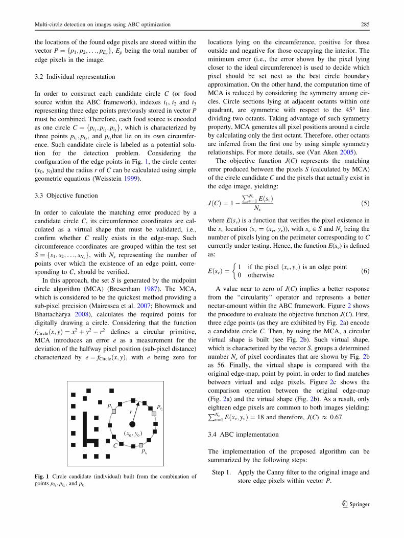
tion for the detection problem. Considering the

configuration of the edge points in Fig. 1, the circle center

(x0, y0)and the radius r of C can be calculated using simple

geometric equations (Weisstein 1999).

3.3 Objective function

In order to calculate the matching error produced by a

candidate circle C, its circumference coordinates are cal-

culated as a virtual shape that must be validated, i.e.,

confirm whether C really exists in the edge-map. Such

circumference coordinates are grouped within the test set

S ¼ fs1; s2; . . .; sNsg; with Ns representing the number of

points over which the existence of an edge point, corre-

sponding to C, should be verified.

In this approach, the set S is generated by the midpoint

circle algorithm (MCA) (Bresenham 1987). The MCA,

which is considered to be the quickest method providing a

sub-pixel precision (Mairessea et al. 2007; Bhowmick and

Bhattacharya 2008), calculates the required points for

digitally drawing a circle. Considering that the function

fCircleðx; yÞ ¼ x2 þ y2 � r2 defines a circular primitive,

MCA introduces an error e as a measurement for the

deviation of the halfway pixel position (sub-pixel distance)

characterized by e ¼ fCircleðx; yÞ; with e being zero for

locations lying on the circumference, positive for those

outside and negative for those occupying the interior. The

minimum error (i.e., the error shown by the pixel lying

closer to the ideal circumference) is used to decide which

pixel should be set next as the best circle boundary

approximation. On the other hand, the computation time of

MCA is reduced by considering the symmetry among cir-

cles. Circle sections lying at adjacent octants within one

quadrant, are symmetric with respect to the 45� line

dividing two octants. Taking advantage of such symmetry

property, MCA generates all pixel positions around a circle

by calculating only the first octant. Therefore, other octants

are inferred from the first one by using simple symmetry

relationships. For more details, see (Van Aken 2005).

The objective function J(C) represents the matching

error produced between the pixels S (calculated by MCA)

of the circle candidate C and the pixels that actually exist in

the edge image, yielding:

JðCÞ ¼ 1�PNs

v¼1 EðsvÞNs

ð5Þ

where E(sv) is a function that verifies the pixel existence in

the sv location (sv = (xv, yv)), with sv [ S and Ns being the

number of pixels lying on the perimeter corresponding to C

currently under testing. Hence, the function E(sv) is defined

as:

EðsvÞ ¼1 if the pixel ðxv; yvÞ is an edge point

0 otherwise

�ð6Þ

A value near to zero of J(C) implies a better response

from the ‘‘circularity’’ operator and represents a better

nectar-amount within the ABC framework. Figure 2 shows

the procedure to evaluate the objective function J(C). First,

three edge points (as they are exhibited by Fig. 2a) encode

a candidate circle C. Then, by using the MCA, a circular

virtual shape is built (see Fig. 2b). Such virtual shape,

which is characterized by the vector S, groups a determined

number Ns of pixel coordinates that are shown by Fig. 2b

as 56. Finally, the virtual shape is compared with the

original edge-map, point by point, in order to find matches

between virtual and edge pixels. Figure 2c shows the

comparison operation between the original edge-map

(Fig. 2a) and the virtual shape (Fig. 2b). As a result, only

eighteen edge pixels are common to both images yielding:PNs

v¼1 Eðxv; yvÞ ¼ 18 and therefore, J(C) & 0.67.

3.4 ABC implementation

The implementation of the proposed algorithm can be

summarized by the following steps:

Step 1. Apply the Canny filter to the original image and

store edge pixels within vector P.

r1i

p2i

p

3ip

( , )0 0x y

C

Fig. 1 Circle candidate (individual) built from the combination of

points pi1; pi2 ; and pi3


123

Step 2. Initialize required parameters of the ABC

algorithm. Set the colony’s size, the abandon-

ment limit and the maximum number of cycles.

Step 3. Initialize NC circle candidates Cb (original food

sources) with b [ (1, …, NC), and clear all

counters Ab.

Step 4. Obtain the matching fitness (food source

quality) for each circle candidate Cb using (5).

Step 5. Repeat steps 6–10 until a termination criterion is

met.

Step 6. Modify the circle candidates as stated by (2) and

evaluate its matching fitness (send employed

bees onto food sources). Likewise, update all

counters Ab.

Step 7. Calculate the probability value Probb for each

circle candidate Cb. Such probability value will

be used as a preference index by onlooker bees

(4).

Step 8. Generate new circles candidates (using the (2))

from current candidates according to their

probability Probb (send onlooker bees to their

selected food source). Likewise, update coun-

ters Ab.

Step 9. Obtain the matching fitness for each circle

candidate Cb and calculate the best circle

candidate (solution).

Step 10. Stop modifying the circle candidate Cb (food

source) whose counter Ab has reached its

counter ‘‘limit’’ and save it as a possible

solution (global or local optimum) in the

exhausted-source memory. Clear Ab and gener-

ate a new circle candidate according to (1).

Step 11. Analyze solutions previously stored in the

exhausted-source memory (see Sect. 5). The

memory holds solutions (any other potential

circular shape in the image) generated through

the evolution of the optimization algorithm.

In ABC algorithm, the steps 6–10 are repeated until a

termination criterion is met. Typically, two stop criteria

have been employed for meta-heuristic algorithms: either

an upper limit of the fitness function is reached or an upper

limit of the number of generations is attained (Aytug and

Koehler 2000). The first criterion requires an extensive

knowledge of the problem and its solutions (Greenhalgh

and Marshall 2000). On the contrary, by considering the

stop criterion based on the number of generations, feasible

solutions may be found by exploring the search space

through several iterations. For our purpose, the number of

iterations as stop criterion is employed in order to allow the

multi-circle detection. Hence, if a solution representing a

valid circle appears at early stages, it would be stored in the

exhausted-source memory and the algorithm continues

detecting other feasible solutions until depleting the itera-

tion number. Therefore, the main issue is to define a fair

iteration number, which should be big enough to allow

finding circles at the image and small enough to avoid an

exaggerated computational cost. For this study, such a

number was experimentally defined as 300.

4 The multiple-circle detection procedure

The original ABC algorithm considers the so-called aban-

donment limit, which aims to stop the local exploration for

a candidate solution after a trial number is reached. All

‘‘stuck solutions,’’ i.e., those that do not improve further

during the optimization cycle are supposed to be discarded

and replaced by other randomly generated solutions.

However, this paper proposes the use of an ‘‘exhausted-

source memory’’ to store information regarding local

(a) (b) (c)

C

1iP

2iP

3iP1i

P

2iP

3iP

Fig. 2 Procedure to evaluate the objective function J(C): a the original edge-map, b the virtual shape generated by MCA considering C ¼fpi1

; pi2 ; pi3g: c The comparison operation between the original edge-map shown in a and the virtual shape presented by b


123

optima that represent possible solutions for the multi-circle

detection problem.

Several heuristic methods have been employed for

detecting multiple circles as an alternative to classical

Hough transform-based techniques (Ayala-Ramirez et al.

2006; Dasgupta et al. 2009). Such strategies imply that

only one circle can be marked per optimization cycle,

forcing a multiple execution of the algorithm in order to

achieve multiple-circle detection. The surface representing

J(C) holds a multi-modal nature, which contains several

global and local optima that are related to potential circular

shapes in the edge-map. This paper aims to solve the

objective function J(C) using only one optimization pro-

cedure by assuming the multi-detection problem as a multi-

modal optimization issue.

The multi-detection problem can be summarized as

follows: guided by the values of a matching function, the

set of encoded circle candidates are evolved through the

ABC algorithm and the best circle candidate (global opti-

mum) is considered to be the first detected circle over the

edge-only image. Then, an analysis of the incorporated

exhausted-source memory is executed in order to identify

other local optima (other circles). The analysis includes

two operations: arraignment and extraction. In the

arraignment, food sources that are held by the memory are

organized in descending order according to their J(C).

Once the exhausted-source memory has been arranged, the

goal is to extract circles considered to be different (local

optima) from it. Such discrimination is accomplished by

comparing all elements in the arranged memory.

Several local optima (i.e., circles slightly shifted or

holding small deviations) can represent the same circle.

Therefore, a distinctiveness factor Esdiis required to mea-

sure the mismatch between two given circles (food sour-

ces) as follows:

Esdi¼

ffiffiffiffiffiffiffiffiffiffiffiffiffiffiffiffiffiffiffiffiffiffiffiffiffiffiffiffiffiffiffiffiffiffiffiffiffiffiffiffiffiffiffiffiffiffiffiffiffiffiffiffiffiffiffiffiffiffiffiffiffiffiffiffiffiffiffiffiffiffiffiffiffiðxA � xBÞ2 þ ðyA � yBÞ2 þ ðrA � rBÞ2

qð7Þ

where (xA, yA) and rA are the coordinates of the center and

radius of the circle CA, respectively, while (xB, yB) and rB

are the corresponding parameters of the circle CB. In order

to decide whether two circles must be considered different,

a threshold value EsTHis defined as follows:

ESTH¼ a

ffiffiffiffiffiffiffiffiffiffiffiffiffiffiffiffiffiffiffiffiffiffiffiffiffiffiffiffiffiffiffiffiffiffiffiffiffiffiffiffiffiffiffiffiffiffiffiffiffiffiffiffiffiffiffiffiffiffiffiffiffiffiffiffiffiffiffiffiffiffiffiffiffiffiffiffiffiffiffiffiffiffiffiffiðcols� 1Þ2 þ ðrows� 1Þ2 þ ðrmax � rminÞ2

q

ð8Þ

where rows and cols refer to the number of rows and

columns in the image, respectively. rmax and rmin are the

maximum and minimum radii for representing feasible

candidate circles, while a is a sensitivity factor affecting

the discrimination between circles. A high value of aallows circles to be significantly different and still be

considered as the same shape while a low value would

imply that two circles with slight differences in radii or

positions could be considered as different instances. The

EsTHvalue calculated by (8) allows discriminating circles

with no consideration about the image size.

In order to find ‘‘sufficiently different’’ circles, the ele-

ments of the arranged exhausted-source memory must be

contrasted. Each element is compared with the others by

using (7). A circle is considered different enough if its

distinctiveness factor Esdi(found in the comparison) sur-

passes the threshold EsTH:

The multiple-circle detection procedure can thus be

described as follows:

Step 1. The best solution found by the ABC algorithm

and all candidate circles held by the exhausted-

source memory are organized in a decreasing

order of their matching fitness, yielding a new

vector MC = {C1, …, CNe}, with Ne being the

size of the exhausted-source memory plus one

Step 2. The candidate circle C1 showing the highest

matching fitness is identified as the first circle

shape CS1 as it is stored within a vector Ac of

actual circles

Step 3. The distinctiveness factor Esdifor the candidate

circle Cm (element m in MC) is compared with

every element in Ac. If Esdi[ ESTH

is true for

each pair of solutions (those present in Ac and in

the candidate circle Cm), then Cm is considered as

a new circle shape CS and is added to the vector

Ac. Otherwise, the next circle candidate Cm?1 is

evaluated and Cm is discarded

Step 4. Step 3 is repeated until all Ne candidate circles in

MC have been analyzed

Summarizing the overall procedure, Fig. 3 shows the

outcome of the ABC-based circular detector. The input

image (Fig. 3a) has a resolution of 256 9 256 pixels and

shows two circles and two ellipses with a different circu-

larity factor. Figure 3b presents the detected circles with a

distinctive overlay. Figure 3c shows the candidate circles

held by the exhausted-source memory after the optimiza-

tion process. Figure 3d presents the resulting image after

the previously described discrimination procedure has been

applied.

5 Experimental results

Experimental tests have been developed in order to eval-

uate the performance of the circle detector. The experi-

ments address the following tasks:

1. Circle localization,


123

2. shape discrimination,

3. circular approximation: occluded circles and arc

detection.

Table 1 presents the parameters for the ABC algorithm

in this study. They have been retained for all test images

after being experimentally defined.

All the experiments have been executed over a Pentium

IV 2.5 GHz computer under C language programming. All

the images are pre-processed by the standard Canny edge

detector using the image-processing toolbox for MATLAB

R2008a.

5.1 Circle localization

5.1.1 Synthetic images

The experimental setup includes the use of several syn-

thetic images of 320 9 240 pixels. All images contain

varying amounts of circular shapes and some have also

been contaminated by added noise so as to increase the

complexity of the localization task. The algorithm is exe-

cuted over 100 times for each test image, successfully

identifying and marking all circles in the image. The

detection has proved to be robust to translation and scaling,

requiring\1 s. Figure 4 shows the outcome after applying

the algorithm over two images taken from the experimental

set.

5.1.2 Natural images

This experiment tests the circle detection on real-life

images. Twenty-five test images of 640 9 480 pixels have

been captured using a digital camera under an 8-bit color

format. Each natural scene includes circular shapes that

have been pre-processed through the Canny edge detection

algorithm before being fed to the ABC procedure. Fig-

ure 5 shows a multiple-circle detection over a natural

image.

5.2 Shape discrimination tests

This section discusses the detector’s ability to differentiate

circular patterns over any other shape, which might be

present in the image. Figure 6 shows five different syn-

thetic shapes within an image of 540 9 300 pixels that has

been contaminated by salt and pepper noise. Figure 7

repeats the experiment over real-life images.

0100

200300

50100

150200

30

35

40

45

50

Rad

ius

x Coordinatey Coordinate 0100

200300

50100

150200

30

35

40

45

50

Rad

ius

x Coordinatey Coordinate

(a) (b)

(c) (d)

Fig. 3 ABC-based circular detector performance: a the original image and b all detected circles as an overlay. c Candidate circles held by the

exhausted-source memory after optimization process and d remaining circles after the discrimination process

Table 1 ABC detector parameters

Colony size Abandonment limit Number of cycles a Limit

20 100 300 0.05 30


123

5.3 Circular approximation: occluded circles and arc

detection

The ABC detector algorithm is able to detect occluded or

imperfect circles as well as partially defined shapes such as

arc segments. The relevance of such functionality comes

from the fact that imperfect circles are commonly found in

typical computer vision applications. Since circle detection

has been considered as an optimization problem, the ABC

algorithm allows finding circles that may approach a given

shape according to fitness values for each candidate. Fig-

ure 8a shows some examples of circular approximation.

Likewise, the proposed algorithm is able to find circle

parameters that better approach an arc or an occluded

Fig. 4 Circle localization over

synthetic images. The image

a shows the original image

while b presents the detected

circles as an overlay. The image

in c shows a second image with

salt and pepper noise and

d shows detected circles as a

distinctive overlay

(a) (b)

150200

250

100150

20025055

60

65

Rad

ius

x Coordinatey Coordinate150

200250

100150

20025055

60

65

Rad

ius

x Coordinatey Coordinate

(c) (d)

Fig. 5 Circle detection

algorithm over natural images:

a the original image, b the

detected circles as a distinctiveoverlay, c candidate circles

lying at the exhausted-source

memory after the optimization

and d detected circles after

finishing the discrimination

process


123

circle. Figure 8b and c show some examples of this func-

tionality. A small value for J(C), i.e., near zero, refers to a

circle while a slightly bigger value accounts for an arc or

an occluded circular shape. Such a fact does not represent

any trouble as circles can be shown following the obtained

J(C) values.

5.4 Performance evaluation

In order to enhance the algorithm analysis, the ABC pro-

posed algorithm is compared with the BFAOA and the GA

circle detectors over a set of common images.

The GA algorithm follows the proposal of Ayala-Ra-

mirez et al., which considers the population size as 70, the

crossover probability as 0.55, the mutation probability as

0.10 and the number of elite individuals as 2. The roulette

wheel selection and the one-point crossover operator are

both applied. The parameter setup and the fitness function

follow the configuration suggested in Ayala-Ramirez et al.

(2006). The BFAOA algorithm follows the implementation

from Dasgupta et al. (2009) considering the experimental

parameters as: S = 50, Nc = 100, Ns = 4, Ned = 1,

Ped = 0.25, dattract = 0.1, wattract = 0.2, wrepellant = 10,

hrepellant = 0.1, k = 400 and w = 6. Such values are found

to represent the best configuration set according to Das-

gupta et al. (2009).

Images rarely contain perfectly shaped circles. There-

fore, aiming for a test on accuracy for a single-circle, the

detection is challenged by a ground-truth circle, which is

determined manually from the original edge-map. The

parameters (xtrue, ytrue, rtrue) of the reference circle are

computed considering the best matching circle that has

been previously defined over the edge-map. If the center

and the radius of the detected circle are defined as (xD, yD)

and rD, then an error score (Es) can be chosen as follows:

Es ¼ g ðjxtrue � xDj þ jytrue � yDjÞ þ l jrtrue � rDj ð9Þ

The central point difference (|xtrue - xD| ? |ytrue - yD|)

represents the center shift for the detected circle as it is

compared with a benchmark circle. The radio mismatch

(|rtrue - rD|) accounts for the difference between their

radii. g and l represent two weighting parameters, which

are to be applied separately to the central point difference

and to the radius mismatch for the final error Es. In this

study, they are chosen as g = 0.05 and l = 0.1. This

particular choice ensures that the radii difference would be

strongly weighted in comparison to the difference in the

central circular positions of manually detected and

machine-detected circles. In order to use an error metric

for multiple-circle detection, the averaged Es produced

from each circle in the image is considered. Such criterion,

defined as the multiple error (ME), is calculated as follows:

ME ¼ 1

NC

� �XNC

R¼1

EsRð10Þ

where NC represents the number of circles actually present

the image. In case the ME is \1, the algorithm is consid-

ered successful; otherwise it is said to have failed in the

Fig. 6 Shape discrimination

over synthetic images: a the

original image contaminated by

salt and pepper noise and

b detected circles as an overlay

Fig. 7 Shape discrimination in real-life images: a original image and b the detected circle as an overlay


123

detection of the circle set. Notice that for g = 0.05 and

l = 0.1, it yields ME \ 1, which accounts for a maximal

tolerated average difference on radius length of 10 pixels,

whereas the maximum average mismatch for the center

location can be up to 20 pixels. In general, the success rate

(SR) can thus be defined as the percentage of achieving

success after a certain number of trials.

Figure 9 shows six images that have been used to

compare the performance of the GA-based algorithm

(Ayala-Ramirez et al. 2006), the BFOA method (Dasgupta

et al. 2009) and the proposed approach. The performance is

analyzed by considering 35 different executions for each

algorithm over six images. Table 2 presents the averaged

execution time, the success rate (SR) in percentage and the

averaged multiple error (ME). The best entries are bold-

cased in Table 2. Closer inspection reveals that the

proposed method is able to achieve the highest success rate

with the smallest error, and still requires less computational

time for most cases. Figure 9 also exhibits the resulting

images after applying the ABC detector. Such results

present the best and the worst cases obtained throughout 35

runs.

A non-parametric statistical significance proof called

Wilcoxon’s rank sum test for independent samples (Wil-

coxon 1945; Garcia et al. 2008; Santamarıa 2008) has

been conducted at 5% significance level on the multiple

error (ME) data of Table 2. Table 3 reports the p values

produced by Wilcoxon’s test for the pair-wise comparison

of multiple error (ME) between two groups. One group

corresponds to ABC versus GA and the other corresponds

to ABC versus BFOA, one at a time. As a null hypothesis,

it is assumed that there is no significant difference

Fig. 8 ABC approximating

circular shapes and arc sections


123

esactsroWesactseBegamilanigirO

(a)

(b)

(c)

(d)

(e)

(f)

Fig. 9 Test images and their detected circles using the ABC detector. The results show the best and the worst case obtained throughout 35 runs


123

between the mean values of the two groups. The alter-

native hypothesis considers a significant difference

between the mean values of both groups. All p values

reported in the table are \0.05 (5% significance level),

which is a strong evidence against the null hypothesis,

indicating that the best ABC mean values for the perfor-

mance are statistically significant and have not occurred

by chance.

Figure 10 demonstrates the relative performance of

ABC in comparison with the RHT algorithm following the

proposal in Xu et al. (1990). All images belonging to the

test are complicated and contain different noise condi-

tions. The performance analysis is achieved by consider-

ing 35 different executions for each algorithm over the

three images. The results, exhibited in Fig. 10, present the

median-run solution (when the runs were ranked accord-

ing to their final ME value) obtained throughout the 35

runs. On the other hand, Table 4 reports the corresponding

averaged execution time, success rate (in %), and average

multiple error (using (10)) for ABC and RHT algorithms

over the set of images (the best results are bold-cased).

Table 4 shows a decrease in performance of the RHT

algorithm as noise conditions change. Yet the ABC

algorithm holds its performance under the same

circumstances.

6 Conclusions

This paper has presented an algorithm for the automatic

detection of multiple circular shapes from complicated and

noisy images without considering the conventional Hough

transform principles. The detection process is considered to

be similar to a multi-modal optimization problem. In

contrast to other heuristic methods that employ an iterative

procedure, the proposed ABC method is able to detect

single or multiple circles over a digital image by running

only one optimization cycle. The ABC algorithm searches

the entire edge-map for circular shapes by using a combi-

nation of three non-collinear edge points as candidate cir-

cles (food positions) in the edge-only image. A matching

function (objective function) is used to measure the exis-

tence of a candidate circle over the edge-map. Guided by

the values of this matching function, the set of encoded

candidate circles is evolved using the ABC algorithm so

that the best candidate can fit into an actual circle. A novel

contribution is related to the exhausted-source memory that

has been designed to hold ‘‘stuck’’ solutions which, in turn,

represent feasible solutions for the multi-circle detection

problem. A post-analysis on the exhausted-source memory

should indeed detect other local minima, i.e., other

potential circular shapes. The overall approach generates a

fast sub-pixel detector, which can effectively identify

multiple circles in real images despite circular objects

exhibiting a significant occluded portion.

Classical Hough transform methods for circle detection

use three edge points to cast a vote for the potential circular

shape in the parameter space. However, they would require

a huge amount of memory and longer computational times

to obtain a sub-pixel resolution. Moreover, HT-based

methods rarely find a precise parameter set for a circle in

the image (Chen and Chung 2001). In our approach, the

detected circles hold a sub-pixel accuracy inherited directly

from the circle equation and the MCA method.

In order to test the circle detection performance, both

speed and accuracy have been compared. Score functions are

Table 2 The averaged execution time, success rate and the averaged multiple error for the GA-based algorithm, the BFOA method and the

proposed ABC algorithm, considering the six test images shown in Fig. 9

Image Averaged execution time ± SD (s) Success rate (SR) (%) Averaged ME ± SD

GA BFOA ABC GA BFOA ABC GA BFOA ABC

(a) 2.23 ± 0.41 1.71 ± 0.51 0.21 – 0.22 94 100 100 0.41 ± 0.044 0.33 ± 0.052 0.22 – 0.033

(b) 3.15 ± 0.39 2.80 ± 0.65 0.36 – 0.24 81 95 98 0.51 ± 0.038 0.37 ± 0.032 0.26 – 0.041

(c) 4.21 ± 0.11 3.18 ± 0.36 0.20 – 0.19 79 91 100 0.48 ± 0.029 0.41 ± 0.051 0.15 – 0.036

(d) 5.11 ± 0.43 3.45 ± 0.52 1.10 – 0.24 93 100 100 0.45 ± 0.051 0.41 ± 0.029 0.25 – 0.037

(e) 6.33 ± 0.34 4.11 ± 0.14 1.61 – 0.17 87 94 100 0.81 ± 0.042 0.77 ± 0.051 0.37 – 0.055

(f) 7.62 ± 0.97 5.36 ± 0.17 1.95 – 0.41 88 90 98 0.92 ± 0.075 0.88 ± 0.081 0.41 – 0.066

Table 3 p values from Wilcoxon’s test, comparing ABC with GA

and BFOA over the ME from Table 2

Image p value

ABC vs. GA ABC vs. BFOA

(a) 1.8061e-004 1.8288e-004

(b) 1.7454e-004 1.9011e-004

(c) 1.7981e-004 1.8922e-004

(d) 1.7788e-004 1.8698e-004

(e) 1.6989e-004 1.9124e-004

(f) 1.7012e-004 1.9081e-004


123

defined by (9) and (10) in order to measure accuracy and

effectively evaluate the mismatch between manually detec-

ted and machine-detected circles. We have demonstrated

that the ABC method outperforms both the GA (as described

in Ayala-Ramirez et al. 2006) and the BFOA (as described in

Dasgupta et al. 2009) within a statistically significant

framework (Wilcoxon test). In contrast to the ABC method,

the RHT algorithm (Xu et al. 1990) shows a decrease in

performance under noisy conditions. Yet the ABC algorithm

holds its performance under the same circumstances.

Finally, Table 2 indicates that the ABC method can

yield better results on complicated and noisy images

I

II

III

Original image RHT ABC

Fig. 10 Relative performance of RHT and ABC

Table 4 Average time, success rate and averaged error for ABC and HT, considering three test images

Image Average time ± SD (s) Success rate (SR) (%) Average ME ± SD

RHT ABC RHT ABC RHT ABC

(I) 7.82 ± 0.34 0.20 – 0.31 100 100 0.19 ± 0.041 0.20 – 0.021

(II) 8.65 ± 0.48 0.23 – 0.28 70 100 0.47 ± 0.037 0.18 – 0.035

(III) 10.65 ± 0.48 0.22 – 0.21 18 100 1.21 ± 0.033 0.23 – 0.028


123

compared with the GA and the BFOA methods. However,

the aim of this study is not to beat all the circle detector

methods proposed earlier, but to show that the ABC

algorithm can effectively serve as an attractive method to

successfully extract multiple circular shapes.

Acknowledgments Erik Cuevas would like to thank DAAD and

SEP-PROMEP for their economical support. Authors thank to the

European Union, the European Commission and the CONACYT for

their support. This paper has been prepared by an economical support

of the European Commission under grant FONCICYT 93829. The

content of this paper is an exclusive responsibility of the UDEG and

the CIC-IPN and it cannot be considered a reflection of the European

Union position. The proposed algorithm belongs to the visual system

operating on the biped robot which has been supported under the

grant CONACYT CB 82877.

References

Atherton TJ, Kerbyson DJ (1993) Using phase to represent radius in

the coherent circle Hough transform. In: Proceedings of the IEE

colloquium on the Hough transform. IEE, London

Ayala-Ramirez V, Garcia-Capulin CH, Perez-Garcia A, Sanchez-

Yanez RE (2006) Circle detection on images using genetic

algorithms. Pattern Recogn Lett 27:652–657

Aytug H, Koehler GJ (2000) New stopping criterion for genetic

algorithms. Eur J Oper Res 126:662–674

Becker J, Grousson S, Coltuc D (2002) From Hough transforms to

integral transforms. In: Proceedings of the international geosci-

ence and remote sensing symposium 2002 IGARSS_02, vol 3,

pp 1444–1446

Bhowmick P, Bhattacharya BB (2008) Number-theoretic interpreta-

tion and construction of a digital circle. Discrete Appl Math

156:2381–2399

Biswas A, Das S, Abraham A, Dasgupta S (2010) Stability analysis of

the reproduction operator in bacterial foraging optimization.

Theoret Comput Sci 411:2127–2139

Bongiovanni G, Crescenzi P (1995) Parallel simulated annealing for

shape detection. Comput Vis Image Underst 61(1):60–69

Bresenham JE (1987) A linear algorithm for incremental digital

display of circular arcs. Commun ACM 20:100–106

Chen T-C, Chung K-L (2001) An efficient randomized algorithm for

detecting circles. Comput Vis Image Underst 83:172–191

Chen Y, Jiang P (2010) Analysis of particle interaction in particle

swarm optimization. Theoret Comput Sci 411(21):2101–2115

da Fontoura Costa L, Marcondes Cesar R Jr (2001) Shape analisis and

classification. CRC Press, Boca Raton

Dasgupta S, Das S, Biswas A, Abraham A (2009) Automatic circle

detection on digital images whit an adaptive bacterial foraging

algorithm. Soft Comput. doi:10.1007/s00500-009-0508-z

Dorigo M, Maniezzo V, Colorni (1991) A positive feedback as a

search strategy. Technical report 91-016, Politecnico di Milano,

Italy

Fischer M, Bolles R (1981) Random sample consensus: a paradigm to

model fitting with applications to image analysis and automated

cartography. CACM 24(6):381–395

Garcia S, Molina D, Lozano M, Herrera F (2008) A study on the use

of non-parametric tests for analyzing the evolutionary algo-

rithms’ behaviour: a case study on the CEC’2005 special session

on real parameter optimization. J Heurist. doi:10.1007/s10732-

008-9080-4

Greenhalgh D, Marshall S (2000) Convergence criteria for genetic

algorithms. SIAM J Comput 20:269–282

Han JH, Koczy LT, Poston T (1993) Fuzzy Hough transform. In:

Proceedings of the 2nd international conference on fuzzy

systems, vol 2, pp 803–808

Ho SL, Yang S (2009) An artificial bee colony algorithm for inverse

problems. Int J Appl Electromagn Mech 31:181–192

Holland JH (1975) Adaptation in natural and artificial systems.

University of Michigan Press, Ann Arbor

Iivarinen J, Peura M, Sarela J, Visa A (1997) Comparison of

combined shape descriptors for irregular objects. In: Proceedings

of the 8th British machine vision conference, Cochester, UK,

pp 430–439

Jones G, Princen J, Illingworth J, Kittler J (1990) Robust estimation

of shape parameters. In: Proceedings of the British machine

vision conference, pp 43–48

Kang F, Li J, Xu Q (2009) Structural inverse analysis by hybrid

simplex artificial bee colony algorithms. Comput Struct

87:861–870

Karaboga D (2005) An idea based on honey bee swarm for numerical

optimization, technical report-TR06, Erciyes University, Engi-

neering Faculty, Computer Engineering Department

Karaboga N (2009) A new design method based on artificial bee

colony algorithm for digital IIR filters. J Frankl Inst

346:328–348

Karaboga D, Akay B (2009) A comparative study of Artificial Bee

Colony algorithm. Appl Math Comput 214:108–132

Karaboga D, Basturk B (2008) On the performance of artificial bee

colony (ABC) algorithm. Appl Soft Comput 8(1):687–697

Karaboga D, Ozturk C (2011) A novel clustering approach: Artificial

Bee Colony (ABC) algorithm. Appl Soft Comput 11:652–657

Kennedy J, Eberhart R (1995) Particle swarm optimization. In: IEEE

international conference on neural networks, Piscataway, NJ,

pp 1942–1948

Liu Y, Passino K (2002) Biomimicry of social foraging bacteria for

distributed optimization: models, principles, and emergent

behaviors. J Optim Theory Appl 115(3):603–628

Mairessea F, Sliwa T, Binczak S, Voisina Y (2007) Subpixel

determination of imperfect circles characteristics. Pattern Re-

cogn 41:250–271

Muammar H, Nixon M (1989) Approaches to extending the Hough

transform. In: Proceedings of the international conference on

acoustics, speech and signal processing ICASSP_89, vol 3,

pp 1556–1559

Pan Q-K, Fatih Tasgetiren M, Suganthan PN, Chua TJ (2010) A

discrete artificial bee colony algorithm for the lot-streaming flow

shop scheduling problem. Inf Sci. doi:10.1016/j.ins.2009.12.025

Peura M, Iivarinen J (1997) Efficiency of simple shape descriptors. In:

Arcelli C, Cordella LP, di Baja GS (eds) Advances in visual

form analysis. World Scientific, Singapore, pp 443–451

Price K, Storn R, Lampinen A (2005) Differential evolution a

practical approach to global optimization. In: Springer Natural

Computing Series

Roth G, Levine MD (1994) Geometric primitive extraction using a

genetic algorithm. IEEE Trans Pattern Anal Machine Intell

16(9):901–905

Sabat SL, Udgata SK, Abraham A (2010) Artificial bee colony

algorithm for small signal model parameter extraction of

MESFET. Eng Appl Artif Intell 23:689–694

Santamarıa J, Cordon O, Damas S, Garcıa-Torres JM, Quirin A

(2008) Performance evaluation of memetic approaches in 3D

reconstruction of forensic objects. Soft Comput. doi:

10.1007/s00500-008-0351-7

Shaked D, Yaron O, Kiryati N (1996) Deriving stopping rules for the

probabilistic Hough transform by sequential analysis. Comput

Vis Image Underst 63:512–526

Tvrdık J (2009) Adaptation in differential evolution: a numerical

comparison. Appl Soft Comput 9(3):1149–1155


123

http://dx.doi.org/10.1007/s00500-009-0508-z

http://dx.doi.org/10.1007/s10732-008-9080-4

http://dx.doi.org/10.1007/s10732-008-9080-4

http://dx.doi.org/10.1016/j.ins.2009.12.025

http://dx.doi.org/10.1007/s00500-008-0351-7

Van Aken JR (2005) Efficient ellipse-drawing algorithm. IEEE

Comput Graph Appl 4(9):24–35

Weisstein EW (1999) Circle. From Mathworld—a wolfram web

resource. http://mathworld.wolfram.com/Circle.html

Wilcoxon F (1945) Individual comparisons by ranking methods.

Biometrics 1:80–83

Xu L, Oja E, Kultanen P (1990) A new curve detection method:

randomized Hough transform (RHT). Pattern Recogn Lett

11(5):331–338

Xu C, Duan H, Liu F (2010) Chaotic artificial bee colony approach to

Uninhabited Combat Air Vehicle (UCAV) path planning. Aerosp

Sci Technol 14:535–541

Yuen H, Princen J, Illingworth J, Kittler J (1990) Comparative study

of Hough transform methods for circle finding. Image Vis

Comput 8(1):71–77

Zang H, Zhang S, Hapeshia K (2010) A review of nature-inspired

algorithms. J Bionic Eng 7(1):S232–S237

Zhang C, Ouyang D, Ning J (2010) An artificial bee colony approach

for clustering. Expert Syst Appl 37:4761–4767


123

http://mathworld.wolfram.com/Circle.html

Multi-circle detection on images using artificial bee colony (ABC) optimization

Documents

Transcript of Multi-circle detection on images using artificial bee colony (ABC) optimization