Bayesian forecasting of recurrent earthquakes and predictiveperformance for a small sample size

S. Nomura,1 Y. Ogata,1,2 F. Komaki,3 and S. Toda4

Received 9 September 2010; revised 6 January 2011; accepted 27 January 2011; published 30 April 2011.

[1] This paper presents a Bayesian method of probability forecasting for a renewal ofearthquakes.When only limited records of characteristic earthquakes on a fault are available,relevant prior distributions for renewal model parameters are essential to computingunbiased, stable time‐dependent earthquake probabilities. We also use event slip andgeological slip rate data combined with historical earthquake records to improve our forecastmodel. We apply the Brownian Passage Time (BPT) model and make use of the best fitprior distribution for its coefficient of variation (the shape parameter, alpha) relative to themean recurrence time because the Earthquake Research Committee (ERC) of Japan uses theBPT model for long‐term forecasting. Currently, more than 110 active faults have beenevaluated by the ERC, but most include very few paleoseismic events. We objectively selectthe prior distribution with the Akaike Bayesian Information Criterion using all availablerecurrence data including the ERC datasets. These data also include mean recurrence timesestimated from slip per event divided by long‐term slip rate. By comparing the goodnessof fit to the historical record and simulated data, we show that the proposed predictorprovides more stable performance than plug‐in predictors, such as maximum likelihoodestimates and the predictor currently adopted by the ERC.

Citation: Nomura, S., Y. Ogata, F. Komaki, and S. Toda (2011), Bayesian forecasting of recurrent earthquakes and predictiveperformance for a small sample size, J. Geophys. Res., 116, B04315, doi:10.1029/2010JB007917.

1. Introduction

[2] We often use renewal process models for calculatingearthquake probability in which intervals between consecu-tive events are independently and identically distributed. Therenewal model is supported by observations that earthquakerecurrence intervals are periodic rather than random or clus-tered [e.g., Parsons, 2008a; Scharer et al., 2010]. This isone of the simplest history‐dependent stochastic models otherthan the stress release model [Vere‐Jones, 1978].[3] However, one of the difficulties in applying recurrent

earthquake models is the scarcity of the paleoseismic data.Most studied fault segments have few, or only one observedearthquake [Schwartz and Coppersmith, 1984] that oftenhave poorly constrained historic and/or radiocarbon ages. Themaximum likelihood estimate (MLE) from such a small dataset can have a large bias and error, which tends to yield highprobability for the next event in a very short time span whenthe recurrence intervals have similar lengths. To avoid thisdifficulty, estimating the common shape parameter, or intrinsic

variance, of recurrence intervals in all the segments canprovide stable, more realistic estimation [e.g., Nishenko andBuland, 1987] (see also Earthquake Research Committeeof Japan, Regarding methods for evaluating long‐termprobability of earthquake occurrence (in Japanese), 2001,available at http://www.jishin.go.jp/main/choukihyoka/01b/chouki020326.pdf, hereafter referred to as ERC 2001).Alternatively, assuming the prior distribution for the modelparameters and using Bayesian inference can take all theestimation errors into account when forecasting the time ofthe next recurrence [e.g., Ogata, 2001, 2002].[4] In this paper, we first compose a common prior distri-

bution of the parameters for all the considered segments andthen use it for a Bayesian model to forecast the next earth-quake. Information on other segments is also used to providethe intrinsic prior probabilities of the model parameters foreach segment. From various prior models, we select thecommon prior distribution that has the smallest value ofAkaike’s Bayesian Information Criterion (ABIC) [Akaike,1980]. We also use geological information, such as single‐event displacements (U) and slip rate (V) to calculate meanrecurrence time as T =U/V in addition to recurrence intervalsobtained directly from historical accounts and paleoseismicinvestigations [Rhoades et al., 1994]. Zöller et al. [2007]recently proposed a detailed model incorporating these andother tectonic parameters. We call this estimate the slipdeformation ratio (T ), and assume that it is probabilisticallyrelated to the mean parameter of the interevent distribution.[5] We can apply various traditional positive‐valued dis-

tributions such as the lognormal, gamma, Weibull, double

1Department of Statistical Science, Graduate University for AdvancedStudies, Tokyo, Japan.

2Institute of Statistical Mathematics, Tokyo, Japan.3Department of Mathematical Informatics, Graduate School of

Information Science and Technology, University of Tokyo, Tokyo, Japan.4Research Center for Earthquake Prediction, Disaster Prevention

Research Institute, Kyoto University, Kyoto, Japan.

Copyright 2011 by the American Geophysical Union.0148‐0227/11/2010JB007917

JOURNAL OF GEOPHYSICAL RESEARCH, VOL. 116, B04315, doi:10.1029/2010JB007917, 2011

B04315 1 of 18

exponential, and Brownian Passage Time (BPT) to recur-rence intervals. In particular, the BPT model [Kagan andKnopoff, 1987; Matthews et al., 2002] is adopted for long‐term forecasts in California and Japan. The ERC (2001)examined the various distributions in relatively well sampledactive fault data sets and found that the lognormal and BPTdistributions generally showed fits similar to, or slightlybetter than those of the gamma and Weibull distributions interms of the Akaike Information Criterion (AIC) [Akaike,1974]. In addition, Hayashi and Maeda [2009] confirmed asimilar result from data sets for more active faults. The ERCeventually adopted the BPT model because it is compatiblewith the physical mechanism by which rupture occurs in arenewal model: stress accumulated by tectonic loading isvaried by Brownian perturbations that represent stress changeeffects from nearby faults until failure occurs. After failure thestress drops, and the stress accumulation cycle is repeated.[6] On the basis of simulation experiments, Zöller and

Hainzl [2007] argued that the interval distribution is moreconsistent with that of a gamma or Weibull distribution thanBPT or lognormal as the interactions of the faults strengthen.However, the BPT model can be extended to a stronglyinteracting fault system if Coulomb failure stress change dataare available [e.g., Parsons, 2005; Console et al., 2008].

2. Stochastic Model for Recurrent Earthquakes

2.1. Renewal Process

[7] Consider a random series of events, t1 < t2 < � � � < ti < � � �and the interval lengths Xi = ti+1 − ti, i = 1, 2, � � �, betweenconsecutive events. If the sequence {Xi} is independently andidentically distributed, the original series of events {ti} iscalled a renewal process. Let F(·) denote the cumulativedistribution function of each interval length Xi, i = 1, 2, � � �and let f (·) be its probability density function. When the nextearthquake is forecast, there is often an open interval since thelast earthquake. When x years have elapsed since the lastearthquake, the hazard function of the next rupture is definedby

h xð Þ ¼ limD#0

Pr x < X � xþDjX > xf gD

¼ f xð Þ1� F xð Þ ;

and the probability that at least one event occurs inD years iscalculated by

Fx Dð Þ ¼ Pr x < X � xþDjX > xf g ¼ F xþDð Þ � F xð Þ1� F xð Þ

¼ 1� exp �Z xþD

xh yð Þdy

� �: ð1Þ

Thus, we can forecast the next earthquake if the probabilitydensity f (x) or hazard rate h(x) is estimated.

2.2. Parameter Inference and Predictive Distributions

[8] To forecast the next earthquake by the renewal process,we must estimate the probability distribution for the recur-rence times from past observations. Therefore, we apply aparametric class of distribution with unknown parameter �and estimate the distribution of the next recurrence time,called the predictive distribution, by inferring the parameter �.In this section, we introduce some conventional inference

methods for the parameter �, and then we propose a newBayesian forecast method using both occurrence time dataand fault slip information.2.2.1. Plug‐In Methods[9] The most popular forecast method is a plug‐in method,

which is probability forecast using a distribution whoseparameter is set to its estimated value. Specifically, when �̂ isthe estimated value of �, the predictive density of the nextrecurrence interval x is given by

f̂ xð Þ ¼ f�xj�̂�: ð2Þ

One of the most useful estimates is the maximum likelihoodestimate (MLE), which maximizes the following likelihoodfunction

L �jXð Þ ¼Yni¼1

f Xij�ð Þ;

whereX = {Xi; i = 1, 2, � � �, n} are the interval lengths betweenconsecutive main shocks.[10] The plug‐in method works well if the estimation error

is small enough. However, if the estimation error is large orsignificantly biased from the true parameter, its predictiveperformance can be much worse. For example, when we usethe MLE for an asymmetric and heavy‐tailed likelihoodfunction, the MLE provides a biased estimate [e.g., Box andTiao, 1973]. Especially when the sample size is small, theestimate from the sample data may have a large error. Forexample, Parsons [2008b] showed that m is particularlysensitive to the sample mean.2.2.2. Bayesian Inference[11] To consider the effect of estimation errors, we intro-

duce a Bayesian framework for forecasting. We assume aprobability distribution for the model parameter �. We call it aprior distribution and denote its probability density by p(�).Then, given the dataX = {Xi; i = 1, 2, � � �, n} for the recurrencetime intervals between events on a fault, the probabilitydensity, called the posterior density, is defined by

posterior �jXð Þ ¼ L �jXð Þ� �ð ÞRQ

RQ L �jXð Þ� �ð Þd� ; ð3Þ

where Q is the defined region for �. This definition indicatesthat the posterior density is proportional to both the likelihoodfunction L(�∣X) (the information on the parameter knownfrom the data) and the prior density p(�) (the information onthe parameter known from other sources). The posteriordistribution is interpreted as the integrated information on theparameters. From this distribution, the future recurrence timeinterval y is forecast by the Bayesian predictive distribution,whose cumulative distribution and probability density aredefined by

~F yjXð Þ ¼ZQF yj�ð Þ � posterior �jXð Þd�;

~f yjXð Þ ¼ d

dy~F yjXð Þ ¼

ZQf yj�ð Þ � posterior �jXð Þd�:

ð4Þ

The difference between the plug‐in distribution and theBayesian predictive distribution is that, while the plug‐in dis-tribution uses only oneparameter value, theBayesian predictive

NOMURA ET AL.: BAYESIAN FORECASTING FOR A SMALL SAMPLE B04315B04315

2 of 18

distribution uses all values of the parameter and is calculatedby their mean weighted by the posterior distribution.[12] Regarding the evaluation of earthquake probability,

Rhoades et al. [1994] and Ogata [2002] defined the hazardfunction of the predictive distribution as

~h yjXð Þ ¼ZQh yj�ð Þ � posterior �jX; Y > yð Þd�; ð5Þ

where posterior(�∣X, Y > y) is given by (3) with L(�∣X)replaced by

L �jX; Y > yð Þ ¼ 1� F yj�ð Þð ÞYni¼1

f Xij�ð Þ: ð6Þ

Here, we suggest another expression of this hazard functionthat is easier to calculate for some distributions:

~h yjXð Þ ¼~f yjXð Þ

1� ~F yjXð Þ : ð7Þ

[13] A proof that the two expressions of the hazard functionin (5) and (7) are equivalent is given in the Appendix A. Theprobability of the next event is evaluated in the same way asin (1).

2.3. Slip Data–Based Normalization of RecurrenceIntervals

[14] When there are few earthquake observations on a faultsegment, additional information can improve earthquakeforecast drastically [e.g., Fitzenz et al., 2010]. The ERC(2001) sought an alternative way to approximate the meanrecurrence time using geological slip data. This estimate isexpressed as T =U/V, whereU is the plausible coseismic slipinferred from the empirical relationship between earthquakemagnitudes and rupture (segment) lengths, and V is the sliprate (mm/yr) estimated from geological and geomorpholog-ical surveys across the fault. The parameter for a renewalmodel can be supplied using this estimate T (time predictablemodel of Shimazaki and Nakata [1980]). This enables us toapply a renewal model to a fault segment even if only the ageand rupture length of the last earthquake is assumed to beknown.[15] We use the estimated recurrence interval T , hereafter

called the slip deformation ratio, in our Bayesian model. Toinclude this information, we normalize the recurrence inter-vals of the segment by their slip deformation ratio T . In otherwords, when we have slip data for a fault segment, we handlethe normalized data X0 = {Xi /T ; i = 1, 2, � � �, n} and thecorresponding parameters using �0. With this transformation,the mean parameter of the distribution should be around 1,andwe can apply this information to its prior distribution. Therelationship between the likelihood functions of the originaldata and the normalized data is

L �jXð Þ ¼ L �0jX0ð Þ=Tn: ð8Þ

2.4. Measure of Predictive Performance

[16] In principle, the predictive performance of theBayesian predictive distribution is more stable than that ofthe plug‐in distribution when the parameter is sampled from

the prior distribution (see section 5.2 for a specific setup)since it takes all possibilities of parameter value into account.To evaluate the accuracy of an estimated predictive density ~fwith respect to the true density f for a future observation y, therelative entropy is a natural measure for the prediction errorand is defined by

RE f j~f� �¼Z ∞

0log f yð Þ=~f yð Þ� �

f yð Þdy ¼ Ef log f Yð Þ � log ~f Yð Þ� ;

ð9Þ

where Ef represents the expectation with respect to Y. The lastexpression of (9) represents the expected loss in the loglikelihood of the predictive density ~f from that of the truedensity f per future observation Y, and it takes its minimumvalue at 0 if and only if ~f = f. Thus, the relative entropyis regarded as the error function of the predictive density withrespect to the true density in terms of the likelihood. In sta-tistical terms, the relative entropy is identical to the Kullback‐Leibler information [Kullback and Leibler, 1951].[17] Originally, the relative entropy RE(f∣~f ) was described

by Boltzmann [1878], and its negative is approximately thelogarithm of the probability of obtaining a future sample with(the true) distribution f (y) from a predictor ~f (y) [see Akaike,1985]. It is natural to select the most likely model thatminimizes the relative entropy for inference. For example, theMLE is the value of the parameter that minimizes the relativeentropy, or the last term in (9) for an empirical distribution off consisting of past observations. Therefore, the smaller therelative entropy, the more accurate the prediction. Aitchison[1975] showed that the Bayesian predictive distributionminimizes the expected relative entropy among all the pre-dictive methods when the true density is included in themodel and its parameters are distributed with the prior dis-tribution. Thus, if we have the appropriate prior distributionfor themodel parameters, the Bayesian predictive distributionis expected to have the best predictive performance in termsof the likelihood of future data. We will use the relativeentropy to evaluate the predictive performance of simulationexperiments in section 5.2.

2.5. BPT Distribution

[18] The ERC (2001) adopted the BPT distribution,called the inverse Gaussian distribution in statistics, and hasforecast 30 year probabilities for about 100 fault segments(Earthquake Research Committee, Long‐term probabilityforecasts of active faults in Japan (in Japanese), 2010,available at http://www.jishin.go.jp/main/p_hyoka02.htm,hereafter referred to as ERC 2010), which we examine here.We therefore limit our discussion to the BPT distribution forthe intervals of the renewal process, whose probability den-sity function is given by

f xj�; �ð Þ ¼ffiffiffiffiffiffiffiffiffiffiffiffiffiffiffi

�

2��2x3

rexp � x� �ð Þ2

2��2x

( )

and whose cumulative distribution function is given by

F xj�; �ð Þ ¼ Fx� �

�ffiffiffiffiffi�x

p� �

þ exp2

�2

� �F � xþ �

�ffiffiffiffiffi�x

p� �

;

NOMURA ET AL.: BAYESIAN FORECASTING FOR A SMALL SAMPLE B04315B04315

3 of 18

where F denotes the cumulative distribution function of thestandard normal distribution. The two parameters of the BPTdistribution, m and a, represent the mean and coefficient ofvariation, respectively, of the recurrence intervals.2.5.1. Background of the BPT Model[19] One of the main reasons to use the BPT distribution for

the recurrence intervals of earthquakes is its consistency withthe physical interpretation of earthquake generation [Matthewset al., 2002], as follows. In this model, it is assumed that thestress on a fault accumulates by tectonic loading and randomexternal interactions approximated by Brownian motion. Thefault is loaded until it reaches a critical threshold and thenstress is released to a base level after an earthquake. Thisprocedure is formulated by the following stochastic process,which is called a Brownian relaxation oscillator, as

S tð Þ ¼ �t þ �W tð Þ;

where S(t) is the load state at the time t, l is the loading rate,and the term sW(t) consists of a perturbation rate s and astandard Brownian motion W(t), which stands for stressinteractions from earthquakes on nearby fault segments [e.g.,Console et al., 2008]. When S(t) reaches the critical failurestate sf, an earthquake occurs, and S(t) drops to the groundstate s0. If we assume that the failure state sf and ground states0 are constant, the interval times of earthquakes, called theBrownian passage times, are independent and identicallydistributed with the BPT distribution, whose parameters are

related by m = (sf − s0)/l and a = s/ffiffiffiffiffiffiffiffiffiffiffiffiffiffiffiffiffiffiffiffiffi� sf � s0� �q

. Although

it is difficult to measure the parameters in the Brownianrelaxation oscillator directly, the mean parameter m andcoefficient of variation a for the recurrence intervals can beestimated from the recurrence interval data.[20] The ERC (2001) also showed that the BPT distribution

matches geological data on main shocks in Japan as wellas the lognormal distribution as applied by Nishenko andBuland [1987] and Rhoades et al. [1994].2.5.2. Plug‐In Estimates for the BPT Distribution[21] There are several methods to estimate BPT parameters

for recurrent earthquakes on fault segments. Here, we intro-duce the plug‐in estimates of ERC (2001) and describe theirproperties.[22] The mean parameter m has two estimates. One is the

mean of past recurrence intervals, and the other is the slipdeformation ratio T introduced in section 2.2.1. However,these estimates differ greatly in some segments. Therefore,the ERC selects and applies one of these estimates for them value of each fault segment by reviewing the reliabilityof such geological and/or historical data.[23] For the coefficient of variation a, the ERC (2001) uses

a common a value of 0.24, which is the MLE estimated fromthe data sets of fourwell‐studied active faults (cf. those includedin the work ofOgata [1999] for the data), and apply it to all theactive faults in Japan. Note that the MLE of a is biased andunstable when only a few interval records are available. TheMLE of a is expected to be smaller than the true a value:

E �̂2� ¼ n� 1

n� �2;

where n ≥ 2 is the number of recurrence intervals used in afault segment. The calculation of the MLE and its expectation

is shown in Appendix B. Thus, when we need the unbiasedestimate for a, we adjust the MLE of a by multiplying it byffiffiffiffiffiffiffiffiffiffiffiffiffiffiffiffiffiffiffi

n= n� 1ð Þp.

3. Data Sets

[24] The data sets for analysis are shown in Tables 1, 2, and3. To compose a reliable prior distribution for the parameters,we collected a large amount of data obtained from activefaults and subduction zones with occurrence records of twoor more recent earthquakes. The recurrence data consist ofboth historically recorded and geologically determined dates.Errors in radiocarbon dating and the paucity of sedimentaryunits widen the occurrence date, as indicated by “‐” inTables 1, 2, and 3. Although this range could be incorporatedinto the Bayesian formulation, here we use the values in themiddle of the range for the analysis to reduce the computa-tional workload, although Ogata [1999] introduced a priordistribution for the uncertain age of those earthquakes.[25] The data sets in Tables 1 and 2 are drawn from Japan

and come mainly from the ERC (2010), which makes themavailable on its web site. The ERC has investigated the majoractive faults and subduction zones that cause recurrent largeearthquakes in Japan to determine not only their occurrencetimes but also the long‐term slip rates and the plausibleslip per event from their geological surveys. Then, Table 1includes the slip per event U and slip rates V on respectivefault planes to be used for estimating the expected recurrenceinterval T = U/V. Although the part of these slip data isestimated in range, as indicated by “‐”, and could be incor-porated into the Bayesian formulation, we use the values atthe middle of the estimated ranges for U and V, and combinetheir uncertainty and estimation error into the prior distribu-tion for m as in section 4.2.[26] To increase the reliability of the estimated prior distri-

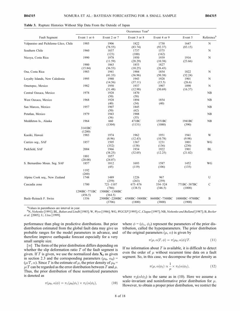
bution, we refer to more data in Tables 2 and 3 from the col-lected data sets ofOkada et al. [2007]; the prior distribution forthe renewal process with a lognormal distribution is estimatedfrom these data. These fault segments have no slip data butmore earthquake recurrence intervals than the data in Table 1.The data sets from Matsuzawa et al. [2002] and Hasegawaet al. [2005] in Table 2 describe a series of repeated earth-quakes whose magnitudes are around 6, which is smaller thanthose on the other listed fault segments. These series areidentified as recurrent events on the same fault segmentbecause they have very similar seismicwaves. Table 3 includesthe survey data from around the circum‐Pacific area presentedbyNishenko andBuland [1987] andNishenko [1991], The datasets on the San Andreas fault are drawn from Bakun and Lindh[1985] and the report of the Working Group on CaliforniaEarthquake Probabilities [Working Group on CaliforniaEarthquake Probabilities (WGCEP), 1995], which evaluatedthe seismic hazard for each segment. In addition,we added datafrom the latest earthquake (in 2004 on the Parkfield segment)from theNational Earthquake Information Center (NEIC)Website, as presented by Okada et al. [2007]. In Kaoiki, Hawaii,no large earthquake has occurred since the 1983 earthquakecited by Wyss [1986]. The data sets for the Cook segment ofthe Alpine fault, New Zealand, introduced by Utsu [1999]show very similar intervals. The series in the Cascadia zoneis taken from Figure 10 of Clague [1997]. The records forthe Basle‐Reinach fault in Switzerland are inferred from

NOMURA ET AL.: BAYESIAN FORECASTING FOR A SMALL SAMPLE B04315B04315

4 of 18

Tab

le1.

Rup

ture

Histories

andSlip

DataforMajor

ActiveFaults

inJapanFrom

theEarthqu

akeResearchCom

mittee

FaultSegment

OccurrenceYeara

Slip

Per

Event

U(m

m)/

Slip

RateV(m

m/yr)

Exp

ected

Intervalb

Event

1or

6Event

2Event

3Event

4Event

5

WestKitakamilowland

2500

BC

2800

0BC–5

000B

C(140

00)

5000

/0.2–0

.416

667

EastYok

otebasin(northernarea)

1896

1500

BC

(339

6)20

00/1

2000

Yam

agatabasin(northernarea)

1900

BC–400

3900

BC–380

0BC

(310

0)75

00BC–680

0BC

(330

0)20

00–3

000/1

2500

EastSho

naiplane(sou

thernarea)

1000

BC–1

780

5900

BC–100

0BC

(384

0)75

00BC–590

0BC

(325

0)10

00–200

0/0.5

3000

WestFuk

ushimabasin

200B

C–3

0080

00BC

(805

0)40

00–500

0/0.7–0.9

5625

WestAizubasin

1611

9000

BC–580

0BC

(901

1)40

00–5

000/1

4500

EastAizubasin

1000

BC–600

BC

9000

BC–560

0BC

(650

0)19

000B

C–140

00BC

(920

0)30

00/0.4

7500

Kushigata

mou

ntains

1200

BC–600

BC

4800

BC–360

0BC

(330

0)90

00BC–670

0BC

(365

0)10

00/0.2–0

.433

33

Sekiyafault

1300

–170

031

00BC–190

0BC

(400

0)64

00BC–380

0BC

(260

0)30

00/1

3000

Kannawa‐Kou

zu‐M

atsuda

1100

–135

040

0BC–100

(137

5)30

00/2–3

1200

Kita‐Izu

1930

838–13

00(861

)80

0BC–5

00(121

9)36

00BC–1

100B

C(220

0)42

00BC–360

0BC

(155

0)20

00–3

000/2

1250

WestNaganobasin

1847

500–10

00(109

7)20

00–300

0/1.2–2.6

1316

WestKisomou

ntains

(north

ofthemainarea)

1200

–130

023

00BC–100

0BC

(290

0)18

000B

C–600

0BC

(103

50)

2600

0BC–1

8000

BC

(100

00)

3000

/0.4

7500

Atotsug

awa

1858

2300

BC–185

8(207

9)33

00BC–200

0BC

(242

9)61

00BC–5

500B

C(315

0)90

00BC–730

0BC

(235

0)45

00–800

0/2–

325

00

Inadani(m

ainarea)

1300

–180

047

00BC–310

0BC

(545

0)11

000B

C–900

0BC

(610

0)60

00/0.2–1

.380

00

Atera

(sou

thof

themainarea)

1586

600–15

00(536

)24

00BC–120

0BC

(285

0)39

00BC–2

100B

C(120

0)45

00BC–400

0BC

(125

0)40

00–500

0/2–

415

00

7000

BC–680

0BC

(265

0)North

Enayama–Sanageyam

a56

00BC–340

0BC

1900

0BC–180

00BC

(140

00)

3200

0BC–200

00BC

(750

0)20

00–300

0/0.2–0.4

8333

Ouchigata

1200

BC–900

1900

BC–4

00BC

(100

0)29

00BC–170

0BC

(115

0)20

00–300

0/0.4–0.8

4167

NOMURA ET AL.: BAYESIAN FORECASTING FOR A SMALL SAMPLE B04315B04315

5 of 18

Tab

le1.

(con

tinued)

FaultSegment

OccurrenceYeara

Slip

Per

Event

U(m

m)/

Slip

RateV(m

m/yr)

Exp

ected

Intervalb

Event

1or

6Event

2Event

3Event

4Event

5

EastFuk

uiplane(m

ainarea)

1400

BC–900

BC

1100

0BC–7

700B

C(820

0)10

00/0.1–0

.350

00

Neodani

1891

2500

BC–189

1(219

5.5)

5300

BC–230

0BC

(349

5.5)

2000–3

000/2

1250

Yoro‐Kuw

ana‐Yok

kaichi

1200

–160

060

0–11

00(550

)50

00–700

0/3–

417

14

Arima‐Takatsuki

1596

794–13

33(532

.5)

1000

BC

(206

3.5)

3000

/1.5

2000

Kyo

to‐N

ishiyama

400B

C–2

0064

00BC–430

0BC

(525

0)11

000B

C–740

0BC

(385

0)30

00–4

000/0.3–1

5385

Sou

thMt.Rok

ko‐eastshore

ofAwaziisland

1500

–160

012

00BC–600

(185

0)50

00–6

000/2

2750

Westshoreof

Awaziisland

1995

0–40

0(179

5)31

00BC–170

0BC

(260

0)20

00/0.7

2857

Yam

azaki(northwestof

themainarea)

868

1400

BC–9

00BC

(201

8)20

00/1

2000

Sou

thSanuk

imou

ntains

‐no

rthIshizuchi

mou

ntains

(eastern

area)

1500

–160

00

(155

0)60

00–700

0/6–

986

7

North

Ishizuchimou

ntains

1500

–160

013

00BC–100

0BC

(270

0)33

00BC–310

0BC

(205

0)60

00/5–6

1091

Oita

plane‐Yub

uin(eastern

area)

200B

C–6

0025

00BC–140

0BC

(215

0)53

00BC–470

0BC

(305

0)20

00–500

0/2–

411

67

Kueno

hirayama‐Kam

eishiyam

a12

00–201

053

00BC–310

0BC

(580

5)30

00/0.1–0

.412

000

Minou

679

1200

0BC–679

(633

9.5)

2000

/0.2

1000

0

Sou

thwestUnzen

faultgrou

p(northernarea)

400B

C–1

100

3600

BC–210

0BC

(320

0)30

00–4

000/1

3500

Izum

i53

00BC–400

BC

1400

0BC–7

100B

C(770

0)10

00–200

0/0.1–0.2

1000

0

EastTakadaplane

1500

BC–1

847

3500

BC–184

7(100

0)20

00/0.9

2222

Akinada

(mainarea)

3600

BC–160

0BC

8000

BC–590

0BC

(435

0)10

00–200

0/0.1

1500

0

a Valuesin

parenthesesareintervalin

year.

bT=U/v.

NOMURA ET AL.: BAYESIAN FORECASTING FOR A SMALL SAMPLE B04315B04315

6 of 18

rockfall deposits [Becker et al., 2005]. These collected datasets are also available in our web site, “http://bemlar.ism.ac.jp/nomura/Datasets.xls.”

4. Composing Prior Distribution Fromthe Data Sets

[27] In Bayesian inference, an appropriate prior distributionis crucial to predictive performance. We consider the distri-bution of the BPT parameter (m, a) for all the recurrentearthquake series and apply it as the prior distribution byconsidering the data from all the fault segments. We analyzedthe data sets in Tables 1, 2, and 3 to select the best fitting priordistribution for the BPT model.

4.1. Separability in the Prior Distribution

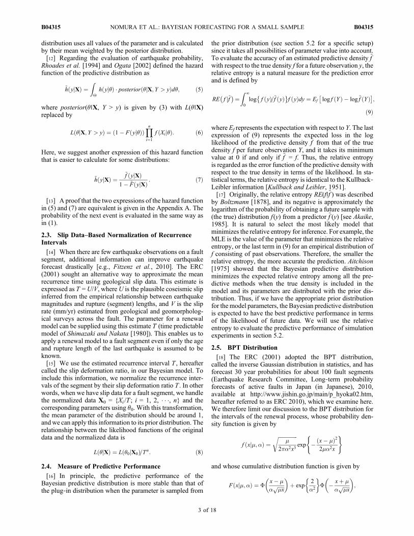
[28] First, we analyzed the relationship between the meanparameter m and the variation parameter a. We calculated the

MLEs for each fault segment and plotted them in Figure 1.The correlation coefficient between the MLE of m and a is0.20 and its 95% confidence interval is (−0.05, 0.43).Although we see that segments with large a MLE of a tendto have a large MLE of m, the correlation coefficient istoo small to conclude that those parameters are correlated.Thus, we assume that m and a are independent in the priordistribution and decompose its prior density as p(m, a) =p1(m) × p2(a).

4.2. Candidates for Each Prior Distribution and TheirSelection Criterion

[29] Here we discuss the prior distribution for eachparameter. Although there are noninformative or vague priordistributions, we estimate an appropriate prior better thannoninformative priors. Even when there is no prior infor-mation for parameters, it is known that there exist Bayesianpredictive distributions based on noninformative priors better

Table 2. Rupture Histories Without Slip Data From Japan

Fault Segment

Occurrence Yeara

ReferencebEvent 1 or 6 Event 2 or 7 Event 3 or 8 Event 4 or 9 Event 5 or 10

Takeyama 300BC–100 1100BC–300BC(600)

3600BC–3400BC(2800)

ERC

Ushikubi 1000–1200 3600BC–2900BC(4350)

13000BC–9000BC(7750)

ERC

Atera (north of the main area) 1400BC–1000BC 4800BC–4500BC(3450)

6000BC–5000BC(850)

ERC

Atsumi fault (northwestern area) 1891 1900BC–600(2541)

4000BC–2000BC(2350)

5300BC–4800BC(2050)

ERC

Umehara 1891 22000BC–20000BC(22891)

29000BC–26000BC(6500)

ERC

Beppu bay ‐ Hideo (eastern area) 1596 200BC–300(1546)

2600BC–1600BC(2150)

4000BC–3300BC(1550)

5300BC–3800BC(900)

ERC

Off Tokachi 2003 1952(51.5)

1843(108.9)

ERC

Off Miyagi prefecture 1978 1936(41.6)

1897(39.7)

1861(35.3)

1835(26.3)

ERC

1793(42.4)

Nankai trough 1947 1855(92)

1707(147.2)

1605(102.7)

ERC

Tounankai trough 1944 1855(89.9)

1707(147.2)

1605(102.7)

1498(106.4)

ERC

Kantou earthquake (Ganroku type) 1704 1000BC(2704)

2900BC(1900)

5100BC(2200)

ERC

Off Sanriku (northern area) 1968 1856(111.8)

1763(93.5)

1677(85.8)

ERC

Off Ibaraki prefecture 2008 1982(25.8)

1965(16.9)

1943(22.4)

1923(19.9)

ERC

Off Kamaishi 2008 2001(6.16)

1995(6.68)

1990(4.65)

1985(5.38)

M

1979(5.62)

1973(5.61)

1968(5.14)

1962(6.22)

1957(4.84)

Off Kesennuma (area A) 2002 1986(15.92)

1973(13.03)

1954(19)

1940(14)

H

Off Kesennuma (area B) 1994 1982(12.2)

1970(11.71)

1953(16.77)

1937(16.92)

H

Off Iwaki 1997 1986(10.58)

1975(11.16)

1966(8.63)

1958(8.7)

H

1950(7.32)

1943(7.34)

1939(4.58)

1929(9.59)

Off north Ibaraki 2002 1989(12.18)

1977(11.98)

1964(13.15)

1954(10.15)

H

1942(11.97)

1929(13.39)

aValues in parentheses are interval in year.bERC, ERC (2010); M, Matsuzawa et al. [2002]; H, Hasegawa et al. [2005].

NOMURA ET AL.: BAYESIAN FORECASTING FOR A SMALL SAMPLE B04315B04315

7 of 18

performance than plug‐in predictive distributions. But priordistribution estimated from the global fault data may give usprobable ranges for the model parameters in advance, andtherefore improve earthquake forecast especially for a verysmall sample size.[30] The form of the prior distribution differs depending on

whether the slip deformation ratio T of the fault segment isgiven. If T is given, we use the normalized data X0 as givenin section 2.3 and the corresponding parameters (m0, a0) =(m/T , a). Since T is the estimate of m, the prior density of m0 =m/T can be regarded as the error distribution between T and m.Thus, the prior distribution of these normalized parametersis denoted as

� �0; �j�ð Þ ¼ �1 �0j�1ð Þ � �2 �j�2ð Þ; ð10Þ

where � = (�1, �2) represent the parameters of the prior dis-tribution, called the hyperparameters. The prior distributionof the original parameters (m, a) is given by

� �; �jT ; �ð Þ ¼ � �0; �j�ð Þ=T : ð11Þ

If no information about T is available, it is difficult to detecteven the order of m without recurrent time data on a faultsegment. So, in this case, we decompose the prior density as

� �; �j�2ð Þ / 1

�� �2 �j�2ð Þ; ð12Þ

where p2(a∣�2) is the same as in (10). Here we assume ascale‐invariant and noninformative prior distribution for m.However, to obtain a proper prior distribution, we restrict the

Table 3. Rupture Histories Without Slip Data From the Outside of Japan

Fault Segment

Occurrence Yeara

ReferencebEvent 1 or 6 Event 2 or 7 Event 3 or 8 Event 4 or 9 Event 5

Valparaiso and Pichilemu‐Llico, Chile 1985 1906(78.55)

1822(83.74)

1730(92.37)

1647(83.15)

N

Southern Chile 1960 1837(123)

1737(100)

1575(162)

N

Nicoya, Costa Rica 1990 1978(11.59)

1950(28.29)

1939(10.38)

1916(23.66)

N

1900(15.84)

1863(36.53)

1853(10.25)

1827(26.43)

Osa, Costa Rica 1983 1941(41.33)

1904(36.96)

1854(50.38)

1822(32.24)

N

Loyalty Islands, New Caledonia 1995 1980(14.56)

1943(37.11)

1928(15.5)

1901(26.6)

N

Ometepec, Mexico 1982 1950(31.48)

1937(12.98)

1907(30.69)

1890(16.37)

N

Central Oaxaca, Mexico 1978 1928(50)

1870(58)

NB

West Oaxaca, Mexico 1968 1928(40)

1894(34)

1854(40)

NB

San Marcos, Mexico 1957 1907(50)

1845(62)

NB

Petatlan, Mexico 1979 1943(36)

1908(35)

NB

Meddleton Is., Alaska 1964 660(1304)

471BC(1131)

1551BC(1080)

1941BC(390)

NB

3141BC(1200)

Kaoiki, Hawaii 1983 1974(8.96)

1962(12.43)

1951(10.78)

1941(9.98)

W

Carrizo seg., SAF 1857 1505(352)

1367(138)

1231(136)

1001(230)

WG

Parkfield, SAF 2004 1966(38.25)

1934(32.05)

1922(12.25)

1901(21.02)

BL

1881(20.08)

1857(24.07)

S. Bernardino Moun. Seg. SAF 1857 1812(45)

1693(119)

1587(106)

1452(135)

WG

1192(260)

Alpine Cook seq., New Zealand 1748 1489(259)

1226(263)

967(259)

U

Cascadia zone 1700 721–1107(786)

675–876(138.5)

334–524(346.5)

771BC–387BC(1008)

C

1290BC–771BC(456.5)

1500BC–1300BC(364.5)

Basle‐Reinach F. Swiss 1356 2500BC–2200BC(3706)

4500BC–3800BC(1800)

8600BC–7300BC(3800)

10000BC–9700BC(1900)

B

aValues in parentheses are interval in year.bN,Nishenko [1991]; BL,Bakun and Lindh [1985];W,Wyss [1986];WG,WGCEP [1995]; C,Clague [1997]; NB,Nishenko and Bulland [1987]; B,Becker

et al. [2005]; U, Utsu [1999].

NOMURA ET AL.: BAYESIAN FORECASTING FOR A SMALL SAMPLE B04315B04315

8 of 18

domain of fi to some range of possible values from 1 yearto 100,000 years. Using “/” instead of “=” means that theright‐hand side of (12) should have a normalizing constantto make the sum of the prior density 1.[31] Then, we apply each pair of factors to the candidate

prior distributions as shown in Table 4. We assume that thevalues of the hyperparameters are common to all consideredfault segments, and we obtain their estimates by maximizingthe integrated posterior distribution (the likelihood of theBayesian model [Akaike, 1980]):

L �ð Þ ¼Ymj¼1

Z ∞

0

Z ∞

0L �j; �jjXj

� �� �j; �jjTj; �� �

d�jd�j;

where the subscript j represents the jth segment of m faultsegments, and p(mj, aj∣Tj, �) is replaced by p(mj, aj∣�2) in(12) if Tj is not available. This maximizing procedure is calledthe type II maximum likelihood method [Good, 1965]. Afterestimating the optimal values of the hyperparameters, weselect the best combination of the prior distribution factorsin (10) that yields the smallest value of the ABIC [Akaike,1980], defined by

ABIC ¼ �2max�

L �ð Þ þ 2 dim �f g;

where dim{�} denotes the number of hyperparameters,which is also shown in Table 4. We can compare the con-fidence or likelihood among the prior distributions by usingtheir ABIC value. Their confidence is proportional to exp(−ABIC/2), which is derived in the samemanner as AIC in thework of Akaike [1978].

4.3. Estimated Prior Distribution From the Data Sets

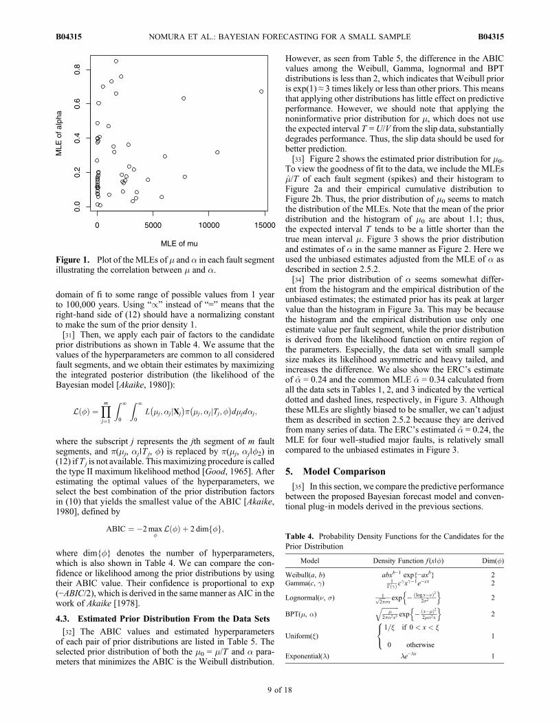
[32] The ABIC values and estimated hyperparametersof each pair of prior distributions are listed in Table 5. Theselected prior distribution of both the m0 = m/T and a para-meters that minimizes the ABIC is the Weibull distribution.

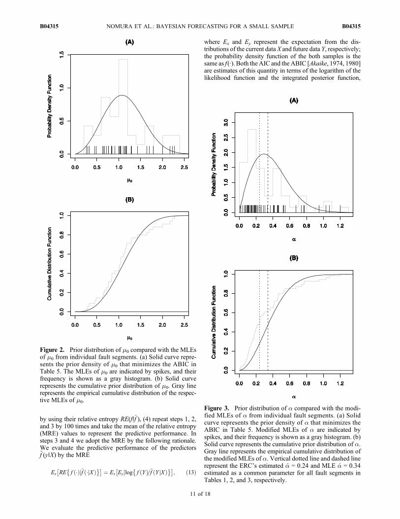
However, as seen from Table 5, the difference in the ABICvalues among the Weibull, Gamma, lognormal and BPTdistributions is less than 2, which indicates that Weibull prioris exp(1) ≈ 3 times likely or less than other priors. This meansthat applying other distributions has little effect on predictiveperformance. However, we should note that applying thenoninformative prior distribution for m, which does not usethe expected interval T =U/V from the slip data, substantiallydegrades performance. Thus, the slip data should be used forbetter prediction.[33] Figure 2 shows the estimated prior distribution for m0.

To view the goodness of fit to the data, we include the MLEs�̂/T of each fault segment (spikes) and their histogram toFigure 2a and their empirical cumulative distribution toFigure 2b. Thus, the prior distribution of m0 seems to matchthe distribution of the MLEs. Note that the mean of the priordistribution and the histogram of m0 are about 1.1; thus,the expected interval T tends to be a little shorter than thetrue mean interval m. Figure 3 shows the prior distributionand estimates of a in the same manner as Figure 2. Here weused the unbiased estimates adjusted from the MLE of a asdescribed in section 2.5.2.[34] The prior distribution of a seems somewhat differ-

ent from the histogram and the empirical distribution of theunbiased estimates; the estimated prior has its peak at largervalue than the histogram in Figure 3a. This may be becausethe histogram and the empirical distribution use only oneestimate value per fault segment, while the prior distributionis derived from the likelihood function on entire region ofthe parameters. Especially, the data set with small samplesize makes its likelihood asymmetric and heavy tailed, andincreases the difference. We also show the ERC’s estimateof �̂ = 0.24 and the common MLE �̂ = 0.34 calculated fromall the data sets in Tables 1, 2, and 3 indicated by the verticaldotted and dashed lines, respectively, in Figure 3. Althoughthese MLEs are slightly biased to be smaller, we can’t adjustthem as described in section 2.5.2 because they are derivedfrom many series of data. The ERC’s estimated �̂ = 0.24, theMLE for four well‐studied major faults, is relatively smallcompared to the unbiased estimates in Figure 3.

5. Model Comparison

[35] In this section, we compare the predictive performancebetween the proposed Bayesian forecast model and conven-tional plug‐in models derived in the previous sections.

Table 4. Probability Density Functions for the Candidates for thePrior Distribution

Model Density Function f (x∣�) Dim(�)

Weibull(a, b) abxb−1 exp{−axb} 2Gamma(c, g) 1

G ð Þ cx�1e�cx 2

Lognormal(n, s) 1ffiffiffiffi2�

p�xexp � log x�ð Þ2

2�2

n o2

BPT(m, a)ffiffiffiffiffiffiffiffiffiffiffi

�2��2x3

qexp � x��ð Þ2

2��2x

n o2

Uniform(x)1=� if 0 < x < �

0 otherwise

8<: 1

Exponential(l) le−lx 1

Figure 1. Plot of the MLEs of m and a in each fault segmentillustrating the correlation between m and a.

NOMURA ET AL.: BAYESIAN FORECASTING FOR A SMALL SAMPLE B04315B04315

9 of 18

5.1. Goodness of Fit for Normalized Recurrence Data

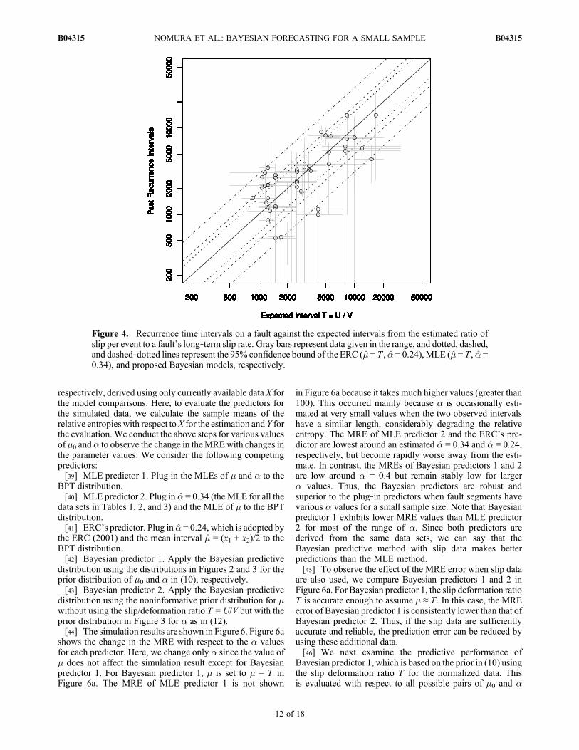
[36] First, we examine the goodness of fit of each predic-tive distribution to past recurrence intervals. Figure 4 showsthe relationship between the past recurrence intervals and theexpected interval T = U/V from the slip data in Table 1. Thepast recurrence intervals appear to be distributed aroundthe expected interval T . However, if we apply the ERC’smethod, which uses the plug‐in predictive distributionf (x∣�̂, �̂) with �̂ = T and �̂ = 0.24, its 95% confidence intervalis too narrow to cover most of the past recurrence intervals.Even if we instead apply �̂ = 0.34, the common MLE for allthe data sets, many outliers from the 95% confidence intervalstill appear. In contrast, the proposedBayesian forecast modelgives appropriate confidence bounds for the recurrence inter-val data.[37] Additionally, in Figure 5 we plot the ratio of the

recurrence interval to the expected interval T as spikes andcompare its histogram and empirical cumulative distribu-tion with each predictive distribution. The plug‐in predictive

distributions of both the ERC and the MLE are concentratedin narrow ranges, whereas the proposed Bayesian predictivedistribution better matches the normalized data. Thus, whenwe use the slip data T = U/V for the mean parameter m, theproposed Bayesian model fits the data better than the othermodels do.

5.2. Simulation Experiment

[38] In addition to fitting the models to past data sets, weshow their theoretical predictive performance by using sim-ulated data sets. We assume a virtual fault whose recurrenceintervals are distributed as the BPT distribution with a fixedparameter (m, a) and the slip deformation ratio T = U/V isgiven. Then, we generate simulated data and evaluate thepredictive performance as follows: (1) generate two consec-utive intervals X = (x1, x2) from the above BPT distribution,(2) apply each forecast model to the generated data andestimate the predictive density [denoted f̂ (y)] as describedbelow, (3) measure the prediction error of f̂ (y) from f (y∣m, a)

Table 5. ABIC Values for Each Combination of Prior Distributionsa

Prior Distribution of m0 Prior Distribution of a

ABIC Difference of ABICDistribution Hyperparameters Distribution Hyperparameters

Weibull a1 = 2.799 b1 = 1.252 Weibull a2 = 2.010 b2 = 0.421 2867.0 0.0Weibull a1 = 2.773 b1 = 1.255 Gamma c2 = 3.208 g2 = 8.596 2867.2 0.2Weibull a1 = 2.742 b1 = 1.258 Lognormal n2 = −1.146 s2 = 0.579 2868.0 1.0Weibull a1 = 2.732 b1 = 1.259 BPT m2 = 0.373 a2 = 0.625 2867.7 0.8Weibull a1 = 2.820 b1 = 1.252 Uniform x2 = 0.724 2867.9 0.9Weibull a1 = 2.812 b1 = 1.283 Exponential l2 = 2.450 2881.6 14.7Gamma c1 = 6.031 g1 = 5.384 Weibull a2 = 2.005 b2 = 0.422 2867.2 0.2Gamma c1 = 5.975 g1 = 5.323 Gamma c2 = 3.194 g2 = 8.532 2867.3 0.4Gamma c1 = 5.902 g1 = 5.245 Lognormal n2 = −1.144 s2 = 0.581 2868.1 1.1Gamma c1 = 5.876 g1 = 5.221 BPT m2 = 0.375 a2 = 0.627 2867.9 0.9Gamma c1 = 6.182 g1 = 5.518 Uniform x2 = 0.728 2868.1 1.2Gamma c1 = 6.815 g1 = 5.919 Exponential l2 = 2.402 2881.6 14.7Lognormal n1 = 0.041 s1 = 0.397 Weibull a2 = 1.991 b2 = 0.429 2868.1 1.1Lognormal n1 = 0.044 s1 = 0.397 Gamma c2 = 3.135 g2 = 8.219 2868.3 1.3Lognormal n1 = 0.048 s1 = 0.397 Lognormal n2 = −1.126 s2 = 0.589 2869.0 2.1Lognormal n1 = 0.047 s1 = 0.398 BPT m2 = 0.383 a2 = 0.637 2868.8 1.8Lognormal n1 = 0.045 s1 = 0.386 Uniform x2 = 0.742 2868.9 2.0Lognormal n1 = 0.096 s1 = 0.337 Exponential l2 = 2.304 2881.9 14.9BPT m1 = 1.127 a1 = 0.400 Weibull a2 = 1.983 b2 = 0.432 2868.2 1.3BPT m1 = 1.130 a1 = 0.398 Gamma c2 = 3.103 g2 = 8.075 2868.4 1.5BPT m1 = 1.135 a1 = 0.396 Lognormal n2 = −1.119 s2 = 0.594 2869.2 2.2BPT m1 = 1.135 a1 = 0.397 BPT m2 = 0.387 a2 = 0.642 2869.0 2.0BPT m1 = 1.127 a1 = 0.389 Uniform x2 = 0.747 2869.1 2.1BPT m1 = 1.167 a1 = 0.342 Exponential l2 = 2.298 2881.8 14.9Uniform x1 = 2.040 Weibull a2 = 1.996 b2 = 0.415 2870.9 3.9Uniform x1 = 2.040 Gamma c2 = 3.192 g2 = 8.681 2871.1 4.1Uniform x1 = 2.063 Lognormal n2 = −1.162 s2 = 0.580 2871.9 4.9Uniform x1 = 2.063 BPT m2 = 0.368 a2 = 0.625 2871.6 4.7Uniform x1 = 2.040 Uniform x2 = 0.722 2871.7 4.7Uniform x1 = 2.085 Exponential l2 = 2.531 2885.2 18.2Exponential l1 = 0.966 Weibull a2 = 2.012 b2 = 0.411 2884.0 17.0Exponential l1 = 0.966 Gamma c2 = 3.241 g2 = 8.908 2884.1 17.2Exponential l1 = 0.966 Lognormal n2 = −1.170 s2 = 0.575 2884.8 17.8Exponential l1 = 0.967 BPT m2 = 0.364 a2 = 0.620 2884.6 17.6Exponential l1 = 0.960 Uniform x2 = 0.724 2885.1 18.1Exponential l1 = 0.946 Exponential l2 = 2.548 2898.8 31.8Non‐informative Weibull a2 = 1.993 b2 = 0.420 2999.1 132.1Non‐informative Gamma c2 = 3.155 g2 = 8.461 2999.2 132.3Non‐informative Lognormal n2 = −1.149 s2 = 0.587 2999.9 133.0Non‐informative BPT m2 = 0.374 a2 = 0.634 2999.7 132.7Non‐informative Uniform x2 = 0.725 3000.1 133.2Non‐informative Exponential l2 = 2.427 3013.3 146.3

aHere, “non‐informative” indicates that the scale‐invariant distribution for m shown in (12) whose domain is bounded from 1 year to 100,000 years, is used.

NOMURA ET AL.: BAYESIAN FORECASTING FOR A SMALL SAMPLE B04315B04315

10 of 18

by using their relative entropy RE(f∣f̂ ), (4) repeat steps 1, 2,and 3 by 100 times and take the mean of the relative entropy(MRE) values to represent the predictive performance. Insteps 3 and 4 we adopt the MRE by the following rationale.We evaluate the predictive performance of the predictors~f (y∣X) by the MRE

Ex RE f �ð Þj~f �jXð Þ� �� ¼ Ex Ey½log f Yð Þ=~f Y jXð Þ� �� ; ð13Þ

where Ex and Ey represent the expectation from the dis-tributions of the current data X and future data Y, respectively;the probability density function of the both samples is thesame as f (·). Both the AIC and the ABIC [Akaike, 1974, 1980]are estimates of this quantity in terms of the logarithm of thelikelihood function and the integrated posterior function,

Figure 2. Prior distribution of m0 compared with the MLEsof m0 from individual fault segments. (a) Solid curve repre-sents the prior density of m0 that minimizes the ABIC inTable 5. The MLEs of m0 are indicated by spikes, and theirfrequency is shown as a gray histogram. (b) Solid curverepresents the cumulative prior distribution of m0. Gray linerepresents the empirical cumulative distribution of the respec-tive MLEs of m0.

Figure 3. Prior distribution of a compared with the modi-fied MLEs of a from individual fault segments. (a) Solidcurve represents the prior density of a that minimizes theABIC in Table 5. Modified MLEs of a are indicated byspikes, and their frequency is shown as a gray histogram. (b)Solid curve represents the cumulative prior distribution of a.Gray line represents the empirical cumulative distribution ofthe modified MLEs of a. Vertical dotted line and dashed linerepresent the ERC’s estimated �̂ = 0.24 and MLE �̂ = 0.34estimated as a common parameter for all fault segments inTables 1, 2, and 3, respectively.

NOMURA ET AL.: BAYESIAN FORECASTING FOR A SMALL SAMPLE B04315B04315

11 of 18

respectively, derived using only currently available data X forthe model comparisons. Here, to evaluate the predictors forthe simulated data, we calculate the sample means of therelative entropies with respect toX for the estimation and Y forthe evaluation. We conduct the above steps for various valuesof m0 anda to observe the change in theMREwith changes inthe parameter values. We consider the following competingpredictors:[39] MLE predictor 1. Plug in the MLEs of m and a to the

BPT distribution.[40] MLE predictor 2. Plug in �̂ = 0.34 (the MLE for all the

data sets in Tables 1, 2, and 3) and the MLE of m to the BPTdistribution.[41] ERC’s predictor. Plug in �̂ = 0.24, which is adopted by

the ERC (2001) and the mean interval �̂ = (x1 + x2)/2 to theBPT distribution.[42] Bayesian predictor 1. Apply the Bayesian predictive

distribution using the distributions in Figures 2 and 3 for theprior distribution of m0 and a in (10), respectively.[43] Bayesian predictor 2. Apply the Bayesian predictive

distribution using the noninformative prior distribution for mwithout using the slip/deformation ratio T = U/V but with theprior distribution in Figure 3 for a as in (12).[44] The simulation results are shown in Figure 6. Figure 6a

shows the change in the MRE with respect to the a valuesfor each predictor. Here, we change only a since the value ofm does not affect the simulation result except for Bayesianpredictor 1. For Bayesian predictor 1, m is set to m = T inFigure 6a. The MRE of MLE predictor 1 is not shown

in Figure 6a because it takes much higher values (greater than100). This occurred mainly because a is occasionally esti-mated at very small values when the two observed intervalshave a similar length, considerably degrading the relativeentropy. The MRE of MLE predictor 2 and the ERC’s pre-dictor are lowest around an estimated �̂ = 0.34 and �̂ = 0.24,respectively, but become rapidly worse away from the esti-mate. In contrast, the MREs of Bayesian predictors 1 and 2are low around a = 0.4 but remain stably low for largera values. Thus, the Bayesian predictors are robust andsuperior to the plug‐in predictors when fault segments havevarious a values for a small sample size. Note that Bayesianpredictor 1 exhibits lower MRE values than MLE predictor2 for most of the range of a. Since both predictors arederived from the same data sets, we can say that theBayesian predictive method with slip data makes betterpredictions than the MLE method.[45] To observe the effect of the MRE error when slip data

are also used, we compare Bayesian predictors 1 and 2 inFigure 6a. For Bayesian predictor 1, the slip deformation ratioT is accurate enough to assume m ≈ T . In this case, the MREerror of Bayesian predictor 1 is consistently lower than that ofBayesian predictor 2. Thus, if the slip data are sufficientlyaccurate and reliable, the prediction error can be reduced byusing these additional data.[46] We next examine the predictive performance of

Bayesian predictor 1, which is based on the prior in (10) usingthe slip deformation ratio T for the normalized data. Thisis evaluated with respect to all possible pairs of m0 and a

Figure 4. Recurrence time intervals on a fault against the expected intervals from the estimated ratio ofslip per event to a fault’s long‐term slip rate. Gray bars represent data given in the range, and dotted, dashed,and dashed‐dotted lines represent the 95% confidence bound of the ERC (�̂ = T , �̂ = 0.24), MLE (�̂ = T , �̂ =0.34), and proposed Bayesian models, respectively.

NOMURA ET AL.: BAYESIAN FORECASTING FOR A SMALL SAMPLE B04315B04315

12 of 18

Figure 5. Predictive distribution of each model comparedwith the recurrence intervals standardized as Xi /T (dividedby the expected interval T = U/V from slip data). (a) Predic-tive densities (curves) and normalized recurrence intervals(spikes and gray histogram). Solid curve is the Bayesian pre-dictive density using the prior density shown in Figures 2and 3. Dotted and dashed curves are the plug‐in predictivedensities with the ERC’s estimates (�̂ = T , �̂ = 0.24) and theMLE of as for all data sets (�̂ = T , �̂ = 0.34), respectively.(b) Cumulative predictive distributions (curves) and empir-ical distribution of normalized recurrence intervals (grayline). Solid, dotted, and dashed curves correspond to thepredictive densities in Figure 5a.

Figure 6. (a) Prediction error (MRE) of MLE predictor 2(dashed line), the ERC’s predictor (dotted line), Bayesian pre-dictor 1 when m0 = 1 (solid line), and Bayesian predictor 2(dashed‐dotted line) for the sampled data with various a.(b) Prediction error (MRE) of Bayes predictor 1 with variousvalues of m0 and a shown in contour lines. Vertical axisshows how the accuracy of the slip/deformation ratio T(i.e., the deviation of m0 from 1) affects the MRE of Bayesianpredictor 1. On the horizontal dashed line, the slip/deforma-tion ratio T just coincides with m.

NOMURA ET AL.: BAYESIAN FORECASTING FOR A SMALL SAMPLE B04315B04315

13 of 18

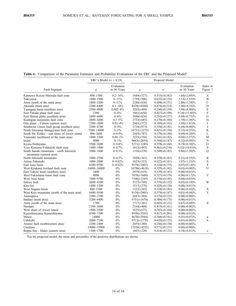
Table 6. Comparison of the Parameter Estimates and Probability Evaluations of the ERC and the Proposed Modela

Fault Segment

ERC’s Model (�̂ = 0.24) Proposal Model

Index inFigure 7�̂

Evaluationin 30 Years �̂ �̂

Evaluationin 30 Years

Kannawa‐Kouzu‐Matsuda fault zone 800–1300 0.2–16% 1449(±327) 0.333(±0.182) 1.66(±2.09)% ATakeyama 1600–1900 6–11% 1759(±506) 0.632(±0.152) 3.33(±1.53)% BAtera (north of the main area) 1800–2500 6–11% 2248(±638) 0.604(±0.151) 2.80(±1.38)% CAkinada (main area) 2300–6400 0.1–10% 8439(±4360) 0.474(±0.214) 1.40(±4.35)% DYamagata basin (northern area) 2500–4000 0.002–8% 3263(±499) 0.244(±0.159) 3.98(±8.00)% EEast Takada plane fault zone 2300 0–8% 1601(±656) 0.427(±0.199) 9.14(±15.49)% FEast Shonai plane (southern area) 2400–4600 0–6% 3696(±656) 0.292(±0.157) 0.44(±0.75)% GKushigata mountains fault zone 2800–4200 0.3–5% 3733(±685) 0.270(±0.160) 1.59(±1.39)% HOita plane ‐ Yubuin (eastern area) 2300–3000 0.03–4% 2043(±372) 0.389(±0.163) 3.09(±1.61)% ISouthwest Unzen fault group (northern area) 2500–4700 0–4% 3718(±973) 0.350(±0.181) 0.49(±0.80)% JNorth Enayama‐Sanageyama fault zone 7200–14000 0–2% 10751(±2273) 0.421(±0.150) 0.35(±0.25)% KSouth Mt. Rokko ‐ east shore of Awazi island 900–2600 0–0.9% 2445(±787) 0.379(±0.188) 0.09(±0.38)% LYamazaki (northwest of the main area) 1800–2300 0.09–1% 2255(±556) 0.341(±0.182) 0.94(±1.27)% MIzumi 8000 0–1% 9663(±2854) 0.366(±0.187) 0.32(±0.49)% NKyoto‐Nishiyama 3500–5600 0–0.8% 5271(±1249) 0.358(±0.160) 0.19(±0.30)% OYoro‐Kuwana‐Yokkaichi fault zone 1400–1900 0–0.7% 1012(±493) 0.461(±0.210) 9.52(±14.63)% PSouth Sanuki mountains ‐ north Ishizuchi

mountains (eastern area)1000–1600 0–0.3% 1316(±278) 0.349(±0.183) 0.86(±1.50)% Q

North Ishizuchi mountains 1000–2500 0–0.3% 1929(±341) 0.359(±0.163) 0.21(±0.55)% RArima‐Takatsuki 1000–2000 0–0.02% 1623(±533) 0.622(±0.161) 1.07(±1.23)% SEast Aizu basin 6300–9300 0–0.02% 8579(±1805) 0.354(±0.155) 0.07(±0.14)% TWest Kitakami lowland fault zone 16000–26000 0% 16796(±4610) 0.355(±0.182) 0.03(±0.08)% UEast Yokote basin (northern area) 3400 0% 2979(±619) 0.339(±0.183) 0.00(±0.01)%West Fukushima basin fault zone 8000 0% 7670(±1609) 0.327(±0.179) 0.06(±0.17)% VWest Aizu basin 7400–9700 0% 7100(±1545) 0.370(±0.185) 0.00(±0.03)%Sekiya fault 2600–4100 0% 3527(±740) 0.376(±0.152) 0.02(±0.10)% WKita‐Izu 1400–1500 0% 1517(±278) 0.429(±0.130) 0.00(±0.01)%West Nagano basin 800–2500 0% 1323(±365) 0.358(±0.183) 0.06(±0.42)% XWest Kiso mountains (north of the main area) 6400–9100 0% 8130(±2005) 0.579(±0.147) 0.01(±0.04)% YAtotsugawa 2300–2700 0% 2647(±384) 0.276(±0.122) 0.00(±0.00)%Inadani (main area) 5200–6400 0% 6751(±1670) 0.306(±0.175) 0.00(±0.01)%Atera (south of the main area) 1700 0% 1717(±361) 0.603(±0.131) 0.67(±0.69)% ZNeodani 2100–3600 0% 2164(±404) 0.419(±0.161) 0.00(±0.06)%West shore of Awazi island 1800–2500 0% 2625(±675) 0.383(±0.164) 0.00(±0.00)%Kuenohirayama‐Kameishiyama 4300–7300 0% 8930(±3565) 0.417(±0.201) 0.00(±0.01)%Minou 14000 0% 8670(±2944) 0.386(±0.191) 0.01(±0.07)% aUshikubi 5000–7100 0% 6712(±1578) 0.420(±0.152) 0.01(±0.06)% bAtsumi fault (northwestern area) 2200–2400 0% 2455(±380) 0.246(±0.138) 0.00(±0.00)%Umehara 14000–15000 0% 15526(±4255) 0.571(±0.151) 0.00(±0.00)%Beppu bay ‐ Hideo (eastern area) 1300–1700 0% 1667(±320) 0.414(±0.131) 0.18(±0.41)% c

aFor the proposed model, the mean and percentiles of the posterior distributions are shown.

NOMURA ET AL.: BAYESIAN FORECASTING FOR A SMALL SAMPLE B04315B04315

14 of 18

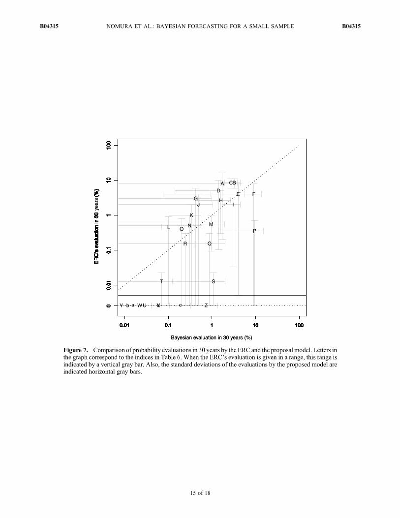
Figure 7. Comparison of probability evaluations in 30 years by the ERC and the proposal model. Letters inthe graph correspond to the indices in Table 6. When the ERC’s evaluation is given in a range, this range isindicated by a vertical gray bar. Also, the standard deviations of the evaluations by the proposed model areindicated horizontal gray bars.

NOMURA ET AL.: BAYESIAN FORECASTING FOR A SMALL SAMPLE B04315B04315

15 of 18

for the data. Figure 6b depicts the change in the MREvalues with respect to m0 and a by contour plots. The MREerror is minimized when m0 and a are around 1.2 and 0.4,respectively, near the mean of the prior distribution. Here,when m0 = m/T is around 1, the mean recurrence time T

estimated from the slip data is close to the true meanparameter m. However, even if m and T differ greatly and theirratio is 2 or 0.5, the MRE error does not become much worse.Therefore, Bayesian predictor 1 shows stable, improvedpredictive performance for various values of m0 and a whenonly a few data are available.

6. Discussion

[47] In this section, we conduct a diagnostic analysis ofsome data sets relative to the predictive distributions. Weapplied the proposed Bayesian method to the data sets ofthe ERC in Tables 1 and 2 to compare the parameter esti-mates and probability evaluations in the next 30 years. Theresults are listed in Table 6. The value ranges in the ERC’sevaluation result from occurrence time uncertainty of pa-leoearthquakes. In contrast, we show the uncertainty of theevaluation of the proposed model by 16% and 84% percen-tiles which represent 1 standard deviation from the meanin a normal distribution. Note that the two parameters m anda are correlated in their posterior distribution while not cor-related in their prior distribution as in section 4.1. The cor-relation is caused by the property of the likelihood of BPTdistribution that the larger coefficient of variation a widenthe probable range of themean recurrence interval m as shownby Parsons [2008b].[48] In Figure 7, we plot the probability evaluations given

in Table 6 to provide a visual comparison of the ERC’sprediction and our proposed model. Both evaluationsare positively correlated on a logarithmic scale, but alsoshow large differences. In particular, in several cases theERC gives probabilities equal to 0, whereas our proposedmodel gives results significantly greater than 0. This isbecause the ERC’s evaluation uses only limited parametervalues that forecast occurrence probabilities of nearly 0. Incontrast, our proposed model takes the mean of the eva-luations for all parameter values, some of which yieldhigher probabilities. Here we give specific examples whereactive faults show considerable differences between theERC and our model. In the Yoro‐Kuwana‐Yokkaichi faultzone, the ERC estimates m at 1700–1900 yr by using theslip deformation ratio, as shown in Table 6. However,the interval between the most recent two events is only100–1000 yr (Table 1), which is much shorter than theERC’s estimate. Our proposed model, considering both pastintervals and the slip deformation ratio, estimates m ataround 1000, which yields a probability evaluation thatdiffers considerably from that of the ERC. In the Arima‐Takatsuki fault zone, the most recent two intervals calcu-lated from Table 1 are about 300–800 yr and 2000 yr andappear quite variable. This implies that the coefficientof variation a of the intervals is substantially larger thanthose of the other fault segments, but the ERC applies �̂ =0.24 to this fault segment as it does to all the fault segmentsin Japan, regardless of its distinctive recurrence data. Incontrast, our proposed model uses the prior distribution fora and gives the posterior mean of a about 0.6 in thisparticular data set. Thus, the large difference in the esti-mates of a causes the large difference in the evaluations.[49] There is significant regional variability in recurrence

parameters; we show the estimates of each parameter on amap in Figure 8. The values of m are lower in subduction

Figure 8. Map of active faults on land and in subductionzones in Japan; colors represent the Bayes estimates (meansof the posterior distributions) of (a) m and (b) a, respec-tively. Figures 8a and 8b represent the locations of theYoro‐Kuwana‐Yokkaichi and Arima fault zones. (c) All ofthe detected active faults on land are shown in red. Largestisland in the center of the map is Honshu.

NOMURA ET AL.: BAYESIAN FORECASTING FOR A SMALL SAMPLE B04315B04315

16 of 18

zones than on land, possibly because of the significantlyhigher loading rates and therefore shorter recurrence times.Some small repeated earthquakes off the east coast ofnorthern Honshu have very short recurrence intervals, onthe order of 10 years, because these earthquakes have smallslip sizes and therefore short loading times.[50] The values of a are highest in the center of Honshu,

where the density of active faults is substantially higher thanin other districts in Japan. Recall the relationship between thea parameter of the BPT distribution and the s parameters ofthe Brownian relaxation oscillator described in section 2.5.1.Higher a values imply larger s values of the Brownian per-turbation rate, which may indicate that the steady stressloading on an active fault is more frequently disturbed bystress transfer from ruptures on other active faults nearby.Indeed, we can expect intensive interactions in regionsdensely occupied by fault systems. In contrast, the smallrepeated earthquakes off the east coast of northern Honshuhave very small a values, indicating regular recurrenceintervals. Hence, a small a value may imply less influenceby stress changes due to ruptures elsewhere. The repeatedearthquakes on the plate boundary occur at asperities isolatedfrom other asperities. These regional variability of the para-meters can be incorporated into the prior distribution, but itremains for future study.

7. Conclusion and Remarks

[51] In this paper, we have proposed a Bayesian predictivemodel to overcome the difficulties in forecasting character-istic earthquakes using very small samples or even one event,in which case the slip per event and long‐term slip rate areused. The prior distribution of the BPT parameters is assumedto be common to recurrence data from all investigated faultsegments globally, and the prior distribution is selected as thatbest fit to them by means of the ABIC using data listed inTables 1, 2, and 3.[52] We have compared the proposed Bayesian model to

conventional plug‐in models using geological data and sim-ulated data. For the real data sets, the Bayesian model is quiteflexible, so its predictive distribution applies broadly,whereas the plug‐in models do not fit well in some situations,because they have fixed shape parameters. In simulationexperiments, we compared the expected predictive perfor-mance in terms of the MRE criterion as an expected predic-tion error. For a wide range of parameter values, the Bayesianpredictors show far more stable and superior performance toconventional MLE‐based plug‐in predictors.[53] In this manuscript we have concentrated on the BPT

model, but we believe that the Bayesian prediction method-ology and the procedure for choosing the best prior modelfor the parameters can be applied to other renewal andproximate models.[54] A problem that remains after some diagnostic anal-

ysis is the reliability of the data, especially the mean recur-rence time calculated from the slip per event divided by thelong‐term fault slip rate. If these geological slip data arenot reliable or not representative, the calculated meanrecurrence time may have a large bias. Therefore, theuncertainty of these data should be carefully considered inthe estimation. We thus suggest that a prior distributionthat takes various errors into account is needed to improve

prediction. A similar problem remains with regard to theuncertainty of the occurrence times in the data, which canbe incorporated into a prior model [cf. Ogata, 1999] to pro-duce a less biased predictor.

Appendix A: Hazard Function of the BayesianPredictive Distribution

[55] The two expressions of the hazard rate function in(5) and (7) are proven to be equivalent by the followingcalculation:

~h yjXð Þ ¼~f yjXð Þ

1� ~F yjXð Þ

¼RQ f yj�ð Þ � posterior �jXð Þd�R

Q 1� F yj�ð Þf g � posterior �jXð Þd�

¼ZQ

f yj�ð Þ1� F yj�ð Þ 1� F yj�ð Þf g L �jXð Þ� �ð ÞR

Q L �jXð Þ� �ð Þd� d� �� Z

Q1� F yj�ð Þf g L �jXð Þ� �ð ÞR

Q L �jXð Þ� �ð Þd� d� �

¼RQ h yj�ð Þ 1� F yj�ð Þf gL �jXð Þ� �ð Þd�R

Q 1� F yj�ð Þf gL �jXð Þ� �ð Þd�

¼RQ h yj�ð ÞL �jX; Y > yð Þ� �ð Þd�R

Q L �jX; Y > yð Þ� �ð Þd�¼

ZQh yj�ð Þ � posterior �jX; Y > yð Þd�:

Appendix B: Bias of the MLE for a[56] When the interval lengthsX1,X2, � � �,Xn, n ≥ 2 between

consecutive events are known, the MLEs of the BPT param-eters, m and a, are given by

�̂ ¼ 1

n

Xni¼1

Xi;

�̂2 ¼ 1

n

Xni¼1

�̂

Xi� 1

� �;

and the expectation of �̂ is calculated as follows:

E �̂2� ¼ E

1

n

Xni¼1

�̂

Xi� 1

� �" #

¼ E1

n

Xni¼1

1n

Pnj¼1 Xj

Xi� 1

( )" #

¼ E1

n2Xi 6¼j

Xj

Xi� 1

� �" #

¼ 1

n2Xi 6¼j

E Xj

� � E 1

Xi

�� 1

� �:

Then, applying E[Xj] = m and E[1/Xi] = (1 + a2)/m gives

E �̂2� ¼ 1

n2Xi 6¼j

�2 ¼ n� 1

n�2:

NOMURA ET AL.: BAYESIAN FORECASTING FOR A SMALL SAMPLE B04315B04315

17 of 18

[57] Acknowledgments. We are grateful to the anonymous reviewersand to an Associate Editor for their painstaking work and useful suggestions.We also thank Tom Parsons for the critical and constructive review whichwas helpful in improving the manuscript. This study was supported in partby the Japan Society for the Promotion of Science under Grant‐in‐Aidfor Scientific Research 20240027 and by the 2010 projects of the Instituteof Statistical Mathematics and the Research Organization of Informationand Systems at the Transdisciplinary Research Integration Center.

ReferencesAitchison, J. (1975), Goodness of prediction fit, Biometrika, 62, 547–554.Akaike, H. (1974), A new look at the statistical model identification, IEEETrans. Autom. Control., 19, 716–723.

Akaike, H. (1978), On the likelihood of a time series model, Statistician,27, 217–235.

Akaike, H. (1980), Likelihood and Bayes procedure, in Bayesian Statistics,edited by J. M. Bernard et al., pp. 1–13, Univ. of Valencia Press, Valencia,Spain.

Akaike, H. (1985), Prediction and entropy, in A Celebration of Statistics,The ISI Centenary Volume, edited by A. C. Atkinson and S. E. Feinberg,pp. 1–24, Springer, New York.

Bakun, W. H., and A. G. Lindh (1985), The Parkfield, California, earth-quake prediction experiment, Science, 229, 619–624.

Becker, A., M. Ferry, K. Monecke, M. Schnellmann, and D. Giardini(2005), Multiarchive paleoseismic record of late Pleistcene and Holocenestrong earthquakes in Switzerland, Tectonophysics, 400, 153–177.

Boltzmann, L. (1878), Weitere Bemerkungen über einige Plobleme dermechanischen Wärmetheorie, Wiener Berichre, 78, 7–46.

Box, G. P. B., and G. C. Tiao (1973), Bayesian Inference in StatisticalAnalysis, 588 pp., Addison‐Wesley, Reading, Mass.

Clague, J. J. (1997), Evidence for large earthquakes at the Cascadia subduc-tion zone, Rev. Geophys., 35, 439–460.

Console, R., M. Murru, G. Falcone, and F. Catalli (2008), Stress inter-action effect on the occurrence probability of characteristic earthquakesin central Apennines, J. Geophys. Res., 113, B08313, doi:10.1029/2007JB005418.

Fitzenz, D. D., M. A. Ferry, and A. Jalobeanu (2010), Long‐term slip his-tory discriminates among occurrence models for seismic hazard assess-ments, Geophys. Res. Lett., 37, L20307, doi:10.1029/2010GL044071.

Good, I. J. (1965), The Estimation of Probabilities, MIT Press, Cambridge,Mass.

Hasegawa, Y., T. Hashimoto, F. Kusano, K. Yoshikawa, and S. Onishi(2005), Detection of the characteristic earthquake activity of the middleclass earthquakes in the Tohoku district, Japan, J. Seismol. Soc. Jpn.,58, 67–70.

Hayashi, Y., and K. Maeda (2009), Comparison between various stochasticrenewal process models of paleoseismic activity data of major active faultzones in Japan (in Japanese with English summary and captions), ActiveFault Res., 30, 27–36.

Kagan, Y. Y., and L. Knopoff (1987), Random stress and earthquake sta-tistics: Time dependence, Geophys. J. R. Astron. Soc., 88, 723–731.

Kullback, S., and R. A. Leibler (1951), On information and sufficiency,Ann. Math. Stat., 22, 79–86.

Matsuzawa, T., T. Igarashi, and A. Hasegawa (2002), Characteristic small–earthquake sequence off Sanriku, northern Honshu, Japan, Geophys. Res.Lett., 29(11), 1543, doi:10.1029/2001GL014632.

Matthews, M. V., W. L. Ellsworth, and P. A. Reasenberg (2002), ABrownian model for recurrent earthquakes, Bull. Seismol. Soc. Am., 92,2233–2250.

Nishenko, S. P. (1991), Circum‐Pacific seismic potential: 1989–1999, PureAppl. Geophys., 135, 169–259.

Nishenko, S. P., and R. Buland (1987), A generic recurrence intervaldistribution for earthquake forecasting, Bull. Seismol. Soc. Am., 77,1382–1399.

Ogata, Y. (1999), Estimating the hazard of rupture using uncertain occur-rence times of paleoearthquakes, J. Geophys. Res., 104, 17,995–18,014.

Ogata, Y. (2001), Biases and uncertainties when estimating the hazard ofthe next Nankai earthquake (in Japanese with English summary and figurecaptions), J. Geogr., 10, 602–614.

Ogata, Y. (2002), Slip‐size‐dependent renewal processes and Bayesianinferences for uncertainties, J. Geophys. Res., 107(B11), 2268,doi:10.1029/2001JB000668.

Okada, M., H. Takayama, F. Hirose, and N. Uchida (2007), A prior distri-bution of the parameters in the renewal model with lognormal distribu-tion used for estimating the probability of recurrent earthquakes (inJapanese with English summary and figure captions), J. Seismol. Soc.Jpn., 60, 85–100.

Parsons, T. (2005), Significance of stress transfer in time‐dependentearthquake probability calculations, J. Geophys. Res., 110, B05S02,doi:10.1029/2004JB003190.

Parsons, T. (2008a), Earthquake recurrence on the south Hayward fault ismost consistent with a time‐dependent, renewal process, Geophys. Res.Lett., 36, L21301, doi:10.1029/2008GL035887.

Parsons, T. (2008b), Monte Carlo method for determining earthquakerecurrence parameters from short paleoseismic catalogs: Example calcu-lations for California, J. Geophys. Res., 113, B03302, doi:10.1029/2007JB004998.

Rhoades, D. A., R. J. Van Dissen, and D. J. Dowrick (1994), On thehandling of uncertainties in estimating the hazard of rupture on a faultsegment, J. Geophys. Res., 99, 13,701–13,712.

Scharer, K. M., G. P. Biasi, R. J. Weldon, and T. E. Furmal (2010), Quasi‐periodic recurrence of large earthquakes on the southern San Andreasfault, Geology, 38, 555–558

Schwartz, D. P., and K. J. Coppersmith (1984), Fault behavior and charac-teristic earthquakes: Examples from the Wasatch and San Andreas faultzones, J. Geophys. Res., 89, 5681–5698.

Shimazaki, K., and T. Nakata (1980), Time‐predictable recurrence modelfor large earthquakes, Geophys. Res. Lett., 7, 279–282.

Utsu, T. (1999), Seismicity Studies: A Comprehensive Review, Univ. ofTokyo Press, Tokyo.

Vere‐Jones, D. (1978), Earthquake prediction: Astatistician’s view, J. Phys.Earth., 26, 129–146.

Wyss, M. (1986), Regular intervals between Hawaiian earthquakes: Impli-cations for predicting the next event, Science, 234, 726–728.

Working Group on California Earthquake Probabilities (1995), Seismichazards in southern California: Probable earthquakes, 1994 to 2024, Bull.Seismol. Soc. Am., 85, 379–439.

Zöller, G., and S. Hainzl (2007), Recurrence time distributions of largeearthquakes in a stochastic model for coupled fault systems: The roleof fault interaction, Bull Seismol. Soc. Am., 97, 1679–1687.

Zöller, G., Y. Ben‐Zion, M. Holschneider, and S. Hainzl (2007), Estimat-ing recurrence times and seismic hazard of large earthquakes on an indi-vidual fault, Geophys. J. Int., 170, 1300–1310.

F. Komaki, Department of Mathematical Informatics, Graduate School ofInformation Science and Technology, University of Tokyo, 7‐3‐1 Hongo,Bunkyo‐ku, Tokyo 113‐8656, Japan.S. Nomura and Y. Ogata, Department of Statistical Science, Graduate

University for Advanced Studies, 10‐3 Midori‐cho, Tachikawa, Tokyo190‐8562, Japan. (nomura@ism.ac.jp)S. Toda, Research Center for Earthquake Prediction, Disaster Prevention

Research Institute, Kyoto University, Gokasho, Uji, Kyoto 611‐0011,Japan.

NOMURA ET AL.: BAYESIAN FORECASTING FOR A SMALL SAMPLE B04315B04315

18 of 18