Initialization and Self-Organized Optimization of Recurrent Neural

Network Connectivity

Joschka Boedecker∗

Dep. of Adaptive Machine Systems,Osaka University,Suita, Osaka,Japan

Oliver Obst

CSIRO ICT Centre,Adaptive Systems Laboratory,Locked Bag 17,North Ryde, NSW 1670,Australia

N. Michael Mayer† and Minoru Asada

JST ERATO Asada Synergistic Intelligence Project,Suita, Osaka,Japan

Reservoir computing (RC) is a recent paradigm in the field of recurrent neu-

ral networks. Networks in RC have a sparsely and randomly connected fixed

hidden layer, and only output connections are trained. RC Networks have re-

cently received increased attention as a mathematical model for generic neural

microcircuits, to investigate and explain computations in neocortical columns.

Applied to specific tasks, their fixed random connectivity, however, leads to sig-

nificant variation in performance. Few problem specific optimization procedures

are known, which would be important for engineering applications, but also in

order to understand how networks in biology are shaped to be optimally adapted

to requirements of their environment. We study a general network initialization

method using permutation matrices and derive a new unsupervised learning rule

based on intrinsic plasticity (IP). The IP based learning uses only local learning,

and its aim is to improve network performance in a self-organized way. Using

three different benchmarks, we show that networks with permutation matrices

for the reservoir connectivity have much more persistent memory than the other

methods, but are also able to perform highly non-linear mappings. We also show

that IP based on sigmoid transfer functions is limited concerning the output

distributions that can be achieved.

† N. Michael Mayer is now with the Dep. of Electrical Engineering, National Chung Cheng University, Chia-Yi,

Taiwan, R.O.C.∗Please address correspondence to: joschka.boedecker@ams.eng.osaka-u.ac.jp

2

INTRODUCTION

Recurrent loops are abundant in the neural circuits of the mammalian cortex. Massive reciprocal con-

nections exist on different scales, linking different brain areas as well as connecting individual neurons in

cortical columns. In these columns as many as 80% of the synapses of neocortical interneurons form a dense

local network (Maass and Markram, 2006) using very specific connectivity patterns for different neuron

types (Douglas et al., 2004). These recurrent microcircuits are very stereotypical and repeated over the

entire neocortex (Silberberg et al., 2002).

Two challenges for computational models of the neocortex are (a) explaining how these stereotypical

microcircuits enable an animal to process a continuous stream of rapidly changing information from its

environment (Maass et al., 2002), and (b) how these circuits contribute to the prediction of future events,

one of the critical requirements for higher cognitive function (Maass and Markram, 2006).

To address these challenges, a mathematical model for generic neural microcircuits, namely the liquid

state machine (LSM), was proposed by Maass et al. (2002). The framework for this model is based on real-

time computation without stable attractors. The neural microcircuits are considered as dynamical systems,

and the time-varying input is seen as a perturbation to the state of the high-dimensional excitable medium

implemented by the microcircuit. The neurons act as a series of non-linear filters, which transform the

input stream into a high-dimensional space. These transient internal states are then transformed into stable

target outputs by readout neurons, which are easy to train (e.g. in order to do prediction or classification

of input signals) and avoid many of the problems of more traditional methods of recurrent neural network

training like slow convergence and vanishing gradients (first described in Hochreiter (1991), see also Bengio

et al. (1994) and Hochreiter et al. (2001)). This approach to neural modeling has become known as reservoir

computing (see Verstraeten et al. (2007) and Lukosevicius and Jaeger (2007) for reviews), and the LSM is

one particular kind of model following this paradigm.

Echo state networks (ESN) (Jaeger, 2001a; Jaeger and Haas, 2004) are another reservoir computing

model similar to LSM. They implement the same concept of keeping a fixed high-dimensional reservoir

of neurons, usually with random connection weights between reservoir neurons small enough to guarantee

stability. Learning procedures train only the output weights of the network to generate target outputs,

but while LSM use spiking neuron models, ESN are usually implemented with sigmoidal nodes, which are

updated in discrete time steps. We use ESN in all the experiments of this study for their better analytical

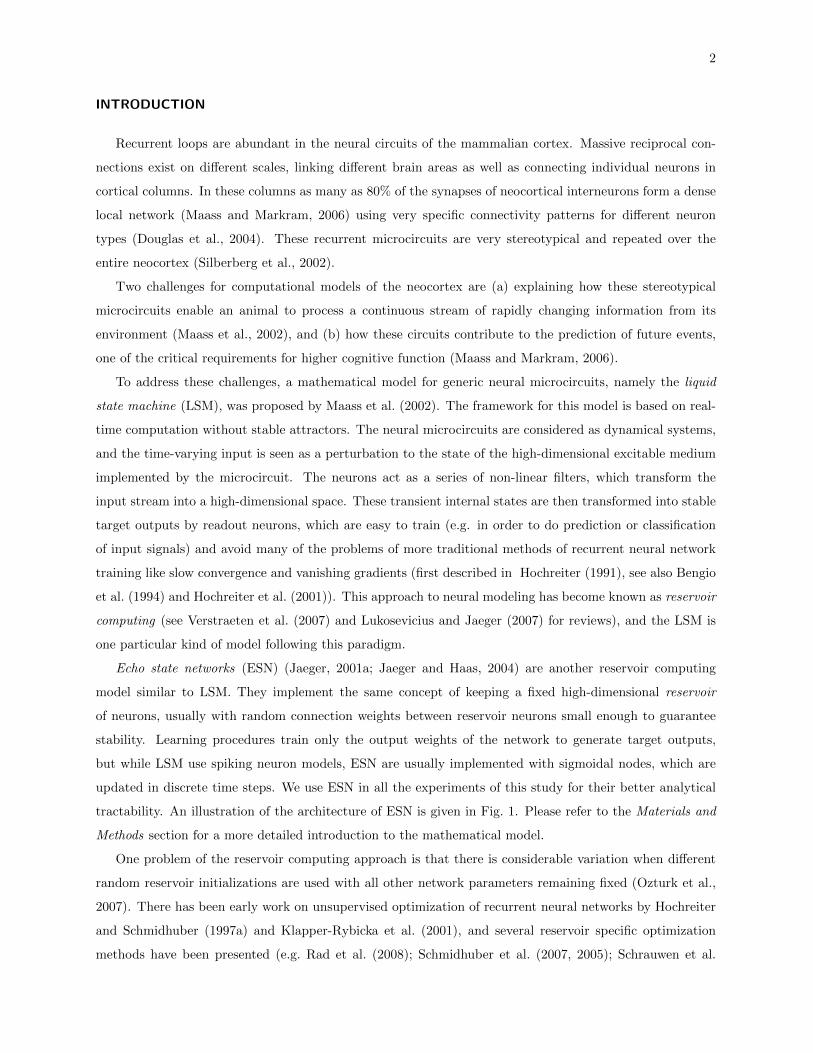
tractability. An illustration of the architecture of ESN is given in Fig. 1. Please refer to the Materials and

Methods section for a more detailed introduction to the mathematical model.

One problem of the reservoir computing approach is that there is considerable variation when different

random reservoir initializations are used with all other network parameters remaining fixed (Ozturk et al.,

2007). There has been early work on unsupervised optimization of recurrent neural networks by Hochreiter

and Schmidhuber (1997a) and Klapper-Rybicka et al. (2001), and several reservoir specific optimization

methods have been presented (e.g. Rad et al. (2008); Schmidhuber et al. (2007, 2005); Schrauwen et al.

3

TABLE I: Glossary

Recurrent Neural Network : A special type of artificial neural network model, which allows loops and recurrent

connections among its nodes.

Echo State Network : A discrete-time recurrent neural network with a hidden layer having fixed (non-

adaptive) random connectivity between its nodes. The only trainable connections

are the output connections. This significantly reduces the learning problem to

basically doing linear regression. An important part of the echo state network

idea is the echo state property. Its definition gives a prerequisite for the global

asymptotic stability of the network for any input it might encounter.

Liquid State Machine: A continuous-time recurrent neural network, which implements the same basic

ideas as echo state networks: to use a hidden layer neurons with fixed random

connectivity and only train the output connections. Liquid state machines were

created in order to model biologically relevant computations (while echo state

networks were conceived as an engineering tool) and as such they are usually

implemented with spiking neuron models (while echo state networks use analog

sigmoid type neurons).

Reservoir Computing : A unified name for different computational approaches using recurrent neural

networks with a fixed random hidden layer and only train a linear output con-

nections. This encompasses Echo State Networks, Liquid State Machines, and,

as a special learning rule, backpropagation-decorrelation (BPDC) learning (Steil,

2004).

Reservoir : Usually denotes the hidden layer of a recurrent neural network following the

reservoir computing approach.

Reservoir Matrix : A matrix whose individual entries are the connection strength values for the

connections between each of the nodes in the reservoir. Sometimes also called

reservoir connectivity matrix.

Spectral Radius: The absolute value of the largest eigenvalue of a matrix. In discrete-time dy-

namical systems such as ESN, the spectral radius will give an indication of the

longest time constant of the network, i.e., how long information will persist in the

network before it decays. A larger spectral radius means longer time constants.

It is also an important measure to determine stability criteria of the network, see

for instance the echo state property in the Materials and Methods section.

Central Limit Theorem: A mathematical theorem in probability theory attributed to Laplace, which states

that the sum of a sufficiently large number of independent and identically dis-

tributed random variables, each with finite mean and variance, will approximate

a Gaussian distribution.

4

win

wout

Recurrent Layer

W

adaptable weights

random weights

Input units Output units

FIG. 1: Architecture of an echo state network. In echo state networks, usually only the connections

represented by the dashed lines are trained, all other connections are setup randomly and remain fixed.

The recurrent layer is also called a reservoir, analogously to a liquid, which has fading memory properties.

As an example, consider throwing a rock into a pond; the ripples caused by the rock will persist for a

certain amount of time and thus information about the event can be extracted from the liquid as long as it

has not returned to its single attractor state — the flat surface.

(2008); Steil (2007); Wierstra et al. (2005); however, as of yet there is no universally accepted standard

method. We study the effect of approaches aiming to reduce this dependency on a random initialization. In

order to do this, we investigate two different approaches: the first one is based on a very specific initialization

of the reservoirs of ESNs (Hajnal and Lorincz, 2006; White et al., 2004), and the second one implements a

pre-training phase for the reservoirs using a local adaptation mechanism. This mechanism models changes

in a neurons intrinsic excitability in response to stimulation. Specifically, it models the phenomenon that

biological neurons lower their firing threshold over time when they receive a lot of stimulation, and raise

it when stimulation is lacking (see e.g. Zhang and Linden (2003) and Daoudal and Debanne (2003) for

more details). A learning rule based on this phenomenon was introduced by Triesch (2005), further studied

in (Triesch, 2007), and has been termed intrinsic plasticity (IP). The reservoir initialization method is based

on the idea of optimally exploiting the high dimensionality of the reservoir. The methods based on IP, while

also using high-dimensional reservoirs, aim to adapt the reservoir for a high entropy of codes. Moreover,

we investigate an IP based learning rule for high sparsity of codes as these have been shown to improve

information processing Field (1994).

We evaluate the different reservoir shaping and initialization methods using three different standard

benchmarks. We find that reservoirs initialized with orthogonal column vectors in their connectivity matrix

exhibit superior short-term memory capacity, and are also able to perform well in tasks requiring highly

non-linear mappings. Furthermore, we identify a problem with an existing IP based rule and point out

limitations of the approach if traditional neuron models are used. We discuss our contributions in the

wider context of recurrent neural network research, and review possible solutions to the limitations that are

identified as consequences of our results in this study.

5

RESULTS

We first present an IP based learning rule that changes a neurons output distribution to approximate

a Laplace distribution. Consequently, we present results for the evaluation of ESN with random reser-

voirs, reservoirs using permutation matrices, and reservoirs pre-trained with IP for Gaussian and Laplace

distributions, respectively.

IP Learning and a Rule for a Laplace Output Distribution

IP learning was introduced in (Triesch, 2005) as a way to improve information transmission in neurons

while adhering to homeostatic constraints like limited energy usage. For a fixed energy expenditure (repre-

sented by a fixed mean of the neurons output distribution), the distribution that maximizes the entropy (and

therefore the information transmission) is the exponential distribution. This was used for single neurons

in (Triesch, 2005) and for neurons in a reservoir in (Steil, 2007) where it lead to a performance improvement

over standard random reservoirs. In (Schrauwen et al., 2008), IP learning for a Gaussian output distribution

of reservoir neurons was investigated, which is the maximum entropy distribution if, in addition to the mean,

the variance of the output distribution is fixed. Again, an overall increase in performance was noted for

several benchmark problems.

A Laplace distribution would lead to sparser codes than the Gaussian, and our hypothesis is that enough

entropy would be preserved for a good input signal approximation. Researching Laplace output distributions

was also suggested in Schrauwen et al. (2008) for similar reasons. Here, analogous to the calculations

in (Schrauwen et al., 2008; Triesch, 2005), we derive an IP learning rule for this distribution to test our

hypothesis.

In order to model the changes in intrinsic excitability of the neurons, the transfer function of our neurons

is generalized with a gain parameter a and a bias parameter b:

y = f(x) = tanh(ax+ b).

The Laplace distribution, which we desire as the reservoir neurons’ output distribution, is defined as

f(x | µ, c) =1

2cexp(−|x− µ|

c), c 6= 0.

Let py(y) denote the sampled output distribution of a reservoir neuron and let the desired output distribution

be p(y), thus p(y) = f(y | µ, c). In the learning process, we try to minimize the difference between py(y)

and p(y), which can be measured with the Kullback-Leibler divergence DKL. Thus, we try to minimize:

DKL =

∫py(y) log

(py(y)

12c exp(− |y−µ|c )

)dy

Taking derivatives of this function with respect to the gain and bias parameters of the neurons’ trans-

fer function (see Materials and Methods section for details), we arrive at the following learning rules for

6

TABLE II: Average memory capacity and normalized root mean squared error (NRMSE) for the NARMA

modeling and the Mackey-Glass prediction tasks in the four different conditions (averaged over 50

simulation runs), standard dev. in parenthesis. Note that the errors for Mackey-Glass are scaled by a

factor of 10−4. For the memory capacity (first row) higher values are better, while lower values in the

errors are better for the prediction tasks (second and third row).

PMT RND IPGAUSS IPLAP

Memory Capacity 62.501 (5.086) 31.884 (2.147) 33.019 (2.464) 32.175 (3.127)

NRMSENARMA 0.385 (0.022) 0.473 (0.035) 0.465 (0.053) 0.482 (0.041)

NRMSEMackey−Glass 3.373 (0.292) 2.411 (0.242) 2.802 (0.416) 2.375 (0.416)

stochastic gradient descent with learning rate η:

∆b = −η(

2y +y(1− y2 + µy)− µ

c|y − µ|

).

∆a = −η(−1

a)− η

(2xy +

yx(1− y2 + µy)− µxc|y − µ|

)=η

a+ ∆bx.

Effects of Reservoir Shape on Memory Capacity and Prediction Accuracy

In order to compare the different reservoir shaping and initialization methods, we tested them on three

different standard benchmarks (cf. Materials and Methods section for details). The first set of experiments

evaluated the short-term memory capacity (MC) of the different networks. In addition, we evaluated the

networks on the task of modeling a 30th order NARMA (nonlinear auto regressive moving average) system,

and with respect to their one-step prediction performance on the Mackey-Glass time-series. These tasks

cover a reasonably wide spectrum of tests for different useful properties of reservoirs and are widely used in

the literature, e.g. in Jaeger (2001a,b); Rad et al. (2008); Schrauwen et al. (2008); Steil (2007).

We tested ESN with four different conditions for the connectivity matrix of the reservoir. In condition

RND, the reservoir matrix was initialized with uniform random values between [−1; 1]. Condition PMT

tested a permutation matrix for the reservoir connectivity. Finally, we used IP optimization with a Gaussian

distribution (cf. Schrauwen et al. (2008)) in IPGAUSS and a Laplace distribution (as described in the

Materials and Methods section) in IPLAP. In all conditions, the reservoirs were scaled to have a spectral

radius of 0.95. In the case of the IP methods, this scaling was done once before the IP training was started.

The results of the experiments are given in Table II, averaged over 50 simulation runs for each of the four

conditions. The networks in the PMT condition essentially show double the memory capacity of networks

in the other conditions, while networks pre-trained with IPGAUSS and IPLAP have very similar values

7

0 20 40 60 80 100 120 140 160 180 2000

0.1

0.2

0.3

0.4

0.5

0.6

0.7

0.8

0.9

1

k

MC k

PMTRNDIPGAUSSIPLAP

FIG. 2: The MCk curves for the uniform random input data. The plot indicates how well the input signal

can be reconstructed (MCk) for increasing delay times k

.

and show a slight increase compared to condition RND. Fig. 2 shows plots of the individual MCk curves

(see Materials and Methods for their definition) for all conditions in the MC task, with the curve for PMT

showing much longer correlations than all the others. The results for the NARMA modeling task are less

pronounced, but look similar in that the PMT networks perform better than the other tested conditions.

The normalized root mean squared error (NRMSE) for IPLAP and IPGAUSS is very similar again,

however, only IPGAUSS has a slight advantage over RND. For the Mackey-Glass one-step prediction, the

performance of the IPLAP networks is better than the other ones, slightly ahead of RND (difference well

within the standard deviation of the error, however). The PMT networks perform worst on this task.

The superior performance of networks in PMT on the short-term memory task could be expected:

networks with a connectivity based on permutation matrices form are a particular instance of orthogonal

networks, which, in turn, can be seen as a multidimensional version of a delay line (for details, see the

Materials and Methods section). From a system theory perspective, the eigenvalues (poles) of the linearized

system implemented by the network correspond to bandpass filters with center frequencies according to their

angle in the complex plane (Ozturk et al., 2007). Larger eigenvalues will lead to longer time constants for the

filters, preserving information for longer time in the network. Figure 3 (a) shows that the eigenvalues of the

connectivity matrix of a 100 node ESN in the PMT condition are all of the same magnitude, and are spaced

relatively uniformly just below the unit circle (the reservoir matrix was scaled to have a maxiumum absolute

eigenvalue of 0.95 in this case, i.e., the matrix elements were either 0 or 0.95). The filters implemented by

this network will thus have long time constants and provide support for many different frequencies in order

to reconstruct the input signal. Compare this to the distribution of the eigenvalues of a connectivity matrix

of an equally sized RND network in Figure 3 (b): they are much less uniformly distributed and have very

different magnitudes, resulting in a mixture of both longer and shorter time constants for the network.

The PMT networks also outperform the other methods on the highly non-linear NARMA task, which

8

FIG. 3: Plot of the reservoir matrix eigenvalues in the complex plane for a 100 node network (a) in the

PMT condition, and (b) in the RND condition. Both matrices have been scaled to have a spectral radius

of 0.95

is less obvious. The NARMA task needs long memory, which the orthogonal reservoirs in PMT are able to

provide; but one might suspect that the specific, rather sparse connectivity would not be able to perform

the kind of non-linear mappings that the task requires (since there is less interaction between neurons in the

reservoir than in networks which are more densely connected). The results show that this is not the case.

The Mackey-Glass prediction task requires shorter time constants and less memory than the other two

tasks. In this case, the IPLAP networks perform best, slightly ahead of the RND condition. The PMT

networks have the same spectral radius as the ones in RND, however, all eigenvalues in PMT have the

same (large) magnitude. Therefore, the network is missing elements implementing shorter time constants,

which would let it react to fast changes in the input. The best results we got on this task were actually

achieved using ESN with fermi neurons and IP learning with an exponential output distribution (results not

9

shown). In this case, the results were significantly better than the ones in RND (cf. also (Steil, 2007)).

IP Revisited

A closer investigation of the almost identical performance of both IP methods revealed that IPLAP

also generated normally distributed output, very similar to IPGAUSS. To better understand the effect of

the different IP rules, we used IP to approximate the Laplace, the Gaussian (both with a tanh activation

function), and the exponential distribution (fermi activation function), respectively, with a single feedfor-

ward unit and uniformly distributed input on the interval [−1; 1]. As expected, the IP learning rule can

successfully generate exponentially distributed output values (Fig. 5 a). IP fails, however, to generate output

distributions that resemble the Gaussian or the Laplace (Fig. 5, b and c). This seems surprising in particular

for the Gaussian, as IP has successfully been used to shape the output distribution of a reservoir (Schrauwen

et al., 2008). A possible explanation for this phenomenon is discussed in the next section.

DISCUSSION

Recurrent neural network models are attractive because they hold the promise of explaining information

processing in biological systems like the human neocortex, as well as being able to serve as tools for engineer-

ing applications. Moreover, they are computationally more powerful than simple feedforward architectures

since they can exploit long-term dependencies in the input when calculating the output. Their theoretical

analysis is complex, yet they are increasingly popular — mainly due to new, efficient architectures and train-

ing methods published in recent years (see (Hammer et al., 2009) for an excellent recent overview). These

include, for instance, self-organizing maps for time series (Hammer et al., 2005), long short-term memory

(LSTM) networks (Hochreiter and Schmidhuber, 1997b), Evolino (Schmidhuber et al., 2007, 2005), and also

the reservoir computing approach as mentioned earlier in the article.

One of the obstacles to the initial applicability of recurrent neural networks was the problem of slow

convergence and instabilities of training algorithms like backpropagation-through-time (BPTT) (Werbos,

1990) or real-time recurrent learning (RTRL) (Williams and Zipser, 1989). One of the important insights

of the reservoir computing approach to overcome these limitations was that it often suffices to choose a

fixed recurrent layer connectivity at random and only train the output connections. Compared to BPTT

or RTRL, this simplifies the training process to a linear regression problem, resulting in significant speed

improvements. It also enabled the use of much larger networks than possible with BPTT or RTRL. Results

on standard benchmarks using reservoir methods were better than any previous of these methods and

practical applications were also shown (Jaeger, 2003).

Compared to “traditional” recurrent neural network learning methods such as BPTT or RTRL, the

reservoir computing paradigm represents a significant step forward for recurrent neural network technolo-

gies. On the other hand, it is clear that the approach gives up many of the degrees of freedom the networks

10

would normally have by fixing the recurrent layer connectivity. Advanced methods such as LSTM net-

works (Hochreiter and Schmidhuber, 1997b) share the advantage of fast learning with ESN, but without

restricting the networks to a fixed connectivity, using a more involved architecture and training method.

For ESN, it has been shown that fixing the connectivity has the effect that different random initializations

of a reservoir will lead to rather large variations in performance if all other parameters of the network setup

remain the same (Ozturk et al., 2007). There have been proposals on how to manually design ESN in

order to give performance that will consistently be better than random initializations (Ozturk et al., 2007),

but there are no universally accepted standard training algorithms to adapt the connectivity in a problem

specific and automatic way, before the output connections are trained.

This article makes two contributions with regard to this problem. As a first contribution, we investigate

permutation matrices for the reservoir connectivity. Their benefit lies in the simple and inexpensive way in

which they can be constructed, and we show that they implement a very effective connectivity for problems

involving a long input history as well as non-linear mappings. For problems requiring fast responses of the

network (or a mixture of slow and fast responses), their usefulness is limited. Furthermore, the method is

general and not problem-specific. The IP based approaches we present and reference throughout the paper

represent a problem-specific training method. They make use of the input signal in order to shape the

output of the reservoir neurons according to a desired probability distribution. The second contribution in

the article is a variation of the IP based approach by deriving a new learning rule to shape the reservoir

node outputs according to a Laplace distribution, and to point out limitations of this method when standard

sigmoidal neuron types are used in the network.

Concerning this last point, the illustration in Fig. 4 sheds light on the reason why an approximation of

some distributions with IP is more difficult than others: given a uniform input distribution and a sigmoid

transfer function, IP learning selects a slice from an output distribution that peaks towards either end of

the input range, but never in the center. The output of an IP trained self-recurrent unit gives an insight

why it is possible to achieve a Gaussian output distribution in a reservoir (Fig. 5, d). From the central limit

theorem it follows that the sum of several i.i.d. random variables approximates a Gaussian. Even though in

case of a recurrent reservoir not all inputs to a unit will be i.i.d., IP has to make input distributions only

similar to each other to approximate a normal distribution in the output. This also explains why the output

of an IP Laplace trained reservoir is normally distributed (several inputs with equal or at least very similar

distributions are summed up). For uniform input and a single unit without recurrence, the best IP can do is

to choose the linear part of the activation function, so that the output is also uniformly distributed (a slice

more in the middle of Fig. 4). With self-recurrent connections, this leads to initially uniform distributions,

which sum up. The resulting output, and eventually the whole reservoir output distribution become more

and more Gaussian. A consequence of this effect is that IP with sigmoid transfer functions cannot be

generalized to arbitrary distributions.

Our results confirm two important points that have been suggested for versatile networks, i.e., networks

which should perform well even when faced with several different input signals or which might be used

11

−1 −0.5 0 0.5 1

1000

2000

3000

−1

−0.5

0

0.5

1

tanh(ax+b)

FIG. 4: Uniform input on the interval [−1; 1] and a tanh(·) transfer function lead to the output

distribution in the histogram. IP selects a slice of this distribution, as illustrated by the vertical lines.

Adapting gain and bias changes width and position of the slice.

for tasks with different requirements. Ozturk et al. (2007) proposed that the eigenvalue distribution of

reservoir matrices should be as uniform as possible, and that it would be needed to scale the effective

spectral radius of the network up or down. For this scaling, they suggested an adaptable bias to the inputs

of each reservoir node. With regard to this proposed requirement, we observed another limitation of purely

IP-based reservoir pre-training: in our experiments (also reported in (Steil, 2007)), the IP learning rule

always increased the spectral radius of the reservoir matrix (dependent on the setting of the IP parameters,

cf. (Schrauwen et al., 2008)), and never decreased it (this is only true for reservoirs which are initialized

with spectral radius < 1). This leads to longer memory, making it harder for the network to react quickly

to new input, and causing interference of slowly fading older inputs with more recent ones. To alleviate this

problem, a combination of instrinsic and synaptic plasticity as studied by Lazar et al. (2007) could enable

scaling of the reservoir matrix depending on the current requirements of the task. The efficiency of synergy

effects that result from a combination of intrinsic and synaptic plasticity was also shown by Triesch (2007),

who additionaly suggested that this combination might be useful in driving networks to the region of best

computational performance (edge of chaos, cf. (Bertschinger and Natschlager, 2004)) while keeping a fixed

energy expenditure for the neurons. In (Lazar et al., 2007), this hypothesis was confirmed to the extent that

networks with a combination of intrinsic and extrinsic plasticity were generally closer to this region than

networks trained with only one form of plasticity.

MATERIALS AND METHODS

Echo State Networks

Learning algorithms for recurrent neural networks have been widely studied (e.g. see Doya (1995) for

an overview). They have, however, not been widely used (Jaeger, 2003) because these learning algorithms,

when applied to arbitrary network architectures, suffer from problems of slow convergence. ESN provide a

12

(a) (b)

(c) (d)

FIG. 5: Panels (a–c) show the effect of IP learning on a single feedforward neuron. Panel (a) shows the

result of IP learning with a single fermi neuron without self-recurrence and a learning rule for the

exponential output distribution. IP successfully produces the desired output distribution. In panels (b)

and (c), we see the effect of IP learning on a single tanh neuron without self-recurrence, trained with a

learning rule for a Gaussian, and a Laplace output distribution, respectively. In both cases, IP learning

fails to achieve the desired result: the best it can do is to drive the neuron to a uniform output

distribution, which has the smallest distance (for the given transfer function) to the desired distributions.

Panel (d) shows the effect of IPGAUSS for a single self-recurrent tanh unit. The achieved output

distribution is significantly more Gaussian-shaped than without the self-recurrence. The effect is amplified

in a network where the neurons receive additional inputs with similar distributions. All units were trained

using 100000 training steps and uniformly distributed input data on the interval [−1; 1].

specific architecture and a training procedure that aims to solve the problem of slow convergence (Jaeger,

2001a; Jaeger and Haas, 2004). ESN are normally used with a discrete-time model, i.e. the network dynamics

are defined for discrete time-steps t, and they consist of inputs, a recurrently connected hidden layer (also

called reservoir) and an output layer (see Fig. 1).

We denote the activations of units in the individual layers at time t by ut , xt , and ot for the inputs,

the hidden layer and the output layer, respectively. We use win, W, wout as matrices of the respective

synaptic connection weights. Using f(x) = tanhx as output nonlinearity for all hidden layer units, the

network dynamics is defined as:

xt = tanh(Wxt−1 + It)

It = winut

ot = woutxt

The main differences of ESN to traditional recurrent network approaches are the setup of the connection

weights and the training procedure. To construct an ESN, units in the input layer and the hidden layer are

connected randomly. Connections between the hidden layer and the output units are the only connections

that are trained, usually with a supervised, offline learning approach: Training data are used to drive

13

the network, and at each time step t, activations of all hidden units x(t) are saved as a new column

to a state matrix. At the same time, the desired activations of output units oteach(t) are collected in a

second matrix. Training in this approach then means to determine the weights wout so that the error

εtrain(t) = (oteach(t)−o(t))2 is minimized. This can be achieved using a simple linear regression (see Jaeger

(2001a) for details on the learning procedure).

For the approach to work successfully, however, connections in the reservoir cannot be completely random;

ESN reservoirs are typically designed to have the echo state property. The definition of the echo state property

has been outlined in Jaeger (2001a). The following section describes this property in a slightly more compact

form.

The Echo State Property

Consider a time-discrete recursive function xt+1 = F (xt ,ut) that is defined at least on a compact sub-

area of the vector-space x ∈ Rn, with n the number of internal units. The xt are to be interpreted as

internal states and ut is some external input sequence, i.e. the stimulus.

The definition of the echo state property is as follows: Assume an infinite stimulus sequence: u∞ =

u0,u1, . . . and two random initial internal states of the system x0 and y0. To both initial states x0 and y0

the sequences x∞ = x0,x1, . . . and y∞ = y0,y1, . . . can be assigned. The update equations for xt+1 and

yt+1 are then:

xt+1 = F (xt ,ut)

yt+1 = F (yt ,ut)

The system F (·) will have the echo states if it is independent from the set ut , and if for any (x0,y0) and

all real values ε > 0, there exists a δ(ε) for which

d(xt ,yt) ≤ ε

for all t ≥ δ(ε), where d is a square Euclidean metric.

Network Setup

For all of the experiments, we used ESNs with 1 input and 100 reservoir nodes. The number of output

nodes was 1 for the NARMA and Mackey-Glass tasks, and 200 for the MC evaluation. In the latter, the 200

output nodes were trained on the input signal delayed by k steps (k = 1 . . . 200). The input weights were

always initialized with values from a uniform random distribution in the range [−0.1; 0.1].

The output weights were computed offline using the pseudoinverse of a matrix X composed of the

reservoir node activations over the last 1000 of a total of 2000 steps as columns, and the input signal. In

the case of the MC task, the delayed input was used as follows: wout,k = (u1001−k ...2000−k ∗X†)T with X†

denoting the pseudoinverse, and k = 1 . . . 200.

14

For all three benchmark tasks, the parameter µ of the IP learning rule (both for IPGAUSS and IPLAP)

was set to 0. The other IP related parameters were set according to table III. For both IP methods

the reservoir was pre-trained for 100000 steps in order to ensure convergence to the desired probability

distribution, with a learning rate of 0.0005. In all conditions, the spectral radius of the reservoir connectivity

matrix was scaled to 0.95 (prior to pre-training in case of IP).

TABLE III: Settings of IP parameters σ (for IPGAUSS) and c (for IPLAP) for the different benchmark

tasks. These settings were determined empirically through systematic search of the parameter space for

the optimal values.

σ c

MC 0.09 0.08

NARMA 0.05 0.06

Mackey-Glass 0.07 0.05

Different input time-series were used for training the output weights and for testing in all cases. The

input length for testing was always 2000 steps. The first 1000 steps of the reservoir node activations were

discarded to get rid of transient states due to initialization with zeros before calculating the output weights

and the test error.

Benchmark Description

To evaluate the short-term memory capacity of the different networks, we computed the k-delay memory

capacity (MCk) defined in Jaeger (2001b) as

MCk =cov2(ut−k ,ot)

σ2(ut−k )σ2(ot)

This is essentially a squared correlation coefficient between the desired signal delayed by k steps and the

reconstruction by the kth output node of the network. The actual short-term memory capacity of the

network is defined as MC =∑∞k=1MCk, but since we can only use a finite number of output nodes, we

limited their number to 200, which is sufficient to see a significant drop-off in performance for the networks

in all of the tested conditions. The input for the MC task was random values sampled from a uniform

random distribution in the range [−0.8; 0.8].

The evaluation for the NARMA modeling and the Mackey-Glass prediction tasks was done using the

normalized root mean squared error measure, defined as:

NRMSE =

√〈(y(t)− y(t))2〉t〈(y(t)− 〈y(t)〉t)2〉t

,

where y(t) is the sampled output and y(t) is the desired output. For the NARMA task, the input time series

x(t) was sampled from a uniform random distribution between [0, 0.5]. The desired output at time t+ 1 was

15

calculated as:

y(t+ 1) = 0.2y(t) + 0.004y(t)

29∑i=0

y(t− i)

+ 1.5x(t− 29)x(t) + 0.001,

The Mackey-Glass time-series for the last experiment was computed by integrating the system

y =0.2y(t− τ)

1 + y(t− τ)10− 0.1y(t),

from time step t to t+ 1. The τ parameter was set to 17 in order to yield a mildly chaotic behavior.

Reservoirs Based on Permutation Matrices

Orthogonal networks (White et al., 2004) have an orthogonal reservoir matrix W (i.e. WWT = 1) and

linear activation functions. These networks are inspired by a distributed version of a delay line, where input

values are embedded in distinct orthogonal directions, leading to high memory capacity (White et al., 2004).

Permutation matrices, as used by Hajnal and Lorincz (2006), consist of randomly permuted diagonal matrices

and are a special case of orthogonal networks. Here, and in Hajnal and Lorincz (2006), the hyperbolic tangent

(tanh) activation function was used, in order to facilitate non-linear tasks beyond memorization.

Derivation of the IP Learning Rule for a Laplace Output Distribution

Using the initial form presented in the Results section, we get:

DKL =

∫py(y) log

(py(y)

12c exp(− |y−µ|c )

)dy

=

∫py(y) log py(y)dy −

∫py(y) log(

1

2c)dy

−∫py(y) log

(exp(−|y − µ|

c)

)dy

=

∫py(y) log py(y)dy +

∫py(y)

|y − µ|c

dy + C

=

∫py(y) log

(px(x)dydx

)dy +

∫py(y)

|y − µ|c

dy + C

=

∫py(y) log px(x)dy −

∫py(y) log(

dy

dx)dy

+

∫py(y)

|y − µ|c

dy + C

= log px(x) + E

(− log(

dy

dx) +|y − µ|c

)+ C

where we have made use of the relation py(y)dy = px(x)dx where px(x) is the sampled distribution of the

input. Writing this as py(y) = px(x)dydx

and substituting it for py(y) in the first term of the above equation. In

16

order to minimize the function DKL, we first derive it with respect to the bias parameter b:

∂DKL

∂b=

∂

∂bE

(− log(

dy

dx) +|y − µ|c

)= E

(−

∂2y∂b∂xdydx

+(y − µ)(1− y2)

c|y − µ|

)The first term in the above equation is

∂2y

∂b∂x

(dy

dx

)−1=−2ay(1− y2)

a(1− y2)= −2y

so we have:

∂DKL

∂b= E

(2y +

y(1− y2 + µy)− µc|y − µ|

)y 6= µ.

The derivation with respect to the gain parameter a is analogous and yields:

∂DKL

∂a= E

(2xy +

yx(1− y2 + µy)− µxc|y − µ|

− 1

a

)y 6= µ.

From these derivatives, we identify the following learning rules for stochastic gradient descent with learning

rate η:

∆b = −η(

2y +y(1− y2 + µy)− µ

c|y − µ|

).

∆a = −η(−1

a)− η

(2xy +

yx(1− y2 + µy)− µxc|y − µ|

)=η

a+ ∆bx.

ACKNOWLEDGEMENTS

This work was partially supported by a JSPS Fellowship for Young Researchers, and by the JST ERATO

Synergistic Intelligence Project. We thank Richard C. Keely for proofreading the manuscript, and the

Reservoir Lab at University of Ghent, Belgium, for providing the Reservoir Computing (RC) toolbox for

Matlab, as well as Herbert Jaeger for making source code available. Furthermore, we thank the anonymous

reviewers for constructive comments on the initial drafts of the manuscript.

REFERENCES

Bengio, Y., Simard, P., and Frasconi, P. (1994). Learning long-term dependencies with gradient descent is

difficult. IEEE Transaction on Neural Networks, 5(2):157–166.

Bertschinger, N. and Natschlager, T. (2004). Real-time computation at the edge of chaos in recurrent neural

networks. Neural Computation, 16(7):1413–1436.

Daoudal, G. and Debanne, D. (2003). Long-term plasticity of intrinsic excitability: Learning rules and

mechanisms. Learning and Memory, 10:456–465.

17

Douglas, R., Markram, H., and Martin, K. (2004). Neocortex. In Shepard, G. M., editor, The Synaptic

Organization of the Brain, pages 499–558. Oxford University Press, 5th edition.

Doya, K. (1995). Recurrent networks: Supervised learning. In Arbib, M. A., editor, The Handbook of Brain

Theory and Neural Networks, pages 796–800. MIT Press, Cambridge, MA, USA.

Field, D. J. (1994). What is the goal of sensory coding? Neural Computation, 6(4):559–601.

Hajnal, M. and Lorincz, A. (2006). Critical echo state networks. Artificial Neural Networks – ICANN 2006,

pages 658–667.

Hammer, B., Micheli, A., Neubauer, N., Sperduti, A., and Strickert, M. (2005). Self organizing maps for

time series. In Proceedings of WSOM 2005, pages 115–122.

Hammer, B., Schrauwen, B., and Steil, J. J. (2009). Recent advances in efficient learning of recurrent

networks. In Verleysen, M., editor, Proceedings of the European Symposium on Artificial Neural Networks

(ESANN), pages 213–226.

Hochreiter, S. (1991). Untersuchungen zu dynamischen neuronalen netzen. Diploma thesis, Technische

Universitat Munchen.

Hochreiter, S., Bengio, Y., Frasconi, P., and Schmidhuber, J. (2001). Gradient flow in recurrent nets: The

difficulty of learning long-term dependencies. In Kremer, S. C. and Kolen, J. F., editors, A Field Guide

to Dynamical Recurrent Neural Networks. IEEE Press.

Hochreiter, S. and Schmidhuber, J. (1997a). Flat minima. Neural Comput., 9(1):1–42.

Hochreiter, S. and Schmidhuber, J. (1997b). Long short-term memory. Neural Comput., 9(8):1735–1780.

Jaeger, H. (2001a). The “echo state” approach to analysing and training recurrent neural networks. Technical

Report 148, GMD – German National Research Institute for Computer Science.

Jaeger, H. (2001b). Short term memory in echo state networks. Technical Report 152, GMD – German

National Research Institute for Computer Science.

Jaeger, H. (2003). Adaptive nonlinear system identification with echo state networks. In Becker, S., Thrun,

S., and Obermayer, K., editors, Advances in Neural Information Processing Systems 15 (NIPS 2002),

pages 593–600. MIT Press.

Jaeger, H. and Haas, H. (2004). Harnessing Nonlinearity: Predicting Chaotic Systems and Saving Energy

in Wireless Communication. Science, 304(5667):78–80.

Klapper-Rybicka, M., Schraudolph, N. N., and Schmidhuber, J. (2001). Unsupervised learning in lstm

recurrent neural networks. In Dorffner, G., Bischof, H., and Hornik, K., editors, ICANN, volume 2130 of

Lecture Notes in Computer Science, pages 684–691. Springer.

Lazar, A., Pipa, G., and Triesch, J. (2007). Fading memory and time series prediction in recurrent networks

with different forms of plasticity. Neural Networks, 20(3):312–322.

Lukosevicius, M. and Jaeger, H. (2007). Overview of reservoir recipes. Technical report, Jacobs University.

Maass, W. and Markram, H. (2006). Theory of the computational function of microcircuit dynamics. In

Grillner, S. and Graybiel, A. M., editors, Microcircuits. The Interface between Neurons and Global Brain

Function, pages 371–392. MIT Press.

18

Maass, W., Natschlager, T., and Markram, H. (2002). Real-time computing without stable states: A new

framework for neural computation based on perturbations. Neural Computation, 14(11):2531–2560.

Ozturk, M. C., Xu, D., and Prıncipe, J. C. (2007). Analysis and design of echo state networks. Neural

Computation, 19(1):111–138.

Rad, A. A., Jalili, M., and Hasler, M. (2008). Reservoir optimization in recurrent neural networks using

Kronecker kernels. In Proceedings of the IEEE Int. Symposium on Circuits and Systems, pages 868–871.

Schmidhuber, J., Wierstra, D., Gagliolo, M., and Gomez, F. (2007). Training recurrent networks by evolino.

Neural Comput., 19(3):757–779.

Schmidhuber, J., Wierstra, D., and Gomez, F. J. (2005). Evolino: Hybrid neuroevolution/optimal lin-

ear search for sequence learning. In Kaelbling, L. P. and Saffiotti, A., editors, IJCAI, pages 853–858.

Professional Book Center.

Schrauwen, B., Wardermann, M., Verstraeten, D., Steil, J. J., and Stroobandt, D. (2008). Improving

reservoirs using intrinsic plasticity. Neurocomputing, 71(7-9):1159–1171.

Silberberg, G., Gupta, A., and Markram, H. (2002). Stereotypy in neocortical microcircuits. Trends in

Neurosciences, 25(5):227–230.

Steil, J. J. (2004). Backpropagation-decorrelation: Online recurrent learning with o(n) complexity. In

Proceedings of the International Joint Conference on Neural Networks (IJCNN), volume 1, pages 843–

848.

Steil, J. J. (2007). Online reservoir adaptation by intrinsic plasticity for backpropagation-decorrelation and

echo state learning. Neural Networks, 20(3):353–364.

Triesch, J. (2005). A gradient rule for the plasticity of a neuron’s intrinsic excitability. In Artificial Neural

Networks: Biological Inspirations – ICANN 2005, pages 65–70. Springer.

Triesch, J. (2007). Synergies between intrinsic and synaptic plasticity mechanisms. Neural Computation,

19(4):885–909.

Verstraeten, D., Schrauwen, B., D’Haene, M., and Stroobandt, D. (2007). An experimental unification of

reservoir computing methods. Neural Networks, 20(4):391–403.

Werbos, P. J. (1990). Backpropagation through time: what it does and how to do it. Proceedings of the

IEEE, 78(10):1550–1560.

White, O. L., Lee, D. D., and Sompolinsky, H. (2004). Short-term memory in orthogonal neural networks.

Physical Review Letters, 92(14):148102.1–148102.4.

Wierstra, D., Gomez, F. J., and Schmidhuber, J. (2005). Modeling systems with internal state using

evolino. In GECCO ’05: Proceedings of the 2005 conference on Genetic and evolutionary computation,

pages 1795–1802, New York, NY, USA. ACM.

Williams, R. J. and Zipser, D. (1989). A learning algorithm for continually running fully recurrent neural

networks. Neural Computation, 1(2):270–280.

Zhang, W. and Linden, D. J. (2003). The other side of the engram: Experience-driven changes in the

neuronal intrinsic excitability. Nature Reviews Neuroscience, 4:885–900.