PHYSICAL REVIEW A VOLUME 38, NUMBER 1 JULY 1, 1988

Self-organized criticality

Per Bak, Chao Tang, and Kurt WiesenfeldDepartment ofPhysics, Brookhaven National Laboratory, Upton, New York 11973

(Received 28 August 1987)

We show that certain extended dissipative dynamical systems naturally evolve into a critical state,with no characteristic time or length scales. The temporal "fingerprint" of the self-organized criti-cal state is the presence of flicker noise or 1/f noise; its spatial signature is the emergence of scale-invariant (fractal) structure.

I. INTRODUCTION

This paper concerns the behavior of spatially extendeddynamical systems —that is, systems with both temporaland spatial degrees of freedom. Such systems are com-mon in physics, biology, and even social sciences such aseconomics. Despite their abundance, there is little under-standing of the spatiotemporal evolution of these com-plex systems. ' Seemingly disconnected from this problemare two widely occurring phenomena whose very general-ity require some unifying underlying explanation. Thefirst is a temporal effect known as 1/f noise or flickernoise; the second concerns the evolution of a spatialstructure with scale-invariant, self-similar (fractal) prop-erties. Here we report the discovery of a general organ-izing principle governing a class of dissipative coupledsystems. Remarkably, the systems evolve naturally to-ward a critical state, with no intrinsic time or lengthscale. The emergence of the self-organized critical stateprovides a connection between nonlinear dynamics, theappearance of spatial self-similarity, and 1/f noise in anatural and robust way. A short account of some ofthese results has been published previously.

The usual strategy in physics is to reduce a given prob-lem to one or a few important degrees of freedom. Theeffect of coupling between the individual degrees of free-dom is usually dealt with in a perturbative manner —orin a "mean-field manner" where the surroundings act ona given degree of freedom as an external field —thusagain reducing the problem to a one-body one. In dy-namics theory one sometimes finds that complicated sys-tems reduce to a few collective degrees of freedom. This"dimensional reduction'* has been termed "self-organization, " or the so-called "slaving principle, " andmuch insight into the behavior of dynamical systems hasbeen achieved by studying the behavior of low-dimensional at tractors.

On the other hand, it is well known that some dynami-cal systems act in a more concerted way, where the indi-vidual degrees of freedom keep each other in a more orless stab1e balance, which cannot be described as a "per-turbation" of some decoupled state, nor in terms of a fewcollective degrees of freedom. For instance, ecologicalsystems are organized such that the different species"support" each other in a way which cannot be under-stood by studying the individual constituents in isolation.

The same interdependence of species also makes theecosystem very susceptible to small changes or "noise."However, the system cannot be too sensitive since then itcould not have evolved into its present state in the firstplace. Owing to this balance we may say that such a sys-tem is "critical. " We shall see that this qualitative con-cept of criticality can be put on a firm quantitative basis.

Such critical systems are abundant in nature. We shaBsee that the dynamics of a critical state has a specific tern-poral fingerprint, namely "flicker noise, " in which thepower spectrum S(f) scales as 1/f at low frequencies.Flicker noise is characterized by correlations extendedover a wide range of time scales, a clear indication ofsome sort of cooperative effect. Flicker noise has beenobserved, for example, in the light from quasars, the in-

tensity of sunspots, the current through resistors, thesand flow in an hour glass, the flow of rivers such as theNile, and even stock exchange price indices. ' All ofthese may be considered to be extended dynamical sys-tems. Despite the ubiquity of flicker noise, its origin isnot well understood. Indeed, one may say that because ofits ubiquity, no proposed mechanism to data can layclaim as the single general underlying root of 1/f noise.We shall argue that flicker noise is in fact not noise butreflects the intrinsic dynamics of self-organized criticalsystems. Another signature of criticality is spatial self-similarity. It has been pointed out that nature is full ofself-similar "fractal" structures, though the physicalreason for this is not understood. " Most notably, thewhole universe is an extended dynamical system where aself-similar cosmic string structure has been claimed.Turbulence is a phenomenon where self-similarity is be-lieved to occur in both space and time.

Cooperative critical phenomena are well known in thecontext of phase transitions in equilibrium statisticalmechanics. ' At the transition point, spatial self-sirnilarity occurs, and the dynamical response functionhas a characteristic power-law "1/f" behavior. (We usequotes because often flicker noise involves frequencyspectra with dependence f ~ with P only roughly equalto 1.0.) Low-dimensional nonequilibrium dynamical sys-tems also undergo phase transitions (bifurcations, modelocking, intermittency, etc.) where the properties of theattractors change. However, the critical point can bereached only by fine tuning a parameter (e.g. , tempera-ture), and so may occur only accidentally in nature: It

38 364 1988 The American Physical Society

38 SELF-ORGANIZED CRITICALITY 365

cannot be invoked as an explanation for the dynamicalphenomena discussed above where no fine tuning is need-ed.

In this paper, we argue and demonstrate numericallythat dynamical systems with extended spatial degrees offreedom in two or three dimensions naturally evolve intoself org-anized critical states. By self-organized we meanthat the system naturally evolves to the state without de-tailed specification of the initial conditions (i.e., the criti-cal state is an attractor of the dynamics). Moreover, thecritical state is robust with respect to variations of pa-rameters, and the presence of quenched randomness. Wesuggest that this self-organized criticality is the commonunderlying mechanism behind the phenomena describedabove.

More specifically, we consider dissipative dynamicalsystems with local, interacting degrees of freedom. It isessential that the system has many rnetastable states. Al-though the details of the local states are not important tothe general theory, for the sake of clarity we focus atten-tion on specific models. We choose the simplest possiblemodels rather than wholly realistic and therefore com-plex models of actual physical systems. Besides our ex-pectation that the overall qualitative features are cap-tured in this way, it is certainly possible that quantitativeproperties (such as scaling exponents) may apply to morerealistic situations, since the system operates at a criticalpoint where universality may apply. The philosophy isanalogous to that of equilibrium statistical physics whereresults are based on Ising models (and Heisenberg mod-els, etc. ) which have only the symmetry in common withreal systems. Our "Ising models" are discrete cellular au-tomata, which are much simpler to study than continu-ous partial differential equations.

To illustrate the basic idea of self-organized criticalityin a transport system, consider a simple "pile of sand. "Suppose we start from scratch and build the pile by ran-domly adding sand, a grain at a time. The pile will grow,and the slope will increase. Eventually, the slope willreach a critical value (called the "angle of repose"' ); ifmore sand is added it will slide off. Alternatively, if westart from a situation where the pile is too steep, the pilewill collapse until it reaches the critical state, such that itis just barely stable with respect to further perturbations.The critical state is an attractor for the dynamics. Thequantity which exhibits I/f noise is simply the flow ofthe sand falling off the pile (this is analogous to the situa-tion in an hour glass). One of the models studied in thispaper can be thought of as a model of a sand pile, or al-ternatively as modeling an array of coupled pendula.These models evolve into a critical state: as the pile isbuilt up, the characteristic size of the largest avalanchesgrows, until at the critical point there are avalanches ofall sizes up to the size of the system, analogous to thedomain distribution of a magnetic system at a phase tran-sition. The energy is dissipated at all length scales. Oncethe critical point is reached, the system stays there. Thebehavior of systems at the self-organized critical point ischaracterized by a number of critical exponents —whichare connected by scaling relations —and the systems obey"finite-size scaling" just as equilibrium statistical systems

at the critical point.The paper is organized as follows. In Sec. II we con-

sider for pedagogical reasons an example in one spatialdimension. In this case the spatial degrees of freedom"decouple" and the system ends up in the least stablemetastable state. This minimally stable state is a trivialcritical state with no spatial patterns and uninterestingtemporal behavior. [In a sense this is similar to the one-dimensional (1D) Ising model at zero temperature, or the1D percolation problem at the percolation threshold. ]The interesting cases of two and three dimensions aretreated in Sec. III, where simulations on two different"sand-pile automata" are presented. It is shown how oneis led naturally to a flicker-noise output spectrum. Theconnection between the automata and actual physicalsystems is also discussed. Scaling laws are conjectured,and a finite-size-scaling hypothesis is successfully tested.It is also shown that the criticality is not affected by vari-ous types of local randomness; this is essential for theself-organized criticality to be a generic property of natu-rally occurring dynamical systems. We close with a dis-

cussion and summary in Sec. IV. In particular, we dis-cuss the relations between our models and "turbulence. "In fact our models can be thought of as "toy" turbulencemodels where energy is dissipated on all length scales,with spatial correlations described by a generalized Kol-mogorov exponent. We also suggest an experiment thereader can perform in his or her own home.

II. THE ONE-DIMENSIONAL CASEAND MINIMAL STABILITY

z„)~z„)—1 .(2.1)

In this section we study a one-dimensional model oftransport. The model has a huge number of metastablestates, growing exponentially with the length of the sys-tern. To understand the origin of this proliferation ofstates, or "attractors" of the dynamics of extended sys-tems, consider for instance an array of N uncoupled oscil-lators, or torsion pendula, each having m stable fixedpoints. Then the array has m stable configurations.The presence of weak coupling does not alter this basicarithmetic. Surprisingly, our model evolves towards thevery least stable of all these state. We call this state theglobal minimally stable state. ' This state is distinctlydifferent from the critical state observed in two and threespatial dimensions, and which is the central focus of thispaper. Nevertheless, an understanding of the minimallystable state is essential also in understanding the self-organized critical state.

Figure 1(a) shows a model of a one-dimensional sandpile of length N. The boundary conditions are such thatsand can leave the system at the right-hand side only.We may think of this arrangement as half of a symmetricsand pile with both ends open. The numbers z„representheight differences z„—=h(n) —h (n +1) between successivepositions along the sand pile. The dynamics is very sim-ple. From the figure one sees that sand is added at thenth position by letting

z„~z„+1,

366 PER BAK, CHAO TANG, AND KURT WIESENFELD 38

When the height difference becomes higher than a fixed

critical value z„oneunit of sand tumbles to the lower

level, i.e.,

z.~z. —2

zn+] n+)+ n & c

(2.2)

Zi

Zn-[ ~ Zn-&+ ~

Zn Zfl 2

Zn~) = Zn+)+I

(0)

(b) ZN=O

FIG. 1. One-dimensional "sand-pile automaton. " The stateof the system is specified by an array of integers representing theheight difference between neighboring plateaus. (a) There is awall at the left and sand can exit only at the right; (b) there arewalls at both ends.

closed and open boundary conditions are used for the leftand right boundaries, respectively,

zo ——0;ZN ZN —1

zN )~zN )+1 for zN &z, .

Equation (2.2) is a nonlinear discretized diffusion equa-tion (nonlinear because of the threshold condition). Theprocess continues until all the z„arebelow threshold, atwhich point another grain of sand is added (at a randomsite) via Eq. (2.1). The model is a cellular automatonwhere the state of the discrete variable z„attime t + 1 de-

pends on the state of the variable and its neighbors attime t.

Alternatively, the system can be thought of as an arrayof damped pendula in a gravitational field, coupled bytorsion springs: The heights h (n) are the winding num-bers of the springs, and the z„arethe spring forces on thependula. When z„exceeds the critical value z„sothatthe spring force exceeds the gravitational force, the pen-dulum rotates one revolution, leading precisely to the dy-namics Eq. (2.2). By a change of language, this nonlineardiffusion dynamics can also be used to model other of thesystems mentioned in the Introduction, describing thefiow of electrons, or water, or light, etc. But for conveni-ence we shall continue to use the "sand" language in or-der to keep in mind a concrete physical picture.

The condition for stability is

z„&z, (n =1,2, . . . , N),so the total number of stable states is z, .

If sand is added randomly from an empty system, thepile will build up, eventually reaching the point where allthe height differences z„assume the critical value z„=z,.This is the least stable of all the stationary states. Anyadditional sand simply falls from site to site (left to right)and falls off at the end n =N, leaving the system in theminimally stable state. Alternatively, if one pushes oneunit downwards it will also continue its fall until itreaches the edge. In the pendulum picture, this corre-sponds to kicking one pendulum in the forward direction.This will cause the force on the two nearest-neighborpendula to exceed the critical value and the perturbationwill propagate by a domino effect until it hits the ends ofthe array. At the end of this process the forces are backto their original values and all pendula have rotated oneperiod. In other words, the effect of a small local pertur-bation is communicated throughout the system, but thesystem is robust with respect to noise insofar as it returnsto the globally minimally stable state. If units are addedrandomly, the resulting sandAow is also random whitenoise, i.e., with power spectrum I/f . As we shall see inthe next section, the robustness of the minimally stablestate is lost in two and higher dimensions.

The dynamical selection principle leading to the leaststable stationary state is quite independent of how thesand pile is built up. Instead of building the pile by add-ing sand, we might start with a flat sand surface andslowly raise the left end of the bar. Or, we could random-ly add "slope, "z„~z„+1,and let the system obey thedynamics [Eq. (2.2)]. This would represent the dynamicsof a system with a random distribution of critical heightdifferences and a uniformly increasing slope. We couldalso start with a very unstable state, z„&z,for all n, andlet the system relax. In all these cases the minimallystable state will be reached even if the boundary condi-tions are such that the sand cannot leave the bar, i.e.,closed boundary conditions at both ends [zo ——zN ——0; Fig.1(b)].

In the more general case of transport (both in one andhigher dimensions), the slope z„canbe thought of as thepressure (or energy, etc.), which builds up precisely to thepoint where the transport is stationary. A lower slope

SELF-ORGANIZED CRITICALITY 367

III. SELF-ORGANIZED CRITICALITYIN TWO AND THREE DIMENSIONS

A. Why do we expect self-organized criticality?

The rules (2. 1) and (2.2) for the one-dimensional modelcan easily be generalized to higher dimensions. In twodimensions

and

z(x —l,y )~z(x —l,y) —1,z (x,y —1)~z(x,y —1)—1,z(x,y}~z(x,y}+2,

(3.1)

z(x,y) ~z (x,y) —4,z (x,y+1 }~z(x,y+1)+ 1,z(x+1,y)~z(x+1,y)+ I for z(x,y) &z, ,

(3.2)

where we have the square array (x,y), for 1(x,y (N. Ifone insists on interpreting this discrete diffusion equationin terms of sand piles, the correspondence between thequantity z and the slope is not as straightforward as inthe 1D case. The sand columns are represented by thebonds between nearest neighbors in the x and y direc-tions, and z (x,y) represents the average slope in the diag-onal direction, i.e., the sum of the height differences inthe x and y direction. Equations (3.1) represent the addi-tion of two units at the upper and left bonds. Equations(3.2) represent two units of sand, located at the left andupper bonds at (x,y) sliding in the diagonal direction tothe right and lower bonds. [If one wants a more "realis-tic" sand pile, one can (for instance) definez (x,y) =2h (x,y) —h (x + l,y) —h (x,y + 1), in analogywith 1D. When z ~z„one unit of sand slides in the xdirection and one in the y direction. The resulting dy-namics will involve next-nearest-neighbor interactionswith the basic physic unchanged; here we stick to thesimplest Ising model (3.2).] In principle the slope in two-dimensional (2D) is a vector field, but the scalar field z iseasier to work with, and these rules incorporate theessential physics involved. Again, we emphasize that weare interested in the general behavior of nonlineardiffusion dynamics such as Eq. (3.2), and not in sandpiles, per se.

will prevent transport, and with a higher slope the outputwill exceed the input for a while until stationarity is re-stored.

In one dimension, the minimally stable state is criticalin the restricted sense that any small perturbation canjust propagate infinitely through the system, while anylowering of the slope will prevent this. This is analogousto some other one-dimensional (1D) critical phenomena,such as percolation where at the percolation thresholdparticles can just percolate to infinity. Also, like other1D systems, the critical state has no spatial structure, andcorrelation functions are trivial. In the next section weshall see that in higher dimensions the critical states andtheir dynamics are dramatically different.

Naively, one might expect that the situation is thesame as in one dimension, namely that the pile wi11 build-

up (or collapse) to the minimally stable state where theslopes z„all assume the critical value. A momentsreflection will convince us that it cannot be so. Supposewe punch two units of sand downwards in the diagonaldirection by applying rule (3.2). This will render the sur-rounding sites unstable (z &z, ), and the noise will spreadto the neighbors, then their neighbors, in a chain reac-tion, ever amplifying since the sites are generally connect-ed with more than two minimally stable sites, and theperturbation eventually propagates throughout the entirelattice. The minimally stable state is thus unstable withrespect to small fluctuations and cannot represent an at-tracting fixed point for the dynamics. As the system fur-ther evolves, more and more more-than-minimally stablestates will be generated, and these states will impede themotion of the noise. The system will become stable pre-cisely at the point when the network of minimally stableclusters has been broken down to the leUel where the noisesignal cannot be communicated through infinite distancesAt this point there will be no length scale, and, consequent-ly, no time scale. Hence one might expect that the systemapproaches, through a self-organizing process, a criticalstate with a power-law correlation function for physicallyobservable quantities, including the power spectrum. Inanalogy with the discussion for the one dimensional case,the slope (or "pressure") will build up to the point wherestationarity is obtained: this is assured by the selforganized critical state, but not the minimally stable state.The slope of the critical state is reduced compared to theslope of the minimally stable state.

Suppose that we perturb the critical state locally, byadding one unit, or by locally changing the slope. We ex-pect the perturbation to grow over all length scales. Thatis, a given perturbation can lead to anything from a shiftof a single unit to an avalanche. The lack of a charac-teristic length scale leads directly to a lack of a charac-teristic time scale for the fluctuations. As is well known,a random superposition of pulses of a physical quantitywith a distribution of lifetimes D(T) = T (weighed bythe average value of the quantity during the pulse) leadsto a power frequency spectrum, S(f)=f +, so apower-law 1/f frequency spectrum is equivalent to apower-law distribution of lifetimes.

The nature of the boundary conditions is essential tothe nature (though not the existence) of the critical state,since the dynamics and the physical situation is largelydefined by the properties at the boundaries, for instancewhether material is being transport in or out. In thissense the criticality introduced here is different from thecriticality at phase transitions where boundary effects al-ways disappear in the thermodynamic limit. We per-formed simulations with two types of boundary condi-tions on the 2D cellular automaton: (i) with "closedboundaries" where "sand" cannot leave the box atx,y =1,N and (ii) with open boundary conditions wheresand can leave the box on two of the sides, namely atx =N and y =N. In the case of closed boundary condi-tions we also performed simulations in three dimensionsand simulations with quenched randomness.

368 PER BAK, CHAO TANG, AND KURT WIESENFELD 38

B. Simulations with closed boundary conditions

In the case of closed boundary conditions, z(O, y)=z(x, O)=z(N+1, y}=z(x,N+1)=0, the system wassimulated with two types of initial condition: far fromequilibrium and from a flat surface. In the first case wechose random initial conditions such that z exceeded thethreshold z, at each and every site. This initial state canbe visualized as a pile of sand with a huge slope in the di-agonal direction. The system then relaxes under the dy-namics (3.2} until it reaches a static state. Note that Eq.(3.2) conserves g„z„exceptat the boundary, so that any"excess z" must be transported to the boundary for globalrelaxation to occur. The relaxation is quite a lengthyprocess. The physical quantity which is transported inthis simulation is the "slope."

Once relaxed, the properties of the state are probed bylocally perturbing the system. Specifically, we randomlyselect a minimally stable site [i.e., with z(x,y)=z, ] andenforce Eq. (3.2). This corresponds to pushing two unitsof sand downward in the diagonal direction; we thus in-duce a "sand slide. " This, in general, will cause furtherslidings as the perturbation spreads. We then measurethe total number of slidings s induced by the single per-turbation. Note that this operationally defines a domainover which a given perturbation is communicated. Aftereach perturbation, the original static state is restored,and another site is perturbed, and so on. Figure 2 showsa typical domain structure obtained from a number ofsingle-site-induced perturbations. The dark sites aredomains affected by perturbing a single interior site. Onesees that domains of a variety of sizes exist, from a singlesite up to one that is comparable to the system size itself.(Note that tickling the interior of a single domain atdifferent individual sites need not result in precisely thesame domain boundary. ) In a sense, we are measuringthe linear response of the system under infinitesimal per-turbations. The quantity being measured is the distribu-tion function D(s) of slide sizes. In the simulation, we

did not "randomly select" the minimally stable seed site,but systematically went through all of them. We thenperformed an ensemble average by starting at each of alarge number of initial far-from-equilibrium configu-rations.

Figure 3(a} shows the results for the distribution func-tion D(s), for a 50X 50 array, averaged over 200 samples.The log-log plot follows a pretty respectable straight line,with slope —1.0, i.e.,

D(s)=s ', r=1.0 for D=2 . (3.3)

(A C3

CI

That this slope is close to minus one is certainly sugges-tive, but our current understanding only tells us to expecta power law without nailing down the exponent. Indeed,in three-dimensional (3D) simulations on a 20X20X20array [Fig. 3(b)] one again finds a power law, but nowD(s) =s ' . At small sizes the curve deviates from thestraight line because discreteness effects of the latticecome into play.

The fact that the distributions in Fig. 3 begin to deviatefrom a power law at large cluster sizes is a finite-sizeeffect. For example, in the 50/ 50 array the deviation be-gins around s =200, whereas simulations on a 20)(20 ar-ray (not shown) deviate at s =70. To verify that this isreally a finite-size effect, we borrowed a page from theanalysis of equilibrium statistical physics and performed

C3C3

C)

10I I I I III) I I I I Illtl I I I I I llli

10 10 10

o I, ~I t

QQ &illII I

C31 IIII/III

~Ol 1 I I I I I 0 ~

I I I I II~III I

I

C)

(A

c:}o

10I f I I Jill I I I I ltlll I 1 I I llll

10 10 10

I

20I

60I

60l

80 100

FIG. 2. Typical domain structures resulted from several localperturbations for a 100X 100 array. Each cluster is triggered bya single perturbation.

FIG. 3. Distribution of cluster sizes at criticality in two andthree dimensions computed as described in the text. The datahave been coarse grained. (a) 50X50 array, averaged over 200samples. The dashed line is a straight line with slope —1.0; (b)20X20&20 array, averaged over 200 samples. The dashedstraight line has a slope —1.37.

SELF-ORGANIZED CRITICALITY

D(T)=Ta=0.43 for D =2, a=0.92 for D=3 .

(3.4}

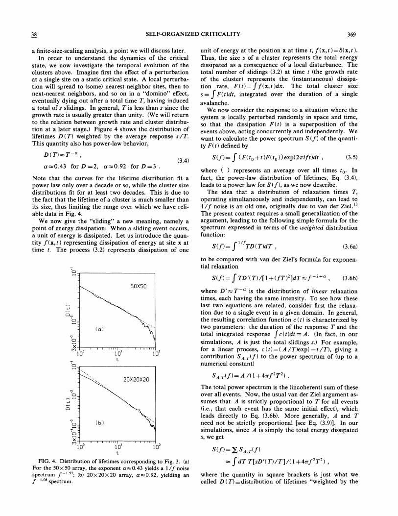
Note that the curves for the lifetime distribution fit apower law only over a decade or so, while the cluster sizedistributions fit for at least two decades. This is due tothe fact that the lifetime of a cluster is much smaller thanits size, thus limiting the range over which we have reli-able data in Fig. 4.

We now give the "sliding" a new meaning, namely apoint of energy dissipation: When a sliding event occurs,a unit of energy is dissipated. Let us introduce the quan-tity f(x, t ) representing dissipation of energy at site x attime t. The process (3.2) represents dissipation of one

a finite-size-scaling analysis, a point we will discuss later.In order to understand the dynamics of the critical

state, we now investigate the temporal evolution of theclusters above. Imagine first the effect of a perturbationat a single site on a static critical state. A local perturba-tion will spread to (some} nearest-neighbor sites, then tonext-nearest neighbors, and so on in a "domino" effect,eventually dying out after a total time T, having induceda total of s slidings. In general, T is less than s since thegrowth rate is usually greater than unity. (We will returnto the relation between growth rate and cluster distribu-tion at a later stage. ) Figure 4 shows the distribution oflifetimes D(T) weighted by the average response s/T.This quantity also has power-law behavior,

S(f}=J TD(T)dT, (3.6a)

to be compared with van der Ziel's formula for exponen-tial relaxation

unit of energy at the position x at time t, f(x, t ) =5(x, t ).Thus, the size s of a cluster represents the total energydissipated as a consequence of a local disturbance. Thetotal number of slidings (3.2) at time t (the growth rateof the cluster) represents the (instantaneous) dissipa-tion rate, F(t)=If(x, t )dx. The total cluster size

s= F t dt, integrated over the duration of a single

avalanche.We now consider the response to a situation where the

system is locally perturbed randomly in space and time,so that the dissipation F(t) is a superposition of theevents above, acting concurrently and independently. Wewant to calculate the power spectrum S (f ) of the quanti-ty F(t) defined by

S(f)= J (F(t o+t)F(to) )exp(2nift)dt, (3.5)

where ( ) represents an average over all times to. Infact, the power-law distribution of lifetimes, Eq. (3.4),leads to a power law for S (f), as we now describe.

The idea that a distribution of relaxation times T,operating simultaneously and independently, can lead to1/f noise is an old one, originally due to van der Ziel. '

The present context requires a small generalization of theargument, leading to the following simple formula for thespectrum expressed in terms of the weighted distributionfunction:

S(f)=f TD'(T)/[1+(fT) ]dT=f + (3.6b)

C3

X

10I I I I I IIIl I

10t

I I I I III1G

where O'=T is the distribution of linear relaxationtimes, each having the same intensity. To see how theselast two equations are related, consider first the relaxa-tion due to a single event in a given domain. In general,the resulting correlation function c (t) is characterized bytwo parameters: the duration of the response T and thetotal integrated response J c(t)dt:—A. (In fact, in oursimulations, A is just the total slidings s.) For example,for a linear process, c ( t) = ( A /T)exp( t /T), giving —acontribution Sz T(f) to the power spectrum of (up to anumerical constant)

C3

C)

X

10I I I I I I III I

10t

I I I I III10

FIG. 4. Distribution of lifetimes corresponding to Fig. 3. (a}For the 50X 50 array, the exponent a=0.43 yields a 1/f noisespectrum f "; (b) 20X20X20 array, a=0.92, yielding an

f '08 spectrum.

Sq T(f)= A/(1+4~f T ) .

The total power spectrum is the (incoherent) sum of theseover all events. Now, the usual van der Ziel argument as-sumes that A is strictly proportional to T for all events(i.e., that each event has the same initial effect), whichleads directly to Eq. (3.6b). More generally, A and Tneed not be strictly proportional [see Eq. (3.9)]. In oursimulations, since A is simply the total energy dissipateds, we get

S(f)=QSg T(f)

=fdT T[sD'(T)/T]/(1+4nf T ),where the quantity in square brackets is just what wecalled D(T)=distribution of lifetimes "weighted by the

370 PER BAK, CHAO TANG, AND KURT WIESENFELD 3S

average response s/T. " Finally, treating the denomina-tor as a high-frequency cutoff, we recover the simple ex-

pression Eq. (3.6a).Thus, the power-law distribution for lifetimes leads irn-

mediately to the 1/f spectrum

C3

S(f)=f P=f

P=1.57 for D =2, P=1.08 for D=3 .(3.7)

Hence, our prediction that the system must go to a criti-cal state with power-law spatial correlations and 1/fnoise is fully consistent with the numerical simulations.The 1/f noise is the temporal signature of the self-similar

properties of the critical state.The critical state can be approached in a different way,

which shows directly how the 1/f noise represents theintrinsic dynamics in a stationary dynamic system in theself-organized critical state. Starting from a flat surface,z„=0,the slope or pressure is increased by one unit at arandom position (x,y),

z(x,y)~z(x, y)+1 . (3.8)

Then z is increased by one at another position n, and soon. When z eventually exceeds the critical value z, some-

where, the system evolves according to (3.2) until it be-comes stable again, and a cluster involving s slidings iscreated. After a while the system arrives at a (statistical-ly) stationary state with clusters of all sizes up to the sizeof the system. The system "self-averages" over manyconfigurations as time progresses, and no resetting isnecessary. The process described here simulates a situa-tion where the slope increases gradually and takes thesystem to the critical point. This has a lot of similaritywith turbulence where energy is fed into the system in along-wavelength mode. We find, as before, that energy isdissipated on all length scales and all time scales. Weshall return to the subject of turbulence in the discussionsection.

Figure 5 shows the distribution of cluster sizes mea-sured in a 2D system of size 50)&50 after the system ar-rived at the critical state. The distribution is indistin-guishable from the one in Fig. 3 obtained from the re-laxed state, indicating that we are indeed dealing with thesame critical state. The distribution of lifetimes was alsomeasured and was indistinguishable from that of Fig. 4.Similar measurements were also performed in a 3D sys-tem of size 20X20X20 and again the results were indis-tinguishable from their counterparts in Figs. 3 and 4.Thus, in a situation where the processes occur indepen-dently, the system exhibits 1/f noise.

In principle, in an actual physical situation, the build-up z(x,y)~z(x, y)+1 might take place at a speed whichis so large that the individual processes will overlap, andthe system will go into a state with higher-than-criticalslope. This will cause a cutoff in the time scales overwhich 1/f noise occurs. This represents the situation fora wildly turbulent system. Thus, for 1/f noise to occurover many orders of magnitude, it is important that thetime scale of the build-up of the critical state is muchlarger than the time scales of the measured noise. Tosummarize, the 1/f noise may be cut off either by finite-

C3I I I I I Illa' I I I I I III( I I I I I ill}

10 10 10 10

FIG. 5. Cluster size distribution for system built up from

scratch according to rules (3.2) and (3.8) for a 50X50 array.The curve is indistinguishable from that in Fig. 3(a). For this

system the system is in a stationary critical state and it is self-

averaging. Rule (3.8) has been applied 100000 times to the sta-

tionary critical state to obtain this curve.

size effects, or by too rapid flow through the stationarystate.

For a picturesque example, consider a mountainlandscape built from some long-wavelength tectonic platemotion. When the landscape reaches the critical state,the landscape will be self-similar, and there will beavalanches on "all time scales. " Clearly, the geologicaltime scales involved in building the landscape separatefrom all realistic avalanche lifetimes.

The fact that 1/f noise arises from the random super-position of events can be demonstrated directly. Figure 6shows the total dissipation as a function of time F(t)formed by superimposing the time dissipation functionsF„(t)for the evolution of the individual clusters in the20&(20)&20 system, starting each cluster at a randomtime. The curve has the features of a 1/f noise, i.e.,there are events on all time scales. It is more regularthan white noise, and less regular than a random walk.Figure 7 shows the power spectrum S(f) of the curve.Indeed, the log-log plot shows a power-law behavior withthe exponent p=0. 98 as expected from the distributionof weighted lifetimes. The crossover to white noise atf= —,', is the same finite-size effect as found for the distri-

bution of lifetimes. The absence of very large clustersreduces correlations at very low frequencies.

How robust are these results? It is important that ourresults be insensitive to randomness to have any chanceto explain 1/f noise in general, since few of the systemswhere 1/f noise occurs are simple translational invariantsystems. To test this, we modified our model by intro-ducing some "quenched randomness. " Specifically, weremoved certain nearest-neighbor connections in the ar-ray, the disrupted connections being fixed through the

38 SELF-ORGANIZED CRITICALITY 371

C3

C)Y)

10I I I I I I I I)

10I I I I I I I I

10

300 600

t900 1200

FIG. 8. Cluster size distribution for 20)(20 array with 10%of the bonds removed, averaged over 1000 samples. The slope is—1.0, same as for the pure system.

FIG. 6. F(t) generated by superimposing randomly theresponse represented by the individual clusters for a 20X 20)&20array. Note the fluctuations on a wide range of time scales.

simulation. We found that removing at random as manyat 25% of the bonds still led to power-law distributions.Figure 8 shows the cluster size distribution for a situationwith 10% of the bonds removed. No change in the ex-ponent was detected. Whether this is due to true univer-sality of the exponent, or due to our inability to detect asmall change numerically is not known. Quantitatively,the presence of this kind of randomness increases themean value of the pressure z since fewer nearest neigh-bors are available to communicate the noise. In the sandpicture, the introduction of impedements causes a build-

The distribution of lifetimes weighted by the averageresponse D ( T} can then be related to the distribution ofcluster sizes

D(T)=(slT)D[s(T)](ds jdT)

T—~ p+ & ~&+2& —T— (3.10)

up to a higher slope, by the self-organization process, un-til criticality is achieved again.

The exponents ~ and a representing the spatial andtemporal evolution of the clusters, respectively, can be re-lated through "scaling relations. " If the perturbationgrows with an exponent y within the clusters, the lifetimeT of a cluster is related to its size by

(3.9)

The scaling laws

a =2—P= (y+ 1 }r 2y— (3.11)

can be directly read off Eqs. (3.7) and (3.10). Since wehave measured a and ~ independently, we can find theanomalous growth exponent y from Eq. (3.11),

y=0. 57 for D =2, y'=0. 71 for D =3 . (3.9')

C. Simulations with open boundaries

C3

X

10I I I I I I III

10I I I I I I II]

10I I I I I III

10

FIG. 7. Power spectrum of the function F(t) depicted in Fig.6. The spectrum is 1/f, varying as f ". The crossover towhite noise at very low frequencies is a finite-size e6ect.

In this set of simulations we consider an "open-ended"system where particles are transported through the sys-tem and are allowed to leave the box at the two edgesx =X and y =N. The idea is to simulate a situationresembling some of the systems known to have 1/f noise.In the hour glass, sand is transported through the system;in quasars (and in the case of sunspots) light is transport-ed through an open-ended system, and in the case ofrivers, water is transported. ' The open-endconfiguration is simulated by modifying the first equationof (3.2) at the boundaries

372 PER BAK, CHAO TANG, AND KURT WIESENFELD 38

z(N, y)~z(N, y) —3,z(x, N)~z(x, N) 3—,

z (N, N) ~z(N, N) —2,(3.12)

In D(T)

S(f)=f ~ p=0 95 (3.13)

(To convince himself that this description has some con-nection with reality, we suggest that the reader studyvisually the fluctuating flow of an hour glass and notesthe pulses of widely different time scales. ) We cannotrule out that the exponent is identical to unity with thepresent numerical accuracy.

To test the assertion that the lifetime distribution isscaling, with cutoff due only to the finite size, we applieda technique familiar from the study of critical phenomena

when the appropriate value of z exceeds the critical value.Starting from scratch, the sand pile is built up by addingparticles randomly according to the rule (3.1). After eachparticle is added, the system is allowed to relax (if needbe) according to (3.2). The relaxation represents the slid-

ing in the diagonal direction of one particle. In additionto the boundary conditions (3.12) we also studied a diago-nally cut system where particles are allowed to leave thepile along the edge x +y =N, perpendicular to the flowdirection. The results for the two systems were the same.Again, the process is continuous and no resetting isnecessary. After an initial transient period, we foundthat the system reached a statistically stationary statewith clusters of all sizes.

Figure 9 shows the critical sandpile in the diagonalcase. The heights represent the value of the bonds as de-scribed above. For each cluster, we monitor only theflow f (t) of sand that falls off the edges of the box. Mostof the time, the relaxation following a single kick resultsin no sand falling off the edge, though, of course, on aver-age one unit of sand falls off for every unit added, oncesteady state has been achieved. For those perturbationswhich do result in a response, we again form D ( T) as be-fore Fig.ure 10 shows D(T) for a 2D system of size75)&75. Again the distribution follows a power law for adecade or so, this time with exponent equal to unity,a = 1.05. The distribution on lifetimes translates directlyinto a power-law frequency spectrum

2

In(T)

FIG. 10. Lifetime distribution of the sand flow for a systemof size 75 &(75. The straight line has a slope —1.05.

of second-order transitions. At a critical point one ex-pects D ( T) to obey a finite-size-scaling relation

D(T)=T F(L /T), (3.14)

where F is a crossover scaling function of the singlescaled variable L /T, and o is a dynamical critical ex-ponent. Similarly, one would expect a scaling relation forthe size s of bulk clusters to obey a relation of the form

D(s)=s 'F'(L /s), (3.15)

where the critical exponent d can be thought of as thefractal dimension of the clusters. Figure 11 shows theproduct D(T)T versus L /T for o =0.75: The pointsfor different L all fall on the same curve F(x) to withinnumerical accuracy. (Actually it would not be surprisingif the scaling was anisotropic —because of the anisotropicboundary conditions —such that Fwould be a function oftwo variables. The exponent found here would then bethe smaller of the two exponents. ) The finite-size-scaling

p{r)T

+L= IOoL=20~ L=30a L=50

FIG. 9. The critical sand pile for a 2D system with open edgeperpendicular to flow.

I 2 31

L/T6 7

FIG. 11. Finite-size-scaling plot.

38 SELF-ORGANIZED CRITICALITY 373

conjecture (3.15) was also successfully tested for theclosed boundary case; in this case the scaling cannot beanisotropic since the dynamics is isotropic. An exponentof d =1.92 was found for the 2D system. We suggestthat experiments be performed to check the finite-size-scaling conjecture. This would be a direct proof of spa-tial organization.

and our simulations may provide an entrance into theproblem of dynamical scale invariance. For instance, wecould measure equal time correlation functions for thedissipation, S(x)=((f(xo+x, t)f(xo, t))), where (( ))denotes a spatial average. Because of the scaling proper-ties of the critical state, we expect

S(x)=xIV. SUMMARY AND DISCUSSION

To summarize, our general arguments and numericalsimulations show that dissipative dynamical systems withextended degrees of freedom can evolve towards a self-organized critical state, with spatial and temporalpower-law scaling behavior. The spatial scaling leads toself-similar "fractal" structure. The frequency spectrumis 1/f noise or flicker noise with a power-law spectrumS(f)=f ~

Thus, in our picture 1/f noise is not noise but reflectsthe generic dynamics of extended dynamical systems. Wefound values of P tolerably close to one (and certainly be-tween 0 and 2). It remains to be seen to what extend sys-tems can be grouped into universality classes withinwhich the exponents are the same, depending on symme-try, dimension, and so on. We strongly suspect that thecriticality discovered here cannot depend on the local de-tails of the models, in analogy with equilibrium second-order phase transitions.

Moreover, we conclude that 1/f noise is intimately re-lated to the underlying spatial organization. This can betested directly, for instance by measuring the frequencycutoff versus the system size. In retrospect, it is hard tosee how 1/f noise, with long temporal correlations, couldpossibly occur without long-range spatial correlations,except by "fine-tuning" models with few degrees of free-dom.

We believe that the concept of self-organized criticalitycan be taken much further and might be the underlyingconcept for temporal and spatial scaling in dissipativenonequilibrium systems. One of our models (with closedboundary conditions} could be considered a toy model ofgeneralized turbulence, with dissipation correlated on alllength scales. Of course, there is no direct connectionwith (for instance) the Navier-Stokes equation, where themetastability is due to the storage of kinetic energy invortices, not potential energy as in the models discussedhere. Nevertheless, there is a one-to-one connection forthe phenomenology used to describe the two situations,

with p the "Kolmogorov exponent" for our "Ising" tur-bulence model. This equation indicates that the dissipa-tion at any given instant takes place on a fractal ratherthan in the bulk. It would be interesting to calculate thisexponent and compare with experiments on real tur-bulence.

Another application might be to the problem of the dy-namics of quenched glasses and spin glasses. These arefrustrated systems far from equilibrium, and it appearsthat they have much in common with our three-dimensional (3D) model. It might be that glasses quenchinto critical states where they are just barely stable withrespect to noise, but this speculation has to be developedfurther. In fact if one wants to understand 1/f noise inresistors one probably first has to understand the"glassy" dynamics of the material forming the resistor.

Finally, we invite the reader to perform the followinghome experiment. To demonstrate self-organized criti-cality, one needs a shoebox and a cup or two of sand—sugar or salt will do in a pinch. Wet the sand with asmall amount of water, mix, and gather the sand into thesteepest possible pile in one corner of the box. The angleof repose (i.e., the threshold slope) is larger for wet sand,so as the water evaporates, one observes a sequence ofslides —some very small, others quite large —occurringat random places on the pile. (The evaporation processcan be sped up by placing the box on a warm surface, orunder direct sunlight. } This is essentially the situationanalogous to that of Fig. 5 where the slope of the pile isincreased gradually, but instead it is the parameter z,that is gradually decreasing. This experiment is also ex-ceptionally portable, and is best done on a sunny day atthe beach.

ACKNOWLEDGMENT

This work was supported by the Division of MaterialsScience, U.S. Department of Energy, under Contract No.DE-AC02-76CH00016.

'For a collection of papers on spatiotemporal dynamical sys-tems, see Physica 23D, 1 —482 (1987).

2For reviews on 1/f noise, see W. H. Press, Comm. Mod. Phy's.

C7, 103 (1978);P. Dutta and P. M. Horn, Rev. Mod. Phys. 53,497 (1981).

3B. Mandelbrot, The Fraetar Geometry of Nature (Freeman, SanFrancisco, 1982).

4P. Bak, C. Tang, and K. Wiesenfeld, Phys. Rev. Lett. 59, 381(1987)~

5H. Haken, Rev. Mod. Phys. 47, 67 (1975).P. L. Nolan et al. , Astrophys. J. 246, 494 (1981);A. Lawrence,

M. G. Watson, K. A. Pounds, and M. Elvis, Nature 325, 694(1987);I. McHardy and B. Czerny, ibid. 325, 696 (1987).

7B. B. Mandelbrot and J. R. Wallis, Water Resour. Res. 5, 321(1969).

SSee, e.g., R. F. Voss and J. Clarke, Phys. Rev. B 13, 556 (1976).K. L. Schick and A. A. Verveen, Nature 251, 599 (1974).B.B. Mandelbrot and J. W. Van Ness, SIAM (Soc. Ind. Appl.

374 PER BAK, CHAO TANG, AND KURT WIESENFELD 38

Math. ) Rev. 10, 422 (1968).L. P. Kadanoff, Phys. Today 39(2), 6 (1986).For a collection of articles on this subject, see Phase Transi-

tions and Critical Phenomena, edited by C. Domb and M. S.Green (Academic, New York, 1972), Vols. 1-6.A. van der Ziel, Physica 16, 359 (1950).C. Tang, K. Wiesenfeld, P. Bak, S. Coppersmith, and P. Lit-tlewood, Phys. Rev. Lett. 58, 1161 (1987).

'~In some realistic situations the quantity which is measured isnot the flow of the quantity which is being transported. Forinstance, in resistors the fluctuations are probably caused bythe dynamics of the bulk material, not by the current itself.In other situations the experiment directly measures the ener-

gy release (photons or phonons) related to the individual pro-cesses in the bulk. These scenarios are more like the "closedboundary" case.