arX

iv:c

ond-

mat

/040

5257

v2 [

cond

-mat

.oth

er]

22

Nov

200

4

Self-Organized Criticality and Stock Market

Dynamics: an Empirical Study.

M. Bartolozzia, D. B. Leinwebera, A. W. Thomasa,b

aSpecial Research Centre for the Subatomic Structure of Matter (CSSM) andDepartment of Physics, University of Adelaide, Adelaide, SA 5005, AustraliabJefferson Laboratory, 12000 Jefferson Ave., Newport News, VA 23606, USA

Abstract

The Stock Market is a complex self-interacting system, characterized by intermit-tent behaviour. Periods of high activity alternate with periods of relative calm. Inthe present work we investigate empirically the possibility that the market is in aself-organized critical state (SOC). A wavelet transform method is used in order toseparate high activity periods, related to the avalanches found in sandpile models,from quiescent. A statistical analysis of the filtered data shows a power law be-haviour in the avalanche size, duration and laminar times. The memory process,implied by the power law distribution of the laminar times, is not consistent withclassical conservative models for self-organized criticality. We argue that a “near-SOC” state or a time dependence in the driver, which may be chaotic, can explainthis behaviour.

Key words: Complex Systems, Econophysics, Self-Organized Criticality, WaveletsPACS:

1 Introduction

Since the publication of the articles of Bak, Tang and Wiesenfeld (BTW) [1],the concept of self-organized criticality (SOC) has been invoked to explain thedynamical behaviour of many complex systems, from physics to biology andthe social sciences [2,3]. The key concept of SOC is that complex systems,that is systems constituted by many interacting elements, although obeyingdifferent microscopic physics, may exhibit similar dynamical behaviour. Inparticular, the statistical properties of these systems can be described by powerlaws, reflecting a lack of any characteristic scale. These features are equivalentto those of physical systems during a phase transition, that is at the criticalpoint. It is worth emphasizing that the original idea [1] was that the critical

Preprint submitted to Elsevier Science 2 February 2008

state was reached “naturally” , without any external tuning. This is the originof the adjective self-organized. In reality a certain degree of tuning is necessary:implicit tunings like local conservation laws and specific boundary conditionsseem to be important ingredients for the appearance of power laws [2].

The classical example of a system exhibiting SOC behaviour is the 2D sandpilemodel [1,2,3]. Here the cells of a grid are randomly filled, by an externalrandom driver, with “sand”. When the gradient between two adjacent cellsexceeds a certain threshold a redistribution of the sand occurs, leading to moreinstabilities and further redistributions. The benchmark of this system, indeedof all systems exhibiting SOC, is that the distribution of the avalanche sizes,their duration and the energy released, obey power laws.

The framework of self-organized criticality has been claimed to play an im-portant role in solar flaring [4], space plasmas [5] and earthquakes [6] in thecontext of both astrophysics and geophysics. In the biological sciences, SOC,has been related, for example, with biodiversity and evolution/extinction [7].Some work has also been carried out in the social sciences. In particular, trafficflow and traffic jams [8], wars [9] and stock-market [3,10,11,12] dynamics havebeen studied. A more detailed list of subjects and references related to SOCcan be found in the review paper of Turcotte [3].

In the present work we will provide empirical evidence for connections be-tween self-organized criticality and the stock market, considered as a complexsystem constituted of many interacting individuals. We analyze the tick-by-tick behaviour of the Nasdaq100 index, P (t), from 21/6/1999 to 19/6/2002for a total of 219 data. A sample of this data is illustrated in Fig. 1(a). Inparticular, we study the logarithmic returns of this index, which are definedas R(t) = ln(P (t+ 1)) − ln(P (t)) and plotted in Fig. 1(b).

To examine the extent to which our findings apply to other stock marketindices we also studied the S&P ASX50 (for the Australian stock market) atintervals of 30 minutes over the period 20/1/1998 to 1/5/2002, for a total of214 data points. Possible differences between daily and high frequency datahave also been taken into consideration though the analysis of the Dow Jonesdaily closures from 2/2/1939 to 13/4/2004. The results are presented in Sec. 3.

From a visual analysis of the time series of returns, Fig. 1(b), we observelong periods of relative tranquility, characterized by small fluctuations, andperiods in which the index goes through very large fluctuations, equivalent toavalanches, clustered in relatively short time intervals. These may be viewedas a consequence of a build-up process leading the system to an extremelyunstable state. Once this critical point has been reached, any small fluctuationcan, in principle, trigger a chain reaction, similar to an avalanche, which isneeded to stabilize the system again.

2

7.76

7.78

7.8

7.82

7.84

7.86

Log N

asdaq

100 I

ndex

20000 22000 24000 26000 28000 30000Ticks

-0.02

-0.01

0

0.01

0.02

Log R

eturn

s

(a)

(b)(b)

Fig. 1. Sample of the tick-by-tick time series of the Nasdaq100(a), as well as thecorresponding returns (b).

2 Wavelet Method

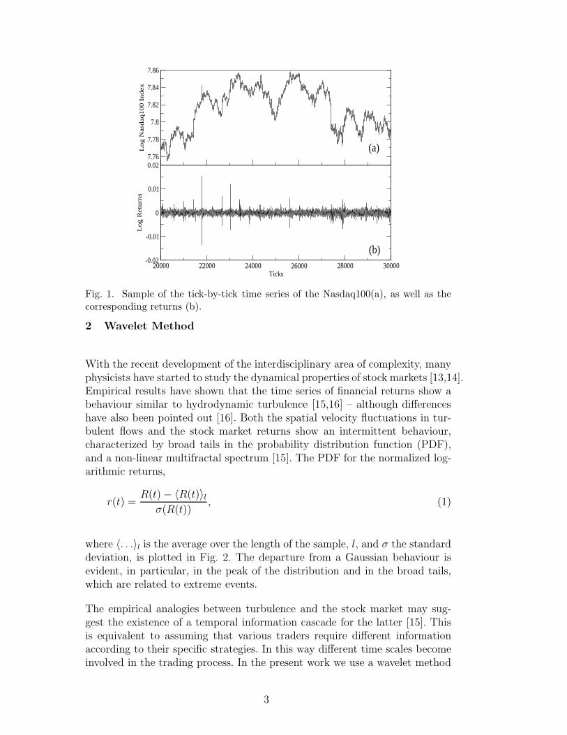
With the recent development of the interdisciplinary area of complexity, manyphysicists have started to study the dynamical properties of stock markets [13,14].Empirical results have shown that the time series of financial returns show abehaviour similar to hydrodynamic turbulence [15,16] – although differenceshave also been pointed out [16]. Both the spatial velocity fluctuations in tur-bulent flows and the stock market returns show an intermittent behaviour,characterized by broad tails in the probability distribution function (PDF),and a non-linear multifractal spectrum [15]. The PDF for the normalized log-arithmic returns,

r(t) =R(t) − 〈R(t)〉l

σ(R(t)), (1)

where 〈. . .〉l is the average over the length of the sample, l, and σ the standarddeviation, is plotted in Fig. 2. The departure from a Gaussian behaviour isevident, in particular, in the peak of the distribution and in the broad tails,which are related to extreme events.

The empirical analogies between turbulence and the stock market may sug-gest the existence of a temporal information cascade for the latter [15]. Thisis equivalent to assuming that various traders require different informationaccording to their specific strategies. In this way different time scales becomeinvolved in the trading process. In the present work we use a wavelet method

3

-20 -10 0 10 20r

1e-06

0.0001

0.01

1

PD

F(r

)

Original Time SeriesFiltered Time SeriesGaussian

0 500 1000 1500 2000

-0.1

-0.05

0

0.05

0.1

Fig. 2. PDF of the logarithmic returns of the Nasdaq100 index before (triangles)and after filtering (circles), with C = 2. The original time series is reduced to thelevel of noise. A Gaussian distribution is plotted for comparison. The insert showsthe fourth member of the Daubechies wavelets used in the filtering.

in order to study multi-scale market dynamics.

The wavelet transform is a relatively new tool for the study of intermittent andmultifractal signals [19]. The approach enables one to decompose the signalin terms of scale and time units and so to separate its coherent parts – thatis, the bursty periods related to the tails of the PDF – from the noise-likebackground, thus enabling an independent study of the intermittent and thequiescent intervals [20].

The continuous wavelet transform (CWT) is defined as the scalar product ofthe analyzed signal, f(t), at scale λ and time t, with a real or complex “motherwavelet”, ψ(t):

WTf(t) = 〈f, ψλ,t〉 =∫

f(u)ψλ,t(u)du =1√λ

∫

f(u)ψ(u− t

λ)du. (2)

The idea behind the wavelet transform is similar to that of windowed Fourieranalysis and it can be shown that the scale parameter is indeed inverselyproportional to the classic Fourier frequency. The main difference betweenthe two techniques lies in the resolution in the time-frequency domain. Inthe Fourier analysis the resolution is scale independent, leading to aliasingof high and low frequency components that do not fall into the frequency

4

range of the window. However in the wavelet decomposition the resolutionchanges according to the scale (i.e. frequency). At smaller scales the temporalresolution increases at the expense of frequency localization, while for largescales we have the opposite. For this reason the wavelet transform is considereda sort of mathematical “microscope”. While the Fourier analysis is still anappropriate method for the study of harmonic signals, where the informationis equally distributed, the wavelet approach becomes fundamental when thesignal is intermittent and the information localized.

The CWT of Eq.(2) is a powerful tool to graphically identify coherent events,but it contains a lot of redundancy in the coefficients. For a time series analysisit is often preferable to use a discrete wavelet transform (DWT). The DWTcan be seen as a appropriate sub-sampling of Eq.(2) using dyadic scales. Thatis, one chooses λ = 2j, for j = 0, ..., L − 1, where L is the number of scalesinvolved, and the temporal coefficients are separated by multiples of λ for eachdyadic scale, t = n2j, with n being the index of the coefficient at the jth scale.The DWT coefficients, Wj,n, can then be expressed as

Wj,n = 〈f, ψj,n〉 = 2−j/2∫

f(u)ψ(2−ju− n)du, (3)

where ψj,n is the discretely scaled and shifted version of the mother wavelet.The wavelet coefficients are a measure of the correlation between the originalsignal, f(t), and the mother wavelet, ψ(t) at scale j and time n. In order to bea wavelet, the function ψ(t) must satisfy some conditions. First it has to bewell localized in both real and Fourier space and second the following relation

Cψ = 2π

+∞∫

−∞

|ψ(k)|2k

dk <∞, (4)

must hold, where ψ(k) is the Fourier transform of ψ(t). The requirement ex-pressed by Eq.(4) is called admissibility and it guarantees the existence of theinverse wavelet transform. The previous conditions are generally satisfied if themother wavelet is an oscillatory function around zero, with a rapidly decay-ing envelope. Moreover, for the DWT, if the set of the mother wavelet and itstranslated and scaled copies form an orthonormal basis for all functions havinga finite squared modulus, then the energy of the starting signal is conservedin the wavelet coefficients. This property is, of course, extremely importantwhen analyzing physical time series [21]. More comprehensive discussions onthe wavelet properties and applications are given in Refs. [22] and [19]. Amongthe many orthonormal bases known, in our analysis we use the fourth mem-ber of the Daubechies wavelets [22], shown in the insert of Fig. 2. The spikyform of this wavelet insures a strong correlation for the bursty events in thetime series. The following method of analysis has also been tested with other

5

wavelets and the results are qualitatively unchanged.

The importance of the wavelet transform in the study of turbulent signalslies in the fact that the large amplitude wavelet coefficients are related to theextreme events in the tails of the PDF, while the laminar or quiescent periodsare related to the ones with smaller amplitude [21]. In this way it is possibleto define a criterion whereby one can filter the time series of the coefficientsdepending on the specific needs. In our case we adopt the method used inRef. [21] and originally proposed by Katul et al [23]. In this method waveletcoefficients that exceed a fixed threshold are set to zero, according to

Wj,n =

Wj,n if W 2j,n < C · 〈W 2

j,n〉n,0 otherwise,

(5)

here 〈. . .〉n denotes the average over the time parameters at a certain scaleand C is the threshold coefficient. In the next section we will see that theprecise value of the parameter C is not critical for our analysis. However itis possible to tune C such that only Gaussian noise is filtered. Once we havefiltered the wavelet coefficients Wj,n we perform an inverse wavelet transform,obtaining a smoothed version, Fig. 3(b), of the original time series, Fig. 3(a).The residuals of the original time series with the filtered one correspond tothe bursty periods which we aim to study, Fig. 3(c).

3 Data Analysis

In the previous section we have introduced the wavelet method in order todistinguish periods of high activity and periods of low or noise-like activity.The results are shown in Fig. 3 for C = 2. In order to choose an appropriatecut-off for the wavelet energy, that is to fix a proper C, we tune this param-eter until the statistics on the kurtosis and the skewness of the filtered timeseries approach the noise levels, namely 3 and 0 respectively. Once we haveisolated the noise part of the time series we are able to perform a reliablestatistical analysis on the coherent events of the residual time series, Fig. 3(c).In particular, we define coherent events as the periods of the residual timeseries in which the volatility, v(t) ≡ |R(t)|, is above a small threshold, ǫ ≈ 0.The smoothing procedure is emphasized by the change in the PDFs beforeand after the filtering – as shown in Fig. 2. From this plot it is clear how thebroad tails, related to the high energy events that we want to study, and theassociated central peak are cut-off by the filtering procedure. The filtered timeseries is basically a Gaussian, related to a noise process.

A parallel between avalanches in the classical sandpile models (BTW models)

6

0 10000 20000 30000 40000 50000-0.02

-0.01

0

0.01

0.02

Nas

daq

Log R

et.

0 10000 20000 30000 40000 50000-0.02

-0.01

0

0.01

0.02F

ilte

red N

asdaq

Log R

et.

0 10000 20000 30000 40000 50000Ticks

-0.02

-0.01

0

0.01

0.02

Res

idual

(a)

(b)

(c)

Fig. 3. A sample of the original time series of logarithmic returns for the Nasdaq100is shown in (a), same as Fig. 1(b). The filtered version is shown in (b). The noise-likebehaviour of this time series is evident. The residual time series is shown in (c). Thiscorresponds to the high activity periods of the time series, related to the broad wingsof the PDF. The cut-off parameter in this case is C = 2.

exhibiting SOC [1] and the previously defined coherent events in the stockmarket is straightforward. In order to test the relation between the two, wemake use of some properties of the BTW models. In particular, we use thefact that the avalanche size distribution and the avalanche duration are dis-tributed according to power laws, while the laminar, or waiting times betweenavalanches are exponentially distributed, reflecting the lack of any temporalcorrelation between them [24,25]. This is equivalent to stating that the trig-gering process has no memory.

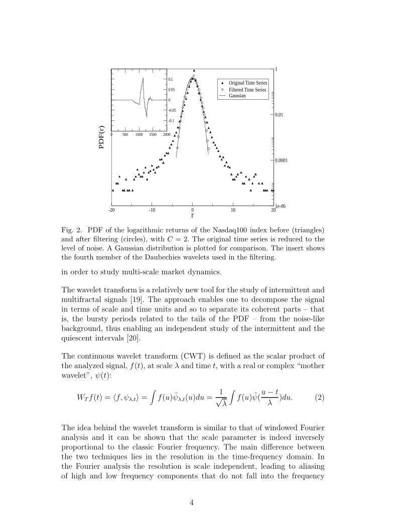
Similarly to the dissipated energy in a turbulent flow, we define an avalanche,V , in the market context as the integrated value of the squared volatility, overeach coherent event of the residual time series. The duration, Dt, is defined asthe interval of time between the beginning and the end of a coherent event,while the laminar time, Lt, is the time elapsing between the end of an eventand the beginning of the next one. The time series for V , Dt and Lt are plottedin Fig. 4 for C = 2.

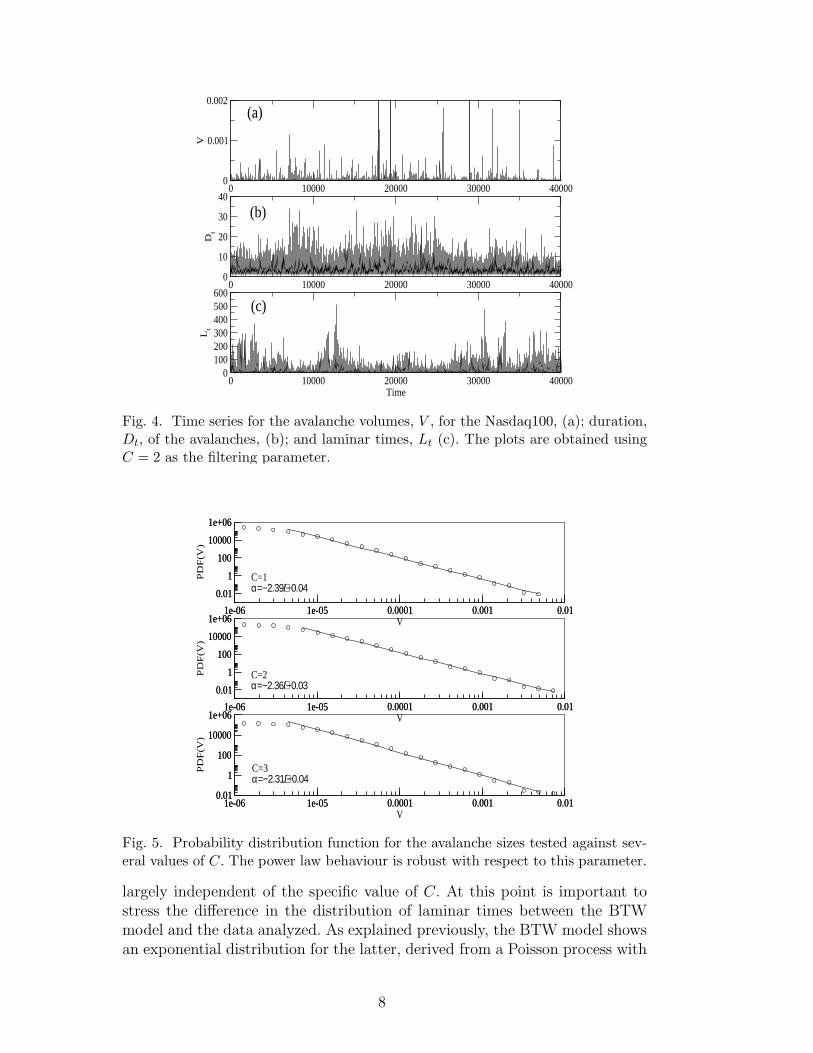
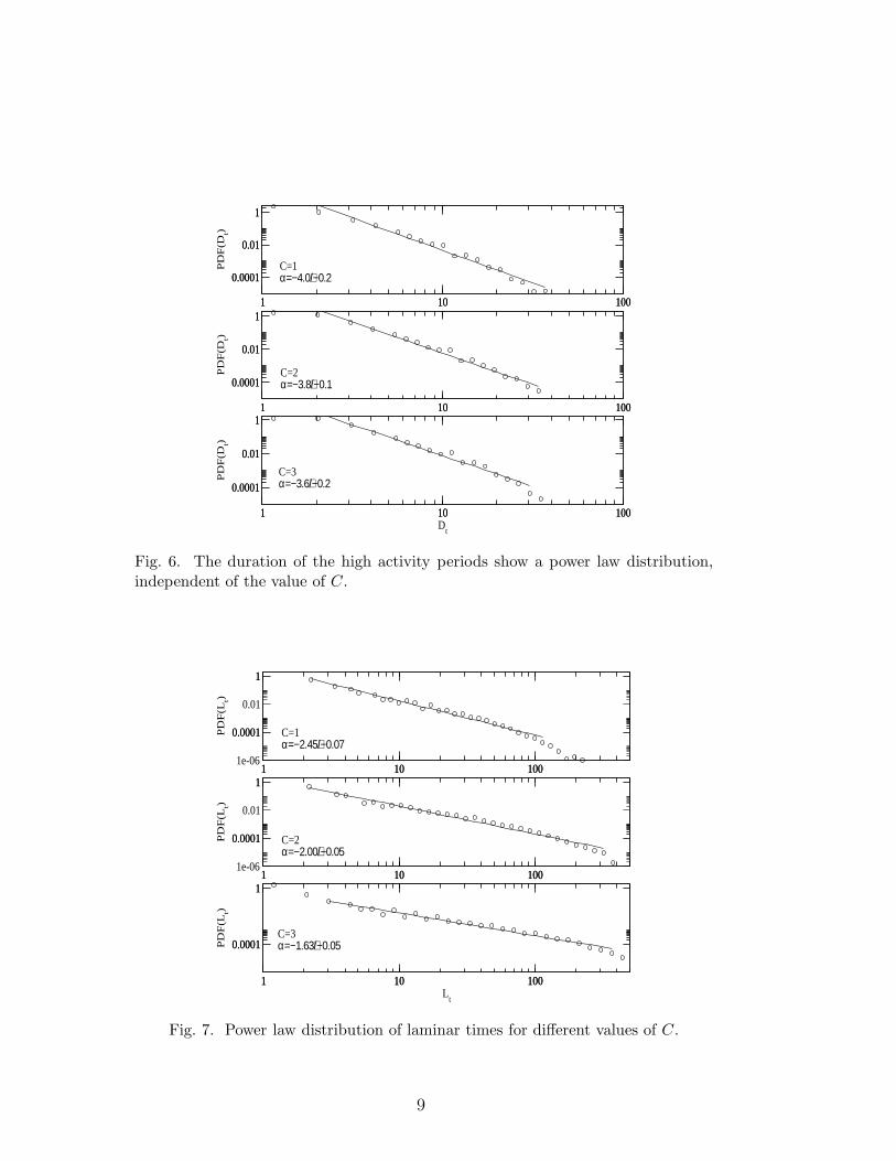
The results for the statistical analysis for the Nasdaq100 index are shownin Figs. 5, 6 and 7, respectively, for the avalanche size, duration and lami-nar times. The robustness of our method has been tested against the energythreshold, we perform the same analysis with different values of C.

A power law relation is clearly evident for all the quantities investigated,

7

0 10000 20000 30000 400000

0.001

0.002

V

0 10000 20000 30000 400000

10

20

30

40D

t

0 10000 20000 30000 40000Time

0100200300400500600

Lt

(a)

(b)

(c)

Fig. 4. Time series for the avalanche volumes, V , for the Nasdaq100, (a); duration,Dt, of the avalanches, (b); and laminar times, Lt (c). The plots are obtained usingC = 2 as the filtering parameter.

1e-06 1e-05 0.0001 0.001 0.01V

0.01

1

100

10000

1e+06

PD

F(V

)

1e-06 1e-05 0.0001 0.001 0.01

0.01

1

100

10000

1e+06

1e-06 1e-05 0.0001 0.001 0.01V

0.01

1

100

10000

1e+06

PD

F(V

)

1e-06 1e-05 0.0001 0.001 0.01

0.01

1

100

10000

1e+06

1e-06 1e-05 0.0001 0.001 0.01V

0.01

1

100

10000

1e+06

PD

F(V

)

1e-06 1e-05 0.0001 0.001 0.010.01

1

100

10000

1e+06

C=1α=−2.39+/−0.04

C=2α=−2.36+/−0.03

C=3α=−2.31+/−0.04

Fig. 5. Probability distribution function for the avalanche sizes tested against sev-eral values of C. The power law behaviour is robust with respect to this parameter.

largely independent of the specific value of C. At this point is important tostress the difference in the distribution of laminar times between the BTWmodel and the data analyzed. As explained previously, the BTW model showsan exponential distribution for the latter, derived from a Poisson process with

8

1 10 100

0.0001

0.01

1P

DF

(Dt)

1 10 100

0.0001

0.01

1

1 10 100

0.0001

0.01

1

PD

F(D

t)

1 10 100

0.0001

0.01

1

1 10 100D

t

0.0001

0.01

1

PD

F(D

t)

1 10 100

0.0001

0.01

1

C=1α=−4.0+/−0.2

C=2α=−3.8+/−0.1

C=3α=−3.6+/−0.2

Fig. 6. The duration of the high activity periods show a power law distribution,independent of the value of C.

1 10 100

0.0001

1

PD

F(L

t)

1 10 1001e-06

0.0001

0.01

1

1 10 100

0.0001

1

PD

F(L

t)

1 10 1001e-06

0.0001

0.01

1

1 10 100L

t

0.0001

1

PD

F(L

t)

1 10 100

0.0001

1

C=1α=−2.45+/−0.07

C=2α=−2.00+/−0.05

C=3α=−1.63+/−0.05

Fig. 7. Power law distribution of laminar times for different values of C.

9

1e-06 1e-05 0.0001 0.001 0.01

1

100

10000

1e+06

PDF(

V)

1e-06 1e-05 0.0001 0.001 0.01

1

100

10000

1e+06

1e-06 1e-05 0.0001 0.001 0.01

1

100

10000

1e+06

PDF(

V)

1e-06 1e-05 0.0001 0.001 0.01

1

100

10000

1e+06

1e-06 1e-05 0.0001 0.001 0.01V

1

100

10000

1e+06

PDF(

V)

1e-06 1e-05 0.0001 0.001 0.01

1

100

10000

1e+06

C=1α=−1.9+/−0.1

C=2α=−1.8+/−0.1

C=3α=−1.7+/−0.2

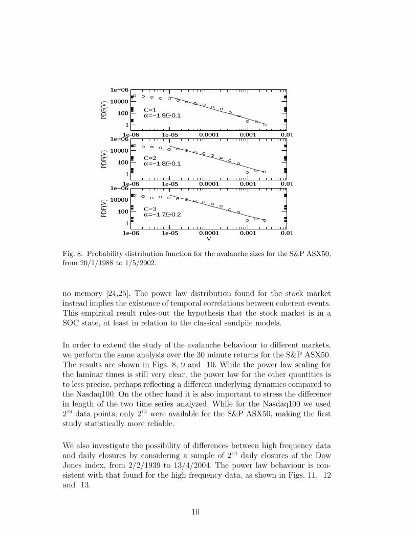
Fig. 8. Probability distribution function for the avalanche sizes for the S&P ASX50,from 20/1/1988 to 1/5/2002.

no memory [24,25]. The power law distribution found for the stock marketinstead implies the existence of temporal correlations between coherent events.This empirical result rules-out the hypothesis that the stock market is in aSOC state, at least in relation to the classical sandpile models.

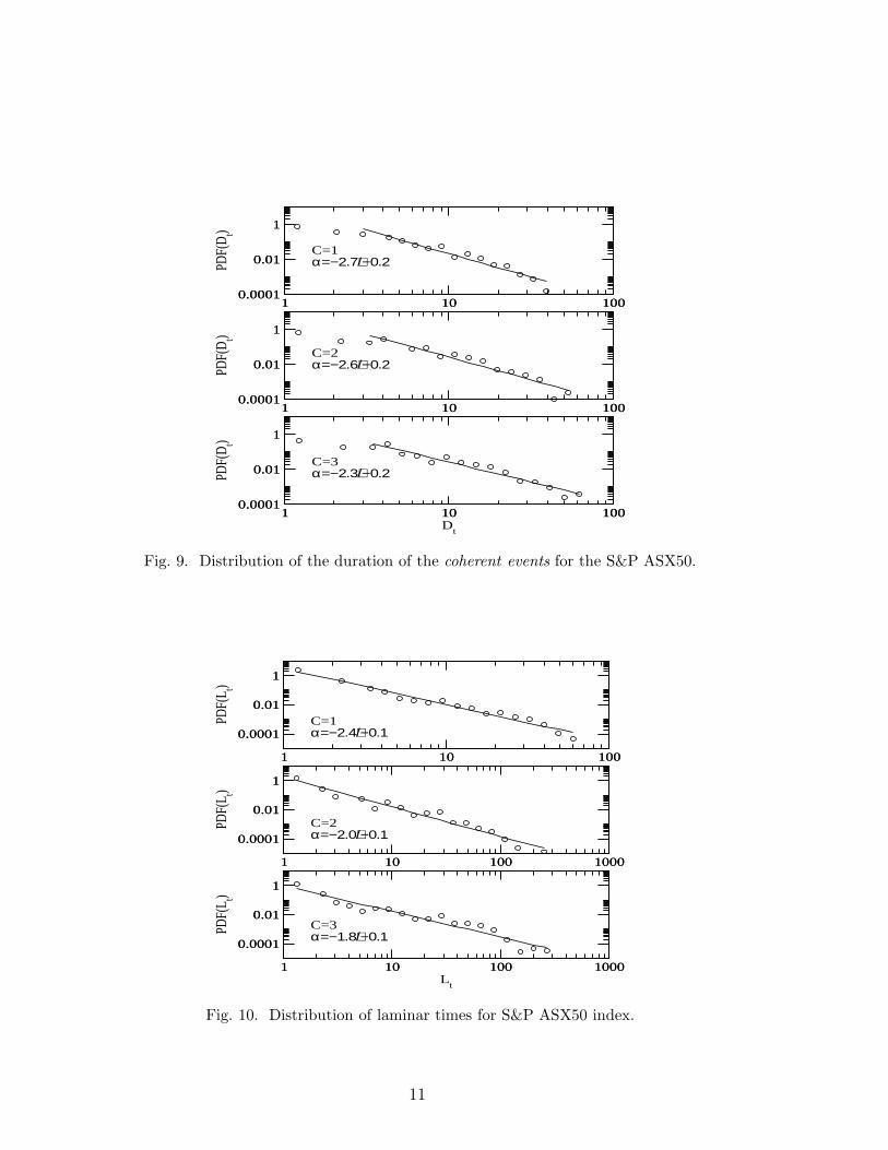
In order to extend the study of the avalanche behaviour to different markets,we perform the same analysis over the 30 minute returns for the S&P ASX50.The results are shown in Figs. 8, 9 and 10. While the power law scaling forthe laminar times is still very clear, the power law for the other quantities isto less precise, perhaps reflecting a different underlying dynamics compared tothe Nasdaq100. On the other hand it is also important to stress the differencein length of the two time series analyzed. While for the Nasdaq100 we used219 data points, only 214 were available for the S&P ASX50, making the firststudy statistically more reliable.

We also investigate the possibility of differences between high frequency dataand daily closures by considering a sample of 214 daily closures of the DowJones index, from 2/2/1939 to 13/4/2004. The power law behaviour is con-sistent with that found for the high frequency data, as shown in Figs. 11, 12and 13.

10

1 10 1000.0001

0.01

1PD

F(D t)

1 10 1000.0001

0.01

1

1 10 1000.0001

0.01

1

PDF(

D t)

1 10 1000.0001

0.01

1

1 10 100D

t

0.0001

0.01

1

PDF(

D t)

1 10 1000.0001

0.01

1

C=1α=−2.7+/−0.2

C=2α=−2.6+/−0.2

C=3α=−2.3+/−0.2

Fig. 9. Distribution of the duration of the coherent events for the S&P ASX50.

1 10 100

0.0001

0.01

1

PDF(

L t)

1 10 100

0.0001

0.01

1

1 10 100 1000

0.0001

0.01

1

PDF(

L t)

1 10 100 1000

0.0001

0.01

1

1 10 100 1000L

t

0.0001

0.01

1

PDF(

L t)

1 10 100 1000

0.0001

0.01

1

C=1α=−2.4+/−0.1

C=2α=−2.0+/−0.1

C=3α=−1.8+/−0.1

Fig. 10. Distribution of laminar times for S&P ASX50 index.

11

0.0001 0.001 0.01 0.10.01

1

100

10000

PDF(

V)

0.0001 0.001 0.01 0.10.01

1

100

10000

0.0001 0.001 0.01 0.10.01

1

100

10000

PDF(

V)

0.0001 0.001 0.01 0.10.01

1

100

10000

0.0001 0.001 0.01 0.1V

0.01

1

100

10000

PDF(

V)

0.0001 0.001 0.01 0.10.01

1

100

10000

C=1α=−1.9+/−0.1

C=2α=−1.8+/−0.1

C=3α=−1.8+/−0.1

Fig. 11. Probability distribution function for the avalanche sizes for the Dow Jonesdaily closures, from 2/2/1939 to 13/4/2004.

1 100.0001

0.001

0.01

0.1

1

10

PDF(

D t)

1 100.0001

0.001

0.01

0.1

1

10

1 100.0001

0.001

0.01

0.1

1

10

PDF(

D t)

1 100.0001

0.001

0.01

0.1

1

10

1 10D

t

0.0001

0.001

0.01

0.1

1

10

PDF(

D t)

1 100.0001

0.001

0.01

0.1

1

10

C=1α=−3.4+/−0.2

C=2α=−3.2+/−0.1

C=3α=−3.0+/−0.2

Fig. 12. Distribution of the duration of the Dow Jones index.

12

1 10 100 1000

0.0001

0.01

1

PDF(

L t)

1 10 100 10001e-05

0.0001

0.001

0.01

0.1

1

1 10 100 1000

0.0001

0.01

1

PDF(

L t)

1 10 100 10001e-05

0.0001

0.001

0.01

0.1

1

1 10 100 1000L

t

1e-06

0.0001

0.01

1

PDF(

L t)

1 10 100 10001e-06

0.0001

0.01

1

C=1α=−2.1+/−0.1

C=2α=−1.8+/−0.1

C=3α=−1.7+/−0.1

Fig. 13. Distribution of laminar times for the Dow Jones index.

4 Discussion

Similar power law behaviour for V , Dt and Lt has been found in the contextof solar flaring [24] and in geophysical time-series [21]. In the case of solarflaring, Boffetta et. al [24] have shown that the characteristic distributionsfound empirically are more similar to the dissipative behaviour of the shellmodel for turbulence [26,27] than to SOC. On the other hand the intermittencyin turbulent flows discussed in Sec 2 is believed to be the result of a non-linear energy cascade that generates non-Gaussian events at small scales [17]where the shape of the PDF is extremely leptokurtic. At larger scales thespatial correlation decreases and the PDF converges toward a Gaussian. Thesefeatures imply the absence of global self-similarity – which, as we have noted,is an intrinsic component of SOC models [18].

Freeman et. al [28] have argued that, although an exponential distributionholds for classical sandpile models, there exist some non-conservative modifi-cations of the BTW models in which departures from an exponential behaviourfor the Lt distribution [29,30,31,32] are observed in the presence of scale-freedynamics for other relevant parameters. The question remains whether or notthese systems are still in a SOC state [28]. If we assume that the power lawscaling of the laminar times corresponds to a breakdown of self-organized crit-icality, then we face the problem of how to explain the observed scale-freebehaviour of the non-conservative models. This ambiguity can be resolved ifwe assume that the system is in a near-SOC state, that is the scaling prop-

13

erties of the system are kept even if it is not exactly critical and temporalcorrelations may be present [28,33]. Another possible scenario is related withthe existence of temporal correlations in the driver [34,35]. In this case thepower law behavior of the waiting time distribution would be explained andthe realization of a SOC state preserved [34,35].

5 Conclusions

In the present work we have investigated empirically the possible relationsbetween the theory of self-organized criticality and the stock market. Theexistence of a SOC state for the market would be of great theoretical impor-tance, as this would impose some constraints on the dynamics of this complexsystem. A bounded attractor in the state space would be implied. Moreover,we would have a better understanding of business cycles.

From the wavelet analysis on a sample of high frequency data for the Nas-daq100 index, we have found that the behaviour of high activity periods, oravalanches, is characterized by power laws in the size, duration and laminartimes. The power laws in the avalanche size and duration are a characteristicfeature of a critical underlying dynamics in the system, but this is not enoughto claim the self-organized critical state. In fact the power law behavior in thelaminar time distribution implies a memory process in the triggering driverthat is absent in the classical BTW models, where an exponential behavioris expected. This does not rule out completely the hypothesis of underlyingself-organized critical dynamics in the market. Non-conservative systems, asfor the case of the stock market, near the SOC state can still show power lawdynamics even in presence of temporal correlations of the avalanches [28,33].Another possible explanation is that the memory process, possibly chaotic,is intrinsic in the driver. In this case the power law behavior of the wait-ing time distribution would be explained and the realization of a SOC statepreserved [34,35].

These findings extend beyond the Nasdaq100 index analysis. A similar quan-titative behaviour has been observed in the S&P ASX50 high frequency datafor the Australian market and the daily closures of the Dow Jones index forthe American market. At this point it is important to stress that this doesnot imply that all the markets must display the same identical characteristics.In the case of a near-SOC dynamics, for example, the power law shape of thedistribution can be influenced by the degree of dissipation of the system whichmay change from market to market, implying a non-universal behaviour.

In conclusion, a definitive relation between SOC theory and the stock markethas not been found. Rather, we have shown that a memory process is related

14

with periods of high activity. The memory could result from some kind ofdissipation of information, similar to turbulence, or possibly a chaotic driverapplied to the self-organized critical system. Of course, a combination of thetwo processes can also be possible. Our future work will be devoted to thestudy of new tests for self-organized criticality and the implementation ofnumerical models [36].

Acknowledgements

This work was supported by the Australian Research Council.

References

[1] P. Bak et al., Phys. Rev. Lett. 59, 381 (1987); P. Bak et al., Phys. Rev. A 38,364 (1988).

[2] H. J. Jensen, Self-Organized Criticality: Emergent Complex Behavior inPhysical and Biological Systems, (Cambridge University Press, Cambridge,1998).

[3] D. L. Turcotte, Rep. Prog. Phys. 62, 1377 (1999).

[4] E.T. Lu and R.J. Hamilton, Astrophys.J. 380, L89 (1991); E.T. Lu et al.,Astrophys.J. 412, 841 (1993).

[5] T. Chang et al., Advences in Space Environmental Research, Vol.I, (KluwerAcademic Publisher,AH Dordrecht, The Netherlands, 2003); A. Valdiva etal., Advences in Space Environmental Research, Vol.I, (Kluwer AcademicPublisher,AH Dordrecht, The Netherlands, 2003).

[6] P. Bak and C. Tang, J. Geophys. Res. 94, 15 635 (1989); Sornette A. andSornette D., Europhys. Lett. 9, 197 (1989); Sornette D. et al.,J. Geophys. Res.95, 17 353 (1990); J. Huang et al., Europhys. Lett. 41, 43 (1998).

[7] P. Bak and K. Snappen, Phys. Rev. Lett. 71, 4083 (1993).

[8] K. Nagel and H.J. Herrmann, Physica A 199, 254 (1993); K. Nagel and M.Paczuski, Phys. Rev. E 51, 2909 (1995); T. Nagatani, J.Phys. A:Math.Gen. 28,L119 (1995); T. Nagatani, Fractals 4, 279 (1996).

[9] D.C. Roberts and D.L. Turcotte, Fractals 6, 351 (1998).

[10] P. Bak et al.,Ric. Econ. 47, 3 (1993).

[11] P. Bak et al.,Physica A 246, 430 (1997).

[12] J. Feigenbaum, Rep. Prog. Phys. 66, 1611 (2003).

15

[13] R. N. Mantegna and H. E. Stanley, An Introduction to Econophysics:Correlation and Complexity in Finance, (Cambridge University Press,Cambridge, 1999); J.-P. Bouchard and M. Potters, Theory of Financial Risk,(Cambridge University Press, Cambridge, 1999).

[14] W. Paul and J. Baschnagel, Stochastic Processes: From Physics to Finance,(Spriger-Verlag, Berlin,1999).

[15] S. Ghashghaie et al., Nature 381, 767 (1996).

[16] R. N. Mantegna and H. E. Stanley, Physica A 239, 225 (1997).

[17] U. Frisch, Turbulence, (Cambridge University Press, Cambridge, 1995).

[18] V. Carbone et al., Europhys. Lett.,58 (3), 349 (2002).

[19] M. Farge, Annu. Rev. Fluid Mech. 24, 395 (1992).

[20] M. Farge et al., Phys. Fluids 11, 2187 (1999).

[21] P. Kovacs et al. Planet. Space Sci. 49, 1219 (2001).

[22] I. Daubechies, Comm. Pure Appl. Math. 41 (7), 909 (1988).

[23] G.G. Katul et al., Wavelets in Geophysics, pp. 81-105, (Academic, San Diego,Calif. 1994)

[24] G. Boffetta et al., Phys. Rev. Lett. 83, 4662 (1999).

[25] M.S. Wheatland et al., Astrophys.J.509, 448 (1998).

[26] T. Bohr et. al., Dynamical System Approach to Turbulence, (CambridgeUniversity Press, Cambridge, 1998).

[27] P. Giuliani and V. Carbone, Europhys. Lett. 43, 527 (1998).

[28] M.P. Freeman et. al., Phys. Rev. E 62, 8794 (2000).

[29] K. Christensen and Z. Olami, Geophys. Res. Lett. 97, 8729 (1992).

[30] Z. Olami and K. Christensen, Phys. Rev. A. 46, R1720 (1992).

[31] T. Hwa and M. Kardar, Phys. Rev. A, 45, 7002 (1992).

[32] H.F. Chau and K.S. Cheng, Phys. Rev. A, 46, R2981 (1992).

[33] J.X. Carvalho and C.P.C. Prado, Phys. Rev. Lett., 84, 4006 (2000).

[34] P. De Los Rios et. al., Phys. Rev. E 56, 4876 (1997).

[35] R. Sanchez et. al., Phys. Rev. Lett. 88, 068302-1 (2002).

[36] M. Bartolozzi and A.W. Thomas, Phys. Rev. E 69, 046112 (2004).

16