5

ISBN 978-954-90537-2-2

26-28 September 2017, Golden Sands, Bulgaria

Organized jointly by: Bulgarian National Committee for the International Hydrological

Programme of UNESCO and National Institute of Meteorology and Hydrology-BAS,

Sofia, Bulgaria with the support of the UNESCO Regional Bureau for Science

and Culture in Europe (Venice, Italy)

Editors: Prof. Plamen Ninov Assoc. prof. Elena Bojilova Thecnical assictance: Radoslava Ivanova Logo design: Sahary Geshev ISBN 978-954-90537-2-2

5

International Scientific Committee

Plamen Ninov IHP Secretariat, National Institute of Meteorology and Hydrology, Sofia, Bulgaria

Elena Bojilova IHP Secretariat, National Institute of Meteorology and Hydrology, Sofia, Bulgaria

Alexsey Benderev Geological Institute – Bulgarian Academy of Sciences

Martina Pechinova

Institute of Architecture and Civil Engineering

Ulrich Schröder German IHP/HWRP National Committee, Federal Institute of Hydrology

Gunter Blöschl Vienna University of Technology, Vienna, Austria

Pavol Miklanek Slovak Committee for Hydrology, Institute of Hydrology SAS

Mitja Brilly University of Ljubliana, IHP Slovenia

M-J Adler National Institute of Hydrology and Water Management, Bucharest, Romania

Philippe Pypaert UNESCO Regional Bureau for Science and Culture in Europe (Venice, Italy)

Jovan Despotovic Serbian IHP National Committee

I. Liska National Commission for Protection of Danube River, Vienna

6

Local Scientific Committee

Plamen Ninov IHP Secretariat, National Institute of Meteorology and Hydrology, Sofia, Bulgaria

Tzviatka Karagiozova

IHP Secretariat, National Institute of Meteorology and Hydrology, Sofia, Bulgaria

Elena Bojilova IHP Secretariat, National Institute of Meteorology and Hydrology, Sofia, Bulgaria

Organizing Committee

Plamen Ninov IHP Secretariat, National Institute of Meteorology and Hydrology, Sofia, Bulgaria

Elena Bojilova IHP Secretariat, National Institute of Meteorology and Hydrology, Sofia, Bulgaria

Tzviatka Karagiozova

IHP Secretariat, National Institute of Meteorology and Hydrology, Sofia, Bulgaria

Hristomir Branzov National Institute of Meteorology and Hydrology, Sofia, Bulgaria

Milena Milenkova National Institute of Meteorology and Hydrology, Sofia, Bulgaria

Radoslava Ivanova

National Institute of Meteorology and Hydrology, Sofia, Bulgaria

7

Foreword Cooperation of the Danubian countries in the area of hydrology started in 1961, hosting the first conference on hydrological forecast in Budapest. The conference took place even before the International Hydrological Decade was proclaimed (1965-1975), a 10-year program that provided an important stimulus to international collaboration in hydrology, and before the International Hydrological Programme of UNESCO was established. Since 1975, cooperation has been conducted within the framework of the International Hydrological Programme (IHP) of UNESCO. The XXVII conference, in a series of biennial conferences alternatingly held by the Danubian countries, is now presented. In 2014 the VIII phase of the IHP of UNESCO starts with the main topic ″Water security: Responses to local, regional, and global challenges”. To deal with these complex, rapid environmental and demographical changes (e.g. population growth and vulnerability to hydrological disasters, global and climate changes, uncontrolled urban expansion, and land use changes) holistic, multidisciplinary and environmentally sound approaches to water resources management and protection policy are necessary. Water security in IHP VIII is defined as the capacity of a population to safeguard access to adequate quantities of water of acceptable quality for sustaining human and ecosystem health on a watershed basis, and to ensure efficient protection of life and property against water related hazards - floods and droughts. The XXVII Conference of Danubian Countries is taking place 26-28 September 2017, in Golden Sands, Bulgaria. It has been organized jointly by the IHP Committee of Bulgaria, Bulgarian National Commission for UNESCO, under the support of UNESCO and the National Institute of Meteorology and Hydrology – Bulgarian Academy of Sciences. The conference brings together more than 187 participants from 19 countries from the Danube River Basin and outside Europe also. We have maintained traditional structuring into the following topics: 1. Basis of hydrology 2. Hydrological data management 3. Hydrological modelling and forecasting 4. Disaster events 5. Administrative structures for water management 6. River Basin and Water Management 7. Water quality and pollutants 8. Ecohydrology

8

As usual an International and a Local Scientific Commission carried out the scientific assessment and selection of the contributions and poster proposed.

The highest number of presentations covered Topic 2: Hydrological data management and Topic 3: Hydrological modelling and forecasting.

The results of the conference, achieved through the presentations and participation in plenary, oral and poster sessions, are summarized in the present proceedings. We hope that they will have stimulated further research and debate on the topics of hydrology. We are proud to welcome you at the XXVII Conference of Danubian Countries on the hydrological forecasting and hydrological bases of water management!

Plamen Ninov Elena Bojilova

Bulgarian NC IHP UNESCO

9

CONTENTS PLENARY SPEECHES 17 TOPIC 1: BASIC OF HYDROLOGY 33 ISSUES OF INTRODUCING THE MODERN INSTRUMENTS OF HYDROMETRIC MEASUREMENTS IN THE HYDROMETEOROLOGICAL SERVICE OF UKRAINE 33 Viacheslav Manukalo, Mykola Nastiuk, Natalia Samoylenko METHODICAL APPROACHES TO THE ESTIMATION OF REPRESENTATIVENESS OF BENCHMARK CLIMATE STATIONS 38 Stanislav Moskalenko CОNTEMPORARY DEVICES FOR MEASURMENT OF WATER DISCHARGE IN OPEN FLOWS 44 Plamen Atanasov HYDRAULIC DESIGN OF CULVERTS 53 Dániel Koch, Katalin Bene, Gábor Keve HOW AFFECT THE APPLICATION OF BIOCHAR THE WATER REGIME OF AGRICULTURAL SOIL WHEN A MAIZE (ZEA MAYS L.) IS GROWN? 60 Justina Vitkova, Peter Surda UTILIZATION OF GAINED EXPERIENCES BASED ON ICE OBSERVATION BY WEBCAMERAS 68 Gábor Keve TOPIC 2: HYDROLOGICAL DATA MANAGEMENT 79 EXPECTED CHANGES IN THE 100-YEAR RIVER DISCHARGE IN THE 21ST CENTURY AT THE DANUBE RIVER IN BRATISLAVA 79 Ladislav Gaál, Danica Lešková, Eva Uhliarová THE ROLE OF THE GROUNDWATER IN THE FORMATUION OF RIVER FLOW OF THE ARDA RIVER BASIN (SOTHERN BULGARIA) 90 Marin Ivanov, Tatiana Orehova, Aglaida Toteva, Mila Trayanova, Aleksey Benderev SPATIO-TEMPORAL FLUCTUATIONS OF MINIMUM FLOW IN THE DANUBE BASIN WITHIN UKRAINE 100 Gorbachova Liudmyla HYDRO-GENETIC ANALYSIS OF THE LONG-TERM FLUCTUATIONS OF THE AVERAGE ANNUAL WATER TEMPERATURE IN THE SIVERSKYI 105

10

DONETS RIVER BASIN (WITHIN UKRAINE) Tetiana Bauzha IDENTIFICATION OF CHANGES IN THE HYDROLOGICAL REGIME DUE TO GABČÍKOVO WATER DAM OPERATION 112 Lotta Blaškovičová, Jan Gavurník, Martin Belan, Jana Poórová, Zuzana Paľušová THE UNCERTAINTY INTERVAL OF THE MAXIMUM DISCHARGES WITH HIGH RETURN PERIOD 124 Radu Drobot, M. Aurelian Florentin Draghia, Romică Trandafir, Daniel Ciuiu A DESIGN FLOOD ESTIMATION AT THE HYDROLOGICAL GAUGING STATIONS – WHAT THAT COULD BE? 132 Stevan Prohaska, Aleksandra Ilić INFLUENCE OF NATURAL FACTORS ON THE REGIME OF THE LARGEST KARST SPRINGS IN NORTHWESTERN BULGARIA 146 Evelina Damyanova, Neyko Neykov, Marin Ivanov, Aleksey Benderev IMPACT OF DROUGHT PERIODS ON THE GROUNDWATER RECHARGE IN THE DOBRICH REGION, NORTHEASTERN BULGARIA 156 Veselina Pavlova, Tatiana Orehova SEASONAL PRECIPITATION TREND ANALYSIS IN CLIMATIC STATIONS IN THE EASTERN SLOVAKIA 165 Martina Zeleňáková, Peter Blišťan, Pavol Purcz, Helena Hlavatá , Daniel Constantin Diaconu, Maria Manuela Portela CHANGES IN WATER TEMPERATURE IN SELECTED STRAMS OF THE MORAVA RIVER BASIN 174 Ondrej Ledvinka, Antonin Maly NATURAL AND ANTHROPOGENIC TRANSFORMATION OF ANNUAL RUNOFF OF TRANSBOUNDARY RIVERS OF KURA RIVER BASIN 182 Farda Imanov, Aytan Guliyeva, Jovan Despotovich, Anar Nuriyev UPDATE OF THE TECHNOLOGICAL SCHEME FOR ASSESSMENT OF SURFACE WATER RESOURCES ON THE TERRITORY OF BULGARIA 191 Plamen Ninov, Tzviatka Karagiozova, Elena Bojilova, Neviana Todorova, Kamelia Krumova, Rymiana Dobreva, Antoaneta Boeva, Radoslava Ivanova, Maya Rankova DIFFERENT APPROACHES TO DESIGN FLOOD ASSESSMENT AT THE DANUBE AND THE DRAVA CONFLUENCE 201 Aleksandra Ilić, Stevan Prohaska, Boris Pokorni

11

ANNUAL WATER RESOURCES ASSESSMENT USING DIFFERENT OBSERVATIONS AND MODELS 215 Eram Artinyan, Dobri Dimitrov, Kamelia Kroumova, Maya Rankova DEVELOPING THE INFORMATION-ANALYTICAL SYSTEM "STRATIGRAPHY AND PHYSICAL-MECHANICAL PROPERTIES OF THE SNOWPACK" 223 Oleksandr Aksiuk, Pavlo Poperechnyi, Ganna Goncharenko THE LONG-TERM FLUCTUATIONS OF MAXIMUM WATER LEVELS OF THE COLD PERIOD FLOODS IN DANUBE RIVER BASIN (UKRAINIAN PART) 233 Ievgeniia Vasylenko TOPIC 3: HYDROLOGICAL MODELING AND FORECASTING 238 NEW PRODUCTS IN HYDROLOGICAL FORECASTING SYSTEM ON MORAVA RIVER 238 Petr Janál, Jakub Jansa MODELING AND FORECASTING OF THE RIVERFLOW IN LOWER COURSE OF OSAM, VIT AND OGOSTA RIVERS 245 Nikolay Nedkov, Eram Artinyan SHORT-TERM FORECASTING OF WATER INFLOW TO DNIESTER RESERVOIR USING NUMERICAL WEATHER FORECAST MODEL DATA 252 Borys Khrystyuk HYDROLOGICAL SIMULATIONS BASED ON REGIONAL CLIMATE MODEL OUTPUTS 258 Anna Kis, János Adolf Szabó, Rita Pongrácz, Judit Bartholy RESERVOIRS CASCADE SIMULATION ADD-ON FOR RIVERFLOW FORECASTING OF ARDA AND TUNDZHA RIVERS 265 Petko Tsarev, Eram Artinyan ASPECTS OF STOCHASTIC MODELING IN WATER RESOURCE MАNАGEMENT 269 Anna Yordanova, Igor Niagolov, Irena Ilcheva STOCHASTIC REGULARITIES OF LONG-TERM FLUCTUATION OF AVERAGE ANNUAL RUNOFF OF RIVERS OF TISZA RIVER BASIN (WITHIN THE UKRAINE) 280 Olga Lukianets EXTENDING THE OLSER FORECASTING SYSTEM FOR SMALL 291

12

CATCHMENTS IN HUNGARY András Csík, Balázs Gauzer, Boglárka Gnandt, Zoltán Liptay, Katalin Molnár APPLYING A NEW MODEL IN WATER LEVEL FORECASTING FOR THE COMMON HUNGARIAN-CROATIAN SECTION OF DRAVA RIVER AT THE HUNGARIAN HYDROLOGICAL FORECASTING SERVICE 295 Adrienn Hunyady ENHANCING THE NATIONAL CAPACITY TO MONITOR, EVALUATE AND FORECAST DANGEROUS METEOROLOGICAL AND HYDROLOGICAL PHENOMENA, SERBIAN EXPERIENCE 305 Bojan Palmar, Carlo Cacciamani, Slavimir Stevanovic, Borjanka Palmar BACKWATER EFFECT IN THE SAVINJA RIVER CATCHMENT ON THE FLOOD SAFETY AND HYDROLOGICAL DATA 315 Nejc Bezak, Mojca Šraj, Mitja Brilly, Andrej Vidmar HYDROLOGICAL STRUCTURE OF THE CATCHMENT DURING THE FLOODS 322 Mitja Brilly, Mojca Šraj, Nejc Bezak, Andrej Vidmar CALIBRATION OF HYDROLOGICAL MODEL WITH PROGRAMME PEST 323 Andrej Vidmar, Andrej Kryžanowski, Nejc Bezak, Mojca Šraj, Mitja Brilly HYDROLOGICAL- HYDRAULIC MODEL FOR REAL TIME FORECASTING ON SAVA RIVER IN CROATIA 331 Tatjana Vujnovic, Dijana Oskorus, Toni Jurlina, Petra Mutic, Jadran Berbic CASE STUDIES OF 2D HYDRO-DYNAMIC MODELING OF DIFFERENT DANUBE REACHES IN HUNGARY 339 István Göttlinger, Enikő Anna Tamás, György Varga, László Vas INTER-ANNUAL DISTRIBUTION FOR YANTRA RIVER BASIN, NORTH BULGARIA 346 Elena Bojilova STOCHASTIC RAINFALL-RUNOFF MODELLING TO EVALUATE THE SPATIAL CONCURRENCE OF THE RUNOFF OF INN TRIBUTARIES 356 Jürgen Komma, Thomas Nester, Jose Luis Salinas, Günter Blöschl APPLICATION OF THE TOPKAPI MODEL ON THE OGOSTA RIVER BASIN 357 Valeriya Yordanova, Snezhanka Balabanova, Vesela Stoyanova ASSESSING RISKS AND COSTS OF CLIMATE CHANGE IMPACTS ON 365

13

FLOODS AND DROUGHTS WITH THE FUTURE DANUBE MODEL Fred Foko Hattermann, Stefan Liersch, Michel Wortmann, Stephen Hardwick, Kai Schröter, Miklós Gyalai-Korpos FLOOD VULNERABLE AREAS IN SLOVAKIA BASED ON MULTICRITERIA ANALYSIS 372 Martina Zeleňáková, Peter Blišťan, Pavol Purcz TOPIC 4: DISASTER EVENTS 373 REGIONALIZATION APPROACH FOR DETERMINATION OF SPECIFIC WATER QUANTITIES FOR ARDA AND BYALA RIVERS IN BULGARIA - AT LOW, MEDIUM AND HIGH WATER LEVELS 373 Radoslava Ivanova SEVERE FLASH FLOODS IN SLOVAKIA, JULY 2016 383 Michaela Bírová, Beata Randusová, Valéria Wendlová, Peter Smrtník UNUSUAL FEBRUARY 2016 IN SLOVAK RIVER BASINS 393 Kateřina Hrušková, Daniela Kyselová, Soňa Liová, Katarína Matoková, Dorota Simonová, Marcel Zvolenský A DAILY WETNESS INDEX BASED ON SATELLITE GRAVITY FOR FLOOD AND DROUGHT FORECASTING IN THE DANUBE BASIN 402 Ben Gouweleeuw, Andreas Kvas, Christian Gruber, Tortsen Mayer-Gürr, Frank Flechtner, Andreas Güntner CONTINUOUS SPATIO-TEMPORAL CORRELATED RAINFALL SIMULATION FOR REGIONAL FLOOD RISK ASSESSMENT – APPLICATION IN THE AUSTRIAN ALPS 408 Jose Luis Salinas, Thomas Nester, Jürgen Komma, Günter Blöschl FLOOD REGIME OF RIVERS IN THE DANUBE RIVER BASIN 409 Pavol Miklanek, Pavla Pekarova, Jan Pekar ASSESSMENT OF FLOOD PRONE AREAS ALONG DANUBE RIVER USING OPTICAL SATELLITE DATA 419 Diana Achim, Viorel Chendeş DROUGHT IDENTIFICATION AND MONITORING 428 Jana Poórová, Zuzana Danáčová, Katarína Melová, Lotta Blaškovičová PROBLEMS OF WATER RESOURCES MANAGEMENT OF 429 DANUBE RIVER BASIN IN CHERNIVTSI REGION OF UKRAINE Lyudmyla Kuzmych EVALUATION OF THE THRESHOLDS FOR FLOOD FORECASTING AND 435

14

WARNING Vesela Stoyanova, Snezhanka Balabanova, Valeriya Yordanova SURFACE WATER RESOURCES CHARACTERISTICS ESTIMATION VIA STATISTICAL MODELS 444 Maya Rankova, Kamelia Kroumova ANALYSIS OF NATURAL DISASTERS IN BULGARIA IN LAST YEARS 452 Iordanka Koleva-Lizama, Bernardo Lizama Rivas ANN MODEL FOR FLOOD RISK IDENTIFICATION: SEVLIEVO, BULGARIA 460 Maria Mavrova-Guirguinova, Denislava Pencheva WATER RESOURCES STATISTICAL ESTIMATES IN BULGARIA CHARACTERISTICS AND FEATURES 470 Dobri Dimitrov, Maya Rankova, Kamelia Kroumova TOPIC 5: ADMINISTRATIVE STRUCTURES FOR WATER MANAGEMENT 476 DEVELOPING THE EYARLY FLOOD WARNING SYSTEM AS THE IMPORTANT COMPONENT OF THE NATURAL HAZARDS RISK MANAGEMENT: CASE STUDY FROM UKRAINE 476 Viacheslav Manukalo, Victoria Boiko DEVELOPING STANDARDIZATION OF THE HYDROMETEOLOGICAL ACTIVITY IN UKRAINE: PRESENT STATE AND NEW NEEDS 483 Viacheslav Manukalo,Tetiana Mytnyk, Liudmyla Kovalska AN IMPACT ASSESSMENT OF CLIMATE CHANGE IN THE DANUBE RIVER BASIN – ANALYZING RESEARCH PROJECTS TO DETERMINE ADAPTATION STRATEGIES 489 Roswitha Stolz, Monika Prasch, Franziska Koch, Michael Weber, Wolfram Mauser FLOOD RISK ASSESSMENT IN ROMANIA BASED ON SOCIAL, ECONOMIC AND CULTURAL EXPOSURE 496 Viorel Chendeş, Daniela Rădulescu, Sorin Rândaşu, Diana Achim, Anca Gorduza EVALUATION OF THE WATER USE IN COMPARISON TO THE SURFACE WATER RESOURCES FOR SELECTED PERIOD BASED ON THE RESULTS OF WATER RESOURCE BALANCE (WRB) 497 Ľubica Lovásová, Katarína Melová, Zuzana Danáčová, Lotta Blaškovičová

15

TOPIC 6: RIVER BASIN AND WATER MANAGEMENT 502 MONTE CARLO SIMULATIONS TO EVALUATE THE POTENTIAL OF ALPINE RETENTION MEASURES 502 Thomas Nester, Jürgen Komma, Jose Luis Salinas, Günter Blöschl THE ASSESSMENT OF LEVEL OF FLASH FLOODS THREAT OF URBANIZED AREAS 509 Pavla Štěpánková, Miroslav Dumbrovský, Karel Drbal TRENDS ASSESMENT OF METEOROLOGICAL FACTORS, RIVER FLOW AND DROUGHTS IN NORTHWESTERN BULGARIA 521 Yordan Dimitrov, Anna Yordanova WATER RESOURCE MANAGEMENT FOR AGRICULTURAL DEVELOPMENT IN KOPAI RIVER BASIN OF WEST BENGAL, INDIA 531 Ajit Kumar Bera THE WATER LEVEL REGIME OF THE DANUBE RIVER BETWEEN KIENSTOCK AND BRATISLAVA 532 Veronika Bacova Mitkova INVESTIGATE THE CAUSES OF WATER CRISIS IN CENTRAL IRAN’S BASINS: CLIMATE CHANGE OR MISMANGMENT WATER RESOURCES 540 Fatemeh Ghader, Mohammad Hajiketabi, Uwe Tröger POTENTIAL CLIMATE CHANGE IMPACT ON MEAN FLOW IN ROMANIA 548 Ciprian Corbuș, Rodica-Paula Mic, Marius Mătreață, Viorel Chendeş, Alexandru Preda RIVER BASIN MODELING UNDER FUTURE CLIMATE CONDITIONS. IMPACT APPROACH. PART I 558 Elena Bojilova DETERMINATION OF WATER RESOURCES IN THE NATIONAL PARK RILA IN THE ABSENCE OF A MONITORING NETWORK 570 Tzviatka Karagiozova, Plamen Ninov AN INTEGRATED SOLUTION FOR RAINFALL RUNOFF AT THE BRIDGE OVER SAVA A CASE STUDY OF OSTRUZNICA BRIDGE INCLUDING RUNOFF CONTROL TROUGH PREVENTION, DRAINAGE, TREATMENT AND IRRIGATION SYSTEM, GROUNDWATER RECHARGE AND MONITORING 583 Jovan Despotovic, Aleksandar Djukic, Nenad Jacimovic, Jasna Plavsic, M. Stanic, Andrijana Todorovic, Nenad Vrvic, Uros Urosevic

16

TOPIC 7: WATER QUALITY AND POLLUTION 585 THE ION RUNOFF OF THE LOWER DANUBE RIVER AND ESTIMATION OF THE STATE BY MINERALIZATION 585 N. Osadcha, D. Klebanov ASSESSMENT OF THE BALANCE OF WASTE WATER DISCHARGED INTO A SURFACE-FLOWS IN SLOVAKIA 595 Jana Döményová, Daniela Ďurkovičová, Jana Poórová TOPIC 8: ECOHYDROLOGY 600 METHODOLOGY FOR DEVELOPING AND ANALYZING MULTI-PRESSURES MATRIX ACTING ON FUNCTIONAL ELEMENTARY CATCHMENTS (FEC) IN THE DANUBE CATCHMENT 600 Lidija Globevnik, Maja Koprivšek, Luka Snoj THE USE OF REMOTE SENSING TECHNOLOGIES FOR ESTIMATION OF THE CARPATHIAN MOUNTAINS LAND SURFACE TEMPERATURE 610 Viktor Vyshnevskyi, Sergii Shevchuk THE USE OF REMOTE SENSING DATA TO EVALUATE THE STATE OF THE DANUBE RIVER DOWNSTREAM AND ADJACENT LAKES 616 Sergii Shevchuk, Viktor Vyshnevskyi Viacheslav Manukalo, Mykola Nastiuk, Natalia Samoylenko

17

PLENARY SPEECHES WATER POLICY AND HYDROLOGY IN THE COUNTRIES IN TRANSITION,

CLIMATE CHANGE AND FLOODS

Mitja Brilly FGG University of Ljubljana, Slovenia

Corresponding author: Mitja Brilly, Faculty of civil and geodetic engineering, University of Ljubljana Jamova 2, Ljubljana, email mbrilly@fgg.uni-lj.si

UNESCO’s Electoral Group II comprises former socialist countries that underwent transition in the 1990s. The transition caused both positive and negative changes in water policy. The policy lost the sense of long-term directions in developing water management. Water regime processes typically take a long time and leave a permanent mark on spatial morphology. Therefore, long-term plans and guidelines are necessary for successful management. Politicians change in power relatively quickly, so they have no need for long-term directions, as they are not able to carry out long-term plans. In 2015, UNESCO celebrated its 70th anniversary, and UNESCO’s International Hydrological Programme (IHP) its 50th anniversary. Region II representatives met in September 2015 in Moscow and adopted a common position on the problems in hydrology in the countries in transition. Representatives of IHP committees met again in March 2016 in Škocjan, Slovenia, and adopted a common position regarding the problems in water management. Due to the reduced budgetary funds, in most countries the funds for hydrological observations and research were cut. In Hungary, VITUKI, the world-renowned water research institute, stopped its operations. Slovenia is an exception in developing hydrological observations, where EU funds have been used to update the hydrological observation network and produce a state-of-the-art system of flood forecasting. Due to Election Group II’s large territory expanding on two continents, interregional cooperation, particularly with Regions I and IV, is extremely important. The cooperation of IHP National Committees in the Danube River Basin started already with the start of the International Hydrological Decade 1965–1975. XXVI conferences of the Danube countries have been held so far. The monograph on the river basin, based on measurement data in the period 1930–1970, was published in 1988. Major research achievements until 2008 were published in a monograph »Hydrological Processes of the Danube River Basin« (2010). Please find more on the Danube cooperation at http://www.unesco.org/new/en/venice/natural-sciences/water/danube-cooperation/ In recent decades, the IHP UNESCO activities have focused on cooperation between UNESCO Centers and UNESCO Chairs. As a Category 1 Center, IHP UNESCO-IHE comprises 37 water-related UNESCO category 2 centres and 38 Water Chairs. We

18

expect that the Chair “Water related Disaster Risk Reduction” will be announced shortly. With the growing population, industrialization and urbanization, the inundated areas and wetlands have been consumed and, through river engineering, watercourses have been regulated so that the space belonging to water has been reduced. Since ancient times, and more intensively from the mid-19th century, riverbeds have been shortened and narrowed, and levees have been built for flood protection; this resulted in the serious reduction of floodplains and wetlands. The surfaces ‘taken’ from rivers were intended primarily for agriculture and urban development. The situation was similar in Slovenia. Twenty years ago the maintenance of embankments of regulated natural watercourses was brought to a halt, and the new practice was seen as eco-friendly maintenance of watercourses. Many river banks were overgrown with bushes and the space for water was only further reduced. In some places, the vegetation in the narrow channels completely obscured the surface of the water. The serious damages due to the recent floods and, last but not least, fatalities, are the price that we pay today. This situation will be further aggravated by the expected impact of climate change. Since 2013, the Slovenian Committee of UNESCO IHP has taken part in the activities focusing on the campaign ‘More Room for Water’. The activities of ‘More Room for Water’ satisfy the requirements of both the EU Flood Directive and the Water Framework Directive.

1. INTRODUCTION The Eastern European IHP UNESCO region covers a large area of Eastern Europe and North Asia, extending from the Mediterranean Sea to the Pacific Ocean and from the Caspian Sea to the Arctic region. Countries of the region are: Albania, Armenia, Azerbaijan, Belarus, Bosnia and Herzegovina, Bulgaria, Croatia, Czech Republic, Estonia, Georgia, Hungary, Latvia, Lithuania, Former Yugoslav Republic of Macedonia, Moldova, Montenegro, Poland, Romania, Russian Federation, Serbia, Slovakia, Slovenia and Ukraine, Figure 1. The climate is very diverse, from humid to arid, and mainly cold. Due to Election Group II’s large territory expanding on two continents, interregional cooperation, particularly with Regions I and IV, is extremely important.

19

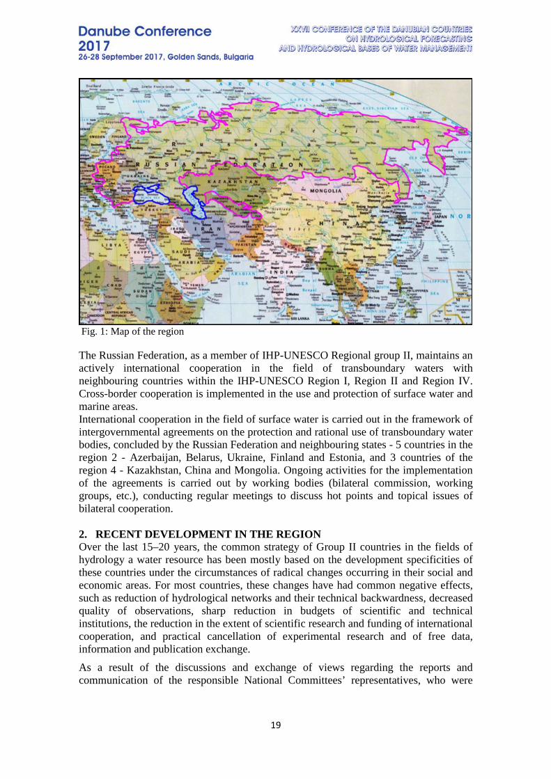
Fig. 1: Map of the region The Russian Federation, as a member of IHP-UNESCO Regional group II, maintains an actively international cooperation in the field of transboundary waters with neighbouring countries within the IHP-UNESCO Region I, Region II and Region IV. Cross-border cooperation is implemented in the use and protection of surface water and marine areas. International cooperation in the field of surface water is carried out in the framework of intergovernmental agreements on the protection and rational use of transboundary water bodies, concluded by the Russian Federation and neighbouring states - 5 countries in the region 2 - Azerbaijan, Belarus, Ukraine, Finland and Estonia, and 3 countries of the region 4 - Kazakhstan, China and Mongolia. Ongoing activities for the implementation of the agreements is carried out by working bodies (bilateral commission, working groups, etc.), conducting regular meetings to discuss hot points and topical issues of bilateral cooperation. 2. RECENT DEVELOPMENT IN THE REGION Over the last 15–20 years, the common strategy of Group II countries in the fields of hydrology a water resource has been mostly based on the development specificities of these countries under the circumstances of radical changes occurring in their social and economic areas. For most countries, these changes have had common negative effects, such as reduction of hydrological networks and their technical backwardness, decreased quality of observations, sharp reduction in budgets of scientific and technical institutions, the reduction in the extent of scientific research and funding of international cooperation, and practical cancellation of experimental research and of free data, information and publication exchange. As a result of the discussions and exchange of views regarding the reports and communication of the responsible National Committees’ representatives, who were

20

present in the meeting in, Škocjan Caves, Slovenia, 16-18 March 2016, among others the following conclusions were adopted: • Due to the geographical location of countries of the IHP UNESCO Group II, an initiative for trans-regional cooperation with neighboring regions was expressed. Examples of good practice of such cooperation are in the Danube basin, in the Nordic region, and in Central Asia. Furthermore, setting up new relationships is recommended in Central Asia region. • The cooperation and support of IHP UNESCO in the field of hydrology in the less developed countries of region II in Europe and Asia should be improved (e.g. through the UNESCO Secretariat, permanent delegations or national commissions for UNESCO). Some effort should be made to establish IHP Committees in newly developed countries. Also the information about the changes regarding the contact persons of IHP Committees should be updated promptly. • Water policy and hydrology need long-term planning for their proper development. We would like to ask countries to produce such strategy documents and increase funding for long-term hydrological observations. The collected hydrological data should be used free of charge. • Countries suggest that formal region IHP representative meetings are held yearly or at least before Council meetings. • Report on the hydrology in the Volga river basin should be translated and published in English. The National Committees should also support publications or translations of scientific work resulting from the cooperation within the Danube region and thus keep this region being recognized by other scientific communities. • Knowledge and technology transfer throughout the region is of high importance; therefore, the international (or even global) conferences taking place within IHP UNESCO’s Group II must be supported. Countries give full emphasis on the cooperation of Danube countries having the tradition of more than 60 years. The next city hosting the conference following the Deggendorf 2014 conference will be Sofia, Bulgaria, but not earlier than in late 2017. • Better cooperation among the Danube Commission, the International Commission for the Protection of the Danube River (ICPDR) and IHP Danube region is necessary. The region was established due to political and not geographical reason. There are several well establish trans regional cooperation’s on water issue with long tradition. Well known are:

1. The cooperation of IHP National Committees in the Danube River Basin with the start of the International Hydrological Decade 1965–1975. XXVI conferences of the Danube countries have been held so far. The monograph on the river basin, based on measurement data in the period 1930–1970, was published in 1988. Major research achievements until 2008 were published in a monograph »Hydrological Processes of the Danube River Basin« (2010). Please find more on the Danube cooperation at http://www.unesco.org/new/en/venice/natural-sciences/water/danube-cooperation/.

21

2. The Nordic countries cooperation in the framework of BARENTS EURO-ARCTIC council (BEAC). Working Group on Environment, Subgroup on Water Issues. http://www.beac.st/en/Working-Groups/BEAC-Working-Groups/Environment/Water-Issues,

3. The Commission on the Protection of the Black Sea Against Pollution (the Black Sea Commission or BSC), http://www.blacksea-commission.org/,

4. Hydro meteorological services of the Caspian countries with the active support of the World Meteorological Organisation (WMO)in 1994 have established the Coordinating Committee on Hydrometeorology and Pollution Monitoring of the Caspian Sea (CASPCOM) http://www.caspcom.com/index.php?razd=main&lang=2,

5. There is also need on Central Asia Cooperation between countries of IHP-UNESCO Region II and Region IV.

Electoral Group II countries cover a relatively large area of Europe and Asia. Therefore, there are distinct differences in climate, culture, and development. Furthermore, the individual countries are affected by problems related to the scarcity of water resources, water contamination and pollution, Tran’s boundary effects, and flood control. These big differences lead to different interests of the individual countries. Although the countries are joined in the electoral group, their cooperation and coordination of positions are inadequate. The region suffers by water scarcity due to inadequate water management and low level of cooperation. Also the region is presented only with 4 representatives in the IHP Council. We suggest increasing the number of representatives up to 6, as are representatives of other regions. Increase of representatives of II region will promote and increase visibility of IHP activity in the region.

3. UNESCO CHAIRS AND CENTRES IN THE REGION The UNESCO IHP water family has 37 chairs and 26 category two centers. Recently we lost UNESCO IHE as category I center. Among others only 6 chairs are from Region II:

6. UNESCO Chair in Water Resources, established in 2001 at Irkutsk State University, Russian Federation 9. UNESCO Chair in Hydrogeology, established in 2003 at the Eötvös Loránd University, Budapest, Hungary 20. UNITWIN Network on Water Resources, established in 2009 at Irkutsk State University, Russian Federation 22. UNESCO Chair on Water Resources Management and Ecohydrology, established in 2010 at the Water Problem Institute of the Russian Academy of Sciences, Russian Federation 28. UNESCO Chair in Water for Ecologically Sustainable Development, established in 2012 at the University of Belgrade, Serbia UNESCO Chair on Water Related Disaster Risk Reduction established in 2016 at the University of Ljubljana We have only three Category II centers and two of them are in Belgrade:

22

2. International Research and Training Centre on Urban Drainage (IRTCUD), Established in 1987 in Belgrade. 9. European Regional Centre for Ecohydrology (ERCE) established in 2006 in Poland 22. Centre for Water for Sustainable Development and Adaptation to Climate Change established in 2013 in Belgrade. The trouble is that policy and development are close related to the UNESCO Centers.

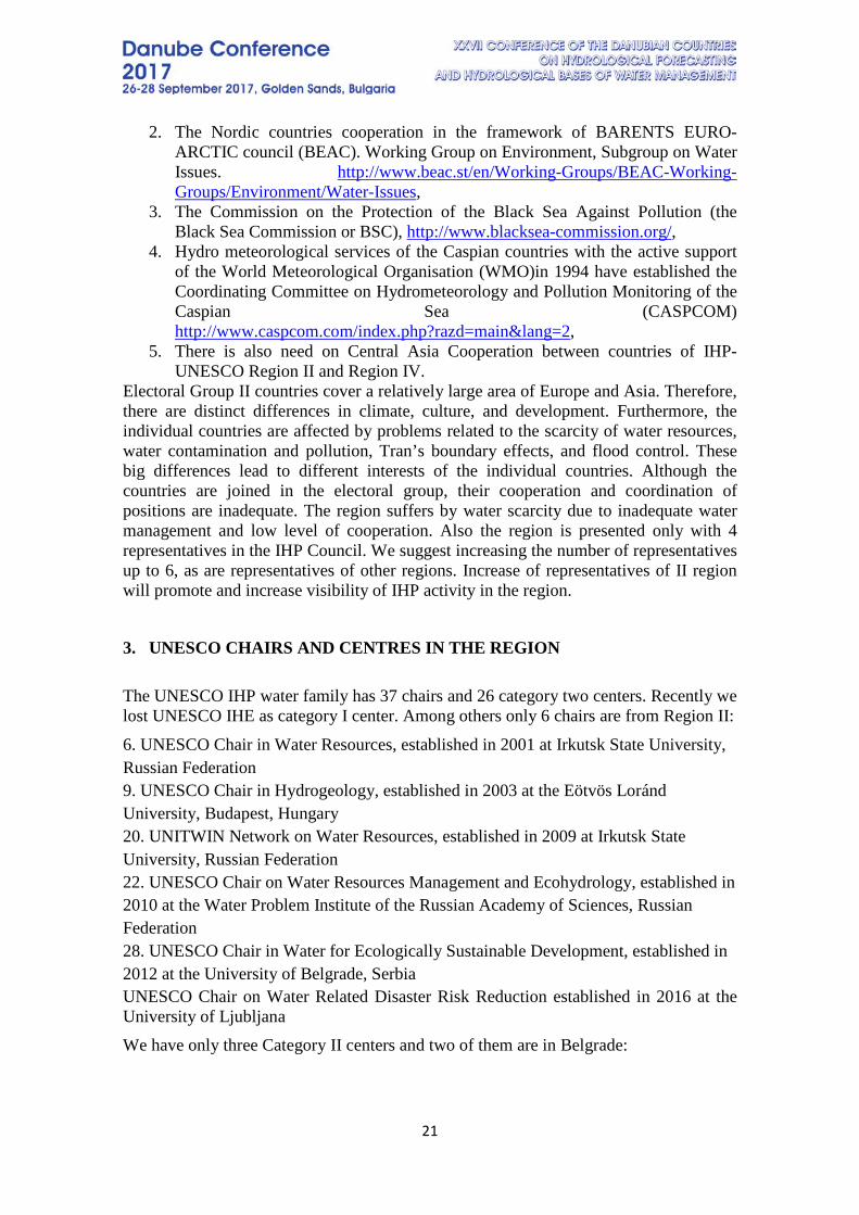
4. RECENT DEVELOPMENT IN THE SLOVENIA Twenty years ago the maintenance of embankments of regulated natural watercourses was brought to a halt, and the new practice was seen as eco-friendly maintenance of watercourses. Many river banks were overgrown with bushes and the space for water was only further reduced. In some places, the vegetation in the narrow channels completely obscured the surface of the water (Fig. 2). The serious damages due to the recent floods and, last but not least, fatalities, are the price that we pay today; examples are the floods of the Gradaščica and Vipava River in 2010. To make matters worse, the pressure on the water land is increasing in urban areas. A particular problem is the culverting of streams for urban purposes. It is ecologically extremely inappropriate; open water disappears from the environment in which it can only be enriched. Channels are diverted and small streams are put in culverts, despite the requirements of the Water Framework Directive. Water land which was often flooded is now occupied by roadways and parking lots.

Fig. 2: Consequence of overgrowing vegetation.

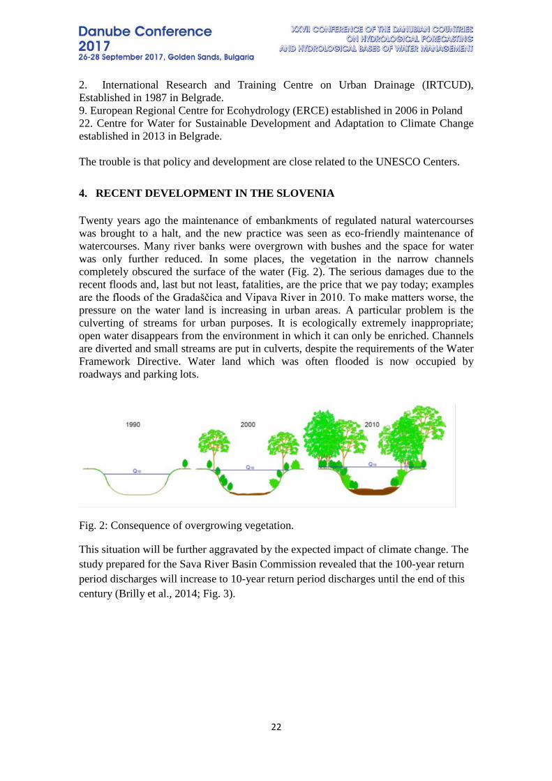
This situation will be further aggravated by the expected impact of climate change. The study prepared for the Sava River Basin Commission revealed that the 100-year return period discharges will increase to 10-year return period discharges until the end of this century (Brilly et al., 2014; Fig. 3).

23

Fig. 3: Climate change impacts on probability curves of Water Station Čatež on the Sava River.

Today, developments in urban water management should allow the increase of the room for water and, moreover, give back to the river at least some of the space that it once possessed. An important European project on this topic is underway in the Netherlands entitled ‘Room for the River’ (Klijna et al. 2013). The project, worth several billion Euros, covers 30 locations along the Dutch rivers. Similar activities are being carried out in other European countries, and also in the USA.

5. CONCLUSIONS In the recent twenty years, the countries in the region have been in political transition.

Transregional cooperation is crucial for the countries in the region.

Cooperation inside the region is not strong enough and not well organized and there are not enough centers and chairs that would support UNESCO IHP activities.

Today, developments in urban water management should allow the increase of the room for water and, moreover, give back to the river at least some of the space that it once possessed.

6. REFERENCES Brilly M., 2010, Hydrological processes of the Danube river basin : perspectives from the Danubian countries. Dordrecht [etc.]: Springer, cop. 2010. XIV, 436 pp.

24

Brilly, M., et al. (2014) Climate change impact on flood hazard in the Sava River Basin. In: The Sava River. Springer-Verlag Berlin-Heidelberg-New York

Klijna F., et al. (2013) Design quality of room-for-the-river measures in the Netherlands: role and assessment of the quality team (Q-team). International Journal of River Basin Management 11(3),

Slovene NC IHP, 2016, Minutes of the meeting of representatives of National Committees – members of IHP UNESCO’s Group II – Central and Eastern Europe, 16-18 March 2016, Škocjan Caves, Slovenia, Available from:

http://www.ksh.fgg.uni-lj.si/IHP/Data/Minutes%20of%20the%20meeting%20%20–%20members%20of%20IHP%20UNESCO’s%20Group%20II%20.pdf, [Accessed 26 September 2016]

UNESCO IHP, 2016, UNESCO’s Intergovernmental Scientific Cooperative Programme in Hydrology and Water Resources, Available from:

http://www.unesco.org/new/en/natural-sciences/environment/water/ihp, [Accessed 26 September 2016]

UNESCO OFFICE IN VENICE 2016, Danube Cooperation, Available from http://www.unesco.org/new/en/venice/natural-sciences/water/danube-cooperation/ , [Accessed 26 September 2016]

25

REGIONAL COOPERATION AMONG THE DANUBE COUNTRIES IN THE FRAMEWORK OF THE INTERNATIONAL HYDROLOGICAL PROGRAMME –

IHP/UNESCO

Stevan Prohaska

Institute for the Development of Water Resources “Jaroslav Černi”, Belgrade, Serbia

e-mail: stevan.prohaska@jcerni.co.rs

The General Conference of UNESCO established the International Hydrological Programme (IHP) in 1965 within UNESCO’s Division of Water Sciences. All member states of the United Nations have formed their National IHP Committees through which overall cooperation in IHP implementation is achieved. A special International Council for IHP was formed at UNESCO in Paris, along with a Secretariat responsible for global IHP implementation, including monitoring and execution of certain themes and projects under a predefined program of activities.

IHP projects are implemented by National IHP Committees of individual countries, National IHP Committees for several countries in the region or in the international river basin, and international and national science associations. From the scientific point of view, IHP topics are closely linked to the activities of international non-governmental organizations, such as the International Association for Hydrological Sciences (IAHS), the International Association for Hydraulic Research (IAHR), the International Hydrogeologists Association (IAH), the International Irrigation and Drainage Commission (ICID), International Water Resources Association (IWRA), and others.

The IHP International Council, as well as its Secretariat at UNESCO headquarters, is responsible for the implementation of the IHP on a global scale and for monitoring and coordination of the implementation of particular program topics. Each country contributes to its own development by participating in the implementation of individual projects in the International Program, within limits of its material and personnel capabilities. At the same time, the achievements of each country are available to other UNESCO member countries. This knowledge transfer is one of the essential components of UNESCO programs.

Cooperation of experts from the Danube countries takes place in two directions, through:

26

• A regional conference of the Danube countries on hydrological forecasting, and

• Regional hydrological monographs and thematic projects related to the Danube River Basin.

1. REGIONAL CONFERENCE OF THE DANUBE COUNTRIES ON HYDROLOGICAL FORECASTING

The first conference of the Danube countries on hydrological forecasting was organized in Budapest in 1961, on the initiative of then distinguished scientists in the Danube region (Dumitrescu, Kaczmarek, Kalinin, Lasyloffy and others). The idea was to bridge the gap between two blocs – at the time eight Danube countries were behind the iron curtain. These conferences of the Danube countries have acquired a rich tradition as the main gathering point for exchange of experiences and synthesis of hydrological knowledge in the Danube River Basin.

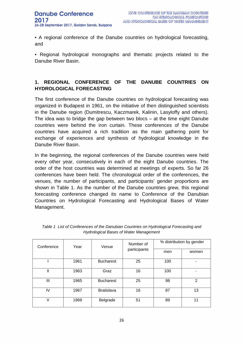
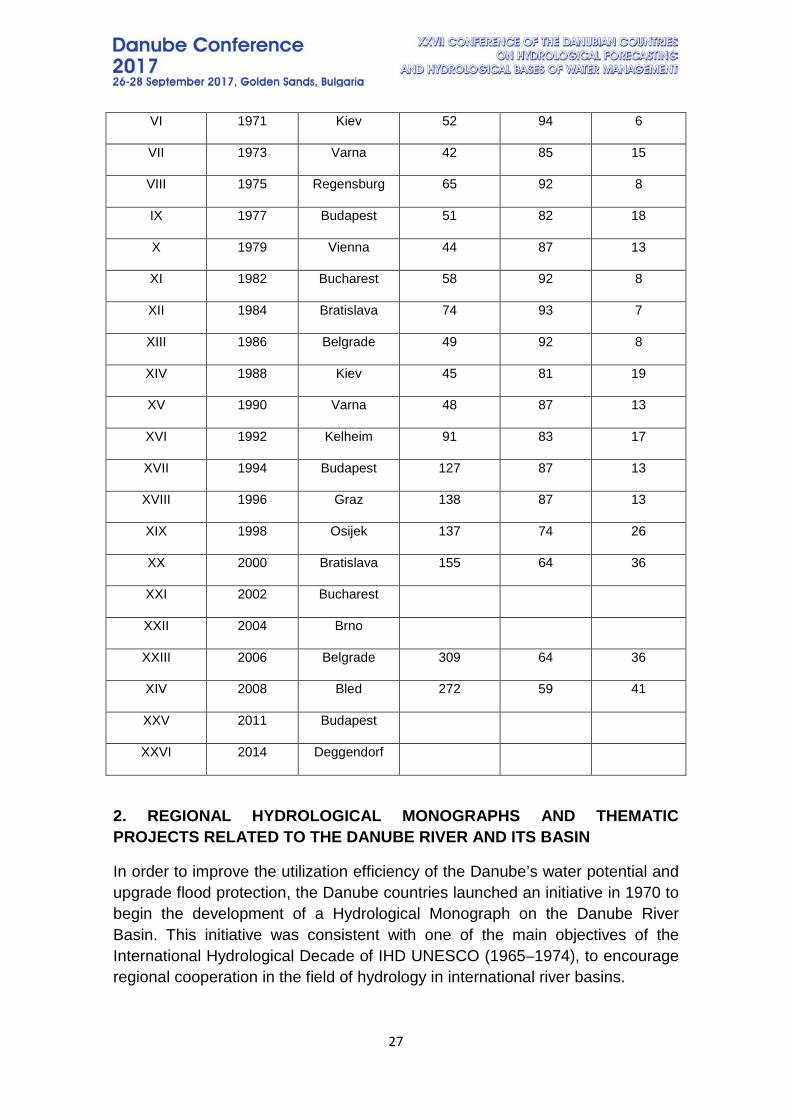
In the beginning, the regional conferences of the Danube countries were held every other year, consecutively in each of the eight Danube countries. The order of the host countries was determined at meetings of experts. So far 26 conferences have been held. The chronological order of the conferences, the venues, the number of participants, and participants’ gender proportions are shown in Table 1. As the number of the Danube countries grew, this regional forecasting conference changed its name to Conference of the Danubian Countries on Hydrological Forecasting and Hydrological Bases of Water Management.

Table 1 List of Conferences of the Danubian Countries on Hydrological Forecasting and Hydrological Bases of Water Management

Conference Year Venue Number of participants

% distribution by gender

men women

I 1961 Bucharest 25 100 -

II 1963 Graz 16 100 -

III 1965 Bucharest 25 98 2

IV 1967 Bratislava 16 87 13

V 1969 Belgrade 51 89 11

27

VI 1971 Kiev 52 94 6

VII 1973 Varna 42 85 15

VIII 1975 Regensburg 65 92 8

IX 1977 Budapest 51 82 18

X 1979 Vienna 44 87 13

XI 1982 Bucharest 58 92 8

XII 1984 Bratislava 74 93 7

XIII 1986 Belgrade 49 92 8

XIV 1988 Kiev 45 81 19

XV 1990 Varna 48 87 13

XVI 1992 Kelheim 91 83 17

XVII 1994 Budapest 127 87 13

XVIII 1996 Graz 138 87 13

XIX 1998 Osijek 137 74 26

XX 2000 Bratislava 155 64 36

XXI 2002 Bucharest

XXII 2004 Brno

XXIII 2006 Belgrade 309 64 36

XIV 2008 Bled 272 59 41

XXV 2011 Budapest

XXVI 2014 Deggendorf

2. REGIONAL HYDROLOGICAL MONOGRAPHS AND THEMATIC PROJECTS RELATED TO THE DANUBE RIVER AND ITS BASIN

In order to improve the utilization efficiency of the Danube’s water potential and upgrade flood protection, the Danube countries launched an initiative in 1970 to begin the development of a Hydrological Monograph on the Danube River Basin. This initiative was consistent with one of the main objectives of the International Hydrological Decade of IHD UNESCO (1965–1974), to encourage regional cooperation in the field of hydrology in international river basins.

28

The first outcome of the regional cooperation of the Danube countries in this regard was the publication of national monographs:

"Hydrological balance of the Danube River"

produced applying the same methodology in all eight Danube countries.

The coordinators of the entire undertaking were:

• Institute VUVH from Bratislava

which coordinated the work of a group of experts from Czechoslovakia (CS), Hungary (H), Bulgaria BG) and the Soviet Union (SU), and

• Technical Secretariat (NC for IHP YU) from Belgrade

which coordinated the work of a group of experts from Germany (D), Austria (A), Yugoslavia (YU) and Romania (RO).

During that period (from 1971 to 1986), experts from all eight Danube countries met every other year and coordinators each year, and agreed to create a single monograph for the entire Danube River Basin. Following harmonization of data and water balance maps between neighboring countries, the following publications were issued:

1. "Die Donau und Ihr Einzugsgebiet – Eine hydrologische Monographic" in German (München, 1986), and

2. "Donau i ego basseyn – Gidrologicheskaya Monografiya" in Russian.

3. Representative monograph "Hydrology of the River Danube", printed in four languages (English, Russian, German and French) (UNESCO, Bratislava 1988).

With the collapse of socialist countries in Eastern Europe, new countries were formed in the Danube River Basin (now 19 in total), which also joined the regional cooperation effort under UNESCO IHP. Today, active participants in regional cooperation are National IHP Committees of the following countries:

IHP National Committees that have signed the "Principles":

Germany (D), Austria (A), Czech Republic (CZ), Slovakia (SK), Hungary (H), Slovenia (SL), Croatia (CR), Bosnia and Herzegovina (BiH), Serbia (SR), Romania (RO), Bulgaria (BG), Moldova (MD), and Ukraine (UA).

IHP National Committees which have not signed the "Principles":

29

Switzerland (CH), Italy (I), Poland (PO), Albania (AL), Macedonia (MC) and Montenegro (MN).

In the period from 1993 to 2017, the above-mentioned Danube countries participated in the implementation of eleven thematic projects. So far, the following projects or subprojects have been completed and published, while some are in the process of implementation:

1. Project No 1: Sediment regime of the Danube and its tributaries (Budapest, 1993 – Head Dr. Rakoci, Hungary) – in Russian and German.

2. Project No 2: Thermal and ice conditions of the Danube and its major tributaries (Bratislava, 1993 – Head Dr. Stančikova, Slovakia) – in Russian and German.

3. Project No 3: Long-term fluctuations of precipitation in the Danube basin (NK-IHP Austria) – unfinished project.

4. Project No 4: Coincidence of flood flow of the Danube River and its tributaries (Bratislava, 1999 – Head Dr. Prohaska, Yugoslavia) – in English.

5. Project No 5: Reambulation of the Hydrological Monograph of the Danube River Basin

a. Subproject No 5.1: Inventory of the main hydraulic structures in the Danube Basin (Bucharest, 2004 – Head Dr. Pasoi, Romania) – in English.

b. Subproject No 5.2: Flow regime of the River Danube and its Catchment (Koblenz, 2004 – Head Dr. Belz, Germany) – in Russian, English and German.

c. Subproject No 5.3: Basin-wide water balance in the Danube River Basin (Bratislava, 2006 – Head Dr. Petrovič, Slovakia) – in English.

d. Subproject No 5.4: Characterization of the runoff regime and its stability in the Danube Catchment (Budapest 2006 – Head Dr. Kovacs, Hungary) – in English.

6. Project No 6: The condition of the Danube riverbed

a. Subproject No 6.1: Palaeogeography of the Danube and its Catchment (Budapest, 1999 – Head Dr. Nepel et al., Hungary) – in English.

b. Subproject No 6.2: The Danube River channel training (Bratislava, 1999 – Head Dr. Stančikova, Slovakia) – in Russian and German.

c. Subproject No 6.3: The fords of the Danube (Budapest, 1993 – Head Dr. Goda, Hungary) – in Russian and German.

d. Subproject No 6.4: Meanders and falls on the Danube River and geomorphological parameters in the riverbed (Analysis of geomorphological processes) – unfinished subproject.

30

7. Project No 7: Regional analysis of annual peak discharges in the Danube Catchment (Bucharest, 2004 - Head Dr. Stanescu, Romania) – in English.

8. Project No 8: Hydrological bibliography referring to the Danube Basin

a. Subproject No 8.1: Hydrological bibliography referring to the Danube River Basin (Koblenz, ??? – Head Dr. Schreoder, Germany) – unfinished subproject

b. Subproject No 8.2: Danube River Basin coding (Ljubljana, 2000 – Head Dr. Brilly, Slovenia) – in English, Russian and German.

9. Project No 9: Flood regime of rivers in the Danube Basin (Bratislava, Head Dr. Pekarova, Slovakia) – unfinished project.

10. Project No 10: Sediment balance in the Danube Basin (Vienna, Head Dr. Nachtnebei, Austria) – unfinished project.

11. Project No 11: Low flow and hydrological drought in the Danube Basin (Sofia, Head Dr. Dakova, Bulgaria) – unfinished project.

Experts from the Danube countries provide data from their territory for the development of thematic projects, participate in the assessment of results, and approve publication. The work of experts from the Danube countries is carried out at regular working meetings (once a year in certain countries) and extraordinary working meetings (once in two years – during the Conference of the Danube Countries on Hydrological Forecasting). The working meetings are managed by the country/expert coordinator selected at two-to-three year intervals, each time from another Danube country.

As a crown to the successful cooperation of the Danube countries, the book "Hydrological Processes of the Danube River Basin – Perspectives from the Danubian Countries" was published by Springer in 2010. It was edited by Mitja Brilly (SLO).

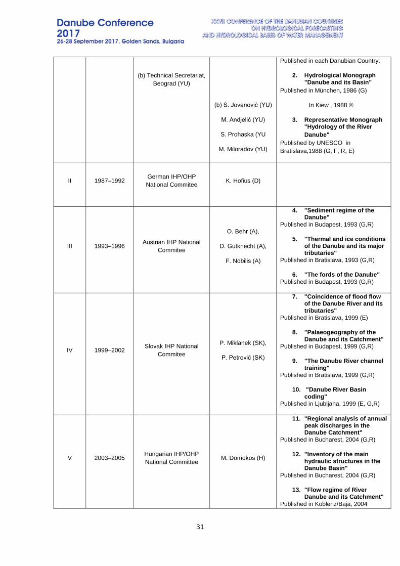
A list of current coordinators of regional cooperation in the Danube countries in the field of hydrology is given in Table 2.

Table 2 List of chief coordinators from the Danube countries in the field of hydrology Phase of cooperati

on Period

Chief coordinating Results/ Publications

Institution(s) Expert(s)

I 1971–1986 (a) Water resources

Institute VUVH, Bratislava (CS)

(a) A. Sikora (CS), A.

Stančik (CS)

1. Eight National Monographs "Hydrological balance of the River Danube"

31

(b) Technical Secretariat, Beograd (YU)

(b) S. Jovanović (YU)

M. Andjelić (YU)

S. Prohaska (YU

M. Miloradov (YU)

Published in each Danubian Country.

2. Hydrological Monograph "Danube and its Basin"

Published in München, 1986 (G)

In Kiew , 1988 ®

3. Representative Monograph "Hydrology of the River Danube"

Published by UNESCO in Bratislava,1988 (G, F, R, E)

II 1987–1992 German IHP/OHP National Commitee K. Hofius (D)

III 1993–1996 Austrian IHP National Commitee

O. Behr (A),

D. Gutknecht (A),

F. Nobilis (A)

4. "Sediment regime of the Danube"

Published in Budapest, 1993 (G,R)

5. "Thermal and ice conditions of the Danube and its major tributaries"

Published in Bratislava, 1993 (G,R)

6. "The fords of the Danube" Published in Budapest, 1993 (G,R)

IV 1999–2002 Slovak IHP National Commitee

P. Miklanek (SK),

P. Petrovič (SK)

7. "Coincidence of flood flow of the Danube River and its tributaries"

Published in Bratislava, 1999 (E)

8. "Palaeogeography of the Danube and its Catchment"

Published in Budapest, 1999 (G,R)

9. "The Danube River channel training"

Published in Bratislava, 1999 (G,R)

10. "Danube River Basin coding"

Published in Ljubljana, 1999 (E, G,R)

V 2003–2005 Hungarian IHP/OHP National Committee M. Domokos (H)

11. "Regional analysis of annual peak discharges in the Danube Catchment"

Published in Bucharest, 2004 (G,R)

12. "Inventory of the main hydraulic structures in the Danube Basin"

Published in Bucharest, 2004 (G,R)

13. "Flow regime of River Danube and its Catchment"

Published in Koblenz/Baja, 2004

32

(E,G,R)

14. "Basin-wide water balance in the Danube River Basin"

Published in Bratislava, 2006 (E)

VI 2006–2008 IHP National Commitee of Serbia M. Miloradov (SR)

15. "The hydrological meta-database of the countries sharing the Danube Catchment"

Published in Koblenz/Baja, 2008 (E,G,R)

16. "Characterization of the runoff regime and its stability in the Danube Catchment"

Published in Budapest, 2006 (E)

VII 2009–2011 IHP National Commitee of Croatia D. Biondić (CR)

17. "Long-term fluctuations of precipitation in the Danube Basin"

18. "Flood regime of rivers in the Danube Basin"

In procedure

19. "Sediment balance in the Danube Basin"

In procedure

20. "Low flow and hydrological drough in the Danube Basin"

VIII 2012–? IHP National Commitee of Romania D. Radulescu (RO)

33

TOPIC 1: BASIC OF HYDROLOGY

ISSUES OF INTRODUCING THE MODERN INSTRUMENTS OF HYDROMETRIC MEASUREMENTS IN THE HYDROMETEOROLOGICAL

SERVICE OF UKRAINE

Viacheslav Manukalo1, Mykola Nastiuk2, Natalia Samoylenko3

1Ukrainian Hydrometeorological Institute, 2Chernivtsi Centre on Hydrometeorology, 3Central Geophysical Observatory

Corresponding author: V. Manukalo, Ukrainian Hydrometeorological Institute, 37, Nauki Prospect, 03028, Kyiv, Ukraine, manukalo@ukr.net

ABSTRACT Improving the accuracy and timeliness of hydrological forecasts, as well as the assessment of water resources requires a technical upgrade of the network of hydrometric measurements of the Ukrainian Hydrometeorological Service. Currently the Hydrometeorological Service is undertaking efforts for putting in operation the modern technology for hydrological measurement, first of all, the automated measurement stations and devices which use the advanced technologies of measuring the river flow. In the paper are presented some results of operation in the Regional Centre on Hydrometeorology (CHM) located in the Chernivtsi city: a) the automated hydrometeorological stations: PHMA (produced by the Ukrainian enterprise “Techprylad”, located in the Lviv city) and Vaisala HydroMet™ MAWS100 (produced by the Vaisala Oyj, Finland); b) OTT Qliner2 device for a mobile measurement of river flows. The analysis of problematic issues has allowed to develop and put in operation a number of methodological and organizational recommendations for more efficient use of modern hydrometric instruments in the hydrometeorological service of Ukraine.

Keywords: Modern Instruments, Using, Experience

1. INTRODUCTION Improving the accuracy and timeliness of hydrological forecasts, as well as the assessment of water resources requires a technical upgrade of the network of hydrometric measurements of the Ukrainian Hydrometeorological Service. Currently the Hydrometeorological Service has undertaken efforts for putting in operation of modern technology for hydrological measurement, first of all, automated measurement stations and devices which use the advanced technologies of measuring the river flow. A number of results of exploitation of above mentioned equipments in the Ukrainian Hydrometeorological Service have been obtained. These results allow us to draw some conclusions about the possibilities of these technologies and to consider problematic issues related to their operation.

The aim of this article is presenting some results of exploitation in the Regional Centre on Hydrometeorology (CHM) located in the Chernivtsi city: a) the automated hydrometeorological stations: PHMA (produced by the Ukrainian enterprise “Techprylad”,located in the Lviv city) and Vaisala HydroMet™ MAWS100 (produced

34

by the Vaisala Oyj, Finland); b) OTT Qliner2 device for a mobile measurement of river flows.

CHM is responsible for providing hydrological measurements on the Dniester, Prut and Siret rivers and their tributaries. These rivers are located in Carpathian mountains region and have the very complicated hydrological regime with often river floods of different origin.

2. DISCUSSION OF RESULTS

2.1. Automated hydrological stations

The Ukrainian station have been started to put in operation in 2007, the Finnish station - in 2012. The Ukrainian and Finnish automated stations provide with a measurement of water level, water and air temperature as well as precipitation with the subsequent on-line transmission of measured parameters to the forecasting centers. The operation of the Finnish station, including, the collection and processing of measured data is provided by the Vaisala Data Logger QML 201 platform with the Vaisala Setup Software Lizard. The software Ukrainian produced is used in the Ukrainian station. Following problematic issues were identified in the operation of stations.

Hardware. Ensuring a reliable function of water level sensor in the Ukrainian station and precipitation sensor in the Finnish one were the most common problems in their work. Two types of sensors for water level measurement are used in the Ukrainian station: 1) which works on the principle of measuring a hydrostatic pressure; 2) which works on the barbotage principle.

In the first case, the failure in the work of sensor was related to a damage of hose and an ingress of water inside this device. The maintenance of pressure in a system for operation of second type of sensor is needed. The special compressor is provided the pressure in the system. This complicates the work of system, and in the case of reducing the pressure in the system, causes the water level measurement errors. Sometimes these errors can reach up to 8-10 cm.

In the Finnish station the ice has been formed in the enclosure of sensor for measuring the precipitation at the negative air temperatures. This factor was the reason of reducing the amount of measured solid precipitation.

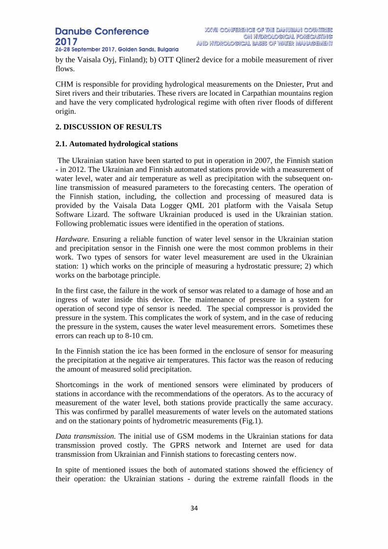
Shortcomings in the work of mentioned sensors were eliminated by producers of stations in accordance with the recommendations of the operators. As to the accuracy of measurement of the water level, both stations provide practically the same accuracy. This was confirmed by parallel measurements of water levels on the automated stations and on the stationary points of hydrometric measurements (Fig.1).

Data transmission. The initial use of GSM modems in the Ukrainian stations for data transmission proved costly. The GPRS network and Internet are used for data transmission from Ukrainian and Finnish stations to forecasting centers now.

In spite of mentioned issues the both of automated stations showed the efficiency of their operation: the Ukrainian stations - during the extreme rainfall floods in the

35

Dniester river basin in 2008 and 2010; the Finnish stations - during the spring flood in the Prut river basin in 2013.

Fig 1. Graph of connection of water levels measured with using the staff gauge and

with using the technical complex Vaisala HydroMet ™ MAWS100 on the Prut river at Chernivtsi city for the period April - June 2013

2.2. OTT Qliner2 device

The accuracy of this device measurement was assessed in 2012 – 2013 by comparing discharges of water, which were measured with using this device and with using the traditional current water meters. The measurement of water discharges was carried out on the Dniester river at the Mohilev-Podolsky city, on the Prut river at the Chernivtsi city, on the Prut river at the Marshyntsi village, on the Siret river at the Staroginets town. The complex structure of river channels is characterized for all cross-sections, except the Dniester river at the Mogilev - Podolsky city. The comparative measurements of water discharges have been performed mostly during the summer-autumn periods with the low flow and during the period of recession of spring flood. Depths of water in river channels were measured in the traditional way with using hydrometric winches, as well as with using the instrument OTT Qliner 2 in the pillars of water, consisting of sections of 30 × 30 cm. The differences in a structure of river

36

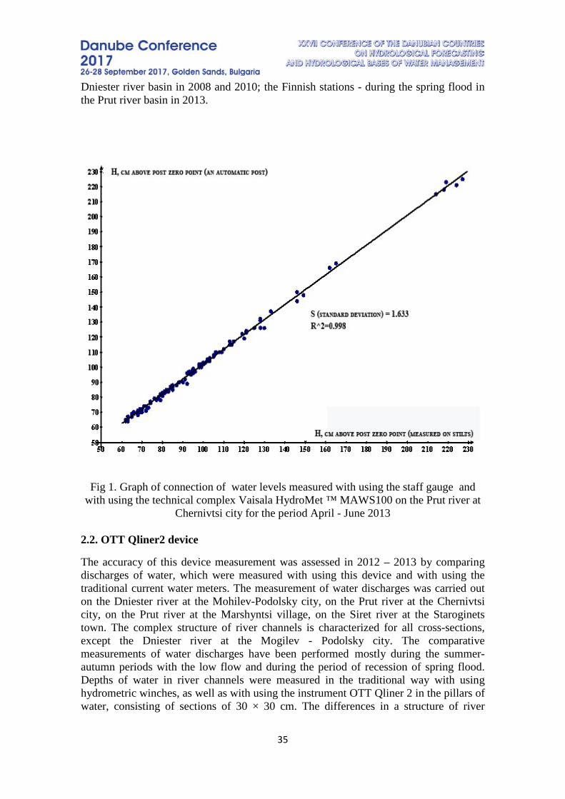
channels, as well as in principles of measuring hydrometric parameters between current meters and ultrasonic flow meters do not allow to measure water discharges with using Qliner2 exactly on the same vertical as with using the hydrometric winches. That leads to some minor differences in depths measured on some velocity verticals (Fig. 2), but these differences do not affect significantly the accuracy of measuring water discharges.

Fig 2. Profiles of the cross-section of the Prut river at Chernivtsi city measured by different devices

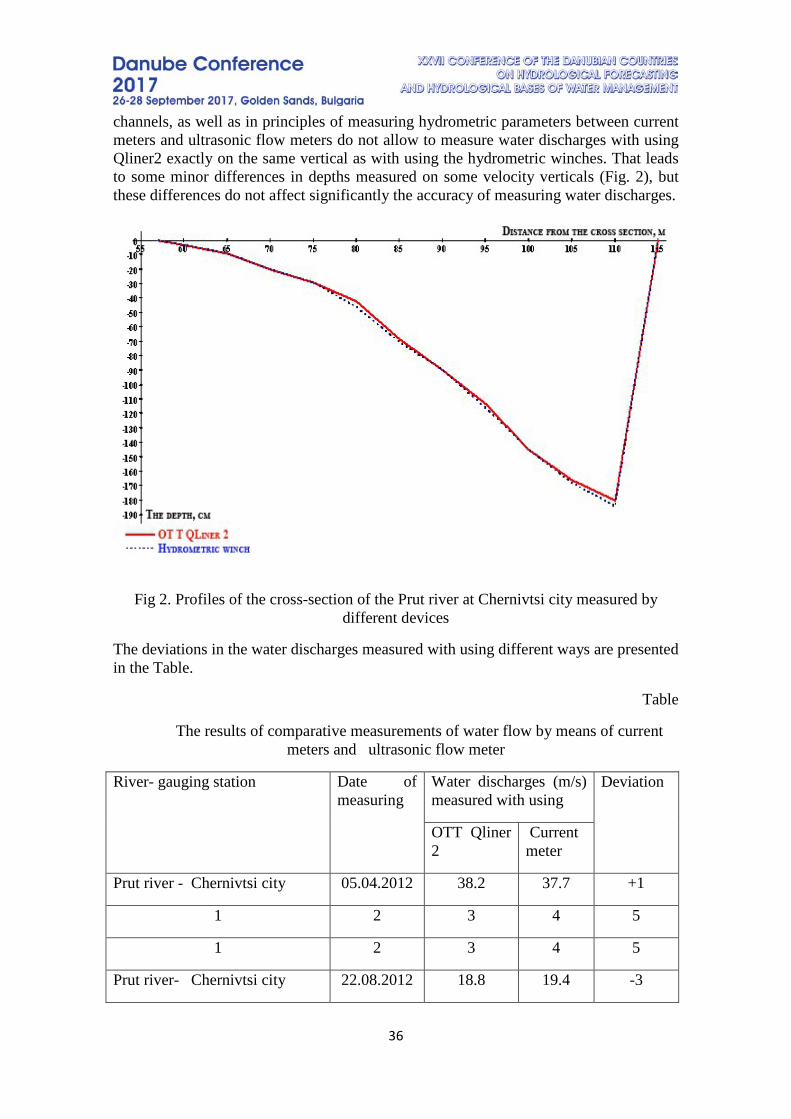
The deviations in the water discharges measured with using different ways are presented in the Table.

Table

The results of comparative measurements of water flow by means of current meters and ultrasonic flow meter

River- gauging station Date of measuring

Water discharges (m/s) measured with using

Deviation

OTT Qliner 2

Current meter

Prut river - Chernivtsi city 05.04.2012 38.2 37.7 +1

1 2 3 4 5

1 2 3 4 5

Prut river- Chernivtsi city 22.08.2012 18.8 19.4 -3

37

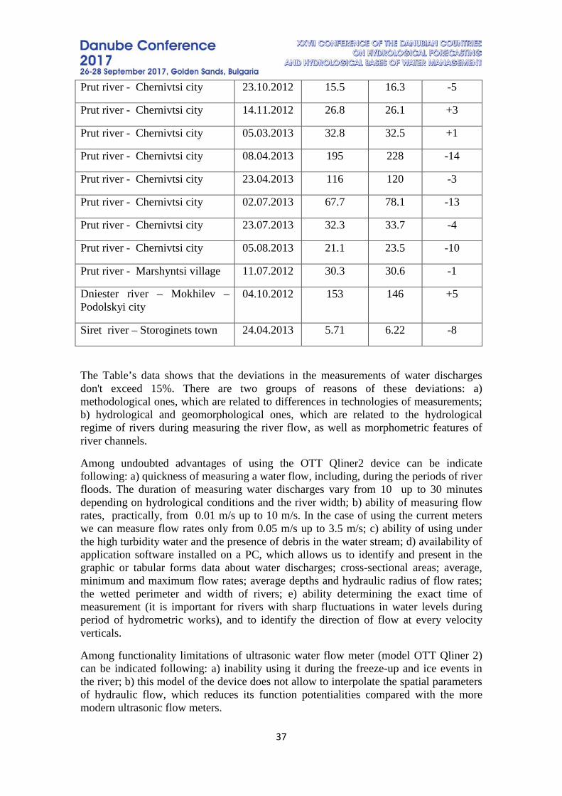
Prut river - Chernivtsi city 23.10.2012 15.5 16.3 -5

Prut river - Chernivtsi city 14.11.2012 26.8 26.1 +3

Prut river - Chernivtsi city 05.03.2013 32.8 32.5 +1

Prut river - Chernivtsi city 08.04.2013 195 228 -14

Prut river - Chernivtsi city 23.04.2013 116 120 -3

Prut river - Chernivtsi city 02.07.2013 67.7 78.1 -13

Prut river - Chernivtsi city 23.07.2013 32.3 33.7 -4

Prut river - Chernivtsi city 05.08.2013 21.1 23.5 -10

Prut river - Marshyntsi village 11.07.2012 30.3 30.6 -1

Dniester river – Mokhilev –Podolskyi city

04.10.2012 153 146 +5

Siret river – Storoginets town 24.04.2013 5.71 6.22 -8

The Table’s data shows that the deviations in the measurements of water discharges don't exceed 15%. There are two groups of reasons of these deviations: a) methodological ones, which are related to differences in technologies of measurements; b) hydrological and geomorphological ones, which are related to the hydrological regime of rivers during measuring the river flow, as well as morphometric features of river channels.

Among undoubted advantages of using the OTT Qliner2 device can be indicate following: a) quickness of measuring a water flow, including, during the periods of river floods. The duration of measuring water discharges vary from 10 up to 30 minutes depending on hydrological conditions and the river width; b) ability of measuring flow rates, practically, from 0.01 m/s up to 10 m/s. In the case of using the current meters we can measure flow rates only from 0.05 m/s up to 3.5 m/s; c) ability of using under the high turbidity water and the presence of debris in the water stream; d) availability of application software installed on a PC, which allows us to identify and present in the graphic or tabular forms data about water discharges; cross-sectional areas; average, minimum and maximum flow rates; average depths and hydraulic radius of flow rates; the wetted perimeter and width of rivers; e) ability determining the exact time of measurement (it is important for rivers with sharp fluctuations in water levels during period of hydrometric works), and to identify the direction of flow at every velocity verticals.

Among functionality limitations of ultrasonic water flow meter (model OTT Qliner 2) can be indicated following: a) inability using it during the freeze-up and ice events in the river; b) this model of the device does not allow to interpolate the spatial parameters of hydraulic flow, which reduces its function potentialities compared with the more modern ultrasonic flow meters.

38

3. CONCLUSIONS

The experience gained by experts from the Chernivtsi Regional Centre on Hydrometeorology has allowed to develop the skills to work with modern hydrometric equipment, to assess their advantages and to identify problematic issues in their practical application. The generalization of obtained experience makes it possible to give some recommendations that may be useful in the further technical development of the hydrological network of the Hydrometeorological Service of Ukraine.

The operational exploitation of the automated hydrometeorological stations and mobile device for a measurement of river flows has shown the promise of their use for practical and scientific purposes. The automated hydrometeorological stations significantly improve the efficiency of hydrological forecasting. The information from these stations is a prerequisite of increasing an earliness and an accuracy of hydrological forecasts and warnings. The use of the mobile ultrasonic water flow meter allows to obtain the important information about the dynamic of changing hydraulic parameters in the beds of mountain rivers, that is impossible when we use conventional methods of measuring river flow. The use of ultrasonic flow meters is effective during flood periods, when there is no a possibility to measure river flow using hydrometric current meters.

Putting in operation of the modern high-tech hydrometric technologies also requires solving a number of methodological and organizational issues, among them we would like to indicate following: a) it is necessary to include the issues of using the modern technologies of hydrometric measurements in the regulatory guidelines on hydrological measurements used in the Hydrometeorological Service; b) creating the service center (possibly - several centers) to service the modern hydrometric equipment; c) creating the permanent system for training (retraining) the hydrological personnel to work with the modern hydrometric equipment.

39

METHODICAL APPROACHES TO THE ESTIMATION OF REPRESENTATIVENESS OF BENCHMARK CLIMATE STATIONS

Stanislav Moskalenko

Ukrainian Hydrometeorological Institute, Kyiv, Ukraine Corresponding author: Ukrainian Hydrometeorological Institute, 37 Nauki Ave., Kyiv

28-03650, Ukraine, stas_univer@mail.ru

ABSTRACT Using a series of meteorological elements for monitoring climate, water balance calculations, evaluation of water resources requires a more thorough quantitative verification of representativeness and homogeneity of series of observations. Particular attention should be paid to the benchmark climate stations (BCS). Methodical approaches to the estimation of "creeping" heterogeneity in the ranks of meteorological elements. For example, observational data of meteorological stations Kyiv, which is of benchmark climate stations shows the sequence of calculations to identify "creeping" heterogeneity in the ranks of average values of air temperature, water vapor pressure, wind speed and precipitation amounts in January and July for the period 1981-2010 years. The calculation results showed statistically significant value "creeping" heterogeneity ranks only wind speed in summer. Keywords: climate monitoring, representativeness of observational data, benchmarks climate station, city’s influence, «creeping» heterogeneity

1. INTRODUCTION For monitoring and climate research, identifying its natural fluctuations and human impact are important measurement data held in the benchmark climate stations Hydrometeorological Service (hereinafter - BCS) [3]. BCS - meteorological station for consistent continuous number of similar observations not less than 30 years, located in places where environmental change caused by human activities are minimal. These stations are designed to establish the age trends changing climate in a particular area. Therefore, it is important to periodically check the representativeness of observational data, especially in cases where the stations are located within large urban areas, which can affect weather conditions. The station is representative (typical) if the results of observations are indicative for the surrounding area (within a radius of several dozen kilometers). Because of this observation, stations can get the value by interpolation points in the surrounding area with some precision adopted in accordance with the method provided the meteorological regime of the territory is homogeneous. In particular, it is recommended to periodically check series of meteorological observations for the so-called "creeping" heterogeneity, which may be due to changing weather conditions under the influence of the city.

40

In the Ukrainian Hydrometeorological Institute conducted the study to clarify the methodological approach to the evaluation of "creeping" heterogeneity in the ranks of meteorological variables and provides detailed examples for conditions Ukraine [3].

2. INITIAL DATA AND METHODOLOGICAL APPROACHES To identify "creeping" heterogeneity using a technique which consists in building a "stepwise trend" and assessment of statistical significance of changes in the level range. It does not analyze the value of meteorological elements. The analysis of differences or relationships values of meteorological elements measured at stations located within the city, and the nearest station is located in an area where human impact on meteorological conditions can be considered minimal. If "creeping" heterogeneity among meteorological values should be observed several relatively small but growing or flowing from the values of step homogeneous areas. When assessing the presence of "creeping" heterogeneity in the ranks of meteorological variables can be divided into two main stages. In the first stage of determining changes level meteorological variables in the time. The ranks divided into intervals within which the process of changing in the time difference can be considered homogeneous. In the second stage determine how changes differences between homogeneous areas statistically significant. Definition of homogeneous regions in the sequence of meteorological variables performed as follows. Members of the chronological series of differences numbered from 1 to N. The entire range of the differences is divided into equal on size gradations. For approximate estimation of the required number of gradations , which is divided set of variables used the formula [2]:

. (1)

Countdown differences in each gradation start the from the first number and the first difference in each gradation is the difference between the number N= 1 and the first number that came to this graduation. The final difference in every gradation calculated between the last number totality of differences and the last number of gradations. If you find that two adjacent numbers in a given gradation remote far apart and the difference between them more than a certain critical value, it gives reason to believe that they belong to two different stationary plots, ie there between the differences big gap. Critical values for each gradation difference is calculated using the formula:

, (2) where - the last number of graduation; - the number of cases of graduation; - statistics Kolmogorov [1, 3, 4].

Taking the probability of exceeding 99.99% (corresponding to the level of significance 0,01%) on the Table of Kolmogorov find appropriate this level statistical value = 0,33. Next, consider a couple of numbers with the lowest number on the left. Choose a pair of numbers with others gradations. Their number the left does not exceed to the right in this graduation. That is, choose a pair of crossing this. Of all the numbers of couples are

xnN

xn N=

CR CR K KN mλ∆ = ⋅

KN

Km

CRλ

41

crossing this, choose the smallest number of year in which there was a the first change level in the ranks (ie, number of year, which ends the first part of the uniform the rank). Then choose the next closest to this part of the rank a couple of numbers. So, find a second number, which varies the level of the rank (second change level in the ranks). This procedure is repeated until the entire rank is exhausted. It should be noted that the Year of violation of homogeneity is the beginning of the next permanent part of the rank. For all identified homogeneous parts is calculated averages. Thus prepared stepwise function, which determined whether or not "creeping" heterogeneity in chronological series of meteorological values. If it is present, it should be observed several relatively small but growing or killing homogeneous parts studied sequence characteristics.

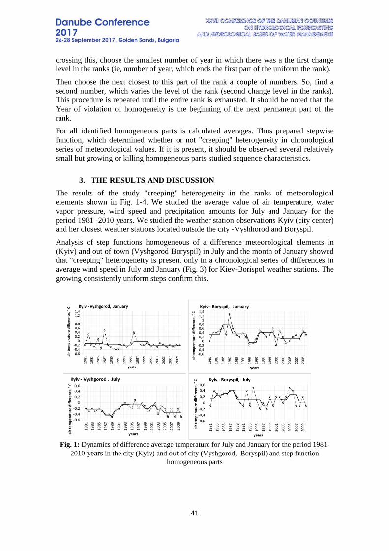
3. THE RESULTS AND DISCUSSION The results of the study "creeping" heterogeneity in the ranks of meteorological elements shown in Fig. 1-4. We studied the average value of air temperature, water vapor pressure, wind speed and precipitation amounts for July and January for the period 1981 -2010 years. We studied the weather station observations Kyiv (city center) and her closest weather stations located outside the city -Vyshhorod and Boryspil. Analysis of step functions homogeneous of a difference meteorological elements in (Kyiv) and out of town (Vyshgorod Boryspil) in July and the month of January showed that "creeping" heterogeneity is present only in a chronological series of differences in average wind speed in July and January (Fig. 3) for Kiev-Borispol weather stations. The growing consistently uniform steps confirm this.

Fig. 1: Dynamics of difference average temperature for July and January for the period 1981-

2010 years in the city (Kyiv) and out of city (Vyshgorod, Boryspil) and step function homogeneous parts

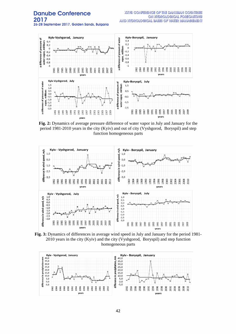
42

Fig. 2: Dynamics of average pressure difference of water vapor in July and January for the period 1981-2010 years in the city (Kyiv) and out of city (Vyshgorod, Boryspil) and step

function homogeneous parts

Fig. 3: Dynamics of differences in average wind speed in July and January for the period 1981-

2010 years in the city (Kyiv) and the city (Vyshgorod, Boryspil) and step function homogeneous parts

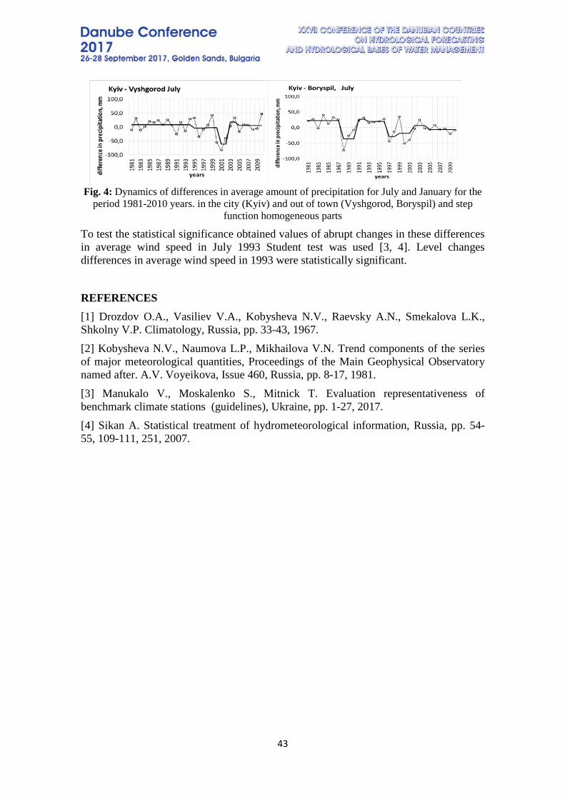
43

Fig. 4: Dynamics of differences in average amount of precipitation for July and January for the

period 1981-2010 years. in the city (Kyiv) and out of town (Vyshgorod, Boryspil) and step function homogeneous parts

To test the statistical significance obtained values of abrupt changes in these differences in average wind speed in July 1993 Student test was used [3, 4]. Level changes differences in average wind speed in 1993 were statistically significant.

REFERENCES [1] Drozdov O.A., Vasiliev V.A., Kobysheva N.V., Raevsky A.N., Smekalova L.K., Shkolny V.P. Climatology, Russia, pp. 33-43, 1967. [2] Kobysheva N.V., Naumova L.P., Mikhailova V.N. Trend components of the series of major meteorological quantities, Proceedings of the Main Geophysical Observatory named after. A.V. Voyeikova, Issue 460, Russia, pp. 8-17, 1981. [3] Manukalo V., Moskalenko S., Mitnick T. Evaluation representativeness of benchmark climate stations (guidelines), Ukraine, pp. 1-27, 2017. [4] Sikan A. Statistical treatment of hydrometeorological information, Russia, pp. 54-55, 109-111, 251, 2007.

44

CОNTEMPORARY DEVICES FOR MEASURMENT OF WATER DISCHARGE IN OPEN FLOWS Plamen Atanasov

National Institute of Meteorology and Hydrology (NIMH)-BAS - Bulgaria

Corresponding author: Eng.Plamen Atanasov Angelov, National Institute of Meteorology and Hydrology (NIMH) -BAS, Address: 66, Tsarigradsko Shose blvd Sofia 1784, BULGARIA,

email: Plamen.Angelov@meteo.bg

ABSTRACT The modernization of hydrometric equipment became extremely importants because of the increasing actuality of sustainable water protection in recent years. The present paper presents four innovative means of water discharge measurement: 1.Hydrometric current metter (model C31, brand OTT Germany. 2.Magnetic induction hydrometric device (model CLS, brand OTT Germany). 3.Acoustic hydrometric device (model Q Liner2 ADCP Boat, brand OTT Germany). 4.Non-contact water discharge measurement device by means of radar technology for open flows (measurement in condition of high waters). The main objective of the conducted experiments is to determine the accuracy of the measurements as well as to test the feasibility of the equipment in the operational activities of NIMH-BAS. The experiments were carried out in the laboratory of Hydraulics of NIMH. The reference instrument used was a high accuracy flow meter. Some of the facilities in consideration were already cheked in practical measurements on our rivers and provided good results. Keywords: current meter, measurements, open channel, rivers, modernization

45

1. INTRODUCTION

Discharge is the volume of water moving down a stream or river per unit of time, commonly expressed in cubic feet per second or gallons per day. In general, river discharge is computed by multiplying the area of water in a channel cross section by the the average velocity of the water in that cross section average velocity of the water in that cross section:

Figure1. Determining the discharge of water in the river or open channel Figure:1 Determining the discharge of water in the open river or open channel , comparison of modern innovative hydrometric methods allows precise measurement of direct measurements and comparison at high water stage and low stage. In this report, we make laboratory measurements that will determine the error of each instrument, we using a high precision reference flow meter. 1.1 Hydrometric current meter (model C31, brand OTT Germany).

A current meter is a device with a rotor which revolves at a speed which is a function of the local velocity of flow. By placing the current meter at a point in the stream and recording the number of revolutions over a known period of time, the velocity at that point can be determined from the revolution-velocity rating of the current meter. The number of revolutions of the rotor is obtained by an electrical circuit through a contact which completes the circuit at a selected number of revolutions. The

46

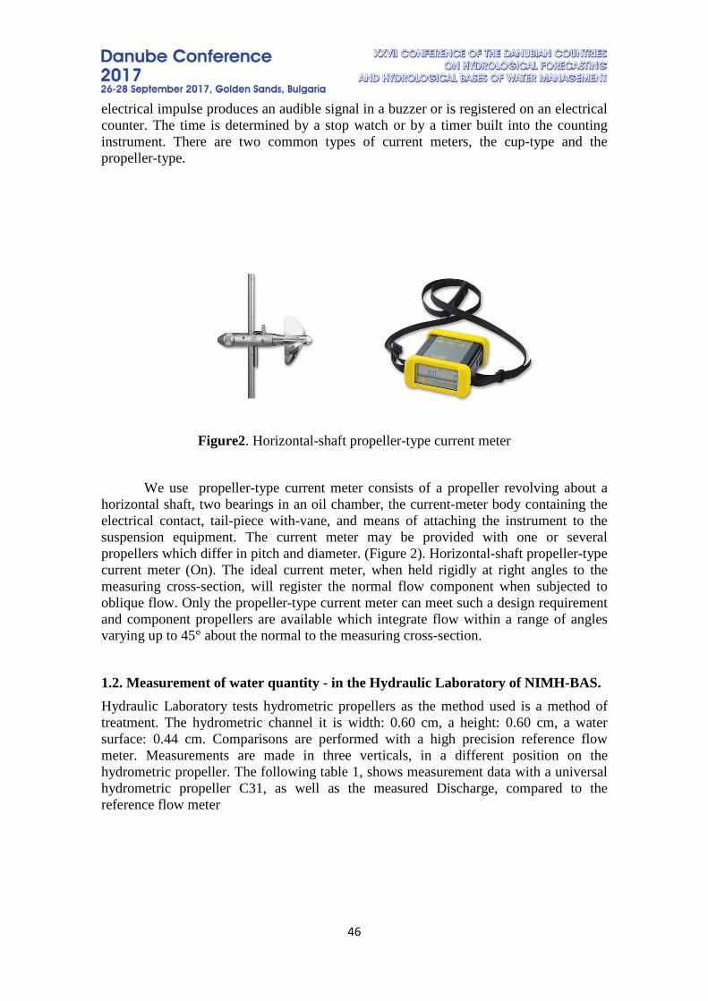
electrical impulse produces an audible signal in a buzzer or is registered on an electrical counter. The time is determined by a stop watch or by a timer built into the counting instrument. There are two common types of current meters, the cup-type and the propeller-type.

Figure2. Horizontal-shaft propeller-type current meter

We use propeller-type current meter consists of a propeller revolving about a horizontal shaft, two bearings in an oil chamber, the current-meter body containing the electrical contact, tail-piece with-vane, and means of attaching the instrument to the suspension equipment. The current meter may be provided with one or several propellers which differ in pitch and diameter. (Figure 2). Horizontal-shaft propeller-type current meter (On). The ideal current meter, when held rigidly at right angles to the measuring cross-section, will register the normal flow component when subjected to oblique flow. Only the propeller-type current meter can meet such a design requirement and component propellers are available which integrate flow within a range of angles varying up to 45° about the normal to the measuring cross-section.

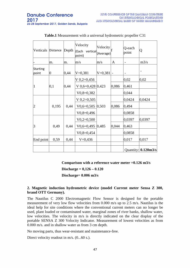
1.2. Measurement of water quantity - in the Hydraulic Laboratory of NIMH-BAS. Hydraulic Laboratory tests hydrometric propellers as the method used is a method of treatment. The hydrometric channel it is width: 0.60 cm, a height: 0.60 cm, a water surface: 0.44 cm. Comparisons are performed with a high precision reference flow meter. Measurements are made in three verticals, in a different position on the hydrometric propeller. The following table 1, shows measurement data with a universal hydrometric propeller C31, as well as the measured Discharge, compared to the reference flow meter

47

Table.1 Measurement with a universal hydrometric propeller C31

Comparison with a reference water meter =0.126 m3/s Discharge = 0,126 – 0.120 Discharge= 0.006 m3/s

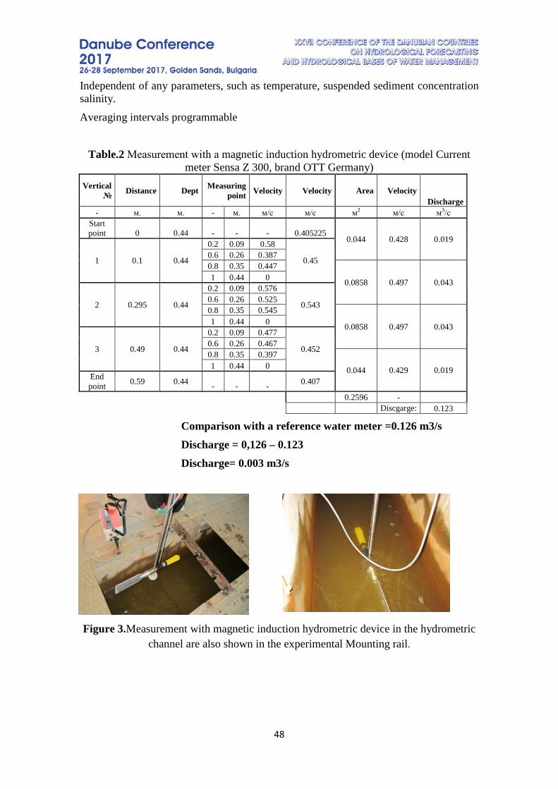
2. Magnetic induction hydrometric device (model Current meter Sensa Z 300, brand OTT Germany). The Nautilus C 2000 Electromagnetic Flow Sensor is designed for the portable measurement of very low flow velocities from 0.000 m/s up to 2.5 m/s. Nautilus is the ideal help for site conditions where the conventional current meters can no longer be used, plant loaded or contaminated water, marginal zones of river banks, shallow water, low velocities. The velocity in m/s is directly indicated on the clear display of the portable SENSA Z 300 Velocity Indicator. Measurement of lowest velocities as from 0.000 m/s. and in shallow water as from 3 cm depth. No moving parts, thus wear-resistant and maintenance-free. Direct velocity readout in m/s. (0...60 s.).

Verticals Distance Depth Velocity (Each vertical point)

Velocity (Average)

f Q-each point Q

- m. m. m/s m/s A - m3/s

Starting point 0 0,44 V=0,381 V=0,381 - - -

1 0,1 0,44

V 0,2=0,456

0,423

0,02 0,02

V 0,6=0,428 0,086 0,461

V0,8=0,382 0,044

2 0,195 0,44

V 0,2=0,505

0,503

0,0424 0,0424

V0,6=0,505 0,086 0,494

V0,8=0,496 0,0858

3 0,49 0,44

V0,2=0,500

0,485

0,0397 0,0397

V0,6=0,495 0,044 0,463

V0,8=0,454 0,0858

End point 0,59 0,44 V=0,436 0,017 0,017

Quantity: 0.120m3/s

48

Independent of any parameters, such as temperature, suspended sediment concentration salinity. Averaging intervals programmable

Table.2 Мeasurement with a magnetic induction hydrometric device (model Current

meter Sensa Z 300, brand OTT Germany) Vertical

№ Distance Dept Measuring point Velocity Velocity Area Velocity

Discharge - м. м. - м. м/с м/с м2 м/с м3/с

Start point 0 0.44 - - - 0.405225

0.044 0.428 0.019

1 0.1 0.44

0.2 0.09 0.58

0.45 0.6 0.26 0.387 0.8 0.35 0.447

0.0858 0.497 0.043 1 0.44 0

2 0.295 0.44

0.2 0.09 0.576

0.543 0.6 0.26 0.525 0.8 0.35 0.545

0.0858 0.497 0.043 1 0.44 0

3 0.49 0.44

0.2 0.09 0.477

0.452 0.6 0.26 0.467 0.8 0.35 0.397

0.044 0.429 0.019 1 0.44 0 End point 0.59 0.44 - - - 0.407

0.2596 -

Discgarge: 0.123

Comparison with a reference water meter =0.126 m3/s Discharge = 0,126 – 0.123 Discharge= 0.003 m3/s

Figure 3.Measurement with magnetic induction hydrometric device in the hydrometric channel are also shown in the experimental Mounting rail.

49

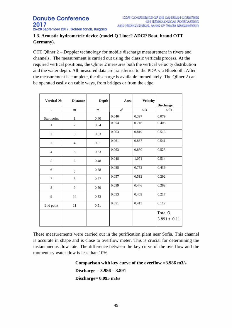
1.3. Acoustic hydrometric device (model Q Liner2 ADCP Boat, brand OTT Germany).

OTT Qliner 2 – Doppler technology for mobile discharge measurement in rivers and channels. The measurement is carried out using the classic verticals process. At the required vertical positions, the Qliner 2 measures both the vertical velocity distribution and the water depth. All measured data are transferred to the PDA via Bluetooth. After the measurement is complete, the discharge is available immediately. The Qliner 2 can be operated easily on cable ways, from bridges or from the edge.

These measurements were carried out in the purification plant near Sofia. This channel is accurate in shape and is close to overflow meter. This is crucial for determining the instantaneous flow rate. The difference between the key curve of the overflow and the momentary water flow is less than 10%

Comparison with key curve of the overflow =3.986 m3/s Discharge = 3.986 – 3.891 Discharge= 0.095 m3/s

Vertical № Distance Depth Area Velocity Discharge

- m m м2 м/s м3/s

Start point 1 0.40 0.040 0.397 0.079

1 2 0.54 0.054 0.746 0.403

2 3 0.63 0.063 0.819 0.516

3 4 0.61 0.061 0.887 0.541

4 5 0.63 0.063 0.830 0.523

5 6 0.48 0.048 1.071 0.514

6 7 0.58 0.058 0.752 0.436

7 8 0.57 0.057 0.512 0.292

8 9 0.59 0.059 0.446 0.263

9 10 0.53 0.053 0.409 0.217

End point 11 0.51 0.051 0.413 0.112

Total Q 3.891 ± 0.11

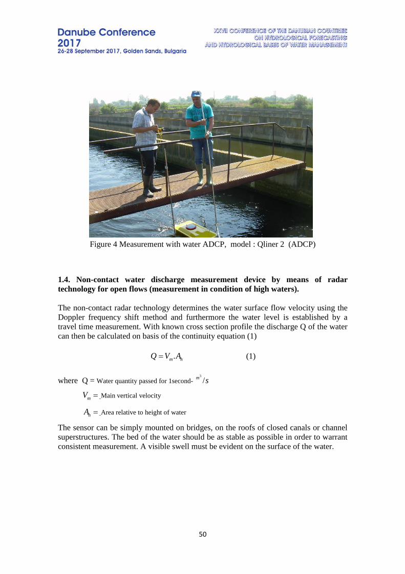
50

Figure 4 Measurement with water ADCP, model : Qliner 2 (ADCP)

1.4. Non-contact water discharge measurement device by means of radar technology for open flows (measurement in condition of high waters).

The non-contact radar technology determines the water surface flow velocity using the Doppler frequency shift method and furthermore the water level is established by a travel time measurement. With known cross section profile the discharge Q of the water can then be calculated on basis of the continuity equation (1)

.m hQ V A= (1)

where Q = Water quantity passed for 1second- 3

/m s

mV = Main vertical velocity

hA = Area relative to height of water

The sensor can be simply mounted on bridges, on the roofs of closed canals or channel superstructures. The bed of the water should be as stable as possible in order to warrant consistent measurement. A visible swell must be evident on the surface of the water.

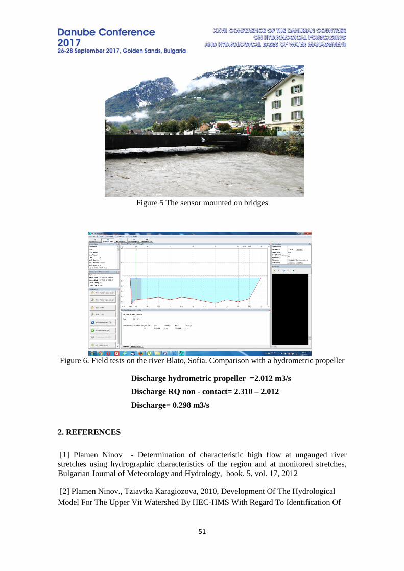
51

Figure 5 The sensor mounted on bridges

Figure 6. Field tests on the river Blato, Sofia. Comparison with a hydrometric propeller

Discharge hydrometric propeller =2.012 m3/s Discharge RQ non - contact= 2.310 – 2.012 Discharge= 0.298 m3/s

2. REFERENCES [1] Plamen Ninov - Determination of characteristic high flow at ungauged river stretches using hydrographic characteristics of the region and at monitored stretches, Bulgarian Journal of Meteorology and Hydrology, book. 5, vol. 17, 2012 [2] Plamen Ninov., Tziavtka Karagiozova, 2010, Development Of The Hydrological Model For The Upper Vit Watershed By HEC-HMS With Regard To Identification Of

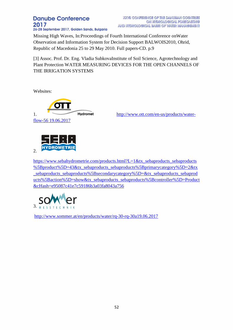
52

Missing High Waves, In:Proceedings of Fourth International Conference onWater Observation and Information System for Decision Support BALWOIS2010, Ohrid, Republic of Macedonia 25 to 29 May 2010. Full papers-CD. p.9

[3] Assoc. Prof. Dr. Eng. Vladia SubkovaInstitute of Soil Science, Agrotechnology and Plant Protection WATER MEASURING DEVICES FOR THE OPEN CHANNELS OF THE IRRIGATION SYSTEMS

Websites:

1. http://www.ott.com/en-us/products/water-flow-56 19.06.2017

2.

https://www.sebahydrometrie.com/products.html?L=1&tx_sebaproducts_sebaproducts%5Bproduct%5D=43&tx_sebaproducts_sebaproducts%5Bprimarycategory%5D=2&tx_sebaproducts_sebaproducts%5Bsecondarycategory%5D=&tx_sebaproducts_sebaproducts%5Baction%5D=show&tx_sebaproducts_sebaproducts%5Bcontroller%5D=Product&cHash=e95087c41e7c59186b3a03fa8043a756

3.

http://www.sommer.at/en/products/water/rq-30-rq-30a19.06.2017

53

HYDRAULIC DESIGN OF CULVERTS

Dániel Koch1 , Katalin Bene2 , Gábor Keve1 1 Institute for Hydraulic engineering and Water management / National University of Public

Service, Hungary 2 Department of Transport Infrastructure / Széchenyi István University, Hungary

Corresponding author: Dániel Koch, Institute for Hydraulic engineering and Water management / National University of Public Service, 14. Bajcsy-Zs. street, Baja HU-6500, koch.daniel@uni-nke.hu

ABSTRACT Culverts are important structures that provide cross-drainage under roads, and railways, as well as control water depth in water management systems, such as wetlands, detention-retention ponds. Ecological passages (blue corridors) have also become important on small streams. Sizing of culverts is a demanding and complex problem. There are several computer programs that aid in designing culvert hydraulic problems. We selected the HY8 program as a baseline of comparison in our study. The HY8 program was developed based on the Federal Highway Administration (FHWA) culvert classification system, hydraulic calculations. The goal of this project was to develop an excel program that adapt the program capabilities to Hungarian standards, and expand the use not only for design, but for field measurements as well. Keywords: hydraulic design, culvert, flow type, headwater, tailwater, performance curve

1. INTRODUCTION In the XXI. century climate change increased extreme weather conditions. As a consequence, our engineering facilities are subject to greater and more concentrated floods [1]. For smaller streams culverts are used often instead of bridges. Based on their ever-widening application, it can be said that their construction is fast and economical. At culver entrances significant headwater changes can occur due to highly variable flow conditions. Culverts reduce flow in the water transport system, that can cause substantial backwater effects. Traditionally, design requirements include not exceeding allowable headwater depths or outlet velocities. In Hungary, culverts are the most common cross-drainage structures, and play an important role in the infrastructure. Here, smaller cross-sections are standardized, while larger ones have to be individually designed. It is a common practice in Hungary to design culverts for the simplest hydraulic flow case, which does not determine flow velocity distribution, and parameters that are influencing barrel discharge. This approach is limiting their application. Based on literature review [2-7] we defined six basic flow type conditions. Not all flow types can be described with the help of an energy equations, and empirical calculations have been developed as well [6]. Depending on culvert inlet structure and barrel geometry different empirical constants were determined by Bodhaine int he USGS report [3], FHWA [7] and, other researchers [8]. HY - 8 program was selected from the

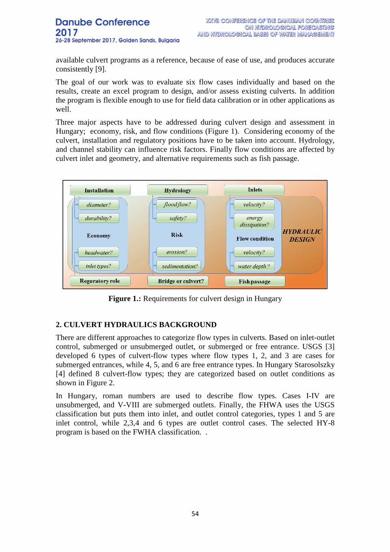
54

available culvert programs as a reference, because of ease of use, and produces accurate consistently [9]. The goal of our work was to evaluate six flow cases individually and based on the results, create an excel program to design, and/or assess existing culverts. In addition the program is flexible enough to use for field data calibration or in other applications as well. Three major aspects have to be addressed during culvert design and assessment in Hungary; economy, risk, and flow conditions (Figure 1). Considering economy of the culvert, installation and regulatory positions have to be taken into account. Hydrology, and channel stability can influence risk factors. Finally flow conditions are affected by culvert inlet and geometry, and alternative requirements such as fish passage.

Figure 1.: Requirements for culvert design in Hungary

2. CULVERT HYDRAULICS BACKGROUND There are different approaches to categorize flow types in culverts. Based on inlet-outlet control, submerged or unsubmerged outlet, or submerged or free entrance. USGS [3] developed 6 types of culvert-flow types where flow types 1, 2, and 3 are cases for submerged entrances, while 4, 5, and 6 are free entrance types. In Hungary Starosolszky [4] defined 8 culvert-flow types; they are categorized based on outlet conditions as shown in Figure 2. In Hungary, roman numbers are used to describe flow types. Cases I-IV are unsubmerged, and V-VIII are submerged outlets. Finally, the FHWA uses the USGS classification but puts them into inlet, and outlet control categories, types 1 and 5 are inlet control, while 2,3,4 and 6 types are outlet control cases. The selected HY-8 program is based on the FWHA classification. .

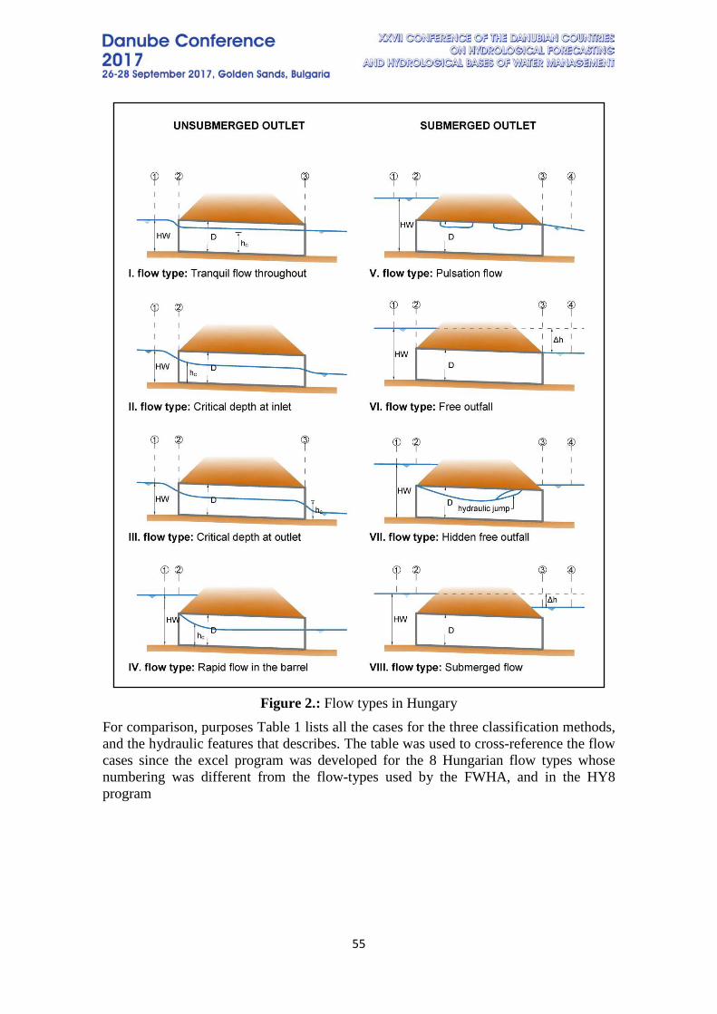
55

Figure 2.: Flow types in Hungary

For comparison, purposes Table 1 lists all the cases for the three classification methods, and the hydraulic features that describes. The table was used to cross-reference the flow cases since the excel program was developed for the 8 Hungarian flow types whose numbering was different from the flow-types used by the FWHA, and in the HY8 program

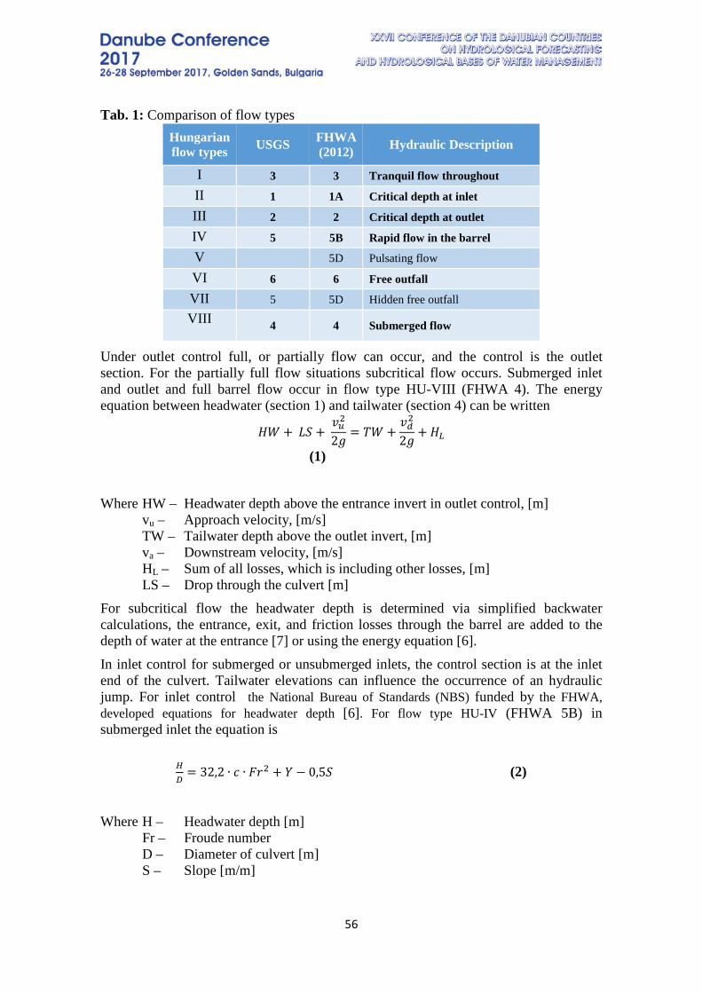
56

Tab. 1: Comparison of flow types Hungarian flow types USGS FHWA

(2012) Hydraulic Description

I 3 3 Tranquil flow throughout

II 1 1A Critical depth at inlet

III 2 2 Critical depth at outlet

IV 5 5B Rapid flow in the barrel

V 5D Pulsating flow

VI 6 6 Free outfall

VII 5 5D Hidden free outfall

VIII 4 4 Submerged flow

Under outlet control full, or partially flow can occur, and the control is the outlet section. For the partially full flow situations subcritical flow occurs. Submerged inlet and outlet and full barrel flow occur in flow type HU-VIII (FHWA 4). The energy equation between headwater (section 1) and tailwater (section 4) can be written

𝐻𝐻𝐻𝐻 + 𝐿𝐿𝐿𝐿 + 𝑣𝑣𝑢𝑢2

2𝑔𝑔= 𝑇𝑇𝐻𝐻 +

𝑣𝑣𝑑𝑑2

2𝑔𝑔+ 𝐻𝐻𝐿𝐿

(1) Where HW – Headwater depth above the entrance invert in outlet control, [m] vu – Approach velocity, [m/s] TW – Tailwater depth above the outlet invert, [m] va – Downstream velocity, [m/s] HL – Sum of all losses, which is including other losses, [m] LS – Drop through the culvert [m] For subcritical flow the headwater depth is determined via simplified backwater calculations, the entrance, exit, and friction losses through the barrel are added to the depth of water at the entrance [7] or using the energy equation [6]. In inlet control for submerged or unsubmerged inlets, the control section is at the inlet end of the culvert. Tailwater elevations can influence the occurrence of an hydraulic jump. For inlet control the National Bureau of Standards (NBS) funded by the FHWA, developed equations for headwater depth [6]. For flow type HU-IV (FHWA 5B) in submerged inlet the equation is

𝐻𝐻𝐷𝐷

= 32,2 ∙ 𝑐𝑐 ∙ 𝐹𝐹𝐹𝐹2 + 𝑌𝑌 − 0,5𝐿𝐿 (2)

Where H – Headwater depth [m] Fr – Froude number D – Diameter of culvert [m] S – Slope [m/m]

57

A – Full cross-sectional area of culvert barrel [m2] Fr-Froude number at the entrance In the equation, the Froude number is calculated at the entrance.

𝐹𝐹𝐹𝐹 = 𝑄𝑄

𝐴𝐴 �𝑔𝑔∙𝐷𝐷 (3)

The 32.2 constant in the equation represent the conversion from English to SI. The c and Y empirical constants depend on the culvert entrance geometry, the culvert shape, and material. Equation 1. can be applied for Fr ≥ 0.7. For mitered inlet +0.7S a correction parameter is applied [6]. For type HU-II (FHWA 1A) the following non-dimensional best-fit power equation is used:

𝐸𝐸𝐶𝐶 = ℎ𝐶𝐶 +� 𝑄𝑄𝐴𝐴𝐶𝐶 ∙ 𝐶𝐶

�2

2𝑔𝑔𝐻𝐻𝐷𝐷

=𝐸𝐸𝐶𝐶𝐷𝐷

+ 𝐾𝐾 ∙1,811

𝑀𝑀2

�𝑔𝑔∙ 𝐹𝐹𝐹𝐹𝑀𝑀 − 0,5𝐿𝐿

(4)

Where EC – Energy under critical-flow, [m] C – Discharge coefficient AC – Area under critical-flow [m2] Form 2:

𝐻𝐻𝐷𝐷

= 𝐾𝐾′ ∙ 1,811𝑀𝑀′2

√𝑔𝑔∙ 𝐹𝐹𝐹𝐹𝑀𝑀′

(5)

The (M, M’, K, K’) parameters are dimensionless constants and can be found in tables from the FHWA report [7] based on barrel shape and entrance. For mitered inlets a slope correction factor of +0.7S should be used instead of -0.5S. The equation is applicable for Fr ≤ 0.6.

3. PROGRAM FEATURES The USGS [3], FHWA [7], Chin [6] and simplified equations were used to evaluate each flow-case type. At each methods different barrel diameter, and discharge values, were used to predict headwater elevation then the results were compared to the HY8 output. For the excel program we selected the simplest equations that still provided a good approximation to the reference HY8 output. The excel calculation method is as follows; after basic design input parameters are given, the program determines the normal and critical depth and then performs loss calculations. Next it determines the appropriate and/or possible flow types, and calculates headwater elevations. If more than one headwater is determined the excel

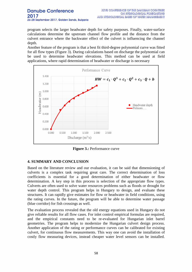
58

program selects the larger headwater depth for safety purposes. Finally, water-surface calculations determine the upstream channel flow profile and the distance from the culvert entrance where the backwater effect of the culvert is influencing the channel depth. Another feature of the program is that a best fit third-degree polynomial curve was fitted for all flow types (Figure 3). During calculations based on discharge the polynomial can be used to determine headwater elevations. This method can be used at field applications, where rapid determination of headwater or discharge is necessary

Figure 3.: Performance curve

4. SUMMARY AND CONCLUSION Based on the literature review and our evaluation, it can be said that dimensioning of culverts is a complex task requiring great care. The correct determination of loss coefficients is essential for a good determination of either headwater or flow determination. A key step in this process is selection of the appropriate flow types. Culverts are often used to solve water resources problems such as floods or drought for water depth control. This program helps in Hungary to design, and evaluate these structures. It can rapidly give estimates for flow or headwater in field conditions, using the rating curves. In the future, the program will be able to determine water passage (blue corridor) for fish crossings as well. The evaluation process revealed that the old energy equations used in Hungary do not give reliable results for all flow cases. For inlet control empirical formulas are required, and the empirical constants need to be re-evaluated for Hungarian inlet barrel geometries. The program helps to modernize the Hungarian culvert design process. Another application of the rating or performance curves can be calibrated for existing culvert, for continuous flow measurements. This way one can avoid the installation of costly flow measuring devices, instead cheaper water level sensors can be installed.

𝑯𝑯𝑯𝑯 = 𝒄𝒄𝟏𝟏 ∙ 𝑸𝑸𝟑𝟑 + 𝒄𝒄𝟐𝟐 ∙ 𝑸𝑸𝟐𝟐 + 𝒄𝒄𝟑𝟑 ∙ 𝑸𝑸 + 𝒃𝒃

59

After calibration based on headwater and tailwater depth measurements the flow can be determined using the rating curve.

5. REFERENCES [1] R. Kuti – L. Földi: Extreme weather phenomena, improvement of preparedness, Hadmérnök on-line, a Nemzeti Közszolgálati Egyetem Hadtudományi és Honvédtisztképző Kar és a Katonai Műszaki Doktori Iskola on-line tudományos folyóirata, ISSN 1788 1919 VII. Évfolyam 3. szám, 60-65. o. 2012. szeptember. [2] R. W. Carter: Coputation of Peak Discharge at Culverts, Geological Survey Circular 376, Washington, D. C., 1957 [3] G. L. Bodhaine: Measurement of Peak Discharge at Culverts by Indirect Methods, Techniques of Water Reaources Investigations of the USGS, United States Government Printing Office, 1982 [4] Ö. Starosolszky: Vízépítési Hidraulika, Műszaki Könyvkiadó, Budapest, 493-512. o., 1970 [5] R. H. French: Open-Channel Hydraulics, McGraw-Hill, New York, 1985 [6] Chin Davis A.: Water Resources Engineering Pierson Education (3rd edition), ISBN-13: 978-0132833219, 2013 [7] FHWA: Hydraulic Design of Highway Culverts, Third Editon, Publication No. FHWA-HIF-12-026, U.S. Department of Transportation, Federal Highway Administration, April 2012 [8] B. P. Tullis, S. C. Robinson: Quantifying exit losses, Journal of Irrigation and Drainage Engineering 134(2) 2008 [9] E. A. Thiele: Culvert hydraulics: comparison of current computer models, Msc Theses, Brigham Young University, 2007

60

HOW AFFECT THE APPLICATION OF BIOCHAR THE WATER REGIME OF AGRICULTURAL SOIL WHEN A MAIZE (ZEA MAYS L.) IS GROWN?

Justina Vitkova, Peter Surda

Institute of Hydrology of the Slovak Academy of Sciences, Slovakia

Corresponding author: Justina Vitkova, Institute of Hydrology of the Slovak Academy of Sciences, Dubravska cesta 9, 841 04 Bratislava, Slovakia, vitkova@uh.savba.sk

ABSTRACT In recent decades we have witnessed a variety of weather extremes. We are experiencing intense torrential rainfall, prolonged periods without precipitation or temperatures records in winter and summer months. Regardless of whether it is climate change or the frequent extremity of weather, production capacity of the soil is one of the factors that are most affected. Biochar, a product of the thermal degradation of biomass rich in carbon, is currently in the focus of attention of the scientific community especially for its ability to improve soil quality parameters and mitigate the speed of climate change. Despite of numerous studies dedicated to the issue of biochar, its impact on the basic hydrophysical characteristics is not completely clear. In recent years, also professionals in Slovakia are dealing with the issue of biochar, but research in field conditions is unique. Now we present the results of the field experiment, which began in March of 2014. Certified biochar has been incorporated into the soil to a depth of 10 cm. The aim of this paper was to evaluate the impact of the biochar application on moisture regime of the sandy loam soil in surface layer during the growing season of 2015. The crop grown during this year was maize (Zea mays subsp. Mays L.). Four sensors 5TM (Decagon Devices) were installed at experimental site to measure the soil moisture and temperature at a depth of 5-10 cm. Two of them were placed on plot without biochar, two on the plot, with application of biochar in the equivalent of 20 t/ha. Data logger recorded values in 5 minute intervals, which allowed us to analyze also the dynamics of soil moisture caused by the short-term precipitation. Due to the recently known effects of biochar on soil, we assumed that at the plot with applied biochar we will measure higher values of soil moisture than at the plot without biochar. This assumption was not confirmed in the conditions of our experiment (with maize as a crop). There may be several reasons. Whether it is the material from which the biochar was produced, the dose of applied biochar or there were other factors, which had a greater impact than biochar, but cannot be eliminated in the conditions of field experiment. Keywords: biochar, field measurements, soil moisture

1. INTRODUCTION In recent decades we have witnessed a variety of weather extremes. We are experiencing intense torrential rainfall, prolonged periods without precipitation or temperatures records in winter and summer months. Regardless of whether it is climate change or the frequent extremity of weather, production capacity of the soil is one of the factors that are most affected. Biochar, a product of the thermal degradation of biomass rich in carbon, is currently in the focus of attention of the scientific community. Innovative tools are required to help deal with complex challenges, which have fuelled

61

interest in biochar as a potential soil amendment to improve soil quality and crop productivity [1]. Biochar may alter the physical properties of the soil, including increasing aeration and water holding capacity of certain soils [2]. Chan et al. [3] show that biochar application in addition to fertilizer addition can lead to plant growth benefits, but a negative effect is sometimes observed without fertilization, due to reduced bio-availability, through sorption of nitrogen [4]. Biochar addition has been shown to positively reduce N2O emissions from soil [5], suppress plant disease [6], improve plant growth [7], ameliorate soil acidity [8] and stimulate soil microbial activity [9]. Moreover, most trials with biochar have been carried out in the laboratory over short time periods making translation of these results to field conditions difficult. Another aspect of these studies is that most have tended to focus on problem soils (e.g. with excessive soil acidity or salinity, severe nutrient imbalances, critically low soil organic matter) where the responses of biochar addition can often be dramatic. However, these soils are not representative of fertile agricultural areas where the likelihood of biochar application from a practical and economic perspective may be greatest [10]. In Slovakia, we have started with biochar experiment in field condition in March of the 2014, when certified biochar has been incorporated into the soil to a depth of 10 cm. The aim of this paper was to evaluate the impact of the biochar application on moisture regime of the sandy loam soil in surface layer during the selected time period of the year 2015.

2. MATERIAL AND METHODS Location site Malanta (Fig. 1) is located approximately 5 km north-east of the city Nitra, Slovakia (N 48°19'00''; E 18°09'00''). Altitude location is 175 MASL [11]. Soil type is classified as an Orthic Luvisol [12]. Morphological and morphometric relief type is mildly to moderately rugged hilly. Malanta falls under hot climatic zone, slightly dry with mild winter. Soil characteristics at experimental area are shown in Table 1. On experimental area was geodetically set out 45 plots measuring 6x4 m separated by 0.5 m bands. On these plots were conducted experiment variations: control - without adding biochar (Control), B10 variant with the addition of biochar dose 10 t/ha and B20 variant with a dose of biochar 20 t/ha. The experiment started on 10th of March in 2014. After the uniform distribution of biochar on the plots it was incorporated to soil depth about 10 cm using a cultivator machine. We focused on an analysis the Control and B20 plots. During the experimental measurements the area was agriculturally used, cultivated crop was maize (Zea mays subsp. Mays L.) in the 2015.

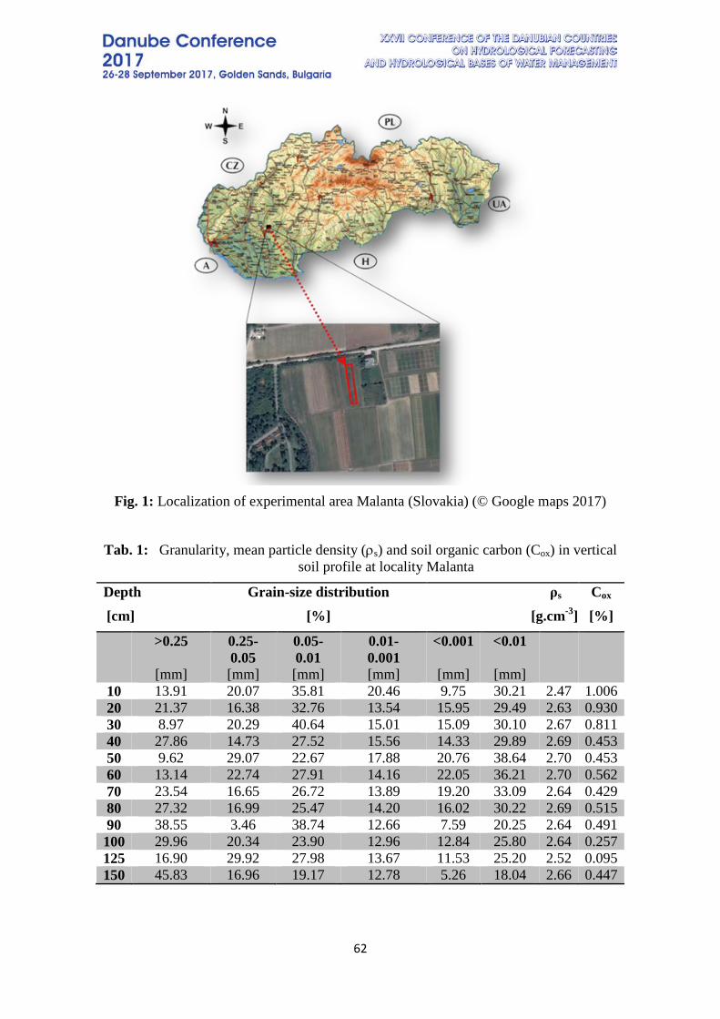
62

Fig. 1: Localization of experimental area Malanta (Slovakia) (© Google maps 2017)

Tab. 1: Granularity, mean particle density (ρs) and soil organic carbon (Cox) in vertical soil profile at locality Malanta

Depth [cm]

Grain-size distribution [%]

ρs [g.cm-3]

Cox [%]

>0.25

[mm]

0.25-0.05 [mm]

0.05-0.01 [mm]

0.01- 0.001 [mm]

<0.001

[mm]

<0.01

[mm]

10 13.91 20.07 35.81 20.46 9.75 30.21 2.47 1.006 20 21.37 16.38 32.76 13.54 15.95 29.49 2.63 0.930 30 8.97 20.29 40.64 15.01 15.09 30.10 2.67 0.811 40 27.86 14.73 27.52 15.56 14.33 29.89 2.69 0.453 50 9.62 29.07 22.67 17.88 20.76 38.64 2.70 0.453 60 13.14 22.74 27.91 14.16 22.05 36.21 2.70 0.562 70 23.54 16.65 26.72 13.89 19.20 33.09 2.64 0.429 80 27.32 16.99 25.47 14.20 16.02 30.22 2.69 0.515 90 38.55 3.46 38.74 12.66 7.59 20.25 2.64 0.491 100 29.96 20.34 23.90 12.96 12.84 25.80 2.64 0.257 125 16.90 29.92 27.98 13.67 11.53 25.20 2.52 0.095 150 45.83 16.96 19.17 12.78 5.26 18.04 2.66 0.447

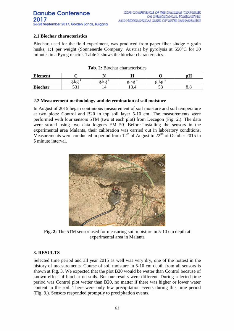
63

2.1 Biochar characteristics Biochar, used for the field experiment, was produced from paper fiber sludge + grain husks; 1:1 per weight (Sonnenerde Company, Austria) by pyrolysis at 550°C for 30 minutes in a Pyreg reactor. Table 2 shows the biochar characteristics.

Tab. 2: Biochar characteristics

Element C N H O pH g.kg-1 g.kg-1 g.kg-1 g.kg-1 - Biochar 531 14 18.4 53 8.8

2.2 Measurement methodology and determination of soil moisture In August of 2015 began continuous measurement of soil moisture and soil temperature at two plots: Control and B20 in top soil layer 5-10 cm. The measurements were performed with four sensors 5TM (two at each plot) from Decagon (Fig. 2.). The data were stored using two data loggers EM 50. Before installing the sensors in the experimental area Malanta, their calibration was carried out in laboratory conditions. Measurements were conducted in period from 12th of August to 22nd of October 2015 in 5 minute interval.

Fig. 2: The 5TM sensor used for measuring soil moisture in 5-10 cm depth at

experimental area in Malanta

3. RESULTS Selected time period and all year 2015 as well was very dry, one of the hottest in the history of measurements. Course of soil moisture in 5-10 cm depth from all sensors is shown at Fig. 3. We expected that the plot B20 would be wetter than Control because of known effect of biochar on soils. But our results were different. During selected time period was Control plot wetter than B20, no matter if there was higher or lower water content in the soil. There were only few precipitation events during this time period (Fig. 3.). Sensors responded promptly to precipitation events.

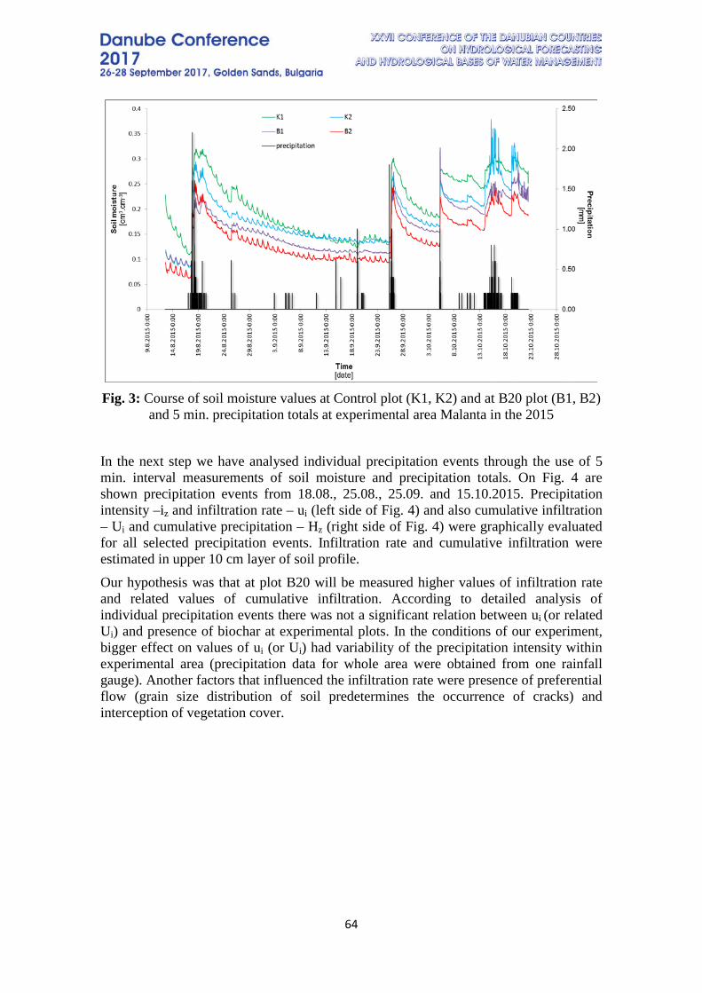
64

Fig. 3: Course of soil moisture values at Control plot (K1, K2) and at B20 plot (B1, B2)

and 5 min. precipitation totals at experimental area Malanta in the 2015

In the next step we have analysed individual precipitation events through the use of 5 min. interval measurements of soil moisture and precipitation totals. On Fig. 4 are shown precipitation events from 18.08., 25.08., 25.09. and 15.10.2015. Precipitation intensity –iz and infiltration rate – ui (left side of Fig. 4) and also cumulative infiltration – Ui and cumulative precipitation – Hz (right side of Fig. 4) were graphically evaluated for all selected precipitation events. Infiltration rate and cumulative infiltration were estimated in upper 10 cm layer of soil profile. Our hypothesis was that at plot B20 will be measured higher values of infiltration rate and related values of cumulative infiltration. According to detailed analysis of individual precipitation events there was not a significant relation between ui (or related Ui) and presence of biochar at experimental plots. In the conditions of our experiment, bigger effect on values of ui (or Ui) had variability of the precipitation intensity within experimental area (precipitation data for whole area were obtained from one rainfall gauge). Another factors that influenced the infiltration rate were presence of preferential flow (grain size distribution of soil predetermines the occurrence of cracks) and interception of vegetation cover.

65

Fig. 4: Course of precipitation intensity (iz), infiltration rate (ui), cumulative infiltration (Ui) and cumulative precipitation (Hz) at Control plot (K1, K2) and at B20 plot (B1, B2)

at experimental area Malanta in the 2015

66

4. CONCLUSIONS 1. The results of our study did not confirm the positive effect of biochar (with

above mentioned characteristics), used in our field experiment, on moisture regime of the sandy loam soil during selected time period of the year 2015, when a maize was grown.

2. Analysis of individual precipitation events confirmed, that the effect of applied dose of biochar (20 t/ha) on infiltration rate in upper 10 cm layer of soil profile in the conditions of field experiment was irrelevant compared to another natural factors (mentioned in previous chapter).

5. REFERENCES [1] Lehmann, J., Gaunt, J., Rondon,M. Bio-char sequestration in terrestrial ecosystems - a review. Mitig. Adapt. Strateg. Glob. Chang. 11, pp 403–427, 2006. [2] Sohi, S.P. Appendix 1. Analysis of scientific studies published on the function of char, its quantification, and its stability in soil. In An Assessment of the Benefits and Issues Associated with the Application of Biochar to Soil; Shackley, S., Sohi, S.P., Eds.; A Report to the Department for Environment, Food and Rural Affairs and the Department of Energy and Climate Change: London, UK, pp 1–4, 2010. [3] Chan, K.Y., Van Zwieten, L., Meszaros, I., Downie, A., Joseph, S. Agronomic values of greenwaste biochar as a soil amendment. Aust. J. Soil Res., vol. 45, pp 629–634, 2007. [4] Case, S.J., McNamara, N.P., Reay, D.S., Whitaker, J. The effect of biochar addition on N2O and CO2 emissions from a sandy loam soil—The role of soil aeration. Soil Biol. Biochem., vol. 51, pp 125–134, 2012. [5] Taghizadeh-Toosi, A. Biochar incorporation into pasture soil suppresses in situ nitrous oxide emissions from ruminant urine patches. Journal of Environmental Quality, vol. 40, pp 468-476, 2011. [6] Elad, Y., David, D.R., Harel, Y.M., Borenshtein, M., Ben Kalifa, H., Silber, A., Graber, E.R. Induction of systemic resistance in plants by biochar, a soilapplied carbon sequestering agent. Phytopathology, vol. 100, pp 913-921, 2010. [7] Graber, E.R., Harel, Y.M., Kolton, M., Cytryn, E., Silber, A., David, D.R., Tsechansky, L., Borenshtein, M., Elad, Y. Biochar impact on development and productivity of pepper and tomato grown in fertigated soilless media. Plant and Soil, vol. 337, pp 481-496, 2010. [8] Yuan, J.H., Xu, R.K. The amelioration effects of low temperature biochar generated from nine crop residues on an acidic Ultisol. Soil Use and Management, vol. 27, pp 110-115, 2011. [9] Smith, J.L., Collins, H.P., Bailey, V.L. The effect of young biochar on soil respiration. Soil Biology & Biochemistry, vol. 42, pp 2345-2347, 2010. [10] Jones, D.L., Rousk, J., Edwards-Jones, G., DeLuca, T.H., Murphy, D.V. Biochar-mediated changes in soil quality and plant growth in a three year field trial. Soil Biology & Biochemistry, vol. 45, pp 113-124, 2012.

67

[11] Surda, P., Vitkova, J. Impact of biochar application on soil moisture dynamics and saturated hydraulic conductivity. 16th International Multidisciplinary Scientific GeoConference SGEM 2016, vol. 1. Hydrology and Water Resources, pp 445-451, 2016. [12] Simansky, V. et al. Soil tillage and fertilization of Orthic Luvisol and their influence on chemical properties, soil structure stability and carbon distribution in water-stable macro-aggregates. Soil Tillage Resources, vol. 100, pp 125 –132, 2008.

6. ACKNOWLEDGEMENTS This work was supported by Slovak Research and Development Agency No. APVV-0512-12 and Scientific Grant Agency No. VEGA 2/0189/17 and No. VEGA 2/0013/15. It is also the result of the project implementation ITMS 26240120004 Centre of excellence for integrated flood protection of land supported by the Research & Development Operational Programme funded by the ERDF.

68

UTILIZATION OF GAINED EXPERIENCES BASED ON ICE OBSERVATION

BY WEBCAMERAS

Gábor KEVE

Faculty of Water Sciences/National University of Public Service, Hungary Corresponding author: Gábor KEVE, National University of Public Service/Faculty of Water

Sciences,Hungary 6500 Baja, Bajcsy Zs. u. 12-14., keve.gabor@uni-nke.hu

ABSTRACT An ice monitoring system was developed during the last 15 years in the region for a 130 km segment of the Danube in Hungary. All together five cameras were installed at a 30-40 km interval to achieve optimal observational capabilities along the river. In January 2009 and than in February 2012 later in 2017 three ice events were successfully recorded at the monitoring locations. Analysis of the recorded events combined with ice depth measurements, morphological information and hydro-meteorological data showed great potential to derive space-time characteristics of the floating ice. These include ice formation, size composition, motion and rearrangement due to secondary currents and occasional packing or release at places. Repeated measurements have been done to quantify the space-time characteristics of the ice formation and to improve the monitoring system. There have been several chances for utilization our gained experiences such as characterization of drifting floes, study of the hydrodynamic conditions during icy periods, verification of floe modelling, discharge estimation using LSPIV technique and additionally development of ice forecasting. Last but not least a new ice thickness staff was introduced for the easy and safe measurements of ice floes on rivers. Keywords: river ice, floe, ice depth, webcamera, monitoring

1. INTRODUCTION In 2001, a webcamera was installed on top of a high building at the Danube riverbank in Baja (Hungary). The webcamera was developed using earlier experiences with conventional black and white photography. In 2008 based on the success of the first measurements a monitoring program was developed, by installing 5 additional cameras. The monitoring sites were placed at a 30-40 km interval along a 130 km reach. In the first winter after installation (January 2009), a two-week-long ice period was successfully recorded at the five locations. Since then, in February 2010, 2012 and january 2017 was ice observed on this reach of Danube. In 2012 and 2017 the ice flow of Danube was taken seriously by the river managers and even the ice breaker fleet was activated. During the first time the ice breaker ships were used for ice thickness measurement as well. To achieve quick and reliable measurements a new and easy equipment was introduced called “Keve-staff” [1]. A primary analysis showed that when these measurements are combined with morphological information and meteorological data, space-time characteristics of the floating ice can be potentially derived. These characteristics include size composition, motion and rearrangement due to secondary currents and occasional packing or release

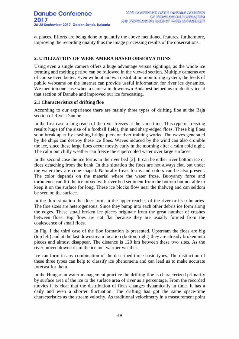
69

at places. Efforts are being done to quantify the above mentioned features, furthermore, improving the recording quality thus the image processing results of the observations.

2. UTILIZATION OF WEBCAMERA BASED OBSERVATIONS Using even a single camera offers a huge advantage versus sightings, as the whole ice forming and melting period can be followed in the viewed section. Multiple cameras are of course even better. Even without an own distribution monitoring system, the feeds of public webcams on the internet can provide useful information for river ice dynamics. We mention one case when a camera in downtown Budapest helped us to identify ice at that section of Danube and improved our ice forecasting.

2.1 Characteristics of drifting floe According to our experience there are mainly three types of drifting floe at the Baja section of River Danube. In the first case a long reach of the river freezes at the same time. This type of freezing results huge (of the size of a football field), thin and sharp-edged floes. These big floes soon break apart by crashing bridge piers or river training works. The waves generated by the ships can destroy these ice floes. Waves induced by the wind can also crumble the ice, since these large floes occur mostly early in the morning after a calm cold night. The calm but chilly weather can freeze the supercooled water over large surfaces. In the second case the ice forms in the river bed [2]. It can be either river bottom ice or floes detaching from the bank. In this situation the floes are not always flat, but under the water they are cone-shaped. Naturally freak forms and colors can be also present. The color depends on the material where the water froze. Buoyancy force and turbulence can lift the ice mixed with river bed sediment from the bottom but not able to keep it on the surface for long. These ice blocks flow near the thalweg and can seldom be seen on the surface. In the third situation the floes form in the upper reaches of the river or its tributaries. The floe sizes are heterogeneous. Since they bump into each other debris ice form along the edges. These small broken ice pieces originate from the great number of crashes between floes. Big floes are not flat because they are usually formed from the coalescence of small floes. In Fig. 1 the third case of the floe formation is presented. Upstream the floes are big (top left) and at the last downstream location (bottom right) they are already broken into pieces and almost disappear. The distance is 120 km between these two sites. As the river moved downstream the ice met warmer weather. Ice can form in any combination of the described three basic types. The distinction of these three types can help to classify ice phenomena and can lead us to make accurate forecast for them. In the Hungarian water management practice the drifting floe is characterized primarily by surface area of the ice to the surface area of river as a percentage. From the recorded movies it is clear that the distribution of floes changes dynamically in time. It has a daily and even a shorter fluctuation. The drifting has got the same space-time characteristics as the stream velocity. As traditional velocimetry in a measurement point

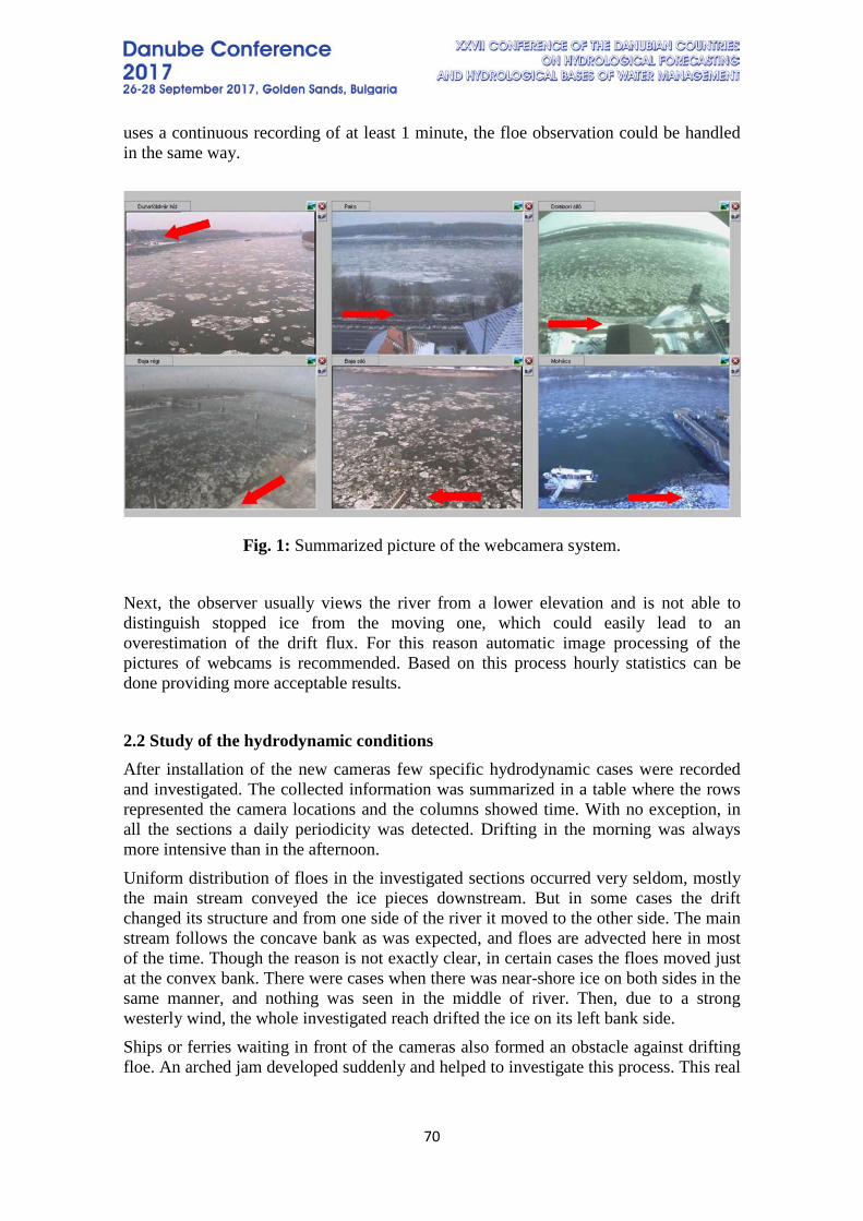
70

uses a continuous recording of at least 1 minute, the floe observation could be handled in the same way.

Fig. 1: Summarized picture of the webcamera system. Next, the observer usually views the river from a lower elevation and is not able to distinguish stopped ice from the moving one, which could easily lead to an overestimation of the drift flux. For this reason automatic image processing of the pictures of webcams is recommended. Based on this process hourly statistics can be done providing more acceptable results.

2.2 Study of the hydrodynamic conditions After installation of the new cameras few specific hydrodynamic cases were recorded and investigated. The collected information was summarized in a table where the rows represented the camera locations and the columns showed time. With no exception, in all the sections a daily periodicity was detected. Drifting in the morning was always more intensive than in the afternoon. Uniform distribution of floes in the investigated sections occurred very seldom, mostly the main stream conveyed the ice pieces downstream. But in some cases the drift changed its structure and from one side of the river it moved to the other side. The main stream follows the concave bank as was expected, and floes are advected here in most of the time. Though the reason is not exactly clear, in certain cases the floes moved just at the convex bank. There were cases when there was near-shore ice on both sides in the same manner, and nothing was seen in the middle of river. Then, due to a strong westerly wind, the whole investigated reach drifted the ice on its left bank side. Ships or ferries waiting in front of the cameras also formed an obstacle against drifting floe. An arched jam developed suddenly and helped to investigate this process. This real

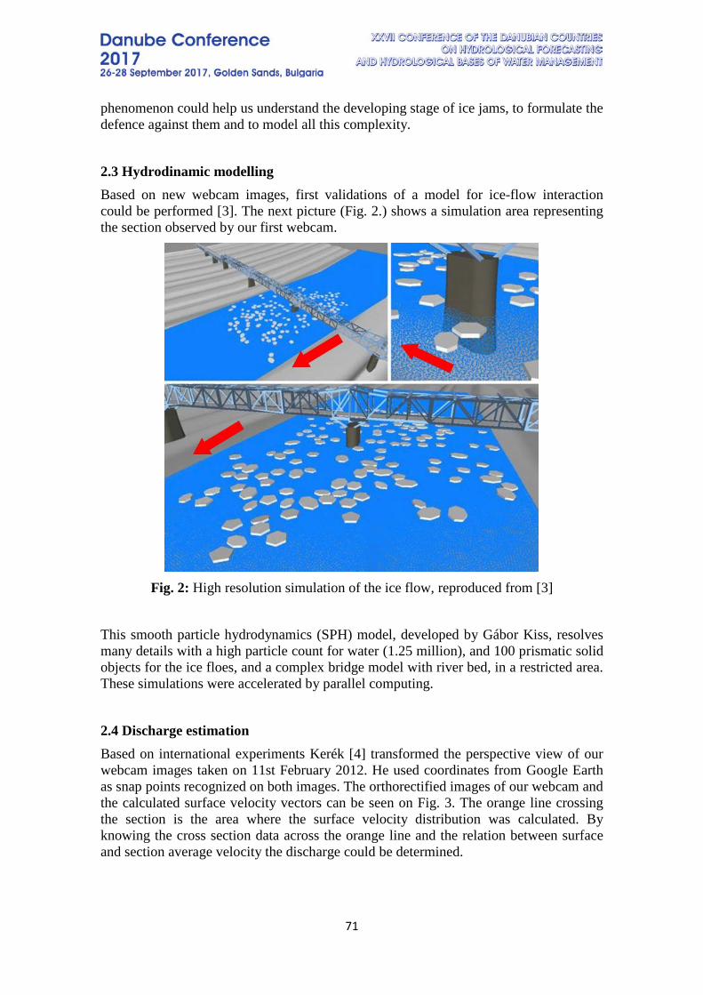
71

phenomenon could help us understand the developing stage of ice jams, to formulate the defence against them and to model all this complexity.

2.3 Hydrodinamic modelling Based on new webcam images, first validations of a model for ice-flow interaction could be performed [3]. The next picture (Fig. 2.) shows a simulation area representing the section observed by our first webcam.

Fig. 2: High resolution simulation of the ice flow, reproduced from [3]

This smooth particle hydrodynamics (SPH) model, developed by Gábor Kiss, resolves many details with a high particle count for water (1.25 million), and 100 prismatic solid objects for the ice floes, and a complex bridge model with river bed, in a restricted area. These simulations were accelerated by parallel computing.

2.4 Discharge estimation Based on international experiments Kerék [4] transformed the perspective view of our webcam images taken on 11st February 2012. He used coordinates from Google Earth as snap points recognized on both images. The orthorectified images of our webcam and the calculated surface velocity vectors can be seen on Fig. 3. The orange line crossing the section is the area where the surface velocity distribution was calculated. By knowing the cross section data across the orange line and the relation between surface and section average velocity the discharge could be determined.

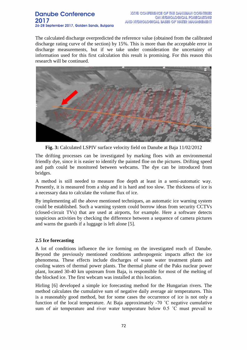
72

The calculated discharge overpredicted the reference value (obtained from the calibrated discharge rating curve of the section) by 15%. This is more than the acceptable error in discharge measurements, but if we take under consideration the uncertainty of information used for this first calculation this result is promising. For this reason this research will be continued.

Fig. 3: Calculated LSPIV surface velocity field on Danube at Baja 11/02/2012

The drifting processes can be investigated by marking floes with an environmental friendly dye, since it is easier to identify the painted floe on the pictures. Drifting speed and path could be monitored between webcams. The dye can be introduced from bridges. A method is still needed to measure floe depth at least in a semi-automatic way. Presently, it is measured from a ship and it is hard and too slow. The thickness of ice is a necessary data to calculate the volume flux of ice. By implementing all the above mentioned techniques, an automatic ice warning system could be established. Such a warning system could borrow ideas from security CCTVs (closed-circuit TVs) that are used at airports, for example. Here a software detects suspicious activities by checking the difference between a sequence of camera pictures and warns the guards if a luggage is left alone [5].

2.5 Ice forecasting A lot of conditions influence the ice forming on the investigated reach of Danube. Beyond the previously mentioned conditions anthropogenic impacts affect the ice phenomena. These effects include discharges of waste water treatment plants and cooling waters of thermal power plants. The thermal plume of the Paks nuclear power plant, located 30-40 km upstream from Baja, is responsible for most of the melting of the blocked ice. The first webcam was installed at this location. Hirling [6] developed a simple ice forecasting method for the Hungarian rivers. The method calculates the cumulative sum of negative daily average air temperatures. This is a reasonably good method, but for some cases the occurrence of ice is not only a function of the local temperature. At Baja approximately -70 ˚C negative cumulative sum of air temperature and river water temperature below 0.5 ˚C must prevail to

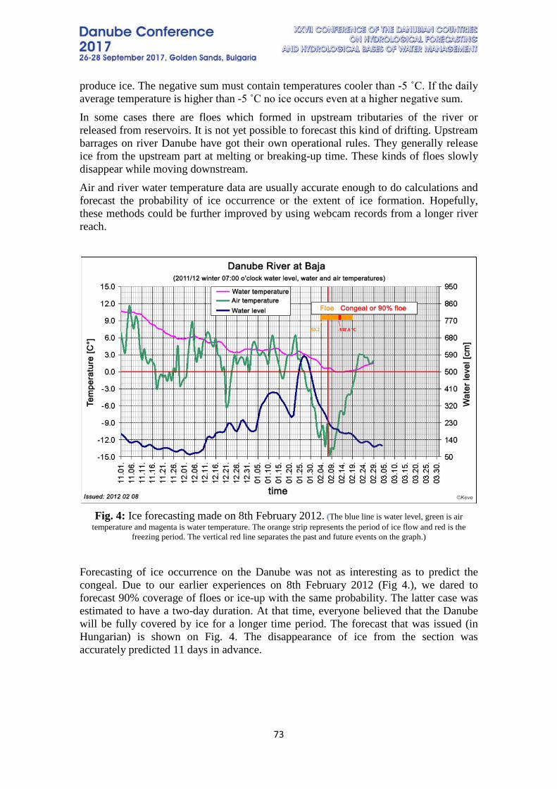
73

produce ice. The negative sum must contain temperatures cooler than -5 ˚C. If the daily average temperature is higher than -5 ˚C no ice occurs even at a higher negative sum. In some cases there are floes which formed in upstream tributaries of the river or released from reservoirs. It is not yet possible to forecast this kind of drifting. Upstream barrages on river Danube have got their own operational rules. They generally release ice from the upstream part at melting or breaking-up time. These kinds of floes slowly disappear while moving downstream. Air and river water temperature data are usually accurate enough to do calculations and forecast the probability of ice occurrence or the extent of ice formation. Hopefully, these methods could be further improved by using webcam records from a longer river reach.

Fig. 4: Ice forecasting made on 8th February 2012. (The blue line is water level, green is air

temperature and magenta is water temperature. The orange strip represents the period of ice flow and red is the freezing period. The vertical red line separates the past and future events on the graph.)

Forecasting of ice occurrence on the Danube was not as interesting as to predict the congeal. Due to our earlier experiences on 8th February 2012 (Fig 4.), we dared to forecast 90% coverage of floes or ice-up with the same probability. The latter case was estimated to have a two-day duration. At that time, everyone believed that the Danube will be fully covered by ice for a longer time period. The forecast that was issued (in Hungarian) is shown on Fig. 4. The disappearance of ice from the section was accurately predicted 11 days in advance.

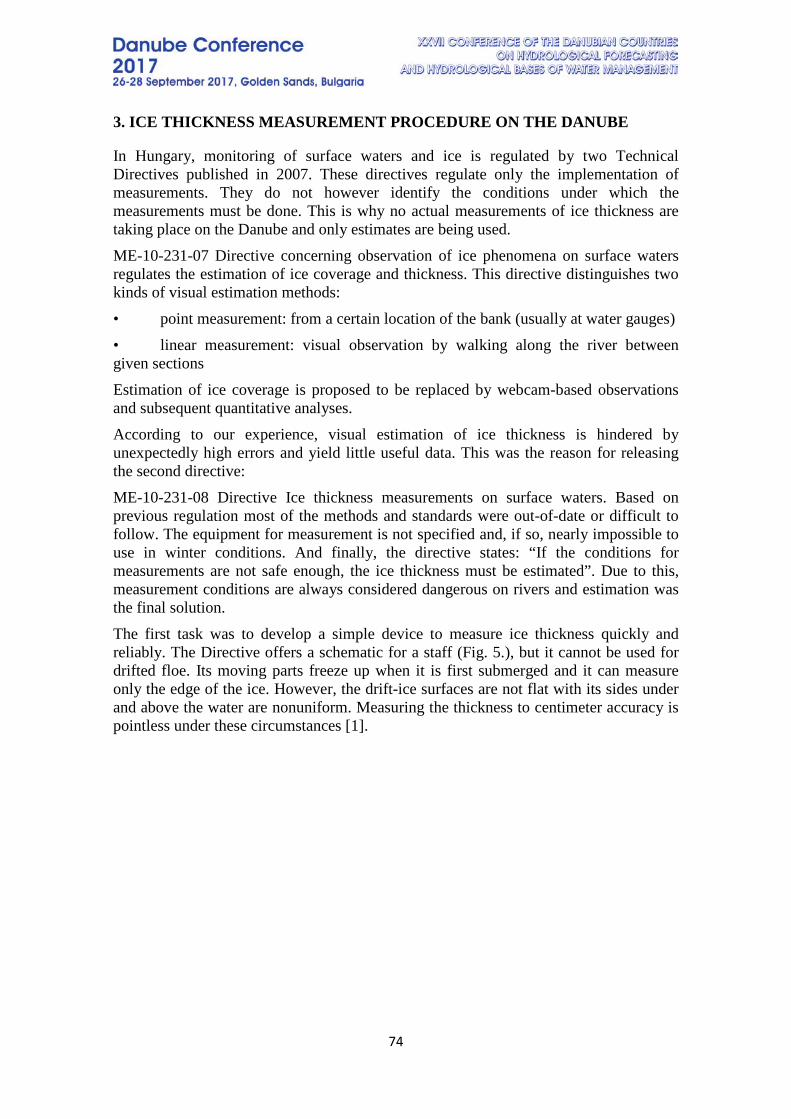
74

3. ICE THICKNESS MEASUREMENT PROCEDURE ON THE DANUBE

In Hungary, monitoring of surface waters and ice is regulated by two Technical Directives published in 2007. These directives regulate only the implementation of measurements. They do not however identify the conditions under which the measurements must be done. This is why no actual measurements of ice thickness are taking place on the Danube and only estimates are being used. ME-10-231-07 Directive concerning observation of ice phenomena on surface waters regulates the estimation of ice coverage and thickness. This directive distinguishes two kinds of visual estimation methods: • point measurement: from a certain location of the bank (usually at water gauges) • linear measurement: visual observation by walking along the river between given sections Estimation of ice coverage is proposed to be replaced by webcam-based observations and subsequent quantitative analyses. According to our experience, visual estimation of ice thickness is hindered by unexpectedly high errors and yield little useful data. This was the reason for releasing the second directive: ME-10-231-08 Directive Ice thickness measurements on surface waters. Based on previous regulation most of the methods and standards were out-of-date or difficult to follow. The equipment for measurement is not specified and, if so, nearly impossible to use in winter conditions. And finally, the directive states: “If the conditions for measurements are not safe enough, the ice thickness must be estimated”. Due to this, measurement conditions are always considered dangerous on rivers and estimation was the final solution. The first task was to develop a simple device to measure ice thickness quickly and reliably. The Directive offers a schematic for a staff (Fig. 5.), but it cannot be used for drifted floe. Its moving parts freeze up when it is first submerged and it can measure only the edge of the ice. However, the drift-ice surfaces are not flat with its sides under and above the water are nonuniform. Measuring the thickness to centimeter accuracy is pointless under these circumstances [1].

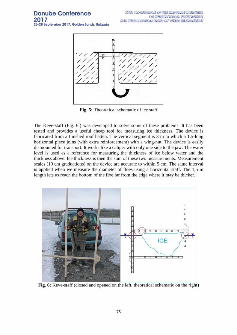
75

Fig. 5: Theoretical schematic of ice staff

The Keve-staff (Fig. 6.) was developed to solve some of these problems. It has been tested and provides a useful cheap tool for measuring ice thickness. The device is fabricated from a finished roof batten. The vertical segment is 3 m to which a 1,5-long horizontal piece joins (with extra reinforcement) with a wing-nut. The device is easily dismounted for transport. It works like a caliper with only one side to the jaw. The water level is used as a reference for measuring the thickness of ice below water and the thickness above. Ice thickness is then the sum of these two measurements. Measurement scales (10 cm graduations) on the device are accurate to within 5 cm. The same interval is applied when we measure the diameter of floes using a horizontal staff. The 1,5 m length lets us reach the bottom of the floe far from the edge where it may be thicker.

Fig. 6: Keve-staff (closed and opened on the left, theoretical schematic on the right)

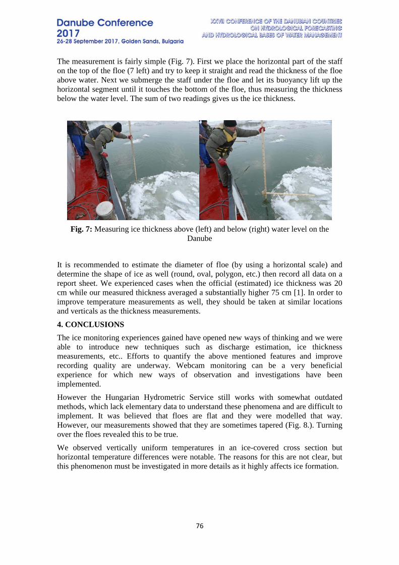
76

The measurement is fairly simple (Fig. 7). First we place the horizontal part of the staff on the top of the floe (7 left) and try to keep it straight and read the thickness of the floe above water. Next we submerge the staff under the floe and let its buoyancy lift up the horizontal segment until it touches the bottom of the floe, thus measuring the thickness below the water level. The sum of two readings gives us the ice thickness.

Fig. 7: Measuring ice thickness above (left) and below (right) water level on the

Danube

It is recommended to estimate the diameter of floe (by using a horizontal scale) and determine the shape of ice as well (round, oval, polygon, etc.) then record all data on a report sheet. We experienced cases when the official (estimated) ice thickness was 20 cm while our measured thickness averaged a substantially higher 75 cm [1]. In order to improve temperature measurements as well, they should be taken at similar locations and verticals as the thickness measurements.

4. CONCLUSIONS The ice monitoring experiences gained have opened new ways of thinking and we were able to introduce new techniques such as discharge estimation, ice thickness measurements, etc.. Efforts to quantify the above mentioned features and improve recording quality are underway. Webcam monitoring can be a very beneficial experience for which new ways of observation and investigations have been implemented. However the Hungarian Hydrometric Service still works with somewhat outdated methods, which lack elementary data to understand these phenomena and are difficult to implement. It was believed that floes are flat and they were modelled that way. However, our measurements showed that they are sometimes tapered (Fig. 8.). Turning over the floes revealed this to be true. We observed vertically uniform temperatures in an ice-covered cross section but horizontal temperature differences were notable. The reasons for this are not clear, but this phenomenon must be investigated in more details as it highly affects ice formation.

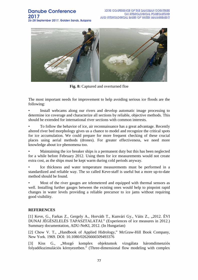
77

Fig. 8: Captured and overturned floe

The most important needs for improvement to help avoiding serious ice floods are the following: • Install webcams along our rivers and develop automatic image processing to determine ice coverage and characterize all sections by reliable, objective methods. This should be extended for international river sections with common interests. • To follow the behavior of ice, air reconnaissance has a great advantage. Recently altered river bed morphology gives us a chance to model and recognize the critical spots for ice accumulation. We could prepare for more frequent checking of these crucial places using aerial methods (drones). For greater effectiveness, we need more knowledge about ice phenomena too. • Maintaining the ice breaker ships is a permanent duty but this has been neglected for a while before February 2012. Using them for ice measurements would not create extra cost, as the ships must be kept warm during cold periods anyway. • Ice thickness and water temperature measurements must be performed in a standardized and reliable way. The so called Keve-staff is useful but a more up-to-date method should be found. • Most of the river gauges are telemetered and equipped with thermal sensors as well. Installing further gauges between the existing ones would help to pinpoint rapid changes in water levels providing a reliable precursor to ice jams without requiring good visibility.

REFERENCES [1] Keve, G., Farkas Z., Gergely A., Horváth T., Kunvári Gy., Váits Z., „2012. ÉVI DUNAI JÉGÉSZLELÉS TAPASZTALATAI.” (Experiences of ice measures in 2012.) Summary documentation, ADU-NeKI, 2012. (In Hungarian) [2] Chow V. T., „Handbook of Applied Hidrology,” McGraw-Hill Book Company, New York. 1969. DOI: 10.1080/02626666509493376 [3] Kiss G., „Mozgó komplex objektumok vizsgálata háromdimenziós folyadékszimulációs környezetben.” (Three-dimensional flow modeling with complex

78

moving-object interactions.) Bsc final project report, Budapest University of Technology and Economics, Faculty of Civil Engineering, Hidrológiai Tájékoztató, pp. 24-25. 2014. (In Hungarian) [4] Kerék, G., „Applicability of video-based flow measurements in small streams,” MSc thesis, Budapest University of Technology and Economics, Faculty of Civil Engineering, 2015. [5] Keve, G., „Space-time ice monitoring of Danube in Hungary by multiple web-cameras.” Riverflow2010. International Conference on Fluvial Hydraulics September 8-10, 2010, TU Braunschweig, Germany. 2010. [6] Hirling, Gy., „Forecast of the ice phenomena in river Danube and Tisza,” VIZDOK. Budapest., 1981. (In Hungarian)

79

TOPIC 2: HYDROLOGICAL DATA MANAGEMENT

EXPECTED CHANGES IN THE 100-YEAR RIVER DISCHARGE IN THE 21ST CENTURY AT THE DANUBE RIVER IN BRATISLAVA

Ladislav Gaál1, Danica Lešková2, Eva Uhliarová2

1 MicroStep-MIS s.r.o., Bratislava, Slovakia 2 Slovak Hydrometeorological Institute, Bratislava, Slovakia

Corresponding author: Ladislav Gaál, MicroStep-MIS s.r.o., Cavojskeho 1, 841 04 Bratislava, Slovakia, ladislav.gaal@microstep-mis.com

ABSTRACT The paper presents first results of the local case study ‘Flood warnings in a changing climate’ carried out within the framework of the SWICCA project. We assess the changes in Q100 (i.e., the 100-year return value of river discharge or simply the 100-year flood) that might be expected to occur due to climate change during the 21st century. The target location is the Danube River in Bratislava, Slovakia. We define a simple indicator CCQ100 termed as Climate Change Indicator of the 100-year Flood, which is the ratio of the 100-year floods estimated on the basis of future and past datasets. For the past, the observed data from the period of 1984−2014 are used. For the future (2015−2100), a number of simulated time series of river discharge from the SWICCA database are processed. They are the outcomes of the combination of 3 hydrological models (HYPE, VIC and Lisflood) and 11 regional climate models. The case study is an at-site and basically a non-stationary frequency analysis. The data samples are derived on the basis of the block maxima approach (annual maxima), and the flood quantiles are modeled by the Generalized Extreme Value (GEV) distribution. In case there is a significant linear trend in the data samples, the non-stationary approach is adopted with a time-dependent location parameter of the GEV distribution. Flood quantiles and their confidence intervals are estimated on the basis of the Differential Evolution Markov Chain approach. The results indicate that: (a) The overall performance of the datasets are rather balanced: increase (decrease) in Q100 appears in 13 (12) cases, while no change (0.95 ≤ CCQ100 ≤ 1.05) is found in 7 cases; (b) Increases dominate in the case of hydrological models HYPE and Lisflood; (c) The HYPE model indicates the largest positive changes overall, also with the highest value of CCQ100 (= 1.40); and (d) The VIC model only yields decrease in Q100. The most remarkable drop is of about 33% (CCQ100 = 0.67). Overall, the multitude of model outcomes is an excellent basis to get the first sight on the possible range of expected changes in the 100-year flood. On the other hand, at this stage of the analysis one cannot arrive to a clear conclusion concerning the sign of these changes. It is believed that further information will be obtained by the adoption of a frequency analysis on the basis of the peaks-over-threshold methodology. This, hopefully, will reveal more insight into the expected behavior of floods with low

80

probability of occurrence, and the knowledge might be transformed into flood management and adaptation plans of the capital city of Slovakia. Keywords: frequency analysis, climate change, 100-year flood, Danube, SWICCA

1. INTRODUCTION Flood frequency analysis is a part of the operational services of the Slovak Hydrometeorological Institute (SHMI). So far, estimation of T-year return values of floods has generally been based on local data (at-site approach), using principle of the stationarity of environment, and analyzing annual or seasonal maxima. While in the last couple of years, regional approaches to a flood frequency analysis have been successfully adopted in Slovakia [1] and the Central European region [2], no methods accounting for the non-stationarity of environment were developed and implemented in the practice. Similarly, little efforts have been done with implementing the peaks-over-threshold (POT) methodology (where all independent events exceeding a pre-defined threshold are taken into account; e.g., [3]), which is generally considered as a more rigorous statistical approach when compared to the block maxima method (e.g., [4]). Therefore, MicroStep-MIS and SHMI co-operate on the local case study ‘Flood warnings in a changing climate’, which aims at developing flood frequency estimation methods with two novel directions. First, the non-stationarity of environment will be accounted for, and secondly, the return levels of river discharges will be estimated using the POT methodology. Nevertheless, before dealing with the POT method, an interim step is adopted where flood quantiles are assessed on the basis of the annual maxima series (AMS) approach – and the result of this procedure are presented in the current study. The case study ‘Flood warnings in a changing climate’ is being carried out under the framework of the SWICCA project (http://swicca.climate.copernicus.eu/). SWICCA (Service for Water Indicators in Climate Change Adaptation) is more than a two-year project governed by the Swedish Meteorological and Hydrological Institute, and serves as a proof-of-concept for a Sectorial Information Service on water management to Copernicus Climate Change Services. The goal of the SWICCA project is to offer freely available climatological and hydrological data (climate change indicators) collected from a number of Pan-European climate/hydrological model runs, to facilitate working with climate change adaptation in the water sector and the decision-making process of water managers. The transfer of the information from the global to regional and/or local scales are demonstrated by means of a number of local case studies from different regions across the whole Europe.

2. METHODS The presented study aims at assessing the changes in the 100-year return value of river discharge (or simply the 100-year flood, Q100) that might be expected to occur due to the climate change during the 21st century compared to what was observed during the past couple of decades. We define a simple indicator CCQ100 termed as Climate Change Indicator of the 100-year Flood:

𝐶𝐶𝐶𝐶𝑄𝑄100 = 𝑄𝑄100,𝑓𝑓𝑓𝑓𝑓𝑓𝑓𝑓𝑓𝑓𝑓𝑓

𝑄𝑄100,𝑝𝑝𝑝𝑝𝑝𝑝𝑓𝑓 (1)

81

which is the ratio of the 100-year floods estimated on the basis of the future and the past datasets. For the past, the observed data are used, as usual. For the future, a number of simulated time series of river discharge from the SWICCA database are processed. Since the outputs of regional climate models are generally affected by bias (errors due to conceptualization, discretization and spatial averaging), bias correction has to be applied to make the model outputs more similar to the reality. For this reason, the so called linear scaling methodology of bias correction [5] is adopted that makes use of the monthly statistics (averages and standard deviations) derived from the common period where both the observed and the modelled discharge data are available. The basis of the case study is an at-site and non-stationary frequency analysis. The data samples are derived according to the block maxima approach (namely, the annual maxima are identified for each year), and the flood quantiles are statistically modeled by the Generalized Extreme Value (GEV) distribution [6]. The rigorousness of the AMS/GEV approach is justified by the extreme value theory (e.g., [7]). The stationarity of the time series is analyzed by means of the Mann-Kendall test for the presence of monotonic trends [8] at the significance level of α = 0.05. In the case there is a significant linear trend in the data samples, the non-stationary approach to a frequency estimation is adopted with a time-dependent location parameter of the GEV distribution. Flood quantiles and their confidence intervals are estimated on the basis of the Differential Evolution Markov Chain (DEMC) approach [9]. DEMC is an enhanced alternative to the Markov Chain Monte Carlo (MCMC) approaches where target posterior distributions are sampled through five Markov Chains constructed in parallel; however, in DEMC, the chains are allowed to learn from each other, and this feature ensures simplicity, speed of calculation, and convergence over the conventional MCMC [10].

3. DATA 3.1 Observed data The presented frequency analysis focuses at a single target site, which is Bratislava, the capital city of Slovakia along the Danube River. The daily discharge data from the Bratislava station (with geographical co-ordinates 48.1397 N, and 17.1082 E) cover the period from January 1st, 1984 till December 31st, 2014, i.e., 31 complete calendar years with no missing values are available for the analysis.

3.2 Simulated data From the SWICCA database, simulations of daily discharge data were downloaded for the grid box (48.14 N, 17.11 E) corresponding to the location of the Bratislava station, and for the combination of 11 climate (Tab. 1) and 3 hydrological models (Tab. 2).

Since the real observations are from the period 1984−2014, and the control period of the modelled data is 1971−2000, we decided to use the 17 years long common period 1984−2000 as the basis to derive the statistical characteristics for the bias correction. In line with this decision, the period 2015−2100 was declared as the ‘future’.

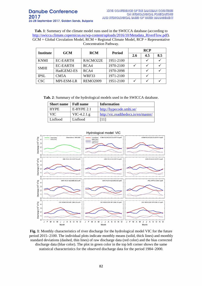
82

Tab. 1: Summary of the climate model runs used in the SWICCA database (according to http://swicca.climate.copernicus.eu/wp-content/uploads/2016/10/Metadata_RiverFlow.pdf). GCM = Global Circulation Model, RCM = Regional Climate Model, RCP = Representative

Concentration Pathway.

Institute GCM RCM Period RCP

2.6 4.5 8.5 KNMI EC-EARTH RACMO22E 1951-2100

SMHI EC-EARTH RCA4 1970-2100 HadGEM2-ES RCA4 1970-2098

IPSL CM5A WRF33 1971-2100 CSC MPI-ESM-LR REMO2009 1951-2100

Tab. 2: Summary of the hydrological models used in the SWICCA database.

Short name Full name Information HYPE E-HYPE 2.1 http://hypecode.smhi.se/ VIC VIC-4.2.1.g http://vic.readthedocs.io/en/master/ Lisflood Lisflood [11]

Fig. 1: Monthly characteristics of river discharge for the hydrological model VIC for the future period 2015−2100. The individual plots indicate monthly means (solid, thick lines) and monthly standard deviations (dashed, thin lines) of raw discharge data (red color) and the bias corrected

discharge data (blue color). The plot in green color in the top left corner shows the same statistical characteristics for the observed discharge data for the period 1984−2000.

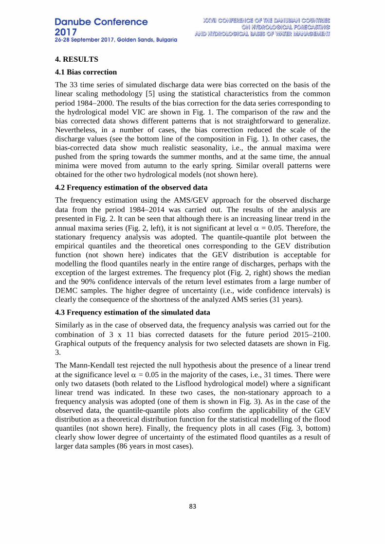
83

4. RESULTS 4.1 Bias correction The 33 time series of simulated discharge data were bias corrected on the basis of the linear scaling methodology [5] using the statistical characteristics from the common period 1984−2000. The results of the bias correction for the data series corresponding to the hydrological model VIC are shown in Fig. 1. The comparison of the raw and the bias corrected data shows different patterns that is not straightforward to generalize. Nevertheless, in a number of cases, the bias correction reduced the scale of the discharge values (see the bottom line of the composition in Fig. 1). In other cases, the bias-corrected data show much realistic seasonality, i.e., the annual maxima were pushed from the spring towards the summer months, and at the same time, the annual minima were moved from autumn to the early spring. Similar overall patterns were obtained for the other two hydrological models (not shown here).

4.2 Frequency estimation of the observed data The frequency estimation using the AMS/GEV approach for the observed discharge data from the period 1984−2014 was carried out. The results of the analysis are presented in Fig. 2. It can be seen that although there is an increasing linear trend in the annual maxima series (Fig. 2, left), it is not significant at level α = 0.05. Therefore, the stationary frequency analysis was adopted. The quantile-quantile plot between the empirical quantiles and the theoretical ones corresponding to the GEV distribution function (not shown here) indicates that the GEV distribution is acceptable for modelling the flood quantiles nearly in the entire range of discharges, perhaps with the exception of the largest extremes. The frequency plot (Fig. 2, right) shows the median and the 90% confidence intervals of the return level estimates from a large number of DEMC samples. The higher degree of uncertainty (i.e., wide confidence intervals) is clearly the consequence of the shortness of the analyzed AMS series (31 years).

4.3 Frequency estimation of the simulated data Similarly as in the case of observed data, the frequency analysis was carried out for the combination of 3 x 11 bias corrected datasets for the future period 2015−2100. Graphical outputs of the frequency analysis for two selected datasets are shown in Fig. 3. The Mann-Kendall test rejected the null hypothesis about the presence of a linear trend at the significance level α = 0.05 in the majority of the cases, i.e., 31 times. There were only two datasets (both related to the Lisflood hydrological model) where a significant linear trend was indicated. In these two cases, the non-stationary approach to a frequency analysis was adopted (one of them is shown in Fig. 3). As in the case of the observed data, the quantile-quantile plots also confirm the applicability of the GEV distribution as a theoretical distribution function for the statistical modelling of the flood quantiles (not shown here). Finally, the frequency plots in all cases (Fig. 3, bottom) clearly show lower degree of uncertainty of the estimated flood quantiles as a result of larger data samples (86 years in most cases).

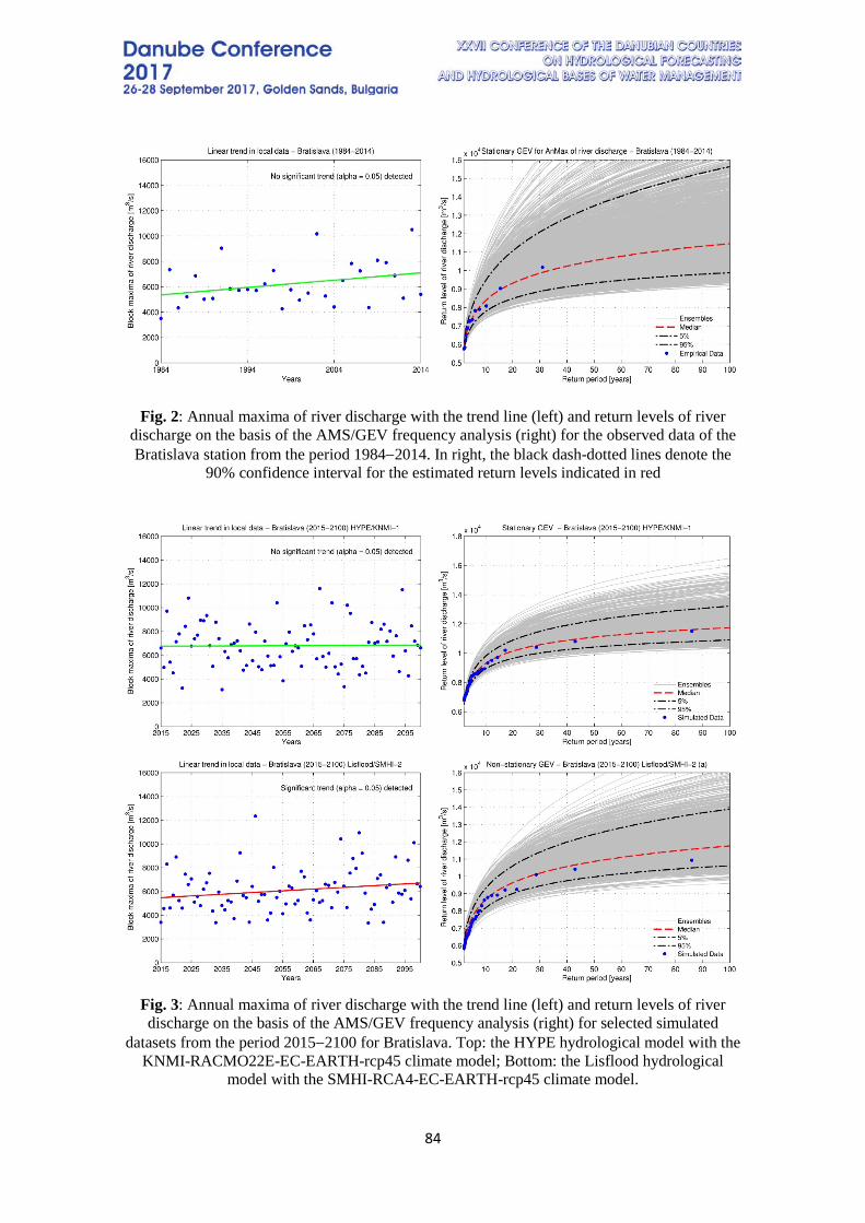
84

Fig. 2: Annual maxima of river discharge with the trend line (left) and return levels of river discharge on the basis of the AMS/GEV frequency analysis (right) for the observed data of the Bratislava station from the period 1984−2014. In right, the black dash-dotted lines denote the

90% confidence interval for the estimated return levels indicated in red

Fig. 3: Annual maxima of river discharge with the trend line (left) and return levels of river discharge on the basis of the AMS/GEV frequency analysis (right) for selected simulated

datasets from the period 2015−2100 for Bratislava. Top: the HYPE hydrological model with the KNMI-RACMO22E-EC-EARTH-rcp45 climate model; Bottom: the Lisflood hydrological

model with the SMHI-RCA4-EC-EARTH-rcp45 climate model.

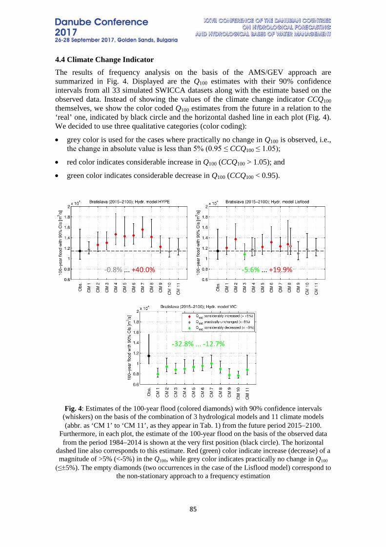
85

4.4 Climate Change Indicator The results of frequency analysis on the basis of the AMS/GEV approach are summarized in Fig. 4. Displayed are the Q100 estimates with their 90% confidence intervals from all 33 simulated SWICCA datasets along with the estimate based on the observed data. Instead of showing the values of the climate change indicator CCQ100 themselves, we show the color coded Q100 estimates from the future in a relation to the ‘real’ one, indicated by black circle and the horizontal dashed line in each plot (Fig. 4). We decided to use three qualitative categories (color coding):

• grey color is used for the cases where practically no change in Q100 is observed, i.e., the change in absolute value is less than 5% (0.95 ≤ CCQ100 ≤ 1.05);

• red color indicates considerable increase in Q100 (CCQ100 > 1.05); and

• green color indicates considerable decrease in Q100 (CCQ100 < 0.95).

Fig. 4: Estimates of the 100-year flood (colored diamonds) with 90% confidence intervals

(whiskers) on the basis of the combination of 3 hydrological models and 11 climate models (abbr. as ‘CM 1’ to ‘CM 11’, as they appear in Tab. 1) from the future period 2015−2100.

Furthermore, in each plot, the estimate of the 100-year flood on the basis of the observed data from the period 1984−2014 is shown at the very first position (black circle). The horizontal

dashed line also corresponds to this estimate. Red (green) color indicate increase (decrease) of a magnitude of >5% (<-5%) in the Q100, while grey color indicates practically no change in Q100

(≤±5%). The empty diamonds (two occurrences in the case of the Lisflood model) correspond to the non-stationary approach to a frequency estimation

-0.8% ... +40.0%

-32.8% ... -12.7%

-5.6% ... +19.9%

86

Fig. 4 reveals interesting features:

• Increases dominate in the case of two hydrological models (HYPE and Lisflood). The difference between these two models lies in the magnitude of the increase: the HYPE model indicates the largest positive changes overall.

• The highest value of CCQ100 (= 1.40) appears in the case of the HYPE hydrological model and the SMHI-RCA4-HadGEM2-ES-rcp85 climate model.

• The VIC model only yields decrease in Q100.

• In rough approximation, the patterns of the change in Q100 are similar for the hydrological models HYPE and VIC. The largest (smallest) Q100 appears both at CM7 - SMHI-RCA4-HadGEM2-ES-rcp8 (CM10 - CSC-REMO2009-MPI-ESM-LR-rcp45), and such an analogy holds for a number of the climate models when comparing HYPE vs. VIC models. From this perspective, the Lisflood hydrologic model shows a fuzzier pattern.

• The overall performance of the datasets are rather balanced: increase (decrease) appears in 13 (12) cases, while no change is indicated in 7 cases (see also Tab. 3).

• Results of the non-stationary approach are also displayed; these are indicated by empty diamonds in the case of Lisflood model. It can be concluded that there are negligible differences between the corresponding results related to stationary vs. non-stationary approach. The variability among the different climate models is much larger than that stemming from the assumption of stationarity or non-stationarity.

Tab. 3 summarizes the most important statistics of the analysis.

Tab. 3: Summary of the results of the frequency analysis based on the approach AMS/GEV. CCQ100 stands for the Climate Change Indicator of the 100-year Flood.

Hydrol. model

Climate models

CCQ100 > 1.05

CCQ100 = 1.05…0.95

CCQ100 < 0.95

Largest increase

Largest decrease

HYPE 11 8 3 0 40% -1% VIC 11 0 0 11 --- -33%

Lisflood 11 5 4 1 20% -6% All 33 13 7 12 40% -33%

5. DISCUSSION AND CONCLUSIONS The current paper presents an analysis of the expected changes in estimates of the 100-year flood during the 21st century at the selected target site, Bratislava. The analysis made use of the database of the SWICCA project that consists of a wide variety of climate and hydrological model runs that are available for the upcoming decades from different international projects and databases. In the next paragraphs, we are first going to discuss some particular settings of the analysis that are expected to have influenced

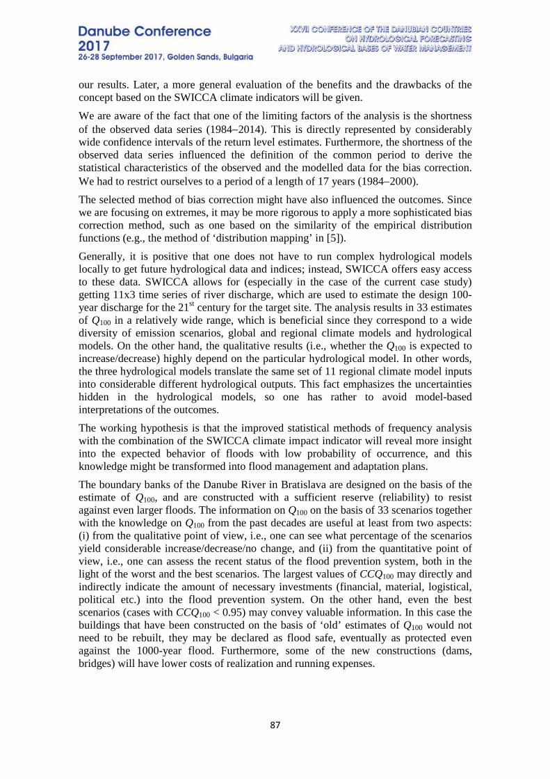
87

our results. Later, a more general evaluation of the benefits and the drawbacks of the concept based on the SWICCA climate indicators will be given. We are aware of the fact that one of the limiting factors of the analysis is the shortness of the observed data series (1984−2014). This is directly represented by considerably wide confidence intervals of the return level estimates. Furthermore, the shortness of the observed data series influenced the definition of the common period to derive the statistical characteristics of the observed and the modelled data for the bias correction. We had to restrict ourselves to a period of a length of 17 years (1984−2000). The selected method of bias correction might have also influenced the outcomes. Since we are focusing on extremes, it may be more rigorous to apply a more sophisticated bias correction method, such as one based on the similarity of the empirical distribution functions (e.g., the method of ‘distribution mapping’ in [5]). Generally, it is positive that one does not have to run complex hydrological models locally to get future hydrological data and indices; instead, SWICCA offers easy access to these data. SWICCA allows for (especially in the case of the current case study) getting 11x3 time series of river discharge, which are used to estimate the design 100-year discharge for the 21st century for the target site. The analysis results in 33 estimates of Q100 in a relatively wide range, which is beneficial since they correspond to a wide diversity of emission scenarios, global and regional climate models and hydrological models. On the other hand, the qualitative results (i.e., whether the Q100 is expected to increase/decrease) highly depend on the particular hydrological model. In other words, the three hydrological models translate the same set of 11 regional climate model inputs into considerable different hydrological outputs. This fact emphasizes the uncertainties hidden in the hydrological models, so one has rather to avoid model-based interpretations of the outcomes. The working hypothesis is that the improved statistical methods of frequency analysis with the combination of the SWICCA climate impact indicator will reveal more insight into the expected behavior of floods with low probability of occurrence, and this knowledge might be transformed into flood management and adaptation plans. The boundary banks of the Danube River in Bratislava are designed on the basis of the estimate of Q100, and are constructed with a sufficient reserve (reliability) to resist against even larger floods. The information on Q100 on the basis of 33 scenarios together with the knowledge on Q100 from the past decades are useful at least from two aspects: (i) from the qualitative point of view, i.e., one can see what percentage of the scenarios yield considerable increase/decrease/no change, and (ii) from the quantitative point of view, i.e., one can assess the recent status of the flood prevention system, both in the light of the worst and the best scenarios. The largest values of CCQ100 may directly and indirectly indicate the amount of necessary investments (financial, material, logistical, political etc.) into the flood prevention system. On the other hand, even the best scenarios (cases with CCQ100 < 0.95) may convey valuable information. In this case the buildings that have been constructed on the basis of ‘old’ estimates of Q100 would not need to be rebuilt, they may be declared as flood safe, eventually as protected even against the 1000-year flood. Furthermore, some of the new constructions (dams, bridges) will have lower costs of realization and running expenses.

88

Overall, the multitude of the model outcomes is an excellent basis to get the first sight on the possible range of the expected changes in the 100-year flood. On the other hand, at this stage of the analysis one cannot arrive to a clear conclusion concerning the sign of these changes. Generally, it is expected that adoption of the novel frequency estimation approach (peaks-over-threshold method) and its comparison with the current AMS/GEV approach will shed more light on the unresolved problems. It is anticipated that POT method will show more beneficial statistical behavior (i.e., narrower confidence intervals of the return levels); nevertheless, this analysis is still to be carried out.

ACKNOWLEDGEMENTS The support of the SWICCA project is gratefully acknowledged.

REFERENCES [1] Gaál, L., Kyselý, J., Szolgay, J.: Region-of-influence approach to a frequency analysis of heavy precipitation in Slovakia. Hydrology and Earth System Sciences, 12 (3), 825−839, 2008. doi:10.5194/hess-12-825-2008. [2] Gaál, L., Kyselý, J.: Comparison of region-of-influence methods for estimating high quantiles of precipitation in a dense dataset in the Czech Republic. Hydrology and Earth System Sciences, 13 (11), 2203−2219, 2009. doi:10.5194/hess-13-2203-2009. [3] Bačová-Mitková, V., Onderka, M.: Analysis of extreme hydrological events on the Danube using the peak over threshold method. Journal of Hydrology and Hydromechanics, 58 (2), 88–101, 2010. doi:10.2478/v10098-010-0009-x. [4] Madsen, H., Rasmussen, P.F., Rosbjerg, D.: Comparison of annual maximum series and partial duration series methods for modeling extreme hydrologic events. 1: At-site modeling. Water Resources Research, 33 (4), 747–757, 1997. doi:10.1029/96WR03848. [5] Teutschbein, C., Seibert, J.: Bias correction of regional climate model simulations for hydrological climate-change impact studies: Review and evaluation of different methods. Journal of Hydrology, 456–457, 12–29, 2012. doi:10.1016/j.jhydrol.2012.05.052. [6] Coles, S.: An introduction to statistical modeling of extreme values. London : Springer, 2001. [7] Katz, R.W., Parlange, M.B., Naveau, P.: Statistics of extremes in hydrology. Advances in Water Resources, 25, 1287−1304, 2002. doi:10.1016/S0309-1708(02)00056-8. [8] Wilks, D.S.: Statistical methods in the atmospheric sciences. Oxford : Academic Press, 2011. 3rd ed. [9] Cheng, L., AghaKouchak, A., Gilleland, E., Katz, R.W.: Non-stationary extreme value analysis in a changing climate. Climatic Change, 127, 353−369, 2014. doi:10.1007/s10584-014-1254-5. [10] Cheng, L., AghaKouchak, A.: Nonstationary precipitation intensity-duration-frequency curves for infrastructure design in a changing climate. Scientific Reports, 4, 7093, 2014. doi:10.1038/srep07093.

89

[11] Burek, P.A., van der Knijff, J., de Rio, A.: LISFLOOD − Distributed Water Balance and Flood Simulation Model - Revised User Manual 2013. Joint Research Centre, Report EUR 26162 EN. Luxembourg : Publication Office of the European Commission, 2013.

90

THE ROLE OF THE GROUNDWATER IN THE FORMATUION OF RIVER FLOW OF THE ARDA RIVER BASIN (SOTHERN BULGARIA)

Marin Ivanov1, Tatiana Orehova2, Aglaida Toteva2, Mila Trayanova2, Aleksey

Benderev2 1 National Institute of Meteorology and Hydrology – BAS, Bulgaria

2 Geological Institute – BAS, Bulgaria

Corresponding author: Marin Ivanov, National Institute of Meteorology and Hydrology, 66 Tsarigradsko Shose, Blvd, 1784 Sofia, Bulgaria, email: marin.ivanov@meteo.bg

ABSTRACT The Arda River is the main river course in the mountain range Rhodopes located in Southern Bulgaria. Its river basin is characterized by highly variable relief and diversified geological and hydrogeological conditions. The groundwater is recharged mostly from precipitation and forms baseflow of the Arda River and its tributaries. The aim of the study is to evaluate the contribution of groundwater in the formation of river flow within the Arda River basin. For this purpose, the groundwater recharge index GWI (groundwater recharge as a ratio of total runoff) is defined. Available hydrogeological information is scarce, and limited to particular areas. Therefore, indirect methods and GIS approach are used to evaluate the role of groundwater in the river runoff formation for the study area. The main factors controlling the groundwater recharge and flow: the relief, soil texture, and aquifer permeability are taken into account. The resulting map provides information on the spatial distribution of groundwater recharge index over the study area. The obtained results are validated with data from baseflow separation of the river flows at several gauging stations within the study area. Keywords: groundwater, baseflow, GIS, Arda River basin, Bulgaria

1. INTRODUCTION The role of groundwater in the formation of river flow is evident – it supports river runoff during low flow periods. Low permeable rocks restrict the baseflow, resulting in high river flow variability. On the contrary, the groundwater-dominated rivers typically related to major aquifers, are characterized with rather stable river runoff and relatively high baseflow [1]. The aim of the study is to evaluate the contribution of groundwater in the formation of river flow for the Arda River basin located in Southern Bulgaria. The groundwater is recharged mainly from precipitation, and forms the baseflow of the Arda River and its tributaries. The quantitative hydrogeological information is scarce and limited to particular areas. A reliable approach for such cases is the heuristic method of Döll et al. [2, 3] successfully applied for several Bulgarian study areas [4, 5]. This method provides spatial distribution on the groundwater recharge index GWI defined as a ratio of the groundwater recharge to the total runoff.

91

2. DESCRIPTION OF THE STUDY AREA The Arda River is the main river course in the mountain range Rhodopes in Southern Bulgaria. The study area covers Bulgarian part of the Arda River basin, with total drainage area of 5213 km2.

2.1 Physical environment The climate of the study area is under influence of the Mediterranean Sea. The mean annual air temperature across the Arda River basin varies between 8 and 13°C, with lower values for mountains. The hottest month is July with mean monthly air temperature from 17 to 24°C depending on elevation. The coldest month is January with monthly average temperature in Eastern Rhodopes about 1.5-2°C above zero. In the mountains, with increase in elevation the air temperature is falling below zero. The total annual precipitation in the region of Kardzhali is 600-650 mm, and for the south-east Rhodopes over 1000 mm. The driest months are August and September. Most of precipitation falls during the cold half-year (from November to February). Mild winters are typical for the area. Due to frequent warming periods in winter, the snowpack is not stable – the snow melts several times during cold season. The Arda River takes its source from a karst spring and drains eastern parts of Western Rhodopes and almost entirely Eastern Rhodopes. The elevation of the Arda River basin ranges from 2126 m to 32 m asl at its influence to the Maritsa River on the territory of Turkey. The mountains in Eastern Rhodopes are low with flattened form, and they are divided by broad valleys. The main tributaries of the Arda River are: Malka Arda, Cherna, Elhovska, Varbitsa, and Krumovitsa Rivers. The river flows are measured in several hydrometric stations operated by the National Institute of Meteorology and Hydrology at Bulgarian Academy of Sciences (NIMH-BAS). The drainage areas for the studied river gauging stations within the Arda River basin are presented in Fig. 1.

2.2 Hydrogeological setting The Arda River basin is characterized by complex geological structure. Numerous block and fault structures are identified shown in tectonic sketch by Boyanov and Goranov [6]. Proterozoic metamorphic rocks are presented mainly by schists and gneisses with discrete packages of marbles and amphibolites. When fractured, marbles tend to develop high conduit permeability. The high-grade basement rocks are intruded by late Cretaceous – Oligocene granitoids. Paleogenic volcano-sedimentary rocks widespread in the study area are divided in several lithotectonic units. The most permeable Paleogenic rock is limestone from the marlstone-limestone formation. Quaternary deposits consist mainly of alluvial sediments along the river courses. As a result of highly variable relief and complex geological structure, diverse hydrogeological settings are observed over the study area. Low permeable bedrocks prevail in the study area, such as the volcano-sedimentary formations that are locally fissured. Major aquifers are related to karstified carbonate formations (Proterozoic marbles and Paleogene limestone). The Quaternary alluvial and proluvial deposits are permeable, and favor the groundwater formation.

92

Fig. 1: Study area

3. METHODS AND DATABASE The precipitation falling over the study area is partitioned into evapotranspiration and runoff, which is divided into direct runoff and baseflow. The last component of the river runoff is more stable and supports the river flow during low flow periods. In this study, such partitioning of the total river runoff is done in GIS environment based on the method proposed and used by Döll et al. [2, 3]. For validation, the river hydrograph separation method is applied based on data for hydrometric stations within the study area.

3.1 Method of Doll et al. Döll et al. [2, 3] developed and applied new heuristic method to evaluate both the groundwater recharge and the role of groundwater in the total river runoff formation. This method takes into account the main factors controlling the groundwater recharge, such as topographic slope, soil texture, and permeability of the rocks. Evidently, with steeper slopes, finer soil textures and less permeable aquifers, groundwater recharge as a fraction of total runoff from land is expected to decrease. The groundwater recharge factor , which reflects the proportion of groundwater in the total river flow, is defined based on equation:

(1)

gwf

atsgw ffff ××=

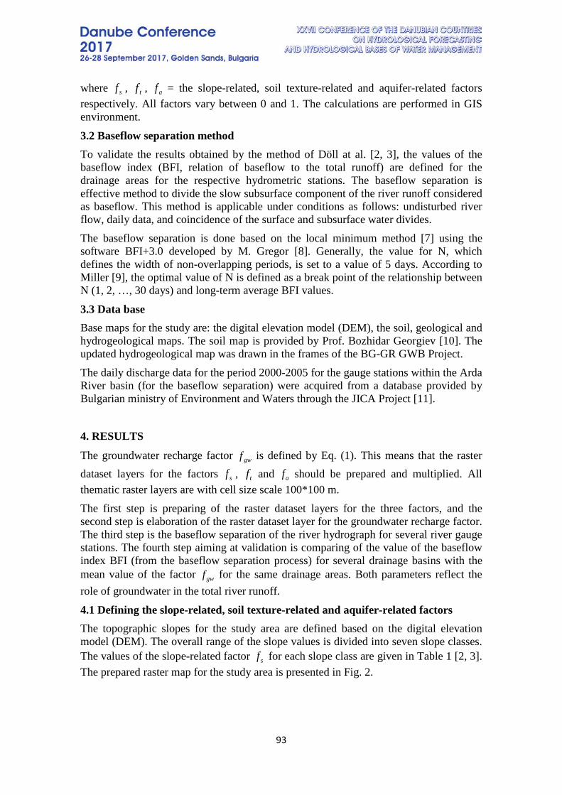
93

where , , = the slope-related, soil texture-related and aquifer-related factors respectively. All factors vary between 0 and 1. The calculations are performed in GIS environment.

3.2 Baseflow separation method To validate the results obtained by the method of Döll at al. [2, 3], the values of the baseflow index (BFI, relation of baseflow to the total runoff) are defined for the drainage areas for the respective hydrometric stations. The baseflow separation is effective method to divide the slow subsurface component of the river runoff considered as baseflow. This method is applicable under conditions as follows: undisturbed river flow, daily data, and coincidence of the surface and subsurface water divides. The baseflow separation is done based on the local minimum method [7] using the software BFI+3.0 developed by M. Gregor [8]. Generally, the value for N, which defines the width of non-overlapping periods, is set to a value of 5 days. According to Miller [9], the optimal value of N is defined as a break point of the relationship between N (1, 2, …, 30 days) and long-term average BFI values.

3.3 Data base Base maps for the study are: the digital elevation model (DEM), the soil, geological and hydrogeological maps. The soil map is provided by Prof. Bozhidar Georgiev [10]. The updated hydrogeological map was drawn in the frames of the BG-GR GWB Project. The daily discharge data for the period 2000-2005 for the gauge stations within the Arda River basin (for the baseflow separation) were acquired from a database provided by Bulgarian ministry of Environment and Waters through the JICA Project [11].

4. RESULTS

The groundwater recharge factor is defined by Eq. (1). This means that the raster dataset layers for the factors , and should be prepared and multiplied. All thematic raster layers are with cell size scale 100*100 m. The first step is preparing of the raster dataset layers for the three factors, and the second step is elaboration of the raster dataset layer for the groundwater recharge factor. The third step is the baseflow separation of the river hydrograph for several river gauge stations. The fourth step aiming at validation is comparing of the value of the baseflow index BFI (from the baseflow separation process) for several drainage basins with the mean value of the factor for the same drainage areas. Both parameters reflect the role of groundwater in the total river runoff.

4.1 Defining the slope-related, soil texture-related and aquifer-related factors The topographic slopes for the study area are defined based on the digital elevation model (DEM). The overall range of the slope values is divided into seven slope classes. The values of the slope-related factor for each slope class are given in Table 1 [2, 3]. The prepared raster map for the study area is presented in Fig. 2.

sf tf af

gwf

sf tf af

gwf

sf

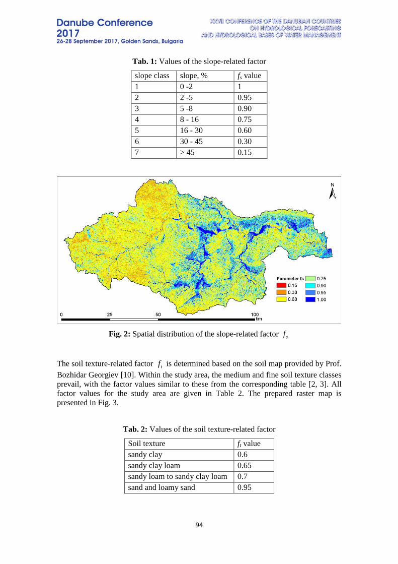
94

Tab. 1: Values of the slope-related factor

slope class slope, % fs value 1 0 -2 1 2 2 -5 0.95 3 5 -8 0.90 4 8 - 16 0.75 5 16 - 30 0.60 6 30 - 45 0.30 7 > 45 0.15

Fig. 2: Spatial distribution of the slope-related factor

The soil texture-related factor is determined based on the soil map provided by Prof. Bozhidar Georgiev [10]. Within the study area, the medium and fine soil texture classes prevail, with the factor values similar to these from the corresponding table [2, 3]. All factor values for the study area are given in Table 2. The prepared raster map is presented in Fig. 3.

Tab. 2: Values of the soil texture-related factor

Soil texture ft value sandy clay 0.6 sandy clay loam 0.65 sandy loam to sandy clay loam 0.7 sand and loamy sand 0.95

sf

tf

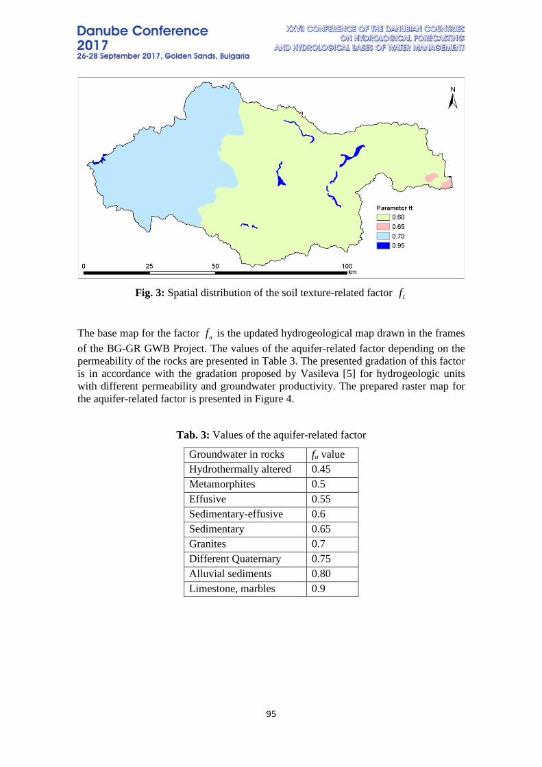
95

Fig. 3: Spatial distribution of the soil texture-related factor

The base map for the factor is the updated hydrogeological map drawn in the frames of the BG-GR GWB Project. The values of the aquifer-related factor depending on the permeability of the rocks are presented in Table 3. The presented gradation of this factor is in accordance with the gradation proposed by Vasileva [5] for hydrogeologic units with different permeability and groundwater productivity. The prepared raster map for the aquifer-related factor is presented in Figure 4.

Tab. 3: Values of the aquifer-related factor

Groundwater in rocks fa value Hydrothermally altered 0.45 Metamorphites 0.5 Effusive 0.55 Sedimentary-effusive 0.6 Sedimentary 0.65 Granites 0.7 Different Quaternary 0.75 Alluvial sediments 0.80 Limestone, marbles 0.9

tf

af

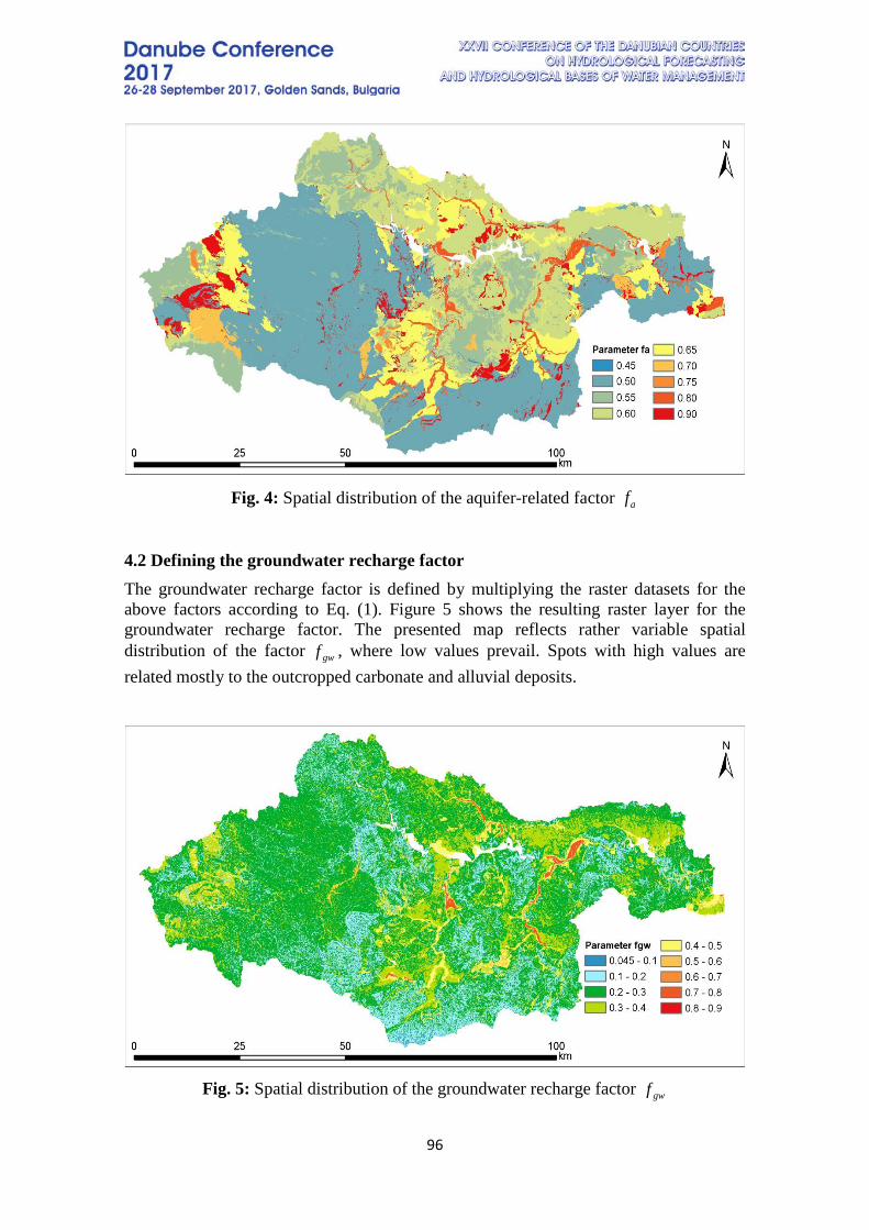
96

Fig. 4: Spatial distribution of the aquifer-related factor

4.2 Defining the groundwater recharge factor The groundwater recharge factor is defined by multiplying the raster datasets for the above factors according to Eq. (1). Figure 5 shows the resulting raster layer for the groundwater recharge factor. The presented map reflects rather variable spatial distribution of the factor , where low values prevail. Spots with high values are related mostly to the outcropped carbonate and alluvial deposits.

Fig. 5: Spatial distribution of the groundwater recharge factor

af

gwf

gwf

97

4.3 Validation of the results and discussion The baseflow separation is applied for river discharge from the hydrometric stations within the Arda River basin for the 2000-2005 period. For the purpose the local minimum method from the software BFI+3.0 is used. According to the advice of Miller [9], the values of BFI are computed for a range in N values, and the optimal value of N is identified as a break point of the relationship between N and the BFI values. The resulting values of BFI values along with the optimal values of parameter N (Nopt) for the studied hydrometric stations are given in Table 3. In the rightmost column of the table, the mean value of the parameter is given for the respective drainage area.

Tab. 3: The BFI data for the river gauge stations within the Arda River basin

N River Location Area, km2 Nopt, days BFI Mean fgw 61650 Arda Rudozem 258.8 15 0.432 0.288 61350 Cherna reka Taran 237.4 8 0.479 0.278 61700 Arda Vehtino 860.3 8 0.387 0.260 61550 Krumovitsa Krumovgrad 500.3 10 0.245 0.263 61450 Varbitsa Varli dol 472.2 16 0.205 0.235 61500 Varbitsa Dzhebel 1151.8 7 0.247 0.258

The comparison of the values of BFI and the factor show that they are similar for watersheds of the Varbitsa and the Krumovitsa Rivers that are built from low permeable formations. On the contrary, other drainage areas show BFI values much higher compared to the mean values of factor . Evidently, this difference is due to outcropping karstified formations within the watersheds of the Arda River at Rudozem (N 61650), the Arda River at Vehtino (N 61700), and the Cherna Reka River at Taran (N 61350). It is known that karst aquifers receive direct inflow from the river courses crossing the carbonate formations. This focused recharge is not taken into account by the model of Döll at al. [2, 3], which considers only diffuse groundwater recharge. Therefore, only watersheds of the Krumovitsa and the Varbitsa Rivers (given in the last three rows of Table 3) are eligible for validation and the respective values of BFI and

are similar.

The obtained results are in line with the statement of L. Zyapkov [12] that the watersheds of the Varbitsa and the Krumovitsa Rivers are characterized by lower baseflow due to unfavourable soil and land cover conditions, which restrict groundwater recharge. The river runoff data for the Malka Arda River at Banite (N 61400) and for the Elhovska River at Rudozem (N 61330) are not used for the baseflow separation as the registered backwater effect has led to inaccurate data.

gwf

gwf

gwf

gwf

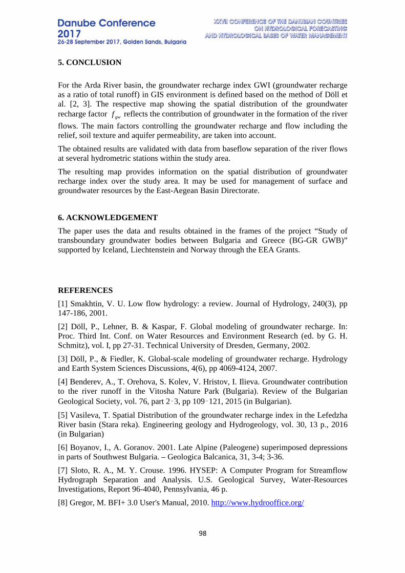
98

5. CONCLUSION For the Arda River basin, the groundwater recharge index GWI (groundwater recharge as a ratio of total runoff) in GIS environment is defined based on the method of Döll et al. [2, 3]. The respective map showing the spatial distribution of the groundwater recharge factor reflects the contribution of groundwater in the formation of the river flows. The main factors controlling the groundwater recharge and flow including the relief, soil texture and aquifer permeability, are taken into account. The obtained results are validated with data from baseflow separation of the river flows at several hydrometric stations within the study area. The resulting map provides information on the spatial distribution of groundwater recharge index over the study area. It may be used for management of surface and groundwater resources by the East-Aegean Basin Directorate.

6. ACKNOWLEDGEMENT The paper uses the data and results obtained in the frames of the project “Study of transboundary groundwater bodies between Bulgaria and Greece (BG-GR GWB)” supported by Iceland, Liechtenstein and Norway through the EEA Grants.

REFERENCES [1] Smakhtin, V. U. Low flow hydrology: a review. Journal of Hydrology, 240(3), pp 147-186, 2001. [2] Döll, P., Lehner, B. & Kaspar, F. Global modeling of groundwater recharge. In: Proc. Third Int. Conf. on Water Resources and Environment Research (ed. by G. H. Schmitz), vol. I, pp 27-31. Technical University of Dresden, Germany, 2002. [3] Döll, P., & Fiedler, K. Global-scale modeling of groundwater recharge. Hydrology and Earth System Sciences Discussions, 4(6), pp 4069-4124, 2007. [4] Benderev, A., T. Orehova, S. Kolev, V. Hristov, I. Ilieva. Groundwater contribution to the river runoff in the Vitosha Nature Park (Bulgaria). Review of the Bulgarian Geological Society, vol. 76, part 2–3, pp 109–121, 2015 (in Bulgarian).

[5] Vasileva, T. Spatial Distribution of the groundwater recharge index in the Lefedzha River basin (Stara reka). Engineering geology and Hydrogeology, vol. 30, 13 p., 2016 (in Bulgarian) [6] Boyanov, I., A. Goranov. 2001. Late Alpine (Paleogene) superimposed depressions in parts of Southwest Bulgaria. – Geologica Balcanica, 31, 3-4; 3-36. [7] Sloto, R. A., M. Y. Crouse. 1996. HYSEP: A Computer Program for Streamflow Hydrograph Separation and Analysis. U.S. Geological Survey, Water-Resources Investigations, Report 96-4040, Pennsylvania, 46 p. [8] Gregor, M. BFI+ 3.0 User's Manual, 2010. http://www.hydrooffice.org/

gwf

99

[9] Miller, M. P., Johnson, H. M., Susong, D. D., & Wolock, D. M. Journal of Hydrology, 522, pp 203-210, 2015. [10] Georgiev, B. Balance of soil resources and agricultural land in Bulgaria. Geography and Friends, Proceedings of the 60th Anniversary of Prof. Dr. Vesselin Boyadjiev and 35 years of teaching at Sofia University "St. Kliment Ohridski", ISBN 978-954-326-273-1. Paradigma Publishing House, pp 57-68, 2016 (in Bulgarian) [11] The Study on Integrated Water Management in the Republic of Bulgaria. Draft Final Report, 2009. JICA CTI Engineering International Co. Ltd. Manuscript. [12] Zyapkov, L. 1970. Altitude zones of the water balance types in Bulgaria. Bulletin of the Geographical Institute, vol. 13, pp 91-108, 1970 (in Bulgarian)

100

SPATIO-TEMPORAL FLUCTUATIONS OF MINIMUM FLOW IN THE DANUBE BASIN WITHIN UKRAINE

Gorbachova Liudmyla

Ukrainian Hydrometeorological Institute, Ukraine

Corresponding author: Ukrainian Hydrometeorological Institute, 37, Prospekt Nauki, Kyiv, Ukraine, 03028, e-mail: gorbachova@uhmi.org.ua

1 INTRODUCTION Minimum flow is one of the basic concepts that are used in hydrology for analysis and streamflow calculations. The minimum discharge is a major hydrological characteristic that is used to calculate of the design, construction and operation of hydraulic structures on rivers. Thus, the study of the current spatio-temporal fluctuations of the minimum flow of rivers is an actual task. In the world two methodological approaches to detect changes in the hydrological observation series: deterministic and statistical is wide using. Each approach reflects the idea about a flow formation mechanism. The deterministic approach is presented the graphic methods that mainly include various correlation graphs, frequency of values, histograms, mass curve, double mass curve, residual mass curve, chronological charts. Among them, vast majority of researchers is preferred the methods of mass curve, double mass curve, residual mass curve. Many scientists in their researches methodical approaches on using these methods were developed. Among them, the most contribution is created: Ріппл У., 1883; Merriam C.F., 1937; Searcy J.K. & Hardison C.H., 1960 et al. [1-3]. Nevertheless, the guidelines for these methods were developed separately for each method and for solving a particular problem. However, with certain graphic (hydro-genetic) methods can successfully carried out the assessing of the spatio-temporal fluctuations of runoff. Therefore, in this paper the methodological approaches for the hydro-genetic methods are used. This approach was developed by Gorbachova [4-6]. The goal of this paper is study of the spatio-temporal fluctuations of the averages 30 daily minimum discharges for summer, autumn and winter periods, and for the rivers with unstable freeze-up in the Danube basin within Ukraine based on using hydro-genetic methods. 2 DATA AND METHODOLOGY For mountain rivers Danube Basin within Ukraine the low water is observed for the winter period. During this period, the rivers have the groundwater feed. The low water for summer is much higher than winter because in summer often fall intense rains that cause rise in water levels, leading to interruption of low water. The basins rivers Uzh, Latoritsa and Borzhava are exceptions because these have the low water of summer is lower than the winter [7]. The rivers of the Danube basin within Ukraine belong to mountain streams with stable and unstable freeze-up. The study the long-term (since the beginning of the observations to 2010) of the averages 30 daily minimum discharges for summer, autumn and winter periods, and for the rivers with unstable freeze-up were

101

carried out for mountain rivers Danube Basin within Ukraine (34 gauging stations). At the 20 gauging stations carries out observations for the averages 30 daily minimum discharges of the summer, autumn and winter periods and at the 14 gauging stations carries out observations for the averages 30 daily minimum discharges for rivers with the unstable freeze-up. In this paper, the hydro-genetic methods of the assessing the homogeneity and stationarity of hydrological series were used. These methodological approaches on the principle "of simple to complex" based on the using of graphical (hydro-genetic) methods were developed. The main ones are the mass curve, the residual mass curve and the graphics combined. In 1883 W. Rippl developed methods mass curve and the residual mass curve [1]. Now the mass curve used to detect the influence of anthropogenic factors (hydraulic structures, canals) and of climate change (the presence of trends in the data series). If on the mass curve will not be found "jumping", "emissions" or unidirectional deviation, then the process the forming of the runoff in the study area is homogeneous, and conversely. The mass curve is defining with formula [1]:

, (1)

where W – the total runoff of river for period time Т;

w(t) – the runoff of t-th year. The analysis of the residual mass curve allows to define the stationarity of data series, namely the sustainability of the average value the hydrological characteristic in course of time. The average value of the time series is stable in the presence of at least one full closed cycle (dry and wet phase) of long-period fluctuations [8]. The residual mass curve is defining according to [1, 8]:

, (2)

where Cv – the variation coefficients of runoff;

k(t) = Q(t)/Q0 – the modulus coefficients; Q(t) and Q0 – the discharge of t-th year and the average discharge for the period of time T.

Combined graphs of characteristics allows defining synchrony/asynchrony of long-term fluctuations in different rivers within the one hydrological homogeneous area. In turn, the synchronous fluctuations indicate on the homogeneous climatic conditions of formation runoff.

)(1

∑==

T

t

twW

)()1)((

1 tfCv

tkT

t =∑ −=

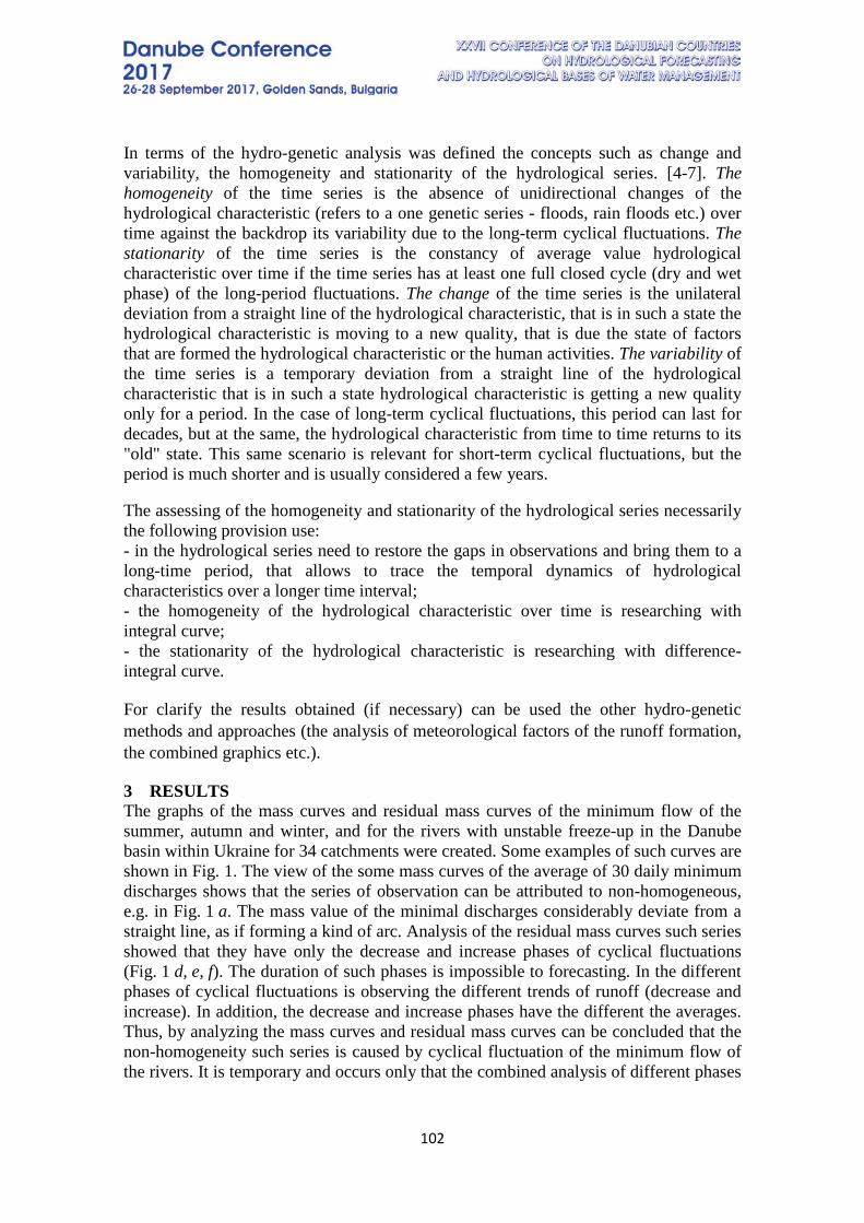
102

In terms of the hydro-genetic analysis was defined the concepts such as change and variability, the homogeneity and stationarity of the hydrological series. [4-7]. The homogeneity of the time series is the absence of unidirectional changes of the hydrological characteristic (refers to a one genetic series - floods, rain floods etc.) over time against the backdrop its variability due to the long-term cyclical fluctuations. The stationarity of the time series is the constancy of average value hydrological characteristic over time if the time series has at least one full closed cycle (dry and wet phase) of the long-period fluctuations. The change of the time series is the unilateral deviation from a straight line of the hydrological characteristic, that is in such a state the hydrological characteristic is moving to a new quality, that is due the state of factors that are formed the hydrological characteristic or the human activities. The variability of the time series is a temporary deviation from a straight line of the hydrological characteristic that is in such a state hydrological characteristic is getting a new quality only for a period. In the case of long-term cyclical fluctuations, this period can last for decades, but at the same, the hydrological characteristic from time to time returns to its "old" state. This same scenario is relevant for short-term cyclical fluctuations, but the period is much shorter and is usually considered a few years. The assessing of the homogeneity and stationarity of the hydrological series necessarily the following provision use: - in the hydrological series need to restore the gaps in observations and bring them to a long-time period, that allows to trace the temporal dynamics of hydrological characteristics over a longer time interval; - the homogeneity of the hydrological characteristic over time is researching with integral curve; - the stationarity of the hydrological characteristic is researching with difference-integral curve. For clarify the results obtained (if necessary) can be used the other hydro-genetic methods and approaches (the analysis of meteorological factors of the runoff formation, the combined graphics etc.). 3 RESULTS The graphs of the mass curves and residual mass curves of the minimum flow of the summer, autumn and winter, and for the rivers with unstable freeze-up in the Danube basin within Ukraine for 34 catchments were created. Some examples of such curves are shown in Fig. 1. The view of the some mass curves of the average of 30 daily minimum discharges shows that the series of observation can be attributed to non-homogeneous, e.g. in Fig. 1 a. The mass value of the minimal discharges considerably deviate from a straight line, as if forming a kind of arc. Analysis of the residual mass curves such series showed that they have only the decrease and increase phases of cyclical fluctuations (Fig. 1 d, e, f). The duration of such phases is impossible to forecasting. In the different phases of cyclical fluctuations is observing the different trends of runoff (decrease and increase). In addition, the decrease and increase phases have the different the averages. Thus, by analyzing the mass curves and residual mass curves can be concluded that the non-homogeneity such series is caused by cyclical fluctuation of the minimum flow of the rivers. It is temporary and occurs only that the combined analysis of different phases

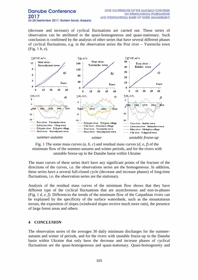
103

(decrease and increase) of cyclical fluctuations are carried out. These series of observation can be attributed to the quasi-homogeneous and quasi-stationary. Such conclusion is confirmed by the analysis of other series that have several different phases of cyclical fluctuations, e.g. in the observation series the Prut river – Yaremcha town (Fig. 1 b, e).

summer-autumn

winter

unstable freeze-up

Fig. 1 The some mass curves (a, b, c) and residual mass curves (d, e, f) of the minimum flow of the summer-autumn and winter periods, and for the rivers with

unstable freeze-up in the Danube basin within Ukraine

The mass curves of these series don't have any significant points of the fracture of the directions of the curves, i.e. the observations series are the homogeneous. In addition, these series have a several full-closed cycle (decrease and increase phases) of long-time fluctuations, i.e. the observation series are the stationary. Analysis of the residual mass curves of the minimum flow shows that they have different type of the cyclical fluctuations that are asynchronous and non-in-phases (Fig. 1 d, e, f). Differences the trends of the minimum flow of the Carpathian rivers can be explained by the specificity of the surface watersheds, such as the mountainous terrain, the exposition of slopes (windward slopes receive much more rain), the presence of large forest areas and others. 4 CONCLUSION The observation series of the averages 30 daily minimum discharges for the summer-autumn and winter of periods, and for the rivers with unstable freeze-up in the Danube basin within Ukraine that only have the decrease and increase phases of cyclical fluctuations are the quasi-homogeneous and quasi-stationary. Quasi-homogeneity and

104

quasi-stationary of the observation series is temporary and occurs only at the comparative analysis of increase and decrease phases of cyclical fluctuations. Series of observation that have several different phases of cyclical fluctuations are homogeneous and stationary. The observation series of the minimum flow in the Danube basin within Ukraine have different type of the cyclical fluctuations that are asynchronous and non-in-phases. It can be explained by features of the surface watershed and climatic factors in river basins that are manifested in the uneven distribution of rainfall, temperature and evaporation. 5 REFERENCES [1] Rippl W. The capacity of storage reservoirs for water supply, Proceedings of the Institute of Civil Engineers, vol. 71, pp 270-278, 1883. [2] Merriam C.F. A comprehensive study of the rainfall on the Susquehanna Valley, Transactions American Geophysical Union, vol. 18/2, pp 471-476, 1937. [3] Searcy J.K. & Hardison H.C. Double-mass curves. Manual of Hydrology: Part 1. General Surface-Water Techniques. Geological Survey Water-Supply Paper 1541-B, Washington: United States Government Printing Office, 36 p, 1960. [4] Gorbachova L. Methodical approaches the assessment of the homogeneity and stationarity of hydrological observation series, Hydrology, Hydrochemistry and Hydroecology, vol. 5 (32), pp 22-31, 2014. [In Ukrainian]. [5] Gorbachova L. & Khrystyuk B. Hydro-genetic methods of the analysis of the average annual runoff in the Danube basin, Proceeding XXVI conference of the Danubian countries on hydrological forecasting and hydrological bases of water management, Bridging the sciences – crossing borders, 22-24 September 2014, Deggendorf, Germany, pp 71-74, 2014. [6] Gorbachova L.O. Place and role of hydro-genetic analysis among modern research methods runoff, Proceedings of Ukrainian Hydrometeorological Institute, vol. 268, pp 73-81, 2015. [In Ukrainian]. [7] Gorbachova L.O. Modern the intra-annual streamflow distribution of Ukraine Rivers. Ukrainian Geographical Journal, vol. 3, pp 16-23, 2015. [In Ukrainian]. [8] Andreyanov V.G. Cyclical fluctuations of annual runoff and their account at hydrological calculations, Proceedings of State Hydrlogical Institute, vol. 68, pp 3-49, 1959. [In Russian].

105

HYDRO-GENETIC ANALYSIS OF THE LONG-TERM FLUCTUATIONS OF THE AVERAGE ANNUAL WATER TEMPERATURE IN THE SIVERSKYI

DONETS RIVER BASIN (WITHIN UKRAINE)

Tetiana Bauzha Ukrainian Hydrometeorological Institute, Ukraine

Corresponding author: Bauzha Tetiana, Ukrainian Hydrometeorological Institute, Nauki Prospect 37, 03028, Kyiv, Ukraine, bauzha@gmail.com

1. INTRODUCTION The thermal regime of rivers is one of the issues that have significant scientific and practical interest. According to the forecasts and researches of many scientists throughout this century will be and already occurring significant changes in water temperature of rivers due to global warming. So, fluctuations of water temperature usually corresponds the changes of air temperature in general. However, the uniqueness of relationship between air temperature and water temperature in rivers is disturbed local features that are characteristic the river as a whole or its individual parts. The most rivers of Siverskyi Donets River Basin have the significant effect of human activities (dumping into rivers industrial and domestic waste water, mine water, over-regulation of rivers by reservoirs and ponds) that in turn leads to changes in thermal regime. The goal of this paper is the estimation of the homogeneity of the long-term fluctuations of the average annual temperature water in the Siverskyi Donets River. It will allow to reveal possible changes and to analyze reasons for these changes.

2. MATERIAL AND METHODS Siverskyi Donets River is the largest river in eastern Ukraine and the largest tributary of the Don (Fig. 1). The total length of the river is 1053 km, and the area of its drainage basin is 98 900 km². Long-term average annual water discharge in gauging section Siverskyi Donets River – Kruzhylivka village is 137 m s-1 (1957-2010). The analysis of the average annual water temperature was carried out for the data 33 hydrological gauges of the Siverskyi Donets River Basin. The period of observation on these gauging stations is from 24 (Lopan River – Kozacha Lopan village) to 61 years (Vilkhova River – Luhansk town) (from the start of observations till 2013 inclusive). To analyze average annual temperature the data from 14 weather stations were used. To operate with the observational data one must adhere to the conditions of homogeneity and stationarity of the members of a statistical series [7]. In this paper the hydro-genetic analysis of homogeneity the average annual water temperature and air temperature was carried out. Methodological approaches to the assessment of the homogeneity and stationarity of hydrological series based on hydro-genetic methods (the mass curves, the difference integral curves, the combined chronological graphs) are used. This approach was developed by Gorbachova [1]. The mass curve is used to detect the influence of anthropogenic factors (hydraulic structures, canals) and of climate change (the presence of trends in the data series) [3].

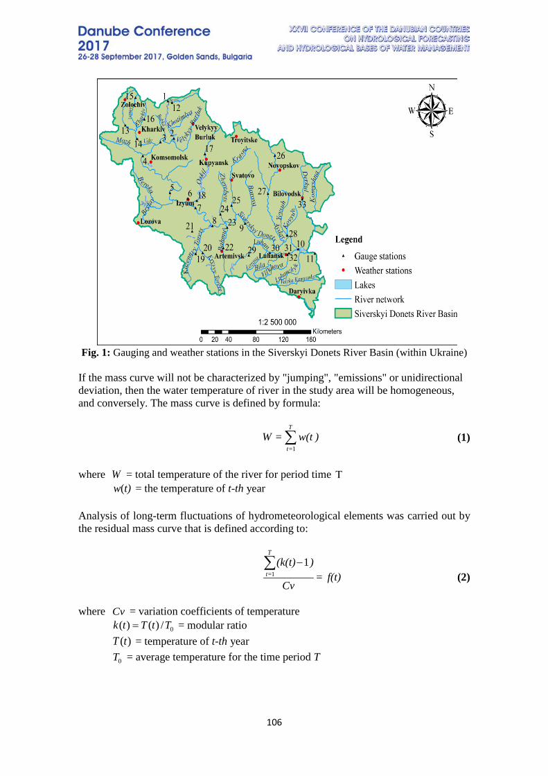
106

Fig. 1: Gauging and weather stations in the Siverskyi Donets River Basin (within Ukraine)

If the mass curve will not be characterized by "jumping", "emissions" or unidirectional deviation, then the water temperature of river in the study area will be homogeneous, and conversely. The mass curve is defined by formula:

(1)

where = total temperature of the river for period time

= the temperature of t-th year Analysis of long-term fluctuations of hydrometeorological elements was carried out by the residual mass curve that is defined according to:

(2)

where = variation coefficients of temperature

= modular ratio = temperature of t-th year

= average temperature for the time period T

)w(t=WT

=t∑

1

W Τt)w(

f(t)=Cv

)(k(t)T

t=∑ −

11

Cv0/)()( TtTtk =

)(tT0T

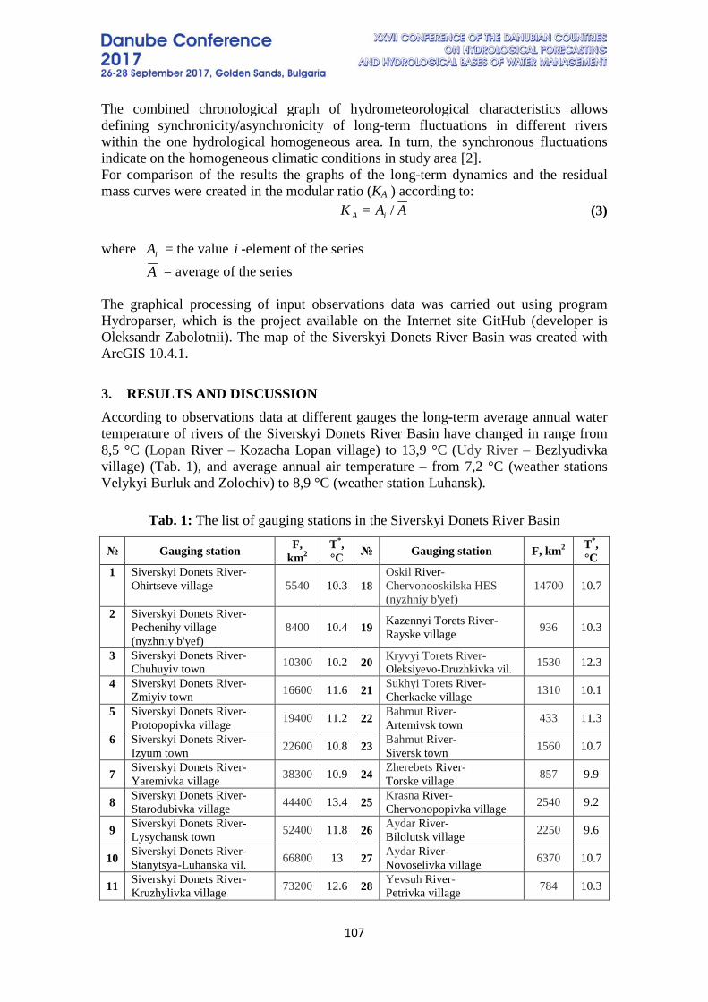
107

The combined chronological graph of hydrometeorological characteristics allows defining synchronicity/asynchronicity of long-term fluctuations in different rivers within the one hydrological homogeneous area. In turn, the synchronous fluctuations indicate on the homogeneous climatic conditions in study area [2]. For comparison of the results the graphs of the long-term dynamics and the residual mass curves were created in the modular ratio (KA ) according to:

(3)

where = the value -element of the series = average of the series

The graphical processing of input observations data was carried out using program Hydroparser, which is the project available on the Internet site GitHub (developer is Oleksandr Zabolotnii). The map of the Siverskyi Donets River Basin was created with ArcGIS 10.4.1.

3. RESULTS AND DISCUSSION According to observations data at different gauges the long-term average annual water temperature of rivers of the Siverskyi Donets River Basin have changed in range from 8,5 °C (Lopan River – Kozacha Lopan village) to 13,9 °C (Udy River – Bezlyudivka village) (Tab. 1), and average annual air temperature – from 7,2 °C (weather stations Velykyi Burluk and Zolochiv) to 8,9 °C (weather station Luhansk).

Tab. 1: The list of gauging stations in the Siverskyi Donets River Basin

№ Gauging station F, km2

T*, °C № Gauging station F, km2 T*,

°C 1 Siverskyi Donets River-

Ohirtseve village 5540 10.3 18 Oskil River-Chervonooskilska HES (nyzhniy b'yef)

14700 10.7

2 Siverskyi Donets River- Pechenihy village (nyzhniy b'yef)

8400 10.4 19 Kazennyi Torets River- Rayske village 936 10.3

3 Siverskyi Donets River- Chuhuyiv town 10300 10.2 20 Kryvyi Torets River-

Oleksiyevo-Druzhkivka vil. 1530 12.3

4 Siverskyi Donets River- Zmiyiv town 16600 11.6 21 Sukhyi Torets River-

Cherkacke village 1310 10.1

5 Siverskyi Donets River- Protopopivka village 19400 11.2 22 Bahmut River-

Artemivsk town 433 11.3

6 Siverskyi Donets River- Izyum town 22600 10.8 23 Bahmut River-

Siversk town 1560 10.7

7 Siverskyi Donets River- Yaremivka village 38300 10.9 24 Zherebets River-

Torske village 857 9.9

8 Siverskyi Donets River- Starodubivka village 44400 13.4 25 Krasna River-

Chervonopopivka village 2540 9.2

9 Siverskyi Donets River- Lysychansk town 52400 11.8 26 Aydar River-

Bilolutsk village 2250 9.6

10 Siverskyi Donets River- Stanytsya-Luhanska vil. 66800 13 27 Aydar River-

Novoselivka village 6370 10.7

11 Siverskyi Donets River- Kruzhylivka village 73200 12.6 28 Yevsuh River-

Petrivka village 784 10.3

AA=K iA /

iA iA

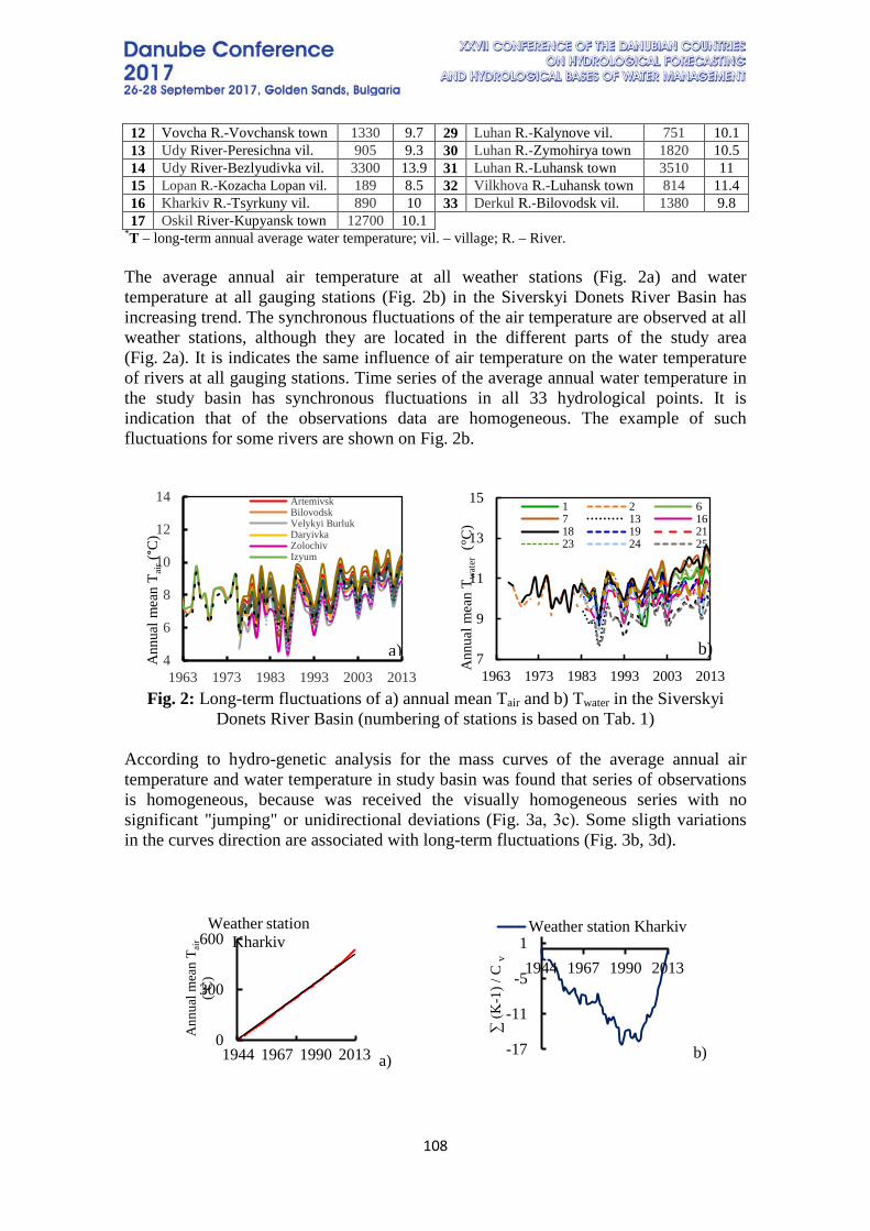
108

12 Vovcha R.-Vovchansk town 1330 9.7 29 Luhan R.-Kalynove vil. 751 10.1 13 Udy River-Peresichna vil. 905 9.3 30 Luhan R.-Zymohirya town 1820 10.5 14 Udy River-Bezlyudivka vil. 3300 13.9 31 Luhan R.-Luhansk town 3510 11 15 Lopan R.-Kozacha Lopan vil. 189 8.5 32 Vilkhova R.-Luhansk town 814 11.4 16 Kharkiv R.-Tsyrkuny vil. 890 10 33 Derkul R.-Bilovodsk vil. 1380 9.8 17 Oskil River-Kupyansk town 12700 10.1

*T – long-term annual average water temperature; vil. – village; R. – River. The average annual air temperature at all weather stations (Fig. 2a) and water temperature at all gauging stations (Fig. 2b) in the Siverskyi Donets River Basin has increasing trend. The synchronous fluctuations of the air temperature are observed at all weather stations, although they are located in the different parts of the study area (Fig. 2a). It is indicates the same influence of air temperature on the water temperature of rivers at all gauging stations. Time series of the average annual water temperature in the study basin has synchronous fluctuations in all 33 hydrological points. It is indication that of the observations data are homogeneous. The example of such fluctuations for some rivers are shown on Fig. 2b.

Fig. 2: Long-term fluctuations of a) annual mean Tair and b) Twater in the Siverskyi

Donets River Basin (numbering of stations is based on Tab. 1)

According to hydro-genetic analysis for the mass curves of the average annual air temperature and water temperature in study basin was found that series of observations is homogeneous, because was received the visually homogeneous series with no significant "jumping" or unidirectional deviations (Fig. 3a, 3с). Some sligth variations in the curves direction are associated with long-term fluctuations (Fig. 3b, 3d).

a) b)

4

6

8

10

12

14

1963 1973 1983 1993 2003 2013

Ann

ual m

ean

T air (

°C)

ArtemivskBilovodskVelykyi BurlukDaryivkaZolochivIzyum

a) 7

9

11

13

15

1963 1973 1983 1993 2003 2013

Ann

ual m

ean

T wat

er (

°C)

1 2 67 13 1618 19 2123 24 25

b)

0

300

600

1944 1967 1990 2013

Ann

ual m

ean

T air

(°C

)

Weather station Kharkiv

-17

-11

-5

11944 1967 1990 2013

∑ (K

-1) /

C v

Weather station Kharkiv

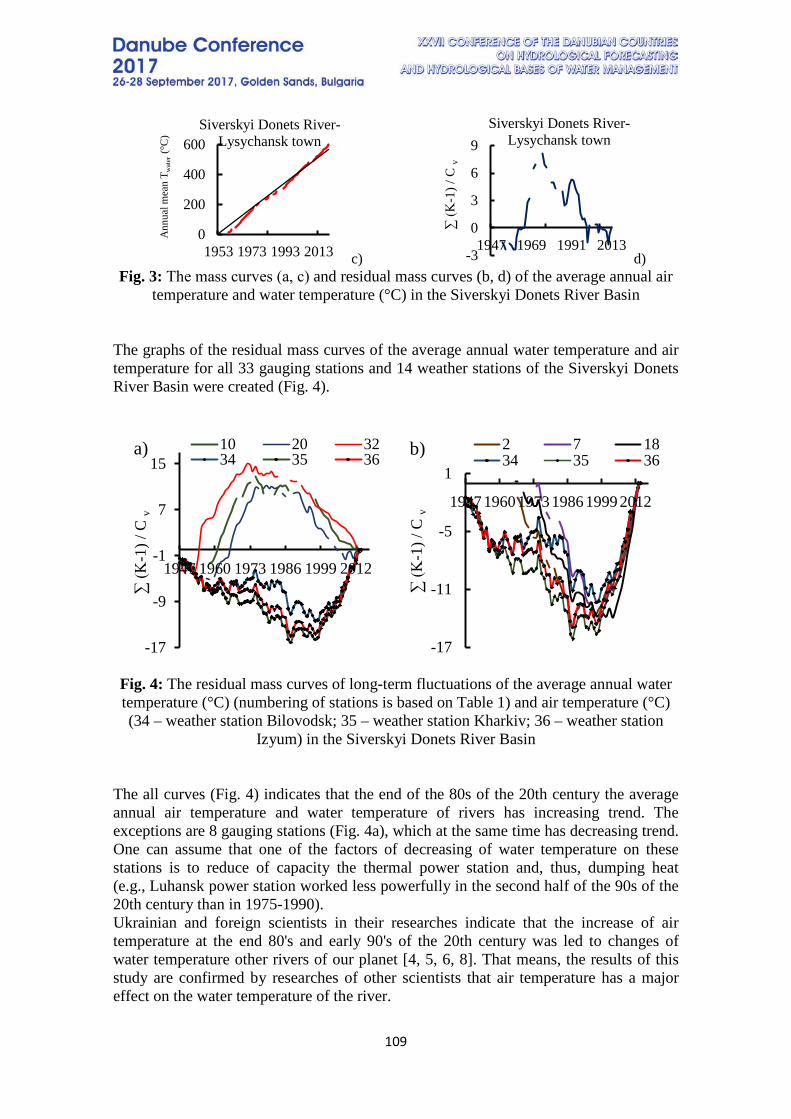
109

c) d)

Fig. 3: The mass curves (а, с) and residual mass curves (b, d) of the average annual air temperature and water temperature (°C) in the Siverskyi Donets River Basin

The graphs of the residual mass curves of the average annual water temperature and air temperature for all 33 gauging stations and 14 weather stations of the Siverskyi Donets River Basin were created (Fig. 4).

Fig. 4: The residual mass curves of long-term fluctuations of the average annual water temperature (°C) (numbering of stations is based on Table 1) and air temperature (°C) (34 – weather station Bilovodsk; 35 – weather station Kharkiv; 36 – weather station

Izyum) in the Siverskyi Donets River Basin The all curves (Fig. 4) indicates that the end of the 80s of the 20th century the average annual air temperature and water temperature of rivers has increasing trend. The exceptions are 8 gauging stations (Fig. 4a), which at the same time has decreasing trend. One can assume that one of the factors of decreasing of water temperature on these stations is to reduce of capacity the thermal power station and, thus, dumping heat (e.g., Luhansk power station worked less powerfully in the second half of the 90s of the 20th century than in 1975-1990). Ukrainian and foreign scientists in their researches indicate that the increase of air temperature at the end 80's and early 90's of the 20th century was led to changes of water temperature other rivers of our planet [4, 5, 6, 8]. That means, the results of this study are confirmed by researches of other scientists that air temperature has a major effect on the water temperature of the river.

0

200

400

600

1953 1973 1993 2013

Ann

ual m

ean

T wat

er (°

C)

Siverskyi Donets River-Lysychansk town

-3

0

3

6

9

1947 1969 1991 2013

∑ (K

-1) /

C v

Siverskyi Donets River-Lysychansk town

-17

-9

-1

7

15

1947 1960 1973 1986 1999 2012

10 20 3234 35 36

∑ (K

-1) /

C v

a)

-17

-11

-5

1

1947 1960 1973 1986 1999 2012

2 7 1834 35 36

∑ (K

-1) /

C v

b)

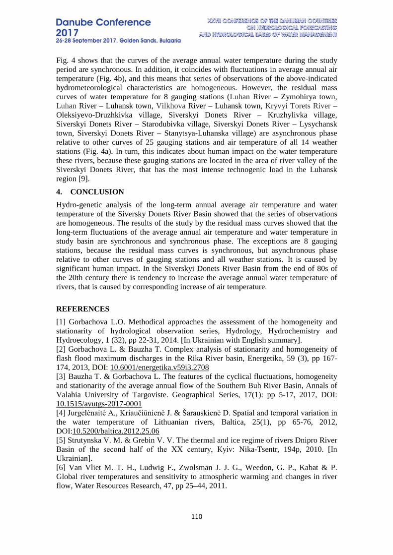
110

Fig. 4 shows that the curves of the average annual water temperature during the study period are synchronous. In addition, it coincides with fluctuations in average annual air temperature (Fig. 4b), and this means that series of observations of the above-indicated hydrometeorological characteristics are homogeneous. However, the residual mass curves of water temperature for 8 gauging stations (Luhan River – Zymohirya town, Luhan River – Luhansk town, Vilkhova River – Luhansk town, Kryvyi Torets River – Oleksiyevo-Druzhkivka village, Siverskyi Donets River – Kruzhylivka village, Siverskyi Donets River – Starodubivka village, Siverskyi Donets River – Lysychansk town, Siverskyi Donets River – Stanytsya-Luhanska village) are asynchronous phase relative to other curves of 25 gauging stations and air temperature of all 14 weather stations (Fig. 4a). In turn, this indicates about human impact on the water temperature these rivers, because these gauging stations are located in the area of river valley of the Siverskyi Donets River, that has the most intense technogenic load in the Luhansk region [9].

4. CONCLUSION Hydro-genetic analysis of the long-term annual average air temperature and water temperature of the Siversky Donets River Basin showed that the series of observations are homogeneous. The results of the study by the residual mass curves showed that the long-term fluctuations of the average annual air temperature and water temperature in study basin are synchronous and synchronous phase. The exceptions are 8 gauging stations, because the residual mass curves is synchronous, but asynchronous phase relative to other curves of gauging stations and all weather stations. It is caused by significant human impact. In the Siverskyi Donets River Basin from the end of 80s of the 20th century there is tendency to increase the average annual water temperature of rivers, that is caused by corresponding increase of air temperature. REFERENCES [1] Gorbachova L.O. Methodical approaches the assessment of the homogeneity and stationarity of hydrological observation series, Hydrology, Hydrochemistry and Hydroecology, 1 (32), pp 22-31, 2014. [In Ukrainian with English summary]. [2] Gorbachova L. & Bauzha T. Complex analysis of stationarity and homogeneity of flash flood maximum discharges in the Rika River basin, Energetika, 59 (3), pp 167-174, 2013, DOI: 10.6001/energetika.v59i3.2708 [3] Bauzha T. & Gorbachova L. The features of the cyclical fluctuations, homogeneity and stationarity of the average annual flow of the Southern Buh River Basin, Annals of Valahia University of Targoviste. Geographical Series, 17(1): pp 5-17, 2017, DOI: 10.1515/avutgs-2017-0001 [4] Jurgelėnaitė A., Kriaučiūnienė J. & Šarauskienė D. Spatial and temporal variation in the water temperature of Lithuanian rivers, Baltica, 25(1), pp 65-76, 2012, DOI:10.5200/baltica.2012.25.06 [5] Strutynska V. M. & Grebin V. V. The thermal and ice regime of rivers Dnipro River Basin of the second half of the XX century, Кyiv: Nika-Tsentr, 194p, 2010. [In Ukrainian]. [6] Van Vliet M. T. H., Ludwig F., Zwolsman J. J. G., Weedon, G. P., Kabat & P. Global river temperatures and sensitivity to atmospheric warming and changes in river flow, Water Resources Research, 47, pp 25–44, 2011.

111

[7] WMO, 2009, Guide to hydrological practices. Volume II: Management of water resources and application of hydrological practices, WMO No 168, Geneva, available at: http:// www.whycos.org/chy/guide/168_Vol_II_en.pdf (data access 06.05.2016). [8] Zhovnir V., Grebin’ V. & Rachmatullina E. The evaluation of homogeneity characteristics of water and air thermal regime within the Southern Bug Basin, Hydrology, Hydrochemistry and Hydroecology, 2(37), pp 86-93, 2015. [In Ukrainian with English summary]. [9] Zhyrnov P.V. Detailed description of Siverskyi Donets River’s pollution sources, Hydrology, Hydrochemistry and Hydroecology, 3 (34), pp 55-65, 2014. [In Ukrainian with English summary].

112

IDENTIFICATION OF CHANGES IN THE HYDROLOGICAL REGIME DUE

TO GABČÍKOVO WATER DAM OPERATION

Lotta Blaškovičová, Ján Gavurník, Martin Belan, Jana Poórová, Zuzana Paľušová Slovak Hydrometeorological Institute, Bratislava, Slovak Republic

Corresponding author: Lotta Blaškovičová, Slovak Hydrometeorological Institute, Jeséniova 17, 833 15 Bratislava, Slovak republic, email: lotta.blaskovicova@shmu.sk

ABSTRACT The Gabčíkovo Dam on Danube River was put into the operation in October 1992. The influence of the water reservoir has been observed mostly on the changes of water levels both on surface waters and groundwaters. The backwater influence on the Danube water levels has reached also the water-gauging station in Bratislava, which is the station with the longest data records among water-gauging stations in Slovakia. Due to the changes of flow velocities manifested into the changes of stage-discharge relations since then the discharge has started to be evaluated from the upper station in Bratislava-Devín. A main topic of this article is the comparison of two 10-year periods: 1979-1988 (before damming) and actual last evaluated 10-year period 2006-2015, in selected monitoring objects of surface waters and groundwater. The changes in discharges are manifested mostly in the part of old Danube channel between the Čunovo weir and Sap, as part of the discharge is flowing through the inlet channel to the hydropower plant. The hydraulic regime of the Danube River under Gabčíkovo (the outlet of the waste channel) is affected just slightly. More significant are the changes in water levels in Danube River channel upstream of the dam, and the changes of velocities, especially in the periods of low flows.

Monitoring of the groundwater levels have confirmed that increased groundwater levels occurred in the surroundings of Bratislava and in the upper part of the Žitný ostrov downstream up to Šamorín and the Little Danube. Decreases of ground water level were recorded in between the entrance into the bypass canal and mouthing of the tailrace canal into the Danube. Besides this, a reduction of amplitudes of ground water level fluctuation occurred along the Danube, Čunovo reservoir and bypass canal; an increase of amplitudes appeared along the tailrace canal and the Danube downstream up to Čičov. The recent general decrease of the ground water level is important in the upper part of the Žitný Ostrov Island, where the largest increases of ground water levels occurred immediately after putting the Gabčíkovo hydraulic structures in operations. Keywords: Gabčíkovo Water Dam, hydrological regime, Danube River This article freely follows the poster presented in 2006 in Belehrad [1], where the changes in Bratislava profile on Danube River under the Nový most (New Bridge) were evaluated for the 20-year period 1986-2005. The aim of this work was to use the results of surface water and groundwater quantity monitoring for the comparison and evaluation of possible changes in hydrological

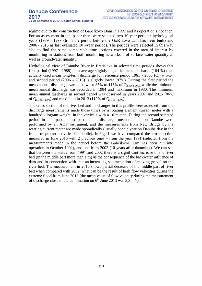
113

regime due to the construction of Gabčíkovo Dam in 1992 and its operation since then. For an assessment in this paper there were selected two 10-year periods: hydrological years (1979 - 1988 (from the period before the Gabčíkovo dam has been built) and 2006 - 2015 as last evaluated 10 –year period). The periods were selected in this way also to find the same comparable time sections covered in the area of interest by monitoring in stations from both monitoring networks – of surface water quantity as well as groundwater quantity. Hydrological view of Danube River in Bratislava in selected time periods shows that first period (1997 - 1988) is in average slightly higher in mean discharge (104 %) than actually used mean long-term discharge for reference period 1961 - 2000 (Qa,1961-2000) and second period (2006 - 2015) is slightly lower (97%). During the first period the mean annual discharges varied between 85% to 116% of Qa,1961-2000, while the minimum mean annual discharge was recorded in 1984 and maximum in 1980. The minimum mean annual discharge in second period was observed in years 2007 and 2015 (86% of Qa,1961-2000) and maximum in 2013 (119% of Qa,1961-2000). The cross section of the river bed and its changes in this profile were assessed from the discharge measurements made those times by a rotating element current meter with a hundred kilogram weight, in the verticals with a 10 m step. During the second selected period in this paper most part of the discharge measurements on Danube were performed by an ADP instrument, and the measurements from New Bridge by the rotating current meter are made sporadically (usually once a year on Danube day in the frame of promo activities for public). In Fig. 1 we have compared the cross section measured in June 2016 with 2 previous ones – from the year 1991 (selected from the measurements made in the period before the Gabčíkovo Dam has been put into operation in October 1992), and one from 2002 (10 years after damming). We can see that between the status from 1991 and 2002 there is a significant increase of the river bed (in the middle part more than 1 m) as the consequence of the backwater influence of dam and in connection with that an increasing sedimentation of moving gravel on the river bed. The measurement in 2016 shows partial decrease of the middle part of river bed when compared with 2002, what can be the result of high flow velocities during the extreme flood from June 2013 (the mean value of flow velocity during the measurement of discharge close to the culmination on 6th June 2013 was 3,3 m/s).

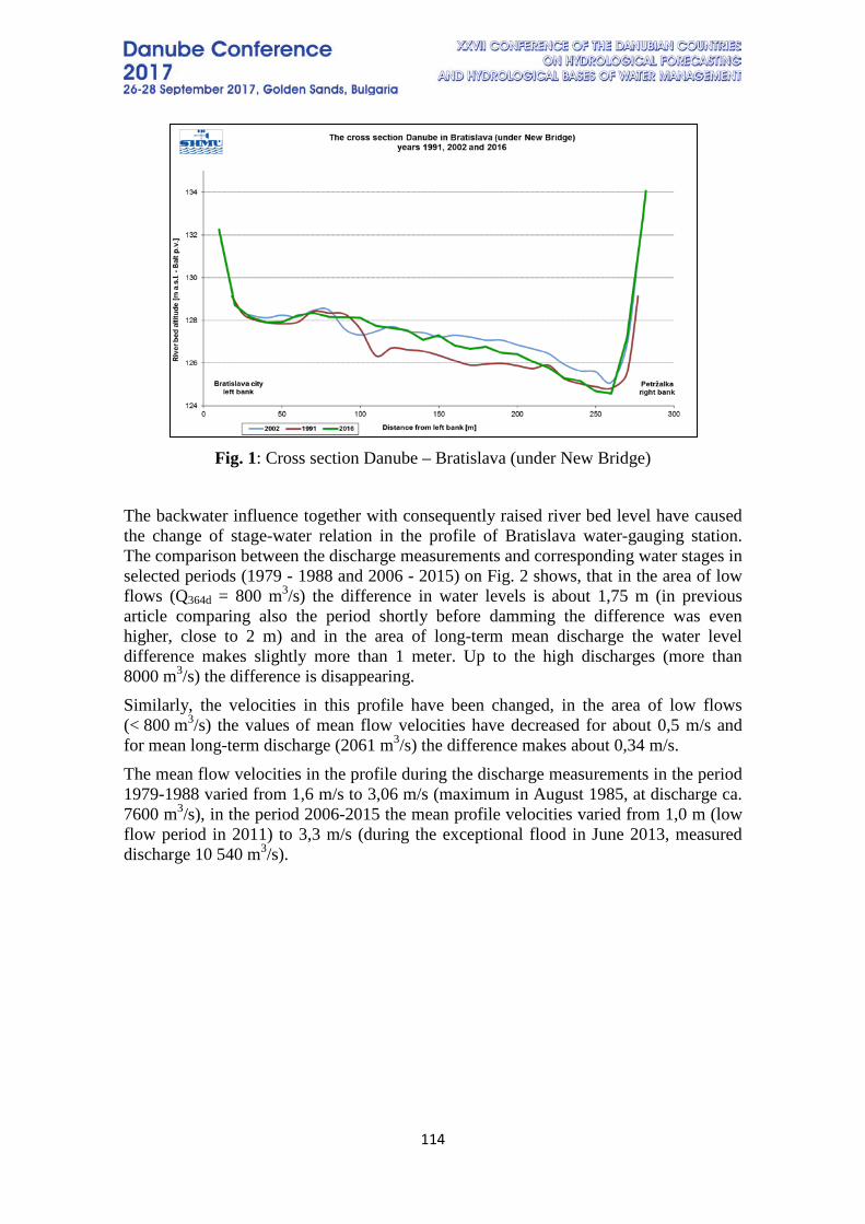
114

Fig. 1: Cross section Danube – Bratislava (under New Bridge)

The backwater influence together with consequently raised river bed level have caused the change of stage-water relation in the profile of Bratislava water-gauging station. The comparison between the discharge measurements and corresponding water stages in selected periods (1979 - 1988 and 2006 - 2015) on Fig. 2 shows, that in the area of low flows (Q364d = 800 m3/s) the difference in water levels is about 1,75 m (in previous article comparing also the period shortly before damming the difference was even higher, close to 2 m) and in the area of long-term mean discharge the water level difference makes slightly more than 1 meter. Up to the high discharges (more than 8000 m3/s) the difference is disappearing. Similarly, the velocities in this profile have been changed, in the area of low flows (< 800 m3/s) the values of mean flow velocities have decreased for about 0,5 m/s and for mean long-term discharge (2061 m3/s) the difference makes about 0,34 m/s. The mean flow velocities in the profile during the discharge measurements in the period 1979-1988 varied from 1,6 m/s to 3,06 m/s (maximum in August 1985, at discharge ca. 7600 m3/s), in the period 2006-2015 the mean profile velocities varied from 1,0 m (low flow period in 2011) to 3,3 m/s (during the exceptional flood in June 2013, measured discharge 10 540 m3/s).

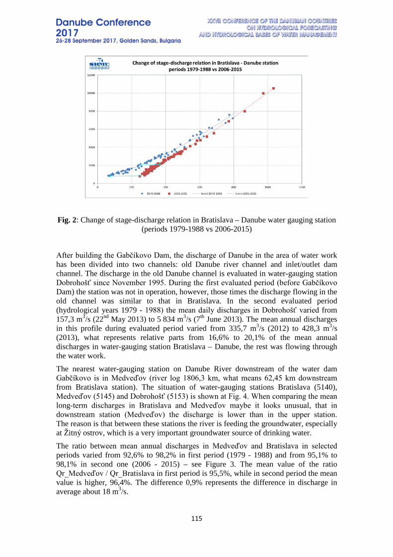
115

Fig. 2: Change of stage-discharge relation in Bratislava – Danube water gauging station

(periods 1979-1988 vs 2006-2015) After building the Gabčíkovo Dam, the discharge of Danube in the area of water work has been divided into two channels: old Danube river channel and inlet/outlet dam channel. The discharge in the old Danube channel is evaluated in water-gauging station Dobrohošť since November 1995. During the first evaluated period (before Gabčíkovo Dam) the station was not in operation, however, those times the discharge flowing in the old channel was similar to that in Bratislava. In the second evaluated period (hydrological years 1979 - 1988) the mean daily discharges in Dobrohošť varied from 157,3 m3/s (22nd May 2013) to 5 834 m3/s (7th June 2013). The mean annual discharges in this profile during evaluated period varied from 335,7 m3/s (2012) to 428,3 m3/s (2013), what represents relative parts from 16,6% to 20,1% of the mean annual discharges in water-gauging station Bratislava – Danube, the rest was flowing through the water work. The nearest water-gauging station on Danube River downstream of the water dam Gabčíkovo is in Medveďov (river log 1806,3 km, what means 62,45 km downstream from Bratislava station). The situation of water-gauging stations Bratislava (5140), Medveďov (5145) and Dobrohošť (5153) is shown at Fig. 4. When comparing the mean long-term discharges in Bratislava and Medveďov maybe it looks unusual, that in downstream station (Medveďov) the discharge is lower than in the upper station. The reason is that between these stations the river is feeding the groundwater, especially at Žitný ostrov, which is a very important groundwater source of drinking water. The ratio between mean annual discharges in Medveďov and Bratislava in selected periods varied from 92,6% to 98,2% in first period (1979 - 1988) and from 95,1% to 98,1% in second one (2006 - 2015) – see Figure 3. The mean value of the ratio Qr_Medveďov / Qr_Bratislava in first period is 95,5%, while in second period the mean value is higher, 96,4%. The difference 0,9% represents the difference in discharge in average about 18 m3/s.

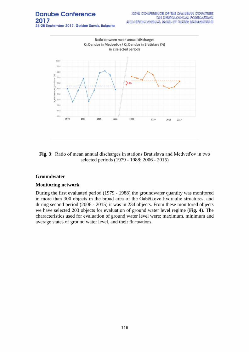
116

Fig. 3: Ratio of mean annual discharges in stations Bratislava and Medveďov in two selected periods (1979 - 1988; 2006 - 2015)

Groundwater Monitoring network During the first evaluated period (1979 - 1988) the groundwater quantity was monitored in more than 300 objects in the broad area of the Gabčíkovo hydraulic structures, and during second period (2006 - 2015) it was in 234 objects. From these monitored objects we have selected 203 objects for evaluation of ground water level regime (Fig. 4). The characteristics used for evaluation of ground water level were: maximum, minimum and average states of ground water level, and their fluctuations.

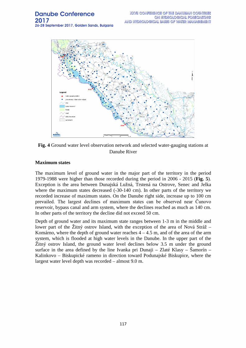
117

Fig. 4 Ground water level observation network and selected water-gauging stations at

Danube River

Maximum states

The maximum level of ground water in the major part of the territory in the period 1979-1988 were higher than those recorded during the period in 2006 - 2015 (Fig. 5). Exception is the area between Dunajská Lužná, Trstená na Ostrove, Senec and Jelka where the maximum states decreased (-30-140 cm). In other parts of the territory we recorded increase of maximum states. On the Danube right side, increase up to 100 cm prevailed. The largest declines of maximum states can be observed near Čunovo reservoir, bypass canal and arm system, where the declines reached as much as 140 cm. In other parts of the territory the decline did not exceed 50 cm. Depth of ground water and its maximum state ranges between 1-3 m in the middle and lower part of the Žitný ostrov Island, with the exception of the area of Nová Stráž – Komárno, where the depth of ground water reaches 4 – 4.5 m, and of the area of the arm system, which is flooded at high water levels in the Danube. In the upper part of the Žitný ostrov Island, the ground water level declines below 3.5 m under the ground surface in the area defined by the line Ivanka pri Dunaji – Zlaté Klasy – Šamorín – Kalinkovo – Biskupické rameno in direction toward Podunajské Biskupice, where the largest water level depth was recorded – almost 9.0 m.

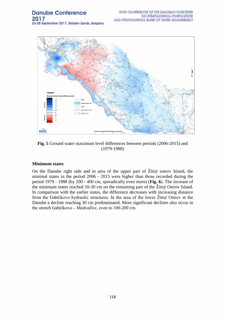
118

Fig. 5 Ground water maximum level differences between periods (2006-2015) and

(1979-1988)

Minimum states On the Danube right side and in area of the upper part of Žitný ostrov Island, the minimal states in the period 2006 - 2015 were higher than those recorded during the period 1979 - 1988 (by 200 - 400 cm, sporadically even more) (Fig. 6). The increase of the minimum states reached 10-30 cm on the remaining part of the Žitný Ostrov Island. In comparison with the earlier states, the difference decreases with increasing distance from the Gabčíkovo hydraulic structures. In the area of the lower Žitný Ostrov at the Danube a decline reaching 30 cm predominated. More significant declines also occur in the stretch Gabčíkovo – Medveďov, even to 100-200 cm.

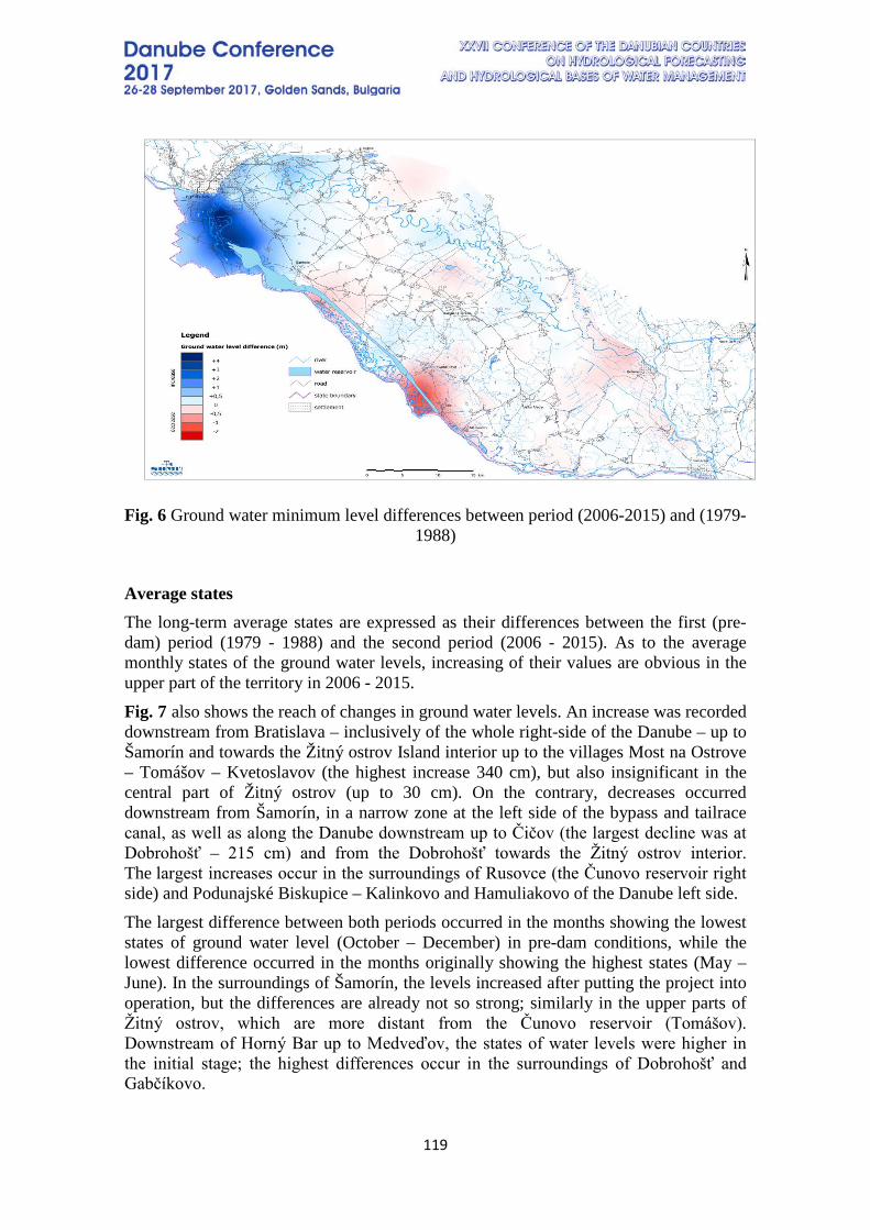
119

Fig. 6 Ground water minimum level differences between period (2006-2015) and (1979-

1988)

Average states The long-term average states are expressed as their differences between the first (pre-dam) period (1979 - 1988) and the second period (2006 - 2015). As to the average monthly states of the ground water levels, increasing of their values are obvious in the upper part of the territory in 2006 - 2015. Fig. 7 also shows the reach of changes in ground water levels. An increase was recorded downstream from Bratislava – inclusively of the whole right-side of the Danube – up to Šamorín and towards the Žitný ostrov Island interior up to the villages Most na Ostrove – Tomášov – Kvetoslavov (the highest increase 340 cm), but also insignificant in the central part of Žitný ostrov (up to 30 cm). On the contrary, decreases occurred downstream from Šamorín, in a narrow zone at the left side of the bypass and tailrace canal, as well as along the Danube downstream up to Čičov (the largest decline was at Dobrohošť – 215 cm) and from the Dobrohošť towards the Žitný ostrov interior. The largest increases occur in the surroundings of Rusovce (the Čunovo reservoir right side) and Podunajské Biskupice – Kalinkovo and Hamuliakovo of the Danube left side. The largest difference between both periods occurred in the months showing the lowest states of ground water level (October – December) in pre-dam conditions, while the lowest difference occurred in the months originally showing the highest states (May – June). In the surroundings of Šamorín, the levels increased after putting the project into operation, but the differences are already not so strong; similarly in the upper parts of Žitný ostrov, which are more distant from the Čunovo reservoir (Tomášov). Downstream of Horný Bar up to Medveďov, the states of water levels were higher in the initial stage; the highest differences occur in the surroundings of Dobrohošť and Gabčíkovo.

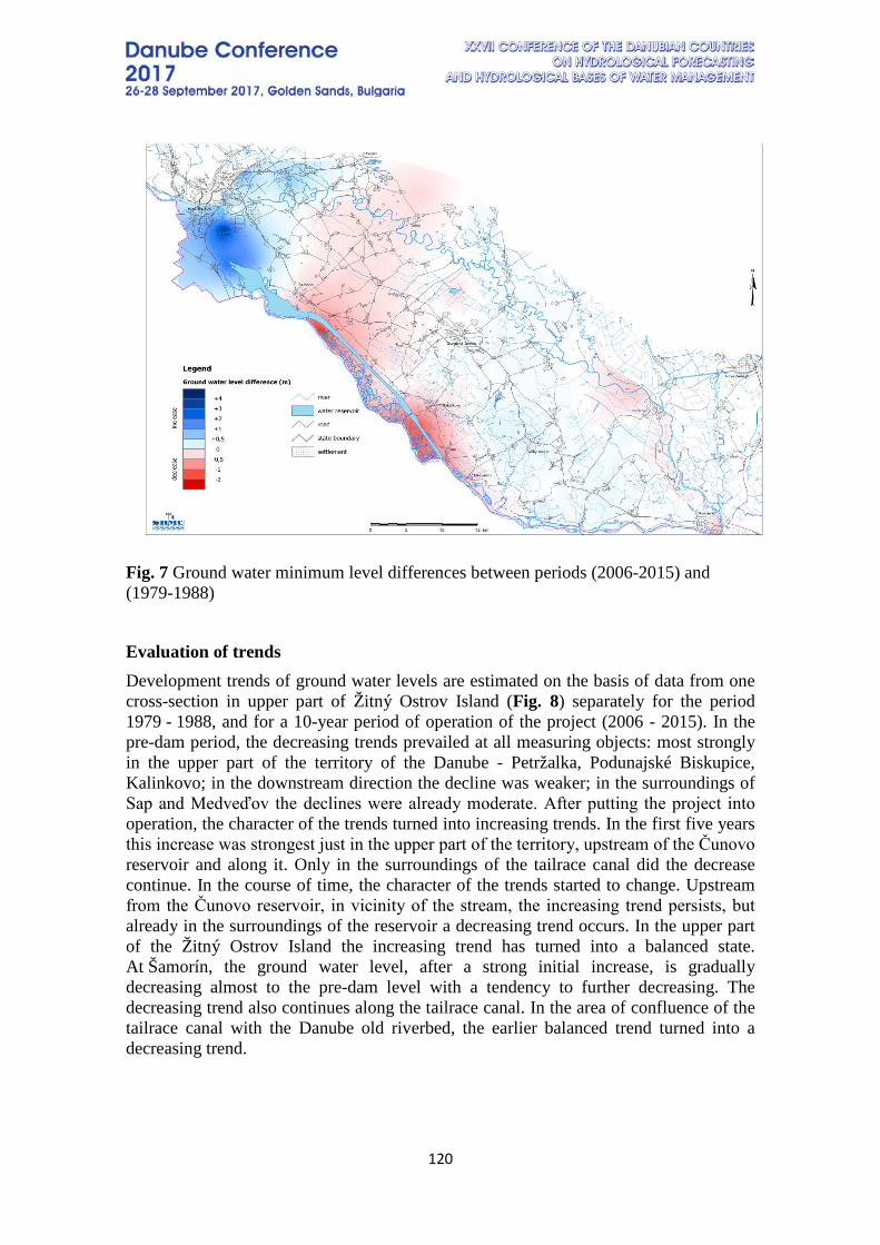
120

Fig. 7 Ground water minimum level differences between periods (2006-2015) and (1979-1988)

Evaluation of trends Development trends of ground water levels are estimated on the basis of data from one cross-section in upper part of Žitný Ostrov Island (Fig. 8) separately for the period 1979 - 1988, and for a 10-year period of operation of the project (2006 - 2015). In the pre-dam period, the decreasing trends prevailed at all measuring objects: most strongly in the upper part of the territory of the Danube - Petržalka, Podunajské Biskupice, Kalinkovo; in the downstream direction the decline was weaker; in the surroundings of Sap and Medveďov the declines were already moderate. After putting the project into operation, the character of the trends turned into increasing trends. In the first five years this increase was strongest just in the upper part of the territory, upstream of the Čunovo reservoir and along it. Only in the surroundings of the tailrace canal did the decrease continue. In the course of time, the character of the trends started to change. Upstream from the Čunovo reservoir, in vicinity of the stream, the increasing trend persists, but already in the surroundings of the reservoir a decreasing trend occurs. In the upper part of the Žitný Ostrov Island the increasing trend has turned into a balanced state. At Šamorín, the ground water level, after a strong initial increase, is gradually decreasing almost to the pre-dam level with a tendency to further decreasing. The decreasing trend also continues along the tailrace canal. In the area of confluence of the tailrace canal with the Danube old riverbed, the earlier balanced trend turned into a decreasing trend.

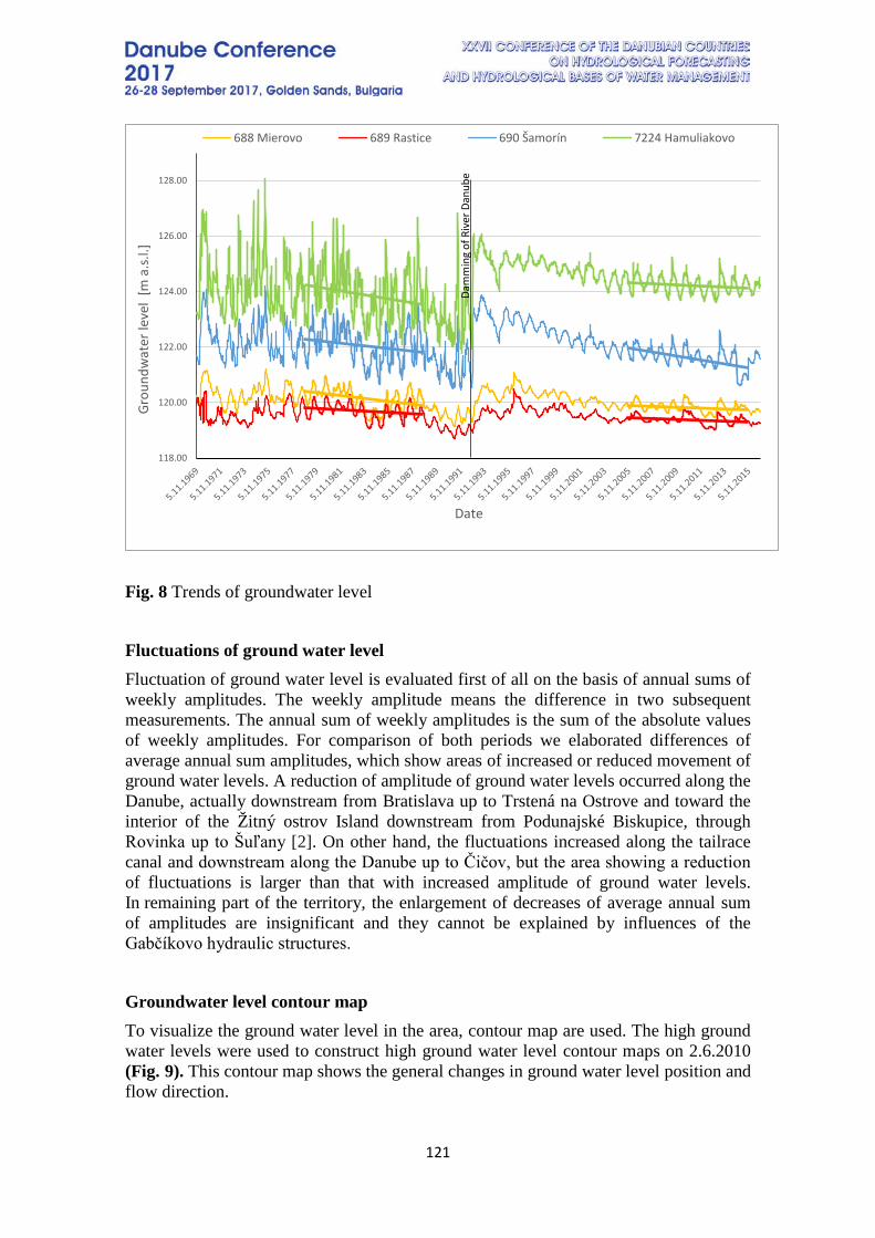
121

Fig. 8 Trends of groundwater level

Fluctuations of ground water level Fluctuation of ground water level is evaluated first of all on the basis of annual sums of weekly amplitudes. The weekly amplitude means the difference in two subsequent measurements. The annual sum of weekly amplitudes is the sum of the absolute values of weekly amplitudes. For comparison of both periods we elaborated differences of average annual sum amplitudes, which show areas of increased or reduced movement of ground water levels. A reduction of amplitude of ground water levels occurred along the Danube, actually downstream from Bratislava up to Trstená na Ostrove and toward the interior of the Žitný ostrov Island downstream from Podunajské Biskupice, through Rovinka up to Šuľany [2]. On other hand, the fluctuations increased along the tailrace canal and downstream along the Danube up to Čičov, but the area showing a reduction of fluctuations is larger than that with increased amplitude of ground water levels. In remaining part of the territory, the enlargement of decreases of average annual sum of amplitudes are insignificant and they cannot be explained by influences of the Gabčíkovo hydraulic structures.

Groundwater level contour map To visualize the ground water level in the area, contour map are used. The high ground water levels were used to construct high ground water level contour maps on 2.6.2010 (Fig. 9). This contour map shows the general changes in ground water level position and flow direction.

118.00

120.00

122.00

124.00

126.00

128.00

Grou

ndw

ater

leve

l [m

a.s

.l.]

688 Mierovo 689 Rastice 690 Šamorín 7224 Hamuliakovo

Date

Dam

min

g of

Riv

er D

anub

e

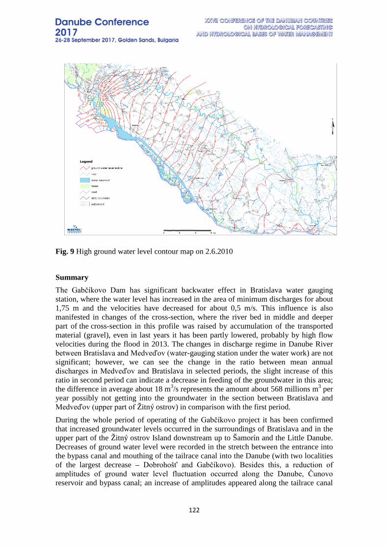
122

Fig. 9 High ground water level contour map on 2.6.2010

Summary The Gabčíkovo Dam has significant backwater effect in Bratislava water gauging station, where the water level has increased in the area of minimum discharges for about 1,75 m and the velocities have decreased for about 0,5 m/s. This influence is also manifested in changes of the cross-section, where the river bed in middle and deeper part of the cross-section in this profile was raised by accumulation of the transported material (gravel), even in last years it has been partly lowered, probably by high flow velocities during the flood in 2013. The changes in discharge regime in Danube River between Bratislava and Medveďov (water-gauging station under the water work) are not significant; however, we can see the change in the ratio between mean annual discharges in Medveďov and Bratislava in selected periods, the slight increase of this ratio in second period can indicate a decrease in feeding of the groundwater in this area; the difference in average about 18 m3/s represents the amount about 568 millions m3 per year possibly not getting into the groundwater in the section between Bratislava and Medveďov (upper part of Žitný ostrov) in comparison with the first period. During the whole period of operating of the Gabčíkovo project it has been confirmed that increased groundwater levels occurred in the surroundings of Bratislava and in the upper part of the Žitný ostrov Island downstream up to Šamorín and the Little Danube. Decreases of ground water level were recorded in the stretch between the entrance into the bypass canal and mouthing of the tailrace canal into the Danube (with two localities of the largest decrease – Dobrohošť and Gabčíkovo). Besides this, a reduction of amplitudes of ground water level fluctuation occurred along the Danube, Čunovo reservoir and bypass canal; an increase of amplitudes appeared along the tailrace canal

123

and the Danube downstream up to Čičov. The recent general decrease of the ground water level is especially important in the upper part of the Žitný Ostrov Island (surrounding of Šamorín), where the largest increases of ground water levels occurred immediately after putting the Gabčíkovo hydraulic structures in operations. These findings are consistent with the evaluation of changed ratio between the Danube dicharges in Bratislava and Medveďov mentioned in previous paragraph.

References [1] Blaškovičová, L. – Martinka, M. – Poórová, J.: „Changes of river cross-sections on Slovak part of Danube in the period 1986-2005“, poster, XXIII Conference of the Danubian countries on the hydrological forecasting and hydrological bases of water management, Belehrad, Srbsko, 2006. [2] Chalupka, J. – Paľušová, Z.: Monitorovanie hydrologického režimu podzemných vôd v oblasti Vodného diela Gabčíkovo, Ročná správa za rok 2002, SHMÚ Bratislava, 2003.

124

THE UNCERTAINTY INTERVAL OF THE MAXIMUM DISCHARGES WITH HIGH RETURN PERIOD

Radu Drobot, Aurelian Florentin Draghia, Romică Trandafir, Daniel Ciuiu

Technical University of Civil Engineering Bucharest, Romania Corresponding author: Radu Drobot, Technical University of Civil Engineering Bucharest,

Bd. Lacul Tei 122-124, 020396 Sector 2, Bucharest, drobot@utcb.ro

ABSTRACT In the present paper an analysis of the interval of uncertainty of the maximum discharges is presented. The analysis was made based on two different approaches: a) considering a single distribution for different volumes of the sample data; b) considering a set of statistical distributions for the same volume of registered data. In both cases, statistical tests were used to select the most adequate distribution(s). A set of 78 values of maximum annual discharges at Turnu Magurele on the Danube River represented the partial time series. In the first case, the log-Pearson 3 distribution was selected and the statistical processing was made both on the basic data and on a set of 1000 generated discharges, by extending progressively the length of the string data. In the second case, a number of 50-60 distributions were analysed and finally 8-10 distributions were selected as appropriate for the initial set of data. In both cases, the maximum discharges cover a significant interval of uncertainty, raising practical issues for the design and operation of the hydraulic structures. Keywords: Danube River, statistical distributions, uncertainty interval.

1. INTRODUCTION The maximum annual discharges during the flood period are variable from one year to another. The main objective of the Flood Frequency Analysis is to derive robust estimates of percentiles P% in the domain of frequent (10-20%), medium (1%) and low (0.1%) probabilities of exceedance. Different statistical distributions can be selected for fitting the empirical distributions [1], [2], [3]. Malamud and Turcotte (2006), cited in [4] showed that, the most commonly used distributions in hydrology can be divided into four groups: the normal family (normal, Lognormal), the general extreme value family (GEV, Gumbel, Fréchet, reverse Weibull), the Pearson type 3 family (Gamma, Pearson type 3, Log-Pearson type 3), and the Generalized Pareto distribution. In practice, all these models are fitted to data and compared using conventional goodness-of-fit tests. Based on empirical comparisons each country choose to fit the annual peak discharges by a certain statistical distribution. Thus, comparing the Lognormal, Gamma, Gumbel, Log-Gumbel, Hazen, and Log-Pearson type 3 distributions, the USA adopted for flood frequency estimation the Log-Pearson type 3 (LP3) distribution, Australia has also adopted the LP3 distribution, the United Kingdom preferred the Generalized Logistic distribution, while China uses the Lognormal (LN) distribution [4]. In many East European countries, Pearson type 3 distribution is mostly used in statistical processing of the peak discharges.

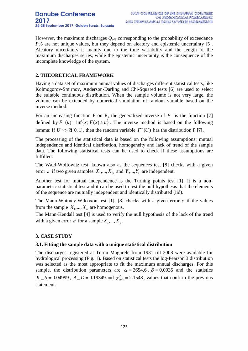
125

However, the maximum discharges Qp% corresponding to the probability of exceedance P% are not unique values, but they depend on aleatory and epistemic uncertainty [5]. Aleatory uncertainty is mainly due to the time variability and the length of the maximum discharges series, while the epistemic uncertainty is the consequence of the incomplete knowledge of the system.

2. THEORETICAL FRAMEWORK Having a data set of maximum annual values of discharges different statistical tests, like Kolmogorov-Smirnov, Anderson-Darling and Chi-Squared tests [6] are used to select the suitable continuous distribution. When the sample volume is not very large, the volume can be extended by numerical simulation of random variable based on the inverse method.

For an increasing function F on R, the generalized inverse of −F is the function [7] defined by { }uxFxuF ≥=− )(;inf)( . The inverse method is based on the following lemma: If ]1,0[~ U>U , then the random variable )(UF − has the distribution F [7].

The processing of the statistical data is based on the following assumptions: mutual independence and identical distribution, homogeneity and lack of trend of the sample data. The following statistical tests can be used to check if these assumptions are fulfilled: The Wald-Wolfowitz test, known also as the sequences test [8] checks with a given error ε if two given samples mXX ,...,1 and nYY ,...,1 are independent.

Another test for mutual independence is the Turning points test [1]. It is a non-parametric statistical test and it can be used to test the null hypothesis that the elements of the sequence are mutually independent and identically distributed (iid).

The Mann-Whitney-Wilcoxon test [1], [8] checks with a given error ε if the values from the sample nXX ,...,1 are homogenous. The Mann-Kendall test [4] is used to verify the null hypothesis of the lack of the trend with a given error ε for a sample nXX ,...,1 .

3. CASE STUDY 3.1. Fitting the sample data with a unique statistical distribution The discharges registered at Turnu Magurele from 1931 till 2008 were available for hydrological processing (Fig. 1). Based on statistical tests the log-Pearson 3 distribution was selected as the most appropriate to fit the maximum annual discharges. For this sample, the distribution parameters are 0035.0,6.2654 == βα and the statistics

04999.0_ =SK , 19349.0_ =DA and 1548.22 =calcc , values that confirm the previous statement.

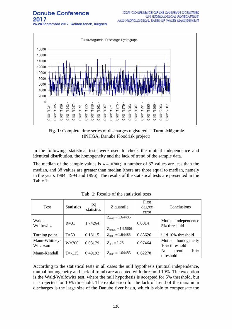
126

Fig. 1: Complete time series of discharges registered at Turnu-Măgurele

(INHGA, Danube Floodrisk project) In the following, statistical tests were used to check the mutual independence and identical distribution, the homogeneity and the lack of trend of the sample data.

The median of the sample values is 10700=µ ; a number of 37 values are less than the median, and 38 values are greater than median (there are three equal to median, namely in the years 1984, 1994 and 1996). The results of the statistical tests are presented in the Table 1:

Tab. 1: Results of the statistical tests

Test Statistics |Z| statistics Z quantile

First degree error

Conclusions

Wald- Wolfowitz R=31 1.74264

64485.105.0 =Z

95996.1025.0 =Z 0.0814 Mutual independence

5% threshold

Turning point T=50 0.18115 64485.105.0 =Z 0.85626 i.i.d 10% threshold Mann-Whitney-Wilcoxon W=700 0.03179 28.11.0 =Z 0.97464 Mutual homogeneity

10% threshold

Mann-Kendall T=-115 0.49192 64485.105.0 =Z 0.62278 No trend 10% threshold

According to the statistical tests in all cases the null hypothesis (mutual independence, mutual homogeneity and lack of trend) are accepted with threshold 10%. The exception is the Wald-Wolfowitz test, where the null hypothesis is accepted for 5% threshold, but it is rejected for 10% threshold. The explanation for the lack of trend of the maximum discharges is the large size of the Danube river basin, which is able to compensate the

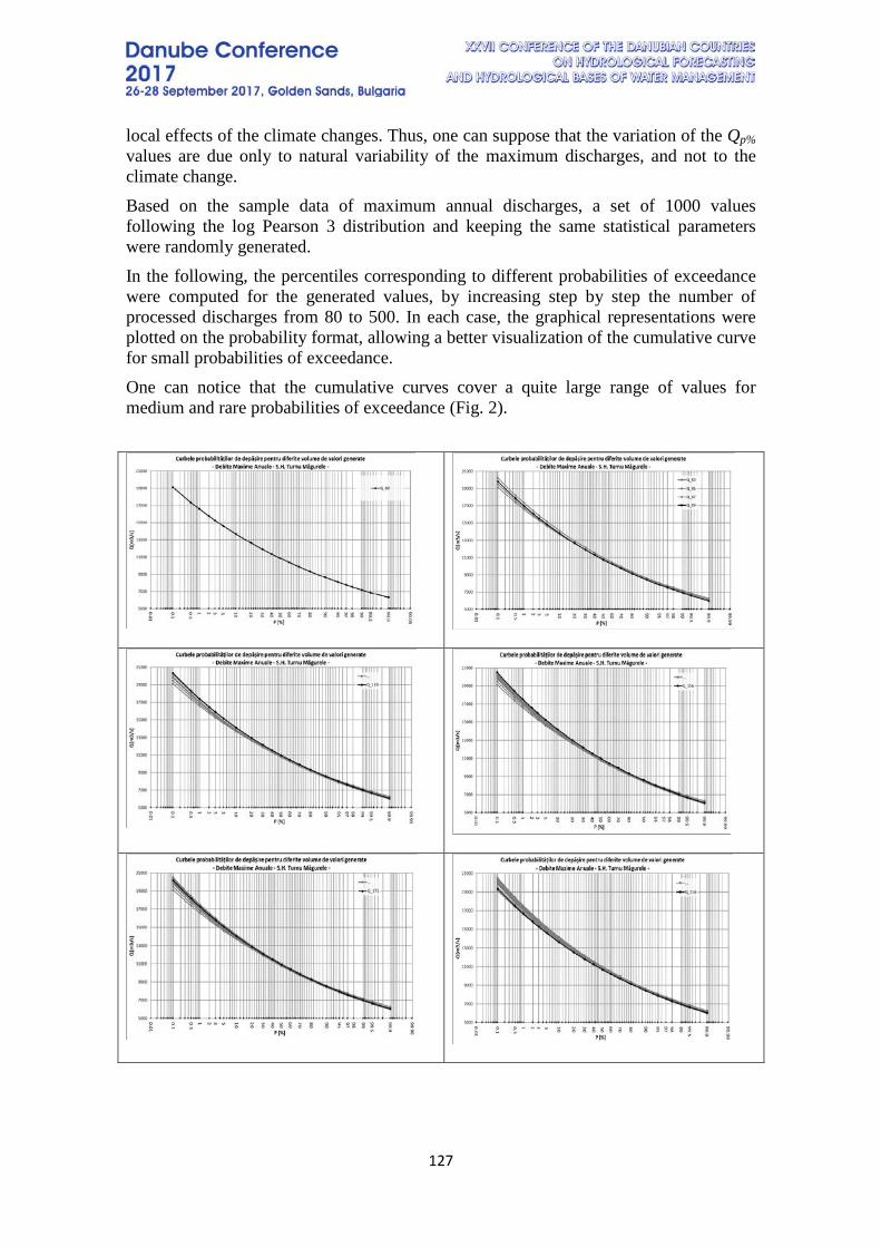
127

local effects of the climate changes. Thus, one can suppose that the variation of the Qp% values are due only to natural variability of the maximum discharges, and not to the climate change. Based on the sample data of maximum annual discharges, a set of 1000 values following the log Pearson 3 distribution and keeping the same statistical parameters were randomly generated. In the following, the percentiles corresponding to different probabilities of exceedance were computed for the generated values, by increasing step by step the number of processed discharges from 80 to 500. In each case, the graphical representations were plotted on the probability format, allowing a better visualization of the cumulative curve for small probabilities of exceedance. One can notice that the cumulative curves cover a quite large range of values for medium and rare probabilities of exceedance (Fig. 2).

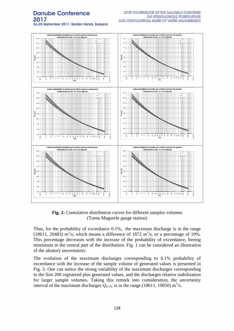
128

Fig. 2: Cumulative distribution curves for different samples volumes (Turnu Magurele gauge station)

Thus, for the probability of exceedance 0.1%, the maximum discharge is in the range (18611, 20483) m3/s, which means a difference of 1872 m3/s, or a percentage of 10%. This percentage decreases with the increase of the probability of exceedance, beeing mimimum in the central part of the distribution. Fig. 1 can be considered an illustration of the aleatory uncerntainty. The evolution of the maximum discharges corresponding to 0.1% probability of exceedance with the increase of the sample volume of generated values is presented in Fig. 3. One can notice the strong variability of the maximum discharges corresponding to the first 200 registered plus generated values, and the discharges relative stabilization for larger sample volumes. Taking this remark into consideration, the uncertainty interval of the maximum discharges Q0.1% is in the range (18611, 19050) m3/s.

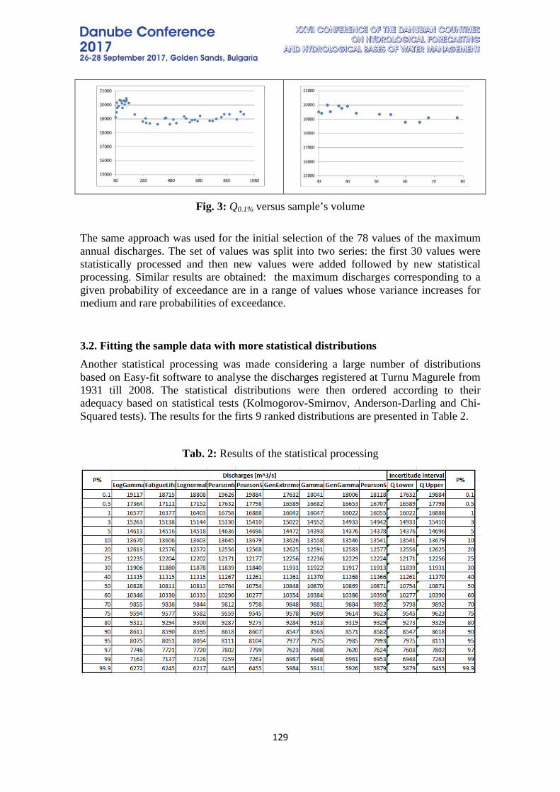
129

Fig. 3: Q0.1% versus sample’s volume

The same approach was used for the initial selection of the 78 values of the maximum annual discharges. The set of values was split into two series: the first 30 values were statistically processed and then new values were added followed by new statistical processing. Similar results are obtained: the maximum discharges corresponding to a given probability of exceedance are in a range of values whose variance increases for medium and rare probabilities of exceedance. 3.2. Fitting the sample data with more statistical distributions Another statistical processing was made considering a large number of distributions based on Easy-fit software to analyse the discharges registered at Turnu Magurele from 1931 till 2008. The statistical distributions were then ordered according to their adequacy based on statistical tests (Kolmogorov-Smirnov, Anderson-Darling and Chi-Squared tests). The results for the firts 9 ranked distributions are presented in Table 2.

Tab. 2: Results of the statistical processing

130

Some graphs putting into evidence the adequacy of the selected distributions are presented in Fig. 4.

Fig. 4: Adequacy of the selected distributions

For two probabilities of exceedance (1% ans 0,1%) the hystogram showing the distribution of the computed values for 30 distributions is presented (Fig. 5).

Fig. 5: Histogram of the maximum discharges - return periods of 100 and 1000 years On 23-24 of April, 2006 a maximum discharge of 16300 m3/s was registered at Turnu-Măgurele gauge station. This value is located in the central part of the hystogram

131

corrresponding to 1% probability of exceedance (Fig. 5) and can be considered the discharge Q1% .

4. CONCLUSIONS The maximum discharges corresponding to a given probability of exceedance are not unique values as normally considered in the current practice, but they belong to an interval of uncertainty. This interval can be put into evidence either by using a single suitable distribution or by analyzing more statistical distributions, the selection being based on Kolmogorov-Smirnov, Anderson-Darling and Chi-Squared tests. In the first case, the aleatory uncertainty is highlighted by analyzing time series of different lengths of the registered or generated maximum discharges. It was shown that for the same value of P%, the values Qp% increase during very wet periods, while after a dry period the same characteristics decrease. For the case study these fluctuations can reach 10% for 1000 years return period and 8% for 100 years return period respectively. In the second case the epistemic uncertainty is put into evidence by analysing 50-60 statistical distributions and selecting the first 8-10 ranked according to one of the statistical tests to fit the registered discharges. The interval of uncertainty is the consequence of the normal climate variability and the climate change. For safety reasons, in the design of the hydraulic structures or in updating studies of risk evaluation is recommended to consider the upper bound or at the limit the median value of the uncertainty interval.

5. REFERENCES [1] Bobée B., Cavadias G., Ashkar F., Bernier J. & Rasmussen P. Towards a systematic approach to comparing distributions used in flood frequency analysis. Journal of Hydrology, vol. 142, issues 1–4, pp 121–136, 1993 [2] Koutsoyiannis, D. Uncertainty, entropy, scaling and hydrological statistics. Hydrological Sciences Journal, 50, 3, p. 404, 2005 [3] Maidment D.R. Handbook of Hydrology. Ch. 18. Frequency analysis of extreme events, McGraw-Hill, 18.12-18.13. 1992 [4] El Adlouni S., Bobée, B. & Ouarda T.B.M.J. On the tails of extreme event distributions in hydrology. Journal of Hydrology. vol. 355, issues 1–4, pp 16–33, 2008 [5] Merz B., Thieken A.H. Flood risk curves and uncertainty bounds. Natural Hazards, vol. 51, issue, 3, pp. 437-458, 2009. [6] Ang A. H-S. & Tang W. H. Probability Concepts in Engineering, Emphasis on Application to Civil and Environmental Engineering, John Wiley & Sons, 2007 [7] Robert C. P. & Casella G. Monte Carlo Statistical Methods, Springer Texts in Statistics, New York, Springer-Verlag, 1999 [8] Brockwell P.J. & Davis R.A. Springer Texts in Statistics, Introduction to Time Series and Forecasting, Springer-Verlag, 2002

132

A DESIGN FLOOD ESTIMATION AT THE HYDROLOGICAL GAUGING STATIONS – WHAT THAT COULD BE?

Stevan Prohaska1, Aleksandra Ilić2

1 Jaroslav Černi Institute for the Development of Water Resources, Belgrade, Serbia 2 University of Niš, Faculty of Civil Engineering and Architecture, Serbia

Corresponding author: Stevan Prohaska, Jaroslav Černi Institute for the Development of Water Resources, Jaroslava Černog St. No. 80, 11000 Belgrade, Serbia, email: stevan.prohaska@jcerni.co.rs

ABSTRACT

In the hydrological practice of most countries, design floods of investigated rivers, where there are gauging stations with long-time series of observed and measured flows, represent theoretical flood waves whose basic parameters (maximum ordinate and hydrograph volume) have the same probability of occurrence. This is not the most appropriate solution because in the process of flood wave formation it is very rare for two parameters of the established hydrograph (peak and volume) to have the same probability of occurrence (confirmed by observed data). Mainly, in nature, there is a significant disparity between the probabilities of these hydrograph parameters, which needs to be taken into account when determining the design flood. Probability disparities can be quantitatively estimated on the basis of probability coincidences (simultaneous occurrences) of the flood waves parameters. This means that both hydrograph parameters, which are in essence random variables, must be coupled (simultaneous events) when their joint probability is defined. A technique based on the two-dimensional theory of stochastic processes is presented in the paper. One of the results is isolines of exceedance probabilities:

P{(Qmax ≥ qmax,P)∩(Wmax ≥wmax, P)} = P where: Qmax – maximum hydrograph ordinate; Wmax - maximum hydrograph volume; P – exceedance probability.

The defined isolines of the two discussed flood wave parameters are used to select the most appropriate combination of parameters for calibrating the method for establishing the design flood. The following combinations are proposed for a selected exceedance probability – P:

1. Maximum annual flow – maximum flood volume; 2. Maximum annual flow – corresponding volume of selected exceedance

probability; 3. Corresponding maximum annual flow of selected exceedance probability –

maximum flood volume; 4. Most probable combination of maximum annual flow and maximum flood

volume for selected exceedance probability.

133

Which of the combinations should be selected for design purposes? This question is an eternal “dilemma”, explained in detail in the paper. The paper is illustrated with a practical example of defining theoretical flood wave probabilities of the Drava River at the hydrologic station of Donji Miholjac. Keywords: design flood, maximum hydrograph ordinate, maximum hydrograph volume, two-dimensional frequency analysis, exceedance probability

1. INTRODUCTION The determination of design (theoretical) flood hydrographs of different probabilities of occurrence is a very important task of applied hydrology, given that they are used to plan hydraulic structures. Various approaches in this regard have been followed in the past in Serbia and other countries in the region, depending on the type and extent of available data. Basically, there are two such methods: (i) those applicable to gauged watersheds (monitoring data available) and (ii) those used for ungauged watersheds (monitoring data not available), albeit with no clear-cut position on which of them is best suited to applied hydrology. The present paper proposes a new approach to the determination of design flood hydrographs at hydrologic stations where perennial monitoring time-series are available. Namely, the authors of the paper have developed a different approach for the definition of theoretical flood hydrographs at hydrologic stations, where all the considered parameters are calibrated based on observed data, specifically time-series of maximum annual flows, maximum flood wave volumes, and characteristics of observed flood wave shapes. The approach is referred to as the limited runoff intensity method (LRIM). The LRIM parameters are calibrated by equating the LRIM-derived theoretical maximum annual flows and maximum annual volumes of the same probabilities of occurrence, or, in other words, the standard procedure for fitting the time-series to theoretical distribution functions commonly used in hydrology. The most suitable combinations of the main hydrograph parameters – flood wave peak and volume – are chosen using characteristic points on the selected exceedance probability line, according to a predefined bivariate probability distribution of the main flood hydrograph parameters. The paper also describes the procedure followed to determine a design flood hydrograph and the coincidence (concurrence) of hydrograph parameters, along with an application of the proposed comprehensive approach to the Drava River at Donji Miholjac. 2. THEORETICAL BACKGROUND OF THE PROPOSED APPROACH IN

THE CASE OF GAUGED WATERSHEDS Design flood hydrographs are theoretical hydrographs of different probabilities of occurrence, whose parameters (maximum ordinate and maximum flood wave volume) correspond to different and/or the same theoretical values of these parameters derived by applying the conventional statistical-probabilistic approach. Design flood hydrographs at gauging stations are defined where perennial time-series are available for maximum annual flows, maximum flood wave volumes, and recorded

134

hydrograph shapes. The flow and volume time-series are used to define the theoretical values of these parameters for different probabilities of occurrence (return periods). Flood hydrograph records from limnigraph stations (continuous monitoring) or gauging stations (one-day time step) are used to define hydrograph shapes. The main flood hydrograph parameters and the hydrograph shape are basically determined applying the limited runoff intensity method (LRIM). The LRIM procedure is described in more detail in the literature [2]. The LRIM starting point is the application of the rational theory of river runoff, according to which the maximum flow of probability of occurrence p ( ) is computed from the formula:

(1)

where: – maximum hydrograph ordinate of probability p in m3/s,

– maximum average rainfall intensity of design rainfall duration , – total runoff coefficient, – catchment area in km2.

τ – time of concentration, in minutes. According to the LRIM theory, the design rainfall duration τ is equal to the time of concentration τp, which is in a causal relationship with the maximum hydrograph ordinate in the form of:

(2)

where:

– time of concentration in minutes, K – rising to falling limb time ratio, ɑ – coefficient dependent on riverbed roughness and weighted channel slope,

– length of main stream in km, ur – weighted channel slope in ‰.

Maximum daily precipitation data and the main properties of heavy-rainfall duration curves from pluviograph stations are used to calculate the maximum average rainfall intensity , as:

(3)

where:

pmax,Q

F)(i,Q pmax,pmax, ⋅ϕ⋅τ⋅= 6716

p,max,Q

)(i pmax, τ τ

ϕ

F

p,max,Q

41316716

/pmax,

/ur

p QIaLK.

⋅⋅⋅⋅

=τ

pτ

LI

)(i pmax, τ

p,dnmax,pp,dnmax,p

pmax, H)(H)(

)(i ⋅τψ=⋅ττψ

=τ

135

τ – rainfall duration in minutes, and – maximum rainfall depth reduction curve ordinate of probability p for rainfall

duration τ, calculated from:

(4)

where:

– theoretical rainfall depth for rainfall duration of probability p, – theoretical maximum daily precipitation total of probability p,

– maximum average rainfall reduction curve ordinate for rainfall duration τ. The flood wave volume is estimated applying the equation:

Wp=1000∙hp·F (5) where: Wp – flood wave hydrograph volume of probability p,

hp – runoff depth in (mm),

hp= p)H(ϕ ∙ )(p τψ . (6)

The flood hydrograph ordinates (i=1,2,3,...,TB, TB – hydrograph time base) are calculated according to the Goodrich law of distribution:

(7)

(8)

where:

– relative abscissa of the hydrograph,

– conditional hydrograph rising limb time of probability p, – maximum runoff modulus (m3/s/km2),

,

– parameter that depends on the skewness coefficient of the hydrograph , or the coefficient of the hydrograph shape ,

)(p τψ

p,dnmax,

pp H

)(H)(

τ=τψ

p)(H τ

p,dnmax,H

)(p τψ

i,pQ

i

i

XX

a

pmax,i,p QQ−

−⋅=

1

10

pmax,

p*

pp qh.

BT⋅λ⋅

⋅=2780

p

ii T

tX =

pT

pmax,q

FQ

q pmax,pmax, =

a SK*λ

136

,

– coefficient to be calibrated,

Wpor– volume under rising hydrograph limb.

The correlations among a, and Ks are discussed in the literature [7].

According to the theoretical background, the conclusion is that the main parameters calibrated applying LRIM are: K – rising to falling limb time ratio, ɑ – coefficient that depends on riverbed roughness and weighted channel slope, and – coefficient.

A predefined bivariate (two-dimensional) probability distribution of the main hydrograph parameters – flood wave peak and volume – serves as a basis for selecting the combinations of characteristic parameters for which the design hydrographs are defined. The hydrograph shape parameters are determined from flood hydrographs actually recorded by the considered gauging station. In the present case, the bivariate distribution function was defined applying the grapho-analytical procedure [1]; details are available in the literature [3] and [4]. The theory is based on practical application of bivariate normal distribution functions of two random variables, X and Y. In essence, the bivariate normal distribution is a distribution whose probability density is defined as [6]:

(9)

where: and – instantaneous occurrence of random variables X and Y, respectively;

and – mathematical expectations of X and Y;

and – standard deviations of X and Y;

– coefficient of correlation of X and Y.

To determine the distribution density function, , the first step is to derive marginal probabilities and as:

(10)

(11)

KKS +

=1

1

por

Ppmax,*

WTQ ⋅

=λ

pB

*λ

pB

( ) ( )( ) ( ) ( ) ( )

σ

µ−+

σ⋅σ

µ−⋅µ−⋅ρ−

σ

µ−⋅

ρ−⋅−

⋅ρ−⋅σ⋅σ⋅π

=2

2

2

2

2

2

121

212

1 y

y

yx

yx

x

x yyxx

yx

ey,xf

x y

xµ yµ

xσ yσ

ρ

( )y,xf),x(f • )y,(f •

∫∞=

−∞=

=•

y

ydy)y,x(f),x(f

∫∞=

−∞=

=•

x

xdx)y,x(f(f )y,

137

Then their cumulative probabilities are:

(12)

and

(13)

The cumulative probability distribution function, , is defined as:

(14)

The subsequent step is to determine the exceedance probability in bivariate probability space [6]:

(15)

Bivariate probability distribution in statistical analysis of various flood hydrograph parameters requires simplification for the above-described procedure to be applicable. The main simplification pertains to the assumption that each of the considered hydrograph parameters follows the normal (log-normal) distribution law, which may not be the case. The established bivariate distribution function, or the coincidence of the main flood hydrograph parameters, is statistically significant if the inequality [8]:

│R│≥ 3σR. (16) is true. 3. CASE STUDY OF THE DRAVA RIVER AT DONJI MIHOLJAC

3.1 Probability of occurrence of main flood hydrograph parameters The above-described methodology for determining design flood hydrographs at river gauging stations was applied to the Donji Miholjac station on the Drava River. Time-series of maximum annual flows, maximum annual volumes, and recorded historic flood hydrograph shapes [5] were used.

∫=

−∞=

•• =xt

tdt),t(f),x(F

∫=

−∞=

•• =xt

tdt),t(f),x(F

)y,x(F

[ ] ∫ ∫=

−∞=

=

−∞=

=≤≤=xt

t

yz

zdtdz)z,t(fyYxXP)y,x(F

)y,x(Φ

[ ] [ ]

)y,x(F)y,(F),x(F

yYxXPyYxXPdtdz)z,t(f)y,x(t

xt

z

yz

+−−=

=<<−=>>==Φ

••

∫ ∫+∞=

=

+∞=

=

1

1

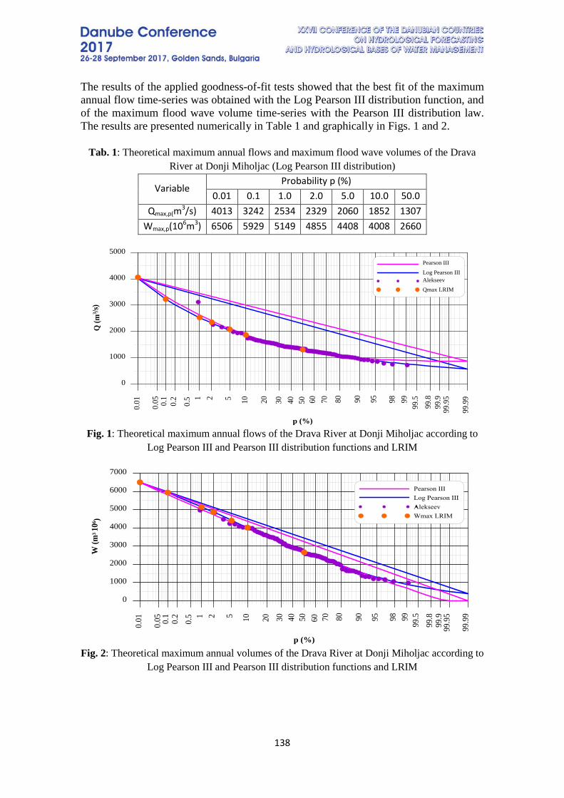
138

The results of the applied goodness-of-fit tests showed that the best fit of the maximum annual flow time-series was obtained with the Log Pearson III distribution function, and of the maximum flood wave volume time-series with the Pearson III distribution law. The results are presented numerically in Table 1 and graphically in Figs. 1 and 2.

Tab. 1: Theoretical maximum annual flows and maximum flood wave volumes of the Drava River at Donji Miholjac (Log Pearson III distribution)

Variable Probability p (%)

0.01 0.1 1.0 2.0 5.0 10.0 50.0 Qmax,p(m3/s) 4013 3242 2534 2329 2060 1852 1307

Wmax,p(106m3) 6506 5929 5149 4855 4408 4008 2660

Fig. 1: Theoretical maximum annual flows of the Drava River at Donji Miholjac according to

Log Pearson III and Pearson III distribution functions and LRIM

Fig. 2: Theoretical maximum annual volumes of the Drava River at Donji Miholjac according to

Log Pearson III and Pearson III distribution functions and LRIM

0.01 0.05 0.1

0.2

0.5 1 2 5 10 20 30 40 50 60 70 80 90 95 98 99

99.5

99.8

99.9

99.9

5

99.9

9

p (%)

0

1000

2000

3000

4000

5000

Q (m

3 /s)

Pearson III

Log Pearson IIIAlekseevQmax LRIM

0.01

0.05 0.1

0.2

0.5 1 2 5 10 20 30 40 50 60 70 80 90 95 98 99

99.5

99.8

99.9

99.9

5

99.9

9

p (%)

0

1000

2000

3000

4000

5000

6000

7000

W (m

3 10

6 )

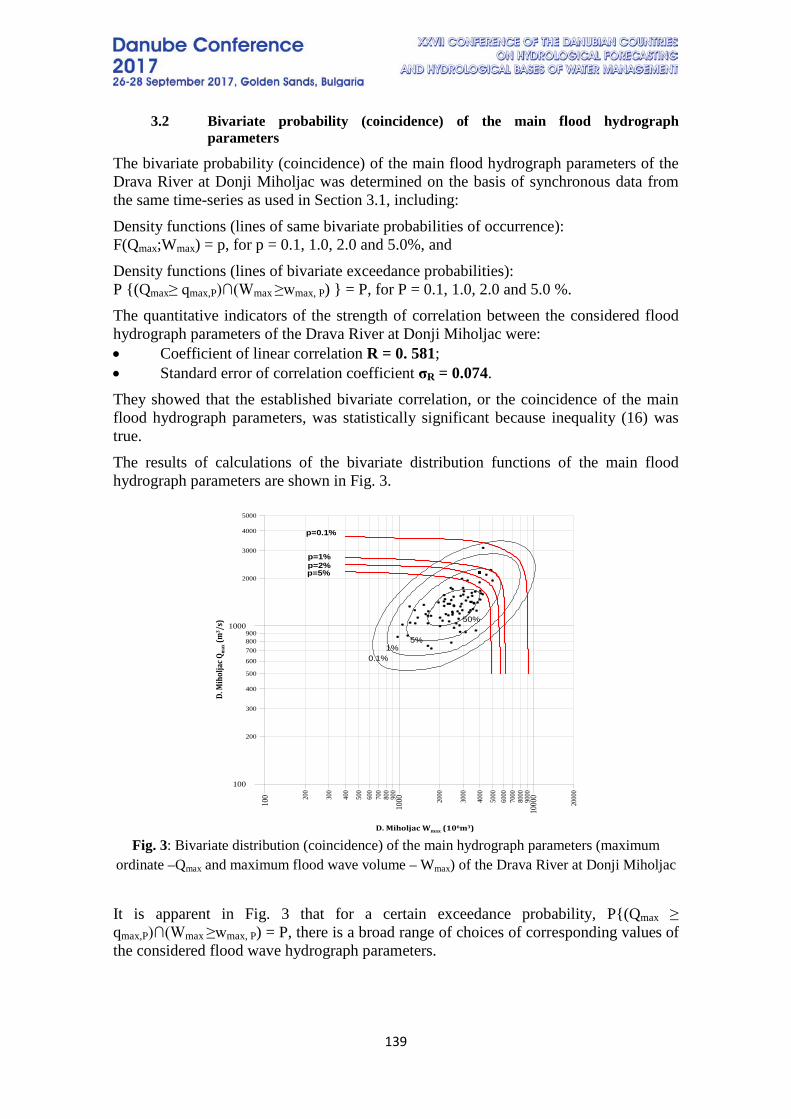
139

3.2 Bivariate probability (coincidence) of the main flood hydrograph parameters

The bivariate probability (coincidence) of the main flood hydrograph parameters of the Drava River at Donji Miholjac was determined on the basis of synchronous data from the same time-series as used in Section 3.1, including: Density functions (lines of same bivariate probabilities of occurrence): F(Qmax;Wmax) = p, for p = 0.1, 1.0, 2.0 and 5.0%, and Density functions (lines of bivariate exceedance probabilities): P {(Qmax≥ qmax,P)∩(Wmax ≥wmax, P) } = P, for P = 0.1, 1.0, 2.0 and 5.0 %. The quantitative indicators of the strength of correlation between the considered flood hydrograph parameters of the Drava River at Donji Miholjac were: • Coefficient of linear correlation R = 0. 581; • Standard error of correlation coefficient σR = 0.074. They showed that the established bivariate correlation, or the coincidence of the main flood hydrograph parameters, was statistically significant because inequality (16) was true. The results of calculations of the bivariate distribution functions of the main flood hydrograph parameters are shown in Fig. 3.

Fig. 3: Bivariate distribution (coincidence) of the main hydrograph parameters (maximum

ordinate –Qmax and maximum flood wave volume – Wmax) of the Drava River at Donji Miholjac

It is apparent in Fig. 3 that for a certain exceedance probability, P{(Qmax ≥ qmax,P)∩(Wmax ≥wmax, P) = P, there is a broad range of choices of corresponding values of the considered flood wave hydrograph parameters.

100

1000

1000

0200

3 00

400

5 00

600

700

8 00

9 00

2 000

300 0

400 0

500 0

6 000

7 000

8 000

9000

2 000

0

100

1000

200

300

400

500

600

700800900

2000

3000

4000

5000

D. Miholjac Wmax (106m3)

50%

0.1%

5%1%

D. M

ihol

jac Q

max

(m3 /s

)

p=0.1%

p=1%p=2%p=5%

140

3.3 Flood hydrograph shape parameters of the Drava River at Donji Miholjac

According to LRIM, all the necessary hydrograph shape parameters are derived from the correlation between the falling and rising limb times (i.e. parameter K). Parameter K is determined using actual data from recorded flood hydrographs. In the case study of the Drava River at Donji Miholjac, histograms from the period 1931-2014 were used. All peak hydrographs by year were represented in the same graphic, after reducing the maximum ordinates to the same point in time. This resulted in a broader temporal spread of the hydrograph, based on which the rising/falling time ratio was defined. Specifically, in the case of the Drava River at Donji Miholjac the ratio was K=2.0, such that the skewness coefficient of the hydrograph was Ks= 0.33.

Based on the correlations among a, and Ks, which are available in the literature [5], the other LRIM parameters needed to define the hydrograph shape were: = 0.8, a = 1.01.

3.4 Design flood hydrographs according to LRIM The proposed approach for determining theoretical flood hydrographs at gauging stations, by combining LRIM and predefined bivariate probability distribution functions of the main hydrograph parameters, is widely applicable in practice. Namely, it provides a number of choices of combinations of main hydrograph parameters, for both probabilities of occurrence p and probabilities of exceedance P. To illustrate the application of the approach in practice, let us assume that there is a very strong functional correlation (R=1.0) between the main flood hydrograph parameters of the Drava River at Donji Miholjac. This practically means that the maximum annual flow of a certain probability of occurrence always coincides with the maximum annual volume of the same probability of occurrence. However, given the results shown in Fig. 3, this is not the case in reality. Still, such a combination of hydrograph parameters makes sense because it in essence represents the “maximum possible” combination, where in the specific case the exceedance probability P is: P {(Qmax ≥ qmax,P)∩(Wmax ≥wmax, P) }>P. For illustration purposes, the first analysis of theoretical flood hydrographs applying LRIM was conducted for the “maximum possible” combination of main flood hydrograph parameters: maximum annual flow and maximum flood wave volume. With these assumptions, the LRIM parameters were calibrated to calculated distribution functions of maximum annual flows (Fig. 1) and maximum flood wave volumes (Fig. 2). The results for the main flood hydrograph parameters of the Drava River at Donji Miholjac are shown in Table 2, along with calibrated LRIM parameters. Tab. 2: Theoretical flood hydrograph elements of the Drava River at Donji Miholjac according

to LRIM Theoretical flood hydrograph elements

p(%) (ϕH)p Fp E(min) S(E) Qp (m3/s) q(m3/s/km2) hp(mm) Wp(106m3) 0.01 152.8 56 753 16 400 0.072 4 063 0.109 175.0 6 500 0.1 129.2 47 987 17 103 0.067 3 233 0.087 159.9 5 937 1.0 108.6 40 336 17 862 0.063 2 534 0.068 138.7 5 151

*λ*λ

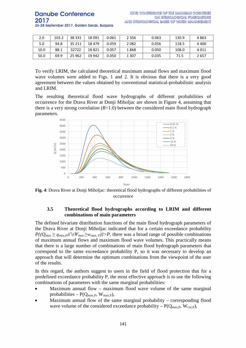
141

2.0 103.2 38 331 18 091 0.061 2 356 0.063 130.9 4 863 5.0 94.8 35 211 18 479 0.059 2 082 0.056 118.5 4 400

10.0 88.1 32722 18 821 0.057 1 868 0.050 108.0 4 011 50.0 69.9 25 962 19 942 0.050 1 307 0.035 71.5 2 657

To verify LRIM, the calculated theoretical maximum annual flows and maximum flood wave volumes were added to Figs. 1 and 2. It is obvious that there is a very good agreement between the values obtained by conventional statistical-probabilistic analysis and LRIM. The resulting theoretical flood wave hydrographs of different probabilities of occurrence for the Drava River at Donji Miholjac are shown in Figure 4, assuming that there is a very strong correlation (R=1.0) between the considered main flood hydrograph parameters.

Fig. 4: Drava River at Donji Miholjac: theoretical flood hydrographs of different probabilities of

occurrence

3.5 Theoretical flood hydrographs according to LRIM and different combinations of main parameters

The defined bivariate distribution functions of the main flood hydrograph parameters of the Drava River at Donji Miholjac indicated that for a certain exceedance probability P{(Qmax ≥ qmax,P)∩(Wmax ≥wmax, P)}>P, there was a broad range of possible combinations of maximum annual flows and maximum flood wave volumes. This practically means that there is a large number of combinations of main flood hydrograph parameters that correspond to the same exceedance probability P, so it was necessary to develop an approach that will determine the optimum combinations from the viewpoint of the user of the results. In this regard, the authors suggest to users in the field of flood protection that for a predefined exceedance probability P, the most effective approach is to use the following combinations of parameters with the same marginal probabilities: • Maximum annual flow – maximum flood wave volume of the same marginal

probabilities – P(Qmax,P, Wmax,P), • Maximum annual flow of the same marginal probability – corresponding flood

wave volume of the considered exceedance probability – P(Qmax,P, Wcor,P),

0

500

1000

1500

2000

2500

3000

3500

4000

4500

0 200 400 600 800 1000 1200 1400 1600 1800

Q (m

3 /s)

hour

0.01 %0.1 %1 %2 %5 %10 %50 %

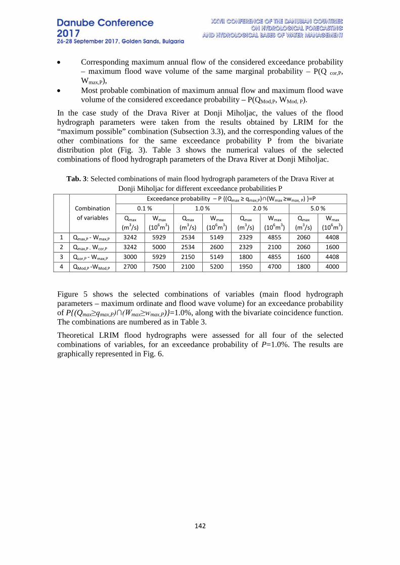
142

• Corresponding maximum annual flow of the considered exceedance probability – maximum flood wave volume of the same marginal probability – P(Q cor,P, Wmax,P),

• Most probable combination of maximum annual flow and maximum flood wave volume of the considered exceedance probability – P(QMod,P, WMod, P).

In the case study of the Drava River at Donji Miholjac, the values of the flood hydrograph parameters were taken from the results obtained by LRIM for the “maximum possible” combination (Subsection 3.3), and the corresponding values of the other combinations for the same exceedance probability P from the bivariate distribution plot (Fig. 3). Table 3 shows the numerical values of the selected combinations of flood hydrograph parameters of the Drava River at Donji Miholjac.

Tab. 3: Selected combinations of main flood hydrograph parameters of the Drava River at Donji Miholjac for different exceedance probabilities P

Combination of variables

Exceedance probability – P {(Qmax ≥ qmax,P)∩(Wmax ≥wmax, P) }=P 0.1 % 1.0 % 2.0 % 5.0 %

Qmax

(m3/s)

Wmax

(106m3)

Qmax

(m3/s)

Wmax

(106m3)

Qmax

(m3/s)

Wmax

(106m3)

Qmax

(m3/s)

Wmax

(106m3)

1 Qmax,P - Wmax,P 3242 5929 2534 5149 2329 4855 2060 4408 2 Qmax,P - Wcor,P 3242 5000 2534 2600 2329 2100 2060 1600 3 Qcor,P - Wmax,P 3000 5929 2150 5149 1800 4855 1600 4408 4 QMod,P -WMod,P 2700 7500 2100 5200 1950 4700 1800 4000

Figure 5 shows the selected combinations of variables (main flood hydrograph parameters – maximum ordinate and flood wave volume) for an exceedance probability of P{(Qmax≥qmax,P)∩(Wmax≥wmax,P)}=1.0%, along with the bivariate coincidence function. The combinations are numbered as in Table 3. Theoretical LRIM flood hydrographs were assessed for all four of the selected combinations of variables, for an exceedance probability of P=1.0%. The results are graphically represented in Fig. 6.

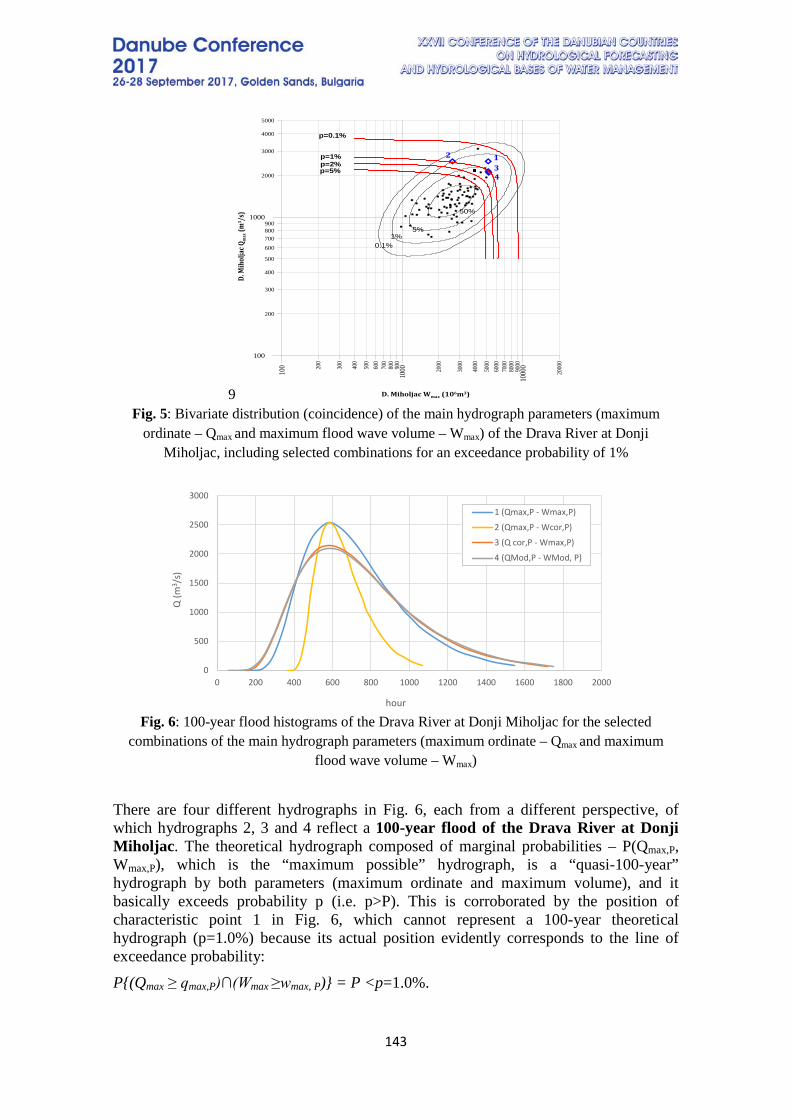
143

9 Fig. 5: Bivariate distribution (coincidence) of the main hydrograph parameters (maximum

ordinate – Qmax and maximum flood wave volume – Wmax) of the Drava River at Donji Miholjac, including selected combinations for an exceedance probability of 1%

Fig. 6: 100-year flood histograms of the Drava River at Donji Miholjac for the selected

combinations of the main hydrograph parameters (maximum ordinate – Qmax and maximum flood wave volume – Wmax)

There are four different hydrographs in Fig. 6, each from a different perspective, of which hydrographs 2, 3 and 4 reflect a 100-year flood of the Drava River at Donji Miholjac. The theoretical hydrograph composed of marginal probabilities – P(Qmax,P, Wmax,P), which is the “maximum possible” hydrograph, is a “quasi-100-year” hydrograph by both parameters (maximum ordinate and maximum volume), and it basically exceeds probability p (i.e. p>P). This is corroborated by the position of characteristic point 1 in Fig. 6, which cannot represent a 100-year theoretical hydrograph (p=1.0%) because its actual position evidently corresponds to the line of exceedance probability: P{(Qmax ≥ qmax,P)∩(Wmax ≥wmax, P)} = P <p=1.0%.

100

1000

1000

0200

300

400

500

6 00

700

800

900

2000

3 000

4000

5000

6 000

7 000

8000

9 000

2 000

0

100

1000

200

300

400

500

600

700800900

2000

3000

4000

5000

D. Miholjac Wmax (106m3)

50%

0.1%

5%1%

D. M

ihol

jac Q

max

(m3 /s

)

12

34

p=0.1%

p=1%p=2%p=5%

0

500

1000

1500

2000

2500

3000

0 200 400 600 800 1000 1200 1400 1600 1800 2000

Q (m

3 /s)

hour

1 (Qmax,P - Wmax,P)

2 (Qmax,P - Wcor,P)

3 (Q cor,P - Wmax,P)

4 (QMod,P - WMod, P)

144

Its real exceedance probability (Fig. 5) is: P{(Qmax ≥ qmax,P)∩(Wmax ≥wmax, P)} = P= 0.33% <p=1.0%. This means that flood hydrograph 1 corresponds to a 300-year return period.

4. CONCLUSION The main idea behind the research was to propose a novel approach for defining theoretical flood hydrographs at river gauging stations, such as official stations with long time-series of river stages and flows. The initial assumption of the approach is that each of the main flood hydrograph parameters is a random variable that adheres to a univariate, bivariate or multivariate distribution law. The bivariate probability analyses presented above show that there is a broad range of possible combinations of hydrograph parameters, which can be used to define a theoretical hydrograph of a certain probability of occurrence. The authors pointed out that for an exceedance probability of P{(Qmax ≥ qmax,P)∩(Wmax ≥wmax, P)} = P, there are four characteristic points whose coordinates (which in effect represent the maximum hydrograph ordinate and flood wave volume) determine the theoretical hydrograph of the same probability of occurrence P≅p. The practical value of theoretical flood hydrographs, determined on the basis of the coordinates of the four characteristics points, for the same exceedance probability P{(Qmax≥qmax,P)∩(Wmax≥wmax,P)}=P≅p, lies in the following: 1. A theoretical hydrograph, composed of marginal probabilities – P(Qmax,P,

Wmax,P), represents the “maximum possible” hydrograph by both parameters (maximum ordinate and maximum volume), and in effect exceeds probability p (i.e. p>P). This is corroborated by the position of characteristic point 1 in Fig. 5, which can represent a 100-year theoretical hydrograph (p=1.0%) but it is evident that its actual position corresponds to the line of probability exceedance P{(Qmax ≥ qmax,P)∩(Wmax ≥wmax, P)} = P <p=1.0%. In other words, its actual exceedance probability (Fig. 5) corresponds to a 300-year return period.

2. A 100-year theoretical hydrograph composed of marginal probabilities – P(Qmax,P, Wcor,P) is a 100-year hydrograph (p=1.0%) only with regard to the maximum ordinate, such that it can only be used to design spillways, levees, bridges, culverts, and the like. It cannot be used to size reservoirs and retentions because the return period of the other hydrograph parameter – flood wave volume – is less than 100 years (p<1.0%).

3. Conversely, a 100-year theoretical hydrograph composed of marginal probabilities P(Qcor,P, Wmax,P) is a 100-year hydrograph (p=1.0%) only with regard to the maximum volume parameter and can be used to design reservoirs and retention areas, but not for spillways, levees, bridges, culverts, etc., because the return period of the other hydrograph parameter – maximum ordinate – is less than 100 years (p<1.0%).

4. A theoretical hydrograph composed of marginal probabilities – P(QMod,P, WMod,

P) is the “most probable” hydrograph, whose exceedance probability P and probability of occurrence p coincide (are identical), i.e. P{(Qmax ≥ qmax,P)∩(Wmax ≥wmax, P)} = P =p.

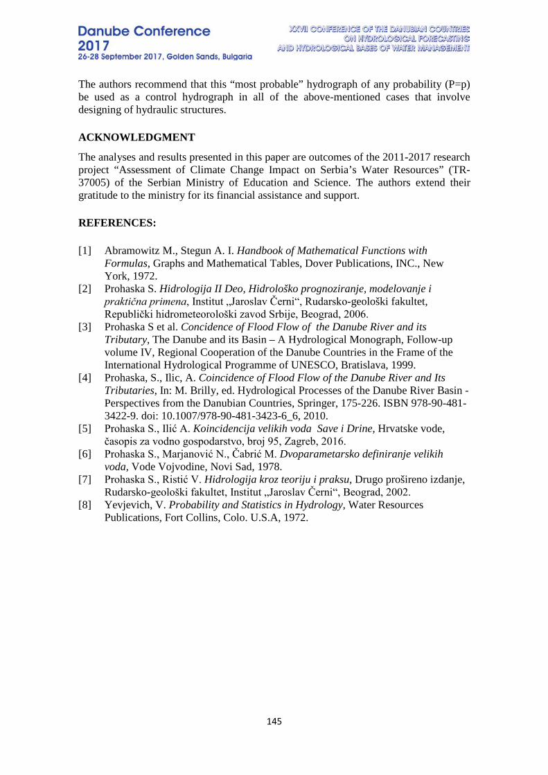
145

The authors recommend that this “most probable” hydrograph of any probability (P=p) be used as a control hydrograph in all of the above-mentioned cases that involve designing of hydraulic structures. ACKNOWLEDGMENT

The analyses and results presented in this paper are outcomes of the 2011-2017 research project “Assessment of Climate Change Impact on Serbia’s Water Resources” (TR-37005) of the Serbian Ministry of Education and Science. The authors extend their gratitude to the ministry for its financial assistance and support. REFERENCES: [1] Abramowitz M., Stegun A. I. Handbook of Mathematical Functions with

Formulas, Graphs and Mathematical Tables, Dover Publications, INC., New York, 1972.

[2] Prohaska S. Hidrologija II Deo, Hidrološko prognoziranje, modelovanje i praktična primena, Institut „Jaroslav Černi“, Rudarsko-geološki fakultet, Republički hidrometeorološki zavod Srbije, Beograd, 2006.

[3] Prohaska S et al. Concidence of Flood Flow of the Danube River and its Tributary, The Danube and its Basin – A Hydrological Monograph, Follow-up volume IV, Regional Cooperation of the Danube Countries in the Frame of the International Hydrological Programme of UNESCO, Bratislava, 1999.

[4] Prohaska, S., Ilic, A. Coincidence of Flood Flow of the Danube River and Its Tributaries, In: M. Brilly, ed. Hydrological Processes of the Danube River Basin - Perspectives from the Danubian Countries, Springer, 175-226. ISBN 978-90-481-3422-9. doi: 10.1007/978-90-481-3423-6_6, 2010.

[5] Prohaska S., Ilić A. Koincidencija velikih voda Save i Drine, Hrvatske vode, časopis za vodno gospodarstvo, broj 95, Zagreb, 2016.

[6] Prohaska S., Marjanović N., Čabrić M. Dvoparametarsko definiranje velikih voda, Vode Vojvodine, Novi Sad, 1978.

[7] Prohaska S., Ristić V. Hidrologija kroz teoriju i praksu, Drugo prošireno izdanje, Rudarsko-geološki fakultet, Institut „Jaroslav Černi“, Beograd, 2002.

[8] Yevjevich, V. Probability and Statistics in Hydrology, Water Resources Publications, Fort Collins, Colo. U.S.A, 1972.

146

INFLUENCE OF NATURAL FACTORS ON THE REGIME OF THE LARGEST KARST SPRINGS IN NORTHWESTERN BULGARIA

Evelina Damyanova1, Neyko Neykov1, Marin Ivanov1, Aleksey Benderev2

1National Institute of Meteorology and Hydrology, 66 Tsarigradsko Shose blvd., 1784 Sofia,

Bulgaria 2Geological Institute – BAS, Acad. G. Bonchev st. bl.24, 1113 Sofia, Bulgaria

Corresponding author: Evelina Damyanova, National Institute of Meteorology and Hydrology,

66 Tsarigradsko Shose blvd., 1784 Sofia, Bulgaria, evelina.damyanova@meteo.bg

ABSTRACT Karst groundwater is widespread in Northwestern Bulgaria. In the higher parts of the Balkan mountain range (Stara Planina) and Fore Balkan typical karst basins are found built mainly from Mesozoic carbonate sediments, whereas in the flat platform part the typical aquifer in the Neogene (Sarmatian) deposits is formed. The drainage of these carbonate sediments is carried out by several karst springs, whose location is determined mainly by geological and geomorphological factors. The formation of their regime is mainly on the account of precipitation, with additional recharge from the river runoff for some of karst basins. The aim of the paper is to discover the impact of different natural factors on the regime of the selected karst springs within the study area. For this purpose the statistical processing of data on spring discharge for karst springs included in the National Monitoring Network of Bulgaria is applied. Comparative assessment of the regime for the selected springs allowed evaluating of the impact of different driving factors on the discharge of karst groundwater in Northwestern Bulgaria. Keywords: karst springs, spring discharge, groundwater regime, Northwestern Bulgaria

1. INTRODUCTION Karst waters are very sensitive to external impacts, which is mostly evident from their regime. Therefore, studying the regime's quantitative and qualitative features, especially for large karst springs, helps to clarify the role of different natural and anthropogenic factors on their regime. The purpose of this study is via applying several statistical methods to do conclusions concerning the similarities and differences in the formation of the discharge for different springs from a relatively small area in Bulgaria, unaffected by anthropogenic influence.

2. DESCRIPTION OF THE STUDY AREA The object of the study are karst springs from Northwestern Bulgaria (Figure 1). The study area with area about 160 km2 is located between the Danube River, the state boundary and the line passing in South-North direction through Berkovitsa town. This study area encompasses parts of the Danube plain, the Fore-Balkan and the Stara Planina (Balkan) Mountain, and the altitude changes from about 30 m at the Danube

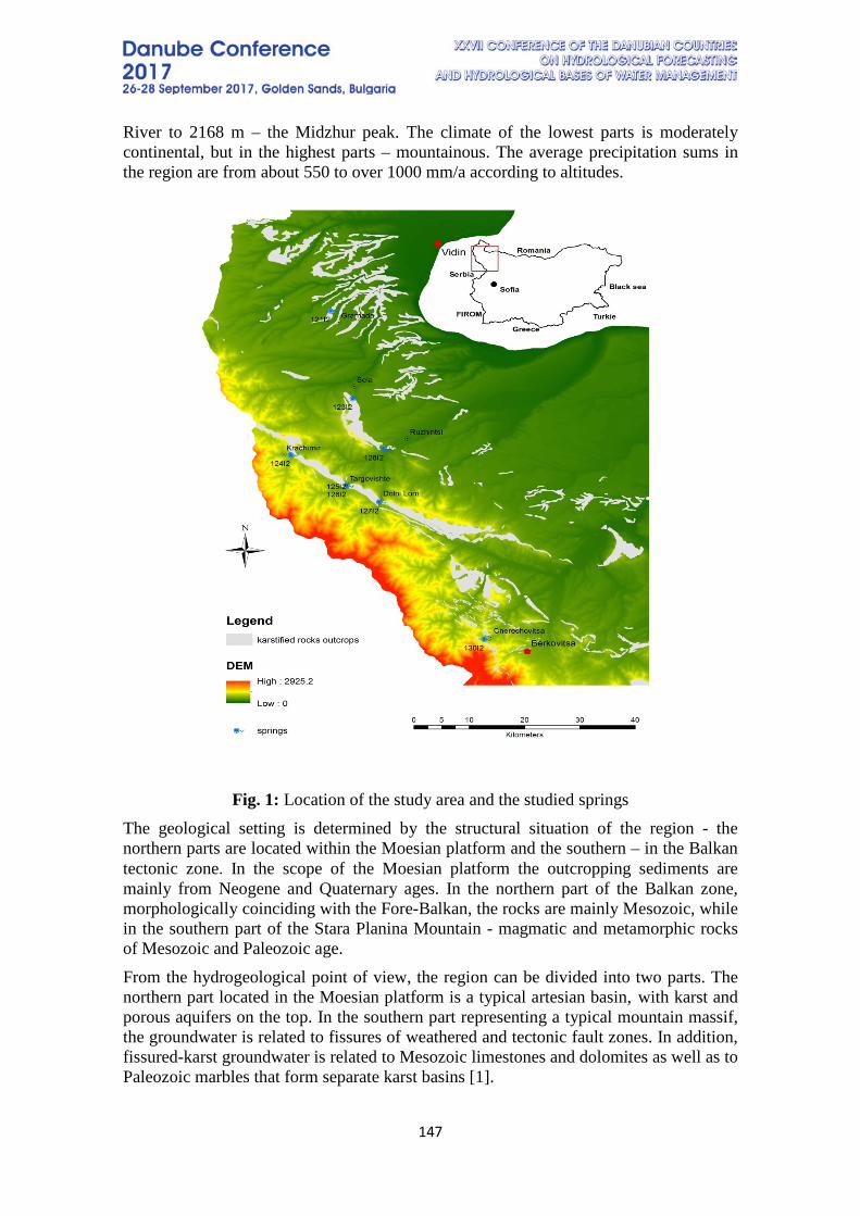
147

River to 2168 m – the Midzhur peak. The climate of the lowest parts is moderately continental, but in the highest parts – mountainous. The average precipitation sums in the region are from about 550 to over 1000 mm/a according to altitudes.

Fig. 1: Location of the study area and the studied springs

The geological setting is determined by the structural situation of the region - the northern parts are located within the Moesian platform and the southern – in the Balkan tectonic zone. In the scope of the Moesian platform the outcropping sediments are mainly from Neogene and Quaternary ages. In the northern part of the Balkan zone, morphologically coinciding with the Fore-Balkan, the rocks are mainly Mesozoic, while in the southern part of the Stara Planina Mountain - magmatic and metamorphic rocks of Mesozoic and Paleozoic age. From the hydrogeological point of view, the region can be divided into two parts. The northern part located in the Moesian platform is a typical artesian basin, with karst and porous aquifers on the top. In the southern part representing a typical mountain massif, the groundwater is related to fissures of weathered and tectonic fault zones. In addition, fissured-karst groundwater is related to Mesozoic limestones and dolomites as well as to Paleozoic marbles that form separate karst basins [1].

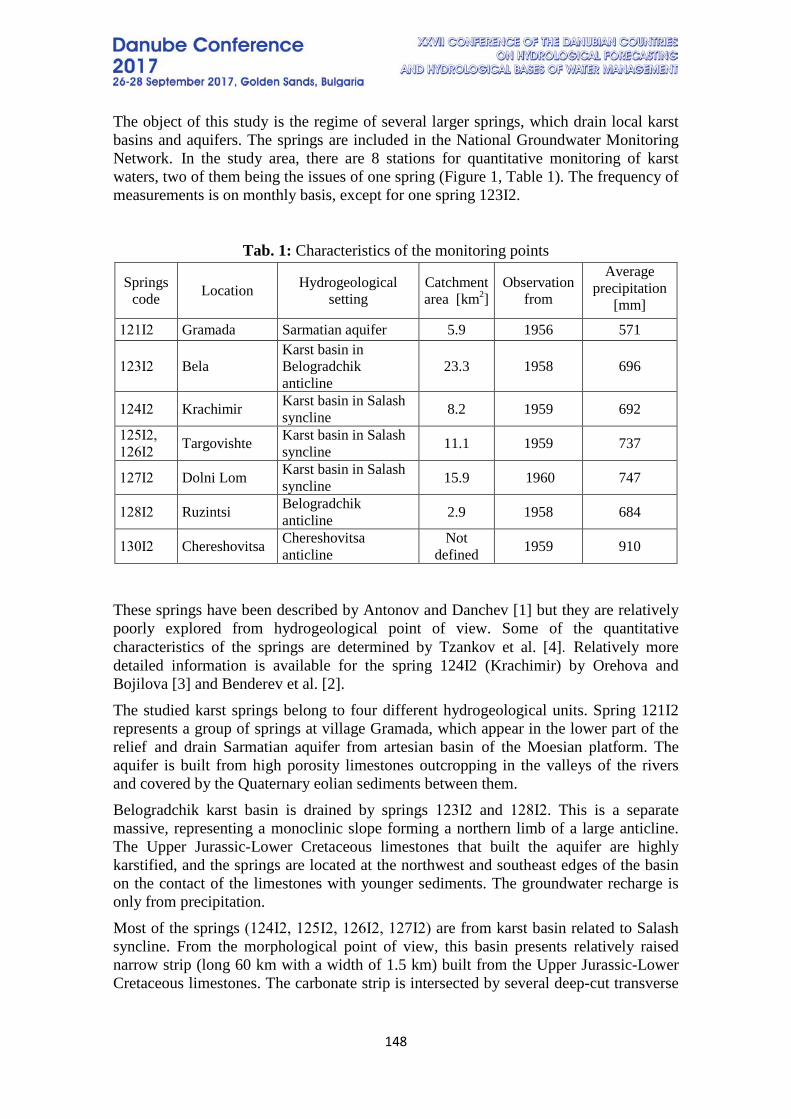
148

The object of this study is the regime of several larger springs, which drain local karst basins and aquifers. The springs are included in the National Groundwater Monitoring Network. In the study area, there are 8 stations for quantitative monitoring of karst waters, two of them being the issues of one spring (Figure 1, Table 1). The frequency of measurements is on monthly basis, except for one spring 123I2.

Tab. 1: Characteristics of the monitoring points

Springs code Location Hydrogeological

setting Catchment area [km2]

Observation from

Average precipitation

[mm]

121І2 Gramada Sarmatian aquifer 5.9 1956 571

123І2 Bela Karst basin in Belogradchik anticline

23.3 1958 696

124І2 Krachimir Karst basin in Salash syncline 8.2 1959 692

125І2, 126І2 Targovishte Karst basin in Salash

syncline 11.1 1959 737

127І2 Dolni Lom Karst basin in Salash syncline 15.9 1960 747

128І2 Ruzintsi Belogradchik anticline 2.9 1958 684

130І2 Chereshovitsa Chereshovitsa anticline

Not defined 1959 910

These springs have been described by Antonov and Danchev [1] but they are relatively poorly explored from hydrogeological point of view. Some of the quantitative characteristics of the springs are determined by Tzankov et al. [4]. Relatively more detailed information is available for the spring 124I2 (Krachimir) by Orehova and Bojilova [3] and Benderev et al. [2]. The studied karst springs belong to four different hydrogeological units. Spring 121I2 represents a group of springs at village Gramada, which appear in the lower part of the relief and drain Sarmatian aquifer from artesian basin of the Moesian platform. The aquifer is built from high porosity limestones outcropping in the valleys of the rivers and covered by the Quaternary eolian sediments between them. Belogradchik karst basin is drained by springs 123І2 and 128І2. This is a separate massive, representing a monoclinic slope forming a northern limb of a large anticline. The Upper Jurassic-Lower Cretaceous limestones that built the aquifer are highly karstified, and the springs are located at the northwest and southeast edges of the basin on the contact of the limestones with younger sediments. The groundwater recharge is only from precipitation. Most of the springs (124І2, 125І2, 126І2, 127І2) are from karst basin related to Salash syncline. From the morphological point of view, this basin presents relatively raised narrow strip (long 60 km with a width of 1.5 km) built from the Upper Jurassic-Lower Cretaceous limestones. The carbonate strip is intersected by several deep-cut transverse

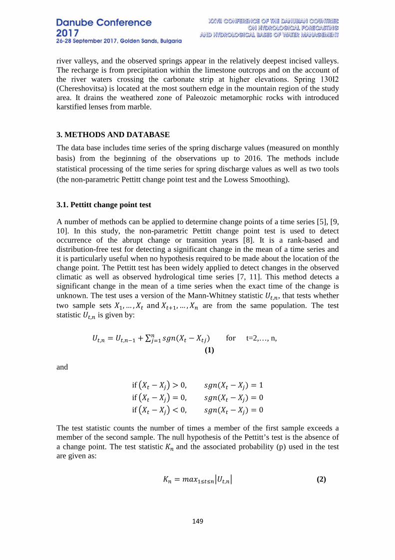
149

river valleys, and the observed springs appear in the relatively deepest incised valleys. The recharge is from precipitation within the limestone outcrops and on the account of the river waters crossing the carbonate strip at higher elevations. Spring 130І2 (Chereshovitsa) is located at the most southern edge in the mountain region of the study area. It drains the weathered zone of Paleozoic metamorphic rocks with introduced karstified lenses from marble.

3. METHODS AND DATABASE The data base includes time series of the spring discharge values (measured on monthly basis) from the beginning of the observations up to 2016. The methods include statistical processing of the time series for spring discharge values as well as two tools (the non-parametric Pettitt change point test and the Lowess Smoothing).

3.1. Pettitt change point test

A number of methods can be applied to determine change points of a time series [5], [9, 10]. In this study, the non-parametric Pettitt change point test is used to detect occurrence of the abrupt change or transition years [8]. It is a rank-based and distribution-free test for detecting a significant change in the mean of a time series and it is particularly useful when no hypothesis required to be made about the location of the change point. The Pettitt test has been widely applied to detect changes in the observed climatic as well as observed hydrological time series [7, 11]. This method detects a significant change in the mean of a time series when the exact time of the change is unknown. The test uses a version of the Mann-Whitney statistic 𝑈𝑈𝑡𝑡,𝑛𝑛, that tests whether two sample sets 𝑋𝑋1, … ,𝑋𝑋𝑡𝑡 and 𝑋𝑋𝑡𝑡+1, … ,𝑋𝑋𝑛𝑛 are from the same population. The test statistic 𝑈𝑈𝑡𝑡,𝑛𝑛 is given by:

𝑈𝑈𝑡𝑡,𝑛𝑛 = 𝑈𝑈𝑡𝑡,𝑛𝑛−1 + ∑ 𝑠𝑠𝑔𝑔𝑠𝑠(𝑋𝑋𝑡𝑡𝑛𝑛

𝑗𝑗=1 − 𝑋𝑋𝑡𝑡𝑗𝑗) for t=2,…, n, (1)

and

if �𝑋𝑋𝑡𝑡 − 𝑋𝑋𝑗𝑗� > 0, 𝑠𝑠𝑔𝑔𝑠𝑠(𝑋𝑋𝑡𝑡 − 𝑋𝑋𝑗𝑗) = 1 if �𝑋𝑋𝑡𝑡 − 𝑋𝑋𝑗𝑗� = 0, 𝑠𝑠𝑔𝑔𝑠𝑠(𝑋𝑋𝑡𝑡 − 𝑋𝑋𝑗𝑗) = 0 if �𝑋𝑋𝑡𝑡 − 𝑋𝑋𝑗𝑗� < 0, 𝑠𝑠𝑔𝑔𝑠𝑠(𝑋𝑋𝑡𝑡 − 𝑋𝑋𝑗𝑗) = 0

The test statistic counts the number of times a member of the first sample exceeds a member of the second sample. The null hypothesis of the Pettitt’s test is the absence of a change point. The test statistic 𝐾𝐾𝑛𝑛 and the associated probability (p) used in the test are given as: 𝐾𝐾𝑛𝑛 = 𝑚𝑚𝑚𝑚𝑚𝑚1≤𝑡𝑡≤𝑛𝑛�𝑈𝑈𝑡𝑡,𝑛𝑛� (2)

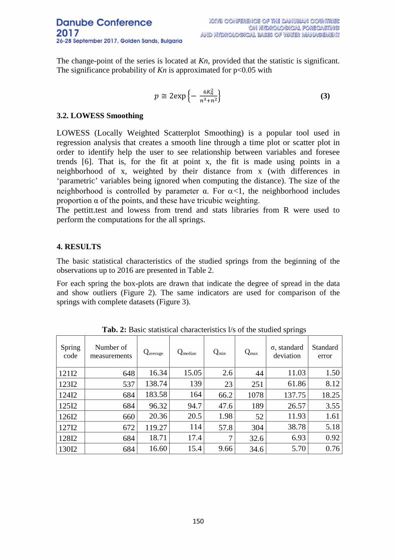
150

The change-point of the series is located at Kn, provided that the statistic is significant. The significance probability of Kn is approximated for p<0.05 with

𝑝𝑝 ≅ 2exp �− 6𝐾𝐾𝑛𝑛2

𝑛𝑛3+𝑛𝑛2� (3)

3.2. LOWESS Smoothing

LOWESS (Locally Weighted Scatterplot Smoothing) is a popular tool used in regression analysis that creates a smooth line through a time plot or scatter plot in order to identify help the user to see relationship between variables and foresee trends [6]. That is, for the fit at point x, the fit is made using points in a neighborhood of x, weighted by their distance from x (with differences in ‘parametric’ variables being ignored when computing the distance). The size of the neighborhood is controlled by parameter α. For α<1, the neighborhood includes proportion α of the points, and these have tricubic weighting. The pettitt.test and lowess from trend and stats libraries from R were used to perform the computations for the all springs.

4. RESULTS

The basic statistical characteristics of the studied springs from the beginning of the observations up to 2016 are presented in Table 2. For each spring the box-plots are drawn that indicate the degree of spread in the data and show outliers (Figure 2). The same indicators are used for comparison of the springs with complete datasets (Figure 3).

Tab. 2: Basic statistical characteristics l/s of the studied springs

Spring code

Number of measurements Qaverage Qmedian Qmin Qmax

σ, standard deviation

Standard error

121I2 648 16.34 15.05 2.6 44 11.03 1.50 123I2 537 138.74 139 23 251 61.86 8.12 124I2 684 183.58 164 66.2 1078 137.75 18.25 125I2 684 96.32 94.7 47.6 189 26.57 3.55 126I2 660 20.36 20.5 1.98 52 11.93 1.61 127I2 672 119.27 114 57.8 304 38.78 5.18 128I2 684 18.71 17.4 7 32.6 6.93 0.92 130I2 684 16.60 15.4 9.66 34.6 5.70 0.76

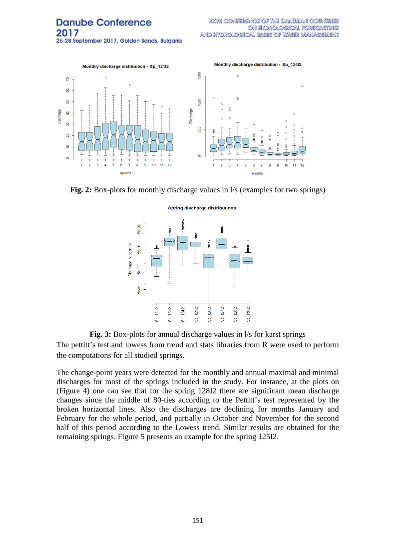
151

Fig. 2: Box-plots for monthly discharge values in l/s (examples for two springs)

Fig. 3: Box-plots for annual discharge values in l/s for karst springs

The pettitt’s test and lowess from trend and stats libraries from R were used to perform the computations for all studied springs.

The change-point years were detected for the monthly and annual maximal and minimal discharges for most of the springs included in the study. For instance, at the plots on (Figure 4) one can see that for the spring 128I2 there are significant mean discharge changes since the middle of 80-ties according to the Pettitt’s test represented by the broken horizontal lines. Also the discharges are declining for months January and February for the whole period, and partially in October and November for the second half of this period according to the Lowess trend. Similar results are obtained for the remaining springs. Figure 5 presents an example for the spring 125I2.

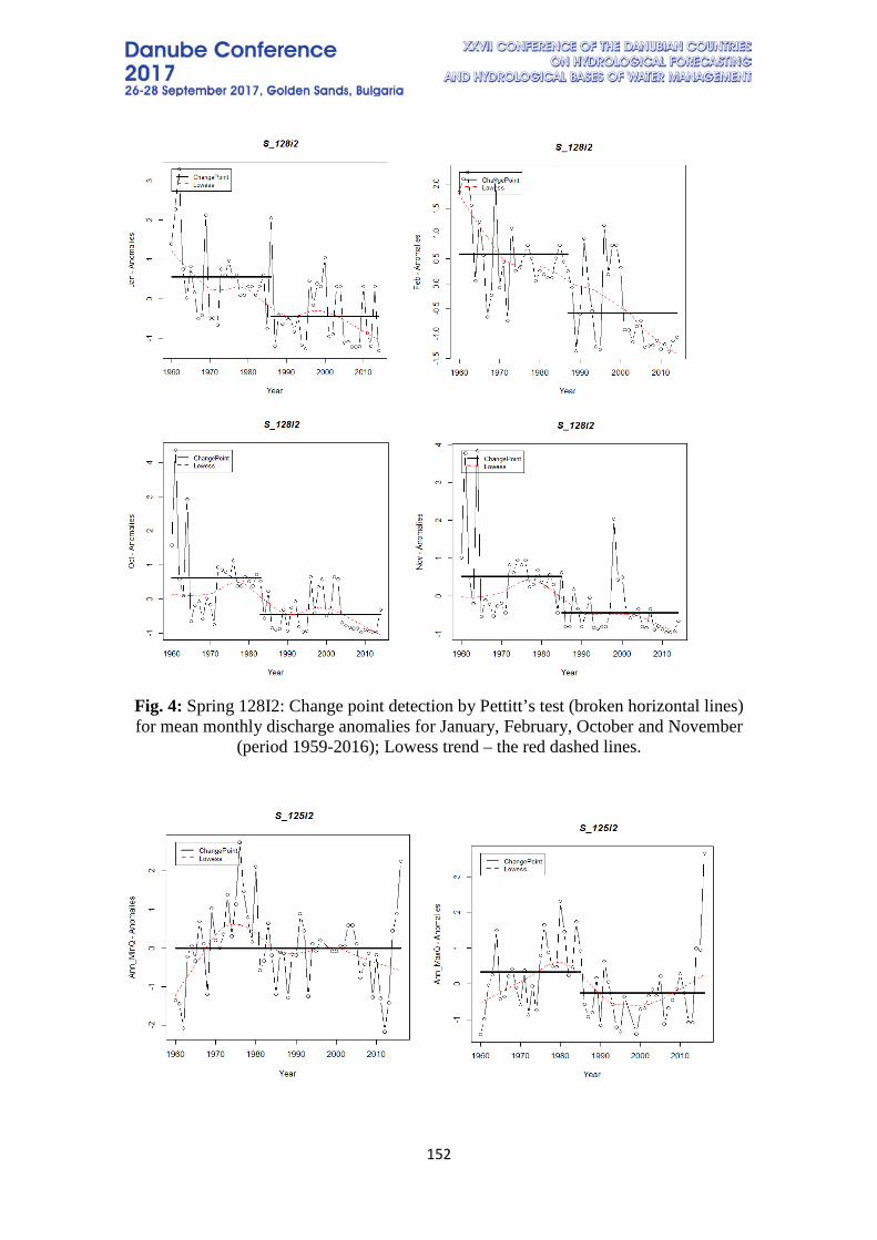
152

Fig. 4: Spring 128I2: Change point detection by Pettitt’s test (broken horizontal lines) for mean monthly discharge anomalies for January, February, October and November

(period 1959-2016); Lowess trend – the red dashed lines.

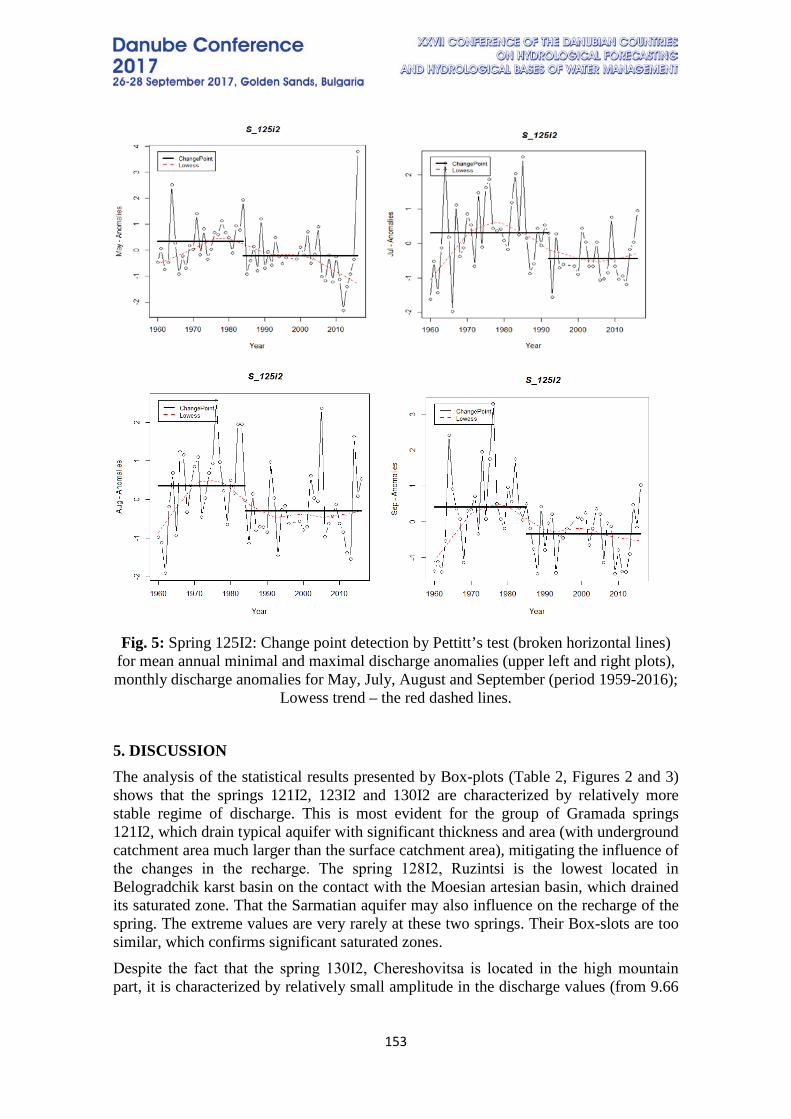
153

Fig. 5: Spring 125I2: Change point detection by Pettitt’s test (broken horizontal lines)

for mean annual minimal and maximal discharge anomalies (upper left and right plots), monthly discharge anomalies for May, July, August and September (period 1959-2016);

Lowess trend – the red dashed lines.

5. DISCUSSION The analysis of the statistical results presented by Box-plots (Table 2, Figures 2 and 3) shows that the springs 121I2, 123I2 and 130I2 are characterized by relatively more stable regime of discharge. This is most evident for the group of Gramada springs 121I2, which drain typical aquifer with significant thickness and area (with underground catchment area much larger than the surface catchment area), mitigating the influence of the changes in the recharge. The spring 128І2, Ruzintsi is the lowest located in Belogradchik karst basin on the contact with the Moesian artesian basin, which drained its saturated zone. That the Sarmatian aquifer may also influence on the recharge of the spring. The extreme values are very rarely at these two springs. Their Box-slots are too similar, which confirms significant saturated zones. Despite the fact that the spring 130І2, Chereshovitsa is located in the high mountain part, it is characterized by relatively small amplitude in the discharge values (from 9.66

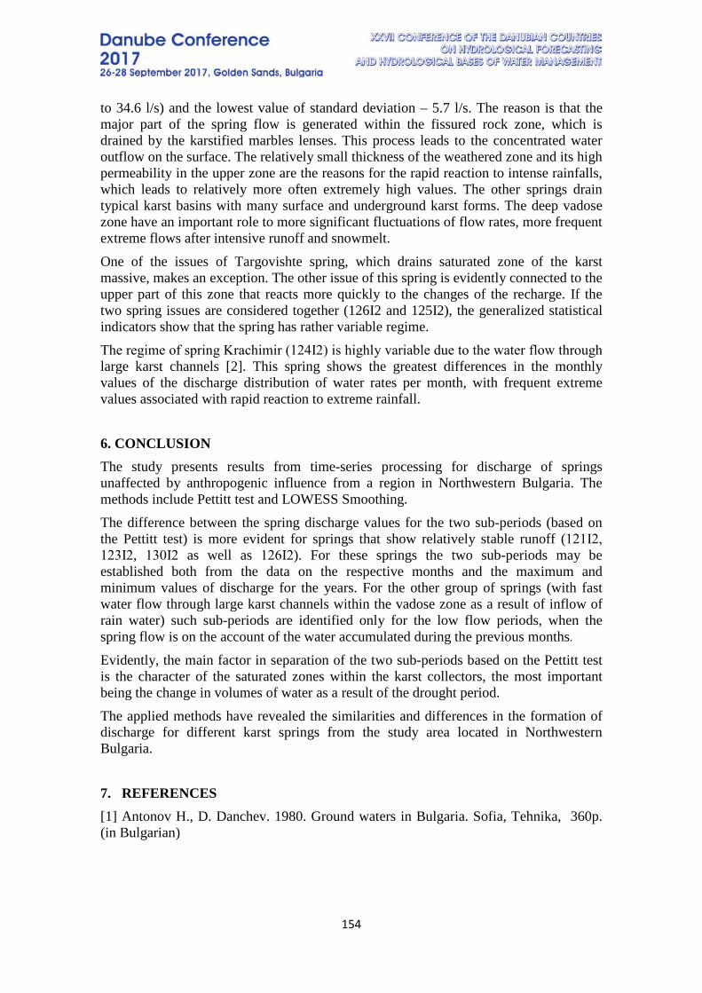
154

to 34.6 l/s) and the lowest value of standard deviation – 5.7 l/s. The reason is that the major part of the spring flow is generated within the fissured rock zone, which is drained by the karstified marbles lenses. This process leads to the concentrated water outflow on the surface. The relatively small thickness of the weathered zone and its high permeability in the upper zone are the reasons for the rapid reaction to intense rainfalls, which leads to relatively more often extremely high values. The other springs drain typical karst basins with many surface and underground karst forms. The deep vadose zone have an important role to more significant fluctuations of flow rates, more frequent extreme flows after intensive runoff and snowmelt. One of the issues of Targovishte spring, which drains saturated zone of the karst massive, makes an exception. The other issue of this spring is evidently connected to the upper part of this zone that reacts more quickly to the changes of the recharge. If the two spring issues are considered together (126I2 and 125I2), the generalized statistical indicators show that the spring has rather variable regime. The regime of spring Krachimir (124І2) is highly variable due to the water flow through large karst channels [2]. This spring shows the greatest differences in the monthly values of the discharge distribution of water rates per month, with frequent extreme values associated with rapid reaction to extreme rainfall.

6. CONCLUSION The study presents results from time-series processing for discharge of springs unaffected by anthropogenic influence from a region in Northwestern Bulgaria. The methods include Pettitt test and LOWESS Smoothing. The difference between the spring discharge values for the two sub-periods (based on the Pettitt test) is more evident for springs that show relatively stable runoff (121І2, 123І2, 130І2 as well as 126І2). For these springs the two sub-periods may be established both from the data on the respective months and the maximum and minimum values of discharge for the years. For the other group of springs (with fast water flow through large karst channels within the vadose zone as a result of inflow of rain water) such sub-periods are identified only for the low flow periods, when the spring flow is on the account of the water accumulated during the previous months. Evidently, the main factor in separation of the two sub-periods based on the Pettitt test is the character of the saturated zones within the karst collectors, the most important being the change in volumes of water as a result of the drought period. The applied methods have revealed the similarities and differences in the formation of discharge for different karst springs from the study area located in Northwestern Bulgaria.

7. REFERENCES [1] Antonov H., D. Danchev. 1980. Ground waters in Bulgaria. Sofia, Tehnika, 360p. (in Bulgarian)

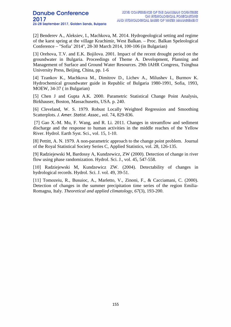
155

[2] Benderev A., Aleksiev, I., Machkova, M. 2014. Hydrogeological setting and regime of the karst spring at the village Krachimir, West Balkan. – Proc. Balkan Speleological Conference – "Sofia’ 2014", 28-30 March 2014, 100-106 (in Bulgarian) [3] Orehova, T.V. and E.K. Bojilova. 2001. Impact of the recent drought period on the groundwater in Bulgaria. Proceedings of Theme A. Development, Planning and Management of Surface and Ground Water Resources. 29th IAHR Congress, Tsinghua University Press, Beijing, China, pp. 1-6 [4] Tzankov K., Machkova M., Dimitrov D., Lichev A., Milushev I., Burmov K. Hydrochemical groundwater guide in Republic of Bulgaria 1980-1991, Sofia, 1993, MOEW, 34-37 ( in Bulgarian) [5] Chen J and Gupta A.K. 2000. Parametric Statistical Change Point Analysis, Birkhauser, Boston, Massachusetts, USA. p. 240. [6] Cleveland, W. S. 1979. Robust Locally Weighted Regression and Smoothing Scatterplots. J. Amer. Statist. Assoc., vol. 74, 829-836.

[7] Gao X.-M. Mu, F. Wang, and R. Li. 2011. Changes in streamflow and sediment discharge and the response to human activities in the middle reaches of the Yellow River. Hydrol. Earth Syst. Sci., vol. 15, 1-10. [8] Pettitt, A. N. 1979. A non-parametric approach to the change point problem. Journal of the Royal Statistical Society Series C, Applied Statistics, vol. 28, 126-135. [9] Radziejewski M, Bardossy A, Kundzewicz, ZW (2000). Detection of change in river flow using phase randomization. Hydrol. Sci. J., vol. 45, 547-558. [10] Radziejewski M, Kundzewicz ZW. (2004). Detectability of changes in hydrological records. Hydrol. Sci. J. vol. 49, 39-51. [11] Tomozeiu, R., Busuioc, A., Marletto, V., Zinoni, F., & Cacciamani, C. (2000). Detection of changes in the summer precipitation time series of the region Emilia-Romagna, Italy. Theoretical and applied climatology, 67(3), 193-200.

156

IMPACT OF DROUGHT PERIODS ON THE GROUNDWATER RECHARGE IN THE DOBRICH REGION, NORTHEASTERN BULGARIA

Veselina Pavlova1, Tatiana Orehova2

1 National Institute of Meteorology and Hydrology – BAS, Bulgaria 2 Geological Institute – BAS, Bulgaria

Corresponding author: Veselina Pavlova, National Institute of Meteorology and Hydrology – BAS Branch Varna, Hydro-meteorological observatory - Dobrich, 25-th September Bul, 80,

Dobrich, Bulgaria, email: veselina.pavlova@meteo.bg

ABSTRACT The study area is located in Dobrudzha (Northeastern Bulgaria) and is characterized by widespread karstified limestone of Sarmatian age covered by the loess formation. The main rivers draining the study area are the Suha River flowing to North and the Batova River flowing eastward to the Black Sea. Total precipitation sums in the region are low (410-520 mm in average), and the water resources are limited. The aim of the paper is to evaluate groundwater recharge for the study area and its temporal variation by the soil water balance method. For this purpose, daily time-series of the precipitation and air temperature from three meteorological stations for the 2000-2012 period are processed. The obtained values of the groundwater recharge show high variability through years in respect to alterations in the precipitation and air temperature. The long-term average annual recharge values are consistent with the results obtained earlier by other methods. The results demonstrate that the formation of the water resources occurs mainly on the account of precipitation during the cold half-year. Mild winters with low precipitation sums leads to reduced water resources in the next months and thus low groundwater recharge values may be anticipated. Keywords: water balance, groundwater recharge, droughts, karst, Dobrudzha

1. INTRODUCTION Climate variability affected the groundwater regime in Bulgaria. Karst and shallow aquifers showed their vulnerability to long-lasting droughts [1]. In particular, for the Dobrich region (Northeastern Bulgaria) it was proven that the fluctuation of the groundwater levels is in conformity with the precipitation regime expressed by the Standardized Precipitation Index [2]. The Dobrich region is an area with limited surface runoff and the water supply is mainly based on groundwater. It is therefore important to assess the groundwater recharge as the groundwater withdrawal should not exceed the mean annual recharge. The aim of the paper is to evaluate groundwater recharge for the study area and its temporal variation by the soil water balance method. Daily time-series of the precipitation and air temperature are processed.

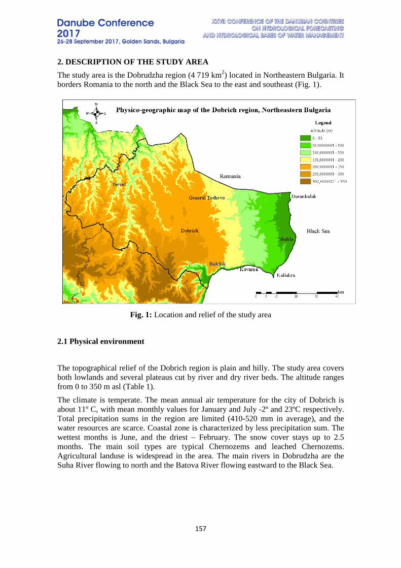
157

2. DESCRIPTION OF THE STUDY AREA The study area is the Dobrudzha region (4 719 km2) located in Northeastern Bulgaria. It borders Romania to the north and the Black Sea to the east and southeast (Fig. 1).

Fig. 1: Location and relief of the study area

2.1 Physical environment The topographical relief of the Dobrich region is plain and hilly. The study area covers both lowlands and several plateaus cut by river and dry river beds. The altitude ranges from 0 to 350 m asl (Table 1). The climate is temperate. The mean annual air temperature for the city of Dobrich is about 11º C, with mean monthly values for January and July -2º and 23ºC respectively. Total precipitation sums in the region are limited (410-520 mm in average), and the water resources are scarce. Coastal zone is characterized by less precipitation sum. The wettest months is June, and the driest – February. The snow cover stays up to 2.5 months. The main soil types are typical Chernozems and leached Chernozems. Agricultural landuse is widespread in the area. The main rivers in Dobrudzha are the Suha River flowing to north and the Batova River flowing eastward to the Black Sea.

158

Tab. 1: Altitude of the study area

Municipality Altitude, m asl

Minimal Maximal Average Balchik 0.00 283.03 200.20 General Toshevo 58.96 256.60 181.74 Dobrich-town 36.95 350.24 234.98 Kavarna 0.00 180.59 107.02 Krushari 54.97 241.51 183.14 Tervel 65.58 290.52 212.49 Dobrichka (Dobrich-rural) 188.15 285.50 238.72 Shabla 0.14 106.49 45.11

2.2 Hydrogeological setting The study area is characterized by widespread karstified limestone of Sarmatian age covered by the loess formation (thick 20-30 m). The Lower Sarmatian aquifer is associated with the sandy sediments of the Frangenska Formation, and the Upper Sarmatian aquifer – with the Odarska and Karvunska Formations, built from karstified limestone [3]. The unconfined aquifers are recharged by rainwater infiltration through the loess cover. Within the Dobrudzha area, the groundwater flow is divergent: it is directed to north, to south and to the Black Sea [4]. Most evidently, the groundwater discharges as baseflow in the Batova River and by springs along this river (with springflows from 0.05 l/s to over 100 l/s, with weak seasonal fluctuations). Important part of the groundwater flow is directed to the Romanian territory. Other part discharges to the coastal wetlands of Durankulak and Shabla or is directed downward to the lower leaky Low-Cretaceous aquifer in northwest part of the study area. Also, there is submarine discharge into the Black Sea [4]. According to previous study in the area in 1995-1996 [5], the groundwater recharge is the lowest in the coastal area (from 32 to 48 mm yearly), with typical values for the area from 60 to 70 mm per year. The highest value (98 mm/y) was obtained only for Vaklino Gully near Shabla. These values were estimated based on the water-table fluctuation method with specific yield value 0.08. Spasov and Pavlova [3] provided an average value of 73 mm for the study area (with spatial variations from 39 to 115 mm across the study area) based on analysis of the water level fluctuation in 6 observational well (period 2006-2011).

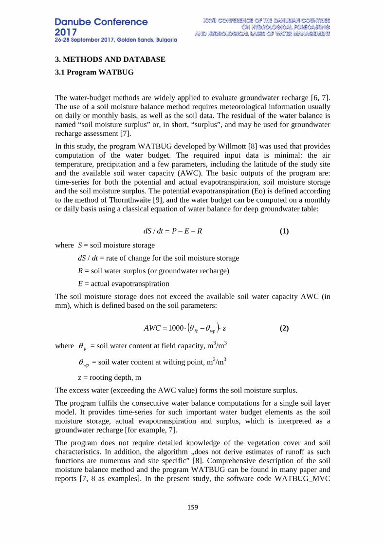
159

3. METHODS AND DATABASE 3.1 Program WATBUG The water-budget methods are widely applied to evaluate groundwater recharge [6, 7]. The use of a soil moisture balance method requires meteorological information usually on daily or monthly basis, as well as the soil data. The residual of the water balance is named “soil moisture surplus” or, in short, “surplus”, and may be used for groundwater recharge assessment [7]. In this study, the program WATBUG developed by Willmott [8] was used that provides computation of the water budget. The required input data is minimal: the air temperature, precipitation and a few parameters, including the latitude of the study site and the available soil water capacity (AWC). The basic outputs of the program are: time-series for both the potential and actual evapotranspiration, soil moisture storage and the soil moisture surplus. The potential evapotranspiration (Eo) is defined according to the method of Thornthwaite [9], and the water budget can be computed on a monthly or daily basis using a classical equation of water balance for deep groundwater table:

REPdtdS −−=/ (1)

where S = soil moisture storage dS / dt = rate of change for the soil moisture storage R = soil water surplus (or groundwater recharge) E = actual evapotranspiration The soil moisture storage does not exceed the available soil water capacity AWC (in mm), which is defined based on the soil parameters:

( ) zAWC wpfc ⋅−⋅= θθ1000 (2)

where fcθ = soil water content at field capacity, m3/m3

wpθ = soil water content at wilting point, m3/m3

z = rooting depth, m The excess water (exceeding the AWC value) forms the soil moisture surplus. The program fulfils the consecutive water balance computations for a single soil layer model. It provides time-series for such important water budget elements as the soil moisture storage, actual evapotranspiration and surplus, which is interpreted as a groundwater recharge [for example, 7]. The program does not require detailed knowledge of the vegetation cover and soil characteristics. In addition, the algorithm „does not derive estimates of runoff as such functions are numerous and site specific” [8]. Comprehensive description of the soil moisture balance method and the program WATBUG can be found in many paper and reports [7, 8 as examples]. In the present study, the software code WATBUG_MVC

160

provided by Dr. M. Van Camp was applied, who had made some corrections to improve the original code (pers. comm.).

3.2 Data base For the purposes of the study, the time-series from three meteorological stations located in the study area (Dobrich, General Toshevo, and Kaliakra) are used. These stations are in operation at the National Institute of Meteorology and Hydrology at Bulgarian Academy of Sciences (NIMH-BAS). The period 2000-2012 is investigated, and the time-series are for the air temperature and precipitation on daily basis. The soil water holding capacity of the topsoil layer is characterized by the parameter AWC, which for Kaliakra was set to 150 mm – a typical value for agricultural lands in Bulgaria. For Dobrich and General Toshevo, the AWC value was set to 200 mm taking into account large thickness of the topsoil and high water holding capacity of Chernozems that are developed on the loess (silt loam) cover [10].

4. RESULTS (from WATBUG) The meteorological data for three stations in the area (Dobrich, General Toshevo and Kaliakra) are processed for the period 2000-2012, and the water balance elements are obtained as outputs of the program WATBUG, run on daily basis. The output daily data are aggregated in monthly time-series. The calculated mean annual values of the water budget elements for this 13-year period are presented in Table 2. Fragment of the output time series for the station Dobrich (period 2006-2011) is presented in Fig. 2 and 3.

Tab. 2: Calculated mean annual water budget elements for the period 2000-2012

Water budget element Dobrich General Toshevo Kaliakra P, mm 540.5 489.4 394.8 Eo, mm 726.4 716.4 696.3 Eo/P 1.344 1.464 1.763 E, mm 438.6 411.6 334.0 E/Eo 0.604 0.575 0.480 Sav, mm 130.1 122.7 82.0 Sav/AWC 0.650 0.614 0.547 R, mm 96.0 68.0 52.7 R/P, % 17.8 13.9 13.3

Comment: Sav – average soil moisture storage The data from Table 2 show that the long-term average annual recharge values are in the range 53-96 mm. Lower values are found in the locations with scarce annual precipitation sum and high aridity index, defined as a ratio of potential evapotranspiration to precipitation.

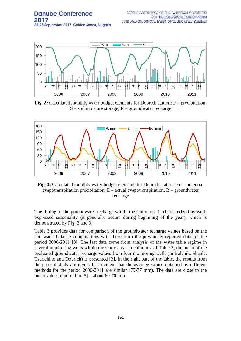
161

Fig. 2: Calculated monthly water budget elements for Dobrich station: P – precipitation,

S – soil moisture storage, R – groundwater recharge

Fig. 3: Calculated monthly water budget elements for Dobrich station: Eo – potential evapotranspiration precipitation, E – actual evapotranspiration, R – groundwater

recharge The timing of the groundwater recharge within the study area is characterized by well-expressed seasonality (it generally occurs during beginning of the year), which is demonstrated by Fig. 2 and 3. Table 3 provides data for comparison of the groundwater recharge values based on the soil water balance computations with these from the previously reported data for the period 2006-2011 [3]. The last data come from analysis of the water table regime in several monitoring wells within the study area. In column 2 of Table 3, the mean of the evaluated groundwater recharge values from four monitoring wells (in Balchik, Shabla, Tsarichino and Dobrich) is presented [3]. In the right part of the table, the results from the present study are given. It is evident that the average values obtained by different methods for the period 2006-2011 are similar (75-77 mm). The data are close to the mean values reported in [5] – about 60-70 mm.

0

50

100

150

2001 4 7 10 1 4 7 10 1 4 7 10 1 4 7 10 1 4 7 10 1 4 7 10

2006 2007 2008 2009 2010 2011

P, mm R, mm S, mm

0306090

120150180

1 4 7 10 1 4 7 10 1 4 7 10 1 4 7 10 1 4 7 10 1 4 7 10

2006 2007 2008 2009 2010 2011

R, mm E, mm Eo, mm

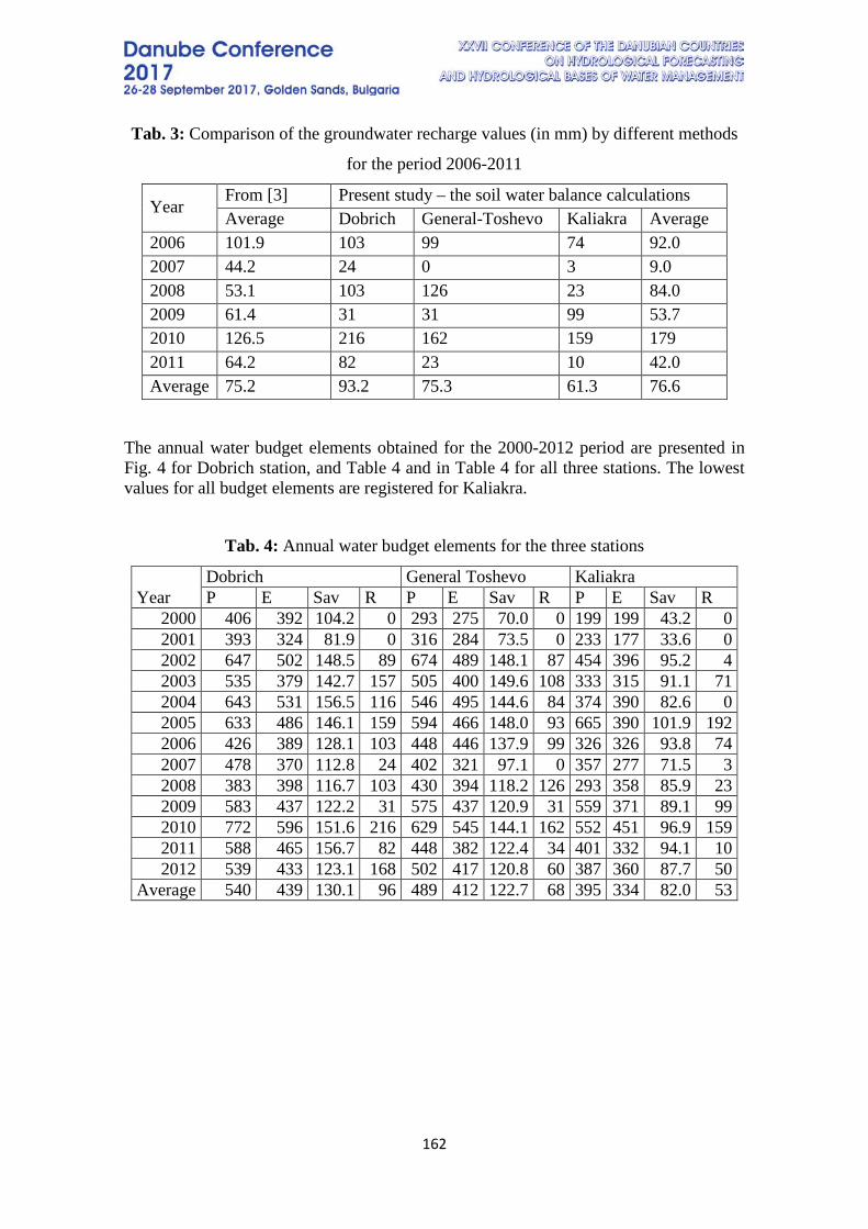
162

Tab. 3: Comparison of the groundwater recharge values (in mm) by different methods

for the period 2006-2011

Year From [3] Present study – the soil water balance calculations Average Dobrich General-Toshevo Kaliakra Average

2006 101.9 103 99 74 92.0 2007 44.2 24 0 3 9.0 2008 53.1 103 126 23 84.0 2009 61.4 31 31 99 53.7 2010 126.5 216 162 159 179 2011 64.2 82 23 10 42.0 Average 75.2 93.2 75.3 61.3 76.6

The annual water budget elements obtained for the 2000-2012 period are presented in Fig. 4 for Dobrich station, and Table 4 and in Table 4 for all three stations. The lowest values for all budget elements are registered for Kaliakra.

Tab. 4: Annual water budget elements for the three stations

Year Dobrich General Toshevo Kaliakra P E Sav R P E Sav R P E Sav R

2000 406 392 104.2 0 293 275 70.0 0 199 199 43.2 0 2001 393 324 81.9 0 316 284 73.5 0 233 177 33.6 0 2002 647 502 148.5 89 674 489 148.1 87 454 396 95.2 4 2003 535 379 142.7 157 505 400 149.6 108 333 315 91.1 71 2004 643 531 156.5 116 546 495 144.6 84 374 390 82.6 0 2005 633 486 146.1 159 594 466 148.0 93 665 390 101.9 192 2006 426 389 128.1 103 448 446 137.9 99 326 326 93.8 74 2007 478 370 112.8 24 402 321 97.1 0 357 277 71.5 3 2008 383 398 116.7 103 430 394 118.2 126 293 358 85.9 23 2009 583 437 122.2 31 575 437 120.9 31 559 371 89.1 99 2010 772 596 151.6 216 629 545 144.1 162 552 451 96.9 159 2011 588 465 156.7 82 448 382 122.4 34 401 332 94.1 10 2012 539 433 123.1 168 502 417 120.8 60 387 360 87.7 50

Average 540 439 130.1 96 489 412 122.7 68 395 334 82.0 53

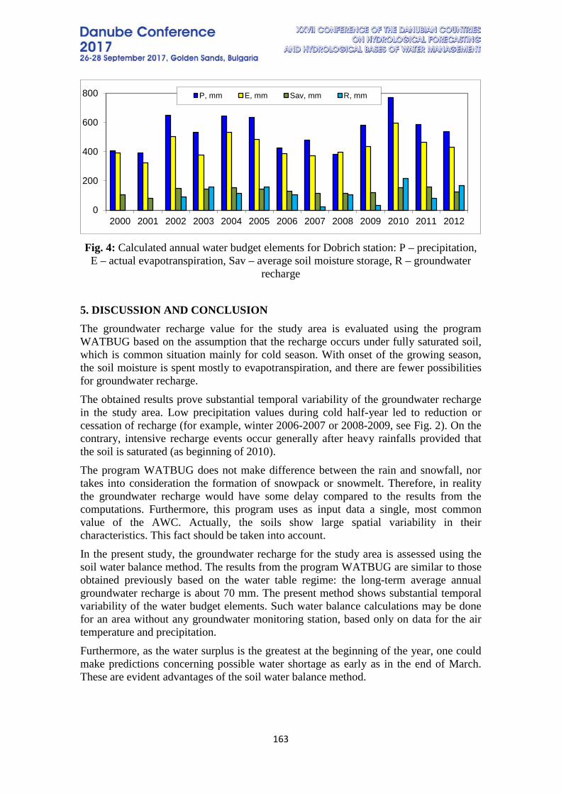
163

Fig. 4: Calculated annual water budget elements for Dobrich station: P – precipitation,

E – actual evapotranspiration, Sav – average soil moisture storage, R – groundwater recharge

5. DISCUSSION AND CONCLUSION The groundwater recharge value for the study area is evaluated using the program WATBUG based on the assumption that the recharge occurs under fully saturated soil, which is common situation mainly for cold season. With onset of the growing season, the soil moisture is spent mostly to evapotranspiration, and there are fewer possibilities for groundwater recharge. The obtained results prove substantial temporal variability of the groundwater recharge in the study area. Low precipitation values during cold half-year led to reduction or cessation of recharge (for example, winter 2006-2007 or 2008-2009, see Fig. 2). On the contrary, intensive recharge events occur generally after heavy rainfalls provided that the soil is saturated (as beginning of 2010). The program WATBUG does not make difference between the rain and snowfall, nor takes into consideration the formation of snowpack or snowmelt. Therefore, in reality the groundwater recharge would have some delay compared to the results from the computations. Furthermore, this program uses as input data a single, most common value of the AWC. Actually, the soils show large spatial variability in their characteristics. This fact should be taken into account. In the present study, the groundwater recharge for the study area is assessed using the soil water balance method. The results from the program WATBUG are similar to those obtained previously based on the water table regime: the long-term average annual groundwater recharge is about 70 mm. The present method shows substantial temporal variability of the water budget elements. Such water balance calculations may be done for an area without any groundwater monitoring station, based only on data for the air temperature and precipitation. Furthermore, as the water surplus is the greatest at the beginning of the year, one could make predictions concerning possible water shortage as early as in the end of March. These are evident advantages of the soil water balance method.

0

200

400

600

800

2000 2001 2002 2003 2004 2005 2006 2007 2008 2009 2010 2011 2012

P, mm E, mm Sav, mm R, mm

164

6. REFERENCES [1] Benderev, A. D., T. V. Orehova, E. K. Bojilova. Some aspects of groundwater regime in Bulgaria with respect to climate variability. In: Geological Society, London, Special Publications; v. 288, pp 13-24, 2008. [2] Orehova, T., V. Pavlova. Groundwater drought in Northeast Bulgaria and the SPI index. Proceedings of XXVI Danube Conference, 22-24 September 2014, Deggendorf, Germany, pp 335-338, 2014. [3] Spasov, V., V. Pavlova. Water table fluctuations, groundwater balance and resources of the Sarmatian aquifer in Northeastern Bulgaria. Review of the Bulgarian Geological Society, vol. 76, part 1, pp 69-78, 2015 (in Bulgarian). [4] Danchev D., A. Damyanov, E. Nikolov, A. Benderev and I. Gushkov. Regularities in the distribution of groundwater in the south Dobrudja and Ludogorie region. Proceedings of the Jubilee Scientific Conference „20 years of the Research sector at the Institute of Mining and Geology“ in Varna, 26-28.10.1981, pp 325-333, 1981 (In Bulgarian). [5] Pulido-Bosch, A., M. Lopez-Chicano, M. Machkova, et al. Ecological problems of karst waters caused by overexploitation and contamination, on the example of North-East Bulgaria. 1997. Project ERB-CIPA-0139, financed by the European Community. [6] Sophocleous, M. A. Combining the soilwater balance and water-level fluctuation methods to estimate natural groundwater recharge: practical aspects. Journal of hydrology, 124(3-4), pp 229-241, 1991. [7] Van Camp M., K. Martens & K. Walraevens. Impact of recent climate variability on an aquifer system in north Belgium. Geologica Belgica, vol. 15/issue 1-2, pp 73-80, 2012. [8] Willmott C.J. WATBUG: a Fortran IV Algorithm for Calculating the Climatic Water Budget, Publications in Climatology, Centerton, New Jersey, vol. 30/issue 2, pp 1–55, 1977. [9] Thornthwaite, C.W. An approach toward a rational classification of climate. Geographical Review, vol. 38(1), pp 55-94, 1948. [10] Christov, I. D. Estimation of Agroecosystem Water Status and Formation of Plant Water Supply in Soils. Monograph, Series Ecology, PublishScieSet-Eco, Sofia, p. 216, 2004 (in Bulgarian).

165

SEASONAL PRECIPITATION TREND ANALYSIS IN CLIMATIC STATIONS IN THE EASTERN SLOVAKIA

Martina Zeleňáková 1 , Peter Blišťan 1, Pavol Purcz 1, Helena Hlavatá 2 , Daniel Constantin Diaconu 3 , Maria Manuela Portela 4

1 Technical University of Košice, Slovakia 2 Slovak Hydrometeorological Institute, Slovakia

3 University of Bucharest, Romania 4 Technical University of Lisbon, Portugal

Corresponding author: Martina Zeleňáková, Technical University of Košice, Vysokoškolská 4, martina.zelenakova@tuke.sk

ABSTRACT The weather in Slovakia changes a lot by the influence of dry continental air from the west and the humid ocean air from the north. The Eastern Slovakia lowland is the warmest and the driest region of eastern Slovakia with an annual average temperature around 8°C and precipitation around 600 mm. The coldest places are mountainous area – the High Tatras in the north of eastern Slovakia with the average temperature of -3°C and with precipitation over 2000 mm. The non-parametric Mann-Kendall statistic test was applied to detect trends and to assess the significance of the trends in the time series. The significance of trends in 53 years precipitation and temperature time series was assessed. The application of trend detection in eastern Slovakia has resulted in the identification of a few increasing significant trends in precipitation but clear increasing significant trends in temperature data. As expected, trends show large variability in magnitude and direction of trend from one station to another related to the topography of the country. It is clear that slight climatic changes may have affected the magnitude and timing of the atmospheric variables within the study area. Keywords: precipitation, statistical analysis, trend, eastern Slovakia

1. INTRODUCTION Atmospheric precipitation is usually considered as the most important meteorological parameter. It belongs also to the most changeable meteorological elements of both spatial and temporal point of view. Atmospheric precipitation is most influenced by geographic location area, altitude, windy area to the predominant flow, bringing moist air masses and frontal systems. The Intergovernmental Panel on Climate Change provides a comprehensive review of the potential impacts on the hydrological variables of the man induced climate changes. It states that such changes will likely increase runoff in the higher latitude regions because of increased precipitation; also, the flood frequency is expected to change in some locations and the severity of drought events could also increase as a result of the changes both in precipitation and evaporation.

166

Observations show that changes are occurring in the amount, intensity, frequency and type of precipitation [1]. In Slovakia, as in many other European countries (Romania, Portugal, Greece), the fresh water related risk, and specifically the droughts are expected to become more frequent, intense and prolonged due to climate change [1]. At the same time, most of the studies about the issue are focused on specific regions or aspects rather than aiming at a comprehensive characterization of the phenomenon for the whole country, based on extensive hydrological ground data e.g. [2] - [7]. This paper presents results of spatial precipitation and temperature trends using Mann-Kendall non-parametric test and geostatistics tools in climatic stations in the eastern part of Slovakia.

2. MATERIAL AND METHODS 2.1 Statistical analysis Trend analysis for hydrological time series is an important and popular tool for better understanding the effects of climate variation and anthropogenic activities. In this study non-parametric Mann-Kendall test is used for the detection of the trend in a time series. This test is widely used in the environmental science because it is simple, robust and can cope with missing values and values below a detection limit. The first proposal of the test was by [8], [9]. The Mann-Kendall (MK) test is a rank-based nonparametric test for assessing the significance of a trend, and has been widely used in hydro-meteorological trend detection studies [10]. A serious problem in detecting and evaluating trends in hydrologic data is the effect of serial dependence [11]. Mann-Kendall test is following statistics based on standard normal distribution (Z), by using Eq.(1).

𝑍𝑍 =

⎩⎪⎨

⎪⎧

𝑆𝑆−1�𝑉𝑉𝑉𝑉𝑉𝑉(𝑆𝑆)

𝑖𝑖𝑖𝑖 𝐿𝐿 > 0

0 𝑖𝑖𝑖𝑖 𝐿𝐿 = 0 𝑆𝑆+1

�𝑉𝑉𝑉𝑉𝑉𝑉(𝑆𝑆) 𝑖𝑖𝑖𝑖 𝐿𝐿 < 0

(1)

in which,

𝐿𝐿 = ∑ ∑ 𝑠𝑠𝑔𝑔𝑠𝑠(𝑚𝑚𝑗𝑗𝑛𝑛 𝑗𝑗=𝑘𝑘+1

𝑛𝑛−1𝑘𝑘=1 − 𝑚𝑚𝑘𝑘) (2)

𝑠𝑠𝑔𝑔𝑠𝑠(𝑚𝑚𝑗𝑗 − 𝑚𝑚 𝑘𝑘) =

⎩⎪⎨

⎪⎧ +1 𝑖𝑖𝑖𝑖 �𝑚𝑚𝑗𝑗 − 𝑚𝑚 𝑘𝑘� > 0

0 𝑖𝑖𝑖𝑖 �𝑚𝑚𝑗𝑗 − 𝑚𝑚 𝑘𝑘� = 0

−1 𝑖𝑖𝑖𝑖 �𝑚𝑚𝑗𝑗 − 𝑚𝑚 𝑘𝑘� < 0

(3)

𝑉𝑉𝑚𝑚𝐹𝐹(𝐿𝐿) = [𝑠𝑠(𝑠𝑠 − 1)(2𝑠𝑠 + 5) − ∑ 𝑡𝑡𝑖𝑖(𝑡𝑡𝑖𝑖 − 1)(2𝑡𝑡𝑖𝑖 + 5)𝑚𝑚𝑖𝑖=1 ]/18 (4)

Where n is the number of data points, m is the number of tied groups (a set of sample data having the same value).

167

Hypothesis H0 - no trend is if (Z < Zα/2) and H1 - there is a trend if Z > Zα/2. Positive values of Z indicate increasing trends, while negative values of Z show decreasing trends. The magnitude of the trend was determined using Sen`s estimator. Sen’s coefficient is calculated by

𝛽𝛽 = 𝑀𝑀𝑀𝑀𝑀𝑀𝑖𝑖𝑚𝑚𝑠𝑠 ��𝑚𝑚𝑗𝑗 − 𝑚𝑚𝑘𝑘�/(𝑗𝑗 − 𝑘𝑘)� (5)

for i = 1, 2, ..., N,. where xj and xk are data values at time j and k (j > k), respectively and

N is a number of all pairs xj and xk. A positive value of β indicates an upward (increasing) trend and a negative value indicates a downward (decreasing) trend in the time series. The non-parametric Mann-Kendall statistic test was applied to detect trends and to assess the significance of the trends in the time series. The non parametric Mann-Kendall statistical test has been widely applied to assess the significance of trends in climatological time series. The significance of trends in 53 years climatological time series was assessed by the Mann-Kendall test at the significance level of 0.05. We investigated the precipitation data in study area – eastern part of the Slovak Republic – in 16 climatic stations in which no gaps in the data were presented.

2.2 Spatial distribution of trends We have used modelling and analysing tools of ArcGIS – Geostatistical Analyst – in modelling of spatial distribution of precipitation and temperature trends. Geostatistics is based on the regionalization of random variable in a given area. A set of random variables generated random function. Random function model is based on a study of the spatial variability of the studied phenomenon in different directions – experimental variogram. Calculation of empirical semivariogram is written in the form [12]:

𝛾𝛾(ℎ) = 12𝑛𝑛(ℎ)

∑ [𝑧𝑧(𝑠𝑠𝑖𝑖) − 𝑧𝑧(𝑠𝑠𝑖𝑖 + ℎ)]2𝑛𝑛(ℎ)𝑖𝑖=1 (6)

Where γ (h) is estimated semivariation for the distance h; n (h) is the number of pairs of measured points separated by a distance h; z(si) is a measured value in point (si).

The results of spatial distribution of precipitation time series trends are presented in Figures 2 – 5.

2.3 Study area Slovakia belongs to the northern moderate climatic zone. There are four seasons during the year – spring, summer, fall and winter. The topography of Slovakia is very diverse and the altitude is an important factor affecting the precipitation. Area under the study and location of climatic stations in eastern Slovakia is depicted in Figure 1.

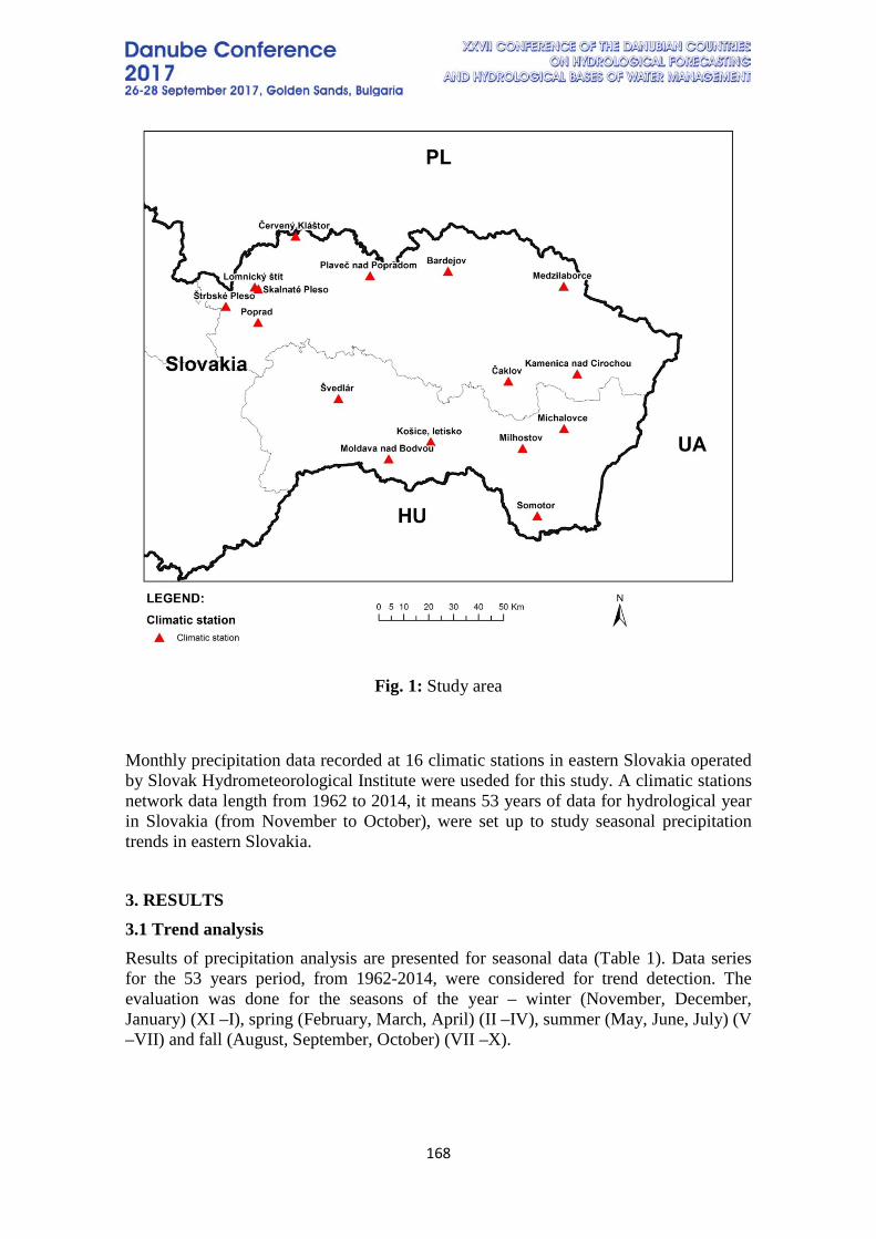
168

Fig. 1: Study area

Monthly precipitation data recorded at 16 climatic stations in eastern Slovakia operated by Slovak Hydrometeorological Institute were useded for this study. A climatic stations network data length from 1962 to 2014, it means 53 years of data for hydrological year in Slovakia (from November to October), were set up to study seasonal precipitation trends in eastern Slovakia.

3. RESULTS 3.1 Trend analysis Results of precipitation analysis are presented for seasonal data (Table 1). Data series for the 53 years period, from 1962-2014, were considered for trend detection. The evaluation was done for the seasons of the year – winter (November, December, January) (XI –I), spring (February, March, April) (II –IV), summer (May, June, July) (V –VII) and fall (August, September, October) (VII –X).

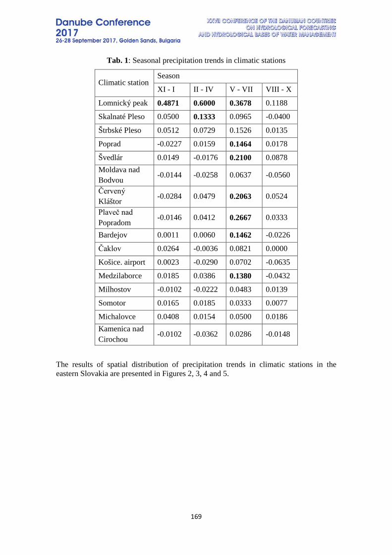
169

Tab. 1: Seasonal precipitation trends in climatic stations

Climatic station Season

XI - I II - IV V - VII VIII - X

Lomnický peak 0.4871 0.6000 0.3678 0.1188

Skalnaté Pleso 0.0500 0.1333 0.0965 -0.0400

Štrbské Pleso 0.0512 0.0729 0.1526 0.0135

Poprad -0.0227 0.0159 0.1464 0.0178

Švedlár 0.0149 -0.0176 0.2100 0.0878 Moldava nad Bodvou -0.0144 -0.0258 0.0637 -0.0560

Červený Kláštor -0.0284 0.0479 0.2063 0.0524

Plaveč nad Popradom

-0.0146 0.0412 0.2667 0.0333

Bardejov 0.0011 0.0060 0.1462 -0.0226

Čaklov 0.0264 -0.0036 0.0821 0.0000

Košice. airport 0.0023 -0.0290 0.0702 -0.0635

Medzilaborce 0.0185 0.0386 0.1380 -0.0432

Milhostov -0.0102 -0.0222 0.0483 0.0139

Somotor 0.0165 0.0185 0.0333 0.0077

Michalovce 0.0408 0.0154 0.0500 0.0186 Kamenica nad Cirochou -0.0102 -0.0362 0.0286 -0.0148

The results of spatial distribution of precipitation trends in climatic stations in the eastern Slovakia are presented in Figures 2, 3, 4 and 5.

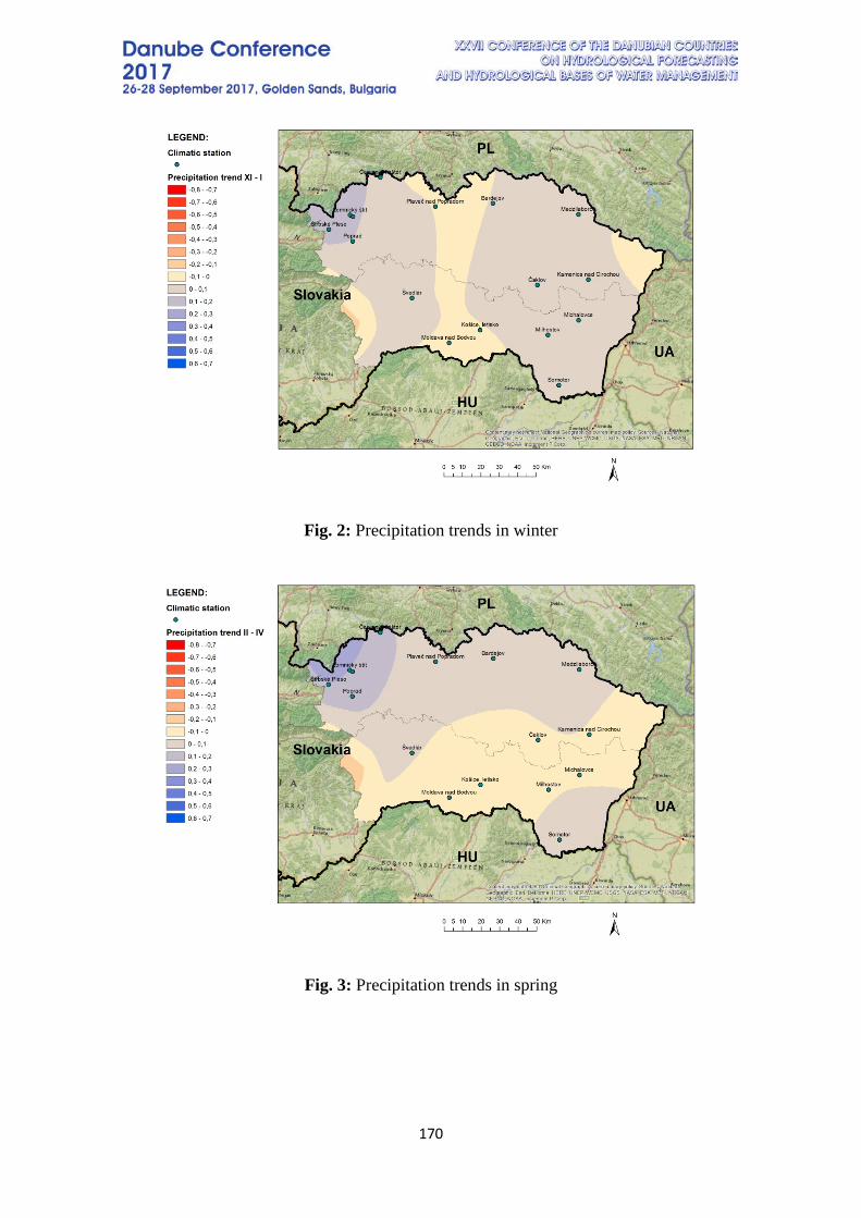
170

Fig. 2: Precipitation trends in winter

Fig. 3: Precipitation trends in spring

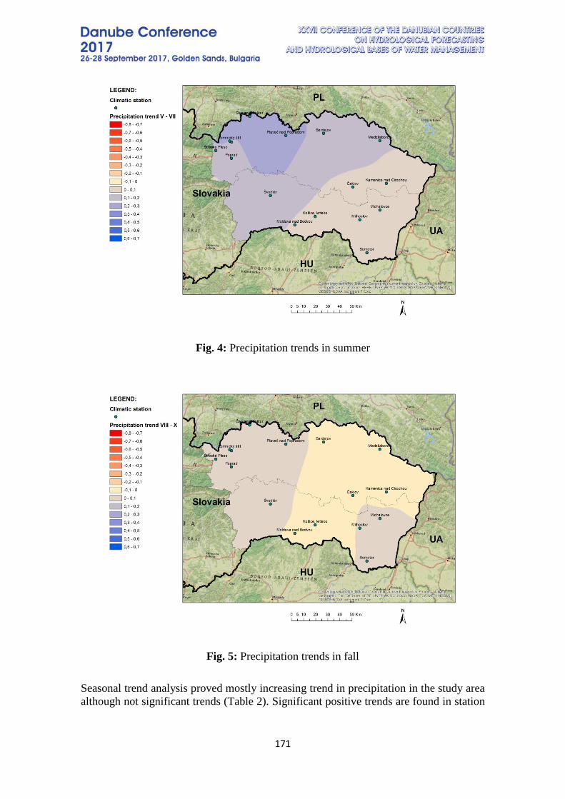
171

Fig. 4: Precipitation trends in summer

Fig. 5: Precipitation trends in fall

Seasonal trend analysis proved mostly increasing trend in precipitation in the study area although not significant trends (Table 2). Significant positive trends are found in station

172

Lomnický štít in the mountains – the High Tatras (north part of Slovakia). Significant positive trends in precipitation are obvious during the summer season. No significant trends are found in fall. Trends in precipitation are also mostly positive during winter and spring, although some negative trends were also found during these seasons.

4. CONCLUSION In this paper, the results of seasonal trend analysis applied to precipitation data is presented for the hydrological year (from November to October) in sixteen climatic stations in eastern Slovakia. The topography of this part of the country is very diverse and it affects the climate. The Mann-Kendall non parametric test coupled with the Sen’s slope was applied to identify the significant long-term climatic trends, as well as the magnitude of those trends. Trends in precipitation are mostly positive during winter and spring, although some negative trends were also found during these seasons. Spatial distribution of precipitation trends was modelled in ArcGIS using geostatistical analysis. The application of trend detection in eastern Slovakia has resulted in the identification of a few increasing significant trends in precipitation data. Spatial differences in the trend results can be expected to occur as a result of spatial differences in the changes in precipitation over the study area and spatial differences in the country characteristics. As expected, trends show large variability in magnitude and direction of trend from one station to another related to the topography of the country. It is clear that slight climatic changes may have affected the magnitude and timing of the atmospheric variables within the study area. This paper develops a picture of recent precipitation trends in climatic stations across the region of eastern Slovakia, which should be of interest to future agriculture and water resource management.

5. REFERENCES [1] Kovats R.S., Valentini R., Bouwer L.M., Georgopoulou E., Jacob D., Martin E., Rounsevell M., & Soussana J.F. Europe. In: Climate Change 2014: Impacts, Adaptation, and Vulnerability. Part B: Regional Aspects. Contribution of Working Group II to the Fifth Assessment Report of the Intergovernmental Panel on Climate Change [Barros, V.R., C.B. Field, D.J. Dokken, M.D. Mastrandrea, K.J. Mach, T.E. Bilir, M. Chatterjee, K.L. Ebi, Y.O. Estrada, R.C. Genova, B. Girma, E.S. Kissel, A.N. Levy, S. MacCracken, P.R. Mastrandrea, and L.L. White (eds.)]. Cambridge University Press, Cambridge, United Kingdom and New York, NY, USA, pp. 1267-1326, 2014. [2] Bara M., Gaál L., Kohnová S., Szolgay J. & Hlavčová, K. On the use of the simple scaling of heavy rainfall in a regional estimation of IDF curves in Slovakia. J. Hydrol. Hydromech., DOI: 10.2478/v10098-010-0006-0 49/ 58, 1, 49–63. 2010. [3] Faško P., Pecho J., Mikulová K. & Nejedlik, P. Trends of selected characteristics of precipitation in the northern Carpathians in the light of water supply for agriculture. In Eitzinger, J., and Kubu, GH. (2009), Impact of Climate Change and Adaptation in Agriculture. Extended abstracts of the International Symposium. Vienne, Austria. 106-

173

109. BOKU-Met Report 17, 106-109, ISSN 1994-4179 (print), ISSN 1994-4187 (online) - http://www.boku.ac.at/met/report. 2009. [4] Fendeková M., Pekárová P., Fendek M., Pekár J. & Škoda, P. Global drivers effect in multi-annual variability of runoff. J. Hydrol. Hydromech., DOI: 10.2478/johh-2014-0027169/ 62, 3, 169–176. 2014. [5] Oosterwijk J., van Loon A. F., Machlica A., Horvát O., van Lanen H.A.J. & Fendeková M. Hydrological drought characteristics of the Nedozery sub catchment, upper Nitra, Slovakia, based on HBY modelling. Technical Report n.º 20. WATCH – Water and Global Change. 2009. [6] Pekárová P., Onderka M., Pekár J., Rončák P. & Miklánek P. Prediction of water quality in the Danube River under extreme hydrological and temperature conditions. J. Hydrol. Hydromech., DOI: 10.2478/v10098-009-0001-53 / 57, 1, 3–15. 2009. [7] Vido J., Tadesse T., Šustek Z., Kandrík R., Hanzelová M., Škvarenina J., Škvareninová, J. & Hayes, M. Drought occurrence in Central European mountainous region (Tatra National Park – Slovakia) within the period 1961-2010. Advances in Meteorology. Hindawi Publishing Corporation. DOI:10.1155/2015/248728/ pp.1-8. 2015. [8] Mann, H.B. Non-parametric tests against trend. Econometrica 13, 245–259. 1945. [9] Kendall, M.G. Rank Correlation Measures. Charles Griffin, London, U.K. 1975. [10] Burn D.H. & Hag Elnur M.A. Detection of hydrologic trends and variability, Journal of Hydrology, DOI:10.1016/S0022-1694(01)00514-5/ 255(1-4), 107–122. 2002. [11] Cunderlik J.M., & Burn D.H. Local and regional trends in monthly maximum flows in southern British Columbia. Canadian Water Resources Journal 27. 2002. [12] Clark I. Practical Geostatistics. Applied Science Publishers, London, U.K. 1979.

6. COPYRIGHT/ACKNOWLEDGEMENTS The contribution is written thanks to support of bilateral project of Slovak Research and Development Agency between Slovakia and Portugal SK-PT-2015-0007.

174

CHANGES IN WATER TEMPERATURE IN SELECTED STREAMS OF THE

MORAVA RIVER BASIN

Antonin Maly, Ondrej Ledvinka

Czech Hydrometeorological Institute, Czechia Corresponding author: Ondrej Ledvinka, Czech Hydrometeorological Institute, Hydrology Database and

Water Budget Department, Na Sabatce 2050/17, 143 06 Prague 412, Czechia, ledvinka@chmi.cz

ABSTRACT Systematic records on flowing water temperature in the Czech part of the Danube River basin started in the late 19th century. However, their detailed analyses have been – even after dozens of years with operating monitoring network – performed very rarely. The aim of the present contribution is therefore to bridge this gap at least partially, and to present the most interesting results stemming from the newly conducted analysis. Series of water temperature in daily time step (represented by morning measurements) from selected water-gauging stations located in the basin of the River Danube delineated by the Morava River are examined. Attention is drawn to the possibilities of checking and extending the records, predominantly at specified times and especially in the monthly time step. Furthermore, water temperature is compared to air temperature, and the Mann–Kendall trend test and a homogeneity check are used in order to find out what types of nonstationarity may be expected relative to water temperature in the area of interest, factoring out the probable errors in the records. Based on the information gained, valuable forecasting models dealing with water temperature in the Morava River basin can be built in the future after performing further analyses recommended at the end of the contribution. Keywords: long-term development, trend analysis, climate change, Moravia

1. INTRODUCTION Compared to discharge, water temperature is often considered more easily measurable variable, which applies also to its spatial and temporal variability. However, the monitoring and the following assessment of flowing water temperature bring specific issues. In the Czech part of the Danube River, the water temperature has been systematically observed since the end of the 19th century (e.g., stations Kroměříž since 1897, Znojmo since 1897, Brno-Pisárky since 1898...), which means that the measurements started about 20 years earlier than the discharge started to be evaluated at these stations. In the past, the temperature was measured at specified times, firstly predominantly at 11, later between 6 and 8 a.m. At present, instruments that measure the water temperature practically continuously do exist. The placement of the instruments (or the location of manual reading in the past), has remarkable influence on the representativeness of the data. Ideally, the measurement of the surface water temperature has to be performed right under the water table, very close to the strongest velocity of flow and, if possible, in the section where shadows cover large part of the stream [1]. However, in practice, these requirements can hardly be satisfied, and this applies to the past as well as to the current conditions. Quality and homogeneity of the

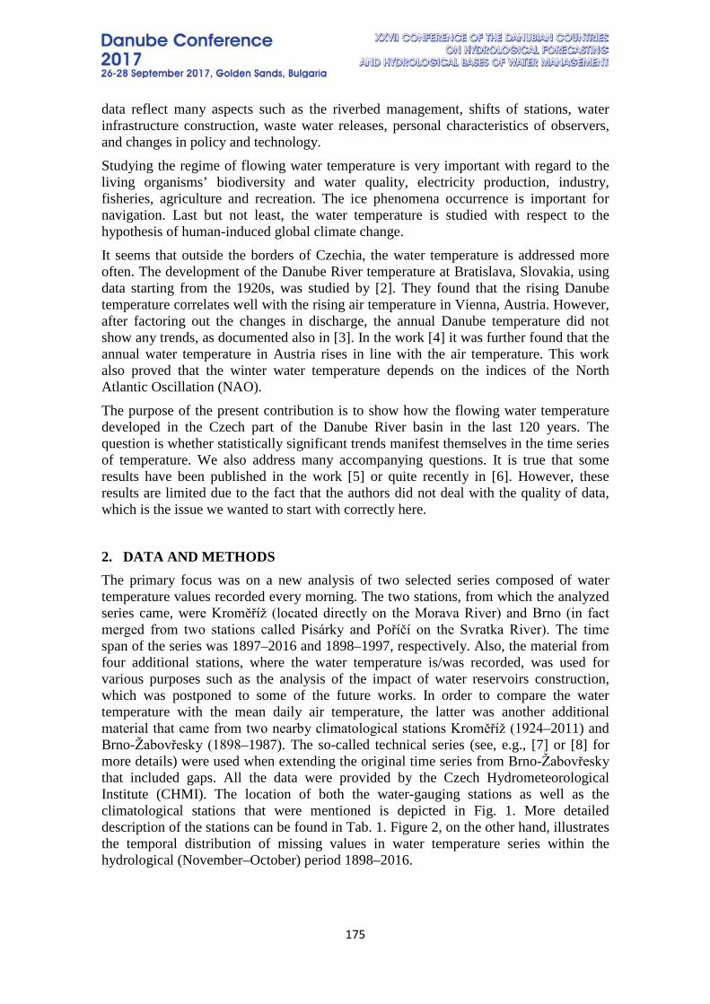
175

data reflect many aspects such as the riverbed management, shifts of stations, water infrastructure construction, waste water releases, personal characteristics of observers, and changes in policy and technology. Studying the regime of flowing water temperature is very important with regard to the living organisms’ biodiversity and water quality, electricity production, industry, fisheries, agriculture and recreation. The ice phenomena occurrence is important for navigation. Last but not least, the water temperature is studied with respect to the hypothesis of human-induced global climate change. It seems that outside the borders of Czechia, the water temperature is addressed more often. The development of the Danube River temperature at Bratislava, Slovakia, using data starting from the 1920s, was studied by [2]. They found that the rising Danube temperature correlates well with the rising air temperature in Vienna, Austria. However, after factoring out the changes in discharge, the annual Danube temperature did not show any trends, as documented also in [3]. In the work [4] it was further found that the annual water temperature in Austria rises in line with the air temperature. This work also proved that the winter water temperature depends on the indices of the North Atlantic Oscillation (NAO). The purpose of the present contribution is to show how the flowing water temperature developed in the Czech part of the Danube River basin in the last 120 years. The question is whether statistically significant trends manifest themselves in the time series of temperature. We also address many accompanying questions. It is true that some results have been published in the work [5] or quite recently in [6]. However, these results are limited due to the fact that the authors did not deal with the quality of data, which is the issue we wanted to start with correctly here.

2. DATA AND METHODS The primary focus was on a new analysis of two selected series composed of water temperature values recorded every morning. The two stations, from which the analyzed series came, were Kroměříž (located directly on the Morava River) and Brno (in fact merged from two stations called Pisárky and Poříčí on the Svratka River). The time span of the series was 1897–2016 and 1898–1997, respectively. Also, the material from four additional stations, where the water temperature is/was recorded, was used for various purposes such as the analysis of the impact of water reservoirs construction, which was postponed to some of the future works. In order to compare the water temperature with the mean daily air temperature, the latter was another additional material that came from two nearby climatological stations Kroměříž (1924–2011) and Brno-Žabovřesky (1898–1987). The so-called technical series (see, e.g., [7] or [8] for more details) were used when extending the original time series from Brno-Žabovřesky that included gaps. All the data were provided by the Czech Hydrometeorological Institute (CHMI). The location of both the water-gauging stations as well as the climatological stations that were mentioned is depicted in Fig. 1. More detailed description of the stations can be found in Tab. 1. Figure 2, on the other hand, illustrates the temporal distribution of missing values in water temperature series within the hydrological (November–October) period 1898–2016.

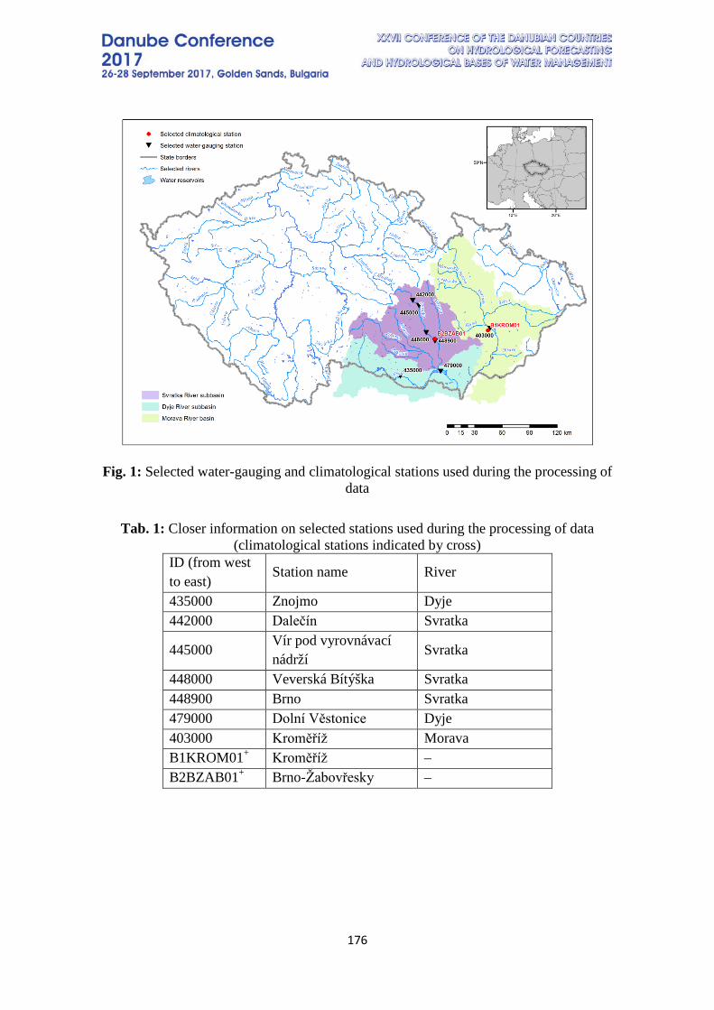
176

Fig. 1: Selected water-gauging and climatological stations used during the processing of data

Tab. 1: Closer information on selected stations used during the processing of data

(climatological stations indicated by cross) ID (from west to east)

Station name River

435000 Znojmo Dyje 442000 Dalečín Svratka

445000 Vír pod vyrovnávací nádrží Svratka

448000 Veverská Bítýška Svratka 448900 Brno Svratka 479000 Dolní Věstonice Dyje 403000 Kroměříž Morava B1KROM01+ Kroměříž – B2BZAB01+ Brno-Žabovřesky –

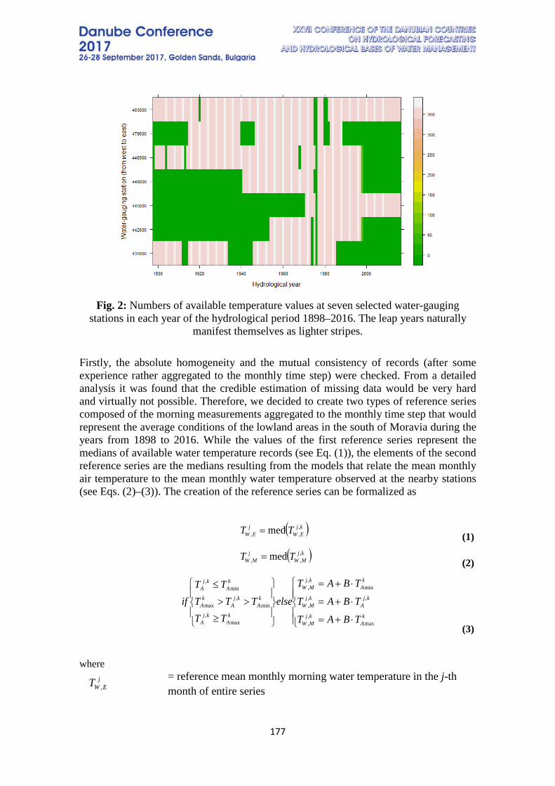
177

Fig. 2: Numbers of available temperature values at seven selected water-gauging

stations in each year of the hydrological period 1898–2016. The leap years naturally manifest themselves as lighter stripes.

Firstly, the absolute homogeneity and the mutual consistency of records (after some experience rather aggregated to the monthly time step) were checked. From a detailed analysis it was found that the credible estimation of missing data would be very hard and virtually not possible. Therefore, we decided to create two types of reference series composed of the morning measurements aggregated to the monthly time step that would represent the average conditions of the lowland areas in the south of Moravia during the years from 1898 to 2016. While the values of the first reference series represent the medians of available water temperature records (see Eq. (1)), the elements of the second reference series are the medians resulting from the models that relate the mean monthly air temperature to the mean monthly water temperature observed at the nearby stations (see Eqs. (2)–(3)). The creation of the reference series can be formalized as

( )kjEW

jEW TT ,

,, med= (1)

( )kjMW

jMW TT ,

,, med= (2)

⋅+=

⋅+=

⋅+=

≥

>>

≤

kA

kjMW

kjA

kjMW

kA

kjMW

kA

kjA

kA

kjA

kA

kA

kjA

TBAT

TBAT

TBAT

elseTT

TTTTT

if

max,,

,,,

min,,

max,

min,

max

min,

(3)

where j

EWT , = reference mean monthly morning water temperature in the j-th month of entire series

178

kjEWT ,

, = mean monthly morning water temperature at the k-th selected station and in the j-th month of entire series

jMWT , = modelled reference mean monthly morning water temperature in

the j-th month of entire series kjMWT ,

, = modelled reference mean monthly morning water temperature in the j-th month and at the k-th station

kjAT ,

= mean monthly air temperature at a climatological station closest to the k-th water-gauging station in the j-th month of entire series

kAT min resp.

kAT max

= lower/upper limiting mean monthly temperature that bound the validity of the linear models between air and water temperature at k-th water-gauging station and its closest climatological station

A and B

= parameters of the linear relationship between air and water temperature at the k-th water-gauging station and its closest climatological station; they are found by the ordinary least squares method using only the homogeneous segment of entire series

The advantage of the first reference series lies in its empirical character, its disadvantage, on the other hand, in its higher sensitivity to the large errors of random origin and to the presence of apparent inhomogeneities with respect to the operation of water infrastructure and the change in the measurement technology. The second reference series does not possess the just mentioned disadvantages. However, a high degree of idealization may be considered one of its disadvantages as well. Similar to the water temperature, the reference air temperature series were produced according to Eq. (1). From both reference series of monthly water temperature as well as from the reference monthly air temperature, anomalies were computed relative to the long-term monthly values (1898–2016). The anomalies were then smoothed by a 61-month moving window. The courses of smoothed anomalies for water and air were compared visually. In addition, the series of anomalies related to the water and air temperature were aggregated so that they formed the annual time step. These aggregated data were further subjected to the Mann–Kendall (MK) trend test combined with the so-called trend-free pre-whitening (TFPW) modification that accounts for the issue related to the possible presence of short-term persistence (STP) represented by the first-order autoregressive process (AR(1); see [9]). The trend magnitude was calculated using Sen’s approach [10]. The same analysis was performed for each individual month of the year. The last two methods have been widely applied in the recent hydrological papers, so we do not give their detailed description here.

3. RESUTLS AND DISCUSSION The courses of smoothed monthly anomalies of empirical as well as modelled reference morning water temperature, and reference air temperature relative to the long-term average (1898–2016) are presented in Fig. 3. From this plot it can be seen that, in accordance with general experience, the last third of the investigated period shows

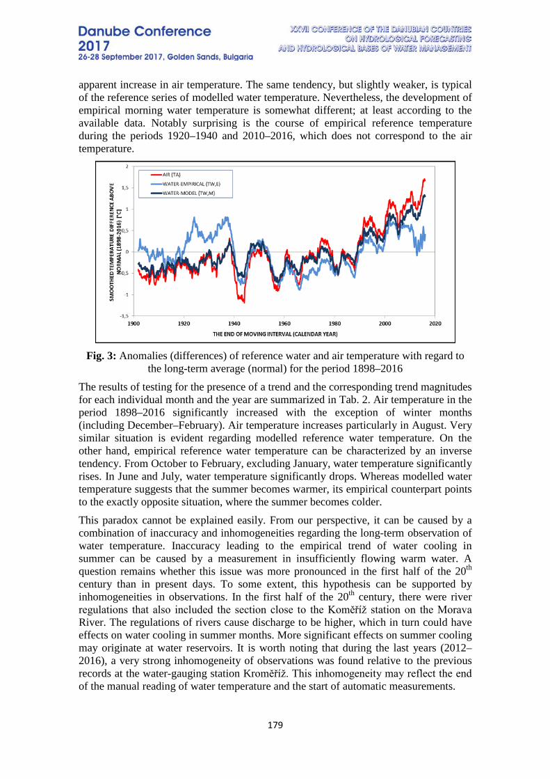
179

apparent increase in air temperature. The same tendency, but slightly weaker, is typical of the reference series of modelled water temperature. Nevertheless, the development of empirical morning water temperature is somewhat different; at least according to the available data. Notably surprising is the course of empirical reference temperature during the periods 1920–1940 and 2010–2016, which does not correspond to the air temperature.

Fig. 3: Anomalies (differences) of reference water and air temperature with regard to

the long-term average (normal) for the period 1898–2016 The results of testing for the presence of a trend and the corresponding trend magnitudes for each individual month and the year are summarized in Tab. 2. Air temperature in the period 1898–2016 significantly increased with the exception of winter months (including December–February). Air temperature increases particularly in August. Very similar situation is evident regarding modelled reference water temperature. On the other hand, empirical reference water temperature can be characterized by an inverse tendency. From October to February, excluding January, water temperature significantly rises. In June and July, water temperature significantly drops. Whereas modelled water temperature suggests that the summer becomes warmer, its empirical counterpart points to the exactly opposite situation, where the summer becomes colder. This paradox cannot be explained easily. From our perspective, it can be caused by a combination of inaccuracy and inhomogeneities regarding the long-term observation of water temperature. Inaccuracy leading to the empirical trend of water cooling in summer can be caused by a measurement in insufficiently flowing warm water. A question remains whether this issue was more pronounced in the first half of the 20th century than in present days. To some extent, this hypothesis can be supported by inhomogeneities in observations. In the first half of the 20th century, there were river regulations that also included the section close to the Koměříž station on the Morava River. The regulations of rivers cause discharge to be higher, which in turn could have effects on water cooling in summer months. More significant effects on summer cooling may originate at water reservoirs. It is worth noting that during the last years (2012–2016), a very strong inhomogeneity of observations was found relative to the previous records at the water-gauging station Kroměříž. This inhomogeneity may reflect the end of the manual reading of water temperature and the start of automatic measurements.

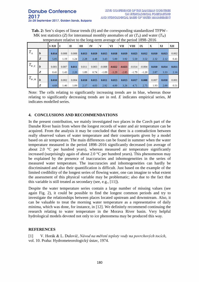
180

Tab. 2: Sen’s slopes of linear trends (b) and the corresponding standardized TFPW–MK test statistics (Z) for interannual monthly anomalies of air (TA) and water (TW)

temperature relative to the long-term average of the period 1898–2016 I-XII I II III IV V VI VII VIII IX X XI XII

AT b 0.014 0.008 0.008 0.013 0.019 0.015 0.018 0.019 0.023 0.012 0.010 0.013 0.002

Z 5.05 1.19 1.24 2.28 4.48 3.43 5.00 3.92 5.50 3.52 2.32 2.12 0.41

EWT , b 0.001 0.007 0.011 0.011 0.003 -0.008 -0.022 -0.023 -0.014 -0.004 0.010 0.014 0.011

Z 0.41 1.43 2.20 1.89 0.74 -1.09 -3.29 -2.85 -1.79 -1.20 2.87 3.33 2.16

MWT , b 0.010 0.002 0.004 0.010 0.015 0.011 0.013 0.013 0.017 0.008 0.007 0.010 0.001

Z 4.69 1.46 1.09 2.17 4.03 2.92 4.00 3.26 4.71 2.75 1.93 2.00 0.51

Note: The cells relating to significantly increasing trends are in blue, whereas those relating to significantly decreasing trends are in red. E indicates empirical series, M indicates modelled series.

4. CONCLUSIONS AND RECOMMENDATIONS In the present contribution, we mainly investigated two places in the Czech part of the Danube River basin from where the longest records of water and air temperature can be acquired. From the analysis it may be concluded that there is a contradiction between really observed values of water temperature and their counterparts given by a model based on air temperature. The main differences can be found in summer when the water temperature measured in the period 1898–2016 significantly decreased (on average of about 2.0 °C per hundred years), whereas measured air temperature significantly increased (surprisingly again of about 2.0 °C per hundred years). This phenomenon may be explained by the presence of inaccuracies and inhomogeneities in the series of measured water temperature. The inaccuracies and inhomogeneities can hardly be discriminated and also their quantification is difficult. Just based on the example of the limited credibility of the longest series of flowing water, one can imagine to what extent the assessment of this physical variable may be problematic; also due to the fact that this variable is still treated as secondary (see, e.g., [11]). Despite the water temperature series contain a large number of missing values (see again Fig. 2), it could be possible to find the longest common periods and try to investigate the relationships between places located upstream and downstream. Also, it can be valuable to treat the morning water temperature as a representative of daily minima, which was done, for instance, in [12]. We definitely recommend continuing the research relating to water temperature in the Morava River basin. Very helpful hydrological models devoted not only to ice phenomena may be produced this way.

REFERENCES [1] V. Horák & L. Dulovič, Návod na měření teploty vody na povrchových tocích, vol. 10. Praha: Hydrometeorologický ústav, 1974.

181

[2] P. Pekárová & D. Halmová, “Vývoj teploty vody Dunaja v Bratislave za období 1926-2005,” Meteorol. Bull., vol. 60, pp. 183–187, 2007. [3] P. Pekarova, D. Halmova, P. Miklanek, M. Onderka, J. Pekar, & P. Skoda, “Is the water temperature of the Danube River at Bratislava, Slovakia, rising?,” J. Hydrometeorol., vol. 9, pp. 1115–1122, Oct. 2008. [4] B. W. Webb & F. Nobilis, “Long-term changes in river temperature and the influence of climatic and hydrological factors,” Hydrol. Sci. J., vol. 52, no. 1, pp. 74–85, 2007. [5] M. Čermák, Teploty vody na moravských tocích. Praha: Hydrometeorologický ústav, 1959. [6] O. Novický et al., Teploty vody v tocích České republiky. Praha: Výzkumný ústav vodohospodářský T. G. Masaryka, 2009. [7] P. Štěpánek, P. Zahradníček, & R. Huth, “Interpolation techniques used for data quality control and calculation of technical series: an example of a Central European daily time series,” Idöjárás, vol. 115, no. 1–2, pp. 87–98, 2011. [8] P. Štěpánek, P. Zahradníček, & A. Farda, “Experiences with data quality control and homogenization of daily records of various meteorological elements in the Czech Republic in the period 1961-2010,” Idöjárás, vol. 117, no. 1, pp. 123–141, 2013. [9] S. Yue, P. Pilon, B. Phinney, & G. Cavadias, “The influence of autocorrelation on the ability to detect trend in hydrological series,” Hydrol. Process., vol. 16, no. 9, pp. 1807–1829, Jun. 2002. [10] P. K. Sen, “Estimates of the regression coefficient based on Kendall’s tau,” J. Am. Stat. Assoc., vol. 63, no. 324, pp. 1379–1389, Dec. 1968. [11] H. G. Orr et al., “Detecting changing river temperatures in England and Wales,” Hydrol. Process., vol. 29, pp. 752–766, 2015. [12] P. Pekárová et al., “Long-term trend and multi-annual variability of water temperature in the pristine Bela River basin (Slovakia),” J. Hydrol., vol. 400, no. 3–4, pp. 333–340, Apr. 2011.

5. ACKNOWLEDGEMENTS The authors would like to thank Dr. Gražyna Knozová for providing them with climatological data and selected literature. Furthermore, Ing. Eva Soukalová, CSc., and Ladislav Budík, p.f., are greatly acknowledged for their substantial help when searching for relevant literature and for a valuable discussion of the presented results.

182

NATURAL AND ANTHROPOGENIC TRANSFORMATION OF ANNUAL RUNOFF OF TRANSBOUNDARY RIVERS OF KURA RIVER BASIN

1 Farda Imanov, 1 Aytan Guliyeva, 2 Jovan Despotovich, 1Anar Nuriyev

1Baku State University, Azerbaijan 2Belgrade State University, Serbia

Corresponding author: Farda Imanov, Baku State University, Azerbaijan, farda_imanov@mail.ru

The Kura River is the longest transboundary river of the South Caucasus and five countries are located in its basin either fully or partially: Turkey, Georgia, Azerbaijan, Armenia and the Islamic Republic of Iran. The Kura River flows into the Caspian Sea and is the recipient of numerous tributaries as it flows downstream . Its water resources are widely used for different purposes in all five countries. Consequently, the annual flow of Kura River undergoes both natural and anthropogenic transformation along the river. At the closing section of the Kura River (Salyan station), annual runoff decreased by 425 m3s-1 or 49.8%: 325 m3s-1 reduction was observed directly in the Kura basin, and 100 m3s-1 reduction in Aras basin. Keywords: the Kura River, transformation of runoff, transboundary rivers, hydrograph, trend analysis, anthropogenic factors One of the pressing global problems of the 21st century is water provision for various sectors of the population and economy. Use of water resources is growing rapidly all over the world due to population growth and economic development, and water supply in most regions and countries is sharply deteriorating. A decreasing tendency in available water resources is observed as a result of global warming. Aggravation of these water problems has a direct impact on food supply for populations and the ecological safety of regions. Moreover, water has become recognized as one of the key factors for sustainable development. One of the important features of river runoff is a quick reaction of its quantitative indicators to external influences, known as ‘transformation of runoff.’ Due to transformation of runoff, several changes are observed:

• Changes in absolute quantity of solute and suspended substances in river runoff in the river system, as well as in water;

• Changes in river runoff and the regime of its transferred substances; • Changes in the composition of solute and suspended substances.

The reasons for transformation of runoff can be both natural and/or anthropogenic. General information about the Kura River Basin The Kura River is the longest transboundary river of the South Caucasus and five countries are located in its basin either fully or partially: Turkey, Georgia, Azerbaijan, Armenia and the Islamic Republic of Iran. The Kura River flows into the Caspian Sea and is the recipient of numerous tributaries as it flows downstream (Figure 1). Its water resources are widely used for different purposes in all five countries. Consequently, the

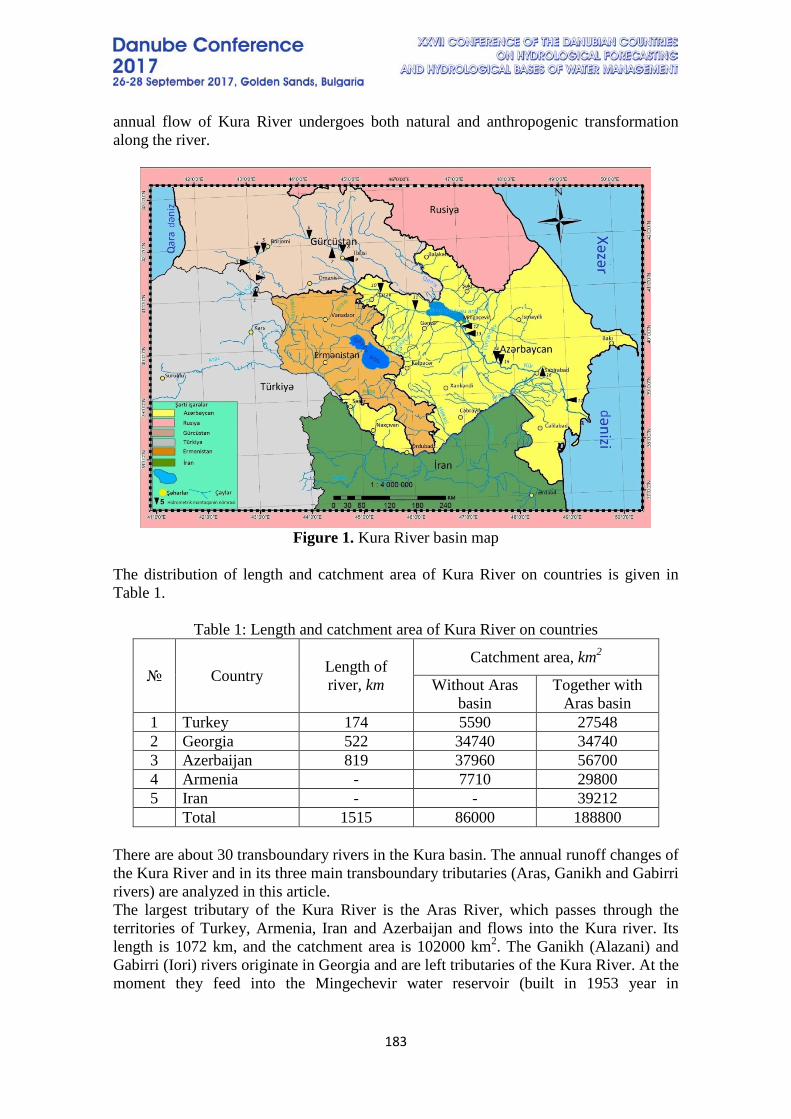
183

annual flow of Kura River undergoes both natural and anthropogenic transformation along the river.

Figure 1. Kura River basin map

The distribution of length and catchment area of Kura River on countries is given in Table 1.

Table 1: Length and catchment area of Kura River on countries

№ Country Length of river, km

Catchment area, km2

Without Aras basin

Together with Aras basin

1 Turkey 174 5590 27548 2 Georgia 522 34740 34740 3 Azerbaijan 819 37960 56700 4 Armenia - 7710 29800 5 Iran - - 39212 Total 1515 86000 188800

There are about 30 transboundary rivers in the Kura basin. The annual runoff changes of the Kura River and in its three main transboundary tributaries (Aras, Ganikh and Gabirri rivers) are analyzed in this article. The largest tributary of the Kura River is the Aras River, which passes through the territories of Turkey, Armenia, Iran and Azerbaijan and flows into the Kura river. Its length is 1072 km, and the catchment area is 102000 km2. The Ganikh (Alazani) and Gabirri (Iori) rivers originate in Georgia and are left tributaries of the Kura River. At the moment they feed into the Mingechevir water reservoir (built in 1953 year in

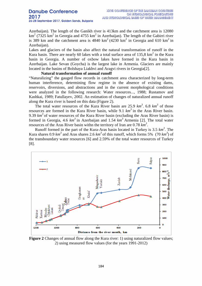
184

Azerbaijan). The length of the Ganikh river is 413km and the catchment area is 12080 km2 (7325 km2 in Georgia and 4755 km2 in Azerbaijan). The length of the Gabirri river is 389 km and the catchment area is 4840 km2 (4230 km2 in Georgia and 610 km2 in Azerbaijan). Lakes and glaciers of the basin also affect the natural transformation of runoff in the Kura basin. There are nearly 60 lakes with a total surface area of 135,8 km2 in the Kura basin in Georgia. A number of oxbow lakes have formed in the Kura basin in Azerbaijan. Lake Sevan (Goycha) is the largest lake in Armenia. Glaciers are mainly located in the basins of Bolshaya Liakhvi and Aragvi rivers in Georgia[2]. Natural transformation of annual runoff “Naturalizing” the gauged flow records in catchment area characterized by long-term human interference, determining flow regime in the absence of existing dams, reservoirs, diversions, and abstractions and in the current morphological conditions were analyzed in the following research: Water resources..., 1988; Rustamov and Kashkai, 1989; Fatullayev, 2002. An estimation of changes of naturalized annual runoff along the Kura river is based on this data (Figure 2). The total water resources of the Kura River basin are 25.9 km3. 6.8 km3 of those resources are formed in the Kura River basin, while 9.1 km3 in the Aras River basin. 9.39 km3 of water resources of the Kura River basin (excluding the Aras River basin) is formed in Georgia, 4.6 km3 in Azerbaijan and 1.54 km3 Armenia [2]. The total water resources of the Aras River basin withn the territory of Iran are 0.78 km3. Runoff formed in the part of the Kura-Aras basin located in Turkey is 3.5 km3. The Kura shares 0.9 km3 and Aras shares 2.6 km3 of this runoff, which forms 5% (70 km3) of the transboundary water resources [6] and 2.59% of the total water resources of Turkey [8].

Figure 2 Changes of annual flow along the Kura river: 1) using naturalized flow values;

2) using measured flow values (for the years 1991-2012)

185

The naturalized long-term annual flow value of the Ganikh river in the closing section is 120 m3s-1 and actually measured is 103 m3s-1 [2]. The water resources of the Gabirri river basin have various estimates. Mean annual water discharge in mouth of river is 15,9 m3s-1: 15,46 m3s-1 of it is formed in the territory of Georgia and 0,44 m3s-1 in Azerbaijan [5]. Anthropogenic transformation of annual runoff Dry climate, unequal distribution of water resources on territories, population growth, and the development of various sectors of the economy – especially the improvement of irrigation in many parts of the Kura basin – has caused an increase in water demand and volume of water abstraction from natural water sources each year, primarily from rivers. An increase in the amount of water taken without recharge has caused significant changes in the regime of Kura river and its main tributaries. The runoff of most rivers has been reduced, and as a result of long-term and in-year control, the natural distribution regularities of monthly and seasonal runoff has been changed. Water reservoirs have been built on the main rivers and their tributaries in all the countries of the basin. The total volume of Samgor, Sion and Tsalki water reservoirs in Georgia is 0.945 km3. There are more than 30 water reservoirs in Armenia. 0.974 km3 water has been collected in the larger water reservoirs of Arpilich, Aparan, Akhuryan, Tolors and Spandaryan [4]. 2,6 million people inhabit the Aras River Basin of the Islamic Republic of Iran. There are 636 000 ha of land suitable for agriculture. A 270 000 ha area is ploughed. Irrigated areas are in the Mughan plain (90 000 ha) and along the areas of the Aras river. Water is mainly used for irrigation. The amount of this water is 3.270 km3: 2.277 km3 of it is surface water and 0.993 km3 underground water. Underground water is mainly used as potable water in this area [9]. Before the construction of the Mingachevir water reservoir, the observed annual runoff of the Kura river changed along the river as follows: near Tbilisi 203 m3s-1, in Mingachevir 397 m3s-1 and in Sabirabad 586 m3s-1 [1]. In the closing section (Sabirabad station) of the river, measured annual runoff has been 267 m3s-1 or 31% less in comparison with naturalized flow value. The main reason for this runoff decreasing is water abstraction from the tributaries of the Kura River for irrigation purposes. As a result of linear trend analysis of observation data through 2010, it has been determined that there is no significant change in the annual runoff of the Kura River up to Tbilisi station over the long term. Reduction in the runoff of the river in Georgia area occurs between the boundaries of Tbilisi and Azerbaijan. Here water is taken from the Kura by irrigation channels, namely the Gardabani (40 m3s-1) and Tasiskari (12 m3s-1). In Georgia 42.3 m3s-1 water is taken from Gabirri (Iori) River by the Upper Samgor (30 m3s-1) and Lower Samgor (30 m3s-1) irrigation channels, and from the Ganikh (Alazani) River by the Main Magistral channel and other channels [5]. Reduction in runoff of the Kura under anthropogenic impacts in the territory of Azerbaijan is occurring. A strong impact of anthropogenic factors on the runoff regime of the river began with the construction of the Varvara and Mingachevir water reservoirs in the years 1950-53. Later, the Shamkir (1982) and Yenikend (2000) water reservoirs over Kura River were built, as well as the Sarsang (1976) over the Terter River, in addition to other water reservoirs over the tributaries of the Kura. Approximately 20.6 km3 of water resources have been accumulated in these water reservoirs [11].

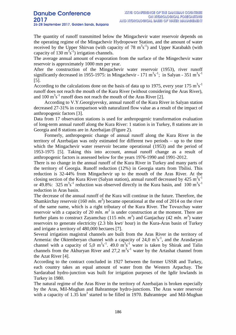
186

The quantity of runoff transmitted below the Mingachevir water reservoir depends on the operating regime of the Mingachevir Hydropower Station, and the amount of water received by the Upper Shirvan (with capacity of 78 m3s-1) and Upper Karabakh (with capacity of 130 m3s-1) irrigation channels. The average annual amount of evaporation from the surface of the Mingechevir water reservoir is approximately 1000 mm per year. After the construction of the Mingachevir water reservoir (1953), river runoff significantly decreased in 1955-1975: in Mingachevir - 171 m3s-1; in Salyan - 351 m3s-1 [5]. According to the calculations done on the basis of data up to 1975, every year 175 m3s-1 runoff does not reach the mouth of the Kura River (without considering the Aras River), and 100 m3s-1 runoff does not reach the mouth of the Aras River [2]. According to V.Y.Georgiyevsky, annual runoff of the Kura River in Salyan station decreased 27-31% in comparison with naturalized flow value as a result of the impact of anthropogenic factors [3]. Data from 17 observation stations is used for anthropogenic transformation evaluation of long-term annual runoff along the Kura River: 1 station is in Turkey, 8 stations are in Georgia and 8 stations are in Azerbaijan (Figure 2). Formerly, anthropogenic change of annual runoff along the Kura River in the territory of Azerbaijan was only estimated for different two periods – up to the time which the Mingachevir water reservoir became operational (1953) and the period of 1953-1975 [5]. Taking this into account, annual runoff change as a result of anthropogenic factors is assessed below for the years 1976-1990 and 1991-2012. There is no change in the annual runoff of the Kura River in Turkey and many parts of the territory of Georgia. Runoff reduction (12%) in Georgia starts from Tbilisi. This reduction is 32-44% from Mingachevir up to the mouth of the Aras River. At the closing section of the Kura River (Salyan station), annual runoff decreased by 425 m3s-1 or 49.8%: 325 m3s-1 reduction was observed directly in the Kura basin, and 100 m3s-1 reduction in Aras basin. The decrease of the annual runoff of the Kura will continue in the future. Therefore, the Shamkirchay reservoir (160 mln. m3) became operational at the end of 2014 on the river of the same name, which is a right tributary of the Kura River. The Tovuzchay water reservoir with a capacity of 20 mln. m3 is under construction at the moment. There are further plans to construct Zayamchay (115 mln. m3) and Ganjachay (42 mln. m3) water reservoirs to generate electricity (2.3 bln kwt/ hour) in the Kura-Aras basin of Turkey and irrigate a territory of 480,000 hectares [7]. Several irrigation magistral channels are built from the Aras River in the territory of Armenia: the Oktemberyan channel with a capacity of 24,0 m3s-1, and the Arasdaryan channel with a capacity of 5,0 m3s-1. 49.0 m3s-1 water is taken by Shirak and Talin channels from the Akhuryan River and 27,2 m3s-1 water by the Artashat channel from the Azat River [4]. According to the contract concluded in 1927 between the former USSR and Turkey, each country takes an equal amount of water from the Western Arpachay. The Sardarabad hydro-junction was built for irrigation purposes of the Igdir lowlands in Turkey in 1980. The natural regime of the Aras River in the territory of Azerbaijan is broken especially by the Aras, Mil-Mughan and Bahramtepe hydro-junctions. The Aras water reservoir with a capacity of 1.35 km3 started to be filled in 1970. Bahramtepe and Mil-Mughan

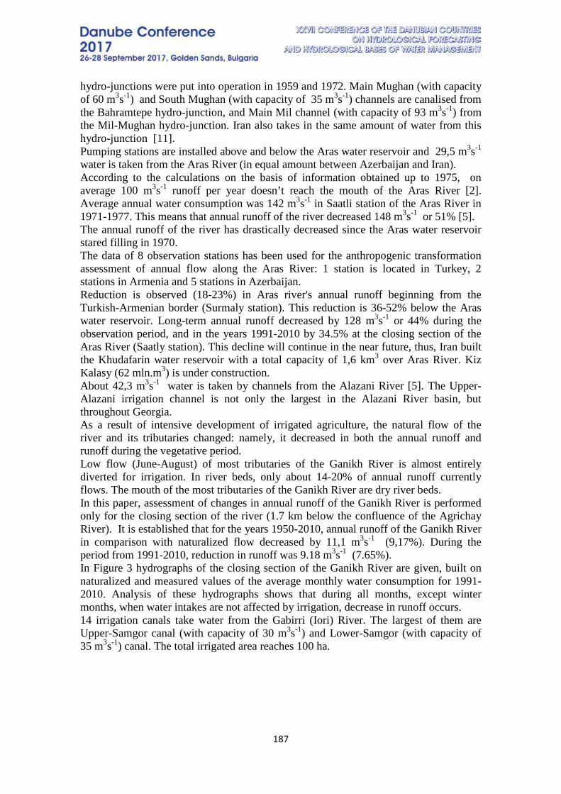
187

hydro-junctions were put into operation in 1959 and 1972. Main Mughan (with capacity of 60 m3s-1) and South Mughan (with capacity of 35 m3s-1) channels are canalised from the Bahramtepe hydro-junction, and Main Mil channel (with capacity of 93 m3s-1) from the Mil-Mughan hydro-junction. Iran also takes in the same amount of water from this hydro-junction [11]. Pumping stations are installed above and below the Aras water reservoir and 29,5 m3s-1 water is taken from the Aras River (in equal amount between Azerbaijan and Iran). According to the calculations on the basis of information obtained up to 1975, on average 100 m3s-1 runoff per year doesn’t reach the mouth of the Aras River [2]. Average annual water consumption was 142 m3s-1 in Saatli station of the Aras River in 1971-1977. This means that annual runoff of the river decreased 148 m3s-1 or 51% [5]. The annual runoff of the river has drastically decreased since the Aras water reservoir stared filling in 1970. The data of 8 observation stations has been used for the anthropogenic transformation assessment of annual flow along the Aras River: 1 station is located in Turkey, 2 stations in Armenia and 5 stations in Azerbaijan. Reduction is observed (18-23%) in Aras river's annual runoff beginning from the Turkish-Armenian border (Surmaly station). This reduction is 36-52% below the Aras water reservoir. Long-term annual runoff decreased by 128 m3s-1 or 44% during the observation period, and in the years 1991-2010 by 34.5% at the closing section of the Aras River (Saatly station). This decline will continue in the near future, thus, Iran built the Khudafarin water reservoir with a total capacity of 1,6 km3 over Aras River. Kiz Kalasy (62 mln.m3) is under construction. About 42,3 m3s-1 water is taken by channels from the Alazani River [5]. The Upper-Alazani irrigation channel is not only the largest in the Alazani River basin, but throughout Georgia. As a result of intensive development of irrigated agriculture, the natural flow of the river and its tributaries changed: namely, it decreased in both the annual runoff and runoff during the vegetative period. Low flow (June-August) of most tributaries of the Ganikh River is almost entirely diverted for irrigation. In river beds, only about 14-20% of annual runoff currently flows. The mouth of the most tributaries of the Ganikh River are dry river beds. In this paper, assessment of changes in annual runoff of the Ganikh River is performed only for the closing section of the river (1.7 km below the confluence of the Agrichay River). It is established that for the years 1950-2010, annual runoff of the Ganikh River in comparison with naturalized flow decreased by 11,1 m3s-1 (9,17%). During the period from 1991-2010, reduction in runoff was 9.18 m3s-1 (7.65%). In Figure 3 hydrographs of the closing section of the Ganikh River are given, built on naturalized and measured values of the average monthly water consumption for 1991-2010. Analysis of these hydrographs shows that during all months, except winter months, when water intakes are not affected by irrigation, decrease in runoff occurs. 14 irrigation canals take water from the Gabirri (Iori) River. The largest of them are Upper-Samgor canal (with capacity of 30 m3s-1) and Lower-Samgor (with capacity of 35 m3s-1) canal. The total irrigated area reaches 100 ha.

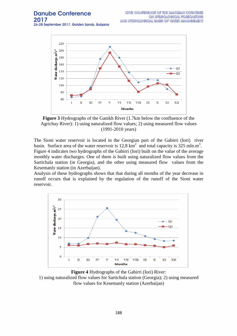
188

Figure 3 Hydrographs of the Ganikh River (1.7km below the confluence of the

Agrichay River): 1) using naturalized flow values; 2) using measured flow values (1991-2010 years)

The Sioni water reservoir is located in the Georgian part of the Gabirri (Iori) river basin. Surface area of the water reservoir is 12,8 km2 and total capacity is 325 mln.m3. Figure 4 indicates two hydrographs of the Gabirri (Iori) built on the value of the average monthly water discharges. One of them is built using naturalized flow values from the Sartichala station (in Georgia), and the other using measured flow values from the Kesemanly station (in Azerbaijan). Analysis of these hydrographs shows that that during all months of the year decrease in runoff occurs that is explained by the regulation of the runoff of the Sioni water reservoir.

Figure 4 Hydrographs of the Gabirri (Iori) River:

1) using naturalized flow values for Sartichala station (Georgia); 2) using measured flow values for Kesemanly station (Azerbaijan)

189

Reduction in the runoff of transboundary rivers of the Kura River basin occurs mainly under the influence of anthropogenic factors. Modern climate change in the region contributes to the reduction of the river runoff as well. Over the past decade, the average annual amount of precipitation decreased by 9.9% in Azerbaijan and by 6.0% in Armenia. Only in Eastern Georgia did they increase by 6.0%. Average annual air temperature generally increased: 0.52°C in Azerbaijan, 0.6°C in Eastern Georgia and 0.85°C in Armenia [10]. Decrease in runoff in the territory of Azerbaijan and the Kura basin has environmental (degradation of specific ecosystems and natural landscapes, reduction in the river's natural ability to clean itself, increase in the concentration of pollutants, etc.) and socio-economic impacts (loss of productivity of agricultural land due to the lack of irrigation water, the reduction in income in the agricultural sector, intensive use of groundwater in order to compensate for the reduction of river runoff).

Conclusion 1. Annual runoff of Kura River decreased by 32-44% from the Mingechevir water

reservoir till the Aras river mouth. The annual runoff in the closing section (Salyan) of the Kura River is 425 m3s-1, having decreased by 49.8%. 325 m3s-1 reduction occurred directly in the Kura basin and 100 m3s-1 reduction occurred in the Aras basin.

2. Anthropogenic reduction (18-23%) of annual flow of the Aras river begins from the boundaries of Turkey and Armenia (Surmali). Below Aras water reservoirs’ dam section this reduction is 36-52%. Annual flow decreased by 128 m3s-1 or 44% during the observation period, and in 1991-2010 years by 34.5% at closing section of the Aras River (Saatly).

3. It was found that for the years 1950-2010, annual river runoff of Ganikh decreased by 11.1 m3s-1 (9.17%) in comparison with naturalized flow value. During the period from 1991-2010, reduction in runoff is 9,18 m3s-1 (7.65%).

4. It was found that in all months of the year, there is a decrease in runoff of Gabirri that is explained by runoff regulation of the Sioni reservoir.

LITERATURE 1. Rustamov S.H. Azerbaijan SSR rivers and their hydrological characteristics. Baku,

Azerb.USSR AS edition, 1960. – 196 p. (in Azeribaijani language) 2. Water resources of the Caucasus (Ed. G.G.Svanidze and V.Sh.Tsomaya):

Hydrometeoizdat, 1988. – 264 p. (in Russian language) 3. Georgievsky V.Y. Change in the runoff of rivers of Russia and the water balance of

the Caspian Sea under the influence of economic activity and global warming. An abstract of dissertation for Phd in Geographycal Sciences – St. Petersburg, 2005 – 39 p. (in Russian language)

4. Fatullayev G.Y. Recent changes in water resources and water regime of rivers of the South Caucasus (within the Caspian basin). Baku, 2002. – 167 p. (in Russian language)

5. Rustamov S.G., Kashkai R.M. Water resources of Azerbaijan USSR. Baku. Sci.,1989. – 184 p. (in Russian language)

6. Ozish U, Y.Ozdemir.Turkey’s Transboundary watercourses and the Euphrates-Tigris Basin.// Transboundary Waters and Turkey. Istambul. 2009.-pp.21-57.

190

7. D.S.İ.,1995: Statistical bulletin with map. Ankara, General Directorate of State Hydraulic Works, n.991-vııı-177, 513p.

8. Yildiz Mehmet, Ozkaya Mustafa, Gurbut Atilla, Uchar Ismail. Turkey Surface Water Patential and its change in time. // International Congress. River Basin Management. Volume I., Antalya-Turkey, 2007.-p.127-138.

9. UNDP/GEF 2007. Transboundary Diagnostic Analysis of the Kura-Aras River Basin.

10. UNDP/GEF 2013. Transboundary Diagnosnic Analysis (Up-dated) of the Kura-Aras River Basin. 202 p.

11. Imanov F. Water infrastructure of Kura River Basin within Azerbaijan // International Congress River Basin Management. Volume I. Antalya-Turkey, 2007, p.99-105.

191

UPDATE OF THE TECHNOLOGICAL SCHEME FOR ASSESSMENT OF SURFACE WATER RESOURCES ON THE TERRITORY OF BULGARIA

Plamen Ninov, Tzviatka Karagiozova, Elena Bojilova, Neviana Todorova, Kamelia

Krumova, Rymiana Dobreva, Antoaneta Boeva, Radoslava Ivanova, Maya Rankova

National Institute of Meteorology and Hydrology – Sofia, Bulgaria

Corresponding author: Plamen Ninov, National Institute of Meteorology and Hydrology, Sofia, Bulgaria, Ninov.Plamen@gmail.com

ABSTRACT Internal renewable water resources are defined as the average annual flow of rivers and recharge of groundwater for a given country or region generated from precipitations. The total actual renewable water resources for a country are defined as the sum of internal renewable water resources and the external renewable water resources. According to the Water Law in Bulgaria the National Institute of Meteorology and Hydrology (NIMH) at Academy of Sciences is a State Institution responsible for surface water resources determination. The present investigation is based on hydrological information from monitoring network supported by NIMH for the approved referent period 1981-2015 characterized with stable and sustainable alteration of surface runoff after the massive and large scale hydrotechnical constructions till late 70-th years of XX century. The last years an increasing need of actualization of technological scheme of surface water resources is imposing. This actualization aims the change of the regional relationships used for resource assessment as result of the new actual and hydrologically different period of observation, alteration in the monitoring network (close or opening of the new gauging stations) and finally assessment of the specific local contributions of some territories situated between the main watersheds into the formation of the total State resource. The used approach of regionalization is based on correlation between characteristic flows (or in our case the average annual flow) at the gauging stations and some characteristics of the watershed after analysis and justification. The regionalization has been done on the base of the average annual flow for the chosen referent period. The amplitude of variation of the annual runoff is assessed by a translation of the average multiannual regression to the real runoff at any concrete year. In the frame of the present study an identification of homogeneous regions has been identified for the whole territory of the country but for the resources assessment are used only the regions at the estuary or boundary areas. In the material are presented some results of the actualized scheme for the surface resources assessment for the country visualized with maps and graphics. The study is address for practical purposes to the Water Institutions in Bulgaria dealing with water management as Ministries and Basin Directorates.

192

INTRODUCTION

According to the Water Law the National Institute of Meteorology and Hydrology is a State institution responsible for fresh surface water resources determination. Till now for water resources determination was used created in 2004 technological approach, developed in the frame of a project of the Ministry of Environment and Water “Determination of average, minimal and maximal flows with different probabilities”. The investigation was based on the referent period of 1961-2002. The assessment of the available water resources in a given region depends mainly on the available hydrological information obtained by the existing monitoring network in the region; the approach of transfer of hydrological information from the limited monitoring points to the non-observed stretches and finally by the actuality of the chosen representative evaluation period or referent period. Nowadays in the country exist different approaches as well different hydrological information for assessment is in used that in many cases lead to different and/or not reliable final results. This, in turn, creates a problem in making adequate water management solutions. The reasons imposing the actualization and a technological update of the scheme for assessment of surface water resources on the territory of Bulgaria are:

- Actualization of the period of evaluation /referent period/ to actual one assessing the new climatic and/or anthropogenic impacts;

- Necessity to take into account the alterations into the monitoring hydrological network – close of some gauging stations or opening the new ones meanwhile;

- Implementation of a unified methodical approach to the transfer of information from the observed to non-observed river stretches.

The present material presents the methodological approach and some results from the actualized methodology for assessment of the internal renewable surface water resources on the territory of Bulgaria.

MONITORING AND HYDROLOGICAL INFORMATION OF SURFACE WATER

The surface water resources of the country are determined on the base of registered flows in the hydrometric network of Bulgaria supported by National Institute of Meteorology and Hydrology. At present the network consists of 200 gauging stations relatively evenly spread on the territory and located mainly on the big rivers and their first level tributaries– Fig. 1. As result of reduction of some stations during the 90_th years of XX century and opening of new gauging stations last years the hydrometric network undergoes significant changes.

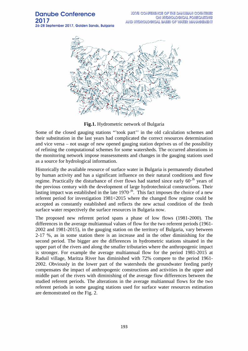
193

Fig.1. Hydrometric network of Bulgaria

Some of the closed gauging stations “’took part’’ in the old calculation schemes and their substitution in the last years had complicated the correct resources determination and vice versa – not usage of new opened gauging station deprives us of the possibility of refining the computational schemes for some watersheds. The occurred alterations in the monitoring network impose reassessments and changes in the gauging stations used as a source for hydrological information. Historically the available resource of surface water in Bulgaria is permanently disturbed by human activity and has a significant influence on their natural conditions and flow regime. Practically the disturbance of river flows had started since early 60_th years of the previous century with the development of large hydrotechnical constructions. Their lasting impact was established in the late 1970_th. This fact imposes the choice of a new referent period for investigation 1981÷2015 where the changed flow regime could be accepted as constantly established and reflects the new actual condition of the fresh surface water respectively the surface resources in Bulgaria now. The proposed new referent period spans a phase of low flows (1981-2000). The differences in the average multiannual values of flow for the two referent periods (1961-2002 and 1981-2015), in the gauging station on the territory of Bulgaria, vary between 2-17 %, as in some station there is an increase and in the other diminishing for the second period. The bigger are the differences in hydrometric stations situated in the upper part of the rivers and along the smaller tributaries where the anthropogenic impact is stronger. For example the average multiannual flow for the period 1981-2015 at Raduil village, Maritza River has diminished with 72% compere to the period 1961-2002. Obviously in the lower part of the watersheds the groundwater feeding partly compensates the impact of anthropogenic constructions and activities in the upper and middle part of the rivers with diminishing of the average flow differences between the studied referent periods. The alterations in the average multiannual flows for the two referent periods in some gauging stations used for surface water resources estimation are demonstrated on the Fig. 2.

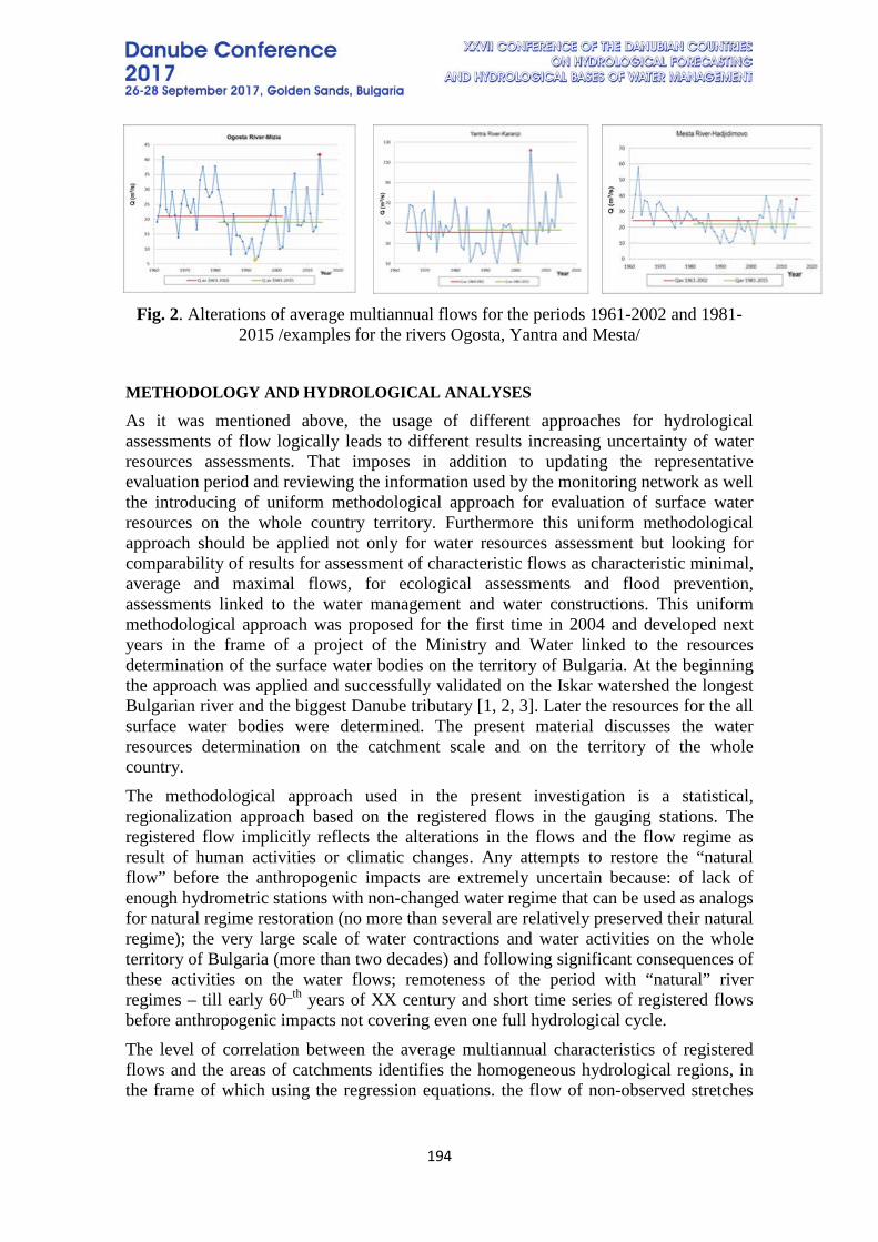
194

Fig. 2. Alterations of average multiannual flows for the periods 1961-2002 and 1981-

2015 /examples for the rivers Ogosta, Yantra and Mesta/

METHODOLOGY AND HYDROLOGICAL ANALYSES

As it was mentioned above, the usage of different approaches for hydrological assessments of flow logically leads to different results increasing uncertainty of water resources assessments. That imposes in addition to updating the representative evaluation period and reviewing the information used by the monitoring network as well the introducing of uniform methodological approach for evaluation of surface water resources on the whole country territory. Furthermore this uniform methodological approach should be applied not only for water resources assessment but looking for comparability of results for assessment of characteristic flows as characteristic minimal, average and maximal flows, for ecological assessments and flood prevention, assessments linked to the water management and water constructions. This uniform methodological approach was proposed for the first time in 2004 and developed next years in the frame of a project of the Ministry and Water linked to the resources determination of the surface water bodies on the territory of Bulgaria. At the beginning the approach was applied and successfully validated on the Iskar watershed the longest Bulgarian river and the biggest Danube tributary [1, 2, 3]. Later the resources for the all surface water bodies were determined. The present material discusses the water resources determination on the catchment scale and on the territory of the whole country. The methodological approach used in the present investigation is a statistical, regionalization approach based on the registered flows in the gauging stations. The registered flow implicitly reflects the alterations in the flows and the flow regime as result of human activities or climatic changes. Any attempts to restore the “natural flow” before the anthropogenic impacts are extremely uncertain because: of lack of enough hydrometric stations with non-changed water regime that can be used as analogs for natural regime restoration (no more than several are relatively preserved their natural regime); the very large scale of water contractions and water activities on the whole territory of Bulgaria (more than two decades) and following significant consequences of these activities on the water flows; remoteness of the period with “natural” river regimes – till early 60_th years of XX century and short time series of registered flows before anthropogenic impacts not covering even one full hydrological cycle. The level of correlation between the average multiannual characteristics of registered flows and the areas of catchments identifies the homogeneous hydrological regions, in the frame of which using the regression equations. the flow of non-observed stretches

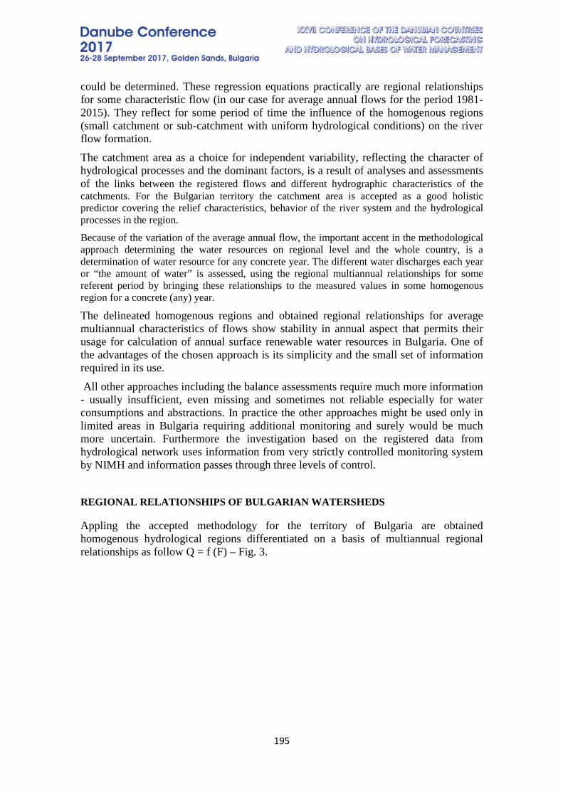
195

could be determined. These regression equations practically are regional relationships for some characteristic flow (in our case for average annual flows for the period 1981-2015). They reflect for some period of time the influence of the homogenous regions (small catchment or sub-catchment with uniform hydrological conditions) on the river flow formation. The catchment area as a choice for independent variability, reflecting the character of hydrological processes and the dominant factors, is a result of analyses and assessments of the links between the registered flows and different hydrographic characteristics of the catchments. For the Bulgarian territory the catchment area is accepted as a good holistic predictor covering the relief characteristics, behavior of the river system and the hydrological processes in the region.

Because of the variation of the average annual flow, the important accent in the methodological approach determining the water resources on regional level and the whole country, is a determination of water resource for any concrete year. The different water discharges each year or “the amount of water” is assessed, using the regional multiannual relationships for some referent period by bringing these relationships to the measured values in some homogenous region for a concrete (any) year.

The delineated homogenous regions and obtained regional relationships for average multiannual characteristics of flows show stability in annual aspect that permits their usage for calculation of annual surface renewable water resources in Bulgaria. One of the advantages of the chosen approach is its simplicity and the small set of information required in its use. All other approaches including the balance assessments require much more information - usually insufficient, even missing and sometimes not reliable especially for water consumptions and abstractions. In practice the other approaches might be used only in limited areas in Bulgaria requiring additional monitoring and surely would be much more uncertain. Furthermore the investigation based on the registered data from hydrological network uses information from very strictly controlled monitoring system by NIMH and information passes through three levels of control. REGIONAL RELATIONSHIPS OF BULGARIAN WATERSHEDS

Appling the accepted methodology for the territory of Bulgaria are obtained homogenous hydrological regions differentiated on a basis of multiannual regional relationships as follow Q = f (F) – Fig. 3.

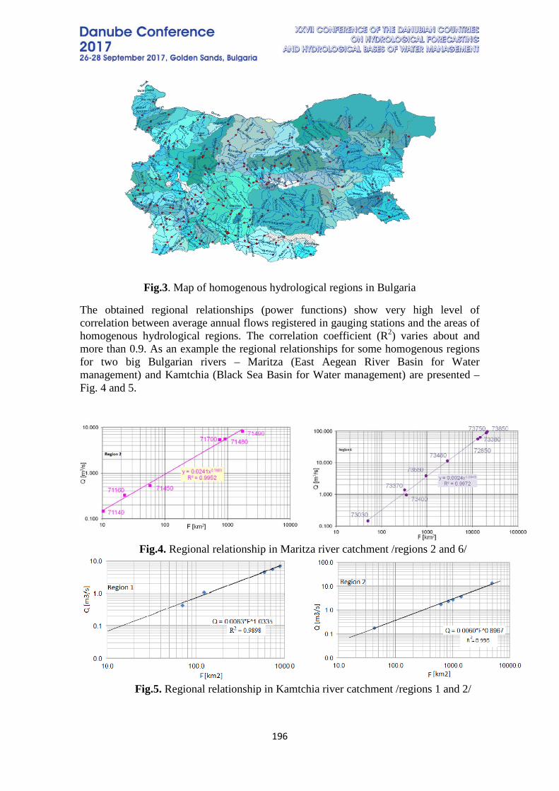
196

Fig.3. Map of homogenous hydrological regions in Bulgaria

The obtained regional relationships (power functions) show very high level of correlation between average annual flows registered in gauging stations and the areas of homogenous hydrological regions. The correlation coefficient (R2) varies about and more than 0.9. As an example the regional relationships for some homogenous regions for two big Bulgarian rivers – Maritza (East Aegean River Basin for Water management) and Kamtchia (Black Sea Basin for Water management) are presented – Fig. 4 and 5.

Fig.4. Regional relationship in Maritza river catchment /regions 2 and 6/

Fig.5. Regional relationship in Kamtchia river catchment /regions 1 and 2/

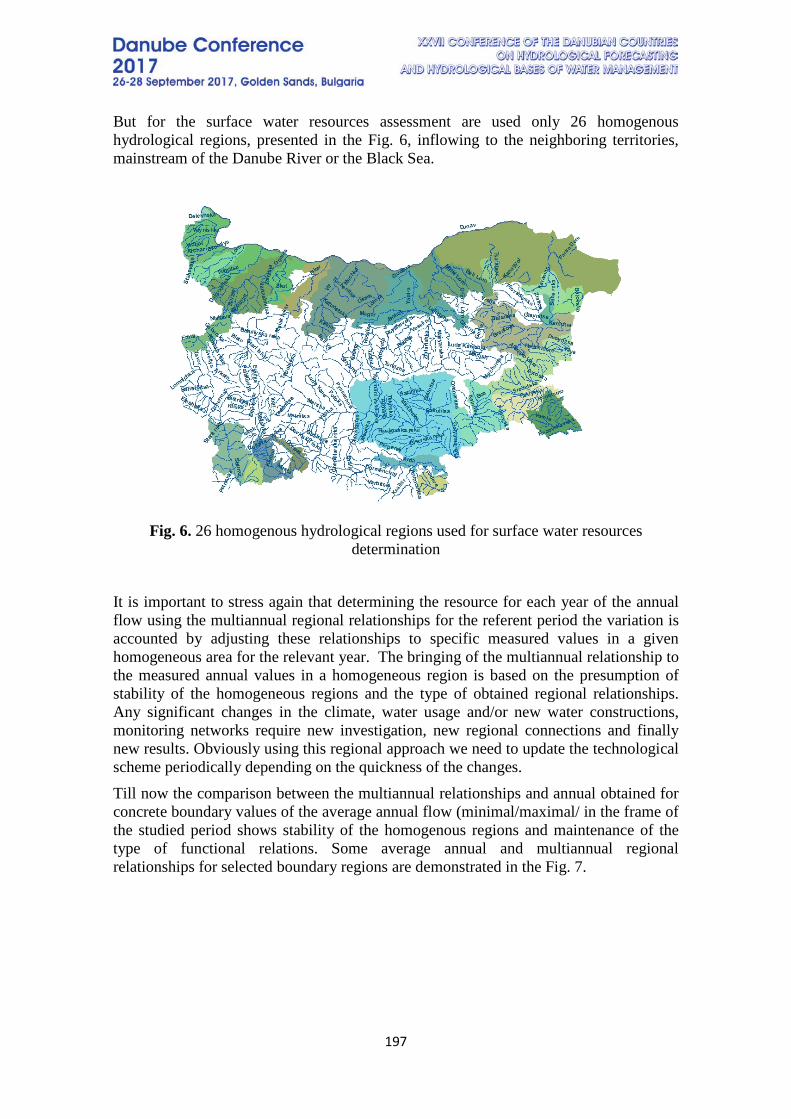
197

But for the surface water resources assessment are used only 26 homogenous hydrological regions, presented in the Fig. 6, inflowing to the neighboring territories, mainstream of the Danube River or the Black Sea.

Fig. 6. 26 homogenous hydrological regions used for surface water resources

determination

It is important to stress again that determining the resource for each year of the annual flow using the multiannual regional relationships for the referent period the variation is accounted by adjusting these relationships to specific measured values in a given homogeneous area for the relevant year. The bringing of the multiannual relationship to the measured annual values in a homogeneous region is based on the presumption of stability of the homogeneous regions and the type of obtained regional relationships. Any significant changes in the climate, water usage and/or new water constructions, monitoring networks require new investigation, new regional connections and finally new results. Obviously using this regional approach we need to update the technological scheme periodically depending on the quickness of the changes. Till now the comparison between the multiannual relationships and annual obtained for concrete boundary values of the average annual flow (minimal/maximal/ in the frame of the studied period shows stability of the homogenous regions and maintenance of the type of functional relations. Some average annual and multiannual regional relationships for selected boundary regions are demonstrated in the Fig. 7.

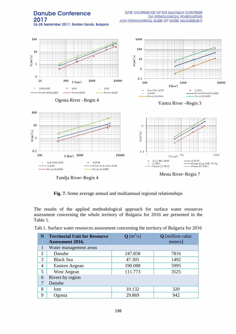
198

Ogosta River –Regin 4

Yantra River –Regin 3

Tundja River–Regin 4

Mesta River–Regin 7

Fig. 7. Some average annual and multiannual regional relationships

The results of the applied methodological approach for surface water resources assessment concerning the whole territory of Bulgaria for 2016 are presented in the Table 1. Tab.1. Surface water resources assessment concerning the territory of Bulgaria for 2016

N Territorial Unit for Resource Assessment 2016.

Q [m3/s] Q [million cubic meters]

1 Water management areas 2 Danube 247.858 7816 3 Black Sea 47.305 1492 4 Eastern Aegean 190.088 5995 5 West Aegean 111.773 3525 6 Rivers by region 7 Danube 8 lom 10.132 320 9 Ogosta 29.869 942

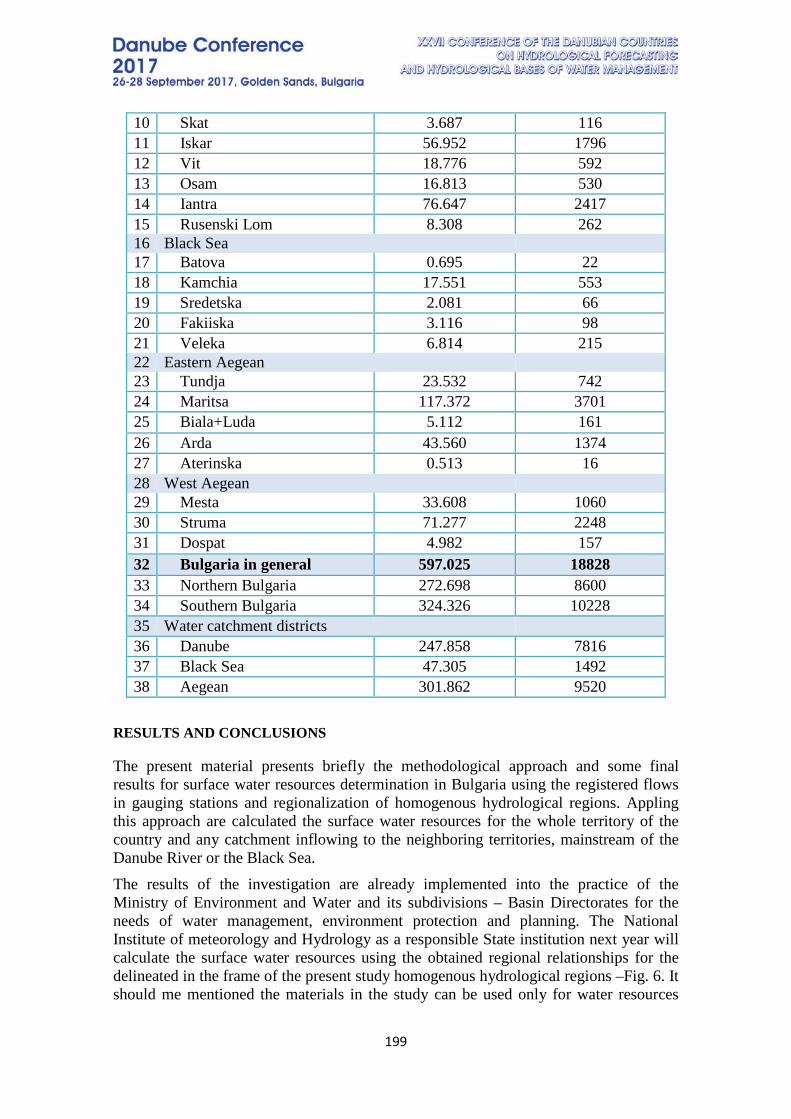
199

10 Skat 3.687 116 11 Iskar 56.952 1796 12 Vit 18.776 592 13 Osam 16.813 530 14 Iantra 76.647 2417 15 Rusenski Lom 8.308 262 16 Black Sea 17 Batova 0.695 22 18 Kamchia 17.551 553 19 Sredetska 2.081 66 20 Fakiiska 3.116 98 21 Veleka 6.814 215 22 Eastern Aegean 23 Tundja 23.532 742 24 Maritsa 117.372 3701 25 Biala+Luda 5.112 161 26 Arda 43.560 1374 27 Aterinska 0.513 16 28 West Aegean 29 Mesta 33.608 1060 30 Struma 71.277 2248 31 Dospat 4.982 157 32 Bulgaria in general 597.025 18828 33 Northern Bulgaria 272.698 8600 34 Southern Bulgaria 324.326 10228 35 Water catchment districts 36 Danube 247.858 7816 37 Black Sea 47.305 1492 38 Aegean 301.862 9520

RESULTS AND CONCLUSIONS

The present material presents briefly the methodological approach and some final results for surface water resources determination in Bulgaria using the registered flows in gauging stations and regionalization of homogenous hydrological regions. Appling this approach are calculated the surface water resources for the whole territory of the country and any catchment inflowing to the neighboring territories, mainstream of the Danube River or the Black Sea. The results of the investigation are already implemented into the practice of the Ministry of Environment and Water and its subdivisions – Basin Directorates for the needs of water management, environment protection and planning. The National Institute of meteorology and Hydrology as a responsible State institution next year will calculate the surface water resources using the obtained regional relationships for the delineated in the frame of the present study homogenous hydrological regions –Fig. 6. It should me mentioned the materials in the study can be used only for water resources

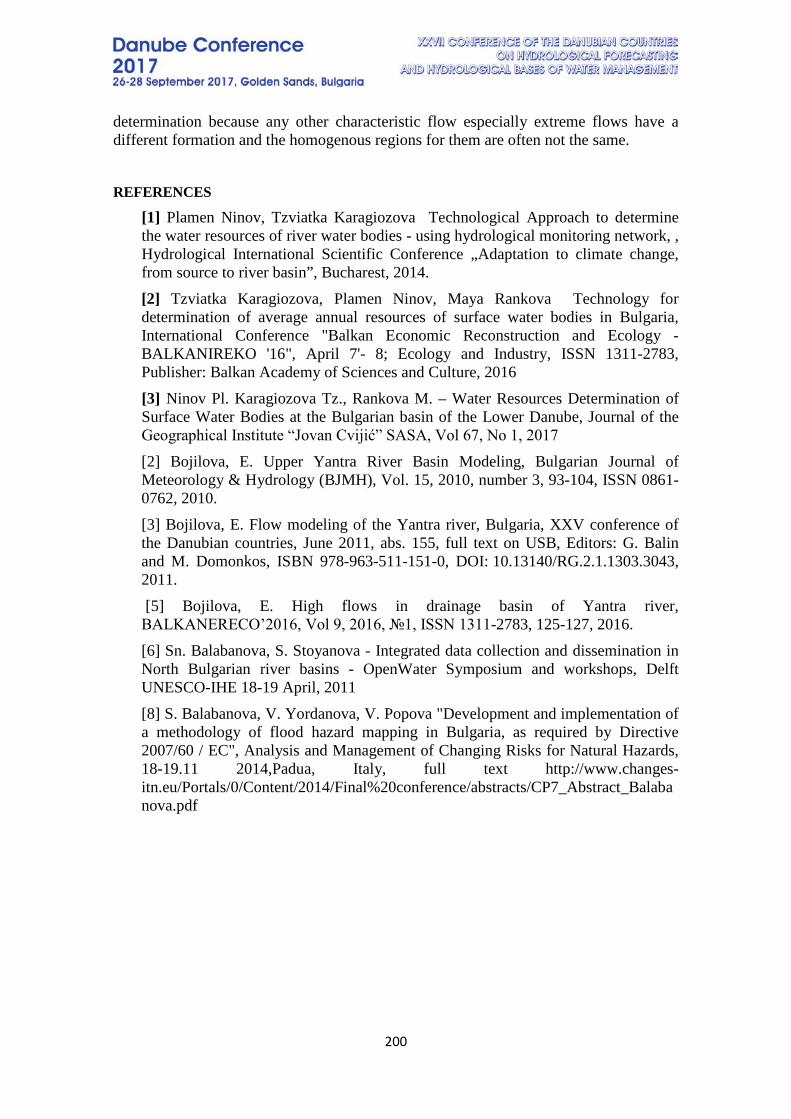
200

determination because any other characteristic flow especially extreme flows have a different formation and the homogenous regions for them are often not the same. REFERENCES

[1] Plamen Ninov, Tzviatka Karagiozova Technological Approach to determine the water resources of river water bodies - using hydrological monitoring network, , Hydrological International Scientific Conference „Adaptation to climate change, from source to river basin”, Bucharest, 2014. [2] Tzviatka Karagiozova, Plamen Ninov, Maya Rankova Technology for determination of average annual resources of surface water bodies in Bulgaria, International Conference "Balkan Economic Reconstruction and Ecology - BALKANIREKO '16", April 7'- 8; Ecology and Industry, ISSN 1311-2783, Publisher: Balkan Academy of Sciences and Culture, 2016 [3] Ninov Pl. Karagiozova Tz., Rankova M. – Water Resources Determination of Surface Water Bodies at the Bulgarian basin of the Lower Danube, Journal of the Geographical Institute “Jovan Cvijić” SASA, Vol 67, No 1, 2017 [2] Bojilova, E. Upper Yantra River Basin Modeling, Bulgarian Journal of Meteorology & Hydrology (BJMH), Vol. 15, 2010, number 3, 93-104, ISSN 0861-0762, 2010. [3] Bojilova, E. Flow modeling of the Yantra river, Bulgaria, XXV conference of the Danubian countries, June 2011, abs. 155, full text on USB, Editors: G. Balin and M. Domonkos, ISBN 978-963-511-151-0, DOI: 10.13140/RG.2.1.1303.3043, 2011. [5] Bojilova, E. High flows in drainage basin of Yantra river, BALKANERECO’2016, Vol 9, 2016, №1, ISSN 1311-2783, 125-127, 2016. [6] Sn. Balabanova, S. Stoyanova - Integrated data collection and dissemination in North Bulgarian river basins - OpenWater Symposium and workshops, Delft UNESCO-IHE 18-19 April, 2011 [8] S. Balabanova, V. Yordanova, V. Popova "Development and implementation of a methodology of flood hazard mapping in Bulgaria, as required by Directive 2007/60 / EC", Analysis and Management of Changing Risks for Natural Hazards, 18-19.11 2014,Padua, Italy, full text http://www.changes-itn.eu/Portals/0/Content/2014/Final%20conference/abstracts/CP7_Abstract_Balabanova.pdf

201

DIFFERENT APPROACHES TO DESIGN FLOOD ASSESSMENT AT THE DANUBE AND THE DRAVA CONFLUENCE

Aleksandra Ilić1, Stevan Prohaska2, Boris Pokorni

1 University of Niš, Faculty of Civil Engineering and Architecture, Serbia 2 Jaroslav Černi Institute for the Development of Water Resources, Belgrade, Serbia

Corresponding author: Aleksandra Ilić, University of Niš, Faculty of Civil Engineering and Architecture, Aleksandra Medvedeva St. No. 14, 18000 Niš, Serbia, email: aleksandra.ilic@gaf.ni.ac.rs

ABSTRACT The flood forming process at a river confluence is complex, from the standpoint of both the origin of the floods on the main stream and tributaries and design flood flow selection for river training works and flood protection planning in the considered river sector. For this purpose, the procedure for adopting the maximum flood flow of a certain return period (flood wave peak) is based on estimated historic maximum annual flow data.

With regard to the origin of flood waves on river reaches that include mouths of tributaries, defining multidimensional dependencies between the parameters that describe the flood wave hydrograph (in this case the maximum flow rate) would determine a real space in which the selected parameters, in different combinations of probability of occurrence, can be found. In the process of design, construction and management of flood protection systems in Serbia, the classical approach of one-dimensional exceedance probability estimates is common. However, in situations where flooding of two or more streams does not occur simultaneously, these estimates do not provide satisfactory results in terms of determining the flood risk. The application of a one-dimensional approach to theoretical value assessment of different return periods makes sense only along river sections that are not under the direct influence of mutual backflow, which regularly occurs in areas where tributaries join the main river. In such areas, the design flood for flood protection is often underestimated or overestimated. In the area of the confluence, where the backed-up flow may be significant, the selection of the design flood flow for a flood protection system is directly dependent on the floods on the main stream and the tributaries. This paper presents a comparative assessment of one-dimensional and two-dimensional frequency analyses and copula application for determining the flow rate for the purposes of sizing a flood protection system in the zone of interaction of the Danube River and the Drava River in Serbia.

Keywords: design flood, univariate frequency analysis, bivariate frequency analysis, copula method, flood peak

202

1. INTRODUCTION

The flood forming process within the zone of the junction of two rivers is highly complex, in terms of both the origin of flood waves on the recipient river and its tributary and the selection of flood discharges for river training works and flood protection planning along the considered river reach. In this regard, the common method for selecting the highest river flow of a certain return period has been to estimate the flood wave peak based on historic maximum annual flow data. Since structural flood protection measures are defined to ensure the required safety downstream, the determination of the design (theoretical) flood is reduced to defining the maximum flow and/or other flood wave characteristics of a certain probability of occurrence. However, novel flood protection concepts reject previous visions of sustainability and instead of a static state, adopt transience, flexibility and decentralization as key features of the system to be developed. According to global, regional and local research of climate change, a new flood management approach is needed, to resemble the way nature functions as closely as possible. From the standpoint of the origin of flood waves along river reaches that include the mouth of a tributary, defining a multivariate correlation between the parameters that describe a flood hydrograph (in this case the maximum flow rate) determines a real space in which the selected parameters, in different combinations of probability of occurrence, can be found. Such correlations are suitable for assessing the probabilistic significance of both historic and future floods, and can also be used to produce real-time forecasts at the exit cross-section of the recipient, where predicted hydrographs at entry cross-sections of the recipient and the tributary are available. Bender et al. [2] mention several studies that address probability distribution in two-dimensional space, such as Moris and Calise (1987) and Raynal and Salas (1987). However, the listing should definitely include monograph chapters that deal with this subject matter in connection with the Danube River and its major tributaries [5], [6]. All these studies point out that the exceedance probability in two-dimensional space is derived based on predefined probability distribution functions, which has generally been a constraint in practice. The use of increasingly popular copula functions departs from the conventional approach that involves a predefined probability distribution function of a random variable and allows for it to be selected from different distribution groups. The present paper includes a comparative assessment of the use of bivariate distributions and copulas to determine the design flood for sizing flood protection systems in the zones of interaction of a recipient river and its tributary.

2. METHODS

Past hydrological practice has relied on univariate exceedance probability assessment to determine design floods for sizing of structural flood protection measures. Solely at a

203

hypothetical level, Prohaska, Marjanović, and Čabrić [7] introduced an analysis of the probability distribution of a complex, multivariate event on the basis of individual (marginal) distributions of each component of the random process, where it is as a rule assumed that the distributions are normal or log-normal. The measure of the relation between the random variables is the correlation coefficient, determined from measured and/or standardized values. The problem of determining the simultaneous occurrence of random variables is solved graphically, using nomograms [1]. The probability thus calculated is in effect the exceedance probability of the event, with predefined combinations of the random variables. The ultimate result is a network of points, where each is characterized by the probability of occurrence of the defined combination and they are used to generate same-probability lines. This approach encountered many difficulties with regard to defining a single distribution law based on ad hoc marginal probabilities. The difficulties and limitations of such an approach began to be resolved with the use of copulas, a method derived from the probability theory that determines the joint multivariate probability distribution of random variables.

2.1. Marginal probabilities

In order to determine the distribution density, , the first step is to arrive at the marginal probabilities and as:

(1)

(2)

Then their cumulative probabilities are:

(3)

and

(4)

Several known probability distribution functions need to be identified and tested as potential marginals. In the standard procedure that involves the determination of the exceedance probability of a considered flood wave parameter in bivariate space, a precondition is that the selected random variables need to adhere to the same probability distribution law. For that purpose, Pearson Type 3 (P3), Log-Pearson Type 3 (LP3), Extreme Value Type 1 – Gumbel (EV1) and Log-normal (LOGN) were selected for potential marginal distributions. The distribution parameters were assessed using the conventional method

( )y,xf),x(f • )y,(f •

∫∞=

−∞=

=•

y

ydy)y,x(f),x(f

∫∞=

−∞=

=•

x

xdx)y,x(f(f )y,

∫=

−∞=

•• =xt

tdt),t(f),x(F

∫=

−∞=

•• =xt

tdt),t(f),x(F

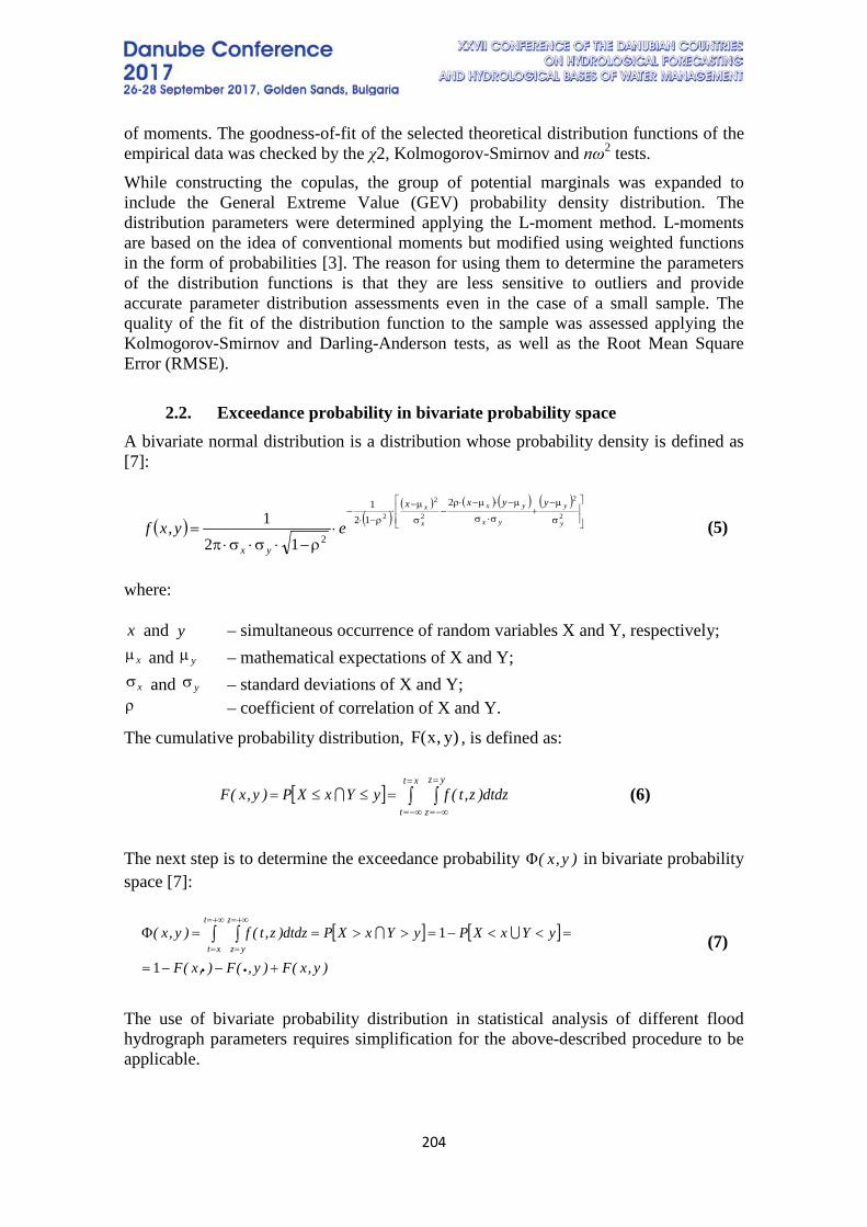
204

of moments. The goodness-of-fit of the selected theoretical distribution functions of the empirical data was checked by the χ2, Kolmogorov-Smirnov and nω2 tests. While constructing the copulas, the group of potential marginals was expanded to include the General Extreme Value (GEV) probability density distribution. The distribution parameters were determined applying the L-moment method. L-moments are based on the idea of conventional moments but modified using weighted functions in the form of probabilities [3]. The reason for using them to determine the parameters of the distribution functions is that they are less sensitive to outliers and provide accurate parameter distribution assessments even in the case of a small sample. The quality of the fit of the distribution function to the sample was assessed applying the Kolmogorov-Smirnov and Darling-Anderson tests, as well as the Root Mean Square Error (RMSE).

2.2. Exceedance probability in bivariate probability space A bivariate normal distribution is a distribution whose probability density is defined as [7]:

(5)

where:

and – simultaneous occurrence of random variables X and Y, respectively; and – mathematical expectations of X and Y; and – standard deviations of X and Y;

– coefficient of correlation of X and Y.

The cumulative probability distribution, , is defined as:

(6)

The next step is to determine the exceedance probability in bivariate probability space [7]:

(7)

The use of bivariate probability distribution in statistical analysis of different flood hydrograph parameters requires simplification for the above-described procedure to be applicable.

( ) ( )( ) ( ) ( ) ( )

σ

µ−+

σ⋅σ

µ−⋅µ−⋅ρ−

σ

µ−⋅

ρ−⋅−

⋅ρ−⋅σ⋅σ⋅π

=2

2

2

2

2

2

121

2121 y

y

yx

yx

x

x yyxx

yx

ey,xf

x y

xµ yµ

xσ yσρ

)y,x(F

[ ] ∫ ∫=

−∞=

=

−∞=

=≤≤=xt

t

yz

zdtdz)z,t(fyYxXP)y,x(F

)y,x(Φ

[ ] [ ]

)y,x(F)y,(F),x(F

yYxXPyYxXPdtdz)z,t(f)y,x(t

xt

z

yz

+−−=

=<<−=>>==Φ

••

∫ ∫+∞=

=

+∞=

=

1

1

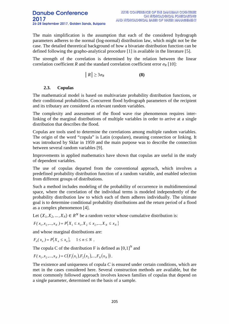
205

The main simplification is the assumption that each of the considered hydrograph parameters adheres to the normal (log-normal) distribution law, which might not be the case. The detailed theoretical background of how a bivariate distribution function can be defined following the grapho-analytical procedure [1] is available in the literature [5]. The strength of the correlation is determined by the relation between the linear correlation coefficient R and the standard correlation coefficient error σR [10]:

│R│≥ 3σR (8)

2.3. Copulas The mathematical model is based on multivariate probability distribution functions, or their conditional probabilities. Concurrent flood hydrograph parameters of the recipient and its tributary are considered as relevant random variables. The complexity and assessment of the flood wave rise phenomenon requires inter-linking of the marginal distributions of multiple variables in order to arrive at a single distribution that describes the flood. Copulas are tools used to determine the correlations among multiple random variables. The origin of the word “copula” is Latin (copulare), meaning connection or linking. It was introduced by Sklar in 1959 and the main purpose was to describe the connection between several random variables [9]. Improvements in applied mathematics have shown that copulas are useful in the study of dependent variables. The use of copulas departed from the conventional approach, which involves a predefined probability distribution function of a random variable, and enabled selection from different groups of distributions. Such a method includes modeling of the probability of occurrence in multidimensional space, where the correlation of the individual terms is modeled independently of the probability distribution law to which each of them adheres individually. The ultimate goal is to determine conditional probability distributions and the return period of a flood as a complex phenomenon [4].

Let (𝑋𝑋1,𝑋𝑋2, … ,𝑋𝑋N) ∈ 𝑅𝑅𝑁𝑁 be a random vector whose cumulative distribution is:

and whose marginal distributions are:

.

The copula C of the distribution F is defined as [0,1]N and

.

The existence and uniqueness of copula C is ensured under certain conditions, which are met in the cases considered here. Several construction methods are available, but the most commonly followed approach involves known families of copulas that depend on a single parameter, determined on the basis of a sample.

{ }NNN xX,...,xX,xXP)x,...,x,x(F ≤≤≤= 221121

{ } Nn,xXP)x(F nnnn ≤≤≤= 1

( ) ( ) ( )( )NNN xF,...,xF,xFC)x,...,x,x(F 221121 =

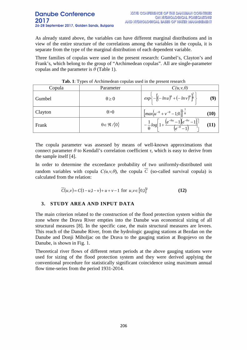
206

As already stated above, the variables can have different marginal distributions and in view of the entire structure of the correlations among the variables in the copula, it is separate from the type of the marginal distribution of each dependent variable. Three families of copulas were used in the present research: Gumbel’s, Clayton’s and Frank’s, which belong to the group of “Archimedean copulas”. All are single-parameter copulas and the parameter is θ (Table 1).

Tab. 1: Types of Archimedean copulas used in the present research Copula Parameter C(u,v,θ)

Gumbel θ 0 (9)

Clayton θ>0 (10)

Frank (11)

The copula parameter was assessed by means of well-known approximations that connect parameter θ to Kendall’s correlation coefficient τ, which is easy to derive from the sample itself [4]. In order to determine the exceedance probability of two uniformly-distributed unit random variables with copula C(u,v,θ), the copula (so-called survival copula) is calculated from the relation:

for (12)

3. STUDY AREA AND INPUT DATA

The main criterion related to the construction of the flood protection system within the zone where the Drava River empties into the Danube was economical sizing of all structural measures [8]. In the specific case, the main structural measures are levees. This reach of the Danube River, from the hydrologic gauging stations at Bezdan on the Danube and Donji Miholjac on the Drava to the gauging station at Bogojevo on the Danube, is shown in Fig. 1. Theoretical river flows of different return periods at the above gauging stations were used for sizing of the flood protection system and they were derived applying the conventional procedure for statistically significant coincidence using maximum annual flow time-series from the period 1931-2014.

≥ ( ) ( )[ ]

−+−− θθθ1

vlnulnexp

{ }[ ] θ−θ−θ− −+

1

01;vumax

{ }0/ℜ∈θ ( )( )( )

−

−−+

θ− θ−

θ−θ−

11111

eeelog

vu

C

( ) ( ) 111 −++−−= vuv,uCv,uC [ ]210,v,u ∈

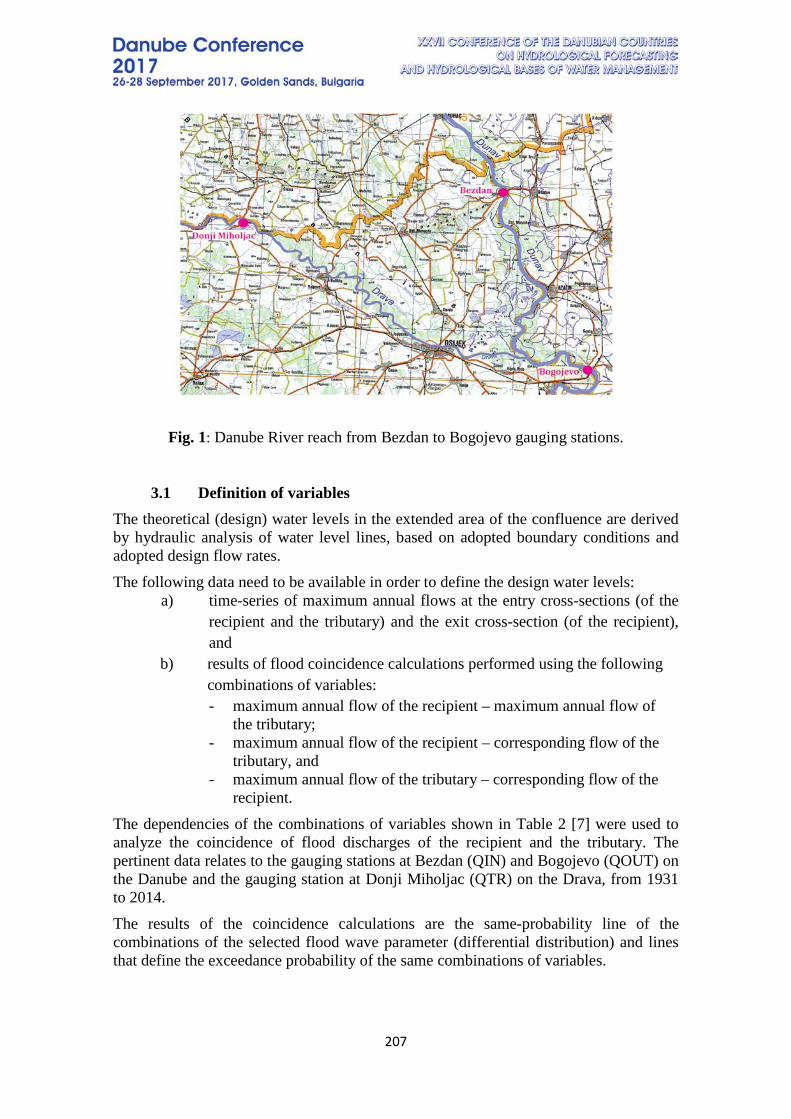
207

Fig. 1: Danube River reach from Bezdan to Bogojevo gauging stations.

3.1 Definition of variables

The theoretical (design) water levels in the extended area of the confluence are derived by hydraulic analysis of water level lines, based on adopted boundary conditions and adopted design flow rates. The following data need to be available in order to define the design water levels:

a) time-series of maximum annual flows at the entry cross-sections (of the recipient and the tributary) and the exit cross-section (of the recipient), and

b) results of flood coincidence calculations performed using the following combinations of variables:

- maximum annual flow of the recipient – maximum annual flow of the tributary;

- maximum annual flow of the recipient – corresponding flow of the tributary, and

- maximum annual flow of the tributary – corresponding flow of the recipient.

The dependencies of the combinations of variables shown in Table 2 [7] were used to analyze the coincidence of flood discharges of the recipient and the tributary. The pertinent data relates to the gauging stations at Bezdan (QIN) and Bogojevo (QOUT) on the Danube and the gauging station at Donji Miholjac (QTR) on the Drava, from 1931 to 2014. The results of the coincidence calculations are the same-probability line of the combinations of the selected flood wave parameter (differential distribution) and lines that define the exceedance probability of the same combinations of variables.

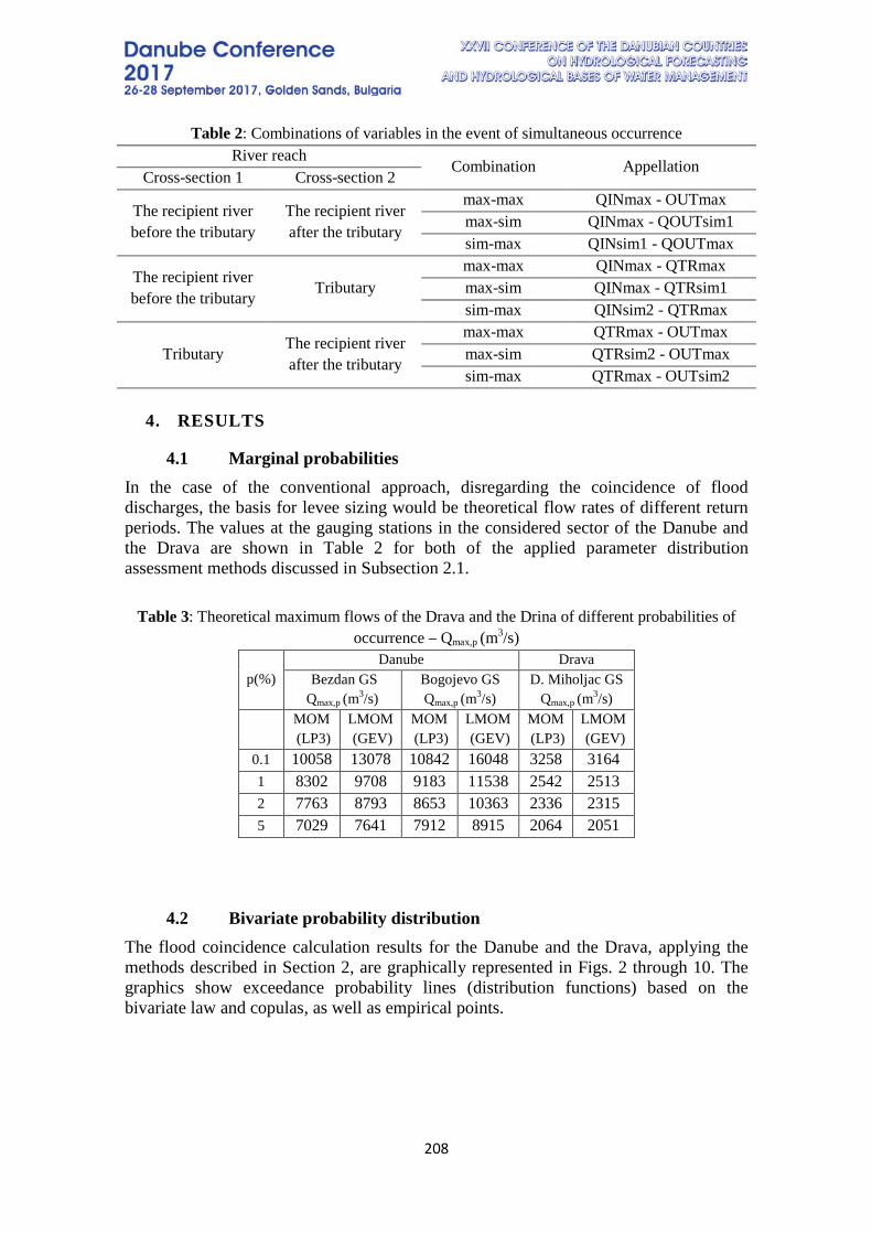
208

Table 2: Combinations of variables in the event of simultaneous occurrence River reach

Combination Appellation Cross-section 1 Cross-section 2

The recipient river before the tributary

The recipient river after the tributary

max-max QINmax - OUTmax max-sim QINmax - QOUTsim1 sim-max QINsim1 - QOUTmax

The recipient river before the tributary

Tributary max-max QINmax - QTRmax max-sim QINmax - QTRsim1 sim-max QINsim2 - QTRmax

Tributary The recipient river after the tributary

max-max QTRmax - OUTmax max-sim QTRsim2 - OUTmax sim-max QTRmax - OUTsim2

4. RESULTS

4.1 Marginal probabilities In the case of the conventional approach, disregarding the coincidence of flood discharges, the basis for levee sizing would be theoretical flow rates of different return periods. The values at the gauging stations in the considered sector of the Danube and the Drava are shown in Table 2 for both of the applied parameter distribution assessment methods discussed in Subsection 2.1.

Table 3: Theoretical maximum flows of the Drava and the Drina of different probabilities of

occurrence – Qmax,p (m3/s)

p(%) Danube Drava

Bezdan GS Qmax,p (m3/s)

Bogojevo GS Qmax,p (m3/s)

D. Miholjac GS Qmax,p (m3/s)

MOM (LP3)

LMOM (GEV)

MOM (LP3)

LMOM (GEV)

MOM (LP3)

LMOM (GEV)

0.1 10058 13078 10842 16048 3258 3164 1 8302 9708 9183 11538 2542 2513 2 7763 8793 8653 10363 2336 2315 5 7029 7641 7912 8915 2064 2051

4.2 Bivariate probability distribution The flood coincidence calculation results for the Danube and the Drava, applying the methods described in Section 2, are graphically represented in Figs. 2 through 10. The graphics show exceedance probability lines (distribution functions) based on the bivariate law and copulas, as well as empirical points.

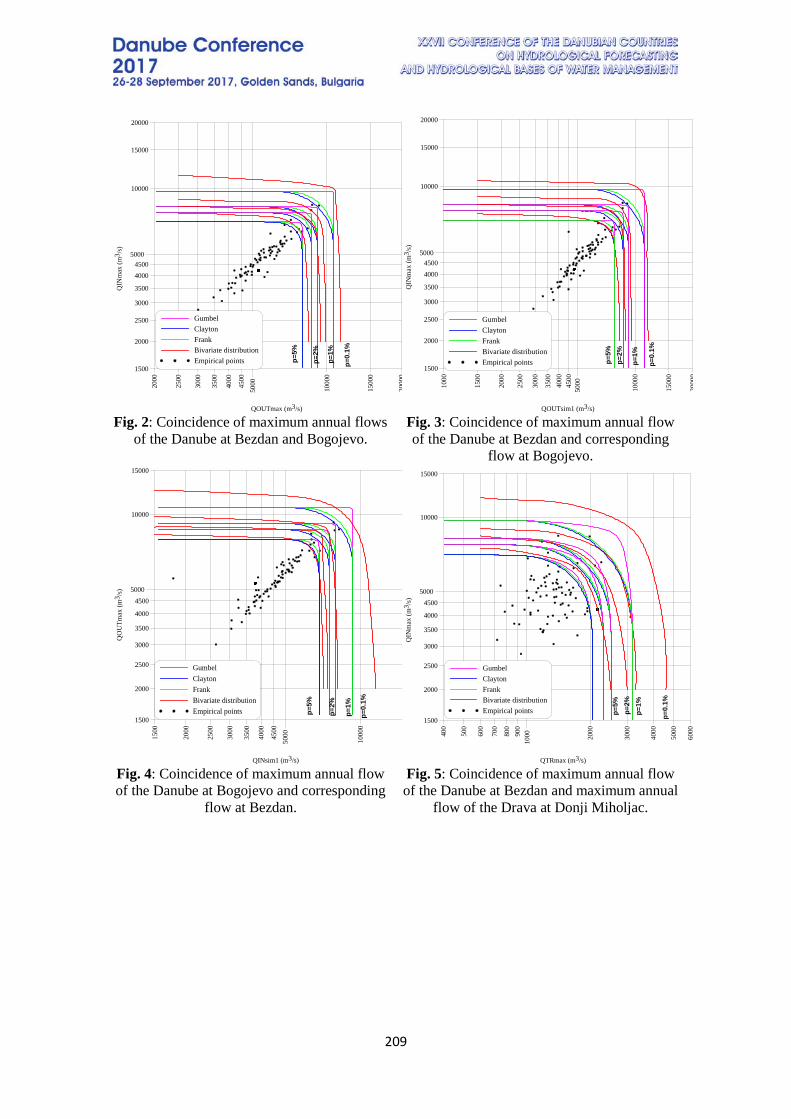
209

Fig. 2: Coincidence of maximum annual flows

of the Danube at Bezdan and Bogojevo. Fig. 3: Coincidence of maximum annual flow of the Danube at Bezdan and corresponding

flow at Bogojevo.

Fig. 4: Coincidence of maximum annual flow of the Danube at Bogojevo and corresponding

flow at Bezdan.

Fig. 5: Coincidence of maximum annual flow of the Danube at Bezdan and maximum annual

flow of the Drava at Donji Miholjac.

500020

00

2500

300 0

3 500

400 0

4 500

1000

0

1 500

0

200 0

0

5000

1500

2000

2500

3000

3500

40004500

10000

15000

20000

GumbelClaytonFrankBivariate distributionEmpirical points

QOUTmax (m3/s)

p=5%

p=1%

p=0.

1%

QIN

max

(m3 /

s)

p=2%

500010

00

1500

2000

2500

3000

3500

4000

4500

1000

0

1500

0

2000

0

5000

1500

2000

2500

3000

3500

40004500

10000

15000

20000

GumbelClaytonFrankBivariate distributionEmpirical points

QOUTsim1 (m3/s)

p=5%

p=1%

p=0.

1%

QIN

max

(m3 /

s)

p=2%

500015

00

2000

2500

3000

3500

4000

4500

1000

0

1500

0

5000

1500

2000

2500

3000

3500

4000

4500

10000

15000

GumbelClaytonFrankBivariate distributionEmpirical points

QINsim1 (m3/s)

p=5%

p=1%

p=0.

1%

QO

UTm

ax (m

3 /s)

p=2%

100 040

0

500

600

700

800

900

200 0

3000

400 0

5000

6000

5000

1500

2000

2500

3000

3500

4000

4500

10000

15000

GumbelClaytonFrankBivariate distributionEmpirical points

QTRmax (m3/s)

p=5%

p=1%

p=0.

1%

QIN

max

(m3 /

s)

p=2%

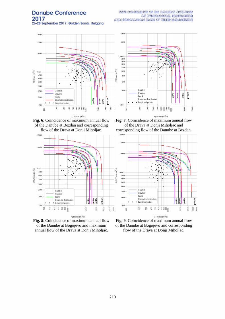
210

Fig. 6: Coincidence of maximum annual flow of the Danube at Bezdan and corresponding

flow of the Drava at Donji Miholjac.

Fig. 7: Coincidence of maximum annual flow of the Drava at Donji Miholjac and

corresponding flow of the Danube at Bezdan.

Fig. 8: Coincidence of maximum annual flow

of the Danube at Bogojevo and maximum annual flow of the Drava at Donji Miholjac.

Fig. 9: Coincidence of maximum annual flow of the Danube at Bogojevo and corresponding

flow of the Drava at Donji Miholjac.

100

100020

0

300

400

500

600

700

800

900

2000

3000

4000

5000

5000

1500

2000

2500

3000

3500

40004500

10000

15000

20000

GumbelClaytonFrankBivariate distributionEmpirical points

QTRsim1 (m3/s)

p=5%

p=1%

p=0.

1%

QIN

max

(m3 /

s)

p=2%

500

500010

00

1500

2000

2500

3000

3500

4000

4500

1000

0

1500

0

2000

0

200

2000

400

600

800

1000

1200140016001800

4000

6000

GumbelClaytonFrankBivariate distributionEmpirical points

QINsim2 (m3/s)

p=5%

p=1%

p=0.

1%

QTR

max

(m3 /

s)

p=2%

100040

0

500

600

700

800

900

2000

3000

4000

5000

6000

5000

1500

2000

2500

3000

3500

4000

4500

10000

15000

GumbelClaytonFrankBivariate distributionEmpirical points

QTRmax (m3/s)

p=5%

p=1%

p=0.

1%

QO

UTm

ax (m

3 /s)

p=2%

100

100020

0

300

400

500

600

700

800

9 00

2000

3000

4000

5000

5000

1500

2000

2500

3000

3500

40004500

10000

15000

20000

GumbelClaytonFrankBivariate distributionEmpirical points

QTRsim2 (m3/s)

p=5%

p=1%

p=0.

1%

QO

UTm

ax (m

3 /s)

p=2%

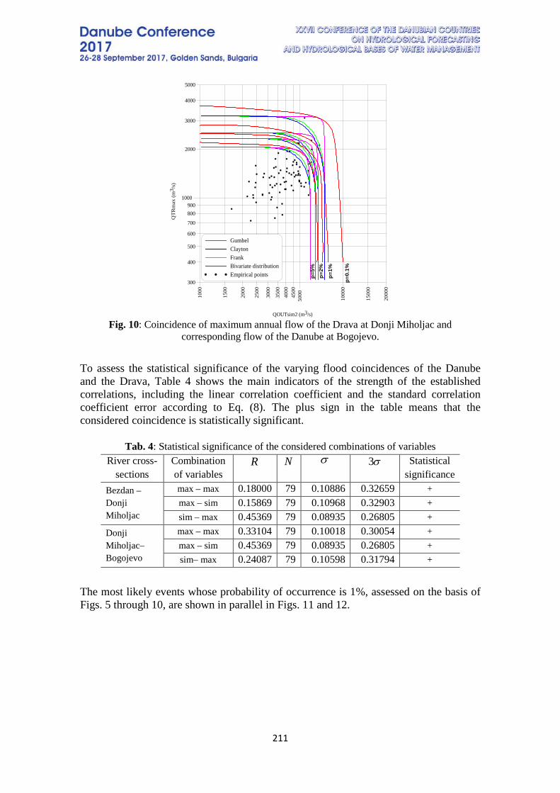
211

Fig. 10: Coincidence of maximum annual flow of the Drava at Donji Miholjac and

corresponding flow of the Danube at Bogojevo.

To assess the statistical significance of the varying flood coincidences of the Danube and the Drava, Table 4 shows the main indicators of the strength of the established correlations, including the linear correlation coefficient and the standard correlation coefficient error according to Eq. (8). The plus sign in the table means that the considered coincidence is statistically significant.

Tab. 4: Statistical significance of the considered combinations of variables River cross-

sections Combination of variables

Statistical significance

Bezdan – Donji Miholjac

max – max 0.18000 79 0.10886 0.32659 + max – sim 0.15869 79 0.10968 0.32903 + sim – max 0.45369 79 0.08935 0.26805 +

Donji Miholjac– Bogojevo

max – max 0.33104 79 0.10018 0.30054 + max – sim 0.45369 79 0.08935 0.26805 + sim– max 0.24087 79 0.10598 0.31794 +

The most likely events whose probability of occurrence is 1%, assessed on the basis of Figs. 5 through 10, are shown in parallel in Figs. 11 and 12.

500010

00

1500

2000

2500

3000

3500

4000

4500

1000

0

1500

0

2000

0

1000

300

400

500

600

700

800900

2000

3000

4000

5000

GumbelClaytonFrankBivariate distributionEmpirical points

QOUTsim2 (m3/s)p=

5%

p=1%

p=0.

1%

QTR

max

(m3 /

s)

p=2%

R N σ σ3

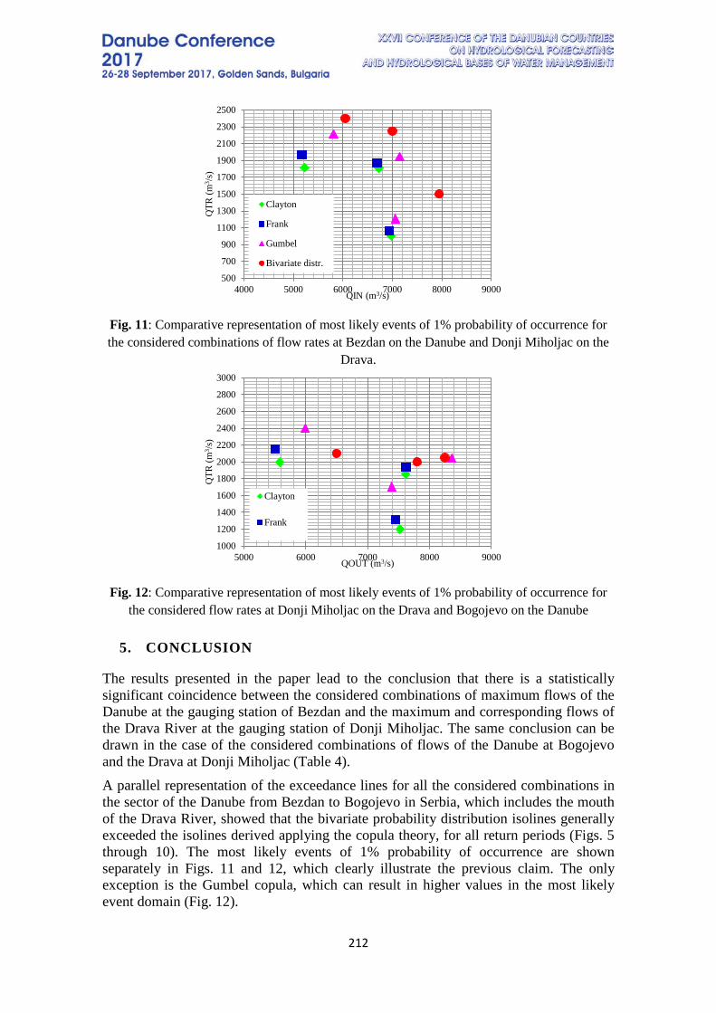
212

Fig. 11: Comparative representation of most likely events of 1% probability of occurrence for the considered combinations of flow rates at Bezdan on the Danube and Donji Miholjac on the

Drava.

Fig. 12: Comparative representation of most likely events of 1% probability of occurrence for the considered flow rates at Donji Miholjac on the Drava and Bogojevo on the Danube

5. CONCLUSION

The results presented in the paper lead to the conclusion that there is a statistically significant coincidence between the considered combinations of maximum flows of the Danube at the gauging station of Bezdan and the maximum and corresponding flows of the Drava River at the gauging station of Donji Miholjac. The same conclusion can be drawn in the case of the considered combinations of flows of the Danube at Bogojevo and the Drava at Donji Miholjac (Table 4). A parallel representation of the exceedance lines for all the considered combinations in the sector of the Danube from Bezdan to Bogojevo in Serbia, which includes the mouth of the Drava River, showed that the bivariate probability distribution isolines generally exceeded the isolines derived applying the copula theory, for all return periods (Figs. 5 through 10). The most likely events of 1% probability of occurrence are shown separately in Figs. 11 and 12, which clearly illustrate the previous claim. The only exception is the Gumbel copula, which can result in higher values in the most likely event domain (Fig. 12).

500

700

900

1100

1300

1500

1700

1900

2100

2300

2500

4000 5000 6000 7000 8000 9000

QTR

(m3 /s

)

QIN (m3/s)

Clayton

Frank

Gumbel

Bivariate distr.

1000

1200

1400

1600

1800

2000

2200

2400

2600

2800

3000

5000 6000 7000 8000 9000

QTR

(m3 /s

)

QOUT (m3/s)

Clayton

Frank

213

The established correlations presented in Section 4 suggest an imminent need to abandon the conventional approach for the determination of design flood discharges used to size flood protection systems along river reaches that include tributaries, based on univariate probabilities of occurrence of maximum annual flows at gauging stations. The analysis showed that that the values obtained for flood discharges within the junction zone of the recipient river and its tributary were lower, which allows engineers to design more economical structural measures, leaving enough room for increasingly important non-structural flood protection measures. The authors recommend that floods be examined as a complex phenomenon and that other flood wave characteristics (e.g. volume) be assessed as well, including their correlations in multidimensional space. ACKNOWLEDGMENT

The results and analyses presented in this paper originate from the outcomes of the scientific research project “Assessment of Climate Change Impact on Serbia’s Water Resources” (TR-37005, 2011–2017) of the Serbian Ministry of Education and Science. The authors extend their gratitude to the ministry for its financial assistance and support. REFERENCES [1] Abramowitz M., Stegun A. I. Handbook of Mathematical Functions with Formulas, Graphs and Mathematical Tables, Dover Publications, INC., New York, 1972. [2] Bender J., Wahl T., Muller A., Jensen J. A multivariate design framework for river confluences, Hydrological Sciences Journal, 61:3, 471-482, 2016. [3] Hosking J. R. M. L-moments: Analysis and Estimation of Distributions using Linear Combinations of Order Statistics, Journal of Royal Statistical Society, Vol. 52, No. 1, pp. 105-124, 1990. [4] Nelsen R. B. An introduction to copulas. Lecture notes in statistics. 2nd ed. New York, Springer, 2006. [5] Prohaska S et al. Concidence of Flood Flow of the Danube River and its Tributary, The Danube and its Basin – A Hydrological Monograph, Follow-up volime IV, Regonal Cooparation of the Danube Countries in the Frame of the International Hydrological Programme of UNESCO, Bratislava, 1999. [6] Prohaska S., Ilic A. Coincidence of Flood Flow of the Danube River and Its Tributaries, (In: Mitja Brilly (Ed.): Hydrological Processes of the Danube River Basin - Perspectives from the Danubian Countries), Publisher: Springer, ISBN 978-90-481-3422-9, Book Chapter 6, p. 175-226, 2010. [7] Prohaska S., Marjanović N., Čabrić M. Dvoparametarsko definisanje velikih voda, Vode Vojvodine, Novi Sad, 1978. [8] Prohaska S., Petković T. Metode za proračun velikih voda, Deo I, Proračun velikih voda na hidrološki izučenim profilima, Građevinski calendar 89, Beograd, 1989.

214

[9] Schmidt T. Coping with Copulas, Forthcoming in Risk Books “Copulas- From Theory to Applications in Finance“, Department of mathematics, university of Leipzig, 2006. [10] Yevjevich V. Probability and Statistics in Hydrology, Water Resources Publications, Fort Collins, Colo. U.S.A, 1972.

215

ANNUAL WATER RESOURCES ASSESSMENT USING DIFFERENT OBSERVATIONS AND MODELS

Eram Artinyan, Dobri Dimitrov, Kamelia Kroumova, Maya Rankova National Institute of Meteorology and Hydrology, BAS, Bulgaria

Corresponding author: E. Artinyan, NIMH, Ruski 139, Plovdiv, Bulgaria, eram.artinian@meteo.bg

ABSTRACT The annual assessment of water resources is an important regular task of the National Institute of Meteorology and Hydrology (NIMH), Sofia, directed to the needs of water management and different national and international agencies. The paper is trying to compare and analyze the last four years results of several different sources of information on the main water balance components like precipitation and river-flow over the territory of Bulgaria and the river basin management districts. Those information sources are:

- Observed precipitation and river flow at different classes of precipitation and river flow gauges maintained by NIMH. The river flow characteristics are extrapolated over the un-gauged regions using statistical and GIS models;

- Land Surface Model – SURFEX applied off-line and forced by meteorological data obtained by Cressman analysis of precipitation and other meteorological observations. The latest, developed by Iliyan Gospodinov in the NIMH Forecasting Dept. with 1 km resolution is assimilating operationally about 350 conventional precipitation gauges and the first guess of ALADIN forecasting model. The precipitation fields used as SURFEX input are prepared in regular square mesh with a coarser resolution of eight kilometers. SURFEX outputs include runoff and evapotranspiration at the same resolution and 3 hour time step.

- The ECMWF ERA Interim reanalysis model. The model is producing various characteristics, including water balance component in a regular geographical mesh of 45’minutes (which is about 83 kilometers).

- The Initial Meteorological Information Objective Analysis System, developed by Valery Spiridonov in the NIMH Forecasting Dept., is using the sweep operator with various predictors. The hourly precipitation totals from about 140 gauges and various raster data from the geostationary Meteosat-9 are used as input data.

The results from the above methods for river basin management districts are compared and analyzed. The pros and cons of each method are discussed. Conclusions are driven about some further development of the methods and models, making them more suitable for quantitative estimation of water resources characteristics. Keywords: basin water balance, runoff, evapotranspiration

216

INTRODUCTION The increasing need of deeper knowledge on water resources and the easier access to computer resources led to fast development of numerical models to estimate the water budget components. National Institute of Meteorology and Hydrology (NIMH) is the responsible institution in Bulgaria for the water budget computation at yearly basis, for the hydrological forecasts and hydrological quantitative monitoring of surface and ground waters. All those tasks require not only effective measurement and data collection but also high level of numerical computing facilities that put the collected data in usable shape. Software models are widely used in hydro-meteorological systems. In Bulgaria they were firstly used from the meteorologists for weather forecast. The physical hydrological models were developed to fill the gap between the processes at the screen level and in (over) the soil. When the models are fed with measured meteorological data they compute the remaining water budget components: runoff, evapotranspiration and drainage. Despite the large number of such models all of them require the same variables as input data for the screen level: precipitations, air temperature and moisture, solar and atmospheric radiation etc. Preparation of that data from the point scale measures to the spatial scale of the basin requires special attention. Difficulties usually come from the scarce measurement data from the mountain parts of the basins combined with high diversity of relief slopes and exposures. Those are usually solved using gradients taken from numerical forecast models. More elaborated methods include fragmentation of the simulation area to climatologically similar sub-zones with variable slope and exposure gradients (Quintana-Seguí, 2008). At NIMH spatial mapping of screen level atmospheric variables was done primarily for seasonally and yearly climatological estimates. Examples are maps over Bulgaria of yearly sum of precipitation and evaporation, monthly air temperature, solar radiation etc. (Hershkovich, 1982). In 2006 the introduction of spatially distributed hydrological model ISBA-Modcou led to the need of operational daily mapping of precipitation and other screen level variables exclusively over East Aegean river basins in south Bulgaria. The methods used are described in Artinyan et al., 2008. MATERIALS AND METHODS At national level 3 hourly interpolated data of the meteorological variables started to be operationally prepared after 2012 by two alternative methods:

1. From the NIMH Forecasting Dept. with 1 km resolution and 3 hour time step. The method, referred further as National High Resolution Meteorological Analysis (NHRMA) (Gospodinov, 2012), uses the Cressman analysis (Cressman, 1959) and assimilates operationally about 350 conventional precipitation gauges, observers of which sent the daily sum, and the first guess of short range ALADIN forecasting model.

2. The Initial Meteorological Information Objective Analysis System (Spiridonov, 2014) referred further as Sp-EUSat method. The former is using the sweep operator with various predictors. The hourly precipitation totals from about 140 gauges and various raster data from the geostationary Meteosat-9 are used as input data beside the first guess of numerical weather model ALADIN. Data is prepared with hourly step at 0.045º resolution (about 3-4 km).

217

Beside the operationally prepared meteorological fields analysis a more detailed precipitation field is prepared using the yearly sums of the precipitation measured from about 500 manually operated precipitation stations. The spatial interpolation of the annual precipitation uses the Natural neighbor interpolation technique. The product is further referred as “Registered” precipitation field. Computing of surface runoff and drainage at national level was made with SURFEX land surface platform (Le Moigne, 2017) in off-line mode. In order to make use of the above operational products we converted them to 8 km regular grid. Processing of products is performed depending on the resolution. The first product (1) contains about 64 points for each SURFEX cell. As we want to obtain the mean value over each cell the first product is simply averaged over SURFEX meshes of 8x8 km. The second product (2) is available in degree grid so it was interpolated to regular grid. The resulting spatial products (1 and 2) were analyzed in two ways: first, comparing the yearly sums of the precipitation of the corresponding SURFEX cell to the yearly sum of the underlying climatological station and second, at basin level to the yearly sum of river basin yearly outflow. Here we will discuss only the results at the basin level. Only for East-Aegean basin a separate model setup is used since 2006 using ISBA-Modcou coupled models. The runoff and drainage produced by ISBA is transferred trough a couple of reservoirs to simulate shallow water table before the routing by the hydrological model Modcou occurs. So ISBA-Modcou coupled model can transfer more water between the years than the SURFEX platform used without a hydrological model. RESULTS AND DISCUSSION

A. Streamflow discharges comparisons According to the targets mentioned above, we would like to test first the possibility to use SURFEX for water balance components evaluation. For that purpose, a basin scale tests were prepared all over the country. The idea is to compare the model results with some observed characteristics like river flow and precipitation. Annual aggregation of the compared variables was used, because of the following reasons: • Water resources characteristics are used for management purposes in Bulgaria at

monthly, seasonal and annual time scale, planning is made annually and knowledge on water balance components with such aggregation is needed;

• The annual averaging helps in filtering some dynamic components having oscillation cycle days and weeks (such as surface detention, infiltration in the vadose zone, etc.), thus simplifying the analysis and giving us a possibility to concentrate on the general things;

• To filter the local conditions influence over the spatial variability of water balance component and to allow comparison between results from models with different scale, the tests were planned over the whole territory of Bulgaria and its four main basin districts.

Implementing the above, the annual evaluations of the river discharge averages for the main river basins and the four basin districts in Bulgaria (Янкова и Крумова, 2016) were collected for the period 2013 – 2015, as they were used for the reporting on EEA, Eurostat, etc. Those evaluations are based on observations over the main river basins and will further be referred as “Registered” flows. Other parts of the comparison were the gridded estimations of the flow computed by SURFEX, ERA Interim (Szczypta, 2011) and ISBA-Modcou (Artinyan, 2008). The models are working on quite different

218

grids. ERA is using about 83 km cell and forced by quite smoothed analyses of meteorological fields, while SURFEX and ISBA-Modcou are set to use 8 km grid and forced with preprocessed meteorological input taken predominantly from local observation stations. It is important to mention that ISBA-Modcou was the first model of a kind used in Bulgaria and its results are available for the East Aegean basin district only. The gridded data on runoff and shallow groundwater infiltration feed are interpreted as river flow and integrated over the river catchments neglecting the concentration time (except for ISBA-Modcou results), which for the Bulgarian conditions vary from 3 to 6 days for the main river basins. Annually averaged results over the period 2013 – 2015 are given in Table 1. Table 1. River flow estimation by different models or computing methods

Basin district Method of water balance components estimation [m3/s]

ERA SURFEX “Registered” ISBA alone*

ISBA-Modcou**

Annual averages of river flow for year 2013 Danube district 225.0 383.6 138.4 Black Sea district 99.6 174.9 51.9 East Aegean district 246.6 404.6 206.5 237.5 308 West Aegean district 108.2 182.2 116.4

Annual averages of river flow for year 2014 Danube district 417.8 614.0 324.3 Black Sea district 110.7 268.5 66.6 East Aegean district 393.9 600.3 282.9 427.8 400 West Aegean district 179.2 183.7 113.5

Annual averages of river flow for year 2015 Danube district 384.3 512.8 284.1 Black Sea district 128.4 346.7 85.5 East Aegean district 406.3 532.8 428.4 310.8 428 West Aegean district 127.2 204.4 154.0 * Available for the East Aegean basin district only. **This column is computed from the modeled streamflow discharge for the three main rivers and the corresponding stations: Maritsa at Svilengrad, Tundzha at Elhovo and Arda at Ivaylovgrad. It is quite clear that all the models are higher than the annual “Registered” means. It should principally be expected to have the “Registered” flow 20 – 30% less than the modeled one because of the anthropogenic losses for irrigation, water supply and for filling the dams. Those losses transfer part of surface and ground water to evapo-transpiration and for storage. From this point of view averaged flow computed by ISBA-Modcou is the closest to our expectations. In 2013 and 2014 ISBA-Modcou computed flow is higher than “Registered”. In 2013 and 2015 the model is releasing more water than produced by ISBA. It might be explained by the mechanism of water transfer from one year to another (mainly by soil, but also by simulated shallow underground reservoirs and snow cover). ERA is generally much closer to “Registered” than SURFEX. Biggest are the differences for the Black Sea district. It might be possible that some problems exist in evaluating the registered flow, due to not enough good predictors in the relationships, some problems with the influence of the Black Sea back waters or other hydrometric problems. SURFEX gives 1.5 to 2.5 times higher discharge than “Registered” for the Danubian and the East Aegean districts. The

219

principle difference in flow formation mechanism between those districts and the West Aegean one is the ratio between surface and shallow ground waters. The Danube and Maritsa valleys have large alluvial parts, which contribution to the surface flow might be different. Those differences between the modeled and the “Registered” flow could also be due to: • Problems in the forcing data: over-estimation of precipitation; theoretically under-

estimation of air temperature might lead to lower evapo-transpiration and higher flow, but this is not likely because of many reasons;

• Problems in models calibration, overestimation of the vertical gradients, problems in the models concept transferring more water to the flow components. B. Precipitations field comparisons

We compare the available sources of spatial information on the annual precipitation amounts. The following sources were considered: ERA precipitation fields, which are obtained from the objective analysis of various ground and satellite data and come as a product of the ECMWF weather forecasting model; NHRMA and Sp-EUSat methods mentioned in Introduction; “Registered” - a spatial interpolation of the annual precipitation totals using the Natural neighbor interpolation techniques; ISBA-Modcou preprocessing - adopted for the East Aegean basin district more than 10 years ago and assimilated all available conventional and automatic telemetric precipitation gauges in the region. Table 2. Precipitation annual sums computed by different methods

Basin district Method of water balance components estimation [mm]

ERA NHRMA Sp-EUSat Registered ISBA-preprocess*

Annual sums for year 2013 Danube district 603.3 748.0 657.2 Black Sea district 514.8 652.1 534.4 East Aegean district 652.1 801.9 647.5 655.0 West Aegean district 750.9 955.4 726.4

Annual sums for year 2014 Danube district 1078.3 1167.5 1378.778 1051.1 Black Sea district 890.7 1104.3 1107.166 1010.9 East Aegean district 1132.4 1304.8 1505.958 1081.0 1121.06 West Aegean district 1271.8 1201.0 1340.398 919.4

Annual sums for year 2015 Danube district 726.1 835.5 1005.522 724.6 Black Sea district 568.9 772.0 814.330 631.7 East Aegean district 834.9 1057.2 1183.315 805.7 824.8 West Aegean district 948.3 1069.2 1134.283 786.0 * Available for the East Aegean basin district only Considering the results on the annual precipitation totals estimation given in the Table 2 above, we could conclude that there are certain similarities with the flow comparison table. Closest to the “Registered” precipitation are the totals estimated by ISBA preprocessing. Differences are less than 5%, which lead to the conclusion that techniques used to preprocess precipitation fields for ISBA-Modcou model are the most relevant ones. The NHRMA method which is supplying the precipitation forcing for the

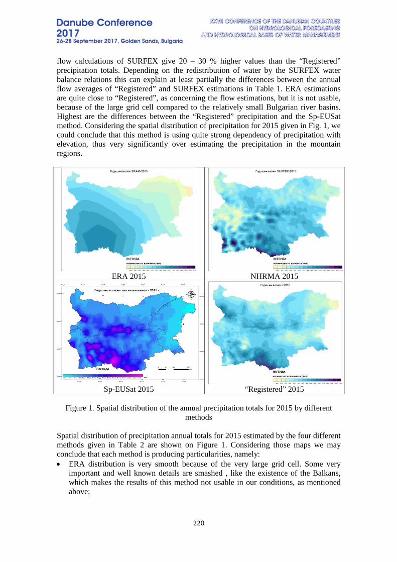
220

flow calculations of SURFEX give 20 – 30 % higher values than the “Registered” precipitation totals. Depending on the redistribution of water by the SURFEX water balance relations this can explain at least partially the differences between the annual flow averages of “Registered” and SURFEX estimations in Table 1. ERA estimations are quite close to “Registered”, as concerning the flow estimations, but it is not usable, because of the large grid cell compared to the relatively small Bulgarian river basins. Highest are the differences between the “Registered” precipitation and the Sp-EUSat method. Considering the spatial distribution of precipitation for 2015 given in Fig. 1, we could conclude that this method is using quite strong dependency of precipitation with elevation, thus very significantly over estimating the precipitation in the mountain regions.

ERA 2015

NHRMA 2015

Sp-EUSat 2015

“Registered” 2015

Figure 1. Spatial distribution of the annual precipitation totals for 2015 by different

methods Spatial distribution of precipitation annual totals for 2015 estimated by the four different methods given in Table 2 are shown on Figure 1. Considering those maps we may conclude that each method is producing particularities, namely: • ERA distribution is very smooth because of the very large grid cell. Some very

important and well known details are smashed , like the existence of the Balkans, which makes the results of this method not usable in our conditions, as mentioned above;

221

• The NHRMA method produces dappled and patched picture, which might not be very likely in annual scale of aggregation. It is also hardly to explain why the area around Sofia, Vitosha and partly Rila are the driest regions.

• The Sp-EUSat method is overestimating precipitation in the mountain regions. The elevation gradients here have high predominance over the final evaluation;

• The “Registered” method is following quite logically the elevation profiles which might not be always true. From the other hand some errors in observation – e.g. Velingrad region are influencing the results heavily.

Conclusions The paper is the first attempt to analyze the quality of the various sources of precipitation field and the possible effect on the modeled annual runoff at national level in Bulgaria. Despite the uncertainties coming from the hydrological model alone the software methods of spatial analysis of precipitation used at national level need further assessment and revision. As discrepancies increase in general with altitude the lack of real-time measuring stations over 600 m a.s.l. is one possible reason for the errors. Therefore an effort should be considered towards the use of reliable methods of screen level meteorological fields’ estimation in near-real-time. This includes the application of altitude gradients based on climatological data. On the other hand, more rain gauges should be automated with telemetry, especially at locations where the analysis error is bigger than the average. The comparison between the simulated average annual runoff by different methods and the measured one shows large differences. Large part of them results from the precipitation overestimation but they also depend on hydrological model schemes and parameters. Therefore a detailed analysis should be performed in order to assess which part of differences come from wrong input forcing (mainly precipitations), which one from the models parameterization (and failed inter-yearly transfers) and which from discrepancies in the hydrological measurements themselves. REFERENCES Yankova, М., Kroumova, К. 2016: Possibility for water resources assessments of surface water in Bulgaria,Water works, NTU, 1/2, 2016, Sofia. Artinyan, E., et al., 2008: Modelling the water budget and the riverflows of the Maritsa basin in Bulgaria. Hydrol Earth Syst Sci 12(1):21–37 Cressman, G. P., 1959: “An operational objective analysis system”, Monthly weather review, Vol.87, N10, October 1959 Gospodinov, I., 2012: National High Resolution Meteorological Analysis (NHRMA), Technical report from NIMH – MOEW annual contract, Sofia, 2012. Hershkovich, E., et al. 1982: Agro-climatological atlas of Bulgaria, Mean Direction of Hydrology and Meteorology – Bulgarian Academy of Sciences, Institute of Hydrology and Meteorology, Institute of Cartography, Sofia, 1982. Le Moigne, P., 2017: The externalised surface model SURFEX. Geoscientific Model Development, special issue. Editor(s): GMD topical editors, Coordinator: P. Le Moigne, 2017.

222

Quintana-Seguí, P. et al. 2008: “Analysis of Near-Surface Atmospheric Variables: Validation of the SAFRAN Analysis over France.” Journal of Applied Meteorology and Climatology 47:92-107. Spiridonov V., 2014: Meteorological fields’ analysis methodology (Sp-EUSat) using ground and satellite data, Sofia, 2014. http://www.hydro.bg/mapValej/metodika_za_satelitni_nazemni.pdf Szczypta, C., et al, 2011: Verification of the new ECMWF ERA-Interim reanalysis over France. Hydrol. Earth Syst. Sci., 15, 647–666, 2011.

223

DEVELOPING THE INFORMATION-ANALYTICAL SYSTEM "STRATIGRAPHY AND PHYSICAL-MECHANICAL PROPERTIES OF THE

SNOWPACK"

Oleksandr Aksiuk , Pavlo Poperechnyi, Hanna Goncharenko

Ukrainian Hydrometeorological Institute, Ukraine

Corresponding author: O. Aksiuk, Ukrainian Hydrometeorological Institute, 37, Nauki Prospect, 03028, Kyiv, Ukraine, alex-aksiyk@ya.ru

ABSTRACT

At present, the important task of the Hydrometeorological Service of Ukraine is the introduction of new technologies in observations of mountain snow cover and avalanche danger forecasting in the Ukrainian Carpathians mountain regions. This process requires a harmonization of the national avalanches observation system with international standards and recommendations. A key element of this is the creation of modern automated information system based on international technical documents regulating all technological stages - from receiving measurement data to provide consumers with services. The guidelines and recommendations of WMO, UNESCO and ISO, as well as other international documents in this area served as the legal framework for this goal. The current state of works in this field is discussed in the article.

Keywords: information system, observations, data

1. INTRODUCTION

The intensive development of regional tourism industry in the Carpathians mountain regions requires providing users with the reliable information about snow and warning about a danger of avalanches. The development of information-analytical system "Stratigraphy and physical-mechanical properties of snowpack" has started in 2014. The aim of this work was to improve local methods of forecasting the avalanche danger based on results of specialized observations of snow cover. A prerequisite for work in this area served as international experts from the Czech Republic, Slovakia and Poland as example of avalanche danger in the Ukrainian Carpathians. As a result of the international monitoring of the winter season 2011-2012 found that Ukrainian avalanche danger forecasts answered 3 level of the European avalanche danger scale. Forecasting the avalanche danger consisted based on meteorological parameters without state stability of the snow cover on the slopes. From 2014 the avalanche stations located in the Ukrainian Carpathians upgraded their instrumentation base and made appropriate changes to the methodology of observations of snow cover. Forward-looking organizations have started to use state stability of the snow cover on the results of observations in the pits. Since 2015 stations avalanche procedures and interpretation of results of observations of snow cover is carried out by "The International Classification of Seasonal Snow on the Ground" and provides

224

communication information-analytical system [3]. Forecasts avalanche danger in the winter of 2016-2017 under the European avalanche danger scale up [2]. In order to improve the efficiency of forecasting an avalanche danger and to provide users with the avalanche-related information in real time the information-analytical system "Stratigraphy and physical-mechanical properties of snowpack" was created by the scientists from the Ukrainian Hydrometeorological Institute. The system meets the modern world standards in this area.

2. METHODOLOGY AND MATERIALS The study is based on: a) the long-term experience of avalanche observations in the mountain regions of Ukraine; b) the international practice in this area.

3. RESULTS AND DISCUSSION

The research institutions located in Russia (mainly in Moscow and Leningrad) were developers of practically all regulation documents which were used by the Hydrometeorological Service of the former Soviet Union. The methodology of snow and avalanche observations in Ukraine is mainly based on these documents. The composition and volume of these observations differs a little from those used in international practice. The main differences are in the parameterization of observations, the presentation of results and units of measurement. Snow is an active environment that has an ability of physical conversion, because the thermodynamic instability is constantly evolving under an influence of external and internal factors. Avalanches occur in case of violation of the stability of the snow due to sudden changes in weather - heavy snowfall, thaw, storm, etc. The features and the underlying surface topography (slope steepness, vegetation, etc.) also affect this process. In the Ukrainian Carpathians avalanches are observed every year. The most avalanches form on slopes with 15 ° and more steep slope and in cases of presence of 30 cm of snow layer. The avalanches can move to a distance from a few tens of meters to 2-3 km with a speed from 1-10 to 80-100 m*s-1. The volumes of avalanche snow fluctuate from tens to one million cubic meters (certain areas of the Ukrainian Carpathians). Currently, in the Ukrainian Carpathians, there are 785 avalanche sites. The largest of them are located within the following mountain ranges: Borzhava, Krasna, Gorgan, Svydovets, Chornohora. But, some small dangerous avalanche area remain unexamined yet. The Ukrainian Carpathians are divided into 21 avalanche area (Fig.1). The basis of the zoning principle laid basin. The division into districts is made by using regional characteristics and mode of snow avalanche activity. Its basis is the three main streams: Tisa (1 - 12 districts), Prut (13 - 15 districts) and Dniester (16 - 21 areas) [1].

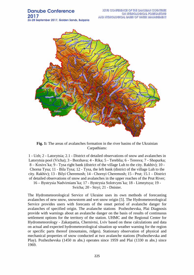
225

Fig. 1: The areas of avalanches formation in the river basins of the Ukrainian Carpathians:

1 - Uzh; 2 - Latorytsia; 2.1 - District of detailed observations of snow and avalanches in Latorytsia pool (Vicha); 3 - Borzhava; 4 - Rika; 5 - Tereblia; 6 - Teresva; 7 - Shopurka; 8 – Kosivs`ka; 9 - Tysa right bank (district of the village Luh to the city. Rakhiv); 10 - Chorna Tysa; 11 - Bila Tysa; 12 - Tysa, the left bank (district of the village Luh to the

city. Rakhiv); 13 - Bilyi Cheremosh; 14 - Chornyi Cheremosh; 15 - Prut; 15.1 – District of detailed observations of snow and avalanches in the upper reaches of the Prut River;

16 – Bystrysia Nadvirnians`ka; 17 - Bystrysia Solotvyns`ka; 18 - Limnytsya; 19 - Svicha; 20 - Stryi; 21 - Dnister.

The Hydrometeorological Service of Ukraine uses its own methods of forecasting avalanches of new snow, snowstorm and wet snow origin [5]. The Hydrometeorological Service provides users with forecasts of the onset period of avalanche danger for avalanches of specified origin. The avalanche stations Pozhezhevska, Plai Diagnosis provide with warnings about an avalanche danger on the basis of results of continuous settlement options for the territory of the station. UHMC and the Regional Center for Hydrometeorology - Zakarpattia, Chernivtsi, Lviv based on these calculations and data on actual and expected hydrometeorological situation up weather warning for the region or specific parts thereof (mountains, ridges). Stationary observation of physical and mechanical properties of snow conducted at two avalanche stations (Pozhezhevska and Play). Pozhezhevska (1450 m abs.) operates since 1959 and Plai (1330 m abs.) since 1969.

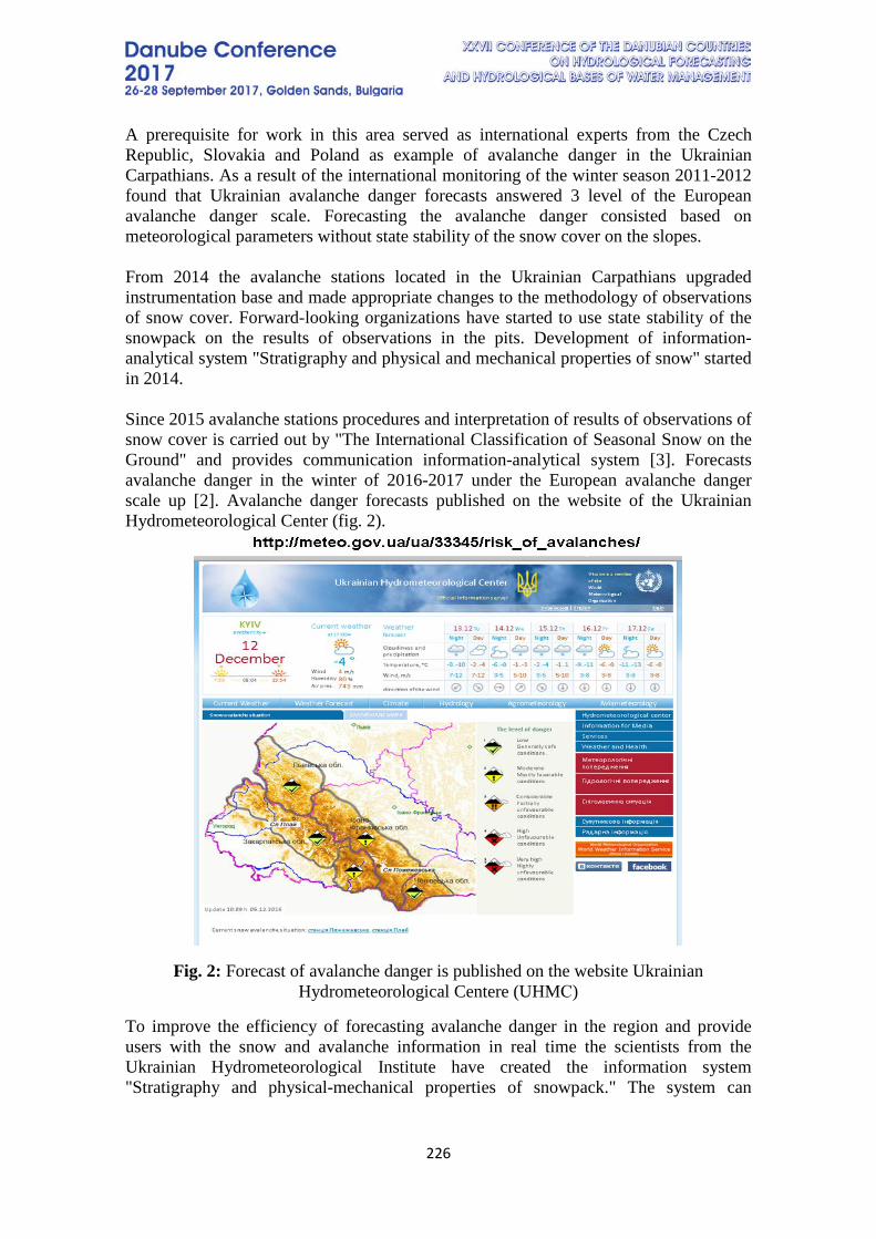
226

A prerequisite for work in this area served as international experts from the Czech Republic, Slovakia and Poland as example of avalanche danger in the Ukrainian Carpathians. As a result of the international monitoring of the winter season 2011-2012 found that Ukrainian avalanche danger forecasts answered 3 level of the European avalanche danger scale. Forecasting the avalanche danger consisted based on meteorological parameters without state stability of the snow cover on the slopes. From 2014 the avalanche stations located in the Ukrainian Carpathians upgraded instrumentation base and made appropriate changes to the methodology of observations of snow cover. Forward-looking organizations have started to use state stability of the snowpack on the results of observations in the pits. Development of information-analytical system "Stratigraphy and physical and mechanical properties of snow" started in 2014. Since 2015 avalanche stations procedures and interpretation of results of observations of snow cover is carried out by "The International Classification of Seasonal Snow on the Ground" and provides communication information-analytical system [3]. Forecasts avalanche danger in the winter of 2016-2017 under the European avalanche danger scale up [2]. Avalanche danger forecasts published on the website of the Ukrainian Hydrometeorological Center (fig. 2).

Fig. 2: Forecast of avalanche danger is published on the website Ukrainian Hydrometeorological Centere (UHMС)

To improve the efficiency of forecasting avalanche danger in the region and provide users with the snow and avalanche information in real time the scientists from the Ukrainian Hydrometeorological Institute have created the information system "Stratigraphy and physical-mechanical properties of snowpack." The system can

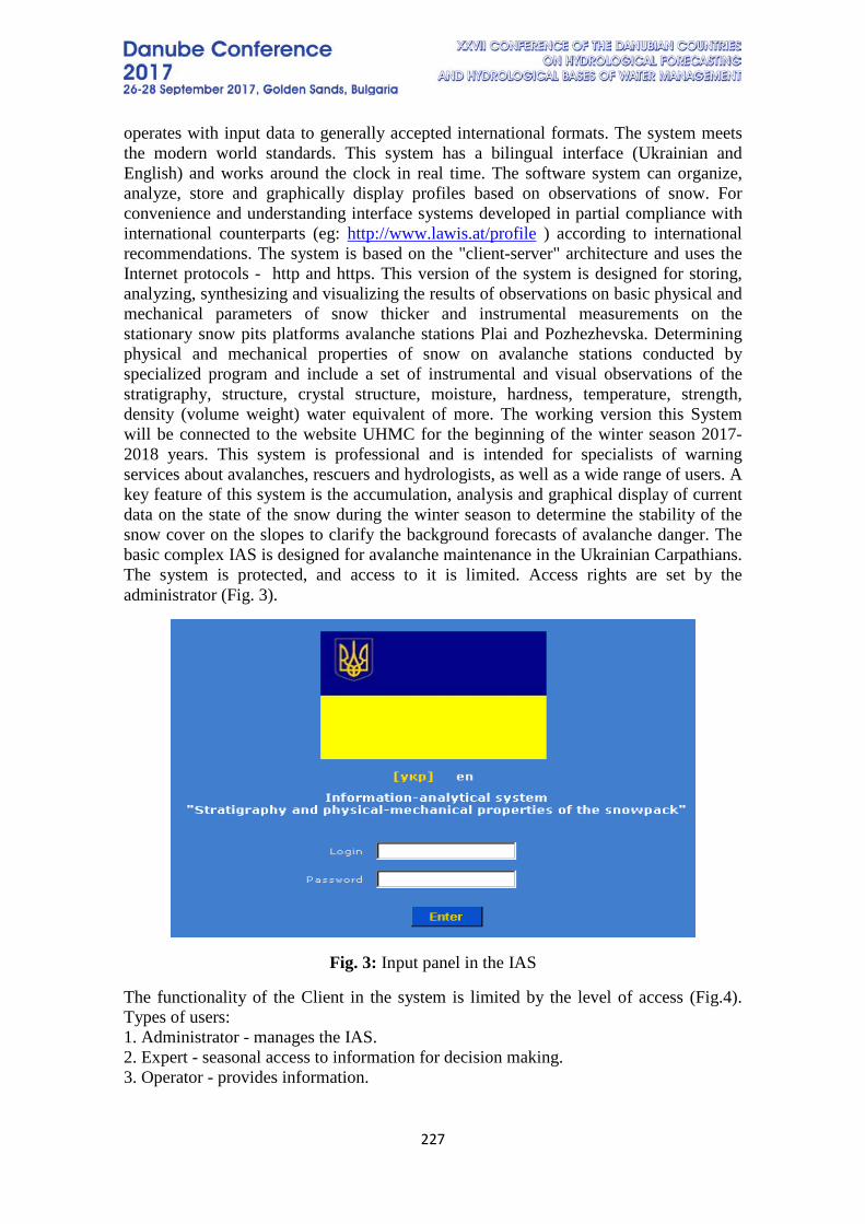
227

operates with input data to generally accepted international formats. The system meets the modern world standards. This system has a bilingual interface (Ukrainian and English) and works around the clock in real time. The software system can organize, analyze, store and graphically display profiles based on observations of snow. For convenience and understanding interface systems developed in partial compliance with international counterparts (eg: http://www.lawis.at/profile ) according to international recommendations. The system is based on the "client-server" architecture and uses the Internet protocols - http and https. This version of the system is designed for storing, analyzing, synthesizing and visualizing the results of observations on basic physical and mechanical parameters of snow thicker and instrumental measurements on the stationary snow pits platforms avalanche stations Plai and Pozhezhevska. Determining physical and mechanical properties of snow on avalanche stations conducted by specialized program and include a set of instrumental and visual observations of the stratigraphy, structure, crystal structure, moisture, hardness, temperature, strength, density (volume weight) water equivalent of more. The working version this System will be connected to the website UHMC for the beginning of the winter season 2017-2018 years. This system is professional and is intended for specialists of warning services about avalanches, rescuers and hydrologists, as well as a wide range of users. A key feature of this system is the accumulation, analysis and graphical display of current data on the state of the snow during the winter season to determine the stability of the snow cover on the slopes to clarify the background forecasts of avalanche danger. The basic complex IAS is designed for avalanche maintenance in the Ukrainian Carpathians. The system is protected, and access to it is limited. Access rights are set by the administrator (Fig. 3).

Fig. 3: Input panel in the IAS

The functionality of the Client in the system is limited by the level of access (Fig.4). Types of users: 1. Administrator - manages the IAS. 2. Expert - seasonal access to information for decision making. 3. Operator - provides information.

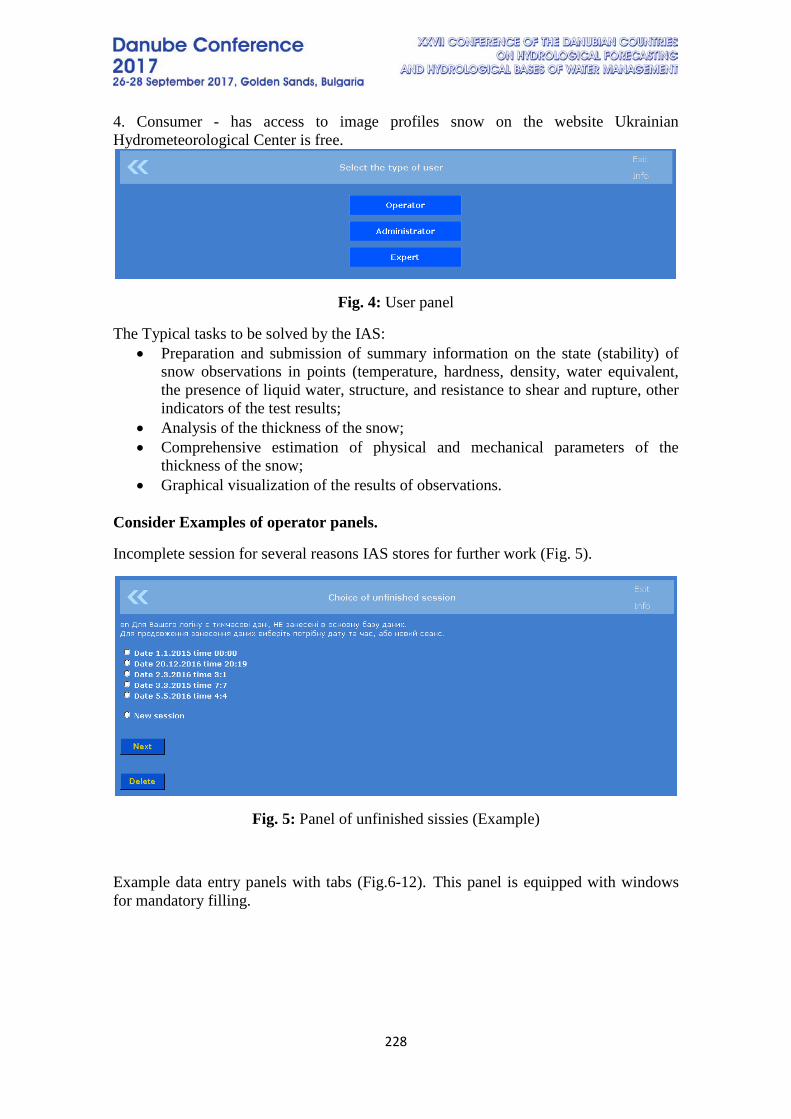
228

4. Consumer - has access to image profiles snow on the website Ukrainian Hydrometeorological Center is free.

Fig. 4: User panel

The Typical tasks to be solved by the IAS: • Preparation and submission of summary information on the state (stability) of

snow observations in points (temperature, hardness, density, water equivalent, the presence of liquid water, structure, and resistance to shear and rupture, other indicators of the test results;

• Analysis of the thickness of the snow; • Comprehensive estimation of physical and mechanical parameters of the

thickness of the snow; • Graphical visualization of the results of observations.

Consider Examples of operator panels.

Incomplete session for several reasons IAS stores for further work (Fig. 5).

Fig. 5: Panel of unfinished sissies (Example)

Example data entry panels with tabs (Fig.6-12). This panel is equipped with windows for mandatory filling.

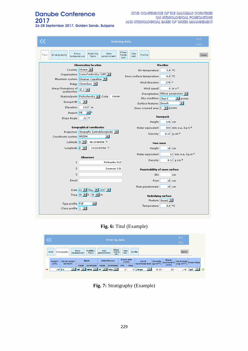
229

Fig. 6: Titul (Example)

Fig. 7: Stratigraphy (Example)

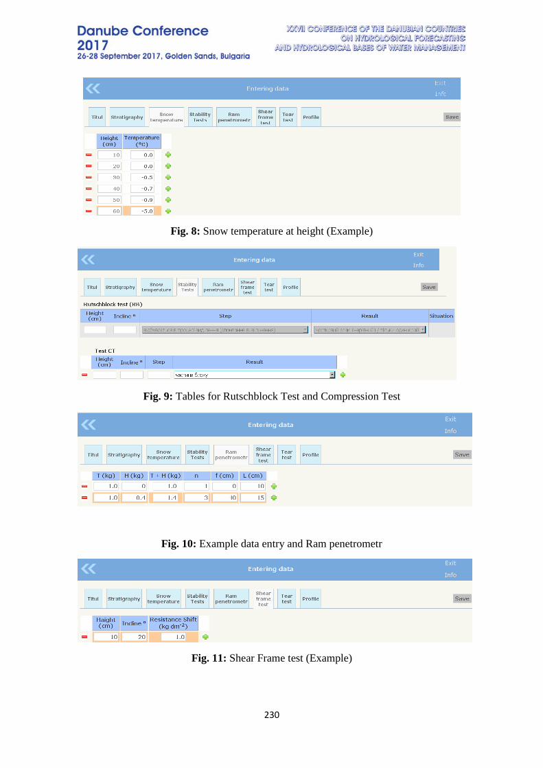
230

Fig. 8: Snow temperature at height (Example)

Fig. 9: Tables for Rutschblock Test and Compression Test

Fig. 10: Example data entry and Ram penetrometr

Fig. 11: Shear Frame test (Example)

231

Fig. 12: Tear test (Example)

Fig. 13: Fragment of active snow profile (Example)

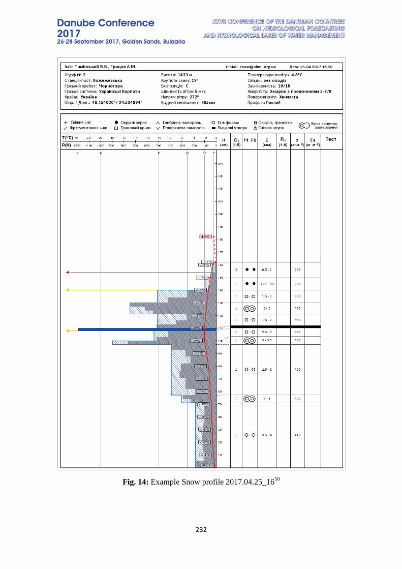
232

Fig. 14: Example Snow profile 2017.04.25_1650

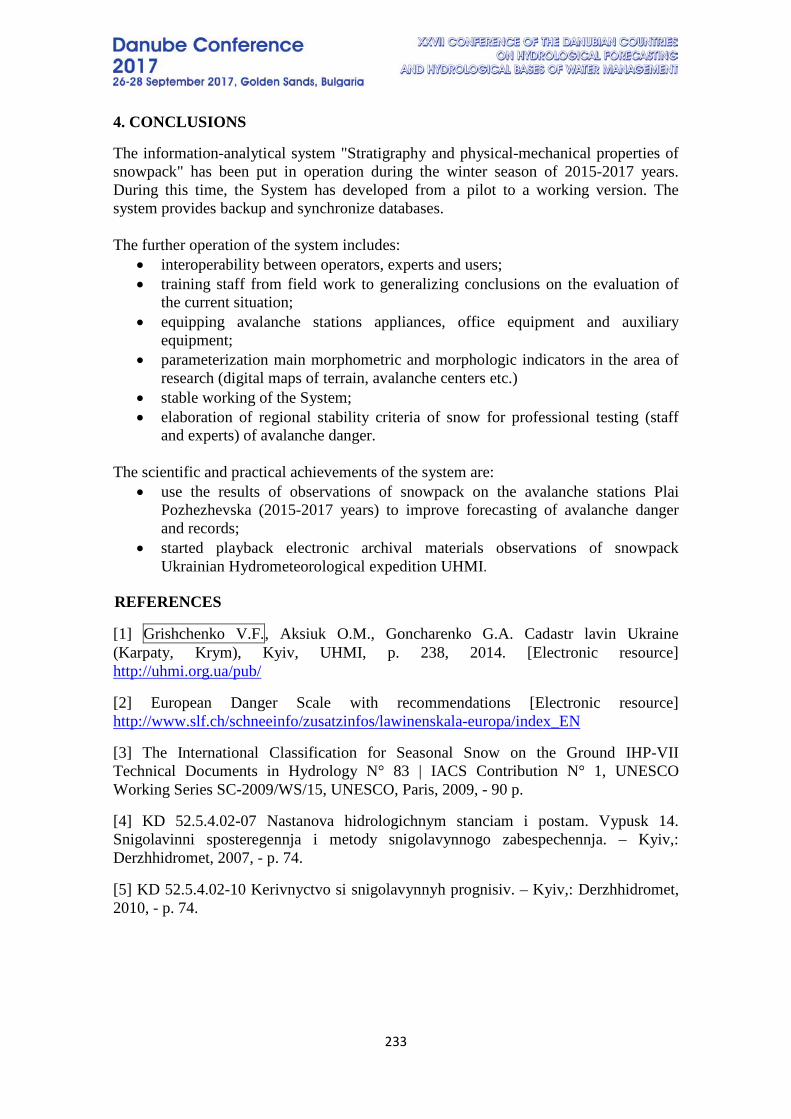
233

4. CONCLUSIONS

The information-analytical system "Stratigraphy and physical-mechanical properties of snowpack" has been put in operation during the winter season of 2015-2017 years. During this time, the System has developed from a pilot to a working version. The system provides backup and synchronize databases. The further operation of the system includes:

• interoperability between operators, experts and users; • training staff from field work to generalizing conclusions on the evaluation of

the current situation; • equipping avalanche stations appliances, office equipment and auxiliary

equipment; • parameterization main morphometric and morphologic indicators in the area of

research (digital maps of terrain, avalanche centers etc.) • stable working of the System; • elaboration of regional stability criteria of snow for professional testing (staff

and experts) of avalanche danger. The scientific and practical achievements of the system are:

• use the results of observations of snowpack on the avalanche stations Plai Pozhezhevska (2015-2017 years) to improve forecasting of avalanche danger and records;

• started playback electronic archival materials observations of snowpack Ukrainian Hydrometeorological expedition UHMI.

REFERENCES

[1] Grishchenko V.F., Aksiuk O.M., Goncharenko G.A. Cadastr lavin Ukraine (Karpaty, Krym), Kyiv, UHMI, p. 238, 2014. [Electronic resource] http://uhmi.org.ua/pub/

[2] European Danger Scale with recommendations [Electronic resource] http://www.slf.ch/schneeinfo/zusatzinfos/lawinenskala-europa/index_EN

[3] The International Classification for Seasonal Snow on the Ground IHP-VII Technical Documents in Hydrology N° 83 | IACS Contribution N° 1, UNESCO Working Series SC-2009/WS/15, UNESCO, Paris, 2009, - 90 p.

[4] KD 52.5.4.02-07 Nastanova hidrologichnym stanciam i postam. Vypusk 14. Snigolavinni sposteregennja i metody snigolavynnogo zabespechennja. – Kyiv,: Derzhhidromet, 2007, - p. 74.

[5] KD 52.5.4.02-10 Kerivnyctvo si snigolavynnyh prognisiv. – Kyiv,: Derzhhidromet, 2010, - p. 74.

234

THE LONG-TERM FLUCTUATIONS OF MAXIMUM WATER LEVELS OF THE COLD PERIOD FLOODS IN DANUBE RIVER BASIN (UKRAINIAN PART)

Ievgeniia Vasylenko

Ukrainian Hydrometeorological Institute, Ukraine Corresponding author: Vasylenko Ievgeniia, Ukrainian Hydrometeorological Institute,

37, Naukiave, Kiev, 03028, Ukraine, evg_vasylenko@ukr.net

INTRODUCTION Necessity of proper consideration of the features and the regularities of many natural phenomena and processes, including the widespread and systematic use of water resources, has increased due to the development of economy and improvement of management. It also has caused an increased interest to the problem of long-term fluctuations of maximum runoff, its cyclicity, synchronicity and non-synchronicity in different river basins and regions [2]. The researches of long-term fluctuations of the main characteristics of river runoff, including the maximum water levels, have been important for the forecasting of disastrous floods on the rivers, for calculation of the computed characteristics values, that are required for the designing of hydraulic structures, for the estimation of flooded areas caused by the passage of the floods with different probability etc.

1. DATA AND METHODS The database for the 34 gauging stations on the Danube River (the river mouth area) and in the basins of its main tributaries (Tysa, Prut etc.) has been formed for the estimation of long-term fluctuations of maximum water levels of the cold period floods in the Danube River basin (within Ukraine). The observation period for gauges has been from 89 (gauges on the Tysa river) to 36 years (Kamianka River – Dora Village). The chronological series of maximum water levels of the cold period floods have had many gaps. Owing to avoid the gaps with years of the highest (P<5 %) and the lowest (P>95 %) mixed origin floods, the procedure of data restoration has been carried out. The procedure of water levels restoration has been done by using the method of pair linear regression. This method consists of the calculating the regression equation by using the data of the analogues rivers. The maximum water levels have been restored, on condition according to current building norm and rules 2.01.14-83 [1, 5]. The gaps in the series of maximum water levels have been restored for the 14 gauging stations in the Danube River basin. Basically, the analogues for restoration of water levels have been the gauges that are located directly on the Danube river and the gauging stations that have the longest series of observations (the rivers Tysa, Prut, etc.). The correlation coefficients between the series of the gauging stations, for which the data have been restored, and the series of the gauges-analogues were ≥ 0,8 (Table 1).

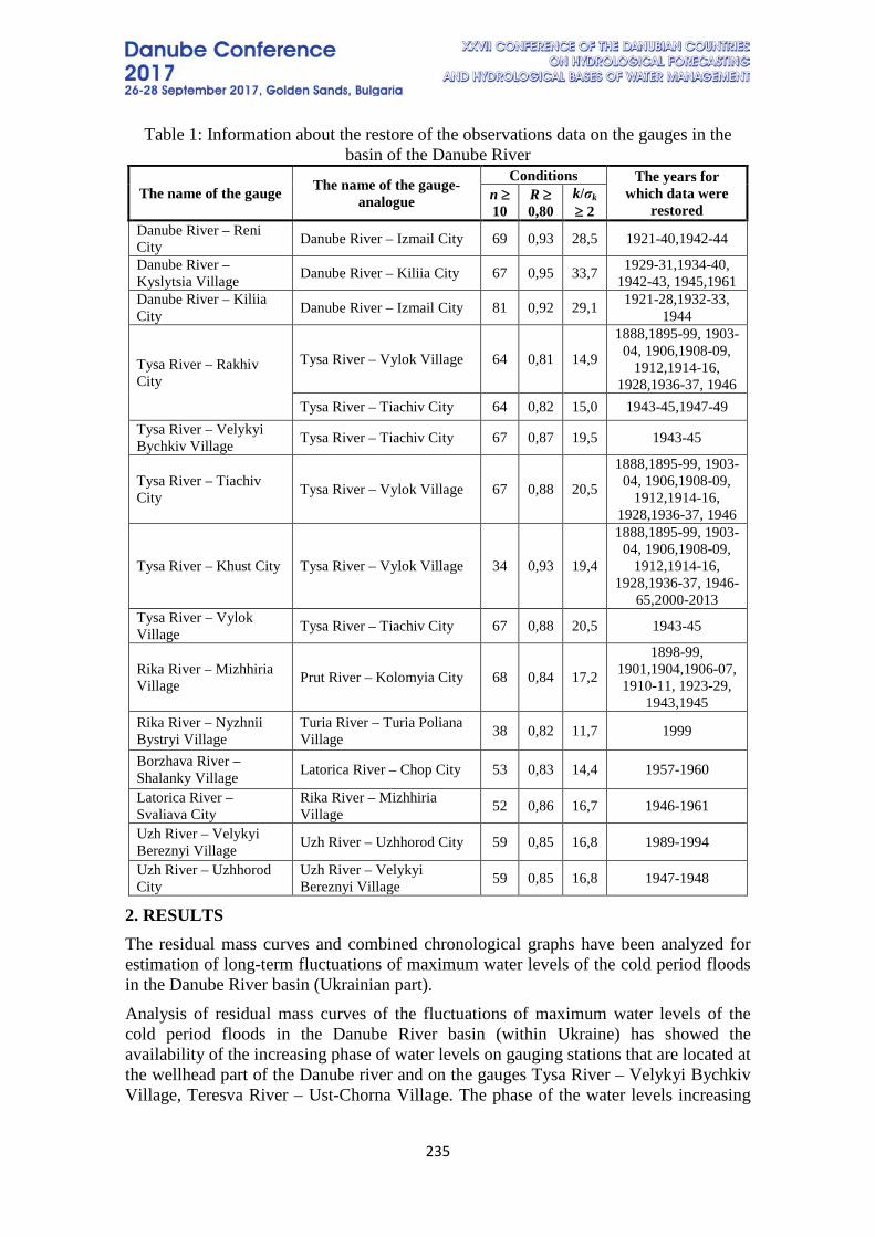
235

Table 1: Information about the restore of the observations data on the gauges in the basin of the Danube River

The name of the gauge The name of the gauge-analogue

Conditions The years for which data were

restored n ≥ 10

R ≥ 0,80

k/σk ≥ 2

Danube River – Reni City Danube River – Izmail City 69 0,93 28,5 1921-40,1942-44

Danube River – Kyslytsia Village Danube River – Kiliia City 67 0,95 33,7 1929-31,1934-40,

1942-43, 1945,1961 Danube River – Kiliia City Danube River – Izmail City 81 0,92 29,1 1921-28,1932-33,

1944

Tysa River – Rakhiv City

Tysa River – Vylok Village 64 0,81 14,9

1888,1895-99, 1903-04, 1906,1908-09,

1912,1914-16, 1928,1936-37, 1946

Tysa River – Tiachiv City 64 0,82 15,0 1943-45,1947-49 Tysa River – Velykyi Bychkiv Village Tysa River – Tiachiv City 67 0,87 19,5 1943-45

Tysa River – Tiachiv City Tysa River – Vylok Village 67 0,88 20,5

1888,1895-99, 1903-04, 1906,1908-09,

1912,1914-16, 1928,1936-37, 1946

Tysa River – Khust City Tysa River – Vylok Village 34 0,93 19,4

1888,1895-99, 1903-04, 1906,1908-09,

1912,1914-16, 1928,1936-37, 1946-

65,2000-2013 Tysa River – Vylok Village Tysa River – Tiachiv City 67 0,88 20,5 1943-45

Rika River – Mizhhiria Village Prut River – Kolomyia City 68 0,84 17,2

1898-99, 1901,1904,1906-07, 1910-11, 1923-29,

1943,1945 Rika River – Nyzhnii Bystryi Village

Turia River – Turia Poliana Village 38 0,82 11,7 1999

Borzhava River – Shalanky Village Latorica River – Chop City 53 0,83 14,4 1957-1960

Latorica River – Svaliava City

Rika River – Mizhhiria Village 52 0,86 16,7 1946-1961

Uzh River – Velykyi Bereznyi Village Uzh River – Uzhhorod City 59 0,85 16,8 1989-1994

Uzh River – Uzhhorod City

Uzh River – Velykyi Bereznyi Village 59 0,85 16,8 1947-1948

2. RESULTS The residual mass curves and combined chronological graphs have been analyzed for estimation of long-term fluctuations of maximum water levels of the cold period floods in the Danube River basin (Ukrainian part). Analysis of residual mass curves of the fluctuations of maximum water levels of the cold period floods in the Danube River basin (within Ukraine) has showed the availability of the increasing phase of water levels on gauging stations that are located at the wellhead part of the Danube river and on the gauges Tysa River – Velykyi Bychkiv Village, Teresva River – Ust-Chorna Village. The phase of the water levels increasing

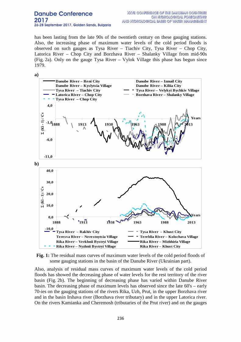
236

has been lasting from the late 90s of the twentieth century on these gauging stations. Also, the increasing phase of maximum water levels of the cold period floods is observed on such gauges as Tysa River – Tiachiv City, Tysa River – Chop City, Latorica River – Chop City and Borzhava River – Shalanky Village from mid-90s (Fig. 2a). Only on the gauge Tysa River – Vylok Village this phase has begun since 1979.

a)

b)

Fig. 1: The residual mass curves of maximum water levels of the cold period floods of

some gauging stations in the basin of the Danube River (Ukrainian part). Also, analysis of residual mass curves of maximum water levels of the cold period floods has showed the decreasing phase of water levels for the rest territory of the river basin (Fig. 2b). The beginning of decreasing phase has varied within Danube River basin. The decreasing phase of maximum levels has observed since the late 60's – early 70-ies on the gauging stations of the rivers Rika, Uzh, Prut, in the upper Borzhava river and in the basin Irshava river (Borzhava river tributary) and in the upper Latorica river. On the rivers Kamianka and Cheremosh (tributaries of the Prut river) and on the gauges

-11,0

-6,0

-1,0

4,0

1888 1913 1938 1963 1988 2013

Years

Σ (К

і - 1

) / C

v

Danube River – Reni City Danube River – Izmail CityDanube River – Kyslytsia Village Danube River – Kiliia CityTysa River – Tiachiv City Tysa River – Velykyi Bychkiv VillageLatorica River – Chop City Borzhava River – Shalanky VillageTysa River – Chop City

-10,0

0,0

10,0

20,0

30,0

40,0

1888 1913 1938 1963 1988 2013

Years

Σ (К

і - 1

) / C

v

Tysa River – Rakhiv City Tysa River – Khust CityTeresva River – Nerestnytsia Village Tereblia River – Kolochava VillageRika River – Verkhnii Bystryi Village Rika River – Mizhhiria VillageRika River – Nyzhnii Bystryi Village Rika River – Khust City

237

Tysa River – Rakhiv City, Tysa River – Khust City, Teresva River – Nerestnytsia Village and Rika River – Khust City – since the early 80s. On some gauging stations of the Danube river basin the decreasing phase of maximum water levels of the cold period flood has observed since the late 80's - early 90-ies of the XX century (upper and lower streams of the river Latorica, Tereblia River – Kolochava Village, Uzh River – Zarichevo Village).

3. CONCLUSION The research of long-term dynamics of maximum water levels of the cold period floods and the analysis of the residual mass curves showed synchronous fluctuations of the water levels for gauges, and the non-in-phase fluctuations for the gauging stations that are located in the mountainous areas (Prut River basin, Tysa River and its tributaries Teresva River, Tereblia River, Rika River, Borzhava River, Uzh River) and the gauging stations that are located within the Transcarpathian (Tysa River – Tiachiv City, Tysa River – Velykyi Bychkiv Village, Tysa River – Chop City, Latorica River – Chop City, Borzhava River – Shalanky Village) and the Black Sea Lowlands (gauges in the Danube River mouth area). In contrast to gauging stations of the mountainous areas, where the decreasing phase of maximum water levels of the cold period floods has been observed, maximum water levels on the gauging stations of the lowlands have had the increasing phase. We can assume that cyclical changes of maximum water levels of the cold period floods in the Danube River basin (within Ukraine) were caused by regularities of multi-annual fluctuations of large-scale atmospheric processes over Europe. These processes correspond to the features of cyclonic activity over the North Atlantic and manifest in changing of the regions of cyclones forming, in shifting of their trajectories and intensity of synoptic processes [3, 4].

REFERENCES [1] BNR (The building norm and rules 2.01.14-83) Determination of the calculation hydrologic characteristics. State committee USSR on the construction, p. 97, 1983. [2] Imanov F., Hasanova N. Long term fluctuations of mountain river maximum flow Proceedings of the Russian State Hydrometeorological University. A theoretical research journal, Russia, pp 40-46, 2009. [3] Lukianets O. The spatial synchronicity of water content in the Carpathian region, IV All-Ukrainian Scientific Conference “Hydrology, hydrochemistry, hydroecology”, Ukraine. – p. 224, 2009. [4] Sosedko M., Lukianets O. Multi-annual fluctuations of water content in Ukraine, Scientific Journal “Hydrology, hydrochemistry, hydroecology”, Ukraine, vol. 4 (21), pp 34-40, 2010. [5] The methodological recommendations for assessment the homogeneity of the hydrological characteristics and definition of their calculation values for the non-homogeneous data, State Hydrological Institute, Saint Petersburg, Russia, pp 39–40, 2010.

238

TOPIC 3: HYDROLOGICAL MODELING AND FORECASTING

NEW PRODUCTS IN HYDROLOGICAL FORECASTING SYSTEM ON

MORAVA RIVER

Petr Janál, Jakub Jansa Czech Hydrometeorological Institute, Czech Republic

Corresponding author: Ing. Petr Janál, Ph.D., Czech Hydrometeorological Institute – Brno Regional Office, Kroftova 43, Brno, 616 67, Czech Republic, petr.janal@chmi.cz

ABSTRACT The error of the precipitation forecast is usually the main factor that influences the accuracy of the discharge forecast. The deterministic discharge forecast based on one rainfall scenario is a great simplification of the real situation – the indeterminations, which influences the whole calculation process, are not expressed in the final discharge forecast. When significant decisions are to be made according to an actual discharge forecast, it is necessary to estimate the hazard factor. That’s why new hydrological forecasting products, such a probabilistic, variant and stochastic forecast, are developed to take into account the uncertainties included in the whole forecasting process. Keywords: Operative hydrology, hydrological forecast, Morava river basin

1. INTRODUCTION Czech Hydrometeorological Institute (CHMI) – the national hydrological service – issues daily deterministic hydrological forecasts with a lead time of 66 h for more than one hundred water-gauge stations. Within the Morava River catchment, there are 25 forecasting profiles in the Czech Republic and 3 forecasting profiles abroad. The last forecasting river profile is the gauging station Hohenau an der March under the junction of Morava and Dyje Rivers. For the operation of flood forecasting service, the international cooperation is necessary because the significant part of upper Dyje catchment spreads in Austria and also there is Myjava River basin in Slovakia. The key organizations for cooperation during forecasting process are Povodí Moravy s.p. (water reservoir control), Austrian hydrological service and Slovak Hydrometeorological Institute. Communication and data transfer within mentioned organizations are crucial for the effective operation of Flood Forecasting Service (FFS) of CHMI.

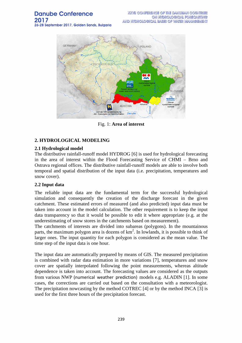
239

Fig. 1: Area of interest

2. HYDROLOGICAL MODELING 2.1 Hydrological model The distributive rainfall-runoff model HYDROG [6] is used for hydrological forecasting in the area of interest within the Flood Forecasting Service of CHMI – Brno and Ostrava regional offices. The distributive rainfall-runoff models are able to involve both temporal and spatial distribution of the input data (i.e. precipitation, temperatures and snow cover).

2.2 Input data The reliable input data are the fundamental term for the successful hydrological simulation and consequently the creation of the discharge forecast in the given catchment. These estimated errors of measured (and also predicted) input data must be taken into account in the model calculation. The other requirement is to keep the input data transparency so that it would be possible to edit it where appropriate (e.g. at the underestimating of snow stores in the catchments based on measurement). The catchments of interests are divided into subareas (polygons). In the mountainous parts, the maximum polygon area is dozens of km2. In lowlands, it is possible to think of larger ones. The input quantity for each polygon is considered as the mean value. The time step of the input data is one hour. The input data are automatically prepared by means of GIS. The measured precipitation is combined with radar data estimation in more variations [7], temperatures and snow cover are spatially interpolated following the point measurements, whereas altitude dependence is taken into account. The forecasting values are considered as the outputs from various NWP (numerical weather prediction) models e.g. ALADIN [1]. In some cases, the corrections are carried out based on the consultation with a meteorologist. The precipitation nowcasting by the method COTREC [4] or by the method INCA [3] is used for the first three hours of the precipitation forecast.

240

Fig. 2: Input data

The manual model calculation by the hydrologists remains the base for the daily forecasting routine. However, the Process of input data producing and model calculation is also automated which enables frequent updating of discharge forecast (every hour if necessary). Thus the hydrologist can (taking into account the most up-to-date data) observe the changing conditions in the catchment, adapt the hydrological model according to the real situation easily and estimate the future development of the flood.

2.3 Uncertainties The hydrological forecast is created under the conditions of significant uncertainty. The error of (not only) predicted data can be great. That’s why there is a need for new approaches in hydrological modeling.

3. PRODUCTS OF HYDROLOGICAL FORECAST 3.1 Deterministic forecast

The deterministic discharge forecast is based usually on the precipitation (and temperature) forecast of NWP model ALADIN. These inputs for the hydrological model can be edited according to the meteorologists if necessary. Deterministic discharge forecast is the best estimate of the future development in the catchment, however, the uncertainty of the inputs is not involved in the hydrological calculation process. The deterministic discharged forecast is published on CHMI website.

3.2 Probabilistic forecast The probabilistic hydrological forecast is provided by CHMI since 2012 in addition to deterministic forecasts. Input data comes from ensemble (16 members) of NWP model ALADIN-LAEF (precipitation and temperature). The resulting hydrological ensemble is evaluated as the probability of exceedance of limit discharges in every forecasting watergauge station and in this form also published on CHMI website.

241

Fig. 3: Preview of the CHMI website for watergauge station Dalečín on

Svratka River where the measured water states and flows are displayed. The blue line represents a deterministic forecast and in the lower right

corner, there is a probabilistic forecast.

3.3 Variant forecast The variant hydrological forecast is also calculated in daily routine (for internal use only). The outputs (precipitation and temperature) from 4 different NWP models are used as inputs to the hydrological model and 4 discharge forecasts are obtained. The variant discharge forecasts is another kind of information which can be useful for hydrologists when there is a danger of flood. It is not published on CHMI website but it can be provided to the CHMI partner organizations within the Flood Forecasting Service. Following NWP models are considered:

• ALADIN (CZ) - resolution 4.5 x 4.5 km (local model) o Available 4 times a day (at 00:00, 06:00, 12:00 and 18:00 CET),

lead time 72 hours [1] • ICON (D) (former name LMEB) - resolution of about 6 x 6 km (local

model) o Available 4 times a day (at 00:00, 06:00, 12:00 and 18:00 CET),

lead time 72 hours [8] • ECMWF (GB) - resolution 16 x 16 km (global model)

o Available 2 times a day (at 00:00 and 12:00 CET), lead time 240 hours [5]

• GFS (USA) - resolution 13 x13 km (global model) o Available 4 times a day (at 00:00, 06:00, 12:00 and 18:00 CET),

lead time 72 hours [2] Figure 4 shows that hydrological forecasts based on particular NWP models can

significantly differ.

242

Fig. 4: Variant forecast – hydrological forecast based on different NWP

models (LMEB is former name for ICON)

3.4 Stochastic forecast The stochastic discharge forecast enables to involve the estimated errors of measured or predicted climatic data (precipitation, temperature, snow cover etc.) to the hydrological calculation of the outflow from the catchment. The set of input data is generated n-times according to the given parameters (mean value, estimated error of measured or predicted data), the correlation matrix ensures the spatial correlation of the inputs. Then the hydrological simulation is run repeatedly and the final set of outflows from given catchment is evaluated as e.g. peak discharge exceedance curve. This product is tested in operation on several catchments within the Dyje River basin since 2017.

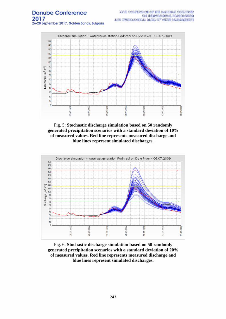
243

Fig. 5: Stochastic discharge simulation based on 50 randomly

generated precipitation scenarios with a standard deviation of 10% of measured values. Red line represents measured discharge and

blue lines represent simulated discharges.

Fig. 6: Stochastic discharge simulation based on 50 randomly

generated precipitation scenarios with a standard deviation of 20% of measured values. Red line represents measured discharge and

blue lines represent simulated discharges.

244

4. CONCLUSION The Flood Forecasting Service ensured by Czech Hydrological Institute has made a great progress within last twenty years. The hydrological models are used for calculation of the discharge forecasts in many river profiles – the deterministic discharge forecast is now a common product well known by subjects involved in the FFS and also by the public. The effort to improve the products of FFS leads to including of the uncertainties of measured and predicted climatic data necessary for the hydrological calculations to the process of the creation of the discharge forecasts. The new products of the hydrological forecast (probabilistic, variant and stochastic forecasts) can contribute to better awareness of experts and public and to improve the flood protection. However, to apply the discharge forecast effectively, it is necessary to interpret it well. Therefore there is a need of continuing in the training of all users of discharge forecasts.

REFERENCES [1] ALADIN International Team (1997). The ALADIN project: Mesoscale modelling seen as a basic tool for weather forecasting and atmospheric research. WMO Bulletin, 46, pp. 317-324. [2] Environmental Modeling Center. (2003). The GFS atmospheric model. NCEP office note 442. Camp Springs, MD: Global Climate and Weather Modeling Branch, EMC. [3] Haiden, T., A. Kann, C. Wittmann , G. Pistotnik, B. Bica, C. Gruber, (2011). The Integrated Nowcasting through Comprehensive Analysis (INCA) system and its validation over the Eastern Alpine region. In: Weather Forecasting, 26. [4] Novák, P., (2007). The Czech Hydrometeorological Institute’s Severe Storm Nowcasting System. In: Atmospheric Research, 83, pp. 450–457. [5] Molteni, F., Buizza, R., Palmer, T. N., & Petroliagis, T. (1996). The ECMWF ensemble prediction system: Methodology and validation. The Quarterly Journal of the Royal Meteorological Society, 122(529), 73-119. [6] Starý, M., (1991-2017). HYDROG, Software for simulation, prediction and operative control of water outflow from the river catchment, Brno, Czech Republic [7] Šálek M., Novák P., Seo D.-J., (2004). Operational application of combined radar and raingauges precipitation estimation at the CHMI. In: ERAD 2004 proceedings, ERAD publication series, Vol. 2, pp. 16-20. [8] Zängl, G., Reinert, D., Ripodas, P., & Baldauf, M. (2015) The ICON (ICOsahedral Non-hydrostatic) modeling framework of DWD and MPI-M: Description of the non-hydrostatic dynamical core. The Quarterly Journal of the Royal Meteorological Society, 141(687), 563-579.

245

MODELING AND FORECASTING OF THE RIVERFLOW IN LOWER COURSE OF OSAM, VIT AND OGOSTA RIVERS

Nikolay Nedkov, Eram Artinyan

National Institute of Meteorology and Hydrology - BAS, Bulgaria

Corresponding author: N. Nedkov, NIMH, H. Dimitar 60, Pleven, Bulgaria,

nikolai.nedkov@meteo.bg, E. Artinyan, NIMH, Ruski 139, Plovdiv, Bulgaria, eram.artinian@meteo.bg

ABSTRACT

In recent years, possibly connected with climate alteration, floods become more frequent, their economic, social and environmental consequences are increasing. In this respect, of great economic importance is to provide high quality hydrological forecasts, on the reliability of which to a certain extent depend prevention and mitigation of dangerous hydrological phenomena, as well as water use efficiency.

The poster presents results of the hydrological model SURFEX - TOPODYN, after it’s calibration to compute the river flow in the lower reaches of Osam, Vit and Ogosta rivers in Bulgaria. For the analysis simulation the models is forced with meteorological data from ground stations. Forecast simulations are forced with the meteorological data from the atmospheric model ALADIN. Quality of the forecasted river flow through the individual points of the river network is estimated using statistical methods against actual measured hydrological data.

The results display that forecasted river flows are close to the measured data at the hydrometric stations of the Vit Osam and Ogosta rivers. They show a successful completion of the calibration process of the model and the readiness of the model for further water balances investigations and scenario’s developments regarding the studied watersheds.

Keywords: hydrological modeling, hydrological forecasting

1. INTRODUCTION One of the most complex problems in hydrologic practice is preparing of hydrological forecast based on the precise description of the spatial heterogeneity of the physiographical and climatic features on the rivers basins. In recent years several types of hydrological models have been developed to solve this problem. Usage of such models improves the accuracy of hydrological forecasts and creates an opportunity to improve the forecasting and create better conditions for the timely warning of floods in the rivers basins.

246

In NIMH branch Pleven from 2015 the forecasting of the river flow is made by the modelling platform SURFEX. It is developed by the Centre National de Recherches Météorologiques (CNRM) within Météo-France in cooperation with the scientific community [1].

This article analyzes the results achieved by the application of the model for hydrological forecasting in lower course of Osam, Vit and Ogosta rivers.

2. METHODOLOGY The modeling platform SURFEX is developed to describe the energy and the water fluxes between the boundary of the atmosphere and the land surface. SURFEX includes a group of models for different types of earth surfaces. The main component in SURFEX, related to the river flow is ISBA model – Interface Soil Biosphere Atmosphere [2]. ISBA combines physical models of the relationship between atmosphere and soil and can calculate the flow as a balance difference between precipitation and evaporation. The model uses a tiled approach for parameterization of the earth surface characteristics. The information about the tiles “nature”, “lake”, “town” and “sea” is grouped into a single database called ECOCLIMAP [3]. The energy and the water fluxes are the average of the fluxes computed over nature, town, sea/ocean or lake, weighted by their respective fraction. SURFEX includes a subset of different schemes for the computing of the same prognostic variables, e.g. for snow pack parameters computation there is 3 different alternative schemes: single layer, “Explicit snow” (ES) – typically with 3 layers and Crocus with up to 50 layers.

The treatment of soil moisture is performed via tree alternative approaches: the more complex ISBA-DIF includes a diffusion scheme; a (2 or 3 layer) force-restore soil scheme; exponential profile of ksat. In the later the soil column assumes an exponential profile of the saturated hydraulic conductivity, ksat, with soil depth [4]. This parameterization depends only on two parameters, which represent the rate of decline of the ksat profile and the depth where ksat reaches its so-called “compacted” value. Applied of the territory of a particular catchment area ISBA generates the values of the surface runoff and infiltration.

When using SURFEX for hydrological purposes it is required to use a hydrological model TOPODYN which can transfer the runoff components to the river network. TOPODYN (a version of TOPMODEL) is based on the topographic features on the river basin [5]. Topographic heterogeneities are described explicitly by using the spatial distribution of the topographic indices λi (m), defined in each cell of the watershed. A full description of the ISBA-TOPODYN coupling can be found in [6] and [7].

3. MODELED AREA The objects of this study are the catchments areas of Osam, Vit and Ogosta rivers located in northern part of Bulgaria. Osam River is formed by the confluence of Cherni Osam and Beli Osam Rivers near the town of Troyan. Both of these main tributaries spring from the northern slopes of the middle section of the Balkan Mountain. Osam River is 314 km long and has a small catchment area of just over 2824

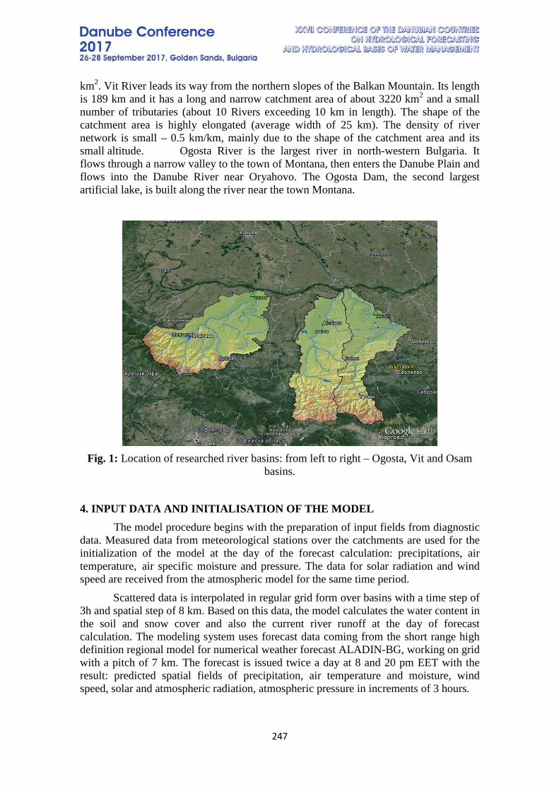
247

km2. Vit River leads its way from the northern slopes of the Balkan Mountain. Its length is 189 km and it has a long and narrow catchment area of about 3220 km2 and a small number of tributaries (about 10 Rivers exceeding 10 km in length). The shape of the catchment area is highly elongated (average width of 25 km). The density of river network is small – 0.5 km/km, mainly due to the shape of the catchment area and its small altitude. Ogosta River is the largest river in north-western Bulgaria. It flows through a narrow valley to the town of Montana, then enters the Danube Plain and flows into the Danube River near Oryahovo. The Ogosta Dam, the second largest artificial lake, is built along the river near the town Montana.

Fig. 1: Location of researched river basins: from left to right – Ogosta, Vit and Osam

basins.

4. INPUT DATA AND INITIALISATION OF THE MODEL The model procedure begins with the preparation of input fields from diagnostic

data. Measured data from meteorological stations over the catchments are used for the initialization of the model at the day of the forecast calculation: precipitations, air temperature, air specific moisture and pressure. The data for solar radiation and wind speed are received from the atmospheric model for the same time period.

Scattered data is interpolated in regular grid form over basins with a time step of 3h and spatial step of 8 km. Based on this data, the model calculates the water content in the soil and snow cover and also the current river runoff at the day of forecast calculation. The modeling system uses forecast data coming from the short range high definition regional model for numerical weather forecast ALADIN-BG, working on grid with a pitch of 7 km. The forecast is issued twice a day at 8 and 20 pm EET with the result: predicted spatial fields of precipitation, air temperature and moisture, wind speed, solar and atmospheric radiation, atmospheric pressure in increments of 3 hours.

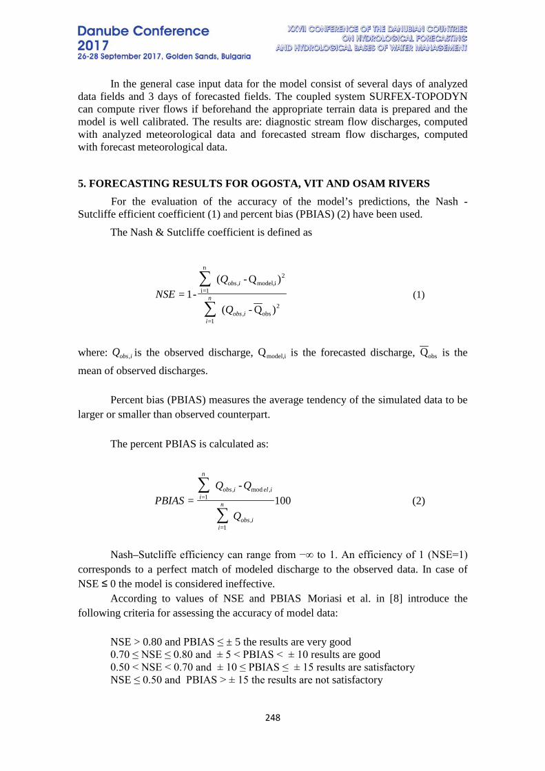
248

In the general case input data for the model consist of several days of analyzed data fields and 3 days of forecasted fields. The coupled system SURFEX-TOPODYN can compute river flows if beforehand the appropriate terrain data is prepared and the model is well calibrated. The results are: diagnostic stream flow discharges, computed with analyzed meteorological data and forecasted stream flow discharges, computed with forecast meteorological data.

5. FORECASTING RESULTS FOR OGOSTA, VIT AND OSAM RIVERS For the evaluation of the accuracy of the model’s predictions, the Nash -

Sutcliffe efficient coefficient (1) and percent bias (PBIAS) (2) have been used. The Nash & Sutcliffe coefficient is defined as

(1)

where: is the observed discharge, is the forecasted discharge, is the

mean of observed discharges. Percent bias (PBIAS) measures the average tendency of the simulated data to be

larger or smaller than observed counterpart. The percent PBIAS is calculated as:

(2)

Nash–Sutcliffe efficiency can range from −∞ to 1. An efficiency of 1 (NSE=1)

corresponds to a perfect match of modeled discharge to the observed data. In case of NSE ≤ 0 the model is considered ineffective.

According to values of NSE and PBIAS Moriasi et al. in [8] introduce the following criteria for assessing the accuracy of model data:

NSE > 0.80 and PBIAS ≤ ± 5 the results are very good 0.70 ≤ NSE ≤ 0.80 and ± 5 < PBIAS < ± 10 results are good 0.50 < NSE < 0.70 and ± 10 ≤ PBIAS ≤ ± 15 results are satisfactory NSE ≤ 0.50 and PBIAS > ± 15 the results are not satisfactory

2obs,

1=

2imodel,,

n

1=i

)Q-(

)Q-(-1=

∑

∑

iobs

n

i

iobs

Q

QNSE

iobsQ , imodel,Q obsQ

100-

=,

1=

,mod1=

,

∑

∑

iobs

n

i

iel

n

iiobs

Q

QQPBIAS

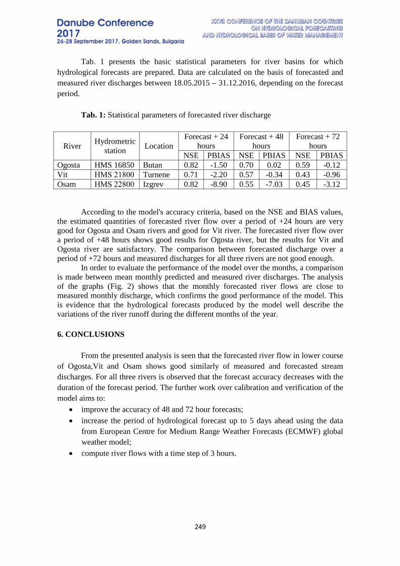
249

Tab. 1 presents the basic statistical parameters for river basins for which hydrological forecasts are prepared. Data are calculated on the basis of forecasted and measured river discharges between 18.05.2015 – 31.12.2016, depending on the forecast period.

Tab. 1: Statistical parameters of forecasted river discharge

River Hydrometric station Location

Forecast + 24 hours

Forecast + 48 hours

Forecast + 72 hours

NSE PBIAS NSE PBIAS NSE PBIAS Ogosta HMS 16850 Butan 0.82 -1.50 0.70 0.02 0.59 -0.12 Vit HМS 21800 Turnene 0.71 -2.20 0.57 -0.34 0.43 -0.96 Osam HМS 22800 Izgrev 0.82 -8.90 0.55 -7.03 0.45 -3.12

According to the model's accuracy criteria, based on the NSE and BIAS values, the estimated quantities of forecasted river flow over a period of +24 hours are very good for Ogosta and Osam rivers and good for Vit river. The forecasted river flow over a period of +48 hours shows good results for Ogosta river, but the results for Vit and Ogosta river are satisfactory. The comparison between forecasted discharge over a period of +72 hours and measured discharges for all three rivers are not good enough. In order to evaluate the performance of the model over the months, a comparison is made between mean monthly predicted and measured river discharges. The analysis of the graphs (Fig. 2) shows that the monthly forecasted river flows are close to measured monthly discharge, which confirms the good performance of the model. This is evidence that the hydrological forecasts produced by the model well describe the variations of the river runoff during the different months of the year.

6. CONCLUSIONS

From the presented analysis is seen that the forecasted river flow in lower course of Ogosta,Vit and Osam shows good similarly of measured and forecasted stream discharges. For all three rivers is observed that the forecast accuracy decreases with the duration of the forecast period. The further work over calibration and verification of the model aims to:

• improve the accuracy of 48 and 72 hour forecasts; • increase the period of hydrological forecast up to 5 days ahead using the data

from European Centre for Medium Range Weather Forecasts (ECMWF) global weather model;

• compute river flows with a time step of 3 hours.

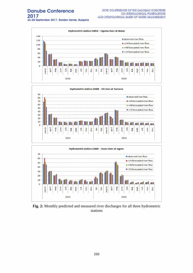
250

Fig. 2: Monthly predicted and measured river discharges for all three hydrometric

stations

251

REFERENCES [1] V. Masson, P. Le Moigne, E. Martin, S. Faroux, A. Alias, R. Alkama, S. Belamari, A. Barbu, A. Boone, F. Bouyssel, P. Brousseau, E. Brun, J.-C. Calvet, D. Carrer, B. Decharme, C. Delire, S. Donier, R. El Khatib, K. Essaouini, A.-L. Gibelin, H. Giordani, F. Habets, M. Jidane, G. Kerdraon, E. Kourzeneva, S. Lafont, C. Lebeaupin, A. Lemonsu, J.-F. Mahfouf, P. Marguinaud, M. Moktari, S. Morin, G. Pigeon, R. Salgado, Y. Seity, F. Taillefer, G. Tanguy, P. Tulet, B. Vincendon, V. Vionnet, A. Voldoire ,The SURFEXv7.2 externalized platform for the simulation of Earth surface variables and fluxes, Geosci. Model Dev., 6 (2013), pp. 929–960.

[2]Noilhan, J., Planton, S., (1989). A simple parameterization of land surface processes for meteorological models. Mon. Weather Rev. 117, 536–549.

[3] Faroux, S., Kaptué Tchuenté, A.T., Roujean, J.-L., Masson, V., Martin, E., Le Moigne, P., 2013. ECOCLIMAP-II/Europe: a twofold database of ecosystems and surfaceparameters at 1 km resolution based on satellite information for use in landsurface, meteorological and climate models. Geosci. Model Dev. 6, 563–582. [4] Decharme, B., Douville, H., Boone, A., Habets, F., Noilhan, J., 2006. Impact of an exponential profile of saturated hydraulic conductivity within the ISBA LSM:simulations over the Rhône Basin. J. Hydrometeorol. 7, 61–80. [5] Beven, K., Kirkby, M.J., 1979. A physically based, variable contributing area model of basin hydrology. Hydrol. Sci. Bull. 24, 43–69. [6] Bouilloud, L., Chancibault, K., Vincendon, B., Ducrocq, V., Habets, F., Saulnier, G.-M.,Anquetin, S., Martin, É., Noilhan, J., 2010. Coupling the ISBA land surface modeland the TOPMODEL hydrological model for Mediterranean flash floodforecasting: description, calibration and validation. J. Hydrometeorol. 11 (2), 315–333. [7] Vincendon, B., Ducrocq, V., Saulnier, G.M., Bouilloud, L., Chancibault, K., Habets, F.,Noilhan, J., 2010. Benefit of coupling the ISBA land surface model with a TOPMODEL hydrological model version dedicated to Mediterranean flashfloods. J. Hydrol. 394, 256–266. [8] Moriasi D.N., Gitau M.W., Pai N., Daggupati P. Hydrologic and Water Quality Models: Performance Measures and Evaluation Criteria // Trans. ASABE. V.58(6). 2015. P. 1763-1785.

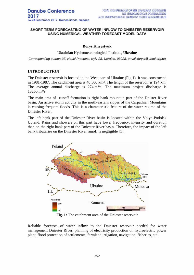
252

SHORT-TERM FORECASTING OF WATER INFLOW TO DNIESTER RESERVOIR USING NUMERICAL WEATHER FORECAST MODEL DATA

Borys Khrystyuk

Ukrainian Hydrometeorological Institute, Ukraine Corresponding author: 37, Nauki Prospect, Kyiv-28, Ukraine, 03028, email:khryst@uhmi.org.ua

INTRODUCTION The Dniester reservoir is located in the West part of Ukraine (Fig.1). It was constructed in 1981-1987. The catchment area is 40 500 km². The length of the reservoir is 194 km. The average annual discharge is 274 m³/s. The maximum project discharge is 13260 m³/s. The main area of runoff formation is right bank mountain part of the Dnister River basin. An active storm activity in the north-eastern slopes of the Carpathian Mountains is causing frequent floods. This is a characteristic feature of the water regime of the Dniester River. The left bank part of the Dniester River basin is located within the Volyn-Podolsk Upland. Rains and showers on this part have lower frequency, intensity and duration than on the right bank part of the Dniester River basin. Therefore, the impact of the left bank tributaries on the Dniester River runoff is negligible [1].

Fig. 1: The catchment area of the Dniester reservoir

Reliable forecasts of water inflow to the Dniester reservoir needed for water management Dniester River, planning of electricity production on hydroelectric power plant, flood protection of settlements, farmland irrigation, navigation, fisheries, etc.

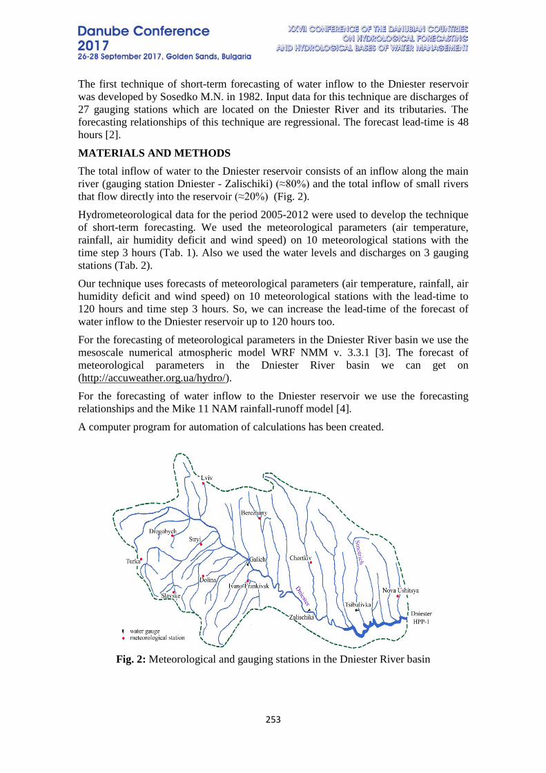
253

The first technique of short-term forecasting of water inflow to the Dniester reservoir was developed by Sosedko M.N. in 1982. Input data for this technique are discharges of 27 gauging stations which are located on the Dniester River and its tributaries. The forecasting relationships of this technique are regressional. The forecast lead-time is 48 hours [2].

MATERIALS AND METHODS The total inflow of water to the Dniester reservoir consists of an inflow along the main river (gauging station Dniester - Zalischiki) (≈80%) and the total inflow of small rivers that flow directly into the reservoir (≈20%) (Fig. 2). Hydrometeorological data for the period 2005-2012 were used to develop the technique of short-term forecasting. We used the meteorological parameters (air temperature, rainfall, air humidity deficit and wind speed) on 10 meteorological stations with the time step 3 hours (Tab. 1). Also we used the water levels and discharges on 3 gauging stations (Tab. 2). Our technique uses forecasts of meteorological parameters (air temperature, rainfall, air humidity deficit and wind speed) on 10 meteorological stations with the lead-time to 120 hours and time step 3 hours. So, we can increase the lead-time of the forecast of water inflow to the Dniester reservoir up to 120 hours too. For the forecasting of meteorological parameters in the Dniester River basin we use the mesoscale numerical atmospheric model WRF NMM v. 3.3.1 [3]. The forecast of meteorological parameters in the Dniester River basin we can get on (http://accuweather.org.ua/hydro/). For the forecasting of water inflow to the Dniester reservoir we use the forecasting relationships and the Mike 11 NAM rainfall-runoff model [4]. A computer program for automation of calculations has been created.

Fig. 2: Meteorological and gauging stations in the Dniester River basin

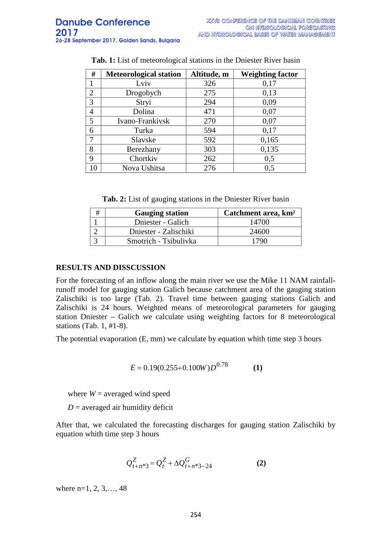
254

Tab. 1: List of meteorological stations in the Dniester River basin

# Meteorological station Altitude, m Weighting factor 1 Lviv 326 0,17 2 Drogobych 275 0,13 3 Stryi 294 0,09 4 Dolina 471 0,07 5 Ivano-Frankivsk 270 0,07 6 Turka 594 0,17 7 Slavske 592 0,165 8 Berezhany 303 0,135 9 Chortkiv 262 0,5 10 Nova Ushitsa 276 0,5

Tab. 2: List of gauging stations in the Dniester River basin

# Gauging station Catchment area, km² 1 Dniester - Galich 14700 2 Dniester - Zalischiki 24600 3 Smotrich - Tsibulivka 1790

RESULTS AND DISSCUSSION For the forecasting of an inflow along the main river we use the Mike 11 NAM rainfall-runoff model for gauging station Galich because catchment area of the gauging station Zalischiki is too large (Tab. 2). Travel time between gauging stations Galich and Zalischiki is 24 hours. Weighted means of meteorological parameters for gauging station Dniester – Galich we calculate using weighting factors for 8 meteorological stations (Tab. 1, #1-8). The potential evaporation (E, mm) we calculate by equation whith time step 3 hours

(1)

where W = averaged wind speed

D = averaged air humidity deficit

After that, we calculated the forecasting discharges for gauging station Zalischiki by equation whith time step 3 hours

(2)

where n=1, 2, 3,…, 48

DWE )100.0255.0(19.0 78.0+=

QQQ Gnt

Zt

Znt ∆+= −++ 243*3*

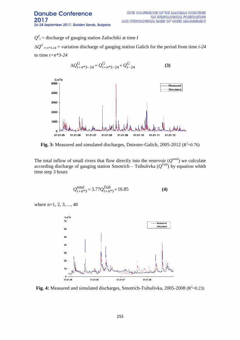
255

QZt = discharge of gauging station Zalischiki at time t

∆QG t+n*3-24 = variation discharge of gauging station Galich for the period from time t-24

to time t+n*3-24

(3)

Fig. 3: Measured and simulated discharges, Dniester-Galich, 2005-2012 (R2=0.76)

The total inflow of small rivers that flow directly into the reservoir (Qtotal) we culculate according discharge of gauging station Smotrich – Tsibulivka (QTsib) by equation whith time step 3 hours

(4)

where n=1, 2, 3,…, 40

Fig. 4: Measured and simulated discharges, Smotrich-Tsibulivka, 2005-2008 (R2=0.23)

QQQ Gt

Gnt

Gnt 24243*243* −−+−+ +=∆

85.1677.3 3*3* += ++ QQ Tsibnt

totalnt

256

For the forecasting of discharges of gauging station Smotrich – Tsibulivka whith time step 3 hours we use the Mike 11 NAM rainfall-runoff model. Weighted means of meteorological parameters for this gauging station we calculate using weighting factors for 2 meteorological stations (Tab. 1, #9-10). The potential evaporation (E, mm) we calculate by equation whith time step 3 hours

(5)

CONCLUSIONS The forecasts of meteorological parameters by mesoscale numerical atmospheric model WRF NMM v. 3.3.1 allows to increase the lead-time of the forecast of water inflow to the Dniester reservoir up to 120 hours. Simulated discharges by the Mike 11 NAM rainfall-runoff model for gauging station Dniester – Galich are in good agreement whith measured discharges. Coefficient of determination is 0.76. The results of simulation of discharges for gauging station Smotrich – Tsibulivka is not so good. Coefficient of determination is 0.23.

REFERENCES 1. L.O. Gorbachova, B.F. Khrystyuk, The hydrologic regionalization of the territory of Ukraine for the formation conditions of the annual streamflow based of Andrews’ curves, Ukrainian Geographical Journal, Ukraine, № 3, pp 27-33, 2016 2. M. N. Sosedko, Technique of short-term forecast of the Dniester River run-off on the site of Galich-Zhvanchik (guidelines), Ukrainian regional scientific and research institute, 18 p, 1982 3. Recommendations for the verification and intercomparison of QPFs and PQPFs from Operational NWP Models, WMO TD No. 1485, 37 p, 2009 4. MIKE11. A Modelling System for River and Channels, User guide, DHI, vol. 2, 204 p, 2012

DWE )100.0255.0(15.0 78.0+=

257

HYDROLOGICAL SIMULATIONS BASED ON REGIONAL CLIMATE MODEL OUTPUTS

Anna Kis1, János Adolf Szabó2, Rita Pongrácz1,3, Judit Bartholy1,3

1 Dept. of Meteorology, Eötvös Loránd University - Hungary 2 HYDROInform Ltd. - Hungary

3 Faculty of Science, Excellence Center, Eötvös Loránd University - Hungary Corresponding author: Anna Kis, Dept. of Meteorology, Eötvös Loránd University, Pázmány P. st. 1/A,

Budapest, 1117, Hungary, email – kisanna@nimbus.elte.hu

1. INTRODUCTION Beside its evident ecological importance, hydrology plays a key role in human life, as it is a very important factor in the socio-economical system. Hydrological processes and their dynamics (e.g. snow accumulation and melting, evapotranspiration, runoff) are determined by meteorological conditions; therefore climate change clearly has an effect on them. Both the lack and excess of water may result in various problems in different sectors, like agriculture, public water demand, energy supply, transportation or flood protection. In order to mitigate these potential hazards – related to hydrology –, it is essential to build adaptation strategies in time, taking into account the projected climate change. Therefore providing assistance to decision makers is inevitable, for which the cooperation of hydrological and climatological modellers is advisable. In our analysis, first, the calibration of the hydrological model (HM) against historical runoff records is completed, in which the historical meteorological data represented the upper boundary conditions. Then, hydrological simulation driven by regional climate model outputs for the past is completed. In order to test how reliable these simulations are, a statistical comparison of runoff values is carried out for a historical period. In the followings, data and methods are described, and then the results are presented focusing on the estimated historical and future runoff values. Finally, we summarise the main conclusions of the study.

2. DATA AND METHODS Our ultimate aim in this study is to develop a methodology, which is able to reconstruct runoff values in the recent past, as well, as simulate runoff in the future. In order to achieve this goal, we run a hydrological model driven by different meteorological time series for the Upper-Tisza catchment (22.5–25.5°E, 47–49°N). In the next subsections, the data and methods are presented briefly.

2.1 The DIWA hydrological model In order to get the hydrological responses (runoff) to the different meteorological inputs, the DIWA (DIstributed WAtershed [1,2]) HM was used. DIWA is a distributed, physically based model, which takes into account all the relevant processes of the hydrological cycle and also the key factors, which determine these processes (Fig. 1). To run the model, precipitation, mean and minimum temperature time series are

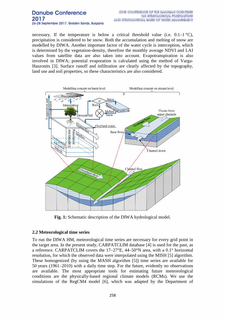
258

necessary. If the temperature is below a critical threshold value (i.e. 0.1–1 °C), precipitation is considered to be snow. Both the accumulation and melting of snow are modelled by DIWA. Another important factor of the water cycle is interception, which is determined by the vegetation-density, therefore the monthly average NDVI and LAI values from satellite data are also taken into account. Evapotranspiration is also involved in DIWA; potential evaporation is calculated using the method of Varga-Haszonits [3]. Surface runoff and infiltration are clearly affected by the topography, land use and soil properties, so these characteristics are also considered.

Fig. 1: Schematic description of the DIWA hydrological model.

2.2 Meteorological time series To run the DIWA HM, meteorological time series are necessary for every grid point in the target area. In the present study, CARPATCLIM database [4] is used for the past, as a reference. CARPATCLIM covers the 17–27°E, 44–50°N area, with a 0.1° horizontal resolution, for which the observed data were interpolated using the MISH [5] algorithm. These homogenized (by using the MASH algorithm [5]) time series are available for 50 years (1961–2010) with a daily time step. For the future, evidently no observations are available. The most appropriate tools for estimating future meteorological conditions are the physically-based regional climate models (RCMs). We use the simulations of the RegCM4 model [6], which was adapted by the Department of

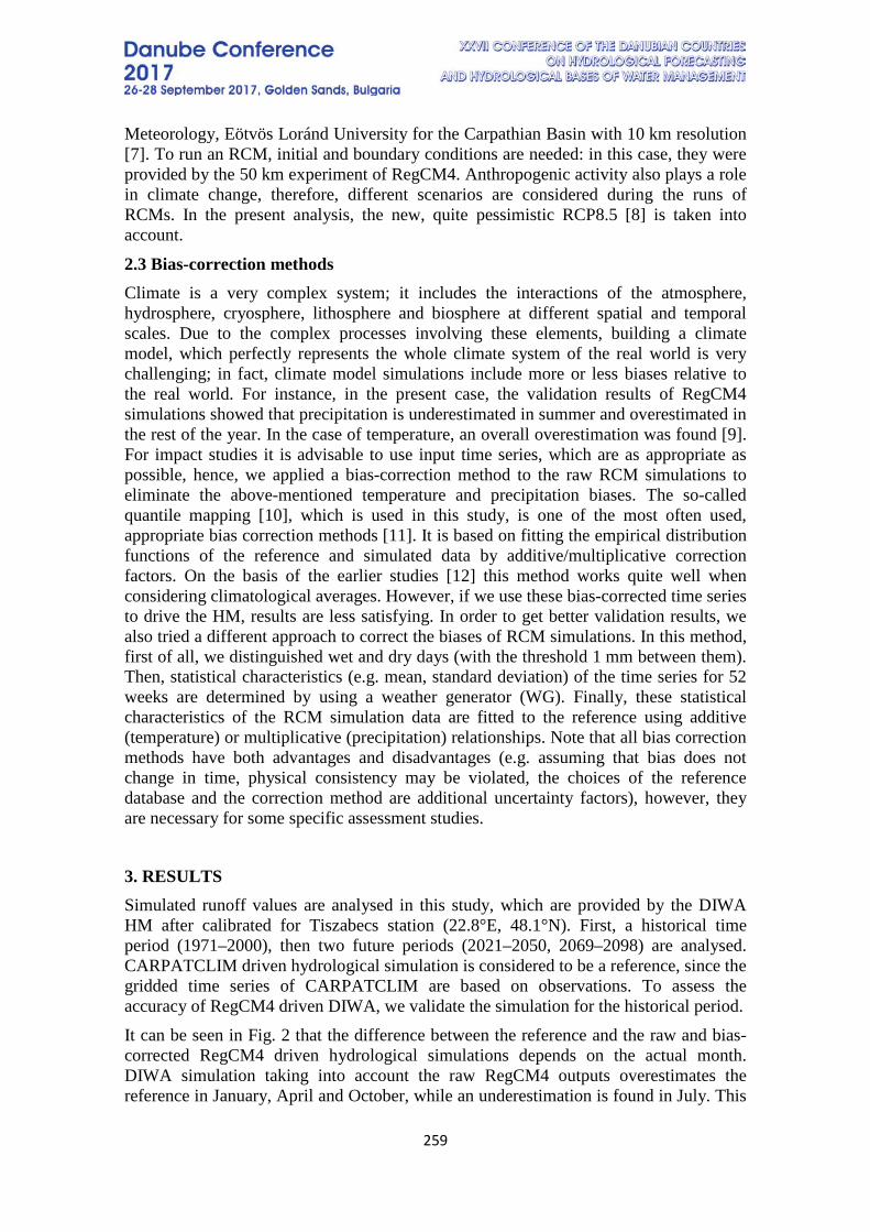
259

Meteorology, Eötvös Loránd University for the Carpathian Basin with 10 km resolution [7]. To run an RCM, initial and boundary conditions are needed: in this case, they were provided by the 50 km experiment of RegCM4. Anthropogenic activity also plays a role in climate change, therefore, different scenarios are considered during the runs of RCMs. In the present analysis, the new, quite pessimistic RCP8.5 [8] is taken into account.

2.3 Bias-correction methods Climate is a very complex system; it includes the interactions of the atmosphere, hydrosphere, cryosphere, lithosphere and biosphere at different spatial and temporal scales. Due to the complex processes involving these elements, building a climate model, which perfectly represents the whole climate system of the real world is very challenging; in fact, climate model simulations include more or less biases relative to the real world. For instance, in the present case, the validation results of RegCM4 simulations showed that precipitation is underestimated in summer and overestimated in the rest of the year. In the case of temperature, an overall overestimation was found [9]. For impact studies it is advisable to use input time series, which are as appropriate as possible, hence, we applied a bias-correction method to the raw RCM simulations to eliminate the above-mentioned temperature and precipitation biases. The so-called quantile mapping [10], which is used in this study, is one of the most often used, appropriate bias correction methods [11]. It is based on fitting the empirical distribution functions of the reference and simulated data by additive/multiplicative correction factors. On the basis of the earlier studies [12] this method works quite well when considering climatological averages. However, if we use these bias-corrected time series to drive the HM, results are less satisfying. In order to get better validation results, we also tried a different approach to correct the biases of RCM simulations. In this method, first of all, we distinguished wet and dry days (with the threshold 1 mm between them). Then, statistical characteristics (e.g. mean, standard deviation) of the time series for 52 weeks are determined by using a weather generator (WG). Finally, these statistical characteristics of the RCM simulation data are fitted to the reference using additive (temperature) or multiplicative (precipitation) relationships. Note that all bias correction methods have both advantages and disadvantages (e.g. assuming that bias does not change in time, physical consistency may be violated, the choices of the reference database and the correction method are additional uncertainty factors), however, they are necessary for some specific assessment studies.

3. RESULTS Simulated runoff values are analysed in this study, which are provided by the DIWA HM after calibrated for Tiszabecs station (22.8°E, 48.1°N). First, a historical time period (1971–2000), then two future periods (2021–2050, 2069–2098) are analysed. CARPATCLIM driven hydrological simulation is considered to be a reference, since the gridded time series of CARPATCLIM are based on observations. To assess the accuracy of RegCM4 driven DIWA, we validate the simulation for the historical period. It can be seen in Fig. 2 that the difference between the reference and the raw and bias-corrected RegCM4 driven hydrological simulations depends on the actual month. DIWA simulation taking into account the raw RegCM4 outputs overestimates the reference in January, April and October, while an underestimation is found in July. This

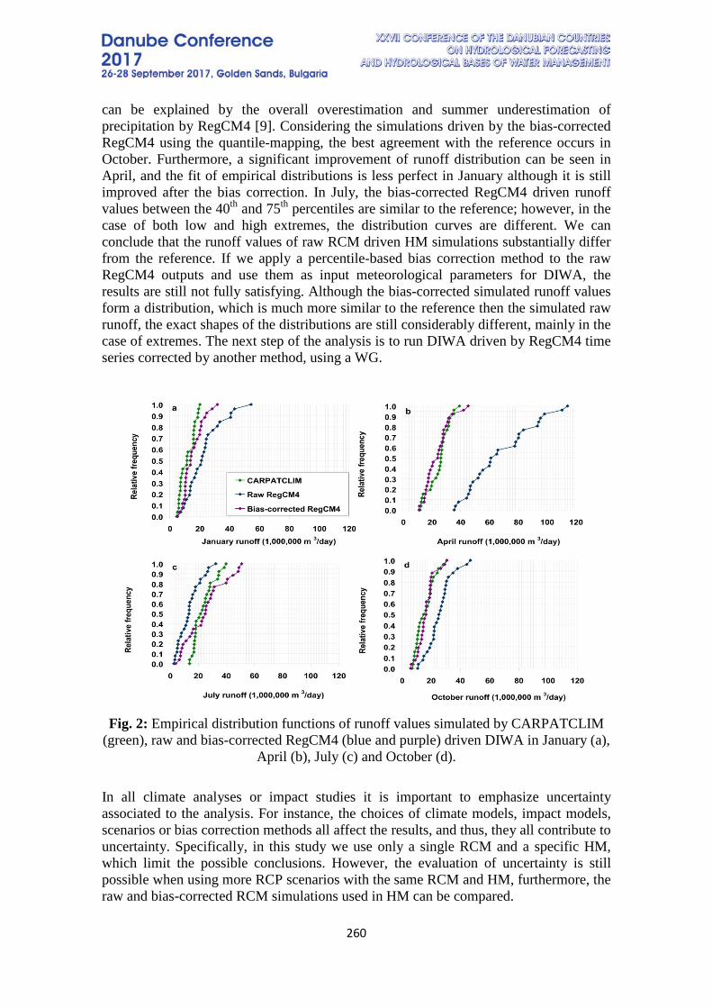
260

can be explained by the overall overestimation and summer underestimation of precipitation by RegCM4 [9]. Considering the simulations driven by the bias-corrected RegCM4 using the quantile-mapping, the best agreement with the reference occurs in October. Furthermore, a significant improvement of runoff distribution can be seen in April, and the fit of empirical distributions is less perfect in January although it is still improved after the bias correction. In July, the bias-corrected RegCM4 driven runoff values between the 40th and 75th percentiles are similar to the reference; however, in the case of both low and high extremes, the distribution curves are different. We can conclude that the runoff values of raw RCM driven HM simulations substantially differ from the reference. If we apply a percentile-based bias correction method to the raw RegCM4 outputs and use them as input meteorological parameters for DIWA, the results are still not fully satisfying. Although the bias-corrected simulated runoff values form a distribution, which is much more similar to the reference then the simulated raw runoff, the exact shapes of the distributions are still considerably different, mainly in the case of extremes. The next step of the analysis is to run DIWA driven by RegCM4 time series corrected by another method, using a WG.

Fig. 2: Empirical distribution functions of runoff values simulated by CARPATCLIM

(green), raw and bias-corrected RegCM4 (blue and purple) driven DIWA in January (a), April (b), July (c) and October (d).

In all climate analyses or impact studies it is important to emphasize uncertainty associated to the analysis. For instance, the choices of climate models, impact models, scenarios or bias correction methods all affect the results, and thus, they all contribute to uncertainty. Specifically, in this study we use only a single RCM and a specific HM, which limit the possible conclusions. However, the evaluation of uncertainty is still possible when using more RCP scenarios with the same RCM and HM, furthermore, the raw and bias-corrected RCM simulations used in HM can be compared.

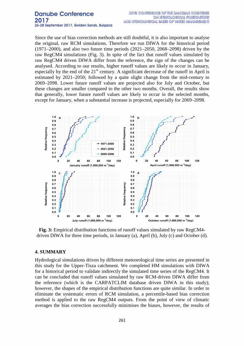
261

Since the use of bias correction methods are still doubtful, it is also important to analyse the original, raw RCM simulations. Therefore we run DIWA for the historical period (1971–2000), and also two future time periods (2021–2050, 2068–2098) driven by the raw RegCM4 simulations (Fig. 3). In spite of the fact that runoff values simulated by raw RegCM4 driven DIWA differ from the reference, the sign of the changes can be analysed. According to our results, higher runoff values are likely to occur in January, especially by the end of the 21st century. A significant decrease of the runoff in April is estimated by 2021–2050; followed by a quite slight change from the mid-century to 2069–2098. Lower future runoff values are projected also for July and October, but these changes are smaller compared to the other two months. Overall, the results show that generally, lower future runoff values are likely to occur in the selected months, except for January, when a substantial increase is projected, especially for 2069–2098.

Fig. 3: Empirical distribution functions of runoff values simulated by raw RegCM4-

driven DIWA for three time periods, in January (a), April (b), July (c) and October (d).

4. SUMMARY Hydrological simulations driven by different meteorological time series are presented in this study for the Upper-Tisza catchment. We completed HM simulations with DIWA for a historical period to validate indirectly the simulated time series of the RegCM4. It can be concluded that runoff values simulated by raw RCM-driven DIWA differ from the reference (which is the CARPATCLIM database driven DIWA in this study); however, the shapes of the empirical distribution functions are quite similar. In order to eliminate the systematic errors of RCM simulation, a percentile-based bias correction method is applied to the raw RegCM4 outputs. From the point of view of climatic averages the bias correction successfully minimises the biases, however, the results of

262

HM driven by the bias corrected RegCM4 data do not fit to the reference so well, as the meteorological drivers of HM. Therefore, another correction method using a WG is applied to RegCM4 outputs, in which wet and dry days are distinguished using the threshold of 1 mm/day. Our further plan is to run DIWA with these bias-corrected time series and evaluate the derived empirical distribution functions relative to the reference (both in terms of the interval of values and the shape of distribution) as well, as to the distributions of previous HM outputs.

REFERENCES [1] Szabó, J.A. Decision Supporting Hydrological Model for River Basin Flood Control, Digital Terrain Modelling: Development and Applications in a Policy Support Environment (Eds.: Peckham, R.J. and Jordan, Gy.). Springer-Verlag, Germany, pp 145–182, 2007. [2] Szabó, J.A., Kuti, L., Bakacsi, Zs., Pásztor, L., Tahy, Á. Spatial Patterns of Drought Frequency and Duration in the Great Hungarian Plain, based on Coupled-Model Simulations, Proceedings of the 4th IAHR International Groundwater Symposium, Spain, pp 289–291, 2010. [3] Varga-Haszonits, Z. Determination of the water content and of the evaporation of bare soil, Időjárás - Quarterly Journal of the Hungarian Meteorological Service, Hungary, vol. 73(6), pp 328–334, 1969. [4] Spinoni, J. and the CARPATCLIM project team (39 authors), 2015: Climate of the Carpathian Region in 1961–2010: Climatologies and Trends of Ten Variables, International Journal of Climatology, vol. 35, pp 1322–1341, 2015. [5] Bihari, Z., Szentimrey, T. CARPATCLIM Deliverable D2.10. Annex 3 – Description of MASH and MISH algorithms, pp 1–100, 2013. [6] Elguindi, N., Bi, X., Giorgi, F., Nagarajan, B., Pal, J., Solmon, F., Rauscher, S., Zakey, A., Giuliani, G. Regional climatic model RegCM – User manual. Version 4.3. ICTP, Italy, pp 1–32, 2011. [7] Bartholy, J., Pongrácz, R., Pieczka, I., Kelemen, F.D., Kis, A., André, K. Regional climate model experiment using RegCM subgridding options in the framework of Med-CORDEX, 95th Annual Meeting of the American Meteorological Society, USA, Paper 591, pp 1–6, 2015. [8] van Vuuren, D.P., Edmonds, J.A., Kainuma, M., Riahi, K., Thomson, A.M., Hibbard, K., Hurtt, G.C., Kram, T., Krey, V., Lamarque, J.-F., Masui, T., Meinshausen, M., Nakicenovic, N., Smith, S.J., Rose, S. The representative concentration pathways: an overview, Climatic Change, vol. 109, pp 5–31, 2011. [9] Pieczka, I., Pongrácz, R., André, K.S., Kelemen, F.D., Bartholy, J. Sensitivity analysis of different parameterization schemes using RegCM4.3 for the Carpathian region. Theoretical and Applied Climatology, in press, doi: 10.1007/s00704-016-1941-4, 2016. [10] Wang, L., Ranasinghe, R., Maskey, S., van Gelder, P.H.A.J.M., Vrijling, K. Comparison of empirical statistical methods for downscaling daily climate projections

263

from CMIP5 GCMs: a case study of the Huai River Basin, China, International Journal of Climatology, vol. 36, pp 145–164, 2016. [11] Teutschbein, C., Seibert, J. Bias correction of regional climate model simulations for hydrological climate-change impact studies: Review and evaluation of different methods, J. Hydrol, vol. 456–457, pp 12–29, 2012. [12] Kis, A., Pongrácz, R., Bartholy, J. Multi-model analysis of regional dry and wet conditions for the Carpathian Region, International Journal of Climatology, in press, doi: 10.1002/joc.5104, 2017.

5. ACKNOWLEDGEMENTS Research leading to this paper has been supported by the Ministry of National Development of the Hungarian Government via the AGRÁRKLIMA2 project (VKSZ_12-1-2013-0034), the Széchenyi 2020 programme, the European Regional Development Fund and the Hungarian Government (GINOP-2.3.2-15-2016-00028). Furthermore, we acknowledge the CARPATCLIM Database © European Commission – JRC, 2013.

264

RESERVOIRS CASCADE SIMULATION ADD-ON FOR RIVERFLOW FORECASTING OF ARDA AND TUNDZHA RIVERS

Petko Tsarev1, Eram Artinyan2

1East Aegean River Basin Directorate (EARBD), Bulgaria 2National Institute of Meteorology and Hydrology, BAS, Bulgaria

Corresponding author: P. Tsarev, EARBD, 35 Yanko Sakazov str., Plovdiv, Bulgaria, petko.tsarev@gmail.com

ABSTRACT The paper describes the set-up and usage of reservoir simulation add-on for river flows forecasting. For the first time the add-on was integrated in the flood warning system ArdaForecast to predict the outflow of the dams on Arda River - Kardhzali, Studen Kladenets and Ivailovgrad. The Arda River is causing the most hazardous floods in the southeast Balkans, which are increasing in the downstream of Maritza/Evros and are causing serious losses at the BG-GR CBC region. Although the basin is subject of very fast high waves the Greek part of the basin is usually protected by the retention capacity of three big dams located on the river’s middle course in Bulgaria. After the first integration the add-on was used in a warning system for the upper Tundzha River basin including the dams Koprinka and Zhrebchevo. The warning system is based on the Land Surface Model – SURFEX platform. The model computes the forecasted inflow for each dam every 12 hours at 8 am and 8 pm. The add-on calculates the outflow from the dams. The outflow of the upper dam is included as an additional inflow for the dam down the cascade. The add-on reads the latest updated in real-time values of the levels in the dams and the latest streamflow forecast from an SQL database. The application generates the free volume, the time until overflowing and series of controls (checks) are performed on the basis of logical flags for future scenarios. The construction characteristics of each dam (spillway, outlet, hydropower plan) are integrated in the add-on. We use an analysis of the historical records of the cascade’s work and the parameters of the dams, including rating curves, curves of overflow and spillway crest elevation. The add-on calculation of the flow from each spillway is based on the level - discharge relation for each spillway and the expected water level in the reservoir. The result is a file with water discharge values [m3/s] for every 3 hours for the next 5 days. The application is autonomous and starts every hour reflecting recent changes: new water discharge forecast for the next 5 days and new measured levels in reservoirs.

Keywords: overflow forecasting, reservoir levels forecasting, spillway overflow

265

1. INTRODUCTION The add-on are used to calculate the outflow of the five dams in Bulgaria – tree

on Arda River (Kardhzali, Studen Kladenets and Ivailovgrad) and two on upper Tundzha River basin (Koprinka and Zhrebchevo). The calculations are based on the water balance model and are made in Excel. The autonomous operation of the application is regulated by Excel VBA Model.

The basis of the add-on is a cascade simulation of high wave in cascade dams. This article analyzes the results achieved by the application of the add-on for

hydrological forecasting in Arda and Tundhza rivers

2. METHODOLOGY The add-on use start data from SURFEX-TOP modelling system and the actual

data for the levels in each dam. The SURFEX-TOP system is calculating inflow for catchment for each dam on every 12 hours at 8 am and 8 pm and the add-on calculates the outflow from the dams on every hour. The outcome of upper dam is included as an additional inflow for dams down the cascade.

The add-on reads the latest updated values of the levels in the dams from MySQL database and the latest forecast for inflow calculated by SURFEX-TOP model. The application is calculating the free volume, time until overflowing and series of controls (checks) are performed on the basis of true/false for future scenarios. The results from the system are the level of water and the size of the flood control pool in each reservoir (for every 3h for the next 5 days).

The construction characteristics of each dam (spillway, outlet, hydro power plan) was integrated in the add-on. We use an analysis of the historical records of the cascade’s work and the parameters of the dams but mainly the curves of overflow and spillway crest elevation.

The application is autonomous and starts every hour reflecting recent changes (new forecast, new levels in dams).

Based on the level - discharge relation for each spillway and measuring the water level in real time we know the overflow in cubic meter per second.

The forecast for overflowing is on the basis of forecasted volumes in the reservoir and the expected spillway crest elevation.

As a result the data is written to text file format which contains a forecast of water quantities in stations under each of the dams.

3. FORECASTING RESULTS

For the evaluation of the accuracy of the model’s predictions, the Nash - Sutcliffe efficient coefficient [1] and percent bias (PBIAS) have been used.

Percent bias (PBIAS) measures the average tendency of the simulated data to be larger or smaller than observed counterpart.

The percent PBIAS is calculated as:

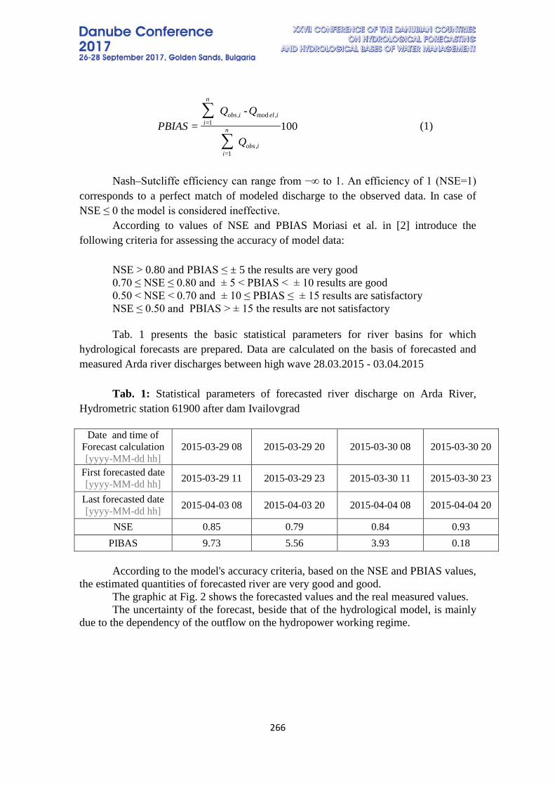
266

100-

=,

1=

,mod1=

,

∑

∑

iobs

n

i

iel

n

iiobs

Q

QQPBIAS (1)

Nash–Sutcliffe efficiency can range from −∞ to 1. An efficiency of 1 (NSE=1)

corresponds to a perfect match of modeled discharge to the observed data. In case of NSE ≤ 0 the model is considered ineffective.

According to values of NSE and PBIAS Moriasi et al. in [2] introduce the following criteria for assessing the accuracy of model data:

NSE > 0.80 and PBIAS ≤ ± 5 the results are very good 0.70 ≤ NSE ≤ 0.80 and ± 5 < PBIAS < ± 10 results are good 0.50 < NSE < 0.70 and ± 10 ≤ PBIAS ≤ ± 15 results are satisfactory NSE ≤ 0.50 and PBIAS > ± 15 the results are not satisfactory Tab. 1 presents the basic statistical parameters for river basins for which

hydrological forecasts are prepared. Data are calculated on the basis of forecasted and measured Arda river discharges between high wave 28.03.2015 - 03.04.2015

Tab. 1: Statistical parameters of forecasted river discharge on Arda River,

Hydrometric station 61900 after dam Ivailovgrad

Date and time of Forecast calculation [yyyy-MM-dd hh]

2015-03-29 08 2015-03-29 20 2015-03-30 08 2015-03-30 20

First forecasted date [yyyy-MM-dd hh] 2015-03-29 11 2015-03-29 23 2015-03-30 11 2015-03-30 23

Last forecasted date [yyyy-MM-dd hh] 2015-04-03 08 2015-04-03 20 2015-04-04 08 2015-04-04 20

NSE 0.85 0.79 0.84 0.93 PIBAS 9.73 5.56 3.93 0.18 According to the model's accuracy criteria, based on the NSE and PBIAS values,

the estimated quantities of forecasted river are very good and good. The graphic at Fig. 2 shows the forecasted values and the real measured values. The uncertainty of the forecast, beside that of the hydrological model, is mainly

due to the dependency of the outflow on the hydropower working regime.

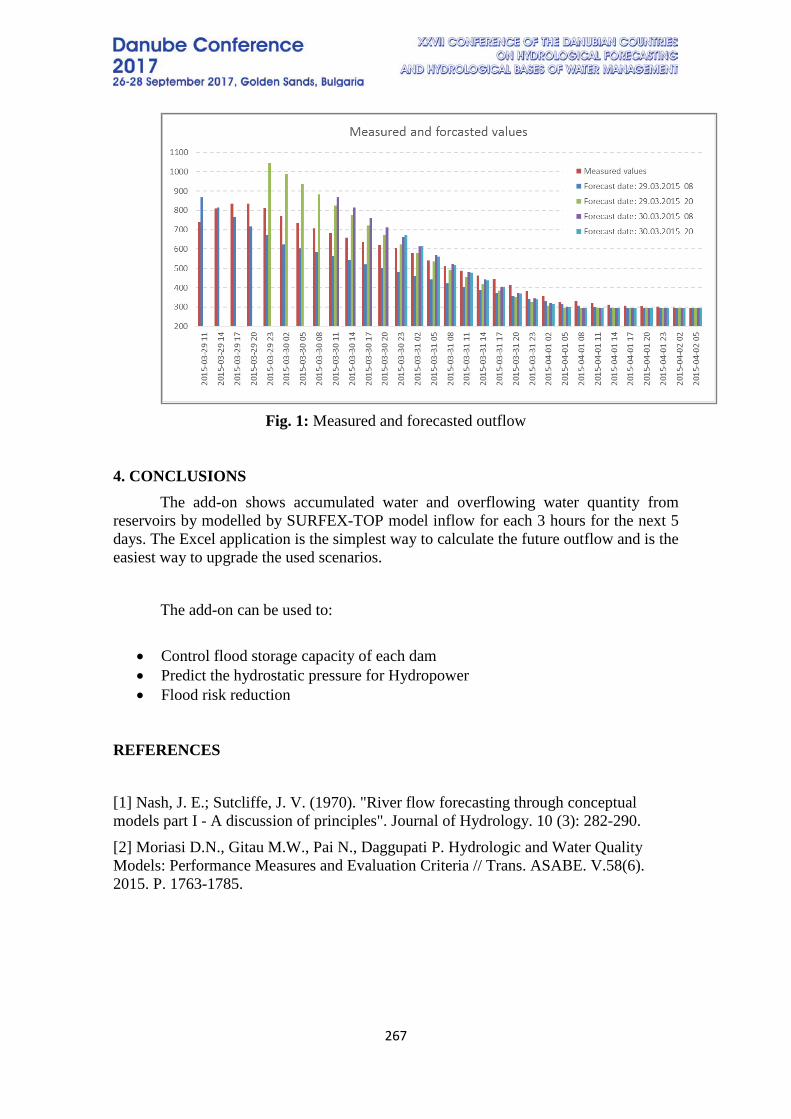
267

Fig. 1: Measured and forecasted outflow

4. CONCLUSIONS

The add-on shows accumulated water and overflowing water quantity from reservoirs by modelled by SURFEX-TOP model inflow for each 3 hours for the next 5 days. The Excel application is the simplest way to calculate the future outflow and is the easiest way to upgrade the used scenarios.

Тhe add-on can be used to:

• Control flood storage capacity of each dam • Predict the hydrostatic pressure for Hydropower • Flood risk reduction

REFERENCES [1] Nash, J. E.; Sutcliffe, J. V. (1970). "River flow forecasting through conceptual models part I - A discussion of principles". Journal of Hydrology. 10 (3): 282-290. [2] Moriasi D.N., Gitau M.W., Pai N., Daggupati P. Hydrologic and Water Quality Models: Performance Measures and Evaluation Criteria // Trans. ASABE. V.58(6). 2015. P. 1763-1785.

268

ASPECTS OF STOCHASTIC MODELING IN WATER RESOURCE MАNАGEMENT

Anna Yordanova, Igor Niagolov, Irena Ilcheva National Institute of Meteorology and Hydrology- BAS, Republic of Bulgaria

Corresponding author: Anna Yordanova, NIMH, 66 Tsarigradsko Shose blvd Sofia 1784, BULGARIA email: yordanova61@gmail.com

ABSTRACT Stochastic modeling is widely used in hydrologic practice, where water

specialists face with uncertain key factors in: the assessment and risk management in water supply systems, drought management plans development, management of low and high water and others. For this reason, a methodical approach and software for stochastic Monte Carlo (by autoregressive and autoregressive moving average models) modeling and simulation modeling are developed in NIMH. This approach gives a possibility for various problem solutions of water management systems under stochastic formulation, taking into consideration different water resource scenarios options, various alternative schemes and future water demand level. Stochastic modeling models are applied in practice on a number of projects and contracts with different institutions. In this paper an example for Iskar river runoff simulation by long-term ARMA-model is presented. Keywords: hydrology, stochastic modeling, climate change, water resource management 1. INTRODUCTION

The river flow is a non-stationary, random process, whose adequate description should be based on the methods of random function theory. Available natural flow hydrographs do not give its full probabilistic description as the observations do not cover all possible sequence combinations in the runoff that form the general population. The use of more sophisticated methods and tools in hydrology is related to the optimization of the planning and design of water economic systems and requires the development of methods for mathematical modeling of river runoff in order to more adequately imitate and predict it and to obtain sustainable parameters for conditions close to the general population. The accumulated hydrological experience convincingly shows that, the runoff data are interdependent in the most general case and they can be adequately described mathematically from the positions of the stochastic hydrology and not from the positions of the random event theory, which is a particular case of the random processes where the runoff data are statistically independent. In this case, the stochastic modeling find a good application, considering the data of the runoff as correlated, because many runoff sequences show constancy in the appearance of contiguous values of the outflow with close sizes.

269

Stochastic modeling is characterized by the generation of a hypothetical sequence for flow, based on the results of the statistical and probability characteristics of the observed sequences. The method is also called stochastic imitation, comparable to deterministic imitation in physical models. The stochastic modeling procedure consists of two parts:

- selecting an appropriate probability distribution for the input information; - selecting a suitable generating model.

The used models are based on Markov's processes. In Markov's processes the data are considered as a two-component composition - random and determinate. For example, for a simple Markov process, it is assumed that the runoff is sum of:

1) Average runoff; 2) A part of the deviation of the runoff from its mean value for the previous step; 3) Random component (residual).

The stochastic modeling can be used for a sufficiently long series of flow observations. In other cases, determinate modeling should be applied. 2. TYPES OF STOCHASTIC MODELS

Markov models are the first stochastic models used to generate runoff sequences (Thomas and Firing 1962, Yevjevich 1963). These models, also called autoregressive (AR), are short-memory models. The consideration of short-term and long-term dependencies led to the development of alternative models for generating synthetic hydrological series [2]. In order to take into account the long run cycles in the flow process, the FGN and Mandelbrot (1968) model were developed, and in order to describe the wide range of behaviors of the time series, Box and Jenkins (1970) developed a family of autoregression models with moving average (ARMA). Although each of these models has its advantages and has been successfully applied in practice, they also have their drawbacks. They are all criticized for one or more of the following reasons:

1) They can’t reproduce short-term dependence; 2) They can’t reproduce long-term dependence; 3) They are labor-intensive when calculating the parameters; 4) They have restrictions for generating long sequences; 5) There is lack of physical justification; 6) They have too many parameters.

The main requirement for the generated synthetic runoff sequences is to have the same statistical parameters and characteristics as those of the observed ones.

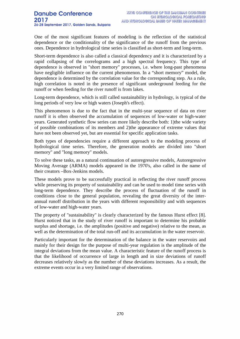
270

One of the most significant features of modeling is the reflection of the statistical dependence or the conditionality of the significance of the runoff from the previous ones. Dependence in hydrological time series is classified as short-term and long-term. Short-term dependence is also called a classical dependency and it is characterized by a rapid collapsing of the correlograms and a high spectral frequency. This type of dependence is observed in "short memory" processes, i.e. where long-past phenomena have negligible influence on the current phenomenon. In a “short memory” model, the dependence is determined by the correlation value for the corresponding step. As a rule, high correlation is noted in the presence of significant underground feeding for the runoff or when feeding for the river runoff is from lakes. Long-term dependence, which is still called sustainability in hydrology, is typical of the long periods of very low or high waters (Joseph's effect). This phenomenon is due to the fact that in the multi-year sequence of data on river runoff it is often observed the accumulation of sequences of low-water or high-water years. Generated synthetic flow series can more likely describe both: 1)the wide variety of possible combinations of its members and 2)the appearance of extreme values that have not been observed yet, but are essential for specific application tasks. Both types of dependencies require a different approach to the modeling process of hydrological time series. Therefore, the generation models are divided into "short memory" and "long memory" models. To solve these tasks, as a natural continuation of autoregressive models, Autoregressive Moving Average (ARMA) models appeared in the 1970's, also called in the name of their creators –Box-Jenkins models. These models prove to be successfully practical in reflecting the river runoff process while preserving its property of sustainability and can be used to model time series with long-term dependence. They describe the process of fluctuation of the runoff in conditions close to the general population, revealing the great diversity of the inter-annual runoff distribution in the years with different responsibility and with sequences of low-water and high-water years. The property of "sustainability" is clearly characterized by the famous Hurst effect [8]. Hurst noticed that in the study of river runoff is important to determine his probable surplus and shortage, i.e. the amplitudes (positive and negative) relative to the mean, as well as the determination of the total run-off and its accumulation in the water reservoir. Particularly important for the determination of the balance in the water reservoirs and mainly for their design for the purpose of multi-year regulation is the amplitude of the integral deviations from the mean value. A characteristic feature of the runoff process is that the likelihood of occurrence of large in length and in size deviations of runoff decreases relatively slowly as the number of these deviations increases. As a result, the extreme events occur in a very limited range of observations.

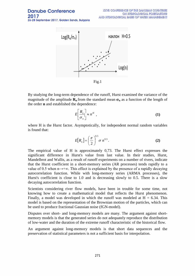
271

Fig.1

By studying the long-term dependence of the runoff, Hurst examined the variance of the magnitude of the amplitude Rn from the standard mean σn as a function of the length of the order n and established the dependence:

, (1)

where H is the Hurst factor. Asymptotically, for independent normal random variables is found that:

(2)

The empirical value of H is approximately 0,73. The Hurst effect expresses the significant difference in Hurst's value from last value. In their studies, Hurst, Mandelbrot and Wallis, as a result of runoff experiments on a number of rivers, indicate that the Hurst coefficient in a short-memory series (AR processes) tends rapidly to a value of 0.5 when n→+∞. This effect is explained by the presence of a rapidly decaying autocorrelation function. While with long-memory series (ARMA processes), the Hurst's coefficient is close to 1.0 and is decreasing slowly to 0.5. There is a slow decaying autocorrelation function. Scientists considering river flow models, have been in trouble for some time, not knowing how to create a mathematical model that reflects the Hurst phenomenon. Finally, a model was developed in which the runoff was modeled at H = 6.34. This model is based on the representation of the Brownian motion of the particles, which can be used to produce fractional Gaussian noise (fGN-model). Disputes over short- and long-memory models are many. The argument against short-memory models is that the generated series do not adequately reproduce the distribution of low-water and the duration of the extreme runoff characteristic of the historical flow. An argument against long-memory models is that short data sequences and the preservation of statistical parameters is not a sufficient basis for interpolation.

Log(Rn/σn) наклон H=0.5

Log(n)

H

n

n nRE ≈

σ

[ ] .2

5,05,0

nRE n σπ

=

272

Long-memory models, however, are better in the presentation of the effect of Joseph. They are recommended as suitable for non-Gaussian and with seasonal dependence data. These are the series of maximum/minimum runoff data. None of the two types of models adequately describes the effect of Noah (repeated observation of high-water over a short time interval). Therefore it is necessary, in each case, to decide which properties of the time series are required to be preserved and to consider the possible consequences of non-maintenance of the others. 2.1 MODELS WITH SHORT MEMORY Models of short- memory refer to the linear Markov (autoregressive) models. They are statistically well-studied. Autoregressive (AR) models belong to the number of the first stochastic models used to generate runoff sequences. These models have a short-term dependence, as their correlation functions decrease rapidly. They can’t preserve the accumulated features of the river flow process. First and second order of the AR-models is accurate enough for practical use, when long-term changes in water resources for a system are not significant. The use of these models in hydrology is convenient mainly due to the fact that:

1) They use the normal distribution; 2) They are based on autoregressive dependence, that reflects the time relation of

the flow; 3) They are the simplest models for use.

The historical development of AR-models in hydrology can be divided into two periods: 1)that of the 6-th decade of the last century, characterized mainly by the work of Thomas and Fering (1962) and Matalas, Yevjevic and Svanadse, and 2)that of the 7-th decade, presented by Box and Jenkins models. In the first period, the usual procedure for model parameters calculating is based on the method of moments, and the good approximation test is based on the correlation analysis. Autoregression models can have constant or variable parameters, or a combination of both types. The first type is used for annual runoff, while the other two type parameters are proper for series in smaller time intervals - parts of the year. After 1970 the hydrologists use more precise methodologies, proposed by Box, Jenkins and other scientists to improve model parameter evaluation, to check the model assumptions and to optimize the choice from alternative models. Some types of AR models that can be used to consider a stationary Markov time series yt with a normal distribution and parameters µ and σ are the following [4,12]:

Thomas and Fering (1962) (3) 1,.)1()( 22

1

21

=−+−+= −=∑ εσεσµφµ tjt

p

jjt Ryy

273

Yevjevic and Matalas (1962) (4)

Box and Jenkins (1970) (5)

These are AR-models of order p, i.e. AR(p) for which xt is an independent standard normal variable, εt is a non-correlation time component, which is independent of yt and has a normal distribution (µ=1 and σt

2); the coefficients φ1, φ2, ..., φp are called autoregressive. The set (µ, σ2, φ1, ..., φp, σε

2, R2) are constant parameters. In case, autoregressive coefficients are periodic, then AR-models are called periodic. The properties of the latter are more complex and not well-studied. These models are non-stationary, because both: mean and deviation are periodic. Their modeling is difficult because the recurrent hydrological series reflect the impact of the hydrological cycle, which generates periodic changes in some or all of the statistical characteristics. Application of Fourier series[12] is desirable, because it reduces the number of parameters in the model. There are three main limitations, using the AR-models:

1) They can be applied only in the presence of a stationary process, but in essence, in the most general case, river flow is a non-stationary process.

2) It is considered, that the AR (p) models preserve statistical characteristics (mean, standard deviation and first p correlations) of the observed series.

For example, the correlograms of the AR-model coincides with rk only for the first p steps and deviates for the rest ones.

3) The third factor is related to the modeling of asymmetric variables. For this purpose, three approaches are known in the literature: - Transforming the observed asymmetrically distributed values by appropriately

converting into normally distributed and then computing the received data; - An autoregressive model is used to observed series and the distribution of

residual members is sought; - The dependence (if any) between the first two moment estimates of the

observed series with ones of the normal series is used in such a way that the normalization of the observed asymmetric to preserve the moments.

The researcher should judge and decide by himself on a case-by-case which of these three approaches to use. Despite the limitations of the autoregression models, they are widely used in hydrological research and contribute to significant advances in their development.

+=

=+=

+=

∑

∑

=−

=−

p

jtjtjt

p

jtjtjt

tt

zz

zz

zy

1

1

2 1,

,.

εσφ

σεφ

σµ

ε

ε

+−=

=+−=

+=

∑

∑

=−

=−

p

jtjtjt

p

jtjtjt

tt

yz

yz

zy

1

1

2

).(

1,).(

,

εσµφ

σεµφ

µ

ε

ε

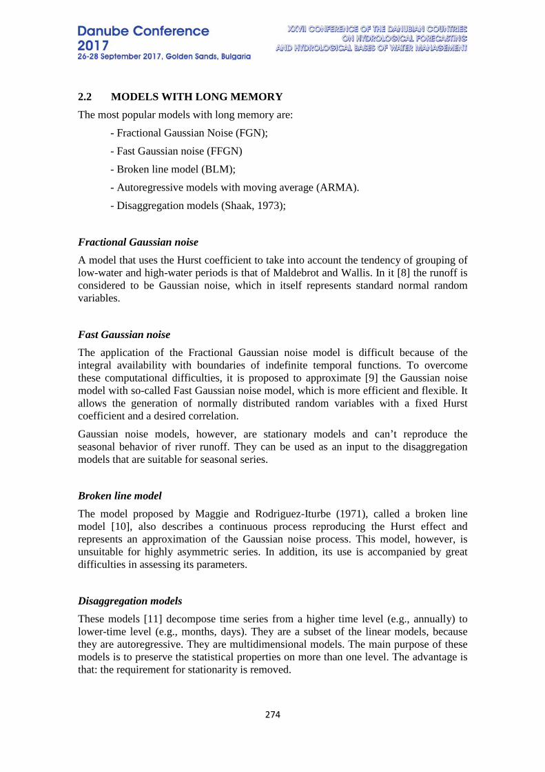
274

2.2 MODELS WITH LONG MEMORY The most popular models with long memory are:

- Fractional Gaussian Noise (FGN); - Fast Gaussian noise (FFGN) - Broken line model (BLM); - Autoregressive models with moving average (ARMA). - Disaggregation models (Shaak, 1973);

Fractional Gaussian noise A model that uses the Hurst coefficient to take into account the tendency of grouping of low-water and high-water periods is that of Maldebrot and Wallis. In it [8] the runoff is considered to be Gaussian noise, which in itself represents standard normal random variables.

Fast Gaussian noise The application of the Fractional Gaussian noise model is difficult because of the integral availability with boundaries of indefinite temporal functions. To overcome these computational difficulties, it is proposed to approximate [9] the Gaussian noise model with so-called Fast Gaussian noise model, which is more efficient and flexible. It allows the generation of normally distributed random variables with a fixed Hurst coefficient and a desired correlation. Gaussian noise models, however, are stationary models and can’t reproduce the seasonal behavior of river runoff. They can be used as an input to the disaggregation models that are suitable for seasonal series.

Broken line model The model proposed by Maggie and Rodriguez-Iturbe (1971), called a broken line model [10], also describes a continuous process reproducing the Hurst effect and represents an approximation of the Gaussian noise process. This model, however, is unsuitable for highly asymmetric series. In addition, its use is accompanied by great difficulties in assessing its parameters.

Disaggregation models These models [11] decompose time series from a higher time level (e.g., annually) to lower-time level (e.g., months, days). They are a subset of the linear models, because they are autoregressive. They are multidimensional models. The main purpose of these models is to preserve the statistical properties on more than one level. The advantage is that: the requirement for stationarity is removed.

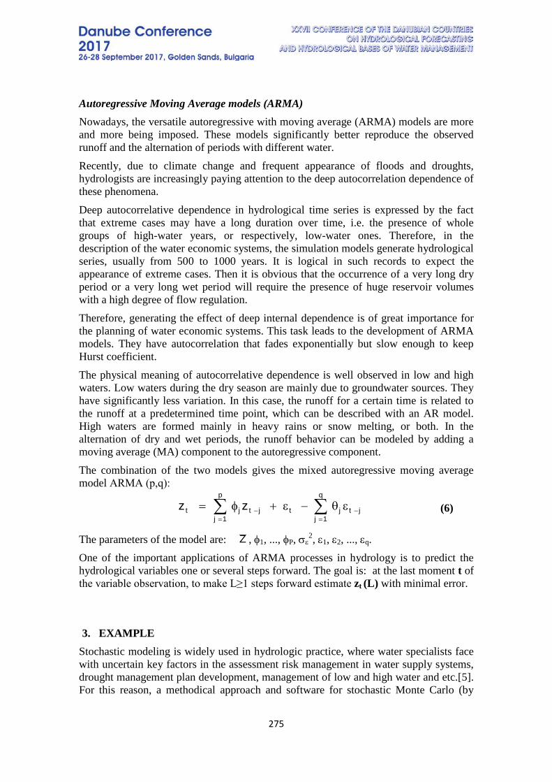
275

Autoregressive Moving Average models (ARMA) Nowadays, the versatile autoregressive with moving average (ARMA) models are more and more being imposed. These models significantly better reproduce the observed runoff and the alternation of periods with different water. Recently, due to climate change and frequent appearance of floods and droughts, hydrologists are increasingly paying attention to the deep autocorrelation dependence of these phenomena. Deep autocorrelative dependence in hydrological time series is expressed by the fact that extreme cases may have a long duration over time, i.e. the presence of whole groups of high-water years, or respectively, low-water ones. Therefore, in the description of the water economic systems, the simulation models generate hydrological series, usually from 500 to 1000 years. It is logical in such records to expect the appearance of extreme cases. Then it is obvious that the occurrence of a very long dry period or a very long wet period will require the presence of huge reservoir volumes with a high degree of flow regulation. Therefore, generating the effect of deep internal dependence is of great importance for the planning of water economic systems. This task leads to the development of ARMA models. They have autocorrelation that fades exponentially but slow enough to keep Hurst coefficient. The physical meaning of autocorrelative dependence is well observed in low and high waters. Low waters during the dry season are mainly due to groundwater sources. They have significantly less variation. In this case, the runoff for a certain time is related to the runoff at a predetermined time point, which can be described with an AR model. High waters are formed mainly in heavy rains or snow melting, or both. In the alternation of dry and wet periods, the runoff behavior can be modeled by adding a moving average (MA) component to the autoregressive component. The combination of the two models gives the mixed autoregressive moving average model АRМА (р,q):

(6)

The parameters of the model are: , φ1, ..., φP, σε2, ε1, ε2, ..., εq.

One of the important applications of ARMA processes in hydrology is to predict the hydrological variables one or several steps forward. The goal is: at the last moment t of the variable observation, to make L≥1 steps forward estimate zt (L) with minimal error.

3. EXAMPLE

Stochastic modeling is widely used in hydrologic practice, where water specialists face with uncertain key factors in the assessment risk management in water supply systems, drought management plan development, management of low and high water and etc.[5]. For this reason, a methodical approach and software for stochastic Monte Carlo (by

∑∑=

−−=

εθ−ε+φ=q

1jjtjtjt

p

1jjt zz

Z

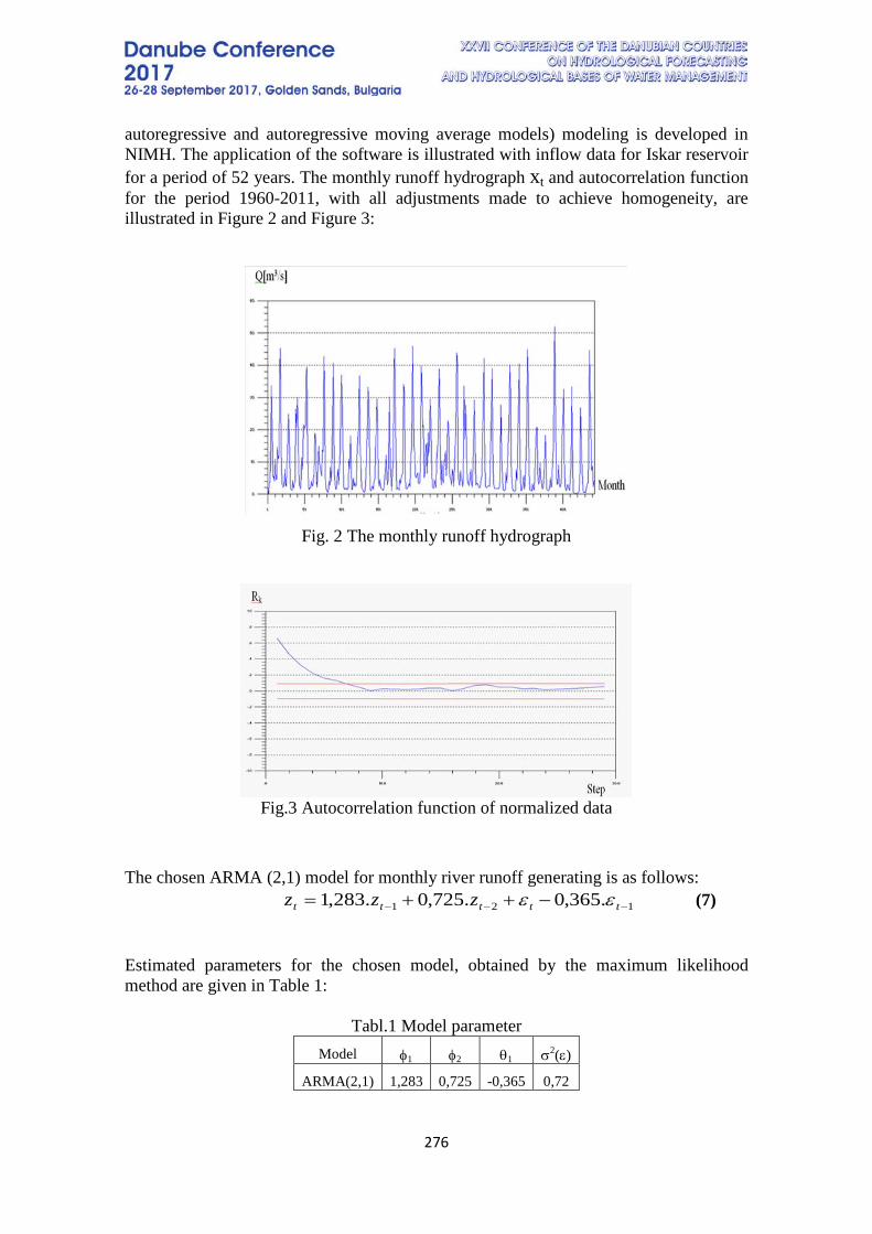
276

autoregressive and autoregressive moving average models) modeling is developed in NIMH. The application of the software is illustrated with inflow data for Iskar reservoir for a period of 52 years. The monthly runoff hydrograph xt and autocorrelation function for the period 1960-2011, with all adjustments made to achieve homogeneity, are illustrated in Figure 2 and Figure 3:

Fig. 2 The monthly runoff hydrograph

Fig.3 Autocorrelation function of normalized data

The chosen ARMA (2,1) model for monthly river runoff generating is as follows: (7) Estimated parameters for the chosen model, obtained by the maximum likelihood method are given in Table 1:

Tabl.1 Model parameter Model φ1 φ2 θ1 σ2(ε)

ARMA(2,1) 1,283 0,725 -0,365 0,72

121 .365,0.725,0.283,1 −−− −++= ttttt zzz εε

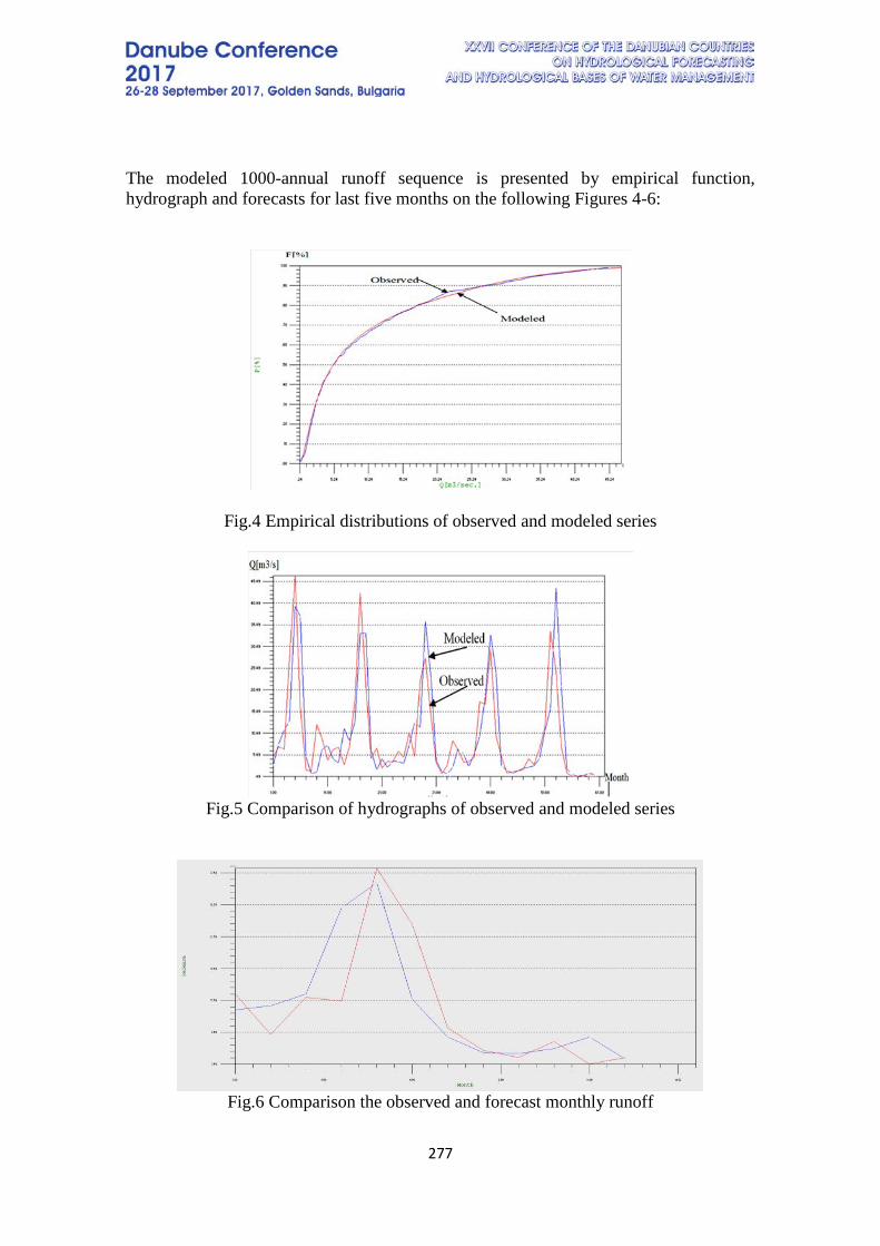
277

The modeled 1000-annual runoff sequence is presented by empirical function, hydrograph and forecasts for last five months on the following Figures 4-6:

Fig.4 Empirical distributions of observed and modeled series

Fig.5 Comparison of hydrographs of observed and modeled series

Fig.6 Comparison the observed and forecast monthly runoff

278

Consequently, this approach gives a possibility for a solutions of various problem in water management systems under stochastic formulation, taking into consideration different water resource scenarios options, various alternative schemes and future water demand level. 4. CONCLUSION

Existing models for generating synthetic runoff series allow a representative description of a stationary and non-stationary process with arbitrary probability distribution function and taking into account correlation relationships of a general type. The synthetic time series find a significant place in describing the process of reservoir management with a high level of runoff regulation [1,3,6]. Stochastic modeling models are applied in practice on a number of projects and contracts with different institutions: 1)Complete Water Resources System Plan for Sofia (for Iskar river basin – from its springs to Novi Iskar town), UASG, team-leader Em.Marinov (contract with Sofia Municipality, 1998г.); 2)Water resources balance of the Srechenska Bara reservoir with and without dam upgrading (contract with Ministry of Regional Development and Public Works, team-leader I.Nyagolov, 2009); 3)Methodology for Reservoirs Water Allocation, IWP (present NIMH), team-leader I.Nyagolov (contract with Ministry of Environmental and Water of Bulgaria, 2004); 4)Development of Water Balance of the territory of the Vitosha Nature Park, NIMH, team-leader I. Ilcheva (financed under OP “Environment 2007 - 2013, 2014); etc.

LITERATURE [1] Loucks,D., Water Resources Systems Planning and Management, UNESCO

publishing, 2005. [2] Svanidze,G.G., Mathematical modeling of hydrologic series, Gydrometeoizdat,

1977. [3] Chang, Daily Precipitation Modelling by Discrete Autoregressive Moving Avarege

Processes, v.20,No.5, 1984. [4] Delleur, J., and M. L. Kavvas, Stochastic models for Monthly Rainfall forecasting

and synthetic Generation, Jour. Appl. Meteor., 17, 10, 1978. [5] Guidebook on low flow management for drought prevention in the flood Danube

River plain, Danube WATER Project, Project leader Adler Mari-Jan, Team leader D. Dimitrov, 2015.

[6] Hipel,K.W., Advances In Box-Jenkins Modelling, Water Resources Research, 13, No.3,1977.

[7] Hurst, H.E., Long-term storage capacity of reservoirs. Trans. ASCE 116. 1951 [8] Mandelbrot,B.B., Fraction Brownian Motions, Fractional Noises and Applications,

Rev.Soc.Ind.Appl.Math.10, 1969. [9] Mandelbrot,B.B., A Fast Fractional Gaussian Noise Generation, Water Resources

research, 7, ,No.3. 1971.

279

[10] Mandelbrot,B.B., Broken Line Process Derived as An Approximation to Fraction Noise, Water Resources Research, 8, No. 5. 1972

[11] Mejia, J.M., Rousselle, Dissagregation Models in Hydrology Revisited, Water Resources Research, v.12, No. 2, 1979.

[12] Salas,J.D. and Obeysekera, J, "Conceptual Basis of Seasonal Streamflow Time Series Models," ASCE J. Hydraulic Eng., 118(8), 1186-1194., 1992.

280

STOCHASTIC REGULARITIES OF LONG-TERM FLUCTUATION OF AVERAGE ANNUAL RUNOFF OF RIVERS OF TISZA RIVER BASIN (WITHIN

THE UKRAINE)

Lukianets Olga

Taras Shevchenko National University of Kyiv, Ukraine Corresponding author: Taras Shevchenko National University of Kyiv, Glushkov

prospekt, 2A, Kyiv, SMP680, Ukraine, luko15_06@ukr.net

ABSTRACT Knowledge of the cyclicity features in the fluctuations of river runoff, duration and nature of the low-water and high-water period interchange in one or other river basins, and especially their prediction provides invaluable assistance in the planning and sound management of the water resources, improving the operational efficiency of the hydropower, reclamation and other water facilities. Currently, the interest in the study of long-term cyclical fluctuations in the river runoff, as well as patterns of fluctuations of its underlying factor highly increased due to their use in the long-term forecasts. Time series of annual water runoff for Tisza river basin were estimated with the use of mathematical tools, methodological framework of which is based on a statistical means of summarizing, systemization of the input data, evaluation methods of time random sets of the runoff characteristics, methods of analysis of the time series variability and manifestation of their structure. Keywords: long-term fluctuations of runoff, water content, Tisza river basin. 1. PHYSICAL AND GEOGRAPHICAL FEATURES OF THE UKRAINIAN

CARPATHIANS RIVER BASINS Ukrainian Carpathians are the territory of Ukraine (6 % of the total area) located in the west and south-west and are the part of the great Carpathian mountain system ("Carpathian arc") in Central Europe. In addition to Ukraine, they cover Poland, Slovakia, Czech Republic, Hungary and Romania. In Ukraine, the mountains spread from the southeast to the northwest at nearly 300 km in length and the width of 100-150 km [11]. The mountain relief makes a significant impact on the climate of the Ukrainian Carpathians – moderately continental with excessive and sufficient moisture, mild winters with thaws, unstable long spring, cool summer and warm autumn. There is a vertical climatic zoning that affects the interaction between the radiation and circulation processes. Here the Atlantic and transformed continental air masses dominate. Anticyclonic circulation prevails over the cyclonic one. Cyclones which come from the Mediterranean are accompanied by significant rainfall and strong winds. In mountain areas of the Ukrainian Carpathians the annual average precipitations are 1100-1800 mm, in the foothills - 800-1100 mm, in the lowlands - 650-800 mm [2, 4].

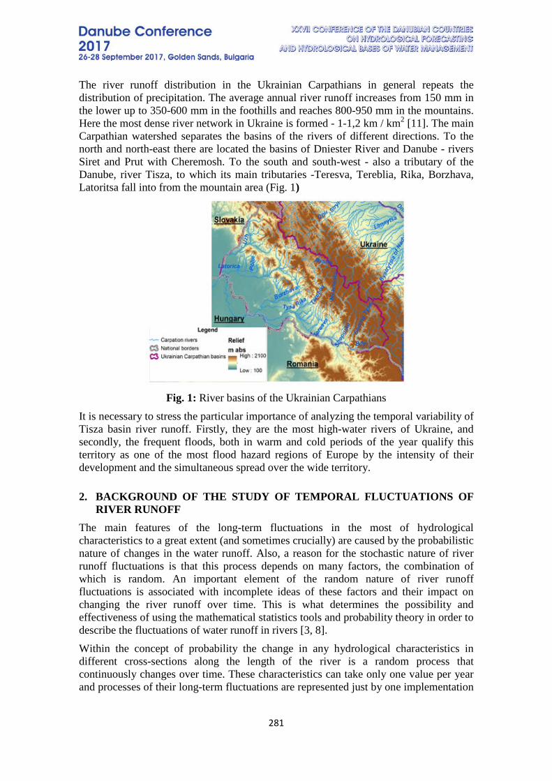
281

The river runoff distribution in the Ukrainian Carpathians in general repeats the distribution of precipitation. The average annual river runoff increases from 150 mm in the lower up to 350-600 mm in the foothills and reaches 800-950 mm in the mountains. Here the most dense river network in Ukraine is formed - 1-1,2 km / km2 [11]. The main Carpathian watershed separates the basins of the rivers of different directions. To the north and north-east there are located the basins of Dniester River and Danube - rivers Siret and Prut with Cheremosh. To the south and south-west - also a tributary of the Danube, river Tisza, to which its main tributaries -Teresva, Tereblia, Rika, Borzhava, Latoritsa fall into from the mountain area (Fig. 1)

Fig. 1: River basins of the Ukrainian Carpathians

It is necessary to stress the particular importance of analyzing the temporal variability of Tisza basin river runoff. Firstly, they are the most high-water rivers of Ukraine, and secondly, the frequent floods, both in warm and cold periods of the year qualify this territory as one of the most flood hazard regions of Europe by the intensity of their development and the simultaneous spread over the wide territory. 2. BACKGROUND OF THE STUDY OF TEMPORAL FLUCTUATIONS OF

RIVER RUNOFF The main features of the long-term fluctuations in the most of hydrological characteristics to a great extent (and sometimes crucially) are caused by the probabilistic nature of changes in the water runoff. Also, a reason for the stochastic nature of river runoff fluctuations is that this process depends on many factors, the combination of which is random. An important element of the random nature of river runoff fluctuations is associated with incomplete ideas of these factors and their impact on changing the river runoff over time. This is what determines the possibility and effectiveness of using the mathematical statistics tools and probability theory in order to describe the fluctuations of water runoff in rivers [3, 8]. Within the concept of probability the change in any hydrological characteristics in different cross-sections along the length of the river is a random process that continuously changes over time. These characteristics can take only one value per year and processes of their long-term fluctuations are represented just by one implementation

282

for the period of observation. For this reason there are random processes for which obtaining of statistical conclusions for single implementation is not only possible, but even can be realized with satisfactory precision at sufficient length of such implementation. Long-term fluctuations in each of these hydrological characteristics Q are treated as a random process Q (t) with discrete time t𝜖𝜖T, which takes integer values (random sequence). In particular, the value t = 1, 2, ..., N can be attributed to the available number of observations for N years; values t = N + 1, N + 2, ... refer to the following periods of time, and the value t = 0, -1, -2, ... - to the previous periods. In order to describe the process Q (t) need to know the whole range of functions, the most important of which are: the function of mathematical expectation m(t)=M{Q(t)}; dispersion function D(t)=D{Q(t)} or mean-square deviation σ(t)=√𝐷𝐷 (t); probability distribution function F(x,t)=Р{Q(t)<х}; autocorrelation function R(t, τ)= corr{Q(t), Q(t +τ)}, etc.[10, 12]. Many scientists were involved in the study of long-term runoff fluctuations, mainly its annual values. Much of the research is devoted to finding the physical nature of river runoff cyclicity, the use of various methods of analyzing its variability and mathematical models for describing the structure of time series. Positive results were obtained by Yu. Alehin [1], who for the first time used the apparatus of the random function theory to develop extrapolation (dynamical and statistical) method of ultra long-term forecasts of the average annual runoff of a number of rivers and other natural macroprocesses. Availability of the in-series connection in series of river runoff was firstly noted by P. Yukhymovych, who calculated for series of river cross-sections the autocorrelation coefficients with time shifts τ = 1, 2, 3 years. Later, they were represented in more full forms with shift of τ = 30, in the form of empirical autocorrelation functions applied by I. Druzhynin to identify cyclical fluctuations in river runoff. 3. OUTPUT DATA The greatest success in the study of temporal runoff fluctuations can be achieved if one considers the long time series of hydrological characteristics in large scale [5, 7, 8], i.e. the water runoff of large basins which are not significantly affected by the random factors and local conditions. River runoff in closing cross-section is an integral feature of humidifying the basin, which smooths randomness in the mode of precipitation in small areas. The research was conducted using the average annual runoff values for river Tisza (near the hydrological stations Vylok with basin F = 9140 km2, for the period of observations 1935-2012 and Vásárosnamény (Hungary) (F = 29057 km2, 1883-2012)). Two hydrological cross-sections were taken from Tisza river for restoration of the sequences of average annual water discharges at Vylok station for the period from 1883 to 1934 with water discharges at Vásárosnamény station. For these stations there is a runoff synchronicity along the length of the river, as evidenced by the relationship between the average annual water discharges of two stations with the correlation ratio r = 0,84).

Studied average water runoff Q is considered as a random process Q (t), which is represented by sample x1…xN, i.e. set with N of its independent and homogeneous implementations.

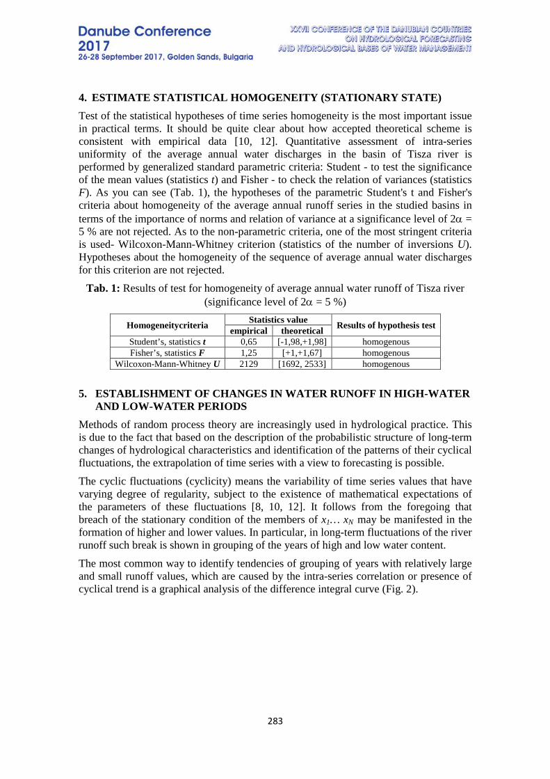
283

4. ESTIMATE STATISTICAL HOMOGENEITY (STATIONARY STATE) Test of the statistical hypotheses of time series homogeneity is the most important issue in practical terms. It should be quite clear about how accepted theoretical scheme is consistent with empirical data [10, 12]. Quantitative assessment of intra-series uniformity of the average annual water discharges in the basin of Tisza river is performed by generalized standard parametric criteria: Student - to test the significance of the mean values (statistics t) and Fisher - to check the relation of variances (statistics F). As you can see (Tab. 1), the hypotheses of the parametric Student's t and Fisher's criteria about homogeneity of the average annual runoff series in the studied basins in terms of the importance of norms and relation of variance at a significance level of 2α = 5 % are not rejected. As to the non-parametric criteria, one of the most stringent criteria is used- Wilcoxon-Mann-Whitney criterion (statistics of the number of inversions U). Hypotheses about the homogeneity of the sequence of average annual water discharges for this criterion are not rejected.

Tab. 1: Results of test for homogeneity of average annual water runoff of Tisza river (significance level of 2α = 5 %)

Homogeneitycriteria Statistics value Results of hypothesis test empirical theoretical Student’s, statistics t 0,65 [-1,98,+1,98] homogenous Fisher’s, statistics F 1,25 [+1,+1,67] homogenous

Wilcoxon-Mann-Whitney U 2129 [1692, 2533] homogenous

5. ESTABLISHMENT OF CHANGES IN WATER RUNOFF IN HIGH-WATER

AND LOW-WATER PERIODS Methods of random process theory are increasingly used in hydrological practice. This is due to the fact that based on the description of the probabilistic structure of long-term changes of hydrological characteristics and identification of the patterns of their cyclical fluctuations, the extrapolation of time series with a view to forecasting is possible. The cyclic fluctuations (cyclicity) means the variability of time series values that have varying degree of regularity, subject to the existence of mathematical expectations of the parameters of these fluctuations [8, 10, 12]. It follows from the foregoing that breach of the stationary condition of the members of x1… xN may be manifested in the formation of higher and lower values. In particular, in long-term fluctuations of the river runoff such break is shown in grouping of the years of high and low water content. The most common way to identify tendencies of grouping of years with relatively large and small runoff values, which are caused by the intra-series correlation or presence of cyclical trend is a graphical analysis of the difference integral curve (Fig. 2).

284

Fig. 2: Difference integral curves of average annual water discharges in river Tisza –

village Vylok

Positive increasing amount of deviation (a phase of high water content) on average means the increase of water runoff. Negative decreasing amount

(phase of low water content) characterizes the average reduction of water runoff.

5.1 Check of the statistical reliability existence of water content phase and their duration The statistical reliability of the existence of such groups (phases of high and low water content), and therefore a breach of stationary conditions can be checked by means of criteria of the series [12]. The series should be understood as any part of the sequence n, consisting of elements of the same kind. A series of elements n1 includes members of the sequence, the value of which exceeds the sample mean (or median) number a, and a series of elements n2 - the members with less value. The values form a series of higher values if: . Series of low values is detected similarly. After determining the total value of quantity of series u, consisting of the quantity of high u1 and low series u2, the statistics of criterion is calculated . For water runoff values of river Tisza - village Vylok at significance level the criteria statistics is. This means an abnormally low number of series that indicates statistically significant tendency to formation of the groups (series) of higher and lower values and the presence of sufficiently high positive correlation between adjacent members of the sequence.

The statistics of the longest length of series is used as test statistics of the duration of higher or lower groups of year [12]. Theoretically proved that for random independent sets the analytical value of the statistical duration of higher or lower groups of years is expressed by the formula

(1)

where – probability (in fractions of 1), along with which in sampling by volume in 𝑠𝑠 members one can meet a series of elements of the higher or lower groupings with a length K or more.

When testing the hypothesis, the empirical value of statistics is compared with the analytical at a certain significance level 𝛼𝛼. According to the data on the average annual runoff and formation of the series with elements of higher or lower groups for the major rivers of the Ukrainian Carpathians, the hypothesis that the probability

1( 1) /n

i vik C

=−∑

1( 1) /n

i vik C

=−∑

1 ;tx a− < ;tx a≥ 1;t k t kx a x a+ + −≥ <

ut5%α =

K

Kα

lg( / lg 2 1ln(1 )

nKα α

= − − −

α

KKα

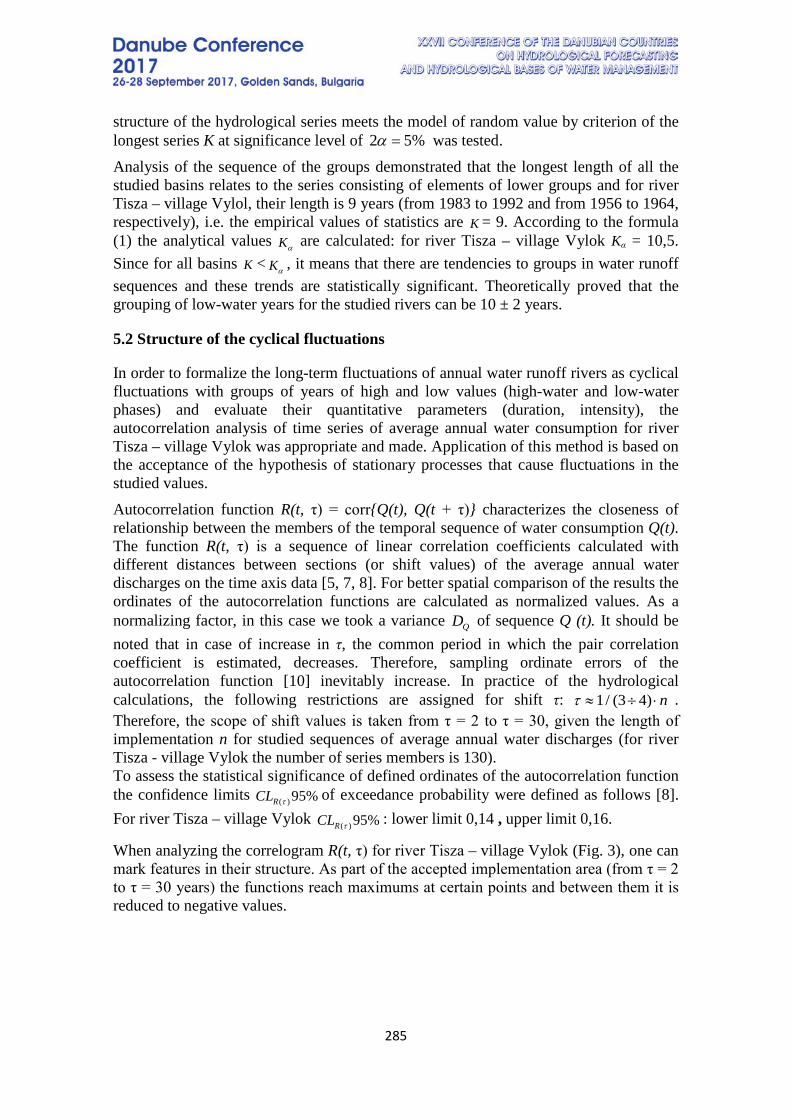
285

structure of the hydrological series meets the model of random value by criterion of the longest series K at significance level of was tested. Analysis of the sequence of the groups demonstrated that the longest length of all the studied basins relates to the series consisting of elements of lower groups and for river Tisza – village Vylol, their length is 9 years (from 1983 to 1992 and from 1956 to 1964, respectively), i.e. the empirical values of statistics are = 9. According to the formula (1) the analytical values are calculated: for river Tisza – village Vylok Kα = 10,5. Since for all basins < , it means that there are tendencies to groups in water runoff sequences and these trends are statistically significant. Theoretically proved that the grouping of low-water years for the studied rivers can be 10 ± 2 years.

5.2 Structure of the cyclical fluctuations

In order to formalize the long-term fluctuations of annual water runoff rivers as cyclical fluctuations with groups of years of high and low values (high-water and low-water phases) and evaluate their quantitative parameters (duration, intensity), the autocorrelation analysis of time series of average annual water consumption for river Tisza – village Vylok was appropriate and made. Application of this method is based on the acceptance of the hypothesis of stationary processes that cause fluctuations in the studied values. Autocorrelation function R(t, τ) = corr{Q(t), Q(t + τ)} characterizes the closeness of relationship between the members of the temporal sequence of water consumption Q(t). The function R(t, τ) is a sequence of linear correlation coefficients calculated with different distances between sections (or shift values) of the average annual water discharges on the time axis data [5, 7, 8]. For better spatial comparison of the results the ordinates of the autocorrelation functions are calculated as normalized values. As a normalizing factor, in this case we took a variance of sequence Q (t). It should be noted that in case of increase in τ, the common period in which the pair correlation coefficient is estimated, decreases. Therefore, sampling ordinate errors of the autocorrelation function [10] inevitably increase. In practice of the hydrological calculations, the following restrictions are assigned for shift τ: . Therefore, the scope of shift values is taken from τ = 2 to τ = 30, given the length of implementation n for studied sequences of average annual water discharges (for river Tisza - village Vylok the number of series members is 130). To assess the statistical significance of defined ordinates of the autocorrelation function the confidence limits of exceedance probability were defined as follows [8]. For river Tisza – village Vylok : lower limit 0,14 , upper limit 0,16.

When analyzing the correlogram R(t, τ) for river Tisza – village Vylok (Fig. 3), one can mark features in their structure. As part of the accepted implementation area (from τ = 2 to τ = 30 years) the functions reach maximums at certain points and between them it is reduced to negative values.

2 5%α =

KKα

K Kα

QD

1/ (3 4) nτ ≈ ÷ ⋅

( ) 95%RCL τ

( ) 95%RCL τ

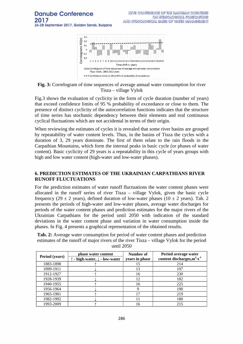
286

Fig. 3: Correlogram of time sequences of average annual water consumption for river

Tisza – village Vylok Fig.3 shows the evaluation of cyclicity in the form of cycle duration (number of years) that exceed confidence limits of 95 % probability of exceedance or close to them. The presence of distinct cyclicity of the autocorrelation functions indicates that the structure of time series has stochastic dependency between their elements and real continuous cyclical fluctuations which are not accidental in terms of their origin. When reviewing the estimates of cycles it is revealed that some river basins are grouped by repeatability of water content levels. Thus, in the basins of Tisza the cycles with a duration of 3, 29 years dominate. The first of them relate to the rain floods in the Carpathian Mountains, which form the internal peaks in basic cycle (or phases of water content). Basic cyclicity of 29 years is a repeatability in this cycle of years groups with high and low water content (high-water and low-water phases).

6. PREDICTION ESTIMATES OF THE UKRAINIAN CARPATHIANS RIVER RUNOFF FLUCTUATIONS For the prediction estimates of water runoff fluctuations the water content phases were allocated in the runoff series of river Tisza – village Vylok, given the basic cycle frequency (29 ± 2 years), defined duration of low-water phases (10 ± 2 years). Tab. 2 presents the periods of high-water and low-water phases, average water discharges for periods of the water content phases and prediction estimates for the major rivers of the Ukrainian Carpathians for the period until 2050 with indication of the standard deviations in the water content phase and variation in water consumption inside the phases. In Fig. 4 presents a graphical representation of the obtained results. Tab. 2: Average water consumption for period of water content phases and prediction estimates of the runoff of major rivers of the river Tisza – village Vylok for the period

until 2050

Period (years) phase water content Number of years in phase

Period average water content discharges,m3·s-1 ↑ - high-water, ↓ - low-water

1883-1898 ↑ 15 214 1899-1911 ↓ 13 197 1912-1927 ↑ 16 230 1928-1939 ↓ 12 182 1940-1955 ↑ 16 225 1956-1964 ↓ 9 190 1965-1981 ↑ 17 219 1982-1992 ↓ 11 180 1993-2009 ↑ 16 215

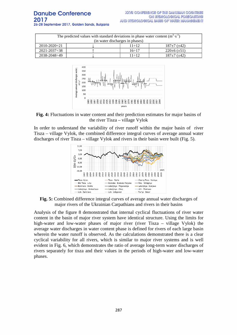
287

The predicted values with standard deviations in phase water content (m3·s-1) (in water discharges in phases)

2010-2020÷21 ↓ 11÷12 187±7 (±42) 2021-2037÷38 ↑ 16÷17 220±6 (±51) 2038-2048÷49 ↓ 11÷12 187±7 (±42)

Fig. 4: Fluctuations in water content and their prediction estimates for major basins of

the river Tisza – village Vylok In order to understand the variability of river runoff within the major basin of river Tisza – village Vylok, the combined difference integral curves of average annual water discharges of river Tisza – village Vylok and rivers in their basin were built (Fig. 5).

Fig. 5: Combined difference integral curves of average annual water discharges of

major rivers of the Ukrainian Carpathians and rivers in their basins Analysis of the figure 8 demonstrated that internal cyclical fluctuations of river water content in the basin of major river system have identical structure. Using the limits for high-water and low-water phases of major river (river Tisza – village Vylok) the average water discharges in water content phase is defined for rivers of each large basin wherein the water runoff is observed. As the calculations demonstrated there is a clear cyclical variability for all rivers, which is similar to major river systems and is well evident in Fig. 6, which demonstrates the ratio of average long-term water discharges of rivers separately for tisza and their values in the periods of high-water and low-water phases.

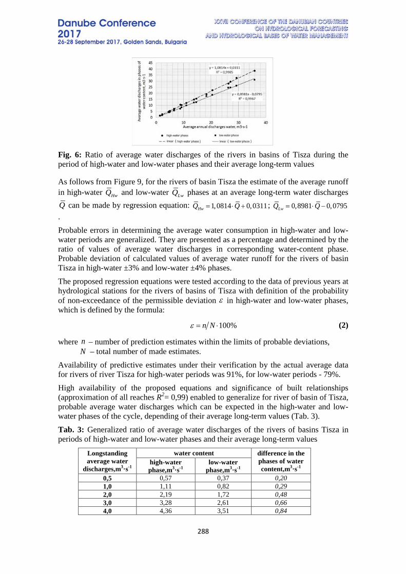
288

Fig. 6: Ratio of average water discharges of the rivers in basins of Tisza during the period of high-water and low-water phases and their average long-term values

As follows from Figure 9, for the rivers of basin Tisza the estimate of the average runoff in high-water and low-water phases at an average long-term water discharges

can be made by regression equation: ; . Probable errors in determining the average water consumption in high-water and low-water periods are generalized. They are presented as a percentage and determined by the ratio of values of average water discharges in corresponding water-content phase. Probable deviation of calculated values of average water runoff for the rivers of basin Tisza in high-water ±3% and low-water ±4% phases. The proposed regression equations were tested according to the data of previous years at hydrological stations for the rivers of basins of Tisza with definition of the probability of non-exceedance of the permissible deviation in high-water and low-water phases, which is defined by the formula:

(2)

where – number of prediction estimates within the limits of probable deviations, – total number of made estimates. Availability of predictive estimates under their verification by the actual average data for rivers of river Tisza for high-water periods was 91%, for low-water periods - 79%. High availability of the proposed equations and significance of built relationships (approximation of all reaches R2= 0,99) enabled to generalize for river of basin of Tisza, probable average water discharges which can be expected in the high-water and low-water phases of the cycle, depending of their average long-term values (Tab. 3). Tab. 3: Generalized ratio of average water discharges of the rivers of basins Tisza in periods of high-water and low-water phases and their average long-term values

Longstanding average water

discharges,m3·s-1

water content difference in the phases of water content,m3·s-1

high-water phase,m3·s-1

low-water phase,m3·s-1

0,5 0,57 0,37 0,20 1,0 1,11 0,82 0,29 2,0 2,19 1,72 0,48 3,0 3,28 2,61 0,66 4,0 4,36 3,51 0,84

HwQ LwQQ 1,0814 0,0311HwQ Q= ⋅ + 0,8981 0,0795LwQ Q= ⋅ −

ε

100%n Nε = ⋅

nN

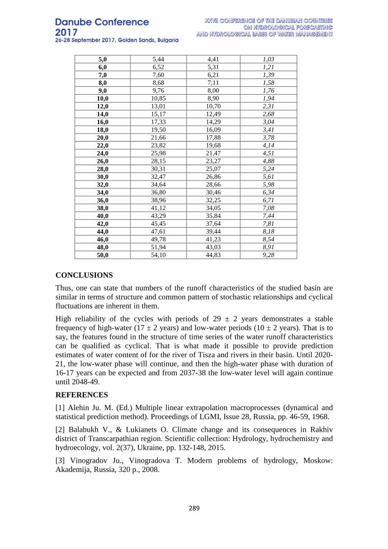
289

5,0 5,44 4,41 1,03 6,0 6,52 5,31 1,21 7,0 7,60 6,21 1,39 8,0 8,68 7,11 1,58 9,0 9,76 8,00 1,76

10,0 10,85 8,90 1,94 12,0 13,01 10,70 2,31 14,0 15,17 12,49 2,68 16,0 17,33 14,29 3,04 18,0 19,50 16,09 3,41 20,0 21,66 17,88 3,78 22,0 23,82 19,68 4,14 24,0 25,98 21,47 4,51 26,0 28,15 23,27 4,88 28,0 30,31 25,07 5,24 30,0 32,47 26,86 5,61 32,0 34,64 28,66 5,98 34,0 36,80 30,46 6,34 36,0 38,96 32,25 6,71 38,0 41,12 34,05 7,08 40,0 43,29 35,84 7,44 42,0 45,45 37,64 7,81 44,0 47,61 39,44 8,18 46,0 49,78 41,23 8,54 48,0 51,94 43,03 8,91 50,0 54,10 44,83 9,28

CONCLUSIONS Thus, one can state that numbers of the runoff characteristics of the studied basin are similar in terms of structure and common pattern of stochastic relationships and cyclical fluctuations are inherent in them. High reliability of the cycles with periods of 29 ± 2 years demonstrates a stable frequency of high-water (17 ± 2 years) and low-water periods (10 ± 2 years). That is to say, the features found in the structure of time series of the water runoff characteristics can be qualified as cyclical. That is what made it possible to provide prediction estimates of water content of for the river of Tisza and rivers in their basin. Until 2020-21, the low-water phase will continue, and then the high-water phase with duration of 16-17 years can be expected and from 2037-38 the low-water level will again continue until 2048-49.

REFERENCES [1] Alehin Ju. M. (Ed.) Multiple linear extrapolation macroprocesses (dynamical and statistical prediction method). Proceedings of LGMI, Issue 28, Russia, pp. 46-59, 1968. [2] Balabukh V., & Lukianets O. Climate change and its consequences in Rakhiv district of Transcarpathian region. Scientific collection: Hydrology, hydrochemistry and hydroecology, vol. 2(37), Ukraine, pp. 132-148, 2015. [3] Vinogradov Ju., Vinogradova T. Modern problems of hydrology, Moskow: Akademija, Russia, 320 p., 2008.

290

[4] Hrebin' V. (Ed.) The modern water regime of rivers Ukraine (landscape and hydrologic analysis), Kyiv: Nika, Ukraine, 316 p., 2010. [5] Luk’yanets O. & Sosyedko M. Die Abflussbewertung auf nächste Jahre in den Karpaten unter Berücksichtigung der mehrjaehrigen Abflusschwankungen. Sammelband der XIX. Konferenz der Donaulaender, Kroatien, рр. 393-401, 1998. [6] Luk’yanets O. & Sosyedko M. Long-term water level fluctuations in the Carpathians, Book of abstracts: International Conference «Natural phenomena in the Carpathians», Ukraine, pp.195-199, 1999. [7] Luk’yanets, O., Sosyedko, M., & Balabukh, V. Forecast’s assessment of water content in Ukraine in the first half of XXIth century, Book of abstracts: ХХVІ Conference of Danubian countries on the hydrological forecasting and hydrological bases of water management, Slovenia, рр. 111-112, 2008. [8] Lukyanets O., Kaminska T. Regularities and spatial synchrony of perennial cyclical fluctuations in the water runoff of the Ukrainian Carpathians rivers, Scientific Bulletin of Chernivtsi University: Collection of scientific papers: Vol. 744-745: Geography, Ukraine, pp. 18-24, 2015. [9] Lukianets Olga & Obodovskyi Iurii Spatial, Temporal and Forecast Evaluation of Rivers’ Streamflow of the Drainage Basin of the Upper Tisa under the Conditions of Climate Change. Scientific Journal: Environmental Research, Engineering and Management, No. 71(1), Kaunas: KTU, Lithuania, pр. 36-46, 2015. [10] Sikan A. Statistical treatment of hydrometeorological information, Russia, pp.160-180, 2007. [11] Sosyedko M. & Luk’yanets O. The Carpathians – flood danger region of Ukraine. Basin runoff forecasting system in Zakarpattya: Methodical and technological basis of its components, Ukraine, pp. 38-63, 2010. [12] Khristophorov A. Theory of stochastic processes in hydrology, Russia, 143 p., 1994.

291

EXTENDING THE OLSER FORECASTING SYSTEM FOR SMALL CATCHMENTS IN HUNGARY

András Csík, Balázs Gauzer, Boglárka Gnandt, Zoltán Liptay

Katalin Molnár General Directorate of Water Management, Hungary Corresponding author: Csik.andras@onf.hu

ABSTRACT In the last few years, a massive need for hydrological forecasts on smaller catchments was emphasized mainly by professionals involved in flood protection. The OLSER hydrological simulation and forecasting system of Hungarian Hydrological Forecasting Service (HHFS) was originally developed for large river catchments like Danube or Tisza. Due to intense improvements of the system effectuated in the previous years, OLSER became suitable for application on smaller catchments (with the size of a few 1000 km2). Latest upgrades contain both Zala and Zagyva river systems. As a result, HHFS forecasts are issued daily for almost 100 gauging stations over the country at the moment. This relatively high number of forecast stations require a more effective dissemination system, therefore HHFS’s HYDROINFO publication system has been extended with English version and also with mobile optimized webpages and a mobile application. Keywords: hydrological forecasting, small catchments, OLSER, Hungarian Hydrological Forecasting Service, mobile application

1. THE OPERATING METHOD OF THE HUNGARIAN HYDROLOGICAL FORECASTING SERVICE AND THE STRUCTURE OF ITS FORECASTING SYSTEM The Hungarian Hydrological Forecasting Service (HHFS) prepares water level forecasts for the key gauges for major Hungarian water courses every day of the year. HHFS primarily uses its own website network (www.hydroinfo.hu) to convey information to users but telephone and email hotlines are also available means of communication. OLSER, the runoff forecasting and simulation system of the Hungarian Hydrological Forecasting Service, is basically a model system built from modules (building blocks) [2]. The models of the individual parts identifiable within the complex system of the runoff process are the functional modules. These can be used to calculate hydrological process parts (e.g. snow accumulation and melting or runoff components) and applied to any user-defined structure of a catchment. It must be noted that the Hungarian Hydrological Forecasting Service (HHFS) is not only an organisation regularly operating the forecasting system but also a forecasting service, which issues a forecast every day throughout the year reviewed by qualified staff whose practical experience and up-to-date knowledge are guaranteed by their rotational work schedule. In addition, the forecasting and modelling system used in daily operations is HHFS’s own proprietary tool, a rarity in and of itself, which warrants

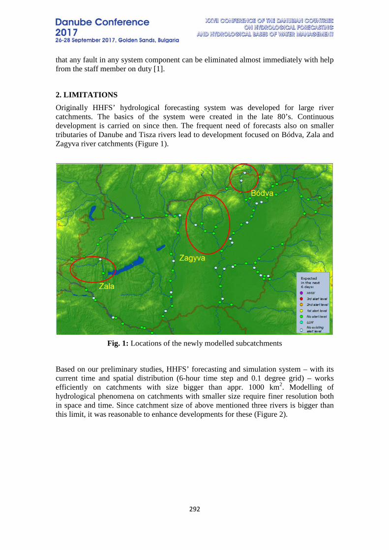
292

that any fault in any system component can be eliminated almost immediately with help from the staff member on duty [1].

2. LIMITATIONS Originally HHFS’ hydrological forecasting system was developed for large river catchments. The basics of the system were created in the late 80’s. Continuous development is carried on since then. The frequent need of forecasts also on smaller tributaries of Danube and Tisza rivers lead to development focused on Bódva, Zala and Zagyva river catchments (Figure 1).

Fig. 1: Locations of the newly modelled subcatchments

Based on our preliminary studies, HHFS’ forecasting and simulation system – with its current time and spatial distribution (6-hour time step and 0.1 degree grid) – works efficiently on catchments with size bigger than appr. 1000 km2. Modelling of hydrological phenomena on catchments with smaller size require finer resolution both in space and time. Since catchment size of above mentioned three rivers is bigger than this limit, it was reasonable to enhance developments for these (Figure 2).

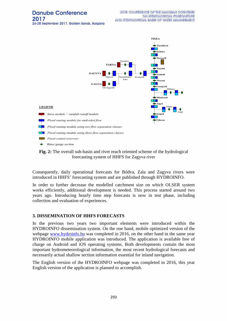
293

Fig. 2: The overall sub-basin and river reach oriented scheme of the hydrological

forecasting system of HHFS for Zagyva river Consequently, daily operational forecasts for Bódva, Zala and Zagyva rivers were introduced in HHFS’ forecasting system and are published through HYDROINFO. In order to further decrease the modelled catchment size on which OLSER system works efficiently, additional development is needed. This process started around two years ago. Introducing hourly time step forecasts is now in test phase, including collection and evaluation of experiences.

3. DISSEMINATION OF HHFS FORECASTS In the previous two years two important elements were introduced within the HYDROINFO dissemination system. On the one hand, mobile optimized version of the webpage www.hydroinfo.hu was completed in 2016, on the other hand in the same year HYDROINFO mobile application was introduced. The application is available free of charge on Android and iOS operating systems. Both developments contain the most important hydrometeorological information, the most recent hydrological forecasts and necessarily actual shallow section information essential for inland navigation. The English version of the HYDROINFO webpage was completed in 2016, this year English version of the application is planned to accomplish.

294

4. SUMMARY Owing to the continuously developments, the HHFS could involve new subcatchments into its OLSER system and produce hydrological forecasts for 9 new gauges. Number of the gauges published in the HYDROINFO dissemination system reached almost 100. With the newly developed publishing solutions – namely optimized webpage for mobile devices and the mobile application – the dissemination and usability of the daily hydrological forecasts have become easier both for the professional and common users.

REFERENCES [1] Szöllősi-Nagy, A.: Learn from your errors – If you can!, UNESCO-IHE, Delft, The Netherlands, p.102., 2009. [2] Gauzer, B. & Bartha, P. (2001): Árvízi szimulációs vizsgálatok a Tisza Tokaj-Szeged közötti szakaszán. Vízügyi Közlemények, LXXXIII. Volume 4., pp.512-537., 2001.

295

APPLYING A NEW MODEL IN WATER LEVEL FORECASTING FOR THE

COMMON HUNGARIAN-CROATIAN SECTION OF DRAVA RIVER AT THE

HUNGARIAN HYDROLOGICAL FORECASTING SERVICE

Adrienn Hunyady

General Directorate of Water Management, Hungarian Hydrological Forecasting Service, Hungary

Adrienn Hunyady, General Directorate of Water Management, Márvány utca 1/D, Budapest, Hungary H-1012, hunyady.adrienn@ovf.hu

ABSTRACT In the last decade several changes have been implemented to improve the accuracy of hydrological forecasts. New hydrological gauging stations and meteorological in-situ stations have been installed. Developments in computer science, geoinformatics and widespread internet connectivity in recent years now allow for at least 6 hourly monitoring of gauging stations. The reliability and lead time of meteorological forecasts have also become much better. These favorable developments have made it possible to overhaul the entire flood forecasting system for the Drava River by 2012. Currently, there is a complex forecasting system in operation to provide water level forecasts for the common Hungarian-Croatian section of the Drava River. The core part of the complex system is the Operative Hydrological Forecasting and Simulation System (OLSER) which is developed and operated by the Hungarian Hydrological Forecasting Service (HHFS). The West Transdanubian Environmental and Water Directorate (STEWD) and Hrvatske Vode (HV) independently operate local parts of the complex system, which is mainly based on the HEC-RAS model developed by US Army Crops and Engineers. OLSER makes water level forecasts for 9 gauging stations of the common Hungarian-Croatian section of Drava River at least once a day based on modeling rainfall/runoff processes on the entire Drava-Mur basin. It is also the task of OLSER to produce data that serves as boundary conditions for the local parts of the system, which STEWD or HV may decide run, if needed. In practice, this occurs only in the case of floods. Timely and reliable forecasts are not only essential for flood protection, but also for any technical planning. Moreover, engineering applications require forecasts along the entire river section and not only for 9 gauging stations. Therefore, HHFS has decided to build a 1D hydraulic model into OLSER, which is able to make operative water level forecasts between Őrtilos and the estuary of Drava River. In this paper we are going to present the new 1D channel routing module of OLSER and some water level forecast results obtained with the 1D module. Keywords: Drava River, hydraulic modeling, 1-D hydrodynamic model, discrete linear cascade model.

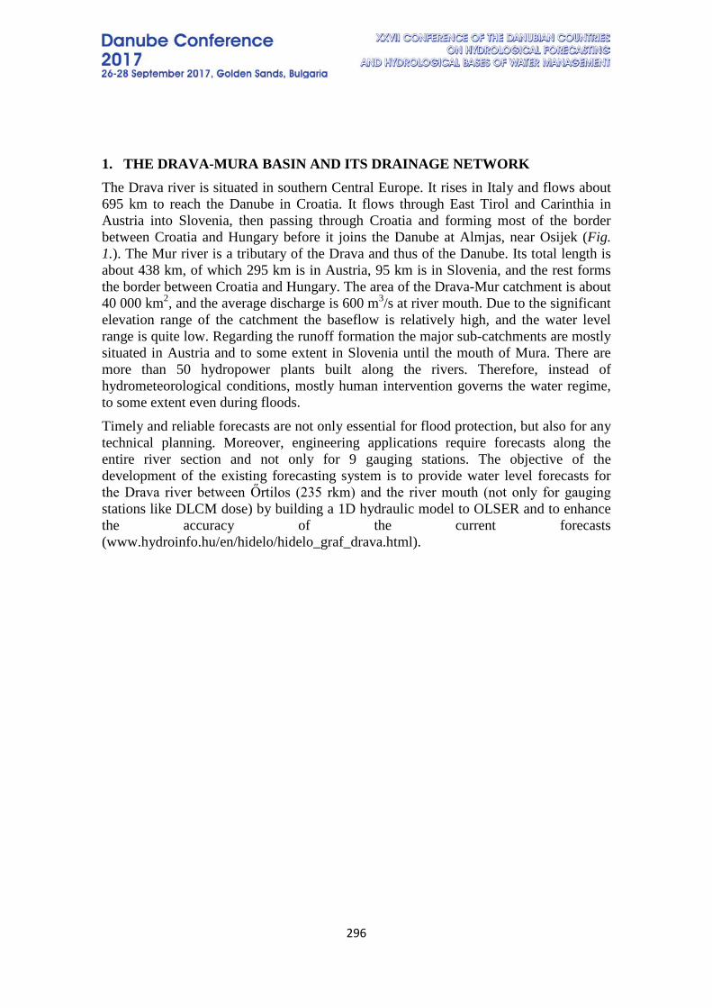
296

1. THE DRAVA-MURA BASIN AND ITS DRAINAGE NETWORK The Drava river is situated in southern Central Europe. It rises in Italy and flows about 695 km to reach the Danube in Croatia. It flows through East Tirol and Carinthia in Austria into Slovenia, then passing through Croatia and forming most of the border between Croatia and Hungary before it joins the Danube at Almjas, near Osijek (Fig. 1.). The Mur river is a tributary of the Drava and thus of the Danube. Its total length is about 438 km, of which 295 km is in Austria, 95 km is in Slovenia, and the rest forms the border between Croatia and Hungary. The area of the Drava-Mur catchment is about 40 000 km2, and the average discharge is 600 m3/s at river mouth. Due to the significant elevation range of the catchment the baseflow is relatively high, and the water level range is quite low. Regarding the runoff formation the major sub-catchments are mostly situated in Austria and to some extent in Slovenia until the mouth of Mura. There are more than 50 hydropower plants built along the rivers. Therefore, instead of hydrometeorological conditions, mostly human intervention governs the water regime, to some extent even during floods. Timely and reliable forecasts are not only essential for flood protection, but also for any technical planning. Moreover, engineering applications require forecasts along the entire river section and not only for 9 gauging stations. The objective of the development of the existing forecasting system is to provide water level forecasts for the Drava river between Őrtilos (235 rkm) and the river mouth (not only for gauging stations like DLCM dose) by building a 1D hydraulic model to OLSER and to enhance the accuracy of the current forecasts (www.hydroinfo.hu/en/hidelo/hidelo_graf_drava.html).

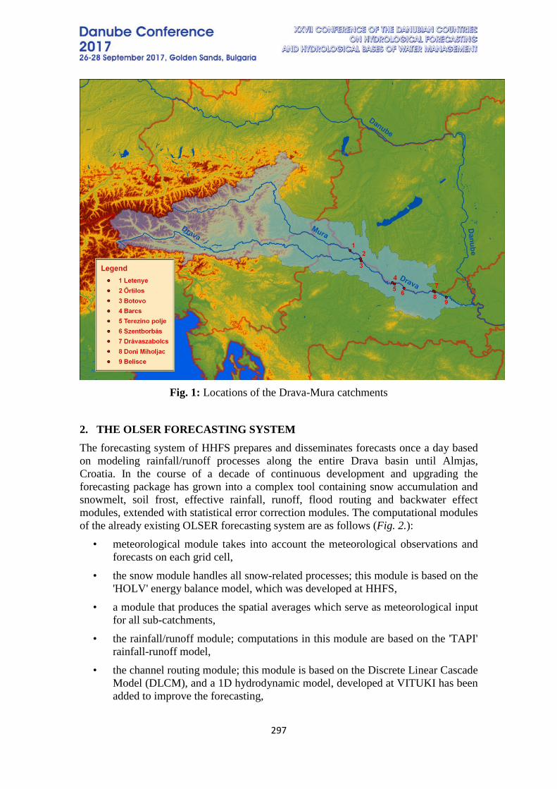
297

Fig. 1: Locations of the Drava-Mura catchments

2. THE OLSER FORECASTING SYSTEM The forecasting system of HHFS prepares and disseminates forecasts once a day based on modeling rainfall/runoff processes along the entire Drava basin until Almjas, Croatia. In the course of a decade of continuous development and upgrading the forecasting package has grown into a complex tool containing snow accumulation and snowmelt, soil frost, effective rainfall, runoff, flood routing and backwater effect modules, extended with statistical error correction modules. The computational modules of the already existing OLSER forecasting system are as follows (Fig. 2.):

• meteorological module takes into account the meteorological observations and forecasts on each grid cell,

• the snow module handles all snow-related processes; this module is based on the 'HOLV' energy balance model, which was developed at HHFS,

• a module that produces the spatial averages which serve as meteorological input for all sub-catchments,

• the rainfall/runoff module; computations in this module are based on the 'TAPI' rainfall-runoff model,

• the channel routing module; this module is based on the Discrete Linear Cascade Model (DLCM), and a 1D hydrodynamic model, developed at VITUKI has been added to improve the forecasting,

298

• a forecasting error correction module; special algorithms were developed which are able to recognize patterns in hydropower plants' operation

• a module to model the interaction of the lower Drava and the receiving Danube, i.e. backwater and drawdown processes

The employed modules on the grid are distributed and from the catchment are of the concentrated parameter type. The two main kinds of meteorological input for the forecasting system are the measurements of the in situ meteorological stations and the forecasts of the numerical weather models, respectively. Meteorological measurements are accessed by daily (FTP) data exchange or downloaded from web-based services. The system is capable of utilizing both the forecasts of the ECMWF model (which is widely used in Hungarian forecasting practice) and of the GFS (Global Forecasting system). Taking into limitations due to data availability, we use the following data from meteorological in situ stations:

• precipitation sum, four times daily (00, 06, 12, 18 UTC) • daily maximum and minimum temperature • wind speed, twice daily (06, 08 UTC)

299

Fig 2: The functional modules of the global forecasting system

Prior to use, meteorological measurements and forecasts are transformed to a common format. This format is chosen to be a 0.1x0.1 degree geographical grid. There are strong orographic effects to be reckoned with for all types of data (precipitation, temperature extremes and wind speed), and the interpolation procedure are take these effects into account. The forecasting system uses the following hydrological data:

1 D

300

• hourly (at least 4x daily) water level and water discharge data from stations involved in water level forecasting, or bi-variate discharge rating curve in place of the latter

• for all other stations, hourly (or at least 4x daily) water discharge data

3. THE 1D FLOOD ROUTING MODULE The applied 1D model solves the full 1D Saint Venant equations for unsteady open channel flow:

Continuity equation: ∂Q∂x

+ 𝐵𝐵 ∂z∂t

= 0 (1)

Momentum equation: 𝜕𝜕𝜕𝜕𝜕𝜕𝜕𝜕

+ 1𝑔𝑔𝐴𝐴

𝜕𝜕𝑄𝑄𝜕𝜕𝑡𝑡− 𝑄𝑄

𝑔𝑔𝐴𝐴2𝜕𝜕𝐴𝐴𝜕𝜕𝑡𝑡

+ 𝛼𝛼𝑄𝑄𝑔𝑔𝐴𝐴2

𝜕𝜕𝑄𝑄𝜕𝜕𝜕𝜕− 𝑄𝑄2

𝑔𝑔𝐴𝐴3𝜕𝜕𝐴𝐴𝜕𝜕𝜕𝜕

+ 𝑄𝑄2

𝐾𝐾2= 0 (2)

Q: discharge in the cross section, z: water level in the main channel, x: independent variable for position, t: independent variable for time, g: gravity, B: channel width at water surface, A: wet area of the cross section, α: dispersion coefficient of the kinetic energy,

K: specific discharge coefficient (𝐾𝐾 = 𝑄𝑄√𝑆𝑆

)

S: the slope of the hydraulic grade line R: hydraulic radius (A/P) P: wet perimeter of the cross section The above equations are a set of non-linear differential equations, to solve them we transformed the Saint Venant equations to a set of linear difference equations by using the implicit differential Preissmann scheme. We also add the upper (discharge time series) and the lower boundary (water level time series) conditions to solve the equations using Gauss elimination with partial pivoting.

1 D model of river Drava from Őrtilos to the river mouth Our study area is mainly river Drava, but in order to take the backwater effect of the Danube into consideration sufficiently we added our model by a short Danube section between Mohács and Almjas. Therefore, in our model we calculate with 3 river branches (one for river Drava and 2 for the Danube) and 1 node in between the branches.

301

Cross sections The characteristics of a cross section are not fixed. Due to the unsteady character of the water flow in a river, the wet perimeter and wet area of the cross section change. A river bed consists of:

• Main channel • Floodplains (left and right side)

During low and medium range periods the water flows in the main channel. During floods the river overflow to the floodplains, where the roughness is much higher. In our model we calculate with 850 cross sections, 837 on river Drava and 10+3 cross sections of the Danube. The distance between the cross section is varying, Δx is not constant. The cross section data is measured by Hrvatske Vode in 2009 and was an outcome of an IPA project (‘Flood Forecasting in the Watershed Area of Drava River’ project, which is co-financed by the European Union through the Hungary-Croatia IPA Cross-border Co-operation Programme).

Boundary conditions In order to run the model we should determine driving forces, which generate a flood wave. These are the discharges at the upper boundary of the model, at Őrtilos and Mohács and water levels at the lower boundary, at Almjas.

Initial conditions Spatial distribution of water levels and discharges (initial conditions) is essential to be known prior to the calculations. We built in two different methods to determine the initial conditions:

• Cold start: calculation of steady gradually varying flow • Hot start: using previous model results

We usually apply the cold start at the beginning of the calculations. Due to the fact that steady gradually varying flow is very rare we load our calculation with an initial error. This is why a spin-up time is essential to apply, in this model we calculate with 23 days spin-up time.

Calibration and validation The aim of the calibration was to set the Strickler smoothness coefficient to minimalize the difference between the measured and simulated water levels during 01.23/2009-06.01/2009. The chosen period contains two moderate and two greater flood waves. We started the model run at 01.01/2009, but we did not calculated with the first 23 day, the spin-up time of the model. We chose the period of 23.07/2012-01.12/2012 to validate the model. There were also two greater and three moderate flood waves.

302

4. RESULTS As we presented in Chapter 2, OLSER makes water level forecasts for 9 gauging stations of the common Hungarian-Croatian section of Drava River (for stations presented on Fig. 1.) at least once a day based on modeling rainfall/runoff processes on the entire Drava-Mura basin. It is also the task of OLSER to produce data that serves as boundary conditions for the 1D model. One of the advantages of using 1D model is to get forecast along the entire river and not only the gauging stations, where historical data are exist (like DLCM). Additionally, we also expected a more accurate forecasting result comparing with DLCM. The analysis of the results is based on comparison with the DLCM model's forecasts between 2010.02.01 and 2010. 12.31. MSE is used quantify the forecast accuracy. We also note, that examining the role of hydropower stations, we can conclude that the power stations along River Mura have a negligible impact on the Drava's hydrological regime downstream Őrtilos, whereas the Croatian plants along the Drava often have a considerable effect. Those power plants influence the Drava below Őrtilos even during floods, especially the most downstream one (Dubrava). However, the water releases of the power plants are not available as those are proprietary information, therefore we cannot take into account in our calculations.

Table 1: Mean square errors of the 1-6 days water level forecasts between 2010.02.01 and 2010.12.31. for the investigated sections of Drava river

Gauging station Model 1st day 2nd day 3rd day 4th day 5th day 6th day

Őrtilos DLCM 23.6 25.9 30.5 32.2 32.0 33.2

1D 20.4 22.7 26.9 28.8 28.8 30.2 error reduction (%) 13.6 12.4 11.8 10.6 10.0 9.0

Barcs DLCM 20.9 24.0 25.9 28.9 31.4 32.2

1D 17.9 20.9 22.9 25.9 28.3 29.6 error reduction (%) 14.4 12.9 11.6 10.4 9.9 8.1

Szentborbás DLCM 18.2 26.9 30.6 33.7 35.4 34.9

1D 16.3 24.5 28.1 31.3 33.0 33.1 error reduction (%) 10.4 8.9 8.2 7.1 6.8 5.2

Drávaszabolcs DLCM 8.9 20.1 24.1 26.7 30.6 33.3

1D 8.0 18.3 22.4 24.9 28.8 31.6 error reduction (%) 10.1 9.0 7.1 6.7 5.9 5.1

303

Fig 3: Longitudinal section of the Drava between Őrtilos and the estuary at 1st of June

2009. The blue line shows the water level and the red is the discharge. The results lead to following conclusions:

• Compared to the DLC model, forecast accuracy improved substantially everywhere, mostly by 8-12%, but the highest error reductions exceed 14%, while the lowest reductions are above 5%.

• The reason of the higher accuracy is mostly based on the more precise description of the terrain of the Drava between Őrtilos and the river mouth.

• The one-day-ahead forecast error for the Drava at Őrtilos is more than twice that of the forecast error at Drávaszabolcs and nearly the same for the 6th day. Differences between the one-day-ahead and six-day-ahead forecasts are higher at the lower sections compared to the upper sections. This is due to the substantial effects of the Croatian hydropower plants, especially Dubrava. This feature can be observed in case of both models.

• The error reduction is higher in case of upper sections and also in case of shorter lead time by using the 1D model. The forecast error decreases continuously along the Drava, which is mostly due to the decreasing disturbance of the hydropower stations in case of both models.

• There are available forecasts for the entire river (between Őrtilos and the estuary) and not only for the gauging stations as it can be seen on Fig.3.

REFERENCES [1] Abbott, M. B.: Computational Hydraulics, Pittman Publishing Limited, Boston. London, Melbourne, 1979. [2] Abbott, M. B. – Basco, D. R.: Computational Fluid Dynamics, Longman Scientific & Technical, Harlow, 1989.

Longitudinal section Z

(maB

) Q (m

3/s)

water level discharge

304

[3] Bakonyi, P.: Simulation of Unsteady Flow due to Ice Jam Formation, International Conference on Fluvial Hydraulics, Budapest, 1988. [4] Bakonyi, P. – Bognár, S.: A Kis-Delta beeresztő műtárgy hidraulikai méretezése, VITUKI Consult Rt, 1997. [5] Cunge, J. A. – Holly Jr., F. M. – Verwey, A.: Practical Aspects of Computational River Hydraulics, Pittman Publishing Limited, Boston. London, Melbourne, 1980. [6] Fread, D. L.: DAMBRK: The NWS Dam Break Flood Forecasting Model. National Weather Service(NWS) Report, NOAA, Silver Spring, Maryland. 1984. [7] Gauzer, B. & Bartha, P. (2001): Árvízi szimulációs vizsgálatok a Tisza Tokaj-Szeged közötti szakaszán. Vízügyi Közlemények, LXXXIII. Volume 4., pp.512-537., 2001.

305

ENHANCING THE NATIONAL CAPACITY TO MONITOR, EVALUATE AND FORECAST DANGEROUS METEOROLOGICAL AND HYDROLOGICAL

PHENOMENA, SERBIAN EXPERIENCE

Bojan Palmar1, Carlo Cacciamani2, Slavimir Stevanovic1, Borjanka Palmar1

1 Republic Hydrometeorological Service, Serbia 2Hydro-meteorological and Climatological Service of Emilia Romagna, Italy

Corresponding author: Bojan Palmar, Republic Hydrometeorological Service, Kneza Viseslava 66, Belgrade, Serbia, bojan.palmar@hidmet.gov.rs

ABSTRACT Disastrous flood events of May 2014 in Serbia, caused considerable number of deaths and negative economic impact estimated at 1.6 billion Euros (0.9 billion for damages and 0.7 billion for losses), made dramatically evident that there is a need to strengthening the existing infrastructures and upgrade the observation system, as well as to improve overall Disaster Management. Through the Instrument of Pre-Accession Assistance IPA 2014, the European Union has allocated the funds for financing flood prevention projects to reduce the risk of new catastrophes. Improvement of flood forecasting systems is one of the pre-requisites to reduce disaster risks. Enhancing the national capacity to monitor, evaluate and forecast dangerous meteorological and hydrological phenomena, has been identified as the most urgent actions to “get prepared” in case of the natural disasters, focusing as much as possible to the local scale, to provide timely and reliable real-time data, early warnings and alerts to Civil Protection, local authorities and all Agencies in charge of the safety of population and the environment. In this paper the concept for the improvement of the national Early Warning System, meteorological and hydrological monitoring, data acquisition, analysis, forecasting and dissemination system is presented. Special emphasis is given to the analysis of user requirements, conducted by the assessment of the user behavior and survey among users of the internet site of the national hydro-meteorological service. This paper also deals with the improvement of the risk communication, developed and proposed during the Central European Initiative (CEI), Know-How Exchange Project (KEP) “Alert: Strengthening Serbian Multi - Hazard Early Warning and Alert System”, conducted jointly by the Regional Environmental Protection Agency, Hydro-meteorological and Climatological Service of Emilia Romagna (Arpae SIMC), Italy and Republic Hydrometeorological Service of Serbia (RHMSS). The strategy presented in the paper is based on the survey of risk perception conducted in selected municipalities in Italy and Serbia. Keywords: floods, risk perception, risk communication, Early Warning System

306

1. INTRODUCTION The flood prevention projects financed by EU are the part of the Country Action Program directed towards re-establishing of regular functioning of public services, through rehabilitation of the damaged regional and local transport network, restoration of the power supply and distribution facilities, towards reconstruction and improvement of flood prevention systems and emergency response systems. The objective of the Country Action Program - Recovery of flood damages, is to assist Serbia in the recovery effort in the aftermath of floods that hit the region during several months of 2014, and to improve prevention and emergency response system. Those events, once unusual for a temperate climate zone, are expected to become more and more frequent, being the impact of the climate change, and therefore cannot be regarded as isolated cases. Getting prepared, reducing damages and – as far as possible – avoiding the loss of human lives is therefore a priority. Intended interventions are proposed, among other actions, by the Action Plan for the Implementation of the National Disaster Risk Management Program of the Republic of Serbia (2016-2020) [1], Component 4: System for early warning and preparedness. This component addresses the Priority for Action 4 of the Sendai Framework for Disaster Risk Reduction 2015-2030: Enhancing disaster preparedness for effective response and to “Build Back Better” in recovery, rehabilitation and reconstruction. While building back better has been defined in many ways, at its core, it advocates for the restoration of communities and assets in a manner that makes them less vulnerable to disasters and strengthens their resilience [2]. The project is also consistent with the World Meteorological Organization (WMO) concerns, expressed in the letter addressed by the Secretary General to the Permanent Representative of Serbia on the 6 June 2014, pointing out the need of “strengthening the operational capabilities of National Meteorological and Hydrological Service and the need to further develop and implement mitigation measures and resilience programs”. Although a lot has been done in recent years, Serbia still suffers from the “gaps”, and must urgently act to fully upgrade, modernize and expand the whole Early Warning System. The availability and fully reliable operation of a modern hydro-meteorological monitoring, Early Warning and alarm System, covering the entire Country represents the very starting point to reach those goals. Serbia has made significant investments in the hazard forecasting and hydro-meteorological early warning systems. The Republic Hydrometeorological Service of Serbia (RHMSS) currently has a functional and relatively robust hydrological and meteorological monitoring network. This allows RHMSS to deliver real-time meteorological and hydrological data to the Sector for Emergency Management (SEM), including observations, various forecasts across short, medium and long timescales, alerts and warnings [3]. Additional investments in RHMSS Early Warning System, monitoring, data acquisition, data analysis, forecasting and dissemination system, will enhance technical capacities to issue timely, more accurate and reliable real-time data, forecasts and early warnings to the Sector for Emergency Management, Civil Protection and other stakeholders in the flood protection and flood risk management system.

307

2. EARLY WARNING SYSTEM The recent flood events show that early warnings need to be more timely and accurate and properly reach local communities. To be capable to provide reliable real-time data on rainfall, water levels and discharge, RHMSS needs to rehabilitate, strengthen and upgrade density of the meteorological and hydrological monitoring network for forecasting and early warning purposes. The scarce real-time data availability on small and medium catchments, lack of automatic rain-gauges largely affects hydrological forecasting activity, especially during short and very intense events. Significant amount of hydrological real-time data is available and cooperation with neighboring countries is in place, but a hydraulic modeling on large rivers needs to be improved. The present Project is conceived in 5 Actions: Action I: Rehabilitation and upgrade of hydrological stations and infrastructure damaged during the floods (11 hydrological stations and 4 cableways for stream gauging); Action II: Upgrade and strengthening of the observing network in the most sensitive and flood prone areas. The target is to increase efficiency of the hydrological and meteorological observation system. A total of 39 stations are considered, including hydrological, rain-gauges (the majority) and climatological stations. Purchase of hydrometric instruments for flood discharge measurement, ADCPs and surface velocity radars is also foreseen. Action III: Upgrade of the Real-Time data transmission system. To face emergencies like in May 2014, the system must guarantee a transmission full capacity under all weather conditions. A redundant transmission system is foreseen, based on UHF radio network and GPRS mobile network. Radio frequencies must be carefully selected to avoid interruptions or interferences. Action IV: Upgrade of the Main Control Center in Belgrade and control centers in regional offices. It is necessary to improve hardware and software for system configuration, monitoring, acquisition and presentation. The system must also be compliant to easily accept new models for hydrological / hydraulic forecast. Special attention will be given to the web presentation and mobile apps as tools for data and product dissemination. Action V: Upgrade of the model for the real-time flood forecast, to be implemented in the Velika Morava river basin as a pilot system, improve hydraulic and hydrologic modeling capabilities, make use of GIS based software tools to display and analyze flood forecast and model results. Meteorological and hydrological models should be integrated in to the single model chain, taking advantage as much as possible of the available numerical weather prediction products (deterministic, probabilistic), weather radar observations and other real- time data sources. Consistently with WMO recommendations, hydro-meteorological network must be considered as Information and Communication Technology product. “In order to ensure sustainability of the investment in modern real-time ground-based observation systems these should be recognized as Information and Communication Technology (ICT) items

308

and integrated with ICT systems to be able to provide reliable information that is of vital importance to preserve human lives and livelihoods with high efficiency”. [4]. The hydro-meteorological information system consists of the data acquisition (meteorological and hydrological real-time monitoring), transmission and processing (data management and analysis). The supply of hydrological and meteorological monitoring system, is intended as perfectly operational and working in all its components (hardware, software, services) and also compatible with existing infrastructures and software platforms. All system components (stations, transmission devices, applications) must be extremely “robust”, to guarantee the full operation and high availability of data during the most severe weather conditions. Reliability of data measured, transmitted, received and processed is a prerequisite.

3. RISK COMMUNICATION Early warning systems, preparedness and response are raised as essential issues that had to be improved to obtain a substantial reduction of risks and related costs. Permanent involvement of municipal and local authorities and the population is recognized as critical to achieve this target. Based on the above, a dedicated “Disaster Risk Communication Action”, was launched in the framework of the CEI KEP “Alert” Project. 3.1 Disaster Risk Communication Action The Action was carried out in two activities: international workshop on Disaster Risk Communication and survey on flood risk perception on pilot locations in Serbia. Two-day “Workshop on Disaster Risk Communication” was organized in partnership with the OSCE Mission to Serbia, aimed at getting media and citizens better involved in the disaster risk communication chain, which has the starting point in Hydro-Meteorological Service. Disaster Risk Reduction cannot be effectively achieved without a strong commitment of all partners involved in the “risk communication chain” – starting from Hydro-Meteorological Services, and then moving to SEM, Civil Protection and to its regional units, city mayors, and, as the last mile end-users e.g. citizens. Also, media can help the communication to properly flow to get to the targets. Through the media RHMSS informs the public on the potentially dangerous condition on weather, climate and water. RHMSS is official source for the alerts, forecasts and warnings on dangerous phenomena of meteorological and hydrological origin. It has been demonstrated that both affected and unaffected communities have trust in media reports. The information broadcasted over the radio, TV, on-line news or newspapers is perceived as a reliable advice and people take it seriously. From RHMSS perspective, it seems that print/electronic media do not entirely recognize RHMSS institutional mandate, making often incorrect comments, reporting statements without citing the sources, tending to sensationalism. To improve communication with media, we should start with a correct identification of the problems, and then work on strengthening direct communication through formally defined partnerships, with all stakeholders involved. A specific action should be taken in this direction, with journalist

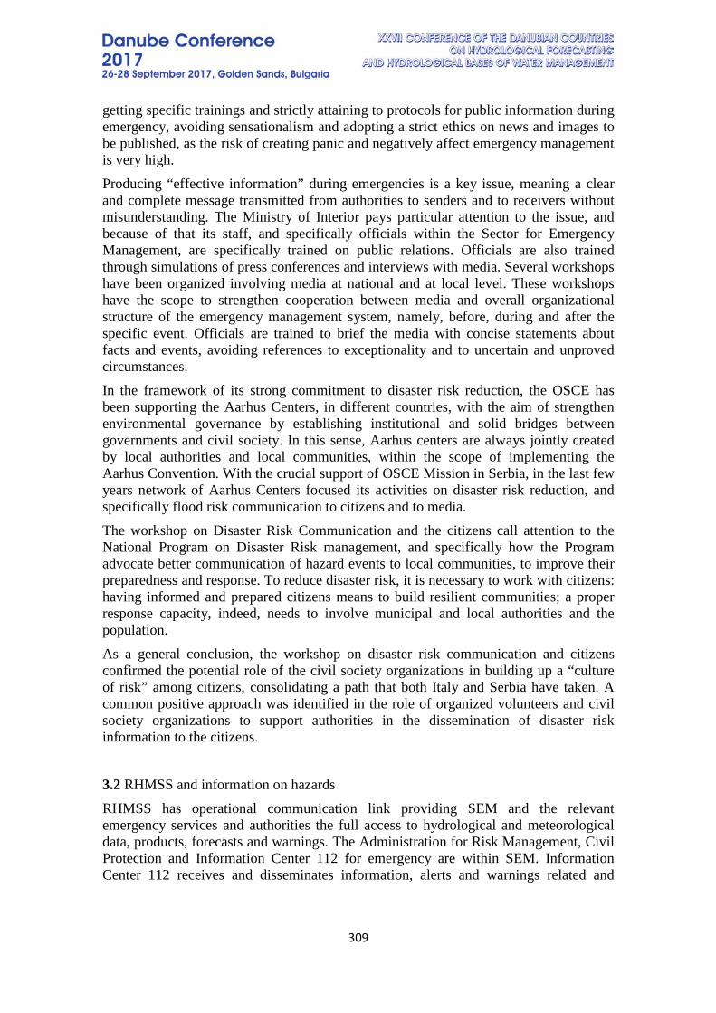
309

getting specific trainings and strictly attaining to protocols for public information during emergency, avoiding sensationalism and adopting a strict ethics on news and images to be published, as the risk of creating panic and negatively affect emergency management is very high. Producing “effective information” during emergencies is a key issue, meaning a clear and complete message transmitted from authorities to senders and to receivers without misunderstanding. The Ministry of Interior pays particular attention to the issue, and because of that its staff, and specifically officials within the Sector for Emergency Management, are specifically trained on public relations. Officials are also trained through simulations of press conferences and interviews with media. Several workshops have been organized involving media at national and at local level. These workshops have the scope to strengthen cooperation between media and overall organizational structure of the emergency management system, namely, before, during and after the specific event. Officials are trained to brief the media with concise statements about facts and events, avoiding references to exceptionality and to uncertain and unproved circumstances. In the framework of its strong commitment to disaster risk reduction, the OSCE has been supporting the Aarhus Centers, in different countries, with the aim of strengthen environmental governance by establishing institutional and solid bridges between governments and civil society. In this sense, Aarhus centers are always jointly created by local authorities and local communities, within the scope of implementing the Aarhus Convention. With the crucial support of OSCE Mission in Serbia, in the last few years network of Aarhus Centers focused its activities on disaster risk reduction, and specifically flood risk communication to citizens and to media. The workshop on Disaster Risk Communication and the citizens call attention to the National Program on Disaster Risk management, and specifically how the Program advocate better communication of hazard events to local communities, to improve their preparedness and response. To reduce disaster risk, it is necessary to work with citizens: having informed and prepared citizens means to build resilient communities; a proper response capacity, indeed, needs to involve municipal and local authorities and the population. As a general conclusion, the workshop on disaster risk communication and citizens confirmed the potential role of the civil society organizations in building up a “culture of risk” among citizens, consolidating a path that both Italy and Serbia have taken. A common positive approach was identified in the role of organized volunteers and civil society organizations to support authorities in the dissemination of disaster risk information to the citizens. 3.2 RHMSS and information on hazards RHMSS has operational communication link providing SEM and the relevant emergency services and authorities the full access to hydrological and meteorological data, products, forecasts and warnings. The Administration for Risk Management, Civil Protection and Information Center 112 for emergency are within SEM. Information Center 112 receives and disseminates information, alerts and warnings related and

310

relevant to the safety of the population to the local emergency and civil protection centers, local authorities and communities. RHMSS regularly provides data and warning products for water management and operational flood protection to the Water Directorate (WD), according to the Water law and Decrees on the General plan for flood protection and the Operational plan for flood protection. RHMSS uses two dedicated web-sites, namely www.meteoalarm.rs and www.hidmet.gov.rs to disseminate data, information, forecasts, warnings and alerts to institutional users and to the public. These web sites are comprehensive and up-to-date sources of RHMSS operational products. One way we track user interests, opinion and satisfaction is by questionnaires on our web site. The limitations of this method could be that the relatively limited number of users are willing to participate in surveys. We have observed fall in the number of respondents from 2800 in 2012 to 780 in 2014, and at the same time steady increase in number of users.

Fig. 1: User’s opinion regarding content quality

Our customers, 86% of our websites users, highly assess the quality, timeliness, reliability and accuracy of the given information, especially as forecast and actual data are concerned (Fig. 1). Typical user, 89% of them, visits our web page at least once a week. When asked, will they recommend our web site to other people, 81% responded: very likely or most likely. We have learned that in everyday use most popular categories are weather forecast and data on actual weather, but during the extreme events user interest tends to concentrate on more specific subjects, as for instance hydrological data and forecasts in case of flood events, or meteorological forecast and data in case of thunderstorms, heavy rain and hailstorms. Another way we track user interests is by Google Analytics tool. By means of this tool we are able to collect valuable data on user interests and behavior, and better tailor our services to their needs. The number of regular users, 3.584.907 in year 2014 of the web site www.hidmet.gov.rs is disproportional to those of www.meteoalarm.rs, 91.669 in the same year. Users have generated 226.423 page views daily in average in year 2014 with the daily maximum of 774.273 page views on 17 May 2014, compare to 3.642 page views daily in average in

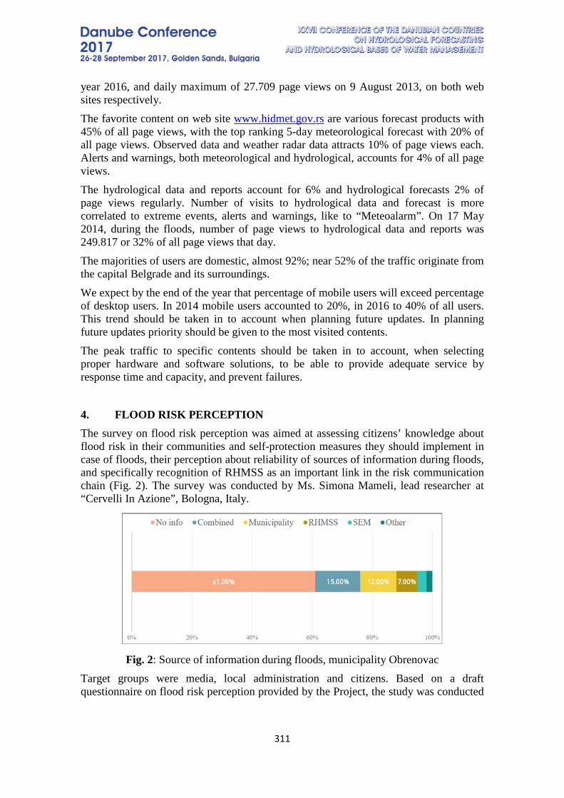
311

year 2016, and daily maximum of 27.709 page views on 9 August 2013, on both web sites respectively. The favorite content on web site www.hidmet.gov.rs are various forecast products with 45% of all page views, with the top ranking 5-day meteorological forecast with 20% of all page views. Observed data and weather radar data attracts 10% of page views each. Alerts and warnings, both meteorological and hydrological, accounts for 4% of all page views. The hydrological data and reports account for 6% and hydrological forecasts 2% of page views regularly. Number of visits to hydrological data and forecast is more correlated to extreme events, alerts and warnings, like to “Meteoalarm”. On 17 May 2014, during the floods, number of page views to hydrological data and reports was 249.817 or 32% of all page views that day. The majorities of users are domestic, almost 92%; near 52% of the traffic originate from the capital Belgrade and its surroundings. We expect by the end of the year that percentage of mobile users will exceed percentage of desktop users. In 2014 mobile users accounted to 20%, in 2016 to 40% of all users. This trend should be taken in to account when planning future updates. In planning future updates priority should be given to the most visited contents. The peak traffic to specific contents should be taken in to account, when selecting proper hardware and software solutions, to be able to provide adequate service by response time and capacity, and prevent failures.

4. FLOOD RISK PERCEPTION The survey on flood risk perception was aimed at assessing citizens’ knowledge about flood risk in their communities and self-protection measures they should implement in case of floods, their perception about reliability of sources of information during floods, and specifically recognition of RHMSS as an important link in the risk communication chain (Fig. 2). The survey was conducted by Ms. Simona Mameli, lead researcher at “Cervelli In Azione”, Bologna, Italy.

Fig. 2: Source of information during floods, municipality Obrenovac

Target groups were media, local administration and citizens. Based on a draft questionnaire on flood risk perception provided by the Project, the study was conducted

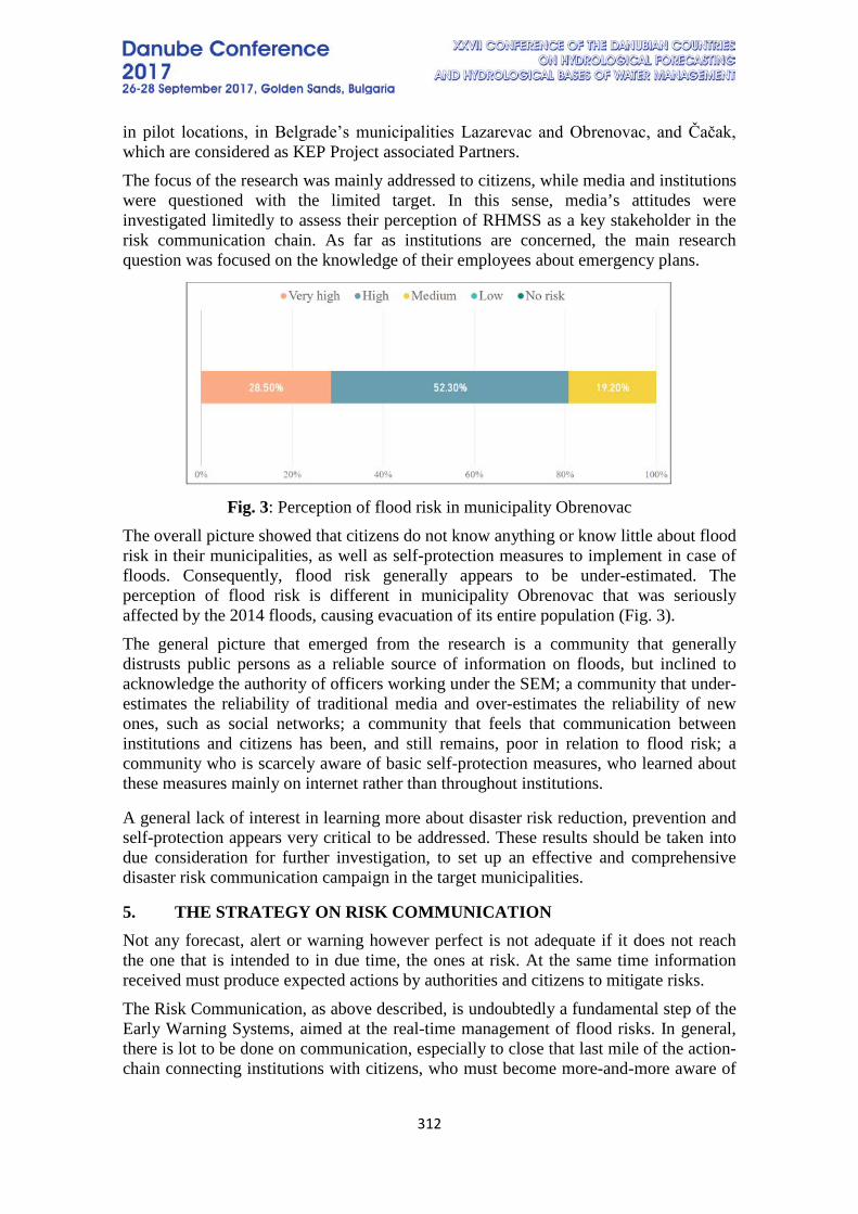
312

in pilot locations, in Belgrade’s municipalities Lazarevac and Obrenovac, and Čačak, which are considered as KEP Project associated Partners. The focus of the research was mainly addressed to citizens, while media and institutions were questioned with the limited target. In this sense, media’s attitudes were investigated limitedly to assess their perception of RHMSS as a key stakeholder in the risk communication chain. As far as institutions are concerned, the main research question was focused on the knowledge of their employees about emergency plans.

Fig. 3: Perception of flood risk in municipality Obrenovac

The overall picture showed that citizens do not know anything or know little about flood risk in their municipalities, as well as self-protection measures to implement in case of floods. Consequently, flood risk generally appears to be under-estimated. The perception of flood risk is different in municipality Obrenovac that was seriously affected by the 2014 floods, causing evacuation of its entire population (Fig. 3). The general picture that emerged from the research is a community that generally distrusts public persons as a reliable source of information on floods, but inclined to acknowledge the authority of officers working under the SEM; a community that under-estimates the reliability of traditional media and over-estimates the reliability of new ones, such as social networks; a community that feels that communication between institutions and citizens has been, and still remains, poor in relation to flood risk; a community who is scarcely aware of basic self-protection measures, who learned about these measures mainly on internet rather than throughout institutions.

A general lack of interest in learning more about disaster risk reduction, prevention and self-protection appears very critical to be addressed. These results should be taken into due consideration for further investigation, to set up an effective and comprehensive disaster risk communication campaign in the target municipalities.

5. THE STRATEGY ON RISK COMMUNICATION Not any forecast, alert or warning however perfect is not adequate if it does not reach the one that is intended to in due time, the ones at risk. At the same time information received must produce expected actions by authorities and citizens to mitigate risks. The Risk Communication, as above described, is undoubtedly a fundamental step of the Early Warning Systems, aimed at the real-time management of flood risks. In general, there is lot to be done on communication, especially to close that last mile of the action-chain connecting institutions with citizens, who must become more-and-more aware of

313

the risk conditions of the territory where they live and know much better than now what are the safety plans of the Civil protection. Today, most of the time, people believed extreme events are unlikely to happen and the perception of this risk is rather weak. If, as it is very likely, climate change will make these severe weather events more frequent, situations of severe weather causing, for example, floods and/or landslides, may grow in frequency of occurrence. More severe event occurrence may increase “social anxiety”. And the anxiety, as we know, does not help to make rational actions. Underestimating the risk can have tragic consequences. Overestimating the risk can produce too many false alarms, making lower and lower the confidence of the Early Warning System. How to find the right balance between the unjustified optimism and a state of perpetual anxiety? The answer is in the preparation of a system that can make citizens ready and at the same time confident in their ability to react to events, by increasing the feeling of control on them and reducing the cognitive uncertainty. If short-term extreme events of high intensity will be more frequent, thus we will need better and more efficient forecasting systems. But, will it be reliable; it will always be a margin of uncertainty that cannot be eliminated: the forecast will, inherently, be probabilistic both regarding the location, space and time of the events, and by their intensity. The risk of a failure or a false alarm will always be present, and therefore the credibility of the alert system will be at stake, but it will be possible to overcome this problem by producing and sharing procedures for alert management in a transparent way, taking in consideration the uncertainty management. It has become imperative and mandatory to create codes of language and behavior to finally standardize the different local realities and, furthermore, prepare and activate the civil protection plans in emergency, at national and decentralized scale. The early warning procedure, once established, must be strictly followed: in practice, when a certain threshold of occurrence of a certain extreme weather and hydrological event will be reached and eventually exceeded, then the law enforcement actions should be activated without delay. Society must adapt to absorb the consequences of missing or false alarms, inherent uncertainty of predictions; to achieve this goal, it is necessary to improve the sense of responsibility of the media and the capability of citizens to self-protect themselves from the impacts of severe weather. The institutions can shape and apply new skills in the field of risk communication to offer media products less susceptible to manipulation. These professionals will handle communication tools like the Internet, and especially social networks that bring people to the institutions. During the emergency situations, the information must be neither excess nor poor, but must meet the real needs of the recipient, at all levels of the system. Even in a context of uncertainty, as always in a risk situation, the margin of subjectivity and randomness should be reduced as much as possible with clear and well-defined communication procedures, which is entirely complementary for the whole operational risk management, as confirmed repeatedly by the recent experience of extreme events occurred in Italy and Republic of Serbia.

314

CONCLUSIONS Country Action Program - Recovery of flood damages is opportunity for setting up modern, robust and efficient Hydrological and Meteorological Early Warning system with all its components: monitoring, communication and forecasting improved, enhancing the National capacity to monitor, evaluate and forecast dangerous meteorological and hydrological phenomena. Experience gained during the “Alert" Know - How Exchange Project enabled our experts to properly define and prepare actions needed to strengthen and enhance our technical capacities. National meteorological and hydrological services should pay particular attention on how information and warnings are communicated, received and interpreted by the local communities; together with them and other stakeholders in disaster management we should learn how to further improve our services to efficiently mitigate risks. To reduce disaster risk, it is necessary to work with citizens: having informed and prepared citizens means to build resilient communities. An effective end-to-end early warning system will not be possible without the active participation of various national agencies, municipal authorities and local population. That is why improving the system in all these levels is a must. There is still much to be done to determine how to better manage extreme events to produce the least possible damage. The debate has just begun. Surely climate change will force the growth of awareness, especially by administrators who in many cases have no practical knowledge on how to deal with underlying risks.

REFERENCES [1] The Capacity for Disaster Reduction Initiative (CADRI), Action Plan for the Implementation of the National Disaster Risk Management Programme of the Republic of Serbia (2016-2020), CADRI (Online), Switzerland, pp 2-53, 2016. [2] Ministerial Roundtable, Reconstructing after disasters: Build back better, UN World ISSUE BRIEF - Conference on Disaster Risk Reduction Sendai (Online), Japan, pp 1, 2015. [3] Public Investment Management Office, Serbian National Disaster Risk Management Program Concept Note, Public Investment Management Office Documents (Online), Serbia, pp 8-10, 2014. [4] WMO, World Meteorological Organization Executive Council 66th session, WMO - No. 1136: Executive Council Reports, Switzerland, pp 91, 2014.

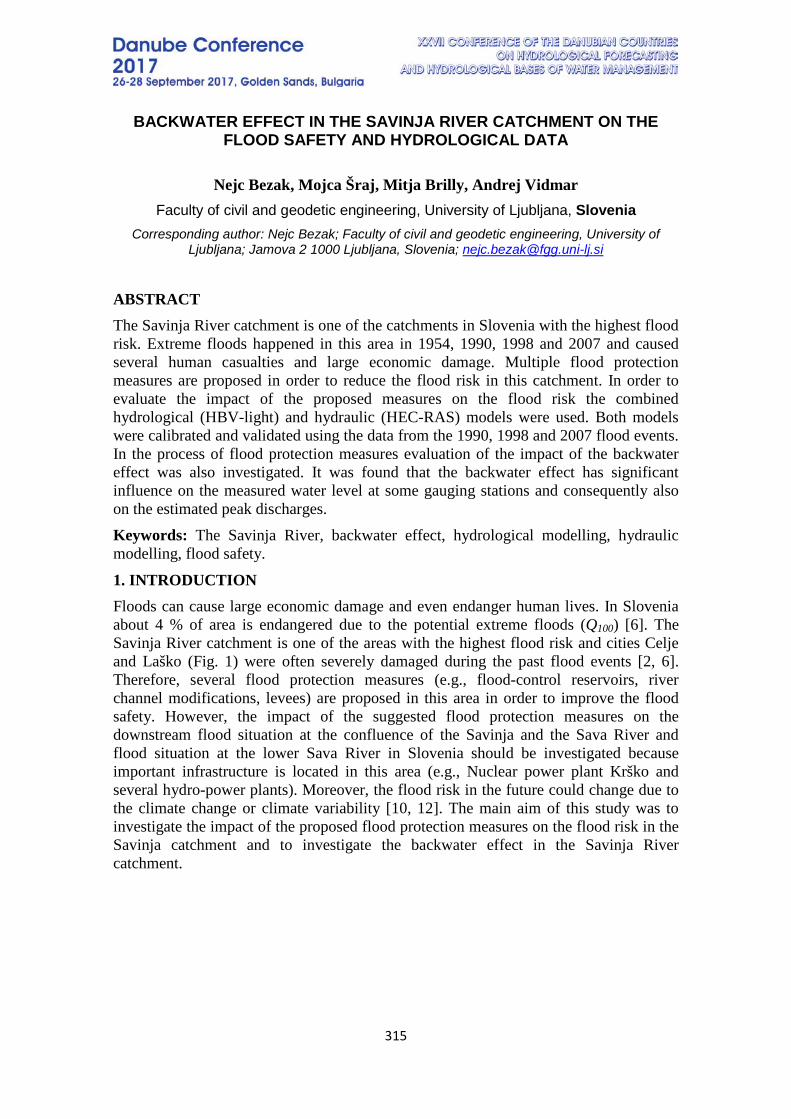
315

BACKWATER EFFECT IN THE SAVINJA RIVER CATCHMENT ON THE FLOOD SAFETY AND HYDROLOGICAL DATA

Nejc Bezak, Mojca Šraj, Mitja Brilly, Andrej Vidmar

Faculty of civil and geodetic engineering, University of Ljubljana, Slovenia Corresponding author: Nejc Bezak; Faculty of civil and geodetic engineering, University of

Ljubljana; Jamova 2 1000 Ljubljana, Slovenia; nejc.bezak@fgg.uni-lj.si

ABSTRACT The Savinja River catchment is one of the catchments in Slovenia with the highest flood risk. Extreme floods happened in this area in 1954, 1990, 1998 and 2007 and caused several human casualties and large economic damage. Multiple flood protection measures are proposed in order to reduce the flood risk in this catchment. In order to evaluate the impact of the proposed measures on the flood risk the combined hydrological (HBV-light) and hydraulic (HEC-RAS) models were used. Both models were calibrated and validated using the data from the 1990, 1998 and 2007 flood events. In the process of flood protection measures evaluation of the impact of the backwater effect was also investigated. It was found that the backwater effect has significant influence on the measured water level at some gauging stations and consequently also on the estimated peak discharges. Keywords: The Savinja River, backwater effect, hydrological modelling, hydraulic modelling, flood safety.

1. INTRODUCTION Floods can cause large economic damage and even endanger human lives. In Slovenia about 4 % of area is endangered due to the potential extreme floods (Q100) [6]. The Savinja River catchment is one of the areas with the highest flood risk and cities Celje and Laško (Fig. 1) were often severely damaged during the past flood events [2, 6]. Therefore, several flood protection measures (e.g., flood-control reservoirs, river channel modifications, levees) are proposed in this area in order to improve the flood safety. However, the impact of the suggested flood protection measures on the downstream flood situation at the confluence of the Savinja and the Sava River and flood situation at the lower Sava River in Slovenia should be investigated because important infrastructure is located in this area (e.g., Nuclear power plant Krško and several hydro-power plants). Moreover, the flood risk in the future could change due to the climate change or climate variability [10, 12]. The main aim of this study was to investigate the impact of the proposed flood protection measures on the flood risk in the Savinja catchment and to investigate the backwater effect in the Savinja River catchment.

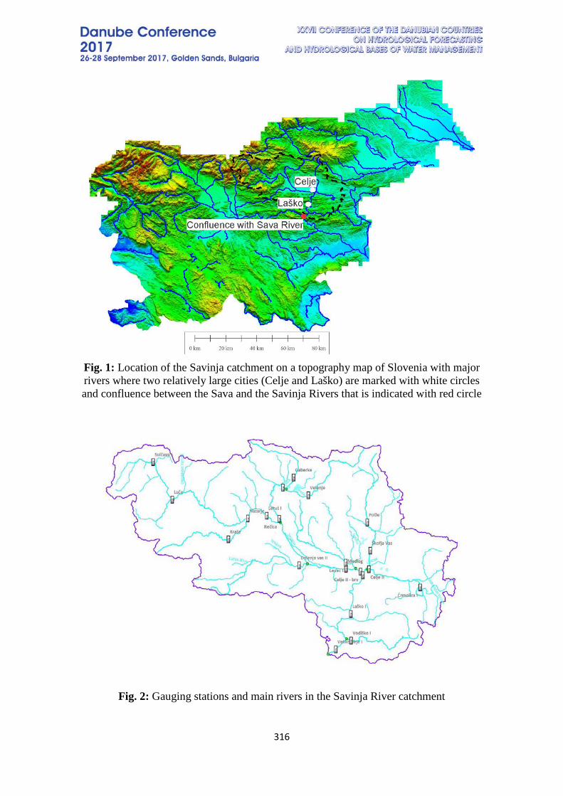
316

Fig. 1: Location of the Savinja catchment on a topography map of Slovenia with major rivers where two relatively large cities (Celje and Laško) are marked with white circles and confluence between the Sava and the Savinja Rivers that is indicated with red circle

Fig. 2: Gauging stations and main rivers in the Savinja River catchment

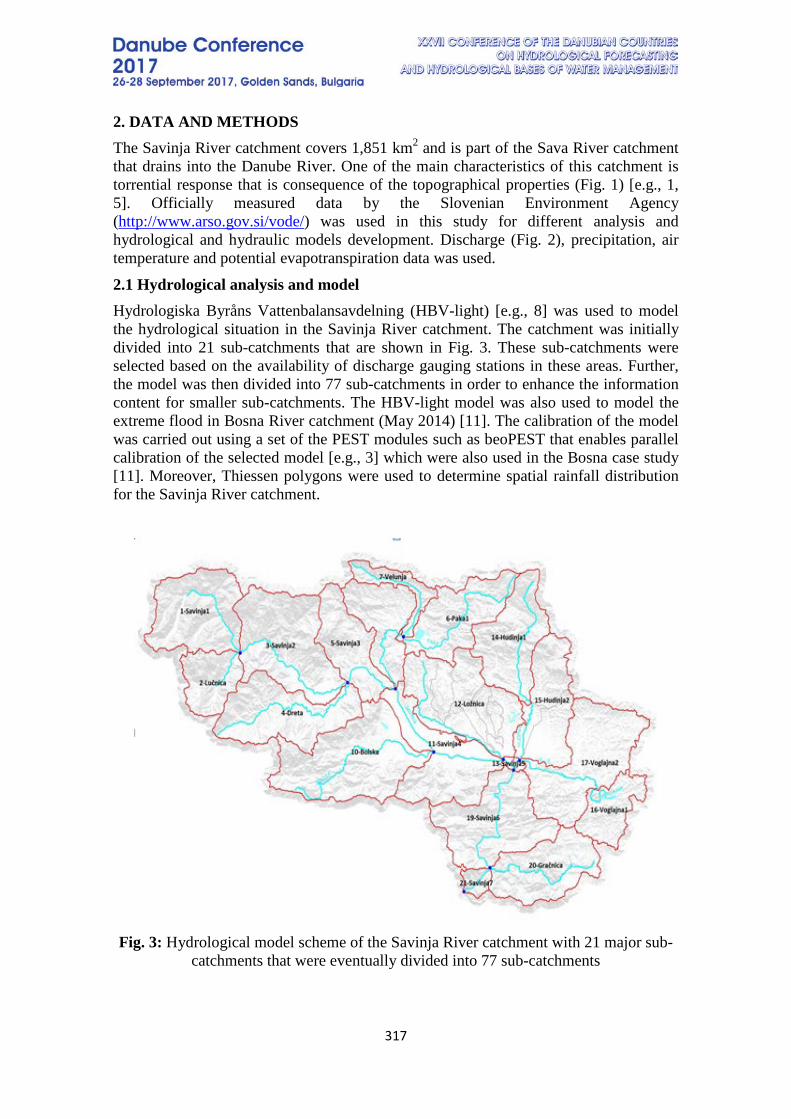
317

2. DATA AND METHODS The Savinja River catchment covers 1,851 km2 and is part of the Sava River catchment that drains into the Danube River. One of the main characteristics of this catchment is torrential response that is consequence of the topographical properties (Fig. 1) [e.g., 1, 5]. Officially measured data by the Slovenian Environment Agency (http://www.arso.gov.si/vode/) was used in this study for different analysis and hydrological and hydraulic models development. Discharge (Fig. 2), precipitation, air temperature and potential evapotranspiration data was used.

2.1 Hydrological analysis and model Hydrologiska Byråns Vattenbalansavdelning (HBV-light) [e.g., 8] was used to model the hydrological situation in the Savinja River catchment. The catchment was initially divided into 21 sub-catchments that are shown in Fig. 3. These sub-catchments were selected based on the availability of discharge gauging stations in these areas. Further, the model was then divided into 77 sub-catchments in order to enhance the information content for smaller sub-catchments. The HBV-light model was also used to model the extreme flood in Bosna River catchment (May 2014) [11]. The calibration of the model was carried out using a set of the PEST modules such as beoPEST that enables parallel calibration of the selected model [e.g., 3] which were also used in the Bosna case study [11]. Moreover, Thiessen polygons were used to determine spatial rainfall distribution for the Savinja River catchment.

Fig. 3: Hydrological model scheme of the Savinja River catchment with 21 major sub-

catchments that were eventually divided into 77 sub-catchments

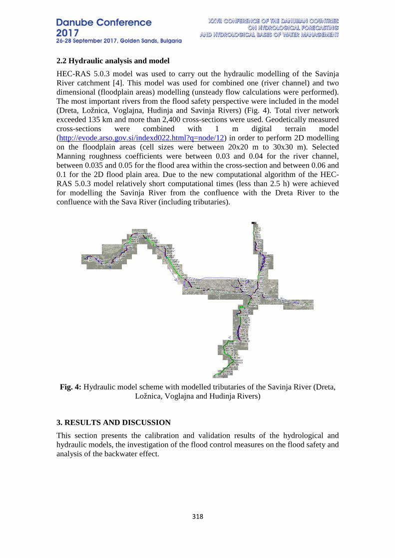
318

2.2 Hydraulic analysis and model HEC-RAS 5.0.3 model was used to carry out the hydraulic modelling of the Savinja River catchment [4]. This model was used for combined one (river channel) and two dimensional (floodplain areas) modelling (unsteady flow calculations were performed). The most important rivers from the flood safety perspective were included in the model (Dreta, Ložnica, Voglajna, Hudinja and Savinja Rivers) (Fig. 4). Total river network exceeded 135 km and more than 2,400 cross-sections were used. Geodetically measured cross-sections were combined with 1 m digital terrain model (http://evode.arso.gov.si/indexd022.html?q=node/12) in order to perform 2D modelling on the floodplain areas (cell sizes were between 20x20 m to 30x30 m). Selected Manning roughness coefficients were between 0.03 and 0.04 for the river channel, between 0.035 and 0.05 for the flood area within the cross-section and between 0.06 and 0.1 for the 2D flood plain area. Due to the new computational algorithm of the HEC-RAS 5.0.3 model relatively short computational times (less than 2.5 h) were achieved for modelling the Savinja River from the confluence with the Dreta River to the confluence with the Sava River (including tributaries).

Fig. 4: Hydraulic model scheme with modelled tributaries of the Savinja River (Dreta,

Ložnica, Voglajna and Hudinja Rivers)

3. RESULTS AND DISCUSSION This section presents the calibration and validation results of the hydrological and hydraulic models, the investigation of the flood control measures on the flood safety and analysis of the backwater effect.

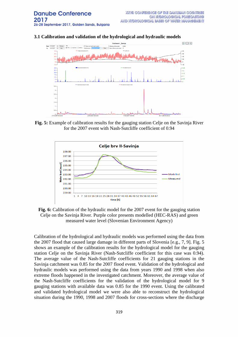
319

3.1 Calibration and validation of the hydrological and hydraulic models

Fig. 5: Example of calibration results for the gauging station Celje on the Savinja River

for the 2007 event with Nash-Sutcliffe coefficient of 0.94

Fig. 6: Calibration of the hydraulic model for the 2007 event for the gauging station Celje on the Savinja River. Purple color presents modelled (HEC-RAS) and green

measured water level (Slovenian Environment Agency) Calibration of the hydrological and hydraulic models was performed using the data from the 2007 flood that caused large damage in different parts of Slovenia [e.g., 7, 9]. Fig. 5 shows an example of the calibration results for the hydrological model for the gauging station Celje on the Savinja River (Nash-Sutcliffe coefficient for this case was 0.94). The average value of the Nash-Sutcliffe coefficients for 21 gauging stations in the Savinja catchment was 0.85 for the 2007 flood event. Validation of the hydrological and hydraulic models was performed using the data from years 1990 and 1998 when also extreme floods happened in the investigated catchment. Moreover, the average value of the Nash-Sutcliffe coefficients for the validation of the hydrological model for 9 gauging stations with available data was 0.85 for the 1990 event. Using the calibrated and validated hydrological model we were also able to reconstruct the hydrological situation during the 1990, 1998 and 2007 floods for cross-sections where the discharge

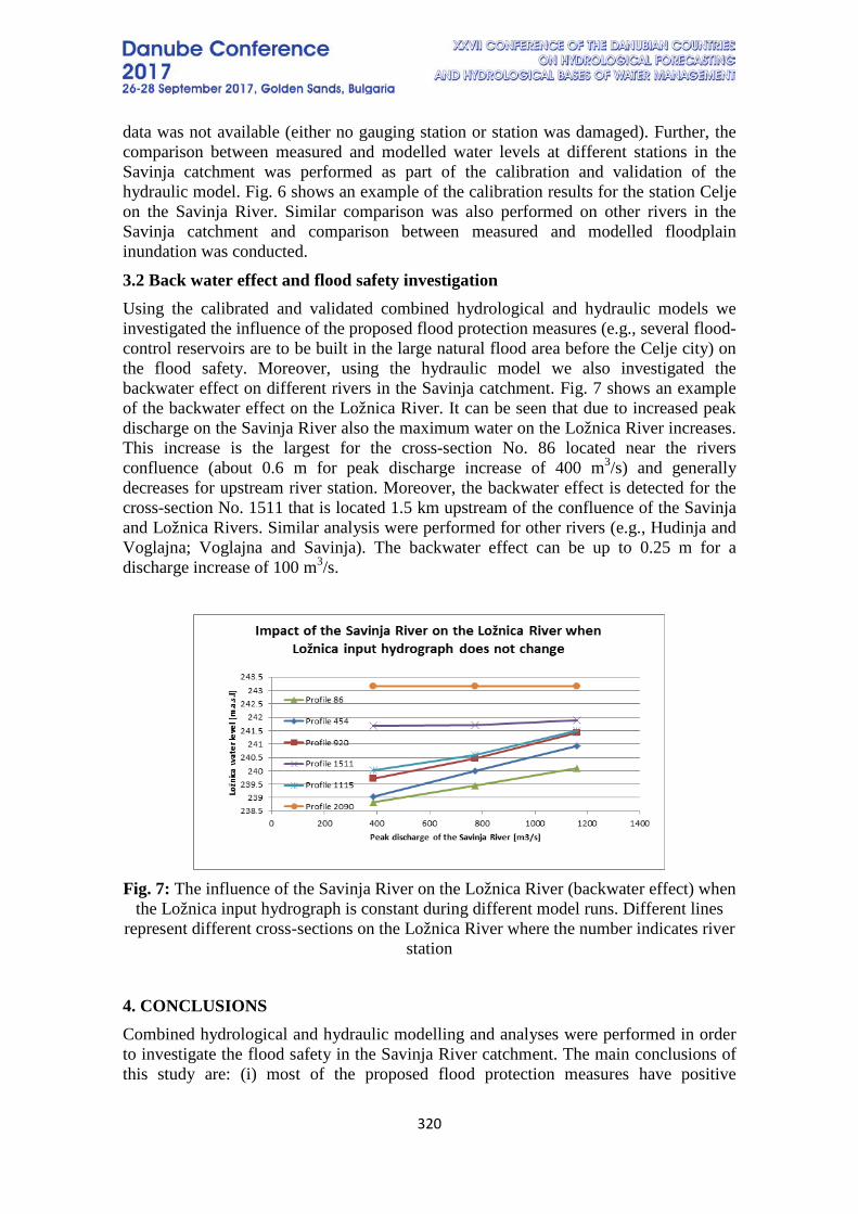
320

data was not available (either no gauging station or station was damaged). Further, the comparison between measured and modelled water levels at different stations in the Savinja catchment was performed as part of the calibration and validation of the hydraulic model. Fig. 6 shows an example of the calibration results for the station Celje on the Savinja River. Similar comparison was also performed on other rivers in the Savinja catchment and comparison between measured and modelled floodplain inundation was conducted.

3.2 Back water effect and flood safety investigation Using the calibrated and validated combined hydrological and hydraulic models we investigated the influence of the proposed flood protection measures (e.g., several flood-control reservoirs are to be built in the large natural flood area before the Celje city) on the flood safety. Moreover, using the hydraulic model we also investigated the backwater effect on different rivers in the Savinja catchment. Fig. 7 shows an example of the backwater effect on the Ložnica River. It can be seen that due to increased peak discharge on the Savinja River also the maximum water on the Ložnica River increases. This increase is the largest for the cross-section No. 86 located near the rivers confluence (about 0.6 m for peak discharge increase of 400 m3/s) and generally decreases for upstream river station. Moreover, the backwater effect is detected for the cross-section No. 1511 that is located 1.5 km upstream of the confluence of the Savinja and Ložnica Rivers. Similar analysis were performed for other rivers (e.g., Hudinja and Voglajna; Voglajna and Savinja). The backwater effect can be up to 0.25 m for a discharge increase of 100 m3/s.

Fig. 7: The influence of the Savinja River on the Ložnica River (backwater effect) when

the Ložnica input hydrograph is constant during different model runs. Different lines represent different cross-sections on the Ložnica River where the number indicates river

station

4. CONCLUSIONS Combined hydrological and hydraulic modelling and analyses were performed in order to investigate the flood safety in the Savinja River catchment. The main conclusions of this study are: (i) most of the proposed flood protection measures have positive

321

influence on the flood situation in the Savinja catchment and also at the confluence with the Sava River. However, additional analysis should be carried out regarding some important measures (e.g., flood-control reservoirs) and (ii) the backwater effect in the Savinja River catchment can be up to 0.25 m for a peak discharge increase of 100 m3/s.

5. REFERENCES [1] Bezak, N., Horvat, A. & Brilly, M. Analysis of flood events in Slovenian streams, Journal of Hydrology and Hydromechanics, pp 134-144, 2015. [2] Brilly, M. & Polic, M. Public perception of flood risks, flood forecasting and mitigation, Natural Hazards and Earth System Sciences, pp 345-355, 2005. [3] Doherty, J. Addendum to the PEST Manual, Brisbane, Australia, Water Numerical Computing, 2012. [4] HEC-RAS 5.0.: Reference Manual. Available at: http://www.hec.usace.army.mil/software/hec-ras/documentation/HEC-RAS%205.0%20Reference%20Manual.pdf, 2016. [5] Kobold, M. & Brilly, M. The use of HBV model for flash flood forecasting, Natural Hazards and Earth System Sciences, pp 407-417, 2006. [6] Mikoš, M., Brilly, M. & Ribičič, M. Floods and Landslides in Slovenia, Acta hydrotechnica, pp 113-133, 2004. [7] Rusjan, S., Kobold, M. & Mikoš, M. Characteristics of the extreme rainfall event and consequent flash floods in W Slovenia in September 2007, Natural Hazards and Earth System Sciences, pp 947-956, 2009. [8] Seibert, J. & Vis, M.J.P. Teaching hydrological modeling with user-friendly catchment-runoff-model software package, Hydrology and Earth System Sciences, pp 3315-3325, 2012. [9] Šraj, M., Bezak, N., Rusjan, S. & Mikoš, M. Review of hydrological studies contributing to the advancement of hydrological sciences in Slovenia, Acta hydrotechnica, pp 47-71, 2016. [10] Šraj, M., Menih, M. & Bezak, N. Climate variability impact assessment on the flood risk in Slovenia, Physical Geography, pp 73-87, 2016. [11] Vidmar, A., Globevnik, L., Koprivšek, M., Sečnik, M., Zabret, K., Đurović, B., Anzeljc, D., Kastelic, J., Kobold, M., Sušnik, M., Borojevič, D., Kupusović, T., Kupusović, E., Vihar, A. & Brilly, M. The Bosna River floods in May 2014, Natural Hazards and Earth System Sciences, pp 2235-2246, 2016. [12] Watts, G., Battarbee, R. W., Bloomfield, J. P., Crossman, J., Daccache, A., Durance, I., … & Wilby, R. L. Climate change and water in the UK – Past changes and future prospects, Progress in Physical Geography, pp 6-28, 2015.

322

HYDROLOGICAL STRUCTURE OF THE CATCHMENT DURING THE FLOODS

Mitja Brilly, Mojca Šraj, Nejc Bezak, Andrej Vidmar

Faculty of civil and geodetic engineering, University of Ljubljana, Slovenia Corresponding author: Nejc Bezak; Faculty of civil and geodetic engineering, University

of Ljubljana; Jamova 2 1000 Ljubljana, Slovenia; mbvrilly@fgg.uni-lj.si

The Savinja River is one of the tributaries of the Sava River in Slovenia. Savinja River catchment covers 1,851 km2 and it is located in the eastern part of Slovenia. This catchment is one of the areas with the highest flood risk in Slovenia. Extreme floods happened in 1990, 1998 and 2007 in the Savinja River catchment. There are significant relations in coincidence in timing of flood peaks in tributaries and main stream in any catchment. The specific coincidence is also on inflow of the Savinja River to the Sava River. The coincidence of flood peaks depends on the space structure of the catchment and characteristics of rainfall events that are specific for extraordinary flood events. Knowing that we could properly design flood protection measures with optimal results. The same measures on different subcatchments could increase or decrease flood peaks in the main stream. Keywords: Savinja River, Sava River, hydrological modelling, flood safety.

323

CALIBRATION OF HYDROLOGICAL MODEL WITH PROGRAMME PEST

Andrej Vidmar, Andrej Kryžanowski, Nejc Bezak, Mojca Šraj, Mitja Brilly Faculty of civil and geodetic engineering, University of Ljubljana; Slovenia

Corresponding author: Andrej Vidmar; Faculty of civil and geodetic engineering, University of Ljubljana; Jamova 2 1000 Ljubljana, Slovenia; avidmar@fgg.uni-lj.si

ABSTRACT PEST is tool based on minimization of an objective function related to the root mean square error between the model output and the measurement.We use “singular value decomposition”, section of the PEST control file, and Tikhonov regularization method for successfully estimation of model parameters. The PEST sometimes failed if inverse problems were ill-posed, but (SVD) ensures that PEST maintains numerical stability. The choice of the initial guess for the initial parameter values is an important issue in the PEST and need expert knowledge (Doherty, 2005).

The flexible nature of the PEST software and its ability to be applied to whole catchments at once give results of calibration performed extremely well across high number of sub catchments. Use of parallel computing version of PEST called BeoPEST was successfully useful to speed up calibration process. BeoPEST employs smart slaves and point-to-point communications to transfer data between the master and slaves computers.

The HBV-light model is a simple multi-tank-type model for simulating precipitation-runoff. It is conceptual balance model of catchment hydrology which simulates discharge using rainfall, temperature and estimates of potential evaporation. Version of HBV-light-CLI allows the user to run HBV-light from the command line. Input and results files are in XML form. This allows to easily connecting it with other applications such as pre and post-processing utilities and PEST itself.

The procedure was applied on hydrological model of Savinja catchment (1852 km2) and consists of seventy seven sub-catchments. Data are temporary processed on hourly basic with Nash-Sutcliffe coefficient more than 0,9 in results of calibration and validation.

Keywords: hydrological modelling, Savinja River, calibration, validation, catchment characteristics.

1. INTRODUCTION Hydrological phenomena take place in the hydrological system, which is governed by nature, and are essentially stochastic. These phenomena are unique, non-recurring, and changeable across space and time. They are simulated through various hydrological models that seek to integrate complex processes, as demonstrated by continuous functions. This procedure is hindered by the lack of data and simplifications used to solve the mathematical model. These limitations are responsible for the errors or

324

deviations in calculation results given by the model and measurements in the field. When calibrating the model we are trying to determine the coefficients appearing in individual functions, so that the differences between the calculations and measurements are kept at a minimum. Since any river basin with its own natural characteristics, and any hydrological event therein, is unique, this is a complex process that is not researched enough. Calibration is a procedure of determining the parameters of a model that are not known well enough. Input and output variables and mathematical model expressions are known, while only individual model parameters are unknown, which are determined based on the known characteristics of the system analysed or by calibrating the model. In more simple models, the parameters can be determined directly by calculating the inversely transformed mathematical model. The problem is most often solved using simulations, so that the values of unknown parameters are changed to the point that the error between the measured and calculated output is reduced to an acceptable value. In doing this, we want to achieve that the deviation between the calculation and measurements behaves as a random variable with a minimum dispersion. Here, by changing the sample, the parameters can change as well, so the model must be verified on a dataset that was not considered during calibration. Also, it is recommended to analyse the model sensitivity to the changing values of individual parameters. Most software for using hydrological models is equipped with algorithms for automatic determination of the optimum set of parameters. These algorithms do not take into account the natural characteristics of the hydrological system, so the forecasting results of such a model can be worse than if a different set of parameters, along with expert knowledge, is used. The goal of the research it to improve the calibration of hydrological models using an expertly managed and monitored process. In this way we will improve the calibration of models and, finally, the understanding of the hydrological system simulated; furthermore, the set of model coefficients will be defined on an expert, conceptual basis. With a smaller number of parameters (i.e. up to three) this procedure is simple, while with a larger number of parameters it is more complex. For example, given 14 parameters, with three values each, there are 4,782,969 possible simulation combinations. Using the appropriate expert knowledge and information, the parameters are pondered, and the pattern of optimum model parameters is formed. Thus, we directly, and proportionally to the expert knowledge, affect the outcome of the inversion procedure and achieve better results than if the procedure had been left to the selected optimisation algorithm.

2. METHODS USED We used HBV-light model and coupling it with PEST (Model-Independent Parameter Estimation & Uncertainty Analysis). The HBV model is a conceptual model for continuous calculation of runoff used to simulate hydrological forecasting. It was originally developed in the 1970's at SMHI, the Swedish Meteorological and Hydrological Institute. It was named after the Hydrological Bureau Water Balance section (the abbreviation of Hydrologiska Byrans

325

Vattenbalansavdelning) (IHMS, 1999, Bergström, 1995), figure 1.. It provides the runoff simulation using the time series precipitation data, air temperature data and potential evapotranspiration data. We can say that it is a partly distributed model because we can divide the basin in more sub basins and each sub basin can be further divided on different elevation and vegetation zones (Seibert and Beven, 2009). For the model calibration we need time series of measured discharge data in the point of the sub basin outflow (IHMS 1999). The number of parameters normally used in the model is in the order of 20–33. While in most cases 5 of them are set to standard values it is very important to calibrate approximately 15 of the parameters, Figure 2. And table 1 and 2.

Figure 1. Rainfall runoff modelling by HBV

HBV model now exists in several versions, which differ in complexity and usefulness (Aghakouchak and Habib, 2010). SMHI on the basic point model developed in a distributed, the latest version is HBV-96 (Lindström et al., 1997). Development program is running elsewhere, at the University of Uppsala in 1993 using the programming language Microsoft Visual Basic made HBV-light (Seibert and Vis, 2012). The for further we development we has used the latest version of the program HBV-light, which was developed at the University of Zurich-u. The main motivation for its formation was to provide a user-friendly model, designed primarily for the education of students at higher levels of study and application in research projects (Seibert and Vis, 2012).

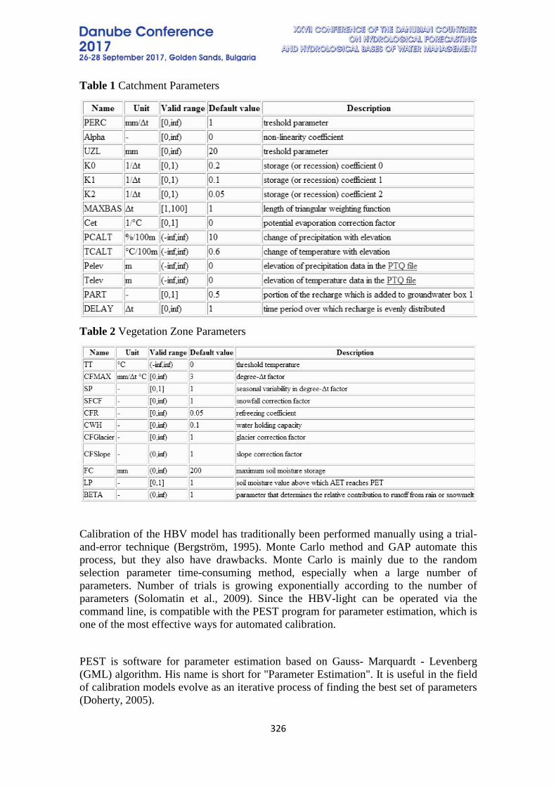
326

Table 1 Catchment Parameters

Table 2 Vegetation Zone Parameters

Calibration of the HBV model has traditionally been performed manually using a trial-and-error technique (Bergström, 1995). Monte Carlo method and GAP automate this process, but they also have drawbacks. Monte Carlo is mainly due to the random selection parameter time-consuming method, especially when a large number of parameters. Number of trials is growing exponentially according to the number of parameters (Solomatin et al., 2009). Since the HBV-light can be operated via the command line, is compatible with the PEST program for parameter estimation, which is one of the most effective ways for automated calibration. PEST is software for parameter estimation based on Gauss- Marquardt - Levenberg (GML) algorithm. His name is short for "Parameter Estimation". It is useful in the field of calibration models evolve as an iterative process of finding the best set of parameters (Doherty, 2005).

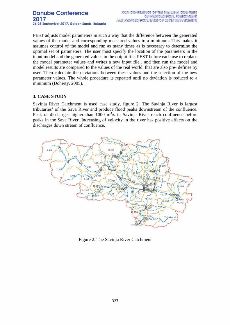
327

PEST adjusts model parameters in such a way that the difference between the generated values of the model and corresponding measured values to a minimum. This makes it assumes control of the model and run as many times as is necessary to determine the optimal set of parameters. The user must specify the location of the parameters in the input model and the generated values in the output file. PEST before each use to replace the model parameter values and writes a new input file , and then run the model and model results are compared to the values of the real world, that are also pre- defines by user. Then calculate the deviations between these values and the selection of the new parameter values. The whole procedure is repeated until no deviation is reduced to a minimum (Doherty, 2005).

3. CASE STUDY Savinja River Catchment is used case study, figure 2. The Savinja River is largest tributaries’ of the Sava River and produce flood peaks downstream of the confluence. Peak of discharges higher than 1000 m3/s in Savinja River reach confluence before peaks in the Sava River. Increasing of velocity in the river has positive effects on the discharges down stream of confluence.

Figure 2. The Savinja River Catchment

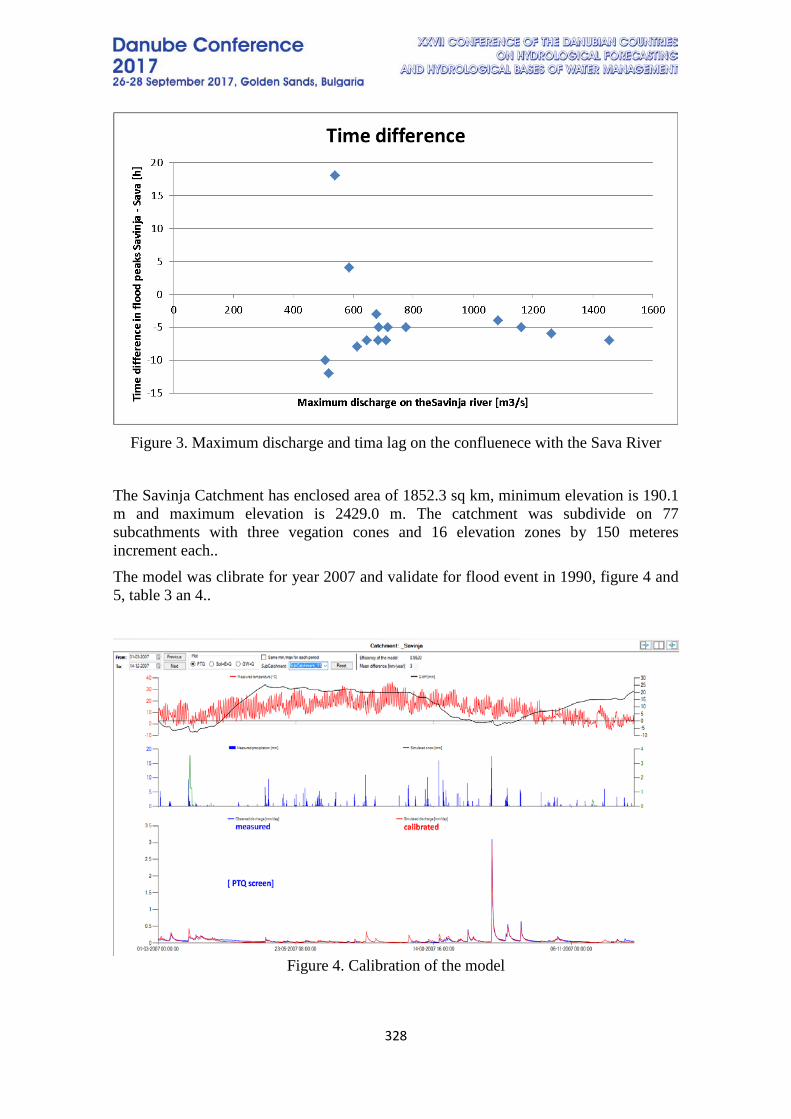
328

Figure 3. Maximum discharge and tima lag on the confluenece with the Sava River

The Savinja Catchment has enclosed area of 1852.3 sq km, minimum elevation is 190.1 m and maximum elevation is 2429.0 m. The catchment was subdivide on 77 subcathments with three vegation cones and 16 elevation zones by 150 meteres increment each.. The model was clibrate for year 2007 and validate for flood event in 1990, figure 4 and 5, table 3 an 4..

Figure 4. Calibration of the model

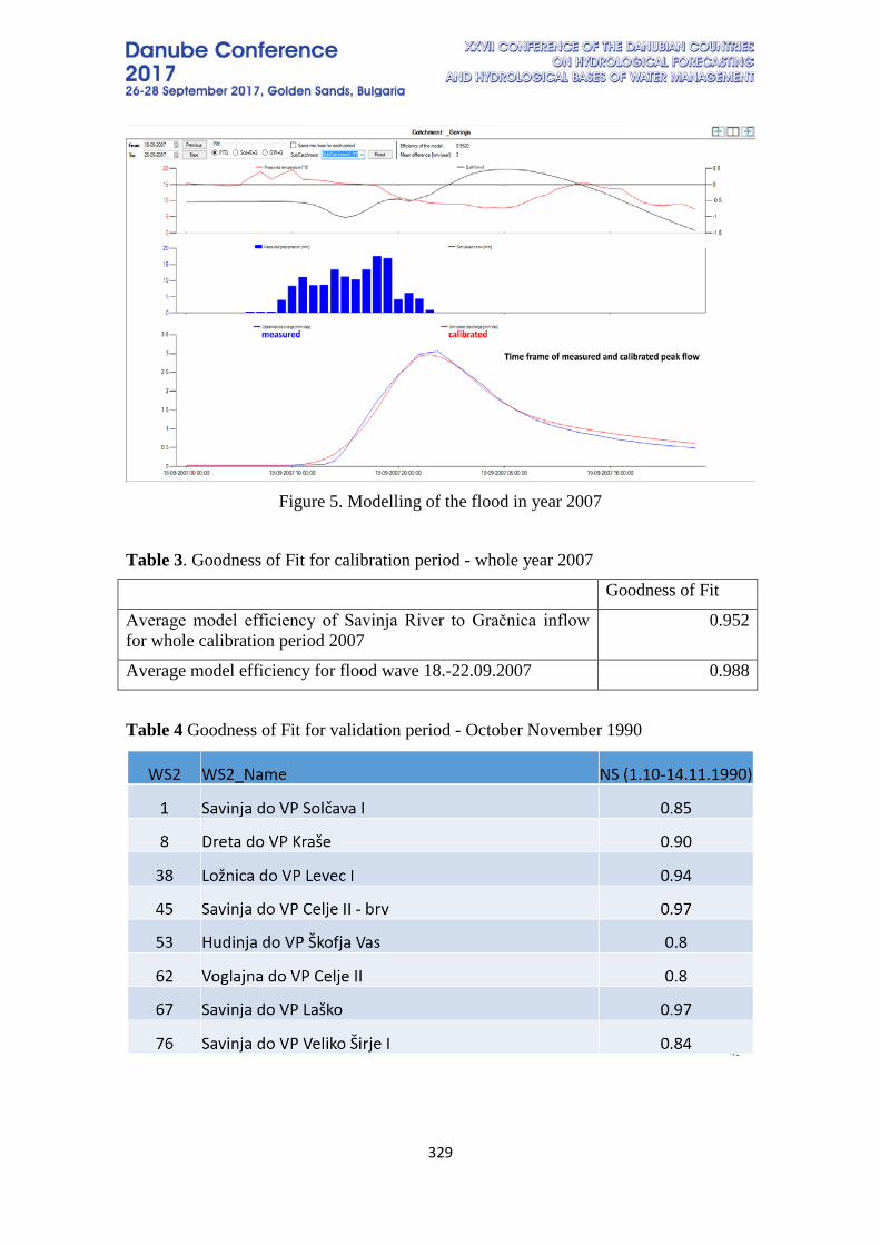
329

Figure 5. Modelling of the flood in year 2007

Table 3. Goodness of Fit for calibration period - whole year 2007

Goodness of Fit

Average model efficiency of Savinja River to Gračnica inflow for whole calibration period 2007

0.952

Average model efficiency for flood wave 18.-22.09.2007 0.988

Table 4 Goodness of Fit for validation period - October November 1990

330

4. CONCLUSIONS Process of calibration managed by expert directly, and proportionally to the expert knowledge, affects the outcome of the inversion procedure. We achieved very good results with unexpected high NS coefficients.

5. REFERENCES Aghakouchak, A., Habib, E. 2010. Application of a Conceptual Hydrologic Model in Teaching Hydrologic Processes. International Journal of Engineering Education 26, 4: 963–973 http://amir.eng.uci.edu/publications/10_EduHBV_IJEE.pdf Bergström, S. 1995. The HBV Model. In: Singh, V. P. Computer Models of Watershed Hydrology. Littleton, Colorado, Water Resources Publications: 443–476. Doherty, J. 2005. PEST, Model-Independent Parameter Estimation, User Manual: 5th Edition. Brisbane, Water Numerical Computing. IHMS. 1999. Integrated Hydrological Modelling System. Manual, Version 4.5. Norrköping, Sweden, Swedish Meteorological and Hydrological Institute: 121 p. Lindström, G., Johansson, B., Persson, M., Gardelin, M., Bergström, S. 1995. Development and test of the distributed HBV-96 hydrological model. Journal of Hydrology 201, 1–4: 272–288. Prohaska, S. 2009. Hydrology Report for The Sava River Basin Analysis – Draft Final Report. The Sava River Basin Commission.

Seibert, J., Vis, M. J. P. 2012. Teaching hydrological modeling with user-friendly catchment-runoff-model software package. Hydrology and Earth System Sciences 16, 11: 3315–3325.

Solomatine, D. P., Dibike, Y. B., Kukuric, N. 1999 Automatic calibration of groundwater models using global optimization techniques. Hydrological Sciences Journal – Journal des Sciences Hydrologiques, 44, 6: 879-894.

331

HYDROLOGICAL- HYDRAULIC MODEL FOR REAL TIME FORECASTING ON SAVA RIVER IN CROATIA

Jadran Berbic, Toni Jurlina, Dijana Oskorus, Tatjana Vujnovic

Croatian Hydrological and Meteorological Service, Croatia Corresponding author: Jadran Berbic, berbic@cirus.dhz.hr

ABSTRACT For the purpose of reducing flood risk and achieving of adequate preparing of flood defense in Sava river basin, Croatian Hydrological and Meteorological Service in the cooperation with Croatian waters initiated development of the real-time forecasting model of Sava river. The model includes the part of Sava from hydrological station Jesenice near border of Slovenia and Croatia to the border between Croatia and Serbia (hydrological station Gunja). In fact, model accounts the whole basin of Sava river which influences the Croatian part of the main river channel: Slovenian part characterized with upper boundary condition in model at hydrological station Jesenice, Croatian part described through significantly large Kupa tributary and other tributaries, BH (Bosnia and Herzegovina) rivers and other significant tributaries. The whole basin area included in a hydrological model is 67846 km2, which accounts for totally 159 subbasins and 3082 km of rivers and tributaries. The hydraulic part of the model includes 3060 cross sections, 13 retentions, 25 weirs and 15 control objects. Real time data from 40 Croatian, 18 BH and 11 Slovenian meteorological stations, as well from 92 Croatian, 15 BH, and 11 Slovenian hydrological station come with time sequence of one hour, as also as precipitation and temperature from Aladin and ECMWF weather prediction models. The results of the model are simulated water levels and discharges for the following 144 time points. The model is calibrated by optimizing the coefficient of determination on hydrological stations and hydraulic structures. Therefore a detailed description of model setup and results is given in the paper. Keywords: Sava river model, real-time forecasting, flood defense warning system

1. INTRODUCTION Extreme flood events in the last 15 years, especially the flood of river Sava in the

May of 2014 in eastern part of Slavonija, point out the need for decreasing of the flood risk by using of adequate prognostic system. Making of flood risk management plans is provided by EU Directive on the estimation and management of flood risks (EU/60/2007). One of the key nonstructural measures included in the flood risk management plan (in croatian Plan upravljanja poplavnim rizicima) is the production of flood forecasting and early warning system. Accordant to mentioned facts, Croatian Hydrological and Meteorological Service and Croatian waters started the establishment of forecasting mathematical model of Sava basin and engaged consultant company Proning DHI for model development. During 2014, after the established consultation and operation with Slovenian forecasters, it was decided to use MIKE 11 software

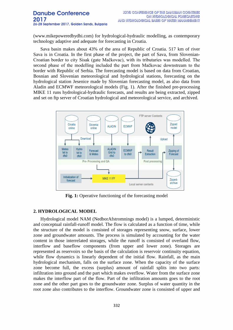
332

(www.mikepoweredbydhi.com) for hydrological-hydraulic modelling, as contemporary technology adaptive and adequate for forecasting in Croatia.

Sava basin makes about 43% of the area of Republic of Croatia. 517 km of river Sava is in Croatia. In the first phase of the project, the part of Sava, from Slovenian-Croatian border to city Sisak (gate Mačkovac), with its tributaries was modelled. The second phase of the modelling included the part from Mačkovac downstream to the border with Republic of Serbia. The forecasting model is based on data from Croatian, Bosnian and Slovenian meteorological and hydrological stations, forecasting on the hydrological station Jesenice made by Slovenian forecasting model, as also data from Aladin and ECMWF meteorological models (Fig. 1). After the finished pre-processing MIKE 11 runs hydrological-hydraulic forecasts, and results are being extracted, zipped and set on ftp server of Croatian hydrological and meteorological service, and archived.

Fig. 1: Operative functioning of the forecasting model

2. HYDROLOGICAL MODEL Hydrological model NAM (NedborAfstromnings model) is a lumped, deterministic

and conceptual rainfall-runoff model. The flow is calculated as a function of time, while the structure of the model is consisted of storages representing snow, surface, lower zone and groundwater amounts. The process is simulated by accounting for the water content in those interrelated storages, while the runoff is consisted of overland flow, interflow and baseflow components (from upper and lower zone). Storages are represented as reservoirs so the basis of the calculation is reservoir continuity equation, while flow dynamics is linearly dependent of the initial flow. Rainfall, as the main hydrological mechanism, falls on the surface zone. When the capacity of the surface zone become full, the excess (surplus) amount of rainfall splits into two parts: infiltration into ground and the part which makes overflow. Water from the surface zone makes the interflow part of the flow. Part of the infiltration amounts goes to the root zone and the other part goes to the groundwater zone. Surplus of water quantity in the root zone also contributes to the interflow. Groundwater zone is consisted of upper and

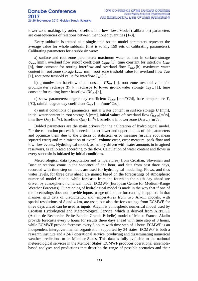
333

lower zone making, by order, baseflow and low flow. Model (calibration) parameters are consequencies of relations between mentioned quantities [1-3].

Every subbasin is treated as a single unit, so the model parameters represent the average value for whole subbasin (that is totally 159 sets of calibrating parameters). Calibrating parameters for a subbasin were:

a) surface and root zone parameters: maximum water content in surface storage Umax [mm], overland flow runoff coefficient CQOF [1], time constant for interflow CKIF [h], time constant for routing interflow and overland flow CK12 [h], maximum water content in root zone storage Lmax [mm], root zone treshold value for overland flow TOF [1], root zone treshold value for interflow TIF [1],

b) groundwater: baseflow time constant CKBF [h], root zone treshold value for groundwater recharge TG [/], recharge to lower groundwater storage CQlow [1], time constant for routing lower baseflow CKlow [h],

c) snow parameters: degree-day coefficient Csnow [mm/°C/d], base temperature T0 [°C], rainfall degree-day coefficient Crain [mm/mm/°C/d],

d) initial conditions of parameters: initial water content in surface storage U [mm], initial water content in root storage L [mm], initial values of: overland flow QOF,0 [m3/s], interflow QIF,0 [m3/s], baseflow QBF,0 [m3/s], baseflow in lower zone QBFlow,0 [m3/s].

Bolded parameters are the main drivers for the calibration of hydrological model. For the calibration process it is needed to set lower and upper bounds of this parameters and optimize them due to the criteria of statistical error measure (usually root mean squared error) and minimization of overall volume error, error measure, peak flow and low flow events. Hydrological model, as mainly driven with water amounts in imagined reservoirs, is calibrated according to the flow. Calculation of water content and flows in every subbasin is initiated by initial conditions.

Meteorological data (precpitation and temperatures) from Croatian, Slovenian and Bosnian stations come in the sequence of one hour, and data from past three days, recorded with time step on hour, are used for hydrological modelling. Flows, and thus water levels, for three days ahead are gained based on the forecastings of atmospheric numerical model Aladin, while forecasts from the fourth to the sixth day ahead are driven by atmospheric numerical model ECMWF (European Centre for Medium-Range Weather Forecasts). Functioning of hydrological model is made in the way that if one of the forecastings does not provide inputs, usage of another forecasting is applied. In that manner, grid data of precipitation and temperatures from two Aladin models, with spatial resolutions of 8 and 4 km, are used, but also the forecastings from ECMWF for three days ahead can be used as inputs. Aladin is atmospheric numerical model used by Croatian Hydrological and Meteorological Service, which is derived from ARPEGE (Action de Recherche Petite Echelle Grande Echelle) model of Meteo-France. Aladin provide forecasts every 6 hours for results three days ahead with time step of 3 hours, while ECMWF provide forecasts every 3 hours with time step of 1 hour. ECMWF is an independent intergovernmental organisation supported by 34 states. ECMWF is both a research institute and a 24/7 operational service, producing and disseminating numerical weather predictions to its Member States. This data is fully available to the national meteorological services in the Member States. ECMWF produces operational ensemble-based analyses and predictions that describe the range of possible scenarios and their

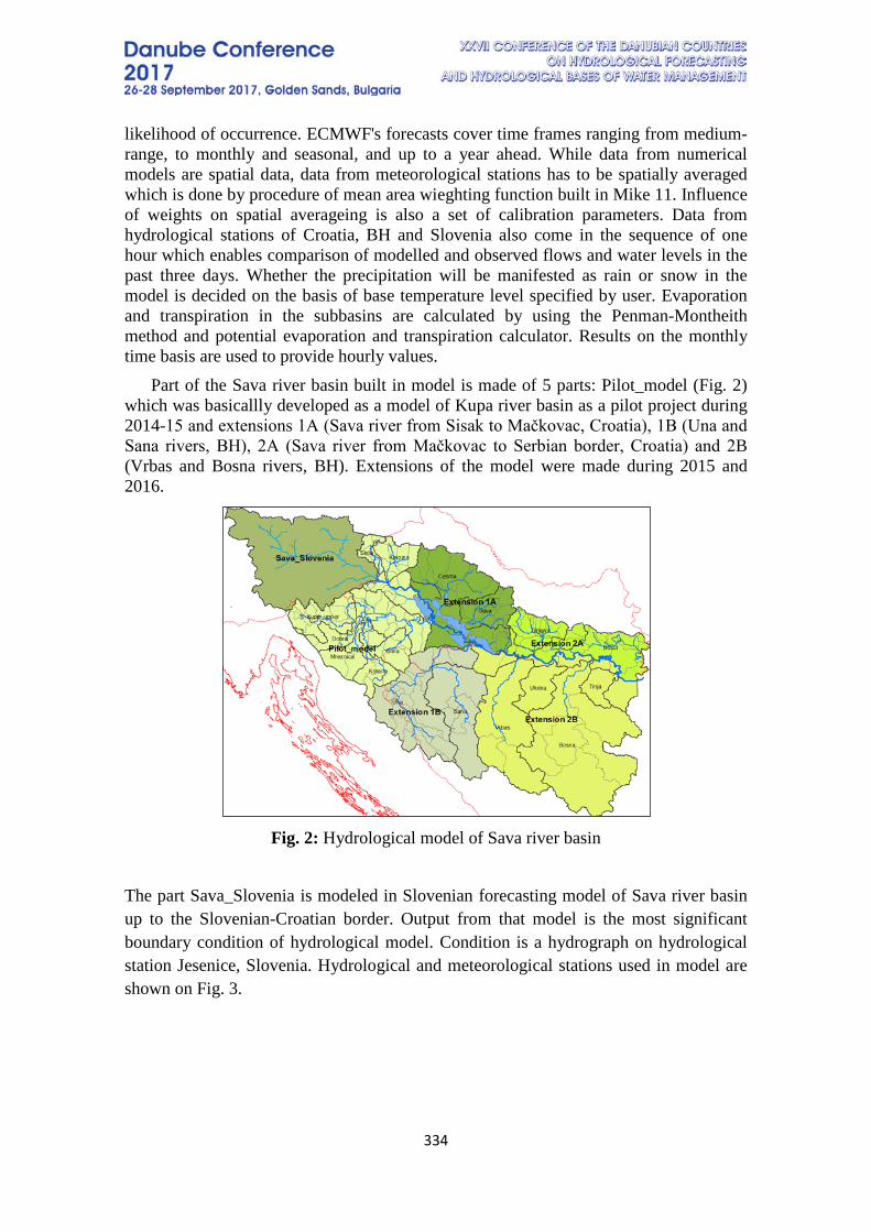
334

likelihood of occurrence. ECMWF's forecasts cover time frames ranging from medium-range, to monthly and seasonal, and up to a year ahead. While data from numerical models are spatial data, data from meteorological stations has to be spatially averaged which is done by procedure of mean area wieghting function built in Mike 11. Influence of weights on spatial averageing is also a set of calibration parameters. Data from hydrological stations of Croatia, BH and Slovenia also come in the sequence of one hour which enables comparison of modelled and observed flows and water levels in the past three days. Whether the precipitation will be manifested as rain or snow in the model is decided on the basis of base temperature level specified by user. Evaporation and transpiration in the subbasins are calculated by using the Penman-Montheith method and potential evaporation and transpiration calculator. Results on the monthly time basis are used to provide hourly values.

Part of the Sava river basin built in model is made of 5 parts: Pilot_model (Fig. 2) which was basicallly developed as a model of Kupa river basin as a pilot project during 2014-15 and extensions 1A (Sava river from Sisak to Mačkovac, Croatia), 1B (Una and Sana rivers, BH), 2A (Sava river from Mačkovac to Serbian border, Croatia) and 2B (Vrbas and Bosna rivers, BH). Extensions of the model were made during 2015 and 2016.

Fig. 2: Hydrological model of Sava river basin

The part Sava_Slovenia is modeled in Slovenian forecasting model of Sava river basin up to the Slovenian-Croatian border. Output from that model is the most significant boundary condition of hydrological model. Condition is a hydrograph on hydrological station Jesenice, Slovenia. Hydrological and meteorological stations used in model are shown on Fig. 3.

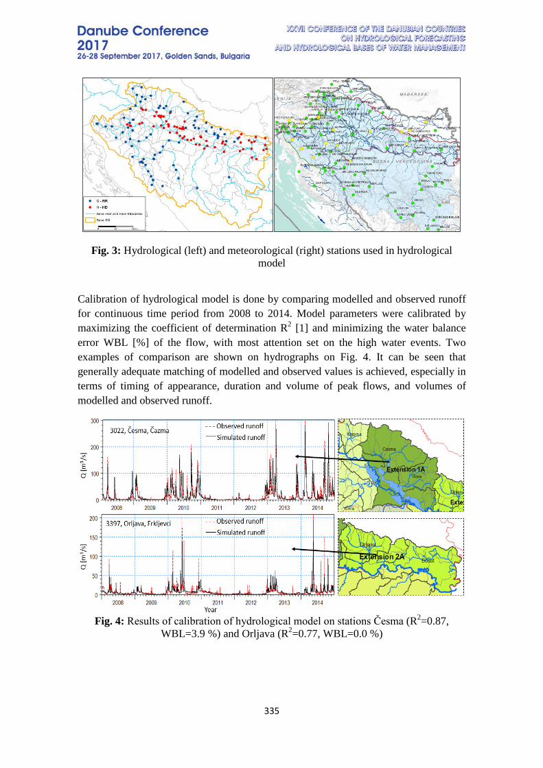
335

Fig. 3: Hydrological (left) and meteorological (right) stations used in hydrological model

Calibration of hydrological model is done by comparing modelled and observed runoff for continuous time period from 2008 to 2014. Model parameters were calibrated by maximizing the coefficient of determination R2 [1] and minimizing the water balance error WBL [%] of the flow, with most attention set on the high water events. Two examples of comparison are shown on hydrographs on Fig. 4. It can be seen that generally adequate matching of modelled and observed values is achieved, especially in terms of timing of appearance, duration and volume of peak flows, and volumes of modelled and observed runoff.

Fig. 4: Results of calibration of hydrological model on stations Česma (R2=0.87,

WBL=3.9 %) and Orljava (R2=0.77, WBL=0.0 %)

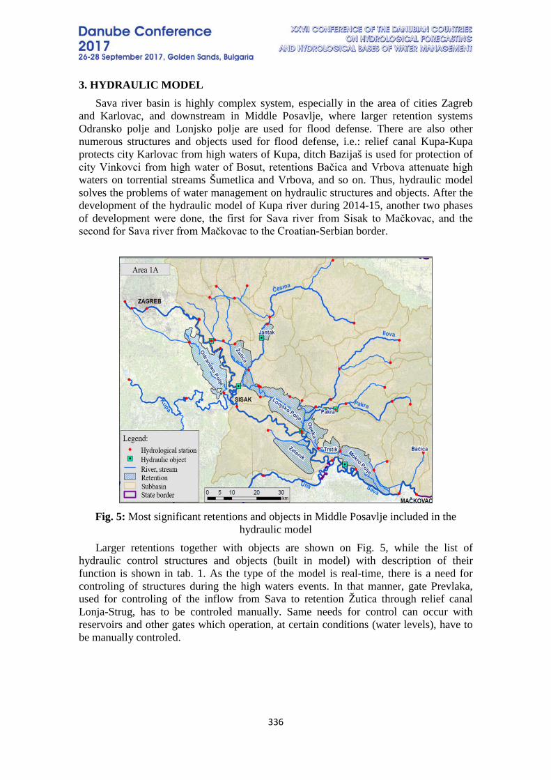
336

3. HYDRAULIC MODEL Sava river basin is highly complex system, especially in the area of cities Zagreb

and Karlovac, and downstream in Middle Posavlje, where larger retention systems Odransko polje and Lonjsko polje are used for flood defense. There are also other numerous structures and objects used for flood defense, i.e.: relief canal Kupa-Kupa protects city Karlovac from high waters of Kupa, ditch Bazijaš is used for protection of city Vinkovci from high water of Bosut, retentions Bačica and Vrbova attenuate high waters on torrential streams Šumetlica and Vrbova, and so on. Thus, hydraulic model solves the problems of water management on hydraulic structures and objects. After the development of the hydraulic model of Kupa river during 2014-15, another two phases of development were done, the first for Sava river from Sisak to Mačkovac, and the second for Sava river from Mačkovac to the Croatian-Serbian border.

Fig. 5: Most significant retentions and objects in Middle Posavlje included in the

hydraulic model Larger retentions together with objects are shown on Fig. 5, while the list of

hydraulic control structures and objects (built in model) with description of their function is shown in tab. 1. As the type of the model is real-time, there is a need for controling of structures during the high waters events. In that manner, gate Prevlaka, used for controling of the inflow from Sava to retention Žutica through relief canal Lonja-Strug, has to be controled manually. Same needs for control can occur with reservoirs and other gates which operation, at certain conditions (water levels), have to be manually controled.

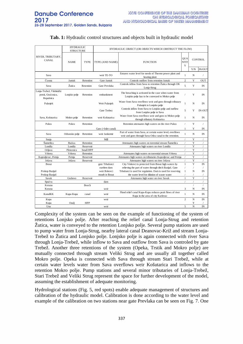
337

Tab. 1: Hydraulic control structures and objects built in hydraulic model

Complexity of the system can be seen on the example of functioning of the system of retentions Lonjsko polje. After reaching the relief canal Lonja-Strug and retention Žutica, water is conveyed to the retention Lonjsko polje. Several pump stations are used to pump water from Lonja-Strug, nearby lateral canal Deanovac-Križ and stream Lonja-Trebež to Žutica and Lonjsko polje. Lonjsko polje is again connected with river Sava through Lonja-Trebež, while inflow to Sava and outflow from Sava is controled by gate Trebež. Another three retentions of the system (Opeka, Trstik and Mokro polje) are mutually connected through stream Veliki Strug and are usually all together called Mokro polje. Opeka is connected with Sava through stream Stari Trebež, while at certain water levels water from Sava overflows weir Košutarica and inflows to the retention Mokro polje. Pump stations and several minor tributaries of Lonja-Trebež, Stari Trebež and Veliki Strug represent the space for further development of the model, assuming the establishment of adequate monitoring. Hydrological stations (Fig. 5, red spots) enable adequate management of structures and calibration of the hydraulic model. Calibration is done according to the water level and example of the calibration on two stations near gate Prevlaka can be seen on Fig. 7. One

Y/N IN/OUT

Sava weir TE-TOEnsures water level for needs of Thermo power plant and

heating plant1 N /

Česma Jantak Retention Gate Jantak Controls outflow from retention Jantak 2 Y OUT

Sava Žutica Retention Gate PrevlakaControls inflow from Sava to retention Žutica through OK

Lonja-Strug5 Y IN

Lonja-Trebež, Vlahinički potok, Gračenica,

RepušnicaLonjsko polje Retention embankment

The breaching is activated in the case when water from Lonjsko polje has to be conveyed to Mokro polje

/ Y IN

Palanjek Weir PalanjekWater from Sava overflows weir and goes through tributary

Palanjek to Lonjsko polje1 N IN

Gate TrebezControls inflow from Sava to Lonjsko polje and outflow

from Lonjsko polje to Sava5 Y IN-OUT

Sava, Košutarica Mokro polje Retention weir KošutaricaWater from Sava overflows weir and goes to Mokro polje

through tributary Košutarica1 N IN

Pakra Pakra Retention Retention attenuates high waters on the river Pakra / Y /

Gate (+Inlet canal) 1 Y IN

Sava Odransko polje Retention weir JankomirPart of water from Sava, at certain water level, overflows weir and goes through Sava-Odra canal to the retention.

1 N IN

Sunja Mill / Y /Šumetlica Bačica Retention Attenuates high waters on torrential stream Šumetlica / Y /Londža Londža Reservoir Attenuates high waters on river Londža / Y /Orljava Pleternica Small HPP / Y /Vrbova Vrbova Retention Attenuates high waters on torrential stream Vrbova / Y /

Kapraljevac, Petnja Petnja Reservoir Attenuates high waters on tributaries Kapraljevac and Petnja / Y /Jošava Jošava Reservoir Attenuates high waters on river Jošava / Y /Bosut gate Trbušanci 1 Y IN

earthen dam / / /Prokop Bazijaš weir Rokovci 1 N INProkop Bazijaš mouth in Bosut / / /

Savak Grabovo Reservoir Attenuates high water on river Savak 1 Y /Spačva dam / / /Korana Beach / /Korana weir 3 N IN

KanalKK Kupa-Kupa canal weirFlood relief canal Kupa-Kupa reduces peak flows of river

Kupa in the area of city Karlovac1 N IN

Kupa weir 2 N INKupa Ozalj HPP Y /Una weir 5 N IN

City Vinkovci is protected from Bosut high waters by relieving the part of water through ditch Bazijaš. Gate

Trbušanci is used for regulation. Dam is used for reserving the water level for dilution of waste water

HYDRAULIC OBJECT (OR OBJECTS WHICH OBSTRUCT THE FLOW)

CONTROLTYPE TYPE (AND NAME)

QUANTIT

Y

HYDRAULIC STRUCTURE

RIVER, TRIBUTARY, CANAL

FUNCTIONNAME

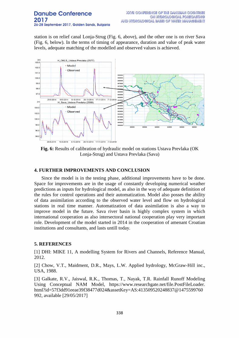
338

station is on relief canal Lonja-Strug (Fig. 6, above), and the other one is on river Sava (Fig. 6, below). In the terms of timing of appearance, duration and value of peak water levels, adequate matching of the modelled and observed values is achieved.

Fig. 6: Results of calibration of hydraulic model on stations Ustava Prevlaka (OK

Lonja-Strug) and Ustava Prevlaka (Sava)

4. FURTHER IMPROVEMENTS AND CONCLUSION

Since the model is in the testing phase, additional improvements have to be done. Space for improvements are in the usage of constantly developing numerical weather predictions as inputs for hydrological model, as also in the way of adequate definition of the rules for control operations and their automatization. Model also posses the ability of data assimilation according to the observed water level and flow on hydrological stations in real time manner. Automatization of data assimilation is also a way to improve model in the future. Sava river basin is highly complex system in which international cooperation as also intersectoral national cooperation play very important role. Development of the model started in 2014 in the cooperation of amenant Croatian institutions and consultants, and lasts untill today.

5. REFERENCES [1] DHI: MIKE 11, A modelling System for Rivers and Channels, Reference Manual, 2012. [2] Chow, V.T., Maidment, D.R., Mays, L.W. Applied hydrology, McGraw-Hill inc., USA, 1988. [3] Galkate, R.V., Jaiswal, R.K., Thomas, T., Nayak, T.R. Rainfall Runoff Modeling Using Conceptual NAM Model, https://www.researchgate.net/file.PostFileLoader. html?id=57f3dd91eeae39f38477d024&assetKey=AS:413509520248837@1475599760992, available [29/05/2017]

339

CASE STUDIES OF 2D HYDRO-DYNAMIC MODELING OF DIFFERENT DANUBE REACHES IN HUNGARY

István Göttlinger1, Enikő Anna Tamás1, György Varga1, László Vas2

1 National University of Public Service, Faculty of Water Sciences, Institute for Hydraulic engineering and Water management, Hungary

2 Lower Danube-valley Water Management Directorate, Hungary Corresponding author: István Göttlinger, National University of Public Service, Faculty of Water

Sciences, Institute for Hydraulic engineering and Water management, Baja, Hungary, gottlinger.istvan@uni-nke.hu

ABSTRACT In Hungary the elaboration of an internationally acceptable level of discharge-capacity, the size of our navigation ways and, at the same time, the management of the side branches of the River Danube are of high concern. [1]

A tool to support both river-regulation and wetland restoration works is two dimensional hydro-dynamic modelling. One of the solutions to be used is HEC-RAS modeling software, which requires highly standardized, precise and detailed field measurements in order to provide reliable results.

The aim of 2 D hydro-dynamical modeling is to reach a state where the model and real world correlates each other well. To achieve this, we need to use water-level and discharge time series, measured water levels, free surface elevations, as well as standards and professional literature. With a well-calibrated model we can observe the impacts of the various river regulation methods, like dredging, groynes, horizontal and vertical structures and other artificial regulating actions.

We have worked out and tested the methodology of reliable, standardized bathymetry and data collection which is replicating the riverbed precisely, in order to develop the best possible DTM. Different applied research projects based on field surveys and 2D modeling focused on low-flow river management structures, the development and management of shallows and side branch management for floodplain rehabilitation.

Keywords: river regulation, methodology, 2D modeling, field survey, bathymetry

1. INTRODUCTION Thanks to the developed technology of nowadays any process can be linked to models. The developed and accurate programs enable us to examine the future impacts of complex processes. However, the most important part of a modeling software is the engineer sitting in front of the computer.

340

Nowadays, there is a trend outlining: checking the calculated values by modeling. In the “water-management industry” modeling could be a very useful method for this verifying. Depending on the aim of the calculations, several kinds of models are available. In Hungary, the most common method is 1D modeling (calculating 1 hydraulic properties in a cross-section). For river-regulation purposes 2D modeling is more applicable. 2D models are based on a calculation mesh, and the hydraulic properties are calculated on the grid points. In this article, we would like to present how to make an accurate model (from the surveying until the calibration and use).

2. NECESSARY DATA OF A TWO DIMENSIONAL MODEL To create an accurate 2D model, the geometry of the bed; water-level and discharge time-series; rating curves and free surface elevations are necessary. Thanks to the work of the Hungarian water-managers, the number of the gauging stations is adequate on the Hungarian reach of the Danube. These gauging stations are providing water-level and discharge values every hour. Furthermore, in a few stations authentic rating curves are available as well. To create a model, surveying of the bed and the floodplains is essential. Based on this surveying, an accurate digital elevation model can be constructed, where the runoff can be simulated.

2.1. SURVEYING We have worked out and tested the methodology of reliable, standardized bathymetry and data collection which is replicating the riverbed precisely, in order to develop the best possible DEM (Digital Elevation Model). The bathymetry is done from a measuring boat. During the surveying, a GPS and an ultrasonic depth-meter are synchronized to measure the bed. We measure the river in cross-sections, which are perpendicular to the centerline. The average distance between the cross-sections is 200 meters. The density of the cross-sections was increased near structures, side-branches and low-radius bends. Scattered point measurements were carried out where the flow conditions justified it. During the bed measurement, the free surface elevations were measured as well. To determine this surface, we have established base-points near to the water (visible from the water as well). We have placed base-points in every 1 kilometer. The bed and the free surface elevation measurement were carried out simultaneously. The surveying of the river-regulating structures (depending on the water-level) is possible from the bank or from the water.

2.2. BUILDING DEM BASED ON THE MEASURED DATA During the bathymetry, the number of the gathered points are much more than necessary (2 points/second). During the processing, the depth and the coordinate values will be synchronized, and only the necessary values will be kept. The method of the sorting is the following:

1. Calculating the distance and the height difference between two successive points.

2. Setting a threshold for the distance and the height difference.

341

3. If the distance or the height difference is higher than the threshold, the point will be kept.

4. If it is not, then the point will be erased. With this method we can assure the accuracy of the DEM with fewer points. The final step of the processing is to make a DEM (in “.geotiff” format) using CAD software, which can be imported by HEC-RAS.

2.3. BOUNDARY CONDITIONS For a 2D hydro-dynamical model upper and lower boundary conditions are necessary, lateral is optional. As an upper boundary condition, we used water-level time-series, the lower boundary condition was discharge time-series. Depending on the desirable result, steady or unsteady model variables can be created.

2.4. BUILDING AND CALIBRATING A MODEL The geometry of the runoff modeling is based on the DEM created by the surveyed data. To this DEM, an adequate calculation mesh (25x25 m, 10x10 m, 5x5 m) is fitted. Densifying of this mesh is possible if it is necessary for the calculation. After the fitting of the mesh, the adequate boundary conditions must be set. When the mesh and boundary conditions are ready, the model has to be calibrated. To calibrate a model we usually use measured discharge value and the measured free surface elevation. When the model finishes the calculation, we get a computed free surface elevation. We have to compare this computed surface elevation to the measured one. If there are major differences between the surfaces, the roughness coefficient has to be changed. The coefficient has to be varied until the calculated and the measured surface elevations are adequately close to each other. If the calibration is successful, the model has to be validated. During the validation, the boundary conditions have to be set to time-series which are different and independent from the calibration time-series. To validate a model, another measured discharge values and free surface elevations are needed. During the validation, the differences between the calculated and the measured results have to be analyzed. If these differences are adequately little, the model can be used for further calculations. 3. CASE STUDIES In the past few years, our Institute took part in several 2D modeling tasks. We made a base-model for contamination transport modeling and a model to support the river-regulation plan. Currently we are working on a model to detect impacts of a dam closing a side-branch.

3.1. CALIBRATION OF SZÁZHALOMBATTA-PAKS (1619-1524 RKM) DANUBE REACH

During this project, our task was to measure, build and calibrate a model of the Danube between 1619 and 1524 river kilometers. The main task was to survey this 95 rkm long reach of the river near the mean water-level. The bathymetry was done by measuring boat with the previously described method. The distance between the cross-sections was

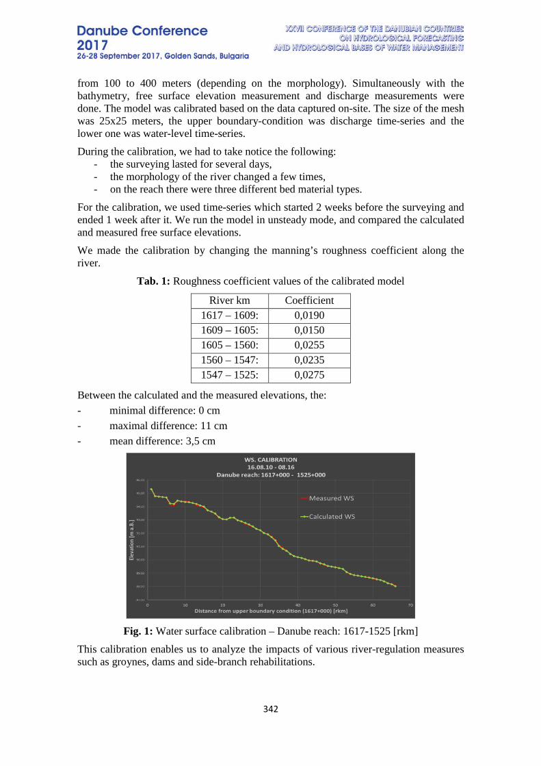
342

from 100 to 400 meters (depending on the morphology). Simultaneously with the bathymetry, free surface elevation measurement and discharge measurements were done. The model was calibrated based on the data captured on-site. The size of the mesh was 25x25 meters, the upper boundary-condition was discharge time-series and the lower one was water-level time-series. During the calibration, we had to take notice the following:

- the surveying lasted for several days, - the morphology of the river changed a few times, - on the reach there were three different bed material types.

For the calibration, we used time-series which started 2 weeks before the surveying and ended 1 week after it. We run the model in unsteady mode, and compared the calculated and measured free surface elevations. We made the calibration by changing the manning’s roughness coefficient along the river.

Tab. 1: Roughness coefficient values of the calibrated model

River km Coefficient 1617 – 1609: 0,0190 1609 – 1605: 0,0150 1605 – 1560: 0,0255 1560 – 1547: 0,0235 1547 – 1525: 0,0275

Between the calculated and the measured elevations, the: - minimal difference: 0 cm - maximal difference: 11 cm - mean difference: 3,5 cm

Fig. 1: Water surface calibration – Danube reach: 1617-1525 [rkm]

This calibration enables us to analyze the impacts of various river-regulation measures such as groynes, dams and side-branch rehabilitations.

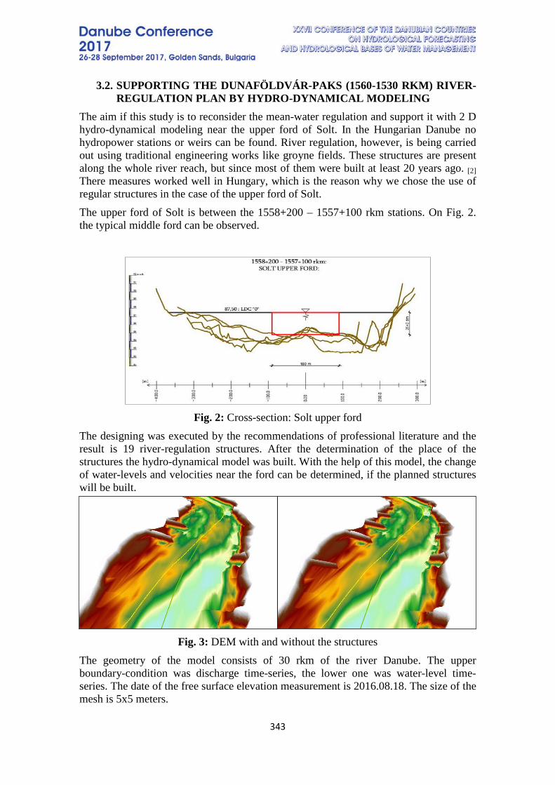
343

3.2. SUPPORTING THE DUNAFÖLDVÁR-PAKS (1560-1530 RKM) RIVER-REGULATION PLAN BY HYDRO-DYNAMICAL MODELING

The aim if this study is to reconsider the mean-water regulation and support it with 2 D hydro-dynamical modeling near the upper ford of Solt. In the Hungarian Danube no hydropower stations or weirs can be found. River regulation, however, is being carried out using traditional engineering works like groyne fields. These structures are present along the whole river reach, but since most of them were built at least 20 years ago. [2] There measures worked well in Hungary, which is the reason why we chose the use of regular structures in the case of the upper ford of Solt. The upper ford of Solt is between the 1558+200 – 1557+100 rkm stations. On Fig. 2. the typical middle ford can be observed.

Fig. 2: Cross-section: Solt upper ford

The designing was executed by the recommendations of professional literature and the result is 19 river-regulation structures. After the determination of the place of the structures the hydro-dynamical model was built. With the help of this model, the change of water-levels and velocities near the ford can be determined, if the planned structures will be built.

Fig. 3: DEM with and without the structures The geometry of the model consists of 30 rkm of the river Danube. The upper boundary-condition was discharge time-series, the lower one was water-level time-series. The date of the free surface elevation measurement is 2016.08.18. The size of the mesh is 5x5 meters.

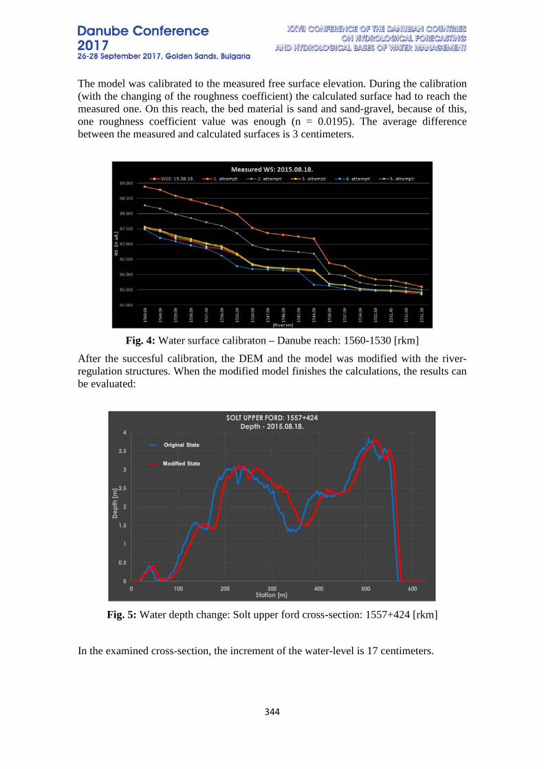
344

The model was calibrated to the measured free surface elevation. During the calibration (with the changing of the roughness coefficient) the calculated surface had to reach the measured one. On this reach, the bed material is sand and sand-gravel, because of this, one roughness coefficient value was enough (n = 0.0195). The average difference between the measured and calculated surfaces is 3 centimeters.

Fig. 4: Water surface calibraton – Danube reach: 1560-1530 [rkm]

After the succesful calibration, the DEM and the model was modified with the river-regulation structures. When the modified model finishes the calculations, the results can be evaluated:

Fig. 5: Water depth change: Solt upper ford cross-section: 1557+424 [rkm]

In the examined cross-section, the increment of the water-level is 17 centimeters.

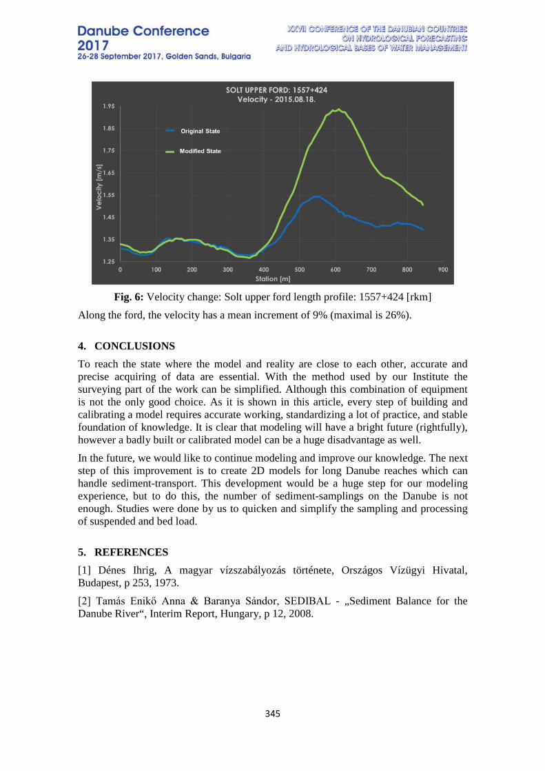
345

Fig. 6: Velocity change: Solt upper ford length profile: 1557+424 [rkm] Along the ford, the velocity has a mean increment of 9% (maximal is 26%). 4. CONCLUSIONS To reach the state where the model and reality are close to each other, accurate and precise acquiring of data are essential. With the method used by our Institute the surveying part of the work can be simplified. Although this combination of equipment is not the only good choice. As it is shown in this article, every step of building and calibrating a model requires accurate working, standardizing a lot of practice, and stable foundation of knowledge. It is clear that modeling will have a bright future (rightfully), however a badly built or calibrated model can be a huge disadvantage as well. In the future, we would like to continue modeling and improve our knowledge. The next step of this improvement is to create 2D models for long Danube reaches which can handle sediment-transport. This development would be a huge step for our modeling experience, but to do this, the number of sediment-samplings on the Danube is not enough. Studies were done by us to quicken and simplify the sampling and processing of suspended and bed load. 5. REFERENCES [1] Dénes Ihrig, A magyar vízszabályozás története, Országos Vízügyi Hivatal, Budapest, p 253, 1973. [2] Tamás Enikő Anna & Baranya Sándor, SEDIBAL - „Sediment Balance for the Danube River“, Interim Report, Hungary, p 12, 2008.

346

INTER-ANNUAL DISTRIBUTION FOR YANTRA RIVER BASIN, NORTH BULGARIA

Elena Bojilova National Institute of Meteorology and Hydrology-BAS, Sofia, Bulgaria

Corresponding author: Elena Bojilova, NIMH-BAS, Tzarigradsko chaussee 66, 1784 Sofia,

Bulgaria, Elena.Kirilova.Bojilova@gmail.com

In the present study inter-annual distribution of the Yantra river discharge is investigated. Yantra river basin is situated in North Bulgaria in temperate climate. Typical for this climate is resistant snow cover in the mountain parts during the winter mounts; rainfalls during the spring and beginning of the summer. The summer is characterized with intensive precipitations with short duration; drought conditions and maximum air temperatures.

In the catchment of Yantra river the hydrological network consists of sixteen hydrological gauge stations. Three of them are located on the main river body and the others are distributed on the tributaries. For inter-annual distribution the monthly time step is used. Two types of results are discussed: discharge layers (in mm) and percent distribution. Two periods of investigation are studied. The obtained results are presented.

Keywords: Inter-annual distribution, discharge layer.

RIVER INFORMATION

The drainage basin of Yantra River is located with geographical coordinates 42° 40' and 43°40' north latitude and between 24° 45' and 26° 30' east longitude. The bordering river basins are Osam River basin from west and Kamchia and Rusenski Lom river basins from east. In south direction the Balkan range is natural border of the basin. The total drainage area of the basin is about 7869 km2.

The total length of Yantra River is about 285 km. The begging of the river is the foot of peak Hadji Dimitar at 1340 m elevation a.s.l. The coordinates of the spring are 42° 44' 20" north latitude and 25° 25' 80" east longitude. Up to Veliko Turnovo town the river flows in north-east direction. After Veliko Turnovo the river turn in east direction making curve and since that is flowing in north direction. Yantra joins Danube River near Krivina village. The outflow coordinates are 430 38' 20" north latitude and 25° 34' 40" east longitude with elevation of 18 m a.s.l. (Mandadjuev, 1982).

The density of river network for the main river body is 0.7 km/km2 and for it’s tributaries varied between 0.3 km/km2 (for Eleeiska River) to 1.5 km/km2 (Ostreshka River). From all 30 tributaries with length more than 10 km only 9 have density of river network above 1. The average mean elevation of the whole Yantra drainage basin is about 470 m. The average slope of the main river is 4.6 ‰.

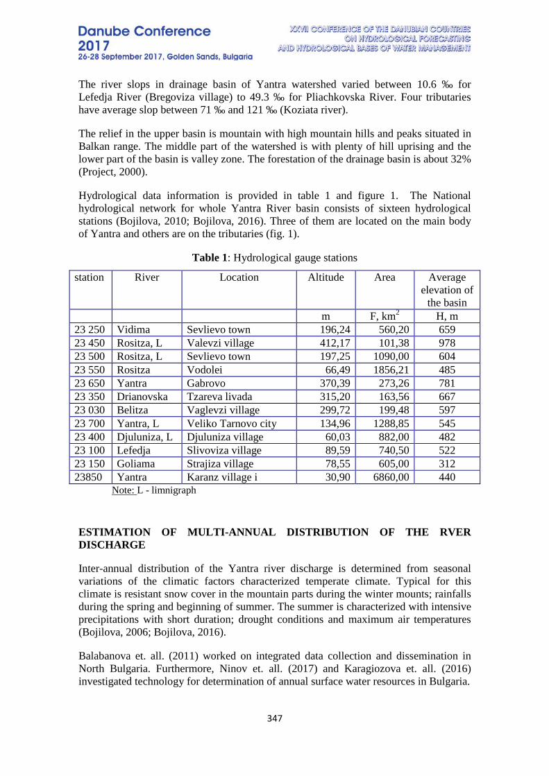
347

The river slops in drainage basin of Yantra watershed varied between 10.6 ‰ for Lefedja River (Bregoviza village) to 49.3 ‰ for Pliachkovska River. Four tributaries have average slop between 71 ‰ and 121 ‰ (Koziata river).

The relief in the upper basin is mountain with high mountain hills and peaks situated in Balkan range. The middle part of the watershed is with plenty of hill uprising and the lower part of the basin is valley zone. The forestation of the drainage basin is about 32% (Project, 2000).

Hydrological data information is provided in table 1 and figure 1. The National hydrological network for whole Yantra River basin consists of sixteen hydrological stations (Bojilova, 2010; Bojilova, 2016). Three of them are located on the main body of Yantra and others are on the tributaries (fig. 1).

Table 1: Hydrological gauge stations

station

River Location Altitude Area Average elevation of

the basin m F, km2 H, m 23 250 Vidima Sevlievo town 196,24 560,20 659 23 450 Rositza, L Valevzi village 412,17 101,38 978 23 500 Rositza, L Sevlievo town 197,25 1090,00 604 23 550 Rositza Vodolei 66,49 1856,21 485 23 650 Yantra Gabrovo 370,39 273,26 781 23 350 Drianovska Tzareva livada 315,20 163,56 667 23 030 Belitza Vaglevzi village 299,72 199,48 597 23 700 Yantra, L Veliko Tarnovo city 134,96 1288,85 545 23 400 Djuluniza, L Djuluniza village 60,03 882,00 482 23 100 Lefedja Slivoviza village 89,59 740,50 522 23 150 Goliama Strajiza village 78,55 605,00 312 23850 Yantra Karanz village i 30,90 6860,00 440

Note: L - limnigraph

ESTIMATION OF MULTI-ANNUAL DISTRIBUTION OF THE RVER DISCHARGE

Inter-annual distribution of the Yantra river discharge is determined from seasonal variations of the climatic factors characterized temperate climate. Typical for this climate is resistant snow cover in the mountain parts during the winter mounts; rainfalls during the spring and beginning of summer. The summer is characterized with intensive precipitations with short duration; drought conditions and maximum air temperatures (Bojilova, 2006; Bojilova, 2016).

Balabanova et. all. (2011) worked on integrated data collection and dissemination in North Bulgaria. Furthermore, Ninov et. all. (2017) and Karagiozova et. all. (2016) investigated technology for determination of annual surface water resources in Bulgaria.

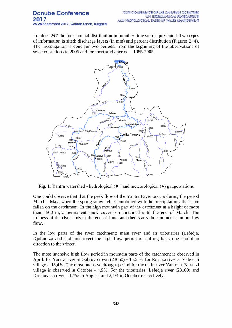
348

In tables 2÷7 the inter-annual distribution in monthly time step is presented. Two types of information is sited: discharge layers (in mm) and percent distribution (Figures 2÷4). The investigation is done for two periods: from the beginning of the observations of selected stations to 2006 and for short study period – 1985-2005.

Fig. 1: Yantra watershed - hydrological (►) and meteorological (●) gauge stations

One could observe that that the peak flow of the Yantra River occurs during the period March - May, when the spring snowmelt is combined with the precipitations that have fallen on the catchment. In the high mountain part of the catchment at a height of more than 1500 m, a permanent snow cover is maintained until the end of March. The fullness of the river ends at the end of June, and then starts the summer - autumn low flow.

In the low parts of the river catchment: main river and its tributaries (Lefedja, Djulunitza and Goliama river) the high flow period is shifting back one mount in direction to the winter.

The most intensive high flow period in mountain parts of the catchment is observed in April: for Yantra river at Gabrovo town (23650) - 15,5 %, for Rositza river at Valevchi village - 18,4%. The most intensive drought period for the main river Yantra at Karanzi village is observed in October - 4,9%. For the tributaries: Lefedja river (23100) and Drianovska river – 1,7% in August and 2,1% in October respectively.

Studen

a

Yantra

Rosiza

Rosiza

Eliiska

Mugura

ChaparataVidima

Vidim

a

Lolychniza

Drian

ovs

ka

Beliza

Veselina

Kote

lskaB

abrovska

Dju

luniz

a

Golia

ma

Ialadere

Goliama

Negovanka

Bohot

Alex Stamboliiski Reservoir

KrapezYastrebino reservoir

Novgrad

Polikraiche

Karanzi

Samovodiane

Biala

Gorna Oriahoviza

Veliko Tarnovo

Gabrovo

Sevlievo

Pavlikeni

Drianovo

Elena

Yant

ra

Danube

Krycheto

23700

236500743006470

70406020

6480

6010

06401 06410

06420

7010

7020

7050

23180

23200

23230

23250

23500

23450

23550

2335023030

23400

23150

23570

23850

50600

7440

7470

22020

22460

7420

22530

23100

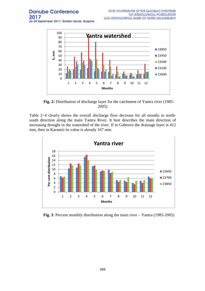
349

Fig. 2: Distribution of discharge layer for the catchment of Yantra river (1985-2005)

Table 2÷4 clearly shows the overall discharge flow decrease for all months in north-south direction along the main Yantra River. It best describes the main direction of increasing drought in the watershed of the river. If in Gabrovo the drainage layer is 412 mm, then in Karantzi its value is already 167 mm.

Fig. 3: Percent monthly distribution along the main river – Yantra (1985-2005)

0102030405060708090

100

1 2 3 4 5 6 7 8 9 10 11 12

h, m

m

Months

Yantra watershed

23850

23450

23500

23100

23400

02468

1012141618

1 2 3 4 5 6 7 8 9 10 11 12

Per c

ent d

istr

ibut

ion

Months

Yantra river

23650

23700

23850

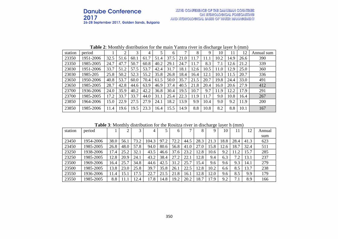
350

Table 2: Monthly distribution for the main Yantra river in discharge layer h (mm) station period 1 2 3 4 5 6 7 8 9 10 11 12 Annual sum 23350 1951-2006 32.5 51.6 60.1 61.7 51.4 37.5 21.0 11.7 11.1 10.2 14.9 26.6 390 23350 1985-2005 24.7 47.7 50.7 60.8 40.2 29.1 24.7 11.7 8.3 7.1 12.6 21.2 339 23030 1951-2006 33.7 51.2 57.5 53.7 42.4 31.7 18.1 12.6 10.5 11.0 12.9 25.0 360 23030 1985-205 25.8 50.2 52.3 55.2 35.8 26.8 18.4 16.4 12.1 10.3 11.5 20.7 336 23650 1950-2006 40.8 53.7 60.0 70.4 61.5 50.0 35.7 21.5 20.7 19.8 24.4 33.0 491 23650 1985-2005 28.7 42.8 44.6 63.9 46.9 37.4 40.5 21.8 20.4 16.0 20.6 27.9 412 23700 1936-2006 24.0 35.9 40.2 42.2 36.8 30.4 19.5 10.7 9.7 11.9 12.2 17.9 291 23700 1985-2005 17.2 33.7 33.7 44.0 31.1 25.4 22.3 11.9 11.7 9.0 10.8 16.4 267 23850 1964-2006 15.0 22.9 27.5 27.9 24.1 18.2 13.9 9.9 10.4 9.0 9.2 11.9 200 23850 1985-2006 11.4 19.6 19.5 23.3 16.4 15.5 14.9 8.8 10.8 8.2 8.8 10.1 167

Table 3: Monthly distribution for the Rositza river in discharge layer h (mm) station period 1 2 3 4 5 6 7 8 9 10 11 12 Annual

sum 23450 1954-2006 38.0 56.1 73.2 104.3 97.2 72.2 44.5 28.3 21.3 18.8 28.4 41.3 623 23450 1985-2005 26.8 48.0 57.8 94.0 80.6 56.8 41.0 27.0 15.8 12.6 18.7 32.4 511 23250 1938-2006 17.4 25.2 32.1 43.5 46.6 37.6 23.2 12.8 10.6 9.2 11.2 15.7 285 23250 1985-2005 12.8 20.9 24.1 43.2 38.4 27.2 22.1 12.8 9.4 6.3 7.2 13.1 237 23500 1969-2006 16.4 25.7 34.8 44.6 42.5 31.2 25.7 15.4 9.6 9.6 9.3 14.1 279 23500 1985-2005 13.8 23.0 25.8 39.7 35.8 26.1 22.5 12.8 10.2 6.6 8.5 13.7 238 23550 1936-2006 11.4 15.1 17.5 22.7 21.5 21.8 16.1 12.8 12.0 9.6 8.5 9.9 179 23550 1985-2005 8.8 11.1 12.4 17.8 14.8 19.2 20.2 18.7 17.9 9.2 7.1 8.9 166

351

Table 4: Monthly distribution for the Lefedja river in discharge layer h (mm) station period 1 2 3 4 5 6 7 8 9 10 11 12 Annual

sum 23100 1951-2006 27.0 40.8 44.5 41.4 29.9 21.2 8.6 6.1 6.7 4.2 10.4 19.0 260 23100 1985-2005 20.7 38.4 39.8 42.1 23.7 15.5 6.6 4.0 6.9 4.2 11.0 15.2 228 23150 1978-2006 6.2 13.8 14.2 16.9 11.3 7.4 7.8 4.0 5.5 4.9 3.4 3.9 99 23150 1985-2005 5.6 12.4 9.7 14.0 7.2 6.7 8.5 3.8 5.5 4.9 3.1 3.7 85 23400 1978-2005 19.5 32.6 38.1 39.5 25.7 19.0 10.8 5.7 7.4 5.6 10.0 15.9 230 23400 1985-2005 17.1 31.2 30.5 38.2 19.2 19.5 10.8 5.3 6.9 5.9 9.5 15.5 210

Table 5: Percent distribution of river discharges for Yantra river station period 1 2 3 4 5 6 7 8 9 10 11 12 Sum 23350 1951-2006 8.3 13.2 15.4 15.8 13.2 9.6 5.4 3.0 2.8 2.6 3.8 6.8 100 23350 1985-2005 7.3 14.1 15.0 17.9 11.9 8.6 7.3 3.4 2.5 2.1 3.7 6.3 100 23030 1951-2006 9.4 14.2 16.0 14.9 11.8 8.8 5.0 3.5 2.9 3.0 3.6 6.9 100 23030 1985-2005 7.7 15.0 15.6 16.5 10.7 8.0 5.5 4.9 3.6 3.1 3.4 6.2 100 23650 1950-2006 8.3 10.9 12.2 14.3 12.5 10.2 7.3 4.4 4.2 4.0 5.0 6.7 100 23650 1985-2005 7.0 10.4 10.8 15.5 11.4 9.1 9.8 5.3 5.0 3.9 5.0 6.8 100 23700 1936-2006 8.2 12.3 13.8 14.5 12.6 10.4 6.7 3.7 3.3 4.1 4.2 6.2 100 23700 1985-2005 6.4 12.6 12.6 16.5 11.7 9.5 8.4 4.5 4.4 3.4 4.0 6.1 100 23850 1964-2006 7.5 11.5 13.8 14.0 12.1 9.1 7.0 4.9 5.2 4.5 4.6 5.9 100 23850 1985-2006 6.8 11.7 11.7 13.9 9.8 9.3 8.9 5.3 6.5 4.9 5.3 6.1 100

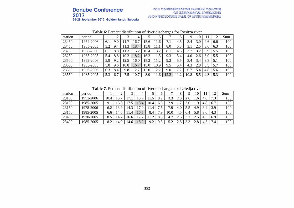
352

Table 6: Percent distribution of river discharges for Rositza river station period 1 2 3 4 5 6 7 8 9 10 11 12 Sum 23450 1954-2006 6.1 9.0 11.7 16.7 15.6 11.6 7.1 4.5 3.4 3.0 4.6 6.6 100 23450 1985-2005 5.2 9.4 11.3 18.4 15.8 11.1 8.0 5.3 3.1 2.5 3.6 6.3 100 23250 1938-2006 6.1 8.8 11.3 15.2 16.4 13.2 8.1 4.5 3.7 3.2 3.9 5.5 100 23250 1985-2005 5.4 8.8 10.2 18.2 16.2 11.5 9.3 5.4 4.0 2.6 3.0 5.5 100 23500 1969-2006 5.9 9.2 12.5 16.0 15.2 11.2 9.2 5.5 3.4 3.4 3.3 5.1 100 23500 1985-2005 5.8 9.6 10.8 16.7 15.0 10.9 9.5 5.4 4.3 2.8 3.5 5.7 100 23550 1936-2006 6.3 8.4 9.8 12.7 12.0 12.2 9.0 7.2 6.7 5.4 4.8 5.6 100 23550 1985-2005 5.3 6.7 7.5 10.7 8.9 11.6 12.2 11.2 10.8 5.5 4.3 5.3 100

Table 7: Percent distribution of river discharges for Lefedja river station period 1 2 3 4 5 6 7 8 9 10 11 12 Sum 23100 1951-2006 10.4 15.7 17.1 15.9 11.5 8.2 3.3 2.3 2.6 1.6 4.0 7.3 100 23100 1985-2005 9.1 16.8 17.5 18.4 10.4 6.8 2.9 1.7 3.0 1.9 4.8 6.7 100 23150 1978-2006 6.2 13.9 14.3 17.0 11.4 7.5 7.9 4.0 5.5 4.9 3.4 3.9 100 23150 1985-2005 6.6 14.6 11.4 16.5 8.4 7.9 10.0 4.5 6.4 5.8 3.6 4.3 100 23400 1978-2005 8.5 14.2 16.6 17.2 11.2 8.3 4.7 2.5 3.2 2.5 4.3 6.9 100 23400 1985-2005 8.2 14.9 14.6 18.2 9.2 9.3 5.2 2.5 3.3 2.8 4.5 7.4 100

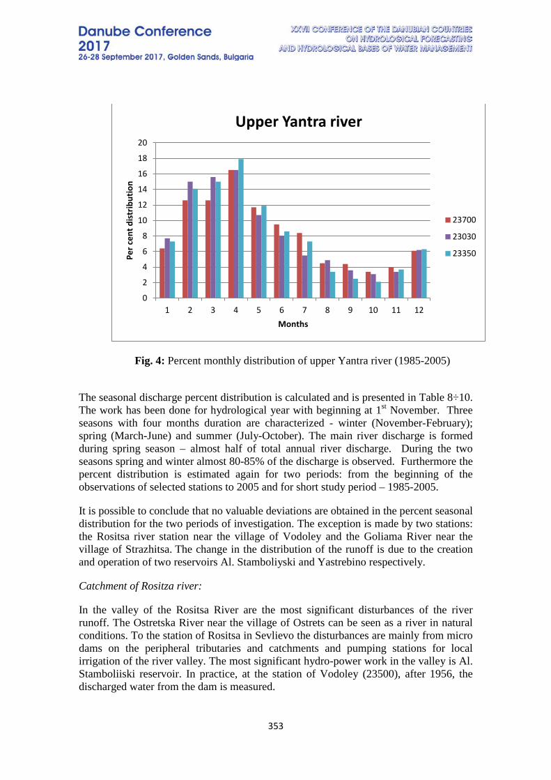
353

Fig. 4: Percent monthly distribution of upper Yantra river (1985-2005)

The seasonal discharge percent distribution is calculated and is presented in Table 8÷10. The work has been done for hydrological year with beginning at 1st November. Three seasons with four months duration are characterized - winter (November-February); spring (March-June) and summer (July-October). The main river discharge is formed during spring season – almost half of total annual river discharge. During the two seasons spring and winter almost 80-85% of the discharge is observed. Furthermore the percent distribution is estimated again for two periods: from the beginning of the observations of selected stations to 2005 and for short study period – 1985-2005.

It is possible to conclude that no valuable deviations are obtained in the percent seasonal distribution for the two periods of investigation. The exception is made by two stations: the Rositsa river station near the village of Vodoley and the Goliama River near the village of Strazhitsa. The change in the distribution of the runoff is due to the creation and operation of two reservoirs Al. Stamboliyski and Yastrebino respectively.

Catchment of Rositza river:

In the valley of the Rositsa River are the most significant disturbances of the river runoff. The Ostretska River near the village of Ostrets can be seen as a river in natural conditions. To the station of Rositsa in Sevlievo the disturbances are mainly from micro dams on the peripheral tributaries and catchments and pumping stations for local irrigation of the river valley. The most significant hydro-power work in the valley is Al. Stamboliiski reservoir. In practice, at the station of Vodoley (23500), after 1956, the discharged water from the dam is measured.

0

2

4

6

8

10

12

14

16

18

20

1 2 3 4 5 6 7 8 9 10 11 12

Per c

ent d

istr

ibut

ion

Months

Upper Yantra river

23700

23030

23350

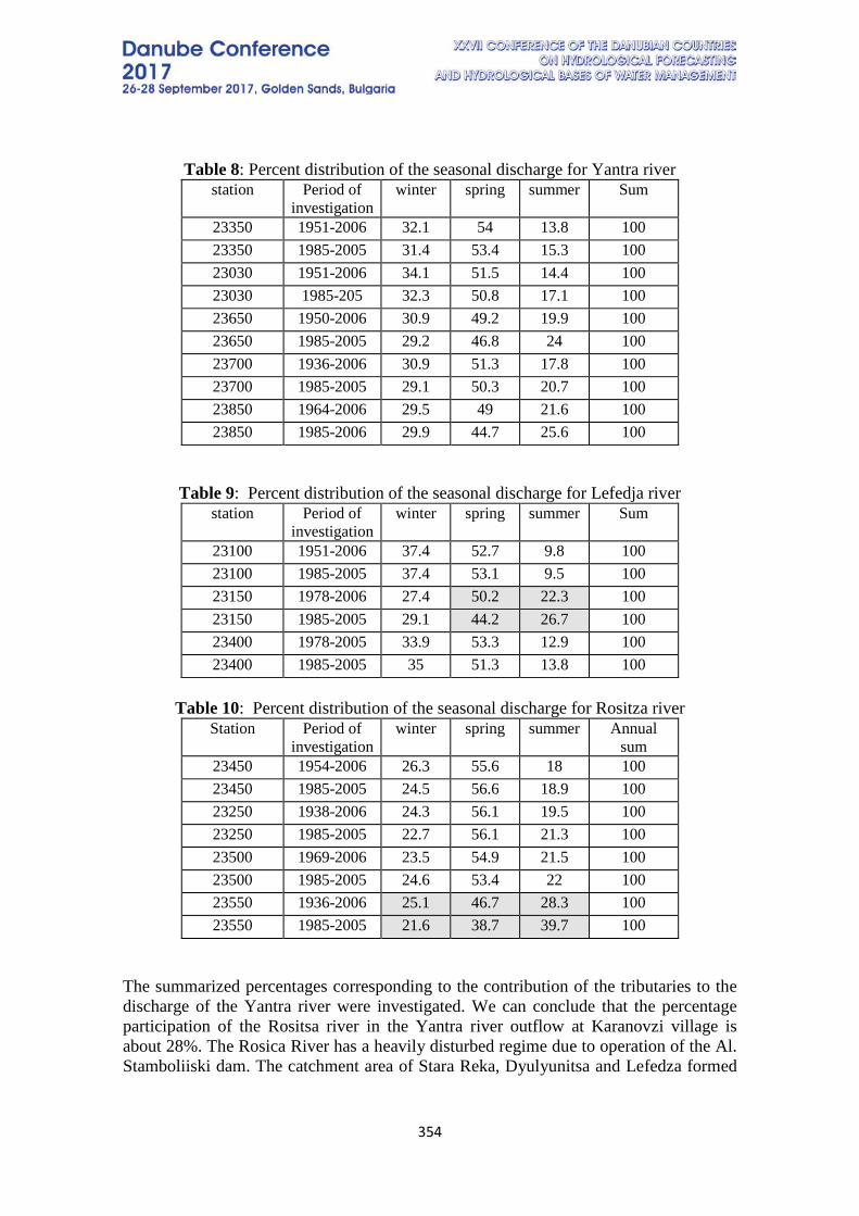
354

Table 8: Percent distribution of the seasonal discharge for Yantra river station Period of

investigation winter spring summer Sum

23350 1951-2006 32.1 54 13.8 100 23350 1985-2005 31.4 53.4 15.3 100 23030 1951-2006 34.1 51.5 14.4 100 23030 1985-205 32.3 50.8 17.1 100 23650 1950-2006 30.9 49.2 19.9 100 23650 1985-2005 29.2 46.8 24 100 23700 1936-2006 30.9 51.3 17.8 100 23700 1985-2005 29.1 50.3 20.7 100 23850 1964-2006 29.5 49 21.6 100 23850 1985-2006 29.9 44.7 25.6 100

Table 9: Percent distribution of the seasonal discharge for Lefedja river station Period of

investigation winter spring summer Sum

23100 1951-2006 37.4 52.7 9.8 100 23100 1985-2005 37.4 53.1 9.5 100 23150 1978-2006 27.4 50.2 22.3 100 23150 1985-2005 29.1 44.2 26.7 100 23400 1978-2005 33.9 53.3 12.9 100 23400 1985-2005 35 51.3 13.8 100

Table 10: Percent distribution of the seasonal discharge for Rositza river

Station Period of investigation

winter spring summer Annual sum

23450 1954-2006 26.3 55.6 18 100 23450 1985-2005 24.5 56.6 18.9 100 23250 1938-2006 24.3 56.1 19.5 100 23250 1985-2005 22.7 56.1 21.3 100 23500 1969-2006 23.5 54.9 21.5 100 23500 1985-2005 24.6 53.4 22 100 23550 1936-2006 25.1 46.7 28.3 100 23550 1985-2005 21.6 38.7 39.7 100

The summarized percentages corresponding to the contribution of the tributaries to the discharge of the Yantra river were investigated. We can conclude that the percentage participation of the Rositsa river in the Yantra river outflow at Karanovzi village is about 28%. The Rosica River has a heavily disturbed regime due to operation of the Al. Stamboliiski dam. The catchment area of Stara Reka, Dyulyunitsa and Lefedza formed

355

around 40% of Yantra river outfllow. About 25% is the outflow along the main Yantra River at Cholakovtsi station and the rivers Dryanovska and Belitsa.

CONCLUDING REMARKS

Inter-annual distribution of the Yantra river discharge was investigated. Yantra river basin is situated in North Bulgaria in temperate climate. Typical for this climate is resistant snow cover in the mountain parts during the winter mounts; rainfalls during the spring and beginning of the summer. The summer is characterized with intensive precipitations with short duration; drought conditions and maximum air temperatures.

For inter-annual distribution the monthly time step is used and two types of results were discussed: discharge layers (in mm) and percent distribution. It is possible to conclude that the peak flow of the Yantra River occurs during the period March – May. The obtained results clearly show the overall discharge flow decrease for all months in north-south direction along the main Yantra River. REFERENCES [1] Balabanova, Sn., Stoyanova, S. Integrated data collection and dissemination in North Bulgarian river basins – Open Water Symposium and workshops, Delft UNESCO-IHE 18-19 April, 2011 [2] Bojilova, E. Integrated river basin modelling, Bulgarian case study, HydroEco2006, Multidisciplinary conference, Karlovy Vary, Czech Republic, ISBN 80-903635-1-2, 187-190. DOI: 10.13140/2.1.1587.8404, 2006. [3] Bojilova, E. Upper Yantra River Basin Modeling, Bulgarian Journal of Meteorology & Hydrology (BJMH), Vol. 15, 2010, number 3, 93-104, ISSN 0861-0762, 2010.

[4] Bojilova, E. About the changes in the frequency of the maximum annual river discharges for two pilot watersheds in Bulgaria, BALKANERECO’2016, Vol. 9, 2016, №1, ISSN 1311-2783, 122-125, 2016.

[5] Bojilova, E. High flows in drainage basin of Yantra river, BALKANERECO’2016, Vol 9, 2016, №1, ISSN 1311-2783, 125-127, 2016.

[6] Karagiozova, Tz., Ninov, Pl., Rankova, M. Technology for determination of average annual resources of surface water bodies in Bulgaria, International Conference "Balkan Economic Reconstruction and Ecology - BALKANIREKO '16", April 7- 8; Ecology and Industry, ISSN 1311-2783, Publisher: Balkan Academy of Sciences and Culture, 2016

[7] Ninov Pl. Karagiozova Tz., Rankova M. – Water Resources Determination of Surface Water Bodies at the Bulgarian basin of the Lower Danube, Journal of the Geographical Institute “Jovan Cvijić” SASA, Vol 67, No 1, 2017

356

STOCHASTIC RAINFALL-RUNOFF MODELLING TO EVALUATE THE SPATIAL CONCURRENCE OF THE RUNOFF OF INN TRIBUTARIES

Jürgen Komma, Thomas Nester, Jose Luis Salinas, Günter Blöschl

Institute for Hydraulic and Water Resources Engineering /Vienna Technical University, Austria

Corresponding author: Thomas Nester, Karlsplatz 13/222, 1040 Vienna, Austria, nester@hydro.tuwien.ac.at

The study region is the Inn catchment from the Austrian-German border to the confluence of the Inn with the Danube in Passau. The Inn originates in the Swiss Alps and runs through Tyrol, before it enters Germany. At the Austrian-German border, the average runoff of the Inn is 305 m³/s, and the highest observed runoff is 2340 m³/s (2005); in Passau, the average runoff is 740 m³/s and the highest observed runoff is 6820 m³/s (2013). Major tributaries to the Inn in Germany are the Mangfall, Attel, Isen, Alz and Rott; major Austrian tributaries are the Salzach, Mattig, Antiesen and Pram. The topography of the Inn catchment ranges from 291 m a.s.l. in Passau to more than 4000 m a.s.l. in the Swiss Alps. The aim of the study is to evaluate the spatial concurrence of runoff in the Inn tributaries. This can be important for the design of flood retention basins, as a flood with a return period of e.g. 100 years at the Inn could be the result of the interaction of different tributaries. For instance, the origin of a 100 year flood at the Inn could be in Tyrol, but then it is not necessarily a 100 year flood in Passau. Or, the origin of a 100 year flood in Passau could be both the Inn and Salzburg tributaries where the return period could be smaller. To evaluate the effect of the spatial concurrence of river runoff, we used a stochastic precipitation model to generate a dataset of 10.000 years of hourly precipitation data. The precipitation model was calibrated on a set of around 900 precipitation stations and is able to reproduce the statistical properties and the spatial correlation structure of the observed precipitation. The generated precipitation is then used as driver for a distributed hydrological model (spatial scale 1x1 km, temporal scale 1 hour), calibrated on 35 years of observed runoff data of around 170 gauges. We use Monte Carlo simulations to generate 10.000 years of runoff data which eventually cover many different situations leading to a 100 year flood in Passau. The main outcome of the study is to get an overview of the spatial interplay of Inn tributaries and their contribution to extreme flood events to the Inn. Keywords: floods, retention, precipitation model, hydrological model, Monte Carlo

357

APPLICATION OF THE TOPKAPI MODEL ON THE OGOSTA RIVER BASIN

Valeriya Yordanova, Snezhanka Balabanova, Vesela Stoyanova National Institute of Meteorology and Hydrology at the Bulgarian Academy of Science,

Bulgaria

Corresponding author: Tzarigradsko chaussee 66, 1784 Sofia, Bulgaria, e-mails: Valeriya.Yordanova@meteo.bg ; Snezana.Balabanova@meteo.bg ; Vesela.Popova@meteo.bg

ABSTRACT The flood forecasting and warning systems are essential in regional and national strategies to protect the population and the infrastructure from flooding. Recently they are widely used as a tool in flood forecasting and to assist the decision makers to manage extreme events. The hydrological processes are very complex and the hydrological and hydraulic models are the main components in the flood forecasting and warning systems. They identify the dominant hydrological processes which influence the water balance and result in conditions of extreme water events. There are variety of hydrological models. Nowadays with the development of the automatic stations networks, the ability of satellite information, numerical weather prediction models with high resolution and digital spatial information for elevation data, soils and land cover the fully distributed hydrological models are broadly used in flood forecasting. In this study the physically-based and fully distributed hydrological TOPKAPI (TOPographic Kinematic APproximation and Integration) model is applied on Ogosta river basin. The model utilities three non-linear reservoir differential equations for the drainage in the soil, the overland flow on saturated or impervious soil, and the channel flow along the drainage network. The advantage of the model is that it is physically based and the model parameters can be directly obtained from the existing spatial datasets. Meteorological information for 21 stations and hydrological information for 10 stations are used to set up the model. The model is calibrated for 2009-2012 and validated for 2014 year. The years are selected after analysis of the rainfall and flow data. The data set includes periods with high waves and with flow data below long-term averages. After sensitive analysis the most sensitive parameters controlling the runoff production are obtain and applied in a model in order to minimize root mean square error (RMSE) objective function comparing modelled and observed discharges at a daily time step. Keywords: hydrology, flood forecast, fully distributed hydrological model, TOPKAPI, GIS

INTRODUCTION Floods are among the most devastating natural disasters and affect many regions around the world each year. Society is increasingly concerned about the potential impacts of climate change on floods occurrence and magnitude. Furthermore, flood risk is likely to increase in the future as a result of socio-economic changes, such as increasing population in the cities, river regulation measures, changes in land use and deforestation. Hydrologic flood forecasting models are a major part of a comprehensive early flood warning system [5]. One of the purposes in the current study is to use the fully distributed TOPKAPI (TOPographic Kinematic APproximation and Integration)

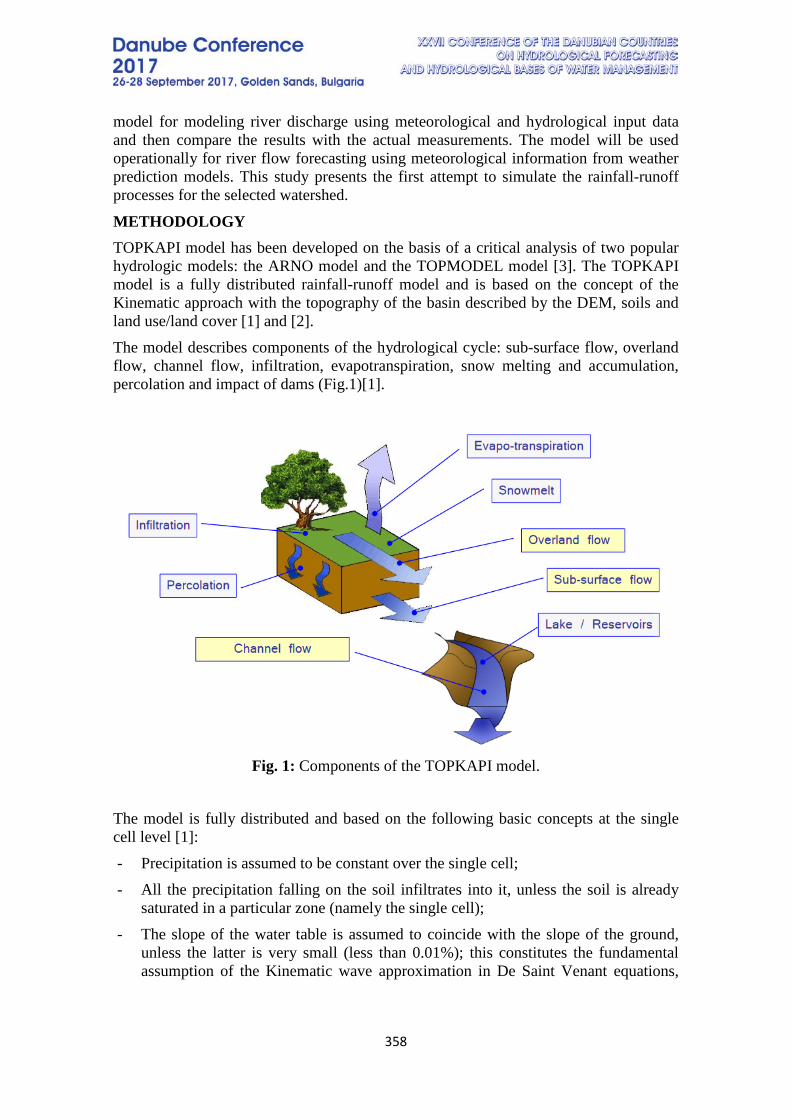
358

model for modeling river discharge using meteorological and hydrological input data and then compare the results with the actual measurements. The model will be used operationally for river flow forecasting using meteorological information from weather prediction models. This study presents the first attempt to simulate the rainfall-runoff processes for the selected watershed.

METHODOLOGY TOPKAPI model has been developed on the basis of a critical analysis of two popular hydrologic models: the ARNO model and the TOPMODEL model [3]. The TOPKAPI model is a fully distributed rainfall-runoff model and is based on the concept of the Kinematic approach with the topography of the basin described by the DEM, soils and land use/land cover [1] and [2]. The model describes components of the hydrological cycle: sub-surface flow, overland flow, channel flow, infiltration, evapotranspiration, snow melting and accumulation, percolation and impact of dams (Fig.1)[1].

Fig. 1: Components of the TOPKAPI model.

The model is fully distributed and based on the following basic concepts at the single cell level [1]: - Precipitation is assumed to be constant over the single cell; - All the precipitation falling on the soil infiltrates into it, unless the soil is already

saturated in a particular zone (namely the single cell); - The slope of the water table is assumed to coincide with the slope of the ground,

unless the latter is very small (less than 0.01%); this constitutes the fundamental assumption of the Kinematic wave approximation in De Saint Venant equations,

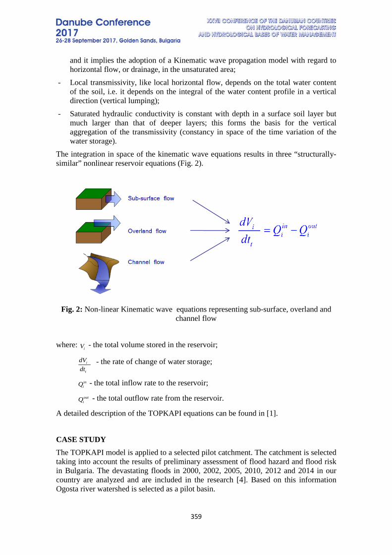
359

and it implies the adoption of a Kinematic wave propagation model with regard to horizontal flow, or drainage, in the unsaturated area;

- Local transmissivity, like local horizontal flow, depends on the total water content of the soil, i.e. it depends on the integral of the water content profile in a vertical direction (vertical lumping);

- Saturated hydraulic conductivity is constant with depth in a surface soil layer but much larger than that of deeper layers; this forms the basis for the vertical aggregation of the transmissivity (constancy in space of the time variation of the water storage).

The integration in space of the kinematic wave equations results in three “structurally-similar” nonlinear reservoir equations (Fig. 2).

Fig. 2: Non-linear Kinematic wave equations representing sub-surface, overland and

channel flow

where: - the total volume stored in the reservoir;

- the rate of change of water storage;

- the total inflow rate to the reservoir;

- the total outflow rate from the reservoir.

A detailed description of the TOPKAPI equations can be found in [1].

CASE STUDY The TOPKAPI model is applied to a selected pilot catchment. The catchment is selected taking into account the results of preliminary assessment of flood hazard and flood risk in Bulgaria. The devastating floods in 2000, 2002, 2005, 2010, 2012 and 2014 in our country are analyzed and are included in the research [4]. Based on this information Ogosta river watershed is selected as a pilot basin.

iV

i

t

dVdt

iniQ

outiQ

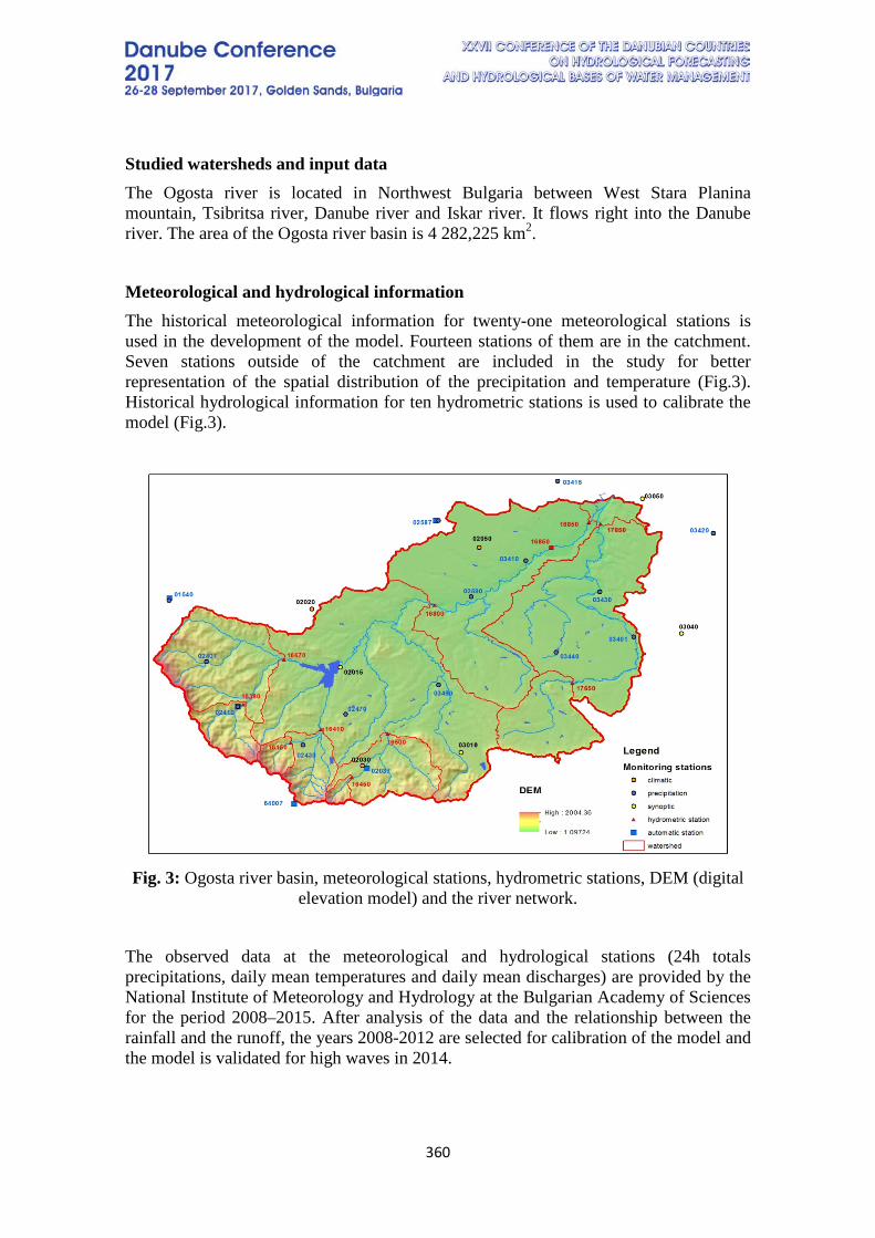
360

Studied watersheds and input data The Ogosta river is located in Northwest Bulgaria between West Stara Planina mountain, Tsibritsa river, Danube river and Iskar river. It flows right into the Danube river. The area of the Ogosta river basin is 4 282,225 km2.

Meteorological and hydrological information The historical meteorological information for twenty-one meteorological stations is used in the development of the model. Fourteen stations of them are in the catchment. Seven stations outside of the catchment are included in the study for better representation of the spatial distribution of the precipitation and temperature (Fig.3). Historical hydrological information for ten hydrometric stations is used to calibrate the model (Fig.3).

Fig. 3: Ogosta river basin, meteorological stations, hydrometric stations, DEM (digital

elevation model) and the river network.

The observed data at the meteorological and hydrological stations (24h totals precipitations, daily mean temperatures and daily mean discharges) are provided by the National Institute of Meteorology and Hydrology at the Bulgarian Academy of Sciences for the period 2008–2015. After analysis of the data and the relationship between the rainfall and the runoff, the years 2008-2012 are selected for calibration of the model and the model is validated for high waves in 2014.

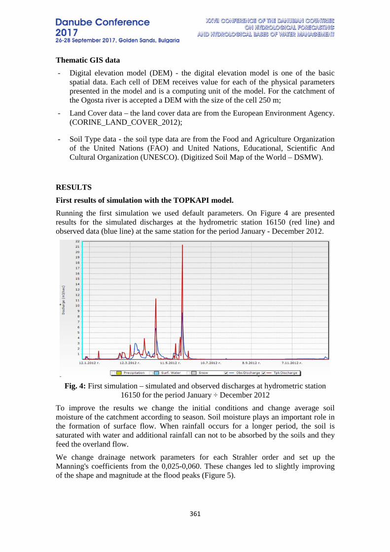
361

Thematic GIS data - Digital elevation model (DEM) - the digital elevation model is one of the basic

spatial data. Each cell of DEM receives value for each of the physical parameters presented in the model and is a computing unit of the model. For the catchment of the Ogosta river is accepted a DEM with the size of the cell 250 m;

- Land Cover data – the land cover data are from the European Environment Agency. (CORINE_LAND_COVER_2012);

- Soil Type data - the soil type data are from the Food and Agriculture Organization of the United Nations (FAO) and United Nations, Educational, Scientific And Cultural Organization (UNESCO). (Digitized Soil Map of the World – DSMW).

RESULTS First results of simulation with the TOPKAPI model. Running the first simulation we used default parameters. On Figure 4 are presented results for the simulated discharges at the hydrometric station 16150 (red line) and observed data (blue line) at the same station for the period January - December 2012.

Fig. 4: First simulation – simulated and observed discharges at hydrometric station

16150 for the period January ÷ December 2012 To improve the results we change the initial conditions and change average soil moisture of the catchment according to season. Soil moisture plays an important role in the formation of surface flow. When rainfall occurs for a longer period, the soil is saturated with water and additional rainfall can not to be absorbed by the soils and they feed the overland flow. We change drainage network parameters for each Strahler order and set up the Manning's coefficients from the 0,025-0,060. These changes led to slightly improving of the shape and magnitude at the flood peaks (Figure 5).

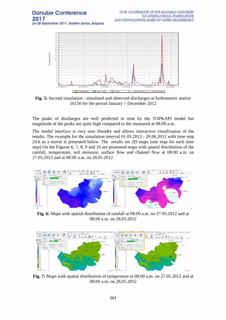
362

Fig. 5: Second simulation - simulated and observed discharges at hydrometric station

16150 for the period January ÷ December 2012 The peaks of discharges are well predicted in time by the TOPKAPI model but magnitude of the peaks are quite high compared to the measured at 08:00 a.m. The model interface is very user friendly and allows interactive visualization of the results. The example for the simulation interval 01.05.2012 - 20.06.2012 with time step 24 h as a movie is presented below. The results are 2D maps (one map for each time step) On the Figures 6, 7, 8, 9 and 10 are presented maps with spatial distribution of the rainfall, temperature, soil moisture, surface flow and channel flow at 08:00 a.m. on 27.05.2012 and at 08:00 a.m. on 28.05.2012.

Fig. 6: Maps with spatial distribution of rainfall at 08:00 a.m. on 27.05.2012 and at

08:00 a.m. on 28.05.2012

Fig. 7: Maps with spatial distribution of temperature at 08:00 a.m. on 27.05.2012 and at

08:00 a.m. on 28.05.2012

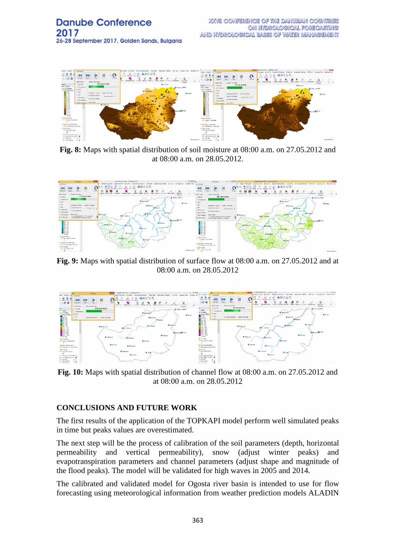
363

Fig. 8: Maps with spatial distribution of soil moisture at 08:00 a.m. on 27.05.2012 and

at 08:00 a.m. on 28.05.2012.

Fig. 9: Maps with spatial distribution of surface flow at 08:00 a.m. on 27.05.2012 and at

08:00 a.m. on 28.05.2012

Fig. 10: Maps with spatial distribution of channel flow at 08:00 a.m. on 27.05.2012 and

at 08:00 a.m. on 28.05.2012

CONCLUSIONS AND FUTURE WORK The first results of the application of the TOPKAPI model perform well simulated peaks in time but peaks values are overestimated. The next step will be the process of calibration of the soil parameters (depth, horizontal permeability and vertical permeability), snow (adjust winter peaks) and evapotranspiration parameters and channel parameters (adjust shape and magnitude of the flood peaks). The model will be validated for high waves in 2005 and 2014. The calibrated and validated model for Ogosta river basin is intended to use for flow forecasting using meteorological information from weather prediction models ALADIN

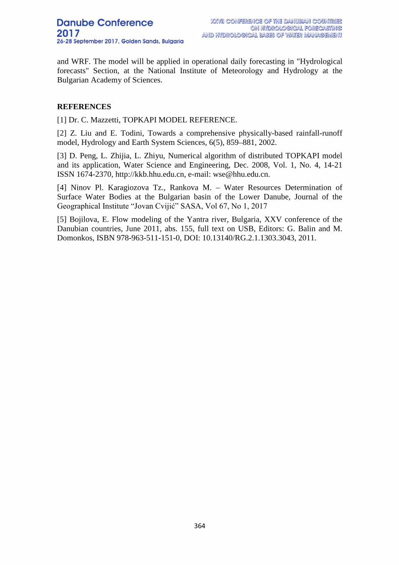
364

and WRF. The model will be applied in operational daily forecasting in "Hydrological forecasts" Section, at the National Institute of Meteorology and Hydrology at the Bulgarian Academy of Sciences.

REFERENCES [1] Dr. C. Mazzetti, TOPKAPI MODEL REFERENCE. [2] Z. Liu and E. Todini, Towards a comprehensive physically-based rainfall-runoff model, Hydrology and Earth System Sciences, 6(5), 859–881, 2002. [3] D. Peng, L. Zhijia, L. Zhiyu, Numerical algorithm of distributed TOPKAPI model and its application, Water Science and Engineering, Dec. 2008, Vol. 1, No. 4, 14-21 ISSN 1674-2370, http://kkb.hhu.edu.cn, e-mail: wse@hhu.edu.cn. [4] Ninov Pl. Karagiozova Tz., Rankova M. – Water Resources Determination of Surface Water Bodies at the Bulgarian basin of the Lower Danube, Journal of the Geographical Institute “Jovan Cvijić” SASA, Vol 67, No 1, 2017 [5] Bojilova, E. Flow modeling of the Yantra river, Bulgaria, XXV conference of the Danubian countries, June 2011, abs. 155, full text on USB, Editors: G. Balin and M. Domonkos, ISBN 978-963-511-151-0, DOI: 10.13140/RG.2.1.1303.3043, 2011.

365

ASSESSING RISKS AND COSTS OF CLIMATE CHANGE IMPACTS ON FLOODS AND DROUGHTS WITH THE FUTURE DANUBE MODEL

Fred Foko Hattermann1 , Stefan Liersch1, Michel Wortmann1, Stephen Hardwick2,

Kai Schröter3, Miklós Gyalai-Korpos4 1 Potsdam Institute for Climate Impact Research (PIK), Germany

2 Imperial College London, United Kingdom 3 German Research Centre for Geosciences GFZ, Germany

4 Pannon Pro Innovations Ltd, Hungary

Corresponding author: Fred F. Hattermann, Potsdam Institute for Climate Impact Research (PIK), 14473 Potsdam, Telegraphenberg A31, hattermann@pik-potsdam.de

ABSTRACT The Future Danube Model is a multi-hazard and risk model suite for the Danube region that is currently developed and consists of modules for estimating different perils such as heavy precipitation, heat waves, floods, and droughts under recent and future conditions considering climate change and possible adaptation measures. As a result, it provides spatially consistent information on extreme events and natural resources throughout the entire Danube catchment, which can be used to support the implementation of EU framework directives as well as for urban and land use planning, water resources management and climate proofing of large scale infrastructure planning. The Future Danube Model consists of the following five individual and exchangeable modules: A weather and climate module, a hydrological module, a risk module, an adaptation module, and a web-based visualization module. They are linked in such a way that output from one module can either be used standalone or fed into subsequent modules. The weather and climate module was used to produce long-term daily weather time series (10,000 years) statistically representing current and future climate conditions, for the historical period and two future periods. Based on these weather time series (all in all 200,000 years), the hydrological module was employed to simulate river discharges focusing on flood events and their return periods in more than 13,000 river reaches in the entire Danube catchment. The output of the hydrological module is used by the risk module which translates hydrological extremes into financial losses. 2D hydro-dynamic simulations are performed to derive inundation depth, return period and flow velocity maps as flood intensity metrics. Outputs of the risk module are loss estimates for damage to residential buildings within the inundated areas with quantitative information about the uncertainty associated with these results. A web-based Geographic Information System is used to visualise the simulation results. The utility of the tool is currently being tested by project partners and stakeholders in the pilot region Hungary. The first results indicate the potential for large shifts in flood return periods, i.e. higher order floods may occur more frequently. Keywords: Danube River basin, Flood risk, Flood return periods, Climate change

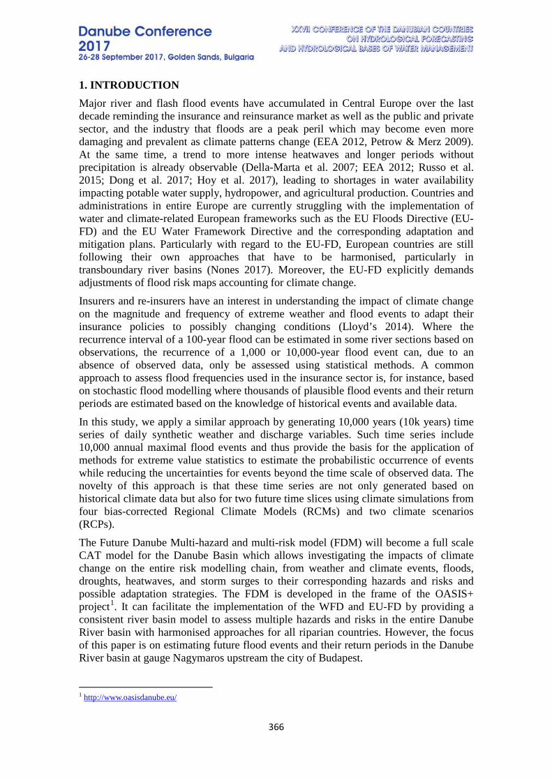
366

1. INTRODUCTION Major river and flash flood events have accumulated in Central Europe over the last decade reminding the insurance and reinsurance market as well as the public and private sector, and the industry that floods are a peak peril which may become even more damaging and prevalent as climate patterns change (EEA 2012, Petrow & Merz 2009). At the same time, a trend to more intense heatwaves and longer periods without precipitation is already observable (Della-Marta et al. 2007; EEA 2012; Russo et al. 2015; Dong et al. 2017; Hoy et al. 2017), leading to shortages in water availability impacting potable water supply, hydropower, and agricultural production. Countries and administrations in entire Europe are currently struggling with the implementation of water and climate-related European frameworks such as the EU Floods Directive (EU-FD) and the EU Water Framework Directive and the corresponding adaptation and mitigation plans. Particularly with regard to the EU-FD, European countries are still following their own approaches that have to be harmonised, particularly in transboundary river basins (Nones 2017). Moreover, the EU-FD explicitly demands adjustments of flood risk maps accounting for climate change. Insurers and re-insurers have an interest in understanding the impact of climate change on the magnitude and frequency of extreme weather and flood events to adapt their insurance policies to possibly changing conditions (Lloyd’s 2014). Where the recurrence interval of a 100-year flood can be estimated in some river sections based on observations, the recurrence of a 1,000 or 10,000-year flood event can, due to an absence of observed data, only be assessed using statistical methods. A common approach to assess flood frequencies used in the insurance sector is, for instance, based on stochastic flood modelling where thousands of plausible flood events and their return periods are estimated based on the knowledge of historical events and available data. In this study, we apply a similar approach by generating 10,000 years (10k years) time series of daily synthetic weather and discharge variables. Such time series include 10,000 annual maximal flood events and thus provide the basis for the application of methods for extreme value statistics to estimate the probabilistic occurrence of events while reducing the uncertainties for events beyond the time scale of observed data. The novelty of this approach is that these time series are not only generated based on historical climate data but also for two future time slices using climate simulations from four bias-corrected Regional Climate Models (RCMs) and two climate scenarios (RCPs). The Future Danube Multi-hazard and multi-risk model (FDM) will become a full scale CAT model for the Danube Basin which allows investigating the impacts of climate change on the entire risk modelling chain, from weather and climate events, floods, droughts, heatwaves, and storm surges to their corresponding hazards and risks and possible adaptation strategies. The FDM is developed in the frame of the OASIS+ project1. It can facilitate the implementation of the WFD and EU-FD by providing a consistent river basin model to assess multiple hazards and risks in the entire Danube River basin with harmonised approaches for all riparian countries. However, the focus of this paper is on estimating future flood events and their return periods in the Danube River basin at gauge Nagymaros upstream the city of Budapest.

1 http://www.oasisdanube.eu/

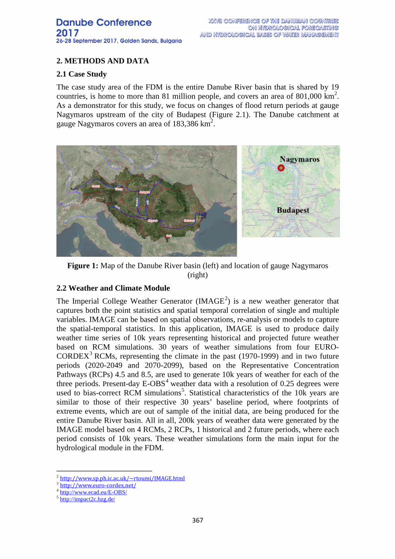
367

2. METHODS AND DATA 2.1 Case Study The case study area of the FDM is the entire Danube River basin that is shared by 19 countries, is home to more than 81 million people, and covers an area of 801,000 km2. As a demonstrator for this study, we focus on changes of flood return periods at gauge Nagymaros upstream of the city of Budapest (Figure 2.1). The Danube catchment at gauge Nagymaros covers an area of 183,386 km2.

Figure 1: Map of the Danube River basin (left) and location of gauge Nagymaros (right)

2.2 Weather and Climate Module The Imperial College Weather Generator (IMAGE2) is a new weather generator that captures both the point statistics and spatial temporal correlation of single and multiple variables. IMAGE can be based on spatial observations, re-analysis or models to capture the spatial-temporal statistics. In this application, IMAGE is used to produce daily weather time series of 10k years representing historical and projected future weather based on RCM simulations. 30 years of weather simulations from four EURO-CORDEX3 RCMs, representing the climate in the past (1970-1999) and in two future periods (2020-2049 and 2070-2099), based on the Representative Concentration Pathways (RCPs) 4.5 and 8.5, are used to generate 10k years of weather for each of the three periods. Present-day E-OBS4 weather data with a resolution of 0.25 degrees were used to bias-correct RCM simulations5. Statistical characteristics of the 10k years are similar to those of their respective 30 years’ baseline period, where footprints of extreme events, which are out of sample of the initial data, are being produced for the entire Danube River basin. All in all, 200k years of weather data were generated by the IMAGE model based on 4 RCMs, 2 RCPs, 1 historical and 2 future periods, where each period consists of 10k years. These weather simulations form the main input for the hydrological module in the FDM.

2 http://www.sp.ph.ic.ac.uk/~rtoumi/IMAGE.html 3 http://www.euro-cordex.net/ 4 http://www.ecad.eu/E-OBS/ 5 http://impact2c.hzg.de/

368

The IMAGE weather generator is not limited to generate weather variables at the daily time step but can also be employed to generate sub-hourly time series. Such generated data would be useful to study projected changes of pluvial flood events, which are particularly relevant for the city of Budapest where such events occur frequently (e.g. in May 2017). The requirements are available high-resolution weather observations serving as input to the weather generator.

2.3 Hydrological Module The Soil and Water Integrated Model (SWIM), is an eco-hydrological model that was developed at PIK Potsdam (Krysanova et al. 2005) to investigate impacts of climate, land use, and water management (reservoirs and irrigation) changes on the catchment hydrology (including floods and droughts) and vegetation processes (e.g. crop yields) at the regional scale. It is a spatially semi-distributed model that operates at the daily time step. In the FDM, the hydrological module creates the link between the weather/climate (IMAGE) and the risk modules. The SWIM model was set up to the entire Danube River basin with a spatially very detailed resolution represented by about 14,000 subbasins and 190,000 hydrological response units. This high-resolution model enables us to zoom into any location of interest, like small tributaries. The 200k years of weather data generated by IMAGE, serve as input to SWIM to simulate daily discharges and to investigate the impacts of climate change on hydrological parameters such as future flood and drought return periods and average seasonal or annual discharge patterns.

2.4 Risk Module The purpose of the risk module is to translate the flood events, simulated by the hydrological module, into inundation depths maps and to apply probabilistic, multi-variable damage functions to estimate flood losses and damages to residential buildings and private households. Even though the estimation of flood loss is very sensitive to the choice of the vulnerability model, the standard approach to loss estimation is normally based on highly simplified functions which relate the damage for the element at risk to inundation depth. The reliability of flood loss estimates can be increased if probabilistic modelling approaches are applied which inherently provide information about the uncertainty associated with loss estimates as an important basis for informed decision making (Schröter et al. 2014). The damage models use multiple variables to explain flood loss including information about buildings types, building characteristics, flood experience, precaution and other factors to characterize building resistance. The approach is based on Bayesian networks which enable the inference of the complete probability density of flood damage losses and hence inherently provide damage estimates with uncertainty bounds. This probabilistic approach enables the estimation of flood losses even with incomplete and particularly considering uncertain observations. Inundation depth is a key input variable to flood loss models. The transformation of hydrological flows available from the Hydrological module (current and future simulations) are transformed into water levels and inundation depth maps using GIS techniques at larger scales or a non-stationary 2D hydrodynamic model at smaller scales (Falter et al. 2015).

369

2.5 Adaptation Module Well-planned adaptation measures can help prevent or reduce the adverse effects (economic losses, damage to infrastructure, lives lost) of weather related hazards that are likely to be exacerbated by climate change. Decisions on adaptation are inherently based on knowledge about climate risks i.e. the probability of specific hazards and their expected impacts. Likewise, appropriate adaptation may allow populations to benefit from potential opportunities of climate change. Robust adaptation decisions are generally obtained by considering the benefits and costs i.e. the potential reduction of risks or losses associated with a specific adaptation vs. the costs incurred by installing these adaptive measures e.g. flood protection, changed management strategies, etc. The adaptation assessment, which often takes the form of a cost-benefit analysis, confronts the costs (or risks) related to the impacts of a future climate scenario with "no adaptation" installed with the situation where adaptation is present i.e. the damages avoided by implementing relevant adaptation measures while taking into account the costs incurred by installing the adaptation(s). Interaction with stakeholders is crucial to establish which adaptation measures are to be considered, data needs, the local decision-making context, and realistic values with respect to costs and (co-)benefits. The adaptation module relies primarily on a dedicated cost-benefit tool, however, depending on the specific stakeholder framing, a suite of additional tools will be available.

2.6 GIS Module Internet-based open Geographic Information Systems (GIS) technology integrating OpenStreetMap data is used to visualize and graphically overlay and analyse the perils and other spatial information such as population density or assets. The approach enables user interaction with maps and other results using the default web browser and without having to install additional GIS software. The tool is already under construction and data uploading is possible6. The results can be visualized for larger parts of the basin or for smaller areas such as municipalities, districts, river sections, sub-regions etc. Some results of the Hydrological and Meteorological and Climate modules will be available for the entire basin and its sub-regions ready for visualisation and analysis, while more specific evaluations e.g. of flash floods in cities will only be available for selected stakeholders commissioning a specific investigation, in a pilot this will be done for the Municipality of Budapest.

3. RESULTS As an example to demonstrate the results of the hydrological model of the FDM, flood return periods at gauge Nagymaros (upstream Budapest) were calculated based on the 10k years weather time series, produced by the IMAGE weather generator. Figure 3.1 shows return periods of annual maximal discharge peaks (AMAX) based on E-OBS (historical), and the multi-model mean of four CORDEX RCMs for the historical and two future periods and two climate scenarios (RCP 4.5 left and RCP 8.5 right). Instead of estimating the return periods based on an extreme value distribution function, an empirical approach was used, because the time series consist of 10k AMAX values

6 http://www.pik-potsdam.de/~wortmann/swimdanube/

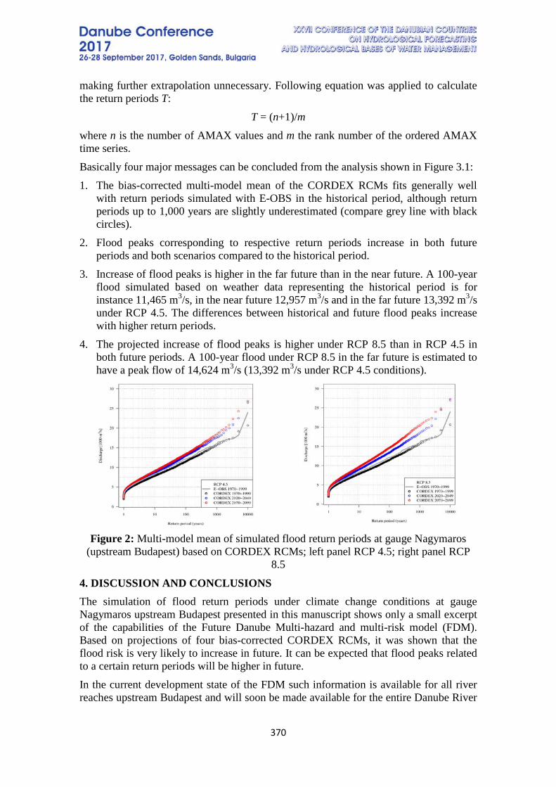
370

making further extrapolation unnecessary. Following equation was applied to calculate the return periods T:

T = (n+1)/m where n is the number of AMAX values and m the rank number of the ordered AMAX time series. Basically four major messages can be concluded from the analysis shown in Figure 3.1: 1. The bias-corrected multi-model mean of the CORDEX RCMs fits generally well

with return periods simulated with E-OBS in the historical period, although return periods up to 1,000 years are slightly underestimated (compare grey line with black circles).

2. Flood peaks corresponding to respective return periods increase in both future periods and both scenarios compared to the historical period.

3. Increase of flood peaks is higher in the far future than in the near future. A 100-year flood simulated based on weather data representing the historical period is for instance 11,465 m3/s, in the near future 12,957 m3/s and in the far future 13,392 m3/s under RCP 4.5. The differences between historical and future flood peaks increase with higher return periods.

4. The projected increase of flood peaks is higher under RCP 8.5 than in RCP 4.5 in both future periods. A 100-year flood under RCP 8.5 in the far future is estimated to have a peak flow of 14,624 m3/s (13,392 m3/s under RCP 4.5 conditions).

Figure 2: Multi-model mean of simulated flood return periods at gauge Nagymaros

(upstream Budapest) based on CORDEX RCMs; left panel RCP 4.5; right panel RCP 8.5

4. DISCUSSION AND CONCLUSIONS The simulation of flood return periods under climate change conditions at gauge Nagymaros upstream Budapest presented in this manuscript shows only a small excerpt of the capabilities of the Future Danube Multi-hazard and multi-risk model (FDM). Based on projections of four bias-corrected CORDEX RCMs, it was shown that the flood risk is very likely to increase in future. It can be expected that flood peaks related to a certain return periods will be higher in future. In the current development state of the FDM such information is available for all river reaches upstream Budapest and will soon be made available for the entire Danube River

371

basin. 10k years of weather and climate projection data are already available for the entire basin at a resolution of 0.25 degrees and flood maps were produced by the risk module for the German part of the Danube basin. However, the full potential of the FDM is much larger than demonstrated here and unfolds in the interplay of its modules. Due to the holistic and harmonised approach of simulating and integrating climate change and its impacts on various sectors in the entire Danube River basin, the FDM is a valuable tool for integrated and transboundary river basin planning and management, particularly with regard to European climate and water-related directives. An important aspect driving the development of the FDM is the close collaboration with stakeholders. User demands have shaped and will influence future developments. So far, the main aim of the FDM was to satisfy the demands of the insurance sector by providing information related to climate change impacts on flood risks. The results produced with the FDM are in compliance with and will be used within the OASIS Loss Modelling Framework7 and will be made available using the OASIS Hub8. Different data licence models will allow accessing the data either free of charge or for a fee, depending on the dataset, the business model, and the type of customer requesting the data.

5. REFERENCES Della-Marta, P. M.; Haylock, M. R.; Luterbacher, J. & Wanner, H. Doubled length of western European summer heat waves since 1880 Journal of Geophysical Research: Atmospheres, vol. 112, 2007.

Dong, B., Sutton, R. T. & Shaffrey, L. Understanding the rapid summer warming and changes in temperature extremes since the mid-1990s over Western Europe Climate Dynamics, 48, pp 1537-1554, 2017.

EEA 2012. Climate change, impacts and vulnerability in Europe 2012. An indicator-based report. EEA Report No 12/2012.

Falter, D., Schröter, K., Dung, N. V., Vorogushyn, S., Kreibich, H., Hundecha, Y., Apel, H. and Merz, B.: Spatially coherent flood risk assessment based on long-term continuous simulation with a coupled model chain, Journal of Hydrology, 524, 182–193, doi:10.1016/j.jhydrol.2015.02.021, 2015.

Hoy, A., Hänsel, S., Skalak, P., Ustrnul, Z. & Bochníček, O. The extreme European summer of 2015 in a long-term perspective International Journal of Climatology, John Wiley & Sons, Ltd, 37, pp 943-962, 2017.

Krysanova, V., Hattermann, F. & Wechsung, F. Development of the ecohydrological model SWIM for regional impact studies and vulnerability assessment. Hydrological Processes, 19, pp 763-783, 2005.

Lloyd’s. Catastrophy modeling and climate change. 2014.

Nones, M. Flood hazard maps in the European context. Water International, 42, pp 324-332, 2017.

Petrow, T. & Merz, B. Trends in flood magnitude, frequency and seasonality in Germany in the period 1951–2002. Journal of Hydrology, 371, pp 129 – 141, 2009.

Russo,S., Sillmann J., & Fischer, E.M. Top ten European heatwaves since 1950 and their occurrence in the coming decades. Environmental Research Letters, 10, 2015.

Schröter, K., Kreibich, H., Vogel, K., Riggelsen, C., Scherbaum, F. and Merz, B.: How useful are complex flood damage models?, Water Resour. Res., 50(4), 3378–3395, doi:10.1002/2013WR014396, 2014.

7 www.oasislmf.org/ 8 https://oasishub.co/

372

FLOOD VULNERABLE AREAS IN SLOVAKIA BASED ON MULTICRITERIA ANALYSIS

Martina Zeleňáková, Peter Blišťan, Pavol Purcz

Technical University of Košice, Slovakia

Corresponding author: Martina Zeleňáková, Technical University of Košice, Vysokoškolská 4, martina.zelenakova@tuke.sk

Flood vulnerability is a common effect of two independent mechanisms natural conditions and the human activities in the basin. The primary impulses of floods are usually extremely intense precipitation. The total catchment’s hydrological response to intense rainfall is determined by its natural environment, a whole complex of characteristics of the basin. The aim of the present study is to generate a composite map for decision makers using selected factors causing floods. In the analyses, some of the causative factors for flooding in a basin area are taken into account, such as precipitation, geology, land use, size of the catchment and basin slope. A case study of flood vulnerability identification in catchments’ areas in Slovakia is employed to illustrate the different approaches. A geographical information system is integrated with multicriteria analysis in the paper. We created two multicriteria vulnerability maps for Slovakia. Our pilot study showed significant differences between both methods – Ranking method and Analytical Hierarchy Process. The different results obtained from these two methods indicate the importance of the decision maker in determining the weights and the proper method, and making the decision. The weighting of the criteria significantly affects the results of the overall evaluation. Keywords: geographical information system, flood risk, multicriteria analysis

373

TOPIC 4: DISASTER EVENTS

REGIONALIZATION APPROACH FOR DETERMINATION OF SPECIFIC WATER QUANTITIES FOR ARDA AND BYALA RIVERS IN BULGARIA - AT

LOW, MEDIUM AND HIGH WATER LEVELS

Radoslava Ivanova National Institute of Meteorology and Hydrology – BAS, Sofia, Bulgaria

Corresponding author: National Institute of Meteorology and Hydrology, Sofia, Bulgaria, Tzarigradsko chaussee 66, 1784 Sofia, Bulgaria e-mails:

Radoslava.ivanova@meteo.bg

ABSTRACT The statistical characteristics of the runoff, such as mean, minimum and maximum river discharges, are used for various purposes, including hydro-technical design, flood control and water management. These assessments need often to be implemented in areas where observation data are not available. In these cases the transfer of information from observed to non-observed sections is usually done with regression equations. The article summarizes the results of several applied scientific tasks developed in the National Institute of Meteorology and Hydrology (NIMH) and related to the implementation of the regionalization approach for transfer of information through regression equations. The regionalization approach is based on the correlation between measured water flows and the orographic characteristics of their catchments. The article reviews the results of the methodology for regionalization and transfer of information applied by the author to Arda and Byala catchments for minimum, mean and maximum river discharges. Based on the established regional relationships the studied basins are grouped into homogeneous hydrological regions. The grouping is performed according to the following characteristics: minimum monthly mean discharge with 95% probability of exceedance, mean annual river discharge for multi-annual period of observation and maximum river discharge with 5%, 1% and 0.1% probability of exceedance. Keywords: regionalization, regional relationships, low, average and high water

1. INTRODUCTION The present study on the characteristic water flows for the Arda and the Byala river basins have been implemented in the framework of several applied scientific projects developed by the National Institute of Meteorology and Hydrology – BAS [7, 8, 9, 10, 11]. These projects are intended to support water management in the country, environment protection and disaster struggle at national and regional level by the Ministry of Environment and Waters and the Basin Directorates. The scale of the studies is the territory of the whole country or only the East Aegean River Basin District

374

[7]. To determine different water flows in the three above-mentioned investigations has been applied a regionalization approach and transfer of information by regression equations. This paper summarizes the research carried out and summarizes the results obtained by the author for the Arda and the Byala basins in the framework of the above-mentioned national tasks.

2. SUBJECT OF THE RESEARCH The Arda and the Byala rivers are part of the East Aegean Basin District (Fig.1).

Fig. 1: Map of the East Aegean region with the basins of the Arda and the Byala rivers,

with landed HMStations

The Arda river is the largest Rodopean river and one of Maritsa's biggest tributaries. The area of its catchment area to the border is 5213 km2. Although there is a typical mountain character, Arda river has a small average slope of 5.8 ‰ and a relatively large coefficient of curvature - 1.9. The density of the river network is 1.32 km / km2. Into the Arda river inflow 25 tributaries; more important of them are: Varbitsa river - with catchment area of 1203 km2; Krumovitsa river - area 671 km2 and others. The average slope for the tributaries of Arda is between 11 ‰ (Varbitsa River) and 78 ‰ (Chereshovska River). The density of the river network varies between 0.71 km / km2 (Kulidjiiska River) and 3.41 km / km2 (Uvadjik River). In the basin of the Arda river is built a “Dolna Arda” Cascade with several big dams: Studen Kladenets dam, Kardjali dam and Ivaylovgrad dam. The Byala river has a relatively small area (594 km2), the river leaving the territory of the country alone and in this sense it is “a single basin”. The climatic characteristics of the Arda and the Byala rivers define them as a part of the Continental-Mediterranean area where the winter is comparatively softer and the summer is warmer. The altitude there is smaller and the river valleys offer an easy way to the warmer air from the south.

375

On the territory of the Arda and Byala water catchments there are a total of 11 hydrometric stations: HMS №61050 - Byala Reka in Bostina; HMS №61330 - Elhovska reka near Rudozem; HMS №61350 - Cherna Reka near Turunr; HMS №61400 - Malka Arda near Banite; HMS №61450 - Varbitsa river near Vurley Dol; HMS №61500 - Varbitsa river near Jebel; HMS №61510 – Perperek river near Svatbare; HMS №61550 - Krumovitsa river near Krumovgrad; HMS №61650 - Arda river near Rudozem; HMS №61700 - Arda river at Vehtino; HMS №62800 - Byala river near Dolno Lukovo. Hydrometric stations on the Arda river are concentrated mainly at the upper part of the watershed. Three of them are located along its main right tributaries - Varbitsa and Krumovitsa and one of them at its left tributary river Perperek. In the basin of the Byala river the runoff is registered only in one hydrometric station.

3. METHODOLOGICAL APPROACH In the world practice there are two basic methodological approaches for determining water flows in not covered areas with monitoring network: regionalization of characteristic water flows depending on the physical geographic factors and the balance approach. The balance approach requires a huge amount of information related to the water usage of different kinds (water supply, irrigation, abstraction, etc.), the accumulation of water from reservoirs and their transfer etc. This information mentioned above is often missing or is not reliable [2, 3, 4, 5, 6]. In the present study the determination of minimum, mean and maximum water flows a regionalization approach was applied on the basis of the recorded flows in the hydrometric stations of the observation network to NIMH-BAS and transfer of information using regional relationships (regression equations). The identification to homogenous regions is determined by the correlation between the some characteristic water flows and the area of their catchment areas. There are numerous reasons why the catchment area is a good predictor. The characteristics of topography, ‘behaviour’ of river system and hydrological processes after increasing the catchment area. For example high mountains have steep slopes and a very quick formation of the run-off while in the plain watersheds, ordinarily bigger, dominates the influence of groundwater. These plain watersheds have large terraces and the floods could be frequent events. That means the catchment area reflects the run-off formation conditions [2, 3, 4, 5, 6]. Depending on the climatic, topographic and physico-geographic features of the catchments in the construction of regional correlation relationships can be included adjacent watersheds with similar hydrological conditions. On the other hand, especially for the conditions in Bulgaria where rivers usually spring in mountainous areas, their lower areas are flat with different hydrological conditions. The definition of homogeneous hydrological areas requires the creation of several regional correlation links within a one single catchment. In absence of regional relationships in some area or in the presence of too few observation stations the method of analogy is used to determine the water flows and the exact transfer of the specific flows from the point of measurement to the not observed stretches.

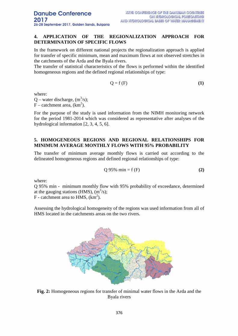
376

4. APPLICATION OF THE REGIONALIZATION APPROACH FOR DETERMINATION OF SPECIFIC FLOWS In the framework on different national projects the regionalization approach is applied for transfer of specific minimum, mean and maximum flows at not observed stretches in the catchments of the Arda and the Byala rivers. The transfer of statistical characteristics of the flows is performed within the identified homogeneous regions and the defined regional relationships of type: Q = f (F) (1) where: Q – water discharge, (m3/s); F – catchment area, (km2). For the purpose of the study is used information from the NIMH monitoring network for the period 1981-2014 which was considered as representative after analyses of the hydrological information [2, 3, 4, 5, 6].

5. HOMOGENEOUS REGIONS AND REGIONAL RELATIONSHIPS FOR MINIMUM AVERAGE MONTHLY FLOWS WITH 95% PROBABILITY The transfer of minimum average monthly flows is carried out according to the delineated homogeneous regions and defined regional relationships of type:

Q 95% min = f (F) (2) where: Q 95% min - minimum monthly flow with 95% probability of exceedance, determined at the gauging stations (HMS), (m3/s); F - catchment area to HMS, (km2). Assessing the hydrological homogeneity of the regions was used information from all of HMS located in the catchments areas on the two rivers.

Fig. 2: Homogeneous regions for transfer of minimal water flows in the Arda and the

Byala rivers

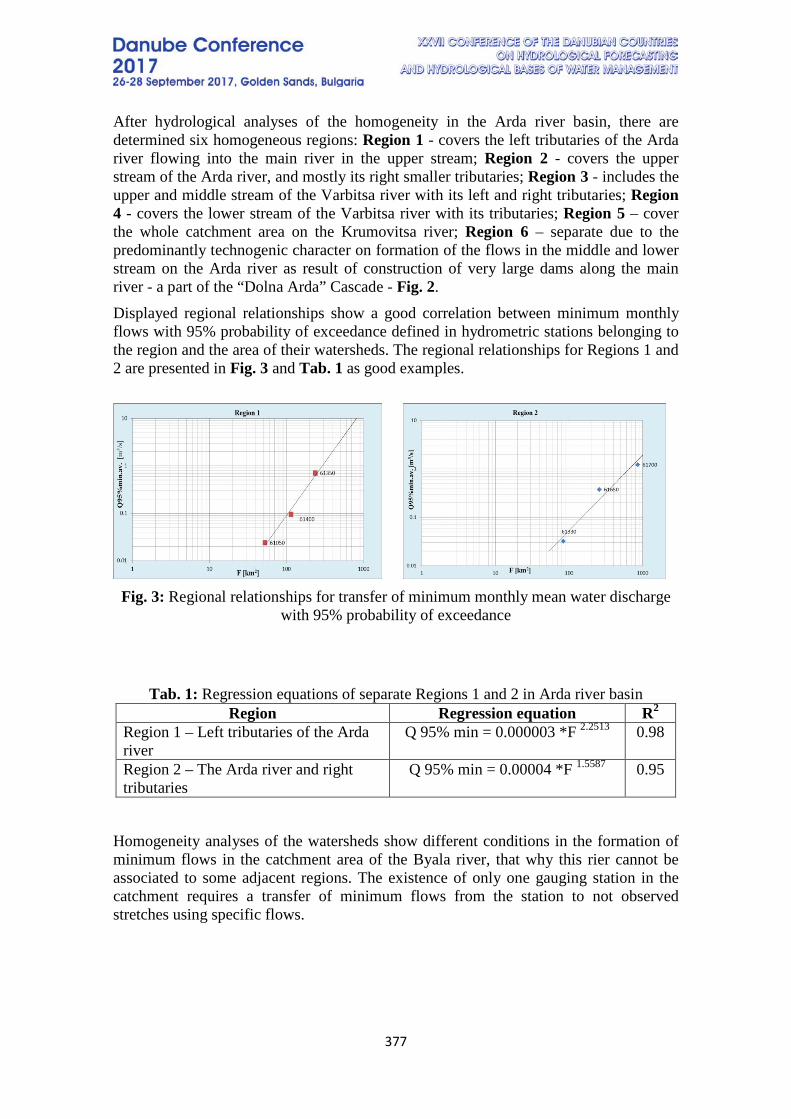
377

After hydrological analyses of the homogeneity in the Arda river basin, there are determined six homogeneous regions: Region 1 - covers the left tributaries of the Arda river flowing into the main river in the upper stream; Region 2 - covers the upper stream of the Arda river, and mostly its right smaller tributaries; Region 3 - includes the upper and middle stream of the Varbitsa river with its left and right tributaries; Region 4 - covers the lower stream of the Varbitsa river with its tributaries; Region 5 – cover the whole catchment area on the Krumovitsa river; Region 6 – separate due to the predominantly technogenic character on formation of the flows in the middle and lower stream on the Arda river as result of construction of very large dams along the main river - a part of the “Dolna Arda” Cascade - Fig. 2. Displayed regional relationships show a good correlation between minimum monthly flows with 95% probability of exceedance defined in hydrometric stations belonging to the region and the area of their watersheds. The regional relationships for Regions 1 and 2 are presented in Fig. 3 and Tab. 1 as good examples.

Fig. 3: Regional relationships for transfer of minimum monthly mean water discharge

with 95% probability of exceedance

Tab. 1: Regression equations of separate Regions 1 and 2 in Arda river basin

Region Regression equation R2 Region 1 – Left tributaries of the Arda river

Q 95% min = 0.000003 *F 2.2513 0.98

Region 2 – The Arda river and right tributaries

Q 95% min = 0.00004 *F 1.5587 0.95

Homogeneity analyses of the watersheds show different conditions in the formation of minimum flows in the catchment area of the Byala river, that why this rier cannot be associated to some adjacent regions. The existence of only one gauging station in the catchment requires a transfer of minimum flows from the station to not observed stretches using specific flows.

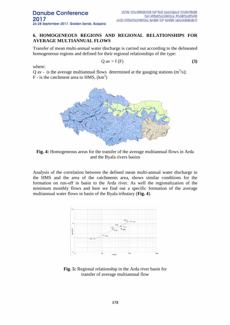
378

6. HOMOGENEOUS REGIONS AND REGIONAL RELATIONSHIPS FOR AVERAGE MULTIANNUAL FLOWS Transfer of mean multi-annual water discharge is carried out according to the delineated homogeneous regions and defined for their regional relationships of the type:

Q av = f (F) (3) where: Q av - is the average multiannual flows determined at the gauging stations (m3/s); F - is the catchment area to HMS, (km2)

Fig. 4: Homogeneous areas for the transfer of the average multiannual flows in Arda

and the Byala rivers basins

Analysis of the correlation between the defined mean multi-annual water discharge in the HMS and the area of the catchments area, shows similar conditions for the formation on run-off in basin to the Arda river. As well the regionalization of the minimum monthly flows and here we find out a specific formation of the average multiannual water flows in basin of the Byala tributary (Fig. 4).

Fig. 5: Regional relationship in the Arda river basin for transfer of average multiannual flow

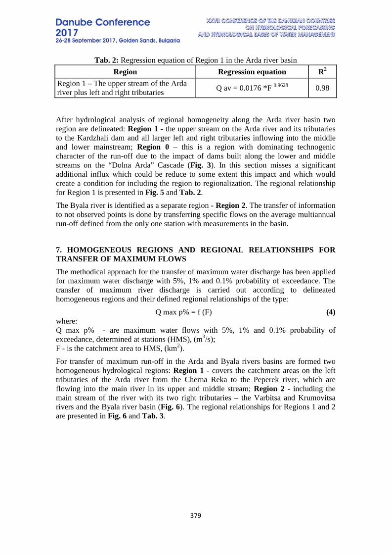
379

Tab. 2: Regression equation of Region 1 in the Arda river basin Region Regression equation R2

Region 1 – The upper stream of the Arda river plus left and right tributaries Q av = 0.0176 *F 0.9628 0.98

After hydrological analysis of regional homogeneity along the Arda river basin two region are delineated: Region 1 - the upper stream on the Arda river and its tributaries to the Kardzhali dam and all larger left and right tributaries inflowing into the middle and lower mainstream; Region 0 – this is a region with dominating technogenic character of the run-off due to the impact of dams built along the lower and middle streams on the “Dolna Arda” Cascade (Fig. 3). In this section misses a significant additional influx which could be reduce to some extent this impact and which would create a condition for including the region to regionalization. The regional relationship for Region 1 is presented in Fig. 5 and Tab. 2. The Byala river is identified as a separate region - Region 2. The transfer of information to not observed points is done by transferring specific flows on the average multiannual run-off defined from the only one station with measurements in the basin.

7. HOMOGENEOUS REGIONS AND REGIONAL RELATIONSHIPS FOR TRANSFER OF MAXIMUM FLOWS The methodical approach for the transfer of maximum water discharge has been applied for maximum water discharge with 5%, 1% and 0.1% probability of exceedance. The transfer of maximum river discharge is carried out according to delineated homogeneous regions and their defined regional relationships of the type:

Q max p% = f (F) (4) where: Q max p% - are maximum water flows with 5%, 1% and 0.1% probability of exceedance, determined at stations (HMS), (m3/s); F - is the catchment area to HMS, (km2). For transfer of maximum run-off in the Arda and Byala rivers basins are formed two homogeneous hydrological regions: Region 1 - covers the catchment areas on the left tributaries of the Arda river from the Cherna Reka to the Peperek river, which are flowing into the main river in its upper and middle stream; Region 2 - including the main stream of the river with its two right tributaries – the Varbitsa and Krumovitsa rivers and the Byala river basin (Fig. 6). The regional relationships for Regions 1 and 2 are presented in Fig. 6 and Tab. 3.

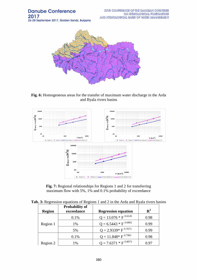
380

Fig. 6: Homogeneous areas for the transfer of maximum water discharge in the Arda

and Byala rivers basins

Fig. 7: Regional relationships for Regions 1 and 2 for transferring maximum flow with 5%, 1% and 0.1% probability of exceedance

Tab. 3: Regression equations of Regions 1 and 2 in the Arda and Byala rivers basins

Region Probability of

exceedance Regression equation R2 0.1% Q = 13.076 * F 0.6145 0.98

Region 1 1% Q = 6.5443 * F 0.6802 0.99 5% Q = 2.9339* F 0.7673 0.99 0.1% Q = 11.848* F 0.7901 0.98

Region 2 1% Q = 7.6371 * F 0.8073 0.97

10

100

1000

10000

10 100 1000F (km2)

Q ma

x p =

0.1% (

m3 /s)

Region 1 Region 2 Power (Region 1) Power (Region 2)

10

100

1000

10000

10 100 1000F (km2)

Q ma

x p =

1% (m

3 /s)

Region1 Region 2 Power (Region1) Power (Region 2)

10

100

1000

10000

10 100 1000F (km2)

Q ma

x p =

5% (m

3 /s)

Region 1 Region 2 Power (Region 1) Power (Region 2)

381

Region Probability of

exceedance Regression equation R2 5% Q = 4.8454 * F 0.8278 0.96

5. COMPARATIVE ANALYSIS AND RATING The results of implementation to presented regionalization approach for a wide range of multiannual characteristics of flows show the spatial variability of homogeneous hydrological areas within studied catchments for different characteristic water discharge. The highest homogeneity on hydrological processes is revealed at the regionalization of minimum monthly flows where six homogeneous regions are delineated in the Arda and Byala catchments. It is assumed that this homogeneity is mainly a result of the local anthropogenic impacts which in the highest degree reflect the run-off during periods of low water. In the regionalization of average multiannual flows there exists an uniformity in run-off formation processes on the mainstream and its tributaries outside a lower region where technogenic flows are dominant. Again we find out specificity in the formation of average multiannual run-off in the Byala river basin delineated as a single region. The presented results from applied regionalization approach, based on the presumption the catchment area is the most important factor reflecting on the run-off formation, confirm a good correlation between multiannual characteristics of flows measured in hydrometric stations and the accepted catchment area as a holistic predictor of the watersheds in the delineated homogeneous regions.

6. CONCLUSIONS The presented hydrological research summarizes the results of applied by author well-known methodology for regionalization and transfer of information in the Arda and Byala rivers basins for specific minimum, mean and maximum flows. Creative applications by the author of an uunified regionalization approach for the transfer of statistical hydrological information over a wide quantitative range, illustrates the changes in behavior of the river system and hydrological processes into formation of minimal, mean and maximum run-off. The presented results have an applied and scientific significance for engineering design activities as well as for a large scope of practices related to the protection of environment, prevention activities for water protection and struggle with disasters.

7. REFERENCES [1] Geoghraphy of Bulgaria, monograph, Bulgaria, Dr. Boris Todorov Kolev and

collective from the Bulgarian Academy of Sciences, 2002 [2] Plamen Ninov, Tzviatka Karagiozova, Technological Approach to determine the

water resources of river water bodies - using hydrological monitoring network, Hydrological International Scientific Conference „Adaptation to climate change, from source to river basin”, Bucharest, 2014.

382

[3] Tzviatka Karagiozova, Plamen Ninov, Maya Rankova, Technology for determination of average annual resources of surface water bodies in Bulgaria, International Conference "Balkan Economic Reconstruction and Ecology - BALKANIREKO '16", Ecology and Industry, ISSN 1311-2783, Publisher: Balkan Academy of Sciences and Culture, April 7'- 8 2016.

[4] Karagiozova T., Ninov P. - Determination of the maximum characteristic flows in the urbanized territory, XXVI Conference of the Danube Countries on hydrological forecasting and hydrological bases of water management, pp 101-105, Deggendorf, Germany, 2014

[5] Ninov Pl., Karagiozova Tz., Rankova M. – Water Resources Determination of Surface Water Bodies at the Bulgarian basin of the Lower Danube, Journal of the Geographical Institute “Jovan Cvijić” SASA, Vol 67, No 1, 2017

[6] Plamen Ninov Regionalization approach for determination of flows with different probabilities of maximum runoff using regional flood frequency curves and regional relationships /Example with 1% probability of maximum runoff for the estuary parts of ungauged catchments of Tutchenica and Tchernialka - subcatchments of the Vit Watershed in Bulgaria/ , vol. 16, number 3-4, 2011.

[7] Map elaboration for the regions under a flood threat and for the regions with a flood risk in the East Aegean water Directorate, Project of East Aegean water Directorate - Plovdiv, 2015-2016

[8] Determination of average annual values of water resources for the water bodies in Bulgaria for a referent period. Project of Ministry of Environment and Waters, 2015

[9] Evaluation of average annual values of water resources for the water bodies in Bulgaria for normal, dry and wet year. Creation of GIS table with point characteristics at the end of each water body, Project of Ministry of Environment and Waters, 2015

[10] Assessment of the minimal average monthly quantity at 95% probability at the point of any construction for water regulation of flow or water abstraction on the Bulgarian territory, Project of Ministry of Environment and Waters, 2016

[11] Assessment of 10% of average multiannual water quantity at the point of any construction for water regulation of flow or water abstraction on the Bulgarian territory, Project of Ministry of Environment and Waters, 2016

383

SEVERE FLASH FLOODS IN SLOVAKIA, JULY 2016

Michaela Bírová, Valéria Wendlová, Beata Randusová, Peter Smrtník Slovak Hydrometeorological Institute, Slovakia

Corresponding author: M. Bírová, Slovak Hydrometeorological Institute, Jeséniova 17, michaela.birova@shmu.sk

ABSTRACT Floods are the most common and widespread of all weather-related natural disasters. Flash floods are the most dangerous floods because of their high speed and unpredictability. In summer they are usually caused by heavy storms, and thus occur in a short time and on small areas, which makes their forecasting challenging. Urban areas, especially, face severe flooding as the impervious surfaces capture all the rainfall and sewer systems have often difficulty to drain water that runs off. Storms with heavy rainfall occurred in Slovakia at the end of July 2016 causing local flooding of several cities. The extreme precipitations reached the historical maximum in several rain gage stations. There were meteorological and hydrological warnings for intense rainfall and flash floods issued by Slovak Hydrometeorological Institute. Flash floods caused flooding of streets, several family houses and other buildings, gardens, cellars, public sites and roads, and damage of electric supply lines. This study is focused on hydrological phenomena of flash flood, its causes, forecast, development, and consequences, with a target on events in late July, 2016. Keywords: Flash flood, rainfall, intensity

1. INTRODUCTION Flash floods, in comparison to other types of floods, represent a higher risk namely because of its abrupt increase of water level (several meters per hour) and flow speed. Attendant phenomenon to flash floods is often a presence of strong wind and hail, which may result in intensive erosion and mud floods. The crucial factor here is therefore a short time for warning the citizens. A special type of flash floods is an urban flood, where due to very intense precipitation, flooding is not caused by the rise of water level, but by the insufficient capacity of urban sewerage. The development of floods is influenced by the type of soil and saturation of the basin. In the case of low-permeable subsoil, the soil does not absorb large amount of water, the stream erodes river banks and often carries other objects that can cause obstructions, block the bridge passages and channels. If flood occurs in lowland areas, as it is in our case in Komárno, where the street rain drains could not drain away extreme volumes of water, the streets and public spaces are flooded. In smaller villages, water gets into yards, floods cellars and, in worse cases, floods houses, reaching a height of several ten centimetres.

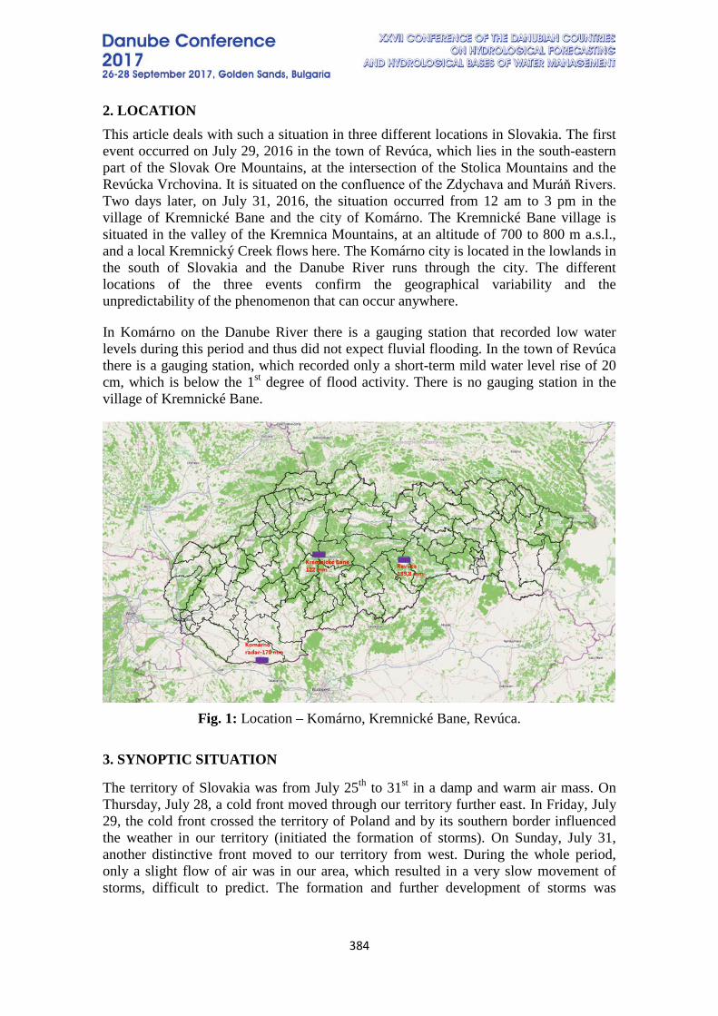
384

2. LOCATION This article deals with such a situation in three different locations in Slovakia. The first event occurred on July 29, 2016 in the town of Revúca, which lies in the south-eastern part of the Slovak Ore Mountains, at the intersection of the Stolica Mountains and the Revúcka Vrchovina. It is situated on the confluence of the Zdychava and Muráň Rivers. Two days later, on July 31, 2016, the situation occurred from 12 am to 3 pm in the village of Kremnické Bane and the city of Komárno. The Kremnické Bane village is situated in the valley of the Kremnica Mountains, at an altitude of 700 to 800 m a.s.l., and a local Kremnický Creek flows here. The Komárno city is located in the lowlands in the south of Slovakia and the Danube River runs through the city. The different locations of the three events confirm the geographical variability and the unpredictability of the phenomenon that can occur anywhere.

In Komárno on the Danube River there is a gauging station that recorded low water levels during this period and thus did not expect fluvial flooding. In the town of Revúca there is a gauging station, which recorded only a short-term mild water level rise of 20 cm, which is below the 1st degree of flood activity. There is no gauging station in the village of Kremnické Bane.

Fig. 1: Location – Komárno, Kremnické Bane, Revúca.

3. SYNOPTIC SITUATION

The territory of Slovakia was from July 25th to 31st in a damp and warm air mass. On Thursday, July 28, a cold front moved through our territory further east. In Friday, July 29, the cold front crossed the territory of Poland and by its southern border influenced the weather in our territory (initiated the formation of storms). On Sunday, July 31, another distinctive front moved to our territory from west. During the whole period, only a slight flow of air was in our area, which resulted in a very slow movement of storms, difficult to predict. The formation and further development of storms was

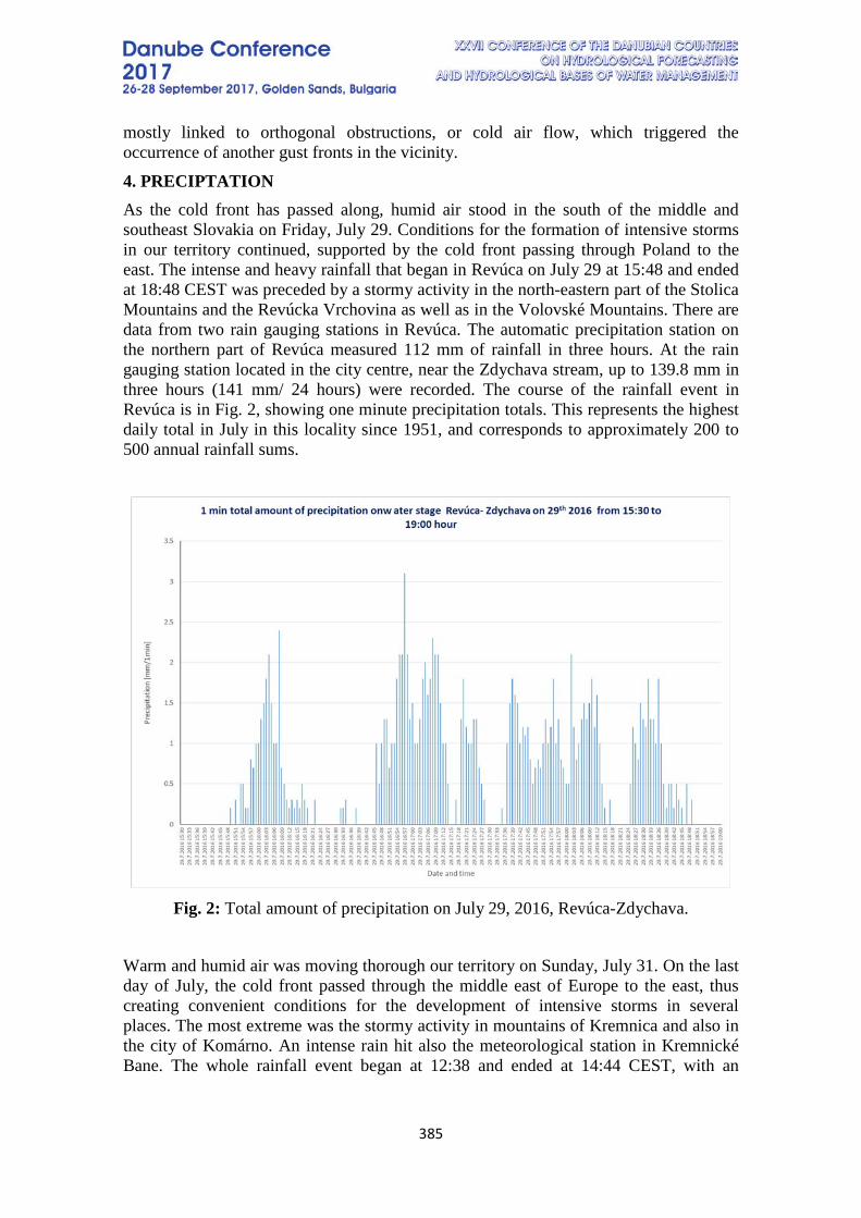
385

mostly linked to orthogonal obstructions, or cold air flow, which triggered the occurrence of another gust fronts in the vicinity.

4. PRECIPTATION As the cold front has passed along, humid air stood in the south of the middle and southeast Slovakia on Friday, July 29. Conditions for the formation of intensive storms in our territory continued, supported by the cold front passing through Poland to the east. The intense and heavy rainfall that began in Revúca on July 29 at 15:48 and ended at 18:48 CEST was preceded by a stormy activity in the north-eastern part of the Stolica Mountains and the Revúcka Vrchovina as well as in the Volovské Mountains. There are data from two rain gauging stations in Revúca. The automatic precipitation station on the northern part of Revúca measured 112 mm of rainfall in three hours. At the rain gauging station located in the city centre, near the Zdychava stream, up to 139.8 mm in three hours (141 mm/ 24 hours) were recorded. The course of the rainfall event in Revúca is in Fig. 2, showing one minute precipitation totals. This represents the highest daily total in July in this locality since 1951, and corresponds to approximately 200 to 500 annual rainfall sums.

Fig. 2: Total amount of precipitation on July 29, 2016, Revúca-Zdychava.

Warm and humid air was moving thorough our territory on Sunday, July 31. On the last day of July, the cold front passed through the middle east of Europe to the east, thus creating convenient conditions for the development of intensive storms in several places. The most extreme was the stormy activity in mountains of Kremnica and also in the city of Komárno. An intense rain hit also the meteorological station in Kremnické Bane. The whole rainfall event began at 12:38 and ended at 14:44 CEST, with an

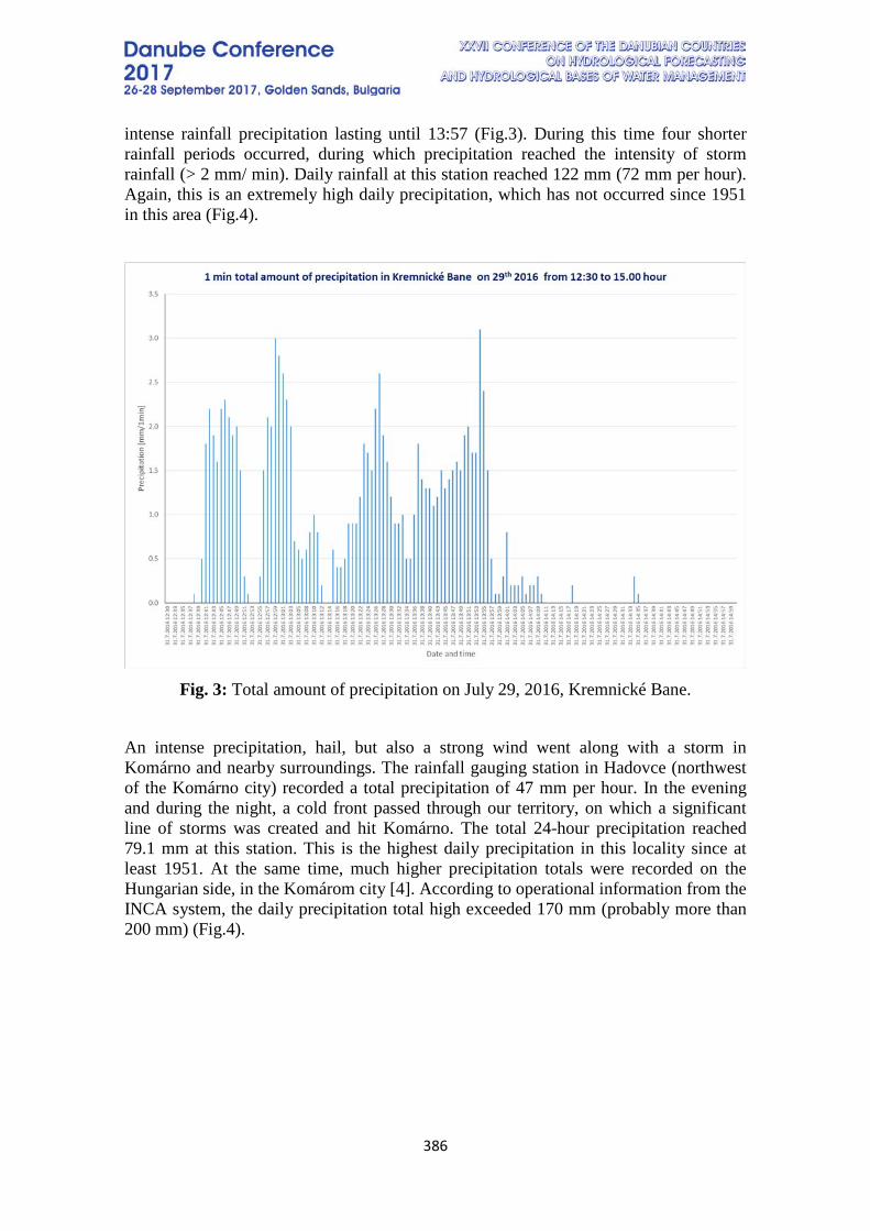
386

intense rainfall precipitation lasting until 13:57 (Fig.3). During this time four shorter rainfall periods occurred, during which precipitation reached the intensity of storm rainfall (> 2 mm/ min). Daily rainfall at this station reached 122 mm (72 mm per hour). Again, this is an extremely high daily precipitation, which has not occurred since 1951 in this area (Fig.4).

Fig. 3: Total amount of precipitation on July 29, 2016, Kremnické Bane.

An intense precipitation, hail, but also a strong wind went along with a storm in Komárno and nearby surroundings. The rainfall gauging station in Hadovce (northwest of the Komárno city) recorded a total precipitation of 47 mm per hour. In the evening and during the night, a cold front passed through our territory, on which a significant line of storms was created and hit Komárno. The total 24-hour precipitation reached 79.1 mm at this station. This is the highest daily precipitation in this locality since at least 1951. At the same time, much higher precipitation totals were recorded on the Hungarian side, in the Komárom city [4]. According to operational information from the INCA system, the daily precipitation total high exceeded 170 mm (probably more than 200 mm) (Fig.4).

387

Fig.4: 24-hour precipitation totals in Slovakia on August, 1st, 2016 at 4 am UTC.

Difficulties in the localities were not caused by the precipitation totals, but by the short-term intensity of rainfall, when the land was not able to absorb the extreme volume of water, or flow away through the sewage system and nearby river.

5. FORECAST AND FLOOD NOTIFICATION One of the main tasks of Slovak Hydrometeorological Institute (SHMI) is to alert flood authorities and the general public to flood risk. Time and space localization of possible storm rainfall is not a simple task. SHMI has a dense network of modern monitoring facilities, 4 new radars, meteorological and hydrological models, which make it much easier to predict storm rainfall. At the present, in the POVAPSYS project, a new flash flood forecasting system is being tested, based on the INCA precipitation analysis, ALADIN rainfall forecasts, and taking into account land saturation, geographic and soli properties, as well as land use. The meteorological and hydrological warnings on affected districts were issued and continuously updated during the mentioned period for the danger of floods from storm rainfall. For the Revúca district, a weather warning of the first degree for storms (with a total of 20 - 40 mm) was issued on July 29, 2016 at 9:35 am CEST. According to the meteorological situation, the warning was increased at 15:10 CEST to the 2nd degree (with a total of 50 - 80 mm) and at 15:55 CEST to 3rd degree (with a total of 50-120mm).

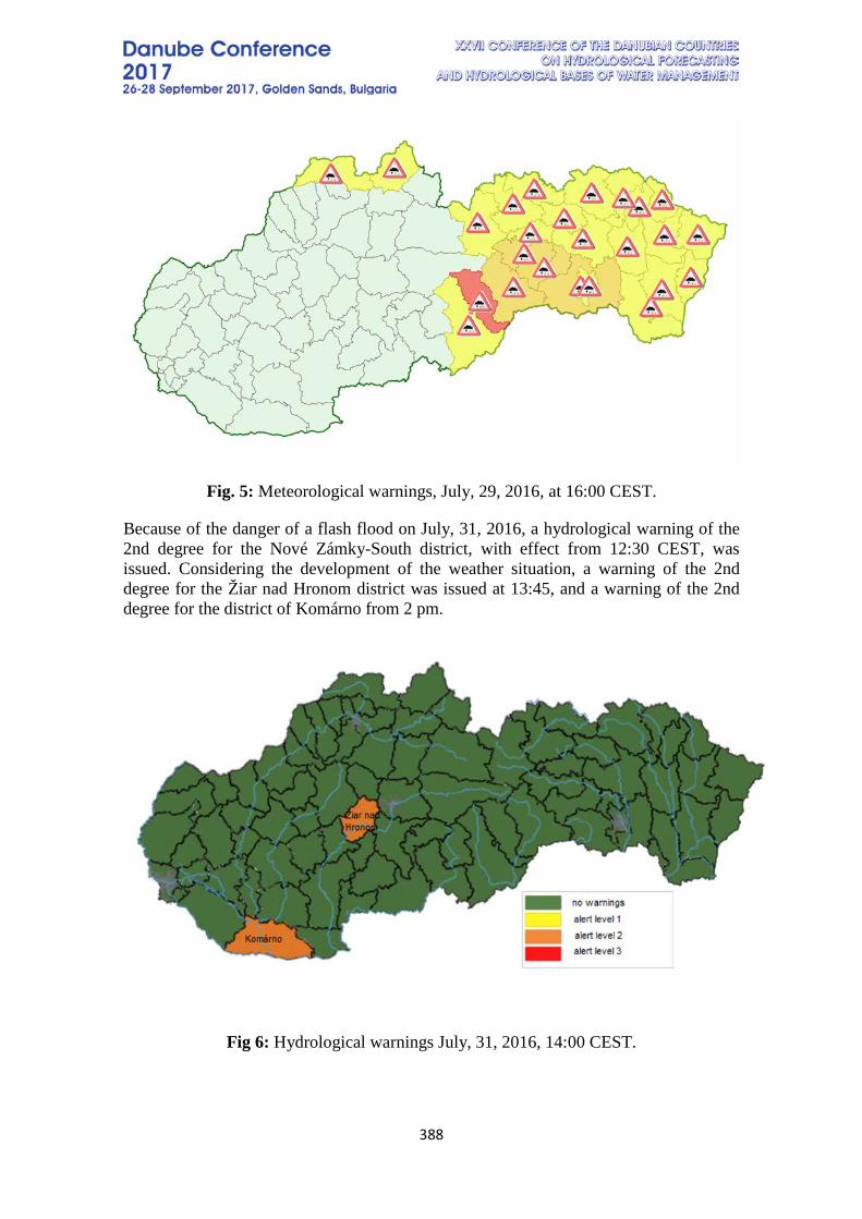
388

Fig. 5: Meteorological warnings, July, 29, 2016, at 16:00 CEST.

Because of the danger of a flash flood on July, 31, 2016, a hydrological warning of the 2nd degree for the Nové Zámky-South district, with effect from 12:30 CEST, was issued. Considering the development of the weather situation, a warning of the 2nd degree for the Žiar nad Hronom district was issued at 13:45, and a warning of the 2nd degree for the district of Komárno from 2 pm.

Fig 6: Hydrological warnings July, 31, 2016, 14:00 CEST.

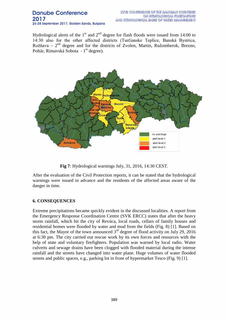
389

Hydrological alerts of the 1st and 2nd degree for flash floods were issued from 14:00 to 14:30 also for the other affected districts (Turčianske Teplice, Banská Bystrica, Rožňava – 2nd degree and for the districts of Zvolen, Martin, Ružomberok, Brezno, Poltár, Rimavská Sobota - 1st degree).

Fig 7: Hydrological warnings July, 31, 2016, 14:30 CEST.

After the evaluation of the Civil Protection reports, it can be stated that the hydrological warnings were issued in advance and the residents of the affected areas aware of the danger in time.

6. CONSEQUENCES

Extreme precipitations became quickly evident in the discussed localities. A report from the Emergency Response Coordination Centre (SVK ERCC) states that after the heavy storm rainfall, which hit the city of Revúca, local roads, cellars of family houses and residential homes were flooded by water and mud from the fields (Fig. 8) [1]. Based on this fact, the Mayor of the town announced 3rd degree of flood activity on July 29, 2016 at 6:30 pm. The city carried out rescue work by its own forces and resources with the help of state and voluntary firefighters. Population was warned by local radio. Water culverts and sewage drains have been clogged with flooded material during the intense rainfall and the streets have changed into water plane. Huge volumes of water flooded streets and public spaces, e.g., parking lot in front of hypermarket Tesco (Fig. 9) [1].

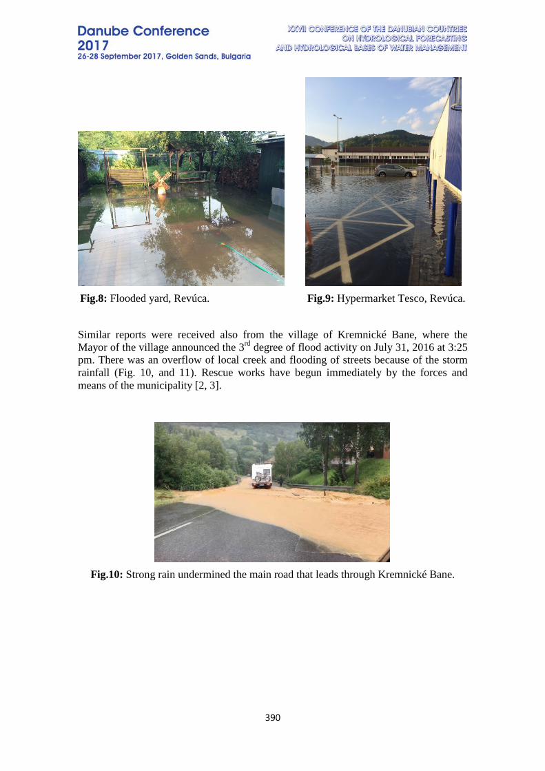
390

Fig.8: Flooded yard, Revúca. Fig.9: Hypermarket Tesco, Revúca.

Similar reports were received also from the village of Kremnické Bane, where the Mayor of the village announced the 3rd degree of flood activity on July 31, 2016 at 3:25 pm. There was an overflow of local creek and flooding of streets because of the storm rainfall (Fig. 10, and 11). Rescue works have begun immediately by the forces and means of the municipality [2, 3].

Fig.10: Strong rain undermined the main road that leads through Kremnické Bane.

391

Fig.11: The first class road between Žiar nad Hronom and Turčianske Teplice, which

runs through Kremnické Bane, was closed for several days.

The most serious situation was in Komárno. Mayor of the city announced, together with an extraordinary situation, the 3rd degree of flood activity on July 31, 2016 at 3:35 pm. The storm rainfall caused flooding of streets, underpasses, garages, cellars, courtyards, industrial parks, and family houses (Fig. 12). There was uprooting of trees, a breakdown of the branches, which resulted in the tearing of the electricity lines and failure of the electricity supply. The units of the District Directorate of the Fire and Rescue Corps and the District Police Forces, volunteer firemen of Komárno city and volunteers were engaged.

Fig.12: Streets flooded in the town of Komárno.

Damages by wind were recorded in the Komárno city. Despite the many firefighters, residents had to help as they knew.

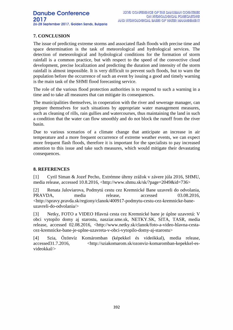
392

7. CONCLUSION The issue of predicting extreme storms and associated flash floods with precise time and space determination is the task of meteorological and hydrological services. The detection of meteorological and hydrological conditions for the formation of storm rainfall is a common practice, but with respect to the speed of the convective cloud development, precise localization and predicting the duration and intensity of the storm rainfall is almost impossible. It is very difficult to prevent such floods, but to warn the population before the occurrence of such an event by issuing a good and timely warning is the main task of the SHMI flood forecasting service. The role of the various flood protection authorities is to respond to such a warning in a time and to take all measures that can mitigate its consequences. The municipalities themselves, in cooperation with the river and sewerage manager, can prepare themselves for such situations by appropriate water management measures, such as cleaning of rills, rain gullies and watercourses, thus maintaining the land in such a condition that the water can flow smoothly and do not block the runoff from the river basin. Due to various scenarios of a climate change that anticipate an increase in air temperature and a more frequent occurrence of extreme weather events, we can expect more frequent flash floods, therefore it is important for the specialists to pay increased attention to this issue and take such measures, which would mitigate their devastating consequences.

8. REFERENCES [1] Cyril Siman & Jozef Pecho, Extrémne úhrny zrážok v závere júla 2016, SHMU, media release, accessed 10.8.2016, <http://www.shmu.sk/sk/?page=2049&id=736> [2] Renata Jaloviarova, Podmytú cestu cez Kremnické Bane uzavreli do odvolania, PRAVDA, media release, accessed 03.08.2016, <http://spravy.pravda.sk/regiony/clanok/400917-podmytu-cestu-cez-kremnicke-bane-uzavreli-do-odvolania/> [3] Netky, FOTO a VIDEO Hlavná cesta cez Kremnické bane je úplne uzavretá: V obci vytopilo domy aj starostu, nasziar.sme.sk, NETKY.SK, SITA, TASR, media release, accessed 02.08.2016, <http://www.netky.sk/clanok/foto-a-video-hlavna-cesta-cez-kremnicke-bane-je-uplne-uzavreta-v-obci-vytopilo-domy-aj-starostu> [4] Szia, Özönvíz Komáromban (képekkel és videókkal), media release, accessed31.7.2016, <http://sziakomarom.sk/ozonviz-komaromban-kepekkel-es-videokkal/>

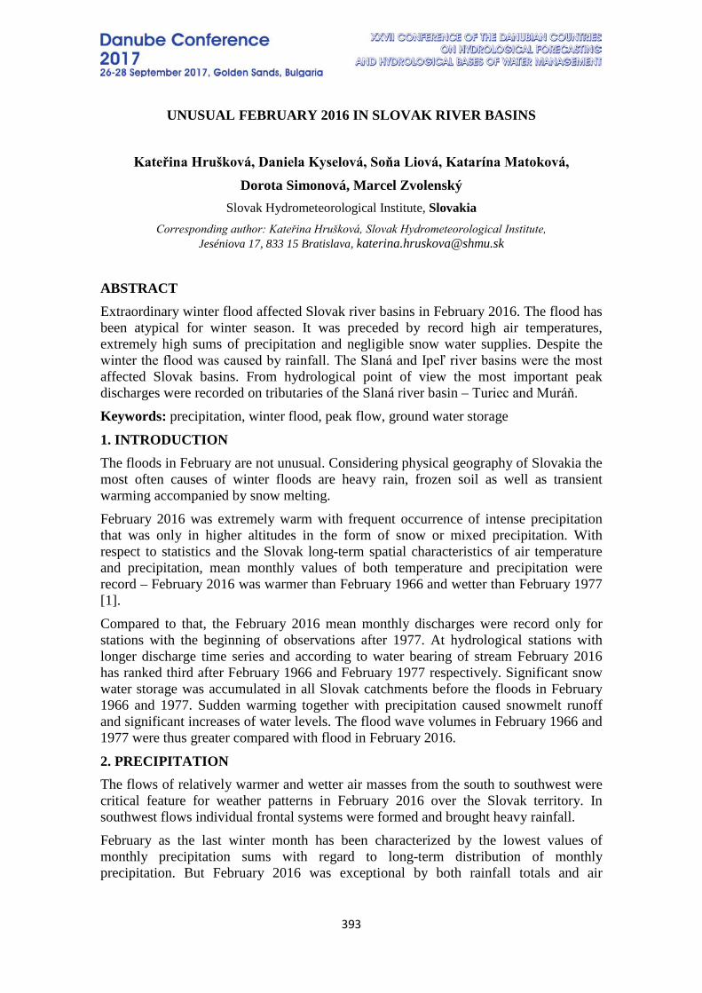
393

UNUSUAL FEBRUARY 2016 IN SLOVAK RIVER BASINS

Kateřina Hrušková, Daniela Kyselová, Soňa Liová, Katarína Matoková, Dorota Simonová, Marcel Zvolenský

Slovak Hydrometeorological Institute, Slovakia Corresponding author: Kateřina Hrušková, Slovak Hydrometeorological Institute,

Jeséniova 17, 833 15 Bratislava, katerina.hruskova@shmu.sk

ABSTRACT Extraordinary winter flood affected Slovak river basins in February 2016. The flood has been atypical for winter season. It was preceded by record high air temperatures, extremely high sums of precipitation and negligible snow water supplies. Despite the winter the flood was caused by rainfall. The Slaná and Ipeľ river basins were the most affected Slovak basins. From hydrological point of view the most important peak discharges were recorded on tributaries of the Slaná river basin – Turiec and Muráň. Keywords: precipitation, winter flood, peak flow, ground water storage

1. INTRODUCTION The floods in February are not unusual. Considering physical geography of Slovakia the most often causes of winter floods are heavy rain, frozen soil as well as transient warming accompanied by snow melting. February 2016 was extremely warm with frequent occurrence of intense precipitation that was only in higher altitudes in the form of snow or mixed precipitation. With respect to statistics and the Slovak long-term spatial characteristics of air temperature and precipitation, mean monthly values of both temperature and precipitation were record – February 2016 was warmer than February 1966 and wetter than February 1977 [1]. Compared to that, the February 2016 mean monthly discharges were record only for stations with the beginning of observations after 1977. At hydrological stations with longer discharge time series and according to water bearing of stream February 2016 has ranked third after February 1966 and February 1977 respectively. Significant snow water storage was accumulated in all Slovak catchments before the floods in February 1966 and 1977. Sudden warming together with precipitation caused snowmelt runoff and significant increases of water levels. The flood wave volumes in February 1966 and 1977 were thus greater compared with flood in February 2016.

2. PRECIPITATION The flows of relatively warmer and wetter air masses from the south to southwest were critical feature for weather patterns in February 2016 over the Slovak territory. In southwest flows individual frontal systems were formed and brought heavy rainfall. February as the last winter month has been characterized by the lowest values of monthly precipitation sums with regard to long-term distribution of monthly precipitation. But February 2016 was exceptional by both rainfall totals and air

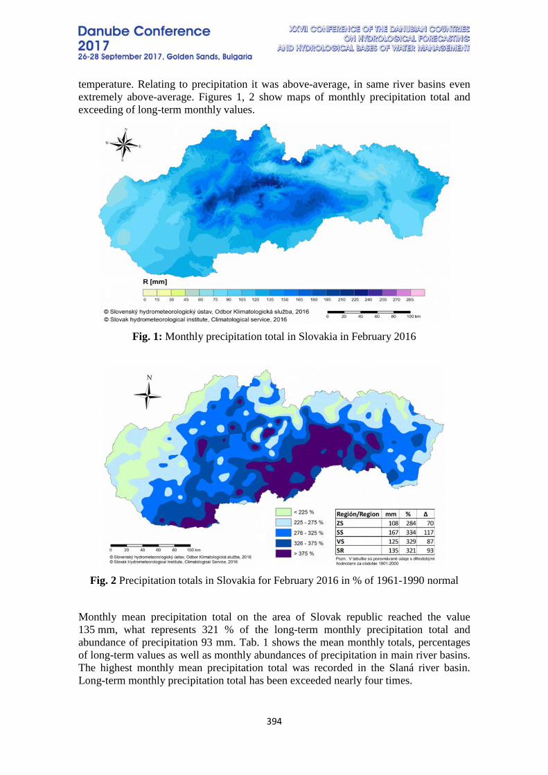
394

temperature. Relating to precipitation it was above-average, in same river basins even extremely above-average. Figures 1, 2 show maps of monthly precipitation total and exceeding of long-term monthly values.

Fig. 1: Monthly precipitation total in Slovakia in February 2016

Fig. 2 Precipitation totals in Slovakia for February 2016 in % of 1961-1990 normal

Monthly mean precipitation total on the area of Slovak republic reached the value 135 mm, what represents 321 % of the long-term monthly precipitation total and abundance of precipitation 93 mm. Tab. 1 shows the mean monthly totals, percentages of long-term values as well as monthly abundances of precipitation in main river basins. The highest monthly mean precipitation total was recorded in the Slaná river basin. Long-term monthly precipitation total has been exceeded nearly four times.

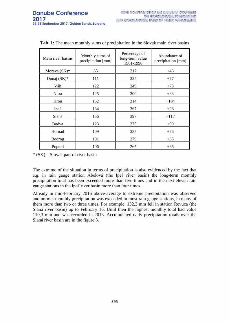
395

Tab. 1: The mean monthly sums of precipitation in the Slovak main river basins

Main river basins Monthly sums of precipitation [mm]

Percentage of long-term value

1961-1990

Abundance of precipitation [mm]

Morava (SK)* 85 217 +46

Dunaj (SK)* 111 324 +77

Váh 122 249 +73

Nitra 125 300 +83

Hron 152 314 +104

Ipeľ 134 367 +98

Slaná 156 397 +117

Bodva 123 375 +90

Hornád 109 335 +76

Bodrog 101 279 +65

Poprad 106 265 +66

* (SK) – Slovak part of river basin

The extreme of the situation in terms of precipitation is also evidenced by the fact that e.g. in rain gauge station Ábelová (the Ipeľ river basin) the long-term monthly precipitation total has been exceeded more than five times and in the next eleven rain gauge stations in the Ipeľ river basin more than four times. Already in mid-February 2016 above-average to extreme precipitation was observed and normal monthly precipitation was exceeded in most rain gauge stations, in many of them more than two or three times. For example, 132,3 mm fell in station Revúca (the Slaná river basin) up to February 16. Until then the highest monthly total had value 110,3 mm and was recorded in 2013. Accumulated daily precipitation totals over the Slaná river basin are in the figure 3.

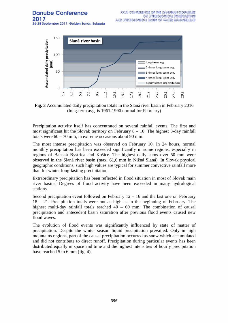
396

Fig. 3 Accumulated daily precipitation totals in the Slaná river basin in February 2016

(long-term avg. is 1961-1990 normal for February)

Precipitation activity itself has concentrated on several rainfall events. The first and most significant hit the Slovak territory on February 8 – 10. The highest 3-day rainfall totals were 60 – 70 mm, in extreme occasions about 90 mm. The most intense precipitation was observed on February 10. In 24 hours, normal monthly precipitation has been exceeded significantly in some regions, especially in regions of Banská Bystrica and Košice. The highest daily sums over 50 mm were observed in the Slaná river basin (max. 61,6 mm in Nižná Slaná). In Slovak physical geographic conditions, such high values are typical for summer convective rainfall more than for winter long-lasting precipitation. Extraordinary precipitation has been reflected in flood situation in most of Slovak main river basins. Degrees of flood activity have been exceeded in many hydrological stations. Second precipitation event followed on February 12 – 16 and the last one on February 18 – 21. Precipitation totals were not as high as in the beginning of February. The highest multi-day rainfall totals reached 40 – 60 mm. The combination of causal precipitation and antecedent basin saturation after previous flood events caused new flood waves. The evolution of flood events was significantly influenced by state of matter of precipitation. Despite the winter season liquid precipitation prevailed. Only in high mountains regions, part of the causal precipitation occurred as snow which accumulated and did not contribute to direct runoff. Precipitation during particular events has been distributed equally in space and time and the highest intensities of hourly precipitation have reached 5 to 6 mm (fig. 4).

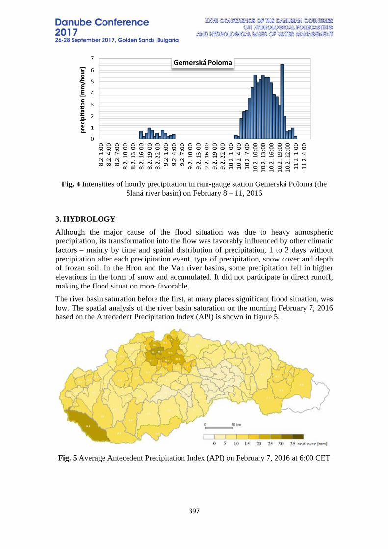
397

Fig. 4 Intensities of hourly precipitation in rain-gauge station Gemerská Poloma (the

Slaná river basin) on February 8 – 11, 2016

3. HYDROLOGY Although the major cause of the flood situation was due to heavy atmospheric precipitation, its transformation into the flow was favorably influenced by other climatic factors – mainly by time and spatial distribution of precipitation, 1 to 2 days without precipitation after each precipitation event, type of precipitation, snow cover and depth of frozen soil. In the Hron and the Vah river basins, some precipitation fell in higher elevations in the form of snow and accumulated. It did not participate in direct runoff, making the flood situation more favorable. The river basin saturation before the first, at many places significant flood situation, was low. The spatial analysis of the river basin saturation on the morning February 7, 2016 based on the Antecedent Precipitation Index (API) is shown in figure 5.

Fig. 5 Average Antecedent Precipitation Index (API) on February 7, 2016 at 6:00 CET

398

Water levels started to rise on February 8 and significant increases were observed on February 10. In most tributaries and upper parts of the main river basins, the February peak levels were recorded on February 10 and 11. Discharge wave in Gemerská Ves on the Turiec River with marked N-year flood discharges and the water levels in Bretka on Muráň River with marked levels corresponding to the level of flood activity are in figure 6 and 7. In this two water stations hydrologically the most significant maximum peak discharges of February 2016 flood were recorded.

Fig. 6 Course of 15-min discharges in Gemerská Ves on Turiec River in Slaná river

basin in February 2016 with marked N-year flood discharges

Fig. 7 Course of 15-min water levels in Bretka on Muráň River in Slaná river basin in

February 2016 with marked levels corresponding to the degree of flood activity

Groundwater water levels also had a positive impact on the development of the hydrological situation. The flood situation generally means an intensive feeding of the groundwater through the flood waters. Groundwater levels in Slovakia have been decreasing practically from July to October 2015. Since November 2015, there was only a marginal slow replenishment of the groundwater. But already in first days of the

399

February flood, along with the onset of flood waves, there was a significant replenishment of the groundwater in the inundation river zones and after a short time, the groundwater levels reached their maximum. During this flood event the groundwater levels reached their maximum levels in the hydrological year 2016 (Gemerská Ves – Hrkáč well, figure 8). In the inundation river zones they reached only a few centimeters below the surface, at some places they even got on the ground. Changes in groundwater levels from selected well as well as the direct influence of groundwater level from the surface flow are shown in figure 9.

Fig. 8 Altitude of groundwater level in Gemerská Ves – Hrkáč well in Slaná river basin

form November 2014 to February 2016

Fig. 9 The courses of groundwater level depth from the terrain level and water levels in

selected objects of underground (Nová Baňa well) and surface water (Brehy gauging station) in the Hron river basin in February 2016

Relatively even distribution of precipitation in time and space, mainly positive soil temperature and also low groundwater levels before the flood favorably influenced the

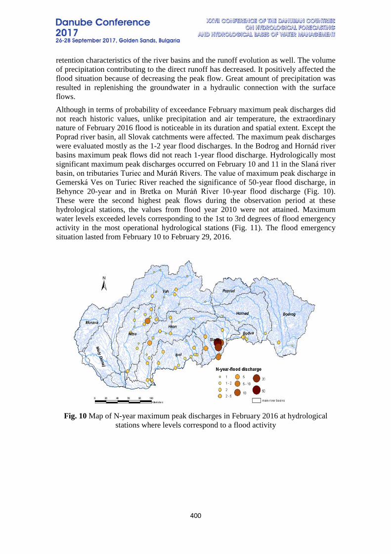
400

retention characteristics of the river basins and the runoff evolution as well. The volume of precipitation contributing to the direct runoff has decreased. It positively affected the flood situation because of decreasing the peak flow. Great amount of precipitation was resulted in replenishing the groundwater in a hydraulic connection with the surface flows. Although in terms of probability of exceedance February maximum peak discharges did not reach historic values, unlike precipitation and air temperature, the extraordinary nature of February 2016 flood is noticeable in its duration and spatial extent. Except the Poprad river basin, all Slovak catchments were affected. The maximum peak discharges were evaluated mostly as the 1-2 year flood discharges. In the Bodrog and Hornád river basins maximum peak flows did not reach 1-year flood discharge. Hydrologically most significant maximum peak discharges occurred on February 10 and 11 in the Slaná river basin, on tributaries Turiec and Muráň Rivers. The value of maximum peak discharge in Gemerská Ves on Turiec River reached the significance of 50-year flood discharge, in Behynce 20-year and in Bretka on Muráň River 10-year flood discharge (Fig. 10). These were the second highest peak flows during the observation period at these hydrological stations, the values from flood year 2010 were not attained. Maximum water levels exceeded levels corresponding to the 1st to 3rd degrees of flood emergency activity in the most operational hydrological stations (Fig. 11). The flood emergency situation lasted from February 10 to February 29, 2016.

Fig. 10 Map of N-year maximum peak discharges in February 2016 at hydrological

stations where levels correspond to a flood activity

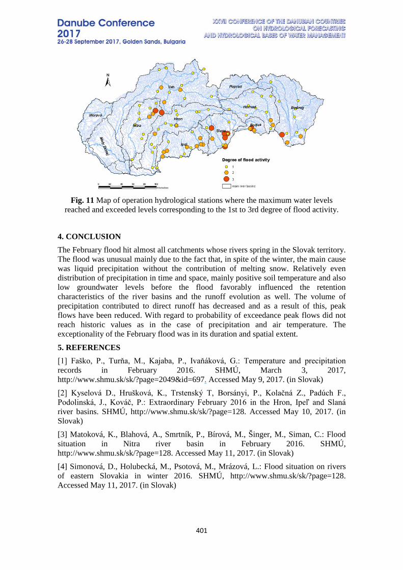
401

Fig. 11 Map of operation hydrological stations where the maximum water levels

reached and exceeded levels corresponding to the 1st to 3rd degree of flood activity.

4. CONCLUSION The February flood hit almost all catchments whose rivers spring in the Slovak territory. The flood was unusual mainly due to the fact that, in spite of the winter, the main cause was liquid precipitation without the contribution of melting snow. Relatively even distribution of precipitation in time and space, mainly positive soil temperature and also low groundwater levels before the flood favorably influenced the retention characteristics of the river basins and the runoff evolution as well. The volume of precipitation contributed to direct runoff has decreased and as a result of this, peak flows have been reduced. With regard to probability of exceedance peak flows did not reach historic values as in the case of precipitation and air temperature. The exceptionality of the February flood was in its duration and spatial extent.

5. REFERENCES [1] Faško, P., Turňa, M., Kajaba, P., Ivaňáková, G.: Temperature and precipitation records in February 2016. SHMÚ, March 3, 2017, http://www.shmu.sk/sk/?page=2049&id=697. Accessed May 9, 2017. (in Slovak) [2] Kyselová D., Hrušková, K., Trstenský T, Borsányi, P., Kolačná Z., Padúch F., Podolinská, J., Kováč, P.: Extraordinary February 2016 in the Hron, Ipeľ and Slaná river basins. SHMÚ, http://www.shmu.sk/sk/?page=128. Accessed May 10, 2017. (in Slovak) [3] Matoková, K., Blahová, A., Smrtník, P., Bírová, M., Šinger, M., Siman, C.: Flood situation in Nitra river basin in February 2016. SHMÚ, http://www.shmu.sk/sk/?page=128. Accessed May 11, 2017. (in Slovak) [4] Simonová, D., Holubecká, M., Psotová, M., Mrázová, L.: Flood situation on rivers of eastern Slovakia in winter 2016. SHMÚ, http://www.shmu.sk/sk/?page=128. Accessed May 11, 2017. (in Slovak)

402

A DAILY WETNESS INDEX BASED ON SATELLITE GRAVITY FOR FLOOD AND DROUGHT FORECASTING IN THE DANUBE BASIN

Ben Gouweleeuw1, Andreas Kvas2, Christian Gruber1, Tortsen Mayer-Gürr2,

Frank Flechtner1, Andreas Güntner1

1 GFZ German Research Centre for Geosciences, Germany 2 Graz University of Technology, Institute of Geodesy, Austria

Corresponding author: Ben Gouweleeuw, GFZ German Research Centre for Geosciences, Telegrafenberg, 14473 Potsdam, Germany, bingo@gfz-potsdam.de

ABSTRACT Contrary to other Earth observation data, satellite-based measurements of gravity represent total water storage variations (i.e., variations of all surface and subsurface water storage compartments). As such, it provides unique information on the wetness state of a river basin with regard to its actual flood generation potential or its susceptibility to a drought. For the development and testing of indices of hydrological extreme events, the Horizon 2020 funded European Gravity Service for Improved Emergency Management (EGSIEM) project takes advantage of the integrative nature of gravity data. It evaluates how large-scale water storage anomalies derived by near real-time (NRT), daily and regional satellite-based products of the Gravity Recovery And Climate Experiment (GRACE, April 2002-present) can be used as early warning indicators in flood and drought monitoring and alerting services. A wetness index is proposed, which expresses the satellite-derived total water storage anomaly as a departure of the seasonal cycle in dimensionless units of standard deviation. Results for the Danube basin show a built-up of total water storage, which culminated in widespread flooding in 2006 and 2010 several months later, illustrating the potential of gravity data as complementary information for flood forecasting in the Danube basin. Smaller floods in 2013 and 2014 are also detected with shorter lead times, possibly indicating a different flood triggering mechanism with less water storage built up. Lead time for the 2002 basin-wide flooding is also relatively short, probably due to technical initialization issues of the GRACE twin-satellite mission (launch date: March 2017) at that time. A low of the wetness index reflects dry conditions during the 2003 and 2015 European heatwaves. Keywords: gravity, satellite, index, forecast, flood, drought.

1. INTRODUCTION Since April 2002, the Gravity Recovery and Climate Experiment (GRACE) satellite mission has been producing water storage anomaly data, which has been shown to be a unique descriptor of large-scale hydrological extreme events. Nonetheless, efforts to assess the comprehensive information from GRACE on total water storage variations for near-real time flood or drought monitoring have been limited so far drought [1] [2], primarily due to its coarse temporal (weekly to monthly) and spatial (> 150.000 km2) resolution and the latency of standard products of about 2 months.

403

Now, 15 years later, as of 1 April, the Horizon 2020 funded EGSIEM (European Gravity Service for Improved Emergency Management) project launched a demonstrator near-real time (NRT) daily gravity field service. Compared to the official GRACE gravity products, the NRT solutions not only increase the temporal resolution from one month to one day, but also reduce the current latency from two months to five days. Thus, the NRT service allows for the monitoring of extremes in total water storage variations as they occur, as opposed to a ‘confirmation after occurrence’, which has been the situation up to only recently.

2. DAILY GLOBAL SOLUTIONS

Because the satellite data coverage within one day does not allow for a gravity field solution based on GRACE data alone, the computation of daily gravity maps employs a prediction – correction principle. Information obtained from geophysical models on the temporal behavior of the gravity field are used to predict the following day, which is subsequently improved with the available GRACE observations in a Kalman filter approach [3].

Daily gravity field solutions are made available by the GFZ German Research Centre for Geosciences and the Graz University of Technology (TUG), with each analysis center providing an independent solution. TUG focuses on improving global gravity field solutions, whereas GFZ implements tailored regional representations of the gravity field [4]. Both approaches complement each other, providing global coverage, with increased spatial resolution for regional areas of interest.

Additional processing converts the resulting gravity field solutions, expressed in terms of spherical harmonics coefficients, into global 1⁰ x 1⁰ gridded map of total water storage anomaly (TWSA) in equivalent water height (cm). A Wetness Index (WI) expresses the deviation from the mean seasonal cycle in units of standard deviation.

Figure 1: TUG (left) and GFZ (right) GRACE-based Wetness Index of 10 June 2017.

3. NRT GLOBAL TEST RUN

Contrary to other earth observation data, gravity represents total water storage variations (i.e., variations of all surface and subsurface water storage compartments). As such, it provides unique information on the wetness state of a river basin with regard to its actual flood generation potential or its susceptibility to a drought. For the development

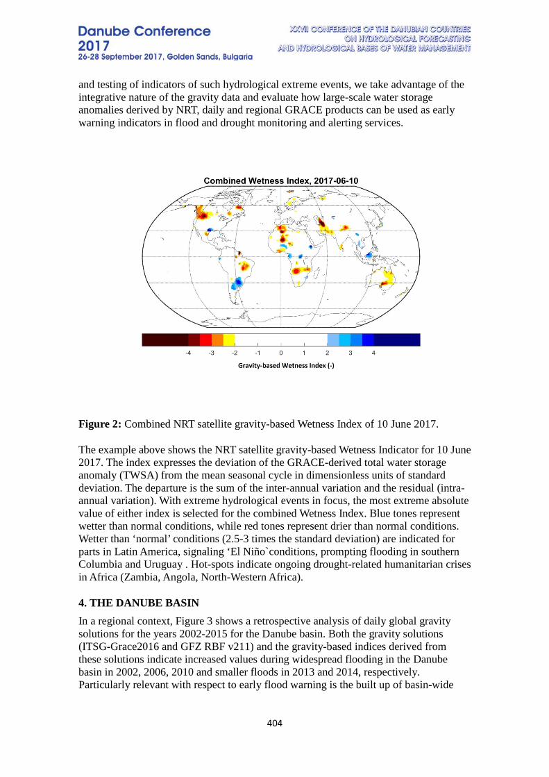
404

and testing of indicators of such hydrological extreme events, we take advantage of the integrative nature of the gravity data and evaluate how large-scale water storage anomalies derived by NRT, daily and regional GRACE products can be used as early warning indicators in flood and drought monitoring and alerting services.

Figure 2: Combined NRT satellite gravity-based Wetness Index of 10 June 2017.

The example above shows the NRT satellite gravity-based Wetness Indicator for 10 June 2017. The index expresses the deviation of the GRACE-derived total water storage anomaly (TWSA) from the mean seasonal cycle in dimensionless units of standard deviation. The departure is the sum of the inter-annual variation and the residual (intra-annual variation). With extreme hydrological events in focus, the most extreme absolute value of either index is selected for the combined Wetness Index. Blue tones represent wetter than normal conditions, while red tones represent drier than normal conditions. Wetter than ‘normal’ conditions (2.5-3 times the standard deviation) are indicated for parts in Latin America, signaling ‘El Niño`conditions, prompting flooding in southern Columbia and Uruguay . Hot-spots indicate ongoing drought-related humanitarian crises in Africa (Zambia, Angola, North-Western Africa).

4. THE DANUBE BASIN In a regional context, Figure 3 shows a retrospective analysis of daily global gravity solutions for the years 2002-2015 for the Danube basin. Both the gravity solutions (ITSG-Grace2016 and GFZ RBF v211) and the gravity-based indices derived from these solutions indicate increased values during widespread flooding in the Danube basin in 2002, 2006, 2010 and smaller floods in 2013 and 2014, respectively. Particularly relevant with respect to early flood warning is the built up of basin-wide

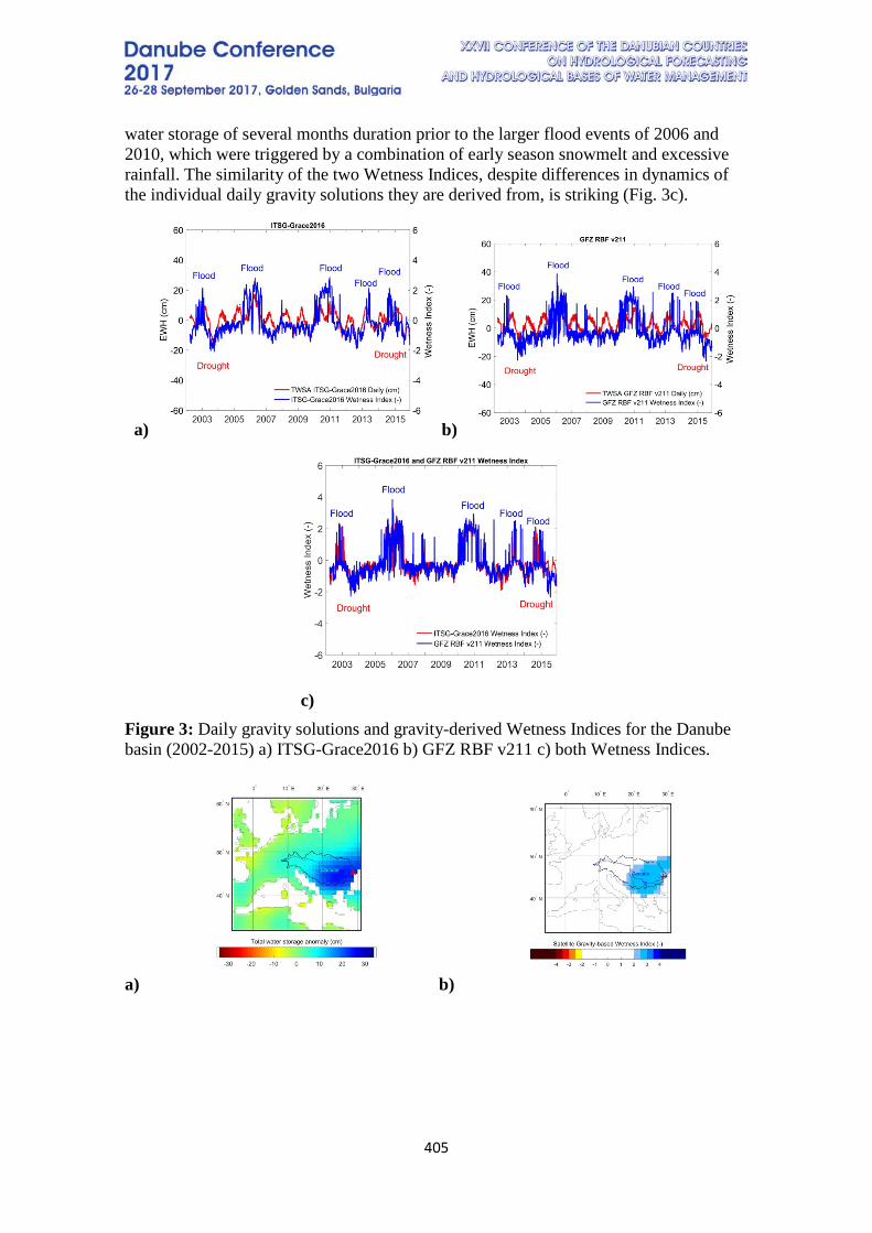
405

water storage of several months duration prior to the larger flood events of 2006 and 2010, which were triggered by a combination of early season snowmelt and excessive rainfall. The similarity of the two Wetness Indices, despite differences in dynamics of the individual daily gravity solutions they are derived from, is striking (Fig. 3c).

a) b)

c)

Figure 3: Daily gravity solutions and gravity-derived Wetness Indices for the Danube basin (2002-2015) a) ITSG-Grace2016 b) GFZ RBF v211 c) both Wetness Indices.

a) b)

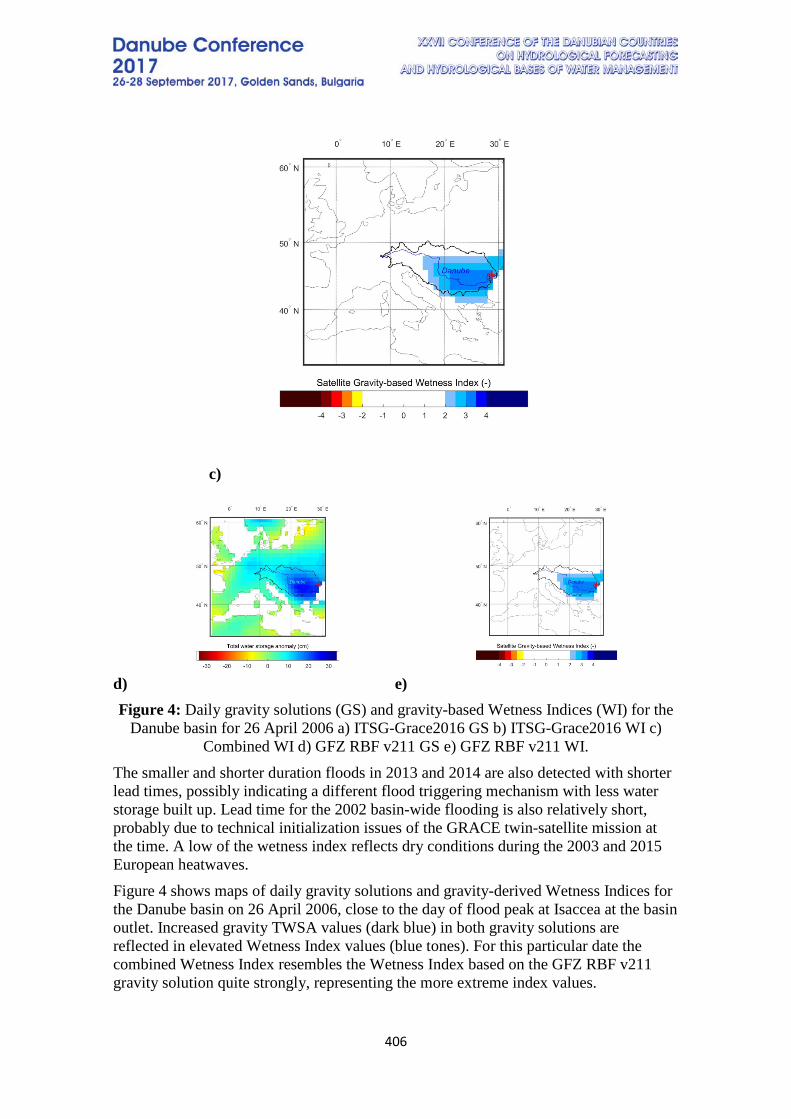
406

c)

d) e) Figure 4: Daily gravity solutions (GS) and gravity-based Wetness Indices (WI) for the

Danube basin for 26 April 2006 a) ITSG-Grace2016 GS b) ITSG-Grace2016 WI c) Combined WI d) GFZ RBF v211 GS e) GFZ RBF v211 WI.

The smaller and shorter duration floods in 2013 and 2014 are also detected with shorter lead times, possibly indicating a different flood triggering mechanism with less water storage built up. Lead time for the 2002 basin-wide flooding is also relatively short, probably due to technical initialization issues of the GRACE twin-satellite mission at the time. A low of the wetness index reflects dry conditions during the 2003 and 2015 European heatwaves. Figure 4 shows maps of daily gravity solutions and gravity-derived Wetness Indices for the Danube basin on 26 April 2006, close to the day of flood peak at Isaccea at the basin outlet. Increased gravity TWSA values (dark blue) in both gravity solutions are reflected in elevated Wetness Index values (blue tones). For this particular date the combined Wetness Index resembles the Wetness Index based on the GFZ RBF v211 gravity solution quite strongly, representing the more extreme index values.

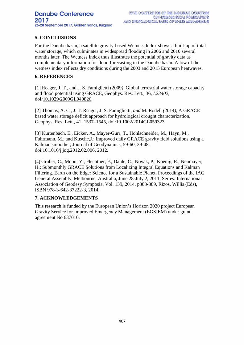
407

5. CONCLUSIONS For the Danube basin, a satellite gravity-based Wetness Index shows a built-up of total water storage, which culminates in widespread flooding in 2006 and 2010 several months later. The Wetness Index thus illustrates the potential of gravity data as complementary information for flood forecasting in the Danube basin. A low of the wetness index reflects dry conditions during the 2003 and 2015 European heatwaves.

6. REFERENCES

[1] Reager, J. T., and J. S. Famiglietti (2009), Global terrestrial water storage capacity and flood potential using GRACE, Geophys. Res. Lett., 36, L23402, doi:10.1029/2009GL040826.

[2] Thomas, A. C., J. T. Reager, J. S. Famiglietti, and M. Rodell (2014), A GRACE-based water storage deficit approach for hydrological drought characterization, Geophys. Res. Lett., 41, 1537–1545, doi:10.1002/2014GL059323

[3] Kurtenbach, E., Eicker, A., Mayer-Gürr, T., Hohlschneider, M., Hayn, M., Fuhrmann, M., and Kusche,J.: Improved daily GRACE gravity field solutions using a Kalman smoother, Journal of Geodynamics, 59-60, 39-48, doi:10.1016/j.jog.2012.02.006, 2012.

[4] Gruber, C., Moon, Y., Flechtner, F., Dahle, C., Novàk, P., Koenig, R., Neumayer, H.: Submonthly GRACE Solutions from Localizing Integral Equations and Kalman Filtering. Earth on the Edge: Science for a Sustainable Planet, Proceedings of the IAG General Assembly, Melbourne, Australia, June 28-July 2, 2011, Series: International Association of Geodesy Symposia, Vol. 139, 2014, p383-389, Rizos, Willis (Eds), ISBN 978-3-642-37222-3, 2014.

7. ACKNOWLEDGEMENTS This research is funded by the European Union’s Horizon 2020 project European Gravity Service for Improved Emergency Management (EGSIEM) under grant agreement No 637010.

408

CONTINUOUS SPATIO-TEMPORAL CORRELATED RAINFALL SIMULATION FOR REGIONAL FLOOD RISK ASSESSMENT –

APPLICATION IN THE AUSTRIAN ALPS

Jose Luis Salinas, Thomas Nester, Jürgen Komma, Günter Blöschl Institute of Hydraulic Engineering and Water Resources Management / Vienna University of

Technology, Austria

Corresponding author: Dr. Jose Luis Salinas – salinas@hydro.tuwien.ac.at

Understanding the spatial and temporal correlation of rainfall is of pivotal importance for assessing regional hydroclimatic hazard, and for addressing problems like confluences, or joint probability of flood waves. Furthermore, if one aims to simulate precipitation as the input for long term rainfall runoff simulations, the correct reproduction of the observed rainfall characteristics, such as regional intensity-duration-frequency curves, or spatial and temporal correlations, is necessary to adequately model the magnitude and frequency of the flood peaks. In this work, we present a modification of the model presented by Bardossy and Platte (1992), where precipitation is modeled on a station basis as a mutivariate autoregressive model (mAr) in a Normal space, and then transformed to a Gamma-distributed space. In order to model seasonality, the parameters of the Gamma distributions are assumed to vary monthly according to a sinusoidal function, and are calibrated trying to simultaneously reproduce i) mean annual rainfall, ii) mean daily rainfall amounts, iii) standard deviations of daily rainfall amounts, and iv) 24-hours intensity duration frequency curve. The spatial and temporal correlation structures are imposed in the normal space, allowing for a different temporal autocorrelation parameter for each station, and simultaneously ensuring the positive-definiteness of the correlation matrices for both the mAr errors, and the Normal-space rainfall. The calibration of the spatial and temporal correlation parameters is performed with a focus on extremes, trying to reproduce the variograms of a series of relevant rainfall events over the last 50 years in the region of interest (Tirolean Alps in Austria – Inn river and confluence Inn/Danube), as well as intensity-duration-frequency curves aggregated at different spatial and temporal scales. Bardossy, A., and E. Plate (1992), Space-time model for daily rainfall [...] Water Resour. Res.,28(5), 1247

409

FLOOD REGIME OF RIVERS IN THE DANUBE RIVER BASIN

Pavol Miklanek1, Pavla Pekarova1, Jan Pekar2

1 Institute of Hydrology SAS, Slovakia 2 Comenius University in Bratislava, Faculty of Mathematics, Physics, and Informatics,

Slovakia

Corresponding author: Dr. Pavol Miklanek, Institute of Hydrology SAS, Dubravska cesta 9, 814 04 Bratislava, Slovakia, miklanek@uh.savba.sk

ABSTRACT The territory of the Danube river basin is one the most flood-endangered regions in Europe. The main reason is location of the Alpine and Carpathian mountain ridges on the way of moist air masses coming from Atlantic Ocean. According to this fact, the rain and rain-snow-melting floods on the Alpine and Carpathian rivers have essential frequency, great intensity and a large spatial scope. From time to time, floods become dangerous with destructive consequences. Essential floods took place in all states of Central and Eastern Europe during the last twenty years (e.g. floods in November 1998, March 2001, August 2002, April 2006, May 2010 or June 2013). The paper presents selected results of the IHP UNESCO Regional cooperation of the Danube Countries Project No. 9 FLOOD REGIME OF RIVERS IN THE DANUBE RIVER BASIN. With the help of collaborating countries the database was completed which includes the high quality and long data series, relatively anthropogenically uninfluenced, on rivers within the Danube basin. So far, data were processed from 46 river gauging stations on tributaries, and 20 stations on the river Danube itself. All available information has been collected on the basis of the mean daily and maximum annual discharge data. The aim of this paper is to analyse temporal changes in the magnitude, duration and frequency of high flows in 20 stations along the Danube River. Keywords: the Danube River, runoff regime, floods, cycles, long-term trends

1. INTRODUCTION With the increase of population – and with the development of civilization in general – an increase of vulnerability of the society is closely connected. It concerns also the threats by high floods as well as by incidents of long periods of droughts. Economic prosperity of each country is closely connected with the availability of sufficient water resources. In general, the economic development and increase of living standard, leads to higher demands of the water consumption. Considering the fact that the water resources are limited, in many regions of the world the social and economic growth will be expressively limited in the future. According to Directive 2007/60/EC of the European Parliament of 23 October 2007 on the assessment and management of flood risks [1], the Member States shall among others to prepare description of the floods which have occurred in the past and which had significant adverse impacts on human. It is also needed to elaborate for each river basin district flood hazard maps according to the following scenarios:

410

(a) floods with a low probability, or extreme event scenarios; (b) floods with a medium probability (likely return period ≥ 100 years); (c) floods with a high probability. In large international river basins – such as the Danube – it is necessary to synchronise the methodologies and to prepare common procedures. In 1971, the hydrologists of eight Danube Countries launched on a voluntary basis a regional hydrological cooperation aiming to produce consistent hydrological information about the whole Danube Catchment. Since 1987, this cooperation has been carried out in the framework of the International Hydrological Programme (IHP) of UNESCO. The cooperation of the Danube countries within framework of the IHP of UNESCO is based on the one hand on project work and on the other on regular conferences. Several projects were finalized within the Danube collaboration. The topic of floods was touched by several of them in last years:

• Project No.4: Coincidence of flood flow of the Danube River and its tributaries (prepared by Prohaska [2]);

• Project No. 5.2: Flow regime of river Danube and its catchment (prepared by Belz and Goda [3]);

• Project No. 7: Regional analysis of the annual peak discharges in the Danube catchment (prfepared by Stănescu [4]).

The project No. 9 Flood regime of rivers in the Danube River basin has eight objectives: O1: Average daily discharge and annual peak discharge series collection [5]. O2: Analysis of homogeneity of annual time series. O3: Analysis of cyclicity and long-term trends of annual series, and Qmax series [6]. O4: Analysis of the intra-annual regime changes based on monthly series. O5: Development of relations between values of NAO, QBO and Sun activity indexes and discharge series [7]. O6: History and downstream propagations of Danube floods [8]. O7: Statistical analyses of extreme discharges. O8: Regionalization of flood regimes according to magnitude of fluctuations, NAO, and their synchronicity The preliminary results of the project are presented on the WEB page of the project www.ih.savba.sk/danubeflood. The results will be finalised in uniform format as a follow-up volume of the Danube monograph. The aim of this paper is to analyse temporal changes in the magnitude, duration and frequency of high flows in 20 stations along the Danube River.

2. RESULTS 2.1 Data The first water stage observations started on the river Danube at Komárno in 1805, then at Vienna in 1821, and at Bratislava in 1823. As defined in the Project proposal, it is assumed within the objective O1 to create the database of mean daily discharges from selected stations on the Danube River with high quality and long data series, as well as of other data series of relatively large and anthropogenically uninfluenced rivers within the Danube basin. So far, 20 time series of

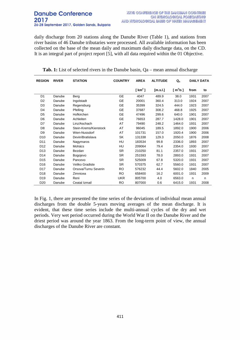
411

daily discharge from 20 stations along the Danube River (Table 1), and stations from river basins of 46 Danube tributaries were processed. All available information has been collected on the base of the mean daily and maximum daily discharge data, on the CD. It is an integral part of project report [5], with all data required within the 01 Objective.

Tab. 1: List of selected rivers in the Danube basin, Qa – mean annual discharge

REGION RIVER STATION COUNTRY AREA ALTITUDE Qa DAILY DATA

[ km2 ] [m.s.l.] [ m3/s ] from to

D1 Danube Berg GE 4047 489.9 38.0 1931 2007 D2 Danube Ingolstadt GE 20001 360.4 313.0 1924 2007 D3 Danube Regensburg GE 35399 324.5 444.0 1923 2007 D4 Danube Pfelling GE 37687 308.2 468.8 1925 2007 D5 Danube Hofkirchen GE 47496 299.6 640.0 1901 2007 D6 Danube Achleiten GE 76653 287.7 1428.0 1901 2007 D7 Danube Linz/Aschach AT 79490 248.2 1464.0 1931 2007 D8 Danube Stein-Krems/Kienstock AT 96045 189.5 1892.0 1900 2006 D9 Danube Wien-Nussdorf AT 101731 157.0 1920.4 1900 2006

D10 Danube Devin/Bratislava SK 131338 129.3 2050.0 1876 2008 D11 Danube Nagymaros HU 183534 99.8 2336.0 1893 2007 D12 Danube Mohács HU 209064 79.4 2354.0 1930 2007 D13 Danube Bezdan SR 210250 81.1 2357.0 1931 2007 D14 Danube Bogojevo SR 251593 78.0 2893.0 1931 2007 D15 Danube Pancevo SR 525009 67.8 5320.0 1931 2007 D16 Danube Veliko Gradiste SR 570375 62.7 5560.0 1931 2007 D17 Danube Orsova/Turnu Severin RO 576232 44.4 5602.0 1840 2005 D18 Danube Zimnicea RO 658400 16.2 6001.0 1931 2009 D19 Danube Reni UKR 805700 4.0 6563.0 n n D20 Danube Ceatal Izmail RO 807000 0.6 6415.0 1931 2008

In Fig. 1, there are presented the time series of the deviations of individual mean annual discharges from the double 5-years moving averages of the mean discharge. It is evident, that these time series include the multi-annual cycles of the dry and wet periods. Very wet period occurred during the World War II on the Danube River and the driest period was around the year 1863. From the long-term point of view, the annual discharges of the Danube River are constant.

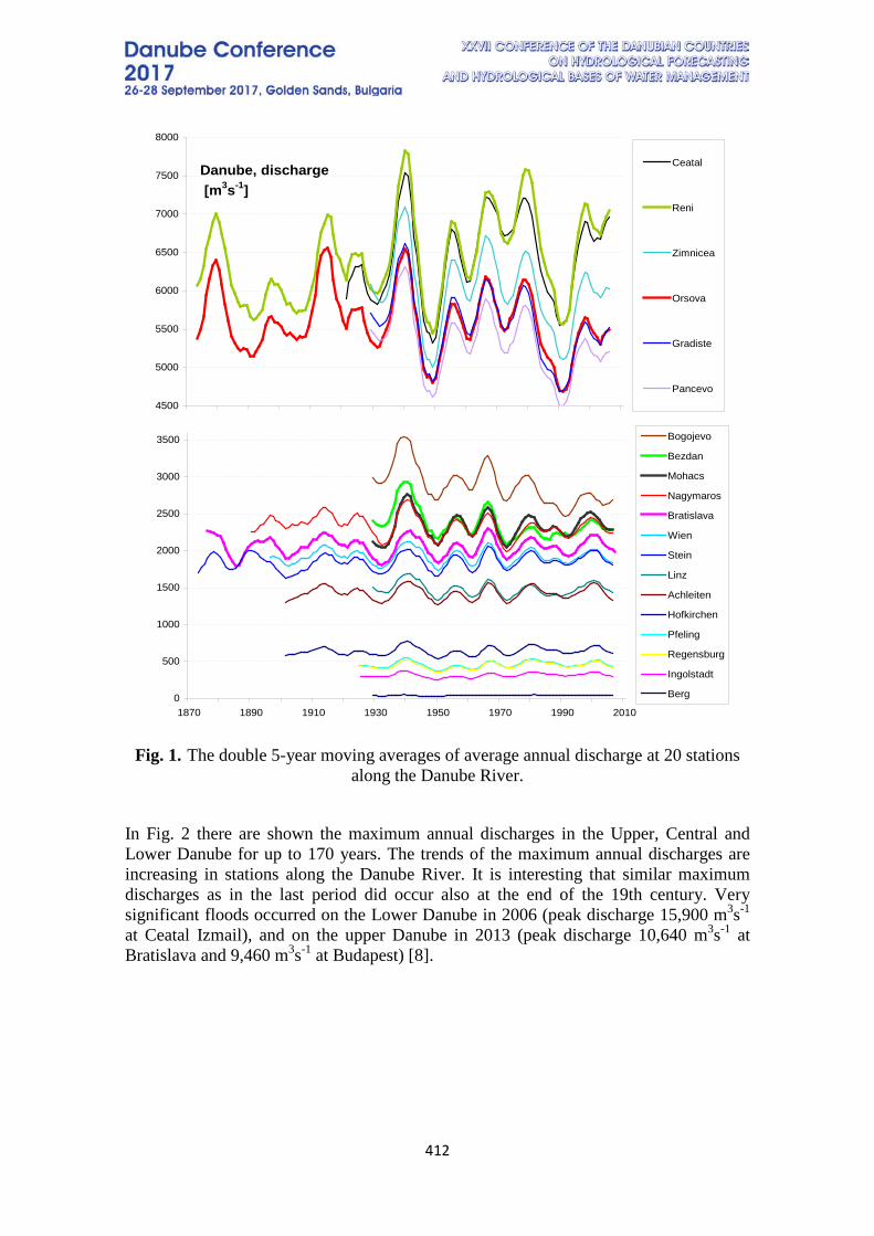
412

Fig. 1. The double 5-year moving averages of average annual discharge at 20 stations

along the Danube River. In Fig. 2 there are shown the maximum annual discharges in the Upper, Central and Lower Danube for up to 170 years. The trends of the maximum annual discharges are increasing in stations along the Danube River. It is interesting that similar maximum discharges as in the last period did occur also at the end of the 19th century. Very significant floods occurred on the Lower Danube in 2006 (peak discharge 15,900 m3s-1 at Ceatal Izmail), and on the upper Danube in 2013 (peak discharge 10,640 m3s-1 at Bratislava and 9,460 m3s-1 at Budapest) [8].

0

500

1000

1500

2000

2500

3000

3500

1870 1890 1910 1930 1950 1970 1990 2010

Bogojevo

Bezdan

Mohacs

Nagymaros

Bratislava

Wien

Stein

Linz

Achleiten

Hofkirchen

Pfeling

Regensburg

Ingolstadt

Berg

4500

5000

5500

6000

6500

7000

7500

8000

Ceatal

Reni

Zimnicea

Orsova

Gradiste

Pancevo

Danube, discharge [m3s-1]

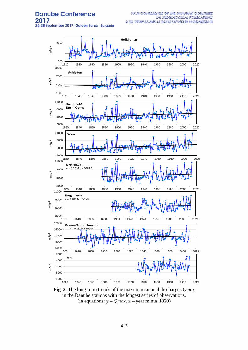
413

Fig. 2. The long-term trends of the maximum annual discharges Qmax

in the Danube stations with the longest series of observations. (in equations: y – Qmax, x – year minus 1820)

2000

5000

8000

11000

1820 1840 1860 1880 1900 1920 1940 1960 1980 2000 2020

m3 s

-1

Bratislavay = 6.2551x + 5098.6

1000

4000

7000

10000

1820 1840 1860 1880 1900 1920 1940 1960 1980 2000 2020

m3 s

-1

Achleiten

y = 6.2116x + 9624.4

5000

8000

11000

14000

17000

1820 1840 1860 1880 1900 1920 1940 1960 1980 2000 2020

m3 s

-1

Orsova/Turnu Severin

5000

8000

11000

14000

17000

1820 1840 1860 1880 1900 1920 1940 1960 1980 2000 2020

m3 s

-1

Reni

2000

5000

8000

11000

1820 1840 1860 1880 1900 1920 1940 1960 1980 2000 2020

m3 s

-1

Nagymarosy = 3.4813x + 5178

500

3500

1820 1840 1860 1880 1900 1920 1940 1960 1980 2000 2020

m3 s

-1

Hofkirchen

2000

5000

8000

11000

1820 1840 1860 1880 1900 1920 1940 1960 1980 2000 2020

m3 s

-1

Kienstock/Stein Krems

2000

5000

8000

11000

1820 1840 1860 1880 1900 1920 1940 1960 1980 2000 2020

m3 s

-1

Wien

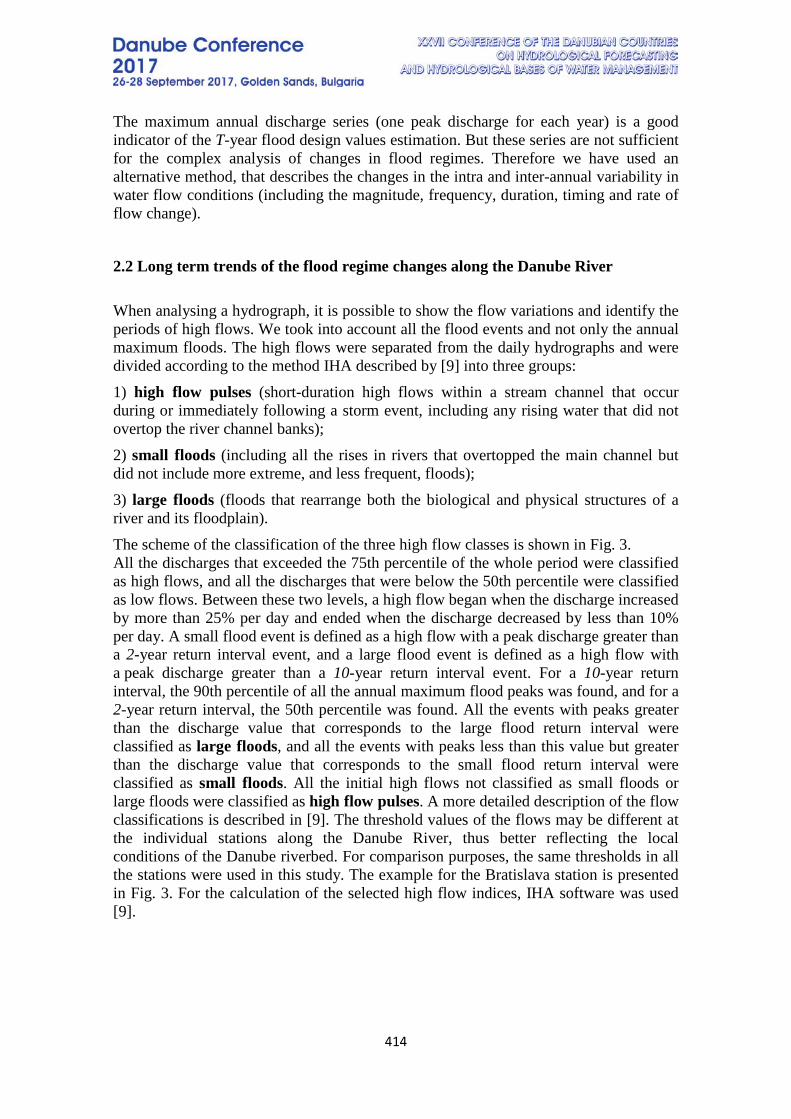
414

The maximum annual discharge series (one peak discharge for each year) is a good indicator of the T-year flood design values estimation. But these series are not sufficient for the complex analysis of changes in flood regimes. Therefore we have used an alternative method, that describes the changes in the intra and inter-annual variability in water flow conditions (including the magnitude, frequency, duration, timing and rate of flow change).

2.2 Long term trends of the flood regime changes along the Danube River When analysing a hydrograph, it is possible to show the flow variations and identify the periods of high flows. We took into account all the flood events and not only the annual maximum floods. The high flows were separated from the daily hydrographs and were divided according to the method IHA described by [9] into three groups: 1) high flow pulses (short-duration high flows within a stream channel that occur during or immediately following a storm event, including any rising water that did not overtop the river channel banks); 2) small floods (including all the rises in rivers that overtopped the main channel but did not include more extreme, and less frequent, floods); 3) large floods (floods that rearrange both the biological and physical structures of a river and its floodplain). The scheme of the classification of the three high flow classes is shown in Fig. 3. All the discharges that exceeded the 75th percentile of the whole period were classified as high flows, and all the discharges that were below the 50th percentile were classified as low flows. Between these two levels, a high flow began when the discharge increased by more than 25% per day and ended when the discharge decreased by less than 10% per day. A small flood event is defined as a high flow with a peak discharge greater than a 2-year return interval event, and a large flood event is defined as a high flow with a peak discharge greater than a 10-year return interval event. For a 10-year return interval, the 90th percentile of all the annual maximum flood peaks was found, and for a 2-year return interval, the 50th percentile was found. All the events with peaks greater than the discharge value that corresponds to the large flood return interval were classified as large floods, and all the events with peaks less than this value but greater than the discharge value that corresponds to the small flood return interval were classified as small floods. All the initial high flows not classified as small floods or large floods were classified as high flow pulses. A more detailed description of the flow classifications is described in [9]. The threshold values of the flows may be different at the individual stations along the Danube River, thus better reflecting the local conditions of the Danube riverbed. For comparison purposes, the same thresholds in all the stations were used in this study. The example for the Bratislava station is presented in Fig. 3. For the calculation of the selected high flow indices, IHA software was used [9].

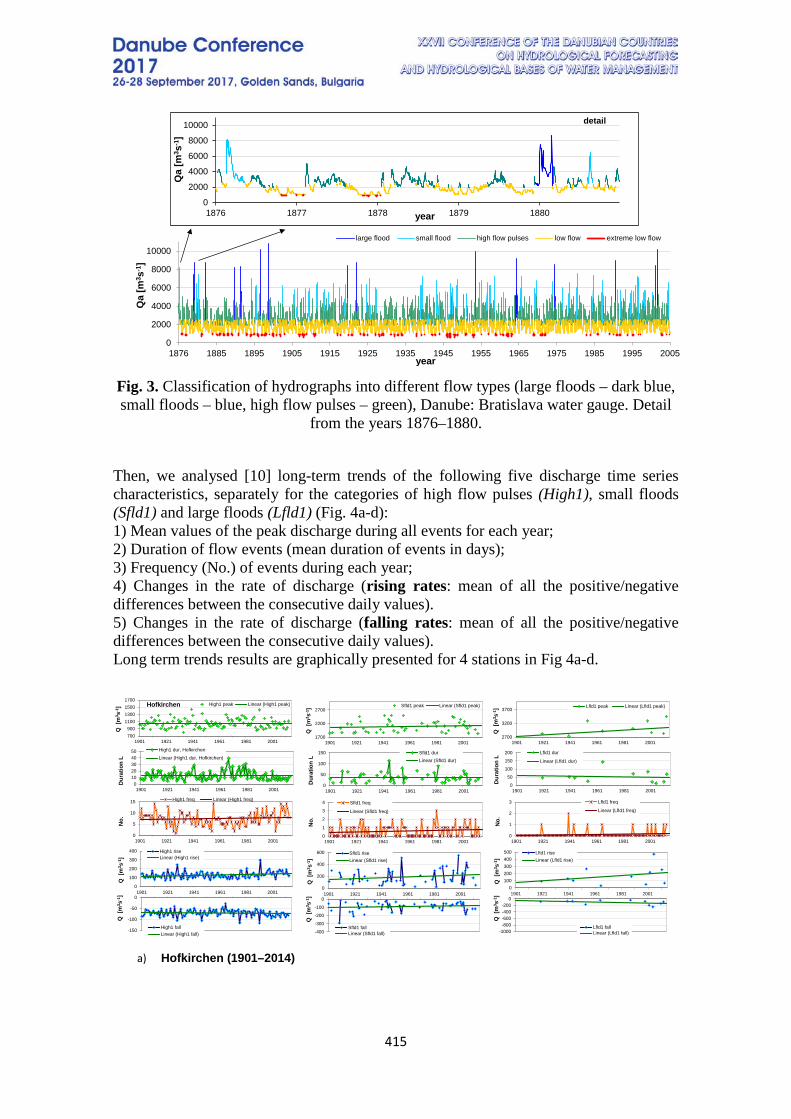
415

Fig. 3. Classification of hydrographs into different flow types (large floods – dark blue, small floods – blue, high flow pulses – green), Danube: Bratislava water gauge. Detail

from the years 1876–1880.

Then, we analysed [10] long-term trends of the following five discharge time series characteristics, separately for the categories of high flow pulses (High1), small floods (Sfld1) and large floods (Lfld1) (Fig. 4a-d): 1) Mean values of the peak discharge during all events for each year; 2) Duration of flow events (mean duration of events in days); 3) Frequency (No.) of events during each year; 4) Changes in the rate of discharge (rising rates: mean of all the positive/negative differences between the consecutive daily values). 5) Changes in the rate of discharge (falling rates: mean of all the positive/negative differences between the consecutive daily values). Long term trends results are graphically presented for 4 stations in Fig 4a-d.

a) Hofkirchen (1901–2014)

0

2000

4000

6000

8000

10000

1876 1877 1878 1879 1880

Qa

[m3 s

-1]

year

detail

0

2000

4000

6000

8000

10000

1876 1885 1895 1905 1915 1925 1935 1945 1955 1965 1975 1985 1995 2005

large flood small flood high flow pulses low flow extreme low flow

Qa

[m3 s

-1]

year

700900

1100130015001700

1901 1921 1941 1961 1981 2001

Q [

m3 s

-1] Hofkirchen High1 peak Linear (High1 peak)

0

5

10

15

1901 1921 1941 1961 1981 2001

No.

High1 freq Linear (High1 freq)

01020304050

1901 1921 1941 1961 1981 2001

Dur

atio

n L

High1 dur, HofkirchenLinear (High1 dur, Hofkirchen)

0

100

200

300

400

1901 1921 1941 1961 1981 2001

Q [

m3 s

-1]

High1 riseLinear (High1 rise)

-150

-100

-50

01901 1921 1941 1961 1981 2001

Q [

m3 s

-1]

High1 fallLinear (High1 fall)

1700

2200

2700

1901 1921 1941 1961 1981 2001

Q [

m3 s

-1] Sfld1 peak Linear (Sfld1 peak)

0

1

2

3

4

1901 1921 1941 1961 1981 2001

No.

Sfld1 freq

Linear (Sfld1 freq)

0

50

100

150

1901 1921 1941 1961 1981 2001

Dur

atio

n L

Sfld1 durLinear (Sfld1 dur)

0

200

400

600

1901 1921 1941 1961 1981 2001

Q [

m3 s

-1]

Sfld1 riseLinear (Sfld1 rise)

-400

-300

-200

-100

01901 1921 1941 1961 1981 2001

Q [

m3 s

-1]

Sfld1 fallLinear (Sfld1 fall)

2700

3200

3700

1901 1921 1941 1961 1981 2001

Q [

m3 s

-1] Lfld1 peak Linear (Lfld1 peak)

0

1

2

3

1901 1921 1941 1961 1981 2001

No.

Lfld1 freq

Linear (Lfld1 freq)

0

50

100

150

200

1901 1921 1941 1961 1981 2001

Dur

atio

n L

Lfld1 dur

Linear (Lfld1 dur)

0100200300400500

1901 1921 1941 1961 1981 2001

Q [

m3 s

-1]

Lfld1 riseLinear (Lfld1 rise)

-1000-800-600-400-200

01901 1921 1941 1961 1981 2001

Q [

m3 s

-1]

Lfld1 fallLinear (Lfld1 fall)

416

b) Achleiten

c) Bratislava (1876–2014)

d) Orsova

Fig. 4. Long-term trends of the: 1. mean high flow pulses (left), small floods (middle), and large floods (right); 2. mean duration; 3. frequency during year; 4. mean rate of

changes in discharges per day - the rising wave rate, and 5. falling wave rate.

0

1000

2000

3000

1901 1921 1941 1961 1981 2001

Q [

m3 s

-1]

High1 peak Linear (High1 peak)

0

5

10

15

20

1901 1921 1941 1961 1981 2001

No.

High1 freq

Linear (High1 freq)

01020304050

1901 1921 1941 1961 1981 2001

Dur

atio

n L

High1 dur, Achleiten

Linear (High1 dur, Achleiten)

0

200

400

600

800

1901 1921 1941 1961 1981 2001

Q [

m3 s

-1]

High1 riseLinear (High1 rise)

-250-200-150-100-50

01901 1921 1941 1961 1981 2001

Q [

m3 s

-1]

High1 fallLinear (High1 fall)

0

2000

4000

6000

1901 1921 1941 1961 1981 2001

Q [

m3 s

-1]

Sfld1 peak Linear (Sfld1 peak)

00.5

11.5

22.5

1901 1921 1941 1961 1981 2001

No.

Sfld1 freq

Linear (Sfld1 freq)

0

50

100

150

200

1901 1921 1941 1961 1981 2001

Dur

atio

n L

Sfld1 durLinear (Sfld1 dur)

0

500

1000

1500

2000

1901 1921 1941 1961 1981 2001

Q [

m3 s

-1]

Sfld1 riseLinear (Sfld1 rise)

-600

-400

-200

01901 1921 1941 1961 1981 2001

Q [

m3 s

-1]

Sfld1 fallLinear (Sfld1 fall)

0

5000

10000

15000

1901 1921 1941 1961 1981 2001

Q [

m3 s

-1]

Lfld1 peak Linear (Lfld1 peak)

0

1

2

3

1901 1921 1941 1961 1981 2001

No.

Lfld1 freq

Linear (Lfld1 freq)

0

50

100

150

1901 1921 1941 1961 1981 2001

Dur

atio

n L Lfld1 dur

Linear (Lfld1 dur)

0

500

1000

1500

2000

1901 1921 1941 1961 1981 2001

Q [

m3 s

-1]

Lfld1 riseLinear (Lfld1 rise)

-1000-800-600-400-200

01901 1921 1941 1961 1981 2001

Q [

m3 s

-1]

Lfld1 fallLinear (Lfld1 fall)

0

1000

2000

3000

4000

5000

1875 1895 1915 1935 1955 1975 1995 2015

Q [

m3 s

-1]

High1 peak Linear (High1 peak)

Bratislava

0

5

10

15

20

1875 1895 1915 1935 1955 1975 1995 2015

No.

High1 freq

Linear (High1 freq)

0

20

40

60

80

1875 1895 1915 1935 1955 1975 1995 2015

Dura

tion

L

High1 dur

Linear (High1 dur)

0200400600800

1000

1875 1895 1915 1935 1955 1975 1995 2015

Q [

m3 s

-1]

High1 riseLinear (High1 rise)

-400

-300

-200

-100

01875 1895 1915 1935 1955 1975 1995 2015

Q [

m3 s

-1]

High1 fallLinear (High1 fall)

02000400060008000

10000

1875 1895 1915 1935 1955 1975 1995 2015

Q [

m3 s

-1]

Sfld1 peak Linear (Sfld1 peak)

0

1

2

3

4

1875 1895 1915 1935 1955 1975 1995 2015

No.

Sfld1 freq

Linear (Sfld1 freq)

0

50

100

150

200

1875 1895 1915 1935 1955 1975 1995 2015

Dura

tion

L

Sfld1 dur

Linear (Sfld1 dur)

0500

1000150020002500

1875 1895 1915 1935 1955 1975 1995 2015

Q [

m3 s

-1]

Sfld1 riseLinear (Sfld1 rise)

-800

-600

-400

-200

01875 1895 1915 1935 1955 1975 1995 2015

Q [

m3 s

-1]

Sfld1 fallLinear (Sfld1 fall)

02000400060008000

1000012000

1875 1895 1915 1935 1955 1975 1995 2015

Q [

m3 s

-1]

Lfld1 peak Linear (Lfld1 peak)

0

1

2

3

1875 1895 1915 1935 1955 1975 1995 2015

No.

Lfld1 freq

Linear (Lfld1 freq)

0

50

100

150

200

1875 1895 1915 1935 1955 1975 1995 2015Du

ratio

n L Lfld1 dur

Linear (Lfld1 dur)

0

500

1000

1500

1875 1895 1915 1935 1955 1975 1995 2015

Q [

m3 s

-1]

Lfld1 riseLinear (Lfld1 rise)

-1000-800-600-400-200

01875 1895 1915 1935 1955 1975 1995 2015

Q [

m3 s

-1]

Lfld1 fallLinear (Lfld1 fall)

0

5000

10000

15000

1850 1870 1890 1910 1930 1950 1970 1990 2010

Q [

m3 s

-1]

High1 peak Linear (High1 peak)

Orsova

0

5

10

15

20

1850 1870 1890 1910 1930 1950 1970 1990 2010

No.

High1 freq Linear (High1 freq)

050

100150200

1850 1870 1890 1910 1930 1950 1970 1990 2010

Dur

atio

n L

High1 durLinear (High1 dur)

0

1000

2000

3000

4000

1850 1870 1890 1910 1930 1950 1970 1990 2010

Q [

m3 s

-1]

High1 riseLinear (High1 rise)

-1500

-1000

-500

01850 1870 1890 1910 1930 1950 1970 1990 2010

Q [

m3 s

-1]

High1 fallLinear (High1 fall)

0

5000

10000

15000

1850 1870 1890 1910 1930 1950 1970 1990 2010

Q [

m3 s

-1]

Sfld1 peak Linear (Sfld1 peak)

00.5

11.5

22.5

1850 1870 1890 1910 1930 1950 1970 1990 2010

No.

Sfld1 freq

Linear (Sfld1 freq)

0100200300400

1850 1870 1890 1910 1930 1950 1970 1990 2010

Dur

atio

n L

Sfld1 durLinear (Sfld1 dur)

0

500

1000

1500

1850 1870 1890 1910 1930 1950 1970 1990 2010

Q [

m3 s

-1]

Sfld1 riseLinear (Sfld1 rise)

-400-300-200-100

01850 1870 1890 1910 1930 1950 1970 1990 2010

Q [

m3 s

-1]

Sfld1 fallLinear (Sfld1 fall)

12000

13000

14000

15000

16000

1850 1870 1890 1910 1930 1950 1970 1990 2010

Q [

m3 s

-1]

Lfld1 peak Linear (Lfld1 peak)

0

1

2

1850 1870 1890 1910 1930 1950 1970 1990 2010

No.

Lfld1 freq

Linear (Lfld1 freq)

050

100150200250

1850 1870 1890 1910 1930 1950 1970 1990 2010

Dur

atio

n L

Lfld1 dur

Linear (Lfld1 dur)

0100200300400500

1850 1870 1890 1910 1930 1950 1970 1990 2010

Q [

m3 s

-1]

Lfld1 riseLinear (Lfld1 rise)

-500-400-300-200-100

01850 1870 1890 1910 1930 1950 1970 1990 2010

Q [

m3 s

-1]

Lfld1 fallLinear (Lfld1 fall)

417

3. CONCLUSIONS The analysis of the long-term trends of the five hydrological characteristics (peak discharges, number and duration of events, and rising and falling rates of the waves) for the three categories (high flow pulses, small floods, and large floods) in all the 20 stations along the Danube gave the same results, but from another point of view. Our study suggests that the selected flow characteristics of the Danube have changed (e.g., the duration of high flow pulses and small as well as large floods have decreased at almost all the stations; the rising and falling rates of the high flow pulses and small flood events have increased at all the stations). These results show that while the characteristics of the high flow pulses and small floods on the Danube have changed significantly, in the case of floods with a return period over 10 years, the changes in the statistical characteristics are not statistically significant. The reasons for the higher rising and falling rates of the flood waves are probably partially due to the training of the Danube channel, i.e., the construction of dams and a decrease in the inundation areas. High flow pulses (with a return period of less than 2 years) and small (with a return period between 2-10 years) flood waves are moving downstream with a much higher degree of celerity with decreasing travel times. In the case of extreme floods (with a return period above 10 years), the travel time is not significantly changing, as was mentioned above. The long-term high flow changes were found to be different in three individual high flow classes. The duration of the category of high flow pulses is decreasing at 19 stations on the Danube and is statistically significant at the Linz, Vienna, Bratislava and Orsova stations. The frequency of the high flow pulses is increasing in all 20 stations. Also, the rising and falling rates of the high flow pulse category are increasing at the majority of the stations. The long-term trends of the selected characteristics of the small floods are very similar to the trends of the high flow pulses, i.e., the duration of small floods is decreasing, and their mean number per year is increasing. In the category of large floods the changes were not proved. ACKNOWLEDGEMENTS This work was supported by the project VEGA No. 2/0009/15 and it results from the project implementation of the “Centre of excellence for integrated flood protection of land” (ITMS 26240120004).

4. REFERENCES [1] EC: Directive 2007/60/EC of the European Parliament and of the Council of 23

October 2007 on the assessment and management of flood risks, European Parliament, Council, 2007.

[2] RCDC (Regional Cooperation of the Danube Countries): Coincidence of flood flow of the Danube River and its tributaries. (Follow-up volume No.IV to the Danube Monograph) VÚVH, Bratislava, 1999.

[3] RCDC (Regional Cooperation of the Danube Countries): Flow regime of River Danube and its Catchment. (Follow-up volume No. VIII/2 to the Danube Monograph) Koblenz/Germany ― Baja/Hungary, 2004.

418

[4] RCDC (Regional Cooperation of the Danube Countries): Regional analysis of annual peak discharges in the Danube Catchment. (Follow-up volume No. VII to the Danube Monograph) Bucureşti, 2004.

[5] Pekárová, P., Miklánek, P., Halmová, D., Flood regime of rivers in the Danube river basin - Objective O1 - Average daily discharge and annual peak discharge series collection. Internal report, Institute of Hydrology SAS, Bratislava, 17 p., 2009.

[6] Pekárová, P., Pekár, J., Miklánek, P., Flood regime of rivers in the Danube river basin - Objective O3 - Analysis of multi-annual variability and long-term trends of the annual Danube discharge series. Internal report, Institute of Hydrology SAS, Bratislava, 24 p., 2009.

[7] Pekárová, P., Miklánek, P., Rončák, P., Halmová, D., Flood regime of rivers in the Danube river basin - Objective O5 - Development of relations between values of NAO indexes and discharge series. Internal report, Institute of Hydrology SAS, Bratislava, 36 p., 2010.

[8] Pekárová, P., Miklánek, P., Melo, M., Halmová, D., Pekár, J., Bačová Mitková, V., Flood Marks along the Danube River between Passau and Bratislava. VEDA and the Slovak Committee for Hydrology - National Committee for the International Hydrological Programme of UNESCO (SVH - NC IHP UNESCO), Bratislava, pp. 104, 2014.

[9] The Nature Conservancy, Indicators of Hydrologic Alteration, Version 7.1. User's Manual. The Nature Conservancy (publisher), 81 pp., 2009.

[10] Pekárová, P., Pramuk, B., Halmová, D., Miklánek, P., Prohaska, S.: Identification of long-term high-flow regime changes in selected stations along the Danube River. Journal of Hydrology and Hydromechanics, Vol. 64, 4, pp. 393–403, 2016.

419

ASSESSMENT OF FLOOD PRONE AREAS ALONG DANUBE RIVER USING OPTICAL SATELLITE DATA

Diana Achim, Viorel Chendeş

National Institute of Hydrology and Water Management, Romania Corresponding author: Diana Achim, N.I.H.W.M., 97E, Bucuresti-Ploiesti, 013686, Bucharest, Sector 1,

Romania, diana.achim@hidro.ro

ABSTRACT Satellite remote sensing is an extremely powerful instrument for many domains, including hydrology. Many international scientific cooperation programs are based on information obtained from distance, captured images allowing monitoring of very large areas at different time and spectral resolution. Processing and analysis of satellite images have applicability for hydrological system, the most relevant being floods, assessing the thickness of snow cover, snow water equivalent, soil moisture, hydrological forecast etc. In European countries, over the past 25 years, there were recorded many floods that affected more than 3.6 million people and caused damage worth $ 104 billion [6]. Commercial or public satellites which monitor environmental conditions record these events and during a flood affected area can be delineated using suitable software and processing techniques. Such an analysis was performed after the flood on the Danube River in April 2006 on Bistret-Rast branch. This is the most important flood recorded during the observation period 1840-2015, water level remaining for a long period of time above warning levels at most hydrometric gauging stations, e.g. 38 days at Calafat gauging station. To delineate the area affected, Landsat 7 satellite images were used free downloaded from the dedicated sites. Satellite image processing techniques consisted of: creating a mosaic of available images, creating natural or false color images, classification and flooded area extraction. Extent of the flood area affected by the levee failure of the agricultural enclosure Rast-Bistret was finally compared to the band flooding with 0.1% probability of exceedance obtained from hydraulic modeling [4]. In a world facing a high risk of natural and engineering disasters, remote sensing complements existing capabilities, in order to improve emergency management. European Union find this domain very important, the best proof is the new program Copernicus [9] which consists in a set of services for data collection and free supply for Member States of the European Space Agency, using satellites and ground sensors to observe the natural phenomena that occur on Earth. Keywords: floods, Danube River, Remote Sensing, Landsat

INTRODUCTION Many international collaborative scientific programs such as the World Climate Research Project or the International Geosphere Biosphere Program (based on the study

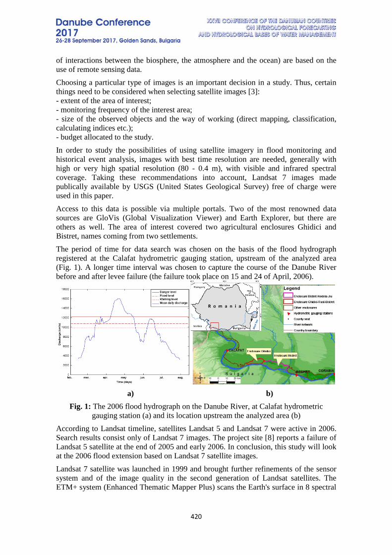
420

of interactions between the biosphere, the atmosphere and the ocean) are based on the use of remote sensing data. Choosing a particular type of images is an important decision in a study. Thus, certain things need to be considered when selecting satellite images [3]: - extent of the area of interest; - monitoring frequency of the interest area; - size of the observed objects and the way of working (direct mapping, classification, calculating indices etc.); - budget allocated to the study. In order to study the possibilities of using satellite imagery in flood monitoring and historical event analysis, images with best time resolution are needed, generally with high or very high spatial resolution (80 - 0.4 m), with visible and infrared spectral coverage. Taking these recommendations into account, Landsat 7 images made publically available by USGS (United States Geological Survey) free of charge were used in this paper. Access to this data is possible via multiple portals. Two of the most renowned data sources are GloVis (Global Visualization Viewer) and Earth Explorer, but there are others as well. The area of interest covered two agricultural enclosures Ghidici and Bistret, names coming from two settlements. The period of time for data search was chosen on the basis of the flood hydrograph registered at the Calafat hydrometric gauging station, upstream of the analyzed area (Fig. 1). A longer time interval was chosen to capture the course of the Danube River before and after levee failure (the failure took place on 15 and 24 of April, 2006).

a) b)

Fig. 1: The 2006 flood hydrograph on the Danube River, at Calafat hydrometric gauging station (a) and its location upstream the analyzed area (b)

According to Landsat timeline, satellites Landsat 5 and Landsat 7 were active in 2006. Search results consist only of Landsat 7 images. The project site [8] reports a failure of Landsat 5 satellite at the end of 2005 and early 2006. In conclusion, this study will look at the 2006 flood extension based on Landsat 7 satellite images. Landsat 7 satellite was launched in 1999 and brought further refinements of the sensor system and of the image quality in the second generation of Landsat satellites. The ETM+ system (Enhanced Thematic Mapper Plus) scans the Earth's surface in 8 spectral

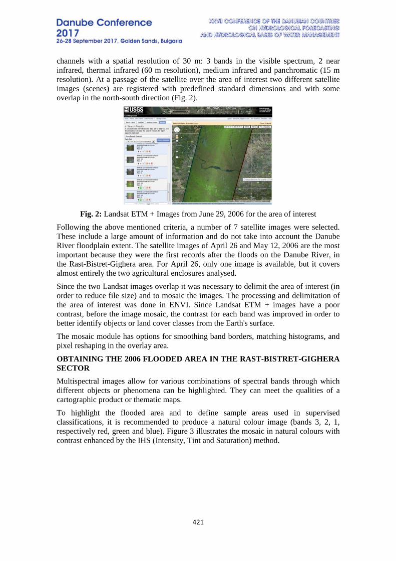
421

channels with a spatial resolution of 30 m: 3 bands in the visible spectrum, 2 near infrared, thermal infrared (60 m resolution), medium infrared and panchromatic (15 m resolution). At a passage of the satellite over the area of interest two different satellite images (scenes) are registered with predefined standard dimensions and with some overlap in the north-south direction (Fig. 2).

Fig. 2: Landsat ETM + Images from June 29, 2006 for the area of interest

Following the above mentioned criteria, a number of 7 satellite images were selected. These include a large amount of information and do not take into account the Danube River floodplain extent. The satellite images of April 26 and May 12, 2006 are the most important because they were the first records after the floods on the Danube River, in the Rast-Bistret-Gighera area. For April 26, only one image is available, but it covers almost entirely the two agricultural enclosures analysed. Since the two Landsat images overlap it was necessary to delimit the area of interest (in order to reduce file size) and to mosaic the images. The processing and delimitation of the area of interest was done in ENVI. Since Landsat ETM + images have a poor contrast, before the image mosaic, the contrast for each band was improved in order to better identify objects or land cover classes from the Earth's surface. The mosaic module has options for smoothing band borders, matching histograms, and pixel reshaping in the overlay area.

OBTAINING THE 2006 FLOODED AREA IN THE RAST-BISTRET-GIGHERA SECTOR Multispectral images allow for various combinations of spectral bands through which different objects or phenomena can be highlighted. They can meet the qualities of a cartographic product or thematic maps. To highlight the flooded area and to define sample areas used in supervised classifications, it is recommended to produce a natural colour image (bands 3, 2, 1, respectively red, green and blue). Figure 3 illustrates the mosaic in natural colours with contrast enhanced by the IHS (Intensity, Tint and Saturation) method.

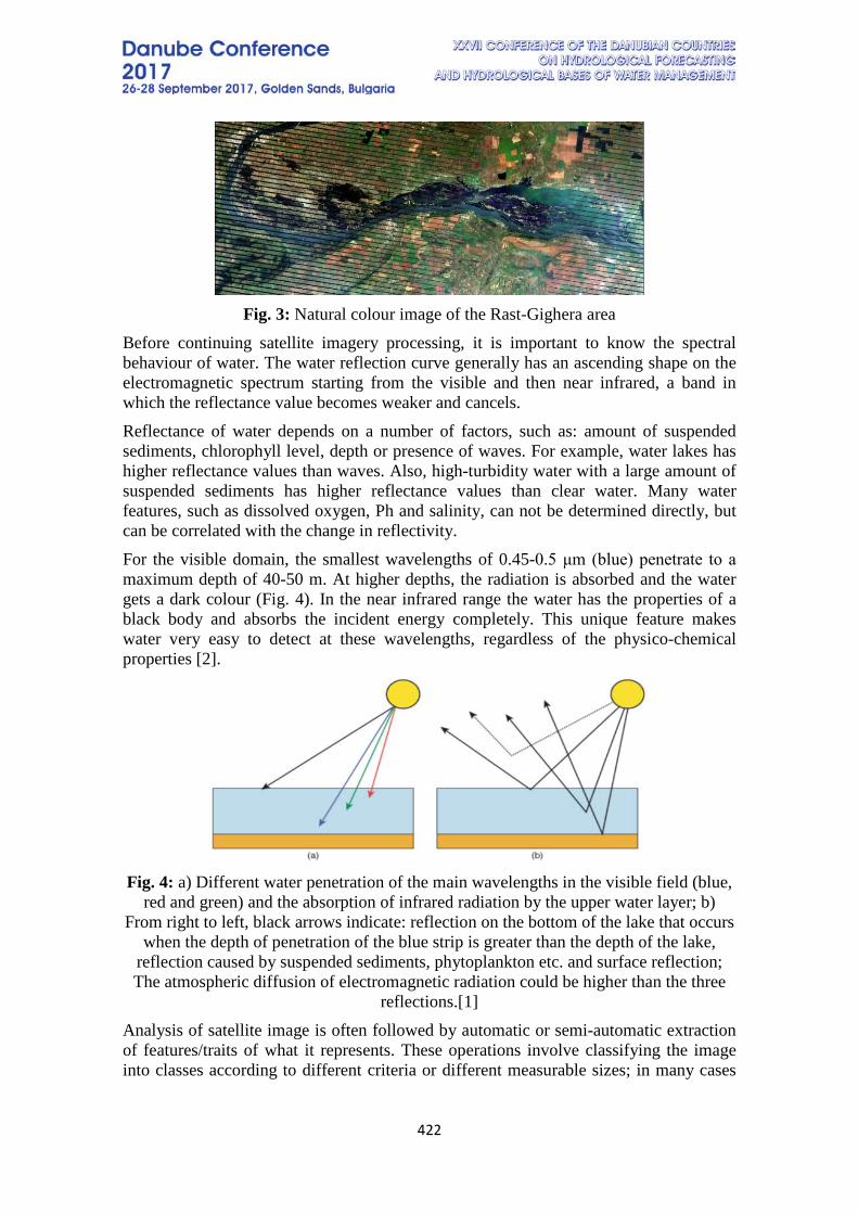
422

Fig. 3: Natural colour image of the Rast-Gighera area

Before continuing satellite imagery processing, it is important to know the spectral behaviour of water. The water reflection curve generally has an ascending shape on the electromagnetic spectrum starting from the visible and then near infrared, a band in which the reflectance value becomes weaker and cancels. Reflectance of water depends on a number of factors, such as: amount of suspended sediments, chlorophyll level, depth or presence of waves. For example, water lakes has higher reflectance values than waves. Also, high-turbidity water with a large amount of suspended sediments has higher reflectance values than clear water. Many water features, such as dissolved oxygen, Ph and salinity, can not be determined directly, but can be correlated with the change in reflectivity. For the visible domain, the smallest wavelengths of 0.45-0.5 μm (blue) penetrate to a maximum depth of 40-50 m. At higher depths, the radiation is absorbed and the water gets a dark colour (Fig. 4). In the near infrared range the water has the properties of a black body and absorbs the incident energy completely. This unique feature makes water very easy to detect at these wavelengths, regardless of the physico-chemical properties [2].

Fig. 4: a) Different water penetration of the main wavelengths in the visible field (blue,

red and green) and the absorption of infrared radiation by the upper water layer; b) From right to left, black arrows indicate: reflection on the bottom of the lake that occurs

when the depth of penetration of the blue strip is greater than the depth of the lake, reflection caused by suspended sediments, phytoplankton etc. and surface reflection; The atmospheric diffusion of electromagnetic radiation could be higher than the three

reflections.[1] Analysis of satellite image is often followed by automatic or semi-automatic extraction of features/traits of what it represents. These operations involve classifying the image into classes according to different criteria or different measurable sizes; in many cases

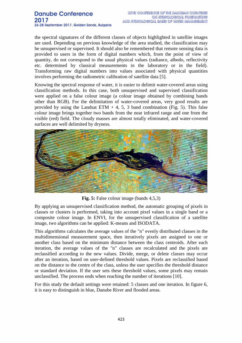
423

the spectral signatures of the different classes of objects highlighted in satellite images are used. Depending on previous knowledge of the area studied, the classification may be unsupervised or supervised. It should also be remembered that remote sensing data is provided to users in the form of digital numbers which, from the point of view of quantity, do not correspond to the usual physical values (radiance, albedo, reflectivity etc. determined by classical measurements in the laboratory or in the field). Transforming raw digital numbers into values associated with physical quantities involves performing the radiometric calibration of satellite data [5]. Knowing the spectral response of water, it is easier to delimit water-covered areas using classification methods. In this case, both unsupervised and supervised classification were applied on a false colour image (a colour image obtained by combining bands other than RGB). For the delimitation of water-covered areas, very good results are provided by using the Landsat ETM + 4, 5, 3 band combination (Fig. 5). This false colour image brings together two bands from the near infrared range and one from the visible (red) field. The cloudy masses are almost totally eliminated, and water-covered surfaces are well delimited by dryness.

Fig. 5: False colour image (bands 4,5,3)

By applying an unsupervised classification method, the automatic grouping of pixels in classes or clusters is performed, taking into account pixel values in a single band or a composite colour image. In ENVI, for the unsupervised classification of a satellite image, two algorithms can be applied: K-means and ISODATA. This algorithms calculates the average values of the "n" evenly distributed classes in the multidimensional measurement space, then iteratively pixels are assigned to one or another class based on the minimum distance between the class centroids. After each iteration, the average values of the "n" classes are recalculated and the pixels are reclassified according to the new values. Divide, merge, or delete classes may occur after an iteration, based on user-defined threshold values. Pixels are reclassified based on the distance to the centre of the class, unless the user specifies the threshold distance or standard deviation. If the user sets these threshold values, some pixels may remain unclassified. The process ends when reaching the number of iterations [10]. For this study the default settings were retained: 5 classes and one iteration. In figure 6, it is easy to distinguish in blue, Danube River and flooded areas.

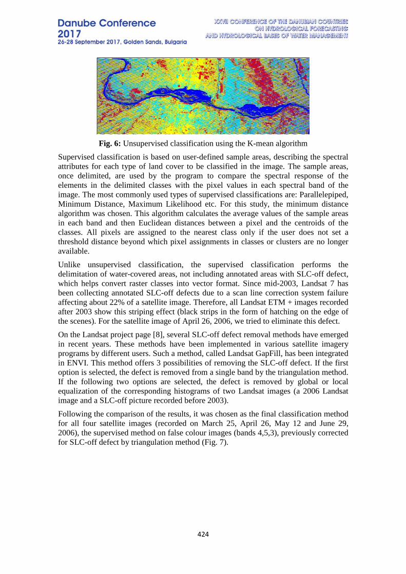
424

Fig. 6: Unsupervised classification using the K-mean algorithm

Supervised classification is based on user-defined sample areas, describing the spectral attributes for each type of land cover to be classified in the image. The sample areas, once delimited, are used by the program to compare the spectral response of the elements in the delimited classes with the pixel values in each spectral band of the image. The most commonly used types of supervised classifications are: Parallelepiped, Minimum Distance, Maximum Likelihood etc. For this study, the minimum distance algorithm was chosen. This algorithm calculates the average values of the sample areas in each band and then Euclidean distances between a pixel and the centroids of the classes. All pixels are assigned to the nearest class only if the user does not set a threshold distance beyond which pixel assignments in classes or clusters are no longer available. Unlike unsupervised classification, the supervised classification performs the delimitation of water-covered areas, not including annotated areas with SLC-off defect, which helps convert raster classes into vector format. Since mid-2003, Landsat 7 has been collecting annotated SLC-off defects due to a scan line correction system failure affecting about 22% of a satellite image. Therefore, all Landsat ETM + images recorded after 2003 show this striping effect (black strips in the form of hatching on the edge of the scenes). For the satellite image of April 26, 2006, we tried to eliminate this defect. On the Landsat project page [8], several SLC-off defect removal methods have emerged in recent years. These methods have been implemented in various satellite imagery programs by different users. Such a method, called Landsat GapFill, has been integrated in ENVI. This method offers 3 possibilities of removing the SLC-off defect. If the first option is selected, the defect is removed from a single band by the triangulation method. If the following two options are selected, the defect is removed by global or local equalization of the corresponding histograms of two Landsat images (a 2006 Landsat image and a SLC-off picture recorded before 2003). Following the comparison of the results, it was chosen as the final classification method for all four satellite images (recorded on March 25, April 26, May 12 and June 29, 2006), the supervised method on false colour images (bands 4,5,3), previously corrected for SLC-off defect by triangulation method (Fig. 7).

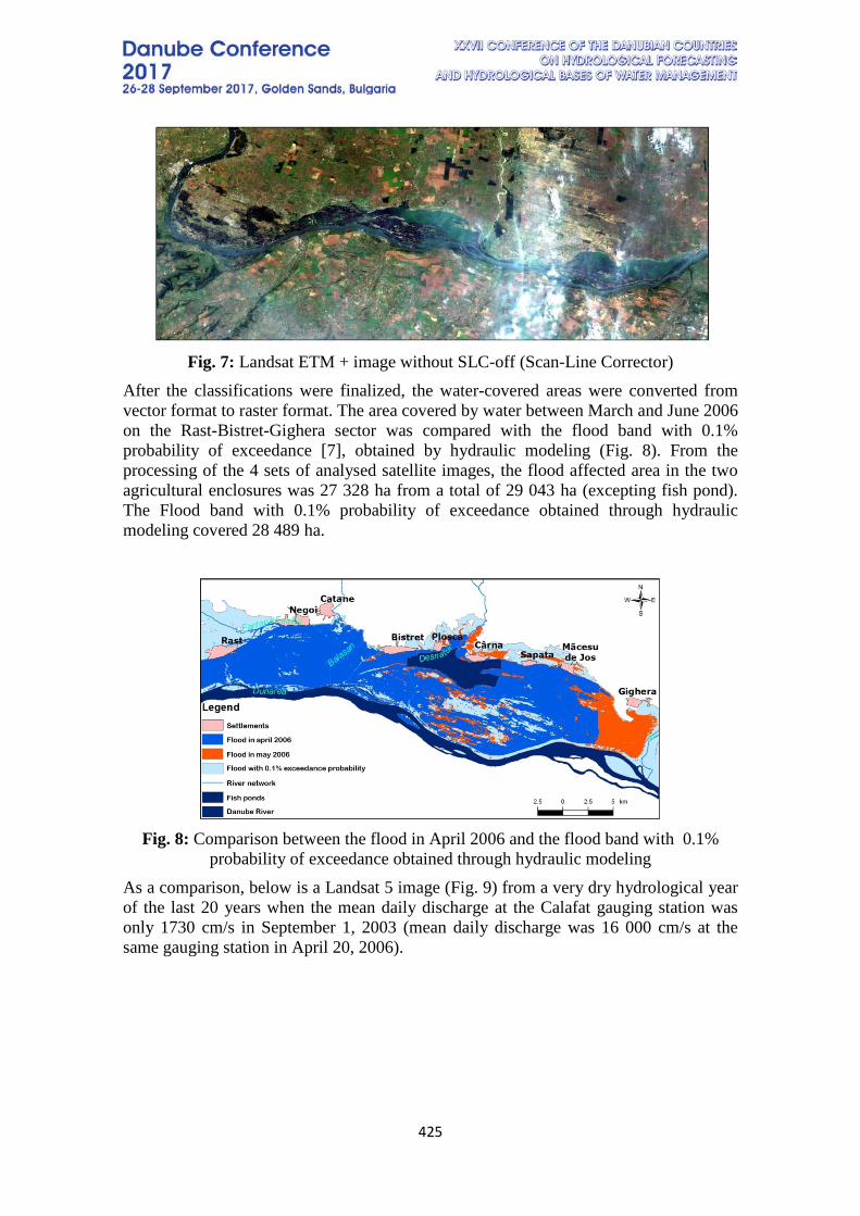
425

Fig. 7: Landsat ETM + image without SLC-off (Scan-Line Corrector)

After the classifications were finalized, the water-covered areas were converted from vector format to raster format. The area covered by water between March and June 2006 on the Rast-Bistret-Gighera sector was compared with the flood band with 0.1% probability of exceedance [7], obtained by hydraulic modeling (Fig. 8). From the processing of the 4 sets of analysed satellite images, the flood affected area in the two agricultural enclosures was 27 328 ha from a total of 29 043 ha (excepting fish pond). The Flood band with 0.1% probability of exceedance obtained through hydraulic modeling covered 28 489 ha.

Fig. 8: Comparison between the flood in April 2006 and the flood band with 0.1%

probability of exceedance obtained through hydraulic modeling As a comparison, below is a Landsat 5 image (Fig. 9) from a very dry hydrological year of the last 20 years when the mean daily discharge at the Calafat gauging station was only 1730 cm/s in September 1, 2003 (mean daily discharge was 16 000 cm/s at the same gauging station in April 20, 2006).

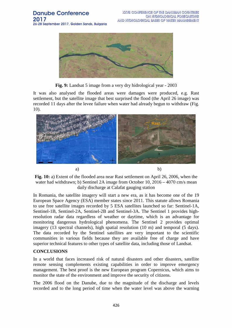
426

Fig. 9: Landsat 5 image from a very dry hidrological year - 2003 It was also analysed the flooded areas were damages were produced, e.g. Rast settlement, but the satellite image that best surprised the flood (the April 26 image) was recorded 11 days after the levee failure when water had already begun to withdraw (Fig. 10).

a) b)

Fig. 10: a) Extent of the flooded area near Rast settlement on April 26, 2006, when the water had withdrawn; b) Sentinel 2A image from October 10, 2016 – 4070 cm/s mean

daily discharge at Calafat gauging station In Romania, the satellite imagery will start a new era, as it has become one of the 19 European Space Agency (ESA) member states since 2011. This statute allows Romania to use free satellite images recorded by 5 ESA satellites launched so far: Sentinel-1A, Sentinel-1B, Sentinel-2A, Sentinel-2B and Sentinel-3A. The Sentinel 1 provides high-resolution radar data regardless of weather or daytime, which is an advantage for monitoring dangerous hydrological phenomena. The Sentinel 2 provides optimal imagery (13 spectral channels), high spatial resolution (10 m) and temporal (5 days). The data recorded by the Sentinel satellites are very important to the scientific communities in various fields because they are available free of charge and have superior technical features to other types of satellite data, including those of Landsat.

CONCLUSIONS In a world that faces increased risk of natural disasters and other disasters, satellite remote sensing complements existing capabilities in order to improve emergency management. The best proof is the new European program Copernicus, which aims to monitor the state of the environment and improve the security of citizens. The 2006 flood on the Danube, due to the magnitude of the discharge and levels recorded and to the long period of time when the water level was above the warning

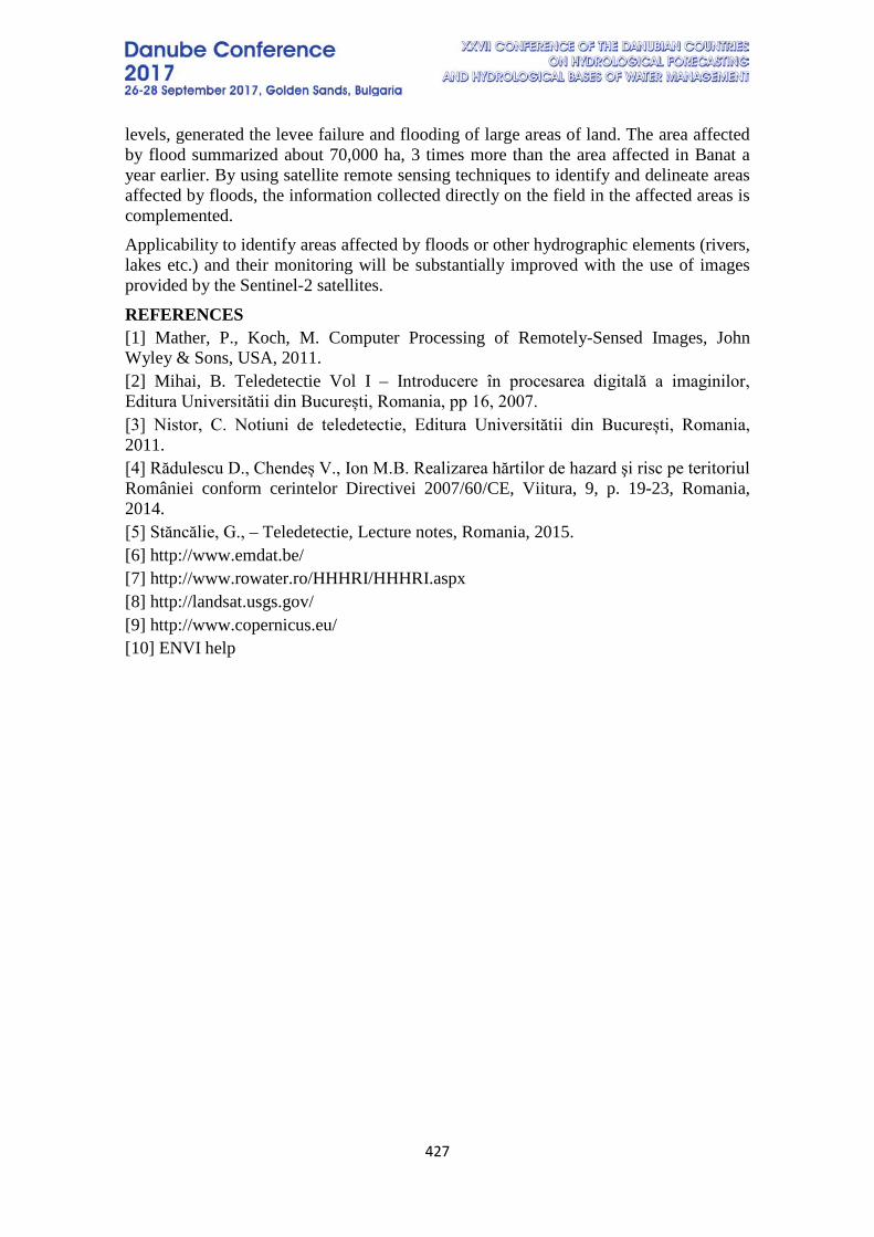
427

levels, generated the levee failure and flooding of large areas of land. The area affected by flood summarized about 70,000 ha, 3 times more than the area affected in Banat a year earlier. By using satellite remote sensing techniques to identify and delineate areas affected by floods, the information collected directly on the field in the affected areas is complemented. Applicability to identify areas affected by floods or other hydrographic elements (rivers, lakes etc.) and their monitoring will be substantially improved with the use of images provided by the Sentinel-2 satellites.

REFERENCES [1] Mather, P., Koch, M. Computer Processing of Remotely-Sensed Images, John Wyley & Sons, USA, 2011. [2] Mihai, B. Teledetectie Vol I – Introducere în procesarea digitală a imaginilor, Editura Universitătii din București, Romania, pp 16, 2007. [3] Nistor, C. Notiuni de teledetectie, Editura Universitătii din București, Romania, 2011. [4] Rădulescu D., Chendeș V., Ion M.B. Realizarea hărtilor de hazard şi risc pe teritoriul României conform cerintelor Directivei 2007/60/CE, Viitura, 9, p. 19-23, Romania, 2014. [5] Stăncălie, G., – Teledetectie, Lecture notes, Romania, 2015. [6] http://www.emdat.be/ [7] http://www.rowater.ro/HHHRI/HHHRI.aspx [8] http://landsat.usgs.gov/ [9] http://www.copernicus.eu/ [10] ENVI help

428

DROUGHT IDENTIFICATION AND MONITORING

Jana Poórová, Zuzana Danáčová, Katarína Melová, Lotta Blaškovičová

Slovak Hydrometeorological Institute, Bratislava, Slovak Republic

Corresponding author: Dr. Melová Katarína, Slovak Hydrometeorological Institute, Jeséniova 17, 833 15 Bratislava, Slovak Republic, katarina.melova@shmu.sk

Historically some years are being referred to as dry or very dry ones, but they can be defined as dry from different points of view – climatological (precipitation deficit), hydrological (water deficit in surface waters and groundwater), agricultural (plants suffering from soil moisture deficit) etc. Identification and monitoring of the hydrological drought (in connection with water scarcity as well) is becoming one of the most important tasks of present surface water hydrology, also according to the increasing public interest. Analyzing the data series from state surface water monitoring network the periods of low flow can be relatively easily selected. However, one of the crucial steps in this evaluation is the definition of limit values (thresholds). After the definition of these limit values, based on statistical analysis of long-term data series we can examine the drought periods. Depending on the selected threshold value, the characteristics of drought periods (duration, deficit volume, minimum values etc.) may vary significantly in time and space. Based on these analyzes, we can make regionalization according to the appearance of drought periods and trends of minimum discharges in Slovakia. Actually the on-line presentation on web site of Slovak Hydrometeorological Institute of the flow situation in selected water-gauging stations is being prepared, where the actual daily discharge values are graphically compared with long term low-flow characteristics for particular stations, to set an easily understandable visualization, whether the drought situation is becoming serious.

429

PROBLEMS OF WATER RESOURCES MANAGEMENT OF DANUBE RIVER BASIN IN CHERNIVTSI REGION OF UKRAINE

Lyudmyla Kuzmych

National University of Water and Environmental Engineering, Ukraine

Corresponding author: Lyudmyla Kuzmych, National University of Water and Environmental Engineering, Soborna str., 11, Rivne, Ukraine, 33000, l.v.kuzmych@nuwm.edu.ua

Currently the problem of water resources at the international level is an integrated management of transboundary waters, which includes a number of aspects. Water resources of Ukraine are formed mainly due to cross-border waterways, including the Siret river and Prut river – the tributaries of the Danube river. The analysis of the geographic and climatic conditions, geological structure, soils, and vegetation of the Siret and Prut rivers basins is done; the causes of the formation of floods in the region are discovered. Analysis of the operation of hydraulic engineering facilities showed that due to lack of funding programs in flood risk is for 73 towns (over 40 thousand people) with an area of possible flooding more than 200 km2. In addition, as a result of the passage of floods for previous years there was changed the state border of Ukraine and the Romanian side moved away about 15 hectares of wetlands. A retrospective analysis showed that uncontrolled and scientifically ungrounded felling of forest area in the Carpathians has a direct immediate impact on the flood regime of Mountain Rivers, leading to more catastrophic floods in recent years.

Keywords: transboundary waters, integrated management, Siret river, Prut river, flood regime, flood protection. Water resources of Ukraine are derived of the transit river waters from foreign countries, local runoff and underground water. Potential resources of river waters constitute 209.8 km3, of which only a quarter is formed in Ukraine; the rest comes from Russia, Belarus, Romania and Moldova. Projected reserves of underground waters are 21 km3 [1]. For Ukraine, the special economic and ecological importance such cross-border rivers as the Dnieper (shared by 3 countries) and Danube (shared by 18 countries), which impact largely on the state of the Black Sea, which in turn brings together 10 countries of Central and Eastern Europe. Concerns of citizens of European countries, including Ukraine, on the state of water resources is one of the reasons the European Commission of water protection - a priority. These facilities include water basins of the rivers Siret and Prut, where water resources are transboundary, because these basins are subbasins of the Danube river basin [2, 3]. Prut river basin covers the territory of Ivano-Frankivsk and Chernivtsi regions of Ukraine and of Romania and Moldova. Prut River originates on the southeast slope of Mount

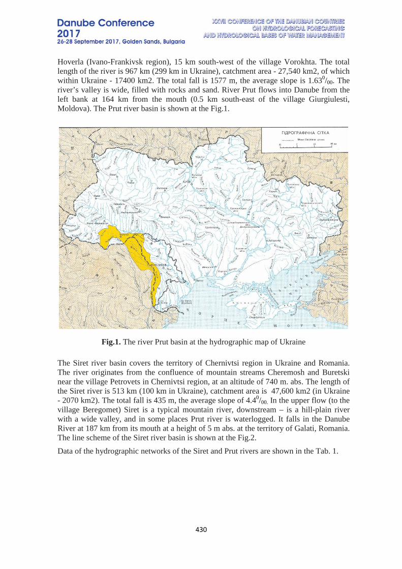
430

Hoverla (Ivano-Frankivsk region), 15 km south-west of the village Vorokhta. The total length of the river is 967 km (299 km in Ukraine), catchment area - 27,540 km2, of which within Ukraine - 17400 km2. The total fall is 1577 m, the average slope is 1.630/00. The river’s valley is wide, filled with rocks and sand. River Prut flows into Danube from the left bank at 164 km from the mouth (0.5 km south-east of the village Giurgiulesti, Moldova). The Prut river basin is shown at the Fig.1.

Fig.1. The river Prut basin at the hydrographic map of Ukraine

The Siret river basin covers the territory of Chernivtsi region in Ukraine and Romania. The river originates from the confluence of mountain streams Cheremosh and Buretski near the village Petrovets in Chernivtsi region, at an altitude of 740 m. abs. The length of the Siret river is 513 km (100 km in Ukraine), catchment area is 47,600 km2 (in Ukraine - 2070 km2). The total fall is 435 m, the average slope of 4.40/00. In the upper flow (to the village Beregomet) Siret is a typical mountain river, downstream – is a hill-plain river with a wide valley, and in some places Prut river is waterlogged. It falls in the Danube River at 187 km from its mouth at a height of 5 m abs. at the territory of Galati, Romania. The line scheme of the Siret river basin is shown at the Fig.2. Data of the hydrographic networks of the Siret and Prut rivers are shown in the Tab. 1.

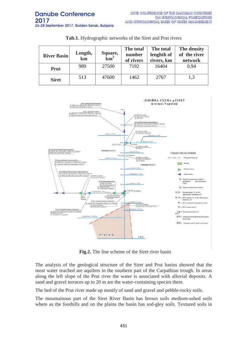
431

Tab.1. Hydrographic networks of the Siret and Prut rivers

River Basin Length, km

Square, km2

The total number of rivers

The total lenghth of rivers, km

The density of the river

network

Prut 989 27500 7192 16404 0,94

Siret 513 47600 1462 2767 1,3

Fig.2. The line scheme of the Siret river basin

The analysis of the geological structure of the Siret and Prut basins showed that the most water reached are aquifers in the southern part of the Carpathian trough. In areas along the left slope of the Prut river the water is associated with alluvial deposits. A sand and gravel terraces up to 20 m are the water-containing species there. The bed of the Prut river made up mostly of sand and gravel and pebble-rocky soils. The mountainous part of the Siret River Basin has brown soils medium-ashed soils where as the foothills and on the plains the basin has sod-gley soils. Textured soils in

432

the mountains belong to medium loamy sand, on the plains - easy to loamy. The underlying layer has a low permeability. The formation of the hydrological regime of the Siret and Prut rivers and their reservoirs has an important role for vegetation in the adjacent areas. The most densely hydraulic network of Ukraine is in the Carpathians region that is on average 0.5-0.7 km per km2. There are about 9426 rivers and streams with a total length of 19,793 km and an annual runoff is more than 12 billion m3. Under such hydrometeorological and difficult terrain conditions the forests perform an important a water and soil protect function and any water engineering structure cannot do these functions better. Mature beech forests are able to hold up to 25% of rainfall and fir - 36.9%. Thus, the uncontrolled and scientifically ungrounded felling of forest area in the Carpathians has a direct impact on the flood regime of mountain rivers, leading to more catastrophic floods in recent years. Historically, the main task of water management organizations in the region of the Siret and Prut rivers basins for recent years is the protection of human settlements, agricultural land and other economic facilities from the harmful effects of water. One of the most dangerous manifestations of the harmful effects of water are catastrophic floods. The mechanism of occurrence and causes of the floods in the region is well known. The main cause of floods are intense rains on wet background or backdrop sudden thaw and rapid snowmelt. A main cause of frequent flooding in the region of the Siret and Prut rivers basins is the hydrometeorological situation and structure of the river, and economic activity in the basins. These include [4]:

• global climate change; • cyclic occurrence of periods of raising the level of undergroundwater; • uncontrolled economic activity in the catchment area and violation of the rules of

construction on this area, including floodplains of mountain district of the Siret and Prut rivers basins;

• large sloping of the rivers and significant slopes and a lack of the water transport capacity;

• significant reduction of the area of forests and forest plantations, especially unsystematic deforestation on the slopes, which accelerating the runoff water in the rivers and floods abrupt formation of high levels;

• consumerism practice in the valleys of the rivers and the mountains, especially in the areas of forests;

• lack of water regulating structures financing. Taken together, these natural processes and human factors lead to a reduction of a watershed capacity, reducing of the bandwidth of the Siret and Prut rivers, and a high level of development of floodplains. In addition, often in the rivers floodplain there are facts of extraction of gravel and sand, leading to activation of channel processes, rivers deformation and threatens the function of the hydraulic structures.

433

Negative situation in the Siret and Prut rivers basins creates a temporary traffic, which were created by gravel - gravel deposits, a mass of trees, roots, twigs that have accumulated during the annual flooding and are not promptly removed. This establishment also causes a local increase of water levels and in the case of a breakthrough forms a further destructive flood wave. At present, about 20 km among 139 km flood objects which have been being the balance of water management organizations in Chernivtsi region require major repairs and complete reconstruction. As a result, under the threat of flooding and destruction along the Prut and Siret rivers are 73 settlements with an area of a possible flooding more than 200 km2, which lives about 40 thousand people. And given a similar situation on small rivers during floods negative impact on an area of 370 km2 and 156 settlements. Also there is a critical situation at the border area. There were built 15.1 km fasteners, at present about 5.0 km of them are destroyed and need the complete renovation. On average physical wear intact waterworks is about 70%. Furthermore shore areas were identified with a total length of about 2.0 kilometers, where there are intensive processes of destruction. So to prevent the loss of Ukrainian territory appropriate measures are taken to restore the existing and construction of new coastal mounting in the border area at a total length of 7.0 kilometers. During the years 2009-2016 from the state budget for anti-flood measures in the border area actually allocated only 2.6 million UAH (320 thousand dollars). Such situation does not allow to maintain in proper condition the flood facilities in the border area and to prevent loss of Ukrainian territory. As a result of the passage of floods of previous years leads to change the state border that runs along the river through the channel to Romania moved away about 15 hectares of wetlands. In these rivers basins there are a large number of accumulative complexes (over 57 ponds with a total volume 3.04 million m3), but they are not free volume accumulation for flood runoff. The best way to solve this problem is the construction of facilities aimed at protection areas (storage tanks, gabion complexes etc.), that will help to minimize the negative impact of flood waters. The implementation of the flood protection of the area includes the following measures: 1. Construction of reservoirs - 9 pieces 2. Reconstruction of reservoirs - 3 pieces. 3. Reconstruction of bridges. 4. Construction of dams at the Prut river. 5. Construction of the left bank protective dam at the Prut river. 6. Construction of the right bank protective dam at the Prut river. 7. Construction of left bank protective dam at the Siret river. The estimated total cost of construction is 776.250 million UAH (about 30 million Euros).

434

Also in the large-scale international project “Prevention and protection against flooding in the upper basins of the rivers Siret and Prut, by implementing a modern system of automatic monitoring stations - EAST AVERT” has constructed benches totaling about 5.0 million UAH. Low level or complete absence of funding for flood protection measures resulting in deterioration at the rivers basins and, consequently, leading to the growth of social tension among the residents besides the rivers. In view of the above, the main issues of water resources management of the Siret and Prut rivers include:

1. Adequate and stable funding for existing flood control programs; 2. Allocation of funds to fully recover the destroyed water structures, which were

damaged during the floods of previous years; 3. Repairing of the existing water structures and building new structures in the

border area of Chernivtsi region; 4. Lack of funding for the creation of bench protection strips along rivers, around

reservoirs, ponds and other water bodies and drainage channel strips, as required by the Water Code of Ukraine.

5. Cutting down forests, plowing, building of floodplain of the rivers etc., leads to increased stress on water intake, resulting in disturbed natural regime of the river, changing conditions of the flow, frequent floods and rising losses on them.

[1] L.V. Kuzmych, I.M. Andriuk. Rational use of water resources in the Prut River basin // Rational use and protection of natural resources of Ukraine in the context of sustainable development. A collection of scientific articles. – Rivne, NUWEE, pp 31-34, 2016. [2] L.V. Kuzmych, I.M. Andriuk. The problems of water management in the Siret River Basin. Bulletin of the National University of Water and Environmental Engineering. ISSN 2306-5478, volume 4(64), Rivne, pp 112-120, 2015.

[3] L.V. Kuzmych, Y.V. Gavrylyuk. Managing of transboundary waters in Ukraine in conditions of international cooperation. Proceedings of the conference to the World Day of Water, Institute of Water Problems and Land Reclamation NAAS, Kyiv, Ukraine, 2014.

[4] I. Korobiychuk, L. Kuzmych, V. Kvasnikov, P. Novak. The use of remote ground sensing data for assessment of environmental and crop condition of the reclaimed land. Advances in Intelligent Systems and Computing. Springer, vol.550, pp. 418-425, 2016.

435

EVALUATION OF THE THRESHOLDS FOR FLOOD FORECASTING AND WARNING

Vesela Stoyanova, Snezhanka Balabanova, Valeriya Yordanova

National Institute of Meteorology and Hydrology at the Bulgarian Academy of Science, Bulgaria

Corresponding author: Tzarigradsko chaussee 66, 1784 Sofia, Bulgaria, e-mails: Vesela.Popova@meteo.bg ; Snezana.Balabanova@meteo.bg ; Valeriya.Yordanova@meteo.bg

ABSTRACT One of the most important task for hydrological forecasters is to decide if the simulated discharges exceed critical discharges and decide on whether a flood warning should be issued or not. This leads to solving: 1) How to define critical thresholds along all the rivers under survey? 2) How to link locally defined thresholds to simulated discharges, which result from models with specific spatial and temporal resolutions? This study is focused on the assessment of critical thresholds and is a preliminary step for the development of flood forecasting and warning system. Hydrologically based thresholds rely on observed river conditions and forecasts. The process can involve various approaches, from the use of simple correlation techniques between upstream and downstream sites to complex hydrological or hydraulic model based warning levels. A study of scientific literature and good practice related to the problem has been made. After considering available hydrological information and local conditions, some of the methods have been applied to the rivers Cherna and Biala in the Arda river catchment. High waves along the rivers in 2005 and 2006 lead to floods in Smolyan town and causing loss of lives and property. Quantitative characterization of discharges are used to characterize the river discharge/level as low, medium and high. Duration curves for the monitoring stations are defined with historical data series using daily mean discharges/levels. The traditional flood warning approach is also applied. In this method warning thresholds levels are defined based on preliminary determined flood hazard prone area for different scenarios. HEC-RAS model is used for multiple profile analysis and flood threshold levels/ runoffs are identified along the river. Тhis provides the basis for developing threshold-stage based flood early warning system in these rivers. For the studied region will be presented development of warnings based on impact and according WMO recommendation.

KEYWORDS: hydrology, thresholds for flood warning, HEC-RAS model, flood hazard maps, GIS

INTODUCTION Flooding is a natural hazard that threatens lives and causes huge economic losses both in Bulgaria and worldwide. The flooding as an environmental event affects more people than any other natural hazard. In the period from 1970 to 2012, storms and floods caused over one million deaths [1].

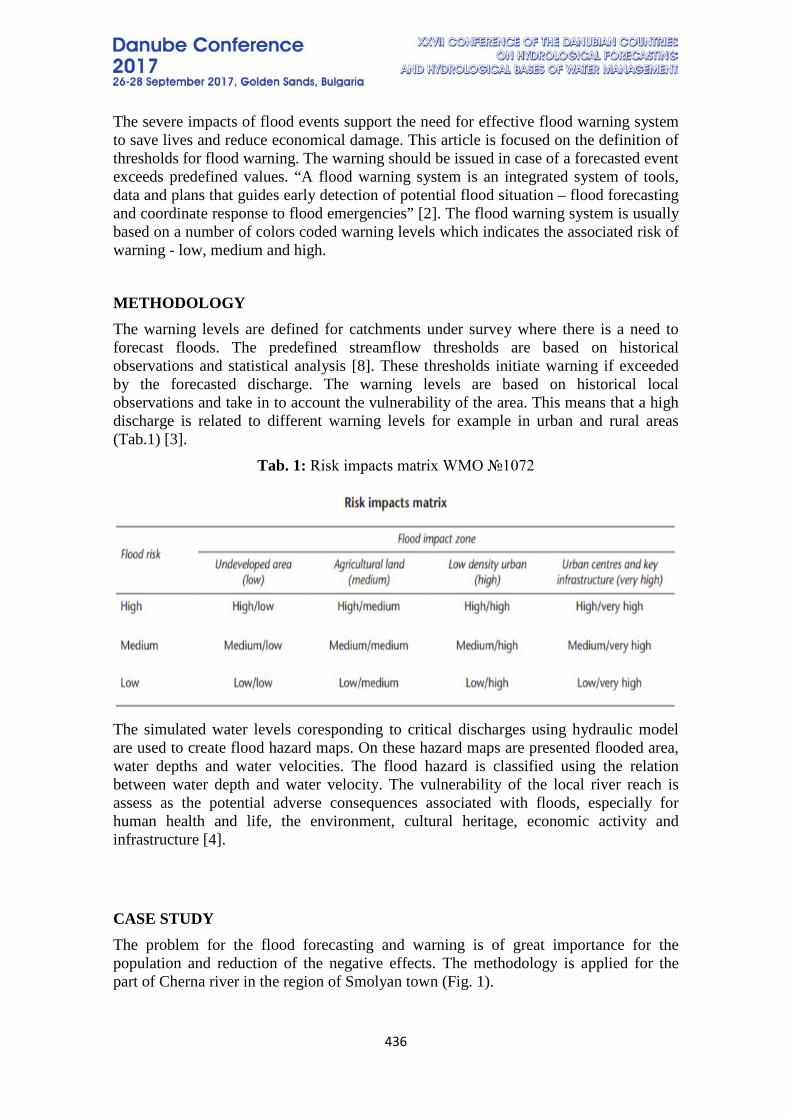
436

The severe impacts of flood events support the need for effective flood warning system to save lives and reduce economical damage. This article is focused on the definition of thresholds for flood warning. The warning should be issued in case of a forecasted event exceeds predefined values. “A flood warning system is an integrated system of tools, data and plans that guides early detection of potential flood situation – flood forecasting and coordinate response to flood emergencies” [2]. The flood warning system is usually based on a number of colors coded warning levels which indicates the associated risk of warning - low, medium and high.

METHODOLOGY The warning levels are defined for catchments under survey where there is a need to forecast floods. The predefined streamflow thresholds are based on historical observations and statistical analysis [8]. These thresholds initiate warning if exceeded by the forecasted discharge. The warning levels are based on historical local observations and take in to account the vulnerability of the area. This means that a high discharge is related to different warning levels for example in urban and rural areas (Tab.1) [3].

Tab. 1: Risk impacts matrix WMO №1072

The simulated water levels coresponding to critical discharges using hydraulic model are used to create flood hazard maps. On these hazard maps are presented flooded area, water depths and water velocities. The flood hazard is classified using the relation between water depth and water velocity. The vulnerability of the local river reach is assess as the potential adverse consequences associated with floods, especially for human health and life, the environment, cultural heritage, economic activity and infrastructure [4].

CASE STUDY The problem for the flood forecasting and warning is of great importance for the population and reduction of the negative effects. The methodology is applied for the part of Cherna river in the region of Smolyan town (Fig. 1).

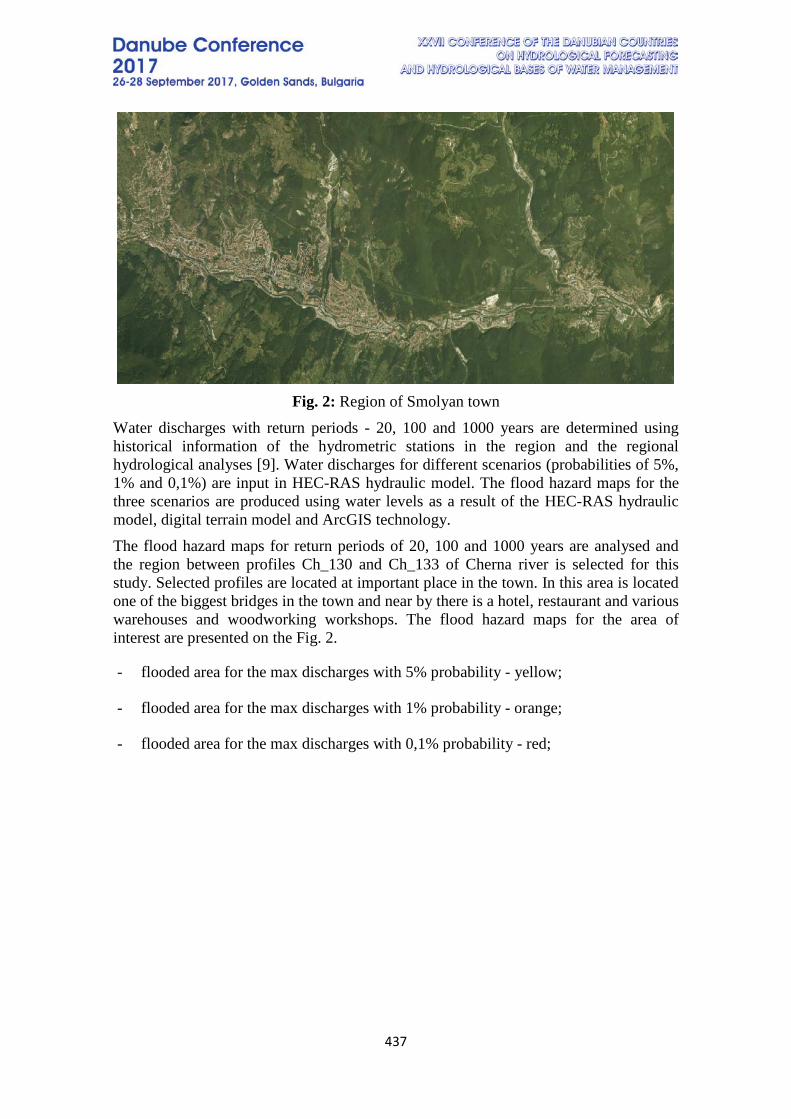
437

Fig. 2: Region of Smolyan town

Water discharges with return periods - 20, 100 and 1000 years are determined using historical information of the hydrometric stations in the region and the regional hydrological analyses [9]. Water discharges for different scenarios (probabilities of 5%, 1% and 0,1%) are input in HEC-RAS hydraulic model. The flood hazard maps for the three scenarios are produced using water levels as a result of the HEC-RAS hydraulic model, digital terrain model and ArcGIS technology. The flood hazard maps for return periods of 20, 100 and 1000 years are analysed and the region between profiles Ch_130 and Ch_133 of Cherna river is selected for this study. Selected profiles are located at important place in the town. In this area is located one of the biggest bridges in the town and near by there is a hotel, restaurant and various warehouses and woodworking workshops. The flood hazard maps for the area of interest are presented on the Fig. 2.

- flooded area for the max discharges with 5% probability - yellow;

- flooded area for the max discharges with 1% probability - orange;

- flooded area for the max discharges with 0,1% probability - red;

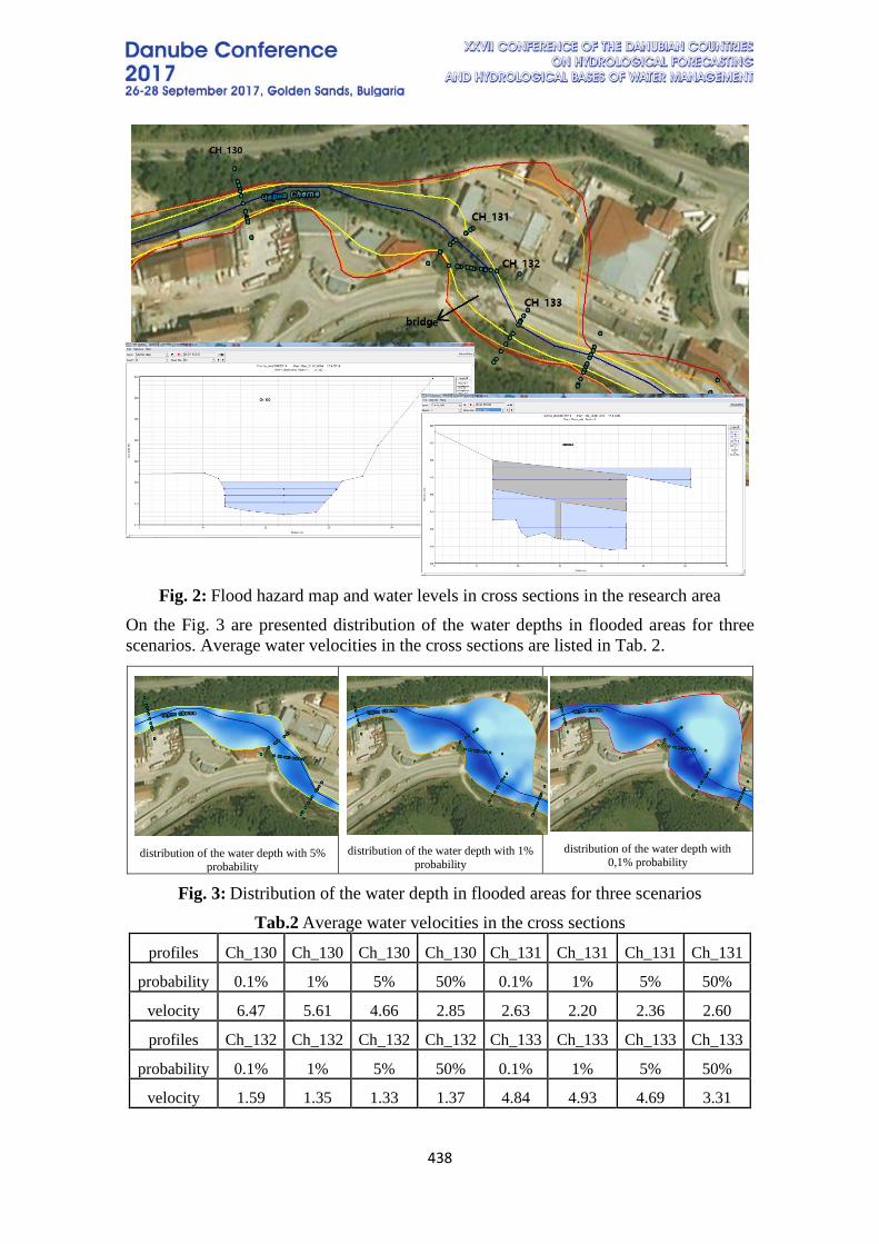
438

Fig. 2: Flood hazard map and water levels in cross sections in the research area On the Fig. 3 are presented distribution of the water depths in flooded areas for three scenarios. Average water velocities in the cross sections are listed in Tab. 2.

distribution of the water depth with 5% probability

distribution of the water depth with 1% probability

distribution of the water depth with 0,1% probability

Fig. 3: Distribution of the water depth in flooded areas for three scenarios

Tab.2 Average water velocities in the cross sections

profiles Ch_130 Ch_130 Ch_130 Ch_130 Ch_131 Ch_131 Ch_131 Ch_131

probability 0.1% 1% 5% 50% 0.1% 1% 5% 50%

velocity 6.47 5.61 4.66 2.85 2.63 2.20 2.36 2.60

profiles Ch_132 Ch_132 Ch_132 Ch_132 Ch_133 Ch_133 Ch_133 Ch_133

probability 0.1% 1% 5% 50% 0.1% 1% 5% 50%

velocity 1.59 1.35 1.33 1.37 4.84 4.93 4.69 3.31

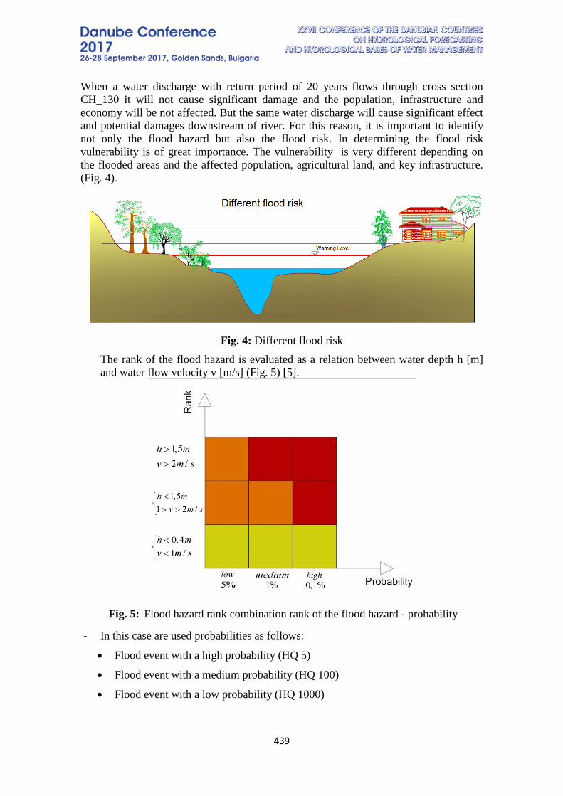
439

When a water discharge with return period of 20 years flows through cross section CH_130 it will not cause significant damage and the population, infrastructure and economy will be not affected. But the same water discharge will cause significant effect and potential damages downstream of river. For this reason, it is important to identify not only the flood hazard but also the flood risk. In determining the flood risk vulnerability is of great importance. The vulnerability is very different depending on the flooded areas and the affected population, agricultural land, and key infrastructure. (Fig. 4).

Fig. 4: Different flood risk

The rank of the flood hazard is evaluated as a relation between water depth h [m] and water flow velocity v [m/s] (Fig. 5) [5].

Fig. 5: Flood hazard rank combination rank of the flood hazard - probability

- In this case are used probabilities as follows:

• Flood event with a high probability (HQ 5)

• Flood event with a medium probability (HQ 100)

• Flood event with a low probability (HQ 1000)

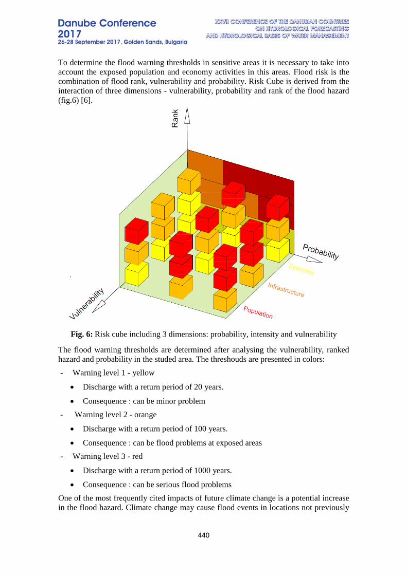
440

To determine the flood warning thresholds in sensitive areas it is necessary to take into account the exposed population and economy activities in this areas. Flood risk is the combination of flood rank, vulnerability and probability. Risk Cube is derived from the interaction of three dimensions - vulnerability, probability and rank of the flood hazard (fig.6) [6].

Fig. 6: Risk cube including 3 dimensions: probability, intensity and vulnerability

The flood warning thresholds are determined after analysing the vulnerability, ranked hazard and probability in the studed area. The threshouds are presented in colors: - Warning level 1 - yellow

• Discharge with a return period of 20 years.

• Consequence : can be minor problem - Warning level 2 - orange

• Discharge with a return period of 100 years.

• Consequence : can be flood problems at exposed areas - Warning level 3 - red

• Discharge with a return period of 1000 years.

• Consequence : can be serious flood problems One of the most frequently cited impacts of future climate change is a potential increase in the flood hazard. Climate change may cause flood events in locations not previously

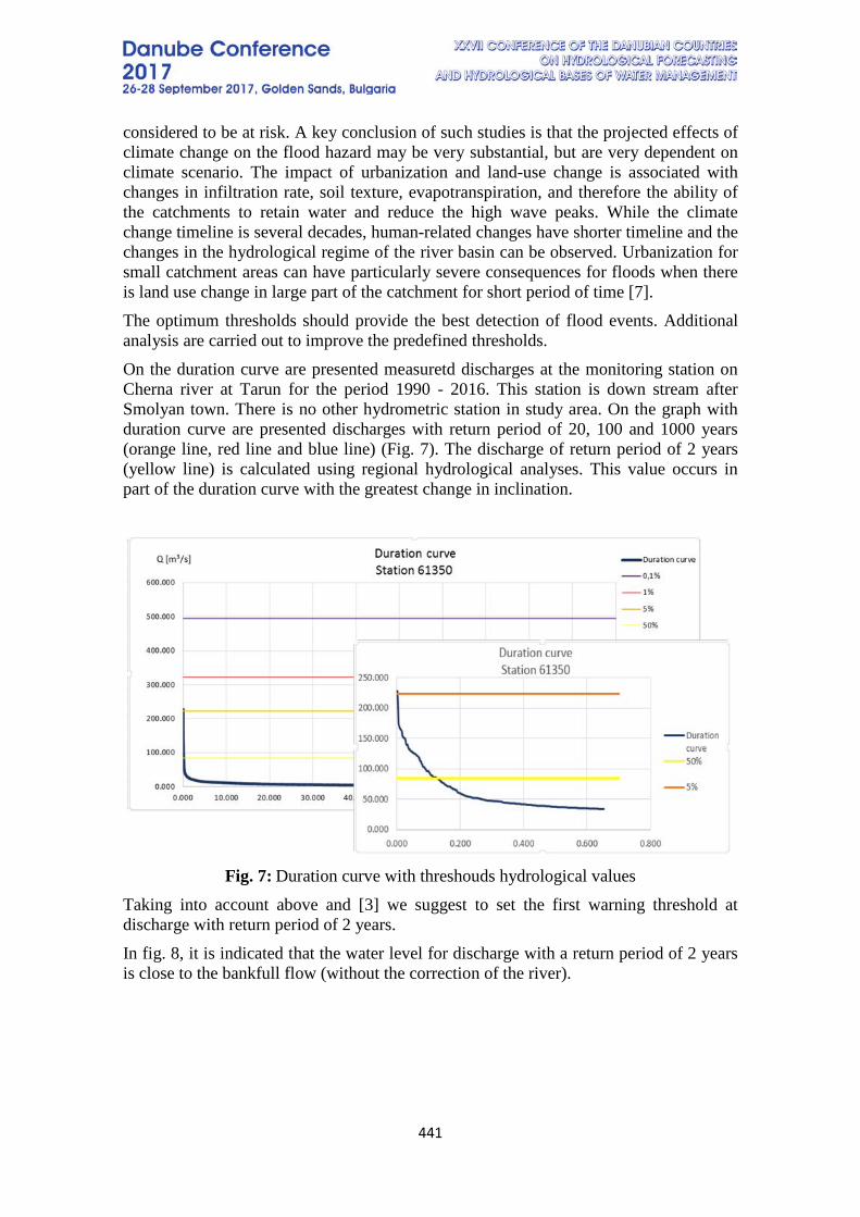
441

considered to be at risk. A key conclusion of such studies is that the projected effects of climate change on the flood hazard may be very substantial, but are very dependent on climate scenario. The impact of urbanization and land-use change is associated with changes in infiltration rate, soil texture, evapotranspiration, and therefore the ability of the catchments to retain water and reduce the high wave peaks. While the climate change timeline is several decades, human-related changes have shorter timeline and the changes in the hydrological regime of the river basin can be observed. Urbanization for small catchment areas can have particularly severe consequences for floods when there is land use change in large part of the catchment for short period of time [7]. The optimum thresholds should provide the best detection of flood events. Additional analysis are carried out to improve the predefined thresholds. On the duration curve are presented measuretd discharges at the monitoring station on Cherna river at Tarun for the period 1990 - 2016. This station is down stream after Smolyan town. There is no other hydrometric station in study area. On the graph with duration curve are presented discharges with return period of 20, 100 and 1000 years (orange line, red line and blue line) (Fig. 7). The discharge of return period of 2 years (yellow line) is calculated using regional hydrological analyses. This value occurs in part of the duration curve with the greatest change in inclination.

Fig. 7: Duration curve with threshouds hydrological values

Taking into account above and [3] we suggest to set the first warning threshold at discharge with return period of 2 years. In fig. 8, it is indicated that the water level for discharge with a return period of 2 years is close to the bankfull flow (without the correction of the river).

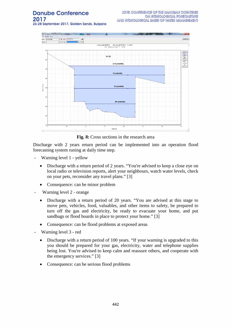
442

Fig. 8: Cross sections in the research area

Discharge with 2 years return period can be implemented into an operation flood forecasting system runing at daily time step. - Warning level 1 - yellow

• Discharge with a return period of 2 years. “You're advised to keep a close eye on local radio or television reports, alert your neighbours, watch water levels, check on your pets, reconsider any travel plans.” [3]

• Consequence: can be minor problem - Warning level 2 - orange

• Discharge with a return period of 20 years. “You are advised at this stage to move pets, vehicles, food, valuables, and other items to safety, be prepared to turn off the gas and electricity, be ready to evacuate your home, and put sandbags or flood boards in place to protect your home.” [3]

• Consequence: can be flood problems at exposed areas - Warning level 3 - red

• Discharge with a return period of 100 years. “If your warning is upgraded to this you should be prepared for your gas, electricity, water and telephone supplies being lost. You're advised to keep calm and reassure others, and cooperate with the emergency services.” [3]

• Consequence: can be serious flood problems

443

CONCLUSION The flood warning thresholds are a critical element in a flood forecasting and a warning system. Flood warnings need to be specific to particular catchments and reaches of rivers. To be able to set realistic thresholds to issue flood warnings it is necessary to prepare flood hazard maps and flood risk maps. Traditional flood warning approach includes: 1) Determine flood hazard prone areas for diferent return periods; 2) Determine flood risk for diferent return period; 3) Define thresholds warning levels; 4) Issue warnings if the forecast reach/exceed threshold level.

REFERENCES [1] Atlas of Mortality and Economic Losses from Weather, Climate and Water Extremes, WMO, 2014). [2] N. Pingel, C. Jones, and D. Ford, “Estimating forecasting lead times,” Natural Hazards Review (ASCE), vol. 6, no. 2, pp. 60–66, 2005. [3] Manual on Flood Forecasting and Warnin WMO-No. 1072 [4] DIRECTIVE 2007/60/EC [5] METODIKA TVORBY MAP POVODŇOVÉHO NEBEZPEČÍ A POVODŇOVÝCH RIZIK prosinec 2009 poslední aktualizace 13. 3. 2012 [6] H.Madsen at all Review of trend analysis and climate change projections of extreme precipitation and floods in Europe, Journal of Hydrology Volume 519, Part D, 27 November 2014, Pages 3634-3650 [7] Karl Spachinger1, Wolfgang Dorner1, Rudolf Metzka1, Kamal Serrhini2 and Sven Fuchs3, Flood Risk and Flood hazard maps – Visualisation of hydrological risks © 2008 IOP Publishing Ltd [8] Bojilova, E. About the changes in the frequency of the maximum annual river discharges for two pilot watersheds in Bulgaria, BALKANERECO’2016, Vol. 9, 2016, №1, ISSN 1311-2783, 122-125, 2016. [9] Plamen Ninov, Tzviatka Karagiozova Technological Approach to determine the water resources of river water bodies - using hydrological monitoring network, , Hydrological International Scientific Conference „Adaptation to climate change, from source to river basin”, Bucharest, 2014.

444

SURFACE WATER RESOURCES CHARACTERISTICS ESTIMATION VIA STATISTICAL MODELS

Maya Rankova, Kamelia Kroumova National Institute of Meteorology and Hydrology, BAS, Bulgaria

Corresponding author: National Institute of Meteorology and Hydrology, Sofia, Bulgaria, Tzarigradsko chaussee 66, 1784 Sofia, Bulgaria e-mails: maya.rankova@gmail.com

The present paper considers the quantification of surface fresh water resources and application of different regionalization schemes for the annual average for river discharges. Brief overview of possible methodologies and their applicability to the Bulgarian conditions is also given including rainfall runoff distributes parameters models, modeling the heat and humidity fluxes between soil and atmosphere, GIS approaches and regionalization of annual averages of the registered river discharges. The presently used technology based on 1961-2002 estimations is for this quantification is referenced and results for 2014 year for the Bulgarian Danube district are displayed. The necessity for reevaluating the regionalization of river discharges is discussed. Results of the three presently available regionalization schemes are compared and analyzed. The mentioned statistical approach was also applied for the evaluation of the ecological minimal river discharge threshold according to the national regulations namely: 10% of the annual average, but not less than the minimal monthly flow with 95% probability. Conclusions are made that new regionalization scheme should further be elaborated for the territory of Bulgaria. Keywords: water resources, river flow formation factors, river flow regionalization INTRODUCTION

In the present paper are considered methodological and technological issues about determination of surface water river flow characteristics necessary for their effective management.

River flow strongly depends on climatic, topographical and physico- geographic features of the catchments, as well as on the anthropogenic impact. Significant part of the Bulgarian waters are regulated by dams and water intake facilities, making it difficult to quantify them in an annual and multi-annual aspect. From other hand rivers spring up from mountainous regions pass through the hills and reach the plains, which also determines different river flow formation factors.

METHODOLOGY One of the main task of the hydrological research is river flow characteristics

determination for river sections without any hydrological observations. From the other hand there is partial and in most cases unrepresentative information about usage of water bodies both within individual catchments and in the transfer of waters between them. This determines the search of different ways to determine water quantities in non-monitored sections.

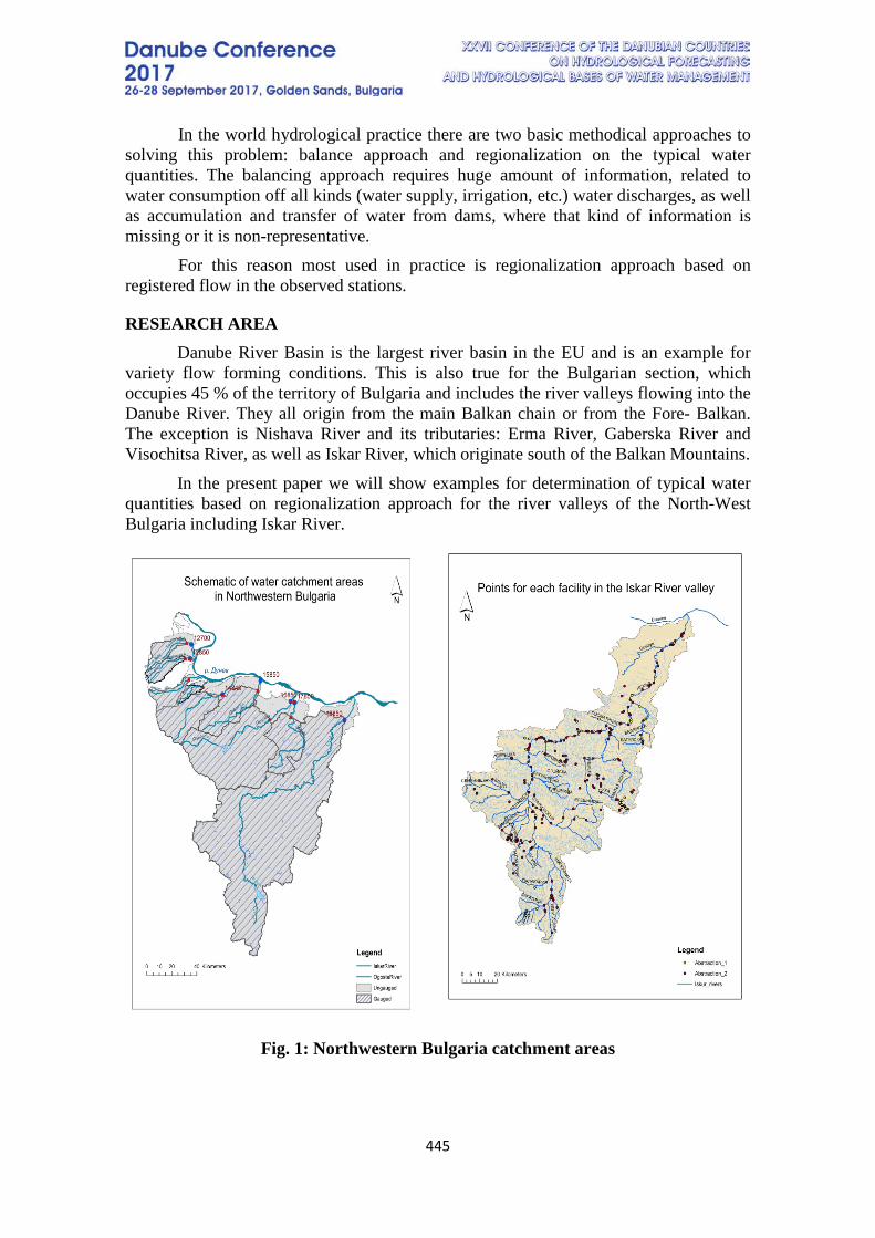
445

In the world hydrological practice there are two basic methodical approaches to solving this problem: balance approach and regionalization on the typical water quantities. The balancing approach requires huge amount of information, related to water consumption off all kinds (water supply, irrigation, etc.) water discharges, as well as accumulation and transfer of water from dams, where that kind of information is missing or it is non-representative.

For this reason most used in practice is regionalization approach based on registered flow in the observed stations.

RESEARCH AREA Danube River Basin is the largest river basin in the EU and is an example for

variety flow forming conditions. This is also true for the Bulgarian section, which occupies 45 % of the territory of Bulgaria and includes the river valleys flowing into the Danube River. They all origin from the main Balkan chain or from the Fore- Balkan. The exception is Nishava River and its tributaries: Erma River, Gaberska River and Visochitsa River, as well as Iskar River, which originate south of the Balkan Mountains.

In the present paper we will show examples for determination of typical water quantities based on regionalization approach for the river valleys of the North-West Bulgaria including Iskar River.

Fig. 1: Northwestern Bulgaria catchment areas

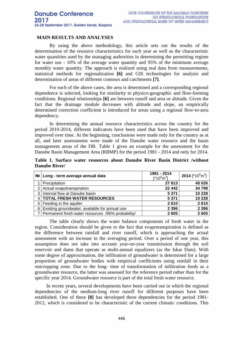
446

MAIN RESULTS AND ANALYSES By using the above methodology, this article sets out the results of the

determination of the resource characteristics for each year as well as the characteristic water quantities used by the managing authorities in determining the permitting regime for water use - 10% of the average water quantity and 95% of the minimum average monthly water quantity. The approach is realized using real data from measurements, statistical methods for regionalization [6] and GIS technologies for analysis and determination of areas of different contours and catchments [7].

For each of the above cases, the area is determined and a corresponding regional dependence is selected, looking for similarity to physico-geographic and flow-forming conditions. Regional relationships [6] are between runoff and area or altitude. Given the fact that the drainage module decreases with altitude and slope, an empirically determined correction coefficient is introduced for areas using a regional flow-to-area dependency.

In determining the annual resource characteristics across the country for the period 2010-2014, different indicators have been used that have been improved and improved over time. At the beginning, conclusions were made only for the country as at all, and later assessments were made of the Danube water resource and the basin management areas of the DB. Table 1 gives an example for the assessment for the Danube Basin Management Area (RBMP) for the period 1981 - 2014 and only for 2014.

Table 1. Surface water resources about Danube River Basin District /without Danube River/

№ Long - term average annual data 1981 - 2014 [*106m3] 2014 [*106m3]

1 Precipitation 27 813 45 026 2 Actual evapotranspiration 22 442 34 798 3 Internal flow at Danube basin 5 371 10 228 4 TOTAL FRESH WATER RESOURCES 5 371 10 228 5 Feeding in the aquifer 2 610 2 610 6 Existing groundwater, available for annual use 2 396 2 396 7 Permanent fresh water resources /95% probability/ 2 605 2 605

The table clearly shows the water balance components of fresh water in the region. Consideration should be given to the fact that evapotranspiration is defined as the difference between rainfall and river runoff, which is approaching the actual assessment with an increase in the averaging period. Over a period of one year, this assumption does not take into account year-on-year transmission through the soil reservoir and dams that operate as multi-annual equalizers (as the Iskar Dam). With some degree of approximation, the infiltration of groundwater is determined for a large proportion of groundwater bodies with empirical coefficients using rainfall in their outcropping zone. Due to the long- time of transformation of infiltration feeds as a groundwater resource, the latter was assessed for the reference period rather than for the specific year 2014. Groundwater resource is part of the total fresh water resource.

In recent years, several developments have been carried out in which the regional dependencies of the medium-long river runoff for different purposes have been established. One of these [8] has developed these dependencies for the period 1981-2012, which is considered to be characteristic of the current climatic conditions. This

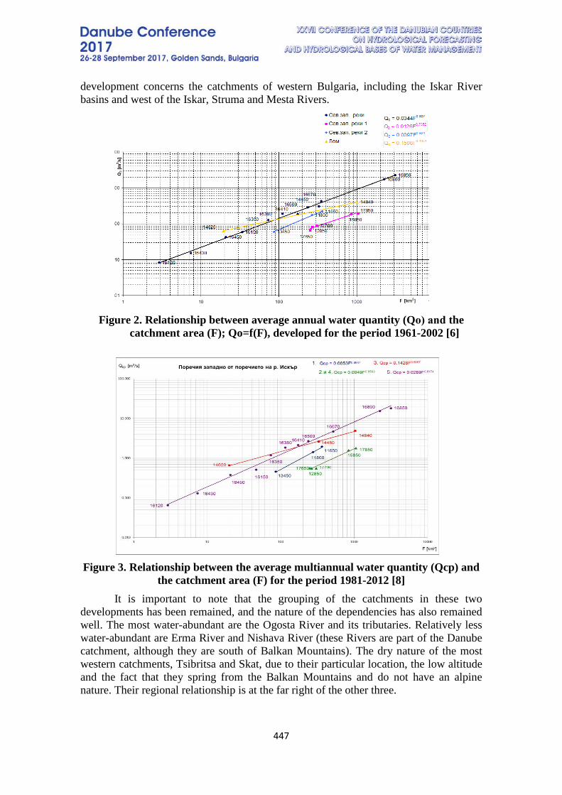
447

development concerns the catchments of western Bulgaria, including the Iskar River basins and west of the Iskar, Struma and Mesta Rivers.

Figure 2. Relationship between average annual water quantity (Qо) and the

catchment area (F); Qo=f(F), developed for the period 1961-2002 [6]

Figure 3. Relationship between the average multiannual water quantity (Qcp) and

the catchment area (F) for the period 1981-2012 [8] It is important to note that the grouping of the catchments in these two

developments has been remained, and the nature of the dependencies has also remained well. The most water-abundant are the Ogosta River and its tributaries. Relatively less water-abundant are Erma River and Nishava River (these Rivers are part of the Danube catchment, although they are south of Balkan Mountains). The dry nature of the most western catchments, Tsibritsa and Skat, due to their particular location, the low altitude and the fact that they spring from the Balkan Mountains and do not have an alpine nature. Their regional relationship is at the far right of the other three.

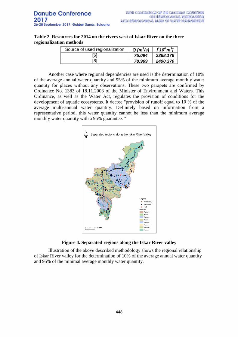
448

Table 2. Resources for 2014 on the rivers west of Iskar River on the three regionalization methods

Another case where regional dependencies are used is the determination of 10% of the average annual water quantity and 95% of the minimum average monthly water quantity for places without any observations. These two parapets are confirmed by Ordinance No. 1383 of 18.11.2003 of the Minister of Environment and Waters. This Ordinance, as well as the Water Act, regulates the provision of conditions for the development of aquatic ecosystems. It decree "provision of runoff equal to 10 % of the average multi-annual water quantity. Definitely based on information from a representative period, this water quantity cannot be less than the minimum average monthly water quantity with a 95% guarantee. "

Figure 4. Separated regions along the Iskar River valley

Illustration of the above described methodology shows the regional relationship of Iskar River valley for the determination of 10% of the average annual water quantity and 95% of the minimal average monthly water quantity.

Source of used regionalization Q [m3/s] [*106 m3] [6] 75.094 2368.179 [8] 78.969 2490.370

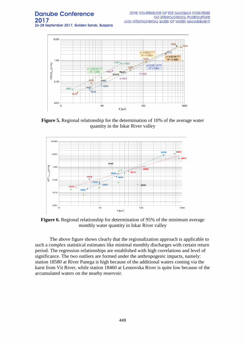
449

Figure 5. Regional relationship for the determination of 10% of the average water quantity in the Iskar River valley

Figure 6. Regional relationship for determination of 95% of the minimum average

monthly water quantity in Iskar River valley

The above figure shows clearly that the regionalization approach is applicable to such a complex statistical estimates like minimal monthly discharges with certain return period. The regression relationships are established with high correlations and level of significance. The two outliers are formed under the anthropogenic impacts, namely: station 18580 at River Panega is high because of the additional waters coming via the karst from Vit River, while station 18460 at Lesnovska River is quite low because of the accumulated waters on the nearby reservoir.

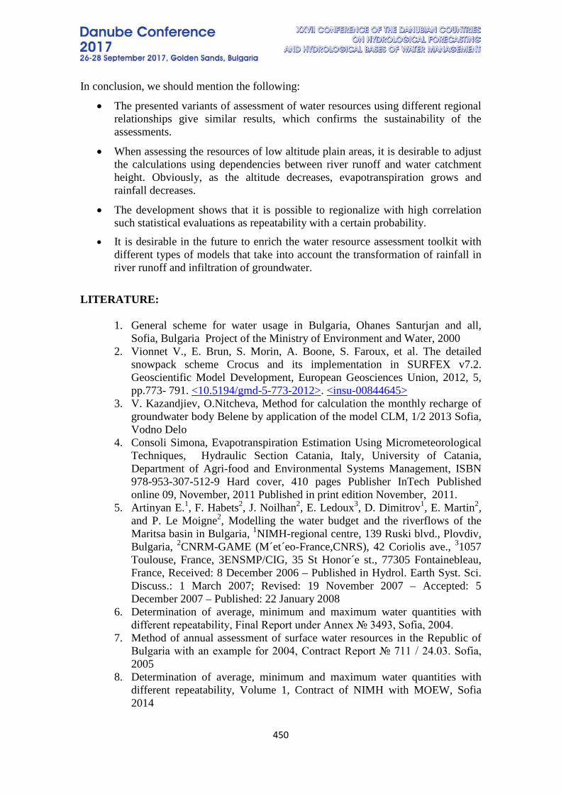
450

In conclusion, we should mention the following:

• The presented variants of assessment of water resources using different regional relationships give similar results, which confirms the sustainability of the assessments.

• When assessing the resources of low altitude plain areas, it is desirable to adjust the calculations using dependencies between river runoff and water catchment height. Obviously, as the altitude decreases, evapotranspiration grows and rainfall decreases.

• The development shows that it is possible to regionalize with high correlation such statistical evaluations as repeatability with a certain probability.

• It is desirable in the future to enrich the water resource assessment toolkit with different types of models that take into account the transformation of rainfall in river runoff and infiltration of groundwater.

LITERATURE:

1. General scheme for water usage in Bulgaria, Ohanes Santurjan and all, Sofia, Bulgaria Project of the Ministry of Environment and Water, 2000

2. Vionnet V., E. Brun, S. Morin, A. Boone, S. Faroux, et al. The detailed snowpack scheme Crocus and its implementation in SURFEX v7.2. Geoscientific Model Development, European Geosciences Union, 2012, 5, pp.773- 791. <10.5194/gmd-5-773-2012>. <insu-00844645>

3. V. Kazandjiev, O.Nitcheva, Method for calculation the monthly recharge of groundwater body Belene by application of the model CLM, 1/2 2013 Sofia, Vodno Delo

4. Consoli Simona, Evapotranspiration Estimation Using Micrometeorological Techniques, Hydraulic Section Catania, Italy, University of Catania, Department of Agri-food and Environmental Systems Management, ISBN 978-953-307-512-9 Hard cover, 410 pages Publisher InTech Published online 09, November, 2011 Published in print edition November, 2011.

5. Artinyan E.1, F. Habets2, J. Noilhan2, E. Ledoux3, D. Dimitrov1, E. Martin2, and P. Le Moigne2, Modelling the water budget and the riverflows of the Maritsa basin in Bulgaria, 1NIMH-regional centre, 139 Ruski blvd., Plovdiv, Bulgaria, 2CNRM-GAME (M´et´eo-France,CNRS), 42 Coriolis ave., 31057 Toulouse, France, 3ENSMP/CIG, 35 St Honor´e st., 77305 Fontainebleau, France, Received: 8 December 2006 – Published in Hydrol. Earth Syst. Sci. Discuss.: 1 March 2007; Revised: 19 November 2007 – Accepted: 5 December 2007 – Published: 22 January 2008

6. Determination of average, minimum and maximum water quantities with different repeatability, Final Report under Annex № 3493, Sofia, 2004.

7. Method of annual assessment of surface water resources in the Republic of Bulgaria with an example for 2004, Contract Report № 711 / 24.03. Sofia, 2005

8. Determination of average, minimum and maximum water quantities with different repeatability, Volume 1, Contract of NIMH with MOEW, Sofia 2014

451

9. Determination of average long-term value of resources of surface water bodies for a reference period for the whole country, Contract of NIMH with MOEW, Sofia 2015.

452

ANALYSIS OF NATURAL DISASTERS IN BULGARIA IN LAST YEARS

Iordanka Koleva-Lizama, Bernardo Lizama Rivas

University of Forestry, Department of Ecology, Sofia, Bulgaria

Corresponding author: University of Forestry, Department of Ecology, 10 Kliment Ohridski, 1756 Sofia, Bulgaria, B. Lizama Rivas, bernardo_330@abv.bg

ABSTRACT Natural disasters occur when large numbers of people or economic assets are damaged or destroyed during a natural hazard event. Disasters have two sets of causes. The first set is the natural hazards themselves, including floods, drought, tropical storms, earthquakes, volcanoes, and landslides. The second set comprises the vulnerabilities of elements at risk - populations, infrastructure, and economic activities—that make them more or less susceptible to being harmed or damaged by a hazard event. The impacts of natural disasters have changed over the past years. As a result of human development, these events are having increasing impacts in term of costs and benefits for ecological and human systems. Interactions of modern human activities with ecosystems have contributed to increasing human vulnerability. The aim of this paper is to analyze the natural disasters in Bulgaria, occurred in the last 40 years. The analysis requires proper understanding of the history of disasters and the nature of impacts, trends, the severity of different disasters, and the vulnerability of population and property. For relative vulnerability assessments various variables, like the number of events, the number of deaths, the size of the affected population and the amount of economic loss have been used. Appropriate management of ecosystems can reduce vulnerability and negative impacts of extreme events. Ecosystem conditions may increase or reduce both costs and benefits at various temporal and spatial scales. In conclusion, Bulgaria is more vulnerable to flood than to any other hazard. Taking into consideration the hazard intensities and vulnerability, the country should initiate loss assessments, and develop a risk funding strategy for catastrophic events. The country needs to upgrade river regulation, flood protection infrastructure and its mechanisms for early warning. Keywords: natural hazard events, ecological and human systems, extreme events

1. INTRODUCTION Natural hazard events can have catastrophic impacts and can lead to economic, social and environmental damages affecting overall economic activity, lifestyles causing disruption of communities and natural resources. These events can vary in magnitude or intensity, frequency, duration, area of extent, spatial dispersion and temporal spacing. The extent of damage depends on the vulnerability of affected areas. The analysis requires proper understanding of these factors, including the history of disasters and the nature of impacts, trends, the severity of different disasters, and the vulnerability of population and property. Severity is sometimes assessed against a country’s gross domestic product (GDP). Assessment of vulnerability and risk of these events is always a difficult matter, but for relative vulnerability assessments various variables, like the number of events, the number of deaths, the size of the affected population and the

453

amount of economic loss have been used. Hazard assessment consists of determining when and where hazardous processes have occurred in the past, the severity of the physical effects of past hazardous processes (magnitude), the frequency of occurrence of hazardous processes, the likely effects of a process of a given magnitude and all this information should be available in a form useful to planners and public officials responsible for making decisions in event of a disaster. Natural hazards can be divided into geologic hazards (earthquakes, volcanic eruptions, tsunami, landslides, floods and subsidence), atmospheric hazards (tropical cyclones, tornadoes, droughts, severe thunderstorms, lightening) and other natural hazards (insect infestations, disease epidemics and wildfires). Natural Hazards, which have devastating consequences to huge numbers of people, or have a worldwide effect, such as impacts with large space objects, huge volcanic eruptions, world-wide disease epidemics, and world-wide droughts can be divided into catastrophic hazards. Such catastrophic hazards only have a small chance of occurring, but can have devastating results if they do occur. Natural Hazards can also be divided into rapid onset hazards, such as Volcanic Eruptions, Earthquakes, Flash floods, Landslides, Severe Thunderstorms, Lightening, and wildfires, which develop with little warning and strike rapidly. Drought, insect infestations, and disease epidemics take years to develop and they can be defined like a slow onset hazards. There is evidence to suggest that weather related disasters are becoming more frequent, compared to other disasters like earthquakes. For example, the frequency of disasters from tropical cyclones and floods has been increasing; the frequency of earthquakes has changed little. Although this is what we expect from global warming, there is not yet enough statistical data to prove this right now. Human population has been increasing at an exponential rate. With more people, vulnerability increases because there are more people to be affected by otherwise natural events. Human population is moving toward coastal areas. These are areas most vulnerable to natural hazards such as tropical cyclones, tsunami, and, to some extent, earthquakes. Our ability to communicate news of natural disasters has been increasing, especially since the invention of the internet. Earlier in human history there may have been just as many disasters, but there were few ways the news of such disasters could be communicated throughout the world. The aim of this paper is to analyze the natural hazard events in Bulgaria occurred in the recent years.

2. MATERIAL AND METHODS Bulgaria is situated in south-eastern Europe and has a total surface area of 110879 square kilometers, with a total population of 7740000. The population density is 70 people per square kilometer (http://www.worldbank.org). Considering its small size, the country has a great variety of topographical features; the land may be divided into plains, plateaus, hills, mountains, basins, gorges, and deep river valleys. Bulgaria is noted for its diversity, with a landscape ranging from the snow-capped peaks of Rila and Pirin in the south-west, and of the Balkan Mountains, to the mild and sunny weather of the Black Sea coast; from the typically continental Danubian plain in the north, to the strong Mediterranean influence in the valleys of Struma and Mesta rivers, and the lowlands in the southernmost parts of Thrace. According to the European Environment Agency's Digital Map of European Ecological Regions, the territory subdivides into two main ecoregions: the Balkan mixed forests and Rhodope Mountain mixed forests. The country lies between the strongly contrasting continental and Mediterranean climatic

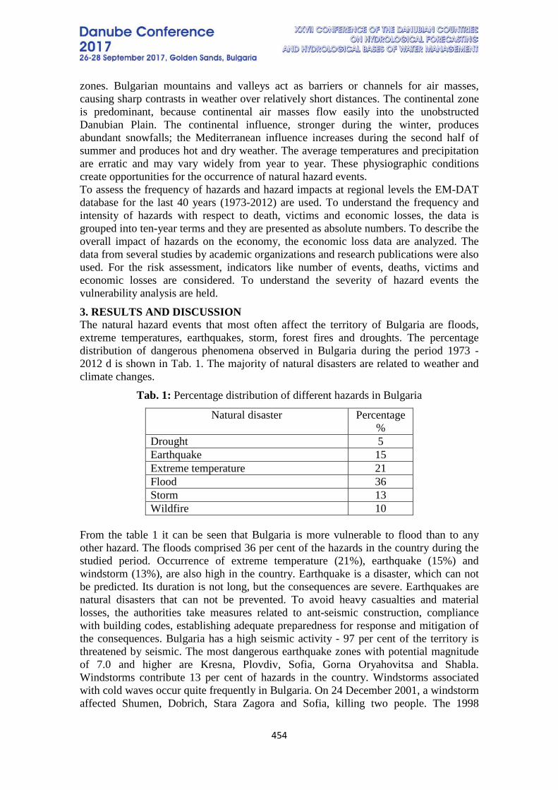
454

zones. Bulgarian mountains and valleys act as barriers or channels for air masses, causing sharp contrasts in weather over relatively short distances. The continental zone is predominant, because continental air masses flow easily into the unobstructed Danubian Plain. The continental influence, stronger during the winter, produces abundant snowfalls; the Mediterranean influence increases during the second half of summer and produces hot and dry weather. The average temperatures and precipitation are erratic and may vary widely from year to year. These physiographic conditions create opportunities for the occurrence of natural hazard events. To assess the frequency of hazards and hazard impacts at regional levels the EM-DAT database for the last 40 years (1973-2012) are used. To understand the frequency and intensity of hazards with respect to death, victims and economic losses, the data is grouped into ten-year terms and they are presented as absolute numbers. To describe the overall impact of hazards on the economy, the economic loss data are analyzed. The data from several studies by academic organizations and research publications were also used. For the risk assessment, indicators like number of events, deaths, victims and economic losses are considered. To understand the severity of hazard events the vulnerability analysis are held.

3. RESULTS AND DISCUSSION The natural hazard events that most often affect the territory of Bulgaria are floods, extreme temperatures, earthquakes, storm, forest fires and droughts. The percentage distribution of dangerous phenomena observed in Bulgaria during the period 1973 - 2012 d is shown in Tab. 1. The majority of natural disasters are related to weather and climate changes.

Tab. 1: Percentage distribution of different hazards in Bulgaria

Natural disaster Percentage %

Drought 5 Earthquake 15 Extreme temperature 21 Flood 36 Storm 13 Wildfire 10

From the table 1 it can be seen that Bulgaria is more vulnerable to flood than to any other hazard. The floods comprised 36 per cent of the hazards in the country during the studied period. Occurrence of extreme temperature (21%), earthquake (15%) and windstorm (13%), are also high in the country. Earthquake is a disaster, which can not be predicted. Its duration is not long, but the consequences are severe. Earthquakes are natural disasters that can not be prevented. To avoid heavy casualties and material losses, the authorities take measures related to ant-seismic construction, compliance with building codes, establishing adequate preparedness for response and mitigation of the consequences. Bulgaria has a high seismic activity - 97 per cent of the territory is threatened by seismic. The most dangerous earthquake zones with potential magnitude of 7.0 and higher are Kresna, Plovdiv, Sofia, Gorna Oryahovitsa and Shabla. Windstorms contribute 13 per cent of hazards in the country. Windstorms associated with cold waves occur quite frequently in Bulgaria. On 24 December 2001, a windstorm affected Shumen, Dobrich, Stara Zagora and Sofia, killing two people. The 1998

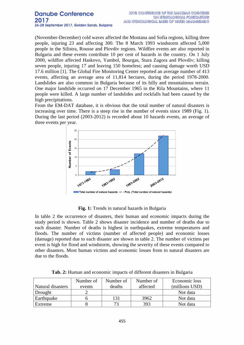
455

(November-December) cold waves affected the Montana and Sofia regions, killing three people, injuring 23 and affecting 300. The 8 March 1993 windstorm affected 5,000 people in the Silistra, Rousse and Plovdiv regions. Wildfire events are also reported in Bulgaria and these events contribute 10 per cent of hazards in the country. On 1 July 2000, wildfire affected Haskovo, Yambol, Bourgas, Stara Zagora and Plovdiv; killing seven people, injuring 17 and leaving 150 homeless; and causing damage worth USD 17.6 million [1]. The Global Fire Monitoring Center reported an average number of 413 events, affecting an average area of 11,814 hectares, during the period 1978-2000. Landslides are also common in Bulgaria because of its hilly and mountainous terrain. One major landslide occurred on 17 December 1965 in the Rila Mountains, where 11 people were killed. A large number of landslides and rockfalls had been caused by the high precipitations. From the EM-DAT database, it is obvious that the total number of natural disasters is increasing over time. There is a steep rise in the number of events since 1989 (Fig. 1). During the last period (2003-2012) is recorded about 10 hazards events, an average of three events per year.

Fig. 1: Trends in natural hazards in Bulgaria In table 2 the occurrence of disasters, their human and economic impacts during the study period is shown. Table 2 shows disaster incidence and number of deaths due to each disaster. Number of deaths is highest in earthquakes, extreme temperatures and floods. The number of victims (number of affected people) and economic losses (damage) reported due to each disaster are shown in table 2. The number of victims per event is high for flood and windstorm, showing the severity of these events compared to other disasters. Most human victims and economic losses from to natural disasters are due to the floods.

Tab. 2: Human and economic impacts of different disasters in Bulgaria

Natural disasters Number of

events Number of

deaths Number of

affected Economic loss (millions USD)

Drought 2

Not data Earthquake 6 131 3962 Not data Extreme 8 73 393 Not data

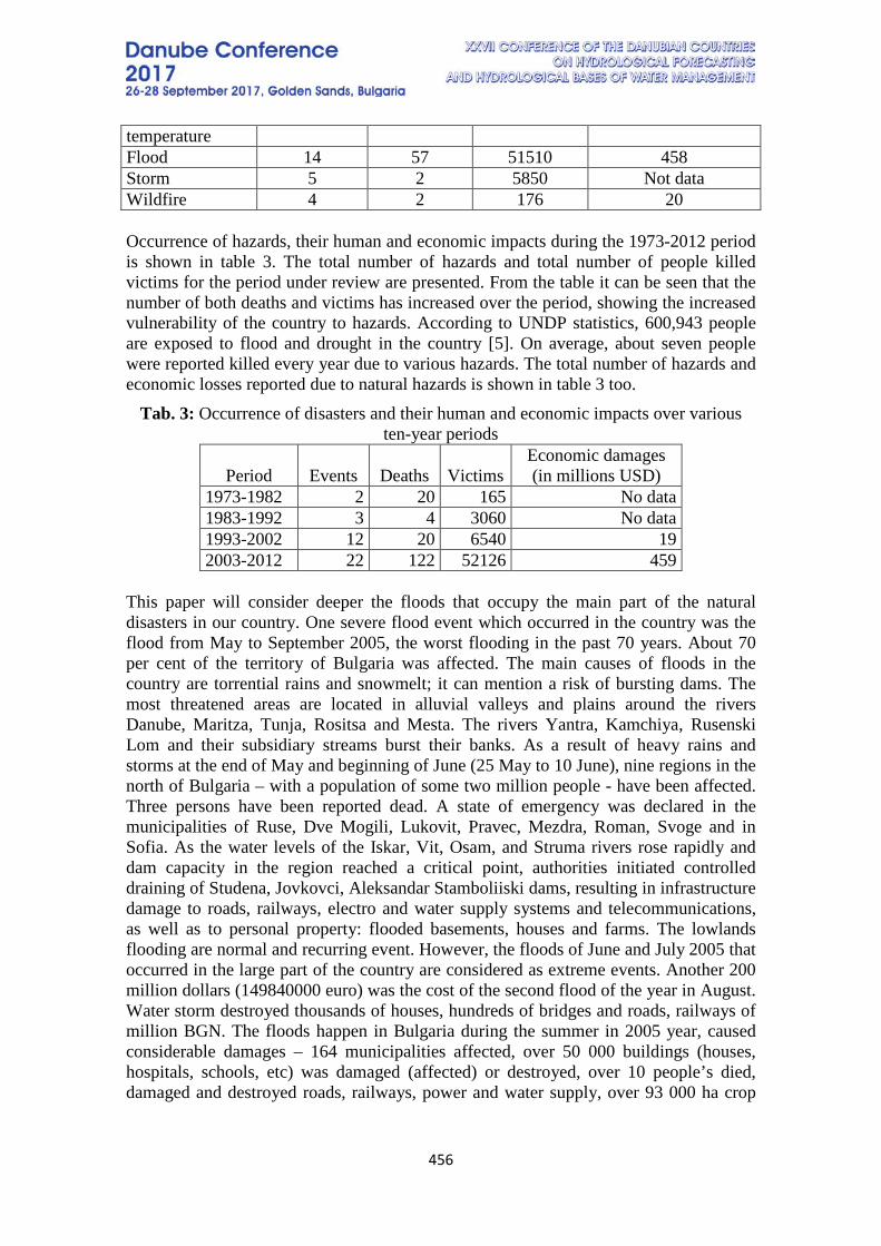
456

temperature Flood 14 57 51510 458 Storm 5 2 5850 Not data Wildfire 4 2 176 20 Occurrence of hazards, their human and economic impacts during the 1973-2012 period is shown in table 3. The total number of hazards and total number of people killed victims for the period under review are presented. From the table it can be seen that the number of both deaths and victims has increased over the period, showing the increased vulnerability of the country to hazards. According to UNDP statistics, 600,943 people are exposed to flood and drought in the country [5]. On average, about seven people were reported killed every year due to various hazards. The total number of hazards and economic losses reported due to natural hazards is shown in table 3 too.

Tab. 3: Occurrence of disasters and their human and economic impacts over various ten-year periods

Period Events Deaths Victims Economic damages (in millions USD)

1973-1982 2 20 165 No data 1983-1992 3 4 3060 No data 1993-2002 12 20 6540 19 2003-2012 22 122 52126 459

This paper will consider deeper the floods that occupy the main part of the natural disasters in our country. One severe flood event which occurred in the country was the flood from May to September 2005, the worst flooding in the past 70 years. About 70 per cent of the territory of Bulgaria was affected. The main causes of floods in the country are torrential rains and snowmelt; it can mention a risk of bursting dams. The most threatened areas are located in alluvial valleys and plains around the rivers Danube, Maritza, Tunja, Rositsa and Mesta. The rivers Yantra, Kamchiya, Rusenski Lom and their subsidiary streams burst their banks. As a result of heavy rains and storms at the end of May and beginning of June (25 May to 10 June), nine regions in the north of Bulgaria – with a population of some two million people - have been affected. Three persons have been reported dead. A state of emergency was declared in the municipalities of Ruse, Dve Mogili, Lukovit, Pravec, Mezdra, Roman, Svoge and in Sofia. As the water levels of the Iskar, Vit, Osam, and Struma rivers rose rapidly and dam capacity in the region reached a critical point, authorities initiated controlled draining of Studena, Jovkovci, Aleksandar Stamboliiski dams, resulting in infrastructure damage to roads, railways, electro and water supply systems and telecommunications, as well as to personal property: flooded basements, houses and farms. The lowlands flooding are normal and recurring event. However, the floods of June and July 2005 that occurred in the large part of the country are considered as extreme events. Another 200 million dollars (149840000 euro) was the cost of the second flood of the year in August. Water storm destroyed thousands of houses, hundreds of bridges and roads, railways of million BGN. The floods happen in Bulgaria during the summer in 2005 year, caused considerable damages – 164 municipalities affected, over 50 000 buildings (houses, hospitals, schools, etc) was damaged (affected) or destroyed, over 10 people’s died, damaged and destroyed roads, railways, power and water supply, over 93 000 ha crop

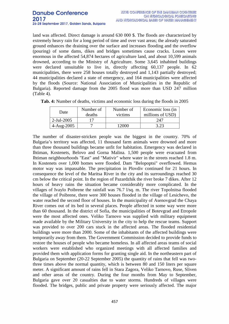
457

land was affected. Direct damage is around 630 000 $. The floods are characterized by extremely heavy rain for a long period of time and over vast areas; the already saturated ground enhances the draining over the surface and increases flooding and the overflow (pouring) of some dams, dikes and bridges sometimes cause cracks. Losses were enormous in the affected 54,874 hectares of agriculture land, and about 10,599 animals drowned, according to the Ministry of Agriculture. Some 3,645 inhabited buildings were declared unsuitable to live in, directly affecting 60,137 people. In 62 municipalities, there were 258 houses totally destroyed and 1,143 partially destroyed; 44 municipalities declared a state of emergency, and 164 municipalities were affected by the floods (Source: National Association of Municipalities in the Republic of Bulgaria). Reported damage from the 2005 flood was more than USD 247 million (Table 4).

Tab. 4: Number of deaths, victims and economic loss during the floods in 2005

Date Number of deaths

Number of victims

Economic loss (in millions of USD)

2-Jul-2005 17 247 4-Aug-2005 7 12000 3.23

The number of disaster-stricken people was the biggest in the country. 70% of Bulgaria’s territory was affected, 11 thousand farm animals were drowned and more than three thousand buildings became unfit for habitation. Emergency was declared in Ihtiman, Kostenets, Belovo and Gorna Malina. 1,500 people were evacuated from Ihtiman neighbourhoods "East" and "Mativir" where water in the streets reached 1.8 m. In Kostenets over 1,000 homes were flooded. Dam "Belopoptsi" overflowed. Hemus motor way was impassable. The precipitation in Plovdiv continued for 21 hours. In consequence the level of the Maritsa River in the city and its surroundings reached 30 cm below the critical point. In the region of Pazardzhik the river broke 7 dikes. After 12 hours of heavy rains the situation became considerably more complicated. In the villages of Ivaylo Poibrene the rainfall was 76.7 l/sq. m. The river Topolnitsa flooded the village of Poibrene, there were 300 houses flooded in the village of Lesichevo, the water reached the second floor of houses. In the municipality of Asenovgrad the Chaya River comes out of its bed in several places. People affected in some way were more than 60 thousand. In the district of Sofia, the municipalities of Botevgrad and Etropole were the most affected ones. Veliko Tarnovo was supplied with military equipment made available by the Military University in the city to help the rescue teams. Support was provided to over 200 cars stuck in the affected areas. The flooded residential buildings were more than 2000. Some of the inhabitants of the affected buildings were temporarily away from them. The Government Commission decided to provide funds to restore the houses of people who became homeless. In all affected areas teams of social workers were established who organized meetings with all affected families and provided them with application forms for granting single aid. In the northeastern part of Bulgaria on September (20-22 September 2005) the quantity of rains that fell was two-three times above the normal quantity, which is between 80 and 150 liters per square meter. A significant amount of rains fell in Stara Zagora, Veliko Tarnovo, Ruse, Sliven and other areas of the country. During the four months from May to September, Bulgaria gave over 20 casualties due to water storms. Hundreds of villages were flooded. The bridges, public and private property were seriously affected. The major

458

cause for floods in 2005 turned to be the lack of preventive maintenance of riverbeds, protection dikes and the management of dam and river flows. There was no early warning system for disasters. As a result of the rains poured down over the country, 30% of the stations of the National Institute of Hydrology and Meteorology broke down. The UN Office for Coordination of Humanitarian Affairs noted in its release that floods in Bulgaria caused damages of 633 million dollars (474 243 600 euro) and killed more than 20 people. As a result of high rain rates during the whole summer and extensive regions affected by floods, Bulgaria sought for international assistant because of impossibility to cope with own resources. Other flood events that took place in the recent past occurred on 14 December 1997, 10 August 2002 and 10 April 2006. The events and scale of the damages showed that central and local authorities could hardly respond to disasters with similar scales. The reasons were different: the poor condition of water facilities, uncleaned river beds, embankments and fortifications were neglected, illegally built river terraces. Another reason for the great flood was the poor management of dams. Bulgaria has 3700 dams. The situation is complicated by the fact that the ministries, the principals of these companies do not communicate each other. The major problem for Bulgaria is related to floods caused by inefficient management of waters, especially dams, which overflow after intense rainfalls and snow melting. Such a situation occurred in February 2012 year, when as a result of a heavy rainfall and increased temperatures there were significant flooding not only in Bulgaria, but also in neighboring regions in Turkey and Greece. In addition, there were significant damages due to breakage of the dam wall near the village of Bisser, district of Haskovo.

4. CONCLUSION On the base of the analysis of hazardous phenomena can be concluded that Bulgaria is more vulnerable to flood than to any other hazard. Taking into consideration the hazard intensities and vulnerability, the country should initiate loss assessments, and develop a risk funding strategy for catastrophic events. In conclusion, it should be noted that in order to deal with the effects of floods, we must upgrade river regulation, flood protection infrastructure and its mechanisms for early warning.

5. REFERENCES [1] Emergency Events Data Base (EM-DAT), A global disaster data-base maintained by

the Centre for Research on the Epidemiology and Disasters (CRED) in Brussels. http://www.em-dat.net/glossary.htm.

[2] Gergov, G. Filkov, I., Karagiozova, Tz., Bardarska, G., and Pencheva, K. Flash floods in Bulgaria (ARFM Project of WMO-GWP). Report, 2004, p. 31.

[3] IFRC. Bulgaria: Floods Minor Emergency, International Federation of Red Cross and Red Crescent Societies, no. 05ME047, Nov. 21, 2005, p. 4

[4] UN/ISDR - WB. South Eastern Europe Disaster Risk Mitigation and Adaptation Initiative: Risk Assessment in South Eastern Europe - A Desk Study Review. Geneva, Switzerland: UN, 2008, p. 56.

[5] UNDP. A Global Report on Reducing Disaster Risk: A Challenge for Development, United Nations Development Programme, Bureau for Crisis Prevention and Recovery. 2004, p. 169

[6] WMO/GWP. Study of historical floods in Central and Eastern Europe from an integrated flood management viewpoint. WMO/GWP, 2005, p. 32

459

[7] World Bank. Hazards of Nature, Risks to Development An IEG Evaluation of World Bank Assistance for Natural Disasters, the World Bank, 2006, p. 236.

460

ANN MODEL FOR FLOOD RISK IDENTIFICATION: SEVLIEVO,

BULGARIA

Maria Mavrova-Guirguinova

Denislava Pencheva University of Architecture, Civil Engineering and Geodesy - Bulgaria

Corresponding author: Assoc.Prof. Dr. Maria Mavrova-Guirguinova, University of Architecture, Civil Engineering and Geodesy – 1 Hristo Smirnenski Blv., Sofia, Bulgaria,

margir_fhe@abv.bg

ABSTRACT The process of Flood Risk Management Planning and adaptation of measures for flood risk reduction as the Early Warning provoke the necessity of surveys involving Identification aspects. This project presents risk identification combining two lines of analysis: (1) Creation a mathematical model of rainfall-runoff processes in a watershed based on limited number of observed input and output variables; (2) Procedures for determination of critical thresholds - discharges/water levels corresponding to certain consequences. The pilot region is Rossitsa river basin, Sevlievo, Bulgaria. The first line of analysis is followed by four steps: (a) Creation and calibration of Unit Hydrograph Models based on limited number of observed data for discharge and precipitation; The survey at the selected region has 22 observations for excess rainfall and discharge. (b) The relations of UHM coefficients from the input parameters have been determined statistically, excluding the ANN model of the run-off coefficient as a function of 3 parameters (amount of precipitation two days before, soil condition, intensity of the rainfall) where a feedforward neural network is used. (c) Additional simulations with UHM aiming at generation of synthetic data for rainfall-runoff events, which extend the range of observed data; (d) Training, validation and testing a generalized regional ANN Model for discharge forecasting with 4 input parameters, where the training data set consists of synthetic data, validation and testing data sets consists of observations. A function between consequences and discharges has been reached in the second line of analysis concerning critical hazard levels determination. Unsteady simulations with the hydraulic model using three typical hydrographs for determination of the existing time for reaction from one to upper critical threshold are made. Correction of the critical thresholds aiming at providing necessary time for reaction between the thresholds and probability analysis of the finally determined critical thresholds are made. The result of the described method is a Catalogue for off-line flood hazard and risk identification. It can be used as interactive computer system, based on simulations of the ANN “Catalogue”. Flood risk identification of the future rainfall event is made in a multi-dimensional space for each kind of soil conditions (dry, average wet and wet

461

condition) and observed amount of precipitation two days before. Rainfall-runoff scenarios in case of intensive rainfall or sustained rainfall (more than 6 hours) are taken into account. Critical thresholds and hazard zones needed of specific operative activities (rescue and recovery) corresponded to each of the regulated flood protection levels (unite, municipality, regional or national) are presented. The Catalogue gives the opportunity for flood hazard scenarios extraction. Regarding that, the Catalogue is useful on the prevention stage of flood protection planning (emergency operations, measures and resources for their implementation planning) and creation of scenarios for training the Emergency Plans. Concerning application for Early Warning, it gives approximate forecast for flood hazard. The Catalogue supplies the necessary time for reaction of about 24 hours. Thus, Early Warning is possible to the responsible authorities, all parts if the Unified Rescue System, members of suitable Headquarters for disaster protection (on municipality, region or national level). Keywords: Flood Risk, ANN, Identification

462

INTRODUCTION The evaluation of artificial neural networks (ANNs) in hydrology and hydraulic engineering has increased steadily over the last decades in many fields [3]. In this article ANNs have been developed as tools to aid decision making by addressing problems of flood risk identification. It is not difficult to imagine why this is the case. The increasing use of variables in decision making has considerably increased the complexity of the issues. As a consequence, large amounts of complex information with many variables have to be assimilated and processed if adequate decisions are to be made. On the other hand, in dealing with extreme events such as floods always a lack of enough examples to cover the full range of variations exists. These situations ideally lend themselves to the application of ANNs, which are good in situations where data can be complex, relatively imprecise, and not amenable to the development of rules or algorithms. To date, the application of ANNs to decision making in the disaster protection field has been relatively uncommon. This article shows the application of ANNs in a completing missing data, in a development of an ANN model - a core of the Catalogue of the floods for the territory of Sevlievo with focus on the potential use of ANNs in the Unified Rescue System for disaster protection.

1. ARTIFICIAL NEURAL NETWORKS An artificial neural network (ANN) [4] is an information-processing system that is based on generalizations of human cognition or neural biology and are electronic or computational models based on the neural structure of the brain. The brain basically learns from experience. There are two types of ANN, the first one with only feedforward connections is called feedforward ANN, and the second one with arbitrary connections without any direction, are often called recurrent ANN (RANN). The most common type of ANN consists of different layers, with some neurons on each of them and connected with feedforward connections and trained with the backpropagation algorithm [5]. An ANN has a remarkable ability to derive meaning from complicated or imprecise data. The ANN can be used to extract patterns and detect trends that are too complex to be noticed by either humans or other computer techniques. A trained ANN can be considered as an “expert” in the category of information it has received to analyze. The ANNs have shown to be a powerful tool in many different applications, but they have a big problem: their reasoning process cannot be explained, that is, there is no clear relationship between the inputs presented to the network and the outputs it returns. A wide range of applications have been investigated in the field of water resources management. ANNs can be applied for prediction, simulation, identification, classification, and optimization. If significant variables are known, but not their exact relationships, an ANN is able to perform a kind of function fitting by using multiple parameters on the existing information and predict the possible relationships for the coming future. This sort of problem includes rainfall runoff prediction, water level and discharge relations, drinking water demand, flow, and sediment transport, water quality prediction, and so forth. Some examples of ANN use are the following:

463

• Prediction of both water level and flow of a river was investigated on the specific case of the Nile River in Egypt [1]. The estimation of the river flow can have a significant economic impact mainly regarding agricultural water management, protection from water shortages, and possible flood damage. • [6] studied the application of an ANN for prediction of runoff coefficient by the use of simple catchment data. The input data for the ANN consists on conventional catchment characteristics such as catchment size, or percentage of impervious area, which can be easily derived from normal topographic maps. By the measurement of two rain gauges in Copenhagen, the measurement of the third one was restored. The result was compared with the simple substitution method and the satisfactory result obtained illustrated the ANN ability to deal with this type of problem. • [8] used radial basis function (RBF) network and cascade correlation (CC) networks for predicting the sewer flow on the basis of historical rainfall data. Data for sewer flows were continuously measured by ultrasonic level sensors at three cross-section points in the sewer system. Rainfall data was measured from the gauge in the town center. CC neural network is a special type of error backpropagation ANN that performed better than RBF network for prediction of sewer flow ahead. The advantage of CC neural network is that it optimizes the topology by itself.

2. FLOOD RISK IDENTIFICATION AND MANAGEMENT PLANNING The process of Flood Risk Management Planning and adaptation of measures for flood risk reduction in Early Warning is based on solving some tasks of identification. Here the identification approaches are applied in two parallel and independent lines of analysis: 1) Creation a mathematical model of rainfall-runoff processes in a watershed based on limited number of observed input and output variables for a rough flood peak forecasting; 2) Procedures for determination of critical thresholds - discharges/water levels corresponding to certain consequences for the region. The pilot region of the project is the Rossitsa river basin, town of Sevlievo, Bulgaria. The catchment of the Rositsa river to Sevlievo includes the catchments of Rositsa and its left tributary - Vidima. The catchment area of Rositsa to Sevlievo is 1020 km² and the Vidima catchment area is 560 km². The conclusion of the research presents combination of the results of both lines of analysis into a Catalogue for flood hazard identification. A chart flow of the catalogue creation is shown on the Fig.1.

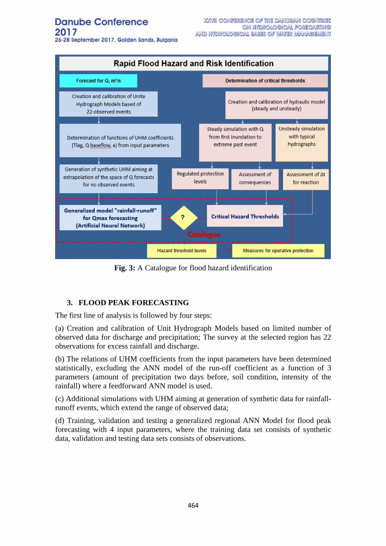
464

Fig. 3: A Catalogue for flood hazard identification

3. FLOOD PEAK FORECASTING

The first line of analysis is followed by four steps: (a) Creation and calibration of Unit Hydrograph Models based on limited number of observed data for discharge and precipitation; The survey at the selected region has 22 observations for excess rainfall and discharge. (b) The relations of UHM coefficients from the input parameters have been determined statistically, excluding the ANN model of the run-off coefficient as a function of 3 parameters (amount of precipitation two days before, soil condition, intensity of the rainfall) where a feedforward ANN model is used. (c) Additional simulations with UHM aiming at generation of synthetic data for rainfall-runoff events, which extend the range of observed data; (d) Training, validation and testing a generalized regional ANN Model for flood peak forecasting with 4 input parameters, where the training data set consists of synthetic data, validation and testing data sets consists of observations.

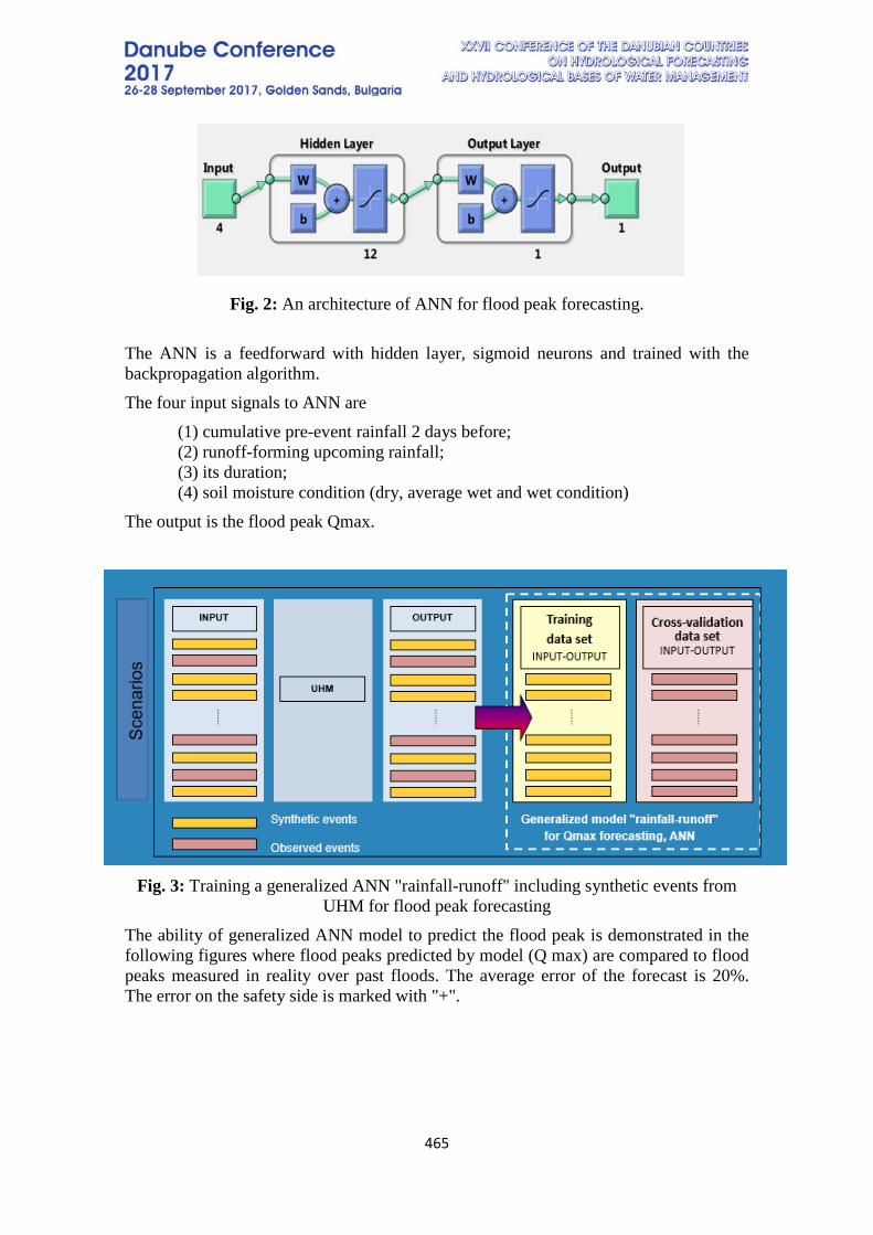
465

Fig. 2: An architecture of ANN for flood peak forecasting.

The ANN is a feedforward with hidden layer, sigmoid neurons and trained with the backpropagation algorithm. The four input signals to ANN are

(1) cumulative pre-event rainfall 2 days before; (2) runoff-forming upcoming rainfall; (3) its duration; (4) soil moisture condition (dry, average wet and wet condition)

The output is the flood peak Qmax.

Fig. 3: Training a generalized ANN "rainfall-runoff" including synthetic events from

UHM for flood peak forecasting The ability of generalized ANN model to predict the flood peak is demonstrated in the following figures where flood peaks predicted by model (Q max) are compared to flood peaks measured in reality over past floods. The average error of the forecast is 20%. The error on the safety side is marked with "+".

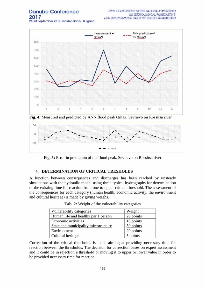
466

Fig. 4: Measured and predicted by ANN flood peak Qmax, Sevlievo on Rossitsa river

Fig. 5: Error in prediction of the flood peak, Sevlievo on Rossitsa river

4. DETERMINATION OF CRITICAL TRESHOLDS A function between consequences and discharges has been reached by unsteady simulations with the hydraulic model using three typical hydrographs for determination of the existing time for reaction from one to upper critical threshold. The assessment of the consequences for each category (human health, economic activity, the environment and cultural heritage) is made by giving weighs.

Tab. 2: Weight of the vulnerability categories

Vulnerability categories Weight Human life and healthy per 1 person 20 points Economic activities State and municipality infrastructure

10 points 50 points

Environment 20 points Cultural heritage 5 points

Correction of the critical thresholds is made aiming at providing necessary time for reaction between the thresholds. The decision for correction bases on expert assessment and it could be in rejection a threshold or moving it to upper or lower value in order to be provided necessary time for reaction.

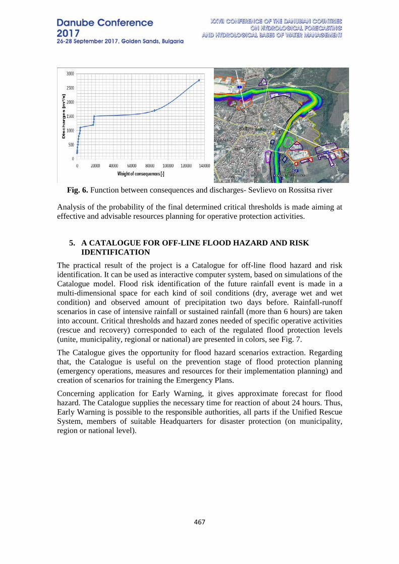
467

Fig. 6. Function between consequences and discharges- Sevlievo on Rossitsa river

Analysis of the probability of the final determined critical thresholds is made aiming at effective and advisable resources planning for operative protection activities.

5. A CATALOGUE FOR OFF-LINE FLOOD HAZARD AND RISK IDENTIFICATION

The practical result of the project is a Catalogue for off-line flood hazard and risk identification. It can be used as interactive computer system, based on simulations of the Catalogue model. Flood risk identification of the future rainfall event is made in a multi-dimensional space for each kind of soil conditions (dry, average wet and wet condition) and observed amount of precipitation two days before. Rainfall-runoff scenarios in case of intensive rainfall or sustained rainfall (more than 6 hours) are taken into account. Critical thresholds and hazard zones needed of specific operative activities (rescue and recovery) corresponded to each of the regulated flood protection levels (unite, municipality, regional or national) are presented in colors, see Fig. 7. The Catalogue gives the opportunity for flood hazard scenarios extraction. Regarding that, the Catalogue is useful on the prevention stage of flood protection planning (emergency operations, measures and resources for their implementation planning) and creation of scenarios for training the Emergency Plans. Concerning application for Early Warning, it gives approximate forecast for flood hazard. The Catalogue supplies the necessary time for reaction of about 24 hours. Thus, Early Warning is possible to the responsible authorities, all parts if the Unified Rescue System, members of suitable Headquarters for disaster protection (on municipality, region or national level).

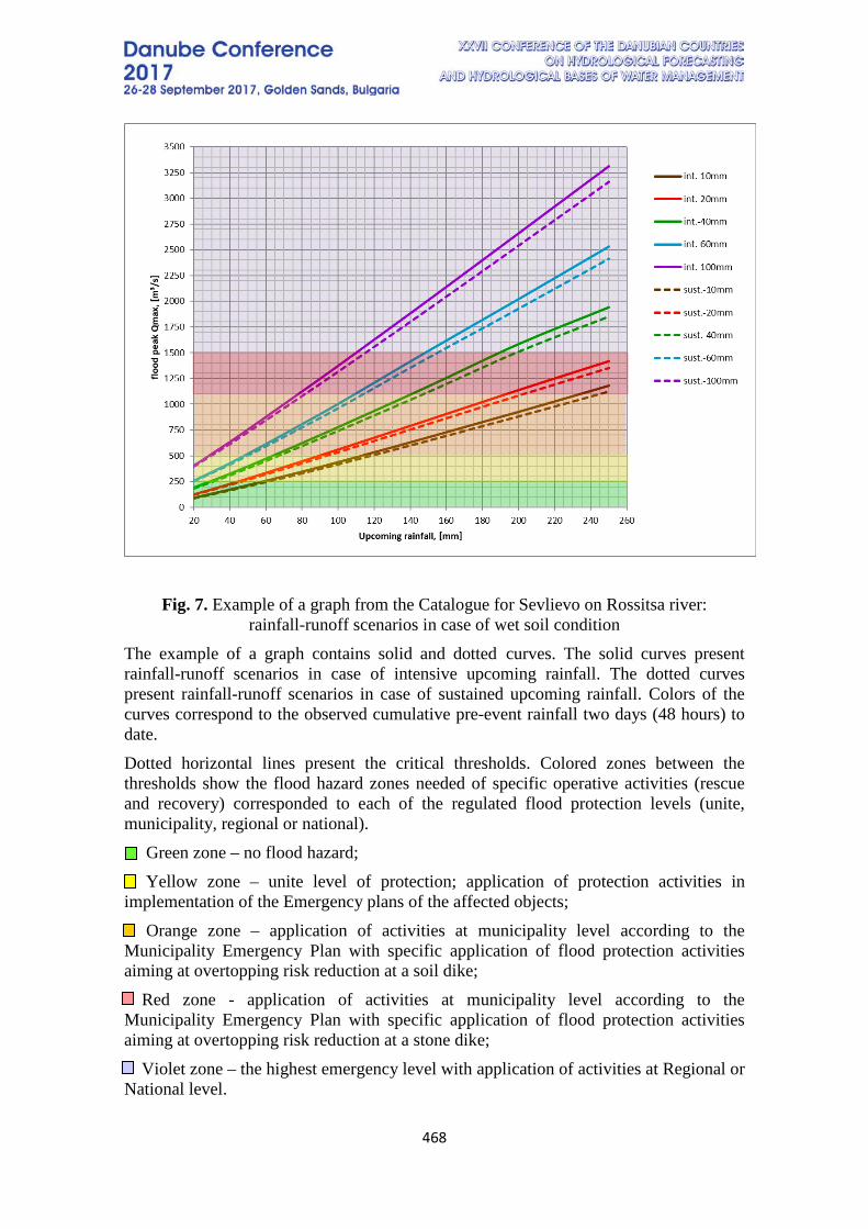
468

Fig. 7. Example of a graph from the Catalogue for Sevlievo on Rossitsa river: rainfall-runoff scenarios in case of wet soil condition

The example of a graph contains solid and dotted curves. The solid curves present rainfall-runoff scenarios in case of intensive upcoming rainfall. The dotted curves present rainfall-runoff scenarios in case of sustained upcoming rainfall. Colors of the curves correspond to the observed cumulative pre-event rainfall two days (48 hours) to date. Dotted horizontal lines present the critical thresholds. Colored zones between the thresholds show the flood hazard zones needed of specific operative activities (rescue and recovery) corresponded to each of the regulated flood protection levels (unite, municipality, regional or national). Green zone – no flood hazard; Yellow zone – unite level of protection; application of protection activities in implementation of the Emergency plans of the affected objects; Orange zone – application of activities at municipality level according to the Municipality Emergency Plan with specific application of flood protection activities aiming at overtopping risk reduction at a soil dike; Red zone - application of activities at municipality level according to the Municipality Emergency Plan with specific application of flood protection activities aiming at overtopping risk reduction at a stone dike; Violet zone – the highest emergency level with application of activities at Regional or National level.

469

6. CONCLUSIONS The results prove that the output signal, obtained from the ANN model for flood peak forecasting based on synthetic data and observations, is quite similar to the real one, so the used method appears to be useful and promising to offer some improvement for flood hazard analysis in practice in case of limited number of observed data for discharge and precipitation. In case of 24h rainfall forecast, the ANN helps for Flood risk identification and Early Warning to the responsible authorities.

REFERENCES [1] Atiya, A., El-Shoura, S., Shaheen, S., & El-Sherif, M. A comparison between neural-network forecasting techniques. Case study: River flow forecasting. IEEE Transactions on Neural Networks, 10, 402-409, 1999. [2] Dreyfus G. Neural Networks: Methodology and Applications, Springer, 2005 [3] Govindaraju, R.S., & Rao, A.R. Artificial neural networks in hydrology. Water Science and Technology Library (vol. 36). Kluwer Academic Publishers, 2000. [4] Haykin, S. Neural networks, a comprehensive foundation. NJ: Prentice-Hall, 1999. [5] Johansson, E.M., Dowla, F.U., & Goodman, D.M. Backpropagation learning for multi-layer feed-forward neural networks using the conjugate gradient method. International Journal of Neural Systems, 2(4), 291-301, 1992. [6] Loke, E., Warnaar, E.A., Jacobsen, P., Nelen, F., & do Ceu Almeida, M. Artificial neural networks as a tool in urban storm drainage. Water Science and Technology, 36(8-9), 101-109, 1997. [7] Pencheva, D. & Mavrova-Girginova M. Hazard identification and risk of flooding for programming purposes of protection of the population in the city of Sevlievo, Water Affairs Magazine- issue ¾, 2015. [8] Sinak, P., Bundzel, M., Soka, M., Sztruhar, D., & Marsalek, J. Urban runoff prediction by neural networks. In V. Babovic & L. C. Larsen (Eds.), Proceedings of Hydroinformatics ’98 Conference, Balkema, Rotterdam (pp. 791-796), 1998. [9] Xingui He, Shaohua Xu. Process Neural Networks: Theory and Applications, Springer, 2010

470

WATER RESOURCES STATISTICAL ESTIMATES IN BULGARIA CHARACTERISTICS AND FEATURES

Dobri Dimitrov, Maya Rankova, Kamelia Kroumova National Institute of Meteorology and Hydrology-BAS, Bulgaria

Corresponding author: Dobri Dimitrov, National Institute of Meteorology and Hydrology, 66 Tsarigradsko Shose, Blvd, 1784 Sofia, Bulgaria, email: dimitrov.dobri@gmail.com

ABSTRACT The poster is aiming to consider the annual water resources estimates and particularly the river discharge characteristics. The water resources evaluation technics is demonstrated on the Danube pilot district and its major Bulgarian basins and some means given to river basins management. Basic features of annual river flow and precipitation totals probability distribution are considered, bi-modality of their distribution is distinguished. The time variability and spatial homogeneity of the annual river flow are investigated too. Cluster analysis is applied to classify the annual river flow hydrographs, reasonable suggestion is made on the relation between the prevailing climatic influence, river flow and the modality of the probability distribution.

Keywords: water resources, river flow formation factors, precipitation, statistical estimates, cluster analysis. 1. Preface The suitability of water resources management needs adequate knowledge on the statistical characteristics of various hydrological parameters. That includes their probability distribution, values with certain return period, spatial variability and others. 2. The pilot The pilot comprises the Bulgarian part of the Danube basin, which main rivers are the rivers Ogosta, Iskur, Vit, Osam, Jantra and Rusenski Lom. Three types of landscape conditions are outlined here [1]: lowland along the Danube, hilly terrain with average elevation 300 – 600 m, mountain zone comprising the northern slopes of the Balkans with predominant elevation 800 – 1700 m. The regional climate is formed mostly by the Atlantic advection and not so often by Mediterranean transfer from the Adriatic. The mean annual precipitation totals are varying for the BG part of the Danube basin between 500 – 550 mm for the lowland and more than 1200 mm for the high mountain part of the Central Balkans. The positive gradient of precipitation with elevation is very well outlined, while some tendency of precipitation decrease is visible to east. Some decrease of precipitation at the very west part of the region is recently detected too.

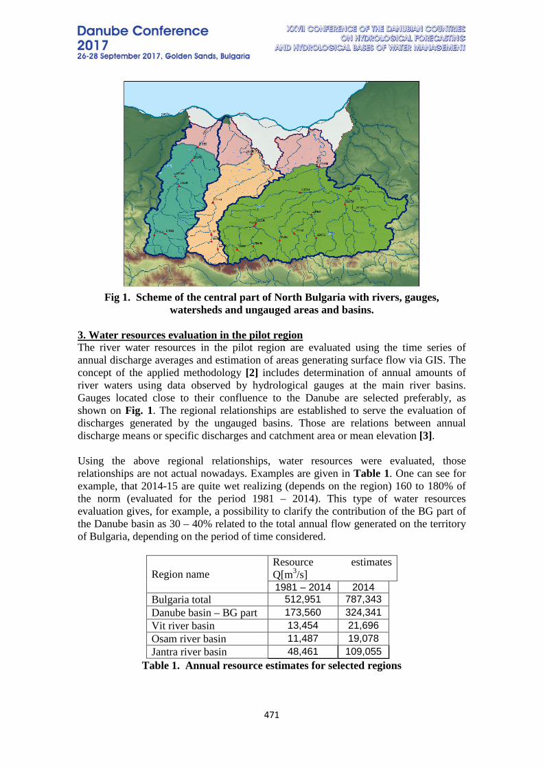
471

Fig 1. Scheme of the central part of North Bulgaria with rivers, gauges,

watersheds and ungauged areas and basins. 3. Water resources evaluation in the pilot region The river water resources in the pilot region are evaluated using the time series of annual discharge averages and estimation of areas generating surface flow via GIS. The concept of the applied methodology [2] includes determination of annual amounts of river waters using data observed by hydrological gauges at the main river basins. Gauges located close to their confluence to the Danube are selected preferably, as shown on Fig. 1. The regional relationships are established to serve the evaluation of discharges generated by the ungauged basins. Those are relations between annual discharge means or specific discharges and catchment area or mean elevation [3]. Using the above regional relationships, water resources were evaluated, those relationships are not actual nowadays. Examples are given in Table 1. One can see for example, that 2014-15 are quite wet realizing (depends on the region) 160 to 180% of the norm (evaluated for the period 1981 – 2014). This type of water resources evaluation gives, for example, a possibility to clarify the contribution of the BG part of the Danube basin as 30 – 40% related to the total annual flow generated on the territory of Bulgaria, depending on the period of time considered.

Region name Resource estimates Q[m3/s] 1981 – 2014 2014

Bulgaria total 512,951 787,343 Danube basin – BG part 173,560 324,341 Vit river basin 13,454 21,696 Osam river basin 11,487 19,078 Jantra river basin 48,461 109,055

Table 1. Annual resource estimates for selected regions

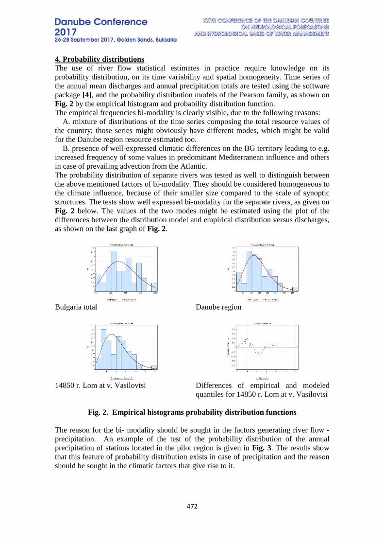
472

4. Probability distributions The use of river flow statistical estimates in practice require knowledge on its probability distribution, on its time variability and spatial homogeneity. Time series of the annual mean discharges and annual precipitation totals are tested using the software package [4], and the probability distribution models of the Pearson family, as shown on Fig. 2 by the empirical histogram and probability distribution function. The empirical frequencies bi-modality is clearly visible, due to the following reasons: A. mixture of distributions of the time series composing the total resource values of the country; those series might obviously have different modes, which might be valid for the Danube region resource estimated too. B. presence of well-expressed climatic differences on the BG territory leading to e.g. increased frequency of some values in predominant Mediterranean influence and others in case of prevailing advection from the Atlantic. The probability distribution of separate rivers was tested as well to distinguish between the above mentioned factors of bi-modality. They should be considered homogeneous to the climate influence, because of their smaller size compared to the scale of synoptic structures. The tests show well expressed bi-modality for the separate rivers, as given on Fig. 2 below. The values of the two modes might be estimated using the plot of the differences between the distribution model and empirical distribution versus discharges, as shown on the last graph of Fig. 2.

Bulgaria total

Danube region

14850 r. Lom at v. Vasilovtsi

Differences of empirical and modeled quantiles for 14850 r. Lom at v. Vasilovtsi

Fig. 2. Empirical histograms probability distribution functions

The reason for the bi- modality should be sought in the factors generating river flow - precipitation. An example of the test of the probability distribution of the annual precipitation of stations located in the pilot region is given in Fig. 3. The results show that this feature of probability distribution exists in case of precipitation and the reason should be sought in the climatic factors that give rise to it.

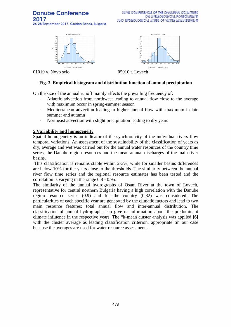
473

01010 v. Novo selo

05010 t. Lovech

Fig. 3. Empirical histogram and distribution function of annual precipitation

On the size of the annual runoff mainly affects the prevailing frequency of:

- Atlantic advection from northwest leading to annual flow close to the average with maximum occur in spring-summer season

- Mediterranean advection leading to higher annual flow with maximum in late summer and autumn

- Northeast advection with slight precipitation leading to dry years

5.Variability and homogeneity Spatial homogeneity is an indicator of the synchronicity of the individual rivers flow temporal variations. An assessment of the sustainability of the classification of years as dry, average and wet was carried out for the annual water resources of the country time series, the Danube region resources and the mean annual discharges of the main river basins. This classification is remains stable within 2-3%, while for smaller basins differences are below 10% for the years close to the thresholds. The similarity between the annual river flow time series and the regional resource estimates has been tested and the correlation is varying in the range 0.8 - 0.95. The similarity of the annual hydrographs of Osam River at the town of Lovech, representative for central northern Bulgaria having a high correlation with the Danube region resource series (0.9) and for the country (0.82) was considered. The particularities of each specific year are generated by the climatic factors and lead to two main resource features: total annual flow and inter-annual distribution. The classification of annual hydrographs can give us information about the predominant climate influence in the respective years. The “k-mean cluster analysis was applied [6] with the cluster average as leading classification criterion, appropriate tin our case because the averages are used for water resource assessments.

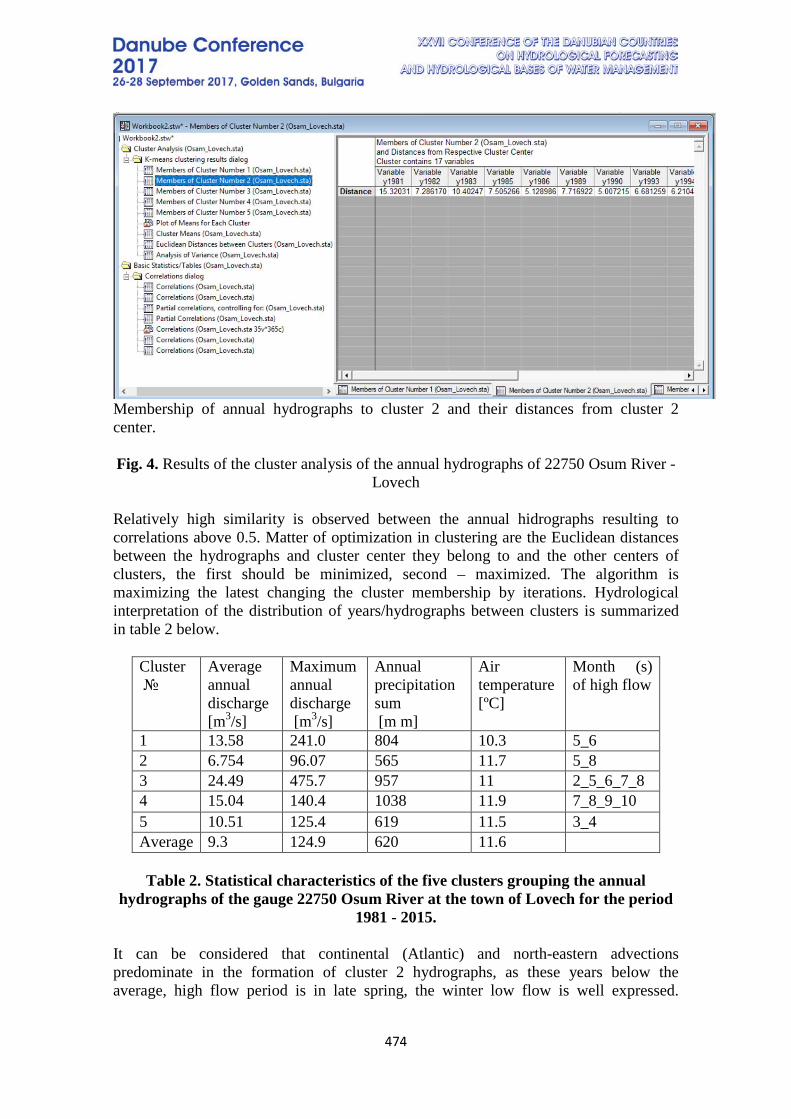
474

Membership of annual hydrographs to cluster 2 and their distances from cluster 2 center. Fig. 4. Results of the cluster analysis of the annual hydrographs of 22750 Osum River -

Lovech Relatively high similarity is observed between the annual hidrographs resulting to correlations above 0.5. Matter of optimization in clustering are the Euclidean distances between the hydrographs and cluster center they belong to and the other centers of clusters, the first should be minimized, second – maximized. The algorithm is maximizing the latest changing the cluster membership by iterations. Hydrological interpretation of the distribution of years/hydrographs between clusters is summarized in table 2 below.

Cluster №

Average annual discharge [m3/s]

Maximum annual discharge [m3/s]

Annual precipitation sum [m m]

Air temperature [ºC]

Month (s) of high flow

1 13.58 241.0 804 10.3 5_6 2 6.754 96.07 565 11.7 5_8 3 24.49 475.7 957 11 2_5_6_7_8 4 15.04 140.4 1038 11.9 7_8_9_10 5 10.51 125.4 619 11.5 3_4 Average 9.3 124.9 620 11.6

Table 2. Statistical characteristics of the five clusters grouping the annual

hydrographs of the gauge 22750 Osum River at the town of Lovech for the period 1981 - 2015.

It can be considered that continental (Atlantic) and north-eastern advections predominate in the formation of cluster 2 hydrographs, as these years below the average, high flow period is in late spring, the winter low flow is well expressed.

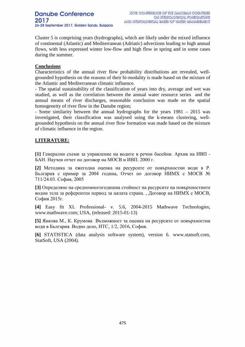
475

Cluster 5 is comprising years (hydrographs), which are likely under the mixed influence of continental (Atlantic) and Mediterranean (Adriatic) advections leading to high annual flows, with less expressed winter low-flow and high flow in spring and in some cases during the summer. Conclusions Characteristics of the annual river flow probability distributions are revealed, well-grounded hypothesis on the reasons of their bi-modality is made based on the mixture of the Atlantic and Mediterranean climatic influence. - The spatial sustainability of the classification of years into dry, average and wet was studied, as well as the correlation between the annual water resource series and the annual means of river discharges, reasonable conclusion was made on the spatial homogeneity of river flow in the Danube region; - Some similarity between the annual hydrographs for the years 1981 – 2015 was investigated, their classification was analysed using the k-means clustering, well-grounded hypothesis on the annual river flow formation was made based on the mixture of climatic influence in the region. LITERATURE: [1] Генерални схеми за управление на водите в речни басейни. Архив на ИВП -БАН. Научен отчет по договор на МОСВ и ИВП. 2000 г. [2] Методика за ежегодна оценка на ресурсите от повърхностни води в Р. България с пример за 2004 година, Отчет по договор НИМХ с МОСВ № 711/24.03. София, 2005 [3] Определяне на средномногогодишна стойност на ресурсите на повърхностните водни тела за референтен период за цялата страна. , Договор на НИМХ с МОСВ, София 2015г. [4] Easy fit XL Professional- v. 5.6, 2004-2015 Mathwave Technologies; www.mathwave.com; USA, (released: 2015-01-13) [5] Янкова М., К. Крумова Възможност за оценка на ресурсите от повърхностни води в България. Водно дело, НТС, 1/2, 2016, София. [6] STATISTICA (data analysis software system), version 6. www.statsoft.com, StatSoft, USA (2004).

476

TOPIC 5: ADMINISTRATIVE STRUCTURES FOR WATER MANAGEMENT

DEVELOPING THE EYARLY FLOOD WARNING SYSTEM AS THE IMPORTANT COMPONENT OF THE NATURAL HAZARDS RISK

MANAGEMENT: CASE STUDY FROM UKRAINE

Viacheslav Manukalo1, Victoria Boiko2 1 Ukrainian Hydrometeorological Institute, Ukraine 2 Ukrainian Hydrometeorological Centre, Ukraine

Corresponding author: V. Manukalo, Ukrainian Hydrometeorological Institute, 37, Nauki Prospect,03028, Ukraine,manukalo@ukr.net

ABSTRACT The river floods have imposed the most severe damages to the sectors of economy and human communities in Ukraine. Taking into account this fact, the issue of development of comprehensive flood risk management measures is of great significance. The paper deals with the study in developing the Early Flood Warning System (EFWS) as the essential informational component of the national system for the natural hazards risk management.

The existing conception of separate development of each component of EFWS was reconsidered, and the integrated approach "From sensors to decision-making” was proposed. EFWS includes two principal parts: the technological part and the management one. Efficient functioning of system requires support by governance, coordination mechanisms from national to regional and local levels, and by appropriate infrastructure and financing.

The problematic issues, current capabilities and needs of the Hydrometeorological Service to ensure the successful implementation of tasks provided for each component of EFWS are considered in the paper.

Keywords: Floods Risk Management, Early Warnings

1. INTRODUCTION According to the statistic data the river floods have imposed the most severe damages to the sectors of economy and the human communities in Ukraine. A large part of the country’s territory, especially located in the Carpathians mountains region, suffer from floods, practically, every year. Annually river inundations cause damage to the national economy estimated to be equal to tens of millions of US dollars. The cost of inundations sometimes includes the loss of human life. Taking into account this fact, the issue of development of comprehensive flood risk management measures is of great significance. But, the experience of floods of the last years indicated a number of problems in the flood management policy and showed that the existing flood risk management system does not meet the increased requirements of different categories of

477

users regarding the accuracy and timeliness of warnings as well as the quantitative estimation of socio-economic vulnerability to floods.

Among the non-structural measures of flood risk management it is very important to develop the effective Early Flood Warning System which enhances all (structural and non-structural) measures. The paper deals with the study in developing the Early Flood Warning System (EFWS) as the essential informational component of the national system for the natural hazards risk management.

2. METHODOLOGY AND MATERIALS

The study is based on: a) results of the National Program of Protection from Technogenic and Natural Emergencies; b) the Strategy of Development of Hydrometeorological Service of Ukraine; c) recommendations of the Directive 2007/60/EC on Assessment and Management of Flood Risks; d) recommendations of the Hyogo Framework for Action and the Sendai Framework for Disaster Risk Reduction 2015-20304; c) new information technologies which are used in the hydrometeorology and the hazards risk management;

3. DISCUSSION OF RESULTS 3.1 Flood disasters The flood disasters can be categorized as small, large, very large and catastrophic, depending on the size of areas inundated and on the value of damages done (Manukalo, 1998). Small flood disasters lead to the insignificant damage in some settlements. They occur on each river about once in 4-5 years. Large flood disasters lead to flooding of significant stretches of a river valley and disturb the normal economy within the large areas. The frequency of these disasters is about once in 20-25 years. The very large flood disasters involve a large river system with a number of cities. The economic activity is paralyzed by them and population and property should to be evacuated. The frequency of these flood disasters is about once in 50-100 years. The catastrophic flood disasters occur in a number of river systems and many cities. The economic objects, and engineering communications are flooded. The human victims also accompany these flood disasters. The frequency of catastrophic flood disasters is about once in 100-200 years. The catastrophic flood disasters during last 100 years occurred; in springs of 1931 and 1970 - on the Dnipro river and its the largest tributaries – the Prypyat' and Desna rivers; in 1969 and 2008 - on the Dniester river; in 1998 and 2001 – on the Tisza river.

3.2. Vulnerability to floods

Unfortunately, in Ukraine the issue of quantitative estimation of socio-economic vulnerability to floods has been studied not enough. We have proposed the methodology of assessment of vulnerability to floods based on an analysis of the following vulnerability indicators: a) hazards to human life and health; b) a destruction of city’s infrastructure (residential and industrial buildings, power and communication networks); c) environmental pollution. The magnitude and scope of impacts have been used as criteria for this evaluation. The information about the mentioned flood consequences can be taken from reports of central and local branches of the State Service of Ukraine on Emergencies.

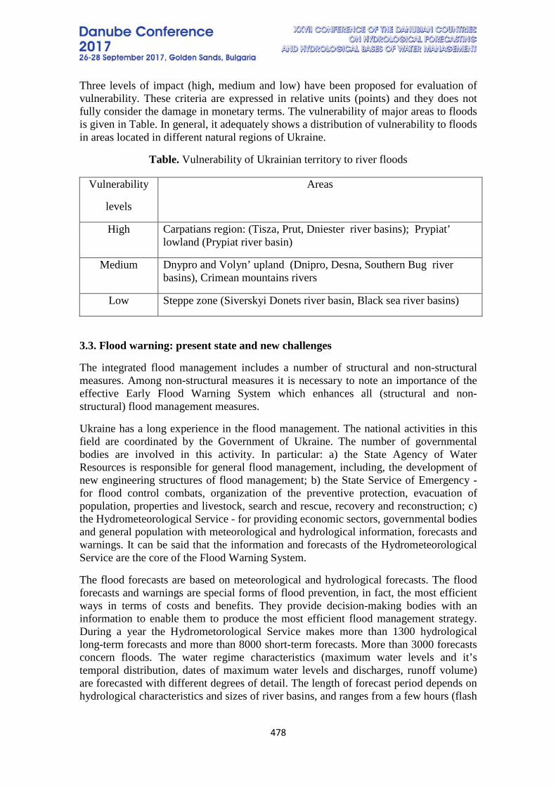
478

Three levels of impact (high, medium and low) have been proposed for evaluation of vulnerability. These criteria are expressed in relative units (points) and they does not fully consider the damage in monetary terms. The vulnerability of major areas to floods is given in Table. In general, it adequately shows a distribution of vulnerability to floods in areas located in different natural regions of Ukraine.

Table. Vulnerability of Ukrainian territory to river floods

Vulnerability

levels

Areas

High Carpatians region: (Tisza, Prut, Dniester river basins); Prypiat’ lowland (Prypiat river basin)

Medium Dnypro and Volyn’ upland (Dnipro, Desna, Southern Bug river basins), Crimean mountains rivers

Low Steppe zone (Siverskyi Donets river basin, Black sea river basins)

3.3. Flood warning: present state and new challenges

The integrated flood management includes a number of structural and non-structural measures. Among non-structural measures it is necessary to note an importance of the effective Early Flood Warning System which enhances all (structural and non-structural) flood management measures.

Ukraine has a long experience in the flood management. The national activities in this field are coordinated by the Government of Ukraine. The number of governmental bodies are involved in this activity. In particular: a) the State Agency of Water Resources is responsible for general flood management, including, the development of new engineering structures of flood management; b) the State Service of Emergency - for flood control combats, organization of the preventive protection, evacuation of population, properties and livestock, search and rescue, recovery and reconstruction; c) the Hydrometeorological Service - for providing economic sectors, governmental bodies and general population with meteorological and hydrological information, forecasts and warnings. It can be said that the information and forecasts of the Hydrometeorological Service are the core of the Flood Warning System.

The flood forecasts are based on meteorological and hydrological forecasts. The flood forecasts and warnings are special forms of flood prevention, in fact, the most efficient ways in terms of costs and benefits. They provide decision-making bodies with an information to enable them to produce the most efficient flood management strategy. During a year the Hydrometorological Service makes more than 1300 hydrological long-term forecasts and more than 8000 short-term forecasts. More than 3000 forecasts concern floods. The water regime characteristics (maximum water levels and it’s temporal distribution, dates of maximum water levels and discharges, runoff volume) are forecasted with different degrees of detail. The length of forecast period depends on hydrological characteristics and sizes of river basins, and ranges from a few hours (flash

479

floods on mountains rivers) up to 30-90 days (spring flows characteristics for large plain rivers).

The hydrometeorological forecasts and warnings are the component (subsystem) of the National Early Warning System for the Hazards Risk Management which is operated by the Ukrainian Government. It includes facilities to get forecasts, to analyze a current hydrometeorological situation, to make a flood risk assessment and to disseminate warnings using communication facilities. The central, regional and municipal Governments, the Civil Defense, a number of sectors of economy as well as Mass Media are recipients of flood warnings.

The recent experience of floods has indicated a number of problems in the flood management and has showed that the existing flood warning system does not meet increased requirements of different categories of users regarding the accuracy and timeliness of hydrological forecasts and warnings.

In response to these challenges the proposals aimed a development of the Early Flood Warning and Decision Support System, as the essential informational component of the National Early Warning System for the Hazards Risk Management were prepared by authors of this paper.

The existing conception of separate development of each component of EFWDSS was reconsidered, and the integrated approach "From sensors to decision-making” was proposed. According to this approach, the flood risk management is based on a use of the comprehensive end-to-end service delivery which includes many stakeholders. EFWDSS is aimed at increasing a lead-time of flood forecasting and warnings, that is very important for a creation of the effective Early Warning System. This approach is based on using the modern information technologies which were developed in the areas of hydrometeorology and civil protection.

EFWDSS includes two principal large parts: the technological part and the management one. The technological part consists of the following elements: a) hydrometeorological measurement network, data storage and real-time transmission; b) GIS database which is coupled with electronic maps for a hazard’s risk assessment; c) forecasting and warning; d) hazard risk assessment on different temporal and spatial scales; e) multi-hazards database; f) submitting information and warnings to users on national, regional and local levels.

The management part includes: a) planning, coordination and control of works and communication among the Hydrometeorological Service and users of information, forecasts and warnings; b) education and training programs for staff of different agencies involved in EFWDSS and for general public.

The efficient function of each element and the system as a whole requires support by governance, coordination mechanisms from national to regional and local levels, and by appropriate infrastructure and financing. Practically, there are direct and return linkages there are between all components of the system. These links need to be coordinated across many authorities at national, regional and community levels to ensure the system’s work.

480

This system should help the hazard risk management authorities to: a) identify the hazard risk level, including, the possible social, economic and environmental damages; b) determine the best protection measures on the basis of continuous monitoring, forecasting and warning of extreme weather-related events.

However, it is the risk that the technical implementation of this system will face a number of problematic issues. The problematic issues, current capabilities and needs of the Hydrometeorological Service to ensure the successful implementation of tasks provided for each component of EFWDSS are considered below.

The hydrometeorological measurement network, data storage and real-time transmission

The primary factors which influence the accuracy and lead - time of hydrological forecasts are the accuracy, speed and reliability with the real-time values of collected hydrological and meteorological variables. The hydrometeorological observation system includes 187 points of meteorological observation and more than 400 points of hydrological observation. But, the density of the ground network for hydrometeorological observation (especially for precipitation measuring in mountain parts of the Carpathians river basins) is comparatively low, its distribution in the river basins is unfavourable. This density of observation points does not allow to forecast flash floods in mountain river basins, especially, distribution of flow in time, with the essential accuracy.

There are a lot of technological problems in hydrometeorological observations. Mostly old types of hydrometric instruments are used in the Hydrometeorological Service for measuring water levels and discharges. The automated hydrological stations are installed only at 5% of points of hydrological observations. A number of Doppler flow velocity meters in the Hydrometeorological Service is extremely limited.

The automation of precipitation measurement and the installation of meteorological Doppler radars are also the priority for the Hydrometeorological Service.

Forecasting and warning

The flood forecasts which are based on meteorological and hydrological forecasting are the core of the EFWDDS. The forecasting of hydrological events in Ukraine started in 1930s. At present the water regime characteristics (water levels and discharges, their temporal distribution, dates of maximum water levels and discharges, runoff volume) are forecasted with different degrees of detail. The length of forecast periods depends on hydrological characteristics and size of river basis. Periods range from a few hours (rain floods on mountain rivers) up to 30-90 days (spring runoff volume and water inflow to reservoirs in plain river basins). The methods of forecasting are based on mathematical modeling of process that take place in river basins and determine the conditions of flood formation: precipitation types, soil moisture and soil freezing, geomorphologic characteristics of river basins.

Developing the forecasting methods which are based on GIS-technologies and are integrated with data of observations of automatic stations is a priority for the nearest period.

481

A methodology of providing users with warnings should be also improved. This methodology should be impact-based and it must to allow all groups of population to get warnings timely.

Hazard risks assessment by different time and spatial scales

The methodology, which now is used for an assessment of society’s vulnerability to flood disasters does not meet the demand of flood risk management. The improved methodology is being elaborated now by the experts from the Hydrometeorological Service and the State Service of Emergencies. It will take in consideration recommendations of experts who has an experience in the implementation of the Directive 2007/60/EC on Assessment and Management of Flood Risks. This methodology will take into account the frequency and level of flood hazards for different natural zones of the country and for different seasons of the year. Data on flood hazards for a long period will be consolidated in a database, which will be the segment of national multi - hazards database.

Planning and coordination works and communication among stakeholders

This component of management part is critical to the successful operation of entire system at both phases: the pre-disaster and the post-disaster activities.

The effective governance of flood management and protection can only be achieved by coordination and integration of work of multiple government agencies as well as local communities. The lack of proper coordination and communication between stakeholders will minimize the efficiency of hydrometeorological forecasts and warnings.

The following shortcomings in this component of the system can be indicated: a) in some cases, the presence duplication of activities in the flood risk management by the different agencies; b) the problems with understanding and effective using the information and warnings from the Hydrometeorological Service by agencies; c) the scarcity of budget funds for providing the sustainable activity of flood risk management.

Education and training programs for staff of the Hydrometeorological Service and stakeholders

In general, the education system in Ukraine guarantees training of skilled professionals. However, introducing the new methods and technologies in the hydrometeorology and flood management require additional training for practicing professionals and revision of the curricula in tertiary education institutions.

Besides, it is needed to strength the capacity-building of experts from the agencies responsible for the flood risk management in order to improve a skills of using the hydrometeorological information and services through the relevant training programs.

In order to solve this problem, the Hydrometeorological Service should develop the training program of skills upgrading for professionals from its organizations and for managers working in agencies which are responsible for flood management and protection.

482

4. CONCLUSIONS

Floods are inevitable, but their impacts can be reduced through the adequate planning of mitigation and prevention measures, including establishment of adequate preparedness systems to increase the effectiveness of emergency response triggered by early warnings and emergency operation. In spite of economical problems Ukraine is developing its floods management policy. A lot of attention is given to development of the Early Flood Warning and Decision Support System as one of component of the National System of Protection from Hazards of Natural and Technogenic Origin. The hydrometeorological information, forecasts and warnings of the Hydrometeorological Service are extremely valuable to ensure the effective flood risk management.

5. REFERENCES

[1] Manukalo V. River flood warning system in Ukraine, IAHS Publication, no. 239, pp.163-167, 1998.

483

DEVELOPING STANDARDIZATION OF THE HYDROMETEOLOGICAL ACTIVITY IN UKRAINE: PRESENT STATE AND NEW NEEDS

Viacheslav Manukalo, Tetiana Mytnyk, Liudmyla Kovalska

Ukrainian Hydrometeorological Institute

Corresponding author: V. Manukalo, Ukrainian Hydrometeorological Institute, 37, Nauki Prospect, 03028, Kyiv, Ukraine, manukalo@ukr.net

ABSTRACT Presently, the most important task of the Hydrometeorological Service of Ukraine is to introduce the new technologies of observation, forecasting and servicing. This process requires elaboration of appropriate standards, other technical documents which regulate all technological stages of hydrometeorological activity - from obtaining the measured data up to providing consumers with services. The elaboration of national base of technical documents was started after 1992. The Ukrainian Hydrometeorological Institute became the principal developer of standards, guides, other regulations. The legislation of Ukraine in the fields of hydrometeorology and standardization, and the recommendations of WMO and ISO served as the regulatory and legal framework in this work. During twenty years, more than 60 technical documents have been elaborated. The present state and new needs in the development of national regulations in the area of hydrometeorological observations, forecasting and services are considered in the paper.

Keywords: Hydrometeorological Activity, Standardisation

1. INTRODUCTION The issues of standardization in the areas of meteorology, hydrology and climatology belong to major directions of work of the Hydrometeorological Services (on national level) and the World Meteorological Organization (on international level).

In Ukraine the Law “On Standardization” regulates the development and implementation of standards and other regulatory acts in the relevant fields, including, the hydrometeorological activity. The standard-making role of WMO was established by the Convention, which indicates that the purposes of WMO are “… to promote the standardization of meteorological and related observations and to ensure the uniform publication of observations and statistics”.

Presently, the most important task of the Hydrometeorological Service of Ukraine is to introduce the new technologies of observation, forecasting and servicing. This process requires elaboration of appropriate standards, other technical documents which regulate all technological stages of hydrometeorological activity - from obtaining the measured data up to providing consumers with services.

The present state and new needs in the development of national regulations in the area of hydrometeorological observations, forecasting and services are considered in the paper.

484

2. METHODOLOGY AND MATERIALS The paper is based on the analysis of: a) more than twenty years experience of elaboration of standards in the area of hydrometeorological activity by the Ukrainian Hydrometeorological Institute; b) the international practice in this area; c) the demands of the new Ukrainian standardization’s legislation.

3. RESULTS AND DISCUSSION

The research institutions located in Russia (mainly in Moscow and Leningrad) were developers of practically all regulation documents which were used by the Hydrometeorological Service of the former Soviet Union. These documents were also used by the National Hydrometeorological Service of Ukraine in the first years after its establishment.

The elaboration of the national base of regulation documents was initiated in Ukraine after 1992. The Ukrainian Hydrometeorological Institute (the leading scientific organization of Ukraine in the area of meteorology, hydrology and climatology) became the principal developer of standards, guidelines, other technical regulations. The Technical Committee TC-109 "Hydrometeorology" was created by the order of the State Committee of Ukraine for Standardization for "…providing the leadership, coordination and support works on standardization in the field of hydrometeorology". The Secretariat of TC-109 was functioning at the Ukrainian Hydrometeorological Institute. The representatives of scientific, educational, design and other organizations, whose activities were related to the meteorology, hydrology, climatology and monitoring of pollution environment, were included in the TC-109.

The development of new technical regulations for the Hydrometeorological Service of Ukraine has been carried out considering the framework of the national policy in creating the national regulatory base in the relevant areas of economic and social activities on the basis of: a) the long-term plans (for 3-5 years) of elaboration of technical regulations that have been approved by the central executive body in the area of hydrometeorological activity; b) the respective annual plans that have been formed on the basis of long-term plans, and that have taken into account priority needs of the Hydrometeorological Service.

The Institute carried out the development of technical regulations within the planned topics of researches. The legislation of Ukraine in the fields of hydrometeorological activity and standardization, and the recommendations of WMO and ISO served as the regulatory and legal framework in this area. The leading scientists from the Institute as well as the highly skilled experts from the methodological centers of the Hydrometeorological Service have been involved for these researches.

At the first phase of work, special attention was paid to the creation of the normative documents, which formed the basis for further expansion and improvement of the regulatory framework in the field of hydrometeorological activity. During this period, the following documents have been elaborated:

• national standards of Ukraine on the terms and definitions of basic concepts in a meteorology, a surface hydrology, a synoptic meteorology, a climatology, a

485

aeronautical meteorology, a physical oceanography, an agricultural meteorology, an atmospheric ozone and an actinometry;

• branch standards of Ukraine governing the order of elaboration of normative documents in the area of hydrometeorological activity: “The system of branch standards for hydrometeorology. Basic provisions”; “The system of branch standards for hydrometeorology. Categories and types of regulation documents”; “The system of branch standards for hydrometeorology. The order of development, approval and registration of branch regulation documents”; “The system of branch standards for hydrometeorology. Planning the work on standardization. Basic provisions”; “The procedure for calculating the cost and duration of work on standardization in the field of hydrometeorology”; “The creation and maintenance of the information funds in the field of hydrometeorology; “The classification of regulations for hydrometeorology”.

Practically, at the same time the elaboration of regulation documents which define functioning of the system of hydrometeorological observations and forecasting was initiated. The work in this field has been especially intensified in the last ten years. For the purpose of regulation of hydrometeorological observations and measurements, including the issues of metrology, the following regulations were developed: “The methods of hydrometeorological observation and measurements”; “The instruction for evaluating the quality of hydrometeorological observations and works”; “The Guidelines for hydrometeorological stations and posts. Issue 2. Part 1: The meteorological observations on posts”; “The Guidelines for hydrometeorological stations and posts. Issue 3. Part 1: The meteorological observations on stations”; “The Guidelines for hydrometeorological stations and posts. Issue 13. Observations of the total ozone”; “The Guidelines for hydrometeorological stations and posts. Issue 11. Agrometeorological observations”; “The Guidelines on determination of agro - hydrological properties of soils”; The Guidelines for hydrometeorological stations and posts. Issue 14. Methods of observations and provision of service about a danger of snow avalanches”. “The metrological certification of methods of observation and measurement. The organization and order of carry out”; "The Guidance on the parallel meteorological observations "; "The regulations on the organization of registration and control of measuring instruments in the hydrometeorological organizations.

The considerable attention was paid to development of regulation documents which regulate the laboratory measurements and control of environmental pollution monitoring. In particular, the following documents were elaborated: “The Guidance on methods of hydrobiological analysis of surface water and sediments on the base network of observation of the Hydrometeorological Service. Phytoplankton and its products"; “The Guidelines for hydrometeorological stations and posts. Issue12: Observation on radioactive contamination of the environment. Part 1. Observation on radioactive contamination of air and aerosols”; “The Guidelines for hydrometeorological stations and posts. Issue12: Observation on radioactive contamination of the environment. Part 2. Observation on radioactive contamination of surface and sea waters”; “The methods of determination of the content of strontium-90 in surface and sea waters”.

A number of regulations were designed to organize and improve service users with the hydrometeorological information, forecasts and warnings. The following regulation

486

documents were elaborated in this area: “The Guidance on forecasting and warning of hazardous weather events”; “The Guidance on the hydrometeorological provision of the sectors of the national economy. Issue1, Part 1: Meteorological provision. Basic provisions”. Part 2. Agro-meteorological provision”; “The Manual on forecasting of the snow avalanches in the mountain regions of Ukraine”, “The assessment of the method’s quality and the accuracy of forecasting the regime of surface waters”.

A lot of attention was also paid to other methodological and organizational issues. In order to create the methodological principles of the economic efficiency evaluation of hydrometeorological information and forecasts, as well as to introduce the economic instruments in the activity of the Hydrometeorological Service "The Guidance on the assessment of the cost of hydrometeorological products" was developed.

The issues of work safety at the time of hydrometeorological observations and works were reflected in the following regulations: "The rules of fire safety for organizations and facilities of the Hydrometeorological Service" and " The safety rules during the hydrometeorological observations and works".

In order to improve the meteorological service of civil aviation and pursuant to "The Rules of meteorological provision of aviation in Ukraine” the package of regulations on quality management system of aviation meteorological services was elaborated. This package of documents consists of one manual, five procedures, seven methods and two instructions. These documents define the components of the Quality Management System - the organizational structure, planning, processes, resources and documentation which are used to provide and improve the quality of products and services as well as to meet the requirements of users of information and forecasts. The system of quality management of meteorological provision of aviation is based on the principles of quality management, fundamentals of which are described in international standards ISO 9000, adopted by the International Organization for Standardization.

Currently, in the frame of the research theme "The development of regulations in accordance to the perspective plan of preparation of national regulations in the field of hydrometeorological activity up to 2017" the following regulations are elaborated:

• “The rules of development, agreement, approval and marking of the regulations in the field of hydrometeorology”. This document will change a number of the branch standards which were designed before 2000 and don’t meet the requirements of new legislation of Ukraine now;

• “The manual for the meteorological stations and posts. Issue 3, Part 2. Processing the materials of meteorological observations ";

• “The Guidelines for the assessment of representativeness of reference stations".

While summarizing almost twenty years of experience related to the development of regulations in the field of hydrometeorological activity, the authors would like to share their views on issues that arose in the process of this work. These issues can be divided into two groups: organizational and financial ones.

In the first group of issues we should especially indicate the absence of experience of carrying out the researches in this area at the Institute. The practice has shown that the

487

small expert group established to develop the regulation documents, was unable to ensure the implementation of these works in appropriate ways because of the diversity of themes that to be considered in documents. At the first phase of works the level of Ukrainian experts had insufficient awareness on the relevant regulations designed in the hydrometeorological services of European countries. In a number of cases, the differences of opinion on the content of regulation documents have complicated the elaboration of these documents. In general, these problematic issues were overcome till 2005.

Currently, the main factor that affects the state of regulations elaboration is inadequate funding of this work. This factor does not allow to expand the elaboration of documents which are essential to the effective functioning of the hydrometeorological service of Ukraine. This concerns the documents which regulate the hydrological observations and works, including measuring instruments using modern technologies (automatic stations, remote-sensing devices); monitoring of environment pollution; some meteorological observations; introducing the ISO quality management recommendations. These factors caused the delay in forming a national fund of regulations in the field of hydrometeorological activity. As a result, a lot of regulations which now are used by the Hydrometeorological Service of Ukraine were designed still in the former USSR.

A new stage for the creation of regulation documents in the field of hydrometeorological activity began with the adoption of the new Law of Ukraine "On Standardization", which entered into force in January 2015. The Law was designed to improve the legal and organizational basis for national standardization in accordance with the international, first of all, the European practice. The law provides only two levels of regulation documents: 1) the national standards which can be adopted by the special national authority in the field of standardization; 2) standards, other regulation documents which can be adopted by enterprises, institutions and organizations. Under this Law, during fifteen years the central authorities have to check, review or cancel their regulation documents adopted before the entry into force of this Law, and the branch standards of the former Soviet Union. The Law provides the more rights for subjects of standardization in shaping its policy in this area, in particular, the determination of level of regulation documents.

Besides, national activities in the area of standardization should be more coordinated with directions of relevant activity of WMO and ISO. It is known that these international organizations pay the considerable attention to issues of standardization in the area of meteorology and hydrology.

In order to organize the work of the review and elaboration of new standards and other regulation documents the special working group was established. The representatives from the central authority in the areas of hydrometeorology and standardization, the Ukrainian hydrometeorological institute, the leading methodological centers of the Hydrometeorological Service of Ukraine and the Ukrainian manufactures of the hydrometeorological instruments were included in this working group. Until September of 2017 this group should prepare the lists of: 1) new documents which should be elaborated; 2) documents which can be used further as the standards or other regulation documents; 3) documents which should be re-designed.

488

4. CONCLUSIONS

Putting in the operation of new measurement instrumentations on the network of hydrometeorological observation demands the considerable investment for the Hydrometeorological Service of Ukraine. The prerequisite for the efficient use of funds and the adequate accuracy of measurements is the development and continuous improvement of standards and other regulation documents that govern the conduct of observation, forecasting and customer servicing. Currently, the Hydrometeorological Service of Ukraine undertakes considerable efforts to develop its base of standards, other regulation documents in the area of hydrometeorological activity. The relevant documents of ISO, WMO as well as the new Ukrainian legislation in the area of standardization are the methodological basis of these works.

489

AN IMPACT ASSESSMENT OF CLIMATE CHANGE IN THE DANUBE

RIVER BASIN – ANALYZING RESEARCH PROJECTS TO DETERMINE

ADAPTATION STRATEGIES

Roswitha Stolz, Monika Prasch, Franziska Koch, Michael Weber, Wolfram Mauser

Department of Geography, University of Munich LMU, Germany Corresponding author: Dr. Roswitha Stolz, Department of Geography, LMU, Luisenstr. 37, 80333

Munich

ABSTRACT Climate change is likely to strongly affect the entire hydrological cycle and water demand may grow due to warmer temperatures. Thus water management may face a multitude of new challenges. The International Commission for the Protection of the Danube River (ICPDR) in cooperation with the German Federal Ministry for Environment, Nature Conservation and Nuclear Safety (BMU) initiated a study to develop a Strategy on Adaptation to Climate Change for the whole Danube River Basin, which was performed by the University in Munich (LMU) in 2011/12. The outcome of this study is the ICPDR Strategy on the Adaptation to Climate Change. As in the last 6 years, new high-resolution regional climate change ensembles have been established for Europe (EURO-CORDEX), an update of this study is highly desirable. Within this update, it will be investigated, how the new results from climate simulations are considered in the ongoing projects and studies in all bordering countries, and how this will influence the ongoing and planned adaptation measures and strategies. In order to identify the differences between the first study and the state of the art, recent research projects, studies and strategies (ongoing or finalized since 2011), are analysed and compared to the former study. The main aim of the update of the Danube Study is to evaluate potential changes in the scientific knowledge base and to compare resulting impacts on different water related fields, i.e. water availability, agriculture / irrigation, navigation and hydrological and meteorological extremes as well as related adaptation measures. First results already show differences between the first Danube Study of 2011/12 and the current update. The new findings will be implemented in an advancement of the ICPDR Climate Change Adaptation Strategy. First results on this will be presented in the following. Keywords: ICPDR Strategy on the Adaptation to Climate Change, water availability, Danube river basin management, climate change scenarios 1. INTRODUCTION Climate change is likely to strongly affect the entire hydrological cycle and the water demand in many hydrological application fields (e.g., irrigation, drinking water) may grow drastically due to warmer temperatures. Thus water management may face a multitude of new challenges. With the aim to develop a Strategy on Adaptation to Climate Change for the whole Danube River Basin (DRB), the ICPDR (International Commission for the Protection of the Danube River) in cooperation with the German

490

Federal Ministry for Environment, Nature Conservation and Nuclear Safety (BMU) initiated a study to reach these objectives, which was performed by the Department of Geography of the University of Munich (LMU) in 2011/12. The outcome of this study is the ICPDR Strategy on Adaptation to Climate Change [1] (Danube Study 2011/12).This study investigated for the first time, the state of the art of climate change research findings on meteorological (e.g. precipitation and temperature) and hydrological parameters (e.g. runoff, low flow, floods) as well as findings on diverse water sectors (e.g. energy, navigation, tourism) in the entire Danube region. It summarizes the outcome of more than 100 climate change projects and studies. Moreover, this study gives for the first time a comprehensive overview on the availability of adaptation strategies for each of the 14 Danube River Basin countries which are contracting to the ICPDR and summarizes their main contents. At present, this study is therefore a highly considered guide for adaptation measure and strategy actions in the entire Danube region. However, since 2011, new IPCC emission scenarios and high-resolution regional climate change ensembles started to be established in the European countries (i.e. EURO-CORDEX). As the implementation of these new climate findings were not immediately undertaken in running projects and country-based adaptation strategies, they couldn’t be taken into account in this first study. Therefore, since January 2017, an update of this study was initialized. Within this update, it will be investigated how the new results from updated climate simulations are up to now considered in the ongoing projects and studies in the different Danube River Basin countries, and how this will influence the ongoing and planned adaptation measures and strategies. 2. PROJECT OBJECTIVES The first Danube-Study from 2011/12 and its recent update are closely linked. This first study aimed to provide foundations for a common, Danube‐wide understanding and procedure for adaptation to water resources management related climate impacts with the aim to develop suitable adaptation strategies for the entire Danube River Basin. In order to identify climate change impacts in the DRB and appropriate adaptation measures, ongoing and finalized research and development projects and studies as well as adaptation activities were analysed. The outcomes of the study provided the basis for the development of a basin‐wide adaptation strategy in the Danube River Basin with the ICPDR team of experts [1]. However, within the last 6 years modelling of the future climate significantly improved. This is the main driver for an update of the Danube Study. Modified climate change scenarios and improved global and regional circulation models (GCMs and RCMs) necessitate examining the impacts of climate change on the water availability in the DRB with respect to these new boundary conditions. Thus, in the update of the Danube study conducted in 2017/18 the main focus is on:

- Evaluating changes in the scientific knowledge base, especially climate scenarios and models, and their potential impact on water availability.

- Comparing the findings on the impact of climate change on meteorology, hydrology and the water use, as well as the country-based adaptation strategies from 2011/12 and 2017/18 and quantify differences within the Danube River Basin.

- Documenting whether and to which extent the adaptation of the different water sectors will change due to new findings in climate change research. A strong

491

focus is set on droughts, low water and navigation, agriculture/irrigation, forestry and extreme events.

- Evaluating whether the guidelines of the ICDR Strategy on Adaptation to Climate Change had been considered in the development of adaptation measures

- Documenting still existing knowledge gaps and inconsistencies in project results and studies.

3. METHODOLOGY Similar to the first study, neither further model calculations are carried out nor adaptation activities will be suggested by the authors. The results solely base on the analysis of studies, projects and adaptation activities [2]. A data base enables a utilization of the analysed projects in terms of commonalities, differences and contradictions in results and approaches, as well as for dependencies, competing interests and conflicts. In order to compile all relevant information also all ongoing, adopted and planned adaptation activities on a regional and national level in the water sector in the DRB are collected and integrated in the data base, if available. This is done in two steps. Firstly, the national communications under the UNFCCC (NC) and the National Adaptation Strategies (NAS) which provide an overview of the present and future impact of climate change and adaptation measures per country and at the EU level were analysed. The climate change data base extracted from the 6th NCs of all countries in the DRB (2013–2015) is compared to that one from the 5th NC (2009/2010) in order to address possible differences, uncertainties and commodities. In a second step, relevant scientific projects and studies and further activities on the administrative level in relation to climate change impacts are considered, as for example the Austrian Assessment Report 2014 [4], EURO-CORDEX [5], the JRC report on Water Scenarios for the Danube River Basin [6]. 4. FIRST RESULTS 4.1 Climate scenarios applied in National Adaptation and Regional Strategies (NAS) and National Communications under the UNFCCC (NC) The national communications (NC) provide an overview of the present and future impact of climate change and adaptation measures per country and at the EU level. Both, national and regional adaptation strategies (NAS) and the 6th NC (2nd for Bosnia-Herzegovina, Serbia, Ukraine) were analysed according to the applied emission scenarios and models. Compared to 2011, as a positive aspect, in seven more countries national adaptation strategies were adopted meanwhile; in three more countries they are already under preparation, which are Bulgaria, Croatia and Moldavia. Moreover, in Bavaria (has its own regional adaptation strategy), Romania and Hungary the NAS are under revision. In Germany the Strategy for Adaptation to Climate Change (APA I) was updated in 2016/2017 generating APA II. Targeted measures and proposed actions described in the strategies are based on IPCC emission scenarios and global and regional climate models (GCM, RCM). Since the 5th IPCC report was published (2013) in an increasing amount of research studies, but also in NAS the RCP (radiative concentration pathway) 8.5 and 4.5 are used in combination with improved GCM and RCM, such as CORDEX (see Tab.1).

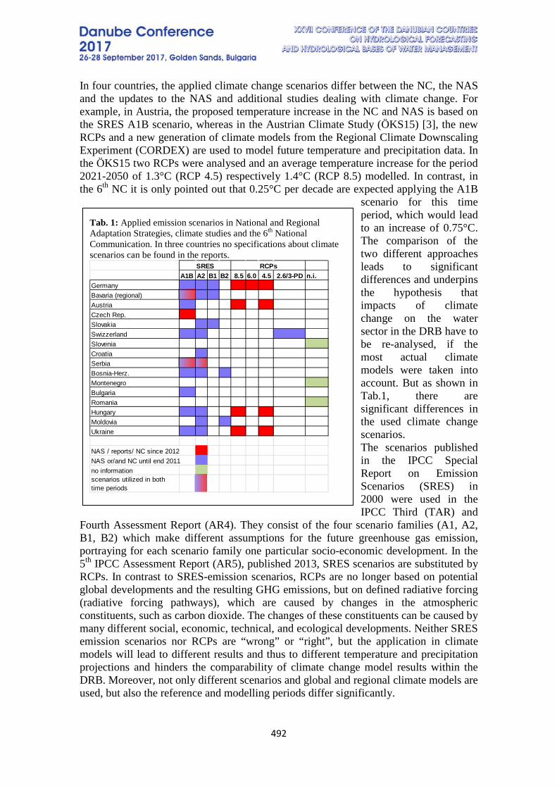
492

Tab. 1: Applied emission scenarios in National and Regional Adaptation Strategies, climate studies and the 6th National Communication. In three countries no specifications about climate scenarios can be found in the reports.

A1B A2 B1 B2 8.5 6.0 4.5 2.6/3-PD n.i.GermanyBavaria (regional)AustriaCzech Rep.SlovakiaSwizzerlandSloveniaCroatiaSerbiaBosnia-Herz. MontenegroBulgariaRomaniaHungaryMoldoviaUkraine

NAS / reports/ NC since 2012NAS or/and NC until end 2011no information scenarios utilized in both time periods

SRES RCPs

In four countries, the applied climate change scenarios differ between the NC, the NAS and the updates to the NAS and additional studies dealing with climate change. For example, in Austria, the proposed temperature increase in the NC and NAS is based on the SRES A1B scenario, whereas in the Austrian Climate Study (ÖKS15) [3], the new RCPs and a new generation of climate models from the Regional Climate Downscaling Experiment (CORDEX) are used to model future temperature and precipitation data. In the ÖKS15 two RCPs were analysed and an average temperature increase for the period 2021-2050 of 1.3°C (RCP 4.5) respectively 1.4°C (RCP 8.5) modelled. In contrast, in the 6th NC it is only pointed out that 0.25°C per decade are expected applying the A1B

scenario for this time period, which would lead to an increase of 0.75°C. The comparison of the two different approaches leads to significant differences and underpins the hypothesis that impacts of climate change on the water sector in the DRB have to be re-analysed, if the most actual climate models were taken into account. But as shown in Tab.1, there are significant differences in the used climate change scenarios. The scenarios published in the IPCC Special Report on Emission Scenarios (SRES) in 2000 were used in the IPCC Third (TAR) and

Fourth Assessment Report (AR4). They consist of the four scenario families (A1, A2, B1, B2) which make different assumptions for the future greenhouse gas emission, portraying for each scenario family one particular socio-economic development. In the 5th IPCC Assessment Report (AR5), published 2013, SRES scenarios are substituted by RCPs. In contrast to SRES-emission scenarios, RCPs are no longer based on potential global developments and the resulting GHG emissions, but on defined radiative forcing (radiative forcing pathways), which are caused by changes in the atmospheric constituents, such as carbon dioxide. The changes of these constituents can be caused by many different social, economic, technical, and ecological developments. Neither SRES emission scenarios nor RCPs are “wrong” or “right”, but the application in climate models will lead to different results and thus to different temperature and precipitation projections and hinders the comparability of climate change model results within the DRB. Moreover, not only different scenarios and global and regional climate models are used, but also the reference and modelling periods differ significantly.

493

4.2. Comparison of the results of climate change scenarios in National

Adaptation Strategies and National Communications under the UNFCCC

In the first Danube Study 2011/12, the findings in most of the strategies, communications and projects used the IPCC scenarios A1B and B2, and less of them A2 and B1. The results were achieved by different combinations of IPCC emission scenarios, GCMs, RCMs and downscaling methods. Comparing the analysis results from the NAS and the 6th NC, differences in predicted future temperature and precipitations could be addressed. Fig. 1 shows as an example a comparison of the modelled future mean annual temperatures between the 2011/12 Danube Study and the update of the study for the time period far future (2071-2100). Two facts have to be pointed out:

- Most countries did not quantify the temperature increase in the 6th NC. Only qualitative information such as “significant temperature increase” is given.

- The use of different time base lines and scenarios hinders a more detailed comparison of the results.

5. Conclusions The main aim of the update of the Danube Study is to evaluate potential changes in the scientific knowledge base and comparing resulting impacts on the water sector and adaptation measures. First results show that there are already differences between the first Danube Study of 2011/12 and the current update. The main difference lies in a larger variation of applied emission scenarios and climate models which hinders the comparison of modelled temperature and precipitation distribution. Moreover, it was found that the qualitative and quantitative values for temperature and precipitation given in NC and NAS differ in several cases significantly from the model results in actual research projects. In general, an increase in country-based NAS was determined which highlights the awareness of the individual countries regarding climate change issues and represents a good basis for a better transboundary application of adaptation measures. To develop these measures, a common scientific data base would be favourable.

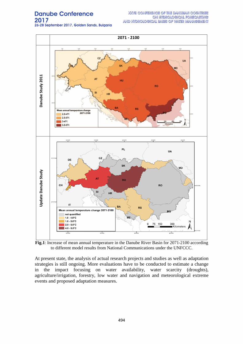
494

2071 - 2100 Da

nube

Stu

dy 2

011

Upd

ate

Danu

be S

tudy

Fig.1: Increase of mean annual temperature in the Danube River Basin for 2071-2100 according to different model results from National Communications under the UNFCCC.

At present state, the analysis of actual research projects and studies as well as adaptation strategies is still ongoing. More evaluations have to be conducted to estimate a change in the impact focusing on water availability, water scarcity (droughts), agriculture/irrigation, forestry, low water and navigation and meteorological extreme events and proposed adaptation measures.

495

6. REFERENCES

[1] ICPDR (2012). ICPDR Strategy on Adaptation to Climate Change. Vienna [2] Prasch, M., Koch, F., Weidinger, R., Mauser, W. (2012): Danube Study – Climate Change Adaptation. Ludwig‐Maximilians Universität Munich. [3] Ministerium für ein lebenswertes Österreich (ed) (2015): ÖKS15-Klimaszenarien für Österreich. [4] Austrian Panel on Climate Change (2014): Austrian Assessment Report 2014. Verlag Österreichische Akademie der Wissenschaften. [5] Jacob, D., Petersen, J.& Eggert, B. et al (2014): EURO-CORDEX: New high-resolution climate change projections for European impact research. Regional Environmental Change vol. 14, p.563-578 [6] Pistocchi, A., Beck, H. & Bisselink, B. etal.(2015): Water scenarios for the Danube River Basin. JRC Technical Reports, EUR 27700 EN

7. ACKNOWLEDGEMENT Financial support by the German Federal Ministry for Environment, Nature Conservation and Nuclear Safety (BMU) within the Danube Study is gratefully acknowledged. We thank the members of the International Commission for the Protection of the Danube ICPDR for fruitful cooperation and discussions within its various groups.

496

FLOOD RISK ASSESSMENT IN ROMANIA BASED ON SOCIAL, ECONOMIC AND CULTURAL EXPOSURE

Viorel Chendeş1, Daniela Rădulescu1, Sorin Rândaşu2, Diana Achim1, Anca

Gorduza2 1 National Institute of Hydrology and Water Management, Romania

2 “Romanian Waters” National Administration, Romania

Corresponding author: Viorel Chendeş, I.N.H.G.A., 97E, Bucuresti-Ploiesti, 013686, Bucharest, Sector 1, Romania, viorel.chendes@hidro.ro

The measures to reduce flood risk in Romania present a high interest, given the fact that Romania is considered one of the countries with the most severe and frequent floods in the last 10 years in Europe. Many extreme events occurred on certain rivers lead to significant economic damage and even fatalities. Thus, the flood risk assessment has to consider the social, economic and cultural receptors affected by these phenomena. For the implementation of the Floods Directive, the development of flood hazard maps was followed by the risk mapping. For the risk maps published at national level a procedure of zoning the risk was elaborated, taking into account the magnitude of the hazard, respectively water depth and elements exposed to floods with a certain probability of occurrence, respectively land use types. Definition of exposure classes was based on the CLC (Corine Land Cover) classification, amended at the national level in order to meet specific requirements. The developed methodology involves elaboration of a matrix as a function of the level of hazard and exposure/vulnerability. The risk was classified into 4 categories: no risk (insignificant residual risk), low risk, medium risk and high risk. Flood risk maps show the location and the current importance degree of the exposed elements. In order to assess the importance of each Areas with Potential Significant Flood Risk (APSFR), a system of 11 indicators was developed, each indicator reflecting the importance or extent of a certain type of receptor (consequences). Due to the fact that the indicators values vary from one APSFR to another, these indicators were rated from 0 to 5. These 11 used indicators allow the risk assessment and ranking for each APSFR sites. Keywords: Floods Directive, Romania, flood risk, flood receptors, exposure

497

EVALUATION OF THE WATER USE IN COMPARISON TO THE SURFACE WATER RESOURCES FOR SELECTED PERIOD BASED ON

THE RESULTS OF WATER RESOURCE BALANCE (WRB)

Ľubica Lovásová, Katarína Melová, Zuzana Danáčová, Lotta Blaškovičová Slovak Hydrometeorological Institute, Jeséniova 17, 833 15 Bratislava, Slovak Republic

Corresponding author: Dr. Melová Katarína, Slovak Hydrometeorological Institute, Jeséniova 17, 833 15 Bratislava, Slovak Republic, katarina.melova@shmu.sk

ABSTRACT Harmonization of water requirements with water resources is a key prerequisite for a rational use of water resources. It is therefore very important to identify water resources in terms of quantity, quality, time and space, as well as to assess their use in terms of water needs. Keywords: water resource balance, runoff, water use (abstraction and discharge)

1. INTRODUCTION In the document called “Water resources balance of surface water for the previous year”, we assess the quantitative relationship between water resources and water demand annually in the water resource balance in Slovakia. Also we determine when and where the water resources do not cover the water needs.

2. THE WATER RESOURCE BALANCE The water resource balance in Slovakia is used as a basis for water management planning since 1973. After the implementation of the WFD into the national legislation, the methodology of water resource balance has been modified in this context as well and it has been used as a basis for quantitative assessment of water resources. Water resource balance is done on annual basis, and evaluates the previous calendar year. The processing is done in monthly step spatially for the whole territory of Slovakia. For the evaluation of the water resource balance a specific method is used. The method allows to assess the detailed surface water use with calculated influence of groundwater use. Water requirements are represented by the actual consumption of surface and groundwater and discharging of wastewater and special water, which are derived in accordance with § 20 and § 22 of Decree No. MPŽPaRR SR. 418/2010 Coll. on the implementation of certain provisions of the Water Act. Among the water management measures in the water resource balance, we assess the impact of dams and water transfer. In the water resource balance equation on the side of water sources, there are discharges in rivers, precipitation totals and inflows from countries situated at upstream of river basins (in case of Danube River it represents an important part). It makes a significant

498

difference in calculations if we assume the own country water sources or we calculate with the inflow from neighboring countries as well. The assessment of the water balance and determination of the resource capacity are calculated in two alternatives:

1. under the conditions of natural discharges when we are considering the water demand and also the recharges of the wastewater (BSC),

2. under the conditions when we taking into consideration the impact of water reservoirs or water transfer too (BSENP).

The basic equation of the water balance takes into account the sources with needs and the basic formulas for the balance evaluation in order to calculate the balance rate and the usable water capacity. In case of balance status, we calculate the ratio of the resources to requirements. In case of usable water capacity, the calculation is based on the difference between the water sources and requirements. Water resources represents natural flows and the flows affected by water reservoirs, water transfer and distribution facilities, and water requirements include surface water abstractions, groundwater abstraction, waste water discharges and minimum flow rates that together represent the minimum required discharge in the river. Based on the calculated value of the balance status, it could have three positions:

BSC (BSENP) > 1.1 - Category A - active balance 1.1 > BSC (BSENP) > 0.9 - Category B - stressed balance 0.9 > BSC (BSENP) > 0 - Category C - passive balance.

3. WATER RESOURCES IN SLOVAKIA Within the water balance of the previous year, precipitation and runoff for the entire territory of Slovakia is also assessed for individual sub-basins. The territory of Slovakia has sufficient water resources, which are much higher compared to the annual drainage of the Slovak Republic. This is because the boundaries of the Slovak Republic are not identical to the hydrological sub-catchments of individual river basins. The Danube (from the territory of Austria Fig. 1), which has a long-term flow rate of 2061 m3.s-1, has the largest share in our territory. The area of the river basin, which forms the total available water resources of Slovakia represents 21% the Slovak territory. The long-term average annual outflow from the territory of Slovakia is 363.7 m3.s-1 (234 mm), and this is only 14% of the total amount of the water sources. The catchment of River Vah and its tributaries contribute 38% of the average annual runoff, where as Hron and Bodrog consist 14% and the rest is contributed with other basins of Slovakia. The only water source of our rivers is coming from the atmospheric precipitation. The total precipitation amount gives us about 31% of the surface runoff of SR.

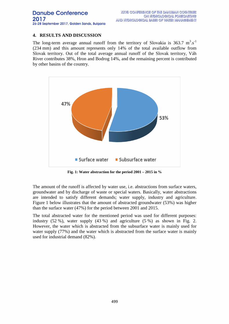
499

4. RESULTS AND DISCUSSION The long-term average annual runoff from the territory of Slovakia is 363.7 m3.s-1 (234 mm) and this amount represents only 14% of the total available outflow from Slovak territory. Out of the total average annual runoff of the Slovak territory, Váh River contributes 38%, Hron and Bodrog 14%, and the remaining percent is contributed by other basins of the country.

Fig. 1: Water abstraction for the period 2001 – 2015 in %

The amount of the runoff is affected by water use, i.e. abstractions from surface waters, groundwater and by discharge of waste or special waters. Basically, water abstractions are intended to satisfy different demands; water supply, industry and agriculture. Figure 1 below illustrates that the amount of abstracted groundwater (53%) was higher than the surface water (47%) for the period between 2001 and 2015. The total abstracted water for the mentioned period was used for different purposes: industry (52 %), water supply (43 %) and agriculture (5 %) as shown in Fig. 2. However, the water which is abstracted from the subsurface water is mainly used for water supply (77%) and the water which is abstracted from the surface water is mainly used for industrial demand (82%).

500

Fig. 2: Water abstraction for the period 2001 – 2015 in % divided to main categories The water use in the Slovak Republic has in the recent period a downward trend in all of above-mentioned categories (Fig. 3). We have been experiencing this change since the early 1990s, mainly as a result of changes in the economy, which resulted in the extinction of many users, and other users were divided into separate smaller users.

Fig. 3 Water use during the period 2001 – 2015 in Slovakia

In Fig. 3, we can also see some increased values of the water recharge in years 2010 and 2013. This is because of that these two years were very wet from hydrological point of view, and the water recharge values include huge amount of the rain “recharged” from different users. At that time we had not differentiated the rainwater inflow from industrial areas into the rivers. The calculated results of the water use on the river basin level has shown, that the water abstractions from all river basins over the evaluated

501

period has declining trend in all categories with the exception of three sub-catchments i.e. the Malý Dunaj, Bodva and Poprad catchments. In case of calculation of the water balance status under the natural conditions (BSC) in yearly step in all our balancing profiles the balance status is active except the river basin of Malý Dunaj, where is a huge donation of surface water from the main stream of the Danube. It is necessary to mention, that yearly steps of the calculation eliminates the effects of shorter water scarcity periods, and sometimes the monthly step is not enough for the identification of some local short-term problems. On the other hand, the water resource balance in Slovakia gives us information about the water management in our country and can define some problems related proper use of water.

5. CONCLUSIONS We can declare, that the water balance serves to verify whether the expected water management objectives have been met in the past year – quantifying water status, assessing water use, and then assessing water coverage. It specifies the areas in which there have been problems with securing the minimum required discharge and determines the stressed and passive river sections in monthly step. We have to realize, that not just the quantity is important but also the annual distribution of water resources as well as the requirements on these waters. The other possibilities are to make the estimation with use of selected ecological limits, what can have important outputs for setting the appropriate ecological measures.

6. REFERENCES Poórová, J.: Metódy vodohospodárskej bilancie. Dizertačná práca na získanie vedecko-akademickej hodnosti philosophiae doctor v odbore doktorandského štúdia: 39-41-9 Hydrológia a vodné hospodárstvo.2007. STU Bratislava. Danáčová, Z., Lovásová, Ľ., Gápelová, V., Podolinská, J., Ľupták, Ľ., Melová, K., Škoda, P., Liová, S., Síčová, B., Staňová, J. Vodohospodárska bilancia množstva povrchových vôd za roky 2001 až 2015. SHMÚ Bratislava. Lovásová, Ľ., Danáčová, Z., Čaučík, P., Döményová, J., Molnárová, A. Správa o vodohospodárskej bilancii vôd v SR za rok 2010, SHMÚ Bratislava, 2011.

502

TOPIC 6: RIVER BASIN AND WATER MANAGEMENT

MONTE CARLO SIMULATIONS TO EVALUATE THE POTENTIAL OF

ALPINE RETENTION MEASURES

Thomas Nester, Jürgen Komma, Jose Luis Salinas, Günter Blöschl

Institute for Hydraulic and Water Resources Engineering /Vienna Technical University, Austria Corresponding author: Thomas Nester, Karlsplatz 13/222, 1040 Vienna, Austria,

nester@hydro.tuwien.ac.at

ABSTRACT In this study we evaluate the potential of alpine retention measures. The main question is to quantify the potential reduction of floods in the Inn at a regional scale that could be obtained with these alpine retention measures. 130 potential sites for retention measures are assumed all over the catchment, each with a dam height of 10 m, combining to a total volume of 21 million m³. To evaluate the effect of the potential retention measures, we use a stochastic precipitation model and a rainfall-runoff model. The stochastic precipitation model is used to generate a dataset of 10.000 years of hourly precipitation data. The precipitation model is calibrated on a set of around 500 precipitation stations and reproduces the statistical properties of the observed precipitation. The generated precipitation is then used as driver for a distributed hydrological model (spatial scale 1x1 km, temporal scale 1 hour), calibrated on 35 years of observed runoff data of 71 gauges. We use two different model configurations for the Monte Carlo simulations: (1) without retention measures, and (2) with potential alpine retention measures. Results show that the effect retention measures on the Inn floods is only marginal with a flood peak reduction in the order of 2-3%. Results also show that the effect of the retention measures differs with the spatial extent of the precipitation. Keywords: floods, retention, precipitation model, hydrological model, Monte Carlo

1. CATCHMENT AND DATA The study region is the Austrian part of the Inn catchment, Tyrol. The source of the Inn is in the Swiss Alps, from where it runs north-eastwards through Switzerland and Tyrol before entering Germany, discharging a total area of about 9800 km². At the Austrian-German border, the average runoff is 305 m³/s, and the highest observed runoff is 2340 m³/s (2005). Tyrol is a mountainous country with elevations from 480 m a.s.l. to 3768 m a.s.l. (mean 1890 m a.s.l.) and hence land for building is scarce due to topography. In the Inn valley there are areas which would be suitable for building, however, these areas are in flood prone areas or in areas which are designated as retention areas. Alternatively, retention measures could be built in alpine areas. Figure 1 shows the Inn catchment from the origin in Switzerland to the Austrian-German border at Oberaudorf (9712 km²). Blue

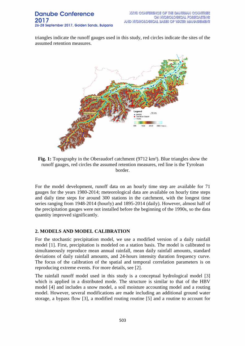
503

triangles indicate the runoff gauges used in this study, red circles indicate the sites of the assumed retention measures.

Fig. 1: Topography in the Oberaudorf catchment (9712 km²). Blue triangles show the

runoff gauges, red circles the assumed retention measures, red line is the Tyrolean border.

For the model development, runoff data on an hourly time step are available for 71 gauges for the years 1980-2014; meteorological data are available on hourly time steps and daily time steps for around 300 stations in the catchment, with the longest time series ranging from 1948-2014 (hourly) and 1895-2014 (daily). However, almost half of the precipitation gauges were not installed before the beginning of the 1990s, so the data quantity improved significantly.

2. MODELS AND MODEL CALIBRATION For the stochastic precipitation model, we use a modified version of a daily rainfall model [1]. First, precipitation is modeled on a station basis. The model is calibrated to simultaneously reproduce mean annual rainfall, mean daily rainfall amounts, standard deviations of daily rainfall amounts, and 24-hours intensity duration frequency curve. The focus of the calibration of the spatial and temporal correlation parameters is on reproducing extreme events. For more details, see [2]. The rainfall runoff model used in this study is a conceptual hydrological model [3] which is applied in a distributed mode. The structure is similar to that of the HBV model [4] and includes a snow model, a soil moisture accounting model and a routing model. However, several modifications are made including an additional ground water storage, a bypass flow [3], a modified routing routine [5] and a routine to account for

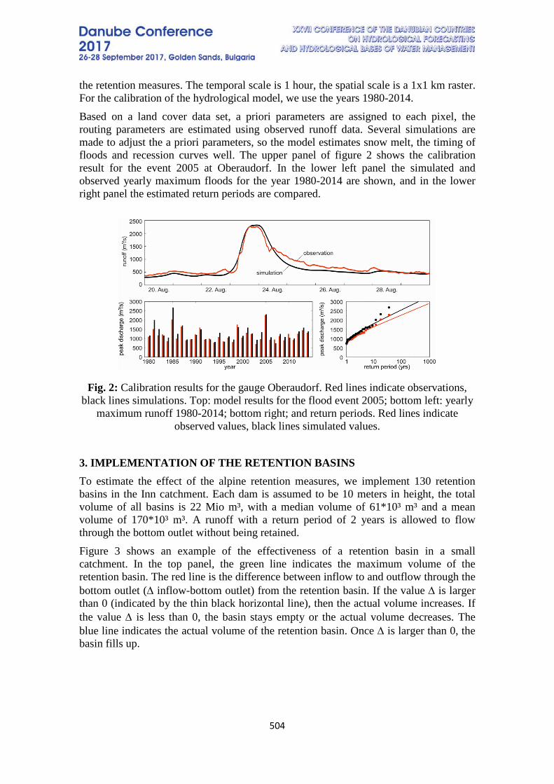
504

the retention measures. The temporal scale is 1 hour, the spatial scale is a 1x1 km raster. For the calibration of the hydrological model, we use the years 1980-2014. Based on a land cover data set, a priori parameters are assigned to each pixel, the routing parameters are estimated using observed runoff data. Several simulations are made to adjust the a priori parameters, so the model estimates snow melt, the timing of floods and recession curves well. The upper panel of figure 2 shows the calibration result for the event 2005 at Oberaudorf. In the lower left panel the simulated and observed yearly maximum floods for the year 1980-2014 are shown, and in the lower right panel the estimated return periods are compared.

Fig. 2: Calibration results for the gauge Oberaudorf. Red lines indicate observations, black lines simulations. Top: model results for the flood event 2005; bottom left: yearly

maximum runoff 1980-2014; bottom right; and return periods. Red lines indicate observed values, black lines simulated values.

3. IMPLEMENTATION OF THE RETENTION BASINS To estimate the effect of the alpine retention measures, we implement 130 retention basins in the Inn catchment. Each dam is assumed to be 10 meters in height, the total volume of all basins is 22 Mio m³, with a median volume of 61*10³ m³ and a mean volume of 170*10³ m³. A runoff with a return period of 2 years is allowed to flow through the bottom outlet without being retained. Figure 3 shows an example of the effectiveness of a retention basin in a small catchment. In the top panel, the green line indicates the maximum volume of the retention basin. The red line is the difference between inflow to and outflow through the bottom outlet (∆ inflow-bottom outlet) from the retention basin. If the value ∆ is larger than 0 (indicated by the thin black horizontal line), then the actual volume increases. If the value ∆ is less than 0, the basin stays empty or the actual volume decreases. The blue line indicates the actual volume of the retention basin. Once ∆ is larger than 0, the basin fills up.

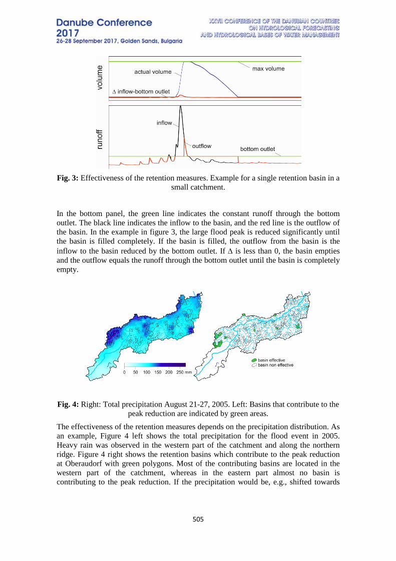
505

Fig. 3: Effectiveness of the retention measures. Example for a single retention basin in a

small catchment. In the bottom panel, the green line indicates the constant runoff through the bottom outlet. The black line indicates the inflow to the basin, and the red line is the outflow of the basin. In the example in figure 3, the large flood peak is reduced significantly until the basin is filled completely. If the basin is filled, the outflow from the basin is the inflow to the basin reduced by the bottom outlet. If ∆ is less than 0, the basin empties and the outflow equals the runoff through the bottom outlet until the basin is completely empty.

Fig. 4: Right: Total precipitation August 21-27, 2005. Left: Basins that contribute to the

peak reduction are indicated by green areas. The effectiveness of the retention measures depends on the precipitation distribution. As an example, Figure 4 left shows the total precipitation for the flood event in 2005. Heavy rain was observed in the western part of the catchment and along the northern ridge. Figure 4 right shows the retention basins which contribute to the peak reduction at Oberaudorf with green polygons. Most of the contributing basins are located in the western part of the catchment, whereas in the eastern part almost no basin is contributing to the peak reduction. If the precipitation would be, e.g., shifted towards

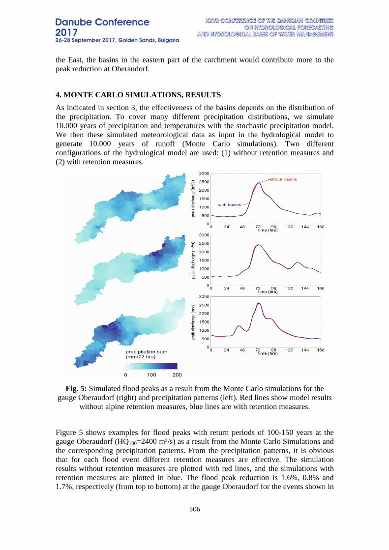
506

the East, the basins in the eastern part of the catchment would contribute more to the peak reduction at Oberaudorf.

4. MONTE CARLO SIMULATIONS, RESULTS As indicated in section 3, the effectiveness of the basins depends on the distribution of the precipitation. To cover many different precipitation distributions, we simulate 10.000 years of precipitation and temperatures with the stochastic precipitation model. We then these simulated meteorological data as input in the hydrological model to generate 10.000 years of runoff (Monte Carlo simulations). Two different configurations of the hydrological model are used: (1) without retention measures and (2) with retention measures.

Fig. 5: Simulated flood peaks as a result from the Monte Carlo simulations for the

gauge Oberaudorf (right) and precipitation patterns (left). Red lines show model results without alpine retention measures, blue lines are with retention measures.

Figure 5 shows examples for flood peaks with return periods of 100-150 years at the gauge Oberaudorf (HQ100=2400 m³/s) as a result from the Monte Carlo Simulations and the corresponding precipitation patterns. From the precipitation patterns, it is obvious that for each flood event different retention measures are effective. The simulation results without retention measures are plotted with red lines, and the simulations with retention measures are plotted in blue. The flood peak reduction is 1.6%, 0.8% and 1.7%, respectively (from top to bottom) at the gauge Oberaudorf for the events shown in

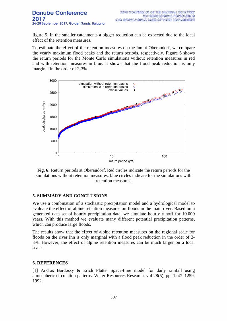
507

figure 5. In the smaller catchments a bigger reduction can be expected due to the local effect of the retention measures. To estimate the effect of the retention measures on the Inn at Oberaudorf, we compare the yearly maximum flood peaks and the return periods, respectively. Figure 6 shows the return periods for the Monte Carlo simulations without retention measures in red and with retention measures in blue. It shows that the flood peak reduction is only marginal in the order of 2-3%.

Fig. 6: Return periods at Oberaudorf. Red circles indicate the return periods for the

simulations without retention measures, blue circles indicate for the simulations with retention measures.

5. SUMMARY AND CONCLUSIONS We use a combination of a stochastic precipitation model and a hydrological model to evaluate the effect of alpine retention measures on floods in the main river. Based on a generated data set of hourly precipitation data, we simulate hourly runoff for 10.000 years. With this method we evaluate many different potential precipitation patterns, which can produce large floods. The results show that the effect of alpine retention measures on the regional scale for floods on the river Inn is only marginal with a flood peak reduction in the order of 2-3%. However, the effect of alpine retention measures can be much larger on a local scale.

6. REFERENCES [1] Andras Bardossy & Erich Platte. Space-time model for daily rainfall using atmospheric circulation patterns. Water Resources Research, vol 28(5), pp 1247–1259, 1992.

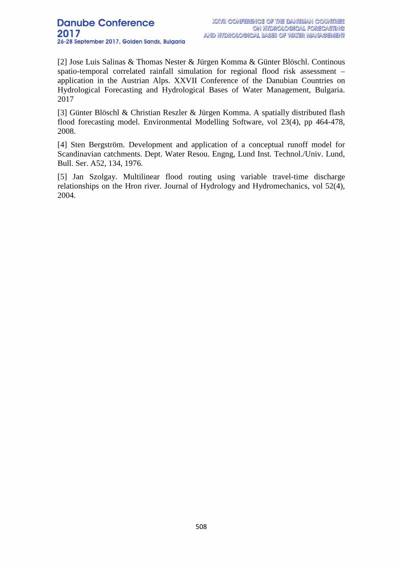
508

[2] Jose Luis Salinas & Thomas Nester & Jürgen Komma & Günter Blöschl. Continous spatio-temporal correlated rainfall simulation for regional flood risk assessment – application in the Austrian Alps. XXVII Conference of the Danubian Countries on Hydrological Forecasting and Hydrological Bases of Water Management, Bulgaria. 2017 [3] Günter Blöschl & Christian Reszler & Jürgen Komma. A spatially distributed flash flood forecasting model. Environmental Modelling Software, vol 23(4), pp 464-478, 2008. [4] Sten Bergström. Development and application of a conceptual runoff model for Scandinavian catchments. Dept. Water Resou. Engng, Lund Inst. Technol./Univ. Lund, Bull. Ser. A52, 134, 1976. [5] Jan Szolgay. Multilinear flood routing using variable travel-time discharge relationships on the Hron river. Journal of Hydrology and Hydromechanics, vol 52(4), 2004.

509

THE ASSESSMENT OF LEVEL OF FLASH FLOODS THREAT OF URBANIZED AREAS

Pavla Štěpánková1, Miroslav Dumbrovský2, Karel Drbal1

1 T. G. Masaryk Water Research Institute, p.r.i., Brno Branch, Czech Republic

2Institute of Water Landscape Management, Faculty of Civil Engineering, Brno University of Technology, Czech Republic

Corresponding author:Pavla Štěpánková, T. G. Masaryk Water Research Institute, p.r.i., Brno Branch, Mojmírovo nám. 16, Beno, 612 00, Czech Republic, pavla_stepankova@vuv.cz

ABSTRACT

Flash floods (or torrential rain flooding) is another type of flood hazard which has caused casualties and significant property damages. A methodology for identification of urban areas, which can potentially be burdened by that type of flood hazard, was proposed. This method, also called Method of Critical Points (CP), is a repeatable process able to identify areas, which are significant in terms of formation of surface run-off and erosion. As addition to the preliminary flood risk assessment according to EU Directive 2007/60/ES on the Assessment and Management of Flood Risks, the presented methodology was applied for the entire area of the Czech Republic and the results are being used for the updating of non-technical measures, e.g. urban planning.

In the article, the principles of methodology of CP are described and results of the first application in the Czech Republic are presented, as well as possible interpretations of them.

Keywords: water erosion, critical point, flood risk, catchment area, porosity, concentrated surface runoff

1. INTRODUCTION

The contemporary landscape has a considerably diminished potential for water retention, which is primarily the result of inappropriate use, especially on hilly terrain, where there is more rapid surface runoff. Intensive precipitation can lead to flooding, while in dry periods the landscape suffers from drought. The way to improve this situation is to change the way the land is managed through the use of appropriate measures in the catchment area. Roughly half the agricultural land in the Czech Republic is threatened by water erosion. The solution to this problem will be a demanding process in terms of time and money. To ensure successful and optimal implementation, it is essential to define a schedule for the solution in time and space.

Identification of the most-threatened areas is possible, e.g. via land categorization in terms of potential occurrence of torrential rain flooding, with a negative effect on built-up areas. The approach described in this article combines an increase in the water-

510

retention capability of the landscape with flood prevention and soil conservation measures. Based on the same principle, the study proposes the identification, in catchment area plans, of areas with a high risk of storm flooding with potential impact on urban areas.

This approach is based on methodology for localisation of land threatened by torrential rain flooding, which was drawn up within the preliminary assessment of flood risk in 2009 (Drbal et al., 2009a). This methodical approach was drawn up in response to the fact that storm flooding caused by intensive localised downpours occurs relatively often in summertime in CZ, and such storms can occur practically anywhere. The combined difficulty of time and space localisation of the causal effect of storm flooding, and the high level of uncertainty in expressing the probability of occurrence (period of repetition) for a certain locality, were the reasons for the development of the so-called Critical Point method (Drbal, Dumbrovský et al., 2009).

In principal, the method uses a repeatable procedure of identification of decisive areas in terms of the creation of concentrated surface runoff, with the aim of defining so-called critical points (CP) within built-up areas as an auxiliary indicator of the threat of concentrated surface runoff and transport of solid matter by torrential rains. For each contributory area, a value is worked out as a so-called indicator of critical conditions for the occurrence of negative effects of torrential rain flooding. The need to find a fitting approach is also based on the requirements of Directive 2007/60/ES. This requires all EU member states, in a phase known as preliminary identification of significant flooding risk, to examine all relevant types of flooding threat. The proposed procedure was actually tested in conditions and on data from pilot projects/studies in the Luha and Jičínka water catchment areas.

The identification of CP presents a repeatable approach to identifying decisive areas in terms of the creation of concentrated surface runoff, with the aim of determining areas of land within built up areas threatened by concentrated surface runoff and transport of solid matter by storm rainfall. The results of this approach should primarily serve the needs of local councils of potentially affected areas as a basis for the formation of flood-prevention and land-use plans, and for the proposal of measures within land consolidation.

The results of the critical point method identify contributory areas of land, which are only inter-related to a certain extent. In some regions, however, especially in relation to the level of urbanisation, their occurrence has increased distinctly. Therefore, for further use, an aggregation was carried out based on the weighted arithmetic mean of so-called indicator of critical conditions of contributory areas in relation to the size of grade 4 catchment areas. The result is the categorisation of the hydrological units/ into three levels of threat of storm flooding to urban areas. These categories should help in the proposal and implementation of appropriate measures to reduce the possible negative

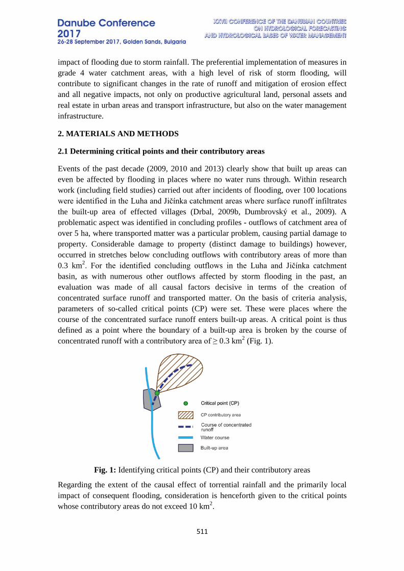
511

impact of flooding due to storm rainfall. The preferential implementation of measures in grade 4 water catchment areas, with a high level of risk of storm flooding, will contribute to significant changes in the rate of runoff and mitigation of erosion effect and all negative impacts, not only on productive agricultural land, personal assets and real estate in urban areas and transport infrastructure, but also on the water management infrastructure.

2. MATERIALS AND METHODS

2.1 Determining critical points and their contributory areas

Events of the past decade (2009, 2010 and 2013) clearly show that built up areas can even be affected by flooding in places where no water runs through. Within research work (including field studies) carried out after incidents of flooding, over 100 locations were identified in the Luha and Jičínka catchment areas where surface runoff infiltrates the built-up area of effected villages (Drbal, 2009b, Dumbrovský et al., 2009). A problematic aspect was identified in concluding profiles - outflows of catchment area of over 5 ha, where transported matter was a particular problem, causing partial damage to property. Considerable damage to property (distinct damage to buildings) however, occurred in stretches below concluding outflows with contributory areas of more than 0.3 km2. For the identified concluding outflows in the Luha and Jičínka catchment basin, as with numerous other outflows affected by storm flooding in the past, an evaluation was made of all causal factors decisive in terms of the creation of concentrated surface runoff and transported matter. On the basis of criteria analysis, parameters of so-called critical points (CP) were set. These were places where the course of the concentrated surface runoff enters built-up areas. A critical point is thus defined as a point where the boundary of a built-up area is broken by the course of concentrated runoff with a contributory area of ≥ 0.3 km2 (Fig. 1).

Fig. 1: Identifying critical points (CP) and their contributory areas

Regarding the extent of the causal effect of torrential rainfall and the primarily local impact of consequent flooding, consideration is henceforth given to the critical points whose contributory areas do not exceed 10 km2.

512

Further selection of critical points made use of the basic physical-geographical characteristics of their contributory areas: physical area, average slope, type of soil/use and proportion of arable land. For the contributory area of each CP a calculation was made of the value of the so-called critical conditions indicator for the occurrence of negative effects of torrential rain flooding (F).

For any specific CP contributory area, this indicator presents the combination of physical-geographical conditions, the form of land use, regional variations in landscape cover, and potential occurrence of extreme torrential rains (in relation to synoptic conditions):

(1)

where F is the critical conditions indicator [-],

a is the weight vector [1.48876; 3.09204; 0.467171], Pp,r is the relative value of the size of the contributory area (considering a max. 10 km2) [-], Ip is the value of average slope of contributory area [%], ORP is the proportion of arable land in the area [%], CNII represents characteristic of surface in consideration of run-off [-], Hm,r is the relative value of total one day torrential rains with a repetition period of 100 years for territory within the Czech Republic [-]

Data for determination of CNII and Hm,r in ESRI GRID format for CZ territory is provided by the Czech Hydrometeorological Institute.

The subsequent selection of critical points was carried out according to the following parameters:

C1 - size of contributory area 0.3–10.0 km2, C2 - average slope of contributory area Ip ≥ 3.5 %, C3 - proportion of arable land in basin ORP ≥ 40 %. C4 - critical conditions indicator F ≥ 1.85.

On the basis of investigation using model catchment basins, where damage occurred even from areas with a proportion of arable land lower than 40%, or completely forested areas, the selection carried out according to the conditions of criteria C1 - C4 was extended to include critical points with contributory areas of 1 km2 and above, with an average slope of 5% or more:

C1A - size of contributory area 1.0–10.0 km2, C2A - average slope of contributory area ≥ 5 %.

513

On the basis of these parameters of combined criteria, critical points and their contributory areas were determined for the whole of the Czech Republic.

2.2 The level of threat to urban areas from torrential rain flooding

The presented model for determining critical points identifies contributory areas which, to a certain extent, are inter-related, or even overlap. An overlap of CP contributory areas occurs if a course of concentrated runoff (often with a standard water course running through it) incorporates several independent urban areas, and the land above the points at which these courses of concentrated runoff cross the boundary of the built-up area fulfils the C1 - C4 criteria (or C1A and C2A). In such a case, the contributory area of one critical point is a subset of the contributory area of another CP (Fig. 2). Multiple overlaps can occur.

Information on the localization of individual CP and their contributory areas is a useful basis for the proposal of complex land consolidation, or within landscape planning – i.e. on a "local level". From a regional perspective, including complete hydrological units, the information is still relatively fragmented. It was therefore preferable to extend the classification of torrential rain flood risk to cover a larger area. Aggregation was proposed based on a weighted arithmetic mean of critical conditions indicator (Fw4r), projected to the area of a hydrological unit, in this case grade 4 catchment basin.

Within the Czech Republic around 9000 grade 4 catchment basins are identified (as at 2014). CP contributory areas are predominantly subsets of individual grade 4 basins. In exceptional cases (grade 4 basin of relatively small area) the CP contributory area can overlap into several grade 4 basins. Each contributory area (or part of one) lying within a grade 4 basin is characterised by a value of critical conditions indicator (Fw4r). The weight for calculation of the weighted arithmetical mean is derived from the area that a given contributory area occupies in a grade 4 basin. If contributory areas overlap, then this overlap is included more than once in the calculation of the weighted average, always with the appropriate F value and the appertaining surface area (Fig. 2).

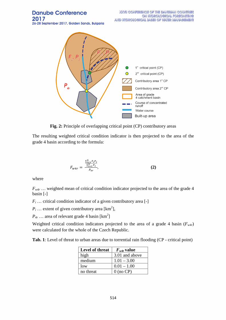
514

Fig. 2: Principle of overlapping critical point (CP) contributory areas

The resulting weighted critical condition indicator is then projected to the area of the grade 4 basin according to the formula:

𝐹𝐹𝑤𝑤4𝑉𝑉 = ∑ 𝐹𝐹𝑖𝑖𝑃𝑃𝑖𝑖𝑛𝑛𝑖𝑖=1∑ 𝑃𝑃𝑖𝑖𝑛𝑛𝑖𝑖=1𝑃𝑃4𝑓𝑓

, (2)

where

Fw4r … weighted mean of critical condition indicator projected to the area of the grade 4 basin [-] Fi … critical condition indicator of a given contributory area [-] Pi … extent of given contributory area [km2], P4r … area of relevant grade 4 basin [km2] Weighted critical condition indicators projected to the area of a grade 4 basin (Fw4r) were calculated for the whole of the Czech Republic.

Tab. 1: Level of threat to urban areas due to torrential rain flooding (CP - critical point)

Level of threat Fw4r value high 3.01 and above medium 1.01 – 3.00 low 0.01 – 1.00 no threat 0 (no CP)

515

On the basis of results of research (including field studies) carried out in the Husí Potok, Luha and Jičínka basins, the level of threat to urban areas due to torrential rain flooding is separated into three categories (Tab. 1)

The results were then verified on land in the pilot Husí Potok basin (Fig. 3), within the Luha and Jičínka basin.

Fig. 3: Critical points (CP) and their contributory areas, and the level of threat of torrential rain flooding in the Husí Potok locality.

3. RESULTS

On the basis of parameters of combined criteria C1 to C4, or C1A and C2A, a total of 9,261 critical points were chosen for the whole Czech Republic which have a greater (unknown) probability of occurrence of negative impact of torrential rain flooding (Fig. 4). The overall area of contributory areas of selected critical points in relation to built-up areas in CZ is 18,112.2 km2, which represents 23% of all land in the whole country. The results are available on the povis.cz portal.

For the districts in question this provides information on places where concentrated surface runoff can be expected to infiltrate built-up areas, and on what property may be at risk in the event of torrential rain. Local and national government have thus gained the basis for preparation of landscape planning and development. In the second round of planning (according to Directive 2007/60/EC ), which ended in 2015, this basis was used in drawing up chapter V.2.3.3 Danger of torrential rain flooding in individual plans of partial catchment basins (MZe, 2015)

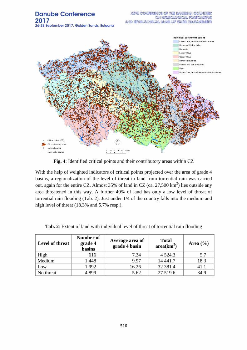
516

Fig. 4: Identified critical points and their contributory areas within CZ

With the help of weighted indicators of critical points projected over the area of grade 4 basins, a regionalization of the level of threat to land from torrential rain was carried out, again for the entire CZ. Almost 35% of land in CZ (ca. 27,500 km2) lies outside any area threatened in this way. A further 40% of land has only a low level of threat of torrential rain flooding (Tab. 2). Just under 1/4 of the country falls into the medium and high level of threat (18.3% and 5.7% resp.).

Tab. 2: Extent of land with individual level of threat of torrential rain flooding

Level of threat Number of

grade 4 basins

Average area of grade 4 basin

Total area(km2) Area (%)

High 616 7.34 4 524.3 5.7 Medium 1 448 9.97 14 441.7 18.3 Low 1 992 16.26 32 381.4 41.1 No threat 4 899 5.62 27 519.6 34.9

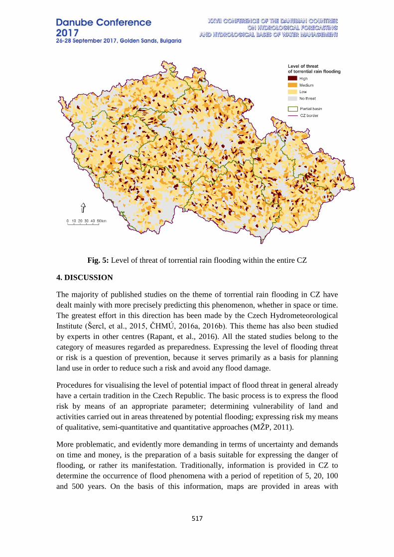
517

Fig. 5: Level of threat of torrential rain flooding within the entire CZ

4. DISCUSSION

The majority of published studies on the theme of torrential rain flooding in CZ have dealt mainly with more precisely predicting this phenomenon, whether in space or time. The greatest effort in this direction has been made by the Czech Hydrometeorological Institute (Šercl, et al., 2015, ČHMÚ, 2016a, 2016b). This theme has also been studied by experts in other centres (Rapant, et al., 2016). All the stated studies belong to the category of measures regarded as preparedness. Expressing the level of flooding threat or risk is a question of prevention, because it serves primarily as a basis for planning land use in order to reduce such a risk and avoid any flood damage.

Procedures for visualising the level of potential impact of flood threat in general already have a certain tradition in the Czech Republic. The basic process is to express the flood risk by means of an appropriate parameter; determining vulnerability of land and activities carried out in areas threatened by potential flooding; expressing risk my means of qualitative, semi-quantitative and quantitative approaches (MŽP, 2011).

More problematic, and evidently more demanding in terms of uncertainty and demands on time and money, is the preparation of a basis suitable for expressing the danger of flooding, or rather its manifestation. Traditionally, information is provided in CZ to determine the occurrence of flood phenomena with a period of repetition of 5, 20, 100 and 500 years. On the basis of this information, maps are provided in areas with

518

significant risk of flooding to show the depth and speed of water flow, and to show the threat and risk of flooding (MŽP, 2013). This information deals with only one of the forms of flood risk in CZ, that of flooded rivers.

Torrential rain flooding, however, is characteristic in its randomness, and therefore also its extreme nature in terms of expressing probability of occurrence. Other characteristics of this form of flooding are: possible occurrence at any point throughout the whole country, very limited or inaccurate spatio-temporal forecast of causal rainfall, local extent of impact worsened by inappropriate form of land use etc.

Identification of critical points (and their contributory areas) and categorization of land within CZ according to risk of torrential rain flooding give further basis for decision-making on preventive measures, especially on land in a catchment basin that is used to a greater extent as agricultural land.

The procedures used were chosen in order to make it possible to carry out calculations for the entire Czech Republic, and to allow repetition in the case of more detailed or more precise data (e.g. digital model of terrain). The critical point method, in particular, is still developing, further parameters are being sought which would enable at least a semi-quantitative expression of risk, or rather the extent of potential impact of torrential rain flooding.

5. CONCLUSION

The torrential rain flooding is a phenomenon with tragic consequences in the Czech Republic. Looking for a solution is highly demanding task. Visualizing the degree of potential consequences of this type of danger is one of them.

The main aim of the proposed methodology is to identify so-called critical points and their contributory areas. A critical point is defined as a spot where the boundary of a built-up area is intersected by the course of concentrated surface runoff. The size of the contributory area must range between 0.3 and 10.0 km2. This methodology was used for whole territory of the Czech Republic. More than 9 000 of those critical points have been found. The sum of contributory areas of selected critical points in relation to built-up areas in CZ is more than 18 000 km2, which represents 23 % of the whole country’s area.

Information on the localization of individual critical points and their contributory areas is a useful basis for the proposal of complex land consolidation, or within landscape planning – i.e. on a "local level". From a regional perspective, including complete hydrological units, the information is still relatively fragmented. It was therefore preferable to extend the classification of torrential rain flood risk to cover a larger area. Aggregation was proposed based on a weighted arithmetic mean of critical conditions indicator, projected to the grade 4 catchment basin.

519

The hydrological units chosen by means of the set parameters represent the recommended prioritisation in the proposal and implementation of appropriate measures to reduce the potentially negative impact of torrential rain flooding. The selection of hydrological units also represents a proposal of areas where the implementation of measures based purely on CP contributory areas would contribute to a significant improvement in the drainage ratio and a reduction in erosion effect and all negative implications, not only on productive agricultural land, personal assets and real estate in urban areas and transport infrastructure, but also on the water management infrastructure.

6. REFERENCES

ČHMÚ. 2016a. Water Forecast Service of CHMI [in Czech: Hlásná a předpovědní povodňová služba ČHMÚ]. [Online]. Available at: http://www.chmi.cz/files/portal/docs/poboc/CB/pruvodce/pruvodce_vodohospodari_ffg.html. [Accessed: 2016, November 16]. ČHMU. 2016b. Flash Flood Guidance [in Czech: Indikátor přívalových povodní]. [Online] Available at: http://hydro.chmi.cz/hpps/main_rain.php?mt=ffg. [Accessed: 2016, November 16]. DRBAL, K. et al. (2009a): Proposal of Preliminary Flood Risk Assessment Methodology in the Czech Republic [in Czech: Návrh metodiky předběžného vyhodnocení Povodňových rizik v České republice]. Ministry of Environment, Prague, 7 s. DRBAL, K. et al. (2009b): Flash Floods in the Czech Republic in June and July 2009, Part: Methodology of Flood Risk Mapping [in Czech: Vyhodnocení povodní v červnu a červenci 2009 na území České republiky, DÚ: Metodika mapování povodňového rizika]. VÚV TGM, Ministry of Environment, Prague, 85 s. DRBAL, K., DUMBROVSKÝ, M. et al. (2009): Methodology fo Identification of Critical Points [in Czech: Metodický návod pro identifikaci KB]. Ministry of Environment, Prague, 7 s. DUMBROVSKÝ, M. et al. (2009): Flash Floods in the Czech Republic in June and July 2009, Part: Assessment of Floods Impact on Lanscape and Environment [in Czech: Vyhodnocení povodní v červnu a červenci 2009 na území České republiky, DÚ: Vyhodnocení dopadů povodní na krajinu a životní prostředí]. Ministry of Environment, Prague, 45 s. MZe. 2015. River Basin District Management Plans [in Czech: Plány dílčích povodí]. [on-line]. Available at: http://eagri.cz/public/web/mze/voda/planovani-v-oblasti-vod/priprava-planu-povodi-pro-2-obdobi/plany-dilcich-povodi/. [Accessed: 2016, October 10]. MŽP. 2011. Methodology of flood hazard and flood risk mapping. [in Czech: Metodika tvorby map povodňového nebezpečí a povodňových rizik]. Věstník MŽP IV/2011, Praha.

520

MŽP. 2013. Maps of flood hazard and flood risk [in Czech: Mapy povodňového nebezpečí a povodňového rizika]. [Online]. Available at: http://cds.chmi.cz/?lang=en [Accessed: 2016, October 14]. ŠERCL, P. et al. 2015. Possibilities of Prediction of Flash Floods in the Conditions of the Czech Republic [in Czech: Možnosti predikce přívalových povodní v podmínkách České republiky]. Sborník prací Českého hydrometeorologického ústavu, sv. 60. ČHMÚ Praha, 49 p. RAPANT, P., KOLEJKA, J., et al. 2016. Possibilities of prediction of flash flood risk according to meteorological radar data. [in Czech: Možnosti predikce rizika vzniku přívalové povodně z dat meteorologického radaru]. GIS Ostrava 2016, Ostrava, 16. – 18. 3. 2016. [Online] Available at: http://gisak.vsb.cz/GIS_Ostrava/GIS_Ova_2016/sbornik/papers/gis2016568a33ce4e9ba.pdf

ACKNOWLEDGEMENTS This paper was elaborated with the support The National Agency for Agricultural Research for the project “New approaches to optimization of systems of integrated area protection in the context of their economic sustainability” [QJ1520268] and project "Erosion processes and their influence on the production capacity of soils and erosion control measures in the design process of land consolidation" [QJ1320157].

521

TRENDS ASSESMENT OF METEOROLOGICAL FACTORS, RIVER FLOW AND DROUGHTS IN NORTHWESTERN BULGARIA

Yordan Dimitrov, Anna Yordanova

National Institute of Meteorology and Hydrology, Republic of Bulgaria

Corresponding author: Yordan Dimitrov, NIMH, Tsarigradsko Shosse blvd 66, Sofia 1784, BULGARIA email:yordan.dimitrov14@gmail.com

ABSTRACT Water resources are subject of a growing pressure due to climate and land use

changes. European Water Framework Directive (WFD) sets new goals and objectives in plans for river basin management. The accent in WFD is the assessment of the likely additional impact of climate change on existing anthropogenic pressures and measures. Reduction of natural resources in water sources such as rivers, lakes, aquifers (“hydrological drought“) is associated with the reduction in available water resources for water supply including regulating runoff and water transfer (“water scarcity”). An analysis of key factors and processes is required.

For this purpose, approach for integrated spatial-temporal analysis of drought, low flow and water scarcity is applied. For each stage of the approach relevant indices, methods, tools and software are justified and adapted. The report presents some of the results of the methodological and experimental studies. The main developments and trends in north-western Bulgaria are analysed, in accordance with the approach DPSIR (Drivers-Pressure-State-Impact-Response).

The approach is applied experimentally at three levels: in the valleys of Northwestern Bulgaria, valley of Ogosta river (cascade "Petrokhan" and water supply system "Ogosta" dam - "Srechenska bara") and Botunya River. A special feature of the area is the transfer of water through water intakes, dams and collecting derivations from transboundary basin of Nishava River to Ogosta River and from one sub-basin to another. In the area there are valuable protected areas and Natura 2000 sites.

The results can be applied in practice from Basin Directorate "Danube Region" for management plans of north-western river basins in Bulgaria. The aim is to support the measures programme for managing a drought condition, low water and water shortages. The article have a connection with development of early warning systems and decision support. Keywords: drought, low flow, Mann-Kendall test, climate change, drought management plans. 1. INTRODUCTION Water resources are subject of a growing pressure due to climate and land use changes. European Water Framework Directive (WFD) sets new goals and objectives in plans for river basin management. The accent in WFD is the assessment of the likely additional impact of climate change on existing anthropogenic pressures and measures. Reduction of natural resources in water sources such as rivers, lakes, aquifers (“hydrological

522

drought“) is associated with the reduction in available water resources for water supply including regulating runoff and water transfer (“water scarcity”). An analysis of key factors and processes is required. The aim is: • to carry out an integrated spatial-temporal analysis of drought, low water and water

scarcity, assessment of river runoff and its change in connection with the anthropogenic and natural processes;

• to identify and analyze the main factors, interactions and trends in Northwestern Bulgaria in accordance with the WFD;

• to propose appropriate measures in support of the Northwestern Bulgaria River Basin Management Plans in conditions of drought, low water and water scarcity.

2. METHODOLOGY APPROACH AND METHODS For this purpose, approach for integrated spatial-temporal analysis of drought, low flow and water scarcity is applied. For each stage of the approach relevant indices, methods, tools and software are justified and adapted. The main developments and trends in Northwestern Bulgaria are analyzed, in accordance with the approach DPSIR (Drivers-Pressure-State-Impact-Response). The methodology consists of five stages: First stage. Analysis and assessment of natural factors. Assessment of climate factors trends and identification of meteorological drought. Climate factors are the main natural driving force for the water resource change and drought. Trend identification is important for the interpretation of possible future changes. An assessment and identification of drought is performed with Standardized Precipitation Index (SPI), DeMarton index, etc. Second stage. Analysis and assessment of water resources. Assessment of trends and hydrologic drought identification. The stage includes:

- Evaluation of water resources and regional dependencies; - Evaluation of the trends of water resources; - The Indicators of hydrologic alteration (IHA, Acreman, 2009), threshold method

and other methods are applied for low flow charactersation; - An assessment and identification of drought is performed with Standardized

Runoff Index(SRI), groundwater level, etc. - Evaluation of natural resources and changes through the rainfall-runoff relation.

Appropriate estimation in drought, low water and water scarcity gives the US Geological Survey model for monthly water balance (McCabe ...). The model was adapted and implemented under CC_WaterS, 2012 (Ilcheva, I., NIMH, 2013; Marinov, Iv., Et al., CC_WaterS Monograph, 2012).

Third stage. Update of the calculation scheme and the water economic balances of the basins from Northwestern Bulgaria The changes in reservoir level are also an indicator for water resource availability. The simulation model SIMYL (developed in NIMH) is applied at this stage. The available water

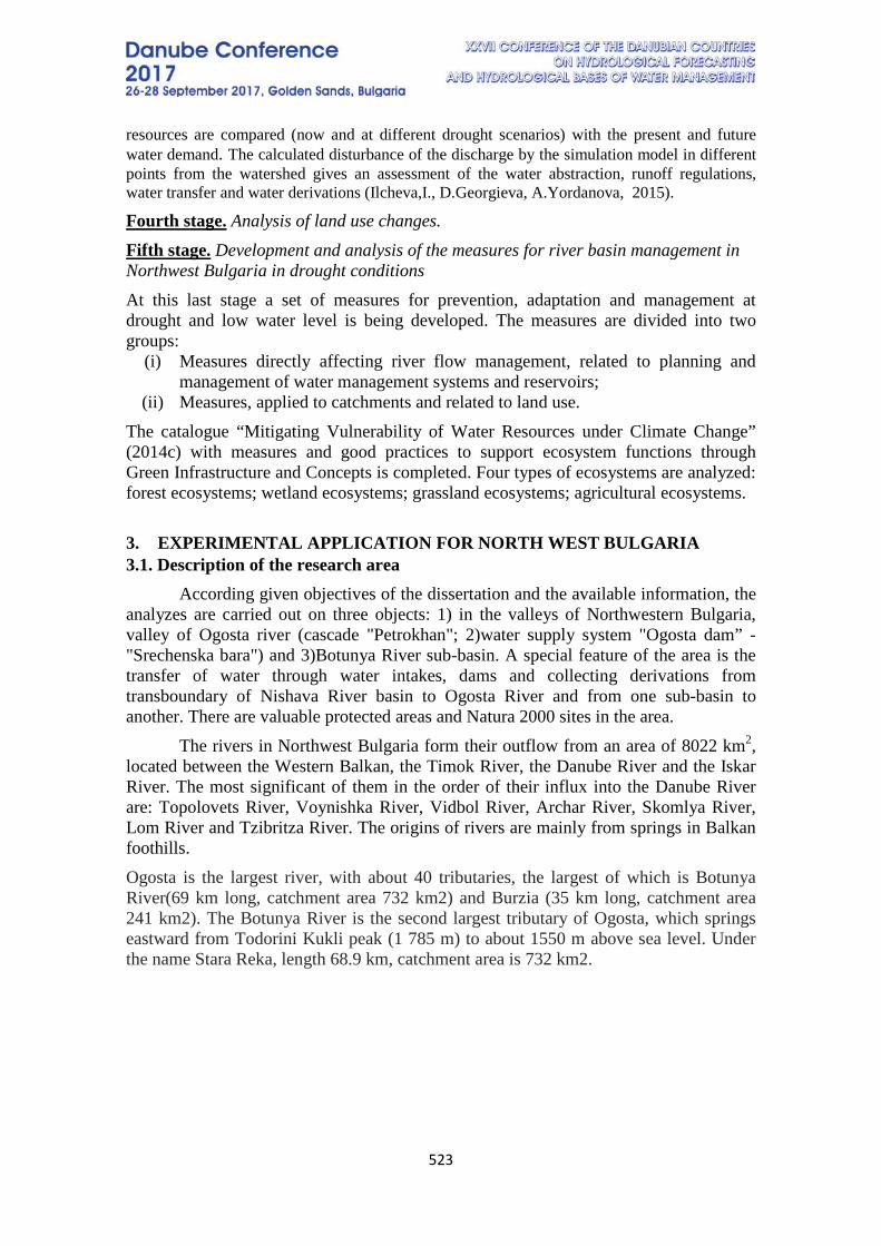
523

resources are compared (now and at different drought scenarios) with the present and future water demand. The calculated disturbance of the discharge by the simulation model in different points from the watershed gives an assessment of the water abstraction, runoff regulations, water transfer and water derivations (Ilcheva,I., D.Georgieva, A.Yordanova, 2015).

Fourth stage. Analysis of land use changes. Fifth stage. Development and analysis of the measures for river basin management in Northwest Bulgaria in drought conditions At this last stage a set of measures for prevention, adaptation and management at drought and low water level is being developed. The measures are divided into two groups:

(i) Measures directly affecting river flow management, related to planning and management of water management systems and reservoirs;

(ii) Measures, applied to catchments and related to land use. The catalogue “Mitigating Vulnerability of Water Resources under Climate Change” (2014c) with measures and good practices to support ecosystem functions through Green Infrastructure and Concepts is completed. Four types of ecosystems are analyzed: forest ecosystems; wetland ecosystems; grassland ecosystems; agricultural ecosystems. 3. EXPERIMENTAL APPLICATION FOR NORTH WEST BULGARIA 3.1. Description of the research area

According given objectives of the dissertation and the available information, the analyzes are carried out on three objects: 1) in the valleys of Northwestern Bulgaria, valley of Ogosta river (cascade "Petrokhan"; 2)water supply system "Ogosta dam” - "Srechenska bara") and 3)Botunya River sub-basin. A special feature of the area is the transfer of water through water intakes, dams and collecting derivations from transboundary of Nishava River basin to Ogosta River and from one sub-basin to another. There are valuable protected areas and Natura 2000 sites in the area.

The rivers in Northwest Bulgaria form their outflow from an area of 8022 km2, located between the Western Balkan, the Timok River, the Danube River and the Iskar River. The most significant of them in the order of their influx into the Danube River are: Topolovets River, Voynishka River, Vidbol River, Archar River, Skomlya River, Lom River and Tzibritza River. The origins of rivers are mainly from springs in Balkan foothills. Ogosta is the largest river, with about 40 tributaries, the largest of which is Botunya River(69 km long, catchment area 732 km2) and Burzia (35 km long, catchment area 241 km2). The Botunya River is the second largest tributary of Ogosta, which springs eastward from Todorini Kukli peak (1 785 m) to about 1550 m above sea level. Under the name Stara Reka, length 68.9 km, catchment area is 732 km2.

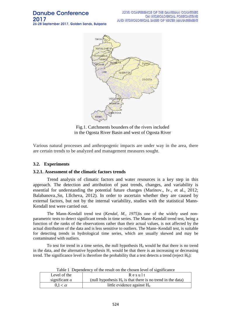
524

Fig.1. Catchments bounders of the rivers included

in the Ogosta River Basin and west of Ogosta River

Various natural processes and anthropogenic impacts are under way in the area, there are certain trends to be analyzed and management measures sought. 3.2. Experiments 3.2.1. Assessment of the climatic factors trends

Trend analysis of climatic factors and water resources is a key step in this approach. The detection and attribution of past trends, changes, and variability is essential for understanding the potential future changes (Мarinov., Iv., et al., 2012; Balabanova.,Sn, I.Ilcheva, 2012). In order to ascertain whether they are caused by external factors, but not by the internal variability, studies with the statistical Mann-Kendall test were carried out.

The Mann–Kendall trend test (Kendal, M., 1975)is one of the widely used non-parametric tests to detect significant trends in time series. The Mann–Kendall trend test, being a function of the ranks of the observations rather than their actual values, is not affected by the actual distribution of the data and is less sensitive to outliers. The Mann–Kendall test, is suitable for detecting trends in hydrological time series, which are usually skewed and may be contaminated with outliers.

To test for trend in a time series, the null hypothesis H0 would be that there is no trend in the data, and the alternative hypothesis H1 would be that there is an increasing or decreasing trend. The significance level is therefore the probability that a test detects a trend (reject H0):

Table 1 Dependency of the result on the chosen level of significance Level of the significant α

R e s u l t (null hypothesis H0 is that there is no trend in the data)

little evidence against Н0 α<1,0

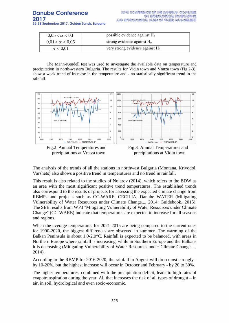
525

possible evidence against Н0

strong evidence against Н0

very strong evidence against Н0

The Mann-Kendell test was used to investigate the available data on temperature and precipitation in north-western Bulgaria. The results for Vidin town and Vratza town (Fig.2-3), show a weak trend of increase in the temperature and - no statistically significant trend in the rainfall.

Fig.2 Annual Temperatures and Fig.3 Annual Temperatures and precipitations at Vratza town precipitations at Vidin town

The analysis of the trends of all the stations in northwest Bulgaria (Montana, Krivodol, Varshets) also shows a positive trend in temperatures and no trend in rainfall. This result is also related to the studies of Nojarov (2014), which refers to the BDW as an area with the most significant positive trend temperatures. The established trends also correspond to the results of projects for assessing the expected climate change from RBMPs and projects such as CC-WARE, CECILIA, Danube WATER (Mitigating Vulnerability of Water Resources under Climate Change..., 2014; Guidebook...2015). The SEE results from WP3 "Mitigating Vulnerability of Water Resources under Climate Change" (CC-WARE) indicate that temperatures are expected to increase for all seasons and regions. When the average temperatures for 2021-2015 are being compared to the current ones for 1990-2020, the biggest differences are observed in summer. The warming of the Balkan Peninsula is about 1.0-2.0°C. Rainfall is expected to be balanced, with areas in Northern Europe where rainfall is increasing, while in Southern Europe and the Balkans it is decreasing (Mitigating Vulnerability of Water Resources under Climate Change ..., 2014). According to the RBMP for 2016-2020, the rainfall in August will drop most strongly - by 10-20%, but the highest increase will occur in October and February - by 20 to 30%. The higher temperatures, combined with the precipitation deficit, leads to high rates of evapotranspiration during the year. All that increases the risk of all types of drought – in air, in soil, hydrological and even socio-economic.

1,005,0 << α05,001,0 << α

01,0<α

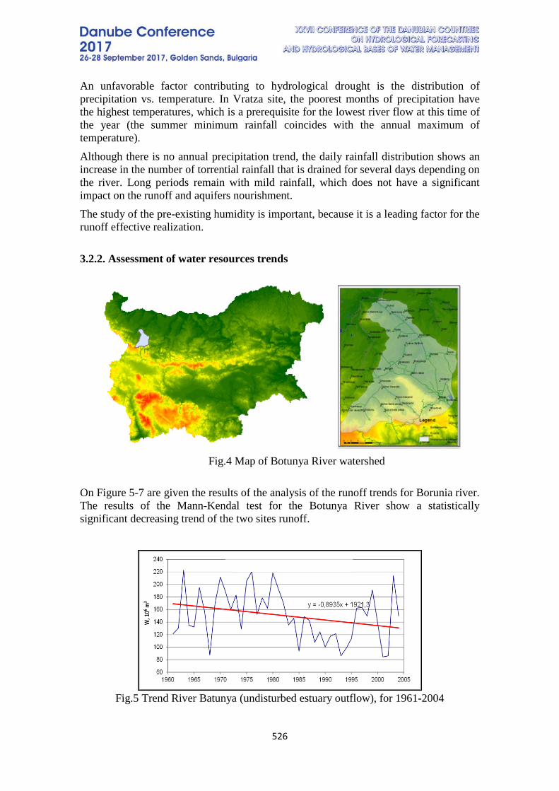
526

An unfavorable factor contributing to hydrological drought is the distribution of precipitation vs. temperature. In Vratza site, the poorest months of precipitation have the highest temperatures, which is a prerequisite for the lowest river flow at this time of the year (the summer minimum rainfall coincides with the annual maximum of temperature). Although there is no annual precipitation trend, the daily rainfall distribution shows an increase in the number of torrential rainfall that is drained for several days depending on the river. Long periods remain with mild rainfall, which does not have a significant impact on the runoff and aquifers nourishment. The study of the pre-existing humidity is important, because it is a leading factor for the runoff effective realization. 3.2.2. Assessment of water resources trends

Fig.4 Map of Botunya River watershed

On Figure 5-7 are given the results of the analysis of the runoff trends for Borunia river. The results of the Mann-Kendal test for the Botunya River show a statistically significant decreasing trend of the two sites runoff.

Fig.5 Trend River Batunya (undisturbed estuary outflow), for 1961-2004

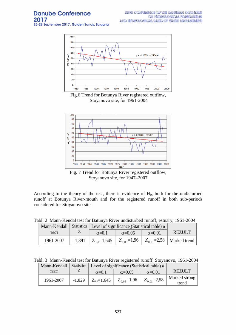
527

Fig.6 Trend for Botunya River registered outflow,

Stoyanovo site, for 1961-2004

Fig. 7 Trend for Botunya River registered outflow,

Stoyanovo site, for 1947–2007

According to the theory of the test, there is evidence of H0, both for the undisturbed runoff at Botunya River-mouth and for the registered runoff in both sub-periods considered for Stoyanovo site. Tabl. 2 Mann-Kendal test for Batunya River undisturbed runoff, estuary, 1961-2004

Tabl. 3 Mann-Kendal test for Batunya River registered runoff, Stoyanovo, 1961-2004

Mann-Kendall тест

Statistics Z

Level of significance (Statistical table) α REZULT α=0,1 α=0,05 α=0,01

1961-2007 -1,891 Z 0,1=1,645 05,0Z =1,96 01,0Z =2,58 Marked trend

Mann-Kendall тест

Statistics Z

Level of significance (Statistical table) α REZULT α=0,1 α=0,05 α=0,01

1961-2007 -1,829 Z0,1=1,645 05,0Z =1,96 01,0Z =2,58 Marked strong trend

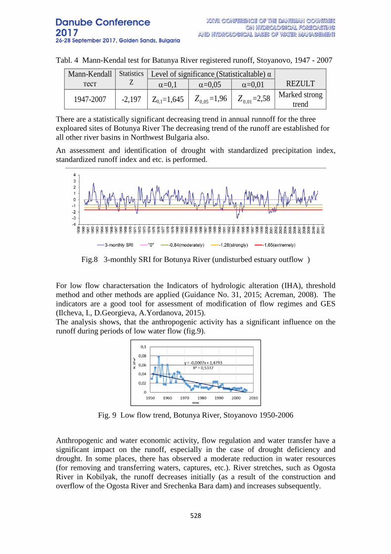
528

Tabl. 4 Mann-Kendal test for Batunya River registered runoff, Stoyanovo, 1947 - 2007

There are a statistically significant decreasing trend in annual runnoff for the three exploared sites of Botunya River The decreasing trend of the runoff are established for all other river basins in Northwest Bulgaria also. An assessment and identification of drought with standardized precipitation index, standardized runoff index and etc. is performed.

Fig.8 3-monthly SRI for Botunya River (undisturbed estuary outflow )

For low flow charactersation the Indicators of hydrologic alteration (IHA), threshold method and other methods are applied (Guidance No. 31, 2015; Acreman, 2008). The indicators are a good tool for assessment of modification of flow regimes and GES (Ilcheva, I., D.Georgieva, A.Yordanova, 2015). The analysis shows, that the anthropogenic activity has a significant influence on the runoff during periods of low water flow (fig.9).

Fig. 9 Low flow trend, Botunya River, Stoyanovo 1950-2006

Anthropogenic and water economic activity, flow regulation and water transfer have a significant impact on the runoff, especially in the case of drought deficiency and drought. In some places, there has observed a moderate reduction in water resources (for removing and transferring waters, captures, etc.). River stretches, such as Ogosta River in Kobilyak, the runoff decreases initially (as a result of the construction and overflow of the Ogosta River and Srechenka Bara dam) and increases subsequently.

Mann-Kendall тест

Statistics Z

Level of significance (Statisticaltable) α REZULT α=0,1 α=0,05 α=0,01

1947-2007 -2,197 Z0,1=1,645 05,0Z =1,96 01,0Z =2,58 Marked strong trend

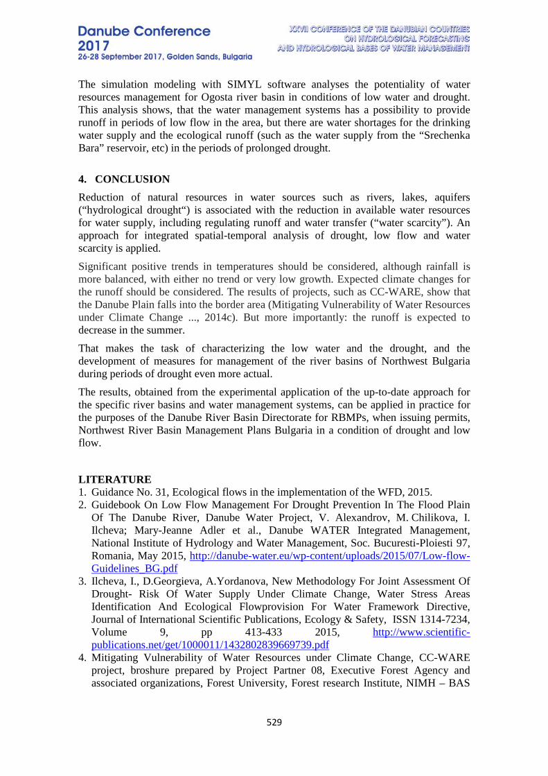
529

The simulation modeling with SIMYL software analyses the potentiality of water resources management for Ogosta river basin in conditions of low water and drought. This analysis shows, that the water management systems has a possibility to provide runoff in periods of low flow in the area, but there are water shortages for the drinking water supply and the ecological runoff (such as the water supply from the “Srechenka Bara” reservoir, etc) in the periods of prolonged drought. 4. CONCLUSION Reduction of natural resources in water sources such as rivers, lakes, aquifers (“hydrological drought“) is associated with the reduction in available water resources for water supply, including regulating runoff and water transfer (“water scarcity”). An approach for integrated spatial-temporal analysis of drought, low flow and water scarcity is applied. Significant positive trends in temperatures should be considered, although rainfall is more balanced, with either no trend or very low growth. Expected climate changes for the runoff should be considered. The results of projects, such as CC-WARE, show that the Danube Plain falls into the border area (Mitigating Vulnerability of Water Resources under Climate Change ..., 2014c). But more importantly: the runoff is expected to decrease in the summer. That makes the task of characterizing the low water and the drought, and the development of measures for management of the river basins of Northwest Bulgaria during periods of drought even more actual. The results, obtained from the experimental application of the up-to-date approach for the specific river basins and water management systems, can be applied in practice for the purposes of the Danube River Basin Directorate for RBMPs, when issuing permits, Northwest River Basin Management Plans Bulgaria in a condition of drought and low flow.

LITERATURE 1. Guidance No. 31, Ecological flows in the implementation of the WFD, 2015. 2. Guidebook On Low Flow Management For Drought Prevention In The Flood Plain

Of The Danube River, Danube Water Project, V. Alexandrov, M. Chilikova, I. Ilcheva; Mary-Jeanne Adler et al., Danube WATER Integrated Management, National Institute of Hydrology and Water Management, Soc. Bucuresti-Ploiesti 97, Romania, May 2015, http://danube-water.eu/wp-content/uploads/2015/07/Low-flow-Guidelines_BG.pdf

3. Ilcheva, I., D.Georgieva, A.Yordanova, New Methodology For Joint Assessment Of Drought- Risk Of Water Supply Under Climate Change, Water Stress Areas Identification And Ecological Flowprovision For Water Framework Directive, Journal of International Scientific Publications, Ecology & Safety, ISSN 1314-7234, Volume 9, pp 413-433 2015, http://www.scientific-publications.net/get/1000011/1432802839669739.pdf

4. Mitigating Vulnerability of Water Resources under Climate Change, CC-WARE project, broshure prepared by Project Partner 08, Executive Forest Agency and associated organizations, Forest University, Forest research Institute, NIMH – BAS

530

(V.Spiridonov, I.Ilcheva, Kr.Nikolova, Sn.Balabanova, I.Niagolov), 2014; http://www.iag.bg/docs/lang/1/cat/5/index

5. Nojarov, P., 2015, Circulation factors affecting precipitation over Bulgaria, Theor Appl Climatol, Springer-Verlag Wien 2015

6. Tallaksen, L. M. , van Lanen, H. A. J., 2004 Eds. Hydrologycal Drought – Processes and Estimation Methods for Streamflow and Groundwater. Developments in Water Sciences 48. Elsevier B. V., the Netherlands.

531

WATER RESOURCE MANAGEMENT FOR AGRICULTURAL DEVELOPMENT IN KOPAI RIVER BASIN OF WEST BENGAL, INDIA

Ajit Kumar Bera Professor (Guest Faculty), Post-Graduate Department of Geography, India

Corresponding author: A Bera, Post-Graduate Department of Geography

Barrackpore R.S. College , Kolkata – 700120, India ajitbera@rediffmail.com

Water serves important function related to consumption, production and ecology and the functions further link with the food supply and livelihood of the human community. Water consumption function is related to drinking and cleaning for both human and animals. In this function, the quality as well as availability of water has a direct effect on the quality of life as well as on livelihood. When used for irrigation, water becomes a wealth generating productive function. Access to irrigation gives the poor right over water and enhances their income by increasing agricultural productivity of their land. Improper use of or poor access to water resources can and does adversely affect the economy and livelihood of the people. In order to live, man must use earth resources, and the demand for basic needs such as water and food is increasing rapidly as population is increasing at exponential rates. The present paper deals with the balance between the need for water resources and their availability utility and future potentiality assessment, across the Kopai River Basin in West Bengal (India). The basin hold 442 sq. kilometre area. It looks forward for the additional water resource development and the option which could be implemented if needed. Detailed study with the help of published data, information, intensive field study and Remote Sensing and GIS tools and techniques have used. The general overview of the basin area where is human population 9257482 and domestic cattle is 45,605 as per 2011 census (Govt. of India). The specific problems are identified i.e. (i) Decadal growth of population (2001-2011) is 13.56 in the basin area where 73.00 percent people depend on agriculture; (ii) Average annual rainfall is 160 cm but 85.00 percent rainfall is concentrated in the month of July to September, (iii) there is only 27,00 percent agricultural land is under irrigation; (iv) 53,78 percent worker directly engaged in agricultural activities; (v) 36,43 percent people is living below poverty line (BPL Group) and (vi) 22,17 percent (Age group 18-59year) people is unemployed (as per 2011 census). Finally water resource management for agricultural development in the study area has classified into eight landscape ecological zones and strategies and polices are formulated separately to each and every categories landscape. For development purpose, two stages of planning for sustainable development of the area is recommended and formulated (i) a short – term approach (1 to 3 years) to provide immediate benefits to the inhabitants; and (ii) a long – term approach (5 to 10 years) for assessment and understanding problems and providing more practical and permanent solution for realizing the maximum potentiality of the available water resources in particular area which will be help to the local community for their socio-economic development and employment generation.

532

THE WATER LEVEL REGIME OF THE DANUBE RIVER BETWEEN KIENSTOCK AND BRATISLAVA

Veronika Bacova Mitkova

Institute of Hydrology Slovak Academy of Sciences, Dúbravska cesta 9, 841 08 Bratislava, Phone: +421232293502, e-mail: mitkova@uh.savba.sk, Slovak Republic

Corresponding author: Veronika Bacova Mitkova, IH SAS, Dúbravska cesta 9, 841 08 Bratislava, Phone: +421232293502, e-mail: mitkova@uh.savba.sk, SR

ABSTRACT One of the factors that recall the necessity to establish empirical - regression relationships was increasing of water levels of the Danube River at Bratislava (due to sediments accumulation at Bratislava). Therefore we analyzed changes in correlation between water levels of the Danube River at Bratislava and Kienstock. Studied period of 1991-2013 included one or three hour measured water levels of the Danube River at Bratislava and Kienstock. Shorter periods (1991–1995, 1999–2002, and 2004–2013) were selected for identification of changes of the Danube water levels at Bratislava. Periods were selected based on the availability of data, anthropogenic activities, and large flood events. Number of 68 maximum water levels over 300 cm (simultaneously at Kienstock and at Bratislava) was found. These relationships can be used for simple forecast of water levels at Bratislava using water levels data from Kienstock. Derived empirical relationships were used to simulate the water levels and travel time of two major Danube floods occurred in August, 2002, and June, 2013. Keywords: the Danube River, Bratislava, Kienstock, water level, flood, regression, water level changes.

1. INTRODUCTION Three types of hydrologic changes are likely to result from regulation of rivers: increased frequency of high flows; redistribution of water from periods of base flow to periods of storm flow, and increased daily variation in stream flow. These changes do not necessarily occur in all regulated rivers, but they are common and need to be addressed as part of any comprehensive effort to rehabilitate regulated rivers. Forecasting of hydrological characteristics becomes more difficult with respect to above mentioned changes, because the forecast relationships and parameters of the models are changing. This process cannot be considered as closed. Therefore, models and methods have to be constantly updated on the latest conditions and current situation in the river. We focused on the Danube River with respect to several reasons listed below. • The Danube River represents a very important hydrological and hydrographical system in Europe, which consists of some large tributaries. General summary of floods on tributaries of the Upper Danube and their impact on society and the population is published in [1]. For example, authors [2] and [3] presented in their publications the European flood alert system (EFAS). Gan [4] dealt with mapping the flooding of the Danube by radar imaging SAR (Synthetic Aperture Radar). Changes in the hydrological regime due to climate change and its impact on the rate of flow is published in [5].

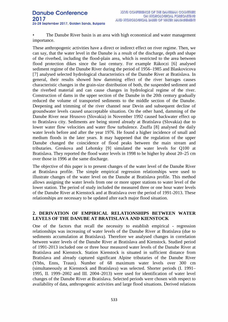
533

• The Danube River basin is an area with high economical and water management importance. These anthropogenic activities have a direct or indirect effect on river regime. Then, we can say, that the water level in the Danube is a result of the discharge, depth and shape of the riverbed, including the flood-plain area, which is restricted to the area between flood protection dikes since the last century. For example Rákoczi [6] analysed sediment regime of the Danube River during the period of 1956–1985 and Blaskovicova [7] analysed selected hydrological characteristics of the Danube River at Bratislava. In general, their results showed how damming effect of the river barrages causes characteristic changes in the grain-size distribution of both, the suspended sediment and the riverbed material and can cause changes in hydrological regime of the river. Construction of dams in the upper section of the Danube in the 20th century gradually reduced the volume of transported sediments to the middle section of the Danube. Deepening and trimming of the river channel near Devin and subsequent decline of groundwater levels caused unacceptable situation. On the other hand, damming of the Danube River near Hrusovo (Slovakia) in November 1992 caused backwater effect up to Bratislava city. Sediments are being stored already at Bratislava (Slovakia) due to lower water flow velocities and water flow turbulence. Zsuffa [8] analysed the daily water levels before and after the year 1976. He found a higher incidence of small and medium floods in the later years. It may happened that the regulation of the upper Danube changed the coincidence of flood peaks between the main stream and tributaries. Greskova and Lehotsky [9] simulated the water levels for Q100 at Bratislava. They reported the flood water levels in 1998 to be higher by about 20–25 cm over those in 1996 at the same discharge. The objective of this paper is to present changes of the water level of the Danube River at Bratislava profile. The simple empirical regression relationships were used to illustrate changes of the water level on the Danube at Bratislava profile. This method allows assigning the water levels from one or more upper stations to water level of the lower station. The period of study included the measured three or one hour water levels of the Danube River at Kienstock and at Bratislava over the period of 1991-2013. These relationships are necessary to be updated after each major flood situation.

2. DERIVATION OF EMPIRICAL RELATIONSHIPS BETWEEN WATER LEVELS OF THE DANUBE AT BRATISLAVA AND KIENSTOCK One of the factors that recall the necessity to establish empirical - regression relationships was increasing of water levels of the Danube River at Bratislava (due to sediments accumulation at Bratislava). Therefore we analysed changes in correlation between water levels of the Danube River at Bratislava and Kienstock. Studied period of 1991-2013 included one or three hour measured water levels of the Danube River at Bratislava and Kienstock. Station Kienstock is situated in sufficient distance from Bratislava and already captured significant Alpine tributaries of the Danube River (Ybbs, Enns, Traun). Number of 68 maximum water levels over 300 cm (simultaneously at Kienstock and Bratislava) was selected. Shorter periods (I. 1991–1995, II. 1999–2002 and III. 2004–2013) were used for identification of water level changes of the Danube River at Bratislava. Selected periods were chosen with respect to availability of data, anthropogenic activities and large flood situations. Derived relations

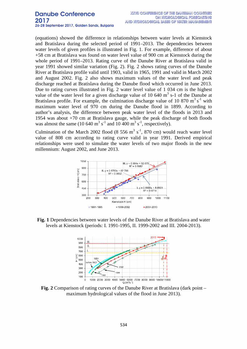
534

(equations) showed the difference in relationships between water levels at Kienstock and Bratislava during the selected period of 1991–2013. The dependencies between water levels of given profiles is illustrated in Fig. 1. For example, difference of about +58 cm at Bratislava was found on water level value of 900 cm at Kienstock during the whole period of 1991–2013. Rating curve of the Danube River at Bratislava valid in year 1991 showed similar variation (Fig. 2). Fig. 2 shows rating curves of the Danube River at Bratislava profile valid until 1903, valid in 1965, 1991 and valid in March 2002 and August 2002. Fig. 2 also shows maximum values of the water level and peak discharge reached at Bratislava during the Danube flood which occurred in June 2013. Due to rating curves illustrated in Fig. 2 water level value of 1 034 cm is the highest value of the water level for a given discharge value of 10 640 m3 s-1 of the Danube at Bratislava profile. For example, the culmination discharge value of 10 870 m3 s-1 with maximum water level of 970 cm during the Danube flood in 1899. According to author’s analysis, the difference between peak water level of the floods in 2013 and 1954 was about +70 cm at Bratislava gauge, while the peak discharge of both floods was almost the same (10 640 m3 s-1 and 10 400 m3 s-1, respectively). Culmination of the March 2002 flood (8 556 m3 s-1, 870 cm) would reach water level value of 808 cm according to rating curve valid in year 1991. Derived empirical relationships were used to simulate the water levels of two major floods in the new millennium: August 2002, and June 2013.

Fig. 1 Dependencies between water levels of the Danube River at Bratislava and water

levels at Kienstock (periods: I. 1991-1995, II. 1999-2002 and III. 2004-2013).

Fig. 2 Comparison of rating curves of the Danube River at Bratislava (dark point –

maximum hydrological values of the flood in June 2013).

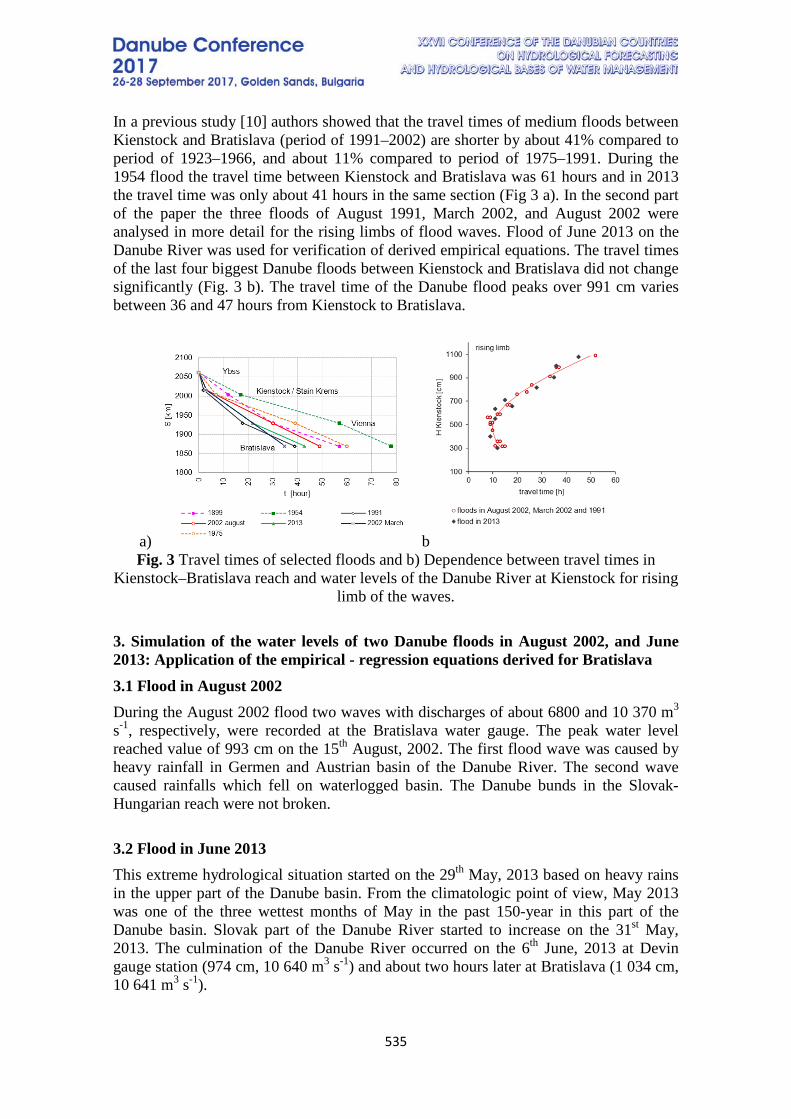
535

In a previous study [10] authors showed that the travel times of medium floods between Kienstock and Bratislava (period of 1991–2002) are shorter by about 41% compared to period of 1923–1966, and about 11% compared to period of 1975–1991. During the 1954 flood the travel time between Kienstock and Bratislava was 61 hours and in 2013 the travel time was only about 41 hours in the same section (Fig 3 a). In the second part of the paper the three floods of August 1991, March 2002, and August 2002 were analysed in more detail for the rising limbs of flood waves. Flood of June 2013 on the Danube River was used for verification of derived empirical equations. The travel times of the last four biggest Danube floods between Kienstock and Bratislava did not change significantly (Fig. 3 b). The travel time of the Danube flood peaks over 991 cm varies between 36 and 47 hours from Kienstock to Bratislava.

a) b Fig. 3 Travel times of selected floods and b) Dependence between travel times in

Kienstock–Bratislava reach and water levels of the Danube River at Kienstock for rising limb of the waves.

3. Simulation of the water levels of two Danube floods in August 2002, and June 2013: Application of the empirical - regression equations derived for Bratislava 3.1 Flood in August 2002 During the August 2002 flood two waves with discharges of about 6800 and 10 370 m3 s-1, respectively, were recorded at the Bratislava water gauge. The peak water level reached value of 993 cm on the 15th August, 2002. The first flood wave was caused by heavy rainfall in Germen and Austrian basin of the Danube River. The second wave caused rainfalls which fell on waterlogged basin. The Danube bunds in the Slovak-Hungarian reach were not broken.

3.2 Flood in June 2013 This extreme hydrological situation started on the 29th May, 2013 based on heavy rains in the upper part of the Danube basin. From the climatologic point of view, May 2013 was one of the three wettest months of May in the past 150-year in this part of the Danube basin. Slovak part of the Danube River started to increase on the 31st May, 2013. The culmination of the Danube River occurred on the 6th June, 2013 at Devin gauge station (974 cm, 10 640 m3 s-1) and about two hours later at Bratislava (1 034 cm, 10 641 m3 s-1).

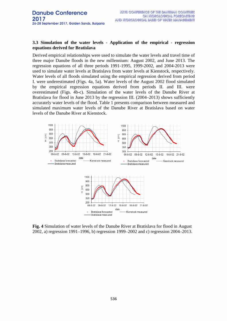
536

3.3 Simulation of the water levels - Application of the empirical - regression equations derived for Bratislava Derived empirical relationships were used to simulate the water levels and travel time of three major Danube floods in the new millennium: August 2002, and June 2013. The regression equations of all three periods 1991-1995, 1999-2002, and 2004-2013 were used to simulate water levels at Bratislava from water levels at Kienstock, respectively. Water levels of all floods simulated using the empirical regression derived from period I. were underestimated (Figs. 4a, 5a). Water levels of the August 2002 flood simulated by the empirical regression equations derived from periods II. and III. were overestimated (Figs. 4b-c). Simulation of the water levels of the Danube River at Bratislava for flood in June 2013 by the regression III. (2004–2013) shows sufficiently accurately water levels of the flood. Table 1 presents comparison between measured and simulated maximum water levels of the Danube River at Bratislava based on water levels of the Danube River at Kienstock.

Fig. 4 Simulation of water levels of the Danube River at Bratislava for flood in August 2002, a) regression 1991–1996, b) regression 1999–2002 and c) regression 2004–2013.

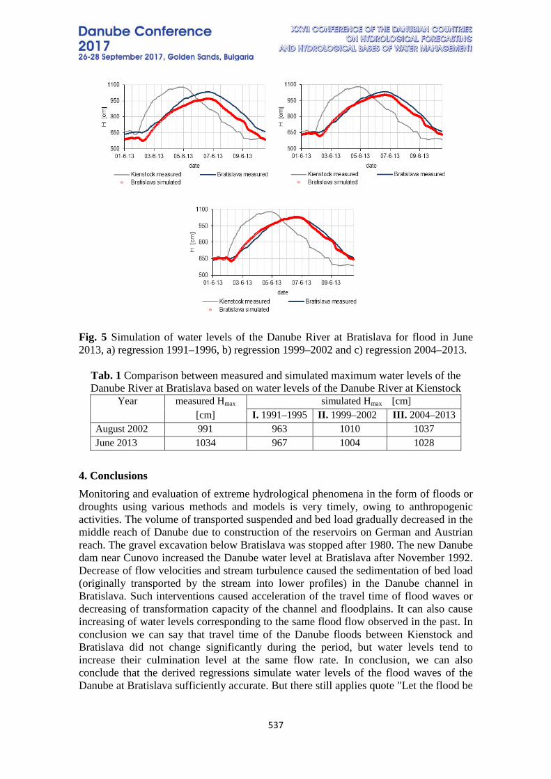
537

Fig. 5 Simulation of water levels of the Danube River at Bratislava for flood in June 2013, a) regression 1991–1996, b) regression 1999–2002 and c) regression 2004–2013.

Tab. 1 Comparison between measured and simulated maximum water levels of the Danube River at Bratislava based on water levels of the Danube River at Kienstock

Year measured Hmax simulated Hmax [cm] [cm] I. 1991–1995 II. 1999–2002 III. 2004–2013

August 2002 991 963 1010 1037 June 2013 1034 967 1004 1028

4. Conclusions Monitoring and evaluation of extreme hydrological phenomena in the form of floods or droughts using various methods and models is very timely, owing to anthropogenic activities. The volume of transported suspended and bed load gradually decreased in the middle reach of Danube due to construction of the reservoirs on German and Austrian reach. The gravel excavation below Bratislava was stopped after 1980. The new Danube dam near Cunovo increased the Danube water level at Bratislava after November 1992. Decrease of flow velocities and stream turbulence caused the sedimentation of bed load (originally transported by the stream into lower profiles) in the Danube channel in Bratislava. Such interventions caused acceleration of the travel time of flood waves or decreasing of transformation capacity of the channel and floodplains. It can also cause increasing of water levels corresponding to the same flood flow observed in the past. In conclusion we can say that travel time of the Danube floods between Kienstock and Bratislava did not change significantly during the period, but water levels tend to increase their culmination level at the same flow rate. In conclusion, we can also conclude that the derived regressions simulate water levels of the flood waves of the Danube at Bratislava sufficiently accurate. But there still applies quote "Let the flood be

538

however large, there always comes up even larger one in the future", as it follows from the theory of extremes and experience confirms this. ACKNOWLEDGEMENTS This work was supported by the project VEGA No. 2/0009/15 and it results from the project implementation of the “Centre of excellence for integrated flood protection of land” (ITMS 26240120004).

5. REFERENCES [1] Rohr, CH., Floods of the Upper Daube River and its tributaries and their impact on urban economies: The examples of the towns of Krems/Stein and Wels. Environment and History, vol. 19, pp. 133–148, 2013. [2] Thielen J., Bartholmes J., Ramos M.-H., de Roo A., The European Flood Alert System – Part 1: Concept and development. Hydrol. Earth Syst. Sci., vol. 13, doi:10.5194/hess-13-125-2009, pp. 125-140, 2009. [3] Bartholmes J. C., Thielen J., Ramos M. H., Gentilini, S., The European flood alert system EFAS – Part 2: Statistical skill assessment of probabilistic and deterministic operational forecasts. Hydrol. Earth Syst. Sci., vol. 13, doi:10.5194/hess-13-141-2009, pp. 141-153, 2009. [4] Gan T.Y., Zunic F., Strobl T., Flood mapping of Danube River at Romania using single and multi-date ERS2-SAR images. International Journal of Applied Earth Observation and Geoinformation, vol. 18, pp. 69–81, 2012. [5] Hlavcova K., Szolgay J., Halmova D., Parajka J., Kohnova S., Changes in the hydrological regime of Slovak rivers and other adaptation measures to climate change in water management. In the National Climate Program of the Slovak Republic - NHL 12/08: Impact of climate change and adaptation. Bratislava: The Ministry of the Environment, pp. 61–86, 2008. ISBN 978-80-88907-63. [6] Rakoczi L., Sediment Regime of the River Danube (1986–1985). In Hydrological Processes of the Danube River Basin: Perspectives from Danubian Countries. DOI 10.1007/978-90-481-3423-6_9, Springer Science+Business Media B. V, p. 436, 2010. [7] Blaskovicova L., Danacova Z., Lovasova L., Simor V., Skoda, P., Development of selected hydrological characteristics of the Danube in Bratislava. Slovak Hydrometeorological Institute report, p. 15, 2014. [8] Zsuffa, I., Impact of Austrian hydropower plants on the flood control safety of the Hungarian Danube. Hydrological Sciences Journal, vol. 44, no. 3, pp. 363-371, 1999. [9] Greskova A., Lehotsky M., Hydrogeomorphic response assessment of the Danube River channel and floodplain to the 2002 flood events. In: CD Proc. XXIInd Conf. of the Danube Countries on the Hydrological Forecasting and Hydrological Bases of Water Management (Brno, Czech Republic), 2004, ISBN 80-86690-19-9.

539

[10] Mitkova, V., Pekarova, P., Miklanek, P., Pekar, J., Analysis of flood propagation changes in the Kienstock-Bratislava reach of the Danube River. Hydrological Sciences Journal, IAHS Press, ISSN 0262-6667, vol. 50, no. 4, pp. 655-668, 2005.

540

INVESTIGATE THE CAUSES OF WATER CRISIS IN CENTRAL IRAN’S BASINS: CLIMATE CHANGE OR MISMANGMENT WATER RESOURCES

Fatemeh Ghader1, Mohammad Hajiketabi2, Uwe Tröger 1 1 Technische Universität Berlin, Germany 2Zayandab Consult Engineer Office, Iran

Corresponging authors: F Ghader, Institut für Angewandte Geowissenschaften, Germany, e-mail: fatemeh.ghader@campus.tu-berlin.de

Abstract In recent years climate change has had a significant impact on water resources in many parts of the world. This study investigated the water resources balance in two great basins in the center of Iran with a population about 8 million, Gavkhoni and Maharlu-Bakhtegan. The population in this basins represents ten percent of the total population. Reasons of the water crisis in these two basins studied and compared. Using meteorology, hydrology and groundwater statistics, the water balance assessed a basis on 40-year precipitation in the meteorological year 2012-2013. Based on these results water resources balance respectively are -460.2 and -838.8 cubic million meters in Gavkhoni and Maharlu-Bkhtegan basin. While the amount of precipitation during the five years leading up to balance assessment decreased about 20 percent compare to 40 years average precipitation. Two large dams Zayanderoud and Drodzan in Gavkhoni and Mahrlu-Bakhtegan basin supply agriculture, industry and drinking water in vast part of these basins, moreover these dams are the main supplier of drinking water for two metropolis cities Esfahan and Shiraz. Inflow rate to Drodzan and Zayanderoud dam respectively 50 and 40 percent has decreased between 2008-2013 compared to the 40 years average inflow rate; according to available information the annual volume of two dams by 10 percent compare to the same period has decreased. The main reasons for this reduction after reviewing the groundwater, water resources statistics, and field inspection are decreased river fed with groundwater upstream of the dams, increased uptake of water during cultivation seasons and decline in precipitation, inappropriate irrigation system and also low irrigation efficiency. Forecast in the study shows that in the absence of proper management of water resources in two basins until 10 years, supply drinking water and agriculture into large basins would be largest social challenges. Keyword: Water balance, Dam, Runoff, Inflow, Water management, Drinking water, Agriculture Introduction

Iran is located in arid and semi-arid climate, Iran has an annual precipitation range 252 millimeter on third of global. In recent years drying lakes, declining groundwater level in the most of plains, land subsidence, water contamination, reducing and damage to agriculture, force migration to cities because of agriculture losses and growth rate of unemployment and ecosystem damages are main problems of shortage water in Iran

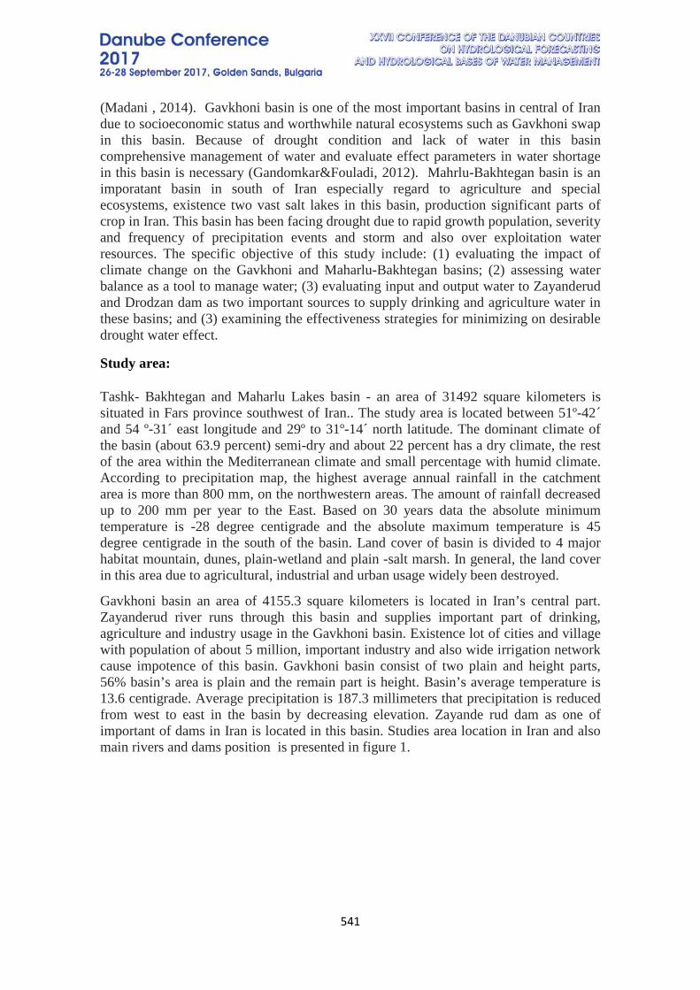
541

(Madani , 2014). Gavkhoni basin is one of the most important basins in central of Iran due to socioeconomic status and worthwhile natural ecosystems such as Gavkhoni swap in this basin. Because of drought condition and lack of water in this basin comprehensive management of water and evaluate effect parameters in water shortage in this basin is necessary (Gandomkar&Fouladi, 2012). Mahrlu-Bakhtegan basin is an imporatant basin in south of Iran especially regard to agriculture and special ecosystems, existence two vast salt lakes in this basin, production significant parts of crop in Iran. This basin has been facing drought due to rapid growth population, severity and frequency of precipitation events and storm and also over exploitation water resources. The specific objective of this study include: (1) evaluating the impact of climate change on the Gavkhoni and Maharlu-Bakhtegan basins; (2) assessing water balance as a tool to manage water; (3) evaluating input and output water to Zayanderud and Drodzan dam as two important sources to supply drinking and agriculture water in these basins; and (3) examining the effectiveness strategies for minimizing on desirable drought water effect.

Study area:

Tashk- Bakhtegan and Maharlu Lakes basin - an area of 31492 square kilometers is situated in Fars province southwest of Iran.. The study area is located between 51º-42´ and 54 º-31´ east longitude and 29º to 31º-14´ north latitude. The dominant climate of the basin (about 63.9 percent) semi-dry and about 22 percent has a dry climate, the rest of the area within the Mediterranean climate and small percentage with humid climate. According to precipitation map, the highest average annual rainfall in the catchment area is more than 800 mm, on the northwestern areas. The amount of rainfall decreased up to 200 mm per year to the East. Based on 30 years data the absolute minimum temperature is -28 degree centigrade and the absolute maximum temperature is 45 degree centigrade in the south of the basin. Land cover of basin is divided to 4 major habitat mountain, dunes, plain-wetland and plain -salt marsh. In general, the land cover in this area due to agricultural, industrial and urban usage widely been destroyed.

Gavkhoni basin an area of 4155.3 square kilometers is located in Iran’s central part. Zayanderud river runs through this basin and supplies important part of drinking, agriculture and industry usage in the Gavkhoni basin. Existence lot of cities and village with population of about 5 million, important industry and also wide irrigation network cause impotence of this basin. Gavkhoni basin consist of two plain and height parts, 56% basin’s area is plain and the remain part is height. Basin’s average temperature is 13.6 centigrade. Average precipitation is 187.3 millimeters that precipitation is reduced from west to east in the basin by decreasing elevation. Zayande rud dam as one of important of dams in Iran is located in this basin. Studies area location in Iran and also main rivers and dams position is presented in figure 1.

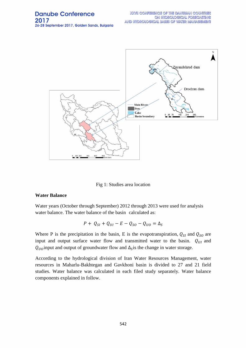
542

Fig 1: Studies area location

Water Balance

Water years (October through September) 2012 through 2013 were used for analysis water balance. The water balance of the basin calculated as:

𝑃𝑃 + 𝑄𝑄𝑆𝑆𝑆𝑆 + 𝑄𝑄𝑈𝑈𝑆𝑆 − 𝐸𝐸 − 𝑄𝑄𝑆𝑆𝑆𝑆 − 𝑄𝑄𝑈𝑈𝑆𝑆 = ∆𝑆𝑆

Where P is the precipitation in the basin, E is the evapotranspiration, 𝑄𝑄𝑆𝑆𝑆𝑆 and 𝑄𝑄𝑆𝑆𝑆𝑆 are input and output surface water flow and transmitted water to the basin. 𝑄𝑄𝑈𝑈𝑆𝑆 and 𝑄𝑄𝑈𝑈𝑆𝑆input and output of groundwater flow and ∆𝑆𝑆is the change in water storage.

According to the hydrological division of Iran Water Resources Management, water resources in Maharlu-Bakhtegan and Gavkhoni basin is divided to 27 and 21 field studies. Water balance was calculated in each filed study separately. Water balance components explained in follow.

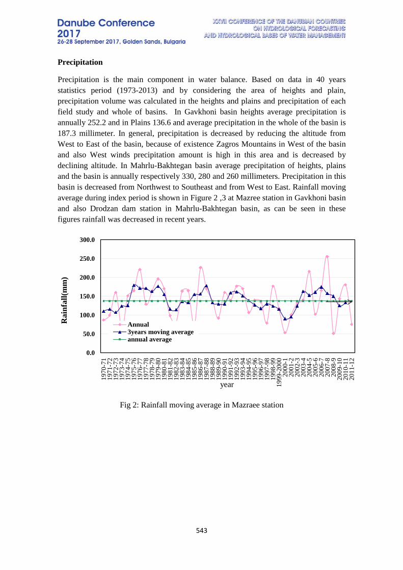
543

Precipitation

Precipitation is the main component in water balance. Based on data in 40 years statistics period (1973-2013) and by considering the area of heights and plain, precipitation volume was calculated in the heights and plains and precipitation of each field study and whole of basins. In Gavkhoni basin heights average precipitation is annually 252.2 and in Plains 136.6 and average precipitation in the whole of the basin is 187.3 millimeter. In general, precipitation is decreased by reducing the altitude from West to East of the basin, because of existence Zagros Mountains in West of the basin and also West winds precipitation amount is high in this area and is decreased by declining altitude. In Mahrlu-Bakhtegan basin average precipitation of heights, plains and the basin is annually respectively 330, 280 and 260 millimeters. Precipitation in this basin is decreased from Northwest to Southeast and from West to East. Rainfall moving average during index period is shown in Figure 2 ,3 at Mazree station in Gavkhoni basin and also Drodzan dam station in Mahrlu-Bakhtegan basin, as can be seen in these figures rainfall was decreased in recent years.

Fig 2: Rainfall moving average in Mazraee station

0.0

50.0

100.0

150.0

200.0

250.0

300.0

1970

-71

1971

-72

1972

-73

1973

-74

1974

-75

1975

-76

1976

-77

1977

-78

1978

-79

1979

-80

1980

-81

1981

-82

1982

-83

1983

-84

1984

-85

1985

-86

1986

-87

1987

-88

1988

-89

1989

-90

1990

-91

1991

-92

1992

-93

1993

-94

1994

-95

1995

-96

1996

-97

1997

-98

1998

-99

1999

-200

020

00-1

2001

-220

02-3

2003

-420

04-5

2005

-620

06-7

2007

-820

08-9

2009

-10

2010

-11

2011

-12

Rai

nfal

l(mm

)

year

Annual3years moving averageannual average

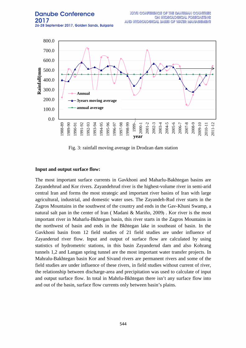
544

Fig. 3: rainfall moving average in Drodzan dam station

Input and output surface flow:

The most important surface currents in Gavkhoni and Maharlu-Bakhtegan basins are Zayandehrud and Kor rivers. Zayandehrud river is the highest-volume river in semi-arid central Iran and forms the most strategic and important river basins of Iran with large agricultural, industrial, and domestic water uses. The Zayandeh-Rud river starts in the Zagros Mountains in the southwest of the country and ends in the Gav-Khuni Swamp, a natural salt pan in the center of Iran ( Madani & Mariño, 2009) . Kor river is the most important river in Maharlu-Bkhtegan basin, this river starts in the Zagros Mountains in the northwest of basin and ends in the Bkhtegan lake in southeast of basin. In the Gavkhoni basin from 12 field studies of 21 field studies are under influence of Zayanderud river flow. Input and output of surface flow are calculated by using statistics of hydrometric stations, in this basin Zayanderud dam and also Kohrang tunnels 1,2 and Langan spring tunnel are the most important water transfer projects. In Mahralu-Bakhtegan basin Kor and Sivand rivers are permanent rivers and some of the field studies are under influence of these rivers, in field studies without current of river, the relationship between discharge-area and precipitation was used to calculate of input and output surface flow. In total in Mahrlu-Bkhtegan there isn’t any surface flow into and out of the basin, surface flow currents only between basin’s plains.

0.0

100.0

200.0

300.0

400.0

500.0

600.0

700.0

800.0

1988

-89

1989

-90

1990

-91

1991

-92

1992

-93

1993

-94

1994

-95

1995

-96

1996

-97

1997

-98

1998

-99

1999

-…20

00-1

2001

-220

02-3

2003

-420

04-5

2005

-620

06-7

2007

-820

08-9

2009

-10

2010

-11

2011

-12

Rai

nfal

l(mm

year

Annual

3years moving average

annual average

545

Input and output groundwater flow:

Input groundwater flows currents mainly from Highlands and surrounding plains to aquifer and input flow currents toward lakes and downstream plains. Groundwater input and output flow are calculated by using Darcy equation, based on transmissibility map, groundwater level, and hydraulic gradient. Darcy equation is as follow:

𝑄𝑄𝑈𝑈𝑆𝑆,𝑈𝑈𝑆𝑆=𝑇𝑇𝐿𝐿𝑆𝑆

𝑄𝑄𝑈𝑈𝑆𝑆,𝑈𝑈𝑆𝑆= Input and output groundwater flow

T= Aquifer transmissibility

𝐿𝐿𝑆𝑆= Hydraulic gradient

Maharlu-Bakhtegan and Gavkhoni basins are the second order basin in Iran hydrology division, in the most second order basin there is not groundwater flow to another basins, groundwater just flows between plains in the basin, this condition also can be seen in field studies. To evaluate groundwater changes in the index period were used unit hydrograph of plains. Unit hydrograph in each plain by using water fluctuations in observed wells was prepared. There are 504 and 625 observed well in Mahrlu-Bakhtegan and Gavkhoni basins. According to unit hydrographs in all the plain in two basin there is sharp decline in groundwater for example in Damenedaran and Saadatabad plain respectively in Gavkhoni and Maharlu-Bakhtegan lakes basin during 15 years there was declined 20 and 12 meters in groundwater levels.

Evapotranspiration:

Evapotranspiration is an important output component in water balance; Evapotranspiration is in various forms such as evapotranspiration of precipitation (actual), groundwater evaporation and evapotranspiration of net water usage. Evapotranspiration of precipitation in heights and plains of basins was calculated using Thornth Waite method. The total amount of evapotranspiration of precipitation in Mahrlu-Bakhtegan and Gavkhoni basin is. Groundwater evaporation amount is based on groundwater level and only is calculated in the area which groundwater level is below than 5 meters. Evaporation of water surface is calculated in filed studied that have natural or artificial lake and according to statistics of evaporation stations. In Maharlu-Bakhtegan basin evaporation of water surface was calculated from Bakhtegan and Mahrlu lakes and also lake of Drodzan dam, In Gavkhoni basin this amount calculated from Gavkhoni wetland.

Storage changes:

Water balance calculation in basins shows that reduction of groundwater storage in index period in Gavkhoni basin is -429.6 and in Maharlu-Bkhtegan basin is -800 cubic million meters.

546

Input and output changes in dams:

The drought condition and lake of water also affected on dams in studies area. Drodzan and Zayanderud dams are important dams in the south and center of Iran that supply main part of agriculture and industrial water and also supplies drinking water for two metropolises cities Esfahan and Shiraz. Assessment input water to these dams during 40 years shows input flow to dams has fluctuation and between 2008-2013 this amount decreased sharply. Evaluate the amount of discharge in upstream stations shows that flow rate in these station has declined by 40 and 50 percent compare to 40 years average.

Results and discussion:

Precipitation as an important recharge component in basins has been a lot of changes in recent years since precipitation changes show that during 2008-2013 by 30 percent reduction compare to 40 years annual precipitation. Evaluation groundwater level fluctuation of two basins has been done according to unit hydrograph, in the most field studies groundwater level declined, minimum groundwater level is in September and October (because lack of rainfall and extraction water for agriculture) and the maximum amount of water level is related to March and April (by rainfall or melting snow). In other words, the amount of rainfall and groundwater extraction is an important factor of changes groundwater level in basins. Discharge and extraction of groundwater in basins have increased in last two decades so that in water year 2012-2013 in Maharlu-Bakhtegan basin was and in Gavkhon basin cubic million meters and has increased compared to 5 years end to 2013.

The drought condition and lack of water isn’t limited also to the plain also affected on dams in studies area. Drodzan and Zayanderud dams are important dams in the south and center of Iran that supply main part of agriculture and industrial water and also supplies drinking water for two metropolises cities Esfahan and Shiraz. Assessment input water to these dams during 40 years shows input flow to dams has fluctuation and between 2008-2013 this amount decreased sharply. Evaluate the amount of discharge in upstream stations shows that flow rate in these station has declined by 40 and 50 percent compare to 40 years average.

Conclusion

Studied basins are located in semi-arid climate region. Negative water balance shows an impressive decline in groundwater reservoirs. The main reason for decrease storage changes includes; declining rainfall, over-extraction of groundwater resources, using traditional irrigation methods and low irrigation efficiency which cause loss lot amount of water ( irrigation efficiency in these basin are less than 50 percent), incorporate crop pattern that is not match to climate condition and also water resources. According to

547

available conditions, water resources management is an essential need to deal with water shortage.

References:

A. Gandomkar, K. Fouladi, The Necessity of Optimized Management on Surface Water Sources of Zayanderood Basin, International Journal of Environmental, Chemical, Ecological, Geological and Geophysical Engineering Vol:6, No:5, 2012.

K. Madani, Water Management in Iran: What is causing the Looming Crisis? , J Environ Stud Sci (2014), DOI 10.1007/s13412-014-0182-z.

K. Madani, M. Mariño, System Dynamics Analysis for Managing Iran’s Zayandeh-Rud River Basin, J Water Resource Manage (2009) 23:2163–2187 ,DOI 10.1007/s11269-008-9376-z.

548

POTENTIAL CLIMATE CHANGE IMPACT ON MEAN FLOW IN ROMANIA Ciprian Corbuș, Rodica-Paula Mic, Marius Mătreață, Viorel Chendeş, Alexandru

Preda National Institute of Hydrology and Water Management, Romania

Corresponding author: Viorel Chendeş, I.N.H.G.A., 97E, Bucuresti-Ploiesti, 013686, Bucharest, Sector 1, Romania, viorel.chendes@hidro.ro

ABSTRACT The warming of the global climate caused by greenhouse effect can induce essential changes in the hydrological regime and water resources at a different time and space scale. In order to estimate the changes induced by climate change on the mean flow in Romania for the time horizon 2021 – 2050 the hydrological models WATBAL and CONSUL were used, using as input data series of precipitation and temperature. Parameters of models were calibrated by the monthly flow simulation in 275 analysed cross-sections from 20 river basins using as input data the precipitation and temperatures recorded at weather stations located into the area, during 2000-2006, considered as calibration period. Then, long-term hydrological simulations were performed taking into account two scenarios: Scenario 0, in which mean monthly discharge was computed for the 1971-2000 reference period, considering the meteorological inputs simulated with the climate model, and Scenario 1, which suppose the simulation of the mean monthly discharge for the future period 2021-2050, with the same hydrological model, considering as inputs the climate change projections. As input data, for both simulations were used the precipitation and temperature time series resulted from two different simulations of climate change evolution performed within CLAVIER Project (with REMO model, version 5.7): (i) a simulation for the reference period and (ii) another simulation for the modified regime period, corresponding to the evolution scenario of greenhouse gases emission A1B, using as boundary conditions the global model simulations with coupled ocean-atmosphere ECHAMP5. Further, it was made a comparative analysis of average monthly, seasonal and multiannual discharge for two periods of simulation, determining the relative deviation of them. The analysis is based on morphometric characteristics of river basins were obtained by GIS database processing. Keywords: climatic changes, surface water, WATBAL model, CONSUL model, water balance

1. INTRODUCTION In order to determine the vulnerability of water resources to climate change and to establish the adaptation measures at the level of each river basin, specific analyzes are required for assessing the impact of climate change on water resources in these analyzed river basins.

549

Taking into account this requirement, the main objective of the paper is to estimate the impact of climate change on the average flow rate of rivers, in Romania, which is based on long-term simulations made using a hydrological model, having as input data the series of precipitations and temperature, resulting from the climatic evolution simulations performed using a regional meteorological model.

2. METHODOLOGY The used methodology is based on the following stages: • Establishment of the climate change scenario, which includes climatic projections, obtained using a meteorological model, which are available for a grid with a spatial resolution as higher as possible. Two types of simulations were available for this study: a simulation obtained in a control run for a historical period in order to establish the reference climate regime and a simulation corresponding to the scenario of evolution of greenhouse gas emissions in the future using, as boundary conditions, the simulations made with the global coupled ocean-atmosphere meteorological model. • Pre-processing of input meteorological data at a spatial and temporal resolution corresponding to hydrological modelling requirements, by performing the following operations: applying corrections of simulated values using statistical methods and grid data set based on observation with the best spatial and temporal resolution; Performing a temporal downscaling on the corrected values from the available time step to the required time step in hydrological modelling, and making a spatial downscaling over the meteorological values from available resolution to the hydrological model needs. • Obtaining the series of precipitation and temperatures, average on sub-basins, at the calculation time step used by the hydrological model, according to the topological scheme for each of the analyzed river basins, using as input the meteorological gridded dataset series. • Calibration of the hydrological model based on historic data, which is then used, with the optimal set of parameters resulting from calibration, for long-term simulation of the discharge series using climatic scenario data. • Flow simulation over two long periods using the hydrological model, the first simulation being performed for the reference period and the second for the future period. In order to estimate the impact of climate change on the hydrological regime the simulations are performed for the natural flow regime, without taking into account the influence of the exploitation of the reservoirs. • Analysis of the study results concerning the impact of climate changes and variability on the hydrological regime of the monthly, seasonal and annual mean discharges.

3. APPLICATIONS ON THE ROMANIAN RIVERS The presented methodology was applied in 20 Romanian river basins (Figure 1), having surfaces ranging between 82 to 27890 km2, (Table 1). The total area of the 20 analysed river basins is 170124 km2, which represents 71.63% of Romania's surface area.

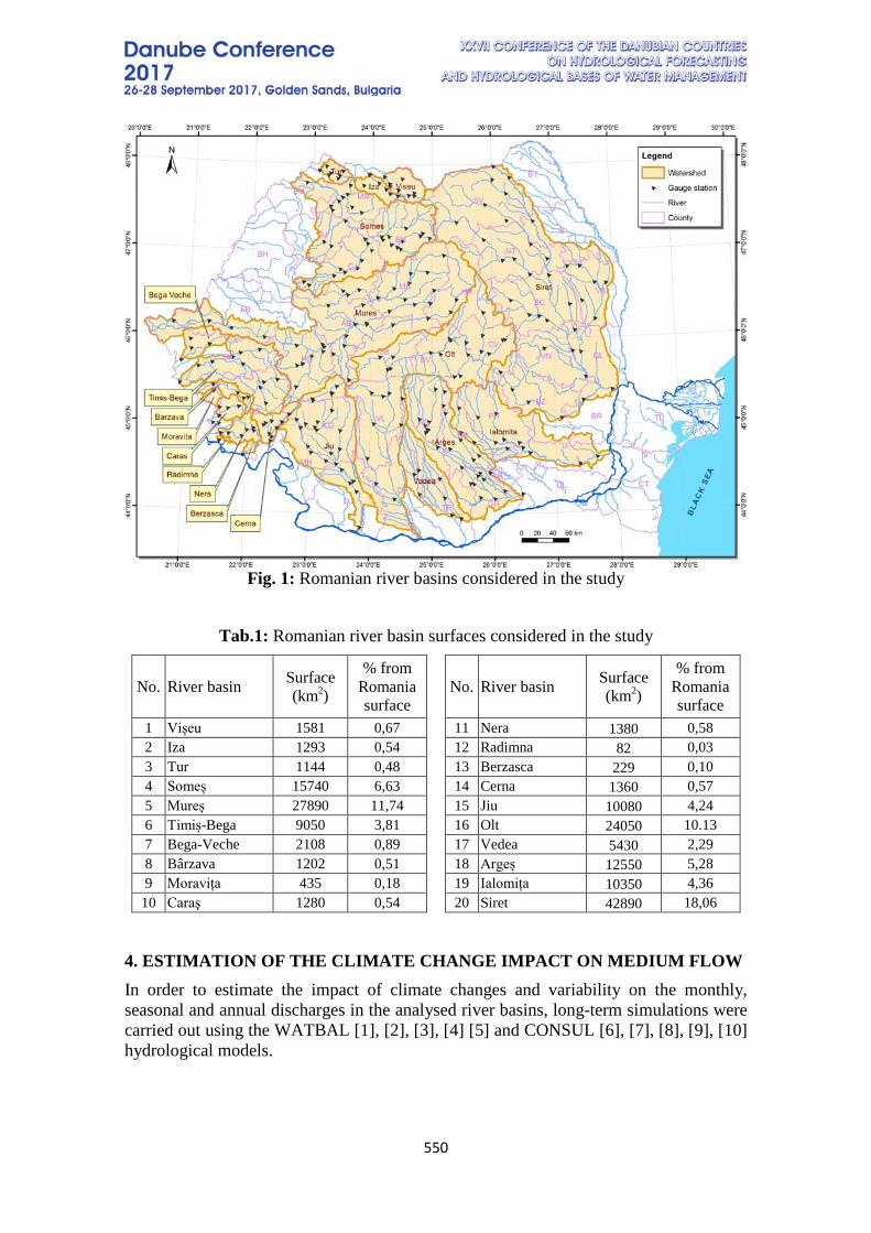
550

Fig. 1: Romanian river basins considered in the study

Tab.1: Romanian river basin surfaces considered in the study

No. River basin Surface (km2)

% from Romania surface

No. River basin Surface (km2)

% from Romania surface

1 Vișeu 1581 0,67 11 Nera 1380 0,58 2 Iza 1293 0,54 12 Radimna 82 0,03 3 Tur 1144 0,48 13 Berzasca 229 0,10 4 Someș 15740 6,63 14 Cerna 1360 0,57 5 Mureș 27890 11,74 15 Jiu 10080 4,24 6 Timiș-Bega 9050 3,81 16 Olt 24050 10.13 7 Bega-Veche 2108 0,89 17 Vedea 5430 2,29 8 Bârzava 1202 0,51 18 Argeș 12550 5,28 9 Moravița 435 0,18 19 Ialomița 10350 4,36

10 Caraş 1280 0,54 20 Siret 42890 18,06

4. ESTIMATION OF THE CLIMATE CHANGE IMPACT ON MEDIUM FLOW In order to estimate the impact of climate changes and variability on the monthly, seasonal and annual discharges in the analysed river basins, long-term simulations were carried out using the WATBAL [1], [2], [3], [4] [5] and CONSUL [6], [7], [8], [9], [10] hydrological models.

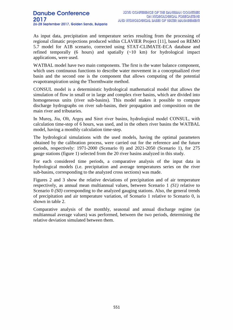
551

As input data, precipitation and temperature series resulting from the processing of regional climatic projections produced within CLAVIER Project [11], based on REMO 5.7 model for A1B scenario, corrected using STAT-CLIMATE-ECA database and refined temporally (6 hours) and spatially (~10 km) for hydrological impact applications, were used. WATBAL model have two main components. The first is the water balance component, which uses continuous functions to describe water movement in a conceptualized river basin and the second one is the component that allows computing of the potential evapotranspiration using the Thornthwaite method. CONSUL model is a deterministic hydrological mathematical model that allows the simulation of flow in small or in large and complex river basins, which are divided into homogeneous units (river sub-basins). This model makes it possible to compute discharge hydrographs on river sub-basins, their propagation and composition on the main river and tributaries. In Mureş, Jiu, Olt, Argeş and Siret river basins, hydrological model CONSUL, with calculation time-step of 6 hours, was used, and in the others river basins the WATBAL model, having a monthly calculation time-step. The hydrological simulations with the used models, having the optimal parameters obtained by the calibration process, were carried out for the reference and the future periods, respectively: 1971-2000 (Scenario 0) and 2021-2050 (Scenario 1), for 275 gauge stations (figure 1) selected from the 20 river basins analyzed in this study. For each considered time periods, a comparative analysis of the input data in hydrological models (i.e. precipitation and average temperatures series on the river sub-basins, corresponding to the analyzed cross sections) was made. Figures 2 and 3 show the relative deviations of precipitation and of air temperature respectively, as annual mean multiannual values, between Scenario 1 (S1) relative to Scenario 0 (S0) corresponding to the analyzed gauging stations. Also, the general trends of precipitation and air temperature variation, of Scenario 1 relative to Scenario 0, is shown in table 2. Comparative analysis of the monthly, seasonal and annual discharge regime (as multiannual average values) was performed, between the two periods, determining the relative deviation simulated between them.

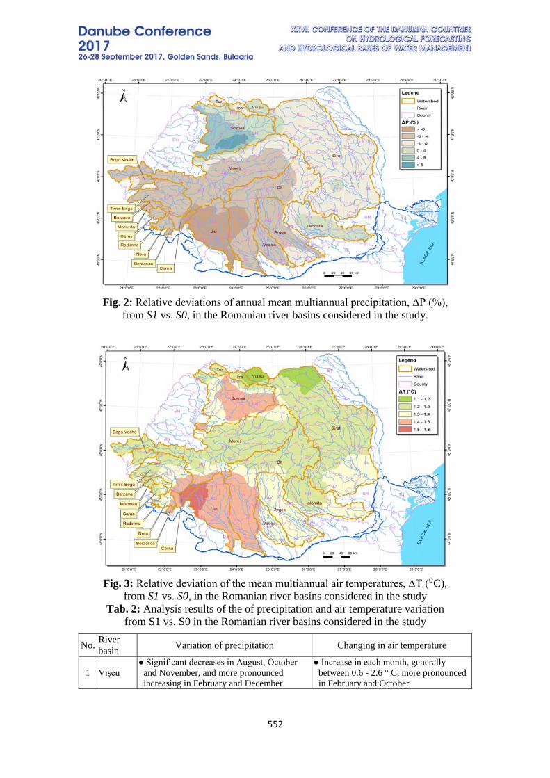
552

Fig. 2: Relative deviations of annual mean multiannual precipitation, ΔP (%),

from S1 vs. S0, in the Romanian river basins considered in the study.

Fig. 3: Relative deviation of the mean multiannual air temperatures, ΔT (⁰C),

from S1 vs. S0, in the Romanian river basins considered in the study Tab. 2: Analysis results of the of precipitation and air temperature variation

from S1 vs. S0 in the Romanian river basins considered in the study

No. River basin Variation of precipitation Changing in air temperature

1 Vișeu ● Significant decreases in August, October

and November, and more pronounced increasing in February and December

● Increase in each month, generally between 0.6 - 2.6 ° C, more pronounced in February and October

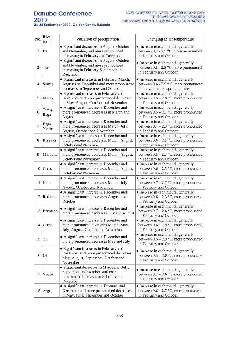
553

No. River basin Variation of precipitation Changing in air temperature

2 Iza ● Significant decreases in August, October

and November, and more pronounced increasing in February and December

● Increase in each month, generally between 0,7 - 2,5 °C, more pronounced in February and October

3 Tur

● Significant decreases in August, October and November, and more pronounced increasing in February September and December

● Increase in each month, generally between 0,5 - 2,3 °C, more pronounced in February and October

4 Someș ● Significant increases in February, March,

August and December and more pronounced decreases in September and October

● Increase in each month, generally between 0.6 - 2.5 ° C, more pronounced in the winter and spring months

5 Mureș ● Significant increases in February and

December and more pronounced decreases in May, August, October and November

● Increase in each month, generally between 0.5 – 2.8 °C, more pronounced in February and October

6 Timiș-Bega

● A significant increase in December and more pronounced decreases in March and August

● Increase in each month, generally between 0.5 – 2.7 °C, more pronounced in February and October

7 Bega Veche

● A significant increase in December and more pronounced decreases March, July, August, October and November

● Increase in each month, generally between 0.4 – 2.3 °C, more pronounced in February and October

8 Bârzava ● A significant increase in December and

more pronounced decreases March, August, October and November

● Increase in each month, generally between 0.6 – 2.5 °C, more pronounced in February and October

9 Moravița ● A significant increase in December and

more pronounced decreases March, August, October and November

● Increase in each month, generally between 0.5 – 2.3 °C, more pronounced in February and October

10 Caras ● A significant increase in December and

more pronounced decreases March, August, October and November

● Increase in each month, generally between 0.6 – 2.5 °C, more pronounced in February and October

11 Nera ● A significant increase in December and

more pronounced decreases March, July, August, October and November

● Increase in each month, generally between 0.7 – 2.7 °C, more pronounced in February and October

12 Radimna ● A significant increase in December and

more pronounced decreases August and October

● Increase in each month, generally between 0.6 – 2.3 °C, more pronounced in February and October

13 Berzasca ● A significant increase in December and more pronounced decreases July and August

● Increase in each month, generally between 0.7 – 2.6 °C, more pronounced in February and October

14 Cerna ● A significant increase in December and

more pronounced decreases March, May, July, August, October and November

● Increase in each month, generally between 0.6 – 2.9 °C, more pronounced in February and October

15 Jiu ● A significant increase in December and more pronounced decreases May and July

● Increase in each month, generally between 0.5 – 2.9 °C, more pronounced in February and October

16 Olt

● Significant increases in February and December and more pronounced decreases May, August, September, October and November

● Increase in each month, generally between 0.5 – 3.0 °C, more pronounced in February and October

17 Vedea

● Significant decreases in May, June, July, September and October, and more pronounced increases in February and December

● Increase in each month, generally between 0.7 – 2.6 °C, more pronounced in February and October

18 Argeș ● A significant increase in February and

December and more pronounced decreases in May, June, September and October

● Increase in each month, generally between 0.6 – 2.7 °C, more pronounced in February and October

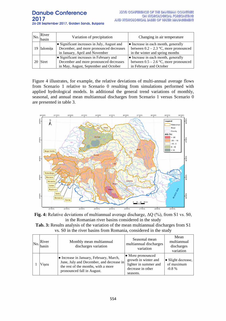
554

No. River basin Variation of precipitation Changing in air temperature

19 Ialomița ● Significant increases in July, August and

December, and more pronounced decreases in January, April and November

● Increase in each month, generally between 0.2 – 2.3 °C, more pronounced in the winter and spring months

20 Siret ● Significant increases in February and

December and more pronounced decreases in May, August, September and October

● Increase in each month, generally between 0.5 – 2.6 °C, more pronounced in February and October

Figure 4 illustrates, for example, the relative deviations of multi-annual average flows from Scenario 1 relative to Scenario 0 resulting from simulations performed with applied hydrological models. In additional the general trend variations of monthly, seasonal, and annual mean multiannual discharges from Scenario 1 versus Scenario 0 are presented in table 3.

Fig. 4: Relative deviations of multiannual average discharge, ΔQ (%), from S1 vs. S0,

in the Romanian river basins considered in the study Tab. 3: Results analysis of the variation of the mean multiannual discharges from S1

vs. S0 in the river basins from Romania, considered in the study

No. River basin

Monthly mean multiannual discharges variation

Seasonal mean multiannual discharges

variation

Mean multiannual discharges variation

1 Vișeu

● Increase in January, February, March, June, July and December, and decrease in the rest of the months, with a more pronounced fall in August.

● More pronounced growth in winter and lighter in summer and decrease in other seasons.

● Slight decrease, of maximum -0.8 %

555

No. River basin

Monthly mean multiannual discharges variation

Seasonal mean multiannual discharges

variation

Mean multiannual discharges variation

2 Iza ● A significant increase in the winter

months and a more pronounced decrease in April and August.

● Growth in winter and decrease in other seasons.

● Slight decrease, of maximum -2.6 %

3 Tur

● Increase in January, February, June, July, September and December, and decrease in the rest of the months, with the fall being more pronounced in April, August, October and November.

● Growth in winter and decrease in other seasons.

● Slight decrease, of maximum -3.6 %

4 Someș ● Significant increase in December,

January, February and March, and decrease in May and October.

● Growth in winter, spring and summer and decrease in autumn.

● Increase, of maximum 23.4 %

5 Mureș ● Significant increase in January, February

and March, and decrease in August, September, October and November.

● Growth in winter and decrease in other seasons.

● Decrease, of maximum -14.2 %

6 Timiș-Bega

● Significant increase in February and December and decrease in March, April and August-November.

● Growth in winter and decrease in other seasons.

● Decrease, of maximum -14.3 %

7 Bega Veche

● Slight increase in June and decrease in the other months, with more pronounced decreases between September and November.

● Slighter decrease in the summer and more pronounced in the autumn.

● Decrease, of maximum -15.5 %

8 Bârzava

● Increase in February and decrease in the other months, with more pronounced decreases in March, April and between September and November.

● Slight increase in winter and decrease slighter in summer and more pronounced in other seasons.

● Decrease, of maximum -14.6 %

9 Moravița ● Decrease of discharges in all months of

the year, more pronounced in March, April and September – December.

● Decrease in all the seasons

● Decrease, of maximum -24.6 %

10 Caraş

● Slight increase in February and decrease in the other months, with more pronounced decreases in March and September to November.

● Lighter decreasing, in summer and winter and more pronounced in other seasons

● Decrease, of maximum -18.8 %

11 Nera

● Increase in January, February, June and December and decreases in the other months, with more pronounced decrease in March-April and August-November

● Growth in winter and decrease in other seasons.

● Decrease, of maximum -11.1 %

12 Radimna

● Increase in February and decrease in the other months, with more pronounced decreases in March and the period August to November.

● Growth in winter and decrease in other seasons.

● Decrease, of maximum -10.4 %

13 Berzasca

● Increase in February and decreases in the other months, with more pronounced decreases in March and between August and November

● Slight increase in winter and decrease in other seasons.

● Decrease, of maximum -14.5 %

14 Cerna

● Increase in December, January and February and decreases in the other months, more pronounced in April and May.

● Growth in winter and decrease in other seasons.

● Decrease, of maximum -13.0 %

15 Jiu ● Significant increase in January and

February and decrease in May, September and November.

● Growth in winter and decrease in other seasons.

● Decrease, of maximum -22.3 %

556

No. River basin

Monthly mean multiannual discharges variation

Seasonal mean multiannual discharges

variation

Mean multiannual discharges variation

16 Olt ● Significant increase in January and

February and decrease in April, May, June, October and November

● Growth in winter and decrease in other seasons.

● Decrease, of maximum -14.4 %

17 Vedea ● Increase in February and decrease in all

other months, more pronounced in the period March – July.

● Slight increase in winter and decrease in other seasons.

● Decrease, of maximum -38.4 %

18 Argeș ● Significant increase in February, March

and December, and decrease in May, September and October.

● Growth in winter and decrease in other seasons.

● Decrease, of maximum -12.2 %

19 Ialomița ● Significant increase in February, August

and September and decrease in April, May and June

● Growth in winter and autumn and decrease in other seasons.

● Decrease, of maximum -8.5 %

20 Siret ● A significant increase in February and

March and decrease in April, May, August, September and November.

● Growth in winter and decrease in other seasons.

● Decrease, of maximum -13.4 %

5. CONCLUSIONS From the comparative analysis for Scenario 1 relative to Scenario 0, the precipitation and mean temperatures on the sub-basins, corresponding to the considered gauging stations from the analyzed river basins, resulted the following:

• The monthly precipitation regime, multiannual averages, has a general individualized tendency on the 20 analyzed river basins, as follows: Vişeu ▪ increase of 0,4% (between a minimum of 0,1% and a maximum of 0,9%); Iza ▪ decrease of -0,5% (-0,9% ÷ -0,1%); Tur ▪ decrease of -1,3% (-1,8% ÷ -0,8%); Someş ▪ increase of 5,6% (2,0% ÷ 12,2%); Mureş ▪ decrease of -5,0% (-8,0% ÷ -2,9%); Timiş-Bega ▪ decrease of -6,5% (-6,7% ÷ -6,2%); Bega Veche ▪ decrease of -3,8% (-4,7% ÷ -3,3%); Bârzava ▪ decrease of -6,5% (-6,7% ÷ -6,4%); Moraviţa ▪ decrease of -6,3%; Caraş ▪ decrease of -6,1% (-6,3% ÷ -5,8%); Nera ▪ decrease of -6,7% (-7,4% ÷ -6,5%); Radimna ▪ decrease of -5,8%; Berzasca ▪ decrease of -7,8%; Cerna ▪ decrease de -8,3% (-9,3% ÷ -7,0%); Jiu ▪ decrease of -8,9% (-10,6% ÷ -7,2%); Olt ▪ decrease of -5,3% (-8,9% ÷ -2,2%); Vedea ▪ decrease of -5,0% (-5,8% ÷ -3,8%); Argeş ▪ decrease of -4,7% (-6,0% ÷ -2,4%); Ialomiţa ▪ increase of 1,1% (-2,2% ÷ 3,5%); Siret ▪ decrease of -1,4% (-2,8% ÷ 1,2%).

• From the point of view of the air temperatures, monthly multi-annual average, there is a general increasing in all of 20 the analyzed river basins, as follows: Vişeu ▪ 1,2°C; Iza ▪ 1,2°C; Tur ▪ 1,2°C; Someş ▪ 1,4°C; Mureş ▪ 1,3°C; Timiş-Bega ▪ 1,3°C; Bega Veche ▪ 1,2 °C; Bârzava ▪ 1,3 °C; Moraviţa ▪ 1,2 °C; Caraş ▪ 1,3 °C; Nera ▪ 1,4°C; Radimna ▪ 1,3°C; Berzasca ▪ 1,4°C; Cerna ▪ 1,5°C; Jiu ▪ 1,5°C; Olt ▪ 1,3°C; Vedea ▪ 1,4°C; Argeş ▪ 1,4°C; Ialomiţa ▪ 1,3°C; Siret ▪ 1,3°C.

Following the analysis of the hydrological simulations determined by these trends of the meteorological parameters variation, the following changes of the multiannual average discharge regime are observed:

• Vişeu ▪ decrease of -0,1% (between a minimum of -0,8% and a maximum of 0,6%); Iza ▪ decrease of -1,9% (-2,6% ÷ -0,3%); Tur ▪ decrease of -2,5% (-3,6% ÷ -1,4%);

557

Someş ▪ increase of 6,2% (-0,5% ÷ 23,4%); Mureş ▪ decrease of -9,9% (-14,2% ÷ -6,9%); Timiş-Bega ▪ decrease of -13,1% (-14,3% ÷ -12,1%); Bega Veche ▪ decrease of -13,9% (-15,5% ÷ -11,6%); Bârzava ▪ decrease of -11,9% (-14,6% ÷ -10,3%); Moraviţa ▪ decrease of -21,9% (-24,6% ÷ -19,2%); Caraş ▪ decrease of -14,7% (-18,8% ÷ -8,5%); Nera ▪ decrease of -9,2% (-11,1% ÷ -8,1%); Radimna ▪ decrease of -10,4%; Berzasca ▪ decrease of -14,5%; Cerna ▪ decrease of -10,0% (-13,0% ÷ -8,4%); Jiu ▪ decrease of -11,0% (-22,3% ÷ -3,8%); Olt ▪ decrease of -9,5% (-14,4% ÷ -4,6%); Vedea ▪ decrease of -24,6% (-38,4% ÷ -11,6%); Argeş ▪ decrease of -8,6% (-12,2% ÷ -1,7%); Ialomiţa ▪ decrease of -5,8% (-8,5% ÷ -2,2%); Siret ▪ decrease of -9,6% (-13,4% ÷ -4,6%).

6. REFERENCES [1] Kaczmarek, Z. Water Balance Model for Climate Impact Analysis, ACTA Geophysica Polonica, v. 41, no. 4, 1-16, 1993.

[2] Yates, D. WatBal – An Integrated Water Balance Model for Climate Impact Assessment of River Basin Runoff, IIASA Working Paper, WP-94-64, Laxenburg, Austria, 1994.

[3] Shuttelworth, W. J. Evaporation. In: Maidment D. R. (Ed.) Handbook of Hydrology, McGraw-Hill Book Company, New York City, New York, 4.1-4.53, 1993.

[4] Priestly, C., Taylor, R. On the Assessment of Surface Heat Flux and Evaporation Using Large Scale Parameters, Mon. Weather Rev., vol. 100, pp. 81-92, 1972.

[5] Ozga-Zielinska, M., Brzenzinski, J., Feluch, W. Meso-Scale Hydrologic Modeling for Climate Impact Assessment: A Conceptual and a Regression Approach, IIASA, CP-94-10, 1994.

[6] Corbuş, C., Mic, R., Mătreaţă, M. Assessment of climate change impact on peak flow regime in the Mureş river basin, XXVth Conference of Danubian Countries, 16 - 17 June, Budapest, 2011.

[7] Şerban P., Simota M. Forecast model of flood waves on Romanian rivers, tributary of the Iron Gates Reservoir, Meteorology and Hydrology no. 1, I.N.M.H., Bucharest, 1992.

[8] Şerban, P., Simota, M., Corbuş, C. Model for the forecasting of daily mean discharges. XVI Konferenz der Donauländer über hydrologische Vorhersagen und hydrologisch-wasserwirtschaftliche Grundlagen, 18-22 Mai, Kelheim, 1992.

[9] Şerban, P., Simota, M., Corbuş, C. Runoff simulation model in the mountain hydrographic basins, International Conference Developments in Hydrology of Mountainous Areas, 12-16 September, Stará Lesná, Slovakia, 1994.

[10] Mic, R.P., Corbuş, C., Mătreaţă, M. Long-term flow simulation in Bârlad river basin using Romanian hydrological model Consul. Carpathian Journal of Earth and Environmental Sciences, ISSN 1842-4090, November 2015, Vol. 10, No 4, p. 145 – 156, 2015.

[11] *** CLAVIER project - "Variables and Climate Change: the Impact on Central and Eastern Europe", funded by the European Union under the 6th Framework Program, 2006-2009.

558

RIVER BASIN MODELING UNDER FUTURE CLIMATE CONDITIONS. IMPACT APPROACH. PART I

Elena Bojilova

National Institute of Meteorology and Hydrology – Bulgarian Academy of Sciences, Sofia, Bulgaria

Corresponding author: Elena Bojilova, National Institute of Meteorology and Hydrology, Tzarigradsko chaussee 66, 1784 Sofia, Bulgaria, Elena.Kirilova.Bojilova@gmail.com

The global climate change and climate variability may have serious impacts on the frequency, magnitude, location and duration of hydrological extremes. Changed hydrological extremes will have important implications on the water resources management, flood-plane development, design of hydraulic structure etc. We are proposing the impact approach (IPCC, 2001 and 2007) to investigate the potential impact of a changed climate to the timing and magnitude of hydrological extremes in populated and urbanized river basins in North Bulgaria. The assessment of climate variability and change effects on the hydrological cycle is of vital importance to all socioeconomic sectors. It challenges the international efforts to promote social and environmental sustainability. According to the Intergovernmental Panel on Climate Change (IPCC, 2007) with regards to its current sensitivities to climate, Southeastern Europe (in particularly Bulgaria) was found to be most sensitive to the: - extreme seasons, in particular exceptionally hot and dry summers and mild winters and; - short-duration events such as windstorms and heavy rains. We could base our research on the outcomes from a global 20-km mesh atmospheric general circulation model. Using data computed from the model projections, environmental changes that may lead to disasters such as floods, droughts or a heavy rainfall events will be evaluated for North Bulgaria. Moreover, impact assessment of climate change on water resources in selected watersheds in North Bulgaria is performed. The impact approach has three steps (IPCC, 2001, 2007): calibration and verification of an appropriate hydrological model using observed hydrological and meteorological data; derivation of climate change scenarios; and run of the model under new climate conditions, analyzing impacts by comparing the results with the so-called baseline simulation. The semi-distributed hydrological model is proposed and applied to the selected river basins located in North Bulgaria. An ensemble of future climate scenarios will be used. Further, the climate scenarios will be applied as input into hydrological models of the study watersheds. Our main task will be to analyses the impacts by comparing the results with the baseline simulation.

INTRODUCTION One of the most significant potential consequences of climate variability and change may be alternations in the regional hydrological cycle and subsequent changes in river

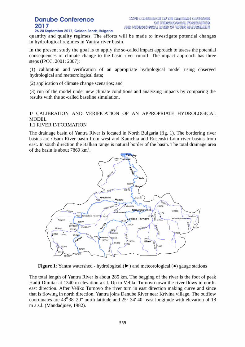
559

quantity and quality regimes. The efforts will be made to investigate potential changes in hydrological regimes in Yantra river basin. In the present study the goal is to apply the so-called impact approach to assess the potential consequences of climate change to the basin river runoff. The impact approach has three steps (IPCC, 2001; 2007): (1) calibration and verification of an appropriate hydrological model using observed hydrological and meteorological data; (2) application of climate change scenarios; and (3) run of the model under new climate conditions and analyzing impacts by comparing the results with the so-called baseline simulation. 1/ CALIBRATION AND VERIFICATION OF AN APPROPRIATE HYDROLOGICAL MODEL 1.1 RIVER INFORMATION The drainage basin of Yantra River is located in North Bulgaria (fig. 1). The bordering river basins are Osam River basin from west and Kamchia and Rusenski Lom river basins from east. In south direction the Balkan range is natural border of the basin. The total drainage area of the basin is about 7869 km2.

Figure 1: Yantra watershed - hydrological (►) and meteorological (●) gauge stations

The total length of Yantra River is about 285 km. The begging of the river is the foot of peak Hadji Dimitar at 1340 m elevation a.s.l. Up to Veliko Turnovo town the river flows in north-east direction. After Veliko Turnovo the river turn in east direction making curve and since that is flowing in north direction. Yantra joins Danube River near Krivina village. The outflow coordinates are 430 38' 20" north latitude and 25° 34' 40" east longitude with elevation of 18 m a.s.l. (Mandadjuev, 1982).

Studen

a

Yantra

Rosiza

Rosiza

Eliiska

Mugura

ChaparataVidima

Vidima

Lolychniza

Dria

novs

ka

Beliza

Veselina

KotelskaBabrovska

Dju

luni

za

Goliam

a

Ialadere

Goliama

Negovanka

Bohot

Alex Stamboliiski Reservoir

KrapezYastrebino reservoir

Novgrad

Polikraiche

Karanzi

Samovodiane

Biala

Gorna Oriahoviza

Veliko Tarnovo

Gabrovo

Sevlievo

Pavlikeni

Drianovo

Elena

Yant

ra

Danube

Krycheto

23700

236500743006470

70406020

6480

6010

06401 06410

06420

7010

7020

7050

23180

23200

23230

23250

23500

23450

23550

2335023030

23400

23150

23570

23850

50600

7440

7470

22020

22460

7420

22530

23100

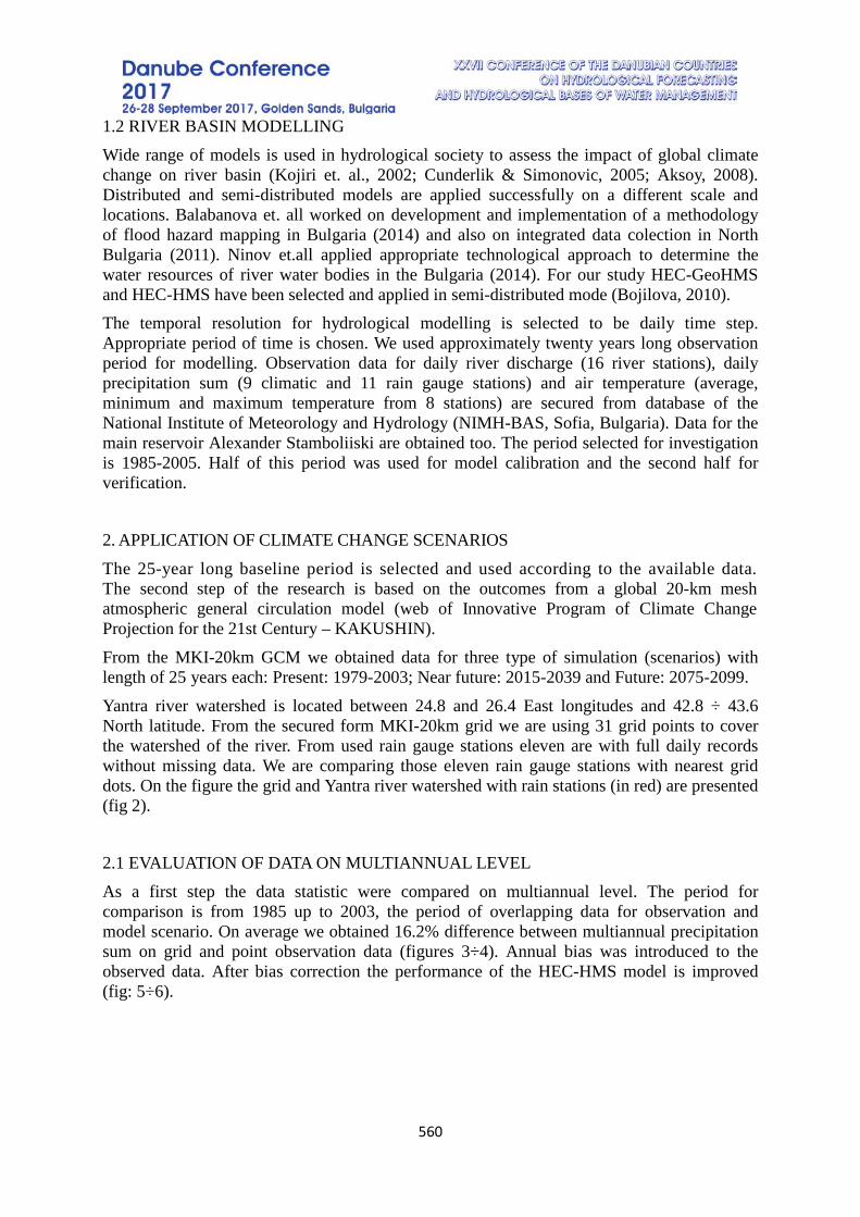
560

1.2 RIVER BASIN MODELLING Wide range of models is used in hydrological society to assess the impact of global climate change on river basin (Kojiri et. al., 2002; Cunderlik & Simonovic, 2005; Aksoy, 2008). Distributed and semi-distributed models are applied successfully on a different scale and locations. Balabanova et. all worked on development and implementation of a methodology of flood hazard mapping in Bulgaria (2014) and also on integrated data colection in North Bulgaria (2011). Ninov et.all applied appropriate technological approach to determine the water resources of river water bodies in the Bulgaria (2014). For our study HEC-GeoHMS and HEC-HMS have been selected and applied in semi-distributed mode (Bojilova, 2010). The temporal resolution for hydrological modelling is selected to be daily time step. Appropriate period of time is chosen. We used approximately twenty years long observation period for modelling. Observation data for daily river discharge (16 river stations), daily precipitation sum (9 climatic and 11 rain gauge stations) and air temperature (average, minimum and maximum temperature from 8 stations) are secured from database of the National Institute of Meteorology and Hydrology (NIMH-BAS, Sofia, Bulgaria). Data for the main reservoir Alexander Stamboliiski are obtained too. The period selected for investigation is 1985-2005. Half of this period was used for model calibration and the second half for verification. 2. APPLICATION OF CLIMATE CHANGE SCENARIOS The 25-year long baseline period is selected and used according to the available data. The second step of the research is based on the outcomes from a global 20-km mesh atmospheric general circulation model (web of Innovative Program of Climate Change Projection for the 21st Century – KAKUSHIN). From the MKI-20km GCM we obtained data for three type of simulation (scenarios) with length of 25 years each: Present: 1979-2003; Near future: 2015-2039 and Future: 2075-2099. Yantra river watershed is located between 24.8 and 26.4 East longitudes and 42.8 ÷ 43.6 North latitude. From the secured form MKI-20km grid we are using 31 grid points to cover the watershed of the river. From used rain gauge stations eleven are with full daily records without missing data. We are comparing those eleven rain gauge stations with nearest grid dots. On the figure the grid and Yantra river watershed with rain stations (in red) are presented (fig 2). 2.1 EVALUATION OF DATA ON MULTIANNUAL LEVEL As a first step the data statistic were compared on multiannual level. The period for comparison is from 1985 up to 2003, the period of overlapping data for observation and model scenario. On average we obtained 16.2% difference between multiannual precipitation sum on grid and point observation data (figures 3÷4). Annual bias was introduced to the observed data. After bias correction the performance of the HEC-HMS model is improved (fig: 5÷6).

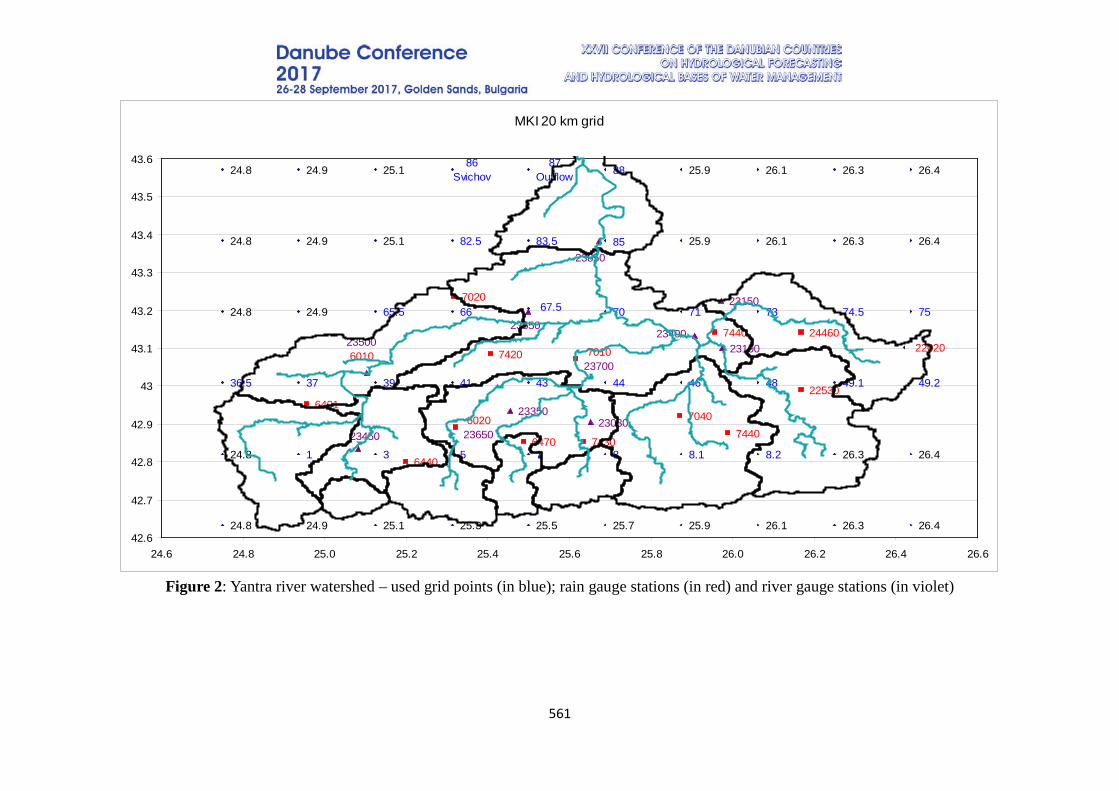
561

Figure 2: Yantra river watershed – used grid points (in blue); rain gauge stations (in red) and river gauge stations (in violet)

MKI 20 km grid

24.8 24.9 25.1 25.3 25.5 25.7 25.9 26.1 26.3 26.4

24.8 26.3 26.4

24.8

24.8 24.9 25.1 25.9 26.1 26.3 26.4

24.8 24.9 25.1 25.9 26.1 26.3 26.4

23850

235006010

23550

8887

Outflow86

Svichov

8583.582.5

74.573717067.56665.524.9

48464443413936.5 37

87531

49.1

757020 23150

2340023100

7440 2446022020

22530

74407040

8.1 8.274306470

701023700

7420

23350230306020

23650

6401

23450

6440

49.2

42.6

42.7

42.8

42.9

43

43.1

43.2

43.3

43.4

43.5

43.6

24.6 24.8 25.0 25.2 25.4 25.6 25.8 26.0 26.2 26.4 26.6

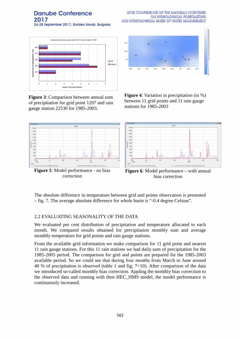
562

Figure 3: Comparison between annual sum of precipitation for grid point 1207 and rain gauge station 22530 for 1985-2003.

Figure 4: Variation in precipitation (in %) between 11 grid points and 11 rain gauge stations for 1985-2003

Figure 5: Model performance - no bias

correction

Figure 6: Model performance – with annual

bias correction

The absolute difference in temperature between grid and points observation is presented – fig. 7. The average absolute difference for whole basin is “-0.4 degree Celsius”. 2.2 EVALUATING SEASONALITY OF THE DATA We evaluated per cent distribution of precipitation and temperature allocated to each month. We compared results obtained for precipitation monthly sum and average monthly temperature for grid points and rain gauge stations. From the available grid information we make comparison for 11 grid point and nearest 11 rain gauge stations. For this 11 rain stations we had daily sum of precipitation for the 1985-2005 period. The comparison for grid and points are prepared for the 1985-2003 available period. So we could see that during four months from March to June around 40 % of precipitation is observed (table 1 and fig: 7÷10). After comparison of the data we introduced so-called monthly bias correction. Appling the monthly bias correction to the observed data and running with then HEC_HMS model, the model performance is continuously increased.

Comparison betw een gride point 1207-48 and station 22530

0 1 2 3 4 5 6 7 8

850

750

650

550

400

annu

al s

um o

f pre

cipi

tatio

n, m

m

numer of occurrences

grid

stations

24.8 25 25.2 25.4 25.6 25.8 26 26.2 26.4

43

43.2

43.4

-8-6-4-202468101214161820222426283032343638404244

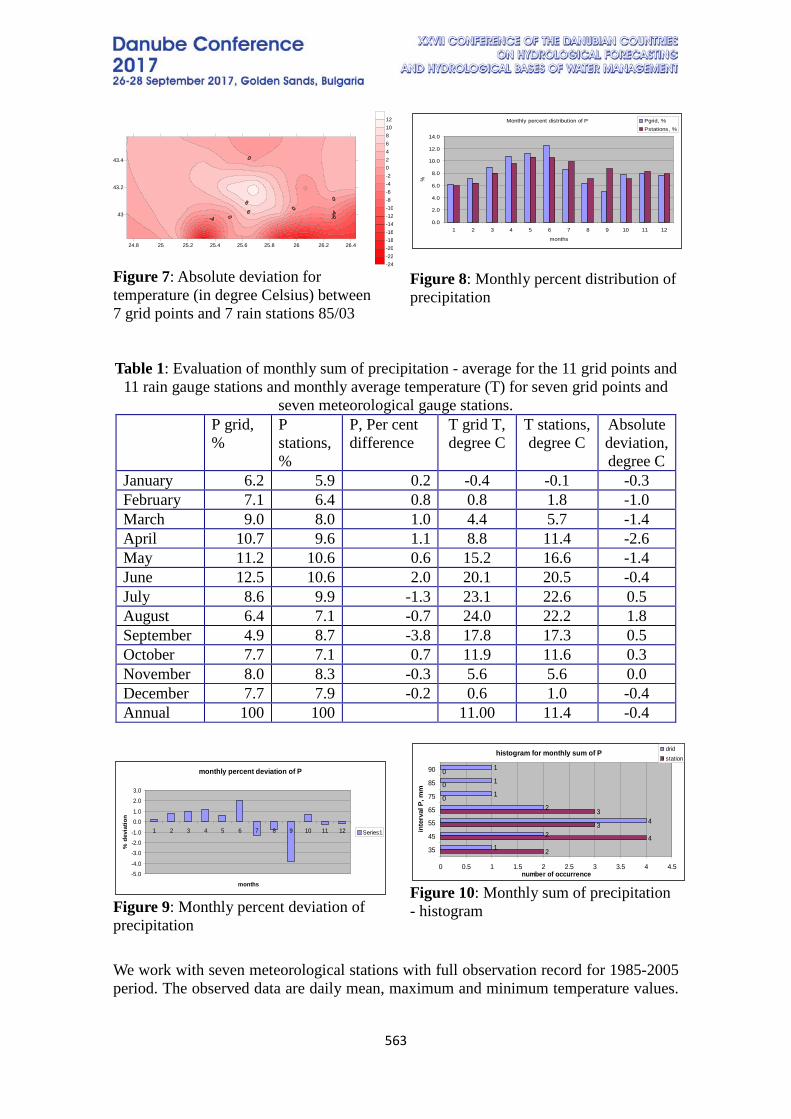
563

Figure 7: Absolute deviation for temperature (in degree Celsius) between 7 grid points and 7 rain stations 85/03

Figure 8: Monthly percent distribution of precipitation

Table 1: Evaluation of monthly sum of precipitation - average for the 11 grid points and 11 rain gauge stations and monthly average temperature (T) for seven grid points and

seven meteorological gauge stations. P grid,

% P stations, %

P, Per cent difference

T grid T, degree C

T stations, degree C

Absolute deviation, degree C

January 6.2 5.9 0.2 -0.4 -0.1 -0.3 February 7.1 6.4 0.8 0.8 1.8 -1.0 March 9.0 8.0 1.0 4.4 5.7 -1.4 April 10.7 9.6 1.1 8.8 11.4 -2.6 May 11.2 10.6 0.6 15.2 16.6 -1.4 June 12.5 10.6 2.0 20.1 20.5 -0.4 July 8.6 9.9 -1.3 23.1 22.6 0.5 August 6.4 7.1 -0.7 24.0 22.2 1.8 September 4.9 8.7 -3.8 17.8 17.3 0.5 October 7.7 7.1 0.7 11.9 11.6 0.3 November 8.0 8.3 -0.3 5.6 5.6 0.0 December 7.7 7.9 -0.2 0.6 1.0 -0.4 Annual 100 100 11.00 11.4 -0.4

Figure 9: Monthly percent deviation of precipitation

Figure 10: Monthly sum of precipitation - histogram

We work with seven meteorological stations with full observation record for 1985-2005 period. The observed data are daily mean, maximum and minimum temperature values.

24.8 25 25.2 25.4 25.6 25.8 26 26.2 26.4

43

43.2

43.4

-24-22-20-18-16-14-12-10-8-6-4-2024681012 Monthly percent distribution of P

0.0

2.0

4.0

6.0

8.0

10.0

12.0

14.0

1 2 3 4 5 6 7 8 9 10 11 12

months

%

Pgrid, %Pstations, %

monthly percent deviation of P

-5.0-4.0

-3.0-2.0-1.0

0.01.0

2.03.0

1 2 3 4 5 6 7 8 9 10 11 12

months

% d

evia

tion

Series1

histogram for monthly sum of P

1

1

1

2

4

2

1

0

0

0

3

3

4

2

0 0.5 1 1.5 2 2.5 3 3.5 4 4.5

90

85

75

65

55

45

35

inte

rval

P, m

m

number of occurrence

dridstation

564

From the MKI – 20 km GC Model we received hourly data record for 1979-2003 period. For comparison in our research we used daily mean temperature, monthly average temperature and annual mean temperature for 1985-2003. (table 1 and figures 11÷12).

Figure 11: Monthly mean temperatures

Figure 12: Absolute differences in temperature, (degree C)

2.3 SCENARIOS COMPARISON We do compare the three scenarios from MKI-20km GCM: Present 1979-2003; Near future 2015-2039 and Future 2075-2099. From the GCModel we had hourly data for precipitation, temperature and wind speed. Also we had three hourly data for Downward Shortwave Radiation (SWdn, in W/m2), Downward Long-wave Radiation (LWdn in W/m2); Specific Humidity (Qair, kg/kg) and Surface Air Pressure (Psfc, in Pa) For precipitation we prepared variation map in percent using following expression: Variation=(Pnear future- Ppresent)/ Ppresent*100, in % and also Variation =(Pfuture- Ppresent)/ Ppresent*100, in %. We used the same formula to calculate variation for Downward Shortwave and Long-wave Radiation. Generally we prepare two maps for every parameter for the cases:

- case one: Near future-Present and - case two: Future-Present.

For annual mean temperature and annual average wind speed we used absolute deviation: Deviation =(Tnear future- Tpresent), in degree C and Deviation=(Tfuture- Tpresent), in degree C. Similar expression is used for calculation of deviation for specific humidity (in kg/kg) and surface air pressure (in Pa). The received up to now results are shown in the list of figures from 30 up to 43. In table 2 average values for the grid for the seven parameters for comparison between two scenarios: Near future-Present and Future-Present are presented. So we could observed that deviation in annul sum of precipitation is increased from 3.5% to 5.33%. As in agreement with most of the existing climate change scenarios we expected decrease in precipitation sum and increase in temperature (fig:

Monthly multiannual temperature

-5.0

0.0

5.0

10.0

15.0

20.0

25.0

30.0

1 2 3 4 5 6 7 8 9 10 11 12

Temperature, degree C

mon

ths

average gridaverage Yantra stations

delta

-3.0-2.5-2.0

-1.5-1.0-0.50.00.5

1.01.52.0

1 2 3 4 5 6 7 8 9 10 11 12

Months

devi

atio

n: T

grid

-Tst

atio

ns, d

egre

e C

delta

565

13÷***). For multiannual wind speed and Surface Air Pressure we could not detect significant signals for changes. We could expect according to the scenarios increase in Downward Shortwave Radiation from 2.17% for the Near future-Present to 3.63% for scenario Future-Present. Similar tendency we could expect in Downward Long-wave Radiation from 2.28% up to 5.76%.

Figure 13: Variation for precipitation: comparison between Near future and Present (%)

Figure 14: Variation for precipitation: comparison between Future and Present (%)

Figure 15: Absolute deviation for temperature: Near future – Present, (degree C)

Figure 16: Absolute deviation for temperature: Future – Present (degree C)

Figure 17: Absolute variation for annual average wind speed: Near future–Present, (m/s)

Figure 18: Absolute variation for annual average wind speed: Future – Present (m/s)

Figure 19: Variation in Downward long-wave radiation: Near Future-Present, (W/m2)

Figure 20: Variation in Downward long-wave radiation: Future-Present, (W/m2)

24.8 25 25.2 25.4 25.6 25.8 26 26.2 26.4

43

43.2

43.4

-11-10-10-9.5-9-8.5-8-7.5-7-6.5-6-5.5-5-4.5-4-3.5-3-2.5-2-1.5-1-0.500.511.522.5

24.8 25 25.2 25.4 25.6 25.8 26 26.2 26.4

43

43.2

43.4

-8.5

-8

-7.5

-7

-6.5

-6

-5.5

-5

-4.5

-4

-3.5

-3

-2.5

-2

-1.5

-1

24.8 25 25.2 25.4 25.6 25.8 26 26.2 26.4

43

43.2

43.4

0.8

0.9

1

1.1

1.2

1.3

1.4

1.5

1.6

1.65

1.7

24.8 25 25.2 25.4 25.6 25.8 26 26.2 26.4

43

43.2

43.4

3.33.323.343.363.383.43.423.443.463.483.53.523.543.563.583.63.623.64

24.8 25 25.2 25.4 25.6 25.8 26 26.2 26.4

43

43.2

43.4

0.010.0150.020.0250.030.040.050.060.070.080.090.10.110.120.130.140.15

24.8 25 25.2 25.4 25.6 25.8 26 26.2 26.4

43

43.2

43.4

0.0140.0180.0220.0260.0280.0320.0360.040.0440.0480.0520.0560.060.0640.0680.0720.076

24.8 25 25.2 25.4 25.6 25.8 26 26.2 26.4

43

43.2

43.4

-4.5-4-3.5-3-2.5-2-1.5-1-0.500.511.522.533.544.55

24.8 25 25.2 25.4 25.6 25.8 26 26.2 26.4

43

43.2

43.4

44.24.44.64.855.25.45.65.866.26.46.66.877.27.47.67.888.28.4

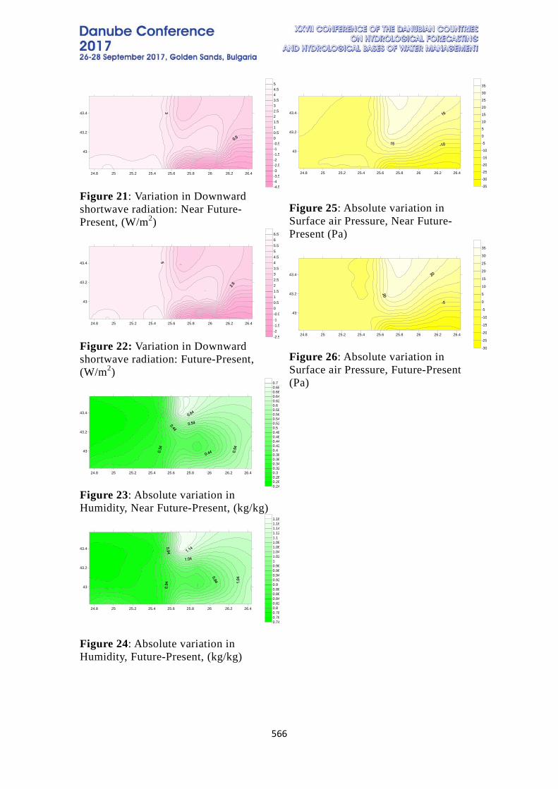
566

Figure 21: Variation in Downward shortwave radiation: Near Future-Present, (W/m2)

Figure 22: Variation in Downward shortwave radiation: Future-Present, (W/m2)

Figure 23: Absolute variation in Humidity, Near Future-Present, (kg/kg)

Figure 24: Absolute variation in Humidity, Future-Present, (kg/kg)

Figure 25: Absolute variation in Surface air Pressure, Near Future-Present (Pa)

Figure 26: Absolute variation in Surface air Pressure, Future-Present (Pa)

24.8 25 25.2 25.4 25.6 25.8 26 26.2 26.4

43

43.2

43.4

-4.5-4-3.5-3-2.5-2-1.5-1-0.500.511.522.533.544.55

24.8 25 25.2 25.4 25.6 25.8 26 26.2 26.4

43

43.2

43.4

-2.5-2-1.5-1-0.500.511.522.533.544.555.566.5

24.8 25 25.2 25.4 25.6 25.8 26 26.2 26.4

43

43.2

43.4

0.240.260.280.30.320.340.360.380.40.420.440.460.480.50.520.540.560.580.60.620.640.660.680.7

24.8 25 25.2 25.4 25.6 25.8 26 26.2 26.4

43

43.2

43.4

0.740.760.780.80.820.840.860.880.90.920.940.960.9811.021.041.061.081.11.121.141.161.18

24.8 25 25.2 25.4 25.6 25.8 26 26.2 26.4

43

43.2

43.4

-35

-30

-25

-20

-15

-10

-5

0

5

10

15

20

25

30

35

24.8 25 25.2 25.4 25.6 25.8 26 26.2 26.4

43

43.2

43.4

-30

-25

-20

-15

-10

-5

0

5

10

15

20

25

30

35

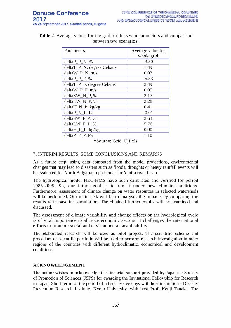
567

Table 2: Average values for the grid for the seven parameters and comparison between two scenarios.

Parameters Average value for whole grid

deltaP_P_N, % -3.50 deltaT_P_N, degree Celsius 1.49 deltaW_P_N, m/s 0.02 deltaP_P_F, % -5.33 deltaT_P_F, degree Celsius 3.49 deltaW_P_F, m/s 0.05 deltaSW_N_P, % 2.17 deltaLW_N_P, % 2.28 deltaH_N_P, kg/kg 0.41 deltaP_N_P, Pa -0.01 deltaSW_F_P, % 3.63 deltaLW_F_P, % 5.76 deltaH_F_P, kg/kg 0.90 deltaP_F_P, Pa 1.10

*Source: Grid_Uji.xls 7. INTERIM RESULTS, SOME CONCLUSIONS AND REMARKS As a future step, using data computed from the model projections, environmental changes that may lead to disasters such as floods, droughts or heavy rainfall events will be evaluated for North Bulgaria in particular for Yantra river basin. The hydrological model HEC-HMS have been calibrated and verified for period 1985-2005. So, our future goal is to run it under new climate conditions. Furthermore, assessment of climate change on water resources in selected watersheds will be performed. Our main task will be to analyses the impacts by comparing the results with baseline simulation. The obtained further results will be examined and discussed. The assessment of climate variability and change effects on the hydrological cycle is of vital importance to all socioeconomic sectors. It challenges the international efforts to promote social and environmental sustainability. The elaborated research will be used as pilot project. The scientific scheme and procedure of scientific portfolio will be used to perform research investigation in other regions of the countries with different hydroclimatic, economical and development conditions.

ACKNOWLEDGEMENT The author wishes to acknowledge the financial support provided by Japanese Society of Promotion of Sciences (JSPS) for awarding the Invitational Fellowship for Research in Japan, Short term for the period of 54 successive days with host institution - Disaster Prevention Research Institute, Kyoto University, with host Prof. Kenji Tanaka. The

568

necessary data were provided from NIMH-BAS for modelling of the Yantra River Basin and from DPRI-KU for the MRI – 20km GCM model. Balabanova et.all worked on development and implementation of a methodology of flood hazard mapping in Bulgaria (2014) and also on integrated data colection in North Bulgaria (2011). Ninov et.all evelueted appropriate technological approach to determine the water resources of river water bodies in the Bulgaria (2014).

REFERENCES Balabanova, Sn., Stoyanova, S. Integrated data collection and dissemination in North

Bulgarian river basins. Open Water Symposium and workshops, Delft UNESCO-IHE 18-19 April, 2011

Balabanova, Sn., Yordanova, V., Popova. V. Development and implementation of a methodology of flood hazard mapping in Bulgaria, as required by Directive 2007/60 / EC", Analysis and Management of Changing Risks for Natural Hazards, 18-19.11 2014, Padua, Italy, full paper text at http://www.changes-itn.eu/Portals/0/Content/2014/Final%20conference/abstracts/CP7_Abstract_Balabanova.pdf

Bojilova, E. 2006, Integrated river basin modelling, Bulgarian case study, HydroEco2006, Multidisciplinary conference, Karlovy Vary, Czech Republic, ISBN 80-903635-1-2, 187-190. DOI: 10.13140/2.1.1587.8404

Bojilova, E. (2010): Upper Yantra River Basin Modeling, Bulgarian Journal of Meteorology & Hydrology (BJMH), Volume 15, 2010, number 3, 93-104, ISSN 0861-0762.

Bojilova E., 2011: Flow modeling of the Yantra river, Bulgaria, XXV conference of the Danubian countries, June 2011, abs. 155, пълен текст на USB, Editors: G. Balin and M. Domonkos, ISBN 978-963-511-151-0. DOI: 10.13140/RG.2.1.1303.3043

Bojilova E., 2016: About the changies in the frequency of the maximum annual river discharges for two pilot watersheds in Bulgaria, BALKANERECO’2016, Vol 9, 2016, №1, ISSN 1311-2783, 122-125

Bojilova E., 2016: High flows in drainage basin of Yantra river, BALKANERECO’2016, Vol 9, 2016, №1, ISSN 1311-2783, 125-127

CECILIA (Central and Eastern Europe Climate Change Impact and Vulnerability Assessment) project N: 037005, in part: Climate variability and expectations for Bulgaria, VI FP, Special Target research project.

Cunderlik, J. & Simonovic, S. (2005). Hydrological extremes in a south-western Ontario basin under future climate conditions. Hydrol. Sci. J., 50(4) August 2005, 631-654.

Kitoh, A., T. Ose, K. Kurihara, S. Kusunoki, M. Sugi and KAKUSHIN Team-3 Modeling Group : Projection of changes in future weather extremes using super-high-resolution global and regional atmospheric models in the KAKUSHIN Program: Results of preliminary experiments, Hydrological Research Letters, 3, 49-53, 2009.

Kojiri, T., et al. (2002). Integrated river basin environment assessment on water quantity and quality considering utilization processes. Proc. of Int. Conference on water resources and environment research, 397-401.

569

Ninov, Pl., Karagiozova Tz. Technological Approach to determine the water resources of river water bodies - using hydrological monitoring network, Hydrological International Scientific Conference „Adaptation to climate change, from source to river basin”, Bucharest, 2014. Republic of Bulgaria, Fourth National Communication of Climate Change, United Nation Framework Convention on Climate Change, Sofia 2006, 139 p. 875.602.5 UVO-ROSTE, 196-UNESCO (2002-2006) Assessment of climate change impact on the elements of the hydrological cycle. Sn. Dakova, H. Aksoy, V. Alexandrov, E. Bojilova, Kr. Stanev et. all.

570

DETERMINATION OF WATER RESOURCES IN THE NATIONAL PARK RILA IN THE ABSENCE OF A MONITORING NETWORK

Tzviatka Karagiozova, Plamen Ninov

National Institute of Meteorology and Hydrology – Bulgarian Academy of Sciences, Bulgaria

Corresponding author: Plamen Ninov, National Institute of Meteorology and Hydrology-BAS, Tzarigradsko chaussee 66, 1784 Sofia, Bulgaria, NinovPlamen@gmail.com

ABSTRACT The management of protected territories in Bulgaria is a subject to the Bulgarian and European environmental legislation. The used plans for management provide basic information on the condition of abiotic and biotic components of the natural environment in the protected territories and Guidelines for their management, control and conservation. The water resources with their specificity and dynamics of alteration are a major abiotic component that impacts on functioning, development and conservation of ecosystems in these territories. According to the Bulgarian legislation, the surface water resource is determined on the basis of information from the hydrometer stations of the monitoring system in the country maintained by National Institute of Meteorology and Hydrology. The stations of the monitoring network record the actual and available water flows. The major problem of the present investigation is the absence of a monitoring network in the frame of the whole National Park and necessity of realistic water resources determination. National Park Rila is situated in one of the highest mountain catchment areas on the territory of the country with significant water sources. There begin the biggest and the longest Bulgarian rivers as Iskar and Maritza. Despite the status of protected area in the Rila National Park there are no functioning hydrometric stations providing up-to-date information required for the assessment of water resources. This paper examines the specificity of the hydrographic network, the genesis and the conditions of the flow formation. The material presents the assessment of available water resources in Rila National Park using indirect methodological approach in the absence of any information on the actual water flows. The results were used in updating the management plan of the Rila National Park. Keywords: Water, Resources, Protected territories

1. INTRODUCTION

National Park Rila (NP Rila) is the biggest national park in Bulgaria and is situated in the central and highest part of the Rila mountain. The creation of the park aims protection of the several separate ecosystems as well as some historical and cultural

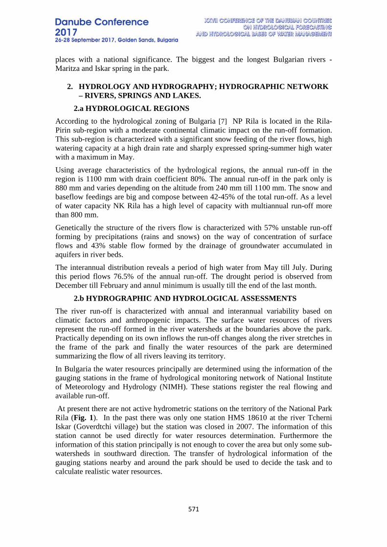
571

places with a national significance. The biggest and the longest Bulgarian rivers - Maritza and Iskar spring in the park.

2. HYDROLOGY AND HYDROGRAPHY; HYDROGRAPHIC NETWORK – RIVERS, SPRINGS AND LAKES.

2.a HYDROLOGICAL REGIONS According to the hydrological zoning of Bulgaria [7] NP Rila is located in the Rila-Pirin sub-region with a moderate continental climatic impact on the run-off formation. This sub-region is characterized with a significant snow feeding of the river flows, high watering capacity at a high drain rate and sharply expressed spring-summer high water with a maximum in May. Using average characteristics of the hydrological regions, the annual run-off in the region is 1100 mm with drain coefficient 80%. The annual run-off in the park only is 880 mm and varies depending on the altitude from 240 mm till 1100 mm. The snow and baseflow feedings are big and compose between 42-45% of the total run-off. As a level of water capacity NK Rila has a high level of capacity with multiannual run-off more than 800 mm. Genetically the structure of the rivers flow is characterized with 57% unstable run-off forming by precipitations (rains and snows) on the way of concentration of surface flows and 43% stable flow formed by the drainage of groundwater accumulated in aquifers in river beds. The interannual distribution reveals a period of high water from May till July. During this period flows 76.5% of the annual run-off. The drought period is observed from December till February and annul minimum is usually till the end of the last month.

2.b HYDROGRAPHIC AND HYDROLOGICAL ASSESSMENTS The river run-off is characterized with annual and interannual variability based on climatic factors and anthropogenic impacts. The surface water resources of rivers represent the run-off formed in the river watersheds at the boundaries above the park. Practically depending on its own inflows the run-off changes along the river stretches in the frame of the park and finally the water resources of the park are determined summarizing the flow of all rivers leaving its territory. In Bulgaria the water resources principally are determined using the information of the gauging stations in the frame of hydrological monitoring network of National Institute of Meteorology and Hydrology (NIMH). These stations register the real flowing and available run-off. At present there are not active hydrometric stations on the territory of the National Park Rila (Fig. 1). In the past there was only one station HMS 18610 at the river Tcherni Iskar (Goverdtchi village) but the station was closed in 2007. The information of this station cannot be used directly for water resources determination. Furthermore the information of this station principally is not enough to cover the area but only some sub-watersheds in southward direction. The transfer of hydrological information of the gauging stations nearby and around the park should be used to decide the task and to calculate realistic water resources.

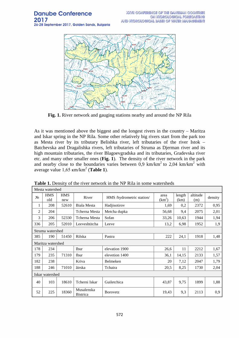
572

Fig. 1. River network and gauging stations nearby and around the NP Rila

As it was mentioned above the biggest and the longest rivers in the country – Maritza and Iskar spring in the NP Rila. Some other relatively big rivers start from the park too as Mesta river by its tributary Belishka river, left tributaries of the river Istok – Batchevska and Dragalishka rivers, left tributaries of Struma as Djerman river and its high mountain tributaries, the river Blagoevgradska and its tributaries, Gradevska river etc. and many other smaller ones (Fig. 1). The density of the river network in the park and nearby close to the boundaries varies between 0,9 km/km2 to 2,04 km/km2 with average value 1,65 кm/km2 (Table 1).

Table 1. Density of the river network in the NP Rila in some watersheds Mesta watershed

№ HMS old

HMS new River HMS /hydrometric station/ area

(km2) length (km)

altitude (m) density

1 208 52610 Biala Mesta Hadjisotirov 1,69 0,2 2372 0,95 2 204 Tcherna Mesta Metcha dupka 56,68 9,4 2075 2,01 3 206 52330 Tcherna Mesta Sofan 33,26 10,63 1944 1,94

336 205 52010 Leeveshtitcha Leeve 13,2 6,98 1952 1,9

Struma watershed 385 190 51450 Rilska Pastra 222 24,1 1918 1,48

Maritza watershed 178 234 Ibur elevation 1900 26,6 11 2212 1,67 179 235 71310 Ibur elevetion 1400 36,1 14,15 2133 1,57 182 238 Kriva Belmeken 20 7,12 2047 1,79 188 246 71010 ãirska Tchaira 20,5 8,25 1730 2,04

Iskar watershed

40 103 18610 Tcherni Iskar Guiletchica 43,87 9,75 1899 1,88

52 225 18360 Musalenska Bistrica Borovetz 19,43 9,3 2113 0,9

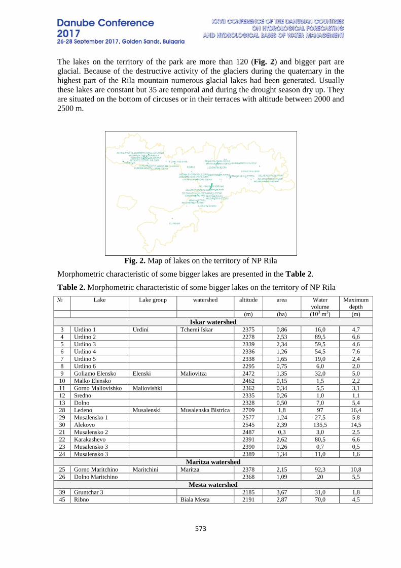
573

The lakes on the territory of the park are more than 120 (Fig. 2) and bigger part are glacial. Because of the destructive activity of the glaciers during the quaternary in the highest part of the Rila mountain numerous glacial lakes had been generated. Usually these lakes are constant but 35 are temporal and during the drought season dry up. They are situated on the bottom of circuses or in their terraces with altitude between 2000 and 2500 m.

Fig. 2. Map of lakes on the territory of NP Rila

Morphometric characteristic of some bigger lakes are presented in the Table 2. Table 2. Morphometric characteristic of some bigger lakes on the territory of NP Rila № Lake Lake group watershed altitude area Water

volume Maximum

depth (m) (ha) (103 m3) (m)

Iskar watershed 3 Urdino 1 Urdini Tcherni Iskar 2375 0,86 16,0 4,7 4 Urdino 2 2278 2,53 89,5 6,6 5 Urdino 3 2339 2,34 59,5 4,6 6 Urdino 4 2336 1,26 54,5 7,6 7 Urdino 5 2338 1,65 19,0 2,4 8 Urdino 6 2295 0,75 6,0 2,0 9 Goliamo Elensko Elenski Maliovitza 2472 1,35 32,0 5,0 10 Malko Elensko 2462 0,15 1,5 2,2 11 Gorno Maliovishko Maliovishki 2362 0,34 5,5 3,1 12 Sredno 2335 0,26 1,0 1,1 13 Dolno 2328 0,50 7,0 5,4 28 Ledeno Musalenski Musalenska Bistrica 2709 1,8 97 16,4 29 Musalensko 1 2577 1,24 27,5 5,8 30 Alekovo 2545 2,39 135,5 14,5 21 Musalensko 2 2487 0,3 3,0 2,5 22 Karakashevo 2391 2,62 80,5 6,6 23 Musalensko 3 2390 0,26 0,7 0,5 24 Musalensko 3 2389 1,34 11,0 1,6

Maritza watershed 25 Gorno Maritchino Maritchini Maritza 2378 2,15 92,3 10,8 26 Dolno Maritchino 2368 1,09 20 5,5

Mesta watershed 39 Gruntchar 3 2185 3,67 31,0 1,8 45 Ribno Biala Mesta 2191 2,87 70,0 4,5

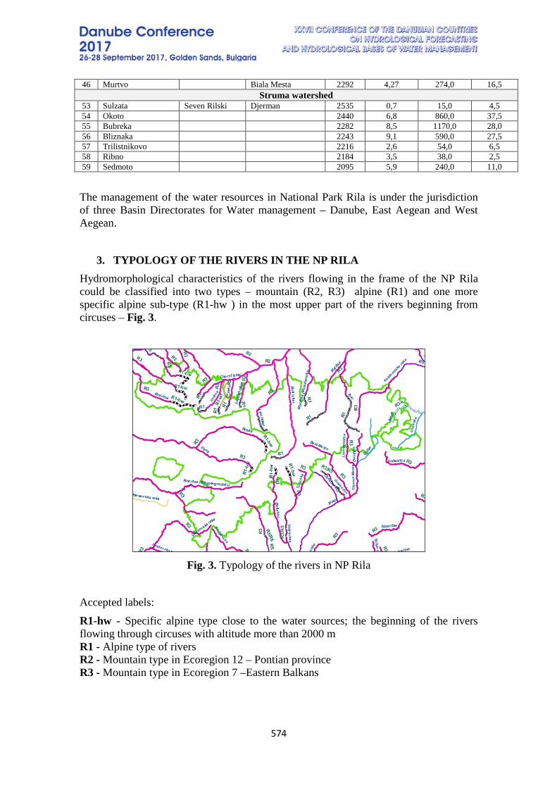
574

46 Murtvo Biala Mesta 2292 4,27 274,0 16,5 Struma watershed

53 Sulzata Seven Rilski Djerman 2535 0,7 15,0 4,5 54 Okoto 2440 6,8 860,0 37,5 55 Bubreka 2282 8,5 1170,0 28,0 56 Bliznaka 2243 9,1 590,0 27,5 57 Trilistnikovo 2216 2,6 54,0 6,5 58 Ribno 2184 3,5 38,0 2,5 59 Sedmoto 2095 5,9 240,0 11,0 The management of the water resources in National Park Rila is under the jurisdiction of three Basin Directorates for Water management – Danube, East Aegean and West Aegean.

3. TYPOLOGY OF THE RIVERS IN THE NP RILA Hydromorphological characteristics of the rivers flowing in the frame of the NP Rila could be classified into two types – mountain (R2, R3) alpine (R1) and one more specific alpine sub-type (R1-hw ) in the most upper part of the rivers beginning from circuses – Fig. 3.

Fig. 3. Typology of the rivers in NP Rila

Accepted labels: R1-hw - Specific alpine type close to the water sources; the beginning of the rivers flowing through circuses with altitude more than 2000 m R1 - Alpine type of rivers R2 - Mountain type in Ecoregion 12 – Pontian province R3 - Mountain type in Ecoregion 7 –Eastern Balkans

575

Maritza river – marishki circus , upper stream ,

specific alpine type R1-hw

Maritza river – above Raduil village, upper sream

mountain type R3

Maritza river – above the inflow of Prava Maritza,

upper sream mountain type R1

Photos 1. Photos of the Maritza river

The widespread type in the Rila park is a mountain river type characterized with a coarse substratum usually with a stepwise beds and with series of natural thresholds and pools, very fast flows. The specific alpine type is observed in the circus bottoms close the water sources, the river bed is shallow. The type is heterogenic regarding the substratum and the stream characteristics. The alpine type is observed in short, close to rectilinear river sections, with significant slope (more than 10%) in narrow V-shaped river valleys. The substratum is coarse including rocky blocks, stormy streams, numerous cascades, waterfalls and pools - Photos 1. The presented in the Fig. 3 typology of the rivers is a part Actualization of typology and classification system for assessment of the surface water bodies in categories – river, lake and transitional waters in the Plans for water management in Bulgaria.

4. WATER RESOURCES DETERMINATION IN THE NP RILA

As it was mentioned above the lack of hydrometric network is the biggest problem in the water resources determination. For this reason the information from the gauging stations cannot be used directly for determining the water resource in the Rila National

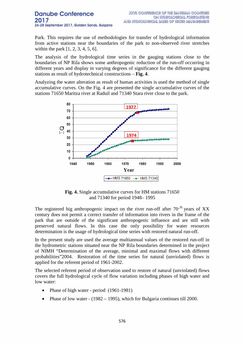
576

Park. This requires the use of methodologies for transfer of hydrological information from active stations near the boundaries of the park to non-observed river stretches within the park [1, 2, 3, 4, 5, 6]. The analysis of the hydrological time series in the gauging stations close to the boundaries of NP Rila shows some anthropogenic reduction of the run-off occurring in different years and display in varying degrees of significance for the different gauging stations as result of hydrotechnical constructions – Fig. 4. Analyzing the water alteration as result of human activities is used the method of single accumulative curves. On the Fig. 4 are presented the single accumulative curves of the stations 71650 Maritza river at Raduil and 71340 Stara river close to the park.

Fig. 4. Single accumulative curves for HM stations 71650

and 71340 for period 1948– 1995

The registered big anthropogenic impact on the river run-off after 70_th years of XX century does not permit a correct transfer of information into rivers in the frame of the park that are outside of the significant anthropogenic influence and are still with preserved natural flows. In this case the only possibility for water resources determination is the usage of hydrological time series with restored natural run-off. In the present study are used the average multiannual values of the restored run-off in the hydrometric stations situated near the NP Rila boundaries determined in the project of NIMH “Determination of the average, minimal and maximal flows with different probabilities”2004. Restoration of the time series for natural (unviolated) flows is applied for the referent period of 1961-2002. The selected referent period of observation used to restore of natural (unviolated) flows covers the full hydrological cycle of flow variation including phases of high water and low water:

• Phase of high water - period (1961-1981)

• Phase of low water - (1982 – 1995), which for Bulgaria continues till 2000.

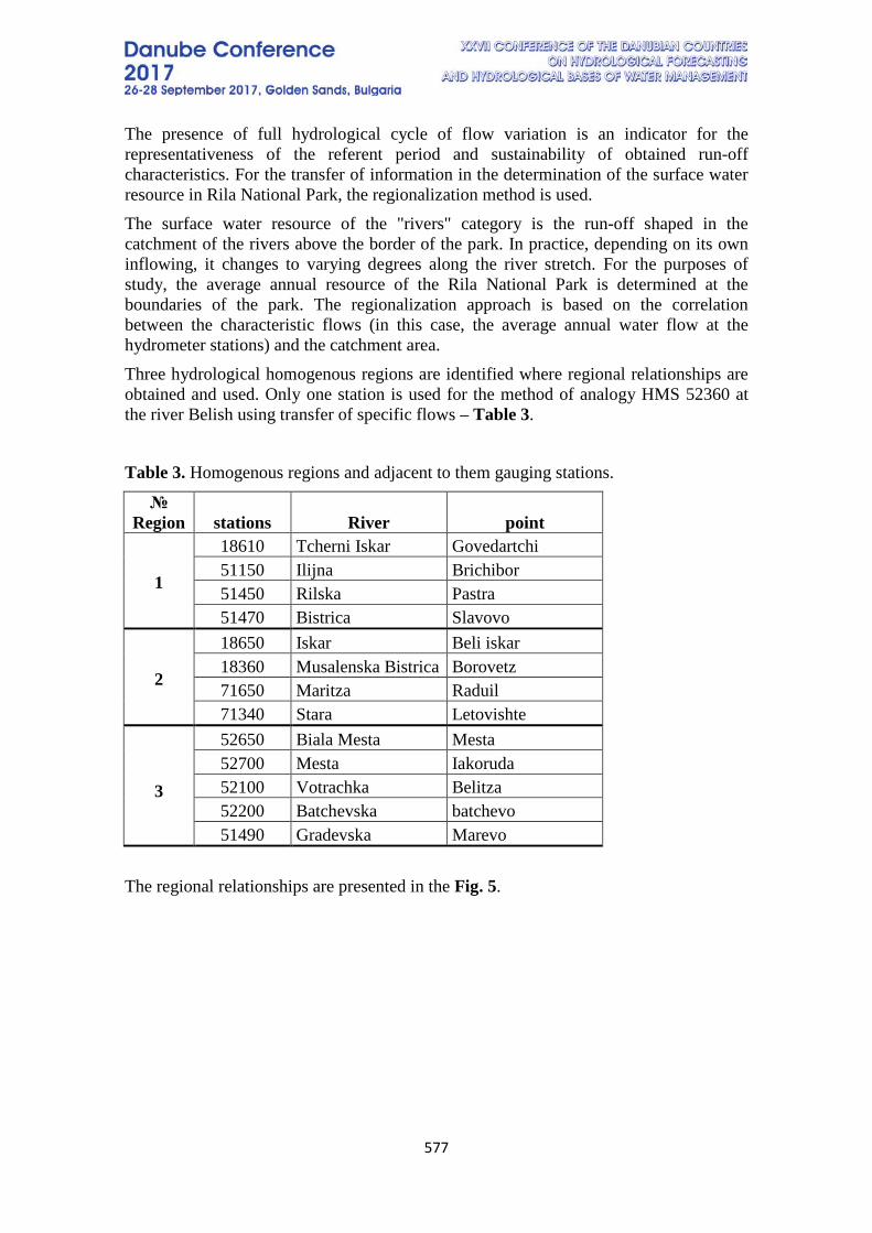
577

The presence of full hydrological cycle of flow variation is an indicator for the representativeness of the referent period and sustainability of obtained run-off characteristics. For the transfer of information in the determination of the surface water resource in Rila National Park, the regionalization method is used. The surface water resource of the "rivers" category is the run-off shaped in the catchment of the rivers above the border of the park. In practice, depending on its own inflowing, it changes to varying degrees along the river stretch. For the purposes of study, the average annual resource of the Rila National Park is determined at the boundaries of the park. The regionalization approach is based on the correlation between the characteristic flows (in this case, the average annual water flow at the hydrometer stations) and the catchment area. Three hydrological homogenous regions are identified where regional relationships are obtained and used. Only one station is used for the method of analogy HMS 52360 at the river Belish using transfer of specific flows – Table 3. Table 3. Homogenous regions and adjacent to them gauging stations.

№ Region stations River point

1

18610 Tcherni Iskar Govedartchi 51150 Ilijna Brichibor 51450 Rilska Pastra 51470 Bistrica Slavovo

2

18650 Iskar Beli iskar 18360 Musalenska Bistrica Borovetz 71650 Maritza Raduil 71340 Stara Letovishte

3

52650 Biala Mesta Mesta 52700 Mesta Iakoruda 52100 Votrachka Belitza 52200 Batchevska batchevo 51490 Gradevska Marevo

The regional relationships are presented in the Fig. 5.

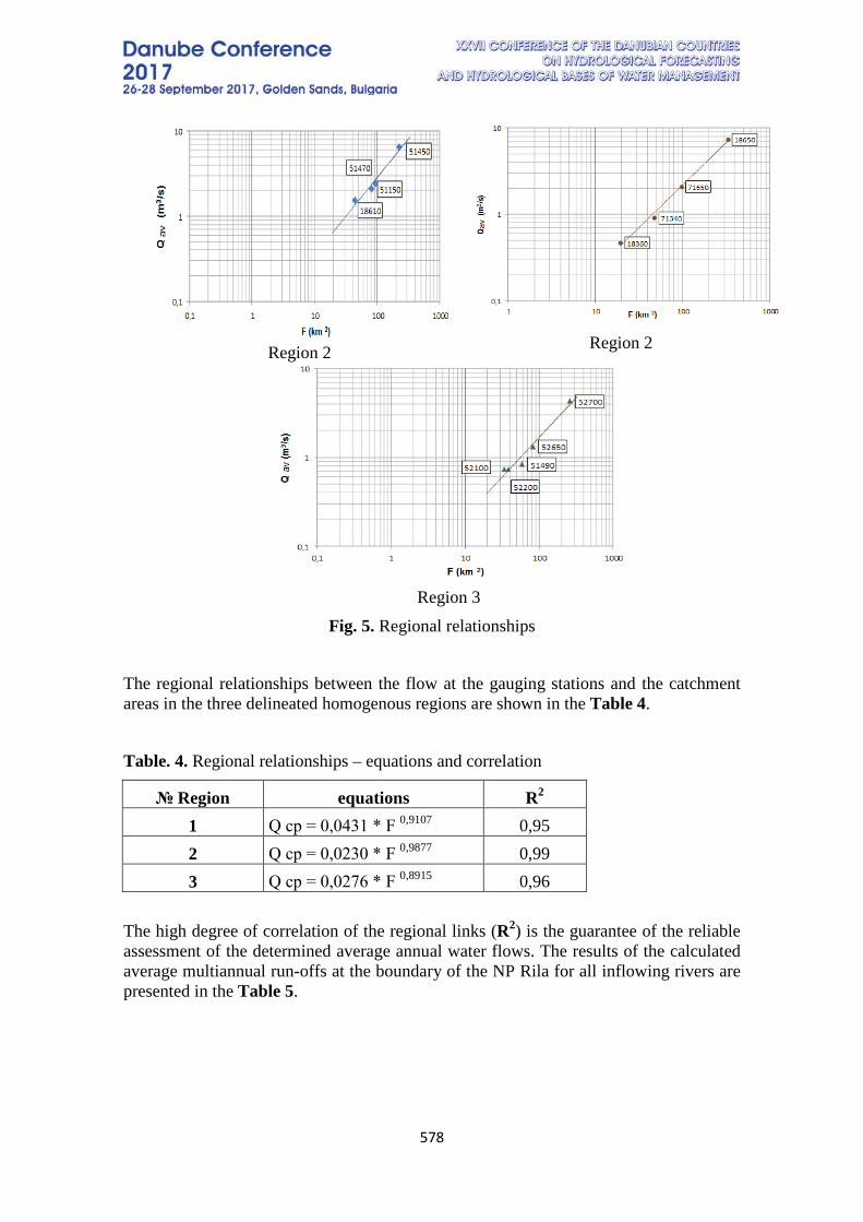
578

Region 2

Region 2

Region 3

Fig. 5. Regional relationships

The regional relationships between the flow at the gauging stations and the catchment areas in the three delineated homogenous regions are shown in the Table 4. Table. 4. Regional relationships – equations and correlation

№ Region equations R2 1 Q ср = 0,0431 * F 0,9107 0,95 2 Q ср = 0,0230 * F 0,9877 0,99 3 Q ср = 0,0276 * F 0,8915 0,96

The high degree of correlation of the regional links (R2) is the guarantee of the reliable assessment of the determined average annual water flows. The results of the calculated average multiannual run-offs at the boundary of the NP Rila for all inflowing rivers are presented in the Table 5.

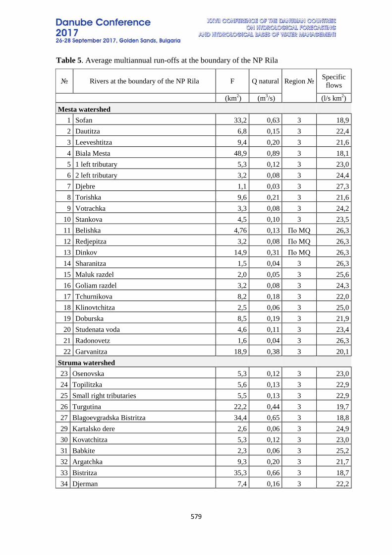
579

Table 5. Average multiannual run-offs at the boundary of the NP Rila

№ Rivers at the boundary of the NP Rila F Q natural Region № Specific flows

(km2) (m3/s) (l/s km2) Mesta watershed

1 Sofan 33,2 0,63 3 18,9 2 Dautitza 6,8 0,15 3 22,4 3 Leeveshtitza 9,4 0,20 3 21,6 4 Biala Mesta 48,9 0,89 3 18,1 5 1 left tributary 5,3 0,12 3 23,0 6 2 left tributary 3,2 0,08 3 24,4 7 Djebre 1,1 0,03 3 27,3 8 Torishka 9,6 0,21 3 21,6 9 Votrachka 3,3 0,08 3 24,2

10 Stankova 4,5 0,10 3 23,5 11 Belishka 4,76 0,13 По MQ 26,3 12 Redjepitza 3,2 0,08 По MQ 26,3 13 Dinkov 14,9 0,31 По MQ 26,3 14 Sharanitza 1,5 0,04 3 26,3 15 Maluk razdel 2,0 0,05 3 25,6 16 Goliam razdel 3,2 0,08 3 24,3 17 Tchurnikova 8,2 0,18 3 22,0 18 Klinovtchitza 2,5 0,06 3 25,0 19 Doburska 8,5 0,19 3 21,9 20 Studenata voda 4,6 0,11 3 23,4 21 Radonovetz 1,6 0,04 3 26,3 22 Garvanitza 18,9 0,38 3 20,1

Struma watershed 23 Osenovska 5,3 0,12 3 23,0 24 Topilitzka 5,6 0,13 3 22,9 25 Small right tributaries 5,5 0,13 3 22,9 26 Turgutina 22,2 0,44 3 19,7 27 Blagoevgradska Bistritza 34,4 0,65 3 18,8 29 Kartalsko dere 2,6 0,06 3 24,9 30 Kovatchitza 5,3 0,12 3 23,0 31 Babkite 2,3 0,06 3 25,2 32 Argatchka 9,3 0,20 3 21,7 33 Bistritza 35,3 0,66 3 18,7 34 Djerman 7,4 0,16 3 22,2

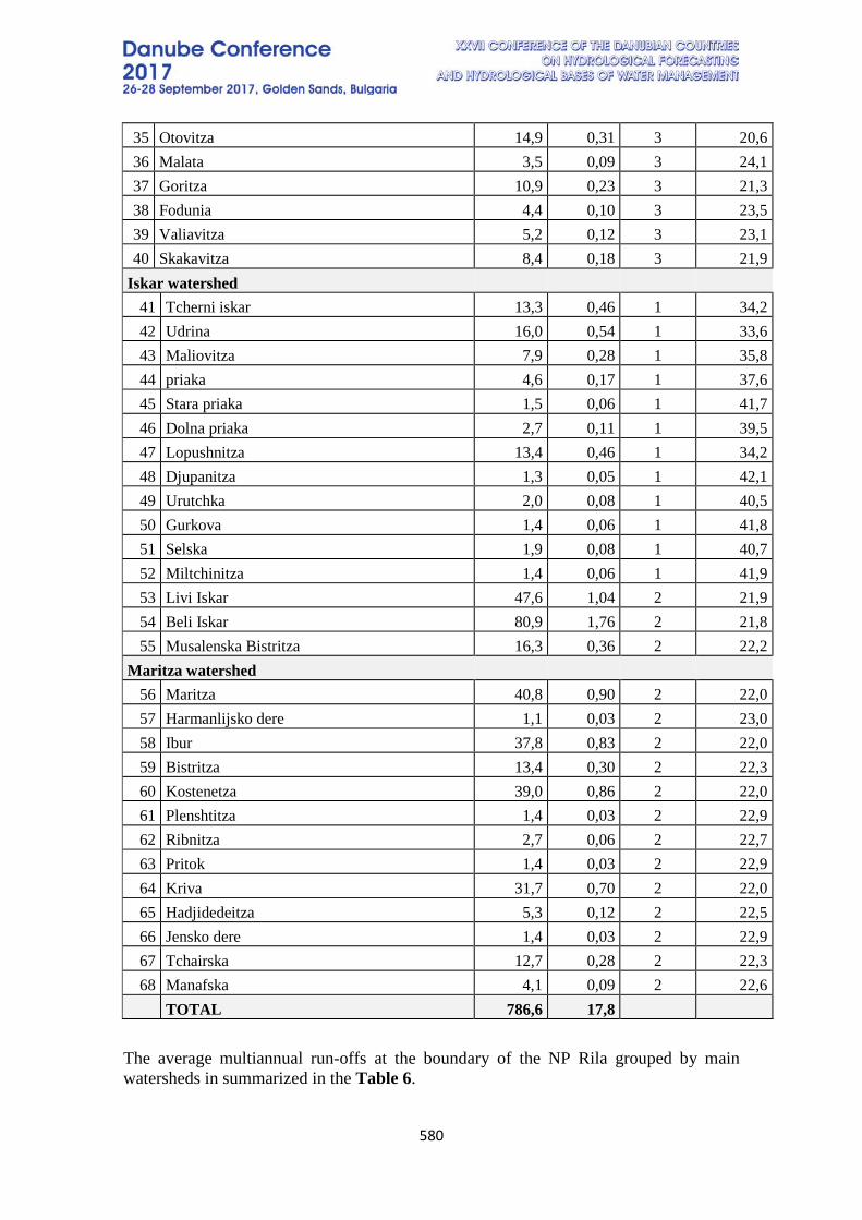
580

35 Otovitza 14,9 0,31 3 20,6 36 Malata 3,5 0,09 3 24,1 37 Goritza 10,9 0,23 3 21,3 38 Fodunia 4,4 0,10 3 23,5 39 Valiavitza 5,2 0,12 3 23,1 40 Skakavitza 8,4 0,18 3 21,9

Iskar watershed 41 Tcherni iskar 13,3 0,46 1 34,2 42 Udrina 16,0 0,54 1 33,6 43 Maliovitza 7,9 0,28 1 35,8 44 priaka 4,6 0,17 1 37,6 45 Stara priaka 1,5 0,06 1 41,7 46 Dolna priaka 2,7 0,11 1 39,5 47 Lopushnitza 13,4 0,46 1 34,2 48 Djupanitza 1,3 0,05 1 42,1 49 Urutchka 2,0 0,08 1 40,5 50 Gurkova 1,4 0,06 1 41,8 51 Selska 1,9 0,08 1 40,7 52 Miltchinitza 1,4 0,06 1 41,9 53 Livi Iskar 47,6 1,04 2 21,9 54 Beli Iskar 80,9 1,76 2 21,8 55 Musalenska Bistritza 16,3 0,36 2 22,2

Maritza watershed 56 Maritza 40,8 0,90 2 22,0 57 Harmanlijsko dere 1,1 0,03 2 23,0 58 Ibur 37,8 0,83 2 22,0 59 Bistritza 13,4 0,30 2 22,3 60 Kostenetza 39,0 0,86 2 22,0 61 Plenshtitza 1,4 0,03 2 22,9 62 Ribnitza 2,7 0,06 2 22,7 63 Pritok 1,4 0,03 2 22,9 64 Kriva 31,7 0,70 2 22,0 65 Hadjidedeitza 5,3 0,12 2 22,5 66 Jensko dere 1,4 0,03 2 22,9 67 Tchairska 12,7 0,28 2 22,3 68 Manafska 4,1 0,09 2 22,6

TOTAL 786,6 17,8 The average multiannual run-offs at the boundary of the NP Rila grouped by main watersheds in summarized in the Table 6.

581

Table 6. Average multiannual run-offs grouped by main watersheds

Watersheds Drainage area

Average multiannual run-offs

(km2) m3* 10 6

1 Danube BD Iskar watershed 212,1 175,76 2 East Aegean BD Maritza watershed 192,8 134,38 3 West Aegean BD Mesta watershed 199,1 132,96 Struma watershed 182,5 118,72 TOTAL 786,6 561,82

5. CONCLUSION The present material represents a methodological approach to determine water resources in a not observed territory with preserved nature as National Park Rila by using restored natural run-offs of the rivers at the gauging stations situated close to the boundaries of the park. The applied approach is demonstrated with calculated average flows of all rivers inflowing in the park. The result from the transfer of restored natural run-off to the not observed stretches depends significantly on the accuracy of information linked to the water usage (water supply, irrigation, water abstraction etc.) used for restoration of the hydrological time series. The results are already in use in the Management Authority of the National Park Rila for further development of Management Plan and environmental assessments.

6. REFERENCES [1] Zhang, Y., Chiew, F.H.S., (2009). Relative merits of different methods for runoff predictions in ungauged catchments. Water Resour. Res., 45(7): W07412, doi: 10.1029/2008wr007504. [2] Viglione, A., Parajka, J., Rogger, M., Salinas, J. L., Laaha, G., Sivapalan, M., and Bl¨oschl, G.: Sivapalan, M., and Bloschl, G., (2013). Comparative assessment of predictions in ungauged basins – Part 3: Runoff signatures in Austria, Hydrol. Earth Syst. Sci. Discuss., 10, 449–485, doi:10.5194/hessd-10-449-2013, 2013. [3] Plamen Ninov, Tzviatka Karagiozova Technological Approach to determine the water resources of river water bodies - using hydrological monitoring network, , Hydrological International Scientific Conference „Adaptation to climate change, from source to river basin”, Bucharest, 2014. [4] Tzviatka Karagiozova, Plamen Ninov, Maya Rankova Technology for determination of average annual resources of surface water bodies in Bulgaria, International Conference "Balkan Economic Reconstruction and Ecology - BALKANIREKO '16", April 7'- 8; Ecology and Industry, ISSN 1311-2783, Publisher: Balkan Academy of Sciences and Culture, 2016

582

[5] Bojilova, E. About the changes in the frequency of the maximum annual river discharges for two pilot watersheds in Bulgaria, BALKANERECO’2016, Vol. 9, 2016, №1, ISSN 1311-2783, 122-125, 2016. [6] S. Balabanova , Operational system for streamflow forecasting in the Iskar river basin based on Artificial Neural Networks " INHGA - Scientific Conference, Румъния, Букурещ, 10-11November 2014 [7] Iordanov and all, 1997, Geography of Bulgaria, Edition of Bulgarian Academy of Sciences, 2002

583

AN INTEGRATED SOLUTION FOR RAINFALL RUNOFF AT THE BRIDGE OVER SAVA A CASE STUDY OF OSTRUZNICA BRIDGE INCLUDING

RUNOFF CONTROL TROUGH PREVENTION, DRAINAGE, TREATMENT AND IRRIGATION SYSTEM, GROUNDWATER RECHARGE AND

MONITORING

Jovan Despotovic1,2*, Aleksandar Djukic, Nenad Jacimovic, Jasna Plavsic, M. Stanic,

Andrijana Todorovic, Nenad Vrvic3, Uros Urosevic3

1University of Belgrade, Faculty of Civil Engineering, Boulevard of the King Alexander 73, P.O. Box 42, 11120 Belgrade, Serbia

2CEKIBEO Consulting Company, Zahumska str. 26, 11000 Belgrade, Serbia 3Belgrade Water Supply System, Belgrade, Serbia

Corresponding author: jdespotovic@gf.bg.ac.rs ABSTRACT The poster presents an analysis, design and construction of rainfall runoff at the bridge Ostruznica deck including drainage and treatment. In addition, filtered water is put into irrigation in ground close by as a recharge, in the vicinity to a series of wells situated within sanitary protection zone of the Belgrade Water Supply System (BWSS). The old bridge was constructed without drainage system almost 20 years ago. The constraints and conditions for runoff discharge, including runoff water quality are severe, concerning location of the bridge within the BWSS. The poster presents an integral solution of drainage and irrigation and/or discharge water into the Sava river of pre - treated runoff from the portion of highway E-75 from Dobanovci – Bubanj Potok and the bridge. The first portion of rainfall runoff, i.e. app. first third of the criteria volume should be taken for a pre / treatment with a Stormfilter vault, but also the rest of hydrograph to a lesser degree. An assessment of the recharge water potentials is based on data from previously analysed Belgrade wellhead, consisting of a series of wells as a source of water. This solution will be analysed as an improvement of water cycle in a water safety plans. Also is proposed monitoring as an obligation of water quality impacts. Further phases in accordance to the Water Act, conditions and terms for protection zones by all authorities, accounting for quality of water for aquifer recharge. This is also first time in Serbia of designed and constructed a complete system for preventing accidents incl. SWERM, such as leakage or damages of vehicles and potential pollution. Such a solution is also considered as an additional source of water by the rivers’ banks, and so bridges, highways and roads are even more worthwhile within the climate treats. KEYWORDS Bridge; river Sava ; Belgrade; rainfall runoff; drainage; filtration; aquifer recharge.

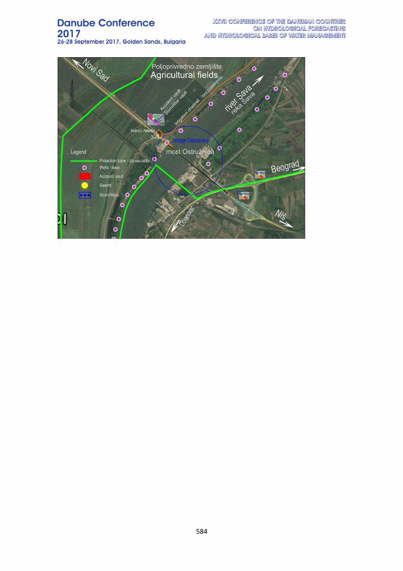
584

585

TOPIC 7: WATER QUALITY AND POLLUTION

THE ION RUNOFF OF THE LOWER DANUBE RIVER AND ESTIMATION OF THE STATE BY MINERALIZATION

Natalia Osadcha, Denys Klebanov

Ukrainian Hydrometeorological Institute, Ukraine

Corresponding author: Klebanov Denys, Ukrainian Hydrometeorological Institute, 37, Nauki ave, Kiev, 03028, Ukraine, den@uhmi.org.ua

ABSTRACT The research is carried out in the Ukrainian reach of the Lower Danube where all the headstream run-off transformation is as good as finished and the removal into the Black sea is formed. The pressure on river water resources has effect on its ecological state, essentially the North-West part of the Black Sea shelf where the river runs into. A method for the assessment of water status of mineralization using a Flow Duration Curve. Graphical method with use of double mass curve was also applied for studying of uniformity of water and main ions runoff formation in Danube catchment. This curve reflects relation between two sequentially summed values of water runoff and emission of main ions. Generally, one can speak about dominating influence of water runoff on main ions washout. The estimation of the water status by water mineralization has shown that it meets the "High" or "Good" category in the lower Danube. A method for the estimation of the water status by water mineralization using a Flow Duration Curve. It has shown that it meets the "High" or "Good" category in the lower Danube. Keywords: Danube, main ions, mineralization, influence, estimation, runoff.

1. INTRODUCTION The Danube river is the second and most international waterway in Europe flowing through the territory of 19 countries. It is the important European thruway having the status of a transport corridor which begins in Schwarzwald and ends in the Black Sea. There is a small part of the Danube basin corresponding 4.5% in Ukraine. [1] The most part of it is in Romania (83%), the least one is in Ukraine (17%). The Lower Danube in Ukraine stretches 170 km and besides the delta includes a near-delta area upstream. The Lower Danube has the properties of a typical plain stream but there are also the Tissa and Prut subbasins running off from the Carpathians. Taking into account the great importance of the Lower Danube in the Ukraine economy and also its influence on a fishery zone of the North-West Black Sea region the first hydrochemical research of the Lower Danube in Ukraine was conducted in 1948-1950 and then continued in 1958-1959 [0, 3]. The work was organized as expeditionary observations and stationary operations.

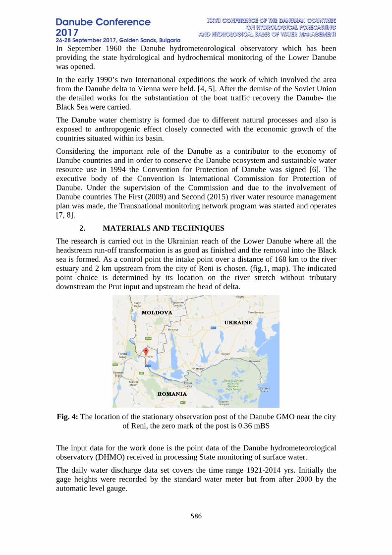
586

In September 1960 the Danube hydrometeorological observatory which has been providing the state hydrological and hydrochemical monitoring of the Lower Danube was opened. In the early 1990’s two International expeditions the work of which involved the area from the Danube delta to Vienna were held. [4, 5]. After the demise of the Soviet Union the detailed works for the substantiation of the boat traffic recovery the Danube- the Black Sea were carried. The Danube water chemistry is formed due to different natural processes and also is exposed to anthropogenic effect closely connected with the economic growth of the countries situated within its basin. Considering the important role of the Danube as a contributor to the economy of Danube countries and in order to conserve the Danube ecosystem and sustainable water resource use in 1994 the Convention for Protection of Danube was signed [6]. The executive body of the Convention is International Commission for Protection of Danube. Under the supervision of the Commission and due to the involvement of Danube countries The First (2009) and Second (2015) river water resource management plan was made, the Transnational monitoring network program was started and operates [7, 8].

2. MATERIALS AND TECHNIQUES The research is carried out in the Ukrainian reach of the Lower Danube where all the headstream run-off transformation is as good as finished and the removal into the Black sea is formed. As a control point the intake point over a distance of 168 km to the river estuary and 2 km upstream from the city of Reni is chosen. (fig.1, map). The indicated point choice is determined by its location on the river stretch without tributary downstream the Prut input and upstream the head of delta.

Fig. 4: The location of the stationary observation post of the Danube GMO near the city

of Reni, the zero mark of the post is 0.36 mBS The input data for the work done is the point data of the Danube hydrometeorological observatory (DHMO) received in processing State monitoring of surface water. The daily water discharge data set covers the time range 1921-2014 yrs. Initially the gage heights were recorded by the standard water meter but from after 2000 by the automatic level gauge.

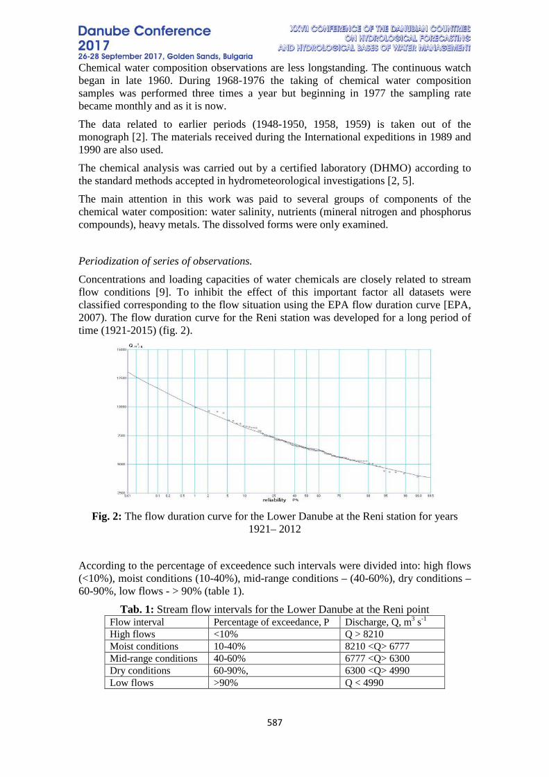
587

Chemical water composition observations are less longstanding. The continuous watch began in late 1960. During 1968-1976 the taking of chemical water composition samples was performed three times a year but beginning in 1977 the sampling rate became monthly and as it is now. The data related to earlier periods (1948-1950, 1958, 1959) is taken out of the monograph [2]. The materials received during the International expeditions in 1989 and 1990 are also used. The chemical analysis was carried out by a certified laboratory (DHMO) according to the standard methods accepted in hydrometeorological investigations [2, 5]. The main attention in this work was paid to several groups of components of the chemical water composition: water salinity, nutrients (mineral nitrogen and phosphorus compounds), heavy metals. The dissolved forms were only examined. Periodization of series of observations. Concentrations and loading capacities of water chemicals are closely related to stream flow conditions [9]. To inhibit the effect of this important factor all datasets were classified corresponding to the flow situation using the EPA flow duration curve [EPA, 2007). The flow duration curve for the Reni station was developed for a long period of time (1921-2015) (fig. 2).

Fig. 2: The flow duration curve for the Lower Danube at the Reni station for years

1921– 2012

According to the percentage of exceedence such intervals were divided into: high flows (<10%), moist conditions (10-40%), mid-range conditions – (40-60%), dry conditions – 60-90%, low flows - > 90% (table 1).

Tab. 1: Stream flow intervals for the Lower Danube at the Reni point Flow interval Percentage of exceedance, P Discharge, Q, m3 s-1 High flows <10% Q > 8210 Moist conditions 10-40% 8210 <Q> 6777 Mid-range conditions 40-60% 6777 <Q> 6300 Dry conditions 60-90%, 6300 <Q> 4990 Low flows >90% Q < 4990

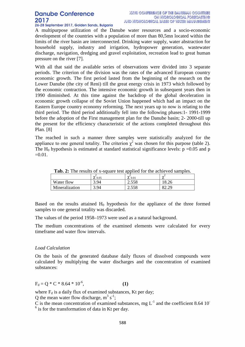
588

A multipurpose utilization of the Danube water resources and a socio-economic development of the countries with a population of more than 80,5mn located within the limits of the river basin are interconnected. Drinking water supply, water abstraction for household supply, industry and irrigation, hydropower generation, wastewater discharge, navigation, dredging and gravel exploitation, recreation lead to great human pressure on the river [7]. With all that said the available series of observations were divided into 3 separate periods. The criterion of the division was the rates of the advanced European country economic growth. The first period lasted from the beginning of the research on the Lower Danube (the city of Reni) till the great energy crisis in 1973 which followed by the economic contraction. The intensive economic growth in subsequent years then in 1990 diminished. At this time against the backdrop of the global deceleration in economic growth collapse of the Soviet Union happened which had an impact on the Eastern Europe country economy reforming. The next years up to now is relating to the third period. The third period additionally fell into the following phases:1- 1991-1999 before the adoption of the First management plan for the Danube basin; 2- 2000-till up the present for the efficiency characteristic of the actions completed throughout this Plan. [8] The reached in such a manner three samples were statistically analyzed for the appliance to one general totality. The criterion χ2 was chosen for this purpose (table 2). The H0 hypothesis is estimated at standard statistical significance levels: p =0.05 and p =0.01.

Tab. 2: The results of x-square test applied for the achieved samples. χ2

0.05 χ20.01 χ2

Water flow 3.94 2.558 18.26 Mineralization 3.94 2.558 82.29

Based on the results attained H0 hypothesis for the appliance of the three formed samples to one general totality was discarded. The values of the period 1958–1973 were used as a natural background. The medium concentrations of the examined elements were calculated for every timeframe and water flow intervals. Load Calculation On the basis of the generated database daily fluxes of dissolved compounds were calculated by multiplying the water discharges and the concentration of examined substances: Fd = Q * C * 8.64 * 10-6, (1) where Fd is a daily flux of examined substances, Kt per day; Q the mean water flow discharge, m3 s-1; C is the mean concentration of examined substances, mg L-1 and the coefficient 8.64 10-

6 is for the transformation of data in Kt per day.

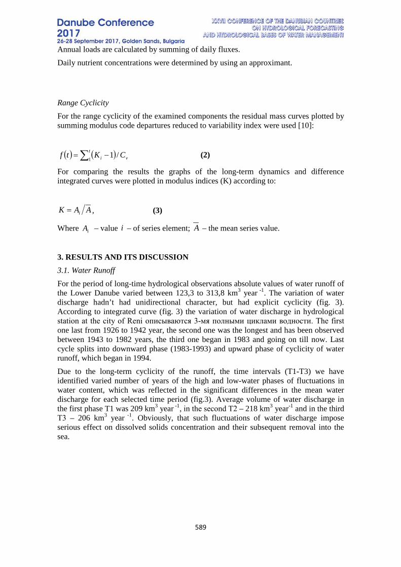
589

Annual loads are calculated by summing of daily fluxes. Daily nutrient concentrations were determined by using an approximant. Range Cyclicity For the range cyclicity of the examined components the residual mass curves plotted by summing modulus code departures reduced to variability index were used [10]:

(2)

For comparing the results the graphs of the long-term dynamics and difference integrated curves were plotted in modulus indices (K) according to:

, (3)

Where – value – of series element; – the mean series value.

3. RESULTS AND ITS DISCUSSION 3.1. Water Runoff For the period of long-time hydrological observations absolute values of water runoff of the Lower Danube varied between 123,3 to 313,8 km3 year -1. The variation of water discharge hadn’t had unidirectional character, but had explicit cyclicity (fig. 3). According to integrated curve (fig. 3) the variation of water discharge in hydrological station at the city of Reni описываются 3-мя полными циклами водности. The first one last from 1926 to 1942 year, the second one was the longest and has been observed between 1943 to 1982 years, the third one began in 1983 and going on till now. Last cycle splits into downward phase (1983-1993) and upward phase of cyclicity of water runoff, which began in 1994. Due to the long-term cyclicity of the runoff, the time intervals (T1-T3) we have identified varied number of years of the high and low-water phases of fluctuations in water content, which was reflected in the significant differences in the mean water discharge for each selected time period (fig.3). Average volume of water discharge in the first phase T1 was 209 km3 year -1, in the second Т2 – 218 km3 year-1 and in the third Т3 – 206 km3 year -1. Obviously, that such fluctuations of water discharge impose serious effect on dissolved solids concentration and their subsequent removal into the sea.

( ) ( ) vt

i CKtf /11∑ −=

AAK i=

iA i A

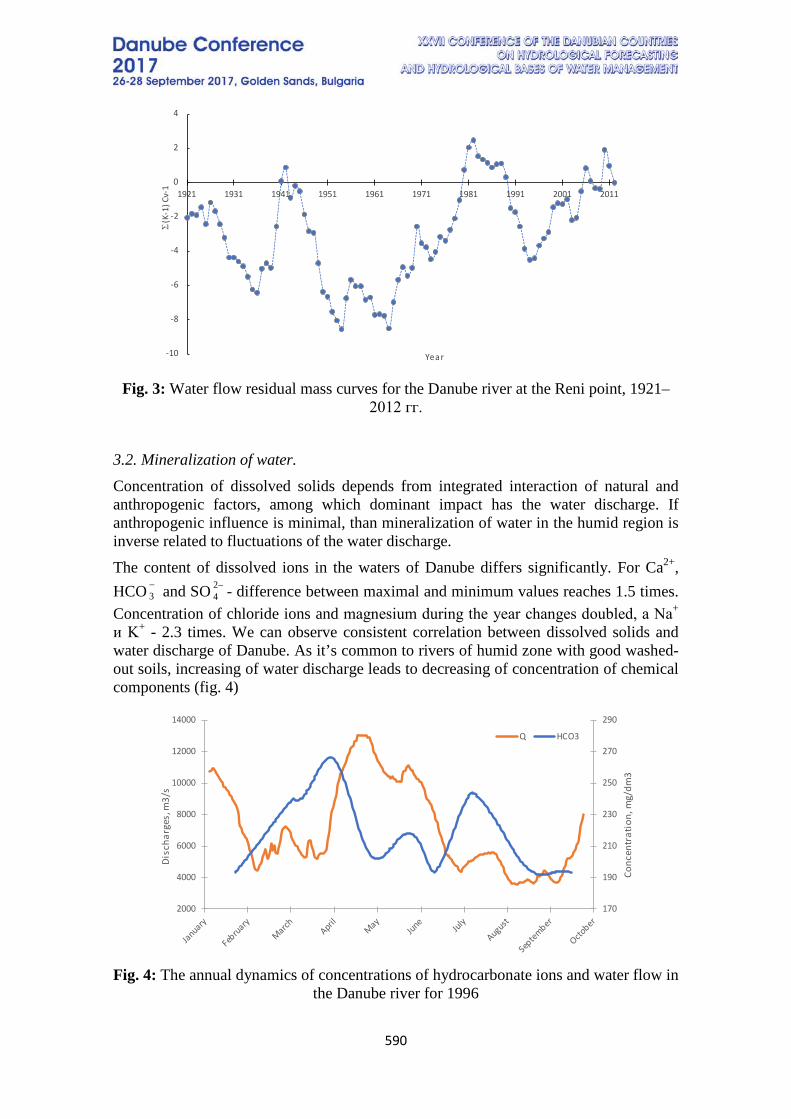
590

Fig. 3: Water flow residual mass curves for the Danube river at the Reni point, 1921–

2012 гг.

3.2. Mineralization of water. Concentration of dissolved solids depends from integrated interaction of natural and anthropogenic factors, among which dominant impact has the water discharge. If anthropogenic influence is minimal, than mineralization of water in the humid region is inverse related to fluctuations of the water discharge. The content of dissolved ions in the waters of Danube differs significantly. For Ca2+, HCO and SO - difference between maximal and minimum values reaches 1.5 times. Concentration of chloride ions and magnesium during the year changes doubled, а Na+ и K+ - 2.3 times. We can observe consistent correlation between dissolved solids and water discharge of Danube. As it’s common to rivers of humid zone with good washed-out soils, increasing of water discharge leads to decreasing of concentration of chemical components (fig. 4)

Fig. 4: The annual dynamics of concentrations of hydrocarbonate ions and water flow in

the Danube river for 1996

-10

-8

-6

-4

-2

0

2

4

1921 1931 1941 1951 1961 1971 1981 1991 2001 2011

Σ(K

-1) C

v-1

Year

−3

−24

170

190

210

230

250

270

290

2000

4000

6000

8000

10000

12000

14000

Conc

entr

atio

n,m

g/dm

3

Dis

char

ges,

m3/

s

Q HCO3

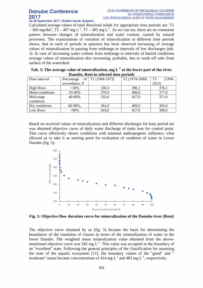
591

Calculated average values of total dissolved solids for appropriate time periods are: Т1 – 360 mg/dm3, Т2 – 407 mg L-1, Т3 – 385 mg L-1. As we can see, there are no consistent pattern between changes of mineralization and water content, caused by natural processes. The examinations of variation of mineralization in different time periods shows, that in each of periods in question has been observed increasing of average values of mineralization in passing from midrange to intervals of low discharges (tab. 3). In case of increasing water content from midrange to intervals of humid conditions average values of mineralization also increasing, probable, due to wash off salts from surface of the watershed.

Tab. 3: The average value of mineralization, mg L-1 at the lower part of the river. Danube, Reni in selected time periods

Flow interval Percentage of exceedance, P

Т1 (1968-1973) Т2 (1974-1989) Т3 (1990-2012)

High flows <10% 330,3 396,1 376,1 Moist conditions 10-40% 370,0 406,0 377,0 Mid-range conditions

40-60% 332,0 427,0 371,0

Dry conditions 60-90%, 361,0 409,0 395,0 Low flows >90% 416,0 427,0 390,0

Based on received values of mineralization and different discharges for base period are was obtained objective curve of daily water discharge of main ions for control point. This curve effectively shows conditions with minimal anthropogenic influence, what allowed us to take it as starting point for evaluation of condition of water in Lower Danube (fig. 5).

Fig. 5: Objective flow duration curve for mineralization of the Danube river (Reni) The objective curve obtained by us (fig. 5) became the basis for determining the boundaries of the transition of classes in terms of the mineralization of water in the lower Danube. The weighted mean mineralization value obtained from the above-mentioned objective curve was 345 mg L-1. This value was accepted as the boundary of an "excellent" state. Following the general principles of the classification for assessing the state of the aquatic ecosystem [11], the boundary values of the "good" and " moderate" status became concentrations of 414 mg L-1 and 483 mg L-1, respectively.

100

150

200

250

300

350

400

0 10 20 30 40 50 60 70 80 90 100

Mai

n Io

ns,K

t/da

y

Flow Duration Intervals,%

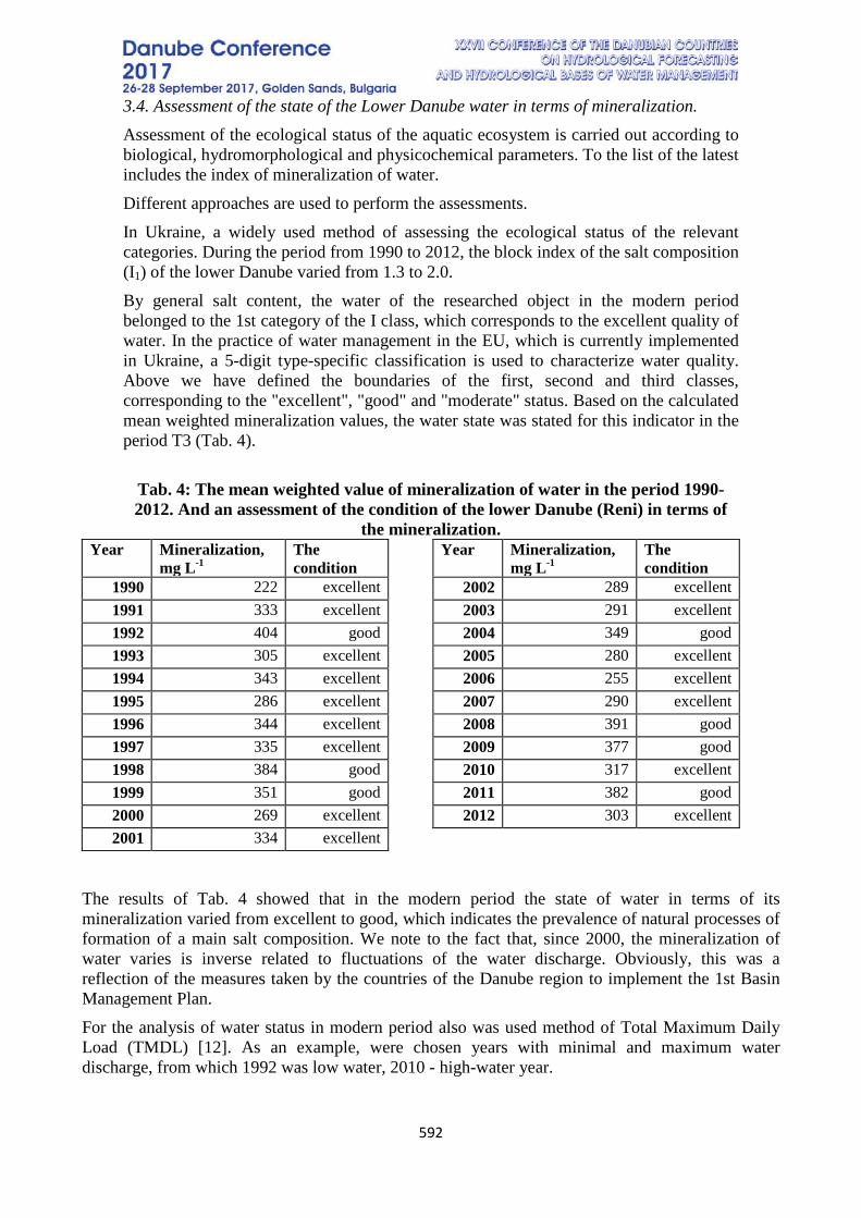
592

3.4. Assessment of the state of the Lower Danube water in terms of mineralization. Assessment of the ecological status of the aquatic ecosystem is carried out according to biological, hydromorphological and physicochemical parameters. To the list of the latest includes the index of mineralization of water. Different approaches are used to perform the assessments. In Ukraine, a widely used method of assessing the ecological status of the relevant categories. During the period from 1990 to 2012, the block index of the salt composition (I1) of the lower Danube varied from 1.3 to 2.0. By general salt content, the water of the researched object in the modern period belonged to the 1st category of the I class, which corresponds to the excellent quality of water. In the practice of water management in the EU, which is currently implemented in Ukraine, a 5-digit type-specific classification is used to characterize water quality. Above we have defined the boundaries of the first, second and third classes, corresponding to the "excellent", "good" and "moderate" status. Based on the calculated mean weighted mineralization values, the water state was stated for this indicator in the period T3 (Tab. 4).

Tab. 4: The mean weighted value of mineralization of water in the period 1990-2012. And an assessment of the condition of the lower Danube (Reni) in terms of

the mineralization. Year Mineralization,

mg L-1 The condition

1990 222 excellent 1991 333 excellent 1992 404 good 1993 305 excellent 1994 343 excellent 1995 286 excellent 1996 344 excellent 1997 335 excellent 1998 384 good 1999 351 good 2000 269 excellent 2001 334 excellent

Year Mineralization, mg L-1

The condition

2002 289 excellent 2003 291 excellent 2004 349 good 2005 280 excellent 2006 255 excellent 2007 290 excellent 2008 391 good 2009 377 good 2010 317 excellent 2011 382 good 2012 303 excellent

The results of Tab. 4 showed that in the modern period the state of water in terms of its mineralization varied from excellent to good, which indicates the prevalence of natural processes of formation of a main salt composition. We note to the fact that, since 2000, the mineralization of water varies is inverse related to fluctuations of the water discharge. Obviously, this was a reflection of the measures taken by the countries of the Danube region to implement the 1st Basin Management Plan. For the analysis of water status in modern period also was used method of Total Maximum Daily Load (TMDL) [12]. As an example, were chosen years with minimal and maximum water discharge, from which 1992 was low water, 2010 - high-water year.

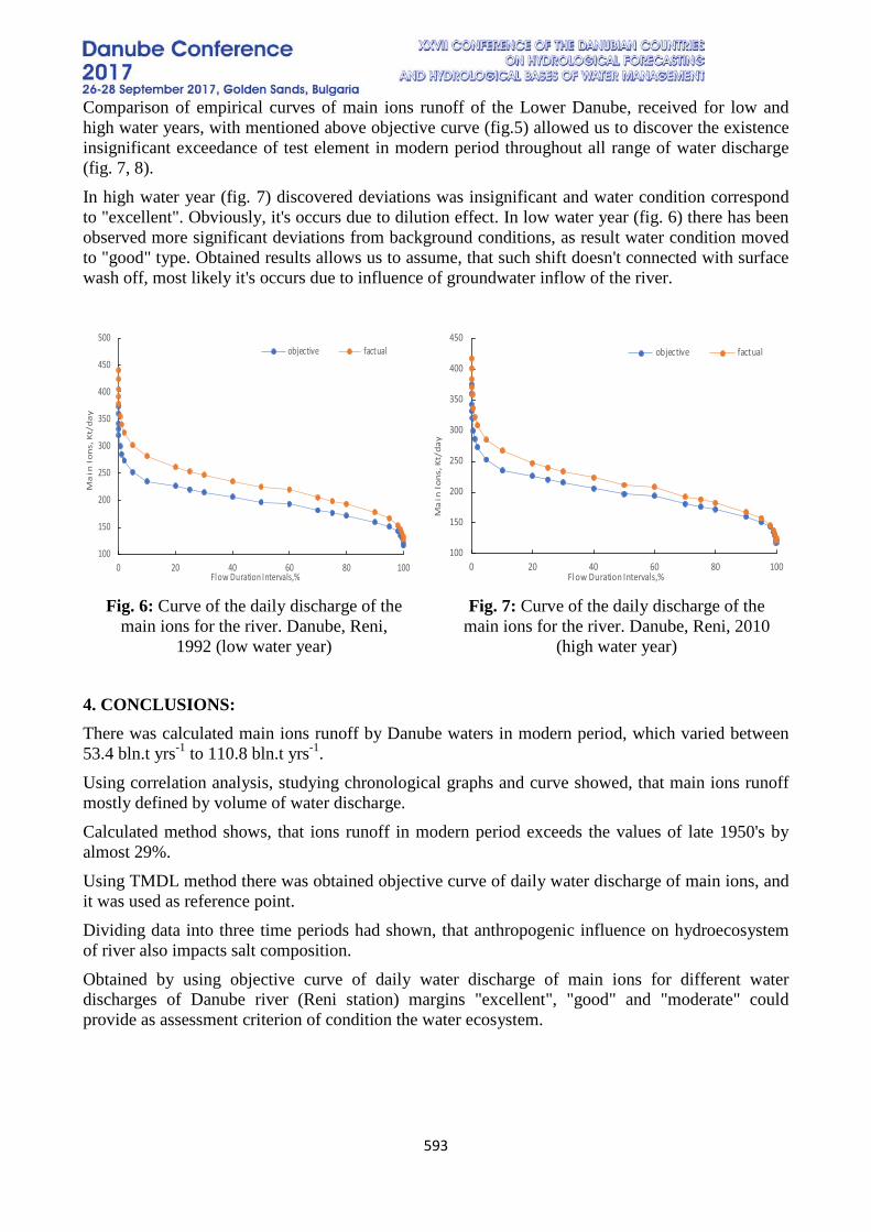
593

Comparison of empirical curves of main ions runoff of the Lower Danube, received for low and high water years, with mentioned above objective curve (fig.5) allowed us to discover the existence insignificant exceedance of test element in modern period throughout all range of water discharge (fig. 7, 8). In high water year (fig. 7) discovered deviations was insignificant and water condition correspond to "excellent". Obviously, it's occurs due to dilution effect. In low water year (fig. 6) there has been observed more significant deviations from background conditions, as result water condition moved to "good" type. Obtained results allows us to assume, that such shift doesn't connected with surface wash off, most likely it's occurs due to influence of groundwater inflow of the river.

Fig. 6: Curve of the daily discharge of the

main ions for the river. Danube, Reni, 1992 (low water year)

Fig. 7: Curve of the daily discharge of the main ions for the river. Danube, Reni, 2010

(high water year)

4. CONCLUSIONS: There was calculated main ions runoff by Danube waters in modern period, which varied between 53.4 bln.t yrs-1 to 110.8 bln.t yrs-1. Using correlation analysis, studying chronological graphs and curve showed, that main ions runoff mostly defined by volume of water discharge. Calculated method shows, that ions runoff in modern period exceeds the values of late 1950's by almost 29%. Using TMDL method there was obtained objective curve of daily water discharge of main ions, and it was used as reference point. Dividing data into three time periods had shown, that anthropogenic influence on hydroecosystem of river also impacts salt composition. Obtained by using objective curve of daily water discharge of main ions for different water discharges of Danube river (Reni station) margins "excellent", "good" and "moderate" could provide as assessment criterion of condition the water ecosystem.

100

150

200

250

300

350

400

450

500

0 20 40 60 80 100

Ma

in I

on

s,K

t/d

ay

Flow Duration Intervals,%

objective factual

100

150

200

250

300

350

400

450

0 20 40 60 80 100

Ma

in Io

ns,K

t/da

y

Flow Duration Intervals,%

objective factual

594

5. REFERENCES [1] Main results of the assessment of transboundary rivers, lakes and groundwater in Eastern and Northern Europe that flow into the Black Sea: materials of the Working Group on Monitoring and Evaluation, 15-16 December 2010 (WGMA/Extra2010/Inf.1). [2] Almazov A.M. Hydrology of the estuary of the Danube / A.M. Almazov, F.M. K. Bondar, N.F. Vagin – M.: Hydrometizdat, 1963. − 382p. [3] Nikiforov Y.D. Hydrology of the estuary of the Danube / Nikiforova Y.D. And Dyakonu K. – M.: Hydrometizdat, 1963. – 83–350p. [4] Materials of the second international complex expedition to study the Danube (July-August 1993) // Water resources. – M: Nauka, 1993. – Т. 20, №4. – 440–446p. [5] Materials of the first international complex expedition to study the Danube (March 1988). - P.1.- Kiev, 1989. - Manuscript of the Dep. In VINITI, № 210 – 417p. [6] Convention on Cooperation for the Protection and Sustainable use of the Danube river (Danube river Protection Convention), signed on June 29 1994 // International Commission on Danube River Protection ICDPR. – 1998. – 22p. [7] Ecological Action Program for the Danube River Basin. Strategic Action Plan. Part 3. Problems and priorities. // International Commission for the Protection of the DanubeRiver. – www.icpdr.orgwww.menr.gov.ua/dovkil [8] Management Plans for the Danube River Basin published 2015 [Електронний ресурс]. – Режим доступу: www.icpdr.org/main/management-plans-danube-river-basin-published. [9] Osadchyi V. Et all / V. Osadchyi, B.Nabyvanets, P.Linnik, N.Osadcha, Yu.Nabyvanets (2016) Processes Determining Surface Water Chemistry. Springer.-2016, 265 р. [10] Andreyyanov V.G. Cyclic fluctuations in the annual runoff and their accounting for hydrological calculations / V.G. Andreevanov // Proceedings of GGI. - L.: Gidrometeoizdat, 1959. - Issue. 68. 3–49p. [11] Directive 2000/60/EC of European Parliament and of the Council of 23 October 2000 es-tablishing a framework for Community action in the field of water policy // Official Journal of the European Communities, 22.12 2000. L – 327/1. – 118 p. [12] U.S. EPA. 2007. Report on the Environment: Science Report. EPA’s 2007 EPA/600/R-07/045. Washington, DC.

595

ASSESSMENT OF THE BALANCE OF WASTE WATER DISCHARGED INTO A SURFACE FLOWS IN SLOVAKIA

Poórová Jana, Döményová Jana, Ďurkovičová Daniela Slovak Hydrometeorological Institute, Jeséniova 17, 833 15 Bratislava, Slovak Republic

ABSTRACT Information and data on the quantity and polluting discharges of wastewater from point sources of pollution within the Slovak Water Act are annually reported to the Central Water Register (so called: “Súhrnná evidencia o vodách”) performed by Slovak Hydrometeorological Institute. Based on these data the balance of pollution in wastewater is annually evaluated. The causes of pollution of the waste water and evaluation of the pollution in the years 2000 – 2016 are analysed. Analysis of the significant sources of the pollution in the different sub-basins of Slovakia provide the basic data for evaluation of the status of surface water and to control the effectiveness of measures set to reduce the pollution in surface flows. The development of the pollution of waste water in the years 2000 – 2016 were analysed. Keywords: water use, Central Water Register, waste water, pollution, surface water, annual balance

1 INTRODUCTION The basis of processing of the balance of the waste water in the Slovak republic are reported by the water users, who carry out their activity according to the issued permits for use of the water. Water users have an obligation to notify the data of waste water discharges to the Slovak Hydrometeorological Institute (SHMI) on the prescribed forms in accordance Act No. 364/2004 Coll. on water and on amendment and supplement to act No. 372/1990 Coll. delicts in wording of later regulations (Water act) as follows: „Any person who discharges waste water or special water into surface water or groundwater in quantities of more than 10 000 m3 per year or over 1 000 m3 per month from household and who produces and discharges waste water, special water or geothermal water in the course of entrepreneurial activities, is obliged to report the annual data...“ (Forms for the commencement of discharges of waste water within 30 days of the establishment of the reporting obligation and annual forms until 31 January of the following calendar year.) Information and data on the quantity and the pollution of discharged waste water from point sources of pollution within the Slovak Water Act shall be reported annually to the Central Water Register (so called: “Súhrnná evidencia o vodách”) performed by SHMI. Information database system (Central Water Register) is able to perform the data collection, their evaluation and reporting in accordance with national and EU legislative regulations valid in water sector.

596

The annual notifications of the waste water discharges into surface waters shall include the monthly amounts of the discharged waste water and the results of analyses of the produced pollution and the discharged pollution and other necessary information. Based on these data the balance of pollution in waste water is annually evaluated. Analysis of the major sources of the pollution in the different sub-basins of Slovakia provides the basic data for the evaluation of the status of surface water and to control the effectiveness of the measures set to reduce the pollution in surface flows. The development of the pollution of waste water in the years 2000 – 2016 were analysed.

2 METHODOLOGY FOR PROCESSING OF THE WASTE WATER DATA The annual balance of discharged pollution from point sources to surface water is expressed by the individual parameters and processed according to the methodology valid in Slovakia: If the frequency of pollutant measurements is at least once a month, the annual balance of pollution shall be calculated as the sum of the monthly values of balance (in kg or tonnes per year). If the frequency of pollutant measurements is less, an average annual value of the concentration for the selected parameter shall be determined and multiplied by the annual amount of discharged waste water from a specific point source (in kg or tonnes per year). The list of parameters:

• BOD5, CODCr, Ntotal and Ptotal • Synthetic and non-synthetic pollutants: priority substances (WFD) and pollutants

relevant for the Slovakia.

3 ASSESSMENT OF THE BALANCE OF WASTE WATER DISCHARGED INTO A SURFACE FLOWS

Figure 1 shows the development of waste water discharged into surface water from 2000 to 2016.

597

Fig. 1: Development of discharged waste water into surface water

At present, the decreasing trend of discharged pollution (BOD5, CODCr) is observed in comparison with 2000. (Fig. 2).

Fig. 2: Development of the waste water pollution discharged into surface water

Fig. 3 shows the amount of pollutants (BOD5, CODCr, Ntotal and Ptotal) discharged in river basins in Slovakia. More significant amount of pollutions were identified in the river basins of Váh, Hron and Bodrog.

0

200000

400000

600000

800000

1000000

2000 2001 2002 2003 2004 2005 2006 2007 2008 2009 2010 2011 2012 2013 2014 2015 2016

Amou

nt o

f was

te w

ater

[tho

usan

d m

3 / y

ear]

Year

0

10000

20000

30000

40000

50000

60000

2000 2001 2002 2003 2004 2005 2006 2007 2008 2009 2010 2011 2012 2013 2014 2015 2016

Para

met

er

[ton

nes/

year

]

Year BOD (5) COD (Cr)

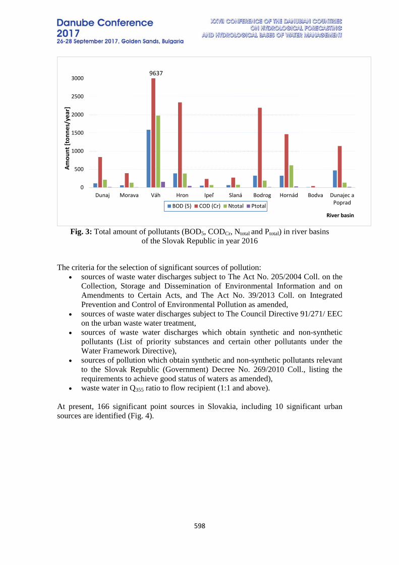
598

Fig. 3: Total amount of pollutants (BOD5, CODCr, Ntotal and Ptotal) in river basins

of the Slovak Republic in year 2016 The criteria for the selection of significant sources of pollution:

• sources of waste water discharges subject to The Act No. 205/2004 Coll. on the Collection, Storage and Dissemination of Environmental Information and on Amendments to Certain Acts, and The Act No. 39/2013 Coll. on Integrated Prevention and Control of Environmental Pollution as amended,

• sources of waste water discharges subject to The Council Directive 91/271/ EEC on the urban waste water treatment,

• sources of waste water discharges which obtain synthetic and non-synthetic pollutants (List of priority substances and certain other pollutants under the Water Framework Directive),

• sources of pollution which obtain synthetic and non-synthetic pollutants relevant to the Slovak Republic (Government) Decree No. 269/2010 Coll., listing the requirements to achieve good status of waters as amended),

• waste water in Q355 ratio to flow recipient (1:1 and above).

At present, 166 significant point sources in Slovakia, including 10 significant urban sources are identified (Fig. 4).

River basin

0

500

1000

1500

2000

2500

3000

Dunaj Morava Váh Hron Ipeľ Slaná Bodrog Hornád Bodva Dunajec aPoprad

Amou

nt [t

onne

s/ye

ar]

9637

BOD (5) COD (Cr) Ntotal Ptotal

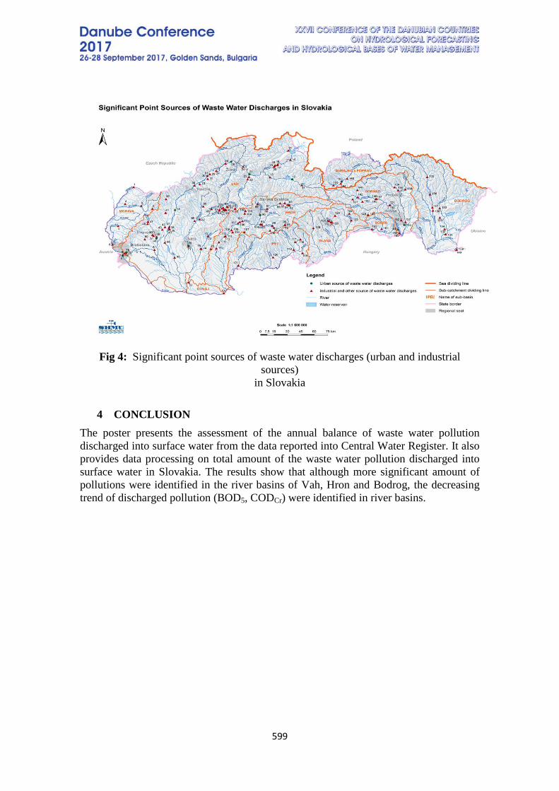
599

Fig 4: Significant point sources of waste water discharges (urban and industrial

sources) in Slovakia

4 CONCLUSION

The poster presents the assessment of the annual balance of waste water pollution discharged into surface water from the data reported into Central Water Register. It also provides data processing on total amount of the waste water pollution discharged into surface water in Slovakia. The results show that although more significant amount of pollutions were identified in the river basins of Vah, Hron and Bodrog, the decreasing trend of discharged pollution (BOD5, CODCr) were identified in river basins.

600

TOPIC 8: ECOHYDROLOGY

METHODOLOGY FOR DEVELOPING AND ANALYZING MULTI-

PRESSURES MATRIX ACTING ON FUNCTIONAL ELEMENTARY

CATCHMENTS (FEC) IN THE DANUBE CATCHMENT

Lidija Globevnik, Maja Koprivšek, Luka Snoj

1 University of Ljubljana Faculty for Civil Engineering and Geodesy, Slovenia Corresponding author: Lidija Globevnik, University of Ljubljana Faculty for Civil Engineering and

Geodesy, Jamova 28, Ljubljana, email: lidija.globevnik@guest.arnes.si

ABSTRACT River ecology is affected by a lot of pressures Mostly, they act at the same time, but their effect may be additive, synergistic or antagonistic. Considering this it is important to analyze the impact of all of pressures at the same time. Since effects of multiple pressures vary depending on the typology of a river water body and the geographic region where water body is located, we have used the broad river typology (20 river types) and the broad hydro-regions of Europe in order to analyze relations between pressures and ecological status. This paper presents a methodology of developing multi-pressures matrix acting on river in the Danube catchment and ranking pressures with the greatest impact on the ecological status of rivers. Knowledge on the most important pressures may serve as a basis for decisions on to identify such measures that give the best effects in order to improve the ecological status of water bodies. The rivers in the Danube River catchment mostly belong to the Eastern Continental region. The highest share have low-land (lower than 200 m asl)/medium to large rivers (100 – 10000 km2) rivers with calcareous and mixed geology (20 % of all FECs in the Danube River catchment) and mid-altitude (200 – 800 m asl.) /medium to large rivers with calcareous with mixed geology (15 %). As reported in 1st RBMP, 40 % of river water bodies are in good or more than good ecological status. In general, in the Eastern Continental region all three types of pressures, namely, hydrological, morphological and chemical are equally important. But, on small and mid-latitude/medium to large rivers, hydrological pressures may prevail over the other two groups of pressures. Keywords: broad river typology, multi pressures, ecological status, random forest, functional elementary catchments (FEC).

601

INTRODUCTION European rivers are affected by different kinds of pressures such as pollution of water with organic, inorganic and toxic substances, degradation of riverbed, water abstraction, regulation of river flow, land use/cover in the river corridor and catchment area as well as pressures related to climate changes. Mostly several types of pressures act at the same time, but their effect may be additive, synergistic or antagonistic ([1], [2], [3]). Researches on pressures on European rivers are important for decision making regarding monitoring and management. It is important to focus on “anthropogenic pressures”, which can be mitigated by implementing sufficient management measures. While the same factor or the same factor value, respectively, can have different effects on different river types, it is necessary to consider also natural and geographical factors such as longitude, latitude, altitude and size of drainage area. For this reasons the analysis have been done separately considering different river types and broadhydro regions. To achieve these objectives we classified all rivers in the Danube River catchment into broad river types and broad hydroregions as described below. For the river water bodies in the catchment pressure analysis we used the methodology developed within 7th FP project MARS (www.mars-project.eu). We used publicly available data on pressures and their drivers, such are urban waste water, industrial, electrical and material processing facilities, land use/covere data, diffuse pressures of nutrients from agriculture) and ecological status of water bodies as reported under Water Framework Directive in 2010. Data have been interlinked when necessary and stored in an integrated database from where it was used for statistical analyses and ranking of pressures with the greatest impact on the ecological status of rivers water bodies in Europe. The findings here are the preliminary results of pressure on rivers in the Danube River catchment. We describe river typology and regions, ecological status of rivers, selected pressures indicators and data coverage of pressure in the Danube River catchment. We compare ecological statutes and pressures by broadhydro regions and indicate which pressures are important.

1. DATA AND MATERIALS 1.1 Broad river typology and broad hydroregions To facilitate comparison of ecological status, European rivers were classified into 20 broad river types [4], which combine rivers with similar physical-geographical characteristics, such as size of drainage area, elevation and geology. Altitude is divided into three categories: lowland (≤ 200 m a. s. l.), mid-altitude (200 – 800 m a. s. l.) and highland (> 800 m a. s. l.). Catchment area is divided into three categories: very small – small (≤ 100 km2), medium – large (100 – 10000 km2) and very large (≥ 10000 km2). Geology is divided into four categories: siliceous, calcareous, organic/humic and mixed. Glacial rivers are combined into one category and Mediterranean rivers into four categories, both irrespective of geology categories. Very large rivers are combined in one category irrelevant of geology and altitude categories.

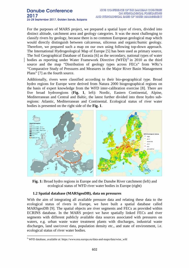
602

For the purposes of MARS project, we prepared a spatial layer of rivers, divided into distinct altitude, catchment area and geology categories. It was the most challenging to classify rivers by geology, because there is no common European geological map which would directly distinguish between calcareous, siliceous and organic/humic geology. Therefore, we prepared such a map on our own using following top-down approach. The International Hydrogeological Map of Europe [5] has been used as primary source, The Soil Geographical Database of Eurasia [6] as the secondary, national types of water bodies as reporting under Water Framework Directive (WFD)9 in 2010 as the third source and the map “Distribution of geology types across FECs” from WRc’s “Comparative Study of Pressures and Measures in the Major River Basin Management Plans” [7] as the fourth source. Additionally, rivers were classified according to their bio-geographical type. Broad hydro regions for Europe were derived from Natura 2000 biogeographical regions on the basis of expert knowledge from the WFD inter-calibration exercise [8]. There are five broad hydroregions (Fig. 1, left): Nordic, Eastern Continental, Alpine, Mediterranean and Central and Baltic, the latest further divided into three hydro sub-regions: Atlantic, Mediterranean and Continental. Ecological status of river water bodies is presented on the right side of the Fig. 1.

Fig. 1: Broad hydro regions in Europe and the Danube River catchment (left) and

ecological status of WFD river water bodies in Europe (right)

1.2 Spatial database (MARSgeoDB), data on pressures With the aim of integrating all available pressure data and relating these data to the ecological status of rivers in Europe, we have built a spatial database called MARSgeoDB [9]. The spatial objects are river segments and FECs as provided within ECRINS database. In the MARS project we have spatially linked FECs and river segments with different publicly available data sources associated with pressures on waters, e.g. urban waste water treatment plants with discharges, industrial waste discharges, land use/cover data, population density etc., and state of environment, i.e. ecological status of river water bodies. 9 WFD database, available at: https://www.eea.europa.eu/data-and-maps/data/wise_wfd

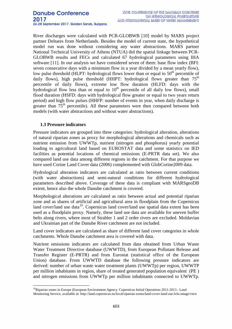
603

River discharges were calculated with PCR-GLOBWB [10] model by MARS project partner Deltares from Netherlands. Besides the model of current state, the hypothetical model run was done without considering any water abstractions. MARS partner National Technical University of Athens (NTUA) did the spatial linkage between PCR-GLOBWB results and FECs and calculated 67 hydrological parameters using IHA software [11]. In our analysis we have considered seven of them: base flow index (BFI: seven consecutive days with a minimum flow in a year divided by a mean yearly flow), low pulse threshold (HLPT: hydrological flows lower than or equal to 50th percentile of daily flows), high pulse threshold (HHPT: hydrological flows greater than 75th percentile of daily flows), extreme low flow duration (HLFD: days with the hydrological flow less than or equal to 10th percentile of all daily low flows), small flood duration (HSFD: days with hydrological flow greater or equal to two years return period) and high flow pulses (HHFP: number of events in year, when daily discharge is greater than 75th percentile). All these parameters were then compared between both models (with water abstractions and without water abstractions).

1.3 Pressure indicators

Pressure indicators are grouped into three categories: hydrological alteration, alterations of natural riparian zones as proxy for morphological alterations and chemicals such as nutrient emission from UWWTp, nutrient (nitrogen and phosphorus) yearly potential loading to agricultural land based on EUROSTAT data and some statistics on IED facilities as potential locations of chemical emissions (E-PRTR data set). We also compared land use data among different regions in the catchment. For that purpose we have used Corine Land Cover data (2006) complemented with GlobCorine2009 data. Hydrological alteration indicators are calculated as ratio between current conditions (with water abstractions) and semi-natural conditions for different hydrological parameters described above. Coverage of these data is compliant with MARSgeoDB extent, hence also the whole Danube catchment is covered. Morphological alterations are calculated as ratio between actual and potential riparian zone and as shares of artificial and agricultural area in floodplain from the Copernicus land cover/land use data10. Copernicus land cover/land use spatial data extent has been used as a floodplain proxy. Namely, these land use data are available for uneven buffer belts along rivers, where most of Strahler 1 and 2 order rivers are excluded. Moldavian and Ukrainian part of the Danube River catchment are not included. Land cover indicators are calculated as share of different land cover categories in whole catchments. Whole Danube catchment area is covered with data. Nutrient emissions indicators are calculated from data obtained from Urban Waste Water Treatment Directive database (UWWTD), from European Pollutant Release and Transfer Register (E-PRTR) and from Eurostat (statistical office of the European Union) database. From UWWTD database the following pressure indicators are derived: number of urban waste water treatment plants (UWWTp) per region, UWWTP per million inhabitants in region, share of treated generated population equivalent (PE ) and nitrogen emissions from UWWTp per million inhabitants connected to UWWTp.

10Riparian zones in Europe (European Environment Agency. Copernicus Initial Operations 2011-2013 - Land Monitoring Service, available at: http://land.copernicus.eu/local/riparian-zones/land-cover-land-use-lclu-image/view

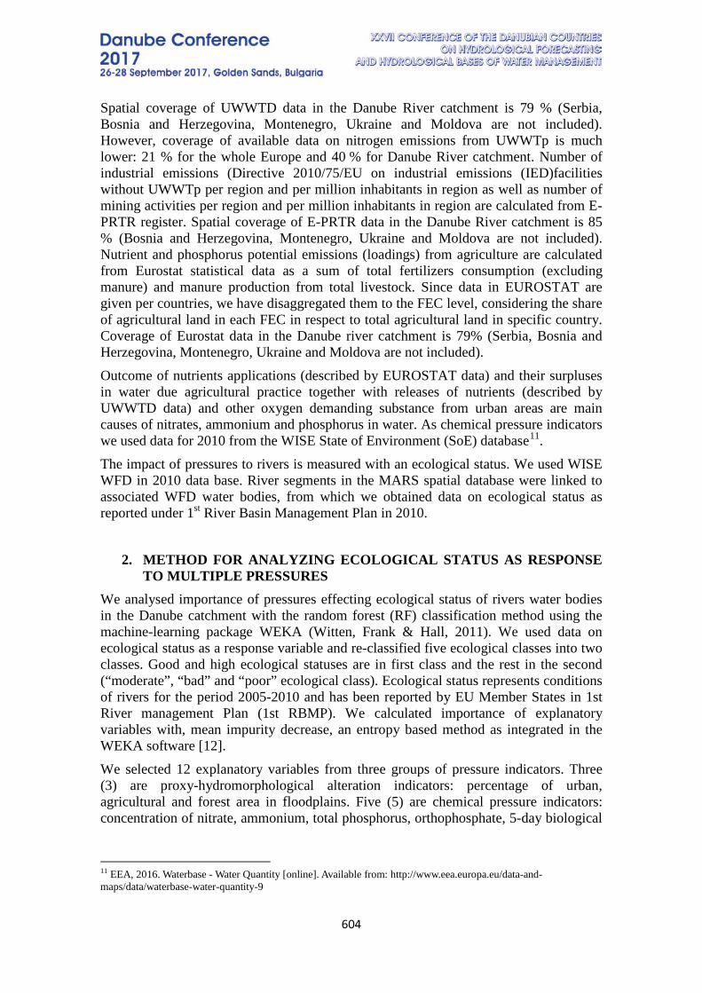
604

Spatial coverage of UWWTD data in the Danube River catchment is 79 % (Serbia, Bosnia and Herzegovina, Montenegro, Ukraine and Moldova are not included). However, coverage of available data on nitrogen emissions from UWWTp is much lower: 21 % for the whole Europe and 40 % for Danube River catchment. Number of industrial emissions (Directive 2010/75/EU on industrial emissions (IED)facilities without UWWTp per region and per million inhabitants in region as well as number of mining activities per region and per million inhabitants in region are calculated from E-PRTR register. Spatial coverage of E-PRTR data in the Danube River catchment is 85 % (Bosnia and Herzegovina, Montenegro, Ukraine and Moldova are not included). Nutrient and phosphorus potential emissions (loadings) from agriculture are calculated from Eurostat statistical data as a sum of total fertilizers consumption (excluding manure) and manure production from total livestock. Since data in EUROSTAT are given per countries, we have disaggregated them to the FEC level, considering the share of agricultural land in each FEC in respect to total agricultural land in specific country. Coverage of Eurostat data in the Danube river catchment is 79% (Serbia, Bosnia and Herzegovina, Montenegro, Ukraine and Moldova are not included). Outcome of nutrients applications (described by EUROSTAT data) and their surpluses in water due agricultural practice together with releases of nutrients (described by UWWTD data) and other oxygen demanding substance from urban areas are main causes of nitrates, ammonium and phosphorus in water. As chemical pressure indicators we used data for 2010 from the WISE State of Environment (SoE) database11. The impact of pressures to rivers is measured with an ecological status. We used WISE WFD in 2010 data base. River segments in the MARS spatial database were linked to associated WFD water bodies, from which we obtained data on ecological status as reported under 1st River Basin Management Plan in 2010.

2. METHOD FOR ANALYZING ECOLOGICAL STATUS AS RESPONSE TO MULTIPLE PRESSURES

We analysed importance of pressures effecting ecological status of rivers water bodies in the Danube catchment with the random forest (RF) classification method using the machine-learning package WEKA (Witten, Frank & Hall, 2011). We used data on ecological status as a response variable and re-classified five ecological classes into two classes. Good and high ecological statuses are in first class and the rest in the second (“moderate”, “bad” and “poor” ecological class). Ecological status represents conditions of rivers for the period 2005-2010 and has been reported by EU Member States in 1st River management Plan (1st RBMP). We calculated importance of explanatory variables with, mean impurity decrease, an entropy based method as integrated in the WEKA software [12]. We selected 12 explanatory variables from three groups of pressure indicators. Three (3) are proxy-hydromorphological alteration indicators: percentage of urban, agricultural and forest area in floodplains. Five (5) are chemical pressure indicators: concentration of nitrate, ammonium, total phosphorus, orthophosphate, 5-day biological

11 EEA, 2016. Waterbase - Water Quantity [online]. Available from: http://www.eea.europa.eu/data-and-maps/data/waterbase-water-quantity-9

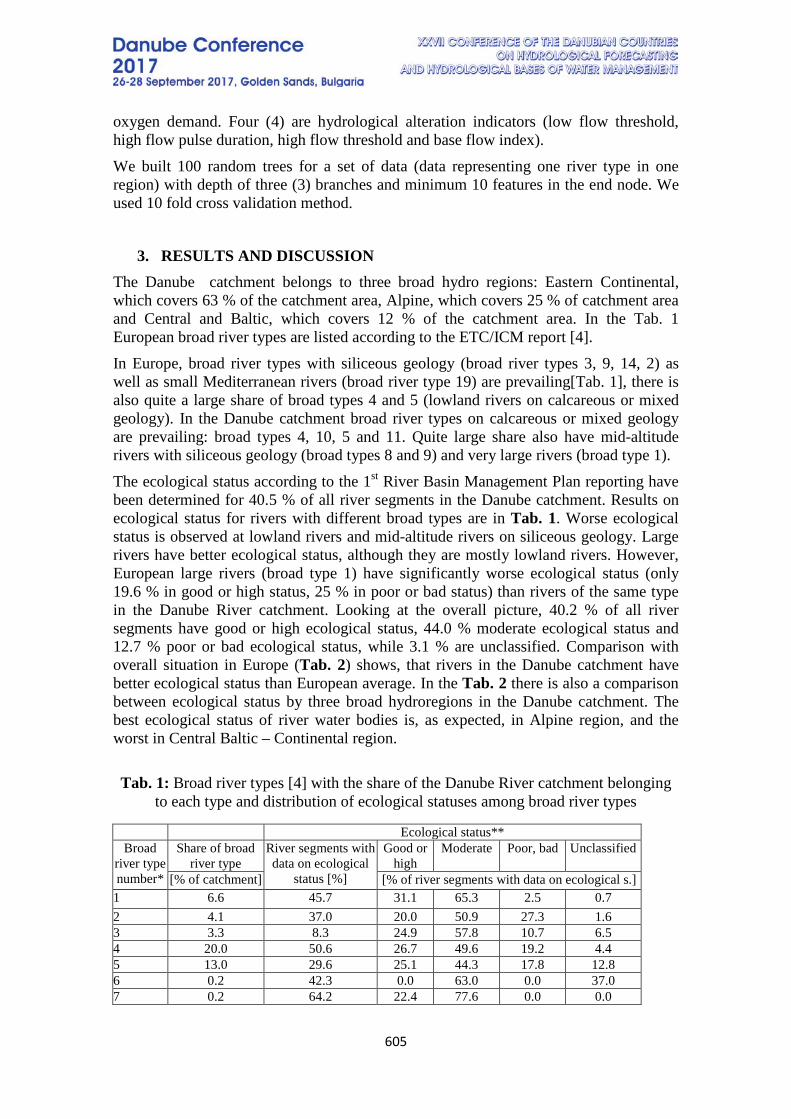
605

oxygen demand. Four (4) are hydrological alteration indicators (low flow threshold, high flow pulse duration, high flow threshold and base flow index). We built 100 random trees for a set of data (data representing one river type in one region) with depth of three (3) branches and minimum 10 features in the end node. We used 10 fold cross validation method.

3. RESULTS AND DISCUSSION The Danube catchment belongs to three broad hydro regions: Eastern Continental, which covers 63 % of the catchment area, Alpine, which covers 25 % of catchment area and Central and Baltic, which covers 12 % of the catchment area. In the Tab. 1 European broad river types are listed according to the ETC/ICM report [4]. In Europe, broad river types with siliceous geology (broad river types 3, 9, 14, 2) as well as small Mediterranean rivers (broad river type 19) are prevailing[Tab. 1], there is also quite a large share of broad types 4 and 5 (lowland rivers on calcareous or mixed geology). In the Danube catchment broad river types on calcareous or mixed geology are prevailing: broad types 4, 10, 5 and 11. Quite large share also have mid-altitude rivers with siliceous geology (broad types 8 and 9) and very large rivers (broad type 1). The ecological status according to the 1st River Basin Management Plan reporting have been determined for 40.5 % of all river segments in the Danube catchment. Results on ecological status for rivers with different broad types are in Tab. 1. Worse ecological status is observed at lowland rivers and mid-altitude rivers on siliceous geology. Large rivers have better ecological status, although they are mostly lowland rivers. However, European large rivers (broad type 1) have significantly worse ecological status (only 19.6 % in good or high status, 25 % in poor or bad status) than rivers of the same type in the Danube River catchment. Looking at the overall picture, 40.2 % of all river segments have good or high ecological status, 44.0 % moderate ecological status and 12.7 % poor or bad ecological status, while 3.1 % are unclassified. Comparison with overall situation in Europe (Tab. 2) shows, that rivers in the Danube catchment have better ecological status than European average. In the Tab. 2 there is also a comparison between ecological status by three broad hydroregions in the Danube catchment. The best ecological status of river water bodies is, as expected, in Alpine region, and the worst in Central Baltic – Continental region. Tab. 1: Broad river types [4] with the share of the Danube River catchment belonging

to each type and distribution of ecological statuses among broad river types

Ecological status** Broad

river type number*

Share of broad river type

River segments with data on ecological

status [%]

Good or high

Moderate

Poor, bad

Unclassified

[% of catchment] [% of river segments with data on ecological s.] 1 6.6 45.7 31.1 65.3 2.5 0.7 2 4.1 37.0 20.0 50.9 27.3 1.6 3 3.3 8.3 24.9 57.8 10.7 6.5 4 20.0 50.6 26.7 49.6 19.2 4.4 5 13.0 29.6 25.1 44.3 17.8 12.8 6 0.2 42.3 0.0 63.0 0.0 37.0 7 0.2 64.2 22.4 77.6 0.0 0.0

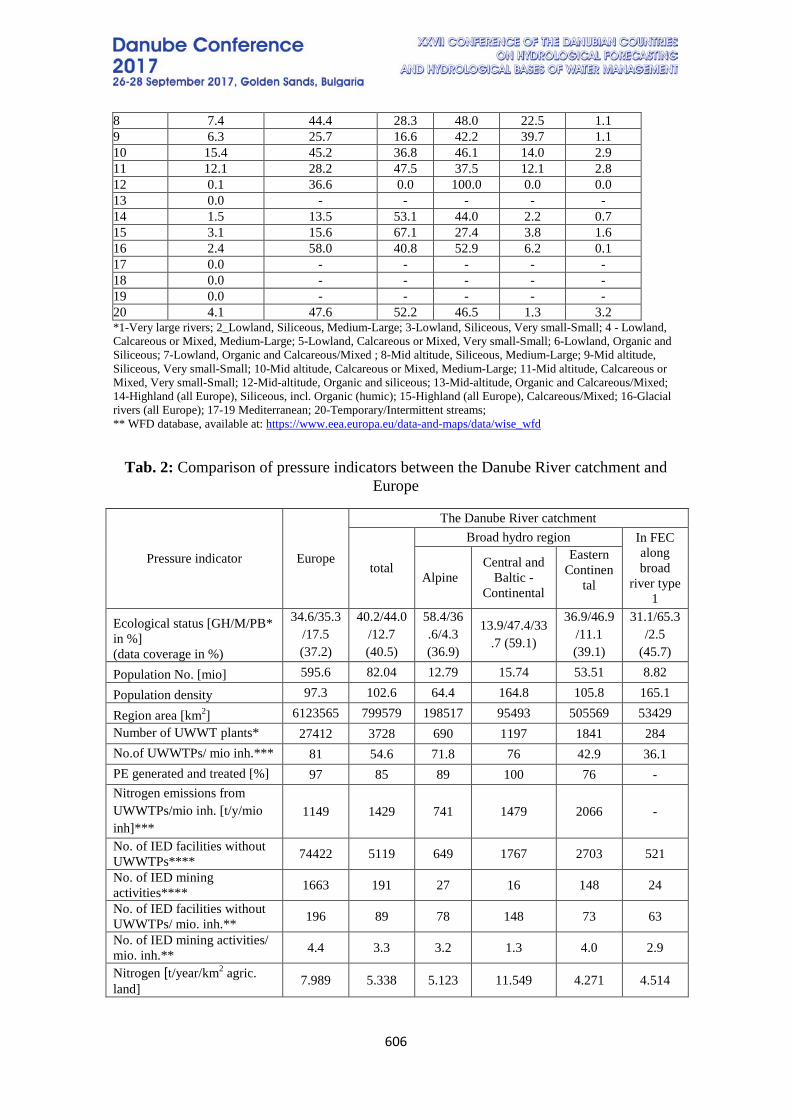
606

8 7.4 44.4 28.3 48.0 22.5 1.1 9 6.3 25.7 16.6 42.2 39.7 1.1 10 15.4 45.2 36.8 46.1 14.0 2.9 11 12.1 28.2 47.5 37.5 12.1 2.8 12 0.1 36.6 0.0 100.0 0.0 0.0 13 0.0 - - - - - 14 1.5 13.5 53.1 44.0 2.2 0.7 15 3.1 15.6 67.1 27.4 3.8 1.6 16 2.4 58.0 40.8 52.9 6.2 0.1 17 0.0 - - - - - 18 0.0 - - - - - 19 0.0 - - - - - 20 4.1 47.6 52.2 46.5 1.3 3.2 *1-Very large rivers; 2_Lowland, Siliceous, Medium-Large; 3-Lowland, Siliceous, Very small-Small; 4 - Lowland, Calcareous or Mixed, Medium-Large; 5-Lowland, Calcareous or Mixed, Very small-Small; 6-Lowland, Organic and Siliceous; 7-Lowland, Organic and Calcareous/Mixed ; 8-Mid altitude, Siliceous, Medium-Large; 9-Mid altitude, Siliceous, Very small-Small; 10-Mid altitude, Calcareous or Mixed, Medium-Large; 11-Mid altitude, Calcareous or Mixed, Very small-Small; 12-Mid-altitude, Organic and siliceous; 13-Mid-altitude, Organic and Calcareous/Mixed; 14-Highland (all Europe), Siliceous, incl. Organic (humic); 15-Highland (all Europe), Calcareous/Mixed; 16-Glacial rivers (all Europe); 17-19 Mediterranean; 20-Temporary/Intermittent streams; ** WFD database, available at: https://www.eea.europa.eu/data-and-maps/data/wise_wfd

Tab. 2: Comparison of pressure indicators between the Danube River catchment and Europe

Pressure indicator Europe

The Danube River catchment

total

Broad hydro region In FEC along broad

river type 1

Alpine Central and

Baltic - Continental

Eastern Continen

tal

Ecological status [GH/M/PB* in %] (data coverage in %)

34.6/35.3/17.5 (37.2)

40.2/44.0/12.7 (40.5)

58.4/36.6/4.3 (36.9)

13.9/47.4/33.7 (59.1)

36.9/46.9/11.1 (39.1)

31.1/65.3/2.5

(45.7)

Population No. [mio] 595.6 82.04 12.79 15.74 53.51 8.82

Population density 97.3 102.6 64.4 164.8 105.8 165.1

Region area [km2] 6123565 799579 198517 95493 505569 53429 Number of UWWT plants* 27412 3728 690 1197 1841 284 No.of UWWTPs/ mio inh.*** 81 54.6 71.8 76 42.9 36.1 PE generated and treated [%] 97 85 89 100 76 - Nitrogen emissions from UWWTPs/mio inh. [t/y/mio inh]***

1149 1429 741 1479 2066 -

No. of IED facilities without UWWTPs**** 74422 5119 649 1767 2703 521

No. of IED mining activities**** 1663 191 27 16 148 24

No. of IED facilities without UWWTPs/ mio. inh.** 196 89 78 148 73 63

No. of IED mining activities/ mio. inh.** 4.4 3.3 3.2 1.3 4.0 2.9

Nitrogen [t/year/km2 agric. land]

7.989 5.338 5.123 11.549 4.271 4.514

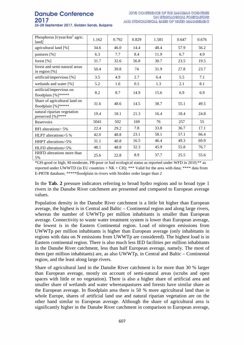
607

Phosphorus [t/year/km2 agric. land] 1.162 0.792 0.829 1.581 0.647 0.676

agricultural land [%] 34.6 46.0 14.4 48.4 57.9 56.2 pastures [%] 6.3 7.7 8.4 11.9 6.7 4.9 forest [%] 31.7 32.6 56.8 30.7 23.5 19.5 forest and semi-natural areas in region [%] 50.4 39.8 74 31.9 27.8 23.7

artificial/impervious [%] 3.5 4.9 2.7 6.4 5.5 7.1 wetlands and water [%] 5.2 1.6 0.5 1.3 2.1 8.1 artificial/impervious on floodplain [%]***** 8.2 8.7 14.9 15.6 6.9 6.9

Share of agricultural land on floodplain [%]***** 31.6 48.6 14.5 38.7 55.1 49.5

natural riparian vegetation preserved [%]**** 19.4 18.1 21.3 16.4 18.4 24.8

Reservoirs 5041 502 169 76 257 55

BFI alterations> 5% 22.4 29.2 7.8 33.8 36.7 17.1

HLPT alterations>5 % 42.0 48.8 23.1 58.1 57.1 66.4

HHPT alterations>5% 31.1 40.8 16.5 46.4 49.3 69.9

HLFD alterations>5% 48.1 48.8 32.3 45.9 55.8 76.7 HHFD alterations more than 5% 25.6 22.8 8.9 37.7 25.5 55.6

*GH-good or high, M-moderate, PB-poor or bad ecological status as reported under WFD in 2010;** as reported under UWWTD (in EU countries + NK + CH); *** Valid for the area with data; **** data from E-PRTR database; *****floodplain in rivers with Strahler order larger than 2

In the Tab. 2 pressure indicators referring to broad hydro regions and to broad type 1 rivers in the Danube River catchment are presented and compared to European average values. Population density in the Danube River catchment is a little bit higher than European average, the highest is in Central and Baltic – Continental region and along large rivers, whereas the number of UWWTp per million inhabitants is smaller than European average. Connectivity to waste water treatment system is lower than European average, the lowest is in the Eastern Continental region. Load of nitrogen emissions from UWWTp per million inhabitants is higher than European average (only inhabitants in regions with data on N emissions from UWWTp are considered). The highest load is in Eastern continental region. There is also much less IED facilities per million inhabitants in the Danube River catchment, less than half European average, namely. The most of them (per million inhabitants) are, as also UWWTp, in Central and Baltic – Continental region, and the least along large rivers. Share of agricultural land in the Danube River catchment is for more than 30 % larger than European average, mostly on account of semi-natural areas (scrubs and open spaces with little or no vegetation). There is also a higher share of artificial area and smaller share of wetlands and water whereaspastures and forests have similar share as the European average. In floodplain area there is 50 % more agricultural land than in whole Europe, shares of artificial land use and natural riparian vegetation are on the other hand similar to European average. Although the share of agricultural area is significantly higher in the Danube River catchment in comparison to European average,

608

nitrogen and phosphorus loads on agricultural land are in general lower than European average. They are both higher from European average only in Central and Baltic – Continental region and the lowest in Eastern Continental region, which has the highest share of agricultural land. Out of this we can assume agriculture in Eastern Continental region is less intensive as European. Hydrological alterations are in the Danube River catchment more significant than in European. For all considered hydrological indicators they are the smallest in the Alpine region.. The smallest change for all three broad hydro regions that appear in the Danube River catchment is in base flow index and high flow duration. There are higher changes in indicators referring to low flow conditions (low pulse threshold, extreme low flow duration). In broad type 1 rivers, hydrological alterations are higher than whole catchment’s average, and additionally to low flow conditions there are also high changes in high flow conditions (high pulse threshold, high flow duration). The pressures (pressure indicators ranked by importance) that have the highest effect on ecological status of large rivers in the Eastern continental region are high flow pulse duration, hydromophological alteration of floodplain due urbanisation and concentrations of nitrate, total phosphorus and ammonium in water. If the share of forest (with shrubs and transitional forest) in floodplain is larger than 62%, there is a higher probability that ecological status will be better than moderate. Hydromorphological alteration of floodplain due urbanisation, base flow index, share of forest (with shrubs and transitional forest) in floodplain and pollution of oxygen demanding substances (measured with 5-day biological demand) are the most influential pressures in lowland calcareous medium to large rivers (catchment size between 100 and 10000 km2). The high flow pulse duration has also a large effect on ecological state and should not be altered with more than 2%.

4. CONCLUSIONS The rivers in the Danube River catchment mostly belong to the Eastern Continental region and to low-land/medium to large rivers (100 – 10000 km2) with calcareous and mixed geology, low-land/small rivers with calcareous and mixed geology and mid-altitude/small with calcareous and mixed geology. 40 % of river water bodies are in good or more than good ecological status as reported under WFD within 1st RBMP. Considering the pressure indicators statistics, “European part” of the Danube River catchment (Central and Baltic – Continental broad hydro region) is being exposed to larger chemical pressure while in the whole catchment there are higher hydrological alterations than on European average. Importance of pressure indicators described above and their decisive effect on ecological status will be further analyzed within the MARS project using multiple regression analyses.

REFERENCES [1] Calapez, A. R., Branco, P., Santos, J. M., Ferreira, T., Hein, T., Brito, A. G., Joao Feio, M. Macroinvertebrate short-term responses to flow variation and oxygen depletion: A mesocosm approach, Science of the Total Environment, vol. 599-600, pp 1202-1212, 2017.

609

[2] Bondar-Kunze, E., Maier, S., Schönauer, D., Bahl, N., Hein, T. Antagonistic and synergistic effects on a stream periphyton community under the influence of pulsed flow velocity increase and nutrient enrichment, vol. 573, pp 594-602, 2017. [3] Schinegger, R., Palt, M., Segurado, P., Schmutz, S. Untangling the effects of multiple human stressors and their impacts on fish assemblages in European running waters, vol. 573, pp 1079-1088, 2016. [4] ETC/ICM. European Freshwater Ecosystem Assessment: Cross-walk between the Water Framework Directive and Habitats Directive types, status and pressures. ETC/ICM Technical Report 2/2015. Germany, Magdeburg: European Topic Centre on inland, coastal and marine waters, 95 pp. plus Annexes, 2015. [5] BGR, 2014. Metadata of the International Hydrogeological Map of Europe 1:1,500,000 in Vector Format (Version IHME1500 v1.1), Germany, 6 pp, 2014. [6] Tóth, G., Montanarella, L., Stolbovoy, V., Máte, F., Bódis, K., Jones, A., Panagos, P., Van Liedekerke, M. (European Commission, JRC). Soils of the European Union, Italy, 100 pp, 2008. DOI 10.2788/87029 [7] Nixon, S., Bewes, V. and Mills, D. (WRc).Task 2a Comparison of typologies. Top-down approach – development of a European typology. Contribution to a report to the European Parliament Pressures and Measures project. 140 pp, 2012. [8] Poikane, S., Zampoukas, N., Borja, A., Davies, S.P., Bund, W. and Birk, S. Intercalibration of aquatic ecological assessment methods in the European Union: Lessons learned and way forward, Environmental Science and Policy, vol. 44, pp 237-246, 2014. [9] Globevnik L., Koprivsek M. & Snoj L., 2017. Metadata to the MARS spatial database. Freshwater Metadata Journal 21: 1-7. https://doi.org/10.15504/fmj.2017.21 [10] PCR-GLOBWB website [online]: http://www.globalhydrology.nl/ [11] The Nature Conservancy. Indicators of Hydrologic Alteration Version 7.1 User's Manual, 76 pp, 2009. [12] Witten, I.H., Frank E. and Hall, M.A. 2011. Data Mining: Practical Machine Learning

Tools and Techniques. Morgan Kaufmann, Burlington, MA, 525 pp.

5. COPYRIGHT/ACKNOWLEDGEMENTS This work was funded by the MARS project (Managing Aquatic ecosystems and water resources under multiple stress), funded by the European Union under the 7th Framework Programme, contract no. 603378.

610

THE USE OF REMOTE SENSING TECHNOLOGIES FOR ESTIMATION OF THE CARPATHIAN MOUNTAINS LAND SURFACE TEMPERATURE

Viktor Vyshnevskyi, Sergii Shevchuk

Institute of Water Problems and Land Reclamation, Kyiv, Ukraine

Corresponding author: Viktor Vyshnevskyi, Institute of Water Problems and Land Reclamation, Ukraine, 03022, Kyiv, str. Vasilkivska, 37, vishnev@voliacable.com

ABSTRACT There were presented the results of use remote sensing technologies for the estimation of Carpathian Mountains land surface temperature. This investigation was provided on the background of STRM and Landsat 8 data. It was found that significant impact on the surface temperature has the exhibition of slopes. In sunny weather, regardless of season, the lowest temperature is observed not on the mountain peaks but on their northern and north-western slopes. Meanwhile, on the southern and south-eastern slopes the surface temperature is much higher. The difference in temperature on different slopes can exceed 10 °C. Key words: remote sensing technologies, the Carpathian Mountains, land surface temperature

INTRODUCTION The Carpathian Mountains are in the shape of arc, the main part of which belongs to the Danube river basin. These mountains have a large number of peaks and slopes, those are frequently visited by tourists both in summer and winter. At the same time the temperature conditions of mountains are not investigated sufficiently. It is rather difficult operating only meteorological stations data. Their quantity isn’t very large and they are located not on mountain peaks. Under these circumstances for the estimation of land surfer temperature it is possible to use remote sensing data. The main source of data was images of satellite Landsat 8 that was launched on the beginning of 2013. The main attention was paid for two regions of mountains: the Tatra Mountains, located previously on the territory of Slovak Republic and the Ukrainian Carpathian Mountains located in Ukraine.

THE REMOTE SENSING DATA

There were used STRM data for the creation of digital elevation model of Carpathian Mountains. For the evaluation of land surface temperature the data of Landsat 8 were used. This satellite provides the scanning of land surface in some diapasons of spectrum including two ones in infrared: B 10 and B 11. These data are being gathered by the Geological Survives of USA (http://glovis.usgs.gov) and is open to access for the scientific aims. The Tatra Mountains are presented on images series LC8188026. The time of photography – 9:33 UT that corresponds to 11:33 of local time. The investigated region of Ukrainian Mountains are presented on images series LC8185026. The time of

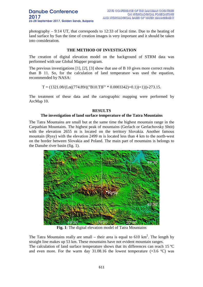
611

photography – 9:14 UT, that corresponds to 12:33 of local time. Due to the heating of land surface by Sun the time of creation images is very important and it should be taken into consideration.

THE METHOD OF INVESTIGATION

The creation of digital elevation model on the background of STRM data was performed with use Global Mapper program. The previous investigations [1], [2], [3] show that use of B 10 gives more correct results than B 11. So, for the calculation of land temperature was used the equation, recommended by NASA:

T = (1321.08/(Ln((774.89/(("B10.TIF" * 0.0003342)+0.1))+1)))-273.15.

The treatment of these data and the cartographic mapping were performed by ArcMap 10.

RESULTS

The investigation of land surface temperature of the Tatra Mountains The Tatra Mountains are small but at the same time the highest mountain range in the Carpathian Mountains. The highest peak of mountains (Gerlach or Gerlachovsky Shtit) with the elevation 2655 m is located on the territory Slovakia. Another famous mountain (Rysy) with the elevation 2499 m is located less than 4 km to the north-west on the border between Slovakia and Poland. The main part of mountains is belongs to the Danube river basin (fig. 1).

Fig. 1: The digital elevation model of Tatra Mountains

The Tatra Mountains really are small – their area is equal to 610 km2. The length by straight line makes up 53 km. These mountains have not evident mountain ranges. The calculation of land surface temperature shows that its differences can reach 15 ºC and even more. For the warm day 31.08.16 the lowest temperature (+3.6 ºC) was

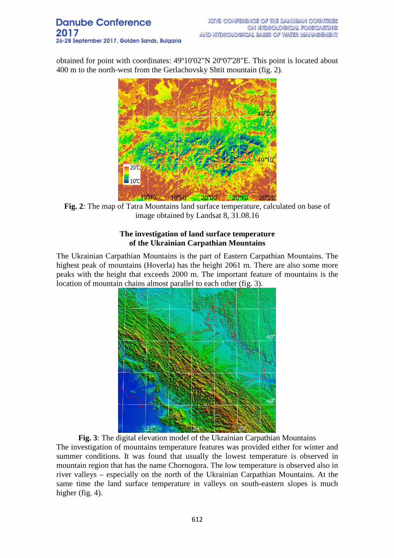
612

obtained for point with coordinates: 49º10'02"N 20º07'28"E. This point is located about 400 m to the north-west from the Gerlachovsky Shtit mountain (fig. 2).

Fig. 2: The map of Tatra Mountains land surface temperature, calculated on base of

image obtained by Landsat 8, 31.08.16

The investigation of land surface temperature of the Ukrainian Carpathian Mountains

The Ukrainian Carpathian Mountains is the part of Eastern Carpathian Mountains. The highest peak of mountains (Hoverla) has the height 2061 m. There are also some more peaks with the height that exceeds 2000 m. The important feature of mountains is the location of mountain chains almost parallel to each other (fig. 3).

Fig. 3: The digital elevation model of the Ukrainian Carpathian Mountains

The investigation of mountains temperature features was provided either for winter and summer conditions. It was found that usually the lowest temperature is observed in mountain region that has the name Chornogora. The low temperature is observed also in river valleys – especially on the north of the Ukrainian Carpathian Mountains. At the same time the land surface temperature in valleys on south-eastern slopes is much higher (fig. 4).

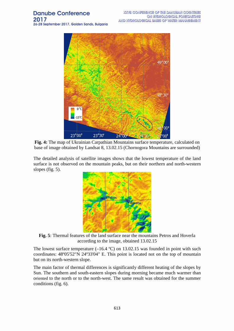
613

Fig. 4: The map of Ukrainian Carpathian Mountains surface temperature, calculated on base of image obtained by Landsat 8, 13.02.15 (Chornogora Mountains are surrounded) The detailed analysis of satellite images shows that the lowest temperature of the land surface is not observed on the mountain peaks, but on their northern and north-western slopes (fig. 5).

Fig. 5: Thermal features of the land surface near the mountains Petros and Hoverla

according to the image, obtained 13.02.15 The lowest surface temperature (–16.4 ºC) on 13.02.15 was founded in point with such coordinates: 48º05'52"N 24º33'04" E. This point is located not on the top of mountain but on its north-western slope. The main factor of thermal differences is significantly different heating of the slopes by Sun. The southern and south-eastern slopes during morning became much warmer than oriented to the north or to the north-west. The same result was obtained for the summer conditions (fig. 6).

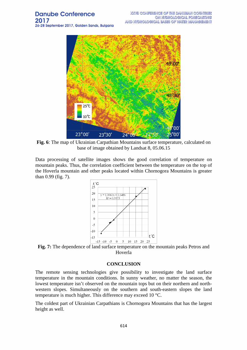
614

Fig. 6: The map of Ukrainian Carpathian Mountains surface temperature, calculated on

base of image obtained by Landsat 8, 05.06.15 Data processing of satellite images shows the good correlation of temperature on mountain peaks. Thus, the correlation coefficient between the temperature on the top of the Hoverla mountain and other peaks located within Chornogora Mountains is greater than 0.99 (fig. 7).

Fig. 7: The dependence of land surface temperature on the mountain peaks Petros and

Hoverla

CONCLUSION The remote sensing technologies give possibility to investigate the land surface temperature in the mountain conditions. In sunny weather, no matter the season, the lowest temperature isn’t observed on the mountain tops but on their northern and north-western slopes. Simultaneously on the southern and south-eastern slopes the land temperature is much higher. This difference may exceed 10 °C. The coldest part of Ukrainian Carpathians is Chornogora Mountains that has the largest height as well.

615

REFERENCES

[1] Barsi J.A., Schott J.R., Hook S.J. et al. Landsat-8 Thermal Infrared Sensor (TIRS) Vicarious Radiometric Calibration. Remote Sens, USA, 6, pp. 11607–11626, 2014. [2] Rozenstein O., Qin Z., Derimian Y., & Karnieli A. Derivation of land surface temperature for Landsat-8 TIRS using a split window algorithm. Sensors, USA, 14 (4). pp. 5768–5780, 2014. [3] Shevchuk S.A., Vyshnevskyi V.I. Using of Landsat 8 satellite data for determinination of microclimatic peculiarities of Kyiv. Ukrainian Journal of Remote Sensing, Ukraine, vol. 10, pp. 4–9, 2016.

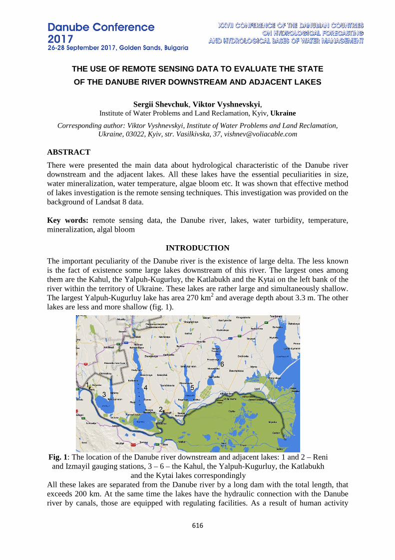
616

THE USE OF REMOTE SENSING DATA TO EVALUATE THE STATE OF THE DANUBE RIVER DOWNSTREAM AND ADJACENT LAKES

Sergii Shevchuk, Viktor Vyshnevskyi,

Institute of Water Problems and Land Reclamation, Kyiv, Ukraine

Corresponding author: Viktor Vyshnevskyi, Institute of Water Problems and Land Reclamation, Ukraine, 03022, Kyiv, str. Vasilkivska, 37, vishnev@voliacable.com

ABSTRACT There were presented the main data about hydrological characteristic of the Danube river downstream and the adjacent lakes. All these lakes have the essential peculiarities in size, water mineralization, water temperature, algae bloom etc. It was shown that effective method of lakes investigation is the remote sensing techniques. This investigation was provided on the background of Landsat 8 data. Key words: remote sensing data, the Danube river, lakes, water turbidity, temperature, mineralization, algal bloom

INTRODUCTION The important peculiarity of the Danube river is the existence of large delta. The less known is the fact of existence some large lakes downstream of this river. The largest ones among them are the Kahul, the Yalpuh-Kugurluy, the Katlabukh and the Kytai on the left bank of the river within the territory of Ukraine. These lakes are rather large and simultaneously shallow. The largest Yalpuh-Kugurluy lake has area 270 km2 and average depth about 3.3 m. The other lakes are less and more shallow (fig. 1).

Fig. 1: The location of the Danube river downstream and adjacent lakes: 1 and 2 – Reni and Izmayil gauging stations, 3 – 6 – the Kahul, the Yalpuh-Kugurluy, the Katlabukh

and the Kytai lakes correspondingly All these lakes are separated from the Danube river by a long dam with the total length, that exceeds 200 km. At the same time the lakes have the hydraulic connection with the Danube river by canals, those are equipped with regulating facilities. As a result of human activity

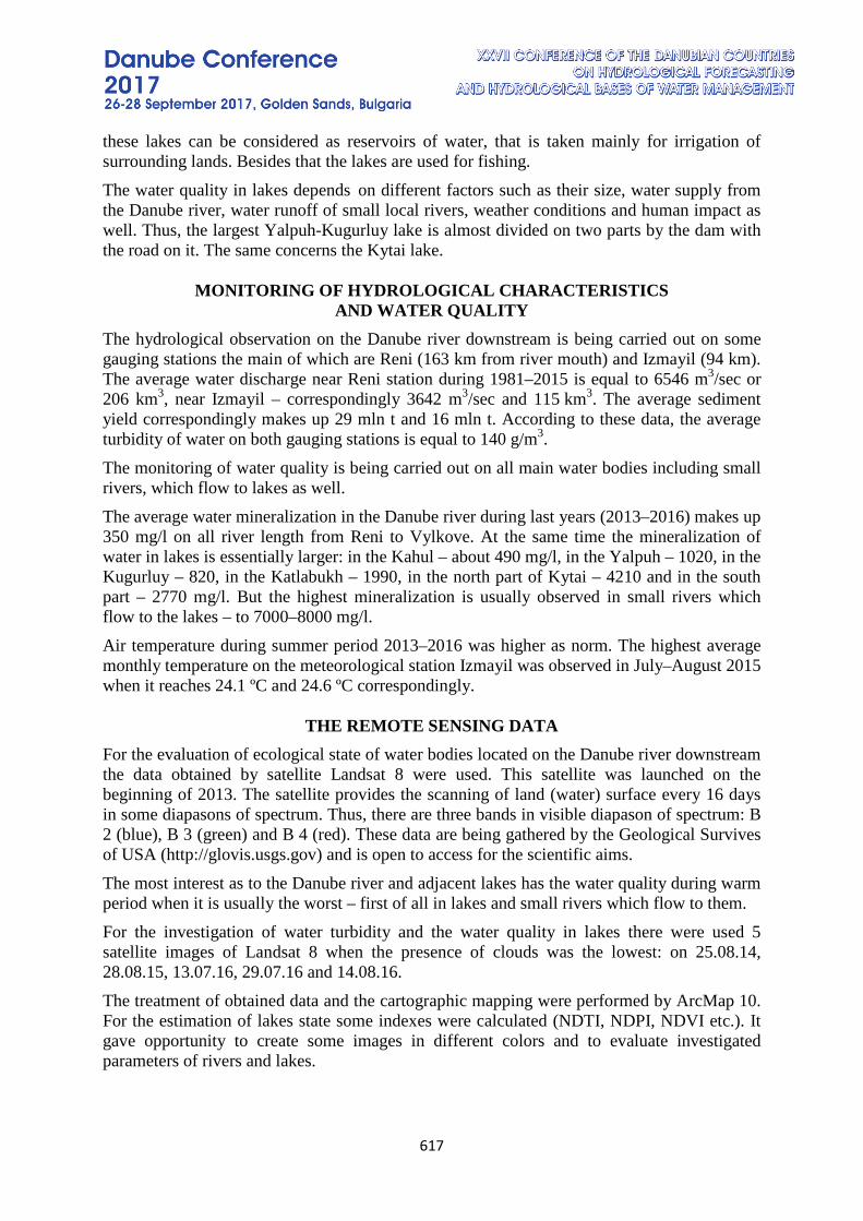
617

these lakes can be considered as reservoirs of water, that is taken mainly for irrigation of surrounding lands. Besides that the lakes are used for fishing. The water quality in lakes depends on different factors such as their size, water supply from the Danube river, water runoff of small local rivers, weather conditions and human impact as well. Thus, the largest Yalpuh-Kugurluy lake is almost divided on two parts by the dam with the road on it. The same concerns the Kytai lake.

MONITORING OF HYDROLOGICAL CHARACTERISTICS

AND WATER QUALITY The hydrological observation on the Danube river downstream is being carried out on some gauging stations the main of which are Reni (163 km from river mouth) and Izmayil (94 km). The average water discharge near Reni station during 1981–2015 is equal to 6546 m3/sec or 206 km3, near Izmayil – correspondingly 3642 m3/sec and 115 km3. The average sediment yield correspondingly makes up 29 mln t and 16 mln t. According to these data, the average turbidity of water on both gauging stations is equal to 140 g/m3. The monitoring of water quality is being carried out on all main water bodies including small rivers, which flow to lakes as well. The average water mineralization in the Danube river during last years (2013–2016) makes up 350 mg/l on all river length from Reni to Vylkove. At the same time the mineralization of water in lakes is essentially larger: in the Kahul – about 490 mg/l, in the Yalpuh – 1020, in the Kugurluy – 820, in the Katlabukh – 1990, in the north part of Kytai – 4210 and in the south part – 2770 mg/l. But the highest mineralization is usually observed in small rivers which flow to the lakes – to 7000–8000 mg/l. Air temperature during summer period 2013–2016 was higher as norm. The highest average monthly temperature on the meteorological station Izmayil was observed in July–August 2015 when it reaches 24.1 ºC and 24.6 ºC correspondingly.

THE REMOTE SENSING DATA For the evaluation of ecological state of water bodies located on the Danube river downstream the data obtained by satellite Landsat 8 were used. This satellite was launched on the beginning of 2013. The satellite provides the scanning of land (water) surface every 16 days in some diapasons of spectrum. Thus, there are three bands in visible diapason of spectrum: B 2 (blue), B 3 (green) and B 4 (red). These data are being gathered by the Geological Survives of USA (http://glovis.usgs.gov) and is open to access for the scientific aims. The most interest as to the Danube river and adjacent lakes has the water quality during warm period when it is usually the worst – first of all in lakes and small rivers which flow to them. For the investigation of water turbidity and the water quality in lakes there were used 5 satellite images of Landsat 8 when the presence of clouds was the lowest: on 25.08.14, 28.08.15, 13.07.16, 29.07.16 and 14.08.16. The treatment of obtained data and the cartographic mapping were performed by ArcMap 10. For the estimation of lakes state some indexes were calculated (NDTI, NDPI, NDVI etc.). It gave opportunity to create some images in different colors and to evaluate investigated parameters of rivers and lakes.

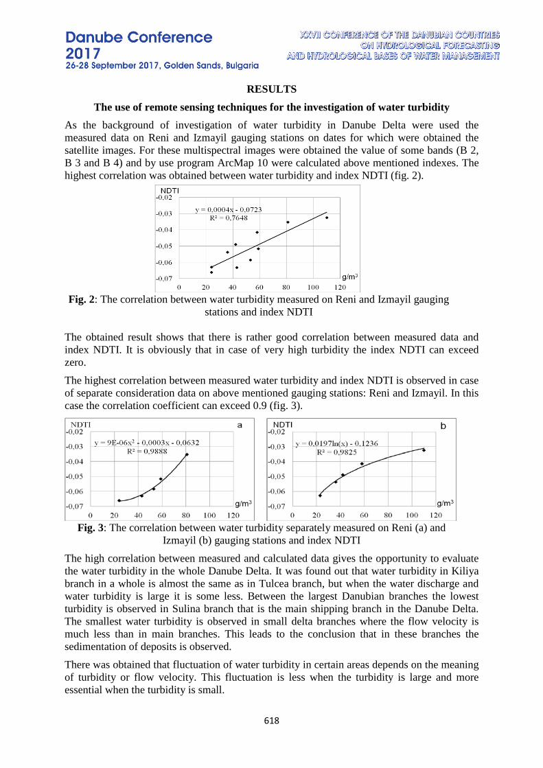
618

RESULTS The use of remote sensing techniques for the investigation of water turbidity

As the background of investigation of water turbidity in Danube Delta were used the measured data on Reni and Izmayil gauging stations on dates for which were obtained the satellite images. For these multispectral images were obtained the value of some bands (B 2, B 3 and B 4) and by use program ArcMap 10 were calculated above mentioned indexes. The highest correlation was obtained between water turbidity and index NDTI (fig. 2).

Fig. 2: The correlation between water turbidity measured on Reni and Izmayil gauging

stations and index NDTI The obtained result shows that there is rather good correlation between measured data and index NDTI. It is obviously that in case of very high turbidity the index NDTI can exceed zero. The highest correlation between measured water turbidity and index NDTI is observed in case of separate consideration data on above mentioned gauging stations: Reni and Izmayil. In this case the correlation coefficient can exceed 0.9 (fig. 3).

Fig. 3: The correlation between water turbidity separately measured on Reni (a) and

Izmayil (b) gauging stations and index NDTI The high correlation between measured and calculated data gives the opportunity to evaluate the water turbidity in the whole Danube Delta. It was found out that water turbidity in Kiliya branch in a whole is almost the same as in Tulcea branch, but when the water discharge and water turbidity is large it is some less. Between the largest Danubian branches the lowest turbidity is observed in Sulina branch that is the main shipping branch in the Danube Delta. The smallest water turbidity is observed in small delta branches where the flow velocity is much less than in main branches. This leads to the conclusion that in these branches the sedimentation of deposits is observed. There was obtained that fluctuation of water turbidity in certain areas depends on the meaning of turbidity or flow velocity. This fluctuation is less when the turbidity is large and more essential when the turbidity is small.

619

The evaluable data give opportunity to discover the distribution of water turbidity along the river. The most interesting results are obtained for the conditions of the beginning and the end of floods when the water turbidity can differ in some times.

The use of remote sensing techniques for the evaluation of water temperature Water temperature is one of the most important ecological factors that has influence on the quantity of dissolve oxygen, the intensity of biochemical process etc. The evaluation of temperature can be made by use bands B 10 and B 11 on-board Landsat 8. The previous investigation [1], [3], [5] showed that more correct results give the use of band 10 and equation, recommended by NASA:

T = (1321.08/(Ln((774.89/(("B10.TIF" * 0.0003342)+0.1))+1)))-273.15.

The correspondent treatment of data with use of ArcMap 10 gives the possibility to obtain the images with temperature meaning (fig. 4).

Fig. 4: The temperature of land and water surface in the Danube river downstream and

adjacent lakes obtained by Landsat 8, 29.07.16 Among four largest lakes the highest water temperature during summer usually is observed in Katlabukh (in the center of photo). In shallow places it can reach 28 ºC and even more. At the same time the water temperature in the Danube river is much less – it seldom reaches 23 ºC.

The use of remote sensing techniques for the evaluation of algal bloom It is known that algal bloom is the result of large concentration of tiny algal (cyanobacteria) in fresh water. These microorganisms contain chlorophyll a that is the reason of green color of water. As a rule the high algal bloom is observed in water bodies with high nutrient concentration (particularly phosphorus and nitrogen), when the temperature of water is high. For the evaluation of algal bloom usually is used the ratio between some spectral bands (most often – green and some adjacent) [2], [3], [6]. We also used the similar approach. But the first stage was to obtain the images in colors which are similar to natural ones. For this aim was used the combination of B 2, B 3 and B 4 of Landsat 8 (fig. 5).

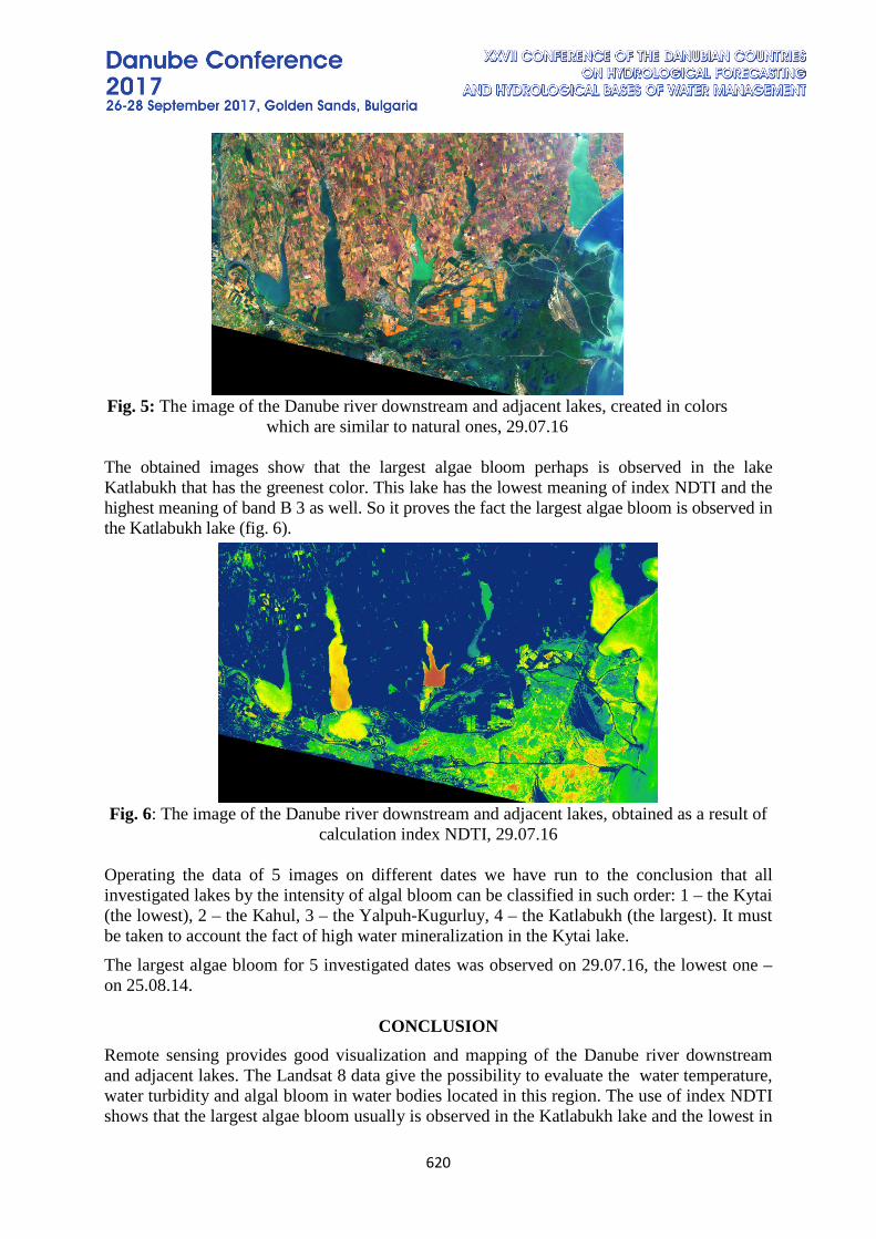
620

Fig. 5: The image of the Danube river downstream and adjacent lakes, created in colors

which are similar to natural ones, 29.07.16 The obtained images show that the largest algae bloom perhaps is observed in the lake Katlabukh that has the greenest color. This lake has the lowest meaning of index NDTI and the highest meaning of band B 3 as well. So it proves the fact the largest algae bloom is observed in the Katlabukh lake (fig. 6).

Fig. 6: The image of the Danube river downstream and adjacent lakes, obtained as a result of

calculation index NDTI, 29.07.16

Operating the data of 5 images on different dates we have run to the conclusion that all investigated lakes by the intensity of algal bloom can be classified in such order: 1 – the Kytai (the lowest), 2 – the Kahul, 3 – the Yalpuh-Kugurluy, 4 – the Katlabukh (the largest). It must be taken to account the fact of high water mineralization in the Kytai lake. The largest algae bloom for 5 investigated dates was observed on 29.07.16, the lowest one – on 25.08.14.

CONCLUSION

Remote sensing provides good visualization and mapping of the Danube river downstream and adjacent lakes. The Landsat 8 data give the possibility to evaluate the water temperature, water turbidity and algal bloom in water bodies located in this region. The use of index NDTI shows that the largest algae bloom usually is observed in the Katlabukh lake and the lowest in

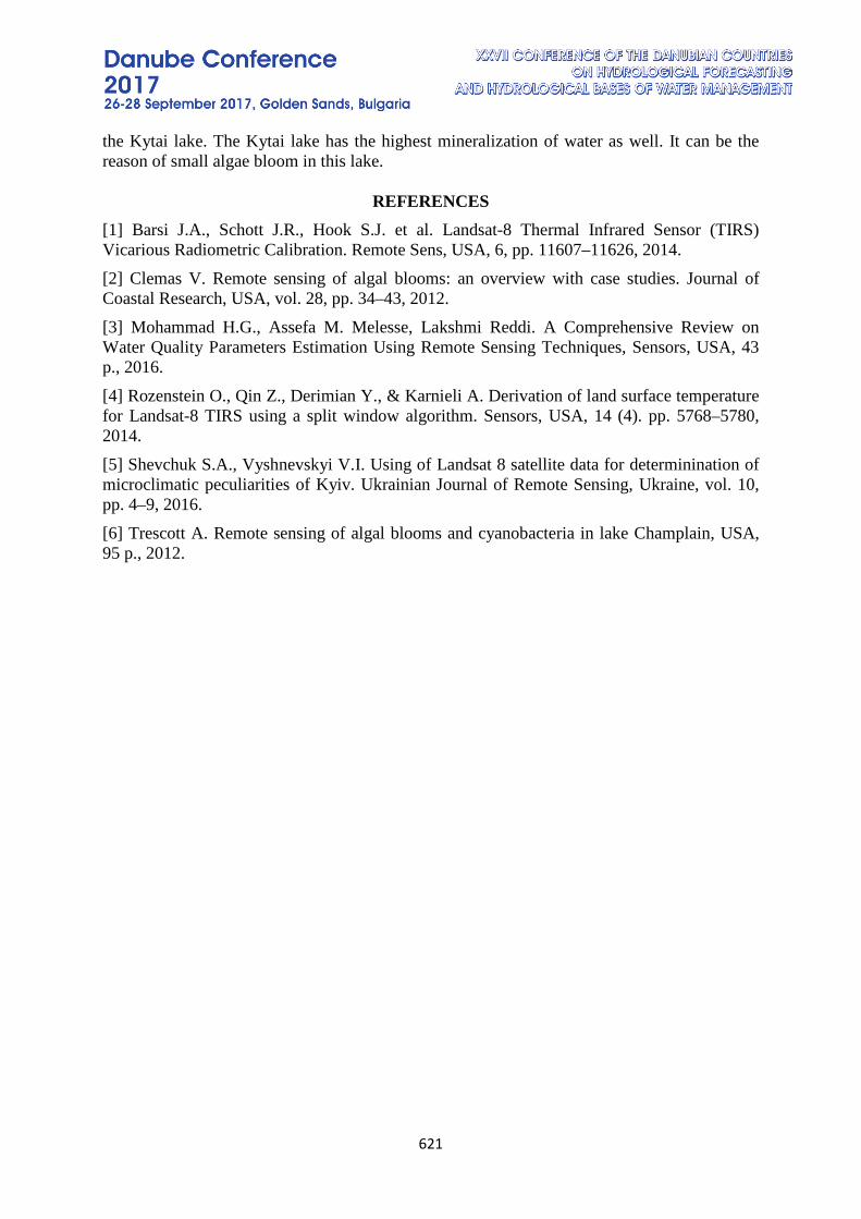
621

the Kytai lake. The Kytai lake has the highest mineralization of water as well. It can be the reason of small algae bloom in this lake.

REFERENCES

[1] Barsi J.A., Schott J.R., Hook S.J. et al. Landsat-8 Thermal Infrared Sensor (TIRS) Vicarious Radiometric Calibration. Remote Sens, USA, 6, pp. 11607–11626, 2014. [2] Clemas V. Remote sensing of algal blooms: an overview with case studies. Journal of Coastal Research, USA, vol. 28, pp. 34–43, 2012. [3] Mohammad H.G., Assefa M. Melesse, Lakshmi Reddi. A Comprehensive Review on Water Quality Parameters Estimation Using Remote Sensing Techniques, Sensors, USA, 43 p., 2016. [4] Rozenstein O., Qin Z., Derimian Y., & Karnieli A. Derivation of land surface temperature for Landsat-8 TIRS using a split window algorithm. Sensors, USA, 14 (4). pp. 5768–5780, 2014. [5] Shevchuk S.A., Vyshnevskyi V.I. Using of Landsat 8 satellite data for determinination of microclimatic peculiarities of Kyiv. Ukrainian Journal of Remote Sensing, Ukraine, vol. 10, pp. 4–9, 2016. [6] Trescott A. Remote sensing of algal blooms and cyanobacteria in lake Champlain, USA, 95 p., 2012.

622

623

624