Bayesian Filtering in Spiking Neural Networks: Noise,

Adaptation, and Multisensory Integration

Omer Bobrowski, Ron Meir and Yonina C. EldarDepartment of Electrical Engineering

Technion, Israel

September 2008

Neural Computation, In Press

Abstract

A key requirement facing organisms acting in uncertain dynamic environmentsis the real-time estimation and prediction of environmental states, based uponwhich effective actions can be selected. While it is becoming evident that or-ganisms employ exact or approximate Bayesian statistical calculations for thesepurposes, it is far less clear how these putative computations are implementedby neural networks in a strictly dynamic setting. In this work we make use ofrigorous mathematical results from the theory of continuous time point processfiltering, and show how optimal real-time state estimation and prediction may beimplemented in a general setting using simple recurrent neural networks. Theframework is applicable to many situations of common interest, including noisyobservations, non-Poisson spike trains (incorporating adaptation), multisensoryintegration and state prediction. The optimal network properties are shown torelate to the statistical structure of the environment, and the benefits of adapta-tion are studied and explicitly demonstrated. Finally, we recover several existingresults as appropriate limits of our general setting.

1 Introduction

The selection of appropriate actions in the face of uncertainty is a formidable task facedby any organism attempting to actively survive in a hostile dynamic environment. Thistask is further exacerbated by the fact that the organism does not have direct accessto the environment (or to its internal body state), but must assess these states throughnoisy sensors, often representing the world via random spike trains. It is becoming in-creasingly evident that in many cases organisms employ exact or approximate Bayesianstatistical calculations (Averbeck, Latham, & Pouget, 2006; Deneve, Latham, & Pouget,

1

2001; Ma, Beck, Latham, & Pouget, 2006; Pouget, Deneve, & Duhamel, 2002; Doya,Ishii, Pouget, & Rao, 2007; Knill & Pouget, 2004) in order to continuously estimate theenvironmental (or bodily) state, integrate information from multiple sensory modalities,form predictions and choose actions. What is less clear is how these putative computa-tions are implemented by neural networks in a dynamic setting. Moreover, given thatthe environment itself is uncertain, it would seem natural to capture this uncertainty bya distribution over states rather than a single state estimator (Zemel, Dayan, & Pouget,1998). This full distribution can be later utilized differentially in various contexts, and,in particular, for the optimal combination of different information sources. Thus, theeffective representation of full probability distributions by neural networks is also animportant issue which needs to be resolved.

The problem of hidden state estimation based on multiple noisy spike trains has beenreceiving increasing attention over the past few years. Much emphasis has been laidon Bayesian approaches, which facilitate the natural incorporation of prior information,and which can often be guaranteed to yield optimal solutions. While many naturallyoccurring problems are dynamic in nature, a large fraction of the work to-date hasfocused on static stimuli (e.g., (Averbeck et al., 2006; Deneve et al., 2001; Ma et al., 2006;Pouget et al., 2002; Pouget, Dayan, & Zemel, 2003; Zemel et al., 1998)). More recentlyattention has shifted to dynamic phenomena and online estimation (e.g., (Barbieri etal., 2004; Beck & Pouget, 2007; Deneve, 2008; Eden, Frank, Solo, & Brown, 2004; Huys,Zemel, Natarajan, & Dayan, 2007; Pitkow, Sompolinsky, & Meister, 2007)). Our work,formulated within the rigorous theory of real-time nonlinear filtering, and applied todynamic spike train decoding, offers several advantages over previous work, as describedin more detail in Section 7.3. In fact, our results indicate that optimal real-time stateestimation based on point process observations is achievable by relatively simple neuralarchitectures. As opposed to much previous work, there is no need for time discretizationand input process smoothing, which may lead to loss of information. These resultssuggest a solid theoretical foundation for dynamic neural decoding and computation,and recover many previous results in appropriate limits. A particularly useful featureof the present framework is the demonstration that the computation of the posteriordistribution can be achieved in real-time by a bilinear neural network. Ultimately,however, the merit of a model is based not only on its mathematical elegance, but onits power to explain existing experiments, and to predict novel behaviors. While somelimits of our formulation, e.g., the static limit, lead to results which have already beenexperimentally verified, the main advantage of the general framework is in setting thestage for mathematically precise, yet experimentally verifiable, predictions for futureexperiments dealing directly with dynamic phenomena.

Consider the following generic situation. An agent observes the environment througha set of noisy (possibly multimodal) sensory neurons. Based on these observationsthe agent needs to estimate the state of the environment (more generally, the statedistribution) with the highest accuracy possible. It is well known that if the stochasticdynamics of the environment and the observation process are fully known, then the statedistribution can be optimally recovered through the so-called Bayes filter (Jazwinsky,1970; Thrun, Burgard, & Fox, 2005) based on an exact calculation of the posterior state

2

distribution. For example, if both the environmental and observational processes arelinear, and are corrupted by Gaussian noise, the optimal filter reduces to the classicKalman filter (Anderson & Moore, 2005). For the state estimation procedure to beeffective in a biological context, it must be possible to implement it robustly in realtime by a neural network. In a biological setting, the agent observes the environmentthrough a set of sensory neurons, each of which emits spikes at a rate which depends onthe current state of the environment according to the neuron’s fixed response function(a.k.a. tuning curve). These spike trains are continually sent to a neural network whichcomputes a probability distribution over environmental states.

Surprisingly it turns out that under well-defined mathematical conditions (hiddenMarkov process and Poisson spiking activity; see Section 2 for precise definitions) thesolution to the problem of spike train decoding has been known for many years see, forexample, (Bremaud, 1981), and the historical survey provided therein. However, themathematical derivation in (Bremaud, 1981) is highly intricate, relying on sophisticatedmathematical techniques from the theory of stochastic processes, which may not bewidely available. This abstruseness may be one reason for the fact that this exact andrigorous body of theory has rarely been used by the computational neuroscience com-munity (see, for example, (Twum-Danso & Brockett, 2001) for a notable exception). Infact, some of the results presented over the past few years in the context of hidden stateestimation and neural decoding can be viewed as special cases of the general theory de-veloped in (Boel & Benes, 1980) and (Bremaud, 1981). Because of the intricate natureof the derivation in (Bremaud, 1981), we present a simplified derivation available as anonline appendix1. This online appendix will enable readers who are unfamiliar with theadvanced theory of martingales to follows the derivation using simple techniques. Withinthis framework, the optimal posterior distribution over environmental states (the Bayesfilter), given the sensory spike trains, is exactly computed in real-time by a bilinearrecurrent neural network. It is essential to note that the posterior distribution is basedon the exact spike times, so that no temporal information is lost (as is often the casewhen time is discretized or other approximations are made). A preliminary version ofthe results appears in (Bobrowski, Meir, Shoham, & Eldar, 2007). Next, we summarizethe main contributions of this work.

The main contributions of this work: (1) Incorporation of environmental noisein the general filtering framework. Within this setting we establish the existence ofan optimal width for the tuning function of the sensory cells. This width depends onthe noise level, suggesting that for optimal performance the system must adapt to thespecific environmental conditions. (2) Application of the framework to the multisensoryintegration of signals. Our results provide novel predictions in the dynamic setting, andrecover previous results in the static limit (e.g., (Deneve et al., 2001)); see section 4for details. Furthermore, they provide succinct explanations for several experimentallyobserved phenomena related to enhanced response and inverse effectiveness. (3) Devel-opment of a framework for history dependent spike trains, and a consideration of theeffect of adaptation on system performance. Interestingly, we can show that adapta-tion can benefit neural computation. More specifically, when the system is subjected to

1See http://www.technion.ac.il/∼rmeir/BobMeiEld-appendix.pdf

3

energy constraints (e.g., limits on the overall number of spikes fired per unit time), adap-tation leads to near optimal performance. (4) Showing how a simply modified systemaddresses prediction of future states, rather than estimating the current state).

The remainder of this paper is organized as follows: Section 2 describes the preciseproblem formulation, and the basic filtering equation based on (Bremaud, 1981). Weshow how this equation can be implemented by a simple recurrent neural network,followed by several simulations demonstrating the system’s performance. Section 3 in-corporates environmental noise and studies its effect. Section 4 considers multisensoryintegration, and Section 5 discusses in detail the case where the stimulus (or worldstate) is static. Section 6 presents an extension to a larger class of point processes, anddemonstrates how phenomena such as adaptation can easily be incorporated. Section 7briefly describes additional extensions (prediction, log-posterior computation) as well asa detailed comparison to previous work.

2 Filtering a Markov Process from Poisson Mea-

surements

Consider a dynamic process Xt representing the state of the world (e.g., the locationof an object, its shape, orientation, velocity, etc.). We assume that Xt is a continuoustime finite state Markov process, with a finite state-space S = {s1, . . . , sN} and aninfinitesimal generator matrix Q = [qij]. This implies that the transition probabilitiesare given by

P(τ)ij

△= P (Xt+τ = sj |Xt = si ) =

{qijτ + o(τ) i 6= j1 + qiiτ + o(τ) i = j,

(2.1)

with qii = −∑j 6=i qij < 0 (see (Grimmett & Stirzaker, 2001) for more details).

The state Xt is not directly observed, but is processed through a set of M sensory cells,each of which produces a spike train, associated with a counting process N

(m)t . At this

point we take the spikes to be generated by an inhomogeneous Poisson process, wherethe process rate depends on the current environmental state (such process are referredto as doubly-stochastic Poisson processes, see (Snyder & Miller, 1991)). We denote therate of the process generated by the m-th cell by λm(Xt), where λm(·) represents thetuning curve of the m-th cell. The firing events of the different sensory cells are assumedto be independent given the state. Our goal is to compute the posterior probabilities

pi(t)△= P

(

Xt = si

∣∣∣N

(1)[0,t], . . . , N

(M)[0,t]

)

,

where N(m)[0,t] =

{

N(m)s

}t

s=0is the full history of the process Nt. More specifically, we are

looking for an online computation method that can be carried out by a neural network.

In the remainder of this section we present the solution derived in (Bremaud, 1981),and discuss the interpretation of this solution as a neural network, followed by simula-tions. For completeness we present a full, albeit simplified, derivation of these results

4

in an online appendix. We note that simplified derivations of special cases of the fil-tering equations in (Bremaud, 1981), based on time discretization followed by a limitprocess, have been recently presented in (Deneve, 2008) and (Pitkow et al., 2007); seealso (Twum-Danso & Brockett, 2001) for an intuitive explanation of the results from(Bremaud, 1981) in a continuous time context. We discuss this work in a comparativesetting in Section 7.

2.1 The Filtering Equation

There is increasing interest in providing an answer to the problem presented above indifferent neuroscience contexts. Interestingly, as stated in Section 1, this mathematicalfiltering problem was addressed in the 1970s and rigorous solutions, under well definedmathematical conditions, exist since then. In a historical context we note that a mathe-matically rigorous approach to point process filtering in continuous time was developedduring the early 1970s following the seminal work of Wonham (Wonham, 1965) for finitestate Markov processes observed in Gaussian noise, and of Kushner (Kushner, 1967) andZakai (Zakai, 1969) for diffusion processes. One of the first papers presenting a math-ematically rigorous approach to nonlinear filtering in continuous time based on pointprocess observations was Snyder (Snyder, 1972), extended later by Segall et al. (Segall,Davis, & Kailath, 1975). We comment that this paper considers only the case of a finitestate space. The formalism for continuous state spaces is also available in some cases(e..g, (Boel & Benes, 1980)), but will not be pursued in this work.

The solution presented in (Bremaud, 1981) introduces a new set of non-negative andnon-normalized functions ρ

i(·), related to pi (t) by

pi(t) =ρi(t)

∑N

j=1 ρj(t). (2.2)

It is shown in Section VI.4 of (Bremaud, 1981) (see also the online appendix) that{ρi(t)}N

i=1 obey the following set of N differential equations,

ρi(t) =N∑

k=1

qkiρk(t)+

(M∑

m=1

(λm(si) − 1)νm(t)

)

ρi(t)−λ(si)ρi(t), i = 1, . . . , N, (2.3)

where

λ(si) =M∑

m=1

λm(si) ; νm(t) =∑

n

δ(t − t(m)

n

),

and{

t(m)n

}∞

n=1denote the spiking times of the m-th sensory cell. In other words, the

function νm(t) represents the spike train of the m-th sensory cell. The parameters qki

are elements of the generator matrix Q. This set of equations can be written in vectorform as

ρ(t) = Q⊤ρ(t) +

(M∑

m=1

(Λm − I) νm(t)

)

ρ(t) − Λρ(t), (2.4)

5

where I is the identity matrix, and

ρ(t) = (ρ1(t), . . . , ρN(t))⊤ ; Λm = diag (λm(s1), . . . , λm(sN)) ; Λ =M∑

m=1

Λm.

In appendix A we present a full closed form solution to (2.4). Examining the solutiongiven in (A.3), we can analyze this network’s activity pattern. Between spikes, ρ(t)depends exponentially and smoothly on time, varying at a time scale which depends onthe eigenvalues of Q and on the maximal firing rates of the sensory cells (through thetuning curves). Upon the arrival of a spike from the m-th sensory cell at time t, ρ(t) isupdated according to ρ(t+) = Λmρ(t−). In other words, the variable ρi(t) evolves on aslow time scale between spikes and on a fast time scale upon the arrival of a spike.

Network interpretation

The variables {ρ1, · · · , ρN} in (2.3) can be interpreted as representing the activity of aset of N neurons in a recurrent (posterior) neural network. The second term in (2.3)represents the effect of the sensory inputs on each such posterior neuron. Each sensoryneuron emits a Poisson spike train2 based on the current input and its receptive field,and affects the posterior cell through its impulse train νm(t). In addition, the first termin (2.3) shows that each posterior neuron receives inputs from other posterior neuronsbased on the weights {qij}. The third term represents a simple, state-dependent, decayof the non normalized distribution. In many cases the variables λ(si) are near constant,in which case they affect the posterior variables ρi only the overall normalization, andcan be dropped. A graphical display of the network and its interpretation can be foundin Figure 1. Note that the first term in (2.3) represents a ‘mapping of the world’ onto therecurrent decoding network, establishing a representation of the environment throughthe synaptic weights; this can be interpreted as a Bayesian prior in a Bayesian setting.

One possible implementational problem with (2.3) is that the solution may explodeexponentially. Since the physical variable of interest is the posterior probability, obtainedby renormalizing ρi(t) as in (2.2), the overall normalization is irrelevant. Note, however,that in some cases (e.g., computing the minimum mean squared error estimator) thenormalized distribution is required. In any event, as long as we are interested in thelargest posterior probability, it is clear that the normalization has no effect. In principle,one can add to (2.3) an operation which periodically renormalizes the variables so that∑N

i=1 ρi(t) = 1. Alternatively, one can add a term to the equation which guarantees thatthis normalization be automatically obeyed at each step, as was done, for example, inequation (2.13) of (Beck & Pouget, 2007). In the numerical demonstrations presented inthe sequel we have renormalized ρi(t) periodically in order to prevent explosive solutions.

The network described in (2.3) can be viewed as a formal neural network. While it seemsto be somewhat removed from a direct physiological interpretation, we believe that aphysiologically plausible network can be constructed based on its principles. We discuss

2The Poisson assumption will be relaxed in Section 6.

6

the main interpretational issues here, but defer a full physiological implementation ofthese ideas to future work.

First, we note that while the sensory neurons produce spike trains represented throughthe variables νm(t), the posterior neurons are described by a continuous variable ρi(t).Within a biological implementation of (2.4) one may view ρi(t) as the probability ofspiking (see also (Pitkow et al., 2007)). This interpretation may seem to pose difficultiesin a biological context since the probability of spiking cannot be directly communicatedbetween neurons. However, an easy remedy for this would be to simply replicate eachposterior neuron many times, and allow each such replicated neuron to fire Poisson spiketrains at a rate consistent with (2.3). This would correspond to the well-studied linearPoisson spiking network, e.g., (Gerstner & Kistler, 2002). Since spikes can be directlycommunicated between neurons, such an implementation would be biologically feasible.A second difficulty with the physiological interpretation relates to the multiplicativegain, the second term in (2.4). This terms requires that the activity of the posteriorneuron i be modulated by a multiplicative term based on the activity of the sensoryneurons. While not entirely standard, there is an increasing evidence for this type ofmultiplicative gain in biological neural networks in both the visual and somatosensorycortices (e.g., (C. J. McAdams & Maunsell, 1999; C. McAdams & Reid, 2005; Sripati& Johnson, 2006)), and such interactions are thought to play an important role in neu-ral computation (Salinas & Thier, 2000). Moreover, specific biophysical mechanismsand computational models have been proposed for these phenomena (Murphy & Miller,2003; Sripati & Johnson, 2006). A third issue which can be raised against the plausi-bility of the network proposed is that posterior neurons are affected differentially basedon the feedforward input sensory neurons (multiplicative gain) and additively throughthe posterior network recurrent weights. However, given the very different nature ofthe two types of inputs, and their effects on the postsynaptic target through differentdistributions of receptors, it is not implausible that the two types of interactions leadto very different effects; see, for example, (Rivadulla, Sharma, & Sur, 2001). In fact,there is solid evidence for the existence of multiplicative interactions based on the specialproperties of the NMDA receptor (Rivadulla et al., 2001), which is ubiquitous in corticalcircuits and is widely believed to lead to coincidence detection (Tsien, 2000). Next, wecomment on the renormalization issue alluded to above. This can be addressed within aphysiological context using the well documented phenomenon of divisive inhibition (e.g.,(Cavanaugh, Bair, & Movshon, 2002)); see, for example, (Beck & Pouget, 2007) for asimple implementation of divisive inhibition, in a context related to (2.4), leading tonormalization.

Finally, we comment briefly on the possible implementation of the formal network (2.3)in the brain. In a visual context we view the sensory layer in the model as correspond-ing to the inputs from the retina via the LGN to the cortex (a similar interpretation,mutatis mutandis, would hold for other sensory modalities). The recurrent connections{Qij} within the posterior network would then correspond to the lateral connectionsbetween cortical pyramidal neurons. The latter are well known to play an essential rolein cortical processing, overwhelming the thalamic inputs by a wide margin. Interest-ingly, within our model, stronger connections Qij exist between neurons which represent

7

similar states. For example, in a dynamic context, the matrix elements between similarstates are larger, corresponding to higher transition probabilities between such states.This observation is consistent with the larger observed functional connectivity betweencells of similar orientation selectivity (e.g., (Ts’o, Gilbert, & Wiesel, 1986)). Moreover,the competitive dynamics of our model’s posterior network is also consistent with the softwinner-take-all view of the lateral interactions between cortical neurons; see (Douglas &Martin, 2004) for a physiological motivation and demonstration. Experimental tests ofour proposed model could consist of differentially interfering with the feedforward mul-tiplicative interactions (possibly through NMDA receptor antagonists) and the lateraladditive interactions suggested by our model, thereby comparing the different spatialand temporal effects of the two information streams. For example, we would expectthat disrupting lateral connections (‘prior knowledge’) would lead to particularly sig-nificant performance degradation when the sensory input is sparse. We note that anequation similar to (2.4) has been derived recently in (Pitkow et al., 2007) for a twodimensional random walk Markov process. The latter paper provides further support tothe idea that the visual area V1 may naturally implement this type of network.

Figure 1: The decoding network structure. The sensory cells respond to a stimulus with spike

trains N(m)t . The connection strength between the mth sensory cell and the ith posterior net-

work cell is λm(si) (as in (2.3)). This connection weight multiples the sensory cell activity andis passed as input to the second recurrent layer. This layer computes the posterior probabilitiesρ(t) based on (2.3). The recurrent synaptic weights in the posterior network are controlled bythe prior transition parameters qji.

2.1.1 Numerical demonstrations of the filtering equations

Next, we examine the system behavior by numerically solving (2.4) and its extensions3.The numerical solution corresponds to an actual implementation of the abstract neuralnetwork described in (2.3,2.4). These results are aimed at demonstrating performance,and can be viewed as a simple implementation of the experimental setup considered in(Warland, Reinagel, & Meister, 1997) in the context of retinal decoding.

3A closed form solution to (2.4) can be found in Appendix A

8

We consider a simple setting where the decoding system attempts to track a movingparticle; this basic setup, with modifications, will serve for all the numerical demonstra-tions in this work. Consider a small object moving vertically on a line, jumping betweena set of discrete states {si}N

i=1, each representing the position of the object. The objectis observed by a retina consisting of M sensory cells, where each sensory cell m generatesa Poisson spike train with rate λm(Xt) where Xt is the world state at time t. The tun-ing curve of the mth sensory cell is taken to be a Gaussian4 centered at cm, of width α,height λmax, and baseline level λbase , namely λm(s) = λbase+λmax exp (−(s − cm)2/2α2).The tuning-curve centers cm are uniformly spread over the input domain. The same ex-perimental protocol is used throughout the paper with slight variations required by theextended settings described in sections 3, 4 and 6.

For the simulations presented throughout this paper we use different Q matrices torepresent the world state dynamics. The Q matrices are constructed in such a way thatthe most likely transitions are from any state to one of its neighbors, where a a neighboris defined by the Euclidean distance between the physical states. The general structureof the Q matrix is as follows:

qij =

{

ci exp(

(i−j)2

2β2

)

i 6= j

−µ i = j,(2.5)

where β and µ are positive real numbers, and ci = µ/∑

j 6=i

(

exp(

(i−j)2

2β2

))

, so that∑

j qij = 0. The average number of transitions per unit time is µ.

Figure 2 displays the motion of the particle between N = 250 different states, fora choice of Q matrix as described above. The spiking activity of M = 125 positionsensitive sensory cells, and the tracked posterior distribution. In Figure 2(a)-2(c) thetuning curve parameters are chosen to produce only a few spikes. In this case we cansee how the level of uncertainty (posterior variance) increases between spike arrivals,when no information is provided. In Figure 2(d)-2(f), the spiking activity is much moreintense, leading to more accurate results (lower posterior variance).

Next, we consider a naturally discrete state discrimination task. This example alsodemonstrates how to achieve improved performance by enriching the state space ofthe model. Specifically, we augment the state representation by adding the movementdirection as well as the visibility mode of the stimulus. Define a new set of states sijk =(si, dj, vk), where si represent the object’s locations, dj denotes the current movementdirection (in this case d1 = up, d2 = down), and vk represents whether or not thestimulus is visible to the system (v1 = visible, v2 = invisible). The tuning curves λijk,i = 1, 2, · · · , N, j, k = 1, 2, are constructed as follows. For states where the stimulus isvisible, the tuning curves are Gaussian functions of the location as before. However, forthe states where the stimulus is invisible, the cells cannot differentiate between differentlocations and hence they all respond with the same spontaneous rate λspon. Note thatthe movement direction is not encoded in the firing rate of the sensory cells.

4The results are demonstrated for a Gaussian tuning curve, but the theory applies to arbitrarytuning functions.

9

0 0.25 0.5 0.75 1−1

−0.5

0

0.5

1

t

Xt

stimulus location

(a)

0 0.25 0.5 0.75 1−1

−0.5

0

0.5

1

t

pref

erre

d lo

catio

n

sensory spiking activity

(b)

0 0.25 0.5 0.75 1−1

−0.5

0

0.5

1

t

loca

tion

posterior network activity

(c)

0 0.25 0.5 0.75 1−1

−0.5

0

0.5

1

t

Xt

stimulus location

(d)

0 0.25 0.5 0.75 1−1

−0.5

0

0.5

1

t

pref

erre

d lo

catio

n

sensory spiking activity

(e)

0 0.25 0.5 0.75 1−1

−0.5

0

0.5

1

t

loca

tion

posterior network activity

(f)

Figure 2: Tracking the motion of a single object in 1D. (a) The trajectory of the object’smovement. (b) Sensory activity. A dot represents a spike arriving from a sensory cell, wherethe y-axis represents the cell’s preferred location. In this simulation the firing rates are ex-tremely low (λmax = 15, λbase = 0). (c) The activity of the posterior network. The y-axisrepresents the location represented by each cell, and the black intensity represents the prob-ability P (Xt |spiking activity), ranging from 0=white to 1=black. (d)-(f) Same setup, withλmax = 75, λbase = 2.5 leading to an intense sensory activity. In both simulations N = 250,M = 125, α = 0.016, β = 2 and µ = 500.

The basic dynamic setup is as in Figure 2, except that the states are augmented asdescribed in the previous paragraph. Denoting the non-normalized probabilities of this3D state by ρijk(t) we can retrieve the distribution of the location alone, by using themarginal distribution ρs

i (t) =∑

j,k ρijk(t). The results are presented in Figure 3(c).Alternatively, by pooling the probabilities over all possible locations and visibility modes,we get ρd

j (t) =∑

i,k ρijk(t) - the discrete probabilities discriminating between the twopossible movement directions. The results presented in Figure 3(d) demonstrate thehigh quality of the binary decision possible by classifying the direction of motion basedon the maximal posterior probability for the (up,down) directions. Similarly, by poolingthe probabilities over all possible locations and directions we get ρv

k(t) =∑

i,j ρijk(t) -the discrete probabilities discriminating between stimulus visibility and non-visibility.The results are presented in Figure 3(e).

The Q matrix used in this simulation is different than the previous one, and somewhatmore complicated, as it has to include the transitions between directions and visibilitymodes. As there are N × 2 × 2 = 4N possible states, Q is of size 4N × 4N . Theconstruction of the matrix Q in this example is provided for completeness in appendixB.

10

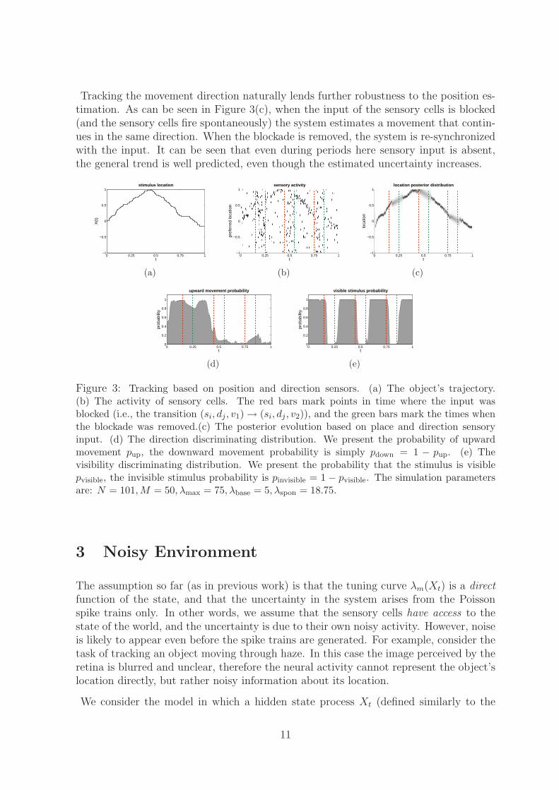
Tracking the movement direction naturally lends further robustness to the position es-timation. As can be seen in Figure 3(c), when the input of the sensory cells is blocked(and the sensory cells fire spontaneously) the system estimates a movement that contin-ues in the same direction. When the blockade is removed, the system is re-synchronizedwith the input. It can be seen that even during periods here sensory input is absent,the general trend is well predicted, even though the estimated uncertainty increases.

0 0.25 0.5 0.75 1−1

−0.5

0

0.5

1

t

X(t

)

stimulus location

(a)

0 0.25 0.5 0.75 1−1

−0.5

0

0.5

1

t

pref

erre

d lo

catio

n

sensory activity

(b)

0 0.25 0.5 0.75 1−1

−0.5

0

0.5

1

t

loca

tion

location posterior distribution

(c)

0 0.25 0.5 0.75 10

0.2

0.4

0.6

0.8

1

t

prob

abili

ty

upward movement probability

(d)

0 0.25 0.5 0.75 10

0.2

0.4

0.6

0.8

1

t

prob

abili

ty

visible stimulus probability

(e)

Figure 3: Tracking based on position and direction sensors. (a) The object’s trajectory.(b) The activity of sensory cells. The red bars mark points in time where the input wasblocked (i.e., the transition (si, dj , v1) → (si, dj , v2)), and the green bars mark the times whenthe blockade was removed.(c) The posterior evolution based on place and direction sensoryinput. (d) The direction discriminating distribution. We present the probability of upwardmovement pup, the downward movement probability is simply pdown = 1 − pup. (e) Thevisibility discriminating distribution. We present the probability that the stimulus is visiblepvisible, the invisible stimulus probability is pinvisible = 1 − pvisible. The simulation parametersare: N = 101, M = 50, λmax = 75, λbase = 5, λspon = 18.75.

3 Noisy Environment

The assumption so far (as in previous work) is that the tuning curve λm(Xt) is a directfunction of the state, and that the uncertainty in the system arises from the Poissonspike trains only. In other words, we assume that the sensory cells have access to thestate of the world, and the uncertainty is due to their own noisy activity. However, noiseis likely to appear even before the spike trains are generated. For example, consider thetask of tracking an object moving through haze. In this case the image perceived by theretina is blurred and unclear, therefore the neural activity cannot represent the object’slocation directly, but rather noisy information about its location.

We consider the model in which a hidden state process Xt (defined similarly to the

11

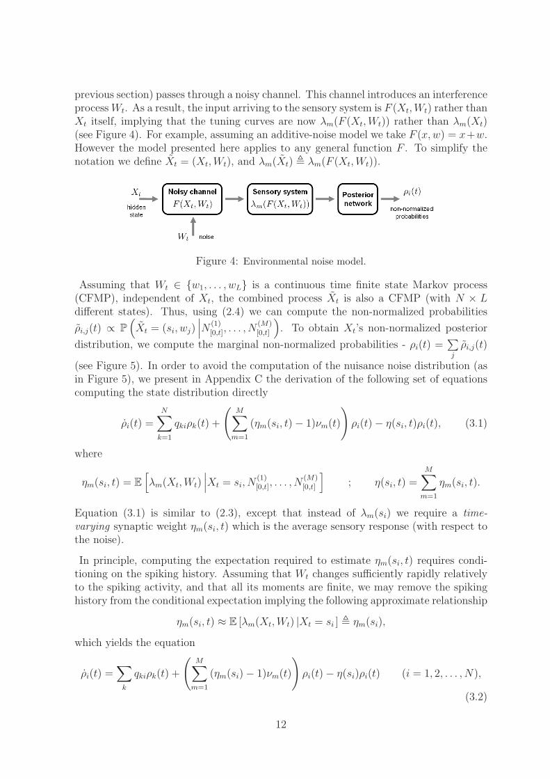
previous section) passes through a noisy channel. This channel introduces an interferenceprocess Wt. As a result, the input arriving to the sensory system is F (Xt,Wt) rather thanXt itself, implying that the tuning curves are now λm(F (Xt,Wt)) rather than λm(Xt)(see Figure 4). For example, assuming an additive-noise model we take F (x,w) = x+w.However the model presented here applies to any general function F . To simplify thenotation we define Xt = (Xt,Wt), and λm(Xt) , λm(F (Xt,Wt)).

Figure 4: Environmental noise model.

Assuming that Wt ∈ {w1, . . . , wL} is a continuous time finite state Markov process(CFMP), independent of Xt, the combined process Xt is also a CFMP (with N × Ldifferent states). Thus, using (2.4) we can compute the non-normalized probabilities

ρi,j(t) ∝ P

(

Xt = (si, wj)∣∣∣N

(1)[0,t], . . . , N

(M)[0,t]

)

. To obtain Xt’s non-normalized posterior

distribution, we compute the marginal non-normalized probabilities - ρi(t) =∑

j

ρi,j(t)

(see Figure 5). In order to avoid the computation of the nuisance noise distribution (asin Figure 5), we present in Appendix C the derivation of the following set of equationscomputing the state distribution directly

ρi(t) =N∑

k=1

qkiρk(t) +

(M∑

m=1

(ηm(si, t) − 1)νm(t)

)

ρi(t) − η(si, t)ρi(t), (3.1)

where

ηm(si, t) = E

[

λm(Xt,Wt)∣∣∣Xt = si, N

(1)[0,t], . . . , N

(M)[0,t]

]

; η(si, t) =M∑

m=1

ηm(si, t).

Equation (3.1) is similar to (2.3), except that instead of λm(si) we require a time-varying synaptic weight ηm(si, t) which is the average sensory response (with respect tothe noise).

In principle, computing the expectation required to estimate ηm(si, t) requires condi-tioning on the spiking history. Assuming that Wt changes sufficiently rapidly relativelyto the spiking activity, and that all its moments are finite, we may remove the spikinghistory from the conditional expectation implying the following approximate relationship

ηm(si, t) ≈ E [λm(Xt,Wt) |Xt = si ] , ηm(si),

which yields the equation

ρi(t) =∑

k

qkiρk(t) +

(M∑

m=1

(ηm(si) − 1)νm(t)

)

ρi(t) − η(si)ρi(t) (i = 1, 2, . . . , N),

(3.2)

12

Figure 5: Computing the posterior distribution in the presence of noise. The full posteriornetwork computes the posterior distribution of the combined state Xt = (Xt, Wt). By a simplesummation we get the posterior distribution of the state Xt alone.

where η(si) =∑M

m=1 ηm(si). The equation set (3.2) calculates the posterior distributionof the state process Xt alone, using the average responses of the sensory cells, withrespect to the noise process Wt.

Similarly to the noiseless case, we can represent (3.2) in a vector form, as

ρ(t) = Q⊤ρ(t) +

(M∑

m=1

(Φm − I) νm(t)

)

ρ(t) − Φρ(t), (3.3)

where

Φm = diag (ηm(s1), . . . , ηm(sN)) ; Φ =M∑

m=1

Φm.

Figure 6 presents the performance of the system in the presence of noise. Figure 6(a)-6(c) present a single trial of tracking a stimulus moving through N = 250 states, observedby M = 125 sensory cells. The state model is similar to the one used in Figure 2. Thenoise state-space is uniformly distributed in the range [w1, wL] with w1 = −1/2, wL =1/2, L = 1000. The noise distribution is of the form c exp

(−w2

j/2σ2w

)with σ2

w = 0.01,and we assume that it contributes additively to the input, i.e., F (Xt,Wt) = Xt + Wt. Itcan be observed that the posterior network filters out the noise significantly. In Figure6(d) we simulate different levels of noise, and compare the performance of the originalfiltering equation (2.4) with its noisy version (3.3). The comparison is based on theempirical mean squared error (MSE) of the minimum MSE (MMSE) optimal estimatorcalculated from the posterior distribution represented by the network, i.e.,

Xt =∑

i

siP

(

Xt = si

∣∣∣N

(1)[0,t], . . . , N

(M)[0,t]

)

.

13

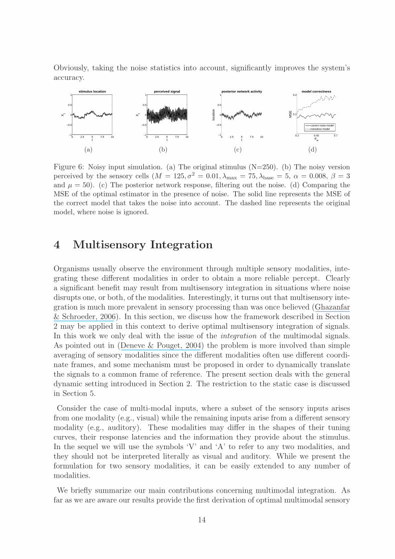
Obviously, taking the noise statistics into account, significantly improves the system’saccuracy.

0 2.5 5 7.5 10−1

−0.5

0

0.5

1

t

Xt

stimulus location

(a)

0 2.5 5 7.5 10−1

−0.5

0

0.5

1

tX

t

perceived signal

(b)

0 2.5 5 7.5 10−1

−0.5

0

0.5

1

t

loca

tion

posterior network activity

(c)

0.2 0.45 0.7

0.1

0.2

σw

MS

E

model correctness

correct noise modelnoiseless model

(d)

Figure 6: Noisy input simulation. (a) The original stimulus (N=250). (b) The noisy versionperceived by the sensory cells (M = 125, σ2 = 0.01, λmax = 75, λbase = 5, α = 0.008, β = 3and µ = 50). (c) The posterior network response, filtering out the noise. (d) Comparing theMSE of the optimal estimator in the presence of noise. The solid line represents the MSE ofthe correct model that takes the noise into account. The dashed line represents the originalmodel, where noise is ignored.

4 Multisensory Integration

Organisms usually observe the environment through multiple sensory modalities, inte-grating these different modalities in order to obtain a more reliable percept. Clearlya significant benefit may result from multisensory integration in situations where noisedisrupts one, or both, of the modalities. Interestingly, it turns out that multisensory inte-gration is much more prevalent in sensory processing than was once believed (Ghazanfar& Schroeder, 2006). In this section, we discuss how the framework described in Section2 may be applied in this context to derive optimal multisensory integration of signals.In this work we only deal with the issue of the integration of the multimodal signals.As pointed out in (Deneve & Pouget, 2004) the problem is more involved than simpleaveraging of sensory modalities since the different modalities often use different coordi-nate frames, and some mechanism must be proposed in order to dynamically translatethe signals to a common frame of reference. The present section deals with the generaldynamic setting introduced in Section 2. The restriction to the static case is discussedin Section 5.

Consider the case of multi-modal inputs, where a subset of the sensory inputs arisesfrom one modality (e.g., visual) while the remaining inputs arise from a different sensorymodality (e.g., auditory). These modalities may differ in the shapes of their tuningcurves, their response latencies and the information they provide about the stimulus.In the sequel we will use the symbols ‘V’ and ‘A’ to refer to any two modalities, andthey should not be interpreted literally as visual and auditory. While we present theformulation for two sensory modalities, it can be easily extended to any number ofmodalities.

We briefly summarize our main contributions concerning multimodal integration. Asfar as we are aware our results provide the first derivation of optimal multimodal sensory

14

state estimation in a dynamic setting. Even though they follow directly from the generalformulation in Section 3, they provide some specific insight into multisensory integration.First, we note that while it is clear that multisensory information is essential in providinginformation when one of the sensory sources disappears or is occluded, we show in Section4.2 that it is essential also in standard noisy situations where multisensory informationsources exist simultaneously. More specifically, given a fixed number of sensory cells, weshow that splitting the information gathering between two sensory modalities leads tosuperior performance. As we show in Section 4.2 this occurs due to the independenceof the noise processes contaminating each observation. Second, we provide a simplemechanistic explanation for the widely observed phenomenon of inverse effectiveness.Finally, we show in Section 5.1 that the dynamic extension to multisensory integrationoffered in this section, yields well known results that had been derived previously onlyin the static limit (Witten & Knudsen, 2005; Deneve & Pouget, 2004).

4.1 Multimodal Equations

We start with the simpler case, where no environmental noise is present. Consider thefollowing case - we have a state process Xt that is observed via a set of Mv visual sensory

cells with spiking activities -{

Nv,(1)t , . . . , N

v,(Mv)t

}

firing at rates{λv

1(Xt), . . . , λvMv

(Xt)},

and a set of Ma auditory sensory cells with spiking activities{

Na,(1)t , . . . , N

a,(Ma)t

}

firing

at rates{λa

1(Xt), . . . , λaMa

(Xt)}. We are interested in calculating the posterior probabil-

itiespi(t) = P

(

Xt = si

∣∣∣N

v,(1)[0,t] , . . . , N

v,(Mv)[0,t] , N

a,(1)[0,t] , . . . , N

a,(Ma)[0,t]

)

.

Extending the unimodal case, it is easy to show that the non-normalized probabilitiesin this case satisfy

ρ(t) = Q⊤ρ(t) +

(Mv∑

m=1

(Λvm − I) νv

m(t) +Ma∑

m=1

(Λam − I) νa

m(t)

)

ρ(t) − Λρ(t), (4.1)

where

νvm(t) =

∑

n δ(

t − tv,(m)n

)

Λvm = diag(λv

m(s1), λvm(s2), . . . , λ

vm(sN))

νam(t) =

∑

n δ(

t − ta,(m)n

)

Λam = diag(λa

m(s1), λam(s2), . . . , λ

am(sN))

Λ =∑Mv

m=1 Λvm +

∑Ma

m=1 Λam

Equation (4.1) represents the optimal multisensory computation in this case.

The formulation in the presence of environmental noise is as follows. Consider a stateprocess Xt that has two projections - Vt = Fv (Xt,W

vt ) and At = Fa (Xt,W

at ). Each

of these projections contains partial and noisy information about Xt. We assume thatVt and At are independent given Xt. The input to the visual system is Vt (instead ofXt), namely the visual tuning curves are

{λv

1(Vt), . . . , λvMv

(Vt)}. Similarly, the input to

the auditory system is At, so the auditory tuning curves are{λa

1(At), . . . , λaMa

(At)}. In

15

other words, we introduce different sources of noise to each of the modalities. Extendingthe derivation in Section 3 it is easy to show that the filtering equation in this case is,

ρ(t) = Q⊤ρ(t) +

(Mv∑

m=1

(Φvm − I) νv

m(t) +Ma∑

m=1

(Φam − I) νa

m(t)

)

ρ(t) − Φρ(t), (4.2)

where

ηvm(si) = E [λv

m(Vt) |Xt = si ] ηam(si) = E [λa

m(At) |Xt = si ]Φv

m = diag(ηvm(s1), η

vm(s2), . . . , η

vm(sN)) Φa

m = diag(ηam(s1), η

am(s2), . . . , η

am(sN))

Φ =∑Mv

m=1 Φvm +

∑Ma

m=1 Φam

Note that this representation is very general. The only assumption made is that Vt, At

have some statistical relationship with Xt. This allows, for example, for each of theinputs Vt and At to convey different pieces of information about the state Xt, withdifferent levels of uncertainty and noise.

4.2 Multimodal observations provide more information

The following discussion is qualitative, and aims to provide some intuition for the benefitgained by multimodal processing, especially in the noisy setting. Looking at (4.2) it mayseem that having Mv visual cells and Ma auditory cells yields the same results as a systemwith Mv + Ma sensory cells of the same modality. This claim, however, is incorrect.

Consider two sensory modalities denoted by ‘V’ and ‘A’, each of which observes noisystate processes {Vt} and {At}, respectively (see Section 3 for a definition). The mostaccurate information that can be extracted about the state from the sensory spike trainsof each modality alone are the probabilities P

(Xt = si

∣∣V[0,t]

)and P

(Xt = si

∣∣A[0,t]

). In

the multisensory case, the ideal state reconstruction is given by P(Xt = si

∣∣V[0,t], A[0,t]

),

which is never worse than the reconstruction offered based on a single modality. Thisoccurs because all inputs of the same modality are driven by the same partial noisyinformation, and therefore the accuracy level of such a unimodal system is restricted.However, adding inputs from a different modality provides a second observation on thesame data, and increases the system’s accuracy significantly. We demonstrate this effectin Figure 7, by showing that for a fixed number of sensory cells it is advantageous tosplit the resources between two sensory modalities rather than using a single modalitywith the same number of sensory cells5.

Consider a tracking task where the number of states is N = 51, and we use Mv = 25sensory cells of the V modality. We now add to those sensory cells another group ofMa cells of a second modality, for varying values of Ma. The state and noise setup hereare similar to those of Fig.6, only now we solve (4.2) instead of (3.3). The solid linerepresents the empirical MSE of the MMSE optimal estimator in a multimodal networkreceiving Mv inputs from the first modality and Ma inputs from a second modality.

5The example provided of this enhancement applies to a specific setup. Establishing general condi-tions for it to hold is an interesting open question.

16

Recall that each sensory modality is driven by a different noise process. The dashedline represents the MSE in a unimodal network receiving Mv + Ma inputs from a singlemodality. Following the discussion above, since the second modality is driven by adifferent noise process, it provides a second observation on the process, which for thischoice of parameters, improves the system’s accuracy.

0 50 100 150 200 2500.01

0.015

0.02

0.025

0.03

0.035

0.04

Ma

MS

E

unimodal vs. multimodal

multimodalunimodal

Figure 7: Increasing accuracy by using a second modality. Solid line - Taking Mv inputsfrom one modality and Ma inputs from the other modality. Dashed line - Using Mv + Ma

inputs from a single modality. The noise variance for both modalities was equal to 0.2. Weplot the empirical MSE of the optimal estimator for different values of Ma. The remaining thesimulation parameters are N = 51, Mv = 25, λmax = 50, λbase = 1 and α = 0.02; results areaveraged over five trials.

5 The Static Case

In this section we examine the case of a static (yet random) stimulus, in order to gainfurther insight into the system’s behavior. As stated in Section 1, much earlier work hasdealt with this limit, and we show how many previous results are recovered with thissetting. Moreover, we present some explicit experimental predictions in this context.

The assumption that the process Xt ≡ X is constant in time, implies that Q = 0.Using (A.3) is it easy to see that

ρi(t) = ρi(0) exp

(

−t

M∑

m=1

λm(si)

)M∏

m=1

(λm(si))N

(m)t , (5.1)

where N(m)t is the number of spikes arriving from the m-th input cell during the interval

[0, t]. This result has already been presented in previous work, e.g., (Sanger, 1996).

5.1 The Gaussian Case

We examine the static stimulus results, assuming Gaussian tuning functions, and aGaussian prior. In the unimodal case we show that the optimal estimator can be ap-

17

proximated by the population vector method (see (Georgopoulos, Kalaska, Caminiti,& Massey, 1982)). We can also show that the optimal multisensory estimator can beapproximated by a weighted average of the optimal unimodal estimators. Similar resultshave been described in previous work (e.g., (Deneve & Pouget, 2004; Witten & Knudsen,2005)), and are supported by experimental data.

We start by examining the model without noise, and extend the results in the noisemodel later.

Unimodal case Assume that all the tuning functions are shifted versions of the sameprototype Gaussian, namely

λm(s) = λmax exp

(

−(s − cm)2

2α2

)

. (5.2)

The parameter λmax represents the maximal firing rate of the cells and will remainconstant throughout this discussion. The cell’s preferred location is represented bycm, where we assume that all the cms are uniformly spread over a given range (i.e.cm = m∆c). The tuning function’s width is represented by α. The assumption on theprior is that ρi(0) is a ‘discrete Gaussian’ of the form

ρi(0) ∝ exp(−s2

i /2σ2x

). (5.3)

Assuming that the state space spans a wide range, and that |si − si−1| → 0, we canregard σ2

x as the prior’s variance. Applying (5.2) and (5.3) to (5.1) yields

ρi(t) = c exp(−s2

i /2σ2x

)exp

(

−t

M∑

m=1

λm(si)

)M∏

m=1

(

λmax exp

(

−(si − cm)2

2α2

))N(m)t

.

(5.4)When the tuning functions are dense enough, the sum in the second exponential is aconstant (independent of i), and by combining all the other exponentials we obtain aposterior distribution that is still discrete, but its expression is the same as a Gaussiandistribution with the following mean and variance

µ =

∑M

m=1 cmN(m)t

α2

σ2x

+∑M

m=1 N(m)t

; σ2 =

(

1

σ2x

+

∑M

m=1 N(m)t

α2

)−1

. (5.5)

Thus, if we consider sufficiently many cells in the network (dense enough si’s), then themean and variance of the posterior distribution calculated by the system are those in(5.5). Note that both the minimum mean squared error (MMSE) and the maximuma-posteriori (MAP) estimators in this case equal to µ. Interestingly, when we take theprior to be flat (i.e. σx → ∞) the posterior mean is given by a average of the receptivefield centers, weighted by the spiking activity of the corresponding sensory cells, leadingto the well known population vector estimator (Georgopoulos et al., 1982). However, asis clear from our analysis, the population vector is optimal only under very restrictiveconditions.

Multimodal case The Bayesian approach is widely used in the framework of multisen-sory integration (e.g., (Deneve & Pouget, 2004; Witten & Knudsen, 2005)). Assume we

18

have a random variable X observed via two abstract measurements V and A, and thatgiven the value of X the measurements V and A are independent. In this case, usingBayes theorem

p(X|V,A) =p(V,A|X)p(X)

p(V,A)=

p(V |X)p(A|X)p(X)

p(V,A)∝ p(X|V )p(X|A)

p(X), (5.6)

and when the prior over X is flat we get

p(X|V,A) ∝ p(X|V )p(X|A). (5.7)

Equations (5.6) and (5.7) are extensively used in the multisensory integration literature,and are supported by experimental evidence (see (Witten & Knudsen, 2005)). Usingour framework, it is easy to show that in the static case

ρv,ai (t) =

ρvi (t)ρ

ai (t)

ρi(0), (5.8)

analogously to (5.6). Now, assume that the different modalities have different tuning-curve widths, denoted by αv and αa. Decoding using each modality separately, accordingto (5.5) we get approximately the following mean and variance for the calculated poste-rior distributions

µv =

∑Mv

m=1 cmNv,(m)t

α2v

σ2x

+∑Mv

m=1 Nv,(m)t

; σ2v =

(

1

σ2x

+

∑Mv

m=1 Nv,(m)t

α2v

)−1

µa =

∑Ma

m=1 cmNa,(m)t

α2a

σ2x

+∑Ma

m=1 Na,(m)t

; σ2a =

(

1

σ2x

+

∑Ma

m=1 Na,(m)t

α2a

)−1

.

Using (5.8), it is easy to show that the posterior distribution produced by the multimodalnetwork is also a Gaussian with the following mean and variance

µv,a =

(1/σ2

v

1/σ2v + 1/σ2

a − 1/σ2x

)

µv +

(1/σ2

a

1/σ2v + 1/σ2

a − 1/σ2x

)

µa

σ2v,a =

1

1/σ2v + 1/σ2

a − 1/σ2x

.

This implies that the optimal MMSE (or MAP) estimator in this case is a linear com-bination of the unimodal optimal estimators (µv, µa), where the weight applied to eachmodality is inversely proportional to its posterior variance. If we assume that the audi-tory input, for example, supplies no information about the stimulus then σ2

a = σ2x, which

leads us back to the unimodal case. Also, taking σx → ∞ (a ‘flat’ prior), yields

µv,a =

(1/σ2

v

1/σ2v + 1/σ2

a

)

µv +

(1/σ2

a

1/σ2v + 1/σ2

a

)

µa ; σ2v,a =

1

1/σ2v + 1/σ2

a

. (5.9)

The posterior mean estimate based on a weighted mixture of the single modality re-sponses has been experimentally observed (e.g., (Ernst & Banks, 2002; Deneve & Pouget,

19

2004; Witten & Knudsen, 2005)). One possible application of these ideas concerns thesituation where different contrast levels distinguish between the two modalities. In thiscase the modality with lower contrast will lead to reduced firing activity, and increasedvariance (see equations above for the dependence of the variance on the spiking activity),thereby reducing its relative contribution.

We now turn to extend the results above to the noisy setting. Note that the onlydifference between the recursive equations (2.4),(3.3) is the replacement of Λm by Φm.Assuming that the noise follows a ‘discrete Gaussian’ distribution, it is not hard to show

that in this case, ηm(si) ∝ λmax exp(

− (si−cm)2

2(α2+σ2w)

)

. Following the steps described in the

unimodal setting above results in a ‘discrete Gaussian’ posterior distribution with thefollowing mean and variance

µ =

∑M

m=1 cmN(m)t

α2+σ2w

σ2x

+∑M

m=1 N(m)t

; σ2 =

(

1

σ2x

+

∑M

m=1 N(m)t

α2 + σ2w

)−1

. (5.10)

Note, that by taking σw = 0 (no external noise), we get the same result as in (5.5). Theresults in the multimodal case are similar.

The multi-modal case offers specific predictions for the optimal weighting of differentsensory modalities. From (5.9) we see that the optimal posterior mean estimate is givenby a weighted average of the unimodal means, weighted by their inverse variances (thisresult has been established previously). Such a weighted combination seems to be ageneral feature of multisensory integration (Witten & Knudsen, 2005), and has beenobserved in both the visual-auditory case (Deneve & Pouget, 2004) and in a visual-haptic setup (Ernst & Banks, 2002). Another interesting feature of our solution relatesto the strength of the response of multisensory neurons, as compared to the responsesto individual modalities. It has been observed (Stanford, Quessy, & Stein, 2005) thatmultisensory neurons in the mammalian superior colliculus exhibit an enhanced responsewhen a bimodal stimulus is presented. The enhancement can be super-additive, additiveor sub-additive. Moreover, the phenomenon of inverse effectiveness has been observed,whereby neurons which respond weakly to either of two sensory modalities respondsuper-additively when receiving bimodal input. In the case where both modalities alonerespond vigorously, no such enhancement is observed. In Figure 8 we use (5.9) to presenttypical bimodal responses in two cases, which agree qualitatively with these observationsrelated to cross-modal enhancement; see figure captions for details. These results providea mechanistic explanation for the phenomenon of cross-modal enhancement, an explana-tion which has hitherto been lacking (Stanford et al., 2005). Finally, we comment thatthe relation established between the optimal tuning curve width to the environmentalnoise level leads to a clear and testable prediction.

5.2 Optimal Tuning-Curve Width

In this section we demonstrate the existence of an optimal value for the tuning curvewidth, which depends on the environment. The intuition behind this is simple. Consider

20

−2 −1 0 1 20

0.02

0.04

0.06

0.08

0.1

preferred location

neur

al a

ctiv

ity (

norm

aliz

ed)

multimodal enhancement − sub−additivity

VAVAV+A

−2 −1 0 1 20

0.02

0.04

0.06

0.08

0.1

preferred location

neur

al a

ctiv

ity (

norm

aliz

ed)

multimodal enhancement − super−additivity

VAVAV+A

Figure 8: Multimodal Enhancement based on (5.9). (a) Typical Gaussian responses (afternormalization) to strong and coherent stimuli. Here, we observe that neurons respondingto both modalities exhibit a sub-additive enhancement (i.e., the response to the multimodalstimulus is smaller than the sum of the responses to the unimodal stimuli). (b) TypicalGaussian responses (after normalization) to weak stimuli. Here, we observe that neuronsresponding to both modalities exhibit a super-additive enhancement (i.e., the response to themultimodal stimulus is larger than the sum of the responses to the unimodal stimuli).

a fixed number of tuning curves covering some finite domain. Narrow tuning curves leadto a low number of spikes, but to good localization of the source once a spike is detected.When the tuning curves are wide, a large number of spikes is detected, while only poorlocalization can be achieved. Interestingly, we find that the optimal width of the tuningcurve is proportional to the noise level.

Similarly to (5.5), we can show that in the presence of additive noise, where the tuning-functions, the prior distribution, and the noise distribution are Gaussians, the posteriordistribution computed by the network is a ‘discrete Gaussian’ with the following meanand variance

µ =

∑M

m=1 cmN(m)t

α2+σ2w

σ2x

+∑M

m=1 N(m)t

; σ2 =

(

1

σ2x

+

∑M

m=1 N(m)t

α2 + σ2w

)−1

. (5.11)

where α is the tuning-curve width, σ2x is the prior variance, and σ2

w is the noise variance.Notice the ambivalent effect of the tuning curve’s width on the posterior variance (whichis strongly related to the MSE, as will be shown soon). In the variance expression givenby (5.5) we can see that as the width of the tuning-curve increases (larger α), σ2 increases,which makes the input less reliable. On the other hand wider tuning-curves cause anincrease in the total activity of the cells (since they respond to a wider range of states),thus decreasing the value of σ2. In this section we explore the system’s performanceas a function of the tuning curve width. The time parameter t will remain constantthroughout this discussion.

The optimal estimator of X in the MSE sense, given the observations N(1)[0,t], . . . , N

(M)[0,t]

is the conditional expectation X = E

[

X∣∣∣N

(1)[0,t], . . . , N

(M)[0,t]

]

. Recalling that both X and

σ2 are random variables (as they are functions of the stochastic spike counts), it is easy

21

to show that

E

[(

X − X)2]

= E[σ2].

This means that the expectation of σ2 is actually the MSE of the optimal estimator.Thus, it is desirable to choose a value of α that minimizes E[σ2].

Defining the random variable Y =∑M

m=1 N(m)t , we can write the MSE as

MSE(α) = E[σ2]

= E

[(1

σ2x

+Y

α2 + σ2w

)−1]

. (5.12)

Given the value of X and the full trajectory of the noise {Ws; 0 ≤ s ≤ t}, we know that

N(m)t ∼ Poisson

(∫ t

0λm(X,Ws)ds

)

, and that N(1)t , . . . , N

(M)t are independent. Therefore,

Y is also a Poisson random variable, with rate parameter which can be shown (assuminga large value of M and a small value of ∆c) to be given by

λ =∑

m

∫ t

0

λm(X,Ws)ds ≈ λmaxt

√2πα

∆c.

Note that this value is independent of the specific realization of X and W[0,t], andtherefore for the current discussion we shall treat Y as being a Poisson random variable,with a constant parameter λ = λmaxt

√2πα∆c

.

Evaluating the expression in (5.12) analytically is complicated, however we can ap-proximate it numerically. In Figure 9 we plot the MSE as a function of the width αfor different values of environmental noise level (σw). As we can see in Figure 9(b)-9(c),there is indeed an optimal value for the width α, which increases monotonically withthe noise level. In other words, as the noise level increases, the tuning curve must adaptand increase its width accordingly. Such a result is of ecological significance, as it relatesthe properties of the environment (noise level) to the optimal system properties (tuningcurve width).

6 History Dependent Point Processes and Sensory

Adaptation

So far we assumed that the input spike trains emitted by the sensory cells are Poissonspike trains, with state-dependent rate functions λm(Xt). Poisson spike trains serveas a convenient model that is often used for mathematical tractability. However, thisassumption falls short from providing an adequate model for many well known biophys-ical phenomena such as refractoriness and adaptation. In this section we introduce alarger family of processes, which, similarly to Poisson processes, are characterized by arate function, except that this rate function depends on the history of the process itself.This class of processes is referred to as Self Exciting Point Processes in (Snyder & Miller,

22

0 1 2 3 4 5 60

0.2

0.4

0.6

0.8

1

α/σx

MS

E/σ

x2

(b) tuning−curve width Vs. MSE

0 0.5 1 1.5 20

0.5

1

1.5

2

2.5(c) optimal width vs. environmental noise level

σw

/σx

α opt/σ

x

0 50 1000

20

40

low α

x

λ m(x

)

0 50 1000

20

40

intermediate α

x

λ m(x

)

0 50 1000

20

40

high α

x

λ m(x

)

optimal tc widthα=σ

w

σw

=0.0σx

σw

=0.5σx

σw

=1.0σx

σw

=1.5σx

σw

=2.0σx

optimal width

(a) different tuning curve setups

Figure 9: Determining the optimal tuning curve. (a) Sample tuning curves with differentwidths covering the input domain. (b) The MSE as a function of the tuning curve width,computed using (5.12) (normalized by the prior standard deviation σx), for increasing levelsof environmental noise, with ∆c = 10−3, λmax = 50, t = 10−3(c) The optimal value of α, as afunction of the environmental noise level σ2

w.

1991); however, in order to conform to the nomenclature in the neuroscience literature(e.g., (Eden et al., 2004)) we use the term history-dependent point processes, which weabbreviate as HDPP. This family contains the Poisson, general renewal, and other morecomplex processes. Using such processes we can model complex biophysical phenomena.Surprisingly, assuming general history dependent point processes as inputs instead ofPoisson inputs, yields similar results to the ones that were presented throughout thispaper. history dependent point processes have been used previously in (Barbieri et al.,2004; Eden et al., 2004) in the context of a discrete time approximation to optimalfiltering.

An important motivation for weakening the assumption of Poisson firing relates toadaptation. Adaptation is a ubiquitous phenomenon in sensory systems, whereby asystem changes its response properties as a function of the environmental stimuli (see(Wark, Lundstrom, & Fairhall, 2007) for a recent review). In some cases adaptation isshown to improve performance and reduce ambiguity (e.g., (Fairhall, Lewen, Bialek, &Ruyter Van Steveninck, 2001; Sharpee et al., 2006)). We have already seen an exampleof adaptation in Section 3, where we showed that improved performance in the face of

23

increasing noise can be obtained by modifying the properties of the cells’ tuning curves.However, we did not consider dynamic mechanisms for achieving adaptation. In thissection we allow the sensory cells’ responses to change dynamically depending on theirpast behavior. We show that adaptation indeed leads to improved performance whenresources are limited. More specifically, we show that given energetic constraints (e.g.,a limit on the number of spikes fired within a given interval), adaptation outperforms anaive approach which does not use adaptation.

The precise mathematical definition of HDPPs which can be characterized by a con-ditional rate function can be found in (Snyder & Miller, 1991). Such processes extendPoisson processes in allowing the rate function to depend on the history of the process.The conditional rate function (a.k.a. intensity process) is given by

λ(t, N[0,t]

) △= lim

δ→0

1

δP(N(t,t+δ] = 1

∣∣N[0,t]

). (6.1)

In analogy to the definition of doubly stochastic Poisson processes, we define the doublystochastic history dependent point process as a HDPP for which the intensity has somestochastic element (other than the history).

6.1 Filtering a CFMP from HDPP Observations

We aim here to weaken the assumption about the sensory activity. Instead of assum-ing that each spike train is a DSPP with rate function λm(Xt), we assume now thateach spike train is a doubly stochastic HDPP with state-dependent intensity processλm(t, N[0,t], Xt). To simplify the notation we will use the abbreviation λm(t,Xt). In thiscase, similar derivation to the Poisson case (see appendix D) leads to the following setof equations computing the posterior distribution

ρi(t) =∑

k

qkiρk(t) +

(M∑

m=1

(λm (t, si) − 1) νm(t)

)

ρi(t) − λ(t, si)ρi(t), (6.2)

where λ(t, si) =∑M

m=1 λm(t, si). This equation is similar to (2.3), except that here theefficacy of the input depends on its history in addition to the current state. Next, weshow how adaptation can be captured within this general framework.

6.2 Application to Sensory Adaptation

As in the Poisson case, we interpret the set of equations in (6.2) as representing theactivity of a recurrent neural network, where the synaptic weights are represented bythe values of qki. In contrast to the Poisson setting, here the efficacy of the input istime-dependent rather than constant. A spike arriving from the m-th sensory cell at

time t(m)n affects the network according to the time-dependent tuning-curve λm

(

t(m)n , si

)

.

The present framework significantly expands the class of processes that can be handledby the model, and the types of phenomena that can be examined. As an example

24

we demonstrate how a simple adaptation mechanism can be implemented within thisframework. Using this model we can show not only that adaptation can be used toreduce the total number of spikes emitted by the sensory cells (energy saving) withoutdegrading performance, but also that in some cases adaptation helps in improving thesystem’s precision.

To model adaptation we use the rate function

λm(t, si) = µm(t)φm(si) (6.3)

where φm(si) = λmax exp (−(si − cm)/2α2) is a deterministic Gaussian state response,and µm(t) is the adaptation factor (a similar model was used in (Berry & Meister, 1998)).The variable µm(t) obeys the following dynamics:

• When no spikes are emitted by the m-th cell,

τ µm(t) = 1 − µm(t).

This leads to an exponential recovery to 1 with a time-scale of τ .

• When the m-th cell emits a spike, µm(t) is updated according to

µm(t+) =[µm(t−) − ∆

]

+,

where x+ = max(0, x). In other words, each spike reduces the firing potential ofa cell, a phenomenon referred to as spike rate adaptation.

This adaptation scheme decreases the firing-rate of sensory cells that fire most inten-sively, while the others are hardly affected. The parameters τ and ∆ control the speedand strength of the adaptation process.

Note, that upon the arrival of the n-th spike from the m-th sensory cell, ρi(t) is mul-

tiplied by λm

(

t(m)n , si

)

= µm

(

t(m)n

)

φm(si). Since the term µm

(

t(m)n

)

is independent of

i, and constant multiplication does not affect the normalized distribution, we can writethe recursive equation in this case as

ρi(t) =∑

k

qkiρk(t) +

(M∑

m=1

(φm(si) − 1) νm(t)

)

ρi(t) − λ(t, si)ρi(t), (6.4)

where λ(t, si) =∑M

m=1 λm(t, si).

Next, we demonstrate that a non-adapting system with a fixed rate leads to inferiorperformance with respect to an adaptive system, which fires far fewer spikes. Figure10 compares the performance of the system with and without adaptation, for differentvalues of ∆ and τ . We examine two parameters - the spike-count ratio and the MSEratio, defined by

spike-count ratio =total spike-count {∆, τ}

total spike-count {no adaptation}

MSE ratio =MSE {∆, τ}

MSE {no adaptation} .

25

In Figure 10(a) we see that increasing the level of adaptation (by increasing either τor ∆) reduces the total amount of spikes emitted by the system. In Figure 10(b) weobserve that in spite of the lower spiking activity, the error in the adapting system doesnot increase, on the contrary - in most cases it even decreases. Figures 10(a) and 10(b)represent a temporal average over a window of 10 seconds, averaged over 25 differentrealizations. This phenomenon can be explained by examining the self-inhibition termrepresented by λ(t, si). The dashed line in Figure 10(c) represents λ(t, si) (for a constantvalue of t) without adaptation. In this case, λ is nearly constant, slightly decreasing atthe edges. This implies that the variables ρi corresponding to states near the edge of thedomain exhibit weaker self inhibition. Thus, when no spikes arrive these posterior cellsdominate the others, implying that low sensory spiking activity strengthens the beliefthat the stimulus is outside the network’s coverage area. However, when an adaptationmechanism is introduced (the solid line in Figure 10(c)), λ(t, si) displays a local minimumin the neighborhood of the true state, which implies that the posterior cells in thisneighborhood will exhibit weaker self inhibition. This effect helps to maintain higherprobability for the true state even though the sensory activity decays.

7 Extensions and Comparisons to Previous Work

7.1 Prediction

The network discussed so far deals with estimating the current state of the world. How-ever, in order to perform real-time tasks and act in a dynamic environment, an organismmust be able to make predictions about future world states. In this section we showhow our framework can be easily adjusted to predict future states.

In appendix E we present a simple extension of our framework to compute the non-normalized future probability vector denoted by ρ

τ (t), which represents the posteriorprobability distribution for the state at time t + τ based on the sensory data availableup to time t. The prediction equation in this case is

ρτ (t) = Q⊤

ρτ (t) +

(M∑

m=1

(Λτm − I)νm(t)

)

ρτ (t) − Λτ

ρτ (t), (7.1)

whereΛτ

m =(P(τ)

)⊤Λm

(P(τ)

)−⊤; Λτ =

(P(τ)

)⊤Λ(P(τ)

)−⊤

and (·)−⊤ represents the inverse of the transpose. Note that (7.1) is identical to (2.4)except for a change in the tuning curve matrices Λm. The underlying connectivitystructure of the posterior network, given by the matrix Q, is unchanged.

7.2 Computing the Log-Posterior Distribution

Another approach often used in the field of neural decoding is based on computing thelogarithm of the posterior probabilities, rather than the probabilities themselves (e.g.,

26

0.5 1 1.5 20.4

0.6

0.8

1

1.2

1.4

τ

spik

e−co

unt r

atio

total spike−count

∆=0.1∆=0.15∆=0.2

(a)

0.5 1 1.5 20.5

0.6

0.7

0.8

0.9

1

1.1

τ

MS

E r

atio

error performance with adaptation

∆=0.1∆=0.15∆=0.2

(b)

−1 −0.5 0 0.5 10

50

100

150

200

250

300

350

s (location)

λ(s)

self inhibition and adaptation

no adaptationwith adaptationstimulus location

(c)

Figure 10: Comparing the performance of the system with and without adaptation, for dif-ferent values of τ and ∆. (a) Comparing the total spiking activity, by examining the spike-count ratio. Clearly, for most values of τ , the overall number of spikes in the adaptationmodel is significantly lower than the non-adaptive model. The simulation parameters areN = 101, M = 50, λbase = 0, α = 0.04, β = 5 and µ = 5. In the non-adapting model we useand λmax = 40, while in the adapting model λmax = 75. (b) Comparing the MSE performance,by examining the MSE ratio. Evidently, for most values of ∆ and τ , the MSE ratio is less than1, implying that the adapting system is more accurate (even though less spikes are emitted).(c) A sample of the self inhibition term λ(t, si) =

∑

m λm(t, si). Solid line - the self inhibitionterm in the adaptation model. One can observe a local minimum where the stimulus is located.Dashed line - the self inhibition term without adaptation. Here λ is nearly constant, with nopreference to the current state.

(Rao, 2004, 2006) ). Using the framework suggested in this paper, it is easy to derivethe filtering equations computing the log of the non-normalized probabilities denotedby ri(t) = log ρi(t). The derivation, presented appendix F, yields the following set ofequations

ri(t) =N∑

k=1

qki exp (rk(t) − ri(t)) +M∑

m=1

log (λm(si)) νm(t) − λ(si). (7.2)

One advantage of the log representation is that the input arriving from the sensorycells contributes linearly to the evolution of ri (instead of multiplicatively as in (2.3)).However, the recurrent interaction between the different elements is non-linear (as therk variables appears in an exponent). Note also that the periodic normalization required

27

to retain stability in (2.3) renders the equations nonlinear.

Considering a binary process Xt ∈ {0, 1}, and denoting

Lt = logP

(

Xt = 1∣∣∣N

(1)[0,t], . . . , N

(M)[0,t]

)

P

(

Xt = 0∣∣∣N

(1)[0,t], . . . , N

(M)[0,t]

) ,

then Lt = r1(t) − r0(t), and thus, using (7.2), it is easy to show that

Lt = q01

(1 + e−Lt

)− q10

(1 + eLt

)+

M∑

m=1

log

(λm(s1)

λm(s0)

)

νm(t) − (λ(s1) − λ(s0)).

This equation was introduced in a recent paper (Deneve, 2008), where it was suggestedthat a single-cell computes this log-ratio.

7.3 Comparison to Previous Work

In order to place our contribution in context we briefly review existing work, and thenstress the novelty of the approach taken here. We would like to stress that our mainmotivation has been on the real time implementation of state estimation by a neuralnetwork in continuous time. While a fair amount of work has been devoted to developingeffective discrete time numerical schemes for filtering in the context of neural decoding(e.g., (Barbieri et al., 2004; Eden et al., 2004; Shoham et al., 2005)), our aim differs insuggesting a scheme which can be implemented by a neural system. Moreover, we haveprovided significant extensions of this framework (summarized in Section 1), which, tothe best of our knowledge, have not appeared previously in the literature.

As stated in the first part of the paper, a large fraction of the work to date has focused onstatic stimuli. The work most closely related to ours, and dealing with time-dependentphenomena, appears in (Deneve et al., 2001; Rao, 2004, 2006; Barbieri et al., 2004;Eden et al., 2004; Huys et al., 2007). Rao (Rao, 2004) proposed a mechanism forrepresenting time-varying probability distributions in the neurons’ activity patterns,where the network’s connectivity structure and intrinsic dynamics are responsible forperforming the required computation. Rao’s networks (Rao, 2004) use linear dynamicsand discrete time to approximately compute the log-posterior distributions from noisycontinuous inputs (rather than actual spike trains). However, the domain of applicabilityof the approximations suggested in (Rao, 2004) is unclear (see (Beck & Pouget, 2007)for further discussion). The work of (Rao, 2006) suggests a discrete time formulationfor stat estimation in the log probability domain, and proposes several physiologicalmechanisms for implementing these algorithms. The work suggest performing exactinference in nonlinear networks, and approximate inference in linear networks. Barbieriet al. (Barbieri et al., 2004) consider a continuous state linear dynamical system incontinuous time, observed through an inhomogeneous point process model, and developa recursive decoding algorithm. This derivation requires time discretization and theapproximation of the posterior distribution by a Gaussian. No neural implementation

28

is offered for their algorithm. Beck and Pouget (Beck & Pouget, 2007), probably closestin spirit to our work, introduced networks in which the neurons directly represent andcompute approximate posterior probabilities (rather than their logarithms as in (Rao,2004)) from discrete-time approximate firing rate inputs, using non-linear mechanismssuch as multiplicative interactions and divisive normalization. The main distinctionswith the work presented here are: (i) The state estimation is approximate; (ii) a timediscretization process is used in the derivation, thereby limiting the class of observationprocesses for which the results hold (see Eq. (2.7) in (Beck & Pouget, 2007)). Huys et al.(Huys et al., 2007) have recently suggested an exact solution to spike train decoding ofreal-valued states evolving in continuous time, and observed through Poisson spike trains.This work assumes a Gaussian process prior over input trajectories and Gaussian tuningcurves, facilitating an exact calculation of the posterior state distribution. The optimalstate estimator derived is nonlinear and cannot be implemented in real time. Moreover,no neural architecture is offered for state estimation (but, see (Zemel, Huys, Natarajan,& Dayan, 2005) for an approximate neural solution). However, this work suggesteda very interesting approach to dynamic spike train decoding through population codes,based on different underlying assumptions than those used here. Finally, we comment ontwo recent papers suggesting a solution to the problem of dynamic spike train decoding.The work of Deneve (Deneve, 2008) considers a binary state process and derives thedifferential equation for the logarithm of the ratio of the posterior probabilities. As shownin Section 7 equation (2.4) can be manipulated to establish Deneve’s results. Anotherderivation of the filtering equation appeared recently in (Pitkow et al., 2007), where theauthors suggested a mechanism by which the visual system may identify objects in spiteof retinal jitter. The retinal motion was modeled as a two-dimensional random walk,which is a special case of the hidden Markov model in the present formulation. We notethat the object in (Pitkow et al., 2007) was static, while the dynamics was due to therandom jitter of the retina. In fact, it is possible to use the formulation presented inSection 3 to extend this work to the detection of moving objects.

In summary, we have developed an approach which leads to exact dynamic spike traindecoding using neural networks operating in real time. The framework is sufficientlygeneral to deal effectively with noise, multimodality, adaptation and prediction within asingle unified setting. However, in the context of continuous state spaces our approachis approximate since, in this case, it would be based on discretization. Since sensorysystems possess a finite resolution, we do not think this is a major restriction, but thisis clearly an issue which warrants further detailed study. As far as we are aware noneof the work in the literature, which deals with continuous state spaces, has suggestedexact continuous time online neural solutions. We view this issue a a significant openquestion for future research in neural decoding.

8 Discussion

We have presented a mathematically rigorous and biologically plausible approach tostate estimation and prediction based on computation by spiking neurons. The estima-

29

tion is performed by a recurrent neural network incorporating prior information throughits synaptic weights, and receiving a continuous stream of environmental data throughspiking sensory cells. The proved optimality of the solution under rather general condi-tions, and its implementation through a neural network, provide a solid foundation forfuture extensions. The approach extends very naturally to noisy inputs, to multimodalobservations, and to non-Poisson spiking processes. In the static limit we recover wellknown and experimentally verified solutions.

We view this work as providing only a first step in a long road towards understandingthe means by which a neural system can use spiking sensory activity to estimate and pre-dict environmental states in real time. A recent example (Pitkow et al., 2007) presentsan application of this framework to the decoding of retinal signals. Many extensions canbe envisaged, of which we mention only three. First, it is important to provide detailedbiophysical mechanisms by which the decoding network dynamics can be implementedby real biological neurons and synapses, rather than the more abstract neurons describedin this work. Second, we have assumed prior information is available through the transi-tion matrix Q. Ideally, this matrix, forming the synaptic connectivity in (2.3) should belearned on a slow time scale through interacting with the environment, and the utiliza-tion of biologically plausible synaptic plasticity rules. Finally, our current formulationleads to a representation in which each neuron corresponds to a single environmentalstate (grandmother cell representation). An open question relates to the derivation of adistributed state representation, which is optimal in terms of state estimation, similarlyto the current network, while offering further robustness and error-correction abilitiescharacteristic of distributed representations.

Acknowledgment The work of RM was partially supported by a grant from the Centerfor Complexity Science.

30

Appendix

A Closed-Form Solution

In this section we present a closed-form solution to the filtering equation (2.4). Thesolution will be later used to analyze the system’s behavior.

Denote by ti the time of arrival of the i-th event in the combined group of processes{

N(1)[0,t], . . . , N

(M)[0,t]

}

, and by m(ti) the index of the input process emitting the event at ti.

For every t in [ti, ti+1) (during which no events occur) we have

ρ(t) =(Q⊤ − Λ

)ρ(t).

The solution to this equation is

ρ(t) = e(Q⊤−Λ)(t−ti)ρ(ti) ti ≤ t < ti+1. (A.1)

When an event is emitted at time ti+1 by input m(ti+1) the vector ρ is instantly updatedaccording to

ρ(ti+1) = ρ(t−i+1) +(Λm(ti+1) − I

)ρ(t−i+1) = Λm(ti+1)ρ(t−i+1), (A.2)

Combining (A.1) and (A.2) yields the closed-form solution to (2.4),

ρ(t) = e(Q⊤−Λ)(t−tn)

(n∏

i=1

Λm(ti)e(Q⊤−Λ)(ti−ti−1)

)

ρ(0), (A.3)

where tn is the last event in the interval [0, t], and t0 = 0.

B Construction of the transition matrix in Section

2.1.1

We describe the construction of the matrix Q for the example in section 2.1.1 where the‘direction’ and ‘visibility’ modes are contained in the state definition (see Figure 3).

Figure 11 demonstrates the Q matrix for 5 possible locations. As we have 2 possibledirections and 2 possible visibility modes, there are 5 × 2 × 2 = 20 states overall. Wenumber the composite states as follows: states 1−5: {visible, up}; states 6−10: {visible,down}; states 11 − 15: {invisible, up}; states 16 − 20: {invisible, down}.The dark blue squares along the diagonal represent the average time spent in each

state (as in any generator matrix). The orange squares describe a transition to thenext location (depending on the movement direction) without changing the directionor the visibility mode. For example, state #2 = (2, up, visible) to state #3 = (3, up,visible). The yellow squares describe changing the movement direction, and the location

31

Q matrix

5 10 15 20

2

4

6

8

10

12

14

16

18

20

0−1/τp

1/τ

p2/τ

p3/τ

p4/τ

Figure 11: The matrix Q chosen for the example of Figure 3

accordingly. The visibility is unchanged. For example: state #2 = (2, up,visible) tostate #6 = (1, down, visible). The brown squares describe a transition from the edgelocations (1 or 5). For example, state #1 = (1, up, visible) to #2 = (2, up, visible).The probability represented in brown is the sum of the probabilities from the yellow andorange squares. Finally, the light-blue squares describe visibility changes. The locationand direction remains unchanged. For example, state #2 = (2, up, visible) to state #12= (2, up, invisible).

C Noise Model

We present the derivation of (3.1) for the non-normalized posterior distribution in thecase of noisy observations. Consider a CFMP Xt passing through a noisy channel. Thisnoise channel introduces an interference process Wt. We model the sensory tuning curvesin this case as a function of the combined process Xt = (Xt,Wt), namely λm(Xt). Weassume that Wt is a CFMP with state-space W = {w1, . . . , wL}.

Notation: Throughout this section, terms related to the combined process Xt areannotated with the tilde symbol ∼.

The derivation in the noisy case relies on the observation that the combined processXt is also a CFMP (with N × L states). Therefore, we can apply equation (2.4) to

compute the non-normalized probabilities ρi(t) ∝ P

(

Xt = si

∣∣∣N

(1)[0,t], . . . , N

(M)[0,t]

)

, where

i = (ix, iw) ∈ N2 is a double-entry index, and si = (six , wiw) represents a combined

state. To obtain Xt’s non-normalized posterior distribution, we compute the marginalnon-normalized probabilities - ρi(t) =

∑

iw

ρi,iw(t).

32

C.1 Filtering the Combined Process (State & Noise)

As mentioned previously, the process Xt = (Xt,Wt) is a CFMP with N × L differentstates. Thus, using (2.3) we have

d

dtρi(t) =

N∑

k=1

qk,iρk(t) +

(M∑

m=1

(λm(si) − 1)νm(t)

)

ρi(t) − λ(si)ρi(t). (C.1)

where qk,i is an element in Xt’s generator matrix Q ∈ RNL×NL.

In order to simplify the equations, we explore the structure of Q. Denoting the tran-

sition probabilities of the process Xt by P(τ)

ki= P

(

Xt+τ = (six , wiw)∣∣∣Xt = (skx

, wkw))

,

yields

qk,i =d

dτP

(τ)

ki

∣∣∣∣τ=0

.

However, recalling that Xt and Wt are independent, clearly P(τ)

ki= P

(τ)kxix

Pw,(τ)kwiw

, where

Pw,(τ)kwiw

is the transition probability of the noise process Wt. Therefore

qk,i =d

dτ

(

P(τ)kxix

Pw,(τ)kwiw

)∣∣∣∣τ=0

=

(d

dτP

(τ)kxix

Pw,(τ)kwiw

+ P(τ)kxix

d

dτP

w,(τ)kwiw

)

τ=0

= qkx,ixPw,(0)kwiw

+ P(0)kxix

qwkw,iw

= qkx,ixδkw,iw + δkx,ixqwkw,iw

.

(C.2)

Substituting (C.2) into (C.1) yields

d

dtρi(t) =

∑

k

(qkx,ixδkw,iw + δkx,ixq

wkw,iw

)ρk(t) +

(M∑

m=1

(λm(si) − 1)νm(t)

)

ρi(t) − λ(si)ρi(t)

=∑

kx

qkx,ix ρkx,iw(t) +∑

kw

qwkw,iw

ρix,kw(t) +

(M∑

m=1

(λm(si) − 1)νm(t)

)

ρi(t) − λ(si)ρi(t).

(C.3)

The recursive set of equations in (C.3) computes the posterior distribution of the joint(state and noise) process Xt. However, since the system is required to estimate the state,rather than the noise, we show how to reduce this set of equations so that the posteriorstate distribution is obtained.

33

C.2 Filtering the State Process

Recalling that ρi(t) =∑

iwρi,iw(t) we can use (C.3) to derive a differential equation for

Xt’s non-normalized posterior distribution,

ρi(t) =∑

iw

d

dtρi,iw(t)

=∑

kx,iw

qkx,iρkx,iw(t)

︸ ︷︷ ︸

S1

+∑

kw,iw

qwkw,iw

ρi,kw(t)

︸ ︷︷ ︸

S2

+M∑

m=1

(νm(t) − 1)∑

iw

(λm(si, wiw) − 1)ρi,iw(t)

︸ ︷︷ ︸

S3

−∑

iw

λ(si, wiw)ρi,iw(t)

︸ ︷︷ ︸

S4

(C.4)

Examining the first two sums in (C.4) yields

S1 =∑

kx

qkx,i

∑

iw

ρkx,iw(t) =∑

kx

qkx,iρkx(t), (C.5)

S2 =∑

kw

ρi,kw(t)∑

iw

qwkw,iw

︸ ︷︷ ︸

=0

= 0. (C.6)

In order to simplify S3 recall that

P

(

Wt = wiw

∣∣∣Xt = si, N

(1)[0,t], . . . , N

(M)[0,t]

)

=P

(

Wt = wiw , Xt = si

∣∣∣N

(1)[0,t], . . . , N

(M)[0,t]

)

P

(

Xt = si

∣∣∣N

(1)[0,t], . . . , N

(M)[0,t]

) =ρi,iw(t)

ρi(t),

or alternatively

ρi,iw(t) = ρi(t)P(

Wt = wiw

∣∣∣Xt = si, N

(1)[0,t], . . . , N

(M)[0,t]

)

.

Therefore,

S3 = ρi(t)∑

iw

(λm(si, wiw) − 1) P

(

Wt = wiw

∣∣∣Xt = si, N

(1)[0,t], . . . , N

(M)[0,t]

)

= ρi(t)(

E

[

λm(Xt,Wt)∣∣∣Xt = si, N

(1)[0,t], . . . , N

(M)[0,t]

]

− 1)

.

Denoting ηm(si, t) = E

[

λm(Xt,Wt)∣∣∣Xt = si, N

(1)[0,t], . . . , N

(M)[0,t]

]

, we can write

S3 = (ηm(si, t) − 1)ρi(t). (C.7)

Similarly, one can show thatS4 = η(si, t)ρi(t), (C.8)

34

where η(si, t) =∑M

m=1 ηm(si, t).

Substituting (C.5)-(C.8) into (C.4), yields

ρi(t) =N∑

k=1

qkiρk(t) +

(M∑

m=1

(ηm(si, t) − 1)νm(t)

)

ρi(t) − η(si, t)ρi(t). (C.9)

The equation set (C.9) calculates the posterior distribution of the state process Xt only,using the average responses of the sensory cells, with respect to the noise process Wt.This set of equations is presented as (3.1) in the main text.

D Filtering a CFMP from SEPP Observations

Consider a CFMP Xt observed via a set of SEPPs N(1)t , . . . , N

(M)t , with history dependent

rate functions denoted by λ1(t,Xt), . . . , λm(t,Xt). The derivation in (Bremaud, 1981)(and also in the online appendix) for Poisson observations is based on the likelihoodfunction (or sample-density function) of each of the Poisson processes. It can be proved(see section 6.2 in (Snyder & Miller, 1991)) that given the trajectory of Xt, the likelihood

function for a realization of N(m)t is given by

fN(m)

(

N(m)[0,t]

)

=

(∏

tn≤t

λm (tn, Xtn)

)

exp

−t∫

0

λm (s,Xs) ds

. (D.1)

where {tn}n∈Nare the event arrival times of the process N

(m)t . This expression is similar

in structure to the likelihood function of the Poisson process (see section 2.3 in (Snyder& Miller, 1991), and also VI.3 in (Bremaud, 1981)). Thus, it is possible to verify thatall the steps in the Poisson derivation still hold, and therefore the filtering equation inthis case is the one presented in (6.2).

E Prediction

In this section we show how our framework can be easily adjusted to predict futurestates. Formally speaking, we define the prediction problem as calculating the posteriorprobabilities

pτi (t) = Pr

(

Xt+τ = si|N (1)[0,t], . . . , N

(M)[0,t]

)

.

Denoting the non-normalized prediction probability vector by ρτ (t), and recalling that

Xt is a CFMP, it is easy to show that

ρτ (t) =

(P(τ)

)⊤ρ(t), (E.1)

and thus, using (2.4) we find that

ρτ (t) =

(P(τ)

)⊤ρ(t) =

(P(τ)

)⊤(

Q⊤ +M∑

m=1

(Λm − I)νm(t) − Λ

)

ρ(t).

35

Assuming that P(τ) is a non-singular matrix, according to (E.1) we can replace ρ(t)

with(P(τ)

)−⊤ρ

τ (t), where (·)−⊤ denotes the inverse of the transpose. This yields

ρτ (t) =

(P(τ)

)⊤(

Q⊤ +M∑

m=1

(Λm − I)νm(t) − Λ

)

(P(τ)

)−⊤ρ

τ (t)

= Q⊤ρ

τ (t) +M∑

m=1

(Λτm − I)νm(t)ρτ (t) − Λτ

ρτ (t),

whereΛτ

m =(P(τ)

)⊤Λm

(P(τ)

)−⊤; Λτ =

(P(τ)

)⊤Λ(P(τ)

)−⊤

using the fact that(P(τ)

)⊤Q(P(τ)

)−⊤= Q. This equation is presented as (7.1) in the

main text.

F Computing the Log-Posterior Distribution

In this section we show how to compute the logarithm of the non-normalized probabilitiesdenoted by ri(t) = log (ρi(t)). In order to find the differential equation computing ri(t)we examine the original equation in two different cases.

Between spike arrivals:During the periods between spike arrivals, ρi(t) is a differentiable function. Thereforewe can write

ri(t) =d

dtlog (ρi(t)) =

ρi(t)

ρi(t). (F.1)

Using equation (2.3), during these periods, ρi(t) evolves according to

ρi(t) =∑

k

qkiρk(t) − λ(si)ρi(t). (F.2)

Combining (F.1) and (F.2) yields

ri(t) =∑

k

qki

ρk(t)

ρi(t)− λ(si) =

N∑

k=1

qki

ρk(t)

ρi(t)− λ(si).

Recalling that ρi(t) = exp (ri(t)) we get

ri(t) =N∑

k=1

qki exp (rk(t) − ri(t)) − λ(si). (F.3)

At a spike arrival:Recall, that when a spike arrives from the m-th sensory cell, the effect on ρi is (see(A.2))

ρi(tn) = λm(si)ρi(t−n ).

36

Therefore, the effect on ri is

ri(tn) = log (ρi(tn)) = log(λm(si)ρi(t

−n ))

= log λm(si) + ri(t−n ),

implying thatri(tn) − ri(t

−n ) = log λm(si). (F.4)

Combining (F.3),(F.4) leads to

ri(t) =N∑

k=1

qki exp (rk(t) − ri(t)) − λ(si) +M∑

m=1

log (λm(si)) νm(t). (F.5)

This equation is presented as equation (7.2) in the main text.

References

Anderson, B., & Moore, J. (2005). Optimal filtering. Dover Books.Averbeck, B., Latham, P., & Pouget, A. (2006). Neural correlations, population coding

and computation. Nat Rev Neurosci , 7 (5), 358–366.Barbieri, R., Frank, L., Nguyen, D., Quirk, M., Solo, V., Wilson, M., et al. (2004).

Dynamic analyses of information encoding in neural ensembles. Neural Comput ,16 (2), 277-307.

Beck, J., & Pouget, A. (2007). Exact inferences in a neural implementation of a hiddenmarkov model. Neural Comput , 19 (5), 1344–1361.

Berry, M., & Meister, M. (1998). Refractoriness and neural precision. J Neurosci , 18 (6),2200–2211.

Bobrowski, O., Meir, R., Shoham, S., & Eldar, Y. (2007). A neural network implement-ing optimal state estimation based on dynamic spike train decoding. In D. Koller &Y. Singer (Eds.), Neural information processing systems (Vol. NIPS). MIT Press.(To appear)

Boel, R., & Benes, V. (1980). Recusrive nonlinear estimation of a diffusion acting asthe rate of an observed Poisson process. IEEE Tras Inf Theory , 26 (5), 561-575.

Bremaud, P. (1981). Point processes and queues: Martingale dynamics. Springer, NewYork.

Cavanaugh, J., Bair, W., & Movshon, J. A. (2002). Nature and interaction of signals fromthe receptive field center and surround in macaque v1 neurons. J Neurophysiol ,88 (5), 2530–2546.

Deneve, S. (2008). Bayesian spiking neurons i: inference. Neural Comput , 20 (1),91–117.

Deneve, S., Latham, P., & Pouget, A. (2001). Efficient computation and cue integrationwith noisy population codes. Nat Neurosci , 4 (8), 826–831.

Deneve, S., & Pouget, A. (2004). Bayesian multisensory integration and cross-modalspatial links. J Physiol Paris , 98 (1-3), 249–258.

Douglas, R., & Martin, K. (2004). Neuronal circuits of the neocortex. Annu RevNeurosci , 27 , 419–51.

37

Doya, K., Ishii, S., Pouget, A., & Rao, R. (2007). Bayesian brain: Probabilistic ap-proaches to neural coding. MIT Press.

Eden, U., Frank, L., Solo, V., & Brown, E. (2004). Dynamic analysis of neural encodingby point process adaptive filtering. Neural Computation, 16 , 971-998.

Ernst, M., & Banks, M. (2002). Humans integrate visual and haptic information in astatistically optimal fashion. Nature, 415 (6870), 429–433.

Fairhall, A., Lewen, G., Bialek, W., & Ruyter Van Steveninck, R. de. (2001). Efficiencyand ambiguity in an adaptive neural code. Nature, 412 (6849), 787-92.

Georgopoulos, A., Kalaska, J., Caminiti, R., & Massey, J. (1982, Nov). On the relationsbetween the direction of two-dimensional arm movements and cell discharge inprimate motor cortex. J Neurosci , 2 (11), 1527–1537.

Gerstner, W., & Kistler, W. (2002). Spiking neuron models. Cambridge UniversityPress.

Ghazanfar, A., & Schroeder, C. (2006). Is neocortex essentially multisensory? TrendsCogn Sci , 10 (6), 278–285.

Grimmett, G., & Stirzaker, D. (2001). Probability and random processes (Third ed.).Oxford University Press.

Huys, Q., Zemel, R., Natarajan, R., & Dayan, P. (2007). Fast population coding. NeuralComput , 19 (2), 404–441.

Jazwinsky, A. (1970). Stochastic processes and filtering theory. Academic Press.Knill, D., & Pouget, A. (2004). The bayesian brain: the role of uncertainty in neural

coding and computation. Trends Neurosci , 27 (12), 712–719.Kushner, H. (1967). Dynamical equations for optimal nonlinear filtering. J. Differential

Equations , 3 , 179-190.Ma, W., Beck, J., Latham, P., & Pouget, A. (2006). Bayesian inference with probabilistic

population codes. Nat Neurosci , 9 (11), 1432–1438.McAdams, C., & Reid, R. (2005). Attention modulates the responses of simple cells in

monkey primary visual cortex. J Neurosci , 25 , 11023–11033.McAdams, C. J., & Maunsell, J. H. (1999). Effects of attention on the reliability of

individual neurons in monkey visual cortex. Neuron, 23 (4), 765–773.Murphy, B. K., & Miller, K. D. (2003). Multiplicative gain changes are induced by

excitation or inhibition alone. J Neurosci , 23 , 10040–10051.Pitkow, X., Sompolinsky, H., & Meister, M. (2007, Dec). A neural computation for

visual acuity in the presence of eye movements. PLoS Biol , 5 (12), e331. Availablefrom http://dx.doi.org/10.1371/journal.pbio.0050331

Pouget, A., Dayan, P., & Zemel, R. (2003). Inference and computation with populationcodes. Annu. Rev. Neurosci , 26 , 381-410.

Pouget, A., Deneve, S., & Duhamel, J. (2002). A computational perspective on theneural basis of multisensory spatial representations. Nat Rev Neurosci , 3 (9), 741–747.

Rao, R. (2004). Bayesian computation in recurrent neural circuits. Neural Comput ,16 (1), 1–38.

Rao, R. (2006). Neural models of Bayesain belief propagation. In K. Doya, S. Ishii,A. Pouget, & R. Rao (Eds.), Bayesian brain (chap. 11). MIT Press.

Rivadulla, C., Sharma, J., & Sur, M. (2001). Specific roles of nmda and ampa recep-

38

tors in direction-selective and spatial phase-selective responses in visual cortex. JNeurosci , 21 , 1710–1719.

Salinas, E., & Thier, P. (2000). Gain modulation: a maor computational principle ofthe central nervous system. Neuron, 27 , 15–21.

Sanger, T. (1996). Probability density estimation for the interpretation of neural pop-ulation codes. J Neurophysiol , 76 (4), 2790–2793.

Segall, A., Davis, M., & Kailath, T. (1975). Nonlinear filtering with counting observa-tions. IEEE Tran. Information Theory,, 21(2), 143-149.

Sharpee, T., Sugihara, H., Kurgansky, A., Rebrik, S., Stryker, M., & Miller, K. (2006).Adaptive filtering enhances information transmission in visual cortex. Nature,439 (7079), 936–942.

Shoham, S., Paninski, L., Fellows, M., Hatsopoulos, N., Donoghue, J., & Norman, R.(2005). Statistical encoding model for a primary motor cortical brain-machineinterface. IEEE Trans Biomed Eng., 52 (7), 1312-22.

Snyder, D. (1972). Filtering and detection for doubly stochastic Poisson processes. IEEETransactions on Information Theory , IT-18 , 91–102.

Snyder, D., & Miller, M. (1991). Random point processes in time and space (Seconded.). New York: Springer.

Sripati, A., & Johnson, K. (2006). Dynamic gain changes during attentional modulation.Neural Comput , 18 , 1847–1867.

Stanford, T., Quessy, S., & Stein, B. (2005). Evaluating the operations underlyingmultisensory integration in the cat superior colliculus. J Neurosci , 25 (28), 6499–6508.

Thrun, S., Burgard, W., & Fox, D. (2005). Probabilistic robotics. MIT Press.Tsien, J. (2000). Linking Hebb’s coincidence-detection to memory formation. Curr Opin

Neurobiol , 10 (2), 266-73.Ts’o, D. Y., Gilbert, C. D., & Wiesel, T. N. (1986). Relationships between horizontal

interactions and functional architecture in cat striate cortex as revealed by cross-correlation analysis. J Neurosci , 6 (4), 1160–1170.

Twum-Danso, N., & Brockett, R. (2001). Trajectory estimation from place cell data.Neural Netw , 14 (6-7), 835–844.

Wark, B., Lundstrom, B., & Fairhall, A. (2007). Sensory adaptation. Curr OpinNeurobiol , 17 (4), 423–429.

Warland, D. K., Reinagel, P., & Meister, M. (1997). Decoding visual information froma population of retinal ganglion cells. J Neurophysiol , 78 (5), 2336–2350. (n1079)

Witten, I., & Knudsen, E. (2005, Nov). Why seeing is believing: merging auditory andvisual worlds. Neuron, 48 (3), 489–496.

Wonham, W. (1965). Some applications of stochastic differential equations to optimalnonlinear filtering. J. SIAM Control , 2(3), 347-369.

Zakai, M. (1969). On the optimal filtering of diffusion processes. Z. Wahrscheinlichkei-theorie verw Gebiete, 11 , 230-243.

Zemel, R., Dayan, P., & Pouget, A. (1998). Probabilistic interpretation of populationcodes. Neural Comput , 10 (2), 403–430.

Zemel, R., Huys, Q., Natarajan, R., & Dayan, P. (2005). Probabilistic computation inspiking populations. In L. Saul, Y. Weiss, & L. Bottou (Eds.), Advances in neuralinformation processing systems 17 (p. 1609-1616). Cambridge, MA: MIT Press.

39