Noninvertibility in neural networks

Computers and Chemical Engineering 24 (2000) 2417–2433

Noninvertibility in neural networks

Ramiro Rico-Martınez a, Raymond A. Adomaitis b, Ioannis G. Kevrekidis c,*a Departamento de Ingenierıa Quımica, Instituto Tecnologico de Celaya, Celaya, Gto. 38010 Mexico

b Department of Chemical Engineering, Uni6ersity of Maryland, College Park, MD 20742, USAc Department of Chemical Engineering, School of Engineering & Applied Science, Princeton Uni6ersity, Olden Street, Princeton,

NJ 08544-5263, USA

Received 21 July 1999; received in revised form 30 May 2000; accepted 30 May 2000

Abstract

We present and discuss an inherent shortcoming of neural networks used as discrete-time models in system identification, timeseries processing, and prediction. Trajectories of nonlinear ordinary differential equations (ODEs) can, under reasonableassumptions, be integrated uniquely backward in time. Discrete-time neural network mappings derived from time series, on theother hand, can give rise to multiple trajectories when followed backward in time: they are in principle nonin6ertible. Thisfundamental difference can lead to model predictions that are not only slightly quantitatively different, but qualitativelyinconsistent with continuous time series. We discuss how noninvertibility arises, present key analytical concepts and some of itsphenomenology. Using two illustrative examples (one experimental and one computational), we demonstrate when noninvertibilitybecomes an important factor in the validity of artificial neural network (ANN) predictions, and show some of the overallcomplexity of the predicted pathological dynamical behavior. These concepts can be used to probe the validity of ANN time seriesmodels, as well as provide guidelines for the acquisition of additional training data. © 2000 Elsevier Science Ltd. All rightsreserved.

Keywords: Noninvertibility; Artificial neural networks; Time-series processing; System identification

www.elsevier.com/locate/compchemeng

1. Introduction

Input/output mappings constructed using artificialneural networks (ANNs) are used extensively for non-linear system identification. Both the short- and thelong-term dynamic behavior of experimental systemscan often be successfully predicted using such neuralnetwork-based approximations (see e.g. Weigend &Gershenfeld, 1993). By including one (or more) operat-ing parameter(s) as input(s) to the network, the depen-dence of the dynamics on the parameter(s) can bestudied. In particular, instabilities and transitions of thepredicted long-term attractors (both local and globalbifurcations) can be analyzed by varying the parameterin the resulting model and exploiting numerical bifurca-tion algorithms (see e.g. Kevrekidis, Rico-Martınez,Ecke, Lapedes & Farber, 1994).

When we study the predictions of a neural networkas a function of the input parameter(s), we expect thatnot only the short term predictions, but also the longterm attractors (their nature and bifurcations) shouldreflect those of the original system. If the physicalsystem is described by a set of ordinary differentialequations in time

Xb; = fb (Xb ;g� ), Xb �Rq, g� �Rp, fb :Rq×Rp�Rq (1)

and the states of the system (Xb ) are recorded at discretetime intervals, (n−1)Dt, nDt, (n+1)Dt,... a numericalintegrator can be used to effectively construct a mapbetween Xb n and Xb n+1: i.e. given the complete state ofthe system Xb n and the operating parameter values g� , acall to an accurate numerical integrator will provide(after a number of integration steps to satisfy errorcontrol) an accurate estimate of Xb n+1. In completelyanalogous fashion, the equations can be integratednumerically backwards in time (the numerical integra-tor routine called with a negative time horizon) toprovide a unique accurate estimate of Xb n−1. A numeri-cal integrator can therefore be used to construct a map

* Corresponding author. Tel.: +1-609-2582818; fax: +1-609-2580211.

E-mail address: [email protected] (I.G. Kevrekidis).

0098-1354/00/$ - see front matter © 2000 Elsevier Science Ltd. All rights reserved.PII: S0098-1354(00)00599-8

R. Rico-Martınez et al. / Computers and Chemical Engineering 24 (2000) 2417–24332418

Xb n+1=Fb (Xb n ;g� ) (2)

as well as another map,

Xb n−1=Gb (Xb n ;g� ). (3)

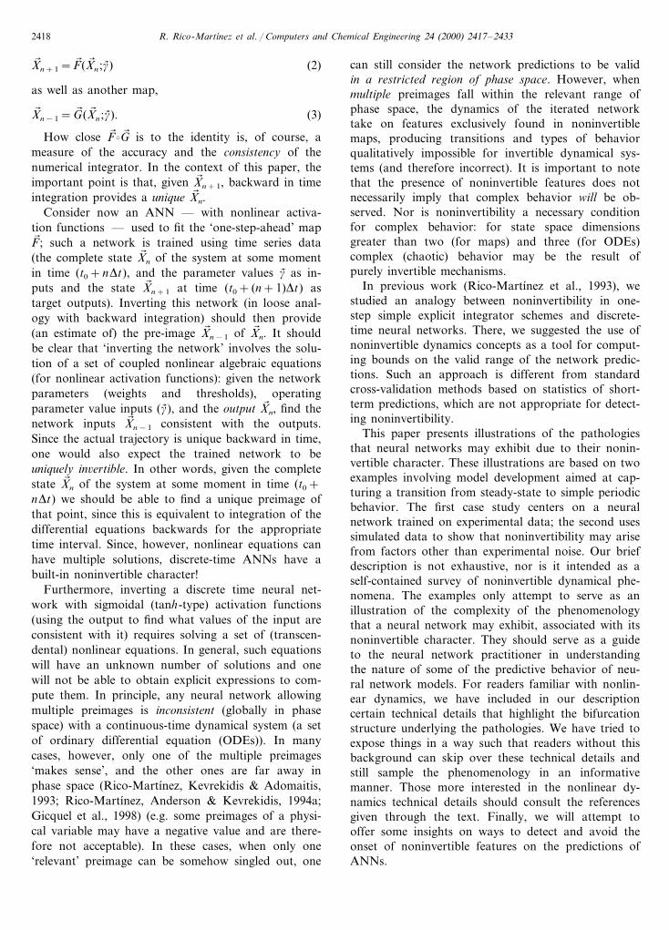
How close Fb $Gb is to the identity is, of course, ameasure of the accuracy and the consistency of thenumerical integrator. In the context of this paper, theimportant point is that, given Xb n+1, backward in timeintegration provides a unique Xb n.

Consider now an ANN — with nonlinear activa-tion functions — used to fit the ‘one-step-ahead’ mapFb ; such a network is trained using time series data(the complete state Xb n of the system at some momentin time (t0+nDt), and the parameter values g� as in-puts and the state Xb n+1 at time (t0+ (n+1)Dt) astarget outputs). Inverting this network (in loose anal-ogy with backward integration) should then provide(an estimate of) the pre-image Xb n−1 of Xb n. It shouldbe clear that ‘inverting the network’ involves the solu-tion of a set of coupled nonlinear algebraic equations(for nonlinear activation functions): given the networkparameters (weights and thresholds), operatingparameter value inputs (g� ), and the output Xb n, find thenetwork inputs Xb n−1 consistent with the outputs.Since the actual trajectory is unique backward in time,one would also expect the trained network to beuniquely in6ertible. In other words, given the completestate Xb n of the system at some moment in time (t0+nDt) we should be able to find a unique preimage ofthat point, since this is equivalent to integration of thedifferential equations backwards for the appropriatetime interval. Since, however, nonlinear equations canhave multiple solutions, discrete-time ANNs have abuilt-in noninvertible character!

Furthermore, inverting a discrete time neural net-work with sigmoidal (tanh-type) activation functions(using the output to find what values of the input areconsistent with it) requires solving a set of (transcen-dental) nonlinear equations. In general, such equationswill have an unknown number of solutions and onewill not be able to obtain explicit expressions to com-pute them. In principle, any neural network allowingmultiple preimages is inconsistent (globally in phasespace) with a continuous-time dynamical system (a setof ordinary differential equation (ODEs)). In manycases, however, only one of the multiple preimages‘makes sense’, and the other ones are far away inphase space (Rico-Martınez, Kevrekidis & Adomaitis,1993; Rico-Martınez, Anderson & Kevrekidis, 1994a;Gicquel et al., 1998) (e.g. some preimages of a physi-cal variable may have a negative value and are there-fore not acceptable). In these cases, when only one‘relevant’ preimage can be somehow singled out, one

can still consider the network predictions to be validin a restricted region of phase space. However, whenmultiple preimages fall within the relevant range ofphase space, the dynamics of the iterated networktake on features exclusively found in noninvertiblemaps, producing transitions and types of behaviorqualitatively impossible for invertible dynamical sys-tems (and therefore incorrect). It is important to notethat the presence of noninvertible features does notnecessarily imply that complex behavior will be ob-served. Nor is noninvertibility a necessary conditionfor complex behavior: for state space dimensionsgreater than two (for maps) and three (for ODEs)complex (chaotic) behavior may be the result ofpurely invertible mechanisms.

In previous work (Rico-Martınez et al., 1993), westudied an analogy between noninvertibility in one-step simple explicit integrator schemes and discrete-time neural networks. There, we suggested the use ofnoninvertible dynamics concepts as a tool for comput-ing bounds on the valid range of the network predic-tions. Such an approach is different from standardcross-validation methods based on statistics of short-term predictions, which are not appropriate for detect-ing noninvertibility.

This paper presents illustrations of the pathologiesthat neural networks may exhibit due to their nonin-vertible character. These illustrations are based on twoexamples involving model development aimed at cap-turing a transition from steady-state to simple periodicbehavior. The first case study centers on a neuralnetwork trained on experimental data; the second usessimulated data to show that noninvertibility may arisefrom factors other than experimental noise. Our briefdescription is not exhaustive, nor is it intended as aself-contained survey of noninvertible dynamical phe-nomena. The examples only attempt to serve as anillustration of the complexity of the phenomenologythat a neural network may exhibit, associated with itsnoninvertible character. They should serve as a guideto the neural network practitioner in understandingthe nature of some of the predictive behavior of neu-ral network models. For readers familiar with nonlin-ear dynamics, we have included in our descriptioncertain technical details that highlight the bifurcationstructure underlying the pathologies. We have tried toexpose things in a way such that readers without thisbackground can skip over these technical details andstill sample the phenomenology in an informativemanner. Those more interested in the nonlinear dy-namics technical details should consult the referencesgiven through the text. Finally, we will attempt tooffer some insights on ways to detect and avoid theonset of noninvertible features on the predictions ofANNs.

R. Rico-Martınez et al. / Computers and Chemical Engineering 24 (2000) 2417–2433 2419

2. The neural network configuration

In the examples to be presented, we made use of a‘standard’ neural network configuration consisting offour layers (see Fig. 1), including two nonlinear hiddenlayers (of equal size) with the customary sigmoidalactivation function [g(y)=1/2(1+ tanh(y))]. Thisconfiguration has been established as a good choice forblack-box identification of nonlinear systems (see e.g.Lapedes & Farber, 1987) through the construction ofdiscrete approximations of the type

Xb (t+t)=F(Xb (t),Xb (t−t),…;g� ) (4)

where g� is the vector of operating parameters, Xb is thevector of states and t is the delay. The vector of inputsis then the vector of states at the current time interval(and possibly at some previous time intervals) alongwith the (one or more) operating parameters. Similarly,the output layer gives the prediction of the vector ofstates at the next time interval. Both input and outputlayers are linear. Posing the identification problem inthis particular way is common practice on the identifi-

Fig. 1. Schematic of the neural network conguration used. The future state of the system X(t+t) is predicted using the current value of the state,one (or more) ‘delayed’ values (X(t), X(t+t), etc.) and the parameter (g).


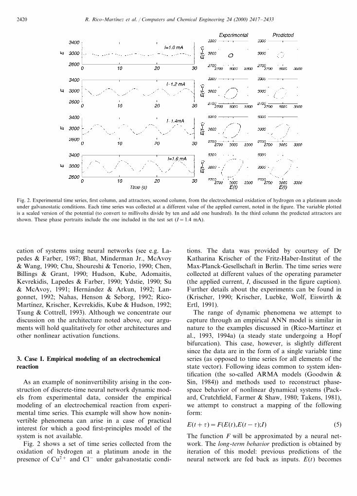
Fig. 2. Experimental time series, first column, and attractors, second column, from the electrochemical oxidation of hydrogen on a platinum anodeunder galvanostatic conditions. Each time series was collected at a different value of the applied current, noted in the figure. The variable plottedis a scaled version of the potential (to convert to millivolts divide by ten and add one hundred). In the third column the predicted attractors areshown. These phase portraits include the one included in the test set (I=1.4 mA).

cation of systems using neural networks (see e.g. La-pedes & Farber, 1987; Bhat, Minderman Jr., McAvoy& Wang, 1990; Chu, Shoureshi & Tenorio, 1990; Chen,Billings & Grant, 1990; Hudson, Kube, Adomaitis,Kevrekidis, Lapedes & Farber, 1990; Ydstie, 1990; Su& McAvoy, 1991; Hernandez & Arkun, 1992; Lan-gonnet, 1992; Nahas, Henson & Seborg, 1992; Rico-Martınez, Krischer, Kevrekidis, Kube & Hudson, 1992;Tsung & Cottrell, 1993). Although we concentrate ourdiscussion on the architecture noted above, our argu-ments will hold qualitatively for other architectures andother nonlinear activation functions.

3. Case I. Empirical modeling of an electrochemicalreaction

As an example of noninvertibility arising in the con-struction of discrete-time neural network dynamic mod-els from experimental data, consider the empiricalmodeling of an electrochemical reaction from experi-mental time series. This example will show how nonin-vertible phenomena can arise in a case of practicalinterest for which a good first-principles model of thesystem is not available.

Fig. 2 shows a set of time series collected from theoxidation of hydrogen at a platinum anode in thepresence of Cu2+ and Cl− under galvanostatic condi-

tions. The data was provided by courtesy of DrKatharina Krischer of the Fritz-Haber-Institut of theMax-Planck-Gesellschaft in Berlin. The time series werecollected at different values of the operating parameter(the applied current, I, discussed in the figure caption).Further details about the experiments can be found in(Krischer, 1990; Krischer, Luebke, Wolf, Eiswirth &Ertl, 1991).

The range of dynamic phenomena we attempt tocapture through an empirical ANN model is similar innature to the examples discussed in (Rico-Martınez etal., 1993, 1994a) (a steady state undergoing a Hopfbifurcation). This case, however, is slightly differentsince the data are in the form of a single variable timeseries (as opposed to time series for all elements of thestate vector). Following ideas common to system iden-tification (the so-called ARMA models (Goodwin &Sin, 1984)) and methods used to reconstruct phase-space behavior of nonlinear dynamical systems (Pack-ard, Crutchfield, Farmer & Shaw, 1980; Takens, 1981),we attempt to construct a mapping of the followingform:

E(t+t)=F(E(t),E(t−t);I) (5)

The function F will be approximated by a neural net-work. The long-term beha6ior prediction is obtained byiteration of this model: previous predictions of theneural network are fed back as inputs. E(t) becomes


E(t−t), E(t+t) becomes E(t), and thus the value ofE(t+2t) can be computed.

The neural network in this case contains eight neu-rons in each of the two hidden layers, and has oneoutput (E(t+t)) and three inputs (E(t), E(t−t), andI). The time delay t was chosen to be 1.25 s (about onefifth of the period of oscillation). The training set wasconstructed using 102 points from each of six timesseries taken at 0.975, 1.0, 1.05, 1.1, 1.2 and 1.6 mA, fora total of 612 training vectors. These training dataincluded the initial transient to the final attractor (ap-parently an oscillation, or limit cycle, whose amplitudeand period vary with the operating parameter I). Aseventh experimental time series (at I=1.4 mA) wasreserved to provide data for the test set. Training wasperformed using a conjugate gradient (CG) algorithm,and was considered complete after seven complete CGcycles (the average error was below 1.5%). The criterionto declare convergence included additional training forten more CG cycles without any significant improve-ment on the predictive capabilities of the network. It isimportant to note that the neural network was nottrained to convergence. A stopping criterion basedupon standard cross-validation techniques was used toensure that the training was terminated for a minimumof the generalization error (as measured for the testset), and not for a minimum of the error with respect tothe training set. Thus, the phenomena described beloware not a result of over-fitting.

Fig. 2 compares also the experimental and observedlong-term attractors, including the parameter value cor-responding to the test set. Let us emphasize that this isnot the short-term, one-step-ahead prediction, but thelong-term attractors of the two systems. Any initialcondition in the general neighborhood of these attrac-tors will give rise to transients eventually attracted tothem. What for the system (and its unknown ODEmodel) is a stable limit cycle becomes a stable (attract-ing) in6ariant circle for the discrete-time neural networkmap. The location of the long-term attractors and their‘appearance’ seem to indicate that the neural networksucceeds in capturing all the features of the system,including the Hopf bifurcation predicted at 0.83 mA(compared with the experimental value of approxi-mately 0.95 mA). While the iterated prediction in timeinevitably deteriorates, and the real and predicted timeseries do not necessarily match point by point after asufficiently long period of time, the attractors of thetwo dynamical systems as sets in phase space lie close toeach other forever. This means that the qualitati6edynamics are accurately reproduced. Note that timeseries at parameter values before the Hopf bifurcationpoint were not available; thus the poor prediction ofthe location of the bifurcation can be attributed to thelack of training data in this region of the parameterrange.

3.1. Pathology I: Jn cur6es and multiple preimages

In Fig. 2, we see that the predicted attractors ‘visu-ally’ appear to faithfully reproduce the experimentallyobserved data. However, there are features ‘hidden’ inthe phase space which play an important role in thestructure and bifurcations of the attractors as I varies.These features are important for determining wheninterpolations/extrapolations of the empirical ANNmodel predictions to other parameter values can beconsidered admissible. This onset of inadmissibility issignaled by curves in phase space defined by the vanish-ing of the determinant of the linearization of the for-ward-time mapping — locations where at least oneeigenvalue of the linearization is zero. These hypersur-faces of codimension-1 (curves in a two-dimensionalphase space) are called J0 curves (surfaces) in thenoninvertible map literature (Gumowski & Mira, 1980;Mira, 1987; Frouzakis, Gardini, Kevrekidis, Millerioux& Mira, 1997). Recently the terms LC (from the French‘ligne critique’) for J1 and LC−1 for J0 have also beenused (Gardini, 1991). Along with their nth iterations (Jn

curves), these critical curves play a crucial role ingenerating noninvertible dynamical features, featuresnot possible in the original data set. These criticalcurves undergo complicated sequences of transitionsthemselves as the operating parameter I varies, affect-ing the global dynamical behavior.

Following the ideas illustrated in (Rico-Martınez etal., 1993, 1994a) we construct the critical curves (Jn)numerically; in our examples the phase space is two-di-mensional and so these are indeed curves. Working intwo phase space dimensions makes both the presenta-tion and the understanding of the concepts and thephenomenology much more tractable. The J0 curves aredefined by the points where the determinant of the2×2 Jacobian matrix (the linearization) of Eq. (6)around (xn,yn) (E(t),E(t−t)) vanishes

xn+1=F(xn,yn ;I)

yn+1=xn. (6)

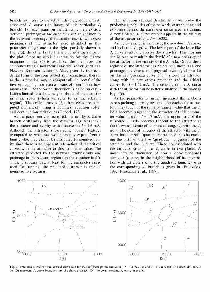
When iterating forward in time, the phase space is‘folded’ along the J0 curves and mapped ‘within’ itself(the ANN map is an endomorphism). The image, J1, ofthe J0 curve constitutes then (after folding and map-ping) the edge of a region whose points possess morethan one preimage; it can be constructed by iteratingonce, forward in time, points on the J0 curve (Gu-mowski & Mira, 1980; Mira, 1987; Frouzakis et al.,1997). Fig. 3 shows the ANN-predicted invariant circlefor I=1.1 mA and I=1.6 mA (in the training range)along with the nearby J0 and J1 curves — more pre-cisely, J0 and J1 sets, consisting each of severalbranches — computed for the converged ANN map.At the lower parameter value we observe a J0 curve


branch 6ery close to the actual attractor, along with itsassociated J1 curve (the image of this particular J0

branch). For each point on the attractor, there exists a‘relevant’ preimage on the attractor itself. In addition tothe ‘relevant’ preimage (the attractor itself), two excesspreimages of the attractor were identified in thisparameter range: one to the right, partially shown inFig. 3(a), the other far to the left outside the range ofthe plot. Since no explicit expression for the inversemapping of Eq. (5) is available, the preimages arecomputed using a nonlinear numerical solver (such as aNewton–Raphson iteration). Also, given the transcen-dental form of the constructed approximations, there isneither a practical way to compute all the ‘roots’ of theinverse mapping, nor even a means of determining howmany exist. The following discussion is based on calcu-lations limited to a finite neighborhood of the attractorin phase space (which we refer to as ‘the relevantregion’). The critical curves (Jn) themselves are com-puted numerically using a nonlinear equation solverand continuation techniques (Doedel, 1981).

As the parameter I is increased, the nearby J0 curvebranch ‘drifts away’ from the attractor. Fig. 3(b) showsthe attractor and nearby critical curves at I=1.6 mA.Although the attractor shows some ‘pointy’ features(compared to what one would visually expect from alimit cycle), they cannot be attributed to noninvertibil-ity since there is no apparent interaction of the criticalcurves with the attractor at this parameter value. Theattractor predicted by the network exhibits only onepreimage in the relevant region (on the attractor itself).Thus, it appears that, at least for the parameter rangeused for training, the predicted attractor is free ofnoninvertible features.

This situation changes drastically as we probe thepredictive capabilities of the network, extrapolating andexploring beyond the parameter range used in training.A new isolated J0 curve branch appears in the vicinityof the attractor around I=1.6302.

As the parameter is increased, the new-born J0 curve,and its iterate J1, grow. The lower part of the lense-likeJ1 curve eventually crosses the attractor. This crossingcan be seen to result in the ‘birth’ of a new preimage ofthe attractor in the vicinity of the J0 isola. Only a shortsegment of the attractor has points with more than onepreimage; the excess, non-physical meaningful ones lieon this new preimage curve. Fig. 4 shows the attractoralong with its new excess preimage and the criticalcurves for I=1.65 mA. The crossing of the J1 curvewith the attractor can be better visualized in the blowupFig. 4(c).

As the parameter is further increased the newbornexcess preimage curve grows and approaches the attrac-tor. They touch at the same parameter value that the J0

isola becomes tangent to the attractor. At this parame-ter value (around I=1.7 mA), the upper part of thelense-like J1 isola becomes tangent to the attractor atthe (forward) iterate of its point of tangency with the J0

isola. The point of tangency of the attractor with the J1

curve has a special ‘quartic’ character, due to its mark-ing the birth of the two ‘quadratic’ tangencies of theattractor and the J1 curve. These are associated withthe attractor crossing the J0 curve in two places. Amore detailed discussion of how a one-dimensionalattractor (a curve in the neighborhood of its intersec-tion with J0) gives rise to the quadratic tangency withthe corresponding J1 branch is given in (Frouzakis,1992; Frouzakis et al., 1997).

Fig. 3. Predicted attractors and critical curve sets for two different parameter values: I=1.1 mA (a) and I=1.6 mA (b). The dash–dot curves(A–D) represent J0 curve branches and the short dash (A%–D%) the corresponding J1 curve branches.


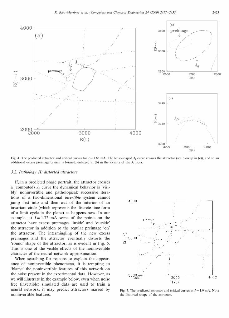
Fig. 4. The predicted attractor and critical curves for I=1.65 mA. The lense-shaped J1 curve crosses the attractor (see blowup in (c)), and so anadditional excess preimage branch is formed, enlarged in (b) in the vicinity of the J0 isola.

3.2. Pathology II: distorted attractors

If, in a predicted phase portrait, the attractor crossesa (computed) J0 curve the dynamical behavior is ‘visi-bly’ noninvertible and pathological: successive itera-tions of a two-dimensional in6ertible system cannotjump first into and then out of the interior of aninvariant circle (which represents the discrete-time formof a limit cycle in the plane) as happens now. In ourexample, at I=1.72 mA some of the points on theattractor have excess preimages ‘inside’ and ‘outside’the attractor in addition to the regular preimage ‘on’the attractor. The intermingling of the new excesspreimages and the attractor eventually distorts the‘round’ shape of the attractor, as is evident in Fig. 5.This is one of the visible effects of the noninvertiblecharacter of the neural network approximation.

When searching for reasons to explain the appear-ance of noninvertible phenomena, it is tempting to‘blame’ the noninvertible features of this network onthe noise present in the experimental data. However, aswe will illustrate in the example below, even when noisefree (invertible) simulated data are used to train aneural network, it may predict attractors marred bynoninvertible features.

Fig. 5. The predicted attractor and critical curves at I=1.9 mA. Notethe distorted shape of the attractor.


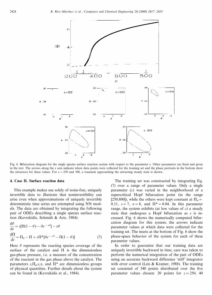
Fig. 6. Bifurcation diagram for the single species surface reaction system with respect to the parameter e. Other parameters are fixed and givenin the text. The arrows along the e axis indicate where data points were collected for the training set and the phase portraits in the bottom showthe attractors for these values. For e=250 and 300, a transient approaching the attracting steady state is shown.

4. Case II. Surface reaction data

This example makes use solely of noise-free, uniquelyinvertible data to illustrate that noninvertibility canarise even when approximations of uniquely invertibledeterministic time series are attempted using NN mod-els. The data are obtained by integrating the followingpair of ODEs describing a single species surface reac-tion (Kevrekidis, Schmidt & Aris, 1984):

du

dt=o [P(1−u)−ue−au]−su

dPdt

=P0−P+oP* [ue−au−P(1−u)] (7)

Here u represents the reacting species coverage of thesurface of the catalyst and P is the dimensionlessgas-phase pressure, i.e. a measure of the concentrationof the reactant in the gas phase above the catalyst. Theparameters o,P0,s,a, and P* are dimensionless groupsof physical quantities. Further details about the systemcan be found in (Kevrekidis et al., 1984).

The training set was constructed by integrating Eq.(7) over a range of parameter values. Only a singleparameter (o) was varied in the neighborhood of asupercritical Hopf bifurcation point (in the range[250,800]), while the others were kept constant at P0=0.11, s=7, a=8, and P*=0.04. In this parameterrange, the system exhibits (at low values of o) a steadystate that undergoes a Hopf bifurcation as o is in-creased. Fig. 6 shows the numerically computed bifur-cation diagram for this system; the arrows indicateparameter values at which data were collected for thetraining set. The insets at the bottom of Fig. 6 show thephase-space behavior of the system for each of theseparameter values.

In order to guarantee that our training data areuniquely invertible backward in time, care was taken toperform the numerical integration of the pair of ODEsusing an accurate backward difference ‘stiff’ integratorwith error control (Leis & Kramer, 1988). The trainingset consisted of 340 points distributed over the fiveparameter values chosen: 20 points for o=250, 40


points for o=300, 80 points for o=350 and 100 pointseach for o=500 and o=800. The trajectories on whichthese points lie include initial transients approachingthe attractors as well as data on the attractors them-selves. Note that more points have been added to thetraining set at parameter values where more compli-cated long term behavior (larger amplitude oscillations)is observed; here, ‘complicated’ should be compared toparameter values where ‘simpler’ trajectories approach-ing a steady state are found.

4.1. The neural network

The mapping we seek to construct is of the form:

u(t+t)=F(u(t),P(t);o)

P(t+t)=G(u(t),P(t);o)

where the functions F and G are approximated by theneural network. The delay t was chosen to be 0.22 unitsof time (approximately one-fifth of the period of theoscillations). A four-layer neural network was used,consisting of eight neurons in each hidden layer, threeinputs (o, u(t), and P(t)), and two outputs (u(t+t),and P(t+t)). The results presented below were ob-tained after 170 complete conjugate gradient (CG) cy-cles, when the average norm error dropped below 1.5%of the available range in the training set. The criterionfor stopping training involved using a test set consistingsolely of points not in the training set. Training wascontinued over 100 more CG cycles without observingany appreciable improvement in predictions (nor anysignificant qualitative change of the noninvertible phe-nomena described below). Once again, the results re-ported are for a minimum on the generalization erroras measured for the test set and not the result ofover-fitting.

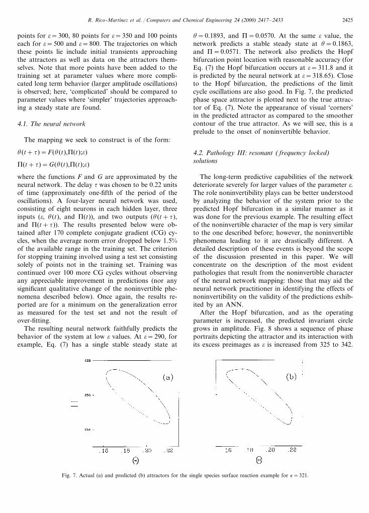
The resulting neural network faithfully predicts thebehavior of the system at low o values. At o=290, forexample, Eq. (7) has a single stable steady state at

u=0.1893, and P=0.0570. At the same o value, thenetwork predicts a stable steady state at u=0.1863,and P=0.0571. The network also predicts the Hopfbifurcation point location with reasonable accuracy (forEq. (7) the Hopf bifurcation occurs at o=311.8 and itis predicted by the neural network at o=318.65). Closeto the Hopf bifurcation, the predictions of the limitcycle oscillations are also good. In Fig. 7, the predictedphase space attractor is plotted next to the true attrac-tor of Eq. (7). Note the appearance of visual ‘corners’in the predicted attractor as compared to the smoothercontour of the true attractor. As we will see, this is aprelude to the onset of noninvertible behavior.

4.2. Pathology III: resonant ( frequency locked)solutions

The long-term predictive capabilities of the networkdeteriorate severely for larger values of the parameter o.The role noninvertibility plays can be better understoodby analyzing the behavior of the system prior to thepredicted Hopf bifurcation in a similar manner as itwas done for the previous example. The resulting effectof the noninvertible character of the map is very similarto the one described before; however, the noninvertiblephenomena leading to it are drastically different. Adetailed description of these events is beyond the scopeof the discussion presented in this paper. We willconcentrate on the description of the most evidentpathologies that result from the noninvertible characterof the neural network mapping: those that may aid theneural network practitioner in identifying the effects ofnoninvertibility on the validity of the predictions exhib-ited by an ANN.

After the Hopf bifurcation, and as the operatingparameter is increased, the predicted invariant circlegrows in amplitude. Fig. 8 shows a sequence of phaseportraits depicting the attractor and its interaction withits excess preimages as o is increased from 325 to 342.

Fig. 7. Actual (a) and predicted (b) attractors for the single species surface reaction example for e=321.


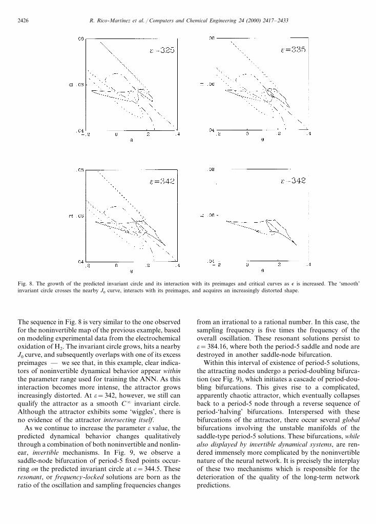
Fig. 8. The growth of the predicted invariant circle and its interaction with its preimages and critical curves as e is increased. The ‘smooth’invariant circle crosses the nearby J0 curve, interacts with its preimages, and acquires an increasingly distorted shape.

The sequence in Fig. 8 is very similar to the one observedfor the noninvertible map of the previous example, basedon modeling experimental data from the electrochemicaloxidation of H2. The invariant circle grows, hits a nearbyJ0 curve, and subsequently overlaps with one of its excesspreimages — we see that, in this example, clear indica-tors of noninvertible dynamical behavior appear withinthe parameter range used for training the ANN. As thisinteraction becomes more intense, the attractor growsincreasingly distorted. At o=342, however, we still canqualify the attractor as a smooth C� invariant circle.Although the attractor exhibits some ‘wiggles’, there isno evidence of the attractor intersecting itself.

As we continue to increase the parameter o value, thepredicted dynamical behavior changes qualitativelythrough a combination of both noninvertible and nonlin-ear, in6ertible mechanisms. In Fig. 9, we observe asaddle-node bifurcation of period-5 fixed points occur-ring on the predicted invariant circle at o=344.5. Theseresonant, or frequency-locked solutions are born as theratio of the oscillation and sampling frequencies changes

from an irrational to a rational number. In this case, thesampling frequency is five times the frequency of theoverall oscillation. These resonant solutions persist too=384.16, where both the period-5 saddle and node aredestroyed in another saddle-node bifurcation.

Within this interval of existence of period-5 solutions,the attracting nodes undergo a period-doubling bifurca-tion (see Fig. 9), which initiates a cascade of period-dou-bling bifurcations. This gives rise to a complicated,apparently chaotic attractor, which eventually collapsesback to a period-5 node through a reverse sequence ofperiod-‘halving’ bifurcations. Interspersed with thesebifurcations of the attractor, there occur several globalbifurcations involving the unstable manifolds of thesaddle-type period-5 solutions. These bifurcations, whilealso displayed by in6ertible dynamical systems, are ren-dered immensely more complicated by the noninvertiblenature of the neural network. It is precisely the interplayof these two mechanisms which is responsible for thedeterioration of the quality of the long-term networkpredictions.


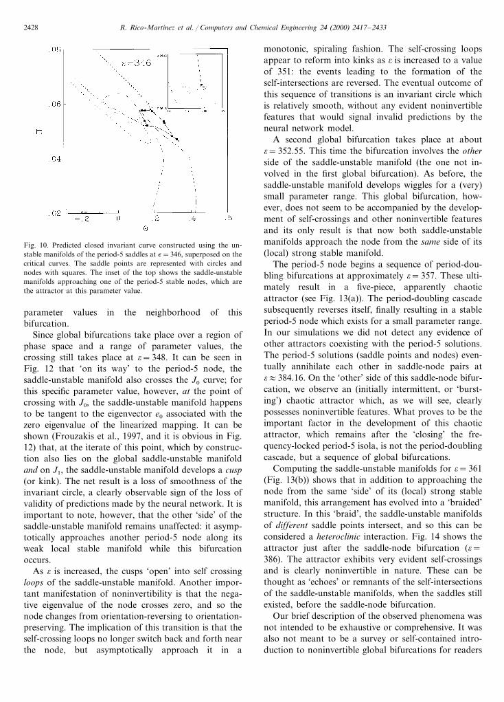
To analyze the global bifurcations responsible for theloss of smoothness of the invariant circle (from behav-ior A to C of Fig. 9), we reconstruct the invariant circleby computing the unstable manifolds of the saddle-typeperiod-5 solutions (which we refer to here as the ‘sad-dle-unstable manifolds’). Since we wish only to illus-trate some of the possible dynamic phenomenology,and not delve into the theory of the observed bifurca-tions, we briefly note that the definition of global stableand unstable manifolds valid for invertible mappingsdoes not directly hold for noninvertible ones and mustbe modified. Nevertheless, it is possible to define localversions of both stable and unstable manifolds, as wellas a global unstable manifold (Robinson, 1994; Frouza-kis et al., 1997). Fig. 10 shows the result of one suchcalculation: a wiggly, but still smooth circle connectingthe saddle period-5 points and the period-5 nodes.However, we see from Fig. 10 that this structure crossesone J0 and one J1 curve and so we should suspect thatnoninvertibility will come into play during the bifurca-tions and transitions which will occur for larger o.

4.3. Pathology IV: global bifurcations andself-intersecting attractors

The presence of ‘wiggles’ in the saddle-unstable man-ifold in the neighborhood of the period-5 node of Fig.10 indicates the onset of a global bifurcation. Thisglobal bifurcation involves the crossing of the unstablemanifold of the period-5 saddle with the (local) strongstable manifold of the period-5 node. Fig. 11 consists ofsnapshots of the different stages of this transition. Ato=345, just after the period-5 frequency locking, thewiggly unstable manifold is still far from the (local)strong stable manifold of the node-period-5, but ap-proaches it and eventually crosses it at approximatelyo=347. The node period-5 solutions are born with onenegative eigenvalue. This means that iterations alongthe strong stable eigendirection alternate from one sideof the (strong stable eigenvector of the) node to theother, and so the saddle-unstable manifold also has toswitch back and forth as it asymptotes to the node for

Fig. 9. A portion of the bifurcation diagram predicted by the neural network mapping constructed using simulated data for the surface reactionmodel. Stable fixed points are indicated by solid curves, unstable fixed points by broken curves and invariant circles (A) by filled circles. Thebranch of period-5 periodic points (B) resulting from a resonance (frequency-locking) on the invariant circle is indicated in the plot. This branchundergoes a sequence of period doubling bifurcations, of which only one is included in the diagram. After the disappearance of the locked statesthe resulting attractor (C) appears chaotic.


Fig. 10. Predicted closed invariant curve constructed using the un-stable manifolds of the period-5 saddles at e=346, superposed on thecritical curves. The saddle points are represented with circles andnodes with squares. The inset of the top shows the saddle-unstablemanifolds approaching one of the period-5 stable nodes, which arethe attractor at this parameter value.

monotonic, spiraling fashion. The self-crossing loopsappear to reform into kinks as o is increased to a valueof 351: the events leading to the formation of theself-intersections are reversed. The eventual outcome ofthis sequence of transitions is an invariant circle whichis relatively smooth, without any evident noninvertiblefeatures that would signal invalid predictions by theneural network model.

A second global bifurcation takes place at abouto=352.55. This time the bifurcation involves the otherside of the saddle-unstable manifold (the one not in-volved in the first global bifurcation). As before, thesaddle-unstable manifold develops wiggles for a (very)small parameter range. This global bifurcation, how-ever, does not seem to be accompanied by the develop-ment of self-crossings and other noninvertible featuresand its only result is that now both saddle-unstablemanifolds approach the node from the same side of its(local) strong stable manifold.

The period-5 node begins a sequence of period-dou-bling bifurcations at approximately o=357. These ulti-mately result in a five-piece, apparently chaoticattractor (see Fig. 13(a)). The period-doubling cascadesubsequently reverses itself, finally resulting in a stableperiod-5 node which exists for a small parameter range.In our simulations we did not detect any evidence ofother attractors coexisting with the period-5 solutions.The period-5 solutions (saddle points and nodes) even-tually annihilate each other in saddle-node pairs ato:384.16. On the ‘other’ side of this saddle-node bifur-cation, we observe an (initially intermittent, or ‘burst-ing’) chaotic attractor which, as we will see, clearlypossesses noninvertible features. What proves to be theimportant factor in the development of this chaoticattractor, which remains after the ‘closing’ the fre-quency-locked period-5 isola, is not the period-doublingcascade, but a sequence of global bifurcations.

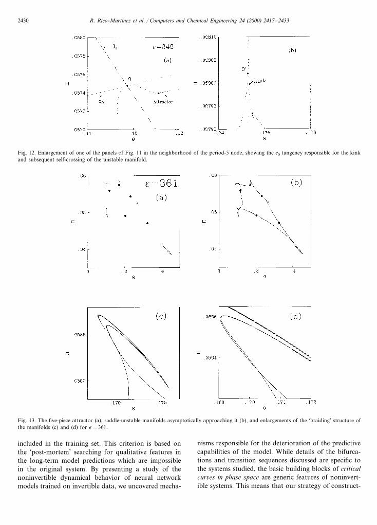
Computing the saddle-unstable manifolds for o=361(Fig. 13(b)) shows that in addition to approaching thenode from the same ‘side’ of its (local) strong stablemanifold, this arrangement has evolved into a ‘braided’structure. In this ‘braid’, the saddle-unstable manifoldsof different saddle points intersect, and so this can beconsidered a heteroclinic interaction. Fig. 14 shows theattractor just after the saddle-node bifurcation (o=386). The attractor exhibits very evident self-crossingsand is clearly noninvertible in nature. These can bethought as ‘echoes’ or remnants of the self-intersectionsof the saddle-unstable manifolds, when the saddles stillexisted, before the saddle-node bifurcation.

Our brief description of the observed phenomena wasnot intended to be exhaustive or comprehensive. It wasalso not meant to be a survey or self-contained intro-duction to noninvertible global bifurcations for readers

parameter values in the neighborhood of thisbifurcation.

Since global bifurcations take place over a region ofphase space and a range of parameter values, thecrossing still takes place at o=348. It can be seen inFig. 12 that ‘on its way’ to the period-5 node, thesaddle-unstable manifold also crosses the J0 curve; forthis specific parameter value, however, at the point ofcrossing with J0, the saddle-unstable manifold happensto be tangent to the eigenvector e0 associated with thezero eigenvalue of the linearized mapping. It can beshown (Frouzakis et al., 1997, and it is obvious in Fig.12) that, at the iterate of this point, which by construc-tion also lies on the global saddle-unstable manifoldand on J1, the saddle-unstable manifold develops a cusp(or kink). The net result is a loss of smoothness of theinvariant circle, a clearly observable sign of the loss ofvalidity of predictions made by the neural network. It isimportant to note, however, that the other ‘side’ of thesaddle-unstable manifold remains unaffected: it asymp-totically approaches another period-5 node along itsweak local stable manifold while this bifurcationoccurs.

As o is increased, the cusps ‘open’ into self crossingloops of the saddle-unstable manifold. Another impor-tant manifestation of noninvertibility is that the nega-tive eigenvalue of the node crosses zero, and so thenode changes from orientation-reversing to orientation-preserving. The implication of this transition is that theself-crossing loops no longer switch back and forth nearthe node, but asymptotically approach it in a


not familiar with the phenomenology of noninvertiblemappings, or even with global bifurcations of invertiblemappings of the plane. For readers not familiar withthis terminology and phenomena we hope that thisserves as a brief anthology, and as an indication of therichness and complexity of the types of noninvertibledynamics that can be predicted by NN models. Clearly,even if the predicted time series appear ‘reasonable’,phase space plots exhibiting such phenomena invalidatethe NN models.

5. Discussion

In this paper, we discussed an inherent deficiency ofANN-based discrete-time nonlinear models obtainedfrom time series. This deficiency, noninvertibility, pro-vides also an alternative method for judging the validityof predictions made by the ANN models. This ideadiffers from what might be considered the ‘traditional’methods for assessing the predictive capabilities of theANN models, such as validation with test data not

Fig. 11. A sequence of blowups of one of the period-5 nodes born from the locking on the invariant circle, illustrating the global bifurcationinvolving the unstable manifold of the saddle period-5 and the node’s strong stable manifold (double-dash curve). Note that the ‘wiggling’ of theunstable manifold increases as it approaches (in parameter space) the crossing with the strong stable manifold. The unstable manifold alsodevelops self-intersections as a result of its interaction with the critical curves.


Fig. 12. Enlargement of one of the panels of Fig. 11 in the neighborhood of the period-5 node, showing the e0 tangency responsible for the kinkand subsequent self-crossing of the unstable manifold.

Fig. 13. The five-piece attractor (a), saddle-unstable manifolds asymptotically approaching it (b), and enlargements of the ‘braiding’ structure ofthe manifolds (c) and (d) for e=361.

included in the training set. This criterion is based onthe ‘post-mortem’ searching for qualitative features inthe long-term model predictions which are impossiblein the original system. By presenting a study of thenoninvertible dynamical behavior of neural networkmodels trained on invertible data, we uncovered mecha-

nisms responsible for the deterioration of the predictivecapabilities of the model. While details of the bifurca-tions and transition sequences discussed are specific tothe systems studied, the basic building blocks of criticalcur6es in phase space are generic features of noninvert-ible systems. This means that our strategy of construct-


ing critical curves and studying their interactions withthe predicted attractors is applicable to other neuralnetwork models, provided that the dimension of thephase space is relatively low (53).

Adjustable factors such as the size and architectureof the neural network, the size and composition of thetraining set, the degree of training, and the magnitudeof the delay can, and will, affect the particular mannerin which noninvertible behavior appears. These choices,however, cannot alter the fundamentally noninvertiblenature of the neural networks discussed in this pa-per — noninvertibility will appear in one way or an-other in this type of model. The best that can be doneis to use the choices mentioned above to ‘displace’ thenoninvertible phenomena out of the rele6ant region ofphase space. For example, determining where in phaseand parameter space the critical curves begin to interactwith the predicted attractors can be used as a guidelinefor the acquisition of more training data to improve thepredictions. Smaller time delays may also reduce nonin-vertible effects, although the increased correlation be-tween points in the time series will work against more

accurate predictions. It would be interesting to examinehow one might include the distance of J0 curves as aconstraint in the training, and thus devise trainingalgorithms that would guarantee the lack of spuriousexcess preimages in the relevant region of phase space.

Another interesting direction of research involves theuse of pruning algorithms in order to diminish theeffects of noninvertibility. In classification applications,the pruning of neural network often results in increas-ing smoothing of the decision boundaries (Reed, 1993).For noninvertible neural network predictors, pruningmay result in the modification of the J curves interac-tion with the predicted attractors. However, the currentpruning algorithms should be modified to consider theeffect of eliminating connections on the long-term be-havior of the NN model.

An alternative approach to eliminating noninvertibledynamical features is to avoid them completely fromthe outset. This can be accomplished by constructinginput/output neural network mappings which approxi-mate the time deri6ati6es of the states at each time step(the right-hand-side of the system ODEs) (e.g. Chu &

Fig. 14. The predicted chaotic attractor (a), superposed with its neighboring critical curves (b) at e=386, just after the saddle-node bifurcation.The predicted, apparently chaotic, attractor is characterized by self-intersections (see the enlargements in (c) and (d)), clearly indicating itsnoninvertible nature.


Shoureshi, 1991; Rico-Martınez et al., 1992; Rico-Martınez, Anderson & Kevrekidis, 1994b; Rico-Mar-tınez et al., 1995; Rico-Martınez & Kevrekidis, 1993;Olurotimi, 1994). We thus construct continuous timemodels, and then using an accurate numerical integra-tor, follow the time evolution of the system, ratherthan predict the state at the next (fixed) time stepdirectly. ‘Perfect’ integration is by constructionuniquely invertible: trajectories, given the appropriateconditions on the right-hand-side, are unique in re-verse time. A numerically accurate integration be-tween two points in a time series would guaranteethat the excess preimages (also always present in nu-merical integration schemes (Lorenz, 1989)) will notinterfere with the local dynamics.

From the examples presented here, it is clear thatnoninvertibility plays a very important role in the de-terioration of the predictive capabilities of discreteneural network approximations of continuous-timenonlinear dynamical systems. The numerical computa-tion of critical cur6es in phase space, on the otherhand, can be used as a tool to assess the validityrange of ANN predictions. Although we have stressedthe effect of noninvertibility on the long-term predic-tion capabilities of the ANN models, noninvertibilitytranslates also in important local effects that maydrastically affect the quality of the short-term predic-tions over a limited region of phase space (in theclose vicinity of J0 curves). For example, in discussingpathology IV we found a noninvertible transition thatchanges an attractor from orientation preserving toorientation reversing. Locally, this observation trans-lates also in incorrect short-term predictions becauseit implies that the trajectories will go from the ‘out-side’ to the ‘inside’ of the periodic orbit. While againthis is a valid possibility for discrete noninvertiblesystems, it is simply impossible for continuous sys-tems.

The study of noninvertible dynamical systems is animportant and recently flourishing research subject initself. Some of the phenomena described here havenot yet been widely observed or reported in the liter-ature. Multistable noninvertible dynamical systemscan have disconnected and highly distorted basin ofattraction boundaries (Adomaitis & Kevrekidis, 1991).An interesting research problem might be the study ofbasin boundary structures of neural network modelstrained on data obtained from multistable, in6ertiblesystems to determine the role of noninvertibility inthe breakdown of predictions of these systems. Fi-nally, it is important to consider the implications ofnoninvertibility in neural network model-based feed-back control systems, especially in terms of the com-plexity noninvertibility introduces into assessing theglobal stability of such systems.

Acknowledgements

The authors would like to acknowledge the supportof the National Science Foundation and UTRC. Oneof the authors (R.R.M.) was partially supported byCONACyT; the hospitality of the Center for Nonlin-ear Studies at the Los Alamos National Laboratory isgratefully acknowledged.

References

Adomaitis, R. A., & Kevrekidis, I. G. (1991). Noninvertibility andthe structure of basins of attraction of a model adaptive controlsystem. Journal of Nonlinear Science, 1, 95–105.

Bhat, N. V., Minderman Jr., P. A., McAvoy, T., & Wang, N. S.(1990). Modeling chemical process systems via neural computa-tion. IEEE Control Systems Magazine, April, 24–29.

Chen, S., Billings, S. A., & Grant, P. M. (1990). Non-linear systemidentification using neural networks. International Journal of Con-trol, 51, 1191–1214.

Chu S. R., Shoureshi, R., & Tenorio, M. (1990). Neural networks forsystem identification. IEEE Control Systems Magazine, April,31–35.

Chu, S. R., & Shoureshi, R. (1991). A neural network approach foridentification of continuous-time nonlinear dynamic systems. Pro-ceedings of the 1991 American Control Conference, 1, 1–5.

Doedel, E. J. (1981). AUTO: a program for the automatic bifurcationanalysis of autonomous systems. Congressus Numerantium, 30,265–284.

Frouzakis, C. E. (1992). Dynamics of systems under control: quan-tifying stability. Ph.D. Thesis, Princeton University, Departmentof Chemical Engineering.

Frouzakis, C. E., Gardini, L., Kevrekidis, I. G., Millerioux, G., &Mira, C. (1997). On some properties of invariant sets of two-di-mensional non-invertible maps. International Journal of Bifurca-tions and Chaos, 7, 1167–1194.

Gardini, L. (1991). On the global bifurcation of two-dimensionalendomorphisms by use of critical lines. Non Linear Analysis,Theory, Methods and Applications, 18, 361–399.

Gicquel, N., Anderson, J. S., & Kevrekidis, I. G. (1998). Noninverti-bility and resonance in discrete-time neural networks for timeseries processing. Physics Letters A, 238, 8–18.

Goodwin, G. C., & Sin, K. S. (1984). Adapti6e filtering, prediction andcontrol. Englewood Cliffs, NJ: Prentice Hall.

Gumowski, I., & Mira, C. (1980). Recurrences and discrete dynamicsystems, Lecture Notes in Mathemathics, Springer, Heidelberg.

Hernandez, E., & Arkun, Y. (1992). Study of the control-relevantproperties of backpropagation neural network models of nonlin-ear dynamical systems. Computers & Chemical Engineering, 16,227–240.

Hudson, J. L., Kube, M., Adomaitis, R. A., Kevrekidis, I. G.,Lapedes, A. S., & Farber, R. M. (1990). Nonlinear signal process-ing and system identification: applications to time series fromelectrochemical reactions. Chemical Engineering Science, 45,2075–2081.

Kevrekidis, I., Schmidt, L. D., & Aris, R. (1984). Rate multiplicityand oscillations in single species surface reactions. Surface Sci-ence, 137, 151–166.

Kevrekidis, I. G., Rico-Martınez, R., Ecke, R. E., Lapedes, A. S., &Farber, R. M. (1994). Global bifurcation analysis in Rayleigh–Benard convection experiments, empirical maps and numericalbifurcation analysis. Physica D, 71, 342–362.


Krischer, K. (1990). Nichtlineare dynamik zweier grenzflachenreak-tionen — Kinetische oszillationen, bifurkationen und determin-istisches chaos. Ph.D. Thesis, Free University Berlin, Germany.

Krischer, K., Luebke, M., Wolf, W., Eiswirth, M., & Ertl, G. (1991).Chaos and interior crisis in an electrochemical reaction. Berichteder Bunsengesellschaft fuer Physikalische Chemie, 95, 820–823.

Langonnet, P. (1992). Process control with neural networks: anexample. Applications of Artificial Neural Networks III, SPIE1709:468–475.

Lapedes, A. S., & Farber, R. M. (1987). Nonlinear signal processingusing neural networks: prediction and system modeling, LosAlamos Report LA-UR 87-2662.

Leis, J. R., & Kramer, M. A. (1988). ODESSA — an ordinarydifferential equation solver with explicit simultaneous sensitivityanalysis. ACM Transactions on Mathemathics Software, 14, 61–67.

Lorenz, E. N. (1989). Computational chaos — a prelude to compu-tational instability. Physica D, 35, 299–317.

Mira, C. (1987). Chaotic dynamics. From the one-dimensional endo-morphism to the two-dimensional diffeomorphism. Singapore:World Scientific.

Nahas, E. P., Henson, M. A., & Seborg, D. E. (1992). Nonlinearinternal model control strategy for neural network models. Com-puters & Chemical Engineering, 16, 1039–1057.

Packard, N. H., Crutchfield, J. P., Farmer, J. D., & Shaw, R. S.(1980). Geometry from a time series. Physical Re6iew Letters, 45,712–716.

Olurotimi, O. (1994). Recurrent neural network training with feedfor-ward complexity. IEEE Transactions on Neural Networks, 5,185–197.

Reed, R. (1993). Pruning algorithms — a survey. IEEE TransactionsNeural Networks, 4, 740–747.

Rico-Martınez, R., & Kevrekidis, I. G. (1993). Continuous-timemodeling of nonlinear systems: a neural network approach. Pro-ceedings of the 1993 IEEE International Conference on NeuralNetworks, III, 1522–1525.

Rico-Martınez, R., Krischer, K., Kevrekidis, I. G., Kube, M. C., &Hudson, J. L. (1992). Discrete- vs. continuous-time nonlinear

signal processing of Cu electrodissolution data. Chemical Engi-neering Communications, 118, 25–48.

Rico-Martınez, R., Kevrekidis, I. G., & Adomaitis, R. A. (1993).Noninvertibility in neural networks. Proceedings of 1993 IEEEInternational Conference on Neural Networks, I, 382–386.

Rico-Martınez, R., Kevrekidis. I. G., & Adomaitis, R. A. (1994a).Noninvertible dynamics in neural network models. Proceedings ofthe Twenty-Eighth Annual Conference on Information Sciences andSystems (pp. 965–969). Princeton, NJ: Princeton University.

Rico-Martınez, R., Anderson, J. S., & Kevrekidis, I. G. (1994b).Continuous-time nonlinear signal processing: a neural networkbased approach for gray box identification, Proceedings of the1994 IEEE Workshop on Neural Networs for Signal Processing(pp. 596–605). IEEE Publications.

Rico-Martınez, R., Kevrekidis, I. G., & Krischer, K. (1995). Nonlin-ear system identification using neural networks: dynamics andinstabilities. In: Bulsari, A., Neural networks for chemical engi-neers (pp. 409–442). Amsterdam: Elsevier, (Chapter 16).

Robinson, C. (1994). Dynamical systems: stability, symbolic dynamics,and chaos. Boca Raton, FL: CRC Press.

Su, H.-T., & McAvoy, T. J. (1991). Identification of chemical pro-cesses using recurrent networks. Proceedings of the 1991 AmericanControl Conference (pp. 2314–2319).

Takens, F. (1981). Detecting strange attractors in turbulence. In:Rand, D. A., & Young, L. S., Dynamical systems and turbulence,Lecture Notes in Mathemathics (pp. 366–381). Heidelberg:Springer.

Tsung, F.-S., & Cottrell, G. W. (1993). Phase-space learning inrecurrent networks. Technical Report CS93-285, Deptartment ofComputer Science & Engineering, University of California, SanDiego.

Weigend, A. S., & Gershenfeld, N. A. (1993). Time series prediction:Forecasting the future and understanding the past. Reading, MA:Addison-Wesley.

Ydstie, B. E. (1990). Forecasting and control using adaptive connec-tionist networks. Computers & Chemical Engineering, 14, 583–599.

.

Noninvertibility in neural networks

Documents

Transcript of Noninvertibility in neural networks