Application of neural networks in chain curvemodelling

Iza Rejer1, Andrzej Piegat1,2 and Marek Mikolajczyk1

1 University of Szczecin, 64/66 Mickiewicza Street, 71-101 Poland,2 Technical University of Szczecin, 49 Zolnierska Street, 71-210 Poland{iza.rejer, andrzej.piegat, marek.mikolajczyk}@uoo.univ.szczecin.pl

Abstract. A modelling process of an unknown multi-dimension systemis mostly performed with methods, like neural networks (NNs), whichdescribe the system by a multi-dimension surface. Some systems, how-ever, does not have a surface nature. On the contrary - their behaviourresembles multi-dimension chains. Obviously, as it was proved in numer-ous real applications, always better results can be obtained when themodelling method is in agreement with the system nature. Therefore,when a data distribution of an unknown system has a chain character-istic, the system should be also modelled with a chain, not a surface,method. The aim of this article is to present the alternative approachto the modelling process, in which the multi dimension model of an un-known system is built on the basis of a set of two dimension NNs insteadof one multi dimension NN. The proposed approach results in a chainmulti dimension model of the analyzed system.

1 Introduction

The most popular approach to the modelling process of an unknown real systemof one output variable is to describe its behavior by a surface mapping its inputvariables into output variable. This approach very often results in a correct andsatisfactory input-output mapping, however, there are not always reasons to itsuse. One of the cases in which surface modelling can result in a model of a loweffectiveness is the case of a system described by a very large dimension of theinput vector. The weak performance of the surface model is caused by the factthat data distribution in multi-dimension input space is often not appropriateto build a surface model. Gershenfeld [Ge1] proved that in a low-dimensionspace, most data comes from the center of the analyzing space, while in a high-dimension space almost all data comes from its border. That means that evenin a huge data set, placed in a high-dimension space, there can be no data inthe centre of the analyzing space. Therefore, each analysis of such space will bedominated by ”border effects” [Kl1].

This tendency can readily be observed via Monte-Carlo method applied forgenerating points in multi-dimension regions. It occurs that a ratio betweenpoints situated inside those regions to all points tends to one when the regiondimension increases. That means that the probability that the point will be

situated on the region border tends to one. The important fact is that this effectappears relatively quick (for example for 20 dimensions about 90% of data aresituated on the region border [Kl1]).

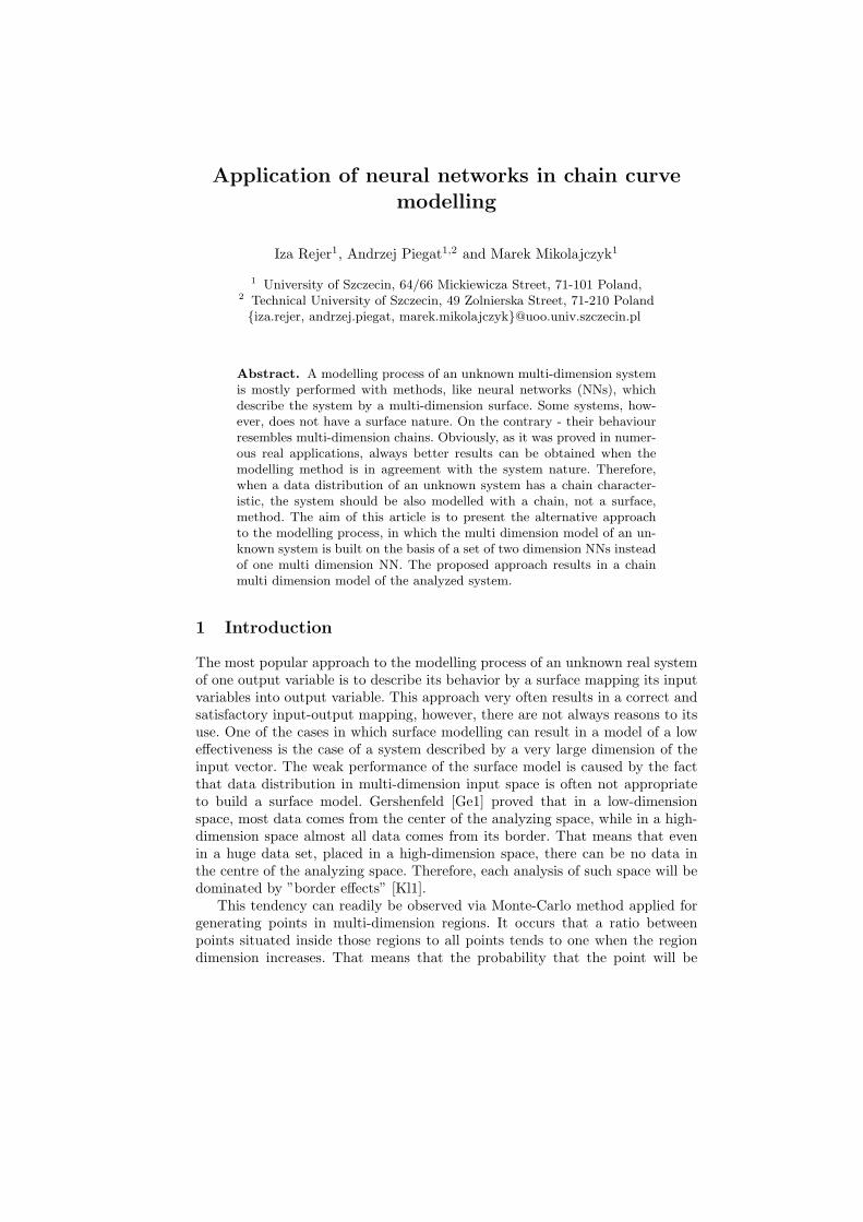
The multi-dimension space is not the only one in which surface approximationcan sometimes result in not satisfactory input-output mapping. Even in 3D spaceexamples of systems which cannot be properly modelled by a surface model canbe found. An example of such a system is shown in the fig. 1a.

Systems of chain characteristic are also very common in economics. Thefigure 1b presents the behavior of an unemployment rate in Poland in relationto money supply and number of inhabitants.

(a) (b)

Fig. 1. a) System which should not be modelled by a surface b) Economic chain system

In situations in which it is not reasonable to approximate an unknown realsystem by a surface model another approaches should be considered. The pro-posal of the authors of this article is to replace multi dimension surface models,created mostly by multi dimension NNs, with multi dimension parametric curvesbuilt on the basis of a set of two dimension NNs.

2 Parametric curve modelling method in a multidimension space

The main idea of the parametric curve modelling method is to build a set oftwo dimensional NNs, where each NN describes behavior of one variable (inputor output) in regard to the known parameter t. These two dimensional NNs arethen assembling together in order to create a multi-dimensional model describingthe input-output mapping in the whole space.

The application of the parametric curve modelling method will be shown viaa 3D system described by the following parametric equation:

x = sin(t)t

y = cos(t)t

z = t

(1)

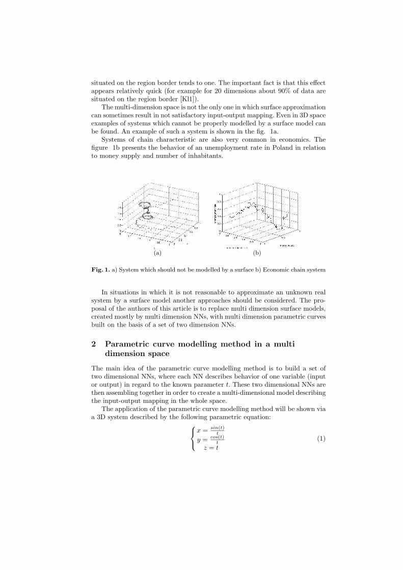
Equation (1) was used to build a data set consisted of one thousand data points.Data was generated for parameter t = [Π, 8Π]. In order to make the problemmore realistic the data was interfered by adding random noise from interval〈−10%, 10%〉. The interfered data set is shown in the figure 2.

Fig. 2. The interfered data set built with the eq. 1

Before building 2D models of the analyzed system each variable (input andoutput) was normalized to the interval 〈0.1, 0.9〉, according to the equation (2)[Ma1]:

Vn = 0.1 + 0.8 ∗ V − Vmin

Vmax − Vmin(2)

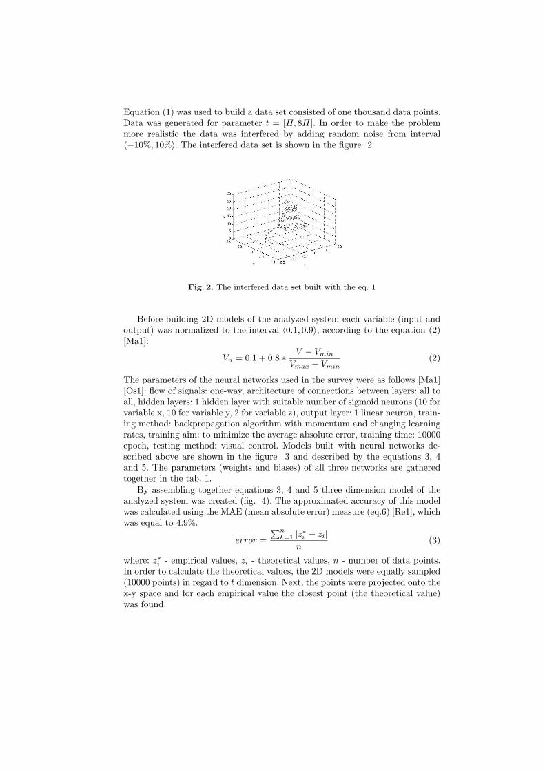
The parameters of the neural networks used in the survey were as follows [Ma1][Os1]: flow of signals: one-way, architecture of connections between layers: all toall, hidden layers: 1 hidden layer with suitable number of sigmoid neurons (10 forvariable x, 10 for variable y, 2 for variable z), output layer: 1 linear neuron, train-ing method: backpropagation algorithm with momentum and changing learningrates, training aim: to minimize the average absolute error, training time: 10000epoch, testing method: visual control. Models built with neural networks de-scribed above are shown in the figure 3 and described by the equations 3, 4and 5. The parameters (weights and biases) of all three networks are gatheredtogether in the tab. 1.

By assembling together equations 3, 4 and 5 three dimension model of theanalyzed system was created (fig. 4). The approximated accuracy of this modelwas calculated using the MAE (mean absolute error) measure (eq.6) [Re1], whichwas equal to 4.9%.

error =∑n

k=1 |z∗i − zi|n

(3)

where: z∗i - empirical values, zi - theoretical values, n - number of data points.In order to calculate the theoretical values, the 2D models were equally sampled(10000 points) in regard to t dimension. Next, the points were projected onto thex-y space and for each empirical value the closest point (the theoretical value)was found.

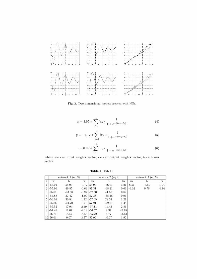
Fig. 3. Two-dimensional models created with NNs.

x = 3.95 +10∑

i=1

lwi ∗ 11 + e−(iwi+bi)

(4)

y = −4.17 +10∑

i=1

lwi ∗ 11 + e−(iwi+bi)

(5)

z = 0.09 +10∑

i=1

lwi ∗ 11 + e−(iwi+bi)

(6)

where: iw - an input weights vector, lw - an output weights vector, b - a biasesvector

Table 1. Tab.1 1

network 1 (eq.3) network 2 (eq.4) network 3 (eq.5)

i iw b lw iw b lw iw b lw

1 -56.01 55.99 -0.72 55.99 -56.01 3.21 8.51 -6.60 1.942 -55.96 49.85 -0.69 57.31 -48.21 0.66 -6.02 0.76 -3.933 55.81 -43.68 -0.97 -57.50 41.55 0.824 -55.88 37.42 -1.09 57.38 -35.18 0.965 -56.09 30.84 1.42 -57.45 28.31 1.216 55.86 -24.70 1.71 57.21 -22.01 1.487 -56.52 17.94 2.49 -57.11 14.41 2.818 -54.45 11.07 -4.19 -56.57 9.97 -2.189 56.71 -5.52 -5.53 -55.72 6.77 -3.1310 56.01 0.07 2.27 55.99 -0.07 1.92

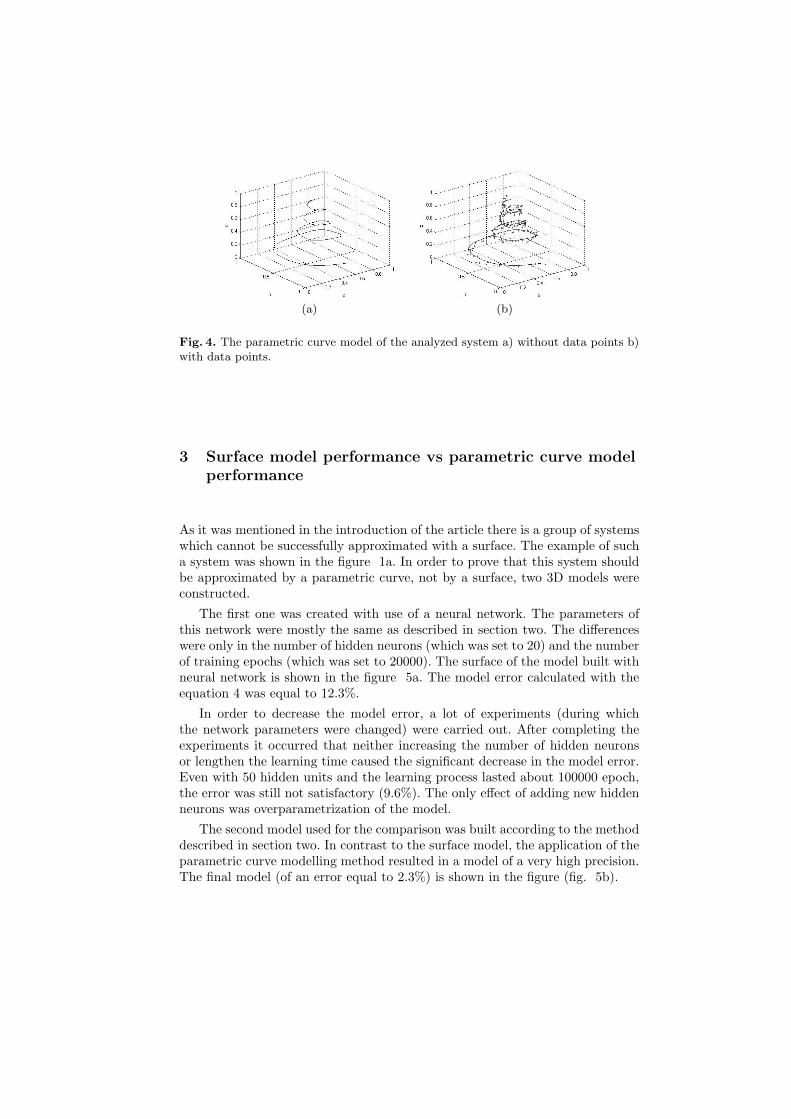
(a) (b)

Fig. 4. The parametric curve model of the analyzed system a) without data points b)with data points.

3 Surface model performance vs parametric curve modelperformance

As it was mentioned in the introduction of the article there is a group of systemswhich cannot be successfully approximated with a surface. The example of sucha system was shown in the figure 1a. In order to prove that this system shouldbe approximated by a parametric curve, not by a surface, two 3D models wereconstructed.

The first one was created with use of a neural network. The parameters ofthis network were mostly the same as described in section two. The differenceswere only in the number of hidden neurons (which was set to 20) and the numberof training epochs (which was set to 20000). The surface of the model built withneural network is shown in the figure 5a. The model error calculated with theequation 4 was equal to 12.3%.

In order to decrease the model error, a lot of experiments (during whichthe network parameters were changed) were carried out. After completing theexperiments it occurred that neither increasing the number of hidden neuronsor lengthen the learning time caused the significant decrease in the model error.Even with 50 hidden units and the learning process lasted about 100000 epoch,the error was still not satisfactory (9.6%). The only effect of adding new hiddenneurons was overparametrization of the model.

The second model used for the comparison was built according to the methoddescribed in section two. In contrast to the surface model, the application of theparametric curve modelling method resulted in a model of a very high precision.The final model (of an error equal to 2.3%) is shown in the figure (fig. 5b).

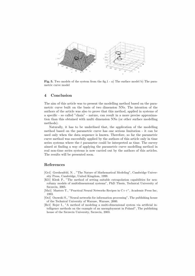
Fig. 5. Two models of the system from the fig.1 - a) The surface model b) The para-metric curve model

4 Conclusion

The aim of this article was to present the modelling method based on the para-metric curve built on the basis of two dimension NNs. The intention of theauthors of the article was also to prove that this method, applied in systems ofa specific - so called ”chain” - nature, can result in a more precise approxima-tion than this obtained with multi dimension NNs (or other surface modellingmethods).

Naturally, it has to be underlined that, the application of the modellingmethod based on the parametric curve has one serious limitation - it can beused only when the data sequence is known. Therefore, so far the parametriccurve method was succesfully applied by the authors of this article only in timeseries systems where the t parameter could be interpreted as time. The surveyaimed at finding a way of applying the parametric curve modelling method inreal non-time series systems is now carried out by the authors of this articles.The results will be presented soon.

References

[Ge1] Gershenfeld, N. , ”The Nature of Mathematical Modeling”, Cambridge Univer-sity Press, Cambridge, United Kingdom, 1999.

[Kl1] Klesk P., ”The method of setting suitable extrapolation capabilities for neu-rofuzzy models of multidimensional systems”, PhD Thesis, Technical University ofSzczecin, 2005.

[Ma1] Masters T., ”Practical Neural Networks Recipes in C++”, Academic Press Inc,1993.

[Os1] Osowski S., ”Neural networks for information processing”, The publishing houseof the Technical University of Warsaw, Warsaw, 2000.

[Re1] Rejer I., ”A method of modeling a multi-dimensional system via artificial in-telligence methods on the example of an unemployment in Poland”, The publishinghouse of the Szczecin University, Szczecin, 2003.