Automated Architecture Design forDeep Neural Networks

by

Steven Abreu

Jacobs University Bremen

Bachelor Thesis in Computer Science

Prof. Herbert Jaeger

Bachelor Thesis Supervisor

Date of Submission: May 17th, 2019

Jacobs University — Focus Area Mobility

arX

iv:1

908.

1071

4v1

[cs

.LG

] 2

2 A

ug 2

019

With my signature, I certify that this thesis has been written by me using only the in-dicated resources and materials. Where I have presented data and results, the data andresults are complete, genuine, and have been obtained by me unless otherwise acknowl-edged; where my results derive from computer programs, these computer programs havebeen written by me unless otherwise acknowledged. I further confirm that this thesis hasnot been submitted, either in part or as a whole, for any other academic degree at this oranother institution.

Signature Place, Date

Abstract

Machine learning has made tremendous progress in recent years and received large amountsof public attention. Though we are still far from designing a full artificially intelligentagent, machine learning has brought us many applications in which computers solve humanlearning tasks remarkably well. Much of this progress comes from a recent trend withinmachine learning, called deep learning. Deep learning models are responsible for manystate-of-the-art applications of machine learning.

Despite their success, deep learning models are hard to train, very difficult to understand,and often times so complex that training is only possible on very large GPU clusters.Lots of work has been done on enabling neural networks to learn efficiently. However,the design and architecture of such neural networks is often done manually through trialand error and expert knowledge. This thesis inspects different approaches, existing andnovel, to automate the design of deep feedforward neural networks in an attempt to createless complex models with good performance that take away the burden of deciding on anarchitecture and make it more efficient to design and train such deep networks.

iii

Contents

1 Motivation 11.1 Relevance of Machine Learning . . . . . . . . . . . . . . . . . . . . . . . . . 11.2 Relevance of Deep Learning . . . . . . . . . . . . . . . . . . . . . . . . . . . 1

1.2.1 Inefficiencies of Deep Learning . . . . . . . . . . . . . . . . . . . . . 11.3 Neural Network Design . . . . . . . . . . . . . . . . . . . . . . . . . . . . . . 2

2 Introduction 32.1 Supervised Machine Learning . . . . . . . . . . . . . . . . . . . . . . . . . . 32.2 Deep Learning . . . . . . . . . . . . . . . . . . . . . . . . . . . . . . . . . . 3

2.2.1 Artificial Neural Networks . . . . . . . . . . . . . . . . . . . . . . . . 42.2.2 Feedforward Neural Networks . . . . . . . . . . . . . . . . . . . . . . 42.2.3 Neural Networks as Universal Function Approximators . . . . . . . . 42.2.4 Relevance of Depth in Neural Networks . . . . . . . . . . . . . . . . 62.2.5 Advantages of Deeper Neural Networks . . . . . . . . . . . . . . . . 72.2.6 The Learning Problem in Neural Networks . . . . . . . . . . . . . . 8

3 Automated Architecture Design 93.1 Neural Architecture Search . . . . . . . . . . . . . . . . . . . . . . . . . . . 9

3.1.1 Non-Adaptive Search - Grid and Random Search . . . . . . . . . . . 103.1.2 Adaptive Search - Evolutionary Search . . . . . . . . . . . . . . . . . 10

3.2 Dynamic Learning . . . . . . . . . . . . . . . . . . . . . . . . . . . . . . . . 113.2.1 Regularization Methods . . . . . . . . . . . . . . . . . . . . . . . . . 113.2.2 Destructive Dynamic Learning . . . . . . . . . . . . . . . . . . . . . 123.2.3 Constructive Dynamic Learning . . . . . . . . . . . . . . . . . . . . . 143.2.4 Combined Destructive and Constructive Dynamic Learning . . . . . 17

3.3 Summary . . . . . . . . . . . . . . . . . . . . . . . . . . . . . . . . . . . . . 17

4 Empirical Findings 194.1 Outline of the Investigation . . . . . . . . . . . . . . . . . . . . . . . . . . . 19

4.1.1 Investigated Techniques for Automated Architecture Design . . . . . 194.1.2 Benchmark Learning Task . . . . . . . . . . . . . . . . . . . . . . . . 204.1.3 Evaluation Metrics . . . . . . . . . . . . . . . . . . . . . . . . . . . . 204.1.4 Implementation Details . . . . . . . . . . . . . . . . . . . . . . . . . 21

4.2 Search Algorithms . . . . . . . . . . . . . . . . . . . . . . . . . . . . . . . . 214.2.1 Manual Search . . . . . . . . . . . . . . . . . . . . . . . . . . . . . . 224.2.2 Random Search . . . . . . . . . . . . . . . . . . . . . . . . . . . . . . 234.2.3 Evolutionary Search . . . . . . . . . . . . . . . . . . . . . . . . . . . 244.2.4 Conclusion . . . . . . . . . . . . . . . . . . . . . . . . . . . . . . . . 27

4.3 Constructive Dynamic Learning Algorithm . . . . . . . . . . . . . . . . . . 304.3.1 Cascade-Correlation Networks . . . . . . . . . . . . . . . . . . . . . 304.3.2 Forward Thinking . . . . . . . . . . . . . . . . . . . . . . . . . . . . 384.3.3 Automated Forward Thinking . . . . . . . . . . . . . . . . . . . . . . 404.3.4 Conclusion . . . . . . . . . . . . . . . . . . . . . . . . . . . . . . . . 42

4.4 Conclusion . . . . . . . . . . . . . . . . . . . . . . . . . . . . . . . . . . . . 43

5 Future Work 45

iv

1 Motivation

1.1 Relevance of Machine Learning

Machine Learning has made tremendous progress in recent years. Although we are notable to replicate human-like intelligence with current state-of-the-art systems, machinelearning systems have outperformed humans in some domains. One of the first importantmilestones has been achieved when DeepBlue defeated the world champion Garry Kasparovin a game of chess in 1997. Machine learning research has been highly active since thenand pushed the state-of-the-art in domains like image classification, text classification,localization, question answering, natural language translation and robotics further.

1.2 Relevance of Deep Learning

Many of today’s state-of-the-art systems are powered by deep neural networks (see Section2.2). AlphaZero’s deep neural network coupled with a reinforcement learning algorithmbeat the world champion in Go - a game that was previously believed to be too complexto be played competitively by a machine [Silver et al., 2018]. Deep learning has also beenapplied to convolutional neural networks - a special kind of neural network architecturethat was initially proposed by Yann LeCun [LeCun and Bengio, 1998]. One of these deepconvolutional neural networks, using five layers, has been used to achieve state-of-the-artperformance in image classification [Krizhevsky et al., 2017]. Overfeat, an eight layerdeep convolutional neural network, has been trained on image localization, classificationand detection with very competitive results [Sermanet et al., 2013]. Another remarkablycomplex CNN has been trained with 29 convolutional layers to beat the state of the art inseveral text classification tasks [Conneau et al., 2016]. Even a complex task that requirescoordination between vision and control, such as screwing a cap on a bottle, has been solvedcompetitively using such deep architectures. Levine et al. [2016] used a deep convolutionalneural network to represent policies to solve such robotic tasks. Recurrent networks areparticularly popular in time series domains. Deep recurrent networks have been trainedto achieve state-of-the-art performance in generating captions for given images [Vinyalset al., 2015]. Google uses a Long Short Term Memory (LSTM) network to achieve state-of-the-art performance in machine translation [Wu et al., 2016]. Other deep networkarchitectures have been proposed and successfully achieved state-of-the-art performance,such as dynamic memory networks for natural language question answering [Kumar et al.,2016].

1.2.1 Inefficiencies of Deep Learning

Evidently, deep neural networks are currently powering many, if not most, state-of-the-artmachine learning systems. Many of these deep learning systems train model that are richerthan needed and use elaborate regularization techniques to keep the neural network fromoverfitting on the training data.

Many modern deep learning systems achieve state-of-the-art performance using highlycomplex models by investing large amounts of GPU power and time as well as feedingthe system very large amounts of data. This has been made possible through the recent

1

explosion of computational power as well as through the availability of large amounts ofdata to train these systems.

It can be argued that deep learning is inefficient because it trains bigger networks thanneeded for the function that one desires to learn. This comes at a high expense in theform of computing power, time and the need for larger training datasets.

1.3 Neural Network Design

The goal of designing a neural network is manifold. The primary goal is to minimize theneural network’s expected loss for the learning task. Because the expected loss cannotalways be computed in practice, this goal is often re-defined to minimizing the loss on aset of unseen test data.

Aside from maximizing performance, it is also desirable to minimize the resources neededto train this network. I differentiate between computational resources (such as computingpower, time and space) and human resources (such as time and effort).In my opinion, the goal of minimizing human resources is often overlooked. Many models,especially in deep learning, are designed through trial, error and expert knowledge. Thismanual design process is rarely interpretable or reproducible and as such, little formalknowledge is gained about the working of neural networks - aside from having a neuralnetwork design that may work well for a specific learning task.

In order to avoid the difficulties of defining and assessing the amount of human resourcesneeded for the neural network design process, I am introducing a new goal for the design ofneural networks: level of automaticity. The level of automaticity in neural network designis inversely proportional to the number of decision that need to be made by a human inthe neural network design process.

When dealing with computational resources for neural networks, one might naturally focuson optimizing the amount of computational resources needed during the training process.However, the amount of resources needed for utilizing the neural network in practice arealso very important. A neural network is commonly trained once and then used many timesonce it is trained. The computational resources needed for the utilization of the trainedneural network sums up and should be considered when designing a neural network. Agood measure is to reduce the model complexity or network size. This goal reduces thecomputational resources needed for the neural network in practice while simultaneouslyacting as a regularizer to incentivize neural networks to be smaller - hence prefering simplermodels over more complex ones, as Occam’s razor states.

To conclude, the goal of designing a neural network is to maximize performance (usuallyby minimizing a chosen loss function on unseen test data), minimize computational re-sources (during training), maximize the level of automaticity (by minimizing the amountof decisions that need to be made by a human in the design process), and to minimize themodel’s complexity (e.g. by minimizing the network’s size).

2

2 Introduction

2.1 Supervised Machine Learning

In this paper, I will be focusing on supervised machine learning. In supervised machinelearning, one tries to estimate a function

f : EX 7→ EY

where typically EX ⊆ Rm and EY ⊆ Rn, given training data in the form of (xi, yi)i=1,..,N ,with yi ≈ f(xi). This training data represents existing input-output pairs of the functionthat is to be estimated.

A machine learning algorithm takes the training data as input and outputs a functionestimate fest with fest ≈ f . The goal of the supervised machine learning task is tominimize a loss function L:

L : EY × EY 7→ R≥0

In order to assess a function estimate’s accuracy, it should always be assessed on a set ofunseen input-output pairs. This is due to overfitting, a common phenomenon in machinelearning in which a machine learning model memorizes part of the training data whichleads to good performance on the training set and (often) bad generalization to unseenpatterns. One of the biggest challenges in machine learning is to generalize well. It istrivial to memorize training data and correctly classifying these memorized samples. Thechallenge lies in correctly classifying previously unseen samples, based on what was seenin the training dataset.

A supervised machine learning problem is specified by labeled training data (xi, yi)i=1,..,N

with xi ∈ EX , yi ∈ EY and a loss function which is to be minimized. Often times, the lossfunction is not part of the problem statement and instead needs to be defined as part ofsolving the problem.

Given training data and the loss function, one needs to decide on a candidate set C offunctions that will be considered when estimating the function f .

The learning algorithm L is an effective procedure to choose one or more particular func-tions as an estimate for the given function estimation task, minimizing the loss functionin some way:

L(C, L, (xi, yi)i=1,..N ) ∈ CTo summarize, a supervised learning problem is given by a set of labeled data points(xi, yi)i=1,..N which one typically calls the training data. The loss function L gives us ameasure for how good a prediction is compared to the true target value and it can beincluded in the problem statement. The supervised learning task is to first decide on acandidate set C of functions that will be considered. Finally, the learning algorithm Lgives an effective procedure to choose one function estimate as the solution to the learningproblem.

2.2 Deep Learning

Deep learning is a subfield of machine learning that deals with deep artificial neural net-works. These artificial neural networks (ANNs) can represent arbitrarily complex func-tions (see section 2.2.3).

3

2.2.1 Artificial Neural Networks

An artificial neural network (ANN) (or simply, neural network) consists of a set V ofv = |V | processing units, or neurons. Each neuron performs a transfer function of theform

yi = fi

n∑j=1

wijxj − θi

where yi is the output of the neuron, fi is the activation function (usually a nonlinearfunction such as the sigmoid function), xj is the output of neuron j, wij is the connectionweight from node j to node i and θi is the bias (or threshold) of the node. Input units areconstant, reflecting the function input values. Output units do not forward their outputto any other neurons. Units that are neither input nor output units are called hiddenunits.

The entire network can be described by a directed graph G = (V,E) where the directededges E are given through a weight matrix W ∈ Rv×v. Any non-zero entry in the weightmatrix at index (i, j), i.e. wij 6= 0 denotes that there is a connection from neuron j toneuron i.

A neural network is defined by its architecture, a term that is used in different ways. Inthis paper, the architecture of a neural network will always refer to the network’s nodeconnectivity pattern and the nodes’ activation functions.

ANN’s can be segmented into feedforward and recurrent networks based on their networktopology. An ANN is feedforward if there exists an ordering of neurons such that everyneuron is only connected to a neuron further down the ordering. If such an orderingdoes not exist, then the network is recurrent. In this thesis, I will only be consideringfeedforward neural networks.

2.2.2 Feedforward Neural Networks

A feedforward network can be visualized as a layered network, with layers L0 through LK .The layer L0 is called the input layer and LK is called the output layer. Intermediatelayers are called hidden layers.

One can think of the layers as subsequent feature extractors: the first hidden layer L1 isa feature extractor on the input unit. The second hidden layer L2 is a feature extractoron the first hidden layer - thus a second order feature extractor on the input. The hiddenlayers can compute increasingly complex features on the input.

2.2.3 Neural Networks as Universal Function Approximators

A classical universal approximation theorem states that standard feedforward neural net-works with only one hidden layer using a squashing activation function (a function Ψ :R 7→ [0, 1] is a squashing function, according to Hornik et al. [1989], if it is non-decreasing,Ψλ→∞(λ) = 1 and Ψλ→−∞(λ) = 0) can be used to approximate any continuous functionon compact subsets of Rn with any desired non-zero amount of error [Hornik et al., 1989].The only requirement is that the network must have sufficiently many units in its hiddenlayer.

4

A simple example can demonstrate this universal approximation theorem for neural net-works. Consider the binary classification problem in Figure 1 of the kind f : [0, 1]2 →{0, 1}. The function solving this classification problem can be represented using an MLP.As stated by the universal approximation theorem, one can approximate this function toarbitrary precision using an MLP with one hidden layer.

Figure 1: Binary classification problem. Yellow area is one class, everything else is theother class. Right is the shallow neural network that should represent the classificationfunction. Figure taken from Bhiksha Raj’s lecture slides in CMU’s ’11-785 Introductionto Deep Learning’.

The difficulty in representing the desired classification function is that the classificationis split into two separate, disconnected decision regions. Representing either one of theseshapes is trivial. One can add one neuron per side of the polygon which acts as a featuredetector to detect the decision boundary represented by this side of the polygon. One canthen add a bias into the hidden layer with a value of bh = −N (N is the number of sides ofthe polygon), use a relu-activated output unit and one has built a simple neural networkwhich returns 1 iff all hidden neurons fire, i.e. when the point lies within the boundary ofevery side of the polygon, i.e. when the point lies within the polygon.

(a) Decision bound-ary for a square

(b) Decision bound-ary for a hexagon

(c) Decision plot fora square

(d) Decision plotfor a hexagon

Figure 2: Decision plots and boundaries for simple binary classification problems. Figurestaken from Bhiksha Raj’s lecture slides in CMU’s ’11-785 Introduction to Deep Learning’.

This approach generalizes neither to shapes that are not convex nor to multiple, discon-nected shapes. In order to approximate any decision boundary using just one hiddenlayer, one can use an n-sided polygon. Figure 2a and 2b show the decision boundaries fora square and a hexagon. A problem arises when the two shapes are close to each other; theareas outside the boundaries add up to values larger or equal to those within the bound-aries of each shape. In the plots of Figure 2c and 2d, one can see that the boundaries of

5

the decision regions don’t fall off quickly enough and will add up to large values, if thereare two or more such shapes in close proximity.

Figure 3: Decision plot and corresponding MLP structure for approximating a circle.Figure taken from Bhiksha Raj’s lecture slides in CMU’s ’11-785 Introduction to DeepLearning’.

However, as one increases the sides n of the polygon, the boundaries will fall off morequickly. In the limit of n → ∞, the shape becomes a near perfect cylinder, with value nfor the area within the cylinder and n/2 outside. Using a bias unit of bh = −n/2, one canturn this into a near-circular shape with value n/2 in the shape and value 0 everywhereelse, as shown in Figure 3. One can now add multiple near-circles together in the samelayer of the neural network. Given this setup, one can now compose an arbitrary figure byfitting it with an arbitrary number of near-circles. The smaller these near-circles, the moreaccurate this classification problem can be represented by a network. With this setup, itis possible to capture any decision boundary.

This procedure to build a neural network with one hidden layer to build a classifier forarbitrary figures has a problem: the number of hidden units needed to represent thisfunction become arbitrarily high. In this procedure, I have set n, the number of hiddenunits to represent a circle to be very large and I am using many of these circles to representthe entire function. This will result in a very (very) large number of units in the hiddenlayer.

This is a general phenomenon: even though a network with just one hidden layer can rep-resent any function (with some restrictions, see above) to arbitrary precision, the numberof units in this hidden layer often becomes intractably large. Learning algorithms oftenfail to learn complicated functions correctly without overfitting the training data in such”shallow” networks.

2.2.4 Relevance of Depth in Neural Networks

The classification function from Figure 1 can be built using a smaller network, if one allowsfor multiple hidden layers. The first layer is a feature detector for every polygon’s edge.The second layer will act as an AND gate for every distinct polygon - detecting all thosepoints that lie within all the polygon’s edges. The output layer will then act as an ORgate for all neurons in the second layer, thus detecting all points that lie in any of thepolygons. With this, one can build a simple network that perfectly represents the desiredclassification function. The network and decision boundaries are shown in Figure 4.

6

Figure 4: Decision boundary and corresponding two-layer classification network. Figuretaken from Bhiksha Raj’s lecture slides in CMU’s ’11-785 Introduction to Deep Learning’.

By adding just one additional layer into the network, the number of hidden neurons hasbeen reduced from nshallow → ∞ to ndeep = 12. This shows how the depth of a networkcan increase the resulting model capacity faster than an increase in the number of unitsin the first hidden layer.

2.2.5 Advantages of Deeper Neural Networks

It is difficult to understand how the depth of an arbitrary neural network influences whatkind of functions the network can compute and how well these networks can be trained.Early research has focused on shallow networks and their conclusions cannot be generalizedto deeper architectures, such as the universal approximation theorem for networks withone hidden layer [Hornik et al., 1989] or an analysis of a neural network’s expressivitybased on an analogy to boolean circuits by Maass et al. [1994].

Several measures have been proposed to formalize the notion of model capacity and thecomplexity of functions which a statistical learning algorithm can represent. One of themost famous such formalization is that of the Vapnik Chervonenkis dimension (VC di-mension) [Vapnik and Chervonenkis, 2015].

Recent papers have focused on understanding the benefits of depth in neural networks. TheVC dimension as a measure of capacity has been applied to feedforward neural networkwith piecewise polynomial activation functions, such as relu, to prove that a network’smodel capacity grows by a factor of W

logW with depth compared to a similar growth inwidth [Bartlett et al., 1999].

There are examples of functions that a deeper network can express and a more shallownetwork cannot approximate unless the width is exponential in the dimension of the input([Eldan and Shamir, 2016] and [Telgarsky, 2015]). Upper and lower bounds have beenestablished on the network complexity for different numbers of hidden units and activationfunctions. These show that deep architectures can, with the same number of hidden units,realize maps of higher complexity than shallow architectures [Bianchini and Scarselli,2014].

However, the aforementioned papers either do not take into account the depth of moderndeep learning models or only present findings for specific choices of weights of a deepneural network.

7

Using Riemannian geometry and dynamical mean field theory, Poole et al. [2016] showthat generic deep neural networks can ”efficiently compute highly expressive functions inways that shallow networks cannot” which ”quantifies and demonstrates the power of deepneural networks to disentangle curved input manifolds” [Poole et al., 2016].

Raghu et al. [2017] introduced the notion of a trajectory ; given two points in the inputspace x0, x1 ∈ Rm, the trajectory x(t) is a curve parametrized by t ∈ [0, 1] with x(0) = x0and x(1) = x1. They argue that the trajectory’s length serves as a measure of networkexpressivity. By measuring the trajectory lengths of the input as it is transformed bythe neural network, they found that the network’s depth increases complexity (given bythe trajectory length) of the computed function exponentially, compared to the network’swidth.

2.2.6 The Learning Problem in Neural Networks

A network architecture being able to approximate any function does not always meanthat a network of that architecture is able to learn any function. Whether or not neuralnetwork of a fixed architecture can be trained to represent a given function depends onthe learning algorithm used.

The learning algorithm needs to find a set of parameters for which the neural networkcomputes the desired function. Given a function, there exists a neural network to representthis function. But even if such an architecture is given, there is no universal algorithmwhich, given training data, finds the correct set of parameters for this network such thatit will also generalize well to unseen data points [Goodfellow et al., 2016].

Finding the optimal neural network architecture for a given learning task is an unsolvedproblem as well. Zhang et al. [2016] argue that most deep learning systems are built onmodels that are rich enough to memorize the training data.

Hence, in order for a neural network to learn a function from data, it has to learn the net-work architecture and the parameters of the neural network (connection weights). This iscommonly done in sequence but it is also possible to do both simultaneously or iteratively.

8

3 Automated Architecture Design

Choosing a fitting architecture is a big challenge in deep learning. Choosing an unsuitablearchitecture can make it impossible to learn the desired function. Choosing an optimalarchitecture for a learning task is an unsolved problem. Currently, most deep learningsystems are designed by experts and the design relies on hyperparameter optimizationthrough a combination of grid search and manual search [Bergstra and Bengio, 2012] (seeLarochelle et al. [2007], LeCun et al. [2012], and Hinton [2012]).

This manual design is tedious, computationally expensive, and architecture decisions basedon experience and intuition are very difficult to formalize and thus, reuse. Many algorithmshave been proposed for the architecture design of neural networks, with varying levels ofautomaticity. In this thesis, I will be referring to these algorithms as automated architecturedesign algorithms.

Automated architecture algorithms can be broadly segmented into neural network archi-tecture search algorithms (also called neural architecture search, or NAS) and dynamiclearning algorithms, both of which are discussed in this section.

3.1 Neural Architecture Search

Neural architecture search is a natural choice for the design of neural networks. NASmethods are already outperforming manually designed architectures in image classificationand object detection ([Zoph et al., 2018] and [Real et al., 2018]).

Elsken et al. [2019] propose to categorize NAS algorithms according to three dimensions:search space, search strategy, and performance estimation strategy. The authors describethese as follows. The search space defines the set of architectures that are considered bythe search algorithm. Prior knowledge can be incorporated into the search space, thoughthis may limit the exploration of novel architectures. The search strategy defines thesearch algorithm that is used to explore the search space. The search algorithm defineshow the exploration-exploitation tradeoff is handled. The performance estimation strategydefines how the performance of a neural network architecture is assessed. Naively, one maytrain a neural network architecture but this is object to random fluctuations due to initialrandom weight initializations, and obviously very computationally expensive.

In this thesis, I will not be considering the search space part of the NAS algorithms.Instead, I will keep the search space constant across all NAS algorithms. I will not go indepth about the performance estimation strategy in the algorithms either, instead usingone constant form of constant estimation - training a network architecture once for thesame number of epochs (depending on time constraints).

Many search algorithms can be used in NAS algorithms. Elsken et al. [2019] namesrandom search, Bayesian optimization, evolutionary methods, reinforcement learning, andgradient-based methods. Search algorithms can be divided into adaptive and non-adaptivealgorithms, where adaptive search algorithms adapt future searches based on the perfor-mance of already tested instances. In this thesis, I will only consider grid search andrandom search as non-adaptive search algorithms, and evolutionary search as an adaptivesearch algorithm.

For the following discussion, let A be the set of all possible neural network architectures

9

and A′ ⊆ A be the search space defined for the NAS algorithm - a subset of all possiblearchitectures.

3.1.1 Non-Adaptive Search - Grid and Random Search

The simplest way to automatically design a neural network’s architecture may be to simplytry different architectures from a defined subset of all possible neural network architec-tures and choose the one that performs the best. One chooses elements ai ∈ A′, tests theseindividual architectures and chooses the one that performs the best. The performance isusually measured through evaluation on an unseen testing set or through a cross valida-tion procedure - a technique which artificially splits the training data into training andvalidation data and uses the unseen validation data to evaluate the model’s performance.

The two most widely known search algorithms that are frequently used for hyperparame-ter optimization (which includes architecture search) are grid search and random search.Naive grid search performs an exhaustive, enumerated search within the chosen subsetA′ of possible architectures - where one needs to also specify some kind of step size, adiscretization scheme which determines how ”fine” the search within the architecture sub-space should be. Adaptive grid search algorithms use adaptive grid sizes and are notexhaustive. Random search does not need a discretization scheme, it chooses elementsfrom A′ at random in each iteration. Both grid and random search are non-adaptive algo-rithms: they do not vary the course of the experiment by considering the performance ofalready tested instances [Bergstra and Bengio, 2012]. Larochelle et al. [2007] finds that, inthe case of a 32-dimensional search problem of deep belief network optimization, randomsearch was not as good as the sequential combination of manual and grid search from anexpert because the efficiency of sequential optimization overcame the inefficiency of thegrid search employed at every step [Bergstra and Bengio, 2012]. Bergstra and Bengio[2012] concludes that sequential, adaptive algorithms should be considered in future workand random search should be used as a performance baseline.

3.1.2 Adaptive Search - Evolutionary Search

In the past three decades, lots of research has been done on genetic algorithms and artificialneural networks. The two areas of research have also been combined and I shall refer to thiscombination as evolving artificial neural networks (EANN), based on a literature reviewby Yao [1999]. Evolutionary algorithms have been applied to artificial neural networks toevolve connection weights, architectures, learning rules, or any combination of these three.These EANN’s can be viewed as an adaptive system that is able to learn from data aswell as evolve (adapt) its architecture and learning rules - without human interaction.

Evolutionary algorithms are population based search algorithms which are derived from theprinciples of natural evolution. They are very useful in complex domains with many localoptima, as is the case in learning the parameters of a neural network [Choromanska et al.,2015]. They do not require gradient information which can be a computational advantageas the gradients for neural network weights can be quite expensive to compute, especiallyso in deep networks and recurrent networks. The simultaneous evolution of connectionweights and network architecture can be seen as a fully automated ANN design. Theevolution of learning rules can be seen as a way of ”learning how to learn”. In this paper,

10

I will be focusing on the evolution of neural network architectures, staying independent ofthe algorithm that is used to optimize connection weights.

The two key issues in the design of an evolutionary algorithm are the representation andthe search operators. The architecture of a neural network is defined by its nodes, theirconnectivity and each node’s transfer function. The architecture can be encoded as astring in a multitude of ways, which will not be discussed in detail here.

A general cycle for the evolution of network architectures has been proposed by Yao [1999]:

1. Decode each individual in the current generation into an architecture.

2. Train each ANN in the same way, using n distinct random initializations.

3. Compute the fitness of each architecture according to the averaged training results.

4. Select parents from the population based on their fitness.

5. Apply search operators to parents and generate offspring to form the next generation.

It is apparent that the performance of an EANN depends on the encoding scheme of thearchitecture, the definition of the fitness function, and the search operators applied tothe parents to generate offspring. There will be some residual noise in the process dueto the stochastic nature of ANN training. Hence, one should view the computed fitnessas a heuristic value, an approximation, for the true fitness value of an architecture. Thelarger the number n of different random initializations that are run for each architecture,the more accurate training results (and thus, the fitness computation) becomes. However,increasing n leads to a large increase in time needed for each iteration of the evolutionaryalgorithm.

3.2 Dynamic Learning

Dynamic learning algorithms in neural networks are algorithms that modify a neuralnetwork’s hyperparameters and topology (here, I focus on the network architecture) dy-namically as part of the learning algorithm, during training. These approaches present theopportunity to develop optimal network architectures that generalize well [Waugh, 1994].The network architecture can be modified during training by adding complexity to thenetwork or by removing complexity from the network. The former is called a constructivealgorithm, the latter a destructive algorithm. Naturally, the two can be combined into analgorithm that can increase and decrease the network’s complexity as needed, in so-calledcombined dynamic learning algorithms. These changes can affect the nodes, connectionsor weights of the network - a good overview of possible network changes is given by Waugh[1994], see Figure 5.

3.2.1 Regularization Methods

Before moving on to dynamic learning algorithms, it is necessary to clear up the clas-sification of these dynamic learning algorithms and clarify some underlying terminology.The set of destructive dynamic learning algorithms intersects with the set of so-calledregularization methods in neural networks. The origin of this confusion is the definitionof dynamic learning algorithms. Waugh [1994] defines dynamic learning algorithms tochange either the nodes, connections, or weights of the neural network. If we continue

11

Figure 5: Possible network topology changes, taken from Waugh [1994]

with this definition, we will include all algorithms that reduce the values of connectionsweights in the set of destructive dynamic learning, which includes regularization methods.

Regularization methods penalize higher connection weights in the loss function (as a re-sult, connection weights are reduced in value). Regularization is based on Occam’s razorwhich states that the simplest explanation is more likely to be correct than more com-plex explanations. Regularization penalizes such complex explanations (by reducing theconnection weights’ values) in order to simplify the resulting model.

Regularization methods include weight decay, in which a term is added to the loss functionwhich penalizes large weights, and dropout, which is explained in Section 3.2.2. Forcompleteness, I will cover these techniques as instances of dynamic learning, however Iwill not run any experiments on these regularization methods as the goal of this thesisis to inspect methods to automate the architecture design, for which the modification ofconnection weights is not relevant.

3.2.2 Destructive Dynamic Learning

In destructive dynamic learning, one starts with a network architecture that is larger thanneeded and reduces complexity in the network by removing nodes, connections or reducingexisting connection weights.

A key challenge in this destructive approach is the choice of starting network. As opposedto a minimal network - which could simply be a network without any hidden units - it isdifficult to define a ”maximal” network because there is no upper bound on the networksize [Waugh, 1994]. A simple solution would be to choose a fully connected network withK layers, where K is dependent on the learning task.

An important downside to the use of destructive algorithms is the computational cost.Starting with a very large network and then cutting it down in size leads to many redundantcomputations on the large network.

Most approaches to destructive dynamic learning that modify the nodes and connections(rather than just the connection weights) are concerned with the pruning of hidden nodes.The general approach is to train a network that is larger than needed and prune parts of thenetwork that are not essential. Reed [1993] suggests that most pruning algorithms can be

12

divided into two groups; algorithms that estimate the sensitivity of the loss function withrespect to the removal of an element and then removes those elements with the smallesteffect on the loss function, and those that add terms to the objective function that rewardsthe network for choosing the most efficient solution - such as weight decay. I shall referto those two groups of algorithms as sensitivity calculation methods and penalty-termmethods, respectively - as proposed by Waugh [1994].

Other algorithms have been proposed but will not be included in this thesis for brevityreasons (most notably, principal components pruning [Levin et al., 1994] and soft weight-sharing as a more complex Penalty-Term method [Nowlan and Hinton, 1992]).

Dropout

This section follows Srivastava et al. [2014]. Dropout refers to a way of regularizing aneural network by randomly ”dropping out” entire nodes with a certain probability p ineach layer of the network. At the end of training, each node’s outgoing weights are thenmultiplied with its probability p of being dropped out. As the networks connection weightsare multiplied with a certain probability value p, where p ∈ [0, 1], one can consider thistechnique a kind of connection weight pruning and thus, in the following, I will considerdropout to be a destructive algorithm.

Intuitively, dropout drives hidden units in a network to work with different combinationsof other hidden units, essentially driving the units to build useful features without relyingon other units. Dropout can be interpreted as a stochastic regularization technique thatworks by introducing noise to its units.

One can also view this ”dropping out” in a different way. If the network has n nodes(excluding output notes), dropout can either include or not include this node. This leadsto a total of 2n different network configurations. At each step during training, one ofthese network configurations is chosen and the weights are optimized using some gradientdescent method. The entire training can hence be seen as training not just one networkbut all possible 2n network architectures. In order to get an ideal prediction from aflexible-sized model such as a neural network, one should average over the predictions ofall possible settings of the parameters, weighing each setting by its posterior probabilitygiven the training data. This procedure quickly becomes intractable. In essence, dropoutis a technique that can combine exponentially (exponential in the number of nodes) manydifferent neural networks efficiently.

Due to this model combination, dropout is reported to take 2-3 times longer to train thana standard neural network without dropout. This makes dropout an effective algorithmthat deals with a trade-off between overfitting and training time.

To conclude, dropout can be seen as both a regularization technique and a form of modelaveraging. It works remarkably well in practice. Srivastava et al. [2014] report largeimprovements across all architectures in an extensive empirical study. The overall archi-tecture is not changed, as the pruning happens only in terms of the magnitude of theconnection weights.

Penalty-Term Pruning through Weight Decay

13

Weight decay is the best-known regularization technique that is frequently used in deeplearning applications. It works by penalizing network complexity in the loss function,through some complexity measure that is added into the loss function - such as the numberof free parameters or the magnitude of connection weights. Krogh and Hertz [1992] showthat weight decay can improve generalization of a neural network by suppressing irrelevantcomponents of the weight vector and by suppressing some of the effect of static noise onthe targets.

Sensitivity Calculation Pruning

Sietsma [1988] removes nodes which have little effect on the overall network output andnodes that are duplicated by other nodes. The author also discusses removing entire layers,if they are found to be redundant [Waugh, 1994]. Skeletonization is based on the sameidea of the network’s sensitivity to node removal and proposes to remove nodes from thenetwork based on their relevance during training [Mozer and Smolensky, 1989].

Optimal brain damage (OBD) uses second-derivative information to automatically deleteparameters based on the ”saliency” of each paramter - reducing the number of parametersby a factor of four and increasing its recognition accuracy slightly on a state-of-the-artnetwork [LeCun et al., 1990]. Optimal Brain Surgeon (OBS) enhances the OBD algorithmby dropping the assumption that the Hessian matrix of the neural network is diagonal (theyreport that in most cases, the Hessian is actually strongly non-diagonal), and they reporteven better results [Hassibi et al., 1993]. The algorithm was extended again by the sameauthors [Hassibi et al., 1994].

However, methods based on sensitivity measures have the disadvantage that they do notdetect correlated elements - such as two nodes that cancel each other out and could beremoved without affecting the networks performance [Reed, 1993].

3.2.3 Constructive Dynamic Learning

In constructive dynamic learning, one starts with a minimal network structure and itera-tively adds complexity to the network by adding new nodes or new connections to existingnodes.

Two algorithms for the dynamic construction of feed-forward neural networks are pre-sented in this section: the cascade-correlation algorithm (Cascor) and the forward thinkingalgorithm.

Other algorithms have been proposed but, for brevity, will not be included in this paper’sanalysis (node splitting [Wynne-Jones, 1992], the tiling algorithm [Mezard and Nadal,1989], the upstart algorithm [Frean, 1990], a procedure for determining the topology fora three layer neural network [Wang et al., 1994], and meiosis networks that replace one”overtaxed” node by two nodes [Hanson, 1990]).

Cascade-correlation Networks

14

The cascade-correlation learning architecture (short: Cascor) was proposed by Fahlmanand Lebiere [1990]. It is a supervised learning algorithm for neural networks that contin-uously adds units into the network, trains them one by one and then freezes those unit’sinput connections. This results in a network that is not layered but has a structure inwhich all input units are connected to all hidden units and the hidden units have a hierar-chical ordering in which the one hidden unit’s output is fed into subsequent hidden units asinput. When training, Cascor keeps a ”pool” of candidate units - possibly using differentnonlinear activation functions - and chooses the best candidate unit. Figure 6 visualizesthis architecture. So-called residual neural networks have been very successful in taskssuch as image recognition [He et al., 2016] through the use of similar skip connections.Cascor takes the idea of skip connections and applies it to include network connectionsfrom the input to every hidden node in the network.

Figure 6: The cascade correlation neural network architecture after adding two hiddenunits. Squared connections are frozen after training them once, crossed connections areretrained in each training iteration. Figure taken and adapted from Fahlman and Lebiere[1990].

Cascor aims to solve two main problems that are found in the widely used backpropagationalgorithm: the step-size problem, and the moving target problem.

The step size problem occurs in gradient descent optimization methods because it is notclear how big the step in each parameter update should be. If the step size is too small,the network takes too long to converge to a local minimum, if it is too large, the learningalgorithm will jump past local minima and possibly not converge to a good solution at all.Among the most successful ways of dealing with this step size problem are higher-ordermethods, which compute second derivatives in order to get a good estimate of what thestep size should be (which is very expensive and often times intractable), or some form of”momentum”, which keeps track of earlier steps taken to make an educated guess abouthow large the step size should be at the current step.

The moving target problem occurs in most neural networks when all units are trained atthe same time and cannot communicate with each other. This leads to all units trying tosolve the same learning task - which changes constantly. Fahlman and Lebiere propose aninteresting manifestation of the moving target problem which they call the ”herd effect”.Given two sub-tasks, A and B, that must be performed by the hidden units in a network,each unit has to decide independently which of the two problems it will tackle. If task Agenerates a larger or more coherent error signal than task B, the hidden units will tend to

15

concentrate on A and ignore B. Once A is solved, the units will then see B as a remainingsource of error. Units will move towards task B and, in turn, problem A reappears.Cascor aims to solve this moving target problem by only training one hidden unit at atime. Other approaches, such as the forward thinking formulation, are less restricted andallow the training of one entire layer of units at a time [Hettinger et al., 2017].

In their original paper, Fahlman and Lebiere reported good benchmark results on thetwo-spirals problem and the n-input parity problem. The main advantages over networksusing backpropagation were faster training (though this might also be attributed to theuse of the Quickprop learning algorithm), deeper networks without problems of vanishinggradients, possibility of incremental learning and, in the n-input parity problem, fewerhidden units in total.

In the literature, Cascor has been criticized for poor performance on regression tasks dueto an overcompensation of errors which comes from training on the error correlation ratherthan on the error signal directly ([Littmann and Ritter, 1992], [Prechelt, 1997]). Cascorhas also been criticized for the use of its cascading structure rather than adding eachhidden unit into the same hidden layer.

Littmann and Ritter [1992] present a different version of Cascor that is based on errorminimization rather than error correlation maximization, called Caser. They also presentanother modified version of Cascor, called Casqef, which is trained on error minimizationand uses additional non-linear functions on the output of cascaded units. Caser doesn’tdo any better than Cascor, while Casqef outperforms Cascor in more complicated tasks- likely because of the additional nonlinearities introduced by the nonlinear functions onthe cascaded units.

Littmann and Ritter [1993] show that Cascor is favorable for ”extracting information fromsmall data sets without running the risk of overfitting” when compared with shallow broadarchitectures that contain the same number of nodes. However, this comparison does nottake into account deep layered architectures that are popular in today’s deep learninglandscape.

Sjogaard [1991] suggests that the cascading of hidden units has no advantage over thesame algorithm adding each unit into the same hidden layer.

Prechelt [1997] finds that Cascor’s cascading structure is sometimes better and sometimesworse than adding all the units into one single hidden layer - while in most cases it doesn’tmake a significant difference. They also find that training on covariance is more suitablefor classification tasks while training on error minimization is more suitable for regressiontasks.

Yang and Honavar [1998] find that in their experiments, Cascor learns 1-2 orders of magni-tude faster than a network trained with backpropagation, results in substantially smallernetworks and only a minor degradation of accuracy on the test data. They also find thatCascor has a large number of design parameters that need to be set, which is usually donethrough exploratory runs which, in turn, translates into increased computational costs.According to the authors, this might be worth it ”if the goal is to find relatively smallnetworks that perform the task well” but ”it can be impractical in situations where fastlearning is the primary goal”.

Most of the literature available for Cascor is over 20 years old. Cascor seems to not havebeen actively investigated in recent years. Through email correspondence with the original

16

paper’s author, Scott E. Fahlman at CMU, and his PhD student Dean Alderucci, I wasmade aware of the fact that research on Cascor has been inactive for over twenty years.However, Dean is currently working on establishing mathematical proofs involving howCascor operates, and adapting the recurrent version of Cascor tosentence classifiers andpossibly language modeling. With my experiments, I am starting a preliminary investiga-tion into whether Cascor is still a promising learning algorithm after two decades.

Forward Thinking

In 2017, Hettinger et al. [2017] proposed a general framework for a greedy training ofneural networks one layer at a time, which they call ”forward thinking”. They give ageneral mathematical description of the forward thinking framework, in which one layeris added at a time, then trained on the desired output and finally added into the networkwhile freezing the layer’s input weights and discarding its output weights. There are noskip connections, as in Cascor. The goal is to make the data ”more separable”, i.e. betterbehaved after each layer.

In their experiments, Hettinger et al. [2017] used a fully-connected neural network withfour hidden layers to compare training using forward thinking against traditional back-propagation. They report similar test accuracy and higher training accuracy with theforward thinking network - which hints at overfitting, thus more needs to be done forregularization in the forward thinking framework. However, forward thinking was signifi-cantly faster. Training with forward thinking was about 30% faster than backpropagation- even though they used libraries which were optimized for backpropagation. They alsoshowed that a convolutional network trained with forward thinking outperformed a net-work trained with backpropagation in training accuracy, testing accuracy while each epochtook about 50% less time. In fact, the CNN trained using forward thinking achieves nearstate-of-the-art performance after being trained for only 90 minutes on a single desktopmachine.

Both Cascor and forward thinking construct neural networks in a greedy way, layer bylayer. However, forward thinking trains layers instead of individual units and while Cascoruses old data to train new units, forward thinking uses new, synthetic data to train a newlayer.

3.2.4 Combined Destructive and Constructive Dynamic Learning

As mentioned before, it is also possible to combine the destructive and constructive ap-proach to dynamic learning. I was not able to find any algorithms that fit into this area,aside from Waugh [1994], who proposed a modification to Cascor which also prunes thenetwork.

3.3 Summary

Many current state-of-the-art machine learning solutions rely on deep neural networkswith architectures much larger than necessary in order to solve the task at hand. Throughearly stopping, dropout and other regularization techniques, these overly large networksare prevented from overfitting on the data. Finding a way to efficiently automate the

17

architecture design of neural networks could lead to better network architectures thanpreviously used. In the beginning of this section, I have presented some evidence for neuralnetwork architectures that have been designed by algorithms and outperform manuallydesigned architectures.

Automated architecture design algorithms might be the next step in deep learning. Asdeep neural networks continue to increase in complexity, we may have to leverage neuralarchitecture search algorithms and dynamic learning algorithms to design deep lerningsystems that continue to push the boundary of what is possible with machine learning.

Several algorithms have been proposed to dynamically and automatically choose a neu-ral network’s architecture. This thesis aims to give an overview of the most popular ofthese techniques and to present empirical results, comparing these techniques on differentbenchmark problems. Furthermore, in the following sections, I will also be introducingnew algorithms, based on existing algorithms.

18

4 Empirical Findings

4.1 Outline of the Investigation

So far, this thesis has demonstrated the relevance of deep neural networks in today’smachine learning research and shown that deep neural networks are more powerful inrepresenting and learning complex functions than shallow neural networks. I have alsooutlined downsides to using such deep architectures; the trial and error approach to de-signing a neural network’s architecture and the computational inefficiency of oversizedarchitectures that is found in many modern deep learning solutions.

In a preliminary literature review of possible solutions to combat the computational ineffi-ciencies of deep learning in a more automated, dynamic way, I presented a few algorithmsand techniques which aim to automate the design of deep neural networks. I introduceddifferent categories of such techniques; search algorithms, constructive algorithms, de-structive algorithms (including regularization techniques), and mixed constructive anddestructive algorithms.

I will furthermore empirically investigate a chosen subset of the presented techniques andcompare them in terms of final performance, computational requirements, complexity ofthe resulting model and level of automation. The results of this empirical study maygive a comparison of these techniques’ merit and guide future research into promisingdirections. The empirical study may also result in hypotheses about when to use thedifferent algorithms that will require further study to verify.

As the scope of this thesis is limited, the results that will be presented hereby will not besufficient to confirm or reject any hypotheses about the viability of different approaches toautomated architecture design. The experiments presented in this program will act onlyas a first step of the investigation into which algorithms are worthy of closer inspectionand which approaches may be suited for different learning tasks.

4.1.1 Investigated Techniques for Automated Architecture Design

The investigated techniques for automated architecture design have been introduced inSection 3. This section outlines the techniques that will be investigated in more detail inan experimental comparison.

As search-based techniques for neural network architecture optimization, I will investigaterandom search and evolving neural networks.

Furthermore, I am running experiments on the cascade-correlation learning algorithmand forward thinking neural networks as algorithms for the dynamical building of neuralnetworks during training. In these algorithms, only one network is considered but eachlayer is chosen from a set of possible layers from which the best one is chosen.

I will not start an empirical investigation of destructive dynamic learning algorithm. Ido not consider any of the introduced destructive dynamic learning algorithms as auto-mated. Neither regularization nor pruning existing networks contribute to the automationof neural network architecture design. They are valuable techniques that can play a role inthe design of neural networks, in order to reduce the model’s complexity and/or improve

19

the network’s peformance. However, as they are not automated algorithms, I will not beconsidering them in my empirical investigation.

I furthermore declare the technique of manual search - the design of neural networksthrough trial and error - as the baseline for this experiment.

The following list shows all techniques that are to be investigated empirically:

• Manual search (baseline)

• Random search

• Evolutionary search

• Cascade-correlation networks

• Forward thinking networks

4.1.2 Benchmark Learning Task

In order to compare different automated learning algorithms, a set of learning tasks need tobe decided on which each architecture will be trained, in order to assess their performance.Due to the limited scope of this research project, I will limit myself to the MNIST digitrecognition dataset.

MNIST is the most widely used dataset for digit recognition in machine learning, main-tained by LeCun et al. [1998]. The dataset contains handwritten digits that are size-normalized and centered in an image of size 28x28 with pixel values ranging from 0 to255. The dataset contains 60,000 training and 10,000 testing examples. Benchmark re-sults reported using different machine learning models are listed on the website here. Theresulting function is

fmnist : {0, .., 255}784 7→ {0, .., 9}

wherefmnist(x) = i iff x shows the digit i

The MNIST dataset is divided into a training set and a testing set. I further divide thetraining set into a training set and a validation set. The validation set consists of 20% ofthe training data. From this point onwards, I will be referring to the training set as the80% of the original training set that I am using to train the algorithms and the validationset as the 20% of the original training set that I am using for a performance metric duringtraining. The testing set will not be used until the final model architecture is decided on.All model decisions (e.g. early stopping) will be based on the network’s performance onthe validation and training data - not the testing data.

4.1.3 Evaluation Metrics

The goal of neural network design was discussed in Section 1.3. Based on this, the followinglist of metrics shows how the different algorithms will be compared and assessed:

• Model performance: assessed by accuracy on the unseen testing data.

20

• Computational requirements: assessed by the duration of training (subject to ad-justments, due to code optimization and computational power difference betweenmachines running the experiment).

• Model complexity: assessed by the number of connections in the resulting network.

• Level of automation: assessed by the number of parameters that require optimiza-tion.

4.1.4 Implementation Details

I wrote the code for the experiments entirely by myself, unless otherwise specified. Allmy implementations were done in Keras, a deep learning framework in Python, usingTensorflow as a backend. Implementing everything with the same framework makes iteasier to compare metrics such as training time easier.

All experiments were either run on my personal computer’s CPU or on a GPU cloudcomputing platform called Google Colab. Google Colab offers free GPU power for researchpurposes. More specifically, for the experiments I had access to a Tesla K80 GPU with2496 CUDA cores, and 12GB of GDDR5 VRAM. My personal computer uses a 3.5 GHzIntel Core i7 CPU with 16 GB of memory.

Some terminology is used without being formally defined. The most important of theseterms are defined in the appendix, such as activation functions, loss functions and opti-mization algorithms that are used in the experiments.

4.2 Search Algorithms

The most natural way to find a good neural network architecture is to search for it.While the training of a neural network is an optimization problem itself, we can alsoview the search for an optimal (or simply, a good) neural network architecture as anoptimization problem. Within the space of all neural network architectures (here onlyfeedforward architectures), we want to find the architecture yielding the best performance(for example, the lowest validation error).

The obvious disadvantage is that searching is very expensive. A normal search consistsof different stages. First, we have to define the search space, i.e. all neural networkarchitectures that we will be considering in our search. Second, we will search throughthis space of architectures, assessing the performance of each neural networks by training ituntil some stopping criterion (depending on the time available, one often does not train thenetworks until convergence). Third, one evaluates the search results and the performanceof each architecture. Now, one can fully train some (or simply one) of the best candidates.Alternatively, we can use the information from the search results to restrict our searchspace and re-run the search on this new, restricted search space.

It is important to note that this is not an ideal approach. Ideally, one would train eachnetwork architecture to convergence (even multiple times, to get a more reliable perfor-mance metric) and then choose the best architecture. However, in order to save time,we only train each network for a few epochs and assess its performance based on that.There are other performance estimation techniques [Elsken et al., 2019], however in theseexperiments I will train networks for a few epochs and assess their performance based

21

on the resulting accuracy on the testing data. However, as a result of this performanceestimation, the search results may be biased to prefer network architectures that performwell in the first few epochs.

4.2.1 Manual Search

One of the most widely used approaches by researchers and students is manual search[Elsken et al., 2019]. I also found the names Grad Student Descent or Babysitting for it.This approach is 100% manual and based on trial and error, as well as personal experience.One iterates through different neural network setups until one runs out of time or reachessome pre-defined stopping criterion.

I am also including a research step: researching previously used network architectures thatworked well on the learning task (or on similar learning tasks). I found an example MLParchitecture on the MNIST dataset in the code of the Keras deep learning framework.They used a feedforward neural network with two hidden layers of 512 units each, usingthe rectified linear units (relu) activation function and a dropout (with the probabilityof dropping out being p = 0.2) after each hidden layer. The output layer uses the soft-max activation function (see Appendix A.2). The network is optimized using the RootMean Square Propagation algorithm (RMSProp, see Appendix A.3.2), with the categor-ical crossentropy as a loss function (see Appendix A.1). They report a test accuracy of98.40% after 20 epochs [Keras, 2019].

For this thesis, I do not consider regularization techniques such as dropout, hence I amtraining a similar network architecture without using dropout. I trained a 2x512 neuralnetwork using relu which didn’t perform very well so I used the tanh activation functioninstead - classic manual search, trying different architectures manually. The final network’sperformance over the training epochs is shown in Figure 7.

Figure 7: Performance of the neural network found using manual search. Two hidden layersof 512 units each, using the tanh activation function in the hidden units and softmax inthe output layer. Trained using RMSProp. Values averaged over 20 training runs.

The network’s average accuracy on the testing set is 97.3% with a standard deviation of0.15%. The training is stopped after an average of 23 epochs (standard deviation 5.5),after the validation accuracy has not improved for five epochs in a row. Since I am notusing dropout (which is likely to improve performance), this result is in agreement withthe results reported by Keras [2019].

22

4.2.2 Random Search

As mentioned in Section 3.1.1, random search is a good non-adaptive search algorithm[Bergstra and Bengio, 2012]. For this thesis, I implemented a random search algorithmto find a good network architecture (not optimizing hyperparameters for the learningalgorithm). I start by defining the search space; it consists of:

• Topology: how many hidden units per layer and how many layers in total. Thenumber of hidden units per layer h is specified to be 100 ≤ h ≤ 1000 (for simplicity,using only multiples of 50) and the number of hidden layers l is specified to be1 ≤ l ≤ 10.

• Activation function: either the relu or tanh function in the hidden layers. Theactivation function on the output units is fixed to be softmax.

• Optimization algorithm: either stochastic gradient descent (SGD) (fixed learningrate, weight decay, using momentum, see Appendix A.3) or RMSProp.

Including the topology and activation function in the search space is necessary, as the goalis to search for a good network architecture. I chose not to optimize other hyperparameters,as the focus is to find a good network architecture. However, I did include the choice ofoptimization algorithm (SGD or RMSProp) to ensure that the optimization algorithmcannot be blamed for bad performance of the networks. As shown in the experiments,RMSProp almost always outperformed SGD. Though I could have only used RMSPropas an optimization algorithm, I chose to leave the optimizer in the search space in orderto assess how well the search algorithms performs with ”unnecessary” parameters in thesearch space (unnecessary because RMSProp is better than SGD in all relevant cases, asshown later).

The program will randomly sample 100 configurations from the search space. Each of thesampled networks will be trained on the training data for five epochs and the performancewill be assessed on the training set and the testing set. In order to reduce the noise in theexperiment, each network will be trained three times, with different initial weights. Allnetworks are trained using categorical crossentropy loss (see Appendix A.1 with a batchsize of 128 (see Appendix A.3).

Table 1 shows the ten best results of the experiment. It becomes immediately obvious thatRMSProp is a better fit as training algorithm than SGD, as mentioned above. Tanh seemsto outperform relu as an activation function in most cases. However, deep and narrow(few hidden units in each layer, with more than five layers) seem to perform better whentrained using the relu activation function.

A similar architecture to the two layer architecture from Section 4.2.1 shows up in rank3, showing that manual search yielded a network setup performing (almost) as well asthe best network setup found through the random search experiment. However, note thatthese are only preliminary results - the networks were only trained for three epochs, notuntil convergence.

It is important to note that the experiment was by far not exhaustive: many hyperparam-eters were not considered in the random search and the parameters that were considereddid not cover all possible choices. This is a comparative study, hence the results of the ran-dom search algorithm are only meaningful in comparison to other automated architecturedesign algorithms.

23

Time Test acc Train acc Activation Layers Optimizer

7.76s 96.41% 96.11% relu 9 x 100 RMSProp6.20s 96.00% 95.78% tanh 3 x 800 RMSProp5.19s 95.85% 95.86% tanh 2 x 700 RMSProp5.44s 95.68% 95.66% tanh 3 x 550 RMSProp5.63s 95.56% 95.85% tanh 2 x 800 RMSProp6.20s 95.51% 95.91% relu 6 x 150 RMSProp5.00s 95.42% 95.66% tanh 2 x 550 RMSProp6.16s 95.30% 95.23% tanh 4 x 600 RMSProp5.18s 95.18% 95.17% tanh 3 x 350 RMSProp5.61s 95.06% 94.72% tanh 4 x 300 RMSProp

Table 1: Ten best-performing network setups from random search results. All networkstrained using categorical cross entropy with softmax in the output layer. Values areaveraged over three training runs. Each network was trained for three epochs.

I continued by training the ten best-performing candidates (based on the averaged accuracyon the validation set) found through the random search experiment until convergence(using early stopping, I stopped training the network once the accuracy on the validationset did not increase for five epochs in a row), I obtain the results shown in Table 2, sortedby their final performance on the test data.

Epochs Train acc Test acc Layers Activation Time

18 ± 5 98.3% ± 0.2% 97.3% ± 0.2% 2 x 800 tanh 31.2s ± 8.1s24 ± 5 98.5% ± 0.2% 97.2% ± 0.2% 2 x 550 tanh 37.8s ± 8.0s19 ± 5 98.3% ± 0.2% 97.1% ± 0.5% 2 x 700 tanh 30.6s ± 8.0s22 ± 5 98.2% ± 0.2% 97.0% ± 0.2% 3 x 350 tanh 36.9s ± 8.7s18 ± 4 98.3% ± 0.2% 97.0% ± 0.2% 3 x 550 tanh 31.0s ± 6.3s18 ± 5 98.1% ± 0.3% 96.9% ± 0.3% 3 x 800 tanh 34.8s ± 10.5s26 ± 5 98.1% ± 0.2% 96.8% ± 0.1% 4 x 300 tanh 44.8s ± 8.1s17 ± 5 97.9% ± 0.3% 96.7% ± 0.5% 9 x 100 relu 38.5s ± 12.9s20 ± 6 97.9% ± 0.3% 96.7% ± 0.3% 4 x 600 tanh 38.0s ± 11.6s13 ± 5 71.8% ± 42.5% 70.6% ± 41.7% 6 x 150 relu 26.2s ± 11.4s

Table 2: Best-performing network architectures from random search, sorted by final ac-curacy on the testing data. The table shows average values and their standard deviationsover ten training runs for each network architecture.

The results show that the networks using the tanh activation function mostly outperformthose using the relu activation function. The best-performing networks are those using twohidden layers, as the one that was trained through manual search. The final performanceof the best networks found through random search can be considered equal to the networkfound through random search.

4.2.3 Evolutionary Search

As an adaptive search algorithm, I implemented an evolving artificial neural network whichis basically an evolutionary search algorithm applied to neural network architectures, sinceI am not evolving the connection weights of the network. Evolutionary search algorithms

24

applied to neural networks are also called neuroevolution algorithms. The parameter spaceis the same as for random search, see Section 4.2.2.

There are several parameters that adjust the evolutionary search algorithm’s performance.The parameters that can be adjusted in my implementation are:

• Population size: number of network architectures that are assessed in each searchiteration.

• Mutation chance: the probability of a random mutation taking place (after breeding).

• Retain rate: how many of the fittest parents should be selected for the next genera-tion.

• Random selection rate: how many parents should be randomly selected (regardlessof fitness, after retaining the fittest parents).

The listing in Figure 8 shows a simplified version of the search algorithm.

def evo lv ing ann ( ) :populat ion = Populat ion ( parameter space , p o p u l a t i o n s i z e )while not s t o p p i n g c r i t e r i o n :

populat ion . c o m p u t e f i t n e s s v a l u e s ( )parents = populat ion . f i t t e s t ( k )parents += populat ion . random ( r )c h i l d r e n = parents . randomly breed ( )c h i l d r e n . randomly mutate ( )populat ion = parents + c h i l d r e n

return populat ion

Figure 8: Simplified pseudo code for the implementation of evolving artificial neural net-works

In my implementation, I set the population size to 50, the mutation chance to 10%, theretain rate to 40% and the random selection rate to 10%. These values for the algorithm’sparameters were taken from Harvey [2017] and adjusted. The fitness is just the accuracyof the network on the testing set after training for three epochs. As was done in randomsearch, each network is trained three times. The average test accuracy after three epochsis taken as the network’s fitness.

In order to make the random search and the evolutionary search experiments comparable,they are both testing the same number of networks. In random search, I picked 200networks at random. In this evolutionary search algorithm, I stopped the search once200 networks have been trained. This happened after seven iterations in the evolutionarysearch.

I ran the algorithm twice, once allowing for duplicate network architectures in the popu-lation and once removing these duplicates.

With duplicates

25

Without removing duplicate configurations, the search algorithm converges to only sixdifferent configurations, shown in Table 3. The table shows these six configurations.

It is important to note that by allowing duplicate neural network configurations, thealgorithm is training multiple instances for each well-performing configuration - henceimproving the overall network performance slightly by choosing the best random weightinitialization(s).

Layers Optimizer Hidden Fitness

3 x 450 RMS Prop tanh 95.95%4 x 600 RMS Prop tanh 95.90%2 x 450 RMS Prop tanh 95.70%3 x 350 RMS Prop tanh 95.59%2 x 350 RMS Prop tanh 95.45%1 x 500 RMS Prop tanh 94.25%

Table 3: Network architectures from evolutionary search without removing duplicate con-figurations.

When fully training these configurations, I get the results shown in Table 4. The bestnetwork architectures perform similarly to the best ones found through random search.Notably, all networks use tanh as activation function and RMSProp as optimizer.

Epochs Train acc Test acc Layers Activation Time

22 ± 4 98.2% ± 0.2% 97.2% ± 0.1% 2 x 350 tanh 33.8s ± 5.5s24 ± 6 98.4% ± 0.2% 97.2% ± 0.2% 2 x 450 tanh 37.7s ± 10.2s22 ± 7 98.4% ± 0.3% 97.0% ± 0.1% 3 x 450 tanh 37.2s ± 11.3s22 ± 5 98.2% ± 0.2% 96.9% ± 0.2% 3 x 350 tanh 35.7s ± 8.1s18 ± 5 97.9% ± 0.2% 96.8% ± 0.2% 4 x 600 tanh 33.8s ± 8.7s24 ± 9 96.4% ± 0.2% 96.0% ± 0.2% 1 x 500 tanh 34.2s ± 13.0s

Table 4: Fully trained networks obtained from evolutionary search without removingduplicate configurations.

Without duplicates

When removing duplicate configurations, there will naturally be more variety in the neuralnetwork configurations that will appear in later iterations of the search algorithm. Table5 shows the ten best neural network configurations found using the evolutionary searchalgorithm when removing duplicate architectures.

The results are better than the ones obtained from the evolutionary search with duplicatearchitectures. This is likely due to the increased variety in network architectures that areconsidered by the search algorithm. Fully training these networks yields the results inTable 6.

These results are also very similar to the ones obtained through random search and manualsearch. The best-performing architectures are using two hidden layers, though here thenumber of neurons in these hidden layers is larger than previously seen.

26

Layers Optimizer Hidden Test accuracy

9 x 150 RMSProp tanh 96.24%2 x 850 RMSProp tanh 96.23%2 x 950 RMSProp tanh 96.12%3 x 500 RMSProp tanh 95.78%9 x 100 RMSProp tanh 95.74%4 x 600 RMSProp tanh 95.71%4 x 800 RMSProp tanh 95.56%4 x 400 RMSProp tanh 95.42%9 x 100 RMSProp tanh 95.32%4 x 650 RMSProp tanh 95.31%

Table 5: Top ten neural network configurations found using EANNs without duplicateconfigurations.

Epochs Train acc Test acc Layers Act. time

20 ± 6 98.3% ± 0.3% 97.3% ± 0.1% 2 x 850 tanh 33.6s ± 10.3s18 ± 5 98.2% ± 0.2% 97.2% ± 0.3% 2 x 950 tanh 31.2s ± 8.4s19 ± 5 98.3% ± 0.2% 96.9% ± 0.2% 3 x 500 tanh 32.2s ± 7.8s25 ± 7 98.2% ± 0.3% 96.8% ± 0.2% 4 x 400 tanh 43.3s ± 11.7s20 ± 6 98.0% ± 0.2% 96.7% ± 0.2% 4 x 600 tanh 37.3s ± 10.7s21 ± 7 97.9% ± 0.2% 96.7% ± 0.3% 4 x 650 tanh 41.7s ± 13.4s20 ± 5 97.7% ± 0.2% 96.7% ± 0.2% 4 x 800 tanh 42.4s ± 10.5s27 ± 5 96.5% ± 0.3% 95.5% ± 0.3% 9 x 150 tanh 62.6s ± 10.9s24 ± 7 95.8% ± 0.4% 94.9% ± 0.5% 9 x 100 tanh 54.1s ± 16.5s

Table 6: Top ten neural network configurations found using EANNs without duplicateconfigurations, fully trained (until validation accuracy hasn’t improved for five epochs ina row).

The animation in Figure 9 shows how the population in this evolutionary search algorithmchanges between iterations. The animation demonstrates how the accuracy of the networksin the population increases with each search iteration, with some random fluctuationsdue to the random mutations that are sometimes disadvantageous. It also shows thatRMSProp is quickly adopted as the optimizer mainly used in the iterations and thattanh is adopted as the activation function that is mainly used. The model complexity isshown on the x axis and the animation shows that the evolutionary search converges toresults at the lower end of the model complexity scale. This confirms that smaller networkarchitectures are more suited for the learning task at hand than larger architectures.

4.2.4 Conclusion

All three search algorithms yield the same final performance, with minor differences. Theyall find that architectures using two hidden layers seem to work the best and only differ inthe width of these hidden layers. Hence, the performance of the three search algorithmscan be considered equal.

The complexity of the resulting model (measured by the number of hidden layers and thewidth of these layers) is also comparable between the three search algorithms, as they find

27

Figure 9: Animation of how the population in the evolutionary search algorithm changesbetween iterations (best viewed in Adobe Acrobat).

similar network architectures. To be very exact, evolutionary search (when allowing forduplicates in the population) finds the smallest network architecture (two hidden layersof 350 or 450 neurons each), followed by manual search (two hidden layers of 512 neuronseach), then random search (two hidden layers of 800, 550, or 700 neurons each) and finalevolutionary search (when removing duplicate architectures from the population) with twohidden layers of 850 or 950 neurons each. However, I do not consider these findings veryrelevant but consider them to be due to random noise in the experiments - multiple runs ofthe search algorithms will give more statistically significant results and may come up witha different ordering in the resulting network’s complexity, since the difference between thenetwork architectures does not seem very significant in the experiments that I ran.

The level of automation differs significantly between the three algorithms. Manual searchis obviously not automated at all. Evolutionary search is automated but still has a lot ofhyperparameters that need to be decided (listed in Section 4.2.3). Random search is themost automated algorithm, it merely requires the specification of the search space.

The computational requirements for the different search algorithms are difficult to com-pare. Technically, my implementation of manual search was very efficient - I only trainedtwo network architectures until reaching the architecture that I reported my findings for.However, in practice, manual search is often an iterative process, in which one tries dif-ferent architectures and decides on an architecture based on this trial and error. Thisis difficult, if not impossible, to quantify. Comparing the random search and evolution-ary search algorithm with respect to computational requirements is not straight-forwardeither. Their space requirements are similar (assuming an efficient way of storing thepopulation in evolutionary search, which is the case in my implementation). The timerequirements of the two algorithms is difficult to compare. Due to the random nature ofboth algorithms, and because I am only reporting one run for each of the search algo-rithms, it is not possible to compare the algorithm’s time requirements in a meaningfulway based on the experiments I conducted.

A meaningful comparison is the exploration of the search space, i.e. how much of thesearch space has been explored by the algorithm. Figure 10 shows how the two versionof evolutionary search compare with the random search algorithm. As expected, randomsearch explores the search space very evenly. When removing duplicates in the population,

28

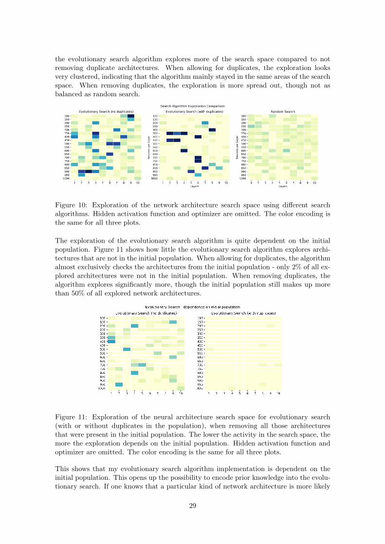
the evolutionary search algorithm explores more of the search space compared to notremoving duplicate architectures. When allowing for duplicates, the exploration looksvery clustered, indicating that the algorithm mainly stayed in the same areas of the searchspace. When removing duplicates, the exploration is more spread out, though not asbalanced as random search.

Figure 10: Exploration of the network architecture search space using different searchalgorithms. Hidden activation function and optimizer are omitted. The color encoding isthe same for all three plots.

The exploration of the evolutionary search algorithm is quite dependent on the initialpopulation. Figure 11 shows how little the evolutionary search algorithm explores archi-tectures that are not in the initial population. When allowing for duplicates, the algorithmalmost exclusively checks the architectures from the initial population - only 2% of all ex-plored architectures were not in the initial population. When removing duplicates, thealgorithm explores significantly more, though the initial population still makes up morethan 50% of all explored network architectures.

Figure 11: Exploration of the neural architecture search space for evolutionary search(with or without duplicates in the population), when removing all those architecturesthat were present in the initial population. The lower the activity in the search space, themore the exploration depends on the initial population. Hidden activation function andoptimizer are omitted. The color encoding is the same for all three plots.

This shows that my evolutionary search algorithm implementation is dependent on theinitial population. This opens up the possibility to encode prior knowledge into the evolu-tionary search. If one knows that a particular kind of network architecture is more likely

29

to perform well than another, this can be represented in the initial population for thesearch.

To summarize my findings of different neural network architecture search algorithms, eachone of the three search algorithms has its advantages and disadvantages. When the de-signer of the neural network is knowledgeable and experienced in the design of neuralnetwork architectures, or has resources such as previously used networks for the learningtasks available, manual search is a good choice. It is very cheap and highly customizable.When the goal is to automate the architecture design, random search and evolutionarysearch are more suitable choices. Evolutionary search allows for more customization andthe encoding of prior knowledge which may save time during the search. Random searchis good algorithm to explore the entire search space evenly, if the goal is to not overlookany architectures.

4.3 Constructive Dynamic Learning Algorithm

In constructive dynamic learning, it is not necessary to define the search space explic-itly. However, one can argue that different constructive dynamic learning algorithms haveimplicit restrictions on the type of network architecture that they consider. The cascade-correlation learning algorithm can only build network architectures that are cascaded ina very particular way. The original forward thinking algorithm requires specification ofthe exact network architecture, thus not automating the architecture design. This is whyI am proposing a new algorithm, based on forward thinking, which also automates thearchitecture design.

4.3.1 Cascade-Correlation Networks

The originally proposed Cascor algorithm requires many hyperparameters to be set [Yangand Honavar, 1998]. It does not specify when to stop training each unit before adding thenext one and it does not specify when to stop adding new units altogether. Other papershave also questioned the choice of training on error correlation maximization rather than”standard” error minimization training [Littmann and Ritter, 1992]. I implemented andran experiments on several different versions of Cascor, aiming to find a version of Cascorthat is suitable to a more modern, higher-dimensional dataset such as MNIST (as opposedto the low dimensional, small datasets used in the original paper by Fahlman and Lebiere[1990]). The largest dataset for which I found evidence that Cascor had been trained on isa learning task with 120 inputs and 3,175 samples, and a learning task with 21 inputs and7,100 samples reported by Littmann and Ritter [1992]. MNIST, the dataset I am using inthis thesis, has 784 inputs and 80,000 samples.

All experiments reported in this section were run on my personal computer, see Section4.1.4 for details.

The parameters that needed to be decided on for the Cascor algorithm are:

• Activation function

• Loss function: the originally proposed error correlation, or error minimization.

• When to stop training each unit before adding a new one

• When to stop adding new units

30

Cascor

The originally proposed cascade-correlation learning algorithm was described in Section3.2.3. I implemented the algorithm, as well as the proposed error correlation training.The error correlation loss is described in Appendix A.1.2.

The network performs very poorly when trained using the originally proposed error cor-relation maximization. Training the network several times, it never reached a validationaccuracy above 70%, as shown in Figure 12. I have tried different approaches to improvethe network’s performance but I was not able to report any good findings.

Figure 12: Cascade-correlation learning algorithm, as proposed by Fahlman and Lebiere[1990]. The algorithm was run ten times, with a candidate pool of size eight, trainingeach hidden unit in the candidate pool for two epochs and then choosing the one withthe highest validation accuracy. This unit is then added into the network and traineduntil convergence (i.e. until the validation accuracy doesn’t improve for three epochs in arow). Results are averaged over the ten runs, with the shaded area representing the 95%confidence interval.

Littmann and Ritter [1992] report that error correlation training is inferior to error mini-mization training on regression tasks. In classification tasks, it converges faster - thoughthe final performance seems to be the same for both (the authors do not explicitly stateso, but it seems to be implied in their conclusion’s wording). It may be that the error cor-relation training overcompensates for errors Prechelt [1997] due to the high dimensionalityof the dataset, though this requires further investigation.

Caser

The next approach is Caser, as proposed by Littmann and Ritter [1992] - a variation ofCascor in which the network is trained on error minimization. My implementation of thenetwork is using softmax in the output layer, tanh in the hidden units and is trained onthe categorical cross entropy loss function. Hidden units are added into the network asdescribed in the original paper. I am using a candidate pool of eight units. Each candidateunit is trained for one epoch after which the candidate unit with the highest accuracy onthe validation set is inserted into the network. Once inserted, the unit is trained untilconvergence using RMSProp (until the testing accuracy stops increasing for more thantwo epochs in a row) after which the unit’s input weights are frozen. The output weight

31

vector is discarded whenever a new unit is added into the network and retrained, similarlyto forward thinking. Figure 13 shows the training graphs of this architecture, averagedover ten runs. Overall, this looks much better than the error correlation training in Figure12.

Figure 13: Caser algorithm, as originally proposed by Littmann and Ritter [1992]. Resultsare averaged over the ten runs, with the shaded area representing the 95% confidenceinterval.

Running this architecture shows some interesting behavior when a new unit is addedinto the network. Whenever a new hidden unit is added into the network, the networkperformance changes - sometimes quite drastically. Figure 14 shows how unpredictablethis turns out in individual training runs. On the left, after adding the second hidden unit,the network accuracy improves to over 90% but adding a third hidden unit decreases theaccuracy down to 60%, even after training this third unit to convergence. The networknever recovers from this performance dip and doesn’t reach an accuracy better than 85%again. This is likely because the output weight vector that the network converged to whentraining the second hidden unit was discarded and the network will choose a new outputweight vector at random (from the pool of eight candidate units). If the candidate poolonly contains ”bad” weight vectors for the output layer, the network will be stuck in oneof these bad local minima.

Figure 14: Unpredictable behavior when adding new units into the Caser network. Leftplot shows the Caser network using a candidate pool size of eight, whereas on the right, acandidate pool of size 16 was used. Green dotted lines show the insertion of a new hiddenunit into the network.

In order to remove these sudden (and seemingly uncontrollable) performance jumps, one

32

may increase the candidate pool size, in an attempt to increase the probability of findinga weight vector close to a good local minimum. The right plot in Figure 14 shows theperformance of a network that uses a candidate pool size of 16 (instead of eight, as theleft plot) and shows a large performance decrease after adding the second hidden unit, butrecovers to the previous ”good” performance with the insertion of the seventh hidden unit.It decreases again with the eighth unit and increases to a new maximum performance withthe tenth hidden unit. Luckily, that was the last hidden unit so the final network reaches agood performance. Increasing the candidate pool size is not a deterministic way of findinga better weight vector. A more reliable method is needed to improve Caser’s performance.

CaserRe

The question of when to stop the training remains, and the random jumps in networkperformance make it difficult to decide on a stopping criterion. Instead of increasing thecandidate pool’s size, I initialized the weight vectors for new hidden units close to thelocal minimum that was found in training the previous hidden unit. As Figure 15 shows,this removes performance decreases and yields ”smoother” training improvements. I amcalling this CaserRe because it is based on Caser and extends it by re-using the outputweight vector when a new hidden unit is added into the network.

Figure 15: Reusing the output weight for all units in the candidate pool for Caser. Resultsare averaged over the ten runs, with the shaded area representing the 95% confidenceinterval. Lighter colored lines show the single runs.

However, this makes the network very dependent on the initially found local minimum. Bytaking the weight vector from the previous hidden unit’s training I remove performancedips that would have appeared otherwise - but I also removed performance increases thatwould otherwise be possible and would help the network jump to a better local minimum.This is shown on individual training runs in Figure 16. If the first hidden unit finds agood local minimum, the overall result will be good, though only slightly improving onthe network’s performance with one hidden unit. However, if the initial local minimum isnot good, the network seems to be stuck.

In order to avoid the pitfalls of a bad weight initialization at the beginning of training, itmay help to train the candidate pool of hidden units, choose the best performing hiddenunit and, if the performance is not significantly worse than it was before adding thishidden unit, the unit should be added as it is. If the performance is significantly worsethan before, the unit should be added reusing the previous output weight vector - thus

33

Figure 16: Caser’s dependence on the initial weight vector. On the left, the network finds agood initial local minimum whereas on the right, the network finds a worse local minimumand does not improve its performance significantly.

initializing the output weight vector close to the previously found local minimum. Thiswill remove performance dips, while keeping the chance to find better local minima whenadding new hidden units.

Figure 17 reuses the previous output weight vector if the new unit decreases the validationaccuracy by more than 5%. The overall performance of the network is improved, however,the figure shows some drastic performance drops during training.

Figure 17: Caser, reusing the previous output weight vector if all units in the candidatepool decrease the networks accuracy by more than 5%.

Another approach is to modify the candidate pool. Instead of training eight candidateunits, we can train seven new candidate units and one candidate unit that reuses theprevious output weights. In this way, we will only change the output weights if it leads toan increase in test accuracy. Obviously, the newly trained units will only be trained forone epoch while the unit reusing output weights has been trained to convergence. To makeup for this difference, we could set a compensation factor. In the experiments plotted inFigure 18, I did not use such a compensation factor for the sake of automaticity (the fewertunable parameters, the better).

This shows good results, with the network reaching an accuracy of over 90% in 7 out of10 training runs, with the remaining 3 runs achieving an accuracy of over 83%.

So far, it seems like all experiments on Cascor, Caser, and CaserRe have been underfitting

34

Figure 18: Using a candidate pool of seven new units and one unit reusing the previousoutput weights. Results averaged over ten runs, with the shaded area representing a 95%confidence interval. Lighter colored lines show the single runs.

on the MNIST learning task, as they have been using only ten hidden units in total - ascompared to standard MLPs that have hundreds of hidden units. I trained the algorithmwhose results are shown in Figure 18 for 100 cascading hidden units for two training runs,using a candidate pool size of four. The results are shown in Figure 19; both networksreach a validation accuracy of 92.7%.

Figure 19: Using a candidate pool of three new units and one unit reusing the previousoutput weights. Adding a total of 100 cascading hidden units. Results averaged over tworuns, with the shaded area representing a 95% confidence interval. Lighter colored linesshow the single runs.

A comparable MLP with one hidden layer of 100 neurons reaches a validation accuracyof around 94.0% (trained with RMSProp on crossentropy loss, using tanh in hidden unitsand softmax in the output layer).This shows that CaserRe is close to the performanceof comparable layered networks. However, in order to be competitive on the MNISTlearning task, a testing accuracy of over 95% should be achieved. The complexity of theCaserRe network needs to be increased in an attempt to learn the MNIST task to a higheraccuracy. The insertion of hidden units is computationally expensive due to the trainingof the candidate pool and modifications to the computational graph of the neural network.Complexity may be added into the network more efficiently by increasing the complexityof each hidden unit, e.g. by replacing a hidden unit by a hidden cascading layer. To thebest of my knowledge, this has not been done before.

35

I ran another experiment, using candidate layers rather than single candidate units. Eachcandidate layer contains 50 neurons and a total of 50 of these cascading layers were insertedinto the network. I used a candidate pool of size four. The result is shown in Figure 20, thenetwork reaches a validation accuracy of 92.85% (averaged over five runs with a standarddeviation of 0.20%). This is slightly better than the Caser architecture with 100 cascadinghidden units and worse than layered networks of similar architecture.

Figure 20: Using a candidate pool of three new units and one unit reusing the previousoutput weights. Adding a total of 50 cascading hidden layers of 50 units each. Resultsaveraged over five runs, with the shaded area representing a 95% confidence interval.Lighter colored lines show the single runs.

In another experiment, I used layers of size 100, adding a total of 15 of these cascadinglayers into the network - again using a candidate pool size of four. The results for thisarchitecture are shown in Figure 21. The network reaches a validation accuracy of 88.58%(averaged over ten runs and a standard deviation of 4.11%) with a maximum accuracyof 92.93% and a minimum of 83.57%. Again, this is worse than comparable layeredarchitectures.

Figure 21: Using a candidate pool of three new units and one unit reusing the previousoutput weights. Adding a total of 15 cascading hidden layers of 100 units each. Resultsaveraged over five runs, with the shaded area representing a 95% confidence interval.Lighter colored lines show the single runs.

Even though the resulting networks are very large, they do not overfit on the MNISTdataset and the final performance does not significantly change when adding more com-plexity into the network (by adding cascading layers rather than single units to increasethe width or by increasing the depth of the cascading units/layers). A more detailed in-

36

vestigation into the connection weight values from the hidden activation vector comparedto the input activation vector may bring some insights. In order to prioritize the cascadedhidden units/layers over the input vector, one may drop out or reduce some of the input-to-output connection weights (through dropout or weight decay) in order to incentivizethe network to make more use of the new hidden activation vector.

Cascor Summary

After some additional work based on Cascor and Caser, I was able to find a well-performinglearning algorithm, which I called CaserRe. Though the final algorithm is able to find goodlocal minima with an average accuracy of over 90%, adding more units and layers into thenetwork does not increase performance to anything above 93% testing accuracy.

One reason for this may be that the input to each subsequent hidden unit is still verynoisy. Traditional layered neural networks map the input to a different dimension throughthe first hidden layer. Subsequent hidden layers work only on the output of previouslayers. Hidden layers could be seen as making the data more well-behaved, as suggestedby Hettinger et al. [2017]. This may be why the forward thinking algorithm seems to workmuch better than my current implementation of different Cascor versions which are facingproblems with the aforementioned volatility.

Another way to look at is that the error surface (with respect to the weights) is veryhigh dimensional, as the weight vector is very high dimensional. With each added unit,the network tries to find a new local minimum, with one weight being fixed (i.e. onedegree of freedom on the error surface frozen) and the rest still to be varied. Since theinput dimension is much higher than the dimension of all hidden units combined (inmy experiments, no more than one hundred hidden units/layers have been inserted intothe network while the input layer has over 700 units), the error minimization problem isdominated by the connections weights from the input to the output. In order for this issueto disappear, one would have to train a very deep cascading network in order for the hiddenweights to be more important in relation to the input-to-output-connection weights. Thiswould explain why Cascor performs well on datasets with lower dimensionality, such asthe problems treated in the original paper, because there the input-to-output-connectionweights are much fewer and thus less relevant in comparison to the hidden weights.

In terms of performance, training these cascading networks can be very efficient usingmodern deep learning frameworks, with each epoch taking no more than a few seconds.However, the cascading structure requires making changes to the computational graph,which sum up to be a large overhead. The deeper networks (50 cascading layers of 50 unitseach, 100 cascading layers of single units, and 100 15 cascading layers of 100 units each)took over 30 minutes to train, with the vast majority of the time spent on the trainingof candidate unit/layers. This can be done much more efficiently, since the candidatetraining allows for perfect parallelization. Hence the candidate unit training can be donein parallel and yield a time decrease of up to 8x.

Since most modern neural networks deal with very high-dimensional data, more work onCascor is required in order to make it competitive in the world of modern neural networks.A comprehensive study on different cascading architectures can give more conclusive ev-idence for whether or not these cascading architectures can perform as well, or better,compared to similar layered architectures.

37

4.3.2 Forward Thinking

The forward thinking algorithm trains a fully-connected neural network by building upthe network one hidden layer at a time [Hettinger et al., 2017]. The originally proposedalgorithm does not automate the layer construction. One needs to specify how manylayers can be added, as well as the width of the layer and the activation function used.The networks in my experiments will be trained on cross entropy loss using RMS Prop.Hidden units use the tanh or relu activation function, output units use softmax.

Parameters that needed to be decided on include:

• Hidden layers: how many layers, how many units in each layer, activation functions.

• Layer construction time: when to add new layers.

For this experiment, a new layer will be added when the training of the current layer hasnot improved the accuracy on the validation data for two epochs in a row (and training willbe stopped after the validation accuracy hasn’t improved for three epochs in a row whentraining the last layer). I am running the forward thinking algorithm on three differentarchitectures: two layers of 512 tanh units each, three layers of 850 tanh units each, andfive layers of 750 tanh units each - taking the best-performing neural network setups fromthe random search results using two, three and five hidden layers.

Figure 22 shows the performance of these networks. It is interesting to see that the testingaccuracy seems to reach its maximum around half-way through each layer-wise training (oreven slightly before) while the training accuracy continuously increases. Moreover, whilethe training accuracy decreases significantly when a new layer is inserted, the testingaccuracy does not suffer from this decrease. Near the training’s end, the training accuracykeeps increasing significantly more than the validation accuracy. This looks strange - itdoesn’t seem to be overfitting, as the validation accuracy keeps improving as well. This isvery similar to the findings reported by Hettinger et al. [2017].

Figure 22: Training and validation accuracy per epoch in forward thinking. Results areaveraged over 20 runs, the shaded areas show the 95% confidence interval.

However, looking at the loss, shown in Figure 23, demonstrates that the network is indeedstarting to overfit, but the accuracy doesn’t suffer from the overfitting. This effect is moresignificant in deeper networks.

Hettinger et al. [2017] do not report the loss of their network, hence a direct comparisonis not possible. The accuracy is computed through an argmax operation on the output

38

Figure 23: Training and validation loss per epoch in forward thinking. Results are averagedover 20 runs, the shaded areas show the 95% confidence interval.

vector (see Appendix A.1). As long as the maximum value in the output vector belongs tothe same class, the accuracy does not change. However, if the output vector becomes lesscertain about the class - meaning that the difference between the maximum argument andother arguments decreases - the loss will increase, penalizing this increased uncertainty.Hence, the forward thinking algorithm is indeed starting to overfit on the training data,with the overfitting being more significant in deeper networks.

Early stopping on the accuracy doesn’t seem to avoid overfitting as well as early stoppingon the loss would. Hence, the following experiments will be applying early stopping to thevalidation loss, rather than the validation accuracy.

The final performance of these networks is shown in Table 7 and for a direct comparisonbetween forward thinking and ”standard” training, the same statistics are shown in Table8 for a network trained using backpropagation.

Layers Epochs Train Accuracy Validation Accuracy Time

2 x 512 18 ± 4 98.75% ± 0.48% 96.85% ± 0.28% 28.9s ± 6.5s3 x 850 21 ± 4 99.30% ± 0.27% 97.27% ± 0.23% 35.7s ± 5.8s5 x 750 29 ± 4 99.91% ± 0.08% 97.54% ± 0.12% 47.4s ± 5.7s

Table 7: Network performances when trained with forward thinking. Results show theaverages and standard deviations over 20 training runs.

Layers Epochs Train Accuracy Validation Accuracy Time

2x512 23 ± 6 98.45% ± 0.24% 97.27% ± 0.15% 36.5s ± 8.8s3x850 18 ± 5 98.09% ± 0.19% 96.92% ± 0.26% 36.2s ± 9.2s5x750 20 ± 6 97.19% ± 0.23% 96.10% ± 0.32% 48.4s ± 14.8s

Table 8: Network performances when trained using backpropagation (for a direct com-parison between backpropagation and forward thinking. Results show the averages andstandard deviations over 20 training runs.

The results show that the two layer network performs 0.4% better (on average) whentrained using backpropagation. The three and five layer networks show a 0.3% and 1.5%increase in validation accuracy (on average) when trained with forward thinking. This isin agreement with forward thinking being more efficient in training deep neural networks,

39

as there is no need to propagate the error signal through many layers. More experimentson other learning tasks are needed in order to solidify this hypothesis.

Hettinger et al. [2017] reported a 30% decrease in training time on a four-layer neuralnetwork. Though forward thinking was, on average, faster for all three network archi-tectures, I cannot report the same magnitude of speedup. This may be due to the factthat the training happens on the GPU but the computational graph is modified aftereach layer-wise training which entails that data has to be moved to and from the CPU.This leads to a larger overhead in computation, as previously mentioned for the cascadingnetworks in Section 4.3.1. In order to test this hypothesis, I ran the same experiment onmy personal computer’s CPU (running the training once for backpropagation and once forforward thinking due to time constraints). This indeed shows a much larger improvementin training time for forward thinking compared to backpropagation - 46% for the 5 x 750network, 25% for the 2 x 512 network and 53% for the 3 x 850 network. The test accuracyis similar to the ones reported previously. The result is shown in Table 10 in AppendixA.4.

4.3.3 Automated Forward Thinking

In order to automate forward thinking more, one might want to automate the choice oflayers that will be added into the network. Inspired by the original Cascor algorithm[Fahlman and Lebiere, 1990], I use a pool of candidate layers - training each one for a fewepochs and choosing the best layer from the candidate pool to insert into the network. Tothe best of my knowledge, this has not been done before.

Figure 24: The automated forward thinking algorithm, trained for ten layers. Resultingnetwork has the layers: [950, 700, 700, 500, 50, 200, 500, 850, 550, 350].

In my experiments, I used a candidate pool of eight layers, each layer being trained fortwo epochs. The width of each candidate layer is chosen at random within the interval[50, 1000], restricted to multiples of 50. The best performing of these eight candidatelayers will be inserted into the network and fully trained (until the validation accuracystops improving). This already works reasonably well, as shown in Figure 24. However,not all layers are needed for the final model to perform as well as it does. The firsttwo layers offer significant increases in accuracy, but this increase in model performanceflattens quickly. A stopping criterion which detects this performance flattening could yieldsmaller networks with similar performance.

The stopping criterion is an opportunity to automate the algorithm further. Early stopping

40

seems to be a reasonable choice. I ran some experiments using early stopping, which endsthe training when the layer’s final validation accuracy hasn’t improved over the previouslayer’s final validation accuracy. Figure 25 shows that this approach is not ideal. In Figure25a, one can argue that training was stopped too early, the network could have improvedfurther, whereas in Figure 25b, training was stopped too late, adding more layers thannecessary as one can see from the flattened training accuracy after the fourth layer wasinserted. It might help to train each layer for a longer time, in order to have a morereliable value for the final layer’s validation accuracy.

(a) Training stopped too early. (b) Training stopped too late.

Figure 25: Automated forward thinking with early stopping when the validation accuracydoes not increase after adding a layer. The network on the left has two layers: [950, 1000],whereas the network on the right has six layers: [950, 500, 150, 300, 50, 300].

Early stopping is commonly used to stop training neural networks of fixed architecturesand to avoid overfitting. Normally, the penalty of training a neural network for one (ora few) epochs is not very high. However, the penalty of adding one (or a few) layersmore into a neural network is very large - the complexity of the resulting model increasessubstantially. A stricter version of early stopping is needed.

Layers Test Acc Train Acc Total Train Layers

4 97.86% 99.95% 185.16s 99.33s [900, 600, 600, 300]4 97.68% 100.00% 180.60s 99.77s [700, 700, 400, 300]4 97.68% 100.00% 184.44s 96.82s [900, 900, 300, 300]4 97.64% 99.99% 184.97s 103.40s [900, 500, 400, 200]4 97.51% 99.99% 146.33s 66.36s [800, 600, 100, 100]4 97.47% 99.53% 163.28s 84.37s [1000, 200, 100, 100]3 97.46% 100.00% 148.40s 91.36s [1000, 200, 100]3 97.44% 99.90% 140.55s 83.30s [900, 100, 100]3 97.30% 100.00% 144.90s 86.53s [600, 500, 300]3 97.16% 99.62% 112.55s 55.35s [800, 100, 100]

Table 9: Ten smallest architectures found by running the automated forward thinkingalgorithm 20 times. Train gives the actual training duration, while Total gives the totaltraining time, including the candidate unit training.

Considering that the training using forward thinking is quite fast, it is computationallyfeasible to insert more layers into the network than needed, storing the network perfor-

41

mance for all number of layers. Based on this, one may assess with how many layers thetraining reaches an optimal tradeoff of performance against model complexity. Finally,unnecessary layers can be removed from the network and the output weight vector can beretrained. I implemented and ran the algorithm 20 times, yielding 20 unique architectures.I furthermore restrict the algorithm to only use layers of subsequently decreasing widthsas that is how most neural network architectures are designed. This decision is subjectto more discussion, though I will ommit this discussion in my thesis. Table 9 shows allarchitectures using fewer than five layers. Figure 26 shows the training graph for this.

Figure 26: The automated forward thinking algorithm run 20 times. Shaded area showsthe 95% confidence interval.

Across 20 runs of the algorithm, the average test accuracy is 97.54% (with a standarddeviation of only 0.17%) - which is better than any other algorithm I have investigated inthis thesis. Half of the architectures use below five layers, the other half uses five or morelayers. The best performing network architecture is [900, 600, 600, 300] with a testingaccuracy of 97.86%.

The increased performance over layered neural networks likely stems from the difficulty oftraining deep networks with backpropagation. Training the network using forward think-ing may enable the algorithm to take deeper, more complex architectures into considerationand train them more efficiently than backpropagation could.

4.3.4 Conclusion

In this section of constructive dynamic learning algorithms, I compared cascading networksand forward thinking networks, each being a category of several learning algorithms. Themost promising algorithms are CaserRe, forward thinking and automated forward think-ing. However, as forward thinking does not design its own architecture - it is an algorithmto train a neural network - I will not be considering it as an automated architecture designalgorithm.

In terms of automation, both automated forward thinking and CaserRe show a similarlevel of automaticity. Both algortihms search for a suitable architecture automatically, in arandomized greedy way through the use of a candidate pool. Automated forward thinkingneeds an upper and lower bound for the hidden layers’ widths. In CaserRe, one also needsto specify whether hidden units or hidden layers should be inserted in a cascading way(and how large these hidden layers may be).

42

Automated forward thinking outperforms CaserRe in the MNIST learning task by 5% onthe testing accuracy (CaserRe with 50 cascading hidden layers of 50 units each).

The automated forward thinking and CaserRe algorithms have very similar computationalrequirements (given the same candidate pool sizes). However, CaserRe needs to add morecascading units (or layers) into the network than automated forward thinking needs toadd layers, hence CaserRe could be said to be slower than automated forward thinking.However, as there is a significant performance difference between the two algorithms, noexact comparison in terms of computational requirements can be made.

The resulting model complexity of automated forward thinking networks and CaserRenetworks is difficult to assess, as there is a performance difference between the two andbecause I have no basis for comparing layered networks with cascading networks - otherthan the empirical evidence that cascading networks do not seem to be able to learn theMNIST learning task as well as automated forward thinking.

In summary, CaserRe is in need of further investigation in order to get its performancelevels to competitive standards, or in order to explain why this cascading structure maynot be suitable for a learning task such as MNIST. Automated forward thinking seemsto be a very well-performing constructive learning algorithm, outperforming all neuralnetworks trained using standard backpropagation that I covered in this thesis. Furtherempirical evidence is needed to confirm the experimental results from my work in thisthesis.

4.4 Conclusion

The empirical investigation laid out in this thesis give a preliminary overview of some tech-niques for the automated architecture design of deep feedforward neural networks. Goodresults have been reported and preliminary hypotheses about the suitability of differentalgorithms have been made.

The experimental findings show that different neural architecture search algorithms areable to find suitable network architectures that perform well on the learning task. Theneural architecture search investigation hints at possible use cases to search for well-performing architectures. Manual search is best used when a lot of knowledge about goodarchitectures is available, either through experience or through available results in theliterature. Random search can be used to evenly explore the search space, if the goal isto explore the entire search space without any bias introduced through prior knowledge.Evolutionary search strikes a compromise between the unbiasedness of random search andthe manual search algorithm driven primarily by prior (human) knowledge.

Furthermore, as constructive dynamic learning algorithms, this thesis includes a prelim-inary investigation of two families of such algorithms: the recently proposed forwardthinking algorithm and the cascade-correlation learning architecture that was proposedover twenty years ago. Both algorithms have been implemented on the digit classificationlearning task. I extended both algorithms to improve their performance and level of auto-maticity. Results have been reported on the learning task and the algorithms’ merits havebeen discussed. The investigated cascading architectures were not able to perform as wellas standard layered networks - more work is needed to assess, and possibly enhance, theirviability on modern learning tasks. The forward thinking algorithm outperformed all lay-ered neural networks investigated in this thesis and shows promise for future work, despite

43

more work being needed on regularizing this architecture in order to combat overfittingand improve generalization.

Automated forward thinking extends the greedy-wise training proposed by forward think-ing into a fully automated architecture design algorithm for neural networks. The algo-rithm builds a network deeper than the standard MLP architectures found with the searchalgorithms described above and yields better performance on the test data than any MLPinvestigated in this thesis. As such, automated forward thinking shows a promising tech-nique that may further be investigated in more comprehensive studies.

To summarize, this thesis has given a preliminary overview of exisiting algorithms forthe automation of architecture design and reported some results on a selected learningtask of digit classification. The results of this thesis may be used as a starting point forfurther work on fully, and partially, automated architecture design algorithms for deepneural networks. If the trend of creating more and more complex deep learning modelscontinues, these automated architecture design algorithms may be the main tools to designneural networks for new learning tasks in the future.

44

5 Future Work

As stated previously, this thesis merely gives a preliminary overview of automated archi-tecture design algorithms for deep feedforward neural networks and empirical results toguide the direction of future research. Possible future research directions in the field ofautomated architecture design are outlined in this section.

The first large restriction of this research project is the limitation to feedforward neuralnetworks. Future research may investigate techniques for the automated architecturedesign of other types of neural networks, most notably convolutional neural networksand recurrent neural networks. The original forward thinking algorithm has also beenapplied to convolutional neural networks [Hettinger et al., 2017] and a recurrent versionof cascade-correlation neural networks was proposed by Fahlman [1991].

Neural architecture search has already been applied to a large variety of different neuralnetworks. For example, Real et al. [2018] evolved a neural network architecture that ul-timately outperformed manually crafted architectures for the first time on the ImageNetlearning task. They are using the NASNet search space for the evolution of their archi-tecture that was designed by Zoph et al. [2018]. Real et al. [2018] further also comparedtheir evolutionary search with different neural architecture search algorithms, specificallywith random search and reinforcement learning applied to neural network architectures.Future work in the field may run more comparative studies on neural architecture searchalgorithms, establishing some empirical evidence for the circumstances under which eachneural architecture search algorithm performs well. Moreover, an in-depth analysis ofdifferent neural architecture search based on the properties of the search space may beable to establish some formal proofs or evidence of certain search algorithms being moreadvantageous than others, for different kinds of learning tasks. Such a general analysisis inherently difficult and may only be possible after comprehensive empirical evidence isavailable on a large set of diverse learning tasks. The survey provided by Elsken et al.[2019] on neural architecture search algorithms may be a starting point for such in-depth,largely task-independent research.

Neural networks that change their network architecture based on the learning task, i.e.learning both the architecture and the connection weights simultaneously have not beenworked on in the same magnitude as the field of neural architecture search, to the bestof my knowledge. This may be due to the lack of a unifying term of such algorithms.Waugh [1994] uses the term dynamic learning for such models, Cortes et al. [2017] usesthe term adaptive structural learning, and Yao [1999] uses the term evolving ANNs forneural networks whose architecture and parameters are learned simultaneously using evo-lutionary search algorithms. One term that may contain all these terms is automatedmachine learning, or AutoML. However, I was not able to find such a term specificallyfor neural networks, which could be seen as a subset of AutoML. Moreover, the mostrecent survey of such models that I was able to find at the beginning of this researchproject was over 20 years old, by Waugh [1994]. In April 2019, Zoeller and Huber [2019]submitted a survey on automated machine learning to the Journal of Machine LearningResearch (pending review). The survey gives a good overview of recent work in the fieldof automated machine learning, but I found it to not be comprehensive with respect toautomated architecture design for neural networks, as its focus lies more in the automationof the entire machine learning pipeline. As automated machine learning can be seen as asuperset of automated architecture design for neural networks, the survey is still highly

45

relevant but not comprehensive. Future work in the field of automated neural networkarchitecture design should include a survey that gives an overview of the most relevanttechniques - techniques that learn both the architecture and the paramters of the networkssimultaneously.

The future work in the field of automated architecture design for neural network withI am proposing in this thesis can be summarized as (1) compiling a survey of the mostrelevant techniques for automated architecture design, (2) gathering empirical evidencefor the performance and comparison of different algorithms on diverse learning tasks, and(3) establishing formal proofs or concrete evidence for task-independent performance ofdifferent algorithms.

46

A Appendix

A.1 Loss functions

A.1.1 Crossentropy Loss

The crossentropy loss is a loss function for multi-class classification problems. The cate-gorical cross-entropy loss refers to the use of the softmax activation function on the outputand then the cross-entropy loss.

Let N be the number of patterns in the dataset, C the number of classes, and pmodel(yi ∈Cc) is the probability given by the model that pattern i belongs to the class c.

− 1

N

N∑i=1

C∑c=1

1yi∈Cc log pmodel(yi ∈ Cc)

where

1yi∈Cc =

{1 yi ∈ Cc0 yi /∈ Cc

A.1.2 Error Correlation Maximization

The error correlation maximization was proposed to train cascade-correlation neural net-work by Fahlman and Lebiere [1990]. The objective of the algorithm is to maximize theerror correlation S, which is given by:

S =∑o∈O

∣∣∣∣∣∣∑p∈P

(Vp − V )(Ep,o − Eo)

∣∣∣∣∣∣where O is the set of output units and P is the training dataset. Vp is the hidden unit’svalue (its activation) when the training pattern p was passed through the network. V isthe hidden unit’s value averaged over all training patterns. Ep,o is the error at the outputunit o on the training pattern p and Eo is the error at output unit o averaged over alltraining patterns.

A.1.3 Accuracy Computation

In the experiments contained in this thesis, the primary performance metric is the accuracyof the neural network’s predictions on a classification task. Let C be the set of |C| = cclasses. Let the output of the neural network be given by y where y ∈ Rc. After passingthe output of the neural network through the softmax function σ, we obtain z = σ(y)where z ∈ Rc. The accuracy τ can be computed as follows:

τ = argmaxi z

47

where i ∈ {1, . . . , c}.

A.2 Activation functions

In my thesis, I am using three different activation functions, namely relu (Rectified LinearUnit), tanh (hyperbolic tangent), and softmax.

The relu function is a function relu : R→ R:

relu(x) =

{0 x < 0

x x

The tanh function is a function tanh : R→ R:

tanh(x) =ex − e−x

ex + e−x∈ [−1, 1]

Both the relu and the tanh function can be applied to vectors of real numbers by applyingthe function to each of its elements individually.

The softmax function σ is defined on a vector of K real numbers and normalizes thatvector into a probability vector, σ : RK → RK :

σ(z)i =ezi∑Kj=1 e

zj∈ [0, 1]

where z ∈ RK and 1 ≤ i ≤ K.

A.3 Neural Network Optimization Algorithms

This section closely follows and paraphrases the paper by Ruder [2016] which gives a goodoverview of different gradient descent optimization algorithms commonly used for trainingneural networks.

A.3.1 Stochastic Gradient Descent

There are different variations of the standard gradient descent algorithm that vary in theamount of data that they take in before updating the parameters.

Let N be the number of patterns in the training data, η be the learning rate, θ be theparameter vector (the vector of all connection weights in a neural network), Li(θ) be theloss for pattern i (given parameter vector θ), then the standard (”batch”) gradient descentalgorithm updates the weight vector in the following way:

θt+1 = θt − η1

N

N∑i=1

∇Li(θt)

48

where t indicates the step of the gradient descent optimization.

This computation can be slow and for large datasets even intractable if they do not fitinto memory. We can break down the update rule and update the parameter vector withevery single pattern that we train on. This is called stochastic gradient descent, which isapplied for every pattern i ∈ {1, . . . , N}:

θt+1 = θt − η∇Li(θt)

However, this is not very efficient either, because we update the parameter vector forevery single pattern in the dataset. In order to strike a compromise between batch gradientdescent and stochastic gradient descent, one may use so-called ”mini-batches”, i.e. subsetsof the total training data of size m, after each of which the parameters are updated asfollows:

θt+1 = θt − η1

m

m∑i=1

∇Li(θt)

This is called mini-batch gradient descent and it is the algorithm that I am referringto as SGD (stochastic gradient descent) because this is what the algorithm is called inKeras, the deep learning framework that I am using for my code implementations. For allexperiments found in this thesis, I used a mini-batch size of 128.

A.3.2 RMS Prop

RMS Prop (Root Mean Square Propagation) is the optimization algorithm that I usedto train most neural networks in this thesis. It deals with some of the challenges thatvanilla gradient descent methods face. RMS Prop belongs to a family of gradient descentoptimization algorithms that use momentum and/or adaptive learning rates. A moredetailed discussion of these methods can be found in Ruder [2016]. Herein, I am usingRMS Prop without further discussion.

In RMS Prop, the learning rate is adapted for every single parameter in the parametervector θ. The idea is to divide the learning rate for a weight by a running average of themagnitudes of recent gradients for that weight [Tieleman and Hinton, 2012]. This runningaverage is computed by:

vt+1(θ) = γ vt(θ) + (1− γ)∇Li(θ)2

where vt is the moving average at step t and γ is the momentum rate, or forgetting factor.The parameter vector is then updated as follows:

θt+1 = θt −η√

vt+1(θt)∇Li(θt)

In my implementations, I am using the recommended values γ = 0.9 and η = 0.001 [Ruder,2016] and [Tieleman and Hinton, 2012].

49

A.4 Futher Results

Layers Epochs Time Train acc Test acc

5 x 750 50 / 27 266.9s / 493.1s 100.00% / 97.58% 97.67% / 96.38%2 x 512 33 / 28 92.3s / 123.3s 99.95% / 98.53% 97.42% / 97.57%3 x 850 24 / 21 133.1s / 284.16s 99.78% / 98.36% 97.36% / 96.97%

Table 10: Network performances when trained using forward thinking (left values) andbackpropagation (right values).

50

References

Bartlett, P. L., Maiorov, V., and Meir, R. (1999). Almost Linear VC Dimension Boundsfor Piecewise Polynomial Networks. In Kearns, M. J., Solla, S. A., and Cohn, D. A.,editors, Advances in Neural Information Processing Systems 11, pages 190–196. MITPress.

Bergstra, J. and Bengio, Y. (2012). Random Search for Hyper-Parameter Optimization.The Journal of Machine Learning Research, 13(Feb):281–305.

Bianchini, M. and Scarselli, F. (2014). On the Complexity of Shallow and Deep NeuralNetwork Cassifiers. In European Symposium on Artificial Neural Networks, volume 22,pages 371–376.

Choromanska, A., Henaff, M., Mathieu, M., Arous, G. B., and LeCun, Y. (2015). The LossSurfaces of Multilayer Networks. In Proceedings of the 18th International Conferenceon Artificial Intelligence and Statistics, volume 38 of JMLR: W&CP, pages 192–204.JMLR.org.

Conneau, A., Schwenk, H., Barrault, L., and Lecun, Y. (2016). Very Deep ConvolutionalNetworks for Text Classification. arXiv preprint arXiv:1606.01781.

Cortes, C., Gonzalvo, X., Kuznetsov, V., Mohri, M., and Yang, S. (2017). Adanet: Adap-tive Structural Learning of Artificial Neural Networks. In Proceedings of the 34th In-ternational Conference on Machine Learning, volume 70, pages 874–883. JMLR.

Eldan, R. and Shamir, O. (2016). The Power of Depth for Feedforward Neural Networks.In Conference on Learning Theory, volume 49, pages 907–940.

Elsken, T., Metzen, J. H., and Hutter, F. (2019). Neural Architecture Search: A Survey.The Journal of Machine Learning Research, 20(55):1–21.

Fahlman, S. E. (1991). The Recurrent Cascade-Correlation Architecture. In Lippmann,R. P., Moody, J. E., and Touretzky, D. S., editors, Advances in Neural InformationProcessing Systems 3, pages 190–196. Morgan-Kaufmann.

Fahlman, S. E. and Lebiere, C. (1990). The Cascade-Correlation Learning Architecture.In Touretzky, D. S., editor, Advances in Neural Information Processing Systems 2, pages524–532. Morgan-Kaufmann.

Frean, M. (1990). The Upstart Algorithm: A Method for Constructing and TrainingFeedforward Neural Networks. Neural Computation, 2(2):198–209.

Goodfellow, I., Bengio, Y., and Courville, A. (2016). Deep Learning. MIT press.

Hanson, S. J. (1990). Meiosis Networks. In Touretzky, D. S., editor, Advances in NeuralInformation Processing Systems 2, pages 533–541. Morgan-Kaufmann.

Harvey, M. (2017). Lets evolve a neural network with a genetic algorithm code included.

Hassibi, B., Stork, D. G., and Wolff, G. (1994). Optimal Brain Surgeon: Extensions andPerformance Comparisons. In Cowan, J. D., Tesauro, G., and Alspector, J., editors, Ad-vances in Neural Information Processing Systems 6, pages 263–270. Morgan-Kaufmann.

Hassibi, B., Stork, D. G., and Wolff, G. J. (1993). Optimal brain surgeon and generalnetwork pruning. In IEEE International Conference on Neural Networks, volume 1,pages 293–299. IEEE.

51

He, K., Zhang, X., Ren, S., and Sun, J. (2016). Deep Residual Learning for ImageRecognition. In Proceedings of the IEEE Conference on Computer Vision and PatternRecognition, volume 1, pages 770–778.

Hettinger, C., Christensen, T., Ehlert, B., Humpherys, J., Jarvis, T., and Wade, S. (2017).Forward Thinking: Building and Training Neural Networks One Layer at a Time. arXivpreprint arXiv:1706.02480.

Hinton, G. E. (2012). A Practical Guide to Training Restricted Boltzmann Machines. InNeural Networks: Tricks of the Trade, pages 599–619. Springer.

Hornik, K., Stinchcombe, M., and White, H. (1989). Multilayer Feedforward NetworksAre Universal Approximators. Neural Networks, 2(5):359–366.

Keras (2019). Simple Deep Neural Network on the MNIST Dataset.

Krizhevsky, A., Sutskever, I., and Hinton, G. E. (2017). ImageNet Classification withDeep Convolutional Neural Networks. Commununity of the Association of ComputingMachinery, 60(6):84–90.

Krogh, A. and Hertz, J. A. (1992). A Simple Weight Decay Can Improve Generalization.In Moody, J. E., Hanson, S. J., and Lippmann, R. P., editors, Advances in NeuralInformation Processing Systems 4, pages 950–957. Morgan-Kaufmann.

Kumar, A., Irsoy, O., Ondruska, P., Iyyer, M., Bradbury, J., Gulrajani, I., Zhong, V.,Paulus, R., and Socher, R. (2016). Ask Me Anything: Dynamic Memory Networks forNatural Language Processing. In Proceedings of the 33rd International Conference onMachine Learning, volume 48, pages 1378–1387. JMLR.

Larochelle, H., Erhan, D., Courville, A., Bergstra, J., and Bengio, Y. (2007). An EmpiricalEvaluation of Deep Architectures on Problems with Many Factors of Variation. InProceedings of the 24th International Conference on Machine Learning, pages 473–480.ACM.

LeCun, Y. and Bengio, Y. (1998). Convolutional Networks for Images, Speech, and TimeSeries. In Arbib, M. A., editor, The Handbook of Brain Theory and Neural Networks,pages 255–258. MIT Press.

LeCun, Y., Bottou, L., Bengio, Y., Haffner, P., et al. (1998). Gradient-Based LearningApplied to Document Recognition. Proceedings of the IEEE, 86(11):2278–2324.

LeCun, Y., Denker, J. S., and Solla, S. A. (1990). Optimal Brain Damage. In Touretzky,D. S., editor, Advances in Neural Information Processing Systems 2, pages 598–605.Morgan-Kaufmann.

LeCun, Y. A., Bottou, L., Orr, G. B., and Muller, K.-R. (2012). Efficient Backprop. InNeural Networks: Tricks of the Trade, pages 9–48. Springer.

Levin, A. U., Leen, T. K., and Moody, J. E. (1994). Fast Pruning Using Principal Com-ponents. In Cowan, J. D., Tesauro, G., and Alspector, J., editors, Advances in NeuralInformation Processing Systems 6, pages 35–42. Morgan-Kaufmann.

Levine, S., Finn, C., Darrell, T., and Abbeel, P. (2016). End-To-End Training of DeepVisuomotor Policies. The Journal of Machine Learning Research, 17(1):1334–1373.

Littmann, E. and Ritter, H. (1992). Cascade network architectures. In [Proceedings 1992]

52

IJCNN International Joint Conference on Neural Networks, volume 2, pages 398–404.IEEE.

Littmann, E. and Ritter, H. (1993). Generalization Abilities of Cascade Network Archi-tecture. In Hanson, S. J., Cowan, J. D., and Giles, C. L., editors, Advances in NeuralInformation Processing Systems 5, pages 188–195. Morgan-Kaufmann.

Maass, W., Schnitger, G., and Sontag, E. D. (1994). A Comparison of the ComputationalPower of Sigmoid and Boolean Threshold Circuits. In Theoretical Advances in NeuralComputation and Learning, pages 127–151. Springer.

Mezard, M. and Nadal, J.-P. (1989). Learning in Feedforward Layered Networks: TheTiling Algorithm. Journal of Physics A: Mathematical and General, 22(12):2191.

Mozer, M. C. and Smolensky, P. (1989). Skeletonization: A Technique for Trimming theFat from a Network via Relevance Assessment. In Touretzky, D. S., editor, Advances inNeural Information Processing Systems 1, pages 107–115. Morgan-Kaufmann.

Nowlan, S. J. and Hinton, G. E. (1992). Simplifying Neural Networks by Soft Weight-Sharing. Neural Computation, 4(4):473–493.

Poole, B., Lahiri, S., Raghu, M., Sohl-Dickstein, J., and Ganguli, S. (2016). Exponen-tial Expressivity in Deep Neural Networks Through Transient Chaos. In Lee, D. D.,Sugiyama, M., Luxburg, U. V., Guyon, I., and Garnett, R., editors, Advances in NeuralInformation Processing Systems 29, pages 3360–3368. Curran Associates, Inc.

Prechelt, L. (1997). Investigation of the Cascor Family of Learning Algorithms. NeuralNetworks, 10(5):885–896.

Raghu, M., Poole, B., Kleinberg, J., Ganguli, S., and Dickstein, J. S. (2017). On the Ex-pressive Power of Deep Neural Networks. In Proceedings of the 34th International Con-ference on Machine Learning, volume 70 of JMLR: W&CP, pages 2847–2854. JMLR.org.

Real, E., Aggarwal, A., Huang, Y., and Le, Q. V. (2018). Regularized evolution for imageclassifier architecture search. arXiv preprint arXiv:1802.01548.

Reed, R. (1993). Pruning algorithms - a survey. IEEE Transactions on Neural Networks,4(5):740–747.

Ruder, S. (2016). An Overview of Gradient Descent Optimization Algorithms. arXivpreprint arXiv:1609.04747.

Sermanet, P., Eigen, D., Zhang, X., Mathieu, M., Fergus, R., and LeCun, Y. (2013). Over-feat: Integrated Recognition, Localization and Detection Using Convolutional Networks.arXiv preprint arXiv:1312.6229.

Sietsma, J. (1988). Neural Net Pruning - Why and How. In Proceedings of InternationalConference on Neural Networks, volume 1, pages 325–333.

Silver, D., Hubert, T., Schrittwieser, J., Antonoglou, I., Lai, M., Guez, A., Lanctot, M.,Sifre, L., Kumaran, D., Graepel, T., et al. (2018). A General Reinforcement Learning Al-gorithm that Masters Chess, Shogi, and Go through Self-Play. Science, 362(6419):1140–1144.

Sjogaard, S. (1991). A Conceptual Approach to Generalisation in Dynamic Neural Net-works. PhD thesis, Aarhus University.

53

Srivastava, N., Hinton, G., Krizhevsky, A., Sutskever, I., and Salakhutdinov, R. (2014).Dropout: A Simple Way to Prevent Neural Networks from Overfitting. The Journal ofMachine Learning Research, 15(1):1929–1958.

Telgarsky, M. (2015). Representation Benefits of Deep Feedforward Networks. arXivpreprint arXiv:1509.08101.

Tieleman, T. and Hinton, G. (2012). Lecture 6.5-rmsprop.

Vapnik, V. N. and Chervonenkis, A. Y. (2015). On the Uniform Convergence of RelativeFrequencies of Events to Their Probabilities. In Measures of Complexity, pages 11–30.Springer.

Vinyals, O., Toshev, A., Bengio, S., and Erhan, D. (2015). Show and tell: A neural imagecaption generator. In IEEE Conference on Computer Vision and Pattern Recognition,volume 28, pages 3156–3164.

Wang, Z., Di Massimo, C., Tham, M. T., and Morris, A. J. (1994). A Procedure for De-termining the Topology of Multilayer Feedforward Neural Networks. Neural Networks,7(2):291–300.

Waugh, S. (1994). Dynamic learning algorithms. Department of Computer Science, Uni-versity of Tasmania.

Wu, Y., Schuster, M., Chen, Z., Le, Q. V., Norouzi, M., Macherey, W., Krikun, M.,Cao, Y., Gao, Q., Macherey, K., et al. (2016). Google’s Neural Machine TranslationSystem: Bridging the Gap Between Human and Machine Translation. arXiv preprintarXiv:1609.08144.

Wynne-Jones, M. (1992). Node Splitting: A Constructive Algorithm for Feed-ForwardNeural Networks. In Moody, J. E., Hanson, S. J., and Lippmann, R. P., editors, Advancesin Neural Information Processing Systems 4, pages 1072–1079. Morgan-Kaufmann.

Yang, J. and Honavar, V. (1998). Experiments with the Cascade-Correlation Algorithm.Microcomputer Applications, 17(2):40–46.

Yao, X. (1999). Evolving Artificial Neural Networks. Proceedings of the IEEE, 87(9):1423–1447.

Zhang, C., Bengio, S., Hardt, M., Recht, B., and Vinyals, O. (2016). Understanding DeepLearning Requires Rethinking Generalization. arXiv preprint arXiv:1611.03530.

Zoeller, M. and Huber, M. (2019). Survey on automated machine learning. arXiv preprintarXiv:1904.12054.

Zoph, B., Vasudevan, V., Shlens, J., and Le, Q. V. (2018). Learning Transferable Archi-tectures for Scalable Image Recognition. In The IEEE Conference on Computer Visionand Pattern Recognition (CVPR), volume 1.

54