Hierarchical Text Categorization Using Neural Networks

Information Retrieval, 5, 87–118, 2002c© 2002 Kluwer Academic Publishers. Manufactured in The Netherlands.

Hierarchical Text CategorizationUsing Neural Networks

MIGUEL E. RUIZ AND PADMINI SRINIVASANSchool of Library and Information Science, The University of Iowa, 3087 Main Library, Iowa City,IA 52242-1420, USA

Received May 24, 1999; Revised August 13, 2001; Accepted August 24, 2001

Abstract. This paper presents the design and evaluation of a text categorization method based on the HierarchicalMixture of Experts model. This model uses a divide and conquer principle to define smaller categorization problemsbased on a predefined hierarchical structure. The final classifier is a hierarchical array of neural networks. Themethod is evaluated using the UMLS Metathesaurus as the underlying hierarchical structure, and the OHSUMEDtest set of MEDLINE records. Comparisons with an optimized version of the traditional Rocchio’s algorithmadapted for text categorization, as well as flat neural network classifiers are provided. The results show that the useof the hierarchical structure improves text categorization performance with respect to an equivalent flat model. Theoptimized Rocchio algorithm achieves a performance comparable with that of the hierarchical neural networks.

Keywords: automatic text categorization, applied neural networks, hierarchical classifiers

1. Introduction

A system that performs text categorization aims to assign appropriate labels (or categories)from a predefined classification scheme to incoming documents. These assignments mightbe used for varied purposes such as filtering, or retrieval. Given the rapid growth of in-formation, automatic text categorization is an important goal. This task has been exploredby many researchers in the Information Retrieval (IR), and the Artificial Intelligence (AI)communities. Different approaches such as decision trees (ID 3) (Moulinier and Ganascia1996), rule learning (Apte et al. 1994), neural networks (Ng et al. 1997, Wiener et al.1995), linear classifiers (Lewis et al. 1996), K -nearest neighbor (KNN) algorithms (Yangand Pedersen 1997), support vector machine (SVM) (Joachims 1997), and Naive Bayesmethods (Lewis and Ringuette 1994, McCallum and Nigam 1998) have been explored.Interestingly it is only recently that researchers (Koller and Sahami 1997, McCallum et al.1998, Mladenic 1998, Ng et al. 1997, Weigend et al. 1999) have tried to take advantage ofthe hierarchical structure available in certain classification schemes, e.g. Medical SubjectHeadings (MeSH), Yahoo! topic hierarchy.

The hierarchical structure of a classification scheme reflects relations between conceptsin the domain covered by the classification. The hierarchy typically encodes a set inclusionrelation, also called IS-A relation, between category members. For example, in a classifi-cation of living things the set of animals includes the set of fish which includes the set oftrouts. Thus a directional (IS-A) hierarchical link connects the narrower concept of ‘trout’

88 RUIZ AND SRINIVASAN

to ‘fish’ which in turn has a similar connection to ‘animal’. The IS-A relation is asymmetric(e.g. all dogs are animals, but not all animals are dogs) and transitive (e.g., all pines areevergreens, and all evergreens are trees; therefore all pines are trees). We believe that givensuch a hierarchical classification the properties used to categorize an entity as a ‘trout’ mustbe more closely related to the properties for the class ‘fish’ in comparison to the proper-ties corresponding to the class ‘evergreens’. We suggest that by ignoring the conceptualconfigurations that accompany classification schemes one may limit the potential of textcategorization methods. Thus our primary research goal is to explore the hypothesis thata text categorization procedure capable of exploiting the conceptual connections betweencategories is more effective than a procedure that is not designed to exploit such information.

More specifically, we explore a categorization strategy designed to exploit the hierar-chical structure underlying the UMLS (Unified Medical Language System) Metathesaurus(National Library of Medicine 1999) and test its effectiveness using the OHSUMED testcollection (Hersh et al. 1994). Our hierarchical classifier is inspired by the HierarchicalMixture of Experts model proposed by Jordan and Jacobs (1993). Built as a collection ofneural networks, our classifier should scale to larger collections of categories and documentsbecause it divides the categorization problem into a set of related sub-problems.

We present experiments that explore the value of our hierarchical classifier in comparisonto a non hierarchical (flat) baseline classifier and a state-of-the-art implementation of theRocchio classifier. Part of our research goal is to study feature selection as well as theselection of training examples within the overall goal of exploring hierarchical classifiers.

In Section 2 we present the theoretical background of the Hierarchical Mixture of Expertsmodel and in Section 3 the details of its implementation. Sections 4 and 5 explain thedifferent methods used for feature selection and training set selection while Sections 6 and7 describe the experimental collection and the evaluation measures respectively. Section 8presents the details of the experiments performed. Section 9 presents an analysis of resultswhile Section 10 compares our approach with other work in hierarchical text categorization.Section 11 presents our conclusions and future research plans.

2. Theoretical framework

The Hierarchical Mixture of Experts (HME) model is a supervised feedforward networkthat may be used for classification or regression (Jordan and Jacobs 1993). It is based on theprinciple of “divide and conquer” in which a large problem is divided into many smaller,easier to solve problems whose solutions can be combined to yield a solution to the complexproblem. Various methods for subdividing large problems have been proposed. The simplestapproach is to divide the problem into sub-problems that have no common elements, alsocalled a “hard split” of the data. The optimum solution of the smaller problems can then bechosen on a “winner-takes-all” basis. Classification and Regression Trees (CART) (Breimanet al. 1984) are based on this principle. Stacked Generalization (Wolpert 1993) also uses ahard split of the data and a weighted sum with weights derived from the performance of thesmaller problems in their partition space. In contrast, HME divides the large problem intosub-problems that can have common elements—a “soft split” of the elements into a seriesof overlapping clusters. The outputs of the simple problems are combined stochastically to

HIERARCHICAL TEXT CATEGORIZATION 89

Figure 1. Hierarchical mixture of experts model.

obtain a global solution. The model has two basic components: gating networks and expertnetworks. The gating networks, located at the intermediate level nodes of the tree, receivethe input x(m) (a vector x of m input features representing a document) and produce scalaroutput that weights the contribution of the child networks. The expert networks, locatedat the leaf nodes, receive the input x(m) to produce an estimate of the output. An exampleHME with binary branching is shown in figure 1. This HME may be seen as a cascade ofnetworks that works in a “bottom-up” fashion: the input is first presented to the expertsthat generate an output, then the output of the experts are combined by the second levelgates, generating a new output. Finally the outputs of the second level gates are combined bythe root gate to produce the appropriate result y(n) (a vector y of n components where n is thenumber of outputs). The

∑nodes in the tree represent the convex sum of the output of the

child nodes which is computed as y(n) = ∑j g j y(n)

j where g j is the output of the gate andy(n)

j is the output of the corresponding child node.In the original model proposed by Jordan and Jacobs all the networks in the tree are linear

(perceptrons). The expert network produces its output y as a generalized linear function ofthe input x:

y = f (Ux) (1)


where U is a weight matrix and f is a fixed continuous non linear function. The vector xis assumed to include a fixed component with value one to allow for an intercept term. Forbinary classification problems, f (·) is the logistic function, in which case the expert outputsare interpreted as the log odds of “success” under a Bernoulli probability model. Othermodels (e.g., multi-way classification, counting, rate estimation and survival estimation)are handled by making other choices for f (·).

The gating networks are also generalized linear functions. The i th output of the gatingnetwork is the “softmax” function of the intermediate variable ψi (Bridle 1989, McCullaghand Nelder 1989).

gi = eψi

∑j=1,...,l eψ j

(2)

where l is the number of child nodes of the gating network, and the intermediate variableψi is defined as:

ψi = vTi x (3)

where vi is a weight vector and T is the transpose operation. The gi s are positive and sumto one for each x. They can be interpreted as providing a “soft” partitioning of the inputspace.

The output vector at each nonterminal node of the tree is the weighted sum of the outputof the children below that nonterminal. For example, the output at the i th nonterminal inthe second layer of the two-level tree in figure 1 is:

y(n)i =

∑

j

gi · j y(n)i · j (4)

where j = 1, . . . , l, l is the number of child nodes connected to the gate, y(n)i · j is the output

of expert j which is a child of gate i , and gi · j is the j th output of the gate i . Note that sinceboth the g’s and the y’s depend on the input x, the output is a nonlinear function of theinput.

The general HME model is very flexible. One may choose a function f (Eq. 1) forthe gate and expert decision modules that is appropriate for the application. Moreover,since gates and experts depend only upon the input x, one may choose either bottom-upor top-down processing whichever is appropriate for the problem. In our variation of theHME model we use a binary classification function at the gates. Also, we train and useour model top-down. The choice of this direction was made based upon the number ofcategories. As will be described in detail later, we have a collection of 119 categories in thedataset and moreover aim towards a scalable categorization procedure that can handle largeclassification schemes. The UMLS classification presently has more than 350, 000 conceptswhile the full OHSUMED dataset has about 14, 000 concepts. A bottom-up approach wouldbe very inefficient given that there is an expert module for each category. The computationalrequirements are especially severe when the decision module at each expert node is a neuralnetwork. In contrast our top-down approach along with a binary classification at each gate


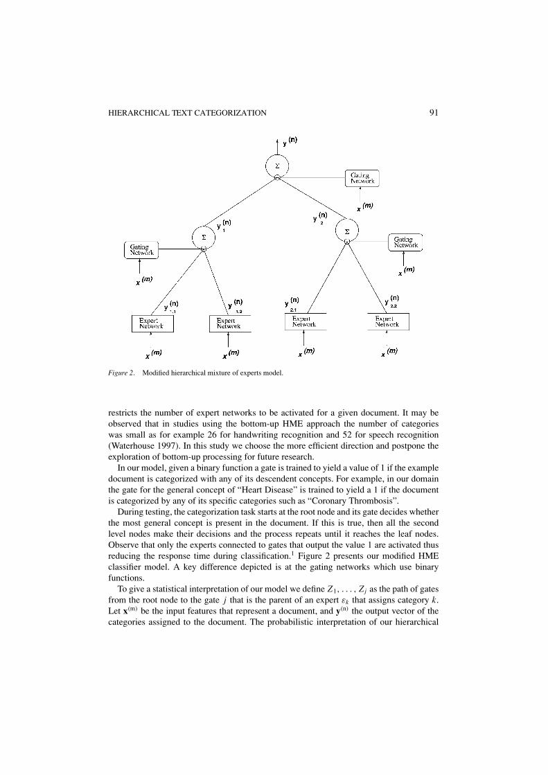
Figure 2. Modified hierarchical mixture of experts model.

restricts the number of expert networks to be activated for a given document. It may beobserved that in studies using the bottom-up HME approach the number of categorieswas small as for example 26 for handwriting recognition and 52 for speech recognition(Waterhouse 1997). In this study we choose the more efficient direction and postpone theexploration of bottom-up processing for future research.

In our model, given a binary function a gate is trained to yield a value of 1 if the exampledocument is categorized with any of its descendent concepts. For example, in our domainthe gate for the general concept of “Heart Disease” is trained to yield a 1 if the documentis categorized by any of its specific categories such as “Coronary Thrombosis”.

During testing, the categorization task starts at the root node and its gate decides whetherthe most general concept is present in the document. If this is true, then all the secondlevel nodes make their decisions and the process repeats until it reaches the leaf nodes.Observe that only the experts connected to gates that output the value 1 are activated thusreducing the response time during classification.1 Figure 2 presents our modified HMEclassifier model. A key difference depicted is at the gating networks which use binaryfunctions.

To give a statistical interpretation of our model we define Z1, . . . , Zj as the path of gatesfrom the root node to the gate j that is the parent of an expert εk that assigns category k.Let x(m) be the input features that represent a document, and y(n) the output vector of thecategories assigned to the document. The probabilistic interpretation of our hierarchical


Figure 3. Example of a backpropagation network with 5 inputs.

model is as follows:

P(y(n)

∣∣ x(m)) =

n∑

k=1

P(Z1 = 1

∣∣ x(m))P

(Z2 = 1

∣∣ Z1 = 1, x(m)). . .

P(Z j = 1

∣∣ Z1 = 1, . . . , Z j−1 = 1, x(m))P

(εk = 1

∣∣ x(m))

The hierarchical structure in a HME model is predefined2 in our case by the hierarchyof the “Heart Disease” subset of the UMLS classification system. Moreover, the HMEhierarchy is generally limited to the classes that appear in the training set. Given our trainingset (described later) we are able to use only 103 concepts of the 119 in the “Heart Disease”subset.

There are several alternatives for training a HME model. Jordan and Jacobs (1993)and Waterhouse (1997) use a method based on expectation maximization. They assumethat the classification follows a multinomial model, which implies that an object can beassigned to one and only one of the multiple categories available for classification. This isa 1-of-K classification task which may be viewed as a competition problem. In contrast,we are interested in a k-of-K (multi-way) classification problem which is equivalent to kindependent 1-of-2 classifications (McCullagh and Nelder 1989, Rumelhart et al. 1996). Toallow for multi-way classification we use backpropagation neural networks in both gates andexperts and use a gradient descent method for training. The gates are trained to recognize


whether or not any of the categories of their descendants is present in the document. Theexperts are trained to recognize the presence or absence of particular categories.

The backpropagation networks that we use have three layers (see figure 3). We havetested several configurations and these results will be discussed in detail later. In general,our neural networks have m nodes in the input layer corresponding to the set of m featuresselected for each expert (or gate), the middle layer has n nodes, and the output layer isa single node. In this case the sigma nodes are responsible for combining the outputs ofthe gate i and expert j to obtain the kth component yk = gi yi · j (where k = 1..n) of theoutput Y (n)

i at each intermediate node of the HME. Observe that the general model allowsfor experts to have an output vector of size n. Our implicit assumption for this paper is thateach category assignment is independent.

Given an appropriate set of features and a training set of manually categorized documents,the backpropagation network learns to make the appropriate decisions. Observe that forexperts and gates the set of positive examples is different. The set of positive examples forthe experts is a subset of the positive examples of any ancestor gate. As a consequence, twoidentical neural networks trained with these different subsets learn different probabilisticfunctions. The backpropagation neural network as an expert node learns to use the inputto estimate the desired output value (category), while as a gate it computes the confidencevalue of the combined outputs of its children.

3. Implementation of the HME

We want to build a classifier that is able to effectively use the structured knowledge con-tained in the UMLS Metathesaurus (National Library of Medicine 1999). In particular weare interested in the hierarchical relationships which link general concepts to the morespecific ones. The 1999 UMLS Metathesaurus contains about 350, 000 concepts collectedby combining 79 vocabularies for the health sciences. In this study we limit ourselves toMeSH (Medical Subject Headings)3 which is one of the 79 vocabularies. Since documentsin the OHSUMED test collection are a subset of MEDLINE, they have been manuallycategorized with MeSH terms. Each MEDLINE document is assigned between 8 and 10MeSH concepts. Thus our categorization task is a multi-way classification problem. In ourmodel the gates represent the general concepts of this hierarchy.

Interestingly, the manual assignment of a high level MeSH category is not automaticallydetermined by the assignment of its lower level categories. That is, the fact that a documentis assigned the category “angina unstable” does not automatically grant it the assignmentof any of the ancestors in the tree (“Heart diseases”, “Myocardial Ischemia”, “CoronaryDiseases”, or “Angina Pectoris”). In fact the manual assignment of such high level categoriesis usually done when the MEDLINE document is about the topic at the associated level ofgenerality or abstraction. Therefore in our model, each nonterminal node is represented bytwo networks. The first is the expert network for the node’s category while the second is agating network representing the general concept at that level of the classification scheme.Thus at the “Heart Diseases” node there is a gate that learns to recognize the general concept(representing all the documents that are about any of its descendants), and an expert networkthat learns to assign this specific category “Heart Diseases”. Note that from this point on


Figure 4. A part of the UMLS hierarchy for the heart diseases subtree.

unless explicitly specified, we mean both categories and concepts when we use the word‘category’.

For the purpose of comparing results with other studies we will show the results obtainedusing only the MeSH subtree of “Heart Diseases”. (Figure 4 shows a part of this hierarchy).However, our method especially given its top-down processing, is general and can be appliedto the whole set or to any other subset of the UMLS.

4. Feature selection

In text categorization the set of possible input features consists of all the different wordsthat appear in a collection of documents. This is usually a large set since even small textcollections could have hundreds of thousands of features. Reduction of the set of featuresto train the neural networks is necessary because the performance of the network and the


cost of classification are sensitive to the size and quality of the input features used to trainthe network (Yang and Honovar 1998). A first step towards reducing the size of the featureset is the elimination of stop words, and the use of stemming algorithms. Even after that isdone the set of features is typically too large to be useful for training a neural network.

Two broad approaches for feature selection have been presented in the literature: thewrapper approach, and the filter approach (John et al. 1994). The wrapper approach attemptsto identify the best feature subset to use with a particular algorithm. For example, for a neuralnetwork the wrapper approach selects an initial subset and measures the performance ofthe network; then it generates an “improved set of features” and measures the performanceof the network. This process is repeated until it reaches a termination condition (either aminimal value of performance or a number of iterations). The filter approach, which is morecommonly used in text categorization, attempts to assess the merits of the feature set fromthe data alone. The filtering approach selects a set of features using a preprocessing step,based on the training data. In this paper we use the filter approach, but we plan to explorethe wrapper approach in future research. We select three methods that have been used inprevious works: correlation coefficient, mutual information, and odds ratio. During featureselection we first delete all instances of 571 stop words from the MEDLINE records, andthen use Porter’s algorithm to stem the remaining words. We eliminate those stems thatoccur in less than 5 documents in the training collection. Since feature selection is done foreach category, based on its zone (explained later) we also remove stems that occur in lessthan 5% of the positive example documents. We then rank the remaining stems by the featureselection measure and select a pre-defined number of top ranked stems as the feature set.

4.1. Correlation coefficient

Correlation coefficient C is a feature selection measure proposed by Ng et al. (1997) and isdefined as:

C(w, c) = (Nr+Nn− − Nr−Nn+)√

N√(Nr+ + Nr−)(Nn+ + Nn−)(Nr+ + Nn+)(Nr− + Nn−)

(5)

where Nr+(Nr−) is the number of positive examples of category c in which feature w

occurs(does not occur), and Nn+(Nn−) is the number of negative examples of category cin which feature w occurs(does not occur). This measure is derived from the χ2 measurepresented by Schutze et al. (1995), where C2 = χ2. The correlation coefficient can beinterpreted as a “one-side” χ2 measurement. The χ2 measure has been reported as a goodmeasure for text categorization by Yang and Pedersen (1997). The correlation coefficientpromotes features that have high frequency in the relevant examples but are rare in the nonrelevant documents. When features are ranked by this method, the positive values correspondto features that indicate presence of the category while the negative values indicate absenceof the category. In contrast, the χ2 ranks features higher if they more strongly indicate thepresence or the absence of a category. That is, more ambiguous features are ranked lower.We compared the χ2 and correlation coefficient for feature selection using neural networkswith the same architecture. We found that the neural networks trained with features selected


using correlation coefficient outperformed those trained using χ2 in 78 out of 103 categories.This confirms similar results reported by Ng et al. (1997). Note that Yang and Pedersen(1997) use an average of the χ2 value across categories to measure the goodness of a termin a global sense, while we use it for local (category-level) feature selection.

In contrast with mutual information, both χ2 and correlation coefficient produce nor-malized values because they are based on the χ2 statistic. However, the normalization doesnot hold for low populated cells in the contingency table. This makes the scores of χ2 andcorrelation coefficient for low frequency terms unreliable. This is one reason for removingrare features as described before.

4.2. Mutual information

Mutual information is a measure that has been used in text categorization by several re-searchers (Schutze et al. 1995, Yang and Pedersen 1997). This method is based on the mutualinformation concept developed in information theory. For a feature w and a category c it isdefined as:

I (w, c) = logP(w ∧ c)

P(w) × P(c)(6)

where P(w) is the probability of the term w occurring in the whole collection, P(c) is theprobability of the category c occurring in the whole collection, and P(w ∧ c) is their jointprobability.

Yang and Pedersen (1997) used mutual information4 to measure the goodness of a termin a global feature selection approach by combining the category specific scores of a termin two ways:

Iavg(w) =n∑

i=1

P(ci )I (w, ci ) (7)

Imax(w) = nmaxi=1

{I (w, ci )} (8)

where n is the number of categories.In contrast, we use feature selection to evaluate the goodness of a term with respect to

individual categories. In other words, we do not average the values of mutual informationover multiple categories. This variation may be sufficient to produce the different resultsthat we obtain (described later). Yang and Pedersen also point out that the score producedby mutual information is strongly influenced by the marginal probabilities of terms. This isevident from the following equivalent formula:

I (w, c) = log P(w | c) − log P(w) (9)

For terms with equal conditional probability P(w | c), rare terms will have higher scoresthan common terms. This implies that the scores of terms with extremely different


Figure 5. Graph of odds ratio. The x axis represents P(w | pos), while the y axis represents the P(w | neg).

frequencies might still not be comparable. Our frequency threshold described earlier, com-pensates for this effect.

4.3. Odds ratio

Odds ratio was proposed originally by van Rijsbergen et al. (1979) for selecting termsfor relevance feedback. Odds ratio is used for the binary-valued class problem where thegoal is to make a good prediction for one of the class values (Rijsbergen et al. 1979). Itis based on the idea that the distribution of features on the relevant documents is differentfrom the distribution of features on the non-relevant documents. It has been recently usedby Mladenic (1998) for selecting terms in text categorization. The odds ratio of a featurew, given the set of positive examples pos and negative examples neg for a category c, isdefined as follows:

OddsRatio(w, c) = logP(w | pos)(1 − P(w | neg))

(1 − P(w | pos))P(w | neg)(10)

Observe that this formula can also be interpreted as the sum of the logarithm of theratios of the distribution of the feature on the relevant documents (log P(w | pos)

(1−P(w | pos)) ) and onthe non-relevant documents (log (1−P(w | neg))

P(w | neg)). If a document appears in more than half of

the relevant documents the logarithm of the ratio on the relevant documents is positive. Incontrast a feature is penalized if it appears in more than half of the non-relevant documents.In other words, a feature that appears frequently in the relevant documents and infrequentlyin the non relevant documents will have a high score. Figure 5 shows a graph of the oddsratio. The function presents singularity points when P(w | pos) = 1 or when P(w | neg) = 0(we map this case to the highest positive value). Also the logarithm is not defined whenP(w | pos) = 0 or when P(w | neg) = 1 (we map this case to the smallest negative value).

Mladenic (1998) report that odds ratio was the most successful feature selection methodfor a hierarchical Bayesian classifier compared to mutual information, cross entropy, infor-mation gain, and weight of evidence.


In this study we select features for both expert and gating networks using correlationcoefficient, mutual information and odds ratio methods.

5. Training set selection

A supervised learning algorithm requires the use of a training set in which each elementhas already been correctly categorized. One would expect that the availability of a largetraining set (such as OHSUMED) will be beneficial for training the algorithm. In practicethis does not seem to be the case. The problem occurs when there is also a large collectionof categories with each assigned to a relatively small number of documents. This thencreates a situation in which each category has a small number of positive examples and anoverwhelming number of negative examples. When a machine learning algorithm is trainedto learn the assignment function with such an unbalanced training set, the algorithm willlearn that the best decision is to not assign the category. The overwhelming amount ofnegative examples hides the assignment function. To overcome this problem an appropriateset of training examples must be selected. We call this training subset the “category zone”.This notion of category zone is similar to the local regions described in Wiener et al. (1995),and Ng et al. (1997) but is inspired by the query zone proposed by Singhal et al. (1997) fortext routing. Their “query zoning” is based on the observation that in a large collection aquery will have a set of documents that constitutes its domain. Non-relevant documents thatare outside the domain are easy to identify, but it is more difficult to differentiate betweenrelevant and non-relevant documents within the query domain. Singhal et al. (1997) definea procedure that tries to approximate the domain of the query and then they use this domainto train their routing method. We suggest that in text categorization, each category also hasits own domain. It will be easier to train a learning algorithm with those documents fromthe category domain and also potentially achieve better categorization performance. Weexplore two different methods for building the category zone. The first method creates thecategory zone using a method similar to that presented by Singhal et al. (1997). This firstcategory zone that we call centroid-based is created as follows:

1. Take all the positive examples for a category and obtain their centroid.2. Using this centroid as a query perform retrieval and obtain the top 10, 000 documents.

This subset will contain most if not all of the positive examples and many negativeexamples that are at least “closely related” to the domain of the category.

3. Obtain the category zone by adding any unretrieved positive examples to the set obtainedin the previous step.

This method creates category zones that have at least 10, 000 documents and the sizeincreases for categories that have positive examples outside the retrieved set.

The second method for creating the category zone uses a Knn approach in which thecategory zone consists of the set of K nearest neighbors for each positive example of thecategory. This method will produce variable sized category zones. We explored severalvalues of K (10, 50, 100 and 200). Our main concern with this method was to obtain atraining set large enough to train a neural network without overfitting.


Figure 6. Example record from OHSUMED.

6. Experimental collection

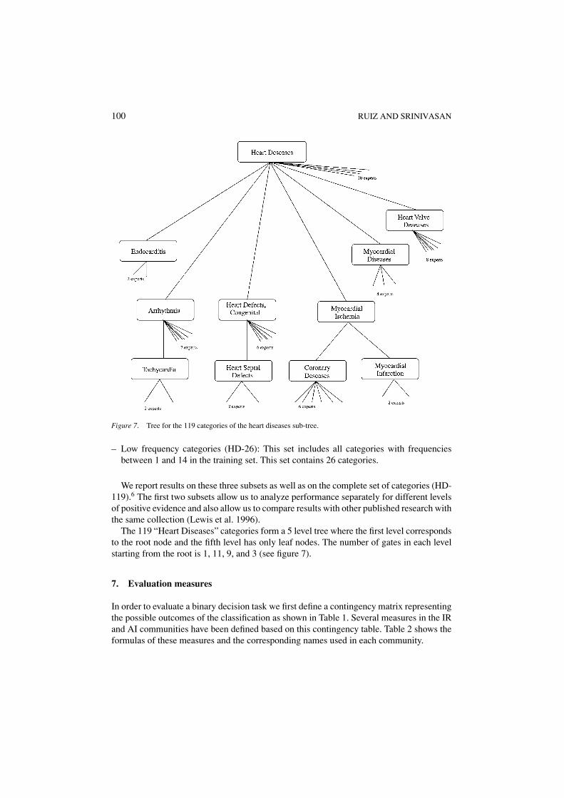
We use the OHSUMED collection created by Hersh and his collaborators (Hersh et al. 1994).This collection has 348, 543 records from the MEDLINE collection from 1987 to 1991.Each record from this collection has several fields (see figure 6). We use the following: title(.T), and abstract (.W). In the training set we also use the MeSH (.M) field which representsthe manual categorization decisions for the MEDLINE documents. We selected the 233, 455records that have titles, abstracts and MeSH categories (the remaining do not have abstracts).The first four years of data dated 1987 through 1990 (183,229 records) are used for training,and the year 1991 (50,216 records) is used for testing. This corresponds to the same split asused by Lewis et al. (1996). We also use the 119 categories from the Heart Disease subtreeof the Cardiovascular Diseases tree structure of the UMLS.5 However, only 103 of these119 categories have positive examples in the training set. Thus we limit our experiments tothese 103 categories. We further divide this set of 103 categories into three sets:

– High frequency categories (HD-49): This includes all categories with at least 75 examplesin the training set. This set contains 49 categories (which is the same as the set of highfrequency categories used by Lewis et al.).

– Medium frequency categories (HD-28): This set includes all categories with frequenciesbetween 15 and 74 in the training set. This set contains 28 categories (this is equivalentto the second set of categories used by Lewis et al.).


Figure 7. Tree for the 119 categories of the heart diseases sub-tree.

– Low frequency categories (HD-26): This set includes all categories with frequenciesbetween 1 and 14 in the training set. This set contains 26 categories.

We report results on these three subsets as well as on the complete set of categories (HD-119).6 The first two subsets allow us to analyze performance separately for different levelsof positive evidence and also allow us to compare results with other published research withthe same collection (Lewis et al. 1996).

The 119 “Heart Diseases” categories form a 5 level tree where the first level correspondsto the root node and the fifth level has only leaf nodes. The number of gates in each levelstarting from the root is 1, 11, 9, and 3 (see figure 7).

7. Evaluation measures

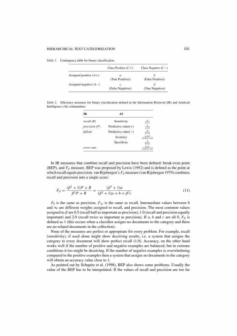
In order to evaluate a binary decision task we first define a contingency matrix representingthe possible outcomes of the classification as shown in Table 1. Several measures in the IRand AI communities have been defined based on this contingency table. Table 2 shows theformulas of these measures and the corresponding names used in each community.


Table 1. Contingency table for binary classification.

Class Positive (C+) Class Negative (C−)

Assigned positive (A+) a b(True Positives) (False Positives)

Assigned negative (A−) c d(False Negatives) (True Negatives)

Table 2. Efficiency measures for binary classification defined in the Information Retrieval (IR) and ArtificialIntelligence (AI) communities.

IR AI

recall (R) Sensitivity aa+c

precision (P) Predictive value(+) aa+b

fallout Predictive value(−) bb+d

Accuracy a+da+b+c+d

Specificity db+d

error rate b+ca+b+c+d

In IR measures that combine recall and precision have been defined: break-even point(BEP), and Fβ measure. BEP was proposed by Lewis (1992) and is defined as the point atwhich recall equals precision. van Rijsbergen’s Fβ measure (van Rijsbergen 1979) combinesrecall and precision into a single score:

Fβ = (β2 + 1)P × R

β2 P + R= (β2 + 1)a

(β2 + 1)a + b + β2c(11)

F0 is the same as precision, F∞ is the same as recall. Intermediate values between 0and ∞ are different weights assigned to recall, and precision. The most common valuesassigned to β are 0.5 (recall half as important as precision), 1.0 (recall and precision equallyimportant) and 2.0 (recall twice as important as precision). If a, b and c are all 0, Fβ isdefined as 1 (this occurs when a classifier assigns no documents to the category and thereare no related documents in the collection).

None of the measures are perfect or appropriate for every problem. For example, recall(sensitivity), if used alone might show deceiving results, i.e. a system that assigns thecategory to every document will show perfect recall (1.0). Accuracy, on the other handworks well if the number of positive and negative examples are balanced, but in extremeconditions it too might be deceiving. If the number of negative examples is overwhelmingcompared to the positive examples then a system that assigns no documents to the categorywill obtain an accuracy value close to 1.

As pointed out by Schapire et al. (1998), BEP also shows some problems. Usually thevalue of the BEP has to be interpolated. If the values of recall and precision are too far


then BEP will show values that are not achievable by the system. Also the point whererecall equals precision is not informative and not necessarily desirable from the user’sperspective.

van Rijsbergen’s F measure is the best suited measure, but still has the drawback that itmight be difficult for the user to define the relative importance of recall and precision. Wereport F1 values because it allows us to compare results with other researchers who haveused the same dataset (Lam and Ho 1998, Lewis et al. 1996, Yang 1996). In general the F1

performance is reported as an average value. There are two ways of computing this average:macro-average, and micro-average. With macro-average the F1 value is computed for eachcategory and these are averaged to get the final macro-averaged F1. With micro-averagewe first obtain the global values for the true positive, true negative, false positive, and falsenegative decisions and then compute the micro-averaged F1 value using the micro-recalland micro-precision (computed with these global values). The results reported in this paperare macro-averaged F1. This allows us to compare our results with those of other researchersworking with the OHSUMED dataset.

8. Experiments

There are two main questions that we address in this research (1) Does a hierarchicalclassifier built on the HME model improve performance when compared to a flat classifier?(2) How does our hierarchical method compare with other text categorization approaches?With these two research questions in mind we present a series of experiments using theOHSUMED collection.

8.1. Baselines

Our first baseline represents a classical Rocchio classifier which is described in the nextsection. Our second baseline is a flat neural network classifier. Comparing the performanceof the HME classifier against the flat classifier will allow us to answer our first researchquestion. Comparing the HME method with a Rocchio classifier as well as with otherpublished results will allow us to answer our second research question. Thus we haveimplemented a Rocchio classifier, a HME classifier, and a flat neural network classifierwhich are detailed next.

8.2. Rocchio classifier

Rocchio’s algorithm was developed in the mid 1960’s to improve queries using relevancefeedback. It has proven to be one of the most successful feedback algorithms. Rocchio(1971) showed that the optimal query vector is the difference vector of the centroid vectorsfor the relevant and the non-relevant documents. Salton and Buckley (1995) included theoriginal query (Qorig) to preserve the focus of the query, and added coefficients (α, β and γ )


to control the contribution of each component. The mathematical formulation of this versionis:

�Qnew = α �Qorig + β1

R

∑

d∈rel

�d − γ1

N − R

∑

d /∈rel

�d (12)

where �d is the weighted document vector, R = |Rel| is the number of relevant documents,and N is the total number of documents. Any negative components of the final vector �Qnew

are set to zero. Several techniques have been proposed to improve the effectiveness ofRocchio’s method: better weighting schemes (Singhal et al. 1996), query zoning (Singhalet al. 1997), and dynamic feedback optimization (Buckley and Salton 1995).

As pointed out by Schapire et al. (1998) most of the studies that use Rocchio as a baselinehave constructed a weak version of the classifier (Lam and Ho 1998, Lewis et al. 1996, Yang1996,1999). They also show that a properly optimized Rocchio’s algorithm could achievequite competitive performance. We have noticed that Rocchio’s classifiers benefit from anoptimal feature selection step. To make a fair comparison between the neural networksand the Rocchio classifiers we use the set of features selected using correlation coefficientand the same category zones used to train the neural network classifiers for each category.Observe that this is an important difference with respect to previously published researchthat use Rocchio classifiers (in all these studies the vector is computed over the whole set offeatures). Since we use feature selection measures that select features indicative of presenceof the category, each classifier has its centroid vector defined in a different subspace (thesub-space of the selected features) generated from the category zone.

We build a Rocchio classifier by presenting training examples from the category zoneand computing the weights of the classifier using Rocchio’s formula. We then rank the fulltraining collection according to the similarity with this classifier vector. A threshold (τ ) onthe similarity value that maximizes the F1 measure (described in the evaluation measuressection) is selected. The optimal Rocchio classifier for a category is then a weighted vectorof selected features along with a similarity threshold.

During the evaluation phase we compute similarity between the optimal Rocchio clas-sifier vector and the test document vectors and assign the class to all documents above thethreshold τ .

8.3. Hierarchical mixture of experts

Our HME approach is represented in figure 2. First a zone of domain documents is identifiedfor each category as explained before. Next feature selection is applied within each categoryzone to extract the “best” set of features. We tested all three feature selection methods inour experiments. Then for each expert network a backpropagation neural network is trainedusing the corresponding category zone and the selected set of features. Similarly, eachgating network is also a backpropagation network. However a gate’s training subset is thecombined category zones of its descendants in the classification hierarchy. Feature selectionfor the gate is then performed on its combined subset. This strategy of combining zonesfrom descendent nodes for a gate is reasonable if we consider the fact that gates representhierarchical concepts and not particular categories as described before in Section 3.


The input feature vectors for documents are weighted using t f × id f weights where t fis the frequency of the term in the document, and id f is the inverse document frequencydefined as:

idf = logN

n(13)

where N is the total number of documents in the training collection, and n is the numberof documents that contain the term in the training collection.

Experts and gates are trained independently using the following parameters: learningrate = 0.5, error tolerance = 0.01, maximum number of epochs = 1, 000. These parametervalues are fixed for all our experiments. The training of each network takes between 15to 30 minutes for an expert (depending on the number of examples), and around 60 to 90minutes for a gating network using a HP-700 workstation. Using 15 workstations and adynamic scheduling program specifically designed for this task we trained the 103 expertsand the 21 gating networks in about 8 hours.

Once experts and gates have been trained individually we assemble them according tothe UMLS hierarchical structure. Since the output of each network is a real value be-tween 0 and 1, we need to transform each output value into a binary decision. This stepis called thresholding. We do this by selecting thresholds that optimize the F1 values forthe categories. We use the complete training set to select the optimal thresholds. Sincewe are working with a modular hierarchical structure we have several choices to per-form thresholding. Our approach is to make a binary decision in each of the gates andthen optimize the threshold on the experts using only those examples that reach the leafnodes.

Observe that computing the optimal thresholds for binary decisions at the gates and theexperts is a multidimensional optimization problem. We decided to optimize the gates bygrouping them into levels and finding the value of the threshold at each level that maximizesthe average F1 value for all the experts. Each expert’s threshold is then optimized to maxi-mize the F1 value of the examples in the training set that reach the expert. In order to constrainthe potentially explosive combination of parameters we decide to fix the thresholds for thegates across all our experiments. For this purpose we conducted a preliminary experimentin which we search the best combination of thresholds per level varying each threshold onfixed values and computing performance on the whole training set. The optimal thresholdswere set to 0.01, 0.005, 0.01 and 0.01 for levels 1(root), 2, 3 and 4 respectively. These valueswere obtained by selecting the best results over 1, 764 threshold combinations (0.005, 0.01,0.05, and 0.10 for level 1, 0.005, 0.01, 0.05, 0.10, 0.15, 0.20, . . . 0.95 for levels 2, 3 and 4).7

This experiment was run using correlation coefficient for feature selection and a standardconfiguration of 25 input nodes and 50 hidden nodes. The best threshold are fixed across allruns.

The test set is processed using the trained networks assembled hierarchically with theestablished thresholds for each level of gates and each expert network.


8.4. Flat neural network classifier

In order to assess the advantage gained by exploiting the hierarchical structure of theclassification scheme, we built a flat neural network classifier. We decided to build a flatmodular classifier that is implemented as a set of 103 individual expert networks. This issimilar to our Rocchio model where the training phase results in a set of 103 classifiervectors. In this model the experts are trained independently using the optimal feature setand the category zone for each individual category. The thresholding step is performed byoptimizing the F1 value of each expert using the entire training set. These are the valuesthat we report in the next section for the flat neural network classifier. Observe also that theuse of this model allows us to assess the contribution of adding the hierarchical structure,i.e., our first research question.

9. Results

As stated before, we report results on the “Heart Diseases” sub-tree. We present resultson this set of 103 categories (HD-119) and on three frequency-based subsets of categoriesHD-49, HD-28 and HD-26 as defined in Section 6.

9.1. Effect of feature selection and the neural network architecture

It may be observed that network architecture and feature selection methods must be studiedin combination. In fact, at a basic level feature selection is one of the factors that define theconfiguration of the network. Given the many complex combinations in terms of featureselection methods and numbers of nodes in the different layers for both the expert andgating networks we approach the problem in stages. We follow a top-down approach thatoptimizes the gates and then the experts.

First we focused our attention on the gating networks. We used experts with 25 inputfeatures and 50 nodes in the hidden layers. We then explored 5, 10, 25, 50, 100, and 150input features for the gating networks with hidden layer that had twice the number of inputnodes. We also tried all three different feature selection methods (Mutual Information, OddsRatio and Correlation Coefficient). This experiment was done only on the “high frequencycategories” (HD-49) because they allow appropriate training of the neural networks andalso because the variance between different training runs is smaller than the variance forlower frequency categories.

Interestingly the differences between the three feature selection methods on the gatingnetworks are not significant. Thus we only report results on the 18 different combinationsobtained using correlation coefficient in the gates. Table 3 shows an increase in perfor-mance between 5 and 25 features and a slight decrease for networks with larger number ofinput nodes. It is possible for this slight decrease to be caused by the limit in the numberof iterations (1, 000) that a network was allowed to run during training. Usually a largernetwork needs more iterations on the training set to converge to an optimal value. Observethat all the three feature selection methods show no significant differences either for thegates or for the expert networks. This was somewhat surprising since Yang and Pedersen


Table 3. Effect of the number of input nodes to the gating networks and the feature selection methods for theexpert networks (the feature selection method for the gating networks is correlation coefficient).

Expert networks

Gating networksNo. of inputs Corr. coef. Odds ratio Mutual inf.

5 0.4455 0.4531 0.4589

10 0.4604 0.4695 0.4712

25 0.4984 0.4961 0.4956

50 0.4894 0.4903 0.4900

100 0.4894 0.4929 0.4840

150 0.4827 0.4890 0.4850

Flat 0.4449 0.4488 0.4548

All expert networks have 25 input features selected by the indicatedfeature selection method, 50 nodes in the middle layer, and 1 output.The last row shows performance of the flat classifier. (Performanceis measured in macro-averaged F1 on the HD-49 set.)

(1997) reported that mutual information does not perform well compared to other meth-ods. As noted before, instead of averaging values across multiple classes to find the meritof the features from a global perspective, we use mutual information for local feature se-lection. We also discard rare terms that will in general be ranked very high by mutualinformation.

We further explored feature selection using mutual information by running our experi-ments without discarding rare terms and selecting the top 25 features. The average precisionfor the HD-49 subset was 0.05 and 0.20 for the flat neural network and the HME modelrespectively. This is significantly lower than the performance obtained when we discard lowfrequency terms and shows conclusively that mutual information alone is not a good featureselection measure unless we address its major weakness and discard low frequency terms.This might also be addressed by selecting a larger number of input features. However, thiswill go against our goal of reducing the number of input features to improve training andprocessing time for the neural networks.

After optimizing the gates we address the number of input nodes for the expert networksby exploring them individually, i.e., independent of the hierarchical structure. We testedexpert networks with 5, 10, 25, 50, 100, and 150 input features. In each case we used twicethe number of input nodes for the hidden layer and three feature selection methods. Thebest result was obtained using 25 input features with 50 nodes in the hidden layer.

Having determined the optimal number of inputs, next we explore the effect of the sizeof the hidden layer for our networks. (Note that so far we have only explored the simplestrategy of having twice the input nodes in the middle layer.) Table 4 shows the variationsin performance with different sizes of the middle layer. In this case all networks have 25inputs and a single output node. The best performance is obtained with expert networks thathave 6 nodes in the hidden layer. The difference between 6 and 10 nodes is relatively small.We ran similar experiments on the gating networks varying the size of the middle layer


Table 4. Effect of the number of hidden nodes on the expert networks.

No. of hidden nodes Flat NN HME

6 0.5033 0.5241

10 0.4807 0.4975

25 0.4320 0.4824

50 0.4479 0.4867

All expert networks have 25 input features se-lected with the correlation coefficient feature se-lection method. (Performance is measured bymacro-averaged F1 on the HD-49 set.)

Table 5. Effect of the number of hidden nodes on the gating networks.

No. of hidden nodes HME

6 0.5219

10 0.5202

25 0.5241

50 0.5158

All expert networks have 25 inputfeatures and 6 hidden nodes. Thegates have 25 inputs selected withcorrelation coefficient(Performanceis measured by macro-averaged F1

on the HD-49 set.)

(6, 10, 25, 50) and found that the best size of the hidden layer was 25 (Table 5). However,the difference between these runs is very small. Observe also that the flat neural networkshave their best performance when the number of nodes in the hidden layer is 6. This isnot surprising since a smaller hidden layer tends to produce a better generalization of eachcategory.

In the following sections we present results using neural networks with 25 inputs, 6hidden nodes and 1 output for the experts and 25 inputs, 25 hidden nodes and 1 output forthe gating network.

9.2. Comparing the category zone methods

As mentioned before, we explore two different types of category zones: The centroid-basedcategory zone and the Knn-based category zone. We compare these two zoning strategieswith respect to their zone sizes as well as classifier performance.

The centroid-based category zone generates zones that have at least 10,000 examples.For our training set of 103 categories we found that this type of category zone has anaverage size of 10,027 with a maximum of 10,778 while 75% of the zones are below


Table 6. Comparison of categorization performance using the centroid-based and Knn-based category zones.

Centroid-based zone Knn-based zone

Flat NN HME Flat NN HME

HD-49 0.5033 0.5241 0.5042 0.5150

HD-28 0.3589 0.4304 0.3613 0.4159

HD-26 0.5653 0.5794 0.4599 0.4828

HD-119 0.4797 0.5126 0.4542 0.4798

Values are macro-averaged F1 over the respective set of cate-gories on the test set (50, 216 documents).

10,010. The Knn-based category zone generate zones with sizes proportional to the numberof positive examples in the category. We found that “compact” categories have in generalsmall category zones. We explore different values of K (10, 50, 100, and 200). Small valuesof K are problematic for low frequency categories because they tend to generate a very smalltraining set that the neural network overfits easily. Thus we settled for K = 200 because itproduces category zones large enough for the rare categories as well as zones of reasonablesize for the more frequent categories. For our 103 categories we found that the averagesize of the Knn-based category zone is 6,098 examples with a maximum of 35,917, and aminimum of 200. 75% of the category zones generated by this method are below 6,814. Asmentioned before the category zone for a gate is the union of the individual category zonesof its descendants in the hierarchy.

To measure the impact of each zoning method we trained both gating and expert networkswith the documents of the corresponding zones. The categorization results on the test set areshown in Table 6. There are small differences in performance across zones for classifiersin the high frequencies (HD-49) set and for those classifiers in the medium frequencies(HD-28) set. However, these differences are not statistically significant.

The low frequency categories (HD-26) show a statistically significant difference in favorof the centroid-based zones for both flat and hierarchical classifiers. A detailed analysisshowed that the high value of this difference is due in part to the contribution of somecategories that have one or zero examples in the test set. For these categories the functionbecomes more of a hit or miss function.8 Since these category zone training sets have at least10,000 examples the classifier learns to reject most of the documents and in consequence itgets an F1 value of 1.0 for most of them. In contrast, the Knn-based zones for low frequencycategories generate a smaller zone and the neural networks trained with them tend to assignat least a few documents. The classifiers trained with centroid-based zones outperform theKnn-based classifiers on 13 categories, while the classifiers trained on Knn-based zonesoutperform the centroid-based classifiers only on 5 categories (in the remaining 8 categoriesthere is no difference between them).

On the whole set HD-119 the classifiers trained with centroid-based zones outperformthose trained with the Knn-based zones. However this difference is statistically significantonly for the HME classifiers. Given our results with these two zoning methods we sug-gest that centroid-based category zones are the most appropriate for training hierarchical


Table 7. Comparison between the flat NN, HME and the optimized Rocchio classifiers.

Flat NN HME Opt-Rocchio

Macro HD-49 0.5033 0.5241 0.5491

Avg F1 HD-28 0.3589 0.4304 0.5176

HD-26 0.5653 0.5794 0.4524

HD-119 0.4797 0.5126 0.5161

Variance HD-49 0.02589 0.02298 0.02470

HD-28 0.06746 0.06773 0.05467

HD-26 0.17879 0.14583 0.16775

HD-119 0.08000 0.06754 0.06877

classifiers that span categories of varying frequencies. The same conclusion may be madefor flat classifiers but with somewhat reduced confidence.

9.3. Comparing HME, flat NN, and optimized Rocchio

Table 7 shows the performance of our flat neural network, the HME model and the optimizedRocchio classifier, all trained using the centroid-based zoning method and features selectedusing correlation coefficient. The HME classifier consistently outperforms the flat neuralnetwork classifier in all category sets. The difference is statistically significant for HD-29,HD-28 and HD-119. Another important feature that we must point out is that our HMEmodel has lower variance in performance in all the category sets. This result confirms thetheoretical claim by Jordan and Jacobs that soft splitting is a variance reduction method(Jordan and Jacobs 1993). This is in general a desirable property of a classifier since thisindicates performance that is more stable across categories. Comparing the HME againstthe optimized Rocchio classifier we note that Rocchio significantly outperforms the HMEon the HD-49 and HD-28 categories while the HME significantly outperforms Rocchio forthe HD-26 categories. However, there is no significant difference between both classifierson the HD-119 set. As suggested by a reviewer, the good performance of the Rocchioclassifier may in part be due to the particular combination of category zoning and featureselection methods used for our classifiers. To remind the reader, first a centroid-basedcategory zone is identified for each category. This zone of documents is then used forfeature selection. Although this approach is a “filter” approach (described in Section 4)the specifics of the centroid-based category zoning technique suggests that the approach ismore of a “wrapper” for the Rocchio classifier while it is definitely a “filter” for the neuralnet models. Unfortunately the expense of a wrapper approach for the neural net modelsprohibits us from further exploration of this aspect. This is one of the limitations of theneural net models. Our Rocchio results also emphasize the conclusion by Schapire et al.that when the Rocchio classifier is properly trained, it performs as well as other methods(Schapire et al. 1998). This result is in contrast with the performance of Rocchio classifiersobserved by other researchers (Lam and Ho 1998, Lewis et al. 1996, Yang 1999).


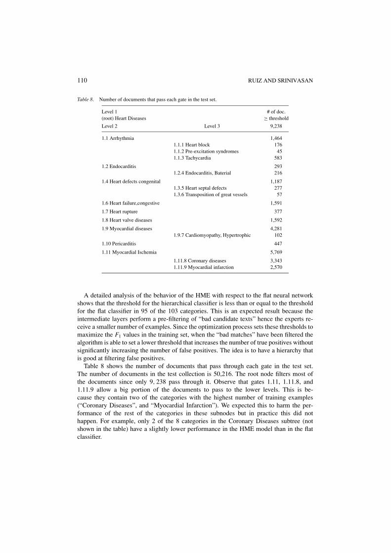
Table 8. Number of documents that pass each gate in the test set.

Level 1 # of doc.(root) Heart Diseases ≥ threshold

Level 2 Level 3 9,238

1.1 Arrhythmia 1,4641.1.1 Heart block 1761.1.2 Pre-excitation syndromes 451.1.3 Tachycardia 583

1.2 Endocarditis 2931.2.4 Endocarditis, Baterial 216

1.4 Heart defects congenital 1,1871.3.5 Heart septal defects 2771.3.6 Transposition of great vessels 57

1.6 Heart failure,congestive 1,591

1.7 Heart rupture 377

1.8 Heart valve diseases 1,592

1.9 Myocardial diseases 4,2811.9.7 Cardiomyopathy, Hypertrophic 102

1.10 Pericarditis 447

1.11 Myocardial Ischemia 5,769

1.11.8 Coronary diseases 3,3431.11.9 Myocardial infarction 2,570

A detailed analysis of the behavior of the HME with respect to the flat neural networkshows that the threshold for the hierarchical classifier is less than or equal to the thresholdfor the flat classifier in 95 of the 103 categories. This is an expected result because theintermediate layers perform a pre-filtering of “bad candidate texts” hence the experts re-ceive a smaller number of examples. Since the optimization process sets these thresholds tomaximize the F1 values in the training set, when the “bad matches” have been filtered thealgorithm is able to set a lower threshold that increases the number of true positives withoutsignificantly increasing the number of false positives. The idea is to have a hierarchy thatis good at filtering false positives.

Table 8 shows the number of documents that pass through each gate in the test set.The number of documents in the test collection is 50,216. The root node filters most ofthe documents since only 9, 238 pass through it. Observe that gates 1.11, 1.11.8, and1.11.9 allow a big portion of the documents to pass to the lower levels. This is be-cause they contain two of the categories with the highest number of training examples(“Coronary Diseases”, and “Myocardial Infarction”). We expected this to harm the per-formance of the rest of the categories in these subnodes but in practice this did nothappen. For example, only 2 of the 8 categories in the Coronary Diseases subtree (notshown in the table) have a slightly lower performance in the HME model than in the flatclassifier.


Table 9. Performance comparison between the flat NN, HME and Rocchio classifiers, and classifiers in Yang(1996) (Y) and Lewis et al. (1996) (L).

Lewis et al. (1996)

MethodYang (1996)

HD-119 HD-49 HD-28

Y:LLSF 0.55 – –

Y:ExpNet 0.54 – –

Y:STR 0.38 – –

L:Rocchio – 0.44 0.33

L:EG – 0.50 0.39

L:WH – 0.55 0.39

Flat NN 0.564 0.503 0.358

HME 0.557 0.524 0.430

Opt-Rocchio 0.558 0.549 0.518

9.4. Comparing results with other published works

The OHSUMED collection has been used by very few researchers for text categorization.Moreover, to the best of our knowledge only two studies have used its entire set of 14, 000MeSH categories (Lam et al. 1999, Yang 1996). The main reason for this is that manytext categorization methods do not scale to such a large dataset. Yang (1996), Lewis et al.(1996), and Lam and Ho (1998) have published results using the subset of categories fromthe “Heart Diseases” sub-tree (HD-119). This has become a standard set for comparingresults for text categorization in the OHSUMED collection. However, when reading thesethree works carefully we found that each paper uses a different test set and report resultson a different number of categories.

Lewis et al. use the set of 183, 229 documents from 1987 to 1990 for training and allthe 50, 216 documents from the year 1991 as a test set. Our experiments follow exactlythis partition with a further reduction for training (using zoning techniques) but the test setis the same. Table 9 shows that our flat neural network model performs at the same levelfor HD-49 and slightly worse for HD-28, as the Exponentiated Gradient (EG) algorithm inLewis et al. (1996). EG is the second ranked and the top ranked algorithm for HD-49 andHD-28 respectively in Lewis et al. (1996). (Note that the last three rows of the table showresults from our work that are most comparable). The HME model on the other hand showsa performance slightly lower (4.7%) than the top ranked Widrow-Hoff (WH) for HD-49but significantly higher than the best (10.2%) performance for HD-28. Both the flat NNand HME outperform the Rocchio classifier reported as a baseline by Lewis et al. (1996).Interestingly, our optimized Rocchio classifier performs at the same level as WH for HD-49but significantly better than all other classifiers for HD-28.

Yang (1996) conducts a very different experiment by reducing the collection to onlythose documents that are positive examples of the categories of the HD-119. This limits thetraining set to 12, 284 documents and the test set to 3, 760 documents. She explains that the


reason for such reduction is the scalability of the LLSF method which needs to compute aSingular Values Decomposition, a procedure that cannot be performed efficiently on a largematrix. However, this simplification creates a partition of the OHSUMED collection that isstructurally different from the one originally proposed by Lewis et al. In order to exploredifferences we used our trained classifiers on this reduced test set (with the same thresholdsas before). The results obtained are 0.525, 0.521 and 0.530 for the flat neural networks, theHME and optimized Rocchio respectively. Observe that for our hierarchical model, Yang’sreduction is equivalent to having a perfect classifier at the root node of the tree and thususing only gates at levels 2, 3 and 4. We then ran a second experiment where althoughwe did not retrain the neural networks or Rocchio classifiers on the reduced training set,threshold selection was done only on the set of 12, 824 positive examples in the training set(instead of using the whole set of 183, 229 documents of the training set) and the gates inlevels 2, 3 and 4 were used. The results for our flat neural networks, HME and optimizedRocchio classifiers on this reduced subset are 0.564, 0.557, and 0.558 respectively, scoreswhich are significantly higher than those we found using the Lewis et al. partition. Thesescores are about the same as the ones reported by Yang for the LLSF and ExpNet classifiers,and significantly above Yang’s baseline STR classifier. Interestingly the HME model doesnot outperform the flat neural network model in this constrained experiment. We lookedclosely at each category and found that this was due to the fact that our originally trainedgates discard documents that are relevant to their descendants which then impacts the finalperformance of the classifier. Although performance may be improved if we train the gatesusing only the set of positive examples,9 we believe that our original categorization task ismore realistic since we include both positive and negative examples in the test set.

Lam and Ho (1998) report results of experiments using the Generalized Instance Set(GIS) algorithm. They use the documents from 1991 and take the first 33,478 documentsfor training and the last 16,738 documents for testing. In contrast to Yang’s reduction, this ismore consistent with the partition proposed by Lewis et al. because it retains all documentsfrom the collection (not just the positive examples). Lam and Ho report results using microaveraged BEP on the set of 84 categories that have at least one example in both training andtest sets. We tested our previously trained HME model in this reduced test set and obtaineda micro-averaged BEP value of 0.502 which is significantly lower than their performanceof 0.572 for their GIS algorithm with Rocchio generalization. In future research we willtrain and test our HME model using their data set.

Joachims (1999) has also published results for the OHSUMED collection using supportvector machines. His work uses the first 20, 000 documents of the year 1991 dividing itinto two sets of 10, 000 documents each that are used for training and testing respectively.He reports impressive results but his text categorization task is very different from the onesin the previously discussed works. Joachims assumes that if a category in the UMLS treeis assigned then its more general category in the hierarchy is also present. Although this issimilar to our definition of gates, the difference is that he uses only the high level diseasecategories. This simplifies the categorization task considerably and probably explains thegood results obtained in the reported SVM experiments. The focus on general disease cate-gories alone prevents comparison of Joachims’ results with any of the previously publishedresults. We did not run our experiments limited to high level disease categories. However,


we consider that the use of SVM can be a good choice for building an architecture like theone we have proposed, and we plan to explore this in our future research.

We believe that the combination of category zoning and feature selection gives a signifi-cant boost to Rocchio performance. Optimized versions of the Rocchio classifier in previouswork have focused on query zoning and dynamic feedback optimization (Schapire et al.1998). We are not aware of any previous work on reducing the set of features used in thecentroid vector for text categorization purposes.10 Observe that our feature selection methodfavors features indicative of the presence of the category and discards features that indicatethe absence of the category. Feature selection has an important impact because similaritycomputation between the document and the centroid vector are made only on the subspaceformed by the selected features.

10. Comparison with related work in hierarchical categorization

We now focus on methods exploring the hierarchical structures of classification schemes.Koller and Sahami (1997) and Sahami (1998) proposed a hierarchical approach that

trains independent Bayesian classifiers for each node of the hierarchy. The classificationscheme then starts at the root and greedily selects the best link to a second level classifier.This process is repeated until a leaf is reached or until no child node is a good candi-date. Observe that their method selects a single path (the one with highest probability) andassigns all the categories in the path to the document. According to their approach, thehierarchical structure is used as a filter that activates only a single best classification path.Also errors in classification at the higher levels are irrecoverable in the lower levels. Theytested their results in the Reuters collection defining as higher nodes in the hierarchy thosecategories that subsume other categories. Although similar in spirit, our approach differsin the classification assignment model. We separate the identification of general conceptsfrom the assignment of general categories. Our approach also activates more than a singlepath in the hierarchy in contrast to their “the winner takes all” approach. There is also an ob-vious difference in the machine learning algorithm since they use Bayesian classifiers whilewe use neural networks. However in future work we plan to explore Bayesian classifierswithin the HME approach.

Ng et al. (1997) build their hierarchical classifier using perceptrons. Each node of thehierarchical tree is represented by a perceptron. They distinguish two types of nodes, leafnodes and non-leaf nodes. They apply this to the Reuters corpus where the categories reflecta geographical/topical hierarchy. Their hierarchy has as a first level all the possible countries,and for each country different topics are defined, e.g., economics and politics. The leaf nodesare specific categories of the second level (e.g., for economics they have communications,industry, etc.). The hierarchical classifier receives a document and checks whether it belongsto any of the first level nodes (the root node only connects to the different country nodes). Ifthe tested document activates any of the first level nodes, then the descendant categories ofthat node are tested recursively. If at any of the non-leaf nodes the process finds that none ofits children is a good candidate, then the categorization stops at that branch of the recursion.The output of the classifier is the final set of leaf nodes reached in the recursion (zero, oneor more). This is similar to the Pachinko machine proposed by Koller and Sahami (1997)


but with multiple outputs instead of a single output. Our approach is similar to Ng et al.(1997) in that we also use a top-down approach. The difference is in the type of classifier.We use non-linear classifiers in each node while they use linear classifiers. Although thecombination of the linear classifiers in the hierarchy creates a non-linear classifier somestudies have shown that this covers a limited number of non linear problems11 (Jordanand Jacobs 1993, Waterhouse 1997). Our approach also differs significantly in the wayfeature selection and subset training selection is done. Although their experiments also usecorrelation coefficient for feature selection their results for the hierarchical classifier arewell below other methods that use the Reuters collection. They report F1 values of 0.52 forthe best automatic feature selection method and 0.728 for the manually selected features(which is considerable lower than 0.85 (Yang 1999)). Their best results with the hierarchicalclassifier are obtained using manually selected features. We believe that their good resultsmay be a consequence of manual feature selection. Furthermore, our approach based oncategory zones combined with exploiting the hierarchy is more robust and allows us to getresults similar to some of the best methods reported in the literature.

McCallum and his collaborators have been working in text categorization specificallytargeting the problem of classifying web pages (McCallum et al. 1998). Their approachis based on Bayesian classifiers. They use the hierarchical classification structure to im-prove the accuracy of Bayesian classifiers using a statistical technique called shrinkage thatsmoothes parameter estimates of a child node with its ancestors in order to obtain morerobust estimates. The Bayesian classification schemes involve estimating the parameters ofthe model from the training collection and then applying the shrinkage method to improvethe estimates using the predefined hierarchy of categories. The classification of the test setis performed by computing the posterior probability of each class given the words observedin the test document, and selecting the class with the highest probability. Their experimentsshow that shrinkage improves the performance when the training data is sparse, reducingthe classification error by up to 29%. Our approach is totally different from McCallum’sapproach in terms of the classification method used, as well as the assumptions in the cat-egorization task. Observe that their approach assumes that a document belongs to a singlecategory and their model reflects it by selecting the most probable classification.

Mladenic (1998) also explored hierarchical structures using the Yahoo! hierarchy toclassify web pages. Her approach builds a Bayesian classifier. For each node in the subjecthierarchy a classifier is induced. To train each of the non-leaf classifiers a set of positiveexamples is defined as all the positive examples of the node (the intermediate nodes arealso valid categories) plus the positive examples of any descendants. These examples areweighted according to their position in the tree. The classification process works as describedbefore for the Bayesian classifiers with the set of categories with predicted probability≥0.95 are assigned. Our approach differs from Mladenic’s work in terms of the classifieralgorithms used, as well as the way in which the hierarchy is used for feature selection.Her main effort is in creating a weighting scheme for combining probabilities obtained atdifferent nodes of the tree.

The work on topic spotting by Wiener et al. (1995) inspired us to try our approach usingHME. During the review process of this article they published a sequel to their work appliedto hierarchical classifiers (Weigend et al. 1999). They use a meta-topic network using a two


level hierarchy for the Reuters collection and present results that are competitive with thoseof other methods. Our work differs from theirs in the definition of the gates (our gates behavelike binary filters while their meta-topic network helps more to weight the contribution ofthe experts). Our work also extends the hierarchical model to more than two levels an ideathat is suggested but not developed in Weigend et al. (1999). Finally, our evaluation onthe OHSUMED collection instead of the Reuters collection allows us to test the benefit ofexploiting a real hierarchical classification scheme.

We think that our main contribution is a general method for combining the hierarchicalstructure of a classification with feature selection and category zones. The zones containsmall but optimal subsets of documents that yield features suitable for training neuralnetworks. Our approach shows that even with a set of only 25 features per node, we can getresults that are comparable with other methods that use larger feature sets.12

11. Conclusions

This paper presents a machine learning method for text categorization that takes advantage ofpre-existing classification hierarchical structures. In response to our first research questionwe find that exploiting the hierarchical structure via the HME model increases performancesignificantly. In response to our second research question we find that although the HMEapproach is equivalent in performance to an optimized Rocchio approach for the full setof categories, the Rocchio approach is better for medium and high frequency categorieswhile HME is better for the remaining low frequency ones. In comparison with previousresults with the Rocchio classifier we find that the approach benefits from category zoningfor training set selection followed by feature selection. These results confirm the resultspublished by Schapire et al. (1998) that a carefully trained Rocchio algorithm might performas well as other more sophisticated methods.

Our method should scale to large test collections and vocabularies because it divides theproblem into smaller tasks that can be solved in shorter time. The top-down processingapproach tested here was selected specifically with scalability in mind. Category zoningis also very valuable for large collections since it counters the overwhelming presence ofnegative examples.

With respect to the feature selection methods tested, we found no significant differencein performance between correlation coefficient, odds ratio, and mutual information whenthey are used for local feature selection. In particular our results with mutual information,which has been reported before as a poor method when used for global feature selection(Yang and Pedersen 1997), point towards the importance of addressing the weaknesses offeature selection methods on low frequency terms.

To close, the results obtained by the HME model are comparable with those reportedpreviously in the literature, and significantly better than our flat neural network classifier.For future work we would like to try different ways to construct the hierarchical structuresuch as using support vector machines. We would also like to change the training strategyto use a variation of boosting adapted to the hierarchical approach. We also hope to improvethe performance of our classifier by adding richer features (i.e., n-grams, or phrases) thathave been reported to help in the text categorization process (Mladenic 1998). Finally, we


plan to explore whether the use of different classifiers, such as linear classifiers and SVMshow the same improvements obtained using neural networks.

Acknowledgement

We want to thank Professors David Eichmann, Ted Herman, Gregg Oden, and Alberto Segre,from The University of Iowa for their initial comments and feedback that encouraged us towrite this article. We also want to thank Dr. Fabrizio Sebastini and the two anonymous re-viewers for their excellent comments and suggestion that helped us to significantly improvethis article.

Notes

1. Hybrid neural trees have been proposed by d’Alche–Buc et al. (1994) using a method called Trio-Learning tobuild a decision tree whose nodes are neural networks. Trio-learning uses a decision tree algorithm to partitionthe examples into positive and negative classes and recursively builds the hierarchy. Similar to CART thismethod performs a “hard split” of the set of examples at each level. Observe that our model uses a predefinedhierarchical structure. Another difference is that we use a “soft split” of the data that allows overlappingclusters.

2. It should be noted that Waterhouse has proposed a HME model that dynamically generates the hierarchicalstructure (waterhouse 1997).

3. Observe that we could have used the MeSH hierarchy directly. We decided to use the UMLS hierarchy becauseit provides a conceptual mapping that has been extended to many areas of the health sciences.

4. There is some confusion with the term “mutual information”. For instance, it has been used by other researchers(McCallum et al. 1998) to refer to the measure that Yang and Pedersen (1997) present as “information gain”.

5. We use the 1994 version of the UMLS.6. We label this set HD-119 in order to stay consistent with the labeling in Yang (1996) even though there are

actually only 103 categories with positive examples in the training set.7. Since we only have two gates in level 4 we set their optimal values to the same values of the gates in level 3.

This gives us 4 × 21 × 21 = 1,764 possible combinations for the thresholds in the gates.8. Categories with no examples in the test set will have F1 = 0 if a document is assigned to the class or F1 = 1

if no documents are assigned to the class.9. In fact, in experimentation with Knn zoning which uses a smaller training set that more closely resembles the

positive examples, HME was better than the flat neural network classifier.10. During the review of this article two works that use feature selection in the context of a Rocchio approach

have been published. (Caropreso et al. 2001, Galavotti et al. 2000)11. This is due to the fact that the high level nodes can only create linear boundaries between adjacent expert

regions in the input space.12. Most (Ng et al. 1997, Weigend et al. 1999, Wiener et al. 1995) have used feature sets of 200 or more features

per category. In Lewis et al. (1996) the authors have used all features present in the collection.

References

Apte C, Damerau F and Weiss SM (1994) Automated learning of decision rules for text categorization. ACMTransactions on Information Systems, 3(12):233–251.

Bridle J (1989) Probabilistic interpretation of feedforward classification network outputs, with relationships tostatistical pattern recognition. In: Fogelman-Soulie F. and Herault J. Eds., Neuro-computing: Algorithms, Ar-chitectures, and Applications. Springer-Verlag, New York.


Breiman L, Friedman JH, Olshen RA and Stone CJ (1984) Classification and Regression Trees. WadsworthInternational Group, Belmont, CA.

Buckley C and Salton G (1995) Optimization of relevance feedback weights. In: Proceedings of the 18th AnnualInternational ACM SIGIR Conference on Research and Development in Information Retrieval, Seattle, WA,July 1995, pp. 351–357.

Caropreso MF, Matwin S and Sebastiani F (2001) A learner-independent evaluation of the usefulness of statisticalphrases for automated text categorization. In: Amita G. Chin Ed., Text Databases and Document Management:Theory and Practice. Idea Group Publishing, 2001, pp. 78–102.

Cohen W and Singer Y (1996) Context-sensitive learning methods for text categorization. In: Proceedings of the19th International ACM SIGIR Conference on Research and Development in Information Retrieval, Zurich,Switzerland, July 1996, pp. 307–315.

d’Alche–Buc F, Zwierski D and Nadal JP (1994) Trio-Learning: A tool for building hybrid neural trees. Interna-tional Journal of Neural Systems, 5(4): December 1994, pp. 259–274.

Galavotti L, Sebastiani F and Simi M (2000) Experiments on the use of feature selection and negative evidencein automated text categorization. In: Proceedings of ECDL-00, 4th European Conference on Research andAdvanced Technology for Digital Libraries, Lisbon, Portugal, pp. 59–68.

Hersh W, Buckley C, Leone TJ and Hickman D (1994) OHSUMED: An interactive retrieval evaluation and newlarge test collection for research. In: Bruce W. Croft and Van Rijsbergen CJ. Eds., Proceedings of the 17thAnnual International ACM SIGIR Conference on Research and Development in Information Retrieval, Dublin,Ireland, July 1994, pp. 192–201.

Joachims T (1997) Text categorization with support vector machines: Learning with many relevant features.Technical Report LS-8 Report 23, University of Dortmund, 1997.

Joachims T (1999) Estimating the generalization performance of a SVM efficiently. Technical report LS-8 Report25. Universitat Dortmund, Dortmund, Dec. 1999.

John G, Kohavi R and Pfleger K (1994) Irrelevant features and the subset selection problem. In: Machine Learn-ing: Proceedings of the Eleventh International Conference, Morgan Kaufman Publishers, San Francisco, CA,pp. 121–129.

Jordan MI and Jacobs RA (1993) Hierarchical mixtures of experts and the EM algorithm. Technical report A.I.Memo No. 1440, Massachusetts Institute of Technology.

Koller D and Sahami M (1997) Hierarchically classifying documents using very few words. In: ICML-97: Pro-ceedings of the Fourteenth International Conference on Machine Learning, San Francisco, CA, pp. 170–178.

Lam W and Ho CY (1998) Using a generalized instance set for automatic text categorization. In: Proceedingsof the 21st International ACM SIGIR Conference on Research and Development in Information Retrieval,pp. 81–89.

Lam W, Ruiz ME and Srinivasan P (1999) Automatic text categorization and its application to text retrieval. IEEETransactions on Knowledge and Data Engineering, 11(6): pp. 865–879.

Lewis DD (1992) An evaluation of phrasal and clustered representations on a text categorization task. In: Proceed-ings of the 15th International ACM SIGIR Conference on Research and Development in Information Retrieval,June 1992, pp. 37–50.

Lewis D and Ringuette M (1994) Comparison of two learning algorithms for text categorization. In: Proceedingsof the Third Annual Symposium on Document Analysis and Information Retrieval (SDAIR’94).

Lewis DD, Schapire RE, Callan JP and Papka R (1996) Training algorithms for linear text classifiers. In: Proceed-ings of the 19th International ACM SIGIR Conference on Research and Development in Information Retrieval,Zurich, Switzerland, July 1996, pp. 298–303.

Liu H and Motoda H (1998) Less is more. In: Liu Huan and Motoda Hiroshi Eds., Feature Extraction Constructionand Selection: A Data Mining Perspective. Kluwer Academic Publishers, Boston, MA, 1998, Ch. 1, pp. 3–12.

McCallum A and Nigam K (1998) A comparison of event models for naive Bayes text classification. In: Learningfor Text Categorization: Papers from the 1998 Workshop. AAAI Technical Report WS-98-05. AAAI, AAAIPress, San Francisco, CA, July 1998, pp. 41–48.

McCallum A, Rosenfeld R, Mitchell T and Ng AY (1998) Improving text classification by shrinkage in a hier-archy of classes. In: Proceedings of the 15th International Conference on Machine Learning. AAAI, MorganKaufmann, July 1998.


McCullagh P and Nelder JA (1989) Generalized Linear Models. Chapman and Hall, London.Mladenic D (1998) Machine learning on non-homogeneous, distributed text data. PhD Dissertation, University of

Ljubljana, Faculty of Computer an Information Science, Ljubljana, Slovenia.Moulinier I and Ganascia JG (1996) Applying an existing machine learning algorithm to text categorization. In:

S Wermer, E Riloff and G Scheler Eds., Connectionist, Statistical, and Symbolic Approaches to Learning forNatural Language Processing, Springer Verlag, Heidelberg, Germany, pp. 343–354.

National Library of Medicine (1999) Unified Medical Language System (UMLS) Knowledge Sources. 10th edition,U.S. Department of Health and Human Services, National Institute of Health, National Library of Medicine,Jan. 1999.

Ng HT, Goh WB and Low KL (1997) Feature selection, perceptron learning, and a usability case study for textcategorization. In: Belkin Nicholas, Desai Narasimhalu A and Willett Peter Eds., Proceedings of the 20th AnnualInternational ACM SIGIR Conference on Research and Development in Information Retrieval, Philadelphia,PA, July 1997, pp. 67–73.

Rocchio JJ (1971) Relevance feedback in information retrieval. In: Gerald Salton Ed., The SMART Re-trieval System: Experiments in Automatic Document Processing. Prentice Hall, Englewood Cliffs, NewJersey.

Rumelhart DE, Durbin R, Golden R and Chauvin Y, Backpropagation: The basic theory. In: Smolensky P. MozerMC and Rumelhart DE Eds., Mathematical Perspectives on Neural Networks. Lawrence Earlbaum Associates,Hillsdale, NJ, pp. 533–566.

Sahami M (1998) Using Machine Learning to Improve Information Access. PhD Thesis, Stanford University,Computer Science Department.

Schapire RE, Singer Y and Singhal A (1998) Boosting and Rocchio applied to text filtering. In: Proceedings ofthe 21st Annual International ACM SIGIR Conference on Research and Development in Information Retrieval,Melbourne, Australia, Aug. 1998. pp. 215–223.

Schutze H, Hull DA and Pedersen JO (1995) A comparison of classifiers and document representations for therouting problem. In: Proceedings of the 18th Annual International ACM SIGIR Conference on Research andDevelopment in Information Retrieval, Seattle, WA, July 1995, pp. 229–237.

Singhal A, Buckley C and Mitra M (1996) Pivoted document length normalization. In: Proceedings of the 19thAnnual International ACM SIGIR Conference on Research and Development in Information Retrieval, Zurich,Switzerland, Aug. 1996. pp. 21–29.

Singhal A, Mitra M and Buckley C (1997) Learning routing queries in a query zone. In: Proceedings of the20th Annual International ACM SIGIR Conference on Research and Development in Information Retrieval,Philadelphia, PA, July 1997. pp. 25–32.

van Rijsbergen CJ (1979) Information Retrieval, 2nd ed. Butterworths, London.Waterhouse SR (1997) Classification and regression using mixtures of experts. PhD. Dissertation, University of

Cambridge, Cambridge England.Waterhouse SR and Robinson AJ (1994) Classification using hierarchical mixture of experts. In: Proceedings of

the 1994 IEEE Workshop on Neural Networks for Signal Processing IV, pp. 177–186.Weigend AS, Wiener ED and Pedersen JO (1999) Exploiting hierarchy in text categorization. Information Retrieval,

1(3):193–216.Wiener E, Pedersen JO and Weigend AS (1995) A neural network approach to topic spotting. In: Proceedings of

SDAIR’95, pp. 317–332.Wolpert DH (1993) Stacked generalization. Tech. Rep. LA-UR-90-3460, The Santa Fe Institute, Santa Fe, NM.Yang J and Honovar V (1998) Feature subset selection using a genetic algorithm. In: Liu Huan and Motoda Hiroshi

Eds., Feature Extraction, Construction and Selection: A Data Mining Perspective. Kluwer Academic Publishers,Boston, MA, Ch. 8, pp. 117–136.

Yang Y (1996) An evaluation of statistical approaches to MEDLINE indexing. In: Proceedings of the AmericanMedical Informatic Association (AMIA), pp. 358–362.

Yang Y (1999) An evaluation of statistical approaches to text categorization. Information Retrieval,1(1):69–90.

Yang Y and Pedersen JO (1997) A comparative study on feature selection in text categorization. In: Proceedingsof the Fourteenth International Conference on Machine Learning (ICML’97). Morgan Kaufmann Publishers,San Francisco, CA, July 1997.

Hierarchical Text Categorization Using Neural Networks

Documents

Transcript of Hierarchical Text Categorization Using Neural Networks