Scene Categorization with Spectral Features

Salman H. Khan1,3, Munawar Hayat2 and Fatih Porikli3

1Data61-CSIRO, 2University of Canberra, 3Australian National University

{salman.khan,fatih.porikli}@anu.edu.au, munawar.hayat@canberra.edu.au

Abstract

Spectral signatures of natural scenes were earlier found

to be distinctive for different scene types with varying spa-

tial envelope properties such as openness, naturalness,

ruggedness, and symmetry. Recently, such handcrafted fea-

tures have been outclassed by deep learning based repre-

sentations.

This paper proposes a novel spectral description of con-

volution features, implemented efficiently as a unitary trans-

formation within deep network architectures. To the best of

our knowledge, this is the first attempt to use deep learning

based spectral features explicitly for image classification

task. We show that the spectral transformation decorrelates

convolutional activations, which reduces co-adaptation be-

tween feature detections, thus acts as an effective regular-

izer. Our approach achieves significant improvements on

three large-scale scene-centric datasets (MIT-67, SUN-397,

and Places-205). Furthermore, we evaluated the proposed

approach on the attribute detection task where its superior

performance manifests its relevance to semantically mean-

ingful characteristics of natural scenes.

1. Introduction

Scene recognition is a challenging task with a broad

range of applications in content-based image indexing and

retrieval systems. The knowledge about the scene cate-

gory can also assist in context-aware object detection, ac-

tion recognition, and scene understanding [29, 64]. Spec-

tral signature of an image has been shown to be distinc-

tive and semantically meaningful for indoor and outdoor

scenes. Initial work from Oliva et al. [37] used power spec-

trum as a global feature descriptor to characterize scenes.

Later, Torralba and Oliva proposed a spatial envelope model

that estimates the shape of a scene (a.k.a. ‘the gist’) using

the statistics of both global and localized spectral informa-

tion [36, 54]. However, these global features work only for

categorization of scenes into a general set of classes (e.g.,

beach, highway, forest, and mountain) and fail to tackle

fine-grained scene classification, which involves discrimi-

nating highly confusing scene categories with subtle differ-

ences (e.g., bus station, train station, and airport).

In this work, we propose to use spectral features ob-

tained from intermediate convolutional layer activations of

-100

-100

Figure 1: t-SNE visualization of gist and spectral features

for the MIT-67 indoor scene dataset. (Best viewed in color)

deep neural networks for scene classification (Fig. 1). We

demonstrate that these feature representations perform sur-

prisingly well for the scene categorization task and result

in significant performance gains. Further, these spectral

features can be used to automatically tag scenes with se-

mantically meaningful attributes (e.g., man-made, dense,

natural). These attributes not only pertain to appearance

based characteristics but also relate to functional and mate-

rial properties, illustrating that the learned spectral features

can capture meaningful information about a scene, closely

linked with the mid-level, human-interpretable attributes.

Such a global scene-centric representation can be computed

efficiently without involving segmentation, detection, and

grouping procedures. Therefore, it could assist in local im-

age analysis or as an attention mechanism to focus on spe-

cific details in complex and cluttered scenes. It is notewor-

thy to point out that such a visual processing approach is

consistent with the remarkable ability of human visual per-

ception which quickly identifies a scene in its first glance

and uses this information to selectively attend to the salient

scene details at a finer scale [5, 55].

The proposed spectral features are derived from the

learned convolutional activations in a deep neural network

using an orthogonal unitary transformation. Orthogonal

transforms possess decorrelation properties, thus they tend

to concentrate feature energy into only a small number of

coefficients [2]. In terms of decorrelation and energy com-

paction, Karhunen-Loeve Transform (KLT) provides an op-

timal solution [1] by identifying the principle directions

(eigenvectors) of the data covariance matrix and project-

ing the data onto these orthogonal basis to achieve maximal

decorrelation (independence) and energy compaction (con-

centration). However, a serious drawback of KLT is its high

15638

computational cost (O(n2) complexity), which prevents its

deployment to large-scale scene classification problems.

We show that for a large number of neurons, KLT can be

well approximated by the spectral-domain discrete Fourier

transforms. These approximations can be efficiently com-

puted, thanks to the fast algorithms that utilize precomputed

basis functions. A beneficial consequence of a spectral

transformation is that it tends to regularize the deep net-

work by reducing feature co-adaptations and therefore en-

hances its generalization ability. Previous literature demon-

strates the significance of having uncorrelated and disentan-

gled representations for supervised and unsupervised learn-

ing tasks [8, 52, 12]. Another major motivation is that the

human visual sensory mechanism also favors sparse and

non-redundant representations [57].

Deep neural networks with fixed parameters, such as the

wavelet scattering networks [9, 26, 49], have been reported

to perform efficiently for specific tasks. However, these

rigid architectures do not generalize and are outperformed

by data-driven features. As an alternative, we propose a

spectral transformation of Convolutional Neural Network

(CNN) activations on fixed basis vectors while learning

the rest of the network parameters from data. We demon-

strate that the spectral transformation with fixed parameters

achieves better classification performance than the conven-

tionally learned parameters. The resulting architecture not

only performs superior on task-specific learning problems

but also generalizes to transfer learning scenarios.

We report performance improvements on three large-

scale scene classification datasets, MIT-67, SUN-397 and

Places-205. Furthermore, our experiments on two attribute

datasets (SUN Attribute and Outdoor Scene Attribute) show

significant performance gains. In addition to the improved

classification performance, the spectral transformation does

not require any additional supervision or data dependent

statistics to enforce independence between feature detec-

tors. Its integration within any CNN architecture is straight-

forward, and a unitary transformation could be achieved

with insignificant additional computation load during the

training and testing processes.

We review related approaches in § 2. Our proposed fea-

ture representation is described in § 3 and the experiments

on scene classification and attribute recognition are summa-

rized in § 4 and § 5, respectively. A comprehensive ablation

analysis is provided in § 4.4 as well.

2. Related Work

Scene Classification: Popular approaches reported in the

literature for scene classification use global descriptors

[62, 36], mid-level distinctive parts [27, 15], bag-of-word

style models [33, 6], and deep neural networks [29, 46]. Re-

cent best performing methods on scene recognition either

employ feature encoding approaches on CNN activations

[17, 22] or leverage from large-scale scene-centric datasets

[67] and feature jittering [20]. In contrast to these works,

we introduce a simple and efficient solution to obtain high-

performing spectral features within regular CNNs, which is

computationally inexpensive (in comparison to feature en-

coding methods), efficiently generalizable, and able to ben-

efit from large-scale scene datasets.

Deep Networks: CNNs have obtained state-of-the-art per-

formance on several key computer vision tasks including

classification [31, 21], detection [47, 30], localization [66],

segmentation [34], and retrieval [3]. Beginning with the

rudimentary LeNet model, several revamped and extended

architectures (e.g., AlexNet [31], GoogLeNet [53], VGGnet

[51], and ResNet [23]) have been proposed for image clas-

sification. More specialized models such as FCN [34] and

R-CNN [47] have been used for segmentation and localiza-

tion. All of these models have been learned in a data-driven

manner from the raw data. In contrast, our work proposes

a simple spectral transformation layer that provides signif-

icant improvements, although its parameters do not require

learning. Previous works that use fixed or random parame-

ter layers had limited generalization properties and suffered

from performance degradation [26, 40, 49].

Spectral Representations: According to the convolution

theorem, there exists an equivalence between convolution

operation in the spatial domain and point-wise multipli-

cation in the spectral domain [38]. Therefore, frequency

domain transforms have traditionally been considered in

deep networks to achieve computational gains [4, 35]. For

small convolution kernels (e.g., 3×3 in state-of-the-art VG-

Gnet model) computational gain was found to be minimal

[56, 32]. Similarly, spectral transforms along with hashing

techniques have been used to reduce the memory footprint

of the deep networks by eliminating redundancy [10, 11].

In this work, we show that spectral features are more pow-

erful for classification than their counterparts in the spatial

domain. In this aspect, our work is relevant to the spec-

tral pooling [48] approach that improves the down sampling

process by retaining informative frequency coefficients.

Regularization: Feature co-adaptations are avoided in

[52, 58] by randomly reducing neurons or their connections

to zero during the training process. Batch normalization

is another popular approach that indirectly improves gen-

eralization capacity by minimizing the internal covariance

shifts [25]. There is also recent work on imposing sparsity

in network layers [68] and using modified losses to avoid

imbalanced set representations [28]. These methods, how-

ever, do not explicitly decorrelate individual feature detec-

tors. Some recent approaches [14, 12] employ covariance

based loss functions as regularizers to reduce co-adaptations

during the training process. Different from these works, our

approach uses a spectral transformation to decorrelate fea-

ture detectors without any explicit training regime.

25639

3. Proposed Approach

KLT is one of the ideal choices in terms of signal decor-

relation, data compression, and energy compaction. Given

a symmetric positive semi-definite data covariance matrix,

Cn ∈ Rn×n, the KLT basis vectors (Φi) can be obtained by

solving the following eigenvalue problem:

(Cn − λiIn)Φi = 0, i ∈ [1, n] (1)

where, λi are the eigenvalues and I represents identity ma-

trix. It is evident from Eq. 1 that the basis functions for

KLT can not be predetermined due to their dependence on

the data covariance matrix. Therefore, the diagonalization

of covariance matrix to generate KLT basis vectors is a com-

putationally expensive process (especially when n is large).

For high dimensional data, the Discrete Fourier Trans-

form (DFT) of the covariance matrix of a stationary first-

order Markov signal is asymptotically equivalent to its KLT

[18]. Note that for a first-order Markov process, the data

covariance matrix has a symmetric Toeplitz structure which

is asymptotically equivalent to a circulant matrix for a large

n (it is well known that the eigenvectors of a circulant ma-

trix are the basis of DFT). Here, we first show that spectral

transformation of convolutional activations has a decorrela-

tion effect. Note that the following analysis has particular

relevance to CNN activations which have high dimension-

ality and somewhat low correlation beforehand.

Suppose that Cn denotes the class of covariance matrices

which model the correlation between n feature detectors in

a fully-connected layer (ℓ) of the CNN:

Cn = cov(F ) = E[(F − E(F ))(F − E(F ))T ],

where, F ∈ Rn×m is the matrix comprising of n-

dimensional feature vectors corresponding to m images.

Since the convolutional activations are real valued, Cn rep-

resents real symmetric matrices i.e., Cn=CTn and Im(Cn)

1=0n×n. The feature detectors generate m responses cor-

responding to a given dataset X = {X1, . . . , Xm}.

Also, consider Tn ∈ Rn×n to be a class of Toeplitz

(constant-diagonal) matrices whose elements are defined

as, T i,jn = τi−j , where τi−j is a constant from the set

{τ1−n, . . . , τn−1}. In the following theorem, we establish

equivalence between the two classes of matrices, Cn and Tn,

under certain conditions.

Theorem 3.1. For a large number of feature detectors n in

layer ℓ, the process is asymptotically weakly stationary such

that: Cn ∼ Tn, where ∼ denotes asymptotic equivalence.

Proof. Asymptotic equivalence between Cn and Tn can be

proved by satisfying the following two properties [45]:

• The matrix classes Cn and Tn are bounded in terms of

both operator and Hilbert-Schmidt norms (lemma 3.2).

1Im(·) denotes the imaginary part.

• The Hilbert-Schmidt norm of the matrix difference

(Cn − Tn) vanishes when n is large (lemma 3.3).

We prove these properties below.

Lemma 3.2. The matrix classes Cn and Tn are strongly

bounded such that:

‖ Cn ‖, ‖ Tn ‖< z <∞ (2)

Proof. Here, we only consider the matrix class Cn and note

that similar arguments can be applied for matrix class Tn.

Since, Cn is Hermitian, it’s operator norm is defined as:

‖ Cn ‖= supy∈Rn:〈y,y〉=1

yT Cny = maxi

|λiC |.

We assume that the individual entries of the covariance ma-

trix Cn are bounded: |Ci,jn | ≤ u. Furthermore, the off-

diagonal entries are smaller compared to the diagonal:∣

∣

∣

∣

Ci,jn

Ci,in

∣

∣

∣

∣

≤ 1 : j 6= i.

Using the Gershgorin circle theorem, we can see that the

eigenvalues of Cn are bounded by the Gershgorin discs,

s.t., maxi

|λiC | < D(Ci,in ,

∑

j 6=i

|Ci,jn |).

A matrix bounded in the operator norm is also bounded in

the Hilbert-Schmidt norm, since: |Cn| ≤‖ Cn ‖. Hence,

Eq. 2 is the necessary and sufficient condition to satisfy the

first property.

Lemma 3.3. The Hilbert-Schmidt norm of the matrix dif-

ference between Cn and Tn vanishes as n→ ∞, i.e.,

limn→∞

|Cn − Tn| = 0. (3)

Proof. Since both Cn and Tn are Hermitian, we can decom-

pose them as follows:

Cn = PnΣCPTn , Tn = QnΣTQ

Tn .

Here, Pn, Qn are the unitary transforms which diagonalize

the covariance matrices Cn and Tn to:

ΣC = diag(λiC), ΣT = diag(λiT ),

where, λiC and λiT denote the eigen values, i ∈ [1, n]. Con-

sider the matrix class Cn under the unitary transformation

Qn to be:

An = QTnCnQn = QT

nPnΣCPTn Qn. (4)

Approximating An as: An = diag(An), the projection onto

Pn can be defined as: ψQ[Cn] = PnAnPTn . The asymptotic

equivalence can then be established considering the Hilbert-

Schmidt norm of the difference between Cn and it’s projec-

35640

Output Feature MapInput Feature Map Spectral Transformation Layer

ℎ × � × � 1 × � ℎ × � × � 1 × �1 × � 1 × �1×1×

�

Figure 2: As shown, the spectral transformation is implemented as a convolutional layer in the CNN model. The transforma-

tion can be used after a fully-connected layer (right) as a convolutional layer (left) as well.

tion ψQ[Cn] :

|Cn − ψQ[Cn]| =

√

√

√

√

1

n

n∑

i=1

(

λiC2−

˜Ai,i

n

2)

. (5)

Here, λiC2

and˜Ai,i

n

2

can be represented in terms of matrix

product as follows:

n∑

i=1

λiC2

= λCλCT ,

n∑

i=1

˜Ai,i

n

2

= AnATn = λCBnB

Tn λC

T

where, λC is the vector of all eigenvalues of Cn and Bn =diag(QT

nPn) = diag(〈qk,pk〉) s.t. k ∈ [1, n], where

qk,pk are the columns of matrices Qn, Pn respectively.

Substituting the above expressions in Eq.5:

|Cn − ψQ[Cn]| =

√

1

n

(

λC(In −BnBTn )λC

T)

. (6)

Here, the eigenvalues are bounded (as per lemma 3.2). Fur-

thermore, since the matrices Qn, Pn are unitary, the sum∑n

i=1(˜Ai,i

n )2 is also bounded and therefore:

limn→∞

|Cn − ψQ[Cn]| = 0,

which proves the lemma.

Having the asymptotic equivalence established, we quote

two important results [7, 19]. The corollary 3.3.1 im-

mediately follows from the lemma 3.3 and the Wielandt-

Hoffman theorem [24] for Hermitian matrices, while the

corollary 3.3.2 follows from the lemma 3.2 [18].

Corollary 3.3.1. If matrix classes Cn and Tn with eigenval-

ues λiC and λiT are asymptotically equivalent, we have:

limn→∞

1

n

n∑

i=1

(λiC − λiT ) = 0

Corollary 3.3.2. If two matrix classes Cn and Tn with

eigen-values λiC and λiT are asymptotically equivalent such

that λiC , λiT have a lower bound z′ > 0, then:

limn→∞

n

√

det Cn − n

√

det Tn = 0

Next, we describe the details of the spectral transforma-

tion used in our CNN model.

3.1. Spectral Transform

Having established the asymptotic equivalence between

the KLT and the DFT for a general class of discrete signals,

we investigate efficient ways to implement spectral transfor-

mation within a deep neural network. Although, fast algo-

rithms for DFT computation are available (e.g., Fast Fourier

Transform), a complex Fourier transform seems less desir-

able because phase information is not much useful for clas-

sification. Furthermore, our experiments show that a closely

related real-valued DCT transform performs slightly better

in practice (see § 4.4 for details). The spectral transform is

implemented as a convolution layer which can be placed at

any level in the CNN architecture. Given an input activa-

tions tensor Yℓ−1 from the ℓ− 1 layer, we have:

Y sℓ = Y t

ℓ−1∗ kt,sℓ , (7)

where ‘∗’ denotes the convolution operation and k denotes

1 × 1 dimensional filter which maps the tth feature map

from the input tensor to the sth feature map of the output

tensor. An illustration of the spectral transformation layer

implementation in a CNN is given in Fig. 2.

3.2. Complexity Analysis

Computational complexity of a convolution operation

per kernel is O(n2k2) for an n × n input and a k × k ker-

nel (normally n >> k). Previous works apply Fast Fourier

Transform (FFT) for spectral transformation which leads to

efficient computations due to equivalent Hadamard prod-

ucts in the spectral domain [35, 38]. However, the FFT

computation introduces an additional transformation cost of

O(n2 log2n2). In comparison, our approach only requires

a matrix multiplication in the Fully-Connected (FC) layers

and a 1 × 1 convolution operation in the intermediate con-

volution layers leading to a cost of O(n2) in both cases.

We notice that a direct FFT transform has a lower com-

putational cost of O(n log n), however a standard convo-

lutional layer based implementation allows the adaptation

of preceding network layers via error propagation. Such an

implementation is also efficient since it uses fast BLAS rou-

45641

Figure 3: Qualitative results on the Places-205 dataset shows more informative regions in an image using a heat map.

Approach Accuracy (%)

OOM-semClusters [16] 68.6CNN-MOP [17] 68.9

CNNaug-SVM [50] 69.0Hybrid-CNN [67] 70.8SSICA-CNN [20] 74.4Places-CNDS [60] 76.1

Deep Filter Banks [13] 81.0

Baseline CNN (Places-VGGnet [59]) 80.9Places VGGnet + Spectral Features 84.3

Table 1: Average accuracy on the MIT-67 Indoor Scene

dataset. For fairness, we only report comparisons with

methods based on deep networks.

tines for matrix multiplication. Furthermore, since we are

harnessing spectral representations, we do not require the

transformation back to the spectral domain as in [35].

4. Scene Classification

4.1. Implementation Details

We used a VGGnet-16 model trained on the Places-205

dataset [59]. The VGGnet has demonstrated excellent per-

formances on the object detection and scene classification

tasks [51, 29]. The spectral transformation layer is deployed

before the first FC layer, and the network is fine-tuned with

relatively high learning rates in the subsequent FC layers

but very small learning rates in the earlier convolution lay-

ers. An equidimensional spectral transformation has been

applied; thus the input to the first FC layer still remains a

4096-dimensional feature vector. For training the network,

we augment each image with its flipped, cropped, and ro-

tated versions [20]. Specifically, from the original image,

we first crop five images (four from the corners and one

from the center). We then rotate the original image by π6

and −π6

radians. Finally, we horizontally flip all these eight

images (one original, five cropped and two rotated). The

augmented set of an image, therefore, has 16 images.

4.2. Datasets

MIT-67 Dataset [42] contains a total of 15,620 images be-

longing to 67 indoor scene classes. For our experiments, we

follow the standard evaluation protocol, which uses a train

and test split of 80%− 20% for each class.

Places-205 Dataset [67] is a large-scale scene-centric

Approach Accuracy (%)

Places-AlexNet [67] 50.0Places-GoogLeNet [53] 55.5

Places-CNDS [60] 55.7Places-VGGnet-11 [59] 59.0

Baseline CNN (Places-VGGnet [59]) 60.3Places VGGnet + Spectral Features 61.2

Table 2: Average accuracy on the Places-205 Scene Dataset.

dataset containing nearly 2.5 million labeled images. Each

scene category contains 5,000-15,000 images for training,

100 images for validation and 200 images for testing.

SUN-397 Dataset [64] consists of 108,754 images belong-

ing to 397 categories. Each scene category contains at least

100 images. The dataset is divided into 10 train/test splits,

each split comprising of 50 train images and 50 test images

per category.

It is important to note that the Places and SUN datasets

use several same scene categories based on the WordNet hi-

erarchy, however both datasets do not contain any overlap-

ping images, and therefore, have complementary strengths.

4.3. Results

Our experimental results on the MIT-67, Places-205 and

SUN-397 datasets are presented in Table 1, 2 and 3 re-

spectively. As a baseline, we use features extracted from

VGGnet-16 pre-trained on the Places-205 dataset [59] and

fine-tuned on the respective dataset. For comparison with

existing methods, we only report performances of methods

that employ learned feature representations from deep neu-

ral networks. The experimental results in Tables 1, 2 and 3

indicate the effectiveness of the proposed spectral features.

Specifically, we noticed a consistent relative improvement

of 4.2%, 1.5% and 1.0% on the MIT-67, Places-205 and

SUN-397 datasets respectively. Class-wise improvements

in classification accuracy for spectral features on MIT-67

dataset are shown in Fig. 4. We also give examples of fail-

ure cases in Fig. 5 to illustrate the highly challenging nature

of the confused classes. It is noteworthy to mention that al-

though we run our experiments with a VGGnet model, our

proposed spectral features can be used in conjunction with

any network configuration.

55642

40

50

60

70

80

90

100

airp

ort i

nsid

ear

tstu

dio

audi

toriu

mba

kery bar

bath

room

bedr

oom

book

stor

ebo

wlin

gbu

ffet

casin

och

ildre

n ro

omch

urch

insid

ecl

assr

oom

cloi

ster

clos

etcl

othi

ngst

ore

com

pute

rroo

mco

ncer

t hal

lco

rrid

or deli

dent

alof

fice

dini

ng ro

omel

evat

orfa

stfo

od re

stau

rant

floris

tga

mer

oom

gara

gegr

eenh

ouse

groc

erys

tore

gym

hairs

alon

hosp

italro

omin

side

bus

insid

e su

bway

jew

elle

ry sh

opki

nder

gard

enki

tche

nla

bora

tory

wet

laun

drom

atlib

rary

livin

groo

mlo

bby

lock

er ro

om mal

lm

eetin

g ro

omm

ovie

thea

ter

mus

eum

nurs

ery

offic

eop

erat

ing

room

pant

rypo

olin

side

priso

ncel

lre

stau

rant

rest

aura

nt k

itche

nsh

oesh

opst

airs

case

stud

iom

usic

subw

ayto

ysto

retr

ains

tatio

ntv

stud

iovi

deos

tore

wai

ting

room

war

ehou

sew

inec

ella

r

Clas

s Acc

urac

y (M

IT-6

7)

B aseline C NN Spectral Features

Figure 4: Comparison of class-wise accuracies on the MIT-67 dataset obtained using the baseline and the proposed spectral

features based approach. (Best seen when enlarged)

Approach Accuracy (%)

ImageNet-VGGnet-16 [51] 51.7Hybrid-CNN [67] 53.8

Deep19-DAG CNN [65] 56.2MetaObject-CNN [63] 58.1

Places-CNDS [60] 60.7

Baseline CNN (Places-VGGnet [59]) 66.9Places-VGGnet + Spectral Features 67.6

Table 3: Average accuracy on the SUN397 Scene Dataset.

4.4. Analysis and Discussion

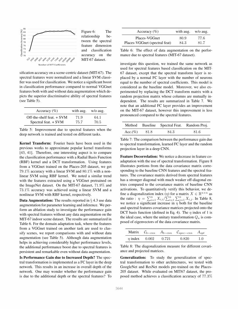
Dimensionality Analysis: We study the relationship be-

tween the number of DCT coefficients and the correspond-

ing performance on the MIT-67 dataset (see Fig. 6). An in-

crease in spectral coefficients generally yields an improve-

ment in the classification performance, however beyond the

4096 feature dimension, the trend reaches a plateau and no

significant improvement is observed. We notice a slight

drop in performance beyond ∼ 10k spectral coefficients.

Due to this trend and for the sake of a fair comparison with

baseline and VGGnet based approaches that use a 4096-

dimensional feature dimension, we use an equidimensional

spectral transform in the CNN model.

Fourier Transform and Phase Information: We also test

the closely related DFT features. For classification pur-

poses, only real-valued feature vectors can be used. There-

fore, we analyze the performance independently using the

magnitude and phase information as well as the combina-

tion of both. For this experiment, we use features before

the first FC layer of the VGGnet (pretrained on the Places

dataset) and a two-layer MLP classifier for classification af-

ter spectral transformation, and feature normalization on the

MIT-67 dataset. The results are reported in Table 4. We

note that the DFT features perform slightly lower compared

to the DCT features, while the phase information performs

considerably lower than the magnitude features on the scene

classification task. When we concatenate both the normal-

Bedroom Hotel room Beach Sandbar

Chemistry lab Biology lab Dining Room Dinette

Kitchen Kitchenette Bar Pub

Figure 5: Pairs from the SUN dataset which were confused

with each other by the classification algorithm. We also

show one example from each class that was mistakenly cat-

egorized as the second class.

DCT DFT Mag. DFT Phase DFT Mag. + Phase

80.1 78.2 59.6 74.7

Table 4: Performance comparison between the magnitude

and phase components of spectral transform.

ized phase and magnitude feature representations, the re-

sulting accuracy is lower than the performance due to only

magnitude features. This indicates that the phase informa-

tion does not help in scene classification.

Domain Transfer: Here, we evaluate the performance of

spectral features on the domain transfer task. To this end,

we obtained off-the-shelf feature representations before the

first fully connected layer of the VGGnet model which is

pretrained on the ImageNet objects dataset. Given these fea-

tures, we apply DCT transform to generate spectral features

(10k dimension), which are then used to test the scene clas-

65643

70

72

74

76

78

80

82

84

86

Cla

ssif

ica

tio

n A

ccu

racy

(%

)

Number of DCT Coefficients

The relationship between Spectral Feature

Dimension and Accuracy

Figure 6: The

relationship be-

tween the spectral

feature dimension

and classification

accuracy on the

MIT-67 dataset.

sification accuracy on a scene-centric dataset (MIT-67). The

spectral features were normalized and a linear SVM classi-

fier was used for classification. We notice a significant boost

in classification performance compared to normal VGGnet

features both with and without data augmentation which de-

picts the superior discriminative ability of spectral features

(see Table 5).

Accuracy (%) with aug. w/o aug.

Off-the-shelf feat. + SVM 71.9 64.1Spectral feat. + SVM 75.7 70.5

Table 5: Improvement due to spectral features when the

deep network is trained and tested on different tasks.

Kernel Transform: Fourier basis have been used in the

previous works to approximate popular kernel transforms

[43, 41]. Therefore, one interesting aspect is to compare

the classification performance with a Radial Basis Function

(RBF) kernel and a DCT transformation. Using features

from a VGGnet trained on the Places-205 dataset, we get

79.1% accuracy with a linear SVM and 80.1% with a non-

linear SVM using RBF kernel. We noted a similar trend

with the features extracted using a VGGnet pretrained on

the ImageNet dataset. On the MIT-67 dataset, 71.9% and

73.1% accuracy was achieved using a linear SVM and a

nonlinear SVM with RBF kernel, respectively.

Data Augmentation: The results reported in § 4.3 use data

augmentation for parameter learning and inference. We per-

form an ablation study to investigate the performance gain

with spectral features without any data augmentation on the

MIT-67 indoor scene dataset. The results are summarized in

Table 6. For the domain adaptation task, where the features

from a VGGnet trained on another task are used to clas-

sify scenes, we report comparisons with and without data

augmentation (see Table 5). Although data augmentation

helps in achieving considerably higher performance levels,

the additional performance boost due to spectral features is

persistent and remarkable even without data augmentation.

Is Performance Gain due to Increased Depth? The spec-

tral transformation is implemented as a FC layer in the deep

network. This results in an increase in overall depth of the

network. One may wonder whether the performance gain

is due to the additional depth or the spectral features? To

Accuracy (%) with aug. w/o aug.

Places-VGGnet 80.9 77.6Places-VGGnet (spectral feat) 84.3 81.7

Table 6: The effect of data augmentation on the perfor-

mance due to spectral features (MIT-67 dataset).

investigate this question, we trained the same network as

used for spectral features based classification on the MIT-

67 dataset, except that the spectral transform layer is re-

placed by a normal FC layer with the number of neurons

equal to the number of spectral coefficients. This model is

considered as the baseline model. Moreover, we also ex-

perimented by replacing the DCT transform matrix with a

random projection matrix whose columns are mutually in-

dependent. The results are summarized in Table 7. We

note that an additional FC layer provides an improvement

on the MIT-67 dataset, however this improvement is less

pronounced compared to the spectral features.

Method Baseline Spectral Feat. Random Proj.

Acc.(%) 81.8 84.3 81.6

Table 7: The comparison between the performance gain due

to spectral transformation, learned FC layer and the random

projection layer in a deep CNN.

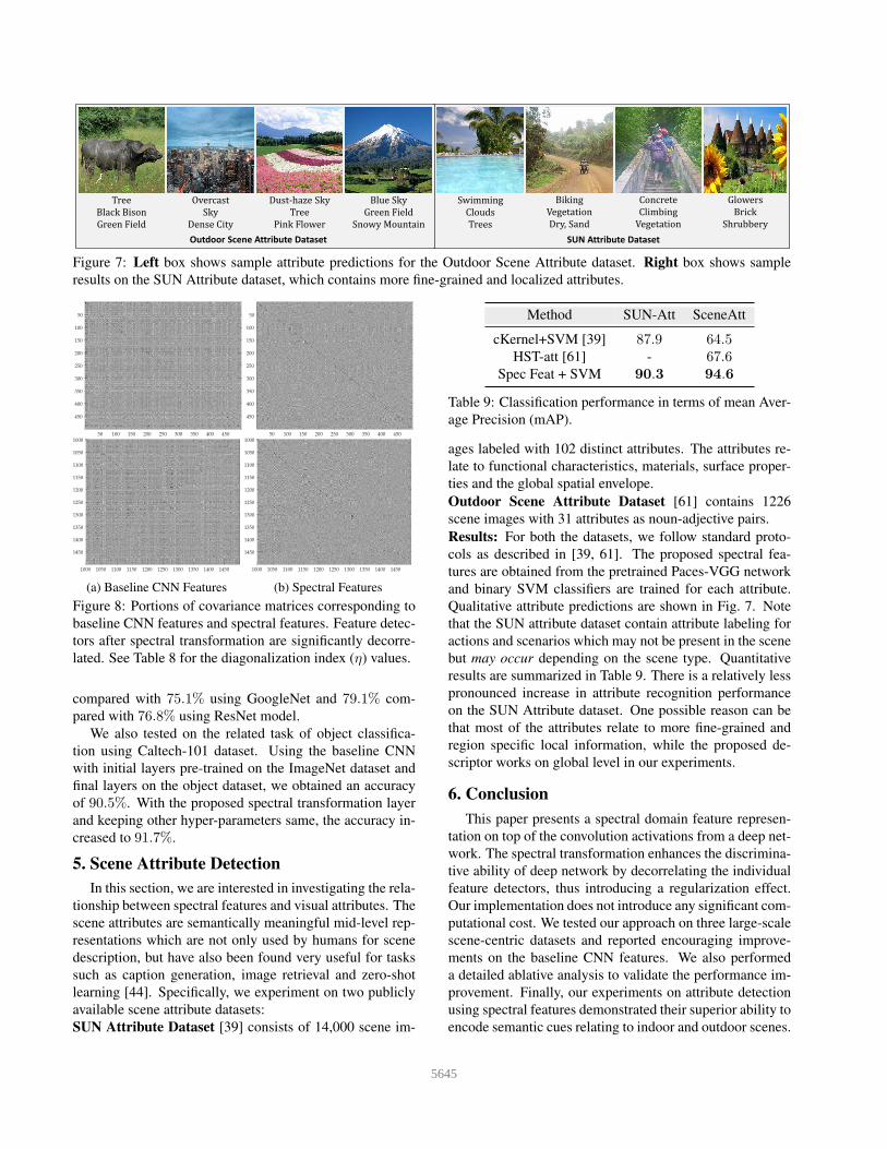
Feature Decorrelation: We notice a decrease in feature co-

adaptation with the use of spectral transformation. Figure 8

illustrates portions from the data covariance matrix corre-

sponding to the baseline CNN features and the spectral fea-

tures. The covariance matrix derived from spectral features

has a stronger diagonal with much weaker off-diagonal en-

tries compared to the covariance matrix of baseline CNN

activations. To quantitatively verify this behavior, we de-

fine a diagonalization index (η) for a matrix X ∈ Rn×n as

the ratio : η =∑n

i=1Xi,i/

∑n

i=1

∑n

j=1Xi,j . In Table 8,

we notice a significant increase in η both for the baseline

and spectral features covariance matrices projected onto the

DCT basis function (defined in Eq. 4). The η index of 1 is

the ideal case, where the unitary transformation Qn is com-

posed of eigenvectors of the data covariance matrix.

Matrix Cb−cnn Ab−cnn Cspec−cnn Aopt

η index 0.002 0.721 0.820 1.0

Table 8: The diagonalization measure for different covari-

ance and projected matrices.

Generalization: To study the generalization of spec-

tral transformation to other architectures, we tested with

GoogleNet and ResNet models pre-trained on the Places-

205 dataset. While evaluated on MIT67 dataset, the pro-

posed method achieves a classification accuracy of 77.3%

75644

Tree

Black Bison

Green Field

Overcast

Sky

Dense City

Dust-haze Sky

Tree

Pink Flower

Blue Sky

Green Field

Snowy Mountain

Swimming

Clouds

Trees

Biking

Vegetation

Dry, Sand

Concrete

Climbing

Vegetation

Glowers

Brick

Shrubbery

Outdoor Scene Attribute Dataset SUN Attribute Dataset

Figure 7: Left box shows sample attribute predictions for the Outdoor Scene Attribute dataset. Right box shows sample

results on the SUN Attribute dataset, which contains more fine-grained and localized attributes.

50 100 150 200 250 300 350 400 450

50

100

150

200

250

300

350

400

450

50 100 150 200 250 300 350 400 450

50

100

150

200

250

300

350

400

450

1000 1050 1100 1150 1200 1250 1300 1350 1400 1450

1000

1050

1100

1150

1200

1250

1300

1350

1400

1450

(a) Baseline CNN Features

1000 1050 1100 1150 1200 1250 1300 1350 1400 1450

1000

1050

1100

1150

1200

1250

1300

1350

1400

1450

(b) Spectral Features

Figure 8: Portions of covariance matrices corresponding to

baseline CNN features and spectral features. Feature detec-

tors after spectral transformation are significantly decorre-

lated. See Table 8 for the diagonalization index (η) values.

compared with 75.1% using GoogleNet and 79.1% com-

pared with 76.8% using ResNet model.

We also tested on the related task of object classifica-

tion using Caltech-101 dataset. Using the baseline CNN

with initial layers pre-trained on the ImageNet dataset and

final layers on the object dataset, we obtained an accuracy

of 90.5%. With the proposed spectral transformation layer

and keeping other hyper-parameters same, the accuracy in-

creased to 91.7%.

5. Scene Attribute Detection

In this section, we are interested in investigating the rela-

tionship between spectral features and visual attributes. The

scene attributes are semantically meaningful mid-level rep-

resentations which are not only used by humans for scene

description, but have also been found very useful for tasks

such as caption generation, image retrieval and zero-shot

learning [44]. Specifically, we experiment on two publicly

available scene attribute datasets:

SUN Attribute Dataset [39] consists of 14,000 scene im-

Method SUN-Att SceneAtt

cKernel+SVM [39] 87.9 64.5HST-att [61] - 67.6

Spec Feat + SVM 90.3 94.6

Table 9: Classification performance in terms of mean Aver-

age Precision (mAP).

ages labeled with 102 distinct attributes. The attributes re-

late to functional characteristics, materials, surface proper-

ties and the global spatial envelope.

Outdoor Scene Attribute Dataset [61] contains 1226

scene images with 31 attributes as noun-adjective pairs.

Results: For both the datasets, we follow standard proto-

cols as described in [39, 61]. The proposed spectral fea-

tures are obtained from the pretrained Paces-VGG network

and binary SVM classifiers are trained for each attribute.

Qualitative attribute predictions are shown in Fig. 7. Note

that the SUN attribute dataset contain attribute labeling for

actions and scenarios which may not be present in the scene

but may occur depending on the scene type. Quantitative

results are summarized in Table 9. There is a relatively less

pronounced increase in attribute recognition performance

on the SUN Attribute dataset. One possible reason can be

that most of the attributes relate to more fine-grained and

region specific local information, while the proposed de-

scriptor works on global level in our experiments.

6. Conclusion

This paper presents a spectral domain feature represen-

tation on top of the convolution activations from a deep net-

work. The spectral transformation enhances the discrimina-

tive ability of deep network by decorrelating the individual

feature detectors, thus introducing a regularization effect.

Our implementation does not introduce any significant com-

putational cost. We tested our approach on three large-scale

scene-centric datasets and reported encouraging improve-

ments on the baseline CNN features. We also performed

a detailed ablative analysis to validate the performance im-

provement. Finally, our experiments on attribute detection

using spectral features demonstrated their superior ability to

encode semantic cues relating to indoor and outdoor scenes.

85645

References

[1] N. Ahmed and K. R. Rao. Orthogonal transforms for digi-

tal signal processing. Springer Science & Business Media,

2012.

[2] S. An, M. Hayat, S. H. Khan, M. Bennamoun, F. Boussaid,

and F. Sohel. Contractive rectifier networks for nonlinear

maximum margin classification. In Proceedings of the IEEE

international conference on computer vision, pages 2515–

2523, 2015.

[3] A. Babenko, A. Slesarev, A. Chigorin, and V. Lempitsky.

Neural codes for image retrieval. In European Conference

on Computer Vision, pages 584–599. Springer, 2014.

[4] S. Ben-Yacoub, B. Fasel, and J. Luettin. Fast face detection

using mlp and fft. In Proc. Second International Confer-

ence on Audio and Video-based Biometric Person Authen-

tication (AVBPA” 99), number EPFL-CONF-82563, pages

31–36, 1999.

[5] I. Biederman. Recognition-by-components: a theory of hu-

man image understanding. Psychological review, 94(2):115,

1987.

[6] A. Bosch, A. Zisserman, and X. Muoz. Scene classifi-

cation using a hybrid generative/discriminative approach.

Transactions on Pattern Analysis and Machine Intelligence,

30(4):712–727, 2008.

[7] A. Bottcher and S. M. Grudsky. Toeplitz matrices, asymp-

totic linear algebra, and functional analysis. Birkhauser,

2012.

[8] L. Breiman. Bagging predictors. Machine learning,

24(2):123–140, 1996.

[9] J. Bruna and S. Mallat. Invariant scattering convolution net-

works. IEEE transactions on pattern analysis and machine

intelligence, 35(8):1872–1886, 2013.

[10] W. Chen, J. T. Wilson, S. Tyree, K. Q. Weinberger, and

Y. Chen. Compressing convolutional neural networks. arXiv

preprint arXiv:1506.04449, 2015.

[11] Y. Cheng, F. X. Yu, R. S. Feris, S. Kumar, A. Choudhary,

and S.-F. Chang. An exploration of parameter redundancy

in deep networks with circulant projections. In Proceedings

of the IEEE International Conference on Computer Vision,

pages 2857–2865, 2015.

[12] B. Cheung, J. A. Livezey, A. K. Bansal, and B. A. Olshausen.

Discovering hidden factors of variation in deep networks.

arXiv preprint arXiv:1412.6583, 2014.

[13] M. Cimpoi, S. Maji, I. Kokkinos, and A. Vedaldi. Deep fil-

ter banks for texture recognition, description, and segmenta-

tion. International Journal of Computer Vision, 118(1):65–

94, 2016.

[14] M. Cogswell, F. Ahmed, R. Girshick, L. Zitnick, and D. Ba-

tra. Reducing overfitting in deep networks by decorrelating

representations. arXiv preprint arXiv:1511.06068, 2015.

[15] C. Doersch, A. Gupta, and A. A. Efros. Mid-level visual ele-

ment discovery as discriminative mode seeking. In Advances

in Neural Information Processing Systems, pages 494–502,

2013.

[16] M. George, M. Dixit, G. Zogg, and N. Vasconcelos. Seman-

tic clustering for robust fine-grained scene recognition. In

European Conference on Computer Vision, pages 783–798.

Springer, 2016.

[17] Y. Gong, L. Wang, R. Guo, and S. Lazebnik. Multi-scale

orderless pooling of deep convolutional activation features.

In European Conference on Computer Vision, pages 392–

407. Springer, 2014.

[18] R. M. Gray et al. Toeplitz and circulant matrices: A review.

Foundations and Trends R© in Communications and Informa-

tion Theory, 2(3):155–239, 2006.

[19] U. Grenander and G. Szego. Toeplitz forms and their appli-

cations, volume 321. Univ of California Press, 2001.

[20] M. Hayat, S. H. Khan, M. Bennamoun, and S. An. A spatial

layout and scale invariant feature representation for indoor

scene classification. IEEE Transactions on Image Process-

ing, 25(10):4829–4841, Oct 2016.

[21] M. Hayat, S. H. Khan, N. Werghi, and R. Goecke. Joint reg-

istration and representation learning for unconstrained face

identification. In Proceedings of the IEEE Conference on

Computer Vision and Pattern Recognition, pages –, 2017.

[22] K. He, X. Zhang, S. Ren, and J. Sun. Spatial pyramid pooling

in deep convolutional networks for visual recognition. In

European Conference on Computer Vision, pages 346–361.

Springer, 2014.

[23] K. He, X. Zhang, S. Ren, and J. Sun. Deep residual learn-

ing for image recognition. arXiv preprint arXiv:1512.03385,

2015.

[24] A. J. Hoffman, H. W. Wielandt, et al. The variation of the

spectrum of a normal matrix.

[25] S. Ioffe and C. Szegedy. Batch normalization: Accelerating

deep network training by reducing internal covariate shift.

In Proceedings of the 32nd International Conference on Ma-

chine Learning (ICML-15), pages 448–456, 2015.

[26] K. Jarrett, K. Kavukcuoglu, Y. Lecun, et al. What is the

best multi-stage architecture for object recognition? In 2009

IEEE 12th International Conference on Computer Vision,

pages 2146–2153. IEEE, 2009.

[27] M. Juneja, A. Vedaldi, C. Jawahar, and A. Zisserman. Blocks

that shout: Distinctive parts for scene classification. In Inter-

national Conference on Computer Vision and Pattern Recog-

nition, pages 923–930. IEEE, 2013.

[28] S. H. Khan, M. Bennamoun, F. Sohel, and R. Togneri. Cost

sensitive learning of deep feature representations from im-

balanced data. IEEE transactions on neural networks and

learning systems, 2017.

[29] S. H. Khan, M. Hayat, M. Bennamoun, R. Togneri, and F. A.

Sohel. A discriminative representation of convolutional fea-

tures for indoor scene recognition. IEEE Transactions on

Image Processing, 25(7):3372–3383, 2016.

[30] S. H. Khan, X. He, F. Porikli, M. Bennamoun, F. Sohel, and

R. Togneri. Learning deep structured network for weakly su-

pervised change detection. Proceedings of the International

Joint Conference on Artificial Intelligence, 2017.

[31] A. Krizhevsky, I. Sutskever, and G. E. Hinton. Imagenet

classification with deep convolutional neural networks. In

Advances in Neural Information Processing Systems, pages

1097–1105, 2012.

[32] A. Lavin. Fast algorithms for convolutional neural networks.

arXiv preprint arXiv:1509.09308, 2015.

95646

[33] S. Lazebnik, C. Schmid, and J. Ponce. Beyond bags of

features: Spatial pyramid matching for recognizing natural

scene categories. In International Conference on Computer

Vision and Pattern Recognition, volume 2, pages 2169–2178.

IEEE, 2006.

[34] J. Long, E. Shelhamer, and T. Darrell. Fully convolutional

networks for semantic segmentation. In Proceedings of the

IEEE Conference on Computer Vision and Pattern Recogni-

tion, pages 3431–3440, 2015.

[35] M. Mathieu, M. Henaff, and Y. LeCun. Fast training

of convolutional networks through ffts. arXiv preprint

arXiv:1312.5851, 2013.

[36] A. Oliva and A. Torralba. Modeling the shape of the scene: A

holistic representation of the spatial envelope. International

Journal of Computer Vision, 42(3):145–175, 2001.

[37] A. Oliva, A. Torralba, A. Guerin-Dugue, and J. Herault.

Global semantic classification of scenes using power spec-

trum templates. In Proceedings of the 1999 international

conference on Challenge of Image Retrieval, pages 9–9.

British Computer Society, 1999.

[38] A. V. Oppenheim and R. W. Schafer. Discrete-time signal

processing. Pearson Higher Education, 2010.

[39] G. Patterson, C. Xu, H. Su, and J. Hays. The sun attribute

database: Beyond categories for deeper scene understanding.

International Journal of Computer Vision, 108(1-2):59–81,

2014.

[40] N. Pinto, D. Doukhan, J. J. DiCarlo, and D. D. Cox. A high-

throughput screening approach to discovering good forms of

biologically inspired visual representation. PLoS Comput

Biol, 5(11):e1000579, 2009.

[41] F. Porikli and H. Ozkan. Data driven frequency mapping

for computationally scalable object detection. In IEEE Ad-

vanced Video and Signal based Surveillance (AVSS), 2011.

[42] A. Quattoni and A. Torralba. Recognizing indoor scenes.

In International Conference on Computer Vision and Pattern

Recognition. IEEE, 2009.

[43] A. Rahimi and B. Recht. Random features for large-scale

kernel machines. In Advances in neural information pro-

cessing systems, pages 1177–1184, 2007.

[44] S. Rahman, S. H. Khan, and F. Porikli. A unified approach

for conventional zero-shot, generalized zero-shot and few-

shot learning. arXiv preprint arXiv:1706.08653, 2017.

[45] K. R. Rao and P. Yip. Discrete cosine transform: algorithms,

advantages, applications. Academic press, 2014.

[46] A. S. Razavian, H. Azizpour, J. Sullivan, and S. Carlsson.

Cnn features off-the-shelf: an astounding baseline for recog-

nition. arXiv preprint arXiv:1403.6382, 2014.

[47] S. Ren, K. He, R. Girshick, and J. Sun. Faster r-cnn: Towards

real-time object detection with region proposal networks. In

Advances in neural information processing systems, pages

91–99, 2015.

[48] O. Rippel, J. Snoek, and R. P. Adams. Spectral representa-

tions for convolutional neural networks. In C. Cortes, N. D.

Lawrence, D. D. Lee, M. Sugiyama, and R. Garnett, edi-

tors, Advances in Neural Information Processing Systems 28,

pages 2440–2448. Curran Associates, Inc., 2015.

[49] A. Saxe, P. W. Koh, Z. Chen, M. Bhand, B. Suresh, and A. Y.

Ng. On random weights and unsupervised feature learning.

In Proceedings of the 28th international conference on ma-

chine learning (ICML-11), pages 1089–1096, 2011.

[50] A. Sharif Razavian, H. Azizpour, J. Sullivan, and S. Carls-

son. Cnn features off-the-shelf: an astounding baseline for

recognition. In Proceedings of the IEEE Conference on Com-

puter Vision and Pattern Recognition Workshops, pages 806–

813, 2014.

[51] K. Simonyan and A. Zisserman. Very deep convolu-

tional networks for large-scale image recognition. CoRR,

abs/1409.1556, 2014.

[52] N. Srivastava, G. E. Hinton, A. Krizhevsky, I. Sutskever, and

R. Salakhutdinov. Dropout: a simple way to prevent neu-

ral networks from overfitting. Journal of Machine Learning

Research, 15(1):1929–1958, 2014.

[53] C. Szegedy, W. Liu, Y. Jia, P. Sermanet, S. Reed,

D. Anguelov, D. Erhan, V. Vanhoucke, and A. Rabinovich.

Going deeper with convolutions. In Proceedings of the IEEE

Conference on Computer Vision and Pattern Recognition,

pages 1–9, 2015.

[54] A. Torralba and A. Oliva. Statistics of natural image cate-

gories. Network: computation in neural systems, 14(3):391–

412, 2003.

[55] S. K. Ungerleider and L. G. Mechanisms of visual atten-

tion in the human cortex. Annual review of neuroscience,

23(1):315–341, 2000.

[56] N. Vasilache, J. Johnson, M. Mathieu, S. Chintala, S. Pi-

antino, and Y. LeCun. Fast convolutional nets with

fbfft: A gpu performance evaluation. arXiv preprint

arXiv:1412.7580, 2014.

[57] W. E. Vinje and J. L. Gallant. Sparse coding and decorrela-

tion in primary visual cortex during natural vision. Science,

287(5456):1273–1276, 2000.

[58] L. Wan, M. Zeiler, S. Zhang, Y. L. Cun, and R. Fergus. Reg-

ularization of neural networks using dropconnect. In Pro-

ceedings of the 30th International Conference on Machine

Learning (ICML-13), pages 1058–1066, 2013.

[59] L. Wang, S. Guo, W. Huang, and Y. Qiao. Places205-

vggnet models for scene recognition. arXiv preprint

arXiv:1508.01667, 2015.

[60] L. Wang, C.-Y. Lee, Z. Tu, and S. Lazebnik. Training

deeper convolutional networks with deep supervision. arXiv

preprint arXiv:1505.02496, 2015.

[61] S. Wang, J. Joo, Y. Wang, and S.-C. Zhu. Weakly supervised

learning for attribute localization in outdoor scenes. In Pro-

ceedings of the IEEE Conference on Computer Vision and

Pattern Recognition, pages 3111–3118, 2013.

[62] J. Wu and J. M. Rehg. Centrist: A visual descriptor for scene

categorization. Transactions on Pattern Analysis and Ma-

chine Intelligence, 33(8):1489–1501, 2011.

[63] R. Wu, B. Wang, W. Wang, and Y. Yu. Harvesting discrimi-

native meta objects with deep cnn features for scene classifi-

cation. In Proceedings of the IEEE International Conference

on Computer Vision, pages 1287–1295, 2015.

[64] J. Xiao, J. Hays, K. A. Ehinger, A. Oliva, and A. Torralba.

Sun database: Large-scale scene recognition from abbey to

105647

zoo. In International Conference on Computer Vision and

Pattern Recognition, pages 3485–3492. IEEE, 2010.

[65] S. Yang and D. Ramanan. Multi-scale recognition with dag-

cnns. In Proceedings of the IEEE International Conference

on Computer Vision, pages 1215–1223, 2015.

[66] B. Zhou, A. Khosla, A. Lapedriza, A. Oliva, and A. Torralba.

Object detectors emerge in deep scene cnns. arXiv preprint

arXiv:1412.6856, 2014.

[67] B. Zhou, A. Lapedriza, J. Xiao, A. Torralba, and A. Oliva.

Learning deep features for scene recognition using places

database. In Advances in neural information processing sys-

tems, pages 487–495, 2014.

[68] H. Zhou, J. Alverez, and F. Porikli. Less is more: Towards

compact cnns,. In Proceedings of the European Conference

on Computer Vision, 2016.

115648