Robust Automatic Rodent Brain Extraction Using 3-D Pulse-Coupled Neural Networks (PCNN)

2554 IEEE TRANSACTIONS ON IMAGE PROCESSING, VOL. 20, NO. 9, SEPTEMBER 2011

Robust Automatic Rodent Brain Extraction Using3-D Pulse-Coupled Neural Networks (PCNN)

Nigel Chou, Jiarong Wu, Jordan Bai Bingren, Anqi Qiu, and Kai-Hsiang Chuang

Abstract—Brain extraction is an important preprocessing stepfor further processing (e.g., registration and morphometric anal-ysis) of brain MRI data. Due to the operator-dependent and time-consuming nature of manual extraction, automated or semi-au-tomated methods are essential for large-scale studies. Automaticmethods are widely available for human brain imaging, but theyare not optimized for rodent brains and hence may not performwell. To date, little work has been done on rodent brain extraction.We present an extended pulse-coupled neural network algorithmthat operates in 3-D on the entire image volume. We evaluated itsperformance under varying SNR and resolution and tested thismethod against the brain-surface extractor (BSE) and a level-setalgorithm proposed for mouse brain. The results show that thismethod outperforms existing methods and is robust under low SNRand with partial volume effects at lower resolutions. Together withthe advantage of minimal user intervention, this method will facil-itate automatic processing of large-scale rodent brain studies.

Index Terms—MRI, pulse-coupled neural networks (PCNNs),rodent brain, segmentation, skull-stripping.

I. INTRODUCTION

R ODENT brains have been used as preclinical modelsto investigate brain development, disease progression,

and neurodegeneration [1]–[4]. With the increasing prevalenceof high-resolution MRI studies in rodents to study changesin structure and function, the ability to automatically processrodent brain images has become critical. One essential pro-cessing step, brain extraction, is the removal of nonbrain tissue

Manuscript received August 11, 2010; revised December 28, 2010; acceptedFebruary 10, 2011. Date of publication March 14, 2011; date of current versionAugust 19, 2011. This work was supported by the Intramural Research programof the Biomedical Sciences Institutes, Agency for Science, Technology and Re-search (A*STAR), Singapore. The associate editor coordinating the review ofthis manuscript and approving it for publication was Dr. Ali Bilgin.

N. Chou is with the Laboratory of Molecular Imaging, Singapore BioimagingConsortium, Agency for Science, Technology and Research (A*STAR), Singa-pore 138667, Singapore (e-mail: [email protected]).

J. Wu and J. Bai Bingren are with the Division of Bioengineering,National University of Singapore, Singapore 117576, Singapore (e-mail:[email protected]; [email protected]).

A. Qiu is with the Division of Bioengineering, National University of Sin-gapore, Singapore 117576, Singapore, and also with the Clinical Imaging Re-search Center, Centre for Life Sciences, National University of Singapore, Sin-gapore 117456, Singapore (e-mail: [email protected]).

K.-H. Chuang is with the Laboratory of Molecular Imaging, SingaporeBioimaging Consortium, Agency for Science, Technology and Research(A*STAR), Singapore 138667, Singapore, with the Clinical Imaging ResearchCenter, Centre for Life Sciences, National University of Singapore, Singapore117456, Singapore, and also with the Department of Physiology, Yong LooLin School of Medicine, National University of Singapore, Singapore 117597,Singapore (e-mail: [email protected]).

Color versions of one or more of the figures in this paper are available onlineat http://ieeexplore.ieee.org.

Digital Object Identifier 10.1109/TIP.2011.2126587

from an image. It is an important prerequisite for further pro-cessing such as segmentation, inter-subject registration, andmorphometric analysis [5]–[13]. The resulting brain mask canalso be used directly to study changes in brain volume [14],[15]. While manual brain extraction by trained individualsprovides the most accurate results, it is labor-intensive and op-erator-dependent, making it unfeasible for high-throughput andlarge-scale studies, especially ones that utilize high-resolution3-D imaging. Hence, there is a need for robust and accurateautomatic methods to facilitate such studies.

Automatic methods are widely available for brain extractionin humans, utilizing a variety of region-growing [16], edge-based [17], surface-based as well as hybrid [18] approaches.These methods have been validated in numerous human studies[19]–[21]. However, these algorithms often perform poorly onrodent brains due to the different shape and contrasts betweenbrain and surrounding tissues in human and rodent brains. Anumber of such methods make assumptions of a spherical or el-lipsoidal surface [22] or make use of human brain atlases as priorinformation [23]. Others make use of anisotropic diffusion fil-tering together with edge-detection [17], but its effectiveness inrodent brains is reduced by the much narrower gap and weakercontrast between the brain and scalp tissue compared to humanbrains. Due to the failure of existing methods to accurately seg-ment rodent brains, there is a pressing need to develop algo-rithms that are specifically optimized for rodent brains.

To date, there has been little published work on automaticbrain extraction in rodents. In the literature, two methods havebeen proposed: Constraint level-sets (CLS) [24] and pulse-cou-pled neural networks (PCNNs) [25]. CLS is a semi-automaticmethod that uses a level-set algorithm to evolve a user-definedinitial surface toward the brain boundary. User intervention isrequired, involving tracing of the brain boundary on a numberof sagittal and coronal slices, which are used both as an ini-tial surface and as constraint points. As with all level-set-basedmethods, this algorithm is sensitive to its initial surface andparameters.

The PCNN is a biologically inspired neural-network algo-rithm [26] with numerous applications in image processing,most notably in image segmentation [27]–[29]. Murugavel etal. first applied a PCNN algorithm for brain extraction. In theirmethod, a 2-D network was used to segment selected coronalslices of rat head MRI (and hence will be dubbed as 2-D PCNNin the following). It showed improved performance over theBrain-Extraction Tool (BET) [16], a human brain-extractionalgorithm. The algorithm’s key strengths are its robustness tonoise and ability to accurately segment irregular boundaries.However, while this algorithm successfully segments central

1057-7149/$26.00 © 2011 IEEE

CHOU et al.: ROBUST AUTOMATIC RODENT BRAIN EXTRACTION USING 3-D PCNNS 2555

coronal slices, it was unable to correctly identify brain tissue inthe anterior slices, where the eyes were larger than the olfactorylobe and in some posterior slices where protruded parts of thebrain were isolated. Furthermore, this method requires selectionof an optimal brain mask for each slice and hence slows downthe throughput especially with high-resolution 3-D image data.Although the authors trained another artificial neural network(ANN) to “automatically” determine the optimal brain mask,the ANN would need to be retrained for different species or fordiseased animals. Even with use of the ANN, accuracy wouldnot be consistent across slices and each slice will still need tobe checked manually to determine if the correct iteration hasbeen chosen.

In this paper, we extend the 2-D PCNN method proposed byMurugavel et al.to overcome the above-mentioned limitations.An important reason for poor performance on certain brain re-gions was that neighboring information in the third dimensionwas not considered. We expanded the network to a 3-D modelwith spherically symmetric 3-D weighting matrices that can bescaled according to the actual voxel dimensions, so that all of theprotruding parts across slices can be properly identified. Fur-thermore, based on the 3-D model, we propose a simple yeteffective method to automatically determine the optimal brainmask which does not require a trained ANN nor human inter-vention, making the 3-D PCNN method fully automatic. Theaccuracy of the 3-D PCNN method was evaluated on a mousehead MRI acquired using 3-D and 2-D multislice Turbo SpinEcho T2-weighted sequences. Our method was first tested forrobustness to noise and partial volume effects by simulating avariety of SNR levels and resolutions. It was then compared withexisting human brain-extraction algorithms such as the BrainSurface Extractor (BSE) [17], and rodent brain-extraction tech-niques: the 2-D PCNN and CLS algorithms.

II. MATERIALS AND METHODS

A. Overview of Processing Flow

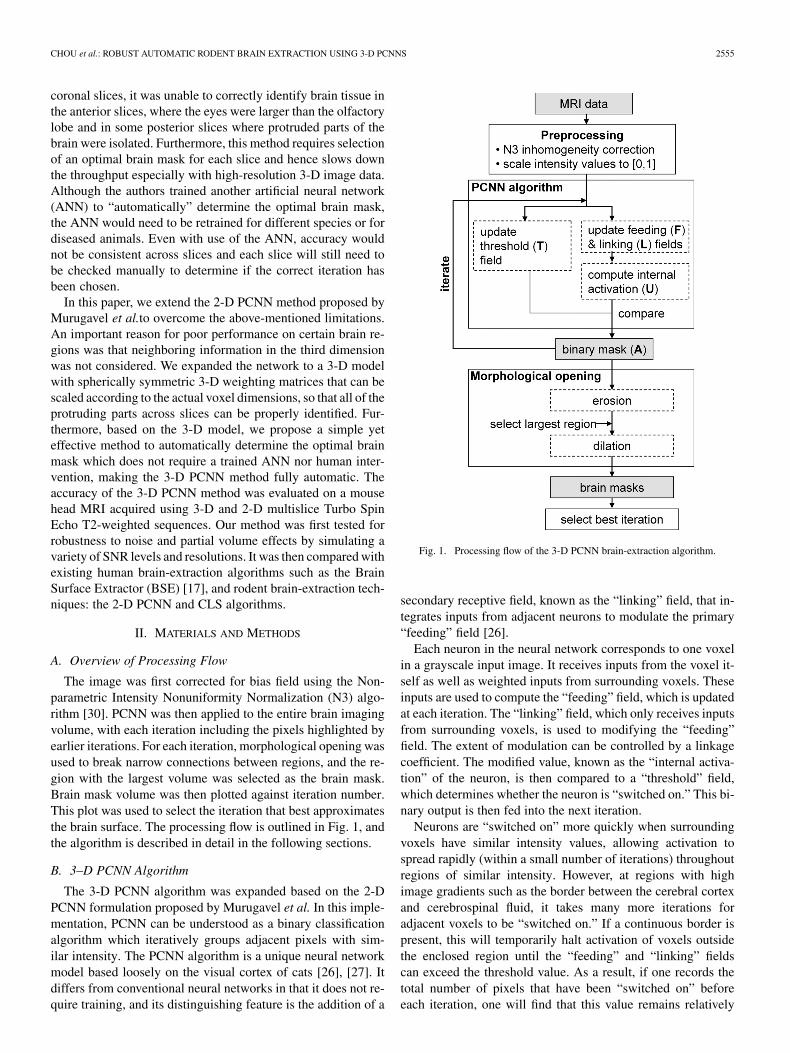
The image was first corrected for bias field using the Non-parametric Intensity Nonuniformity Normalization (N3) algo-rithm [30]. PCNN was then applied to the entire brain imagingvolume, with each iteration including the pixels highlighted byearlier iterations. For each iteration, morphological opening wasused to break narrow connections between regions, and the re-gion with the largest volume was selected as the brain mask.Brain mask volume was then plotted against iteration number.This plot was used to select the iteration that best approximatesthe brain surface. The processing flow is outlined in Fig. 1, andthe algorithm is described in detail in the following sections.

B. 3–D PCNN Algorithm

The 3-D PCNN algorithm was expanded based on the 2-DPCNN formulation proposed by Murugavel et al. In this imple-mentation, PCNN can be understood as a binary classificationalgorithm which iteratively groups adjacent pixels with sim-ilar intensity. The PCNN algorithm is a unique neural networkmodel based loosely on the visual cortex of cats [26], [27]. Itdiffers from conventional neural networks in that it does not re-quire training, and its distinguishing feature is the addition of a

Fig. 1. Processing flow of the 3-D PCNN brain-extraction algorithm.

secondary receptive field, known as the “linking” field, that in-tegrates inputs from adjacent neurons to modulate the primary“feeding” field [26].

Each neuron in the neural network corresponds to one voxelin a grayscale input image. It receives inputs from the voxel it-self as well as weighted inputs from surrounding voxels. Theseinputs are used to compute the “feeding” field, which is updatedat each iteration. The “linking” field, which only receives inputsfrom surrounding voxels, is used to modifying the “feeding”field. The extent of modulation can be controlled by a linkagecoefficient. The modified value, known as the “internal activa-tion” of the neuron, is then compared to a “threshold” field,which determines whether the neuron is “switched on.” This bi-nary output is then fed into the next iteration.

Neurons are “switched on” more quickly when surroundingvoxels have similar intensity values, allowing activation tospread rapidly (within a small number of iterations) throughoutregions of similar intensity. However, at regions with highimage gradients such as the border between the cerebral cortexand cerebrospinal fluid, it takes many more iterations foradjacent voxels to be “switched on.” If a continuous border ispresent, this will temporarily halt activation of voxels outsidethe enclosed region until the “feeding” and “linking” fieldscan exceed the threshold value. As a result, if one records thetotal number of pixels that have been “switched on” beforeeach iteration, one will find that this value remains relatively


constant for a number of iterations before suddenly increasing.This property is utilized to identify the iteration(s) at which thesurface of the mask is at a border.

To explain the algorithm in more detail, let be the 3-Dimage matrix, after intensity rescaling to the range of .

, , and representing the “feeding,” “linking,” and“threshold” fields, respectively, are defined as follows:

(1)

(2)

(3)

where , , and are decay factors that control how thevalues of , , and decay over time in the absence ofexternal stimuli. , and are amplification factors thatscale the inputs from adjacent pixels to their respective fields.

and represent 3-D weighting matrices that control theweightage of adjacent voxel inputs. is the outputof the neuron from the previous iteration. The representsconvolution.

All neurons in and have a value of 0 initially whilethose in have an initial value of 1. For our implementation,

. The weighting matrix is a normalized 3-D Gaussianfunction ( ) with peak at the center and radius, i.e., with a window size of . We chose as larger

values did not improve results and introduced additional compu-tational complexity. In the case of anisotropic voxel dimensions,we scaled the values of the matrix accordingly but retained thedimensions of the window.

The “internal activation” of the neuron is then computedfrom and as

(4)

where is the linkage coefficient controlling the effect of the“linking” field on . , the output of the neuron, is ob-tained by comparing the threshold value to the internalactivation as

ifif .

(5)

To ensure that any voxel that is switched “on” remains “on”even if it falls below the threshold value in later iterations, anaccumulated output is then obtained by accumulating allpixels before and including the present iteration:

(6)

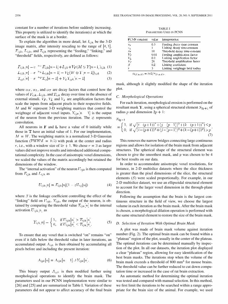
This binary output is then modified further usingmorphological operations to identify the brain mask. Theparameters used in our PCNN implementation were similar to[26] and [25] and are summarized in Table I. Variation of theseparameters did not appear to affect accuracy of the final brain

TABLE IPARAMETERS USED IN PCNN

mask, although it slightly modified the shape of the iterationplot.

C. Morphological Operations

For each iteration, morphological erosion is performed on theresultant mask , using a spherical structural element ofradius and dimension :

ifif

(7)

This removes the narrow bridges connecting large continuousregions and allows for isolation of the brain mask from adjacentstructures. The spherical shape of the structural element waschosen to give the smoothest mask, and was chosen to be 4for best results on our data.

In order to accommodate anisotropic voxel resolutions, forinstance, in 2-D multislice datasets where the slice thicknessis greater than the pixel dimensions of the slice, the structuralelements ( ) were scaled proportionally. For example, in our2-D multislice dataset, we use an ellipsoidal structural elementto account for the larger voxel dimension in the through-planedirection.

Following the assumption that the brain is the largest con-tinuous structure in the field of view, we choose the largestvolume in each iteration as the brain mask. After the brain maskis chosen, a morphological dilation operation is performed withthe same structural element to restore the size of the brain mask.

D. Selection of Iteration With Optimal Brain Mask

A plot was made of brain mask volume against iterationnumber (Fig. 2). The optimal brain mask can be found within a“plateau” region of the plot, usually in the center of the plateau.The optimal iterations can be determined manually by inspec-tion of the plot. In all our datasets, the iteration plot displayeda clear “plateau” region, allowing for easy identification of thebest brain masks. The iterations stop when the volume of thebrain mask exceeds a threshold of 800 mm for mouse brains.The threshold value can be further reduced to cut down compu-tation time or increased in the case of rat brain extraction.

An automatic method for determining the optimal iterationwas tested and compared with manual selection. In this method,we first limit the iterations to be searched within a range appro-priate for the brain size of the animal. For example, we used


Fig. 2. Illustration of the generated brain mask volume at each iteration in 3-D PCNN showing brain masks at five selected iterations. (a) Iteration 37. (b) Iteration38. (c) Iteration 52. (d) Iteration 59. (e) Iteration 60. A Manual mask (not including brain-stem) is shown at the lower right corner as a reference. Iteration 52 isthe best iteration. Note that iteration 59, though not the ideal brain mask, still conforms relatively well to the manual brain boundary.

the range of 100–550 mm for our mouse brain data. We thenfind the largest decrease and increase in gradient over this re-gion, which correspond approximately to the start and end ofthe “plateau” region, respectively. The ideal iteration is chosenas the iteration halfway between these two iterations.

E. MRI

All animal procedures were approved by the InstitutionalAnimal Care and Use Committees of the Biomedical SciencesInstitutes, Agency for Science, Technology and Research(A*STAR). Ten adult male C57BL/6 mice (23–28 g) wereinitially anesthetized by 1.5% isoflurane mixed in 2:1 air: .The anesthetized animals were secured in a stereotactic holderwith breathing and temperature monitored during imaging

(SAII, NY, USA). The Isoflurane level was varied between1%–1.5% to maintain a stable breathing rate of 60–90 breathsper minute. Body temperature was maintained using a waterheating system.

Images were acquired on a Bruker 7T/20 cm ClinScan(Bruker BioSpin MRI GmbH, Ettlingen, Germany) using avolume coil for transmit and a Bruker mouse brain 2 2 arraycoil for receive. 2-D T2-weighted Turbo Spin Echo (TSET2-wt) images were acquired in five mice with the followingparameters: TR/ TE 2710/42 ms, echo train length .The field of view (FOV) was 25 mm 25 mm, with a matrixof 256 256 ( m m). 51 coronal slicesof 0.30 mm with no slice gap were acquired to cover the wholebrain (total acquisition time 10 min).


The other five mice were scanned with a 3-DTSE T2-wt sequence. Acquisition parameters wereTR/TE 2000/46 ms, echo train length andtotal acquisition time 1 hr 23 min. The field of view (FOV)was 9 mm 13 mm 25 mm, with a matrix of 88 140 256(voxel size m m m).

F. Implementation and Evaluation

The 3-D PCNN algorithm was implemented in MATLABR2008b (Mathworks, Natick, MA, USA). 3-D visualizationof brain surface, simulation and evaluation were also carriedout in MATLAB. Inhomogeneity correction was performedusing the N3 algorithm in MIPAV 4.0.3 (National Institutes ofHealth, Bethesda, MD, USA), with field distance 2.5 mm,maximum iterations , end tolerance andkernel FWHM . 3-D PCNN was also implemented inC++ and compiled with cmake v2.8.1, but evaluation of thisimplementation is not included in this paper.

The 3-D PCNN brain-extraction algorithm was first tested forits robustness to noise and partial volume effects by comparingresults at different simulated noise levels and resolutions respec-tively. It was then evaluated both quantitatively and qualitativelyagainst three other automatic methods: BSE, CLS, and the orig-inal 2-D PCNN algorithm [25].

To simulate varying noise levels, Gaussian noise was addedto both 2-D multislice and 3-D datasets such that the SNR, de-fined as a ratio of mean intensity in cortex to standard deviationof background, was 10 and 5 for each image. SNR was mea-sured on rectangular ROI drawn manually on both cortex andbackground over ten slices in each dataset. Results were thencompared to the original images, where SNR ranged from 32 to44 for the 3-D dataset and 21 to 37 for the 2-D multislice dataset.

To simulate the partial-volume effects at lower resolutions,we downsampled the 3-D dataset by 2 and 3 by averagingadjacent pixels in all three dimensions. Downsampling was firstdone on the plane of each coronal slice, with both and direc-tions downsampled equally. Downsampling was then applied inthe direction perpendicular to the coronal plane (through-planedirection) to simulate the effect of using larger slice-thicknessin 2-D multislice acquisitions.

3-D PCNN was compared to three other automated methods:CLS, 2-D PCNN and BSE. The first two methods were de-signed for rodent brains, while the third (BSE) was developedfor human brains. Another human brain-extraction algorithm,the BET as implemented in MIPAV, was tested but not includedin this comparison as its performance on mouse brain data waspoor. It consistently excluded large sections of brain tissue, de-spite attempts at adjusting parameter settings.

BSE combines anisotropic diffusion filtering with edge-detection, followed by morphological operations to identifythe brain mask. BSE was applied to the entire image volumeusing BrainSuite09 (Laboratory of NeuroImaging, UCLA,CA), with the following parameters: diffusion iterations

, diffusion constant , edge constant ,erosion size 1 pixel.

The CLS technique is based on a variation of the level-setmethod [31] with the incorporation of prior knowledge as con-straint points. The technique works by evolving an initial level

surface iteratively towards the brain boundary, where the imagegradient is the highest. This is controlled by the weighting fac-tors , , and . determines the amount of weight given to theinternal force which penalizes deviation of the level set functionfrom the previous iteration, while and determine the weightgiven to the driving force. The user must first manually extractthe brain region on three sagittal and two axial slices to serve asprior knowledge and define the initial level surface. Constraintpoints are then extracted from these orthogonal contours in thecoronal view. The initial level surface is defined by joining theconstraint points with straight lines in every coronal slice, thenstacking these contours to form a closed surface. In addition, byincreasing and decreasing and at the constraint points, thepropagation of the level surface is blocked from going beyondthese points. Uberti et al. implemented CLS on entire imagevolumes (3-D CLS) and separately on each slice (2-D CLS).We chose to use 3-D CLS as it performed better in T2-weightedimages. 3-D CLS was applied to the 2-D or 3-D image volumeswith weighting factors , , and , whilethose of the constraint points were set to , ,and . CLS was implemented in MATLAB using an inter-face obtained from the authors [24].

To quantitatively evaluate the effectiveness of 3-D PCNN andother automatic methods, manual masks were traced separatelyby two raters on all datasets with reference to the Paxinos andFranklin atlas [32] and used as the gold standard. Masks weredrawn on coronal slices, starting from the slice where the cere-bellum is first clearly visible. These manual brain masks wereoutlined using the volume of interest (VOI) tool in MIPAV. Inall cases, three indexes were used to measure similarity of thebrain masks from each automatic method ( ) to the manualstandard ( ).

Jaccard index:

(8)

True-positive rate (TPR):

(9)

False-positive rate (FPR):

(10)

where is the total head volume that includes all voxels greaterthan 5% of the maximum intensity. The Jaccard index is a mea-sure of how closely the automatic mask overlaps the manualmask, and is used as the main index for comparison. The TPRmeasures the fraction of pixels correctly labeled by the auto-matic mask, while the FPR gives an indication of how manypixels identified by the automatic mask were outside the manualmask.

The Jaccard index of the manual masks between the two raterswas computed, and the mean Jaccard index used as a measureof inter-operator variability. The Jaccard index, TPR and FPRwere computed for each automatic mask relative to both sets ofmanual masks. The two values were then averaged, and used to


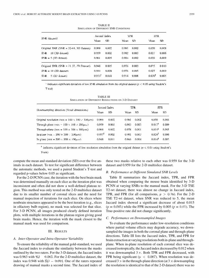
TABLE IISIMULATION OF DIFFERENT SNR CONDITIONS

TABLE IIISIMULATION OF DIFFERENT RESOLUTIONS ON 3-D DATASET

compute the mean and standard deviation (SD) over the five an-imals in each dataset. To test for significant difference betweenthe automatic methods, we used a paired Student’s T-test andregarded p-values below 0.05 as significant.

For the 2-D PCNN case, the iteration with the best brain maskwas determined manually on each slice as the iteration plot wasinconsistent and often did not show a well-defined plateau re-gion. This method was only tested on the 2-D multislice datasetdue to its smaller number of coronal slices and the need formanual inspection of iterations for each slice. On slices wherenonbrain structures appeared to be the best iteration (e.g., slicesin olfactory bulb region), no mask was selected for that slice.For 3-D PCNN, all images produced clearly defined iterationplots, with multiple iterations in the plateau region giving goodbrain masks. Hence, the iteration with the mask closest to themanual mask was used for comparison.

III. RESULTS

A. Inter-Operator and Intra-Operator Variability

To ensure the reliability of the manual gold-standard, we usedthe Jaccard index to evaluate the similarity between the masksoutlined by the two raters. For the 3-D dataset, the Jaccard indexwas 0.963 with . For the 2-D multislice dataset, theindex was 0.948 with . One of the raters repeateddrawing of manual masks a second time. The Jaccard index of

these two masks relative to each other was 0.959 for the 3-Ddataset and 0.959 for the 2-D multislice dataset.

B. Performance at Different Simulated SNR Levels

Table II summarizes the Jaccard index, TPR, and FPRobtained when comparing the mouse brain identified by 3-DPCNN at varying SNRs to the manual mask. For the 3-D TSET2-wt dataset, there was almost no change in Jaccard index,TPR, and FPR (for all comparisons, ). For the 2-DTSE T2-wt dataset, when SNR was reduced to 5, the meanJaccard index showed a significant decrease of about 0.015( ) while the FPR increased by 0.005 ( ). TheTrue-positive rate did not change significantly.

C. Performance on Downsampled Images

To evaluate the performance under low-resolution conditionswhere partial volume effects may degrade accuracy, we down-sampled the images in both the coronal plane and through-planedirections. Table III lists the Jaccard index, TPR, and FPR forbrain extraction at varying resolutions both in-plane and through-plane. When in-plane resolution of each coronal slice was de-creased isotropically, the Jaccard index decreased by 0.012 whenit was downsampled 3 . Both TPR and FPR decreased, withFPR being significant ( ). When resolution was de-creased 3 in the through-plane direction (at 3 downsamplingthe resolution is identical to that of the 2-D dataset) there was no


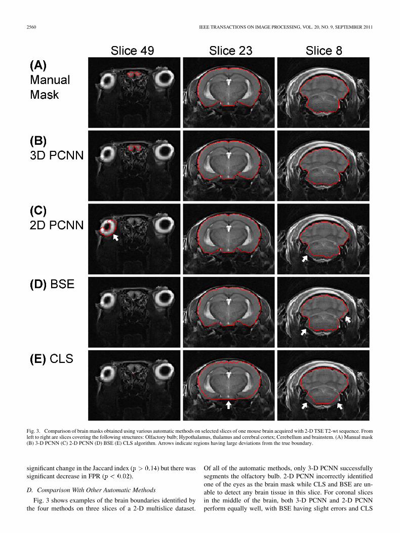
Fig. 3. Comparison of brain masks obtained using various automatic methods on selected slices of one mouse brain acquired with 2-D TSE T2-wt sequence. Fromleft to right are slices covering the following structures: Olfactory bulb; Hypothalamus, thalamus and cerebral cortex; Cerebellum and brainstem. (A) Manual mask(B) 3-D PCNN (C) 2-D PCNN (D) BSE (E) CLS algorithm. Arrows indicate regions having large deviations from the true boundary.

significant change in the Jaccard index ( ) but there wassignificant decrease in FPR ( ).

D. Comparison With Other Automatic Methods

Fig. 3 shows examples of the brain boundaries identified bythe four methods on three slices of a 2-D multislice dataset.

Of all of the automatic methods, only 3-D PCNN successfullysegments the olfactory bulb. 2-D PCNN incorrectly identifiedone of the eyes as the brain mask while CLS and BSE are un-able to detect any brain tissue in this slice. For coronal slicesin the middle of the brain, both 3-D PCNN and 2-D PCNNperform equally well, with BSE having slight errors and CLS


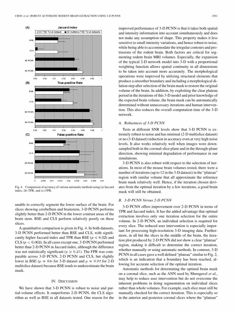
Fig. 4. Comparison of accuracy of various automatic methods using (a) Jaccardindex, (b) TPR, and (c) FPR.

unable to correctly segment the lower surface of the brain. Forslices showing cerebellum and brainstem, 3-D PCNN performsslightly better than 2-D PCNN in the lower contrast areas of thebrain stem. BSE and CLS perform relatively poorly on theseslices.

A quantitative comparison is given in Fig. 4. In both datasets,3-D PCNN performed better than BSE and CLS, with signifi-cantly higher Jaccard index and TPR than BSE ( ) andCLS ( ). In all cases except one, 3-D PCNN performedbetter than 2-D PCNN in Jaccard index, although the differencewas not statistically significant ( ). The FPR was com-parable across 3-D PCNN, 2-D PCNN and CLS, but slightlylower in BSE ( for 3-D dataset and for 2-Dmultislice dataset) because BSE tends to underestimate the brainmask.

IV. DISCUSSION

We have shown that 3-D PCNN is robust to noise and par-tial-volume effects. It outperforms 2-D PCNN, the CLS algo-rithm as well as BSE in all datasets tested. One reason for the

improved performance of 3-D PCNN is that it takes both spatialand intensity information into account simultaneously and doesnot make any assumption of shape. This property makes it lesssensitive to small intensity variations, and hence robust to noise,while being able to accommodate the irregular contours and pro-trusions of the rodent brain. Both factors are critical for seg-menting rodent brain MRI volumes. Especially, the expansionof the typical 2-D network model into 3-D with a proportionalweighting function allows spatial continuity in all dimensionsto be taken into account more accurately. The morphologicaloperations were improved by utilizing structural elements thatproduce a smoother boundary and including a morphological di-lation step after selection of the brain mask to restore the originalvolume of the brain. In addition, by exploiting the clear plateauperiod in the iterations of this 3-D model and prior knowledge ofthe expected brain volume, the brain mask can be automaticallydetermined without unnecessary iterations and human interven-tion. This also reduces the overall computation time of the 3-Dnetwork.

A. Robustness of 3-D PCNN

Tests at different SNR levels show that 3-D PCNN is ex-tremely robust to noise and has minimal (2-D multislice dataset)or no (3-D dataset) reduction in accuracy even at very high noiselevels. It also works relatively well when images were down-sampled both in the coronal-slice plane and in the through-planedirection, showing minimal degradation of performance in oursimulations.

3-D PCNN is also robust with respect to the selection of iter-ations. In most of the mouse brain volumes tested, there were anumber of iterations (up to 12 in the 3-D dataset) in the “plateau”region with similar volume that all approximate the referencebrain mask relatively well. Hence, if the iteration chosen devi-ates from the optimal iteration by a few iterations, a good brainmask will still be obtained.

B. 3-D PCNN Versus 2-D PCNN

3-D PCNN offers improvement over 2-D PCNN in terms ofTPR and Jaccard index. It has the added advantage that optimalextraction involves only one iteration selection for the entirevolume. In 2-D PCNN, an individual selection is required forevery slice. The reduced user intervention is especially impor-tant for processing high-resolution 3-D imaging data. Further-more, in all but the slices in the middle of the brain, the itera-tion plot produced by 2-D PCNN did not show a clear “plateau”region, making it difficult to determine the correct iteration,whether manually or using automatic methods. In contrast, 3-DPCNN in all cases gave a well defined “plateau” similar to Fig. 2,which is an indication that a boundary has been reached, al-lowing for accurate selection of the optimal iteration.

Automatic methods for determining the optimal brain maskon a coronal slice, such as the ANN used by Murugavel et al.,may help to reduce user intervention but do not overcome theinherent problems in doing segmentation on individual slicesrather than whole volumes. For example, each slice must still bemanually checked for the correct iteration. This is especially soin the anterior and posterior coronal slices where the “plateau”


region is poorly defined and any method to automatically de-termine the optimal iteration is likely to fail. In addition, usingan ANN requires training, which will have to be repeated on anumber of animals whenever a new strain or disease model isused. These limitations make 2-D PCNN cumbersome to use inlarge-scale studies.

Another important benefit of 3-D PCNN is that it allowsknowledge of brain volume (e.g., 450–550 mm for adult mice)to be incorporated in the algorithm, which was not possible in2-D PCNN, where brain area varies from slice to slice. Brainvolume information can be used to aid selection of the correctiteration by limiting the range of iterations to check. It can alsobe used to significantly cut down computation time by stoppingiterations once the brain mask volume exceeds the maximumexpected brain volume.

In our experiments, 3-D PCNN always produced iterationplots with clearly defined plateau regions. This property, to-gether with our knowledge of expected brain volume allowedus to devise a simple but effective way to automatically deter-mine the optimal iteration. We compared the average Jaccardindex for each dataset from iterations selected with this methodto that obtained from iterations with the highest Jaccard index.The difference in Jaccard index was smaller than 0.002 for both3-D and 2-D multislice datasets. Hence, this would be a viablemethod to aid in the selection of the optimal iteration.

Although 3-D PCNN inevitably has a higher computationalcomplexity due to whole volume processing, it is still prefer-able to 2-D PCNN due to its consistent performance, use ofout-of-slice information, ease of selection of optimal brain maskand minimal requirement for user intervention. Computationtime on a PC with Intel Xeon X5450 3.0 GHz and 16 GB RAMrunning Linux without use of parallel processing was 32–39 minfor the 2-D multislice dataset and 38–48 min for the 3-D datasetusing 3-D PCNN, compared with 13 min on the 3-D dataset and7.5 min for the 2-D multislice dataset using 2-D PCNN. Notethat the code used in our evaluation has not been fully optimized,hence computation time can be further decreased for example byusing Fourier convolution for the convolution steps or reducingthe brain mask volume at which to stop iterations. Moreover,a significant portion of the computation time was taken up bythe morphological operations (the main PCNN algorithm tookup comparatively little time), hence utilizing more efficient codefor the morphological operations may also greatly improve com-putational efficiency.

C. Comparison With Other Automatic Methods

Among human brain-extraction methods, BSE appears to beone that is better suited for rodent brains due to its minimaluse of human brain specific assumptions. However, it does notperform as well in rodent brains due to the smaller number ofpixels and reduced contrast between the brain surface and ad-jacent tissue. In many cases, BSE detects edges slightly insidethe surface of the brain and erroneously designates these edgesas part of the brain surface. This leads to reduced performanceas well as a strong tendency to underestimate the brain surface,which accounts for its lower FPR relative to all other methodstested.

In our comparison, CLS performed much worse than 3-DPCNN and 2-D PCNN. It showed similar results to BSE inthe 3-D dataset but had even worse performance than BSE inthe 2-D multislice dataset, despite being optimized for rodent(mouse) brains. One reason for this poor performance could bethat the image resolution of 100 m used in our experiment islower than the 78 m used in Uberti’s paper [24]. As a result,the partial volume effect along the brain/nonbrain boundary forthe images used in our experiment may result in reduced ac-curacy compared with that of Uberti. CLS is also strongly de-pendent on initial conditions and choice of landmarks whichmay contribute to its inability to correctly converge on the truebrain surface. Finally, the need for a regularization term ( ) pre-vents the algorithm from correctly detecting the irregular con-tours especially at the ventral part of the brain where curvaturechanges rapidly (see Fig. 3). In our experiment, even with theincorporation of manually segmented orthogonal slices as priorknowledge, the algorithm is unable to converge to the brainboundary well. Increasing the number of manually segmentedsagittal slices from 5 to 7 did not improve the results of CLSbrain extraction. Adding more landmarks where there are largercurvature changes may help to improve the problem, but willsignificantly increase user intervention.

D. Limitations of 3-D PCNN

3-D PCNN does have some limitations. Like all of the otherautomatic methods mentioned in this paper, it has difficultysegmenting images with low contrast between cortex and skull,such as in T1-weighted rodent brain images acquired at highfield. We also acquired 3-D MPRAGE T1-weighted images insome animals. However, due to the low intensity of gray matter(as opposed to T2-weighted images where gray matter hashigh intensity), the contrast of the brain boundary was ratherlow. This may be why most existing MRI rodent brain atlaseswere acquired with T2-weighting [33]–[37]. Therefore, it isrecommended to acquire T2-weighted data for segmentationand registration.

V. CONCLUSION

We have shown that 3-D PCNN is an effective and robustmethod that is well suited for rodent brain extraction. It per-forms better than existing human and rodent brain extractionalgorithms, while overcoming the issues faced by the 2-DPCNN method. This method will facilitate application ofautomatic registration and morphometric analysis methods torodent brains.1

ACKNOWLEDGMENT

The authors would like to thank J. Tan and A. B. M. A. Asadfor assistance in acquisition of MRI images and animalhandling.

1Software for 3-D PCNN brain extraction will be freely available onour websites. The MATLAB and C++ executables will be available athttp://www.sbic.a-star.edu.sg/research/lmi/software.php and http://www.bioeng.nus.edu.sg/cfa/mousebrainatlas/index.html.


REFERENCES

[1] O. Natt, T. Watanabe, S. Boretius, J. Radulovic, J. Frahm, and T.Michaelis, “High-resolution 3d mri of mouse brain reveals smallcerebral structures in vivo,” J. Neurosci. Meth., vol. 120, no. 2, pp.203–209, 2002.

[2] N. D. Greene, M. F. Lythgoe, D. L. Thomas, R. L. Nussbaum, D. J.Bernard, and H. M. Mitchison, “High resolution mri reveals globalchanges in brains of cln3 mutant mice,” Eur. J. Paediatric Neurol., vol.5, no. Supplement 1, pp. 103–107, 2001.

[3] J. Zhang, Q. Peng, Q. Li, N. Jahanshad, Z. Hou, M. Jiang, N. Masuda,D. R. Langbehn, M. I. Miller, S. Mori, C. A. Ross, and W. Duan, “Lon-gitudinal characterization of brain atrophy of a huntington’s diseasemouse model by automated morphological analyses of magnetic reso-nance images,” NeuroImage, vol. 49, no. 3, pp. 2340–2351, 2010.

[4] B. A. Moffat, C. J. Galbán, and A. Rehemtulla, “Advanced mri: Trans-lation from animal to human in brain tumor research,” NeuroimagingClin. North Amer., vol. 19, no. 4, pp. 517–526, 2009.

[5] K. O. Babalola, B. Patenaude, P. Aljabar, J. Schnabel, D. Kennedy,W. Crum, S. Smith, T. Cootes, M. Jenkinson, and D. Rueckert, “Anevaluation of four automatic methods of segmenting the subcorticalstructures in the brain,” NeuroImage, vol. 47, no. 4, pp. 1435–1447,2009.

[6] S. X. Liu, C. Imielinska, A. Laine, W. S. Millar, E. S. Connolly, andA. L. D’Ambrosio, “Asymmetry analysis in rodent cerebral ischemiamodels,” Academic Radiol., vol. 15, no. 9, pp. 1181–1197, 2008.

[7] A. A. Ali, A. M. Dale, A. Badea, and G. A. Johnson, “Automatedsegmentation of neuroanatomical structures in multispectral mr mi-croscopy of the mouse brain,” NeuroImage, vol. 27, no. 2, pp. 425–435,2005.

[8] M. H. Bae, R. Pan, T. Wu, and A. Badea, “Automated segmentation ofmouse brain images using extended MRF,” NeuroImage, vol. 46, no. 3,pp. 717–725, 2009.

[9] S. Maheswaran, H. Barjat, S. T. Bate, P. Aljabar, D. L. Hill, L. Tilling,N. Upton, M. F. James, J. V. Hajnal, and D. Rueckert, “Analysis ofserial magnetic resonance images of mouse brains using image regis-tration,” NeuroImage, vol. 44, no. 3, pp. 692–700, 2009.

[10] M. Falangola, B. Ardekani, S.-P. Lee, J. Babb, A. Bogart, V. Dyakin,R. Nixon, K. Duff, and J. Helpern, “Application of a non-linear imageregistration algorithm to quantitative analysis of T2 relaxation time intransgenic mouse models of AD pathology,” J. Neurosci. Meth., vol.144, no. 1, pp. 91–97, 2005.

[11] S. Sawiak, N. Wood, G. Williams, A. Morton, and T. Carpenter,“Voxel-based morphometry in the R6/2 transgenic mouse reveals dif-ferences between genotypes not seen with manual 2D morphometry,”Neurobiol. Disease, vol. 33, no. 1, pp. 20–27, 2009.

[12] A. Badea, A. Ali-Sharief, and G. Johnson, “Morphometric analysis ofthe C57BL/6J mouse brain,” NeuroImage, vol. 37, no. 3, pp. 683–693,2007.

[13] J. Zhang, Q. Peng, Q. Li, N. Jahanshad, Z. Hou, M. Jiang, N. Masuda,D. R. Langbehn, M. I. Miller, S. Mori, C. A. Ross, and W. Duan, “Lon-gitudinal characterization of brain atrophy of a huntington’s diseasemouse model by automated morphological analyses of magnetic reso-nance images,” NeuroImage, vol. 49, no. 3, pp. 2340–2351, 2010.

[14] M. Battaglini, S. M. Smith, S. Brogi, and N. D. Stefano, “Enhancedbrain extraction improves the accuracy of brain atrophy estimation,”NeuroImage, vol. 40, no. 2, pp. 583–589, 2008.

[15] T. He, K. Chen, E. M. Reiman, C. Hicks, T. Trouard, J.-P. Galons, B.Hauss-Wegrzyniak, G. D. Stevenson, J. Valla, G. L. Wenk, and G. E.Alexander, “P2–192 the computation of mannitol-induced changes inmouse brain volume using sequential MRI and an iterative principalcomponent analysis,” Neurobiol. Aging, vol. 25, no. Supplement 2, pp.S283–S283, 2004.

[16] S. M. Smith, “Fast robust automated brain extraction,” Human BrainMapping, vol. 17, no. 3, pp. 143–155, 2002.

[17] D. W. Shattuck and R. M. Leahy, “Brainsuite: An automated corticalsurface identification tool,” Med. Image Anal., vol. 6, no. 2, pp.129–142, 2002.

[18] F. Ségonne, A. M. Dale, E. Busa, M. Glessner, D. Salat, H. K. Hahn,and B. Fischl, “A hybrid approach to the skull stripping problem inMRI,” NeuroImage, vol. 22, no. 3, pp. 1060–1075, 2004.

[19] C. Fennema-Notestine, I. B. Ozyurt, C. P. Clark, S. S. Morris, A.Bischoff-Grethe, M. W. Bondi, T. L. Jernigan, B. Fischl, F. Segonne,D. W. Shattuck, R. M. Leahy, D. E. Rex, A. W. Toga, K. H. Zou,M. Birn, and G. G. Brown, “Quantitative evaluation of automatedskull-stripping methods applied to contemporary and legacy images:Effects of diagnosis, bias correction, and slice location,” Human BrainMapping, vol. 27, no. 2, pp. 99–113, 2006.

[20] K. Boesen, K. Rehm, K. Schaper, S. Stoltzner, R. Woods, E. Lüders,and D. Rottenberg, “Quantitative comparison of four brain extractionalgorithms,” NeuroImage, vol. 22, no. 3, pp. 1255–1261, 2004.

[21] S. Hartley, A. Scher, E. Korf, L. White, and L. Launer, “Analysis andvalidation of automated skull stripping tools: A validation study basedon 296 MR images from the Honolulu Asia aging study,” NeuroImage,vol. 30, no. 4, pp. 1179–1186, 2006.

[22] S. M. Smith, “Robust automated brain extraction,” NeuroImage, vol.11, no. 5, Supplement 1, pp. S625–S625, 2000.

[23] S. Sandor and R. Leahy, “Surface-based labeling of cortical anatomyusing a deformable atlas,” IEEE Trans. Med. Imaging, vol. 16, no. 1,pp. 41–54, Feb. 1997.

[24] M. G. Uberti, M. D. Boska, and Y. Liu, “A semi-automatic image seg-mentation method for extraction of brain volume from in vivo mousehead magnetic resonance imaging using constraint level sets,” J. Neu-rosci. Meth., vol. 179, no. 2, pp. 338–344, 2009.

[25] M. Murugavel and J. M. Sullivan Jr., “Automatic cropping of MRI ratbrain volumes using pulse coupled neural networks,” NeuroImage, vol.45, no. 3, pp. 845–854, 2009.

[26] J. Johnson and M. Padgett, “PCNN models and applications,” IEEETrans. Neural Netw., vol. 10, no. 3, pp. 480–498, May 1999.

[27] G. Kuntimad and H. Ranganath, “Perfect image segmentation usingpulse coupled neural networks,” IEEE Trans. Neural Netw., vol. 10,no. 3, pp. 591–598, May 1999.

[28] M. Yi-de, L. Qing, and Q. Zhi-bai, “Automated image segmentationusing improved pcnn model based on cross-entropy,” in Proc. Int.Symp. Intell. Multimedia, Video Speech Process., 2004, pp. 743–746.

[29] Y. Qiao, J. Miao, L. Duan, and Y. Lu, “Image segmentation using dy-namic mechanism based PCNN model,” in Proc. IEEE Int. Joint Conf.Neural Netw. World Congress Computat. Intell., 2008, pp. 2153–2157.

[30] J. Sled, A. Zijdenbos, and A. Evans, “A nonparametric method for auto-matic correction of intensity nonuniformity in MRI data,” IEEE Trans.Med. Imaging, vol. 17, no. 1, pp. 87–97, Feb. 1998.

[31] C. Li, C. Xu, C. Gui, and M. Fox, “Level set evolution without re-ini-tialization: A new variational formulation,” in Proc. IEEE CVPR, 2005,vol. 1, pp. 430–436.

[32] G. Paxinos and C. Watson, The Rat Brain in Stereotaxic Coordinates.New York: Academic, 1986.

[33] Y. Ma, P. Hof, S. Grant, S. Blackband, R. Bennett, L. Slatest, M.McGuigan, and H. Benveniste, “A three-dimensional digital atlas data-base of the adult C57bl/6j mouse brain by magnetic resonance mi-croscopy,” Neuroscience, vol. 135, no. 4, pp. 1203–1215, 2005.

[34] E. Chan, N. Kovacevíc, S. Ho, R. Henkelman, and J. Henderson, “De-velopment of a high resolution three-dimensional surgical atlas of themurine head for strains 129S1/SVIMJ and C57BL/6J using magneticresonance imaging and micro-computed tomography,” Neuroscience,vol. 144, no. 2, pp. 604–615, 2007.

[35] A. Dorr, J. Lerch, S. Spring, N. Kabani, and R. Henkelman, “High res-olution three-dimensional brain atlas using an average magnetic reso-nance image of 40 adult C57bl/6j mice,” NeuroImage, vol. 42, no. 1,pp. 60–69, 2008.

[36] A. J. Schwarz, A. Danckaert, T. Reese, A. Gozzi, G. Paxinos, C.Watson, E. V. Merlo-Pich, and A. Bifone, “A stereotaxic MRI tem-plate set for the rat brain with tissue class distribution maps andco-registered anatomical atlas: Application to pharmacological MRI,”NeuroImage, vol. 32, no. 2, pp. 538–550, 2006.

[37] M. Aggarwal, J. Zhang, M. Miller, R. Sidman, and S. Mori, “Magneticresonance imaging and micro-computed tomography combined atlasof developing and adult mouse brains for stereotaxic surgery,” Neuro-science, vol. 162, no. 4, pp. 1339–1350, 2009.

Nigel Chou received the B.S. degree in biomedicalengineering from Duke University, Durham, NC, in2009. He is currently working toward the Ph.D. de-gree in biological engineering at the MassachusettsInstitute of Technology, Cambridge.

He was with the Singapore Bioimaging Consor-tium from 2009 to 2010. His research interests in-clude biomedical image processing and biological in-strumentation and measurement.


Jiarong Wu received the B.Eng. (Hons) degree fromthe National University of Singapore, Singapore, in2010.

Jordan Bai Bingren is currently working towardthe M.S. degree at the Computational FunctionalAnatomy Laboratory, Division of Bioengineering,National University of Singapore, Singapore.

Anqi Qiu received the Ph.D. degree from Johns Hop-kins University, Laurel, MD, in 2006.

She is an Assistant Professor with the NationalUniversity of Singapore. Her research focuses onmultimodal brain magnetic resonance imaginganalysis.

Kai-Hsiang Chuang received the Ph.D. degree inelectrical engineering from National Taiwan Univer-sity, Taipei, Taiwan, in 2001.

He did postdoctoral work with the National Insti-tutes of Health until 2007. He joined the SingaporeBioimaging Consortium as the head of MRI group in2008. His research interest is on functional imagingfor early detection of neurodegenerative diseases.

Robust Automatic Rodent Brain Extraction Using 3-D Pulse-Coupled Neural Networks (PCNN)

Documents

Transcript of Robust Automatic Rodent Brain Extraction Using 3-D Pulse-Coupled Neural Networks (PCNN)