Reliability importance analysis of Markovian systems at

steady state using perturbation analysis

Phuc Do Van, Anne Barros, Christophe Berenguer

Universite de technologie de Troyes

Institut Charles Delaunay - FRE CNRS 2848

Systems Modeling and Dependability Group

12, rue Marie Curie - BP 2060 -10010 Troyes cedex - France

Tel : +33 3 25 71 80 27 - Fax: +33 3 25 71 56 49

Corresponding author: Anne Barros

E-mail : anne.barros@utt.fr

Abstract

ABSTRACT: Sensitivity analysis has been primarily defined for static systems, i.e.

systems described by combinatorial reliability models (fault or event trees). Several struc-

tural and probabilistic measures have been proposed to assess the components importance.

For dynamic systems including inter-component and functional dependencies (cold spare,

shared load, shared ressources, ....), and described by Markov models or, more generally,

by discrete events dynamic systems models, the problem of sensitivity analysis remains

widely open. In this paper, the perturbation method is used to estimate an importance fac-

tor, called multi-directional sensitivity measure, in the framework of Markovian systems.

Some numerical examples are introduced to show why this method offers a promising tool

for steady state sensitivity analysis of Markov processes in reliability studies.

Keywords: perturbation analysis; sensitivity analysis; importance measure; Markov

process; dynamic system

1

hal-0

0705

179,

ver

sion

1 -

7 Ju

n 20

12Author manuscript, published in "Reliability Engineering and System Safety 93 (2008) 1605- 1615"

DOI : 10.1016/j.ress.2008.02.020

1 Introduction

The sensitivity analysis of the results of a system reliability study (i.e. reliability im-

portance analysis) helps to identify which components contribute the most to system

(un)performance (reliability, maintainability, safety, or any other performance measure).

Hence, the reliability sensitivity analysis provides fruitful insight into the system be-

havior, helps to find design weaknesses or operation bottlenecks and to suggest optimal

modifications for system upgrade (improved design, better maintenance, ...). To take full

advantage of reliability studies, it is thus of great importance to have at one’s disposal

efficient sensitivity analysis methods which can be implemented on industrial systems,

without oversimplifying assumptions.

Sensitivity analysis has been well defined and investigated for static systems, i.e. sys-

tems with independent components described by combinatorial reliability models (fault or

event trees). Several structural and probabilistic measures have been proposed to assess

components’ importance [17, 19]. Most of these measures are linked to each other and

the Birnbaum importance, defined as the partial derivative of the system availability with

respect to the availability of its components is one of the most widely used. A well estab-

lished methodology exists to compute the sensitivity measures, the most efficient being

based on binary decision diagrams (BDD), [11].

For dynamic systems including inter-component and functional dependencies (cold

spare, shared load, shared resources, ....), and described by Markov models or, more

generally, by discrete events dynamic systems models, the problem of sensitivity analysis

remains widely open. The primary objective of this paper is thus to propose, in the context

of Markov process modelling and stationary performance measure, an importance measure

based on partial derivative with respect to a parameter, rather than to the availability of a

component. This measure (called multi-directional sensitivity measure) can be an efficient

tool to investigate not only the importance of a given component, but also the importance

of a class of components, the importance of a system state, and, more generally, the effect

of the simultaneous change of several design parameters that are related to the components

or the system state. Then, a calculation method is proposed by the use of Perturbation

Analysis and one of its variants, Perturbation Realization [6, 7]. The aim is to show that

the multi-directional sensitivity measure can be estimated with realistic feedback data

set: it is supposed that the infinitesimal generator of the Markov process is unknown, the

operational condition of the system has no need to be modified to evaluate the impact

2

hal-0

0705

179,

ver

sion

1 -

7 Ju

n 20

12

of the change of one parameter, the size of the system can be quite considerable. Hence

the present work relies on the joint use of the multi-directional sensitivity measure as an

importance factor and Perturbation Realization as an estimation method for this factor.

The paper is organized as follows: section 2 presents the main issue of the paper, that is

the problem of importance reliability analysis in case of inter-dependent components, the

proposition of a new importance measure in the context of Markov process at steady state,

and the study of its properties. Section 3 is devoted to the evaluation of this importance

measure by the use of Perturbation Realization approach. At last, two specific numerical

examples are provided in section 4 to show why this method offers a promising tool for

steady state sensitivity analysis of Markov processes in reliability studies. Finally, section

5 presents the conclusions drawn from this work.

Notation list

A asymptotic availability of the system

D realization matrix

D estimated realization matrix

dij realization factor

ηt(M,X lt) performance function of process X l

t at time t

ηt(M) performance measure at time t

η(M) limit of ηt(M)

I(A) indicator function (equals 1 when event A is true)

IQ multi-directional importance measure

ICQ multi-directional importance measure at the component level

ISQ multi-directional importance measure at the system level

λ, µ failure and repair rate of one unit

M transition rate matrix

n number of system parameters

π stationary probabilities vector

Q directional perturbation matrix

S discrete state space

θ system parameters set

W ∗ minimum level required of system performance

3

hal-0

0705

179,

ver

sion

1 -

7 Ju

n 20

12

Figure 1: A parallel structure of 2 independent units

2 Sensitivity analysis of Markovian systems: prob-

lem statement

2.1 Classical importance measures

Markov models are frequently used in reliability analysis to assess different measurements

of interest, e.g. system reliability, availability, maintainability. Within this Markov mod-

elling framework, the traditional reliability importance factors (e.g. Birnbaum importance

or critical importance factor) used to analyze the system performance sensitivity with re-

spect to the failure availability of its components can be computationally expensive to

evaluate. Moreover, in the context of dynamic Markovian systems with inter-component

and functional dependencies (cold spare, shared load, shared resources, ...), even the mean-

ing and the definition of these traditional importance factors become questionable.

Take for example a system consisting of two independent units C1 and C2 in a parallel

structure with constant failure rates λ1, λ2 and constant repair rates µ1, µ2 (see Figure

1). The transition matrix of this system is given by:

M =

−λ1 − λ2 λ1 λ2 0

µ1 −µ1 − λ2 0 λ2

µ2 0 −µ2 − λ1 λ1

0 µ2 µ1 −µ1 − µ2

The system availability at steady state equals:

A = 1− (1− a1)(1− a2)

4

hal-0

0705

179,

ver

sion

1 -

7 Ju

n 20

12

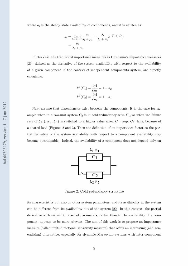
where ai is the steady state availability of component i, and it is written as:

ai = limt→+∞

(µi

λi + µi+

λi

λi + µie−(λi+µi)t)

=µi

λi + µi

In this case, the traditional importance measures as Birnbaum’s importance measures

[23], defined as the derivative of the system availability with respect to the availability

of a given component in the context of independent components system, are directly

calculable:

IB(C1) =∂A

∂a1= 1− a2

IB(C2) =∂A

∂a2= 1− a1

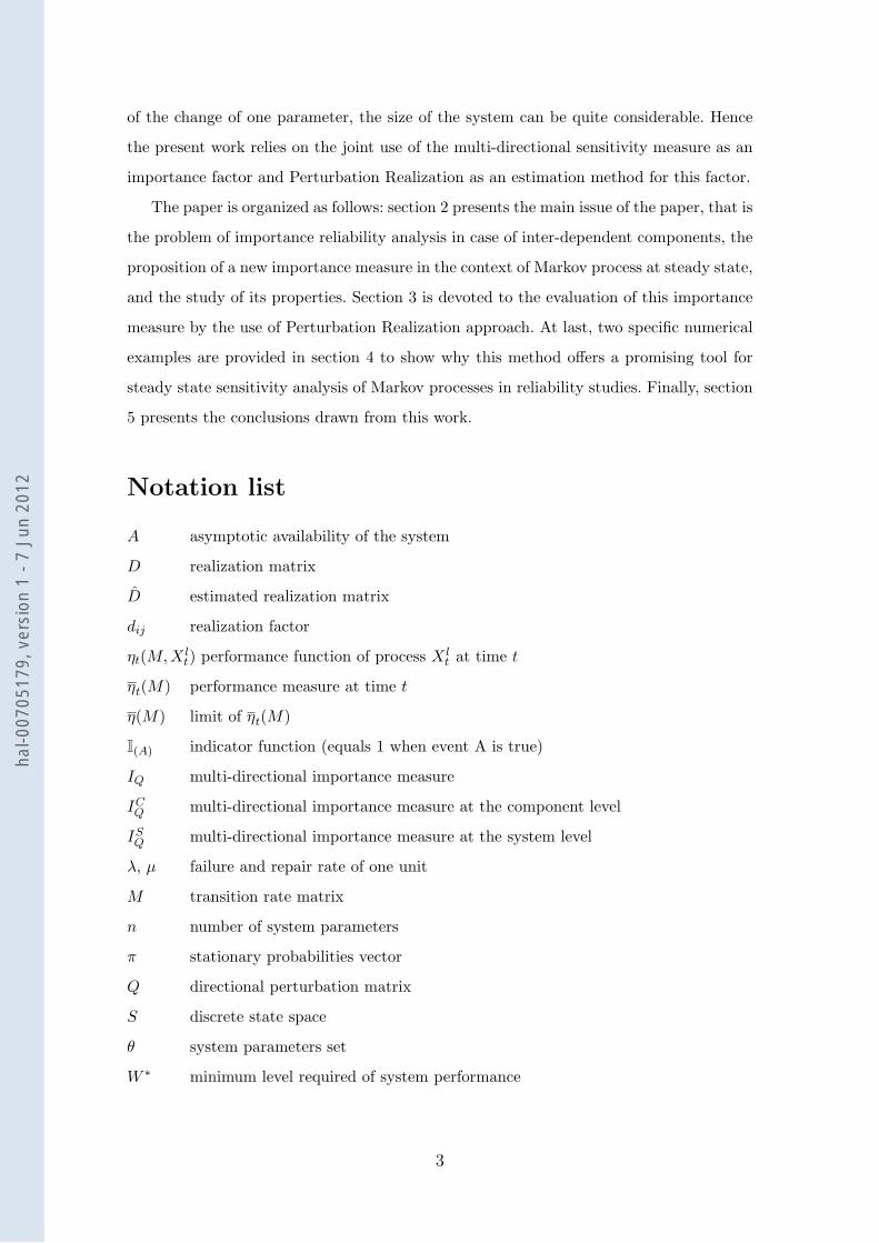
Next assume that dependencies exist between the components. It is the case for ex-

ample when in a two-unit system C2 is in cold redundancy with C1, or when the failure

rate of C2 (resp. C1) is switched to a higher value when C1 (resp. C2) fails, because of

a shared load (Figures 2 and 3). Then the definition of an importance factor as the par-

tial derivative of the system availability with respect to a component availability may

become questionable. Indeed, the availability of a component does not depend only on

Figure 2: Cold redundancy structure

its characteristics but also on other system parameters, and its availability in the system

can be different from its availability out of the system [20]. In this context, the partial

derivative with respect to a set of parameters, rather than to the availability of a com-

ponent, appears to be more relevant. The aim of this work is to propose an importance

measure (called multi-directional sensitivity measure) that offers an interesting (and gen-

eralizing) alternative, especially for dynamic Markovian systems with inter-component

5

hal-0

0705

179,

ver

sion

1 -

7 Ju

n 20

12

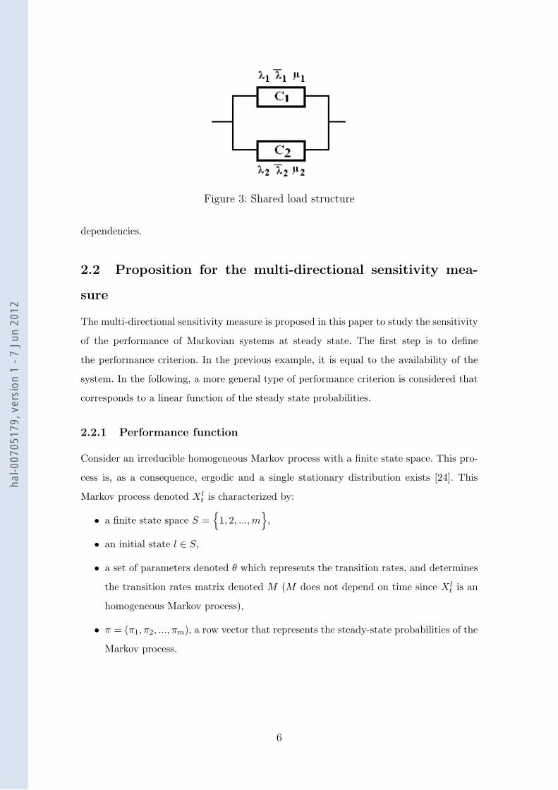
Figure 3: Shared load structure

dependencies.

2.2 Proposition for the multi-directional sensitivity mea-

sure

The multi-directional sensitivity measure is proposed in this paper to study the sensitivity

of the performance of Markovian systems at steady state. The first step is to define

the performance criterion. In the previous example, it is equal to the availability of the

system. In the following, a more general type of performance criterion is considered that

corresponds to a linear function of the steady state probabilities.

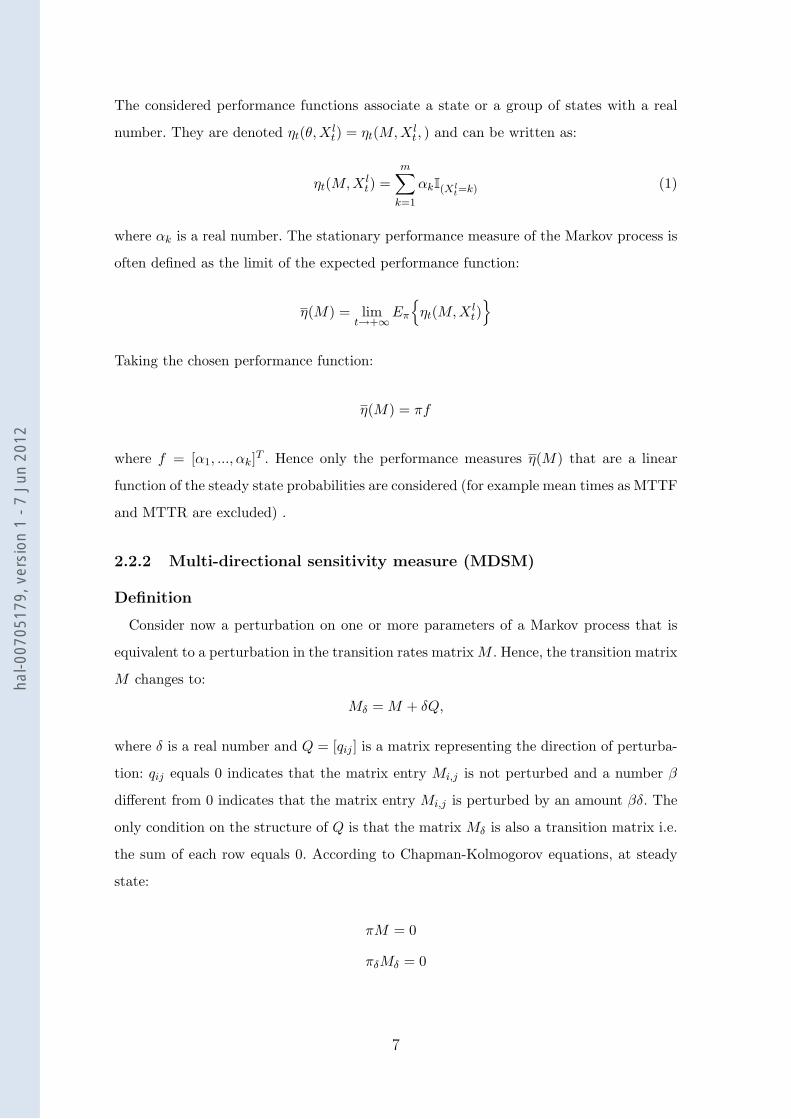
2.2.1 Performance function

Consider an irreducible homogeneous Markov process with a finite state space. This pro-

cess is, as a consequence, ergodic and a single stationary distribution exists [24]. This

Markov process denoted X lt is characterized by:

• a finite state space S =

1, 2, ...,m

,

• an initial state l ∈ S,

• a set of parameters denoted θ which represents the transition rates, and determines

the transition rates matrix denoted M (M does not depend on time since X lt is an

homogeneous Markov process),

• π = (π1, π2, ..., πm), a row vector that represents the steady-state probabilities of the

Markov process.

6

hal-0

0705

179,

ver

sion

1 -

7 Ju

n 20

12

The considered performance functions associate a state or a group of states with a real

number. They are denoted ηt(θ, X lt) = ηt(M,X l

t , ) and can be written as:

ηt(M,X lt) =

m∑k=1

αkI(Xlt=k) (1)

where αk is a real number. The stationary performance measure of the Markov process is

often defined as the limit of the expected performance function:

η(M) = limt→+∞

Eπ

ηt(M,X l

t)

Taking the chosen performance function:

η(M) = πf

where f = [α1, ..., αk]T . Hence only the performance measures η(M) that are a linear

function of the steady state probabilities are considered (for example mean times as MTTF

and MTTR are excluded) .

2.2.2 Multi-directional sensitivity measure (MDSM)

Definition

Consider now a perturbation on one or more parameters of a Markov process that is

equivalent to a perturbation in the transition rates matrix M . Hence, the transition matrix

M changes to:

Mδ = M + δQ,

where δ is a real number and Q = [qij ] is a matrix representing the direction of perturba-

tion: qij equals 0 indicates that the matrix entry Mi,j is not perturbed and a number β

different from 0 indicates that the matrix entry Mi,j is perturbed by an amount βδ. The

only condition on the structure of Q is that the matrix Mδ is also a transition matrix i.e.

the sum of each row equals 0. According to Chapman-Kolmogorov equations, at steady

state:

πM = 0

πδMδ = 0

7

hal-0

0705

179,

ver

sion

1 -

7 Ju

n 20

12

Figure 4: Perturbation on λ2

State 1 : C1C2 State 2 : C1C2

State 3 : C1C2 State 4 : C1 C2

The stationary performance measure of the perturbed Markov process (that is the Markov

process with transition matrix Mδ) is denoted η(Mδ) = πδf . Consequently, the derivative

of η(M) in the direction of Q can be defined as:

dη(M)dQ

= limδ→0

η(Mδ)− η(M)δ

. (2)

The aim is to propose the use of the system performance derivative with respect to Q

as an importance factor. It is called multi-directional sensitivity measure (MDSM) in the

following and denoted IQ:

IQ =dη(M)

dQ(3)

Two types of MDSM: ICQ and IS

Q

Consider the previous example on Figure 1. The state diagram of this system is sketched

in Figures 4 and 5 for two different types of perturbations. Figure 4 sketches the Markov

graph with a perturbation on one specific parameter, namely λ2, which corresponds to

the directional perturbation matrix Q1:

Q1 =

−1 0 1 0

0 −1 0 1

0 0 0 0

0 0 0 0

.

Figure 5 presents the Markov graph modified by a perturbation on the exit transition

8

hal-0

0705

179,

ver

sion

1 -

7 Ju

n 20

12

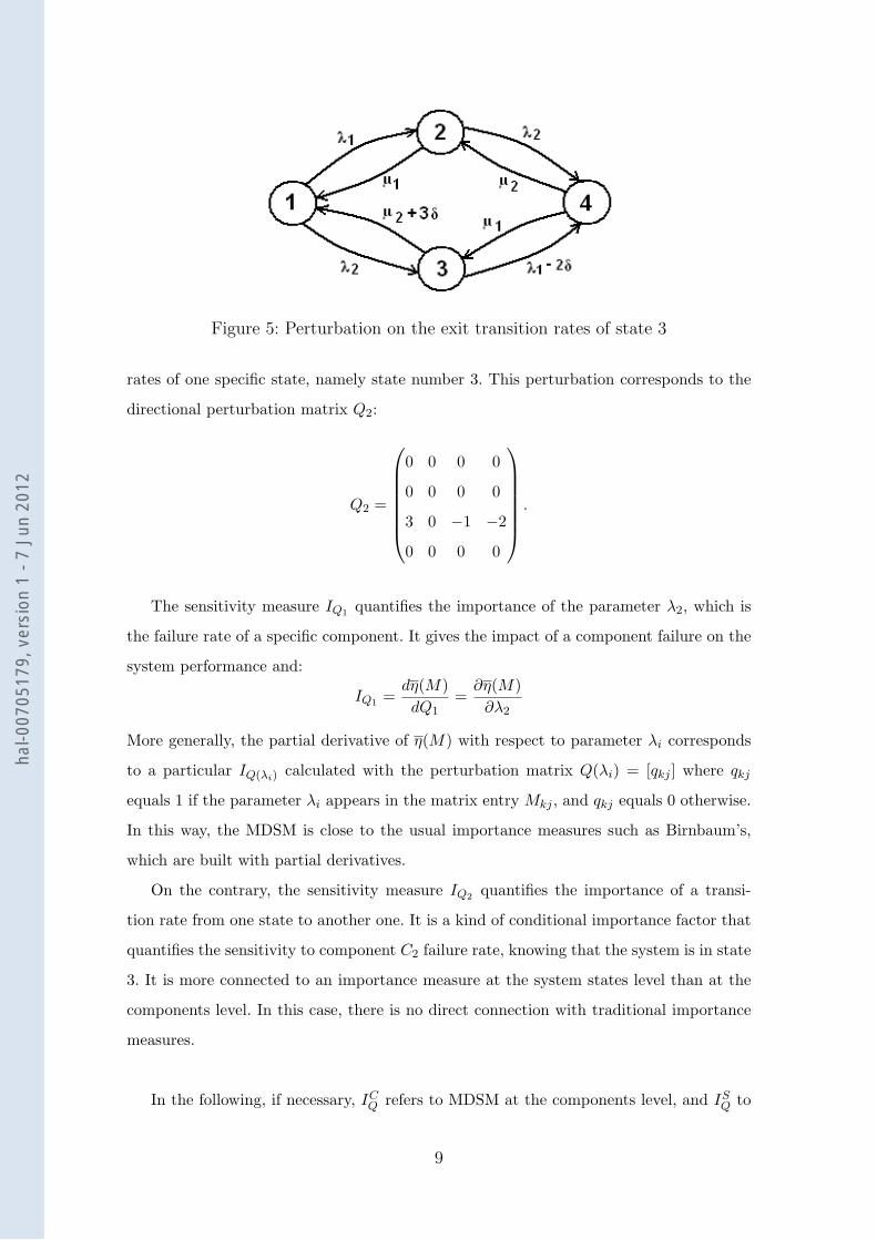
Figure 5: Perturbation on the exit transition rates of state 3

rates of one specific state, namely state number 3. This perturbation corresponds to the

directional perturbation matrix Q2:

Q2 =

0 0 0 0

0 0 0 0

3 0 −1 −2

0 0 0 0

.

The sensitivity measure IQ1 quantifies the importance of the parameter λ2, which is

the failure rate of a specific component. It gives the impact of a component failure on the

system performance and:

IQ1 =dη(M)dQ1

=∂η(M)

∂λ2

More generally, the partial derivative of η(M) with respect to parameter λi corresponds

to a particular IQ(λi) calculated with the perturbation matrix Q(λi) = [qkj ] where qkj

equals 1 if the parameter λi appears in the matrix entry Mkj , and qkj equals 0 otherwise.

In this way, the MDSM is close to the usual importance measures such as Birnbaum’s,

which are built with partial derivatives.

On the contrary, the sensitivity measure IQ2 quantifies the importance of a transi-

tion rate from one state to another one. It is a kind of conditional importance factor that

quantifies the sensitivity to component C2 failure rate, knowing that the system is in state

3. It is more connected to an importance measure at the system states level than at the

components level. In this case, there is no direct connection with traditional importance

measures.

In the following, if necessary, ICQ refers to MDSM at the components level, and IS

Q to

9

hal-0

0705

179,

ver

sion

1 -

7 Ju

n 20

12

MDSM at the system states level. In particular, ICQ(λi)

refers to the partial derivative of

the performance function with respect to parameter λi.

2.3 Properties of the MDSM

2.3.1 MDSM and classical importance factor

Consider the example in Figure 1 and take as performance function η(M) = A, the system

availability. IQ1 = ICQ(λ2) corresponds to ∂A/∂λ2, i.e. the partial derivative of the system

availability with respect to λ2. In this case, the link with the Birnbaum’s importance

measure is directly established using the chain rule:

IB(C2) =∂A

∂a2

=∂A

∂λ2/∂a2

∂λ2(4)

IB(C2) = IQ1/∂a2

∂λ2= IC

Q(λ2)/∂a2

∂λ2. (5)

In the case of a system with inter-dependent components as in Figure 2, the link between

MDSM and Birnbaum’s importance measure cannot be directly established since the latter

is no longer defined. However, a MDSM of ICQ type gives the same kind of information

as a Birnbaum factor, since it can provide partial derivatives with respect to any system

parameters.

2.3.2 Relation with the transition matrix

The particular structure of the Chapman-Kolmogorov equations and the linearity of the

performance measure lead to the following expression of the measure derivatives [4]:

dη(M)dQ

= −πQM∗f (6)

where M∗ is the inverse group of M defined as:

M∗ = (M − eπ)−1 − eπ,

where e is a column vector of size (n, 1) with ei,1 = 1 for any i.

10

hal-0

0705

179,

ver

sion

1 -

7 Ju

n 20

12

2.3.3 Joint sensitivity

Because of the linear structure of Equation 6, if a perturbation matrix Q is a linear

function of elementary perturbation matrixes Qi, it is possible to evaluate the multi-

directional importance measure related to Q on the basis of the elementary perturbation

measures related to the Qi. For instance in the case of the system in Figure 1, for the joint

sensitivity of the group of parameters (λ1, λ2) , it is possible to define a joint perturbation

matrix:

Q(λ1, λ2) = Q(λ1) + Q(λ2)

where the matrix entry qi,j(λk) equals 1 if the parameter λk is in the matrix entry Mi,j

and qi,j(λk) equals 0 otherwise. Then:

ICQ(λ1,λ2) =

∂η(M)∂Q(λi, λj))

= −πQ(λi, λj)M∗f

= −π(Q(λi) + Q(λj)

)M∗f

= −πQ(λi)M∗f + Q(λj)M∗f

= ICQ(λi)

+ ICQ(λj)

In this way, the joint sensitivity to a group of parameters can be the sum of the sensitivity

measures to each parameter of the group. More generally, if a joint perturbation matrix

with a different derivative direction for each parameter of a group of n parameters is

defined as:

Q(α1λ1, α2λ2, ...., αnλn) =n∑

i=1

αiQ(λi),

then:

IQ(α1λ1,α2λ2,....,αnλn) = −π(α1Q(λ1) + α2Q(λ2) + ...αnQ(λn)

)M∗f

=n∑

i=1

αiIQ(λi) (7)

This property of the joint sensitivity cannot directly be connected to the additivity

property of the differential importance measure presented by Borgonovo & al. in [1, 2]:

it concerns perturbation directions but not the components. In some particular cases,

i.e. when the sensitivity measure related to one component can be defined by only one

11

hal-0

0705

179,

ver

sion

1 -

7 Ju

n 20

12

perturbation direction, the joint sensitivity to a group of components can be expressed as

the sum of the sensitivity to the components. But it is not true as a rule and especially

for system under consideration in this paper, i.e. with stochastic dependences.

As a conclusion, if the MDSM related to elementary perturbation directions are cal-

culated, the joint MDSM related to any linear combination of these directions requires no

additional calculations.

3 Multi-directional sensitivity measure calcula-

tion

Many solutions have been proposed in literature to evaluate sensitivity measures cor-

responding to partial derivatives. Exact solutions rely on Frank’s approach in [12]: the

classical set of differential equations is extended to a bigger set of equations including

the sensitivity factor equations. However, this approach is computationally burdensome

and almost unusable or highly inefficient on realistic-size systems because the state space

dimension is too great. To cope with this problem, some approximate solutions have been

proposed but they are often only applicable to a limited class of systems (e.g. acyclic

Markov models with no repair), [20].

Many simulation methods have been also proposed to estimate derivative measure.

The simplest methods rely on the use of finite differences (FD) [8], and simultaneous

perturbation (SP) [25]. These methods imply the change of the parameters for each simu-

lation, which can be numerically burdensome and unfeasible for many real world systems,

especially for those that need to be reliable. Methods based on common random num-

bers [8] offer a solution to this problem but if the value of the perturbation is too small,

the resulting difference estimator could be severely affected by interference. The deriva-

tive estimation based on likelihood ratios (LR) has been proposed in [16, 14], and weak

derivatives (WD) was introduced by Pflug [21, 22]. These methods provide an unbiased

estimator, which leads to faster convergence rates when implemented in a simulation op-

timization algorithm, e.g., stochastic approximation [14].

In the framework of reliability studies, the perturbation analysis (PA) [3] and its vari-

ants, infinitesimal perturbation analysis (IPA), smoothed perturbation analysis (SPA)[13],

structural IPA [9], Perturbation Realization [4] seem to be much promising. These meth-

12

hal-0

0705

179,

ver

sion

1 -

7 Ju

n 20

12

ods are based on the use of the stochastic gradient that can be estimated from one single

sample path (i.e. without any change of the model parameters) [15]. Concerning Markov

process modelling and stationary performance measure, Perturbation Realization is par-

ticularly well adapted [6, 7]. It allows for:

• the evaluation of multi-directional sensitivity measures at the component level (ICQ ),

• the evaluation of multi-directional sensitivity measures at the system level (ISQ),

• the evaluation of these sensitivity measures with operating feedback data, without

any change of parameters, and without any knowledge of the infinitesimal generator

of the Markov process.

3.1 Introduction

In the following, the main idea and the main steps of Perturbation Realization are pre-

sented. If:

• Xit , is a Markov process with transition matrix M and initial state i,

• Xjt , is a Markov process with transition matrix M and initial state j,

• Y i,jt = (Xi

t , Xjt ),

• K = (k, k), k ∈ S,

and:

T (i,j) = inf(t, t > 0, Y i,jt ∈ K),

then the realization factor dij related to states i and j equals:

dij = E∫ T (i,j)

0[ηt(M,Xj

t )− ηt(M,Xit)]dt

.

Consider a matrix D, called the realization matrix, so that D(i, j) = dij . Using a

Lyapunov equation verified by M and D, Cao showed in [4] that:

IQ =dη(M)

dQ= πQDT πT . (8)

The derivative dη(M)/dQ is estimated on the basis of this equality. The advantages

are that the inversion of matrix (M − eπ) in Equation 6 is avoided and that the matrix

D estimation relies on a single sample path. Hence, the realization factor defined for the

13

hal-0

0705

179,

ver

sion

1 -

7 Ju

n 20

12

steady state performance of a Markov process allows for, a direct estimation without

matrix inversion, the estimation of the MDSM with a single sample path (from this point

of view, this estimation method is part and parcel of Perturbation Analysis), and a very

simple calculation of the MDSM for any perturbation matrix Q (once the matrix D is

estimated).

Paragraph 3.2 is devoted to the interpretation of matrix M and paragraph 3.3 to its

estimation.

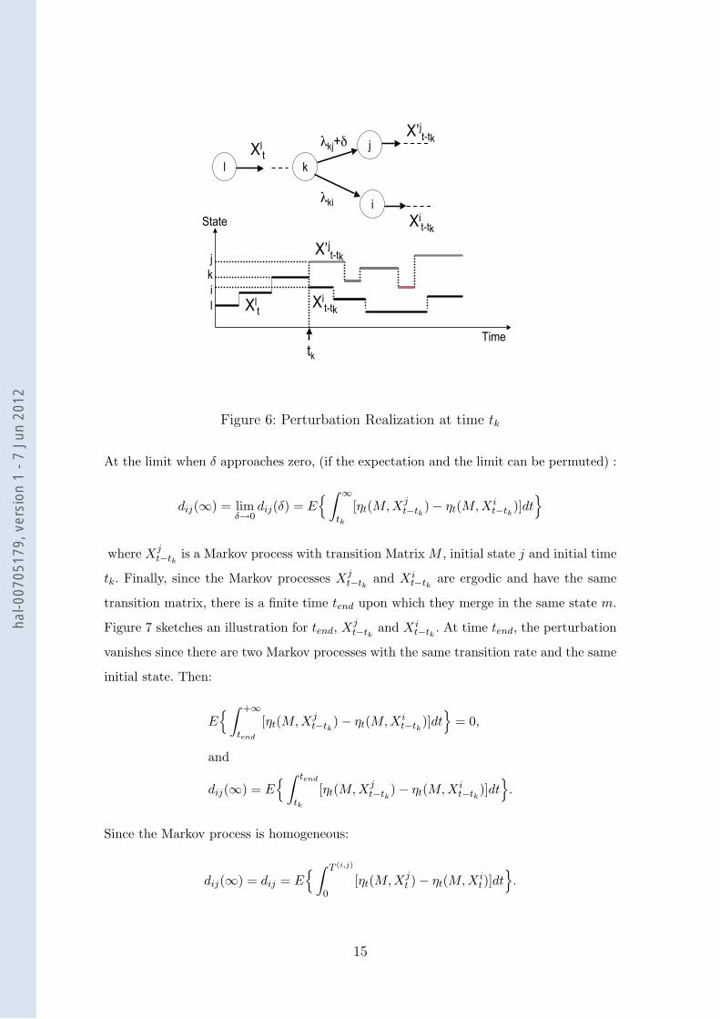
3.2 Perturbation Realization factor

In order to give an interpretation of the realization factor dij , consider the quantity

dij(δ,∞) so that:

dij(δ,∞) = E∫ ∞

tk

[ηt(Mδ, X′jt−tk

, )− ηt(M,Xit−tk

)]dt

with:

tk = the time upon which a perturbation occurs,

X ′jt−tk

, a Markov process with transition matrix Mδ, initial state j and initial time tk,

Xit−tk

, a Markov process with transition matrix M , initial state i and initial time tk,

X lt , a Markov process with transition matrix M , initial state l and initial time 0.

Figure 6 gives an illustration for X ′jt−tk

, X it−tk

, tk. First, there is a Markov process X lt , with

initial state l and transition matrix M . If, when the system is in state k, the transition

rates λkj is perturbed by an amount +δ, it is possible that at the next transition time

denoted tk, the resulting perturbed Markov process X′jt−tk

goes from state k to state j

(perturbed sample path) instead of going from state k to state i as X lt would do. In this

case, the perturbation is “realized”. If this is the only realized perturbation, then the

impact of the perturbation on the performance measure is quantified by dij(δ,∞). Then,

since the Markov process is homogeneous:

dij(δ,∞) = E∫ ∞

tk

[ηt(Mδ, X′jt−tk

)− ηt(M,Xit−tk

)]dt

14

hal-0

0705

179,

ver

sion

1 -

7 Ju

n 20

12

λki

λkj+δ

k

j

i

l

X’jt-tkXlt

tk

kj

iXlt

X’jt-tk

State

Time

Xit-tk

Xit-tk

l

Figure 6: Perturbation Realization at time tk

At the limit when δ approaches zero, (if the expectation and the limit can be permuted) :

dij(∞) = limδ→0

dij(δ) = E∫ ∞

tk

[ηt(M,Xjt−tk

)− ηt(M,Xit−tk

)]dt

where Xjt−tk

is a Markov process with transition Matrix M , initial state j and initial time

tk. Finally, since the Markov processes Xjt−tk

and Xit−tk

are ergodic and have the same

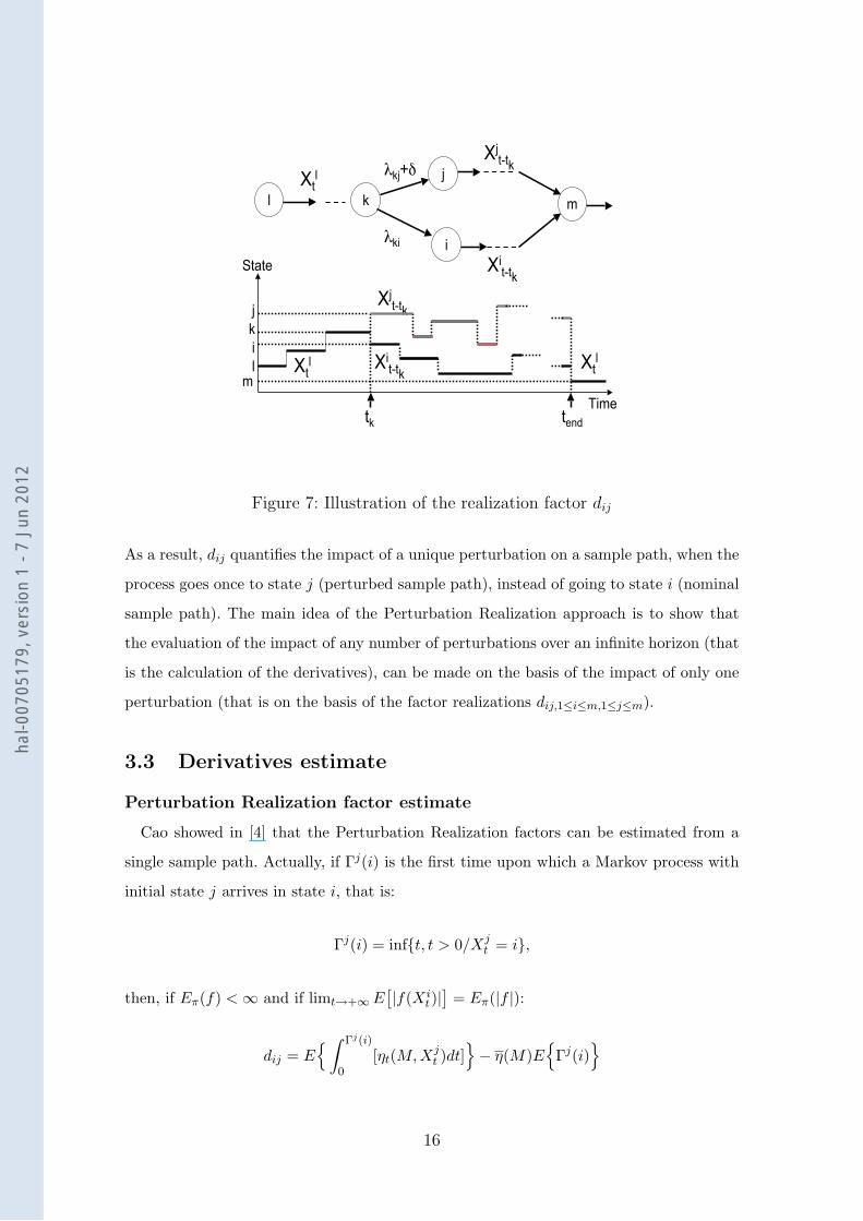
transition matrix, there is a finite time tend upon which they merge in the same state m.

Figure 7 sketches an illustration for tend, Xjt−tk

and Xit−tk

. At time tend, the perturbation

vanishes since there are two Markov processes with the same transition rate and the same

initial state. Then:

E∫ +∞

tend

[ηt(M,Xjt−tk

)− ηt(M,Xit−tk

)]dt

= 0,

and

dij(∞) = E∫ tend

tk

[ηt(M,Xjt−tk

)− ηt(M,Xit−tk

)]dt

.

Since the Markov process is homogeneous:

dij(∞) = dij = E∫ T (i,j)

0[ηt(M,Xj

t )− ηt(M,Xit)]dt

.

15

hal-0

0705

179,

ver

sion

1 -

7 Ju

n 20

12

λki

λkj+δ

k

j

i

l m

m

Xjt-tkXtl

tendtk

kj

iXtl Xtl

Xjt-tk

State

Time

Xit-tk

Xit-tk

l

Figure 7: Illustration of the realization factor dij

As a result, dij quantifies the impact of a unique perturbation on a sample path, when the

process goes once to state j (perturbed sample path), instead of going to state i (nominal

sample path). The main idea of the Perturbation Realization approach is to show that

the evaluation of the impact of any number of perturbations over an infinite horizon (that

is the calculation of the derivatives), can be made on the basis of the impact of only one

perturbation (that is on the basis of the factor realizations dij,1≤i≤m,1≤j≤m).

3.3 Derivatives estimate

Perturbation Realization factor estimate

Cao showed in [4] that the Perturbation Realization factors can be estimated from a

single sample path. Actually, if Γj(i) is the first time upon which a Markov process with

initial state j arrives in state i, that is:

Γj(i) = inft, t > 0/Xjt = i,

then, if Eπ(f) < ∞ and if limt→+∞E[|f(Xi

t)|]

= Eπ(|f |):

dij = E∫ Γj(i)

0[ηt(M,Xj

t )dt]− η(M)E

Γj(i)

16

hal-0

0705

179,

ver

sion

1 -

7 Ju

n 20

12

The first passage time Γj(i) and the stationary probability vector π (and consequently

η(M)) can be estimated from Xj = (Xjt , t ≥ 0) as follows. A Markov process X l

t (initial

state l and transition matrix M) is observed with the two time sequences js and is

so that:

• i0 = 0,

• js= is the time upon which X lt is in state j for the first time after time is−1,

• is= is the time upon which X lt is in state i for the first time after time js,

• Ljs(i) = is − js for s ≥ 1 (independent and identically distributed),

• Rs =∫ is−1k=js

ηt(X lk)dt (independent and identically distributed).

Then Γj(i),∫ Γj(i)0 [ηt(X

jt )dt], and η(M) are estimated by Γj(i), I, and η(M) respectively

:

Γj(i) =1n

n∑s=1

Ljs(i),

I =1n

n∑s=1

Rs,

η(M) = πf with πi =1N

N∑k=1

I(Xltk

=i), (9)

where n is the number of observed sequences from j to i, N is the total number of observed

sequences and tk is the k-th transition time. Consequently:

dij = I − η(M)Γj(i). (10)

The convergence of these estimators based on the realization matrix has been studied and

proved by Cao in [4].

The estimation of the matrix D can also be computationally burdensome because it

must be made for each couple (i, j) (complexity of order O(m2)). That is why an approx-

imate estimate (with potential vector) is proposed in [5] which reduces the complexity of

the calculation to the order O(m).

Hence, thanks to the ergodicity of the process under consideration, the Perturbation

Realization concept gives an estimate of the MDSM that:

• can be evaluated from a single sample path. This is very interesting from a prac-

17

hal-0

0705

179,

ver

sion

1 -

7 Ju

n 20

12

tical point of view for on-line performance optimization, when the parameters are

impossible to change intentionally, or when the simulation of each perturbed path

is computationally burdensome;

• can be evaluated without knowing the infinitesimal generator M of the Markov

process;

• can be evaluated in any direction by changing only the directional matrix Q.

4 Application to reliability studies: numerical

experiments

The numerical results presented in this section are obtained with simulated operating

feedback data. The aim is to show how the joint use of multi-directional sensitivity mea-

sure and the realization factors for their estimation can help in the sensitivity analysis

of stationary performance in reliability studies. A first simple case is studied to make

a connection between usual analytical results and estimation results with Perturbation

Analysis in the case of Birnbaum’s importance measure. Then, a more complex system is

presented to enhance the advantages of multi directional sensitivity measure with Pertur-

bation analysis. In both cases, the transition rate matrix is assumed to be unknown for

the estimation, and the data set is made of the transition dates from one state to another.

The performance measure is the asymptotic availability and the simulations are made for

100000 transitions.

4.1 Binary-state systems with independent components

4.1.1 Expression of the performance function

For binary-state systems, a performance function η(M) at steady state can be the

availability, expressed as:

η(M) =∑i∈Ωo

πi,

with πi is the stationary probability of state i, and Ωo is the set of the running states of

the system.

18

hal-0

0705

179,

ver

sion

1 -

7 Ju

n 20

12

4.1.2 Comparison of analytical and estimated results

Consider first the two-unit system sketched in Figure 4. The availability of units C1, C2

at steady state are written as:

a1 =µ1

λ1 + µ1, a2 =

µ2

λ2 + µ2.

The asymptotic availability of the system can be obviously calculated with Kolmogorov

equations at steady state:

−(λ1 + λ2)π1 + λ1π2 + λ2π3 = 0

µ1π1 − (µ1 + λ2)π2 + λ2π4 = 0

µ2π1 − (λ1 + µ2)π3 + λ1π4 = 0

µ2π2 + µ1π3 − (µ1 + µ2)π4 = 0

π1 + π2 + π3 + π4 = 1

By solving these equations, the availability of the system is finally obtained:

A = π1 + π2 + π3 =µ1µ2 + µ1λ2 + µ2λ1

(λ1 + µ1)(λ2 + µ2). (11)

The derivative of A with respect to λi, µi (i = 1, 2), can be obtained easily from this

formula.

To compare with the estimated results, a set of data with transition instants λ1 =

0.01, λ2 = 0.01, µ1 = 0.05, µ2 = 0.05 is generated. Then the realization matrix D and the

steady-state probability vector π are estimated with Equation 10:

D =

0 −1.3648 −1.4528 −11.2053

1.3648 0 −0.0850 −9.8446

1.4528 0.0850 0 −9.8063

11.2053 9.8446 9.8063 0

,

and

π = (0.6898, 0.1406, 0.1413, 0.0283).

Consider now the perturbation on a parameter level, more precisely on λ2, correspond-

ing to the directional matrix Q1 given in section 2.2.2. Then, using the estimators D and

19

hal-0

0705

179,

ver

sion

1 -

7 Ju

n 20

12

π, Equation 8 gives:

E(IQ1) = E(ICQ(λ2)) = −2.3014,

var(IQ1) = var(ICQ(λ2)) = 0.0357.

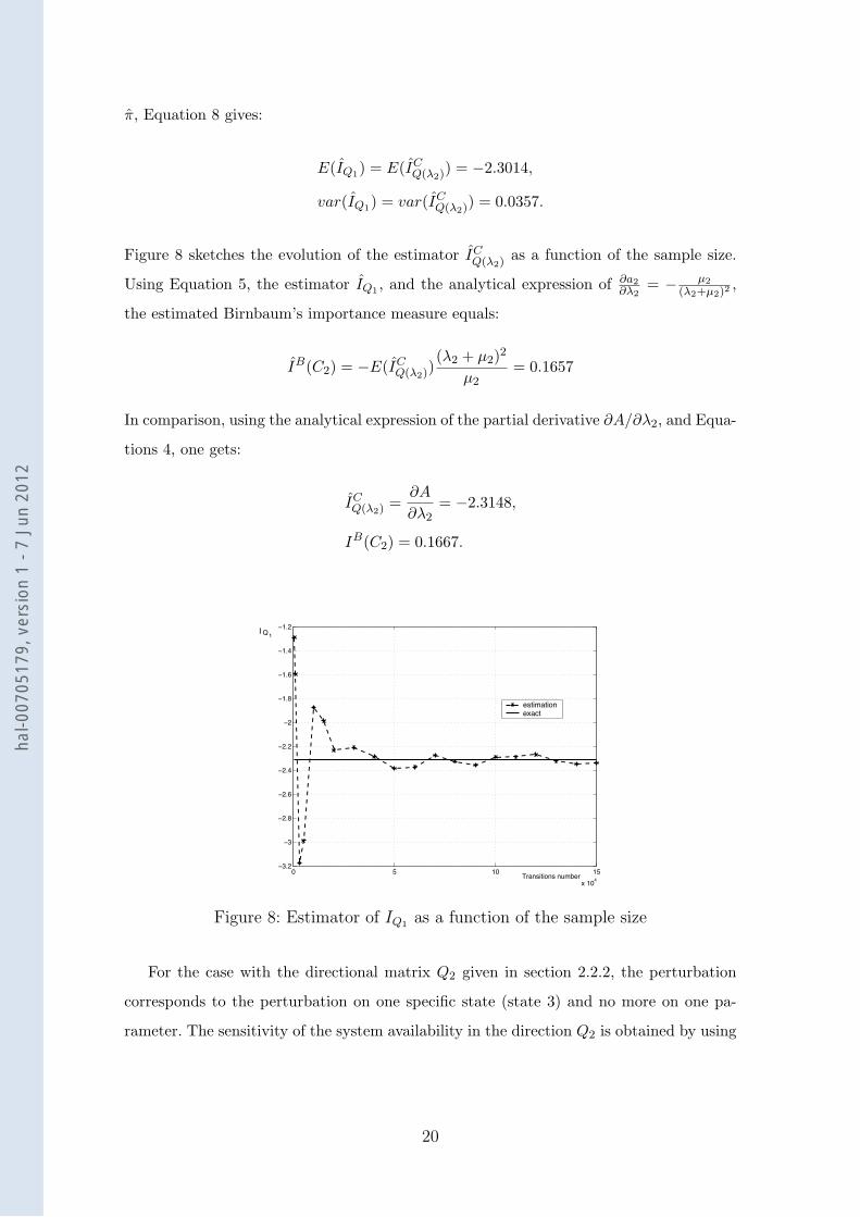
Figure 8 sketches the evolution of the estimator ICQ(λ2) as a function of the sample size.

Using Equation 5, the estimator IQ1 , and the analytical expression of ∂a2∂λ2

= − µ2

(λ2+µ2)2,

the estimated Birnbaum’s importance measure equals:

IB(C2) = −E(ICQ(λ2))

(λ2 + µ2)2

µ2= 0.1657

In comparison, using the analytical expression of the partial derivative ∂A/∂λ2, and Equa-

tions 4, one gets:

ICQ(λ2) =

∂A

∂λ2= −2.3148,

IB(C2) = 0.1667.

0 5 10 15x 104

!3.2

!3

!2.8

!2.6

!2.4

!2.2

!2

!1.8

!1.6

!1.4

!1.2

,ransitions n4m6er

estimation exact

I Q 1

Figure 8: Estimator of IQ1 as a function of the sample size

For the case with the directional matrix Q2 given in section 2.2.2, the perturbation

corresponds to the perturbation on one specific state (state 3) and no more on one pa-

rameter. The sensitivity of the system availability in the direction Q2 is obtained by using

20

hal-0

0705

179,

ver

sion

1 -

7 Ju

n 20

12

the same estimators D, and π:

E(IQ2) = E(ISQ2

) = 3.2815,

var(IQ2) = var(ISQ2

) = 0.0288.

This derivative means that if the repair rate µ2 on state 3 is increased by an amount

3δ, and at the same time, the failure rate λ1 on state 3 is decreased by an amount 2δ,

then the system availability will increase by an amount 3.2815δ. This value quantifies

the gain for the system availability if the probability of being in state 3 is perturbed.

Since state 3 is a running state and since the perturbation in the direction Q2 increases

the probability of in staying state 3, the availability increases and ISQ2

indicates at which

speed. To obtain the analytical result in this case, it would be necessary to rewrite the

system of differential equations by distinguishing all transition rates between all states,

for example to distinguish the parameter λ1 representing the transition rate from state

1 towards state 2, from the parameter λ1 representing the transition rate from state 3

towards state 4.

4.2 Multi-state systems with dependent components

4.2.1 Presentation of the system

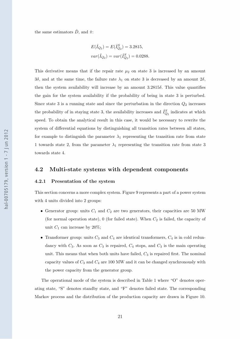
This section concerns a more complex system. Figure 9 represents a part of a power system

with 4 units divided into 2 groups:

• Generator group: units C1 and C2 are two generators, their capacities are 50 MW

(for normal operation state), 0 (for failed state). When C2 is failed, the capacity of

unit C1 can increase by 20%;

• Transformer group: units C3 and C4 are identical transformers, C4 is in cold redun-

dancy with C3. As soon as C3 is repaired, C4 stops, and C3 is the main operating

unit. This means that when both units have failed, C3 is repaired first. The nominal

capacity values of C3 and C4 are 100 MW and it can be changed synchronously with

the power capacity from the generator group.

The operational mode of the system is described in Table 1 where “O” denotes oper-

ating state, “S” denotes standby state, and “F” denotes failed state. The corresponding

Markov process and the distribution of the production capacity are drawn in Figure 10.

21

hal-0

0705

179,

ver

sion

1 -

7 Ju

n 20

12

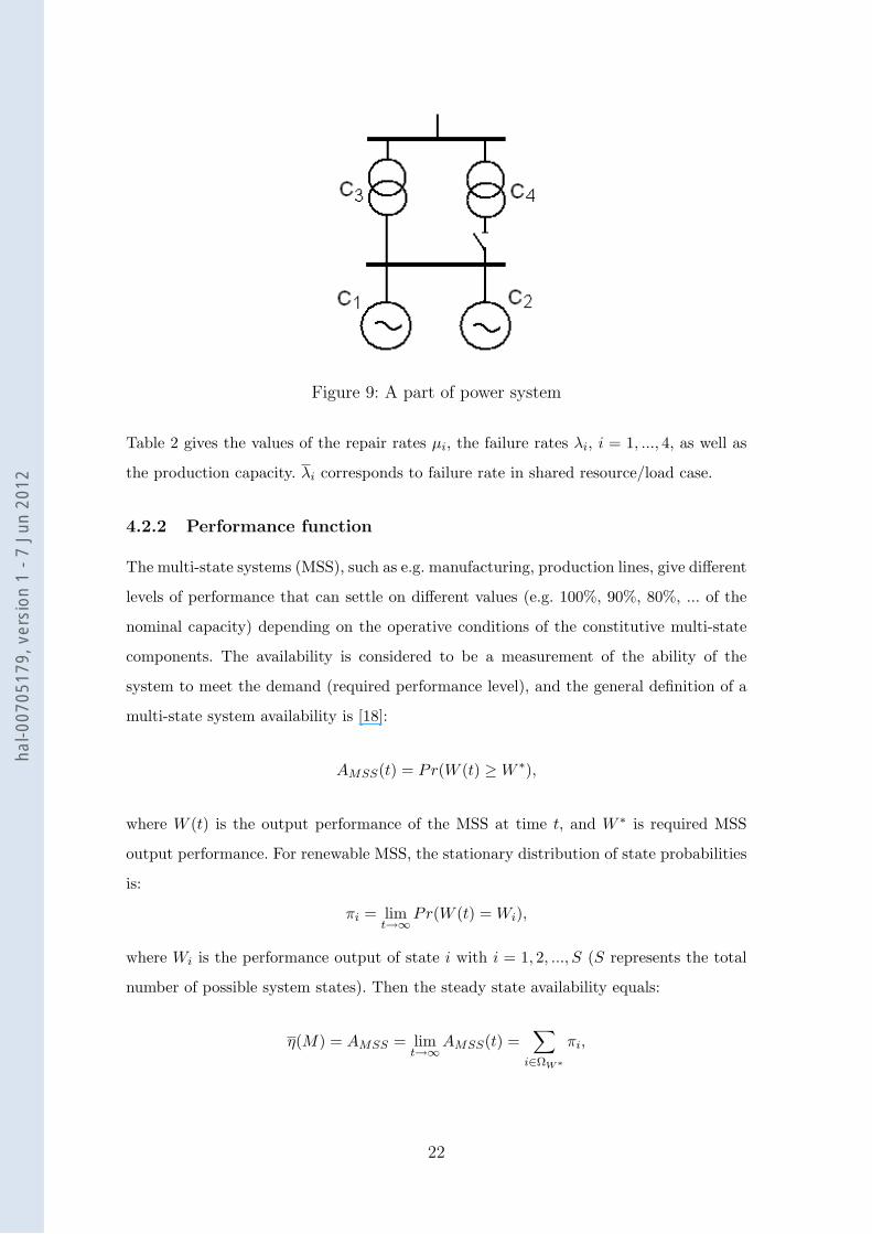
Figure 9: A part of power system

Table 2 gives the values of the repair rates µi, the failure rates λi, i = 1, ..., 4, as well as

the production capacity. λi corresponds to failure rate in shared resource/load case.

4.2.2 Performance function

The multi-state systems (MSS), such as e.g. manufacturing, production lines, give different

levels of performance that can settle on different values (e.g. 100%, 90%, 80%, ... of the

nominal capacity) depending on the operative conditions of the constitutive multi-state

components. The availability is considered to be a measurement of the ability of the

system to meet the demand (required performance level), and the general definition of a

multi-state system availability is [18]:

AMSS(t) = Pr(W (t) ≥ W ∗),

where W (t) is the output performance of the MSS at time t, and W ∗ is required MSS

output performance. For renewable MSS, the stationary distribution of state probabilities

is:

πi = limt→∞

Pr(W (t) = Wi),

where Wi is the performance output of state i with i = 1, 2, ..., S (S represents the total

number of possible system states). Then the steady state availability equals:

η(M) = AMSS = limt→∞

AMSS(t) =∑

i∈ΩW∗

πi,

22

hal-0

0705

179,

ver

sion

1 -

7 Ju

n 20

12

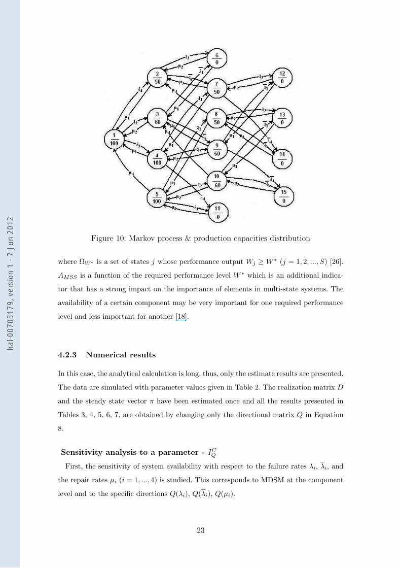
Figure 10: Markov process & production capacities distribution

where ΩW ∗ is a set of states j whose performance output Wj ≥ W ∗ (j = 1, 2, ..., S) [26].

AMSS is a function of the required performance level W ∗ which is an additional indica-

tor that has a strong impact on the importance of elements in multi-state systems. The

availability of a certain component may be very important for one required performance

level and less important for another [18].

4.2.3 Numerical results

In this case, the analytical calculation is long, thus, only the estimate results are presented.

The data are simulated with parameter values given in Table 2. The realization matrix D

and the steady state vector π have been estimated once and all the results presented in

Tables 3, 4, 5, 6, 7, are obtained by changing only the directional matrix Q in Equation

8.

Sensitivity analysis to a parameter - ICQ

First, the sensitivity of system availability with respect to the failure rates λi, λi, and

the repair rates µi (i = 1, ..., 4) is studied. This corresponds to MDSM at the component

level and to the specific directions Q(λi), Q(λi), Q(µi).

23

hal-0

0705

179,

ver

sion

1 -

7 Ju

n 20

12

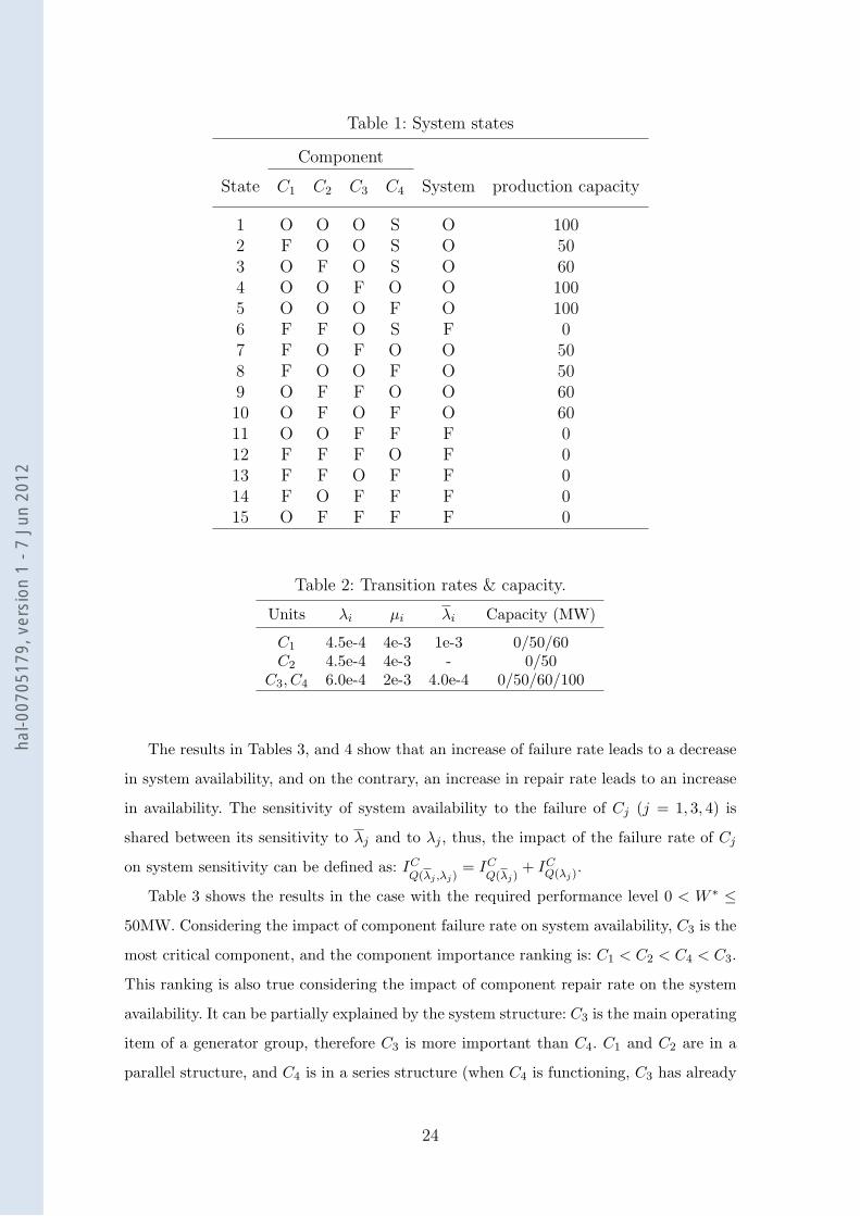
Table 1: System states

Component

State C1 C2 C3 C4 System production capacity

1 O O O S O 1002 F O O S O 503 O F O S O 604 O O F O O 1005 O O O F O 1006 F F O S F 07 F O F O O 508 F O O F O 509 O F F O O 6010 O F O F O 6011 O O F F F 012 F F F O F 013 F F O F F 014 F O F F F 015 O F F F F 0

Table 2: Transition rates & capacity.

Units λi µi λi Capacity (MW)

C1 4.5e-4 4e-3 1e-3 0/50/60C2 4.5e-4 4e-3 - 0/50

C3, C4 6.0e-4 2e-3 4.0e-4 0/50/60/100

The results in Tables 3, and 4 show that an increase of failure rate leads to a decrease

in system availability, and on the contrary, an increase in repair rate leads to an increase

in availability. The sensitivity of system availability to the failure of Cj (j = 1, 3, 4) is

shared between its sensitivity to λj and to λj , thus, the impact of the failure rate of Cj

on system sensitivity can be defined as: ICQ(λj ,λj)

= ICQ(λj)

+ ICQ(λj)

.

Table 3 shows the results in the case with the required performance level 0 < W ∗ ≤

50MW. Considering the impact of component failure rate on system availability, C3 is the

most critical component, and the component importance ranking is: C1 < C2 < C4 < C3.

This ranking is also true considering the impact of component repair rate on the system

availability. It can be partially explained by the system structure: C3 is the main operating

item of a generator group, therefore C3 is more important than C4. C1 and C2 are in a

parallel structure, and C4 is in a series structure (when C4 is functioning, C3 has already

24

hal-0

0705

179,

ver

sion

1 -

7 Ju

n 20

12

Table 3: Sensitivity analysis to failure & repair rates, case 0 < W ∗ ≤ 50

Units Value Order Value Order

C1ICQ(λ1) -2.3270

4 ICQ(µ1) 1.9277 4

ICQ(λ1)

-8.4298

C2 ICQ(λ2) -23.4837 3 IC

Q(µ2) 3.1516 3

C3ICQ(λ3) -78.0152

1 ICQ(µ3) 42.0794 1

ICQ(λ3)

-16.0406

C4ICQ(λ4) -61.6264

2 ICQ(µ4) 4.5391 2

CIQ(λ4) -12.3478

Table 4: Sensitivity analysis to failure & repair rates, case 50 < W ∗ ≤ 60

Units Value Order Value Order

C1ICQ(λ1) -163.8876

1 ICQ(µ1) 22.6118 1

ICQ(λ1)

-16.1538

C2 ICQ(λ2) -13.8236 4 IC

Q(µ2) 1.2707 4

C3ICQ(λ3) -71.0226

2 ICQ(µ3) 20.7130 2

ICQ(λ3)

-13.8683

C4ICQ(λ4) -55.7066

3 ICQ(µ4) 4.1319 3

ICQ(λ4)

-10.9899

failed) so the impact of C4 on system availability behavior is more important than C1 and

C2.

The results of sensitivity analysis in the case of the required performance level 50 <

W ∗ ≤ 60MW are presented in Table 4. In this case, the set of functioning states of

system is ΩW ∗ = 1, 3, 4, 5, 9, 10 (see Figure 10). According to the results of importance

measures showed in Table 4, the new components importance ranking related to failure

rates is: C2 < C4 < C3 < C1. The maximum capacity of C2 is only 50MW, hence if

C1 fails the system is unable to supply the demand W ∗ and it is considered as failed.

Consequently, component C1 ranks first and C2 becomes the least important one. C3 is

still more important than C4 since C3 is the main operating unit of the standby structure.

The results in Tables 3 and 4 show that the component importance ranking of multi-

25

hal-0

0705

179,

ver

sion

1 -

7 Ju

n 20

12

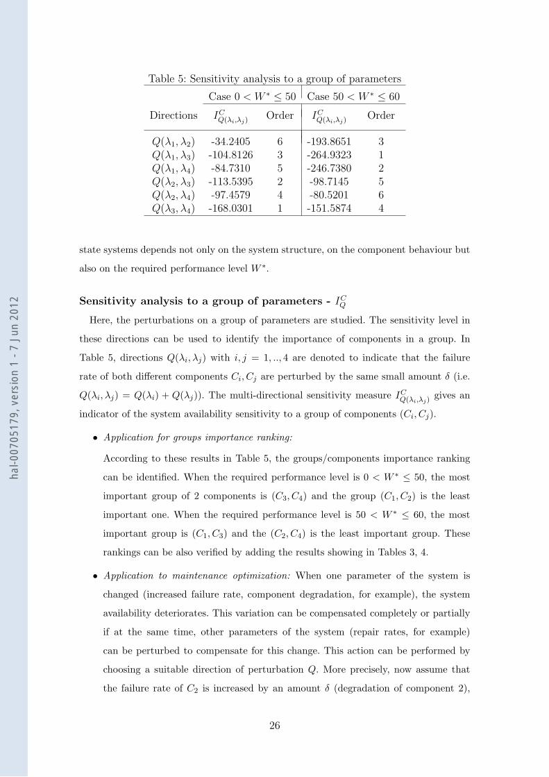
Table 5: Sensitivity analysis to a group of parameters

Case 0 < W ∗ ≤ 50 Case 50 < W ∗ ≤ 60

Directions ICQ(λi,λj)

Order ICQ(λi,λj)

Order

Q(λ1, λ2) -34.2405 6 -193.8651 3Q(λ1, λ3) -104.8126 3 -264.9323 1Q(λ1, λ4) -84.7310 5 -246.7380 2Q(λ2, λ3) -113.5395 2 -98.7145 5Q(λ2, λ4) -97.4579 4 -80.5201 6Q(λ3, λ4) -168.0301 1 -151.5874 4

state systems depends not only on the system structure, on the component behaviour but

also on the required performance level W ∗.

Sensitivity analysis to a group of parameters - ICQ

Here, the perturbations on a group of parameters are studied. The sensitivity level in

these directions can be used to identify the importance of components in a group. In

Table 5, directions Q(λi, λj) with i, j = 1, .., 4 are denoted to indicate that the failure

rate of both different components Ci, Cj are perturbed by the same small amount δ (i.e.

Q(λi, λj) = Q(λi) + Q(λj)). The multi-directional sensitivity measure ICQ(λi,λj)

gives an

indicator of the system availability sensitivity to a group of components (Ci, Cj).

• Application for groups importance ranking:

According to these results in Table 5, the groups/components importance ranking

can be identified. When the required performance level is 0 < W ∗ ≤ 50, the most

important group of 2 components is (C3, C4) and the group (C1, C2) is the least

important one. When the required performance level is 50 < W ∗ ≤ 60, the most

important group is (C1, C3) and the (C2, C4) is the least important group. These

rankings can be also verified by adding the results showing in Tables 3, 4.

• Application to maintenance optimization: When one parameter of the system is

changed (increased failure rate, component degradation, for example), the system

availability deteriorates. This variation can be compensated completely or partially

if at the same time, other parameters of the system (repair rates, for example)

can be perturbed to compensate for this change. This action can be performed by

choosing a suitable direction of perturbation Q. More precisely, now assume that

the failure rate of C2 is increased by an amount δ (degradation of component 2),

26

hal-0

0705

179,

ver

sion

1 -

7 Ju

n 20

12

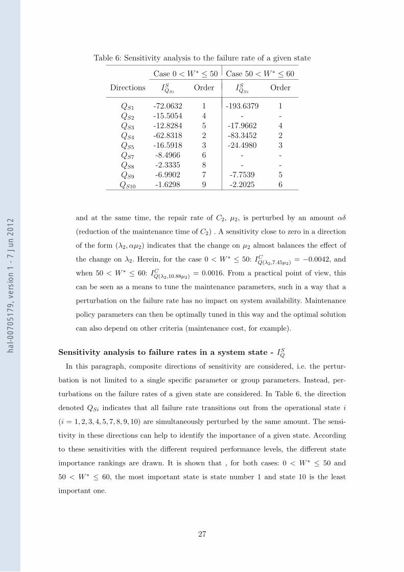
Table 6: Sensitivity analysis to the failure rate of a given state

Case 0 < W ∗ ≤ 50 Case 50 < W ∗ ≤ 60

Directions ISQSi

Order ISQSi

Order

QS1 -72.0632 1 -193.6379 1QS2 -15.5054 4 - -QS3 -12.8284 5 -17.9662 4QS4 -62.8318 2 -83.3452 2QS5 -16.5918 3 -24.4980 3QS7 -8.4966 6 - -QS8 -2.3335 8 - -QS9 -6.9902 7 -7.7539 5QS10 -1.6298 9 -2.2025 6

and at the same time, the repair rate of C2, µ2, is perturbed by an amount αδ

(reduction of the maintenance time of C2) . A sensitivity close to zero in a direction

of the form (λ2, αµ2) indicates that the change on µ2 almost balances the effect of

the change on λ2. Herein, for the case 0 < W ∗ ≤ 50: ICQ(λ2,7.45µ2) = −0.0042, and

when 50 < W ∗ ≤ 60: ICQ(λ2,10.88µ2) = 0.0016. From a practical point of view, this

can be seen as a means to tune the maintenance parameters, such in a way that a

perturbation on the failure rate has no impact on system availability. Maintenance

policy parameters can then be optimally tuned in this way and the optimal solution

can also depend on other criteria (maintenance cost, for example).

Sensitivity analysis to failure rates in a system state - ISQ

In this paragraph, composite directions of sensitivity are considered, i.e. the pertur-

bation is not limited to a single specific parameter or group parameters. Instead, per-

turbations on the failure rates of a given state are considered. In Table 6, the direction

denoted QSi indicates that all failure rate transitions out from the operational state i

(i = 1, 2, 3, 4, 5, 7, 8, 9, 10) are simultaneously perturbed by the same amount. The sensi-

tivity in these directions can help to identify the importance of a given state. According

to these sensitivities with the different required performance levels, the different state

importance rankings are drawn. It is shown that , for both cases: 0 < W ∗ ≤ 50 and

50 < W ∗ ≤ 60, the most important state is state number 1 and state 10 is the least

important one.

27

hal-0

0705

179,

ver

sion

1 -

7 Ju

n 20

12

Table 7: Sensitivity analysis to the failure rates of a group of states

Case 0 < W ∗ ≤ 50 Case 50 < W ∗ ≤ 60

Directions States ISQ(CiCj)

Order States ISQ(CiCj)

Order

Q(C1C2) 1,4,5 -15.0073 5 1,4,5 -175.6364 2Q(C1C3) 1,3,5,10 -96.1990 2 1,3,5,10 -228.4462 1Q(C1C4) 4,9 -66.7465 4 4,9 -90.9881 3Q(C2C3) 1,2,5,8 -107.6237 1 1,5 -82.6828 4Q(C2C4) 4,7 -71.0516 3 4 -55.7766 5

Sensitivity analysis to failure rates in a group of states - ISQ

This paragraph explores the sensitivity of the failure rates of a group of sates. In Ta-

ble 7, the direction denoted Q(CiCj) (i, j = 1, 2, 3, 4) indicates that when the system is in

operational state where both Ci, Cj are functioning, the failure rates of Ci, Cj are simulta-

neously perturbed by the same amount. From a practical point of view, this perturbation

could be caused by, for example, electrical shock, changing environmental conditions, etc.

The sensitivity of system availability in this direction gives impact of the operational

components group on system availability.

The results in Table 7 show that with the different required performance levels, the

sensitivity of system availability to operational component groups is different. When the

required performance level is 0 < W ∗ ≤ 50, the most important group of 2 operational

components is (C2, C3) and the group (C1, C2) is the least important one. And if the

required performance level is 50 < W ∗ ≤ 60, the most important group is (C1, C3) and

the group (C2, C4) is the least important one.

5 Conclusions

The results presented in this paper are a natural extension of the classical methods of

sensitivity analysis developed for “static systems”. The main idea is to obtain the deriva-

tives of a performance measure without using exact or approximate methods which are

burdensome, neither FD/SP methods which require data from both the nominal and the

perturbed system behaviour. In fact, the data of the perturbed system can be unavail-

able in many real-life cases when the parameters cannot be intentionally modified (for

economic or safety reasons for example).

28

hal-0

0705

179,

ver

sion

1 -

7 Ju

n 20

12

With PA and IPA, methods have been developed to estimate the sensitivity measure

of discrete event dynamic system models on the basis of nominal system behavior only. In

the framework of Markov process modeling, the Perturbation Realization approach based

on a single sample path is particularly well formalized. From a practical point of view,

it allows the estimation of sensitivity measures on the basis of operating feedback data

in nominal conditions, without knowing the generator of the underlying Markov process.

The present work shows that after one Perturbation Realization matrix estimation, many

different sensitivity measures, sensitivity to one or more parameters with any directional

derivative, sensitivity to the transition rates, can be led with no additional calculations

and can be used in many reliability studies: identification of a group of critical compo-

nents, quantification of the impact of a component failure in a given state, adaptation of

the maintenance parameters to keep a constant availability level in case of components

degradation,etc...

This paper is the development of our research in the framework of the sensitivity

importance analysis of dynamic systems presented in part in [10]. Our further research

will focus on more detailed applications of Perturbation Realization to the sensitivity

studies of dynamic systems and the development of methods to analyze the transient

state of a Markov processes.

References

[1] E. Borgonovo and G.E. Apostolakis. A new importance measure for risk-informed

decision making. Reliability Engineering and System Safety, 72(2):193–212, 2001.

[2] E. Borgonovo, G.E. Apostolakis, S. Tarantola, and A. Saltelli. Comparison of global

sensitivity analysis techniques and importance measures in PSA. Reliability Engi-

neering and System Safety, (79):175–185, 2003.

[3] X.-R Cao. Perturbation analysis of discrete event systems: Concepts, algorithms and

applications. European Journal of Operation Research, 91:1–13, 1995.

[4] X.-R. Cao and H.-F. Chen. Pertubation realization, potentials, and sensitivity analy-

sis of markov processes. IEEE Transactions on Automatic Control, 42(10):1382–1393,

1997.

29

hal-0

0705

179,

ver

sion

1 -

7 Ju

n 20

12

[5] X.-R. Cao and Y.-W. Wan. Algorithms for sensitivity analysis of markov systems

through potential and perturbation realization. IEEE Transactions on Automatic

Control, 6(4):482–494, 1998.

[6] X.-R Cao, X.M Yuan, and L. Qiu. A single sample path-based performance sensitivity

formula for Markov chains. IEEE Transactions on Automatic Control, 41(12):1814–

1817, 1996.

[7] L. Dai. Sensitivity analysis of stationary performance measures for Markov chains.

Mathematical and Computer Modelling, 23(11-12):143–160, 1996.

[8] L. Dai. Rate of convergence for derivative estimation of discrete-time Markov chains

via finite-difference approximation with common random numbers. SIAM Journal

on Applied Mathematics, 57(3):731–751, 1997.

[9] L. Dai and C.-Y. Ho. Structural infinitesimal perturbation analysis (SIPA) for deriva-

tive estimation of discrete-event dynamic systems. IEEE Transactions on Automatic

Control, 40(7):1154–1166, 1995.

[10] P. Do Van, S. Khalouli, A. Barros, and C. Berenguer. Sensitivity & importance

analysis of markov models using perturbation analysis: Applications in reliability.

In C. Guedes-Soares and E. Zio, editors, Safety and Reliability for Managing Risk -

Proc. of ESREL 2006, 18-22 sep. 2006, Estoril, Portugal, pages 1769–1775. Taylor

& Francis, 2006.

[11] Y. Dutuit and A. Rauzy. Efficient algorithms to assess component and gate impor-

tance in fault tree analysis. Reliability Engineering and System Safety, 72:213–222,

2001.

[12] P. Frank. Introduction to system sensitivity. Academic press, 1978.

[13] M.C. Fu and J.Q. Hu. Smoothed perturbation analysis derivative estimation for

Markov chains. Operations Research Letters, 15:241–251, 1994.

[14] P. Glasserman. Derivative estimates from simulation of continuous-time Markov

chains. Operations Research, 40(2):292–308, 1992.

[15] S. Glasserman, P. Tayur. Sensitivity analysis for base-stock levels in multiechelon

production-inventory systems. Management Science, 41(2), 1995.

[16] P.W. Glynn. Likelihood ratio gradient estimation for stochastic systems. Communi-

cations of the ACM, 33:75–84, 1990.

30

hal-0

0705

179,

ver

sion

1 -

7 Ju

n 20

12

[17] A.B. Huseby. Importance measures for multicomponent binary systems. Technical

Report Statistical Research Report No. 11-04 - ISSN 0806-3842, University of Oslo -

Dept. of Math., December 2004.

[18] G. Levitin and A. Lisnianski. Importance and sensitivity analysis of multi-state

systems using the universal generating function method. Reliability Engineering and

System Safety, 65:271–281, 1999.

[19] B. Natvig. Reliability: Importance of components. Encyclopedia of Statistical Sci-

ences, (8), 1988.

[20] Y. Ou and J. Bechta-Dugan. Approximate sensitivity analysis for acyclic Markov

reliability models. IEEE Transactions on Reliability, 52(2):220–231, 2003.

[21] G.C. Pflug. Sampling derivatives of probabilities. Computing, 42:315–328, 1989.

[22] G.C. Pflug. On-line optimization of simulated markovian processes. Mathematics of

Operations Research, 15:381–395, 1990.

[23] M. Rausand and H. Hoyland. System Reliability Theory - Models, Statistical methods

and Application. Wiley Series in Probability and Statistics. Wiley Interscience, second

edition edition, 2004.

[24] S. Ross. Stochastic Processes. Wiley Series in Probability and Statistics. John Wiley

& Sons, Inc., 1996.

[25] J.C. Spall. Multivariate stochastic approximation using a simultaneous perturbation

gradient approximation. IEEE Transactions on Automatic Control, 37(4):332–341,

1992.

[26] E. Zio and L. Podofillini. Importance measures of multi-state components in multi-

state systems. International Journal of Reliability, Quality and Safety Engineering,

10(3):289–310, 2003.

31

hal-0

0705

179,

ver

sion

1 -

7 Ju

n 20

12