Perturbation Biology: Inferring Signaling Networks inCellular SystemsEvan J. Molinelli1,2., Anil Korkut1., Weiqing Wang1., Martin L. Miller1, Nicholas P. Gauthier1,

Xiaohong Jing1, Poorvi Kaushik1,2, Qin He1, Gordon Mills3, David B. Solit4,5, Christine A. Pratilas4,6,

Martin Weigt7, Alfredo Braunstein8, Andrea Pagnani8, Riccardo Zecchina8, Chris Sander1*

1 Computational Biology Program, Memorial Sloan-Kettering Cancer Center, New York, New York, United States of America, 2 Tri-Institutional Program for Computational

Biology and Medicine, Weill Cornell Medical College, New York, New York, United States of America, 3 Department of Systems Biology, The University of Texas MD

Anderson Cancer Center, Houston, Texas, United States of America, 4 Program in Molecular Pharmacology, Memorial Sloan-Kettering Cancer Center, New York, New York,

United States of America, 5 Human Oncology and Pathogenesis Program, Memorial Sloan-Kettering Cancer Center, New York, New York, United States of America,

6 Department of Pediatrics, Memorial Sloan-Kettering Cancer Center, New York, New York, United States of America, 7 Laboratoire de Genomique des Microorganismes,

Universite Pierre et Marie Curie, Paris, France, 8 Politecnico di Torino and Human Genetics Foundation, HuGeF, Torino, Italy

Abstract

We present a powerful experimental-computational technology for inferring network models that predict the response ofcells to perturbations, and that may be useful in the design of combinatorial therapy against cancer. The experiments aresystematic series of perturbations of cancer cell lines by targeted drugs, singly or in combination. The response toperturbation is quantified in terms of relative changes in the measured levels of proteins, phospho-proteins and cellularphenotypes such as viability. Computational network models are derived de novo, i.e., without prior knowledge ofsignaling pathways, and are based on simple non-linear differential equations. The prohibitively large solution space of allpossible network models is explored efficiently using a probabilistic algorithm, Belief Propagation (BP), which is threeorders of magnitude faster than standard Monte Carlo methods. Explicit executable models are derived for a set ofperturbation experiments in SKMEL-133 melanoma cell lines, which are resistant to the therapeutically important inhibitorof RAF kinase. The resulting network models reproduce and extend known pathway biology. They empower potentialdiscoveries of new molecular interactions and predict efficacious novel drug perturbations, such as the inhibition of PLK1,which is verified experimentally. This technology is suitable for application to larger systems in diverse areas of molecularbiology.

Citation: Molinelli EJ, Korkut A, Wang W, Miller ML, Gauthier NP, et al. (2013) Perturbation Biology: Inferring Signaling Networks in Cellular Systems. PLoS ComputBiol 9(12): e1003290. doi:10.1371/journal.pcbi.1003290

Editor: Florian Markowetz, Cancer Research UK Cambridge Research Institute, United Kingdom

Received October 1, 2012; Accepted August 26, 2013; Published December 19, 2013

Copyright: � 2013 Molinelli et al. This is an open-access article distributed under the terms of the Creative Commons Attribution License, which permitsunrestricted use, distribution, and reproduction in any medium, provided the original author and source are credited.

Funding: The research was supported by a grant from the Integrative Cancer Biology Program (ICBP CCS U54CA148967), the Pathway Commons grant (NHGRI-U41HG006623), the Melanoma Research Alliance (236191), and the National Resource for Network Biology grant (NIGMS-GM103504). EJM and PK were partiallysupported by a training grant from the Tri-Institutional Program for Computational Biology and Medicine (National Institute of General Medical SciencesT32GM083937). RZ was supported by the European Research Council (ERC) grant n. 267915 .The funders had no role in study design, data collection and analysis,decision to publish, or preparation of the manuscript.

Competing Interests: The authors have declared that no competing interests exist.

* E-mail: perturbation-biology@cbio.mskcc.org

. These authors contributed equally to this work.

Introduction

Signaling in cancer cellsAbnormal biomolecular information flow as a result of genetic

or epigenetic alterations may lead to tumorigenic transformation

and malignancy and is classically modeled as changes in

signaling pathways [1]. Targeted anti-cancer drugs, which bind

and inhibit specific components of aberrant signaling pathways,

are a promising alternative to conventional chemotherapy, with

recent successes in melanoma (RAF inhibitor) [2] and prostate

cancer (AR inhibitor) [3,4] following in the footsteps of the

pioneering BCR-ABL inhibitor Imatinib [5] and EGFR inhib-

itors Gefitinib and Erlotinib [6,7,8]. Combinations of targeted

anticancer drugs hold considerable promise because of the

emergence of resistance to initially successful single agents and

the highly robust nature of the signaling pathways with multiple

feedback mechanisms [9].

Data-driven models of cell biologyHigh throughput measurements on response profiles of living

cells to multiple perturbations such as drug combinations provide

a rich set of information to construct quantitative cell biology

models. In this paper, we construct context specific de novo

mathematical models of signaling pathways through the use of

systematic paired perturbation experiments and network inference

algorithms. Such network models provide insight into mechanistic

details of signaling pathways, predict the response of cellular

systems to multiple perturbations beyond those from which models

are derived, and guide the design of perturbations for a desired

response.

State of the art in network inference in cell biologyPrevious mathematical models of molecular signaling in cells

have been effective in modeling pathways and enhancing drug

discovery [10,11,12,13,14,15,16,17,18,19]. Techniques for net-

PLOS Computational Biology | www.ploscompbiol.org 1 December 2013 | Volume 9 | Issue 12 | e1003290

work modeling of signaling pathways span a wide spectrum of

complexity. Detailed chemical kinetics and spatiotemporal

models [17,20,21] can provide mechanistic explanations of

observed behavior, but are often incompletely parameterized,

needing tens or hundreds of sensitive parameters for medium-

sized systems. Moreover, such models may not be valid in

biological contexts that differ substantially from dilute solution

chemistry. On the other end of the spectrum, pattern matching or

machine learning models such as neural networks and correla-

tion-based models such as maximum entropy [22] can accurately

provide purely data-driven models of signaling. However, such

methods have limited power to explain mechanistic details and,

in most cases, are insufficient for quantitative predictions of

system behavior in conditions beyond those from which the

models are derived.

Data-driven and context-specific predictive modelsWe take a unique modeling approach to construct context

specific, de novo and predictive network models of signaling

pathways from drug perturbation data (Figure 1). Here, de novo

means that network inference is done without depending on

known molecular interactions extracted from literature or pathway

databases, which do not account for biological context. This

approach also emphasizes context specificity since it relies on rich

experimental data from a single biological context as its training

set. The models are constructed through parameterization of a

simple model equation, which has been used in other network

modeling approaches [13,23,24,25,26,27]. The model equations

contain parameters that are mechanistically descriptive of direct or

indirect interactions in the system. Finally, the models are

computationally predictive of cell-type specific response to new

drug perturbations and their combinations. We expect that this

conceptual framework and the technical advances in network

inference will empower the community to identify unique drug

targets and combinations that are particularly efficacious within

specific disease contexts.

Network modeling de novo or with prior informationDe novo construction of signaling network models at scales

relevant to problems related to complex biological phenomena

such as cancer has long been a challenge in system biology. Thus,

quantitative models of protein signaling pathways are typically

constructed on the basis of existing prior knowledge from literature

searches [16,17] and interaction databases [19,28,29]. However,

different cancer contexts have unique genetic and proteomic

Author Summary

Drugs that target specific effects of signaling proteins arepromising agents for treating cancer. One of the manyobstacles facing optimal drug design is inadequatequantitative understanding of the coordinated interactionsbetween signaling proteins. De novo model inference ofnetwork or pathway models refers to the algorithmicconstruction of mathematical predictive models fromexperimental data without dependence on prior knowl-edge. De novo inference is difficult because of theprohibitively large number of possible sets of interactionsthat may or may not be consistent with observations. Ournew method overcomes this difficulty by adapting amethod from statistical physics, called Belief Propagation,which first calculates probabilistically the most likelyinteractions in the vast space of all possible solutions,then derives a set of individual, highly probable solutionsin the form of executable models. In this paper, we testthis method on artificial data and then apply it to modelsignaling pathways in a BRAF-mutant melanoma cancercell line based on a large set of rich output measurementsfrom a systematic set of perturbation experiments usingdrug combinations. Our results are in agreement withestablished biological knowledge, predict novel interac-tions, and predict efficacious drug targets that are specificto the experimental cell line and potentially to relatedtumors. The method has the potential, with sufficientsystematic perturbation data, to model, de novo andquantitatively, the effects of hundreds of proteins oncellular responses, on a scale that is currently unreachablein diverse areas of cell biology. In a disease context, themethod is applicable to the computational design of novelcombination drug treatments.

Figure 1. Perturbation cell biology. Perturbing cancer cells with targeted drugs singly and in pairs (A) reveals context-specific response totherapies and illuminates protein interactions. We construct dynamic mathematical models of the cells’ response to drugs that have bothquantitative parameters (B) and a qualitative network interpretation (C). We use an inference algorithm called Belief Propagation (BP) to construct aset of good, i.e., predictive models (D).doi:10.1371/journal.pcbi.1003290.g001

Perturbation Cell Biology

PLOS Computational Biology | www.ploscompbiol.org 2 December 2013 | Volume 9 | Issue 12 | e1003290

alterations to normal protein signaling. For example, distinct

mutations in effector proteins of the PI3K pathway are oncogenic

in unique ways, i.e., they lead to distinctly context dependent

functional consequences in different cancer types, subtypes and

patients [30]. The method we introduce here is capable of

inferring parameterized network models with prior knowledge, yet

the results in this study do not include prior knowledge. An

advantage of de novo inference is independence from prior

knowledge interactions that may be incorrect or incomplete in a

particular biological context.

Model inference from perturbation data for largersystems is hard

The largest obstacle to de novo model construction is the

combinatorial explosion in the number of possible network

models, which defines the solution space [31]. Model inference

problems of this type are NP-hard [32]. The number of possible

configurations for a model with N nodes, and K possible values for

each parameter grows super-exponentially as KN2

. We have

previously described a method named CoPIA for de novo

construction of dynamic nonlinear network models from pertur-

bation data [33]. CoPIA is based on the combined use of a Monte

Carlo stochastic search algorithm, which is used to search the

network configurations and an efficient gradient descent algorithm

[34] for quantitative parameter optimization. However, without

algorithmic improvements, such Monte Carlo based methods are

limited to modeling fewer than approximately 15–20 biological

entities [33]. Increasing the scale of network (or pathway) models

of cellular signaling processes to levels sufficient to describe

complex biological problems in quantitative detail is therefore

extremely challenging and has been approached with a diversity of

methods [35].

A statistical physics approach can handle the complexityfor larger systems

An ingenious, two-step approach to deal with network

inference in larger systems is based on first calculating probability

distributions for each possible interaction in the model and then

computing distinct solutions by sampling these probability

distributions. For this purpose, we employ a probability model

of network configurations inspired from statistical physics

principles. Following a set of approximations to simplify the

probability model, we apply a custom adaptation of an iterative

algorithm called Belief Propagation (BP). BP involves local

optimization updates to probability distributions of individual

model parameters that converge to a stable set of probability

distributions, which collectively describe a set of good network

model solutions [36,37,38]. BP has been applied to various

complex inference problems, some of them NP-Hard such as K-

SAT [38] and graph coloring [39]. BP has garnered some

attention in biological network inference [40,41] and parameter

estimation [42,43]. Here, we tailor the BP algorithm to large-

scale perturbation data that is capable of increasing the scope of

the models to hundreds of nodes. The result of BP is a set of

probability distributions for each model parameter, often referred

to as marginal probability distributions, or ‘marginals’. Each

marginal describes the inferred distribution of a particular

parameter across a range of high probability solutions. Individual

models are created via sampling from these marginals [44].

Consequently, the time-complexity of the problem is strongly

reduced, the prohibitive cost from combinatorial complexity is

circumvented and, although the method provides only an

approximate solution, one obtains useful, non-trivial results.

In practice: from systematic perturbation to responseprofiling to network model inference

Our algorithmic network pharmacology approach involves four

major steps: (i) perturbation experiments with combinations of

targeted compounds; (ii) high-throughput quantitative measure-

ments of proteomic changes (e.g., reverse phase protein arrays or

mass spectrometry) and phenotypic changes (e.g., cell viability or

apoptosis); (iii) inference of quantitative network models of protein

signaling that explain and link these changes; and (iv) use of the

network models to predict cellular and molecular responses to

diverse perturbations, beyond the conditions on which the network

models are derived.

Experimental and computational technology for networkmodel inference and application to drug effects onmelanoma cell lines

In this work, we adapt BP to construct quantitative network

models of signaling pathways from systematic perturbation

experiments. We evaluate the speed and accuracy of BP on toy

data generated from biologically inspired network structures. The

inference on this toy data reveals that BP offers a significant

improvement in computational efficiency compared to traditional

Monte Carlo simulations without a sacrifice in accuracy.

Furthermore, we construct network models of signaling in a

RAF inhibitor resistant melanoma cell line (SKMEL-133), which

has the BRAFV600E mutation [45,46]. The models are predictive

of both the proteomic and phenotypic response to drug

combinations. Model simulations successfully predict the pheno-

typic response profiles of SKMEL-133 cells to novel drug targets.

With the introduction of many novel targeted drugs and patient

specific genomic profiling, this network pharmacology approach

aims to provide an effective tool to develop individualized

combination therapies against multiple cancer forms.

Results

TheoryMathematical framework of the network model. Key

decisions in modeling a biological cellular system include the

choice of variables and the mathematical framework for repre-

senting system dynamics. Here, we work with a fairly simple but

powerful ansatz or framework, in which the time behavior of the

cellular system {xi(t)} in a set of perturbation conditions {uim} is

modeled as a series of coupled non-linear differential equations

(Equation 1) [33].

Equation 1: Non-linear network model for the time behavior of the cellular

system

dxmi tð Þdt

~eiwXN

j=i

wijxmj tð Þzu

mi

!{aix

mi tð Þ

w(z)~tanh(z)

ð1Þ

The system variables x represent quantities of particular

biological entities one wishes to measure and model. In this work,

quantities are restricted to relative changes in protein and

phospho-protein abundances and cell viability levels. The

variables are nodes in the network model. The model parameters

w in the matrix W formally quantify the interactions between

nodes and correspond to directed edges in the network model.

Equation 1 includes an independent time variable t, which denotes

that variables are functions of time. The term u represents an

Perturbation Cell Biology

PLOS Computational Biology | www.ploscompbiol.org 3 December 2013 | Volume 9 | Issue 12 | e1003290

external force on a model variable, which models interventions

from targeted drug perturbations. A vector of u-values defines the

set of targeted perturbations; combinations are simple additions of

these vectors. In principle, u is time-dependent, but not in the

current implementation. The variable index i maps to a single

network node, and the experimental index (m) maps to a single

experimental perturbation condition. A biological system is

therefore modeled by a collection of coupled equations of the

form defined in Equation 1. Perturbations to any node propagate

in time through the network interactions producing trajectories

x(t), which present the behavior of the system over time.

Theoretically, the model variables can quantify any measure of

interest. While absolute protein concentrations are one option,

such data is difficult to acquire in high throughput assays. In this

study, we focus on log2-ratios of abundances in perturbed

conditions to abundances in the unperturbed condition. Conse-

quently, model variables can take both negative and positive

values, which denote decreased or increased quantities of the

corresponding biological entity. We choose to normalize all

measurement levels against unperturbed levels in order to focus

on signaling differences due directly to perturbation.

The rate of change of any variable, in this formulation, is

predominantly influenced by the additive linear combination of

upstream nodes {xj} weighted by their respective interaction

strength {wij}. Only non-zero values of wij are interactions in the

network model. We incorporate nonlinearity with a sigmoidal

function w(z) that limits both the maximum positive and negative

rates of change [24], controlled by the parameter e. The aparameter models the rate of restoration at which a model variable

would return to its initial value before perturbation, in the absence

of interactions. This is analogous to the degradation rate in models

of positively valued protein concentrations. The parameters e and

a are not inferred with BP. For the remainder of this section they

are assumed to be 1, and are dropped from the equations. They

are reintroduced in the final stage of modeling, when individual

models are optimized with gradient descent.

The network models are parameterized by the square interac-

tion matrix W = {wij} of size N (N2 entries), where wij represents a

directed interaction between nodes, quantifying the influence of xj

on the rate of change of xi. In chemical kinetics, the wij is analogous

to rate constants in units of inverse time, although no explicit rates

are derived here. Equation 1 describes the dynamic behavior of

the system, given a constant interaction matrix W. In this work, we

explicitly forbid self-interactions, therefore the N diagonal entries

of W are set to 0 and only the remaining N2-N are subject to

fitting. These apparently simple models can represent biologically

realistic regulatory motifs, such as serial and parallel pathway

connectivity, positive and negative feedback loops and feed-

forward control. The models used here are dynamic in the sense

that they can be simulated as temporal trajectories that converge

to a steady state. In this work, the parameters are inferred based

solely on data assumed to represent the biological steady state.

Thus, only the endpoints of the simulated trajectories are

constrained. Despite not being used in this study, both the model

and the learning method can generalize to incorporate time-series

data.

The problem of model inference. The problem of deriving

useful models of a (biological) system is called ‘model inference’.

The objective of model inference, given a mathematical frame-

work like that described above, is to find a set of parameters such

that the model equations best reproduce a training set of

experimental data and have predictive power beyond the training

set. In the present modeling framework, we aim to find numerical

values for the N2–N free parameters in the interaction matrix W,

such that descriptive and predictive power of the model is

optimized. Genuine predictive power, rather than just descriptive

power, requires both low error and low complexity of the model,

combined as low cost. We quantify the cost of W by an objective

cost function C(W) that penalizes: (i) discrepancies between

predicted xmi (tl) and experimentally measured x

m�i (tl) values of

the system observables at a set of time points {tl} in condition m;

and (ii) the number of non-zero interactions in W. Lower cost

models tend to have more predictive power than higher cost

models.

Equation 2: Model configuration cost function

C(W)~bXL

l

XN

i

XMm

xmi (tl){x

m�i (tl)

� �2zl

XN

i

XN

j=i

d(wij) ð2:aÞ

d(wij)~1 if wij=0

d(wij)~0 if wij~0ð2:bÞ

C(W) is thus the error-plus-complexity cost of a parameter

configuration W. The cost components are weighted by b and l,

respectively. The complexity cost term is an L0 penalty

[47,48,49,50,51] that penalizes non-zero entries in W and is

included to both avoid overfitting and reflect the empirical

observation that realistic biological networks such as gene

regulatory networks or protein-protein interaction networks are

sparse [52]. While L1 penalties are convex and therefore amenable

to efficient convex optimization methods, they are not used here

since they provide weaker constraint on the complexity of the

interaction matrix W [25,53,54,55]. We do not wish to include

direct self-interaction in the present version; thus, the sum in the

complexity term does not include the diagonal elements wii. The

computational challenge of network inference is to translate the

information contained in a set of experimental observations into

an optimal set of models, as represented by a set of low cost

interaction matrices W. In this report, we work in the steady-state

approximation and thus ignore the time variable in the cost

function in Equation 2.

De novo network inference is a hard problem. In

principle, to infer optimal network configurations one has to

compute the cost of all possible network configurations. However,

explicit enumeration and cost calculation of all possible parameter

configurations W is a prohibitively complicated task for even

moderately sized systems. To estimate the complexity of this task,

assume that any wij can take on K discrete values out of a value

range V, for example, V= {21,0,+1} for K = 3, representing

inhibition, no interaction and activation, respectively. As the

number of model nodes N increases, the number of possible

parameter configurations increases as KO(N2). Even for moderate

N, e.g., 20 nodes, the number of distinct configurations is of order

10190, obviously a very large number, making explicit enumeration

prohibitive.

The solution space refers to the set of all possible model

configurations. A reasonably clever strategy to traverse this

enormous solution space is guided random exploration, e.g., by

a traditional Monte Carlo search, in which random moves in

multi-dimensional parameter space are kept or rejected based on

the cost of the resulting configuration, with a non-zero but small

probability of accepting higher cost configurations in order to

facilitate the escape from local minima. In an earlier study, we

successfully used a Monte Carlo search followed by a modified

Perturbation Cell Biology

PLOS Computational Biology | www.ploscompbiol.org 4 December 2013 | Volume 9 | Issue 12 | e1003290

gradient descent method to derive a set of low cost models for a

relatively small system. This earlier algorithm achieved a

reasonable exploration of solution space for a system of 14

variables, as assessed by the recurrence of dominant interactions

across the set of a few hundred low-cost models and the agreement

of those interactions with well-established knowledge of signaling

pathways in cell biology. However, the KO(N2)argument above and

explicit computational benchmarking indicate that such Monte

Carlo searches become prohibitively expensive for larger systems.

Fast inference via a probability model of network

configurations. In search of a more efficient algorithm, we

adopt an idea originally developed in statistical physics, and widely

used in solving complicated optimization problems in computer

science and other areas. Instead of sampling a prohibitively large,

unrestricted solution space by traversing a set of individual

configurations, the idea is to first calculate high probability regions

and then restrict exploration to this smaller solution space. In

particular, we describe high probability regions by calculating

probability distributions of individual model parameters over

possible value assignments. Then, we can generate distinct model

configurations by sampling from the calculated probability

distributions.

Models with a large error (or cost) have low probability, while

those with a low error have high probability. More precisely, the

probability of any particular model can be computed from its cost,

which depends on the parameters in the interaction matrix W and

the experimental data (Equation 2). In statistical physics, there is

an analogous relationship between the Hamiltonian for the states

of a system and its Boltzmann-Gibbs probability distribution over

all states. In terms of Bayesian inference, the equation below

relates the posterior distribution of the model on the left to the

likelihood function and prior distributions on the right.

Equation 3: The probability model of network configurations

P(W)~1

Ze{C Wð Þ~

1

Ze{bPN

i

PMm

(xmi{x

m�i

)2

e

{lPNi~1

PNj=i

d(wij )

The variable Z is the partition function, which ensures that the

sum of the probabilities over all model configurations is equal to

one. In the statistical physics analogy, the exponents contain

interaction energies and the parameter b is an inverse temperature

(1/T), such that higher values of b assign higher probability to

lower cost configurations. The parameter l is the weight of the

complexity penalty. The choice of b and l is non-trivial and is an

open area of research (see Methods). Given the probabilistic model

in Equation 3, the practical challenge is to identify configurations

of model parameters in W that represent maximally probable

models, given the data. The explicit computation of probabilities

for all possible sets of parameters is not feasible even for

moderately sized (N.15) systems. One therefore has to invent

practical algorithms for effectively exploring the total solution

space and approximately determining sets of good models.

Iterative optimization of the probability model. An

effective solution is to use an iterative algorithm to approximate

the probability distributions of the individual parameters by

themselves, often called marginal probability distributions, or

simply ‘marginals’. From these marginals, we can describe high

probability model configurations for the full system. This iterative

algorithm begins with a set of random marginals. In each iteration

step, one assumes approximate knowledge of all parameter

marginals (‘global information’) and then performs optimization

updates on an individual marginal (‘local update’). The local

update takes immediate effect and becomes part of the ‘global

information’ for successive iterations as the algorithm traverses

over all marginals for individual updating. The iteration termi-

nates when it converges to a stable set of marginals. The nature of

any local update to a single parameter (e.g., a node-node

interaction parameter) is a calculation optimizing a balance of

fitness to experimental data and consistency with the global

information. The iterative application of this ‘global to local and

back’ optimization strategy results in marginals for all system

parameters given a probabilistic model. Such optimal marginals

are informative by themselves, but are also useful for constructing

a population of explicit individual high probability model

configurations, which are useful for model simulation studies.

This type of probabilistic method originates in statistical physics

and has been generalized to a number of hard optimization

problems in statistical physics and computer science. An early

application of such probabilistic inference was inverse parameter

inference for disordered diluted spin systems [56,57,58]. A well

known formulation in terms of Bayesian statistics led to the term

‘belief propagation’ [59] (BP).

The BP approach, also known as the Bethe-Peierls approxima-

tion or cavity method in statistical physics, provides an approximate

method for computing marginal probability distributions on a class

of probabilistic graphical models called factor graphs. In general, a

joint probability distribution over many variables may factorize into

a product of factors. A factor in a factor graph represents an

independent contribution to the joint probability distribution, and is

connected to the variables that depend on that factor. Typically, a

factor defines a constraint on a subset of variables. The BP method

is proven to be exact on tree-shaped factor graphs. It has many

useful applications in approximating distributions on sparse factor-

graphs [60,61] where the influence of loops in the factor graph is

expected to be weak. More recently, several applications to dense,

loopy factor-graphs have been proposed [40,62,63,64,65]. The

problem we address here is a dense factor graph, where each factor

is connected to N variables, which in this framework are the model

parameters in Equation 1 (Figure 2).

A major advantage of BP algorithms is the reduction of

computational complexity. This not only leads to a substantial

reduction in computational effort for smaller systems but also

opens the door to solving inference problems for larger systems,

which would otherwise be prohibitive.

Simplified probability model of network configu-

rations. We use a series of assumptions, described below, to

factorize the probability model in Equation 3 into a form that can be

efficiently calculated without sacrificing the quantitative and predic-

tive nature of the models. The assumptions below reduce the problem

from a probability distribution over whole model configurations

(Equation 3) into a collection of marginal probability distributions for

each individual parameter. Subsequent sampling from these individ-

ual marginals will result in efficient exploration of high probability

model configurations.

Assumption 1: Discrete set of real valued parameter

assignments. To simplify the probability model, we compute

the probability distributions for model parameters over discrete

values, from a set V, rather than for continuous values. The choice

of discretization is an important detail and affects the convergence

properties of the BP algorithm and the quality of the resulting

marginals. Empirically, with the data set at hand we find that a set

of 11 discrete values, centered at zero, rarely fails to converge to a

stable set of marginals. Conversely, searching over only 3 weight

values results in a high rate of non-convergence. As for the quality

of the resulting marginals, the entropies are close to zero if we limit

the search to only 3 discrete values (see Supplemental Text S1).

Perturbation Cell Biology

PLOS Computational Biology | www.ploscompbiol.org 5 December 2013 | Volume 9 | Issue 12 | e1003290

The entropy is a statistical measure of the uncertainty in

distributions, such that zero entropy distributions imply absolute

certainty, i.e., each parameter is predicted to be 100% zero or

100% non-zero. This is an undesirable quality; one wants the BP

marginals to constrain a set of highly probable solutions, not

return one model configuration. In practice, discretizing with 11

weights gives intuitively reasonable marginals and balances the

restriction and exploration of solution space. In the final stage of

network inference strategy, we refine the set of discrete valued

model parameters to solutions with continuous model parameters

using a local gradient descent optimization algorithm [33].

Assumption 2: Decoupling of variables at steady

state. In the dynamic model, the system variables are coupled

such that a change to any variable propagates to all others via the

time derivatives as in Equation 1. A rigorous way to compute the

fitness of a configuration is to simulate a configuration and then

compare simulation output to the training data. Such a

computation, while feasible in principle, is very costly. An

alternative is to take advantage of the relationship at the steady

state (Equation 4) where the time-derivative is equal to zero.

Equation 4: Model equation at steady state

xmi ~w

XN

j=i

wijxmj zu

mi

!for all variables i and experiments m

Equation 4 is a system of self-consistent equations for all variables

{xi}. To avoid having to do numerical simulation, we replace {xjm}

on the right hand side of Equation 4 with experimentally observed

{xjm*} at the expense of self-consistency (Equation 5).

Equation 5: Approximate model equation at steady-state

xmi ~w

XN

j=i

wijxm�j zu

mi

!

Figure 2. Iteration process for Belief Propagation. Top panel: the global information consists of collecting the probability distributions of thenon-cavity parameters without the contribution from the cavity condition. This is a simple product over all rn(wij) factors except that from the cavityconstraint m. Distributions centered on zero denote unlikely interactions (see j = 2), centered on the right of zero denote likely positive interactions(see j = 3), and centered on the left denote likely negative interactions (see j = N). These distributions inform the parameters of the Gaussiandistribution for the mean-field, aggregate sum variable s

mk . The distribution Pm(s

mk) summarizes the state of the non-cavity parameters. Bottom panel:

we calculate the probability of each possible parameter assignment v[V to the cavity parameter wik constrained to the data in the cavity condition.This calculation boils down to a simple convolution of the fitness function with a fixed parameter assignment Fm(s

mk) with the probability of the

aggregate sum variable Pm(smk), obtained by integrating over all values of s

mk . Each assignment v[V contributes proportional to the area under the

curve. The resulting update is the contribution of condition m on the distribution of wik , denoted rm(wik). This recently updated distribution becomespart of the global information for successive updates to other parameters.doi:10.1371/journal.pcbi.1003290.g002

Perturbation Cell Biology

PLOS Computational Biology | www.ploscompbiol.org 6 December 2013 | Volume 9 | Issue 12 | e1003290

This approximation decouples the variables from each other:

the model predicted value of xmi depends only on the parameters in

the ith row of the interaction weight matrix W and on the set {xjm*}

of experimentally measured values in condition m. Thus, the

posterior probability P(W) can be factorized as a product of

independent posterior probability distributions over configurations

of individual rows of the weight matrix. Consequently, we have an

independent probability distribution for each row of the interac-

tion weight matrix Wi~ wi1, . . . ,wiNf g. These rows describe

interactions from variables xj Vj[f1 . . . Ng to the single variable

xi. The resulting factorized expressions are:

Equation 6a–d: Probability model of configurations with decoupled nodes

P(W)~PN

iP(Wi) ð6:aÞ

P(Wi)~1

Zi

(e

PMm

{b(xmi{x

m�i

)2

e

{lPNj=i

d(wij )

) ð6:bÞ

Fm(Wi)~e{b(x

mi{x

m�i

)2 ð6:cÞ

P(Wi)~e

{lPNj=i

d(wij )

Zi

PM

mFm(Wi)

� �ð6:dÞ

We introduce the notation Fm(Wi) to denote the fitness of the

model configuration Wi to the data from experimental m. It is

important to note that the posterior probability distribution in

Equation 6d factorizes over the fitness functions, such that Fm(Wi)contributes independently to the full probability distribution of

that configuration. The probability distribution in 6d, however,

does not factorize any further, since each parameter wik in Wi

depends on the other parameters in Wi. In order to reach good

solutions for 6d without enumerating all configurations Wi, we

apply an iterative method to infer marginals for the constituent

parameters {wij V j}.

Belief Propagation algorithm: Iterative updates of

probability estimates. As already mentioned above, the BP

method consists of randomly ordered updates to the marginal

probabilities for individual parameters, one at time. Updates

continue until convergence, when the marginal probabilities do

not change between consecutive updates. We describe the method

in detail below for single Wi since the procedure is independent

and identical for all rows i[f1 . . . Ng due to Assumption 2. The

update calculation is schematically diagramed in Figure 2.

Local updates with global information. A local update

takes place inside an abstract ‘cavity’, which isolates a single

parameter whose marginal distribution is to be updated (wik) and

data from a single experimental condition (m). The global

information is simply the most up-to-date approximation of the

marginal distributions for all the other parameters plus the

experimental data. A local update optimizes the balance between

fitting the experimental data in the cavity condition m and

compatibility with global information, which evolves as the

algorithm iterates. A single distribution is locally updated in one

step and becomes part of the global information for updating

other distributions in successive steps. This local update is

repeated in all possible cavities (i.e. all combinations of

parameters and conditions) until global convergence of the

distributions is reached.

Recall that we are optimizing parameters in a single row of Wso for the following equations the index i is fixed. We define rm(wij)

to be a factor, which is a probability distribution of a single

parameter that describes its fitness to the data in a single

experiment m that is compatible with the other parameters. By

definition, each factor is independent so that the final marginal is

simply the product of all of its factors.

The BP algorithm begins with random rm(wij) for all m and j.

The initial choice of cavity parameter (wik) and cavity condition (m)

is also random. Once the cavity is selected, the algorithm collects

the global information, which is simply the set of approximations

for the marginal probabilities of all the other model parameters

(Equation 7). They are approximate in two ways: they lack the

contribution from the cavity factor m; and until the algorithm

converges, the factors collectively do not describe the true

marginal distribution.

Equation 7: Global information of non-cavity parameters

Pm(wij)~1

Zij

e{ld(wij )PMn=mru(wij) Vj=k

d(wij)~0 if wij~0

d(wij)~1 if wij=0

The exponent ld(wij) is an independent penalty for non-zero

parameter assignments, which encodes prior knowledge that any

parameter is likely to be zero. The superscript m in Pm(wij) denotes

the exclusion of the contribution from experimental condition m.

In the following step, the factor rm(wik) is updated to fit the data in

a single experiment m given the global information.Calculating local update to rm(wik). We define Wi\k to be a

configuration of the ith row of W where the parameter wik is fixed

to some value v. The factor rm(wik) reflects the fitness of the

parameter with Wi\k weighted by the probability of observing the

particular configuration (Wi\k) as in Equation 8.

Equation 8: Local update to probability distribution ofcavity parameter

rm(wik~v)~XWi\k

Fm(W i\k)Pm(W i\k)� �

Vv [ V ð8:aÞ

Fm(Wi\k)~e{b x

m�i

{xmi

� �2

ð8:bÞ

In the field of optimization algorithms, these equations are

sometimes referred to as messages because they communicate

information between variable nodes and factor nodes on the factor

graph, where in this case the variable nodes in the factor graph

correspond to model parameters. Thus, BP belongs to a class of

‘message-passing’ algorithms. It is common to see Equation 7

referred to as messages from the variable nodes to the factor nodes

and denoted Pj?m(wij). Similarly, Equation 8 can be thought of as

a message update from a factor node to a variable node, denoted

rm?k(wik).

Assumption 3: Independent model parameter

distributions. Equation 8 is the mathematical definition of

the factor distribution rm(wik). However, a brute force approach for

Perturbation Cell Biology

PLOS Computational Biology | www.ploscompbiol.org 7 December 2013 | Volume 9 | Issue 12 | e1003290

calculating rm(wik) as in Equation 8a is computationally prohib-

itive. The first complication is that computation of the joint-

probability distribution Pm(Wi\k) is not possible if we consider the

interdependencies of the non-cavity parameters. To circumvent

this problem, we assume that in the context of the local update,

each parameter probability distribution is independent. Then the

joint probability distribution can be approximated as the product

of the individual parameter distributions.

Equation 9: Approximation of the joint distribution for the cavity update

Pm(Wi\k)~ PN

j=kPm(wij)

Therefore, Equation 8 becomes Equation 10.

Equation 10: Local update with factorized probability distributions

rm(wik~v)~XWi\k

Fm(Wi\k) PN

j=kPm(wij)

� �

This equation is equivalent to the sum-product formulation,

which is standard in BP literature [60]. It is important to note that

the assumption that the joint probability distribution factorizes as

the product of individual distributions (Equation 9) is exact on

tree-shaped factor graphs, but is only an approximation in general.

This assumption does not extend beyond the context of the cavity

update calculation.

Assumption 4: Gaussian mean-field approxima-

tion. Another complication in Equation 10 is that a brute force

implementation of the sum operation requires enumeration over

an exponentially large number of configurations, which in total is

KN-1. Here, we replace the sum over multivariate configurations

(Wi\k) with an integral over a single scalar variable (smk). To achieve

this, we substitute the fitness function’s dependence on the

multivariate configuration Wi\k with a single scalar variable smk.

This substitution is explicitly defined in Equation 11, where the

new variable smk represents the aggregate contribution of the non-

cavity parameters to the fitness.

Equation 11: Aggregate effect of non-cavity parameters

Fm(smk)~Fm(Wi\k)~e

{b xm�i

{w(smkzwikx

m�k

)

� �2

ð11:aÞ

smk~

XN

j=k

wijxm�j zu

mi ð11:bÞ

To complete the substitution of Wi\k for smk in Equation 10, we also

require a description of the probability distribution for the new

variable i.e., P(smk). Note that the dependence of s

mk on Wi\k is

through a linear combination of the individual parameters (Equation

11.b), which by assumption 3 are independently distributed. We

invoke the central limit theorem to approximate P(smk) as a Gaussian

[66]. The mean and variance of this Gaussian are described by the

means and variances of the distributions Pm(wij) Vj=k. Thus, we

replace the sum over multivariate configurations (Equation 10) with

the Gaussian integration of smk (Equation 12).

Equation 12: Gaussian integration of local update to cavity parameter

rm(wik~v)&ð?

{?

Fm(smk)Pm(s

mk)ds

mk

The explicit calculation of Pm(smk) is described in Equations 13a–

d, where the over-bar denotes the arithmetic mean.

Equations 13a–d: Statistical description of mean-field parameters

Pm(smk)~

1ffiffiffiffiffiffiffiffiffiffiffi2pDm

k

q e{

smk{s

mk

� �2

2Dmk ð13:aÞ

smk~

XN

j=i,k

wijxm�j zu

mi ð13:bÞ

Dmk~

XN

j=i,k

wij2{w2

ij

� �(x

m�j )2 ð13:cÞ

wij~X

v

vPm(wij~v) ð13:dÞ

Iteration of update equations. In summary, the following

BP equations are calculated for each cavity update iteratively until

convergence.

Equations 14a–b: Update equations

Pm wij

� �~

1

Zij

e{ld wij

� �PM

u=mru wij

� �Vj=k ð14:aÞ

rm(wik~v)~1

Zik

1ffiffiffiffiffiffiffiffiffiffiffi2pDm

k

qð?

{?

e{b x

m�i

{w(smkzwikx

m�k

)

� �2

e{

(smk{s

mk

)2

2Dmk ds

mk Vv [ V

ð14:bÞ

Calculation of parameter probability distributions. When

the above iterative process converges, the final marginals are

calculated from the set of factors, reflecting the information from

experimental constraints.

Equation 15: Final marginal calculation

P(wij)~e{ld(wij ) P

M

mrm(wij)

The BP algorithm provides marginals characterizing a set of

good models. Thus, we reduce the unbounded model search space

to a set of tractable probability distributions for model parameters.

Perturbation Cell Biology

PLOS Computational Biology | www.ploscompbiol.org 8 December 2013 | Volume 9 | Issue 12 | e1003290

Next, one must generate high probability models by drawing from

the BP calculated marginals.

Network model instantiation by BP guided

decimation. We need distinct model solutions to proceed with

predictive and quantitative analysis of signaling pathways via

explicit model simulations. Distinct solutions are derived by the BP

guided decimation algorithm [44]. The decimation algorithm

works as follows: (i) an initial BP is run to compute probability

distributions P(wij) for all possible interactions; (ii) a possible

interaction (suppose an edge that connects node k and node l) and

an associated edge value (wkl = v) is chosen with probability

proportional to the corresponding BP marginal; (iii) a subsequent

round of BP is run with P(wkl = v) = 1; (iv) steps i–iii are repeated

until an edge value is fixed for all possible interactions in the

system. Parallel repetition of this procedure generates any number

of network models with varying configurations and error profiles.

The non-zero parameters in each model are further optimized

using a gradient descent algorithm, which relaxes the discretiza-

tion of parameter values and further lowers the error by fine-

tuning the real number values of the parameters. Moreover, the

gradient descent refinement ensures that the network models are

mathematically in steady state and the nodes in the network

models are fully coupled [33]. Each model is then a set of

differential equations describing the behavior of the system in

response to perturbations.

Direct vs. Indirect Interactions. Due to limitations in

experimental measurements, not all proteins and their many

phosphorylated states are directly measureable. The result is that

many key intermediate players are excluded from the model. For

this reason, direct interactions in our model do not necessarily

imply direct biological interactions (Supplemental Figure S15).

Increasing the number and quality of protein and phospho-protein

measurements increases the chance of modeling direct interac-

tions.

Technical performanceThe success of BP depends on whether or not the simulations of

the models taken from BP are quantitatively predictive of cellular

response to drug combinations. It is also useful, as an exercise, to

evaluate the overall performance of the BP algorithm on data sets

engineered from completely known networks. With such toy

datasets we achieve the following: (i) demonstrate that BP

converges quickly and correctly; (ii) compare BP network models

to a known data-generating network; and (iii) evaluate perfor-

mance in biologically realistic conditions of noisy data from sparse

perturbations. The synthetic data is generated without the

assumptions used in the formulation of BP, and therefore serves

as a reasonable test of the sensitivity of the BP method to those

assumptions. See methods for more information on how the toy

data is generated.

Belief Propagation is fast and accurate. Monte Carlo

(MC) simulation and optimization is a strategy for sampling the

space of explicit solutions, in which full parameter configurations

are searched as a whole. Short of infinite coverage, a thorough

MC search yields reasonably accurate approximations of the ‘true’

probability distributions: both posterior probability distributions of

explicit configurations, and marginal probabilities of individual

parameters, which are calculated by counting the frequency of any

parameter assignment across the set of good solutions. MC is a

frequently used optimization strategy in statistical physics, and

thus a valuable candidate for comparison. We examine speed and

accuracy performance of MC and BP for increasingly large

models. To do this, one toy data generator is constructed for each

of the ten different sizes from N = 10 to N = 100. In each case, the

number of training patterns equals the number of nodes for

consistency of comparison, i.e., M = N. Both methods search a

very large parameter space of 41 possible parameter assignments

with V~f{2, {1:9, . . . ,1:9,2:0g; thus for this toy dataset the

search space of all configurations is of size 41N.

The first criterion of interest is time of convergence (Figure 3A).

For both methods, the time required for convergence increases as

the size of the system increases, but MC is consistently three orders

of magnitude slower than BP. The speed advantage of BP is vital

for our ability to scale up the size of de novo model construction for

biological systems with hundreds of nodes.

The second criterion is accuracy. While we are interested

primarily in the accuracy of predicting responses to new

perturbations, we are also interested in the accuracy of the

inferred interactions as an indicator of the models’ explanatory

and predictive power. In practice, we find that BP does no worse

than MC on these datasets given reasonable termination

conditions for MC (Supplemental Text-S2).

A Pearson correlation coefficient between the set of non-zero

parameters in the data generators and the average values inferred

by BP is a reasonable measure of agreement between true and

inferred parameters. BP results in a correlation of R = 0.7,

(Figure 3B) which is quite high considering the relatively small

Figure 3. BP is significantly faster than Monte Carlo (MC) withcomparable accuracy. (A) BP converges three orders of magnitudefaster than MC, even as the size of the system increases to 100 nodes. Inthis test, the number of training patterns equals the number of nodes inboth BP and MC. (B) The means of the distributions from BP are plottedagainst the true non-zero parameters from the set of the datagenerators. BP has a high correlation (R = 0.7) with the true parametervalues, with many points exactly on the diagonal. (C) MC and BPproduce low errors per data point compared to random interactionassignments (Red bar).

Perturbation Cell Biology

PLOS Computational Biology | www.ploscompbiol.org 9 December 2013 | Volume 9 | Issue 12 | e1003290

number of training patterns used for each inference (M = N). As

the number and quality of training pattern increases, the

correlation approaches 1 (Supplemental Text S3, Supplemental

Figures S2 and S3). A more critical metric of accuracy is the

agreement with the training data. The average parameter

strengths inferred from BP and MC are used to calculate the

expected value of the data points. Both MC and BP reproduce the

training data very well as quantified by mean squared error per

data point (Figure 3C). For reference, both BP and MC errors are

at least two orders of magnitude lower than what was expected at

random.

While other parameter search methods such as genetic

algorithms [67], simulated annealing [68], regression [54,69],

Lasso-regression [54], Hybrid Monte Carlo [70,71,72] and

Kalman filtering [73] may offer improvements in speed over the

standard MC comparison used here, they also suffer from poor

scaling properties in the absence of prior knowledge. A statistical-

mechanics analysis demonstrates that BP outperforms mutual

information based inference algorithms since BP takes into

account the collective influence from multiple inputs [74]. We

conclude that BP offers a tremendous speed advantage over MC at

no observable loss of accuracy.

BP reproduces true interactions. BP inference is fast and

almost perfect when the system has been sufficiently explored by

perturbations. In the case of toy data, one can perturb any set of

nodes simultaneously with complete control, and generate

information-rich data sets. Use of rich data sets provided a

sufficient training set for BP to nearly perfectly infer the underlying

system (Supplemental Figure S2 and S3). In biological experi-

mental conditions, however, we are limited by the availability,

strength and specificity of the drugs, by the availability of reporters

(such as antibodies), and by the technical accuracy of the

measurements. We are further limited by the financial and

temporal cost of testing all combinations, even for the drugs that

are available.

Here, we evaluate BP performance in biologically realistic

conditions; small number of sparse perturbations applied individ-

ually and in pairs. The inference is repeated with added noise to

evaluate sensitivity to noise. The Gene Network Generator

GeNGe [75] constructed the structure of positive and negative

interactions for the data generator. The data generator network

contains several common regulatory motifs, including feedback

loops, single/multiple input motifs, multi-component loops and

regular chains. For this study, a drug is represented as exhibiting

strong inhibition of a main target and smaller positive or negative

effects on four or fewer other nodes, which are meant to simulate

off-target effects. Complete knowledge of the perturbations and

off-target effects is used for the noise-free results, while only

knowledge of the main targets is used for the noisy data results,

thus mimicking inference on drugs with unknown off-target effects.

We simulate the system to steady state in response to each

condition of 14 in silico drugs applied individually and in pairs. The

steady state profiles are recorded and serve as the training data,

while those conditions that oscillate are excluded.

Ultimately, the predictive power of the inferred models can only

be assessed by explicit simulation of individual models and

comparison with experiment. However, the average value of the

BP inferred probability distributions can be used in a descriptive

sense and either guide human intuitive understanding of biological

pathways or be compared to prior knowledge.

The performance features for evaluating the inferred interac-

tions are recall and precision. Recall is the fraction of interactions

from the data-generating network that are correctly inferred by BP

marginals. False negatives decrease the recall fraction. Precision is

the fraction of interactions inferred from BP marginals that are

also in the data-generator. False positives lower the precision

fraction.

The average interactions from the BP marginals yield a sparse

network with a significant number of true interactions (Figure 4A).

Importantly, some incorrectly inferred interactions are not

mutually exclusive of correctly inferred interactions. That is, since

each row of W is inferred independently (Assumption 2), one

might expect a row to be either all correct or all incorrect, yet

many rows in Figure 3B have both true and false inferences.

Figure 4. Detailed performance on a single synthetic data-generating network. The average parameters from the BP distribu-tions are compared with the true interactions in the synthetic datagenerator. The color-coded matrix (A) summarizes all inferred and trueinteractions. While BP recovers many of the true interactions, some ofthe interactions are missing (orange; false negatives) while others areincorrect (yellow; false positives). We identified three compensatorymotifs (B), which relate false positives to false negatives. Collectively,these classes of compensatory motifs contribute to most of the falsenegatives (C) and false positives (D). In D, we’ve also included acategory for interactions that have a significant probability of beingzero (a non interaction). Even in the presence of considerable noise, (E,F) a significant number of interactions are correctly captured and mostof the falsely inferred edges participate in compensatory motifs.doi:10.1371/journal.pcbi.1003290.g004

Perturbation Cell Biology

PLOS Computational Biology | www.ploscompbiol.org 10 December 2013 | Volume 9 | Issue 12 | e1003290

Interestingly, false positives and false negatives are somehow

structurally related. In other words, BP tends to miss one or more

true interactions (false negatives) and replace them with one or

more compensatory interactions (false positives) that are structur-

ally adjacent to the missed interactions. We observe three common

structural correlation motifs, which we refer to as (a) upstream, (b)

symmetric, and (c) co-regulation motifs (Figure 4B).

In the upstream motif, nodes A and C are connected through an

intermediate node B, but an edge is inferred from A to C directly.

In the symmetric motif, a false positive connects two directly

connected nodes but in the wrong direction. In the co-regulation

motif, node A directly regulates B and C separately, but a false

positive exists between B and C directly. In addition to being

structurally correlated, the numerical correlation between nodes

involved in false positives are observably high in the training data

(Supplemental Figure S1).

BP misses 17 of the 60 true interactions, giving a recall of 74%.

Only 4 of these 17 false-negatives are not involved in one of the

three structural correlation motifs. Meanwhile, BP predicts 37 false

positive interactions for a precision of 55%. However, 29 of these

are either involved in one of the three motifs or have a significant

probability of being zero (and therefore ceasing to be false-

positives). Consequently, we conclude that while many of the false

positives may seem worrisome, they are supported in the data and

in the underlying data-generating network.

The results on this toy data confirm that this implementation of

BP has trouble disambiguating correlation and causation from

steady-state data, which is a difficulty common in analysis of

steady-state data [76]. BP infers interactions between highly

correlated nodes even if they are not causally connected. BP is

better able to infer causality when there is sufficient perturbation

of the nodes involved in a potential interaction.

It is likely that the assumptions inherent in this BP algorithm

may cause the incorrect edge predictions, in particular assumption

2, which separates the likelihood function from the dynamics of

the system. We expect that combining a tailored likelihood

function to incorporate time-series data may dramatically improve

the ability of a similar BP method to infer causality more

efficiently.

The inference of network parameters is only moderately

sensitive to noise. With toy data, we can accurately analyze

the effect that noisy data has on the accuracy of inferring network

interactions. Noise from measurement technology can have

deleterious effects on network inference and introduce sensitivity

to data outliers. For example, RPPA produces Gaussian distrib-

uted data in the absence of substantial biological variability [77].

We estimate a coefficient of variance (CV) of 15% on the

measurements from RPPA. To examine the effects of Gaussian

noise on BP inference, we apply Gaussian distributed noise (G0,c)

with a mean of zero and a standard deviation of c representing the

CV as in Equation 16.

Equation 16

xmi ~x

mi (1zG0,c)

We construct two data sets with added Gaussian noise; one with

a realistic CV of 15% (c~0:15) and one with high CV of 30%

(c~0:3) as a worst-case scenario. Though both recall and

precision decrease with added noise (Figure 4E, 4F), the number

of unexplained interactions stays roughly constant. Importantly,

BP is still able to identify key regulatory influences from the noisy

steady-state data from sparse perturbations without any depen-

dence on prior knowledge.

This analysis of BP inferred interactions is limited to a thorough

examination of a single set of interactions, taken as the average of

each parameter from the BP generated marginal probabilities. We

demonstrate that BP is fast, accurate and minimally sensitive to

realistic amounts of noise. Moreover, BP is sufficiently strong in

distinguishing causal from correlated relationships even though we

are currently limited to steady-state data from a small set of

perturbation conditions. We know how good the inference of

interactions is in a scenario where a perfect model of the data

generator exists. The comparison gives us an idea of the structural

plausibility of the interactions inferred in real biological contexts.

Network models of signaling pathways in melanomacells

The probabilistic nature of the BP algorithm is the key feature

that enables de novo inference on large and complex problems in

cell biology, e.g., signaling processes involving more than a

hundred molecular and phenotypic variables, which previous

methods could not reach. Given this opportunity, we apply our

network pharmacology approach to SKMEL-133, a melanoma

cell line resistant to the RAF inhibitor (Vemurafenib, PLX4032),

which inhibits the BRAFV600E mutant protein kinase more

strongly than other RAF proteins.

Experiments: Systematic perturbation of SKMEL-133

cells using drug pairs. We systematically perturb SKMEL-

133 cells with a panel of 8 targeted drugs (Figure 5) used singly and

in pairwise combinations totaling 44 unique experiments. The set

of perturbations includes the 8 drugs applied individually at two

unique doses (low and high) and all pairs of the 8 drugs at the

single low dose. The drugs are selected on the basis of their target

specificity, availability and usability in clinical settings. The

selected drugs predominantly target the PI3K/AKT and MAPK

pathways, which are known to affect the response to RAF and

MEK inhibitors in some melanoma cell lines and clinical samples

[78,79,80,81,82]. Drug doses are chosen based on the measured

effect of each single drug on a presumed downstream effector of its

target. The changes to presumed targets are measured with

Western blot experiments in different drug concentrations, and

protein IC40 values are estimated from the dose-response curve

(Supplemental Figure S4). Protein IC40s are the drug concentra-

tions that reduce the abundances of a presumed downstream

effector by 40%; compared to proliferation IC-values, which relate

drug doses to phenotypes such as cell viability, protein IC-values

tend to be much smaller than the proliferation IC-values.

As an example, the AKT inhibitor (AKTi) concentration is

chosen based on reduction in AKT phosphorylation at S473

(AKTpS473). The drug dose response curve indicates that

,5000 nM of AKTi is required to reduce AKTpS473 levels by

40% compared to untreated controls. Therefore, 5000 nM is the

so-called protein IC40. In this study, we choose to work with

protein IC40 concentrations, which is a compromise between the

competing requirements of gentle perturbations and observable

effects.

The main intent of the systematic perturbations is to explore

diverse aspects of the signaling response and to maximize

information in the response profiles for model inference.

Experiments: Observation of response profiles in

SKMEL-133 cells. We use an array technique (reverse phase

protein arrays, RPPA [83]), in which cell lysates are interrogated

by antibodies against proteins and phospho-proteins of interest.

Compared to Western blot assays, RPPA has the advantage of

higher throughput, higher sensitivity and better dynamic range.

These are crucial advantages for the quantitative inference of

network models. However, unlike Western blots, RPPA cannot

Perturbation Cell Biology

PLOS Computational Biology | www.ploscompbiol.org 11 December 2013 | Volume 9 | Issue 12 | e1003290

separate stain based on size, which limits the number of suitable

antibodies and puts high specificity requirements on RPPA

antibodies. Three independent biological replicates are spotted

for each experimental condition. After perturbation, we quantify

the response for each protein as the log2-ratio of the measured

level in the perturbed condition against the measured level in the

untreated control condition. In this work, a response refers to a

log2-ratio value. Viability of the cells after drug perturbation is

measured using a resazurin assay 72 hours after the cells are

perturbed.

Concept of network models of signaling in SKMEL-

133. Collectively, the responses for 16 protein/phospho-proteins

and the cell viability phenotype from the 44 perturbation

conditions constitute the training data for de novo network

inference. We also include 8 activity nodes (see Methods section)

to represent the perturbed but unmeasured activity of the drug

targets. We build network models of signaling pathways in the

melanoma cell line SKMEL-133 to predict the response of

inhibition to single and multiple protein targets. We expect the

network models to generate hypotheses about previously uniden-

tified interactions, some of which may be accessible to biochemical

experimental tests. Further, these models provide a quantitative

and intuitive model of the signaling cascades in SKMEL-133 cells

and predict novel single drug targets that may be effective in

reducing cell proliferation. In future work, we expect similar

models will guide discoveries to overcome or prevent the

emergence of drug resistance.

Leave-k-out tests of predictive power of network

models. In order to test the accuracy and the predictive power

of the models, we use a leave-k-out cross validation test. For each

leave-k-out test, we withhold k experiments from the training data,

infer network models from the corresponding subset of training

data, predict response profiles (via simulation) for the withheld

perturbation conditions, and then compare the predicted profiles

against those from the withheld test data. Specifically, each leave-

k-out test focuses on the removal of a single drug from the training

data; all combinations involving the drug of interest are removed,

leaving only data from the experiment in which the drug of

interest was applied alone (single dose). For each test, we generate

1000 network models with the BP guided decimation algorithm

and keep only the top 100 models (those with lowest error in the

training set). Overall, eight sets of network models are generated;

one for each of the 8 unique drugs.

High correlations between simulated and withheld experimental

profiles indicate substantial agreement for each of the 8

independent tests (Figure 6). The comparison reveals an overall

Figure 5. Systematic perturbation experiments. (A) Perturbation experiments with systematic combinations of eight small molecule inhibitors,applied in pairs and as single agents in low (light green) and high (dark green) doses. The perturbation agents target specific signaling molecules,detailed in the table. The listed drug dose is the standard drug dose (light green), and two times the standard dose was used for the high doseconditions (dark green). The degree of response is the approximate ratio of downstream effector levels in treated condition compared to untreatedcondition. (B) The response profile of melanoma cells to perturbations. The response profile includes changes in 16 protein levels (total and phosho-levels, measured with RPPA technology) and cell viability phenotype relative to those in no-drug applied condition. The slashed-zero superscriptdenotes the unperturbed data.doi:10.1371/journal.pcbi.1003290.g005

Perturbation Cell Biology

PLOS Computational Biology | www.ploscompbiol.org 12 December 2013 | Volume 9 | Issue 12 | e1003290

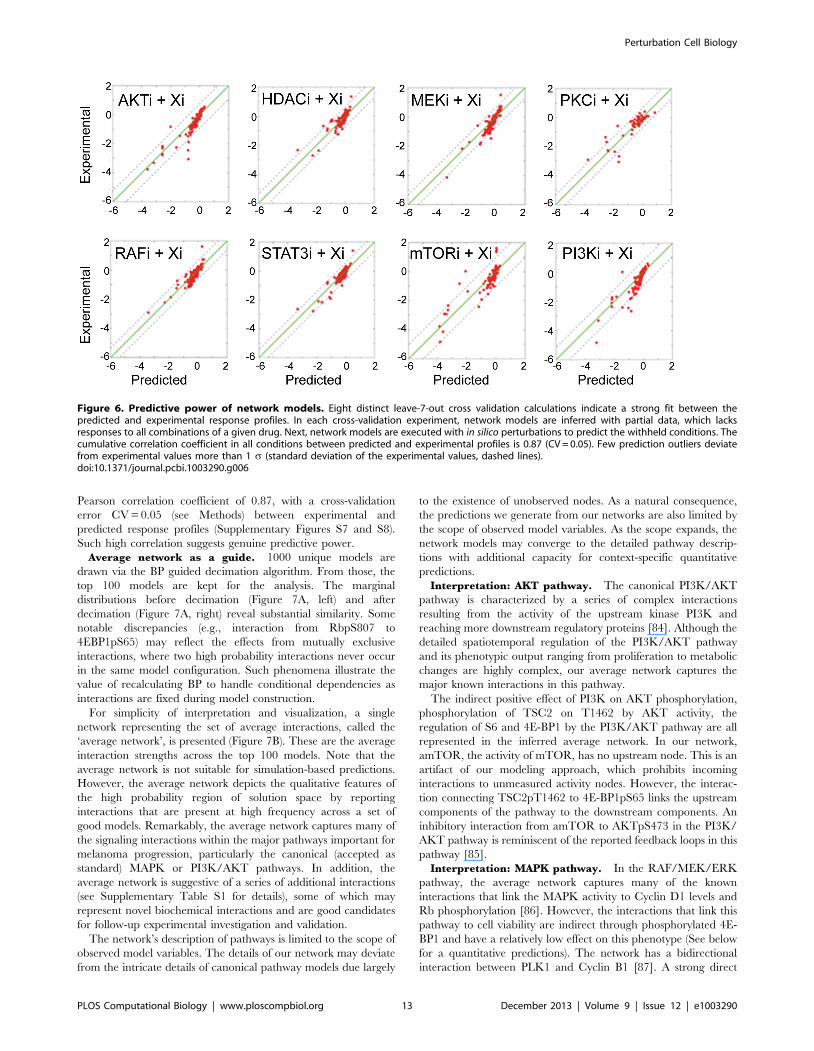
Pearson correlation coefficient of 0.87, with a cross-validation

error CV = 0.05 (see Methods) between experimental and

predicted response profiles (Supplementary Figures S7 and S8).

Such high correlation suggests genuine predictive power.

Average network as a guide. 1000 unique models are

drawn via the BP guided decimation algorithm. From those, the

top 100 models are kept for the analysis. The marginal

distributions before decimation (Figure 7A, left) and after

decimation (Figure 7A, right) reveal substantial similarity. Some

notable discrepancies (e.g., interaction from RbpS807 to

4EBP1pS65) may reflect the effects from mutually exclusive

interactions, where two high probability interactions never occur

in the same model configuration. Such phenomena illustrate the

value of recalculating BP to handle conditional dependencies as

interactions are fixed during model construction.

For simplicity of interpretation and visualization, a single

network representing the set of average interactions, called the

‘average network’, is presented (Figure 7B). These are the average

interaction strengths across the top 100 models. Note that the

average network is not suitable for simulation-based predictions.

However, the average network depicts the qualitative features of

the high probability region of solution space by reporting

interactions that are present at high frequency across a set of

good models. Remarkably, the average network captures many of

the signaling interactions within the major pathways important for

melanoma progression, particularly the canonical (accepted as

standard) MAPK or PI3K/AKT pathways. In addition, the

average network is suggestive of a series of additional interactions

(see Supplementary Table S1 for details), some of which may

represent novel biochemical interactions and are good candidates

for follow-up experimental investigation and validation.

The network’s description of pathways is limited to the scope of

observed model variables. The details of our network may deviate

from the intricate details of canonical pathway models due largely

to the existence of unobserved nodes. As a natural consequence,

the predictions we generate from our networks are also limited by

the scope of observed model variables. As the scope expands, the

network models may converge to the detailed pathway descrip-

tions with additional capacity for context-specific quantitative

predictions.

Interpretation: AKT pathway. The canonical PI3K/AKT

pathway is characterized by a series of complex interactions

resulting from the activity of the upstream kinase PI3K and

reaching more downstream regulatory proteins [84]. Although the

detailed spatiotemporal regulation of the PI3K/AKT pathway

and its phenotypic output ranging from proliferation to metabolic

changes are highly complex, our average network captures the

major known interactions in this pathway.

The indirect positive effect of PI3K on AKT phosphorylation,

phosphorylation of TSC2 on T1462 by AKT activity, the

regulation of S6 and 4E-BP1 by the PI3K/AKT pathway are all

represented in the inferred average network. In our network,

amTOR, the activity of mTOR, has no upstream node. This is an

artifact of our modeling approach, which prohibits incoming

interactions to unmeasured activity nodes. However, the interac-

tion connecting TSC2pT1462 to 4E-BP1pS65 links the upstream

components of the pathway to the downstream components. An

inhibitory interaction from amTOR to AKTpS473 in the PI3K/

AKT pathway is reminiscent of the reported feedback loops in this

pathway [85].

Interpretation: MAPK pathway. In the RAF/MEK/ERK

pathway, the average network captures many of the known

interactions that link the MAPK activity to Cyclin D1 levels and

Rb phosphorylation [86]. However, the interactions that link this

pathway to cell viability are indirect through phosphorylated 4E-

BP1 and have a relatively low effect on this phenotype (See below

for a quantitative predictions). The network has a bidirectional

interaction between PLK1 and Cyclin B1 [87]. A strong direct

Figure 6. Predictive power of network models. Eight distinct leave-7-out cross validation calculations indicate a strong fit between thepredicted and experimental response profiles. In each cross-validation experiment, network models are inferred with partial data, which lacksresponses to all combinations of a given drug. Next, network models are executed with in silico perturbations to predict the withheld conditions. Thecumulative correlation coefficient in all conditions between predicted and experimental profiles is 0.87 (CV = 0.05). Few prediction outliers deviatefrom experimental values more than 1 s (standard deviation of the experimental values, dashed lines).doi:10.1371/journal.pcbi.1003290.g006

Perturbation Cell Biology

PLOS Computational Biology | www.ploscompbiol.org 13 December 2013 | Volume 9 | Issue 12 | e1003290

interaction between PLK1 and cell viability is also present in the

network, consistent with the known PLK1 and Cyclin B1

regulation of the G2 to M transition in the cell cycle and the

multifaceted role that PLK1 plays in mitosis, including spindle

formation [87].

Prediction: Logical and biochemical interactions in the

melanoma cell line. In addition to the agreement with well-

studied biological interactions, the average network also indicates

a series of potentially novel interactions.

First, a strong bidirectional interaction is inferred between

RbpS807 and MEKpS217. One hypothesis for the MEK to Rb

interaction is that it stands in for the known direct RAF to Rb

interaction in the absence of any measurements of phosphorylated

RAF. Disruption of the RAF to Rb interaction induces apoptosis

in melanoma [88,89]. Conversely, the Rb to MEK interaction has

not been previously reported. Given that RAF, RAS, and MAPK

are all in the same pathway with MEK, the Rb to MEK

interaction is plausibly consistent with the observations that: (i)

RB1 (the gene that encodes the Rb protein) and KRAS double-

knockout mice studies indicate genetic interaction between Rb and

KRAS [90]; and (ii) inactivation of Rb results in elevated RAS and

MAPK activity [91,92]. It is important to note that the

phosphorylation of Rb on S807 is an inhibitory modification, so

a positive interaction from RbpS807 to MEKpS217 is consistent

with Rb inhibition causing an increase in phosphorylated MEK

levels.

An inhibitory interaction from aHDAC (activity of HDAC) to

SRCpY527, a critical phosphorylation site for the auto-inhibition

of SRC [93], is consistent with the direct and indirect interactions

of HDAC isoforms with Src observed in multiple cancer contexts

[94,95]. Finally, positive interactions connecting Cyclin D1 and

TSC2pY1462 to the SRCpY527 node are inferred. To the best of

our knowledge, no such interactions have been reported. The

observed edges may correspond to logical indirect interactions that

Figure 7. The distribution of edges in all network models and average network model. The probability distribution of edge values (wij)after BP (A, left) are similar to the histograms of the corresponding interactions after decimation (A, right). An interaction strength is nonzero when ithas high amplitude and frequency in solution space. We generate instantiated models with BP guided decimation algorithm followed by gradientdescent optimization. According to the agreement between the distributions in two panels, BP probability distribution and final model histogram aresimilar to each other with important exceptions. The BP guided decimation algorithm goes beyond simply sampling from the BP models and mayencounter features such as mutual exclusivity during the creation of the final models. (B) The average network model over the 100 best solutions withlowest error capture known interactions such as those in the RAF/MEK/MAPK and PI3K/AKT pathways. The opacities of the edges scale with theabsolute probability of the edges. Note that the letter 9a9 is prefixed to so-called activity nodes as explained in Methods section.doi:10.1371/journal.pcbi.1003290.g007

Perturbation Cell Biology

PLOS Computational Biology | www.ploscompbiol.org 14 December 2013 | Volume 9 | Issue 12 | e1003290

coordinate negative feedback loops acting on Src from the MAPK

and PI3K pathways. All of the predicted interactions are

suggestive of follow-up genetic and/or biochemical experiments.

Prediction: drug target identification in SKMEL-133 via

computation of viability changes in response to previously

untested perturbations. Given a set of network models of

SKMEL-133 cells, we predict the effect of arbitrary in silico

perturbations acting on any protein node present in the model.

Such in silico perturbations predict the quantitative effects of

hypothetical drugs (i.e., virtual drugs that target the nodes in a

model) on the cellular phenotypes. Furthermore, one can

quantitatively track signaling processes beyond the qualitative

interpretation of the average network model.

As an example, we predict the cell viability response of

SKMEL-133 cells to various targeted perturbations via explicit

numerical simulations of our network models. The simulations for

each of the network models produce predictions of the temporal

trajectories for all model nodes: proteins, phospho-proteins and

phenotypes, alike. In each simulation, a single perturbation to a

single protein node i is encoded as an external force (ui) that

reduces the relative abundance of that node by 50% (xi = -

log2(0.5) = 21), which in turn propagates throughout the network

model. The simulated steady-state responses to four particular,

individually perturbed target nodes predict substantial decrease in

cell viability (Figure 8) and therefore represent potential novel,

efficacious drug targets.

The most significant reduction in cell viability comes from the

predicted response to perturbation of STAT3pS705, whose mean

predicted inhibition of cell viability is roughly 56%, i.e., 44% of

the unperturbed cell viability (xi = 21.16). In the average network,

STAT3pS705 is downstream of aPKC, and our perturbation

experiments do show that PKC inhibition leads to low cell counts.

Thus, the response of STAT3pS705 inhibition simply reflects the

effect of known PKC inhibition, which is included in the training

set. Next, perturbation of both PLK1 and Cyclin B1 protein nodes

lead to significant reduction in cell viability at 45% (xi = 20.85)

and 38% (xi = 2.69) inhibition, respectively. PLK1 and Cyclin B1

are two important cell cycle proteins regulating G2 to M transition

and highly specific PLK1 inhibitors are potential agents in

targeted therapy [96]. Importantly, the network approach predicts

the effect of PLK1 and Cyclin B1 perturbations on cell viability

without any training to responses of perturbations to these nodes.

We subsequently tested one of these predictions in the lab by

treating the SKMEL-133 cells with the PLK1 inhibitor (BI 2536)

and measuring cell viability response with the resazurin assay

(Figure 9). The experimental tests reveal that the cell viability IC50

for the PLK1 inhibitor is 5.5nM in SKMEL-133 cells and that

approximately 99% of the cells are eliminated with a 15nM

concentration.

The fourth perturbation that predicts significant change in cell

viability is TSC2pT1462 inhibition, which has a central role in the

average network model, particularly in PI3K/AKT pathway. It is

regulated by AKTpS473 and also interacts with MAPK14pT180,

which is upstream of PLK1 and Cyclin B1 in the models. Note

that SKMEL-133 cell line is PTEN-null and that a constitutively

active PI3K/AKT pathway may play a role in drug resistance in

this cell line [46]. Thus, it is not surprising to us that deactivation

of a central player in this pathway leads to reduction in cell

viability. The corresponding best drug target is the kinase that

leads to phosphorylation of TSC2 on T1462.

The predicted effect on cell viability for each of these four

computationally perturbed nodes has at least one of the following

explanations: consistent with known perturbation responses of

immediately adjacent nodes, present in model training; consistent

with the known genetic background of the model cell line (e.g.,

SKMEL-133 is PTEN-null); or represents a genuinely novel drug

Figure 8. Novel predictions from in silico perturbations. (A) The histogram of phenotypic response profiles to the four most effective virtualperturbations from the best 100 network models. The response to STAT3p705 reflects the effect of PKCi on cell viability. Viability changes in responseto perturbations on cell cycle proteins PLK1 and Cyclin B1 are genuine predictions from the network models. Perturbation of TSC2pT1462 (inhibitoryphosphorylation) down regulates the PI3K/AKT pathway and leads to a decrease in cell viability in the PTEN null SKMEL133 cell line. (B) The perturbednodes that lead to reduction in cell viability in the context of average network model (Circled in red).doi:10.1371/journal.pcbi.1003290.g008

Perturbation Cell Biology

PLOS Computational Biology | www.ploscompbiol.org 15 December 2013 | Volume 9 | Issue 12 | e1003290

target, predicted to be highly efficacious and subsequently

validated experimentally.

Discussion

Beyond classical molecular biologyWe describe a combination of experimental and computational

methods, in the field of network pharmacology, to construct

quantitative and predictive network models of signaling pathways.

The particular contribution is a set of algorithmic advances, which

we adapted from statistical physics to infer network models in sizes

and complexities not reachable by classical gene-by-gene molec-

ular biology. The necessity of inference of complex network

models stems from the fact that classical methods, in which a small

number of perturbation experiments lead to functional description

of carefully selected sets of genes and gene products is reaching

technical limits. High-throughput proteomic and genomic profil-

ing technologies provide much richer and more complex

information about cellular responses than can be analyzed by a

scientist’s thought processes. At these levels of completeness and

detail, predicting changes in physiological attributes from molec-

ular data requires computational modeling and quantitative

analysis. Our quantitative network models not only capture

already known biological interactions but also nominate novel

interactions and may detect complex regulatory mechanisms, such

as feedback loops, in specific biological contexts. The quantitative

analysis of molecular and cellular behavior in these models

provides detailed understanding of the coupling between signaling

processes and global cellular behavior. Such understanding is hard

to achieve by reductionist approaches that focus on the relation

between single or few molecules and cellular processes. Further-

more, we provide a systems biology platform to predict the cellular

(i.e., proteomic and phenotypic) response profiles to multiple

perturbations such as those in combinatorial cancer therapies.

Network pharmacology in the era of personalizedmedicine

This investigation constitutes a proof-of-principle of a particular

technology: a combination of a network inference algorithm and a

technology for perturbing cells and measuring their response. The

overall context is network pharmacology, by which we mean the

science of using network models to derive and then test effective

therapeutic targets and combinations. The particular challenge in

cancer biology is the complexity and individual variation of

genetic and epigenetic alterations that are plausibly cancer

causing, and thus modulate the response to therapy; and, the

emergence of resistance to successful targeted therapies, such as

EGFR inhibitors in lung cancer or RAF inhibitors in melanoma.

In our view, the fairly fragmented gene-by-gene classical methods

of molecular biology, while extremely powerful as a reductionist

method, are reaching a clear limit. Those methods struggle with

effects such as ‘cross-pathway coupling’, ‘multigenic diseases’ or

individual variation of response to therapy. More comprehensively

quantitative and computationally predictive methods (‘systems

biology’) are likely not only to increase our predictive abilities but

also save substantial overall effort by computationally testing large

numbers of cellular states on a large variety of genetic backgrounds

and in exhaustively explored perturbation conditions.

Figure 9. Experimental testing of computational predictions. Qualitative analysis of networks from in silico simulations nominates PLK1 andCyclin B1 as potential targets to kill RAF inhibitor resistant melanoma cells. A validation experiment with the PLK1 inhibitor BI2536 shows extensivegrowth inhibition in SKMEL133 cells (Cell viability IC50 = 5.8 nm). PLK1 inhibitor is a pure prediction of the approach and was not included in theexperimental drug set.doi:10.1371/journal.pcbi.1003290.g009

Perturbation Cell Biology

PLOS Computational Biology | www.ploscompbiol.org 16 December 2013 | Volume 9 | Issue 12 | e1003290

Power and limitations of the belief propagation methodfor network modeling of signaling pathways

The implementation of our BP algorithm enables us to infer

much larger network models than are reachable with standard

Monte Carlo search methods. First, we use biologically realistic toy

data to illustrate the dramatic speed improvement of the BP

method over standard MC methods. BP convergence times scale

favorably with the size of the models at no measureable loss of

accuracy. This is a desirable property for constructing large

network models de novo. Even in the biologically realistic conditions

of noisy data from sparse perturbation, BP infers most of the

dominant interactions in the data-generating network. Although a

fraction of the likely BP interactions are false positives, these false

positives are consistent with the data and connect structurally

correlated nodes. The assumptions inherent in this BP implemen-

tation are potential limitations to the overall efficacy and accuracy

of our approach. However, assumption 1, while important, does

not dramatically affect the results beyond a critical level of

discretization. Furthermore, since BP performs as well or better

than MC, which employs neither assumption 3 nor 4, we suspect

by process of elimination that assumption 2 is the largest

contributor to the observed limitations of our current method.

For real biological data, the quality of BP’s performance depends

on the applicability of the model equations and both the richness

and quality of the data used for training.

We previously published an MCF7 breast cancer cell line

dataset, for which network models were derived with a nested MC

search algorithm (CoPIA) [97]. Reassuringly, many of the

strongest interactions from CoPIA are recovered by the BP

method (Supplementary Text-S4, Figure S10). We have also

modeled the same SKMEL-133 dataset with Gaussian Graphical

Models, a popular probabilistic model that goes beyond pairwise

correlations to distinguish between direct and indirect correlations.

A comparison to the BP derived interactions suggests non-trivial

overlap in the strongest couplings. A more detailed analysis is

available in the supplement (Supplementary Text –S5, Figures S11

and S12). Finally, we have also compared BP against both prior

knowledge models and Bayesian network models inferred with

Bayesian inference [98]. That analysis indicates superior perfor-

mance for the BP derived models for at least this kind of data and

this style of model (See Supplemental Text S7 and Figure S17).

Confirmed and predicted interactions in malignantmelanoma cells

We are able to capture the known interactions in MAPK and

AKT/PI3K canonical pathways through de novo network infer-

ence. Moreover, we predict potential interactions, either direct or

indirect, such as a bidirectional interaction between Rb and

MAPK pathways and a potential feedback loop from PI3K and

MAPK pathways acting on SRC activity through inhibitory

phosphorylation at SRCpY527. We also quantitatively predict the

effect on cell viability from inhibition of novel targets via explicit in

silico simulation. The in silico perturbations of Cyclin B1 and PLK1

lead to comparable reduction in cell viability. As neither Cyclin

B1/PLK1 nor their direct regulators are inhibited for the model

training dataset, this result is a genuine and nontrivial prediction.

We test and validate the PLK1 prediction by measuring the cell

viability after treating SKMEL-133 cells with a potent and

selective PLK1 inhibitor. Indeed, the PLK1 inhibitor reduces

cellular growth significantly in SKMEL-133 cells even when

treated with the drug at nanomolar concentrations (Figure 9).

Moreover, none of the in silico perturbations of the MAPK

pathway lead to a significant change in cell viability, which is

consistent with the experimental responses to perturbations acting

on MEK and BRAFV600E and RAF inhibitor resistance of

SKMEL-133 cells.

The problem of drug specificityWe are aware that drugs do not usually have a single specific

target. While this is potentially problematic for modeling and

simulating drug effects, we find that the inference is driven largely

by the correlations in the data arising from the effect of

perturbations on the overall system. We estimate that BP is most

sensitive to strong and untrue assumptions about the direct effects

of a given drug. The use of activity nodes is an indirect way of

dealing with off-target drug effects. These nodes, which are

perturbed but not measured, represent the coupling of a drug to

the rest of the system. Such coupling includes both specific and off-

target effects. BP may infer interactions from these activity nodes

to any number other measured nodes thus simultaneously

inferring targets for the particular drug used. Drug specificity also

affects the predictive power of the resulting models. All effects from

the AKT inhibitor, for example, are assigned to single inhibition of

the aAKT node, even if other targets of the AKT inhibitor are

partially responsible for the measured outcomes. Therefore, any

simulation-based prediction regarding perturbation of the aAKT

node will be tethered to the off-target effects of the AKT inhibitor

used in training. The complete solution of the drug specificity

problem requires a more comprehensive and systematic analysis to

determine the effect of off-target effects on quality and predictive

power of inferred models.

Failed predictions and optimal design of experimentThe leave-k-out analysis reveals few outlier points, where the

predicted response profiles largely disagrees with test data. These

(mis)predictions fall into two major categories. In the first category,

(mis)predictions arise due to measurements with very low signal to

noise ratios and high experimental uncertainties. The (mis)pre-

dicted S6pS240 levels and cell viability phenotypes in some of the

perturbation conditions fall into this category. Note that the

models are trained and simulated after logarithmic conversion (i.e.,

xi = log2-ratios of measured signals), which exaggerates the errors

for low signals. In linear space, no such outliers are observed

suggesting that those outliers can be considered as an artifact of

our analysis in logarithmic space. In the second category,

(mis)predictions arise due to insufficient experimental constraints.

(Mis)prediction of AKTpS473 levels after mTOR inhibition falls

into this category. mTOR inhibition leads to an increase in AKT

phosphorylation possibly due to the disruption of a feedback loop.

In our current analysis, mTOR inhibition and steady state

measurements on AKT phosphorylation are the sole experimental

inputs to detect the changes in this feedback mechanism. When

the mTOR inhibition is withheld in leave-k-out tests, experimental

constraints become insufficient to describe the regulation of AKT

phosphorylation, thus leading to the (mis)predictions. A systematic

experimental design to enrich the perturbations, better character-

ization of the AKT phosphorylation dynamic range and richer

proteomic measurements on this part of signaling pathways are

possible ways to improve the quality of these particular predic-

tions. In general, careful optimization of perturbation conditions

(drugs and combinations) and observations (protein arrays, mass

spectrometry target list), within available resources, would

significantly enhance the predictive power of this approach.

Perturbation Cell Biology

PLOS Computational Biology | www.ploscompbiol.org 17 December 2013 | Volume 9 | Issue 12 | e1003290

Predicting effective novel drug combinations with BPbased network modeling

Predicting the effect of drug combinations is highly challenging

and has been the subject of many studies, e.g., [99,100]. When a

large repertoire of targeted drugs are available for screening, the

search space for useful combinations of two or more drugs is

combinatorially complex. Moreover, therapeutically promising

drug combinations are not limited to simultaneously introduced

perturbations. Potentially useful drug combinations may consist of

combinations of relative doses, for two, three and four drugs

applied simultaneously or sequentially after well-defined time

intervals. Identification of such complicated combinations through

experimental screening tests is prohibitively cumbersome. Here,

we provide a potential solution to this problem in that in silico

screens using predictive network models can cover a large space of

possible drug combinations. The predictive power of the models

derived here is apparent from the reasonable accuracy of

predicting the results of withheld experiments using a leave-k-out

cross validation. Network models inferred from perturbation

experiments can thus be used to predict the responses to novel

combinations. One can enlarge the search space for drug

treatments from a few hundred experimentally screened combi-

nations to tens of thousands of computationally tested combina-

tions and guide subsequent, highly efficient experimental screens

of the top predicted candidates.

Beyond the computational power of well-constrained and

robustly derived network models, one may expect to achieve a

conceptual understanding of the principles of epistasis of drug

effects and the mechanisms of resistance to targeted therapeutics.

For example, the initial system response to drug intervention on

the scale of minutes to days may be indicative of subsequent

epigenetic and genetic changes in a population of treated cells that

represent the long-term and hard-to-treat emergence of drug

resistance. In this context, reliable dynamic network modeling may

be an excellent guide to strategies for blocking the emergence of

resistance in the first place. The pre-clinical consequence is the

selection of combinations of therapeutic interventions that not only

are effective in slowing the proliferation or promoting the

elimination of cancer cells, but also counteract resistance to

otherwise effective treatments, such as RAF inhibitors in

melanoma or AR inhibitors in advanced prostate cancer, in

clinical trials.

Method improvementWhile the approximate solutions to the problem of network

inference deliver interpretable biological results, there is much

room for improving the power and information value of the

method. For example, when time-dependent response measure-

ments after perturbation are available, one can use analogous,

extended algorithms to infer probability distributions over (time-

independent) interaction parameters W that describe the behavior

of a time-dependent system. Another extension of the formalism is

the use of more complicated forms of the differential equations,

such as those of enzyme kinetics. Also, even in the current

approximation, careful design of experiments selecting a minimal

set of maximally informative perturbation conditions would

increase the efficiency of this experimental-theoretical approach.

A straightforward and powerful extension is the systematic use

of prior information in the form of directed interactions adapted

from the current scientific literature or pathway databases. Such

prior information is easily incorporated as a set of additional

constraints on the probability distributions of W in Equation 3.

This has been utilized in our related work on modeling

dedifferentiated liposarcoma drug combinations [43]. We are also

actively pursuing a method for the systematic inclusion of prior

knowledge interactions from curated databases. On the experi-

mental side, measurement of richer phenotypic attributes of cells,

such as apoptosis or cell cycle arrest, as well as markers of

differentiation states would greatly increase the predictive power

by providing more links between molecular and phenotypic

quantities.

The network pharmacology approach described here provides a

strong tool for a system level description of signaling events in

cancer cells. Moreover, it presents a step forward in quantitative

prediction of responses of cancer cells to drug perturbations.

Beyond cancer biology, there is no reason to believe that the

proposed technology cannot be used to derive accurate quantita-

tive and predictive network models for biological cellular systems

in general, provided sufficiently diverse experimental perturba-

tions and sufficiently rich readouts are accessible. In this way, we

hope to extend the power of classical molecular biology to a broad

spectrum of cellular systems with targeted, and possibly clinical,

applications.

Materials and Methods

MaterialsChoice of drugs and drug concentrations. Eight small

molecule drugs targeting mainly the MAPK or AKT/PI3K

pathways were chosen based on the knowledge of target specificity

and relevance for exploring BRAF signaling in SKMEL-133 cells

(Figure 5). In order to select an appropriate drug concentration for

the RPPA assay, Western blots were used to measure the dose-

response effect of each drug on its presumed targets or

downstream effectors (Supplementary Figure S4). We use the so-

called ‘protein IC-values’, which are the concentrations that

inhibit the most immediate downstream protein by a certain

percentage. This is in contrast to the more common proliferation

IC-values, which are the concentrations that reduce the number of

proliferating cells by a certain percentage

RPPA and western blots. For Western blotting and reverse-

phase protein arrays (RPPA) assays, BRAFV600E mutant

SKMEL-133 cells were grown in 6-well plates to around 40%

confluence in RPMI-1640 medium containing 10% fetal bovine

serum (FBS). In a series of perturbation experiments, cells were

perturbed with 8 drugs either singly or in paired combinations,

and harvested after 24 hours by collecting and freezing the cell

pellet. Non-perturbed control cells were treated with drug vehicle

(DMSO) for 24 hours (elsewhere called ‘‘no-drug control’’). Cells

were thawed, lysed and protein concentrations were determined

by the Bradford assay. Protein concentrations were adjusted to 1–

1.5 mg/mL and proteins denatured in 2% SDS for 5 minutes at

95uC. For RPPA, cell lysates were spotted on nitrocellulose-coated

slides in Gordon Mills’ laboratory at MD Anderson Cancer

Center, as described previously [83] and stain with antibodies.

Each sample was represented in triplicates originating from three

different biological samples (wells). The resulting antibody staining

intensities are quantified using the MicroVigene automated RPPA

module (VigeneTech, Inc.) and normalized as describes in [83].

Resazurin cell viability assay. Cells were grown in 6-well

plates and perturbed in the same way as for the RPPA assays.

After 72 hr drug treatment, resazurin (Sigma-Aldrich, Catalog #R7017) was added at a final concentration of 44 mM to each well

and the fluorescent signals were measured after 1 hr incubation,

using 530 nm excitation wavelength and 590 nm emission

wavelength. For control wells (0 hr drug treatment), the fluores-

cent signals were monitored after 4 hr incubation. Standard curves

of cell numbers were generated as well to back calculate the cell

Perturbation Cell Biology

PLOS Computational Biology | www.ploscompbiol.org 18 December 2013 | Volume 9 | Issue 12 | e1003290

numbers in different wells. Cell viability measurements at 72 hours

are used to ensure the phenotypic responses reached to steady

state. Significant phenotypic response is observed as a conse-

quence of changes in relatively early proteomic responses to drug

perturbations. Indeed, analysis of cell viability changes at 0, 24, 72

and 120 hours after drug perturbations revealed no significant

changes in cell viability between 72 and 120 hours. Conversely,

the cell viability response at 24 hours had not reached steady state.

MethodsSetting up belief propagation calculations for network

inference. Network models are constructed using the mea-

sured proteomic and phenotypic response profiles to drug

perturbations as experimental data. The reported network

models contain 25 nodes and are trained to protein plus

phenotype response profiles from 44 experimental observations.

Each measured protein level is log normalized with respect to its

measured level at no-drug control condition. For quantification of

the activity nodes, see below. The probability distribution for

each possible interaction strength in the system is computed using

the belief propagation algorithm. In the current implementation,

the edge strengths can assume values within the interval [21, 1]

with discrete steps of 0.2. The initial messages are sampled

uniformly from a random distribution and the BP algorithm is

run until the difference between marginals in consecutive

iterations is less than 1026.

The inverse-temperature scaling constant b and the complexity

penalty term l are the parameters in the BP algorithm that

influence expected network connectivity. A systematic approach is

taken to ensure the right approximate connectivity in the network

models in order to prevent both non-descriptive, sparse models

and overfit, highly connected models. Very sparsely connected

network models have discontinuities in information flow and low

predictive power. Overfit models lack generalizability of predictive

power. Empirical representations of signaling networks in the

extant literature are fairly sparse, with approximately 1–2

interactions per node. Generally, one has to select b and l from

a set of BP calculations with systematically varied b and l such

that a typical BP derived network has a desired connectivity (edges

per node). In this work, we explored b and l values in the interval

(0,5.0], and selected the b and l which resulted in the lowest

expected error among the representative networks that had a

desired connectivity of ,1.5 edges per node. Representative

networks in this case were based on the most probable parameter

value for all parameters, each from their respective marginals; we

also set a threshold of 0.2 below which parameters were set to

zero. The optimal values (b = 2, l = 5) are used for the

computation of the instantiated solutions in subsequent decimation

calculations. For each node. ai is taken as 1 and ei is estimated

from the dynamic range of each proteomic measurement sampled

in the biological dataset. The ei and ai parameters are further

optimized with a gradient descent algorithm.

Inferring distinct, executable network models of

signaling. Distinct model solutions are computed with the BP-

guided decimation algorithm. The interaction parameters in each

model are further optimized using the Pineda gradient descent

algorithm [33], relaxing the assumptions of discrete interaction

values and factorized probability distributions (Equation 6d). The

gradient descent algorithm also includes optimization of both ei

and ai parameters. The optimized models are ranked according to

their model errors and the best 100 models are used for

simulations and the average network model (Supplementary

Figure S6). The average network model is for summary and

illustration purposes and is not in itself executable. Instead,

predictions are made by simulation of individual, or sets of,

instantiated network models.

Simulating signaling network models. Each network

solution is simulated individually with specific virtual perturbations

according to the model Equation 1 until the system reaches its

steady state (Supplementary Figure S9) i.e., until no system

variable changes in consecutive steps of simulation within machine

precision. The DLSODE integration method (ODEPACK) [101]

is used in simulations (default settings with, MF = 10, ATOL = 1e-

10, RTOL = 1e-20) is used for simulations. Trajectories for the

best 100 model solutions yield an ensemble of predicted outcomes

in response to in silico perturbations.

Activity nodes. ‘‘Activity node’’ is a technical term defined

within the context of applied perturbations and derived network

models (Figure 7-Right, Supplemental Figure- S15). Each activity

node quantitatively represents a molecular process or reaction,

such as phosphorylation, involving a particular protein (or other

signaling molecule) that is affected by a perturbation agent. Since

we measure protein and phospho-protein levels and do not directly

measure the biochemical activity of any kinase, the activity nodes

stand in for the effect of each drug perturbation on the

biochemical activity of the drug targets. At a basal level (no

perturbation), the quantitative measure of an activity node is equal

to the activity level in no-drug control experiments and is set equal

to 0 as a reference point. In the presence of an inhibitor molecule

affecting a particular activity node, it is calculated based on the

influence of the drug on its presumed immediate or downstream

target validated with Western blot experiments (Supplementary

Figure S4). We demonstrate this with an example quantification of

the MEK activity node (aMEK). We measure the strength of a

MEK inhibitor by measuring the phosphorylation of its down-

stream target MAPK1 at residue T202. If the level of MAPK

phosphorylation inhibition is 55% compared to a no-drug control

experiment, the strength of the inhibition is ui = -

log2(0.55) = 20.863. Based on the model equations (Equation 1),

the value for the activity node is xi = (b/a) tanh(ui) = 20.697. The

a/b is initially assumed to be 1 and refined by the final gradient

descent optimization step. Activity nodes are not allowed to have

any upstream regulators except the inhibitor since we do not have

any direct measurement of the activity node. All of the activity

nodes are quantified using the above procedure and the responses

from presumed targets.

Mathematical description of perturbations. A constant

perturbation (ui) acting on a particular node i (Equation 1) impacts

both the time derivative and the final steady state value (xi) of the

perturbed node. The set of interactions and their strengths (wij) are

independent of the perturbation. As modeled by Equation 1, the

dynamic properties and steady state value of node xi are a

functions of the combination of influence from all upstream nodes

(xj) with nonzero interaction strengths wij and the strength of the

perturbation. The perturbation term in Equation 1 models the

effect of targeted interventions such as targeted small molecules.

The model equation can also incorporate other perturbation forms

such as genetic alterations or RNA interference (RNAi). In case of

genetic alterations, the impact can be modeled by fixing xi to a

desired value. For example, fixing a particular xi value to a large

negative value (large relative to a given dataset) represents genetic

knockdown of the corresponding gene, such as perturbations with

RNAi. One may also fix the value of xi to a positive value to model

the impact of amplification of a gene product (e.g., DNA copy

number change).

Toy data. We generated toy data based on toy network

models in order to test the performance of BP against a known set

of true interactions. The toy models are generated by first fixing a

Perturbation Cell Biology

PLOS Computational Biology | www.ploscompbiol.org 19 December 2013 | Volume 9 | Issue 12 | e1003290

topology of positive and negative values, which are then assigned a

set of real values by drawing from an even distribution between 0

and a maximum strength of 2. The topologies are designed to

represent cascade-like hierarchical networks to include parallel

chains, feed-forward and feedback motifs. For the analysis focusing

on true interactions, the topology is generated with the web-service

Gene Network Generator (GeNGe). At the time of this analysis,

popular toy data generators such as GeneNetWeaver focus on

scale-free like network topologies that are common in gene

regulatory networks, but not typical for signal transduction

pathways. Given the network model, the data is generated by

simulating the model according to Equation 1 in response to

external perturbation, until the system reaches a stable steady

state. The steady state values for all nodes are recorded in each

perturbation condition. In rare cases, the simulations encountered

perpetual oscillations and these results are excluded from the final

toy data set. These simulations are purely deterministic as no

stochasticity is incorporated into the simulations. Noise is added to

the data post-simulation. We chose to simulate the dynamics of the

toy networks with Equation 1 so as to remove the choice of model

equation as a source of error.

Supporting Information

Code S1 This directory contains all of the fotran90source code for performing all of the Belief Propagation,gradient descent and simulation analysis described inthis paper.(ZIP)

Data Set S1 This directory contains all of theSKMEL133 perturbation and protein data analyzed inthis paper and is properly formatted to work with theprovided version of the BP code.(ZIP)

Data Set S2 This directory contains all of the modelsand data analyzed in Supplemental Figure S17. The data

in this directory is from a separate study of dedifferentiated

liposarcoma from the DDLS8817 cell line.

(ZIP)

Figure S1 Comparison of the correlations betweenfalse-positives and true-positives. The nodes connected by

false positive edges inferred by BP tend to be highly correlated

(blue dots in Figures S1A and S1B), as analyzed here for two

example false positives, each from different false positive motifs.

Indeed the falsely connected nodes seem to have stronger

correlation than the nodes connected by real edges (red and

green dots). This analysis indicates that BP is indeed capturing

significant correlations in the data although through false

interactions. It also indicates that the edge parameters that BP

misses (red and green edges) are somehow compensated by the

false positive parameter (blue edges). In the absence of temporal

data or more perturbations of the nodes in this sub-network, there

may not be sufficient evidence to correctly infer the causal

relationship between these connected nodes.

(TIF)

Figure S2 Alternative higher-order perturbations pro-duce better data for inference with BP than thesystematic pair perturbation strategy. Performance for

both datasets is analyzed with mean squared errors (A), recall (B),

precision (C), and the total number of BP-inferred interactions (D).

The correlations between the training patterns are shown in

analyzed in (E) for both perturbation strategies.

(TIF)

Figure S3 Perfect BP inference with ideal data. Totally

randomized data (A) produces low correlations between training

patterns (B). With this maximally informative, BP reproduces all of

the true interactions (D), except 2 with zero false positives when

compared against the underlying data generating network (C).

(TIF)

Figure S4 Dose response curve of singe agent drugperturbations. Dose response curves determined based on

Western Blot experiments, shown on top. See table S1 for protein

IC40 values, which are calculated with these curves and used in all

paired perturbation experiments. Cell viability curve (not shown)

was used to estimate PKC inhibitor (Ro-31-7549) IC40.

(TIF)

Figure S5 Model abstraction in network models ofsignaling. A relatively detailed model of biochemical events in

PI3K/AKT pathway (i.e. consecutive phosphorylation of AKT at

T308 and S473) (reactome.org) and the coarse-grained network

model abstraction used in this paper (Red arrows and rectangles).

In the model abstraction, PI3K and AKT activity nodes influence

the final output of the activation mechanism (i.e. AKTpS473). In

princible, we can improve and extend the model with additional

measurements such as measurements on PDK1, AKTp308

(circled in gray) etc without altering the model abstraction. Such

model improvement requires richer measurements and will lead to

a shift from logical to potential physical interactions. Lower left.

The PI3K/AKT interactions in the average network model

computed with BP-guided decimation.

(TIF)

Figure S6 6 of the 10 best network models. Better models

have lower cost. Two nodes (horizontal and vertical list) can be

connected by a positive (red) or negative (blue) interaction Wij.

Although each model is different in detail, each model represents

the data well in the predictive sense. The differences reflect

genuine uncertainties of model inference, normally not represent-

ed in molecular biology cartoon models. Substantial similarity

exists between the top 6 models shown in Figure S6 A–F.

(TIF)

Figure S7 Predictive power tested by prediction ofwithheld data. The 8 distinct heatmaps of withheld (upper

right) and predicted (lower right) respone profiles to withheld

perturbations (upper left). For quantitative analysis of predictive

power, please see Figure 7 in the main manuscript.

(TIF)

Figure S8 Cumulative predictive power. The cumulative

scatter plot that combines the information in Figure S7 (C = 0.87).

(TIF)

Figure S9 Sample simulated trajectory. Pseudo-time

trajectory of a single network model when perturbed with an in

silico perturbation on AKTpS473 at virtual IC50 (i.e. log2

([AKTpS47]final/([AKTpS47]initial) = 21).

(TIF)

Figure S10 BP comparison with CoPIA results on mcf7perturbation data. The CoPIA network inference method is an

older method based on a nested Monte Carlo search, and was

previously applied to infer network models of mcf7 breast cancer

data. The CoPIA network edges are color-coded based on the

existence of those edges in BP inference (A) has many agreeing

edges (green). Furthermore, most of the significant BP edges (B)

are also significant in the CoPIA models (green). Further analysis is

available in Supplementary Text – S4.

(TIF)

Perturbation Cell Biology

PLOS Computational Biology | www.ploscompbiol.org 20 December 2013 | Volume 9 | Issue 12 | e1003290

Figure S11 Gaussian model couplings for the mostlikely cutoff. The inference with no reweighting produces the

highest likelihood estimate (A). The distribution of J and H

couplings (B and C, respectively) are strongly centered at zero,

demonstrating some discerning power between all possible

couplings. Further analysis is available in Supplementary Text –

S5.

(TIF)

Figure S12 Comparison of the most likely Gaussianmodel couplings and those from BP. The ROC curve (A)

lies firmly above the diagonal line. The set of GGM edges taken

from the F1-max cutoff (B) has many agreeing edges with those

returned from BP (C). Further analysis is available in Supplemen-

tary Text – S5.

(TIF)

Figure S13 Entropy as a function of the number of bins.Entropy is normalized by the ratio of total entropy to maximum

possible entropy. This analysis is focused on exploring the effects of

different discretization strategies (Assumption 1) on the BP

inference. Further analysis is available in Supplementary Text –

S1.

(TIF)

Figure S14 Entropy as a function of the number of bins.This time, entropy is calculated on a collapsed distribution over

three regions; aggregate probability mass for negative values, zero

values and positive values. Further analysis is available in

Supplementary Text-S1.

(TIF)

Figure S15 Schematic illustration of interpreting modeledges and activity nodes. Direct interactions in our models do

not necessarily imply direct biological interactions (A). Rather the

separation between any two connected nodes is dependent on

those nodes that are included in the model, which is in turn a

function of the availability and specificity of assays for various

proteins and phospho-proteins. Consider the linear cascade of 5

nodes (A). When intermediate nodes are excluded from the model,

for whatever reason, the true direct interactions are also excluded.

In their stead, the model will have interactions between the

neighboring nodes. In that case, the direct model interactions do

no correspond to direct biological interactions. The use of activity

nodes may also confuse the interpretation of our model

interactions. Activity nodes stand in for the activity of a protein

(or phosphorylated protein) that is not directly measureable, as

explained in the Materials and Methods section of the main

manuscript. It is this activity that is being targeted by a given drug.

We can assume that the activity is below basal (x is negative) when

the drug is applied. However, in those conditions in which the

drug is not applied we have no data or reasonable assumption with

which to approximate the activity nodes. Consequently we do not

have enough data with which to infer interactions into activity

nodes. Activity nodes are therefore restricted to exist as ‘root

nodes’ such that they have only outgoing edges (B). We consider

the activity nodes to represent the effect of ad rug on the rest of the

model nodes.

(TIF)

Figure S16 Algorithm flow chart.

(TIF)

Figure S17 BP comparison against Bayesian Inferenceof Bayesian network models. We compare models created

from both BP and Bayesian inference (BI) against random and

prior knowledge network models. For each class of model, we

compare only the top 100 models based on mean squared error

after simulation. Both BP and BI (purple and yellow, respectively)

outperform both random and prior knowledge models (red and

green, respectively). The analysis shows clear separation between

all four classes of models, confirming that both BI and BP models

are demonstrably informed by the data. Although BP models

outperform BI models in this study, it is unclear whether this is

generally true, which method predicts biological interactions more

accurately, or how low the MSE should be for genuine predictive

power to novel perturbations. See Supplementary Text S7 for

more information.

(PDF)

Table S1 This table provides notes curated from theliterature for each of the most probable interactionsinferred by BP for the melanoma data described in thispaper.

(DOCX)

Text S1 Discretization of parameter space. This section

focuses on the consequences of different strategies for discretizing

the network parameter space.

(DOCX)

Text S2 Monte Carlo inference. This section described in

detail the Monte Carlo inference method used in the comparison

studies in this manuscript.

(DOCX)

Text S3 Training patterns. This section contains results from

an in silico experiment comparing the informative value of data

from systematic low order perturbations (drug pairs) against

random higher order perturbations (more than two drugs) with

respect to BP inference.

(DOCX)

Text S4 MCF7. This section examines BP performance on a

previously published dataset of perturbation responses in breast

cancer from the MCF7 cell line. This section also compares BP to

our previously published method for inferring models based on a

greedy Monte Carlo search.

(DOCX)

Text S5 Gaussian graphical models. This section reports

the results of modeling the melanoma data described in this

manuscript with Gaussian Graphical Models; a popular and

statistically rigorous method for discriminating between direct and

indirect correlations between system variables.

(DOCX)

Text S6 Implementation details. This section briefly

explains some of the more tedious details regarding implementa-

tion of the BP algorithm described in this paper.

(DOCX)

Text S7 Comparison with Bayesian Inference. This

section reports the results of a preliminary comparison of BP

models against those inferred from Bayesian Inference. It also

compares both class of models to random models and prior

knowledge models. The data used in this preliminary study is from

similar perturbation experiments on the dedifferentiated liposar-

coma cell line DDLS8817.

(DOCX)

Acknowledgments

We gratefully acknowledge the help of Deb Bemis in organizing and Ed

Reznik in improving the manuscript. We thank Debora Marks, Doug

Perturbation Cell Biology

PLOS Computational Biology | www.ploscompbiol.org 21 December 2013 | Volume 9 | Issue 12 | e1003290

Lauffenburger and Peter Sorger for discussions and Sven Nelander for

early guidance, discussions and comments on the manuscript.

Author Contributions

Conceived and designed the experiments: EJM AK WW CS . Performed

the experiments: WW MLM NPG XJ PK QH. Analyzed the data: EJM

AK. Contributed reagents/materials/analysis tools: GM DBS CAP. Wrote

the paper: EJM AK WW AP CS. Reverse Phase Protein Array Platform:

GM. Cell lines: DBS CAP. Development and optimization of code: EJM

AK AB AP. Statistical physics: MW AB AP RZ. Network modeling with

synthetic data: EJM. Network modeling with biological data: AK.

References

1. Hanahan D, Weinberg RA (2011) Hallmarks of cancer: the next generation.

Cell 144: 646–674.

2. Bollag G, Hirth P, Tsai J, Zhang J, Ibrahim PN, et al. (2010) Clinical efficacy of

a RAF inhibitor needs broad target blockade in BRAF-mutant melanoma.

Nature 467: 596–599.

3. de Bono JS, Logothetis CJ, Molina A, Fizazi K, North S, et al. (2011)

Abiraterone and increased survival in metastatic prostate cancer. N Engl J Med

364: 1995–2005.

4. Tran C, Ouk S, Clegg NJ, Chen Y, Watson PA, et al. (2009) Development of a

second-generation antiandrogen for treatment of advanced prostate cancer.

Science 324: 787–790.

5. Druker BJ, Talpaz M, Resta DJ, Peng B, Buchdunger E, et al. (2001) Efficacy

and safety of a specific inhibitor of the BCR-ABL tyrosine kinase in chronic

myeloid leukemia. N Engl J Med 344: 1031–1037.

6. Lynch TJ, Bell DW, Sordella R, Gurubhagavatula S, Okimoto RA, et al. (2004)

Activating mutations in the epidermal growth factor receptor underlying

responsiveness of non-small-cell lung cancer to gefitinib. N Engl J Med 350:

2129–2139.

7. Paez JG, Janne PA, Lee JC, Tracy S, Greulich H, et al. (2004) EGFR

mutations in lung cancer: correlation with clinical response to gefitinib therapy.

Science 304: 1497–1500.

8. Pao W, Miller V, Zakowski M, Doherty J, Politi K, et al. (2004) EGF receptor

gene mutations are common in lung cancers from ‘‘never smokers’’ and are

associated with sensitivity of tumors to gefitinib and erlotinib. Proc Natl Acad

Sci U S A 101: 13306–13311.

9. Fitzgerald JB, Schoeberl B, Nielsen UB, Sorger PK (2006) Systems biology and

combination therapy in the quest for clinical efficacy. Nat Chem Biol 2: 458–

466.

10. Kumar N, Hendriks BS, Janes KA, de Graaf D, Lauffenburger DA (2006)

Applying computational modeling to drug discovery and development. Drug

Discov Today 11: 806–811.

11. Wang DY, Cardelli L, Phillips A, Piterman N, Fisher J (2009) Computational

modeling of the EGFR network elucidates control mechanisms regulating

signal dynamics. BMC Syst Biol 3: 118.

12. di Bernardo D, Thompson MJ, Gardner TS, Chobot SE, Eastwood EL, et al.

(2005) Chemogenomic profiling on a genome-wide scale using reverse-

engineered gene networks. Nat Biotechnol 23: 377–383.

13. Gardner TS, di Bernardo D, Lorenz D, Collins JJ (2003) Inferring genetic

networks and identifying compound mode of action via expression profiling.

Science 301: 102–105.

14. Luan D, Zai M, Varner JD (2007) Computationally derived points of fragility

of a human cascade are consistent with current therapeutic strategies. PLoS

Comput Biol 3: e142.

15. Cho CR, Labow M, Reinhardt M, van Oostrum J, Peitsch MC (2006) The

application of systems biology to drug discovery. Curr Opin Chem Biol 10:

294–302.

16. Morris MK, Saez-Rodriguez J, Clarke DC, Sorger PK, Lauffenburger DA

(2011) Training signaling pathway maps to biochemical data with constrained

fuzzy logic: quantitative analysis of liver cell responses to inflammatory stimuli.

PLoS Comput Biol 7: e1001099.

17. Schoeberl B, Eichler-Jonsson C, Gilles ED, Muller G (2002) Computational

modeling of the dynamics of the MAP kinase cascade activated by surface and

internalized EGF receptors. Nat Biotechnol 20: 370–375.

18. Christopher R, Dhiman A, Fox J, Gendelman R, Haberitcher T, et al. (2004)

Data-driven computer simulation of human cancer cell. Ann N Y Acad Sci

1020: 132–153.

19. Steffen M, Petti A, Aach J, D’Haeseleer P, Church G (2002) Automated

modelling of signal transduction networks. BMC Bioinformatics 3: 34.

20. Aldridge BB, Burke JM, Lauffenburger DA, Sorger PK (2006) Physicochemical

modelling of cell signalling pathways. Nat Cell Biol 8: 1195–1203.

21. Nakakuki T, Birtwistle MR, Saeki Y, Yumoto N, Ide K, et al. Ligand-specific c-

Fos expression emerges from the spatiotemporal control of ErbB network

dynamics. Cell 141: 884–896.

22. Lezon TR, Banavar JR, Cieplak M, Maritan A, Fedoroff NV (2006) Using the

principle of entropy maximization to infer genetic interaction networks from

gene expression patterns. Proc Natl Acad Sci U S A 103: 19033–19038.

23. D’Haeseleer P, Liang S, Somogyi R (2000) Genetic network inference: from co-

expression clustering to reverse engineering. Bioinformatics (Oxford, England)

16: 707–726.

24. Weaver DC, Workman CT, Stormo GD (1999) Modeling regulatory networks

with weight matrices. Pacific symposium on biocomputing 4: 112–123.

25. Bonneau R, Reiss DJ, Shannon P, Facciotti M, Hood L, et al. (2006) The

Inferelator: an algorithm for learning parsimonious regulatory networks fromsystems-biology data sets de novo. Genome biology 7: R36.

26. de Jong H (2003) Modeling and simulation of genetic regulatory networks.

Positive Systems: 111–118.

27. Mjolsness E, Mann T, Castano R, Wold B (1999) From coexpression tocoregulation: an approach to inferring transcriptional regulation among gene

classes from large-scale expression data. Neural Information ProcessingSystems 12: 928–934.

28. Toschi L, Janne PA (2008) Single-agent and combination therapeutic strategies

to inhibit hepatocyte growth factor/MET signaling in cancer. Clin Cancer Res14: 5941–5946.

29. Saez-Rodriguez J, Alexopoulos LG, Epperlein J, Samaga R, Lauffenburger

DA, et al. (2009) Discrete logic modelling as a means to link protein signallingnetworks with functional analysis of mammalian signal transduction. Mol Syst

Biol 5: 331.

30. Yuan TL, Cantley LC (2008) PI3K pathway alterations in cancer: variations on

a theme. Oncogene 27: 5497–5510.31. Klamt S, Stelling J (2002) Combinatorial complexity of pathway analysis in

metabolic networks. Mol Biol Rep 29: 233–236.

32. Chandrasekaran V, Srebro N, Harsha P (2008) Complexity of inference in

graphical models. In Proc 24th Conference on Uncertainty in ArticialIntelligence (UAI).

33. Nelander S, Wang W, Nilsson B, She QB, Pratilas C, et al. (2008) Models from

experiments: combinatorial drug perturbations of cancer cells. Mol Syst Biol 4:216.

34. Pineda FJ (1987) Generalization of back-propagation to recurrent neural

networks. Phys Rev Lett 59: 2229–2232.

35. Prill RJ, Saez-Rodriguez J, Alexopoulos LG, Sorger PK, Stolovitzky G (2011)Crowdsourcing Network Inference: The DREAM Predictive Signaling

Network Challenge. Science signaling 4: mr7-mr7.

36. Yedida JS, Freeman WT, Weiss Y (2003) Understanding Belief Propagationand its generalizations. In: Lakemeyer G, Nebel B, editors. Exploring Artificial

Intelligence in the New Millenium.

37. Gallager RG, Monograph (1963) Low Density Parity Check Codes: M.I.T.Press.

38. Mezard M, Parisi G, Zecchina R (2002) Analytic and algorithmic solution of

random satisfiability problems. Science 297: 812–815.

39. Braunstein A, Mulet R, Pagnani A, Weigt M, Zecchina R (2003) Polynomialiterative algorithms for coloring and analyzing random graphs. Phys Rev E Stat

Nonlin Soft Matter Phys 68: 036702.

40. Bailly-Bechet M, Braunstein A, Pagnani A, Weigt M, Zecchina R (2010)

Inference of sparse combinatorial-control networks from gene-expression data:a message passing approach. BMC Bioinformatics 11: 355.

41. Vaske CJ, House C, Luu T, Frank B, Yeang C-H, et al. (2009) A Factor Graph

Nested Effects Model To Identify Networks from Genetic Perturbations. PLoSComput Biol 5: e1000274.

42. Koh G, Hsu D, Thiagarajan PS (2011) Component-based construction of bio-

pathway models: The parameter estimation problem. Theoretical ComputerScience 412: 2840–2853.

43. Miller ML, Molinelli EJ, Nair JS, Sheikh T, Samy R, et al. (2013) Drug

Synergy Screen and Network Modeling in Dedifferentiated LiposarcomaIdentifies CDK4 and IGF1R as Synergistic Drug Targets. Science signaling 6:

ra85.

44. Montanari A, Ricci-Tersenghi F, Semerjian G (2007) Solving Constraint

Satisfaction Problems through Belief Propagation-guided decimation. ar-Xiv:07091667v2: .

45. Villanueva J, Vultur A, Herlyn M (2011) Resistance to BRAF inhibitors:

unraveling mechanisms and future treatment options. Cancer Res 71: 7137–7140.

46. Xing F, Persaud Y, Pratilas CA, Taylor BS, Janakiraman M, et al. (2012)

Concurrent loss of the PTEN and RB1 tumor suppressors attenuates RAFdependence in melanomas harboring (V600E)BRAF. Oncogene 31: 446–457.

47. Julius A, Zavlanos M, Boyd S, Pappas GJ (2009) Genetic network identification

using convex programming. IET Systems Biology 3: 155.

48. Slavov N (2010) Inference of sparse networks with unobserved variables.Application to gene regulatory networks. International Conference on Artificial

Intelligence and Statistics: 757–764.

49. Zhana D, Yong W, Shigeru S, Katsuhisa H (2012) Inferring gene regulatorynetwork for cell reprogramming. Control Conference (CCC), 2012 31st

Chinese: 7437–7442.

50. Andrecut M, Kauffman SA (2008) On the Sparse Reconstruction of Gene

Networks. Journal of Computational Biology 15: 21–30.

Perturbation Cell Biology

PLOS Computational Biology | www.ploscompbiol.org 22 December 2013 | Volume 9 | Issue 12 | e1003290

51. Zavlanos MM, Julius AA, Boyd SP, Pappas GJ (2008) Identification of stable

genetic networks using convex programming. American Control Conference,2008: 2755–2760.

52. Leclerc RD (2008) Survival of the sparsest: robust gene networks are

parsimonious. Mol Syst Biol 4: 213.53. Fujita A, Sato JR, Garay-Malpartida HM, Morettin PA, Sogayar MC, et al.

(2007) Time-varying modeling of gene expression regulatory networks using thewavelet dynamic vector autoregressive method. Bioinformatics (Oxford,

England) 23: 1623–1630.

54. Menendez P, Kourmpetis YA, ter Braak CJ, van Eeuwijk FA (2010) Generegulatory networks from multifactorial perturbations using Graphical Lasso:

application to the DREAM4 challenge. PLoS One 5: e14147.55. Wang Y, Joshi T, Zhang XS, Xu D, Chen L (2006) Inferring gene regulatory

networks from multiple microarray datasets. Bioinformatics (Oxford, England)22: 2413–2420.

56. Mezard M, Parisi G (2003) The cavity method at zero temperature. Journal of

Statistical Physics 111: 1–34.57. Mezard M, Parisi G, Virasoro MA (1986) SK Model: the replica solution

without replicas. , Europhys Lett 1: 77–82.58. Sherrington D, Kirkpatrick S (1975) Solvable Model of a Spin-Glass. Phys Rev

Lett 35: 1792–1796.

59. Pearl J (1982) Reverend Bayes on inference engines: A distributed hierarchicalapproach. Proceedings of the Second National Conference on Artificial

Intelligence AAAI-82: 133–136.60. Kschischang FR, Frey BJ, Loeliger H (2001) Factor Graphs and the Sum-

Product Algorithm. IEEE TRANSACTIONS ON INFORMATION THE-ORY 47: 498–519.

61. Braunstein A, Mezard M, Zecchina R (2005) Survey propagation: An

algorithm for satisfiability. Random Structures & Algorithms 27: 201–226.62. Braunstein A, Zecchina R (2006) Learning by message passing in networks of

discrete synapses. Physical Review Letters 96.63. Frey BJ, Dueck D (2007) Clustering by passing messages between data points.

Science 315: 972–976.

64. Leone M, Sumedha, Weigt M (2007) Clustering by soft-constraint affinitypropagation: applications to gene-expression data. Bioinformatics 23: 2708–

2715.65. Uda S, Kabashima Y (2005) Statistical mechanical development of a sparse

Bayesian classifier. Journal of the Physical Society of Japan 74: 2233–2242.66. Braunstein A, Pagnani A, Weigt M, Zecchina R (2008) Inference algorithms for

gene networks: a statistical mechanics analysis. Journal of Statistical Mechanics:

Theory and Experiment 2008: P12001.67. Ando S, Iba H (2001) Inference of gene regulatory model by genetic

algorithms. IEEE Congress on Evolutionary Computation. Seoul, Korea. pp.712–719.

68. Gonzalez OR, Kuper C, Jung K, Naval PC, Mendoza E (2007) Parameter

estimation using Simulated Annealing for S-system models of biochemicalnetworks. Bioinformatics (Oxford, England) 23: 480–486.

69. Yeung MK, Tegner J, Collins JJ (2002) Reverse engineering gene networksusing singular value decomposition and robust regression. Proc Natl Acad

Sci U S A 99: 6163–6168.70. Mazur J, Ritter D, Reinelt G, Kaderali L (2009) Reconstructing nonlinear

dynamic models of gene regulation using stochastic sampling. BMC

Bioinformatics 10: 448.71. Neal RM (1992) Bayesian training of backpropagation networks by the hybrid

Monte Carlo method.72. Neal RM (1995) Bayesian learning for neural networks.

73. Sun X, Jin L, Xiong M (2008) Extended kalman filter for estimation of

parameters in nonlinear state-space models of biochemical networks. PLoSOne 3: e3758.

74. Braunstein A, Pagnani A, Weigt M, Zecchina R (2008) Gene-network inferenceby message passing. Journal of Physics: Conference Series 95: 012016.

75. Hache H, Wierling C, Lehrach H, Herwig R (2009) GeNGe: systematic

generation of gene regulatory networks. Bioinformatics 25: 1205–1207.76. Pearl J (2009) Causal inference in statistics: An overview. Statistics Surveys 3:

96–146.77. Kreutz C, Bartolome Rodriguez MM, Maiwald T, Seidl M, Blum HE, et al.

(2007) An error model for protein quantification. Bioinformatics 23: 2747–2753.

78. Johannessen CM, Boehm JS, Kim SY, Thomas SR, Wardwell L, et al. (2010)

COT drives resistance to RAF inhibition through MAP kinase pathwayreactivation. Nature 468: 968–972.

79. Nazarian R, Shi H, Wang Q, Kong X, Koya RC, et al. (2010) Melanomas

acquire resistance to B-RAF(V600E) inhibition by RTK or N-RAS upregula-

tion. Nature 468: 973–977.

80. Pratilas CA, Taylor BS, Ye Q, Viale A, Sander C, et al. (2009) (V600E)BRAF is

associated with disabled feedback inhibition of RAF-MEK signaling and

elevated transcriptional output of the pathway. Proc Natl Acad Sci U S A 106:

4519–4524.

81. Smalley KS, Haass NK, Brafford PA, Lioni M, Flaherty KT, et al. (2006)

Multiple signaling pathways must be targeted to overcome drug resistance in

cell lines derived from melanoma metastases. Mol Cancer Ther 5: 1136–1144.

82. Solit DB, Garraway LA, Pratilas CA, Sawai A, Getz G, et al. (2006) BRAF

mutation predicts sensitivity to MEK inhibition. Nature 439: 358–362.

83. Tibes R, Qiu Y, Lu Y, Hennessy B, Andreeff M, et al. (2006) Reverse phase

protein array: validation of a novel proteomic technology and utility for analysis

of primary leukemia specimens and hematopoietic stem cells. Mol Cancer Ther

5: 2512–2521.

84. Cantley LC (2002) The phosphoinositide 3-kinase pathway. Science 296:

1655–1657.

85. Chandarlapaty S, Sawai A, Scaltriti M, Rodrik-Outmezguine V, Grbovic-

Huezo O, et al. (2011) AKT inhibition relieves feedback suppression of

receptor tyrosine kinase expression and activity. Cancer Cell 19: 58–71.

86. McCubrey JA, Steelman LS, Chappell WH, Abrams SL, Wong EW, et al.

(2007) Roles of the Raf/MEK/ERK pathway in cell growth, malignant

transformation and drug resistance. Biochim Biophys Acta 1773: 1263–1284.

87. van Vugt MA, Gardino AK, Linding R, Ostheimer GJ, Reinhardt HC, et al.

(2010) A mitotic phosphorylation feedback network connects Cdk1, Plk1,

53BP1, and Chk2 to inactivate the G(2)/M DNA damage checkpoint. PLoS

Biol 8: e1000287.

88. Singh S, Davis R, Alamanda V, Pireddu R, Pernazza D, et al. Rb-Raf-1

interaction disruptor RRD-251 induces apoptosis in metastatic melanoma cells

and synergizes with dacarbazine. Mol Cancer Ther 9: 3330–3341.

89. Dasgupta P, Sun J, Wang S, Fusaro G, Betts V, et al. (2004) Disruption of the

Rb–Raf-1 interaction inhibits tumor growth and angiogenesis. Mol Cell Biol

24: 9527–9541.

90. Takahashi C, Contreras B, Bronson RT, Loda M, Ewen ME (2004) Genetic

interaction between Rb and K-ras in the control of differentiation and tumor

suppression. Mol Cell Biol 24: 10406–10415.

91. Takahashi C, Bronson RT, Socolovsky M, Contreras B, Lee KY, et al. (2003)

Rb and N-ras function together to control differentiation in the mouse. Mol

Cell Biol 23: 5256–5268.

92. Takahashi C, Contreras B, Iwanaga T, Takegami Y, Bakker A, et al. (2006)

Nras loss induces metastatic conversion of Rb1-deficient neuroendocrine

thyroid tumor. Nat Genet 38: 118–123.

93. Nagar B, Hantschel O, Young MA, Scheffzek K, Veach D, et al. (2003)

Structural basis for the autoinhibition of c-Abl tyrosine kinase. Cell 112: 859–

871.

94. Dehm SM, Bonham K (2004) SRC gene expression in human cancer: the role

of transcriptional activation. Biochem Cell Biol 82: 263–274.

95. Longworth MS, Laimins LA (2006) Histone deacetylase 3 localizes to the

plasma membrane and is a substrate of Src. Oncogene 25: 4495–4500.

96. Strebhardt K (2010) Multifaceted polo-like kinases: drug targets and antitargets

for cancer therapy. Nat Rev Drug Discov 9: 643–660.

97. Nelander S, Wang W, Nilsson B, She Q-B, Pratilas C, et al. (2008) Models from

experiments: combinatorial drug perturbations of cancer cells. Molecular

systems biology 4: 216.

98. Sachs K, Perez O, Pe’er D, Lauffenburger DA, Nolan GP (2005) Causal

protein-signaling networks derived from multiparameter single-cell data.

Science 308: 523–529.

99. Geva-Zatorsky N, Dekel E, Cohen AA, Danon T, Cohen L, et al. (2010)

Protein dynamics in drug combinations: a linear superposition of individual-

drug responses. Cell 140: 643–651.

100. Gupta S, Maurya MR, Subramaniam S (2010) Identification of crosstalk

between phosphoprotein signaling pathways in RAW 264.7 macrophage cells.

PLoS Comput Biol 6: e1000654.

101. Hindmarsh AC (1993) ODEPACK, a systematized collection of ODE solvers.

In: Stepleman RS, Carver M, Peskin R, Ames WF, Vichnevetsky R, editors.

Scientific Computing. Amsterdam: North-Holland Publishing Company. pp.

55–64.

Perturbation Cell Biology

PLOS Computational Biology | www.ploscompbiol.org 23 December 2013 | Volume 9 | Issue 12 | e1003290