Bayesian Analysis (2006) 1, Number 2, pp. 249–264

Inferring Particle Distribution in a Proton

Accelerator Experiment

Herbert K. H. Lee∗, Bruno Sanso†, Weining Zhou‡, and David M. Higdon

Abstract. A beam of protons is produced by a linear charged particle accelerator,then focused through the use of successive quadrupoles. The initial state of thebeam is unknown, in terms of particle position and momentum. Wire scans providethe only available data on the current state of the beam as it passes throughand beyond the focusing region; the goal is to infer the initial state from theseposition histograms. This setup is that of an inverse problem, in which a computersimulator is used to link an initial state configuration to observable values (wirescans), and then inference is performed for the distribution of the initial state. OurBayesian approach allows estimation of uncertainty in our initial distributions andbeam predictions.

Keywords: computer simulator, inverse problem, exponentially-dampened cosinecorrelation

1 Introduction

Particle accelerators are used in a variety of experiments in physics. For an acceleratorto be useful, it is important to understand exactly what the accelerator is producing.First, the particle beam emitted from the accelerator must be focused, so that it canbe directed to the region of interest. The focusing process depends on the initial stateof the beam. Second, information about the emitted particles may be critical in futurecalculations of the experiment. Thus, the statistical problem of interest is that ofinferring the initial distribution (position and momentum) of the particles when theyare first emitted from the accelerator.

The challenge of the problem arises because it is difficult to directly measure infor-mation about the particles. What can be observed are one-dimensional histograms ofparticle frequencies at various points along the path of the beam. Measurements aretaken as the beam passes through a series of focusing quadrupole magnets. A computersimulator can be used to link an initial distribution state to future spatial location dis-tributions. We are thus faced with a classic inverse problem, in that we are trying tolearn about the unobservable initial state from highly transformed and simplified data,

∗Department of Applied Mathematics and Statistics at the University of California, Santa Cruz,CA, http://www.ams.ucsc.edu/~herbie/

†Department of Applied Mathematics and Statistics at the University of California, Santa Cruz,CA, http://www.ams.ucsc.edu/~bruno/

‡Department of Applied Mathematics and Statistics at the University of California, Santa Cruz,CA, http://www.ams.ucsc.edu/~zhouwn/

§Division of Statistical Sciences, Los Alamos National Laboratory, Los Alamos, NM,http://www.stat.lanl.gov/people/dhigdon.shtml

c© 2006 International Society for Bayesian Analysis ba0002

250 Proton Particle Distribution

with computer code providing the link (see for example, Yeh 1986). Proposed initialstates can be run through the simulator, the predicted results computed, and then theinitial proposal can be modified in an attempt to better match the computed resultsand the observed data. This process is iterated until convergence.

We take a Bayesian approach as it allows better accounting of uncertainty, particu-larly in the context of computer experiments and inverse problems(c. f. Kennedy and O’Hagan 2001, where in addition to finding the calibration param-eters, they also attempt to model the computer simulator). In many inverse problems,the problem is underspecified, in that many initial states will be able to produce similarfits for the data. Thus it is helpful for the statistician to produce a range of highlyplausible initial states, which can be done naturally through the Bayesian paradigm byreporting posterior distributions or intervals.

In the next section we describe the physical experiment, along with the data that arecollected. The following section discusses our statistical model for this problem, whichaccounts for some interesting features in the data. We then present some results, andconclude with some comments and future directions.

2 Physical Setup and Data

The LEDA accelerator is a linear accelerator that produces a beam of protons. Theexact composition of the beam is not known, so the goal of this experiment is to inferthe composition of the beam. The states of the particles in the beam are determined bytheir cross-sectional distributions (in the x and y directions) of position and momentum,denoted (x, px, y, py). The x and y dimensions are treated as independent. However theposition and momentum are expected to be correlated within a dimension, as discussedbelow.

With the initial distributions of position and momentum, the future paths of theparticles can be predicted reasonably accurately with physical models (employing, forexample, the Vlasov equation and the Poisson equation) for the particle movementas well as accounting for external forces on the particles (the focusing magnets thatwill be described shortly) and the inter-particle Coulomb field (Dragt et al. 1988). Weare working with computer code (MLI 5.0) supplied by Los Alamos that simulates theparticle paths via numerical solutions of the differential equations generated by thephysical system (Qiang et al. 2000). A typical high fidelity run on a SunBlade 1000workstation takes about six minutes; a lower fidelity run (with only 8,000 particlesinstead of 100,000) runs in about two minutes.

In order for this beam to be useful, it must be further focused, which is done witha series of magnets called quadrupoles. Magnets are used in sets of pairs, with the firstone focusing the beam in the y direction, but de-focusing in the x direction. The secondpair focuses x but de-focuses y. Through iterative focusing and de-focusing, the beam isgradually sharpened in both directions. Figure 1 shows a simulation (via the computercode) of the 5-th, 15-th, . . . , 95-th percentiles of the positions of particles in the beam

Lee, Sanso, Zhou and Higdon 251

distance along beam path

x be

am tr

ajec

torie

s

−0.0

040.

000

0.00

4

0.0 0.5 1.0 1.5 2.0 2.5 3.0 3.5

y be

am tr

ajec

torie

s

−0.0

040.

000

0.00

4

0.0 0.5 1.0 1.5 2.0 2.5 3.0 3.5

Figure 1: Simulation of particle beamlines passing through a series of quadrupole mag-nets. The upper panel corresponds to the progression of the particles in the x dimension;the lower panel is the y dimension. Magnets are denoted by shaded areas, with alter-nating magnets focusing and de-focusing in each direction. The wires are denoted bydashed lines.

252 Proton Particle Distribution

as they pass through eight pairs of magnets. The y focusing magnets are shown in red(dark gray in grayscale), x focusing in blue (light gray). Notice how the beam widensin the x dimension as it passes through the red magnets and narrows passing throughthe blue ones, with the reverse effect for the beam in the y dimension.

Note that this focusing affects the beam. In particular, it induces a negative corre-lation between the position and momentum—i.e., it causes particles further away fromthe center to be pushed back toward the center, with the force being a function of thedistance. This is a consequence of Maxwell’s equations for electromagnetic fields. Incontrast, de-focusing will induce a positive correlation.

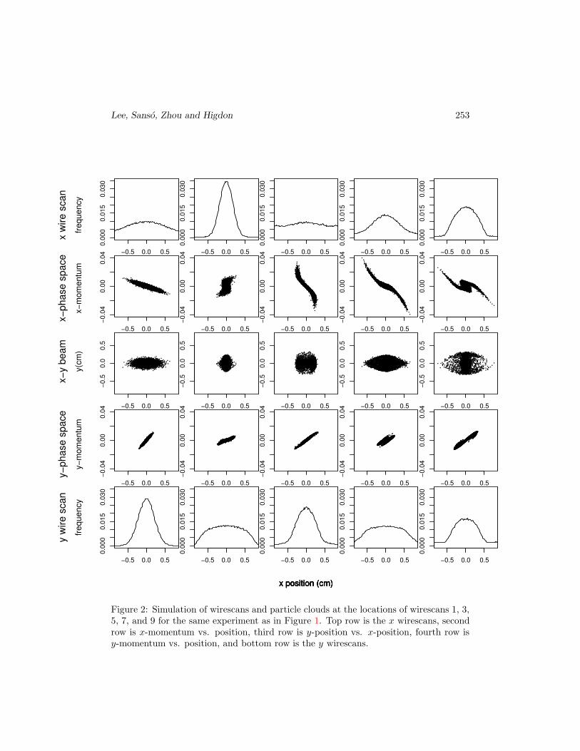
The dashed vertical lines in Figure 1 represent wirescans. As the beam crosses theselines, electrical current is produced and a histogram (here with 256 bins, which makes itappear sort of like a curve) of particle positions can be created. It is these nine wirescansin each dimension that are the observable data. Figure 2 shows some additional views.The top row are the first, third, fifth, seventh, and ninth (final) wirescans in the xdirection, with the bottom row showing the y wirescans. For illustration, particle cloudsare also shown in Figure 2. The second row shows the x-position versus x-momentumdistribution at these five wirescan locations, and the fourth row are the correspondingdistributions for the y position and momentum. The middle row shows the joint x andy positions. Notice that these are independent.

The plots in these two figures all fit together. For example, at the start of the beam(the left side) in Figure 1 is the first wirescan, where the trajectories are shown assomewhat spread apart for x and relatively tight for y. The upper left plot of Figure 2shows the resulting spread out x wirescan and the lower left shows the highly peakedhistogram for y position. After passing through two sets of magnets, the second columnof Figure 2 shows the wirescans and particle clouds at the third wirescan (third dashedline from the left in each panel of Figure 1). Now the x positions are relatively tightwhile the y distribution is wider. Note also the non-linear behavior of the particle clouds,showing intriguing relationships between position and momentum in each direction.

In practice, we will only be able to observe wirescans, and not any of the trajectoriesor particle clouds, which we have been able to plot here by running the computer codeon simulated data. Furthermore, the Heisenberg uncertainty principle declares that it isnot possible to measure both the position and momentum of a particle. Thus we mustmake do with just the series of wirescan position histograms (the top and bottom rowsof Figure 2) and attempt to work backwards by combining this information with theparticle simulator to to infer the initial distribution statistically.

3 Statistical Model

We start our analysis by performing a simulation study using a high fidelity simulatedbeam of 100,000 particles as a proxy for a real particle accelerator beam. We use thesimulator with a much lower fidelity beam of 8,000 particles to explore the known initialdistribution of the high fidelity beam. We configure the simulator to have nine wires

Lee, Sanso, Zhou and Higdon 253

−0.5 0.0 0.5

0.00

00.

015

0.03

0

x(cm)

frequ

ency

x wi

re s

can

frequ

ency

−0.5 0.0 0.5

−0.0

40.

000.

04

x(cm)

px

x−ph

ase

spac

ex−

mom

entu

m

−0.5 0.0 0.5

−0.5

0.0

0.5

x (cm)

y (c

m)

x−y

beam

y(cm

)

−0.5 0.0 0.5

−0.0

40.

000.

04

y(cm)

py

y−ph

ase

spac

ey−

mom

entu

m

−0.5 0.0 0.5

0.00

00.

015

0.03

0

y(cm)

frequ

ency

y wi

re s

can

frequ

ency

x position (cm)

−0.5 0.0 0.5

0.00

00.

015

0.03

0

x(cm)

frequ

ency

−0.5 0.0 0.5

−0.0

40.

000.

04

x(cm)

px

−0.5 0.0 0.5

−0.5

0.0

0.5

x (cm)

y (c

m)

−0.5 0.0 0.5

−0.0

40.

000.

04

y(cm)

py

−0.5 0.0 0.5

0.00

00.

015

0.03

0

y(cm)

frequ

ency

x position (cm)

−0.5 0.0 0.50.

000

0.01

50.

030

x(cm)

frequ

ency

−0.5 0.0 0.5

−0.0

40.

000.

04

x(cm)

px

−0.5 0.0 0.5

−0.5

0.0

0.5

x (cm)

y (c

m)

−0.5 0.0 0.5

−0.0

40.

000.

04

y(cm)

py

−0.5 0.0 0.5

0.00

00.

015

0.03

0

y(cm)

frequ

ency

x position (cm)

−0.5 0.0 0.5

0.00

00.

015

0.03

0

x(cm)

frequ

ency

−0.5 0.0 0.5

−0.0

40.

000.

04x(cm)

px

−0.5 0.0 0.5

−0.5

0.0

0.5

x (cm)

y (c

m)

−0.5 0.0 0.5

−0.0

40.

000.

04

y(cm)

py

−0.5 0.0 0.5

0.00

00.

015

0.03

0

y(cm)

frequ

ency

x position (cm)

−0.5 0.0 0.5

0.00

00.

015

0.03

0

x(cm)

frequ

ency

−0.5 0.0 0.5

−0.0

40.

000.

04

x(cm)

px−0.5 0.0 0.5

−0.5

0.0

0.5

x (cm)

y (c

m)

−0.5 0.0 0.5

−0.0

40.

000.

04

y(cm)

py

−0.5 0.0 0.5

0.00

00.

015

0.03

0

y(cm)

frequ

ency

x position (cm)

Figure 2: Simulation of wirescans and particle clouds at the locations of wirescans 1, 3,5, 7, and 9 for the same experiment as in Figure 1. Top row is the x wirescans, secondrow is x-momentum vs. position, third row is y-position vs. x-position, fourth row isy-momentum vs. position, and bottom row is the y wirescans.

254 Proton Particle Distribution

with 256 bins each. 8,000 particles were chosen since such number provides reasonableapproximations to the high fidelity beam, yet low enough computational times to makeMCMC feasible. We use a family of Gaussian distributions to parameterize the initialdistribution for the cloud of particles. The likelihood is based on a modified squared-error loss, in that we use a correlated Gaussian structure for the discrepancies betweenthe high fidelity wirescans and the low fidelity ones. We expect errors in nearby bins tobe dependent as explained below.

We first validated our model using the high fidelity simulations. Next we considereddata obtained from actual readings of four wirescans in a particle accelerator.

3.1 Probability model for the initial particle clouds

We model x position and momentum as bivariate normal and y position and momentumas bivariate normal independently of x. Thus,

x, px, y, py ∼ N4

0000

,

σ2x ρxσxσpx

0 0ρxσxσpx

σ2px

0 00 0 σ2

y ρyσyσpy

0 0 ρyσyσpyσ2

py

,

and so the initial configuration is described by parameters: σx, σpx, σy, σpy

, ρx and ρy.Our prior specifications are fairly vague, in fact, we assume that

1

σ2x

,1

σ2y

∼ Exp

(

1

100

)

;1

σ2px

,1

σ2py

∼ Exp

(

1

1000

)

; ρx ∼ U(0, 1) and ρy ∼ U(−1, 0).

We note that ρx and ρy must have opposite signs because of physical constraints asdiscussed previously.

3.2 Correlation structure of the wirescans

Inverse problems typically require that the likelihood function be fully specified, sincethere is insufficient information in the data to estimate both the initial configuration andadditional parameters in the likelihood (see, for example, Oliver et al. 1997; Lee et al.2002). In order to specify our likelihood, we used the errors between the readings atthe nine wirescans produced by the high fidelity and the low fidelity simulations, usingthe same initial configuration. The errors in bin counts are not independent, as nearbybins are correlated. Heuristically, the scientists expect “blobs” of mass in the initialdistribution (e.g., ellipsoid contours). Such a structure leads to a relatively smoothwirescan, and so if one bin is too large, we also expect the nearby bins to be too large. Asthe frequencies must total to one, we also expect negative correlation at larger distances.We obtained empirical correlograms and observed a distinctive sinusoidal decay. Thuswe model the error correlation between bins with an exponentially-dampened cosinefunction. For each wirescan j, the correlation function is defined by parameters λj and

Lee, Sanso, Zhou and Higdon 255

ωj . Let d be the distance between two bins, then

ρj(d) = e−3d/λj cos(ωjd) . (1)

This defines a valid positive definitive covariance, as shown in Yaglom (1986). Figure 3shows the fits obtained for some of the wirescans using ρj for both x and y dimensions.

The likelihood is obtained by assuming that the errors of the wirescans for each di-mension are conditionally normal. Let Σxj

and Σyjdenote the covariances correspond-

ing to the j-th wirescans in the x and y dimensions respectively. These are obtainedusing the correlation in (1). Denote the corresponding errors as exj

and eyj. Then the

likelihood is proportional to

9∏

j=1

(2πτ2)−2∗256/2 exp

{

− 1

2τ2(e′xj

Σ−1xj

exj+ e′yj

Σ−1yj

eyj)

}

.

We assume that τ2, Σxjand Σyj

, j = 1, . . . , 9 are known. The Σs were determined fromsimulation experiments; τ2 requires additional attention. First we note that in manyinverse problems, such as this one, there is not enough information to fully estimate allof the parameters and here τ 2 is a problematic one (see, for example, Oliver et al. 1997;Lee et al. 2002). Ideally it will be chosen based on considerations about the expectedsize of discrepancies in the wirescans, relying on knowledge from subject area expertsin a real application. In practice, the choice of τ 2 represents a trade-off between (i) thecloseness of the fitted wirescans to the observed ones and (ii) the convergence propertiesof the MCMC sampler. Smaller values of τ 2 will produce better matches between thefitted and observed wirescans. The problem is that if τ 2 is too small, it can be nearlyimpossible to get the MCMC sampler to fully explore the posterior space, and the chainwill typically fail to find a good fit in a reasonable amount of time (i.e., not gettinganywhere near the posterior mode in two weeks). Without starting MCMC very closeto the posterior mode (which would not be known ahead of time in practice), the chainwill fail to converge properly when τ 2 is too small. Thus τ2 must be chosen to be largeenough for the chain to effectively explore the parameter space, yet not too large thatthe discrepancies in the fits are unbearable. Our choice here is a practical compromise.

3.3 MCMC

We use a Metropolis-Hastings algorithm (see for example, Gamerman 1997) to explorethe distributions of the six parameters that define the distribution of the initial config-uration. We sample the parameters in two blocks, one for the variances and correlationof the x dimension and another for those of the y dimension. To produce proposalsfor the variances we use random walks on the log scale. Proposals for the correlationparameters are obtained with constrained random walks. The x dimension correlationis constrained to the interval (0, 1), while the y dimension correlation is constrained to(−1, 0), since the physics of the problem requires that the correlations have oppositesigns (as discussed in Section 2).

256 Proton Particle Distribution

x wi

re s

can

acf

y wi

re s

can

acf

scan 1 scan 3 scan 5 scan 7 scan 9

Figure 3: Autocorrelation function plots for the differences between wirescans of high andlow fidelity simulated beams. Only the odd numbered wirescans are shown. The dotted linescorrespond to the empirical autocorrelations. The continuous line corresponds to the leastsquares fit using the correlation function defined in (1).

Lee, Sanso, Zhou and Higdon 257

3.4 Simulation Results

Figure 4 shows our results on the simulated data. Each column represents a wire. Therewere actually nine wirescans, but only four are shown to improve the visibility of thegraphs; the other five are similar in character. The top two rows are for the x dimension,the bottom two rows for the y dimension. The first and third rows are the estimatedposterior distributions of the particle cloud (x or y position and momentum) as thebeam passes through the quadrupole magnets. The second and fourth rows show thetrue wirescans (circles), the estimated posterior mean scans (solid line), and posteriorinterval estimates (dashed lines). Only 32 bins are pictured so that the results canbe seen visually (using all of them produces a smear of black ink). This number waschosen to match the number of bins used in the real data example of the next section.The posterior mean is generally close to the truth, and the credible intervals provide ameasure of our uncertainty.

Figure 5 shows the estimated posterior distribution for the six parameters of ourinverse problem (the variance of position and momentum for each of x and y, and thecorrelation between the position and momentum for each of x and y), along with thetrue values (the large black dots). We are pleased that the estimated posterior has mostof its mass near the truth for all six parameters.

We note that the fit is not perfect in some of the plots. This is partly a result ofthe choice of τ2, which represents a trade-off between goodness-of-fit and computationalefficiency in convergence of the MCMC. Here we used a value of τ 2 = 0.0005, whichleaves the likelihood somewhat “loose” in the sense that the wirescans match most ofthe time but not all, as shown in Figure 4. The reason we do this is that each MCMCiteration requires a run of the simulator and that takes about two minutes. So a 3000-iteration MCMC run takes about five days on a SunBlade 1000 workstation. Withthis value of τ2, this number of iterations is sufficient for convergence of the chain fromtypical arbitrary starting values. When we try to use smaller values of τ 2 to decrease theerror in the fitted values, we find that convergence of the chain decreases significantly.An order of magnitude decrease in τ 2 appears to increase the time to convergence by atleast an order of magnitude, which makes the computational requirements impracticalwith the current technology. As computers get faster, we expect that our approach willbe able to achieve better fidelity. For the present, we must accept some error in our fitsin order to be able to produce results in a reasonable amount of time. In our goal ofinferring the initial distribution, Figure 5 shows that we are doing a reasonable job inthat regard.

4 Application to Real Data

We now apply our methodology to a real dataset provided by scientists at Los AlamosNational Laboratory (Allen et al. 2002; Allen and Pattengale 2002). In this setting, onlyfour wirescans are available, analogous to the first four scans in the simulated exampleabove. From these four scans we attempt to infer the unknown initial distribution ofthe beam. The data seem a bit more complex than can be perfectly matched under our

258 Proton Particle Distribution

paired bivariate normal model, but the model captures the key features in the data.We note that for the real dataset, the correlation parameter for x is positive and y isnegative, the reverse of our simulated example (the physical constraint is merely thatthe signs must be opposite), so we modify the relevant priors and proposal distributionsaccordingly.

Figure 6 shows our results on this dataset. As in Figure 4, each column is a wire; thetop two rows are for x, the bottom two for y, with estimated particle cloud posteriorsand fitted scans with 95% credible intervals for each. As with the simulated data, thereis room for improvement in some of the fits, but the computational requirements make itdifficult to achieve significant improvements. Our methodology provides a good startingpoint for solving this inverse problem. The bivariate normal assumption is useful for itsintuitive simplicity yet it provides enough flexibility to do a reasonable job of modelingthe true process.

5 Conclusions

The Bayesian approach is helpful in this problem as it gives a natural measure of un-certainty. Such an uncertainty estimate would be nearly impossible to obtain from aclassical analysis, yet is valuable in understanding the functioning of the particle ac-celerator. As with many inverse problems, multiple initial conditions can be consistentwith the observed data, and the Bayesian approach also provides a natural mechanismfor either exploring this multimodal surface, or for restricting the problem through theimposition of structure in the prior based on substantive information (as we do here).

Extensions of the current model can be considered in several directions. One is theacceleration of computations and the other is exploring more complex distributions forthe initial configuration. A typical MCMC run would take several days because of thetime spent running the simulator at each iteration. To make the MCMC faster, we canconsider a multiresolution approach where a very low fidelity simulator (faster but lessaccurate) is coupled with a high fidelity one (slower but more reliable); we expect that amultiresolution approach will also help improve the time necessary for convergence of theMCMC sampler. An alternative approach is that of replacing the current simulator witha simplified version that uses linear or non-linear approximations between subsequentpositions of the accelerator, such as in Craig et al. (1996) or O’Hagan et al. (1999).Improvements to the initial configuration may be obtained by using a more flexiblefamily of distributions, such as mixtures of normals or Gaussian processes.

References

Allen, C. K., Chan, K. C. D., Colestock, P. L., Crandall, K. R., Garnett, R. W.,Gilpatrick, J. D., Lysenko, W., Qiang, J., Schneider, J. D., Schulze, M. E., Sheffield,R. L., Smith, H. V., and Wangler, T. P. (2002). “Beam-halo measurements in high-current proton beams.” Physical Review Letters, 89(214802). 257

Lee, Sanso, Zhou and Higdon 259

Allen, C. K. and Pattengale, N. D. (2002). “Theory and technique of beam envelopesimulation: Simulation of bunched particle beams with ellipsoidal symmetry andlinear space charge forces.” Technical Report LA-UR-02-4979, Los Alamos NationalLaboratory. 257

Craig, P. S., Goldstein, M., Seheult, A. H., and Smith, J. A. (1996). “Bayes LinearStrategies for History Matching of Hydrocarbon Reservoirs.” In Bernardo, J. M.,Berger, J. O., Dawid, A. P., and Smith, A. F. M. (eds.), Bayesian Statistics 5 , 69–95.Oxford: Clarendon Press. 258

Dragt, A., Neri, F., Rangarjan, G., Douglas, D., Healy, L., and Ryne, R. (1988). “LieAlgebraic Treatment of Linear and Nonlinear Beam Dynamics.” Annual Review ofNuclear and Particle Science, 38: 455–496. 250

Gamerman, D. (1997). Markov Chain Monte Carlo. London, UK: Chapman and Hall.255

Kennedy, M. C. and O’Hagan, A. (2001). “Bayesian Calibration of Computer Models.”Journal of the Royal Statistical Society, Series B, 63: 425–464. 250

Lee, H., Higdon, D., Bi, Z., Ferreira, M., and West, M. (2002). “Markov Random FieldModels for High-Dimensional Parameters in Simulations of Fluid Flow in PorousMedia.” Technometrics, 44: 230–241. 254, 255

O’Hagan, A., Kennedy, M. C., and Oakley, J. E. (1999). “Uncertainty Analysis andother Inference Tools for Complex Computer Codes.” In Bernardo, J. M., Berger,J. O., Dawid, A. P., and Smith, A. F. M. (eds.), Bayesian Statistics 6 , 503–524.Oxford University Press. 258

Oliver, D. S., Cunha, L. B., and Reynolds, A. C. (1997). “Markov Chain Monte CarloMethods for Conditioning a Permeability Field to Pressure Data.” MathematicalGeology , 29(1): 61–91. 254, 255

Qiang, J., Ryne, R. D., Habib, S., and Decyk, V. (2000). “An Object-Oriented ParallelParticle-In-Cell Code for Beam Dynamics Simulation in Linear Accelerators.” Journalof Computational Physics, 163: 434–451. 250

Yaglom, A. (1986). Correlation Theory of Stationary and Related Random FunctionsI: Basic Results. Springer Series in Statistics. New York: Springer-Verlag. 255

Yeh, W. W. (1986). “Review of Parameter Identification in Groundwater Hydrology:the Inverse Problem.” Water Resources Research, 22: 95–108. 250

Acknowledgments

Herbert Lee’s work was partially supported by grant DMS 0233710 from the National Science

Foundation. Bruno Sanso’s work was partially supported by grant 74328-001-03 3D from Los

Alamos National Laboratory. Weining Zhou’s work was partially supported by grant 74328-

001-03 3D from Los Alamos National Laboratory. The authors would like to thank the editors,

260 Proton Particle Distribution

two anonymous referees, Charles Nakhleh, and Vidya Kumar for their helpful comments and

suggestions.

Lee, Sanso, Zhou and Higdon 261

262 Proton Particle Distribution

−0.3 −0.1 0.1 0.3

−0.0

100.

005

X pos

X m

om

−0.5 0.0 0.5

0.00

00.

020

X Wirescan 01

X pos

−0.3 −0.1 0.1 0.3

−0.0

100.

005

Y pos

Y m

om

−0.5 0.0 0.5

0.00

00.

020

Y Wirescan 01

Y po

s

−0.2 0.0 0.2

−0.0

100.

005

X pos

X m

om

−0.5 0.0 0.5

0.00

00.

020

X Wirescan 03

X pos

−0.2 0.0 0.2−0.0

150.

005

Y pos

Y m

om

−0.5 0.0 0.5

0.00

00.

020

Y Wirescan 03

Y po

s

−0.2 0.0 0.2−0.0

150.

005

X pos

X m

om

−0.5 0.0 0.5

0.00

00.

020

X Wirescan 05

X pos

−0.2 0.0 0.2

−0.0

100.

005

Y pos

Y m

om

−0.5 0.0 0.5

0.00

00.

020

Y Wirescan 05

Y po

s

−0.4 0.0 0.2

−0.0

100.

010

X pos

X m

om

−0.5 0.0 0.5

0.00

00.

020

X Wirescan 07

X pos

−0.3 −0.1 0.1 0.3

−0.0

100.

010

Y pos

Y m

om

−0.5 0.0 0.5

0.00

00.

020

Y Wirescan 07

Y po

s

Figure 4: Results for the simulated dataset: the columns are the positions of the four wires-cans. The top row shows the estimated posterior particle cloud distributions for x position vs.momentum. The second row shows the data (circle), posterior mean (solid line), and posterior95% interval estimates (dashed lines). The third and fourth rows are the analogous plots forthe y dimension.

Lee, Sanso, Zhou and Higdon 263

Histogram of sigma2x

sigma2x

Dens

ity

0.005 0.010 0.015 0.020 0.025

020

6010

014

0

Histogram of sigma2y

sigma2y

Dens

ity0.004 0.006 0.008 0.010 0.012 0.014 0.016

050

100

150

200

Histogram of sigma2px

sigma2px

Dens

ity

0e+00 1e−05 2e−05 3e−05 4e−05 5e−05 6e−05 7e−05

020

000

6000

0

Histogram of sigma2py

sigma2py

Dens

ity

0e+00 1e−05 2e−05 3e−05 4e−05

020

000

6000

0

Histogram of rx

rx

Dens

ity

−1.0 −0.8 −0.6 −0.4 −0.2 0.0

0.0

0.5

1.0

1.5

2.0

Histogram of ry

ry

Dens

ity

0.3 0.4 0.5 0.6 0.7 0.8 0.9 1.0

02

46

Figure 5: Posterior distribution estimates for the parameters for the simulated data set. Thetruth is shown as the large black dot.

264 Proton Particle Distribution

−0.2 −0.1 0.0 0.1 0.2

−0.

005

X pos

X m

om

−0.5 0.0 0.5

0.0

0.2

0.4

X Wirescan 01

X pos

−0.10 −0.05 0.00 0.05 0.10

−0.

005

0.00

5

Y pos

Y m

om

−0.5 0.0 0.5

0.0

0.2

0.4

Y Wirescan 01

Y p

os

−0.6 −0.2 0.2 0.4 0.6

−0.

020.

01

X pos

X m

om

−0.5 0.0 0.5

0.0

0.2

0.4

X Wirescan 02

X pos

−0.4 −0.2 0.0 0.2

−0.

020.

000.

02

Y pos

Y m

om

−0.5 0.0 0.5

0.0

0.2

0.4

Y Wirescan 02

Y p

os

−0.2 −0.1 0.0 0.1 0.2

−0.

020.

01

X pos

X m

om

−0.5 0.0 0.5

0.0

0.2

0.4

X Wirescan 03

X pos

−0.3 −0.1 0.1 0.2 0.3

−0.

005

Y pos

Y m

om

−0.5 0.0 0.5

0.0

0.2

0.4

Y Wirescan 03

Y p

os

−0.4 −0.2 0.0 0.2 0.4

−0.

005

0.00

5

X pos

X m

om

−0.5 0.0 0.5

0.0

0.2

0.4

X Wirescan 04

X pos

−0.10 −0.05 0.00 0.05 0.10

−0.

010

0.00

5

Y pos

Y m

om

−0.5 0.0 0.5

0.0

0.2

0.4

Y Wirescan 04

Y p

os

Figure 6: Results for the real dataset: the columns are the positions of the four wirescans.The top row shows the estimated posterior particle cloud distributions for x dimension vs.momentum. The second row shows the data (circle), posterior mean (solid line), and posterior95% interval estimates (dashed lines). The third and fourth rows are the analogous plots forthe y dimension.