arX

iv:1

404.

6254

v1 [

hep-

th]

24

Apr

201

4

DAMTP-2014-27HRI/ST1406

String Perturbation Theory Around Dynamically

Shifted Vacuum

Roji Piusa, Arnab Rudrab and Ashoke Sena

aHarish-Chandra Research Institute

Chhatnag Road, Jhusi, Allahabad 211019, IndiabDepartment of Applied Mathematics and Theoretical Physics

Wilberforce Road, Cambridge CB3 0WA, UK

E-mail: rojipius@mri.ernet.in, A.Rudra@damtp.cam.ac.uk, sen@mri.ernet.in

Abstract

In some string theories, e.g. SO(32) heterotic string theory on Calabi-Yau manifolds, a

massless field with a tree level potential can acquire a tachyonic mass at the one loop level,

forcing us to quantize the theory around a new background that is not a solution to the classical

equations of motion and hence is not described by a conformally invariant world-sheet theory.

We describe a systematic procedure for carrying out string perturbation theory around such

backgrounds.

1

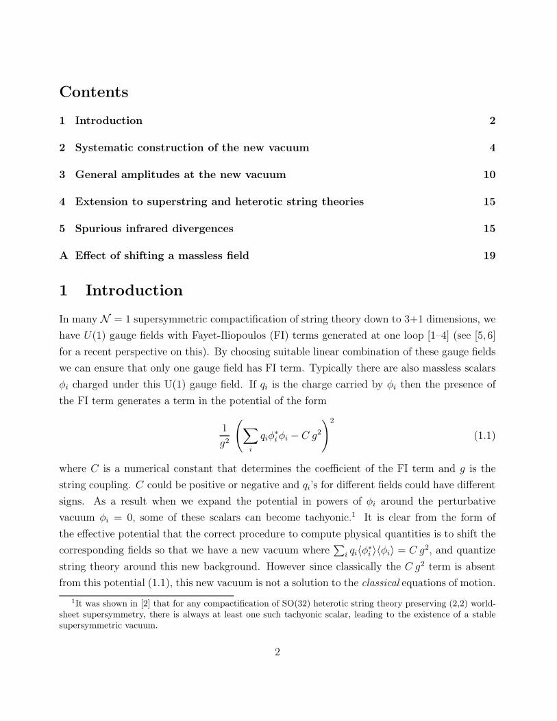
Contents

1 Introduction 2

2 Systematic construction of the new vacuum 4

3 General amplitudes at the new vacuum 10

4 Extension to superstring and heterotic string theories 15

5 Spurious infrared divergences 15

A Effect of shifting a massless field 19

1 Introduction

In many N = 1 supersymmetric compactification of string theory down to 3+1 dimensions, we

have U(1) gauge fields with Fayet-Iliopoulos (FI) terms generated at one loop [1–4] (see [5, 6]

for a recent perspective on this). By choosing suitable linear combination of these gauge fields

we can ensure that only one gauge field has FI term. Typically there are also massless scalars

φi charged under this U(1) gauge field. If qi is the charge carried by φi then the presence of

the FI term generates a term in the potential of the form

1

g2

(∑

i

qiφ∗iφi − C g2

)2

(1.1)

where C is a numerical constant that determines the coefficient of the FI term and g is the

string coupling. C could be positive or negative and qi’s for different fields could have different

signs. As a result when we expand the potential in powers of φi around the perturbative

vacuum φi = 0, some of these scalars can become tachyonic.1 It is clear from the form of

the effective potential that the correct procedure to compute physical quantities is to shift the

corresponding fields so that we have a new vacuum where∑

i qi〈φ∗i 〉〈φi〉 = C g2, and quantize

string theory around this new background. However since classically the C g2 term is absent

from this potential (1.1), this new vacuum is not a solution to the classical equations of motion.

1It was shown in [2] that for any compactification of SO(32) heterotic string theory preserving (2,2) world-sheet supersymmetry, there is always at least one such tachyonic scalar, leading to the existence of a stablesupersymmetric vacuum.

2

As a result on-shell methods [7–11], which require that we begin with a conformally invariant

world-sheet theory, is not suitable for carrying out a systematic perturbation expansion around

this new background.

Although the above example provides the motivation for our analysis, we shall address this

in a more general context. At the same time we shall simplify our analysis by assuming that

only one scalar field is involved instead of multiple scalar fields. So we consider a general

situation in string theory where at tree level we have a massless real scalar with a non-zero

four point coupling represented by a potential

Aφ4 + · · · (1.2)

where · · · denote higher order terms. We suppose further that at one loop the scalar receives a

negative contribution −2Cg2 to its mass2. Here A and C are g-independent constants. Then

the total potential will be

Aφ4 − C g2 φ2 + · · · . (1.3)

This has a minimum at

φ2 =1

2

C

Ag2 + · · · . (1.4)

Our goal will be to understand how to systematically develop string perturbation theory around

this new background and also to correct the expectation value of φ due to higher order correc-

tions. If we had an underlyng string field theory that is fully consistent at the quantum level,

e.g. the one described in [12], then that would provide a natural framework for addressing

this issue. Our method does not require the existence of an underlying string field theory,

although the requirement of gluing compatibility of the local coordinate system that we shall

use is borrowed from string field theory.

The method we shall describe can be used to address other similar problems in string theory

where loop correction induces small shift in the vev of a massless field. For example suppose

we have a massless field χ with a tree level cubic potential and suppose further that one loop

correction generates a tadpole for this field. Then from the effective field theory approach it

is clear that there is a nearby perturbative vacuum where the field χ is non-tachyonic. Usual

string perturbation theory does not tell us how to deal with this situation, but the method we

describe below can be used in this case as well.

There are of course also problems involving tadpoles of massless fields without tree level

potential, e.g. of the kind discussed in [13] and many follow up papers. As of now our method

does not offer any new insight into such problems.

3

The rest of the paper is organised as follows. In §2 we describe the procedure for construct-

ing amplitudes in the presence of a small shift in the vacuum expectation value of a massless

scalar following the procedure of [14]. We also discuss systematic procedure for determining

the shift by requiring absence of tadpoles. In §3 we show that the amount of shift in the scalar,

needed to cancel the tadpole, depends on the choice of local coordinate system that we use

to construct the amplitudes. However general physical amplitudes in the presence of the shift

are independent of the choice of local coordinate system as long as we use a gluing compatible

system of local coordinates for defining the amplitude. This is our main result. For simplicity

we restrict our analysis in §2 and §3 to bosonic string theory, but in §4 we discuss generaliza-

tion of our analysis to include NS sector states in heterotic and superstring theories. In §5 we

describe the procedure for regulating the spurious infrared divergences in loops, arising from

the fact that the shift in the vacuum renders some of the originally massless states massive.

2 Systematic construction of the new vacuum

We shall carry out our analysis under several simplifying assumptions. These are made mainly

to keep the analysis simple, but we believe that none of these (except 4) is necessary.

1. We shall assume that there is a symmetry under which φ → −φ so that amplitudes with

odd number of external φ fields vanish.

2. We shall assume that φ does not mix with any other physical or unphysical states of

mass level zero even when quantum corrections are included.

3. Shifting the φ field can sometimes induce tadpoles in other massless fields. If there is

a tree level potential for this field then we can cancel the tadpole by giving a vacuum

expectation value (vev) to that field and determine the required vev by following the

same procedure that we used to determine the shift in φ. We shall assume that such a

situation does not arise and that φ is the only field that needs to be shifted. However

extension of our analysis to this more general case should be straightforward.

4. If on the other hand shifting φ leads to the tadpole of a massless field which has vanishing

tree level potential then it is not in general possible to find a nearby vacuum where all

tadpoles vanish. In this case the vacuum is perturbatively unstable. We shall assume

that this is not the case here.

4

5. When the theory has other massless fields besides φ but their tadpoles vanish, then the

situation can be dealt with in the manner discussed in §7.2 of [7] and will not be discussed

here any further.2

6. In this section and in §3 we shall restrict our analysis to the bosonic string theory.

However the result can be generalized to include the case where φ is Neveu-Schwarz (NS)

sector field in the heterotic string theory or NS-NS sector field in type IIA or IIB string

theory. This is discussed briefly in §4.

As discussed in detail in [17,18], for computing renormalized masses and S-matrix of general

string states we need to work with off-shell string theory. This requires choosing a set of gluing

compatible local coordinate system on the (super-)Riemann surfaces. The result for off-shell

amplitude depends on the choice of local coordinates, but the renormalized masses and S-

matrix elements computed from it are independent of this choice. Our analysis will be carried

out in this context.

The off-shell amplitudes do not directly compute the off-shell Green’s functions. Instead

they compute truncated off-shell Green’s functions. If we denote by G(n)(k1, b1; · · ·kn, bn) the

n-point off-shell Green’s function of fields carrying quantum numbers {bi} and momenta {ki},

then the truncated off-shell Green’s functions are defined as

Γ(n)(k1, b1; · · ·kn, bn) = G(n)(k1, b1; · · ·kn, bn)n∏

i=1

(k2i +m2bi) , (2.1)

where mb is the tree level mass of the state carrying quantum number b. The usual on-shell

amplitudes of string theory compute Γ(n) at k2i = −m2bi. This differs from the S-matrix elements

by multiplicative wave-function renormalization factors for each external state and also due to

the fact that the S-matrix elements require replacing m2bi’s by physical mass2’s in this formula.

However from the knowledge of off-shell amplitude Γ(n) defined in (2.1) we can extract the

physical S-matrix elements following the procedure described in [17, 18].

Our goal is to study what happens when we switch on a vev of φ. For this we shall first

consider a slightly different situation. Suppose that φ is an exactly marginal deformation in

string theory and furthermore that it remains marginal even under string loop corrections.

In this case there is no potential for φ and we can give any vacuum expectation value λ to

2In the special case of the D-term potential in supersymmetric theories discussed in §1 the dilaton tadpoledoes not vanish in the perturbative vacuum [1,7, 15, 16], but is expected to vanish in the shifted vacuum sincethe latter has zero energy density.

5

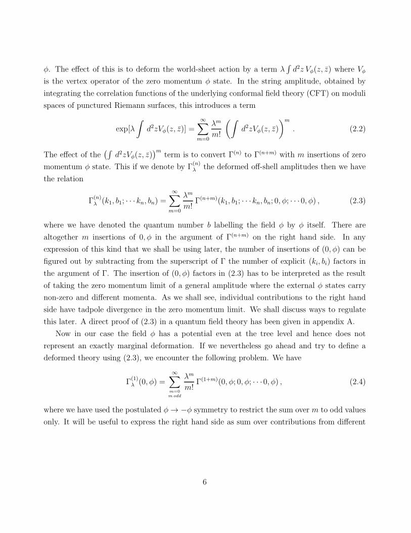
φ. The effect of this is to deform the world-sheet action by a term λ∫d2z Vφ(z, z̄) where Vφ

is the vertex operator of the zero momentum φ state. In the string amplitude, obtained by

integrating the correlation functions of the underlying conformal field theory (CFT) on moduli

spaces of punctured Riemann surfaces, this introduces a term

exp[λ

∫d2zVφ(z, z̄)] =

∞∑

m=0

λm

m!

(∫d2zVφ(z, z̄)

)m

. (2.2)

The effect of the(∫

d2zVφ(z, z̄))m

term is to convert Γ(n) to Γ(n+m) with m insertions of zero

momentum φ state. This if we denote by Γ(n)λ the deformed off-shell amplitudes then we have

the relation

Γ(n)λ (k1, b1; · · · kn, bn) =

∞∑

m=0

λm

m!Γ(n+m)(k1, b1; · · ·kn, bn; 0, φ; · · ·0, φ) , (2.3)

where we have denoted the quantum number b labelling the field φ by φ itself. There are

altogether m insertions of 0, φ in the argument of Γ(n+m) on the right hand side. In any

expression of this kind that we shall be using later, the number of insertions of (0, φ) can be

figured out by subtracting from the superscript of Γ the number of explicit (ki, bi) factors in

the argument of Γ. The insertion of (0, φ) factors in (2.3) has to be interpreted as the result

of taking the zero momentum limit of a general amplitude where the external φ states carry

non-zero and different momenta. As we shall see, individual contributions to the right hand

side have tadpole divergence in the zero momentum limit. We shall discuss ways to regulate

this later. A direct proof of (2.3) in a quantum field theory has been given in appendix A.

Now in our case the field φ has a potential even at the tree level and hence does not

represent an exactly marginal deformation. If we nevertheless go ahead and try to define a

deformed theory using (2.3), we encounter the following problem. We have

Γ(1)λ (0, φ) =

∞∑

m=0

modd

λm

m!Γ(1+m)(0, φ; 0, φ; · · ·0, φ) , (2.4)

where we have used the postulated φ→ −φ symmetry to restrict the sum over m to odd values

only. It will be useful to express the right hand side as sum over contributions from different

6

genera. Thus we write3

Γ(1)λ (0, φ) =

∞∑

s=0

g2s∞∑

m=0

modd,m+2s≥3

λm

m!Γ(1+m;s)(0, φ; 0, φ; · · ·0, φ) , (2.5)

where Γn;s denotes genus s contribution to the n-point function in the unperturbed theory.

The s = 0, m = 3 term on the right hand side is non-zero since it is proportional to the four

point function of zero momentum φ states and is proportional to A according to (1.2). Thus

in the deformed theory there is a zero momentum φ tadpole proportional to λ3. This is clearly

not an acceptable vacuum at the tree level since it will give divergent results for higher point

amplitudes.

But now consider the effect of one loop correction given by the m = 1, s = 1 term on the

right hand side of (2.5). This is non-zero and represents the second term in (1.3). We now see

that by a suitable choice of λ, given by the solution to

1

6λ3 Γ(4;0)(0, φ; 0, φ; 0, φ; 0, φ) + λ g2 Γ(2;1)(0, φ; 0, φ) = 0 (2.6)

we can cancel the net contribution to the φ tadpole to order g3. This vanishes for three distinct

values of λ, one of which is given by λ = 0 and the other two are related by φ→ −φ symmetry.

We shall be considering the situation where in the λ = 0 vacuum the field φ is tachyonic and

hence this solution needs to be avoided. This fixes λ to a specific value of order g up to the

φ→ −φ symmetry.

With this choice of λ we make Γ(1)λ (0, φ) vanish to order g3. To extend the analysis to

higher order in g we express the condition of vanishing of (2.5) as

1

6λ2 Γ(4;0)(0, φ; 0, φ; 0, φ; 0, φ) + g2 Γ(2;1)(0, φ; 0, φ)

= −∞∑

m,s=0

modd;m+2s≥5

1

m!λm−1 g2s Γ(1+m;s)(0, φ; 0, φ; · · ·0, φ) , (2.7)

and then solve this equation iteratively using the leading order solution (2.6) as the starting

point. Note that in arriving at (2.7) we have divided (2.5) by λ, thereby removing the trivial

3We have dropped an overall 1/g2 factor from the definition of Γ(n) so that we can drop a g2 factor fromthe definition of the propagator later in (2.9). If we use the standard convention where 1/g2 appears as anoverall multiplicative factor in the tree level action, then the propagator ∆ will have an extra factor of g2 andthe Γ(n)’s will have extra factor of 1/g2. If we denote these by Γstandard = g−2Γ and ∆standard = g2∆, then itis straightforward to check that all our subsequent equations hold with Γ replaced by Γstandard and ∆ replacedby ∆standard without any extra factor of g2.

7

solution λ = 0. To each order in iteration we substitute on the right hand side of (2.7) the

solution for λ to the previous order and then solve (2.7). Due to the φ → −φ symmetry and

the fact that the genus expansion is in powers of g2, the solution for λ takes the form

λ2 =

∞∑

n=0

Ang2n+2 , (2.8)

for constants An. Furthermore note that by adjusting λ2 to order g2n+2, we can satisfy (2.7)

to terms of order g2n+2, ı.e. make the right hand side of (2.5) vanish to order g2n+3.4

There are however some additional subtleties in this analysis, since the individual terms

on the right hand side of (2.7) can diverge due to φ tadpole. These divergences arise from

regions of moduli integral where a Riemann surface degenerates into two distinct Riemann

surfaces connected by a long handle. As mentioned at the end of §1, we shall proceed with

the assumption that the only relevant divergences are associated with tadpoles of φ. To deal

with these divergences we need to first regularize these divergences, solve for λ, and at the

end remove the regulator. For this we shall work with a choice of gluing compatible local

coordinates according to the procedure described in §3.2 of [18] and express a general amplitude

contributing to the right hand side of (2.4) as a sum of products of ‘one particle irreducible’

(1PI) amplitudes joined by the propagator

∆ =1

4π

∫ ∞

0

ds

∫ 2π

0

dθ e−(s−iθ)L0−(s+iθ)L̄0 . (2.9)

The divergence in individual contributions come from the s→ ∞ limit on the right hand side

of (2.9). We shall regulate the divergence by replacing ∆ by

1

4π

∫ Λ

0

ds

∫ 2π

0

dθ e−(s−iθ)L0−(s+iθ)L̄0 , (2.10)

where Λ is a fixed large number. The relevant divergence in ∆ comes from the choice where

the propagating state is a zero momentum φ. Since L0 and L̄0 vanish for zero momentum φ,

the contribution to ∆ from this term goes as Pφ Λ/2, where Pφ denotes projection to the CFT

state corresponding to zero momentum φ. It will be convenient to define,5

∆φ =1

2ΛPφ, ∆̄ = ∆−∆φ for momentum k = 0 ,

4Due to the φ → −φ symmetry and the fact that the genus expansion is in powers of g2, the contributions

to Γ(1)λ

(0, φ) involve only odd powers of g after using (2.8). Thus making Γ(1)λ

(0, φ) vanish to order g2n+3 alsomakes it vanish to order g2n+4.

5For computation of Γ(1)λ

using (2.5) all propagators carry zero momentum and hence the second line of

(2.11) is irrelevent, but this definition will be useful for analyzing Γ(n)λ

in the next section.

8

Γ(1)λ

= Γ̄(1)λ Γ̄

(2)λ Γ̄

(3)λ

Γ(1)λ Γ

(1)λ

Γ(1)λ

+ + 12× × × × + · · ·

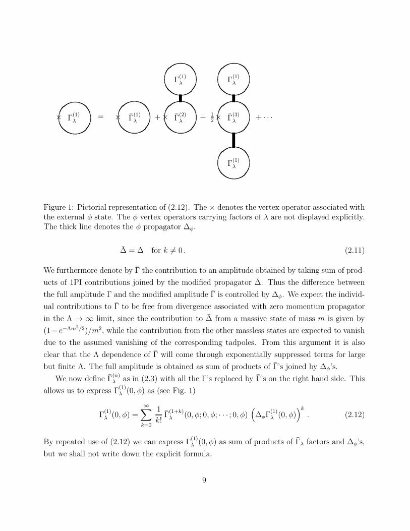
Figure 1: Pictorial representation of (2.12). The × denotes the vertex operator associated withthe external φ state. The φ vertex operators carrying factors of λ are not displayed explicitly.The thick line denotes the φ propagator ∆φ.

∆̄ = ∆ for k 6= 0 . (2.11)

We furthermore denote by Γ̄ the contribution to an amplitude obtained by taking sum of prod-

ucts of 1PI contributions joined by the modified propagator ∆̄. Thus the difference between

the full amplitude Γ and the modified amplitude Γ̄ is controlled by ∆φ. We expect the individ-

ual contributions to Γ̄ to be free from divergence associated with zero momentum propagator

in the Λ → ∞ limit, since the contribution to ∆̄ from a massive state of mass m is given by

(1− e−Λm2/2)/m2, while the contribution from the other massless states are expected to vanish

due to the assumed vanishing of the corresponding tadpoles. From this argument it is also

clear that the Λ dependence of Γ̄ will come through exponentially suppressed terms for large

but finite Λ. The full amplitude is obtained as sum of products of Γ̄’s joined by ∆φ’s.

We now define Γ̄(n)λ as in (2.3) with all the Γ’s replaced by Γ̄’s on the right hand side. This

allows us to express Γ(1)λ (0, φ) as (see Fig. 1)

Γ(1)λ (0, φ) =

∞∑

k=0

1

k!Γ̄(1+k)λ (0, φ; 0, φ; · · · ; 0, φ)

(∆φΓ

(1)λ (0, φ)

)k. (2.12)

By repeated use of (2.12) we can express Γ(1)λ (0, φ) as sum of products of Γ̄λ factors and ∆φ’s,

but we shall not write down the explicit formula.

9

Now suppose that λ to order g2n+1, obtained by solving (2.7) to order g2n+2, or equivalently

by demanding the vanishing of Γ(1)λ (0, φ) to order g2n+3, has finite limit as Λ → ∞. Our goal

will be to prove that the result also holds with n replaced by n+1. For determining λ to next

order, we need to compute Γ(1)λ (0, φ) to order g2n+5 and then require this to vanish. Using the

result that Γ̄(2)λ (0, φ; 0, φ) has its expansion beginning at order g2, one can show that in order to

compute the right hand side of (2.12) to order g2n+5 we need to know the Γ(1)λ (0, φ) appearing

on the right hand side of (2.12) at most to order g2n+3. By assumption this contribution

vanishes. Thus only the k = 0 term contributes on the right hand side of (2.12), showing that

to order g2n+5, Γ(1)λ (0, φ) = Γ̄

(1)λ (0, φ). This means that in order to determine the order g2n+3

correction to λ we can replace Γ by Γ̄ on the right hand side of (2.7).6 Since Γ̄’s by construction

are finite as Λ → ∞ we see that the order g2n+3 correction to λ is also finite as Λ → ∞. This

proves the desired result.

We shall see in §3 that even though λ determined using this procedure is finite in the

Λ → ∞ limit, it is ambiguous ı.e. it depends on the choice of local coordinate system used

for the computation. Nevertheless all physical amplitudes will turn out to be free from this

ambiguity.

3 General amplitudes at the new vacuum

Once λ is determined, we can use (2.3) to compute the general n-point amplitude in the

deformed theory. However we need to ensure that this has finite Λ → ∞ limit and that it

is unambiguous, e.g. independent of the choice of local coordinates used to define the 1PI

amplitudes. Our discussion will follow closely that of §7.6 of [7]. However in [7] the massless

tadpoles were assumed to cancel at every genus while here we consider the case where the

cancelation is between the contributions from different genera. Furthermore in [7] the massless

fields were assumed to have flat potential while here the relevant field φ has a potential even

at the tree level.

First we examine the issue of finiteness in the Λ → ∞ limit. We shall assume that all the

external states (labelled by 1, · · ·n in (2.3)) carry generic non-zero momentum. Thus possible

source of zero momentum propagators on the right hand side of (2.3) are propagators which

connect two Riemann surfaces, one of which carry all the external states 1, · · ·n and possibly

some of the zero momentum φ vertex operators and the other one carries only zero momentum

6Γ’s appearing on the left hand side of (2.7) are in any case equal to the corresponding Γ̄’s.

10

Γ(n)λ

= Γ̄(n)λ Γ̄

(n+1)λ Γ̄

(n+2)λ

Γ(1)λ Γ

(1)λ

Γ(1)λ

+ + 12×

××

××

××

×

××

××

×

××

××

×

××

+ · · ·

Figure 2: Pictorial representation of (3.1). The × denotes the vertex operator associatedwith the external states carrying quantum numbers (k1, b1; · · ·kn, bn). The φ vertex operatorscarrying factors of λ are not displayed explicitly. The thick line denotes the propagator ∆φ.

φ vertex operators. For studying the divergences associated with these zero momentum propa-

gators, we shall define ∆̄ as in (2.11) and introduce the amplitudes Γ̄ by following the procedure

described below (2.11). It is easy to see that we now have the following generalization of (2.12)

(see Fig. 2)

Γ(n)λ (k1, b1; · · ·kn, bn) =

∞∑

k=0

1

k!Γ̄(n+k)λ (k1, b1; · · · kn, bn; 0, φ; · · ·0, φ)

(∆φΓ

(1)λ (0, φ)

)k. (3.1)

Now λ has been chosen so that Γ(1)λ (0, φ) vanishes. This shows that only the k = 0 term

contributes to the right hand side of (3.1). Since Γ̄(n)λ (k1, b1; · · · kn, bn) is finite as Λ → ∞, this

establishes that Γ(n)λ (k1, b1; · · ·kn, bn) also has a finite limit as Λ → ∞.

We now have to show that Γ(n)λ (k1, b1; · · · kn, bn) is independent of the choice of local coor-

dinate system, except for the expected dependence associated with the off-shell external states

carrying momenta k1, · · · kn. These latter dependences can be analyzed and treated in the same

way as in [17, 18], and we shall not discuss them any further. To focus on the real issue we

can for example concentrate on the case where these external states are massless states that

do not suffer from mass renormalization so that the corresponding vertex operators do not

introduce any dependence on the choice of local coordinates.7 The problematic dependence

7The wave-function renormalization factors do depend on the choice of local coordinates, but this can betreated as in [7].

11

on local coordinates arises from the following source [7] (§7.6). Let us consider two Riemann

surfaces A and B, glued at their punctures P1 and P2 by plumbing fixture procedure:

w1w2 = e−s+iθ (3.2)

where w1 and w2 are the local coordinates around the punctures P1 and P2 and (s, θ) are the

same variables which appear in the definition (2.9) of the propagator. Having the cut-off s ≤ Λ

then corresponds to requiring

|w1w2| ≥ e−Λ . (3.3)

Now suppose we change the local coordinates to w′1, w

′2 related to w1 and w2 via the relations

w1 = f(w′1), w2 = g(w′

2) , (3.4)

where f and g are some specific functions satisfying f(0) = 0, g(0) = 0. Since for small w1

and w2 we have

w1 = f ′(0)w′1, w2 = g′(0)w′

2 , (3.5)

we can express (3.3) as

|w′1w

′2| ≥ e−Λ′

, Λ′ = Λ+ 2ξA + 2ξB, ξA ≡1

2ln |f ′(0)|, ξB ≡

1

2ln |g′(0)| . (3.6)

Here A and B refer to the two Riemann surfaces that are connected by the propagator whose

change we are considering. A and B are abstract symbols which characterize information on

the external legs, genus, as well as the point in the moduli space we are in, since f ′(0) and

g′(0) could depend on all these informations. Note however that ξA does not depend on the

Riemann surface B and ξB does not depend on the Riemann surface A provided we choose a

gluing compatible local coordinate system.

(3.6) shows that changing the local coordinates correspond to effectively changing the cut-

off. This in turn changes the regulated propagator (2.10) by

δΛ∆ = (ξA + ξB)Pφ . (3.7)

We have ignored the change in the propagator due to massive states since they are exponentially

suppressed in the Λ → ∞ limit, and also from other massless states with vanishing tadpole

since their effect can be taken care of by following the procedure described in [7] (see also [19]).

This justifies the appearance of the projection operator Pφ to zero momentum φ states.

12

Now consider the right hand side of (2.7). Individual terms in this expression are divergent

in the Λ → ∞ limit, but when we use the value of λ by solving (2.7) to certain order, and

then substitute this on the right hand side of (2.7) to compute λ to the next order, the right

hand side of (2.7) has been shown to have a finite Λ → ∞ limit. Nevertheless since under a

general change of local coordinates different terms on the right hand side of (2.7) could have

their effective Λ’s changed differently, there is no guarantee that the right hand side of (2.7)

will remain unchanged. In other words, although we have argued that λ determined by solving

(2.7) has a finite Λ → ∞ limit, it could depend on the choice of local coordinates. Similar

arguments show that the right hand side of (3.1) could also depend on the choice of local

coordinates. Our goal will be to show that the explicit dependence of the right hand side

of (3.1) on the choice of local coordinates through the cut-off Λ cancels against the implicit

dependence of (3.1) on the choice of local coordinates through λ, so that the final result for

Γ(n)λ (k1, b1; · · · kn, bn) is independent of the choice of local coordinates.

From now on we shall consider infinitesimal changes in local coordinates so that the ξA and

ξB in (3.7) are infinitesimal. Using (3.7) the change in Γ(n)λ (k1, b1; · · ·kn, bn) due to a change in

Λ induced by change of local coordinates take the form

δΛΓ(n)λ (k1, b1; · · ·kn, bn) =

∑

A,B

Γ(n+1)λ,A (k1, b1; · · · kn, bn; 0, φ) (ξA + ξB)Γ

(1)λ,B(0, φ) , (3.8)

where sum over A and B denotes sum over all Riemann surfaces (including integration over

moduli and sum over genus) that contributes to Γ(n+1)λ (k1, b1; · · · kn, bn; 0, φ) and Γ

(1)λ (0, φ) re-

spectively. This can be expressed as

{∑

A

ξAΓ(n+1)λ,A (k1, b1; · · · kn, bn; 0, φ)

}∑

B

Γ(1)λ,B(0, φ)

+

{∑

A

Γ(n+1)λ,A (k1, b1; · · · kn, bn; 0, φ)

}∑

B

ξBΓ(1)λ,B(0, φ) ,

=

{∑

A

ξAΓ(n+1)λ,A (k1, b1; · · · kn, bn; 0, φ)

}Γ(1)λ (0, φ)

+Γ(n+1)λ (k1, b1; · · ·kn, bn; 0, φ)

∑

B

ξBΓ(1)λ,B(0, φ) . (3.9)

The first term on the right hand side vanishes since λ has been chosen so that Γ(1)λ (0, φ)

13

vanishes. This allows us to write (3.9) as

δΛΓ(n)λ (k1, b1; · · ·kn, bn) = Γ

(n+1)λ (k1, b1; · · ·kn, bn; 0, φ)

∑

B

ξBΓ(1)λ,B(0, φ) . (3.10)

Now suppose δλ denotes the compensating change in λ required to make Γ(1)λ (0, φ) vanish

with the new choice of local coordinates. Using (2.3) we see that this induces a change in

Γ(n)λ (k1, b1; · · · kn, bn) of the form

δλΓ(n)λ (k1, b1; · · ·kn, bn) = δλ Γ

(n+1)λ (k1, b1; · · · kn, bn; 0, φ) . (3.11)

Adding (3.10) to (3.11) we get the total change in Γ(n)λ (k1, b1; · · ·kn, bn):

δΓ(n)λ (k1, b1; · · · kn, bn) = Γ

(n+1)λ (k1, b1; · · · kn, bn; 0, φ)

{δλ+

∑

B

ξBΓ(1)λ,B(0, φ)

}. (3.12)

Now setting n = 1 in (3.12) we get

δΓ(1)λ (0, φ) = Γ

(2)λ (0, φ; 0, φ)

{δλ+

∑

B

ξBΓ(1)λ,B(0, φ)

}. (3.13)

δλ has to be adjusted so that δΓ(1)λ (0, φ) vanishes since Γ

(1)λ (0, φ) vanishes both before and after

the change. This means that we must have

δλ+∑

B

ξBΓ(1)λ,B(0, φ) = 0 . (3.14)

This in turn makes the right hand side of (3.12) vanish, showing that Γ(n)λ (k1, b1; · · ·kn, bn)

remains invariant under a change in the local coordinate system.

Before concluding this section we would like to emphasize one important ingredient under-

lying our analysis. In arriving at (3.8), (3.9) it was crucial that the change in Λ under a change

of local coordinates had the form ξA + ξB and not a quantity that has general dependence

on both A and B. This follows from the fact that we used a set of gluing compatible local

coordinates to define 1PI and 1PR amplitudes. If instead we had chosen a more general local

coordinate system – e.g. one where the choice of local coordinate on the puncture of the first

Riemann surface depends on the genus of the Riemann surface to which it is being glued – and

used it for introducing the cut-off Λ then this property will not be respected.

14

4 Extension to superstring and heterotic string theories

We shall now briefly discuss the extension of our analysis to superstring and heterotic string

theories when the field φ arises from the Neveu-Schwarz (NS) sector of heterotic string theory

or NSNS sector of type II string theory. Let us for definiteness focus on the heterotic string

theory – the generalization to the case of superstrings is straightforward. The analysis proceeds

more or less as in the case of bosonic string theory; however in this case the local coordinate

system at a puncture requires specifying the holomorphic super-coordinates (w, ζ) and anti-

holomorphic coordinate w̃. The generalization of (3.2) takes the form [7]

w1w2 = e−s+iθ, w2ζ1 = ε e−(s−iθ)/2ζ2, w1ζ2 = −ε e−(s−iθ)/2 ζ1, ζ1ζ2 = 0, w̃1w̃2 = e−s−iθ ,

(4.1)

with the s integral running from 0 to Λ in the definition of the propagator. ε takes value

±1 and we have to sum over both values at the end to implement GSO projection. Now

under a change of local (superconformal) coordinates Λ still gets shifted by a term of the form

ξA + ξB as in (3.6), but with ξA possibly containing even nilpotent parts that depend on the

super-moduli of the punctured Riemann surface A and ξB containing even nilpotent parts that

depend on the super-moduli of the punctured Riemann surface B. As a result our analysis still

goes through, with the sums over A and B in various equations in §3 now being interpreted to

include integration over supermoduli space.

5 Spurious infrared divergences

Observations made below (3.1) show that the n-point truncated Green’s function Γ(n)λ is equal

to Γ̄(n)λ . Since the latter is manifestly free from tadpole divergences, the n-point amplitude

computed in the shifted background is free from tadpole divergences. However the individual

contributions to Γ̄(n)λ can still suffer from spurious infrared divergence from loop momentum

integral since (2.3) (with Γ replaced by Γ̄ on both sides) involves computing amplitudes with

zero momentum external φ legs in the original vacuum. To understand the origin of these

divergences and their resolution it will be useful to work with a finer triangulation of the

moduli space than the one discussed in [17,18] for dividing the contributions into 1PI and 1PR

parts. This is done as follows:

1. We begin with a three punctured sphere with some specific choice of local coordinates

at the three punctures. The local coordinates are chosen to be symmetric under the

15

k k k k

Figure 3: A subdiagram containing spurious infrared divergence. The thick line denotes amassless φ propagator carrying momentum k and the dashed lines denote λ insertions.

exchange of any two of the punctures.

2. Now we can generate a family of one punctured tori by gluing two of the punctures of

the sphere by the propagator (2.9). We declare these one punctured tori to be composite

one punctured tori. The rest of the one punctured tori are labelled as elementary. For

the latter we can choose the local coordinate at the puncture in an arbitrary fashion

but it must match smoothly to those on the composite one punctured tori across the

codimension one subspace of the moduli space that divides composite one-punctured tori

from elementary one punctured tori.

3. Similarly by gluing two three punctured spheres across one each of the punctures we can

get a family of four punctured spheres. We declare them to be composite four punctured

spheres. The rest of the four punctured spheres are declared as elementary. The choice of

local coordinates at the punctures of the latter is arbitrary subject to the requirement of

symmetry and smoothness across the codimension one subspace of the moduli space that

separates the elementary four punctured spheres from composite four punctured spheres.

4. We now repeat the process iteratively. At the end we declare as composite all punc-

tured Riemann surfaces which are obtained by gluing two or more punctures of one or

more elementary Riemann surfaces of lower genus and/or lower number of punctures

by propagators. The rest of the Riemann surfaces are declared as elementary. The full

set of punctured Riemann surfaces contributing to an amplitude are then built in the

same way that Feynman diagrams are built by gluing vertices with propagators, with

the elementary punctured Riemann surfaces playing the role of the vertices. Indeed this

is exactly the way the off-shell amplitudes are constructed in string field theory in the

Siegel gauge [12], although we do not assume that the triangulation of the moduli space

we are using necessarily comes from any underlying gauge invariant string field theory.

With this triangulation of the moduli space it is easy to see the origin of the spurious

infrared divergences. Consider for example the case where we have an internal φ propagator

16

carrying momentum k propagating in the loop. Then by inserting a pair of external zero

momentum φ through the Γ(4,0)(k, φ;−k, φ; 0, φ; 0, φ) vertex we can increase the number of

internal φ propagators carrying the same momentum k by 1. Repeating this process we can

get a factor of (see Fig. 3)

(1/k2)n (5.1)

with arbitrary n inside a diagram. For sufficiently large n the integration over loop momentum

k will give an infrared divergent contribution, invalidating perturbation theory.

If we use the language of quantum field theory with all the heavy fields integrated out, then

the solution to this problem is clear. Let c denote the net contribution to 1PI 2-point function

of the originally masless fields in the shifted background. Then the full propagator is given by

1

k2+

1

k2c1

k2+

1

k2c1

k2c1

k2+ · · · =

1

k2 − c. (5.2)

Thus we can replace the massless propagator by (5.2) and drop all diagrams containing one

or more insertions of 1PI 2-point function of massless fields. In this case there are no infrared

divergences arising from internal factors of the kind given in (5.1).

The procedure described above requires computing the full 1PI two point function c to

a given order for determining the modified propagator, but this is not necessary. Suppose c

has a power series expansion in the coupling constant g of the form∑

n≥1 cng2n ≡ c1g

2 + δc.

Then it is sufficient to use the leading order correction c1g2 to define the modified propagator

1/(k2 − c1g2). The full propagator will now have an expansion of the form

1

k2 − c1g2 − δc=

1

k2 − c1g2+

1

k2 − c1g2δc

1

k2 − c1g2+

1

k2 − c1g2δc

1

k2 − c1g2δc

1

k2 − c1g2+ · · · .

(5.3)

For k2 ∼ g2 the factors of 1/(k2 − c1g2) can become of order 1/g2 but each such factor

will be accompanied by δc ∼ g4 and hence the successive terms in this expansion will give

smaller contributions.8 Thus these terms can be treated perturbatively. In fact we can add an

arbitrary order g4 and higher contribution to c1g2 in the definition of the modified propagator

and subtract the corresponding contribution from δc without changing the final result.

In order to implement this procedure systematically in string theory we proceed as follows:

8The integration contour of k can always be deformed in the complex plane to make |k2 − c1g2| remain of

order g2 or larger. Note however that the k-integration will introduce non-analytic dependence on the shiftedmass which in the present context will translate to non-analytic dependence on the string coupling constant.

17

1. From the triangulation of the moduli space described above it is clear that possible

infrared divergent contributions come only from the composite Riemann surfaces where

the integration variable s of (2.9) associated with one or more propagators becomes

large. To isolate this divergence we split the propagator into its contribution ∆massless

from massless states9 and the rest of the contribution ∆̃:

∆ = ∆massless + ∆̃ . (5.4)

Note that unlike in the case of (2.11), no cut-off Λ on s-integration is necesasry for

definining ∆massless since we are working at non-zero momentum.

2. We also define Γ̃ as the net contribution to an amplitude where all the ∆’s are replaced

by ∆̃. Γ̃ defined this way is manifestly free from infrared divergences. Furthermore the

full amplitude can now be obtained by gluing Γ̃’s by the propagator ∆massless. These are

generically infrared divergent from the loop momentum integrals. Note that diagrams

where ∆massless connects a tadpole to the rest of the diagram vanish by our previous

construction since all massless tadpoles have been made to cancel.

3. Let C(k) denote the contribution to the two point function of massless fields carrying

momentum k which are 1PI in massless states, ı.e. do not contain an internal ∆massless

propagator that is not part of a loop. If there are more that one massless states then C(k)

is a matrix. We now sum over all insertions of C(k) into a propagator by using

∆massless +∆masslessC(k)∆massless +∆masslessC(k)∆masslessC(k)∆massless + · · ·

= (∆−1massless − C(k))−1 . (5.5)

The rule for computing the amplitudes to a given order in perturbation theory is now

to replace all internal ∆massless factors by (∆−1massless − C(k))−1 with C(k) computed to

that particular order, and at the same time drop all contributions to the amplitude that

contain a C(k) factor on an internal leg. This renders the amplitudes free from infrared

divergence.

4. Note that the computation of C(k) itself could suffer from infrared divergences of the

kind discussed above from subdiagrams. Thus the construction of C(k) needs to be

9Here massless states refer to fields which were massless in the original vacuum. For simplicity we shallignore the possibility of mixing between physical massless states with unphysical states of the kind discussedin [18], but it should be possible to relax this assumption.

18

carried out iteratively. We begin with the lowest order contribution to C(k) which is

free from infrared divergence and define the lowest order modified propagator via (5.5).

This is then used to compute the next order contribution to C(k) following the procedure

described above. This process is then repeated. In fact since the computation of λ via

(2.7) also suffers from such spurious infrared divergences, this iterative procedure must

be carried out simultaneously for determining λ and C(k) to successively higher order.

5. The expression for C(k) obtained this way would in general depend on the choice of local

coordinates – only the locations of the poles of the propagator in the k2 plane are free

from ambiguity [17, 18]. This ambiguity essentially reflects the freedom of moving some

contributions from the propagators to the vertices and vice versa. However due to the

argument given below (5.3) we expect that the final result for any physical amplitude

should not suffer from any ambiguity as long as the procedure we are using renders them

free from any spurious infrared divergences.

Acknowledgement: We thank Rajesh Gopakumar, Michael Green, Boris Pioline, Edward

Witten and Barton Zwiebach for useful discussions. The work of R.P. and A.S. was supported

in part by the DAE project 12-R&D-HRI-5.02-0303. A.R. was supported by the Ramanujan

studentship of Trinity College, Cambridge, and his research leading to these results has also

received funding from the European Research Council under the European Community’s Sev-

enth Framework Programme (FP7/2007-2013) / ERC grant agreement no. [247252]. The work

of A.S. was also supported in part by the J. C. Bose fellowship of the Department of Science

and Technology, India.

A Effect of shifting a massless field

Let us consider a quantum field theory containing a massless field φ and a set of other massless

and massive fields. Let us suppose that we have computed the 1PI amplitude involving these

fields. Then the truncated Green’s functions can be computed by summing up the contributions

from tree level graphs with the propagators and vertices constructed from the 1PI amplitudes.

We shall study how these truncated Green’s functions change when we shift the background

value of the field φ by a constant λ, without necessarily assuming that the background is a

solution to the equations of motion. Our goal will be to prove (2.3).

19

Now since eventually we shall be interested in setting the background value of φ to a solution

to its equations of motion, or equivalently demand that the tadpole of the field φ vanishes,

it will be natural to demand that all other fields also satisfy their equations of motion. Does

this require shifting other fields as well? As in the text, we shall assume that none of the

other massless fields need to be shifted even when φ is shifted, so we only have to worry about

a possible shift of the massive fields. To this end we note that only zero momentum modes

of the massive fields may be shifted. Since our goal will be to analyze amplitudes where all

the external states carry generic non-zero momentum, except possibly some zero momentum

φ fields, we shall integrate out all the zero momentum modes of massive fields, ı.e. include in

the 1PI amplitude also those which are one particle reducible in one or more zero momentum

propagator of massive states. Now the only shift will be in the φ field, and eventually when

we require φ to satisfy its equation of motion all the massive fields will automatically satisfy

their equations of motion.

To proceed we note that (2.3) is equivalent to

∂Γ(n)λ (k1, b1; · · ·kn, bn)

∂λ= Γ

(n+1)λ (k1, b1; · · ·kn, bn; 0, φ) . (A.1)

Thus it is enough to establish (A.1) for arbitrary λ. To compute the left hand side we shall

divide the 1PI action into its kinetic term and the interaction term, and include in the kinetic

term only genuine tree level contributions at λ = 0, including the rest of the contribution into

the interaction term. Then neither the kinetic terms, nor the∏

i(k2i +m2

bi) terms appearing in

(2.1), have any dependence on λ. Let ψ̃b(k) denote the general set of fields in the momentum

space. If Vλ denotes the interaction term in the 1PI action in the shifted background, then, by

noting that φ and λ must appear in the combination φ + λ in the interaction part of the 1PI

action, we see that

∂Γ(n)λ (k1, b1; · · ·kn, bn)

∂λ=

n∏

i=1

(k2i +m2bi)

⟨n∏

i=1

ψ̃bi(ki)

(−∂Vλ∂λ

)⟩

=

n∏

i=1

(k2i +m2bi)

⟨n∏

i=1

ψ̃bi(ki)

(−

δVλ

δφ̃(0)

)⟩, (A.2)

where 〈 〉 denotes the tree level amplitude computed with the 1PI action. Let us now examine

the right hand side of (A.1). This has to be interpreted as the k → 0 limit of the expression

20

where 0, φ is replaced by k, φ. Since the genuine tree level mass of φ is zero, we have

Γ(n+1)λ (k1, b1; · · ·kn, bn; k, φ) =

n∏

i=1

(k2i +m2bi)

⟨n∏

i=1

ψ̃bi(ki)(k2 φ̃(k))

⟩. (A.3)

Now the equation of motion of φ computed from the 1PI action is

k2 φ̃(k) +

(δVλ

δφ̃(−k)

)= 0 . (A.4)

Since equation of motion inserted into tree level amplitude computed from 1PI action vanishes,

we get

n∏

i=1

(k2i +m2bi)

⟨n∏

i=1

ψ̃bi(ki)(k2 φ̃(k))

⟩=

n∏

i=1

(k2i +m2bi)

⟨n∏

i=1

ψ̃bi(ki)

(−

δVλ

δφ̃(−k)

)⟩. (A.5)

Taking the k → 0 limit of this expression we establish the equivalence of (A.2) and (A.3). This

in turn proves (A.1).

We would like to end with the remark that the individual Feynman diagrams contributing

to both sides of (A.1) (and (2.3)) are divergent as they may contain zero momentum internal

φ-propagators. Thus at this stage our analysis should be taken as a proof of equality of

the combinatorial factors which appear when we express the two sides of (2.3) as a sum of

Feynman diagrams in the λ = 0 theory. Once the infrared divergences on both sides of (2.3)

are regularized using (2.10), it becomes a true algebraic equality.

References

[1] M. Dine, N. Seiberg and E. Witten, Nucl. Phys. B 289, 589 (1987).

[2] J. J. Atick, L. J. Dixon and A. Sen, “String Calculation of Fayet-Iliopoulos d Terms in

Arbitrary Supersymmetric Compactifications,” Nucl. Phys. B 292, 109 (1987).

[3] M. Dine, I. Ichinose and N. Seiberg, “F Terms and d Terms in String Theory,” Nucl. Phys.

B 293, 253 (1987).

[4] M. B. Green and N. Seiberg, “Contact Interactions in Superstring Theory,” Nucl. Phys.

B 299, 559 (1988).

[5] E. Witten, “More On Superstring Perturbation Theory,” arXiv:1304.2832 [hep-th].

21

[6] N. Berkovits and E. Witten, “Supersymmetry Breaking Effects using the Pure Spinor

Formalism of the Superstring”, arXiv:1404.5346 [hep-th].

[7] E. Witten, “Superstring Perturbation Theory Revisited,” arXiv:1209.5461 [hep-th].

[8] A. Belopolsky, “De Rham cohomology of the supermanifolds and superstring BRST co-

homology,” Phys. Lett. B 403, 47 (1997) [hep-th/9609220]; “New geometrical approach

to superstrings,” hep-th/9703183; “Picture changing operators in supergeometry and su-

perstring theory,” hep-th/9706033.

[9] E. D’Hoker and D. H. Phong, “Two loop superstrings. I. Main formulas,” Phys. Lett.

B 529, 241 (2002) [hep-th/0110247]. “II. The Chiral measure on moduli space,” Nucl.

Phys. B 636, 3 (2002) [hep-th/0110283]. “III. Slice independence and absence of ambigu-

ities,” Nucl. Phys. B 636, 61 (2002) [hep-th/0111016]. “IV: The Cosmological constant

and modular forms,” Nucl. Phys. B 639, 129 (2002) [hep-th/0111040]. “V. Gauge slice in-

dependence of the N-point function,” Nucl. Phys. B 715, 91 (2005) [hep-th/0501196].

“VI: Non-renormalization theorems and the 4-point function,” Nucl. Phys. B 715, 3

(2005) [hep-th/0501197]. “VII. Cohomology of Chiral Amplitudes,” Nucl. Phys. B 804,

421 (2008) [arXiv:0711.4314 [hep-th]].

[10] E. Witten, “Notes On Supermanifolds and Integration,” arXiv:1209.2199 [hep-th]; “Notes

On Super Riemann Surfaces And Their Moduli,” arXiv:1209.2459 [hep-th]; “Notes On

Holomorphic String And Superstring Theory Measures Of Low Genus,” arXiv:1306.3621

[hep-th]; “The Feynman iǫ in String Theory,” arXiv:1307.5124 [hep-th].

[11] R. Donagi and E. Witten, “Supermoduli Space Is Not Projected,” arXiv:1304.7798 [hep-

th].

[12] B. Zwiebach, “Closed string field theory: Quantum action and the B-V master equation,”

Nucl. Phys. B 390, 33 (1993) [hep-th/9206084].

[13] W. Fischler and L. Susskind, “Dilaton Tadpoles, String Condensates and Scale Invari-

ance,” Phys. Lett. B 171, 383 (1986). “Dilaton Tadpoles, String Condensates and Scale

Invariance. 2.,” Phys. Lett. B 173, 262 (1986).

[14] B. W. Lee, “Renormalization of the sigma model,” Nucl. Phys. B 9, 649 (1969). K. Bar-

dakci, “Dual models and spontaneous symmetry breaking,” Nucl. Phys. B 68, 331 (1974);

22

“Dual models and spontaneous symmetry breaking ii,” Nucl. Phys. B 70, 397 (1974);

K. Bardakci and M. B. Halpern, “Explicit Spontaneous Breakdown in a Dual Model,”

Phys. Rev. D 10, 4230 (1974).

[15] J. J. Atick and A. Sen, “Two Loop Dilaton Tadpole Induced by Fayet-iliopoulos D Terms

in Compactified Heterotic String Theories,” Nucl. Phys. B 296, 157 (1988).

[16] E. D’Hoker and D. H. Phong, “Two-loop vacuum energy for Calabi-Yau orbifold mod-

els,” Nucl. Phys. B 877, 343 (2013) [arXiv:1307.1749]; E. D’Hoker Topics in Two-Loop

Superstring Perturbation Theory arXiv:1403.5494 [hep-th];

[17] R. Pius, A. Rudra and A. Sen, “Mass Renormalization in String Theory: Special States,”

arXiv:1311.1257 [hep-th].

[18] R. Pius, A. Rudra and A. Sen, “Mass Renormalization in String Theory: General States,”

arXiv:1401.7014 [hep-th].

[19] J. J. Atick, G. W. Moore and A. Sen, “Catoptric Tadpoles,” Nucl. Phys. B 307, 221

(1988).

23