Dynamically Identifying and TrackingContaminants in Water Bodies

Craig C. Douglas1,2, Martin J. Cole3, Paul Dostert4, Yalchin Efendiev4,Richard E. Ewing4, Gundolf Haase5, Jay Hatcher1, Mohamed Iskandarani6,

Chris R. Johnson3, and Robert A. Lodder7

1 University of Kentucky, Department of Computer Science, 773 Anderson Hall,Lexington, KY 40506-0046, USA

hatch22@fastmail.us2 Yale University, Department of Computer Science, P.O. Box 208285

New Haven, CT 06520-8285, USAdouglas-craig@cs.yale.edu

3 University of Utah, Scientific Computing and Imaging Institute, Salt Lake City, UT84112, USA

{crj,mjc}@cs.utah.edu4 Texas A&M University, Institute for Scientific Computation, 612 Blocker, 3404

TAMU, College Station, TX 77843-3404, USArichard ewing@tamu.edu, {dostert,efendiev}@math.tamu.edu

5 Karl-Franzens University of Graz, Mathematics and Computational Sciences,A-8010 Graz, Austria

gundolf.haase@uni-graz.at6 University of Miami, Rosenstiel School of Marine and Atmospheric Science, 4600

Rickenbacker Causeway, Miami, FL 33149-1098, USAmohamed.iskandarani@rsmas.miami.edu

7 University of Kentucky, Department of Chemistry, Lexington, KY, 40506-0055, USAlodder@contactincontext.org

Abstract. We present an overview of an ongoing project to build aDDDAS for identifying and tracking chemicals in water. The project in-volves a new class of intelligent sensor, building a library to opticallyidentify molecules, communication techniques for moving objects, anda problem solving environment. We are developing an innovative envi-ronment so that we can create a symbiotic relationship between com-putational models for contaminant identification and tracking in waterbodies and a new instrument, the Solid-State Spectral Imager (SSSI), togather hydrological and geological data and to perform chemical analy-ses. The SSSI is both small and light and can scan ranges of up to about10 meters. It can easily be used with remote sensing applications.

1 Introduction

In this paper, we describe an intelligent sensor and how we are using it to createa dynamic data-driven application system (DDDAS) to identify and track con-taminants in water bodies. This DDDAS has applications to tracking polluters,

Y. Shi et al. (Eds.): ICCS 2007, Part I, LNCS 4487, pp. 1002–1009, 2007.c© Springer-Verlag Berlin Heidelberg 2007

Dynamically Identifying and Tracking Contaminants in Water Bodies 1003

finding sunken vehicles, and ensuring that drinking water supplies are safe. Thispaper is a sequel to [1].

In Sec. 2, we discuss the SSSI. In Sec. 3, we discuss the problem solvingenvironment that we have created to handle data to and from SSSI’s in the field.In Sec. 4, we discuss In Sec. 5, we state some conclusions.

2 The SSSI

Using a laser-diode array, photodetectors, and on board processing, the SSSIcombines innovative spectroscopic integrated sensing and processing with a hy-perspace data analysis algorithm [2]. The array performs like a small networkof individual sensors. Each laser-diode is individually controlled by a program-mable on board computational device that is an integral part of the SSSI andthe DDDAS.

Ultraviolet, visible, and near-infrared laser diodes illuminate target points us-ing a precomputed sequence, and a photodetector records the amount of reflectedlight. For each point illuminated, the resulting reflectance data is processed toseparate the contribution of each wavelength of light and classify the substancespresent. An optional radioactivity monitor can enhance the SSSI’s identificationabilities.

The full scale SSSI implementation will have 25 lasers in discrete wavelengthsbetween 300 nm and 2400 nm with 5 rows of each wavelength, consume lessthan 4 Watts, and weigh less than 600 grams. For water monitoring in the openocean, imaging capability is unnecessary. A single row of diodes with one diodeat each frequency is adequate. Hence, power consumption of the optical systemcan be reduced to approximately one watt.

Several prototype implementations of SSSI have been developed and are beingtested at the University of Kentucky. These use an array of LEDs instead oflasers.

The SSSI combines near-infrared, visible, and ultraviolet spectroscopy with astatistical classification algorithm to detect and identify contaminants in water.Nearly all organic compounds have a near-IR spectrum that can be measured.Near-infrared spectra consist of overtones and combinations of fundamental mid-infrared bands, which makes near-infrared spectra a powerful tool for identifyingorganic compoundswhile still permitting somepenetration of light into samples [3].

The SSSI uses one of two techniques for encoding sequences of light pulses inorder to increase the signal to noise ratio: Walsh-Hadamard or ComplementaryRandomized Integrated Sensing and Processing (CRISP).

In a Walsh-Hadamard sequence multiple laser diodes illuminate the target atthe same time, increasing the number of photons received at the photo detector.The Walsh-Hadamard sequence can be demultiplexed to individual wavelengthresponses with a matrix-vector multiply [4]. Two benefits of generating encodingsequences by this method include equivalent numbers of on and off states for eachsequence and a constant number of diodes in the on state at each resolution pointof a data acquisition period.

1004 C.C. Douglas et al.

Fig. 1. SCIRun screen with telemetry module in forefront

CRISP encoding uses orthogonal pseudorandom codes with unequal numbersof on and off states. The duty cycle of each code is different, and the codes areselected to deliver the highest duty cycles at the wavelengths where the mostlight is needed and lowest duty cycle where the least light is needed to make thesum of all of the transmitted (or reflected) light from the samples proportionalto the analyte concentration of interest.

3 Problem Solving Environment SCIRun

SCIRun version 3.0 [5,6], a scientific problem solving enironment, was released inlate 2006. It includes a telemetry module based on [7], which provides a robustand secure set of Java tools for data transmission that assumes that a knownbroker exists to coordinate sensor data collection and use by applications. Eachtool has a command line driven form plus a graphical front end that makes it soeasy that even the authors can use the tools.

In addition there is a Grid based tool that can be used to play back al-ready collected data. We used Apple’s XGrid environment [8] (any Grid envi-ronment will work, however) since if someone sits down and uses one of thecomputers in the Grid, the sensors handled by that computer disappear fromthe network until the computer is idle again for a small period of time. Thisgives us the opportunity to develop fault tolerant methods for unreliable sensornetworks.

The clients (sensors or applications) can come and go on the Internet, changeIP addresses, collect historical data, or just new data (letting the missed datafall on the floor). The tools were designed with disaster management [9] in mindand stresses ease of use when the user is under duress and must get things rightimmediately.

Dynamically Identifying and Tracking Contaminants in Water Bodies 1005

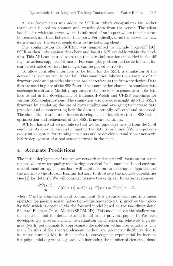
A new Socket class was added to SCIRun, which encapsulates the sockettraffic and is used to connect and transfer data from the server. The clienthandshakes with the server, which is informed of an ip:port where the client canbe reached, and then listens on that port. Periodically, or as the server has newdata available, the server sends data to the listening client.

The configuration for SCIRun was augmented to include libgeotiff [10].SCIRun then links against this client and has its API available within the mod-ules. This API can be used to extract the extra information embedded in the tifftags in various supported formats. For example, position and scale informationcan be extracted so that the images can be placed correctly.

To allow controller interfaces to be built for the SSSI, a simulation of thedevice has been written in Matlab. This simulation follows the structure of thefirmware code and provides the same basic interface as the firmware device. Datafiles are used in place of the SSSI’s serial communication channel to simulate dataexchange in software. Matlab programs are also provided to generate sample datafiles to aid in the development of Hadamard-Walsh and CRISP encodings forvarious SSSI configurations. The simulation also provides insight into the SSSI’sfirmware by emulating the use of oversampling and averaging to increase dataprecision and demonstrating how the data is internally collected and processed.The simulation can be used for the development of interfaces to the SSSI whileoptimization and refinement of the SSSI firmware continues.

SCIRun has a Matlab module so that we can pipe data to and from the SSSIemulator. As a result, we can tie together the data transfer and SSSI componentseasily into a system for training new users and to develop virtual sensor networksbefore deployment of a real sensor network in the field.

4 Accurate Predictions

The initial deployment of the sensor network and model will focus on estuarineregions where water quality monitoring is critical for human health and environ-mental monitoring. The authors will capitalize on an existing configuration ofthe model to the Hudson-Raritan Estuary to illustrate the model’s capabilities(see [1] for details). We will consider passive tracer driven by external sources:

∂C(x, t)∂t

− L(C(x, t)) = S(x, t), C(x, 0) = C0(x) x ∈ Ω,

where C is the concentration of contaminant, S is a source term and L is linearoperator for passive scalar (advection-diffusion-reaction). L involves the veloc-ity field which is obtained via the forward model based on the two-dimensionalSpectral Element Ocean Model (SEOM-2D). This model solves the shallow wa-ter equations and the details can be found in our previous paper [1]. We havedeveloped the spectral element discretization which relies on relatively high de-gree (5-8th) polynomials to approximate the solution within flow equations. Themain features of the spectral element method are: geometric flexibility due toits unstructured grids, its dual paths to convergence: exponential by increas-ing polynomial degree or algebraic via increasing the number of elements, dense

1006 C.C. Douglas et al.

computational kernels with sparse inter-element synchronization, and excellentscalability on parallel machines.

We now present our methodology for obtaining improved predictions basedon sensor data. For simplicity, our example is restricted to synthetic velocityfields. Sensor data is used to improve the predictions by updating the solutionat previous time steps which is used for forecasting. This procedure consistsof updating the solution and source term history conditioned to observationsand reduces the computational errors associated with incorrect initial/boundarydata, source terms, etc., and improves the predictions [11,12,13]. We assumethat the source term can be decomposed into pulses at different time steps(recording times) and various locations. We represent time pulses by δk(x, t)which corresponds to contaminant source at the location x = xk.

We seek the initial condition as a linear combination of some basis functions

C0 (x) ≈ C̃0 (x) =ND∑

i=1

λiϕ0i (x). We solve for each i,

∂ϕi

∂t− L (ϕi) = 0, ϕi (x, 0) = ϕ0

i (x) .

Thus, an approximation to the solution of∂C

∂t− L (C) = 0, C (x, 0) = C0 (x) is

given by C̃ (x, t) =ND∑

i=1

λiϕi (x, t) . To seek the source terms, we consider the

following basis problems

∂ψk

∂t− L (ψk) = δk (x, t) , ψk (x, 0) = 0

for ψ and each k. Here, δk (x, t) represents unit source terms that can be usedto approximate the actual source term. In general, δk (x, t) have larger supportboth in space and time in order to achieve accurate predictions. We denote thesolution to this equation as {ψk (x, t)}Nc

k=1 for each k. Then the solution to ouroriginal problem with both the source term and initial condition is given by

C̃ (x, t) =ND∑

i=1

λiϕi (x, t) +Nc∑

k=1

αkψk (x, t) .

Thus, our goal is to minimize

F (α, λ) =Ns∑

j=1

⎡

⎣(

Nc∑

k=1

αkψk (xj , t) +ND∑

k=1

λkϕk (xj , t) − γj (t)

)2⎤

⎦+

Nc∑

k=1

κ̃k

(αk − β̃k

)2+

ND∑

k=1

κ̂k

(λk − β̂k

)2,

(1)

where Ns denotes the number of sensors. If we denote N = Nc + Nd, μ =[α1, · · · , αNc , λ1, · · · , λND ], η (x, t) = [ψ1, · · · , ψNc , ϕ1, · · · , ϕND ],

Dynamically Identifying and Tracking Contaminants in Water Bodies 1007

β =[β̃1, · · · , β̃Nc , β̂1, · · · , β̂ND

], and κ = [κ̃1, · · · , κ̃Nc , κ̂1, · · · , κ̂ND ] then we

want to minimize

F ( μ) =Ns∑

j=1

⎡

⎣(

N∑

k=1

μkηk (xj , t) − γj (t)

)2⎤

⎦ +N∑

k=1

κk (μk − βk)2 .

This leads to solving the least squares problem Aμ = R where

Amn =N∑

j=1

ηm (xj , t) ηn (xj , t) + δmnκm,

and

Rm =N∑

j=1

ηm (xj , t) γj (t) + κmβm.

We can only record sensor values at some discrete time steps t = {tj}Nt

j=1. Wewant to use the sensor values at t = t1 to establish an estimate for μ, then useeach successive set of sensor values to refine this estimate. After each step, weupdate and then solve using the next sensor value.

Next, we present a representative numerical result. We consider contaminanttransport on a flat surface, a unit dimensionless square, with convective velocityin the direction (1, 1). The source term is taken to be 0.25 in [0.1, 0.3]× [0.1, 0.3]for the time interval from t = 0 to t = 0.05. Initial condition is assumed to havethe support over the entire domain. We derive the initial condition (solution atprevious time step) by solving the original contaminant transport problem withsome source terms assuming some prior contaminant history.

To get our observation data for simulations, we run the forward problemand sample sensor data at every 0.05 seconds for 1.0 seconds. We sample atthe following five locations: (0.5, 0.5) , (0.25, 0.25) , (0.25, 0.75) , (0.75, 0.25) , and(0.75, 0.75).

When reconstructing, we assume that there is a subdomain Ωc ⊂ Ω whereour initial condition and source terms are contained. We assume that the sourceterm and initial condition can be represented as a linear combinations of basisfunctions defined on Ωc. For this particular model, we assume the subdomainis [0, 0.4]× [0, 0.4] and we have piecewise constant basis functions. Furthermore,we assume that the source term in our reconstruction is nonzero for the sametime interval as S(x, t). Thus we assume the source basis functions are nonzerofor only t ∈ [0, 0.05].

To reconstruct, we run the forward simulation for a 4 × 4 grid of piecewiseconstant basis functions on [0, 0.4] × [0, 0.4] for both the initial condition andthe source term. We then reconstruct the coefficients for the initial conditionand source term using the approach proposed earlier. The following plot shows acomparison between the original surface (in green) and the reconstructed surface(in red). The plots are for t = 0.1, 0.2, 0.4 and 0.6. We observe that the recoveryat initial times is not very accurate. This is due to the fact that we have not

1008 C.C. Douglas et al.

Fig. 2. Comparison between reconstructed (red) solution and exact solution at t = 0.1(upper left), t = 0.2 (upper right), t = 0.4 (lower left), and t = 0.6 (lower right)

collected sufficient sensor data. As the time progresses, the prediction resultsimprove. We observe that at t = 0.6, we have nearly exact prediction of thecontaminant transport.

To account for the uncertainties associated with sensor measurements, weconsider an update of initial condition and source terms, within a Bayesianframework. The posterior distribution is set up based on measurement errorsand prior information. This posterior distribution is complicated and involvesthe solutions of partial differential equations. We developed an approach thatcombines least squares with a Bayesian approach, such as Metropolis-HastingMarkov chain Monte Carlo (MCMC) [14], that gives a high acceptance rate. Inparticular, we can prove that rigorous sampling can be achieved by samplingthe sensor data from the known distribution, thus obtaining various realizationsof the initial data. Our approach has similarities with the Ensemble KalmanFilter approach, which can also be adapted in our problem. We have performednumerical studies and these results will be reported elsewhere.

5 Conclusions

In the last year, we have made strides in creating our DDDAS. We have devel-oped software that makes sending data from locations that go on and off theInternet and possibly change IP addresses rather easy to work with. This is astand alone package that runs on any devices that support Java. It has also

Dynamically Identifying and Tracking Contaminants in Water Bodies 1009

been integrated into newly released version 3.0 of SCIRun and is in use by othergroups, including surgeons while operating on patients. We have also developedsoftware that simulates the behavior of the SSSI and are porting the relevantparts so that it can be loaded into the SSSI to get real sensor data. We havedeveloped algorithms that allow us to achieve accurate predictions in the pres-ence of errors/uncertainties in dynamic source terms as well as other externalconditions. We have tested our methodology in both deterministic and stochasticenvironments and have presented some simplistic examples in this paper.

References

1. Douglas, C.C., Harris, J.C., Iskandarani, M., Johnson, C.R., Lodder, R.A., Parker,S.G., Cole, M.J., Ewing, R.E., Efendiev, Y., Lazarov, R., Qin, G.: Dynamic con-taminant identification in water. In: Computational Science - ICCS 2006: 6thInternational Conference, Reading, UK, May 28-31, 2006, Proceedings, Part III,Heidelberg, Springer-Verlag (2006) 393–400

2. Lowell, A., Ho, K.S., Lodder, R.A.: Hyperspectral imaging of endolithic biofilmsusing a robotic probe. Contact in Context 1 (2002) 1–10

3. Dempsey, R.J., Davis, D.G., R. G. Buice, J., Lodder, R.A.: Biological and medicalapplications of near-infrared spectrometry. Appl. Spectrosc. 50 (1996) 18A–34A

4. Silva, H.E.B.D., Pasquini, C.: Dual-beam near-infrared Hadamard. Spectropho-tometer Appl. Spectrosc. 55 (2001) 715–721

5. Johnson, C.R., Parker, S., Weinstein, D., Heffernan, S.: Component-based prob-lem solving environments for large-scale scientific computing. Concur. Comput.:Practice and Experience 14 (2002) 1337–1349

6. SCIRun: A Scientific Computing Problem Solving Environment, Scientific Comput-ing and Imaging Institute (SCI). http://software.sci.utah.edu/scirun.html (2007)

7. Li, W.: A dynamic data-driven application system (dddas) tool for dynamic re-configurable point-to-point data communication. Master’s thesis, University ofKentucky Computer Science Department, Lexington, KY

8. Apple OS X 10.4 XGrid Features, Apple, inc. http://www.apple.com/acg/xgrid(2007)

9. Douglas, C.C., Beezley, J.D., Coen, J., Li, D., Li, W., Mandel, A.K., Mandel,J., Qin, G., Vodacek, A.: Demonstrating the validity of a wildfire DDDAS. In:Computational Science - ICCS 2006: 6th International Conference, Reading, UK,May 28-31, 2006, Proceedings, Part III, Heidelberg, Springer-Verlag (2006) 522–529

10. GeoTiff. http://www.remotesensing.org/geotiff/geotiff.html (2007)11. Douglas, C.C., Efendiev, Y., Ewing, R.E., Ginting, V., Lazarov, R.: Dynamic data

driven simulations in stochastic environments. Computing 77 (2006) 321–33312. Douglas, C.C., Efendiev, Y., Ewing, R.E., Ginting, V., Lazarov, R., Cole, M.J.,

Jones, G.: Least squares approach for initial data recovery in dynamic data-drivenapplications simulations. Comp. Vis. in Science (2007) in press.

13. Douglas, C.C., Efendiev, Y., Ewing, R.E., Ginting, V., Lazarov, R., Cole, M.J.,Jones, G.: Dynamic data-driven application simulations. interpolation and up-date. In: Environmental Security Air, Water and Soil Quality Modelling for Riskand Impact Assessment. NATO Securtity through Science Series C, New York,Springer-Verlag (2006)

14. Robert, C., Casella, G.: Monte Carlo Statistical Methods. Springer-Verlag, NewYork (1999)