Dynamically loaded self-aligning journal bearings - RIT ...

Rochester Institute of Technology Rochester Institute of Technology

RIT Scholar Works RIT Scholar Works

Theses

2004

Dynamically loaded self-aligning journal bearings: A Mobility Dynamically loaded self-aligning journal bearings: A Mobility

method approach method approach

Nathan Mayer

Follow this and additional works at: https://scholarworks.rit.edu/theses

Recommended Citation Recommended Citation Mayer, Nathan, "Dynamically loaded self-aligning journal bearings: A Mobility method approach" (2004). Thesis. Rochester Institute of Technology. Accessed from

This Thesis is brought to you for free and open access by RIT Scholar Works. It has been accepted for inclusion in Theses by an authorized administrator of RIT Scholar Works. For more information, please contact [email protected].

https://scholarworks.rit.edu/

https://scholarworks.rit.edu/theses

https://scholarworks.rit.edu/theses?utm_source=scholarworks.rit.edu%2Ftheses%2F7538&utm_medium=PDF&utm_campaign=PDFCoverPages

https://scholarworks.rit.edu/theses/7538?utm_source=scholarworks.rit.edu%2Ftheses%2F7538&utm_medium=PDF&utm_campaign=PDFCoverPages

mailto:[email protected]

Dynamically Loaded Self-Aligning Journal Bearings: A Mobility Method Approach

by

Nathan Mayer

A Thesis Submitted in Partial Fulfillment of the

Requirement for the

MASTER OF SCIENCE IN

MECHANICAL ENGINEERING

Approved by:

Dr. Stephen Boedo Stephen Boedo Department of Mechanical Engineering (Thesis advisor)

Dr. Hany Ghoneim Hany Ghoneim Department of Mechanical Engineering

Dr. Josef Torok Josef S. Torok Department of Mechanical Engineering

Dr. Edward C. Hensel Edward C. Hensel Department Head of Mechanical Engineering

DEPARTMENT OF MECHANICAL ENGINEERING ROCHESTER INSTITUTE OF TECHNOLOGY

August 2004

Dynamically Loaded Self-Aligning Journal Bearings: A Mobility Method Approach

I, Nathan Mayer, hereby grant permission to the Wallace Library of the Rochester Institute of

Technology to reproduce my thesis in whole or in part. Any reproduction will not be for

commercial use or profit.

Signature of Author: Nat han Mayer

ii

Acknowledgements

First and foremost I would like to thank God for giving the strength and ability to

complete this work.

I want to express my deep appreciation for the support ofmy loving wife. I don't

know how I could have made it the past three years without her. I also want to thankmy

parents for helping me through my education and encouraging me to do my best.

I would like to thank my advisor, Dr. Boedo for sticking with me and supporting me

through this process. I would also like to thank Dr. Torok and Dr. Ghoneim for taking the

time to review my thesis and serve on my committee.

Abstract

Journal bearings are a fundamental component in many pieces ofmachinery. A

properly designed bearing is capable of supporting large loads in rotating systems with

minimal frictional energy losses and virtually no wear even after years of services. These

benefits make an understanding ofdynamic behavior of these devices very valuable.

In applications where journal bearings are subject to misalignment (conditions where

the journal and sleeve axes are not parallel), it has long been understood that bearing

performance can be compromised. To eliminate this problem, self-aligning bearings have

been designed. The sleeves of these bearings are capable ofmoving freely to accommodate

misalignment. The aligning motion of these bearings under dynamic loading is, however,

largely unexplored. Additionally, the impact ofmisalignment on journal midplane motion is

unknown.

Currently, finite element and finite difference analyses are the only available tools for

this kind ofwork. This requires a unique and computationally costly mathematical solution

for every possible bearing configuration.

It is the goal of this thesis to develop a computationally efficient means ofpredicting

journal motion within a self-aligning bearing. This is done by creating a set of"mobility"

mapping functions from finite element bearing models that relate the velocity of the journal

to the applied load. Such maps have previously been built and used successfully for the

design ofperfectly aligned bearings. This expansion ofthe mobility method to self-aligning

bearings provides a valuable tool for the designer and gives valuable insight into the journal

motion for these devices.

IV

Table ofContents

1 Background 1

2 Problem Formulation 6

2.1 Bearing Geometry 6

2.2 Mobility Formulation: Aligned Bearings 9

2.3 Mobility Formulation with Journal Misalignment 13

2.4 Generation ofMobilityMapping Functions 20

2.5 Application oftheMobility Mapping Functions 23

3 Application and Validation 26

3.1 Pure Squeeze 26

3.1.1 Case 1 : Pure Squeeze, Zero Initial Misalignment 29

3.1 .2 Cases 2a and 2b:: Pure Squeeze, Initial Misalignment about the r|-axis 30

3.1.3 Cases 3a and 3b:: Pure Squeeze, Initial Misalignment about the ^-axis 35

3. 1 .4 Cases 4a and 4b:: Pure Squeeze, Initial Misalignment45

from the Force

Vector 39

3.1.5 Case 5 Pure Squeeze, Arbitrary Initial Journal Location 39

3.2 Steady Rotation 47

3.2.1 Cases 6a and 6b: Steady Rotation, Zero Initial Misalignment 48

3.2.2 Cases 7a-8d:: Steady Rotation, Initial Misalignment abou the ^-axis

or r|-axis 51

3.2.3 Cases 9a-9d:: Steady Rotation, Initial Misalignment45

from the Force

Vector 72

3.2.4 Case 10: Steady Rotation, Arbitrary Initial Journal Location 72

3.2.5 Cases 1 la and 1 lb: Steady Rotation, Variable Load 72

4 Conclusions and Future Work 91

Appendices

A Finite Element Based Aligned Bearing Mobility Map 96

B Misalignment Adjustment Functions 97

C Reference Tables ofResults 102

D Multi-Generational Curve Fitting Process 103

E Flowchart ofLogic for Bearing Orbit Calculation usingMobility Maps 104

F Axial Spacing forNon-UniformMeshes 105

Referencs 106

VI

List ofFigures

Figure 1.1 Spherical Socket Self-Aligning Journal Bearing 3

Figure 1.2 Elastomer Supported Self-Aligning Journal Bearing 5

Figure 1.3 Pivoted Sleeve Self-Aligning Journal Bearing 5

Figure 2.1 Bearing Geometry 7

Figure 2.2 Bearing Loads and Kinematics 8

Figure 2.3 Example Mobility Map: Sort bearing model 17

Figure 2.4 Translational Mobility Vector 19

Figure 2.5 3-D Unwrapped Example Elemental Mesh 21

Figure 2.6 3-D Representation ofExample Elemental Mesh 21

Figure 3.1 Coarse Mesh: 14 axial by 40 circumferencial nodes, spacing ratio of 1 .25 27

Figure 3.2 Fine Mesh: 20 axial by 60 circumferencial nodes, spacing ratio of 1.15 27

Figure 3.3 Axial Node Spacing, Scheme 28

Figure 3.4 Time History of Journal Eccentricity: Pure Squeeze, zero initial misalignment

(Casel) 31

Figure 3.5 Time History of Journal Eccentricity: Pure Squeeze, specified misalignment about

the r|-axis (Case 2a) 32

Figure 3.6 Time History of Journal Misalignment: Pure Squeeze, specified misalignment

about the r|-axis (Case 2a) 32

Figure 3.7 Time History of Journal Eccentricity: Pure Squeeze, specified misalignment about

the r|-axis (Case 2b) 33


about the n.-axis (Case 2b) 33

Figure 3.9 Time History of Journal Eccentricity: Pure Squeeze, comparison between aligned

case and initial misalignment about the rj-axis 34


case and initial misalignment about the n-axis (Case 2a) 34

Figure 3.1 1 Time History of Journal Eccentricity: Pure Squeeze, specified misalignment

about the -axis (Case 3a) 36

VII


about the ,-axis (Case 3a) 36

Figure 3.13 Time History of Journal Eccentricity: Pure Squeeze, specified misalignment

about the -axis (Case 3b) 37


about the ^-axis (Case 3b) 37


case and initial misalignmentabout the -axis 38


case and initial misalignmentabout the ^-axis 38

Figure 3.17 Time History of Journal Eccentricity: Pure Squeeze, specified misalignment45

from the load (Case 4a) 40


from the load (Case 4a) 40


45from the load (Case 4a) 41




from the load (Case 4b) 42


from the load (Case 4b) 42


45from the load (Case 4b) 43




case and initial misalignment45

from the load iq-axis 44


case and initial misalignment45

from the load r|-axis 44

VIM

Figure 3.27 Time History of Journal Eccentricity: Pure Squeeze, specified misalignment and

eccentricity (Case 5) 45

Figure 3.28 Time History of Journal Eccentricity: Pure Squeeze, specified misalignment and

eccentricity (Case 5) 45


and eccentricity (Case 5) 46



Figure 3.31 Time History of Journal Eccentricity: Steady Rotation, zero initial misalignment

(Case 6a) 49


(Case 6a) 49


(Case 6b) 50


(Case 6b) 50

Figure 3.35 Time History of Journal Eccentricity: Steady Rotation, specified misalignment




Figure 3.37 Time History of Journal Misalignment: Steady Rotation, specified misalignment



about the n,-axis (Case 7a) 53


about the iq-axis (Case 7b) 54


about the n,-axis (Case 7b) 54


about the r|-axis (Case 7b) 55

IX


about the n-axis (Case 7b) 55


about the r|-axis (Case 7c) 56




about the r)-axis (Case 7c) 57




about the r|-axis (Case 7d) 58


about the r\-axis (Case 7d) 58






about the 4-axis (Case 8a) 60


about the ^-axis (Case 8a) 60


about the ^-axis (Case 8a) 61


about the -axis (Case 8a) 61


about the -axis (Case 8b) 62






about the %-axis (Case 8b) 63


about the %-axis (Case 8c) 64


about the ^-axis (Case 8c) 64


about the ,-axis (Case 8c) 65


about the ^-axis (Case 8c) 65


about the ,-axis (Case 8d) 66


about the ^-axis (Case 8d) 66


about the -axis (Case 8d) 67


about the ^-axis (Case 8d) 67

Figure 3.67 Time History of Journal Eccentricity: Steady Rotation, comparison between

aligned case and initial misalignment about the q-axis 68


aligned case and initial misalignment about the r|-axis 68






aligned case and initial misalignment about the ^-axis 70

XI


aligned case and initial misalignment about the ,-axis 70


aligned case and initial misalignment about the ^-axis 71


aligned case and initial misalignment about the %-axis 71















Figure 3.82 Time History of JournalMisalignment: Steady Rotation, specified misalignment



45from the load (Case 9c) 77

Figure 3.84 Time History of Journal Eccentricity: Steady Rotation, specifiedmisalignment






XII


45from the load (Case 9d) 79








aligned case and initial misalignment45

from the load 81



from the load 81



from the load 82



from the load 82









Figure 3.99 Time History of one Load Cycle (Case 1 1) 86

Figure 3.100 Time History ofJournal Eccentricity: Steady Rotation, variable load with zero

initial misalignment (Case 1 la) 87

Figure 3.101 Time History ofJournal Eccentricity: Steady Rotation, variable load with zero

initial misalignment (Case 11a) 87

Figure 3.102 Time History of Journal Eccentricity: Steady Rotation, variable load with initial

misalignment (Case lib) 88

XIII

Figure 3.103 Time History of Journal Eccentricity: Steady Rotation, variable load with initial

misalignment (Case lib) 88

Figure 3.104 Time History of Journal Misalignment: Steady Rotation, variable load with

initial misalignment (Case 1 lb) 89

Figure 3.105 Time History of Journal Misalignment: Steady Rotation, variable load with

initial misalignment (Case lib) 89


aligned case and initial misalignment with variable load 90

Figure 4.1 Time History of JournalMisalignment and Loading: Variable Loading (Case 1 1).... 93

XIV

List ofTables

Table 3.1: Mesh Parameters 26

Table 3.2: Initial Conditions for Pure Squeeze Simulations 29

Table 3.3: Initial Journal Position and Constant value of/for Steady Rotation Cases 48

Table 3.4: Dimensional Parameters for Cases 1 la and 1 lb 85

Table 3.5: Initial Conditions for Cases 1 la and 1 lb 85

Table 4.1: Comparison ofComputing Times (Case 4b) 91

XV

List of Symbols

c radial clearance [L]

D bearing diameter [L]

e eccentricity [L]

F bearing load [F]

h minimum film thickness [L]

L bearing length [L]

M misaligning moment [FL]

M0 aligned bearing translational mobility magnitude [-]

M misaligned bearing translational mobility magnitude [-]

p fluid fim pressure [FL"2]

R bearing radius [L]

t time [t]

S spacing ratio [-]

T rotational mobility [-]

Y direction ofmobility vector relative to the force vector [-]

5 mobility direction adjustment angle [-]

s midplane eccentricity ratio [-]

k mobility magnitude adjustment factor [-]

p. fluid viscosity[FL"

-T]

p fluid density [FL"4-T2]

x dimenisonless time parameter [-]

<t> axial misalignment angle [-]

cp dimensonless misalignment magnitude [-]

co angular velocity [-]

Symbol Convention

A vector A

AB

The component ofvector A in the B direction [-]

XVI

Chapter 1: Background

Lubrication is an effective means of reducing friction between moving surfaces. A

common lubricated system used in rotating machinery is the journal bearing. A journal

bearing consists ofa lubricated cylindrical journal within a cylindrical sleeve. This device

allows the journal to rotate about its axis at high speeds while the sleeve supports large radial

loads imposed on the journal with minimal frictional losses.

The operation of a journal bearing is based on the fluid dynamics principle that when

two surfaces, wetwith a fluid, move relative to each other pressures can be created within the

fluid. In journal bearings, these pressures serve to support loads applied to the surfaces, thus

reducing the load carried by direct surface asperity contact. Reducing contact loads reduces

frictional forces, energy loss, and wear on surfaces. The benefits of fluid film lubrication

make the ability to predict the behavior of a lubricated system valuable to a designer.

The journal bearing's lubricated surfaces are the outer diameter of the journal and

inner diameter ofthe sleeve. The radius of the journal, Rj, is machined slightly smaller than

the radius ofthe sleeve, Rs. The radial clearance between the two, c= Rs - Rj, is typically on

the order of a thousandth of the journal or sleeve diameter; therefore Rs Rj =R. The

clearance gap is filled with lubricant. For analysis,the journal and sleeve surfaces are treated

as parallel planes because their radii are orders ofmagnitude greater than the clearance

between them.

Historically, journal bearing analyses have been performed under the assumption that

the journal and sleeve axes are parallel (Khonsari and Booser 2001). The designer can then

consider the location of the journal within the sleeve to vary circumferencially but not

axially. This idealized scenario simplifies the calculations involved in such work.

1

Additionally, it reduces the number ofparameters that must be considered. This assumption,

however, is generally untrue.

Misalignment in bearings has been a matter of concern since modern bearing analysis

began. Early automobile designers had experimentally determined that a misalignment as

small as 0.002 inches at a bearing's end per 12 inches ofbearing length could reduce a

bearing's load capacity by over 30% (Pigott, 1941). This was followed by detailed

experimental work on misaligned bearings with results in dimensionless form intended for

bearing design (DuBois et al., 1955).

As computers became available, analysts began examiningmisaligned bearings using

mathematical models. Studies modeling a variety of realistic bearing configurations were

performed using finite difference based models (Pinkus and Bupara, 1979) and finite element

based models (Goenka, 1984B). These studies focused primarily on the impact of

misalignment on maximum film pressure, minimum film thickness, and frictional losses.

This was done by imposing a constant misalignment angle to the bearing model and

observing how these parameters differed from the equivalent aligned case. Recent analytical

work by Boedo and Booker (2003) has investigated load and moment bearing capacity as a

misaligned journal approaches the sleeve in edge point contact

Some authors have suggested that, for bearings subject to loading that may result in

significant amounts ofmisalignment, a self-aligning bearing should be used (Fuller, 1956).

A self-aligning journal bearing is one in which the sleeve is free to rotate and accommodate

misalignment. This can be achieved by installing the bearing sleeve within a low friction

spherical socket (Falz, 1937; DuBois et al., 1955) as shown in Figure 1.1. The spherical

socket is unable to support the moments that are created by the imbalance in fluid film

Spherical

Socket

Journal

Figure 1.1 Spherical Socket Self-Aligning Journal Bearing

pressures along the bearing axis caused by misalignment. As a result, the film pressure in a

misaligned self-aligning bearing will move the bearing sleeve into an aligned condition.

Other designs for self-aligning bearings exist such as ones where the sleeve is

supported by an elastomer connection or a pivoted point as shown in Figures 1.2 and 1.3,

respectively (Fuller, 1956). These types of self-aligning bearings function differently from

the spherical socket type and have not been evaluated in this study.

The nature of self-aligning bearings has often led analysts to assume that they are

always in a perfectly aligned state. However, the dynamic behavior ofa self-aligning bearing

under varying load and speed is largely unexplored. The time needed for a self-aligning

bearing to align itselfand the effect misalignment has on journal midplane motion during the

aligning process is ofparticular concern. It is the goal of this thesis to develop a

computationally efficient means ofdetermining the motion of a journal within a self-aligning

sleeve. This is achieved by developing dimensionless"mobility"

curve fits for finite element

based journal motion calculations. Similarwork has been successfully done for aligned

bearings (Goenka, 1984A). These results expand this design tool for the analysis of

misaligned self-aligning bearings.

///////////////

Elastomer

Support

Sleeve

Journal

///////////////

Figure 1.2 Elastomer Supported Self-Aligning Journal Bearing

/////// / / //////Journal

Sleeve

Figure 1.3 Pivoted Sleeve Self-Aligning Journal Bearing

Chapter 2: Problem Formulation

The objectives of this chapter are to describe the theory behind fluid film lubrication

as it applies to journal bearings and to present the problem created by misalignment in self-

aligning journal bearings.

2.1 Bearing Geometry

In a journal bearing, forces and moments are transmitted from journal to sleeve

through the lubricant film. Figures 2.1 and 2.2 depict a grooveless journal bearing of

diameter D and length L under general loading conditions with features exaggerated radial

clearance c for clarity. Its geometry is explained below.

Figure 2.1 defines two coordinate frames. An (inertial) cartesian"computing"

coordinate frame is fixed to the bearing sleeve center and defined by the x, y, and z axes.

The inertial coordinate system's origin is located on the bearing midplane with the z-axis

coincident with the sleeve axis. The bearing midplane is defined as the plane equidistant

from the ends ofthe bearing sleeve. The journal and sleeve rotate about the z-axis with

angular velocities of coj and gos, respectively. A moving ^-q cartesian coordinate has its

origin at the bearing center with the t, axis defined by the direction ofthe force vector.

In Figure 2.1, the radial force vector F is the load transmitted from the journal to the

sleeve through the lubricant film. Also shown is the journal radial displacement vector e.

The magnitude ofthe radial displacement vector is also known as bearing eccentricity. This

vector measures the midplane displacement of the journal center, Oj, from the sleeve center,

Os. Bearing kinematics, for a complete360

sleeve bearing, require that the bearing

eccentricity always be less than the radial clearance.

In Figure 2.1, the journal misalignment vector is decomposed into x and y

components. It is defined as the angle measured from the sleeve axis to the journal axis. As

a result ofmisalignment, the momentM is transmitted from the journal to the sleeve through

the lubricant film as shown in Figure 2.2.

Both eccentricity and misalignment vectorscan be normalized. For eccentricity, the

dimensionless parameter known as eccentricity ratio is defined by

ViewBViewC

Figure 2.1 Bearing Geometry

Figure 2.2 Bearing Loads and Kinematics

8

e = e/c (2.1)

The eccentricity ratio magnitude varies from a value of 0, where the journal and sleeve axes

share the same point at the bearing midplane, to a value of 1, where the journal and sleeve

surfaces contact at the bearing midplane.

A normalized misalignment angle O is defined by

o =

J> Lty

tan"

'2c> 2c(2.2)

v-w

since for all realistic bearings cL. For a bearing with zero eccentricity, the normalized

misalignment angle has a value of 1 when the journal is in contact with the ends ofthe

bearing sleeve, and it is zero when the journal and sleeve are perfectly aligned.

2.2 Mobility Formulation: Aligned Bearings

The mobility method of solution is a technique developed to generalize the solution to

a dynamically loaded bearing problem where the load history is specified. The method

employs dimensionless maps (generated from bearing solutions) that relate the given force on

the journal to the rate ofjournal displacementwithin the sleeve. This greatly reduces

calculation time for the bearing designer. The mobility method for aligned bearings was

introduced by Booker (1965) and is summarized below.

To simplify the derivation, a bearing with zero journal and zero sleeve angular

velocity, known as a squeeze film bearing, will be examined first. The squeeze film solution

can be expanded to account for journal and sleeve rotation using methods described in

section 2.4. Given a perfectly aligned bearing with incompressible lubricant where variations

in viscosity can be ignored, the film pressure p is governed by the Reynolds equation

d \*& +R2 'h^

DO dd_ dz &.

= \2pR2dh

dt(2.3)

where h is the fluid film thickness, p is the fluid viscosity, and 0 is the circumferential fluid

film coordinate measured from the force vector. For a circumferentially symmetric bearing,

the film thickness is given by

h = c-e^ cos9-eri sinO (2.4a)

and the rate ofchange of film thickness is given by

=-efcosO-en

sin (9 (2 4b)ot

v '

The boundary conditions on the Reynolds equation (2.3) come from oil feed grooves,

the open ends ofthe bearing, and fluid film cavitation. For a grooveless bearing with the

bearing ends at ambient (zero) pressure, the boundary equation at the bearing ends is given

by

p(0,L/2)= O (2.5)

Cavitation boundary conditions capture the phenomena of fluid film rupture, which

occurs because fluids are unable to support negative pressures ofa significant magnitude.

Due to this cavitation boundary condition, there is no known closed form solution ofthe

Reynolds equation. This has led to the development of a number ofapproximate solutions.

These approximate solutions are based on assumptions about lubricant flow and do not

completely satisfy both the Reynolds equation and the boundary conditions. Examples

include the Ocvirk short bearing solution, the Sommerfeld long bearing solution, and the

Warner finite bearing solution. Each solution gives film pressure as a function ofthe bearing

length to diameter ratio L/D and the eccentricity ratio vector e. Formulation details for these

approximate solutions can be found in Booker (1965).

Mobility formulations for these approximate solutions to the Reynolds equation have

been calculated and used to create two-dimensional maps ofmobility, as a function ofe, for a

fixed bearing L/D ratio. In addition to these approximations, a more accurate mobility

10

solution, based on finite element analysis, was developed by Goenka (1984), and is included

in Appendix A.

The film pressures that satisfy the Reynolds equation (2.3) and boundary conditions

(2.5) also need to satisfy

F*=F= jpcosOdA (2.6a)

F"=0= ^psinddA (2.6b)

where F is the given force. These constraints arise from the need for the fluid film pressures

to transmit the specified load. To account for cavitation, the area of integration, A, is limited

to the areas ofpositive pressure. Justification for this method is based on the fact that

numerical results obtained using this method agree reasonably well with experimental data

where inertial effects can be neglected (Booker, 1965).

The equations presented up to this point can be cast into dimensionless form by

defining the following parameters for film pressure and axial film coordinate:

P=^- (2.7)

z=-z (2.8)Lt

Film thickness and its time rate of change can be represented in dimensionless form as

follows:

^ = /?/c = l-^cos0-,sin0 (2.9a)

^U-^cos0-^sin0 (2.9b)dt

When non-dimensionalized, the Reynolds equation for axially aligned bearingsunder pure

squeeze can be written as

11

8_89 89

+'Z^

v-w

d_8z

-3 <^p \2pLD 8h

85] F(c/Rf 8t(2.10)

The boundary conditions and constraints for this partial differential equation, given in

equations 2.5-2.6, are also non-dimensionalized as follows:

p(9,L/2)= 0

\ = -)p-cos9d9dz

0= \psin9d9dz

(2.11)

(2.12a)

(2.12b)

The solution to the dimensionless Reynolds equation under these pressure constraints takes

the following form:

F{c/R)

F{c/R)

(2.13a)

(2.13b)

where Ml and Ml are dimensionless ratios ofjournal translational velocity to force in the ,

and q directions, respectively. These ratios are henceforth denoted as the aligned bearing

mobility relations.

12

2.3 Mobility Formulation with JournalMisalignment

The mobility formulations described in the previous section ignore the effects of

misalignment. A common practice in bearing analysis is to assume a perfectly aligned

bearing. This assumption is almost always not true in practice, but, as discussed in Chapter

1, little work has been done to quantify the errors it introduces. In this section, the theory

that explains journal motion is expanded to account formisalignment in a self-aligning

bearing.

The problem presented by a misaligned self-aligning journal bearing is one where the

following parameters are known at a given instant:

F - force transmitted from journal to sleeve

e -journal displacement (eccentricity)

<|> -journal misalignment

coj -journal angular velocity

cos- sleeve angular velocity

and the following parameters need to be found at that instant:

<|> - time rate of change ofjournal misalignment

e - time rate ofchange ofjournal eccentricity

subject to the additional constraint that there is no misaligning moment, i.e. M = 0 . Figure

2.2 shows the physical representation of these parameters.

The Reynolds equation for a misaligned journal bearing with incompressible

lubricant, constant viscosity, and zero journal and sleeve angular velocities can once again be

written in the following form:

_LJL

R2

89

h3

dp

\2p 89

8+

8z

r h3

dp

K\2p8zjf

where the film thickness, h is now defined as

13

h = c-e4

cos9 -en

sm.9 -

z(/>ncos9 + z<fi 4sin9 (2.15a)

and its time derivative is

=-e<:cos9-e'!sm9-z<f>'>cos9 + z<}>

isin<9 (2.15b)

The pressure boundary condition at the bearing ends is the same as for the aligned case:

p(0,L/2)= O (2.16)

The pressure across the film due to radial forces is the same as for the aligned case.

F4=F= \pcos9dA (2.17a)

F"=0= [ psin9dA (2.17b)

JA

Further constraints on pressure are needed to represent the situation of a self-aligning

bearing. The moments transmitted through the fluid film must be zero and are constrained

with the following equations:

M*=0= \pzsin9dA (2.18a)

A

M7=0 = -\pzcos9dA (2.18b)

A

As with the aligned formulation, the areas ofpressure integration are the portions ofthe fluid

film where the pressure is greater than ambient to account for cavitation.

It is beneficial to express film thickness in dimensionless form using the relationship:

14

h = h/c = \- s 4qos9 -

s "sind-z ncos9 + zQ> 4sir\9 (2.19)

8h ,

=-e icos9-s 'sin 9 -

zO*cos9 + zO

fsin 0 (2.20)

The dimensionless Reynolds equation is then written as

8_89w dp;

89+

'Z^

\^j

_5_

5z Wf\2pLD 8h

F{c/R)2

8t(2.21)

The pressure p is subject to the (dimensionless) integral constraints:

l=-\pcos9dzd9

0= jp sin 9 dzd9

0 = \pzsin9 dz d9

0 = \pzcos9 dz d9

(2.22a)

(2.22b)

(2.22c)

(2.22d)

To determine bearing motion, each ofthe following four quantities must be found which

solve the Reynolds equation (2.21) and satisfy both the pressure and cavitation boundary

conditions:

FiflRfpLDs4

F(c/RfpLDe"

Fjc/Rf

pLD&

F(c/RfpLD<b"

(2.23a)

(2.23b)

(2.23c)

(2.23d)

15

The goal of this thesis is to construct translational mobility mapping functions

pLDs4

F{c/Rf

=M4(z,<b,LlD) (2.24a)

j

-^=M'(e,9,L/D) (2.24b)

F{c/R)

and rotational mobility mapping functions

^^- = T4{e,<t>,L/D) (2.25a)F(c/R)

tS?=t%*'l/d) (2'25b)

from repeated solution of (2.21) for a given range ofL/D, e, and O. The rationale in

constructing mobility mapping functionsM and T is that computation ofeccentricity rates

and misalignment rates directly from (2.21) at each instant in time is computationally costly.

Maps for aligned solutions have only three independent variables: eccentricity ratio,

eccentricity direction, and bearing length to diameter ratio. When L/D is fixed, the map can

be displayed graphically in two dimensions. Figure 2.3 is an example ofone ofthese aligned

bearing mobility maps.

Creating a graphical map is not possible formisaligned bearings because the mobility

equations are functions of five independent variables. Mapping functions, however, can still

be made. The creation of these mapping functions is discussed below.

Translational mobility componentsM*

andA/1 form the vectorM that can also be

written in terms ofmagnitude and direction. Translational mobility magnitude is found using

the following equation:

(2.26)

16

1

Figure 2.3 ExampleMobility Map:

Sort bearing model (Booker, 1971)

17

The direction ofthe mobility vector is measured as an angle y with respect to the force vector

as shown in Figure 2.4.

As mentioned in the previous section, many translational mobility functions for

aligned bearings have already been developed. The development of translational mobility

functions formisaligned bearings relies heavily upon these aligned-based mobility functions.

Specifically, two mobility adjustment functions have been created which, when applied to

aligned bearing mobility functions, account for the effects ofmisalignment.

The first adjustment function is the magnitude magnification factor k. It is applied to

the aligned-based mobility magnitude equation using the following relationship

M(e,0,Z/D) = k(,<S>,L/D)M0(e,L/D) (2.27)

where

M0 =

J(Ml)2+(Ml)2

(2.28)

is the translational mobility magnitude for aligned bearings.

The change in translational mobility direction from misalignment is accounted for

using the mobility directionadjustment angle 8. This angle is added to the aligned-based

mobility direction angle y0 to account for misalignment using the equation

y(z,<S>,L/D)= y0^,L/D) + S(s,<t>,L/D) (2.29)

Proper curve fits for k and 6 should result in having no impact on mobility

calculations for aligned bearings. For the aligned case, 0= 0, the following statements must

be true:

As O -> 0 ,M -> M0 so k -> 1 for any e

As <d _> o , y -> y0 so 8 -> 0 for any e

18

Figure 2.4 TranslationalMobility Vector

19

This serves as a check to confirm these curve fits are reasonable. The fits given in Appendix

B satisfy these criteria.

There are no known previously existing rotational mobility mapping functions.

Therefore, two new functions,f>and 7*1, have been developed to determine misalignment

rates using the relationships

r^(E,o,z/D)^fe/^ =& (230a)pLD

and

T" (e,*, =6"

(2.30b)pLD

2.4 Generation ofMobility Mapping Functions

The mobility formulations described in the previous section require a solution to the

Reynolds equation. The finite element method was used to develop the adjustment functions

presented in this paper. The lubricant film was represented by a uniform array of four-noded

two-dimensional elements. For visualization purposes, the cylindrical fluid film mesh is

shown unwrapped in Figure 2.5. A three dimensional representation ofthe mesh is given in

Figure 2.6.

The finite elementmethod, as it applies to journal bearings, was developed by Booker

and Huebner (1971). In this application, the boundary variable applied to the nodes is film

pressure. For a grooveless bearing, the nodes on the bearing ends are fixed to ambient

pressure. Nodes on the interior ofthe bearing are constrained to have no net outward flow.

Film thickness and its rate of change must be known to solve the Reynolds equation.

Eccentricity, misalignment, and their rates are specified and are used to calculate film

thickness and its rate at each node using equations 2.19 and 2.20.

The finite element solution yields pressures at each node. Nodal pressures can be

summed across the film to determine resultant forces and moments transmitted from the

journal to the sleeve. Unfortunately, when the finite element method is applied in this way

20

Figure 2.5 3-D Unwrapped Example Elemental Mesh

Figure 2.6 3-D Representation ofExample Elemental Mesh

21

the forces and journal positions (eccentricity and misalignment) are known, but the journal

velocities (eccentricity rate and misalignment rate) are unknown. This problem is solved by

taking advantage ofthe fact that the Reynolds equation is linearwith respect to the journal

velocities. Therefore, the finite element mesh is solved for five trials. In the first trial, all

velocities are 'set"to zero. For the remaining four trials each ofthe velocity components, e5,

en, ^, and a/1, are individually set to unit velocities while the others are set to zero. The

results of these five trials form a linear set ofequations that can be solved to find the required

combination ofvelocities to produce the desired net forces and moments on the sleeve.

The velocity combination determined from the linear set ofequations is then run

through the finite element solver. Fluid film cavitation, as discussed in section 2.2, is then

evaluated. Because incompressible fluids cannot sustain negative pressures, nodes that yield

negative pressures are physically impossible. Through an iterative process, these nodes are

given a boundary condition ofzero pressure and the mesh is recalculated. The iterations

continue until no nodes yield negative pressures. This cavitation calculation process is

discussed in detail by LaBouff and Booker (1985).

To create the mobility maps, the results from the finite element solutions were used to

calculate bearing mobility for various combinations ofthe eccentricity vector, the axial

misalignment vector, and the length to diameter ratio. With a wide range ofdata from all

independent variables, the data was curve fit using the following process. The technique

described here was developed specifically for the purpose of this study.

The process taken to create both ofthe adjustment functions began by examining the

behavior ofthe adjustment function with respect to one variable at a time. One variable was

then chosen to be curve fit first, referred to here as the active variable. A simple family of

functions that could approximate the adjustment function behavior with respect to the active

variable, across the ranges ofthe remaining variables was sought. The adjustment function

was then fit with respect to the active variable to this function family for every combination

of inactive variable. This created a set of empirical values corresponding to every

combination of inactive variable. The fit ofthe adjustment data resulting in one set of

empirical values for each combination of inactive variable comprises what will be referred to

here as the first generation fit.

22

With one ofthe variables accounted for, a series of second-generation curve fits

followed the first. In the second generation, the empirical values from the first fit, rather than

the adjustment data points, were each curve fit. A different variable was chosen as the active

variable for each ofthe second generation fits. Like the first generation, families of functions

were chosen that could describe the data for all combinations of inactive variables. When

completed, these fits produced more empirical values. This process was followed by a third

and fourth generation fit to account for all the variables.

The fit results from each generation were then compiled to form functions to

approximate the original adjustment function data. A mathematical representation ofthe

general multi-generation curve fitting process is shown in Appendix D.

In some instances, a suitable family of functions ofthe active variable could not be

found during the curve fitting process. For these cases one ofthe following alternative

approaches were taken:

1 . The empirical value was fit with respect to two active variables at a time.

2. A function family was scaled by a function of several variables before fitting. This

resulted in the use of infinite series in many ofthe curve fits.

3. A selectively inaccurate function family was used. This was done only when the

resulting error in the final adjustment function fitwould be insignificant.

The resulting adjustment functions are given in Appendix B.

2.5 Application oftheMobilityMapping Functions

Mobilitymaps are constructed in a coordinate"map"

frame fixed to the bearing load.

This frame is helpful for the development ofmobility maps, but it is impractical for design

uses. Bearing designers typically need to work in an inertial"computing"

coordinate frame

fixed to the sleeve center like the x-y frame given in Figure 2.1. At a given instant in time,

Fx, Fy, ex, ey, <))x, (|)y, j, and cos are specified with respect to this computing frame.

Translation ofthe force, eccentricity, and misalignment vectors between the map and

computing frames is achieved by a coordinate rotation:

F*

=\F\= J(FXJ +(FyY (2.31a)

23

F"=0

n- COS/? sin/?

-

sin /? cos/?

cos/? sin/?

-

sin /? cos/?

*A<r/c|

fl#V(2c)l

(2.31b)

(2.31c)

(2.3 Id)

The dimensionless eccentricity and misalignment rates can then be calculated using

equations 2.32a through 2.32d where a subscript s denotes the squeeze film contribution:

e*=Zk!*LM<^iLlD)pLD

LI l^J-J

6f = F^Z^rpLD

K ' }

(2.32a)

(2.32b)

(2.32c)

(2.32d)

Once the dimensionless squeeze film eccentricity and misalignment rates are known

they must be converted back into dimensional form and translated back into the inertial

coordinate frame using

ce."

cos{/3) -sin{j3j](cef

sin(/?) cos(/?) {,

~cos(/?) -sin(z?J

sin(z?) cos(/?)_

J2c6f/Z][2c&s/L\

(2.33a)

(2.33b)

Eccentricity rate and misalignment rate in the computing frame accounting for journal

and sleeve angular velocity can then be found using the following relationships based on

Booker (1971):

24

(2.34)

(2.35)

where

a> =^[(J+a}s) (2.36)

With the eccentricity and misalignment rates known in the computing coordinate

frame they can be used to step the journal orientation forward in time. This is done using a

time integration solving routine. The solutions generated in Chapter 3 employ an Euler

routine. This process is repeated for each time step to determine the transient motion of a

bearing. A flowchart depicting this logic is given in Appendix E.

25

Chapter 3: Application and Validation

The purpose of this chapter is to verify the accuracy ofthe curve fit solutions

developed in this study and to demonstrate their usefulness. A number ofclassical transient

and steady state problems are analyzed using both the curve fit solutions presented in this

paper as well as full finite element solutions. The map results are compared with those from

the finite element analyses and assessed for accuracy.

Two meshes ofdifferent densities were used to create the finite element solutions

used for comparison in this chapter. These meshes are shown unwrapped in Figures 3.1 and

3.2. Their parameters are given in Table 3.1. Both meshes are finest at the bearing ends and

decrease in density towards the middle. The axial spacing ofthe nodes is determined by a

spacing ratio defined by the equations given in Appendix F and shown in Figure 3.3. Both

meshes are for a bearing with L/D = 1. This ratio was chosen for all the analyses in this

chapter because data for such bearings is readily available in existing work, and the ratio is

representative ofbearings currently in practice.

Table 3.1: Mesh Parameters

Parameter Coarse Mesh Fine Mesh

Axial Nodes 14 20

Circumferencial Nodes 40 60

Spacing Ratio (S) 1.25 1.15

3.1 Pure Squeeze

The problem ofpure squeeze is one where a constant force is applied to the journal

with no rotation of either the journal or the sleeve. This problem highly approximates the

motion of a wrist-pin bearing found in automotive engines. In such a situation the journal

continually approaches the sleeveat an ever-decreasing rate. For an aligned bearing, a steady

state solution is never achieved because fluid film pressures go to infinity as the minimum

film thickness approaches zero resulting in an infinite load capacity. Therefore, these

problems are presented to demonstrate the transient behavior of a self-aligning bearing.

26

i

^.^-1

v

w

P -t P^ 7^^ K.

Figure 3.1 Coarse Mesh: 14 axial by 40 circumferencial nodes, spacing ratio of 1.25

w^&râ^^w^rx^rx^rM&r*&r^^r*^wî^tuinraiarM&e*^r*a&*2&'*^r*&rMr*^r^^ra^r2^r^&r*&r2^&i&hi^&a&^M

%i9^l?aiBQ0Q0Q0BffB0iQ0^0^0^lSQl0&^Q0&0^0a0Bl?Qi9Q0^0^0î9QiSî0^l0Q0^0a0|^H

01V0aeiQisifnamaKi isbunaniabacusKifl*amabbbuhukanmmflnflbfluisbflbiaEiHKiiaKiianianH

^^^^^^^^^^^^^^^^^^^^^^^^^^^^îJ^^^î?^^^^^^!^^^^^^^^^^^^^^^^^^^^^^^^^^^^^^^^^Î^^^Cl^^^Ql^^^Gf^^^^^^^^^^^^^QllBSfi0B0B0B0B0Q0fiftQ0B0a0lfi0Q0Q0B0Q0B0fi0B0fi0B0a090lQ0QBB0B0B0B0B0M

0Q0Q0Q0Q0B0Q0IS0^0Q9^0QfQ0Q0Q0Q0Q0Q0Q0ia0^0Q0Q0Q0Q0Q0Q0Q0IS0Q0Q|riBflBBQ0O0B0B0B0BBl90B0a000a0B0B0B0B0B0B0B0B0B0a0BBfl0B0BBB0B0B0l

SfiBBBIfiSIBSIfiSaflKBflBBBl&BQiSBOQSaBBfiasaMôaooBflaeisBiasMMiMiaoiBiBiaiBosaflBM^

S5CiaSIQSIQOiaS^SI5^SOSlSIQlBQli5IQi9^00OSeiQISIQ^^SI5r35lSSlS^^SSSlBiaei5eQBIQeiaai0lH

.=%&&&& fl"&!="& iB"=i?&?>==!="5nB"5ii!,5ii"5iC"5.iB'î iE"5i i="=i iS"=i====="iiff Sn? -S..?^"=.=

>.>1nL'nan0Q0M>iL'^Q0^CI0O.ra0>,.Li0rieiri0rj0rIlSQLi>jL<rji>rji9rjiL<rjLiriL^^

Figure 3.2 Fine Mesh: 20 axial by 60 circumferencial nodes, spacing ratio of 1.15

27

zm=l

z3

z2m axial

divisions

Zo

-z,

-z2

-z3

-Zml

?e

m axial

divisions

Figure 3.3 Axial Node Spacing Scheme

(Boedo and Booker, 2003)

28

The pure squeeze analyses in this section employ the dimensionless time parameter x

defined by

plD(3.1)

A number ofcases with various initial conditions are presented here to demonstrate

motion in a self-aligning bearing. The initial parameters used for each ofthese studies are

listed in Table 3.2 and are discussed below.

Table 3.2: Initial Conditions for Pure Squeeze Simulations

Case s^

el & on

1 0 0 0 0

2a 0 0 0 0.4

2b 0 0 0 0.8

3a 0 0 0.4 0

3b 0 0 0.8 0

4a 0 0 0.282843 0.282843

4b 0 0 0.565685 0.565685

5 -0.3 0.3 0.3 0.3

3.1.1 Case 1: Pure Squeeze, Zero InitialMisalignment

The misaligned mobility equations developed in this study require the use of an

existing aligned bearing mobility map. Because of its high degree ofaccuracy, the map

developed by Goenka (1984A) has been chosen for all the analyses presented in this chapter.

This first case compares this perfectly aligned mobility map solution to a full finite element

solution. It serves to demonstrate the accuracy ofthe aligned mobility map that is modified

for the misaligned solutions.

29

In this simulation, as with each ofthe first four pure squeeze calculations, the bearing

begins at an eccentricity ofzero. No initial misalignment was applied in this simulation. The

results of this case are plotted in Figure 3.4. They show a strong agreement between this

aligned bearing mobility map and the finite element solutions for journal motion along the

load line.

3.1.2 Cases 2a and 2b: Pure Squeeze, InitialMisalignment about the q-axis

These cases are intended to demonstrate the simplest possible misalignment. An

initial misalignment is imposed on the bearing solely about the q-axis. Physically, this

means that the journal axis, when projected onto the bearing midplane, is parallel to the

applied load. The simulation was run with two different magnitudes of initial misalignment,

<D = 0.4 and <D = 0.8.

The results for eccentricity ratio and normalized misalignment for these cases are

plotted in Figures 3.5 through 3.8. For both magnitudes of initial misalignment very strong

agreement between the map solution and the finite element solutions is seen in the plots of

eccentricity ratio time histories. The plots ofnormalized misalignment also show agreement

with the map curves trending slightly lower than the finite element curves. As expected, the

misalignment goes to zero simulating the motion of a self-aligning bearing.

Due to the symmetry of this problem, eccentricity in the q direction and misalignment

about the ^-axis should be zero for all time. As expected, the analyses yielded results

numerically equivalent to zero for these two parameters; therefore they are not graphed.

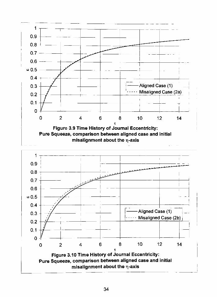
Figures 3.9 and 3.10 show map results for the midplane eccentricity ratio for Cases 2a

and 2b plotted against the eccentricity ratio calculated for Case 1. This is to directly compare

the midplane motion ofthe misaligned bearing to the aligned one. These figures show a

small increase in eccentricity rate as a result ofmisalignment. This increase is much more

pronounced Figure 3.10 which demonstrates the impact ofan initial misalignment ratio of 0.8

to the equivalent aligned case.

30

1

0.9

0.8

0.7

0.6

,0.5

0.4

0.3

0.2

0.1

0

Map Solution

Coarse Mesh

Fine Mesh

10 15 20 25

Figure 3.4 Time History of Journal Eccentricity:

Pure Squeeze, zero initial misalignment (Case 1)

31

--

1r-- - -

0.9 +-

08 -\ _L .

-

_Jw

0 7

!

06 -

J****"^

i

w0 5 Jr__L

0.4 -

0.3 -

0 2 -

Map Solution

Coarse Mesh

i

- - -

^ I I

/ 'Fine Mesh

0 1

0 -/

1

8 10 12


Pure Squeeze, specified misalignment about the q-axis

(Case 2a)

14

e

0.45

0.4

0.35

0.3

0.25

0.2

0.15

0.1

0.05

0

i

i

Map Solution

Coarse Mesh

Fine Mesh

\ - - -

\ ii

i

_ . I..

- - - ~ -

8 10 12

Figure 3.6 Time History of Journal Misalignment:

Pure Squeeze, specified misalignment about the q-axis

(Case 2a)

14

32

0.9

0.8

0.7

0.6

"w0.5

0.4

0.3

0.2

0.1

^^

- -- - -

J^f

f\i

/Map Solution

Coarse Mesh

/ I I/

/ !/ j j _ Fine Mesh

/ l

/ 1

0 8 10 12


Pure Squeeze, Specified misalignment about the q-axis

(Case 2b)

e

0.9

0.8

0.7

0.6

0.5

0.4

0.3

0.2

0.1

0

8 10 12


Pure Squeeze, Specified misalignment about the q-axis

(Case 2b)

14

i

II

i

\\

1

Map Solution\

- - - Coarse Mesh

Fine Mesh

I

I

- - 1 ..

j

14

33

1

0.9

0.8

0.7

0.6

0.5

0.4

0.3

0.2

0.1

y

Aligned Case (1)

Misaligned Case (2a)i

i

8 10 12 14


Pure Squeeze, comparison between aligned case and initial

misalignment about the q-axis

0.9

0.8

0.7

0.6

wO.5

0.4

0.3

0.2

0.1

0

\

I ,_3

^

*-

,"/

y

;/

Aligned Case (1)

Misaligned Case (2b )if

j

0 8 10 12 14




34

3.1.3 Cases 3a and 3b: Pure Squeeze, InitialMisalignment about the -axis

Similar to Cases 2a and 2b, these cases demonstrate the effects of initial misalignment

about only one axis. The same initial misalignment magnitudes ofO = 0.4 and O = 0.8 are

used, but unlike the previous cases the misalignment is about the -axis only.

The eccentricity in the t, direction and the misalignment about the ^-axis for both

initial misalignmentmagnitudes are plotted in Figures 3.1 1 through 3.14. Again, strong

agreement between map and finite element solutions is found for the eccentricity ratio. The

map solution also follows the finite element predictions formisalignment about the x-axis

closely. For the larger initial misalignment, the map solution errs slightly higher than the

finite element results, while the opposite is true for the smaller initial misalignment.

The map results for the eccentricity ratio in these cases are also plotted against the

eccentricity ratio calculated for the aligned squeeze film case (Figures 3.15 and 3.16).

Though smaller than the change in eccentricity ratio rate resulting from misalignment about

the x-axis, an increase in eccentricity ratio rate can also be observed in these squeeze film

cases.

Although this problem is not symmetric, a balance of forces results in no change in

misalignment about the q-axis and no change in eccentricity in the q direction. As a result,

boths71

andOn

remain equal to zero for the duration ofthe analysis. This is due to the fact

that each end of the journal experiences equal film pressure forces. The pressures in the q

direction oppose each other and align the bearing while the pressures in the , direction

counter the applied load F.

A significant point of interest in these cases is that the misalignment dies out at

approximately halfofthe rate as in the previous cases. Thisis most likely due to the fact

that, for equivalent magnitudes ofmisalignment and eccentricity, smallerminimum film

thicknesses occur when the projection ofthe journal axis is parallel to the eccentricity vector.

The smaller film thickness results in greater maximum film pressures. Higher film pressures

result in greater rates ofalignment.

35

1

0.9

0.8

0.7

0.6

*co0.5

0.4

0.3

0.2

0.1

/* i I/ \

/ \

/ jMapSolu tion

eshi- - - Coarse M

11-!

_ pjne |\/|es

^i

1i

10 15 20


Pure Squeeze, specified misalignment about the ^-axis

(Case 3a)

u/1

e

Map Solution

Coarse Mesh

Fine Mesh

25



(Case 3a)

36

1

0.9

0.8

0.7

0.6

^wO.5

0.4

0.3

0.2

0.1

__J-

^_

--

t"

^^

X

/ \ -J

i-

Map Solution- - Coarse Mesh-

.. Fine Mesh

I

10 15 20



(Case 3b)



(Case 3b)

25

37

1

0.9

0.8

0.7

0.6

u 0.5

0.4

0.3

0.2

0.1

y^H

Aligned Case (1)

Misaligned Case (3a)

, [ I

8 10 12 14



misalignment about the ^-axis

0.9

0.8

0.7

0.6

"0.5

0.4

0.3

0.2

0.1

0

' Z&*^^

'

J^\ '

'/ I

i i

y

fy Aligned Case (1)

Misaligned Case (3b)

n

/

10 12 14



misalignment about the ?-axis

38

3.1.4 Cases 4a and 4b: Pure Squeeze, InitialMisalignment45

from the Force Vector

To compare the effects of combining misalignment about both the % and q axes, this

simulation was initialized with equal misalignment about each axis. The same two initial

normalized misalignment magnitudes were used in these cases as with the previous two.

The results from these analyses are plotted in Figures 3.17 through 3.24. Similar

behaviors can be seen for both initial misalignmentmagnitudes. The map curves for bothz%

ando)'1

are nearly indistinguishable from the finite element results. The values for

misalignment about the -axis predicted by the map also agree reasonably well with the finite

element solutions. In these cases, the misalignment resulted in some journal motion

perpendicular to the force vector. This motion is captured in Figures 3.18 and 3.22, the plots

of en. In both cases the maximum eccentricities perpendicular to the force caused by

misalignment were very small. A noticeable relative error in the map model is observed near

the peak inen

for the curves generated by both initial misalignment magnitudes. The

absolute magnitude of these errors is very small.

Figures 3.25 and 3.26 demonstrate the impact of this type ofmisalignment on

eccentricity ratio. As with misalignment purely about the t, and q axes, a small increase in

eccentricity ratio rate can be observed. The increase appears to be of a magnitude greater

than that occurring as a result ofmisalignment about the ^-axis only but less than what was

caused by misalignment solely about the q-axis. This is a logical trend considering

misalignment in Case 4 is a combination ofthe misalignments in Cases 2 and 3.

3.1.5 Case 5: Pure Squeeze, Arbitrary Initial Journal Location

In order to validate the curve fits created in this study, they need to be tested for an

arbitrary set of initial conditions. Thisfinal pure squeeze case uses the initial conditions

listed in Table 3.2.

The transient response of the journal is plotted in Figures 3.27 through 3.30.

Excellent agreement between finite element results and the map solutions is seen for all

parameters with the exception ofOl This parameter, while still following the finite element

results closely, trends slightly lower thanthe accepted values.

39

1

0.9

0.8

0.7

0.6

^wO.5

0.4

0.3

0.2

0.1

J

1

_ _

'"*"*"

"'

1

tion

esh

iviap ooiu

- - - Coarse M

- Fine Mes

0 10 15 20


Pure Squeeze, specified misalignment45

from the load

(Case 4a)



from the load

(Case 4a)

25

40

eo.15

Map Solution

Coarse Mesh

Fine Mesh

10 15 20



from the load

(Case 4a)

25

0.3

0.25

0.2

00-15

0.1

0.05

r

IIL. -

Map Solution

- - Coarse Mesh

Fine Mesh! ii-

I

r_L

!i

\

"^^"- - -'-- - - ' --""

10 15 20



from the load

(Case 4a)

25

41

CO

1

0.9

0.8

0.7

0.6

0.5

0.4

0.3

0.2

0.1

Map Solution

- - Coarse Mesh

t

i

I- Fine Mesh

I III

10 15 20



from the load

(Case 4b)

CO

-0.005

-0.01

-0.015

-0.02

-0.025

-0.03

-0.035



from the load

(Case 4b)

25

I:> 1 0 15 20 25

^r i !I

/,

i

Y i r

Map Solution

\ /" - - Coarse Mesh

Fine Mesh

VJ

42

0.6

Map Solution

Coarse Mesh

Fine Mesh

10 15 20



from the load

(Case 4b)

Map Solution

Coarse Mesh

Fine Mesh



from the load

(Case 4b)

25

43

1

0.9

0.8

0.7

0.6

0.5

0.4

0.3

0.2

0.1

- -

I

/

Alianed Case (Vs

Misaligned Case (4a)!

0 8 10 12 14



misalignment45

from the load q-axis

1

0.9

0.8

0.7

0.6

w0.5

0.4

0.3

0.2

0.1

0

I

,-;

!

y"1

.'/

Aligned Case (1)


J

8 10 12 14



misalignment45

from the load q-axis

44

~L

Map Solution

Coarse Mesh

Fine Mesh

20

-0.4


Pure Squeeze, specified misalignment and eccentricity(Case 5)

0.35

-Map Solution

- Coarse Mesh

Fine Mesh

0 10 15 20


Pure Squeeze, specified misalignment and eccentricity

(Case 5)

25

25

45

0.35

e

0.3

0.25

0.2

0.15

0.05

Map Solution- Coarse Mesh

- Fine Mesh

0 10 15 20


Pure Squeeze, specified misalignment and eccentricity(Case 5)


Pure Squeeze, specified misalignment and eccentricity

(Case 5)

25

0 35 -,

n "3

1

u.o

n or iu.za 1

1I

ition

lesh

h

n o-

iviap OOII

- Coarse i\\J.. T 8

1

F. nn

~

rine ivies

>0i U. ID

U.T

\u.uo

v_) J

0 1 5

I

u

(

-0.05J

i 20 25

46

It is evident from this comparison that curve fits presented in this study are capable of

calculating journal motions comparable to those found using finite element solutions under a

variety ofjournal orientations.

3.2 Steady Rotation

While pure squeeze solutions have academic (and some practical) value, they do not

completely capture the conditions experienced by journal bearings in real world operation.

This section presents transient solutions for bearings with constant rotational speeds that

reach a steady-state journal position.

Because journal rotation has a time component, the dimensionless time constant, x,

used for the constant rotational speed problems is defined by

x = o)jt (3.2)

The addition of rotation increases the number of independent variables that must be

considered. The squeeze film solutions were valid for all bearings with equal L/D ratios

because the dimensions ofthe bearing are accounted for in the definition ofthe time constant.

Here the dimensional parameters are combined to create a new dimensionless parameter/as

defined by

(33)pLDojj

A variation in/can result from a change in applied force or journal speed because of its

linear relationship with these two parameters.

Similar to the pure squeeze analyses, a number of cases with various initial conditions

have been run to compare the map results to those found using a complete finite element

analysis. The value of/and the initial journal orientations used in each of these cases are

listed in Table 3.3. These cases are discussed in detail in the following sections.

47

Table 3.3: Initial Journal Position and Constant value of/for Steady Rotation Cases

Case s^ en & O^

/

6a 0 0 0 015/*-

6b 0 0 0 0 15/(4*-)

7a 0 0 0 0.415/*-

7b 0 0 0 0.815/*-

7c 0 0 0 0.4 15/(4*-)

7d 0 0 0 0.8 15/(4*-)

8a 0 0 0.4 015/*-

8b 0 0 0.8 015/*-

8c 0 0 0.4 0 15/(4*-)

8d 0 0 0.8 0 15/(4*-)

9a 0 0 0.282843 0.28284315/*-

9b 0 0 0.565685 0.56568515/*-

9c 0 0 0.282843 0.282843 15/(4*-)

9d 0 0 0.565685 0.565685 15/(4*-)

10 -0.05 -0.6 0.2 0.615/*-

3.2.1 Case 6a and 6b: Steady Rotation, Zero Initial Misalignment

As in Case 1, the bearing begins with no initial misalignment or eccentricity. These

cases demonstrate the accuracy ofthe aligned bearing mobility map modified to account for

misalignment. Figures 3.31 through 3.34 show the eccentricities predicted by the map model

as it compares to the finite elementmodels. The map curve follows the finite element curve

closely with little error.

48

0.8

0.7

0.6

0.5

,0.4

0.3

0.2

0.1

0

i

!

I

M-ip Solution

arce Mp<:h/ I

Ma

- - - Co

IFine Mesh

1 1


Steady Rotation, zero initial misalignment (Case 6a)

0.5

0.45

0.4

0.35

0.3

,0.25

0.2

0.15

0.1

0.05

0

I Jr"

fI

M-ip Solution

arse Mesh

e Mesh

ivia

- - - Co

_l..... pjn 1

1


Steady Rotation, zeroinitial misalignment (Case 6a)

49


Steady Rotation, zero initial misalignment (Case 6b)

10

p0.3


Steady Rotation, zero initial misalignment (Case 6b)

50

3.2.2 Cases 7a-8d: Steady Rotation, InitialMisalignment about the -axis or q-axis

Cases 7a through 8d are the rotational equivalent of cases 2a through 3b. Cases 7a

through 7d have initial misalignment only about the q-axis while cases 8a through 8d are

initially misaligned only about the -axis. The rotational component in these cases causes

the journal to move offof the load line towards its steady state location. This motion results

in eccentricity in the q direction and the misalignment vector to change direction. These

behaviors were not present in the squeeze film cases where a balance of forces prevented the

misalignment vector from changing direction. The data for these cases is graphed in Figures

3.35 through 3.66.

As with the squeeze film cases, the eccentricity ratio for each case with initial

misalignment is graphed against the equivalent aligned case. Figures 3.67 through 3.74 show

a greater eccentricity rate early on in the transient when misalignment magnitudes were

greatest. This is consistent with the observations made about the squeeze film cases. From

these graphs it is also apparent that the eccentricity ratios in simulations with smaller values

of/are more heavily influenced by misalignment.

For all of these cases, the map-based results follow the finite element results closely

for *% sn. The value ofO"1

in cases 7a through 7d, which initially have misalignment only

about the q-axis, also matches the finite element results. The misalignment about the c^-axis

shows a large relative error near its peak for these four cases. The absolute magnitude of this

error is, however, quite small, and the map curve does follow the same shape as the finite

element curves.

Similarly, cases 8a through 8d show strong agreement between the map results and

the finite element results for values ofO^. In these cases a noticeable relative error occurs at

the peak value of O"1, which had an initial value ofzero.

In the squeeze film solutions it was observed that the rate ofalignment in cases 2a

and 2b was significantly greater than in cases 3a and 3b respectively. This difference in

alignment rate is less pronounced in bearings with constantrotation. Additionally, it appears

that the higher the value of/ the closerthe alignment rates about the two axes become to

equal. This is a reasonable conclusion because therotation term in the mobility rate equation

for bearings with rotation, Equation 2.33, becomesdominant as/increases.

51

0.8

0.7

0.6

0.5

ioO.4

0.3

0.2

0.1

M-ip Solution

arse Mesh

Ma

-

- - - Co.i

Fine ivib&m

8

\1


Steady Rotation, specified misalignment about the q-axis

(Case 7a)

0.5

0.45

0.4

0.35

0.3

,0.25

0.2

0.15

0.1

0.05

0

I

t

!

M-ip Solutionivia

- - - Coarse Mesn

Fine Mesh

0 12 3 4 5 6

T


Steady Rotation, specified misalignmentabout the q-axis

(Case 7a)

52

-$-

-Map Solution

- Coarse Mesh

Fine Mesh



(Case 7a)

e

0.45

0.4

0.35

0.3

0.25

0.2

0.15

0.05

0

-0.05

i

1

i Map Solution

- - - Coarse Mesh

- Fine MeshIi

i

1

\ |.

vV

0'

r

> :\c5 i > 7


Steady Rotation, specifiedmisalignment about the q-axis

(Case 7a)

53

m.,/n;,m-m.\au wm,tM*mu<ty,<<mi<<mMm-"**---'i--'m--u>.

Map Solution

Coarse Mesh

Fine Mesh



(Case 7b)

n ^u.o

0.45 -

0.4 -

0.35 -

0.3

p0.25 -

0.2

0.15 -

0.1 -

0.05 -

I

AI

Map Solution

- - - Coarse Mesh

-

- Fine Mesh

U

(

c

5 12 3 4 5 6/


Jteady Rotation, specifiedmisalignment about the q-axis

(Case 7b)

7

54



(Case 7b)

0.9

0.8

0.7

0.6

0.5

e.4

0.3

0.2

0.1

0

-0.1

jI I

Li

"ii !

-U-

Map Solution

- Coarse Mesh

Fine Mesh11

1i

0 2I '-1 4 5 6 7



(Case 7b)

55

0.5

0.45

0.4

0.35

0.3

"wO.25

0.2

0.15

0.1

0.05

0

Map Solution

Coarse Mesh

Fine Mesh

0 8



(Case 7c)

Fw0.3


Steady Rotation, specified misalignmentabout the q-axis

(Case 7c)

10

56

0.01

8

Map Solution

Coarse Mesh

Fine Mesh

10



(Case 7c)

0.45



(Case 7c)

I !

57

0.5

0.45

0.4

0.35

0.3

"wO.25

0.2

0.15

0.1

0.05

0

"-

Map Solution

- - Coarse Mesh

............ pjne Mesh

l_

1

i0 2 4 6 8

i


Steady Rotation, specified misalignment about theq-axis

(Case 7d)

1.0.3

Figure 3.48 Time History of JournalEccentricity:

Steady Rotation,specified misalignment

about the q-axis

(Case 7d)

10

58



(Case 7d)

n q

0.8 -

0.7 -

0.6 -

0.5 -

eo.4-

0.3

0.2

0.1 -

0 -

r

Map Solution

- - Coarse Mesh

Fine Mesh

0) : > t \ < 5 {J 1-U. 1

i

Figure 3.5

Steady Rotati

0 Time Histor

on, specified

(d

y of Journal

misalignmen

ise 7d)

Misalignment

t about the q-axis

59

0.8

0.7

0.6

0.5

"coO.4

0.3

0.2

0.1

nyinp Solution

arse Mesh

e Mesh

Ma

- - - Co

Pinrin

1


Steady Rotation, specified misalignment about the -axis

(Case 8a)

0.5

0.45

0.4

0.35

0.3

po0.25

0.2

0.15

0.1

0.05

0

0 1 2 3 4 o t


Steady Rotation, specifiedmisalignment about the -axis

(Case 8a)

Mip Solutionivia

- - - Coarse Mesn

_ Fine Mesh

60

-Map Solution

Coarse Mesh

Fine Mesh

1

2_ :3 4 5 6


Steady Rotation, specified misalignment about the ^-axis

(Case 8a)

0.018

Map Solution

Coarse Mesh

Fine Mesh



(Case 8a)

61

0.8

0.7

0.6

0.5

"coO.4

0.3

0.2

0.1

0

--

_,

T

i

i

i

Mnp Solution

arse Mesh

e Mesh

Ma

-

- - - Co

Cinrin

f1


Steady Rotation, specified misalignment about the -axis

(Case 8b)

0.5

0.45

0.4

0.35

0.3

p0.25

0.2

0.15

0.1

0.05

0

I '

I

i

I

IMap Solution

- - - Coarse Mesh

\ Fine Mesh



(Case 8b)

62

n o. _,u.o i"

0.8 - 4

0.7 -

r r

0.6

| I Map Solution

r\ k 1 ' i- - - Coarse Mesh

U.o -1

_ _ ._

Fine Mesh

U.4

U.o

1

U.z-

0.1

0

-01-

V-*^Ji

!) 1 2 3 4 L 6 7


Steady Rotation, specified misalignmentabout the -axis

(Case 8b)

Figure 3.58 Time History ofJournal Misalignment:

Steady Rotation,specified

misalignment about the i;-axis

(Case 8b)

63



(Case 8c)

rco0.3


Steady Rotation, specifiedmisalignment about the i;-axis

(Case 8c)

64

Map Solution

Coarse Mesh

Fine Mesh

8



(Case 8c)

Map Solution

Coarse Mesh

Fine Mesh

-0.01


Steady Rotation, specifiedmisalignment about the 4-axis

(Case 8c)

10

10

65

0.5

0.45

0.4

0.35

0.3

^w0.25

0.2

0.15

0.1

0.05

0

- -

'

^***"**-"%.

1i

j-

Map Solution

- - Coarse Mesh

_ pjne Mesh

1 ! -

1-

J

6 8


Steady Rotation, specified misalignment about the ,-axis

(Case 8d)

Map Solution

Coarse Mesh

Fine Mesh

8


Steady Rotation, specifiedmisalignment about the 4-axis

(Case 8d)

10

10

66

Map Solution

- - - Coarse Mesh

Fine Mesh


Steady Rotation, specified misalignment aboutthe 4-axis

(Case 8d)

Map Solution

- Coarse Mesh

Fine Mesh

Figure 3.66 Time History of JournalMisalignment:

Steady Rotation,specified misalignment

about the c^-axis

(Case 8d)

67

0.9

0.8

0.7

0.6

0.5

0.4

0.3

0.2

0.1

0

Aligned Case (6a)

Misalianed Case (7a^

I

l

1

0 0.5 1 1.5 2

t

2.5 3.5


Steady Rotation, comparison between aligned case and


u

0.9

0.8

0.7

0.6

0.5

0.4

0.3

0.2

0.1

0

,*^r

/yi

1

/

1

'

1 Aligned Case (6a)I Misaligned Case (7b)

1l

0 0.5 1 1.5 2

x

2.5 3.5




68

0 2 4 6 8




10

CO

0.7

0.6

0.5

0.4

0.3

0.2

0.1

?z~z_=-

"

-_

.'yr

/ /

' /

I

Aligned Case (6b)

,J

Misaligned Case (7d)

j

10


Steady Rotation, comparisonbetween aligned case and


69

0.9

0.8

0.7

0.6

0.5

0.4

0.3

0.2

0.1

0

// I

iAligned Case (6a)

Misaligned Case (8a) _

I

0.5 1 1.5 2.5 3.5



initial misalignment about the ^-axis

0.9

0.8

0.7

0.6

0.5

0.4

0.3

0.2

0.1

0

jr

//

7

/

Aligned Case (6a) f

Misaligned Case (8b)/

1

1

I

0.5 1.5 2

x

2.5 3.5


Steady Rotation,comparison between aligned case and

initial misalignment about the-axis

70

0.7

0.6

0.5

0.4

0.3

0.2

0.1

0

- _

\y^

Aligned Case (6b)

Misaligned Case (8c) ;I

8



misalignment about the i^-axis

10

0.7

0.6

0.5

0.4

0.3

0.2

0.1

!I

i

sy

tf

/Aligned Case (6b)

7 Misaligned Case (8d)

_^

1

8 10



misalignment about the -axis

71

3.2.3 Cases 9a-9d: Steady Rotation, InitialMisalignment45

from the Force Vector

These cases demonstrate the effect ofmisalignment about both axes on a bearing with

constant rotation. The transient behavior ofthe bearing is plotted in Figures 3.75 through

3.90. These graphs show agreement between the map curves and the finite element solution

curves.

Figures 3.91 though 3.94 show the midplane eccentricity ratios of these cases as

compared to the matching aligned cases (6a and 6b). Again, an increase in eccentricity rate

is observed as a result ofmisalignment.

3.2.4 Case 10: Steady Rotation, Arbitrary Initial Journal Location

To supplement the validation begun in Case 5, a constant rotation problem with

arbitrary initial conditions is tested in this case. The initial parameters chosen for this case

are listed in Table 3.3.

The map-based results for e^, e'1, andO*1

compare very favorably with the finite

element-based results. The map calculated curves of& follow the same trend as the finite

element curves but do not carry the same degree of accuracy as the other parameters. Plots of

these quantities are given in Figures 3.95 through 3.98.

3.2.5 Cases 11a and lib: Steady Rotation, Variable Load

The final steady rotation cases differ from the others in that the load varies with time.

They are intended to mimic the cyclical loading conditions experienced by many real world

bearings, such as those found in combustion engines. These cases are presented in a

dimensional manner because the load is not constant.

The bearing parameters used for these analyses are given in Table 3.4. The periodic

load history applied to the bearings is plotted in Figure 3.99. The initial conditions used in

these cases are listed in Table 3.5. The initial eccentricity that was used was chosen because

it falls on the orbital path ofthe bearing when it reaches its cyclical steady state condition.

72

0.8

0.7

0.6

0.5

"coO.4

0.3

0.2

0.1

0

.

M-ip Solution

arse Mesh

e Mesh

Ma

-

- - - Co.

. Pin

l_rin

-I

1


Steady Rotation, specified misalignment45

from the load

(Case 9a)

0.5

0.45

0.4

0.35

0.3

,0.25

0.2

0.15

0.1

0.05

0

Mip Solutionivia

- - - LOaibt; iviesn

Fine Mesh


Steady Rotation, specifiedmisalignment

45

from the load

(Case 9a)

73

0.3

0.25

0.2

0.15

0.1

0.05

-0.05

! i

-

M-ip Solution

arse Mesh

ivia

- -

-Co

_ pjne Mesh

VVtion ^Ni

L

\

0 2 3 4 J > 6 \



from the load

(Case 9a)

0.3

0.25

0.2

0.15

0.1

0.05

-0.05



45

from the load

(Case 9a)

I

I1

!

Map Solution

- - - Coarse Mesh

Fine Mesh-1

\

\V

0*> \ *1 ! 5 i > 7

74

0.8

ffliwiTlwlf'-f ffflm

Map Solution

Coarse Mesh

Fine Mesh

0 1



from the load

(Case 9b)

p*0.2



45

from the load

(Case 9b)

75

Map Solution

Coarse Mesh

Fine Mesh



from the load

(Case 9b)

0.6

0.5

0.4

0.3

0.2

0.1

0

-0.1

Ij

lI1

1Map Solution

- - - Coarse Mesh

Fine Mesh

\

0

]; > c) * I ^5 ( 5 1



from the load

(Case 9b)

76

Map Solution

Coarse Mesh

Fine Mesh

8



from the load

(Case9c)

pw0.3



45

from the load

(Case9c)

10

77

Map Solution

Coarse Mesh

Fine Mesh



from the load

(Case9c)

Map Solution

Coarse Mesh

Fine Mesh

10

-0.05



45from the load

(Case9c)

78

Map Solution

Coarse Mesh

Fine Mesh

0 2 4 6 8

T



from the load

(Case 9d)

10

Map Solution

- Coarse Mesh

Fine Mesh



from the load

(Case 9d)

10

79

-Map Solution

- Coarse Mesh

Fine Mesh



from the load

(Case 9d)



45

from the load

(Case 9d)

80

CO

0.9

0.8

0.7

0.6

0.5

0.4

0.3

0.2

0.1

0

" ' ["""

i

Aligned Case (6a)

Misaliqned Case (9a)

I

0.5 1 1.5 2

x

2.5 3.5



initial misalignment45

from the load

0.9

0.8

0.7

0.6

0.5

0.4

0.3

0.2

0.1

0

- " ' ""*~

AH

-^

ii-

'/

fAligned Case (6a)

Misaligned Case (9b) '

1

j

1

0.5 1.5 2

x

2.5 3.5




from the load

81

0 8 10




from the load




from the load

82

""7^ 1 1 1ilBuriliMfflnJIbiiJmmJBBiifiiBhHi

-w.-f-*.-w-*"-

Map Solution

Coarse Mesh

Fine Mesh


Steady Rotation, specified misalignment and eccentricity

(Case 10)

CO

0.6

0.4

0.2

0

-0.2

-0.4

-0.6

-0.8

~11 '

y^

l

i

_^_

2Z*

I vJ '1

_jL_t

\

t 6i 1

\

Map Solution

- - - Coarse Mesh

- Fine Mesh/

tz 1-1

i

! i


Steady Rotation, specifiedmisalignment and eccentricity

(Case 10)

83

Map Solution

Coarse Mesh

Fine Mesh

0.7

0.6

0.5

0.4

0.3

0.2

0.1

0

-0.1


Steady Rotation, specified misalignment and eccentricity

(Case 10)


Steady Rotation, specified misalignment and eccentricity(Case 10)

I i

i i

!Solution

>e Mesh

vlesh

\ Map >

- - - Coars\1 Fine 1

|

j

0f

i :i <X l5 {\

L 8

84

Table 3.4: Dimensional Parameters for Cases 11a and lib

Parameter Value

Lubricant Viscosity 50 mPa-s

Bearing Diameter 40 mm

Bearing Length 40 mm

Radial Clearance 20 pm

Journal Rotational Speed 500 rpm

Table 3.5: Initial Conditions for Cases 11a and lib

Parameter Case 11a Case lib

8^ 0.718375 0.718375

sn 0.024480 0.024480

& 0 0.65

o^ 0 0

Figures 3.100 through 3.103 show the midplane motion ofthe bearing for these two

cases. The bearing misalignment ratios are plotted in Figures 3.104 and 3.105. The

eccentricity magnitudes generated by the map functions for the aligned and misaligned cases

are compared in Figure 3.106.

The midplane motion in this case is effectively captured by the map equations. The

map-based misalignment ratio curves follow the same trends as the finite element curves but

err high in magnitude. The maximum error is approximately 0.025 which is dimensionally

about half a micron. The misalignment magnitude drops rapidly around 0.24 seconds

corresponding to the load increase atthe beginning ofthe second load cycle. The difference

in eccentricity magnitude between cases1 la and 1 lb also decreases significantly at that point

in the load history as seen in Figure 3.106.

85

2500

2000

1500

1000

500

-500

-Fx

"

/

0 0. D4 0. 38 0.12 0.16 0.2 o.:

Figure 3.99: Time History of one Load Cycle (Case 11)

86

1

0.8

0.6

0.4

0.2

0

-0.2

-0.4

-0.6

-0.8

-1

[ n

jlution

,

-

-- -

Map o(

- Coarse Mesn

\V

'

\ i

V i

4 /t \ 1 /o 2 OJ3\ 0 0.5

f

]_


Steady Rotation, variable load with zero initial misalignment

(Case 11a)

CO

1

0.8

0.6

0.4

0.2

0

-0.2

-0.4

-0.6

-0.8

Map Solution

Onareo Moch

0 0 1 \ 0 2 / 0 3 \o 4 / 0 5


Steady Rotation, variable load with zeroinitial misalignment

(Case 11a)

87


Steady Rotation, variable load with initial misalignment

(Case 11b)

-\I

0.8

0.6 -

0.4

0.2 -

>>

CO

0

-0.2

'

-0.4-

-0.6-

Map Solution

- - - Coarse Mesh

) 0 1 \ 0 2 / 0 3 \0 4 / 0 5

-0.8J

t


Steady Rotation, variable load withinitial misalignment

(Case 11b)

88


Steady Rotation, variable load with initial misalignment

(Case 11b)

0.2

0.15

0.1

0.05

0

-0.05

-0.1

-0.15

I / \

I * \

/ A Map Solution

*\

0 0 \ 0f 0 3 0.4 0.5

\ '7


Steady Rotation, variable load withinitial misalignment

(Case 11b)

89

0.9

0.8

0.7

0.6

0.5

0.4

0.3

0.2

0.1

0

Aligned Case (11a)


0.1 0.2 0.3 0.4 0.5 0.6 0.7



initial misalignment with variable load

90

Chapter 4: Conclusions and FutureWork

This study has shown that the dynamic behavior of a self-aligning journal bearing can

be effectively approximated with the closed form equations developed in Chapter 2 and

provided in Appendix B. This method can significantly reduce computation time without

sacrificing a large degree ofaccuracy.

Table 4.1 shows the time required to process Case 4b given in Chapter 3. These

calculations were run for 2500 fixed time steps using an Euler integration routine. The

calculations were performed on a machine with a 1.3 GHz processor speed and 128 Mb of

RAM. It is apparent that processing time is reduced by orders ofmagnitude when this

approximate solution is used instead ofthe finite element method.

Table 4.1 Comparison ofComputing Times (Case 4b)

Calculation Method Processing Time

Map Solution 0.47 sec

Coarse Finite ElementMesh 450 sec

Fine Finite ElementMesh 1555 sec

The effect ofmisalignment on the midplane motion ofa self-aligning bearing is

generally small. This is primarily due to the fact that the self-aligning property of these

bearings continuously reduces the magnitude ofmisalignment. From careful examination of

the equations presented in Appendix B, it can be observed that an increase in misalignment

magnitude will generally result in a greater modification to the aligned bearing mobility map.

Therefore, ifthese misalignments did not dissipate but were sustained (as would be the case

for an applied moment), one could conclude their impact on midplane motion would be

greater.

Comparisons between the midplane motion ofperfectly aligned bearings and of

misaligned self-aligning bearings revealsincreased eccentricity rates. This can be interpreted

as a decrease in load capacity. The knowledge that load capacity is decreased during the

91

aligning process raises concerns about the performance of these bearings under such

conditions.

It is clear from the results in Chapter 3 that the realignment process is not

instantaneous and that normalized alignment rates can be on the same order ofmagnitude as

eccentricity ratio rates. This leads to the conclusion that the minimum film thickness in a

self-aligning bearing can be significantly impacted by misalignment. This is ofparamount

concern because small film thickness can result in journal to sleeve contact and destructive

wear ofbearing surfaces.

From the steady rotation cases it is apparent that alignment rates are significantly

impacted by the value ofthe dimensionless parameter/ Greater values of this parameter

result in faster rates ofalignment. For a given bearing, an increase in/can be caused by an

increase in applied force or a decrease in journal rotational speed. This behavior can also be

seen in the dimensional problem: Case 1 1, where the load varies cyclically. A change in

alignment rate can be observed around the spikes in the load cycle (Figure 4.1). Therefore,

the factors ofbearing load and journal speed need to be considered carefully in evaluating

alignment rates of self-aligning bearings.

A natural extension ofthis work is to consider the effects ofmisalignment in

conventional bearings, that is to say bearings that are not designed to be self-aligning. For

such a study the moments transmitted through the fluid film would vary in magnitude and

direction instead ofbeing constrained to zero. This increases the number of factors that

impact journal motion. One approach to handing this type ofproblem would be to consider

the velocities imposed on the journal by the forces and the moments independently. This

decoupled approach would be based on the assumption that the velocities imposed by radial

forces and the velocities imposed by misaligning moments can be calculated separately and

summed to find the velocities for combined loading. Evidence of such decoupling can be

found in Boedo and Booker (2003).

To develop this method a set ofdimensionless parameters, similar to those found in

Eq. 2.24a-2.25b, would have to be derived for a bearing with an applied moment but no

applied force. The fundamental difference between this derivation and the one presented in

Chapter 2 would be changing the pressure constraintsimposed on the bearing film from Eq.

2.17a-2.18bto

92

0.8 -i

;

-Map Solution

-FEA Solution

Applied Load

- 2500

0 7

- 2000n r

0 sI;

a n id.

Vi

- 1500

z

n ^

I LL

- 1000u.o

0.2

0.1

\'<\^. '*

- 500

\

/

i0

D 0.1 0.2

T

1

0.4

Time (s) \\

Increased

Alignment Rate at

load peak

Figure 4.1 Time History of Journal Misalignment and Loading:

Variable Loading (Case 11)

93

F'=0=\Apcos9dA(41a)

F"=0=[psm9dA(41b)

M4= ^PRzsin9dA (4 lc)

M'= jApRzcos9dA (4 ld)

where

m =

*o (4.2)

Map solutions would then need to be created for these new parameters. Finally, squeeze film

journal motion for amisaligned bearing subject to both radial loading and misaligning

moments could then be calculated as follows:

s 4=M4 (e, <D,L/D)^^- + Vx (M, e,O,L/D) (4.3a)Li i 'I J

i"=M"(e,<S>,L/D)^^- + V2 (M, e,O,L/D) (4.3b)pLD

^=T4(e,0>,L/D)F^J +V3(M,s,<t>,L/D) (4.3c)

6"

^T"{E,a>,L/D)F^ +VA(M,E,q>,L/D) (4.3d)Li 1-jLJ

where Vt are the appropriate velocity components calculated from the maps for a bearing

with applied moment but no applied force.

Another possible extension of this work would be to consider the dynamic effects of

the sleeve. For these studies, the sleeve, mounted within a frictionless spherical bearing, was

assumed to have no mass. In a real self-aligning bearing, inertial effects would have to be

overcome during the alignment process. This effect would take the form ofa moment that

opposes changes in the aligning velocity. Accounting for this factor would slow alignment

rates, increase the impact ofmisalignment on journal midplane motion, and possibly result in

oscillations at the end ofthe alignment process.

94

The spherical socket, in which the sleeve is mounted, could also be modeled more

accurately. In reality it is a spherical bearing that is governed by fluid dynamic principles

similar to those used to model the journal bearing. Viscous forces in this bearing would

impose small moments on the journal bearing that oppose the aligning motion. This

enhancement to the model could also be expected to slow the aligning process.

95

Appendix A

Finite Element Based Aligned BearingMobilityMapFrom Goenka (1984)

Define

Then the aligned mobility approximation equations are:

n

where

A =^-0.24(L/DYe~[''4'^

and

Ml=--^-nf(t,L/D\E + F + G)

where

F =

-0.3(1/0)

G = -0.0161-

,+2#"7 +

15 pT7]0.034

(X/0)2

1

1.03-f J

96

Appendix B

Misalignment Adjustment Functions

Range ofValidity

The following adjustment functions are valid under these criteria:

0 < 9e < n

O < 0.93

s < 0.93

0.25 < L/D < 1

Convergence Criteria

Several adjustment functions contain infinite series ofthe form:

(=1

where

/,<1 and|/2|<l

These are convergent series and need only to be evaluated to a point where dropping the

remaining terms will not significantly impact the total ofthe series. The analyses performed

in Chapter 3 employ a convergence limit for the counter / that is satisfied when the following

statement is true:

D;(/1,ct)]'<io-

YXfM,)]fMj)

Derived Parameters

0=mCT=(i_0)

a=-i

-^"-*-">

(i-4)

97

Translational MobilityMagnitude Adjustment Function

M(s, O,L/D) = k(z, 0>,L/D) M0 (e, L/D)

K(e,O,L/D) = 1 + AK+BK cos(20,-

CK )

where

AK={l21-QA?>LlDlAK+AKBKcosee+AKBKCK\

where

aK= (0.585 -0.0277/13-5)d(183-0-27513)

6

= X[(0.96^)'cos((/ + l)^)];=1

and

flr = (l .28 - 0.57L/Z>R + rfrer cos 0e + dKeJK ]

where

^=(0.343-0.0184A226)-<d(17-0423^15)

eK =1.91

Act115

fK=i,lo.S7Acrl26)cos((i + l)0e)}

and

C = n + gK sint9e + gKhrsin(20e)+ gAA

-sin(30e)+ gA./X

where

gr=-0.937/-92cr(0'97-0'13i2)

^ = 0.54/lcr

y,=0.74Uo-

', =J[(0.98Aff)'

sin((z + 3)0.)]1=1

98

TranslationalMobility Direction Adjustment Function

y(t,&,L/D)=

y0(e,L/D) + S(e,,L/D)

5(e,V,L/D) = AS+BS cos(20,-

Cs )+ Ds sin(40, )

where

As = (1.3 - 0.58L/D\as sint9e + asbs sin(2t9e)+ a8bscs\

where

as=

[0.34l(d>156-O224)-0.0024 sin(3M))pl

bs=lASAcr122

cs= J[(0.99/Lcr)'sin((/ + 2)^)]

1=1

and

Bs = (l .27 - 0.53L/D\d5 + dses cos 0r + dsejs ]

where

ds =(0.425O2

-0.217CD363)-(l + 3.27A2

cr585)

^=1.92Act13

A =X[(0.917^cr,125)cos((z + l)^)]/=i

and

Cs=-x/2 + gssm0e+gshs

where

gs= -0.976

Act1.13

^=|][(0.539Ac717)sin((/ + l)69e)]<=i

and

D, = (l.36-0.16L/D\js+jspscos0e+ jspsqs]

where

99

/,=/,-(0.0346cp168+/5)^+

where

/5=-0.0506cD3,+ 0.0167O8

p5=5AaX31a26"

**=E[(0.44/>Jcos((i + l)60]1=1

Rotational Mobility Functions in the ^-direction

T4=

A4 [b^ sin 6t + C4 cos 0t ]where

Ag=0A32(L/D- 0.0924

)"152-

sin 6>e[o.0269 + 0.046 l(l -L/D)

and

Bi=

a^ sin 9e + b4 sin(2t9e )

where

a(= -7.19(a -o-")^,

^=5.09(c72-cr25)^2

and

Cs=cs+ di cos 0e + d^ei cos(2c9e )

where

c#=-8.68cD +

3.25cD115

ds= 7.56(d) -O2)^

^=(-0.14A +0.058A2)tr2

2,25

100

RotationalMobility Functions in the q-direction

Tr'={Au+Bri)[sm0,+Cncos0,}

where

Av=0.126(1/^-0.037)-'

M[a, + *7cos(20,)]where

an=-13.9<D +

3.88d)2

\=-3.h{cj2-(j21)a2

and

Bn=3.7325(Z,/>)-203(o-12

-a]9)Acos0e

and

C=

dn sin 0e + dnen sin(2t9e )+ rf^/

where

dn=(0.171o-

+0.052cr2

-0.062ct3)a

e^ =0.2152

/7=(0.75^ysin((i + 2)9.)<=i

101

Appendix C

Reference Tables ofResults

These values are provided for the reader's reference.

Translational Mobility Adjustments

L/D O s 9e 9d) K 8

0.5 0.1 0.8 0.785398 1.047198 1.0257 0.00719

0.5 0.2 0.5 0.785398 0.785398 1.0655 -0.01249

0.25 0.4 0.4 0 1.047198 1.3619 -0.11101

0.75 0.5 0.2 1.047198 0 1.0603 0.00431

1.00 0.7 0.1 1.047198 0.785398 1.2681 -0.10706

RotationalMobility Equations

L/D O s ee &4,JlX j,y

0.5 0.1 0.8 0.785398 1.047198 -0.23832 -0.19164

0.5 0.2 0.5 0.785398 0.785398 -0.44681 -0.51721

0.25 0.4 0.4 0 1.047198 -1.29090 -3.72987

0.75 0.5 0.2 1.047198 0 -0.56070 -0.04004

1.00 0.7 0.1 1.047198 0.785398 -0.38117 -0.70035

102

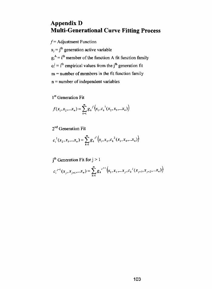
Appendix D

Multi-Generational Curve Fitting Process

/= Adjustment Function

Xj=f1

generation active variable

giA

=i*

member ofthe function A fit function family

d"" =i*

empirical values from thej*

generation fit

m=number ofmembers in the fit function family

n=number of independent variables

1st

Generation Fit

f(xl,x2,..Jcn) = Ydg/(x1,cki(x2,x3,...xn))

2nd

Generation Fit

c,\x2,x3,...x)= Y.Sk \xl,x2,ck2(x3,x4,...xn)j

*=1

jth

Generation Fit for j > 1

mj i / \

c,i~\xj,xj+l,...x)= Y,Sk \x1,x1,...xJ,ckJ(xJ+1,xJ+2,...xn)j

103

Appendix E

Flowchart ofLogic for Bearing Orbit Calculation usingMobilityMaps

Given at an instant (t;)ex,ey,c(.x,ct.y

(computation frame)

Transform force and journal

position vectors into

F5, F\ e5, e*1, \ and ^(map frame)

Convert journal position

vectors to dimensionless form:

e\ sn,\ andOt1

Calculate M5, Mn, T5, andT"

using mobility maps

(Appendices A and B)

Calculate dimensionless

squeeze film journal velocities:

e\ s\ &s, and <b\(Equations 2.24a-2.25b)

Convert squeeze film journal

velocities into dimensional

form:

e%, e\ <j>4s, and ty\

Given for all time t

Fx, Fy, coj and cos

(computation frame)

Calculate journal position at

the next time step (t;+i)ex,ey,.f,<|>y

(Euler's method)

Account for journal rotation to

get ex, ey, (fx, and<jiy

(Equations 2.34-2.36)

Transform vectors into

e\, eys, cfc, and (fys(computation frame)

104

Appendix F

Axial Spacing for Non-Uniform Meshes

From Boedo and Booker (2003)

The physical layout of a mesh created using this spacing technique is given in Figure 3.3.

Given a mesh with m axial divisions at each end, a dimensionless length of z as defined in

Eq. 2.8, and a spacing ratio of S, the axial nodal coordinates are given in the following

equations:

z0=0

z/+1=z,.+j>/^

where

fm-i \

^;sj+m--i

U= /

so that

zl= A

I2=A(l +S'i)

z3 =A(l + 5_1+5"2)

105

References

Boedo, S., and Booker, J.F. (2003). Classical BearingMisalignment and Edge Loading: A

Numerical Study ofLimiting Cases, Proc. STLE/ASME Joint International TribologyConference, Oct. 26-69, 2003.

Booker, J. F. (1965). Dynamically Loaded Journal Bearings: Mobility Method of Solution,ASME Journal ofBasic Engineering, Vol 87, pp. 537-546.

Booker, J.F. (1971). Dynamically-Loaded Journal Bearings: Numerical Application ofthe

Mobility Method, ASME Journal ofLubrication Technology, Vol 93, pp. 168-174.

DuBois, G.B., Ocvirk, F.W., & Wehe, R.L. (1955). Experimental Investigation of

Misaligning Couples and Eccentricity at Ends ofMisaligned Plain Bearings, NACA

Technical Note 3352.

DuBois, G.B., Ocvirk, F.W., & Wehe, R.L. (1957). Properties ofMisaligned Journal

Bearings, Transactions ofthe ASME, Vol 79, pp.1205-1212.

Falz, E. (1937), Principles ofthe Design of Journal Bearings. Proceedings ofthe General

Discussion on Lubrication andLubricants, Vol 1, pp. 93-100. Institution ofMechanical

Engineers, Great Britain.

Fuller, D.D. (1956). Theory andPractice ofLubricationfor Engineers. New York, Wiley.

Goenka, P.K. (1984A). Analytical Curve Fits for Solution Parameters ofDynamically

Loaded Journal Bearings. ASME Journal ofTribology, Vol 106, pp. 421-427.

Goenka, P.K. (1984B). Dynamically Loaded Journal Bearings: Finite ElementMethod

Analysis, ASME Journal ofTribology. Vol 106, pp. 429-439.

Khonsari, M.M. & Booser E.R. (2001). Applied Tribology: BearingDesign andLubrication.

New York, Wiley.

LaBouff, G.A., & Booker, J.F. (1985). Dynamically Loaded Journal Bearings: A Finite

Element Treatment for Rigid and Elastic Surfaces,ASME Journal ofTribology, Vol 107, pp.

505-513.

Pigott, R.J.S. (1941). Engine Design Versus Engine Lubrication,Transactions ofthe SAE,

Vol 48, pp. 165-176.

Pinkus, O., & Bupara, S.S. (1979). Analysis ofMisaligned Grooved Journal Bearings, ASME

Journal ofLubricationTechnology. Vol 101, pp. 503-509.

106

Dynamically loaded self-aligning journal bearings - RIT ...

Documents

Transcript of Dynamically loaded self-aligning journal bearings - RIT ...