An Efficient Method forDynamic Analysis of Gene Regulatory Networks

and in silico Gene Perturbation Experiments

Abhishek Garg, Ioannis Xenarios1, Luis Mendoza2, and Giovanni DeMicheli

Ecole Polytechnique Federale de Lausanne, Lausanne, Switzerland1 Merck Serono, Geneva, Switzerland

2 Instituto de Investigaciones Biomedicas, UNAM, Mexico{abhishek.garg,giovanni.demicheli}@epfl.ch,

ioannis.xenarios@merckserono.net, lmendoza@biomedicas.unam.mx

Abstract. With the increasing availability of experimental data ongene-gene and protein-protein interactions, modeling of gene regulatorynetworks has gained a special attention lately.Tohave abetter understand-ing of these networks it is necessary to capture their dynamical proper-ties, by computing its steady states. Various methods have been proposedto compute steady states but almost all of them suffer from the state spaceexplosion problem with the increasing size of the networks. Hence it be-comes difficult to model even moderate sized networks using these tech-niques. In this paper, we present a new representation of gene regulatorynetworks, which facilitates the steady state computation of networks aslarge as 1200 nodes and 5000 edges. We benchmarked and validated ouralgorithm on the T helper model from [8] and performed in silico knockout experiments: showing both a reduction in computation time and cor-rect steady state identification.

1 Introduction

The face of biological research has evolved at an alarming rate over the last twodecades. From a one-gene/one-protein analysis it has borne witness to a multi-tude of technologies that allows us to capture and integrate a vast amount ofinformation generated by high throughput methods such as DNA microarrays,siRNA knock-down and protein-protein interactions. While a wealth of informa-tion is present on the interaction of the genes and proteins, the exact stoichiom-etry and precise kinetics still evades our technologies and understanding. In suchsituation, one could either wait to gather the crucial information on the precisebiochemical processes or choose to model the flow of information in genetic regu-latory networks. We chose the latter as we think that the information is sufficientalready to identify qualitative behavior of the studied biological system. We alsoclaim that enabling such kind of approaches should further the understandingof the design and identifications of keys elements that dictate cell fate.

The methodology presented here is an improvement of the methods describedby [8] to model dicrete regulatory networks and proposes to use a data structure

T. Speed and H. Huang (Eds.): RECOMB 2007, LNBI 4453, pp. 62–76, 2007.c© Springer-Verlag Berlin Heidelberg 2007

An Efficient Method for Dynamic Analysis of Gene Regulatory Networks 63

called binary decision diagram (BDD) to represent and manipulate Boolean net-works. This data transformation enables the compact representation of the statespace of the network and their efficient dynamic analysis. BDDs have primarilybeen used in several other applications like logic synthesis and testing in thefield of Electronic Design Automation [21,22] and model checking [23,24]. In thispaper, we show their application on biological regulatory networks. Some workon modelling the gene regulatory networks using the formal methods have beenintroduced in [27,28,29].

We use the already published T helper cell regulatory network [8,7] as a frame-work to validate our approach and show that our software, GenYsis finds allsteady states and correctly identifies the outcome of gene perturbation experi-ments. We show that GenYsis scales well with the size of the network and cancompute cell states in the network with size over 1000 nodes in reasonable timeusing modest computing resources.

2 Binary Decision Diagrams

2.1 Introduction

A Binary Decision Diagram(BDD) is a directed acyclic graph consisting of a rootnode, intermediate decision nodes and two terminal nodes, namely 0-terminaland 1-terminal. BDDs can be used for representing Boolean functions. Eachvariable of the function is represented as a decison node of the graph. Eachdecision node has two outgoing edges to represent evaluation of variable to 1and 0. All paths from root node to 1-terminal gives the variable evaluations forwhich the function is true. There might be some variables missing in some of thepaths. These variables have a “Don’t Care” evaluation, i.e. they can take either0 or 1 value.

A simple BDD that represents the Boolean function f = (a AND b) OR cis shown in Figure 1.

It has three paths from root node (node f) to 1-terminal node. For the path,a

0−→ c1−→ 1, two possible assignments (a = 0, b = 1, c = 1) and (a = 0, b = 0,

c = 1) leads to 1-terminal from root node f . Similarly, the path a1−→ b

1−→ 1,

f

a

b

1

c

0

1

1

0

1

0

0

Fig. 1. BDD for the function f = (a ∧ b) ∨ c

64 A. Garg et al.

represents the assignments (a = 1, b = 1, c = 1) and (a = 1, b = 1, c = 0). Finallythe last path a

1−→ b0−→ c

1−→ 1 representing (a = 1, b = 0, c = 1) complete thefive possible TRUE evaluations for the Boolean formula f .

Here, we use Reduced Ordered BDDs (ROBDDs), which are the compactreduced form of BDDs. For the sake of brevity whenever we say BDD in thispaper, we are referring to ROBDDs.

The representation of Boolean functions as BDDs is memory efficient as iso-morphic subgraphs can be shared by multiple nodes. The size of the BDD scaleswell in most cases with the size of the Boolean function and all the logic op-erations like AND, OR, Existential quantification, Universal quantification, etc.can be performed in polynomial (with the size of the BDD) time on this datastructure [1]. This implicit representation does not require the explicit construc-tion of a truth table and can be directly constructed from the Boolean function.Further details on BDD construction and logic operations on them is outside thescope of this paper, interested readers can find details in [1,2,3].

There are many existing packages that can be used for working with BDDslike CUDD, CMUBDD, etc. In this paper we use the CUDD package [20], whichis the most efficient package for BDD representation and evaluation.

2.2 Representation of Gene Regulatory Networks

In this section we show how gene regulatory networks can be mapped to BDDs.We start with the representation of regulatory networks as Boolean functions andthen we use these functions to construct corresponding BDD representation.

Given a gene regulatory network, the state of a node (or gene) i at time t isrepresented with the Boolean variable xi(t). To evaluate the evolution in timeof each node, it is necessary to describe the state of each node at time t + 1 asa function of state of those nodes acting as input at time t [8]:

xi(t + 1) =

⎛⎝

m∨j=1

xaj (t)

⎞⎠ ∧ ¬

⎛⎝

n∨j=1

xinj (t)

⎞⎠ (1)

xi(t + 1) =

⎛⎝

m∨j=1

xaj (t)

⎞⎠ (2)

xi(t + 1) = ¬

⎛⎝

n∨j=1

xinj (t)

⎞⎠ (3)

xj ∈ {0, 1}xa

m and xinn are the set of activators and inhibitors of xi

∧ and ∨ represent logical AND and OR

Equation 1 is used if the gene i has both activators and inhibitors. Equation 2 isused if the gene i has only activators and equation 3, if there are only inhibitors.

An Efficient Method for Dynamic Analysis of Gene Regulatory Networks 65

In equation 1, inhibitors are strong enough to change the state of a gene from 1to 0, while activators can change the state from 0 to 1 if and only if there areno inhibitors acting on that gene.

A snapshot of the activity level of all the genes in the network at a time tis called the state of the network. The state of the network is represented bya Boolean vector of size N (number of genes in the network). Each bit of thisvector represents whether the gene is active or inactive. Another Boolean vectorof size N is used to represent the status of the genes at next step. We call theprevious vector as present state(Vt) and latter one as next state (Vt+1).

The transition between states of the network can be either synchronous andasynchronous. If the transitions are synchronous, all the genes change their stateat the same time point. If the transition is asynchronous, atmost one gene canchange its state between two consecutive states. Biologically, it is more realisticto assume that genes have different response times, and hence an asynchronousnetwork might seem more realistic. In this paper, we use the asynchronous modelto represent state transition of the regulatory network and assume that time pointsare close enough, so that only one gene can make a transition at each time point.

Now we shall see how the Boolean functions in equations 1-3 can be usedto construct a BDD representation. Let Ti(Vt, Vt+1) be the BDD representingtransition of gene i from Vt to Vt+1 and T (Vt, Vt+1) be the BDD representingthe transition from state of the network at time t to state at time t + 1. Therelation between Ti(Vt, Vt+1) and T (Vt, Vt+1) is given by equation 4. Equation4 says that all genes make asynchronous transitions and state of the network attime t can have multiple successor states.

T (Vt, Vt+1) = T0(Vt, Vt+1) ∨ T1(Vt, Vt+1) ∨ ... ∨ TN (Vt, Vt+1) (4)

To impose the constraint that two consecutive states differ in atmost one geneevaluation, we define Ti(Vt, Vt+1) in equation 5, which states that for gene i, itsevaluation at the next time step v′i(∈ Vt+1) and function fi(Vt)(= xi(t+1)) havethe same value, and all the other genes remain at their activation level from theprevious time step.

Ti(Vt, Vt+1) = (v′i ↔ fi(Vt)) ∧∧j �=i

(v′j ↔ vj

)(5)

Let us go through a small example to have a better understanding of theprocess.

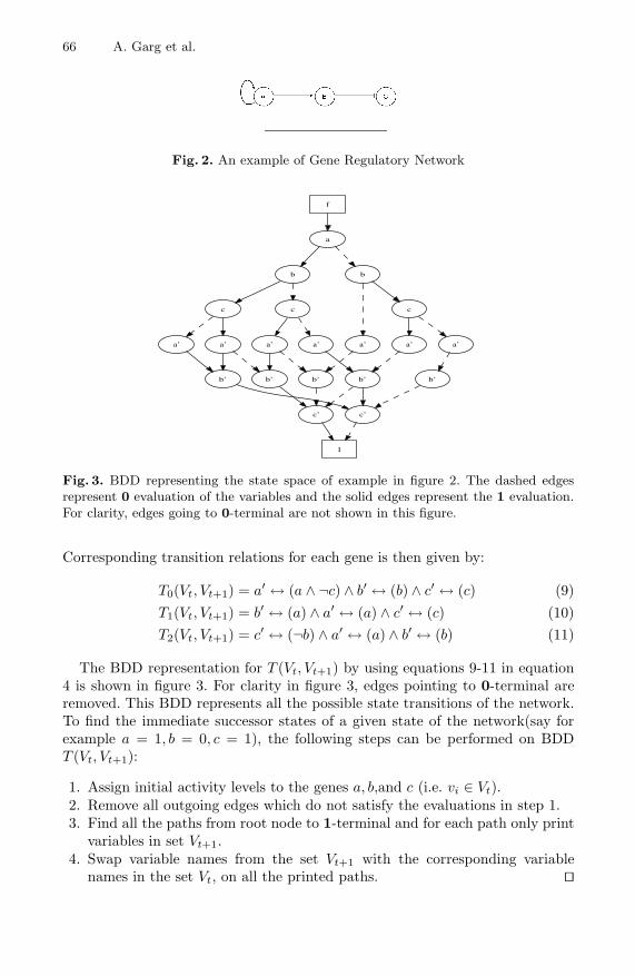
Example 1. In figure 2, gene ‘A’ has an auto-activation and is inhibited by thepresence of gene ‘C’. Gene ‘B’ is activated by the presence of gene ‘A’ andpresence of gene ‘B’ inhibits gene ‘C’. The present state and next state vectorsare given by Vt = {a, b, c} and Vt+1 = {a′, b′, c′} respectively. Boolean functionsdescribing this small network are given by:

a′ = a ∧ ¬c (6)b′ = a (7)c′ = ¬b (8)

66 A. Garg et al.

Fig. 2. An example of Gene Regulatory Network

f

a

b b

c c c

a’a’a’ a’ a’ a’a’

b’b’ b’ b’ b’

c’c’

1

Fig. 3. BDD representing the state space of example in figure 2. The dashed edgesrepresent 0 evaluation of the variables and the solid edges represent the 1 evaluation.For clarity, edges going to 0-terminal are not shown in this figure.

Corresponding transition relations for each gene is then given by:

T0(Vt, Vt+1) = a′ ↔ (a ∧ ¬c) ∧ b′ ↔ (b) ∧ c′ ↔ (c) (9)T1(Vt, Vt+1) = b′ ↔ (a) ∧ a′ ↔ (a) ∧ c′ ↔ (c) (10)T2(Vt, Vt+1) = c′ ↔ (¬b) ∧ a′ ↔ (a) ∧ b′ ↔ (b) (11)

The BDD representation for T (Vt, Vt+1) by using equations 9-11 in equation4 is shown in figure 3. For clarity in figure 3, edges pointing to 0-terminal areremoved. This BDD represents all the possible state transitions of the network.To find the immediate successor states of a given state of the network(say forexample a = 1, b = 0, c = 1), the following steps can be performed on BDDT (Vt, Vt+1):

1. Assign initial activity levels to the genes a, b,and c (i.e. vi ∈ Vt).2. Remove all outgoing edges which do not satisfy the evaluations in step 1.3. Find all the paths from root node to 1-terminal and for each path only print

variables in set Vt+1.4. Swap variable names from the set Vt+1 with the corresponding variable

names in the set Vt, on all the printed paths. ��

An Efficient Method for Dynamic Analysis of Gene Regulatory Networks 67

The steps given in above example can be implemented by using efficient logicfunctions such as “AND” and “Existential Quantify” along with the expressivepower of BDDs [1,2], as follows:

1. Construct a BDD ‘X’ which represents the initial state.2. Take logical ‘AND’ of BDD ‘X’ with the BDD T (Vt, Vt+1).3. Existentially quantify out variables in Vt from the resulting BDD.4. Swap variables v′i ∈ Vt+1 with vi ∈ Vt in the BDD got from the last step.

The BDD formed after executing step 4 represents all the immediate successorstates from a given initial state.

3 Computing the Steady States

In this section, we will see how to efficiently compute steady states on the BDDrepresentation of the gene regulatory networks. But first we shall give somedefinitions that we are going to use in the rest of the section. Let, f be the statetransition function.

Definition 1. Forward image, If (S(Vt)) is the set of immediate successors ofthe states in S(Vt) on the state transition graph.

Definition 2. Backward image, Ib(S(Vt)) is the set of immediate predecessorsof the states in S(Vt) on the state transition graph.

Definition 3. Forward reachable states FR(S0) from the states S0 are all thestates that can be reached from S0 by iteratively computing forward image in thetransition relation T (Vt, Vt+1) until no new states are reachable.

Definition 4. Backward reachable states, BR(S0), are all the states in T (Vt,Vt+1) whose forward reachable states contain S0.

Definition 5. Steady State is the set of states SS(Vt) having the following twoproperties:

1. Forward image If (SS(Vt)) is same as SS(Vt).2. For all the states in SS(Vt), if that state is reached once, then the probability

of revisiting that state is one. [19]

The first property of a steady state implies that there are only three possiblevariants of steady states as shown in figure 4. The second property of steadystate ensures that there are only simple cycles(figure 4(a) and 4(b)) in the setSS(Vps) and invalidates the third kind of steady state(figure 4(c)) with complexloops as some of the states in this loop might not be revisited. The first propertyis contained in the second property of steady states. An efficient algorithm canbe designed for finding steady states that satisfy the first property, though anyefficient algorithm satisfying property 2 is not known yet. Here we use the mod-ified algorithm by [18] for computing the set of steady states satisfying property1 and then remove the false steady states of type III (in figure 4) from that set.

68 A. Garg et al.

(a) Self Loop (b) Simple Loop (c) Complex Loop(false steady state)

Fig. 4. Different types of steady states

Algorithm [18] for computing steady states is based on two main theorems. Forthe sake of completeness of the paper, we present these theorems and algorithmshere again. Proof of these theorems can be found in [18].

Theorem 1. A state i ∈ S is a steady state if and only if FR(i) ⊆ BR(i). Statei is transient otherwise.

Theorem 2. If state i ∈ S is transient, then states in BR(i) are all transient.If state i is steady, then all the states in FR(i) are steady states. In the lattercase set {BR(i) − FR(i)} are all transient.

Based on these two theorems, the algorithm for steady state computation isgiven in Algorithm 2. Algorithm 2 uses the functions forward set() and back-ward set() for computing forward reachable (FR(S)) and backward reachable(BR(S)) states respectively. These functions are given in Algorithm 1. In Algo-rithm 1, FSk and RSk, are the frontier set and reachable set respectively in thekth iteration of the while loop. Frontier set (Backward set) in iteration k + 1,is computed by taking the forward (backward) image of the frontier (backward)set in the kth iteration and removing from this image set the states that havealready been explored in previous iterations (which are stored in Reached Set).Reached Set is updated by adding the new states from frontier(backward) set.This process is iterated until no new states can be added to Reached Set. Thefinal Reached Set represents the forward (backward) reachable set from the setof initial states S0.

The Algorithm 2 uses Theorems 1 and 2. In line 5 of Algorithm 2, a prospec-tive steady state is selected from the state space T ′ and forward and backwardreachable sets from this seed state are computed in lines 6 and 7. Then Theorem1 as implemented in line 8, checks if the seed state is a steady state. If the seedstate is indeed a steady state then using Theorem 2 (as implemented in lines9-12), all the states in forward reachable set are declared steady states in line 9and rest of the states in backward reachable set are declared transient states inline 10. Otherwise, the seed state and all the other states in backward reachableset are declared transient in line 12. In line 13, state space is reduced by remov-ing the states that have already been tested for reachability and the process isrepeated to find another steady state on the reduced state space. This process is

An Efficient Method for Dynamic Analysis of Gene Regulatory Networks 69

Algorithm 1. Computing Forward and Backward reachable setsforward set(S0, T )1

/∗ backward set(S0, T ) ∗/2

begin3

RS(0) ←− ∅, FS(0) ←− {S0}4

k ←− 05

while FS(k) �= ∅ do6

FS(k+1) = If (FS(k))(Vt+1 ← Vt) ∧ RS(k)7

/∗ FS(k+1) = Ib(FS(k))(Vt ← Vt+1) ∧ RS(k) ∗/8

RS(k+1) = RS(k) ∨ FS(k+1)9

k ←− k + 110

return (FR(S0) ←− RS(k))11

/∗ return (BR(S0) ←− RS(k)(Vt+1 ← Vt)) ∗/12

end13

iterated until the whole state space is explored (i.e. until T = ∅). Since in eachiteration, states in backward reachable set are removed from the state space, thesize of the state space reduces in each iteration. The number of iterations alsodepends upon how the seed state is selected.

Function initial state() in Algorithm 2 selects a prospective steady state fromthe given state space T ′. In this function (implemented in lines 17-25), a BDDrepresenting a random path from the root node to 1-terminal, is selected inline 17. The variables vi ∈ Vt+1 on this path P are removed (line 18) andthe resulting BDD is called the intial state,s. Forward reachable set from thisrandom initial state is then computed in lines 19-24. During the forward setcomputation, when the frontier set evaluates to ∅ in iteration k, a random stateis taken from the frontier set in iteration k − 1 and returned as the seed state.The motivation behind this function is that a state in the last frontier set ismore likely to be a steady state then a random state in the state space T . Thisfunction differs from the one given in [18], in which the authors propose to doforward reachability until a user-defined depth (i.e. k is taken as input). Butin our experience the number of iterations of while loop in line 4 of Algorithm2 can be reduced by a large factor if we do complete forward reachability andselect a state from the frontier set in the last iteration as compared to selectingfrom one of the intermediate iterations. This is because any state from frontierset of kth iteration should have a larger backward reachable set then any otherstate in previous k − 1 iterations. And larger the size of backward reachable set,smaller the number of iterations required to exhaust the state space.

The Algorithm 2 gives the set of steady states satisfying property 1 as men-tioned in the definition of steady states. Pseudocode for doing the completedynamic analysis is given in Algorithm 3, which uses the function isFalseLoop()to check for false steady states. In the function isFalseLoop(), given a steadystate S, a random state s0 is selected from this set S and the image of s0 iscomputed in line 14. In lines 15-19, we test if the immediate successor state of

70 A. Garg et al.

Algorithm 2. Steady State Algorithmall Steady States(T )1

begin2

T ′ ←− T3

while T ′ �= ∅ do4

s ←− initial state(T ′)5

FR(s) ←− forward set(s, T ′)6

BR(s) ←− backward set(s, T ′)7

if FR(s) ∧ BR(s) = ∅ then8

report FR(s) as a steady state9

report BR(s) ∧ FR(s) as all transient states10

else11

report s ∨ BR(s) as all transient states12

T ′ ←− T ′ ∧ s ∨ BR(s)13

end14

initial state(T )15

begin16

P = random path to 1 node(T )17

s(Vt) = ∃v∈VtP18

RS(0) ←− ∅, FS(0) ←− {s}19

k ←− 020

while FS(k) �= ∅ do21

FS(k+1) = If (FS(k))(Vt+1 ← Vt) ∧ RS(k)22

RS(k+1) = RS(k) ∨ FS(k+1)23

k ←− k + 124

s ←− random path to 1 node(FS(k−1))25

return s26

end27

this initial state is a single state or a set of state. To do this, a random path(orthe state) from the image set is computed(line 15) and removed from this set inline 16. If the resulting set is not empty (line 17), then the given steady state isdeclared false. Otherwise the lines 13-21 are iterated with the frontier set and thereached set being updated as in line 20 and 21. Function isFalseLoop() removesall the type III steady states, because these steady states will always containone or more states with two possible immediate successors. All the other steadystates are simple loops and are reported genuine by this function.

3.1 Results

We have implemented our software, GenYsis in C++ using the CUDD soft-ware package for BDD manipulation. To analyse the computational efficiency ofour methodology, we have tested GenYsis on a range of biological networks ofvarying complexity. In Table 1 we report the time taken by GenYsis on these

An Efficient Method for Dynamic Analysis of Gene Regulatory Networks 71

Algorithm 3. Computing all genuine Steady States

Input : Transition function TOutput: Steady state array SS[]

comp steady states()1

begin2

SS[] = all Steady States(T )3

for i = 0 to SS[].size() do4

if isFalseLoop(SS[i], T ) == false then5

report SS[i] as a genuine steady state6

end7

isFalseLoop(S,T )8

begin9

s0 = random path to 1 node(S)10

RS(0) ←− ∅, FS(0) ←− {s0}11

k ←− 012

while FS(k) �= ∅ do13

FS(k+1) = If (FS(k))(Vt+1 ← Vt)14

s′ = random path to 1 node(FS(k+1))15

FStemp = FS(k+1) ∧ s′16

if FStemp �= ∅ then17

/* false steady state */18

return true19

FS(k+1) = FS(k+1) ∧ RS(k)20

RS(k+1) = RS(k) ∨ FS(k+1)21

k ←− k + 122

/* genuine steady state */23

return false24

end25

Table 1. Computational results on some gene regulatory networks

Network Nodes EdgesSteady Number of

MemoryTime taken (in sec)

States Iterations Usage BDD const. Steady State TotalTh network 23 34 3 3 < 15 MB 0.001 0.04 0.041network2 114 129 1 1 < 15 MB 0.03 0.001 0.031network3 669 2710 4 10 < 17 MB 0.07 3.15 3.22network4 1263 5031 1 1 < 57 MB 0.95 314.55 315.55

sample networks. The run time is divided into two parts: time taken to constructBDD and time taken to compute steady states. We also measure the memoryrequirements for each sample network when analysed by GenYsis. All the resultsare reported on a 1.6 GHz machine running on linux operating system.

72 A. Garg et al.

In Table 1, we see that the networks with a size as big as 1263 nodes and5235 edges can be analysed in less then 6 minutes by using GenYsis. Findingall possible steady states for large network was not feasible with the previousmethodologies based on finding the characteristic state of all the feedback loopsin the network. Also, GenYsis follows a very intutive way to explore the statespace of the network rather then an indirect and difficult to comprehend way ofcomputing the characteristic state.

4 T Helper Cell Differentiation

The vertebrate immune system is constituted by diverse cell populations. Here,we will focus in the CD4+ T lymphocytes known as T helper (Th) cells. Thesecells conform a particularly suitable differentiation model, because there is a typeof precursors cells (Th0), which upon receiving an appropriate antigenic stimulusin vitro, can be further differentiated into cytokine-secreting effector cells, eitherTh1 or Th2 cells. At the molecular level, Th1 and Th2 cells can be distinguishedby their pattern of cytokine secretion, which are responsible for their central rolein cell mediated immunity (Th1 cells) and humoral responses (Th2 cells). Under-standing the molecular mechanisms that regulate the differentiation process fromTh0 towards either Th1 or Th2 is very important, since an immune response bi-ased towards the Th1 phenotype result in the appearance of autoimmune diseases,and an enhanced Th2 response can originate allergic reactions [4,10].

There are several factors at the cellular and molecular levels that determinethe differentiation of T helper cells. Importantly, the cytokines present in thecellular milieu play a key role in directing Th cell polarization. On the one hand,IFN-γ, IL-12, IL-18 and IL-27 are the major cytokines that promote Th1 devel-opment [11].And on the other hand, IL-4 is the major cytokine responsible fordriving Th2 responses. Besides this positive roles of cytokines in the differentia-tion process, there exist also a mutual inhibitory mechanism. Specifically, IFN-γplay a role in inhibiting the development of Th2 cells, whereas IL-4 inhibits theappearance of Th1 cells. This interplay of positive and negative signals, at boththe cellular and molecular levels, creates a complexity that is very suitable foranalysis by the modeling approach.

Due to its physiological relevance, there are various mathematical models thathave been proposed for describing the differentiation, activation and proliferationof T helper lymphocytes. Most of these models, however, focus on interactionsestablished among the diverse cell populations that somehow modify the dif-ferentiation of Th cells [5,17]. Also, other modeling efforts have been aimed atunderstanding the mechanism of the generation of antibody and T-cell recep-tor diversity, as well as the molecular networks of cytokine or immunoglobulininteractions [6,16].

Recently we published the first analyses on the gene regulatory network thatcontrols the differentiation process from Th0 to either Th1 or Th2 cells [8,7]. Thenetwork (Fig 5) is made of 23 nodes, 26 positive and 8 negative interactions.Importantly, the model does not need to be seen as metabolic pathway, or areaction network, but rather as an information processing network.

An Efficient Method for Dynamic Analysis of Gene Regulatory Networks 73

Fig. 5. Th network. The regulatory network that controls the differentiation processof t helper cells. Positive regulatory interactions are with pointed arrow head andnegetive interactions with round arrow head.

We already studied the dynamical behavior of the Th network using bothdiscrete and continuous approaches. Such studies permitted the identification ofall the stable states of the system. Specifically, the dynamical system obtainedfrom the network has three stable fixed points, which correspond to the patternsof activation observed in normal Th0, Th1 and Th2 cells. Moreover, we wereable to modify the model so as to describe the patterns of expression of nullmutants, as well as constitutive-expression variants.

Central to our previous analyses is the use of the generalized logical analysis[14,15] for the qualitative analysis of the dynamical properties of the system byfocusing on the feedback loops present in the network. Besides helping to under-stand the Th network, the generalized logical analysis has been applied to otherregulatory networks, including those involved in organ differentiation control inthe flowers of Arabidopsis thaliana [9], and in the initiation of segmentation dur-ing Drosophila melanogaster embryogenesis [12,13]. Despite its usefulness, thegeneralized logical analysis has two main drawbacks. First, the computationaltime needed to analyze all possible feedback loops in a network grows very fast,so that it is not feasible to study large networks. And second, to study thebehavior of mutants, it is necessary to create alternative models where the pa-rameters reflect the intended mutation, so that the number of models multipliesby the number of intended mutants. Hence, an alternative, faster and more easilyscalable methodology is required for the study of the dynamical properties of bi-ological networks. Our new approach of BDD representation for gene regulatorynetworks, can provide an alternate way for efficiently analyzing feedback loopsin the network and perform in silico gene perturbation experiments. When weapply GenYsis on the T helper cell network of Figure 5, we get the three wildtype steady states as listed in Table 2.

74 A. Garg et al.

Table 2. Steady state of the wild type and virtual knock-out of IFN-γ and IFN-γR

Knocked Genes Active genes in steady states

wild typeIFN-γ Tbet SOCS-1 IFN-γR

All the genes are inactiveGATA-3 IL-10 IL-10R IL-4 IL-4R STAT3 STAT6

IFN-γ−Tbet SOCS-1

All the genes are inactiveGATA-3 IL-10 IL-10R IL-4 IL-4R STAT3 STAT6

IFN-γR−IFN-γ Tbet SOCS-1

All the genes are inactiveGATA-3 IL-10 IL-10R IL-4 IL-4R STAT3 STAT6

These steady states correspond to the molecular profiles observed in Th0, Th1and Th2 cells respectively. The first steady state reflects the pattern of Th0 cells,which are precursor cells that do not produce any of the cytokines included inthe model (IFN-β, IFN-γ, IL-10, IL-12, IL-18 and IL-4). The second steady staterepresents Th1 cells with high activation of IFN-γ, IFN-γR, T-bet and SOCS1.Finally the third steady state corresponds to the activation observed in th2 cells,with high level of activation of GATA-3, IL-10, IL-10R, IL-4, IL-4R, STAT3 andSTAT6. These results also match those published in [8]. GenYsis took only 0.04seconds to compute these steady states.

In the literature, modeling of Th cell differentiation at the molecular level hasbeen shown to be very useful to bring insight into the origin of the unexpectedphenotypes. Previously [7], we made an explanation for the unexpected pheno-typic similarity between IFN-γ and IFN-γR loss-of-function mutants (figure 5)[26] [25]. Similarly, using our new BDD based methods we performed virtualknock-out on both IFN-γ and IFN-γR (see Table 2) and compared it to theunperturbed system (wild type). In the case of the IFN-γ knock-out, both theIFN-γ and its receptor are removed from the identified steady state. Howeverwhen IFN-γR is knocked out, the steady state observed still contains the pro-duction of IFN-γ. This is similar to what was obtained with the standard GLAapproach from [7], but GenYsis is 100x faster then latter.

5 Conclusion

This paper gives an efficient way for modeling the gene regulatory networks andperform dynamic analysis on them. This new approach can model very efficientlyeven the biggest regulatory networks available to the modeling community andprovide means to perform in silico experiments on them. The proposed methodhas been applied on a T helper cell regulatory network. From the whole range ofexperiments that were tested with GenYsis, we have reported in this paper, twovery interesting knock-outs which have been studied extensively by the mod-elling community for a long time. In future, we will be extending GenYsis toperform whole suite of in silico gene perturbation experiments including geneover-expression and multiple perturbations.

An Efficient Method for Dynamic Analysis of Gene Regulatory Networks 75

Acknowledgements

This work was supported in part by ENFIN, a Network of Excellence fundedby the European Commission within its FP6 Programme, under the thematicarea “Life Sciences, genomics and biotechnology for health”, contract numberLSHG-CT-2005-518254.

Abhishek Garg would like to thank Luca Benini for his help and discussionon the technical details of this paper.

References

1. Bryant, R.E., ‘Graph-Based Algorithms for Boolean Function Manipulation’. IEEETrans. on Computers,Vol. 35 (1986), 677–691.

2. Burch, J.R. and Clarke, E.M. and Long, D.E. and MacMillan, K.L. and Dill, D.L.,‘Symbolic Model Checking for Sequential Circuit Verification’. IEEE Trans. onComputer-Aided Design of Integrated Circuits and Systems, Vol. 13 (1994), 401–424.

3. Touati, H.J, Savoj, H., Lin, B., Brayton, R.K., Sangiovanni-Vincentelli, A., ‘Im-plicit state enumeration of finite-state machines using BDDs’. Proc. of ICCAD,1990.

4. Agnello, D., Lankford, C.S.R., Bream, J., Morinobu, A., Gadina, M., OShea, J.and Frucht, D.M., ‘Cytokines and transcription factors that regulate T helper celldifferentiation: new players and new insights’. J. Clin. Immun., Vol. 23 (2003),147–162

5. Bergmann, C. and van Hemmen, J.L., ‘Th1 or Th2: how an appropriate T helperresponse can be made’. Bull. Math. Bio., Vol. 63 (2001), 405-430.

6. Krueger, G.R., Marshall, G.R., Junker, U., Schroeder, H., Buja, L.M. and Wang,G., ‘Growth factors, cytokines, chemokines and neuropeptides in the modeling ofT-cells’. In Vivo, Vol. 16(2002), 365-586.

7. Mendoza, L., A network model for the control of the differentiation process in Thcells. BioSystems, Vol 84 (2006), 101-114.

8. Mendoza, L. and Xenarios, I., ‘A method for the generation of standardized quali-tative dynamical systems of regulatory networks’. Theoretical Biology and MedicalModelling, Vol. 3 (2006).

9. Mendoza, L., Thieffry, D., Alvarez-Buylla, E.R., ‘Genetic control of flower mor-phogenesis in Arabidopsis thaliana: a logical analysis.’ BioInfo., Vol. 15 (1999),593-606.

10. Murphy, K.M. and Reiner, S.L., ‘The lineage decisions on helper T cells’. Nat. Rev.Immun., 2002, 933-944.

11. Szabo,S.J., Sullivan, B.M., Peng, S.L. and Glimcher, L.H., ‘Molecular mechanismsregulating Th1 immune responses’. Ann. Rev. Immun., Vol. 21 (2003), 713-758.

12. Thieffry, D. and Sanchez, L., ‘Alternative epigenetic states understood in terms ofspecific regulatory structures’. Ann. N.Y. Acad. Sci., Vol. 981 (2002), 135-153.

13. Sanchez, L. and Thieffry, D., ‘Segmenting the fly embryo: a logical analysis of thepair-rule cross-regulatory module’. Jour. Theo. Bio., Vol. 224 (2003), 517-537.

14. Thomas, R., ‘Regulatory networks seen as asynchronous automata: a logical de-scription’. Jour. Theo. Bio., Vol. 153 (1991), 1-23.

15. Thomas, R., Thieffry, D. and Kaufman, M., ‘Dynamical behaviour of biologi-cal regulatory networks-I. Biological role of feedback loops and practical use ofthe concept of the loop-characteristic state’. Bull. Math. Biology, Vol. 57 (1995),247-276.

76 A. Garg et al.

16. Weisbuch, G., DeBoer, R.J. and Perelson, A.S., ‘Localized memories in idiotypicnetworks’. Jour. Theo. Bio., Vol. 146 (1990), 483-499.

17. Yates, A., Bergmann, C., van Hemmen, J.L., Stark, J. and Callard, R., ‘Cytokine-modulated regulation of helper T cell populations’. Jour. Theo. Bio., Vol. 206(2000), 539-560.

18. Xie, A. and Beerel, P.A., ‘Efficient State Classification of Finite State MarkovChains’. Proc. of DAC, 1998.

19. Hachtel, G. Macii, E., Pardo, A. and Somenzi, F., ‘Markovian analysis of largefinite state machines’. IEEE Trans. on CAD, Vol. 15 (1996), 1479-1493.

20. Somenzi, F, ‘CUDD: CU Decision Diagram Package Release 2.4.1.’. University ofColorado at Boulder. 2005.

21. Brayton, R.K., Sangiovanni-Vincentelli, A.L., McMullen, C.T., and Hachtel, G.D.,Logic Minimization Algorithms for VLSI Synthesis. Kluwer Academic Publishers,1984.

22. DeMicheli, G., Synthesis and Optimization of Digital Circuits. McGraw-Hill HigherEducation, 1994.

23. Burch, J.R., Clarke, E.M., MacMillan, K.L., Dill, D.L. and Hwang, L.H., ‘SymbolicModel Checking:: 1020 States and Beyond’. In Proc. of the IEEE Symp. on Logicin Computer Science, 1990.

24. Alur, R., Henzinger, T.A., Mang, F.Y.C., Qadeer, S., Rajamani, S.K. and Tasiran,S., ‘MOCHA: Modularity in Model Checking’. CAV, 1998.

25. Diehl, S., Anguita, J., Hoffmeyer, A., Zapton, T., Ihle, J.N., Fikrig, E. and Rincon,M., ‘Inhibition of Th1 differentiation by IL-6 is mediated by SOCS1’. Immunity,Vol. 13 (2000), 805-815.

26. Tang, H., Sharp, G.C., Peterson, K.P. and Braley-Mullen, H., ‘IFN-g-deficient micedevelop severe granulomatous experimental autoimmune thyroiditis with eosinophilinfiltration in thyroids’. Jour. Immun., Vol. 160 (1998), 5105-5112.

27. Bernot, G., Comet, J.P., Richard, A. and Guespin, J., ‘Application of formal meth-ods to biological regulatory networks: extending Thomas’ asynchronous logical ap-proach with temporal logic’. Jour. Theo. Bio., Vol. 229 (2004), 339-347.

28. Devloo,V., Hansen, P. and Labb, M., ‘Identification Of All Steady States In LargeBiological Systems By Logical Analysis’. Bull. Math. Bio., Vol. 65 (2003), 1025-1051.

29. Chabrier, N., Fages, F. and Soliman, S., ‘BIOCHAM’. Proc. of CMSB, May 2004.