An analysis of a uniformly accurate difference method for a singular perturbation problem
16
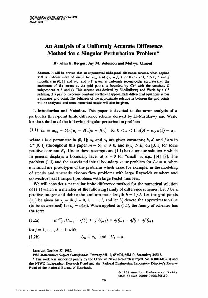
MATHEMATICS OF COMPUTATION VOLUME 37, NUMBER 155 JULY 1981 An Analysis of a Uniformly Accurate Difference Method for a Singular Perturbation Problem* By Alan E. Berger, Jay M. Solomon and Melvyn Ciment Abstract. It will be proven that an exponential tridiagonal difference scheme, when applied with a uniform mesh of size h to: euxx + b(x)ux « fix) for 0 < x < 1, b > 0, b and / smooth, e in (0, 1], and u(0) and u(\) given, is uniformly second-order accurate (i.e., the maximum of the errors at the grid points is bounded by Ch2 with the constant C independent of h and e). This scheme was derived by El-Mistikawy and Werle by a C1 patching of a pair of piecewise constant coefficient approximate differential equations across a common grid point. The behavior of the approximate solution in between the grid points will be analyzed, and some numerical results will also be given. I. Introduction and Notation. This paper is devoted to the error analysis of a particular three-point finite difference scheme derived by El-Mistikawy and Werle for the solution of the following singular perturbation problem (1.1) Lu = euxx + b(x)ux - d(x)u = fix) for 0 < x < 1, «(0) = a0, w(l) = a„ where e is a parameter in (0, 1]; a,, and a, are given constants; b, d, and/are in Cm[0, 1] (throughout this paper m = 5); d > 0, and b(x) > Bx on [0, 1] for some positive constant Bx. Under these assumptions, (1.1) has a unique solution u which in general displays a boundary layer at x = 0 for "small" e, e.g., [14], [8]. The problem (1.1) and the associated initial boundary value problem for Lu = u, when e is small are prototypes of the problems which arise, for example, in the modeling of steady and unsteady viscous flow problems with large Reynolds numbers and convective heat transport problems with large Peclet numbers. We will consider a particular finite difference method for the numerical solution of (1.1) which is a member of the following family of difference schemes. Let J be a positive integer and define the uniform mesh length h = Ï/J. Let the grid points {Xj} be given by Xj = jh,j = 0, 1, . . . , /, and let Uj denote the approximate value (to be determined) for u- = u(x). When applied to (1.1), the family of schemes has the form ( 1.2a) eh-2(rfUj_, + r/Uj + r* Uj+,)= q¡fj_, + qffj+ q/fJ+, foTJ = 1, . . . ,J - 1, with (1.2b) U0 = a0 and Uj=ax. Received October 27, 1980. 1980 Mathematics Subject Classification. Primary65L10, 65M05, 65M10;Secondary 34E15. • This work was supported jointly by the Office of Naval Research (Project No. RR014-03-01) and the NSWC Independent Research Fund and the National Engineering Laboratory Director's Reserve Fund of the National Bureau of Standards. © 1981 American Mathematical Society 002S-5718/81 /0000-0105/SOS.OO 79 License or copyright restrictions may apply to redistribution; see http://www.ams.org/journal-terms-of-use
-
Upload
independent -
Category
Documents
-
view
1 -
download
0
Transcript of An analysis of a uniformly accurate difference method for a singular perturbation problem
MATHEMATICS OF COMPUTATIONVOLUME 37, NUMBER 155JULY 1981
An Analysis of a Uniformly Accurate Difference
Method for a Singular Perturbation Problem*
By Alan E. Berger, Jay M. Solomon and Melvyn Ciment
Abstract. It will be proven that an exponential tridiagonal difference scheme, when applied
with a uniform mesh of size h to: euxx + b(x)ux « fix) for 0 < x < 1, b > 0, b and /
smooth, e in (0, 1], and u(0) and u(\) given, is uniformly second-order accurate (i.e., the
maximum of the errors at the grid points is bounded by Ch2 with the constant C
independent of h and e). This scheme was derived by El-Mistikawy and Werle by a C1
patching of a pair of piecewise constant coefficient approximate differential equations across
a common grid point. The behavior of the approximate solution in between the grid points
will be analyzed, and some numerical results will also be given.
I. Introduction and Notation. This paper is devoted to the error analysis of a
particular three-point finite difference scheme derived by El-Mistikawy and Werle
for the solution of the following singular perturbation problem
(1.1) Lu = euxx + b(x)ux - d(x)u = fix) for 0 < x < 1, «(0) = a0, w(l) = a„
where e is a parameter in (0, 1]; a,, and a, are given constants; b, d, and/are in
Cm[0, 1] (throughout this paper m = 5); d > 0, and b(x) > Bx on [0, 1] for some
positive constant Bx. Under these assumptions, (1.1) has a unique solution u which
in general displays a boundary layer at x = 0 for "small" e, e.g., [14], [8]. The
problem (1.1) and the associated initial boundary value problem for Lu = u, when
e is small are prototypes of the problems which arise, for example, in the modeling
of steady and unsteady viscous flow problems with large Reynolds numbers and
convective heat transport problems with large Peclet numbers.
We will consider a particular finite difference method for the numerical solution
of (1.1) which is a member of the following family of difference schemes. Let J be a
positive integer and define the uniform mesh length h = Ï/J. Let the grid points
{Xj} be given by Xj = jh,j = 0, 1, . . . , /, and let Uj denote the approximate value
(to be determined) for u- = u(x). When applied to (1.1), the family of schemes has
the form
( 1.2a) eh-2(rfUj_, + r/Uj + r* Uj+,) = q¡fj_, + qffj + q/fJ+,
foTJ = 1, . . . ,J - 1, with
(1.2b) U0 = a0 and Uj=ax.
Received October 27, 1980.
1980 Mathematics Subject Classification. Primary 65L10, 65M05, 65M10; Secondary 34E15.• This work was supported jointly by the Office of Naval Research (Project No. RR014-03-01) and
the NSWC Independent Research Fund and the National Engineering Laboratory Director's Reserve
Fund of the National Bureau of Standards.
© 1981 American Mathematical Society
002S-5718/81 /0000-0105/SOS.OO
79
License or copyright restrictions may apply to redistribution; see http://www.ams.org/journal-terms-of-use
80 ALAN E. BERGER, JAY M. SOLOMON AND MELVYN CIMENT
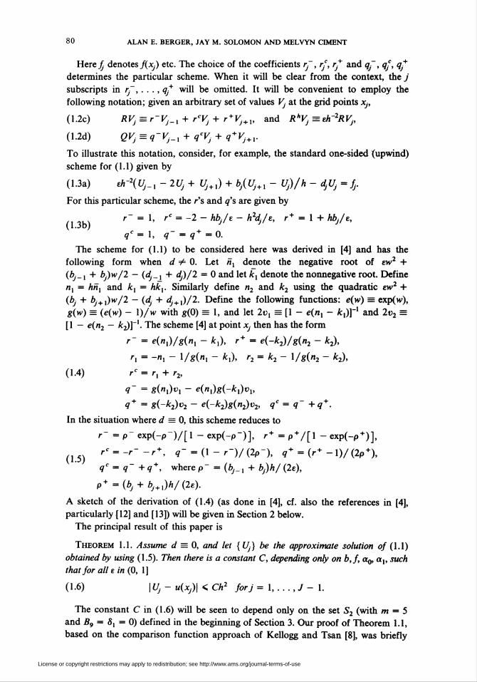
Here^ denotes fixj) etc. The choice of the coefficients r¿~, rj, r* and qj~, qj, q*
determines the particular scheme. When it will be clear from the context, the j
subscripts in r~, . . . , q* will be omitted. It will be convenient to employ the
following notation; given an arbitrary set of values V- at the grid points x,,
(1.2c) RVj = r-Vj_x + rcVj + r + Vj+x, and RhVj =eh~2RVj,
(1.2d) QVj = q-Vj_x + qcVj + q + Vj+x.
To illustrate this notation, consider, for example, the standard one-sided (upwind)
scheme for (1.1) given by
(1.3a) eh-2(Uj_x - 2Uj + Uj+X) + bj(UJ+i - Uj)/h - djUj = fr
For this particular scheme, the r's and q's are given by
(13b) r_ = 1' r° = "2 " hbj/£ ~ h2dj/e' r+ = l+hbj/e>qc= 1, q- = q+ = 0.
The scheme for (1.1) to be considered here was derived in [4] and has the
following form when d ¥= 0. Let n, denote the negative root of ew2 +
(bj_x + bj)w/2 - (dj_x + dj)/2 = 0 and let A, denote the nonnegative root. Define
nx = hrxx and A, = hkx. Similarly define n2 and A2 using the quadratic ew2 +
(bj + bj+x)w/2 — (dj + dJ+x)/2. Define the following functions: e(w) = exp(iv),
g{w) = (e(w) - \)/w with g(0) = 1, and let 2t>, = [1 - e(nx - A,)]"1 and 2v2 =
[1 — e(n2 — ̂ j)]-1. The scheme [4] at point x, then has the form
r~ = e(nx)/g(nx - A,), r+ = e(-k2)/g(n2 - k2),
r, = -nx - \/g(nx - A,), r2= k2 - l/g(n2 - k2),
(1.4) r< = r, + r2,
1~ = g(ni)v\ - e(nx)g(-kx)vx,
q+ = g(-k2)v2 - e(-k2)g{n2)v2, qc = q~ +q + .
In the situation where d = 0, this scheme reduces to
r- =p-exp(-p-)/[l -exp(-p-)], r+ = P+/[l - exp(-p+)],
(15) r< = -r--r\ q~ - (1 - r")/ (2p"), q+ = (r+ - 1)/ (2p+),
qc = q~ +q+, where p~ = (*,._, + b/)h/ (2e),
p+ = (bj + bj+x)h/ (2b).
A sketch of the derivation of (1.4) (as done in [4], cf. also the references in [4],
particularly [12] and [13]) will be given in Section 2 below.
The principal result of this paper is
Theorem 1.1. Assume d = 0, and let {Uj) be the approximate solution of (1.1)
obtained by using (1.5). Then there is a constant C, depending only on b,f, a0, ax, such
that for all e in (0, 1]
(1.6) | Uj - u(xj)\ < Ch2 forj = 1, ...,/- 1.
The constant C in (1.6) will be seen to depend only on the set S2 (with m = 5
and B9 = 8X = 0) defined in the beginning of Section 3. Our proof of Theorem 1.1,
based on the comparison function approach of Kellogg and Tsan [8], was briefly
License or copyright restrictions may apply to redistribution; see http://www.ams.org/journal-terms-of-use
A DIFFERENCE METHOD FOR A PERTURBATION PROBLEM 81
outlined in [3] and [2]. An independent proof of Theorem 1.1 has now also been
obtained by Hegarty, Miller and O'Riordan [6] using the "double mesh method"
(cf. [7], [10]). Lorenz [9] has obtained the result (1.6) for nonzero d(x) for a related
scheme under the assumption that b is a positive constant. Finite element methods
employing particular exponential type functions in the trial and test spaces were
formulated and analyzed in [5].
For a detailed discussion of properties of schemes of the form (1.2) (e.g.,
maximum principle, cell Reynolds number condition, formal application to Lu =
u,) and for a comparison of the theoretical and numerical convergence behavior of
(1.5) with that for a number of other schemes for (1.1) see [3], and also [1], [2], and
the references therein. Here we proceed directly to presenting the basic properties
of (1.4) and then to proving Theorem 1.1. A numerical experiment, whose result is
consistent with the conjecture that (1.4) is also uniformly second-order accurate for
(1.1), is given in Section 5.
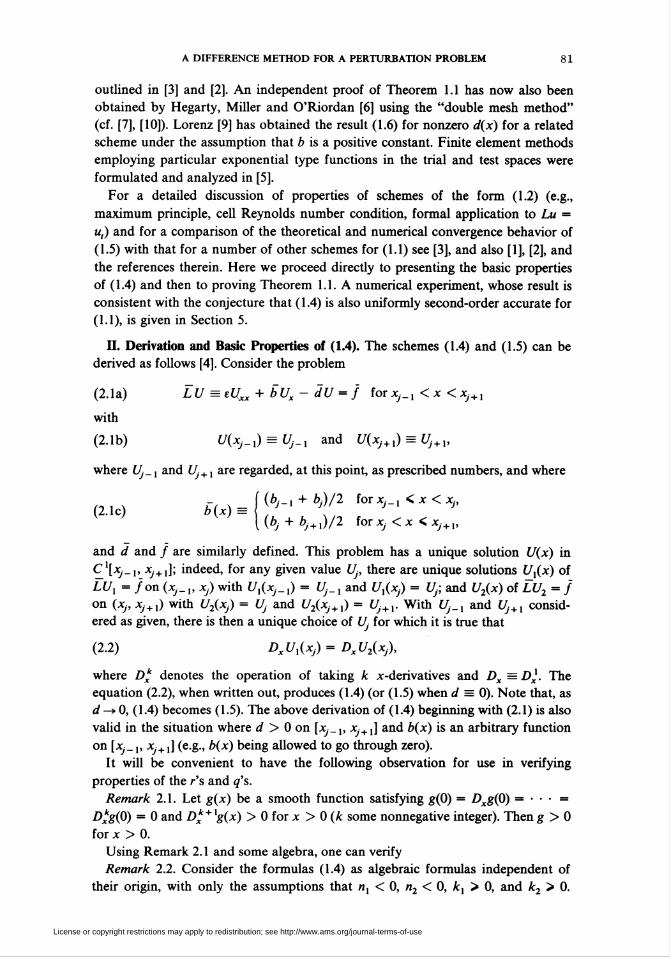
II. Derivation and Basic Properties of (1.4). The schemes (1.4) and (1.5) can be
derived as follows [4]. Consider the problem
(2.1a) LU = eU«x + bUx- dU = f for Xj_, < x <xJ+,
with
(2.1b) U(Xj_x) = Uj_x and t/(x,+1) = UJ+X,
where £/_, and UJ+X are regarded, at this point, as prescribed numbers, and where
f (bi_x + b.)/2 forx, ! < x < x,.,(2.1c) b(x) ={ / \, J J
\(bj + bj+x)/2 ÎOTXj<X<Xj+x,
and d and / are similarly defined. This problem has a unique solution U(x) in
Cx[Xj_x, xJ+x]; indeed, for any given value Up there are unique solutions Ux(x) of
LUX = /on (xj_x, Xj) with Ux(Xj_x) = Uj_x and t/,(x,) = Uf, and U2(x) of LU2 = /
on (Xj, xj+x) with U2(xj) = Uj and U2(xJ+x) = UJ+X. With Uj_x and UJ+1 consid-
ered as given, there is then a unique choice of Uj for which it is true that
(2.2) DxUx(xj) = DxU2(xj),
where Dk denotes the operation of taking k x-derivatives and Dx = Dx. The
equation (2.2), when written out, produces (1.4) (or (1.5) when d = 0). Note that, as
d —> 0, (1.4) becomes (1.5). The above derivation of (1.4) beginning with (2.1) is also
valid in the situation where d > 0 on [xJ_l, xJ+x] and b(x) is an arbitrary function
on [x,_,, Xj+X] (e.g., b(x) being allowed to go through zero).
It will be convenient to have the following observation for use in verifying
properties of the r's and q's.
Remark 2.1. Let g(x) be a smooth function satisfying g(0) = Dxg(0) = • • • =
Dkg(0) = 0 and Dk+ xg(x) > 0 for x > 0 (A some nonnegative integer). Then g > 0
for x > 0.
Using Remark 2.1 and some algebra, one can verify
Remark 2.2. Consider the formulas (1.4) as algebraic formulas independent of
their origin, with only the assumptions that n, < 0, n2 < 0, kx > 0, and k2 > 0.
License or copyright restrictions may apply to redistribution; see http://www.ams.org/journal-terms-of-use
82 ALAN E. BERGER, JAY M. SOLOMON AND MELVYN CIMENT
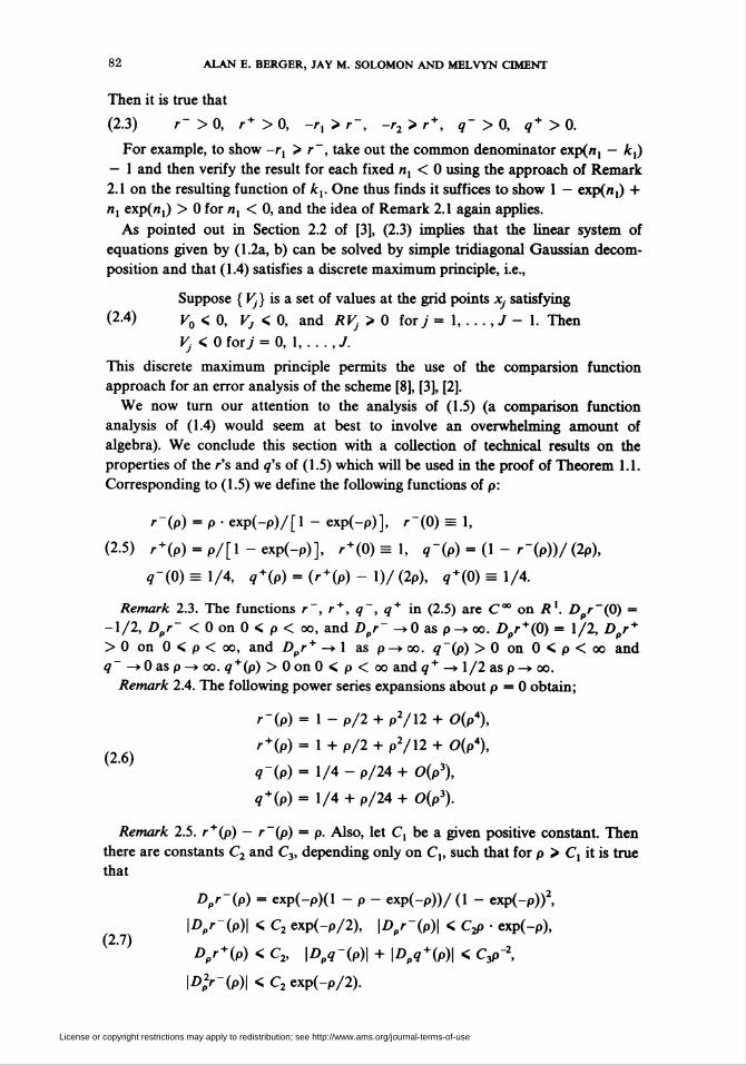
Then it is true that
(2.3) r" > 0, r+ > 0, -rx > r~, -r2 > r+, q~ > 0, q+ > 0.
For example, to show -r, > r~, take out the common denominator exp(/!, — kx)
— 1 and then verify the result for each fixed n, < 0 using the approach of Remark
2.1 on the resulting function of A,. One thus finds it suffices to show 1 — exp(nx) +
nx exp(«,) > 0 for nx < 0, and the idea of Remark 2.1 again applies.
As pointed out in Section 2.2 of [3], (2.3) implies that the linear system of
equations given by (1.2a, b) can be solved by simple tridiagonal Gaussian decom-
position and that (1.4) satisfies a discrete maximum principle, i.e.,
Suppose { Vj) is a set of values at the grid points Xj satisfying
(2-4) v0 < 0, Vj < 0, and RV} > 0 for j = I, . . . ,J - I. Then
Vj < 0 ÎOTJ = 0,l,...,J.
This discrete maximum principle permits the use of the comparsion function
approach for an error analysis of the scheme [8], [3], [2].
We now turn our attention to the analysis of (1.5) (a comparison function
analysis of (1.4) would seem at best to involve an overwhelming amount of
algebra). We conclude this section with a collection of technical results on the
properties of the r's and q's of (1.5) which will be used in the proof of Theorem 1.1.
Corresponding to (1.5) we define the following functions of p:
r~(p) = p • exp(-p)/[l - exp(-p)], r~(0) = 1,
(2.5) r + (p) = p/[l-exp(-p)], r + (0) = 1, q~(p) = (1 - r~(p))/ (2p),
q-(0)=\/A, q + (p) = (r + (p)-l)/(2p), q + (0) = 1/4.
Remark 2.3. The functions r~, r + , q~, q+ in (2.5) are C° on Rl. D r~(0) =
-1/2, Dpr~ < 0 on 0 < p < co, and Dpr~ -»0 as p-+ <x>. Dpr+(0) = 1/2, Dpr+
> 0 on 0 < p < oo, and Dpr+ -> 1 as p -» oo. q ~(p) >0 on 0<p<oo and
q~ —>0as p-> co. q+(p) >0on0<p<oo andq+ -» 1/2 asp^ oo.
Remark 2.4. The following power series expansions about p = 0 obtain;
/•-(p) = l-p/2 + p2/12 + 0(p4),
r+(p) = 1 + P/2 + p2/\2 + 0(p%
q-(p) = 1/4 - p/24 + 0(p3),
q + (p)= 1/4 + p/24+0(p3).
Remark 2.5. r+(p) - r~~(p) = p. Also, let C, be a given positive constant. Then
there are constants C2 and C3, depending only on C,, such that for p > C, it is true
that
DPr~(p) = exp(-p)(l - p - exp(-p))/(l - exp(-p))2,
|Z>pr-(p)| < C2 exp(-p/2), |öp/-(p)| < C& ■ exp(-p),
D„r + (p) < C2, \Dpq-(p)\ + \Dpq+(p)\ < C3p~2,
|Z)2r-(p)|<C2exp(-p/2).
License or copyright restrictions may apply to redistribution; see http://www.ams.org/journal-terms-of-use
A DIFFERENCE METHOD FOR A PERTURBATION PROBLEM 83
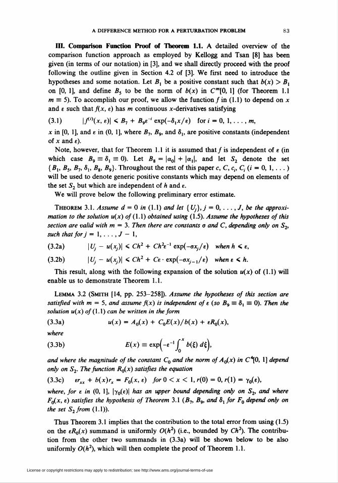
III. Comparison Function Proof of Theorem 1.1. A detailed overview of the
comparison function approach as employed by Kellogg and Tsan [8] has been
given (in terms of our notation) in [3], and we shall directly proceed with the proof
following the outline given in Section 4.2 of [3]. We first need to introduce the
hypotheses and some notation. Let Bx be a positive constant such that b(x) > Bx
on [0, 1], and define B5 to be the norm of ¿>(x) in C"[0, 1] (for Theorem 1.1
m = 5). To accomplish our proof, we allow the function/in (1.1) to depend on x
and e such that fix, e) has m continuous x-derivatives satisfying
(3.1) |/°(x, e)| < Bn + B9e' exp(-5,x/e) for i = 0, 1, . . . , m,
x in [0, 1], and e in (0, 1], where B7, B9, and 8X, are positive constants (independent
of x and e).
Note, however, that for Theorem 1.1 it is assumed that / is independent of e (in
which case B9 = 8X = 0). Let B% = \a0\ + |a,|, and let S2 denote the set
{Bx, B5, B7, 8X, fi8, B9). Throughout the rest of this paper c, C, c„ C, (i = 0, 1, . . . )
will be used to denote generic positive constants which may depend on elements of
the set S2 but which are independent of h and e.
We will prove below the following preliminary error estimate.
Theorem 3.1. Assume d = 0 in (1.1) and let [Uj),j = 0, ...,/, be the approxi-
mation to the solution u(x) o/(l.l) obtained using (1.5). Assume the hypotheses of this
section are valid with m = 3. Then there are constants a and C, depending only on S2,
such that for j = 1, ...,/— 1,
(3.2a) | Uj - u(xj)\ < Ch2 + CA V exp(-ax,/e) when h < e,
(3.2b) \Uj - w(x,)| < Ch2 + Ce ■ exp(-axy_,/e) when e < h.
This result, along with the following expansion of the solution u(x) of (1.1) will
enable us to demonstrate Theorem 1.1.
Lemma 3.2 (Smith [14, pp. 253-258]). Assume the hypotheses of this section are
satisfied with m = 5, and assume fix) is independent of e (so B9 = 8X = 0). Then the
solution u(x) o/(l.l) can be written in the form
(3.3a) u(x) = A0(x) + C0E(x)/b(x) + eRo(x),
where
(3.3b) E(x) = exp(-e-' f* b(£) dfy
and where the magnitude of the constant C0 and the norm ofA0(x) in C^O, 1] depend
only on S2. The function R0(x) satisfies the equation
(3.3c) erxx + b(x)rx = F0(x, e) for0<x< 1, r(0) = 0, r(l) = yQ(e),
where, for e in (0, 1], |y0(e)l nas an upPer bound depending only on S2, and where
F0(x, e) satisfies the hypothesis of Theorem 3.1 (B7, B9, and 8X for FQ depend only on
the set S2from (1.1)).
Thus Theorem 3.1 implies that the contribution to the total error from using (1.5)
on the e/?0(x) summand is uniformly 0(h2) (i.e., bounded by Ch2). The contribu-
tion from the other two summands in (3.3a) will be shown below to be also
uniformly 0(h2), which will then complete the proof of Theorem 1.1.
License or copyright restrictions may apply to redistribution; see http://www.ams.org/journal-terms-of-use
84 ALAN E. BERGER, JAY M. SOLOMON AND MELVYN CIMENT
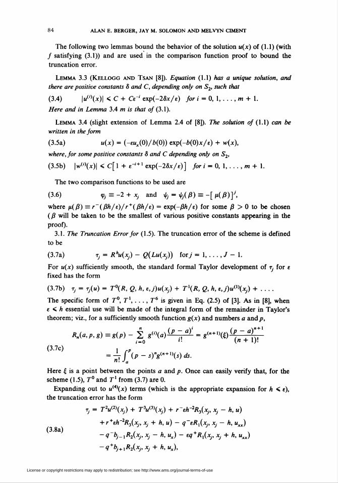
The following two lemmas bound the behavior of the solution u(x) of (1.1) (with
/ satisfying (3.1)) and are used in the comparison function proof to bound the
truncation error.
Lemma 3.3 (Kellogg and Tsan [8]). Equation (1.1) has a unique solution, and
there are positive constants 8 and C, depending only on S2, such that
(3.4) |w(0(x)| < C + Ce"' exp(-25x/e) for i = 0, 1, . . ., m + 1.
Here and in Lemma 3.4 m is that of (3.1).
Lemma 3.4 (slight extension of Lemma 2.4 of [8]). The solution of (1.1) can be
written in the form
(3.5a) u(x) = (-eux(0)/b(0)) exp(-6(0)x/e) + w(x),
where, for some positive constants 8 and C depending only on S2,
(3.5b) |w(,)(x)| < C[ 1 + e~' + 1 exp(-2óx/e)] for i = 0, I, . . . , m + I.
The two comparison functions to be used are
(3.6) <Pj = -2 + Xj and «fy - tfß) s -[fi(ß)]J,
where p.(ß) = r~(ßh/e)/r+(ßh/e) = exp(-ßh/e) for some ß > 0 to be chosen
(ß will be taken to be the smallest of various positive constants appearing in the
proof).
3.1. The Truncation Error for (1.5). The truncation error of the scheme is defined
to be
(3.7a) rj = Rhu(Xj) - Q(Lu(xj)) for/ = 1, . . . , J - 1.
For u(x) sufficiently smooth, the standard formal Taylor development of t. for e
fixed has the form
(3.7b) Tj = Tj(u) = T°(R, Q, h, e,j)u(Xj) + Tl(R, Q, h, e,j)u^(Xj) + ....
The specific form of T°, Tx, . . ., T6 is given in Eq. (2.5) of [3]. As in [8], when
e < h essential use will be made of the integral form of the remainder in Taylor's
theorem; viz., for a sufficiently smooth function g(x) and numbers a andp,
Rn(a,p,g) = g(p) - ¿ g°\a)^r^- = g<"+xKH){P ~ °r
(3.7c)
,fo * w '! ° w (« + 1)!
= ^fP(p-s)Y"+1\s)ds.n\ Jn
Here £ is a point between the points a and p. Once can easily verify that, for the
scheme (1.5), T° and Tx from (3.7) are 0.
Expanding out to t/4)(x) terms (which is the appropriate expansion for h < e),
the truncation error has the form
Tj = T2u(2)(xj) + T3u(3\Xj) + r'eh~2R3(xj, x} - h, u)
+ r+eh~2R3(xj, x + h, u) — q~eRx(x, x — h, uxx)(3.8a) . , . ;
-q bj_xR2(Xj, Xj - h, ux) - eq Rx(xj, x, + h, uxx)
-q+bj+xR2(Xj,Xj + h,ux),
License or copyright restrictions may apply to redistribution; see http://www.ams.org/journal-terms-of-use
A DIFFERENCE METHOD FOR A PERTURBATION PROBLEM 85
(3.9)
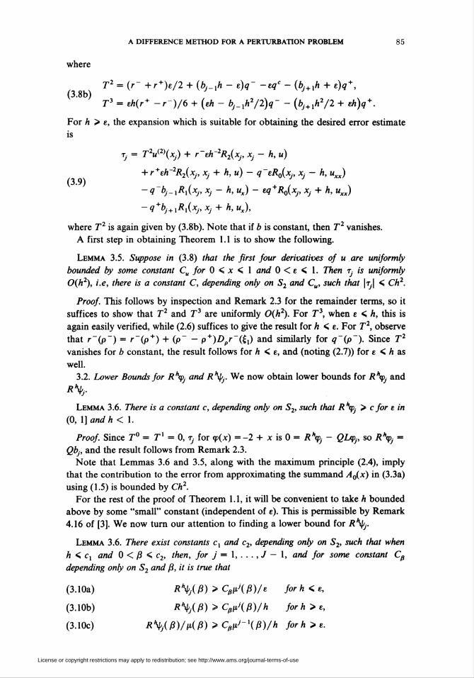
where
,, o^ Tl " (f~ +r + )£/2 + (bJ-lh - e)l~ -*4C - (*i+l* + e)<7 + .(3.8b)
T3 = eh(r+ -r~)/6 + (eh - bj_xh2/2)q~ - {bJ+xh2/2 + eh)q + .
For h > e, the expansion which is suitable for obtaining the desired error estimate
is
Tj = T2um(xj) + r-eh-2R2(xj, x, - h, u)
+ r+eh~2R2(Xj, x, + h, u) - q~eR0(Xj, x, - h, uxx)
-q~bj_xRx(Xj, Xj - h, ux) - eq+R0(xj, Xj + h, uxx)
-q+bJ+xRx(Xj,Xj + h,ux),
where T2 is again given by (3.8b). Note that if b is constant, then T2 vanishes.
A first step in obtaining Theorem 1.1 is to show the following.
Lemma 3.5. Suppose in (3.8) that the first four derivatives of u are uniformly
bounded by some constant Cu for 0 < x < 1 and 0 < e < 1. Then r, is uniformly
0(h2), i.e, there is a constant C, depending only on S2 and Cu, such that \tj\ < Ch2.
Proof. This follows by inspection and Remark 2.3 for the remainder terms, so it
suffices to show that T2 and T3 are uniformly 0(h2). For T3, when e < h, this is
again easily verified, while (2.6) suffices to give the result for h < e. For T2, observe
that r~(p~) = r~(p+) + (p" - p+)Dpr"(|1) and similarly for q~(p~). Since T2
vanishes for b constant, the result follows for h < e, and (noting (2.7)) for e < h as
well.
3.2. Lower Bounds for Rh<Pj and Rty- We now obtain lower bounds for Rh<pj and
R%.
Lemma 3.6. There is a constant c, depending only on S2, such that R *<py > c for e in
(0, I] and h < 1.
Proof. Since T° = Tx = 0, ry for <p(x) =-2 + x is 0 = Rhq>j, - QLcpj, so Rh<pj =
Qbj, and the result follows from Remark 2.3.
Note that Lemmas 3.6 and 3.5, along with the maximum principle (2.4), imply
that the contribution to the error from approximating the summand A0(x) in (3.3a)
using (1.5) is bounded by Ch2.
For the rest of the proof of Theorem 1.1, it will be convenient to take h bounded
above by some "small" constant (independent of e). This is permissible by Remark
4.16 of [3]. We now turn our attention to finding a lower bound for Rty.
Lemma 3.6. There exist constants c, and c2, depending only on S2, such that when
h < c, and 0 < ß < c2, then, for j = 1, . . . , J — 1, and for some constant Cß
depending only on S2 and ß, it is true that
(3.10a) R%(ß) > Cßiij(ß)/e for h < e,
(3.10b) R%(ß) > CßtiJ(ß)/h forh> e,
(3.10c) R%(ß)/p.(ß) > CßliJ~\ß)/h for h > e.
License or copyright restrictions may apply to redistribution; see http://www.ams.org/journal-terms-of-use
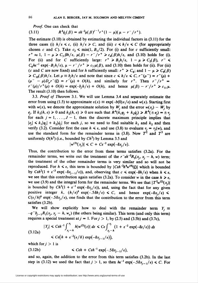
8 fi ALAN E. BERGER, JAY M. SOLOMON AND MELVYN CIMENT
Proof. One can check that
(3.11) R%(ß) = «ft-y/jy-'r+O - u)(u - r~/r+).
The estimate (3.10) is obtained by estimating the individual factors in (3.11) for the
three cases (i) h/e < c, (ii) A/e > C, and (iii) c < A/e < C (for appropriately
chosen c and C). Take c2 < min(l, Bx/2). For (i) and for c sufficiently small:
r+ « 1, 1 - u > CjöA/e, p(ß) - /• V+ > c4(ß)h/e, and (3.10) holds for (i).
For (ii) and for C sufficiently large: r+ > Bxh/e, 1 — u > Cs(ß), r~ <
C6Ae_1 exp(-fi,A/e), p - r"/r+ > c7u(ß), and (3.10) then holds for (ii). For (hi)
(c and C are now fixed) and for A sufficiently small: r+ > Cs; and 1 - u > C9(ß)
> Cxo(ß)h/e. Let p = ¿,A/e and note that since c < A/e < C, r~(p~) = r~(p) +
(p" - p)Dpr~(í) = r"(p) + O(A), and similarly for r+. Then r~/r* =
r~(p)/r+(p) + 0(h) = exp(-bjh/e) + 0(h), and hence p(ß) - r"//-"1" > cuu.
The result (3.10) then follows.
3.3. Proof of Theorem 3.1. We will use Lemma 3.4 and separately estimate the
error from using (1.5) to approximate v(x) = exp(-6(0)x/e) and w(x). Starting first
with w(x), we denote the approximate solution by Wj and the error w(xj) — Wj by
er If kx(h, e) > 0 and A2(A, e) > 0 are such that Rh(kxq>j + k2\pj) > /î*(±e,-) = ± ry
for each / = 1, ... ,J — 1, then the discrete maximum principle implies that
|e,| < kx\<Pj\ + A:2|uV| for each/, so we need to find suitable A, and k2 and then
verify (3.2). Consider first the case A < e, and use (3.8) to evaluate t, = Tj(w), and
use the standard form for the remainder terms in (3.8). Now T2 and T3 are
uniformly 0(A2) (i.e., bounded by CA2) by Lemma 3.5 and
\w(3\xj)\ <C+ Ce2 exp(-8Xj/e).
Thus, the contribution to the error from these terms satisfies (3.2a). For the
remainder terms, we write out the treatment of the r~eh~2R3(Xj, x. — A, w) term;
the treatment of the other remainder terms is very similar and so will not be
reproduced. For A < e, this term is bounded by \Ceh~2h\vi4\Q\ which is bounded
by CeA2(l + e~3 exp(-8Xj_x/e)), and, observing that c < exp(-5A/e) when A < e,
we see that this contribution again satisfies (3.2a). To consider w in the case A > e,
we use (3.9) and the integral form for the remainder terms. We see that | rSv^^x )|
is bounded by CA2(1 + e~' exp(-óxy/e)), and, using the fact that for any given
positive integer k, (A/e)* exp(-.55A/e) < C, and hence exp(-fixy/e) <
C(e/h)k exp(-.55x,/e), one finds that the contribution to the error from this term
satisfies (3.2b).
We will show explicitly how to deal with the remainder term Yj s
-q~bj_xRx(xj, Xj — A, wx) (the others being similar). This term (and only this term)
requires a special treatment at/ = 1. For/ > 1, by (2.5) and (3.5b) and (3.7c),
| Yj\ < CehxfXj A|w(3>(i)| ds < Ce f (1 + e"2 exp(-&/e)) ds(3.12a) *>~h Xj~h
< Ce(h + e~2(e/8) exp(-5x,_,/e)),
which for/ > 1 is
(3.12b) < CeA + CeA"' exp(-.50x,_,/e),
and so, again, the addition to the error from this term satisfies (3.2b). In the last
step in (3.12) we used the fact that/ > 1, so then Ae"1 exp(-.58Xj_x/e) < C. For
License or copyright restrictions may apply to redistribution; see http://www.ams.org/journal-terms-of-use
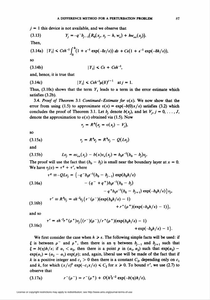
A DIFFERENCE METHOD FOR A PERTURBATION PROBLEM 87
/ = 1 this device is not available, and we observe that
(3.13) Yj = -q-bj_x(R0(Xj, Xj - A, wx) + hwxx(Xj)).
Then,
(3.14a) | Yx\ < CeA"1 [\l + e"1 exp(-8s/e)) ds + Ce(l + e~' exp(-5A/e)),•'o
so
(3.14b) |7,| <Ce + CeA"1,
and, hence, it is true that
(3.14c) |y,| < CeA-V(5y_1 at/ = 1.
Thus, (3.10c) shows that the term Yx leads to a term in the error estimate which
satisfies (3.2b).
3.4. Proof of Theorem 3.1 Continued-Estimate for v(x). We now show that the
error from using (1.5) to approximate t>(x) = exp(-A(0)x/e) satisfies (3.2) which
concludes the proof of Theorem 3.1. Let A, denote b(xj), and let Vj,j = 0,..., J,
denote the approximation to t>(x) obtained via (1.5). Now
Tj = R*(ej = v(Xj) - Vj),
so
(3.15a) Tj = R\ = RhVj - Q(LVj)
and
(3.15b) Lvj = evxx(Xj) - b(x)vx(Xj) = è0e~'(Z>o - A>,.
The proof will use the fact that (b0 — bj) is small near the boundary layer at x = 0.
We have T,(t>) = Tq + rr, where
t" =-QLvj = {-q-b0e-x(b0 - bj_x) exp(V/e)
(3.16a) -(q- +q+)btf-\b0-bj)
-q+b0e-\b0 - bJ+x) exp(-VA)}«,,
Tr = RHVj = eh-2Vj{r-(p-)(cxp(boh/e) - 1)(3.16b)
+ r + (p+)(exp(-60A/e)-l)},
and so
t' = eA-2r + (p+)^{(/--)(p-)//- + (p + )(exp(A0A/e) - 1)(3.16c)
+ exp(-A0A/e) - 1}.
We first consider the case when A > e. The following simple facts will be used: if
£ is between p~ and p+, then there is an ij between è._, and bj+x such that
£ = A(r/)A/e; if ax < a2, then there is a point p in (a,, a^ such that expia^ -
exp(a,) = (a2 - a,) exp(p); and, again, liberal use will be made of the fact that if
A is a positive integer and c, > 0 then there is a constant C2, depending only on c,
and A, for which (x/e)k exp(-C[X/e) < C2 for x > 0. To bound Tr, we use (2.7) to
observe that
(3.17a) r-(p-) = r~(p + ) + 0(h3e~2 cxp(-b(r,)h/'e),
License or copyright restrictions may apply to redistribution; see http://www.ams.org/journal-terms-of-use
88 ALAN E. BERGER, JAY M. SOLOMON AND MELVYN CIMENT
and hence
(3.17b) r~(p-)/r + (p + ) = exp(-p + ) + 0(A2e"' exp(-A(r,)A/e)),
r~(p-)/r + (p + ) = exp(-60A/e) + [exp(-p + ) - exp(-60A/e)](3.17c)
+ 0(h2e~x exp(-A(T,)A/e)).
The second term in (3.17c) is bounded by 0(Xjhe'x exp(-A(p,)A/e)) for some p,
in (0, Xj). Now exp(-b(Pj)h/e) exp(A0A/e) < exp(CAx,/e). Writing v, =
exp2(-.5A(0)x>/e), one of these factors can be used to bound the latter term for A
sufficiently small, and so (3.10b), (3.10c), and (3.17) lead to (3.2b) for the t' term.
For Tq, the last two terms from the right side of (3.16a) are bounded by
CXjt~lt)j < CeA"1 exp(-.5b(0)xj/e) which leads to (3.2b). For the first term on the
right of (3.16a), the observation that Cxj_xe~x exp(60A/e)u, = Cxj_xe~xVj_x suffices
for/ > 2. For y = 1, b0 - bj_x =0 and the proof for A > e is complete.
We now commence the task of treating the error in t>(x) when A < e. The overall
approach is to Taylor expand everything in (3.16b) about p = bjh/e. We have
(3.18a) r-(p-) = r~(p) + (p~ -p)Dpr-(p) + 0(A4/e2),
(3.18b) Dpr-(p) = Dpr~(0) + pD2r~(0) + 0(h2/e2),
and so (throughout the rest of the paper terms which have been reduced to a nice
form where (3.10) yields (3.2) will be generically denoted by N)
(3.18c) r-(p~) = r~(p) - .5(p" -p) + p(p~ -p)/6 + TV,
from which one has
r-(p-) = r~(p) + h2e-xbx(xj)/4 - AV'Mx,)^
-AV26(x,.)6;t(x,.)/12 + N.(3.19a)
Similarly,
(3.19b)r + (p+) = r + (p) + AV'^(x,)/4 + AV'Ax(x,)/8
+ h3e-2b(Xj)bx(Xj)/l2 + N.
Expanding exp(A0A/e) — 1 and exp(-A0A/e) — 1, we find, from (3.16b) and (3.19),
that
(3.20a) t' = eA-2ü,.{r-(p)(exp(A0A/e) - 1) + /-»(expí-Vi/e) - 1)} + N,
and so
(3.20b) Tr = eh-2vjr+(p)(exp(-p) - exp(-A0A/e))(exp(A0A/e) - 1) + N.
Now observe that
Zj = (exp(-p) - exp(-A0A/e))(exp(A0A/e) - 1)
<3-21a> . N + [ _ (bj - bo)h/e + (bj _ h)2h2/ (2e2) j(60A/e - (A0A)2/ (2e2)),
and so
(3.21b) Tr = eA"2ü,(l + p/2)Zj + N,
from which, after considerable cancellation of terms, one finds that
(3.22) Tr = Vj(b0 - bj)b0/e + N.
License or copyright restrictions may apply to redistribution; see http://www.ams.org/journal-terms-of-use
A DIFFERENCE METHOD FOR A PERTURBATION PROBLEM 89
The treatment of t9 is fortunately not quite so tedious. Simply use (2.6) to
expand q~ and q + , expand (¿>0 - bJ+x) and (A0 — bj_x) about (A0 — b), expand
exp(A0A/e) and exp(-A0A/e), and find that
(3.23) T"=-Vj(b0-bj)b0/e + N.
Equations (3.22) and (3.23) combine to complete the proof of Theorem 3.1.
The final step in the proof of Theorem 1.1 is to show uniform 0(A2) accuracy for
the function E(x)/b(x) from (3.3a, b).
3.5. Treatment of E(x)/b(x). Let G(x) = E(x)/b(x), and set z(x) = l/b(x).
Then one can verify that
(3.24) LG = eGxx + b(x)Gx = e£(x)z(2)(x).
We write the truncation error for (1.5) applied to (3.24) as t,(G) = rr + Tq = RhGj
— QLGj, and we will prove that (1.5) gives a uniformly 0(A2) accurate approxima-
tion to G(x). Consider first the case A > e. Then t9 is immediately bounded by
Cehn(Bxy~x/h which by (3.10c) leads to a contribution to the error estimate of
Cehp/~x which is certainly 0(A2). It remains to deal with t' = RhGj. The approach
is to expand all terms about x, or p = bjh/e. Terms which are directly seen to lead
to uniformly 0(h2) additions to the error are simply denoted by TV. Define for
k <m
(3.25a) S(k, m) = expi-e"1 (*" b(£) </{}.
Then
(3.25b)t' = eh-2Ej_x{r-Zj_x + (-/•" -r+)ZjS(j - \,j)
+ r+zJ+xS(j- 1./+1)},
and
(3.26a) r-(p-) = r-(p) + (p~ -p)Dpr-(p) + TV,
(3.26b) Zj+X = Zj + hDxZj + TV, z,_, = z, - hDxZj + TV,
(3.26c) r + (p + ) = r + (p) + (p+ -p)Dpr + (p) + TV,
(3.26d) -e'1 C' b(s) ds=-p + bx(Xj)h2/ (2e) + 0(h3/e),
(3.26e) -£"1/Xy+' b^ ds=-2p+ 0(h3/e).Xj-I
Now for arbitrary a and 17, exp(a + tj) = exp(a) + r/ • exp(a) + .5r/2 exp(£) for
some I between a and a + tj, from which we have
(3.26f) SO" - UJ) = exp(-p) + exp(-p)Ax(x,.)A2/ (2e) + TV,
(3.26g) S(j - \,j + 1) = exp(-2p) + TV.
From (3.25), (3.26) and (3.10) and the fact that
(3.26h) r~(p)(\ - exp(-p)) + r + (p)(exp(-2p) - exp(-p)) = 0,
License or copyright restrictions may apply to redistribution; see http://www.ams.org/journal-terms-of-use
90 ALAN E. BERGER, JAY M. SOLOMON AND MELVYN CIMENT
one verifies that
Tr = eh-2Ej_x{zj(p- -p)Dpr(p) - zx(Xj)hr-(p)
-Zj(p~ -P) exp(-p)Z>pr-(p) - Zj(p+ -p) exp(-p)Dpr+(p)
-zjr-(p) cxp(-p)bx(Xj)h2/ (2e) - zjr+(p) exp(-p)6x(x,)A2/ (2e)
+ zj(p+ -p) exp(-2p)Dpr+(p) + zx(Xj)hr+(p) exp(-2p)}.
Now use the fact that r~(p) = exp(-p)r+(p) and (from Remark 2.5) Dpr~(p) =
Dpr+(p) — 1 to eliminate r~ and Dpr~ from (3.27). Then replace -bx(Xj)Zj by
bjZx(xj) in the two terms where it appears. Again use the latter equality to find that
Zj(p~ -p) = zx(xj)ph/2 + 0(h3/e),
(3.28)Zj(p+ -p) =-zx(Xj)ph/2 + 0(h3/e).
Using (3.28) in the expression for Tr just obtained, one ascertains that Tr has the
form
(3.29) Ej_xeh-2zx(Xj)h{N + P(p)},
where P(p) is a certain function of p. Using (2.5) and the common denominator
(1 - exp(-p))2, one can check that P(p) = 0, and the result is in hand for A > e.
The proof for the case A < e is very similar, but more Taylor expansion terms
must be carried along, viz.,
r-(p~) = r-(p) - bx(xj)h2Dpr-(p)/ (2e)(3.30a)
+ Axx(x,)A3Z)pr-(p)/(4e) + 7V,
r + (P + ) = r + (p) + bx(Xj)h2Dpr + (p)/ (2e)(3.30b)
+ Mxy.)A3Z>pr+(p)/(4e) + TV,
(3.30c) q + (p + ) = q + (p) + TV, q-(p~) = q~(p) + TV,
zxÂxj-i) = zxx(xj) - fizxxx(xj) + TV,
(3.30d)*xx(Xj+l) = Zxx(xj) + hzxxxixj) + ff.
Analogous to (3.26d-g), one has
(3.30e) S(j - 1,/) = exp(-p){ 1 + h2bx(Xj)/ (2e) - h3bxx(Xj)/ (6e)} + TV,
(3.30f) SO - 1,/ + 1) - exp(-2p){ 1 - A\x(x,)/ (3e)} + TV.
Now t' is given by (3.25b), and t* is given by
T« =-eEj_x{zxx(Xj_x)q-(p~) + zxx(Xj)(q-(p-) + q+(p+))S(j - 1,/)
(3.31)+ ^*(*y+1)<7+(P + )SO- 1,7 + 1)}.
Also
(3.32) zxx(xj) = -2bx(Xj)ZjZx(Xj) - z(Xj)2bxx(Xj).
License or copyright restrictions may apply to redistribution; see http://www.ams.org/journal-terms-of-use
A DIFFERENCE METHOD FOR A PERTURBATION PROBLEM 91
Now substitute (3.30) into (3.25b) and (3.31), and also expand zJ+x and Zj_x about
Zj, and use (3.26h) and (3.32) to find that
Tj = eh-2Ej_x{[-hzx(Xj)r- + .5A2zxx(x,K -h3zxxx(xj)r-/6
+ zx(Xj)phDpr-/2 - zxx(xj)ph2Dpr-/4]
+ [(exp(-p)Dpr~ -exp(-p)Dpr+ -r~ exp(-p) - r+ exp(-p))
■(bjh2/(2e))bx(Xj)/b(Xj)2
+ (-exp(-p)Dpr~ -exp(-p)Dpr+ +r~ exp(-p)/1.5
+ r+ exp(-p)/1.5)
■(bjh3/(4e))bxx(Xj)/b(Xj)2]
(3.33) + [(6,A2/ (2e))(bx(Xj)/b(Xj)2) cxp(-2p)Dpr +
+ (exp(-2p)ZV+ -4r+exp(-2p)/3)
.(bjh3/(4e))bxx(Xj)/b(Xj)2
+ r+ cxp(-2p)hzx(Xj) + txp(-2p)(bjh3/(4e))
• 2Ax(x,K(x,)(l/6,)ZV+
+ r+ cxp(-2p)h2zxx(Xj)/2 + r+ exp(-2p)A3zxxx(x,)/6]
+ [A2zxx(x>)(-9--^-exp(-p)- q+exp(-p)- q+exp(-2p))
+ h3zxxx(Xj)(q~ -q+ exp(-2p))]}
+ TV.From (3.33), one can write r, in the form
tj = g\(p)hzx(xj) + g2(p)h2zxx(Xj) + g3(p)h3zxxx(xj)
(3'34) +g4(p)A,.A3e-'Axx(x,)z(xy)2/4.
After replacing r~(p) by exp(-p)r + (p) and Dpr~ by Dpr* — 1, it is quickly seen
that gx(p) is exactly the function P(p) in (3.29) which was found to vanish. Using
(2.6) to expand g2(p) in the form a0 + axp + TV, we find that g2(p) = 0 + TV and,
similarly, with g3 and g4, and the proof is complete.
IV. Accuracy of the Approximate Solution Between the Grid Points. Given
problem (1.1) with d = 0 and approximate solution {Uj} obtained using (1.5), let
U(x) be defined by
et/xx + bUx = / for x,_, < x < x,,
(4.1) U(xj_x) = Uj_x, U(xj) = Uj, b = (bj_x + bj)/2,
f-(fj-x+fj)/2 iorj=l,...,J.
The discussion in Section 2 demonstrates that U(x) is in C'[0, 1], and hence offers
a potential approximation to u(x) (the solution of (1.1)) between the grid points, as
well as to ux. The following result estimates the accuracy of this approximation.
License or copyright restrictions may apply to redistribution; see http://www.ams.org/journal-terms-of-use

92 ALAN E. BERGER, JAY M. SOLOMON AND MELVYN CIMENT
Theorem 4.1. Let U(x) be the function defined by (4.1) and let u(x) be the solution
o/(l.l), where d = 0 and f is independent of e. Assume b and f are in C5[0, 1], and
assume b(x) > Bx on [0, 1] for some positive constant Bx. Then there are positive
constants C and a, depending only on the set S2 of Section 3 (with m = 5 and
B9 = 8X = 0), such that
max | U(x) - u(x)\ < CA2 + CAV2 exp(-ax,/e)Xj<X<XJ+l
(42a) t L* • n j ifor h < e,j = 0, . . ., J - I,
max \U(x) - u(x)\ < CA2 + CA exp(-ax/e)Xj<X<Xj+,
for A > e,j = 0,. . . ,J — 1,
(4.2c) e| Ux(0) - ux(0)\ < CAV1 + Ch2 + Ceh for A < e,
(4.2d) e\Ux(0) - ux(0)\ < CA fore < A.
We note that the last term in (4.2c) is not "sharp." Indeed for e = 1, Pruess [12]
has shown that | Ux(x) - ux(x)\ is everywhere 0(A2). Numerical experiments il-
lustrating (4.2) were presented in [2].
Proof. The proof is obtained by observing that the error e(x) = u(x) — U(x) on
(xj, Xj+X) satisfies the differential equation
(4.3) Me = eexx + Bex = (f - F) + (B - b)ux m g(x) for Xj < x < xj+„
where B = (¿. + bJ+x)/2 and F= (fj + fj+x)/2. Now Theorem 1.1 shows that
e(Xj) and e(xj+,) are 0(h2). For the case A > e in (4.2b), we use the comparison
functions <p(x) = CA(x — x- — 2A) and >//(x) =-Ch • exp(-ox/e), where C and a
are positive constants. Evaluating Mq> and Mxp, using Lemma 3.3 to bound ux,
picking C sufficiently large and a sufficiently small, and applying the maximum
principle for M (e.g., [11, p. 6]), one obtains (4.2b). For the case A < e, letp denote
the particular solution of (4.3) given by
(4.4) p(x) = Bx fXg(s)[\ - exp(B(s - x)/e)] ds.XJ
We will show directly that p(x) satisfies (4.2a). Then e(x) = p(x) + p(x), where
p(x) is a solution of Mp = 0, and p(xy) = e(xf) = 0(h2) while p(xj+x) = 0(A2) —
p(xj+ x). By the maximum principle for M, p is bounded by its values at x, and xJ+ „
and thus (4.2a) holding for p implies it is valid for e. To demonstrate (4.2a) for p
one can quickly reduce the situation to the case
g(s) =[(xj + .5A - *)Ax(x, + .5A) + 0(h2)]ux(s).
For Xj < s < x < Xj+X, exp(0) — exp(ß(i — x)/e) is bounded by Bh/e, and using
(4.4) and Lemma 3.3 then gives (4.2a).
For (4.2c, d), observe that
(4.5) Dj>(x) = el[X g(s) cxp(B(s - x)/e) ds.X-
For A < e, ^^(x)! is bounded by Ce~\h2 + A2e_1 exp(-aXy/e)) while for A > e it
is bounded by Ce"'(Ae + A ■ exp(-ax,/e)). Now,
e(x) = p(x) + C, exp(-B(x - x,)/e) + C2
License or copyright restrictions may apply to redistribution; see http://www.ams.org/journal-terms-of-use
A DIFFERENCE METHOD FOR A PERTURBATION PROBLEM 93
for some numbers C, and C2. Using the fact that e(x,) and é(xj+x) are 0(A2) and
the previously obtained bounds for p, and "solving" for C„ the estimates (4.2c, d)
are obtained.
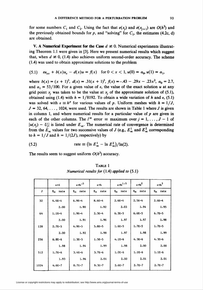
V. A Numerical Experiment for the Case i/ïO. Numerical experiments illustrat-
ing Theorem 1.1 were given in [3]. Here we present numerical results which suggest
that, when d ^ 0, (1.4) also achieves uniform second-order accuracy. The scheme
(1.4) was used to obtain approximate solutions to the problem
(5.1) e«xx + b(x)ux - d(x)u = fix) for 0 < x < 1, «(0) = Oq, m(1) = a,,
where b(x) = (x + l)3, d(x) = .31(x + l)5, fix) =-.43 - .29x - .23x2, a0 = 2.7,
and otx = 53/100. For a given value of e, the value of the exact solution u at any
grid point Xj was taken to be the value at x, of the approximate solution of (5.1),
obtained using (1.4) with A = 1/8192. To obtain a wide variation of A and e, (5.1)
was solved with e = hp for various values of p. Uniform meshes with A = l/J,
J = 32, 64, ... , 1024, were used. The results are shown in Table 1 where J is given
in column 1, and where numerical results for a particular value of p are given in
each of the other columns. The /°° error = maximum over / = 1,. . ., J — 1 of
\u(Xj) — Uj\ is listed under EM. The numerical rate of convergence is determined
from the E^ values for two successive values of J (e.g., E^ and E^ corresponding
to A = l/J and A = 1/(2J), respectively) by
(5.2) rate = (in Exx - In £¿)/ln(2).
The results seem to suggest uniform 0(A2) accuracy.
Table 1
Numerical results for (1.4) applied to (5.1)
e-h e«h e-h'
E„ rate E„ rate E„ rate E„ rate E«, rate E*, rate
32
64
128
256
512
1024
4.4E-4
2.00
1.1E-4
2.00
2.7E-5
2.00
6.8E-6
1.98
1.7E-6
1.93
4.6E-7
6.9E-4
1.90
1.9E-4
1.91
4.9E-5
1.92
1.3E-5
1.94
3.4E-6
1.96
8.7E-7
8.6E-4
1.92
2.3E-4
1.96
5.8E-5
1.98
1.5E-5
1.99
3.7E-6
2.01
9.3E-7
2.6E-4
2.03
6.3E-5
1.97
1.6E-5
1.97
4.1E-6
1.98
1.0E-6
2.00
2.6E-7
2.5E-4
1.94
6.6E-5
1.97
1.7E-5
1.98
4.3E-6
2.00
1.1E-6
2.01
2.7E-7
2.6E-4
1.95
6.7E-5
1.98
1.7E-5
1.99
4.3E-6
2.00
1.1E-6
2.01
2.7E-7
License or copyright restrictions may apply to redistribution; see http://www.ams.org/journal-terms-of-use
94 ALAN E. BERGER, JAY M. SOLOMON AND MELVYN CIMENT
Applied Mathematics Branch-Code R44
Naval Surface Weapons Center
Silver Spring, Maryland 20910
Applied Mathematics Branch-Code R44
Naval Surface Weapons Center
Silver Spring, Maryland 20910
Mathematical Analysis Division
National Bureau of Standards
Washington, D.C. 20234
1. A. E. Berger, J. M. Solomon & M. Ciment, "Higher order accurate tridiagonal difference
schemes for diffusion convection equations," Advances in Computer Methods for Partial Differential
Equations-ïll (R. Vichnevetsky and R. S. Stepleman, Eds.), Proc. Third IMACS Conference on
Computer Methods for Partial Differential Equations, June 1979, Lehigh University, pp. 322-330.
2. A. E. Berger, J. M. Solomon & M. Ciment, Uniformly Accurate Difference Methods for a Singular
Perturbation Problem, Proc. Internat. Conf. on Boundary and Interior Layers, Computational and
Asymptotic Methods, June 3-6, 1980, Trinity College, Dublin, Ireland (J. J. H. Miller, Ed.), Boole Press,
Dublin, 1980, pp. 14-28.3. A. E. Berger, J. M. Solomon, M. Ciment, S. H. Leventhal & B. C. Weinberg, "Generalized
operator compact implicit schemes for boundary layer problems," Math. Comp., v. 35, 1980, pp.
695-731.4. T. M. El-Mistikawy & M. J. Werle, "Numerical method for boundary layers with blowing-The
exponential box scheme," AIAA J., v. 16, 1978, pp. 749-751.
5. P. P. N. de Groen & P. W. Hemker, "Error bounds for exponentially fitted Galerkin methods
applied to stiff two-point boundary value problems," Numerical Analysis of Singular Perturbation
Problems (P. W. Hemker and J. J. H. Miller, Eds.), Academic Press, New York, 1979, pp. 217-249.
6. A. F. Hegarty, J. J. H. Miller & E. O'Riordan, Uniform Second Order Difference Schemes for
Singular Perturbation Problems, Proc. Internat. Conf. on Boundary and Interior Layers, Computational
and Asymptotic Methods, June 3-6, 1980, Trinity College, Dublin, Ireland (J. J. H. Miller, Ed.), Boole
Press, Dublin, 1980, pp. 301-305.7. A. M. Ii. in, "Differencing scheme for a differential equation with a small parameter affecting the
highest derivative," Mat. Zametki, v. 6, 1969, pp. 237-248 = Math. Notes, v. 6, 1969, pp. 596-602.8. R. B. Kellogg & A. Tsan, "Analysis of some difference approximations for a singular
perturbation problem without turning points," Math. Comp., v. 32, 1978, pp. 1025-1039.
9. J. Lorenz, Stability and Consistency Analysis of Difference Methods for Singular Perturbation
Problems, Proc. Conf. on Analytical and Numerical Approaches to Asymptotic Problems in Analysis,
June 9-13, 1980, University of Nijmegen, The Netherlands (O. Axelsson, h. Frank and A. Van der
Sluis, Eds.), North-Holland, Amsterdam, 1981.
10. J. J. H. Miller, "Sufficient conditions for the convergence, uniformly in epsilon, of a three point
difference scheme for a singular perturbation problem," Numerical Treatment of Differential Equations in
Applications (R. Ansorge and W. Tornig, Eds.), Lecture Notes in Math., vol. 679, Springer-Verlag, Berlin
and New York, 1978, pp. 85-91.
11. M. H. Protter & H. P. Weinberger, Maximum Principles in Differential Equations, Prentice-
Hall, Englewood Cliffs, N J., 1967.12. S. A. Pruess, "Solving linear boundary value problems by approximating the coefficients," Math.
Comp., v. 27, 1973, pp. 551-561.
13. M. E. Rose, "Weak-element approximations to elliptic differential equations," Numer. Math., v.
24, 1975, pp. 185-204.
14. D. R. Smith, "The multivariable method in singular perturbation analysis," SIAM Rev., v. 17,
1975, pp. 221-273.
License or copyright restrictions may apply to redistribution; see http://www.ams.org/journal-terms-of-use