arX

iv:1

607.

0293

3v3

[ph

ysic

s.cl

ass-

ph]

23

Aug

201

6

Distributional and regularized radiation fields of

non-uniformly moving straight dislocations, and

elastodynamic Tamm problem

Markus Lazar a,∗ and Yves-Patrick Pellegrini b,†

a Heisenberg Research Group,

Department of Physics,

Darmstadt University of Technology,

Hochschulstr. 6,

D-64289 Darmstadt, Germany

b CEA, DAM, DIF,

F-91297 Arpajon, France

Abstract

This work introduces original explicit solutions for the elastic fields radiated by non-uniformly

moving, straight, screw or edge dislocations in an isotropic medium, in the form of time-integral

representations in which acceleration-dependent contributions are explicitly separated out. These

solutions are obtained by applying an isotropic regularization procedure to distributional expressions

of the elastodynamic fields built on the Green tensor of the Navier equation. The obtained regular-

ized field expressions are singularity-free, and depend on the dislocation density rather than on the

plastic eigenstrain. They cover non-uniform motion at arbitrary speeds, including faster-than-wave

ones. A numerical method of computation is discussed, that rests on discretizing motion along an

arbitrary path in the plane transverse to the dislocation, into a succession of time intervals of con-

stant velocity vector over which time-integrated contributions can be obtained in closed form. As a

simple illustration, it is applied to the elastodynamic equivalent of the Tamm problem, where fields

induced by a dislocation accelerated from rest beyond the longitudinal wave speed, and thereafter

put to rest again, are computed. As expected, the proposed expressions produce Mach cones, the

dynamic build-up and decay of which is illustrated by means of full-field calculations.

Keywords: dislocation dynamics; non-uniform motion; generalized functions; elastodynamics; radi-

ation; regularization.

∗E-mail address: lazar@fkp.tu-darmstadt.de.†E-mail address: yves-patrick.pellegrini@cea.fr.

1

1 Introduction

Dislocations are linear defects whose motion is responsible for plastic deformation in crystalline ma-terials (Hirth and Lothe, 1982). To improve the current understanding of the plastic and elastic fronts(Clifton and Markenscoff, 1981) that go along with extreme shock loadings in metals (Meyers et al., 2009),Gurrutxaga-Lerma et al. (2013) recently proposed to make dynamic simulations of large sets of disloca-tions mutually coupled by their retarded elastodynamic field. Gurrutxaga-Lerma et al. (2014) review thematter and its technical aspects in some detail. This new approach is hoped to provide complementaryinsights over multi-physics large-scale atomistic simulations of shocks in matter (Zhakhovsky et al., 2011).If we leave aside the subsidiary (but physically important) issue of dislocation nucleation, dislocation-dynamics simulations involve two separate but interrelated tasks. First, one needs to compute the fieldradiated by a dislocation that moves arbitrarily. Second, given the past history of each dislocation, thecurrent dynamic stress field incident on it due to the other ones, and the externally applied stress field(e.g., a shock-induced wavefront), the further motion of the dislocation must be determined by a dynamicmobility law. While some progress has recently been achieved in the latter subproblem —which involvesscarcely explored radiation-reaction effects and dynamic core-width variations (Pellegrini, 2014)— thefocus of the present paper is on the former —a very classical one.

Indeed, substantial effort has been devoted over decades to obtaining analytical expressions of elasto-dynamic fields produced by non-uniformly moving singularities such as point loads (Stronge, 1970; Freund,1972, 1973), cracks, and dislocations. Results ranged, e.g., from straightforward applications to linear-elastic and isotropic unbounded media, to systems with interfaces such as half-spaces (Lamb’s problem)or layered media (Eatwell et al., 1982); coupled phenomena such as thermoelasticity (Brock et al., 1997)or anisotropic elastic media (Markenscoff and Ni, 1987; Wu, 2000), to mention but a few popular themes.Elastodynamic fields of dislocations have been investigated in a large number of works, among which(Eshelby, 1951; Kiusalaas and Mura, 1964, 1965; Mura, 1987; Nabarro, 1967; Brock, 1979, 1982, 1983;Markenscoff, 1980; Markenscoff and Ni, 2001a,b; Pellegrini, 2010; Lazar, 2011b, 2012, 2013a,b). Earlynumerical implementations of time-dependent fields radiated by moving sources (Niazy, 1975; Madariaga,1978) were limited to material displacements or velocities. As to stresses, Gurrutxaga-Lerma et al. (2014)based their simulations on the fields of Markenscoff and Clifton (1981) relative to a subsonic edge dislo-cation. Nowadays dynamic fields of individual dislocations or cracks are also investigated by atomisticsimulations (Li and Shi, 2002; Tsuzuki et al., 2009; Spielmannova et al., 2009), or numerical solutions ofthe wave equation by means of finite-element (Zhang et al., 2015), finite-difference, or boundary-integralschemes (Day et al., 2005). Hereafter, the analytical approach is privileged so as to produce referencesolutions.

Disregarding couplings with other fields such as temperature, one might be tempted to believe thatthe simplest two-dimensional problem of the non-uniform motion of rectilinear dislocation lines in anunbounded, linear elastic, isotropic medium, leaves very little room for improvements over past analyticalworks. This is not so, and our present concerns are as follows:

(i) Subsonic as well as supersonic velocities. In elastodynamics, from the 70’s onwards, the method ofchoice for analytical solutions has most often been the one of Cagniard improved by de Hoop (Aki and Richards,2009), whereby Laplace transforms of the fields are inverted by inspection after a deformation of the in-tegration path of the Laplace variable has been carried out by means of a suitable change of variable(see above-cited references). However, to the best of our knowledge, no such solutions can be employedindifferently for subsonic and supersonic motions, in the sense that the supersonic case need be consideredseparately in order to get explicit results as, e.g., in (Stronge, 1970; Freund, 1972; Callias and Markenscoff,1980; Markenscoff and Ni, 2001b; Huang and Markenscoff, 2011). Indeed, carrying out the necessary in-tegrals usually requires determining the wavefront position relatively to the point of observation. To date,the supersonic edge dislocation coupled to both shear and longitudinal waves has not been considered,and existing supersonic analytical solutions for the screw dislocation have not proved usable in full-fieldcalculations, except for the rather different solution obtained within the so-called gauge-field theory ofdislocations (Lazar, 2009), which appeals to gradient elasticity. Thus, one objective of the present work isto provide ‘automatic’ theoretical expressions that do not require wavefront tracking, for both screw andedge dislocations, and can be employed whatever the dislocation velocity. To this aim, we shall employa method different from the Cagniard–de Hoop one. This is not to disregard the latter but following a

2

different route was found more convenient in view of the remaining points listed here.(ii) Distributions and smooth regularized fields. For a Volterra dislocation in supersonic steady mo-

tion, fields are typically concentrated on Dirac measures along infinitely thin lines, to form Mach cones(Stronge, 1970; Callias and Markenscoff, 1980). Thus, the solution is essentially of distributional nature,and its proper characterization involves, beside Dirac measures, the use of principal-value and finite-partsprescriptions (Pellegrini and Lazar, 2015). Of course, in-depth analytical characterizations of wavefrontssingularities can still be extracted out of Laplace-transform integral representations (Freund, 1972, 1973;Callias and Markenscoff, 1980). However their distributional character implies that the solutions cannotdeliver meaningful numbers unless they are regularized by convolution with some source shape func-tion representing a dislocation of finite width. Only by this means can field values in Mach cones becomputed. Consequently, another objective is to provide field expressions for an extended dislocationof finite core width (instead of a Volterra one), thus taming all the field singularities that would oth-erwise be present at wavefronts and at the dislocation location, where Volterra fields blow up. In thework by Gurrutxaga-Lerma et al. (2013), a simple cut-off procedure was employed to get rid of infinities.Evidently, a similar device cannot be used with Dirac measures, which calls for a smoother and moreversatile regularization. Various dislocation-regularizing devices have been proposed in the past, someconsisting in expanding the Volterra dislocation into a flat Somigliana dislocation (Eshelby, 1949, 1951;Markenscoff and Ni, 2001a,b; Pellegrini, 2011). Such regularizations remove infinities, but leave out fielddiscontinuities on the slip path (Eshelby, 1949). A smoother approach consisting in introducing somenon-locality in the field equations has so far only be applied to the time-dependent motion of a screwdislocation. The one to be employed hereafter, introduced in (Pellegrini and Lazar, 2015), achieves anisotropic expansion the Volterra dislocation and smoothly regularizes all field singularities for screw andedge dislocations. In this respect, it resembles that introduced in statics by Cai et al. (2006). However,we believe it better suited to dynamics.

(iii) Field-theoretic framework. The traditional method of solution (Markenscoff, 1980) rests on im-posing suitable boundary conditions on the dislocation path. It makes little contact with field-theoreticnotions of dislocation theory such as plastic strain, or dislocation density and current used in purelynumerical methods of solution (Djaka et al., 2015). Instead, we wish our analytical results to be rootedon a field-theoretic background. One advantage is that the approach will provide a representation ofradiation fields where velocity- and acceleration-dependent contributions are clearly separated out, whichis most convenient for subsequent numerical implementation. Again to the best of our knowledge, nosuch representation of the elastodynamic fields has been given so far. However, previous work in thatdirection can be found in (Lazar, 2011b, 2012, 2013a).

(iv) Integrals in closed form. In (Gurrutxaga-Lerma et al., 2013) the numerical implementation of theresults by Markenscoff and Clifton (1981), where the retarded fields are expressed in terms of an integralover the path abscissa, is not fully explicit. Indeed, this integral is split over path segments, and eachsegment is integrated over numerically — a tricky matter, as pointed out by the former authors. Bycontrast, and dealing with time intervals instead of path segments, the sub-integrals will be expressedhereafter in closed form by means of the key indefinite integrals obtained in (Pellegrini and Lazar, 2015).

(v) Arbitrary paths. Results will be given in tensor form, with the dislocation velocity as a vector.Thus, they can be applied immediately to arbitrary dislocation paths parametrized by time. Using thetime variable as the main parameter is a natural choice, and does not require computing so-called ‘retardedtimes’. Although we must leave such applications to further work, this makes it straightforward toinvestigate radiative losses in various oscillatory motions, e.g., (lattice-induced) periodic oscillations in thedirection transverse to the main glide plane during forward motion, which space-based parametrizationssuch as in the procedure outlined by Brock (1983) make harder to achieve.

Accordingly, our work is organized as follows. First, we begin by computing in Section 2 general formsfor the elastic fields of non-uniformly moving screw and edge dislocations using the theory of distributions,starting from the most general field equations in terms of dislocation densities and currents. Our approachrelies on Green’s functions [e.g., Barton (1989); Mura (1987)]. In Section 2.1, inhomogeneous Navierequations for the elastic fields are derived as equations of motion, with source terms expressed in termsof the fields that characterize the dislocation (dislocation density tensor and dislocation current tensor).The Cauchy problem of the Navier equations is then addressed in Section 2.2, where the solutions forthe elastic fields are written as the convolution of the retarded elastodynamic Green-function tensor —

3

interpreted as a distribution— with the dislocation fields. As a result, the mathematical structure of thelatter is partly inherited from the former. Some connections with past works are made in Section 2.3.Second, we specialize the obtained field expressions to Volterra dislocations: the fields themselves becomedistributions. In Section 3, the structure of the Green tensor and of the elastodynamic radiation fieldsis revealed and analyzed in terms of locally-integrable functions and pseudofunctions (namely, singulardistributions that require a ‘finite part’ prescription). The Volterra screw (Section 3.1) and edge (Section3.2) dislocations are addressed separately for definiteness. The expressions reported are mathematicallywell-defined, and cover arbitrary speeds including faster-then-wave ones, which is the main differencewith classical approaches. Third, since distributional fields, although mathematically correct, cannotin general produce meaningful numbers unless being applied to test functions, we turn the formalisminto one suitable to numerical calculations by means of the isotropic-regularization procedure alludedto above, where the relevant smooth test function represents the dislocation density. The procedure isintroduced in Section 4.1, and regularized expressions for the elastic fields are obtained in integral formin Section 4.2, after the regularized Green tensor has been defined. Next, a numerical implementationscheme that involves only closed-form results is proposed in Section 5, based on the key integrals ofPellegrini and Lazar (2015). As a first illustration, the particular case of steady motion for the edgedislocation is discussed in detail, with emphasis on faster-than-wave motion. Finally, the procedureis applied in Section 6 to the numerical investigation of the elastodynamic equivalent of the Tammproblem, where fields induced by a dislocation accelerated from rest beyond the longitudinal wave speed,and thereafter put to rest again, are computed and analyzed. Section 7 provides a concluding discussion,which summarizes our approach and results, and points out some limitations. The most technical elementsare collected in the Appendix.

2 Basic geometric equations and field equations of motion

2.1 Field identities and equations of motion

In this Section, the equations of motion of the elastic fields produced by moving dislocations are derivedin the framework of incompatible elastodynamics (see, e.g., Mura (1963, 1987); Kosevich (1979); Lazar(2011b, 2013b)). An unbounded, isotropic, homogeneous, linearly elastic solid is considered. In thetheory of elastodynamics of self-stresses, the equilibrium condition is1

pi − σij,j = 0 , (1)

where p and σ are the linear momentum vector and the stress tensor, respectively. For incompatiblelinear elastodynamics, the momentum vector p and the stress tensor σ can be expressed in terms of theelastic velocity (particle velocity) vector v and the incompatible elastic distortion tensor β by means ofthe two constitutive relations

pi = ρ vi , (2a)

σij = Cijklβkl , (2b)

where ρ denotes the mass density, and Cijkl the tensor of elastic moduli or elastic tensor. It enjoys thesymmetry properties Cijkl = Cjikl = Cijlk = Cklij . For isotropic materials, the elastic tensor reduces to

Cijkl = λ δijδkl + µ(δikδjl + δilδjk) , (3)

where λ and µ are the Lame constants. If the constitutive relations (2a) and (2b) are substituted intoEq. (1), the equilibrium condition expressed in terms of the elastic fields v and β may be written as

ρ vi − Cijklβkl,j = 0 . (4)

The presence of dislocations makes the elastic fields incompatible, which means that they are not anymoresimple gradients of the material displacement vector u. In the eigenstrain theory of dislocations (e.g.,

1We use the usual notation βij,k := ∂kβij and βij := ∂tβij .

4

Mura (1987)) the total distortion tensor βT consists of elastic and plastic parts2

βTij := ui,j = βij + βP

ij , (5)

but vi = ui. Here βP is the plastic distortion tensor or eigendistortion tensor. The plastic distor-tion is a well-known quantity in dislocation theory and in Mura’s theory of eigenstrain. Nowadays,this field can be understood as a tensorial gauge field in the framework of dislocation gauge the-ory (Lazar and Anastassiadis, 2008; Lazar, 2010).

For dislocations, the incompatibility tensors are the dislocation density and dislocation current tensors(e.g., Hollander (1962); Kosevich (1979); Lazar (2011a)). The dislocation density tensor α and thedislocation current tensor I are classically defined by (e.g., Kosevich (1979); Landau and Lifschitz (1986))

αij = −ǫjklβPil,k , (6a)

Iij = −βPij , (6b)

or they read in terms of the elastic fields

αij = ǫjklβil,k , (7a)

Iij = βij − vi,j . (7b)

Eqs. (6a) and (6b) are the fundamental definitions of the dislocation density tensor and of the disloca-tion current tensor, respectively, whereas Eqs. (7a) and (7b) are geometric field identities. Originally,Nye (1953) introduced the concept of a dislocation density tensor, and the definition (6a) of α goesback to Kroner (1955, 1958) and Bilby (1955) (see also Kroner (1981)). The tensor I was introducedby Kosevich (1962) under the name ‘dislocation flux density tensor’ —a denomination used by Kosevich(1979); Teodosiu (1970), and Lardner (1974)— and by Hollander (1962) as the ‘dislocation current’ (seealso Kosevich (1979); Landau and Lifschitz (1986); Teodosiu (1970)). We adopt hereafter the latter de-nomination. Both α and I have nine independent components. Moreover, they fulfill the two dislocationBianchi identities (see also Landau and Lifschitz (1986); Lazar (2011a))

αij,j = 0 , (8a)

αij + ǫjklIik,l = 0 , (8b)

which are geometrical consequences due to the definitions (6a)–(7b). Thus,if the dislocation densitytensor and dislocation current tensor are given in terms of the elastic fields and plastic fields accordingto Eqs. (6a)–(7b), then the two dislocation Bianchi identities (8a) and (8b) are satisfied automatically.Conversely, if the two dislocation Bianchi identities (8a) and (8b) are fulfilled, then the dislocation densitytensor and the dislocation current tensor can be expressed in terms of elastic and plastic fields accordingto Eqs. (6a)–(7b) using the additive decomposition (5). Therefore, the dislocation Bianchi identities (8a)and (8b) are a kind of compatibility conditions for the dislocation density tensor and dislocation fluxtensor or ‘dislocation conservation laws’ (see also Kosevich (1979)).

From the physical point of view, Eq. (8a) states that dislocations do not end inside the body andEq. (8b) shows that whenever a dislocation moves or the dislocation core changes its structure and shape,the dislocation current I is nonzero. Thus, the dislocation density can only change via the dislocationcurrent, which means that the evolution of the dislocation density tensor α is determined by the curl ofthe dislocation flux tensor I.

From the equilibrium condition (4), uncoupled field equations for the elastic fields β and v producedby dislocations may be derived as equations of motion (see, e.g., Lazar (2011b, 2013b)). They read

Likβkm = ǫnmlCijkl αkn,j + ρ Iim , (9a)

Likvk = Cijkl Ikl,j , (9b)

2Note, however, that the tensors βij and βPij defined by Mura are the transposed of the ones used in the present work.

The same goes for αij .

5

where Lik stands for the elastodynamic Navier differential operator

Lik = ρ δik∂tt − Cijkl∂j∂l. (10)

Substituting Eq. (3) into Eq. (10), its isotropic form reads

Lik = ρ δik∂tt − µδik ∆− (λ+ µ) ∂i∂k (11)

where ∆ denotes the Laplacian. Eq. (9a) is a tensorial Navier equation for β and Eq. (9b) is a vectorialNavier equation for v, where the dislocation density and current tensors act as source terms.

2.2 Green tensor and integral solutions

We now turn to the solution of the retarded field problem of Eqs. (9a) and (9b). For this purpose weuse Green functions (e.g., Barton (1989)). Let δ(.) denote the Dirac delta function and δij denote theKronecker symbol. The elastodynamic Green tensor G+

ij is the solution, in the sense of distributions,3 ofthe (anisotropic) inhomogeneous Navier equation with unit source

LikG+km(r − r′, t− t′) = δim δ(t− t′)δ(r − r′) , (12)

subjected to the causality constraint

G+ij(r − r′, t− t′) = 0 for t < t′ . (13)

The following properties hold in the equal-time limit (Appendix A):

limτ→0+

G+ij(r, τ) = 0, lim

τ→0+∂tG

+ij(r, τ) = ρ−1δijδ(r). (14)

Now we consider the Cauchy problem of the inhomogeneous Navier equation, expressed by Eqs. (9a)and (9b). For an unbounded medium, its solutions are (see also Eringen and Suhubi (1975); Barton(1989); Vladimirow (1971))

βim(r, t) = ǫnml

∫ t

t0

dt′∫

Cjkpl G+ij(r − r′, t− t′)αpn,k(r

′, t′)dr′

+

∫ t

t0

dt′∫

ρG+ij(r − r′, t− t′) Ijm(r′, t′)dr′

+

∫G+

ij(r − r′, t− t0) βjm(r′, t0) dr′

+

∫G+

ij(r − r′, t− t0)βjm(r′, t0) dr′ (15a)

and

vi(r, t) =

∫ t

t0

dt′∫

Cjklm G+ij(r − r′, t− t′) Ilm,k(r

′, t′) dr′

+

∫G+

ij(r − r′, t− t0) vj(r′, t0) dr

′

+

∫G+

ij(r − r′, t− t0) vj(r′, t0) dr

′ , (15b)

where integrals over r′ are over the whole medium, and where the following functions have been prescribedas initial conditions at t = t0 throughout the medium:

β(r, t0) , β(r, t0) , v(r, t0) , v(r, t0) . (16)

3The ‘plus’ superscript serves to distinguish this distribution from the associated function Gij(r, t) to be introduced inSec. 5.

6

Because the elastodynamic Navier equation is a generalization of the wave equation, Eqs. (15a) and (15b)are similar to the Poisson formula for the latter (Vladimirow, 1971).

Since G+ij(r − r′, t − t0) and G+

ij(r − r′, t − t0) vanish as t0 → −∞, Eqs. (15a) and (15b) can berepresented as convolutions of the Green tensor with the sources of the inhomogeneous Navier equations,only (Mura, 1963; Lazar, 2011b). Letting thus t0 → −∞ the solutions for β and v reduce to

βim(r, t) = ǫnml

∫ t

−∞

dt′∫

Cjkpl G+ij(r − r′, t− t′)αpn,k(r

′, t′) dr′

+

∫ t

−∞

dt′∫

ρG+ij(r − r′, t− t′) Ijm(r′, t′) dr′ , (17a)

vi(r, t) =

∫ t

−∞

dt′∫

Cjklm G+ij(r − r′, t− t′) Ilm,k(r

′, t′) dr′ , (17b)

or equivalently

βim(r, t) = ǫnml

∫ t

−∞

dt′∫

Cjkpl G+ij,k(r − r′, t− t′)αpn(r

′, t′) dr′

+

∫ t

−∞

dt′∫

ρ G+ij(r − r′, t− t′) Ijm(r′, t′) dr′ , (18a)

vi(r, t) =

∫ t

−∞

dt′∫

Cjklm G+ij,k(r − r′, t− t′) Ilm(r′, t′) dr′ . (18b)

Eqs. (17a)–(18b) are valid for general dislocation distributions (continuous distribution of dislocations,dislocation loops, straight dislocations). Later on, we shall specialize to straight dislocations.

Let the velocity V (t) of a moving dislocation be some given function of time. Then, the followingrelation holds between its associated dislocation density and current tensors:

Iij = ǫjkn Vk αin . (19)

This relation means that the current I is caused by the moving dislocation density α. Thus, I is aconvection dislocation current (Gunther, 1973; Lazar, 2013b). Substituting Eq. (19) into relation (8b),the Bianchi identity (8b) reduces to the following form in terms of the dislocation density tensor and thedislocation velocity vector

αij = −ǫjkl(ǫkmnVmαin),l = (Vjαil),l − (Vlαij),l . (20)

Sometimes the Bianchi identity (20) is called dislocation density transport equation (see, e.g., Djaka et al.(2015)).

We moreover obtain from Eqs. (9a) and (9b) the field equations of motion in the form

Likβkm = ǫnml

[Cijkl αkn,j + ρ ∂t(Vlαin)

], (21a)

Likvk = ǫnmlCijkm (Vlαkn),j , (21b)

where the sources are given in terms of the dislocation density tensor and the dislocation velocity vector.Obviously, the validity of Eq. (20) is conditioned by the assumptions that underlie Eq. (19). Thus,Eq. (19) makes sense only for a discrete dislocation line with rigid core, since it neglects changes withtime of its core shape. However, by imposing a suitable parameterization of the dislocation density orof the plastic eigenstrain (e.g., Pellegrini (2014)), an additional term in the current tensor related tocore-width variations could easily be derived from Eq. (6b). Such effects are neglected in the presentstudy. Accordingly, from Eq. (20) and using Vj,l = Vl,l = 0 for the problem considered, we deduce withthe help of the Bianchi identity (8a) that for one single rigid dislocation

αij = −Vk αij,k. (22)

7

2.3 Remarks

It is worthwhile pointing out that although we insisted, for better physical insight, on deriving Eq. (18a)from field equations with sources expressed in terms of dislocation density and current, the latter equationis fully consistent with the perhaps more familiar writing of the elastic distortion in terms of the plasticdistortion and the second derivatives of the Green tensor as (e.g., Mura (1987))4

βij(r, t) = −∫ t

−∞

dt′∫

dr′G+ik,jl(r − r′, t− t′)Cklmnβ

Pmn(r

′, t′)− βPij(r, t) . (23)

Also, the issue of the upper boundary t′ = t of the time-integration in the integral solutions deservessome comments. It is sometimes read in treatises on Green functions, e.g., (Barton, 1989), that the upperboundary should lie slightly above t, which is usually denoted by t+. Such a device helps one to easilycheck that the integral formulas are indeed solutions of the equation of motion they derive from. Becauseof the causality constraint, the upper time-integration boundary can as well be taken as +∞. However,it is less recognized that the boundary can as well be chosen slightly below t, which we denote as t−.This is possible because of the two limiting properties (14), the first of which ensuring that removing theinterval ]t−, t+[ from the integration interval t′ ∈] −∞, t+[ makes no difference on the final result. Thesecond property in (14) allows us to show —in Appendix B— that solutions written with integrals overt′ ∈]−∞, t−[ satisfy the equation of motion as well. Since the solution is unique, all these formulationsgive identical results. However, the use of t−, which amounts to eliminating the immediate vicinity ofthe point t′ = t from time integrals, is much more convenient for numerical and analytical purposes, aswill be shown in Section 5.2. This device has already been employed in (Pellegrini, 2011, 2012, 2014;Pellegrini and Lazar, 2015), but was introduced there without any detailed justification. Until Section 4,we continue denoting the upper boundary as t′ = t in general formulas, for simplicity.

3 Straight Volterra dislocations in the framework of distribu-tions

In this Section, the elastodynamic fields produced by the non-uniform motion of straight screw and edgeVolterra dislocations are studied using the theory of distributions or generalized functions (Schwartz,1950/51; Gel’fand and Shilov, 1964; Kanwal, 2004). The field equations of motion are solved by meansof Green functions. The problem is two-dimensional, of anti-plane strain or plane strain character.

3.1 Screw dislocation

We address first the anti-plane strain problem of a Volterra screw dislocation in non-uniform motionat time t along some arbitrary path s(t′) prescribed in advance in the time range −∞ < t′ ≤ t. Thedislocation line and the Burgers vector bz are parallel to the z-axis. The dislocation velocity has twonon-vanishing components: Vx = sx(t), Vy = sy(t). The dislocation density and dislocation currenttensors are

αzz = bz ℓz δ(R(t)) , Izj = bz ǫjkzVk(t) ℓz δ(R(t)) , (24)

where R(t) = r − s(t) ∈ R2, ℓz is a unit vector in z-direction and i, j, k = x, y. The index z is a fixed

index (no summation).Eqs. (21a) and (21b) simplify enormously for the nonvanishing components βzx, βzy, and vz . Using

Eq. (24) and αzz = −Vkαzz,k, we obtain from Eqs. (21a) and (21b) the following equations of motion ofa screw dislocation:

Lzzβzm = ǫzml

[Czjzl αzz,j + ρ

(Vl αzz − VlVk αzz,k

)], (25a)

Lzzvz = ǫzml Czjzm Vl αzz,j , (25b)

4 Indeed, ignoring our present emphasis on the distributional character of the Green tensor, Eq. (18a) is nothing but Eq.(38.36) on p. 351 of Mura’s treatise. This is realized upon comparing Mura’s Eq. (38.19) with the above definition (6b) ofIij , bearing in mind the transposed character of our dislocation tensors with respect to Mura’s (see note 3).

8

where V is the dislocation acceleration. With the dynamic elastic tensor for non-uniform motion, namely,

Cijkl(V ) = Cijkl − ρ VjVl δik (26)

and using the property of the differentiation of a convolution, the appropriate solution may be writtenas the convolution integrals

βzm(r, t) = ǫzml

∫ t

−∞

dt′∫ {

G+zz,k(r − r′, t− t′) Czkzl(V (t′))

+ ρG+zz(r − r′, t− t′) Vl(t

′)}αzz(r

′, t′) dr′ , (27a)

vz(r, t) = ǫzml

∫ t

−∞

dt′∫

Czkzm G+zz,k(r − r′, t− t′)Vl(t

′)αzz(r′, t′) dr′ , (27b)

The dynamic elastic tensor (26) was originally introduced by Saenz (1953) for uniformly moving disloca-tions (see also Bacon et al. (1979), who use a different index ordering), and employed in elastodynamicsby Wu (2000) with the same index ordering as in Eq. (26). It possesses only the major symmetry

Cijkl(V ) = Cklij(V ).Substituting the dislocation density (24) into Eqs. (27a) and (27b), and performing the integration

over r′, we obtain

βzm(r, t) = bzℓz ǫzml

∫ t

−∞

{G+

zz,k(r − s(t′), t− t′) Czkzl(V (t′)) + ρG+zz(r − s(t′), t− t′) Vl(t

′)}dt′ (28a)

vz(r, t) = bzℓz ǫzml

∫ t

−∞

Czkzm G+zz,k(r − s(t′), t− t′)Vl(t

′) dt′ , (28b)

where G+zz is the retarded Green function (distribution) of the anti-plane problem defined by

LzzG+zz =

(ρ ∂tt − µ∆

)G+

zz = δ(t)δ(r) . (29)

If the material is infinitely extended, the two-dimensional elastodynamic Green-function distributionof the anti-plane problem, which is nothing but the usual Green function of the two-dimensional scalarwave equation (e.g. Morse and Feshbach (1953); Barton (1989)), interpreted as a distribution, reads (see,e.g., Eringen and Suhubi (1975); Kausel (2006))

G+zz(r, t) =

θ(t)

2πµ

(t2 − r2/c2T

)−1/2

+(30)

with the velocity of transverse elastic waves (shear waves, also called S-waves)

cT =√µ/ρ , (31)

and where θ(t) is the Heaviside unit-step function that restricts this causal solution to positive times. Inthis writing, the generalized function xλ

+, defined as (see, e.g., Schwartz (1950/51); Gel’fand and Shilov(1964); Kanwal (2004); de Jager (1969))

xλ+ =

{0 for x < 0

xλ for x > 0 ,(32)

has been used. The derivative of x1/2+ is given by

(x1/2+

)′=

1

2x−1/2+ . (33)

The derivative of x−1/2+ gives a pseudofunction (see Schwartz (1950/51); Gel’fand and Shilov (1964);

Zemanian (1965)):

(x−1/2+

)′= −1

2Pf x

−3/2+ . (34)

9

The symbol Pf in Eq. (34) stands for pseudofunction. In general, pseudofunctions are distributions gen-erated by Hadamard’s finite part of a divergent integral. They arise naturally when certain distributions

are differentiated. In Eq. (34) the regular distribution x−1/2+ was differentiated. Using Eqs. (33) and (34),

the derivative of the Green function (30) is expressed as the pseudofunction

G+zz,k(r, t) =

θ(t)

2πµ

xk

c2TPf

(t2 − r2/c2T

)−3/2

+. (35)

Finally, the elastic fields of a non-uniformly moving screw Volterra dislocation read, in distributionalform

βzx(r, t) =bzℓz2πc2T

∫ t

−∞

(Vy(t

′)[t2 −R2(t′)/c2T

]−1/2

+

+

((1−

V 2y (t

′)

c2T

)Ry(t

′)− Vx(t′)Vy(t

′)

c2TRx(t

′)

)Pf

[t2 −R2(t′)/c2T

]−3/2

+

)dt′ , (36a)

βzy(r, t) = − bzℓz2πc2T

∫ t

−∞

(Vx(t

′)[t2 −R2(t′)/c2T

]−1/2

+

+

((1− V 2

x (t′)

c2T

)Rx(t

′)− Vx(t′)Vy(t

′)

c2TRy(t

′)

)Pf

[t2 −R2(t′)/c2T

]−3/2

+

)dt′ , (36b)

vz(r, t) =bzℓz2πc2T

∫ t

−∞

(Vy(t

′)Rx(t′)− Vx(t

′)Ry(t′))Pf

[t2 −R2(t′)/c2T

]−3/2

+dt′ , (36c)

where t = t− t′.The fields given by Eqs. (36a)–(36c) clearly consist of two parts: (i) Fields depending on the dislocation

velocities Vx and Vy alone and proportional to the pseudofunction distribution of power−3/2—dislocationvelocity-dependent fields or near fields, built from the gradient of the Green tensor; (ii) Fields dependingon the dislocation accelerations Vx and Vy and proportional to the regular distribution of power −1/2—dislocation acceleration-dependent fields or far fields, built on the Green tensor itself. The velocityfield (36c) possesses no acceleration part.

It should be mentioned that it seems to be hard to find a measurement which can distinguish betweenthe acceleration- and velocity-depending fields. Such a decomposition is basically conceptual. In a naturalway, we may separate β into two parts, one which involves the dislocation acceleration and goes to zerofor V = 0, and one which involves only the dislocation velocity and yields the static field for a dislocationwith V = 0. Dislocations at rest or in steady motion do not generate elastodynamic waves. Onlynon-uniformly moving dislocations emit elastodynamic radiation.

Some historical remarks are in order. In the 1950s already, Sauer (1954, 1958) emphasized the interestof introducing the theory of distributions in supersonic aerodynamics. In particular, in gas dynamics andwing theory, pseudofunctions of power −3/2 have been used in the framework of distribution theory, e.g.,Sauer (1954, 1958); Dorfner (1957) (see also de Jager (1969)).

3.2 Edge dislocation

We next turn to the straight edge Volterra dislocation in the plane-strain framework. Its associateddislocation density and current tensors read, respectively,

αij = bi ℓj δ(R(t)) , Iij = bi ǫjklVk(t) ℓl δ(R(t)) , (37)

where R(t) = r − s(t) ∈ R2 and i, j, k = x, y. Using αij = −Vk αij,k, we obtain from Eqs. (21a) and

(21b) the following equations of motion:

Likβkm = ǫnml

[Cijkl αkn,j + ρ

(Vlαin − VlVk αin,k

)], (38a)

Likvk = ǫnml Cijkl Vl αkn,j , (38b)

10

where V = s. Using the property of the differentiation of a convolution, the corresponding solutions ofEqs. (38a) and (38b) are given in convolution form

βim(r, t) = ǫnml

∫ t

−∞

dt′∫ (

G+ij,k(r − r′, t− t′) Cjkpl(V (t′))αpn(r

′, t′)

+ ρG+ij(r − r′, t− t′) Vl(t

′)αjn(r′, t′)

)dr′ , (39a)

vi(r, t) = ǫnml

∫ t

−∞

dt′∫

Cjkpm G+ij,k(r − r′, t− t′)Vl(t

′)αpn(r′, t′) dr′ , (39b)

where the two-dimensional (distributional) Green tensorG+ij is defined as the retarded solution of Eq. (12),

with (11).Substituting Eq. (37) into (39a) and (39b) and performing the r′-integration, we find

βim(r, t) = ǫnml

∫ t

−∞

(G+

ij,k(r − s(t′), t− t′) Cjkpl(V (t′)) bpℓn

+ ρG+ij(r − s(t′), t− t′) Vl(t

′) bjℓn

)dt′ (40a)

vi(r, t) = ǫnml

∫ t

−∞

Cjkpm G+ij,k(r − s(t′), t− t′)Vl(t

′) bpℓn dt′ . (40b)

Using the distributional approach, the two-dimensional retarded Green tensor is given by (see Eason et al.(1956); Eringen and Suhubi (1975); Kausel (2006) for the Green tensor in the classical approach)

G+ij(r, t) =

θ(t)

2πρ

{xixj

r4

[t2(t2 − r2/c2L

)−1/2

++(t2 − r2/c2L

)1/2+

− t2(t2 − r2/c2T

)−1/2

+−

(t2 − r2/c2T

)1/2+

]

− δijr2

[(t2 − r2/c2L

)1/2+

− t2(t2 − r2/c2T

)−1/2

+

]}. (41)

It consists of regular distributions of power 1/2 and −1/2. The shear velocity cL is defined in (31), andcT is the velocity of the longitudinal elastic waves (P-wave) expressed in terms of the Lame constants as

cL =√(2µ+ λ)/ρ. (42)

It is noted that G+zz(r, t), Eq. (30), is twice the spherical part of G+

ij(r, t) in (41). Using Eqs. (33) and(34), the derivative of the Green tensor (41) is obtained as

G+ij,k(r, t) =

θ(t)

2πρ

{(δikxj + δjkxi

r4− 4 xixjxk

r6

)[t2(t2 − r2/c2L

)−1/2

++(t2 − r2/c2L

)1/2+

− t2(t2 − r2/c2T

)−1/2

+−(t2 − r2/c2T

)1/2+

]

+2 δijxk

r4

[(t2 − r2/c2L

)1/2+

− t2(t2 − r2/c2T

)−1/2

+

]

+xixjxk

r4

[t2

c2LPf

(t2 − r2/c2L

)−3/2

+− 1

c2L

(t2 − r2/c2L

)−1/2

+

− t2

c2TPf

(t2 − r2/c2T

)−3/2

++

1

c2T

(t2 − r2/c2T

)−1/2

+

]

+δijxk

r2

[1

c2L

(t2 − r2/c2L

)−1/2

++

t2

c2TPf

(t2 − r2/c2T

)−3/2

+

]}, (43)

which involves pseudofunctions of power −3/2 in addition to distributions of power 1/2 and −1/2. Eqs.(41) and (43) display G+

ij(r, t) and G+ij,k(r, t) in expanded form for clarity. However, more compact

expressions for these distributions that emphasize the occurrence of t solely via well-defined groupscontaining either cTt or cLt can be found in (Pellegrini and Lazar, 2015) [see also Eq. (A.3) below].

11

Substituting Eqs. (41) and (43) into Eqs. (40a) and (40b), we obtain the elastic distortion tensor ofthe non-uniformly moving Volterra edge dislocation as

βim(r, t) =1

2πρǫnml

∫ t

−∞

dt′(Cjkpl(V (t′)) bpℓn

{(δikRj(t

′) + δjkRi(t′)

R4(t′)− 4Ri(t

′)Rj(t′)Rk(t

′)

R6(t′)

)

×[t2(t2 −R2(t′)/c2L

)−1/2

++(t2 −R2(t′)/c2L

)1/2

+

− t2(t2 −R2(t′)/c2T

)−1/2

+−(t2 −R2(t′)/c2T

)1/2

+

]

+2 δijRk(t

′)

R4(t′)

[(t2 −R2(t′)/c2L

)1/2+

− t2(t2 −R2(t′)/c2T

)−1/2

+

]

+Ri(t

′)Rj(t′)Rk(t

′)

R4(t′)

[t2

c2LPf

(t2 −R2(t′)/c2L

)−3/2

+− 1

c2L

(t2 −R2(t′)/c2L

)−1/2

+

− t2

c2TPf

(t2 −R2(t′)/c2T

)−3/2

++

1

c2T

(t2 −R2(t′)/c2T

)−1/2

+

]

+δijRk(t

′)

R2(t′)

[1

c2L

(t2 −R2(t′)/c2L

)−1/2

++

t2

c2TPf

(t2 −R2(t′)/c2T

)−3/2

+

]}

+ ρ Vl(t′) bjℓn

{Ri(t

′)Rj(t′)

R4(t′)

[t2(t2 −R2(t′)/c2L

)−1/2

++(t2 −R2(t′)/c2L

)1/2+

− t2(t2 −R2(t′)/c2T

)−1/2

+−(t2 −R2(t′)/c2T

)1/2+

]

− δijR2(t′)

[(t2 −R2(t′)/c2L

)1/2+

− t2(t2 −R2(t′)/c2T

)−1/2

+

]}), (44)

and the velocity vector reads

vi(r, t) =bpℓn2πρ

ǫnml Cjkpm

∫ t

−∞

dt′ Vl(t′)

{(δikRj(t

′) + δjkRi(t′)

R4(t′)− 4Ri(t

′)Rj(t′)Rk(t

′)

R6(t′)

)

×[t2(t2 −R2(t′)/c2L

)−1/2

++(t2 −R2(t′)/c2L

)1/2

+

− t2(t2 −R2(t′)/c2T

)−1/2

+−(t2 −R2(t′)/c2T

)1/2

+

]

+2 δijRk(t

′)

R4(t′)

[(t2 −R2(t′)/c2L

)1/2+

− t2(t2 −R2(t′)/c2T

)−1/2

+

]

+Ri(t

′)Rj(t′)Rk(t

′)

R4(t′)

[t2

c2LPf

(t2 −R2(t′)/c2L

)−3/2

+− 1

c2L

(t2 −R2(t′)/c2L

)−1/2

+

− t2

c2TPf

(t2 −R2(t′)/c2T

)−3/2

++

1

c2T

(t2 −R2(t′)/c2T

)−1/2

+

]

+δijRk(t

′)

R2(t′)

[1

c2L

(t2 −R2(t′)/c2L

)−1/2

++

t2

c2TPf

(t2 −R2(t′)/c2T

)−3/2

+

]}. (45)

Those elastic fields consist of two different kinds of contributions, about which the same comments as inthe screw case can be made.

Expressions (44)–(45) encompass gliding as well as climbing edge dislocations. If V ‖b, they describea gliding edge dislocation, and with V ⊥ b they deliver the fields of a climbing edge dislocation (see, e.g.,Lazar (2011b); Pellegrini (2010)). If we specialize to non-uniformly moving straight edge dislocationswith Burgers vector in the x-direction, bx, and with the dislocation line ℓz parallel to the z-axis, then thedislocation density and current tensors of a gliding edge dislocation with arbitrary velocity Vx(t) in thex-direction are given by

αxz = bx ℓz δ(R(t)) , Ixy = bx ǫyxzVx(t) ℓz δ(R(t)) , (46)

12

whereR(t) = (x−sx(t), y). For a climbing edge dislocation with arbitrary velocity Vy(t) in the y-direction,they read

αxz = bx ℓz δ(R(t)) , Ixx = bx ǫxyzVy(t) ℓz δ(R(t)) , (47)

where R(t) = (x, y − sy(t)).In general, the elastodynamic fields of straight dislocations have the form of time-integrals over the

history of the motion, and display a so-called ‘afterglow’-type response (Barton, 1989) with slow relax-ation tails. The reason, specific to the two-dimensional problem, is that fields continuously arrive fromremote emission points on past locations of the dislocation line. This effect is accounted for by thetwo-dimensional Green function.

We are therefore left to evaluate time-integrals of considerable complexity, which only in some simplecases yield closed-form results in terms of elementary functions. Consequently, the procedure developedhereafter relies, after a suitable regularization method has been applied, on a decomposition of arbitrarymotion into time-intervals of constant velocity for which explicit field expressions can be given.

4 Regularization in the framework of distributions

4.1 Regularization procedure

Up to now, our results for the fields of non-uniformly moving Volterra dislocations are singular distribu-tions. Although being mathematically well-defined in the latter sense, and therefore free of non-integrablesingularities, they are inconvenient for numerical purposes in the case of arbitrarily prescribed motions(t). In order to get singularity-free fields, we have to regularize these distributions. The standard meansof doing this is the convolution of distributions with a suitable test function. This operation, which iscalled the regularization of a distribution, converts the distribution into an infinitely smooth function.

The procedure we call hereafter isotropic regularization consists in the convolution of the singulardistributions by the following isotropic representation of the two-dimensional Dirac delta distribution(Kanwal, 2004):

δ(r) = δ(x)δ(y) = limε→0

δε(r) , with δε(r) =ε

2π(r2 + ε2)3/2, (48)

which plays here the role of the test function. Here δε(r) is a non-singular Dirac-delta sequence withparametric dependence. For ε finite this corresponds to considering a line source with rotationally-invariant core of radius ε. We start with the regularization of the dislocation density and dislocationcurrent tensors. The regularization of the dislocation density tensor of a Volterra dislocation is denotedby the convolution product

αisoij (r, t) = [αij ∗ δε](r, t) =

∫αij(r − r′, t) δε(r′) dr′ , (49)

where ∗ denotes the two-dimensional spatial convolution. The regularized dislocation density tensor reads

αisoij =

biℓj2πε2

1[(R(t)/ε

)2+ 1

]3/2 . (50)

The dislocation density tensor αisoij is finite and reaches its maximum value of biℓj/(2πε

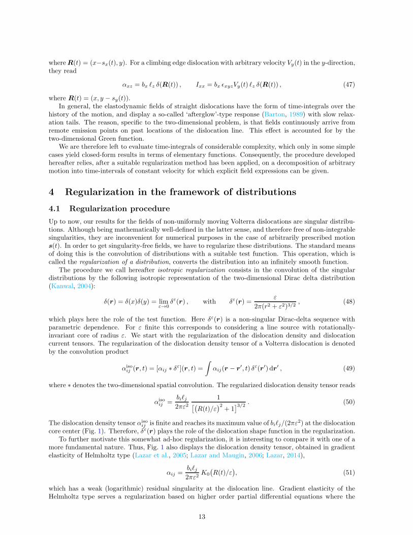
2) at the dislocationcore center (Fig. 1). Therefore, δε(r) plays the role of the dislocation shape function in the regularization.

To further motivate this somewhat ad-hoc regularization, it is interesting to compare it with one of amore fundamental nature. Thus, Fig. 1 also displays the dislocation density tensor, obtained in gradientelasticity of Helmholtz type (Lazar et al., 2005; Lazar and Maugin, 2006; Lazar, 2014),

αij =biℓj2πε2

K0

(R(t)/ε

), (51)

which has a weak (logarithmic) residual singularity at the dislocation line. Gradient elasticity of theHelmholtz type serves a regularization based on higher order partial differential equations where the

13

Figure 1: Scaled dislocation densities versus scaled distance to core center: regularized dislocation densityαisoij (solid), and dislocation density αij from gradient elasticity of Helmholtz type (dashed).

corresponding regularization function is the Green function of the Helmholtz operator (Lazar, 2014). Inthe intermediate range, the dislocation density tensors (50) and (51) are in surprisingly good agreement(see Fig. 1) in spite of markedly different asymptotic behaviors.5 Moreover, the function (50) is finiteeverywhere, in contrast to (51).

The regularized dislocation current tensor is given by

I isoij (r, t) = [Iij ∗ δε](r, t) . (52)

The regularized elastic distortion tensor and elastic velocity vector are defined, respectively, by

βisoij (r, t) = [βij ∗ δε](r, t) , (53a)

visoi (r, t) = [vi ∗ δε](r, t) . (53b)

Using the property of the differentiation of a convolution (see, e.g., Vladimirow (1971)) and the equationsof motion for the elastic fields (9a) and (9b), we can show that the regularized elastic fields (53a) and(53b) satisfy the following inhomogeneous Navier equations

Likβisokm = Lik[βkm ∗ δε] = [Likβkm] ∗ δε = [ǫnmlCijklαkn,j + ρ Iim] ∗ δε = ǫnmlCijklα

isokn,j + ρ I isoim , (54a)

Likvisok = Lik[vk ∗ δε] = [Likvk] ∗ δε = [Cijkl Ikl,j ] ∗ δε = Cijkl I

isokl,j , (54b)

with the regularized dislocation density tensor (49) and the regularized dislocation current tensor (52)as inhomogeneous parts. In addition, using Eqs. (8a) and (8b), it can be shown that the regularizeddislocation density tensor (49) and the regularized dislocation current tensor (52) satisfy Bianchi identities

αisoij,j = ∂j [αij ∗ δε] = [αij,j ] ∗ δε = 0 , (55a)

αisoij = ∂t[αij ∗ δε] = [αij ] ∗ δε = −[ǫjklIik,l] ∗ δε = −ǫjklI

isoik,l . (55b)

4.2 Regularized fields

The regularized elastodynamic fields are now derived using the isotropic regularization. Eq. (37) is notspecific to edge dislocations, but applies to screw dislocations as well upon taking ℓi = δiz and bi = bzδiz.We therefore start from that expression. Using the isotropic-regularized form of αij

αisoij = biℓjδ

ε(R(t)), (56)

5The modified Bessel function behaves as K0(x) ∼√

π/2x−1/2e−x when x ≫ 1 and K0(x) ∼ − ln(x/2)−C for 0 < x ≤ 1(C denotes Euler’s constant).

14

substituting into Eqs. (39a) and (39b), and performing the r′-integration we obtain the regularized fieldsin the form

βisoij (r, t) = ǫnjlbpℓn

∫ t−

−∞

{Giso

iq,k(r − s(t′), t− t′)Ckqpl

(V (t′)

)+ ρGiso

ip (r − s(t′), t− t′)Vl(t′)}dt′ , (57a)

visoi (r, t) = ǫnmlbpℓnCjkpm

∫ t−

−∞

Gisoij,k(r − s(t′), t− t′)Vl(t

′) dt′ , (57b)

where the regularized Green tensor function is

Gisoij (r, t) = [G+

ij ∗ δε](r, t) =∫

G+ij(r − r′, t) δε(r′) dr′, (58)

and where the upper boundary has been chosen as t− (slightly less than t), according to the remark madein Sec. 2.3. The latter convention is used throughout the rest of the paper.

The regularized Green tensor satisfies the inhomogeneous Navier equation

LikGisokm(r − r′, t− t′) = δim δ(t− t′) δε(r − r′) . (59)

Carrying out the convolution in Eq. (58) yields the remarkable result that due to our choice for δε theregularized form Giso(r, t) of the distribution G+

ij(r, t) is conveniently expressed in terms of the functionGij(r, t), continued to complex time, as (Pellegrini and Lazar (2015))

Gisoij (r, t) = θ(t)Re [Gij(r, t)ct→ct+iε] (i, j = x, y), (60a)

Gisozz (r, t) = θ(t)Re [Gzz(r, t)cTt→cTt+iε] , (60b)

where our notations mean that cTt and cLt must be replaced in Gij(r, t) by cTt + iε and cLt + iε,respectively, according to the remark following Eq. (43).

The function Gij(r, t) is readily deduced from the associated distribution G+ij(r, t) by removing causal-

ity and wavefront constraints on its variables (i.e., in practice, by simply removing the θ(t) prefactor andthe ‘plus’ subscripts), which allows for its continuation to complex-valued arguments. For instance, inthe antiplane-strain case,

Gzz(r, t) =1

2πµ

(t2 − r2/c2T

)−1/2, (61)

to be compared with (30). The function Gij(r, t) of the plane-strain case is obtained from Eq. (41) inthe same manner. Similarly, the regularization of the gradient of the Green tensor is given by

Gisoij,k(r, t) = θ(t)Re [Gij,k(r, t)ct→ct+iε] (62)

where Gij,k(r, t) is the function that can be read from the distributional expressions of the gradients(35) (anti-plane-strain) or (43) (plane-strain), removing as above θ(t), the ‘plus’ subscripts, and the‘Pf’ prescriptions. Analytic continuation of functions has long been known as a method of representingpseudofunctions (Bremermann and Durand III , 1961; Gel’fand and Shilov, 1964). Indeed, upon takingthe limit ε → 0+ Eqs. (60) and (62) induce definitions of the distributions G+

ij and G+ij,k as

G+ij(r, t) = lim

ε→0+Giso

ij (r, t), G+ij,k(r, t) = lim

ε→0+Giso

ij,k(r, t). (63)

The functions Gisoij (r, t) and Giso

ij,k(r, t) are nowhere singular in the r-plane, and possess equal-timelimits similar to Eq. (14) (Appendix A):

limt→0+

Gisoij (r, t) = 0, lim

t→0+∂tG

isoij (r, t) = ρ−1δijδ

ε(r). (64)

15

For uniform motion V (t) ≡ V and s(t) = V t. Then, letting τ = t−t′, the regularized field expressions(57a) and (57b) reduce to

βisoij (r, t) = ǫnjlbpℓnCkqlp(V )

∫ +∞

0+Giso

iq,k(r − V t+ V τ, τ) dτ , (65a)

visoi (r, t) = ǫnmlbpℓnCjkmpVl

∫ +∞

0+Giso

ij,k(r − V t+ V τ, τ) dτ . (65b)

Such steady-state fields are usually computed in the co-moving frame centered on the dislocation. Thischange of origin, which consists in turning the position vector r into V t + r, removes the trivial timedependence in (65a) and (65b). In particular, the static fields (V = 0) read

βisoij (r, t) = ǫnjlbpℓnCkqlp

∫ +∞

0+Giso

iq,k(r, τ) dτ , (66a)

visoi (r, t) = 0 . (66b)

Due to the symmetries in the indices l and m, one can replace Cjkmp by Cjkmp in Eq. (65b). Thus,

visoi (r, t) = ǫnmlbpℓnCjkmp(V )Vl

∫ +∞

0+Giso

ij,k(r − V t+ V τ, τ) dτ . (67)

We thus retrieve the following relation for uniform motion between the elastic velocity and the elasticdistortion, which is as a direct consequence of the equation vi = ui:

visoi = −Vjβisoij (uniform motion) . (68)

We focus hereafter on non-uniform motions that begin at t = 0, starting from a steady state ofconstant initial velocity V (0) at times t < 0. The contributions of negative times can then be separatedout into the following integral, which differs from the ones in Eqs. (65) by the lower integration bound:

Iiso(0)ijk (r, t) =

∫ 0−

−∞

Gisoij,k(r − V (0)t′, t− t′) dt′ =

∫ +∞

t+Giso

ij,k(r − V (0)t+ V (0)τ, τ) dτ . (69)

Then, Eqs. (57) read, for t > 0,

βisoij (r, t) = ǫnjlbpℓn

{Iiso(0)iqk (r, t)Ckqpl(V

(0)) (70a)

+

∫ t−

0−

[Giso

iq,k(r − s(t′), t− t′)Ckqpl

(V (t′)

)+ ρGiso

ip (r − s(t′), t− t′)Vl(t′)]dt′

},

visoi (r, t) = ǫnmlbpℓnCjkpm

[Iiso(0)ijk (r, t)V

(0)l +

∫ t−

0−Giso

ij,k(r − s(t′), t− t′)Vl(t′) dt′

], (70b)

whereas at negative times the fields are given by Eqs. (65) with V = V (0). Integral (69) vanishes ast → +∞, accounting for the ‘afterglow-type’ progressive erasure of the steady-state field that was presentprior to non-uniform motion (Pellegrini, 2014).

5 Implementation

We now examine a way of handling Eqs. (70) for numerical purposes.

5.1 Discrete representation of motion

Following a series of studies devoted to the study of inertial effects during non-uniform dislocation mo-tion (Pillon, Denoual and Pellegrini, 2007; Pillon and Denoual, 2009; Pellegrini, 2014), our discretization

16

scheme consists in transforming the physical velocity function V (t) into a piecewise-constant function,whose constant-valued pieces are separated by a finite number of velocity jumps. Specifically, motion issplit into N(t) + 1 time intervals ]tγ−1, tγ [, 0 ≤ γ ≤ N of constant velocity V (γ). By convention the firstinterval γ = 0 is the semi-infinite one of negative times, with t−1 = −∞ and t0 = 0−. Also, the lastinterval γ = N is conventionally bounded upwards by the current time, so that tN = t−. The other onesare of arbitrary duration. The integer N(t) represents the number of velocity jumps that have occurred

up to time t. The velocity jumps are ∆V (γ) = V (γ) − V (γ−1). The velocity and acceleration are thusrepresented as

V (t) = V (N(t)) = V (0) +

N(t)∑

γ=1

θ(t− tγ−1)∆V (γ), (71a)

V (t) =

N(t)∑

γ=1

δ(t− tγ−1)∆V (γ). (71b)

Introducing discrete positions at jump times

sγ =

γ∑

γ′=1

(tγ′ − tγ′−1)V(γ′) (γ < N), (72)

the position reads, consistently with (71a),

s(t) =

{V (0)t if t < 0

sN−1 + (t− tN−1)V(N) if t > 0,

. (73)

5.2 Fields as sums of closed-form time integrals

Expanding the time integrals (70) on the set of constant-velocity intervals and using (71b) yields

βisoij (r, t) = ǫnjlbpℓn

[Iiso(0)iqk (r, t)Ckqpl

(V (0)

)+

N(t)∑

γ=1

Ckqpl

(V (γ)

) ∫ tγ

tγ−1

Gisoiq,k(r − s(t′), t− t′) dt′

+ ρ

N(t)∑

γ=1

Gisoip (r − sγ−1, t− tγ−1)∆V

(γ)l

], (74a)

visoi (r, t) = ǫnmlbpℓnCjkpm

I iso(0)ijk (r, t)V

(0)l +

N(t)∑

γ=1

V(γ)l

∫ tγ

tγ−1

Gisoij,k(r − s(t′), t− t′) dt′

. (74b)

The most important building-block of Eqs. (74) is the time integral

Iiso(γ)ijk (r, t) =

∫ tγ

tγ−1

Gisoij,k(r − s(t′), t− t′) dt′ , (75)

which generalizes (69). Rewriting it by means of (73), it reduces to

Iiso(γ)ijk (r, t) =

∫ tγ

tγ−1

Gisoij,k(r − [sγ−1 + (t− tγ−1)V

(γ)] + (t− t′)V (γ), t− t′) dt′ , (76)

where an extra term tV (γ) has been added and subtracted in the first slot of Gisoij,k. The new vector

involved,

svirtγ (t) = sγ−1 + (t− tγ−1)V(γ), (77)

represents the virtual position that the dislocation would have as instant t if motion had continued atuniform velocity V (γ) after the velocity jump at tγ−1. Such virtual motions determine fields in remote

17

regions of space that have not yet been swept by subsequent acceleration waves (Pillon and Denoual,2009). Introducing the indefinite integral

J isoijk(r, t;V ) =

∫ t

Gisoij,k(r + τV , τ) dτ , (78)

and letting again τ = t− t′, integral (76) now reads

Iiso(γ)ijk (r, t) =

∫ t−tγ−1

t−tγ

Gisoij,k(r − svirtγ (t) + τV (γ), τ) dτ

= J isoijk(r − svirtγ (t), t− tγ−1;V

(γ))− J isoijk(r − svirtγ (t), t− tγ ;V

(γ)) . (79a)

In particular, because tN = t−, the last term γ = N reads

Iiso(N)ijk (r, t) = J iso

ijk(r − svirtγ (t), t− tN−1;V(γ))− J iso

ijk(r − svirtγ (t), 0+;V (γ)) . (79b)

An equation analogous to (79a) applies as well to the γ = 0 term, since by (69) and (78),

Iiso(0)ijk (r, t) = J iso

ijk(r − V (0)t,+∞;V (0))− J isoijk(r − V (0)t, t+;V (0)) . (79c)

Closed-form expressions for the function J isoijk(r, t;V ), derived from the latter reference, are summa-

rized in Appendix C [Eqs. (C.2), (C.3) and (C.5), (C.6)]. Closed-form expressions are provided as wellfor the limiting functions J iso

ijk(r,+∞;V ), needed in (79c) [Eqs. (C.3), (C.12a) and (C.6), (C.12b)]. It isshown in Appendix C.3.4 that the following limits commute:

limτ→+∞

limV →0

J isoijk(r, τ ;V ) = lim

V→0lim

τ→+∞J isoijk(r, τ ;V ) , (80)

so that the static fields at V = 0 are well-defined.Therefore, the fields (74) finally take the following form, to be used in numerical computations:

βisoij (r, t) = ǫnjlbpℓn

[N(t)∑

γ=0

Iiso(γ)iqk (r, t)Ckqpl

(V (γ)

)+ ρ

N(t)∑

γ=1

Gisoip (r − sγ−1, t− tγ−1)∆V

(γ)l

], (81a)

visoi (r, t) = ǫnmlbpℓnCjkpm

N(t)∑

γ=0

V(γ)l I

iso(γ)ijk (r, t) . (81b)

The writing (79a) of the definite integral as a difference of boundary values of the indefinite integral(78) is the key step of the computational procedure. It requires the integrand to be analytic in theimmediate vicinity of the integration intervals (integration paths). This is warranted by the isotropicregularization employed, which ensures that no branch cut of Giso

ij,k(r + τV , τ) is crossed as τ varieswithin these intervals (Pellegrini and Lazar (2015)).

Accordingly, in Eq. (79b) resides the ultimate justification of our using t− as an upper boundary inthe time integrals of Eqs. (65): indeed, t′ = t is a point of analyticity breakdown beyond which the Greentensor and its gradient vanish identically by causality, so that using either t or t+ does not allow one toemploy the integration formula (79a), contrary to using t−.

The above expressions have been implemented in a Fortran code, employed to produce the field mapsbelow, in which the prescriptions t+ and 0+ are translated as t+ η and η, with η = 10−5.

5.3 Steady fields (uniform motion)

The particular case of uniform motion is addressed by letting V (γ) ≡ V for all γ, so that ∆V (γ) ≡ 0.Equations (81) simplify as

βisoij (r, t) = ǫnjlbpℓnCkqpl

(V)N(t)∑

γ=0

Iiso(γ)iqk (r, t) , (82a)

visoi (r, t) = ǫnmlbpℓnCjkpmVl

N(t)∑

γ=0

Iiso(γ)ijk (r, t) . (82b)

18

Moreover, by (72), one has

sγ = V

γ∑

γ′=1

(tγ′ − tγ′−1) = V (tγ − t0) = tγV . (83)

The virtual positions (77) then reduce to svirtγ (t) ≡ V t for all γ. Using the fact that t0 = 0−, andexpressions (79a), (79b), and (79c), it follows that

N(t)∑

γ=0

Iiso(γ)ijk (r, t) = J iso

ijk(r − V t,+∞;V )− J isoijk(r − V t, 0+;V ) . (84)

Substituting the latter expression into Eqs. (82), we deduce that in the co-moving frame the fields aretime-independent, and read

βisoij (r) = ǫnjlbpℓnCkqpl

(V) [

J isoiqk(r,+∞;V )− J iso

iqk(r, 0+;V )

](co-moving frame) , (85a)

visoi (r) = ǫnmlbpℓnCjkpmVl

[J isoijk(r,+∞;V )− J iso

ijk(r, 0+;V )

](co-moving frame) . (85b)

Classical (i.e., non-distributional) expressions for the (singular) fields of a uniformly-moving Volterradislocation, valid for velocities |V | < cT can be retrieved by abruptly setting ε = 0 in those expressions(no limit process). In this case, the second term cancels out (see Appendix C.3.1), so that

βVolterraij (r) = ǫnjlbpℓnCkqpl

(V)J isoiqk(r,+∞;V )|ε=0 (co-moving frame) , (86a)

vVolterrai (r) = ǫnmlbpℓnCjkpmVlJ

isoijk(r,+∞;V )|ε=0 (co-moving frame) . (86b)

The main difference between both sets of expressions is that due to the finite core size ε, fields given byEq. (85) are non-singular everywhere, and correctly display one (cT < |V | < cL) or two (|V | > cL) Machcones for faster-than-wave velocities. Moreover, Volterra-dislocation fields can be made to exhibit Machcones only by carefully taking the limit ε → 0 in the sense of distributions (Pellegrini and Lazar, 2015).However, the latter cones are supported by infinitely thin Dirac lines, and thus cannot be rendered infield maps. In general, distributional expressions are not directly suitable to full-field representation.

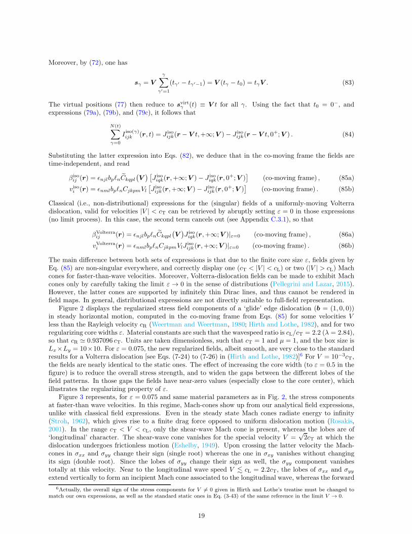
Figure 2 displays the regularized stress field components of a ‘glide’ edge dislocation (b = (1, 0, 0))in steady horizontal motion, computed in the co-moving frame from Eqs. (85) for some velocities Vless than the Rayleigh velocity cR (Weertman and Weertman, 1980; Hirth and Lothe, 1982), and for tworegularizing core widths ε. Material constants are such that the wavespeed ratio is cL/cT = 2.2 (λ = 2.84),so that cR ≃ 0.937096 cT. Units are taken dimensionless, such that cT = 1 and µ = 1, and the box size isLx×Ly = 10×10. For ε = 0.075, the new regularized fields, albeit smooth, are very close to the standardresults for a Volterra dislocation [see Eqs. (7-24) to (7-26) in (Hirth and Lothe, 1982)]6 For V = 10−3cT,the fields are nearly identical to the static ones. The effect of increasing the core width (to ε = 0.5 in thefigure) is to reduce the overall stress strength, and to widen the gaps between the different lobes of thefield patterns. In those gaps the fields have near-zero values (especially close to the core center), whichillustrates the regularizing property of ε.

Figure 3 represents, for ε = 0.075 and same material parameters as in Fig. 2, the stress componentsat faster-than wave velocities. In this regime, Mach-cones show up from our analytical field expressions,unlike with classical field expressions. Even in the steady state Mach cones radiate energy to infinity(Stroh, 1962), which gives rise to a finite drag force opposed to uniform dislocation motion (Rosakis,2001). In the range cT < V < cL, only the shear-wave Mach cone is present, whereas the lobes are of‘longitudinal’ character. The shear-wave cone vanishes for the special velocity V =

√2cT at which the

dislocation undergoes frictionless motion (Eshelby, 1949). Upon crossing the latter velocity the Mach-cones in σxx and σyy change their sign (single root) whereas the one in σxy vanishes without changingits sign (double root). Since the lobes of σyy change their sign as well, the σyy component vanishestotally at this velocity. Near to the longitudinal wave speed V . cL = 2.2cT, the lobes of σxx and σyy

extend vertically to form an incipient Mach cone associated to the longitudinal wave, whereas the forward

6Actually, the overall sign of the stress components for V 6= 0 given in Hirth and Lothe’s treatise must be changed tomatch our own expressions, as well as the standard static ones in Eq. (3-43) of the same reference in the limit V → 0.

19

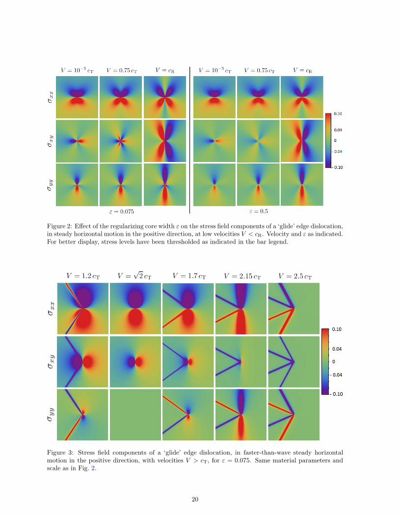
Figure 2: Effect of the regularizing core width ε on the stress field components of a ‘glide’ edge dislocation,in steady horizontal motion in the positive direction, at low velocities V < cR. Velocity and ε as indicated.For better display, stress levels have been thresholded as indicated in the bar legend.

Figure 3: Stress field components of a ‘glide’ edge dislocation, in faster-than-wave steady horizontalmotion in the positive direction, with velocities V > cT, for ε = 0.075. Same material parameters andscale as in Fig. 2.

20

(positive) lobe of σxy vanishes. Two pairs of Mach cones make up the field structure at V > cL withlongitudinal branches in the σxx and σyy components of opposite signs (compressive-like above the glideplane, and tensile-like below it), while Mach cones in σxy are negative. Since in the plane strain set-upthe pressure is p = −(1+ν)(σxx+σyy)/3, where ν = λ/[2(λ+µ)] is Poisson’s ratio, the shear-wave Machcones of σxx and σyy are of opposite sign and same intensity (see Figure), to cancel out mutually in thepressure field, leaving only a longitudinal Mach cone in pressure for supersonic velocities V > cL (notshown).

It should be noted that stable steady motion in the ‘velocity gap’ cR < V <√2cT is impossible on

theoretical grounds (Rosakis, 2001). However, as the present work does not not address the equation ofmotion that drives the dislocation under an external stress, which would forbid such motion, field mapscan be computed anyway in this unphysical regime (V = 1.2 cT in Fig. 3).

6 The two-dimensional elastodynamic Tamm problem for dislo-cations

In this Section, the formalism is applied to a case of non-uniform motion of physical interest. In elec-tromagnetic field theory, the Tamm problem (Tamm, 1939), introduced to help elucidating the natureof the Cerenkov radiation, consists in studying the fields radiated by a charge moving in a polarizablemedium at faster-than-light velocity during a finite time interval, and at rest otherwise. For a recentreview, discussion, and historical account, see Afanasiev (2004).

We transpose hereafter this problem to the elastodynamic fields radiated by a ‘glide’ edge dislocation(for illustrative purposes, but the method applies to the other two characters as well), using Eqs. (81)with core-width parameter ε = 0.075. Material parameters, and dimensionless units, are the same as inthe previous Section. A dislocation, initially at rest, is instantaneously accelerated to faster-than-wavespeed V = 2.5cT at t = 0, and moves uniformly at this speed until it is instantaneously pinned at t = 5into rest again (e.g., by some impurity or by forest dislocations in intersecting glide planes). Then N = 2in Eqs. (81) and the problem allows one to examine fields radiated in both the acceleration and thedeceleration steps.

Figs. 4, 5 and 6 display, respectively, 512×256-pixel pictures of the stress components σxx, σxy andσyy at times: (1) t = 3.30; (2), t = 6.74; (3) t = 9.49; and (4) t = 13.62, in a box of physical sizeLx ×Ly = 40× 20. All three components are plotted for further reference. After the initial acceleration,the dislocation velocity is faster than the longitudinal wave, so that two Mach cones build up. In pictures(1), the initial field of the dislocation at rest has already been erased, and the two concentric expandingrings of the acceleration wave, propagating at velocities cT (inner ring) and cL (outer ring) control thelateral expansion of the Mach cones. The latter remain tangent to the rings. Images (2) to (4) takeplace after dislocation sudden pinning, and illustrate the interplay between the acceleration rings, andthe braking (Bremsstrahlung) waves. The latter delimit the build-up region of the new static field. Afterdislocation pinning, the branches of the Mach cones are released to infinity while remaining tangentto the braking rings. In pictures (2) and (3), the longitudinal acceleration wave has catched up withthe dislocation, while the transverse one still lags behind. The latter overcomes the dislocation only inpictures (4).

It is interesting to observe the reinforcement of the fields, on the part of the boundary of the lon-gitudinal acceleration ring comprised between the two Mach cones, in components σxx and σyy. Thesehigh-field segments have signs opposite to those of the longitudinal Mach cone, so that this region is sub-jected to a high stress gradient. In the example displayed, where the dislocation velocity is rather close tocL, the longitudinal acceleration ring and braking ring closely follow each other, inducing a particularlystrong effect observable in pictures (3) of the figures, near to the forward longitudinal wave front.

The σxy component in Fig. 5 presents another interesting geometric effect: as the stress is negativeon the slip plane ahead of the transverse acceleration ring [picture (1)], the latter screens out part of theright positive lobe of the new static field once it catches up with the pinned dislocation [picture (4)], andthus continues to play a non-negligible role long after the initial acceleration has taken place. Obviously,in all cases the full static fields displayed in Fig. 2 are retrieved in stable form only after the slowest(shear) initial acceleration wave has overcome the dislocation.

21

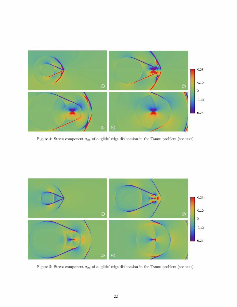
Figure 4: Stress component σxx of a ‘glide’ edge dislocation in the Tamm problem (see text).

Figure 5: Stress component σxy of a ‘glide’ edge dislocation in the Tamm problem (see text).

22

Figure 6: Stress component σyy of a ‘glide’ edge dislocation in the Tamm problem (see text).

7 Concluding discussion

To summarize, we proposed in the field-theoretical framework of continuum dislocation theory a newapproximate procedure to compute analytically fields radiated by dislocations undergoing non-uniformmotion at arbitrary velocities —including supersonic ones— and along arbitrary paths. Our resultshold for an unbounded, isotropic, linear-elastic medium. The procedure becomes exact for motions withpiecewise-constant velocity function V (t). Overall, our work hinges on technical results of two sorts:

1) First, after having clarified the fundamental distributional nature of the Green tensor, a so-calledisotropic regularization procedure has been employed to regularize fields produced by point sources.Using distributions, the theory of the non-uniform motion of straight dislocations becomes formallysimpler: prior to regularization, all the terms that enter the integral solution of the Volterra problem[Eqs. (28) and (40)], are regular distributions and pseudofunctions of clear mathematical meaning, unlikein classical approaches where such terms are usually non-integrable. The bottom line is that with thehelp of these objects, the dynamic Volterra-dislocation theory becomes well-defined, i.e., free of so-callednon-integrable singularities. It then became possible to carry out all differentiations in the elastodynamicfields, and to handle the ‘non-integrable singularities’ in a suitable mathematical way. In particular, theframework legitimates operations such as the interchange of integration and differentiation, which areill-defined in the standard approach (Markenscoff, 1983). Thus, the theory of dislocations in particularand, more generally, that of defects in the elastic continuum, has the theory of distributions as its naturalbackground, as emphasized, e.g., by Pellegrini (2011). However, only few authors have worked along thisline. For static dislocations, Kunin (1965); deWit (1973a,b) and Mura (1987) used already some resultsof distribution theory. Of course, the statics of dislocations is much simpler than their dynamics.

We showed that the regularization could be implemented from the outset, i.e., at the most fundamentallevel of the elastodynamic Green’s tensor and its gradient, by carrying out their spatial convolution witha specific isotropic δ-sequence, used with a fixed width parameter representing the dislocation core width.The nicety is that in practice, this amounts to considering the analytic continuation to complex valuesof the time variable of the function associated with the distributional Green’s tensor, as shown by Eqs.(60) and (62), in which the imaginary part of the time is proportional to the source width, divided bythe relevant wavespeed. Thus, the isotropic regularization is very easy to implement in the isotropic casewhere the wavespeeds have closed-form analytical expressions. On the other hand, the same ‘trick’ wouldneed to be modified for anisotropic media for which (except in a few particular cases) the wavespeedsmust in general be computed numerically (Aki and Richards, 2009; Bacon et al., 1979). It should benoted that the particular Somigliana dislocation of Eshelby (1949) can as well be brought down to an

23

analytic continuation of field expressions with respect to the space coordinate in the direction of motioninstead of time (Pellegrini, 2011). The latter regularization is by essence anisotropic, and might be bettersuited to anisotropic media. However, it was not employed here in view of the next point below, forwhich using the isotropic regularization proved a little easier. Whatever the exact approach employed,this shows that a powerful way of regularizing distributional Green’s functions is to seek regularizationsin the form of analytic continuations. The main virtue of such regularizations is to suppress the need fortracking wavefronts in subsequent calculations, so that the results can be applied without modifications tosupersonic sources. More generally, it has been observed that techniques of analytic continuation greatlysimplify the formulas involved in problems of moving dislocations (Pellegrini, 2011, 2012, 2014).

We expect the same method to apply as well to more complex Green’s functions such as the one(Eatwell et al., 1982) adequate to problems with layered media or free surfaces (Stronge, 1970; Freund,1973), thus alleviating the need to consider separately the subsonic and supersonic cases as in traditionalmethods of solution. Moreover, provided that the Green’s function is known in closed form this analytic-continuation approach should straightforwardly extend to coupled-physics problems, e.g., thermoelasticity(Brock et al., 1997), which we must however leave to further work.

2) The above regularization step does not by itself produce Mach cones, since Green’s functions canonly generate circular wavefronts at each instant. To arrive at Mach cones, which are are caustics ofcircular wavefronts, we need a second type of results. The fields emitted by a moving dislocation involveconvolution integrals over past times of expressions built from the regularized Green’s function. We facedthe problem of their numerical computation. To handle arbitrary dislocation motion, these time integralshave been split into secondary integrals over a discrete set of time intervals in which the dislocationvelocity can be assumed constant. The latter assumption makes it possible to get those secondaryintegrals in closed form, thereby giving the dynamic fields in terms of time-discretized but closed-formexpressions. Time integration provides expressions able to generate Mach cones. By this means, full-fielddynamic maps of the stress field could be produced, even in instances of supersonic motion, which hasnot been previously done from analytical expressions, to our knowledge.

As we carried it out, this second step is much more specific to the isotropic problem at hand than thefirst one above. The key closed-form integrals of Appendix C were first reported in Pellegrini and Lazar(2015), where they were simply proved by differentiation —few details being given as to their method ofobtention. Suffice it to say that the method rests on representing two-dimensional vectors in the planeas complex numbers, which eases the integration over time to obtain indefinite integrals in terms ofelementary functions, in full tensor form. From them stem the expressions for finite-time intervals usedin the present paper. Their complexity is a consequence of the vector character of the velocity, which cantake on any direction. It is very difficult to retrieve from them the known analytical expressions for steadysubsonic motion, and this step is best done numerically from Eqs. (86). This drawback is a relative one,if one bears in mind that those powerful expressions are able to account for regularized fields, Mach conesfor both shear and longitudinal waves, and arbitrary velocity direction. It is not clear that like integralscould be arrived at in generalized problems involving free surfaces, layered media, or even anisotropicmedia. Should closed-form time integration prove unfeasible, numerical integration could be attempted,in the hope of benefitting from the smooth character of the regularized Green kernels. However, somedifficulties might occur in the rendering of Mach cones. This would be worth investigating in the future.

Turning now to the physical content of the results, it must be emphasized that we restricted ourselves,for simplicity, to a rigid dislocation core size. Thus ‘relativistic’ effects of dynamic core-width variations(Pellegrini, 2012, 2014), and their associated radiative contributions, are not accounted for. However,this should not be considered a limitation of the method. How to bypass this restriction, which isnecessary to couple the present calculations to an equation of motion for dislocations, will be examinedelsewhere in connection with the use of Eshelby’s regularization. Indeed, although easier to implement,the isotropic regularization is ill-suited to handling Lorentz-contraction effects (the source must contractin the direction of motion only).

Obviously, the formalism does not need any modification to address dynamic nucleation or annihilationprocesses in the bulk of the material. By conservation of the dislocation density, such events involve pairsof dislocations of opposite signs.7 To account, e.g., for a nucleation event, one only needs to add thefields of each dislocation of the expanding pair, as computed via Eqs. (81). These fields mutually cancel

7Such dipoles are two-dimensional counterparts of dislocation loops in three dimensions.

24

out in the incipient state of pair nucleation when both dislocations are at rest with coinciding positions.Finally, it should be remarked that the fields patterns in Sec. 6 are (unsurprisingly) found symmetric,

up to sign changes, on both sides of the glide plane. However, recent numerical work with a field model ofcontinuum mechanics (Zhang et al., 2015) suggests that non-linear elasticity might be responsible for astrong asymmetry of the fields, and in particular of the Mach cones where fields are strongest. Indeed, thelatter work features asymmetric field patterns much alike those in some atomistic simulations (Li and Shi,2002; Tsuzuki et al., 2009). The ones by Li and Shi (2002) concern tungsten —an almost isotropic metal;hence, the main cause of asymmetry cannot reside in elastic anisotropy. Therefore, another conclusion ofthe present work is that such effects cannot be captured by linear elasticity alone.

Consequently, although the present dynamic fields expressions based on linear isotropic elasticity arequite specific to the problem at hand, and might suffer from some limitations from the physical standpoint,they are appropriate to first investigations of collective radiative properties of dislocations ensembles bymeans of simulations of the type discussed in (Gurrutxaga-Lerma et al., 2014), in the scarcely exploredhigh-velocity/high-acceleration range.

Acknowledgement

M.L. gratefully acknowledges the grants obtained from the Deutsche Forschungsgemeinschaft (GrantNos. La1974/2-1, La1974/2-2, La1974/3-1). Y.-P. P. gratefully thanks C. Denoual for having freelyprovided field maps from an independent dynamic phase-field code (Denoual, 2004), which greatly helpeddebugging the Fortran code developped for the numerical calculations.

A Equal-time limits

We demonstrate here the equal-time limit identities obeyed by the Green tensor, in the two-dimensionalframework of the rest of the paper. For the anti-plane strain case, these identities are well-known fromthe study of the Helmholtz equation, and read (see Barton (1989), p. 241)

limt→0+

G+zz(r, t) = 0 , lim

t→0∂tG

+zz(r, t) = ρ−1δ(r) . (A.1)

We focus hereafter on the plane-strain case, using elements from Section 4. The strategy consists infirst proving the equal-time identities (64) on the isotropic-regularized Green tensor, and then lettingthe regularizing size ε go to zero, to retrieve those identities for G+

ij(r, t), following the general principleexpressed by Eqs. (63).

Starting from definition (60a), and introducing the tensor

Tij = δij − 2xixj

r2, (A.2)

we cast the regularized Green tensor in the form (Pellegrini and Lazar, 2015)

Gisoij (r, t) =

θ(t)

4πρRe

∑

p=T,L

1

cp

{δij ±

1

r2[2(cpt+ iε)2 − r2]Tij

}1√

(cpt+ iε)2 − r2, (A.3)

where the sum is over the wavespeed index, and where the ‘plus’ and ‘minus’ signs apply to the transverse,and longitudinal terms, respectively. Then, immediately,

limt→0+

Gisoij (r, 0) = − 1

4πρRe

∑

p=T,L

i

cp

{δij ∓

1

r2[2ε2 + r2]Tij

}1√

r2 + ε2= 0 , (A.4)

since the expression under the Re operator is purely imaginary.

25

We next appeal to the following identities, demonstrated in Appendix A of (Pellegrini and Lazar,2015), where the Dirac terms originate from the branch cut of the complex square root function:

∂

∂t

√(cpt+ iε)2 − r2 =

cp(cpt+ iε)√(cpt+ iε)2 − r2

+ 2i√r2 + ε2δ(t), (A.5a)

∂

∂t

1√(cpt+ iε)2 − r2

= − cp(cpt+ iε)

[(cpt+ iε)2 − r2]3/2− 2i√

r2 + ε2δ(t) . (A.5b)

From these, we compute

∂tGisoij (r, t) =

θ(t)

4πρRe

∑

p=T,L

cpt+ iε

[(cpt+ iε)2 − r2]3/2

{−δij ±

1

r2[2(cpt+ iε)2 − 3r2]Tij

}, (A.6)

in which the imaginary terms proportional to δ(t) in Eqs. (A.5) have not survived due to the Re operator.Going to the limit t → 0, we deduce

limt→0+

∂tGisoij (r, t) =

1

4πρRe

∑

p=T,L

ε

(r2 + ε2)3/2

[δij ∓

1

r2(r2 + 2ε2)Tij

]= ρ−1 δij

2π

ε

(r2 + ε2)3/2, (A.7)

that is, by definition (48) of δε(r),

limt→0+

∂tGisoij (r, t) = ρ−1δijδ

ε(r) . (A.8)

Letting finally ε → 0+ in Eqs. (A.4) and (A.8) proves Eqs. (14).

B The upper boundary in time integrals

The considerations put forward in Section 2.3 are justified here, using v(r, t) as an example; one wouldproceed in the same manner with β(r, t). Let η > 0 an infinitesimal number, and t± = t± η. Considerfirst the traditional writing of the time-integral with t+ as an upper boundary. From (17b), one reads

vi(r, t) =

∫ t+

−∞

dt′∫

CjklmG+ij(r − r′, t− t′)Ilm,k(r

′, t′) dr′ . (B.1)

Then,

∂tvi(r, t) = Cjklm

[∫G+

ij(r − r′,−η)Ilm,k(r′, t+)dr′ +

∫ t+

−∞

dt′∫

∂tG+ij(r − r′, t− t′)Ilm,k(r

′, t′)dr′

].

(B.2)

The first term within brackets vanishes by the causality property (13). The second time-derivative reads

∂2t vi(r, t) = Cjklm

[∫∂tG

+ij(r − r′,−η)Ilm,k(r

′, t+) dr′ +

∫ t+

−∞

dt′∫

∂2tG

+ij(r − r′, t− t′)Ilm,k(r

′, t′) dr′

]

=

∫ t+

−∞

dt′∫

∂2tG

+ij(r − r′, t− t′)CjklmIlm,k(r

′, t′) dr′ (B.3)

for the same reason. It follows that, by definition of the Green tensor,

Lipvp(r, t) =

∫ t+

−∞

dt′∫

LipG+pj(r − r′, t− t′)CjklmIlm,k(r

′, t′) dr′

=

∫ t+η

−∞

dt′∫

δ(r − r′)δ(t− t′)CiklmIlm,k(r′, t′) dr′ = CiklmIlm,k(r, t

′) , (B.4)

26

so that the integral solution indeed verifies the field equations of motion. This standard demonstration(e.g., Barton (1989)) relies on causality and on the fact that t+ > t.

Consider now using t− as an upper boundary. Then,

∂tvi(r, t) = Cjklm

[∫G+

ij(r − r′, η) Ilm,k(r′, t−) dr′ +

∫ t−

−∞

dt′∫

∂tG+ij(r − r′, t− t′) Ilm,k(r

′, t′)dr′

],

(B.5)

so that

∂2t vi(r, t) = Cjklm

∫G+

ij(r − r′, η)Ilm,k(r′, t−) dr′ + Cjklm

∫∂tG

+ij(r − r′, η) Ilm,k(r

′, t−) dr′

+

∫ t−

−∞

dt′∫

∂2tG

+ij(r − r′, t− t′) Ilm,k(r

′, t′) dr′ . (B.6)

By the equal-time limits (14), the first term in the left-hand side vanishes while the second one reducesto

Cjklm

∫∂tG

+ij(r − r′, η) Ilm,k(r

′, t−) = ρ−1CiklmIlm,k(r, t) . (B.7)

It follows that

Lipvp(r, t) = CiklmIlm,k(r, t) +

∫ t−η

−∞

dt′∫

δ(r − r′)δ(t− t′)CiklmIlm,k(r′, t′) dr′ = CiklmIlm,k(r, t) ,

(B.8)

since now the interval of integration does not contain t′ = t any more. This second method thus relieson the equal-time limits rather than on causality. However, the same result is obtained in both cases, sothat both writings of the integral are correct.

C The indefinite integral J isoijk

For brevity, the reference (Pellegrini and Lazar, 2015) is denoted as (PL) hereafter.

C.1 Preliminary remarks and notations

Although they are of a wider range of application, as the present work demonstrates, the expressions thatwere given in (PL) for the quantity herein denoted by J iso

ijk(r, t;V ) were presented there in a way adaptedto dislocations instantaneously accelerated from rest to constant velocity. The equations of immediateinterest to us being somewhat scattered through the text of the latter reference, the purpose of thisAppendix is to summarize them neatly. The following intermediate quantities are employed:

β = V /c , (C.1a)

n = V /V = β/β , (velocity director) (C.1b)

r = r/r , (C.1c)

R(τ) = r + V τ , (C.1d)

S(τ) =√c2τ2 −R(τ)2 , (C.1e)

A±

ij = (1− β2)(δij − ninj)± ninj , (C.1f)

Xij = riβj − βirj , (C.1g)

where c is a generic placeholder for wavespeeds cT or cL. When V = 0, the unit director n is arbitrary.Except for the index z, all indices below take on values 1 or 2. The introduction of the cross-product Xij

allows for writings of expressions (C.2) and (C.5) below shorter than the ones reported in (PL).

27

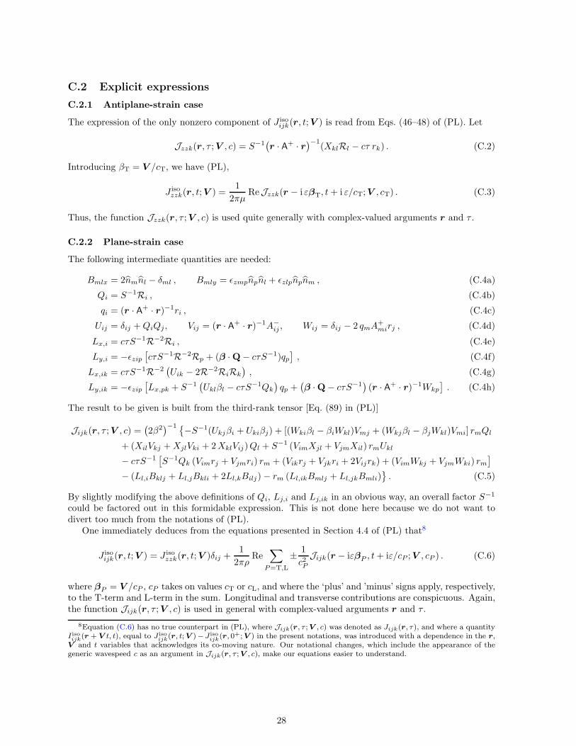
C.2 Explicit expressions

C.2.1 Antiplane-strain case

The expression of the only nonzero component of J isoijk(r, t;V ) is read from Eqs. (46–48) of (PL). Let

Jzzk(r, τ ;V , c) = S−1(r · A+ · r

)−1(XklRl − cτ rk) . (C.2)

Introducing βT = V /cT, we have (PL),

J isozzk(r, t;V ) =

1

2πµReJzzk(r − i εβT, t+ i ε/cT;V , cT) . (C.3)

Thus, the function Jzzk(r, τ ;V , c) is used quite generally with complex-valued arguments r and τ .

C.2.2 Plane-strain case

The following intermediate quantities are needed:

Bmlx = 2nmnl − δml , Bmly = ǫzmpnpnl + ǫzlpnpnm , (C.4a)

Qi = S−1Ri , (C.4b)

qi = (r · A+ · r)−1ri , (C.4c)

Uij = δij +QiQj , Vij = (r · A+ · r)−1A−

ij , Wij = δij − 2 qmA+mirj , (C.4d)

Lx,i = cτS−1R−2Ri , (C.4e)

Ly,i = −ǫzip[cτS−1R−2Rp + (β ·Q− cτS−1)qp

], (C.4f)

Lx,ik = cτS−1R−2(Uik − 2R−2RiRk

), (C.4g)

Ly,ik = −ǫzip[Lx,pk + S−1

(Uklβl − cτS−1Qk

)qp +

(β ·Q− cτS−1

)(r · A+ · r)−1Wkp

]. (C.4h)

The result to be given is built from the third-rank tensor [Eq. (89) in (PL)]

Jijk(r, τ ;V , c) =(2β2

)−1 {−S−1(Ukjβi + Ukiβj) + [(Wkiβl − βiWkl)Vmj + (Wkjβl − βjWkl)Vmi] rmQl

+ (XilVkj +XjlVki + 2XklVij)Ql + S−1 (VimXjl + VjmXil) rmUkl

− cτS−1[S−1Qk (Vimrj + Vjmri) rm + (Vikrj + Vjkri + 2Vijrk) + (VimWkj + VjmWki) rm

]

− (Ll,iBklj + Ll,jBkli + 2Ll,kBilj)− rm (Ll,ikBmlj + Ll,jkBmli)}. (C.5)

By slightly modifying the above definitions of Qi, Lj,i and Lj,ik in an obvious way, an overall factor S−1

could be factored out in this formidable expression. This is not done here because we do not want todivert too much from the notations of (PL).

One immediately deduces from the equations presented in Section 4.4 of (PL) that8

J isoijk(r, t;V ) = J iso

zzk(r, t;V )δij +1

2πρRe

∑

P=T,L

± 1

c2PJijk(r − iεβP , t+ iε/cP ;V , cP ) . (C.6)

where βP = V /cP , cP takes on values cT or cL, and where the ‘plus’ and ’minus’ signs apply, respectively,to the T-term and L-term in the sum. Longitudinal and transverse contributions are conspicuous. Again,the function Jijk(r, τ ;V , c) is used in general with complex-valued arguments r and τ .

8Equation (C.6) has no true counterpart in (PL), where Jijk(r, τ ;V , c) was denoted as Jijk(r, τ), and where a quantityI isoijk(r + V t, t), equal to J iso

ijk(r, t;V )−J isoijk(r, 0

+;V ) in the present notations, was introduced with a dependence in the r,V and t variables that acknowledges its co-moving nature. Our notational changes, which include the appearance of thegeneric wavespeed c as an argument in Jijk(r, τ ;V , c), make our equations easier to understand.

28

C.2.3 Remarks

First, it is emphasized that expressions (C.3) and (C.6) are written in the co-moving frame. This is thereason why they feature the quantity R introduced in Eq. (C.1d); see also remark following Eqs. (65).

Next, it should be pointed out that, as an indefinite integral over time, J isoijk(r, t;V ) is determined up

to an arbitrary time-independent integration constant. This irrelevant term vanishes in the subtractionsthat define expressions (79a) and (79c), while J iso

ijk(r, t;V ) itself is of no definite physical significance.Moreover, we observe that Eqs. (C.3) and (C.6) make use of the simultaneous regularizing substitutions

r → rshift = r− iǫβ and τ → τ + iǫ/c, where ε is the finite core size, which leaves the vector R invariant.For this, an analytic continuation to complex times and positions of the functions Jijk(r, τ ;V , c) isrequired. Accordingly, all square roots are used in the sense of the principal determination —the oneusually implemented in computers. With this convention the following limits hold:

limr→0

rshift = limr→0

√(r − iεβ) · (r − iεβ) = −i sign(r · n)βε , (C.7a)

limr→0

rshift = lim

r→0

rshift

rshift= sign(r · n)n . (C.7b)

Thus, the continuation of the norm r =√r · r of r is in general complex-valued (not a norm any more).

Finally, we observe that by going to the limit ε → 0, expressions (C.3) and (C.6) become distributions,with Mach cones in the form of Dirac-like measures for faster-than-wave velocities. Extracting this limitfor arbitrary velocities is thus a complicated business in general, an instance of which has been given in(PL) in the antiplane-strain case. However, upon neglecting the distributional character of this limit,more classical expressions of the fields a Volterra dislocation are retrieved by letting ε = 0 right away.Of course, such expressions are singular (i.e., infinite, hence not physically meaningful) at the dislocationposition and at wavefronts, and hold only in the absence of Mach cones, i.e., for velocities less than cT.Thus, for Volterra dislocations and |V | < cT, we can take

J isozzk(r, t;V )|ε=0 =

1

2πµReJzzk(r, t;V , cT) , (C.8a)

J isoijk(r, t;V )|ε=0 = J iso

zzk(r, t;V )|ε=0 δij +1

2πρRe

∑

P=T,L

± 1

c2PJijk(r, t;V , cP ) . (C.8b)

C.3 Particular values and limits

The above expressions yield non-singular field values in particular limits of interest. Limiting formsare rather difficult to extract in the plane-strain case, due to the complexity of (C.5). The expressionsreported below have been checked with the help of a symbolic computational toolbox.

C.3.1 Values at τ = 0

For τ = 0, the quantity S(τ) becomes S = i r, while Qi = −i rk and Uij = δij − rirj . It follows that inthe particular case where r and τ are taken real-valued, Jzzk and Jijk are purely imaginary. Hence,

limτ→0+

ReJzzk(r, τ ;V , c) = 0, limτ→0+

ReJijk(r, τ ;V , c) = 0 (r,τ ∈ R) . (C.9)

When ε = 0, inserting these expressions into Eqs. (C.8) we conclude that

J isozzk(r, 0

+;V )|ε=0 = 0, J isoijk(r, 0

+;V )|ε=0 = 0 . (C.10)

C.3.2 Limit τ → +∞This limit is needed to compute the upper boundary term with τ = +∞ in expression (79c). Lettingu = r · n, we introduce the notation

A = r−2(r · A+ · r) = (1− β2) + β2u2 . (C.11)

29

A straightforward but very long calculation yields

limτ→∞

Jzzk(r, τ ;V , c) = − 1

r√

1− β2A[(1− β2)rk + β2u nk

], (C.12a)

limτ→∞

Jijk(r, τ ;V , c) =

√1− β2

rβ2A2

{−[(1− β2)A+ 2β2 u2]δij rk + β2A(riδjk + δik rj)

− β2(A− 2)u δijnk − (1 + β2)Au(niδjk + njδik)

+ [(1 − β2)A+ 2β4 u2](rinj + nirj)nk

+ [(2 − β2)A+ 2β4 u2]ninj rk

+ β2(1− β2)−1[(2− 3β2)A+ 2β4 u2]u ninj nk

+ 2β2(1 − β2)u(nirj + rinj)rk − 2β4 u rirj nk − 2β2(1− β2)rirj rk

}.

(C.12b)

Using these expressions in Eqs. (C.3) and (C.6), which involves using complex values of their argumentr, gives access to the quantities

J isozzk(r,+∞;V ) and J iso

ijk(r,+∞;V ) . (C.13)

The above expressions can also be inserted right away into Eqs. (C.8) to compute, for Volterra dislocationsand velocity |V | < cT the quantities J iso

zzk(r,+∞;V )|ε=0 and J isoijk(r,+∞;V )|ε=0.

C.3.3 Limit V → 0

This limit is needed for static field expressions. We have (PL)

limV →0

Jzzk(r, τ ;V , c) = − cτ

r√c2τ2 − r2

rk , (C.14a)

limV →0

Jijk(r, τ ;V , c) =cτ

r√c2τ2 − r2

rirj rk −cτ

r3

√c2τ2 − r2 Tijk(r) , (C.14b)

where the following third-rank tensor has been used:

Tijk(r) = δjk ri + δik rj + δij rk − 4 rirj rk . (C.15)

Expansions to second order in powers of β would be needed to retrieve Eq. (C.14b) from expression (C.5),which is inversely proportional to β2. A shorter route is discussed in (PL).

C.3.4 Double limit τ → ∞, V → 0

From (C.12a) and (C.14a), it is clear that the limits commute for Jzzk(r, τ ;V , c): one finds

limτ→∞

limV→0

Jzzk(r, τ ;V , c) = limV →0

limτ→∞

Jzzk(r, τ ;V , c) = −1

rrk . (C.16)

The case of Jijk(r, τ ;V , c) is more subtle. Carrying out a Laurent expansion of (C.12b) near V = 0(β = 0), one gets

limτ→∞

Jijk(r, τ ;V ,c) =c2

r[−δij rk − u(niδjk + njδik) + (rinj + rj ni)nk + 2ninj rk]V

−2

+1

r

[1

2(1− 2u2)δij rk + (riδjk + rjδik) + u δijnk −

1

2u(3− 2u2)(niδjk + njδik)

− 1

2(1 + 2u2)(rinj + rj ni)nk + 2u(rinj + rj ni)rk − 2u2ninj rk + 2u ninj nk − 2rirj rk

]

+O(V 2

). (C.17)

30

Despite appearances, it can be shown that the O(V 0) term in this expansion does not depend on thedirector n (!). The task is most easily performed by introducing polar angles for r and n, and reducingeach tensor component of the term by means of trigonometric identities, possibly with the help of analgebraic computational toolbox. The result is equal to

limτ→∞

Jijk(r, τ ;V ,c) =c2

r[−δij rk − u(niδjk + njδik) + (rinj + rj ni)nk + 2ninj rk]V

−2

+1

r

[rirj rk +

1

2Tijk(r)

]+O

(V 2

). (C.18a)

On the other hand, Laurent-expanding (C.14b) near τ = ∞ directly gives

limV →0

Jijk(r, τ ;V , c) = −c2τ2

r3Tijk(r) +

1

r

[rirj rk +

1

2Tijk(r)

]+O

(τ−2

). (C.18b)

The leading terms in expansions (C.18a) and (C.18b) are different from one another, and blow-up inthe limits considered. However, they are physically irrelevant and can be disregarded because they areproportional to c2: such terms (not containing c in any other way) are eliminated between the transverseand longitudinal parts in Eq. (C.6). Since the finite next-to-leading-order terms coincide, we can considerin practice that the limits commute as well for Jijk(r, τ ;V , c), as far as J iso

ijk is concerned.

C.3.5 Limit R → 0

This limit corresponds to letting r → −V τ in the co-moving frame, which provides the fields at theorigin of coordinates in the laboratory frame. In principle, this point should be of no particular interest,except in the static case V = 0 where it locates the center of the dislocation core. However, since, e.g.,Lx,i in (C.4e) has one term proportional to 1/R and moreover Lx,ik in (C.4g) has one term proportionalto 1/R2, we need to verify that no ill-definiteness arises in this limit. Assuming that V 6= 0 the followinglimit and Taylor expansion are obtained:

limr→−V τ

Jzzk(r, τ ;V , c) =1

V τnk , (C.19a)

Jijk(r, τ ;V , c) =c2

V 2R

(1 +

V τ

R

)Tijk(n) +

c2 − (V/2)2

V 3τTijk(n)−

1

4V τ(δjkni + δiknj + δij nk)

+ O(R). (C.19b)

Thus, the antiplane-strain limit (C.19a) is not problematic, whereas the plane-strain expansion (C.19b)is singular as R → 0. However the divergent terms, proportional to c2, are irrelevant for the same reasonas in the previous Section, and can be disregarded. In practice, one can thus consider that

limr→−V τ

Jijk(r, τ ;V , c) ≃ − 1

4V τ[Tijk(n) + (δjkni + δiknj + δij nk)] , (C.20)

which is finite.

References

Afanasiev, G.N, 2004. Vavilov-Cherenkov and synchrotron radiation. Theory and applications. KluwerAcademic Publishers, New York.

Aki, K., Richards, P. G., 2009. Quantitative Seismology, 2nd ed. University Science Books, Mill Valley,CA.

Bacon, D.J., Barnett, D.M., Scattergood, R.O., 1979. Anisotropic continuum theory of defects. Progressin Materials Science. 23, 51–262. doi: 10.1016/0079-6425(80)90007-9.

Barton, G., 1989. Elements of Green’s Functions and Propagation. Oxford University Press, Oxford.

31

Bilby, B.A., 1955. Types of dislocations source. in: Defects in Crystalline Solids, Report of 1954 BristolConference. The Physical Society, London, pp. 123–133.

Bremermann, H.J., Durand III, L., 1961. On analytic continuation, multiplication, and Fourier transfor-mations of Schwartz distributions. J. Math. Phys. 2, 240–258. doi: 10.1063/1.1703706

Brock, L.M., 1979. Two basic wave propagation problems for the non-uniform motion of displacementdiscontinuities in a half-plane. Int. J. Engng. Sci. 17, 1211–1223. doi: 10.1016/0020-7225(79)90103-4

Brock, L.M., 1982. Dynamic solutions for the non-uniform motion of an edge dislocation. Int. J. Engng.Sci. 20, 113–118. doi: 10.1016/0020-7225(82)90077-5

Brock, L.M., 1983. Non-uniform edge dislocation motion along an arbitrary path. J. Mech. Phys.Solids 31, 123–132. doi: 10.1016/0022-5096(83)90046-7

Brock, L.M., Georgiadis, H. G., Tsamaphyros, G., 1997. The coupled thermoelasticity problem of thetransient motion of a line heat/mechanical source over a half-space. J. Thermal Stresses 20, 773–795.doi: 10.1080/01495739708956128

Cai, W., Arsenlis, A., Weinberger, C.R., Bulatov, V.V., 2006. A non-singular continuum theory of dislo-cations. J. Mech. Phys. Solids 54, 561–587. doi: 10.1016/j.jmps.2005.09.005

Callias, C., Markenscoff, X., 1980. The nonuniform motion of a supersonic dislocation. Quart. Appl.Math. 38, 323–330. http://www.jstor.org/stable/43637043

Clifton, R. J. and Markenscoff, X., 1981. Elastic precursor decay and radiation from nonuniformly movingdislocations. J. Mech. Phys. Solids 29, 227–251. doi: 10.1016/0022-5096(81)90028-4

Day, S. M., Dalguer, L. A., Lapusta, N., Liu, Y., 2005. Comparison of finite difference and boundary in-tegral solutions to three-dimensional spontaneous rupture. J. Geophys. Res.: Solid Earth 110, B12307.doi: 10.1029/2005JB003813

de Jager, L.M., 1969. Applications of Distributions in Mathematical Physics, 2nd ed. MathematischCentrum, Amsterdam.

Denoual, C., 2004. Dynamic dislocation modeling by combining Peierls Nabarro and Galerkin methods.Phys. Rev. B 70, 024106 [5 pages]. doi: 10.1103/PhysRevB.70.024106

deWit, R., 1973a. Theory of disclinations II. J. Res. Nat. Bur. Stand. (U.S.) 77A, 49–100.

deWit, R., 1973b. Theory of disclinations IV. J. Res. Nat. Bur. Stand. (U.S.) 77A, 607–658.

Djaka, K.S., Taupin, V., Berbenni, S., C Fressengeas, C., 2015. A numerical spectral approach tosolve the dislocation density transport equation. Modelling Simul. Mater. Sci. Eng. 23, 065008.http://stacks.iop.org/0965-0393/23/i=6/a=065008

Dorfner, K.R., 1957. Dreidimensionale Uberschallprobleme der Gasdynamik., Springer, Berlin.

Eason, G., Fulton, J., Sneddon, I.N., 1956. The generation of waves in an infinite elastic solid by variablebody forces. Philos. Trans. Royal Soc. (London) A248, 575–607. doi: 10.1098/rsta.1956.0010

Eatwell, G. P., Simmons, J. A., Willis, J.R., 1982. A new representation for the dynamic Green’s tensorof an elastic half-space or layered medium. Wave Motion 4, 53–73. doi: 10.1016/0165-2125(82)90014-2

Eringen, A.C., Suhubi, S.S., 1975. Elastodynamics, Volume II, Linear Theory. Academic Press, NewYork.

Eshelby, J.D., 1949. Uniformly moving dislocations. Proc. Phys. Soc. Lond. A 62, 307–314.doi: 10.1088/0370-1298/62/5/307

Eshelby, J. D., 1951. The force on an elastic singularity. Phil. Trans. Roy. Soc. London A 244, 87–112.doi: 10.1098/rsta.1951.0016

32

Freund, L.B., 1972. Wave motion in an elastic solid due to a nonuniformly moving line load. Quart. Appl.Math. 30, 271–281. http://www.jstor.org/stable/43636265

Freund, L.B., 1973. The response of an elastic solid to nonuniformly moving surface loads. ASME J.Appl. Mech. 40, 699–704. doi: 10.1115/1.3423076

Gel’fand I.M, Shilov, G.E., 1964. Generalized Functions, Vol. I. Academic, New York.

Gunther, H., 1973. Zur Dynamik schneller Versetzungen. Akademie-Verlag, Berlin.

Gurrutxaga-Lerma, B., Balint, D.S., Dini, D., Eakins, D.E., Sutton, A.P., 2013. A dynamic discretedislocation plasticity method for the simulation of plastic relaxation under shock loading. Proc. R.Soc. A 469, 20130141 [24 pages]. doi: 10.1098/rspa.2013.0141

Gurrutxaga-Lerma, B., Balint, D.S., Dini, D., Eakins, D.E., Sutton, A.P., 2014. Dynamic discrete dislo-cation plasticity. Adv. Appl. Mech. 47, 93–224. doi: 10.1016/B978-0-12-800130-1.00002-3

Hirth, J.P., Lothe J., 1982 Theory of dislocations, 2nd ed. Wiley & Sons, New York.

Hollander, E.F., 1962. The geometric equation of dislocation dynamics. Czech. J. Phys. B 12, 35–47.doi: 10.1007/BF01688395

Huang, S., Markenscoff, X., 2011. Dislocations accelerating through the shear-wave speed barrierand effect of the acceleration on the Mach front curvature. Int. J. Engng. Sci. 49, 1461–1469.doi: 10.1016/j.ijengsci.2011.03.009

Kanwal, R.P., 2004. Generalized Functions. Theory and Applications, 3rd. ed. Birkhauser, Boston.

Kausel, E., 2006. Fundamental Solutions in Elastodynamics. Cambridge University Press, Cambridge.

Kiusalaas, J., Mura, T., 1964. On the elastic field around an edge dislocation with application to dislo-cation vibration. Phil. Mag. 9, 1–7. doi: 10.1080/14786436408217471

Kiusalaas, J., Mura, T., 1965. On the motion of a screw dislocation. In: Eringen, A.C. (Ed.), RecentAdvances in Engineering Science. Gordon & Breach, New York, pp. 543–564.

Kosevich, A.M., 1962. The deformation field in an isotropic elasticmedium containing moving dislocations. Soviet Physics JETP 15, 108–115.http://www.jetp.ac.ru/cgi-bin/e/index/e/15/1/p108?a=list

Kosevich, A.M., 1979. Crystal dislocations and the theory of elasticity, In: Nabarro, F.R.N. (Ed.), Dis-locations in Solids Vol. 1. North-Holland, Amsterdam, pp. 33–165.

Kroner, E., 1955. Der fundamentale Zusammenhang zwischen Versetzungsdichte und Spannungsfunktio-nen. Zeitschrift fur Physik 142, 463–475. doi: 10.1007/BF01375082

Kroner, E., 1958. Kontinuumstheorie der Versetzungen und Eigenspannungen. Springer, Berlin.

Kroner, E., 1981. Continuum Theory of Defects. In: R. Balian et al. (Eds.), Physics of Defects (LesHouches, Session 35). North-Holland, Amsterdam, pp. 215–315.

Kunin, I.A., 1965. Fields of randomly distributed dislocations and force dipoles in an infinite elasticanisotropic medium. J. Appl. Mech. Tech. Phys. 5, 75–83. doi: 10.1007/BF00913382

Landau, L.D., Lifschitz, E.M., 1986. Theory of Elasticity, 3rd ed. Pergamon, Oxford.

Lardner, R.W., 1974. Mathematical Theory of Dislocations and Fracture. University of Toronto Press,Toronto.

Lazar, M., 2009. The gauge theory of dislocations: a uniformly moving screw dislocation. Proceedings ofthe Royal Society A 465, 2505–2520. doi: 10.1098/rspa.2009.0043

33

Lazar, M., 2010. The gauge theory of dislocations: a nonuniformly moving screw dislocation. PhysicsLetters A 374, 3092–3098. doi: 10.1016/j.physleta.2010.05.044

Lazar, M., 2011a. On the fundamentals of the three-dimensional translation gauge theory of dislocations.Mathematics and Mechanics of Solids 16, 253–264. doi: 10.1177/1081286510370889

Lazar, M., 2011b. On the elastic fields produced by non-uniformly moving dislocations: a revisit. Philo-sophical Magazine 91, 3327–3342. doi: 10.1080/14786435.2011.579584

Lazar, M., 2012. The elastodynamic Lienard-Wiechert potentials and elastic fields of non-uniformly mov-ing point and line forces. Wave Motion 49, 710–718. doi: 10.1016/j.wavemoti.2012.04.009

Lazar, M., 2013a. On retardation, radiation and Lienard-Wiechert type potentials in electrodynamicsand elastodynamics. Wave Motion 50, 1161–1174. doi: 10.1016/j.wavemoti.2013.05.006

Lazar, M., 2013b. On the non-uniform motion of dislocations: The retarded elastic fields, the retardeddislocation tensor potentials and the Lienard-Wiechert tensor potentials. Philosophical Magazine 93,749–776. doi: 10.1080/14786435.2012.732713

Lazar, M., 2014. On gradient field theories: gradient magnetostatics and gradient elasticity. PhilosophicalMagazine 94, 2840–2874. doi: 10.1080/14786435.2014.935512

Lazar, M., Maugin, G.A., Aifantis, E.C., 2005. On dislocations in a special class of generalized elasticity.phys. stat. sol. (b) 242, 2365–2390. doi: 10.1002/pssb.200540078

Lazar, M., Maugin, G.A., 2006. Dislocations in gradient elasticity revisited, Proc. R. Soc. Lond. A 462,3465–3480. doi: 10.1098/rspa.2006.1699

Lazar, M., Anastassiadis, C., 2008. The gauge theory of dislocations: conservation and balance laws.Philosophical Magazine 88, 1673–1699. doi: 10.1080/14786430802255653

Li, Q., Shi, S.-Q., 2002. Dislocation jumping over the sound barrier in tungsten. Appl. Phys. Lett.˜80,3069–3071. doi: 10.1063/1.1473865

Madariaga, R., 1978. The dynamic field of Haskell’s rectangular dislocation fault model. Bull. Seism. Soc.Am. 68, 869–887. http://www.bssaonline.org/cgi/content/abstract/68/4/869

Markenscoff, X., 1980. The transient motion of a nonuniformly moving dislocation. J. Elast. 10, 193–201.doi: 10.1007/BF00044503

Markenscoff, X., Clifton, R.J, 1981. The nonuniformly moving edge dislocation. J. Mech. Phys. Solids 29,253–262. doi: 10.1016/0022-5096(81)90029-6

Markenscoff, X., 1983. On the dislocation fields in terms of the dynamic Green’s function. J. Elast. 13,237–241. doi: 10.1007/BF00042995

Markenscoff, X., Ni, L., 1987, The transient motion of a dislocation in a solid of general anisotropy. WaveMotion 9, 191–199. doi: 10.1016/0165-2125(87)90009-6

Markenscoff, X., Ni, L., 2001a. The transient motion of a dislocation with ramp-like core, J. Mech. Phys.Solids 49, 1603–1619. doi: 10.1016/S0022-5096(00)00062-4

Markenscoff, X., Ni, L., 2001b, The transient motion of a ramp-core supersonic dislocation. ASME J.Appl. Mech. 68, 656–659. doi: 10.1115/1.1380678

Meyers, M.A., Jarmakani, H., Bringa, E.M., Remington, B.A., 2009. Chapter 89 – Dislocations in ShockCompression and Release. In: Hirth, J.P. and Kubin, L. (Eds.), Dislocations in Solids Vol. 15. North-Holland, Amsterdam, pp. 91–197. doi: 10.1016/S1572-4859(09)01502-2

Morse, P.M., Feshbach, H., 1953. Methods of Theoretical Physics I. McGraw-Hill, New York.

34

Mura, T., 1963. Continuous distribution of moving dislocations. Phil. Mag. 8, 843–857.doi: 10.1080/14786436308213841

Mura, T., 1987. Micromechanics of Defects in Solids, 2nd ed. Martinus Nijhoff, Dordrecht.

Nabarro, F.R.N., 1967. Theory of Crystal Dislocations. Oxford University Press, Oxford.

Niazy, A., 1975. An exact solution for a finite, two-dimensional moving dislocation in an elastic half-space with application to the San Fernando earthquake of 1971. Bull. Seism. Soc. Am. 65, 1797–1826.http://www.bssaonline.org/content/65/6/1797.abstract

Nye, J.F., 1953. Some geometrical relations in dislocated crystals. Acta Metall. 1, 153–162.doi: 10.1016/0001-6160(53)90054-6

Pellegrini, Y.-P., 2010. Dynamic Peierls-Nabarro equations for elastically isotropic crystals. Phys. Rev.B 81, 024101 [14 pages]. doi: 10.1103/PhysRevB.81.024101

Pellegrini, Y.-P., 2011. Reply to “Comment on ‘Dynamic Peierls-Nabarro equations for elastically isotropiccrystals’ ”. Phys. Rev. B 83, 056102 [4 pages]. doi: 10.1103/PhysRevB.83.056102

Pellegrini, Y.-P., 2012. Screw and edge dislocations with time-dependent core width: From dynamical coreequations to an equation of motion. J. Mech. Phys. Solids 60, 227–249. doi: 10.1016/j.jmps.2011.11.002

Pellegrini, Y.-P., 2014. Equation of motion and subsonic-transonic transitions of rectilinearedge dislocations: A collective-variable approach. Phys. Rev. B 90, 054120 [18 pages].doi: 10.1103/PhysRevB.90.054120

Pellegrini, Y.-P., Lazar, M., 2015. On the gradient of the Green tensor in two-dimensional elastodynamicproblems, and related integrals: Distributional approach and regularization, with application to non-uniformly moving sources. Wave Motion 57, 44–63. doi: 10.1016/j.wavemoti.2015.03.004

Pillon, L., Denoual, C., Pellegrini, Y.-P., 2007. Equation of motion for dislocations with inertial effects.Phys. Rev. B 90, 224105 [6 pages]. doi: 10.1103/PhysRevB.76.224105

Pillon, L., Denoual, C., 2009. Inertial and retardation effects for dislocation interactions, Philos. Mag.89, 127–141. doi: 10.1080/14786430802600775

Rosakis, P., 2001. Supersonic dislocation kinetics from an augmented Peierls model. Phys. Rev. Lett. 86,95–98. doi: 10.1103/PhysRevLett.86.95

Saenz, A. W., 1953. Uniformly moving dislocations in anisotropic media, J. Rational Mech. Anal. 2,83–98. doi: 10.1512/iumj.1953.2.02003

Sauer, R., 1954. Anwendung der Distributionstheorie auf das Problem des Uberschall-Tragflugels.Memoires sur la mecanique des fluides, offerts a M.D. Riabouchinsky. Publications Scientifiques etTechniques du Ministere de l’Air, Paris, p. 289.

Sauer, R., 1958. Anfangsprobleme bei partiellen Differentialgleichungen, 2nd ed. Springer, Berlin.

Schwartz, L., 1950/1951. Theorie des Distributions, Tomes I et II. Hermann, Paris.

Spielmannova, A., Machova, A., Hora, P., 2009. Crack-induced stress, dislocations and acous-tic emission by 3-D atomistic simulations in bcc iron. Acta Materialia 57, 4065–4073.doi: 10.1016/j.actamat.2009.04.048

Stroh, A.N., 1962. Steady state problems in anisotropic elasticity, J. Mathematics and Physics (Cam-bridge, MA) 41, 77–103.

Stronge, W.J., 1970. A load accelerating on the surface of an acoustic half space, ASME J. Appl. Mech. 37,1077–1082. doi: 10.1115/1.3408662

35

Tamm, I.E. 1939. Radiation induced by uniformly moving electrons, J. Phys. USSR 1, 439–461.

Teodosiu, C., 1970. A dynamic theory of dislocations and its applications to the theory of the elastic-plastic continuum. In: Simmons, J.A., deWit, R., Bullough, R. (Eds.), Fundamental Aspects of Dislo-cation Theory, Vol. 2. Eds. Nat. Bur. Stand. (U.S.), Spec. Publ. 317, pp. 837–876.

Tsuzuki, H., Branicio, P.S., Rino, J.P., 2009. Molecular dynamics simulation of fast dislocations in copper,Acta Materialia 57, 1854–1855. doi: 10.1016/j.actamat.2008.12.025

Vladimirow, V.S., 1971. Equations of Mathematical Physics. Dekker, New York.

Weertman, J., Weertman, J.R., 1980. Moving dislocations. In: Nabarro, F.R.N (Ed.), Dislocations inSolids, Vol. 3. North-Holland, Amsterdam, pp. 1–59.

Wu, K.-C., 2000. Extension of Stroh’s formalism to self-similar problems in two dimensional elastody-namics. Proc. R. Soc. A 456, 869–890. doi: 10.1098/rspa.2000.0540

Zemanian, A.H., 1965. Distribution Theory and Transform Analysis. McGraw-Hill, New York.

Zhakhovsky, V. V., Budzevich, M. M., Inogamov, N. A., Oleynik, I. I., White, C. T.,2011. Two-zone elastic-plastic single shock waves in solids. Phys. Rev. Lett. 107, 135502.doi: 10.1103/PhysRevLett.107.135502

Zhang, X., Acharya, A., Walkington, N., Bielak, J., 2015. A single theory for some quasi-static, su-personic, atomic, and tectonic scale applications of dislocations. J. Mech. Phys. Solids. 84, 145–195.doi: 10.1016/j.jmps.2015.07.004

36