The Effects of Controlling for Distributional Differences on the Mantel-Haenszel Procedure

Daniel F. Bowen

A thesis submitted to the faculty of the University of North Carolina at Chapel Hill in partial

fulfillment of the requirements for the degree of Master of Arts in the School of Education.

Chapel Hill

2011

Approved By:

Dr. Gregory Cizek

Dr. William Ware

Dr. Jeff Greene

brought to you by COREView metadata, citation and similar papers at core.ac.uk

provided by Carolina Digital Repository

ii

ABSTRACT

Daniel F. Bowen: The Effects of Controlling for Distributional Differences on the Mantel-

Haenszel Procedure

(Under the direction of Dr. Gregory J. Cizek)

Propensity score matching was used to control for the distributional differences in

ability between two simulated data sets. One data set represented English speaking

examinees and the second data set represented Spanish speaking examinees who received the

Spanish language version of the same test. The ability distributions of the two populations

were set to mirror the data from a large-scale statewide assessment delivered in both English

and Spanish. The simulated data were used as a benchmark to compare the Mantel-Haenszel

procedure for identifying differential item function (DIF) under the two scenarios with the

hope that controlling for distributional differences would reduce the errors made by the

Mantel-Haenszel procedure in identifying DIF. With the increase in high-stakes testing of

diverse populations in the United States as well as elsewhere in the world, it is critical that

effective methods of identifying DIF be developed for situations where the reference and

focal groups display distributional differences. However, the evidence of this study suggests

that the matched samples did not help the Mantel-Haenszel procedure identify DIF, and in

fact increased its errors.

iii

ACKNOWLEDGEMENTS

I would like to thank all my colleagues in the psychometric department at Measurement Inc.,

especially Dr. Kevin Joldersma for working with me as we attempted to understand

propensity score matching and Caroline Yang for her edits and suggestions. I would like to

thank Dr. Cizek for all his guidance and advice over my journey through graduate school and

Drs. Ware and Greene for their recommendations and participation.

iv

TABLE OF CONTENTS

LIST OF TABLES .................................................................................................................. vii

LIST OF FIGURES ................................................................................................................. ix

Chapter

Introduction ................................................................................................................................1

Literature Review.......................................................................................................................9

Item Response Theory .........................................................................................................10

Logistic Regression ..............................................................................................................13

The Mantel-Haenszel Chi-Square Procedure ......................................................................14

The use of Mantel-Haenszel for indentifying DIF. ..........................................................15

Mantel-Haenszel test-statistic. .....................................................................................16

Mantel-Haenszel odds ratio. ........................................................................................17

ETS DIF classification rules. .......................................................................................17

Benefits of using Mantel-Haenszel in DIF detection. ......................................................18

Research on the Mantel-Haenszel Procedure and Sample Size. ......................................19

Research on the Mantel-Haenszel Procedure and Ability Distribution Differences. ......20

Using DIF for Translated Tests ...........................................................................................21

Propensity Score Matching ..................................................................................................22

Greedy Matching. ............................................................................................................23

Optimal Matching. ...........................................................................................................23

The Importance of DIF Detection for Translated Items ......................................................24

v

Summary ..............................................................................................................................25

Research Question ...................................................................................................................27

Method .....................................................................................................................................28

Variables in Study ................................................................................................................28

Sample Size. .....................................................................................................................28

Ability Distributions. .......................................................................................................28

Amount of DIF. ................................................................................................................29

Data Analyses ......................................................................................................................30

Propensity Score Matching. .............................................................................................31

Summary ..............................................................................................................................33

Results ......................................................................................................................................35

Simulated Data .....................................................................................................................35

Type I Errors ........................................................................................................................39

Type II Errors .......................................................................................................................40

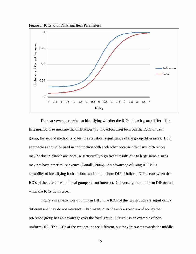
Effects on Type I Errors .......................................................................................................42

Effects on Type II Errors .....................................................................................................43

ETS Classification Agreement Rates ...................................................................................44

Discussion ................................................................................................................................47

Implications of Findings ......................................................................................................47

Type I Errors. ...................................................................................................................47

Type II Errors. ..................................................................................................................48

Effects on Type I Errors ...................................................................................................49

Effects on Type II Errors .................................................................................................51

vi

ETS Classification Agreement Rates ...............................................................................52

Summary of Implications of Findings .............................................................................56

Limitations ...........................................................................................................................56

Suggestions for Future Research .........................................................................................58

Conclusions ..............................................................................................................................61

Appendix A: Simulated Item Parameters and DIF Levels......................................................62

Appendix B: SAS Code ..........................................................................................................63

Appendix C: Item Analysis .....................................................................................................80

References ................................................................................................................................92

vii

LIST OF TABLES

Table 1: Simpson’s Paradox Example .......................................................................................9

Table 2: Contingency table at score point J .............................................................................16

Table 3: Total Test Score Descriptive Statistics for Simulated Data Sets ...............................30

Table 4: Total Test Score Descriptive Statistics for Simulated Data Sets After Matching ....32

Table 5: Descriptive Statistics of Item Difficulties of Simulated Data Sets ...........................36

Table 6: Descriptive Statistics of Item Difficulties of Simulated Data Sets Post-Matching ..37

Table 7: Descriptive Statistics of Point-Biserial Correlation: Pre and Post-Matching ...........38

Table 8: Summary of Cronbach’s Alpha Reliability Estimates and SEMs for

each Simulated Data Set ...........................................................................................38

Table 9: Contingency Table for Type I Errors........................................................................39

Table 10: Total Number of Type I Errors ...............................................................................40

Table 11: Contingency Table for Type II Errors ....................................................................41

Table 12: Total Number of Type II Errors ..............................................................................41

Table 13: Analysis of Variance for Type I Errors ..................................................................43

Table 14: Analysis of Variance for Type II Errors .................................................................43

Table 15: Distribution of A, B, & C Class items for both Pre- and Post-Matching ...............44

Table 16: ETS Classification Contingency Table – Sample Size = 1000;

DIF Level = Low ....................................................................................................45

Table 17: ETS Classification Contingency Table – Sample Size = 500;

DIF Level = Low ....................................................................................................45

Table 18: ETS Classification Contingency Table – Sample Size = 250;

DIF Level = Low ....................................................................................................46

viii

Table 19: ETS Classification Contingency Table – Sample Size = 1000;

DIF Level = High ...................................................................................................46

Table 20: ETS Classification Contingency Table – Sample Size = 500;

DIF Level = High ...................................................................................................46

Table 21: ETS Classification Contingency Table – Sample Size = 250;

DIF Level = High ...................................................................................................46

Table 22: Total Number of Type I Errors in ETS Classification ............................................53

Table 23: Total Number of Type II Errors in ETS Classification ..........................................55

Table A1: Simulated Item Parameters and DIF Levels ...........................................................62

Table C1: Item Analysis: Focal Group = 1000; DIF=Low ......................................................80

Table C2: Item Analysis: Focal Group = 500; DIF=Low ........................................................82

Table C3: Item Analysis: Focal Group = 250; DIF=Low ........................................................84

Table C4: Item Analysis: Focal Group = 1000; DIF=High .....................................................86

Table C5: Item Analysis: Focal Group = 500; DIF=High .......................................................88

Table C6: Item Analysis: Focal Group = 250; DIF=High .......................................................90

ix

LIST OF FIGURES

Figure 1: ICCs with Similar Item Parameters .........................................................................11

Figure 2: ICCs with Differing Item Parameters .......................................................................12

Figure 3: ICCs Displaying Non-Uniform DIF .........................................................................13

Figure 4: Interaction of DIF Level and Method in Type I Errors ...........................................51

Figure 5: Interaction of DIF Level and Method in Type II Errors ..........................................52

Introduction

Tests are a vital part of a functioning society (Mehrens & Cizek, 2001). For example,

when getting a physical examination, tests of blood pressure, eyesight, or hearing might be

administered. The results of those tests allow the doctor to evaluate the patient and decide

whether he or she needs blood pressure medication, glasses, or a hearing aid. However,

imagine the results of those tests were only valid for certain segments of the population, such

as an eyesight examination that yielded accurate information only for people with blue eyes.

Such a result would mean that people with brown eyes would potentially be misdiagnosed or

treated inappropriately. Thus, it is important that medical tests--indeed, all tests--are

routinely evaluated so that they are accurate for all segments of the population.

Analogously, in the development of any psychological or educational test, an

essential consideration is ensuring that the test is fair to all examinees and does not advantage

or disadvantage any relevant sub-population. The results from educational and psychological

tests are often used as guides for understanding the examinee’s achievement or ability and as

one piece of evidence for informing decisions related to advancement, placement, and

licensure. Confident decisions can be made based on test results when the test yields valid

information about the test taker. These inferences can have a range of ramifications: students

pass or fail, treatments are recommended or not, drivers are granted or denied licenses. In

summary, test scores have meaningful implications for individuals and society; therefore, it is

important to identify any possible threats to the validity of the inferences made from test

scores. According to the Standards for Educational and Psychological Testing (AERA,

2

APA, NCME, 1999; hereafter Standards), validity is ―the most fundamental consideration in

developing and evaluating tests‖ (p. 9).

One potential threat to the validity of scores is bias. The Standards (AERA, APA,

NCME, 1999) states that test bias occurs “when deficiencies in a test itself or the manner in

which it is used result in different meanings for scores earned by members of different

identifiable subgroups” (p. 74). One frequent underlying cause of test bias is the

differentiation of examinees based on a characteristic that is irrelevant to the construct being

measured (i.e. construct-irrelevant variance). Construct-irrelevant variance arises from

systematic measurement error. It consistently affects an examinee’s test score due to a

specific trait of the examinee that is irrelevant to the construct of interest (Hadalyna &

Downing, 2004). Dorans and Kulick (1983) used the following example to show construct-

irrelevant variance in an analogical reasoning item that appeared on the SAT:

Decoy: Duck:

(A) net:butterfly (B) web:spider (C) lure:fish (D) lasso:rope (E) detour:shortcut

Dorans and Kulick found the item to be more challenging for females than males of equal

ability. They attributed this discrepancy to male knowledge of hunting and fishing activities,

knowledge that is irrelevant to the analogical reasoning construct being measured. No test

can ever be completely free of bias (Camilli & Shepard, 1994). Crocker and Algina (1986)

posited that test scores will always be subject to sources of construct-irrelevant variance.

However, when the construct-irrelevant variance differs substantially between two subgroups

of examinees, one subgroup of test takers may be unfairly advantaged. When this is present

in a test item, it is referred to as differential item functioning (DIF). When present, DIF

3

contributes to the reduced validity of the inferences made from test scores. By performing

statistical analyses (i.e., DIF analyses) on the items of a test, problematic items measuring

differently for different groups of examinees may be identified and test bias can be

addressed.

Presently, test developers are translating examinations into multiple languages to

accommodate diverse populations of examinees, and the need for test translations is

increasing, especially in elementary and secondary education contexts. For instance, the

Israeli Psychometric Entrance Test (PET) was developed in Hebrew and then subsequently

translated into five languages: Russian, Arabic, French, Spanish, and English. However,

simply translating a test from one language to another does not automatically result in

equivalent test forms (Angoff & Cook, 1988; Robin, Sireci, & Hambleton, 2003; Sireci,

1997). The test translation process may produce items that function differently across

language groups. For instance, Allalouf, Hambleton, and Sireci (1999) noted that examinees

who received the Russian version of the PET tended to perform at a higher level on analogy

items than examinees of equal ability taking the Hebrew version. To explain the differences

between the items, the test translators noted that the Russian language contains fewer

difficult words than Hebrew. However, the threat to the validity of the inferences made from

translated tests is too great to attempt to identify biased items exclusively by judgmental

methods, such as item reviews by translators (Muniz, Hambleton, & Xing, 2001).

Hambleton (2000) listed 22 guidelines for adapting and translating tests into different

languages. As part of the responsibilities of test developers and publishers, he maintained

that "statistical evidence of equivalence of questions for all intended populations" (p. 168)

should be provided. To provide evidence of equivalence, studies to identify possible item

4

bias are recommended. One of the standard approaches for identifying item bias is DIF

analysis (Zumbo, 1999).

It is important to distinguish between DIF and item bias. Zumbo (1999) defined the

occurrence of item bias as "when examinees of one group are less likely to answer an item

correctly (or endorse an item) than examinees of another group because of some

characteristic of the test item or testing situation that is not relevant to the test purpose" (p.

12). However, DIF is defined as "when examinees from different groups show differing

probabilities of success on (or endorsing) the item after matching on the underlying ability

that the item is intended to measure" (p. 12). Thus, not all items that show DIF are biased,

but all items that are biased show DIF.

To illustrate, imagine two classrooms of examinees of equal ability who receive the

same test. Class 1 has the answer to question 5 accidentally posted in classroom decorations.

Class 2 does not receive that advantage. Examinees in Class 1 are likely to perform better on

question 5 than their colleagues in Class 2, irrespective of the examinees latent ability on the

construct. DIF analysis is the process of statistically determining the differing probabilities

for success – after controlling for ability – of the two classes of examinees on question 5.

The systematic measurement error favoring examinees in Class 1 over Class 2 on question 5

is item bias. An item displaying DIF does not necessarily mean that it is inherently biased in

favor of one group or another. Often, DIF will not have a satisfactory explanation as could

be found in the example above. Ideally, DIF analysis will be used to identify items that are

functioning differently for different groups (Camilli, 2006).

After DIF is detected, item-bias analysis needs to be applied to determine if the

differing probabilities of success on the item are due to the item being inherently biased

5

against a subgroup of test takers (Camilli, 2006; Zumbo, 1999). Some degree of DIF is

almost always present. However, once DIF reaches a certain point, it threatens the validity of

test score interpretations (Robin et al., 2003). There are many statistical methods for

identifying DIF available to researchers, including methods based in classical test theory

(CTT), item response theory (IRT), and observed-score methods such as logistic regression,

Mantel-Haenszel, SIBTEST, and the standardized approach (Camilli, 2006; Camilli &

Shepard, 1994; Crocker & Algina, 1986); however, as will be discussed, most are inadequate

for validating the inferences based on test translations and adaptations.

Test translations and test adaptations are terms that are routinely used

interchangeably. Hambleton (2005) has emphasized the differences between the two.

Translating a test from one language to another is only one step in the process of test

adaptation. To adapt the test to another language translators must identify “concepts, words

and expressions that are culturally, psychologically, and linguistically equivalent in a second

language and culture.” (p. 4). Inconspicuous changes in the difficulty of vocabulary words or

the complexity of sentences can have a profound impact on the difficulty of items and

negatively affect the comparability of test adaptations. For instance, Hambleton (1994)

provided this example of an item translated from English into Swedish:

Where is a bird with webbed feet most likely to live?

A) in the mountains

B) in the woods

C) in the sea

D) in the desert

6

In the Swedish translation the phrase “webbed feet” was translated as “swimming feet,”

providing Swedish examinees an obvious cue to the correct answer (C). Not surprisingly, the

test translation process changed the difficulty of the item.

As mentioned previously, there is an increasing need for tests to be translated from

one language to another. There are large-scale test adaptation projects underway in the

United States with the National Assessment of Educational Progress (NAEP) (Hambleton,

2005) and the SAT (Muniz et al., 2001). In the European Union there are 20 official

languages and 30 minority languages that are acknowledged by the European Charter of

Fundamental Rights (Elousa & Lopez-Jaregui, 2007) and efforts are underway to translate

educational assessments to accommodate that diverse population.

Validating inferences made from the administration of translated tests poses unique

problems for educational researchers. In many cases the population that has received the

accommodation to adapt the test to their native language (i.e., the focal group) will be much

smaller than the population taking the test in its original language (i.e., the reference group)

(Robin et al., 2003). Traditional methods for detecting DIF are not suitable for detecting DIF

accurately when there are large discrepancies between reference and focal groups in sample

size, ability level, or dispersion (Hambleton et al., 1993) or when the combined sample size

is small (Muniz et al., 2001). Mazor, Clauser, and Hambleton (1992) found that the Mantel-

Haenszel test statistic--a preferred method for identifying DIF in situations where there are

small sample sizes (Camilli, 2006)--failed to detect 50% of differentially functioning items

when the sample sizes of both the reference and focal groups were less than 500.

Furthermore, they found that when the ability distributions of the reference and focal groups

were unequal, detection rates dropped. Unfortunately, the limitations of DIF detection

7

procedures have meant that little research has been conducted on why DIF occurs in test

translations or other types of tests where there are small sample sizes or large discrepancies

in the ability distributions (Fidalgo, Ferreres, & Muniz, 2004). Some non-statistical

strategies to address these differences have been attempted. However, none has specifically

addressed situations where there are very large discrepancies between the reference and focal

groups in size or ability, as is likely to occur in a test translation DIF study of a high-stakes

statewide assessment. It should be noted that the problems associated with detecting DIF in

test translations are not unique. Large distributional differences in both ability and sample

sizes could occur in licensure and certification testing, medical and psychological

questionnaires, or other scenarios in educational testing. The focus of this thesis is on test

translations; however, the results can be generalized and applied to detecting DIF in testing

situations with similar problems.

A possible solution to control for the large discrepancies in sample size and ability

between the two groups is propensity score matching (PSM). PSM was originally introduced

and applied in the biometric and econometric fields. Rosenbaum and Rubin (1983) applied it

to observational studies in an effort to remove the bias between the characteristics of the

treatment and control groups. Guo and Fraser (2010) noted its use for evaluating programs

where it is impossible or unethical to conduct a randomized clinical trial.

To apply PSM to DIF detection, it is hypothesized that students in the focal group can

be matched to students in the reference group with similar propensity scores based on their

total score on the test (a proxy for ability on the construct of interest), gender, ethnicity, or

other variables deemed appropriate covariates. By doing so, the two distributions –vastly

different both in numbers and ability levels – would be made essentially equal. The next step

8

would be to apply the Mantel-Haenszel procedure to the matched sample of students who

received the standard version of the test (i.e., the reference group) and the students who

received the translated version of the test (i.e., the focal group). It could then be determined

if the items were functioning similarly for both the reference and focal groups, controlling for

the disparities in distributional differences.

Thus, the study described in this thesis addresses the following research questions:

Will matching the distributions improve the performance of the Mantel-Haenszel statistic?

Or, will the loss of reference group cases decrease its power? More specifically, the focus of

this research is to answer the question: What is the effect on the accuracy of the Mantel-

Haenszel procedure in assessing differential item functioning (DIF) when propensity score

matching is used to control for situations where the focal group differs substantially in size

and in ability distribution from the reference group?

Literature Review

Over the years, many different procedures have been used to identify DIF. Some of

the early methods were based upon classical test theory (CTT) (Camilli, 2006; Camilli &

Shepard, 1994). These methods rely on item p-value differences between the reference and

focal groups. A p-value is the proportion of examinees who answer an item correctly. Items

that are the most discriminating between reference and focal groups will show the largest p-

value differences. Thus, p-value methods may be identifying items as displaying DIF, when

in reality the item is doing an exemplary job of differentiating between examinees who

display latent ability on the construct and those who do not. Because methods relying on p-

value difference do not adjust for latent ability on the construct, they are flawed.

Furthermore, Simpson’s Paradox (1951) states that an association between variables may be

reversed in smaller groups of a population. A testing version of Simpson’s Paradox occurs

when an item seems to favor one group when looking at p-value differences between the two

groups; however, when the groups are broken down into sublevels, the item may actually

favor the other group. Table 1 provides a hypothetical illustration of Simpson’s Paradox.

The table shows the performance of two groups, on one item, at three separate levels of

ability.

Table 1: Simpson’s Paradox Example

Focal Reference

0 1 p-value 0 1 p-value

Basic 60 60 .50 30 20 .40

Proficient 15 35 .70 60 90 .60

Advanced 5 20 .80 90 210 .70

Totals 80 115 .59 180 320 .64

10

An examination of the p-values shown in Table 1 reveals that, overall, the reference

group has a 5% better chance of answering this item correctly (i.e., the p-value for the

reference group is .64 versus .59 for the focal group). Paradoxically, however, the item

favors the focal group at each level of ability by 10%. Thus, for multiple reasons, simple

comparisons of p-values are no longer recommended for use in identifying DIF. More

modern methods that control for ability are based on item response theory (IRT) and

observed score methods such as logistic regression and chi-square tests. Observed score

methods are typically used with DIF studies involving small sample sizes (Camilli, 2006).

Item Response Theory

IRT involves using examinee’s responses and item characteristics to estimate an

examinee’s ability via a one-, two-, or three-parameter logistic model. The estimates can

then be compared across focal and reference groups (Camilli & Shepard, 1994). Once scores

are standardized they can be displayed in an item characteristic curve (ICC), where the x-axis

represents examinee ability level and the y-axis represents the probability of getting the item

correct. If the ICCs of each group are equal, then construct-irrelevant variance is absent, or

at least affects each group the same way. DIF exists if the ICCs of each group are different;

in other words, examinees in the reference and focal groups of equal ability levels have

differing probabilities of answering an item correctly (Crocker & Algina, 1986).

Figures 1 and 2 display the probability of a correct response to an item given the

examinees’ ability levels. Figure 1 is a scenario where DIF is not significant. The ICCs

closely mirror each other and examinees with similar ability levels have similar probabilities

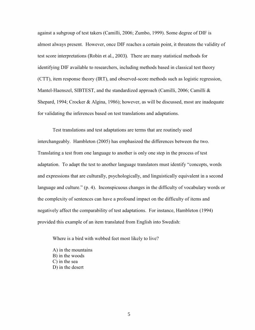
of success on the item, regardless of group membership. Figure 2 displays ICCs that differ

for the two groups of examinees. The differences between the ICCs of the two groups

11

indicate that examinees in the reference and focal groups have differing probabilities of

success on the item. An examinee in the focal group with an ability level of 0 has a

probability of answering the item correctly of approximately .35. On the other hand, an

examinee in the reference group with the exact same ability level has approximately a .50

chance of answering the item correctly.

Figure 1: ICCs with Similar Item Parameters

12

Figure 2: ICCs with Differing Item Parameters

There are two approaches to identifying whether the ICCs of each group differ. The

first method is to measure the differences (i.e. the effect size) between the ICCs of each

group; the second method is to test the statistical significance of the group differences. Both

approaches should be used in conjunction with each other because effect size differences

may be due to chance and because statistically significant results due to large sample sizes

may not have practical relevance (Camilli, 2006). An advantage of using IRT is its

capability of identifying both uniform and non-uniform DIF. Uniform DIF occurs when the

ICCs of the reference and focal groups do not intersect. Conversely, non-uniform DIF occurs

when the ICCs do intersect.

Figure 2 is an example of uniform DIF. The ICCs of the two groups are significantly

different and they do not intersect. That means over the entire spectrum of ability the

reference group has an advantage over the focal group. Figure 3 is an example of non-

uniform DIF. The ICCs of the two groups are different, but they intersect towards the middle

13

of the ability distribution. At the lower end of the ability spectrum the item favors the focal

group. Conversely, at the higher end of the ability spectrum the item favors the reference

group.

Figure 3: ICCs Displaying Non-Uniform DIF

Logistic Regression

Swaminathan and Rogers (1990) recommended using logistic regression as a method

for identifying DIF. Conceptually, logistic regression is a procedure where group, ability,

and a group/ability interaction are used to calculate the probability of a correct or incorrect

answer to an item (Camilli, 2006). Most commonly, the group variable represents group

membership, and an examinee’s total test score is used as a proxy for ability on a given

construct. If the group variable is statistically significant, this indicates that the probability of

getting the item correct is different for each group, after controlling for ability. Ability is

14

almost always statistically significant because unless an item is a misfit item, examinees with

higher ability will have a greater probability of answering it correctly than examinees with

lesser ability. One of the benefits of using logistic regression for DIF detection is its ability

to identify both uniform and non-uniform DIF. If the group/ability interaction is significant,

non-uniform DIF is present.

As is usual in statistical hypothesis testing, the logistic regression test statistic should

be accompanied by a measure of effect size. The Zumbo-Thomas (1997) effect size measure

requires a calculation of pseudo-R2

for two models. The first model is the base model where

the independent variable is ability (total test score). The first model represents an absence of

DIF. Group membership and the interaction between group and ability are introduced in the

second model. The change in R2, ΔR

2, between the two models is the effect size. If ΔR

2 is at

least 0.13 from the first to the second model, and the group membership variable is

statistically significant, then at least moderate DIF is detected. Jodoin and Gierl (2001)

argued that the Zumbo-Thomas effect size measure was not sensitive enough and proposed

that moderate DIF existed when ΔR2

is greater than 0.035 and the group membership variable

is statistically significant.

The Mantel-Haenszel Chi-Square Procedure

In 1959, Nathan Mantel and William Haenszel introduced their extension of the Chi-

square test to address one of the limitations of retrospective studies of rare diseases (Mantel

& Haenszel, 1959). They argued that prospective studies, in which a researcher would

monitor a cohort of subjects for the development of a rare disease, were often unfeasible due

to the sample sizes required and the cost involved. Retrospective studies, on the other hand,

could be much cheaper and accomplished with smaller sample sizes. Mantel and Haenszel’s

15

goal was ―to reach the same conclusions in a retrospective study as would have been

obtained from a forward (prospective) study‖ (p. 722).

The use of Mantel-Haenszel for indentifying DIF. Holland and Thayer (1988)

adapted the Mantel-Haenszel procedure for identifying DIF. The Mantel-Haenszel procedure

is essentially a 2 × 2 × J contingency table. The contents of the columns of the table

represent whether the item was answered correctly or incorrectly, and the row contents

represent whether the examinees are members of the focal or reference groups. The focal

group, typically a minority group or other subgroup of interest, is the group being

investigated to determine whether its member’s responses to an item are an accurate

representation of their standings on a construct. The reference group, typically the majority

group, is the group which is being used as a standard for comparison to the focal group.

Examples of focal and reference groups could be male and female examinees, economically

disadvantaged and non-economically disadvantaged examinees, or Hispanic and Caucasian

examinees, respectively.

The J levels of the Mantel-Haenszel procedure – that is, the strata – should represent

a measurement that allows for an effective comparison of the focal and reference groups. In

educational testing, that measurement might represent total score on an end-of-grade

examination. Without matching on total test score, the difference between the proportions of

students in the reference and focal groups who answered a given item correctly is the impact

of the item. As previously stated, item impact does not imply DIF. Table 2 represents a

typical contingency table at total test score J (Camilli & Shepard, 1994).

16

Table 2: Contingency table at score point J

Group Correct (1) Incorrect (0) Total

White (R) Aj Bj nRj

African-American (F) Cj Dj nFj

Total m1j m0j Tj

When conducting DIF analysis using the Mantel-Haenszel procedure, there would be

a contingency table for each level of J for each item on the test. For instance, if there was a

test with a maximum score point of 10 and a minimum score point of 5, for each item on the

test there would be a contingency table at score points 5-10, assuming the full range of score

points was achieved by the examinees.

Mantel-Haenszel test-statistic. The Mantel-Haenszel procedure requires a calculation

of the following Chi-square test statistic:

(1)

where:

(2)

and

(3)

This chi-square test statistic can be used to identify uniform DIF (Camilli & Shepard,

1994). Dorans and Holland (1993) asserted ―the MH approach is the statistical test

17

possessing the most statistical power for detecting departures from the null DIF hypothesis

that are consistent with the constant odds ratio hypothesis‖ (p. 40). The Aj – E(Aj)

component of Equation 1 represents the difference between the actual number of correct

responses for the item from the reference group for each ability level and the number of times

the reference group would be expected to answer correctly, at the ability level j. If Aj > E(Aj),

then it is possible the item displays DIF in favor of the reference group; whereas if Aj < E(Aj),

then the item displays DIF favoring the focal group.

Mantel-Haenszel odds ratio. In addition to calculating the chi-square test statistic, the

Mantel-Haenszel odds ratio provides a simple measure of effect size and is calculated with

the following formula:

(4)

An odds ratio is the likelihood, or odds, of a reference group member correctly answering an

item compared to a matched focal group member. The odds ratio can be difficult to interpret

because items favoring the reference group range from 1 to infinity, while items favoring the

focal group range from zero to one. To address this concern, Holland and Thayer (1988)

suggested transforming the odds ratio by the natural logarithm so that the scores are centered

around zero and easier to interpret. The range is subsequently transformed to negative

infinity to positive infinity.

ETS DIF classification rules. Dorans and Holland (1993) took the Holland and

Thayer transformation a step further and proposed a system that uses the Mantel-Haenszel

18

procedure to classify test items that display differing degrees of DIF by further transforming

the natural log of the odds ratio by multiplying it by –2.35, yielding the ETS delta value:

|D| = –2.35*ln(αMH) (5)

According to Hambleton (2006), ―An ETS delta value represents item performance for a

specified group of respondents reported on a normalized standard score scale for the

construct measured by the test with a mean of 13 and a standard deviation of 4‖ (p. S184).

After multiplying by –2.35, a positive delta value indicates the item favored the focal group

whereas a negative delta value indicates the item favored the reference group. The categories

are defined as:

Category A: Items display negligible DIF. |D| < 1.0 or MHX2

is not

significantly different than 0.

Category B: Items display intermediate DIF and may need to be reviewed for

bias. MHX2

is significantly different than 0, |D| is > 1.0, and either |D| < 1.5 or

MHX2

is not significantly greater than 1.

Category C: Items display large DIF and are carefully reviewed for bias and

possibly removed from the test. |D| > 1.5 and MHX2

is significantly different

than 1.

Benefits of using Mantel-Haenszel in DIF detection. In their research on the

Mantel-Haenszel procedure, Mazor et al. (1992) and Hambleton (2006) stated its two major

benefits compared to IRT and logistic regression approaches: 1) it requires less computing

power and 2) it is more effective with small sample sizes. According to Muniz et al. (2001),

―the Mantel-Haenszel procedure for item bias detection has been found to be more applicable

with small sample sizes‖ (p. 117). Uttaro and Millsap (1994) noted the simplicity,

19

accessibility, and inexpensiveness as benefits of the Mantel-Haenszel procedure. A Monte

Carlo experiment conducted by Herrera and Gomez (2008) compared the Mantel-Haenszel

procedure with logistic regression and found that uniform DIF detection rates were

significantly higher with Mantel-Haenszel when the reference and focal group sample sizes

were relatively small (reference = 500; focal 500) or when the reference group was up to

five times larger than the focal group. Small, unequal sample sizes are exactly the types of

scenarios associated with DIF studies on test translations.

Research on the Mantel-Haenszel Procedure and Sample Size. Research has been

conducted on improving DIF detection when confronted with small sample sizes. Mazor et

al. (1992) recommended that sample sizes should be at least 200 in each group, and their

recommendation only referred to situations where DIF was most extreme. Van De Viljer

(1997) noted that the Mantel-Haenszel procedure performs well when sample sizes for both

the reference and focal groups are over 200. Parshall and Miller (1995) found that focal

group sizes of at least 100 are needed to reach acceptable levels of DIF detection. Muniz et

al. (2001) attempted to enhance the power of the Mantel-Haenszel procedure for small

sample sizes by combining certain score points into one score level to decrease the number of

score level strata. However, their study was conducted with specific regard to situations

where there are less than 100 cases; this technique is unnecessary when there are focal group

sizes of at least 200, and research has shown that in general, more strata based on ability are

better than fewer strata (Clauser, Mazor, Hambleton, 1994).

In their Monte Carlo study, Herrera and Gomez (2008) tested the influence of unequal

sample sizes on the detection of DIF using the Mantel-Haenszel procedure. As the

differences between the number of cases in the reference (R) and focal (F) groups increased,

20

the DIF detection rate decreased. In examples with unequal and small sample sizes (R = 500

and F = 100), the detection rate was 35%; however, when the distributions were equal (R =

500 and F = 500) the detection rate was 96%. Herrera and Gomez also reported that, with a

reference group as large as 1,500 students, the focal group could be up to one fifth the size of

the reference group without affecting the power of the Mantel-Haenszel procedure, at least

under the circumstances of their experiment. They emphasized, however, that if the Mantel-

Haenszel procedure is to be applied to unequal group sizes, the reference group should be

greater than 1,500 cases and a focal group no more than five times smaller. Neither their

research nor the vast majority of DIF research addresses a scenario where the reference group

was 100 to 200 times larger than the focal group, as is likely to occur in a test translation DIF

study of a high-stakes, statewide assessment.

Research on the Mantel-Haenszel Procedure and Ability Distribution

Differences. In addition to sample size differences, another factor affecting DIF analyses is

the difference in the ability distributions of the reference and focal groups. The power of the

Mantel-Haenszel statistic decreases as the ability distributions become more disparate

(Herrera & Gomez, 2008; Mazor et al., 1992; Muniz et al., 2001; Narayanan &

Swaminathan, 1994). Even with sample sizes of 2,000 in both the reference and focal

groups, if the ability distributions were unequal (i.e. the reference and focal groups differed

significantly in the proportions of their examinees that received each total score point), then

the Mantel-Haenszel procedure correctly identified only 64% of DIF items, as opposed to

74% when the ability distributions were approximately equal (Mazor et al. 1992). A similar

problem existed with reference and focal group sample sizes of 1,000, 500, 200, and 100.

Mazor et al. (1992) recommended that if groups of differing ability distributions are to be

21

compared, sample sizes of the focal group should be as large as possible, and even then DIF

may not be correctly identified.

Using DIF for Translated Tests

A typical test translation in educational achievement testing is not likely to have more

than a few hundred examinees (Fidalgo et al., 2004). IRT and logistic regression require

more examinees to identify DIF effectively. Thus, of the three methods, the Mantel-

Haenszel procedure would be the most effective for use in most test adaptations and other

testing scenarios where there may be small sample sizes such as computer adaptive testing

(CAT). However, there are caveats to this general conclusion. The statistical power of the

Mantel-Haenszel procedure decreases as sample size decreases and as the ability

distributions of the sample sizes of the reference and focal groups are more disparate (Mazor

et al., 1992). The decrease in power as sample size decreases is not surprising; any statistic

will decrease in power as sample size decreases. The decrease in power as the distributions

become increasingly unequal is more disconcerting because the population of examinees

receiving the test translation accommodation is likely to have a vastly different ability

distribution on the construct of interest than the population of examinees receiving the

original (i.e., non-translated) version of the test. If the Mantel-Haenszel procedure is to be

used to compare the reference and focal groups in assessing DIF in test adaptations, a

technique is needed that controls for the disparate distributional differences of the two

populations. Propensity score matching, a relatively new set of statistical methods used to

evaluate the effects of treatments without conducting experiments, could be that technique.

22

Propensity Score Matching

In certain situations it is not practical or ethical to conduct a clinical trial to appraise

the effects of a treatment. In those situations, observational studies may be used to infer

causal relationships. The same concept could be applied to educational experiments. For

example, suppose a researcher was looking to assess the impact of charter schools versus

traditional public schools on achievement. It would not be practical to conduct an

experiment in which students were randomly assigned to treatment (i.e., charter school) and

control (i.e., traditional public school) groups, or to compare the achievement levels of the

schools in question. Among other differences, charter schools have different selection

processes than traditional public schools, and charter schools are not available in some areas

around the country, amongst other differences. In such a situation, however, a researcher

could use propensity score matching to control for differences between the two groups in

variables such as: the selection process, geography, family participation, socio-economic

status, and other variables deemed appropriate, in an effort to make a more valid assessment

of the effects of the treatment (i.e., charter schooling).

A propensity score can be conceptualized as the probability of receiving the treatment

condition in an experiment. Propensity scores may be estimated with various methods

including logistic regression, a probit model, and discriminant analysis. According to Guo

and Fraser (2010), logistic regression is the dominant method for estimating propensity

scores and thus was the approach used for this thesis.

Once the propensity score has been calculated, cases from the treatment group and the

control group can be matched. The concept behind matching is to create a new sample of

cases that share similar probabilities of being assigned to the treatment condition. According

23

to Parsons (2001), there are basically two types of matching algorithms: greedy matching and

optimal matching.

Greedy Matching. Greedy matching involves matching one case from the treatment

group to a case from the non-treatment group with the most similar propensity score. The

match that is made for any given case is always the best available match and once that match

has been made it cannot be reversed. According to Guo and Fraser (2010) greedy matching

requires a sizable common support region for it to work properly. The common support

region is defined as the area of the two distributions of propensity scores where propensity

scores overlap. The cases from each the focal and reference groups that are outside of the

common support region are not matched and subsequently eliminated from analysis. Then,

the greedy algorithm is used to match the propensity score of one case from the treatment

group to one case in the control group. Identification of the rest of the matches will follow

the same procedure.

Optimal Matching. As computers have become faster and software packages more

advanced, the implementation of optimal matching in propensity score analysis has become

more prevalent (Guo & Fraser, 2010). Optimal matching is similar to greedy matching,

except that once a match has been made, matches may be undone if a more desirable match is

found for a case. For example, consider creating two matched pairs from the following four

propensity scores: .1, .4, .5, and .8. Greedy matching would first match .4 and .5 because

their propensity score distance is the closest among the four propensity scores. Then it would

match .1 and .8. The total distance from the two pairs would be |.4 – .5| + |.1 – .8| = .8.

Optimal matching would instead match the first and second propensity scores together and

then match the third and fourth. The total distance would be |.1 – .4| + |.5 – .8| = .6. Optimal

24

matching thus minimizes the distance between matches.

The Importance of DIF Detection for Translated Items

Why is detecting DIF in test translations and adaptations of crucial importance?

There is very little research on why test items in one language measure differently than the

same items in another language (Allalouf et al., 1999). One of the hypothesized reasons for

the lack of research is that there are limited methods for assessing DIF in the scenarios

associated with test translations. The reasons translated items measure differently for

populations taking a test in different languages need to be better understood. Test developers

could use the greater understanding of why DIF occurs in test translations to improve

guidelines for item writing. Furthermore, items that would eventually be translated to

another language could be improved earlier in the test adaptation process. For example,

previous research has shown that translated analogy items display more DIF than sentence

completion or reading comprehension items (Angoff & Cook, 1988; Beller, 1995). In

research done on the Israeli university entrance exam, the Psychometric Entrance Test (PET),

Allalouf et al. (1999) noted four possible reasons why translated items performed differently

for Russian or Hebrew language examinees: 1) changes in difficulty of words or sentences,

2) changes in content, 3) changes in format, and 4) differences in cultural relevance. The

analogy items displayed DIF more regularly than the other item types mainly due to changes

in word difficulty or changes in content. For instance, in Hebrew there are more difficult

synonyms or antonyms to choose from than in Russian. Thus, an analogy question in

Hebrew might be very challenging, but the same item might be relatively easy when

translated into Russian.

In addition to the benefits of identifying problems with translated test items, if more

25

accurate methods were developed for identifying items that were measuring differently for

each sub-group of examinees, then linking the two test forms (i.e. the original and translated)

could be performed with greater accuracy. Sireci (1997) recommended that the linking

process should begin with an evaluation of the translated test items for invariance between

the two tests, and items displaying DIF should be removed. The remaining items not

displaying DIF could then be used as anchors, and the two tests calibrated onto a common

scale. However, if the methods for identifying DIF misidentify items that are functioning

differently for different sets of examinees, then the linking process will not be as accurate as

possible.

Summary

Of all the techniques used to evaluate DIF, the Mantel-Haenszel procedure is the most

effective with small sample sizes. Thus, it is optimal for use in evaluating DIF in a typical

test translation where there are only a few hundred examinees. However, the ability

distributions and the total numbers of examinees are often vastly different when comparing

the population of examinees who received the translated version of the test against the

general population of examinees. The accuracy of the Mantel-Haenszel procedure decreases

as the ability distributions and the total population of examinees become more disparate.

Propensity score matching can be used to control for the distributional differences between

the two populations, possibly enhancing the Mantel-Haenszel procedure for identifying DIF.

If items that are measuring differently for the two populations can be more accurately

identified, the reasons behind the DIF can be better understood. Eventually, that will lead to

improved item writing for items intended to measure similarly in different languages.

Ultimately, a better understanding of DIF will lead to higher quality test information and

26

greater validity of inferences about examinee knowledge, skill, and ability.

Research Question

What is the effect on the accuracy of the Mantel-Haenszel procedure in assessing

differential item functioning (DIF) when propensity score matching is used to control for

situations where the focal group differs substantially in size and in ability distribution from

the reference group?

Method

This study used simulated data to provide a known benchmark against which the

performance of PSM was evaluated. The data for this study were generated using the

program WinGen2 (Han, 2007). The program simulates examinee responses using the type

of IRT model specified by the user. WinGen2 also allows for DIF to be introduced into the

examinee responses. For this study the Rasch model was used because the item parameters

and ability levels of the reference and focal groups were based off of data that was calibrated

with the Rasch model. The Rasch model is commonly used to analyze data in large-scale,

statewide assessments. The data were simulated to resemble a standard administration of a

statewide assessment that was delivered in two versions; in this case, to simulate

administrations of English and Spanish versions. Each data set was simulated with a test

length of 50 items—a test length that would not be unrealistic for a statewide student

achievement test.

Variables in Study

Three primary independent variables were manipulated in this study. The variables

included sample size, ability distributions, and amount of DIF.

Sample Size. One data set of 100,000 examinees was simulated to represent the

reference group. Three other data sets of 250, 500, and 1,000 were simulated to represent the

focal groups.

Ability Distributions. The average ability level of the reference group was set at 1.0

with a standard deviation of 1.0 whereas the average ability level of the focal group was set

29

at –0.30 with a standard deviation of approximately 0.65. The ability distributions were

simulated to resemble a standard administration of a statewide assessment that was delivered

in both English and Spanish. Experience suggests that the population of examinees who

received the Spanish accommodation to test in their native language had significantly lower

ability levels than the English population. The Spanish population’s average ability level

was approximately 1.3 standard deviations lower than the average ability level of the English

population.

Amount of DIF. Experience with translated language testing suggests that DIF is

likely to be observed in approximately 25-40% of translated test items. Therefore, 16 of the

50 items (32%) had DIF introduced to their item difficulty parameters. The 16 items were

selected to be representative of the test as a whole, meaning the range, mean, and standard

deviation of the DIF subtest is similar to the whole test. To increase the generalizability of

the study and because DIF occurs at different levels depending on the test translation, DIF

was introduced in two scenarios in four increments at each level: 0.2, 0.4, 0.6, and 0.8 in the

first scenario and 1.0, 1.2, 1.4, and 1.6 in the second scenario. A DIF level of 1.0 would

mean that the item-difficulty parameter of the focal group had been increased by 1.0. For

instance, item #34 had an item-difficulty parameter of -1.014. A DIF level of 1.0 was added

and the item-difficulty for the focal group changed from -1.014 to -0.014. To introduce DIF

in favor of the focal group the DIF level would be subtracted from the item-difficulty

parameter instead of added. Combined, the two scenarios represent the range of DIF levels

commonly used in DIF simulation studies (Fidalgo et al., 2004; Mazor et al., 1992). Muniz

et al. (2001) noted that DIF levels of 1.5 or higher may be large in simulations that represent

typical gender or ethnic DIF studies; however, in situations where poor test translations have

30

taken place, DIF levels of 1.5 or higher are not uncommon. The first scenario represents a

test with moderate levels of DIF, and the second scenario represents a test with large levels

of DIF. Experience suggests DIF favors the reference group approximately 75% of the time

and the focal group approximately 25% of the time. Thus, 12 of the items have DIF in favor

of the reference group and 4 in favor the focal group. Table A1 in Appendix A shows the

item difficulty parameters for all 50 items as well as the introduction of DIF for each

scenario.

Data Analyses

For each simulation condition, descriptive statistics were calculated including p-

values, response variance, and point-biserial correlations for each item. Reliability estimates

were calculated using Cronbach’s Alpha. The descriptive statistics and reliability estimates

were analyzed to ensure the simulated data resembled a typical administration of high-stakes

statewide assessment. All descriptive statistics and reliability estimates were calculated

using a SAS computer program written by the author. The SAS code used for this thesis is in

Appendix B. Table 3 displays the total test score mean and standard deviation, as well as the

range of scores for all seven simulated data sets.

Table 3: Total Test Score Descriptive Statistics for Simulated Data Sets

Group DIF Level N-Count Mean St. Dev. Min. Max.

Reference None 100,000 36.42 8.40 0 50

Focal Low

1,000 23.87 7.18 5 45

500 24.41 7.17 7 43

250 23.96 7.68 6 42

Focal High

1,000 22.78 6.73 5 44

500 23.04 6.88 4 45

250 22.94 6.91 5 40

31

The Mantel-Haenszel procedure was applied to the entire population of simulated

examinees using a SAS computer program written by the author. The reference group

represented the population of examinees who took the test in the language in which the test

was originally written. The focal group represented the population of examinees who took

the translated version of the test. The results reported in the next section tested the

significance level of the Mantel-Haenszel test statistic at the .05 level. Items were also

classified using the classification system proposed by Dorans and Holland (1993).

Propensity Score Matching. After verifying the simulation conditions were met via

the generated data and classifying each item with the traditional Mantel-Haenszel procedure,

an estimated propensity score was calculated for each case in both the reference and focal

groups for all simulation scenarios. The propensity score was based on total test score. After

obtaining the estimated propensity scores, greedy matching was used to accomplish the

matching. Greedy matching requires less computing power and programming than optimal

matching (Guo and Fraser, 2010). Because there was such a large pool of simulated

reference examinees compared to the relatively small groups of simulated focal examinees,

and because only one variable (total score) was used for matching, it was unlikely that

matching via greedy matching or optimal matching would produce significantly different

matches. Furthermore, the two populations had a large common support region of propensity

scores, meaning the major assumption of greedy matching was satisfied (Parsons, 2001;

Rosenbaum, 2002). The greedy matching was performed with a variation of Parsons’ (2001)

greedy matching macro using SAS software.

The application of greedy matching led to new reference groups with the same

number of cases as the focal groups. Because of the relatively large pool of simulated

32

examinees in the reference group, and because matching was accomplished via total test

score, the means and standard deviations for each group were equal after matching. Table 4

shows the descriptive statistics of all groups after matching.

Table 4: Total Test Score Descriptive Statistics for Simulated Data Sets After Matching

Group DIF Level N-Count Mean St. Dev. Min. Max.

Reference Low

1,000 23.87 7.18 5 45

500 24.41 7.17 7 43

250 23.96 7.68 6 42

Focal Low

1,000 23.87 7.18 5 45

500 24.41 7.17 7 43

250 23.96 7.68 6 42

Reference High

1,000 22.78 6.73 5 44

500 23.04 6.88 4 45

250 22.94 6.91 5 40

Focal High

1,000 22.78 6.73 5 44

500 23.04 6.88 4 45

250 22.94 6.91 5 40

Finally, after the matching was applied and the new reference group and the focal

group were equated in number and ability levels, the Mantel-Haenszel procedure was

applied. For each item, the Mantel-Haenszel test statistic was tested at the .05 level, and

items were re-classified with the ETS classification system. For each scenario, each item

was classified twice by the Mantel-Haenszel procedure, once with the traditional method and

once with an adjustment that controlled for distributional differences. The agreement rates

for ETS classification between the two methods were calculated for each of the six cells of

the design. The agreement rates of the two methods were further analyzed with Cohen’s

Kappa. The two methods were then analyzed by calculating DIF detection rates and Type I

and II error rates for each combination of sample size and DIF level to determine if one

method was correctly identifying DIF at a higher rate than the other method. Two repeated-

measures Analysis of Variances (ANOVA) were conducted to determine if the observed

33

differences in Type I and II errors were statistically significant, or if any of the interactions

between method, sample size, and DIF level were statistically significant.

Summary

The purpose of this thesis is to answer the following research questions:

1) What is the effect on the Type I errors of the Mantel-Haenszel procedure in assessing

DIF when propensity score matching is used to control for distributional differences

between the reference and focal groups?

2) What is the effect on the Type II errors of the Mantel-Haenszel procedure in assessing

DIF when propensity score matching is used to control for distributional differences

between the reference and focal groups?

3) What are the effects of focal group sample size, the level of DIF and the method of

DIF detection (e.g. with or without matching) on Type I errors.

4) What are the effects of focal group sample size, the level of DIF and the method of

DIF detection (e.g. with or without matching) on Type II errors.

5) What is the effect on the ETS classifications of the Mantel-Haenszel procedure in

assessing DIF when propensity score matching is used to control for distributional

differences between the reference and focal groups?

To address research question 1 a repeated measures ANOVA was conducted with

Type I errors for each method of DIF detection as the dependent variable and sample size and

DIF level as the independent variables. To address research question 2 another repeated

measures ANOVA was conducted. In this case, Type II errors for each method of DIF

detection was used as the dependent variable and sample size and DIF level were the

independent variables. The same repeated-measures ANOVAs were used to address research

34

questions 3 and 4. To address research question 5 the ETS classifications agreement rates of

the two methods were calculated and further analyzed with Cohen’s Kappa.

Results

The first component of the results section addresses the simulated data. Do the

simulated data resemble a standard administration of a Language Arts Literacy high-stakes

statewide assessment that was delivered in both English and Spanish? P-values, point-

biserial correlations, and Cronbach’s alpha were calculated and analyzed to answer that

question. The next components of the results section will address each of the research

questions in the order they were presented in the methods section and the subsequent results

of the study.

Simulated Data

As previously stated, the p-values were calculated to ensure the data sets adequately

resembled a standard administration of a Language Arts Literacy high-stakes statewide

assessment that was delivered in both English and Spanish. Table 5 summarizes the item

difficulty descriptive statistics for reference and focal groups, at each combination of DIF

level and focal group size. Based on prior experience, the summary of item difficulties in

Table 5 for each of the seven data sets does not appear unrealistic. Tables C1-C6 are found

in Appendix C. They display the p-values for each item for all six cells of the study’s design,

before and after matching. Tables C1-C6 also display the item variances for each of the six

scenarios, before and after matching. The item variances tended to be larger with the focal

group population than with the reference group. Considering the average p-values in Table 5

the larger item variances associated with the focal groups are not surprising. Items with p-

values close to 0.5 display the largest degree of variance. The average p-value for the

36

reference group was 0.73 compared to average focal group p-values that were much closer to

0.5.

Table 5: Descriptive Statistics of Item Difficulties of Simulated Data Sets

Group DIF Level N-Count Mean St. Dev. Min Max

Reference None 100,000 0.73 0.13 0.32 0.95

Focal Low

1,000 0.48 0.17 0.10 0.88

500 0.49 0.17 0.09 0.89

250 0.48 0.17 0.10 0.90

Focal High

1,000 0.46 0.20 0.07 0.86

500 0.46 0.20 0.09 0.90

250 0.46 0.21 0.08 0.88

Table 6 summarizes the item difficulty descriptive statistics after matching at each

combination of DIF Level and focal group size. The average p-value of the reference group

went from 0.73 to ranging from 0.46 to 0.49, depending on which focal group data set it was

matched to. The matched reference groups’ average p-values are equivalent to the p-values

of their associated focal group. There are slight differences between the standard deviations

of the matched reference groups and the focal groups, as well as the minimum and maximum

p-values. However, the differences are minimal and Table 6 provides more evidence to the

success of the matching.

37

Table 6: Descriptive Statistics of Item Difficulties of Simulated Data Sets Post-Matching

Group DIF Level N-Count Mean St. Dev. Min Max

Reference Low

1,000 0.48 0.16 0.10 0.87

500 0.49 0.17 0.10 0.87

250 0.48 0.17 0.10 0.88

Focal Low

1,000 0.48 0.17 0.10 0.88

500 0.49 0.17 0.09 0.89

250 0.48 0.17 0.10 0.90

Reference High

1,000 0.46 0.16 0.09 0.85

500 0.46 0.17 0.08 0.86

250 0.46 0.17 0.07 0.86

Focal High

1,000 0.46 0.20 0.07 0.86

500 0.46 0.20 0.09 0.90

250 0.46 0.21 0.08 0.88

The point-biserial correlations were also calculated before and after matching to

ensure the simulated data resembled a standard administration of a Language Arts Literacy

high-stakes statewide assessment that was delivered in both English and Spanish. Table 7

summarizes the point-biserial descriptive statistics for each of the six cells of the study’s

design, before and after matching. The descriptive statistics of the point-biserial correlations

pre-matching are almost exactly the same at each combination of focal group size and DIF

level. The similarity of the point-biserial pre-matching was to be expected considering the

reference group size of 100,000 and the relatively small size of each of the focal groups. A

noticeable aspect of Table 7 is the lack of variability among the point-biserials for each of the

cells. This is not surprising considering the Rasch model was used in the simulation and that

IRT model does not vary item-discrimination, unlike the two-, or three-parameter logistic

models. The low variability in the point-biserial correlations is not consistent with a standard

administration of a Language Arts Literacy high-stakes statewide assessment. Tables C1-C6

display all of the point-biserials for each item under each combination of sample size and

DIF level.

38

Table 7: Descriptive Statistics of Point-Biserial Correlation: Pre and Post-Matching

DIF Level Focal Group Size Mean RPB St. Dev. Min Max

Pre-Matching

Low 1,000 0.39 0.04 0.23 0.44

500 0.39 0.05 0.23 0.44

250 0.39 0.04 0.23 0.44

High

1,000 0.39 0.04 0.23 0.44

500 0.39 0.05 0.23 0.44

250 0.39 0.05 0.23 0.44

Post-Matching

Low

1,000 0.30 0.03 0.19 0.35

500 0.30 0.04 0.17 0.36

250 0.32 0.05 0.16 0.44

High

1,000 0.29 0.03 0.19 0.35

500 0.29 0.04 0.19 0.37

250 0.29 0.05 0.19 0.41

Cronbach’s Alpha values were calculated for the reference group and all six focal

groups to ensure the simulated data accurately resembled a typical administration of high-

stakes statewide assessment. Table 8 displays the reliability estimates and standard errors of

measurement of the simulated data. Based on experience with high-stakes statewide

assessments delivered in both English and Spanish, the reliability estimates and standard

errors of measurement measures in Table 8 do not appear unrealistic.

Table 8: Summary of Cronbach’s Alpha Reliability Estimates and SEMs for each Simulated

Data Set

Group DIF Level N-Count Alpha SEM

Reference None 100,000 0.89 2.80

Focal Low

1,000 0.80 3.20

500 0.80 3.20

250 0.83 3.18

Focal High

1,000 0.79 3.11

500 0.80 3.11

250 0.80 3.10

39

Type I Errors

Table 9 displays the contingency table of total Type I errors for both pre- and post-

matching. Only the 34 items where DIF was not introduced were considered in determining

the Type I error rate. Because there were six possible scenarios representing each

combination of the two levels of DIF and the three sample sizes, and 34 items per scenario

that had the potential for Type I errors, there were 204 total repeated measures that were used

in the contingency table shown in Table 9. One finding is the large number of Type I errors

pre-matching. Approximately 30% of items (61 out of 204) were classified as showing

statistically significant DIF, when no DIF had been introduced. Matching decreased the

percentage of Type I errors to 18% (36 out of 204). The results of the repeated-measures

ANOVA (Wilk’s Lambda = .91, F(1,198) = 19.04, p < 0.0001) suggest that the decrease in

Type I errors was statistically significant. Matching is having a positive effect on decreasing

Type I error rates and thus the null hypothesis -- that matching is having no effect on the

Type I error rate of the Mantel-Haenszel procedure -- is rejected.

Table 9: Contingency Table for Type I Errors

Post-Matching

Type I Error No Yes Total

Pre-Matching

No 136 7 143

Yes 32 29 61

Total 168 36 204

Table 10 displays the total number of Type I errors both pre-and post-matching for each

combination of sample size and DIF level. When the DIF level was low the total number of

Type I errors both pre- and post-matching was exactly the same (9%, or 9 out of 102).

However, when the DIF level was high the percentage of Type I errors increased to 51% (52

40

out of 102) pre-matching and to 26% (27 out of 102) post-matching. Table 10 suggests that

the statistically significant decrease in Type I errors after matching is largely due to the

interaction between the method of identifying DIF and the DIF level. The interactions

between the method of identifying DIF, sample size, and DIF level in Type I errors will be

discussed further in a section below.

Table 10: Total Number of Type I Errors

DIF Level Focal Group Size Type I Errors

Pre-Matching

Low

1,000 5

500 2

250 2

High

1,000 28

500 13

250 11

Post-Matching

Low

1,000 4

500 2

250 3

High

1,000 15

500 7

250 5

Type II Errors

Table 11 displays the contingency table of Type II errors for both pre- and post-

matching. Only the 16 items where DIF was introduced were considered in determining the

Type II error rate. Because each item was simulated under six different conditions, there

were 96 possible Type II errors. Pre-matching 7% (7 out of 96) of items displayed Type II

errors. That percentage increased to 12.5% (12 out of 96) Type II errors, post-matching.

According to the repeated-measures ANOVA(Wilk’s Lambda = .96, F(1,90) = 3.95, p <

0.05), the increase in Type II errors post-matching was statistically significant. Matching is

having a statistically significant effect in increasing Type II error rates and thus the null

41

hypothesis -- that matching is having no effect on the Type II error rate of the Mantel-

Haenszel procedure -- is rejected.

Table 11: Contingency Table for Type II Errors

Post-Matching

Type II Error No Yes Total

Pre-Matching

No 83 6 89

Yes 1 6 7

Total 84 12 96

Table 12 displays the total number of Type II errors both pre-and post-matching for each

combination of sample size and DIF level. One major finding is that when the DIF level was

high, neither method produced a Type II error. Regardless of samples size, all 16 items that

had a high level DIF introduced were correctly identified as displaying DIF regardless of

method. Another, less encouraging finding is the number of Type II errors found when the

DIF level was low. Pre-matching and with low levels of DIF, the percentage of Type II

errors was 15% (7 out of 48) and post-matching it increased to 25% (12 out of 48).

Table 12: Total Number of Type II Errors

DIF Level Focal Group Size Type II Errors

Pre-Matching

Low

1,000 2

500 2

250 3

High

1,000 0

500 0

250 0

Post-Matching

Low

1,000 3

500 2

250 7

High

1,000 0

500 0

250 0

42

Effects on Type I Errors

The repeated-measures ANOVA was also conducted to answer research question #3

and determine the effect of the DIF methodology, sample size, and DIF level, as well as the

interactions between those three variables on Type I errors. Table 13 displays the results of

the ANOVA on Type I errors. All three main effects were found to be statistically

significant: method [F(1,198) = 19.04, p <0.0001], sample size [F(2, 198) = 10.95, p

<0.0001], and DIF level [F(1, 198) = 46.46, p <0.0001]. The fact that method is a

statistically significant main effect suggests that the methodology chosen (i.e. matching or no

matching) is having a statistically significant effect on Type I errors. Furthermore, that the

main effects of sample size and DIF level are also statistically significant indicates that as

sample size or the level of DIF increases then an increase in Type I errors can be expected,

regardless whether matching is used to control for ability distributions or not. Two of the

interactions were statistically significant: method x DIF level [F(1, 198) = 19.04, p = .001]

and sample size x DIF level [F(1, 198) = 5.48, p = .0048]. These findings suggest that the

interaction between methodology and DIF level is significant and that the impact of one

factor depends on the level of the other. Thus, any interpretation of the statistical

significance of the methodology without noting the interaction between DIF level and

methodology would be incomplete. Similarly, the statistically significant interaction between

sample size and DIF level indicates that the impact on one variable depends on the other.

43

Table 13: Analysis of Variance for Type I Errors

Source df F p

Method 1 19.04 <0.0001

Sample Size 2 10.95 <0.0001

DIF Level 1 46.46 <0.0001

Method x Sample Size 2 2.22 0.1108

Method x DIF Level 1 19.04 <0.0001

Sample Size x DIF Level 2 5.48 0.0048

Method x Sample Size x DIF Level 2 0.94 0.3906

Effects on Type II Errors

A repeated-measures ANOVA was also conducted to answer research question #4

and determine the effect of the DIF methodology, sample size, and DIF level, as well as the

interactions between those three variables on Type II errors. Table 14 displays the results of

the ANOVA on Type II errors. In Table 14 only two main effects had a statistically

significant impact on Type II errors: method [F(1,90) = 3.95, p =0.05] and DIF level [F(1,90)

= 15.25, p = 0.0002]. Sample size [F(2, 90) = 1.31, p = 0.275] was not statistically

significant. The results in Table 14 suggest that the methodology chosen is making a

statistically significant impact on Type II errors. Method x DIF level [F(1,90) = 3.95, p

=0.05] was the only statistically significant interaction.

Table 14: Analysis of Variance for Type II Errors

Source df F p

Method 1 3.95 0.0500

Sample Size 2 1.31 0.2750

DIF Level 1 15.25 0.0002

Method x Sample Size 2 2.05 0.1344

Method x DIF Level 1 3.95 0.0500

Sample Size x DIF Level 2 1.31 0.2750

Method x Sample Size x DIF Level 2 2.05 0.1344

44

ETS Classification Agreement Rates

Because statistically significant results are not always of practical importance, the

ETS classifications of each of the methods were calculated and analyzed. Table 15 displays

the number of items that were classified as either A, B, or C by the ETS classification

system, at all combinations of DIF level and sample size, both before and after matching.

One finding of Table 15 is that both methods produced very similar distributions of

classifications. The distributions of classifications were exactly the same for both methods

when the DIF level was low and sample size was 250 as well as when the DIF level was high

and sample size was 1,000. A second finding is that both methods appeared to be under

classifying DIF items when the DIF level was low, regardless of sample size. Of the 16

items where DIF was introduced, only 8 to 10 items were flagged as B or C items when the

DIF level was low. Furthermore, when the DIF level was high and samples sizes were 500

or 250, more items were classified as displaying DIF than the 16 items that had DIF

introduced. Tables C1-C6 in Appendix C display the ETS classifications, before and after

matching, for each item at all combinations of DIF level and sample size.

Table 15: Distribution of A, B, & C Class items for both Pre- and Post-Matching

Degree of DIF

DIF Level Focal Group Size A B C

Pre-Matching

Low 1,000 41 4 5

500 42 7 1

250 40 8 2

High

1,000 34 0 16

500 34 0 16

250 31 3 16

Post-Matching

Low

1,000 42 3 5

500 42 6 2

250 40 8 2

High

1,000 34 0 16

500 31 3 16

250 28 7 15

45

Tables 16-21 display the contingency tables for the ETS classification system as well

as the agreement rate and Cohen’s Kappa for each of the six combinations of sample size and

DIF level. The agreement rates were all over 92%. When the sample size was 1,000 and the

DIF level was high the agreement rate of the two methods was 100%. Cohen’s Kappa

statistics ranged from 0.76 to 1.00. According to Landis and Koch (1977) a Kappa statistic

between 0.61 and 0.80 indicates substantial agreement and between 0.81 and 1.00 indicates

almost perfect agreement. The high agreement rates and the large Kappa statistics suggest

that controlling for distributional differences is having a limited affect on the ETS

classification of items.

Table 16: ETS Classification Contingency Table – Sample Size = 1000; DIF Level = Low

Post-Matching

ETS Class. A B C Total

Pre-Matching

A 41 0 0 41

B 1 3 0 4

C 0 0 5 5

Total 42 3 5 50

Agreement Rate = 98% Cohen’s Kappa = 0.93 (p < .0001)

Table 17: ETS Classification Contingency Table – Sample Size = 500; DIF Level = Low

Post-Matching

ETS Class. A B C Total

Pre-Matching

A 41 1 0 42

B 1 5 1 7

C 0 0 1 1

Total 42 6 2 50

Agreement Rate = 94% Cohen’s Kappa = 0.78 (p < .0001)

46

Table 18: ETS Classification Contingency Table – Sample Size = 250; DIF Level = Low

Post-Matching

ETS Class. A B C Total

Pre-Matching

A 38 2 0 40

B 2 6 0 8

C 0 0 2 2

Total 40 8 2 50

Agreement Rate = 92% Cohen’s Kappa = 0.76 (p < .0001)

Table 19: ETS Classification Contingency Table – Sample Size = 1000; DIF Level = High

Post-Matching

ETS Class. A B C Total

Pre-Matching

A 34 0 0 34

B 0 0 0 0

C 0 0 16 16

Total 34 0 16 50

Agreement Rate = 100% Cohen’s Kappa = 1.00 (p = N/A)

Table 20: ETS Classification Contingency Table – Sample Size = 500; DIF Level = High

Post-Matching

ETS Class. A B C Total

Pre-Matching

A 31 3 0 34

B 0 0 0 0

C 0 0 16 16

Total 31 3 16 50

Agreement Rate = 94% Cohen’s Kappa = N/A

Table 21: ETS Classification Contingency Table – Sample Size = 250; DIF Level = High

Post-Matching

ETS Class. A B C Total

Pre-Matching

A 28 3 0 31

B 0 3 0 3

C 0 1 15 16

Total 28 7 15 50

Agreement Rate = 92% Cohen’s Kappa = 0.85 (p < .0001)

Discussion

This section is organized around three major topics. The first topic of interest is the

implications of the findings of this study: What has been learned and why is it important?

The second topic of interest is the limitations of the study; no study is perfect and by

understanding the limitations of this study a greater understanding of the topic in general can

be established. Finally, the avenues for future research are discussed: What are some next

steps in researching identification of DIF in the context of test translations?

Implications of Findings

The focus of this study was to test the effects of controlling for disparate

distributional differences on the Mantel-Haenszel procedure. Would controlling for those

differences increase its ability to detect DIF accurately? To answer that question a repeated-

measures ANOVA was conducted to test the main effects of DIF methodology (pre-matching

Mantel-Haenszel or post-matching Mantel-Haenszel), focal group sample size (1,000, 500, or

250) and DIF level (low or high). The interactions between those three variables were also

tested. Finally, the ETS classifications of each item, using each methodology were analyzed.

The findings suggest that Type I errors of the Mantel-Haenszel test statistic can be decreased

by matching. However, there is a caveat to that finding. The error rate in the ETS

classification of items increased after matching.

Type I Errors. If DIF researchers identify DIF where no DIF exists then valuable

time which could be spent understanding why translated items are functioning differently in

different languages will be spent investigating items where DIF did not actually exist.

48

Research question #1 asked whether matching was having an effect on the Type I error rates.

The statistically significant decrease in Type I errors after matching the ability distributions

of the focal and reference groups is a positive finding. However, it was expected that

matching would result in a statistically significant decrease in the Type I errors made in the

Mantel-Haenszel procedure. As sample size increases, Type I errors should increase as well:

Any test statistic will become more powerful as sample size increases. The statistically

significant decrease in Type I errors should only be interpreted in conjunction with an effect

size measure such as the ETS classification system, which will be discussed when research

question #5 is addressed.

Type II Errors. Just as DIF researchers look to avoid analyzing items for bias that

actually have no DIF, they want items that are biased to be identified as displaying DIF so

that the source of that bias may be investigated. Research question #2 asked whether

matching was having an effect on the Type II errors rates. There was a statistically

significant difference in Type II errors between the Mantel-Haenszel procedure before and

after matching. In this case, the statistically significant results were not in favor of the

Mantel-Haenszel procedure after matching. Thus, the decrease in sample sizes after

matching is decreasing the power of the Mantel-Haenszel procedure enough that it

significantly increased Type II errors. Thus, at least under these simulated conditions, in the

identification of DIF it is more advantageous to maintain disparate distributional differences

between the focal and reference groups than to match the n-counts and ability distributions;

however, the interpretation of this finding related to Type II errors is more fully understood

with the additional findings related to research question #5 regarding effect size measures.

49

Effects on Type I Errors. Research question #3 addressed the effects of focal group

sample size, the level of DIF and the method of DIF detection (e.g. with or without

matching) on Type I errors. The main effects of sample size, DIF level and method were all

determined to be statistically significant, as well as two two-way interactions: method–by-

DIF level as well as sample size–by-DIF level. That method was statistically significant

gives more credence to the argument that matching could decrease Type I errors rates. That

sample size is statistically significant should be of no surprise. As was discussed earlier, as

sample size increases, power increases, and Type I error rates increase. Furthermore, that

DIF level was statistically significant should not have been surprising. The higher the DIF

level the more likely pseudo-DIF will become prevalent in other items. Psuedo-DIF is when

true-DIF in one item causes apparent DIF in other items within the same test, even though

these other items are not truly differentially functioning (Groenvold & Petersen, 2005).

Thus, items without DIF may display pseudo-DIF to compensate for items that actually

display true-DIF. As DIF levels increase, pseudo-DIF increases which might account for the

statistically significant impact of DIF level on Type I errors.

The reason the introduction of true-DIF may lead to pseudo-DIF is that the total test

score variable used by the Mantel-Haenszel procedure is now contaminated by DIF. For

instance, imagine two classrooms of equal students taking the same test. One of the classes

was previously exposed to the correct answer to one question, which the other class was not

privy to. If a DIF study is conducted, the total test score variable no longer means the same

thing for students in each classroom. Thus, the Mantel-Haenszel strata are contaminated if

they are based on the internal criterion of total test score. A student in classroom A could

have got the biased question correct and got a raw score of 26 out of 50 on a test; a student in

50

classroom B might have got the biased correction incorrect and still got a 26. The extra point

student B earned would have had to come from somewhere else on the test, on an item that

was not biased. If the extra points earned by focal group examinees to compensate for the

true-DIF accumulate in enough frequency on one or two items, pseudo-DIF might get large

enough to be statistically significant. The more extreme the DIF, and the less points that are

available in the total test score, the more pseudo-DIF will be a problem, unless the internal

scale is purified as recommended by Clauser, Mazor, and Hambleton (1993).

The interactions between method and DIF level as well as sample size and DIF level

show that the main effects may change over levels of the other variables. Figure 4 displays

the interaction between method and DIF level. The frequency of Type I errors is highly

dependent on the level of DIF and the method chosen to identify DIF. The average number

of Type I errors was the same for each method when the DIF level was low. However, when

the DIF level was high, the average number of Type I errors pre-matching was 17.33. Using

post-matching, it decreased to 9.0. The implications of these findings are that if researchers

are anticipating doing DIF analyses on a test with possible high levels of DIF, such as a test

translation, matching could reduce Type I errors. However, if researchers are performing

DIF analysis on a test with anticipated low levels of DIF, pre-matching and post-matching

will likely produce similar Type I error rates. However, those findings should only be

interpreted in conjunction with a measure of effect size, such as the ETS classification

system.

51

Figure 4: Interaction of DIF Level and Method in Type I Errors

0

2

4

6

8

10

12

14

16

18

20

Low High

DIF Level

Typ

e I

Err

ors

Pre-Matching

Post-Matching

Effects on Type II Errors. Research question #4 addressed the effects of focal

group sample size, the level of DIF and the method of DIF detection (e.g. with or without

matching) on Type II errors. Only the main effects of method and DIF level were deemed

statistically significant. That DIF level was statistically significant was not surprising. When

the DIF level was lower, it was more challenging for the Mantel-Haenszel procedure to

detect DIF.

The two-way interaction method–by-DIF level was also significant. Figure 5 displays

the interaction between method and DIF level. The frequency of Type II errors is highly

dependent on the level of DIF and the method chosen to identify DIF. The average number

of Type II errors was the same for each method when the DIF level was high, because when

the DIF level was high all the items that had DIF introduced were identified as statistically

significant. However, when the DIF level was low the average number of Type I errors post-

52

matching was 4. Using pre-matching, it was only 2.33. The implications of these findings

are that if researchers are anticipating doing DIF analyses on a test with possible low levels

of DIF, matching could increase Type II errors. However, if researchers are performing DIF

analysis on a test with anticipated high levels of DIF, such as a test translation, pre-matching

and post-matching will likely produce similar Type II error rates. However, those findings

should only be interpreted in conjunction with a measure of effect size, such as the ETS

classification system.

Figure 5: Interaction of DIF Level and Method in Type II Errors

0

0.5

1

1.5

2

2.5

3

3.5

4

4.5

Low High

DIF Level

Typ

e I

I E

rro

rs

Pre-Matching

Post-Matching

ETS Classification Agreement Rates. Just looking at Type I or II errors is not a

complete analysis. Effect size measures such as the Mantel-Haenszel log odds ratio, a

component of the ETS classification of items, should also be analyzed. Research question #5

thus addressed whether matching had an effect on the ETS classification of items. The

53

agreement rates between the two methods, as well as the Kappa statistics, indicate substantial

agreement between the traditional Mantel-Haenszel procedure and the Mantel-Haenszel

procedure after matching. Thus, matching may not be making much of a practical impact on

DIF detection.

Unlike the statistically significant reduction of Type I errors, when the ETS

classification of items are analyzed, matching does not appear to be actually reducing errors.

In fact, it may be increasing errors in the ETS classification of items. According to the ETS

classification system, if an item is classified as displaying B- or C-level DIF then that item

should be reviewed for possible bias. If it is assumed that any simulated item that had DIF

introduced to it should have been classified as at least B- or C-level DIF by the Mantel-

Haenszel procedure, then the traditional Mantel-Haenszel procedure actually produced less

false positives than the Mantel-Haenszel procedure after matching. Table 22 displays the

errors in ETS classification that were made by each methodology.

Table 22: Total Number of Type I Errors in ETS Classification

DIF Level Focal Group Size Type I Errors

Pre-Matching

Low

1,000 0

500 0

250 1

High

1,000 0

500 0

250 3

Post-Matching

Low

1,000 0

500 0

250 2

High

1,000 0

500 3

250 6

Similarly, there appears to be no practical benefit to matching when the items that had

DIF introduced have their ETS classifications analyzed. If it is assumed that each item that

54

had DIF introduced should have been classified as displaying either B- or C-level DIF, then

items that had DIF introduced yet were still classified as A-level DIF would be Type II

errors. Table 23 shows that more items that should have been classified as displaying B- or

C-level DIF were classified as displaying A-level DIF after matching than when the

traditional Mantel-Haenszel procedure was used. Thus, even under this criterion, matching

did not improve Type II error rate; it actually made them slightly more prevalent. This is

likely due to a lack of statistical power in the Mantel-Haenszel test statistic due to the loss of

sample size after matching. For instance, Table C3, in Appendix C, displays the Mantel-

Haenszel test statistics, the ETS delta values, and the ETS Classification for each item under

the scenario with low DIF level and focal group sample size of 250. There were nine items

under that scenario that should have been classified as displaying either B- or C-level DIF:

items 6, 12, 22, 24, 31, 34, 38, 41, and 46. After-matching the Mantel-Haenszel procedure

only identified 2 of those 9 items as statistically significant. That automatically makes the

item an A-level item according to the ETS classification system, regardless of the log odds

ratio after it is converted to the ETS delta scale. In comparison, pre-matching the Mantel-

Haenszel procedure identified 5 of the 9 as statistically significant.

The second aspect of the ETS classification system is the ETS delta value, described

in the literature review. There too pre-matching results were closer to being correct than

post-matching. The ETS delta values of the 9 items averaged 0.80 pre-matching in

comparison to post-matching where the average dipped to 0.67. The ETS delta values need

to be greater than 1 and the Mantel-Haenszel test statistic need to be statistically significant

for at least moderate DIF to be identified. Thus, even when both methods misclassified the

items, the traditional Mantel-Haenszel procedure was closer to correctly classifying the items

55

than the Mantel-Haenszel procedure after matching. The power in the Mantel-Haenszel

procedure that is lost when decreasing the sample size is greater than the power that is gained

when the sample sizes and ability distributions are made equal, at least under the conditions

simulated in this study.

Table 23: Total Number of Type II Errors in ETS Classification

DIF Level Focal Group Size Type II Errors

Pre-Matching

Low

1,000 7

500 8

250 7

High

1,000 0

500 0

250 0

Post-Matching

Low

1,000 8

500 8

250 8

High

1,000 0

500 0

250 0

The assumption that an item that did not have DIF introduced should have been

classified as A-level DIF and any item that had DIF introduced should have been classified

as either B- or C-level DIF is tenuous. An item that had a .2 or .4 level of DIF introduced

might not be displaying DIF of practical significance and thus, perhaps it should be classified

as an A item. However, under no combination of DIF level or sample size did matching

samples improve the accuracy of ETS classifications. For the most part, the matching

approach failed to detect the same DIF items that were missed by the traditional Mantel-

Haenszel procedure. Of greater concern was the finding that matching increased the

likelihood that an item that had no DIF would be classified as B- or C-level DIF. Tables C1-

C6 in Appendix C display all the Mantel-Haenszel log odds ratios, tests of statistical

significance, and ETS classifications for all combinations of sample size and DIF level.

56

Summary of Implications of Findings. Table 22 shows that post-matching resulted

in 11 errors in ETS classification compared to 4 errors pre-matching. It is not known if that

increase is statistically significant, but what is known is that the increase is practically

significant. One of the benefits of the Mantel-Haenszel procedure, noted previously in the

literature review, is that it is relatively simple to implement and comprehend. The use of

propensity score matching adds a layer of complexity to DIF detection. If a researcher is to

add such a complex step to the Mantel-Haenszel procedure, there would need to be evidence

that taking that step would improve DIF detection. The findings in this study do not provide

that evidence. In fact, they indicate that matching is likely introducing more errors in the

ETS classification of items than just employing the traditional Mantel-Haenszel procedure

for DIF detection. According to the results of this study, there seems to be no practical

benefit to matching samples from the reference group to the focal group. Without the

practical benefits, the positive statistically significant results reported earlier would seem to

be of little relevance.

Limitations

Perhaps if some of the limitations of this study were addressed, using matched

samples would assist the Mantel-Haenszel in DIF detection. The most substantial limitation

of this study is that it does not utilize propensity score matching to the fullest extent. In a

recent paper presented using propensity score matching, Joldersma and Bowen (2010)

matched samples from the reference group using variables other than just total score,

including: socio-economic status, gender, and ethnicity. Different results might have been

obtained in the present study if the propensity score matching process had used samples from

57

the reference group that matched the focal group not only on total score, but also on gender,

ethnicity, socio-economic status, and other relevant variables.

That leads to a second limitation: the homogeneity of this study’s reference and focal

group. The populations of examinees who receive the English and Spanish versions of a test

translation are not likely to be homogeneous. There are examinees that are females or males,

economically disadvantaged or non-economically disadvantaged, from rural, suburb or city

areas, and that come from diverse ethnic backgrounds. The population that receives the test

translation might have vastly different demographic characteristics than the population of

native language examinees. Matching can be used to not only control for the ability

differences between two groups of examinees, but also the demographic differences. In

another paper, Bowen and Joldersma (2011) simulated two data sets: one to represent the

examinees who took an English version of a test, and one to represent the examinees who

took a translated form of the test. However, in contrast to the study reported here, the

populations simulated by Bowen and Joldersma were more heterogeneous. The reference

group was made up of twelve combinations of simulated examinees, each with their own

unique n-count, average theta, race, gender, and socio-economic status. The focal group was

made up of four combinations of simulated examinees. Each of those four combinations of

simulated examinees varied in n-count, average theta, gender, and socio-economic status.

Ethnicity was held constant for the focal group, making the assumption that the focal group

population would be homogeneous in their ethnicity.

A third limitation involves the method chosen to simulate the data. Most DIF

simulation studies have used the two- (2-PL) or three-parameter logistic (3-PL) models to

simulate item responses, not the Rasch model (Fidalgo et al., 2004; Mazor et al., 1992;

58

Muniz et al., 2001). The Rasch model was used for the present study because the item

difficulty parameters used had been calibrated with the Rasch model. The 2-PL and 3-PL

models allow the researcher to vary the item-discrimination parameter. To the extent that

items discriminate differently for different groups of examinees, different findings might be

observed. A follow-up study could examine the 2-PL or 3-PL models and the item

discrimination parameters could be varied depending on how the items discriminated within

the reference and focal groups.

One final limitation is the design of the simulated test. Although a 50-item MC test is

a fairly typical length for a high-stakes, statewide assessment, the inclusion of more open-

ended items that account for high percentages of the total score could also be studied. It

would have been possible to simulate test questions that would have simulated the item

parameters for both reference and focal groups for the types of open-ended items typically

seen in high-stakes statewide assessments. The addition of open-ended items could have

stabilized the total score variable and thus assisted in off-setting the problem noted earlier

with pseudo-DIF.

Suggestions for Future Research

There are two main paths for future research. The first concerns improving the

simulation conditions to more closely resemble reality. The second involves studying the

reasons for DIF in test translations. The research noted earlier of Bowen and Joldersma

(2011) is a slight step forward towards the first path. Hopefully, it will lead to a greater

understanding of how the Mantel-Haenszel procedure is affected by disparate distributional

differences because it does two things this research does not: 1) it extends the use of

propensity score matching by adding other variables into the matching and 2) it does not

59

assume that the reference and focal groups are homogeneous, as this study does. In addition,

the 2-PL or 3-PL models should be used to calibrate the data from a high-stakes statewide

assessment. The results of that calibration should be used to simulate heterogeneous

reference and focal groups that represent examinees who vary in ethnicity, gender, socio-

economic status, ability level and other variables deemed appropriate by the researchers.

Furthermore, like this study, the Bowen and Joldersma (2011) study only simulated

multiple-choice items, not open-ended items. The trend in high-stakes statewide assessments

is to utilize more open-ended items and for those open-ended items to account for a greater

percentage of the total test score. The addition of open-ended items to the simulation would

provide two benefits. First, it would make the simulation more realistic. Second, it would

stabilize the total score variable in the matching and possibly decrease the effects of pseudo-

DIF.

The second path for future research involves studying the reasons for the DIF in test

translations. The detection of DIF is just one step in the process of an item bias study. The

next step is to identify whether the items are biased towards one population or another. The

qualitative method of expert item review is helpful in identifying the underlying reasons for

DIF. Experts review the items that were flagged for DIF for content, format, and language to

determine where the source of the DIF comes from. Ercikan et al. (2010) suggested taking

the process a step further by attempting to evaluate how the item affects the student’s thought

process. For instance, she has suggested the use of think aloud protocols (TAPs) to confirm

the sources of DIF. According to Ercikan et al. (2010), TAPs have been used in evaluating

the cognitive processes of students as they are solving problems as well as in conceptualizing

differences between experts and novices in areas such as: chess, music, physics, sports, and

60

medicine. In applying TAPs to investigate the sources of DIF, she used a population of

students from British Columbia, Canada that consisted of both French and English speaking

examinees. Similar research could be conducted using bilingual experts and TAPs to foster

understanding of why items function differently after being translated from English to

Spanish. If the why could be understood to a greater degree, eventually the writing of items

intended to measure similarly in different languages could be improved. Ultimately, a better

understanding of DIF will lead to greater validity of the inferences made from assessments,

and to test results that are fairer and more accurate for all examinees regardless of language

group.

Conclusions

One of the reasons the Mantel-Haenszel procedure is recommended for use in

identifying DIF is because it is relatively simple to implement and comprehend. Propensity

score matching is not relatively simple to implement or to comprehend. To justify creating a

technically complicated and resource intensive step before implementing the Mantel-

Haenszel procedure it would need to be conclusively proved that the extra, complicated step

is improving DIF detection rates. This study provided no conclusive evidence to that effect.

In fact, evidence to the contrary was found. Perhaps a more realistic study will validate the

need for using propensity score matching to match equal samples in DIF studies. Many

inferences are made from test scores: students pass or fail, pilots are granted or denied

licenses, firefighters are promoted or not. Considering the high-stakes associated with many

assessments it is essential that tests are fair to all examinees and do not advantage or

disadvantage any relevant sub-population. The problems of DIF detection in scenarios where

there are large distributional differences between the reference and focal groups are real and

are a threat to the validity of inferences made from test scores. Research needs to be

continued so improvements may be found.

62

Appendix A: Simulated Item Parameters and DIF Levels

Table A1: Simulated Item Parameters and DIF Levels

Item Item Parameter DIF Level Low DIF Level High

1 0.837 -0.8* -1.6* 2 0.321 0.4 1.2

3 -1.120 0.0 0.0 4 0.002 0.0 0.0 5 0.569 0.0 0.0 6 0.488 0.6 1.4

7 1.891 0.0 0.0 8 -0.127 0.0 0.0 9 -0.966 0.0 0.0

10 0.268 -0.6* -1.4*

11 0.936 0.0 0.0 12 -1.144 0.6 1.4

13 -0.210 0.0 0.0 14 -0.469 0.8 1.6

15 -0.712 0.0 0.0 16 -1.257 0.0 0.0 17 0.000 0.8 1.6

18 0.657 0.0 0.0 19 0.209 0.0 0.0 20 -1.161 0.0 0.0 21 -2.259 0.0 0.0 22 -0.397 -0.4* -1.2*

23 -0.804 0.0 0.0 24 -0.074 0.6 1.4

25 -0.392 0.0 0.0 26 -0.054 0.0 0.0 27 0.286 0.0 0.0 28 -0.216 0.0 0.0 29 -1.203 0.4 1.2

30 -0.673 0.0 0.0 31 -0.882 0.8 1.6

32 1.103 0.0 0.0 33 -0.229 0.0 0.0 34 -1.014 -0.2* -1.0*

35 0.034 0.0 0.0 36 -0.554 0.0 0.0 37 -0.329 0.0 0.0 38 -0.791 0.2 1.0 39 0.579 0.8 1.6

40 0.467 0.0 0.0 41 -1.297 0.2 1.0

42 -2.461 0.0 0.0 43 -0.725 0.0 0.0 44 -0.597 0.0 0.0 45 0.627 0.0 0.0 46 0.017 0.2 1.0

47 -0.567 0.0 0.0 48 -0.801 0.0 0.0 49 0.198 0.0 0.0 50 -0.848 0.0 0.0

* = Items where DIF was introduced to favor the focal group.

63

Appendix B: SAS Code

/* ************************************* */

/* Step 1: Read in Data */

/* ************************************* */

%let path = F:\Documents\Grad School\Thesis\Data;

%let reference = Reference.txt;

%let focal = FocalHigh250.txt;

%let data = t250_high;

libname desktop "&path";

options nodate;

data reference&data.;

infile "&path\&reference." LRECL = 500 missover;

input

@1 identifier 7.0

@11 MC1S 1.0

@12 MC2S 1.0

@13 MC3S 1.0

@14 MC4S 1.0

@15 MC5S 1.0

@16 MC6S 1.0

@17 MC7S 1.0

@18 MC8S 1.0

@19 MC9S 1.0

@20 MC10S 1.0

@21 MC11S 1.0

@22 MC12S 1.0

@23 MC13S 1.0

@24 MC14S 1.0

@25 MC15S 1.0

@26 MC16S 1.0

@27 MC17S 1.0

@28 MC18S 1.0

@29 MC19S 1.0

@30 MC20S 1.0

@31 MC21S 1.0

@32 MC22S 1.0

@33 MC23S 1.0

@34 MC24S 1.0

@35 MC25S 1.0

@36 MC26S 1.0

@37 MC27S 1.0

@38 MC28S 1.0

@39 MC29S 1.0

@40 MC30S 1.0

@41 MC31S 1.0

@42 MC32S 1.0

@43 MC33S 1.0

@44 MC34S 1.0

@45 MC35S 1.0

@46 MC36S 1.0

@47 MC37S 1.0

@48 MC38S 1.0

64

@49 MC39S 1.0

@50 MC40S 1.0

@51 MC41S 1.0

@52 MC42S 1.0

@53 MC43S 1.0

@54 MC44S 1.0

@55 MC45S 1.0

@56 MC46S 1.0

@57 MC47S 1.0

@58 MC48S 1.0

@59 MC49S 1.0

@60 MC50S 1.0

;

ec = 0;

total = sum (MC1S, MC2S, MC3S, MC4S, MC5S, MC6S, MC7S, MC8S, MC9S, MC10S,

MC11S, MC12S, MC13S, MC14S, MC15S,

MC16S, MC17S, MC18S, MC19S, MC20S, MC21S, MC22S, MC23S,

MC24S, MC25S, MC26S, MC27S, MC28S, MC29S,

MC30S, MC31S, MC32S, MC33S, MC34S, MC35S, MC36S, MC37S,

MC38S, MC39S, MC40S, MC41S, MC42S, MC43S,

MC44S, MC45S, MC46S, MC47S, MC48S, MC49S, MC50S);

run;

data focal&data.;

infile "&path\&focal." LRECL = 500 missover;

input

@1 identifier 7.0

@11 MC1S 1.0

@12 MC2S 1.0

@13 MC3S 1.0

@14 MC4S 1.0

@15 MC5S 1.0

@16 MC6S 1.0

@17 MC7S 1.0

@18 MC8S 1.0

@19 MC9S 1.0

@20 MC10S 1.0

@21 MC11S 1.0

@22 MC12S 1.0

@23 MC13S 1.0

@24 MC14S 1.0

@25 MC15S 1.0

@26 MC16S 1.0

@27 MC17S 1.0

@28 MC18S 1.0

@29 MC19S 1.0

@30 MC20S 1.0

@31 MC21S 1.0

@32 MC22S 1.0

@33 MC23S 1.0

@34 MC24S 1.0

@35 MC25S 1.0

@36 MC26S 1.0

@37 MC27S 1.0

65

@38 MC28S 1.0

@39 MC29S 1.0

@40 MC30S 1.0

@41 MC31S 1.0

@42 MC32S 1.0

@43 MC33S 1.0

@44 MC34S 1.0

@45 MC35S 1.0

@46 MC36S 1.0

@47 MC37S 1.0

@48 MC38S 1.0

@49 MC39S 1.0

@50 MC40S 1.0

@51 MC41S 1.0

@52 MC42S 1.0

@53 MC43S 1.0

@54 MC44S 1.0

@55 MC45S 1.0

@56 MC46S 1.0

@57 MC47S 1.0

@58 MC48S 1.0

@59 MC49S 1.0

@60 MC50S 1.0

;

ec = 1;

total = sum (MC1S, MC2S, MC3S, MC4S, MC5S, MC6S, MC7S, MC8S, MC9S, MC10S,

MC11S, MC12S, MC13S, MC14S, MC15S,

MC16S, MC17S, MC18S, MC19S, MC20S, MC21S, MC22S, MC23S,

MC24S, MC25S, MC26S, MC27S, MC28S, MC29S,

MC30S, MC31S, MC32S, MC33S, MC34S, MC35S, MC36S, MC37S,

MC38S, MC39S, MC40S, MC41S, MC42S, MC43S,

MC44S, MC45S, MC46S, MC47S, MC48S, MC49S, MC50S);

run;

data desktop.&data.;

set reference&data.;

proc append base = desktop.&data. data = focal&data.;

run;

ods html file = "&path.\Averages&data..xls";

proc means data=desktop.&data.;

var total;

by ec;

run;

ods html close;

data desktop.propen_&data.;

set desktop.&data.;

run;

PROC LOGISTIC DATA=desktop.propen_&data.;

66

MODEL EC (event = '1')=total

/ RISKLIMITS

LACKFIT RSQUARE PARMLABEL;

OUTPUT OUT=desktop.propen_&data. prob=prob;

RUN;

/* ************************************* */

/* Greedy 5->1 Digit Matching Macro */

/* ************************************* */

%MACRO GREEDMTCH (Lib, Dataset, depend, matches);

%MACRO SORTCC;

proc sort data=tcases out=&LIB..Scase;

by prob;

run;

proc sort data=tctrl out=&LIB..Scontrol;

by prob randnum;

run;

%MEND SORTCC;

/* Macro to Create the initial Case and

Control Data Sets */

%MACRO INITCC(digits);

data tcases (drop=cprob) tctrl (drop=aprob) ;

set &LIB..&dataset. ;

/* Create the data set of Controls*/

if &depend. = 0 and prob ne .

then do;

cprob = Round(prob,&digits.);

Cmatch = 0;

Length RandNum 8;

RandNum=ranuni(1234567);

Label RandNum='Uniform Randomization Score';

output tctrl;

end;

/* Create the data set of Cases */

else if &depend. = 1 and prob ne .

then do;

Cmatch = 0;

aprob =Round(prob,&digits.);

output tcases;

end;

run;

%SORTCC;

%MEND INITCC;

/* Macro to Perform the Match */

%MACRO MATCH (MATCHED,DIGITS);

data &lib..&matched. (drop=Cmatch randnum aprob cprob start

oldi curctrl matched);

/* select the cases data set */

set &lib..SCase ;

curob + 1;

matchto = curob;

if curob = 1 then do;

start = 1;

oldi = 1;

end;

/* select the controls data set */

DO i = start to n;

67

set &lib..Scontrol point= i nobs = n;

if i gt n then goto startovr;

if _Error_ = 1 then abort;

curctrl = i;

/* output control if match found */

if aprob = cprob then do;

Cmatch = 1;

output &lib..&matched.;

matched = curctrl;

goto found;

end;

/* exit do loop if out of potential

matches */

else if cprob gt aprob then goto nextcase;

startovr: if i gt n then goto nextcase;

END; /* end of DO LOOP */

/* If no match was found, put pointer Posters back*/

nextcase:

if Cmatch=0 then start = oldi;

/* If a match was found, output case and

increment pointer */

found:

if Cmatch = 1 then do;

oldi = matched + 1;

start = matched + 1;

set &lib..SCase point = curob;

output &lib..&matched.;

end;

retain oldi start;

if _Error_=1 then _Error_=0;

run;

/* Get files of unmatched cases and */

/* controls. Note that in the example */

/* data, the student identifiers are CDS code*/

/* (CDS_code) and Identifier (Student */

/* identifier. All cases have complete */

/* data for these two fields. Modify */

/* these fields with the appropriate */

/* patient identifier field(s) */

proc sort data=&lib..scase out=sumcase;

by identifier;

run;

proc sort data=&lib..scontrol out=sumcontrol;

by identifier;

run;

proc sort data=&lib..&matched. out=smatched (keep=Identifier

matchto);

by identifier;

run;

data tcases (drop=matchto);

merge sumcase(in=a) smatched;

by identifier;

if a and matchto = . ;

cmatch = 0;

aprob =Round(prob,&digits.);

68

run;

data tctrl (drop=matchto);

merge sumcontrol(in=a) smatched;

by identifier;

if a and matchto = . ;

cmatch = 0;

cprob = Round(prob,&digits.);

run;

%SORTCC

%MEND MATCH;

/* Note: This section can be */

/* modified to try variations of the */

/* basic algorithm. */

/* Create file of cases and controls */

%INITCC(.00001);

/* Do a 5-digit match */

%MATCH(Match5,.0001);

/* Do a 4-digit match on remaining

unmatched */

%MATCH(Match4,.001);

/* Do a 3-digit match on remaining

unmatched */

%MATCH(Match3,.01);

/* Do a 2-digit match on remaining

unmatched */

%MATCH(Match2,.1);

/* Do a 1-digit match on remaining

unmatched */

%MATCH(Match1,.1);

/* Merge all the matches into one file */

/* The purpose of the marchto variable */

/* is to identify matched pairs for the*/

/* matched pair anlayses. matchto is */

/* initially assigned the observation */

/* number of the case. Since there */

/* would be duplicate numbers after the*/

/* individual files were merged, */

/* matchto is incremented by file. */

/* Note that if the controls file */

/* contains more than N=100,000 records*/

/* and/or there are more than 1,000 */

/* matches made at each match level, */

/* then the incrementation factor must */

/* be changed. */

data &lib..&matches.;

set &lib..match5(in=a)

&lib..match4(in=b) &lib..match3(in=c)

&lib..match2(in=d) &lib..match1(in=e);

if b then matchto=matchto + 100000;

if c then matchto=matchto + 10000000;

if d then matchto=matchto + 1000000000;

if e then matchto=matchto + 100000000000;

run;

/* Sort file -- Need sort for Univariate

analysis in tables

*/

69

proc sort data=&lib..&matches. out =

&lib..S&matches.;

by &depend.;

run;

%MEND GREEDMTCH;

%GREEDMTCH (desktop, propen_&data., ec, Matches_&data.);

/* ******************************************************** */

/* Step 2: Mantel-Haenszel Procedure (w/ and w/out matching */

/* ******************************************************** */

%let path = F:\Documents\Grad School\Thesis\Data;

%let data = t250_high;

libname desktop "&path";

options nodate;

data desktop.thesisMH&data.;

input

item $3. DIF $4.

PC 2.3 PCR 2.3 PCF 2.3 RPB 2.3

TMHOBT 10.20 TMHP 1.20 TDIF $ 2.0 TMHLO 10.20 TBMH 10.20 TDLO 10.20 TD

10.20 TDHI 10.20

TMHFLAG $10. TMH05 $3. TMH01 $3. TMHT1_05 $3. TMHT1_01 $3. TMHT2_05 $3.

TMHT2_01 $3.

MatchPC 2.3 MatchPCR 2.3 MatchPCF 2.3 MatchRPB 2.3

PMHOBT 10.20 PMHP 1.20 PDIF $ 2.0 PMHLO 10.20 PBMH 10.20 PDLO 10.20 PD

10.20 PDHI 10.20

PMHFLAG $10. PMH05 $3. PMH01 $3. PMHT1_05 $3. PMHT1_01 $3. PMHT2_05 $3.

PMHT2_01 $3.

;

DATALINES;

run;

%MACRO RUNTEST (DIF, sc, name);

/*P-Values for Whole Population*/

proc means data = desktop.&data. noprint;

var &sc;

output out = H&sc;

run;

data MZ&sc;

set H&sc;

item = &name;

Pc = round (&sc, .01);

where _stat_ = "MEAN";

keep item pc;

run;

70

/*P-Values for Reference Group*/

proc means data = desktop.&data. noprint;

var &sc;

output out = PcR1&sc;

where ec = 0;

run;

data PcR2&sc;

set PcR1&sc;

item = &name;

PcR = round (&sc, .01);

where _stat_ = "MEAN";

keep item pcR;

run;

/*P-Values for Focal Group*/

proc means data = desktop.&data. noprint;

var &sc;

output out = PcF1&sc;

where ec = 1;

run;

data PcF2&sc;

set PcF1&sc;

item = &name;

PcF = round (&sc, .01);

where _stat_ = "MEAN";

keep item pcF;

run;

/*Point BiSerials for Whole Population*/

proc corr data = desktop.&data. outp = RPB1&sc noprint;

var &sc;

with total;

run;

data RPB2&sc;

set RPB1&sc;

rpb = round (&sc, .01);

where _type_ = "CORR";

item = &name;

drop &sc _type_ _name_;

run;

/*Traditional Mantel-Heanszel for Whole Population*/

proc freq data = desktop.&data. noprint;

tables total*EC*&sc / cmh noprint;

output out = s&sc all;

where (ec = 0 or ec = 1);

run;

data SX&sc;

set s&sc;

DIF = "&DIF.";

TMHobt = _CMHCOR_;

71

TMHdf = DF_CMHCR;

TMHp = P_CMHCOR;

TMHlo = _MHOR_;

item = &name;

TBMH = log(_MHOR_);

TD = -2.35*(log(_MHOR_));

TDLO = -2.35*(log(U_MHOR));

TDHI = -2.35*(log(L_MHOR));

if (TDLO < 0.0 < TDHI) or abs(TD) < 1.0 then TDIF="A";

if ((TD < -1.5) and (TDHI < -1)) or ((TD > 1.5) and (TDLO > 1)) then

TDIF="C";

if TDIF="" then TDIF="B";

if TDIF eq 'C ' and (TD > 0) then TMHFLAG = 'Reference';

if TDIF eq 'C ' and (TD < 0) then TMHFLAG = 'Focal';

if TDIF ne 'C ' then TMHFLAG = ' ';

if TMHP < .05 then TMH05 = 'Yes';

if TMHP < .01 then TMH01 = 'Yes';

if ((DIF = 'None') and (TMH05 = 'Yes')) then TMHT1_05 = 'Yes';

if ((DIF = 'None') and (TMH01 = 'Yes')) then TMHT1_01 = 'Yes';

if ((DIF ne 'None') and (TMH05 ne 'Yes')) then TMHT2_05 = 'Yes';

if ((DIF ne 'None') and (TMH01 ne 'Yes')) then TMHT2_01 = 'Yes';

keep item TDIF TMHobt TMHp TMHlo TBMH TD TDLO TDHI TMHFLAG TMH05 TMH01

TMHT1_05 TMHT1_01 TMHT2_05 TMHT2_01;

run;

/*!!!!!!!!!!!!!!!! After Matching !!!!!!!!!!!!!!!!!!!!*/

/*P-Values for Whole Population*/

proc means data = desktop.smatches_&data. noprint;

var &sc;

output out = PH&sc;

run;

data PMZ&sc;

set PH&sc;

item = &name;

MatchPC = round (&sc, .01);

where _stat_ = "MEAN";

keep item MatchPC;

run;

/*P-Values for Reference Group*/

proc means data = desktop.smatches_&data. noprint;

var &sc;

output out = PPcR1&sc;

where ec = 0;

run;

data PPcR2&sc;

set PPcR1&sc;

item = &name;

MatchPCR = round (&sc, .01);

where _stat_ = "MEAN";

keep item MatchPCR;

run;

72

/*P-Values for Focal Group*/

proc means data = desktop.smatches_&data. noprint;

var &sc;

output out = PPcF1&sc;

where ec = 1;

run;

data PPcF2&sc;

set PPcF1&sc;

item = &name;

MatchPcF = round (&sc, .01);

where _stat_ = "MEAN";

keep item MatchpcF;

run;

/*Point BiSerials for Whole Population*/

proc corr data = desktop.smatches_&data. outp = PRPB1&sc noprint;

var &sc;

with total;

run;

data PRPB2&sc;

set PRPB1&sc;

Matchrpb = round (&sc, .01);

where _type_ = "CORR";

item = &name;

drop &sc _type_ _name_;

run;

proc freq data = desktop.smatches_&data. noprint;

tables total*EC*&sc / cmh noprint;

output out = ps&sc all;

where (ec = 0 or ec = 1);

run;

data PSX&sc;

set ps&sc;

DIF = "&DIF.";

PMHobt = _CMHCOR_;

PMHdf = DF_CMHCR;

PMHp = P_CMHCOR;

PMHlo = _MHOR_;

item = &name;

PBMH = log(_MHOR_);

PD = -2.35*(log(_MHOR_));

PDLO = -2.35*(log(U_MHOR));

PDHI = -2.35*(log(L_MHOR));

if (PDLO < 0.0 < PDHI) or abs(PD) < 1.0 then PDIF="A";

if ((PD < -1.5) and (PDHI < -1)) or ((PD > 1.5) and (PDLO > 1)) then

PDIF="C";

if PDIF="" then PDIF="B";

if PDIF eq 'C ' and (PD > 0) then PMHFLAG = 'Reference';

if PDIF eq 'C ' and (PD < 0) then PMHFLAG = 'Focal';

if PDIF ne 'C ' then PMHFLAG = ' ';

if PMHP < .05 then PMH05 = 'Yes';

73

if PMHP < .01 then PMH01 = 'Yes';

if ((DIF = 'None') and (PMH05 = 'Yes')) then PMHT1_05 = 'Yes';

if ((DIF = 'None') and (PMH01 = 'Yes')) then PMHT1_01 = 'Yes';

if ((DIF ne 'None') and (PMH05 ne 'Yes')) then PMHT2_05 = 'Yes';

if ((DIF ne 'None') and (PMH01 ne 'Yes')) then PMHT2_01 = 'Yes';

keep DIF item PDIF PMHobt PMHp PMHlo PBMH PD PDLO PDHI PMHFLAG PMH05

PMH01 PMHT1_05 PMHT1_01 PMHT2_05 PMHT2_01;

run;

data nextone;

merge MZ&sc PcR2&sc PcF2&sc RPB2&sc SX&sc PMZ&sc PPcR2&sc PPcF2&sc

PRPB2&sc PSX&sc;

by item;

run;

proc datasets;

append base = desktop.thesismh&data. new = nextone force;

quit;

%Mend Runtest;

%RUNTEST (F8,MC1S,"001");

%RUNTEST (R4,MC2S,"002");

%RUNTEST (None,MC3S,"003");

%RUNTEST (None,MC4S,"004");

%RUNTEST (None,MC5S,"005");

%RUNTEST (R6,MC6S,"006");

%RUNTEST (None,MC7S,"007");

%RUNTEST (None,MC8S,"008");

%RUNTEST (None,MC9S,"009");

%RUNTEST (F6,MC10S,"010");

%RUNTEST (None,MC11S,"011");

%RUNTEST (R6,MC12S,"012");

%RUNTEST (None,MC13S,"013");

%RUNTEST (R4,MC14S,"014");

%RUNTEST (None,MC15S,"015");

%RUNTEST (None,MC16S,"016");

%RUNTEST (R8,MC17S,"017");

%RUNTEST (None,MC18S,"018");

%RUNTEST (None,MC19S,"019");

%RUNTEST (None,MC20S,"020");

%RUNTEST (None,MC21S,"021");

%RUNTEST (F4,MC22S,"022");

%RUNTEST (None,MC23S,"023");

%RUNTEST (R6,MC24S,"024");

%RUNTEST (None,MC25S,"025");

%RUNTEST (None,MC26S,"026");

%RUNTEST (None,MC27S,"027");

%RUNTEST (None,MC28S,"028");

%RUNTEST (R4,MC29S,"029");

%RUNTEST (None,MC30S,"030");

%RUNTEST (R8,MC31S,"031");

%RUNTEST (None,MC32S,"032");

%RUNTEST (None,MC33S,"033");

%RUNTEST (F2,MC34S,"034");

%RUNTEST (None,MC35S,"035");

74

%RUNTEST (None,MC36S,"036");

%RUNTEST (None,MC37S,"037");

%RUNTEST (R2,MC38S,"038");

%RUNTEST (R8,MC39S,"039");

%RUNTEST (None,MC40S,"040");

%RUNTEST (R2,MC41S,"041");

%RUNTEST (None,MC42S,"042");

%RUNTEST (None,MC43S,"043");

%RUNTEST (None,MC44S,"044");

%RUNTEST (None,MC45S,"045");

%RUNTEST (R2,MC46S,"046");

%RUNTEST (None,MC47S,"047");

%RUNTEST (None,MC48S,"048");

%RUNTEST (None,MC49S,"049");

%RUNTEST (None,MC50S,"050");

proc print data=desktop.thesisMH&data.;

run;

PROC EXPORT DATA= DESKTOP.thesisMH&data.

OUTFILE= "&path\thesisMH&data..xls"

DBMS=EXCEL REPLACE;

SHEET="MH";

RUN;

/* ***************************** */

/* Step 3: Calculate Alpha Rates */

/* ***************************** */

%let path = F:\Documents\Grad School\Thesis\Data\50Items_3;

libname desktop "&path";

options nodate;

ods html file = "&path\High250_Alphas.xls";

proc corr alpha nocorr data = desktop.t250_high nomiss;

var

MC1S MC2S MC3S MC4S MC5S MC6S MC7S MC8S MC9S MC10S

MC11S MC12S MC13S MC14S MC15S MC16S MC17S MC18S MC19S MC20S

MC21S MC22S MC23S MC24S MC25S MC26S MC27S MC28S MC29S MC30S

MC31S MC32S MC33S MC34S MC35S MC36S MC37S MC38S MC39S MC40S

MC41S MC42S MC43S MC44S MC45S MC46S MC47S MC48S MC49S MC50S

;

title 'ALPHA: Pop = All; Focal Sample Size = 250; DIF = High';

run;

proc corr alpha nocorr data = desktop.t250_high nomiss;

var

MC1S MC2S MC3S MC4S MC5S MC6S MC7S MC8S MC9S MC10S

MC11S MC12S MC13S MC14S MC15S MC16S MC17S MC18S MC19S MC20S

MC21S MC22S MC23S MC24S MC25S MC26S MC27S MC28S MC29S MC30S

MC31S MC32S MC33S MC34S MC35S MC36S MC37S MC38S MC39S MC40S

MC41S MC42S MC43S MC44S MC45S MC46S MC47S MC48S MC49S MC50S

75

;

where ec = 0;

title 'ALPHA: Pop = Reference; Focal Sample Size = 250; DIF = High';

run;

proc corr alpha nocorr data = desktop.t250_high nomiss;

var

MC1S MC2S MC3S MC4S MC5S MC6S MC7S MC8S MC9S MC10S

MC11S MC12S MC13S MC14S MC15S MC16S MC17S MC18S MC19S MC20S

MC21S MC22S MC23S MC24S MC25S MC26S MC27S MC28S MC29S MC30S

MC31S MC32S MC33S MC34S MC35S MC36S MC37S MC38S MC39S MC40S

MC41S MC42S MC43S MC44S MC45S MC46S MC47S MC48S MC49S MC50S

;

where ec = 1;

title 'ALPHA: Pop = Focal; Focal Sample Size = 250; DIF = High';

run;

ods html close;

ods html file = "&path\High500_Alphas.xls";

proc corr alpha nocorr data = desktop.t500_high nomiss;

var

MC1S MC2S MC3S MC4S MC5S MC6S MC7S MC8S MC9S MC10S

MC11S MC12S MC13S MC14S MC15S MC16S MC17S MC18S MC19S MC20S

MC21S MC22S MC23S MC24S MC25S MC26S MC27S MC28S MC29S MC30S

MC31S MC32S MC33S MC34S MC35S MC36S MC37S MC38S MC39S MC40S

MC41S MC42S MC43S MC44S MC45S MC46S MC47S MC48S MC49S MC50S

;

title 'ALPHA: Pop = All; Sample Size = 500; DIF = High';

run;

proc corr alpha nocorr data = desktop.t500_high nomiss;

var

MC1S MC2S MC3S MC4S MC5S MC6S MC7S MC8S MC9S MC10S

MC11S MC12S MC13S MC14S MC15S MC16S MC17S MC18S MC19S MC20S

MC21S MC22S MC23S MC24S MC25S MC26S MC27S MC28S MC29S MC30S

MC31S MC32S MC33S MC34S MC35S MC36S MC37S MC38S MC39S MC40S

MC41S MC42S MC43S MC44S MC45S MC46S MC47S MC48S MC49S MC50S

;

where ec = 0;

title 'ALPHA: Pop = Reference; Sample Size = 500; DIF = High';

run;

proc corr alpha nocorr data = desktop.t500_high nomiss;

var

MC1S MC2S MC3S MC4S MC5S MC6S MC7S MC8S MC9S MC10S

MC11S MC12S MC13S MC14S MC15S MC16S MC17S MC18S MC19S MC20S

MC21S MC22S MC23S MC24S MC25S MC26S MC27S MC28S MC29S MC30S

MC31S MC32S MC33S MC34S MC35S MC36S MC37S MC38S MC39S MC40S

MC41S MC42S MC43S MC44S MC45S MC46S MC47S MC48S MC49S MC50S

;

where ec = 1;

title 'ALPHA: Pop = Focal; Sample Size = 500; DIF = High';

run;

ods html close;

ods html file = "&path\High1000_Alphas.xls";

76

proc corr alpha nocorr data = desktop.t1000_high nomiss;

var

MC1S MC2S MC3S MC4S MC5S MC6S MC7S MC8S MC9S MC10S

MC11S MC12S MC13S MC14S MC15S MC16S MC17S MC18S MC19S MC20S

MC21S MC22S MC23S MC24S MC25S MC26S MC27S MC28S MC29S MC30S

MC31S MC32S MC33S MC34S MC35S MC36S MC37S MC38S MC39S MC40S

MC41S MC42S MC43S MC44S MC45S MC46S MC47S MC48S MC49S MC50S

;

title 'ALPHA: Pop = All; Sample Size = 1000; DIF = High';

run;

proc corr alpha nocorr data = desktop.t1000_high nomiss;

var

MC1S MC2S MC3S MC4S MC5S MC6S MC7S MC8S MC9S MC10S

MC11S MC12S MC13S MC14S MC15S MC16S MC17S MC18S MC19S MC20S

MC21S MC22S MC23S MC24S MC25S MC26S MC27S MC28S MC29S MC30S

MC31S MC32S MC33S MC34S MC35S MC36S MC37S MC38S MC39S MC40S

MC41S MC42S MC43S MC44S MC45S MC46S MC47S MC48S MC49S MC50S

;

where ec = 0;

title 'ALPHA: Pop = Reference; Sample Size = 1000; DIF = High';

run;

proc corr alpha nocorr data = desktop.t1000_high nomiss;

var

MC1S MC2S MC3S MC4S MC5S MC6S MC7S MC8S MC9S MC10S

MC11S MC12S MC13S MC14S MC15S MC16S MC17S MC18S MC19S MC20S

MC21S MC22S MC23S MC24S MC25S MC26S MC27S MC28S MC29S MC30S

MC31S MC32S MC33S MC34S MC35S MC36S MC37S MC38S MC39S MC40S

MC41S MC42S MC43S MC44S MC45S MC46S MC47S MC48S MC49S MC50S

;

where ec = 1;

title 'ALPHA: Pop = Focal; Sample Size = 1000; DIF = High';

run;

ods html close;

ods html file = "&path\Low250_Alphas.xls";

proc corr alpha nocorr data = desktop.t250_low nomiss;

var

MC1S MC2S MC3S MC4S MC5S MC6S MC7S MC8S MC9S MC10S

MC11S MC12S MC13S MC14S MC15S MC16S MC17S MC18S MC19S MC20S

MC21S MC22S MC23S MC24S MC25S MC26S MC27S MC28S MC29S MC30S

MC31S MC32S MC33S MC34S MC35S MC36S MC37S MC38S MC39S MC40S

MC41S MC42S MC43S MC44S MC45S MC46S MC47S MC48S MC49S MC50S

;

title 'ALPHA: Pop = All; Sample Size = 250; DIF = Low';

run;

proc corr alpha nocorr data = desktop.t250_low nomiss;

var

MC1S MC2S MC3S MC4S MC5S MC6S MC7S MC8S MC9S MC10S

MC11S MC12S MC13S MC14S MC15S MC16S MC17S MC18S MC19S MC20S

MC21S MC22S MC23S MC24S MC25S MC26S MC27S MC28S MC29S MC30S

MC31S MC32S MC33S MC34S MC35S MC36S MC37S MC38S MC39S MC40S

MC41S MC42S MC43S MC44S MC45S MC46S MC47S MC48S MC49S MC50S

;

77

where ec = 0;

title 'ALPHA: Pop = Reference; Sample Size = 250; DIF = Low';

run;

proc corr alpha nocorr data = desktop.t250_low nomiss;

var

MC1S MC2S MC3S MC4S MC5S MC6S MC7S MC8S MC9S MC10S

MC11S MC12S MC13S MC14S MC15S MC16S MC17S MC18S MC19S MC20S

MC21S MC22S MC23S MC24S MC25S MC26S MC27S MC28S MC29S MC30S

MC31S MC32S MC33S MC34S MC35S MC36S MC37S MC38S MC39S MC40S

MC41S MC42S MC43S MC44S MC45S MC46S MC47S MC48S MC49S MC50S

;

where ec = 1;

title 'ALPHA: Pop = Focal; Sample Size = 250; DIF = Low';

run;

ods html close;

ods html file = "&path\Low500_Alphas.xls";

proc corr alpha nocorr data = desktop.t500_low nomiss;

var

MC1S MC2S MC3S MC4S MC5S MC6S MC7S MC8S MC9S MC10S

MC11S MC12S MC13S MC14S MC15S MC16S MC17S MC18S MC19S MC20S

MC21S MC22S MC23S MC24S MC25S MC26S MC27S MC28S MC29S MC30S

MC31S MC32S MC33S MC34S MC35S MC36S MC37S MC38S MC39S MC40S

MC41S MC42S MC43S MC44S MC45S MC46S MC47S MC48S MC49S MC50S

;

title 'ALPHA: Pop = All; Sample Size = 500; DIF = Low';

run;

proc corr alpha nocorr data = desktop.t500_low nomiss;

var

MC1S MC2S MC3S MC4S MC5S MC6S MC7S MC8S MC9S MC10S

MC11S MC12S MC13S MC14S MC15S MC16S MC17S MC18S MC19S MC20S

MC21S MC22S MC23S MC24S MC25S MC26S MC27S MC28S MC29S MC30S

MC31S MC32S MC33S MC34S MC35S MC36S MC37S MC38S MC39S MC40S

MC41S MC42S MC43S MC44S MC45S MC46S MC47S MC48S MC49S MC50S

;

where ec = 0;

title 'ALPHA: Pop = Reference; Sample Size = 500; DIF = Low';

run;

proc corr alpha nocorr data = desktop.t500_low nomiss;

var

MC1S MC2S MC3S MC4S MC5S MC6S MC7S MC8S MC9S MC10S

MC11S MC12S MC13S MC14S MC15S MC16S MC17S MC18S MC19S MC20S

MC21S MC22S MC23S MC24S MC25S MC26S MC27S MC28S MC29S MC30S

MC31S MC32S MC33S MC34S MC35S MC36S MC37S MC38S MC39S MC40S

MC41S MC42S MC43S MC44S MC45S MC46S MC47S MC48S MC49S MC50S

;

where ec = 1;

title 'ALPHA: Pop = Focal; Sample Size = 500; DIF = Low';

run;

ods html close;

ods html file = "&path\Low1000_Alphas.xls";

proc corr alpha nocorr data = desktop.t1000_low nomiss;

var

78

MC1S MC2S MC3S MC4S MC5S MC6S MC7S MC8S MC9S MC10S

MC11S MC12S MC13S MC14S MC15S MC16S MC17S MC18S MC19S MC20S

MC21S MC22S MC23S MC24S MC25S MC26S MC27S MC28S MC29S MC30S

MC31S MC32S MC33S MC34S MC35S MC36S MC37S MC38S MC39S MC40S

MC41S MC42S MC43S MC44S MC45S MC46S MC47S MC48S MC49S MC50S

;

title 'ALPHA: Pop = All; Sample Size = 1000; DIF = Low';

run;

proc corr alpha nocorr data = desktop.t1000_low nomiss;

var

MC1S MC2S MC3S MC4S MC5S MC6S MC7S MC8S MC9S MC10S

MC11S MC12S MC13S MC14S MC15S MC16S MC17S MC18S MC19S MC20S

MC21S MC22S MC23S MC24S MC25S MC26S MC27S MC28S MC29S MC30S

MC31S MC32S MC33S MC34S MC35S MC36S MC37S MC38S MC39S MC40S

MC41S MC42S MC43S MC44S MC45S MC46S MC47S MC48S MC49S MC50S

;

where ec = 0;

title 'ALPHA: Pop = Reference; Sample Size = 1000; DIF = Low';

run;

proc corr alpha nocorr data = desktop.t1000_low nomiss;

var

MC1S MC2S MC3S MC4S MC5S MC6S MC7S MC8S MC9S MC10S

MC11S MC12S MC13S MC14S MC15S MC16S MC17S MC18S MC19S MC20S

MC21S MC22S MC23S MC24S MC25S MC26S MC27S MC28S MC29S MC30S

MC31S MC32S MC33S MC34S MC35S MC36S MC37S MC38S MC39S MC40S

MC41S MC42S MC43S MC44S MC45S MC46S MC47S MC48S MC49S MC50S

;

where ec = 1;

title 'ALPHA: Pop = Focal; Sample Size = 1000; DIF = Low';

run;

ods html close;

/* ************************************** */

/* Step 4: Calculate Analysis of Variance */

/* ************************************** */

%let path = F:\Documents\Grad School\Thesis\Data\50Items_3;

libname desktop "&path";

options nodate;

ods html file = "&path.\ANOVA3.xls";

PROC glm DATA=desktop.anova3_t1;

CLASS DIFLEVEL S_SIZE;

MODEL T1ErrorMH T1ErrorPSM = S_size DIFLevel S_Size*DIFLevel;

Repeated method 2 / printe;

LSMEANS S_size DIFLevel S_Size*DIFLevel;

TITLE 'Repeated Measures ANOVA: Type I errors';

RUN;

PROC glm DATA=desktop.anova3_t2;

79

CLASS DIFLEVEL S_SIZE;

MODEL T2ErrorMH T2ErrorPSM = S_size DIFLevel S_Size*DIFLevel;

Repeated method 2 / printe;

LSMEANS S_size DIFLevel S_Size*DIFLevel;

TITLE 'Repeated Measures ANOVA: Type II errors';

RUN;

ods html close;

/* ******************************* */

/* Step 5: Calculate Cohen’s Kappa */

/* ******************************* */

%let path = F:\Documents\Grad School\Thesis\Data\50Items_3;

libname desktop "&path";

options nodate;

ods html file = "&path.\KappaStats.xls";

%Macro Kappa (data);

PROC FREQ data=desktop.thesisMH&data.;

TABLE tdif*pdif / AGREE ; TEST WTKAP;

TITLE "KAPPA for dataset: &data.";

RUN;

%Mend;

%Kappa (t250_low);

%Kappa (t250_high);

%Kappa (t500_low);

%Kappa (t500_high);

%Kappa (t1000_low);

%Kappa (t1000_high);

ods html close;

80

Appendix C: Item Analysis

Table C1: Item Analysis: Focal Group = 1000; DIF=Low Pre-Matching Post-Matching

P-Values Item Variance P-Values Item Variance

Item DIF

Level Total Ref. Focal Total Ref. Focal RPB MHΧ

2 |D| ETS

Class. Total Ref. Focal Total Ref. Focal RPB MHΧ

2 |D| ETS

Class.

1 -0.8* 0.53 0.53 0.40 0.25 0.25 0.24 0.43 <0.0001 -2.0061 C 0.33 0.25 0.40 0.22 0.19 0.24 0.28 <0.0001 -1.8313 C

2 0.4 0.63 0.63 0.29 0.23 0.23 0.21 0.44 0.0004 0.6218 A 0.32 0.35 0.29 0.22 0.23 0.21 0.34 0.0005 0.8367 A

3 0.0 0.86 0.86 0.69 0.12 0.12 0.21 0.35 0.0119 -0.4357 A 0.68 0.67 0.69 0.22 0.22 0.21 0.32 0.2876 -0.2536 A

4 0.0 0.69 0.69 0.43 0.21 0.21 0.25 0.42 0.1587 -0.2266 A 0.40 0.38 0.43 0.24 0.24 0.25 0.30 0.0244 -0.5110 A

5 0.0 0.58 0.59 0.30 0.24 0.24 0.21 0.44 0.2897 -0.1851 A 0.30 0.31 0.30 0.21 0.21 0.21 0.33 0.8371 0.0497 A 6 0.6 0.60 0.60 0.21 0.24 0.24 0.17 0.44 <0.0001 1.1840 B 0.25 0.28 0.21 0.19 0.20 0.17 0.27 0.0001 0.9934 A

7 0.0 0.32 0.32 0.10 0.22 0.22 0.09 0.39 0.5935 0.1367 A 0.10 0.10 0.10 0.09 0.09 0.09 0.19 0.6441 -0.1678 A

8 0.0 0.71 0.72 0.45 0.21 0.20 0.25 0.42 0.5289 -0.1016 A 0.44 0.43 0.45 0.25 0.25 0.25 0.30 0.3941 -0.1893 A

9 0.0 0.84 0.84 0.63 0.13 0.13 0.23 0.37 0.6751 -0.0693 A 0.63 0.63 0.63 0.23 0.23 0.23 0.32 0.8454 -0.0448 A

10 -0.6* 0.64 0.64 0.50 0.23 0.23 0.25 0.43 <0.0001 -1.5989 C 0.42 0.33 0.50 0.24 0.22 0.25 0.29 <0.0001 -1.7843 C

11 0.0 0.51 0.51 0.23 0.25 0.25 0.18 0.43 0.7513 -0.0595 A 0.23 0.23 0.23 0.18 0.18 0.18 0.29 0.7799 -0.0732 A

12 0.6 0.86 0.86 0.54 0.12 0.12 0.25 0.35 <0.0001 1.4085 B 0.59 0.65 0.54 0.24 0.23 0.25 0.30 <0.0001 1.3023 B

13 0.0 0.73 0.73 0.46 0.20 0.20 0.25 0.41 0.5197 -0.1030 A 0.46 0.47 0.46 0.25 0.25 0.25 0.31 0.8874 0.0316 A 14 0.8 0.77 0.77 0.44 0.18 0.18 0.25 0.40 <0.0001 0.7810 A 0.47 0.50 0.44 0.25 0.25 0.25 0.35 0.0049 0.6346 A

15 0.0 0.80 0.81 0.59 0.16 0.15 0.24 0.38 0.2085 -0.2052 A 0.58 0.58 0.59 0.24 0.24 0.24 0.34 0.8468 -0.0440 A

16 0.0 0.87 0.87 0.69 0.11 0.11 0.21 0.34 0.7104 -0.0646 A 0.68 0.67 0.69 0.22 0.22 0.21 0.32 0.2448 -0.2772 A

17 0.8 0.69 0.70 0.24 0.21 0.21 0.18 0.42 <0.0001 1.9839 C 0.33 0.41 0.24 0.22 0.24 0.18 0.27 <0.0001 1.9620 C

18 0.0 0.57 0.57 0.30 0.25 0.25 0.21 0.44 0.0229 -0.3890 A 0.30 0.30 0.30 0.21 0.21 0.21 0.28 0.6851 -0.0966 A

19 0.0 0.66 0.66 0.39 0.22 0.22 0.24 0.43 0.0698 -0.2930 A 0.38 0.37 0.39 0.24 0.23 0.24 0.31 0.2098 -0.2856 A

20 0.0 0.86 0.86 0.70 0.12 0.12 0.21 0.34 0.0630 -0.3235 A 0.68 0.66 0.70 0.22 0.22 0.21 0.32 0.0963 -0.3947 A

21 0.0 0.94 0.94 0.85 0.06 0.06 0.13 0.25 0.8244 0.0488 A 0.84 0.83 0.85 0.13 0.14 0.13 0.26 0.3120 -0.3012 A 22 -0.4* 0.76 0.76 0.61 0.18 0.18 0.24 0.40 <0.0001 -1.1659 B 0.55 0.49 0.61 0.25 0.25 0.24 0.32 <0.0001 -1.2826 B

23 0.0 0.82 0.82 0.61 0.15 0.15 0.24 0.37 0.2074 -0.2046 A 0.61 0.61 0.61 0.24 0.24 0.24 0.30 0.8854 0.0325 A

24 0.6 0.71 0.71 0.31 0.21 0.21 0.21 0.43 <0.0001 1.3739 B 0.37 0.43 0.31 0.23 0.25 0.21 0.32 <0.0001 1.4589 B

25 0.0 0.76 0.76 0.52 0.18 0.18 0.25 0.40 0.1487 -0.2297 A 0.51 0.50 0.52 0.25 0.25 0.25 0.31 0.3448 -0.2092 A

26 0.0 0.70 0.71 0.43 0.21 0.21 0.25 0.42 0.7600 -0.0490 A 0.43 0.42 0.43 0.25 0.24 0.25 0.32 0.7746 -0.0636 A

27 0.0 0.64 0.64 0.36 0.23 0.23 0.23 0.43 0.6819 -0.0685 A 0.35 0.35 0.36 0.23 0.23 0.23 0.32 0.6202 -0.1160 A

28 0.0 0.73 0.73 0.48 0.20 0.20 0.25 0.41 0.3850 -0.1380 A 0.47 0.47 0.48 0.25 0.25 0.25 0.33 0.7393 -0.0742 A 29 0.4 0.86 0.86 0.62 0.12 0.12 0.24 0.34 <0.0001 0.6714 A 0.64 0.67 0.62 0.23 0.22 0.24 0.31 0.0107 0.5902 A

30 0.0 0.80 0.80 0.59 0.16 0.16 0.24 0.38 0.0728 -0.2937 A 0.58 0.57 0.59 0.24 0.25 0.24 0.30 0.3669 -0.2021 A

31 0.8 0.83 0.83 0.45 0.14 0.14 0.25 0.37 <0.0001 1.7138 C 0.53 0.60 0.45 0.25 0.24 0.25 0.27 <0.0001 1.5913 C

32 0.0 0.47 0.48 0.21 0.25 0.25 0.17 0.43 0.4627 -0.1423 A 0.21 0.21 0.21 0.17 0.17 0.17 0.28 0.8630 0.0467 A

33 0.0 0.73 0.74 0.49 0.20 0.19 0.25 0.41 0.0530 -0.3087 A 0.48 0.46 0.49 0.25 0.25 0.25 0.33 0.1703 -0.3059 A

34 -0.2* 0.84 0.85 0.70 0.13 0.13 0.21 0.36 0.0001 -0.6921 A 0.67 0.64 0.70 0.22 0.23 0.21 0.31 0.0037 -0.6870 A

35 0.0 0.69 0.69 0.45 0.21 0.21 0.25 0.42 0.0019 -0.5051 A 0.42 0.39 0.45 0.24 0.24 0.25 0.34 0.0123 -0.5653 A

36 0.0 0.78 0.79 0.54 0.17 0.17 0.25 0.39 0.6514 -0.0733 A 0.53 0.51 0.54 0.25 0.25 0.25 0.32 0.1415 -0.3289 A

37 0.0 0.75 0.75 0.51 0.19 0.19 0.25 0.41 0.1803 -0.2168 A 0.49 0.46 0.51 0.25 0.25 0.25 0.34 0.0454 -0.4487 A

38 0.2 0.81 0.82 0.58 0.15 0.15 0.24 0.38 0.5226 0.1033 A 0.59 0.60 0.58 0.24 0.24 0.24 0.30 0.2932 0.2374 A

39 0.8 0.58 0.58 0.16 0.24 0.24 0.13 0.44 <0.0001 1.8921 C 0.24 0.32 0.16 0.18 0.22 0.13 0.27 <0.0001 2.3072 C

40 0.0 0.60 0.61 0.32 0.24 0.24 0.22 0.43 0.2978 -0.1760 A 0.32 0.32 0.32 0.22 0.22 0.22 0.29 0.9603 0.0116 A

41 0.2 0.87 0.88 0.67 0.11 0.11 0.22 0.34 0.0666 0.3122 A 0.69 0.71 0.67 0.21 0.21 0.22 0.29 0.0694 0.4313 A

42 0.0 0.95 0.95 0.88 0.05 0.05 0.11 0.23 0.4710 -0.1728 A 0.87 0.87 0.88 0.11 0.11 0.11 0.24 0.6275 -0.1594 A

43 0.0 0.80 0.81 0.57 0.16 0.15 0.25 0.38 0.8149 -0.0380 A 0.57 0.58 0.57 0.25 0.24 0.25 0.31 0.9620 0.0107 A

81

Pre-Matching Post-Matching

P-Values Item Variance P-Values Item Variance

Item DIF

Level Total Ref. Focal Total Ref. Focal RPB MHΧ

2 |D| ETS

Class. Total Ref. Focal Total Ref. Focal RPB MHΧ

2 |D| ETS

Class.

44 0.0 0.79 0.79 0.56 0.17 0.17 0.25 0.40 0.1958 -0.2104 A 0.55 0.54 0.56 0.25 0.25 0.25 0.34 0.2941 -0.2355 A

45 0.0 0.57 0.58 0.30 0.25 0.24 0.21 0.44 0.0636 -0.3143 A 0.29 0.28 0.30 0.21 0.20 0.21 0.28 0.2198 -0.2952 A

46 0.2 0.69 0.69 0.37 0.21 0.21 0.23 0.42 0.0243 0.3758 A 0.38 0.40 0.37 0.24 0.24 0.23 0.30 0.2104 0.2838 A

47 0.0 0.79 0.79 0.59 0.17 0.17 0.24 0.39 0.0024 -0.4848 A 0.56 0.53 0.59 0.25 0.25 0.24 0.30 0.0084 -0.5844 A

48 0.0 0.82 0.82 0.63 0.15 0.15 0.23 0.37 0.0125 -0.4119 A 0.62 0.60 0.63 0.24 0.24 0.23 0.32 0.1181 -0.3604 A

49 0.0 0.66 0.66 0.37 0.22 0.22 0.23 0.43 0.9773 -0.0047 A 0.36 0.35 0.37 0.23 0.23 0.23 0.32 0.3499 -0.2159 A

50 0.0 0.82 0.83 0.61 0.15 0.14 0.24 0.37 0.8679 -0.0276 A 0.61 0.62 0.61 0.24 0.24 0.24 0.34 0.6976 0.0892 A

82

Table C2: Item Analysis: Focal Group = 500; DIF=Low Pre-Matching Post-Matching

P-Values Item Variance P-Values Item Variance

Item DIF

Level Total Ref. Focal Total Ref. Focal RPB MHΧ

2 |D| ETS

Class. Total Ref. Focal Total Ref. Focal RPB MHΧ

2 |D| ETS

Class.

1 -0.8* 0.53 0.53 0.40 0.25 0.25 0.24 0.43 <0.0001 -1.8839 C 0.32 0.24 0.40 0.22 0.18 0.24 0.30 <0.0001 -2.0165 C

2 0.4 0.63 0.63 0.27 0.23 0.23 0.20 0.44 0.0002 0.9256 A 0.32 0.36 0.27 0.22 0.23 0.20 0.32 0.0008 1.1408 B

3 0.0 0.86 0.86 0.68 0.12 0.12 0.22 0.35 0.4895 -0.1676 A 0.69 0.70 0.68 0.21 0.21 0.22 0.32 0.5156 0.2198 A

4 0.0 0.69 0.69 0.41 0.21 0.21 0.24 0.42 0.7642 0.0671 A 0.40 0.38 0.41 0.24 0.24 0.24 0.28 0.2812 -0.3443 A

5 0.0 0.59 0.59 0.30 0.24 0.24 0.21 0.44 0.8556 0.0432 A 0.29 0.29 0.30 0.21 0.21 0.21 0.27 0.8287 -0.0732 A 6 0.6 0.60 0.60 0.24 0.24 0.24 0.18 0.44 0.0008 0.8413 A 0.28 0.32 0.24 0.20 0.22 0.18 0.25 0.0059 0.9512 A

7 0.0 0.32 0.32 0.09 0.22 0.22 0.08 0.39 0.0995 0.6236 A 0.09 0.10 0.09 0.08 0.09 0.08 0.17 0.5781 0.2921 A

8 0.0 0.71 0.72 0.47 0.21 0.20 0.25 0.41 0.3855 -0.1960 A 0.45 0.42 0.47 0.25 0.24 0.25 0.30 0.1601 -0.4444 A

9 0.0 0.84 0.84 0.66 0.13 0.13 0.22 0.36 0.2923 -0.2533 A 0.65 0.64 0.66 0.23 0.23 0.22 0.35 0.5723 -0.1871 A

10 -0.6* 0.64 0.64 0.48 0.23 0.23 0.25 0.43 <0.0001 -1.2231 B 0.40 0.33 0.48 0.24 0.22 0.25 0.27 <0.0001 -1.5672 B

11 0.0 0.51 0.51 0.24 0.25 0.25 0.18 0.43 0.9738 -0.0084 A 0.22 0.21 0.24 0.17 0.17 0.18 0.25 0.3465 -0.3506 A

12 0.6 0.86 0.86 0.57 0.12 0.12 0.25 0.35 <0.0001 1.1807 B 0.62 0.67 0.57 0.24 0.22 0.25 0.32 0.0010 1.0720 B

13 0.0 0.73 0.73 0.46 0.20 0.20 0.25 0.41 0.8431 0.0447 A 0.47 0.49 0.46 0.25 0.25 0.25 0.33 0.3827 0.2758 A 14 0.8 0.77 0.77 0.46 0.18 0.18 0.25 0.40 0.0037 0.6532 A 0.49 0.53 0.46 0.25 0.25 0.25 0.36 0.0309 0.6871 A

15 0.0 0.81 0.81 0.63 0.15 0.15 0.23 0.38 0.0129 -0.5824 A 0.62 0.60 0.63 0.24 0.24 0.23 0.33 0.2678 -0.3652 A

16 0.0 0.87 0.87 0.73 0.11 0.11 0.20 0.34 0.1190 -0.3824 A 0.70 0.66 0.73 0.21 0.22 0.20 0.27 0.0225 -0.7768 A

17 0.8 0.69 0.70 0.30 0.21 0.21 0.21 0.42 <0.0001 1.4023 B 0.35 0.40 0.30 0.23 0.24 0.21 0.29 0.0003 1.2003 B

18 0.0 0.57 0.57 0.30 0.25 0.25 0.21 0.44 0.4526 -0.1825 A 0.31 0.33 0.30 0.21 0.22 0.21 0.30 0.2555 0.3761 A

19 0.0 0.66 0.66 0.40 0.22 0.22 0.24 0.43 0.3917 -0.1982 A 0.39 0.37 0.40 0.24 0.23 0.24 0.34 0.4484 -0.2431 A

20 0.0 0.86 0.86 0.67 0.12 0.12 0.22 0.34 0.6823 0.0967 A 0.68 0.69 0.67 0.22 0.21 0.22 0.29 0.4774 0.2389 A

21 0.0 0.94 0.94 0.86 0.06 0.06 0.12 0.24 0.5462 -0.1929 A 0.85 0.83 0.86 0.13 0.14 0.12 0.24 0.1199 -0.6763 A 22 -0.4* 0.76 0.76 0.64 0.18 0.18 0.23 0.40 <0.0001 -1.3505 B 0.58 0.52 0.64 0.24 0.25 0.23 0.32 0.0001 -1.2564 B

23 0.0 0.82 0.82 0.61 0.15 0.15 0.24 0.37 0.7534 -0.0736 A 0.62 0.64 0.61 0.24 0.23 0.24 0.33 0.3330 0.3105 A

24 0.6 0.71 0.71 0.34 0.21 0.21 0.22 0.42 <0.0001 1.0675 B 0.38 0.43 0.34 0.24 0.25 0.22 0.31 0.0025 0.9831 A

25 0.0 0.76 0.76 0.54 0.18 0.18 0.25 0.40 0.1087 -0.3644 A 0.53 0.51 0.54 0.25 0.25 0.25 0.32 0.2772 -0.3466 A

26 0.0 0.70 0.71 0.43 0.21 0.21 0.25 0.42 0.9852 0.0043 A 0.42 0.41 0.43 0.24 0.24 0.25 0.33 0.4943 -0.2212 A

27 0.0 0.64 0.64 0.40 0.23 0.23 0.24 0.43 0.0497 -0.4453 A 0.38 0.36 0.40 0.24 0.23 0.24 0.31 0.1308 -0.4917 A

28 0.0 0.73 0.73 0.47 0.20 0.20 0.25 0.41 0.8590 0.0411 A 0.47 0.48 0.47 0.25 0.25 0.25 0.36 0.7856 0.0868 A 29 0.4 0.86 0.86 0.62 0.12 0.12 0.24 0.34 0.0023 0.6999 A 0.66 0.69 0.62 0.22 0.21 0.24 0.33 0.0234 0.7594 A

30 0.0 0.80 0.80 0.60 0.16 0.16 0.24 0.38 0.3037 -0.2363 A 0.59 0.59 0.60 0.24 0.24 0.24 0.31 0.7359 -0.1059 A

31 0.8 0.83 0.83 0.48 0.14 0.14 0.25 0.37 <0.0001 1.4925 B 0.55 0.61 0.48 0.25 0.24 0.25 0.32 <0.0001 1.3843 B

32 0.0 0.48 0.48 0.22 0.25 0.25 0.17 0.43 0.5483 -0.1591 A 0.22 0.21 0.22 0.17 0.17 0.17 0.25 0.8731 -0.0605 A

33 0.0 0.73 0.74 0.49 0.20 0.19 0.25 0.41 0.3657 -0.2052 A 0.49 0.49 0.49 0.25 0.25 0.25 0.36 0.8392 -0.0639 A

34 -0.2* 0.85 0.85 0.70 0.13 0.13 0.21 0.36 0.0234 -0.5558 A 0.67 0.64 0.70 0.22 0.23 0.21 0.35 0.0366 -0.7139 A

35 0.0 0.69 0.69 0.44 0.21 0.21 0.25 0.42 0.2160 -0.2795 A 0.42 0.41 0.44 0.24 0.24 0.25 0.32 0.2807 -0.3419 A

36 0.0 0.78 0.79 0.57 0.17 0.17 0.25 0.39 0.2616 -0.2578 A 0.55 0.52 0.57 0.25 0.25 0.25 0.34 0.1188 -0.4873 A

37 0.0 0.75 0.75 0.52 0.19 0.19 0.25 0.40 0.3350 -0.2139 A 0.49 0.45 0.52 0.25 0.25 0.25 0.30 0.0333 -0.6605 A

38 0.2 0.82 0.82 0.59 0.15 0.15 0.24 0.38 0.8814 0.0342 A 0.60 0.61 0.59 0.24 0.24 0.24 0.31 0.5408 0.1952 A

39 0.8 0.58 0.58 0.19 0.24 0.24 0.15 0.44 <0.0001 1.4327 B 0.27 0.34 0.19 0.20 0.22 0.15 0.22 <0.0001 1.9223 C

40 0.0 0.60 0.61 0.35 0.24 0.24 0.23 0.43 0.1692 -0.3200 A 0.34 0.33 0.35 0.22 0.22 0.23 0.29 0.5264 -0.2106 A

41 0.2 0.88 0.88 0.66 0.11 0.11 0.22 0.33 0.0146 0.5661 A 0.69 0.72 0.66 0.21 0.20 0.22 0.29 0.0229 0.7600 A

42 0.0 0.95 0.95 0.89 0.05 0.05 0.10 0.23 0.3646 -0.3161 A 0.88 0.87 0.89 0.11 0.11 0.10 0.24 0.3141 -0.4778 A

43 0.0 0.81 0.81 0.60 0.15 0.15 0.24 0.38 0.4156 -0.1816 A 0.58 0.56 0.60 0.24 0.25 0.24 0.26 0.2320 -0.3733 A

44 0.0 0.79 0.79 0.58 0.17 0.17 0.24 0.40 0.2031 -0.2815 A 0.57 0.56 0.58 0.25 0.25 0.24 0.29 0.6382 -0.1466 A

45 0.0 0.57 0.58 0.31 0.25 0.24 0.21 0.44 0.3534 -0.2291 A 0.29 0.28 0.31 0.21 0.20 0.21 0.34 0.3012 -0.3610 A

46 0.2 0.69 0.69 0.42 0.21 0.21 0.24 0.42 0.9689 0.0088 A 0.42 0.43 0.42 0.24 0.25 0.24 0.32 0.6866 0.1282 A

47 0.0 0.79 0.79 0.54 0.17 0.17 0.25 0.39 0.6368 0.1052 A 0.56 0.58 0.54 0.25 0.24 0.25 0.31 0.1597 0.4469 A

48 0.0 0.82 0.82 0.59 0.15 0.15 0.24 0.37 0.4496 0.1745 A 0.60 0.62 0.59 0.24 0.24 0.24 0.32 0.3376 0.3093 A

83

Pre-Matching Post-Matching

P-Values Item Variance P-Values Item Variance

Item DIF

Level Total Ref. Focal Total Ref. Focal RPB MHΧ

2 |D| ETS

Class. Total Ref. Focal Total Ref. Focal RPB MHΧ

2 |D| ETS

Class.

49 0.0 0.66 0.66 0.40 0.22 0.22 0.24 0.43 0.3362 -0.2180 A 0.38 0.36 0.40 0.24 0.23 0.24 0.31 0.1516 -0.4609 A

50 0.0 0.83 0.83 0.63 0.14 0.14 0.23 0.37 0.4859 -0.1596 A 0.63 0.63 0.63 0.23 0.23 0.23 0.29 0.9455 0.0219 A

84

Table C3: Item Analysis: Focal Group = 250; DIF=Low Pre-Matching Post-Matching

P-Values Item Variance P-Values Item Variance

Item DIF

Level Total Ref. Focal Total Ref. Focal RPB MHΧ

2 |D| ETS

Class. Total Ref. Focal Total Ref. Focal RPB MHΧ

2 |D| ETS

Class.

1 -0.8* 0.53 0.53 0.40 0.25 0.25 0.24 0.43 <0.0001 -1.9912 C 0.32 0.24 0.40 0.22 0.18 0.24 0.33 <0.0001 -2.0891 C

2 0.4 0.63 0.63 0.25 0.23 0.23 0.19 0.43 0.0017 1.1579 B 0.29 0.34 0.25 0.21 0.22 0.19 0.39 0.0257 1.0973 B

3 0.0 0.86 0.86 0.68 0.12 0.12 0.22 0.35 0.4011 -0.2857 A 0.67 0.66 0.68 0.22 0.22 0.22 0.36 0.6809 -0.2010 A

4 0.0 0.69 0.69 0.45 0.21 0.21 0.25 0.42 0.1431 -0.4752 A 0.41 0.36 0.45 0.24 0.23 0.25 0.35 0.0279 -1.0165 B

5 0.0 0.59 0.59 0.31 0.24 0.24 0.21 0.44 0.4510 -0.2618 A 0.30 0.29 0.31 0.21 0.21 0.21 0.35 0.5295 -0.3102 A 6 0.6 0.60 0.60 0.23 0.24 0.24 0.18 0.44 0.0087 0.9952 A 0.26 0.28 0.23 0.19 0.20 0.18 0.29 0.1619 0.7164 A

7 0.0 0.32 0.32 0.10 0.22 0.22 0.09 0.39 0.7619 0.1485 A 0.10 0.10 0.10 0.09 0.09 0.09 0.16 1.0000 <0.0001 A

8 0.0 0.72 0.72 0.44 0.20 0.20 0.25 0.41 0.9528 0.0187 A 0.43 0.43 0.44 0.25 0.25 0.25 0.31 0.9250 -0.0426 A

9 0.0 0.84 0.84 0.72 0.13 0.13 0.20 0.36 0.0014 -1.0932 B 0.67 0.62 0.72 0.22 0.24 0.20 0.32 0.0223 -1.0799 B

10 -0.6* 0.64 0.64 0.53 0.23 0.23 0.25 0.43 <0.0001 -1.8957 C 0.42 0.32 0.53 0.24 0.22 0.25 0.34 <0.0001 -2.2693 C

11 0.0 0.51 0.51 0.25 0.25 0.25 0.19 0.43 0.4340 -0.2877 A 0.24 0.22 0.25 0.18 0.17 0.19 0.30 0.3685 -0.4735 A

12 0.6 0.86 0.86 0.59 0.12 0.12 0.24 0.35 0.0079 0.8435 A 0.62 0.65 0.59 0.24 0.23 0.24 0.29 0.1491 0.6609 A

13 0.0 0.73 0.73 0.46 0.20 0.20 0.25 0.41 0.9241 -0.0313 A 0.47 0.48 0.46 0.25 0.25 0.25 0.38 0.5602 0.2644 A 14 0.8 0.77 0.77 0.42 0.18 0.18 0.24 0.40 0.0012 1.0651 B 0.47 0.53 0.42 0.25 0.25 0.24 0.37 0.0056 1.2748 B

15 0.0 0.81 0.81 0.62 0.15 0.15 0.24 0.38 0.0540 -0.6280 A 0.61 0.60 0.62 0.24 0.24 0.24 0.33 0.5010 -0.3042 A

16 0.0 0.87 0.87 0.71 0.11 0.11 0.21 0.34 0.4279 -0.2799 A 0.68 0.65 0.71 0.22 0.23 0.21 0.34 0.1271 -0.7401 A

17 0.8 0.70 0.70 0.28 0.21 0.21 0.20 0.42 <0.0001 1.6689 B 0.35 0.42 0.28 0.23 0.24 0.20 0.39 0.0005 1.7506 B

18 0.0 0.57 0.57 0.28 0.25 0.25 0.20 0.43 0.8446 -0.0674 A 0.31 0.34 0.28 0.21 0.22 0.20 0.29 0.1956 0.5849 A

19 0.0 0.66 0.66 0.36 0.22 0.22 0.23 0.42 0.7226 0.1171 A 0.36 0.37 0.36 0.23 0.23 0.23 0.33 0.8439 0.0917 A

20 0.0 0.86 0.86 0.66 0.12 0.12 0.22 0.34 0.8186 0.0788 A 0.67 0.68 0.66 0.22 0.22 0.22 0.37 0.6097 0.2430 A

21 0.0 0.94 0.94 0.83 0.06 0.06 0.14 0.24 0.3497 0.3859 A 0.83 0.83 0.83 0.14 0.14 0.14 0.20 1.0000 <0.0001 A 22 -0.4* 0.76 0.76 0.56 0.18 0.18 0.25 0.40 0.0350 -0.6445 A 0.54 0.52 0.56 0.25 0.25 0.25 0.30 0.3499 -0.4071 A

23 0.0 0.82 0.82 0.62 0.15 0.15 0.24 0.37 0.3066 -0.3260 A 0.63 0.64 0.62 0.23 0.23 0.24 0.27 0.5574 0.2768 A

24 0.6 0.71 0.71 0.34 0.21 0.21 0.22 0.42 0.0032 1.0431 B 0.37 0.41 0.34 0.23 0.24 0.22 0.44 0.0746 0.8696 A

25 0.0 0.76 0.76 0.53 0.18 0.18 0.25 0.40 0.2745 -0.3625 A 0.52 0.50 0.53 0.25 0.25 0.25 0.37 0.5626 -0.2635 A

26 0.0 0.70 0.71 0.44 0.21 0.21 0.25 0.42 0.6233 -0.1553 A 0.43 0.41 0.44 0.25 0.24 0.25 0.31 0.5077 -0.2930 A

27 0.0 0.64 0.64 0.40 0.23 0.23 0.24 0.43 0.0843 -0.5617 A 0.38 0.36 0.40 0.24 0.23 0.24 0.35 0.2809 -0.4818 A

28 0.0 0.73 0.73 0.48 0.20 0.20 0.25 0.41 0.5525 -0.1893 A 0.47 0.46 0.48 0.25 0.25 0.25 0.34 0.5663 -0.2590 A 29 0.4 0.86 0.86 0.57 0.12 0.12 0.25 0.34 0.0003 1.1323 B 0.63 0.68 0.57 0.23 0.22 0.25 0.35 0.0083 1.2222 B

30 0.0 0.80 0.80 0.64 0.16 0.16 0.23 0.38 0.0070 -0.8999 A 0.60 0.56 0.64 0.24 0.25 0.23 0.33 0.0426 -0.9297 A

31 0.8 0.83 0.83 0.48 0.14 0.14 0.25 0.37 <0.0001 1.4325 B 0.52 0.56 0.48 0.25 0.25 0.25 0.34 0.0469 0.8960 A

32 0.0 0.48 0.48 0.18 0.25 0.25 0.15 0.43 0.2384 0.4670 A 0.19 0.20 0.18 0.15 0.16 0.15 0.26 0.4114 0.4502 A

33 0.0 0.73 0.74 0.49 0.20 0.19 0.25 0.41 0.2960 -0.3534 A 0.48 0.46 0.49 0.25 0.25 0.25 0.42 0.4280 -0.3665 A

34 -0.2* 0.85 0.85 0.69 0.13 0.13 0.21 0.36 0.0558 -0.6411 A 0.66 0.63 0.69 0.22 0.23 0.21 0.35 0.1299 -0.7386 A

35 0.0 0.69 0.69 0.42 0.21 0.21 0.24 0.42 0.4695 -0.2297 A 0.42 0.41 0.42 0.24 0.24 0.24 0.30 0.7053 -0.1682 A

36 0.0 0.78 0.79 0.55 0.17 0.17 0.25 0.39 0.5861 -0.1728 A 0.53 0.50 0.55 0.25 0.25 0.25 0.32 0.2580 -0.5011 A

37 0.0 0.75 0.75 0.47 0.19 0.19 0.25 0.40 0.5598 0.1820 A 0.47 0.48 0.47 0.25 0.25 0.25 0.33 0.9246 0.0418 A

38 0.2 0.82 0.82 0.53 0.15 0.15 0.25 0.38 0.0495 0.6248 A 0.56 0.58 0.53 0.25 0.24 0.25 0.29 0.1926 0.5746 A

39 0.8 0.58 0.58 0.19 0.24 0.24 0.15 0.44 0.0003 1.3701 B 0.26 0.34 0.19 0.19 0.22 0.15 0.23 0.0002 1.7836 B

40 0.0 0.61 0.61 0.32 0.24 0.24 0.22 0.43 0.6534 -0.1546 A 0.33 0.34 0.32 0.22 0.22 0.22 0.38 0.6068 0.2512 A

41 0.2 0.88 0.88 0.64 0.11 0.11 0.23 0.33 0.0620 0.6108 A 0.69 0.73 0.64 0.21 0.20 0.23 0.28 0.0271 1.0509 B

42 0.0 0.95 0.95 0.90 0.05 0.05 0.09 0.23 0.1862 -0.6352 A 0.89 0.88 0.90 0.10 0.11 0.09 0.17 0.4785 -0.4739 A

43 0.0 0.81 0.81 0.54 0.15 0.15 0.25 0.38 0.2744 0.3409 A 0.54 0.53 0.54 0.25 0.25 0.25 0.27 0.8513 -0.0832 A

44 0.0 0.79 0.79 0.56 0.17 0.17 0.25 0.40 0.4906 -0.2098 A 0.56 0.56 0.56 0.25 0.25 0.25 0.30 0.9254 0.0396 A

45 0.0 0.58 0.58 0.31 0.24 0.24 0.21 0.44 0.3262 -0.3475 A 0.29 0.27 0.31 0.21 0.20 0.21 0.37 0.3396 -0.4774 A

46 0.2 0.69 0.69 0.37 0.21 0.21 0.23 0.42 0.2361 0.3901 A 0.38 0.38 0.37 0.24 0.24 0.23 0.32 0.8449 0.0919 A

85

Pre-Matching Post-Matching

P-Values Item Variance P-Values Item Variance

Item DIF

Level Total Ref. Focal Total Ref. Focal RPB MHΧ

2 |D| ETS

Class. Total Ref. Focal Total Ref. Focal RPB MHΧ

2 |D| ETS

Class.

47 0.0 0.79 0.79 0.52 0.17 0.17 0.25 0.39 0.3754 0.2763 A 0.54 0.57 0.52 0.25 0.25 0.25 0.34 0.1866 0.5817 A

48 0.0 0.82 0.82 0.62 0.15 0.15 0.24 0.37 0.3167 -0.3333 A 0.61 0.60 0.62 0.24 0.24 0.24 0.35 0.5458 -0.2849 A

49 0.0 0.66 0.66 0.37 0.22 0.22 0.23 0.43 0.9682 -0.0131 A 0.36 0.35 0.37 0.23 0.23 0.23 0.34 0.6195 -0.2335 A

50 0.0 0.83 0.83 0.64 0.14 0.14 0.23 0.37 0.2291 -0.3978 A 0.64 0.63 0.64 0.23 0.23 0.23 0.31 0.8465 -0.0864 A

86

Table C4: Item Analysis: Focal Group = 1000; DIF=High Pre-Matching Post-Matching

P-Values Item Variance P-Values Item Variance

Item DIF

Level Total Ref. Focal Total Ref. Focal RPB MHΧ

2 |D| ETS

Class. Total Ref. Focal Total Ref. Focal RPB MHΧ

2 |D| ETS

Class.

1 -1.6* 0.53 0.53 0.61 0.25 0.25 0.24 0.43 <0.0001 -4.4437 C 0.42 0.22 0.61 0.24 0.17 0.24 0.23 <0.0001 -4.3646 C

2 1.2 0.63 0.63 0.16 0.23 0.23 0.13 0.44 <0.0001 2.2516 C 0.24 0.32 0.16 0.18 0.22 0.13 0.29 <0.0001 2.3734 C

3 0.0 0.85 0.86 0.65 0.13 0.12 0.23 0.35 0.4965 -0.1133 A 0.65 0.65 0.65 0.23 0.23 0.23 0.30 0.8827 0.0340 A

4 0.0 0.69 0.69 0.43 0.21 0.21 0.25 0.42 0.0016 -0.5072 A 0.40 0.36 0.43 0.24 0.23 0.25 0.29 0.0012 -0.7306 A

5 0.0 0.58 0.59 0.31 0.24 0.24 0.21 0.44 0.0022 -0.5275 A 0.29 0.28 0.31 0.21 0.20 0.21 0.29 0.2000 -0.3093 A 6 1.4 0.60 0.60 0.12 0.24 0.24 0.11 0.44 <0.0001 2.6478 C 0.19 0.26 0.12 0.15 0.19 0.11 0.25 <0.0001 2.4158 C

7 0.0 0.32 0.32 0.09 0.22 0.22 0.08 0.39 0.9922 0.0026 A 0.09 0.09 0.09 0.08 0.08 0.08 0.19 0.7528 -0.1162 A

8 0.0 0.71 0.72 0.48 0.21 0.20 0.25 0.42 <0.0001 -0.7303 A 0.44 0.41 0.48 0.25 0.24 0.25 0.27 0.0005 -0.7712 A

9 0.0 0.84 0.84 0.64 0.13 0.13 0.23 0.36 0.0141 -0.4034 A 0.62 0.61 0.64 0.24 0.24 0.23 0.29 0.1630 -0.3176 A

10 -1.4* 0.64 0.64 0.66 0.23 0.23 0.22 0.42 <0.0001 -3.6015 C 0.48 0.30 0.66 0.25 0.21 0.22 0.26 <0.0001 -3.8431 C

11 0.0 0.51 0.51 0.24 0.25 0.25 0.18 0.43 0.0044 -0.5230 A 0.23 0.21 0.24 0.18 0.17 0.18 0.26 0.0397 -0.5372 A

12 1.4 0.86 0.86 0.37 0.12 0.12 0.23 0.36 <0.0001 2.9674 C 0.50 0.63 0.37 0.25 0.23 0.23 0.31 <0.0001 2.7639 C

13 0.0 0.73 0.73 0.48 0.20 0.20 0.25 0.41 0.0014 -0.5046 A 0.46 0.44 0.48 0.25 0.25 0.25 0.28 0.0933 -0.3690 A 14 1.6 0.77 0.77 0.26 0.18 0.18 0.19 0.41 <0.0001 2.5307 C 0.37 0.47 0.26 0.23 0.25 0.19 0.30 <0.0001 2.3822 C

15 0.0 0.80 0.81 0.61 0.16 0.15 0.24 0.38 0.0001 -0.6782 A 0.58 0.56 0.61 0.24 0.25 0.24 0.35 0.0328 -0.4887 A

16 0.0 0.87 0.87 0.70 0.11 0.11 0.21 0.34 0.0107 -0.4525 A 0.68 0.65 0.70 0.22 0.23 0.21 0.31 0.0086 -0.6279 A

17 1.6 0.69 0.70 0.13 0.21 0.21 0.11 0.43 <0.0001 3.7871 C 0.26 0.38 0.13 0.19 0.24 0.11 0.26 <0.0001 3.7331 C

18 0.0 0.57 0.57 0.29 0.25 0.25 0.21 0.44 0.0038 -0.5033 A 0.28 0.28 0.29 0.20 0.20 0.21 0.29 0.5339 -0.1522 A

19 0.0 0.66 0.66 0.39 0.22 0.22 0.24 0.43 0.0024 -0.5013 A 0.37 0.34 0.39 0.23 0.22 0.24 0.32 0.0346 -0.4904 A

20 0.0 0.86 0.86 0.68 0.12 0.12 0.22 0.34 0.0471 -0.3405 A 0.66 0.64 0.68 0.22 0.23 0.22 0.31 0.1016 -0.3832 A

21 0.0 0.94 0.94 0.86 0.06 0.06 0.12 0.25 0.0317 -0.4892 A 0.84 0.82 0.86 0.13 0.15 0.12 0.23 0.0111 -0.7645 A 22 -1.2* 0.76 0.76 0.77 0.18 0.18 0.18 0.39 <0.0001 -3.3452 C 0.62 0.47 0.77 0.24 0.25 0.18 0.26 <0.0001 -3.3897 C

23 0.0 0.82 0.82 0.61 0.15 0.15 0.24 0.37 0.0092 -0.4235 A 0.60 0.59 0.61 0.24 0.24 0.24 0.29 0.4179 -0.1815 A

24 1.4 0.70 0.71 0.19 0.21 0.21 0.15 0.43 <0.0001 2.6569 C 0.30 0.41 0.19 0.21 0.24 0.15 0.26 <0.0001 2.8238 C

25 0.0 0.76 0.76 0.52 0.18 0.18 0.25 0.40 0.0022 -0.4926 A 0.50 0.48 0.52 0.25 0.25 0.25 0.31 0.0472 -0.4382 A

26 0.0 0.70 0.71 0.43 0.21 0.21 0.25 0.42 0.0551 -0.3153 A 0.41 0.39 0.43 0.24 0.24 0.25 0.34 0.0588 -0.4308 A

27 0.0 0.64 0.64 0.35 0.23 0.23 0.23 0.43 0.0774 -0.2958 A 0.34 0.32 0.35 0.22 0.22 0.23 0.32 0.1215 -0.3646 A

28 0.0 0.73 0.73 0.49 0.20 0.20 0.25 0.41 0.0021 -0.4935 A 0.47 0.45 0.49 0.25 0.25 0.25 0.33 0.0581 -0.4250 A 29 1.2 0.86 0.86 0.43 0.12 0.12 0.25 0.35 <0.0001 2.4157 C 0.54 0.65 0.43 0.25 0.23 0.25 0.31 <0.0001 2.3477 C

30 0.0 0.80 0.80 0.58 0.16 0.16 0.24 0.38 0.0081 -0.4284 A 0.56 0.55 0.58 0.25 0.25 0.24 0.28 0.1108 -0.3531 A

31 1.6 0.82 0.83 0.25 0.15 0.14 0.19 0.38 <0.0001 3.7009 C 0.42 0.59 0.25 0.24 0.24 0.19 0.23 <0.0001 3.6783 C

32 0.0 0.47 0.48 0.20 0.25 0.25 0.16 0.43 0.2305 -0.2372 A 0.19 0.19 0.20 0.15 0.15 0.16 0.24 0.5571 -0.1625 A

33 0.0 0.73 0.74 0.51 0.20 0.19 0.25 0.41 <0.0001 -0.7276 A 0.47 0.43 0.51 0.25 0.25 0.25 0.33 0.0006 -0.7653 A

34 -1.0* 0.85 0.85 0.83 0.13 0.13 0.14 0.35 <0.0001 -2.7816 C 0.72 0.61 0.83 0.20 0.24 0.14 0.27 <0.0001 -2.8428 C

35 0.0 0.69 0.69 0.42 0.21 0.21 0.24 0.42 0.0021 -0.5002 A 0.39 0.37 0.42 0.24 0.23 0.24 0.32 0.0060 -0.6240 A

36 0.0 0.78 0.79 0.57 0.17 0.17 0.25 0.39 0.0001 -0.6566 A 0.53 0.50 0.57 0.25 0.25 0.25 0.30 0.0002 -0.8387 A

37 0.0 0.75 0.75 0.50 0.19 0.19 0.25 0.41 0.0205 -0.3654 A 0.47 0.45 0.50 0.25 0.25 0.25 0.28 0.0197 -0.5126 A

38 1.0 0.81 0.82 0.40 0.15 0.15 0.24 0.38 <0.0001 1.7221 C 0.49 0.58 0.40 0.25 0.24 0.24 0.29 <0.0001 1.9734 C

39 1.6 0.58 0.58 0.07 0.24 0.24 0.07 0.44 <0.0001 3.8981 C 0.19 0.31 0.07 0.15 0.21 0.07 0.23 <0.0001 4.5701 C

40 0.0 0.60 0.61 0.33 0.24 0.24 0.22 0.43 0.0017 -0.5223 A 0.32 0.30 0.33 0.22 0.21 0.22 0.24 0.1985 -0.3011 A

41 1.0 0.87 0.88 0.49 0.11 0.11 0.25 0.34 <0.0001 2.1140 C 0.59 0.69 0.49 0.24 0.21 0.25 0.32 <0.0001 2.1844 C

42 0.0 0.95 0.95 0.86 0.05 0.05 0.12 0.23 0.9399 0.0172 A 0.85 0.85 0.86 0.13 0.13 0.12 0.25 0.6461 -0.1426 A

43 0.0 0.80 0.81 0.60 0.16 0.15 0.24 0.38 0.0007 -0.5664 A 0.58 0.56 0.60 0.24 0.25 0.24 0.33 0.0549 -0.4295 A

44 0.0 0.79 0.79 0.57 0.17 0.17 0.25 0.40 0.0001 -0.6152 A 0.54 0.51 0.57 0.25 0.25 0.25 0.31 0.0026 -0.6702 A

45 0.0 0.57 0.58 0.30 0.25 0.24 0.21 0.44 0.0024 -0.5265 A 0.28 0.26 0.30 0.20 0.19 0.21 0.29 0.0535 -0.4758 A

46 1.0 0.69 0.69 0.21 0.21 0.21 0.17 0.42 <0.0001 2.1799 C 0.29 0.38 0.21 0.21 0.24 0.17 0.25 <0.0001 2.1113 C

87

Pre-Matching Post-Matching

P-Values Item Variance P-Values Item Variance

Item DIF

Level Total Ref. Focal Total Ref. Focal RPB MHΧ

2 |D| ETS

Class. Total Ref. Focal Total Ref. Focal RPB MHΧ

2 |D| ETS

Class.

47 0.0 0.79 0.79 0.56 0.17 0.17 0.25 0.39 0.0062 -0.4400 A 0.53 0.51 0.56 0.25 0.25 0.25 0.31 0.0109 -0.5671 A

48 0.0 0.82 0.82 0.60 0.15 0.15 0.24 0.37 0.0390 -0.3379 A 0.59 0.57 0.60 0.24 0.25 0.24 0.32 0.1635 -0.3160 A

49 0.0 0.66 0.66 0.39 0.22 0.22 0.24 0.43 0.0007 -0.5530 A 0.35 0.32 0.39 0.23 0.22 0.24 0.31 0.0002 -0.8558 A

50 0.0 0.82 0.83 0.62 0.15 0.14 0.24 0.37 0.0074 -0.4385 A 0.61 0.59 0.62 0.24 0.24 0.24 0.29 0.1050 -0.3640 A

88

Table C5: Item Analysis: Focal Group = 500; DIF=High Pre-Matching Post-Matching

P-Values Item Variance P-Values Item Variance

Item DIF

Level Total Ref. Focal Total Ref. Focal RPB MHΧ

2 |D| ETS

Class. Total Ref. Focal Total Ref. Focal RPB MHΧ

2 |D| ETS

Class.

1 -1.6* 0.53 0.53 0.61 0.25 0.25 0.24 0.43 <0.0001 -4.3776 C 0.41 0.21 0.61 0.24 0.17 0.24 0.24 <0.0001 -4.5089 C

2 1.2 0.63 0.63 0.14 0.23 0.23 0.12 0.44 <0.0001 2.6841 C 0.24 0.34 0.14 0.18 0.22 0.12 0.28 <0.0001 2.9411 C

3 0.0 0.86 0.86 0.65 0.12 0.12 0.23 0.35 0.5354 -0.1465 A 0.66 0.66 0.65 0.22 0.22 0.23 0.31 0.7257 0.1161 A

4 0.0 0.69 0.69 0.43 0.21 0.21 0.25 0.42 0.0619 -0.4298 A 0.39 0.35 0.43 0.24 0.23 0.25 0.30 0.0083 -0.8378 A

5 0.0 0.59 0.59 0.33 0.24 0.24 0.22 0.44 0.0012 -0.7785 A 0.31 0.29 0.33 0.21 0.21 0.22 0.33 0.1092 -0.5545 A 6 1.4 0.60 0.60 0.12 0.24 0.24 0.11 0.44 <0.0001 2.8046 C 0.20 0.28 0.12 0.16 0.20 0.11 0.27 <0.0001 2.8398 C

7 0.0 0.32 0.32 0.13 0.22 0.22 0.11 0.39 0.0223 -0.7519 A 0.11 0.08 0.13 0.10 0.07 0.11 0.22 0.0148 -1.2262 B

8 0.0 0.71 0.72 0.46 0.21 0.20 0.25 0.41 0.0418 -0.4545 A 0.43 0.41 0.46 0.25 0.24 0.25 0.29 0.0723 -0.5658 A

9 0.0 0.84 0.84 0.67 0.13 0.13 0.22 0.36 0.0016 -0.7419 A 0.65 0.62 0.67 0.23 0.24 0.22 0.31 0.0523 -0.6279 A

10 -1.4* 0.64 0.64 0.68 0.23 0.23 0.22 0.43 <0.0001 -3.7668 C 0.50 0.32 0.68 0.25 0.22 0.22 0.27 <0.0001 -3.8418 C

11 0.0 0.51 0.51 0.23 0.25 0.25 0.18 0.43 0.3030 -0.2699 A 0.22 0.21 0.23 0.17 0.17 0.18 0.28 0.3395 -0.3558 A

12 1.4 0.86 0.86 0.38 0.12 0.12 0.24 0.35 <0.0001 2.8500 C 0.51 0.64 0.38 0.25 0.23 0.24 0.28 <0.0001 2.7286 C

13 0.0 0.73 0.73 0.47 0.20 0.20 0.25 0.41 0.0663 -0.4231 A 0.47 0.46 0.47 0.25 0.25 0.25 0.34 0.7362 -0.1063 A 14 1.6 0.77 0.77 0.31 0.18 0.18 0.21 0.40 <0.0001 2.0250 C 0.40 0.49 0.31 0.24 0.25 0.21 0.30 <0.0001 2.0222 C

15 0.0 0.81 0.81 0.59 0.15 0.15 0.24 0.38 0.0878 -0.3843 A 0.58 0.57 0.59 0.24 0.25 0.24 0.33 0.5875 -0.1723 A

16 0.0 0.87 0.87 0.69 0.11 0.11 0.21 0.34 0.3222 -0.2357 A 0.66 0.64 0.69 0.22 0.23 0.21 0.27 0.0510 -0.6413 A

17 1.6 0.69 0.70 0.15 0.21 0.21 0.13 0.42 <0.0001 3.4354 C 0.27 0.38 0.15 0.20 0.24 0.13 0.27 <0.0001 3.3065 C

18 0.0 0.57 0.57 0.26 0.25 0.25 0.19 0.44 0.7813 -0.0704 A 0.28 0.30 0.26 0.20 0.21 0.19 0.31 0.1396 0.5165 A

19 0.0 0.66 0.66 0.37 0.22 0.22 0.23 0.43 0.2883 -0.2495 A 0.36 0.36 0.37 0.23 0.23 0.23 0.35 0.6744 -0.1356 A

20 0.0 0.86 0.86 0.67 0.12 0.12 0.22 0.34 0.5621 -0.1339 A 0.66 0.66 0.67 0.22 0.22 0.22 0.27 0.8896 -0.0449 A

21 0.0 0.94 0.94 0.87 0.06 0.06 0.11 0.24 0.0632 -0.6140 A 0.84 0.82 0.87 0.13 0.15 0.11 0.25 0.0191 -1.0051 B 22 -1.2* 0.76 0.76 0.76 0.18 0.18 0.18 0.40 <0.0001 -3.2197 C 0.62 0.47 0.76 0.24 0.25 0.18 0.30 <0.0001 -3.3145 C

23 0.0 0.82 0.82 0.62 0.15 0.15 0.24 0.37 0.0207 -0.5328 A 0.61 0.60 0.62 0.24 0.24 0.24 0.29 0.4184 -0.2558 A

24 1.4 0.71 0.71 0.18 0.21 0.21 0.15 0.42 <0.0001 2.8138 C 0.29 0.39 0.18 0.21 0.24 0.15 0.25 <0.0001 2.6468 C

25 0.0 0.76 0.76 0.51 0.18 0.18 0.25 0.40 0.1083 -0.3630 A 0.48 0.45 0.51 0.25 0.25 0.25 0.31 0.0629 -0.5759 A

26 0.0 0.70 0.71 0.45 0.21 0.21 0.25 0.42 0.0238 -0.5136 A 0.42 0.39 0.45 0.24 0.24 0.25 0.33 0.0239 -0.7351 A

27 0.0 0.64 0.64 0.37 0.23 0.23 0.23 0.43 0.0846 -0.3998 A 0.35 0.33 0.37 0.23 0.22 0.23 0.32 0.2594 -0.3683 A

28 0.0 0.73 0.73 0.46 0.20 0.20 0.25 0.41 0.4261 -0.1840 A 0.45 0.44 0.46 0.25 0.25 0.25 0.37 0.4122 -0.2611 A 29 1.2 0.86 0.86 0.45 0.12 0.12 0.25 0.34 <0.0001 2.2390 C 0.56 0.66 0.45 0.25 0.22 0.25 0.31 <0.0001 2.3566 C

30 0.0 0.80 0.80 0.60 0.16 0.16 0.24 0.38 0.0056 -0.6365 A 0.59 0.57 0.60 0.24 0.25 0.24 0.30 0.2541 -0.3570 A

31 1.6 0.83 0.83 0.31 0.14 0.14 0.21 0.37 <0.0001 2.9995 C 0.45 0.59 0.31 0.25 0.24 0.21 0.28 <0.0001 2.9864 C

32 0.0 0.48 0.48 0.21 0.25 0.25 0.17 0.43 0.2374 -0.3171 A 0.20 0.19 0.21 0.16 0.15 0.17 0.25 0.4125 -0.3130 A

33 0.0 0.73 0.74 0.48 0.20 0.19 0.25 0.41 0.0753 -0.3975 A 0.48 0.47 0.48 0.25 0.25 0.25 0.29 0.7413 -0.1025 A

34 -1.0* 0.85 0.85 0.83 0.13 0.13 0.14 0.36 <0.0001 -2.9186 C 0.72 0.60 0.83 0.20 0.24 0.14 0.30 <0.0001 -3.1782 C

35 0.0 0.69 0.69 0.45 0.21 0.21 0.25 0.42 0.0016 -0.7055 A 0.41 0.37 0.45 0.24 0.23 0.25 0.28 0.0106 -0.8138 A

36 0.0 0.78 0.79 0.60 0.17 0.17 0.24 0.39 0.0002 -0.8388 A 0.55 0.50 0.60 0.25 0.25 0.24 0.31 0.0015 -0.9978 A

37 0.0 0.75 0.75 0.53 0.19 0.19 0.25 0.40 0.0026 -0.6718 A 0.48 0.43 0.53 0.25 0.25 0.25 0.29 0.0007 -1.0702 B

38 1.0 0.81 0.82 0.39 0.15 0.15 0.24 0.38 <0.0001 1.8912 C 0.48 0.58 0.39 0.25 0.24 0.24 0.31 <0.0001 1.9495 C

39 1.6 0.58 0.58 0.09 0.24 0.24 0.08 0.44 <0.0001 3.3873 C 0.20 0.31 0.09 0.16 0.21 0.08 0.21 <0.0001 3.6868 C

40 0.0 0.60 0.61 0.32 0.24 0.24 0.22 0.43 0.1654 -0.3344 A 0.31 0.30 0.32 0.21 0.21 0.22 0.31 0.5667 -0.1931 A

41 1.0 0.87 0.88 0.52 0.11 0.11 0.25 0.34 <0.0001 1.7879 C 0.60 0.68 0.52 0.24 0.22 0.25 0.27 <0.0001 1.8048 C

42 0.0 0.95 0.95 0.90 0.05 0.05 0.09 0.23 0.0303 -0.7631 A 0.88 0.86 0.90 0.11 0.12 0.09 0.19 0.0606 -0.8871 A

43 0.0 0.81 0.81 0.58 0.15 0.15 0.24 0.38 0.2819 -0.2448 A 0.56 0.54 0.58 0.25 0.25 0.24 0.29 0.2865 -0.3329 A

44 0.0 0.79 0.79 0.56 0.17 0.17 0.25 0.40 0.0671 -0.4181 A 0.54 0.53 0.56 0.25 0.25 0.25 0.35 0.3085 -0.3260 A

45 0.0 0.57 0.58 0.27 0.25 0.24 0.20 0.44 0.7432 -0.0797 A 0.26 0.25 0.27 0.19 0.19 0.20 0.27 0.4994 -0.2364 A

46 1.0 0.69 0.69 0.22 0.21 0.21 0.17 0.42 <0.0001 2.0327 C 0.30 0.38 0.22 0.21 0.24 0.17 0.29 <0.0001 1.9913 C

89

Pre-Matching Post-Matching

P-Values Item Variance P-Values Item Variance

Item DIF

Level Total Ref. Focal Total Ref. Focal RPB MHΧ

2 |D| ETS

Class. Total Ref. Focal Total Ref. Focal RPB MHΧ

2 |D| ETS

Class.

47 0.0 0.79 0.79 0.59 0.17 0.17 0.24 0.39 0.0012 -0.7469 A 0.57 0.55 0.59 0.25 0.25 0.24 0.34 0.1566 -0.4491 A

48 0.0 0.82 0.82 0.62 0.15 0.15 0.24 0.37 0.0263 -0.5160 A 0.60 0.58 0.62 0.24 0.24 0.24 0.33 0.1325 -0.4825 A

49 0.0 0.66 0.66 0.36 0.22 0.22 0.23 0.43 0.4247 -0.1882 A 0.35 0.33 0.36 0.23 0.22 0.23 0.33 0.2073 -0.4153 A

50 0.0 0.83 0.83 0.60 0.14 0.14 0.24 0.37 0.4177 -0.1832 A 0.60 0.60 0.60 0.24 0.24 0.24 0.29 0.7876 -0.0861 A

90

Table C6: Item Analysis: Focal Group = 250; DIF=High Pre-Matching Post-Matching

P-Values Item Variance P-Values Item Variance

Item DIF

Level Total Ref. Focal Total Ref. Focal RPB MHΧ

2 |D| ETS

Class. Total Ref. Focal Total Ref. Focal RPB MHΧ

2 |D| ETS

Class.

1 -1.6* 0.53 0.53 0.58 0.25 0.25 0.24 0.43 <0.0001 -4.0297 C 0.39 0.20 0.58 0.24 0.16 0.24 0.24 <0.0001 -4.2508 C

2 1.2 0.63 0.63 0.14 0.23 0.23 0.12 0.44 <0.0001 2.5799 C 0.23 0.31 0.14 0.18 0.21 0.12 0.28 <0.0001 2.5178 C

3 0.0 0.86 0.86 0.68 0.12 0.12 0.22 0.35 0.1632 -0.4598 A 0.67 0.66 0.68 0.22 0.22 0.22 0.28 0.6907 -0.1857 A

4 0.0 0.69 0.69 0.40 0.21 0.21 0.24 0.42 0.7219 -0.1171 A 0.36 0.33 0.40 0.23 0.22 0.24 0.31 0.1167 -0.7328 A

5 0.0 0.59 0.59 0.24 0.24 0.24 0.18 0.44 0.2761 0.4019 A 0.26 0.28 0.24 0.19 0.20 0.18 0.31 0.3261 0.4998 A 6 1.4 0.60 0.60 0.12 0.24 0.24 0.11 0.44 <0.0001 2.7318 C 0.19 0.26 0.12 0.15 0.19 0.11 0.22 <0.0001 2.3635 C

7 0.0 0.32 0.32 0.12 0.22 0.22 0.11 0.39 0.2724 -0.5287 A 0.09 0.07 0.12 0.08 0.07 0.11 0.19 0.0855 -1.3047 A

8 0.0 0.72 0.72 0.48 0.20 0.20 0.25 0.41 0.0172 -0.7528 A 0.43 0.38 0.48 0.25 0.24 0.25 0.28 0.0157 -1.0661 B

9 0.0 0.84 0.84 0.73 0.13 0.13 0.20 0.36 <0.0001 -1.3847 B 0.65 0.57 0.73 0.23 0.25 0.20 0.25 0.0001 -1.8590 B

10 -1.4* 0.64 0.64 0.69 0.23 0.23 0.21 0.43 <0.0001 -3.8435 C 0.50 0.30 0.69 0.25 0.21 0.21 0.27 <0.0001 -4.3282 C

11 0.0 0.51 0.51 0.28 0.25 0.25 0.20 0.43 0.0112 -0.8702 A 0.24 0.20 0.28 0.18 0.16 0.20 0.23 0.0528 -1.0183 B

12 1.4 0.86 0.86 0.45 0.12 0.12 0.25 0.35 <0.0001 2.1407 C 0.53 0.62 0.45 0.25 0.24 0.25 0.33 0.0001 1.8106 B

13 0.0 0.73 0.73 0.44 0.20 0.20 0.25 0.41 0.7730 -0.0926 A 0.46 0.48 0.44 0.25 0.25 0.25 0.30 0.3007 0.4544 A 14 1.6 0.77 0.77 0.28 0.18 0.18 0.20 0.40 <0.0001 2.3582 C 0.39 0.49 0.28 0.24 0.25 0.20 0.34 <0.0001 2.3417 C

15 0.0 0.81 0.81 0.58 0.15 0.15 0.24 0.38 0.3155 -0.3157 A 0.58 0.58 0.58 0.24 0.24 0.24 0.30 1.0000 <0.0001 A

16 0.0 0.87 0.87 0.68 0.11 0.11 0.22 0.34 0.5580 -0.2013 A 0.65 0.61 0.68 0.23 0.24 0.22 0.31 0.0784 -0.8112 A

17 1.6 0.69 0.70 0.14 0.21 0.21 0.12 0.42 <0.0001 3.3761 C 0.26 0.37 0.14 0.19 0.23 0.12 0.25 <0.0001 3.1696 C

18 0.0 0.57 0.57 0.30 0.25 0.25 0.21 0.43 0.0796 -0.6120 A 0.31 0.33 0.30 0.21 0.22 0.21 0.35 0.4704 0.3532 A

19 0.0 0.66 0.66 0.38 0.22 0.22 0.24 0.42 0.1972 -0.4221 A 0.37 0.36 0.38 0.23 0.23 0.24 0.34 0.5556 -0.2767 A

20 0.0 0.86 0.86 0.70 0.12 0.12 0.21 0.34 0.0698 -0.6208 A 0.68 0.66 0.70 0.22 0.22 0.21 0.33 0.2614 -0.5508 A

21 0.0 0.94 0.94 0.88 0.06 0.06 0.11 0.24 0.0427 -0.9785 A 0.85 0.82 0.88 0.13 0.15 0.11 0.24 0.0371 -1.3079 B 22 -1.2* 0.76 0.76 0.74 0.18 0.18 0.19 0.40 <0.0001 -2.9712 C 0.61 0.48 0.74 0.24 0.25 0.19 0.30 <0.0001 -2.9565 C

23 0.0 0.82 0.82 0.66 0.15 0.15 0.22 0.37 0.0033 -0.9771 A 0.64 0.62 0.66 0.23 0.24 0.22 0.29 0.2749 -0.5168 A

24 1.4 0.71 0.71 0.13 0.21 0.21 0.11 0.42 <0.0001 3.9020 C 0.25 0.37 0.13 0.19 0.23 0.11 0.26 <0.0001 3.4790 C

25 0.0 0.76 0.76 0.55 0.18 0.18 0.25 0.40 0.0077 -0.8647 A 0.52 0.48 0.55 0.25 0.25 0.25 0.33 0.0884 -0.7648 A

26 0.0 0.70 0.71 0.46 0.21 0.21 0.25 0.42 0.0644 -0.5831 A 0.43 0.40 0.46 0.25 0.24 0.25 0.29 0.1558 -0.6401 A

27 0.0 0.64 0.64 0.36 0.23 0.23 0.23 0.43 0.2212 -0.4175 A 0.35 0.33 0.36 0.23 0.22 0.23 0.40 0.3539 -0.4436 A

28 0.0 0.73 0.73 0.43 0.20 0.20 0.25 0.41 0.7473 0.1064 A 0.43 0.42 0.43 0.25 0.24 0.25 0.38 0.8466 -0.0872 A 29 1.2 0.86 0.86 0.42 0.12 0.12 0.24 0.34 <0.0001 2.4951 C 0.55 0.68 0.42 0.25 0.22 0.24 0.33 <0.0001 2.7749 C

30 0.0 0.80 0.80 0.56 0.16 0.16 0.25 0.38 0.6785 -0.1317 A 0.55 0.54 0.56 0.25 0.25 0.25 0.31 0.7057 -0.1717 A

31 1.6 0.83 0.83 0.27 0.14 0.14 0.20 0.37 <0.0001 3.4840 C 0.42 0.56 0.27 0.24 0.25 0.20 0.31 <0.0001 3.1736 C

32 0.0 0.48 0.48 0.24 0.25 0.25 0.18 0.43 0.0144 -0.8807 A 0.21 0.18 0.24 0.17 0.15 0.18 0.25 0.0929 -0.8970 A

33 0.0 0.73 0.74 0.43 0.20 0.19 0.25 0.41 0.6587 0.1389 A 0.44 0.45 0.43 0.25 0.25 0.25 0.29 0.5739 0.2538 A

34 -1.0* 0.85 0.85 0.81 0.13 0.13 0.15 0.36 <0.0001 -2.4304 C 0.71 0.61 0.81 0.21 0.24 0.15 0.28 <0.0001 -2.5937 C

35 0.0 0.69 0.69 0.48 0.21 0.21 0.25 0.42 0.0005 -1.1011 B 0.43 0.37 0.48 0.25 0.23 0.25 0.28 0.0088 -1.1647 B

36 0.0 0.78 0.79 0.62 0.17 0.17 0.24 0.39 0.0008 -1.0826 B 0.54 0.47 0.62 0.25 0.25 0.24 0.32 0.0005 -1.5662 B

37 0.0 0.75 0.75 0.50 0.19 0.19 0.25 0.40 0.3171 -0.3127 A 0.47 0.44 0.50 0.25 0.25 0.25 0.30 0.1882 -0.5874 A

38 1.0 0.82 0.82 0.36 0.15 0.15 0.23 0.38 <0.0001 2.2564 C 0.47 0.58 0.36 0.25 0.24 0.23 0.27 <0.0001 2.2723 C

39 1.6 0.58 0.58 0.08 0.24 0.24 0.07 0.44 <0.0001 3.3688 C 0.19 0.29 0.08 0.15 0.21 0.07 0.19 <0.0001 3.6376 C

40 0.0 0.61 0.61 0.36 0.24 0.24 0.23 0.43 0.0063 -0.9332 A 0.33 0.30 0.36 0.22 0.21 0.23 0.41 0.1216 -0.7631 A

41 1.0 0.88 0.88 0.44 0.11 0.11 0.25 0.33 <0.0001 2.6218 C 0.58 0.73 0.44 0.24 0.20 0.25 0.23 <0.0001 3.0584 C

42 0.0 0.95 0.95 0.88 0.05 0.05 0.11 0.23 0.3755 -0.4146 A 0.87 0.86 0.88 0.11 0.12 0.11 0.24 0.4961 -0.4446 A

43 0.0 0.81 0.81 0.62 0.15 0.15 0.24 0.38 0.0357 -0.6812 A 0.59 0.56 0.62 0.24 0.25 0.24 0.31 0.1580 -0.6255 A

44 0.0 0.79 0.79 0.57 0.17 0.17 0.25 0.40 0.0622 -0.6164 A 0.56 0.56 0.57 0.25 0.25 0.25 0.37 0.6964 -0.1791 A

45 0.0 0.57 0.58 0.28 0.25 0.24 0.20 0.44 0.5533 -0.2076 A 0.27 0.26 0.28 0.20 0.19 0.20 0.29 0.6006 -0.2592 A

46 1.0 0.69 0.69 0.21 0.21 0.21 0.17 0.42 <0.0001 2.2301 C 0.30 0.38 0.21 0.21 0.24 0.17 0.24 <0.0001 2.2148 C

91

Pre-Matching Post-Matching

P-Values Item Variance P-Values Item Variance

Item DIF

Level Total Ref. Focal Total Ref. Focal RPB MHΧ

2 |D| ETS

Class. Total Ref. Focal Total Ref. Focal RPB MHΧ

2 |D| ETS

Class.

47 0.0 0.79 0.79 0.54 0.17 0.17 0.25 0.39 0.5378 -0.1940 A 0.55 0.57 0.54 0.25 0.25 0.25 0.32 0.5078 0.2998 A

48 0.0 0.82 0.82 0.63 0.15 0.15 0.23 0.37 0.0698 -0.5970 A 0.62 0.61 0.63 0.24 0.24 0.23 0.34 0.6967 -0.1788 A

49 0.0 0.66 0.66 0.40 0.22 0.22 0.24 0.43 0.0599 -0.6012 A 0.37 0.33 0.40 0.23 0.22 0.24 0.31 0.0983 -0.7802 A

50 0.0 0.83 0.83 0.61 0.14 0.14 0.24 0.37 0.4392 -0.2521 A 0.62 0.62 0.61 0.24 0.24 0.24 0.29 0.7013 0.1725 A

92

References

Allalouf, A., Hambleton, R. K., & Sireci, S. G. (1999). Identifying the causes of DIF in

translated verbal items. Journal of Educational Measurement, 36, 185-198.

American Educational Research Association, American Psychological Association, National

Council on Measurement in Education [AERA/APA/NCME]. (1999). Standards for

educational and psychological testing. Washington, DC: American Psychological

Association.

Angoff, W. H., & Cook, L. L. (1988). Equating the scores of the ―Prueba de Aptitud Academia‖

and the ―Scholastic Aptitude Test‖ (College Board Report No. 88-2). New York: College

Entrance Examination Board.

Beller, M. (1995). Translated versions of Israel’s inter-university Psychometric Entrance Test

(PET). In T. Oakland & R. K. Hambleton (Eds.), International perspective of academic

assessment (pp. 207-217). Boston, MA: Kluwer.

Bowen, D.F., & Joldersma K. B. (2011, April). The effects of controlling for distributional

differences on the Mantel-Haenszel statistic. Paper presented at the annual meeting of the

National Council on Measurement in Education, New Orleans, LA.

Camilli, G. (2006). Test fairness. In R. L. Brennan (Eds.), Educational measurement (pp. 221-

256). Westport, CT: American Council on Education/Praeger.

Camilli, G., & Shepard, L. A. (1994). Methods for identifying biased test items. (Vol. 4)

Thousand Oaks, CA: Sage.

Clauser, B. E., & Mazor, K. M. (1998). Using statistical procedures to identify differential item

functioning test items. Educational Measurement: Issues and Practice, 17, 31-44.

Clauser, B. E., Mazor, K. M., Hambleton, R. K. (1993). The effects of purification of the

matching criterion on the identification of DIF using the Mantel-Haenszel procedure.

Applied Measurement in Education, 6, 269-279.

Clauser, B. E., Mazor, K. M., Hambleton, R. K. (1994). The effects of score group width on the

Mantel-Haenszel procedure. Journal of Educational Measurement, 31, 67-78.

Crocker, L., & Algina, J. (1986). Introduction to classical and modern test theory. Mason, OH:

Thompson-Wadsworth.

Donoghue, J. R., & Allen, N. L. (1993). Thin versus thick matching in the Mantel-Haenszel

procedure for detecting DIF. Journal of Educational Statistics, 18, 131-154.

93

Dorans, N. J., & Holland P. W. (1993). DIF detection and description: Mantel-Haenszel and

standardization. In P. W. Holland & H. Wainer (Eds.), Differential item functioning (pp. 35-

66). Hillsdale, NJ: Lawrence Erlbaum.

Dorans, N. J. & Kulick E. M. (1983). Assessing unexpected differential item performance of

female candidates on SAT and TSWE forms administered in December 1977: An application

of the standardization approach (ETS Research Report RR-83-9). Princeton, NJ: Educational

Testing Service.

Elosua, P., & Lopez-Jauregui, A. (2007). Potential sources of differential item functioning in the

adaptation of tests. International Journal of Testing, 7, 39-52.

Ercikan, K., Arim, R., Law, D., Domene, J., Gagnon, F., & Lacroix, S. (2010). Application of

think aloud protocols for examining and confirming sources of differential item functioning

identified by expert reviews. Educational Measurement: Issues and Practice, 29, 24-35.

Fidalgo, A. M., Ferreres, D., & Muniz, J. (2004). Utility of the Mantel-Haenszel procedure for

detecting differential item functioning in small samples. Educational and Psychological

Measurement, 64, 925-936.

Groenvold, M., & Peterson, M.A. (2005). The role and use of differential item functioning (DIF)

analysis of quality of life data from clinical trials. In P. Fayers & R. Hays (Eds.), Assessing

quality of life in clinical trials. Oxford: Oxford UP.

Guo, S., & Fraser, M. F. (2010). Propensity score analysis: Statistical methods and

applications. Thousand Oaks, CA: Sage.

Haladyna, T. M. & Downing, S. M. (2004). Construct-irrelevant variance in high-stakes testing.

Educational Measurement: Issues and Practices, 23, 17-27.

Hambleton, R. K. (1994). Guidelines for adapting educational and psychological tests: A

progress report. European Journal of Psychological Assessment, 10, 229-234.

Hambleton, R. K. (2000). The next generation of the ITC test translation and adaptation

guidelines. European Journal of Psychological Assessment, 17, 164-172.

Hambleton, R. K. (2005). Issues, designs, and technical guidelines for adapting tests into

multiple languages and cultures. In R. K. Hambleton, P. F. Merenda, & C. D. Spielberger

(Eds.) Adapting educational and psychological tests for cross-cultural assessment. Mahwah,

NJ: Lawrence Erlbaum.

Hambleton, R. K. (2006). Good practices for identifying differential item functioning. Medical

Care, 44, S182-S188.

94

Hambleton, R. K., Clauser, B. E., Mazor, K. M., & Jones, R. W. (1993). Advances in the

detection of differentially functioning test items. European Journal of Psychological

Assessment, 9, 1-18.

Han, K. T. (2007). WinGen: Windows software that generates item response theory parameters

and item responses. Applied Psychological Measurement, 31, 457-459.

Herrera, A. N., & Gomez, J. (2008). Influence of equal or unequal comparison group sample

sizes on the detection of differential item functioning using the Mantel-Haenszel and logistic

regression techniques. Quality & Quantity: International Journal of Methodology, 42, 739-

755.

Hidalgo, D. M., & Lopez-Pina, J. A. (2004). Differential item functioning detection and effect

size: A comparison between Logistic Regression and Mantel-Haenszel procedures.

Educational and Psychological Measurement, 64, 903-915.

Holland, P. W., & Thayer, D. T. (1988). Differential item performance and the Mantel-Haenszel

procedure. In H. Wainer & H. I. Braun (Eds.), Test validity (pp. 129-145). Hillsdale, NJ:

Lawrence Erlbaum.

Jodoin, M. G., & Gierl, M. J. (2001). Evaluating Type I error and power rates using an effect size

measure with logistic regression procedure for DIF detection. Applied Measurement in

Education, 14, 329-349.

Joldersma, K. B., & Bowen, D. F. (2010, May). Application of propensity models in DIF studies

to compensate for unequal ability distributions. Paper presented at the annual meeting of the

National Council on Measurement in Education, Denver, CO.

Landis J. R. & Koch G. G. (1977). The measurement of observer agreement for categorical data.

Biometrics, 33, 159-174.

Mantel, N., & Haenszel, W. (1959). Statistical aspect of the analysis of data from retrospective

studies of disease. Journal of the National Cancer Institute, 22, 719-748.

Mazor, K. M., Clauser, B. E., & Hambleton, R. K. (1992). The effects of sample size on the

functioning of the Mantel-Haenszel statistic. Educational and Psychological Measurement,

52, 443-451.

Mehrens, W. A., & Cizek, G. J. (2001). Standard setting and the public good: Benefits accrued

and anticipated. In G. J. Cizek (ed.), Setting performance standards: Concepts, methods, and

perspectives (pp. 477-486). Mahwah, NJ: Erlbaum.

Miller, T. R., & Spray, J. A. (1993). Logistic discriminant function analysis for DIF

identification of polytomously scored items. Journal of Educational Measurement, 30, 107-

122.

95

Muniz, J., Hambleton, R. K., & Xing, D. (2001). Small sample studies to detect flaws in item

translations. International Journal of Testing, 1, 115-135.

Narayanan, P. & Swaminathan, H. (1994). Performance of the Mantel-Haenszel and

simultaneous item bias procedures for detecting differential item functioning. Applied

Psychological Measurement, 18, 315-328.

New Jersey Assessment of Skill and Knowledge (2010). 2009 Technical Report: Grades 3-8.

Retrieved from http://www.state.nj.us/education/assessment/es/njask_tech_report09.pdf.

Parshall, C. G., & Miller, T. R. (1995). Exact versus asymptotic Mantel-Haenszel DIF statistics:

a comparison of performance under small-sample conditions. Journal of Educational

Measurement, 32, 302-316.

Parsons, L. S. (2001). Reducing bias in a propensity score matched-pair sample using greedy

matching techniques. [SAS SUGI paper 214-26]. Proceedings of the 26th annual SAS

Users' Group International Conference, Cary, NC: SAS Institute.

Robin, F., Sireci, S. G., & Hambleton, R. K. (2003). Evaluating the equivalence of different

language versions of a credentialing exam. International Journal of Testing, 3, 1-20.

Rosenbaum, P. R. (2002). Observational studies (2nd ed.). New York: Springer.

Rosenbaum, P. & Rubin, D., (1983). The central role of the propensity score in observational

studies for causal effects. Biometrika, 70, 41-55.

Simpson, E. H. (1951). The interpretation of interaction in contingency tables. Journal of the

Royal Statistical Society, 13, 238-241.

Sireci, S. G. (1997). Problems and issues in linking assessments across languages. Educational

Measurement: Issues and Practice, 16, 12-19.

Swaminathan, H., & Rogers, H. J. (1990). Detecting differential item functioning using logistic

regression procedures. Journal of Educational Measurement, 27, 361-370.

Uttaro, T., & Millsap, R. E. (1994). Factors influencing the Mantel-Haenszel procedure the

detection of differential item functioning. Applied Psychological Measurement, 18, 15-25.

Van De Viljer, F. J. R., & Poortinga, Y. H. (1997). Towards an integrated analysis of bias in

cross-cultural assessment. European Journal of Psychological Assessment, 13, 29-37.

96

Zumbo, B. D. (1999). A handbook on the theory and methods of differential item functioning

(DIF): Logistic regression modeling as a unitary framework for binary and Likert-types

(ordinal) item scores. Ottawa, ON: Directorate of Human Resources Research and

Evaluation, Department of National Defense.

Zumbo, B. D. & Thomas, D. R. (1997). A measure of effect size for a model-based approach for

studying DIF. Prince George, Canada: University of Northern British Columbia, Edgeworth

Laboratory for Quantitative Behavioral Science.