On the Distributional Effects of Social Security Reform

Review of Economic Dynamics 2, 498–531 (1999)Article ID redy.1999.0051, available online at http://www.idealibrary.com on

On the Distributional Effects of SocialSecurity Reform*

Mark Huggett

Centro de Investigacion Economica-ITAM, Mexico D.F. 10700, Mexico

and

Gustavo Ventura

Economics Department, University of Western Ontario, London,Ontario N6A 5C2, Canada

E-mail: [email protected]

Received November 24, 1997

How will the distribution of welfare, consumption, and leisure across householdsbe affected by social security reform? This paper addresses this question for socialsecurity reforms with a two-tier structure by comparing steady states under a real-istic version of the current U.S. system and under the two-tier system. The first tieris a mandatory, defined-contribution pension offering a retirement annuity propor-tional to the value of taxes paid, whereas the second tier guarantees a minimumretirement income. Our findings, which are summarized in the Introduction, do notin general favor the implementation of pay-as-you go versions of the two-tier sys-tem for the U.S. economy. Journal of Economic Literature Classification Numbers:D3, E6. © 1999 Academic Press

Key Words: social security; distribution

*This paper has benefited substantially from the comments of Selo Imrohoroglu, KentSmetters, the referees of this journal, and seminar participants at Cornell, Western Ontario,the 1997 Meetings of the Society for Economic Dynamics, the 1997 Latin American Meetingof the Econometric Society, the 1997 Conference on Dynamic Models of Policy Analysis, andthe 1997 Meeting of the Latin American and Caribean Economic Association.

498

1094-2025/99 $30.00Copyright © 1999 by Academic PressAll rights of reproduction in any form reserved.

social security reform 499

1. INTRODUCTION

I urge all Americans to reflect on the significance of the Social SecurityAct signed 50 years ago and to celebrate its accomplishments.

—Ronald Reagan1

Although celebrations have been somewhat rare among young Ameri-cans, many people have in recent years joined Ronald Reagan in reflectingon the significance of the U.S. social security system. Much of the reflec-tion has been prompted by concerns over the future solvency of the system.The basic issue is that changing demographics, changing health care costs,and the expansion of social security benefits in past decades are projectedto cause future social security tax rates to increase substantially if currenthealth and retirement income benefit formulas remain unchanged.2

Concerns over solvency have coincided with proposals for fundamentalsocial security reform. These proposals attempt to address the issues of eq-uity and efficiency in addition to the solvency issue. A key question to ask ofthese reform proposals is the following: What are, in quantitative terms, thedistributional effects of social security reform? We focus on distributionaleffects for three main reasons. First, distributional effects are potentiallyquite large for some agents, given the size and scope of the U.S. social se-curity system. Second, exactly who wins and who loses from a proposedreform is key to determining whether a particular proposal will potentiallybe adopted. Finally, a detailed investigation of distributional effects is re-quired, as such effects are not summarized by a present-value calculationof benefits received and taxes paid. This is because social security systemsdistort labor decisions and potentially change insurance possibilities, in ad-dition to redistributing income across households.

This paper investigates social security reforms with a two-tier structure.The first tier is a mandatory, defined-contribution pension scheme, whereasthe second tier guarantees a minimum “floor” income in retirement to thosewhose social security pensions would otherwise fall below this floor level.Social security reforms with these properties have recently been advocatedby the World Bank (see World Bank, 1994) and have been implementedin a number of Latin American countries.3 Thus, our analysis of the re-placement of the U.S. system with a two-tier system, should be of interestto the World Bank economists advocating two-tier systems, as well as toeconomists whose focus is not the U.S. economy.

1 Social Security Bulletin (1985, vol. 48, p. 5).2See Steurle and Bakija (Chap. 3, 1994) for a review of these projections.3Chile, Colombia, Mexico, and Peru all have systems with these features. See Cerda and

Grandolini (1997) and World Bank (1994).

500 huggett and ventura

A number of reform proposals directed at the U.S. economy (e.g., Boskinet al., 1986; Ferrara, 1997) have incorporated a two-tier structure. Thus,our analysis should serve as a useful point of reference for thinking aboutthe potential economic effects of a number of proposals with this feature.Furthermore, as we focus on the specific details of the proposal advocatedfor the United States by Michael Boskin, our analysis has direct implicationsfor this specific proposal. The core features of the “Boskin proposal” aresummarized by Boskin et al. (p. 19, 1986) as follows:

The core of my proposal is to separate our national retirement policies—primarilySocial Security, Medicare, and their related programs—into two distinct parts. Onepart—sometimes called the annuity or insurance part—would provide actuarilyequivalent insurance (i.e., identical returns to each dollar of taxes paid by everyone)for disability, catastrophic hospital care, and survivors and retirement annuities. Theother—sometimes referred to as the welfare or the transfer part—would guaranteea minimally adequate level of retirement income for all citizens.

The “annuity” portion of benefits just described is to be financed eitheron a pay-as-you-go basis or on a fully funded basis from proportional taxeson labor earnings. The “transfer” portion of benefits, which we subsequentlycall the floor benefit, is to be financed out of general revenues.

There are a number of distinct ways in which alternative social secu-rity systems, such as the Boskin proposal, can have economic effects. Inparticular, there can be redistributional, distortionary, and insurance ef-fects. Redistributional effects arise from redistributing income within andacross generations. The U.S. social security system redistributes incomeacross generations via the use of pay-as-you-go financing and redistributesincome within generations, as benefits are not proportional to taxes paid.Changes in the amount of redistribution across generations can have po-tentially large effects on the capital stock within life-cycle models. Distor-tionary effects can arise, even under complete markets, when the presentvalue of marginal benefits received does not equal the value of marginaltaxes paid. Since old-age benefits in the United States are a concave func-tion of an average of past earnings, the marginal benefit to an additionalunit of taxes paid will differ widely, even among households within thesame age group.4 The literature on social security has emphasized the im-pact of these distortions on labor decisions.5 Insurance effects can arise,in the presence of incomplete markets, in a number of ways. We mentionone of these that arises in our analysis. When there is random variation inan individual’s labor productivity that is not insured, then an old-age bene-

4See Hurd and Shoven (1983) and Boskin et al. (1986) for calculations of differential returnsto different households.

5See Aaron (1982) and Thompson (1983) for a review of this literature.


fit that is not proportional to social security tax payments could effectivelyprovide partial insurance.

To analyze the distributional effects of implementing the Boskin pro-posal in place of current U.S. arrangements, we adopt the life-cycle frame-work. The particular model we use is rich enough to analyze the redistribu-tional, distortionary, and insurance effects discussed above.6 In particular,the model allows agents to make labor–leisure decisions. This is importantin order to capture the distortionary effects of social security systems. Inaddition, the model allows agents to differ within an age group in abilitylevels. This permits a rich analysis of welfare changes within age groups(i.e., intragenerational distributional effects). Within this framework dis-tributional effects can be analyzed during the transition period as well asafter the transition is over. We believe that both types of analysis are im-portant. However, we choose to abstract from transition in order to focuswith higher resolution on intragenerational distributional effects after thetransition is over.7

The main results of the paper arise from steady-state comparisons of theU.S. system and the Boskin proposal, each under pay-as-you-go financing.8

The main results are summarized below:

1. The steady-state values of aggregate capital, labor, output, andconsumption under the U.S. system are quite similar to those under ver-sions of the Boskin proposal. This is due to the fact that there is no changein the amount of intergenerational redistribution, as both systems have thesame social security tax rate and both are financed on a pay-as-you-go ba-sis. As aggregate consumption and labor are so similar, the only way for theBoskin proposal to improve welfare for agents at all ability levels at birthis from a superior allocation of consumption and labor, either over the lifecycle or across states of nature.

2. When the floor benefit is set to zero, agents with high abilities atbirth have a welfare gain worth a 10–15% increase in consumption each pe-

6The model we use is quite similar to that used by Huggett (1996) and by Huggett andVentura (1997) to study the distribution of wealth and the distribution of savings in the U.S.economy. These models build upon the work of Auerbach and Kotlikoff (1987), Hubbard andJudd (1987), Imrohoroglu et al. (1995), and others.

7Kotlikoff (1996), Huang, et al. (1997), and Kotlikoff et al. (1997) analyze transitional effectsof changes in social security. In Kotlikoff (1996), agents are identical within a generation andthere is a labor–leisure choice. In Huang et al. (1997), agents are heterogeneous within ageneration, but there is no labor–leisure choice. In Kotlikoff et al. (1997), labor hours areendogenous and agents are heterogeneous within a given cohort, but they face no idiosyncraticuncertainty.

8We assume that the amount of government debt outstanding in steady state is the same inboth systems and is set, for simplicity, to zero. This amounts to assuming a particular transitionpolicy that we do not model.


riod, whereas agents with low abilities at birth have a welfare loss worth a15–35% decrease in consumption. A key and intuitive reason for this find-ing is the elimination of intragenerational redistribution present in the U.S.social security system. Recall that under the Boskin proposal with a zerobenefit floor, social security benefits are strictly proportional to contribu-tions. As the floor benefit increases, both high-ability and low-ability agentscan gain substantially relative to the U.S. system, but median-ability agentsalways experience a welfare loss. By one steady-state welfare measure thatattaches equal weight to the utility of all agents at birth, the aggregategains derived from implementing the Boskin proposal are never positive.This is mainly due to the fact that at birth the majority of the agents in theeconomy are close to median ability.

3. When only the old-age part of the U.S. system is replaced by atwo-tier system, holding health and medical benefits constant across bothsystems, the results are qualitatively the same, even though the magnitudesof welfare gains and losses are smaller. Thus, high-ability and low-abilityagents can still gain, but median-ability agents always experience a welfareloss. In all versions of the Boskin proposal that we consider, the majorityof the agents suffer a welfare loss. This is the case as (i) the majorityof the agents are close to median ability, (ii) the U.S. system has someredistribution to median ability agents through its concave old-age benefitformula, (iii) two-tier systems have built into them a lack of redistributionalflexibility toward median-ability agents (i.e., two-tier systems predominantlyredistribute toward low-ability agents), and (iv) any efficiency gains fromlower distortions on labor supply are not sufficient to improve welfare foragents with median ability levels.

4. Under the Boskin proposal with a low floor benefit, average hoursworked are more than 5% higher for agents between ages 20 and 40. Thisis because benefits are proportional to the total value at retirement of allsocial security taxes paid plus interest. Under the U.S. system the old-agebenefit depends on average indexed earnings over the preretirement periodand not on the timing of these earnings. This finding suggests that socialsecurity systems that credit tax payments with interest could have interestingcareer choice implications as the choice of career alters the shape of theage–earnings profile.

5. As the floor benefit is increased, the labor supply of low-abilityagents decreases significantly. This is due to the fact that these agents willreceive the floor benefit with certainty. For these agents, social security taxpayments provide no marginal benefit.

The paper is organized into five sections. Section 2 describes the modeleconomies and the social security systems we analyze. Section 3 describeshow parameters are set in the model economies. Section 4 presents the


results. Section 5 concludes by presenting the advantages of two-tier systemsas stated by their proponents and stating what our results have to say aboutthese claims.

2. MODEL ECONOMIES

In what follows we describe two different model economies that are iden-tical in the structure of preferences, endowments, and technology but differin the nature of the social security arrangement employed.

2.1. Environment

We consider an overlapping generations economy. Each period a contin-uum of agents is born. Agents live a maximum of N periods. The populationgrows at a constant rate n. All agents face a probability sj of surviving up toage j, conditional on surviving up to age j − 1. These demographic patternsare stable, so that age j agents make up a fraction µj of the population atany point in time.9

All agents have identical preferences over consumption and labor, andthese are given by the following utility function:

E

[ N∑j=1

βj( j∏i=1

si

)u�cj; 1− lj�

]: (1)

The period utility function u�c; 1 − l� is of the constant relative risk-aversion class and is compatible with our focus on steady states:

u�c; 1− l� = �cν�1− l�1−ν��1−σ��1− σ� : (2)

Each agent is endowed with 1 unit of labor time each period. The valueof an agent’s period labor endowment in efficiency units is e�z; j�, whichdepends on age j and an idiosyncratic shock z. The shock z lies in a set Zand follows a Markov process. Labor productivity shocks are independentacross agents. This implies that there is no uncertainty over the aggregatelabor endowment, even though there is uncertainty at the individual agentlevel. The function e�z; j� is described in detail in Section 3.

At any time period t there is a constant returns-to-scale production tech-nology that converts capital K and labor L into output Y . The technologyimproves over time because of labor-augmenting technological change. Thetechnology level At grows at a constant rate, At+1 = �1 + g�At . Each pe-riod capital depreciates at rate δ.

Yt = F�Kt;LtAt� = AKαt �LtAt�1−α: (3)

9The weights µj are normalized to sum to 1, where µj+1 = �sj+1/�1+ n��µj .


2.2. An Agent’s Decision Problem

The decision problem of an agent under each of the two social securityarrangements that we consider can be described by specifying the followingelements �x; y; u�x; j; y�; 0�x; j�;G�x; j; y; z′��:

�x; j� state variables.y control variables.u�x; j; y� period utility of an age j agent in state x using control y.0�x; j� current period budget set as a function of the state �x; j�.G�x; j; y; z′� law of motion determining next period’s state x′ as a func-

tion of the state x, age j, control y; and the shock z′ the agent receives nextperiod.

The decision problem of an agent can then be expressed (after someconvenient transformations that will be discussed shortly) for each socialsecurity system that we consider as the following dynamic programmingproblem. In the problem below the value function is set equal to zero afterthe last period of life, V �x;N + 1� = 0:

V �x; j� = max�y�

u�x; j; y� + β�1+ g�ν�1−σ�sj+1E[V �x′; j + 1� �x]; (4)

subject to y ∈ 0�x; j� and x′ = G�x; j; y; z′�.

2.2.1. Social Security System 1: U.S. System

States and controls: x = �a; e; z�, y = �l; a′�Budget set:

0�x; j� = {�l; a′�: c ≥ 0; a′ ≥ 0; l ∈ �0; 1�yc + a′�1+ g� ≤ a�1+ r�1− τ�� (5)

+�1− τ − θ�le�z; j�w + b�x; j�}Law of motion:

G�x; j; y; z′� = �a′; e′; z′� (6)

e′ ={[e�j − 1� +min�we�z; j�l; emax�

]/j j < R

e j ≥ R:(7)

In the model economies where social security benefits are determined bythe U.S. system, an individual agent’s state variable is x = �a; e; z�. Thestate x = �a; e; z� of an age j agent describes the agent’s asset holdings a,average past earnings e; and idiosyncratic shock z. The state determinesthe current period budget set 0�x; j�. The budget set specifies that con-sumption c plus assets a′ carried over to the next period are no greater


than current period resources. These resources come from labor earningse�z; j�wl, the value of current period assets a�1+ r�; and a social securitybenefit b�x; j�. Agents face a common real wage w per efficiency unit of la-bor and a real interest rate r on asset holdings. There is an income tax τ aswell as a social security tax θ on labor earnings. The period utility u�x; j; y�is obtained from the underlying utility function u�c; 1 − l� after substitut-ing out consumption, using the current period budget set. The budget setalso imposes the restriction that agents face a borrowing constraint in thatnet asset holdings a′ cannot be negative.

Social security benefits b�x; j� are allowed to depend on age j as well asthe state x, although benefits will depend on the state x only through thelevel of average past earnings e. This formulation is capable of capturing anumber of features of the U.S. social security system, such as the fact thatbenefits are paid out as an annuity after a “retirement” age R and the factthat benefits are a concave function of average past earnings. Average pastearnings e is calculated on an indexed basis, so that average earnings inthe economy are the same in all years after indexing. This is accomplishedin the model economies by transforming the wage rate as described below.Note that the calculation of average earnings only credits earnings belowsome maximum level emax. This follows the way in which averaged indexedearnings are calculated in the U.S. social security system.

In the above dynamic programming problem, we assume that the econ-omy is in a constant growth equilibrium in which the real interest rateis constant and in which the real wage grows at the rate of technologi-cal progress. To facilitate the computation of equilibrium, we transformvariables to eliminate the effects of growth. We transform individual as-set holdings, consumption, social security benefits, and wages by dividingby the technology level �At�. This transformation accounts for the unusualterm �1+ g�a′ in the budget set as well as the term �1+ g�ν�1−σ� in the ob-jective of the dynamic programming problem. To eliminate the effects ofgrowth, we transform aggregate capital and labor inputs as well as govern-ment consumption by dividing by AtNt , where Nt is the number of peoplein the economy.

2.2.2. Social Security System 2: Boskin Proposal

States and controls: x = �a1; a2; z�, y = �l; a′1�Budget set:

0�x; j� = {�l; a′1�: c ≥ 0; a′1 ≥ 0; l ∈ �0; 1�yc + a′1�1+ g� ≤ a1�1+ r�1− τ�� (8)

+�1− τ − θj�le�z; j�w + b�x; j�}


Law of motion:

G�x; j; y; z′� = �a′1; a′2; z′� (9)

�1+ g�a′2 ={ �a2 + θle�z; j�w��1+ r� j < R

a2 j ≥ R:(10)

Under the Boskin proposal the state variable x = �a1; a2; z� accounts forprivately held assets a1, the shock z, as well as an accounting variable a2representing the accumulated value of social security taxes paid. At birththe accounting variable is set equal to zero. The period budget set is ofthe same form as under the U.S. system described previously. The keydifference lies in how social security benefits are related to taxes paid. Thebenefit function b�x; j� specifies that benefits are paid out after a retirementage R. These benefits are given by an “annuity payment” b�a2; j�, which isconstant in real terms and is proportional to total taxes paid a2 up to theretirement age, or a floor level b, whichever is greater.10 As the floor willbe set proportional to output per person in the economy, it is possible thatimmediately after retirement the annuity component of benefits could belarger than the floor and that later on the opposite could be true. The socialsecurity tax rate θj is set equal to a constant value θ for agents below theretirement age and equal to zero above the retirement age.

b�x; j� ={0 j < R

max�b; b�a2; j�� j ≥ R:(11)

2.3. Equilibrium

The definition of equilibrium for either social security scheme under pay-as-you-go financing is given below. At a point in time agents are heteroge-neous in their age j and their individual state x. The distribution of age jagents across individual states x is represented by a probability measure ψjdefined on subsets of the individual state space X. So let �X;B�X�; ψj� bea probability space where X = �0;∞� × �0;∞� × Z is the state space un-der both security systems and B�X� is the Borel σ-algebra on X. Thus, foreach set B in B�X�, ψj�B� represents the fraction of age j agents whoseindividual states lie in B as a proportion of all age j agents. These agentsthen make up a fraction µjψj�B� of all agents in the economy, where µjis the fraction of age j agents in the economy. The distribution of age 1

10In Boskin et al. (Chap. 8, 1986), the floor benefit is determined by an income meanstest. Our formulation differs as the floor benefit is independent of labor and asset income inretirement. However, the majority of agents receiving floor benefits in our model economieshave essentially zero labor and asset income in retirement.


agents across individual states is determined by the exogenous initial distri-bution of labor productivity shocks, since all agents start out with no assets.The distributions for age j = 2; 3; : : : ;N agents is then given recursively asfollows:

ψj+1�B� =∫XP�x; j; B�dψj: (12)

The function P�x; j; B� is a transition function which gives the probabilitythat an age j agent transits to the set B next period, given that the agent’scurrent state is x. The transition function is determined by the optimaldecision rule on asset holding and by the exogenous transition probabilitieson the labor productivity shock z.11

Definition. A steady-state equilibrium is (c�x; j�, a�x; j�, l�x; j�, w, r,K, L, G, T , TR, θj , b�x; j�, τ) and distributions �ψ1; : : : ; ψN� such that

1. c�x; j�, a�x; j�; and l�x; j� solve the dynamic programming prob-lem.

2. Competitive input markets: w = F2�K;L� and r = F1�K;L� − δ.3. Markets clear:

(i)∑j µj

∫X �c�x; j� + a�x; j��1 + g��dψj + G = F�K; L� +

�1− δ�K.

(ii)∑j µj

∫X a�x; j�dψj = �1+ n�K.

(iii)∑j µj

∫X l�x; j�e�z; j�dψj = L:

4. Distributions are consistent with individual behavior:

ψj+1�B� =∫XP�x; j; B�dψj for j = 1; : : : ;N − 1 for all B ∈ B�X�:

5. The government budget constraint is satisfied:

G = τ�rK +wL� + T − TR

T =[∑j

µj�1− sj+1�∫Xa�x; j��1+ r�1− τ��dψj

]/�1+ n�

TR = 0 for U.S. system

TR = ∑j≥R

µj

∫�x: b>b�a2; j��

�b− b�a2; j��dψj for Boskin proposal:

11The transition function is P�x; j; B� = Prob��z′: �a�x; j�; e′; z′� ∈ B��z� under the U.S.system and P�x; j; B� = Prob��z′: �a�x; j�; a′2; z′� ∈ B��z� under the Boskin proposal. Therelevant probability is the conditional probability that describes the behavior of the Markovprocess z.


6. Social security budget balance:

w∑j

θjµj

∫Xl�x; j�e�z; j�dψj =

∑j≥R

µj

∫Xb�x; j�dψj for U.S. system

w∑j

θjµj

∫Xl�x; j�e�z; j�dψj =

∑j≥R

µj

∫Xb�a2; j�dψj

for Boskin proposal.

In the above definition conditions 1–4 are fairly standard. Thus, we fo-cus on the remaining two conditions. Condition 5 states that in each periodgovernment consumption G equals income taxes plus the aggregate valueof all accidental bequests T , which the government taxes fully, less theaggregate transfers TR paid out. There are transfers TR financed out ofgeneral revenues under the Boskin proposal, but there are no such trans-fers under the U.S. system. Transfers under the Boskin proposal equal theamount that social security annuity benefits fall below the floor benefit levelwhen summed over the population. Condition 6 says that social security isfinanced on a pay-as-you-go basis with a payroll tax under both the U.S.system and the Boskin proposal. Under the Boskin proposal it is only theannuity component of benefits of current retirees that is financed with thepayroll tax.

3. CALIBRATION

In this section we explain how we select the parameters of the modeleconomy. First, we specify preference, technology, and demographic pa-rameters. Second, we parameterize the labor endowment process. Last, weparameterize each social security system.

3.1. Preferences, Technology, and Demographics

The preference parameters �β;σ; ν� are set using a model period of 1year. We follow the work of Rios-Rull (1996) in our settings of these pa-rameters. The discount factor β is set equal to the estimate in Hurd (1989).This value of the discount factor, together with declining values of the sur-vival probability, is capable of generating a hump-shaped profile of con-sumption over the life cycle. The parameters �σ; ν� determine the elasticityof intertemporal substitution of consumption. This elasticity is �1/1− ν�1−σ�� and equals 0:75 for the parameter values listed in Table I. This is inthe range of values estimated in the microeconomic studies reviewed in


TABLE IModel Parameters

β σ ν A α δ g N n sj

1.011 2.0 0.33 0.895944 0.36 0.06 0.021 81 0.012 U.S. 1994

Auerbach and Kotlikoff (1987) and in Prescott (1986).12 In infinitely livedagent models, the leisure parameter ν is often set so that one-third of dis-cretionary time is devoted to market work in steady state.13 In life-cycleeconomies, there is no simple relationship between the leisure parameter νand the fraction of time devoted to market work. However, we find, as doesRios-Rull (1996), that with the parameter values listed in Table I, agentsunder age 65 devote, on average, 31–32% of their time to market work.This occurs even though market work varies with age over the life cycle.

The technology parameters �A;α; δ; g� are set as follows. Capital’s shareof output α is set following the estimate in Prescott (1986). The technologylevel A can be normalized freely, so we set its value such that, wheneverthe capital-to-output ratio equals 3.0, the wage rate equals 1.0. Using α =0:36, this choice implies the value for A in Table I. The depreciation rateδ is set equal to the estimate in Stokey and Rebelo (1995). The rate oftechnological progress g is set to match the average growth rate of GDPper capita from 1959–94.14

The demographic parameters �N; sj; n� are set using a model period of1 year. Thus, agents are born at a real-life age of 20 (model period 1)and live up to a maximum real-life age of 100 (model period 81). We setthe population growth rate n equal to the average U.S. population growthrate 1959–94 as reported in the Statistical Abstract of the U.S. (1995, Ta-ble 2, p. 8). The survival probabilities are set equal to the Social SecurityAdministration’s survival probabilities for men for the year 1994.15

In the model economies we set government consumption equal to a fixedfraction of output. When government consumption is defined as federal,state, and local government consumption, then government consumption,averaged 19.5% of output from 1959 to 1994 according to the Survey ofCurrent Business (1994, Table 1, and 1995, Table 1.1). Thus, we set G/Y =0:195 in the model economies. The tax rate τ is set endogenously to coverthese consumption expenditures after accounting for the revenue coming

12See Rios-Rull (1996) for an analysis of the importance of this parameter in producingrealistic capital–output ratios in life-cycle models.

13Ghez and Becker (1975) and Juster and Stafford (1991) estimate this fraction.14The GDP data are from the Survey of Current Business (1996, Table 2, p. 110). The

population data are from the Statistical Abstract of the U.S. (1995, Table 2, p. 8).15We thank Jagadeesh Gohkale for providing us with these data.


from estate taxation. Under the Boskin plan the tax rate is set so as tofinance the same path of government consumption as under the U.S. SocialSecurity system. Of course, the tax rate is also set to pay for additionalsocial security benefits for those agents whose annuity benefit is below thefloor benefit level.

3.2. Labor Endowments in Efficiency Units

We consider a labor endowment process where the natural log of thelabor endowment of an age j agent in efficiency units �yj� regresses to themean log endowment of age j agents �yj� at rate γ. This process, as wellas the labor endowment function e�z; j�, are as follows:

yj − yj = γ�yj−1 − yj−1� + εj; (13)

where ε ∼ N�0; σ2ε �, y1 ∼ N�y1; σ2

y1�, and

e�z; j� = exp�z+yj�; (14)

where z ≡ yj − yjThe parameters of the labor endowment process are set as follows. First,

we set the profile of mean log endowment to match the U.S. cross-sectionallabor endowment efficiency profile estimated by Hansen (1993).16 This pro-file is given in Fig. 1.

Second, we need to set values for the parameters �γ; σ2ε ; σ

2y1�. Since the

wage rate w per efficiency unit of labor is common to all agents, the la-bor endowment process is equivalent to an individual-specific wage process.This suggests setting these parameters using data on (i) the magnitude andpersistence of individual-specific wage shocks and (ii) the concentration ofwages. Unfortunately, we do not have data on the magnitude and persis-tence of shocks to log wages, even though there are studies measuring theconcentration of wages. Thus, we will consider indirect methods for settingthese parameters.

We consider two specifications for the wage process. In the “no idiosyn-cratic shock” specification, agents are born with differences in ability lev-els that are perfectly preserved over their lives. Thus we set �γ; σ2

ε � =�1:0; 0:0�. The remaining parameter, σ2

y1; is chosen so that the Gini coeffi-

cient of the wage distribution matches recent estimates of the Gini coeffi-cient of wages in U.S. cross-section data. In this regard, Ryscavage (1994)reports a wage Gini coefficient for all earners equal to 0.345 in 1989. We

16Hansen estimates median wage rates in cross-sectional data for males in different agegroups. We use his values for the center of the age group and linearly interpolate to get theremaining values. We set the labor endowment in efficiency units of agents at a real-life ageof 75 to zero.


FIG. 1. Wage profile. Source: Hansen [8].

therefore choose σ2y1= 0:376 so that the wage Gini equals 0.35 for agents

in our model economy under age 65.17

In the “idiosyncratic shock” specification agents experience idiosyncraticshocks in each period of life. We use the following procedure to set param-eter values. First, we set σ2

y1= 0:27.18 Second, for alternative choices of σ2

ε ,we select values for γ that produce a wage Gini coefficient for agents underage 65 equal to 0.35. Finally, for each of these pairs �γ; σ2

ε � we computeequilibria in model economies with the U.S. social security system and sim-ulate earnings data from these economies. We use the artificial data createdby the model economies to estimate by ordinary least squares the parame-ters of a regression to the mean process for earnings.19 We select the pair�γ; σ2

ε � that replicates the value of the regression to the mean parameterestimated in the literature on labor earnings.

On the basis of this procedure we choose �γ; σ2ε � = �0:985; 0:015�. Ta-

ble II shows that these values replicate the recent estimate of γ from Hub-

17We approximate each wage model with a finite number of discrete values. The shock z ineach model takes on 21 evenly spaced values between −4σy1 and 4σy1 . Transition probabilitiesare calculated by integrating the area under the normal distribution conditional on the valueof z.

18We note that this choice implies that the earnings Gini coefficient of the youngest agentsin the model economies equals 0.306. This is above the estimates reported by Shorrocks (1980),who reports a value of 0.268. We take this as a lower bound, as households with zero earningsare excluded from the sample.

19The estimation of the parameters γ and σ2ε is made for agents 20–64 years old. Agents

with zero earnings are excluded from the sample. Values in parentheses correspond to standarderrors.


TABLE IIEstimates for the Earnings Process

Wage Wage Earnings Earningsσ2ε γ γ σ2

ε R2

0.010 0.992 0.9804 0.0659 0.8999(0.0004)

0.015 0.985 0.9634 0.0868 0.8703(0.00047)

0.020 0.978 0.9432 0.1116 0.8328(0.00055)

bard et al. (1995). These authors report estimates for γ equal to 0.96, 0.95and 0.96 for households with less than 12 years of education, 12–15 years ofeducation, and 16 or more years of education, using annual earnings datafrom 1982–1986.

3.3. Social Security

Under the U.S. system, we set benefits as follows:

b�x; j� ={0 j < R

b+ b�e�/�1+ g�j−R j ≥ R:(15)

In this specification benefits are paid begining at a retirement age R = 46(a real-life age of 65). At a point in time, all agents past the retirement agereceive the common benefit b in addition to an earnings-related benefitb�e�. The earnings-related benefit is paid out as a constant real annuity.As we transform variables by dividing by the technology level, the extraterm �1+ g�j−R appears in the denominator, even though this componentof benefits is constant in real terms for a given person after retirement.

We calibrate the common benefit b based on the hospital and medicalcomponent of social security benefits. These benefits are paid to all qual-ifying members of the U.S. social security system, regardless of earningshistory. Over the period 1990–94 the hospital and medical payment per re-tiree averaged 7.72% and 4.70% of GDP per person over age 20.20 Thus,the common benefit is set at b = 0:1242Y , where Y is GDP per capita. Wenote that the model economies we study abstract from the health risk thatthis component of social security benefits helps to insure. Clearly, a moredetailed model would include these risks as well as benefit payments thatare contingent upon the realization of health shocks.

20Statistical Supplement of the Social Security Bulletin (1996, Tables 8.A.1 and 8.A.2) andEconomic Report of the President (1996, Tables B1 and B30).


FIG. 2. Social security benefits and earnings-related components.

The earnings-related benefit is calibrated to the old-age social securitybenefit formula applicable in the same period. The relationship betweenaverage past earnings �e� and old-age benefits in the model economy isgiven in Fig. 2. As Fig. 2 shows, the earnings-related component is a concavefunction of average past earnings.

We calculate the earnings-related benefit b�e� as follows. In the UnitedStates the old-age benefit is called the primary insurance amount (PIA).The PIA is related to a retiree’s averaged indexed monthly earnings(AIME). In 1994 the PIA equaled 90% of the first $422 of AIME, 32%of the next $2123 of AIME, and 15% of AIME over $2545. The values atwhich these percentages change are called bend points. We calculate thesebend points relative to average earnings in each year 1990–94. The bendpoints occured on average at 0.20 and 1.24 times average earnings.21 Afteramendments to Social Security legislation in 1977, bendpoints have beenincreased automatically in proportion to average earnings.

Recall that only earnings up to some maximum earnings level emax areused in computing the variable average past earnings e. Thus, we also needto set this parameter. As the maximum creditable earnings in the U.S.social security system averaged 2.47 times average earnings over the period1990–94, we set emax equal to 2.47 times average earnings per person.22

Under the Boskin proposal benefits are determined by the greateramount of an annuity payment b�a2; j�, which is constant in real terms andis proportional to the value of taxes paid a2 up to the age of retirement,

21Social Security Bulletin (1993, 1994).22Social Security Handbook (1995); Social Security Bulletin (1993, 1994).


and a floor benefit b:

b�x; j� ={0 j < R

max�b; b�a2; j�� j ≥ R:(16)

We set the benefit parameters as follows. First, the age of receipt ofretirement benefits R as well as the social security tax rate θ are set equalto the values in the model economy with the U.S. social security system.Second, a number of values for the floor benefit level varying from zerotimes ouput per person (b = 0:0Y ) to 0.35 times output per person (b =0:35Y ) are considered. Third, the proportionality factor C determining theannuity benefit must be set, where b�a2; j� = Ca2/�1 + g�j−R. Given thetransformation of variables, transformed benefits shrink for a given personover time at rate g, even though untransformed benefits are constant in realterms. The proportionality factor C is then set so that benefit payments tocurrent retirees equal current social security tax payments (condition 6 inthe definition of equilibrium).

4. Results

Our results are presented in two subsections. We first present some gen-eral features of the model economies. We then analyze the distributionaleffects which are the focus of the paper. Details of how the results arecomputed are described in the Appendix.

4.1. General Features

Tables III and IV below describe some general features of the modeleconomies. Several points are worth noting here. First, for low retirement

TABLE IIIGeneral Features—No Idiosyncratic Shocks

Fraction Percentage ofof time Income retired agents

K/Y L working r Gini at floor level

U.S. system 2.91 0.396 0.314 6.4 0.40 —Boskin

proposalb = 0:0Y 2.96 0.411 0.330 6.2 0.39 0.0b = 0:15Y 2.94 0.407 0.324 6.2 0.40 15.6b = 0:25Y 2.89 0.401 0.315 6.5 0.40 41.0b = 0:35Y 2.81 0.391 0.307 6.8 0.41 59.2


TABLE IVGeneral Features—Idiosyncratic Shocks

Fraction Percentage ofof time Income retired agents

K/Y L working r Gini at floor level

U.S. system 3.06 0.413 0.312 5.8 0.43 —Boskin

proposalb = 0:0Y 3.11 0.434 0.329 5.6 0.43 0.0b = 0:15Y 3.08 0.429 0.322 5.7 0.43 12.7b = 0:25Y 3.02 0.421 0.312 6.0 0.44 39.1b = 0:35Y 2.95 0.413 0.306 6.2 0.44 58.8

floor levels, aggregate capital (K) and labor (L) inputs under the U.S. sys-tem are below those in the Boskin proposal, whereas for relatively highfloor levels (b = 0:35Y ), the opposite pattern is true. However, we notethat economic aggregates as well as factor prices do not differ dramaticallyacross steady states. Intuitively, one reason for this is that the amount ofintergenerational redistribution is similar in the U.S. system and the ver-sions of the Boskin proposal we study. Intergenerational redistribution isquite similar, as social security tax rates are identical across steady statesand as the financing of benefits is always on a pay-as-you-go basis.

Second, we observe that under the Boskin proposal increases in the floorbenefit always reduce aggregate capital and labor inputs. The reduction inaggregate capital is related to the increase in the income tax rate neededto finance transfer benefits for an increasing percentage of agents whoseretirement annuity income falls below the floor level.23 Notice that for b =0:35Y this percentage is about 60% in both the idiosyncratic shock andthe no idiosyncratic shock case. One reason for the reduction in aggregatelabor input is simply that when floor benefit levels are raised, low-abilityagents reduce the fraction of time spent working (see Section 4.2.2). Thisoccurs as low ability agents who will receive the floor benefit with certaintyget no marginal benefit for an additional unit of social security taxes paid.

It is important to point out that the model economies are able to ap-proximate some distributional features of the U.S. economy. In particular,Table IV shows that under the U.S. system the model economy is ableto approximate the U.S. income Gini coefficient estimated by Ryscavage

23For instance, transfers needed to finance b = 0:35Y are on the order of 1.3–1.4% of GDPin the no idiosyncratic case. This results in income tax rates going from 18.7% in the zero floorsituation to 22.3% for b = 0:35Y .


(1995).24 For a discussion of the extent to which similar model economiescan match features of the distribution of wealth and savings, see Huggett(1996) and Huggett and Ventura (1997).

4.2. Distributional Effects of Reform

The analysis of distributional effects focuses first on the changes in wel-fare, and then on changes in the distribution of consumption and labor overthe life cycle produced by versions of the Boskin proposal.

4.2.1. Compensating Variations

We analyze welfare effects by calculating compensating variations foragents born with different ability levels. Our compensating variations listthe negative of the percentage that consumption must be increased or de-creased by each period over a lifetime to leave a given agent as well offin the Boskin proposal as in the U.S. system. Thus, our measure is nega-tive if an agent experiences a welfare loss under the Boskin proposal andis positive if an agent experiences a welfare gain.

Figure 3 shows welfare gains at different log ability levels at birth. Recallthat in our economies agents are born at a real-life age of 20. An abilitylevel of 1 is the lowest, whereas an ability level of 21 is the highest. Recallfrom Section 3.2 that these ability levels are evenly spaced on a log scale andvary from four standard deviations below the mean (−4σy1 ) to four standarddeviations above the mean (4σy1 ). As log ability is normally distributed andcentered at an ability level of 11, most agents have ability levels close tothe median ability.

Figure 3a–b clearly shows that high ability agents are the big winnersand low ability agents are the big losers under the Boskin proposal with afloor level of zero. Under a floor of zero, the magnitudes of the welfarechanges for agents with low and high ability levels are quite striking. High-ability agents experience a gain in consumption ranging from 10% to 15%each period, whereas low-ability agents experience a welfare loss wortha 15–35% decrease in consumption each period. In Section 4.2.2 we willdocument the changes in the profiles of consumption and labor over thelife cycle that generate the distributional effects in Fig. 3a–b. With highersettings of the floor benefit, low-ability and high-ability agents experiencea welfare gain, but agents with median ability levels always suffer a welfareloss. Thus, the distributional effects display the U-shape shown in Fig. 3a–b.

24The concept of income used is labor plus asset income before taxes, plus social securitytransfers. Using data from the Consumer Population Survey and an equivalent definition ofincome, Ryscavage (1995) reports that the income Gini coefficient averaged 0.43 for the period1990–1995.


FIG. 3. (a) Compensating variations. Idiosyncratic uncertainty. U.S. system vs. Boskin pro-posal. (b) Compensating variations. No idiosyncratic uncertainty. U.S. system vs. Boskin pro-posal.

It is interesting to try to develop some intuition for which features of theeconomy determine these distributional effects. The candidates are changesin redistribution, changes in distortions, and changes in insurance, as wellas the general equilibrium effects on factor prices that these three effectsbring about. We find that differences in factor prices are not responsible formuch of the observed patterns. We have verified that when factor prices are


held constant at their values under the U.S. system, the results are almostindistinguishable from those in Fig. 3a–b. This exercise could be thoughtof as a calculation of welfare changes using an open economy assumption.We believe that differences in distortions are not responsible for much ofthe pattern in Fig. 3.25 We have verified that when we fix hours workedover the life cycle for all agents and calculate equilibria under both socialsecurity systems, the compensating variations are quite similar to those inFig. 3. This occurs when we fix the labor profile to be perfectly flat overthe working life or when we fix the labor profile to the average profilecalculated under the U.S. system. These experiments amount to choosingspecific—and sometimes time-varying—period utility functions for the util-ity of consumption. In this way we eliminate any possible distortionary ef-fects of social security on labor, as labor supply is completely exogenous.26

We conjecture that differences across equilibria in redistribution are quiteimportant in explaining the patterns in Fig. 3. Under the Boskin proposalwith a zero floor, benefits are proportional to the accumulated value at re-tirement of taxes paid. Thus, low-ability agents lose both the redistributioncoming from the concave old-age benefit schedule as well as from the com-mon benefit coming from hospital and medical insurance under the U.S.system. This accounts for the welfare loss of low-ability agents and the wel-fare gains of high-ability agents. At higher floor levels the income tax mustbe raised to pay for higher floor benefits. This reduces the welfare gainsof the high-ability agents who are paying these taxes but who unlikely toever be at the floor benefit level. Low-ability agents can experience a wel-fare gain as the higher floor income level in retirement offsets any negativeeffects of the higher income taxes needed to pay for these floor benefits.Figure 3a–b indicates that median-ability agents (e.g., ability level 11) donot gain from participating in any version of the Boskin proposal.

We now provide one possible aggregate measure of steady-state welfaregains to adopting the Boskin proposal in place of the U.S. system. To dothis we create a social welfare measure that is a weighted average of theutilities of different agent types at birth, where the weights are the fractionof the different agent types at birth.27

Using this measure of welfare, compensating variations are calculatedand presented in Table V. One interpretation of this compensating variation

25We believe that labor is not particularly important for the pattern in Fig. 3, despite thefact that we document in Section 4.2.2 that labor supply over the life cycle changes quitemarkedly across the social security systems we investigate.

26All of the calculations we discuss in this paragraph are available from the authors uponrequest.

27More formally, the welfare notion is∑

z p�z�V i�0; 0; z; 1�, where p�z� denotes the frac-tion of age 1 agents receiving shock z, and i = �U.S. system, Boskin proposal�.


TABLE VAggregate Welfare Gains and Agents with Welfare Losses at Birth

No idiosyncratic Idiosyncraticshocks shocks

Model Welfare Agents w/ Welfare Agents w/economy gains �%� losses �%� gains �%� losses �%�b = 0:0Y −3.5 57.9 −2.4 72.5b = 0:15Y −1.9 72.5 −1.3 72.5b = 0:25Y −0.9 80.5 −0.3 72.1b = 0:35Y −1.5 80.5 −0.9 88.3

is the percentage gain or loss (in terms of consumption each period) that anagent receives living under the Boskin proposal relative to living under theU.S. system, given that the ability level at birth is uncertain. Table V showsthat, despite important welfare gains for some agents shown in Fig. 3, theaggregate welfare measure is never positive for the floor levels considered.28

Table V also shows that at birth the majority of agents in the economyexperience a welfare loss by adopting any version of the Boskin proposal.

One plausible conjecture is that the welfare results in Fig. 3 and Table Vare both due to a lack of redistributional flexibility toward agents withmedian earnings ability built into the Boskin proposal and not becauselabor distortions are more onerous under the Boskin proposal. In particular,in adopting the Boskin proposal, median-ability agents lose the commonhospital and medical transfer built into the U.S. system, as well as some ofthe redistribution from the concave benefit formula relating old-age benefitsto average earnings. In the Boskin proposal they either do not receive floorbenefits at all or receive these only in the last few years of life.

We now examine if changing only the old-age component of social secu-rity, while maintaining the hospital and medical transfers in both systems,alters our previous results qualitatively or quantitatively. The results of thisexercise are presented in Fig. 4 and Table VI.29 Qualitatively, the compen-sating variations in Fig. 4 are similar to those reported previously. However,

28One caveat is necessary to interpret properly the welfare gains in Table V. Comparisonsof welfare gains in the idiosyncratic shock economy to those in the no idiosyncratic shockeconomy do not provide a measure of insurance possibilities in the Boskin proposal relativeto the U.S. system. One reason for this is because the variance of the ability shocks differs atbirth in these two economies.

29To carry out the calculations, the payroll tax in the U.S. system is split into two parts�θ1 + θ2 = θ�. The first part is obtained as the one that finances the common transfer b inthe U.S. system. Once the taxes are found, they are kept constant in the calculations for theBoskin proposal. Notice that since θ1 finances the common transfer, θ2 is the rate at whichlabor earnings accumulate in the social security scheme. Benefits at retirement are then equalto max�b; b+ b�a2; j��.


FIG. 4. (a) Compensating variations. Idiosyncratic uncertainty. U.S. system vs. Boskin pro-posal (w/medical benefits). (b) Compensating variations. No idiosyncratic uncertainty. U.S.system vs. Boskin proposal (w/medical benefits).

the magnitudes of welfare gains and losses are quite different. We see that(i) the striking welfare losses of low-ability agents at the lowest level ofthe floor benefit are no longer present and (ii) the large welfare gains forhigh-ability agents are reduced.

Table VI shows that keeping the common transfer of medical and hospi-tal benefits in the Boskin proposal reduces significantly but typically does


TABLE VIAggregate Welfare Gains and Agents with Welfare Losses at Birth

(Medical and Hospital Benefits Held Constant)

No idiosyncratic Idiosyncraticshocks shocks

Model Welfare Agents w/ Welfare Agents w/economy gains �%� losses �%� gains �%� losses �%�b = 0:0Y −1.3 72.5 −0.80 72.6b = 0:15Y −1.3 72.6 −0.81 72.6b = 0:25Y −0.3 76.1 0.16 64.5b = 0:35Y −0.4 69.0 −0.15 69.0

not reverse the sign of the aggregate welfare losses shown previously. In justone particular situation (the case of idiosyncratic shocks and a floor benefitset at b = 0:25Y ), the Boskin proposal dominates the U.S. system in termsof the aggregate welfare measure. However, it is important to note that forall versions of the Boskin proposal that we have explored, the majority ofthe agents suffer a welfare loss at birth relative to the U.S. system. We be-lieve that this is due to (i) a lack of redistributional flexibility toward medianability agents built into two-tier systems such as the Boskin proposal, (ii) thefact that the U.S. system redistributes toward median ability agents throughits concave old-age benefit formula, and (iii) the fact that most agents in theeconomy are close to median ability levels. It is interesting to note that themajority of the agents suffer a welfare loss despite the arguments by propo-nents (e.g., Boskin et al. (p. 147, 1986)) that there are potential efficiencygains that arise from reducing the labor distortions of the social securitytax. This potential efficiency gain is claimed to arise as marginal social se-curity benefits are more tightly related to marginal taxes paid. Evidently,any potential efficiency gains will not make this proposal popular withoutmore attention to changes in redistribution to median-ability agents.

4.2.2. Consumption and Labor Profiles

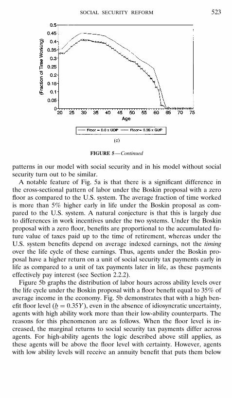
We now document how the cross-sectional profiles of consumption andlabor differ under the U.S. system and the Boskin proposal. These pro-files are graphed in in Figs. 5a–c and 6a–c for the case of no idiosyncraticuncertainty.

In Fig. 5a agents allocate on average 35–40% of their time to marketwork when young under the U.S. system. This percentage declines sharplyas agents approach age 65. The patterns we calculate for the U.S. systemare quite similar to those calculated by Rios-Rull (1996) in a related modelthat abstracted, among other things, from the structure of the U.S. socialsecurity system. Rios-Rull demonstrated that the average fraction of time


FIG. 5. (a) Average labor hours: No idiosyncratic uncertainty. U.S. system vs. Boskin pro-posal �floor = 0�. (b) Labor hours profile. No idiosyncratic uncertainty �floor = 0:35 × Y �:(c) Labor hours of low-ability agents. No idiosyncratic uncertainty (ability level 5).

allocated to market work at different stages of the life cycle in his modelroughly approximated the average labor hour pattern he calculated usingU.S. data from the Current Population Survey. He argued that the patternin his model was determined by the variation in the efficiency of labortime over the life cycle. As we follow Rios-Rull in using the efficiencyprofile calculated by Hansen (1993), previously presented in Fig. 1, and inusing similar magnitudes for the elasticity of intertemporal substitution, the


FIGURE 5—Continued

patterns in our model with social security and in his model without socialsecurity turn out to be similar.

A notable feature of Fig. 5a is that there is a significant difference inthe cross-sectional pattern of labor under the Boskin proposal with a zerofloor as compared to the U.S. system. The average fraction of time workedis more than 5% higher early in life under the Boskin proposal as com-pared to the U.S. system. A natural conjecture is that this is largely dueto differences in work incentives under the two systems. Under the Boskinproposal with a zero floor, benefits are proportional to the accumulated fu-ture value of taxes paid up to the time of retirement, whereas under theU.S. system benefits depend on average indexed earnings, not the timingover the life cycle of these earnings. Thus, agents under the Boskin pro-posal have a higher return on a unit of social security tax payments early inlife as compared to a unit of tax payments later in life, as these paymentseffectively pay interest (see Section 2.2.2).

Figure 5b graphs the distribution of labor hours across ability levels overthe life cycle under the Boskin proposal with a floor benefit equal to 35% ofaverage income in the economy. Fig. 5b demonstrates that with a high ben-efit floor level (b = 0:35Y ), even in the absence of idiosyncratic uncertainty,agents with high ability work more than their low-ability counterparts. Thereasons for this phenomenon are as follows. When the floor level is in-creased, the marginal returns to social security tax payments differ acrossagents. For high-ability agents the logic described above still applies, asthese agents will be above the floor level with certainty. However, agentswith low ability levels will receive an annuity benefit that puts them below


the floor level with certainty. Thus, they will receive a zero marginal returnon all social security tax payments. This reduces labor supply over the lifecycle for these agents, as can be seen in Fig. 5b.

The negative effects of higher floor benefit levels on labor hours suppliedby low-ability agents can be further confirmed in Fig. 5c. This figure graphs,for a relatively low ability level, the distribution of labor hours under theBoskin proposal with the lowest and the highest benefit floors (zero and35% of per capita income, respectively). We observe here that low-abilityagents reduce labor hours significantly, relative to the zero floor situation.

Figure 6a–c graphs the cross-sectional patterns of consumption. Severalfeatures are worth noting here. First, low-ability agents experience an up-ward jump in consumption at the retirement age in the cases of the U.S.system and Boskin proposal with b = 0:35Y . This is explained by the pres-ence of the borrowing constraint, which prevents these agents from borrow-ing early in life in order to smooth the quite important increase due to theold-age and health-related social security benefits (recall that benefits arenot proportional to contributions). Second, notice that the cross-sectionalpattern of consumption for low ability agents differs dramatically betweeenthe U.S. system and the Boskin scheme with a zero benefit floor, as withthe latter (i) social security transfers are proportional to taxes paid, and(ii) the common transfer is lost. These features dictate that the jump inconsumption at age 65 mentioned above is not observed in the version ofthe Boskin plan with a zero retirement floor, as Fig. 6b demonstrates. Thefall in consumption after the retirement age relative to the U.S. systemcase, in conjunction with the lower amount of leisure enjoyed by low-abilityagents under a zero floor, accounts for the quite dramatic welfare lossesfor these agents documented in Fig. 3.

5. CONCLUSION

This paper has focused on the potential distributional effects of replacingthe current U.S. social security system with a two-tier system that we referto as the Boskin proposal. This is a difficult question to answer for a num-ber of reasons, of which we will mention five. First, social security systemsaffect consumers by redistributing income, distorting the labor–leisure de-cision, and changing insurance possibilities when markets are incomplete.Thus, distributional effects are not well summarized by a calculation of thepresent value of taxes paid and benefits received. Second, a complete anal-ysis of distributional effects would focus on the agents who are alive atthe time of transition as well as those who are born after the transition isover. Third, as the current U.S. system is not in a situation in which currenttax rates and benefit formulas appear to be financially feasible over time,


FIG. 6. (a) Consumption profile (U.S. system). No idiosyncratic uncertainty. (b) Con-sumption profile (Boskin proposal). Zero floor; no idiosyncratic uncertainty. (c) Consumptionprofile (Boskin proposal). Floor = 0:35×GDP; no idiosyncratic uncertainty.

a deeper analysis requires the consideration of time-varying tax rates andbenefit formulas as well as projected changes in demographics. Fourth, ameaningful quantitative analysis of distributional effects requires a modelthat at a minimum can reproduce some of the distributional facts of theU.S. economy. Fifth, a meaningful comparison of alternative social secu-


FIGURE 6—Continued

rity systems involves modeling the precise relationship between individualearnings and tax payments and the social security benefits received.

Our strategy for analyzing distributional effects is twofold. First, we havechosen to simplify the problem by abstracting from transitional issues, timevariation in demographics, and social security tax rates and benefit for-mulas, as well as differences in survival probabilities driven by gender orincome. These abstractions allow us to extract cleanly a number of key in-sights that we conjecture would also be present, but in a more complicatedfashion without these abstractions. Second, we use a particular version ofthe life-cycle model that is calibrated to match a number of distributionaland aggregate features of the U.S. economy as our laboratory for evalu-ating distributional effects. Within this framework we are able to capturethe redistributional, distortionary, and insurance effects of social securitysystems as well as model some of the precise details of how benefits arerelated to earnings and taxes paid. We know of no other existing workthat captures these features and allows a rich analysis of intragenerationaldistributional effects.

One of the main conclusions of our analysis is that the majority of thepeople in our model economies are made worse off under any version ofthe Boskin proposal under pay-as-you-go financing we have considered.Simply put, the Boskin proposal is quite unpopular. Our analysis suggeststhat the main reason that two-tier systems are unpopular is that the cur-rent U.S. system redistributes toward median-ability agents through theconcave old-age benefit schedule and that these agents lose this redistribu-tion in two-tier systems. The floor benefit just does not redistribute enough


to median-ability agents for any level of the floor to make two-tier systemsmore popular. This is true even taking into consideration any beneficial ef-fects from reduced labor distortions under the two-tier system. Even thoughwe have not modeled either the political economy of social security reformor transitional issues, the fact that two-tier systems are quite unpopular sug-gests to us that they are unlikely to be adopted in any more complete model.

Proponents of two-tier proposals have put forth a number of argumentsfor why such systems would seem to be a good idea. Boskin et al. (p. 147,1986) states that his two-tier proposal “would be simpler, fairer, and moreefficient than the Social Security system under current law.” The argumentthat it is simpler (Boskin et al. (p. 144, 1986) is that the “two-tier approachalso offers the advantages of easy-to-comprehend annual financial reportsthat will facilitate both the administration of the program and personal fi-nancial planning.” The main arguments that it is fairer are that (i) one-and two-earner families would be treated symetrically under the two-tiersystem, since the spousal benefit to single-earner families would be elim-inated (see Boskin et al. (Chap. 7, 1986) and that (ii) floor benefits (i.e.,benefits beyond those justified by equivalent returns on social security taxpayments) to the elderly would have to be paid out of general revenuesand thus compete with all other social priorities (see Boskin et al. (p. 140,1986). The main argument that two-tier systems are more efficient (Boskinet al. (pp. 146–147, 1986) is that in “the two-tier plan I propose, incremen-tal contributions : : :would provide an actuarially identical return to eachcontributor in terms of his future benefits, as compared to the hodgepodgeof uncertain returns expected under the current system. Thus, the labormarket distortion of piling the payroll tax on top of the income tax wouldbe reduced.”

Given the arguments by Boskin that two-tier systems are simpler, fairer,and more efficient than the current U.S. system, why are all of the two-tier systems we analyze so unpopular? Our answer is that any potentialefficiency gains coming from reduced labor distortions are just swamped byredistributions away from agents with median ability who make up the bulkof the population. Thus, a system that is more efficient is not necessarilyone that is more popular. Of course, in our analysis we have abstractedfrom many things that could potentially be important. For example, in ouranalysis agents understand perfectly both the U.S. system and the Boskinproposal. Furthermore, agents have unlimited mental capacity to use tofigure out how to best make consumption, labor, and saving plans overtheir lifetimes. Thus, there can be no gain in our analysis in the simplicity ofone system relative to another. In addition, we abstract from multimemberhouseholds, so we cannot address some of the fairness issues mentioned byBoskin. We await future research to see if our main finding on the lack ofpopularity of two-tier systems applied to the U.S. economy is overturned.


We close the paper with a question: Why have two-tier social securitysystems been adopted in several countries (e.g., Chile, Colombia, Mexico,and Peru) when we find no strong reasons for adopting them for the U.S.economy? To begin to answer this question, one would need to know agreat deal more about these countries and, in particular, their previoussocial security systems than we do.

APPENDIX

Equilibria to the model of the U.S. system are computed using the fol-lowing algorithm.

1. Guess values for capital, labor, transfers, and tax rates: K, L, T ,τ, and θ.

2. Factor prices are then w = AF2�K;L� and r = AF1�K;L� − δ.3. Calculate optimal decision rules: a�x; j�, l�x; j�, and c�x; j�.4. Calculate values of K, L, T , τ; and θ that are implied by the

optimal decision rules in step 3 and the budget constraints governing socialsecurity and government consumption.

5. If the guessed values from step 1 equal the implied values in step4, then this is a steady-state equilibrium. Otherwise, update the guess instep 1 and repeat these steps.

We now describe how to carry out steps 3 and 4. In step 3 we put a gridon the state space X. We then start in the last period N of an agent’s lifeand solve for the control variables y for each grid point in the state spaceX, setting V �x;N + 1� = 0. Given the maximizing values of controls y ongridpoints, we then can determine values for the value function V �x;N� ongridpoints. We use linear interpolations to get the period N values of thevalue function and decision rules off of these gridpoints. This procedurecan then be repeated to solve for value functions and decision rules forassets and labor for all earlier periods.

We now discuss how we solve the maximization problem for each periodat each grid point. We employ the following procedure, which does notrestrict control variables to lie on a grid:

1. For each gridpoint x, we obtain the best next period asset by firstbracketing the optimum searching over asset gridpoints. Once an intervalin the asset space containing the optimum has been found, the asset deci-sion rule is computed, using a golden section search procedure. See Presset al. (Chap. 10, 1994) for a description of this search procedure and theparticular implementation used. Associated with every trial of a′, either in


the bracketing stage or in the golden section search stage, there is a cor-responding intertemporal labor decision. We use a golden section searchprocedure to maximize over the labor decision, conditional on asset choice.We search only over labor values between the level that would be maximiz-ing abstracting from marginal social security benefits from working more(i.e., the standard intratemporal labor decision), and the level (l = 1) cor-responding to working all of the time, as the maximum must lie in thisinterval.

2. We put a grid of 101, 4, and 21 points on values of �a; e; z�. Thegridpoints on e correspond to zero, the two “bend points” of the socialsecurity benefit schedule and a point consistent with the maximum socialsecurity benefits. The spacing of the shocks was discussed in Section 3.2.The spacing between points on the asset grid increases with asset levels.More specifically, asset gridpoints are placed according to a1 = 0, ak =b�k2:35�, k = 2; : : : ; 101, where b = a/�1012:35� and a is an upper boundimposed on the asset space.

To calculate values of the variables in step 4 we simulate time paths ofconsumption, asset holdings, labor, and social security transfers for a largenumber of agents. The artificial sample is constructed using the Markovprocess, followed by the idiosyncratic shocks to labor productivity, togetherwith the probability distribution that determines shocks at birth. We thenadd up asset holdings and labor in efficiency units in each age group andweigh each group by their population percentage to calculate aggregatecapital and labor inputs, and all of the relevant aggregates. In these calcu-lations we simulate 20,000 agents per cohort. In doing so, decision rules offgridpoints are obtained by interpolating decision rules on gridpoints. Sim-ulations using larger numbers of agents change neither the values of theseaggregates nor the distributional properties of the model economies thatwe have reported.

When we calculate equilibria under the Boskin proposal, we again fol-low steps 1–5. The only changes are that we iterate on �K;L; T; τ� andthe proportionality factor C (defined in Section 3.3) that determines so-cial security benefits in the Boskin proposal. The social security tax rate θand the path of government consumption are set equal to those values ob-tained under the U.S. system. To implement this procedure we put a gridof �101; 40; 21� points on �a1; a2; z�. The spacing of the gridpoints on both�a1; a2� is determined by the spacing used on a1 previously.

REFERENCES

Aaron, H. (1982). Economic Effects of Social Security, Brookings Institution, Washington, DC.Auerbach, A., and Kotlikoff, L., (1987). Dynamic Fiscal Policy, Cambridge Univ. Press.


Boskin, M. (1987). Too Many Promises: The Uncertain Future of Social Security, Dow Jones-Irwin.

Boskin, M., Kotlikoff, L., Puffert, D., and Shoven, J. (1986). “Social Security: A FinancialAppraisal across and within Generations,” NBER working paper no. 1891.

Cerda, L., and Grandolini, G. (1997). “Mexico: La Reforma al Sistema de Pensiones,” Gacetade Economia, 4, 63–105.

Council of Economic Advisers (1996). Economic Report of the President. Washington, DC.Ferrara, P. (1987). A Plan for Privatizing Social Security, Cato Institute SSP 8.Ghez, G., and Becker, G. (1975). The Allocation of Time and Goods Over the Life Cycle,

National Bureau of Economic Research, New York.Hansen, G. (1993). “The Cyclical and Secular Behavior of the Labor Input: Comparing Effi-

ciency Units and Hours Worked, Journal of Applied Econometrics 8, 71–80.Huang, H., Imrohoroglu, S., and Sargent, T. (1997). “Two Computational Experiments to

Fund Social Security,” Macroeconomic Dynamics 1, 1.Hubbard, B., and Judd, K. (1987). “Social Security and Individual Welfare: Precautionary

Saving, Liquidity Constraints and the Payroll Tax,” American Economic Review 77, 630–646.Hubbard, G., Skinner, J., and Zeldes, S. (1995). “Precautionary Savings and Social Insurance,”

Journal of Political Economy 103, 360–399.Huggett, M. (1995). “Wealth Distribution in Life-Cycle Economies,” Journal Monetary Eco-

nomics 38, 469–494.Huggett, M. and Ventura, G. (1997). Understanding why high income households save more

than low income households, mimeograph, University of Illinois.Hurd, M. and Shoven, J. (1983). The Distributional Impact of Social Security, NBER workingpaper 1155.

Hurd, H. (1989). “Mortality Risk and Bequests,” Econometrica 57, 779–813.Imrohoroglu, A., Imrohoroglu, S., and Joines, D. (1995). “A Life Cycle Analysis of Social

Security,” Economic Theory 6, 83–114.Juster, F., and Stafford, F. (1991). “The Allocation of Time: Empirical Findings, Behavioral

Models and Problems of Measurement,” Journal of Economic Literature 29, 471–522.Kotlikoff, L. (1996). “Privatization of Social Security: How It Works and Why it Matters,” Tax

Policy Economy 10, 1–32.Kotlikoff, L., Smetters, K., and Walliser, J. (1997). Opting out of social security, mimeograph.Prescott, E. (1986). “Theory Ahead of Business Cycle Measurement,” Federal Reserve Bankof Minneapolis Quarterly Review, 9–22.

Press, W., Teukolsky, S., Vetterling, W., and Flannery, B. (1994). “Numerical Recipes in For-tran: The Art of Scientific Computing,” 2nd ed., Cambridge Univ. Press.

Rios-Rull, J. V. (1996). “Life-Cycle Economies and Aggregate Fluctuations, Review of Eco-nomic Studies 63, 465–489.

Ryscavage, P. (1994). “Gender Related Shifts in the Distribution of Wages,” Monthly LaborReview, 3–16.

Ryscavage, P. (1995). “A Surge in Growing Income Inequality?” Monthly Labor Review, 51–61.Shorrocks, A. (1980). “Income Stability in the United States,” in The Statics and Dynamicsof Income, (N. Klevmarken and J. Lybeck, Eds.), Clevedon, Avon-Tieto.

Steurle, E. and Bakija, J. (1994). Retooling Social Security for the 21st Century, Washington,DC, The Urban Institute Press.

Stokey, N. and Rebelo, S. (1995). “Growth effects of flat-rate taxes,” Journal of Political Econ-omy 103, 519–550.


Thompson, L. (1983). “The Social Security Reform Debate,” Journal of Economic Literature21, 1425–1467.

U.S. Department of Commerce (1996). “Survey of Current Business” 96, Washington, DC.U.S. Social Security Administration (1985). “Social Security Bulletin” 48, Washington, DC.U.S. Social Security Administration (1993). “Social Security Bullentin” 56, Washington, DC.U.S. Social Security Administration (1993). “Social Security Bullentin” 57, Washington, DC.U.S. Social Security Administration (1996). Statistical Supplement to the Social Security Bulletin.

Washington, DC.U.S. Social Security Administration (1985). Social Security Handbook. Washington, DC.World Bank (1994). “Averting the Old Age Crisis: Policies to Protect the Old and Promote

Growth,” Oxford Univ. Press, London.

On the Distributional Effects of Social Security Reform

Documents

Transcript of On the Distributional Effects of Social Security Reform