3.4 Distributional Patterns: Resources, Communities, and Polities

3.4 Distributional Patterns:Resources, Communities, and Polities

Robert D. Drennan, Dale W. Quattrin, and Christian E. Peterson

The distribution of prehispanic archeological remains in thewestern survey zone of the Valle de la Plata has two char-

acteristics that stand out strongly in comparative con-text—characteristics we really did not expect when we beganto survey. First, evidence of prehispanic occupation is ex-tremely broadly scattered across the landscape, and, second,although prehispanic remains occur over very large areas, theirdensities are generally low within the locations where they oc-cur. These are both indications of a settlement pattern that re-sembles the modern one: a pattern of scattered residence inwhich many individual households live directly on the plots ofland that they cultivate (see the first and second sections of thischapter). Such a scattered settlement pattern is not necessarilyevenly distributed across the region. Today, in parts of thewestern survey zone where the plots of land owned and farmedby individual households are large, most houses are some dis-tance from their nearest neighbors, and occupational density ata regional scale can be said to be low (Figure 3.38). In otherparts of the western survey zone where plots of land aresmaller, regional-scale density is high (Figure 3.39). Espe-cially where density is high, clusters of two or three or fourhouses within a few hundred meters of each other sometimesform where households have chosen to put their houses on ad-jacent corners of their properties. This is the form of the mod-ern “rural” occupation of the western survey zone that wasincorporated into the analysis in the second section of thischapter.

In addition to this dispersed rural settlement of variabledensity, there are today several nucleated communities. Thelargest of these, La Argentina, is the administrative and com-mercial center for the municipality that covers much of thewestern survey zone. Houses in the center of the nucleatedcommunity are immediately adjacent to each other (Figure3.40), and in 1985 it had a population of 1468 (DepartamentoAdministrativo Nacional de Estadística 1986:56, 347) in anarea no more than 20 ha including the artifact scatters pro-duced by trash discarded in the outskirts. These 1468 inhabit-ants comprised 311 households, for an average of 4.72 personsper household—like the modern rural population, not so verydifferent from the rough figure of 5 persons per household weadopted in the second section of this chapter. The modern nu-cleated community has a residential density of some 75 inhab-itants per occupied hectare, in contrast to the 5–10 persons peroccupied hectare that we projected above for the rural popula-

tion and used in making prehispanic population estimates.The nucleated community of La Argentina is a clearly dif-

ferent phenomenon on the modern landscape from the ruraloccupation in the extensive municipal administrative territorythat we have discussed up to now (Figure 3.41). Much of thediscussion above takes the distribution of prehispanic occupa-tion in the western survey zone as broadly analogous to thedistribution of modern rural occupation, omitting the nucle-ated community of La Argentina. As we turn to a consider-ation of prehispanic population distribution and especially ofcentralizing tendencies, we will explore this aspect of our rea-soning with special care.

As discussed in the second section of this chapter, each ru-ral house is surrounded by a garbage scatter of relatively lowdensity (speaking now at the small scale of artifact distribu-tions across tens of meters rather than of house distributionsacross hundreds or thousands of meters). It is the more pre-servable elements of such garbage scatters that provide thearcheologically observable evidence on the landscape of an-cient occupations like this. The eventual archeological mani-festation of such garbage scatters will be denser on average inareas where the garbage scatters from two or more householdsoverlap. When a dozen or more houses are clustered within100–150 m, forming a small village or hamlet, the densitiesare considerably higher, and the archeological remains of sucha small village or hamlet are recognizably different from thoseof more scattered occupation. A nucleated settlement compa-rable in size and density to La Argentina in 1985 would pro-duce even denser archeological remains across an area ofsome 20 ha. If such a settlement were present in prehispanictimes, it would have a major impact on conclusions about re-gional forces of social, cultural, political, or economic central-ization, and would force a reevaluation of the basis for demo-graphic approximations established in the second section ofthis chapter.

The distribution of prehispanic remains did produce size-able areas of continuous distribution within which the mostnotable evidence of a nucleated community would be archeo-logical remains of considerably higher density. We earlier dis-missed the possibility of incorporating systematic assessmentof artifact densities into demographic analysis because vege-tation cover made it impossible to regularly measure artifactdensities in surface collections, and the majority of the settle-ment data comes from surface collection. We can, however,

99

drennan

Typewritten Text

drennan

Typewritten Text

Prehispanic Chiefdoms in the Valle de la Plata, Volume 5: Regional Settlement Patterns / Cacicazgos Prehispánicos del Valle de la Plata, Tomo 5: Patrones de Asentamiento Regionales, Robert D. Drennan, ed., pp. 99–154. University of Pittsburgh Memoirs in Latin American Archaeology, No. 16. 2006.

drennan

Typewritten Text

drennan

Typewritten Text

drennan

Typewritten Text

drennan

Typewritten Text

drennan

Typewritten Text

drennan

Typewritten Text

3.4 Patrones de Distribución: Recursos, Comunidades,y Unidades Políticas

Robert D. Drennan, Dale Quattrin, y Christian Peterson

La distribución de restos arqueológicos prehispánicos en lazona occidental del reconocimiento del Valle de la Plata

tiene dos características que sobresalen de manera importanteen un contexto comparativo—características que realmente noesperábamos cuando comenzamos el reconocimiento. Prime-ro, la evidencia de la ocupación prehispánica es extremada yextensamente dispersa a través del paisaje y, segundo, aunquelos restos prehispánicos ocurren sobre áreas muy grandes, susdensidades generalmente son bajas dentro de los lugares endonde ellos aparecen. Ambos son indicadores de un patrón deasentamiento que se parece al moderno: un patrón de residen-cia dispersa en el que muchas unidades domésticas individua-les viven directamente en las parcelas de tierra que ellascultivan (ver la primera y segunda sección de este capítulo).Tal patrón de asentamiento disperso no necesariamente estádistribuido de forma regular sobre toda la región. Hoy en día,en las partes de la zona occidental de reconocimiento en dondelas parcelas de tierra pertenecientes a unidades domésticas in-dividuales, y en su mayoría cultivadas por ellas mismas, songrandes, la mayoría de las casas se encuentran a alguna distan-cia de sus vecinos más cercanos y la densidad ocupacional aescala regional puede calificarse como baja (Figura 3.38). Enotras partes de la zona occidental de la zona de reconocimien-to, en donde las parcelas de tierra son más pequeñas, la densi-dad a escala regional es alta (Figura 3.39). Especialmente endonde la densidad es alta, los agrupamientos de dos, tres o cua-tro casas dentro de unos pocos cientos de metros de distanciaunas de otras se forman algunas veces en donde las unidadesdomésticas han escogido ubicar sus casas en las esquinas ad-yacentes de sus propiedades. Esta es la forma de la ocupación“rural” moderna de la zona occidental del reconocimiento quefue incorporada en el análisis en la segunda sección de este ca-pítulo.

Sumándose a este asentamiento rural disperso de densidadvariable, hoy en día hay varias comunidades nucleadas. Lamás grande de ellas, La Argentina, es el centro administrativoy comercial del municipio que cubre la mayoría de la zona oc-cidental de reconocimiento. Las casas en el centro de la comu-nidad nucleada están ubicadas inmediatamente adyacentesuna de otra (Figura 3.40), y en 1985 ella tenía una población de1468 personas (Departamento Administrativo Nacional deEstadística 1986:56, 347) en un área no mayor de 20 ha, inclu-yendo las dispersiones de artefactos producidas por la basuradescartada en las afueras. Estos 1468 habitantes comprendían

311 unidades domésticas para un promedio de 4.72 personaspor unidad doméstica—como la población rural moderna, yno muy diferente de la figura de 5 personas por unidad domés-tica adoptada en la segunda sección de este capítulo. La comu-nidad nucleada moderna tiene una densidad residencial deunos 75 habitantes por hectárea ocupada, en contraste con las5–10 personas por hectárea ocupada que proyectamos ante-riormente para la población rural y que hemos usado para ha-cer cálculos sobre la población prehispánica.

La comunidad nucleada de La Argentina es claramente unfenómeno diferente en el paisaje moderno de la ocupación ru-ral en el extenso territorio administrativo del municipio quehemos discutido hasta ahora (Figura 3.41). Mucha de la discu-sión anterior toma a la distribución de la ocupación prehispá-nica en la zona occidental de reconocimiento como bastanteanáloga a la distribución de la ocupación rural moderna, omi-tiendo a la comunidad nucleada de La Argentina. En la medidaen que tornemos a la consideración de la distribución de la po-blación prehispánica y especialmente a las tendencias centra-les, exploraremos este aspecto de nuestro razonamiento conespecial cuidado.

Como se discutió en la segunda sección de este capítulo,cada casa rural está rodeada por una dispersión de basura dedensidad relativamente baja (hablando ahora de la distribu-ción de artefactos a pequeña escala a través de decenas de me-tros más que de distribuciones de casas a través de cientos omiles de metros). Son los elementos más conservables de talesdispersiones de basura los que proveen la evidencia arqueoló-gicamente observable en el paisaje de ocupaciones antiguascomo ésta. La eventual manifestación arqueológica de talesdispersiones de basura será más densa en promedio en áreas endonde se superponen las dispersiones de basura de dos o másunidades domésticas. Cuando una docena o más de casas estánagrupadas dentro de 100–150 m formando una pequeña aldeao caserío, las densidades son considerablemente más altas ylos restos arqueológicos de tal pequeña aldea o caserío son re-conociblemente diferentes de aquellos correspondientes a unaocupación más dispersa. Un asentamiento nucleado compara-ble al tamaño y la densidad del pueblo de La Argentina en1985 produciría restos arqueológicos todavía más densos através de un área de unas 20 ha. Si tal asentamiento hubiera es-tado presente en tiempos prehispánicos, habría tenido un granimpacto en las conclusiones acerca de las fuerzas regionalesde centralización de carácter social, cultural, político, o econó-

100

SETTLEMENT PATTERNS IN THE WESTERN SURVEY ZONE 101

look at the issue of densities via the shovel probes that werepart of the survey methodology. The focus here will be on theRegional Classic and the 928 shovel probes in the western sur-vey zone that produced the Guacas Reddish Brown ceramicsindicative of this period. These probes produced an average of169 sherds of all periods per m3, of which an average of 101sherds per m3 were Guacas Reddish Brown. This, then, is theaverage sherd density we have taken to represent an occupa-tion of 5–10 persons per hectare in scattered rural occupation.The modern nucleated community of La Argentina has, ac-cording to census figures, an occupational density some 10times greater (see above). We might thus expect such a settle-ment to produce archeological density values some 10 timesgreater than those of scattered rural occupation—on the orderof 1000 sherds per m3. The frequency distribution of sherddensities in shovel probes that produced Guacas ReddishBrown (Figure 3.42) shows the expected pattern of manyprobes with low densities, but some are substantially higher.There is a faint hint of multimodality at a density of 500 per m3,so we could adopt this instead of 1000 per m3, as a more con-servative cutoff point for identifying shovel probes worth ex-amining carefully to see if they suggest the presence of largernucleated communities during the Regional Classic.

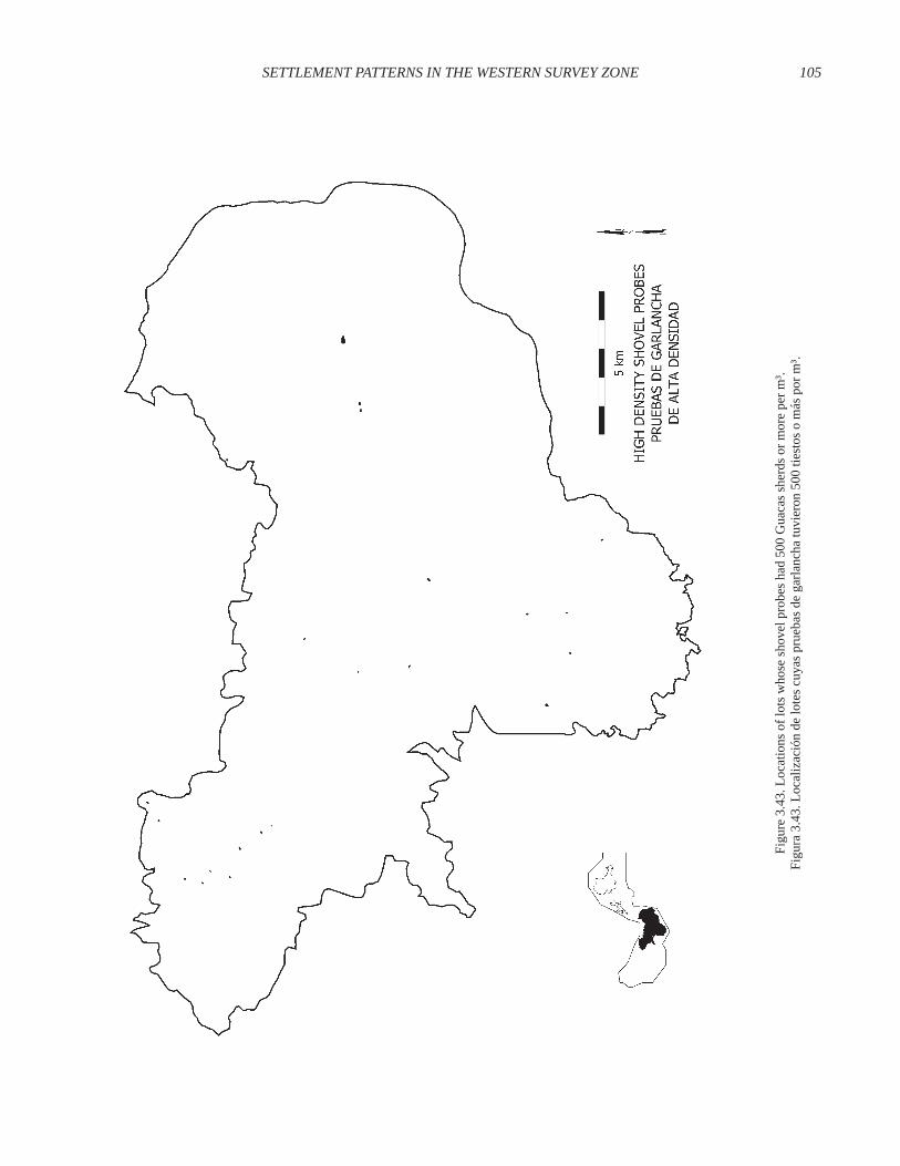
The locations of the 22 lots whose shovel probes had densi-ties of 500 Regional Classic sherds per m3 or more are widelyscattered across the western survey zone (Figure 3.43). No twoare contiguous, and no more than three ever occur within aspace as small as 1 km2. Even when we allow for the fact thatshovel probes represent fewer than one-third of the RegionalClassic period lots (the others are surface collections), this dis-tribution does not suggest that any area of high artifact densityeven approaching the size of the nucleated community of LaArgentina has escaped notice in the survey results. Some of theshovel probes with high artifact densities undoubtedly repre-sent artifact concentrations of very small size (on the order of afew square meters), a phenomenon that has been observed instratigraphic excavations. Some may possibly represent con-centrations of enough households to be identified as smallhamlets, but their areas (and consequently the number ofhouseholds involved) do not seem to be very large, and it doesnot seem possible that there could be very many of them in thewestern survey zone. If such communities existed in the Re-gional Classic, they might be on the order of the modern nucle-ated community of El Pensil (Figure 3.44), some 25 house-holds in an area of about 3 ha.

The presence of a few such groupings would not materiallyalter the demographic estimates arrived at in the second sec-tion of this chapter. Indeed, they are incorporated into those es-timates since only the nucleated community of La Argentinawas excluded from the modern occupation that formed the ba-sis of the analysis. Of more relevance here, the presence of afew small residential groupings of this sort would have verylittle impact on the analyses presented in this section. The bulk

of the prehispanic occupation seems widely scattered, withvery little in the way of nucleated communities. We will returnto the notion of communities, nucleated or otherwise, below,following consideration of the relationship between resourcedistribution and distribution of occupation.

Occupation and Agricultural ResourcesWhen occupation is as dispersed, or scattered, as most

prehispanic occupation in the western survey zone of the Vallede la Plata appears to be, it is very likely that households havechosen to locate their residences very near or directly on theland that they farm. This is largely the case in the region today.Such a close spatial association between residence patternsand farming patterns makes the distribution of occupation avery sensitive indicator of the patterns of exploitation of agri-cultural resources. Sheer economic rationality, in this context,would work toward heavier exploitation of the zones with thehighest agricultural productivity, and progressively lighter ex-ploitation of zones with progressively lower agricultural pro-ductivity. If households located their residences on or verynear the land that they cultivated, then denser occupationshould reflect more intensive agricultural exploitation. If theforces of this aspect of economic rationality were strong in theprehispanic past of the western survey zone, then the densestoccupation should occur in the most productive zones, and thisexpectation provides an approach to assessing the strength ofthose forces.

SoilscapesDensity of occupation in a soilscape is easily calculated as

the percentage of the territory in that soilscape covered by oc-cupation in a particular period. The tabulated areas of occupa-tion for each period in each soilscape are presented in Table3.6, along with their conversion into percentages of total sur-veyed area occupied for each soilscape. These occupationaldensities, expressed as percentages, do not depend on the ab-solute population estimates made in the second section of thischapter. They are simply expressions of the relative intensityof occupation in different soilscapes. As such, they are reason-able measures of varying degrees of density of occupation.That is, it is reasonable to take a soilscape with 3.0% of its areashowing evidence of occupation as roughly twice as denselyoccupied as a soilscape with 1.5% of its area occupied. The ag-ricultural productivity rankings, however, are just that: ranks.Assigning a productivity score of 2 to a soilscape cannot reli-ably be interpreted as meaning that that soilscape is twice asproductive as one to which a score of 1 has been assigned. Asoilscape with a score of 2 has simply been judged more pro-ductive than one assigned a score of 1; we cannot judge howmuch more productive. Given this characteristic of the pro-ductivity rankings, we have measured the correspondence be-tween density of occupation and the productivity of soilscapes

mico, y habría forzado a una reevaluación de las bases para lasaproximaciones demográficas establecidas en la segunda sec-ción de este capítulo.

La distribución de los restos prehispánicos observados en elreconocimiento produjo áreas considerables de distribucióncontinua dentro de las cuales las evidencias más notables deuna comunidad nucleada consistirían en la existencia de zonascon una densidad considerablemente mayor de restos arqueo-lógicos. Anteriormente descartamos la posibilidad de incor-porar la evaluación sistemática de las densidades de artefactosen los análisis demográficos porque la cobertura vegetal hizoimposible medir regularmente la densidad de artefactos en lasrecolecciones superficiales y la mayoría de los datos de asen-tamientos proviene de recolecciones superficiales. Sin embar-go, podemos mirar el aspecto de las densidades a través de laspruebas de garlancha que fueron parte de la metodología delreconocimiento. Se dará atención aquí al Clásico Regional y alas 928 pruebas de garlancha de la zona occidental de recono-cimiento que produjeron la cerámica Guacas Café Rojizo indi-cativa de este período. Estas pruebas produjeron un promediode 169 fragmentos de todos los períodos por m³, de los cualesun promedio de 101 fragmentos por m³ fue del tipo GuacasCafé Rojizo. Este es, entonces, el promedio de densidad de

tiestos que hemos tomado para representar una ocupación de5–10 personas por hectárea de la ocupación rural dispersa. Lacomunidad nucleada moderna de La Argentina tiene, segúnlas figuras del censo, una densidad de ocupación de unas 10veces más (ver arriba). Por lo tanto, podríamos esperar que talasentamiento produjera valores de densidad arqueológica al-rededor de 10 veces mayores que aquellas de la ocupación ru-ral dispersa—del orden de los 1000 tiestos por m³. La distribu-ción de frecuencias de las densidades de tiestos en las pruebasde garlancha que produjeron tiestos Guacas Café Rojizo (Fi-gura 3.42) muestra el patrón esperado de muchas pruebas conbajas densidades, pero algunas son sustancialmente más altas.Hay una ligera impresión de multi-modalidad en la densidadde 500 por m³, así que podríamos adoptar ésta en vez de 1000por m³, como un punto de corte más conservador para identifi-car pruebas de garlancha que valga la pena examinar cuidado-samente para ver si ellas sugieren la presencia de comunidadesnucleadas más grandes durante el Clásico Regional.

La localización de los 22 lotes cuyas pruebas de garlanchatenían densidades de 500 tiestos por m³ del Clásico Regional omás es ampliamente dispersa a través de la zona occidental dereconocimiento (Figura 3.43). No hay dos contiguas y no másde tres ocurren dentro de un espacio del tamaño de 1 km². Aun

102 PATRONES DE ASENTAMIENTO EN LA ZONA OCCIDENTAL DE RECONOCIMIENTO

Figure 3.38. Extremely sparse modern rural settlement in the western survey zone.Figura 3.38. Asentamiento rural moderno extremadamente disperso en la zona occidental de reconocimiento.


Figure 3.40. Nucleated settlement within the modern town of La Argentina.Figura 3.40. Asentamiento moderno nucleado de La Argentina.

Figure 3.39. Denser but still dispersed modern rural settlement in the western survey zone.Figura 3.39. Asentamiento rural moderno más denso pero todavía disperso en la zona occidental de reconocimiento.

cuando tomamos en cuenta el hecho de que las pruebas de gar-lancha representan un poco menos de un tercio de los lotes delperíodo Clásico Regional (los otros son recolecciones superfi-ciales), esta distribución no sugiere que cualquier área con altadensidad de artefactos que se acerque al tamaño de la comuni-dad nucleada de La Argentina haya escapado de ser detectadaen los resultados del reconocimiento. Algunas de las pruebasde garlancha con altas densidades de artefactos indudable-mente representan concentraciones de artefactos de tamañomuy pequeño (del orden de unos pocos metros cuadrados), unfenómeno que ha sido observado en excavaciones estratigráfi-cas. Algunas posiblemente representan concentraciones desuficientes unidades domésticas como para ser identificadascomo pequeños caseríos, pero sus áreas (y consecuentementeel número de casas involucradas) no parecen ser muy grandes,y no parece posible que hubiera muchas de ellas en la zona oc-cidental de reconocimiento. Si tales comunidades existieronen el Clásico Regional ellas pudieron ser del orden de la comu-nidad nucleada moderna de El Pensil (Figura 3.44), unas 25unidades domésticas en un área de cerca de 3 ha.


Figure 3.41.View of the modernnucleated town ofLa Argentina.Figura 3.41.Vista del pobladomoderno nucleadode La Argentina.

Figure 3.42. Histogram of Guacas sherd densities in shovel probesthat yielded Guacas sherds in the western survey zone.

Figura 3.42. Histograma de las densidades de tiestos Guacasen pruebas de garlancha que produjeron cerámica Guacas

en la zona occidental de reconocimiento.


Figu

re3.

43.L

ocat

ions

oflo

tsw

hose

shov

elpr

obes

had

500

Gua

cass

herd

sorm

ore

perm

³.Fi

gura

3.43

.Loc

aliz

ació

nde

lote

scuy

aspr

ueba

sde

garla

ncha

tuvi

eron

500

tiest

oso

más

porm

³.


12

3

12

3B1

4(O

rthen

ts)37

.00.

037

.00.

00.

00.

00.

60.

60.

0%0.

0%0.

0%1.

6%1.

7%2.

0B1

4(H

aplu

dalfs

)21

2.9

0.0

212.

90.

30.

60.

012

.28.

50.

1%0.

3%0.

0%5.

7%4.

0%2.

0B2

185

1.9

0.0

851.

90.

00.

50.

06.

45.

00.

0%0.

1%0.

0%0.

8%0.

6%1.

0B2

281

7.1

0.0

817.

116

.629

.224

.611

3.7

74.6

2.0%

3.6%

3.0%

13.9

%9.

1%1.

0C1

5461

.729

.954

31.8

65.5

149.

010

7.9

557.

252

5.0

1.2%

2.7%

2.0%

10.3

%9.

7%1.

0C2

2(T

ropu

dults

)87

3.2

0.0

873.

28.

852

.175

.328

8.7

214.

41.

0%6.

0%8.

6%33

.1%

24.6

%1.

5C2

2(D

ystro

pept

s)44

0.1

0.0

440.

11.

78.

39.

741

.934

.40.

4%1.

9%2.

2%9.

5%7.

8%1.

5C2

3(T

ropu

dults

)12

18.3

19.2

1199

.15.

513

.322

.486

.989

.60.

5%1.

1%1.

9%7.

2%7.

5%1.

5C2

3(D

ystro

pept

s)15

89.1

81.4

1507

.77.

323

.919

.884

.810

7.5

0.5%

1.6%

1.3%

5.6%

7.1%

1.5

C25

4451

.27.

444

43.8

18.6

62.1

77.1

301.

928

9.5

0.4%

1.4%

1.7%

6.8%

6.5%

3.0

C26

792.

30.

079

2.3

6.2

13.3

23.7

186.

916

6.3

0.8%

1.7%

3.0%

23.6

%21

.0%

2.0

D1

(Dur

usta

lfs)

2462

.329

0.6

2171

.773

.010

3.4

83.9

219.

732

9.9

3.4%

4.8%

3.9%

10.1

%15

.2%

0.0

D1

(Tro

pudu

lts)

1630

.588

.315

42.2

29.9

61.4

36.8

122.

716

8.4

1.9%

4.0%

2.4%

8.0%

10.9

%0.

0D

2(D

ystra

ndep

ts)27

19.9

648.

620

71.3

28.1

62.8

35.7

57.0

141.

71.

4%3.

0%1.

7%2.

7%6.

8%1.

0D

2(O

rthen

ts)13

97.7

375.

610

22.1

0.4

9.2

6.6

18.5

32.0

0.0%

0.9%

0.6%

1.8%

3.1%

1.0

D31

(Hap

ludu

lts)

1056

.245

9.1

597.

111

.38.

910

.421

.733

.71.

9%1.

5%1.

7%3.

6%5.

6%1.

0D

31(I

ncep

tisol

s)21

67.4

572.

915

94.4

23.4

26.4

24.1

44.4

73.3

1.5%

1.7%

1.5%

2.8%

4.6%

1.0

D31

(Tro

porte

nts)

274.

557

.021

7.4

3.7

4.0

6.1

3.4

8.5

1.7%

1.8%

2.8%

1.5%

3.9%

1.0

D32

355.

712

4.8

230.

95.

013

.75.

517

.021

.32.

2%5.

9%2.

4%7.

3%9.

2%0.

0D

3324

48.0

100.

623

47.4

20.1

44.9

37.6

125.

114

7.5

0.9%

1.9%

1.6%

5.3%

6.3%

1.0

Swam

p/Pa

ntan

o46

6.8

466.

80.

0--

----

----

----

----

----

Prod

uc-

tivid

ad

Prod

uc-

tivity

Soils

cape

Are

aO

cupa

da(%

)

Occ

upie

dA

rea

(%)

Form

ativ

e

Form

ativ

oPa

isaje

-Sue

loCl

ásic

oRe

gion

al

Regi

onal

Clas

sic

Reci

ente

Rece

nt

Are

a(h

a)1

2Cl

ásic

oRe

gion

al

Regi

onal

Clas

sic

Reci

ente

Rece

nt

Occ

upie

dA

rea

(ha)

TABL

E3.

6.O

CCU

PIED

ARE

AS

BYPE

RIO

DIN

EACH

SOIL

SCA

PETA

BLA

3.6

ARE

AS

OCU

PAD

AS

ENCA

DA

PAIS

AJE

-SU

ELO

Tota

l

Tota

l

No

Re-

cono

cida

Not

Surv

eyed

Reco

-no

cida

Surv

eyed

Are

a(h

a)Fo

rmat

ivoAre

aO

cupa

da(h

a)

3

12

3

Form

ativ

e

with a rank-order correlation coefficient (Spearman’s). Theoccupation densities and the agricultural productivity scores,converted to rank-orders for the 20 soilscapes (omitting theunproductive swamp), are given in Table 3.7, along with therank-order correlation (rs) for each period and its significancevalue (p). It should be noted, that the actual values of these cor-relations differ somewhat from those presented earlier(Drennan and Quattrin 1995a, 1995b; Drennan 2000) becausethey are based on final corrected settlement data and on a finalrevision of agricultural productivity scores, in an effort to pro-vide the most accurate assessments possible. The conclusionsto be drawn from the correlations have not changed at all fromthe more preliminary versions previously presented.

The pattern shown runs very much counter to the economi-cally rational expectation of high occupation densities inhighly productive soilscapes. In no period does the evidencesupport the notion that people distributed themselves acrossthe landscape, even roughly according to its agricultural pro-ductivity. The sequence begins with a highly significant, butstrongly negative, correlation in Formative 1, indicating highoccupational densities in the less productive soilscapes. Thenegative correlation weakens, but continues, into Formative 2,still with high significance. By Formative 3 the negative corre-lation has weakened substantially, and its significance is verymarginal. The correlation near 0 (with negligible significance)for Regional Classic suggests very little relationship betweenoccupational density and soilscape productivity. Finally, in theRecent period, the correlation turns weakly negative again,with negligible statistical significance.

The negative correlation for Formative 1 owes much of itsstrength to the fact that, of the four soilscapes ranked most

highly for occupational densities (D1 [both soils], D32, andB22), three (D1 [both soils] and D32) are tied for lowest agri-cultural productivity. The next five ranks for high occupa-tional density (D31 [all three soils], D2 [Dystrandepts], andC1) are involved in a tie for the next lowest rung on the agri-cultural productivity ladder. In terms of the maps in Figures3.11 and 3.33, it is clear that Formative 1 settlement is surpris-ingly heavy along the summit of the Serranía de las Minasacross the survey zone’s southern fringes, and farther north onthe ignimbrite high plain. While settlement is not entirely ab-sent from other zones, the balance of the Formative 1 distribu-tion is tipped more toward these high elevations so unfavor-able for agriculture than it is in any subsequent period. Thehighly productive lower elevation C25, C26, and B14 rankvery low for Formative 1 occupational density. It would makethis distribution easier to understand in economic terms if cli-mate were warmer and drier in the Formative, but precisely thereverse is the case (Drennan, Herrera, and Piñeros 1989). It iseven more difficult to understand the attraction of these cold,wet soilscapes under the even colder and wetter conditionsthat prevailed in the Formative.

Occupation seems more abundant in practically all parts ofthe western survey zone in Formative 2 (Figure 3.12), but itgrows especially in the formation of a cluster of settlement inthe east central sector. Much of this cluster falls in the morehighly productive C22; its Tropudults have now become themost densely occupied soilscape, and its Dystropepts haverisen dramatically in the occupational density rankings. Thistrend continues into Formative 3 (Figure 3.13). The apparentthinning of occupation in Formative 3 is at least partly illusory,as discussed in the second section of this chapter, but the con-


Figure 3.44. Modern nucleated small community of El Pensil.Figure 3.44. La pequeña comunidad moderna nucleada de El Pensil.

La presencia de unos pocos de estos grupos no alteraría ma-terialmente los estimativos demográficos a los que hemos lle-gado en la segunda sección de este capítulo. Es más, ellos hansido incorporados a aquellos cálculos ya que únicamente la co-munidad nucleada de La Argentina fue excluida de la ocupa-ción moderna que formó la base del análisis. Lo que es de ma-yor relevancia aquí, la presencia de unos pocos gruposresidenciales de este tipo tendría muy poco impacto en los aná-lisis presentados en esta sección. La mayoría de la ocupaciónprehispánica parece ampliamente dispersa, con muy poca in-dicación de comunidades nucleadas. Retornaremos más ade-lante a la noción de comunidades, nucleadas o de otra forma,después de considerar la relación entre distribución de recur-sos y distribución de la ocupación.

Ocupación y Recursos AgrícolasCuando la ocupación es tan dispersa como la mayoría de la

ocupación prehispánica parece haber sido en la zona occiden-tal de reconocimiento, es muy probable que las unidades do-mésticas hayan escogido localizar sus residencias muy cercade o directamente sobre la tierra que ellos cultivaban. En sumayoría, hoy en día este es el caso en la región. Tal asociaciónespacial tan cercana entre los patrones de residencia y los pa-trones de cultivo hace que la distribución de la ocupación seaun indicador muy sensible de los patrones de explotación delos recursos agrícolas. Una racionalidad económica pura, eneste contexto, produciría una mayor explotación de las zonascon la productividad agrícola más alta y una explotación pro-gresivamente más leve de las zonas con una productividadagrícola progresivamente más baja. Si las unidades domésti-cas localizaron sus residencias sobre o muy cerca de la tierraque ellas cultivaron, entonces las ocupaciones más densas de-berían reflejar una explotación agrícola más intensiva. Si lasfuerzas de este aspecto de la racionalidad económica fueronpoderosas en el pasado prehispánico de la zona occidental dereconocimiento, entonces la ocupación más densa deberíaocurrir en las zonas más productivas y esta expectativa proveeuna forma de evaluar la robustez de esas fuerzas.

Paisajes-SuelosLa densidad de ocupación en un suelo es fácilmente calcu-

lable como el porcentaje de territorio en ese suelo cubierto porla ocupación en un período particular. Las áreas de ocupacióntabuladas para cada período en cada suelo se presentan en laTabla 3.6, junto con su conversión en porcentajes del total delárea reconocida ocupada para cada suelo. Estas densidadesocupacionales, expresadas como porcentajes, no dependen delos cálculos absolutos de población hechos en la segunda sec-ción de este capítulo. Ellas simplemente expresan la intensi-dad relativa de la ocupación en diferentes suelos. Como tales,ellas son medidas razonables de varios grados de densidad dela ocupación. Es decir, es razonable tomar un suelo con el 3%

de su área mostrando evidencia de ocupación como si tuvierael doble de la densidad de ocupación de un suelo con el 1.5%de su área ocupada. Sin embargo, los rangos de productividadagrícola son precisamente eso: rangos. La asignación de unvalor de productividad de 2 a un suelo no puede ser interpreta-da confiablemente como si significara que ese suelo es dos ve-ces más productivo que uno al cual se le ha asignado un valorde 1. Un suelo con valor de 2 simplemente ha sido juzgado másproductivo que uno al cual se le ha asignado un valor de 1; nopodemos juzgar qué tanto más productivo. Dada esta caracte-rística de los rangos de productividad, hemos medido la co-rrespondencia entre la densidad de la ocupación y la producti-vidad de los suelos con un coeficiente de correlación de rangode Spearman. Las densidades de ocupación y los rangos deproductividad agrícola convertidos en un orden de rango paralos 20 suelos (omitiendo el pantano improductivo) se presen-tan en la Tabla 3.7, junto con la correlación de orden de rango(rs) para cada período y su valor de significancia (p). Deberíaser apuntado que los valores de estas correlaciones difieren unpoco de aquellos presentados antes (Drennan y Quattrin1995a, 1995b; Drennan 2000), porque los presentados aquí sebasan en datos de asentamiento finales y corregidos, y en unarevisión definitiva de los valores de productividad agrícola, enun esfuerzo por proveer la evaluación más precisa posible. Lasconclusiones derivadas de las correlaciones no han cambiadode aquellas de las versiones preliminares presentadas previa-mente.

El patrón mostrado va muy en contra de la expectativa ra-cional económica de altas densidades de ocupación en suelosaltamente productivos. En ningún período la evidencia apoyala idea de que la gente se distribuyó a través del paisaje, aun va-gamente, de acuerdo a su productividad agrícola. La secuenciacomienza con una correlación altamente significativa, perofuertemente negativa, en el Formativo 1, para el cual se indicandensidades ocupacionales altas en los suelos menos producti-vos. La correlación negativa, todavía con alta significancia, sedebilita pero continúa en el Formativo 2. Para el Formativo 3 lacorrelación negativa se debilita sustancialmente y su signifi-cancia es muy marginal. La correlación cercana a 0 (con unasignificancia casi nula) para el Clásico Regional sugiere unarelación muy débil entre la densidad de ocupación y la produc-tividad de los suelos. Finalmente, en el período Reciente, lacorrelación se torna débilmente negativa otra vez, con una sig-nificancia estadística casi nula.

La correlación negativa para el Formativo 1 debe mucho desu robustez al hecho de que, de los cuatro suelos con valoresmás altos para las densidades ocupacionales (D1 [ambos sue-los], D32, y B22), tres (D1 [ambos suelos] y D32) están empa-tados por la más baja productividad agrícola. Los siguientescinco rangos en cuanto a densidad ocupacional (D31 [los tressuelos], D2 [Dystrandepts] y C1) están en el siguiente peldañomás bajo en la escala de la productividad agrícola. En términosde los mapas en las Figuras 3.11 y 3.33, resulta claro que el


tinued shift toward lower elevations and higher productivity isevident in the marked reduction in the settlement cluster in C1in the north central sector and in the buildup of occupation inone part of C25, the most productive soilscape, where a settle-ment cluster is now evident in the southwestward protrusion ofthe survey zone boundaries. In sum, then, sedentary occupa-tion begins in Formative 1 with a marked predilection for someof the least productive soilscapes. It is tempting to say that astime goes on the occupational distribution conforms increas-ingly well to the distribution of agricultural productivity, al-though it is more accurate to say the correspondence is de-creasingly poor, because even by Formative 3 the correlationis still negative and with at least a hint of significance.

The lessening of the poor fit between occupational distribu-tion and soilscape productivity continues in the Regional Clas-sic, as all four of the most pro-ductive soilscapes registerincremental increases in theiroccupational density rankings.Much of this is attributable to thegrowth of the two can-yon-bottom settlement clustersin the western sector of the sur-vey zone (Figure 3.14), whichboth involve the highly produc-tive C25. The central cluster alsoexpands more fully southwardinto C26, and occupation is upmarkedly in the small area ofB14 in the northeastern corner ofthe survey zone. Precisely thesetrends reverse themselves some-what in the Recent period, andthe correlation between occupa-tional density and soilscape pro-ductivity returns to negative ter-ritory (although with negligiblesignificance). The distribution ofagricultural resources then, atleast as measured by thesoilscape productivity scores,offers us very little understand-ing of the patterns of distributionof prehispanic occupation in thewestern survey zone. This is aninteresting finding, since itmeans that whatever reasonsthere are behind the distributionof occupation, they remain to besought in other arenas of humanactivity. This result, however, isbased on a failure to find the tidypattern of correlation expected if

occupational distribution depended largely on agriculturalproductivity. One possible reason for such a failure could bethat the soilscape productivity scores do not provide a mean-ingful assessment of agricultural productivity across the sur-vey zone. The availability of a different approach to the char-acterization of agricultural productivity, as discussed in thethird section of this chapter, is thus particularly welcome.

Modern Land UseAt first glance the correspondence between the three cate-

gories of modern land use introduced in the third section ofthis chapter and occupational distribution seems considerablybetter (Table 3.8). Forest seems the least productive of thethree categories, and it has the lowest occupied area percent-age for all periods. Land in grass for cattle pasture seems the


B14 (Orthents) 1.5 1.0 1.5 3.0 2.0 18.0B14 (Hapludalfs) 4.0 3.0 1.5 10.0 5.0 18.0B21 1.5 2.0 3.0 1.0 1.0 8.0B22 18.0 16.0 18.0 18.0 14.0 8.0C1 12.0 14.0 12.0 17.0 16.0 8.0C22 (Tropudults) 11.0 20.0 20.0 20.0 20.0 14.5C22 (Dystropepts) 5.0 12.0 13.0 15.0 13.0 14.5C23 (Tropudults) 7.0 5.0 11.0 12.0 12.0 14.5C23 (Dystropepts) 8.0 8.0 5.0 9.0 11.0 14.5C25 6.0 6.0 9.0 11.0 9.0 20.0C26 9.0 10.0 17.0 19.0 19.0 18.0D1 (Durustalfs) 20.0 18.0 19.0 16.0 18.0 2.0D1 (Tropudults) 17.0 17.0 15.0 14.0 17.0 2.0D2 (Dystrandepts) 13.0 15.0 8.0 5.0 10.0 8.0D2 (Orthents) 3.0 4.0 4.0 4.0 3.0 8.0D31 (Hapludults) 16.0 7.0 10.0 7.0 7.0 8.0D31 (Inceptisols) 14.0 9.0 6.0 6.0 6.0 8.0D31 (Troportents) 15.0 11.0 16.0 2.0 4.0 8.0D32 19.0 19.0 14.0 13.0 15.0 2.0D33 10.0 13.0 7.0 8.0 8.0 8.0r s -0.703 -0.547 -0.296 0.052 -0.148p 0.001 0.013 0.205 0.826 0.534

ProductividadAgrícola (Rango)

TABLE 3.7. OCCUPIED AREA RANKS FOR EACH SOILSCAPE BY PERIOD ANDCORRELATION BETWEEN OCCUPATIONAL DENSITY

AND AGRICULTURAL PRODUCTIVITYTABLA 3.7. RANGOS DE AREAS OCUPADAS PARA CADA PAISIAJE-SUELO POR PERÍODO

Y CORRELACIÓN ENTRE DENSIDAD OCUPACIONAL Y PRODUCTIVIDAD AGRÍCOLA

Paisaje-Suelo

SoilscapeAgriculturalProductivity

(Rank)

1

1

2

2

3

Area Ocupada (Rango)

Occupied Area (Rank)

3

ClásicoRegional

RegionalClassic

Reciente

Recent

Formativo

Formative

asentamiento del Formativo 1 es sorprendentemente denso alo largo de la cima de la Serranía de las Minas a través de lamargen sur de zona de reconocimiento y hacia el norte sobre laaltillanura ignimbrítica. Si bien el asentamiento no está total-mente ausente en otras zonas, el balance de la distribución delFormativo 1 se inclina más por estas elevaciones altas tan des-favorables para la agricultura de lo que lo hace en cualquierperíodo subsiguiente. Las zonas bajas de alta productividad(C25, C26, y B14) tienen un rango muy bajo de densidad deocupación para el Formativo 1. Sería más fácil entender estadistribución en términos económicos si el clima hubiera sidomás cálido y seco en el Formativo, pero el caso es precisamen-te el opuesto (Drennan, Herrera, y Piñeros 1989). Es inclusomás difícil entender la atracción hacia este suelo húmedo y fríobajo condiciones aun más frías y húmedas como las que preva-lecieron en el Formativo.

La ocupación parece más abundante en prácticamente to-das las partes de la zona occidental del reconocimiento en elFormativo 2 (Figura 3.12), pero crece especialmente en la for-mación de un grupo de asentamientos en el sector centraloriental. La mayor parte de este grupo cae en el suelo C22 quees el más productivo; los Tropudults se han convertido ahoraen el suelo más densamente ocupado, y los Dystropepts hanaumentado dramáticamente en el rango de densidad de ocupa-ción en el Formativo 3 (Figura 3.13). La aparente disminuciónde la ocupación en el Formativo 3 es al menos parcialmenteilusoria, como se discutió en la segunda sección de este capítu-lo, pero el continuo cambio hacia más bajas elevaciones y ma-yor productividad es evidente en la marcada reducción de laconcentración de asentamientos en C1 en el sector central nor-te y en el aumento de ocupación en una parte de C25, el suelomás productivo, en donde ahora es evidente un agrupamientode asentamientos en la saliente suroccidental de los límites dela zona de reconocimiento. En resumen, entonces, la ocupa-ción sedentaria comienza en el Formativo 1 con una marcadapredilección por algunos de los suelos menos productivos. Estentador decir que, a medida que el tiempo pasa, la distribu-ción ocupacional se ajusta gradualmente a la distribución de laproductividad agrícola, aunque sería más preciso decir que lacorrespondencia es reducidamente pobre porque, aun para elFormativo 3, la correlación todavía es negativa y con al menosun trazo de significancia.

El aminoramiento de una relación pobre entre la distribu-ción ocupacional y la productividad del suelo continúa en elClásico Regional, a medida que cuatro de los suelos más pro-ductivos registran un incremento en sus rangos de distribuciónde la ocupación. Mucho de esto es atribuible al crecimiento dedos concentraciones de asentamientos en las vegas del cañónen el sector occidental de la zona de reconocimiento (Figura3.14), los cuales incluyen el muy productivo suelo C25. Laconcentración del centro también se expande más hacia el suren C26, y la ocupación aumenta marcadamente en la pequeñaárea de B14 en la esquina nororiental de la zona de reconoci-

miento. Precisamente estas tendencias se invierten un poco enel período Reciente y la correlación entre la densidad ocupa-cional y la productividad del suelo retorna al terreno negativo(aunque con una significancia minúscula). Así, la distribuciónde los recursos agrícolas, al menos como se evaluaron con losrangos de productividad de suelos, nos ofrece muy poca expli-cación para los patrones de distribución de la ocupaciónprehispánica en la zona occidental de reconocimiento. Este esun resultado interesante ya que significa que, cualesquierasean las razones que hay detrás de la distribución de la ocupa-ción, deben ser buscadas en otras arenas de la actividad huma-na. Sin embargo, este resultado está basado en el fracaso de en-contrar el patrón prescrito de la correlación esperada si ladistribución de la ocupación dependiera en su mayor parte dela productividad agrícola. Una razón posible para tal fracasopodría ser que los rangos de productividad de los suelos noprovean una evaluación con sentido de la productividad agrí-cola a través de la zona de reconocimiento. La disponibilidadde una aproximación diferente a la caracterización de la pro-ductividad agrícola, como se discutió en la tercera sección deeste capítulo, es particularmente bienvenida.

Uso Actual de la TierraA primera vista la correspondencia entre las tres categorías

del uso moderno de la tierra introducidas en la tercera secciónde este capítulo y la distribución ocupacional parece conside-rablemente mejor (Tabla 3.8). El bosque parece ser la menosproductiva de las tres categorías y tiene el porcentaje más bajode área ocupada para todos los períodos. La tierra en pastospara forraje de ganado parece ser la categoría media en pro-ductividad y tiene el porcentaje medio del área ocupada paracada período. Finalmente, la tierra cultivada parece ser la másproductiva y tiene el porcentaje más alto de área ocupada paracada período. Esta es una relación de orden de rango perfecta yproduciría una correlación de rs = 1.000 para cada período. Sinembargo, con sólo tres categorías, los niveles de significanciano nos dan mucha confianza en los resultados.

Ahora bien, tomando el uso actual de la tierra como base dela investigación, tenemos unas herramientas más poderosasque la correlación del orden de rango. La distribución de laocupación moderna en la zona occidental de reconocimientoprovee una oportunidad para evaluar qué tanto más densa po-dríamos esperar que fuera una ocupación en la tierra cultivadaque en la tierra usada en pastos para ganado o en el bosque.Con miras a este fin, los porcentajes de ocupación moderna seincluyen en la Tabla 3.8 junto con los prehispánicos. Los por-centajes de la ocupación moderna están basados en la ubica-ción de las casas modernas en los mapas topográficos, comoen los análisis de la distribución de la ocupación moderna de lasegunda sección de este capítulo. El “área ocupada” fue dibu-jada alrededor de cada casa moderna con un círculo de un ra-dio de 54 metros como se derivó de la segunda sección de estecapítulo (Figura 3.45). El radio exacto escogido, en cualquier


middle productivity category, and it has the middle occupiedarea percentage for each period. Finally cultivated land seemsthe most productive, and it has the highest occupied area per-centage for each period. This is a perfect rank-order relation-ship, and would yield a correlation of rs = 1.000 for each pe-riod. With only three categories, however, significance levelsdo not give us much confidence in the results.

With the modern land use approach, however, we can applya more powerful standard of relationship than just rank order.The distribution of modern occupation in the western surveyzone provides an opportunity to assess just how much denserwe would expect occupation to be in the more productive culti-vated land than in land used for cattle pasture or forest. Towardthis end, modern occupation percentages are included in Table3.8 alongside the prehispanic ones. The modern occupationpercentages are based on the locations of modern houses ontopographic maps, as in the analyses of modern occupationaldistribution in the second section of this chapter. An “occupiedarea” was drawn around each modern house as a circle with aradius of 54 m as derived in the second section of this chapter(Figure 3.45). The exact radius chosen would, in any event,have only negligible effect on the comparisons made below,since modern occupied area percentages in all three land usezones would increase or decrease in proportion to that radius,and only their values relative to each other enter into our con-siderations at present. This means of assessing modern occu-pation in each of the three land use zones was chosen as themost directly comparable to the archeological data.

The modern occupied area percentage for forested land isvery low (1.3%), as expected. The modern occupied area per-centage for pasture land (4.1%) is more than three timeshigher, and the modern occupied area percentage for culti-vated land (11.1%) is more than eight times higher. We can usethis as a very rough indication of just how much more produc-tive cultivated land is than the other two categories, since,given the predominant pattern of households living on the landthat they own and cultivate, the occupation percentage com-prises a relative index of how many people the different cate-gories of land are currently supporting. Looked at in this way,the degree of correspondence between the productivity of thethree modern land use categories and the prehispanic occupa-tion percentages does not seem so good.

The five prehispanic periods are compared with the modernproportions in Figure 3.46. The vertical axis of this graph pro-vides for plotting the occupied area percentage for each landuse category in each period as a multiple of that same period’soccupied area percentage for land classed as forest today. Thelines for all periods start at a value of 1.00 for forest, since theforest occupied area percentage for a period is always 1.00times the forest occupied area percentage. They then proceedto rise more steeply for periods when the differences betweenthe occupied area percentages for forest and the more produc-tive categories of land are greater. In no period do the differ-

ences between forest land and pasture or cultivated land evenapproach those of the modern period. The pattern of changethrough time is like the one we saw when approaching thequestion by way of soilscapes. Correspondence between theobserved occupational distribution for Formative 1 and the“expected” distribution, based on modern occupation, is thelowest of all periods. The correspondence improves in Forma-tive 2 and continues to improve in Formative 3. The highestdegree of correspondence is seen in the Regional Classic, al-though it is still not very close, with an occupation multiple forcultivated land less than half what we would expect. In the Re-cent period, correspondence drops again, back to Formativeperiod levels.

Comparison of prehispanic occupational distributions tothe productivity implications of modern land use categorieshas previously been presented as a rank-order correlationanalysis (Drennan and Quattrin 1995a, 1995b; Drennan2000). We have followed a somewhat different course in theanalysis just presented for two principal reasons. First, the pre-vious rank-order correlations were based on four land use cat-egories, but one of them (land in weeds and brush) comprisedonly 2.0 km2 in the entire western survey zone. As one of fourcategories, it carried far more weight in the analysis than itsminuscule area merited, and its productivity implications asdifferent from forested land were, in any event, unclear. Forthis analysis, it has been included in the forest category, as ex-plained in the third section of this chapter. Second, rank-ordercorrelations based on three or four categories simply do nothave enough power to detect interesting relationships reliably,so we feared our previous analyses might have failed to findgood correspondence where it existed. We wished to be con-servative and give our search for correspondence between ag-ricultural productivity and occupational distribution everychance to succeed convincingly, and the approach used hereseemed potentially more convincing and enlightening.Finally, however, we reached the same conclusions here thatanalyses whose results have previously appeared in print havereached: the productivity implications of modern land use cat-egories do not correspond very well to prehispanic occupa-tional distributions.

When we compare the distribution of Formative 1 occupa-tion (Figure 3.11) to the distribution of the three land use cate-gories (Figure 3.37), we see that the cultivated areas at rela-tively lower elevations in the central to northeastern sectors ofthe survey zone are very sparsely occupied, while much For-mative 1 occupation, as noted above, is in the higher areas far-ther south and west where much forest and pasture land occurstoday. The two budding concentrations of settlement in For-mative 2 (Figure 3.12) increase the level of occupation in whatis now cultivated land, but there is still quite considerable oc-cupation outside it, and several prime areas of modern culti-vated land are almost entirely devoid of Formative 2 occupa-tion. The correspondence with expectations derived from



Figu

re3.

45.D

istri

butio

nof

mod

ern

occu

patio

nin

the

wes

tern

surv

eyzo

ne.E

ach

mod

ern

hous

eis

indi

cate

dw

itha

circ

leof

54m

radi

us.

(Ava

ilabl

eas

aG

ISla

yeri

nth

eLa

tinA

mer

ican

Arc

haeo

logy

Dat

abas

e—se

eA

ppen

dix.

)Fi

gure

3.45

.Dis

tribu

ción

dela

ocup

ació

nm

oder

naen

lazo

naoc

cide

ntal

dere

cono

cim

ient

o.C

ada

casa

mod

erna

esin

dica

daco

nun

círc

ulo

dera

dio

de54

m.

(Dis

poni

ble

com

oun

aca

paSI

Gen

laB

ase

deD

atos

enla

Arq

ueol

ogía

deA

mér

ica

Latin

a—ve

rApé

ndic

e.)


12

3

12

3Bo

sque

7729

.517

90.8

5938

.749

.398

.876

.723

8.3

322.

110

2.8

0.8%

1.7%

1.3%

4.0%

5.4%

1.3%

Pasto

s21

577.

310

56.8

2052

0.5

240.

647

0.2

424.

916

82.4

1804

.388

1.4

1.2%

2.3%

2.1%

8.2%

8.8%

4.1%

Culti

vo24

15.6

7.7

2407

.935

.511

7.9

105.

538

9.8

345.

226

8.1

1.5%

4.9%

4.4%

16.2

%14

.3%

11.1

%

Rece

nt

Occ

upie

dA

rea

(%)

Mod

erno

Mod

ern

Reci

ente

Regi

onal

Clas

sic

Reci

ente

Rece

nt

Clás

ico

Regi

onal

Regi

onal

Clas

sicM

oder

nFo

rmat

ive

Form

ativ

o

Occ

upie

dA

rea

(ha)

1

TABL

E3.

8.O

CCU

PIED

ARE

AS

BYPE

RIO

DIN

EACH

LAN

DU

SEZO

NE

TABL

A3.

8.A

REA

SO

CUPA

DA

SPO

RPE

RÍO

DO

ENCA

DA

ZON

AD

EU

TILI

ZACI

ÓN

Util

iza-

ción

Tota

lN

oRe

-co

noci

daRe

cono

cida

Clás

ico

Regi

onal

Mod

erno

Are

aO

cupa

da(h

a)A

rea

(ha)

Are

aO

cupa

da(%

)

2Fo

rmat

ivo

3

Tota

lN

otSu

rvey

edSu

rvey

edLa

ndU

seA

rea

(ha)

12

Form

ativ

e3

Figu

re 3

.46.

Gra

ph o

f occ

upie

d ar

ea p

erce

ntag

es fo

r eac

h m

od-

ern

land

-use

zon

e, e

xpre

ssed

as a

mul

tiple

of t

he o

ccup

ied

area

perc

enta

ge fo

r wha

t is t

oday

fore

st la

nd. F

or e

xam

ple,

the

per-

cent

age

of la

nd c

ultiv

ated

toda

y th

at w

as o

ccup

ied

durin

g th

eR

egio

nal C

lass

ic is

abo

ut fo

ur ti

mes

the

perc

enta

ge o

f lan

d in

fore

st to

day

that

was

occ

upie

d du

ring

the

Reg

iona

l Cla

ssic

.Fi

gura

3.4

6. G

ráfic

a de

por

cent

ajes

de

área

ocu

pada

par

a ca

dazo

na d

e us

o m

oder

no d

e la

tier

ra, e

xpre

sada

com

o un

múl

tiplo

del p

orce

ntaj

e de

áre

a oc

upad

a de

lo q

ue e

s hoy

áre

a de

bosq

ue. P

or e

jem

plo,

el p

orce

ntaj

e de

tier

ra c

ultiv

ada

hoy

endí

a qu

e fu

e oc

upad

a du

rant

e el

Clá

sico

Reg

iona

l es c

erca

de

cuat

ro v

eces

el p

orce

ntaj

e de

tier

ra e

n bo

sque

de

hoy

que

fue

ocup

ada

dura

nte

el C

lási

co R

egio

nal.

caso, sólo tendría un efecto mínimo en las comparaciones he-chas abajo, ya que los porcentajes de área moderna ocupada enlas tres zonas se incrementarían o disminuirían en proporcióna ese radio y, por el momento, sólo sus valores relativos deunos a otros entran en nuestras consideraciones. Esta forma deevaluar la ocupación moderna en cada una de las tres zonas deuso de la tierra fue escogida como la forma más directamentecomparable con los datos arqueológicos.

El porcentaje de área ocupada moderna en la tierra de bos-que es muy bajo (1.3%), como se esperaba. El porcentaje deárea ocupada moderna en pastos (4.1%) es un poco más de tresveces mayor, y el porcentaje de área ocupada moderna en tie-rra cultivada (11.1%) es más de ocho veces superior. Podemosusar esto como una indicación aproximada de cuánto más pro-ductiva es la tierra cultivada que las otras dos categorías, yaque, dado el patrón predominante de ubicar las viviendas en latierra que las unidades domésticas poseen y cultivan, el por-centaje de ocupación comprende un índice relativo de cuántagente se sustenta en este momento en cada una de las diferen-tes categorías de tierra. Mirado de esta forma, el grado de co-rrespondencia entre la productividad de las tres categorías mo-dernas de uso de la tierra y los porcentajes de ocupaciónprehispánica no parece tan bueno.

Los cinco períodos prehispánicos se comparan con las pro-porciones modernas en la Figura 3.46. El eje vertical de la grá-fica corresponde al porcentaje de área ocupada para cada cate-goría de uso actual de la tierra en cada período, expresadocomo múltiplo del porcentaje de área ocupada de ese mismoperíodo en la tierra que hoy en día es bosque. Las líneas paratodos los períodos comienzan con un valor de 1.00 para el bos-que, debido a que el porcentaje de área ocupada de bosque paraun período es siempre un múltiplo de 1.00, con relación al mis-mo porcentaje de área ocupada en bosque. Luego ellas proce-den a aumentar más pronunciadamente para cada períodocuando las diferencias entre los porcentajes de área ocupadaen bosque y en las categorías más productivas de tierra sonmás grandes. Para todos los períodos prehispánicos, las dife-rencias entre la densidad de ocupación en tierra de bosque y enpastos o tierra cultivada son muy pequeñas, comparadas a lasdel período moderno. El patrón de cambio a través del tiempoes como el que vimos cuando enfrentamos la pregunta con laevaluación directa de la calidad de los suelos. La correspon-dencia entre la distribución de la ocupación observada para elFormativo 1 y la distribución “esperada”, con base en la ocu-pación moderna, es la más baja de todos los períodos. La co-rrespondencia mejora en el Formativo 2 y continúa mejorandoen el Formativo 3. El grado más alto de correspondencia es vis-to en el Clásico Regional, aunque aun no es muy cercano, conel múltiplo de ocupación para la tierra cultivada situado en me-nos de la mitad de lo que esperaríamos. En el período Recien-te, la correspondencia cae nuevamente a los niveles del perío-do Formativo.

La comparación de las distribuciones de las ocupacionesprehispánicas con las implicaciones de la productividad de lascategorías del uso moderno de la tierra ha sido presentada pre-viamente como un análisis de correlación de orden de rango(Drennan y Quattrin 1995a, 1995b; Drennan 2000). Hemos se-guido un rumbo un poco diferente en el análisis presentadoaquí por dos razones principales. Primero, las correlaciones deorden de rango previas estuvieron basadas en cuatro catego-rías de uso de la tierra, pero una de ellas (tierra en maleza y ma-torral) comprendía solamente 2.0 km² en toda la zona occiden-tal de reconocimiento. Como una de las cuatro categorías, éstatuvo mucho más peso en el análisis de lo que ameritaba su mi-núscula área, y en cualquier caso, no está claro que esta clasede uso de la tierra tenga implicaciones de productividad dife-rentes de la de la tierra en bosque. Para este análisis, ésta hasido incluida en la categoría de bosque, como se explicó en latercera sección de este capítulo. Segundo, las correlaciones deorden de rango basadas en tres o cuatro categorías simplemen-te no tienen suficiente poder para detectar relaciones intere-santes de forma confiable, de manera que temíamos que nues-tros análisis previos pudiesen haber fallado en encontrar unabuena correspondencia en donde ella existió. Quisimos serconservadores y darle a nuestra búsqueda por una correspon-dencia entre la productividad agrícola y la distribución de laocupación todas las oportunidades de lograr el éxito convin-centemente, y el enfoque usado aquí nos pareció potencial-mente más convincente e informativo. Finalmente, sin embar-go, aquí alcanzamos las mismas conclusiones logradas por losanálisis cuyos resultados han sido publicados con anteriori-dad: las implicaciones del uso actual de la tierra para la pro-ductividad agrícola no se corresponden muy bien con las dis-tribuciones de la ocupación prehispánica.

Cuando comparamos la distribución de la ocupación delFormativo 1 (Figura 3.11) con la distribución de las tres cate-gorías del uso de la tierra (Figura 3.37), vemos que las áreascultivadas a baja altura en los sectores central y nororiental dela zona del reconocimiento están muy dispersamente ocupa-das, mientras que mucha de la ocupación del Formativo 1,como se mencionó antes, se encuentra en las áreas más altasmás hacia el sur y el occidente en donde se encuentran presen-tes hoy en día mucho bosque y tierras de pasto. Las dos con-centraciones prominentes de asentamientos en el Formativo 2(Figura 3.12) incrementan el nivel de ocupación en lo que eshoy tierra cultivada, pero aún hay una considerable ocupaciónpor fuera de ella y muchas áreas de tierra moderna de cultivode primera calidad se encuentran casi desposeídas de ocupa-ción en el Formativo 2. La correspondencia con las expectati-vas derivadas del uso actual de la tierra y la ocupación continúaincrementándose durante el Formativo 3 (Figura 3.13) a medi-da que la concentración de asentamientos en el sector centralnorte se dispersa un poco, el del oriente se intensifica, y elasentamiento a mayor altura comienza a desaparecer. En elClásico Regional (Figura 3.14) el incremento en la correspon-


modern land use and occupation continues to increase in For-mative 3 (Figure 3.13) as the settlement concentration in thenorth-central sector disperses somewhat, the one in the east in-tensifies, and settlement at high elevations begins to wane. Inthe Regional Classic (Figure 3.14) it is primarily the intensifi-cation of the eastern settlement concentration, and secondarilya buildup of occupation in the center of the survey zone that ac-count for the increased correspondence with land use expecta-tions. The intensification of the other three settlement concen-trations, however, continues to limit this correspondence,since cultivation in these areas is today too scattered for themto have been classified primarily as zones of cultivation. In theRecent period (Figure 3.26) the weight of occupation shiftsback toward the central and western concentrations so that thetrends of the Regional Classic are, in effect, reversed, and cor-respondence with our expectations decrease again.

Conclusions on Agricultural ProductivityBoth approaches that we have followed here to analyzing

the relationship between agricultural productivity and the dis-tribution of prehispanic occupation have shown some interest-ing connections between the two. The relationships, however,are not simple and straightforward, and they fall far short offully accounting for the occupational distributions. It would beinaccurate in the extreme to say that the prehispanic distribu-tion of occupation in any period is a direct reflection of the dis-tribution of agricultural resources in the western survey zone.There are some ways in which the archeologically observedoccupational distributions depart very strongly from whatseem the economically advantageous ones. Especially note-worthy in this regard is the high proportion of regional occupa-tion in the earlier part of the Formative in inauspicious cold,wet zones, at a time when the climate was apparently evencolder and wetter than it is now. Occupational distributions dothe least violence to expectations based on the practicalities ofagricultural economics in the Regional Classic, but even thenthe patterns are clearly much more complicated than just dis-tributing occupation in even rough proportion to agriculturalproductivity.

Much of the complexity has to do with the fact that most ofthe unevenness in the distribution of occupation across thewestern survey zone from at least Formative 2 onward is re-lated to the formation of several distinct concentrations of oc-cupation—concentrations we noticed in the settlement mapsbefore engaging in any systematic analysis (see the first sec-tion of this chapter). These concentrations are areas where oc-cupation, while still quite dispersed at a regional scale, isdenser than in the zones of sparser occupation that separatesthe concentrations. Even in the core areas of these concentra-tions, there is no evidence that houses were normally soclosely spaced as to prevent cultivation in many of the areasbetween and around them, so even here, most householdslikely still lived on the land they cultivated. The locations of

these concentrations do seem to make some sense in terms ofagricultural resources, but they are by no means a simple re-sponse to the distribution of agricultural productivity as wehave been able to characterize it. We will return to this issuelater, after discussing a broader attempt to understand the en-vironmental rationale of these concentrations or clusters of oc-cupation.

General Environmental Basis ofSettlement Concentrations

Both of the approaches just taken to understanding the dis-tribution of prehispanic occupation in environmental termsdepend upon assumptions about assessing agricultural pro-ductivity. The assumptions of the two approaches are differentand largely independent of each other, but it is finally impossi-ble to say just how precise either means of assessing produc-tivity is, or to be absolutely certain that either is truly applica-ble to prehispanic agricultural systems. We thus undertook athird analysis to see if we could identify any straightforwardenvironmental basis for the formation and location of the con-centrations of occupation, this time without making any as-sumptions at all about what environmental characteristicswould lead to high agricultural productivity.

This analysis was based on a grid of quadrats, each 500 by500 m, covering the entire western survey zone. First, the totalarea of occupation for each period was measured in each of the1352 quadrats. This was expressed as a percentage of the totalarea in the quadrat since quadrats around the boundaries of thesurvey zone and overlapping unsurveyed areas contained onlya part of the full 25 ha for potential occupation. The standarddeviations of this measurement for each period (Table 3.9)provide an indication of the unevenness of distribution of oc-cupation and how it changes through time. That is, to the ex-tent that occupation tends to cluster in some areas as opposedto others, there will be more quadrats with very high and lowvalues for the observed area of occupation, and the standarddeviation of this measurement will be high. (Actually, sincethere are always many zero and very low values, these are notnormally distributed variables, and use of the mean and stan-dard deviation to characterize them is nonstandard. In thiscase, the standard deviation provides a useful indicator of thespread of the distribution that focuses on high rather than lowvalues—precisely what we are most interested in here.)

Since we examined total occupied area in the second sec-tion of the chapter, it is no surprise to see that the mean occu-pied area per quadrat increases from Formative 1 to Formative2, drops slightly in Formative 3, increases sharply in the Re-gional Classic, and increases slightly again in the Recent. Thestandard deviation follows largely the same pattern, with asharp increase from Formative to Regional Classic and an-other slight increase from Regional Classic to Recent. This issimply the reflection of what we observed about the formation


dencia con las expectativas del uso de la tierra es producto, pri-mero de la intensificación de la concentración del asentamien-to oriental, y segundo del aumento de la ocupación en el centrode la zona de reconocimiento. Sin embargo, la intensificaciónde las otras tres concentraciones de asentamientos continúa li-mitando esta correspondencia porque el cultivo en estas áreases hoy en día demasiado disgregado como para que ellos pue-dan ser clasificados principalmente como zonas de cultivo. Enel período Reciente (Figura 3.26) el peso de la ocupación cam-bia otra vez hacia las concentraciones central y occidental demanera que las tendencias del Clásico Regional de hecho seinvierten y la correspondencia con nuestras expectativas dis-minuye nuevamente.

Conclusiones sobre la Productividad AgrícolaAmbas maneras de analizar la relación entre la productivi-

dad agrícola y la distribución de la ocupación prehispánica hanmostrado algunas conexiones interesantes entre las dos. Sinembargo, las relaciones no son simples y directas y se quedancortas en dar cuenta por completo de las distribuciones de lasocupaciones. Sería en extremo impreciso decir que la distribu-ción de la ocupación prehispánica en cualquier período es elreflejo directo de la distribución de los recursos agrícolas en lazona occidental de reconocimiento. Hay algunas formas en lasque las distribuciones de ocupación observadas arqueológica-mente se alejan mucho de las que parecen ser económicamenteventajosas. Especialmente importante de notar en este aspectoes la alta proporción de la ocupación regional en la parte mástemprana del Formativo en las desfavorables zonas frías y hú-medas en un momento en el que el clima aparentemente eraaun más frío y húmedo de lo que es ahora. La correspondenciaentre la distribución observada de ocupación y las expectativasbasadas en la practicidad económica llega a su máximo duran-te el Clásico Regional, pero aun en este período los patronesson claramente mucho más complicados que la simple distri-bución la ocupación en proporciones que corresponden más omenos bien a la productividad agrícola.

Mucha de la complejidad tiene que ver con el hecho de quela mayoría de la disparidad en la distribución de la ocupación através de la zona occidental del reconocimiento, al menos des-de el Formativo 2 en adelante, está relacionada a la formaciónde varias concentraciones distintivas de ocupación—concen-traciones que notamos en los mapas de asentamientos antes demeternos en cualquier análisis sistemático (ver la primera sec-ción de este capítulo). Estas concentraciones son áreas en don-de la ocupación, aunque es bastante dispersa a una escala re-gional, es más densa que en las zonas de ocupación más escasaque separan a las concentraciones. Aun en los núcleos de estasáreas de concentración, no hay evidencia de que los espaciosentre y alrededor de las viviendas normalmente estuvieran tanreducidos como para impedir el cultivo en muchos de ellos, demanera que aun aquí la mayoría de las unidades domésticasprobablemente tenían sus residencias en la tierra que cultiva-

ban. La ubicación de estas concentraciones parece tenersentido en términos de los recursos agrícolas, pero de ningunamanera ella fue una simple respuesta a la distribución de laproductividad agrícola, tal como nos ha sido posible caracteri-zarla. Retornaremos a este aspecto más adelante, después dediscutir un intento más extenso para entender la racionalidadambiental de estas concentraciones o conglomerados de ocu-pación.

Base General Ambiental de lasConcentraciones de Asentamiento

Los dos análisis descritos arriba con el intento de entenderla distribución de la ocupación prehispánica en términos am-bientales dependen de algunas suposiciones sobre la evalua-ción de la productividad agrícola. Las suposiciones de los dosanálisis son diferentes y bastante independientes las unas delas otras, pero finalmente es imposible decir qué tan precisasson estas formas de evaluar la productividad, o estar completa-mente seguros de que son verdaderamente aplicables a los sis-temas agrícolas prehispánicos. Entonces emprendimos un ter-cer análisis para ver si podíamos identificar alguna baseambiental directa para la formación y localización de las con-centraciones de la ocupación, esta vez sin hacer ninguna supo-sición sobre qué características ambientales llevarían a unaalta productividad agrícola.

Este análisis se basó en una rejilla de cuadrados, cada unode 500 por 500 m, cubriendo toda la zona occidental del reco-nocimiento. Primero, el área total de ocupación para cada pe-ríodo fue medida en cada uno de los 1352 cuadrados. Esta fueexpresada como un porcentaje del total del área en el cuadrado(ya que los cuadrados en los límites de la zona de reconoci-miento y con áreas sin reconocer contenían menos de las 25 hade área reconocida que contiene un cuadrado completo). Lasdesviaciones estándar de esta medida para cada período (Tabla3.9) proveen una indicación de la disparidad de la distribuciónde la ocupación y de cómo ésta cambia a través del tiempo. Esdecir, en la medida en que la ocupación tiende a aglomerarseen algunas áreas en oposición a otras, habrá más cuadradoscon valores muy altos y muy bajos para el área observada deocupación y la desviación estándar de esta medida será alta.(En realidad, puesto que hay muchos valores de cero o muy ba-jos, estas no son variables con distribuciones normales, y eluso del promedio y la desviación estándar para caracterizarlastiene una utilidad muy limitada. En este caso, sin embargo, ladesviación estándar provee un indicador útil de la dispersiónde la distribución que enfatiza valores altos más que valoresbajos—precisamente lo que queremos por el momento.)

Como ya examinamos el área total ocupada en la segundasección de este capítulo, no es sorprendente ver que el prome-dio del área ocupada por cuadrado aumenta del Formativo 1 alFormativo 2, disminuye ligeramente en el Formativo 3, se in-crementa sustancialmente en el Clásico Regional, y nueva-


and intensification of concentrations of occupation when wefirst looked at Figures 3.11–3.14 and 3.26. Maps of the loca-tions of the quadrats whose observed occupied area measure-ments are unusually high for their periods confirm this, and en-able us to begin to delineate more systematically theconcentrations we have previously observed (Figure 3.47).

The environment of each of the quadrats was then charac-terized in terms of the principal relevant variables available tous. We considered the 20 soilscapes described in the third sec-tion of this chapter (excluding the swamp), but this time wemade no assumptions at all about which were more productive.We simply took them as different zones whose attractivenessfor settlement could be evaluated without regard to just whattheir exact characteristics were. We considered elevation, di-vided into 28 different categories in 50 m increments. And weconsidered slope, divided into 5 different categories, as in Fig-ure 3.6. Altogether, then, the western survey zone was dividedinto potentially 2800 different categories, as each of the 20soilscapes was subdivided into as many as 28 different eleva-tion categories, and each of the potentially 560 different result-ing categories was, in turn, divided into as many as 5 categoriesfor steepness of slope. The next step in working with the GISoverlay of these three layers was to overlay the occupied areasfor each period on it. This, of course, has arrived at a level ofdetail and complexity far beyond the possibility of seeing anypatterns by simply looking at the resulting GIS overlay. It wasnecessary to work mathematically with the tabulated results soas to arrive at an intelligible display of spatial patterns.

First, for each period, we calculated the percentage of thearea within each of the 2800 environmental categories that was

occupied during each of the five prehispanic periods. For ex-ample, the combination of soilscape B22, the elevationincrement of 1500–1550 m, and the gentlest slopes (less than10%) is one of the 2800 possible environmental categories.This combination of circumstances occurs in a total of3.516 km2 (351.6 ha) of the western survey zone (which makesit much more abundant than most of the categories). In this351.6 ha, there was a total of 32.4 ha of Regional Classic occu-pation, for an occupied area percentage of 9.2%. This particu-lar combination of environmental conditions, then, was morechosen for occupation than most, since this is greater than theRegional Classic occupied area percentage for the westernsurvey zone as a whole. This same process was repeated witheach of the 2800 environmental categories for each period.

Next, we treated this measurement of overall intensity ofoccupation in each environmental category as the general “ex-pected” density of occupation for that category in that period,and we used these expectations to calculate an expected areaof occupation in each quadrat, based on the area of each of the2800 environmental categories found in the quadrat. We canimagine, for example, a quadrat whose territory includes15.0 ha of the environmental combination referred to above(soilscape B22 at an elevation of 1500–1550 m with slopesless than 10%). We would expect 9.2% of that 15 ha to be oc-cupied during the Regional Classic, for a total expected Re-gional Classic occupation there of 1.4 ha. That 1.4 ha of Re-gional Classic occupation would be added together withwhatever expected occupied areas were calculated from anyother environmental categories occurring within that quadratto arrive at a total expected occupied area for that quadrat. This


Máximo Promedio

Maximum Mean

% % % ha ha r 2

Formative 1Formativo 1 44.1% 1.0% 3.3% 0.8 0.7 0.233



Regional ClassicClásico Regional 93.6% 7.1% 11.3% 2.8 1.9 0.539

RecentReciente 98.9% 7.8% 11.5% 2.9 2.0 0.460

Standard Deviation

CorrelaciónObservado con

Esperado

Correlation ofObserved with

Expected

TABLE 3.9. OBSERVED AND EXPECTED OCCUPIED AREAS BY500 M GRID UNITIN THE WESTERN SURVEYZONE

TABLA 3.9. AREAS OCUPADAS OBSERVADAS YESPERADAS POR CUADRÍCULA DE 500 MEN LA ZONA OCCIDENTAL DEL RECONOCIMIENTO

Observado menosEsperado

(Desviación Estandar)

Observed minusExpected

(Standard Deviation)

Observado

Desviación Estandar

Observed


Figure 3.47. Quadrats (500 m by 500 m) with unusually high observed occupied area in the western survey zone.Hollow squares are quadrats with occupied areas 2 to 3 standard deviations above the mean for all quadrats;

solid squares are quadrats with occupied areas more than 3 standard deviations above the mean.Figura 3.47. Cuadrados (500 m por 500) con un área ocupada observada mucho más grande que la esperada en la zona occidental

de reconocimiento. En los cuadrados vacíos, el valor de área ocupada es de 2 a 3 desviaciones estándar porencima delpromedio para todos los cuadrados; en los cuadrados rellenos es más de

3 desviaciones estándar por encima del promedio.

mente aumenta ligeramente en el Reciente. La desviación es-tándar sigue en gran parte el mismo patrón, con un incrementofuerte desde el Formativo al Clásico Regional y otro ligero au-mento del Clásico Regional al Reciente. Esto simplemente esel reflejo de lo que observamos sobre la formación e intensifi-cación de las concentraciones de la ocupación cuando vimospor primera vez las Figuras 3.11–3.14 y 3.26. Los mapas de lalocalización de los cuadrados cuyas medidas de área ocupadaobservada son inusualmente altas para sus períodos confirmanesto y nos permiten comenzar a delinear más sistemáticamen-te las concentraciones que habíamos observado previamente(Figura 3.47).

En seguida el ambiente de cada uno de los cuadrados fue ca-racterizado en términos de las principales variables relevantesdisponibles. Consideramos los 20 suelos descritos en la terce-ra sección de este capítulo (excluyendo al pantano), pero estavez no hicimos ninguna suposición acerca de cuál era más pro-ductivo. Simplemente los tomamos como zonas diferentescuyo atractivo para el asentamiento podría ser evaluado sin te-ner en cuenta cuáles eran sus características exactas. Conside-ramos la altura, dividida en 28 categorías diferentes en incre-mentos de 50 m. Y consideramos la pendiente, dividida en 5categorías diferentes, como en la Figura 3.6. En conjunto, en-tonces, la zona occidental de reconocimiento fue dividida en2800 diferentes categorías, pues cada uno de los 20 suelos fuesubdividido en 28 categorías de alturas diferentes y cada unade las 560 diferentes categorías potenciales resultantes fue di-vidida a su vez en 5 categorías de inclinación de pendiente. Elsiguiente paso de trabajar con la superposición SIG de estastres capas consistió en superponer las áreas ocupadas paracada período sobre ésta. Esto, naturalmente, llevó al nivel dedetalle y complejidad mas allá de las posibilidades de ver cual-quier patrón simplemente mirando el resultado de la superpo-sición SIG. Fue necesario trabajar matemáticamente con losresultados tabulados para llegar a una forma visual inteligiblede los patrones espaciales.

Primero, calculamos el porcentaje del área dentro de cadauna de las 2800 categorías ambientales que fue ocupada du-rante cada uno de los cinco períodos prehispánicos. Por ejem-plo, la combinación de suelo B22, el incremento de altura de1500–1550 m, y la pendiente más suave (menor de 10%) esuna de las 2800 posibles categorías ambientales. Esta combi-nación de circunstancias ocurre en un total de 3.516 km²(351.6 ha) de la zona occidental de reconocimiento (lo cual lahace mucho más abundante que la mayoría de las categorías).En estas 351.6 ha hubo un total de 32.4 ha de ocupación delClásico Regional, para un porcentaje de área ocupada de 9.2%.Esta combinación particular de condiciones ambientales, en-tonces, fue más escogida para la ocupación que la mayoría, yaque es mayor que el porcentaje total del área ocupada duranteel Clásico Regional para la zona occidental de reconocimien-to. Este mismo proceso fue repetido con cada una de las 2800categorías ambientales para cada período.

Luego, tratamos esta medida de intensidad general de ocu-pación en cada categoría ambiental como la densidad de ocu-pación generalmente “esperada” para esa categoría en ese pe-ríodo, y usamos esas expectativas para calcular el área deocupación esperada en cada cuadrado, con base en el área decada una de las 2800 categorías ambientales encontradas en elcuadrado. Podemos imaginar, por ejemplo, un cuadrado cuyoterritorio incluye 15.0 ha de la combinación ambiental descritaanteriormente (suelo B22 a una altura de 1500–1550 m conpendientes menores de 10%). Esperaríamos que el 9.2% deesas 15 ha fueran ocupadas durante el Clásico Regional, parauna ocupación total esperada de 1.4 ha en el Clásico Regional.Esas 1.4 ha de ocupación del Clásico Regional serían añadidasa las áreas ocupadas esperadas que fueron calculadas de otrascategorías ambientales que ocurren dentro del cuadrángulopara llegar a un total esperado de área ocupada para ese cua-drado. Este mismo proceso fue repetido con cada uno de los1352 cuadrados para cada período.

Finalmente, el área ocupada esperada para cada período encada cuadrado fue substraída del área ocupada observada en elcampo para ese período en ese cuadrado. Los números resul-tantes son negativos para cada cuadrado si la ocupación obser-vada fue menor que la esperada, positiva si la ocupación obser-vada fue mayor que la esperada. Si las característicasambientales de un cuadrado dieron cuenta perfectamente de lacantidad de la ocupación encontrada ahí, el número resultantefue 0, ya que la ocupación observada equivaldría exactamentea la esperada. Siendo más realistas, si la ocupación dependieraen su mayor parte de las condiciones ambientales, entonces losnúmeros para los cuadrados no serían exactamente de cero,sino que ellos estarían relativamente cercanos a cero. Aunmás, un mapa de valores altos, mostrando cuadrados con unaocupación sustancialmente mayor que la esperada, no revela-ría las concentraciones que hemos estado viendo, sino que másbien mostraría una dispersión aleatoria o un patrón diferentede alguna clase. Tal resultado indicaría que las concentracio-nes de ocupación que hemos notado serían más bien una res-puesta a las atracciones de algunas condiciones ambientalesparticulares y nuestro trabajo sería determinar cuáles fueronesas condiciones y cuál la naturaleza de la atracción.

Como una primera indicación de la naturaleza del resulta-do, podemos mirar la desviación estándar de los valores obser-vados menos los esperados para los cuadrados (Tabla 3.9).Para cada período, la desviación estándar es más baja que ladesviación estándar de la simple área ocupada observada porcuadrado. Esto sugiere que las circunstancias ambientalesayudan a predecir la cantidad de ocupación que será encontra-da en un cuadrado. La regresión lineal ayuda a investigar unpoco más esta idea, y vemos que ciertamente hay algún gradode correlación entre el área de ocupación que esperamos encada cuadrado y el área observada. La correlación es positiva yaltamente significativa (p < .0005) para todos los períodos,como bien podría esperarse para una muestra tan grande (1352


same process was repeated for each of the 1352 quadrats foreach period.

Finally, the expected occupied area for each period in eachquadrat was subtracted from the actually observed occupiedarea for that period in each quadrat. The resulting numbers arenegative for a quadrat if the actually observed occupation wasless than the expected, positive if the observed occupation wasgreater than the expected. If the environmental characteristicsof a quadrat accounted perfectly for the amount of occupationfound there, the resulting number was 0, since the observed oc-cupation would exactly equal the expected. In a less perfectworld, if occupation depended largely on environmental con-ditions, then the numbers for the quadrats would not all be ex-actly zero, but they would be relatively close to zero. More-over, a map of high values, showing quadrats withsubstantially more occupation than expected, would no longerreveal the concentrations we have been seeing, but would in-stead show a random scatter or a different pattern of somekind. Such a result would indicate that the concentrations ofoccupation we have noted were largely a response to the attrac-tions of some particular environmental conditions, and ourtask would be to determine what those conditions were and thenature of the attraction.

As a first indication of the nature of the result, we can lookat the standard deviation of the observed minus expected val-ues for the quadrats (Table 3.9). For each period, the standarddeviation is lower than the standard deviation of the simple ob-served occupied area by quadrat. This suggests that the envi-ronmental circumstances do help us to predict the amount ofoccupation to be found in a quadrat. Regression analysis helpsus to pursue this idea a little further, and we see that there is, in-deed, some degree of correlation between the area of occupa-tion we expect in each quadrat and the area actually observed.The correlation is positive and highly significant (p < .0005)for all periods, as might well be expected for such a large sam-ple (1352 quadrats). The r2 values in Table 3.9 indicate that en-vironmental conditions, as represented in this analysis, can besaid to account for about one-fourth of the variability in ob-served occupied areas by quadrat in Formative 1. This risesgradually to just over half in the Regional Classic before de-creasing slightly in the Recent period.

The maps of locations of quadrats with unusually large ex-cesses of observed occupation over expected occupation (Fig-ure 3.48), on the other hand, are remarkably like the originalmaps of observed occupation (Figure 3.47). Far from disap-pearing, the concentrations seen initially have remained al-most entirely unchanged. This tendency of occupation to formconcentrations, then, through much of the prehispanic se-quence, is clearly something much more than just a reflectionof a tendency to live on highly productive land, or any particu-lar kind of land. The result of environmental analysis gives usgreater confidence in the interpretation suggested in the firstsection of this chapter, that the concentrations of occupation

reflect the centripetal forces of centralized sociopoliticalunits.

The surfaces in Figure 3.49 represent the distribution of oc-cupation in the five prehispanic phases in a way that empha-sizes the unevenness of the distributions. Each is a renderingof the observed occupation by quadrat minus the expected oc-cupation. The relative flatness of the Formative 1 surface indi-cates the weakness of the tendency toward clustering of occu-pation in this period. The tendency to concentrate occupationin certain sectors is much stronger in Formative 2, weakensagain in Formative 3, and becomes much stronger in the Re-gional Classic, with an additional modest increment in the Re-cent period. There are fundamentally four sectors of the west-ern survey zone where occupation is concentrated in someperiods. These are the locations of the clusters discussedimpressionistically in the first section of this chapter: theeast-central, the north-central, the protrusion toward thesouthwest, and the northwestern fringe. The first two areclearly present in Formative 2; the second gives way to thethird in Formative 3, and all four all clearly established in theRegional Classic and the Recent periods. The last two becomeespecially strong in the Recent. The high-elevation areaaround the swamp in the southern sector has an especially no-ticeable occupation in Formative 1 and in the Recent period,when its prominence in Figure 3.49 compares to that of two ofthe major clusters. This last, though, is more difficult to see asa concentration of occupation; it may be part of a settlementphenomenon that could only be fully recognized with more in-formation about occupation farther south.

The locations of these concentrations do relate to environ-mental variables, even though, as we have seen, the concentra-tions are not the simple product of environmental conditions.The degree of correspondence we have just seen between envi-ronmentally expected occupation and actually observed occu-pation is most easily understood in terms of the rationale forthe locations of the concentrations. We can begin to explorethe principles involved by looking at the environmental vari-ables separately.

The heights of the bars of the histogram icons of Figure3.50 represent, for each period, the percentage of total occu-pied area in each of the slope categories described in the thirdsection of this chapter The “Surveyed Area” icon is analogousto Figure 3.6, but it represents only the area actually surveyed(omitting the swamp and unsurveyed areas from the 317 km2

of the entire western survey zone). The icons for all five peri-ods have extremely similar shapes, indicating very similar dis-tributions of occupied areas across the slope categories. Thefive shapes all depart somewhat from the shape of the “Sur-veyed Area” icon, in that the left-hand bars, representing thetwo categories of most level land, are higher for occupied areain all periods than they are in the surveyed area at large. Thus,throughout the sequence, there was a similar degree of prefer-ence for more level land. This is, of course, completely unsur-



Figure 3.48. Quadrats (500 m by 500 m) with unusually high observed-minus-expected occupied areas in the western survey zone. Hollowsquares are quadrats with values 2 to 3 standard deviations above the mean for all quadrats; solid squares are quadrats with values more

than 3 standard deviations above the mean.Figura 3.48. Cuadrados (500 m por 500) con un área ocupada observada mucho más grande que la esperada en la zona occidental de

reconocimiento. En los cuadrados vacíos, el valor de área ocupada observada menos área ocupada esperada es de2 a 3 desviaciones estándar por encima del promedio para todos los cuadrados; en los cuadrados rellenos

es más de 3 desviaciones estándar por encima del promedio.


Figure 3.49. Surfaces representing observed-minus-expected occupation in the western survey zone.Figura 3.49. Superficies que representan la ocupación observada menos la esperada en la zona occidental de reconocimiento.

cuadrados). Los valores r² en la Tabla 3.9 indican que las con-diciones ambientales, tal como fueron representadas en esteanálisis, dan cuenta de cerca de un cuarto de la variabilidad enlas áreas de ocupación observadas por cuadrado en el Formati-vo 1. Esto aumenta gradualmente hasta un poco más de la mi-tad en el Clásico Regional antes de disminuir ligeramente en elperíodo Reciente.

Los mapas de localización de los cuadrados con un gran ex-ceso de ocupación observada sobre la ocupación esperada (Fi-gura 3.48), por otro lado, son extraordinariamente similares alos mapas originales de la ocupación observada (Figura 3.47).Lejos de desaparecer, las concentraciones vistas inicialmentehan permanecido casi sin cambiar. Esta tendencia de la ocupa-ción a formar concentraciones a través de la mayor parte de lasecuencia cultural prehispánica es, entonces, claramente mu-cho más que el puro reflejo de una tendencia a vivir en una tie-rra altamente productiva, o en cualquier clase particular de tie-rra. El resultado del análisis ambiental aumenta la confianzaque tenemos en la interpretación sugerida en la primera sec-ción de este capítulo—que las concentraciones de ocupaciónreflejan fuerzas centrípetas de unidades sociopolíticas centra-lizadas.

Las superficies en la Figura 3.49 representan la distribuciónde la ocupación en las cinco fases prehispánicas en una formaque enfatiza la irregularidad de la distribución. Cada una esuna representación de la ocupación observada por cuadradomenos la ocupación esperada. La superficie relativamente pla-na del Formativo 1 indica la debilidad de la tendencia hacia laaglomeración de la ocupación durante este período. La ten-dencia a una ocupación concentrada en ciertos sectores es mu-cho más fuerte en el Formativo 2, se debilita otra vez en el For-mativo 3 y se vuelve mucho más fuerte en el Clásico Regional,con un modesto incremento adicional en el período Reciente.Fundamentalmente hay cuatro sectores en la zona occidentalde reconocimiento en donde la ocupación está concentrada enalgunos períodos. Estos son los lugares de las concentracionesdiscutidas a partir de la impresión inicial en la primera secciónde este capítulo: el oriente central, el norte central, la proyec-ción hacia el sur occidente, y la franja noroccidental. Las dosprimeras están claramente presentes en el Formativo 2, la se-gunda da vía a la tercera en el Formativo 3, y todas ellas estánclaramente establecidas en los períodos Clásico Regional yReciente. Las dos últimas se vuelven especialmente fuertes enel Reciente. El área a gran altura alrededor del pantano en elsur tiene una ocupación especialmente visible en el Formativo1 y en el período Reciente, cuando su prominencia en la Figura3.49 se compara a aquellas de dos de las mayores concentra-ciones. Esta última, sin embargo, es más difícil de ver comouna concentración de la ocupación; puede ser parte de un fenó-meno del asentamiento que podría solo ser enteramente reco-nocido con más información acerca de la ocupación más haciael sur.

Las ubicaciones de estas concentraciones se relacionan convariables ambientales, aun cuando hemos visto que las con-centraciones no son el simple producto de las condiciones am-bientales. El grado de correspondencia que acabamos de verentre la ocupación esperada con base en el ambiente y la ocu-pación observada se entiende más fácilmente en términos de lalógica de la localización de las concentraciones. Podemos co-menzar a explorar los principios involucrados observando in-dividualmente las variables ambientales.

Las alturas de las barras de los iconos en la Figura 3.50 re-presentan el porcentaje del total del área ocupada, para cadaperíodo, en cada una de las categorías de inclinación de pen-diente descritas en la tercera sección de este capítulo. El iconode “Área Reconocida” es análogo a la Figura 3.6, pero repre-senta únicamente el área realmente reconocida (omitiendo alpantano y las zonas sin reconocer de los 317 km² del total de lazona occidental de reconocimiento). Los iconos para los cincoperíodos tienen formas extremadamente similares, lo cual in-dica distribuciones de las áreas ocupadas muy similares a tra-vés de las categorías de las pendientes. Todas las cinco formasse apartan un poco de la forma del icono de “Área Reconocida”en que las barras de la izquierda que representan las dos cate-gorías de tierra más plana son más altas para el área ocupadadurante todos los períodos de lo que ellas son en la zona de re-conocimiento en general. Así, a través de la secuencia parecehaber habido un grado similar de preferencia por tierras másplanas. Esto no es sorprendente; lo que quizás sí es sorpren-dente es que la preferencia no sea considerablemente másfuerte. En todos los períodos hay cantidades nada triviales deocupación incluso en pendientes extremadamente empinadas.

Las proporciones de tierras a través de categorías de alturaen toda el área de reconocimiento y las proporciones de áreaocupada a través de diversas alturas en diferentes períodos (Fi-gura 3.51) tienen una historia más complicada que contar.Como en la Figura 3.50, el icono de “Área Reconocida” es unabase para la comparación, esta vez análoga a la Figura 3.3. Enprimer lugar, los iconos para todos los períodos son altamentebimodales, lo cual indica consistentemente la preferencia pordos alturas diferentes: una centrada en los 1550–1600 m y laotra centrada en los 2000–2050 m (Formativo 1) o en los1950–2000 m (Formativo 2). Como la comparación con el ico-no del “Área Reconocida” pone de manifiesto, por supuestoesto no es un resultado de la distribución de todas las alturas dela región. Las alturas por debajo de 1550 y por encima de2200 m tienen consistentemente muy baja ocupación a travésde la secuencia. Las alturas entre 1650 y 1900 m que separanlas dos zonas favoritas están muy poco ocupadas a través delFormativo y nuevamente en el período Reciente. Sin embargo,durante el Clásico Regional, estas alturas medias se acercan ala proporción de la ocupación total que uno esperaría, dada laproporción del área total reconocida que ellas comprenden.Las inesperadamente altas proporciones de la ocupación alre-dedor de los 1550 y alrededor de los 2000 m alcanzan sus má-


prising; what is perhaps surprising is that the preference is notconsiderably stronger. There are, in all periods, non-trivialamounts of occupation even in extremely steeply sloping sur-roundings.

The proportions of land across elevation categories in thesurveyed area at large and the proportions of occupied areaacross elevations in different periods (Figure 3.51) have amore complicated story to tell. As in Figure 3.50, the “Sur-

veyed Area” icon is a baseline for comparison, this time analo-gous to Figure 3.3. In the first place, the histogram icons for allperiods are strongly bimodal, indicating two consistently dif-ferent preferred elevations for settlement: one centered on1550–1600 m and another centered on 2000–2050 m (Forma-tive 1) or 1950–2000 m (Formative 2). As comparison with the“Surveyed Area” icon makes clear, this is by no means a resultof the overall elevation distribution of the region. Elevations


Figure 3.50. Histogram icons representing distribution ofoccupied area across slope categories in different periods(from gentlest slopes on the left to steepest slopes on the

right of each icon). The “surveyed area” icon indicates, forcomparison, the overall distribution of areas across slope

categories for the entire western survey zone.Figura 3.50. Iconos en forma de histograma que

representan la distribución del área ocupada a través de lascategorías de inclinación en diferentes períodos (desde lainclinación más suave a la izquierda a la inclinación másempinada en la derecha de cada icono). El icono de “área

reconocida” indica, para comparación, la distribución totalde áreas a través de las categorías de inclinación para toda

la zona occidental de reconocimiento.

Figure 3.51. Histogram icons representing distribution ofoccupied area across elevation categories in different

periods (from lowest elevations on the left to highest on theright of each icon). The “surveyed area” icon indicates, for

comparison, the overall distribution of areas acrosselevation categories for the entire western survey zone.

Figura 3.51. Iconos en forma de histograma querepresentan la distribución del área ocupada a través de lascategorías de alturas en diferentes períodos (desde la alturamás baja a la izquierda a la más alta a la derecha de cada

icono). El icono de “área reconocida” indica, paracomparación, toda la distribución de áreas a través de las

categorías de alturas para toda la zona occidental dereconocimiento.

ximos durante este período y esto ocurre a expensas de la ocu-pación de las alturas más bajas y, especialmente, de lasmayores alturas. La zona alta con una ocupación despropor-cionadamente alta es especialmente evidente en la Figura 3.51para el Formativo 1 y disminuye constantemente comparadacon la zona baja en el Formativo 2 y 3. Durante el Clásico Re-gional la zona baja con una ocupación desproporcionadamen-te alta se expande a los 1500–1800 m, un rango más amplioque en cualquier otro período. El desequilibrio entre la propor-ción de la ocupación y la proporción del área disponible enesta zona baja es también mucho más grande durante el Clási-co Regional que durante cualquier otro momento.

Estos patrones de altura e inclinación de pendiente soncomprensibles principalmente en términos de las concentra-ciones de ocupación que ya hemos discutido. En general, el te-rreno no muy inclinado es una de las características de las cua-tro zonas en donde ocurrieron las concentraciones deocupación en varios períodos (Figuras 3.5, 3.11–3.14 y 3.26).Esto produce una tendencia hacia una mayor ocupación de losterrenos con menor inclinación de pendiente. Sin embargo,también hay una buena cantidad de terreno bastante plano endonde nunca hubo una concentración de la ocupación y esto dacuenta del hecho de que la predilección por pendientes mássuaves no fue más fuerte de lo que fue: algunas tierras con pen-dientes bastante empinadas evidentemente fueron ocupadasporque estaban cerca de una concentración de población. De lamisma forma, el área de ocupación concentrada en el sectororiental de la zona de reconocimiento yace en su mayoría entrelos 1500 y los 1700 m; las otras tres tienen una cantidad consi-derable de tierra entre los 1900 y los 2150 m (Figuras 3.2,3.11–3.14 y 3.26). La tendencia de la población a concentrarseen estas dos zonas de altura refleja fuertemente los patrones decambio de ubicación de estas concentraciones. Es durante elClásico Regional que la concentración ubicada más hacia eloriente se hace particularmente más pronunciada (Figura3.49); el fuerte foco de una ocupación contemporánea en los1500–1800 m de altura es la consecuencia.

El patrón en relación a los paisajes-suelos es más complica-do de describir, pero finalmente es más inteligible, como el delas pendientes y alturas, en términos de la formación y loscambios de ubicación de las concentraciones de población. Lazona más oriental de ocupación concentrada cae en su mayorparte en los paisajes-suelos B22 y C22 (Figura 3.52), cierta-mente cultivables, pero aparentemente no dueños de la tierracultivable más productiva, con valores de 1 a 1.5, respectiva-mente. La proporción del área ocupada en estos dos paisa-jes-suelos es sólo un poco mayor que su proporción en el áreareconocida en el Formativo 1. La cantidad de ocupación aquí,sin embargo, se vuelve gradualmente más desproporcionada-mente alta hasta un pico en el Clásico Regional a medida que laconcentración de ocupación más hacia el oriente se vuelvemás prominente (Figuras 3.49 y 3.53). Luego, a medida queesta concentración pierde peso en relación con las del occiden-

te durante el período Reciente, la ocupación desproporciona-damente alta de B22 y C22 desaparece.

El área de concentración en el sector central norte de la zonaoccidental de reconocimiento se centra en el suelo C1 (Figura3.52), con un modesto valor de productividad de 1. Tambiénincluye D1 (Figura 3.52), excepto cuando se contrae en el oc-cidente y se expande hacia el sur en el Clásico Regional (Figu-ra 3.49), cuando incluye más tierra en C25 y C26. La ocupa-ción de suelos C1 es desproporcionadamente fuerte en elFormativo 2, desproporcionadamente ligera en el Formativo 3,más fuerte en el Clásico Regional, y sólo ligeramente menosfuerte en el período Reciente (Figura 3.53). Esta parte reflejaprecisamente el crecimiento y la desaparición de la concentra-ción de ocupación central norte. La ocupación de C25 es des-proporcionadamente ligera a lo largo de la secuencia (Figura3.53), y esto es particularmente difícil de entender porque estesuelo tiene el valor más alto de productividad de todos los pai-sajes-suelos de la zona occidental de reconocimiento. Sin em-bargo, una gran parte de C25 siempre cae entre concentracio-nes de asentamientos. Su ocupación es más alta (esto es,menos desproporcionadamente ligera) en el Clásico Regionalcuando la concentración central norte se expande hacia el sur eincluye su mayor parte (Figura 3.49 y 3.52). Su ocupación seeleva de desproporcionadamente baja en el Formativo 2 a muydesproporcionadamente alta en el Clásico. La ocupación delsuelo D1 es desproporcionadamente alta en su totalidad por-que forma parte de la concentración de asentamiento centralnorte, excepto durante el Clásico Regional, y la contracción dela concentración del occidente se refleja en los valores más ba-jos de la proporción de la ocupación en D1 para este período.

Las dos concentraciones ubicadas más hacia el occidenteincluyen más que nada los paisajes-suelos C25 y D33 (Figura3.52). El suelo D33 siempre tiene una ocupación baja, perobastante de él, así como C25, generalmente cae entre las con-centraciones de asentamientos. Es más bajo en ocupación du-rante el Clásico Regional, cuando las concentraciones de másal occidente son especialmente pequeñas comparadas con lasotras dos. Algo similar puede decirse para C25, pero la inclu-sión de una buena cantidad de éste en la concentración centralnorte durante el Clásico Regional va contra esa tendencia, de-jando un efecto neto menos dramático de lo que de otra formapodría haber sido el caso. Los otros paisajes-suelos no men-cionados en este recuento de la ubicación de concentracionesde ocupación son ocupados a niveles cercanos a o por debajode sus áreas proporcionales en la zona del reconocimientocomo un todo.

La relación entre las variables ambientales y la formaciónde concentraciones de ocupación quizás tiene más sentidocuando es vista desde la perspectiva opuesta, tomando comodadas por el momento las fuerzas sociales que produjeron lasconcentraciones de asentamientos. La localización de la con-centración de más al oriente tiene sentido debido a su ubica-ción en una zona sustancial de pendientes modestas a una altu-


below 1550 m and above 2200 m are consistently un-der-occupied throughout the sequence. The elevations be-tween 1650 and 1900 m that separate the two favored zones arequite under-occupied throughout the Formative and again inthe Recent period. During the Regional Classic, however,these middle elevations have close to the proportion of the to-tal occupation one would expect, given the proportion of thetotal area surveyed that they comprise. The unexpectedly highproportions of occupation at the 1550 and 2000 m peaks dur-ing this period come more at the expense of occupation at thelowest elevations and, especially, at the highest elevations.The higher zone of disproportionately heavy occupation is es-pecially evident in Figure 3.51 for Formative 1, and steadilydiminishes compared to the lower zone in Formative 2 and 3.During the Regional Classic, the lower zone of disproportion-ately heavy occupation expands to 1500–1800 m, a broaderrange than in any other period. The disequilibrium betweenproportion of occupation and proportion of area available inthis lower zone is also greater during the Regional Classic thanat any other time.

These patterns of elevation and slope are most easily under-stood in terms of the concentrations of occupation we have al-ready discussed. Less steeply sloping terrain is, in general, acharacteristic of all four zones where concentrations of occu-pation occurred in various periods (Figures 3.5, 3.11–3.14,and 3.26). This produces a tendency toward greater occupationin less steeply sloped terrain. There is, however, also a goodamount of fairly even terrain where there was never a concen-tration of occupation, and this accounts for the fact that thispredilection for gentle slopes was no stronger than it was:some fairly steeply sloping land was evidently occupied be-cause it was near a concentration of population. By the sametoken, the area of concentrated occupation in the eastern sectorof the survey zone lies largely between 1500 and 1700 m; theother three have a considerable amount of land between about1900 and 2150 m (Figures 3.2, 3.11–3.14, and 3.26). The ten-dency of population to concentrate in these two elevationzones strongly reflects the shifting patterns of these concentra-tions. It is during the Regional Classic that the easternmostconcentration is particularly pronounced (Figure 3.49); thecontemporaneous heavy focus of occupation on the1500–1800 m elevation zone is the consequence.

The patterning with regard to soilscapes is more compli-cated to describe, but it is finally most intelligible, like that forslopes and elevation, in terms of the formation and shifting ofpopulation concentrations of occupation. The easternmostarea of concentrated occupation falls largely in soilscapes B22and C22 (Figure 3.52), certainly cultivable, but not apparentlythe most productive agricultural land, with ratings of 1 and 1.5,respectively. The proportion of total occupied area in these twosoilscapes is only very slightly more than their proportion inthe surveyed area in Formative 1. The amount of occupationhere, however, becomes steadily more disproportionately

heavy up to a peak in the Regional Classic as the easternmostconcentration of occupation becomes more prominent (Fig-ures 3.49 and 3.53). Then, as this concentration loses groundto those farther west during the Recent period, the dispropor-tionately heavy occupation of B22 and C22 wanes.

The area of the concentration in the north-central sector ofthe western survey zone is focused on soilscape C1 (Figure3.52), with a modest productivity score of 1. It also includesD1 (Figure 3.52), except when it contracts on the west and ex-pands southward in the Regional Classic (Figure 3.49), whenit includes more land in C25 and C26. The occupation of C1 isdisproportionately heavy in Formative 2, disproportionatelylight in Formative 3, heaviest in the Regional Classic, and onlyslightly less heavy in the Recent period (Figure 3.53). Thispattern reflects precisely the waxing and waning of thenorth-central concentration of occupation. The occupation ofC25 is disproportionately light throughout the sequence (Fig-ure 3.53), and this is particularly difficult to understand, sinceit has the highest productivity rating of all soilscapes in thewestern survey zone. A very large part of C25, however, al-ways falls between concentrations of settlement. Its occupa-tion is heaviest (that is, least disproportionately light) in theRegional Classic, when the north-central concentration of oc-cupation expands to the south and includes at least some ofC25. Much the same can be said of C26; it falls outside settle-ment concentrations except during the Regional Classic, whenthe north-central concentration expands southward and in-cludes most of it (Figures 3.49 and 3.52). Its occupation risesfrom disproportionately small in Formative 2 to very dispro-portionately heavy in the Classic. D1’s occupation is dispro-portionately heavy throughout because it forms part of thenorth-central settlement concentration, except during the Re-gional Classic, and the contraction of the concentration fromthe west is reflected in the lowest values for occupational pro-portion in D1 at this time.

The two westernmost concentrations include mostlysoilscapes C25 and D33 (Figure 3.52). D33 is always un-der-occupied, but quite a lot of it, like C25 generally falls inbetween settlement concentrations. It is most under-occupiedin the Regional Classic, when the westernmost concentrationsare most heavily overshadowed by the other two. Somethingsimilar can be said for C25, but the inclusion of a good amountof it in the north-central concentration during the RegionalClassic runs counter to that trend, leaving a net effect less dra-matic than might otherwise be the case. The other soilscapesnot mentioned in this account of cluster locations are occupiedat levels near or below their proportional areas in the surveyzone as a whole.

The relationship between environmental variables and theformation of concentrations of occupation perhaps makesmost sense when looked at from the opposite perspective, tak-ing the social forces that produced the settlement concentra-tions as given for the moment. The location of the easternmost



Figu

re3.

52.L

ocat

ions

ofR

egio

nalC

lass

icco

ncen

tratio

nsof

occu

patio

nin

the

wes

tern

surv

eyzo

new

ithre

spec

tto

soils

cape

s.Fi

gura

3.52

.Loc

aliz

ació

nde

lasc

once

ntra

cion

esde

ocup

ació

nde

lClá

sico

Reg

iona

len

lazo

naoc

cide

ntal

dere

cono

cim

ient

oen

rela

ción

alo

spai

saje

s-su

elos

.

concentration makes sense because of its situation in a sub-stantial zone of modest slopes at relatively low elevation forthe western survey zone. This would make travel on footthrough the core of the concentration relatively easy, and pro-vide for warmer temperatures and, consequently, robust cropgrowth. Soil fertility is not especially high, but adequate to theneeds of supporting a population on the smaller amounts ofland per household that would be available within a concentra-tion of occupation. The north-central concentration also fo-cuses on a sizeable area of gentle slopes. Elevations are higherand soils generally less productive than in the area of the east-ern concentration, but a patch of the very productive C25 isregularly included. At times of highest population, the concen-tration expands southward to include a much larger zone ofC25 and C26, despite the fact that it lies across the canyon ofthe Río Loro, which presents an obstacle to travel on foot. Inthis much more highly productive southern section that thesettlement concentration expands into during the RegionalClassic, we find the center with monumental tombs and sculp-ture that also dates to this period. The two westernmost settle-ment concentrations are focused on pockets of the highly pro-ductive C25 at moderate elevations in zones of predominantlyhigher, colder, and wetter conditions.

General Environmental Basis ofSettlement Concentrations

Both of the approaches just taken to understanding the dis-tribution of prehispanic occupation in environmental terms de-pend upon assumptions about assessing agricultural produc-tivity. The assumptions of the two approaches are different andlargely independent of each other, but it is finally impossible tosay just how precise either means of assessing productivity is,or to be absolutely certain that either is truly applicable toprehispanic agricultural systems. We thus undertook a thirdanalysis to see if we could identify any straightforward envi-ronmental basis for the formation and location of the concen-trations of occupation, this time without making any assump-tions at all about what environmental characteristics wouldlead to high agricultural productivity.

This analysis was based on a grid of quadrats, each 500 by500 m, covering the entire western survey zone. First, the totalarea of occupation for each period was measured in each of the1352 quadrats. This was expressed as a percentage of the totalarea in the quadrat since quadrats around the boundaries of thesurvey zone and overlapping unsurveyed areas contained onlya part of the full 25 ha for potential occupation. The standarddeviations of this measurement for each period (Table 3.9)provide an indication of the unevenness of distribution of oc-cupation and how it changes through time. That is, to the extentthat occupation tends to cluster in some areas as opposed toothers, there will be more quadrats with very high and low val-ues for the observed area of occupation, and the standard devi-

ation of this measurement will be high. (Actually, since thereare always many zero and very low values, these are not nor-mally distributed variables, and use of the mean and standarddeviation to characterize them is nonstandard. In this case, thestandard deviation provides a useful indicator of the spread ofthe distribution that focuses on high rather than low val-ues—precisely what we are most interested in here.)

Since we examined total occupied area in the second sec-tion of the chapter, it is no surprise to see that the mean occu-pied area per quadrat increases from Formative 1 to Formative2, drops slightly in Formative 3, increases sharply in the Re-gional Classic, and increases slightly again in the Recent. Thestandard deviation follows largely the same pattern, with asharp increase from Formative to Regional Classic and an-other slight increase from Regional Classic to Recent. This issimply the reflection of what we observed about the formationand intensification of concentrations of occupation when wefirst looked at Figures 3.11–3.14 and 3.26. Maps of the loca-tions of the quadrats whose observed occupied area measure-ments are unusually high for their periods confirm this, andenable us to begin to delineate more systematically the con-centrations we have previously observed (Figure 3.47).

The environment of each of the quadrats was then charac-terized in terms of the principal relevant variables available tous. We considered the 20 soilscapes described in the third sec-tion of this chapter (excluding the swamp), but this time wemade no assumptions at all about which were more produc-tive. We simply took them as different zones whose attractive-ness for settlement could be evaluated without regard to justwhat their exact characteristics were. We considered eleva-tion, divided into 28 different categories in 50 m increments.And we considered slope, divided into 5 different categories,as in Figure 3.6. Altogether, then, the western survey zone wasdivided into potentially 2800 different categories, as each ofthe 20 soilscapes was subdivided into as many as 28 differentelevation categories, and each of the potentially 560 differentresulting categories was, in turn, divided into as many as 5 cat-egories for steepness of slope. The next step in working withthe GIS overlay of these three layers was to overlay the occu-pied areas for each period on it. This, of course, has arrived at alevel of detail and complexity far beyond the possibility of see-ing any patterns by simply looking at the resulting GIS over-lay. It was necessary to work mathematically with the tabu-lated results so as to arrive at an intelligible display of spatialpatterns.

First, for each period, we calculated the percentage of thearea within each of the 2800 environmental categories thatwas occupied during each of the five prehispanic periods. Forexample, the combination of soilscape B22, the elevation in-crement of 1500–1550 m, and the gentlest slopes (less than10%) is one of the 2800 possible environmental categories.This combination of circumstances occurs in a total of3.516 km2 (351.6 ha) of the western survey zone (which makes


drennan

Typewritten Text

Printing error! Text below repeats text on p. 115. Skip to p. 137.

drennan

Typewritten Text

drennan

Typewritten Text

drennan

Typewritten Text

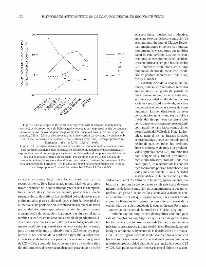
ra relativamente baja para la zona occidental dereconocimiento. Esto haría relativamente fácil viajar a pie através del núcleo de la concentración y tener acceso a tempera-turas más cálidas y, consecuentemente, propiciaría el creci-miento robusto de cultivos. La fertilidad del suelo no es espe-cialmente alta, pero es adecuada para cubrir la necesidad dealimentar a una población en la cantidad más pequeña de tierrapor unidad doméstica que estaría disponible dentro de unaconcentración de ocupación. La concentración central nortetambién se enfoca en un área considerable de pendientes sua-ves. Las elevaciones son más altas y los suelos generalmentemenos productivos que en el área de la concentración oriental,pero un parche del muy productivo suelo C25 se incluye regu-larmente. En tiempos de la población más alta la concentra-ción se expande hacia el sur para incluir una zona más grandede C25 y C26, a pesar del hecho de que yace a través del cañóndel río Loro, el cual presenta un obstáculo para viajar a pie. En

esta sección sur mucho más productiva,en la que se expande la concentración deasentamiento durante el Clásico Regio-nal, encontramos el centro con tumbasmonumentales y esculturas que tambiéndatan de este período. Las dos concen-traciones de asentamientos del occiden-te están enfocadas en parches de suelosC25 altamente productivos en alturasmoderadas dentro de zonas con condi-ciones predominantemente más altas,frías y húmedas.

La distribución de la ocupación, en-tonces, tiene mucho sentido en términosambientales si el punto de partida denuestro razonamiento es, no el ambiente,sino una sociedad en donde las fuerzassociales centralizadoras de alguna clasetienden a crear concentraciones de asen-tamientos. Las localizaciones de estasconcentraciones, así como sus cambios através del tiempo, son comprensiblescomo patrones eficientemente económi-cos para alimentar a las concentracionesde población del Valle de la Plata. La for-taleza general de las fuerzas socialescentralizadoras puede ser medida por elhecho de que, en todos los períodos,áreas sustanciales de muy alta producti-vidad agrícola (como C25) tuvieron unabaja ocupación y fueron presumible-mente subutilizadas. Tomado todo estoen conjunto, los residentes de la zona delreconocimiento podrían haber hecho susvidas más fácilmente si una cantidadsustancial de ellos hubiera vivido y culti-

vado en el suelo C25. Ellos no lo hicieron, aparentemente, de-bido a la importancia que le daban a vivir más cerca de otrosmiembros de la concentración de asentamiento a la que perte-necían. Esto provee un contenido sustancial a la abstracta con-clusión estadística a la que llegamos antes, o sea que las condi-ciones ambientales dan cuenta de cerca de un cuarto de lavariabilidad de la distribución de la ocupación en el Formativo1, aumentando a cerca de la mitad en el Clásico Regional.

También hay una implicación demográfica adicional paraesta última observación. Significa que, a medida que la distri-bución de la ocupación se concentró de forma sustancialmentemás fuerte en cuatro áreas durante el Clásico Regional, mejoróla lógica ambiental subyacente de la distribución de la ocupa-ción. Esto se logró a través de medios tales como la expansiónhacia el sur de la concentración central norte para incluir un te-rritorio de productividad altamente substancial en suelos C25y C26. Esto pudo haber sido necesario con el objeto de susten-


Figure 3.53. Soilscapes in the western survey zone with disproportionately heavy(positive) or disproportionately light (negative) occupations, expressed as the percentage

above or below the overall percentage of the total surveyed area in that soilscape. Forexample, C25 is 15.6% of the surveyed area in the western survey zone; it contains only5.7% of the Formative 1 occupation in the western survey zone; its “disproportion” for

Formative 1, then, is 5.7% – 15.6% = -9.9%.Figura 3.53. Paisajes-suelos en la zona occidental de reconocimiento con ocupacionesdesproporcionadamente altas (positivas) o desproporcionadamente bajas (negativas),

expresadas como el porcentaje por encima o por debajo de todo el porcentaje del total dela zona de reconocimiento en ese suelo. Por ejemplo, C25 es 15.6% del área de

reconocimiento en la zona occidental de reconocimiento; contiene únicamente el 5.7%de la ocupación del Formativo 1 en la zona occidental de reconocimiento; por lo tanto,

su “desproporción” para el Formativo 1es 5.7% – 15.6% = -9.9%.

it much more abundant than most of the categories). In this351.6 ha, there was a total of 32.4 ha of Regional Classic occu-pation, for an occupied area percentage of 9.2%. This particu-lar combination of environmental conditions, then, was morechosen for occupation than most, since this is greater than theRegional Classic occupied area percentage for the westernsurvey zone as a whole. This same process was repeated witheach of the 2800 environmental categories for each period.

Next, we treated this measurement of overall intensity ofoccupation in each environmental category as the general “ex-pected” density of occupation for that category in that period,and we used these expectations to calculate an expected area ofoccupation in each quadrat, based on the area of each of the2800 environmental categories found in the quadrat. We canimagine, for example, a quadrat whose territory includes15.0 ha of the environmental combination referred to above(soilscape B22 at an elevation of 1500–1550 m with slopesless than 10%). We would expect 9.2% of that 15 ha to be occu-pied during the Regional Classic, for a total expected RegionalClassic occupation there of 1.4 ha. That 1.4 ha of RegionalClassic occupation would be added together with whatever ex-pected occupied areas were calculated from any other environ-mental categories occurring within that quadrat to arrive at atotal expected occupied area for that quadrat. This same pro-cess was repeated for each of the 1352 quadrats for each pe-riod.

Finally, the expected occupied area for each period in eachquadrat was subtracted from the actually observed occupiedarea for that period in each quadrat. The resulting numbers arenegative for a quadrat if the actually observed occupation wasless than the expected, positive if the observed occupation wasgreater than the expected. If the environmental characteristicsof a quadrat accounted perfectly for the amount of occupationfound there, the resulting number was 0, since the observed oc-cupation would exactly equal the expected. In a less perfectworld, if occupation depended largely on environmental con-ditions, then the numbers for the quadrats would not all be ex-actly zero, but they would be relatively close to zero. More-over, a map of high values, showing quadrats withsubstantially more occupation than expected, would no longerreveal the concentrations we have been seeing, but would in-stead show a random scatter or a different pattern of somekind. Such a result would indicate that the concentrations ofoccupation we have noted were largely a response to the attrac-tions of some particular environmental conditions, and ourtask would be to determine what those conditions were and thenature of the attraction.

As a first indication of the nature of the result, we can lookat the standard deviation of the observed minus expected val-ues for the quadrats (Table 3.9). For each period, the standarddeviation is lower than the standard deviation of the simple ob-served occupied area by quadrat. This suggests that the envi-ronmental circumstances do help us to predict the amount of

occupation to be found in a quadrat. Regression analysis helpsus to pursue this idea a little further, and we see that there is, in-deed, some degree of correlation between the area of occupa-tion we expect in each quadrat and the area actually observed.The correlation is positive and highly significant (p < .0005)for all periods, as might well be expected for such a large sam-ple (1352 quadrats). The r2 values in Table 3.9 indicate that en-vironmental conditions, as represented in this analysis, can besaid to account for about one-fourth of the variability in ob-served occupied areas by quadrat in Formative 1. This risesgradually to just over half in the Regional Classic before de-creasing slightly in the Recent period.

The maps of locations of quadrats with unusually large ex-cesses of observed occupation over expected occupation (Fig-ure 3.48), on the other hand, are remarkably like the originalmaps of observed occupation (Figure 3.47). Far from disap-pearing, the concentrations seen initially have remained al-most entirely unchanged. This tendency of occupation to formconcentrations, then, through much of the prehispanic se-quence, is clearly something much more than just a reflectionof a tendency to live on highly productive land, or any particu-lar kind of land. The result of environmental analysis gives usgreater confidence in the interpretation suggested in the firstsection of this chapter, that the concentrations of occupationreflect the centripetal forces of centralized sociopoliticalunits.

The surfaces in Figure 3.49 represent the distribution of oc-cupation in the five prehispanic phases in a way that empha-sizes the unevenness of the distributions. Each is a renderingof the observed occupation by quadrat minus the expected oc-cupation. The relative flatness of the Formative 1 surface indi-cates the weakness of the tendency toward clustering of occu-pation in this period. The tendency to concentrate occupationin certain sectors is much stronger in Formative 2, weakensagain in Formative 3, and becomes much stronger in the Re-gional Classic, with an additional modest increment in the Re-cent period. There are fundamentally four sectors of the west-ern survey zone where occupation is concentrated in someperiods. These are the locations of the clusters discussedimpressionistically in the first section of this chapter: theeast-central, the north-central, the protrusion toward thesouthwest, and the northwestern fringe. The first two areclearly present in Formative 2; the second gives way to thethird in Formative 3, and all four all clearly established in theRegional Classic and the Recent periods. The last two becomeespecially strong in the Recent. The high-elevation areaaround the swamp in the southern sector has an especially no-ticeable occupation in Formative 1 and in the Recent period,when its prominence in Figure 3.49 compares to that of two ofthe major clusters. This last, though, is more difficult to see asa concentration of occupation; it may be part of a settlementphenomenon that could only be fully recognized with more in-formation about occupation farther south.


drennan

Typewritten Text

All text on this page is a duplication of previous text. Skip to p. 137.

drennan

Typewritten Text

drennan

Typewritten Text

drennan

Typewritten Text

tar efectivamente a una población que había crecido muy rápi-damente desde finales del Formativo. Este patrón es el másconsistente con la visión de que las poblaciones pequeñas delFormativo pudieron fácilmente permitirse una distribución dela ocupación agronómicamente irracional debido a que los re-cursos de la zona excedían considerablemente lo que era nece-sario para sustentar a sus habitantes. Con una población másgrande en el Clásico Regional, la presión fue más fuerte paradistribuir la ocupación y el cultivo de manera acorde con losrecursos agrícolas; de ahí el aumento de las correlaciones pre-viamente observadas. Aun con poblaciones más grandes en elClásico Regional, sin embargo, nunca hubo una buena corre-lación entre la productividad agrícola y la distribución de laocupación a la escala de toda la zona occidental de reconoci-miento. La correlación simplemente fue menos débil. En el pe-ríodo Reciente, con niveles de población aun más altos, la co-rrelación de hecho empeoró otra vez. La población regional,entonces, aparentemente fue capaz de sustentarse a sí mismaefectivamente, a través de un período de unos 25 siglos, aunsin maximizar el uso efectivo de los recursos agrícolas de la re-gión, al menos tal como lo indican los patrones de distribuciónde la ocupación. Si esto es verdad, entonces no pudo haber ha-bido mucha presión poblacional a través de la región en nin-gún momento durante la secuencia prehispánica, a pesar deuna población regional similar o por encima de los niveles mo-dernos durante el Clásico Regional o el Reciente (como seconcluyó en la segunda sección de este capítulo). Esta conclu-sión es consistente con la evidencia palinológica previamentepresentada de que áreas sustanciales de bosque permanecieronsin talar en la zona occidental de reconocimiento aun durantelos períodos con mayor población (Drennan, Herrera, y Piñe-ros 1989:230–231).

Comunidades y DistritosLos estudios arqueológicos de asentamientos con frecuen-

cia se basan fuertemente en el sitio arqueológico como unaunidad de análisis, asumiendo implícitamente que un sitio ar-queológico es equivalente a un asentamiento humano o unacomunidad. Típicamente se asume que las comunidades loca-les pequeñas de algún tipo (“aldeas” o “caseríos”) son las uni-dades básicas de construcción de la ocupación regional y de laorganización social, política y económica. Tal aproximaciónha sido vigorosamente criticada (por ejemplo en Dunnell yDancey 1983; Dunnell 1992; Ebert 1992; Wandsnider 1998),pero ciertamente no es el caso que los sitios arqueológicos,como unidades de análisis de significado con buena corres-pondencia con comunidades humanas, nunca hayan existido.Demostrablemente ellos existieron, por ejemplo, en la Cuencade México o en el Valle de Oaxaca, o en la región de Chifeng alnorte de China (Drennan y Peterson 2004, 2005; Peterson yDrennan 2005). Sin embargo, como se mencionó en el capítu-lo 2, rápidamente encontramos que era imposible tratar la dis-

tribución de los restos arqueológicos en la zona occidental delreconocimiento del Valle de la Plata asignando “números desitios” a áreas de ocupación espacialmente separadas, cadauna aparentemente representando a una comunidad de algunaclase. Esto es mucho más interesante que una discusión de me-todología arqueológica; es un descubrimiento sustancialmen-te importante en sus propios términos. Lleva a cuestionar lanoción básica de comunidades locales pequeñas como blo-ques de construcción de la organización social en la zona occi-dental del reconocimiento del Valle de la Plata.

La unidad doméstica, probablemente la unidad domésticade familia nuclear, ha dejado claras evidencias de haber sido launidad social básica en el Valle de la Plata y en otras partes delAlto Magdalena. Esta evidencia se discute en la segunda sec-ción de este capítulo, en donde la unidad doméstica es tomadacomo la unidad básica del análisis demográfico. Los mapas dela distribución de asentamientos en este volumen representanlas áreas en las cuales todas las unidades domésticas de un pe-ríodo dispersaron sus basuras, y éstas también son las áreascalculadas en los análisis de distribución de la ocupación. Lacuestión de la existencia de grupos sociales más grandes porencima del nivel de la unidad doméstica queda por ser evalua-da, aunque ya hemos bordeado el asunto en nuestra considera-ción de las cuatro áreas en la zona occidental en donde las con-centraciones de ocupación se formaron con algunapersistencia.

Aquí nos aproximamos a las comunidades humanas desdela perspectiva de la interacción social y aplicamos principiosde interacción-distancia, asumiendo que, en promedio, lasunidades domésticas interactúan más intensivamente conotras unidades domésticas ubicadas cerca de ellas que conaquellas ubicadas más lejos (Peterson y Drennan 2005). Laspequeñas comunidades locales que frecuentemente parecenformar la base de estructuras sociales y políticas a mayor esca-la, entonces, deberían ser vistas en el paisaje como agrupa-mientos de unidades domésticas. Esta es la forma en que típi-camente reconocemos en un paisaje moderno a lascomunidades locales pequeñas que llamamos asentamientos,aldeas o pueblos. Ya hemos visto tales agrupamientos en ladistribución de la ocupación moderna de la zona occidental dereconocimiento, más notablemente en la forma de la comuni-dad nucleada de La Argentina (Figuras 3.40 y 3.41), la cualocurre en el contexto de un patrón de asentamiento rural dis-perso en el cual las unidades domésticas en su mayor parte ubi-can sus residencias en la tierra que cultivan. Hay aglomeracio-nes ocasionales que se forman en esta distribución ruraldispersa, pero ellas son raras y escasas. En la segunda secciónde este capítulo, hemos tomado la distribución de la ocupaciónprehispánica de la zona occidental de reconocimiento comosimilar en naturaleza a esta ocupación rural moderna dispersadebido a la baja densidad general de los materiales arqueológi-cos en áreas de ocupación y al carácter continuo y extensivo deestas zonas de ocupación a través de grandes áreas.


The locations of these concentrations do relate to environ-mental variables, even though, as we have seen, the concentra-tions are not the simple product of environmental conditions.The degree of correspondence we have just seen between envi-ronmentally expected occupation and actually observed occu-pation is most easily understood in terms of the rationale forthe locations of the concentrations. We can begin to explorethe principles involved by looking at the environmental vari-ables separately.

The heights of the bars of the histogram icons of Figure 3.50represent, for each period, the percentage of total occupiedarea in each of the slope categories described in the third sec-tion of this chapter The “Surveyed Area” icon is analogous toFigure 3.6, but it represents only the area actually surveyed(omitting the swamp and unsurveyed areas from the 317 km2

of the entire western survey zone). The icons for all five peri-ods have extremely similar shapes, indicating very similar dis-tributions of occupied areas across the slope categories. Thefive shapes all depart somewhat from the shape of the “Sur-veyed Area” icon, in that the left-hand bars, representing thetwo categories of most level land, are higher for occupied areain all periods than they are in the surveyed area at large. Thus,throughout the sequence, there was a similar degree of prefer-ence for more level land. This is, of course, completely unsur-prising; what is perhaps surprising is that the preference is notconsiderably stronger. There are, in all periods, non-trivialamounts of occupation even in extremely steeply sloping sur-roundings.

The proportions of land across elevation categories in thesurveyed area at large and the proportions of occupied areaacross elevations in different periods (Figure 3.51) have amore complicated story to tell. As in Figure 3.50, the “Sur-veyed Area” icon is a baseline for comparison, this time analo-gous to Figure 3.3. In the first place, the histogram icons for allperiods are strongly bimodal, indicating two consistently dif-ferent preferred elevations for settlement: one centered on1550–1600 m and another centered on 2000–2050 m (Forma-tive 1) or 1950–2000 m (Formative 2). As comparison with the“Surveyed Area” icon makes clear, this is by no means a resultof the overall elevation distribution of the region. Elevationsbelow 1550 m and above 2200 m are consistently un-der-occupied throughout the sequence. The elevations be-tween 1650 and 1900 m that separate the two favored zones arequite under-occupied throughout the Formative and again inthe Recent period. During the Regional Classic, however,these middle elevations have close to the proportion of the totaloccupation one would expect, given the proportion of the totalarea surveyed that they comprise. The unexpectedly high pro-portions of occupation at the 1550 and 2000 m peaks duringthis period come more at the expense of occupation at the low-est elevations and, especially, at the highest elevations. Thehigher zone of disproportionately heavy occupation is espe-cially evident in Figure 3.51 for Formative 1, and steadily di-

minishes compared to the lower zone in Formative 2 and 3.During the Regional Classic, the lower zone of disproportion-ately heavy occupation expands to 1500–1800 m, a broaderrange than in any other period. The disequilibrium betweenproportion of occupation and proportion of area available inthis lower zone is also greater during the Regional Classic thanat any other time.

These patterns of elevation and slope are most easily under-stood in terms of the concentrations of occupation we have al-ready discussed. Less steeply sloping terrain is, in general, acharacteristic of all four zones where concentrations of occu-pation occurred in various periods (Figures 3.5, 3.11–3.14,and 3.26). This produces a tendency toward greater occupa-tion in less steeply sloped terrain. There is, however, also agood amount of fairly even terrain where there was never aconcentration of occupation, and this accounts for the fact thatthis predilection for gentle slopes was no stronger than it was:some fairly steeply sloping land was evidently occupied be-cause it was near a concentration of population. By the sametoken, the area of concentrated occupation in the eastern sectorof the survey zone lies largely between 1500 and 1700 m; theother three have a considerable amount of land between about1900 and 2150 m (Figures 3.2, 3.11–3.14, and 3.26). The ten-dency of population to concentrate in these two elevationzones strongly reflects the shifting patterns of these concentra-tions. It is during the Regional Classic that the easternmostconcentration is particularly pronounced (Figure 3.49); thecontemporaneous heavy focus of occupation on the1500–1800 m elevation zone is the consequence.

The patterning with regard to soilscapes is more compli-cated to describe, but it is finally most intelligible, like that forslopes and elevation, in terms of the formation and shifting ofpopulation concentrations of occupation. The easternmostarea of concentrated occupation falls largely in soilscapes B22and C22 (Figure 3.52), certainly cultivable, but not apparentlythe most productive agricultural land, with ratings of 1 and 1.5,respectively. The proportion of total occupied area in thesetwo soilscapes is only very slightly more than their proportionin the surveyed area in Formative 1. The amount of occupationhere, however, becomes steadily more disproportionatelyheavy up to a peak in the Regional Classic as the easternmostconcentration of occupation becomes more prominent (Fig-ures 3.49 and 3.53). Then, as this concentration loses groundto those farther west during the Recent period, the dispropor-tionately heavy occupation of B22 and C22 wanes.

The area of the concentration in the north-central sector ofthe western survey zone is focused on soilscape C1 (Figure3.52), with a modest productivity score of 1. It also includesD1 (Figure 3.52), except when it contracts on the west and ex-pands southward in the Regional Classic (Figure 3.49), whenit includes more land in C25 and C26. The occupation of C1 isdisproportionately heavy in Formative 2, disproportionatelylight in Formative 3, heaviest in the Regional Classic, and only


drennan

Typewritten Text

All text on this page is a duplication of previous text. Skip to p. 137.

Mirar a la distribución de la ocupación como una superficiecuya elevación depende de la fluctuante densidad de la ocupa-ción a través de la región provee una forma de buscar los agru-pamientos que representarán a las comunidades locales pe-queñas y de delinearlas si se las encuentra (Peterson y Drennan2005). La suavización de tal superficie da una visión de aglo-meración a escalas progresivamente más grandes que no se veen las escalas locales. En tal análisis para el Valle de Oaxaca enla fase Rosario (700–500 a.C.), las superficies sin suavizar re-velan comunidades locales pequeñas bastante distintivas (Fi-gura 3.54), la mayoría de una docena de unidades domésticas,las cuales usualmente han sido llamadas aldeas (por ejemploen Flannery, ed., 1976). A medida que la superficie inicial esgradualmente suavizada la base extendida del pico enfocadoen la aldea central de San José Mogote absorbe varias de lascomunidades vecinas y define a un distrito o unidad política auna escala regional que, no obstante, omite a las comunidadeslocales pequeñas ubicadas demasiado lejos como para ser in-cluidas en el agrupamiento (Peterson y Drennan 2005; Dren-nan y Peterson 2004, 2005; Drennan y Haller n.d.).

Cuando la ocupación de la zona occidental de reconoci-miento del Valle de la Plata es representada de la misma forma,presenta una figura muy diferente (Figuras 3.55–3.59). Las su-perficies iniciales sin suavizar fueron producidas como sugi-rieron Peterson y Drennan (2005), a una resolución de 100 mcon base en los mapas de áreas ocupadas para cada período(Figuras 3.11–3.14 y 3.26). Dentro de cada unidad cuadradadel tamaño de una hectárea en la zona occidental del reconoci-miento, el área total de la ocupación del Clásico Regional fuecalculada y esa figura se convirtió en el valor z, o altura, paraesa hectárea para el dibujo de la superficie inicial. La suaviza-ción se logró al promediar los valores z a través de toda el área,sopesados de acuerdo a una potencia inversa de la distancia. Esdecir, un nuevo valor de la altura suavizada fue determinadopara cada hectárea individual; en cada caso, fue el promedio delos valores de las alturas para todas las hectáreas en la zona oc-cidental de reconocimiento, tras haber dividido cada una pri-mero por su distancia de la hectárea cuyo valor se estaba deter-minado, esa distancia elevada a alguna potencia. Las potenciasmayores de 4 no representan una suavización ya que inclusoalturas a muy cortas distancias adquieren pesos extremada-mente bajos cuando son divididas por sus distancias elevadas ala cuarta potencia. Las superficies que aparecen en este volu-men fueron producidas con el programa Surfer y pueden serreplicadas de los datos disponibles en la Base de Datos en laArqueología de América Latina (ver Apéndice) con ese pro-grama o con programas similares si se toma el cuidado de anu-lar comandos predeterminados que usan los datos en formasdiferentes a las que ya se describieron (ver Peterson y Drennan2005).

La naturaleza de las superficies sin suavizar para todos losperíodos en la zona occidental del reconocimiento del Valle dela Plata (Figuras 3.55–3.59, arriba) es sorprendentemente di-

ferente de la que fue producida en la misma forma para Oaxacaen la fase Rosario (Figura 3.54, arriba). Las superficies de lazona occidental de reconocimiento no muestran indicación decomunidades locales pequeñas, sino más bien un bosque de pi-cos altos, cada uno del tamaño que representa a una unidad do-méstica individual, o grupos de quizás tres o cuatro unidadesdomésticas a lo máximo. En los períodos tardíos, los picos es-tán espaciados muy cercanamente, de tal forma que no hay unespacio abierto real que divida sus bases consistentemente y laocupación se muestra continua a través de grandes áreas. Enlos períodos más tempranos, hay más espacios abiertos en al-gunos sectores, pero los picos individuales no se organizancomo para formar grupos que tengan sentido por encima delnivel de las dos o tres unidades domésticas. Se ha argumenta-do que la superficie sin suavizar de Oaxaca representa diferen-tes pequeñas comunidades locales individuales compuestas deunidades domésticas con una interacción casi diaria cara a cara(Peterson y Drennan 2005; Drennan y Peterson 2004, 2005;Drennan y Haller n.d.). Las unidades domésticas en una de es-tas comunidades locales, entonces, habrían interactuado in-tensamente unas con otras y menos intensivamente con unida-des domésticas de otras unidades domésticas de otraspequeñas comunidades locales. Las superficies de la zona oc-cidental de reconocimiento del Valle de la Plata fueron toma-das como si ellas representaran una estructura de interacciónmuy diferente, una que fue mucho más difusa y desligada de laescala local. La interacción de pequeñas comunidades localesclaramente delineadas simplemente no es evidente en ningunade estas superficies y no provee bases para identificar consis-tentemente caseríos o aldeas a través de la zona occidental dereconocimiento.

Comenzamos esta sección reconociendo que nuestra inha-bilidad para monitorear con precisión las densidades de arte-factos en la zona occidental de reconocimiento significó queun agrupamiento ocasional de unidades domésticas en un ca-serío o aldea pudiera no ser reconocido en nuestra base de da-tos. Sin embargo, aun si este fuera el caso, ello no alteraría laconclusión de que la estructura fundamental de la distribuciónde la ocupación en la zona occidental de reconocimiento du-rante la prehistoria (como en el momento presente) no fue unade pequeñas comunidades locales. La ausencia de tal estructu-ra significa que no hay unidades mínimas con sentido para al-gunas técnicas analíticas comunes en los estudios regionalesde asentamiento, tales como el análisis de áreas de captación,los histogramas de tamaño de sitios, o los gráficos de ran-go-tamaño (rank-size graphs). Por esta razón, nosotros nopracticamos tales análisis aquí. De mucho más interés es laconclusión sustancial de que las unidades sociales más gran-des del Clásico Regional que hemos discutido antes no pare-cen haberse formado a partir de pequeñas comunidades loca-les como bloques de construcción, sino que, en vez de ello, lamayoría se ha construido directamente a partir de unidades do-mésticas como unidades constitutivas.


slightly less heavy in the Recent period (Figure 3.53). This pat-tern reflects precisely the waxing and waning of thenorth-central concentration of occupation. The occupation ofC25 is disproportionately light throughout the sequence (Fig-ure 3.53), and this is particularly difficult to understand, sinceit has the highest productivity rating of all soilscapes in thewestern survey zone. A very large part of C25, however, al-ways falls between concentrations of settlement. Its occupa-tion is heaviest (that is, least disproportionately light) in theRegional Classic, when the north-central concentration of oc-cupation expands to the south and includes at least some ofC25. Much the same can be said of C26; it falls outside settle-ment concentrations except during the Regional Classic, whenthe north-central concentration expands southward and in-cludes most of it (Figures 3.49 and 3.52). Its occupation risesfrom disproportionately small in Formative 2 to very dispro-portionately heavy in the Classic. D1’s occupation is dispro-portionately heavy throughout because it forms part of thenorth-central settlement concentration, except during the Re-gional Classic, and the contraction of the concentration fromthe west is reflected in the lowest values for occupational pro-portion in D1 at this time.

The two westernmost concentrations include mostlysoilscapes C25 and D33 (Figure 3.52). D33 is always un-der-occupied, but quite a lot of it, like C25 generally falls in be-tween settlement concentrations. It is most under-occupied inthe Regional Classic, when the westernmost concentrationsare most heavily overshadowed by the other two. Somethingsimilar can be said for C25, but the inclusion of a good amountof it in the north-central concentration during the RegionalClassic runs counter to that trend, leaving a net effect less dra-matic than might otherwise be the case. The other soilscapesnot mentioned in this account of cluster locations are occupiedat levels near or below their proportional areas in the surveyzone as a whole.

The relationship between environmental variables and theformation of concentrations of occupation perhaps makesmost sense when looked at from the opposite perspective, tak-ing the social forces that produced the settlement concentra-tions as given for the moment. The location of the easternmostconcentration makes sense because of its situation in a sub-stantial zone of modest slopes at relatively low elevation forthe western survey zone. This would make travel on footthrough the core of the concentration relatively easy, and pro-vide for warmer temperatures and, consequently, robust cropgrowth. Soil fertility is not especially high, but adequate to theneeds of supporting a population on the smaller amounts ofland per household that would be available within a concentra-tion of occupation. The north-central concentration also fo-cuses on a sizeable area of gentle slopes. Elevations are higherand soils generally less productive than in the area of the east-ern concentration, but a patch of the very productive C25 isregularly included. At times of highest population, the concen-

tration expands southward to include a much larger zone ofC25 and C26, despite the fact that it lies across the canyon ofthe Río Loro, which presents an obstacle to travel on foot. Inthis much more highly productive southern section that thesettlement concentration expands into during the RegionalClassic, we find the center with monumental tombs and sculp-ture that also dates to this period. The two westernmost settle-ment concentrations are focused on pockets of the highly pro-ductive C25 at moderate elevations in zones of predominantlyhigher, colder, and wetter conditions.

The distribution of occupation, then, makes good environ-mental sense if the starting point of our thinking is, not the en-vironment, but a society in which centralizing social forces ofsome sort tend to create settlement concentrations. The loca-tions of these concentrations, as well as their shifts throughtime, are comprehensible as economically efficient patternsfor supporting concentrations of population and easing com-munication within each one in the environmental context ofthe western survey zone of the Valle de la Plata. The generalstrength of the centralizing social forces can be gauged by thefact that, in all periods, substantial areas of very high agricul-tural productivity (such as C25) were under-occupied and pre-sumably under-utilized. Taken all together, the residents of thesurvey zone would have been able to make their living moreeasily, if substantially more of them had lived in and cultivatedsoilscape C25. They did not do so, apparently, because of theimportance they placed on living closer to other members ofthe settlement concentration to which they belonged. This pro-vides substantive content to the abstract statistical conclusionreached earlier, that environmental conditions account forabout one-fourth of the variability in distribution of occupa-tion in Formative 1, rising to about half in the Regional Clas-sic.

There is a further demographic implication of this last ob-servation as well. It means that, as the distribution of occupa-tion concentrated substantially more strongly in four areasduring the Regional Classic, the underlying environmentallogic of the distribution of occupation improved. This was ac-complished through such means as the southward expansionof the north-central concentration to include substantialhighly productive territory in soilscapes C25 and C26. Thismay have been necessary in order to provide effectively for apopulation that had grown very rapidly since the end of theFormative. This pattern is most consistent with the view thatthe small populations of the Formative could easily afford anagronomically irrational distribution of occupation since theresources of the zone so vastly exceeded what was necessaryto support its inhabitants. With a much larger population in theRegional Classic, pressure was stronger to distribute occupa-tion and cultivation more in accordance with agricultural re-sources; hence the rising correlations previously observed.Even with much larger populations in the Regional Classic,however, there was never any very good correlation between


drennan

Typewritten Text

Text in this column is a duplication of a previous page.

drennan

Typewritten Text

Duplicated text ends here.

drennan

Typewritten Text

Moviéndonos hacia arriba desde la escala local, las superfi-cies más suavizadas de la parte inferior en las Figuras3.55–3.59 muestran claramente la presencia de unidades so-ciales de mayor escala o comunidades de interacción. Estasson las concentraciones de ocupación que ya hemos reconoci-do y discutido de otras maneras. Las superficies en las Figuras3.55–3.59, sin embargo, proveen de una visión más clara deestas comunidades de la que teníamos antes. Ellas parecenmás evidentes cuando miramos a las superficies suavizadascon la distancia inversa a la potencia 0.5 (en el centro derechode las Figuras 3.55–3.59). Tan temprano como en el Formativo1 (Figura 3.55), la concentración de ocupación en el sectorcentral norte de la zona occidental de reconocimiento se en-cuentra en evidencia, así como lo está la concentración de másal oriente (más de lo que cualquier otra lo está en las superfi-cies menos suavizadas en la Figura 3.55); otra en el extremosur alrededor del pantano y ubicada a gran altura puede discer-nirse también. En el Formativo 2 (Figura 3.56), se ve que laconcentración central norte se expande un poco hacia el sur. Laconcentración más oriental continúa formándose; la concen-tración noroccidental se delinea y la del sur crece. En el For-mativo 3 (Figura 3.57), la expansión hacia el sur de la concen-tración central norte es más pronunciada; la concentración queestá más al oriente ha crecido; la concentración del norocci-dente se contrae un poco y una densa ocupación persiste en elextremo sur. En el Clásico Regional, la porción sur de la con-centración central norte sobrepasa a la del norte (justo cuandoel complejo de tumbas y estatuas es establecido en la porciónsur) y absorbe la mayoría de lo que queda de la mayor ocupa-ción en el extremo sur; la concentración del oriente continúacreciendo y las concentraciones suroccidental y la norocci-dental se ven bastante bien definidas, aunque mucho menosimpresionantes que las dos principales (quizás porque partessustanciales de ellas están por fuera de la zona de reconoci-miento). En el período Reciente, la concentración orientalcontinúa siendo intensamente ocupada; el énfasis de la con-centración central norte cambia otra vez hacia su porción nortey la concentración suroccidental ya no está tan claramente se-parada de ella; la ocupación en la concentración noroccidentalse enfoca aun más intensamente justo a lo largo del borde de lazona de reconocimiento; y una pequeña área de ocupación se-parada persiste en el extremo sur.

Estas superficies pueden usarse como base para delinear loslímites de los distritos que abarcan las concentraciones de ocu-pación. Las superficies suavizadas con la distancia elevada a laprimera potencia (en el centro izquierdo de las Figuras3.55–3.59) se prestan mejor para ser descritas en la forma demapas de líneas de contorno, lo cual facilita la identificaciónde los valles de ocupación que separan a los distritos y dan al-guna aproximación a sus límites (líneas fuertes en la Figura3.60). Este procedimiento se basa en el supuesto de que talesdistritos son la manifestación territorial de las comunidades deinteracción de una escala más grande que la local, limitados

por zonas a través de las cuales la interacción, como se ve porla distribución de la ocupación, es menos intensa (Peterson yDrennan 2005). Algunos de los límites entre distritos son am-biguos porque sólo se incluyen fragmentos de distritos en elárea de reconocimiento, pero la delineación de los distritoscentral norte y oriente resulta bien clara, especialmente en losperíodos Clásico Regional y Reciente. Sus antecedentes sonvisibles desde el comienzo del Formativo, aunque son más di-fusos. Especialmente en el Formativo 1, ellos son tan insignifi-cantes que probablemente no hubieran sido notados en ausen-cia del conocimiento que tenemos de los períodos más tardíos.

Debido a que la densidad de la ocupación en los distritoscentral norte y oriental declina tan dramáticamente hacia losbordes de la zona de reconocimiento, parece probable que ten-gamos a estos distritos casi completamente dentro del área delreconocimiento. Sus límites cambian un poco con el tiempo,de manera que sus áreas también varían, pero no por mucho.La concentración central norte siempre cubre un área ligera-mente mayor que la del oriente. En el Formativo 2, cuandoellas adquieren límites más definitivos, los dos distritos sonvirtualmente idénticos en tamaño con 116.6 y 116.7 km². Eldistrito oriental nunca llega a ser sustancialmente más grandeque esto y se reduce a 106.4 km² para el período Reciente,mientras que el distrito central norte también tiene una pobla-ción consistentemente más alta que la del distrito oriental (ba-sándonos en sus contribuciones proporcionales a los cálculosde población regional de la segunda sección de este capítulo).Las poblaciones de los dos distritos cambian a una tasa similara través del Formativo, pero el distrito central norte muestra uncrecimiento más rápido en los períodos Clásico Regional yReciente (Figura 3.61). Para el momento en que los distritosson claros en el Formativo 2, ellos tienen poblaciones de1000–2000 personas (el cálculo máximo sería el doble del mí-nimo mostrado en la Figura 3.61). En el Clásico Regional laspoblaciones de los dos distritos fueron alrededor de tres vecesmás grandes.

La delineación de estos dos distritos hace posible investigarsi la relación entre la distribución de la ocupación y los recur-sos agrícolas es más fuerte o más directa dentro de ellos de loque es a escala de toda la zona occidental de reconocimiento.Aunque los distritos y sus poblaciones centralizadas impidenuna maximización de la distribución económica de la ocupa-ción a través de la región como un todo, es posible que la ocu-pación dentro de cada distrito pueda corresponder muy cerca-namente a la distribución de los recursos agrícolas dentro deese distrito. Podemos acercarnos primero a esto por medio delos valores de productividad agrícola de los suelos, como lo hi-cimos antes para toda la zona de reconocimiento. Las Tablas3.10 y 3.11 dan los porcentajes de área ocupada para cada sue-lo en cada uno de los dos distritos más o menos completos.Como muestran las tablas de coeficientes de correlación derango, los resultados son bastante similares a aquellos obteni-dos para toda la zona de reconocimiento. La única correlación


agricultural productivity and occupational distribution at thescale of the entire western survey zone. The correlation wassimply less weak. In the Recent period, with even higher popu-lation levels, the correlation actually worsened again. The re-gional population, then, was apparently able to support itselfeffectively, through a period of some 25 centuries, even with-out making maximally effective use of the region’s agricul-tural resources, at least as indicated by patterns of occupa-tional distribution. If this is true, then there cannot have beenmuch region-wide population pressure at any point during theprehispanic sequence, despite regional populations at or abovemodern levels during the Regional Classic and Recent (as con-cluded in the second section of this chapter). This conclusionis consistent with previously reported palynological evidencethat substantial areas of uncut forest remained in the westernsurvey zone, even at periods of highest population (Drennan,Herrera, and Piñeros 1989:230–231).

Communities and DistrictsArcheological settlement studies often rely heavily on the

archeological site as a unit of analysis, implicitly assumingthat an archeological site is equivalent to a human settlement,or community. It is typically taken for granted that small localcommunities of some sort (“villages” or “hamlets”) are the ba-sic building blocks of regional occupation and social, political,and economic organization. Such an approach has been vigor-ously criticized (e.g. Dunnell and Dancey 1983; Dunnell1992; Ebert 1992; Wandsnider 1998), but it is certainly not thecase that archeological sites, as meaningful units of analysiswith good correspondence to human communities never exist.They very demonstrably do, for example, in the Basin of Mex-ico or the Valley of Oaxaca, Mexico, or the Chifeng region ofnorth China (Drennan and Peterson 2004, 2005; Peterson andDrennan 2005). As noted in Chapter 2, however, we quicklyfound it impossible to deal with the distribution of archeologi-cal remains in the western survey zone of the Valle de la Plataby assigning “site numbers” to spatially separate areas of oc-cupation, each apparently representing a community of somekind. This is much more interesting than a quibble of archeo-logical methodology; it is an important substantive finding inits own right. It calls into question the basic notion of small lo-cal communities as building blocks of social organization inthe western survey zone of the Valle de la Plata.

The household, probably the nuclear family household, isclearly in evidence in the Valle de la Plata and elsewhere in theAlto Magdalena as a basic social unit. This evidence is dis-cussed in the second section of this chapter, where the house-hold is taken as the basic unit of demographic analysis. Themaps of settlement distribution in this volume represent the ar-eas in which all the households of a period scattered their gar-bage, and these are the areas calculated in analyses of occupa-tional distribution as well. The question of larger social

groupings above the household level remains fully to be ad-dressed, although we have already verged on it in ourconsideration of the four areas in the western survey zonewhere concentrations of occupation formed with some persis-tence.

Here we approach human communities from the perspec-tive of social interaction and apply distance-interaction princi-ples, making the assumption that, on average, households in-teract more intensively with other households located nearbythan with those farther away (Peterson and Drennan 2005).The small local communities that often seem to form the basisof larger-scale social and political structures, then, should beseen on the landscape as clusters of households. This is theway we typically recognize on a modern landscape the smalllocal communities we call settlements, villages, or towns. Wehave already seen such clusters in the modern occupationaldistribution of the western survey zone, most notably in theform of the nucleated community of La Argentina (Figures3.40 and 3.41), which occurs in the context of a very dispersedrural settlement pattern in which households mostly locatetheir residences on the land that they farm. Occasional clustersdo form in this dispersed rural distribution, but they are rareand small. In the second section of this chapter, we have takenthe prehispanic occupational distribution of the western sur-vey zone to be similar in nature to this modern dispersed ruraloccupation because of the generally low densities of archeo-logical materials in areas of occupation and the sprawling con-tinuous nature of these zones of occupation across large areas.

Looking at the distribution of occupation as a surfacewhose elevation depends on the changing density of occupa-tion across the region provides a way of seeking the clustersthat would represent small local communities, and of delineat-ing them if they are found (Peterson and Drennan 2005).Smoothing such a surface mathematically gives a view ofclustering at progressively larger than local scales. In such ananalysis for the Valley of Oaxaca in the Rosario phase(700–500 BC), the unsmoothed surface reveals quite distinctsmall local communities (Figure 3.54), mostly of a dozenhouseholds or so, which have usually been called villages (e.g.Flannery, ed., 1976). As the initial surface is increasinglysmoothed, the spreading base of the peak focused at the centraltown of San José Mogote engulfs a number of nearby commu-nities and defines a district or polity on a regional scale thatnevertheless omits small local communities too far away to beincluded in the cluster (Peterson and Drennan 2005; Drennanand Peterson 2004, 2005; Drennan and Haller n.d.).

When the occupation of the western survey zone of theValle de la Plata is represented in the same way, it presents avery different picture (Figures 3.55–3.59). The initialunsmoothed surfaces were produced as suggested by Petersonand Drennan (2005), at a resolution of 100 m based on themaps of occupied areas for each period (Figures 3.11–3.14and 3.26). Within each square unit 1 ha in size in the western



Figure 3.54. Increasingly smoothed surfaces representing Rosario phase occupation in the Valley of Oaxaca, Mexico (Peterson andDrennan 2005). Inverse distance powers used in the smoothing were (from top to bottom) 4, 2, 1, 0.5, 0.25, and 0.001.

Figura 3.54. Superficies progresivamente más suavizadas que representan la ocupación de la fase Rosario en el Valle de Oaxaca,México (Peterson y Drennan 2005). Las potencias de la distancia inversa usadas en la suavización

fueron (de arriba hacia abajo) 4, 2, 1, 0.5, 0.25 y 0.001.

survey zone, the total area of Regional Classic occupation wascalculated, and that figure became the z-value, or elevation, forthat hectare in drawing the initial surface. Smoothing was ac-complished by averaging z-values across the entire area,weighted according to an inverse power of distance. That is, anew smoothed elevation value was determined for each indi-vidual hectare; in each case it was the average of the elevationvalues for all the hectares in the western survey zone, eachhaving first been divided by its distance from the value whoseaverage was being determined, that distance raised to somepower. Powers greater than about 4 represent no smoothing atall since even elevations at very short distances get extremelylow weights when they are divided by their distances raised tothe fourth power. The surfaces that appear in this volume wereproduced with the program Surfer and can be replicated fromdata available in the Latin American Archaeology Database(see Appendix) with it or other similar programs if care istaken to override default settings that handle the data in waysother than that just described (see Peterson and Drennan2005).

The nature of the unsmoothed surfaces for all periods in thewestern survey zone of the Valle de la Plata (Figures3.55—3.59, top) is strikingly different from the one producedin the same way for Rosario phase Oaxaca (Figure 3.54, top).The western survey zone surfaces show no indication of smalllocal communities at all, but rather a forest of tall spikes, eachof a size to represent a single household, or groups of perhapsthree or four households at most. In the later periods, the spikesare very closely spaced, such that no real open space consis-tently divides their bases, and occupation is continuous acrosslarge areas. In the earlier periods, there is more open space insome sectors, but the individual peaks still do not arrangethemselves so as to make meaningful groupings above thelevel of two or three households. The Oaxaca unsmoothed sur-face has been argued to represent identifiably different indi-vidual small local communities of households in virtuallydaily face-to-face interaction (Peterson and Drennan 2005;Drennan and Peterson 2004, 2005; Drennan and Haller n.d.).The households in one of these local communities, then,would have interacted intensely with each other and only lessintensively with households in other small local communities.We take the Valle de la Plata western survey zone surfaces torepresent a very different interaction structure, one that wasmuch more diffuse and unbounded at the local scale. Clear,bounded, small local interaction communities are simply notin evidence in any of these surfaces, providing no basis forconsistently identifying hamlets or villages across the westernsurvey zone.

We began this section by recognizing that our inability toaccurately monitor artifact densities in the western surveyzone meant that an occasional hamlet-sized cluster of house-holds might escape recognition in our dataset. Even if thiswere the case, however, it would not alter the conclusion that

the fundamental structure of occupational distribution in thewestern survey zone throughout prehistory (as at the presenttime) was not one of small local communities. The absence ofsuch a structure means that there are no meaningful basic unitsfor some analytical approaches common in regional settle-ment studies, such as catchment analysis, site size histograms,or rank-size graphs. For that reason, we do not pursue suchanalyses here. Of much more interest is the substantive con-clusion that the larger social units of the Regional Classic thatwe have discussed above do not seem to be built up of small lo-cal communities as building blocks, but must instead havebuilt directly from households as constituent units.

Moving up from the very local scale, the more smoothedsurfaces toward the bottom in Figures 3.55–3.59 show clearlythe presence of larger scale social units or interaction commu-nities. These are the concentrations of occupation we have al-ready recognized in other ways and discussed. The surfaces inFigures 3.55–3.59, however, provide a clearer view of thesecommunities than we have had before. They seem most evi-dent looking at the surfaces smoothed with inverse distance tothe 0.5 power (in the right center of Figures 3.55–3.59). Asearly as Formative 1 (Figure 3.55), the concentration of occu-pation in the north-central sector of the western survey zone isin evidence, as is the easternmost concentration (more than ei-ther is in the surfaces as seen in Figure 3.55); another in the ex-treme south around the high elevation swamp may be discern-ible as well. In Formative 2 (Figure 3.56), the north-centralconcentration can be seen to expand somewhat toward thesouth; the easternmost concentration continues to form; thenorthwestern concentration is distinct; and the southern onegrows. In Formative 3 (Figure 3.57), the north-central concen-tration’s expansion southward and southwestward is morepronounced; the easternmost concentration has grown; thenorthwestern concentration has shrunk somewhat; and heavyoccupation persists in the extreme south. In the Regional Clas-sic, the southern portion of the north-central concentrationoutweighs the northern (just when the complex of tombs andstatues is established in the southern portion) and absorbsmost of what remains of major occupation in the extremesouth; the easternmost concentration has continued to build;and the southwestern and northwestern concentrations arequite distinct, although far less impressive than the two princi-pal ones (perhaps because substantial parts of them are miss-ing from the survey zone). In the Recent period, the easternconcentration continues to be heavily occupied; the emphasisin the north-central concentration shifts back to its northernportion, and the southwestern concentration is no longer quiteas distinct from it; occupation in the northwestern concentra-tion focuses even more heavily right along the edge of the sur-vey zone; and a small separate area of occupation persists inthe extreme south.

These surfaces can be used as a basis for delineating theboundaries of districts that encompass the concentrations of



Figure 3.55. Increasingly smoothed surfaces representing Formative 1 occupation in the western survey zone. Inverse distance powers usedin the smoothing were (from top to bottom) 4, 2, 1, 0.5, 0.25, and 0.001.

Figura 3.55. Superficies progresivamente más suavizada que representan la ocupación del Formativo 1 en la zona occidental dereconocimiento. Las potencias de la distancia inversa usadas en la suavización fueron (de arriba hacia abajo) 4, 2, 1, 0.5, 0.25, 0.001.


Figure 3.56. Increasingly smoothed surfaces representing Formative 2 occupation in the western survey zone.Inverse distance powers used in the smoothing were (from top to bottom) 4, 2, 1, 0.5, 0.25, and 0.001.

Figura 3.56. Superficies progresivamente más suavizada que representan la ocupación del Formativo 2 en lazona occidental de reconocimiento. Las potencias de la distancia inversa usadas en la suavización

fueron (de arriba hacia abajo) 4, 2, 1, 0.5, 0.25, 0.001.


Figure 3.57. Increasingly smoothed surfaces representing Formative 3 occupation in the western survey zone.Inverse distance powers used in the smoothing were (from top to bottom) 4, 2, 1, 0.5, 0.25, and 0.001.

Figura 3.57. Superficies progresivamente más suavizada que representan la ocupación del Formativo 3 en la zonaoccidental de reconocimiento. Las potencias de la distancia inversa usadas en la suavización


occupation. The surfaces smoothed with inverse distance tothe first power (in the left center of Figures 3.55–3.59) lendthemselves best to being depicted in the form of contour maps,which facilitate recognition of the occupational valleys thatseparate the districts and give some approximation of theirboundaries (heavy lines in Figure 3.60). This procedure isbased on the assumption that such districts are the territorialmanifestation of interaction communities of larger than localscale, bounded by zones through which interaction, as indi-cated by the distribution of occupation, is less intense (Peter-son and Drennan 2005). The delineation of the north-centraland eastern districts is clearest; the others are more ambiguousbecause only fragments of them are included in the surveyarea. These two districts are quite clearly drawn in the Re-gional Classic and Recent periods. Their antecedents are visi-ble from the beginning of the Formative, although they aremore diffuse. Especially in Formative 1, they are so unremark-able that they would probably not be noticed at all in the ab-sence of knowledge of later periods.

Since the density of occupation in the north-central andeastern districts declines so dramatically toward the edges ofthe survey zone, it seems likely that we see these districts al-most entirely within the area surveyed. The boundaries ofthese two districts shift somewhat with time, so their areas alsovary, but not by very much. The north-central concentration al-ways covers a slightly greater area than the eastern one. In For-mative 2, when they take on fairly definitive limits, the two dis-tricts are virtually identical in size at 116.6 and 116.7 km2. Theeastern district is never substantially larger than this, andshrinks to 106.4 km2 by the Recent period, while thenorth-central district grows steadily to a Recent period peak of169.6 km2. The north-central district also has a consistentlyhigher population than the eastern district (based on their pro-portional contributions to the regional population estimates inthe second section of this chapter). The populations of the twodistricts change at similar rates through the Formative, but thenorth-central district shows much more rapid growth in theRegional Classic and Recent periods (Figure 3.61). By thetime the districts are clear in Formative 2, they had populationsof 1000–2000 (the maximum estimate would be twice theminimum shown in Figure 3.61). In the Regional Classic thedistrict populations were about three times that.

The delineation of these two districts makes it possible toinvestigate whether the relationship between occupational dis-tribution and agricultural resources is any stronger or more di-rect within them than it is at the scale of the entire western sur-vey zone. Even though the districts and their centralizedpopulations prevent maximally economical distribution of oc-cupation through the region as a whole, it is possible that occu-pation within each district might correspond quite closely tothe distribution of agricultural resources within that district.We can first approach this by way of the agricultural produc-tivity scores of soilscapes, as we did above for the whole sur-

vey zone. Tables 3.10 and 3.11 give the occupied area percent-ages for each soilscape in each of the two more or less com-plete districts. As the rank order correlations in the tablesshow, results are broadly similar to those obtained for thewhole survey zone. The only correlation of much significanceis again an early and negative one.

Table 3.12 provides the occupied area percentages for theother means of classifying agriculture productivity, modernland use. Here we again see largely the same patterns we sawin the survey zone as a whole. With a single exception, moderncultivated land is most densely occupied in all periods in bothdistricts; land used as cattle pasture today is second mostdensely occupied; and forest land is least densely occupied.The lone exception is the very low percentage of occupied areain cultivated land in the north-central district in Formative 1,and this might well be simply an aberrant result of the tiny sur-veyed area of cultivated land within the Formative 1 bound-aries of the north-central cluster (only 5.8 ha). In thenorth-central district, though, and again as in the analysis ofthe entire western survey zone, the occupied area percentagesin land cultivated today do not exceed those of the less produc-tive land by nearly as much as we would expect. Neither wayof looking at the distribution of agricultural resources, then,has given us any simple or straightforward way to account forwhere people lived within the north-central district—no morethan they did at the scale of the whole survey zone.

In the eastern district, however, after the Formative 1, theoccupied area percentage for cultivated land stays aroundeight times that of forest land, except for the Regional Classic,when it soars to a value nearly 18 times that for forest land.This observation is roughly in line with what we would expectbased on the apparent modern preferences for occupation inthese three land use categories. On closer examination, how-ever, this correspondence is once again produced, not by sys-tematic heavy occupation of the cultivated land use category,but rather by the correspondence of the most densely settledcore of the eastern district with a particular patch of cultivatedland. Occupation dwindles just as rapidly in the cultivatedland as it does in the other categories as one moves out fromthe core (Regional Classic occupation is shown in Figure3.62—the patterns for other periods are similar). It is accurateto observe that the most densely settled core of a populationconcentration was located in the top ranked land use category,but it is not the case that occupation generally is concentratedin what is now cultivated land.

These regional scale interaction communities of the Re-gional Classic, then, each consisted of a few thousand peoplein an area 10–15 km across. This is clearly too many peopleand too large an area for all to engage in face-to-face interac-tion on a daily basis. It might be as much as a 3–4 hour walk tothe center of the district from its farthest periphery, remember-ing that substantial differences in elevation are sometimes in-volved. Most of the population of each district, however, was


de mucha significancia es otra vez una que es temprana y ne-gativa.

La Tabla 3.12 provee los porcentajes de área ocupada parael otro método de clasificar la productividad agrícola: el usoactual de la tierra. Aquí otra vez vemos en gran parte los mis-mos patrones que vimos en la zona de reconocimiento comoun todo. Con una sola excepción, la tierra cultivada hoy en díaestá más densamente ocupada en todos los períodos en ambosdistritos; la tierra usada como pasto para ganado hoy en día esla segunda más densamente ocupada; y la tierra de bosque es lamenos densamente ocupada. La única excepción es un muybajo porcentaje de área ocupada en tierra cultivada en el distri-to central norte en el Formativo 1 y esto puede ser simplementeun resultado aberrante de la diminuta área reconocida en tierracultivada dentro de los límites de la concentración central nor-te durante el Formativo 1 (sólo 8.5 ha). En el distrito centralnorte, sin embargo, y otra vez como en el análisis de toda lazona occidental de reconocimiento, las diferencias entre losporcentajes de área ocupada en tierra cultivada y en tierra me-nos productiva son mucho menores de las que esperaríamos.Ninguna forma de mirar a la distribución de los recursos agrí-colas, entonces, nos ha dado una forma simple y directa de ex-plicar en dónde vivió la gente dentro del distrito central nor-te—no más del porqué ellos lo hicieron a escala de toda la zonade reconocimiento.

Sin embargo, en el distrito oriental, después del Formativo1, el porcentaje de área ocupada para tierra cultivada es cercade ocho veces el de la tierra de bosque, excepto para el ClásicoRegional, cuando se eleva a un valor cercano a las 18 veces elde la de tierra de bosque. Esta observación está bastante en lí-nea con lo que esperaríamos basándonos en las aparentes pre-ferencias modernas en cuanto a la ocupación de estas tres cate-gorías de uso de la tierra. En una revisión más cuidadosa, sinembargo, esta correspondencia se produce, una vez más, nopor una fuerte ocupación sistemática de la categoría de uso detierra cultivada, sino más bien por la correspondencia del cen-tro de asentamiento más denso del distrito oriental con un par-che particular de tierra cultivada. La ocupación disminuye tanrápidamente en la tierra cultivada como lo hace en las otras ca-tegorías a medida que uno se mueve hacia fuera del centro (laocupación del Clásico Regional se muestra en la Figura3.62—los patrones de otros períodos son similares). Es preci-

so observar que el centro más densamente asentado de estaconcentración de población se localizó en la categoría supe-rior de uso de la tierra, pero no es el caso que la ocupación estégeneralmente concentrada en lo que es ahora tierra cultivada.

Cada una de estas comunidades de interacción de escala re-gional durante el Clásico Regional, entonces, consistió enunos pocos miles de personas en un área de 10–15 km de unlado a otro. Claramente esto supone demasiada gente y un áreademasiado grande como para que todos entablaran una inte-racción diaria. Podría haber habido tanto como 3–4 horas decamino hasta el centro del distrito desde la periferia más leja-na, con diferencias sustanciales en altura algunas veces. Lamayoría de la población de cada distrito, sin embargo, se con-centró en un área central más pequeña y probablemente encaróobstáculos menos severos para la interacción. Esta interacciónaparentemente fue lo suficientemente regular e importantecomo para causar que la mayoría de las unidades domésticasescogieran vivir cerca de otras residencias sobre las parcelasmás pequeñas de tierras de cultivo que estaban disponibles enlas áreas nucleares de los distritos, en vez de tener acceso aparcelas más grandes de tierra de cultivo (a veces muy alta-mente productiva) en los sectores periféricos de los distritos.En el centro demográfico del distrito oriental, por ejemplo, unsolo kilómetro cuadrado tiene una densidad de población unas20 veces más alta que la de la zona occidental de reconoci-miento como un todo, mientras que a una distancia de 4–5 kmáreas muy productivas tienen niveles de densidad de poblaciónbastante más bajos que el promedio regional. Las fuerzas so-ciales centralizadoras de las comunidades de interacción deescala regional representadas en el paisaje arqueológico porlos distritos que hemos delineado debieron haber sido bastantefuertes al menos en el Clásico Regional, y para ese entoncesdebieron haber estado creciendo durante un considerable pe-ríodo de tiempo. Estas comunidades de distrito parecen habersido las unidades principales de interacción de la zona occi-dental de reconocimiento; al menos no hemos podido detectarninguna evidencia consistente de unidades constitutivas máspequeñas de mucha importancia. Las unidades domésticas pa-recen haberse amalgamado en distritos sin claras unidades so-ciales intermedias como las comunidades locales. Retomare-mos las implicaciones más generales de estos patronesnuevamente en el Capítulo 6.



1 2 3

1 2 3B14 (Orthents) 2.0 -- -- -- -- --B14 (Hapludalfs) 2.0 -- -- -- -- --B21 1.0 0.0 0.0 0.0 5.9 1.1B22 1.0 -- 3.4 1.6 17.8 10.2C1 1.0 1.6 3.5 2.3 13.3 10.3C22 (Tropudults) 1.5 1.9 0.2 0.0 13.8 12.1C22 (Dystropepts) 1.5 0.2 1.2 1.0 7.0 5.9C23 (Tropudults) 1.5 0.6 2.0 2.4 6.8 7.3C23 (Dystropepts) 1.5 0.2 0.0 0.8 4.7 6.8C25 3.0 0.4 1.6 1.9 4.7 6.5C26 2.0 0.8 1.7 3.0 23.6 21.0D1 (Durustalfs) 0.0 3.4 4.1 3.4 13.9 13.6D1 (Tropudults) 0.0 2.4 4.3 2.7 12.9 13.4D2 (Dystrandepts) 1.0 1.3 -- -- 3.7 7.8D2 (Orthents) 1.0 0.0 -- -- 5.7 6.9D31 (Hapludults) 1.0 5.6 0.0 0.0 6.5 14.0D31 (Inceptisols) 1.0 1.4 0.0 0.0 3.4 6.1D31 (Troportents) 1.0 0.0 0.0 0.0 0.9 1.6D32 0.0 4.7 -- -- 16.1 20.2D33 1.0 0.9 1.7 2.5 3.1 7.1r s with Productivityr s con productividad

-0.458 -0.291 -0.099 -0.071 -0.250

p of r s

p de r s0.065 0.292 0.725 0.780 0.317

Reciente

Produc-tivity

FormativeSoilscape

Occupied Area as % of Surveyed Area

TABLE 3.10. OCCUPIED AREAS BY SOILSCAPES IN THE NORTH-CENTRAL DISTRICTTABLA 3.10. AREAS OCUPADAS POR PAISAJES-SUELOS EN EL DISTRITO NOR-CENTRO

Paisaje-Suelo Produc-tividad

RegionalClassic Recent

Area Ocupada como % del Area ReconocidaFormativo Clásico

Regional


1 2 3

1 2 3

B14 (Orthents) 2.0 0.0 0.0 0.0 1.6 1.7

B14 (Hapludalfs) 2.0 0.1 0.3 0.0 5.7 4.0

B21 1.0 0.0 0.1 0.0 0.7 0.5

B22 1.0 2.0 3.6 3.5 13.1 8.6

C1 1.0 0.8 2.2 1.5 7.1 9.0

C22 (Tropudults) 1.5 0.9 6.2 9.0 34.8 28.1

C22 (Dystropepts) 1.5 0.8 2.7 3.8 15.6 12.6

C23 (Tropudults) 1.5 0.3 0.3 1.7 8.1 8.2

C23 (Dystropepts) 1.5 1.0 2.2 2.1 7.5 8.0

C25 3.0 0.0 0.1 0.0 0.0 0.0

C26 2.0 -- -- -- -- --

D1 (Durustalfs) 0.0 -- -- -- -- --

D1 (Tropudults) 0.0 -- -- -- -- --

D2 (Dystrandepts) 1.0 0.7 1.5 0.5 1.2 3.5

D2 (Orthents) 1.0 0.0 0.2 0.1 0.2 0.7

D31 (Hapludults) 1.0 1.1 0.7 0.8 1.7 2.1

D31 (Inceptisols) 1.0 1.5 1.3 1.2 2.4 3.8

D31 (Troportents) 1.0 2.3 2.0 3.6 1.9 5.1

D32 0.0 0.0 0.0 0.0 0.0 0.0

D33 1.0 0.2 -- 0.0 0.0 --r s with Productivityr s con productividad -0.196 -0.029 0.000 0.287 0.161

p of r s

p de r s0.450 0.914 1.000 0.265 0.550

Reciente

Produc-tivity

FormativeSoilscape


TABLE 3.11. OCCUPIED AREAS BYSOILSCAPES IN THE EASTERN DISTRICTTABLA 3.11. AREAS OCUPADAS POR PAISAJES-SUELOS EN EL DISTRITO ORIENTAL

Paisaje-Suelo Produc-tividad

RegionalClassic Recent

Area Ocupada como % del Area Reconocida

Formativo ClásicoRegional


Figure 3.58. Increasingly smoothed surfaces representing Regional Classic occupation in the western survey zone.Inverse distance powers used in the smoothing were (from top to bottom) 4, 2, 1, 0.5, 0.25, and 0.001.

Figura 3.58. Superficies progresivamente más suavizada que representan la ocupación del Clásico Regional en lazona occidental de reconocimiento. Las potencias de la distancia inversa usadas en la suavización



Figure 3.59. Increasingly smoothed surfaces representing Recent occupation in the western survey zone.Inverse distance powers used in the smoothing were (from top to bottom) 4, 2, 1, 0.5, 0.25, and 0.001.

Figura 3.59. Superficies progresivamente más suavizada que representan la ocupación del Reciente en la zonaoccidental de reconocimiento. Las potencias de la distancia inversa usadas en la suavización


concentrated in a smaller core area, and would face less severeobstacles to interaction. That interaction was apparently ofsufficient regularity and importance to cause most householdschoose to live near other residents on the smaller plots of landfor cultivation that were available in the core areas of districts,rather than have access to larger plots of (sometimes quitehighly productive) farmland in the peripheral sectors of dis-tricts. At the demographic center of the eastern district, for ex-ample, a single square kilometer has a population densitysome 20 times higher than the western survey zone as a whole,while at a distance of 4–5 km very productive areas have popu-lation density levels far below the regional average. The cen-

tralizing social forces of the regional scale interaction commu-nities represented on the archeological landscape by thedistricts we have delineated must have been fairly strong by atleast the Regional Classic and had, by then, been building overa considerable period of time. These district communities ap-pear to have been the principal interaction units of the westernsurvey zone; at least we are unable to detect any consistent evi-dence of smaller constituent units of much importance.Households seem to have amalgamated into districts withoutclear intermediate social units like local communities. We willtake up the broader implications of these patterns again inChapter 6.


1 2 3

1 2 3North-Central District/Distrito Nor-CentroForest/Bosque 1.2 1.9 1.8 5.7 7.1Grass/Pastos 1.4 2.5 2.3 10.2 10.0Cultivated/Cultivos 1.1 4.3 3.1 11.8 10.9Eastern District/Distrito OrientalForest/Bosque 0.6 0.6 0.6 1.0 2.0Grass/Pastos 0.7 1.5 1.4 6.5 6.6Cultivated/Cultivos 1.6 5.1 4.9 17.8 15.9

Area Ocupada como % del Area ReconocidaFormativo Clásico

Regional Reciente

TABLE 3.12. OCCUPIED AREAS BY MODERN LAND USE CATEGORIESIN DISTRICTS

TABLA 3.12. AREAS OCUPADAS POR CATEGORÍAS DE UTILIZACIÓNEN DISTRITOS

RegionalClassic

FormativeRecent



Figure 3.60. Contour maps of the power 1 smoothed surfaces from Figures 3.55–3.59. District boundaries are indicated.(Available as a GIS layer in the Latin American Archaeology Database—see Appendix.)

Figura 3.60. Mapas de líneas de contorno de las superficies suavizadas a la potencia 1 de las Figuras 3.55–3.59.Los límites de los distritos son indicados.

(Disponible como una capa SIG en la Base de Datos en la Arqueología de América Latina—ver Apéndice).


Figure 3.61.Graph of minimum

population estimatesfor north-central and

eastern districts in thewestern survey zone.

Figura 3.61.Gráfica de estimativosmínimos de población

para los distritosnorte-centro y oriental

de la zona occidentalde reconocimiento.

Figure 3.62.Settlement and land-usezones in the central coreof the eastern district inthe western survey zone.Figura 3.62.Asentamiento y zonas deuso de tierras en el cen-tro del distrito orientalde la zona occidental dereconocimiento.

3.4 Distributional Patterns: Resources, Communities, and Polities

Documents

Transcript of 3.4 Distributional Patterns: Resources, Communities, and Polities