Electronic copy available at: http://ssrn.com/abstract=1262610

Testing Distributional Assumptions: A L-moment Approach

Ba Chu and Mark Salmon

Warwick Business School

Preliminary version. Comments are especially welcome

1

Electronic copy available at: http://ssrn.com/abstract=1262610

Abstract

Stein (1972, 1986) provides a flexible method for measuring the deviation of any probability

distribution from a given distribution, thus effectively giving the upper bound of the approx-

imation error which can be represented as the expectation of a Stein’s operator. Hosking

(1990, 1992) proposes the concept of L-moment which better summarizes the characteristics

of a distribution than conventional moments (C-moments). The purpose of the paper is to

propose new tests for conditional parametric distribution functions with weakly dependent

and strictly stationary data generating processes (DGP) by constructing a set of the Stein

equations as the L-statistics of conceptual ordered sub-samples drawn from the population

sample of distribution; hereafter are referred to as the L-moment (GMLM) tests. The lim-

iting distributions of our tests are nonstandard, depending on test criterion functions used

in conditional L-statistics restrictions; the covariance kernel in the tests reflects parametric

dependence specification. The GMLM tests can resolve the choice of orthogonal polynomials

remaining as an identification issue in the GMM tests using the Stein approximation (Bon-

temps and Meddahi, 2005, 2006) because L-moments are simply the expectations of quantiles

which can be linearly combined in order to characterize a distribution function. Thus, our test

statistics can be represented as functions of the quantiles of the conditional distribution under

the null hypothesis. In the broad context of goodness-of-fit tests based on order statistics,

the methodologies developed in the paper differ from existing methods such as tests based on

the (weighed) distance between empirical distribution and a parametric distribution under the

null or the tests based on likelihood ratio of Zhang (2002) in two respects: 1) our tests are

motivated by the L-moment theory and Stein’s method; 2) offer more flexibility because we

can select an optimal number of L-moments so that the sample size necessary for a test to

attain a given level of power is minimal. Finally, we provide some Monte-Carlo simulations for

IID data to examine the size, the power and the robustness of the GMLM test and compare

with both existing moment-based tests and tests based on order statistics.

2

1 Introduction

Over recent years, there have been big advances in goodness-of-fit testing which can be classified

into three groups:

1. tests based on empirical distribution function such as the Cramer-von Mises test, the Watson

test, and the Anderson-Darling test (see e.g. Stephens (1974, 1978)) or tests based on the

likelihood ratio (Zhang, 2002)

2. tests based on moments such as the Meddahi & Bomtemps (MB) test and the Kiefer & Salmon

(KS) test

3. tests based on kernel density, e.g. Zheng (2000).

However, none of those tests are consistent against all types of alternatives to the null and not

robust against outliers in a small sample.

This paper proposes an alternative approach to test for conditional distribution assumptions in

dependent data by making use of L-moment theory and Stein’s equation. Our simulations suggest

that the GMLM tests can potentially avoid the above-mentioned problems of conventional goodness-

of-fit tests by using a bootstrap procedure to estimate the covariance matrix of L-statistics.

The econometric literature on testing for valid conditional distributional assumptions for time-

series data has received much recent interest. (See e.g. Bai 2003; Corradi and Swanson 2006; Li

and Tkacz 2006; Zheng 2000.) The influential work was done by Andrews (1997) who proposes a

conditional Kolmogorov test of model specification for a class of parametric nonlinear regression

models by using a sample of independent data pairs. The test is shown to be consistent against all

possible misspecification of distributions. However, the asymptotic distributions are not free from

nuisance parameters, thus a parametric bootstrap procedure is used to obtain critical values for

the test. Bai (2003); Bai and Chen (2006) make an important attempt to remove parameter uncer-

tainty in the conditional Kolmogorov test by applying the probability integral transform to show

that Ft(yt|Ft−1, θ0) are IID uniform random variable on [0, 1] and the martingale transformation

3

of Khmaladze (1981) to transform empirical processes into martingales which then converge to the

Brownian motions by the FCLT for martingales. As a result, Bai’s tests have the Brownian motion

limit. Zheng (2000) and Stinchcombe and White (1998) provide nonparametric tests of conditional

ditributions by using the distances (e.g. Kullback-Leibler information criterion) between nonpara-

metric estimators of distributions and the hypothesized distribution to construct valid moment

conditions; then the method of consistent conditional moment test proposed by Bierens (1990) is

extended to obtain efficient tests.

All of the above-mentioned methods rely on the topological distance between empirical/nonparametric

estimates of distributions and the true distributions. Bontemps and Meddahi (2005, 2006) pursues

a different approach by using the Stein equation (Stein, 1972, 1986) to construct moment conditions

in their GMM tests. In these papers, they use the result proved by Stein: A random variable X

has a standard normal distribution if and only if for any differential function f ,

E[f′

(X) − Xf(X)] = 0. (1.1)

Bontemps and Meddahi (2005) asserts that orthogonal polynomials can be used for f in the moment

conditions (1.1) because any function f in the Hilbert space can be approximated by a linear

combination of orthogonal polynomials. The heuristic argument behind this approach is: Supposing

that the Carleman criterion (Chow and Teicher, 1997, pp. 303) the standard normal is completely

characterized by its moments; thus there always exist ways to yield linear combinations of moments

which are equal to zero, plausible choices for the functions f are polynomials of X,X2, · · · , XN

in the SpanX,X2, · · · , XN as N is sufficiently large so that the moment conditions as defined in

(1.1) can completely characterize the standard normal (in this case f′

(X)−Xf(X) = H(X), where

H(X) is a Hermite polynomial.) Moreover, Bontemps and Meddahi (2005) shows that the problem

of parameter uncertainty can be dealt with by adding a moment condition into the GMM setting.

L-moments provide a promising alternative to summarize the shape of a distribution. Hosking

(1990, 1992) has shown that L-moments have good properties as measures of distributional shape

4

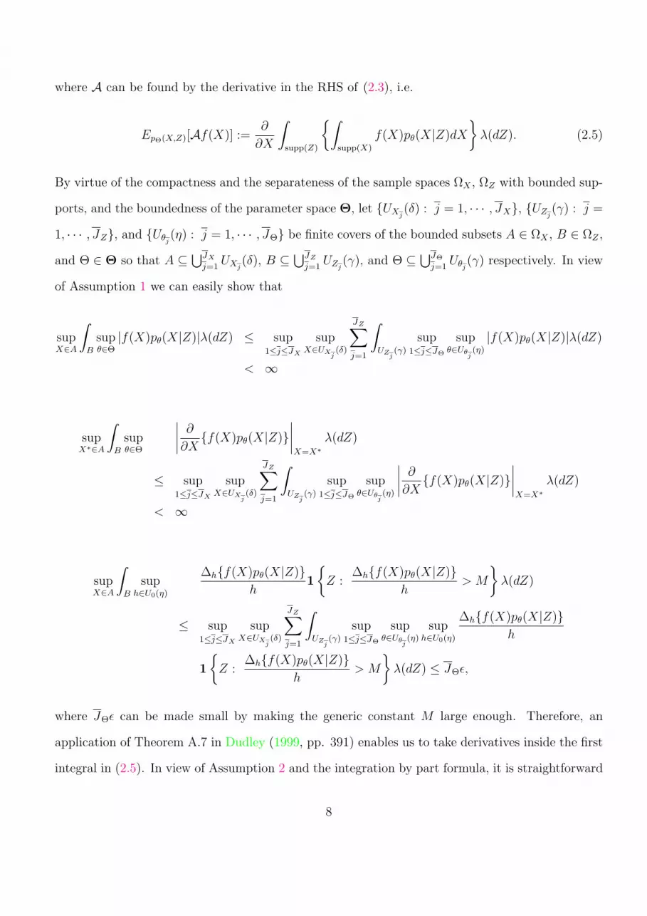
and useful for fitting distribution to data. Since the essential advantages of L-moments are 1)

being more robust to the presence of outliers in the data 2) being less subject to bias in estimation

and approximating their asymptotic values more closely in finite samples (Sankarasubramanian and

Srinivasan, 1999); thus L-moments are useful in formulating goodness-of-fit test statistics.

The formulation of the GMLM tests follows two steps: First we assume strict stationarity

for our DGP, then construct a set of moment conditions EPOS[Af(X)

(N×1)

|Z] = 0, where A is the

Stein operator and f′

(X) = f1(X), · · · , fr(X), · · · , fN(X) with fr(X) is the linear function of

order statistics X1:r, · · · , Xr:r for a given Z in EPOS[fr(X)] = λr, (λr is r-th L-moment); POS

is the probability distribution of the order statistics. Second, we construct different test statistics

associated with different criterion functions g(Z): If g(Z) is an exponential function, the test

statistic is the classical GMM test and the limiting distribution is χ2 with a covariance kernel

dependent on serial dependence structure; if g(Z) is an indicator function, the test statistics are

nonstandard and the limiting distributions are mixed normal.

Although the theory developed in the paper generally holds for any strictly stationary DGP

with a certain mixing level, we implement Monte Carlo simulations only for the IID cases because

computing the estimate of the covariance matrix for serially dependent data is potentially time-

consuming. Designing an efficient computation algorithm to do this could be a topic for future

research. However, we think that this is sufficient to justify our purpose of constructing test statistics

which are more robust against outliers and subject to less biases in a small sample. Simulation

results suggest that our tests have reasonably good power and are robust against big outliers in

rather small samples.

The remainder of the paper is organized as follows; in Section 2 we bring together derivations of

L-moment conditions and formulation of the GMLM statistics. In Section 3, we discuss the limiting

distribution of test statistics and the issues of choosing optimal number of L-moments. Some Monte

Carlo simulations results are provided in Section 4.

5

2 Test Functions as Linear Combinations of Order Statistics

2.1 Stein’s Equation

Let M(f) denotes a set of continuous or piecewise continuously differentiable test functions f(•)

such that EP0 [|f′

(•)|] < ∞. Stein (1972, 1986) shows that for any real function h(•), there exist a

function f ∈ M(f) and the following relation holds

h(X) − EP0 [h(X)] = Af(X), (2.1)

where A is the Stein operator for the probability distribution P0-this can be constructed, e.g.

Barbour’s generator approach (Barbour and Chen, 2005). Lemma 1 below states the functional

form of A for the conditional distribution of the random variable X for a given random event Z,

namely pΘ(X|Z).

We first make some assumptions.

Assumption 1.

supX∈UX0

(δ)

∫

UZ0(γ)

supθ∈Uθ(ǫ)

|f(X)pθ(X|Z)|λ(dZ) < ∞,

supX∗∈UX0

(δ)

∫

UZ0(γ)

supθ∈Uθ(ǫ)

∣∣∣∣∂

∂Xf(X)pθ(X|Z)

∣∣∣∣X=X∗

λ(dZ) < ∞,

and there exists a constant M such that

supX∈UX0

(δ)

∫

UZ0(γ)

suph∈U0(η)

∆hf(X)pθ(X|Z)h

1

Z :

∆hf(X)pθ(X|Z)h

> M

λ(dZ) < ǫ ,

where UX(ǫ) is a neighborhood of X; ǫ, δ and η are arbitrarily small generic constants. ∆hf(X)pΘ(X|Z) =

f(X + h)pΘ(X + h|Z) − f(X)pΘ(X|Z).

Assumption 2. limX−→∂ΩXf(X)pθ(X|Z) = 0 for all Z ∈ ΩZ.

Lemma 1. Let X and Z denote random variables in the compact and separable spaces (ΩX ,FX , P)

6

and (ΩZ ,FZ , λ) with bounded supports supp(X) and supp(Z) respectively; the parameter vector θ

belongs to a bounded set Θ.

Supposing that the functions f(X) ∈ M(f) and pθ(X|Z) belongs to the exponential family.

Moreover, pθ(X|Z) is measurable with respect to (X,Z) and satisfies Assumptions 1 and 2, then

X ∼ pθ(X|Z) is equivalent to

Epθ(X|Z)[Af(X)] = 0, ∀ f ∈ M(f), (2.2)

where A = ∂∂X

+ ∂∂X

log pθ(X|Z).

Let p∗θ(X|Z) denotes a conjugate probability distribution of pθ(X|Z) such that

p∗θ(X|Z)

pθ(X|Z)= κθ(X|Z),

where κθ(X|Z) is a polynomial of X. Then, we have

Ep∗θ(X|Z)[A∗f(X)] = 0, ∀ f ∈ M(f), (2.3)

where A∗ = ∂∂X

+ ∂∂X

log p∗θ(X|Z).

Proof. In the first part, we show that X ∼ pθ∗(X|Z) implies that Epθ∗(X|Z)[Af(X)] = 0. Stein (1972)

asserts that for a given measurable continuous or piecewise continuous function h(X) : ΩX =⇒ R,

we obtain

Ep(Z)

[Epθ(X|Z)[h(X)]

]− Ep(Z)

[Epθ∗ (X|Z)[h(X)]

]= Epθ(X,Z)[Af(X)],

for a function f ∈ M(f). Thus pθ(X|Z) ≡ pθ∗(X|Z) implies that Epθ(X,Z)[Af(X)] = 0. On the

other hand, since ∂∂X

Epθ(X,Z)[f(X)] = 0 we have

Eλ(dZ)[Epθ(X|Z)[Af(X)]] =∂

∂XEλ(dZ)[Epθ(X|Z)[f(X)]], (2.4)

7

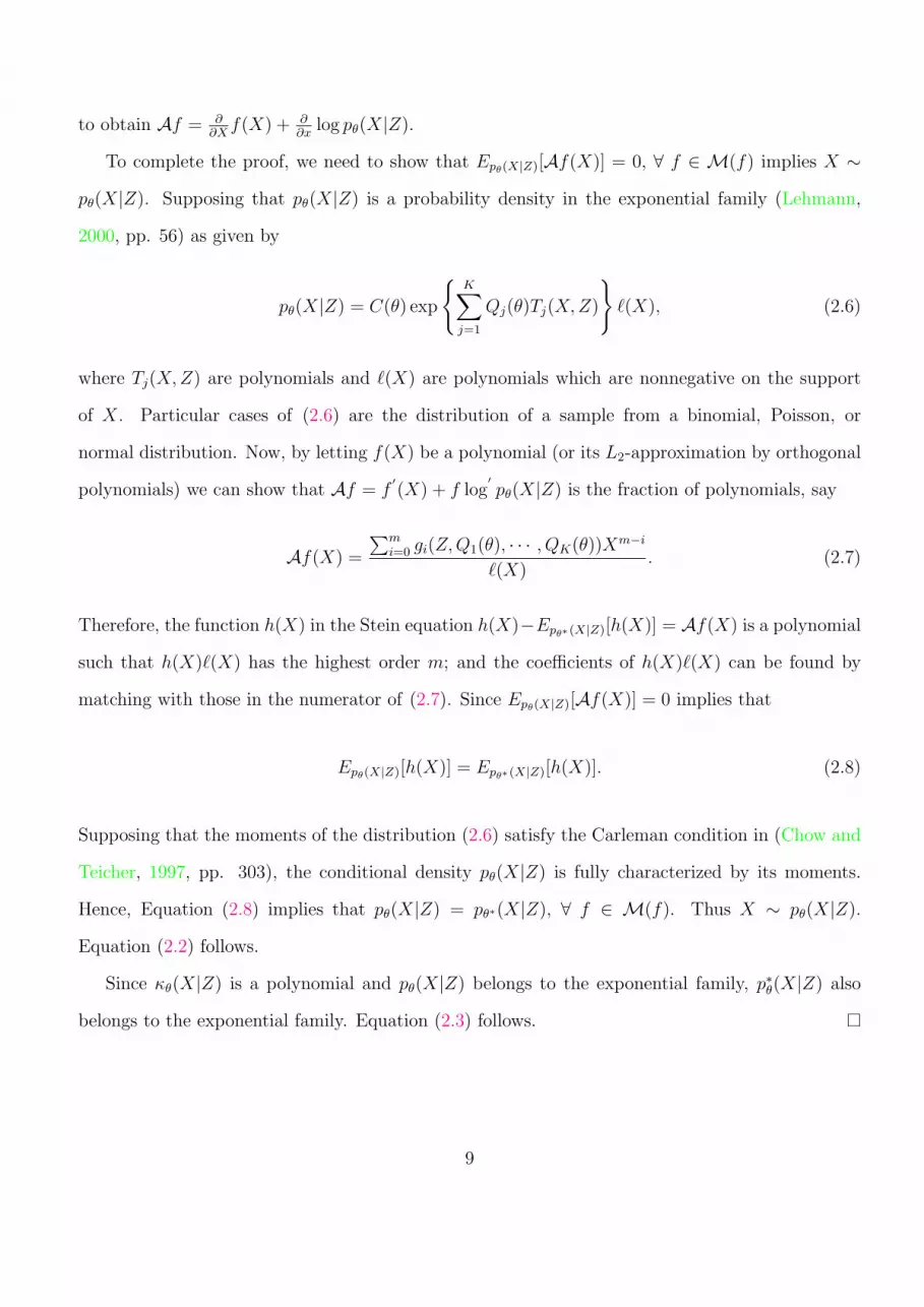
where A can be found by the derivative in the RHS of (2.3), i.e.

EpΘ(X,Z)[Af(X)] :=∂

∂X

∫

supp(Z)

∫

supp(X)

f(X)pθ(X|Z)dX

λ(dZ). (2.5)

By virtue of the compactness and the separateness of the sample spaces ΩX , ΩZ with bounded sup-

ports, and the boundedness of the parameter space Θ, let UXj(δ) : j = 1, · · · , JX, UZj

(γ) : j =

1, · · · , JZ, and Uθj(η) : j = 1, · · · , JΘ be finite covers of the bounded subsets A ∈ ΩX , B ∈ ΩZ ,

and Θ ∈ Θ so that A ⊆ ⋃JX

j=1UXj

(δ), B ⊆ ⋃JZ

j=1UZj

(γ), and Θ ⊆ ⋃JΘ

j=1Uθj

(γ) respectively. In view

of Assumption 1 we can easily show that

supX∈A

∫

B

supθ∈Θ

|f(X)pθ(X|Z)|λ(dZ) ≤ sup1≤j≤JX

supX∈UX

j(δ)

JZ∑

j=1

∫

UZj(γ)

sup1≤j≤JΘ

supθ∈Uθ

j(η)

|f(X)pθ(X|Z)|λ(dZ)

< ∞

supX∗∈A

∫

B

supθ∈Θ

∣∣∣∣∂

∂Xf(X)pθ(X|Z)

∣∣∣∣X=X∗

λ(dZ)

≤ sup1≤j≤JX

supX∈UX

j(δ)

JZ∑

j=1

∫

UZj(γ)

sup1≤j≤JΘ

supθ∈Uθ

j(η)

∣∣∣∣∂

∂Xf(X)pθ(X|Z)

∣∣∣∣X=X∗

λ(dZ)

< ∞

supX∈A

∫

B

suph∈U0(η)

∆hf(X)pθ(X|Z)h

1

Z :

∆hf(X)pθ(X|Z)h

> M

λ(dZ)

≤ sup1≤j≤JX

supX∈UX

j(δ)

JZ∑

j=1

∫

UZj(γ)

sup1≤j≤JΘ

supθ∈Uθ

j(η)

suph∈U0(η)

∆hf(X)pθ(X|Z)h

1

Z :

∆hf(X)pθ(X|Z)h

> M

λ(dZ) ≤ JΘǫ,

where JΘǫ can be made small by making the generic constant M large enough. Therefore, an

application of Theorem A.7 in Dudley (1999, pp. 391) enables us to take derivatives inside the first

integral in (2.5). In view of Assumption 2 and the integration by part formula, it is straightforward

8

to obtain Af = ∂∂X

f(X) + ∂∂x

log pθ(X|Z).

To complete the proof, we need to show that Epθ(X|Z)[Af(X)] = 0, ∀ f ∈ M(f) implies X ∼

pθ(X|Z). Supposing that pθ(X|Z) is a probability density in the exponential family (Lehmann,

2000, pp. 56) as given by

pθ(X|Z) = C(θ) exp

K∑

j=1

Qj(θ)Tj(X,Z)

ℓ(X), (2.6)

where Tj(X,Z) are polynomials and ℓ(X) are polynomials which are nonnegative on the support

of X. Particular cases of (2.6) are the distribution of a sample from a binomial, Poisson, or

normal distribution. Now, by letting f(X) be a polynomial (or its L2-approximation by orthogonal

polynomials) we can show that Af = f′

(X) + f log′

pθ(X|Z) is the fraction of polynomials, say

Af(X) =

∑mi=0 gi(Z,Q1(θ), · · · , QK(θ))Xm−i

ℓ(X). (2.7)

Therefore, the function h(X) in the Stein equation h(X)−Epθ∗(X|Z)[h(X)] = Af(X) is a polynomial

such that h(X)ℓ(X) has the highest order m; and the coefficients of h(X)ℓ(X) can be found by

matching with those in the numerator of (2.7). Since Epθ(X|Z)[Af(X)] = 0 implies that

Epθ(X|Z)[h(X)] = Epθ∗(X|Z)[h(X)]. (2.8)

Supposing that the moments of the distribution (2.6) satisfy the Carleman condition in (Chow and

Teicher, 1997, pp. 303), the conditional density pθ(X|Z) is fully characterized by its moments.

Hence, Equation (2.8) implies that pθ(X|Z) = pθ∗(X|Z), ∀ f ∈ M(f). Thus X ∼ pθ(X|Z).

Equation (2.2) follows.

Since κθ(X|Z) is a polynomial and pθ(X|Z) belongs to the exponential family, p∗θ(X|Z) also

belongs to the exponential family. Equation (2.3) follows.

9

2.2 L-moments and Stein’s Equation

A probability distribution is conventionally summarized by its moments or cumulants. The sample

estimators of moments are shown to suffer from biases due to the presence of outliers in the data or

even the small size of samples. Hosking (1990, 1992) proposed a robust approach based on quantiles

which are called L-moments. Instead of using the expectations of polynomials of a random variable

X to summarize a distribution, Hosking’s approach utilizes linear combinations of the expectations

of the order statistics X1:r ≤ X2:r ≤ · · · ≤ Xr:r for 1 ≤ r ≤ ∞ which are constructed from random

samples drawn from the distribution of X. Define the L-moments of X as

λr = EP(OS)θ

[λr]

= r−1

r−1∑

k=0

(−1)k

(r − 1

k

)E

P(OS)θ,r−k:r

[X], (2.9)

where λr = r−1∑r−1

k=0(−1)k(

r−1k

)Xr−k:r and P

(OS)θ,r−k:r is the probability distribution of the order

statistics Xr−k:r.

Moreover, if Xt is non-IID, for instance Xt has the DGP:

Xt = f(Xt−1, ξt),

where f(X) is an analytical function and ξt is an IID noise. Note that the sample paths XtTt=1 are

initialized by X0. Assume that X0 is a realization of a stochastic process Zs, P(OS)θ,r−k:r is the function

of the conditional distributions Pθ(Xt|Ft−1) where Ft−1 := Xt−1, Xt−2, · · · , X1, Z, ξ0, ξ1, ξ2, · · · , ξt

and the unconditional distribution P (Zs). The L-moment conditions for the sample (Xt1 , · · · , Xtr)|F0 ∼

pθ(X1, · · · , Xr|F0) are given in Lemma 2.

Lemma 2. There exists the nonlinear operators Ar−k,r such that

EP(OS)θ

[λr|Z] − EP(OS)θ∗

[λr|Z] = r−1

r−1∑

k=0

(−1)k

(r − 1

k

)E

P(OS)θ,r−k:r

[Ar−k,rX|Z].

10

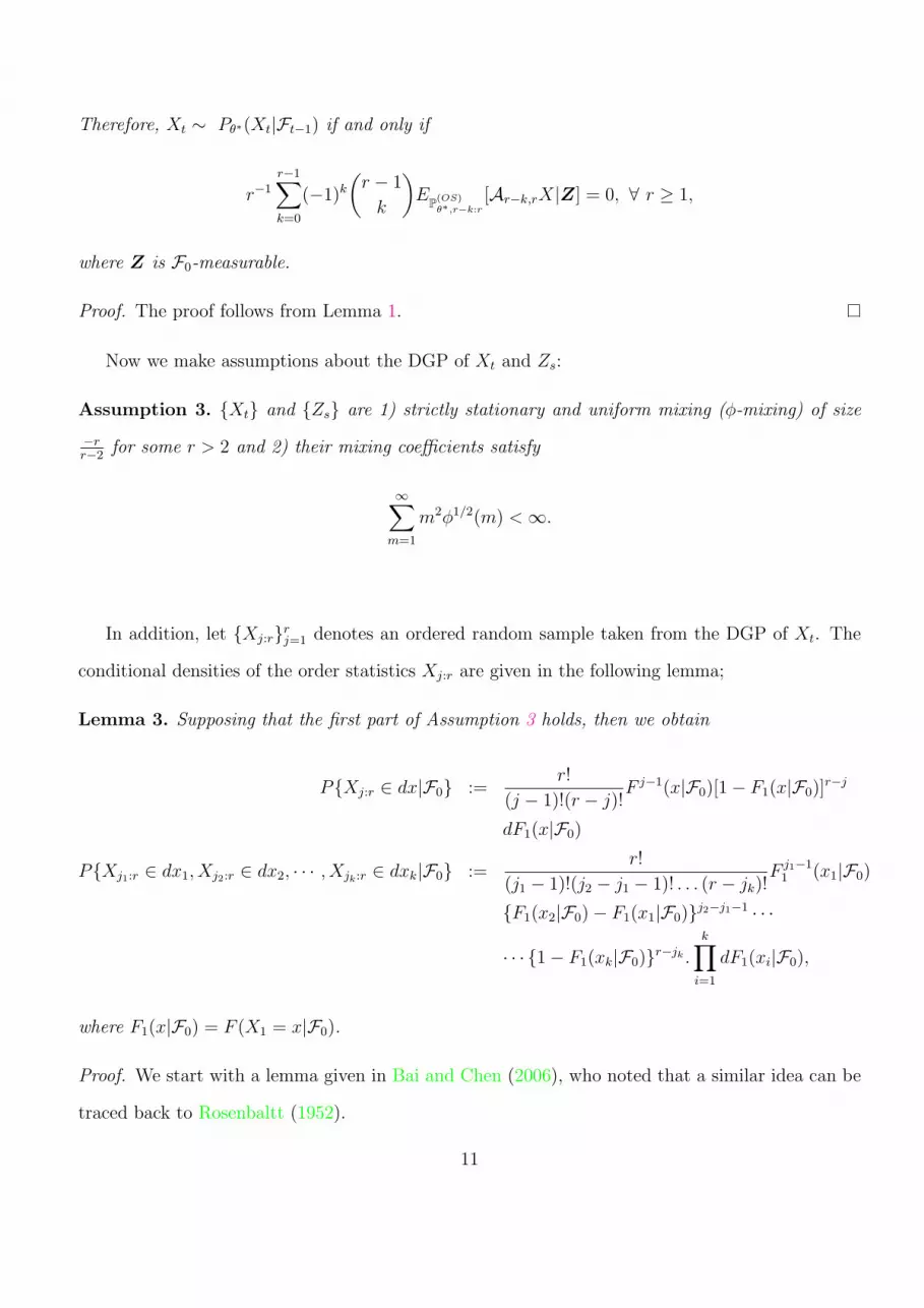
Therefore, Xt ∼ Pθ∗(Xt|Ft−1) if and only if

r−1

r−1∑

k=0

(−1)k

(r − 1

k

)E

P(OS)θ∗,r−k:r

[Ar−k,rX|Z] = 0, ∀ r ≥ 1,

where Z is F0-measurable.

Proof. The proof follows from Lemma 1.

Now we make assumptions about the DGP of Xt and Zs:

Assumption 3. Xt and Zs are 1) strictly stationary and uniform mixing (φ-mixing) of size

−rr−2

for some r > 2 and 2) their mixing coefficients satisfy

∞∑

m=1

m2φ1/2(m) < ∞.

In addition, let Xj:rrj=1 denotes an ordered random sample taken from the DGP of Xt. The

conditional densities of the order statistics Xj:r are given in the following lemma;

Lemma 3. Supposing that the first part of Assumption 3 holds, then we obtain

PXj:r ∈ dx|F0 :=r!

(j − 1)!(r − j)!F j−1(x|F0)[1 − F1(x|F0)]

r−j

dF1(x|F0)

PXj1:r ∈ dx1, Xj2:r ∈ dx2, · · · , Xjk:r ∈ dxk|F0 :=r!

(j1 − 1)!(j2 − j1 − 1)! . . . (r − jk)!F j1−1

1 (x1|F0)

F1(x2|F0) − F1(x1|F0)j2−j1−1 · · ·

· · · 1 − F1(xk|F0)r−jk .

k∏

i=1

dF1(xi|F0),

where F1(x|F0) = F (X1 = x|F0).

Proof. We start with a lemma given in Bai and Chen (2006), who noted that a similar idea can be

traced back to Rosenbaltt (1952).

11

Lemma 4. If the random variable Xt conditional on Ft−1 has the continuous cumulative distribution

function (cdf) F1(Xt|Ft−1). Then the random variables Ut = F1(Xt|Ft−1) are IID uniform on (0, 1).

We shall derive the bivariate conditional probability density for the ordered random sample

Xj:rrj=1. The multivariate case can be shown similarly. First, define the bivariate random set

A(ω) := limδx−→0δy−→0

ω ∈ Ω : x ≤ Xm:r(ω) ≤ x + δx

⋂y ≤ Xℓ:r(ω) ≤ y + δy

for 1 ≤ m ≤ ℓ ≤ r and x ≤ y. We obtain

PA(ω)|F0 = limδx−→0δy−→0

ProbXm−1:r ≤ x

⋂x ≤ Xm:r ≤ x + δx

⋂x ≤ Xm+1:r ≤ · · · ≤ Xℓ−1:r ≤ y

⋂y ≤ Xℓ:r ≤ y + δy

⋂y + δy ≤ Xℓ+1:r ≤ Xℓ+2:r ≤ · · · ≤ Xr:r

= Prob

m−1⋂

j=1

F (Xetj |Fetj−1) ≤ Fetj(x|Fetj−1)︸ ︷︷ ︸

exact r − 1 observations of Xtir

i=1 are less than x

⋂F (Xetm|Fetm−1) ∈ dFetm(x|Fetm−1)

ℓ−1⋂

j=m+1

Fetj(x|Fetj−1) ≤ F (Xetj |Fetj−1) ≤ Fetj(y|Fetj−1)︸ ︷︷ ︸

ℓ − m − 1 observations of Xtir

i=1 are in [x, y]

⋂F (Xetℓ|Fetℓ−1) ∈ dFetℓ(y|Fetℓ−1)

r⋂

j=ℓ+1

F (Xetℓ+1|Fetℓ+1−1) ≥ F (y|Fetℓ+1−1)

︸ ︷︷ ︸exact r − ℓ observations are greater or equal to y

∣∣∣∣∣∣∣∣∣∣

F0

,

where tj is the true time of the order statistics Xj:r in the random sample. Lemma 4 and the strict

stationarity of Xt (i.e. F (Xt|Ft−1) = F (Xt+τ |Ft+τ−1)) yield

PA(ω)|F0 = Prob

m−1⋂

j=1

Uetj ≤ F1(x|F0)⋂

Uetm ∈ dF1(x|F0)ℓ−1⋂

j=m+1

F1(x|F0) ≤ Uetj ≤ F1(y|F0)

⋂Uetℓ ∈ dF1(y|F0)

r⋂

j=ℓ+1

Uetj ≥ F1(y|F0)

.

12

Since Uetjrj=1 are IID, the conventional argument for deriving bivariate probability densities for

IID order statistics can be applied. Therefore, we obtain the main results.

Lemma 5. Suppose that under the null hypothesis (H0), Xt has the cdf F1(Xt|Ft−1) and the pdf

f1(Xt|Ft−1) then the operator Aj,rX as given in Lemma 2 can be written as

Aj,rX := 1 + Xf1(X|F0)

j − 1

F1(X|F0)− r − j

1 − F1(X|F0)

+ X

f′

1(X|F0)

f1(X|F0).

Hence, the L-moment conditions can be written as

r−1

r−1∑

k=0

(−1)k

(r − 1

k

)EP (Z)

[g(Zt).E

P(OS)θ∗,r−k:r

[Ar−k,rX|Z]]

= 0 ∀ r ≥ 1,

where g(•) is any function in the totally revealing space as defined in Stinchcombe and White (1998).

Remark 2.1. According to Stinchcombe and White (1998), the revealing functions g(•) for con-

structing consistent specification tests should be chosen in the class HG := hτ : hτ (x) = G(x′

τ), τ ∈

Rk+1, where x = (1, x

′

)′

and G is analytic. The exponential function expτ ′

x as proposed by

Bierens (1990) is a special case.

By the same argument as Hosking (1992), in view of Lemma 5 and r−1∑r−1

k=0(−1)k(

r−1k

)= 0,

the L-moment conditions given in Lemma 2 can be represented as a probability weighed function

(PWF);

∫

Rk

g(Z)

∫ 1

0

X(F )

f1(X(F )|Z)

[P ∗

r−1(F ) − P ∗∗r−1(F )

]+

f′

1(X(F )|Z)

f1(X(F )|Z)P ∗∗∗

r−1(F )

dFdPZ = 0,

(2.10)

13

where

P ∗r =

r∑

k=0

p∗r,kFk−1

P ∗∗r =

r∑

k=0

p∗∗r,kF k

1 − F

P ∗∗∗r =

r∑

k=0

p∗∗∗r,k F k,

with

p∗r,k = (−1)r−k(r − k)

(r

k

)(r + k

k

)

p∗∗r,k = (−1)r−kk

(r

k

)(r + k

k

)

p∗∗∗r,k = (−1)r−k

(r

k

)(r + k

k

).

Supposing that we have samples of (Xst ,Zs) for s = 1, . . . , T and t = 1, . . . , T , in view of Hosking

(1992) the sample analogue of the L-moment condition in Lemma 2 is the standard U-statistics as

given by

MT,r = T−1

T∑

s=1

(T

r

)−1 ∑· · ·∑

1≤t1≤t2≤···≤tr≤T

r−1

r−1∑

k=0

(−1)k

(r − 1

k

)g(Zs)Ar−k,r(X

str−k:T |Zs),

where Ar−k,r is defined in Lemma 5; the inner sum is the sample estimate of L-moments for an

initial value Z0; and the outer sum is the sample estimate of the moment of g(Z0).

Moreover, the sample estimate of the L-moment condition based on the PWF is

NT,r = T−1

T∑

s=1

g(Zs)T−1

T∑

t=1

Xs

t:T

f1(X

st:T |Zz)

[P ∗

r−1(t/T ) − P ∗∗r−1(t/T )

]+

f′

1(Xst:T |Zs)

f1(Xst:T |Zs)

P ∗∗∗r−1(t/T )

.

Since it is straightforward to prove that |MT,r −NT,r| = op(T−1), the asymptotic distribution of the

statistics MT,r is similar to that of NT,r which can be derived by using the central limit theorem for

14

the weighted sum of functionals of the order statistics of weakly dependent data. Before deriving

the asymptotic distribution for MT,r, we are going to state Theorem 1.

Let TT := T−1∑T

t=1

∑Kj=1 PT,j(t/T )hj(Xt:T ) denotes the weighted sum of functionals of the order

statistics Xt:T . Let (a, b)− and (a, b)+ denote the minimum and the maximum of (a, b) respectively.

We begin with some further assumptions

Assumption 4. The functions hj, ∀ j = 1, · · · , K are absolutely continuous on (F−1(ǫ), F−1(1−ǫ))

for all ǫ > 0, h′

j ∀ j = 1, · · · , K exist a.s. and |h′

j| ≤ Rj a.s., where Rj ∀ j = 1, · · · , K are reproduc-

ing U-shaped (or increasing) function. For a large T , |PT,j| ≤ φj with∫ 1

0q(F )Rj(X(F ))φj(F )dF <

∞, where q(t, θ) = K[t(1 − t)]1/2−θ ∀ 0 < θ ≤ 1/2.

Assumption 5. |hj| ≤ Mj[(1−dF )]−αj for some generic constants Mj and |PT,j(0)|, |PT,j(1)+ =

o(T 1/2−αj).

PT,j −→ Pj a.s. (2.11)

T 1/2

∫ 1

0

PT,j(F )1(X ∈ (F−1(1/T ), F−1(1 − 1/T )) − Pjhj(X(F ))dF −→ 0. (2.12)

Assumption 6. E[|g(Z)|2(r+δ) < ∞ for some r ≥ 2 and δ > 0.

Theorem 1. Supposing that Assumptions 3-5 hold, then

T 1/2(TT − T) =⇒ N(0, σ2),

where T =∫

R

∑Kj=1 Pj(F )hj(X(F ))dF ; and

σ2 =

∫

R2

σ(F (X), F (Y ))K∑

j=1

K∑

k=1

Pj(F (X))Pk(F (Y ))h′

j(X)h′

k(Y )dF (X)dF (Y )

with σ(F,G) := [(F (X), G(Y ))−−F (X).G(Y )]+∑∞

j=2(F1,j(X,Y )−F (X).G(Y ))+∑∞

j=2(F1,j(Y,X)−

F (X).G(Y )), where F1,j(X,Y ) = ProbXj = Y |X1 = X.

15

Proof. See Appendix.

Now let’s define

NT,r,s = T−1

T∑

t=1

Xst:T

f1(X

st:T |Zs)

[P ∗

r−1(t/T ) − P ∗∗r−1(t/T )

]+

f′

1(Xst:T |Zs)

f1(Xst:T |Zs)

P ∗∗∗r−1(t/T )

,

hZ,1(X) = Xf1(X|Z), hZ,2(X) = Xf1(X|Z), and hZ,3 = Xf

′

1(X|Z)

f1(X|Z).

An application of Theorem 1 yields

Corollary 2. If the functions hZ,i (i=1,2, and 3), P ∗r−1, P ∗∗

r−1 and P ∗∗∗r−1 satisfy Assumptions 3-5,

then

T 1/2N

T,r,s =⇒ Ws,

where Ws ∼ N(0, σ2(Zs)) and

σ2(Zs) =

∫

R2

σ(F1(X|Zs), F1(Y |Zs))

hZ,1(X)P ∗

r−1(F1(X|Zs)) + hZ,2P∗∗r−1(F1(X|Zs))

+ hZ,3P∗∗∗r−1(F1(X|Zs))

hZ,1(Y )P ∗

r−1(F1(Y |Zs)) + hZ,2P∗∗r−1(F1(Y |Zs))

+ hZ,3P∗∗∗r−1(F1(Y |Zs))

dF1(X|Zs)dF1(Y |Zs).

Furthermore, supposing that E|σ(Z)|2(r+δ) < ∞ for some r > 2 and δ > 0 and Assumption 6 holds

we have

T 1/2NT,r =⇒ N(0, σ∗2) (2.13)

TNT,r =⇒ N1(0, 1)N2(0, σ∗∗2) (2.14)

where N1(0, 1) and N2(0, σ∗∗2) are independent normal random variables; σ∗2 = E2

P (Z)

[g(Z)σ(Z)

];

and

σ∗∗2 = E[g2(Z1)σ2(Z1)] + 2

∞∑

j=2

E[g(Z1)σ(Z1)g(Zj)σ(Zj)].

16

Proof. The first part follows from Theorem 1. For the second part of the theorem, we first deal

with (2.13), i.e. the asymptotic distribution of T 1/2NT,r = T−1∑T

s=1 g(Zs)T−1/2N

T,r,s. Hence, by

the first part, we have

|T 1/2NT,r − T−1

T∑

s=1

g(Zs)Ws| = op(1). (2.15)

Now, we need to derive the asymptotic distribution of T−1∑T

s=1 g(Zs)Ws. Since T 1/2NT,r,s is

conditioned on the initialization process Zs and the variance of the limiting random variable Ws

depends on Zs, we have

T−1

T∑

s=1

g(Zs)W(0, σ2(Zs)) =⇒∫

supp(Z)

g(Z)W(0, σ2(Z))dF (Z),

which is a mixed normal distribution.

Moreover, Lemma 7 asserts that W is independent of Zs, thus∫

supp(Z)g(Z)W(0, σ2(Z))dF (Z)

d=

N(0, 1)∫

supp(Z)g(Z)σ(Z)dF (Z) and Equation (2.13) follows. To prove Equation (2.14), note that

again by Lemma 7

T−1/2

T∑

s=1

g(Zs)W(0, σ2(Zs))d= N(0, 1)T−1/2

T∑

s=1

g(Zs)σ(Zs).

An application of the central limit theorem for stationary mixing process in Lin and Lu (1989,

pp. 51) yields

T−1/2

T∑

t=1

g(Zt)σ(Zt) =⇒ N2(0, σ∗∗2)

By the same argument as Corollary 2, we obtain the asymptotic multivariate distribution of the

multivariate L-statistics N′

T,N = NT,1, · · · ,NT,r, · · · ,NT,N;

Corollary 3.

T 1/2N

′

T,N =⇒ N (0,Σ∗), (2.16)

17

where Σ∗ = Σ∗1,1, · · · , Σ∗

r,q, · · · , Σ∗N,N, and

Σ∗r,q := E2

P (Z)

[g(Z)Σr,q(Z)

],

Σr,q(Z) =

∫

R2

σ(F1(X|Z), F1(Y |Z))

hZ,1(X)P ∗

r−1(F1(X|Z)) + hZ,2P∗∗r−1(F1(X|Z))

+ hZ,3P∗∗∗r−1(F1(X|Z))

hZ,1(Y )P ∗

q−1(F1(Y |Z)) + hZ,2P∗∗q−1(F1(Y |Z))

+ hZ,3P∗∗∗q−1(F1(Y |Z))

dF1(X|Z)dF1(Y |Z).

2.3 Criterion Test Functions

2.3.1 Exponential revealing functions

In the light of Corollary 3, we obtain the GMLM test;

Mg := TN′

TΣ∗−1NT =⇒ χ2(N).

This suggests a standard GMM test as long as we can consistently estimate the dependence kernel

σ(F1(X|Z), F1(Y |Z)) of the covariance matrix Σ∗. We will come back to this issue in the next

section.

However, the GMM test is not feasible unless we know the functional form of the the revealing

function g(Z). A candidate function is the exponential function as suggested by the following

lemma;

Lemma 6 (Bierens, 1990, Lemma 1). Let ν be a random variable or vector satisfying E|ν| < ∞

and let x be a bounded random vector in Rk such that PE[ν|x] = 0 < 1. Then the set S = t ∈

Rk : E[ν. expt′x] = 0 has Lebesgue measure zero.

The issue of choosing t is discussed in Theorem 4 of Bierens (1990). That is, given a point

t0 ∈ Rk, real numbers γ > 0 and ρ ∈ (0, 1). Let t = argmaxt∈RkM(t), where M signifies the

18

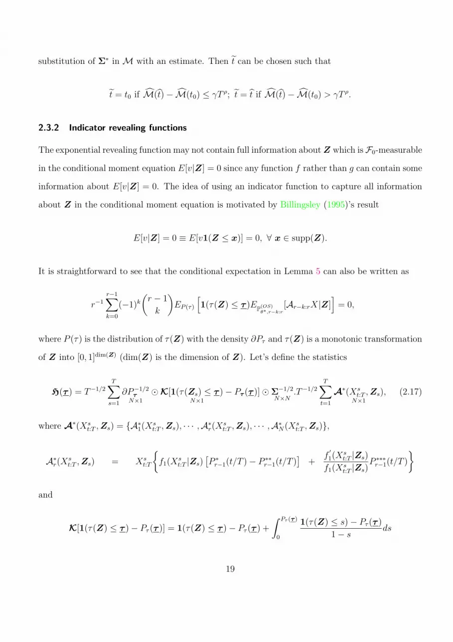
substitution of Σ∗ in M with an estimate. Then t can be chosen such that

t = t0 if M(t) − M(t0) ≤ γT ρ; t = t if M(t) − M(t0) > γT ρ.

2.3.2 Indicator revealing functions

The exponential revealing function may not contain full information about Z which is F0-measurable

in the conditional moment equation E[v|Z] = 0 since any function f rather than g can contain some

information about E[v|Z] = 0. The idea of using an indicator function to capture all information

about Z in the conditional moment equation is motivated by Billingsley (1995)’s result

E[v|Z] = 0 ≡ E[v1(Z ≤ x)] = 0, ∀ x ∈ supp(Z).

It is straightforward to see that the conditional expectation in Lemma 5 can also be written as

r−1

r−1∑

k=0

(−1)k

(r − 1

k

)EP (τ)

[1(τ(Z) ≤ τ )E

P(OS)θ∗,r−k:r

[Ar−k:rX|Z]]

= 0,

where P (τ) is the distribution of τ(Z) with the density ∂Pτ and τ(Z) is a monotonic transformation

of Z into [0, 1]dim(Z) (dim(Z) is the dimension of Z). Let’s define the statistics

H(τ ) = T−1/2

T∑

s=1

∂P−1/2τ

N×1

⊙ K[1(τ(Zs) ≤ τ )N×1

− Pτ(τ )] ⊙ Σ−1/2

N×N.T−1/2

T∑

t=1

A∗(Xs

t:T ,Zs)N×1

, (2.17)

where A∗(Xs

t:T ,Zs) = A∗1(X

st:T ,Zs), · · · ,A∗

r(Xst:T ,Zs), · · · ,A∗

N(Xst:T ,Zs),

A∗r(X

st:T ,Zs) = Xs

t:T

f1(X

st:T |Zs)

[P ∗

r−1(t/T ) − P ∗∗r−1(t/T )

]+

f′

1(Xst:T |Zs)

f1(Xst:T |Zs)

P ∗∗∗r−1(t/T )

and

K[1(τ(Z) ≤ τ ) − Pτ (τ )] = 1(τ(Z) ≤ τ ) − Pτ (τ ) +

∫ Pτ (τ)

0

1(τ(Z) ≤ s) − Pτ (τ )

1 − sds

19

is the martingale transformation proposed by Khmaladze (1981).

Since by Corollary 3, the term behind ⊙ in (2.17) converges to the multivariate normality. In

addition, an application of the central limit theorem for empirical processes yields

T−1/2

T∑

s=1

∂P−1/2τ ⊙ K[1(τ(Zs) ≤ τ ) − Pτ (τ )] =⇒ B(τ ).

Thus, in view of Lemma 7, we obtain

H(τ ) =⇒ B(τ ) ⊙ N(0, I),

where I is a diagonal unity matrix; B(τ ) ∼ N (0, (τ′

, τ′

)−) is the Brownian sheet, and (a, b)−

denotes the minimum operations between all possible pairs of a and b. Hence, we can define the

following statistics:

M∗ = supτ∈[0,1]dim(Z)

H′

(τ )H(τ )

M∗∗ =

∫

[0,1]dim(Z)

H′

(τ )H(τ )dτ .

The main results can be summarized in the following theorem:

Theorem 4.

M∗ =⇒ supτ∈[0,1]N

[N′

(0, I) ⊙ B′

(τ )B(τ ) ⊙ N(0, I)].

M∗∗ =⇒∫

[0,1]N[N

′

(0, I) ⊙ B′

(τ )B(τ ) ⊙ N(0, I)]dτ .

2.3.3 Estimation of covariance matrices

As we can see, the tests are feasible if ∂Pτ and Σ(Z) can be estimated consistently. Since it is

trivial that ∂Pτ can be estimated by nonparametric kernels which are shown to be consistent, we

20

need to discuss the issue of estimating the covariance matrix Σ(Z). Let’s define

A∗∗r (X,Z) = hZ,1(X)P ∗

r−1(F1(X|Z)) + hZ,2P∗∗r−1(Fq(X|Z)) + hZ,3P

∗∗∗r−1(F1(X|Z)).

We can define the estimator

Σr,q(Z) =1

T 2

T∑

t=1

T∑

s=1

σ(F1(Xt|Z), F1(Xs|Z))A∗∗r (Xt,Z)A∗∗

q (Xs,Z),

where

σ(F1(Xt|Z), F1(Xs|Z)) = [(F1(Xt|Z), F1(Xs|Z))− − F1(Xt|Z)F1(Xs|Z)]

+∞∑

j=2

[F1,j(Xt, Xs|Z) − F1(Xt|Z)F1(Xs|Z)]

+∞∑

j=2

[F1,j(Xs, Xt|Z) − F1(Xt|Z)F1(Xs|Z)]

F1,j(X,Y |Z) = F1,j(Y |X)F1(X|Z)

and

F1,j(X|Y ) =

∫ eX0

∫ eY0

p1,j(x, y)dxdy∫ eX0

p(x)dx(X is the monotonic transformation of X from R into [0, 1])

with the kernel estimates1

p1,j(x1, xj) =1

(T − j)a(T − j)b(T − j)

T−j∑

t=1

K1

(x1 − Xt

a(T − j)

)K2

(xj − Xt+j

b(T − j)

)

p(xj) =1

Tc(T )

T∑

t=1

K2

(xj − Xt

c(T )

),

For the consistency of Σ(Z), we make some assumptions:

1An alternative method for estimating a conditional distribution function is discussed in Hall et al. (1999). Theirapproach is shown to suffer less bias than the Nadaraya-Watson estimators and produces distribution estimators thatalways lie between 0 and 1.

21

Assumption 7. The true density p(x) is continuously differentiable to integral order ω ≥ 1 on

[0, 1] and supx∈[0,1] |∂µp(x)| < ∞ ∀ µ with µ ≤ R.

Assumption 8. F1,j(X|Y ) : [0, 1]2 −→ [0, 1] is continuously differentiable of order ω + 2 with

sup(x,y)∈[0,1]2 |DrF1,j(X|Y )| < ∞ for every 0 ≤ r ≤ ω + 2.

Assumption 9. The bandwidth parameters a(T ), b(T ) and c(T ) satisfy C1a1,T ≤ a(T ) ≤ C2a2,T ,

D1b1,T ≤ b(T ) ≤ D2b2,T and E1c1,T ≤ c(T ) ≤ E2c2,T respectively for some sequences of bounded pos-

itive constants a1,T , b1,T , c1,TT≥1 and a2,T , b2,T , c2,TT≥1 and some positive constants C1, C2, D1,

D2, E1, E2. There exists a sequence of positive constants eT −→ ∞ such that eT /c(T )ω −→ ∞,

eT /aω(T − j) −→ ∞, eT /bω(T − j) −→ ∞, and eT T 1/2b(T − j) −→ ∞.

Assumption 10 (Standard assumptions on the kernels). The kernel K satisfies (i) supx∈[0,1] |K(x)| <

∞,∫

[0,1]K(x)dx = 1,

∫[0,1]

xrK(x)dx = 0 if 1 ≤ r ≤ ω − 1 and∫

[0,1]xrK(x)dx < ∞ if r = ω; (ii) K

has a absolutely integrable Fourier transform, i.e.∫

[0,1]expiτ ′

xK(x)dx < ∞.

Assumption 11. supZ∈[0,1]k ‖hZ,i(X,Z)‖4 < ∞ ∀ i = 1, 2, 3.

Theorem 5. Under Assumptions 3 and 7-11, the estimate Σ(Z) is consistent, i.e.

Σ(Z)P

=⇒ Σ(Z).

Proof. As shown by Andrews (1991), Assumptions 3, 7, 8-10 implies that

supx∈[0,1]

|p(x) − p(x)| = Op(T−1/2c−1(T )) + Op(c

ω(T )).

Moreover, by replicating the proof in Komunjer and Vuong (2006), we can show that

sup(x,y)∈[0,1]2

|p1,j(x, y) − p1,j(x, y)| = Op(T−1/2b−1(T − j)) + Op(a

ω(T − j)) + Op(bω(T − j)).

22

Hence, we have

e−1T sup

x∈[0,1]

|p(x) − p(x)| = op(1),

e−1T sup

(x,y)∈[0,1]2|p1,j(x, y) − p1,j(x, y)| = op(1).

It follows that

e−1T

∣∣∣∣∣

∫ eX0

p(x)dx −∫ eX

0

p(x)dx

∣∣∣∣∣ ≤ Xe−1T sup

x∈[0,1]

|p(x) − p(x)|

= op(1), (2.18)

e−1T

∣∣∣∣∣

∫ eX0

∫ eY0

p1,j(x, y)dxdy −∫ eX

0

∫ eY0

p1,j(x, y)dxdy

∣∣∣∣∣ ≤ XY e−1T sup

(x,y)∈[0,1]2|p(x, y) − p(x, y)|

= op(1). (2.19)

Equations (2.18) and (2.19) and the Slutsky lemma yield |F1,j(X|Y ) − F1,j(X, Y )| = op(1). Thus,

|σ(•, •) − σ(•, •)| = op(1).

Since

∣∣∣Σr,q(Z) − Σr,q(Z)∣∣∣ ≤ T−2

T∑

t=1

T∑

s=1

∣∣[σ(•, •) − σ(•, •)]A∗∗r (Xt,Z)A∗∗

q (Xs,Z)∣∣

≤ sup(t,s)∈[1,T ]2

‖σ(•, •) − σ(•, •)‖2T−2

T∑

t=1

T∑

s=1

‖A∗∗r (Xt,Z)A∗∗

q (Xs,Z)‖2

≤ sup(t,s)∈[1,T ]2

‖σ(•, •) − σ(•, •)‖2‖A∗∗q

2(X0,Z)‖2T−2

T∑

t,s=1

‖E[A∗∗r

2(Xt−s,Z)]

+ 2φ1/2(t − s)‖A∗∗r

2(Xt−s,Z)‖2,

where the third inequality follows from Lemma 8.

The dominated convergence theorem implies that: sup(t,s)∈[1,T ]2 ‖σ(•, •) − σ(•, •)‖2 = op(1).

23

Assumptions 3 and 11 imply that

T−2

T∑

t,s=1

‖E[A∗∗r

2(Xt−s,Z)] + 2φ1/2(t − s)‖A∗∗r

2(Xt−s,Z)‖2 < ∞.

Hence, the theorem follows.

2.4 Optimal Number of L-statistics

Because given a particular sample size T the test statistics Mg, M∗, and M∗∗ depends on the

number of L-statistics (N) implied by the Stein equation as given in Lemma 1, the power functions

of the tests are sensitive to the choice of N . Hence, N can be chosen in a such way that the sample

size needed for the tests at a given level to have the power not less than a given bound at a point of

an alternative hypothesis is minimum. In this section, we apply the principle proposed by Bahadur

(1960, 1967) to infer the optimal number of the GMLM conditions used in our test statistics for

independent data.

Consider the problem of testing the hypothesis

H0 : (X,Z) ∼ F0(X|Z)

(i.e., the conditional distribution is F0(X|Z)) against the alternative

H1 : (X,Z) ∼ Gθ(X|Z)

(i.e., the conditional distribution is Gθ(X|Z) for θ ∈ Θ2). Let MT,N(FT ) denotes a test statistic

depending on the empirical distribution of X for a given Z (FT (X|Z)). MT,N(FT ) can be one of

the tests Mg, M∗, and M∗∗ as defined in Section 2.3 with the critical region given by

MT,N(FT ) ≥ c, where c is some real number.

2limθ−→∞ Gθ(X|Z) = F0(X|Z) for nested hypotheses and Gθ(X|Z) 6= F0(X|Z), ∀ θ ∈ Θ for non-nested hypothe-ses

24

The power function of this test is the quantity PMT,N(FT ) ≥ c that varies with respect to the

sequence of alternatives Gθ(X|Z), ∀θ ∈ Θ; and its size is PMT,N(FT ) ≥ c| H0 is true. Let

PMGθ

T,N(FT ) ≥ c and PMF0T,N(FT ) ≥ c denotes the power function and the size of this test

respectively.

Now define for any β ∈ (0, 1) a real sequence cT := cT (β, θ) which satisfies the double inequality

PMGθ

T,N(FT ) > cT ≤ β < PMGθ

T,N(FT ) ≥ cT.

Then

αT (β, θ,N) := PMF0T,N ≥ cT

is the minimum size of the test MT,N for which the power at a point θ ∈ Θ is not less than β. Thus,

it is clear that the positive number

NM(α, β, θ,N) := minτ : αT (β,N) ≤ α for all m ≥ τ

is the minimum sample size necessary for the test at a level α to attain the power not less than β

at a point in the set of alternatives.

Suppose that the sample Xst , ZsT

t=1 for s = 1, . . . , T are independent identically distributed

draws from a distribution for given contexts Zs under the alternative hypothesis. In other words,

the sampling scheme is done in two steps: 1) draw an IID sample ZsTs=1; 2) for each Zs draw an

IID sample of Xst T

t=1. Bahadur (1960) shows that

NM(α, β, θ,N) ∼ 2 ln(1/α)

cM(θ,N), (2.20)

where cM(θ,N) is the Bahadur exact slope of the sequence of the test MT,N(FT ).

The optimal choice of N is the positive integer that minimizes NM(α, β, θ,N) or maximizes the

25

Bahadur exact slope cM(θ,N), i.e.

N∗ = arg maxN

cM(θ,N).

The Bahadur exact slope can be approximated by using the following theorem

Theorem 6 (Bahadur (1960, 1967)). Let for a sequence MT,N the following two conditions be

fulfilled;

MGθ

T,N

Gθ−→ b(θ,N) (2.21)

limT−→∞

T−1 ln PMF0T,N ≥ t = −k(t) (2.22)

for each t from an open interval I on which f is continuous and b(θ,N), θ ∈ Θ ∈ I. Then

cM(θ,N) = 2k(b(θ,N)).

The first part of Theorem 6 (Equation 2.21) easily follows from the central limit theorem for L-

statistics. To derive the second part (Equation 2.22), an application of the large deviations theorem

for functionals of empirical distributions as given in Hoadley (1967) results

limT−→∞

T−1 ln PMF0T,N ≥ a + uT = −KL(Ωa, F0), (2.23)

where Ωa := F ∈ Λ1 : MF0∞,N(F ) ≥ a; Λ1 is the space of conditional distribution functions on R;

uT −→ 0; KL(Q,P ) is the Kullback-Leibler information distance defined as

KL(Q,P ) =

∫ln(dQ

dP)dQ if Q is absolutely continuous with respect to P

+∞ Otherwise

and KL(Ωa, F0) = infKL(Q,F0) : Q ∈ Ωa. Keep in mind that K(∅, P ) = +∞.

26

Now, we use the transformation F0(X|Z) : R −→ [0, 1] to map the domain of distribution

functions on the space Λ1 on to [0, 1], i.e.,

Q(X|Z) = Q(F−10 (t|Z)) = Q∗(t|Z)

dQ∗(t) = q∗(t)dt,

where F−10 is the inverse function of F0. Let’s define the following quantities

Q(t,A) =K∑

k=0

(−1)k

k!φ(k)(t)(a

′

kZ)

q(t,A) =K∑

k=0

(−1)k

k!φ(k+1)(t)(a

′

kZ),

where A = a′

0, . . . ,a′

K is a K × dim(Z) vector (dim(Z) is the dimension of Z and a

′

0Z = 1);

φ(k)(t) is the k-th derivative of the standard normal c.d.f φ(t) = (2φ)−1∫ x

−∞ exp(−y2/2)dy; and

fK,0(A) =

∫

[0,1]

q(t,A) ln q(t,A)dt

fK,1(A) =

∫

[0,1]

q(t,A) − 1

fK,2(A, N) =

∫

[0,1]

m∞,N(Q(t,A)) − m∞,N(Gθ(t|Z)) dt,

where M∞,N(F ) =∫

[0,1]m∞,N(F (t))dt and Gθ(t|Z) = Gθ(F

−10 (t|Z)).

In the light of Theorem 6 and Equation 2.23, we state the following theorem

Theorem 7. The optimal number of L-statistics is given by

N∗∗ := arg limK−→∞

max[fK,0(A(N∗f )), fK,0(A(N∗

c ))],

where N∗f and N∗

c are the floor and ceiling values of N∗ which is the unique solution to the following

27

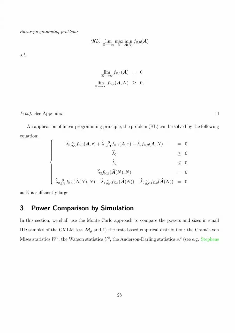
linear programming problem;

(KL) limK−→∞

maxN

minA(N)

fK,0(A)

s.t.

limK−→∞

fK,1(A) = 0

limK−→∞

fK,2(A, N) ≥ 0.

Proof. See Appendix.

An application of linear programming principle, the problem (KL) can be solved by the following

equation:

λ0∂

∂AfK,0(A, r) + λ1

∂∂A

fK,1(A, r) + λ2fK,2(A, N) = 0

λ0 ≥ 0

λ2 ≤ 0

λ2fK,2(A(N), N) = 0

λ0∂

∂NfK,0(A(N), N) + λ1

∂∂N

fK,1(A(N)) + λ2∂

∂NfK,2(A(N)) = 0

as K is sufficiently large.

3 Power Comparison by Simulation

In this section, we shall use the Monte Carlo approach to compare the powers and sizes in small

IID samples of the GMLM test Mg and 1) the tests based empirical distribution: the Cramer-von

Mises statistics W 2, the Watson statistics U2, the Anderson-Darling statistics A2 (see e.g. Stephens

28

(1974, 1978)); 2) the tests based on likelihood ratio ZK , ZA and ZC proposed by Zhang (2002);

ZK = max1≤t≤T

((t − 1/2) log

t − 1/2

TF (Xt:T )

+ (T − t + 1/2) log

T − t + 1/2

T (1 − F (Xt:T ))

)

ZA = −T∑

t=1

log(F (Xt:T ))

T − t + 1/2+

log(1 − F (Xt:T ))

t − 1/2

ZC =T∑

t=1

log

(F (Xt:T )−1 − 1

(T − 1/2)/(t − 3/4) − 1

)2

3) the tests based on conventional moments: the BM test and Kiefer & Salmon test (Kiefer and

Salmon, 1983).

First, note that the IID version of the GMLM test Mg has the following form:

Mg = TN′

T Σ−1NT , where

NT,r = T−1

T∑

t=1

Xt:T

fθ,1(Xt:T )[P ∗

r−1(t/T ) − P ∗∗r−1(t/T )] +

f′

θ,1(Xt:T )

fθ,1(Xt:T )P ∗∗∗

r−1(t/T )

∀ r = 1, . . . , N,

and Σ is an estimate of the covariance matrix of the vector of L-statistics T 1/2NT,rNr=1. Since

there is always loss in the power or distortion in the size of tests in the case when the simulation

sizes are quite small, thus it is of limited practical value to use the exact asymptotic covariance

matrix as given in Corollary 23. We shall rely on the exact bootstrap variance of the L-statistics

T 1/2NT,rNr=1 as proposed by Hutson and Ernst (2000).

The sample sizes for simulation are 15, 20, 25, and 30. The significance level or the probability

of type I error for testing the goodness of fit is 0.05, at which level the critical values of the GMLM

test, the BM test and the KS test are taken from the table of the χ2 distribution. Meanwhile,

the critical values at the level of 0.05 of the tests W 2, U2, A2 are given in Stephens (1977); and

the critical values at the 0.05 level of ZK , ZA, and ZC are computed with simulations of 1 million

replicates (see e.g. Zhang (2002).)

3In the IID case, the covariance kernel σ(F,G) = (F,G)− − FG.

29

3.1 Example 1: H0 : XtTt=1 ∼IID N(0, 1) versus H1 : XtT

t=1 ∼IID

0.5N(0, 1) + 0.5/τN(0, τ 2)

The purpose of this experiment is to examine the performance of the tests for the null of nor-

mality when the true distribution deviates slightly from normality. The degree of divergence from

Normality is controlled by τ . Simulation results are reported in Tables 1a, 1b and 1c.

We assume that the underlying distribution is the standard normal under the null hypothesis.

The alternative hypothesis is a mixture of Gaussian. For the sample size of 15, the powers and

sizes of the BM and GMLM tests are almost similar; both of them outperform the tests based on

the empirical distribution. However, the latter has better size which is very close to theoretical size

that can be attained in a large sample. For the sample size of 25 and 30, the GMLM test does

outperform the BM and KS tests in term of the powers while the sizes are almost the same. In

general, the GMLM test performs better than the tests based on the empirical distribution and the

moments in this study.

3.2 Example 2: H0 : XtTt=1 ∼IID N(0, 1) versus H1 : XtT

t=1 ∼IID N(0, 1)+

Bin(p)Poisson(µ)

The purpose of this experiment is to examine how robust the tests under our consideration against

outliers in the data. The number of outliers in a sample is controlled by the binomial probability

p. Simulation results are reported in Tables 2a, 2b and 2c.

As before, we assume that the null hypothesis is Normality. Then we generate samples of mixed

normal-Poisson random variables with sizes 15, 20, 25, 30, and 50 respectively. The probability that

outliers appear in the samples is controlled by p and the magnitudes of outliers are determined by

µ (the mean of Poisson distribution). For the case µ = 2 and p = 0.2, when the simulation size is

equal to 15 the highest power that the GMLM test can attain is 0.875 with 5 L-moments while the

highest powers are 0.61, 0.38, and 0.50 for the BM test, the KS test, and the ZC test respectively.

When µ is set equal to 6, the powers of the GMLM test still dominates all the other tests. Note

30

that the powers of the GMLM test, the KS test and the tests based on the empirical distribution

are very sensitive to µ while the BM is not very sensitive to µ; (the reason that the KS is very

sensitive to µ is that the moments of Hermite polynomials which are extremely sensitive to outliers

are normalized by their asymptotic covariance matrix). This suggests that the tests based on the

empirical distribution especially the GMLM test are very robust in a small sample with outliers.

Moreover, as either the probability of jumps (p) or the sample size increases, in general the powers

of the tests converges to 1. However, the speed of convergence of the GMLM test is very fast.

Appendices

Proof of Theorem 1. Let ξt = F (Xt); and since the functions of mixing random variables of

finite lags are mixing of the same size, thus ξt satisfies Assumption 3. In view of t/T = FT (Xt:T )

we can rewrite TT as

TT =T∑

t=1

K∑

j=1

PT,j(FT (Xt:T ))hj(Xt:T )∆FT (Xt:T )

(1)=

T∑

t=1

K∑

j=1

∫ Xt+1:T

Xt:T

PT,j(FT (Xt:T ))hj(Xt:T )∆FT (Xt:T )

(2)=

K∑

j=1

∫ +∞

−∞PT,j(FT (x))hj(x)dFT (x)

(3)=

K∑

j=1

∫ +∞

−∞PT,j(UT (u))hj(F

−1(u))dUT (u)

where (2) follows because the range of Xt is (−∞, +∞); (3) follows because UT (u) = 1T

∑Tt=1 1(ξt ≤

u) = FT (F−1(u)). Let

T =K∑

j=1

∫ +∞

−∞Pj(F (x))hj(x)dF (x),

31

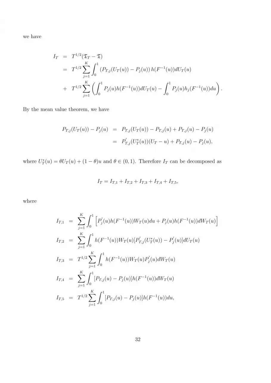
we have

IT = T 1/2(TT − T)

= T 1/2

K∑

j=1

∫ 1

0

(PT,j(UT (u)) − Pj(u)) h(F−1(u))dUT (u)

+ T 1/2

K∑

j=1

(∫ 1

0

Pj(u)h(F−1(u))dUT (u) −∫ 1

0

Pj(u)hj(F−1(u))du

).

By the mean value theorem, we have

PT,j(UT (u)) − Pj(u) = PT,j(UT (u)) − PT,j(u) + PT,j(u) − Pj(u)

= P′

T,j(U∗T (u))(UT − u) + PT,j(u) − Pj(u),

where U∗T (u) = θUT (u) + (1 − θ)u and θ ∈ (0, 1). Therefore IT can be decomposed as

IT = IT,1 + IT,2 + IT,3 + IT,4 + IT,5,

where

IT,1 =K∑

j=1

∫ 1

0

[P

′

j (u)h(F−1(u))WT (u)du + Pj(u)h(F−1(u))dWT (u)]

IT,2 =K∑

j=1

∫ 1

0

h(F−1(u))WT (u)[P′

T,j(U∗T (u)) − P

′

j (u)]dUT (u)

IT,3 = T 1/2

K∑

j=1

∫ 1

0

h(F−1(u))WT (u)P′

j (u)dWT (u)

IT,4 =K∑

j=1

∫ 1

0

[PT,j(u) − Pj(u)]h(F−1(u))dWT (u)

IT,5 = T 1/2

K∑

j=1

∫ 1

0

[PT,j(u) − Pj(u)]h(F−1(u))du,

32

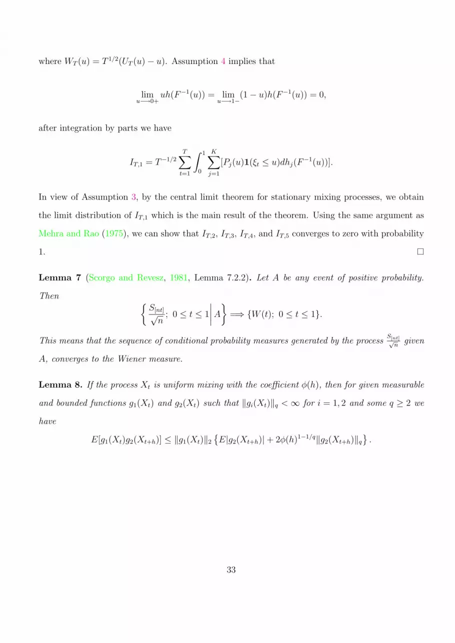
where WT (u) = T 1/2(UT (u) − u). Assumption 4 implies that

limu−→0+

uh(F−1(u)) = limu−→1−

(1 − u)h(F−1(u)) = 0,

after integration by parts we have

IT,1 = T−1/2

T∑

t=1

∫ 1

0

K∑

j=1

[Pj(u)1(ξt ≤ u)dhj(F−1(u))].

In view of Assumption 3, by the central limit theorem for stationary mixing processes, we obtain

the limit distribution of IT,1 which is the main result of the theorem. Using the same argument as

Mehra and Rao (1975), we can show that IT,2, IT,3, IT,4, and IT,5 converges to zero with probability

1.

Lemma 7 (Scorgo and Revesz, 1981, Lemma 7.2.2). Let A be any event of positive probability.

Then S[nt]√

n; 0 ≤ t ≤ 1

∣∣∣∣A

=⇒ W (t); 0 ≤ t ≤ 1.

This means that the sequence of conditional probability measures generated by the processS[nt]√

ngiven

A, converges to the Wiener measure.

Lemma 8. If the process Xt is uniform mixing with the coefficient φ(h), then for given measurable

and bounded functions g1(Xt) and g2(Xt) such that ‖gi(Xt)‖q < ∞ for i = 1, 2 and some q ≥ 2 we

have

E[g1(Xt)g2(Xt+h)] ≤ ‖g1(Xt)‖2

E|g2(Xt+h)| + 2φ(h)1−1/q‖g2(Xt+h)‖q

.

33

Proof.

E[g1(Xt)g2(Xt+h)] = E[E[g1(Xt)g2(Xt+h)|F t

−∞]]

(1)

≤ ‖g1(Xt)‖2‖E[g2(Xt+h)|F t−∞]‖2

(2)

≤ ‖g1(Xt)‖2

‖E[g2(Xt+h)|F t

−∞] − E[g2(Xt+h)]‖2 + E[g2(Xt+h)]

(3)

≤ ‖g1(Xt)‖2E[g2(Xt+h)] + 2φ(h)1−1/q‖g2(Xt+h)‖q

for q ≥ 2. The inequality (1) follows form the Cauchy-Schwartz inequality; the inequality (2) follows

from the Minskowski inequality; and the inequality (3) follows form Lemma 6.16 in Stinchcombe

and White (1998) and Theorem 14.1 in Davidson (2002) which asserts that the processes gi(Xt),

∀ i = 1, 2 are also mixing of the same sizes.

Proof of Theorem 7. In view of Theorem 6, the approximation of the Bahadur exact slope can

be done by solving the Kullback-Leibler entropy minimization problem as given in the RHS of

Equation 2.23. Let’s rewrite this entropy minimization problem as

(KL-0) minq∗

∫

[0,1]

q∗ ln(q∗)dt

s.t.

∫

[0,1]

q∗(t)dt = 1

∫

[0,1]

m∞,N(Q∗(t|Z)) − m∞,N(Gθ(t|Z)) dt ≥ 0.

The problem (KL-0) can be solved by setting up a Lagrangian equation–the optimization of this

equation gives rise to a nonlinear integral equation because m∞,N(Q∗(t|Z)) is a highly nonlinear

function of Q∗(t|Z). Thus, it is difficult to solve or approximate the solution of this nonlinear

integral equation. We apply asymptotic expansions of the conditional distribution Q∗(t|Z) and its

34

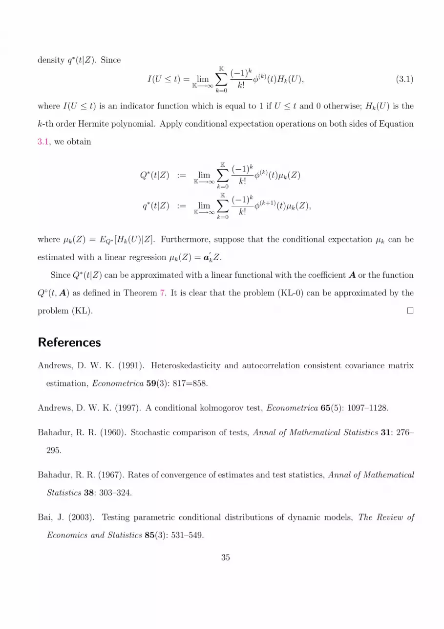
density q∗(t|Z). Since

I(U ≤ t) = limK−→∞

K∑

k=0

(−1)k

k!φ(k)(t)Hk(U), (3.1)

where I(U ≤ t) is an indicator function which is equal to 1 if U ≤ t and 0 otherwise; Hk(U) is the

k-th order Hermite polynomial. Apply conditional expectation operations on both sides of Equation

3.1, we obtain

Q∗(t|Z) := limK−→∞

K∑

k=0

(−1)k

k!φ(k)(t)µk(Z)

q∗(t|Z) := limK−→∞

K∑

k=0

(−1)k

k!φ(k+1)(t)µk(Z),

where µk(Z) = EQ∗ [Hk(U)|Z]. Furthermore, suppose that the conditional expectation µk can be

estimated with a linear regression µk(Z) = a′

kZ.

Since Q∗(t|Z) can be approximated with a linear functional with the coefficient A or the function

Q(t,A) as defined in Theorem 7. It is clear that the problem (KL-0) can be approximated by the

problem (KL).

References

Andrews, D. W. K. (1991). Heteroskedasticity and autocorrelation consistent covariance matrix

estimation, Econometrica 59(3): 817=858.

Andrews, D. W. K. (1997). A conditional kolmogorov test, Econometrica 65(5): 1097–1128.

Bahadur, R. R. (1960). Stochastic comparison of tests, Annal of Mathematical Statistics 31: 276–

295.

Bahadur, R. R. (1967). Rates of convergence of estimates and test statistics, Annal of Mathematical

Statistics 38: 303–324.

Bai, J. (2003). Testing parametric conditional distributions of dynamic models, The Review of

Economics and Statistics 85(3): 531–549.

35

Bai, J. and Chen, Z. (2006). Testing multivariate distributions, Working paper, New York University

.

Barbour, A. D. and Chen, L. H. Y. (2005). Stein’s Method and Applications, World Scientific,

London, Singapore, Hong Kong.

Bierens, H. J. (1990). A consistent conditional moment test of functional form, Econometrica

58(6): 1443–1458.

Billingsley, P. (1995). Probability and Measure, Wiley & Sons, New York.

Bontemps, C. and Meddahi, N. (2005). Testing normality: A gmm approach, Journal of Econo-

metrics 124: 149–186.

Bontemps, C. and Meddahi, N. (2006). Testing distributional assumptions: A GMM approach,

Working paper, Universite de Montreal .

Borovkova, S., Burton, R. and Dehling, H. (2001). Limit theorems for functional of mixing pro-

cesses with applications to u-statistics and dimension estimation, Transactions of the American

Mathematical Society 20(11): 4261–4318.

Bose, A. (1998). A glivenko-cantelli theorem and strong laws for l-statistics, Journal of Theoretical

Probability 11(4): 921–933.

Chow, Y. S. and Teicher, H. (1997). Probability Theory, Springer-Verlag.

Corradi, V. and Swanson, N. R. (2006). Bootstrap conditional distribution tests in the presence of

dynamic misspecification, Journal of Econometrics, forthcoming .

Davidson, J. (2002). Stochastic Limit Theory, Oxford University Press.

Davydov, Y. (1996). Weak convergence of discontinuous processes to continuous ones, Theory of

Probab. and Math. Stat., Proceedings of the sem. deducated to memory of Kolmogorov, Ibragimov

I. and Zaitsev A. (Eds.), Gordon and Breach, pp. 15–18.

36

Dudley, R. M. (1999). Uniform Central Limit Theorems, Cambridge University Press.

Fiorentini, G., Sentana, E. and Calzolari, G. (2004). On the validity of the jarque-bera normality

test in conditionally heteroskedastic dynamic regression models, Economic Letters 83(3): 307–

312.

Hall, P., Wolff, R. C. L. and Yao, Q. (1999). Methods for estimating a conditional distribution

function, Journal of American Statistical Association 94: 154–163.

Hoadley, A. B. (1967). On the probability of large deviations of functions of several empirical

c.d.f.’s, Annal of Mathematical Statistics 38: 360–381.

Hosking, J. R. M. (1990). L-moments: Analysis and estimation of distributions using linear combi-

nations of order statistics, Journal of the Royal Statistical Society, Series B 52(1): 105–124.

Hosking, J. R. M. (1992). Moments or l moments? an example comparing two measures of distri-

butional shape, The American Statistician 46(3): 186–189.

Hutson, A. D. and Ernst, M. D. (2000). The exact bootrap mean and variance of an l-estimator,

Journal of Royal Statistical Society B 62: 89–94.

Jlrech, T. J., Velis, D. R., Woodbury, A. D. and Sacchi, M. D. (2000). L-moments and c-moments,

Stochastic Environmental Research and Risk Assessment 14: 50–68.

Khmaladze, E. V. (1981). Martingale approach in the theory of goodness-of-tests, Theory of Prob-

ability and its Applications XXVI: 240–257.

Kiefer, N. M. and Salmon, M. (1983). Testing normality in econometric models, Economics Letters

11: 123–127.

Komunjer, I. and Vuong, Q. (2006). Efficient conditional quantile estimation: The time series case,

Working paper .

Lehmann, E. L. (2000). Testing Statistical Hypotheses, Springer-Verlag.

37

Li, F. and Tkacz, G. (2006). A consistent bootstrap test for conditional density functions with

time-series data, Journal of Econometrics, forthcoming .

Lin, C. (2006). A robust test for parameter homogeneity in panel data models, Working paper,

University of Michigan .

Lin, Z. and Lu, C. (1989). Limit Theory for Mixing Dependent Random Variables, Science Press,

New York, Beijing.

Mason, D. M. and Shorack, G. R. (1992). Necessary and sufficient conditions for asymptotic

normality of l-statistics, The Annals of Probability 20(4): 1779–1804.

Mehra, K. L. and Rao, S. (1975). On functions of order statistics for mixing processes, The Annals

of Statistics 3(4): 874–883.

Perez, N. H. (2005). A theoretical comparison between moments and l-moments, Working paper,

University of Toronto .

Rosenbaltt, M. (1952). Remarks on a multivariate transformation, Annals of Mathematical Statistics

23: 470–472.

Ruymgaart, F. H. and Zuijlen, M. C. A. V. (1977). Asymptotic normality of linear combinations

of functions of order statistics in the non-iid case, Indag. Math. 80: 432–447.

Sankarasubramanian, A. and Srinivasan, K. (1999). Investigation and comparison of sampling

properties of l-moments and conventional moments, Journal of Hydrology 218: 13–34.

Scorgo, M. and Revesz, P. (1981). Strong Approximations in Probability and Statistics, Academic

Press, New York, San Francisco, London.

Sen, P. K. (1978). An invariance principle for linear combinations of order statistics, Z. Wahrschein-

lichkeitstheorie Verw. Geibiete 42: 327–340.

Serfling, R. J. (1984). Generalized l-, m-, and r-statistics, The Annals of Statistics 12(1): 76–86.

38

Shorack, G. R. (1972). Functions of order statistics, The Annals of Mathematical Statistics

43(2): 412–427.

Stein, C. (1972). A bound for the error in the normal approximation to the distribution of a sum of

dependent random variables, Proc. Sixth Berkeley Symp. Math. Statist. Probab. 2 pp. 583–602.

Stein, C. (1986). Approximate computation of expectations, Institute of Mathematical Statistics,

Hayward, California.

Stephens, M. A. (1974). Edf statistics for goodness-of-fit and some comparisons, Journal of Amer-

ican Statistical Association 69: 730–737.

Stephens, M. A. (1977). Goodness of fit the extreme value distribution, Biometrika 64: 583–588.

Stephens, M. A. (1978). Goodness of fit with special reference to tests for exponentiality, Technical

Report, Stanford University .

Stinchcombe, M. B. and White, H. (1998). Consistent specification testing with nuisance parameters

present only under the alternative, Econometric Theory 14: 295–325.

White, H. (2001). Asymptotic Theory for Econometricians, 2 edn, Academic Press, New York,

London, Tokyo.

Wu, W. B. (2005). Empirical processes of dependent random variables, Technical report, University

of Chicago .

Yoshihara, K. (1976). Limiting behaviour of u-statistics for stationary, absolutely regular processes,

Z. Wahrscheinlichkeitstheorie Verw. Geibiete 35: 237–252.

Zhang, J. (2002). Powerful goodness-of-fit tests based on likelihood ratio, Journal of Royal Statistical

Society B 64: 281–294.

Zheng, J. X. (2000). A consistent test of conditional parametric distributions, Econometric Theory

16: 667–691.

39