Moment of Analytic Statics
70
C HAPTER 1 Moment of Analytic Statics 1.1 Definition-I Moment of a Force Let F be a force and p be the ⊥ distance of its line of action from the fixed point O, then moment of F about O =( F)( p). Figure 1.1 Note that: The moment vanishes if either F = 0 or p = 0 i.e. if the point about which the 1
-
Upload
khangminh22 -
Category
Documents
-
view
1 -
download
0
Transcript of Moment of Analytic Statics

CH
AP
TE
R 1Moment of Analytic Statics
1.1 Definition-I
Moment of a Force
Let F be a force and p be the ⊥ distance of its line of action from the fixed point O,
then moment of F about O = (F)(p).
Figure 1.1
Note that:
The moment vanishes if either F = 0 or p = 0 i.e. if the point about which the
1
2 CHAPTER 1: MOMENT OF ANALYTIC STATICS
moment is being taken lies on the line of action of the force.
Sign of Moment
The moment of a force F about a point O is said to be +ve or −ve according as the
force rotates the body in an anticlockwise or clockwise direction respectively.
1.2 Definition-II
Moment of a Force
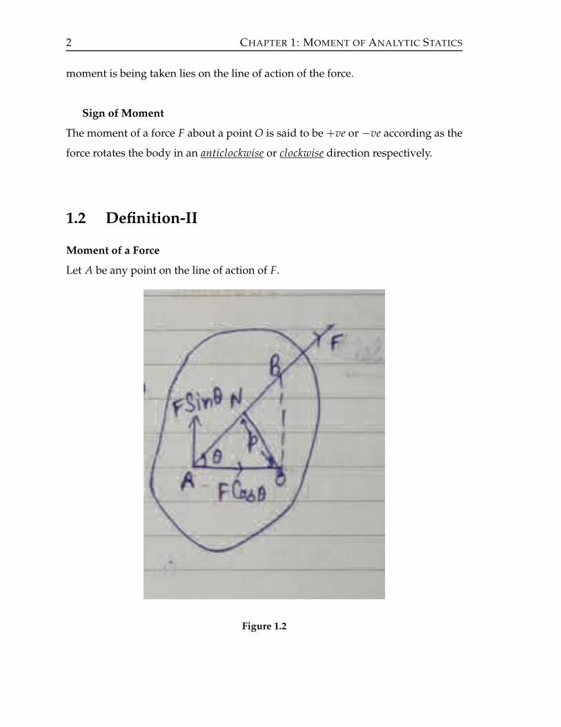
Let A be any point on the line of action of F.
Figure 1.2

CHAPTER 1: MOMENT OF ANALYTIC STATICS 3
AO = γ and ∠OAN = θ then the moment of F about O
= (F)(p)
= (F)(ON)
= (F)(γsinθ)
= (γ)(Fsinθ)
= γFsinθ
= AO (Resolved part of F perpendicular to AO)
(MF)O = γ× F.
Varignon’s Theorem of Moments
The algebraic sum of moments of two forces about any point in their plane is equal
to the moment of their resultant about the same point, i.e
(MP)0 + (MQ)0 = (MR)0.
Note. Resultant of Two ‖ Forces The resultant of two like parallel forces P and Q acting
Figure 1.3
at A&B is equivalent to a force P + Q acting in the same direction at C such that
AC× P = CB×Q
Mohammad Arif
Pencil
4 CHAPTER 1: MOMENT OF ANALYTIC STATICS
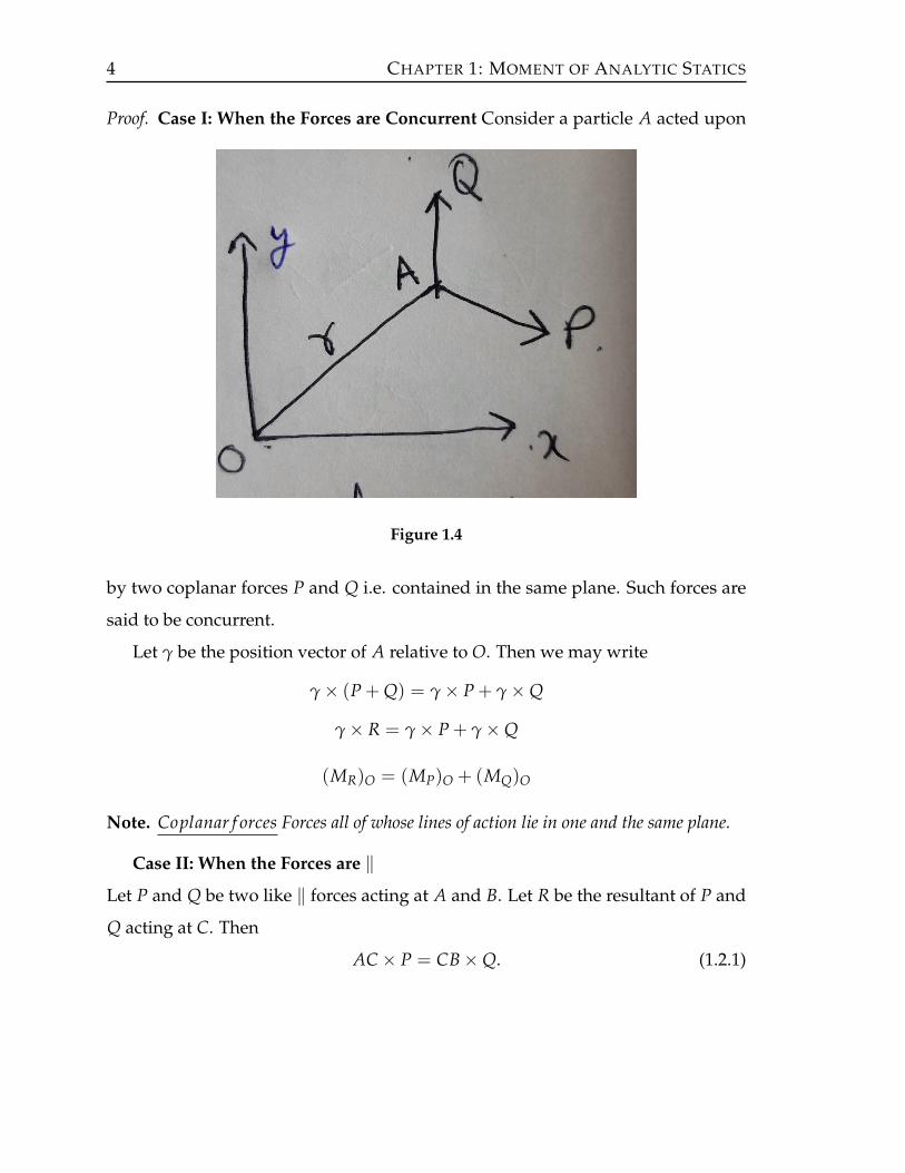
Proof. Case I: When the Forces are Concurrent Consider a particle A acted upon
Figure 1.4
by two coplanar forces P and Q i.e. contained in the same plane. Such forces are
said to be concurrent.
Let γ be the position vector of A relative to O. Then we may write
γ× (P + Q) = γ× P + γ×Q
γ× R = γ× P + γ×Q
(MR)O = (MP)O + (MQ)O
Note. Coplanar f orces Forces all of whose lines of action lie in one and the same plane.
Case II: When the Forces are ‖
Let P and Q be two like ‖ forces acting at A and B. Let R be the resultant of P and
Q acting at C. Then
AC× P = CB×Q. (1.2.1)

CHAPTER 1: MOMENT OF ANALYTIC STATICS 5
Figure 1.5
The sum of the moments of P and Q about O
= OA× P + OB×Q
= (OC + CA)× P + (OC + CB)×Q
= OC× P + CA× P + OC×Q + CB×Q
= OC× (P + Q) + CA× P + CB×Q
= OC× R− AC× P + CB×Q (∵ CA = −AC) (1.2.2)
Now
|AC× P| = ACPsinθ
|CB×Q| = CBQsinθ
From equation (1.2.1) we have
|AC× P| = |CB×Q|
=⇒ −AC× P + CB×Q = 0 (1.2.3)
Now equation (1.2.2) becomes
= OC× R + 0 = OC× R
6 CHAPTER 1: MOMENT OF ANALYTIC STATICS
=⇒ (MP)O + (MQ)O = OC× R
= (MR)O
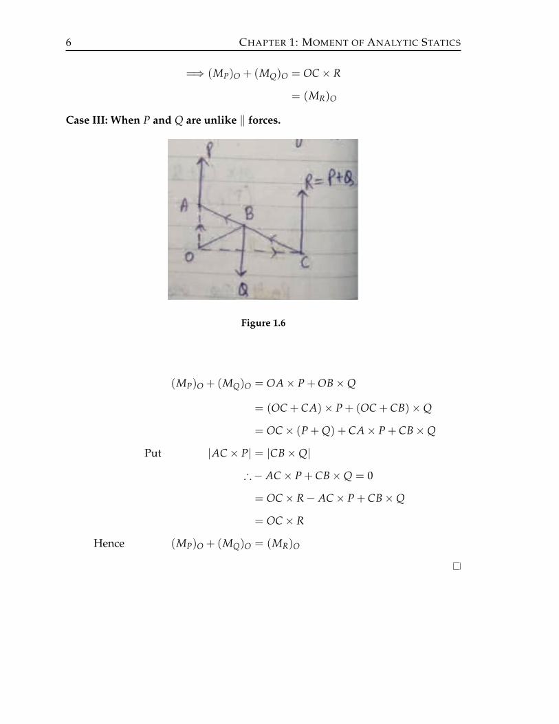
Case III: When P and Q are unlike ‖ forces.
Figure 1.6
(MP)O + (MQ)O = OA× P + OB×Q
= (OC + CA)× P + (OC + CB)×Q
= OC× (P + Q) + CA× P + CB×Q
Put |AC× P| = |CB×Q|
∴− AC× P + CB×Q = 0
= OC× R− AC× P + CB×Q
= OC× R
Hence (MP)O + (MQ)O = (MR)O

CHAPTER 1: MOMENT OF ANALYTIC STATICS 7
1.3 Generalized form of Varignon’s Theorem
The algebraic sum of moments of any number of coplanar forces about any point in
their plane is equal to the moment of their resultant about the same point.
Example 1.3.1. A force F = Fx i + Fy j acts at a point A(x1, y1). Find the moment of F
about a second point B(x2, y2).
Solution.
Figure 1.7
γ = BA
= (x1 − x2)i + (y1 − y2) j
∴ M = γ× F
=
[(x1 − x2)i + (y1 − y2) j
]×[
Fx i + Fy j]
=
[(x1 − x2)Fy − (y1 − y2)Fx
]k (∵ i× j = k and j× i = −k)
M = (x1 − x2)Fy − (y1 − y2)Fx.
Example 1.3.2. A force F = Fx i + Fy j acts at a point of coordinates x and y. Find the ⊥
distance from the line of action of F to the origin O of the system of coordinates.

8 CHAPTER 1: MOMENT OF ANALYTIC STATICS
Solution. We know that the moment of F about a point (0, 0) is given by
Fy(x− 0)− Fx(y− 0) = M (1.3.1)
Also,
M = |F|OL
OL =M|F|
=Fyx− Fxy√
F2x + F2
y
Example 1.3.3. A 10 kg force acts at an ∠ of 60o on the corner C of a 12 by 1–cm plate
ABCD. Determine the moment of force about A.
Figure 1.8

CHAPTER 1: MOMENT OF ANALYTIC STATICS 9
Solution. Resolving the given force at C acting along AD and ⊥ of AD at A we get
F = 10 cos60o i + 10 sin60o j
= 10× 12
i + 10×√
32
j
= 5i + 5√
3 j
= Fx i + Fy j
Now (MF)A = (x1 − x2)Fy + (y1 − y2)Fx
= −(1− 0)5 + (12− 0)5√
3
= −5× 1 + 5√
3× 12
= 5(12√
3− 1)
Example 1.3.4. The point (5, 3) is on the line of action of the force P making an ∠tan−1(34)
with the horizontal. Find the moment of force about the origin of coordinates.
Figure 1.9
Solution. Resolving the given forces at A acting along AB and AC we get
F = P cosθ i + P sinθ j
(MF)O = (5− 0)P sinθ − (3− 0)P cosθ
= 5P sinθ − 3P cosθ
Mohammad Arif
Pencil
Mohammad Arif
Pencil

10 CHAPTER 1: MOMENT OF ANALYTIC STATICS
= 5P(35)− 3P(
45)
= 3P− 12P5
=35
P
The moment of the force about the origin of coordinates (MF)O = 35 P
Example 1.3.5. Three forces P, Q and R act along the sides BC, CA, AB of a triangle
ABC. Show that if their resultant passes through the ortho-centre (Intersection of altitudes),
then
P sec A + Q sec B + R sec C = 0
Figure 1.10
Solution. Taking moment of force about O we have
POD + QOE + ROF = 0 (1.3.2)
Now, in4ODCODOC
= cos B (1.3.3)
in4OECOEOC
= cos A (1.3.4)
from equation (1.3.3) and (1.3.4) we have
=⇒ OEOD
=cos Acos B
Mohammad Arif
Pencil

CHAPTER 1: MOMENT OF ANALYTIC STATICS 11
OE = ODcos Acos B
(1.3.5)
Again in4ODBODOB
= cos C (1.3.6)
in4OFBOFOB
= cos A (1.3.7)
from equation (1.3.6) and (1.3.7) we haveOFOD
=cos Acos C
OF = ODcos Acos C
(1.3.8)
From equations (1.3.3), (1.3.5) and (1.3.8) we get
POD + QODcos Acos B
+ RODcos Acos C
= 0
P + Qcos Acos B
+ Rcos Acos C
= 0 (∵ OD 6= 0)
=⇒ PcosA
+Q
cos B+
Rcos C
= 0
=⇒ P sec A + Q sec B + R sec C = 0
Example 1.3.6. Three forces P, Q and R act along the sides BC, CA and AB of a triangle
ABC. Show that if their resultant passes through the incentre (Intersection of the internal
bisectors of the angles of the triangle) and the circumcentre( Intersection of the bisectors of
the sides of the triangle), thenP
cos B− cos C=
Qcos C− cos A
=R
cos A− cos B
Solution. Let O be the incentre of 4ABC. Let OD, OE, OF be the ⊥ to the sides BC,
CA and AB respectively. If r is the inradius then
OD = OE = OF = r
Taking moments about O we have
P ·OD + Q ·OE + R ·OF = 0 (1.3.9)
⇒ P · r + Q · r + R · r = 0 (1.3.10)
Mohammad Arif
Pencil

12 CHAPTER 1: MOMENT OF ANALYTIC STATICS
Figure 1.11
⇒ P + Q + R = 0 (∵ r 6= 0) (1.3.11)
⇒ R = −(P + Q) (1.3.12)
If O be the circumcentre
Figure 1.12
∴ ∠BOC = 2A
∠AOC = 2B
∠AOB = 2C
Mohammad Arif
Pencil
Mohammad Arif
Pencil

CHAPTER 1: MOMENT OF ANALYTIC STATICS 13
Taking moment of force about O
POD + QOE + ROF = 0
ODR1
= cosA
OER1
= cosB
OFR1
= cosC
PR1cosA + QR1cosB + RR1cosC = O
PcosA + QcosB + RcosC = O (1.3.13)
from equation (1.3.12) we have
PcosA + QcosB− (P + Q)cosC = 0
PcosA + QcosB− PcosC−QcosC = 0
Q(cosB− cosC)− P(cosC− cosA) = 0
QcosC− cosA
=P
cosB− cosC. (1.3.14)
Also from equation (1.3.12)
P = −(Q + R) (1.3.15)
−(Q + R)cosA + QcosB + RcosC = 0
Q(cosB− cosA) + R(cosC− cosA) = 0
QcosC− cosA
=R
cosA− cosB. (1.3.16)
From equation (1.3.14),(1.3.16) we get
PcosB− cosC
=Q
cosC− cosA=
RcosA− cosB
.
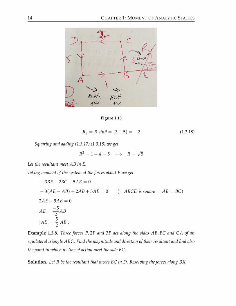
Example 1.3.7. Forces of magnitudes 1, 3, 2, 5 act along the sides of a square taken in order.
Find the magnitude and line of action of their resultant.
Solution. Resolving the forces along AB and AD
Rx = R cosθ = (1− 2) = −1 (1.3.17)
14 CHAPTER 1: MOMENT OF ANALYTIC STATICS
Figure 1.13
Ry = R sinθ = (3− 5) = −2 (1.3.18)
Squaring and adding (1.3.17),(1.3.18) we get
R2 = 1 + 4 = 5 =⇒ R =√
5
Let the resultant meet AB in E.
Taking moment of the system at the forces about E we get
− 3BE + 2BC + 5AE = 0
− 3(AE− AB) + 2AB + 5AE = 0 (∵ ABCD is square ∴ AB = BC)
2AE + 5AB = 0
AE =−52
AB
|AE| = 52|AB|.
Example 1.3.8. Three forces P, 2P and 3P act along the sides AB, BC and CA of an
equilateral triangle ABC. Find the magnitude and direction of their resultant and find also
the point in which its line of action meet the side BC.
Solution. Let R be the resultant that meets BC in D. Resolving the forces along BX

CHAPTER 1: MOMENT OF ANALYTIC STATICS 15
Figure 1.14
R cosθ = 2P− 3P cos60o − P cos60o
= 2P− 3P2− P
2
=4P− 4P
2= 0
=⇒ R cosθ = 0 (1.3.19)
Resolving along BY
R sinθ = 3P sin60o − P sin60o
= 3P√
32− P√
32
(1.3.20)
R sinθ =√
3P (1.3.21)
Squaring and adding (1.3.19) and (1.3.21) we get
R2 cos2θ + R2 sin2θ = 3P2 =⇒ R =√
3P.
16 CHAPTER 1: MOMENT OF ANALYTIC STATICS
Dividing (1.3.21) and (1.3.19) we get
R sinθ
R cosθ=
√3P0
= ∞
tanθ = tan90o =⇒ θ = 90o
Taking moment about B
2P× 0 + 3P× BE + P× 0 = R× BL
3PBC sin60o =√
3PBD sin90o (∵ θ = 90o)
BD =32
BC
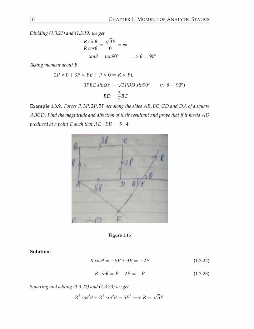
Example 1.3.9. Forces P, 3P, 2P, 5P act along the sides AB, BC, CD and DA of a square
ABCD. Find the magnitude and direction of their resultant and prove that if it meets AD
produced at a point E such that AE : ED = 5 : 4.
Figure 1.15
Solution.
R cosθ = −5P + 3P = −2P (1.3.22)
R sinθ = P− 2P = −P (1.3.23)
Squaring and adding (1.3.22) and (1.3.23) we get
R2 cos2θ + R2 sin2θ = 5P2 =⇒ R =√
5P.

CHAPTER 1: MOMENT OF ANALYTIC STATICS 17
From equation (1.3.22)
R cosθ = −2P
=⇒√
5Pcosθ = −2P
=⇒ cosθ =−2√
5From equation (1.3.23)
R sinθ = −P
=⇒ sinθ =−P√
5P
=⇒ sinθ =−1√
5=⇒ sinθ and cosθ both are negative ∴ θ lies in the third quadrant.
θ = π + tan−1(12)
Let a be the side of the square. Taking moments about A
RAE sinθ = −2Pa− 3Pa = −5Pa
AE =−5PaR sinθ
AE =−5Pa−P
AE = 5a
AE = 5(AE− DE)
AE = 5AE− 5DE
=⇒ 5DE = 4AE
∴ AE : ED = 5 : 4
Example 1.3.10. Forces 3, 4, 5, 6 kg act along the sides of a square taken in order. Find the
magnitude, direction and line of action of resultant the said of square being a.
Solution.
R cosθ = 5− 3 = 2 (1.3.24)
R sinθ = 6− 4 = 2 (1.3.25)

18 CHAPTER 1: MOMENT OF ANALYTIC STATICS
Figure 1.16
Squaring and adding (1.3.24) and (1.3.25) we get
R2 cos2θ + R2 sin2θ = 4 + 4 =⇒ R = 2√
2 kg
tanθ = 1 =⇒ θ = 45o
From equation (1.3.24)
R cosθ = 2
cosθ =2
2√
2From equation (1.3.25)
R sinθ = 2
sinθ =2
2√
2
=1√2
=⇒ sinθ and cosθ both are positive ∴ θ lies in first quadrant. Taking moments about C
R.CK sinθ = 6× CD + 3× CB
2√
2CK sin45o = 6a + 3a
2√
2CK√
2= 9a
CK =9a2

CHAPTER 1: MOMENT OF ANALYTIC STATICS 19
or CD + DK =9a2
a + DK =9a2
DK =9a2− a
=⇒ DK =7a2
.
20 CHAPTER 1: MOMENT OF ANALYTIC STATICS
1.4 Couple
Figure 1.17
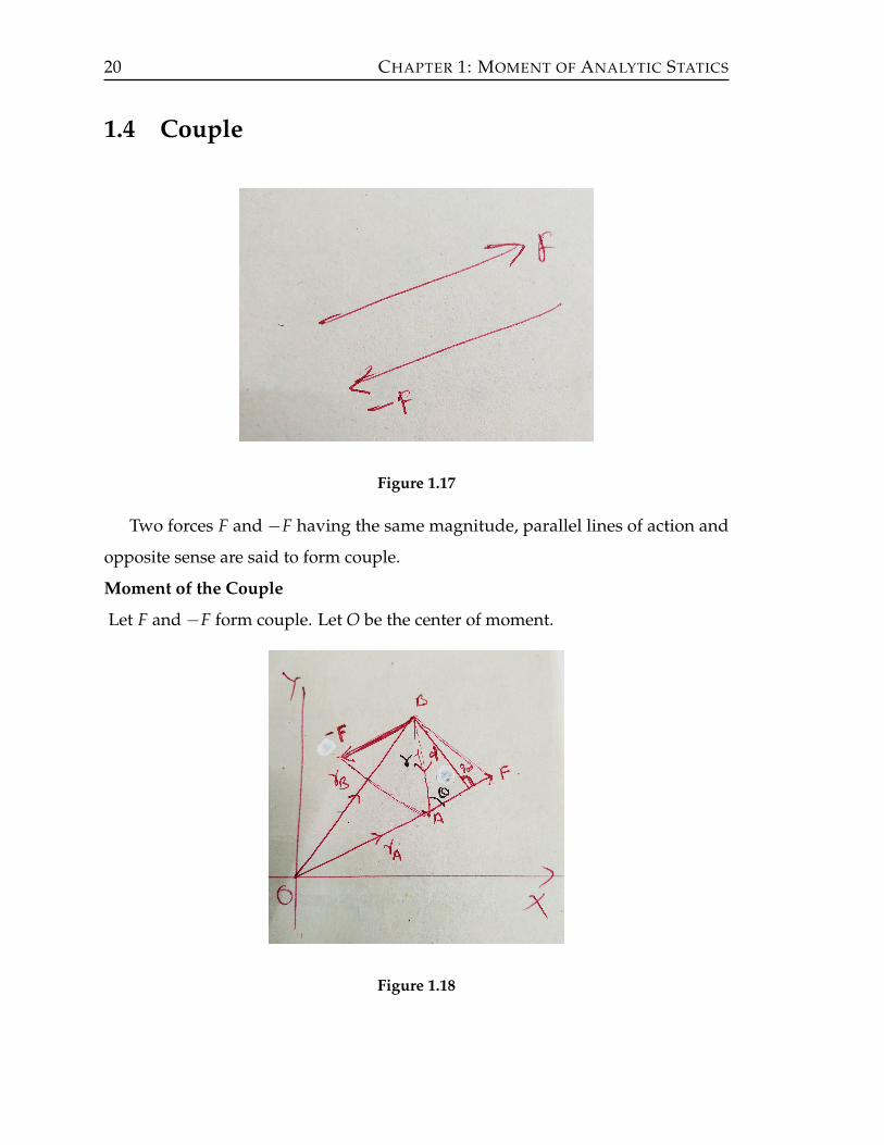
Two forces F and −F having the same magnitude, parallel lines of action and
opposite sense are said to form couple.
Moment of the Couple
Let F and −F form couple. Let O be the center of moment.
Figure 1.18

CHAPTER 1: MOMENT OF ANALYTIC STATICS 21
Now
Moment of the couple = γA × F + γB × (−F)
= (γA − γB)× F
= γ× F were γ = (γA − γB)
M = |γ× F|
= γF sinθ
= Fγ sinθ
= Fd
where d is the ⊥ distance between lines of action of F and − F (called arm of the
couple).
Notation
Couple F and − F with the ⊥ distance between their lines of action will be denoted
by (F, d).
Resultant of a Couple
Theorem 1.4.1. The resultant of any number of couples acting in the same plane on a rigid
body is a couple.
Note. If the resultant of the forces is equal to zero then system reduces to a couple
R = RXi + RY j
RX = 0
RY = 0
=⇒ forms a couple.
Example 1.4.1. ABCD is a rectangle with AB = 4cm, BC = 3cm. Forces 2, 7, 6, 10
and 5 kg weight act along AB, BC, CD, AD, and AC respectively. Show that they are
equivalent to a couple whose moment is equal to 46kg.cm.
Solution. Let ∠BAC = θ then sinθ = 35 and cosθ = 4
5 .

22 CHAPTER 1: MOMENT OF ANALYTIC STATICS
Figure 1.19
Resolving the forces along AB and 5AD cosθ we get
RX = 2− 6 + 5 cosθ
= −4 + 5× 45= 0
RY = 7− 10 + 5 sinθ
= −3 + 5× 35= 0
=⇒ RX = 0 and RY = 0. The system reduces to a couple.
Now taking the moment of the forces about A we get
M = 7× 4 + 6× 3 = 46kg.cm.
Example 1.4.2. Forces 1, 2, 3, 5, P, Q act along AB, BC, CD, DA, AC and BD
respectively and ABCD is a square of side a. Find the values of P and Q for the
system to reduce to a couple. Find also the moment of the couple.

CHAPTER 1: MOMENT OF ANALYTIC STATICS 23
Figure 1.20
Solution. Resolving the forces along AB and AD we get
RX = 1− 3 + P cos45o −Q cos45o
= −2 +P√2− Q√
2
= −2 + (P−Q)1√2
RY = 2− 5 + P sin45o + Q sin45o
= −3 +P√2+
Q√2
= −3 + (P + Q)1√2
.
If the system reduces to a couple =⇒ RX = 0 and RY = 0
=⇒ −2 + (P−Q)1√2= 0
=⇒ (P−Q) = 2√
2
− 3 + (P + Q)1√2= 0
=⇒ (P + Q) = 3√
2
=⇒ P =5√2
and Q =1√2
24 CHAPTER 1: MOMENT OF ANALYTIC STATICS
Let a be the side of square and O its center. Then the distance of O from each side = a2
The moment of couple
M = 1a2+ 2
a2+ 3
a2+ 5
a2=
11a2
.
CHAPTER 1: MOMENT OF ANALYTIC STATICS 25
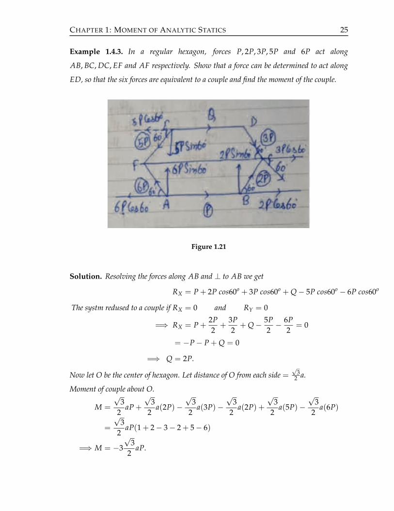
Example 1.4.3. In a regular hexagon, forces P, 2P, 3P, 5P and 6P act along
AB, BC, DC, EF and AF respectively. Show that a force can be determined to act along
ED, so that the six forces are equivalent to a couple and find the moment of the couple.
Figure 1.21
Solution. Resolving the forces along AB and ⊥ to AB we get
RX = P + 2P cos60o + 3P cos60o + Q− 5P cos60o − 6P cos60o
The systm redused to a couple if RX = 0 and RY = 0
=⇒ RX = P +2P2
+3P2
+ Q− 5P2− 6P
2= 0
= −P− P + Q = 0
=⇒ Q = 2P.
Now let O be the center of hexagon. Let distance of O from each side =√
32 a.
Moment of couple about O.
M =
√3
2aP +
√3
2a(2P)−
√3
2a(3P)−
√3
2a(2P) +
√3
2a(5P)−
√3
2a(6P)
=
√3
2aP(1 + 2− 3− 2 + 5− 6)
=⇒ M = −3
√3
2aP.

26 CHAPTER 1: MOMENT OF ANALYTIC STATICS
Example 1.4.4. ABCD is a rhombus of side ` and ∠ α. A square CEFD is constructed
on CD so as to lie on the side of CD away from AB. Forces P each act along the lines
AB, BC, DA, DF, FE, and EC respectively and a force 2P acts along CD. Show that the
system reduces to a couple, the magnitude of whose moment is 2`P(1− sinα).
Figure 1.22
Solution. The ⊥ distance between the sides AB and DC of the rhombus = AD sinα =
` sinα.
Similarly, the ⊥ distance between the sides AD and BC of the rhombus = ` sinα.
The force 2P along CD be replaced by two equal forces P and P along CD.
The force P along FE and a force P along CD form a couple of moment= (−P`).
(clockwise)
Similarly, the force P along DF and force P along EC from a couple of moment= −P`.
The force P along AB and force P along CD from a couple of moment= P` sinα.
(anticlockwise)
Then, the force P along DA and force P along BC from a couple of moment= P` sinα.

CHAPTER 1: MOMENT OF ANALYTIC STATICS 27
The four couples are equivalent to a single couple of moment
= −P`− P`+ P` sinα + P` sinα
= −2P`+ 2P` sinα + P`
= −2P`(1− sinα)
∴ The magnitude of the moment of the couple =2P`(1− sinα).

28 CHAPTER 1: MOMENT OF ANALYTIC STATICS
1.5 Equilibrium of a rigid body
Theorem 1.5.1. A coplanar force system acting on a rigid body is in equilibrium. Then
necessary and sufficient conditions are
F = 0 and M = 0
where F is the resultant of the forces and M is the moment of the system about any arbitrary
point in the plane.
Ist Equivalent Condition
A Coplanar forces system acting an a rigid blog is in equilibrium iff
∑ X = 0, ∑ Y = 0, M = 0
where ∑ X and ∑ Y are the algebraic sums of the components of the forces along
and ⊥ axes respectively.
IInd Equivalent Condition
A Coplanar forces system acting an a rigid blog is in equilibrium iff
X = 0, MA = 0, MB = 0
where A and B be any two arbitrary points on the plane and X is the sum of resolved
parts along any line which is not ⊥ to AB.
IIIrd Equivalent Condition
A Coplanar force system acting an a rigid body is in equilibrium iff
MA = MB = MC = 0
where A, B and C are not collinear ( or non collinear).
Example 1.5.1. A ladder of weight W rests at an angle φ to the horizontal with its ends
resting on a smooth floor and against a smooth vertical wall the lower end being jointed
by a string to the junction of the wall and the floor. Show that the tension of the string is12Wcotφ . Also show that the tension of the string is 5
4Wcotφ when a man whose weight is
equal to that of ladder has ascended the ladder three quarters of its length.
Solution. Let AB be the ladder and C the junction of the wall of the floor

CHAPTER 1: MOMENT OF ANALYTIC STATICS 29
Figure 1.23
Case I: Resolving the forces along AC and BC we get
X = O =⇒ R2 − T = 0 =⇒ R2 = T
Y = O =⇒ R1 −W = 0 =⇒ R1 = W
Taking moment about A we get MA = 0
−W(AF) + R2(BC) = 0
R2(BC) = W(AF)
R2(AB) sinφ = W(AE cosφ)
R2(AB) sinφ = W(AB2
) cosφ
R2 =W2
cotφ
but R2 = T
=⇒T =W2
cotφ

30 CHAPTER 1: MOMENT OF ANALYTIC STATICS
Case II: The man of weight w stands at D where AD = 34 AB (Given)
Let T1 be the tension in this case.
Resolving the forces along AC and CB we get
Figure 1.24
X = O =⇒ R1 = W + W = 2W
R2 = T1
Taking moment about A we get
MA = R2(BC)−W(AF) + W(AM) = 0
= R2(AB sinφ)−W(AE cosφ)−W(ADcosφ) = 0
= R2(AB sinφ)−W(AB2
) cosφ−W(34
ABcosφ) = 0
R2 = (W2
+3W4
)cosφ
sin φ
=5w4
cotφ
but R2 = T1
=⇒ T1 =5w4
cotφ
Example 1.5.2. A door of weight W height 2a and width 2b is hinged at the top and bottom.
If the reaction at the upper hinge has no vertical component. Find the components of reaction
at both hinges. (Assume that the weight of the door acts at its centre)

CHAPTER 1: MOMENT OF ANALYTIC STATICS 31
Solution. Let R be the horizontal component of the reaction at B and R2 and R3 be the
vertical and horizontal component of the reaction at A respectively. Resolving the system
Figure 1.25
along AD and ⊥to AD we get
RX = R1 + R3 = 0 (1.5.1)
RY = R2 −W = 0 (1.5.2)
Taking moment about A we get MA = −W(AF) + R1(AB) = 0
= −W(b) + R1(2a) = 0
R1 =Wb2a
(1.5.3)
from equation (1.5.1) we get
R3 = −R1 = −Wb2a
Example 1.5.3. A reactangular gate of l00 kg, 10 m wide and 6 m high is placed on two
symmetrically placed hinges 4 m apart. The lower hinge can exert only a horizontal reaction.

32 CHAPTER 1: MOMENT OF ANALYTIC STATICS
Find the reaction at both the hinge if a man of wt 50 kg is sitting on the gate at distance 8m
from its outer end.
Figure 1.26
Solution. Let E and F be the hinges having R1, R2 and R3 as the components of the
reactions along AD and ⊥ to AD respectively.
RX = −R1 − R2 = 0 =⇒ R1 + R2 = 0 (1.5.4)
RY = R3 − 50− 100 = 0 =⇒ R3 = 150 (1.5.5)
Taking the moment about E we get
ME = −100(AH)− 50(AK) + R2(EF) = 0
= −100(5)− 50(2) + R2(4) = 0
= −500− 100 + R2(4) = 0
4R2 = 600
R2 = 150
from equation (1.5.4) we got
R1 = −R2 = −150
CHAPTER 1: MOMENT OF ANALYTIC STATICS 33
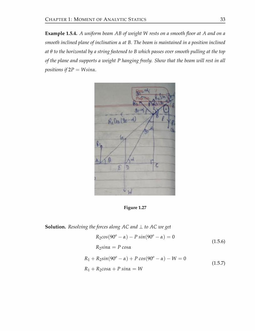
Example 1.5.4. A uniform beam AB of weight W rests on a smooth floor at A and on a
smooth inclined plane of inclination α at B. The beam is maintained in a position inclined
at θ to the horizontal by a string fastened to B which passes over smooth pulling at the top
of the plane and supports a weight P hanging freely. Show that the beam will rest in all
positions if 2P = Wsinα.
Figure 1.27
Solution. Resolving the forces along AC and ⊥ to AC we get
R2cos(90o − α)− P sin(90o − α) = 0
R2sinα = P cosα(1.5.6)
R1 + R2sin(90o − α) + P cos(90o − α)−W = 0
R1 + R2cosα + P sinα = W(1.5.7)

34 CHAPTER 1: MOMENT OF ANALYTIC STATICS
Taking moment about B we get
MB = −R1(AC) + W(EC) = 0
= −R1(AB cosθ) + W(AE) = 0
= −R1(AB cosθ) + W(ADcosθ) = 0
= −R1(AB cosθ) + W(AB2
)cosθ = 0
R1 =W2
(1.5.8)
From eqution (1.5.6) we get
R2 =Pcosα
sinα
Now putting the value in R2 in equation (1.5.8) we get
R1 +P cosα
sinαcosα + Psinα = W
R1 +Pcos2α + Psin2α
sinα= W
R1 +P
sinα= W
using equation (1.5.8)
W2
+P
sinα= W
Psinα
=W2
Wsinα = 2P
Example 1.5.5. A beam of weight W is divided by its centre of gravity G into two portions
AG and GB whose lengths are a and b respectively. The beam rests in a vertical plane on a
smooth floor AC against a smooth wall CB. A string is attached to a hook at C and to the
beam at a point D. If T be the tension of the string and α and β be the inclinations of the
beam and string respectively to the horizontal. Show that T = Wa cosα(a+b)sin(α−β)
.
Solution. Now resolving the forces horizontally, we have
R2 − Tcosβ = 0 =⇒ R2 = Tcosβ (1.5.9)
Taking moments about A we get
−W(AE)− (Tsinβ)(AC) + R2(CB) = 0

CHAPTER 1: MOMENT OF ANALYTIC STATICS 35
Figure 1.28
−W(AGcosα)− (Tsinβ)(ABcosα) + R2(ABsinα) = 0
−W(acosα)− (Tsinβ)(a + b)cosα) + R2(a + b)sinα = 0
R2(a + b)sinα = W(acosα) + Tsinβ(a + b)cosα
using equation(1.5.9) we have
R2 = Tcosβ
Tcosβ(a + b)sinα = W(acosα)− Tsinβ(a + b)cosα
T(a + b)[sinα cosβ− sinβcosα] = Wa cosα
T(a + b)sin(α− β) = Wa cosα
T =Wa cosα
(a + b)sin(α− β)

36 CHAPTER 1: MOMENT OF ANALYTIC STATICS
1.6 Equation of The Line of Action of The Resultant
Let P1, P2, P3, . . . be forces acting at points A1(x1, y1), A2(x2, y2) . . .
Figure 1.29
Let X1, Y1; X2, Y2; X3, Y3; . . . be their resolved parts along the axes. Let R be their
resultant acting at A(x, y), then
R cosθ = X = X1 + X2 + X3 + . . . (1.6.1)
R sinθ = Y = Y1 + Y2 + Y3 + . . . (1.6.2)
Squaring and adding equation (1.6.1),(1.6.2) we get
R2 = X2 + Y2
R =√
X2 + Y2
and
tanθ =YX

CHAPTER 1: MOMENT OF ANALYTIC STATICS 37
Moment of X1 about O = −Y1X1
Moment of Y1 about O = X1Y1
∴ Moment of P1 about O = algebraic sums of the moments of X1, Y1 about O
= X1Y1 −Y1X1
Similarly moment of P2, P3 about O are (X2Y2 −Y2X2), (X3Y3 −Y3X3) . . .
XY−YX = G
which is the equation of line of actions of the single resultant. When G is the
algebraic sum of the moment of forces about origin.
Example 1.6.1. Forces 3, 4 and 7kg act along the sides AB, CB and CA of an equilateral
4. Taking A as origin and CA as x− axis. Show that the resultant acts along the line
7x− 5√
3y + 4a = 0 a being the length of the side of the4.
Figure 1.30
Solution. Resolving the forces along CA and ⊥ to CA we get
X = Rx = 7− 3cos60o + 4cos60o
= 7− 32+
42
=152
Y = Ry = 4sin60o + 3cos60o
= 4
√3
2+ 3
√3
2
= 7
√3
2
38 CHAPTER 1: MOMENT OF ANALYTIC STATICS
Taking the moment M about A we get
M = −4AD = −4
√3
2a (clockwise)
= −2√
3a (∴ AD =
√3
2a)
The equation of the resultant
xY− yX = G
7√
32
x− 152
y = −2√
3a
72
x− 5√
32
y = −2a
7x− 5√
3y + 4a = 0
Example 1.6.2. Find the magnitude of the resultant and line of action of a single force of 8
units acting along the Y− axis (vertically upwards) and a couple in xy− plane of moment
24 units.
Solution. Couple in xy plane of moment = 24 units = 8× 3.
The equation of the line of action of the resultant
X = 3
CH
AP
TE
R 1Catenary
Cable
A rope or cable is defined as material lines which can be bent arbitrarily without
changing its length.
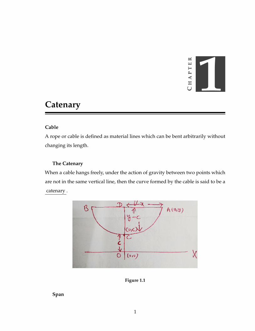
The Catenary
When a cable hangs freely, under the action of gravity between two points which
are not in the same vertical line, then the curve formed by the cable is said to be a
catenary .
Figure 1.1
Span
1

2 CHAPTER 1: CATENARY
The distance AB is called the span of the cable if points of suspension A and B are
in the same horizontal line. Therefore
Span = AB = 2x.
Sag
The vertical depth of the vertex below the span of the cable is called sag of the
cable. Therefore
Sag = CD = y− c.
Parameter
The distance CO = c, i.e. the depth of the X− axis below the vertex of the catenary
is called parameter of the catenary.
1.1 Intrinsic Equation of a Catenary
If a uniform cable hangs freely under its own weight per unit length, then find the
Intrinsic equation of the curve.
Proof. Consider a uniform cable ACB hanging freely under its own weight per unit
length. Let CP be a piece of cable of length s.Therefore
Total weight of CP = Ws,
which is acting vertically downwards. CP is in equilibrium under the following
three forces:
(1) The horizontal tension H at C.
(2) The tension T at P.
(3) Ws, weight of CP, acting through the C.G of the arc CP.
(Since CP is in equilibrium , the lines of action of Ws, T and H meet in one point).

CHAPTER 1: CATENARY 3
Figure 1.2
Resolving the forces horizontally and vertically we have
H = Tcosψ (1.1.1)
Ws = Tsinψ (1.1.2)
where ψ is the angle which the tangent makes with the X − axis. Dividing (1.1.2)
by (1.1.1) we have
tanψ =WsH
(1.1.3)
It is convenient to write
tanψ =s
H/Wor s = ctanψ, (1.1.4)
where c = HW is the parameter of the catenary.
Eqn (1.1.4) is called the Intrinsic equation of the Catenary.
Cartesian Equation of the Catenary
If a uniform cable hangs freely under its own weight per until length, then find

4 CHAPTER 1: CATENARY
the Cartesian equation of the curve.
Solution. We know that Intrinsic equation of catenary is
s = ctanψ.
Again tanψ =dydx
.
∴ s = cdydx
.
Now putting p =dydx
,
we have
s = cp.
Differentiating above eqn with respect to x we have
dsdx
= cdpdx
,
∴ cdpdx
=
√1 + (
dydx
)2 (∵dsdx
=
√1 + (
dydx
)2)
cdpdx
=√
1 + p2
∴dp√
1 + p2=
dxc
.
On Integrating we get
sinh−1(p) =xc+ A, (1.1.5)
where A is the constant of integration.
At the lowest point C, x = 0 and ψ = 0. Therefore
p =dydx
= tan0 = 0.

CHAPTER 1: CATENARY 5
On putting these values in equation (1.1.5) we get
0 = 0 + A
=⇒ A = 0.
sinh−1(p) =xc
p = sinh(xc)
dydx
= sinh(xc)
On Integrating we get
y = c coch(xc) + B
At the lowest point C, x = 0 and y = c =⇒ B = 0.
∴ y = c coshxc
.
Which is called the cartesian equation of the catenary.
1.2 Relation between x, y, T, s and ψ
Parametric Equation of Catenary:
We know that, Intrinsic equation of Catenary is
s = c tanψ. (1.2.1)
Differentiating equation (1.2.1) with respect to x we get,
dsdx
= c sec2 ψdψ
dx√1 + (
dydx
)2 = c sec2ψdψ
dx√1 + tan2ψ = c sec2ψ
dψ
dx

6 CHAPTER 1: CATENARY√sec2ψ = c sec2ψ
dψ
dxdxdψ
= c secψ
dx = c secψ dψ
Integrating above equation, we get,∫dx =
∫c secψ dψ
x = c log {secψ + tanψ}+ C1
At the lowest point c, x = 0, ψ = 0
0 = c log {sec0 + tan0}+ C1
=⇒ C1 = 0.
Therefore, x = c log {secψ + tanψ}.
Again differentiating equation (1.2.1) with respect to y, we get
dsdy
= c sec2ψdψ
dydsdx
dxdy
= c sec2ψdψ
dy√1 + tan2ψ(
1tanψ
) = c sec2 ψdψ
dy
secψ(1
tanψ) = c sec2ψ
dψ
dydydψ
= c secψtanψ
dy = c secψ tanψ dψ.
Integrating we get∫
dy =∫
c secψ tanψ dψ
y = c secψ + C2.
At the lowest point C, y = c, ψ = o
∴ c = c sec0 + C2
=⇒ C2 = 0
∴ y = c secψ.

CHAPTER 1: CATENARY 7
Hence, Parametric equations of Catenary are
x = c log (secψ + tanψ),
y = c secψ.
1.3 Relation between T, y and s
(i) y2 = c2 + s2
Since, y = c secψ. Squaring on both the sides, we get
y2 = c2 sec2ψ
= c2(1 + tan2ψ)
y2 = c2 + c2tan2ψ.
But s = c tanψ
=⇒ y2 = c2 + s2.
(ii) T = Wy
Since Parameter of the Catenary is given by,
c =HW
(1.3.1)
and
H = T cosψ. (1.3.2)
From equation (1.3.1) and (1.3.2),we have
T cosψ = Wc
T =Wc
cosψ=⇒ T = Wc secψ
T = Wy (∵ y = c secψ).
Prove that the span of the cable of length 2` and sagh h is 2`(1-2h2
3`2
):

8 CHAPTER 1: CATENARY
Solution. We know that
s = c sinh(xc)
If 2a is the span.Then, x = a and s = `
∴ ` = c sinh(ac)
ac= sinh−1 (
`
c)
= log{`
c+
√1 + (
`
c)2}
a = c log{`
c+
√1 +
`2
c2
}But c =
`2 − h2
2h
=`2 − h2
2hlog{
``2−h2
2`
+
√1 +
`2
( `2−h2
2h )2
}
=`2 − h2
2hlog{
2h``2 − h2 +
√1 +
4h2`2
(`2 − h2)
}
=`2 − h2
2hlog{
2h``2 − h2 +
√(`2 − h2)2 + 4h2`2
`2 − h2
}=
`2 − h2
2hlog{
2h``2 − h2 +
√`4 + h4 − 2`2h2 + 4h2`2
`2 − h2
}=
`2 − h2
2hlog{
2h``2 − h2 +
√`4 + h4 + 2`2h2
`2 − h2
}=
`2 − h2
2hlog{
2h``2 − h2 +
√(`2 + h2)2
`2 − h2
}=
`2 − h2
2hlog[
2h`+ `2 + h2
`2 − h2
]=
`2 − h2
2hlog[
(h + `)2
(`+ h)(`− h)
]=
`2 − h2
2hlog[
h + `
`− h
]=
`2 − h2
2hlog[`+ h`− h
]
CHAPTER 1: CATENARY 9
=`2 − h2
2hlog[
1 + h`
1− h`
]We know that, log
[1 + x1− x
]= 2
(x +
x3
3+
x5
5+ . . .
)=
(1− h2
`2
2h`2
)2[
h`+
13(
h`)3 +
15(
h`)5 + . . .
]
=
(1− h2
`2
2h`2
)2h`
[1 +
h2
`2 (13) +
h4
`4 (15) + . . .
]= `
(1− h2
`2
) [1 +
h2
`2 (13) +
h4
`4 (15) + . . .
]= `
[1 +
h2
`2 (13)− h2
`2
](Neglecting other higher powers )
a = `
[1− 2
3h2
`2
]Thus, Span = 2a
= 2`[
1− 23
h2
`2
].
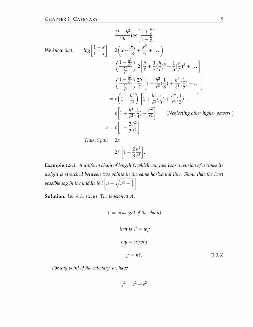
Example 1.3.1. A uniform chain of length `, which can just bear a tension of n times its
weight is stretched between two points in the same horizontal line. Show that the least
possible sag in the middle is `[
n−√
n2 − 14
]Solution. Let A be (x, y). The tension at A,
T = n(weight of the chain)
that is T = wy
wy = n(w`)
y = n`. (1.3.3)
For any point of the catenary, we have
y2 = c2 + s2

10 CHAPTER 1: CATENARY
Figure 1.3
Therefore for the point A
n2`2 = c2 + (`
2
2) (∵ s =
`
2and y = n`)
or c2 = `2[
n2 − 14
]c = `
√n2 − 1
4.
Hence, the sag in the middle is
CD = y− c = n`− `
[√n2 − 1
4
]
= `
[n−
√n2 − 1
4
]∴ CD = `
[n−
√n2 − 1
4
].
Example 1.3.2. If α, β are the inclinations to the horizon of the tangents at the extremities
of a catenary and ` the length of the portion, show that the height of one extremities over the

CHAPTER 1: CATENARY 11
other is`sin
(α+β
2
)cos
(α−β
2
) , the two extremities being on one side of the vertex of the catenary.
Solution. Consider the portion PQ of the catenary. let P = (x2, y2) and Q = (x1, y1)
Tangents at P and Q make angles α and β respectively to the horizontal. Also arc PQ =
`(given). Suppose that arc CQ = s1 and arc CP = s2
=⇒ s2 − s1 = `. (1.3.4)
Figure 1.4
Using the formula
s = c tanψ
we have s1 = c tanβ
and s2 = c tanα

12 CHAPTER 1: CATENARY
Therefore from equation (1.3.4)) we have,
c tanα− c tanβ = `
or c =`
tanα− tanβ.
(1.3.5)
Vertical height of one extremity P above Q
= y2 − y1
= c secα− c secβ
= c [secα− secβ]
=`
tanα− tanβ[
1cosα
− 1cosβ
]
=`
sinαcosα −
sinβcosβ
[1
cosα− 1
cosβ]
= `cosβ− cosα
sinαcosβ− cosαsinβ
= `2 sin( α+β
2 )sin( α−β2 )
sin(α− β)
= `2 sin( α+β
2 )sin( α−β2 )
sin(2α−β2 )
= `2 sin( α+β
2 )sin( α−β2 )
2 sin( α−β2 )cos( α−β
2 )
= `sin( α+β
2 )
cos( α−β2 )
.
Example 1.3.3. A given length 2s of uniform chain has to be hung between two points at
the same level and the tension has not to exceed the weight of a length b of the chain. Show
that the greatest span is√
b2 − s2log( b+sb−s ).

CHAPTER 1: CATENARY 13
Solution. Let A be (x, y)
T = Tension at A
= wy = wb(Given).
∴ y = b.
Figure 1.5
For any point of the catenary we have
y2 = c2 + s2
=⇒ b2 = c2 + s2
c =√
b2 − s2.

14 CHAPTER 1: CATENARY
Hence, the greatest span
= AB
= 2x
= 2c log(secφ + tanφ) (∵ x = Clog(secφ + tanφ))
= 2c log(yc+
sc) (∵ y = c secφ and s = c tanφ)
= 2c log(y + s
c)
= 2√
b2 − s2 log{
b + s√b2 − s2
}(∵ y = b&c =
√b2 − s2)
= 2√
b2 − s2 log{√
b + s√
b + s√b + s
√b− s
}= 2
√b2 − s2 log
{√b + s√b− s
}.
The greatest span
=√
b2 − s2 log{
b + sb− s
}.
Example 1.3.4. A heavy uniform string of length `, is suspended from a fixed point A and
its other end is pulled horizontally by a force equal to the weight of a length a of the string.
Show that the horizontal and vertical distance between A and B are (a sinh−1( `a )) and√`2 + a2 − a respectively.
Solution. Now as
H = wa ( Given ). (1.3.6)
Also, we have
H = wc. (1.3.7)
Form equations (1.3.6) and (1.3.7) we get
wa = wc⇒ c = a.

CHAPTER 1: CATENARY 15
Figure 1.6
Now from the relation at the point A we have,
y2A = c2 + s2 = a2 + `2 (∵ c = a and s = `)
yA =√
a2 + l2,
and yB = c
but c = a
⇒ yB = a.
=⇒ yA − yB =√`2 + a2 − a.
Again fromsc= sinh(
xc) at the point A, we have ,
`
a= sinh(
xA
a)
or sin−1(`
a) = (
xA
a)
⇒ xA = a sinh−1(`
a).
Therefore xA − xB = a sinh−1(`
a)− 0 (∵ xB = 0)
xA − xB = a sinh−1(`
a).
Mohammad Arif
Pencil
Mohammad Arif
Pencil
Mohammad Arif
Typewriter
y_A-y_B
Mohammad Arif
Arrow
Mohammad Arif
Typewriter
X_A-X_B

16 CHAPTER 1: CATENARY
Example 1.3.5. A rope of length 2` m, is suspended between two points at the same level
and the lowest point of rope is b m in below the point of suspension. Show that the horizontal
component of tension is W2b (`
2 − b2), W being the weight of the rope per meter of its length.
Solution. Now as we know that
y2 = c2 + s2.
At the point A(x, y), we have s = `
and y = b + c.
Therefore, we have (b + c)2 = c2 + `2
b2 + c2 + 2bc = c2 + `2
c =`2 − b2
2b.
Hence, H = Wc = W(`2 − b2
2b).
Example 1.3.6. Prove that when c is large compared with the span the catenary
approximates to a parabola.
Solution. As we know that equation of catenary is
y = c cosh(xc)
y = c[1 +12!(
xc)2 +
14!(
xc)4 + . . . ]
(∵ cosh(x) = [1 +x2
2!+
x4
4!+
x6
6!+ . . . ]).
Since x is small, c is large ∴xc
is small we get
y = c +(x)2
2c
y− c =(x)2
2c
=⇒ x2 = 2c(y− c).
Which is a parabola whose latus rectum is 2c and vertex (0, c), the lowest point of the
catenary.

CHAPTER 1: CATENARY 17
1.4 The Parabolic Cable
Let the cable carry a uniform load of W0 per unit length. For CB,
The load = V = W0x
anddydx
= tanψ =VH
.
Now, we havedydx
=W0x
H∫dy =
W0
H
∫xdx
y =W0x2
2H+ c1.
Figure 1.7
If we choose as x− axis the horizontal line passing through C(0, 0) then, c1 = 0.
Therefore y =W0x2
2H.
This is a equation of parabola with axis vertical and vertex at origin.

18 CHAPTER 1: CATENARY
The tension in the parabolic cable is given by
T =√
H2 + (W0x)2.
Example 1.4.1. If a cable is loaded with a uniform horizontal load of W and has a span a
and sag h, show that H = Wa2
8h and that
T =Wa2
(1 +
a2
16h2
) 12
,
where H and T are the tensions at lowest and highest point of the cable,respectively.
Solution. We know that, the equation of parabolic cable is
y =Wx2
2H.
Here y = h and x =a2
.
Now, h =W( a
2)2
2H
h =Wa2
8H
H =Wa2
8h.
Figure 1.8

CHAPTER 1: CATENARY 19
The tension in the parabolic cable is given by
T =√
H2 + (Wx)2
T =
√(
Wa2
8h)2 + (W
a2)2
T =
√W2a4
64h2 +W2a2
4
T =Wa2
√1 +
a2
16h2 .
Example 1.4.2. A length ` of a uniform chain has one end fixed at a heights h above a
rough table and rests in a vertical plane so that a portion of it lies in a straight line on the
table. Prove that if the chain is on the point of slipping, the length on the table is
`+ µh−√[(µ2 + 1)h2 + 2`hµ],
where µ is the coefficient of friction.
Solution. Resolving forces horizontally and vertically, we have
R = Wx (1.4.1)
µR = T0 = Wc. (1.4.2)
From (1.4.1) and (1.4.2), we have
µ(Wx) = Wc,
⇒ c = µx. (1.4.3)
Using the formula y2 = c2 + s2 from the point A we have (∵ y for A =
c + h and s for A = `− x)
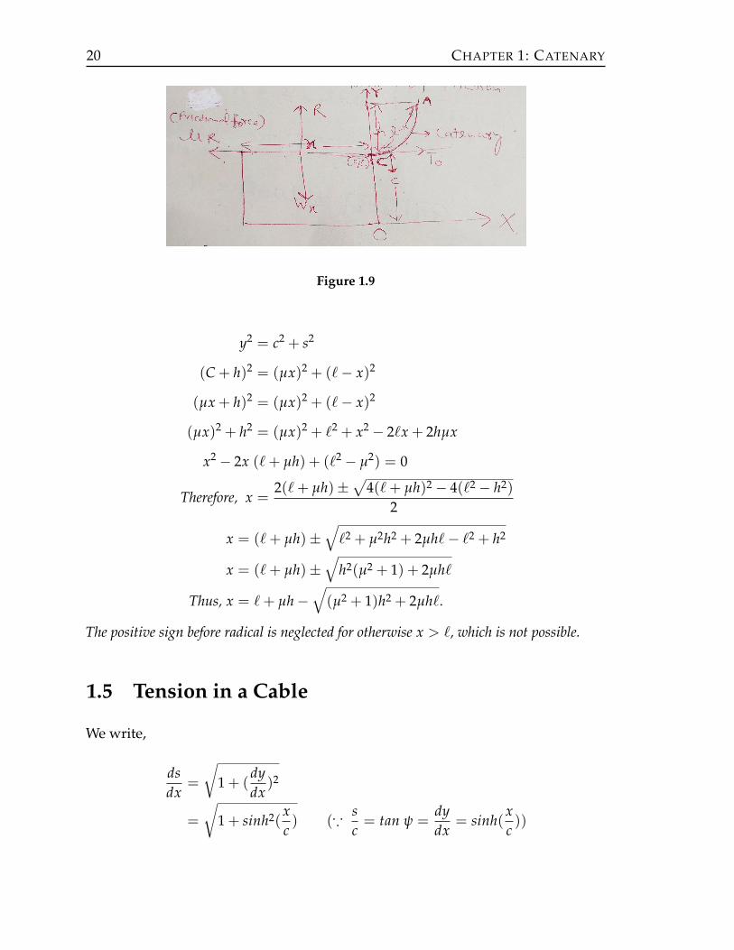
20 CHAPTER 1: CATENARY
Figure 1.9
y2 = c2 + s2
(C + h)2 = (µx)2 + (`− x)2
(µx + h)2 = (µx)2 + (`− x)2
(µx)2 + h2 = (µx)2 + `2 + x2 − 2`x + 2hµx
x2 − 2x (`+ µh) + (`2 − µ2) = 0
Therefore, x =2(`+ µh)±
√4(`+ µh)2 − 4(`2 − h2)
2
x = (`+ µh)±√`2 + µ2h2 + 2µh`− `2 + h2
x = (`+ µh)±√
h2(µ2 + 1) + 2µh`
Thus, x = `+ µh−√(µ2 + 1)h2 + 2µh`.
The positive sign before radical is neglected for otherwise x > `, which is not possible.
1.5 Tension in a Cable
We write,
dsdx
=
√1 + (
dydx
)2
=
√1 + sinh2(
xc) (∵
sc= tan ψ =
dydx
= sinh(xc))

CHAPTER 1: CATENARY 21
Figure 1.10
dsdx
= cosh (xc). (1.5.1)
Also, H = T cosψ
=⇒ T = Hsec ψ.
For any curvedxds
= cosψ
=⇒ dsdx
= secψ.
=⇒ T = H cosh (xc) (from equation 1.5.1).
1.6 Maximum Tension in the Cable
To prove that the maximum tension in the cable of weight W per unit length, span
2a and length 2` is(
Wa√
a6(`−a)
), approximately.
Solution. We know that the maximum tension occurs at A and B. Using the formula
s = c sinh (xc), at the point A

22 CHAPTER 1: CATENARY
Figure 1.11
s = ` and x = a
We have,
` = c sinh (ac)
Or, ` = c[
ac+ (
ac)3 1
3!+ (
ac)5 1
5!+ . . . ] (∵ sinh x = x +
x3
3!+
x5
5!+ . . . )
` = a +a3
6c2 ( Neglecting the higher power terms )
`− a =a3
6c2
c2 =a3
6(`− a)
c =
√a3
6(`− a).

CHAPTER 1: CATENARY 23
We know that, Tension in the cable is given by
T = Hc osh(xc) = H cosh (
ac) (∵ x = a).
Ifac
is small or c is large. Then, Tmax = H = Wc (approximitely)
= W
√a3
6(`− a)
Tmax = Wa√
a6(`− a)
.
Example 1.6.1. A cable 200m long hangs between two points at the same height. The sag
is 20m and the tension at either point of suspension is 120 kg Wt. Find the total weight of
the cable.
Solution. Given that T = 120 kg Wt
Figure 1.12

24 CHAPTER 1: CATENARY
and y− c = sag = 20m.
2s = 200m Given
s = 100m.
y− c = 20
y = 20 + c.
We know that, y2 = c2 + s2
(20 + c)2 = c2 + (100)2
400 + c2 + 40c = c2 + 10000
40c = 9600
c =960040
= 240
y = c + 20
= 240 + 20
y = 260.
As, T = Wy
120 = (W)(260)
W =120260
=6
13
Total weight = 200× 613
= W (2s)
=120013
.
Example 1.6.2. A uniform cable hangs across two smooth pegs at the same height, the ends
hanging down vertically. If the free ends are each 12m long and the tangent to the catenary
at each peg makes an angle of 60o with the horizontal, find the total length of the cable.

CHAPTER 1: CATENARY 25
Solution. At the point B, we have
y = h + c = 12
and y = c secφ.
Now, y = c sec60o
y = 2c
12 = 2c
c = 6.
As, s = c tanψ
= 6 tan60o
s = 6 (√
3).
Figure 1.13
Total Length of the Cable = 2s + 2y
= 2× 6√
3 + 2× 12
= 12√
3 + 24
= 12(√
3 + 2).

26 CHAPTER 1: CATENARY
Example 1.6.3. The extremities of a heavy string of length 2` and weight 2`ω are attached
to two small rings which can slide on a fixed horizontal wire. Each of these rings are acted
on by a horizontal force equal to `ω. Show that the distance apart of the rings is
2` log{
1 +√
2}
.
Solution.
H = ω`
But H = ωc
⇒ ω` = ωc
⇒ ` = c
We know that S = c tan ψ
` = ` tan ψ
tan ψ = 1
⇒ ψ = 45o
Span = AB = 2` log{sec ψ + tan ψ}
Span = 2` log{√
2 + 1}.
Example 1.6.4. If T be the tension at any point P of a catenary and T0 at the lowest point
C, prove that
T2 − T20 = W2,
W being the weight of the arc CP of the catenary.
Solution. We know that
T = wy
Mohammad Arif
Pencil
Mohammad Arif
Typewriter
is
Mohammad Arif
Typewriter
where,

CHAPTER 1: CATENARY 27
and T0 = The tension at the lowest point C
= wc.
Now, T2 − T20 = w2y2 − w2c2
= w2(y2 − c2).
But y2 = c2 + S2
T2 − T20 = w2(y2 − c2)
= w2(c2 + s2 − c2)
= w2s2
= W2 (∵ W = ws).
Example 1.6.5. A uniform chain is hung up from two points at the same level and distant
2a apart. If z is the sag at the middle show that
z = c(cosh(ac)− 1).
If z is small compared to a show that
2zc = a2 (nearly).
Solution. We know that equation of the catenary is
y = c cosh(xc).
Since the span 2x = 2a, x = a for the point A Given that z is the sag in the middle.
∴ z = sag = DC = y− c
= c cosh(xc)− c
= c[cosh(xc)− 1] (∵ x = a at A)
= c[cosh(ac)− 1].

28 CHAPTER 1: CATENARY
Figure 1.14
Again z is small compared with a, therefore c must be very large. Now
z = c[cosh(ac)− 1]
= c[1 +122 (
ac)2]
14!(
ac)4 + · · · − 1
=a2
2c
⇒ 2zc = a2 (nearly).
Example 1.6.6. A uniform chain of length ` is to be suspended from two points A and B
in the same horizontal line so that terminal tension is n times that at the lowest point. Show
that span AB must be`√
n2 − 1log{n +
√n2 − 1}.
Solution. Let the coordinate of the A be (x, y). Then we have
span = AB = 2c log(sec ψ + tan ϕ)
where ψ is the inclination of the tangent at A to x–axis. Given that

CHAPTER 1: CATENARY 29
Figure 1.15
Tension at A = n( Tension at the lowest point c)
= nT0
⇒ T = nT0 = n(ωc) (∵ T0 = ωc)
⇒ ωy = nT0 = n(ωc) (∵ T = ωy)
⇒ y = nc
⇒ c sec ψ = nc (∵ y = c sec ψ)
⇒ n = sec ψ (1.6.1)
∴ tan ψ =√
sec2 ψ− 1
tan ψ =√
n2 − 1. (1.6.2)
Again,
the arc CA = half length of the chain
s =`
2,
we have,`
2= c tan ψ (∵ s = c tan ψ)
=`
2 tan ψ
=`
2√
sec2ψ− 1

30 CHAPTER 1: CATENARY
c =`
2√
n2 − 1. (1.6.3)
Hence,
AB = 2c log{sec ψ + tan ψ}
=`√
n2 − 1log{n +
√n2 − 1}.
Example 1.6.7. A telegraph wire is made of a given material and such a length L is
stretched between two posts, distant d apart and of the same height as will produce the least
possible tension at the posts. Show that
L =dλ
sinh λ
where λ is given by the equation
λ tan λ = 1.
Solution. Let T be the tension at either post. Then the catenary has x = d2 and s = L
2 . We
know that the tension in the cable is given by
T = H cosh(xc)
= H cosh(d2c
)
= Wc cosh(d2c
)
For maximum or minimum of T, we have
dTdc
= 0
=⇒ ddc
(W cosh(
d2c
)
)= 0

CHAPTER 1: CATENARY 31
Figure 1.16
=⇒W[
cosh(d2c
) + c sinh(d2c
)(−d2c2 )
]= 0
or cosh(d2c
)− d2c
sinh(d2c
) = 0
ord2c
tanh(d2c
) = 1.
But λ tanh λ = 1 ( Given)
⇒ d2c
tanh(d2c
) = λ tanh λ
⇒ λ =d2c
.
⇒ c =d
2λ.
As we know, s = c sinh(xc).
Here, s =L2
x =d2
and c =d
2λ
Now, (L2) =
d2λ
sinh(d2c
)
⇒ L =dλ
sinh λ.
Example 1.6.8. If the length of the uniform chain suspended between points at the same

32 CHAPTER 1: CATENARY
level is adjusted so that the tension at the points of support is minimum for that particular
span 2d. Show that the equation to determine c is
coth(dc) =
dc
.
Solution. We know that tension cable is given by
T = H cosh(xc)
⇒ T = H cosh(dc) = Wc cosh(
dc).
For maximum or minimum of T,dTdc
= 0
=⇒ dTdc
= W[c sinh(dc)(−dc2 ) + cosh(
dc)] = 0
=⇒ = W[c sinh(dc)(−dc2 ) + cosh(
dc)] = 0
=⇒ cosh(dc) = (
dc)c sinh(
dc)
cot h(dc) = (
dc).