D S E Working Paper

Banking Permits: EconomicEfficiency and DistrubutionalEffects

Valentina BosettiCarlo CarraroEmanuele Massetti

Dipartimento Scienze Economiche

Department of Economics

Ca’ Foscari University ofVenice

ISSN: 1827/336X

No. 01/WP/2008

W o r k i n g P a p e r s D e p a r t m e n t o f E c o n o m i c s

C a ’ F o s c a r i U n i v e r s i t y o f V e n i c e N o . 0 1 / W P / 2 0 0 8

ISSN 1827-3580

The Working Paper Series is availble only on line

(www.dse.unive.it/pubblicazioni) For editorial correspondence, please contact:

wp.dse@unive.it

Department of Economics Ca’ Foscari University of Venice Cannaregio 873, Fondamenta San Giobbe 30121 Venice Italy Fax: ++39 041 2349210

BANKING PERMITS: ECONOMIC EFFICIENCY AND DISTRIBUTIONAL EFFECTS

Valentina Bosetti, Fondazione Eni Enrico Mattei

Carlo Carraro, University of Venice and Fondazione Eni Enrico Mattei Emanuele Massetti, University of Yale

First Draft: December 29th, 2007

Abstract

Most analyses of the Kyoto flexibility mechanisms focus on the cost effectiveness of “where” flexibility (e.g. by showing that mitigation costs are lower in a global permit market than in regional markets or in permit markets confined to Annex 1 countries). Less attention has been devoted to “when” flexibility, i.e. to the benefits of allowing emission permit traders to bank their permits for future use. In the model presented in this paper, banking of carbon allowances in a global permit market is fully endogenised, i.e. agents may decide to bank permits by taking into account their present and future needs and the present and future decisions of all the other agents. It is therefore possible to identify under what conditions traders find it optimal to bank permits, when banking is socially optimal, and what are the implications for present and future permit prices. We can also explain why the equilibrium rate of growth of permit prices is likely to be larger than the equilibrium interest rate. Most importantly, this paper analyses the efficiency and distributional consequences of allowing markets to optimally allocate emission permits across regions and over time. The welfare and distributional effects of an optimal intertemporal emission trading scheme are assessed for different initial allocation rules. Finally, the impact of banking on carbon emissions, technological progress, and optimal investment decisions is quantified and the incentives that banking provides to accelerate technological innovation and diffusion are also discussed. Among the many results, we show that not only does banking reduce abatement costs, but it also increases the amount of GHG emissions abated in the short-term. It should therefore belong to all emission trading schemes under construction.

Keywords: Emission Trading, Banking.

JEL Codes: C72, H23, Q25, Q28

Address for correspondence: Carlo Carraro

Department of Economics Ca’ Foscari University of Venice

Cannaregio 873, Fondamenta S.Giobbe 30121 Venezia - Italy

Phone: (++39) 041 2349166 Fax: (++39) 041 2349176 e-mail: ccarraro@unive.it

This Working Paper is published under the auspices of the Department of Economics of the Ca’ Foscari University of Venice. Opinions expressed herein are those of the authors and not those of the Department. The Working Paper series is designed to divulge preliminary or incomplete work, circulated to favour discussion and comments. Citation of this paper should consider its provisional character.

1

1. Introduction

In a multi-period market for pollution rights, the possibility to transfer emission allowances to

the future is referred to as banking of emission units. The early use of allowances issued in the

present for later periods is instead referred to as borrowing of emission units. A market of

permits where both banking and borrowing of emission rights are allowed is characterised by

full intertemporal flexibility. In this market, the so-called “when flexibility” is therefore added

to the so-called “where flexibility” (achieved when different countries trade pollution rights). A

fully flexible market is shown to be superior, in terms of efficiency, to a market in which the

transfer of pollution rights is restricted, in either dimension (see, for instance, Leiby and Rubin,

2001). The importance of the “when flexibility” is also recognised by the Kyoto Protocol, which

specifies that in the event that a Party has a surplus of carbon allowances at the end of the first

commitment period, a portion of these credits may be carried-over to a subsequent commitment

period after 2012.1

Despite its relevance, banking is rarely considered in the empirical literature that quantifies the

costs of mitigation policies. In a few cases, intertemporal flexibility is introduced, but the

number of permits that are moved across time, and the future use of the extra-allowances, is

exogenously determined by the modeller (Babiker et al., 2002; Manne and Richels, 2001;

Springer, 2003; Carraro and Galeotti, 2004).

The theoretical literature on emission trading is instead rich in contributions on banking. These

contributions generally show that a permit system with intertemporal flexibility increases

welfare.2 However, the assumptions commonly made in these papers are far from being realistic

and do not mimic the conditions under which a carbon market with intertemporal flexibility is

reasonably expected to operate.

For this reason, one of the objectives of this paper is to introduce a fully endogenous market of

carbon permits with banking in WITCH – the integrated assessment climate-economy hybrid

model used in this paper – and to assess the welfare impacts of a fully intertemporal emission

trading scheme for various allocation rules. The functioning of pollution permit markets with

intertemporal flexibility can thus be analysed under some realistic assumptions that cannot be in

general imposed in analytical models for tractability reasons.

1 Cfr. Article 3(13) of the Kyoto Protocol. 2 See Newell, Pizer and Zhang (2003), for a survey.

2

In their seminal paper, Cronshaw and Kruse (1996) set up the standard framework along which

research on banking of tradable permits has developed so far.3 Their work is characterised by

the following crucial assumptions: (i) there is a constant number of profit-maximising firms

acting with perfect foresight in a competitive market for permits. Firms hurt the environment by

releasing pollutants as a side effect of their production activity; however, they can also acquire

inputs to mitigate emissions. Each firm receives an (ii) equal endowment of permits for each

period and can buy from or sell permits to other firms at a given price. Permits can be

transferred across time by either banking them for future use or (iii) by borrowing future

allowances for use in the present. The authors show that, at the equilibrium, the present value

permit prices must be non-increasing over time. Were discounted prices increasing, firms could

(iv) buy from the market today to sell in future periods (speculative banking) thus increasing

profits. This would lead to an unboundedly large demand for permits in the first period that

would increase today’s price. Hence, this cannot be an equilibrium. Thus, assuming that (v)

marginal abatement costs are constant over time, banking takes place if and only if permit

prices rise over time with the interest rate, i.e. discounted prices are constant.

This result represents a very useful benchmark, but it relies on a set of assumptions which

typically do not hold in the case of carbon markets induced or established by climate policy. To

begin with, marginal abatement costs can hardly be constant over time. They are usually non-

linear, with a time profile that reflects the alternating predominance of two opposite forces: on

the one hand, diminishing returns tend to increase abatement costs over time; on the other hand,

technological change works in the opposite direction and lowers abatement costs over time.

Secondly, contrary to what assumed by Cronshaw and Kruse, climate policy can be realistically

expected to become increasingly tighter over time, with a time-varying, rather than constant,

endowment of annual emission permits. Thirdly, and most importantly, it is highly unrealistic

that any future regulation of carbon trading will allow “speculative banking”, i.e. the possibility

of buying and banking emission permits for pure speculation on the future price of carbon. The

Kyoto Protocol explicitly forbids this type of banking, thus ruling out one of the pillars that

support Cronshaw and Kruse’s result. Finally, borrowing is also likely to be partly restricted

since it has the potential to become a serious threat to the achievement of ambitious stabilisation

targets and an incentive to defect from the climate agreement.

For these reasons, this paper proposes a more articulated set-up to analyse the role of banking in

carbon markets, thus overcoming limitations imposed by analytical approaches. The analysis of

the role of banking will be carried out by using WITCH, a regional model of the world economy 3 For further developments see Rubin (1996), Kling and Rubin (1997), Liski and Montero (2003). For an analysis with uncertainty see Godby et al (1997) and Innes (2003).

3

in which twelve macro-regions have agreed on a mitigation policy based on tradable emission

rights. Regions differ in population, technology, income, energy demand, etc.. They can buy and

sell permits in a competitive world carbon market, which sets marginal abatement costs equal

worldwide. First, we study regions’ optimal choices – i.e. their investments, R&D expenditures,

net demand of permits, etc. – when there is no “when” flexibility. Then, we introduce “when”

flexibility by allowing banking (but not borrowing) of carbon emissions. Speculative banking is

not permitted either. Finally, we examine the effect of banking on the price of permits, on the

time path of CO2 abatement, on optimal investments, on the diffusion of technical change, etc..

This paper has a final additional objective. An important issue in the present debate on climate

policy is the participation of developing countries in the cooperative effort to reduce global

GHG emissions. These countries’ decision crucially depends on the way in which the burden of

controlling GHG emissions is shared among all countries and regions. The burden-sharing issue

is equivalent to the allowance allocation issue if the policy adopted worldwide to control

emissions is a global carbon market. Therefore, in this paper, we analyse the efficiency and

distributional implications of banking for three different allocations of carbon rights, and

investigate the role of banking under these distribution rules. By changing the distribution of

permits among regions, we stress the effect of asymmetries among players in determining

optimal banking decisions and the consequent price of permits over time.

From a policy perspective, we find that banking is a key instrument to comply with increasingly

stringent emission reduction targets. Significant cost savings are indeed possible by allowing

greater intertemporal flexibility. A more original result is that banking provides relevant

incentives to the early adoption of cleaner technologies, thus inducing a positive intertemporal

spillover effect. This effect is stronger when the allocation rule is such that mostly OECD

countries find it optimal to bank permits. The reason is that, in this case, banking also fosters a

positive international technology spillover effect.

Our findings only partly confirm what is predicted by the analytical literature on the efficiency

of “when” flexibility. Some new results – for example on the relationship between banking and

technological change, on the implications of banking for the choice of the allocation rule, and

also on the future equilibrium path of the permit price – are presented in this paper. In

particular, contrary to what stated by Cronshaw and Kruse (1996), we find that a discounted

permit price increasing over time is perfectly consistent with a well-defined carbon market.

Moreover, discontinuities in the price path may arise, due to discontinuities in the evolution of

marginal abatement costs and in the total number of emission allowances.

4

This paper is organised as follows. Section 2 illustrates the basic set-up of the WITCH model

employed for our numerical analysis. Section 3 presents our results on banking of carbon rights

and how (partial) “when flexibility” affects carbon emissions, the carbon market and the permit

price. Section 4 discusses how banking changes optimal investment and R&D decisions, with

consequent impacts on the speed of diffusion of technical change. Section 5 shows the effects of

banking on stabilisation costs for three emission rights allocation rules. A concluding section

summarises the most important findings of our analysis and outlines some policy implications.

2. The WITCH model and Climate Policy Scenarios

The WITCH – World Induced Technical Change Hybrid – model is a regional integrated

assessment model that captures the channels of transmission of climate policy into the economic

system and provides normative information on the optimal responses of world economies to

climate damages and policy (for a complete list of model equations the reader is referred to the

Appendix). It is a hybrid model because it combines features of both top-down and bottom-up

modelling. The top-down component consists of an inter-temporal optimal growth model of the

world economy. Within this framework, the energy input of the aggregate production function

has been expanded to provide a bottom-up like description of the energy sector. World countries

are grouped in 12 regions that strategically interact. A game-theoretic approach is used to

describe these interactions. A climate module and a damage function provide the feedback on

the economy of carbon dioxide emissions into the atmosphere.

WITCH top-down framework guarantees a coherent, fully intertemporal allocation of

investments that have an impact on the level and cost of mitigation – i.e. R&D efforts,

investments in energy technologies, fossil fuel expenditures. The regional specification of the

model and the presence of strategic interaction among regions –through CO2, exhaustible

natural resources, carbon trading and technological spillovers– allows us to account for free-

riding incentives. Investment strategies are optimised by taking into account both economic and

environmental externalities. Optimal strategies belong to the open-loop Nash equilibrium of the

dynamic game defined by the model.

By endogenously modelling fuel (oil, coal, natural gas, uranium) prices, as well as the cost of

storing the CO2 captured, the model can be used to evaluate the implications of mitigation

policies on the energy system in all its components.4

4 Model equations and variables are listed in the Appendix at the end of this article. For a thorough description of the model see Bosetti et al. (2006, 2007a) and Bosetti, Massetti and Tavoni (2007).

5

In this paper, WITCH is used to analyse the cost of stabilising concentrations of CO2 emissions

in the atmosphere at 450ppmv by the end of the century (on this issue see also Bosetti et al.,

2007b). For simplicity and without affecting the main conclusions of the paper, we assume that

all countries and regions agree to achieve the stabilisation objective by establishing a world

carbon market that allows regions to exchange carbon rights. Banking of emission permits is

allowed. “Speculative banking”, i.e. buying and banking permits at the same time, as well as

“borrowing”, are not allowed.

In order to contribute to the burden-sharing debate, we compute stabilisation costs and their

geographical distribution for three different allocation rules: Equal Emissions per Capita,

Contraction and Convergence and Sovereignty. These are the most commonly studied allocation

rules in the environmental economics literature. Independently of the allocation scheme and to

gain in realism, we assume that until 2030 the whole abatement effort is undertaken by High

Income (HI) regions alone, while Low Income countries are allocated their baseline emissions.5

In the Equal Emissions per Capita (EPC) scenario, allowances are distributed among regions in

proportion to their population, so that each individual is endowed with the same CO2 emission

rights. This scenario turns out to be very stringent for industrialised countries, because of their

modest share of world population, which will further decline over the next century.

The Sovereignty (SOV) allocation scheme has opposite implications: allowances are distributed

to each region according to their present share of total emissions. Developing regions may be

penalised because of rapid population and economic growth, while industrialised countries may

reduce emissions at moderate costs.

The Contraction and Convergence allocation scheme (CC) stands between these two extremes.

According to this widely discussed policy option, emission rights are first distributed according

to the sovereignty rule in order not to constrain industrialised economies excessively; then,

greater weight is given to the equal emissions per capita allocation rule, eventually switching to

a full application of this rule by the end of the century.

The reference scenarios are the stabilisation scenarios without “when” flexibility (one for each

allocation rule) and, for the estimate of stabilisation costs, the benchmark is the WITCH

Baseline scenario, in which no climate policy is imposed.

5 High Income regions are: USA, OLDEURO, NEWEURO, KOSAU (South Korea, South Africa and Australia), CAJAZ (Canada, Japan, New Zealand). Low Income regions are: TE (Transition Economies), MENA (Middle East and North Africa), SSA (Sub-Saharan Africa), SASIA (South Asia), CHINA, EASIA (East Asia) and LACA (Latin America and the Caribbean). The aggregation of world regions is discussed in detail in Bosetti, Massetti and Tavoni (2007). For an analysis of the distributional impacts of climate policy see Bosetti et al. (2007b).

6

3. Banking, Emissions, and Carbon Prices

As said, in our scenarios all countries are committed to stabilise GHG concentrations at 450

ppm. The consequent optimal strategic choices in all countries and regions are described in this

section. These choices include the optimal investment profile for all energy technologies, the

optimal R&D investments, the net demand of permits and the number of permits to be banked in

each period of time. Let us start by analysing this latter variable.

3.1 Banking of Carbon Rights

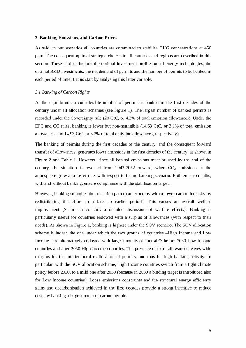
At the equilibrium, a considerable number of permits is banked in the first decades of the

century under all allocation schemes (see Figure 1). The largest number of banked permits is

recorded under the Sovereignty rule (20 GtC, or 4.2% of total emission allowances). Under the

EPC and CC rules, banking is lower but non-negligible (14.63 GtC, or 3.1% of total emission

allowances and 14.93 GtC, or 3.2% of total emission allowances, respectively).

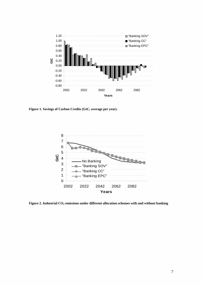
The banking of permits during the first decades of the century, and the consequent forward

transfer of allowances, generates lower emissions in the first decades of the century, as shown in

Figure 2 and Table 1. However, since all banked emissions must be used by the end of the

century, the situation is reversed from 2042-2052 onward, when CO2 emissions in the

atmosphere grow at a faster rate, with respect to the no-banking scenario. Both emission paths,

with and without banking, ensure compliance with the stabilisation target.

However, banking smoothes the transition path to an economy with a lower carbon intensity by

redistributing the effort from later to earlier periods. This causes an overall welfare

improvement (Section 5 contains a detailed discussion of welfare effects). Banking is

particularly useful for countries endowed with a surplus of allowances (with respect to their

needs). As shown in Figure 1, banking is highest under the SOV scenario. The SOV allocation

scheme is indeed the one under which the two groups of countries –High Income and Low

Income– are alternatively endowed with large amounts of “hot air”: before 2030 Low Income

countries and after 2030 High Income countries. The presence of extra allowances leaves wide

margins for the intertemporal reallocation of permits, and thus for high banking activity. In

particular, with the SOV allocation scheme, High Income countries switch from a tight climate

policy before 2030, to a mild one after 2030 (because in 2030 a binding target is introduced also

for Low Income countries). Loose emissions constraints and the structural energy efficiency

gains and decarbonisation achieved in the first decades provide a strong incentive to reduce

costs by banking a large amount of carbon permits.

7

-0.80-0.60

-0.40-0.20

0.000.200.40

0.600.80

1.001.20

2002 2022 2042 2062 2082

Years

GtC

"Banking SOV""Banking CC""Banking EPC"

Figure 1. Savings of Carbon Credits (GtC, average per year).

012345678

2002 2022 2042 2062 2082Years

GtC

No Banking"Banking SOV""Banking CC""Banking EPC"

Figure 2. Industrial CO2 emissions under different allocation schemes with and without banking

8

SOV CC EPC2002-2031 -9% -8% -8%2032-2051 -4% 0% 0%2052-2071 13% 11% 12%2072-2097 2% 5% 5%2002-2097 0% 0% 0%

Table 1. Variations of Industrial CO2 emissions with Banking

3.2 Carbon Market

Banking also affects the size of the emission trading market. The number of emission rights

traded over the whole century is rather constant (slightly lower with reductions of 1.4%, 3.0%

and 1.5% for SOV, CC and EPC, respectively), but significant variations are recorded on shorter

time periods, as shown in Figures 3 to 5. Banking reduces the market size in the first decades,

while it increases the number of permits exchanged in later periods.

0.0

0.5

1.0

1.5

2.0

2.5

3.0

2002 2022 2042 2062 2082Years

GtC

No BankingBanking

0.0

0.5

1.0

1.5

2.0

2.5

3.0

2002 2022 2042 2062 2082Years

GtC

No BankingBanking

Figure 3. Trade of Carbon Credits – SOV Figure 4. Trade of Carbon Credits – CC

9

0.0

0.5

1.0

1.5

2.0

2.5

3.0

2002 2022 2042 2062 2082Years

GtC

No BankingBanking

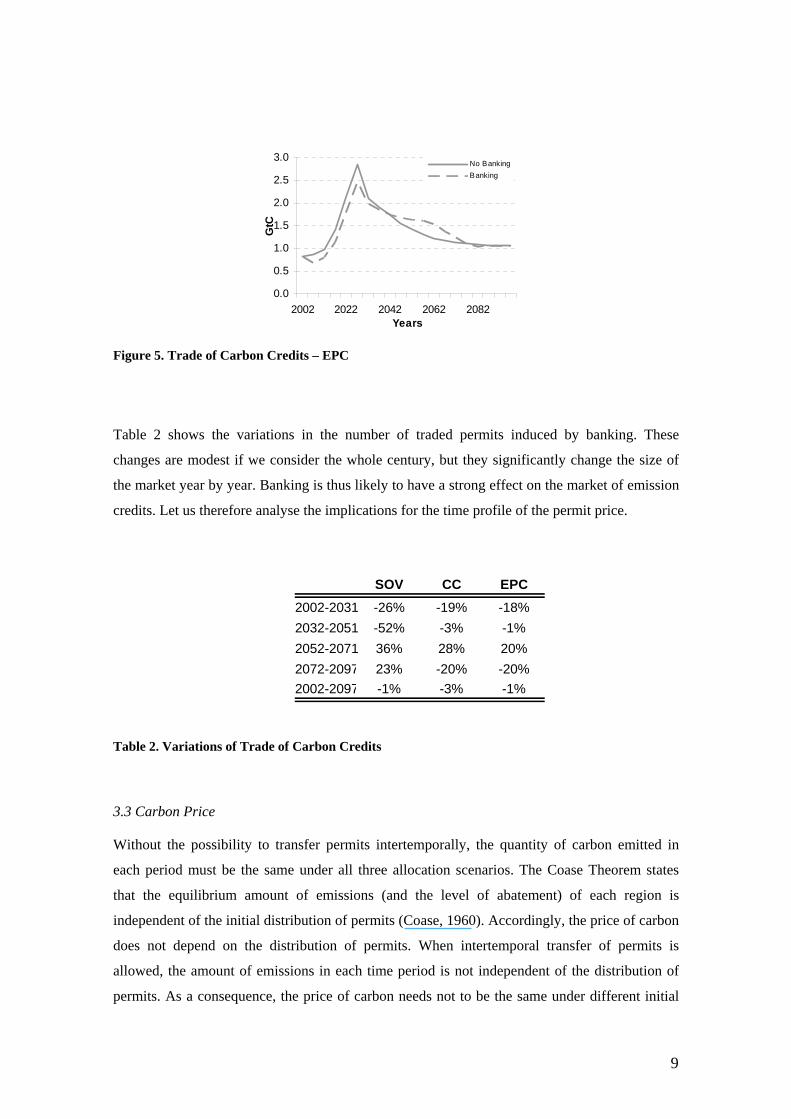
Figure 5. Trade of Carbon Credits – EPC

Table 2 shows the variations in the number of traded permits induced by banking. These

changes are modest if we consider the whole century, but they significantly change the size of

the market year by year. Banking is thus likely to have a strong effect on the market of emission

credits. Let us therefore analyse the implications for the time profile of the permit price.

SOV CC EPC2002-2031 -26% -19% -18%2032-2051 -52% -3% -1%2052-2071 36% 28% 20%2072-2097 23% -20% -20%2002-2097 -1% -3% -1%

Table 2. Variations of Trade of Carbon Credits

3.3 Carbon Price

Without the possibility to transfer permits intertemporally, the quantity of carbon emitted in

each period must be the same under all three allocation scenarios. The Coase Theorem states

that the equilibrium amount of emissions (and the level of abatement) of each region is

independent of the initial distribution of permits (Coase, 1960). Accordingly, the price of carbon

does not depend on the distribution of permits. When intertemporal transfer of permits is

allowed, the amount of emissions in each time period is not independent of the distribution of

permits. As a consequence, the price of carbon needs not to be the same under different initial

10

allocations of permits. This is clearly visible from Figures 6 and 7. Different time paths for

carbon prices will in turn imply different optimal investment strategies and different total

stabilisation costs, as we will see in detail in the next sections.

As shown above, in the presence of “when” flexibility, emission rights are initially banked,

supply drops and prices in the carbon market go up. Banking induces a strong increase in the

carbon price in the first decades of the century, up to 94% higher, as shown in Figure 8.

Subsequently, banked allowances are released, supply increases and the price goes down. Since

carbon prices are very high in the second half of the century, the apparently small percentage

variations imply massive drops in carbon prices. As a result, banking induces a smoother

intertemporal path of the carbon price, as predicted by the analytical models. The rate of growth

of carbon prices is strongly reduced, as Figure 9 portrays. However, it remains always higher

than interest rates (capital markets are not integrated and thus each region has its own interest

rate); this contradicts theory and requires some explanation.

0

200

400

600

800

1000

1200

1400

2002 2007 2012 2017 2022 2027 2032 2037 2042 2047Years

1995

US

D p

er G

tC

No BankingSOVCCEPC

Figure 6. Price of Carbon for different Allocation Schemes (2002-2047).

11

0

1000

2000

3000

4000

5000

6000

7000

8000

2052 2057 2062 2067 2072 2077 2082 2087 2092 2097Years

1995

USD

per

GtC

No BankingSOVCCEPC

Figure 7. Price of Carbon for different Allocation Schemes. (2052-2097)

-50%

0%

50%

100%

150%

200%

250%

2002 2022 2042 2062 2082

SOVCCEPC

Figure 8. Change of Carbon Price, Banking wrt No Banking

0%

20%

40%

60%

80%

100%

2002 2022 2042 2062 2082

No BankingBanking

Figure 9. Rate of Growth of Carbon Price -SOV

12

It may be argued that the reason is the absence of borrowing and of speculative banking, or the

strategic interactions among countries and regions. Therefore, a useful term of reference is the

shadow price of carbon that emerges in the cooperative solution of the model when full

intertemporal flexibility is allowed.6 Our results show that the carbon price still rises faster than

the interest rate. The main reason therefore appears to be the presence of heterogeneous agents

and of increasing marginal abatement costs when a strong policy to control a stock pollutant is

implemented. Thus, our model does not predict a constant path of the discounted price of

permits even when full intertemporal flexibility is allowed. The restrictions on borrowing and

on speculative banking, introduced in the optimisation runs described in sections 3.1 and 3.2,

are additional reasons for the discounted time path of permit prices to be higher than the interest

rate.7

It appears that a “premium” in terms of rate of growth of permit price over the interest rate is

necessary for emissions to be banked. This finding emerges from all our optimisation runs and

is synthesised in Figure 10 and 11, which show banked emissions together with the rate of

growth of the carbon price (under the SOV scenario) and the rate of interest for MENA (Middle

East and North Africa) and NEWEURO.8

-0.5

-0.4

-0.3

-0.2

-0.1

0

0.1

0.2

0.3

0.4

0.5

2002 2022 2042 2062 2082

GtC

-10%

-8%

-6%

-4%

-2%

0%

2%

4%

6%

8%

10%

Savings

Rate of Growth of Carbon Price

Interest Rate

Figure 10. Carbon Market Data for Middle East and North Africa

6 In this kind of exercise, a global social planner maximises the sum of welfare of the twelve macro-regions. This rules out free-riding behaviours, which would instead strongly emerge in a non-cooperative solution of the model. 7 For all regions, in both cooperative and non-cooperative settings, the interest rate is always greater than the intertemporal discount rate. Per capita consumption is rising for all countries. 8 The rate of growth of carbon prices in the first two periods is not shown here because it exceeds the area of the graph (it is 102% in 2002-2006 and becomes 30% in 2007-2011). Rates of growth of carbon price are average per year. Compound interest has been used.

13

-0.5

-0.4

-0.3

-0.2

-0.1

0

0.1

0.2

0.3

0.4

0.5

2002 2022 2042 2062 2082

GtC

-10%

-8%

-6%

-4%

-2%

0%

2%

4%

6%

8%

10%

SavingsPurchases of Carbon RightsRate of Growth of Carbon PriceInterest Rate

Figure 11. Carbon Market Data for New Europe

MENA uses banked emissions well before the interest rate becomes higher than the rate of

carbon price growth. NEWEURO never banks its emission allowances, although during the first

period the rate of growth of carbon price is much higher than its interest rate, being a net buyer

of carbon rights most of the time.

A second interesting feature of the permit market with banking is synthesised by Figure 12,

which refers to the US, again under the SOV scenario. The growth rate of the carbon price is

higher than the interest rate throughout the century. Why then are not all the saved allowances

released at the same time in the last period?

-0.5

-0.4

-0.3

-0.2

-0.1

0

0.1

0.2

0.3

0.4

0.5

2002 2022 2042 2062 2082

GtC

-10%

-8%

-6%

-4%

-2%

0%

2%

4%

6%

8%

10%

Savings

Rate of Growth of Carbon Price

Interest Rate

Figure 12. Carbon Market Data for the US

14

There are two explanations for a gradual release of saved permits. First, without an international

financial market, it is impossible to finance earlier consumption so as to spread the extra

revenues from permit sales over the last period of trade. In our macroeconomic, aggregated,

context, there are only two ways to smooth consumption over time: through savings, embodied

in capital goods, and through savings of emission allowances. Since both work only forward,

allowing to postpone consumption but not to anticipate future positive income shocks, it is not

possible for regions to sell at the most convenient moment and to anticipate consumption in

earlier times. Second, an extremely high supply of permits in a single time period would make

the carbon price sink;9 as can be inferred from Figure 1, the amount of permits banked is

substantial and if concentrated only in a single time period it would outweigh demand by a

factor of two, or more. Thus, contrary to what would be optimal for a single firm with open

access to credit markets and with virtually no impact on prices, regions release banked emission

permits gradually through time.

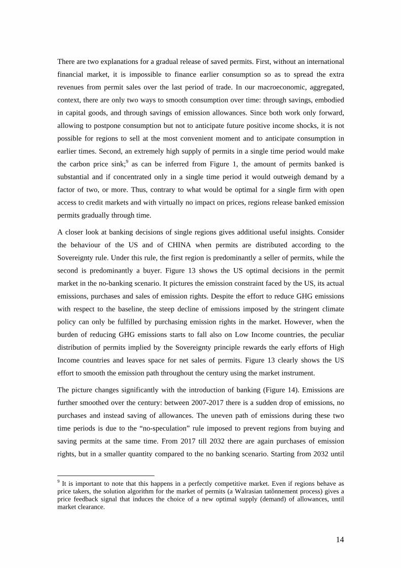
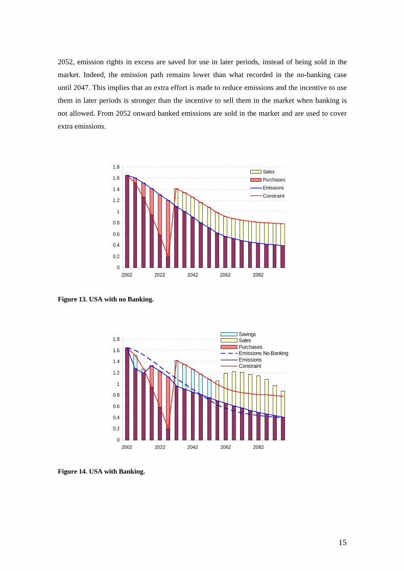
A closer look at banking decisions of single regions gives additional useful insights. Consider

the behaviour of the US and of CHINA when permits are distributed according to the

Sovereignty rule. Under this rule, the first region is predominantly a seller of permits, while the

second is predominantly a buyer. Figure 13 shows the US optimal decisions in the permit

market in the no-banking scenario. It pictures the emission constraint faced by the US, its actual

emissions, purchases and sales of emission rights. Despite the effort to reduce GHG emissions

with respect to the baseline, the steep decline of emissions imposed by the stringent climate

policy can only be fulfilled by purchasing emission rights in the market. However, when the

burden of reducing GHG emissions starts to fall also on Low Income countries, the peculiar

distribution of permits implied by the Sovereignty principle rewards the early efforts of High

Income countries and leaves space for net sales of permits. Figure 13 clearly shows the US

effort to smooth the emission path throughout the century using the market instrument.

The picture changes significantly with the introduction of banking (Figure 14). Emissions are

further smoothed over the century: between 2007-2017 there is a sudden drop of emissions, no

purchases and instead saving of allowances. The uneven path of emissions during these two

time periods is due to the “no-speculation” rule imposed to prevent regions from buying and

saving permits at the same time. From 2017 till 2032 there are again purchases of emission

rights, but in a smaller quantity compared to the no banking scenario. Starting from 2032 until

9 It is important to note that this happens in a perfectly competitive market. Even if regions behave as price takers, the solution algorithm for the market of permits (a Walrasian tatônnement process) gives a price feedback signal that induces the choice of a new optimal supply (demand) of allowances, until market clearance.

15

2052, emission rights in excess are saved for use in later periods, instead of being sold in the

market. Indeed, the emission path remains lower than what recorded in the no-banking case

until 2047. This implies that an extra effort is made to reduce emissions and the incentive to use

them in later periods is stronger than the incentive to sell them in the market when banking is

not allowed. From 2052 onward banked emissions are sold in the market and are used to cover

extra emissions.

0

0.2

0.4

0.6

0.8

1

1.2

1.4

1.6

1.8

2002 2022 2042 2062 2082

SalesPurchasesEmissionsConstraint

Figure 13. USA with no Banking.

0

0.2

0.4

0.6

0.8

1

1.2

1.4

1.6

1.8

2002 2022 2042 2062 2082

SavingsSalesPurchasesEmissions No-BankingEmissionsConstraint

Figure 14. USA with Banking.

16

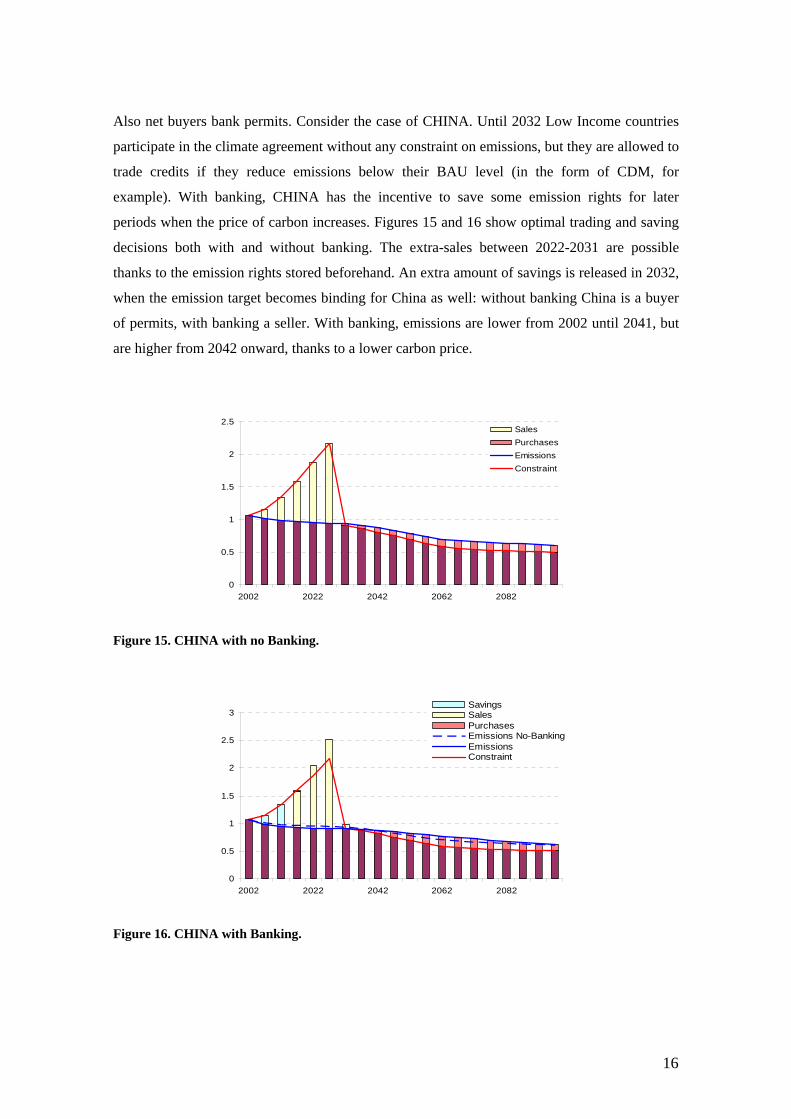
Also net buyers bank permits. Consider the case of CHINA. Until 2032 Low Income countries

participate in the climate agreement without any constraint on emissions, but they are allowed to

trade credits if they reduce emissions below their BAU level (in the form of CDM, for

example). With banking, CHINA has the incentive to save some emission rights for later

periods when the price of carbon increases. Figures 15 and 16 show optimal trading and saving

decisions both with and without banking. The extra-sales between 2022-2031 are possible

thanks to the emission rights stored beforehand. An extra amount of savings is released in 2032,

when the emission target becomes binding for China as well: without banking China is a buyer

of permits, with banking a seller. With banking, emissions are lower from 2002 until 2041, but

are higher from 2042 onward, thanks to a lower carbon price.

0

0.5

1

1.5

2

2.5

2002 2022 2042 2062 2082

SalesPurchasesEmissionsConstraint

Figure 15. CHINA with no Banking.

0

0.5

1

1.5

2

2.5

3

2002 2022 2042 2062 2082

SavingsSalesPurchasesEmissions No-BankingEmissionsConstraint

Figure 16. CHINA with Banking.

17

4. Investments in Energy R&D and in Renewables.

As shown in Section 3, when banking is allowed, prices are higher in the first part of the century

and lower in the second part, with some differences that depend on the adopted allocation rule.

How does the modified price path affect technological change? Does it increase energy

efficiency and/or foster the adoption of low carbon energy sources? The answer is positive.

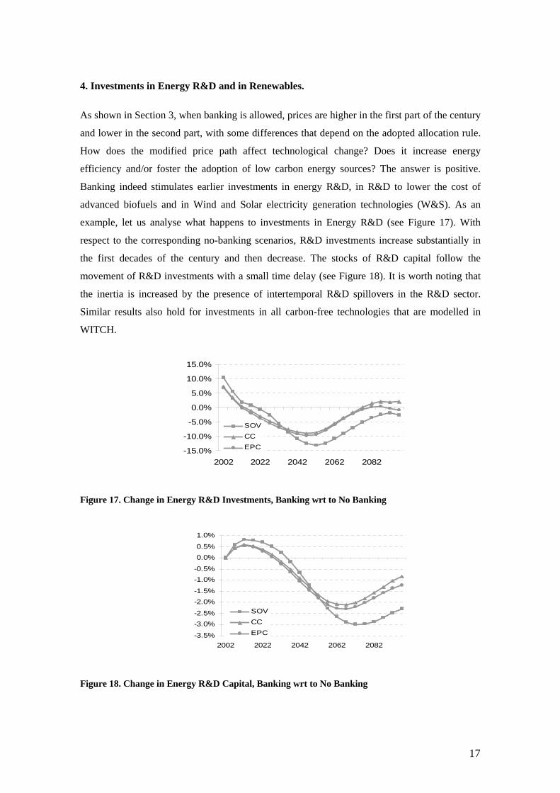
Banking indeed stimulates earlier investments in energy R&D, in R&D to lower the cost of

advanced biofuels and in Wind and Solar electricity generation technologies (W&S). As an

example, let us analyse what happens to investments in Energy R&D (see Figure 17). With

respect to the corresponding no-banking scenarios, R&D investments increase substantially in

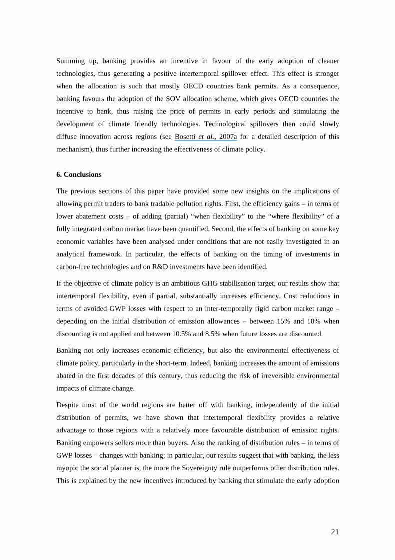
the first decades of the century and then decrease. The stocks of R&D capital follow the

movement of R&D investments with a small time delay (see Figure 18). It is worth noting that

the inertia is increased by the presence of intertemporal R&D spillovers in the R&D sector.

Similar results also hold for investments in all carbon-free technologies that are modelled in

WITCH.

-15.0%

-10.0%

-5.0%

0.0%

5.0%

10.0%

15.0%

2002 2022 2042 2062 2082

SOVCCEPC

Figure 17. Change in Energy R&D Investments, Banking wrt to No Banking

-3.5%

-3.0%-2.5%

-2.0%-1.5%

-1.0%-0.5%

0.0%0.5%

1.0%

2002 2022 2042 2062 2082

SOVCCEPC

Figure 18. Change in Energy R&D Capital, Banking wrt to No Banking

18

The main conclusion is that banking plays an important role in accelerating the adoption and

diffusion of energy efficient and/or carbon-free technologies. By inducing higher carbon prices

in the short term, banking provides the right incentives for firms to switch to climate friendly

technologies earlier than in the absence of banking. This has important macroeconomic and

environmental effects. Earlier adoption of new technologies can indeed reduce stabilisation

costs and enhance the environmental effectiveness of climate policy. These issues will be

discussed in the next section.

5. The Cost of Climate Policy and Equity Considerations

Let us summarise all the results provided above by investigating how banking changes the costs

of stabilisation policy and the distribution of these costs among regions. Table 3 shows our

results.

Undiscounted USA OLDEURO NEWEURO KOSAU CAJAZ TE MENA SSA SASIA CHINA EASIA LACA HI LI World"SOV" 1.75% -0.18% 6.12% 3.79% 0.70% 10.24% 15.34% 10.71% 8.26% 9.70% 9.68% 7.66% 1.93% 9.78% 5.57%"CC" 4.20% 0.98% 8.06% 4.87% 1.76% 13.21% 14.68% -4.73% 4.23% 9.54% 8.56% 6.86% 3.61% 7.72% 5.52%"EPC" 10.04% 3.85% 13.01% 7.46% 4.29% 21.35% 12.79% -44.84% -5.61% 9.45% 5.94% 4.96% 7.76% 2.64% 5.38%"Banking SOV" 0.59% -0.42% 5.79% 3.49% 0.63% 10.08% 13.32% 9.31% 7.20% 8.73% 8.50% 6.45% 1.45% 8.54% 4.74%"Banking CC" 4.14% 0.48% 7.59% 4.36% 1.66% 12.57% 12.81% -3.55% 4.04% 8.79% 7.92% 5.27% 3.31% 6.88% 4.97%"Banking EPC" 9.39% 2.97% 12.00% 6.62% 3.91% 19.86% 11.24% -39.60% -4.77% 8.66% 5.57% 3.48% 6.99% 2.31% 4.82%

Discounted USA OLDEURO NEWEURO KOSAU CAJAZ TE MENA SSA SASIA CHINA EASIA LACA HI LI World"H" 1.48% 0.29% 4.49% 2.64% 0.67% 8.08% 11.07% 8.14% 6.17% 6.44% 7.06% 5.22% 1.50% 6.90% 3.59%"CC" 3.17% 0.99% 6.11% 3.49% 1.34% 10.33% 10.48% -7.82% 2.14% 6.22% 5.99% 4.54% 2.63% 4.97% 3.54%"EPC" 5.91% 2.26% 9.12% 4.98% 2.47% 15.04% 9.23% -37.69% -4.82% 6.08% 4.20% 3.37% 4.60% 1.60% 3.44%"Banking SOV" 1.48% 0.32% 4.38% 2.53% 0.72% 8.19% 9.37% 6.99% 5.28% 5.53% 6.19% 4.34% 1.52% 5.90% 3.21%"Banking CC" 3.28% 0.88% 5.79% 3.23% 1.35% 9.82% 8.92% -6.73% 1.88% 5.53% 5.43% 3.57% 2.57% 4.30% 3.24%"Banking EPC" 5.70% 1.98% 8.43% 4.53% 2.35% 13.94% 7.89% -33.10% -4.26% 5.38% 3.85% 2.47% 4.30% 1.31% 3.14%

Table 3. Stabilisation Cost, measured as GDP loss. [For discounted values, a discount rate of 3% decreasing over time has been applied; negative figures correspond to gains]

As expected, Table 3 shows that greater market flexibility, i.e. banking, reduces policy costs.

Higher early carbon prices induce early investment in R&D and in low carbon technologies,

thus producing an indirect benefit on future abatement costs that adds to the direct benefit from

banking. Savings in early periods are remarkable and suggest that banking might be a key

option for reducing the total cost of climate policy. Table 3 suggests that the undiscounted

aggregate cost, measured as GWP loss, declines from 5.57% to 4.74%, for the SOV allocation

rule, from 5.52% to 4.97%, in the case of CC and from 5.38% to 4.82% for the EPC rule. This is

equivalent to a net reduction of stabilisation costs of 15.0%, 10.0% and 10.4%, for SOV, CC

19

and EPC, respectively. Discounted costs decrease by 10.5%, 8.5% and 8.6%, for SOV, CC and

EPC, respectively. At a more disaggregated level, without discounting, all regions, except the

big sellers of permits in the CC and EPC scenarios, namely SASIA and SSA, are better off with

banking than without. Discounting changes the net position of those regions whose benefits

come late in the future.

Banking also affects the distribution of stabilisation costs. Our results (see Table 4) show that

greater intertemporal flexibility provides larger benefits to regions with the most favourable

initial distribution of emission rights. High Income regions reduce their (already low) share of

stabilisation costs when banking is allowed under the SOV rule, as do Low Income regions

when permits are distributed according to the EPC rule. It thus seems that banking favours

sellers of permits, which can maximise their revenues by optimally distributing carbon rights

across time.

HI LI"H" 19% 81%"CC" 35% 65%"EPC" 77% 23%"Banking SOV" 16% 84%"Banking CC" 36% 64%"Banking EPC" 78% 22%

Table 4. Distribution of Undiscounted Stabilisation Costs

The impact of banking on overall inequality is modest. Table 5 shows that, after 2030, the

allocation of permits that yields the lowest Gini Coefficient, and thus the fairest distribution, is

the EPC, both with and without banking. The most inequitable is instead SOV, as expected.

Banking has a very mild effect on the distribution of policy costs. The only remarkable

difference is a decrease of inequality when banking is allowed under the SOV scenario, because

during the second half of the century carbon permit buyers (developing countries) can benefit

from a lower carbon price. Inequality increases with banking in the EPC scenario, because the

lower price of carbon yields a drop in the inflow of revenues to SSA and SASIA – two among

the poorest regions of the world. Any difference in effort across allocation schemes is smoothed

out during the second half of the century, due to the predominance of Low Income regions as

emitters.

20

BaU "SOV" "CC" "EPC" "Banking SOV" "Banking CC" "Banking EPC"2050 0.485 0.493 0.476 0.464 0.487 0.477 0.4652100 0.406 0.425 0.420 0.358 0.426 0.420 0.359

Table 5. Gini Indicators for 2050 and 2100 across different allocation schemes, with and without banking.

Without banking, the least costly policy is obtained when permits are distributed following the

EPC principle. It is however noticeable how policy costs are extremely high for High Income

countries, while some Low Income countries gain disproportionately from this allocation rule.

By contrast, the SOV allocation, which would be the most likely to be accepted by OECD

countries, appears to be the worst allocation in terms of overall policy costs.

With banking, the greater flexibility allows to smooth out the variance of policy costs across

allocation schemes. Moreover, there are two different rankings, depending on whether costs are

discounted or not. By looking at Table 6 we see that the SOV allocation becomes the first best

strategy the less myopic the decision maker is. The reason is clear if we look at Figures 6 and 7

above. In the SOV scenario, banking creates a sharp increase of carbon price in the first years,

but also the strongest drop after mid-century.

Policy Costs Differences w r t "EPC" Discounted Undiscounted"SOV" 4.30% 3.51%"CC" 2.84% 2.54%"EPC" - -"Banking SOV" 2.14% -1.70%"Banking CC" 3.03% 3.03%"Banking EPC" - -

Table 6. Policy Cost Differences Across Allocation Schemes wrt the EPC allocation scheme [For discounted figures a discount rate of 3% decreasing over time has been applied, negative differences represent gains]

The CC scheme is the one performing worst both with and without banking. Indeed, it benefits

OECD countries immediately after 2030, but not enough to leave them the possibility to save

the amount of permits required to cope with higher prices of permits.

21

Summing up, banking provides an incentive in favour of the early adoption of cleaner

technologies, thus generating a positive intertemporal spillover effect. This effect is stronger

when the allocation is such that mostly OECD countries bank permits. As a consequence,

banking favours the adoption of the SOV allocation scheme, which gives OECD countries the

incentive to bank, thus raising the price of permits in early periods and stimulating the

development of climate friendly technologies. Technological spillovers then could slowly

diffuse innovation across regions (see Bosetti et al., 2007a for a detailed description of this

mechanism), thus further increasing the effectiveness of climate policy.

6. Conclusions

The previous sections of this paper have provided some new insights on the implications of

allowing permit traders to bank tradable pollution rights. First, the efficiency gains – in terms of

lower abatement costs – of adding (partial) “when flexibility” to the “where flexibility” of a

fully integrated carbon market have been quantified. Second, the effects of banking on some key

economic variables have been analysed under conditions that are not easily investigated in an

analytical framework. In particular, the effects of banking on the timing of investments in

carbon-free technologies and on R&D investments have been identified.

If the objective of climate policy is an ambitious GHG stabilisation target, our results show that

intertemporal flexibility, even if partial, substantially increases efficiency. Cost reductions in

terms of avoided GWP losses with respect to an inter-temporally rigid carbon market range –

depending on the initial distribution of emission allowances – between 15% and 10% when

discounting is not applied and between 10.5% and 8.5% when future losses are discounted.

Banking not only increases economic efficiency, but also the environmental effectiveness of

climate policy, particularly in the short-term. Indeed, banking increases the amount of emissions

abated in the first decades of this century, thus reducing the risk of irreversible environmental

impacts of climate change.

Despite most of the world regions are better off with banking, independently of the initial

distribution of permits, we have shown that intertemporal flexibility provides a relative

advantage to those regions with a relatively more favourable distribution of emission rights.

Banking empowers sellers more than buyers. Also the ranking of distribution rules – in terms of

GWP losses – changes with banking; in particular, our results suggest that with banking, the less

myopic the social planner is, the more the Sovereignty rule outperforms other distribution rules.

This is explained by the new incentives introduced by banking that stimulate the early adoption

22

of carbon-free technologies (more in developed countries, where R&D is more effective in

reducing the cost of these technologies).

Banking yields all the expected smoothing effect on emissions, abatement effort, price of

carbon. Emission rights are first banked and then released in later periods, when the policy

constraint becomes very stringent. The carbon market adapts, by first shrinking and then

expanding in later periods. The price of carbon is higher in the first decades but lower in the

second half of the century. Contrary to what predicted by analytical models, we find that an

increasing time profile for the discounted price of carbon is fully consistent with banking. A

“premium” over the interest rate is indeed necessary for agents to bank emission permits at the

equilibrium.

Finally, let us stress we adopted a normative approach and not a descriptive one. Our findings

belong to an ideal world in which all agents behave optimally and with perfect foresight over

their future actions, the other agents’ decisions, and future states of the world. Nevertheless, we

have been able to show that, when a richer framework of analysis is used, “when flexibility”

yields some interesting unexpected results. We believe that these results can be useful both to

economists – who will find a stimulus to build richer analytical models – and to policymakers –

who may find in this paper useful information to design post 2012 carbon markets.

23

References

Babiker, M.H., H.D. Jacoby, J.M. Reilly, and D.M. Reiner (2002). “The Evolution of a Climate Regine: Kyoto to Marrakech.” MIT Joint Program on the Science and Policy of Global Change, Report No. 82.

Bosetti, V., C. Carraro, M. Galeotti, E. Massetti and M. Tavoni, (2006). “WITCH: A World Induced Technical Change Hybrid Model.” The Energy Journal, Special Issue on Hybrid Modeling of Energy-Environment Policies: Reconciling Bottom-up and Top-down, 13-38.

Bosetti, V., C. Carraro, E. Massetti and M. Tavoni, (2007a). “International Energy R&D Spillovers and the Economics of Greenhouse Gas Atmospheric Stabilization”, FEEM Nota di Lavoro 82.07, CEPR Discussion Paper 4703 and CESifo Working Paper N. 2151.

Bosetti, V., C. Carraro, E. Massetti and M. Tavoni, (2007b). “Optimal Energy Investment and R&D Strategies to Stabilise Greenhouse Gas Atmospheric Concentrations”, FEEM Nota di Lavoro 95.07, CEPR Discussion Paper 6549 and CESifo Working Paper N. 2133.

Bosetti, V., E. Massetti and M. Tavoni (2007). “FEEM’s WITCH Model: Structure, Baseline, Solutions.” FEEM Nota di Lavoro 10.07.

Carraro, C. and M. Galeotti (2004). “Does Endogenous Technical Change Make a Difference in Climate Change Policy Analysis? A Robustness Exercise with the FEEM-RICE Model.” FEEM Nota di Lavoro 152.04.

Coase, R.H. (1960). “The Problem of Social Cost.” Journal of Law and Economics, 3: 1-44.

Cronshaw, M. and J. B. Kruse (1996). “Regulated Firms in Pollution Permit Markets with Banking.” Journal of Regulatory Economics, 9: 179-89.

Godby, R.W., S. Mestelman, R.A. Muller and J.D.Welland (1997). “Emissions Trading with Shares and Coupons when Control over Discharges is Uncertain.” Journal of Environmental Economics and Management, 32: 359–381.

Innes, R. (2003). “Stochastic Pollution, Costly Sanctions, and Optimality of Emission Permit Banking.” Journal of Environmental Economics and Management, 45(3): 546-568.

Kling, C. and J. Rubin (1997). “Bankable Permits for the Control of Environmental Pollution.” Journal of Public Economics, 64: 101-115.

Leiby, P. and J. Rubin (2001). “Bankable Permits for the Control of Stock and Flow Pollutants: Optional Intertemporal Greenhouse Gas Emission Trading.” Environmental and Resource Economics, 19: 229-256.

Liski, M. and J.-P. Montero (2003). “A Note on Market Power in an Emission Permits Market with Banking.” Mimeo.

Manne, A.S. and R.G. Richels (2001). “US Rejection of the Kyoto Protocol: the Impact on Compliance Costs and CO2 Emissions.” Working Paper 01-12, AEI- Brookings Joint Center for Regulatory Studies.

24

Newell, R., W. Pizer and J. Zhang (2003). “Managing Permits Markets to Stabilize Prices.” RFF Discussion Paper 03-34, Washington D.C. .

Rubin, J. (1996). “A Model of Intertemporal Emission Trading, Banking and Borrowing.” Journal of Environmental Economics and Management, 31(3): 269-286.

Springer, U. (2003). “The Market for Tradable GH Permits Under the Kyoto Protocol: a Survey of Model Studies.” Energy Economics, 25: 527-551.

25

Appendix: Model Equations and List of Variables.

In this Appendix we reproduce the main equations of the model. For a full description of the model please refer to Bosetti, Massetti and Tavoni (2007). The list of variables is reported at the end. In each region, indexed by n, a social planner maximises the following utility function:

[ ] [ ]{ }∑∑ ==tt

tRtnctnLtRtnLtnCUnW )(),(log),()(),(),,()( , (A1)

where t are 5-year time spans and the pure time preference discount factor is given by:

[ ]∏=

−+=t

v

vtR0

5)(1)( ρ , (A2)

where the pure rate of time preference ρ(v) is assumed to decline over time. Moreover, ),(),(),(

tnLtnCtnc = is

per capita consumption.

Economic module The budget constraint defines consumption as net output less investments:

( ) ( ) ( ) ( ) ( ) ( ) ( )∑ ∑∑ −−−−−=j j jjj jDRENDRC tnO&MtnItnItnItnItnYtnC ,,,,,,, ,&,& (A3)

Where j denotes energy technologies. Output is produced via a nested CES function that combines a capital-labour aggregate and energy; capital and labour are obtained from a Cobb-Douglas function. The climate damage Ω reduces gross output; to obtain net output we subtract the costs of the fuels f and of CCS:

( )( ) ( ) ( )( ) ( )

( )( ) ( ) ( ) ( )( )

( ) ( )tnCCStnP

tnXtPtnXtnP

tn

tnESntnLtnKntnTFPtnY

CCS

f netimpffextrff

nnC

,,

,,,

,

,))(1(,,)(,,

,int

,

/1)()(1

−

+−

Ω

⎥⎦⎤

⎢⎣⎡ ⋅−+⋅

=

∑

−ρ

ρρββ αα

. (A4)

Total factor productivity ( )tnTFP , evolves exogenously with time. Final good capital accumulates following the standard perpetual rule:

t) (nItn K) t(nK CCCC ,)1)(,(1, +−=+ δ . (A5) Labour is assumed to be equal to population and evolves exogenously. Energy services are an aggregate of energy and a stock of knowledge combined with a CES function:

( ) [ ] ESESES tnENtnHEtnES ENHρρρ αα

/1),(),(, += . (A6)

The stock of knowledge ( )tnHE , derives from energy R&D investment:

)1)(,(),(),(1, && DRcb

DR tnHEtnHEtn aI) tHE(n δ−+=+ . (A7) Energy is a combination of electric and non-electric energy:

( ) [ ] ENENEN tnNELtnELtnEN NELELρρρ αα /1),(),(, += . (A8)

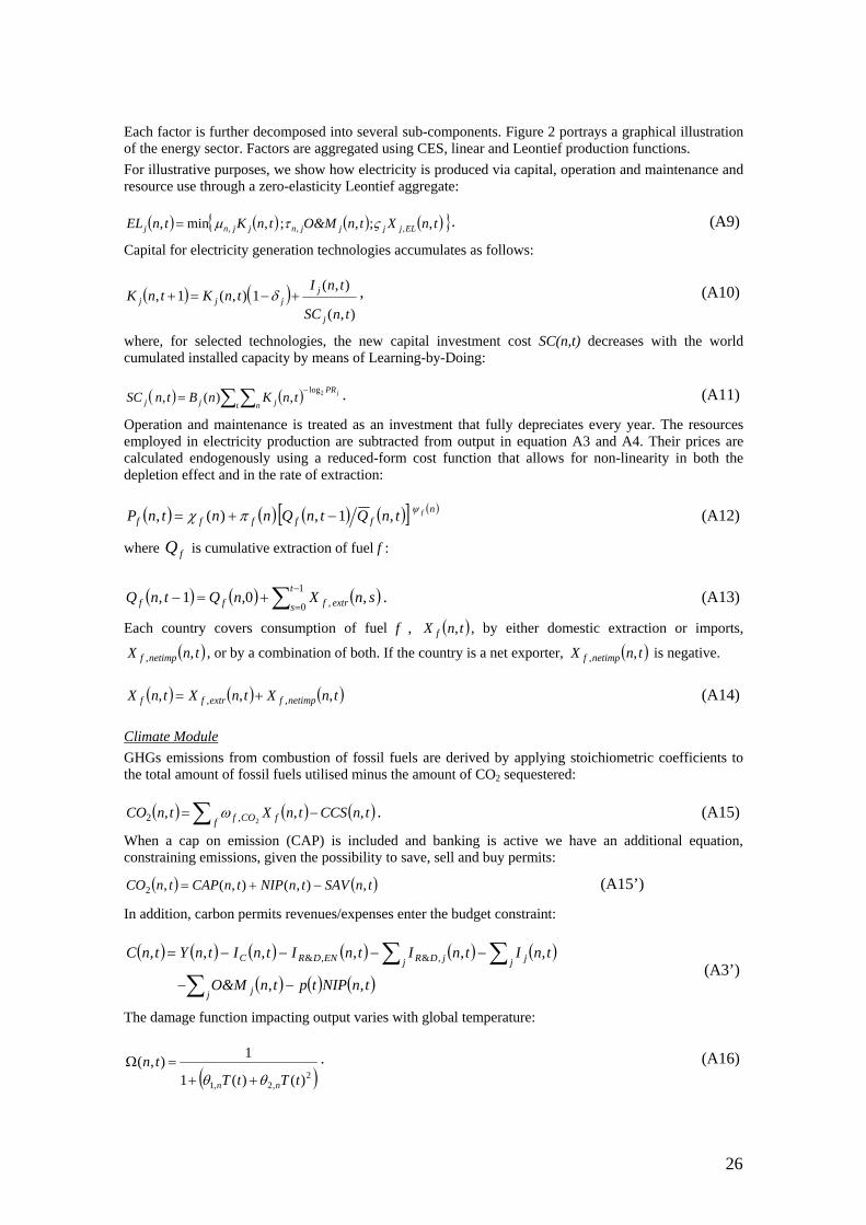
26

Each factor is further decomposed into several sub-components. Figure 2 portrays a graphical illustration of the energy sector. Factors are aggregated using CES, linear and Leontief production functions. For illustrative purposes, we show how electricity is produced via capital, operation and maintenance and resource use through a zero-elasticity Leontief aggregate:

( ) ( ) ( ) ( ){ }tnXtnO&MtnKtnEL ELjjjjnjjnj ,;,;,min, ,,, ςτμ= . (A9)

Capital for electricity generation technologies accumulates as follows:

( ) ( )),(

),(1),(1,

tnSC

tnItnKtnK

j

jjjj +−=+ δ , (A10)

where, for selected technologies, the new capital investment cost SC(n,t) decreases with the world cumulated installed capacity by means of Learning-by-Doing:

( ) ( ) jPR

t n jjj tnKnBtnSC 2log,)(,

−∑ ∑= . (A11)

Operation and maintenance is treated as an investment that fully depreciates every year. The resources employed in electricity production are subtracted from output in equation A3 and A4. Their prices are calculated endogenously using a reduced-form cost function that allows for non-linearity in both the depletion effect and in the rate of extraction:

( ) ( ) ( ) ( )[ ] ( )nfffff

ftnQtnQnntnP ψπχ ,1,)(, −+= (A12)

where fQ is cumulative extraction of fuel f :

( ) ( ) ( )∑ −

=+=−

1

0 , ,0,1,t

s extrfff snXnQtnQ . (A13)

Each country covers consumption of fuel f , ( )tnX f , , by either domestic extraction or imports,

( )tnX netimpf ,, , or by a combination of both. If the country is a net exporter, ( )tnX netimpf ,, is negative.

( ) ( ) ( )tnXtnXtnX netimpfextrff ,,, ,, += (A14)

Climate Module GHGs emissions from combustion of fossil fuels are derived by applying stoichiometric coefficients to the total amount of fossil fuels utilised minus the amount of CO2 sequestered:

( ) ( ) ( )tnCCStnXtnCOf fCOf ,,,

2,2 −=∑ ω . (A15)

When a cap on emission (CAP) is included and banking is active we have an additional equation, constraining emissions, given the possibility to save, sell and buy permits:

( ) ( )tnSAVtnNIPtnCAPtnCO ,),(),(,2 −+= (A15’)

In addition, carbon permits revenues/expenses enter the budget constraint:

( ) ( ) ( ) ( ) ( ) ( )

( ) ( ) ( )tnNIPtptnO&M

tnItnItnItnItnYtnC

j j

j jj jDRENDRC

,,

,,,,,, ,&,&

−−

−−−−=

∑∑∑

(A3’)

The damage function impacting output varies with global temperature:

( )2,2,1 )()(1

1),(tTtT

tnnn θθ ++

=Ω . (A16)

27

Temperature increases through augmented radiating forcing F(t):

[ ]{ })()()()1()()1( 21 tTtTtTtFtTtT LO−−−++=+ σλσ (A17)

which in turn depends on CO2 concentrations:

[ ]{ } )()2log(/)(log)( tOMtMtF PIATAT +−=η , (A18)

caused by emissions from fuel combustion and land use change:

( )[ ] )()()(,)1( 21112 tMtMtLUtnCOtM UPATn

jAT φφ +++=+ ∑ , (A19)

)()()()1( 321222 tMtMtMtM LOATUPUP φφφ ++=+ , (A19)

)()()1( 2333 tMtMtM UPLOLO φφ +=+ . (A20)

28

Model variables are denoted with the following symbols:

W = welfare U = instantaneous utility C = consumption c = per-capita consumption L = population R = discount factor Y = production Ιc=investment in final good ΙR&D, EN=investment in energy R&D Ιj=investment in technology j O&M=investment in operation and maintenance ΤFP=total factor productivity Κc=final good stock of capital ES=energy services Z=flow of new knowledge Ω = damage Pj= fossil fuel prices

Xj= fuel resources PCCS= price of CCS CCS=CO2 sequestered HE=energy knowledge EN=energy EL=electric energy NEL=non-electric energy Κj= stock of capital of technology j SCj=investment cost CO2= emissions from combustion of fossil fuels NIP = Net import of carbon permits SAV = Saved carbon permits p = Price of carbon permits MAT = atmospheric CO2 concentrations LU = land-use carbon emissions MUP = upper oceans/biosphere CO2 concentrations MLO = lower oceans CO2 concentrations F = radiative forcing T= temperature level