Integrating vital rate variability into perturbation analysis: an evaluation for matrix population...

Journal of Ecology

2001

89

, 995–1005

© 2001 British Ecological Society

Blackwell Science Ltd

Integrating vital rate variability into perturbation analysis: an evaluation for matrix population models of six plant species

PIETER A. ZUIDEMA*† and MIGUEL FRANCO‡§

†

Department of Plant Ecology, Utrecht University, PO Box 80084, 3508 TB Utrecht, The Netherlands and Programa Manejo de Bosques de la Amazonía Boliviana (PROMAB), Casilla 107, Riberalta, Beni, Bolivia; and

‡

Instituto de Ecologia, Universidad Nacional Autónoma de México, Apartado Postal 70–275, 04510 Coyoacán, D.F., México

Summary

1

Matrix population models are usually constructed by employing average values ofvital rates (survival, growth and reproduction) for each size category. Perturbation ana-lyses of matrix models assess the influence of vital rates or matrix elements on popula-tion growth rate. They consider the impact of either an unstandardized (sensitivityanalysis) or a mean-standardized (elasticity analysis) change in a model component.Certain vital rates are intrinsically more variable than others. This variation can betaken into account in variance-standardized perturbation analysis, which applieschanges to vital rates in proportion to their variability.

2

We applied variance-standardized perturbation analysis to six plant species with differ-ent life histories (a forest understorey herb, two tropical forest palms and three tropicalforest trees). 1500 random values were drawn from observed frequency distributions ofeach vital rate in each size category, and population growth rates (

λ

) were calculated foreach of the simulations.

3

Variability differed widely between vital rates, being particularly high for growth andreproduction. Vital rate variation was negatively correlated with its effect on

λ

(meas-ured by either sensitivity or elasticity). The variation in

λ

resulting from the samplingprocedure differed between species (with higher values in shorter-lived plants) and vitalrates (with particularly high values due to variation in growth rates).

4

The relationships between

λ

and vital rates were close to linear. Therefore, the productof sensitivity (or elasticity) and degree of variability of a vital rate was a good estimatorof the variation in

λ

, explaining 95% of the variation in

λ

in the six study species.

5

Thus, a reliable estimation of the 95% confidence interval of

λ

due to variation in oneof the vital rates can be calculated as the product of the 95% confidence interval of thevital rate and its sensitivity.

6

Our results suggest that variance-standardized perturbation analyses are a usefultool to determine the impact of vital rate variation on population growth rate.

Key-words

:

demographic variation, plant demography, population growth rate, sensit-ivity analysis, variance-standardized perturbation

Journal of Ecology

(2001)

89

, 995–1005

Introduction

Matrix population models are a widely used tool ofdemographic analysis (Caswell 1989a). An important

development of these models is the family of tech-niques known as perturbation analyses, which com-pare the importance of different model components formodel output – usually population growth. The mostcommonly used perturbation techniques, sensitivity(Caswell 1978) and elasticity (de Kroon

et al

. 1986)analyses, have become standard procedures in a rangeof research fields (Benton & Grant 1999; de Kroon

et al

. 2000). Sensitivity analysis considers the effect onpopulation growth of a fixed infinitesimal changein a vital rate (

unstandardized

perturbation), whereas

*Correspondence and present address: Pieter Zuidema, PlantProduction Systems Group, Wageningen University, POBox 430, 6700 AK Wageningen, The Netherlands (fax +31 317484892; e-mail [email protected]).§Present address: Department of Biological Sciences, Univer-sity of Plymouth, Drake Circus, Plymouth PL4 8AA, UK.

JEC_621.fm Page 995 Wednesday, November 21, 2001 9:01 AM

996

P. A. Zuidema & M. Franco

© 2001 British Ecological Society,

Journal of Ecology

,

89

, 995–1005

elasticity analysis quantifies the influence of an infini-tesimal change that is proportional to the size of eachvital rate (

mean-standardized

perturbation).Matrix population models are most often con-

structed using average values of vital rates (survival,growth and reproduction), and their projections assumethat population dynamics are constant over time andspace. However, vital rates vary between individuals,between populations and over time, and it is importantto evaluate the effect of this demographic variationon (the reliability of) the resulting population growthrates. Several techniques have been developed to assessthe impact of variation in time (e.g. Tuljapurkar 1989;Caswell & Trevisan 1994), space (e.g. Alvarez-Buylla &García-Barrios 1993; Alvarez-Buylla 1994; Pascarella& Horvitz 1998), or both time and space (e.g. Caswell1989b, 1996a; Horvitz

et al

. 1997; Ehrlén & vanGroenendael 1998). Most of these techniques considervariation between populations or over different timeperiods, using sets of transition matrices, each of whichrepresents one (sub)population or one period of time.

Less attention has been paid to the influence ofvariation

within

one population or during one timeperiod, although its significance is widely acknow-ledged (Sarukhán

et al

. 1982; van Tienderen 1995, 2000;Silvertown

et al

. 1996; Ehrlén & van Groenendael 1998;Benton & Grant 1999; Bierzychudeck 1999; de Kroon

et al

. 2000). This variation is not explicit in the transitionmatrix, as the matrix only contains average values. It mayresult from genetic and phenotypic variation betweenindividuals, from differences in microenvironmentalconditions experienced by different individuals and fromuncertainty in parameter estimates (Wisdom & Mills1997; Caswell

et al

. 1998; Hunter

et al

. 2000; Wisdom

et al

. 2000). A first-order approximation of the variancein population growth rate demonstrates how demo-graphic variation leads to uncertainty in populationgrowth (Lande 1988; Caswell 1989a). This concept hasbeen used in the development of methods to determineconfidence limits for population growth rate (Caswell1989a; Alvarez-Buylla & Slatkin 1991, 1993, 1994).

Some vital rates (e.g. seed production) are more vari-able and thus more liable to change than others (e.g.adult survival). Demographic processes with a lowsensitivity value but a very high degree of variation maythus potentially cause more variation in the populationgrowth rate than those processes with high sensitivityand low variability. When the probability of changesin certain vital rates is taken into account, those vitalrates with the greatest ‘influence’ on population growthrate may differ from those suggested by sensitivity orelasticity analysis alone. Van Tienderen (1995) hassuggested a perturbation technique that specificallyincorporates variability in demographic processes,which can be considered

variance-standardized

, sincechanges imposed are proportional to the variability ofeach vital rate (e.g. by using standard deviation units).A similar approach has been adopted by Ehrlén & vanGroenendael (1998), employing several transition matrices.

We conduct such analyses for six plant species withdifferent life histories using Monte Carlo simulationsin which values of vital rates are randomly drawnfrom observed frequency distributions and populationgrowth rates are calculated for each sampling exercise.The advantages of this simulation procedure over theuse of a fixed perturbation unit (e.g. one standarddeviation, as in van Tienderen 1995) are (1) that therelationships between population growth rates andvital rates can be visualized and analysed, and (2) thatfrequency distributions of population growth rates canbe obtained, from which the degree of variability in thepopulation growth rate can be derived. The perturbationapproach adopted here is comparable to sensitivityand elasticity analyses in that it applies a change inone vital rate and in one size category at a time whilekeeping all others constant. In the absence of directinformation we assume that covariation between vitalrates is negligible. Perturbations are carried out directlyon the vital rates (survival, growth and reproduction;also called lower-level parameters) determined in fieldstudies, rather than on matrix elements. Such rates arealso often the focus for intervention in the conserva-tion and management of natural populations (Caswell1996a; Mills

et al

. 1999).Specifically, the goals of our study were: (1) to exam-

ine patterns of variability of vital rates for plant specieswith different life histories; (2) to determine the effectof this variability on population growth; (3) to deter-mine the form of the relationships between populationgrowth rates and vital rates and to test whether theoften-assumed linear approximation of these relationsholds; and (4) to compare the results obtained fromvariance-standardized perturbation analysis to thoseobtained with standard sensitivity and elasticity analysis.

Materials and methods

Matrix population models project the size and structureof populations in time. The basic model is

n

(

t

+ 1) =

An

(

t

), where

A

is a square

m

×

m

matrix with transitionsamong

m

categories during a certain time interval, and

n

is the population vector containing densities of indi-viduals in

m

size (or stage) categories. The dominanteigenvalue (

λ

) of matrix

A

is equivalent to the growthrate of the population (Caswell 1989a). In stage-basedmatrix models (Lefkovitch 1965), elements

a

ij

(with

i

denoting row number and

j

denoting column number)of transition matrix

A

can be grouped into those rep-resenting stasis (

P

j

, the probability of surviving andremaining in stage

j

from one recording date to thenext), progression (

G

ij

, the probability of surviving andgrowing from stage

j

to stage

i

which contains largerindividuals), retrogression (

R

ij

, the probability of surviv-ing and going back from stage

j

to stage

i

which containssmaller individuals) and fecundity (

F

j

, the number ofsexual offspring produced by an individual in stage

j

).


997

Variance-standardized perturbation analysis


Journal of Ecology

,

89

, 995–1005

Matrix elements are built from underlying

vital rates

– survival (

σ

j

), growth (positive:

γ

ij

; negative:

ρ

ij

) andreproductive output (

f

j

) – to which they are relatedby ,

G

ij

=

σ

j

γ

ij

,

R

ij

=

σ

j

ρ

ij

and

F

j

=

σ

j

f

j

. We employ pairs of subscripts only when sev-eral transitions occur (e.g. progression and retrogression),using just the subscript of the source category (

j

) formatrix elements and vital rates that involve a single transi-tion (e.g. stasis) or are specific to a stage (e.g. survival).

In its standard form, sensitivity analysis considers theimpact of changes in

matrix elements

on populationgrowth rate (

λ

):

eqn 1

where

s

ij

is the sensitivity of matrix element

a

ij

,

v

i

and

w

j

are elements of the left (

v

) and right (

w

) eigenvectorsassociated with

λ

, and <

w

,

v

> denotes the scalar prod-uct (Caswell 1978).

However, sensitivities can also be applied to the

vitalrates

(lower-level parameters) (Caswell 1989a, 1996a;Brault & Caswell 1993; Mills

et al

. 1999). This is doneby tracking the changes in

λ

resulting from changes inthe vital rates implicit in matrix elements

a

ij

. For thevital rates mentioned above, the sensitivities of vitalrates are (following Caswell 1989a; pp. 126–129 andCaswell 1996a):

eqn 2

eqn 3

eqn 4

eqn 5

Elasticity values can also be calculated for vital rates.Standard elasticity considers the proportional changein

λ

due to a proportional change in a parameter (deKroon

et al

. 1986):

eqn 6

where

e

ij

is the elasticity of matrix element

a

ij

, and

s

ij

is its sensitivity. Equation 6 shows that elasticity isobtained by multiplying sensitivity by

a

ij

/

λ

. In analogy,elasticity values of vital rates can be obtained bymultiplying vital rate sensitivity by

x/

λ

(Caswell 1989a;p. 135), where

x

is the value of the vital rate under con-sideration (

σ

j

,

γ

ij

,

ρ

ij

or

f

j

).Unlike the values for matrix elements, vital rate sen-

sitivity and elasticity may be negative, but as it is themagnitude of the change that interests us here, ratherthan its sign, absolute values are quoted throughoutthe paper. For vital rates, elasticities do not sum to 1(Caswell 1989a).

-

In order to assess the influence of variability in eachdemographic parameter on the population growth rate(

λ

) we consider variation in vital rates (survival, growthand reproduction), which represent a single demographicprocess, rather than in matrix elements, which combineseveral processes. We consider variation in

one

vital ratein

one

size category at a time. Demographic variationbetween individuals may be caused by genetic, pheno-typic and/or microenvironmental differences within acategory, as well as by temporal variation.

Frequency distributions

Frequency distributions, based on variation in vitalrates between individuals in each category, were firstidentified. For observed transitions, positive and neg-ative growth (

γ

ij

and

ρ

ij

) can be described using a bino-mial frequency distribution (as the basic observationsare whether an individual does or does not move intoanother category). If growth in size is measured for theindividual plants and subsequently used to calculatetransitions using stage durations, individual growthrates mostly follow a (log)normal distribution. Sur-vival probability (

σ

j

) follows a binomial distribution.Reproductive output (

f

j

) may follow either a (log)nor-mal or binomial distribution, or be made up of severalparameters, each with a different frequency distribution(e.g. probability of reproducing [binomial]

×

numberof offspring produced per reproductive individual[ (log)normal]): values are then drawn from the respect-ive distributions and multiplied together. For each cat-egory, the frequency distributions of observed vitalrates are described by their mean and (binomial) stand-ard deviation.

Sampling of individuals

For each combination of size category and vital rate,1500 values were drawn at random, with the restriction

Pj ji

iji

ij ( )= − ∑ − ∑σ γ ρ1

s

a

v wi j

i j

i j ,

= =< >

∂λ∂ w v

Survival:

( )

sP

P

G

G

R

R

F

F

s

s s

j

j j

j

j i j

i j

ji

i j

i j

ji j

j

j

jji

i ji

i j

ii j i j

ii j i j

σ∂λ∂σ

∂λ∂

∂∂σ

∂λ∂

∂∂σ

∂λ∂

∂∂σ

∂λ∂

∂∂σ

γ ργ ρ

= = +

+ +

= − −+ + +

∑

∑1 Σ Σ

Σ Σ s fj j1

Positive growth ( ):

( )

i j sP

P

G

G

s s

iji j j

j

i j

i j

i j

i j

jj j i j j

> = =

+

= − +

γ∂λ

∂γ∂λ∂

∂∂γ

∂λ∂

∂∂γ

σ σ

Negative growth ( ):

( )

i j sP

P

R

R

s s

iji j j

j

i j

i j

i j

i j

jj j i j j

< = =

+

= − +

ρ∂λ∂ρ

∂λ∂

∂∂ρ

∂λ∂

∂∂ρ

σ σ

Fecundity: s

f F

F

fsfj

j j

j

jj j= = =

∂λ∂

∂λ∂

∂∂

σ1

e

a a a

asi j

i j i j i j

i ji j

loglog

//

= = =∂ λ∂

∂λ λ∂ λ


998

P. A. Zuidema & M. Franco


Journal of Ecology

,

89

, 995–1005

that all had to fall within the 95% confidence interval ofthe observed vital rate distribution, and that (bio)log-ically impossible values (negative

γ

ij

and

f

j

values,probability values outside the <0,1> interval) wereexcluded. For vital rates with a binomial frequencydistribution, values were drawn from a normal dis-tribution, as this approximates the binomial distri-bution fairly well for moderately large samples (Sokal& Rohlf 1995). A matrix was constructed for each ofthe 1500 sampled values, using unchanged values forall other vital rates of the category under considera-tion and for matrix elements of all other categories.Population growth rate (

λ

) was then computed foreach matrix.

Analysis of simulation results

Mean, standard deviation, 95% confidence interval(calculated using the SD of the distribution; henceforthreferred to as CI95) and coefficient of variation (CV)were calculated for each vital rate and the resulting

λ

-values. The magnitude of changes in

λ

due to the sim-ulated variation in vital rates was compared betweenspecies and vital rates, and related to both their degreeof variation and to their effect on population growth(sensitivity and elasticity). The relationship betweeneach vital rate and population growth was alsoassessed. Absolute (sensitivity, CI95) as well as relative(elasticity, CV) measures of importance and variabilityof vital rates were calculated.

We applied the perturbation analysis outlined aboveto six plant species with different life histories and lifespans (Table 1), and including small to large-sized transi-tion matrices. Detailed information on demographicstudies, matrix construction and vital rates of the studyspecies can be found in Appendix 1.

Results

Variability of vital rates differed widely, with coeffi-cients of variation ranging from 0 to 77 (MedianCV = 27.1,

n

= 188). Vital rate types differed signific-

antly, both for absolute (CI95; Kruskal–Wallis (KW):

χ

23

= 42.7,

P

< 0.001) and relative (CV;

χ

23

= 120.7,

P

< 0.001) measures of variation. Confidence intervalswere narrower for survival than for positive growth andreproduction (multiple comparisons KW,

P

< 0.05;Siegel & Castellan 1988). No difference was foundbetween species in vital rate variability, either for abso-lute (comparing CI95 values of all vital rates betweenspecies; KW:

χ25 = 8.9, P = 0.11) or for relative meas-

ures (CV values: χ25 = 3.9, P = 0.57).

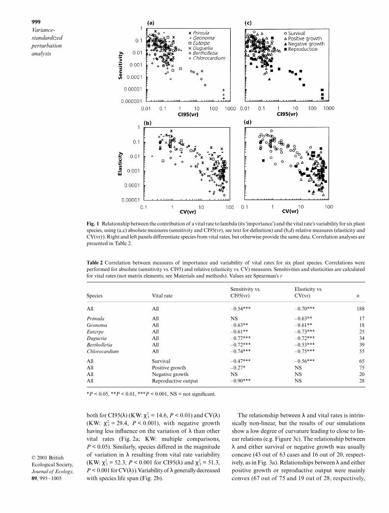
Considered over all vital rates and species, there wasa negative correlation between the variability of a vitalrate and its effect on λ, both when measured in absolute(CI95(vr) vs. sensitivity) and in relative (CV(vr) vs.elasticity) terms (Fig. 1, Table 2). It is clear that repro-ductive output, which spans almost the entire range ofvalues, is mostly responsible for this relationship whenabsolute measures are considered (Fig. 1c; Table 2:Spearman’s r = −0.90). Looking at the contribution byspecies, the points with lowest sensitivity and highestvital rate CI95 values correspond to the reproductiveoutput values of the two longest-living tree species,Chlorocardium rodiei and Bertholletia excelsa (lowerright-hand side of Fig. 1a). In contrast, when consider-ing relative measures (elasticity vs. CVs in Fig. 1b,d),survival rather than reproduction spans the widestrange, and this is mostly responsible for the overallcorrelation (Table 2). Survival in adult categoriesoccupies the high elasticity–low variability end of therelationship, whereas seedling survival occupies theopposite end (KW for CV of drawn values in seed-ling, juvenile and adult categories: χ2

2 = 29.4, n = 65;P < 0.001). When evaluated at the species level, neg-ative correlations between vital rate variability andsensitivity or elasticity of λ were found for most species(Table 2).

-

The variation in population growth rate (λ) resultingfrom the variance-standardized perturbations over allvital rate types and species ranged from 0.000 to 0.077for CI95(λ) and from 0.001 to 1.891 for CV(λ). Signi-ficant differences were found between vital rate types,

Table 1 Characteristics of the six plant species used for variance-standardized perturbation analysis. The value of populationgrowth (λ) is that of the transition matrix using mean vital rates; size is number of categories in matrix. Estimates of life span comefrom the cited references for the first two species, and mean age (and standard deviation) in the last category (Cochran & Ellner1992; S1 – mean age of residence) for the remaining species. More information on study methods, matrix construction and vitalrates is presented in Appendix 1

Species Family Life form λ Size Life span Reference

Primula vulgaris Primulaceae Forest understorey herb 1.038 5 10–30 Valverde & Silvertown 1998Geonoma deversa Palmae Understorey palm (ramets) 1.041 6 c. 37 Zuidema 2000Euterpe precatoria Palmae (Sub)canopy palm 0.977 11 106 (35) Zuidema 2000Duguetia neglecta Annonaceae Understorey tree 1.006 12 255 (95) Zagt 1997Bertholletia excelsa Lecythidaceae Emergent tree 1.007 17 360 (106) Zuidema & Boot, in pressChlorocardium rodiei Lauraceae Canopy tree 0.998 15 444 (156) Zagt 1997


999Variance-standardized perturbation analysis

© 2001 British Ecological Society, Journal of Ecology, 89, 995–1005

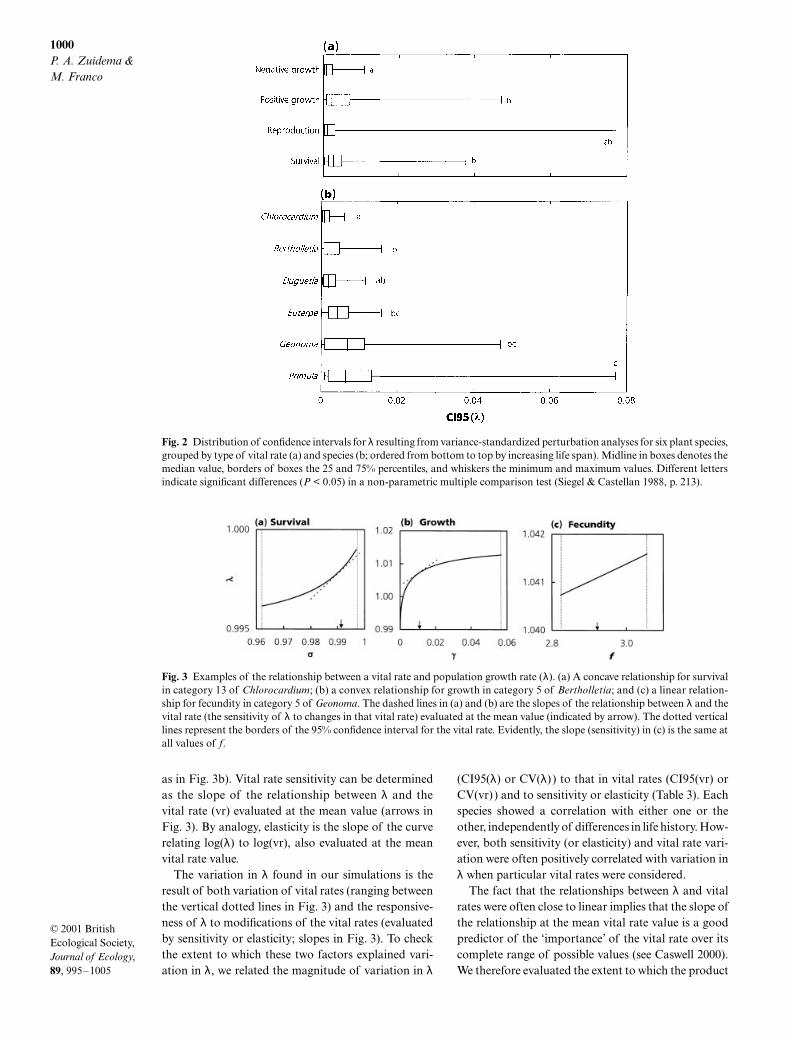
both for CI95(λ) (KW: χ23 = 14.6, P < 0.01) and CV(λ)

(KW: χ23 = 29.4, P < 0.001), with negative growth

having less influence on the variation of λ than othervital rates (Fig. 2a; KW: multiple comparisons,P < 0.05). Similarly, species differed in the magnitudeof variation in λ resulting from vital rate variability(KW: χ2

5 = 52.3, P < 0.001 for CI95(λ) and χ25 = 51.3,

P < 0.001 for CV(λ) ).Variability of λ generally decreasedwith species life span (Fig. 2b).

The relationship between λ and vital rates is intrin-sically non-linear, but the results of our simulationsshow a low degree of curvature leading to close to lin-ear relations (e.g. Figure 3c). The relationship betweenλ and either survival or negative growth was usuallyconcave (43 out of 63 cases and 16 out of 20, respect-ively, as in Fig. 3a). Relationships between λ and eitherpositive growth or reproductive output were mainlyconvex (67 out of 75 and 19 out of 28, respectively,

Fig. 1 Relationship between the contribution of a vital rate to lambda (its ‘importance’) and the vital rate’s variability for six plantspecies, using (a,c) absolute measures (sensitivity and CI95(vr), see text for definition) and (b,d) relative measures (elasticity andCV(vr)). Right and left panels differentiate species from vital rates, but otherwise provide the same data. Correlation analyses arepresented in Table 2.

Table 2 Correlation between measures of importance and variability of vital rates for six plant species. Correlations wereperformed for absolute (sensitivity vs. CI95) and relative (elasticity vs. CV) measures. Sensitivities and elasticities are calculatedfor vital rates (not matrix elements; see Materials and methods). Values are Spearman’s r

Species Vital rateSensitivity vs. CI95(vr)

Elasticity vs. CV(vr) n

All All –0.54*** –0.70*** 188

Primula All NS –0.63** 17Geonoma All –0.63** –0.61** 18Euterpe All –0.61** –0.73*** 25Duguetia All –0.77*** –0.72*** 34Bertholletia All –0.72*** –0.53*** 39Chlorocardium All –0.74*** –0.75*** 55

All Survival –0.47*** –0.56*** 65All Positive growth –0.27* NS 75All Negative growth NS NS 20All Reproductive output –0.90*** NS 28

*P < 0.05, **P < 0.01, ***P < 0.001, NS = not significant.


1000P. A. Zuidema & M. Franco


as in Fig. 3b). Vital rate sensitivity can be determinedas the slope of the relationship between λ and thevital rate (vr) evaluated at the mean value (arrows inFig. 3). By analogy, elasticity is the slope of the curverelating log(λ) to log(vr), also evaluated at the meanvital rate value.

The variation in λ found in our simulations is theresult of both variation of vital rates (ranging betweenthe vertical dotted lines in Fig. 3) and the responsive-ness of λ to modifications of the vital rates (evaluatedby sensitivity or elasticity; slopes in Fig. 3). To checkthe extent to which these two factors explained vari-ation in λ, we related the magnitude of variation in λ

(CI95(λ) or CV(λ) ) to that in vital rates (CI95(vr) orCV(vr)) and to sensitivity or elasticity (Table 3). Eachspecies showed a correlation with either one or theother, independently of differences in life history. How-ever, both sensitivity (or elasticity) and vital rate vari-ation were often positively correlated with variation inλ when particular vital rates were considered.

The fact that the relationships between λ and vitalrates were often close to linear implies that the slope ofthe relationship at the mean vital rate value is a goodpredictor of the ‘importance’ of the vital rate over itscomplete range of possible values (see Caswell 2000).We therefore evaluated the extent to which the product

Fig. 2 Distribution of confidence intervals for λ resulting from variance-standardized perturbation analyses for six plant species,grouped by type of vital rate (a) and species (b; ordered from bottom to top by increasing life span). Midline in boxes denotes themedian value, borders of boxes the 25 and 75% percentiles, and whiskers the minimum and maximum values. Different lettersindicate significant differences (P < 0.05) in a non-parametric multiple comparison test (Siegel & Castellan 1988, p. 213).

Fig. 3 Examples of the relationship between a vital rate and population growth rate (λ). (a) A concave relationship for survivalin category 13 of Chlorocardium; (b) a convex relationship for growth in category 5 of Bertholletia; and (c) a linear relation-ship for fecundity in category 5 of Geonoma. The dashed lines in (a) and (b) are the slopes of the relationship between λ and thevital rate (the sensitivity of λ to changes in that vital rate) evaluated at the mean value (indicated by arrow). The dotted verticallines represent the borders of the 95% confidence interval for the vital rate. Evidently, the slope (sensitivity) in (c) is the same atall values of f.




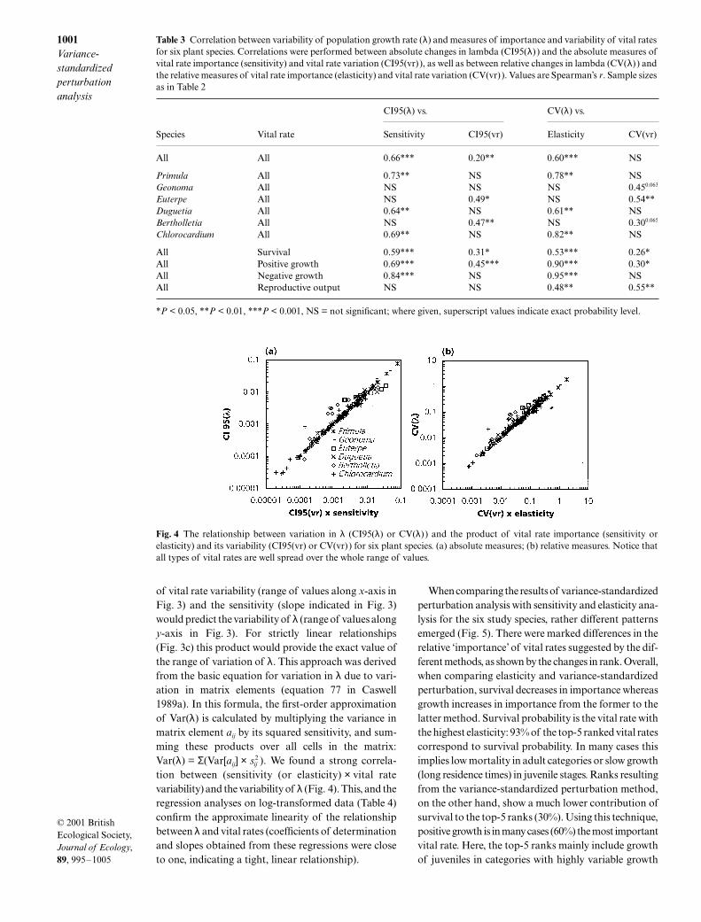
of vital rate variability (range of values along x-axis inFig. 3) and the sensitivity (slope indicated in Fig. 3)would predict the variability of λ (range of values alongy-axis in Fig. 3). For strictly linear relationships(Fig. 3c) this product would provide the exact value ofthe range of variation of λ. This approach was derivedfrom the basic equation for variation in λ due to vari-ation in matrix elements (equation 77 in Caswell1989a). In this formula, the first-order approximationof Var(λ) is calculated by multiplying the variance inmatrix element aij by its squared sensitivity, and sum-ming these products over all cells in the matrix:Var(λ) = Σ(Var[aij] × sij

2 ). We found a strong correla-tion between (sensitivity (or elasticity) × vital ratevariability) and the variability of λ (Fig. 4). This, and theregression analyses on log-transformed data (Table 4)confirm the approximate linearity of the relationshipbetween λ and vital rates (coefficients of determinationand slopes obtained from these regressions were closeto one, indicating a tight, linear relationship).

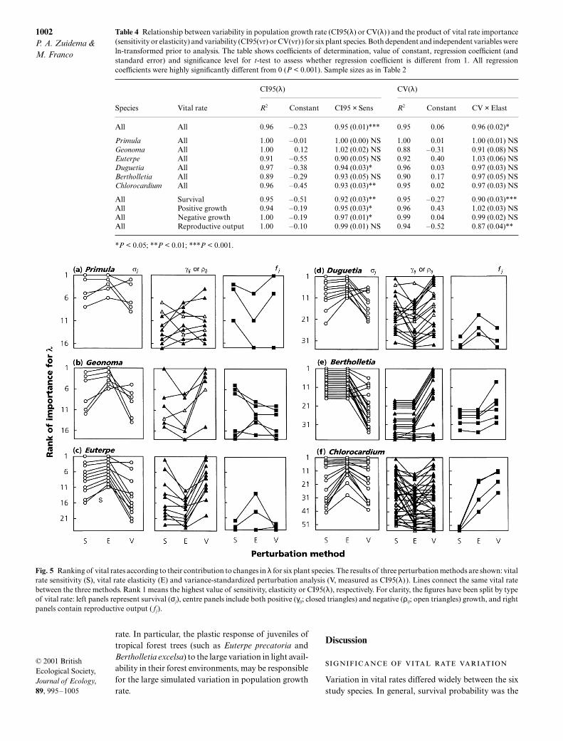
When comparing the results of variance-standardizedperturbation analysis with sensitivity and elasticity ana-lysis for the six study species, rather different patternsemerged (Fig. 5). There were marked differences in therelative ‘importance’ of vital rates suggested by the dif-ferent methods, as shown by the changes in rank. Overall,when comparing elasticity and variance-standardizedperturbation, survival decreases in importance whereasgrowth increases in importance from the former to thelatter method. Survival probability is the vital rate withthe highest elasticity: 93% of the top-5 ranked vital ratescorrespond to survival probability. In many cases thisimplies low mortality in adult categories or slow growth(long residence times) in juvenile stages. Ranks resultingfrom the variance-standardized perturbation method,on the other hand, show a much lower contribution ofsurvival to the top-5 ranks (30%). Using this technique,positive growth is in many cases (60%) the most importantvital rate. Here, the top-5 ranks mainly include growthof juveniles in categories with highly variable growth

Table 3 Correlation between variability of population growth rate (λ) and measures of importance and variability of vital ratesfor six plant species. Correlations were performed between absolute changes in lambda (CI95(λ) ) and the absolute measures ofvital rate importance (sensitivity) and vital rate variation (CI95(vr)), as well as between relative changes in lambda (CV(λ) ) andthe relative measures of vital rate importance (elasticity) and vital rate variation (CV(vr)). Values are Spearman’s r. Sample sizesas in Table 2

Species Vital rate

CI95(λ) vs. CV(λ) vs.

Sensitivity CI95(vr) Elasticity CV(vr)

All All 0.66*** 0.20** 0.60*** NS

Primula All 0.73** NS 0.78** NSGeonoma All NS NS NS 0.450.063

Euterpe All NS 0.49* NS 0.54**Duguetia All 0.64** NS 0.61** NSBertholletia All NS 0.47** NS 0.300.065

Chlorocardium All 0.69** NS 0.82** NS

All Survival 0.59*** 0.31* 0.53*** 0.26*All Positive growth 0.69*** 0.45*** 0.90*** 0.30*All Negative growth 0.84*** NS 0.95*** NSAll Reproductive output NS NS 0.48** 0.55**

*P < 0.05, **P < 0.01, ***P < 0.001, NS = not significant; where given, superscript values indicate exact probability level.

Fig. 4 The relationship between variation in λ (CI95(λ) or CV(λ) ) and the product of vital rate importance (sensitivity orelasticity) and its variability (CI95(vr) or CV(vr)) for six plant species. (a) absolute measures; (b) relative measures. Notice thatall types of vital rates are well spread over the whole range of values.




rate. In particular, the plastic response of juveniles oftropical forest trees (such as Euterpe precatoria andBertholletia excelsa) to the large variation in light avail-ability in their forest environments, may be responsiblefor the large simulated variation in population growthrate.

Discussion

Variation in vital rates differed widely between the sixstudy species. In general, survival probability was the

Table 4 Relationship between variability in population growth rate (CI95(λ) or CV(λ) ) and the product of vital rate importance(sensitivity or elasticity) and variability (CI95(vr) or CV(vr)) for six plant species. Both dependent and independent variables wereln-transformed prior to analysis. The table shows coefficients of determination, value of constant, regression coefficient (andstandard error) and significance level for t-test to assess whether regression coefficient is different from 1. All regressioncoefficients were highly significantly different from 0 (P < 0.001). Sample sizes as in Table 2

Species Vital rate

CI95(λ) CV(λ)

R2 Constant CI95 × Sens R2 Constant CV × Elast

All All 0.96 –0.23 0.95 (0.01)*** 0.95 0.06 0.96 (0.02)*

Primula All 1.00 –0.01 1.00 (0.00) NS 1.00 0.01 1.00 (0.01) NSGeonoma All 1.00 0.12 1.02 (0.02) NS 0.88 –0.31 0.91 (0.08) NSEuterpe All 0.91 –0.55 0.90 (0.05) NS 0.92 0.40 1.03 (0.06) NSDuguetia All 0.97 –0.38 0.94 (0.03)* 0.96 0.03 0.97 (0.03) NSBertholletia All 0.89 –0.29 0.93 (0.05) NS 0.90 0.17 0.97 (0.05) NSChlorocardium All 0.96 –0.45 0.93 (0.03)** 0.95 0.02 0.97 (0.03) NS

All Survival 0.95 –0.51 0.92 (0.03)** 0.95 –0.27 0.90 (0.03)***All Positive growth 0.94 –0.19 0.95 (0.03)* 0.96 0.43 1.02 (0.03) NSAll Negative growth 1.00 –0.19 0.97 (0.01)* 0.99 0.04 0.99 (0.02) NSAll Reproductive output 1.00 –0.10 0.99 (0.01) NS 0.94 –0.52 0.87 (0.04)**

*P < 0.05; **P < 0.01; ***P < 0.001.

Fig. 5 Ranking of vital rates according to their contribution to changes in λ for six plant species. The results of three perturbation methods are shown: vitalrate sensitivity (S), vital rate elasticity (E) and variance-standardized perturbation analysis (V, measured as CI95(λ) ). Lines connect the same vital ratebetween the three methods. Rank 1 means the highest value of sensitivity, elasticity or CI95(λ), respectively. For clarity, the figures have been split by typeof vital rate: left panels represent survival (σj), centre panels include both positive (γij; closed triangles) and negative (ρij; open triangles) growth, and rightpanels contain reproductive output ( fj).




least variable vital rate, particularly in adult categories(Fig. 1). A negative relationship between vital rateimportance (sensitivity or elasticity) and vital rate var-iability was found for all species and vital rates com-bined, but also separately for the six species and formost of the vital rates (Fig. 1, Table 2). Similar inverserelationships between demographic variation and sen-sitivity (or elasticity) have been found for temporal var-iation in a large number of plant and animal species(Ehrlén & van Groenendael 1998; Pfister 1998). Theseresults have been interpreted to suggest that naturalselection promotes population stability by reducingvariability in relation to the importance of the life his-tory traits involved (Pfister 1998).

Our simulations show that variation in vital rates asobserved in demographic field studies may influencethe estimates of population growth rate λ to differentdegrees (Fig. 2). Variation in survival probability andgrowth rate had the strongest impact on λ (Table 3),despite the fact that the former was the least variablevital rate. Comparing species, variation in λ appearedto be large for short-lived species and smaller for thelonger-lived species (Fig. 2b).

The functional relationships between λ and vital ratesapproached linearity in many instances (e.g. Caswell1996a,b, 2000; de Kroon et al. 2000; but see Huenneke& Marks 1987), despite the intrinsically non-linearrelationship between the dominant eigenvalue andeither matrix elements or vital rates. This confirms thatsensitivities and elasticities perform well beyond thepoint at which they are calculated (Caswell 2000; deKroon et al. 2000). Given this linearity, an estimate ofthe variability of λ due to variation in a vital rate isobtained by multiplying the importance of the vitalrate (expressed as sensitivity or elasticity) and its vari-ability (expressed as either its 95% confidence intervalor its coefficient of variation). When applying this tothe six species, very strong relationships were found(Fig. 4, Table 4).

The implication of this result is that the first-orderapproximation for variance in λ (Caswell 1989a) can beused to obtain a simple and reliable estimate of the var-iation in lambda due to variation in a certain vital rate.Two readily available parameters can be multiplied toestimate the variation of λ:

CI95(λ) ≈ CI95(vrj) × sj eqn 7

where CI95(λ) is the 95% confidence interval of thepopulation growth rate resulting from variation ina certain vital rate in category j (vrj), CI95(vrj) is the95% confidence interval of vrj and sj is the sensitivityof vrj. When using relative measures, the analogue ofeqn 7 is:

CV(λ) ≈ CV(vrj) × ej eqn 8

where CV(λ) is the coefficient of variation of λ due tovariation in a vital rate, vrj, in category j, CV(vrj) is thecoefficient of variation of vrj and ej is the elasticity valuefor vrj.

Estimates of variability can be obtained from fielddata or from the literature; sensitivity and elasticity ofvital rates can be calculated using eqns 2–5 (Caswell1989a, 1996a). Whether one applies absolute or relativemeasures does not influence the predictive strength ofthe relationship (in the simulations, both explainedmore than 88% of the variation in ln(λ); Table 4). Itshould be noted that eqns 7 and 8 resemble the equa-tion used for ‘direct perturbation analysis’ (Ehrlén &van Groenendael 1998), which considers the variationin population growth rate of differences in vital ratesbetween populations and time periods. One differ-ence between their approach and ours is the sourceof variation: variation between populations or timeperiods (direct perturbation analysis) vs. that betweenindividuals in a population (variance-standardizedperturbation).

Vital rates are likely to covary and this can happeneither within the same stage of the life cycle or betweendifferent stages. As a consequence, some combinationsof vital rates will be more probable than others, andparticular combinations may be impossible. In oursimulations, we varied one vital rate in one category ata time, while keeping other vital rates in the focal cat-egory and all vital rates in all other categories, con-stant. That is, the variance-standardized perturbationsdid not adjust for covariance between vital rates.Some unrealistic combinations of vital rates may haveresulted from this. However, by drawing values of vitalrates only from the 95% confidence interval, we pre-vented unrealistic values and unrealistic combinationsof values from having a large influence on the variabil-ity of λ. Our approach is thus similar to the applicationof large perturbations, as commonly used for the plan-ning of conservation measures (Heppell et al. 1996;Mills et al. 1999; Caswell 2000; de Kroon et al. 2000).

The influence of demographic covariance on varia-tion in population growth has not often been assessed(Brault & Caswell 1993; Horvitz et al. 1997; Caswell2000). Inclusion of covariance in matrix models isprobably hampered by two factors. Firstly, the twomain techniques that assess the role of covariance havedifferent starting points. In integrated elasticities (vanTienderen 1995, 2000), covariance between vital rates isspecifically modelled using observed or assumed trade-off relationships. In life table response experiments(LTRE; Caswell 1989b, 1996a, 2000), on the otherhand, covariances appear as an integral part of thequantification of contributions to observed variationin λ, thus providing empirical evidence of the role ofcovariation. As LTREs consider differences between(sub)populations or observation periods, to a certain




extent they disregard trade-offs that only becomeapparent at the individual level (these may be included,however, in integrated elasticities). Secondly, the use ofboth integrated elasticity and LTRE is limited by theamount of information gathered in a particular study.Detailed knowledge on covariance structures neces-sary for integrated elasticities and sets of transitionmatrices required for LTRE are usually not available(Menges 2000).

Conceptually, perturbation methods may be groupedinto two families (Caswell 1997; Horvitz et al. 1997),namely prospective and retrospective analyses.Whereas prospective analyses (e.g. sensitivity, elastic-ity) explore the functional dependence of λ on eithermatrix elements or vital rates, retrospective analyses(e.g. life table response experiments: LTREs) deter-mine how an observed pattern of variation has affectedvariation of λ in the past (Caswell 2000). Variance-standardized perturbation analysis, as applied in thispaper, combines considerations of variation in λ due toobserved variation in vital rates (an aspect of retrospect-ive analysis) with the functional relationship of λ tothat vital rate (a subject of prospective analysis; Fig. 3).It can be valuable because it identifies those vital ratesthat, as a result of their intrinsic variability (or uncer-tain estimation) and functional relationship with λ,have a large impact on the variation in populationgrowth rate (see Fig. 5). Such information can beapplied for the identification of manipulable traits forthe management of endangered or exploited species.

When should different perturbation methods bechosen? This depends on the question posed. Elasticityand sensitivity analyses evaluate the potential effect onλ of a change in a vital rate, and therefore answer thequestion ‘What would happen if a particular vital ratewere modified?’. Large modifications of certain vitalrates may be used to assess the impact of conservationmeasures (e.g. Heppell et al. 1996; Mills et al. 1999;Caswell 2000). Life table response experiments(LTREs) evaluate the importance of demographic var-iation on variation in λ, addressing the question ‘Whatare the contributions of different vital rates to observedvariation in population growth rate, for example,between (sub)populations or time periods?’. LTREsuse a set of transition matrices for different populationsor observation periods, and consider the influence ofvariation between these transition matrices on popula-tion growth. They are therefore especially useful fordisentangling complex demographic consequencesof environmental change. Variance-standardizedperturbation analysis asks the question: ‘What are theconsequences for population growth of observed vari-ation in vital rates or uncertainty in their estimation?’,addressing the effect of either random variation betweenindividuals or sampling bias on the rate of popula-tion growth. It considers the variation that is usually

‘hidden’ in the averaged matrix elements. Although thequestions posed by LTREs and variance-standardizedperturbation analysis are similar, they differ in startingpoint and required information. LTREs begin withobserved variation in population growth rate of dif-ferent populations or different time periods, whereasvariance-standardized perturbation starts from observedvariation in vital rates in one population and duringone time period. LTREs therefore require several tran-sition matrices for different (sub)populations or timeperiods, whereas variance-standardized perturbationrequires one transition matrix with information onvariability of the vital rates used for matrix construc-tion. However, the sources of demographic variationused for both methods are related and often overlap:variation between populations can be considered asaggregated between-individual variation, spatialvariation may be included in one transition matrixor specified in several (patch-specific) matrices and,similarly, demographic data from different years maybe combined into one average model or used for severalannual models. Thus, the form in which demographicdata are presented may determine what method can beapplied: LTRE can be used if several transition matricesare available; variance-standardized perturbation analysiscan be used if information on variability of vital rates isavailable. Finally, it should be stressed that, because itaddresses a different question, variance-standardizedperturbation analysis is an additional tool for theanalysis of matrix models.

Acknowledgements

We thank Teresa Valverde and Roderick Zagt for allow-ing us to use their data. Heinjo During, Johan Ehrlén,Carol Horvitz, Xavier Pico and Marinus Werger pro-vided valuable comments on draft versions. PZ acknow-ledges the Instituto de Ecología, UNAM, Mexico, andthe Open University, UK, for their hospitality. Partof this study was financed by grant BO009701 fromthe Netherlands Development Assistance. MF thanksConacyt, Mexico, DGAPA, UNAM, Mexico, theFerguson Trust, and the Open University for supportand hospitality during a sabbatical period.

Supplementary material

The following material is available from http://www.blackwell-science.com/products/journals/suppmat/JEC/JEC622/JEC622sm.htm

Appendix 1 Blackground information on matrixmodels for the six study species.

References

Alvarez-Buylla, E.R. (1994) Density dependence and patchdynamics in tropical rain forests: matrix models andapplications to a tree species. American Naturalist, 143,155–191.

JEC_621.fm 04 Wednesday, November 21, 2001 9:01 AM



Alvarez-Buylla, E.R. & García-Barrios, R. (1993) Models ofpatch dynamics in tropical forests. Trends in Ecology andEvolution, 8, 201–204.

Alvarez-Buylla, E.R. & Slatkin, M. (1991) Finding confid-ence limits on population growth rates. Trends in Ecologyand Evolution, 6, 221–224.

Alvarez-Buylla, E.R. & Slatkin, M. (1993) Finding confidencelimits on population growth rates: Monte Carlo test of asimple analytic method. OIKOS, 68, 273–282.

Alvarez-Buylla, E.R. & Slatkin, M. (1994) Finding confidencelimits on population growth rates: three real examples revised.Ecology, 75, 255–260.

Benton, T.G. & Grant, A. (1999) Elasticity analysis as animportant tool in evolutionary and population ecology.Trends in Ecology and Evolution, 14, 467–470.

Bierzychudeck, P. (1999) Looking backwards: assessing theprojections of a transition matrix models. Ecological Applica-tions, 9, 1278–1287.

Brault, S. & Caswell, H. (1993) Pod-specific demography ofkiller whales Orcinus orca. Ecology, 74, 1444–1454.

Caswell, H. (1978) A general formula for the sensitivity ofpopulation growth rate to changes in life history parameters.Theoretical Population Biology, 14, 215–230.

Caswell, H. (1989a) Matrix Population Models. Sinauer Asso-ciates, Sunderland, MA.

Caswell, H. (1989b) Analysis of life table response experi-ments I. Decomposition of effects on population growthrate. Ecological Modelling, 46, 221–237.

Caswell, H. (1996a) Analysis of life table response experi-ments II. Alternative parameterization for size- and stage-structured models. Ecological Modelling, 88, 73–82.

Caswell, H. (1996b) Second derivatives of population growthrate: calculation and application. Ecology, 77, 870–879.

Caswell, H. (1997) Methods of matrix population analysis.Structured-Population Models in Marine, Terrestrial, andFreshwater Systems (eds S. Tuljapurkar & H. Caswell),pp. 19–58. Chapman & Hall, New York.

Caswell, H. (2000) Prospective and retrospective perturbationanalysis: their roles in conservation biology. Ecology, 81,619–627.

Caswell, H., Brault, S., Read, A.J. & Smith, T.D. (1998) Harborporpoise and fisheries: an uncertainty analysis of incidentalmortality. Ecological Applications, 8, 1226–1238.

Caswell, H. & Trevisan, M.C. (1994) Sensitivity analysis ofperiodic matrix models. Ecology, 75, 1299–1305.

Cochran, M.E. & Ellner, S. (1992) Simple methods for calcu-lating age-based life history parameters for stage-structuredpopulations. Ecological Monographs, 62, 345–364.

Ehrlén, J. & van Groenendael, J. (1998) Direct perturbationanalysis for better conservation. Conservation Biology, 12,470–474.

Heppell, S.S., Crowder, L.B. & Crouse, D.T. (1996) Models toevaluate headstarting as a management tool for long-livedturtles. Ecological Applications, 6, 556–565.

Horvitz, C.C., Schemske, D.W. & Caswell, H. (1997) Therelative ‘importance’ of life-history stages to populationgrowth: prospective and retrospective analyses. Structured-Population Models in Marine, Terrestrial, and FreshwaterSystems (eds S. Tuljapurkar & H. Caswell), pp. 247–271.Chapman & Hall, New York.

Huenneke, L.F. & Marks, P.L. (1987) Stem dynamics of theshrub Alnus incana ssp. rugosa: transition matrix models.Ecology, 68, 1234–1242.

Hunter, C.M., Moller, H. & Fletcher, D. (2000) Parameteruncertainty and elasticity analyses of a population model:setting research priorities for shearwaters. Ecological Model-ling, 134, 299–323.

de Kroon, H., Plaisier, A., van Groenendael, J. & Caswell, H.(1986) Elasticity: the relative contribution of demographicparameters to population growth rate. Ecology, 67, 1427–1431.

de Kroon, H., van Groenendael, J. & Ehrlén, J. (2000) Elas-

ticities: a review of methods and model limitations. Ecology,81, 607–618.

Lande, R. (1988) Demographic models of the northernspotted owl (Strix occidentalis caurina). Oecologia, 75,601–607.

Lefkovitch, L.P. (1965) The study of population growth inorganisms grouped by stages. Biometrics, 21, 1–18.

Menges, E.S. (2000) Population viability analyses in plants:challenges and opportunities. Trends in Ecology and Evolu-tion, 15, 51–56.

Mills, L.S., Doak, D.F. & Wisdom, M.J. (1999) Reliability ofconservation actions based on elasticity analysis of matrixmodels. Biological Conservation, 13, 815–829.

Pascarella, J.B. & Horvitz, C.C. (1998) Hurricane disturbanceand the population dynamics of tropical understory shrub:megamatrix elasticity analysis. Ecology, 79, 547–563.

Pfister, C.A. (1998) Patterns of variance in stage-structuredpopulations: evolutionary predictions and ecological implica-tions. Proceedings of the National Academy of SciencesUSA, 95, 213–218.

Sarukhán, J., Martinez-Ramos, M. & Piñero, D. (1982) Theanalysis of demographic variability at the individual leveland its population consequences. Perspectives on PlantPopulation Ecology (eds R. Dirzo & J. Sarukhán), pp. 83–106. Sinauer, Sunderland, MA.

Siegel, S. & Castellan, N.J. (1988) Nonparametric Statistics forthe Behavioral Sciences. McGraw-Hill, New York.

Silvertown, J., Franco, M. & Menges, E. (1996) Interpretationof elasticity matrices as an aid to the management of plantpopulations for conservation. Conservation Biology, 10,591–597.

Sokal, R.R. & Rohlf, F.J. (1995) Biometry. The Principles andPractice of Statistics in Biological Research, 3rd edn. Free-man, New York.

ter Steege, H., Boot, R.G.A., Brouwer, L.C., Caesar, J.C., Ek,R.C., Hammond, D.S., Haripersaud, P.P., van der Hout, P.,Jetten, V.G., van Kekem, A.J., Kellman, M.A., Khan, Z.,Polak, M., Pons, T.L., Pulles, J., Raaimakers, D., Rose,S.A., van der Sanden, J.J. & Zagt, R.J. (1996) Ecologyand Logging in a Tropical Rain Forest in Guyana. WithRecommendations for Management. Tropenbos Series 14,Wageningen, The Netherlands.

van Tienderen, P.H. (1995) Life cycle trade-offs in matrixpopulation models. Ecology, 76, 2482–2489.

van Tienderen, P.H. (2000) Elasticities and the link betweendemographic and evolutionary dynamics. Ecology, 81, 666–679.

Tuljapurkar, S. (1989) An uncertain life: demography in randomenvironments. Theoretical Population Biology, 35, 227–294.

Valverde, T. & Silvertown, J. (1998) Variation in the demo-graphy of a woodland understorey herb (Primula vulgaris)along the forest regeneration cycle: projection matrix ana-lysis. Journal of Ecology, 86, 545–562.

Wisdom, M.J. & Mills, L.S. (1997) Sensitivity analysis toguide population recovery: prairie chickens as an example.Journal of Wildlife Management, 61, 302–312.

Wisdom, M.J., Mills, L.S. & Doak, D.F. (2000) Life stage simu-lation analysis: estimating vital-rate effects on populationgrowth for conservation. Ecology, 81, 628–641.

Zagt, R.J. (1997) Tree demography in the tropical rain forest ofGuyana. PhD Thesis, Utrecht University, Utrecht.

Zuidema, P.A. (2000) Demography of exploited tree speciesin the Bolivian Amazon. PhD Thesis, Utrecht University,Utrecht.

Zuidema, P.A. & Boot, R.G.A. (in press) Demography of theBrazil nut tree (Bertholletia excelsa) in the Bolivian Amazon:impact of seed extraction on recruitment and populationdynamics. Journal of Tropical Ecology, 18, 1–31.

Received 31 October 2000 revision accepted 9 May 2001


Integrating vital rate variability into perturbation analysis: an evaluation for matrix population...

Documents

Transcript of Integrating vital rate variability into perturbation analysis: an evaluation for matrix population...