RELIABILITY-BASED DESIGN OF AN EARTH AND ...

ADRIAN TORRICO SIACARA

RELIABILITY-BASED DESIGN OF AN EARTH AND

CONCRETE DAM

São Paulo

2021

ADRIAN TORRICO SIACARA

RELIABILITY-BASED DESIGN OF AN EARTH AND

CONCRETE DAM

CORRECTED VERSION

A thesis presented to the Graduate

Program in Civil Engineering at the

Escola Politécnica of the Universidade

de São Paulo to obtain the degree of PhD

of Science.

Concentration Area:

Geotechnical Engineering

Supervisor:

Prof. Dr. Marcos Massao Futai

São Paulo

2021

Autorizo a reprodução e divulgação total ou parcial deste trabalho, por qualquer meio

convencional ou eletrônico, para fins de estudo e pesquisa, desde que citada a fonte.

Catalogação-na-publicação

Siacara, Adrian Torrico

Reliability-based design of an earth and concrete dam / A.T. Siacara --

versão corr. -- São Paulo, 2021.

272 p.

Tese (Doutorado) - Escola Politécnica da Universidade de São Paulo.

Departamento de Engenharia de Estruturas e Geotécnica.

1.Earth dam 2.Concrete dam 3.Direct coupling 4.Reliability analysis 5.

RBDO I.Universidade de São Paulo. Escola Politécnica. Departamento de

Engenharia de Estruturas e Geotécnica II.t.

Este exemplar foi revisado e alterado em relação à versão

original, sob responsabilidade única do autor e com a

anuência de seu orientador.

São Paulo, 04 de agosto de 2021

Assinatura do autor Adrian Torrico Siacara

Assinatura do orientador Marcos Massao Futai

ACKNOWLEDGMENTS

I would like to express the deepest gratitude to my supervisor, Prof. Marcos Massao Futai, who

has provided guidance, invaluable feedback, and assistance to my research throughout all the

stages of my thesis study. Without their support and encouragement, this thesis could not be

eventuated.

A very special acknowledgment goes to Prof. André Teófilo Beck, for the scientific and

technical advice, providing his expertise, knowledge, and hard work which were directly related

to the development of this thesis. I am grateful to Ph.D. Gian Franco Napa García for helping

me during the first steps with the direct coupling technique and reliability analysis.

My acknowledgments go to: (i) the University of São Paulo (USP), for the support provided

during the elaboration of the thesis; (ii) Post-Graduate Program in Civil Engineering (PPGEC),

Geotechnical engineering, as the host institution, for enabling the valuable resources required;

and (iii) the Coordination for the Improvement of Higher Education Personnel (CAPES) (Grant

number nº 88882.145758/2017-01) and the Brazilian National Council of Scientific and

Technological Development (CNPq), for granting the doctoral fellowship to develop this work.

Also, I want to thank my friends in the Geotechnical Engineering Research Group

(GeoInfraUSP) whose support has enabled me to grow professionally and overcome several

challenges.

Finally, my special gratitude belongs to all my family. I am forever grateful to my parents

(Oscar and Telda), my brothers (Martin, Pablo, and Mateo), and my sisters (Andrea and

Estefania) for their love, support, and encouragement.

“O segundo nada mais é do que o primeiro dos perdedores”

Brazilian racing driver, Ayrton Senna

ABSTRACT

SIACARA, A. T. Reliability-based design of an earth and concrete dam. 2021. 272 p..

Doctoral Thesis (PhD. In Civil Engineering) - Post-Graduation Program in Civil Engineering,

Polytechnic School of the University of São Paulo, São Paulo, Brazil, 2021.

In geotechnical engineering, the use of classical deterministic approaches is part of the normal

practice. Most laws and standards are based on engineers’ experience and deterministic

assumptions. In the last four decades, the uncertainties and uncertainty inherent in geotechnical

properties have caught the attention of engineers. They have found that a single factor of safety

(FS) calculated by traditional deterministic analysis methods can not exactly represent the

stability. Recently, to provide a more rational mathematical framework to incorporate different

types of uncertainties in the stability estimation, different types of commercial software, which

include basic probabilistic and deterministic methods, have been widely extended. The failure

probability calculated is a kind of complement to the safety factor.

In this doctoral thesis, reliability concepts have been reviewed first, and some advanced

reliability methods, including Mean Value First-Order Second Moment (MVFOSM), First-

Order Reliability Method (FORM), Second-Order Reliability Method (SORM), Monte Carlo

Simulation (MCS), and importance Monte Carlo Simulation (IMCS), have been described and

successfully applied to the dam stability analyses based on a direct coupling (DC) geotechnical

software with a reliability solver. An advanced literature review on Reliability-Based Design

Optimization (RBDO) was presented to show how accurate and efficient RBDO analyses of a

concrete dam can be performed by using a Mono-level method as a Single-Loop Approach

(SLA).

Numerical methods help understand the behaviors of geotechnical installations. However, the

computational cost may sometimes become prohibitive when structural reliability analysis is

performed, due to repetitive calls to the deterministic solver. In this thesis, we show how

accurate and efficient reliability analyses of geotechnical installations can be performed by

directly coupling geotechnical software with a reliability solver. A dam is used as the study

object under different operating conditions over time. The limit equilibrium method of

Morgenstern-Price is used to calculate factors of safety and to find the critical slip surface. The

commercial software packages Seep/W and Slope/W are coupled with StRAnD structural

reliability software.

Initial analysis in long term steady-state conditions shows close results of the FORM and

SORM, as well as by ISMC simulation. By means of sensitivity analysis, the effective friction

angle (ϕ´) is found to be the most relevant uncertain geotechnical parameter. The correlations

between different geotechnical properties are shown to be relevant in terms of equilibrium

reliability indices. Finally, a critical slip surface, identified in terms of the minimum FS, is

shown not to be the critical surface in terms of reliability index.

Considerable variation between results of commercial software and DC software is found.

FORM, SMC, and MVFOSM are evaluated. The computational cost is very high in commercial

software. The angle of the contribution to the shearing resistance due to the matric suction (ϕb)

has a considerable incidence in reliability analysis.

In transient conditions, seepage analysis with limit equilibrium analysis is performed to

investigate the safety of an earth dam over time, considering different initial conditions, rainfall

intensities, rapid drawdown, and normal operating conditions (NOC). FORM is employed in

reliability analysis. Sensitivity analyses reveal that saturated hydraulic conductivity (ks),

friction angle (ϕ´), and cohesion (c´) are the random parameters with the greatest contribution.

The cumulative effect of random saturated hydraulic conductivity (mainly) makes critical times

and critical slip surfaces different in the probabilistic and deterministic analyses.

In an existing old earth dam, the FORM method is employed in reliability analysis. Sensitivity

analyses reveal the most important geotechnical parameters. A range of values of the

relationship between the reliability index (β) and the factor of safety (FS) was found for all

probabilistic and deterministic results. The differences in terms of pore water pressure between

deterministic and probabilistic approaches are presented. Finally, a critical slip surface,

identified in terms of minimum FS, is shown here not to be the critical surface in terms of the

minimum reliability index.

Finally, we show how accurate and efficient RBDO analyses of a concrete dam can be

performed by using a Mono-level method as SLA. A concrete dam is used as the study object

under different conditions of the target reliability index (βT) and heights of the dam. By means

of sensitivity analysis, the most important geotechnical parameters are pointed out. Finally, for

the lower βT values considered herein, we found the eccentricity limit state function of the active

constraint at the optimum solution. For larger βT values, the sliding limit state is the active

constraint.

Keywords: Earth dam; concrete dam; direct coupling; reliability analysis; RBDO.

RESUMO

SIACARA, A. T. Projeto baseado em confiabilidade de uma barragem de terra e concreto.

2021. 272 p.. Teses doutoral (Dr. Em Engenharia Civil) – Programa de Pós-graduação em

Engenheira Civil, Escola politécnica da Universidade de São Paulo, São Paulo, Brazil, 2021.

Na engenharia geotécnica, o uso de abordagens determinísticas clássicas faz parte da prática

comum. A maioria das leis e normas são baseadas na experiência do engenheiro e em

suposições determinísticas. Nas últimas quatro décadas, as incertezas e incertezas inerentes às

propriedades geotécnicas têm chamado a atenção dos engenheiros. Descobriu-se que um único

fator de segurança (FS) calculado por métodos de análises determinísticas tradicionais pode

não representar exatamente a estabilidade. Recentemente, a fim de fornecer um embasamento

matemático mais racional para incorporar diferentes tipos de incertezas na estimativa de

estabilidade, diferentes softwares comerciais, que incluem métodos probabilísticos básicos e

determinísticos, foram amplamente desenvolvidos.

Nesta tese de doutorado, os conceitos de confiabilidade foram revisados primeiro e alguns

métodos avançados de confiabilidade, incluindo Valor médio, segundo momento de primeira

ordem (MVFOSM), Método de confiabilidade de primeira ordem (FORM), Método de

confiabilidade de segunda ordem (SORM), Simulação de Monte Carlo (MCS) e Simulação de

Monte Carlo por importância (iMCS), foram descritos e aplicados com sucesso às análises de

estabilidade de barragens com base em um software geotécnico de acoplamento direto (DC)

com um solucionador de confiabilidade. Uma revisão de literatura avançada sobre Otimização

de Projeto Baseada em Confiabilidade (RBDO) foi apresentada para mostrar como análises

RBDO precisas e eficientes de uma barragem de concreto podem ser realizadas usando um

método de nível único como uma abordagem de circuito único (SLA).

Os métodos numéricos são úteis para a compreensão do comportamento das estruturas

geotécnicas. No entanto, o custo computacional às vezes pode se tornar impeditivo quando a

análise de confiabilidade estrutural é realizada, devido a chamadas repetitivas do solucionador

determinístico. Nesta tese, mostramos como análises de confiabilidade precisas e eficientes de

estruturas geotécnicas podem ser realizadas por meio do acoplamento direto de software

geotécnico a um solucionador de confiabilidade. Uma barragem de terra é usada como objeto

de estudo. O método de equilíbrio limite de Morgenstern-Price é usado para calcular fatores de

segurança e encontrar a superfície de ruptura crítica. Os pacotes de software comercial Seep/W

e Slope/W são acoplados ao software de confiabilidade estrutural StRAnD.

A análise inicial em regime permanente mostra resultados próximos do FORM e SORM, bem

como por simulação ISMC. Por meio da análise de sensibilidade, o ângulo de atrito efetivo (ϕ´)

é considerado o parâmetro mais relevante. As correlações entre diferentes propriedades

geotécnicas mostram-se relevantes. Por fim, mostra-se que uma superfície crítica de ruptura,

identificada em termos de FS mínimo, não é a superfície crítica em termos de índice de

confiabilidade.

São encontradas variações consideráveis entre os resultados do software comercial e do

software DC. FORM, MCS e MVFOSM são avaliados. O custo computacional é muito elevado

no software comercial. O ângulo de contribuição para a resistência ao cisalhamento devido à

sucção matricial (ϕb) tem uma incidência considerável na análise de confiabilidade.

Em condições transientes, análises de infiltração com de equilíbrio limite são realizadas para

investigar a segurança de uma barragem de terra ao longo do tempo. O FORM é empregado na

análise de confiabilidade. As análises de sensibilidade revelam que a condutividade hidráulica

saturada (ks), o ângulo de atrito (ϕ´) e a coesão (c´) efetivos são os parâmetros aleatórios com

maior influência. Além disso, o efeito cumulativo principalmente da condutividade hidráulica

saturada aleatória torna os tempos críticos e as superfícies de ruptura críticas diferentes nas

análises probabilística e determinística.

Em uma barragem de terra antiga existente, o método FORM é empregado na análise de

confiabilidade. As análises de sensibilidade revelam os parâmetros geotécnicos mais

importantes. Uma faixa de valores da relação entre o índice de confiabilidade (β) e o FS foi

encontrada para todos os resultados probabilísticos e determinísticos. São apresentadas as

diferenças em termos de poropressão. Finalmente, uma superfície crítica de ruptura,

identificada em termos de FS mínimo, é diferente em relação à superfície crítica em termos de

índice de confiabilidade mínimo.

Por fim, mostramos como análises precisas e eficientes de RBDO de uma barragem de concreto

podem ser realizadas usando o método de nível único como SLA. Uma barragem de concreto

é usada como objeto de estudo sob diferentes condições do índice de confiabilidade alvo (βT) e

alturas da barragem. Finalmente, para os menores valores de βT mais baixos aqui considerados,

encontramos a função do estado limite de excentricidade da restrição ativa na solução ótima.

Para valores βT maiores, o estado limite de deslizamento é a restrição ativa.

Palavras chave: Barragem de terra; barragem de concreto; acoplamento direito; analises de

confiabilidade; RBDO.

LIST OF ABBREVIATIONS

ABC Artificial Bee Colony

ACO Colony optimization algorithm

ANNEL National Electric Energy Agency

CI Confidence interval

CDF Cumulative distribution function

CFBR French Committee of Dams and Reservoirs

COPEL Paraná Energy Company

COV Coefficient of variation

COVFS Coefficient of variation of the factor of safety

COVlo Low coefficient of variation

COVme Medium coefficient of variation

COVhi High coefficient of variation

DC Direct coupling

DDO Deterministic design optimization

DEFRA Department for Environment, Food and Rural Affairs

DEM Discrete element method

DP Design point

ELETROBRÁS Brazilian Electric Power Plants

FAO Food and Agriculture Organization of the United Nations

FERC Federal energy regulatory commission

FEM Finite element method

FORM First-order reliability method

GeoInfraUSP Geotechnical engineering research group dedicated to

infrastructure works at the School of Engineering of the

Universidade de Sao Paulo

HLRF Hasofer-Lind-Rackwitz-Fiessler

iHLRF Improved Hasofer-Lind-Rackwitz-Fiessler

ICOLD International Commission on Large Dams

INMET National Institute of Meteorology

ISMC Importance sampling Monte Carlo simulation

ISSMGE International Society for Soil Mechanics and Geotechnical

Engineering

JCSS Joint Committee on Structural Safety

KKT Karush-Kuhn-Tucker

LHS Latin hypercube sampling

LEM Limit equilibrium method

LSSVM Least square support vector machine

MCS “Crude” Monte Carlo simulation

MPM Material point method

MR Mean rainfall

MSW Municipal solid waste

NOC Normal operating conditions

NLP Nonlinear program

NLPSolve Command solves a nonlinear program

OPC Operating case

PEM Point estimate method

PDF Probability density function

PMA Performance measure approach

PWP Pore water pressure

RDD Rapid drawdown

RBDO Reliability-based design optimization

RIA Reliability index approach

SAP Sequential Approximate Programming

SLA Single-Loop Approach

SLS Serviceability limit states

SLSV Single Loop Single Variable

SORM Second-order reliability method

SPT Standard penetration test

SQP Sequential quadratic programming

StRAnD Structural risk analysis and design

SR Small rainfall

SORA Sequential Optimization and Reliability Assessment

SWCC Soil-water characteristic curve

TAM Traditional Approximation Method

TOL Tolerance of the analysis

TRBDO Target reliability-based design optimization

ULS Ultimate limit states

USBR United States Bureau of Reclamation

USCOLD United States Committee on Large Dams

USACE United States Army Corps of Engineers

var(.) Sampling error or variance

W.L. Water level

W.L.MAX. Maximum water level

W.L.MIN. Minimum water level

WR Without rainfall

2D Two-dimensional

LIST OF SYMBOLS

Latin letters

a SWCC fitting parameter [kPa]

a Gallery drainage Length [m]

a1, a2 or a3 Concrete weight moment [kN*m]

aF1 Water moment [kN*m]

aF2 Sedimentary moment [kN*m]

aF3 Uplift moment [kN*m]

aF4 or aF5 Tailwater moment [kN*m]

c´ Effective cohesion [kPa]

c´rc Effective cohesion along the interface between the dam base and the

founding rock [kPa]

c Penalty parameter

d Vector of random geometrical variables

dk Search direction

Ds or Dsi Safety domain

Df or Dfi Failure domain

E(.) Expected value operator

e Eccentricity of the resultant forces

E Hydraulic efficiency

F(.) Marginal cumulative distribution function

FR Resisting forces [kN]

FO Resultant horizontal forces [kN]

FU Resultant uplift pressure forces [kN]

FV Gravitational forces [kN]

F1 Water force [kN]

F2 Sedimentary force [kN]

F3 Uplift force [kN]

F4 or F5 Tailwater force [kN]

FS or FoS Factor of safety

FScr or FoScr Critical factor of safety

FScurrent Current factor of safety

FSO Factor of safety of the overturning failure

FSS Factor of safety of the sliding failure

FSF Factor of safety of the flotation failure

FSB Factor of safety of bearing capacity failure

FSE Factor of safety of eccentricity failure

fstep The fraction of the standard deviation σXi

fX(x) The joint probability density function of x

g(X) Performance function

hi Finite difference step size or increment

hX(x) Positive sampling function centered at the design point

H Total head [m]

He Height of the uplift pressure in the drainage line [m]

H1 Dam height [m]

H2 Geometric height [m]

H3 Height of the gallery drainage from the base of the dam [m]

H4 Reservoir height [m]

H5 Tailwater height [m]

H6 Sedimentary height [m]

IA, B or C Rainfall intensities [mm]

I(x) Indicator function of a realization x

J Jacobian matrix of the transformation

J-1 Inverse of the Jacobian matrix of the transformation

k Relative permeability [m/s]

k Desired confidence

kDG Coefficient of drainage gallery inefficiency

kx Hydraulic conductivity in the x direction [m/s]

ky Hydraulic conductivity in the y direction [m/s]

ks Saturated hydraulic conductivity [m/s]

lb Lower bound vector for all deterministic and probabilistic design

variables

LN Lognormal distribution

L1 Length of the crest [m]

L2 Base length of the dam [m]

L3 Length of gallery drainage from the upstream of dam [m]

mw The slope of the soil-water characteristic curve

m(y) Merit function

MR Resisting moment [kN*m]

MA Overturning moment [kN*m]

N Normal distribution

n Number of steps

n SWCC fitting parameter

nLS Number of limit state functions

nf Number of points in the failure domain

nsi Number of simulations

p Probability content

Pfuncond The unconditional probability of failure

Pf Probability of failure

Pfi Probability of failure for the ith failure mode

PfTi Allowable probability of failure for the ith failure mode

fP Mean probability of failure

qmax Maximum foundation pressure [MPa]

qu Ultimate bearing capacity of rock mass foundation [MPa]

Q Applied boundary flux

R Relationship between reliability index and factor of safety

Rlower Lower relationship between reliability index and factor of safety

Rupper Upper relationship between reliability index and factor of safety

ℝ Set of real numbers

rTi Target safety or target reliability for ith failure mode

rk Relationship of the horizontal and vertical permeabilities

S Vector of maximum and minimum geometrical variables

t Time [s]

tcr Critical time

tcr-d Critical deterministic time

tcr-p Critical probabilistic time

tr Time of rainfall

tRDD Time of rapid drawdown

tk Discretized time step

t0, t1, …, tn Specific time

TN Truncated normal distribution

ub Upper bound vector for all deterministic and probabilistic design

variables

ua Pore air pressure [kPa]

uw Pore water pressure [kPa]

VA, B, C or D Drawdown velocity

VRDD The velocity of rapid drawdown

wi Weight corresponding to each sample

W1, W2 or W3 Concrete weight force [kN]

X Vector of random variables in original space

X Arm of the resultant net forces

x Realization of X

y* Design point

Y Vector of random variables in standard Gaussian space

y Realization of Y

Greek letters

α2 Sensitivity factors

αk Step size

αi0 or αik Normalized gradient vector

β Reliability index

βcr Critical reliability index

βi Reliability index for the ith failure mode

βTi Allowable reliability index for the ith failure mode

βT Target reliability index

Δt Time increment

ϕ Partial factor

ϕ´ Effective friction angle [º]

ϕ´rc

Effective friction angle along the interface between the dam base and

the founding rock [º]

ϕ´s Effective friction angle of the sedimentary material [º]

ϕb Angle that increases the shear strength [º]

Φ(∙) Standard Gaussian cumulative distribution function

∇g(X) Gradient of the limit state function with respect to the vector X

γ Specific weight [kN/m3]

γc Specific weight of the concrete [kN/m3]

γs Specific weight of the sedimentary material [kN/m3]

γw Unit weight of water [kN/m3]

∞ Infinite

µ Mean value

µFS Mean value of the trial factor of safety

ρ Correlation coefficient

ρc´-ϕ´ The correlation coefficient between cohesion and friction angle

ρc´-γ The correlation coefficient between cohesion and specific weight

ργ-ϕ´ The correlation coefficient between specific weight and friction angle

σFS The standard deviation of the trial factor of safety

σn Total normal stress [kPa]

σXi Standard deviation in finite difference

τunsat Shear strength of an unsaturated soil [kPa]

θ Volumetric water content [m3/m3]

θs Saturated volumetric water content [m3/m3]

θr Residual volumetric water content [m3/m3]

ψ Matric suction [kPa]

SUMMARY

1 INTRODUCTION ............................................................................................................ 32

1.1 RESEARCH RELEVANCE AND JUSTIFICATION .............................................................36

1.2 GOALS OF THIS RESEARCH ................................................................................................38

1.3 STRUCTURE AND ORGANIZATION ..................................................................................38

1.4 SOFTWARE USED ..................................................................................................................40

2 LITERATURE REVIEW ................................................................................................ 42

2.1 SOIL CONDITIONS OF THE NUMERICAL MODEL ..........................................................42

2.1.1 Fundamental flow equation ...................................................................................................42 2.1.2 Saturated-unsaturated soils ...................................................................................................43 2.1.3 Shear Strength criteria of an unsaturated soil based on independent stress variables .........43

2.2 RELIABILITY FORMULATION ............................................................................................44

2.2.1 Limit state ...............................................................................................................................44 2.2.2 Performance function .............................................................................................................45 2.2.3 Second-Moment and Transformation Methods ......................................................................46 2.2.4 Simulation Methods................................................................................................................53 2.2.5 Direct coupling method (DC) ................................................................................................54

2.3 OPTIMIZATION FORMULATION ........................................................................................60

2.3.1 Formulation of reliability analysis ........................................................................................60 2.3.2 Reliability-Based Design Optimization (RBDO) ...................................................................61 2.3.3 Single-Loop Approach (SLA) .................................................................................................63 2.3.4 Interative procedure ...............................................................................................................64

2.4 TARGET RELIABILITY INDEX FOR DAMS ......................................................................65

3 RELIABILITY ANALYSIS OF EARTH DAMS USING DIRECT COUPLING ..... 67

3.1 INTRODUCTION.....................................................................................................................68

3.2 PROBLEM SETTING ..............................................................................................................70

3.3 METHODOLOGY ....................................................................................................................71

3.3.1 Steps of the probabilistic modeling ........................................................................................71 3.3.2 The application problem and boundary conditions ...............................................................74 3.3.3 Initial mean value analysis ....................................................................................................80

3.4 RELIABILITY ANALYSES AND RESULTS ........................................................................83

3.4.1 Initial results ..........................................................................................................................83 3.4.2 Sensitivity of variables ...........................................................................................................85 3.4.3 Influence of the reservoir level on the reliability index .........................................................86 3.4.4 Influence of the statistical distribution on the reliability index .............................................87 3.4.5 Influence of the coefficient of variation on the reliability index ............................................89 3.4.6 Influence of the correlation on the reliability index ...............................................................90 3.4.7 Determination of the critical surface .....................................................................................93

3.5 CONCLUSIONS .......................................................................................................................94

4 RELIABILITY ANALYSIS OF AN EARTH DAM COMPARING RESULTS AND

EFFICIENCY OF A COMMERCIAL AND DIRECT COUPLING SOFTWARE ........ 97

4.1 INTRODUCTION.....................................................................................................................98

4.2 PROBLEM SETTING ............................................................................................................100

4.3 METHODOLOGY ..................................................................................................................101

4.3.1 Steps of the probabilistic modeling ......................................................................................101 4.3.2 The application-problem and boundary conditions .............................................................101 4.3.3 Initial mean value analysis ..................................................................................................102

4.4 RELIABILITY ANALYSIS AND RESULTS .......................................................................104

4.4.1 Comparison with all Normal distributions (N) ....................................................................104 4.4.2 Influence of the angle that increases shear strength (ϕb) .....................................................107 4.4.3 Sensitivity of variables .........................................................................................................107 4.4.4 Comparison of critical surfaces ...........................................................................................109

4.5 CONCLUSIONS .....................................................................................................................110

5 RELIABILITY ANALYSIS OF RAPID DRAWDOWN OF AN EARTH DAM

USING DIRECT COUPLING ............................................................................................ 112

5.1 INTRODUCTION...................................................................................................................113

5.2 PROBLEM SETTING ............................................................................................................116

5.2.1 Review of current drawdown standards ...............................................................................116 5.2.2 Transient analysis using FORM ..........................................................................................117

5.3 METHODOLOGY ..................................................................................................................118

5.3.1 Steps of the probabilistic modeling ......................................................................................118 5.3.2 The application-problem and boundary conditions .............................................................121 5.3.3 Initial mean value analysis ..................................................................................................123

5.4 RELIABILITY ANALYSES AND RESULTS ......................................................................127

5.4.1 Rapid drawdown for VRDD = 2.0 m/day.............................................................................127 5.4.2 Analysis for different discharge velocities ...........................................................................130 5.4.3 Sensitivity of variables .........................................................................................................132 5.4.4 Comparison of pore water pressures ...................................................................................133 5.4.5 Comparison of critical surfaces ...........................................................................................136

5.5 CONCLUDING REMARKS ..................................................................................................137

6 RELIABILITY ANALYSIS OF AN EARTH DAM UNDER RAINFALL EFFECTS

140

6.1 INTRODUCTION...................................................................................................................141

6.2 PROBLEM SETTING ............................................................................................................143

6.2.1 Transient analysis using FORM ..........................................................................................143 6.2.2 Review of initial pore water pressure (PWP) conditions .....................................................144

6.3 METHODOLOGY ..................................................................................................................146

6.3.1 Probabilistic modeling .........................................................................................................146 6.3.2 The application-problem and boundary conditions .............................................................148 6.3.3 Initial mean value analysis ..................................................................................................151

6.4 RELIABILITY ANALYSIS AND RESULTS .......................................................................156

6.4.1 Effect of the initial conditions ..............................................................................................156 6.4.2 Effect of the rainfall intensity ...............................................................................................157

6.4.3 Effect of the reservoir ...........................................................................................................159 6.4.4 Sensitivity analysis ...............................................................................................................160 6.4.5 Comparison of pore water pressures ...................................................................................161 6.4.6 Comparison of critical surfaces ...........................................................................................163

6.5 CONCLUSIONS .....................................................................................................................165

7 RELIABILITY ANALYSIS OF AN EARTH DAM IN OPERATING CONDITIONS

USING DIRECT COUPLING ............................................................................................ 168

7.1 INTRODUCTION...................................................................................................................169

7.2 PROBLEM SETTING ............................................................................................................171

7.2.1 Random seepage analysis and random transient pore water pressures ..............................171 7.2.2 Transient analysis using FORM ..........................................................................................172 7.2.3 Review of target reliability index standards ........................................................................172 7.2.4 Relationship between reliability index (β) and factor of safety (FS) for specific dams .......174

7.3 METHODOLOGY ..................................................................................................................175

7.3.1 Probabilistic modeling .........................................................................................................175 7.3.2 The application-problem and boundary conditions .............................................................178 7.3.3 Initial mean value analysis ..................................................................................................184

7.4 RELIABILITY ANALYSES AND RESULTS ......................................................................190

7.4.1 Preliminary screening of random variable importance in NOC ..........................................190 7.4.2 Analysis for Normal Operating Conditions (NOC) .............................................................191 7.4.3 Comparison of pore water pressures ...................................................................................195 7.4.4 Comparison of critical surfaces ...........................................................................................198 7.4.5 Sensitivity of random variables ............................................................................................199


8 RELIABILITY- BASED DESIGN OPTIMIZATION OF A CONCRETE DAM ... 204

8.1 INTRODUCTION...................................................................................................................205

8.2 THE APPLICATION PROBLEM ..........................................................................................209

8.3 OPTIMIZATION OF THE DAM ...........................................................................................215

8.3.1 Optimization modeling using the SLA method .....................................................................215 8.3.2 Definition of limit state functions and procedure for design optimization...........................217

8.4 OPTIMIZATION ANALYSIS AND RESULTS ...................................................................218

8.4.1 Initial results ........................................................................................................................218 8.4.2 RBDO for different βT ..........................................................................................................219 8.4.3 Sensitivity of variables .........................................................................................................220 8.4.4 RBDO for different dam heights ..........................................................................................222 8.4.5 Comparison of RBDO with DDO .........................................................................................223

8.5 CONCLUSIONS .....................................................................................................................225

9 FINAL REMARKS ........................................................................................................ 227

9.1 SUMMARY AND MAIN CONCLUSIONS ..........................................................................227


9.3 FUTURE WORKS ..................................................................................................................233

9.4 PUBLICATIONS FROM THIS RESEARCH ........................................................................233

REFERENCES ..................................................................................................................... 237 APPENDIX A MOMENTS OF RANDOM VARIABLES ............................................... 255 APPENDIX B COMMON UNIVARIATE PROBABILITY DISTRIBUTIONS ........... 258 APPENDIX C MOMENTS OF JOINTLY DISTRIBUTED VARIABLES ................... 261

APPENDIX D COMPLEMENTARY STANDARD NORMAL TABLE ....................... 263 APPENDIX E RELATIONSHIP OF RELIABILITY RESULTS ................................... 269

LIST OF FIGURES

Figure 1.1 – Dam of (a) earth and (b) concrete (COPEL, 2020). ............................................. 35 Figure 2.1 – FORM transformation from (a) original (X) to (b) standard Gaussian (Y) space

(based on Ji et al. (2017), Melchers and Beck (2018)). ............................................................ 48 Figure 2.2 – SORM solution in the standard Gaussian (Y) space (Beck, 2019, 2017). ........... 51

Figure 2.3 – Direct coupling StRAnD and GeoStudio. ............................................................ 57 Figure 2.4 – Input file with extension “.xml” of the GeoStudio software. ............................... 58

Figure 2.5 – Seepage input properties from the Fortran code to the “.xml” file. ..................... 59

Figure 2.6 – Flowchart of compressed/uncompressed GeoStudio file. .................................... 59 Figure 2.7 – Illustrative scheme of DO vs RBDO (Based on Rodríguez (2016)). ................... 62 Figure 3.1 – Flowchart of using StRAnD-GeoInfraUSP for the reliability analysis procedure

by coupling GeoStudio and StRAnD software. ........................................................................ 73

Figure 3.2 – Critical cross section of the dam. ......................................................................... 74 Figure 3.3 – Mean values of hydraulic parameters (a) SWCC (b) Hydraulic conductivity

curve. ........................................................................................................................................ 78 Figure 3.4 – Results of the seepage analysis for OPC 3 with the pore water pressure (kPa) and

total water head (m). ................................................................................................................. 80 Figure 3.5 – Critical surface for operating case 3. ................................................................... 81 Figure 3.6 – Convergence of ISMC simulation in terms of number of samples: (a) Failure

probability (Pf) and 95 % confidence interval, and (b) Reliability index β and 95 %

confidence interval. .................................................................................................................. 84 Figure 3.7 – Sensitivity analysis results for different scenarios: (a) three OPCs with LN

distribution and COVme, (b) OPC 3 with LN distribution and COVlo, COVme and COVhi, and

(c) OPC 3 with N, LN and TN distributions and COVme. .......................................................... 86 Figure 3.8 – Reliability index with COVme and the LN distribution for three OPCs. ............... 87

Figure 3.9 – Reliability index with COVme for three OPCs. ..................................................... 89 Figure 3.10 – Reliability index with the lognormal (LN) distribution for three OPCs............. 90 Figure 3.11 – Reliability index with COVme for OPC 3 and different correlations of ρc´-γ, ρc´- ϕ´

and ργ-ϕ´. .................................................................................................................................... 92

Figure 3.12 – Reliability index with COVme and the TN distribution for different correlations

and OPCs. ................................................................................................................................. 92 Figure 3.13 – Comparison of dam slip surfaces obtained from deterministic and probabilistic

approaches, with the LN distribution and COVme, for three OPCs: (a) OPC 3, (b) OPC 2, and

(c) OPC 1. ................................................................................................................................. 94 Figure 4.1. Analyzed cross-section of the dam. ..................................................................... 101 Figure 4.2. Results of (a) Seepage analysis and (b) Stability analysis. .................................. 103

Figure 4.3. Convergence of SMC simulation in terms of number of samples: Probability of

failure (Pf) and 85 % confidence interval (CI). ...................................................................... 105 Figure 4.4. Reliability index with Normal (N) distribution for different OPCs. .................... 106 Figure 4.5. Reliability index with Normal (N) and Lognormal (LN) distribution with or

without using angle ϕb. ........................................................................................................... 107

Figure 4.6. Sensitivity analysis of the earth dam different OPCs with (a) Normal (N)

distribution (b) Lognormal (LN) distribution. ........................................................................ 108 Figure 4.7. Comparison of the failure surface of an earth dam in a deterministic and

probabilistic approach with (a) Normal (N); (b) Lognormal (LN) distribution. ..................... 109

Figure 5.1 – Flowchart of using StRAnD-GeoInfraUSP for the transient reliability analysis

procedure by coupling the GeoStudio and StRAnD softwares packages. .............................. 120 Figure 5.2 – Schematic procedure of the transient seepage and limit equilibrium reliability

analysis. .................................................................................................................................. 121

Figure 5.3 – Critical cross-section of the dam. ....................................................................... 122 Figure 5.4 – Results of the seepage analysis for the initial condition (t0= 0 days) with pore

water pressure (kPa) and total water head (m). ...................................................................... 124 Figure 5.5 – Results of the seepage analysis for t2= 2 days and VRDD = 2 m/day, with pore

water pressure (kPa) and total water head (m). ...................................................................... 124

Figure 5.6 – Critical slip surfaces for VRDD= 2 m/day (a) t5= 5 days, (b) t10= 10 days and (c)

t20= 20 days. ............................................................................................................................ 125

Figure 5.7 – Results of the limit equilibrium analysis for different times of analysis (t) and

VRDD = 2 m/day. ...................................................................................................................... 126 Figure 5.8 – Safety factors, reliability index and failure probabilities for VRDD = 2.0 m/day (a)

t=40 days, (b) initial transition zone 2-2´ and (c) critical zone 1-1´. ...................................... 129 Figure 5.9 – Convergence histories for VRDD= 2.0 m/day at times (a) t5= 5 (b) t10= 10 (c) t15=

15 (d) t20= 20 days. ................................................................................................................. 130

Figure 5.10 – (a) Factors of safety, (b) reliability indexes and (c) failure probabilities in time

for different discharge velocities: VA= 2.0, VB= 1.5, VC= 1.0 and VD= 0.5 m/day. ................ 131 Figure 5.11 – Sensitivity coefficients of different random variables over time for (a) VA= 2.0

m/day, (b) VB= 1.5 m/day, (c) VC= 1.0 m/day and (d) VD= 0.5 m/day. .................................. 133 Figure 5.12 – Comparison of pore water pressures (PWP) in deterministic and probabilistic

approaches, for VA= 2.0 m/day (a) t3=3 days and (b) t33=33 days. ......................................... 134

Figure 5.13 – Comparison of pore water pressures (PWP) in deterministic and probabilistic

approaches, for VA= 2.0 m/day, vs dam elevation (a) cross-section A-A´ and (b) cross-section

B-B´. ....................................................................................................................................... 135 Figure 5.14 – Change of pore water pressures (PWP) in time, deterministic and probabilistic

approaches, for VA= 2.0 m/day. .............................................................................................. 135 Figure 5.15 – Comparison of slip surfaces, deterministic and probabilistic approaches for VA=

2.0 m/day (a) t3=3 days and (b) t33=33 days. .......................................................................... 136 Figure 6.1 – Illustration of a transient rainfall process. .......................................................... 143 Figure 6.2 – Flowchart of using StRAnD-GeoInfraUSP for the transient reliability analysis

procedure by coupling GeoStudio and StRAnD softwares packages (based in Siacara et al.

(Siacara et al., 2020b, 2020a)). ............................................................................................... 147 Figure 6.3 – Schematic procedure of the steady-state and transient analysis to performed

Limit equilibrium method and reliability analysis. ................................................................ 148

Figure 6.4 – Critical cross-section of the dam. ....................................................................... 149 Figure 6.5 – Boundary conditions of the model. .................................................................... 149 Figure 6.6 – Results of the long-term steady-state for the initial boundary condition (t= 0

days): (a) without rainfall (WR), (b) small rainfall (SR) and (c) average daily rainfall (MR).

151 Figure 6.6 – Results of the transient seepage analysis for t7= 7 days with: (a) IA, (b) IB, and (c)

IC. 152 Figure 6.7 – Critical slip surfaces for t25= 25 days during normal operating conditions: (a)

NOCA, (b) NOCB and (c) NOCC. ............................................................................................. 153

Figure 6.8 – Results of the limit equilibrium analysis for different: (a) initial conditions, (b)

rainfall intensity, and (c) NOC. .............................................................................................. 155 Figure 6.9 – Reliability index for different: (a) initial conditions, (b) extreme rainfall

conditions, and c) NOC. ......................................................................................................... 159

Figure 6.10 – Sensitivity coefficients over time for different: initial conditions (a, b and c),

extreme rainfall (d, e and f) conditions, and NOC (g, h, and i). ............................................. 161 Figure 6.11 – Change in pore water pressures (PWP) over time, deterministic and

probabilistic approaches, for (a) IA, (b) IB, and (c) IC. ............................................................ 162

Figure 6.12 – Comparison of slip surfaces, deterministic and probabilistic approaches at t=10

days, for (a) IA, (b) IB, and (c) IC. ............................................................................................ 164 Figure 7.1 – Flowchart of using StRAnD-GeoInfraUSP for the transient reliability analysis

procedure by coupling GeoStudio and StRAnD softwares packages (based on (Siacara et al.,

2020b, 2020a)). ....................................................................................................................... 177

Figure 7.2 – Schematic procedure of the steady-state and transient analysis to perform the

limit equilibrium reliability analysis. ..................................................................................... 177

Figure 7.3 – The plan view and sections of the dam. ............................................................. 180 Figure 7.4 – Critical cross-section A of the dam. ................................................................... 180 Figure 7.5 – Mean value of hydraulic parameters (a) SWCC (b) hydraulic conductivity curve.

183 Figure 7.6 – Results of the seepage analysis for the initial condition (t= 0 days) with pore

water pressure (kPa) and total water head (m). ...................................................................... 185

Figure 7.7 – Results of the seepage analysis for t= 500 days, with pore water pressure (kPa)

and total water head (m). ........................................................................................................ 186 Figure 7.8 – Results of the seepage analysis for t= 1600 days, with pore water pressure (kPa)

and total water head (m). ........................................................................................................ 186 Figure 7.9 – Critical slip surfaces for the dam: a) t= 0 days, b) t= 500 days and c) t= 1600

days. ........................................................................................................................................ 187

Figure 7.10 – Results of the limit equilibrium analysis for different times of analysis: a)

equilibrium + analysis time; b) zoom at analysis time. .......................................................... 188 Figure 7.11 – Safety factors, reliability index and failure probabilities for zones: a) A, b) B, c)

C and d) D. ............................................................................................................................. 192

Figure 7.12 – Estimation of reliability index (β) from FS and bounds of ratio R= β/FS........ 193 Figure 7.13 – Estimation of the reliability index (β) for the analysis time............................. 194

Figure 7.14 – Comparison of pore water pressures (PWPs) in the deterministic and

probabilistic approaches in NOC: (a) t=1604 days and (b) t=1656 days. .............................. 196 Figure 7.15 – Comparison of pore water pressures (PWP) in the deterministic and

probabilistic approaches, for cross-sections (a) A-A´ and (b) B-B´, vs dam elevation. ......... 197

Figure 7.16 – Change of pore water pressures (PWP) in time, deterministic and probabilistic

approaches, for VA= 2.0 m/day. .............................................................................................. 197 Figure 7.17 – Comparison of slip surfaces, deterministic and probabilistic approaches at

times: a) t=1604 days and b) t=1656 days. ............................................................................. 199 Figure 7.18 – Sensitivity coefficients of different random variables over time for zones A, B,

C and D. .................................................................................................................................. 200 Figure 8.1 – Reliability-based design optimization of a concrete dam: (a) geometry and (b)

forces involved in stability analysis........................................................................................ 210 Figure 8.2 – Flowchart of SLA algorithm for a geotechnical problem (based on (Liang et al.,

2004)). .................................................................................................................................... 216 Figure 8.3 – Comparison of the initial design and the optimal designs obtained with RBDO.

219

Figure 8.4 – Sensitivity coefficients for different failure modes and target reliability indexes

(βT). ......................................................................................................................................... 221 Figure 8.5 – Optimal RBDO solutions for different dam heights. ......................................... 222

LIST OF TABLES

Table 2.1 – Target reliability indexes for dam stability analysis (USACE, 1997). .................. 65 Table 3.1 – Input soil parameters of the application problem. ................................................. 76 Table 3.2 – Correlation coefficient (ρ) matrix between seepage and stability soil properties. 79 Table 3.3 – Results of the reliability analysis for OPC 3 and COVme. ..................................... 85 Table 3.4 – Results of the reliability analysis with COVme and the LN distribution for 3 OPCs.

87

Table 3.5 – Results of the reliability analysis with COVme for three OPCs. ............................ 88

Table 3.6 – Results of the reliability analysis with the lognormal (LN) distribution for three

OPCs. ........................................................................................................................................ 89 Table 3.7 – Results of the reliability analysis with different correlations of the cohesion and

the friction angle (ρc´-ϕ´) for COVme and OPC 3. ....................................................................... 91 Table 3.8 – Results of the reliability analysis with different correlations of the cohesion and

the unit weight (ρc´-γ) for COVme and OPC 3. ........................................................................... 91

Table 3.9 – Results of the reliability analysis with different correlations of the unit weight and

the friction angle (ργ-ϕ´) for COVme and OPC 3. ........................................................................ 91 Table 3.10 – Results of the reliability index with COVme and different correlations and OPCs.

92 Table 4.1 – Input soil parameters of the application problem. ............................................... 102

Table 4.2. Results of the reliability analysis using normal (N) distributions for the maximum

water level............................................................................................................................... 105

Table 5.1 – Input soil parameters of the application problem. ............................................... 123 Table 5.2 – Results of RDD in deterministic analysis. ........................................................... 126 Table 5.3 – Results of RDD in probabilistic analysis. ........................................................... 128

Table 6.1 – Input soil parameters of the application problem. ............................................... 150 Table 6.2 – Results of different rainfall intensities in the probabilistic and deterministic

analysis. .................................................................................................................................. 158 Table 7.1 – Target reliability indexes for dam stability analysis (USACE, 1997). ................ 173 Table 7.2 – Input soil parameters of the application problem. ............................................... 182 Table 7.3 – Duration of the different analyses performed herein. .......................................... 184

Table 8.1 – Forces and moment arms for the rotational failure of the concrete dam. ............ 211 Table 8.2 – Input parameters of the application problem. ...................................................... 212

Table 8.3 – Results of the RBDO reliability analysis. ........................................................... 220 Table 8.4 – Limit state function values at the corresponding design points for different target

reliability index. ...................................................................................................................... 220 Table 8.5 – RBDO and DDO results for Limit state functions in the design point for different

target reliability index. ............................................................................................................ 224

32

1 INTRODUCTION

Dams are some of the most important engineering works for the development of a country.

Dams are usually used for irrigation, supply, and energy production (19.0 % of world supply),

among other uses. The country's economic growth is directly related to the construction of

dams, with more than 55,000 large dams round the world (those with a height of more than 15

m or a reservoir larger than 3 million cubic meters) (ICOLD, 2021). Dams can be classified in

function of their construction material, for instance, into two great groups: embankments dams

and concrete dams (Figure 1.1 (a) and (b)). The first group covers earth, zoned, and rock-fill

dams, and the second group covers all concrete dam geometries (Fell et al., 2015).

The relationship between dam safety and engineering geology has been one of the most

important research topics in geotechnical engineering since the 1960s. In dam failures, the

country suffers considerable human and economic losses, e.g., Teton (1975) in the USA, Tous

(1982) in Spain, El guapo (1999) in Venezuela, and Espora (2008) in Brazil. Zhang et al. (Zhang

et al., 2016) presented a comprehensive study of dam failures from over 50 countries;

additionally, 1443 cases of failure dams have been collected from the literature and compiled

into a database (ICOLD, 2021; Singh, 1996; Stanford University, 1994; USCOLD, 1988, 1975;

Vogel, 1980; Xu and Zhang, 2009). In the research by Menescal (Menescal, 2009) about

accidents and incidents in Brazilian dams, a list of 166 cases was reported from 1954 to 2009.

An important task in terms of dam safety during design and operation is to perform the

stability analysis of dams. The conventional approach for seepage and slope stability analyses

of dams is to use deterministic soil properties to find a deterministic factor of safety (FS). FS is

considered an indicator of the dam stability for different water levels. A critical slip surface

downstream or upstream of the dam is found, and the ratio of available shear strength to shear

stress along a slip surface is determined. A value of FS= 1 would indicate a dam that is on the

limit between stability and instability. If the values of the geotechnical parameters were

perfectly known and if calculation models were perfectly precise, an FS of 1.1, or even 1.01,

would be sufficient to warrant equilibrium. However, uncertainty about geotechnical

parameters and imprecision of engineering models make larger FS necessary (Duncan et al.,

2014). Most often, recommended values for FS are determined based on previous experiences

with similar structures, environments, and calculation models.

33

Although the variability of results during the characterization of the geotechnical

materials is evident and this variability cannot be considered in deterministic methods of

analysis, these deterministic methods are still widely used in geotechnical studies to evaluate

the stability of dams. Several deterministic models based on limit equilibrium methods have

been developed by researchers (Bishop, 1955; Janbu, 1973; Morgenstern and Price, 1965;

Sarma, 1973; Spencer, 1973, 1967), and these are usually used by geotechnical engineers to

assess dam stability (Cheng, 2003; Fredlund and Krahn, 1977; Griffiths and Lane, 1999; Sarma

and Tan, 2006).

The stability of a dam is governed by different factors, e.g., the geometrical design,

geological characteristic, climatic fluctuations, water supply, shear strengths of different

materials, and pore water pressures. These factors may be variable or uncertain. For instance,

the geotechnical parameters in a dam vary, the methods for measuring parameters are not

perfect and the properties of samples are not representative of the overall material. Hence,

considerable uncertainty exists with regard to our knowledge of the input parameters during the

stability analysis.

From those uncertain input parameters, the factor of safety (FS) may not be a consistent

measure of safety; in addition, an FS can have different levels of failure probability depending

on the variability of those uncertain input parameters. Moreover, a deterministic dam design

associated with the average values of input parameters does not take into account these

uncertainties, providing misleading results of stability. Designs based on the deterministic

approach are considered conservative and it may have a significant or unacceptable probability

of failure associated with them. This cannot be detected unless the assessment is made within

a probabilistic framework.

A dam reliability analysis associated with a probabilistic method can only be performed

if the input geotechnical parameters are considered random variables and have been statistically

quantified and described. In the last four decades, much has been done about quantifying the

variability of soil properties (Phoon, 2008; Phoon and Ching, 2015; Phoon and Kulhawy,

1999a, 1999b; Phoon et al., 2006) to support probabilistic approaches. Reliability analyses for

dams have developed continually and significant progress has been made in their application

(Alonso, 1976; Bhattacharya et al., 2003; Calamak and Yanmaz, 2014; Ching et al., 2009;

Christian et al., 1994; Duncan, 2000; Gao et al., 2018; Guo et al., 2018; Li and Lumb, 1987;

Mouyeaux et al., 2018; Sivakumar Babu and Srivastava, 2010; Xue and Gavin, 2007; Yanmaz

et al., 2005; Yi et al., 2015).

34

Probabilistic analyses can be performed using different approaches. Monte Carlo

simulation (MCS) is by far the most intuitive and well-known probabilistic method; however,

it usually implies a very large computational burden. Point estimate methods (PEMs) are

popular in geotechnical engineering (Hong, 1998; Rosenblueth, 1975; Zhao and Ono, 2000),

but they are inaccurate for many problems (Napa-García et al., 2017). Using higher-order

moment methods increases computation accuracy, but the efficiency is lost. Transformation

schemes, such as first- and second-order reliability methods (FORM and SORM) are

competitive with PEMs, in terms of computational effort, but are more appropriate and accurate

for evaluating small failure probabilities controlled by distribution tails. The FORM loses

accuracy when dealing with highly nonlinear limit state functions, where PEMs also fail

(Siacara et al., 2020b, 2020a).

Structural reliability measures, such as the reliability index (β) or the probability of

failure (Pf), can further inform whether a given dam structure is safe or not. Reliability measures

are more complete in the sense that more information about the problem is explicitly

incorporated in the analysis, such as standard deviation and the probabilistic distribution of

geotechnical parameters. The USACE (USACE, 1997) provides guidance on target reliability

index (βT) for different expected dam performances. Although this guidance is a good base, the

definition of a βT is in the function of experience and engineering judgement which depends

significantly on the importance and service time of the dam as do the consequences of failure.

Good engineering practice is performed by deterministic and probabilistic analyses, and use

both results complementarily to each other to have a broad spectrum of understanding.

In terms of optimization, Deterministic Design Optimization (DDO) allows finding the

shape or configuration of a structure that is optimum in terms of mechanics, but the formulation

grossly neglects parameter uncertainty and its effects on structural safety (Beck and Gomes,

2012). Consequently, a deterministic optimum design obtained without considering such

uncertainties can result in an unreliable design (Youn and Choi, 2004). Reliability-Based

Design Optimization (RBDO) has emerged as an alternative to properly model the safety-

under-uncertainty part of the problem. Uncertainties in geotechnical engineering come from

loads, geotechnical properties, and calculation models (Ang and Tang, 2007; Baecher and

Christian, 2003; Phoon, 2008). The purpose of RBDO is to find a balanced design that is not

only economic but also reliable in the presence of uncertainty (Yang and Hsieh, 2011). With

RBDO, one can ensure that a minimum (and measurable) level of safety is achieved by the

optimum structure (Beck and Gomes, 2012).

35

Although the idea of RBDO is attractive, its implementation is generally not easy

because of the coupling between reliability assessment and cost minimization. Traditionally, an

RBDO is conducted through a double-loop approach (also known as a two-level approach) in

which the inner loop computes the constraint reliability and the outer loop conducts the

optimization. For this reason, the double-loop RBDO method is computationally very

expensive and, therefore, almost impractical for large-scale design problems. In this study,

mono-level RBDO approach of Single-Loop Approach (SLA) is presented for designing a

concrete dam under different conditions. This method uses a deterministic optimization

formulation, which eliminates the need for inner reliability loops without increasing the number

of design variables as is the case with some other single-loop algorithms (Agarwal et al., 2004;

Kuschel and Rackwitz, 2000; Streicher and Rackwitz, 2004). Concurrent convergence is thus

obtained, whereby optimal design and βT are obtained simultaneously in the same optimization

loop. SLA has been found to be more efficient, robust, and accurate than many of the competing

methods (Aoues and Chateauneuf, 2010; Lopez and Beck, 2012). The main objective when

using the SLA method is to demonstrate the feasibility of using advanced algorithms in design.

Although reliability and RBDO analyses take into account uncertainties, the

computational effort required is high. Computational cost is one of the major problems for using

probabilistic methods. However, we here show how accurate and efficient reliability and RBDO

analyses of geotechnical installations can be performed by advanced numerical methods with

efficient computational time. The research is focused on showing the stability of earth and

concrete dam under different conditions taking into account probabilistic approaches. Different

tools and methodologies were developed to improve the process of designing new dams and

monitoring existing or old dams.

Figure 1.1 – Dam of (a) earth and (b) concrete (COPEL, 2020).

a) b)

36

1.1 RESEARCH RELEVANCE AND JUSTIFICATION

The law of dam safety Nº 12,334 (Lei de Segurança de Barragens) of 2010, amended by Law

Nº 14,066 of 2020, and ANEEL normative resolution Nº 696 (Resolução Normativa da Agência

Nacional de Energia Elétrica) of 2015 provide periodic evaluation of dam stability in order to

check the current general safety state of the dam. The present study is important because it aims

to provide methodologies for evaluating the safety of a dam based on a probabilistic approach.

Additionally, advanced methods for designing dams were presented using direct coupling and

optimization methods for use in different load conditions.

The classical deterministic approach has long been the main way to design a dam.

However, the probabilistic approach has gained space in recent years with efficient and

improved methods to design. The main reason is the use of uncertainty and its effects on

structural safety. The principal issue in reliability-based stability analysis is the unavailability

of tools and excessive computational cost. However, in this doctoral thesis, different new

methodologies address how to improve these issues. The use of both deterministic and

probabilistic approaches in the same study can ensure a desired dam safety level is achieved

without doubts regarding structural performance.

For earth dams, it is possible to found the following failures modes (ICOLD, 2019; Zhang

et al., 2016): (i) Overtopping (Insufficient spillway capacity and extreme flood exceeding

design criteria; (ii) Quality problems (Internal erosion in dam, sliding of dam, internal erosion

in foundation, internal erosion around spillway, quality issues in spillway, internal erosion

around culverts and other embedded structures, quality issues with culverts and other embedded

structures); (iii) Disasters (Earthquakes, wars and terrorist attacks, breaching of upstream dam,

reservoir landslides, etc.); (iv) Poor management (Loss of reservoir capacity for flood control

due to over storage prior to the flood season, poor maintenance and operation, temporary

heightening of spillway crest not removed in time, organization issue: unclear responsibility for

dam management); (v) Others (Poor design options, poor planning of project layout, etc.).

All the failure modes cited are very important, and a deep study for every failure mode is

necessary. Taking into account all failures dams reported for large dams, the failures modes are

divided into (Zhang et al., 2016): (i) Overtopping 41.0 %; (ii) Quality problems 41.5 %; (iii)

Disasters 4.5 %; (iv) poor management 0.8 %; (v) Others 0.6 %; (vi) Unknown 11.6 %. The

ICOLD (ICOLD, 2019) presents the following division of failures modes in large dams: (i)

Overtopping 40.0 %; Internal erosion 39.0 %; (iii) Structural failure 21.0 %. The ratio of the

37

number of failures divided by the total number of existing large dams has decreased

continuously from 1.42 % during the years 1900-1925 to 0.12 % since 2000. However, the ratio

of failed dams built during a certain period brings a less positive view. This ratio was 0.29 %

for the years 1975-1999 and has been 0.38 % since 2000 (ICOLD, 2019). The present doctoral

thesis was focused on developed computational tools to avoid structural failures of the dam

body.

Dams are used to form reservoirs for accumulating water, being water a resource used

to supply the population and for generating electric power. Structural anomalies in old dams

can halt their operation, causing inconvenience and economic losses. Regular monitoring and

timely correction of anomalies with simultaneous reliability analysis during dam operating

conditions can be of help to avoid economic issues for company owners. In the case of new

dams, minimal dam safety is guaranteed with the use of reliability-based stability analysis

techniques. Future studies and researches in the geotechnical field may use these methodologies

to evaluate other dams in Brazil.

This topic is part of the researches on dam safety from the GeoInfraUSP (geotechnical

engineering research group dedicated to infrastructure works at the School Engineering of the

Universidade de Sao Paulo), and this Doctoral Thesis presents some of the group’s results.

The breaching of a dam may have catastrophic consequences for both people and

properties downstream of the dam through the outburst of floods. Uncertainties prevail in the

analysis of dam breaching consequences, particularly in the identification of failure modes, the

estimation of dam material properties and breaching parameters, and the evaluation of flood

routing and vulnerability. Hence, it is important to consider various sources of uncertainties in

dam risk analysis (Zhang et al., 2016). There are two categories of risk analysis methods: (i)

Qualitative risk analysis uses word form, descriptive, or numeric rating scales to describe the

magnitudes of potential consequences and the likelihood that those consequences will occur;

(ii) quantitative risk analysis is based on numerical values of the probability, vulnerability, and

consequences, resulting in a numerical value of the risk (ISSMGE, 2004). In the second

category, we used all the methodologies developed in this doctoral thesis whereby the dam

reliability results are used as a part of the dam risk analysis.

In this context, the development of this study about reliability-based design earth and

concrete dams was the main objective of this thesis. A doctoral thesis is presented to the

Graduate Program in Civil Engineering at the Escola Politécnica of the Universidade de São

Paulo to obtain a Doctor of Science degree/ a PhD in [Engineering] Science.

38

1.2 GOALS OF THIS RESEARCH

The main objective of this research is the use of reliability-based stability analysis, aiming at

its application to earth and concrete dams. The specific objectives of the present study were:

a) Reliability analysis of earth dams using direct coupling;

b) Reliability analysis of an earth dam comparing results of a commercial and direct

coupling software;

c) Reliability analysis of rapid drawdown of an earth dam using direct coupling;

d) Reliability analysis of an earth dam under rainfall effects;

e) Reliability analysis of an earth dam in operating conditions using direct coupling;

f) Reliability-Based design optimization of a concrete dam.

1.3 STRUCTURE AND ORGANIZATION

This Doctoral thesis is divided into nine chapters to meet all the thesis proposals and specific

objectives. Chapters 3 to 8 were constructed in coherence with the structure of scientific articles

for publication purposes.

Chapter 1 focuses on the work developed within the doctoral thesis framework taking

the following aspects into account: introduction, goals, structure, and organization.

Chapter 2 presents a literature review of the soil conditions of the numerical model,

reliability formulation, optimization formulation, and target reliability index for dams. This

section has a major role in supporting numerical research with fundamental and advanced

concepts of reliability and optimization field.

Chapter 3 shows how accurately and efficiently reliability analyses of earth dams can

be performed by directly coupling geotechnical software with a reliability solver. In essence,

an earth dam was used as the study object under different operating conditions. The commercial

software packages Seep/W and Slope/W are coupled with StRAnD structural reliability

software for long-term steady-state analysis. Additionally, reliability analysis using FORM and

SORM, as well as by ISMC was performed and their efficiency compared in terms of

computational cost. Sensitivity analysis was performed showing the most important

geotechnical parameters for dam equilibrium. The influence of the reservoir level, statistical

distribution, coefficient of variation, and correlation was studied. The critical deterministic and

probabilistic slip surface was presented.

39

Chapter 4 focuses on the advantages of using direct coupling (DC) against the

GeoStudio commercial software. An earth dam is used as an example in reliability analyses.

The computational cost and the sub-products of the DC software present great advantage. The

Mean Value First-Order Second Moment (MVFOSM), “Crude” Monte Carlo simulation

(MCS), and the FORM method were used and compared.

Chapter 5 concentrates on the applications of the proposed direct coupling. Significant

changes were made to improve the initial coupling. The numerical investigation is

accomplished by directly coupling the deterministic software packages Seepage/W and

Slope/W with the StRAnD reliability software for transient analyses. This chapter combines

seepage analysis with limit equilibrium analysis to investigate the safety of an earth dam over

time and during drawdown. The first-order reliability method (FORM) is employed in

reliability analysis. The most important geotechnical parameters were determined over time

using sensitivity analysis. A deep analysis of pore water pressures was conducted. Differences

between critical times and critical slip surfaces were analyzed in terms of probabilistic and

deterministic approaches.

Chapter 6 combines seepage analysis with limit equilibrium analysis to investigate the

safety of an earth dam over time, considering different initial conditions, rainfall intensities,

and normal operating conditions. Important changes were made to implement rainfall in the

proposed direct coupling for transient analysis. The first-order reliability method (FORM) is

employed in reliability analysis. Different sensitivity analyses were performed to know the most

important geotechnical parameters in different feasible conditions. Finally, critical

deterministic and probabilistic slip surfaces were analyzed.

Chapter 7 focuses on the application of the proposed direct coupling to a real case. A

dam in normal operating conditions was analyzed. This study helps to reduce the uncertainty

related to dam performance and provides another tool for evaluating dam safety. One relevant

feature of the study is the use of realistic pore water pressures for each equilibrium analysis,

accomplished by considering a long-term steady-state analysis as an initial condition, followed

by four years of equilibrium analysis, before each transient seepage analysis. The first-order

reliability method (FORM) is employed in reliability analysis. Sensitivity analysis was

conducted to know the most important geotechnical parameters. The differences in terms of

pore water pressure between deterministic and probabilistic approaches are presented. Finally,

a critical slip surface, identified in terms of minimum factor of safety, is compared to the critical

surface in terms of the minimum reliability index.

40

Chapter 8 presents how accurately and efficiently Reliability-based design

optimization (RBDO) analyses of a concrete dam can be performed by using a Mono-level

method as a Single-Loop Approach (SLA). A concrete dam is used as the study object under

different conditions of the target reliability index (βT) and heights of the dam. MAPLE

constrained optimization function, NLPSolve, is used to implement the algorithm. Overturning,

sliding, flotation, and eccentricity failure modes were used as reliability constraints. By means

of sensitivity analysis, the most important geotechnical parameters were identified. The

boundary between governing failure modes in RBDO analysis was presented for different βT.

Chapter 9 includes the final remarks of the work accomplished in addition to the

proposal of some potential future expansions and research approaches within the topics in this

doctoral thesis. In addition, the publications arisen from this work are presented.

From every chapter, all the bibliographic reviews and complements of the theoretical

foundation are presented at the end of this document.

1.4 SOFTWARE USED

The following software was used in this doctoral thesis:

• The FORTRAN code in Visual Studio 2017 and 2019 software compiler was used for

data manipulation of deterministic and probabilistic software.

• The 7-zip 2018 and 2019 software were used to compress/uncompress files.

• The Structural risk analysis and design – StRAnD 1.07 and 2.00 (Beck, 2008) were used

as probabilistic software.

• The GeoStudio 2018 and 2019 (GeoStudio, 2018a, 2018b) was used as deterministic

software. Seep/W and Slope/W were the specific packages.

• MAPLE 2019 (Bernardin et al., 2020; Maplesoft, 2020) software was used to perform

RBDO analysis.

42

2 LITERATURE REVIEW

A detailed literature review was used as a background to the different chapters of this thesis.

This review details the soil conditions of the numerical model (Subsection 2.1), reliability

formulation (Subsection 2.2), optimization formulation (Subsection 2.3), and target reliability

index (βT) for dams (Subsection 2.4). In addition, specific details of the literature review are

presented in some chapters to explain the important characteristic of the problem setting, but

only when necessary.

Five appendices are presented in the final section of this thesis to improve and to support

the following literature review. Appendix A details moments of random variables, Appendix B

presents common univariate probability distributions, Appendix C shows moments of jointly

distributed variables, Appendix D complements the standard normal table, and Appendix E

presents the relationship of reliability results.

2.1 SOIL CONDITIONS OF THE NUMERICAL MODEL

2.1.1 Fundamental flow equation

Rainwater approaching the ground surface can be divided into three processes: surface

moisture, subsurface or unsaturated flow, and groundwater flow (Chatra et al., 2017). Water

retained in soil pores at given suction consists of capillary water and adsorbed water. The

chemical potential of capillary water is attributed to surface tension, but that of adsorbed water

is due to van der Waals’ molecular forces. Both capillary water and adsorbed water are

controlled by suction, pore geometry, and the possibility of capillary condensation (Zhou et al.,

2016).

In the unsaturated seepage analysis, Darcy’s law and the continuity equation were combined to

obtain the governing partial differential equation of isotropic water flow known as Richard’s

equation (Richards, 1931). The finite-element software SEEP/W (GeoStudio, 2018a) of

GeoStudio performs two-dimensional transient water flow analysis under different boundary

conditions (e.g. reservoir variation, climatic conditions, ..., etc.). The governing differential

equation used in software SEEP/W is given by:

t

HγmQ

y

Hk

yx

Hk

xwwyx

=+

+

(2.1)

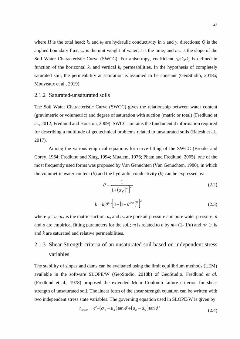
43

where H is the total head; kx and ky are hydraulic conductivity in x and y, directions; Q is the

applied boundary flux; γw is the unit weight of water; t is the time; and mw is the slope of the

Soil Water Characteristic Curve (SWCC). For anisotropy, coefficient rk=kx/ky is defined in

function of the horizontal kx and vertical ky permeabilities. In the hypothesis of completely

saturated soil, the permeability at saturation is assumed to be constant (GeoStudio, 2018a;

Mouyeaux et al., 2019).

2.1.2 Saturated-unsaturated soils

The Soil Water Characteristic Curve (SWCC) gives the relationship between water content

(gravimetric or volumetric) and degree of saturation with suction (matric or total) (Fredlund et

al., 2012; Fredlund and Houston, 2009). SWCC contains the fundamental information required

for describing a multitude of geotechnical problems related to unsaturated soils (Rajesh et al.,

2017).

Among the various empirical equations for curve-fitting of the SWCC (Brooks and

Corey, 1964; Fredlund and Xing, 1994; Mualem, 1976; Pham and Fredlund, 2005), one of the

most frequently used forms was proposed by Van Genuchten (Van Genuchten, 1980), in which

the volumetric water content (θ) and the hydraulic conductivity (k) can be expressed as:

( ) mnψ

θ+

=1

1 (2.2)

( ) 2/12/1 11

mm

s θθkk −−= (2.3)

where ψ= ua-uw is the matric suction, ua and uw are pore air pressure and pore water pressure; n

and α are empirical fitting parameters for the soil; m is related to n by m= (1- 1/n) and n> 1; ks

and k are saturated and relative permeabilities.

2.1.3 Shear Strength criteria of an unsaturated soil based on independent stress

variables

The stability of slopes and dams can be evaluated using the limit equilibrium methods (LEM)

available in the software SLOPE/W (GeoStudio, 2018b) of GeoStudio. Fredlund et al.

(Fredlund et al., 1978) proposed the extended Mohr–Coulomb failure criterion for shear

strength of unsaturated soil. The linear form of the shear strength equation can be written with

two independent stress state variables. The governing equation used in SLOPE/W is given by:

( ) ( ) b

waanunsat uuuc tan´tan´ −+−+= (2.4)

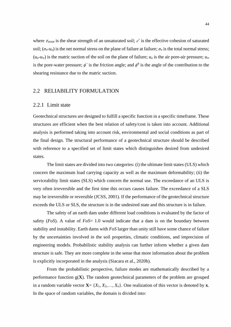
44

where 𝜏unsat is the shear strength of an unsaturated soil; 𝑐´ is the effective cohesion of saturated

soil; (σn-ua) is the net normal stress on the plane of failure at failure; σn is the total normal stress;

(ua-uw) is the matric suction of the soil on the plane of failure; ua is the air pore-air pressure; uw

is the pore-water pressure; ϕ´ is the friction angle; and ϕb is the angle of the contribution to the

shearing resistance due to the matric suction.

2.2 RELIABILITY FORMULATION

2.2.1 Limit state

Geotechnical structures are designed to fulfill a specific function in a specific timeframe. These

structures are efficient when the best relation of safety/cost is taken into account. Additional

analysis is performed taking into account risk, environmental and social conditions as part of

the final design. The structural performance of a geotechnical structure should be described

with reference to a specified set of limit states which distinguishes desired from undesired

states.

The limit states are divided into two categories: (i) the ultimate limit states (ULS) which

concern the maximum load carrying capacity as well as the maximum deformability; (ii) the

serviceability limit states (SLS) which concern the normal use. The exceedance of an ULS is

very often irreversible and the first time this occurs causes failure. The exceedance of a SLS

may be irreversible or reversible (JCSS, 2001). If the performance of the geotechnical structure

exceeds the ULS or SLS, the structure is in the undesired state and this structure is in failure.

The safety of an earth dam under different load conditions is evaluated by the factor of

safety (FoS). A value of FoS= 1.0 would indicate that a dam is on the boundary between

stability and instability. Earth dams with FoS larger than unity still have some chance of failure

by the uncertainties involved in the soil properties, climatic conditions, and imprecision of

engineering models. Probabilistic stability analysis can further inform whether a given dam

structure is safe. They are more complete in the sense that more information about the problem

is explicitly incorporated in the analysis (Siacara et al., 2020b).

From the probabilistic perspective, failure modes are mathematically described by a

performance function g(X). The random geotechnical parameters of the problem are grouped

in a random variable vector X= {X1, X2,…, Xn}. One realization of this vector is denoted by x.

In the space of random variables, the domain is divided into:

45

( ) ( )

( ) ( ) 0DomainFailure

0DomainSafety

=

=

Xx

Xx

gD

gD

f

s (2.5)

The boundary between the safety and failure domains is defined as g(x)=0 and is called the

limit state surface. All limit states are called failure mode. A geotechnical structure may have

more than one failure mode. Therefore, such a structure will have more than one performance

function.

2.2.2 Performance function

In an “n” dimensional hyper-space of variables, the limit state function g(x)= 0 is the boundary

between safe and failure domains. The probability of failure (Pf) is given by:

( ) ( )

==0)(

0x

X xXg

f dfgPP x (2.6)

where fX(x) represents the joint probability density function of the random variable vector X

and the integral is carried out over the failure domain. Therefore, the multidimensional integral

in Equation (2.6) can be very complicated and is usually solved numerically using Monte Carlo

simulations (MCS) or approximate methods such as the first/second-order reliability method

(FORM/SORM). In these cases, it is common to make a transformation y = T(x) to the standard

Gaussian space; the minimum distance of the limit state function g(y)= 0 to the origin is the so-

called reliability index (β), and the point over the limit state with minimum distance to the origin

is called the “design point”. In the standard Gaussian space, the limit state function is

approximated by a hyper-plane, yielding the classic first-order approximation:

( )βΦ −fP (2.7)

where Φ(∙) is the standard Gaussian cumulative distribution function (Beck, 2019, 2017;

Melchers and Beck, 2018).

The limit state function in slope stability problems is generally expressed as (Phoon,

2008):

( ) ( ) ( ) 012121 .x,....,x,xFoSx,....,x,xgg nn −==x (2.8)

where FoS is the factor of safety with respect to stability, a dependent variable (Liang et al.,

1999). In every realization of X, the critical surface and the FoS are found by any limit

equilibrium method, for instance, by the Morgenstern and Price stability analysis method.

46

2.2.3 Second-Moment and Transformation Methods

2.2.3.1 Mean Value First-Order Second Moment (MVFOSM)

The Taylor Series Method (Ang and Tang, 1984, 1975) is referred to as a First-Order Second

Moment analysis, which means that only the first two moments (mean and standard deviation)

are considered in the analysis, and there are no higher order terms in the formulation of this

method (Filz and Navin, 2006). The application of the Taylor Series Method from the MFOSM

to reliability analyses in geotechnical engineering is discussed by different authors (Baecher

and Christian, 2003; Duncan et al., 2014; Phoon, 2008; Phoon and Ching, 2015; USACE, 1997).

The reliability index (β) for a Normal (N) distribution of factor of safety (FS) is defined

in terms of the mean (μFS) and the standard deviation (σFS) of the trial factors of safety (Christian

et al., 1994; GeoStudio, 2018b) and the GeoStudio software uses these concepts as shown in

the following equation.

( )

FS

FS

σ

μβ

0.1−= (2.9)

where β describes the stability by the number of standard deviations (σFS) separating the mean

factor of safety (µFS) from its defined failure value of 1.0. A way of normalizing the factor of

safety with respect to its uncertainty can also be considered.

When the shape of the probability distribution is known, the reliability index can be

related directly to the probability of failure.

Although it may be reasonable and conservative to assume the factor of safety (FS) is

normally distributed, the Taylor Series Method has been widely used in geotechnical

engineering with an assumption that FS is lognormally (LN) distributed. A LN distribution of

FS is a valid assumption when FS is either the product of multiple variables or the sum of

variables that are lognormally distributed (Filz and Navin, 2006).

An expression for β for a LN distribution of FS (Duncan, 2000; Duncan et al., 2014) is

defined by the following equation.

( )2

2

1ln

1ln

FS

FS

FS

COV

COV

μ

β+

+= (2.10)

where β is the Lognormal reliability index, µFS the mean factor of safety and COVFS is the

coefficient of variation of the factor of safety.

47

There is more controversy over the appropriate distribution for the FS. However, it seems

reasonable and simple to assume that FS is normally distributed unless demonstrated otherwise.

The sometimes voiced argument that Normal distributions are inappropriate because they allow

negative values is usually moot since the probabilities of negative realizations are usually

vanishingly small (Hartford and Baecher, 2004).

2.2.3.2 First-order reliability method (FORM)

As mentioned previously, the FORM consists in mapping the problem from the original design

space X to the standard Gaussian space Y by means of a transformation y = T(x), where y is a

realization of Gaussian vector Y. This transformation can deal with non-Gaussian variables as

well as the correlation between random variables (see Figure 2.1). The transformation is

accomplished by means of the principle of normal tail approximation (Der Kiureghian and Liu,

1986; Ditlevsen, 1981) and the Nataf model (Nataf, 1962), following the work by Melchers and

Beck (Melchers and Beck 2018). In standard Gaussian space, the so-called design point is found

by solving the following constrained optimization problem:

( ) 0tosubject

minimizeswichfind T

=y

yy*y

g (2.11)

The solution of this problem requires iterative procedures due to general nonlinearity of the

limit state function, as well as due to nonlinearity of the y = T(x) mapping. Point y*, found as

the solution to the problem in Equation (2.11), is also known as the design point; among all the

points in the failure domain, it is that most likely to occur. Hence, this point corresponds to the

most likely combination of geotechnical parameters leading to loss of equilibrium. As the

critical slip surface is re-evaluated during the search for the design point, the critical surface

found at the end of the iterative procedure corresponds to the critical surface most likely to

occur, herein called the probabilistic slip surface.

At the design point, the original limit state function is replaced by a hyper-plane: the

failure probability becomes the probability mass beyond the hyper-plane. The Hasofer-Lind

reliability index is given by β = [(y*)T(y*)]1/2, and the failure probability estimate is given by

Equation (2.7). The accuracy of the FORM approximation depends on the degree of

nonlinearity of the limit state in Y space (Beck and Ávila da S., 2016). The solution is exact

only for linear functions of independent Gaussian random variables (Kroetz et al., 2018;

Melchers and Beck, 2018).

48

Some alternative schemes have been proposed to solve the FORM problem in the

original space of random variables X (Low and Tang, 2007, 2004, 1997). These schemes

directly find design point x*, by looking for the mode of the failure domain, or the point in the

failure domain where fX(x) is the maximum, or by finding the smallest dispersion ellipsoid

tangent to the limit state surface. These schemes are of very practical implementation, yet they

are not employed herein as they are not available in the StRAnD software.

Figure 2.1 – FORM transformation from (a) original (X) to (b)

standard Gaussian (Y) space (based on Ji et al. (2017), Melchers and

Beck (2018)).

Important sub-products of the FORM solution are the so-called sensitivity factors 𝛼𝑖2, which

are obtained from:

( )( )*

i

*

it

n,...,1iig

g

y

y

y

y

==

= (2.12)

where g y is the gradient of the limit state function with respect to random variables. Since α

is a unitary vector, 12

i = ; hence, the sensitivity factor 2

i shows the relative contribution

of random variable X towards the failure probability for linear or approximately linear limit

state functions (Beck, 2019, 2017; Kroetz et al., 2018).

The above may be formalized for the following algorithm (Melchers and Beck, 2018).

For illustration, the Rosenblatt transformation will be assumed.

(1) Select an initial checking point vector x*= x(1) where x(1) might be the mean value of X

(𝜇X).

a) b)

49

(2) Use the transformation (Equation 2.14) to obtain y(1); this transformation will be of the

simple form Equation (2.13) for any of the components of X that are independent random

variables.

The transformation of an independent basic random variable X of non-Normal

distribution to an equivalent standardized Normal distributed random variable Y can be

expressed as

( ) ( ) ( ) xyyx XX FFp 1or −=== (2.13)

where p is some probability content associated with X= x, and hence with Y= y; FX( )

is the marginal cumulative distribution function of X and Φ(∙) is the cumulative

distribution function for the standardized Normal random variable Y.

The component random variables yi can be obtained by successive inversion:

( )

( )

( ) 1-n1nn

122

11

xxxy

xxy

xy

,...,|

|

1

2

1

1

1

nF

F

F

−

−

−

=

=

=

(2.14)

In general, the valuation will need to be made numerically

(3) Use equations (2.15) and (2.16) to obtain the Jacobian J and its inverse J−1.

Before the above transformations can be incorporated into an iteration algorithm, it is

necessary to determine the transformation of the limit state function from g(x)= 0 to

g(y)= 0. A probability density function defined in the X space is transformed to the Y

space. This transformation also holds for the relationship between any (continuous)

functions in X and Y; in particular it also holds for g(x):

( ) ( )Jyx gg = (2.15)

where the Jacobian J has elements Jij = 𝜕yi/𝜕xj. The differential may be evaluated by

replacing for yi using Equation (2.14), and then noting that, 𝜕yi= [ϕ(y1)]−1𝜕Fi(x1 | x1,…,

xi-1), so that

( )( )

j

1-iii

ij

i

x

xxx

yx

y

=

,...,|1 iF

(2.16)

where ϕ is a partial factor. Evidently, if i< j, 𝜕Fi/𝜕xj= 0, so that J is lower triangular.

This allows the inverse J−1 to be obtained from J by back-substitution.

(4) Compute the direction cosines 𝛼i according to Equation (2.12), the current value of

g(y(1)) and the current estimate of β according to β= −y*T𝛼 (see Figure 2.1) where 𝛼 is

the vector of direction cosines.

(5) A new estimate of the co-ordinates of the checking point in Y space is then given by

Equation (2.17) using the current β value.

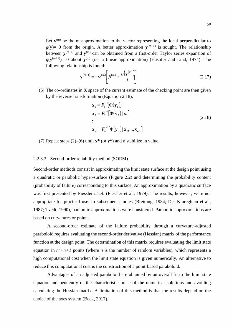
50

Let y(m) be the m approximation to the vector representing the local perpendicular to

g(y)= 0 from the origin. A better approximation y(m+1) is sought. The relationship

between y(m+1) and y(m) can be obtained from a first-order Taylor series expansion of

g(y(m+1))= 0 about y(m) (i.e. a linear approximation) (Hasofer and Lind, 1974). The

following relationship is found:

( ) ( ) ( )( )( )

+−=+

l

gβ

mmm1m y

y (2.17)

(6) The co-ordinates in X space of the current estimate of the checking point are then given

by the reverse transformation (Equation 2.18).

( )

( )

( ) 1-n1nn

122

11

xxyx

xyx

yx

,...,|

|

1

1

2

1

1

=

=

=

−

−

−

nF

F

F

(2.18)

(7) Repeat steps (2)–(6) until x* (or y*) and β stabilize in value.

2.2.3.3 Second-order reliability method (SORM)

Second-order methods consist in approximating the limit state surface at the design point using

a quadratic or parabolic hyper-surface (Figure 2.2) and determining the probability content

(probability of failure) corresponding to this surface. An approximation by a quadratic surface

was first presented by Fiessler et al. (Fiessler et al., 1979). The results, however, were not

appropriate for practical use. In subsequent studies (Breitung, 1984; Der Kiureghian et al.,

1987; Tvedt, 1990), parabolic approximations were considered. Parabolic approximations are

based on curvatures or points.

A second-order estimate of the failure probability through a curvature-adjusted

paraboloid requires evaluating the second-order derivative (Hessian) matrix of the performance

function at the design point. The determination of this matrix requires evaluating the limit state

equation in n2+n+1 points (where n is the number of random variables), which represents a

high computational cost when the limit state equation is given numerically. An alternative to

reduce this computational cost is the construction of a point-based paraboloid.

Advantages of an adjusted paraboloid are obtained by an overall fit to the limit state

equation independently of the characteristic noise of the numerical solutions and avoiding

calculating the Hessian matrix. A limitation of this method is that the results depend on the

choice of the axes system (Beck, 2017).

51

Figure 2.2 – SORM solution in the standard Gaussian (Y) space

(Beck, 2019, 2017).

2.2.3.4 The Hasofer-Lind Rackwitz-Fiesler (HLRF) algorithm

The optimization problem in Equation (2.11) can be solved using various optimization

algorithms, such as the gradient projection method, augmented Lagrangian method, and

sequential quadratic programming method (Beck and Ávila da S., 2016; Val et al., 1996). The

Hasofer-Lind Rackwitz-Fiesler (HLRF) algorithm (Abraham M. Hasofer and Lind, 1974;

Rackwitz and Fiessler, 1978) is based on the Newton method; it is very efficient when it

converges, and this occurs for most well-behaved problems (linear functions of independent

Gaussian random variables) (Liu and Der Kiureghian, 1991). In the dam equilibrium problem

addressed herein, no convergence problems were encountered.

The HLRF algorithm is a good adaptation of a first order optimization algorithm to

special problems in the search for the design point according to the definition of Hasofer and

Lind. It is shown to be effective in many situations even if its convergence is not assured in all

cases (Lemaire et al., 2009). The HLRF algorithm is based on finding the zero of successive

linearizations of the limit state surface, leading to the well-known sequence:

( )( ) ( )( ) ( )kkkk

k

1k yyyyy

y gggg

1 t

2−

=+

(2.19)

where ∇g(yk) is the gradient vector of the limit-state function with respect to y evaluated at yk

(Beck and Ávila da S., 2016).

52

2.2.3.5 Improved Hasofer-Lind Rackwitz-Fiesler (iHLRF) algorithm

An improved version of HLRF (iHLRF) was proposed by Zhang and Der Kiureghian (Zhang

and Der Kiureghian, 1997) by integrating a search for the optimal step. The authors demonstrate

the unconditional convergence of the algorithm. Hence, the iHLRF algorithm is employed in

the dam equilibrium problem addressed herein; no convergence problems were encountered,

following Melchers and Beck (Melchers and Beck, 2018).

In the iHLRF algorithm, a linear search is performed (Sudret and Der Kiureghian, 2000;

Zhang and Der Kiureghian, 1997) through a unit step λk= 1:

kkk1k dyy +=+ (2.20)

in the direction given by the HLRF algorithm:

( )( ) ( )( ) ( ) kkkk

t

k2

k

k1kk gggg

1yyyyy

yyyd −−

=−= +

(2.21)

In Equation (2.20) and (2.21), dk is a search direction and αk is a step size, selected from the

minimization of an appropriate merit function. The following merit function is proposed by the

authors:

( ) ( )yyy gc2

1+=m (2.22)

where c is a penalty parameter. The linear search is defined as:

( ) kkk

*

k min arg dy += m (2.23)

The linear search can be performed approximately using the popular Armijo rule (Luenberger

and Ye, 1984; Vanderplaats, 1984). An appropriate step λk is selected, so as to obtain a

sufficient decrease in the merit function:

( ) ( ) ( ) ,abmbbmax2

k

n

kk

n

k

n

Νik yydy mm −−+=

(0,1)ba, (2.24)

The merit function has two important properties: search direction dk is a descent direction of

the merit function as long as the Equation (2.24) condition is satisfied, and it reaches a minimum

at the design point as long as the same constraint in c is observed.

( )y

y

gc

(2.25)

These two properties are sufficient to ensure the unconditional convergence of the algorithm

(Beck, 2019, 2017; Beck and Ávila da S., 2016; Zhang and Der Kiureghian, 1997).

53

2.2.4 Simulation Methods

2.2.4.1 “Crude” Monte Carlo simulation (MCS)

The probability of failure (Pf) in Equation (2.2) can also be evaluated directly by means of

“crude” MCS. By employing an indicator function I(x), the integration in Equation (2.2) can be

extended over the whole domain, based on samples generated from fX(x):

)Safety(1)(I

)Failure(1)(I

s

if

f

if

D

D

⎯→⎯=

⎯→⎯=

xx

xx (2.26)

Therefore, the expected value of the probability of failure can be estimated, based on a sample

of finite size, by

( )=

==sin

i si

f

si

fn

n

nP

1

I1

ix (2.27)

where nf is the number of points in the failure domain and nsi is the number of simulations. This

value is a non-biased estimator of the probability of failure: the estimate converges to the exact

probability of failure in the limit, as nsi → ∞.

2.2.4.2 Importance sampling Monte Carlo (ISMC) simulation

Importance sampling using design points concentrates sampling points at important regions of

the failure domain. This technique reduces the number of simulations by avoiding excessive

simulation of points away from the region of interest, i.e. away from the failure domain. These

techniques generally use additional information about the problem, such as the coordinates of

the design point. A strictly positive sampling function hX(x) is employed to generate the

samples; this function is centered at the design point:

( )( )( )

( ) xdhh

fPf x

x

xx x

x

x

= I (2.28)

where the weight corresponding to each sample is:

( )

( )i

i

i

fw

h=

X

X

x

x (2.29)

The mean probability of failure, for a sample of size nsi, becomes:

( )( )( )=

sin

i i

ii

si

fh

f

nP

x

xx

x

xI1

(2.30)

54

The solution is subject to a sampling error or variance, which is estimated by:

( )2

1

______

I1

1=

−

−=

sin

i

fii

si

f Pwn

PVar x (2.31)

From Equations (2.30) and (2.31), the confidence interval (CI) of MCS is estimated as:

+

−

______

fffff PVarkPPPVarkP (2.32)

where parameter k is related to the desired confidence (Beck, 2019).

2.2.5 Direct coupling method (DC)

This function reflects geomechanical behavior that must often be modeled by approximated

numerical solutions, from which only outcomes of g(x) are calculable. The application of

reliability-based methods to real technical situations, therefore, requires us to be capable of

ensuring the dialog between the geotechnical model and the reliability model (Lemaire et al.,

2009).

Different numerical methods, such as the Finite Element Method (FEM), Limit

Equilibrium Method (LEM), Material Point Method (MPM), Discrete Element Method (DEM),

or others that model a geotechnical problem can be used without restrictions. Here, the FEM

and LEM are used as numerical methods to model a geotechnical problem. Every calculation

of g(x) is a calculation of the numerical model that can have a wide variation of repetitions. The

number of calculations necessary to meet the convergency criterion is a good indicator of the

efficiency of the coupled method. It must be the lowest possible.

In the study herein, the code written in Visual Studio software drives the reliability

software StRAnD (Beck, 2008) to call the geotechnical software GeoStudio (GeoStudio, 2018a,

2018b) whenever it is necessary to calculate g(x). The direct coupling method can be used with

the First- and Second-order reliability method (FORM and SORM) as well as by importance

sampling Monte Carlo (ISMC) simulation. The “crude” Monte Carlo simulation and others with

intelligent sampling (e.g., Adaptive importance, Latin hypercube sampling, Asymptotic

simulation, Subset simulation, …, etc.) can be used, but the efficiency of these methods must

be tested in terms of computational time. Every Geotechnical problem has different

computational time in function of the complexity of the numerical problem.

55

2.2.5.1 Control of Finite Element Method (FEM) and Limit Equilibrium Method (LEM)

In a geotechnical-reliability calculation, FEM and LEM must be controlled by the reliability

module. FEM and LEM only execute the instructions of the reliability-based module. In each

calculation loop, a dialog must be established between the two modules: geotechnical and

reliability. This interaction is necessary, as it allows the reliability module to analyze the results

of the FEM and LEM calculation and to make the appropriate decisions. Some decisions are

summarized as follows: (i) define x coordinates of a new calculation point and evaluate a new

outcome g(x); (ii) validate the new step size; (iii) detect convergence in case of stabilization of

the results during the iterations; (iv) stop the calculation in case of divergence and take

appropriate actions (Lemaire et al., 2009).

2.2.5.2 Dialog between FEM, LEM and reliability procedures

The reliability-based module controls the calculation operations and the FEM and LEM code,

which is considered as a black box. This dialog must be established using interfacing procedures

between the two modules, geotechnical and reliability. It is therefore imperative for the

reliability module to recognize and to modify the values of the random variables of the FEM

and LEM code data, and to recognize the load effects (output variables) in the FEM and LEM

results. Furthermore, it must be alerted in case of problems in the execution of the mechanical

calculation.

The choice that seems preferable is that of adapting the procedures of reading,

analyzing, and interpreting to the FEM and LEM code format; that is, it is the reliability-based

module that makes the effort to converse with the FEM and LEM procedures, which remain

intact. This solution is probably less direct, but it has the advantage of not intervening at the

FEM and LEM code level, thus helping to preserve its qualities without any disturbance. This

is also the only solution when the coupling is performed with a code for which we do not have

any source programs.

Among the FEM and LEM codes available in engineering, we can distinguish two

families according to whether the code has – or does not have – a parameterized language. The

presence of such a language largely facilitates the task, as the variables are declared explicitly.

Depending on the possibilities of each code, we must therefore adapt the interfacing procedure

on a case-by-case basis.

56

The coupling between geotechnical and reliability models requires an exchange of

information. The protocol to be implemented depends on the capacities of the coupled software

packages and the possibilities for dialog. The reliability module controls the geotechnical

module, which is generally the largest consumer of calculation resources, and a good

performance indicator is the number of calls to the mechanical model.

2.2.5.3 Finite difference evaluation of performance function gradients

Most of the geotechnical-reliability calculation procedures require calculating the gradients to

define the descent direction that minimizes the objective function (distance between the origin

and the limit-state). The gradient vector of the limit-state function in Equation (2.19) and

Equation (2.21) can be evaluated numerically via progressive, regressive, or central finite

differences (Leonel et al., 2011).

The search for the design point in transformed y space using mathematical programming

techniques involves evaluating the gradient of the limit state function with respect to the vector

of random variables:

( )

=

− n1n121 x

g,

x

g,.....,

x

g,

x

gg X

(2.33)

Progressive, regressive, or central finite differences can be employed to evaluate this gradient

numerically. In the progressive finite differences employed herein, each component of ∇g(∙)

requires one computation of the numerical response:

( ) ( )

i

ni21nii21

i h

x,.....,x,......,x,xgx,.....,hx,......,x,xg

x

g −+

(2.34)

where hi is the step size or increment. In the first iteration, the step size is given as a fraction of

the standard deviation of each random variable:

i step Xih f = (2.35)

where fstep is the fraction of the standard deviation σXi used as step size.

From the second iteration onwards, the step is given as a fraction of the change in X

from the past iteration:

( )1 2

1 1

{ , ,..., ,..., }i n

k step k k

h h h h

f+ −

=

= −

h

h x x (2.36)

57

A minimum value of hmin is used to avoid numerical instability in computations. The optimal

size of fstep can be found by minimizing the differentiation and numerical errors of the

approximation (Gill et al. 1981; Scolnik and Gambini 2001).

Given that failure implies the decrease of resistance variables and the increase of load

variables, we can choose the incrementation of the variables in the direction that brings us closer

to failure. However, as the increments are relatively small, the direction of the increments can

only have a very small influence on the convergence of the algorithm (Lemaire et al., 2009).

Each evaluation of the gradient vector requires “n+1” solutions of the numerical model.

The limit state responses in Equation (2.34) are evaluated directly by calling the numerical

solver from the structural reliability software StRAnD 1.07 (Beck, 2008). This approach is

known as DC in the literature (Kroetz et al., 2018; Leonel et al., 2011; Napa-garcía, 2014;

Sudret and Der Kiureghian, 2000). If the numerical algorithm used to find the design point

requires m iterations to converge, the total number of limit state function calls is m(n+1). As

observed by (Leonel et al., 2011), such a solution is more economic than constructing adaptive

surrogate models for the limit state function, a popular approach in geotechnical reliability

analyses.

2.2.5.4 Direct coupling GeoStudio and StRAnD software

Dialog is indispensable in a coupling software package; the reliability-based module StRAnD

1.07 or 2.00 (Beck, 2008) controls the calculation operations and the GeoStudio software 2018

or 2019 (GeoStudio, 2018a, 2018b), which is considered as a black box (Figure 2.3). This dialog

must be established using interfacing procedures between the two modules, mechanical and

reliability.

Figure 2.3 – Direct coupling StRAnD and GeoStudio.

58

The coupling between the GeoStudio software and the StRAnD requires an exchange of

information. The protocol to be implemented depends on the capacities of the coupled software

packages and the possibilities for dialog. By using a commercial software, four interface

possibilities may be envisaged (Lemaire et al., 2009):

(1) Graphic user interface: all the information is entered and read through graphic windows.

(2) Formatted files interface: the information is entered and retrieved in numerical data

exchange files, while retaining all the significant figures.

(3) Parametrized data interface: coupling is largely facilitated if the mechanical module has

an integrated parametrized language.

(4) User-specific interface: such an interface exists in certain calculation codes. Users create

their own procedures for the exchange of results and the control of calculations; the

reliability module is then completely integrated into the mechanical module and any risk

of loss of accuracy by truncation is eliminated.

In this case, the option (3) of parametrized data interface is used. The GeoStudio file contains

the analysis information. The file has a format “.gsz” which is a ZIP file. All input parameters

are changed in the file extension “.xml”, which is changed in every simulation or during a

search for the design point (DP). The input parameters are organized in the original position of

the “.xml” file for every simulation (Figure 2.4). In the case of the seepage analysis, the Soil

Water Characteristic Curve (SWCC) and the hydraulic conductivity function must be

developed with the original equations. Results are presented in the X and Y position for suction

[kPa] and Hydraulic conductivity [m/s] respectively (See Figure 2.5). Omission and errors with

respect to the original position of the properties produce many errors during the compilation of

software.

Figure 2.4 – Input file with extension “.xml” of the GeoStudio

software.

59

Figure 2.5 – Seepage input properties from the Fortran code to the

“.xml” file.

For saving output results, file “.gsz” is compressed/uncompressed from the 7-zip software

saving the FS to find the DP. In the same folder, all the output data are found in file extension

“.csv”, which are used as the input parameters for the reliability analysis. Although, the pore

water pressure (PWP) results were not used in the equation of performance function, all the

results are found in the same folder for every step of time and nodes of the finite element method

(FEM). These PWP results can be used in other studies. The flowchart of the

compressed/uncompressed GeoStudio file is shown in Figure 2.6.

Figure 2.6 – Flowchart of compressed/uncompressed GeoStudio file.

To make analysis automation possible, the GeoCmd.exe application is installed as part of the

GeoStudio installation and can be used to run a ‘.gsz’ file in batch mode from command lines

(See Figure 2.3). Even if the file has more than one analysis, all of them can be performed

without the need for manual intervention.

60

The reliability methods and conditions of correlation materials are defined in the

STRAND_INPUT.txt file of the StRAnD software. The results of the reliability analysis

(number of evaluations and simulations, sensitivity coefficients at DP, reliability index,

probability of failure, evaluation time, DP, etc.) are shown in the STRAND_OUTPUT.txt file.

Visual results and additional information (e.g., pore water pressures in specific coordinates or

critical slip surfaces) of the reliability results are found in the last ".gsz" file of the analysis.

2.3 OPTIMIZATION FORMULATION

2.3.1 Formulation of reliability analysis

Let X= {X1, X2, …, Xn} and d= {d1, d2, …, dn} be vectors of structural system parameters.

Vector 𝐗 ∈ ℝ𝑛𝑅𝑉 contains nRV random variables, and may include dimensions and geometry,

resistance properties of materials or structural members, loads, and model error variables. Some

of these parameters are random in nature; others cannot be defined deterministically due to

uncertainty. Vector 𝐝 ∈ ℝ𝑛𝑅𝑉 contains nDV design variables whose values are to be determined

to maximize the performance of the system, or in order to minimize weight, cost, etc. Typical

variables in vector d are nominal member dimensions, partial safety factors, reinforcement

ratio, design life, parameters of inspection and maintenance programs, etc.

The existence of uncertainty implies uncertainty in the performance of the structure, that

is, the possibility of structural failure. The boundary between safety and failure domain is given

by limit state functions gi(d, X)=0, such that:

( ) ( )

( ) ( ) ,...,,1,0,D

,0,D

LSisi

ifi

nig

g

==

=

Xdxd

Xdxd (2.37)

where Dfi(d) is the failure domain, Dsi(d) is the safety domain, and nLS is the number of limit

state functions. Each limit state describes one possible failure mode of the structure. The

probability of structural failure, or probability of failure, for the ith failure mode, is given by:

( ) ( )==fiD

ifi dfgPP xxXd x0, (2.38)

where fX(x) represents the joint probability density function of the random variable vector X

and the integral is carried out over the failure domain.

61

The probabilities of failure for individual limit states can be evaluated using traditional

structural reliability methods, such as first- and second-order structural methods (FORM and

SORM), as well as by Monte Carlo simulation (MCS). For multiple limit states, system

reliability techniques have to be employed (Beck, 2019, 2017; Melchers and Beck, 2018).

2.3.2 Reliability-Based Design Optimization (RBDO)

The RBDO is the generic name given to (structural) optimization that explicitly takes

uncertainties into account. When the formulation of optimization uses reliability constraints,

one obtains what has been called Reliability-Based Design Optimization (RBDO). A typical

formulation reads:

( )( ) SniPP

f

LSfTifi = dd

d*d

;...,,1,tosubject

minimizeswichfind (2.39)

where Pfi(d) is the failure probability for the ith failure mode, PfTi is the allowable failure

probability for the ith failure mode, nLS is the number of limit states, and S ={dmin, dmax}. The

target safety or target reliability, for the ith failure mode, is rTi=(1-PfTi). Using reliability index

β as a safety measure, Equation (2.40) can also be written as:

( )

( ) Sni

f

LSTii = dd

d*d

;...,,1,tosubject

minimizeswichfind

(2.40)

The main difference between RBDO and deterministic optimization is the introduction of

uncertainties by considering them random variables instead of fixed values. This induces the

emergence of probabilistic constraints, which is required to obtain reliability indices of the

structure in every step of the optimization analysis. A design with the RBDO process assures

the safety of the structure when the parameters involved in the analysis are of random nature.

In contrast, deterministic optimization cannot ensure the safety conditions (Rodríguez, 2016).

An illustrative scheme of deterministic optimization (DO) and RBDO is depicted in Figure 2.7.

In this figure is shown two limit state functions which are jointed

62

Figure 2.7 – Illustrative scheme of DO vs RBDO (Based on

Rodríguez (2016)).

Failure probabilities or reliability indexes can be evaluated by classical structural reliability

methods such as FORM, SORM, or SMC. However, the computational cost of evaluating these

reliabilities needs to be taken into account, as reliability analysis is now performed within an

optimization loop. Hence, structural reliability calculations have to be repeated hundreds to

thousand times. This will often require the use of specialized methods, which can reduce the

overall computational burden (Beck, 2019, 2017; Melchers and Beck, 2018).

The RBDO (Hilton and Feigen, 1960; Hu and Du, 2014; Lopez and Beck, 2012) is a

natural extension of DDO, where deterministic constraints are replaced by probabilistic design

constraints. RBDO does not account for the economical consequences of failure, since the

safety level is a constraint, and not an optimization variable. DDO and RBDO can both be used

to achieve mechanical structural efficiency. The safety-economy tradeoff is addressed by the

Risk optimization formulation (Beck, 2013; Beck and Gomes, 2012; Enevoldsen and Sorensen,

1994; Kroetz et al., 2020; Torii et al., 2019), which is outside the scope of this study.

63

2.3.3 Single-Loop Approach (SLA)

The SLA method operates in function of the single-loop RBDO algorithm (Liang et al., 2007,

2004). This method uses a deterministic optimization formulation, which eliminates the need

for inner reliability loops without increasing the number of design variables as is the case with

some other single-loop algorithms (Agarwal et al., 2004; Kuschel and Rackwitz, 2000;

Streicher and Rackwitz, 2004). Concurrent convergence is thus obtained, whereby optimal

design and target reliability are obtained simultaneously in the same optimization loop. SLA

has been found to be more efficient, robust and accurate than many of the competing methods

(Aoues and Chateauneuf, 2010; Lopez and Beck, 2012).

SLA (Liang et al., 2004) approximates the design point of each reliability constraint by

solving the first order Karush-Kuhn-Tucker (KKT) conditions for each iteration 𝑘. The

formulation is given by:

( )

( ) Snig

f

LSi =

+

dxd

dd 1k

;...,,1,0,tosubject

minimizeswichfind

ik

(2.41)

where vector ( ) ( ) Tiikikkik αxyJx X −= is a linear approximation to the design point *

ix , at the

kth iteration, and vector ( )kX needs to be updated only if random design variables are present.

The Jacobian matrix Jxy of the transformation ( ) XyJyx +== −

xy

1T is given by:

RVRV

m

l nmnld

d...,,1;...,,1

y

xxy ==

=J (2.42)

The design point 𝐲𝑖∗ = 𝑇(𝐱𝑖

∗), is the point over the limit state function with minimal distance to

the origin of the Standard Normal space. As such, it is the most appropriate point to linearize

the limit state function. For each limit state function, the gradient vector is evaluated as:

RVnmm

i

d

dgg

...,,1

iy

=

= (2.43)

In Equation (2.41), vector αi is the normalized gradient of the ith constraint, also known as

direction cosine:

RVnm

αg

g...,,1m

i

ii =

=

=α (2.44)

64

The squared normalized direction cosines 𝛼𝑚2 inform about the contribution of each random

variable to the calculated failure probabilities, since:

12= mm

α (2.39)

The formulation in Equations (2.40) and (2.41) is a generalization of the original formulation

in Liang et al. (Liang et al., 2004), which addresses non-Gaussian and correlated variables. SLA

does not search for the design point of each constraint at each iteration. Instead, an

approximation of the design point of active constraints is obtained by solving the KKT

conditions. An implicit assumption in SLA is that the sequence of design point approximations

converges to the true design point.

If a limit state function is highly non-linear in the reduced variable space or if there are

multiple design points for a given limit state, then SLA may not converge to the global

optimum. Such issues are well-known in FORM and related methods.

The SLA algorithm starts with initial choices for d0 and xi0 (e.g., xi0= µX), for k=0, and

by evaluating the objective function and constraints in Equation (2.7). Point dk+1 is evaluated

using an appropriate optimization algorithm, counter k is updated (k= k+1), and transformation

matrices ( )kxyJ and normalized gradient vectors αi0, i=1, …,nLS are updated. At this point, the

design point estimates can be updated, making ( ) ( ) Tiikikkik αxyJx X −= . During the

interactive procedure, the algorithm first checks if (µx)k has changed from the last iteration. In

a positive case, the αik vectors are updated. If not, the same gradient vector αik is used to

calculate ( ) ( ) Tiikikkik αxyJx X −= . This step is essential to keep vectors (µx)k, and xik

consistent, but it also increases the efficiency of the algorithm (Beck, 2019, 2017; Melchers and

Beck, 2018).

2.3.4 Interative procedure

The numerical procedure adopted to minimize the objective function is the NLPSolve

subroutine of the MAPLE 2019 (Bernardin et al., 2020; Maplesoft, 2020) software. The

NLPSolve command solves a nonlinear program (NLP), which involves computing the

minimum (or maximum) of a real-valued objective function, possibly subject to constraints.

Within the NLPSolve subroutine, the Sequential Quadratic Programming (SQP) method was

selected to solve the optimization problem. Numerical derivatives are computed automatically

throughout iterations.

65

2.4 TARGET RELIABILITY INDEX FOR DAMS

The target reliability indices (βT) guide the expected performance of the dam. If the dam meets

βT ≥ 3 (high performance) for all failure modes, the expected performance will be good. Dams

with a βT < 3(low performance) will be expected to perform poorly and present major

rehabilitation problems. A dam with βT < 1very low performance) is classified as hazardous

with serious structural problems. The U.S. Army Corps of Engineers (USACE, 1997) gives a

guide of 𝛽𝑇 values, as shown in Table 2.1, which is generally used.

Table 2.1 – Target reliability indexes for dam stability analysis

(USACE, 1997).

Expected performance level Reliability index (β) Probability of failure (Pf)

High 5.0 3.0 x10-7

Good 4.0 3.0 x10-5

Above average 3.0 1.0 x10-3

Below average 2.5 6.0 x10-3

Poor 2.0 2.3 x10-2

Unsatisfactory 1.5 0.07

Hazardous 1.0 0.16

67

3 RELIABILITY ANALYSIS OF EARTH DAMS USING

DIRECT COUPLING

ABSTRACT

Numerical methods are helpful for understanding the behaviors of geotechnical installations.

However, the computational cost sometimes may become prohibitive when structural reliability

analysis is performed, due to repetitive calls to the deterministic solver. In this Chapter, we

show how accurate and efficient reliability analyses of geotechnical installations can be

performed by directly coupling geotechnical software with a reliability solver. An earth dam is

used as the study object under different operating conditions. The limit equilibrium method of

Morgenstern-Price is used to calculate factors of safety and find the critical slip surface. The

commercial software packages Seep/W and Slope/W are coupled with StRAnD structural

reliability software. Reliability indices of critical probabilistic surfaces are evaluated by the

first- and second-order structural reliability methods (FORM and SORM), as well as by

importance sampling Monte-Carlo (ISMC) simulation. By means of sensitivity analysis, the

effective friction angle (ϕ´) is found to be the most relevant uncertain geotechnical parameter

for dam equilibrium. The correlations between different geotechnical properties are shown to

be relevant in terms of equilibrium reliability indices. Finally, it is shown herein that a critical

slip surface, identified in terms of the minimum factor of safety (FS), is not the critical surface

in terms of the reliability index.

Keywords: Earth dam; direct coupling; reliability analysis; water level.

68

3.1 INTRODUCTION

The conventional approach for seepage and slope stability analyses of dams is to use

deterministic soil properties to find deterministic factors of safety (FSs) (Cheng, 2003; Fredlund

and Krahn, 1977; Griffiths and Lane, 1999; Sarma and Tan, 2006). On the last four decades,

much work has been done to quantify the variability of soil properties (Phoon and Kulhawy,

1999a, 1999b; Phoon et al., 2006) to determine the reliability index (β) and the probability of

failure (Pf) of slopes and embankments (Alonso, 1976; Bhattacharya et al., 2003; Calamak and

Yanmaz, 2014; Ching et al., 2009; Christian et al., 1994; Duncan, 2000; Guo et al., 2018; Li

and Lumb, 1987; Liang et al., 1999; Mouyeaux et al., 2018; Sivakumar Babu and Srivastava,

2010; Tang et al., 1976; Wu and Kraft, 1970; Xue and Gavin, 2007; Yanmaz et al., 2005; Yi et

al., 2015).

Probabilistic slope and dam stability analyses can be performed using different

approaches. Monte Carlo simulation (MCS) is by far the most intuitive and well-known

probabilistic method; however, it usually implies a very large computational burden. Point

estimate methods (PEMs) are popular in geotechnical engineering (Hong, 1998; Rosenblueth,

1975; Zhao and Ono, 2000), but they are inaccurate for many problems (Napa-García et al.,

2017). Using higher-order moment methods increases computation accuracy, but the efficiency

is lost. Transformation schemes such as first- and second-order reliability methods (FORM and

SORM) are competitive with PEMs, in terms of computational effort, but are more appropriate

and accurate for evaluating small failure probabilities controlled by distribution tails. The

FORM loses accuracy when dealing with highly nonlinear limit state functions, where PEMs

also fail.

One particularity of reliability analysis for stability of slopes and dams is the location

of the critical slip surface, which is critical for safety control. A dam or slope may fail at a

circular or non-circular slip surface, but during the mathematical procedure, an infinite number

of slip surfaces are tested. Evaluating the total failure probability along all potential slip surfaces

is considered as a mathematically formidable task (El-Ramly et al., 2002). It has been shown

that the surface of the minimum FS is not always the surface of the maximum probability of

failure (Hassan and Wolff, 1999); hence, a probabilistic search for the critical surface is

required. Dam or slope reliability is often determined only for one or a limited number of slip

surfaces (El-Ramly et al., 2002; Hassan and Wolff, 1999; Tang et al., 1976; Wang et al., 2011).

It is generally recognized that search for the critical probabilistic slip surface is similar, in

69

principle, to that for the surface of the minimum FS in the deterministic approach (Cheng et al.,

2015). (Low et al., 1998) developed a spreadsheet procedure for evaluating the reliability of

slopes using the method of slices. The procedure is easy to follow, but it is limited to simple

geometries, uniform geotechnical properties and Gaussian random variables. In contrast, the

direct coupling method explored herein can be applied to complex geometries, nonlinear

geotechnical analysis, arbitrary probability distributions and nonuniform pore pressure and

strength profiles.

Some commercial software packages, such as Slope/W (GeoStudio) and Slide

(RocScience), perform slope stability analysis probabilistically using MCS and the following

second-moment approximation (Baecher and Christian, 2003; Duncan et al., 2014; Phoon,

2008; Phoon and Ching, 2015):

FS

FS

1−=

(3.1)

where μFS is the mean value and σFS is the standard deviation of the trial FS. These programs

have some limitations in terms of statistical distributions of hydraulic or mechanical properties,

as well as for specific structural reliability methods, such as FORM and SORM.

Other programs have been developed to integrate slope stability and reliability analyses,

such as 3DSTAB (Yi et al., 2015) and SCU-SLIDE (Wu et al., 2013), which use MCS to

evaluate the reliability index in Equation (3.1). In contrast to the above references and

approaches, the so-called direct coupling (DC) technique (Kroetz et al., 2018; Leonel et al.,

2011; Mouyeaux et al., 2018; Napa-garcía, 2014; Sudret and Kiureghian, 2000) appears to be

an efficient method for finding the critical probabilistic slip surface and evaluating structural

reliability in slope and dam stability problems.

In this Chapter, the DC technique is employed to combine the deterministic software

GeoStudio 2018 (GeoStudio, 2018a, 2018b) with the structural reliability program StRAnD

1.07 (Beck, 2008). In this technique, the StRAnD software establishes the values of the random

geotechnical parameters that the deterministic GeoStudio solution needs to be computed.

StRAnD follows the FORM, SORM or MCS algorithms, as required by the user, and computes

the failure probabilities. Gradients of the limit state function, required in the FORM and SORM,

are evaluated by finite differences. The nomenclature DC is not evident in the literature,

because in structural analysis, for instance, this approach is the rule, with other techniques being

employed eventually (Kroetz et al., 2018). In this Chapter, application of the DC technique to

a case study involving a dam is shown in a step-by-step fashion.

70

The remainder of this Chapter is organized as follows. The problem setting is presented

in Chapter 2 and Section 3.2, which also briefly describes the performance function and

reliability analysis techniques employed in this Chapter. The complete DC methodology is

presented in Section 3.3. The results of the numerical dam equilibrium reliability analysis are

shown and discussed in Section 3.4. Concluding remarks are presented in Section 3.5.

3.2 PROBLEM SETTING

A common approach to perform probabilistic analysis of slope stability is to identify the critical

surface to obtain the minimum FS and then calculate the probability of failure for this surface.

However, the surface of the minimum FS may not be the surface of the maximum probability

of failure (Hassan and Wolff, 1999). This problem has been addressed in a number of recent

publications (Bhattacharya et al., 2003; Cheng et al., 2015; Hassan and Wolff, 1999; Li and

Cheung, 2001; Reale et al., 2016; Sarma and Tan, 2006).

71

3.3 METHODOLOGY

3.3.1 Steps of the probabilistic modeling

The numerical calculations were implemented by coupling GeoStudio 2018 (GeoStudio, 2018a,

2018b) and StRAnD 1.07 (Beck, 2008) software. The coupled program can be used to evaluate

the safety and structural reliability of earth dams in different conditions and other structures

from this developed methodology. Using a deterministic approach and different limit

equilibrium methods (LEMs) (e.g., Morgenstern-Price), factors of safety (FS) are evaluated.

Using the structural reliability methods presented herein (e.g., FORM, SORM and ISMC), the

reliability index (β) and corresponding probabilities of failure (Pf) are evaluated.

This section presents an overview of the procedure implemented to evaluate the

reliability of earth dams based on coupling deterministic software (GeoStudio 2018) with

structural reliability software (StRAnD 1.07). The following procedure is illustrated by the

flowchart in Figure 3.1:

(1) Initial information: Basic studies (e.g., topography, hydrology and geology), previous

studies, standard tests, etc.

(2) Define the deterministic model: Choose and set up a two-dimensional (2D) model

(unique option in GeoStudio 2018 software). There are two steps to perform a

deterministic analysis. First, seepage analysis is performed in Seep/W. Next, the LEM

is performed using the pore water pressure of the previous step in Slope/W. The seepage

analysis contains the representation of the soil-water characteristic curve (SWCC) and

the hydraulic conductivity function; the LEM evaluates the shear failure of the slope for

unsaturated soils.

(3) Define deterministic (nominal) data for geomaterial properties.

(4) Define the probabilistic model: Choose reliability methods in StRAnD 1.07 software.

The reliability methods and conditions of correlation materials are defined in the

STRAND_INPUT.txt file of the StRAnD software.

(5) Define probabilistic data for geomaterial properties.

(6) Master program: All deterministic and probabilistic analyses presented in the flowchart

(Figure 3.1) are performed using Visual Studio 2017 software compiler.

(7) Characteristic of FORTRAN code: The GeoStudio 2018 file contains the Seep/W and

Slope/W information. The file has a format “.gsz” which is a ZIP file. The file is

compressed/uncompressed from the 7-zip software saving the FS to find the design

point (DP). All input parameters are changed in the file extension “.xml”, which is

changed in every simulation or during a search for the DP). In the same folder, all the

output data are found in the file extension “.csv”, which are used as the input parameters

for the reliability analysis.

72

(8) The results of the reliability analysis (number of evaluations and simulations, sensitivity

coefficients at DP, reliability index, probability of failure, evaluation time, DP, etc.) are

shown in the STRAND_OUTPUT.txt file. In the GeoStudio software, all the critical slip

surfaces for every simulation or at the DP are shown.

(9) Changes in the model: The deterministic methods, geometry and load conditions are

changed in the GeoStudio software. The reliability methods and conditions are changed

in the STRAND_INPUT.txt file of the StRAnD software. All changes in the GeoStudio

file produce slight modifications in the FORTRAN code, whereas changes in the

reliability analysis need no modifications in the FORTRAN code.

73

Figure 3.1 – Flowchart of using StRAnD-GeoInfraUSP for the

reliability analysis procedure by coupling GeoStudio and StRAnD

software.

74

3.3.2 The application problem and boundary conditions

An earth dam was used as an example to test the performance of DC in three different operating

cases (OPCs) for a long-term steady-state analysis.

The dam in this study consists of an earth embankment with 20 m height and 7 m width

at the crest. In addition, the dam body was considered homogeneous with its different elements.

The dam has a horizontal filter (approximately 2 m depth) to reduce pore pressure within the

dam, conducting the water downstream. The upstream and downstream side slopes are 1V:3H

(relation in meters of one vertical to three horizontal), and downstream of the dam is a berm

with 3 m width. The freeboard is considered to be 3 m under the crest of the dam, and the outlet

works are considered to be 3 m above the rock foundation; the maximum water level

(W.L.MAX.) is 17 m, and the minimum water level (W.L.MIN.) is 3 m. The dam foundation

is located in unweathered rock.

Three OPCs of water level (W.L.) are studied, measured from the top of the unweathered

rock: Case OPC 1 is the minimum, with a water level 3 m above the unweathered rock; Case

OPC 2 has a water level 10 m above; and Case OPC 3 has a water level of 17 m, 3 m below the

crest. The saturated-unsaturated seepage and the stability of the slopes in the dam, considering

the variability in the soil parameters, are studied herein. The main cross-section of the structure

is shown in Figure 3.2.

Figure 3.2 – Critical cross section of the dam.

Initially, the soil in the embankment is saturated under and unsaturated above the water

table. The initial hydrostatic water pressure is given by the considered water level for each case

of study, with positive pressure under and negative pressure above the water table. The water

head on the upstream boundary beneath the water table is fixed, and the soil above the water

table is permeable. The downstream boundary is treated as a seepage boundary. The bottom

boundary is impervious (bedrock is considered waterproof and impenetrable). The upstream

75

boundary condition is a constant 17 m of head for OPC 3 with the W.L.MAX., 10 m for OPC

2 in an intermediate condition, and 3 m for OPC 1 with the W.L.MIN., whereas the downstream

boundary condition is zero head.

The seepage analysis contains the representation of the SWCC and the hydraulic

conductivity function predicted by using the van Genuchten equation (Van Genuchten, 1980),

and the Morgenstern-Price method (Morgenstern and Price, 1967, 1965) with the shear strength

criteria of unsaturated soils (Fredlund et al., 1978) is used as LEM.

The hydraulic and strength mean parameters and their statistics of the lean clay (CL in

the Unified Soil Classification System) are obtained from related studies in the literature, as

shown in Table 3.1. The random seepage analysis is characterized by the uncertainty of two

SWCC fitting parameters (a and n), the saturated and residual volumetric water contents (θs

and θr), and the saturated hydraulic conductivity parameter (ks). The random stability analysis

is characterized by uncertain specific weight (γ), effective cohesion (c´), effective friction angle

(ϕ´), and the angle that increases shear strength (ϕb). The uncertain parameters of the stability

and seepage analyses are assumed to have normal (N), lognormal (LN) or truncated normal (TN)

distributions in the three different case studies. The mean (µ) and the coefficient of variation

(COV) of all parameters are shown in Table 3.1.

76

Table 3.1 – Input soil parameters of the application problem.

Variable Unit µ COVlo (%) COVme (%) COVhi (%) Min

Value

Max

Value

Observation

Saturated hydraulic conductivity (ks) m/s 5.63 x 10-5 60 80 100 5.63 x 10-6 5.63 x 10-4 [1]

Volumetric water content of saturated (θs) m3 m-3 0.54 13 15 17 0.5 0.58 [2]

Volumetric water content of residues (θr) m3 m-3 0.17 10 30 50 0.12 0.22 [3]

SWCC fitting parameter (a) kPa 8.06 20 50 80 6.06 10.06 [4]

SWCC fitting parameter (n) - 1.76 15 20 25 1.56 1.96 [5]

Specific weight (γ) kN/m3 19 3 7 11 0 20 [6]

Effective cohesion (c´) kPa 10 10 30 50 0 15 [7]

Friction angle (ϕ´) ° 28 10 20 30 0 31 [8]

Angle that increase the shear strength (ϕb) ° 17 10 20 30 0 19 [9]

77

The following remarks are made about the COV values in Table 3.1:

[1] The COV of ks for all the different soils varies from 68 to 90 % and was determined from

Duncan (Duncan, 2000), Harr (Harr, 1987, 1984) and Nielsen et al. (Nielsen et al.,

1973). Other authors show variations from 200 to 300 % (Lacasse and Nadim, 1997;

Lumb, 1974), 42 to 296 % (Meyer et al., 1997), 29 to 622 % (Botros et al., 2009), and

52 to 270 % (Carsel and Parrish, 1988).

[2] The COV of θs is 15 % (Wang et al., 2015), 9 to 19 % (Botros et al., 2009), 13 to 19 %

(Gitirana Jr. and Fredlund, 2005) and 13 to 24 % (Carsel and Parrish, 1988; Meyer et

al., 1997).

[3] The COV of θr is 96 % (Wang et al., 2015) and 25 to 100 % (Botros et al., 2009), and

other authors have shown from 6 to 50 % (Carsel and Parrish, 1988; Meyer et al., 1997).

[4] The COV of a for all the different soils is 136 % (Wang et al., 2015), 9 to 18 % (Botros

et al., 2009), and 17 to 123 % (Meyer et al., 1997), and other authors have shown from

20 to 160 % for different soils (Carsel and Parrish, 1988).

[5] The COV of n for all the different soils is 15 % (Wang et al., 2015), 9 to 62 % (Botros et

al., 2009), and 3 to 10 % (Meyer et al., 1997), and other authors have shown from 3 to

20 % for different soils (Carsel and Parrish, 1988).

[6] The COV of γ for all the different soils varies from 3 to 7 % (Biernatowski, 1985; Duncan,

2000; Hammitt, 1966; Harr, 1984; Kulhawy, 1992; Tan et al., 1993), 1 to 10 % (Lee et

al., 1983; Sherwood, 1970; Singh, 1971; Stamatopoulos and Kotzias, 1975), and 5 to 10

% (Lacasse and Nadim, 1997; Lumb, 1974) and other authors have related a COV of

less than 10 % (Phoon and Kulhawy, 1999a).

[7] The COV of c´ for all the different soils varies from 10 to 50 % and was determined from

Duncan (Duncan, 2000), Fredlund and Dahlman (Fredlund and Dahlman, 1971), Harr,

Kulhawy (Harr, 1987), Lacasse and Nadim (Lacasse and Nadim, 1997), Phoon and

Kulhawy (Phoon and Kulhawy, 1999b) and Tan et al. (Tan et al., 1993); other authors

have shown COV values from 20 to 50 % (Lumb, 1974; Singh, 1971).

[8] The COV of ϕ´ for all the different soils varies from 5 to 15 % in sands (Hoeg and

Murarka, 1974; Lumb, 1974; Schultze, 1975; Singh, 1971) and 12 to 56 % in clays

(Lumb, 1974; Schultze, 1975; Singh, 1971).

[9] The COV of ϕb for all the different soils was assumed to be from 25 to 35 % since the

range of degrees for different authors varies from 15 to 20º (GeoStudio, 2018a, 2018b),

15.3 to 22.6º (Fredlund et al., 2012), and 15.3 to 21.7º (Lu and Likos, 2004) and has a

maximum of 28.5 to 29.0º (equal to ϕ´) and a minimum of 9,0 to 11.0º (Cruz, 2004).

(Oliveira, 2004) reported a value of 15 % for the COV with the use of the three-sigma

rule.

Compacted lean clay (CL) was considered; the nominal seepage parameters were based

on Cuceoglu (Cuceoglu, 2016), and the nominal properties involved in the stability calculation

were taken from Fredlund et al. (Fredlund et al., 2012) and USBR (USBR, 1987).

78

Large ranges of values from the minimum values to the maximum values of soil

parameters were assumed to test the DC methodology in different operating conditions (Table

3.1). As shown in Table 3.1, the minimum values of soil parameters are taken as zero or a small

positive number; this approach is appropriate for geotechnical parameters and avoids problems

in the numerical computations. Minimum values are enforced in reliability analysis by choosing

LN or TN distribution. Minimum values are not respected when geotechnical parameters are

modeled using N distribution. The maximum values in Table 3.1 correspond only to the TN

distribution from the largest value of a material property found in the literature; in addition,

these values were assumed. Maximum values are not respected when geotechnical parameters

are modeled using N and LN distributions.

Observing the COVs of hydraulic properties, the variability in the SWCC parameter n

is smaller than that of parameter a; the variability in parameter θr is smaller than that of

parameter θs; and the COV of the saturated hydraulic conductivity ks is relatively large.

Observing the COVs of the parameters involved in the stability calculation, it is verified that

the variability in parameter γ is smaller than that of c´ and ϕ´; the variability in parameter ϕb is

the same as that of ϕ´.

For the mean values listed in Table 3.1, the corresponding SWCC and hydraulic

conductivity curves are shown in Figure 3.3 (a) and (b), respectively.

Figure 3.3 – Mean values of hydraulic parameters (a) SWCC (b)

Hydraulic conductivity curve.

In terms of COV values, three sets of soil property variabilities (low, medium and high)

were employed, following Phoon (Phoon, 2008). These three sets of COV values depend on the

level of uncertainty of these materials and on the quality of laboratory or field measurements.

A low coefficient of variation (COVlo) is considered corresponding to good quality laboratory

or field measurements; a medium coefficient of variation (COVme) is considered for indirect

a) b)

79

correlations with good field data, with the exception of the standard penetration test (SPT); and

a high coefficient of variation (COVhi) is considered for indirect correlations with SPT field

data and with strictly empirical correlations.

The correlation coefficient (ρ) is a dimensionless quantity that measures the linear

dependency between pairs of random parameters. If the points in the joint probability

distribution of two variables X and Y tend to fall along a line of positive slope, linear correlation

between the variables exists, and the correlation is positive. If the slope is negative, so is the

correlation. Positive or negative correlations imply linear dependency between the variables. If

the variables are independent, the correlation is zero; however, zero correlation does not imply

independency.

The correlation matrix ρ between the seepage and stability soil properties of the dam, as

considered in this Chapter, is shown in Table 3.2. The correlation values are taken from the

literature: the correlation between c´ and γ varies from 0.2 to 0.7; that between ϕ´ and γ varies

from 0.2 to 0.7; and that between c´ and ϕ´ varies from -0.2 to -0.7, following Javankhoshdel

and Bathurs (Javankhoshdel and Bathurst, 2015), Sivakumar Babu and Srivastava (Sivakumar

Babu and Srivastava, 2007), and Wu (Wu, 2013).

Table 3.2 – Correlation coefficient (ρ) matrix between

seepage and stability soil properties.

Analysis Parameters Ks θs θr a n γ c´ ϕ´ ϕb

Seepage

ks (m/s) 1

θs (m3 m-3) 0 1

θr (m3 m-3) 0 0 1

a (kPa) 0 0 0 1 Symmetric

n 0 0 0 0 1

Stability

γ (kN/m3) 0 0 0 0 0 1 c´ (kPa) 0 0 0 0 0 0.50 1 ϕ´ (°) 0 0 0 0 0 0.50 -0.50 1 ϕb (°) 0 0 0 0 0 0 0 0 1

80

3.3.3 Initial mean value analysis

The seepage and stability analyses were performed in the GeoStudio program (Seep/W and

Slope/W) for three OPCs of the water level to obtain a deterministic (mean value) result for the

most critical surface and for the factor of safety (FS). The mean value (µ) of the seepage

properties (Ks, θs, θr, a and n) and properties involved in stability calculation (γ, c´, ϕ´ and ϕb),

presented in Table 3.1, were used in this analysis. A two-dimensional analysis is performed in

this Chapter.

Regarding the seepage analysis, a finite element analysis was performed for an earth

dam to calculate pore water pressures. The finite element seepage analyses were also used to

determine the position of the phreatic surface, which is plotted on the cross section (e.g., the

pore water pressure and the water total head from the OPC 3 analysis are shown in Figure 3.4).

The phreatic surface was assumed to be the line of zero pore water pressure determined from

the seepage analysis, as shown in Figure 3.4.

The pore water pressure and total water head for OPC 3 are shown in Figure 3.4. The

pore water pressures are negative in the uppermost part of the flow region, above the phreatic

surface. Negative pore water pressures were considered in the dam stability calculation.

Negative pore water pressures have a minor contribution to dam stability, yet their effect was

considered in this study.

Figure 3.4 – Results of the seepage analysis for OPC 3 with the pore

water pressure (kPa) and total water head (m).

Dam stability calculations were performed on the downstream slope using the pore

water pressures found in seepage analysis. Morgenstern and Price’s procedure was used for all

calculations. An automatic search was conducted, by the entry and exit specification, to locate

the most critical circle for each representation of pore water pressure and for each OPC. The

discretization for the entry and exit slip surface option was considered at every 0.1 m, and the

circles were defined by specifying radius tangent lines. The critical surface of failure and the

81

minimum factors of safety (FS) were determined using Slope/W; the results for OPC 3 are

shown in Figure 3.5. This figure also shows the finite element mesh used to determine pore

pressures in seepage analysis.

Figure 3.5 – Critical surface for operating case 3.

Limit equilibrium analysis for the three OPCs resulted in different most critical surfaces

and different factors of safety. During the seepage analysis, this analysis applies a phreatic

surface adjustment with the interpolated pore water pressures of the finite elements.

In SLOPE/W, all the slip surfaces must be contained in the domain. If a trial slip surface

intersects the lower boundary of the model, the slip surface follows the boundary. Once a slip

surface is generated, the strength parameters used in stability calculations are taken from the

materials overlying the base of individual slices.

From the stability analysis, a lower factor of safety (FS) value of FS= 1.84 was found

for OPC 3; an intermediate value of FS= 2.31 was found for OPC 2; and FS= 2.64 was found

for OPC 1. Clearly, the results show smaller factors of safety for higher water levels. The effect

of ϕb increases FS more in OPC 1 than in others.

The filter at the dam toe helps increase FS, reducing pore pressures in the dam. The

Bureau of Reclamation (USBR, 1987), U.S. Army Corps of Engineers Slope Stability Manual

(USACE, 2003) and others (Duncan et al., 2014; Fell et al., 2015) recommend a minimum

factor of safety of FS= 1.5 for long-term steady-state seepage analysis of earth dams. All factors

of safety evaluated herein in the mean value (deterministic) analysis satisfy this minimum

stability criterion.

Factors of safety provide a quantitative indication of dam stability for different water

levels. A value of FS= 1.0 would indicate a dam that is on the limit between stability and

instability. If the values of the geotechnical parameters were perfectly known and if calculation

models were perfectly precise, a factor of safety of 1.1, or even 1.01, would be sufficient to

warrant equilibrium. However, uncertainty about geotechnical parameters and imprecision of

82

engineering models make larger factors of safety necessary (Duncan et al., 2014). Most often,

recommended values for factors of safety are determined based on previous experiences with

similar structures, environments and calculation models. Structural reliability measures, such

as the reliability index (β) or the probability of failure (Pf), can further inform whether a given

dam structure is safe. Reliability measures are more complete in the sense that more information

about the problem is explicitly incorporated in the analysis, such as standard deviation (or

COVs) and the probability distribution of geotechnical parameters.

83

3.4 RELIABILITY ANALYSES AND RESULTS

The results described herein were obtained using DC of GeoStudio and StRAnD software to

find the reliability index (β) and the probability of failure (Pf), as described in Chapter 2 and

Sections 3.2 and 3.3. Different sets of random material properties are considered, all taken from

Tables 3.1 and 3.2. The initial analysis considers the whole set of nine random variables: five

seepage random variables (ks, θs, θr, a and n) and four stability random variables (γ, c´, ϕ´ and

ϕb). After sensitivity analysis is performed, some random variables with smaller contributions

to failure probabilities are removed (or considered deterministic at mean values). The initial

analysis considers the median values for coefficients of variation (COVme).

The following reliability analyses are presented in sequence:

(1) Initial results showing accuracy and differences in computational cost of FORM and

SORM solutions, in comparison to ISMC;

(2) Sensitivity of the random variables, revealing the most important geotechnical

parameters; only the most important random variables are considered in the rest of the

analyses;

(3) Influence of the water level on the reliability indices;

(4) Influence of statistical distributions, comparing N, TN and LN distributions for all

geotechnical parameters;

(5) Influence of the coefficients of variation (COVlo, COVme or COVhi) on the reliability

indices;

(6) Influence of correlation (ρ) between material properties; and

(7) Comparison of critical slip surfaces found in deterministic and probabilistic analyses.

The limit state gradients are estimated using finite differences. The search for DP is

performed with the Hasofer-Lind-Rackwitz-Fiessler (HLRF) algorithm for FORM and SORM.

Finally, ISMC simulation is performed, with 2000 realizations.

3.4.1 Initial results

In the present section, the reliability analysis considers (i) only OPC 3 and (ii) only median

values of the coefficients of variation (COVme).

In reliability analysis using high-fidelity numerical models, computational cost and the

method employed are important factors, which determine whether the analysis is feasible or

not. In this study, a common desktop computer was used, with processor speed of 3.5 GHz and

RAM memory of 32 GB.

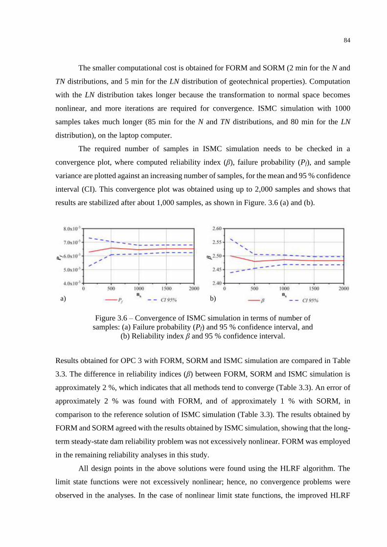
84

The smaller computational cost is obtained for FORM and SORM (2 min for the N and

TN distributions, and 5 min for the LN distribution of geotechnical properties). Computation

with the LN distribution takes longer because the transformation to normal space becomes

nonlinear, and more iterations are required for convergence. ISMC simulation with 1000

samples takes much longer (85 min for the N and TN distributions, and 80 min for the LN

distribution), on the laptop computer.

The required number of samples in ISMC simulation needs to be checked in a

convergence plot, where computed reliability index (β), failure probability (Pf), and sample

variance are plotted against an increasing number of samples, for the mean and 95 % confidence

interval (CI). This convergence plot was obtained using up to 2,000 samples and shows that

results are stabilized after about 1,000 samples, as shown in Figure. 3.6 (a) and (b).

Figure 3.6 – Convergence of ISMC simulation in terms of number of

samples: (a) Failure probability (Pf) and 95 % confidence interval, and

(b) Reliability index β and 95 % confidence interval.

Results obtained for OPC 3 with FORM, SORM and ISMC simulation are compared in Table

3.3. The difference in reliability indices (β) between FORM, SORM and ISMC simulation is

approximately 2 %, which indicates that all methods tend to converge (Table 3.3). An error of

approximately 2 % was found with FORM, and of approximately 1 % with SORM, in

comparison to the reference solution of ISMC simulation (Table 3.3). The results obtained by

FORM and SORM agreed with the results obtained by ISMC simulation, showing that the long-

term steady-state dam reliability problem was not excessively nonlinear. FORM was employed

in the remaining reliability analyses in this study.

All design points in the above solutions were found using the HLRF algorithm. The

limit state functions were not excessively nonlinear; hence, no convergence problems were

observed in the analyses. In the case of nonlinear limit state functions, the improved HLRF

a) b)

85

(iHLRF) algorithm can be employed (see, for instance, the discussion in Ji et al. (Ji et al., 2019,

2017)). Both algorithms (HLRF and iHLRF) were available in the StRAnD software.

Table 3.3 – Results of the reliability analysis for OPC 3 and COVme.

Probability

distributions

ISMC FORM SORM

Pf β Pf β Error

(%) Pf β

Error

(%)

Normal (N) 5.42 x10-3 2.55 6.57 x10-3 2.48 2.67 5.94 x10-3 2.52 1.27

Lognormal (LN) 6.57 x10-4 3.21 7.10 x10-4 3.19 0.70 5.74 x10-4 3.25 1.20

Truncated normal (TN) 6.01 x10-3 2.51 6.57 x10-3 2.48 1.25 6.57 x10-3 2.48 1.25

3.4.2 Sensitivity of variables

An advantage of FORM is the possibility of carrying out a sensitivity analysis through the

direction cosines (α2) at the DP, revealing the contribution of each random variable to the

evaluated failure probabilities.

Sensitivity results are evaluated for different operating cases (OPC), probability

distributions and COV, as shown in Figure 3.7. Figure 3.7 (a) compares the sensitivity values

for the three OPCs using COVme and LN distributions. Figure 3.7 (b) compares the sensitivity

values for OPC 3 and LN distributions for different values of COV. Figure 3.7 (c) compares the

sensitivity values for OPC 3 and COVme for different probability distributions. These results are

computed considering random seepage properties (ks, θs, θr, a and n) and random stability

calculations (γ, c´, ϕ´ and ϕb). Sensitivity coefficients (α2) for seepage properties (ks, θs, θr, a and

n) cannot be seen in Figure 2.8 because they are nearly zero (α2≈0); hence, these random

variables have negligible contributions to the computed failure probabilities and can be

considered deterministic. From the results in Figure 3.7, we also conclude that, for the dam

studied herein, the uncertainty in friction angle ϕ´ has the greatest contribution to the failure

probabilities, for all operational cases, COVs and statistical distributions considered herein. The

second most important random variable is the effective cohesion c´. The unit weight γ has small

importance (α2≠ 0), and the angle that increases the shear strength ϕb increases in importance

from OPC 3 to OPC 1. The unsaturated soil condition has a greater effect when the phreatic

surface is in a low position.

Studies on stochastic pore pressure variability (Bergado and Anderson, 1985) and

stochastic hydraulic conductivity (Gui et al., 2000a), as well as other studies (Srivastava et al.,

2010; Yi et al., 2015), found seepage properties to have great importance in reliability analysis.

86

A comparison of our results with the references above reveals that the COV values in our study

are smaller.

In the remaining reliability analyses, stability properties (γ, c´, ϕ´ and ϕb) are considered

random variables, and seepage properties (ks, θs, θr, a and n) are assumed to be deterministic, at

their mean values.

Figure 3.7 – Sensitivity analysis results for different scenarios: (a)

three OPCs with LN distribution and COVme, (b) OPC 3 with LN

distribution and COVlo, COVme and COVhi, and (c) OPC 3 with N, LN

and TN distributions and COVme.

3.4.3 Influence of the reservoir level on the reliability index

In this section, the reliability analysis considers (i) only the LN distribution and (ii) only median

values of the coefficients of variation (COVme). From the results shown in Figure 3.8 and Table

3.4, we concluded that for the dam studied herein, smaller reliability indices and higher

probabilities of failure were found in higher water levels.

0.17

-0.63 -2.36

11.55 10.59 9.89

88.26 87.4281.73

0.02 1.366.02

17 10 3

0

20

40

60

80

100

Sen

siti

vit

y a

naly

sis

(%)

OPC (m)

γ (kN/m3) c´ (kPa) ϕ´ (°) ϕb (°)

0.04 0.17 0.268.08

11.55 11.68

91.8688.26 88.04

0.02 0.02 0.02

lo me hi0

20

40

60

80

100

COVhiCOVlo COVme

Sen

siti

vit

y a

naly

sis

(%)

COV (%)

γ (kN/m3) c´ (kPa) ϕ´ (°) ϕb (°)

0.01 0.16 0.017.25

11.537.25

92.7388.29

92.73

0.01 0.02 0.01

N LN TN0

20

40

60

80

100

Sen

siti

vit

y a

naly

sis

(%)

Probability Distribution

γ (kN/m3) c´ (kPa) ϕ´ (°) ϕb (°)

a) b)

c)

87

Table 3.4 – Results of the reliability analysis with COVme and the LN

distribution for 3 OPCs.

OPC COVme

Pf β

3 7.10 x10-4 3.19

2 1.44 x10-6 4.68

1 2.91 x10-9 5.82

Figure 3.8 – Reliability index with COVme and the LN distribution for

three OPCs.

3.4.4 Influence of the statistical distribution on the reliability index

In the present section, the reliability analysis considers only the median values of the

coefficients of variation (COVme).

It is well known that geo-mechanical material properties listed in Table 3.1 should be

positive values. Nevertheless, statistical fitting to measured data often yields the normal as a

candidate distribution. Moreover, normal distributions are sometimes assumed, as they simplify

reliability analysis (e.g., linear limit state functions of normal variables allow analytical, closed-

form solutions). Hence, there is relevance in the discussion of using mathematically correct

lognormal (LN), truncated normal (TN) strictly positive distributions, or convenient normal (N)

distributions. As well reported in the literature (Guo et al., 2018; Mouyeaux et al., 2019, 2018),

using normal distributions to represent strictly positive material properties can lead to numerical

computation problems and unrealistic values.

88

Herein, we investigate the influence of the choice of probability distribution on the

computation of reliability indexes for dam stability. Figure 3.9 and Table 3.5 show the results

obtained for the dam stability problem using normal (N), truncated normal (TN) or lognormal

(LN) distributions. First, we observe that lognormal distributions lead to significant increases

in the calculated reliability indexes (up to 60 % for lower reservoir level). Second, we observe

no differences between reliability indexes evaluated using normal or truncated normal

distributions. Note that lognormal distributions are asymmetric with respect to the mean,

whereas the N and TN distributions are symmetric. Third, although GeoStudio does not accept

negative values for geotechnical properties, we did not encounter numerical problems with our

computations using Normal distribution. There are two complementary reasons for this result,

one being that reliability indexes are reasonably large, which causes the design points to be far

from negative values. The second reason is that we employed FORM and importance sampling

Monte Carlo in the computations. The iterative search for the design point in FORM remained

far from negative values during the whole process due to a well-behaved limit state function.

Use of importance sampling also kept sampled points away from the negative region. The use

of simple MCS, and/or smaller reliability indexes would make it more likely for the software

to go into negative values, causing numerical problems in the computations. The use of TN

distributions for strictly positive geotechnical properties is always advisable. In the remainder

of this Chapter, only truncated normal (TN) and lognormal (LN) distributions are employed.

Table 3.5 – Results of the reliability analysis with COVme for three

OPCs.

OPC Probability distribution COVme

Pf β

3

Normal (N)

6.57 x10-3 2.48

2 6.72 x10-4 3.21

1 1.06 x10-4 3.70

3

Lognormal (LN)

7.10 x10-4 3.19

2 1.44 x10-6 4.68

1 2.91 x10-9 5.82

3

Truncated normal (TN)

6.57 x10-3 2.48

2 6.72 x10-4 3.21

1 1.06 x10-4 3.70

89

Figure 3.9 – Reliability index with COVme for three OPCs.

3.4.5 Influence of the coefficient of variation on the reliability index

In the present section, the reliability analysis considers only the lognormal (LN) distribution.

From the results shown in Figure 3.10 and Table 3.6, we conclude that, for the dam

studied herein, the reliability index (β) increases when the coefficient of variation (COV)

decreases. The probability of failure increases when higher values of COV are used in reliability

analysis. The results for different COV values indicate how sensitive the analysis is to assumed

values of soil uncertainty-related parameters (Salgado and Kim, 2014). The dependence of β

on the COVs depends on the problem. For nonlinear problems, reliability indexes will vary in

a nonlinear way with the reciprocal of COV, as shown in our results. Using extreme values

produces 245 % of the change in β between COVhi to COVlo.

Table 3.6 – Results of the reliability analysis with the lognormal (LN)

distribution for three OPCs.

OPC COVlo COVme COVhi

Pf β Pf β Pf β

3 5.14 x10-12 6.80 7.10 x10-4 3.19 2.43 x10-2 1.97

2 22.27 x10-24 9.89 1.44 x10-6 4.68 1.34 x10-3 3.00

1 79.03 x10-36 12.25 2.91 x10-9 5.82 8.39 x10-5 3.76

2 3 4 5 60

2

4

6

8

10

12

14

16

18

20

OPC 3

OPC 2

OPC 1W

ate

r le

vel

(m

)

Reliability Index ()

N TN LN

90

Figure 3.10 – Reliability index with the lognormal (LN) distribution

for three OPCs.

The determination of COV in a reliability analysis of an earth dam is one of the most

important steps. The use of extreme values from the literature due to the lack of laboratory or

field studies has an important influence on the reliability analysis. The experiences of engineers

and the number of laboratory and field tests help in choosing the correct COV for geotechnical

materials and make decisions.

3.4.6 Influence of the correlation on the reliability index

In the present section, the reliability analysis considers (i) only OPC 3; (ii) only median values

of the coefficients of variation COVme; (iii) the correlations between the cohesion and friction

angle (ρc´-ϕ´), cohesion and unit weight (ρc´-γ), unit weight and friction angle (ργ-ϕ´) and the

correlations among all of them.

From the results shown in Table 3.7, we conclude that, for the dam studied herein, the

reliability index (β) increases considerably when the correlation ρc´-ϕ´ is considered, in the case

of LN and TN distributions. The results shown in Table 3.8 and 3.9 show that correlations ρc´-γ

and ργ-ϕ´ have much smaller impacts on the reliability indexes.

1 2 3 4 5 6 7 8 9 10 11 12 130

2

4

6

8

10

12

14

16

18

20

OPC 3

OPC 2

OPC 1W

ate

r le

vel

(m

)


COVlo COVme COVhi

91

Table 3.7 – Results of the reliability analysis with different

correlations of the cohesion and the friction angle (ρc´-ϕ´) for COVme

and OPC 3.

Probability

Distribution

ρc´-ϕ´= 0.0 ρc´-ϕ´= -0.4 ρc´-ϕ´= -0.5 ρc´-ϕ´= -0.6

Pf β Pf β Pf β Pf β

Lognormal (LN) 7.10 x10-4 3.19 8.05 x10-5 3.77 5.29 x10-5 3.88 6.31 x10-5 3.83

Truncated normal (TN) 6.57 x10-4 2.48 2.68 x10-3 2.79 1.98 x10-3 2.88 1.41 x10-3 2.99


correlations of the cohesion and the unit weight (ρc´-γ) for COVme and

OPC 3.

Probability

Distribution

ρc´-γ= 0.0 ρc´-γ= -0.4 ρc´-γ= -0.5 ρc´-γ= -0.6





correlations of the unit weight and the friction angle (ργ-ϕ´) for COVme

and OPC 3.

Probability

Distribution

ργ-ϕ´=0.0 ργ-ϕ´=-0.4 ργ-ϕ´=-0.5 ργ-ϕ´=-0.6




Three different problem configurations are considered in the reliability analysis. The

results are shown in Table 3.10, Figure 3.11 and 3.12. Correlation case ρa considers ρc´-ϕ´´= -

0.4, ρc´-γ= 0.4 and ργ-ϕ´´= 0.4. Correlation case ρb considers ρc´-ϕ´= -0.5, ρc´-γ = 0.4 and ργ-ϕ´= 0.4.

Correlation case ρc considers ρc´-ϕ´= -0.6, ρ c´-γ= 0.4 and ργ-ϕ´= 0.4.

From the results shown in Table 3.10, Figure 3.12 and 3.13, we conclude that, for the

dam studied herein, the reliability index (β) increases considerably in the LN and TN

distributions when different combinations of correlations (ρa, ρb and ρc) are used. The results

obtained herein show that the correlations between geotechnical properties significantly impact

structural reliability, suggesting the importance of further investigating such correlations in the

field.

92

Table 3.10 – Results of the reliability index with COVme and different

correlations and OPCs.

Probability

function OPC

ρ ρa ρb ρc


Lognormal (LN) 3 7.10 x10-4 3.19 9.35 x10-5 3.74 4.05 x10-5 3.94 5.82 x10-5 3.85

Truncated

normal (TN)

3 6.57 x10-3 2.48 2.46 x10-3 2.81 1.67 x10-3 2.94 1.03 x10-3 3.08

2 6.72 x10-4 3.21 1.05 x10-4 3.71 5.98 x10-5 3.85 3.07 x10-5 4.01

1 1.06 x10-4 3.70 7.75 x10-6 4.32 3.86 x10-6 4.47 1.74 x10-6 4.64

Figure 3.11 – Reliability index with COVme for OPC 3 and different

correlations of ρc´-γ, ρc´- ϕ´ and ργ-ϕ´.

Figure 3.12 – Reliability index with COVme and the TN distribution for

different correlations and OPCs.

2 3 4 5 6-0.7

-0.6

-0.5

-0.4

-0.3

-0.2

-0.1

0.0

0.1

ρc

ρb

ρa

ρ

ρc´-γ= 0.4; ργ-ϕ´= 0.4

Co

rrel

ati

on

(ρ

c´-ϕ´)


Truncated Normal (TN) Lognormal (LN)

ρc´-γ= 0.0; ργ-ϕ´= 0.0

93

From the results shown in Table 3.10, Figure 3.11 and 3.12, we conclude that, for the dam

studied herein, the use of all correlations (ρc´-ϕ´, ρc´-γ and ργ-ϕ´) in the same analysis, or

consideration of ρc´-ϕ´ only, leads to similar reliability index results, but the computational cost

increases.

For correlated random variables, the transformation to standard Gaussian space involves

two additional computations: the evaluation of equivalent correlation coefficients and Cholesky

decomposition of the equivalent correlation matrix. This explains the impact in terms of

computational cost of using correlations between variables; hence, it is inefficient to include

correlations with negligible impacts on reliability. Only perfect correlations can reduce costs:

in this case, the dependent random variable can be written as a function of the other, and

problem dimensionality is reduced. However, this is not the case in our examples.

3.4.7 Determination of the critical surface

In this section, the reliability analysis is performed for (i) the LN distribution only, and (ii) the

median values of the coefficients of variation (COVme). A comparison of the corresponding

critical deterministic and probabilistic slip surfaces, for the three OPCs, is presented in Figure

3.13 (a), (b) and (c), respectively.

Reliability analysis using FORM involves a search for the DP. When the random

variables assume the values corresponding to the DP, the slip surface with the highest

probability of occurrence is obtained, which is referred to as the probabilistic slip surface.

Bhattacharya et al. (Bhattacharya et al., 2003) and Hassan and Wolff (Hassan and Wolff,

1999) employed the mean value second-moment theory (MVFOSM) to find the probabilistic

critical slip surface, assuming all random variables to be Gaussian distribution. In contrast, the

direct coupling developed herein allows us to consider non-Gaussian distributions, which

results in more accurate critical slip surfaces, either using FORM or MCS.

When the seepage and stability analyses are performed for the mean values of the

random variables, the slip surface leading to the minimum FS is called the critical slip surface.

As evident in Figure 3.13, these surfaces are not the same. For the homogeneous slope

considered herein, the difference is not too large, but in general, they will be different.

Performing the reliability analysis using the deterministic slip surface leads to incorrect results.

Although Figure 3.13 (a), (b) and (c) gives the impression that the critical slip surfaces are the

same, they are slightly different for each OPC.

94

Figure 3.13 – Comparison of dam slip surfaces obtained from

deterministic and probabilistic approaches, with the LN distribution

and COVme, for three OPCs: (a) OPC 3, (b) OPC 2, and (c) OPC 1.

3.5 CONCLUSIONS

This Chapter addressed accurate and efficient solutions of geotechnical reliability problems by

means of direct coupling of deterministic geotechnical software with a probabilistic solver.

Direct coupling allows solving the reliability problem by means of accurate and efficient

methods such as the first-order reliability method (FORM) and importance sampling Monte

Carlo simulation (ISMC). The coupling feature was illustrated by coupling the deterministic

GeoStudio 2018 software with the StRAnD reliability analysis software. The coupling was also

illustrated in the equilibrium analysis of an earth dam.

a)

b)

c)

95

Equilibrium analysis of the earth dam was done for three different operating cases

(OPCs). Long-term steady-state seepage and stability analyses were performed. Dam reliability

was found to change significantly with the water level above the bedrock. The results obtained

by FORM and SORM agreed with those obtained by ISMC simulation, showing that the earth

dam stability problem is almost linear in random variable space. This observation includes

linearity of the limit state functions and of the transformation of lognormal (LN) variables to

standard normal space.

Sensitivity analysis revealed that the four “stability analysis” variables (c´, ϕ´, γ and ϕb)

dominated failure probabilities, whereas the five “seepage analysis” random variables (Ks, θs,

θr, a and n) had little influence. In all cases studied, the friction angle (ϕ´) and the cohesion (c´)

were found as the most influential parameters in the reliability analysis.

The influence of the reservoir level clearly shows that higher reliability indexes are

found for lower levels of the reservoir, and lower reliability indexes are found for higher levels

of the reservoir. The use of different probabilistic distributions for the geotechnical materials

showed higher values of reliability indexes using the lognormal (LN) distribution, and similar

values for normal (N) and truncated normal (TN) distributions. The truncation of “negative”

material properties, by using TN instead of N distributions showed little influence for the “high

reliability” dam studied herein. This may not be the case for dams with lower reliability.

The coefficients of variation (COVs) of random properties were shown to produce large

impacts on dam reliability. Smaller COVs lead to larger reliability indexes. The assumption of

COVs from the literature may be accepted as an initial approach, but these assumptions have to

be confirmed by field tests.

Correlation between material properties was also considered. Correlation between

cohesion and friction angle (ρc´-ϕ´) was shown to have the largest impact and to increase

reliability indexes. On the other hand, correlations between cohesion and unit weight (ρc´-γ), and

between unit weight and friction angle (ργ-ϕ´) lead to negligible variations in β.

Finally, it was shown that the most probable slip surface, found in the reliability

analysis, is not the same as the critical slip surface found in a mean value analysis for the

minimum factor of safety (FS).

97

4 RELIABILITY ANALYSIS OF AN EARTH DAM

COMPARING RESULTS AND EFFICIENCY OF A

COMMERCIAL AND DIRECT COUPLING SOFTWARE

ABSTRACT

Using commercial software is a normal practice whereby a deterministic approach governs

different geotechnical studies. The implementation of reliability analysis in commercial

software resulted from the increasing acceptance of the probabilistic approach in geotechnical

problems. Commercial software focuses on the deterministic approach, and the probabilistic

approach is just a complement with fewer reliability tools and methods. The main reason is that

most users of commercial software do not use reliability analysis as a first option of a

geotechnical study. We here show a comparison of reliability analyses by the deterministic

software Seepage/W and slope/w coupled with the StRAnD reliability software against a

GeoStudio software (Seepage/W and slope/w are part of GeoStudio software). An earth dam is

used as a study object, under different water level conditions. The limit equilibrium method of

Morgenstern-Price is used to calculate factors of safety (FS) and to find the critical slip surface.

Reliability indexes of critical probabilistic surfaces are evaluated by the first-order reliability

method (FORM), Mean Value First-Order Second Moment (MVFOSM), as well as by “crude”

Monte Carlo Simulation (SMC). They are used to calculate the reliability indexes

corresponding to critical probabilistic surfaces. By means of sensitivity analysis in DC, the

coupled software showed that 4 uncertain geotechnical parameters (effective cohesion c´,

friction angle ϕ´, specific weight γ, and angle that increase the shear strength ϕb) are relevant in

the reliability analysis. The importance of all parameters is a function of the probabilistic

distribution. In turn, the GeoStudio software has restrictions on using all the geotechnical

parameters and uses only 3 stability parameters (c´, ϕ´ and γ). The computational cost of the

GeoStudio software packages is much higher than that of the DC software. There are

considerable differences in the reliability results from the reliability methods used. The effects

of the ϕb and probabilistic distributions were analyzed. Finally, the probabilistic critical slip

surface showed not to be the same as the deterministic critical slip surface.

Keywords: Earth dam, direct coupling, reliability analysis, water level.

98

4.1 INTRODUCTION

Earth dams are commonly used geotechnical infrastructures for water management and electric

power generation. The successful design of a reservoir project over the full range of loading

requires a comprehensive site characterization and a detailed design of each feature. One of the

critical aspects of earth dam design is the stability analysis, that is, the computation of safety

factors (FS) in a deterministic approach (Cheng, 2003; Fredlund and Krahn, 1977; Griffiths and

Lane, 1999; Sarma and Tan, 2006). This is commonly performed in different software to solve

the problem. Probabilistic methodologies (Calamak and Yanmaz, 2014; Guo et al., 2018;

Mouyeaux et al., 2018; Sivakumar Babu and Srivastava, 2010; Yi et al., 2015) have been

recently and more frequently used to take into account the uncertainty of geotechnical materials,

which cannot be handled by the traditional deterministic methods. The application of reliability

analysis offers a useful supplement to conventional stability analysis of earth dams. The result

of the reliability index (β) and the probability of failure (Pf) provides more information and

helps geotechnical engineers to select the best solution about dam safety.

There are different approaches to probabilistic dam stability analysis with differing

assumptions, limitations and levels of mathematical complexity. The most common methods

are approximate methods, i.e. Mean Value First Order Second Moment (MFOSM), First order

reliability method (FORM) and Second order reliability method (SORM), and simulation

methods, such as “crude” Monte Carlo Simulation (MCS) and others with intelligent sampling

(e.g., Adaptive importance, Latin hypercube sampling, Asymptotic simulation, Subset

simulation, …, etc.). The MCS usually has an excessive computational cost in comparison with

approximate methods. There is a growing need for a more rapid assessment of the critical

probabilistic slip surface. The requirement to obtain a structural reliability result and the slip

surface of the dam as soon as possible is a requirement for the current geotechnical practice and

especially for the safety control of dams.

Both the SLIDE software by Rocscience and SLOPE/W software by Geostudio allow

engineers to perform SMC and MFOSM methods for slope stability analyses within their

respective program. The analyses with these types of software have some assumptions and

limitations regarding the way of calculating the reliability index and using statistical

distributions of different geotechnical materials because their focus is deterministic approach.

99

This Chapter proposes the reliability analysis of an earth dam by the so-called direct

coupling (Kroetz et al., 2018; Leonel et al., 2011; Napa-garcía, 2014; Siacara et al., 2020b,

2020a; Sudret and Der Kiureghian, 2000). In direct coupling (DC), the powerful software of

reliability analysis StRAnD v1.07 (Beck, 2008) allows using different reliability methods,

reliability analysis and statistical distributions, and the GeoStudio v2018.00 software

(GeoStudio, 2018a, 2018b) can solve different geotechnical problems with different

geometries, material models and water conditions. The combination of these two powerful tools

of geotechnical analysis and reliability analysis helps to solve different geotechnical problems

in a probabilistic approach.

The numerical model used must have a response that can be read by the reliability

routine. Subsequently, this response is read and used by the reliability routine to plan the next

point to be tested. Finally, the calculation cycle is repeated up to the convergence of the

reliability method.

The DC software uses the responses of numerical or analytical models along with

approximation reliability methods. The nomenclature DC is not evident in the literature

because, in structural analysis, for example, it is the rule, with other techniques being employed

occasionally (Kroetz et al., 2018). In this Chapter, the application of the DC technique and the

use of GeoStudio software to a case study involving an earth dam are shown in a step-by-step

fashion. This topic is part of the researches on dam safety from the GeoInfraUSP (geotechnical

engineering research group dedicated to infrastructure works at the School Engineering of the

University of Sao Paulo), and some of the group´s results are presented.


in Chapter 2 and Section 4.2, which also briefly describes the performance function and

reliability analysis techniques employed herein. The complete direct coupling technique is

described in Section 4.3. Results of the numerical dam equilibrium analysis are presented and

discussed in Section 4.4. Concluding remarks are presented in Section 4.5.

100

4.2 PROBLEM SETTING

Reliability analysis focuses on the most important aspect of performance, namely the

probability of failure (Pf). This Pf clearly depends on both parametric and model uncertainties.

Pf is a more consistent and complete measure of safety because it is invariant to all the

mechanically equivalent definitions of safety and incorporates additional uncertainty

information. There are probabilistic techniques to more efficiently calculate Pf. The chief

drawback is that these techniques are difficult for non-specialists to understand, but they are

not necessarily difficult to implement computationally (Phoon, 2008).

101

4.3 METHODOLOGY


The numerical calculations were implemented by coupling the GeoStudio 2021 (GeoStudio,

2018a, 2018b) and StRAnD 1.07 (Beck, 2008) software. A complete overview of the direct

coupling (DC) procedure is found in Siacara (Siacara et al., 2020b, 2020a). The stability and

structural reliability of an earth dam is performed in DC and GeoStudio software. In a

deterministic approach, the pore water pressure (PWP) was determined by finite element

analysis, and the limit equilibrium analysis was performed to calculate the factors of safety

(FoS). In a probabilistic approach, the reliability index (β) and the corresponding probability of

failure (Pf) are evaluated using the Mean Value First-Order (MVFOSM), First-Order Reliability

Method (FORM) and “Crude” Monte Carlo Simulation (MCS). The DC software performs

FORM analysis and GeoStudio software allows solving reliability analysis using MVFOSM

and the SMC.

4.3.2 The application-problem and boundary conditions

An earth dam was used as an example to present study in different operating cases (OPCs) for

a long-term steady-state analysis. The section is constituted of three different materials: dam

body, transition and filter zone, and is located in unweathered rock. The dam is 30 meters high

and the maximum water level is 27 meters above the reservoir bottom. The dam has a horizontal

and vertical filter to reduce the pore water pressure within the dam, conducting the water

downstream. Five OPCs of water level are studied, measured from the maximum water level to

the minimum water level. Figure 4.1 illustrates the analyzed section.

Figure 4.1. Analyzed cross-section of the dam.

102

The deterministic parameters (nominal parameters) and the uncertainty in soil parameters was

quantified from the literature (Siacara et al., 2020b), as shown in Table 4.1. The seepage

analysis is characterized by the uncertainty of two SWCC fitting parameters (a, n), saturated

and residual volumetric water contents (θs, θr), and the saturated hydraulic conductivity

parameter (ks). The random stability analysis is characterized by uncertain specific weight (γ),

effective cohesion (c´), friction angle (ϕ´) and the angle that increases shear strength (ϕb). The

uncertain parameters of the stability analyses are assumed to have Normal (N) or Lognormal

(LN) distributions. The mean (µ) and the Coefficient of Variation (COV) of all the parameters

are shown in Table 4.1.


Materials Dam body Transition Filter

Parameters µ COV

(%) µ

COV

(%) µ

COV

(%)

Seepage

ks (m/seg) 1x10-6 - 1x10-5 - 1x10-4 -

θs (m3 m-3) 0.50 - 0.48 - 0.43 -

θr (m3 m-3) 0.067 - 0.018 - 0.016 -

a (kPa) 57.67 - 6.84 - 1.62 -

n 1.60 - 1.84 - 1.94 -

Stability

γ (kN/m3) 19.00 7 19.00 7 19.00 7

c´ (kPa) 10.00 30 7.00 30 5.00 30

ϕ´ (°) 28.00 20 29.00 20 30.00 20

ϕb (°) 17.00 20 15.00 20 5.00 20


The seepage analyses were performed in the SEEP/W software, by GeoStudio, which uses the

Finite Element Method (FEM). The water reservoir conditions were taken as those respective

to the operating condition (OPC). The software is equipped with typical SWCC and

permeability curves for different types of soils. The values for constructing these curves are

presented in Table 4.1. Typical curves for gravel were used for the filter and transition zone,

while a typical curve for clays was selected for the dam body.

103

All the analyses were divided in different OPCs, to observe the progress for different

conditions. The pore water pressures (PWP) for each OPC were exported to SLOPE/W, the

software of GeoStudio package dedicated to stability analyses. The Morgenstern-Price method

was selected to calculate the factor of safety (FS) for the downstream face at each OPC. An

automatic search was conducted, by the entry and exit specification, to locate the most critical

circle for each representation of pore water pressure and for each OPC. A two-dimensional

analysis is performed.

The pore water pressure and total water head for a OPC are shown in Figure 4.2 (a). The

pore water pressures are negative in the uppermost part of the flow region, above the phreatic

surface. Dam stability calculations were performed on the downstream slope using the pore

water pressures found in seepage analysis. The critical surface of failure and the minimum

factors of safety (FS) were determined using Slope/W; the results for an OPC are shown in

Figure 4.2 (b).

Figure 4.2. Results of (a) Seepage analysis and (b) Stability analysis.

a)

b)

104

4.4 RELIABILITY ANALYSIS AND RESULTS

The results described herein were obtained using GeoStudio software and DC software to find

the reliability index (β) and the probability of failure (Pf), as described in Chapter 2 and Sections

4.2 and 4.3. The following reliability analyses are presented next:

(1) Comparison with all Normal distributions (N);

(2) Influence of the angle that increases shear strength;

(3) Sensitivity of random variables;

(4) Comparison of critical slip surfaces found in deterministic and probabilistic analyses.

4.4.1 Comparison with all Normal distributions (N)

In the present section, the reliability analysis considers only the normal (N) distribution.

For the dam studied herein, the SMC and MVFOSM methods were performed in

GeoStudio software for 10,000 and 100,000 simulations in different OPCs. The MVFOSM is

found from a relation for a normally distributed factor of safety (Christian et al., 1994;

GeoStudio, 2018b).

From the results in Table 4.2, the same probability of failure (Pf) in SMC and MVFOSM

is found, but different reliability indexes (β) are observed. When the shape of the probability

distribution is known, β can be related directly to Pf. The β of the MVFOSM is found by the

relationship of β to Pf for a normally distributed factor of safety (GeoStudio, 2018b).

The required number of samples in SMC simulation needs to be checked in a

convergence plot, where computed failure probability (Pf), and sample variance are plotted

against an increasing number of samples, for the mean and confidence interval (CI). This

convergence plot was obtained using up to 100,000 samples and shows that results are not

stabilized (Figure 4.3). This means that a greater number of simulations are needed. It is

demonstrated with the 85 % of CI; in converged simulation, it can be in 95 % of CI. It is possible

to use a highest CI, but the sampling error or variance is large. The reduction of the variance is

only possible performing a greater number of simulations.

105

The number of simulations in this case is very important; the computational cost and the

method employed are important factors that determine whether the analysis is feasible or not.

In this study, a common desktop computer was used, with processor speed of 3.5 GHz and

RAM memory of 32 GB. In GeoStudio software, SMC and MVFOSM with 10,000 samples

take 27 hours and 210 hours for 100,000 samples, on the laptop computer. In DC software, the

smaller computational cost is obtained for FORM with 2 min using N distribution of

geotechnical properties. The difference in terms of computational cost is considerable. SMC

and MVFOSM with 10,000 samples were employed in the remaining reliability analyses in this

study.

An error of approximately 2 % was found with FORM in comparison to the reference

solution of the Importance sampling Monte Carlo (ISMC) simulation. The results from FORM

agreed with the results from the ISMC simulation, showing that the long-term steady-state dam

reliability problem was not excessively nonlinear (Siacara et al., 2020b). In this study, the

FORM method gives a Pf= 7.22 x10-3 and β= 2.44 for the same maximum water level, and this

result is considered an exact solution.

Results from the maximum water level with FORM, SMC and MVFOSM are compared.

The difference in reliability indices (β) is approximately from 6 % to 14 %, which indicates that

all methods need more simulations to converge.

Table 4.2. Results of the reliability analysis using normal (N)

distributions for the maximum water level.

Water level

(m)

MVFOSM

nsi= 10,000

MVFOSM

nsi= 100,000

SMC

nsi= 10,000

SMC

nsi= 100,000


27 3.42 x10-3 2.58 2.69 x10-3 2.63 3.42 x10-3 2.70 2.69 x10-3 2.78

Figure 4.3. Convergence of SMC simulation in terms of number of

samples: Probability of failure (Pf) and 85 % confidence interval (CI).

106

From the results in Figure 4.4 using 10,000 simulations, we conclude that, for the dam

studied herein, the reliability index (β) results have a considerable variation between the SMC,

MVFOSM and FORM in different operating conditions. In the same figure, the SMC is

observed to have a variation from the maximum water level to the minimum water level, which

is due to the lack of convergence of the MCS.

In terms of dam safety, the determination of the highest reliability index can report a

misconception of the expected performance level of the dam. Computational results prove

whether the modeled structure meets the safety requirements.

Figure 4.4. Reliability index with Normal (N) distribution for different

OPCs.

Incipient instability was observed by Beck and Ávila (Beck and Ávila da S., 2016)

around β= 8, which increases significantly for β= 9. For β> 9.5, the inverse error function, hence

Φ-1(.) cannot be computed at all. Therefore, a safe operational limit for evaluating functions Φ

and Φ-1 was implemented in the StRAnD software: this limit corresponds to β= 8, for which

Φ(-8)≈ 6 x10-16. Beyond these values, the numerical computations collapse. These limits are

imposed on all random variables, including Gaussian variables. In this study, all the reliability

indexes for different OPCs are less than 8 (β< 8).

107

4.4.2 Influence of the angle that increases shear strength (ϕb)

For the present section, the reliability analysis with the DC software considers: (i) normal (N)

distribution; (ii) lognormal (LN) distribution with and without angle that increases shear

strength (ϕb).

One argument against using a N distribution for the geotechnical materials is about

taking negative values, which are impossible. In contrast, the LN distribution does not admit

negative values. For this reason, in common geotechnical practice, engineers use LN

distributions directly for all the material properties, and this decision gives highest reliability

indexes (β) values.

From the results in Figure 4.5, we conclude that, for the dam studied herein, the use of

uncertainty parameter ϕb affects reliability indexes (β) more in LN distribution than in N

distribution. The effects of ϕb produce more reduction of β in lower reservoir water levels.

Figure 4.5. Reliability index with Normal (N) and Lognormal (LN)

distribution with or without using angle ϕb.


An advantage of the FORM is the possibility of carrying out a sensitivity analysis through the

direction cosines at the design point (α2) found through the HLRF algorithm. Thus, there is an

indication of which variables most affect the structural reliability analysis. Sensitivity analysis

using properties involved in stability calculation (γ, c´, ϕ´ and ϕb) was performed. Figure 4.6 (a)

and (b) compares sensitivity values in different OPCs, using normal (N) distributions, and

lognormal (LN) distributions in all geotechnical parameters, respectively.

108

From the results in Figure 4.6 (a), using all N distributions, we conclude that, for the

dam studied herein, the uncertainty in friction angle ϕ´ of the dam body has the greatest

contribution to failure probabilities for all the operational cases (OPCs). The second most

important random variable is the effective cohesion c´ and changes with the angle that increases

shear strength ϕb in low water levels. In Figure 4.6 (b), using all LN distributions, the uncertainty

in ϕ´ of the dam body and filter has the greatest contribution to failure probabilities for all the

OPCs.

The other properties that not appear in Figure 4.6 have no incidence (α2= 0). The ϕb

increases the incidence from maximum to minimum water level. The unsaturated soils

condition has greater effect when the phreatic surface is in low position. The increase of the

incidence of ϕb is more important in the LN than in the N distribution.

Figure 4.6. Sensitivity analysis of the earth dam different OPCs with

(a) Normal (N) distribution (b) Lognormal (LN) distribution.

109

4.4.4 Comparison of critical surfaces

For the present section, the analysis was performed with some settings of the beginning

configuration in the DC software, specifying: (i) the N distribution, and (ii) the LN distribution.

A comparison of the corresponding critical deterministic and probabilistic slip surfaces, for the

maximum water level, is presented in Figure 4.7 (a) and (b), respectively

Several iterations are needed to converge and to calculate the probability of failure and

the reliability index through the HLRF algorithm. The critical slip surface for the final

realization of the convergence history is referred to as the critical probabilistic slip surface and

is shown in Figure 4.7. The critical slip surface based on the minimum factor of safety (FS) is

not the same critical surface to the reliability index (β).

Another limitation of the GeoStudio against the DC software regards determining the

probabilistic critical surface, the GeoStudio software just determined the deterministic critical

surface in a different number of realizations. The DC software finds the probabilistic critical

surface from the last realization of the HLRF algorithm.

Figure 4.7. Comparison of the failure surface of an earth dam in a

deterministic and probabilistic approach with (a) Normal (N); (b)

Lognormal (LN) distribution.

a)

b)

110

4.5 CONCLUSIONS

In this study, an earth dam was analyzed in different operating conditions (OPC) taking into

account uncertainties. The earth dam underwent an equilibrium analysis for different OPCs.

Long-term steady-state seepage and stability analyses were performed. Direct coupling (DC)

software and GeoStudio software were compared. A considerable number of simulations is

necessary to have 95 % of CI in a MCS method with low variability. The computational cost

for a SMC and MVFOSM method is high, and it is a condition that sometimes defines whether

it is possible to perform the analysis. Direct coupling (DC) allows solving the reliability

problem by means of an accurate and efficient method such as FORM. The computational cost

in SMC and MVFOSM method for 100,000 simulations is 270 hours and 2 minutes for a FORM

method. The efficiency of the FORM method was demonstrated. Results from the maximum

water level with FORM, SMC and MVFOSM are compared. The difference in reliability

indices (β) is approximately from 6 % to 14 %, which indicates that all methods need more

realizations to converge. The use of ϕb affects β more in the LN distribution than in the N

distribution. Sensitivity analysis revealed that, for all the N distributions, the uncertainty in

friction angle ϕ´ of the dam body has the greatest contribution to failure probabilities for all the

operational cases (OPCs). The second most important random variable is the effective cohesion

c´ and changes with the angle that increases shear strength ϕb in low water levels. For all LN

distributions, the uncertainty in ϕ´ of the dam body and filter has the greatest contribution to

failure probabilities for all the OPCs. Finally, it was shown that the probabilistic critical slip

surface was not the same as the deterministic critical slip surface.

112

5 RELIABILITY ANALYSIS OF RAPID DRAWDOWN OF

AN EARTH DAM USING DIRECT COUPLING

ABSTRACT

This Chapter combines seepage analysis with limit equilibrium analysis to investigate the safety

of an earth dam over time and during drawdown. The numerical investigation is accomplished

by directly coupling the deterministic software packages Seepage/W and Slope/W with the

StRAnD reliability software. The first-order reliability method is employed in reliability

analysis. Sensitivity analyses reveal that saturated hydraulic conductivity (ks), friction angle

(ϕ´) and cohesion (c´) are the random parameters with the greatest contribution to failure

probabilities. The cumulative effect of random saturated hydraulic conductivity (mainly) makes

critical times and critical slip surfaces significantly different in the probabilistic and

deterministic analyses.

Keywords: Earth dam reliability; reliability analysis; rapid drawdown; transient analysis,

equilibrium analysis.

113

5.1 INTRODUCTION

The stability of earth dams for long-term conditions depends on its geometry, material

properties, and the forces to which the dam is subjected. The forces due to water are internal

(pore-water pressures and seepage forces) and external (hydrostatic and hydrodynamic effects

(Berilgen, 2007; Lane and Griffiths, 2000)). During water discharge of an earth dam, the

reduction of water level has two principal effects: modification of the internal Pore Water

Pressure (PWP), and reduction of the external stabilizing hydrostatic pressure due to unloading.

Therefore, safe operation of earth dams requires studies of seepage and stability for the

upstream slope of the dam.

The level of water in a reservoir is affected by hydrological events and by user demand,

in case of water supply dams. The partial or total emptying of the reservoir is part of a dam

operation procedures. Partial or total emptying is required during maintenance and in case

extreme events occur, such as earthquakes (stress changes due to earthquakes (Rotili et al.,

2017)), landslide into the reservoir or extreme rainfall. Dam equilibrium during the emptying

procedure depends directly on the discharge velocity, with rapid discharges known to be

critical. This leads to the problem known as Rapid DrawDown (RDD), with the discharge

velocity (VRDD) being a critical parameter. The discharge velocity depends on characteristics of

the hydraulic installations, such as the capacity of spillways.

The usual approach to RDD analysis is a transient seepage and limit equilibrium

analyses using mean soil properties, to find deterministic factors of safety (FoS) (Berilgen,

2007; Song et al., 2015; Viratjandr and Michalowski, 2006). However, the equilibrium depends

on loading conditions and soil parameters, which can be modelled as random variables. In the

last four decades, significant progress has been made into quantifying the variability of soil

properties (Phoon, 2008; Phoon and Ching, 2015; Phoon and Kulhawy, 1999a), and in

performing reliability analysis of slopes and embankments in long term steady-state conditions

(Alonso, 1976; Bhattacharya et al., 2003; Christian et al., 1994; Duncan, 2000; Harr, 2013;

Lacasse et al., 2019; Li and Lumb, 1987; Mouyeaux et al., 2018; Poddar et al., 2016; Song et

al., 2015). However, to the best of our knowledge and based on a comprehensive literature

review, no studies were found addressing reliability of earth dams in transient conditions of

rapid drawdown.

114

Different approaches are possible for probabilistic slope and dam stability analyses.

Point estimate methods (PEM) are very efficient and popular in geotechnical engineering (Harr,

1987; Hong, 1998; Rosenblueth, 1975; Zhao and Ono, 2000) but were shown to be inaccurate

for many problems by Napa-García et al. (Napa-García et al., 2017). Accuracy can be increased

by using higher-order moment methods (Harr, 1989; Panchalingam and Harr, 1994), but

efficiency is lost. Approximation methods such as the first-order reliability method (FORM)

are competitive with PEM in terms of computational cost, but this one is more accurate and

suitable for evaluating small (failure) probabilities at distribution tails. The FORM loses

accuracy to Monte Carlo Simulation (MCS) only if the limit state functions are excessively

nonlinear, in which case PEM also fails.

The equilibrium analysis of earth dams is based on locating the critical slip surface, i.e.,

the surface with the smallest safety factor. In general, only a limited number of slip surfaces is

checked (El-Ramly et al., 2002; Hassan and Wolff, 1999; Tang et al., 1976; Wang et al., 2011).

The critical slip surface, in a probabilistic analysis, is generally believed to correspond to the

minimum safety factor surface in the deterministic approach (Cheng et al., 2015). Likewise,

one could assume that the critical time, in a probabilistic transient analysis, would be the same

critical time of a deterministic analysis. These ideas are challenged herein the present Chapter.

This Chapter addresses the reliability analysis of an example earth dam during the rapid

drawdown. The numerical study is conducted by the so-called Direct Coupling (DC)

(Berveiller, M., Sudret, B. and Lemaire, 2004; Berveiller et al., 2006; Kroetz et al., 2018;

Leonel et al., 2011; Napa-garcía, 2014; Sudret and Der Kiureghian, 2002, 2000) between a

deterministic software for slope stability (GeoStudio 2018 (GeoStudio, 2018a, 2018b)), and a

structural reliability software (StRAnD (Beck, 2008)). The Direct Coupling method is not usual

in geotechnical literature because, due to historical trends, point estimate and response surface

surrogate methods became more popular (Kroetz et al., 2018). However, direct coupling is the

rule when it comes to (super-) structure reliability analysis using numerical models. Direct

coupling allows the full features of deterministic numerical software to be explored in

probabilistic or reliability analyses. In direct coupling, the probabilistic solver treats the

numerical software as a black-box: it defines specific values (outcomes) of the random variables

for which the numerical solution needs to be computed.

115

In this Chapter, the First-Order Reliability Method (FORM) is employed for reliability

analysis, although many other algorithms are available in the StRAnD software (Beck, 2008).

FORM is known to be very efficient, as it computes failure probabilities with a limited number

of calls to the deterministic solver (GeoStudio). The FORM method is based on an interactive

search for the so-called design point, at which the limit state function is linearized. FORM

yields good results when the problem is not excessively non-linear, as is the case for the

transient dam equilibrium problem addressed herein. Searching for the design point requires

gradients of the limit state function, with respect to random variables. These are evaluated by

finite differences in the current implementation (Siacara et al., 2020b).


in Section 5.2, which also briefly describes the performance function and reliability analysis

techniques employed herein. The complete direct coupling technique for transient analysis is

described in Section 5.3. Results of the transient numerical dam equilibrium analysis are

presented and discussed in Section 5.4. Concluding remarks are presented in Section 5.5.

116

5.2 PROBLEM SETTING

5.2.1 Review of current drawdown standards

There are different criteria for addressing the risk of Rapid DrawDown (RDD) in earth dams.

In different codes, the discharge is referenced as: (i) a proportion of dam height; (ii) a proportion

of dam volume; and (iii) a function of height per day (Environment Agency, 2017a, 2017b).

The RDD criteria as a function of dam height proportion (i) recommend drawdown

analyses varying between 10 % and 90 % of the height, within 7 days and 4 months (Babbit

and Mraz, 1999; USACE, 2016a). The velocity of RDD as proportion of dam height is divided

into hazard and risk classes; nine classes in the United States (USBR, 1990) and three classes

in India (Bureau of Indian Standards, 2004).

The criteria of RDD as a function of dam volume proportion (ii) recommend drawdown

to 50 % capacity between 3 and 10 days (Babbit and Mraz, 1999; A. Brown, 2009; Tam and

Humphrey, 2012); of drawdown to 25 % capacity in 28 days (Prentice, 2005). In France, bottom

outlets should be capable of reducing the load on the dam by 50 % in 8 days, while 2.6 % of

height of the reservoir/day is recommended (Combelles et al., 1985).

The RDD criterion as function of height per day (iii) considers velocities between 0.1

m/day (Alonso and Pinyol, 2009) to 3.0 m/day (Song et al., 2015), with intermediate velocities

suggested in (Alonso and Pinyol, 2009; Berilgen, 2007; Environment Agency, 2017b, 2017a;

FAO, 2009; Gao et al., 2018; Gosden et al., 2014; Pinyol et al., 2008; Song et al., 2015). A

formula with 0.3 m/day as initial drawdown, which increases as a function of the dam height

and reservoir area is recommended in (Hinks, 2009).

Other criteria (Brown and Gosden, 2004; D. H. Brown, 2009; DEFRA, 2006; Hinks,

2009; Peters et al., 2016; Philpott et al., 2008) are based on combinations of the last three

principal criteria, and other velocities of RDD (VRDD) are established by the dam designer, in

the consideration of dam stability.

During design, the dam designer uses the dam slope stability and electric power

generation capacity (or demand, in case of water supply dams) of the reservoir to define VRDD.

We here consider the usual values for VRDD: 0.5, 1.0, 1.5 and 2.0 m/day.

117

5.2.2 Transient analysis using FORM

In rapid drawdown problems, the equilibrium condition changes over time, due to the drop in

water level and due to the change in pore pressures. In the deterministic case, it is understood

that the minimal safety factor over time is the critical safety factor. Similarly, the minimal

reliability index evaluated over time is considered to describe the safety of the dam. However,

it is not known in advance when the minimal FoS and β are reached. Hence, the FORM analysis

has to be performed over time, with a discretized time step (tk, k=0,1,…,f).

As will be shown in the sequence, the relative importance of the problems random

variables (factors 2

i ) changes during the transient analysis. The FORM solution depends on

a design point (DP), which, in turn, depends on the cumulative effect of any uncertain variable

up to an analysis time (tk). Hence, the FORM solutions (Equation 2.7 and 2.11) for each time tk

need to be computed since time zero (t0). This makes the FORM solution quite sensitive to the

discretization scheme, as will be shown. In contrast, in the Monte Carlo Simulation (MCS)

solution of transient problems, such as rapid drawdown, each seepage sample produces a

complete time history of pore pressures, which is computed up to final time tf. However, the

numerical equilibrium analysis needs to be repeated for each time tk and for each sample. Hence,

the FORM solution is still competitive, in comparison to MCS, in spite of the need of running

all FORM solutions from time zero (t0).

The failure probabilities evaluated herein (Equation 2.6 and 2.7) are conditional on the

occurrence of a RDD event: Pf =P[F|RDD]. Although not done herein, the unconditional

probabilities of failure can be obtained by considering the probability P[RDD] of occurrence of

the RDD event (Vandenberge, 2014):

RDDPRDDFPPuncond

f = |.

(5.1)

118

5.3 METHODOLOGY


Deterministic and probabilistic calculations were implemented by the coupling GeoStudio 2018

(GeoStudio, 2018a, 2018b) and StRAnD 1.07 (Beck, 2008) software. Details of the coupling

approach are presented and discussed in Siacara et al. (Siacara et al., 2020b). The algorithms

implemented in Siacara et al. (Siacara et al., 2020b) were modified herein to evaluate earth

dams in different long-term steady-state and transient conditions. The factors of safety (FoS)

are evaluated using different limit equilibrium methods (e.g. Morgenstern and Price). The

reliability index (β) and corresponding probabilities of failure (Pf) are evaluated for different

times during the drawdown, using the FORM method. This section presents an overview of the

implemented procedure. The procedure is illustrated by the flowchart shown in Figure 5.1:

(1) Collect the available problem data: topography, previous studies, bibliography,

laboratory and field test, etc.

(2) Define the initial conditions of the deterministic model: choose and set up a 2D model in

the GeoStudio 2018 software and then perform the seepage analysis in Seep/W. The

first step in Seep/W is defining the initial condition (e.g., steady-state analysis with the

specific water level of the reservoir) to find the equilibrium and the initial pore water

pressure of the model (Figure 5.2).

(3) Define the transient conditions of the deterministic model: the second step in Seep/W is

defining the transient conditions (e.g., rapid drawdown or rainfall) to find the phreatic

surface and pore water pressure of the model at every time of the analysis. The time of

the analysis (t) or the duration of the analysis and number of steps (n) is defined, as well

as time increment (Δt). The time of rapid drawdown (tRDD) is a function of the RDD

velocity (VRDD) and is independent of the time of analysis (Figure 5.2).

(4) Define the stability conditions of the deterministic model: choose and set up a 2D model

in the GeoStudio 2018 software, then perform the limit equilibrium analysis in Slope/W.

The last step in Slope/W is to perform the stability analysis. The factor of safety (FoS)

is determined for every step of the seepage analysis or at a specific time of the RDD

analysis. The critical factor of safety (FoScr) is the smallest found during the analysis; it

occurs at the critical time (tcr-d) (Figure 5.2).

(5) Define the probabilistic model: choose reliability methods in the StRAnD 1.07 software.

(6) Define probabilistic data for material properties.

(7) Master program: iterations and analyses are performed using the Visual Studio 2017

software compiler, which executes all the routine tasks and the flowchart of the

procedure.

119

(8) GeoStudio 2018 file: The file “.gsz” from GeoStudio is a ZIP file that contains different

files of the analysis. The definition file includes the input data and other configurations

in the form of an extension file “.xml” that has the same name as the “.gsz” file and is

the file used to change the input parameters. In the same folder, there is a file with the

output data and the file extension “.csv”, which is used as the input parameters for the

reliability analysis. The input parameters are varied at every iteration using the

GeoStudio file “.gsz” , which is decompressed and compressed, saving the FoS to find

the DP.

(9) The results of the reliability analysis (number of evaluations, number of simulations,

reliability index, probability of failure, DP, etc.) are shown in the

STRAND_OUTPUT.txt file, whereas the critical surface is shown in the GeoStudio

software. The critical probabilistic time (tcr-p) is found, corresponding to the critical

reliability index (βcr) (Figure 5.2).

120


transient reliability analysis procedure by coupling the GeoStudio and

StRAnD softwares packages.

121

Figure 5.2 – Schematic procedure of the transient seepage and limit

equilibrium reliability analysis.


A simple homogeneous earth dam is used as a case study of rapid drawdown, with four different

drawdown velocities (VRDD) for the transient analysis. The main cross-section of the structure

is shown in Figure 5.3. The upstream and downstream side slopes are 1V:3H for a 20 m of earth

dam of height and horizontal filter (Figure 5.3). Further details are given in Siacara et al.

(Siacara et al., 2020b).

The maximum water level (W.L.MAX.) is 3 m below the crest and the minimum water

level (W.L.MIN.) is the level of unweathered rock (the bedrock is considered waterproof and

impenetrable). The upstream boundary condition is directly affected by the VRDD, whereas the

downstream boundary condition is zero head case.

The partial or total emptying of the reservoir can be part of the dam operation

procedures, to make maintenance feasible. The VRDD is dependent on the characteristics of the

hydraulic installations, such as the capacity of spillways. Four drawdown velocities are

considered: VA=2.0, VB=1.5, VC=1.0 and VD= 0.5 m/day.

122

The RDD occurs a long time after construction; hence, steady-state is considered at the

start of the analysis. The soils of the dam will have had time to reach equilibrium under a new

effective stress regime. The saturated-unsaturated seepage and the stability of the slopes in the

dam, considering the variability in the soil parameters, are studied herein.

Figure 5.3 – Critical cross-section of the dam.

The seepage analysis considers the SWCC and the hydraulic conductivity function

predicted by the Van Genuchten equation (Van Genuchten, 1980). The Morgenstern and Price

method (Morgenstern and Price, 1967, 1965) with shear strength criteria of unsaturated soils

(Fredlund et al., 1978) is used as LEM. The LEM analysis is performed in the SLOPE/W

software (GeoStudio, 2018b), which considered boundary water forces with total weights. This

is equivalent to considering seepage forces with submerged weights.

The compacted lean clay properties (CL in the Unified Soil Classification System) are

considered; the nominal seepage parameters are based on Cuceoglu (Cuceoglu, 2016); the

nominal stability parameters were taken from Fredlund et al. (Fredlund et al., 2012) and USBR

(USBR, 1987). The coefficient of variability (COV) of the seepage and stability parameters are

based on Siacara et al. (Siacara et al., 2020b). The random seepage analysis is characterized by

the uncertainty of two SWCC fitting parameters (a, n), the saturated and residual volumetric

water contents (θs, θr), and the saturated hydraulic conductivity parameter (ks). The random

stability analysis is characterized by uncertain specific weight (γ), effective cohesion (c´),

effective friction angle (ϕ´) and the angle that increases shear strength (ϕb). The mean (µ) and

coefficient of variation (COV) of all the stability and seepage parameters are shown in Table

5.1. The uncertain parameters are assumed to have normal (N) or lognormal (LN) distributions,

following Table 5.1. No correlation is considered between random stability and seepage

parameters; hence, the correlation matrix is the identity matrix.

123

Some geo-mechanical material properties listed in Table 5.1, like θr and c´, have normal

distribution and large COV. To avoid unacceptable negative values in solutions by Monte Carlo

Simulation, these variables should be assumed lognormal or truncated normal (as done in

Siacara et al. (Siacara et al., 2020b)). In the FORM solution adopted herein, however, using

normal distributions did not result in any numerical problems.


Analysis Parameters µ COV (%) Probabilistic

distribution

Seepage

Ks (m/s) 5.63 x10-5 80 LN

θs (m3 m-3) 0.54 15 N

θr (m3 m-3) 0.17 30 N

a (kPa) 8.06 50 LN

n 1.76 20 LN

Stability

γ (kN/m3) 19 7 N

c´ (kPa) 10 30 N

ϕ´ (°) 28 20 LN

ϕb (°) 17 20 LN


The rapid drawdown analyses are first performed using mean values of random seepage and

stability parameters (Table 5.1). These analyses result in usual factors of safety (FoS) and

critical time. First, a long-term steady-state seepage analysis is performed, resulting in initial

pore water pressures (PWP). The initial finite element seepage analyses also yield position of

the phreatic surface. Pore water pressure and total water head corresponding to initial condition

(t0= 0 days) are shown in Figure 5.4. The phreatic surface was assumed to be the line of zero

pore water pressure determined from the seepage analysis, as shown in Figure 5.4. The PWP

values are negative in the uppermost part of the flow region, above the phreatic surface.

Negative PWP have a minor contribution to dam stability, but their effects are considered in

this study.

The RDD occurs when the water level outside the earth dam drops so quickly that

impermeable soils within the slope do not have sufficient time to drain; therefore, the stabilizing

effect of the water outside the dam is removed, and the shear stresses for equilibrium increase.

The finite element seepage analysis is performed at every time step, to calculate the

corresponding pore water pressures and to find the position of the phreatic surface. PWP and

total water head for t2= 2 days and VRDD= 2 m/day are shown in Figure 5.5.

124

Figure 5.4 – Results of the seepage analysis for the initial condition

(t0= 0 days) with pore water pressure (kPa) and total water head (m).

Figure 5.5 – Results of the seepage analysis for t2= 2 days and VRDD =

2 m/day, with pore water pressure (kPa) and total water head (m).

Dam stability calculations are performed in the upstream slope, using PWPs found at

every time step of the seepage analysis. Morgenstern and Price’s procedure is used for all LEM

calculations. An automatic search is conducted, by the entry and exit specification technique,

to locate the most critical circle for each representation of PWPs, for each time step. The entry

and exit specification technique consist of a variation of the grid-radius method. The entry and

exit slip surface discretization was performed at every 0.1 m, with circles defined by specifying

the radius tangent lines. The computational algorithm ensured that the entry and exit angle of

each slip surface did not exceed 90 degrees and that no straight line (infinite radius) was used

as a possible slip surface. The critical slip surface and the minimum factors of safety (FoS) are

determined using Slope/W; results for VRDD= 2 m/day for times t5= 5, t10= 10 and t20= 20 days

are shown in Figure 5.6 (a), (b) and (c), respectively. The figure also shows the finite element

mesh used to determine pore pressures in the seepage analysis.

125

Figure 5.6 – Critical slip surfaces for VRDD= 2 m/day (a) t5= 5 days,

(b) t10= 10 days and (c) t20= 20 days.

The limit equilibrium analyses yielded different FoS and different critical surfaces at

every time step, as shown in Figure 5.7. The analyses were performed by applying a phreatic

surface adjustment with the interpolated pore pressures resulting from the seepage analysis. In

SLOPE/W, all the slip surfaces must be contained in the domain. If a trial slip surface intersects

the lower boundary of the model, the slip surface would follow the boundary. Once a slip

surface is generated, the strength parameters used in stability calculations are taken from the

materials overlying the base of individual slices. The stability analysis for the initial conditions

(t0= 0 days) yielded the initial safety factor as FoS0= 2.44.

a)

b)

c)

126

Figure 5.7 – Results of the limit equilibrium analysis for different

times of analysis (t) and VRDD = 2 m/day.

The mean value analysis was repeated considering different discharge velocities (VRDD),

as reported in Table 5.2. The same initial conditions were considered for all the analyses. The

results in Table 5.2 show smaller factors of safety for higher velocity values of drawdown, as

expected. Table 5.2 also shows the reduction in safety factors, from the initial to the critical

condition, for different VRDD. The drop in FoS is 30 % for VA= 2 m/day and 23 % for VD= 0.5

m/day. The critical time also changes significantly with VRDD, as shown in Table 5.2.

The Bureau of Reclamation (USBR, 2011a, 1987), U.S. Army Corps of Engineers Slope

Stability Manual (USACE, 2003), Brazilian Power Plants – ELETROBRÁS (ELETROBRÁS,

2003) and others (Cruz, 2004; Wyllie and Mah, 2014) recommend a minimum factor of safety

of FoS= 1.5 for long-term steady-state conditions, and FoS= 1.1 to 1.3 for rapid drawdown

analysis of earth dams. All the factors of safety evaluated herein in the mean value

(deterministic) analysis satisfy this minimum stability criterion.

Table 5.2 – Results of RDD in deterministic analysis.

Description Velocity

VA VB VC VD

VRDD (m/day) 2.0 1.5 1.0 0.5

Mean value analysis

FoS0 2.44 2.44 2.44 2.44

FoScr 1.72 1.75 1.82 1.89

Reduction in FoS 30 % 28 % 25 % 23 %

Critical time comparison

tRDD (day) 9.0 12.0 17.0 34.0

tcr-d (day) 6.0 7.0 12.0 21.0

127


Reliability analyses were performed for the same scenarios described in the mean value

(deterministic) analysis, including four values of VRDD (VA= 2.0, VB= 1.5, VC= 1.0 and VD= 0.5

m/day). Reliability indexes (β) and probabilities of failure (Pf) where evaluated by the Direct

Coupling GeoStudio and StRAnD software packages, as described in Sections 2 and 3. The

limit state gradients were estimated by finite differences. The search for the DP was performed

with the HLRF algorithm. The final analysis time (tf) was 40 days.

The reliability analysis considered 5 random seepage properties (Ks, θs, θr, a and n) and

4 random stability calculation properties (γ, c´, ϕ´ and ϕb), as shown in Table 5.1. The following

reliability analysis results are presented:

(1) Rapid drawdown for VRDD = 2.0 m/day;

(2) Analysis for different discharge velocities;

(3) Sensitivity of failure probabilities w.r.t. random variables of seepage and equilibrium;

(4) Difference of critical PWP and phreatic surface in deterministic and probabilistic

analyses;

(5) Difference of critical surfaces in deterministic and probabilistic analyses.

The limit state gradients were estimated using finite differences. The search of the DP

was performed with the Hasofer-Lind-Rackwitz-Fiessler (HLRF) algorithm for the FORM

method.

5.4.1 Rapid drawdown for VRDD = 2.0 m/day

For VRDD = 2.0 m/day, it takes nine days for the reservoir water level to decrease from 17 to 0

m. The transient analysis is made for a total of tf = t40 = 40 days. Figure 5.8 shows the variation

in the factor of safety (FoS), reliability index (β) and probability of failure (Pf) at every step of

the transient analysis (t0= 0, t1= 1, t2= 2,…., t40= 40 days) for VRDD =2 m/day. The initial

condition (t0= 0 days) from the long-term steady-state analysis corresponds to an initial factor

of safety FoS0= 2.44, reliability index β0= 4.30 and probability of failure Pf0= 8.54 x10-6. The

same initial condition is considered later in the drawdown analysis for different VRDD values. A

sub-index corresponding to the time of analysis (days) is added to the calculated FoS, β, and Pf

values.

128

As expected, the reliability index and safety factors follow similar trends during the

drawdown analysis. Both reach a minimum at what is called the critical time. Surprisingly,

however, critical times for the mean value and probabilistic analyses are not the same. In the

mean value analysis, a minimum “deterministic” factor of safety FoScr= 1.72 is found at the

“deterministic” critical time tcr-d= 6 days. The minimum reliability index, in the probabilistic

analysis, is found as βcr=2.45 at critical time tcr-p= 7 days. The reduction in FoS and β, from the

initial condition, is not the same either: the FoS reduces by 30 % from FoS0 to FoScr, whereas

the reliability index β reduces by 43 % between time zero and the critical time (Tables 5.2 and

5.3).

Table 5.3 – Results of RDD in probabilistic analysis.

Description Velocity

VA VB VC VD

VRDD (m/day) 2.0 1.5 1.0 0.5

Probabilistic analysis

β0 4.3 4.3 4.3 4.3

βcr 2.45 2.57 2.8 3.15

Reduction in β 43 % 40 % 35 % 27 %

Critical time comparison

tRDD (day) 9.0 12.0 17.0 34.0

tcr-p (day) 7.0 8.0 14.0 24.0

Difference in tcr (days) 1.0 1.0 2.0 3.0

Different authors (Bhattacharya et al., 2003; Cheng et al., 2015; Hassan and Wolff,

1999; Reale et al., 2016; Sarma and Tan, 2006; Siacara et al., 2020b) had already found that the

failure surface leading to the minimum FoS is not the same as that leading to the maximum

failure probability. We believe this is the first time it has been shown that critical times are also

different in deterministic and probabilistic analyses.

The resolution of the transient analysis was increased by reducing the discretization

from Δt =1 day to Δt=0.25 days (6 hours). The results are shown in Figure 5.8 (b) and (c), which

correspond to zones 1-1´ and 2-2´ in Figure 5.8 (a). With higher resolution, the critical time in

deterministic analysis changes from 6 days to 5.75 days (5 days and 18 hours), and the critical

probabilistic time changes from 7 days to 6.75 days (6 days and 18 hours), with the difference

between critical times for FoScr and βcr remaining the same 24 hours.

129

Figure 5.8 – Safety factors, reliability index and failure probabilities

for VRDD = 2.0 m/day (a) t=40 days, (b) initial transition zone 2-2´ and

(c) critical zone 1-1´.

As FORM is an interactive solution, it is interesting to see the convergence sequence in

the search for the design point. Figure 5.9 shows the convergence history in terms of reliability

index β, and in terms of the safety factor corresponding to an intermediate configuration of the

random variable vector, for four different times of analysis (t5=5, t10=10, t15=15 and t20=20

days). Figure 5.9 shows that five or six iterations were necessary for convergence.

For this study, a common desktop computer was used, with processor speed of 3.5 GHz

and RAM memory of 32 GB. A complete transient analysis for one discharge velocity took

about 160 hours to compute (with a total analysis time of forty days and discretization of one

day). Each day of transient analysis took about 4 hours to compute.

All design points in the above solutions were found using the HLRF algorithm, starting

at the mean values. No convergence problems were observed, as the limit state functions

considered herein are not excessively nonlinear. For more nonlinear limit state functions, the

improved Hasofer-Lind-Rackwitz-Fiessler (iHLRF) algorithm can be employed (see, for

a)

b) c)

130

instance, the discussion in Ji et al. (Ji et al., 2019, 2017)). Both algorithms (HLRF and iHLRF)

are available in the StRAnD software.

Figure 5.9 – Convergence histories for VRDD= 2.0 m/day at times (a)

t5= 5 (b) t10= 10 (c) t15= 15 (d) t20= 20 days.

5.4.2 Analysis for different discharge velocities

The analysis of rapid drawdown was repeated for discharge velocities of VB = 1.5, VC = 1.0 and

VD = 0.5 m/day. In the following figures and in Table 5.2 and 5.3, the original discharge velocity

if referred to as VA = 2.0 m/day. Table 5.2 and 5.3 summarizes the results in terms of critical

safety factors, critical reliability indexes and corresponding failure probabilities. Table 5.2 and

5.3 also reports the critical times for each analysis and discharge velocity, as well as the

difference in days of the critical times for the deterministic and the probabilistic analysis.

Table 5.2 and 5.3 allows observing that the drawdown problem becomes less severe

with smaller discharge velocities. The reduction in safety factors, from the initial value of FoS0=

2.44, is of 23 % for VD= 0.5 m/day, comparing to 30 % for VA= 2.0 m/day. This decrease,

however, cannot be linearly related to the reduction in reliability indexes. For VA, the drop in β

is 43 %, whereas for VD the reliability index reduces 27 %. As the drawdown problem becomes

slower, there is a delay in critical times (which become longer). Yet there is also a greater

131

difference between critical times of the deterministic and probabilistic analysis. For VD= 0.5

m/day, this difference is of three days.

The effect of different discharge velocities can be better appreciated in Figure 5.10,

where safety factors, reliability indexes and their corresponding failure probabilities are

compared in terms of VRDD. As can be observed, with smaller discharge velocities, the changes

in FoS and β over time become slower, which also explains why the difference in critical times

(between the deterministic and probabilistic analysis) increases.

Figure 5.10 – (a) Factors of safety, (b) reliability indexes and (c)

failure probabilities in time for different discharge velocities: VA= 2.0,

VB= 1.5, VC= 1.0 and VD= 0.5 m/day.

The stability of the earth dam gradually increases over time, with the dissipation of

excess PWP. The values of FoS, β and Pf tend to become stationary towards the end of the

analysis. This is more evident for faster discharge velocities (VA and VB).

a)

b)

c)

132

Finally, it is observed how the choice of discharge velocity impacts the dam safety

during the discharge operation. In a deterministic analysis, changing VRDD from VA to VD

improves the critical safety factor by 10 %. The probabilistic analysis shows an improvement

in reliability index of 28 % for the same situation.


Figure 5.11 shows the direction cosines at the design point (α2) over time for the four values of

VRDD considered. Direction cosines show the relative contribution of each random variable to

calculated failure probabilities, with large α2 values revealing the most important variables. At

initial steady-state conditions, effective friction angle (ϕ´) and effective cohesion (c´) are the

most relevant variables for equilibrium. As expected, seepage variables have zero importance

at initial conditions. On the first days of water discharge, the effective friction angle rapidly

assumes an increasing role, with smaller relevance for effective cohesion. The uncertainty in

seepage variables starts to manifest very slowly, with the importance of saturated hydraulic

conductivity (ks) eventually rising sharply. Towards the end of analysis, effective friction angle

is the most relevant variable, followed by effective cohesion and hydraulic conductivity.

Results are quite similar for different drawdown velocities in terms of the relative importance

of the random variables. These results are valid for the dam studied herein, and reflect the

uncertainties listed in Table 5.1; hence, they should not be generalized.

a)

b)

133

Figure 5.11 – Sensitivity coefficients of different random variables

over time for (a) VA= 2.0 m/day, (b) VB= 1.5 m/day, (c) VC= 1.0 m/day

and (d) VD= 0.5 m/day.

5.4.4 Comparison of pore water pressures

From this subsection onwards, differences between deterministic and probabilistic analysis are

further investigated, only for the base case with VRDD= VA= 2 m/day. Pore Water Pressures

(PWP) are illustrated over the dam and over time, as well as phreatic and failure surfaces. In

the following figures, results of the “deterministic” analysis are obtained using mean values of

the random variables in Table 5.1. The results of the probabilistic analysis are illustrated using

the design point values of the same random variables. These are the problem configurations

most likely to lead to failure by instability. Hence, the figures illustrate the differences between

PWP and critical surfaces considered in each solution.

Figure 5.12 compares PWPs over the dam, in deterministic and probabilistic analyses,

for times t3=3 and t33=33 days. As could be expected, the most likely pore water pressures

leading to equilibrium failure of the dam are significantly higher than mean pore pressures. As

shown by the sensitivity analysis, the saturated hydraulic conductivity parameter (ks) has the

greatest contribution to calculated failure probabilities. Hence, the main differences between

Figures 5.12 (a) and (b) are given by replacing the mean value of ks (5.63 x 10-5 m/s) by the DP

value of ks (3.1 x 10-5 m/s for t3=3 and 3.1 x 10-5 m/s for t33=33 days).

c)

d)

134

Figure 5.13 compares PWPs over dam height for the two cross-sections identified in

Figure 5.12 (A-A´ and B-B´), also for times t3=3 and t33=33 days. Figure 5.14 shows how these

PWP vary in time at points T and U, identified in Figure 5.12. Differences in PWP between

deterministic and probabilistic analyses are observed to increase over time. Again, this can be

attributed to the large impact of the uncertainty on the saturated hydraulic conductivity

parameter (ks).

Figure 5.12 – Comparison of pore water pressures (PWP) in

deterministic and probabilistic approaches, for VA= 2.0 m/day (a) t3=3

days and (b) t33=33 days.

a)

b)

135

Figure 5.13 – Comparison of pore water pressures (PWP) in

deterministic and probabilistic approaches, for VA= 2.0 m/day, vs dam

elevation (a) cross-section A-A´ and (b) cross-section B-B´.

Figure 5.14 – Change of pore water pressures (PWP) in time,

deterministic and probabilistic approaches, for VA= 2.0 m/day.

a)

b)

136


The location of the critical slip surface does not change much over time in the deterministic

(mean value) analysis, as seen in Figure 5.6. However, due to the cumulative effect of

uncertainty in seepage parameters, PWPs and phreatic surfaces are observed to change

significantly over time (Figure 5.12 and 5.13). As a consequence, the location of the critical

slip surface changes significantly over time in the probabilistic analysis. Hence, for transient

drawdown analysis, the difference between deterministic and probabilistic slip surfaces is even

larger than differences found for stationary problems (Cheng et al., 2015). Figure 5.15

illustrates the deterministic and probabilistic slip (and phreatic) surfaces, for transient analyses

at times t3=3 and t33=33 days, for VA=2.0 m/day. Differences in surface locations are observably

small at the beginning of the analysis, and become much wider as the transient analysis

progresses. This adds to the importance of performing reliability analysis for the safety

assessment of dams. Differences could be larger for zoned dams or for dams composed of

different materials.

Figure 5.15 – Comparison of slip surfaces, deterministic and

probabilistic approaches for VA= 2.0 m/day (a) t3=3 days and (b)

t33=33 days.

a)

b)

137

5.5 CONCLUDING REMARKS

This Chapter addressed the transient reliability analysis of earth dams during rapid drawdown

operations. Seepage and equilibrium analyses were performed numerically using the

deterministic GeoStudio 2018 software. Reliability analyses were performed by the first-order

reliability method in StRAnD software. A direct coupling technique was employed, in which

the probabilistic software calls the deterministic software as a black box. An example earth dam

was studied, and four different discharge velocities were considered.

The major conclusions are:

• Dam discharge is well known to produce (temporary) reduction in safety factors (FoS).

The reduction in reliability index (β) is not proportional to the reduction in safety factors.

For a discharge velocity of 2 m/day, the reduction in FoS was 30 %, but the reduction

in β was 43 %, for the dam studied herein.

• It is well known that greater discharge velocities are more critical to equilibrium of earth

dams. The effect of drawdown velocities on critical reliability indexes is not linearly

proportional to the effect on safety factors. In our study, reducing the discharge velocity

by a factor of four resulted in a 10 % increase in critical safety factor, and in a 28 %

increase in critical reliability index.

• Our analysis considered five random seepage parameters and four random equilibrium

parameters. Using statistical data from the literature, our analysis reveals that saturated

hydraulic conductivity (ks) has greater impact on random pore pressures over time, and

ks followed by friction angle (ϕ´) and cohesion (c´) have greater impact on the reliability

analysis for equilibrium.

• Due to the cumulative effect of random saturated hydraulic conductivity (mainly) over

time, the time variations in pore water pressures, phreatic surfaces and critical slip

surfaces become much larger in probabilistic analysis than in deterministic (mean value)

analysis.

• Critical failure times and critical slip surfaces are different in deterministic and in

probabilistic analyses. Also, due to the cumulative effect of random ks over time, these

differences increase over time in transient analysis.

138

Limitations of the direct coupling analysis presented herein are basically those of LEM and

FORM methods. If the problems limit state functions become excessively non-linear,

convergence problems and multiple design points can be encountered. In these cases, it may be

necessary to use advanced Monte Carlo simulation techniques, or brute Monte Carlo coupled

with response surface techniques.

In summary, the conclusions above point to the importance of employing structural

reliability techniques in the safety evaluation of geotechnical infrastructure.

140

6 RELIABILITY ANALYSIS OF AN EARTH DAM UNDER

RAINFALL EFFECTS

ABSTRACT

Climate change with extreme hydrological conditions, such as extreme rainfall, poses new

challenges to numerical methods of earth dam safety. Reliability analysis helps to reduce the

uncertainty of the real behavior of a dam, and provides one more tool to improve dam safety

control. Reliability analysis is very important for unsaturated soil dam under rainfall conditions.

This Chapter combines seepage analysis with limit equilibrium analysis to investigate the safety

of an earth dam over time, considering different initial conditions, rainfall intensities, and

normal operating conditions (NOC). The numerical investigation is accomplished by directly

coupling the deterministic software packages Seepage/W and Slope/W with the StRAnD

reliability software. The first-order reliability method is employed in reliability analysis.

Sensitivity analysis reveals that hydraulic conductivity (ks), friction angle (ϕ´), and cohesion

(c´) are the random parameters with the greatest contribution to failure probabilities. The ks

contribution increases when the rainfall intensity increases and the NOC increases or decreases

the reservoir. Finally, it is shown that a critical deterministic slip surface is very close to the

probabilistic one, but a high difference in terms of pore water pressures is reported.

Keywords: Earth dam reliability; reliability analysis; rainfall; transient analysis, equilibrium

analysis.

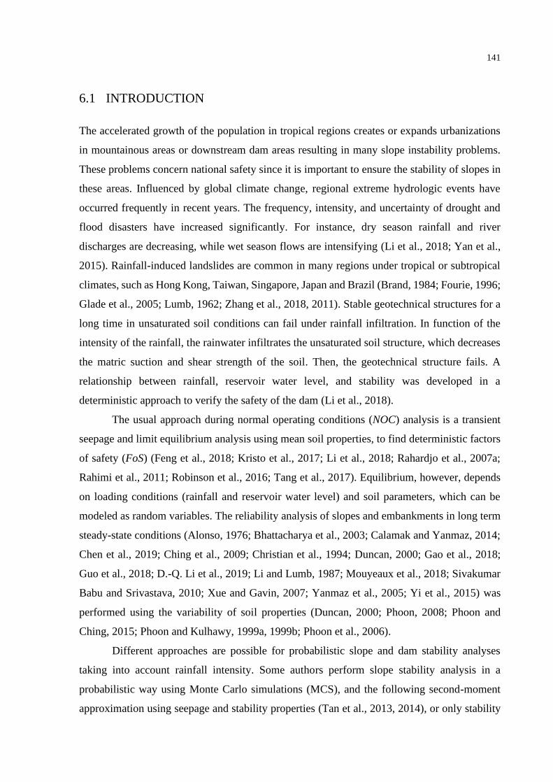
141

6.1 INTRODUCTION

The accelerated growth of the population in tropical regions creates or expands urbanizations

in mountainous areas or downstream dam areas resulting in many slope instability problems.

These problems concern national safety since it is important to ensure the stability of slopes in

these areas. Influenced by global climate change, regional extreme hydrologic events have

occurred frequently in recent years. The frequency, intensity, and uncertainty of drought and

flood disasters have increased significantly. For instance, dry season rainfall and river

discharges are decreasing, while wet season flows are intensifying (Li et al., 2018; Yan et al.,

2015). Rainfall-induced landslides are common in many regions under tropical or subtropical

climates, such as Hong Kong, Taiwan, Singapore, Japan and Brazil (Brand, 1984; Fourie, 1996;

Glade et al., 2005; Lumb, 1962; Zhang et al., 2018, 2011). Stable geotechnical structures for a

long time in unsaturated soil conditions can fail under rainfall infiltration. In function of the

intensity of the rainfall, the rainwater infiltrates the unsaturated soil structure, which decreases

the matric suction and shear strength of the soil. Then, the geotechnical structure fails. A

relationship between rainfall, reservoir water level, and stability was developed in a

deterministic approach to verify the safety of the dam (Li et al., 2018).

The usual approach during normal operating conditions (NOC) analysis is a transient

seepage and limit equilibrium analysis using mean soil properties, to find deterministic factors

of safety (FoS) (Feng et al., 2018; Kristo et al., 2017; Li et al., 2018; Rahardjo et al., 2007a;

Rahimi et al., 2011; Robinson et al., 2016; Tang et al., 2017). Equilibrium, however, depends

on loading conditions (rainfall and reservoir water level) and soil parameters, which can be

modeled as random variables. The reliability analysis of slopes and embankments in long term

steady-state conditions (Alonso, 1976; Bhattacharya et al., 2003; Calamak and Yanmaz, 2014;

Chen et al., 2019; Ching et al., 2009; Christian et al., 1994; Duncan, 2000; Gao et al., 2018;

Guo et al., 2018; D.-Q. Li et al., 2019; Li and Lumb, 1987; Mouyeaux et al., 2018; Sivakumar

Babu and Srivastava, 2010; Xue and Gavin, 2007; Yanmaz et al., 2005; Yi et al., 2015) was

performed using the variability of soil properties (Duncan, 2000; Phoon, 2008; Phoon and

Ching, 2015; Phoon and Kulhawy, 1999a, 1999b; Phoon et al., 2006).

Different approaches are possible for probabilistic slope and dam stability analyses

taking into account rainfall intensity. Some authors perform slope stability analysis in a

probabilistic way using Monte Carlo simulations (MCS), and the following second-moment

approximation using seepage and stability properties (Tan et al., 2013, 2014), or only stability

142

properties (Chung, 2001; Flores Peñalba et al., 2009; Mahmood et al., 2016, 2013) as

randomness. Point estimate methods (PEM) were used in a slope taking into account only

stability properties as randomness (Y. Li et al., 2019). Napa-García et al. (Napa-García et al.,

2017) showed that the PEM is inaccurate for many problems. Accuracy can be increased by

using higher-order moment methods, but efficiency is lost. However, to the best of our

knowledge and based on a comprehensive literature review, no studies were found addressing

reliability of earth dams in transient conditions using approximation methods such as the first-

order reliability method (FORM) and second-order reliability method (SORM). The MCS was

used in a slope taking into account only saturated hydraulic conductivity (ks) as randomness

(Dou et al., 2014). Regression coefficients were used with the MCS method using the Latin

hypercube sampling (LHS) technique to study the influence of the parameters (Chung, 2001).

In this Chapter, the Direct Coupling (DC) technique is employed to combine the

deterministic software GeoStudio 2019 (GeoStudio, 2018a, 2018b) with the structural

reliability program StRAnD, version 2.01 (Beck, 2008). The so-called DC method (Kroetz et

al., 2018; Leonel et al., 2011; Mouyeaux et al., 2018; Napa-garcía, 2014; Siacara et al., 2020b,

2020a; Sudret and Der Kiureghian, 2000) appears to be an efficient method for finding the

critical probabilistic slip surface and evaluating structural reliability in slope and dam stability

problems. StRAnD follows the FORM algorithms, as required by the user, and computes the

failure probabilities. Gradients of the limit state function, required in FORM, are evaluated by

finite differences. The improved HLRF (iHLRF) algorithm (Zhang and Der Kiureghian, 1997)

is employed in the dam equilibrium problem addressed herein. The nomenclature DC is not

evident in the literature because, in structural analysis, for instance, this approach is the rule,

with other techniques being employed eventually (Kroetz et al., 2018). The DC software allows

the full features of deterministic numerical software to be explored in probabilistic or reliability

analyses.

Based on an extreme ten-day rainfall on an earth dam, this Chapter investigates the

effects of initial pore water pressures, rainfall intensity, and effects of the reservoir on

deterministic safety and reliability analysis. This Chapter aims mainly to demonstrate the

feasibility of using reliability analysis in unsaturated soil dams under extreme rainfall, and to

study the incidence of seepage properties and properties involved in stability calculation under

different boundary conditions.

143

6.2 PROBLEM SETTING


During a rainfall event, the equilibrium of a geotechnical structure changes over time, due to

the change in pore water pressures (PWP). Numerically in the deterministic case, it is

understood that the FoS change by the changes of the boundary conditions (e.g. climatic

conditions, fluctuation of the reservoir, …, etc.) over time. Similarly, β is found over time to

describe the safety of the geotechnical structure. A critical safety factor (FoScr) and reliability

index (βcr) are found in the range time of the analysis (t). However, it is not known in advance

when the FoScr and βcr are reached; consequently, the time to failure (tcr) is also uncertain.

Hence, the FORM analysis has to be performed along t and the discretized time step (tk,

k=0,1,…,n) is defined, as well as the time increment (Δt), as is shown in Figure 6.1.

Accumulated rainfall in the t interval is implicitly defined. The Δt gives the possibility to

perform a reliability analysis at any desired time interval (e.g., day, hour, second, …, etc.).

Figure 6.1 – Illustration of a transient rainfall process.

In evaluating the FoS of the dam under rain events, the initial conditions of each tk may

not be exactly the same. For instance, the initial PWP at time t0 is different at t1. The FORM

solution depends on a design point (DP), which, in turn, depends on the cumulative effect of

any uncertain variable up to an analysis time (tk). Hence, the FORM solutions for each time tk

need to be computed since time zero (t0) (Siacara et al., 2020a).

144

In the MCS solution of transient problems, each deterministic analysis is solved by

randomly generated samples of the input variables. The complete time history of PWP and the

number of times at which failure occurs in each time step is registered to find the exact

reliability result. This method is robust, simple, and easy to implement, and it is often used to

validate other analysis techniques. However, MCS requires a tremendous computational effort

to solve the numerical equilibrium analysis repeatedly for each time tk and for each sample.

Besides, the simulation of small probabilities of failure requires an additional computational

cost. Hence, the FORM solution is still competitive, in comparison to MCS, despite the need

of running all FORM solutions from time zero (t0).

6.2.2 Review of initial pore water pressure (PWP) conditions

Transient seepage analyses of dams can be used to predict changes in suction, pore water

pressure (PWP), degree of saturation, and hydraulic conductivity with time. The PWP and

suction values within the dam at the beginning of the analysis comprise the initial conditions.

The initial conditions are the key input information for a transient seepage analysis.

Stark et al. (Stark et al., 2017, 2014) suggests an initial steady-state analysis with the

calibration of the dam structure using field instrumentation (the use of rainfall boundary

conditions was not reported). The USACE (USACE, 2016b) suggests an initial steady-state

analysis as an initial condition for transient analysis. Others authors (Sleep, 2011; Sleep and

Duncan, 2013; Tang et al., 2017; Zhang et al., 2018) suggest three types of initial conditions:

(i) by specifying the position of a phreatic surface, (ii) by performing an initial steady-state

seepage analysis to establish a phreatic surface, or (iii) by specifying a spatial distribution of

initial suction values. Rahimi et al. (Rahimi et al., 2011) and GeoStudio (GeoStudio, 2018a)

suggest that the initial condition obtained from the steady seepage analysis with a small, but

nonzero, rainfall as the boundary condition is more reasonable compared with the initial

condition by applying a zero rainfall as the boundary condition. Luo (Luo, 2008) and Tsaparas

et al. (Tsaparas et al., 2002) assumed that the maximum negative pore water pressure on the

surface of the slope is -75, -50, and -25 kPa. Zhan et al. (Zhan et al., 2012) obtained the initial

condition using the average annual rainfall as the boundary condition in the steady seepage

analysis to obtain the initial condition of the transient seepage analysis. Rahardjo et al.

(Rahardjo et al., 2007b) and Gasmo et al. (Gasmo et al., 2000) obtained the initial condition

from field observation and Chen et al. (Chen et al., 2009) assumed pore-water pressure

distribution based on the wetting front concept.

145

To explore the influence of different methods for determining the initial condition of

PWP distribution on dam stability, three methods, using long term steady-state without rainfall

(WR), small rainfall (SR), and average daily rainfall (MR) as the boundary condition, are

compared herein.

146

6.3 METHODOLOGY

6.3.1 Probabilistic modeling

The direct coupling (DC) of GeoStudio 2019 (GeoStudio, 2018a, 2018b) and StRAnD 1.07

(Beck, 2008) software was implemented to perform deterministic and probabilistic analysis.

The reliability analysis of an earth dam in long-term steady-state and transient conditions using

the DC approach are presented and discussed in Siacara et al. (Siacara et al., 2020b, 2020a).

For this research, the earth dam under rainfall effects is evaluated in different conditions. The

probabilistic framework couples a FORM algorithm with a two-dimensional model that

performs the seepage and dam earth stability via LEM (e.g. Morgenstern and Price). This

section presents an overview of the procedure implemented. The complete procedure is

illustrated by the flowchart shown by Siacara et al. (Siacara et al., 2020b, 2020a), and the

FORTRAN code was modified for this study, as shown in Figure 6.2:

(1) Input data: geometry, historical records, bibliography, laboratory, and field test, etc.

(2) Initial conditions of the deterministic model: choose and set up a long-term steady-state

in a two-dimensional (2D) model in the GeoStudio 2019 software. In the Seep/W

software, define the specific initial boundary conditions (e.g., the water level of the

reservoir, rainfall intensity, spatial distribution of PWP, specific PWP, …, etc.) for time

zero (t= 0). Then, the long-term steady-state analysis is performed using the Seep/W

software to find the equilibrium and the initial PWP of the model (Figure 6.3).

(3) Transient conditions of the deterministic model: choose and set up a transient analysis in

the Seep/W software using the PWP results as initial conditions. In the Seep/W

software, the time of the analysis (t) or the duration of the analysis and number of steps

(n) is defined, as well as time increment (Δt). The time of normal operating conditions

(tNOC) and time of rainfall (tr) is independent of the time of analysis (t). The Δt of the

analysis, reservoir, and rainfall intensity can be different and independent between them,

but these must be defined in the timeframe of t. The boundary conditions in t are defined.

Then, the transient analysis is performed using the Seep/W software to find the phreatic

surface and PWP of the model at every time of the analysis (Figure 6.3).

(4) Stability conditions of the deterministic model: choose and set up a stability analysis in

the Slope/W software using the PWP results at every time of the analysis or only at a

specific time of analysis. The factor of safety (FoS) is determined for every step of the

seepage analysis or at a specific time of the analysis. The critical factor of safety (FoScr)

is the smallest found during the analysis; it occurs at a critical time (tcr-d) (Figure 6.3).

(5) Define the probabilistic model: Choose and set up reliability methods in StRAnD 2.00

software. The reliability methods, correlations, probabilistic and deterministic materials

properties are defined in the STRAND_INPUT.txt file of the StRAnD software.

(6) Define the deterministic (nominal) material properties involved in the analysis.

147

(7) Define the probabilistic data for the material properties involved in the analysis.



procedure.

(9) GeoStudio 2019 file: The file “.gsz” from GeoStudio is a ZIP file that contains different

files of the Seep/W and Slope/W analysis. All the input parameters are defined in the

extension file “.xml” that has the same name as the “.gsz” file. In the same folder, there

is a file with the output data and the file extension “.csv”, which is used as the input

parameters for the reliability analysis. First, the file “.gsz” is uncompressed to update

the input properties. Second, the file is compressed to run the GeoStudio. Then, the FoS

is saved to find the DP.

(10) The results of the reliability analysis (number of evaluations and simulations, sensitivity

coefficients at DP, reliability index, probability of failure, evaluation time, DP, etc.) are

shown in the STRAND_OUTPUT.txt file, whereas the critical surface is shown in the

GeoStudio software. The critical probabilistic time (tcr-p) is found, corresponding to the

critical reliability index (βcr) (Figure 6.3).


transient reliability analysis procedure by coupling GeoStudio and

StRAnD softwares packages (based in Siacara et al. (Siacara et al.,

2020b, 2020a)).

148

Figure 6.3 – Schematic procedure of the steady-state and transient

analysis to performed Limit equilibrium method and reliability

analysis.


A simple homogeneous earth dam considering rainfall effects is used as a case study, with

different initial conditions for the long-term steady-state and variation of rainfall intensities

under NOC for the transient analysis. The main cross-section of the structure is shown in Figure

6.4. The upstream and downstream side slopes are 1V:3H for a 20 m of earth dam of height and

horizontal filter (Figure 6.4). Further details are given in Siacara et al. (Siacara et al., 2020b).

The maximum water level (W.L.MAX.) is 3 m below the crest and the minimum water

level (W.L.MIN.) is the level of the unweathered rock (the bedrock is considered waterproof

and impenetrable). The upstream boundary condition is directly affected by the normal

operating conditions (NOC), whereas the downstream boundary condition is affected by a

rainfall intensity and a filter which uses a zero head case.

149

Figure 6.4 – Critical cross-section of the dam.

The partial or total emptying of the reservoir can be part of the dam operation

procedures, to make maintenance feasible. The NOC is dependent on the characteristics of the

hydraulic installations and the hydrological cycle. The numerical model considers different

cases of study: (i) three cases of initial conditions (WR, SR, and MR); (ii) three different rainfall

intensities (IA, IB, and IC); (iii) three cases of normal operating conditions (NOCA, NOCB, and

NOCC) are considered. In all of the cases, a small rainfall (SR= 2.5 mm/day) was used in the

last 20 days of the analysis, and this was used as an initial condition. The different rainfall

intensities are in function of extreme rainfall (IA), then the rainfall intensities are defined as IA,

IB=IA*1.5, and IC=IA*2.0. The variation of the reservoir and extreme rainfall in function of time

is shown in Figure 6.5.

The annual rainfall in the São Paulo area (Santana station) from 1998 to 2018 (INMET

- National Institute of Meteorology, 2019) was used. The average daily rainfall (MR) is

calculated as a ratio of the average annual rainfall over 365 days, and it is 4.5 mm in this area.

Extreme rainfall (IA) was found from 02/03/2016 to 11/03/2016 (10 days).

Figure 6.5 – Boundary conditions of the model.

150

The NOC occurs a long time after construction; hence, a steady-state is considered at

the start of the analysis. The soils of the dam will have had time to reach equilibrium under a

new effective stress regime. The saturated-unsaturated seepage and the stability of the slopes

in the dam, considering the variability in the soil parameters, are studied herein.

The seepage analysis considers the SWCC and the hydraulic conductivity function

predicted by the Van Genuchten equation (Van Genuchten, 1980). The Morgenstern and Price

method (Morgenstern and Price, 1967, 1965) with shear strength criteria of unsaturated soils

(Fredlund et al., 1978) is used as LEM.

The compacted lean clay properties (CL in the Unified Soil Classification System) are

considered; the nominal seepage parameters are based on Cuceoglu (Cuceoglu, 2016); the

nominal stability parameters were taken from Fredlund (Fredlund et al., 2012) and USBR

(USBR, 1987). The coefficient of variability (COV) of the seepage and stability parameters are

based on Siacara et al. (Siacara et al., 2020b, 2020a). The random seepage analysis is

characterized by the uncertainty of two SWCC fitting parameters (a, n), the saturated and

residual volumetric water contents (θs, θr), and the saturated hydraulic conductivity parameter

(ks). The random stability analysis is characterized by uncertain specific weight (γ), effective

cohesion (c´), effective friction angle (ϕ´), and the angle that increases shear strength (ϕb). The

mean (µ) and coefficient of variation (COV) of all the stability and seepage parameters are

shown in Table 6.1. The uncertain parameters are assumed to have normal (N) or lognormal

(LN) distributions, following Table 6.1.


Analysis Parameters µ COV (%) Probabilistic

distribution

Seepage

ks (m/s) 5.63 x 10-5 80 LN

θs (m3 m-3) 0.54 15 N

θr (m3 m-3) 0.17 30 N

a (kPa) 8.06 50 LN

n 1.76 20 LN

Stability

γ (kN/m3) 19 7 N

c´ (kPa) 10 30 N

ϕ´ (°) 28 20 LN

ϕb (°) 17 20 LN

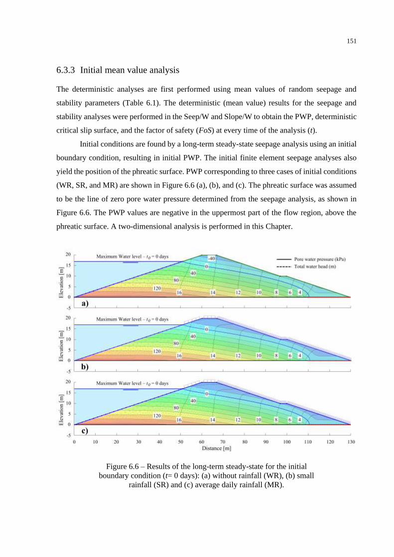
151


The deterministic analyses are first performed using mean values of random seepage and

stability parameters (Table 6.1). The deterministic (mean value) results for the seepage and

stability analyses were performed in the Seep/W and Slope/W to obtain the PWP, deterministic

critical slip surface, and the factor of safety (FoS) at every time of the analysis (t).

Initial conditions are found by a long-term steady-state seepage analysis using an initial

boundary condition, resulting in initial PWP. The initial finite element seepage analyses also

yield the position of the phreatic surface. PWP corresponding to three cases of initial conditions

(WR, SR, and MR) are shown in Figure 6.6 (a), (b), and (c). The phreatic surface was assumed

to be the line of zero pore water pressure determined from the seepage analysis, as shown in

Figure 6.6. The PWP values are negative in the uppermost part of the flow region, above the

phreatic surface. A two-dimensional analysis is performed in this Chapter.

Figure 6.6 – Results of the long-term steady-state for the initial

boundary condition (t= 0 days): (a) without rainfall (WR), (b) small

rainfall (SR) and (c) average daily rainfall (MR).

152

The PWP in every time of analysis (t) is found by a transient seepage analysis using

boundary conditions that are in function of t. The seepage properties of the earth dam are for

impermeable soils; therefore, the rainfall intensity and the NOC affect the dam stability by the

insufficient time to drain the phreatic surface and for reducing the negative PWP. The finite

element seepage analysis is performed at every time step, to calculate the corresponding PWPs,

and to find the position of the phreatic surface. PWP and total water head for t= 7 days using

different rainfall intensities (IA, IB, and IC) are shown in Figure 6.6 (a), (b), and (c).

Figure 6.6 – Results of the transient seepage analysis for t7= 7 days

with: (a) IA, (b) IB, and (c) IC.

Dam stability calculations are performed on the downstream slope, using PWPs found

at every time step of the transient seepage analysis. Morgenstern and Price’s procedure is used

for all LEM calculations. There are several methods for defining the critical slip surface in

Slope/W, and the entry and exit method was selected. One of the problems with the other

methods is that y hinders the visualization of the extents or range of trial slip surfaces. This

difficulty is solved by the entry and exit method because it specifies the region where the trial

slip surfaces should enter the ground surface and where they should exit. Therefore, an

153

automatic search is conducted, by the entry and exit specification technique, to locate the most

critical circle for each representation of PWPs, for each time step. The entry and exit

specification technique consists in defining two lines along the ground surface. These are the

areas where the slip surfaces will enter and exit by the variation of the grid-radius method. The

entry and exit slip surface discretization was performed at every 0.1 m along these two lines,

with circles defined by specifying the radius tangent lines. The computational algorithm

ensured that the entry and exit angle of each slip surface did not exceed 90 degrees and that no

straight line (infinite radius) was used as a possible slip surface. The Entry and Exit slip surface

method is much easier for controlling the position of the trial slip surfaces. The critical slip

surface and the minimum factors of safety (FoS) are determined using Slope/W; results for t=

25 days using different normal operating conditions. (NOCA, NOCB, and NOCC) are shown in

Figure 6.7 (a), (b) and (c), respectively. The figure also shows the finite element mesh used to

determine pore pressures in the seepage analysis.

Figure 6.7 – Critical slip surfaces for t25= 25 days during normal

operating conditions: (a) NOCA, (b) NOCB and (c) NOCC.

154

In the Slope/W software, inherent in limit equilibrium stability analyses is the

requirement to analyze many trial slip surfaces and to find the slip surface that gives the lowest

factor of safety. Included in this trial approach is the form of the slip surface. All slip surfaces

must be contained in the domain of the model. The slip surface follows the boundary of the

model when a trial slip surface intersects the lower boundary. Once a slip surface is generated,

the portion of the slip surface that follows the lower boundary takes on the soil strength of the

materials overlying the base of individual slices. It is just a mechanism to control the shape of

trial slip surfaces (GeoStudio, 2018b; Siacara et al., 2020a).

The mean value analysis was repeated considering different boundary conditions, as

reported in Figures 6.8 (a), (b), and (c). In these figures, the initial conditions (Figure 6.8 (a))

represent three different initial rainfall intensities: without rainfall (WR), small rainfall (SR),

and mean daily rainfall (MR). The rainfall intensity conditions (Figure 6.8(b)) represent three

different extreme rainfall intensities: rainfall intensity (IA), 150% more rainfall intensity

(IA*1.5), and 200% more rainfall intensity (IA*2.0). The normal operating conditions (NOC)

(Figure 5.8(c)) represent three different conditions of the reservoir: NOCA, NOCB, and NOCC.

A boundary condition of the model is presented in Figure 6.5. The results show smaller factors

of safety for higher rainfall intensities values, as expected. The results also show the reduction

in safety factors, from the initial to the critical condition, for different boundary conditions. The

critical time also changes with different boundary conditions.

The Chinese standards (People’s Republic of China industry standard, 2007), U.S.

Army Corps of Engineers Slope Stability Manual (USACE, 2003), Brazilian Power Plants –

ELETROBRÁS (ELETROBRÁS, 2003) and others (Cruz, 2004; Duncan et al., 2014; Fell et

al., 2015) recommend a minimum factor of safety of FoS= 1.5 for long-term steady-state

conditions, and FoS= 1.1 to 1.3 for rapid drawdown analysis of earth dams. All the factors of

safety evaluated herein in the mean value (deterministic) analysis satisfy this minimum stability

criterion.

155

Figure 6.8 – Results of the limit equilibrium analysis for different: (a)

initial conditions, (b) rainfall intensity, and (c) NOC.

156

6.4 RELIABILITY ANALYSIS AND RESULTS

Reliability analyses were performed for the same scenarios described in the mean value

(deterministic) analysis, including different initial conditions, rainfall, and normal operating

cases. Reliability indexes (β) and probabilities of failure (Pf) were evaluated by the Coupling

GeoStudio and StRAnD software packages, as described in Chapter 2 and Sections 6.2 and 6.3.

The limit state gradients were estimated by finite differences. The search for the DP was

performed with the iHLRF algorithm. The extreme rainfall was performed during the first 10

days and the final analysis time (tf) was 30 days.

The reliability analysis considered 5 random seepage properties (ks, θs, θr, a and n) and

4 random stability calculation properties (γ, c´, ϕ´ and ϕb), as shown in Table 6.1. The following

reliability analysis results are presented:

(1) Effects of the initial conditions;

(2) Effects of the rainfall intensity;

(3) Effects of the normal operating case (NOC);

(4) The sensitivity of variables;

(5) The difference between critical PWP and phreatic surface in deterministic and

probabilistic analyses;

(6) The difference between critical surfaces in deterministic and probabilistic analyses.

6.4.1 Effect of the initial conditions

In the present section, the reliability analysis considers (i) the extreme rainfall intensity IA and

(ii) the normal operating case NOCA.

Figure 6.8 (a) and 6.9 (a) show the importance of taking into account the rainfall in the

initial conditions. Every initial condition (t= 0 days) from the long-term steady-state analysis

corresponds to an initial factor of safety (FoS0): 1.841 for WR, 1.837 for SR, and 1.834 for MR.

In the probabilistic analysis, an initial reliability index (β0): 3.122 for WR, 3.109 for SR, and

3.097 for MR are found. A sub-index corresponding to the time of analysis (days) is added to

the calculated FoS and β values.

157

The initial conditions of PWP are very important for the first few days, when the

rainwater infiltrates into the earth dam. The initial FoS and β are higher in the WR condition

than in SR and MR initial conditions. The principal reason is the application of rainfall as an

initial boundary condition; this means that the rainwater has a lot of time to infiltrate into the

dam. After the initial WR condition, the rainwater does not have time to infiltrate into the dam,

which means greater FoS and β in every time of analysis (from t= 0-30 days).

The earth dam has a higher FoS and β during the initial condition and these decrees during

the first 10 days (from t= 0-10 days) of extreme rainfall. The infiltrated rainwater decreases the

negative PWP and the shear strength of the unsaturated soil; FoS and β thus become smaller at

every step of the time. The FoS and β increase gradually when a small rainfall (from t= 10-30

days) is applied and the PWPs are dissipated.

In all the initial conditions analysis, a similar trend between the reliability index and

safety factors is observed, as expected. During a complete deterministic and probabilistic

analysis, the deterministic critical time (tcr-d) and probabilistic critical time (tcr-p) are found by

the minimum value of the reliability index (βcr) and safety factors (FoScr). Figure 6.8 (a) shows

an FScr= 1.804 for WR, 1.803 for SR, and 1.803 for MR. Figure 6.9 (a) shows a βcr= 2.966 for

WR, 2.951 for SR and 2.941 for MR. For the analysis herein, the tcr-d and tcr-p are at the same

time for 11 days. One day later after the extreme rainfall event. The reduction in FoS from the

FoS0 to the FoScr is 2.02 % for WR, 1.85 % for SR, and 1.72 % for MR. In terms of β, a

reduction from the β0 to the β cr is 4.98 % for WR, 5.09 % for SR, and 5.03 % for MR. The

reduction in terms of FoS and β are not the same.

As FORM is an interactive solution, all the design points in the above solutions were

found using the iHLRF algorithm, starting at the mean values. To find the reliability results,

seven iterations were necessary to meet all the convergence criterions. No convergence

problems were observed, as the limit state functions considered herein are not excessively

nonlinear.

6.4.2 Effect of the rainfall intensity

In the present section, the reliability analysis considers (i) the initial condition MR and (ii) the

normal operating case NOCA.

158

The deterministic and probabilistic analysis was repeated with different rainfall

intensities, and the results are shown in Figures 6.8 (b) and 6.9 (b). The initial condition MR is

the same for the cases herein, FoS0= 1.834 and β0= 3.097. The same figures allow observing

that the effect of rainfall intensity is more severe for the highest rainfall intensities. The

reduction in safety factors, from the FoS0, is 4.00 % for IC, comparing to 1.72 % for IA. This

decrease, however, cannot be linearly related to the reduction in reliability indexes. For IA, the

drop in β is 5.03 %, whereas for IC the reliability index reduces by 14.81 %.

Siacara et al. (Siacara et al., 2020a) discuss different critical times for deterministic and

probabilistic analysis in a rapid drawdown analysis. All the tcr-p are one to three days later than

the tcr-d in function of the velocity of drawdown, but in the analysis herein, this affirmation is

not a rule. In the extreme rainfall IA case, the tcr-p and tcr-d happened on the same day of eleven

days. However, in the IB case, the FoScr is found in the t= 11 days and the βcr in the t= 10 days.

The tcr-d happened one day later than the tcr-p. In the last IC case, both critical times happened

on the same day of ten days, one day later than the extreme rainfall. All the tcr-p and tcr-d,

happened in t= 10 or 11 days in function of the intensity of rainfall (Table 6.2).

Table 6.2 – Results of different rainfall intensities in the probabilistic

and deterministic analysis.

Description Extreme rainfall

IA IB IC

FoScr 1.803 1.776 1.761

βcr 2.941 2.820 2.638

tcr-d (day) 11 11 10

tcr-p (day) 11 10 10

Difference in tcr (day) 0 1 0

After the first ten or eleven days of extreme rainfall, the stability of the earth dam

gradually increases over time by the dissipation of PWP. During the last 10 days of analysis,

the FoS and β tend to become stationary towards the end of the analysis. This will be more

evident by increasing the time of analysis (t) up to obtaining the same initial boundary condition

in which the dam meets the same initial conditions.

Finally, the effect of extreme rainfall is observed to impact the dam safety during a NOCA.

In a deterministic analysis, an extreme rainfall IA to IC reduces the critical safety factor by 2.33

%. The probabilistic analysis shows a reduction in the reliability index of 10.30 % for the same

situation.

159

6.4.3 Effect of the reservoir


extreme rainfall IA.

From the results shown in Figure 6.8 (c) and 6.9 (c), smaller reliability indices are found

at higher water levels of the reservoir. In NOC, the water reservoir rises and drops at different

discharge velocities depending on the hydraulic installations. In this case, advanced reliability

analysis is presented taking into account rainfall effects during a NOC. On the initial 10 days,

the same results are found in the reliability analysis for the three NOCs, which means a

convergence of the results using the iHLRF algorithm.

Figure 6.9 – Reliability index for different: (a) initial conditions, (b)

extreme rainfall conditions, and c) NOC.

160

6.4.4 Sensitivity analysis

During the search for the DP in the FORM analysis, the sensitivity analysis is the possibility of

carrying out through the direction cosines (α2) at the DP. These α2 reveal the contribution of

each random variable to the failure probabilities evaluated with large α2 values revealing the

most important variables.

Figure 6.10 shows all the α2 over time for different initial conditions (Figure 6.10 (a), (b),

and (c)), rainfall intensities (Figure 6.10 (d), (e) and (f)), and NOC (Figure 6.10 (e), (f) and (g)).

In all the initial conditions and transient analysis, the ϕ´ and c´ are the most relevant variables

in the reliability analysis. Moreover, seepage variables are nearly zero importance (α2 ≈ 0) at

the initial conditions.

In transient analyses using different initial conditions (WR, SR, and MR), the

importance of saturated hydraulic conductivity (ks) eventually rises to 1 % for MR and less for

the others (Figure 6.10 (a), (b), and (c)). Nevertheless, the importance of ks increases to 8 % for

extreme rainfall IC, and less for the other intensities (Figure 6.10 (d), (e), and (f)). The ks

increases in time when the water of rainfall has more incidence into the dam, which means an

increase of PWP and a reduction of negative PWP. It is more evident when the reservoir

decreases and increases in time, as is shown in NOCs (Figure 6.10 (g), (h) and (i)). The NOCC

show an increase of importance of ks to 12 % during the last 10 days of analysis by the decrease

of the reservoir that affects downstream the dam. These results are valid for the dam studied

herein, and reflect the uncertainties listed in Table 6.1; hence, they should not be generalized.

To study the incidence of the variability in hydraulic parameters, Tan et al. (Tan et al.,

2013) reports a comparison between the reliability index in an earth slope with and without the

variability in hydraulic parameters. They found close results between reliability indices, which

shows that the hydraulic parameters to the reliability index are small and can be neglected to

decrease the computation effort. Nevertheless, Siacara et al. (Siacara et al., 2020a) shows the

importance of the incidence of the hydraulic parameters in a rapid drawdown analysis. In the

analysis herein, all the seepage and stability variables are taken into account in the reliability

analysis. The seepage properties show importance in some cases as demonstrated in Figure

6.10.

For this study, a common desktop computer was used, with a processor speed of 3.5 GHz

and a RAM memory of 32 GB. The complete transient analysis for one analysis took about 120

hours to compute (with a total analysis time of thirty days and discretization of one day). Each

day of transient analysis took about 4 hours to compute.

161

Figure 6.10 – Sensitivity coefficients over time for different: initial

conditions (a, b and c), extreme rainfall (d, e and f) conditions, and

NOC (g, h, and i).


Deterministic and probabilistic differences are further investigated in terms of PWPs. Figure

6.11 shows four points (U, V, W, and X) located in a section of the dam to illustrate the variation

in PWPs in function of the time of analysis. The deterministic PWPs are obtained using the

mean values of the random variables in Table 6.1 by the GeoStudio software. The results of

probabilistic PWPs are obtained in the DP of the probabilistic analysis.

As an example to illustrate the differences in terms of PWPs in time between

deterministic and probabilistic approaches, Figure 6.11 compares the IA, IB, and IC in four points

where the extreme rainfall intensity changes over time. The most likely PWPs leading to the

equilibrium failure of the dam are significantly higher than the mean pore pressures. In Figure

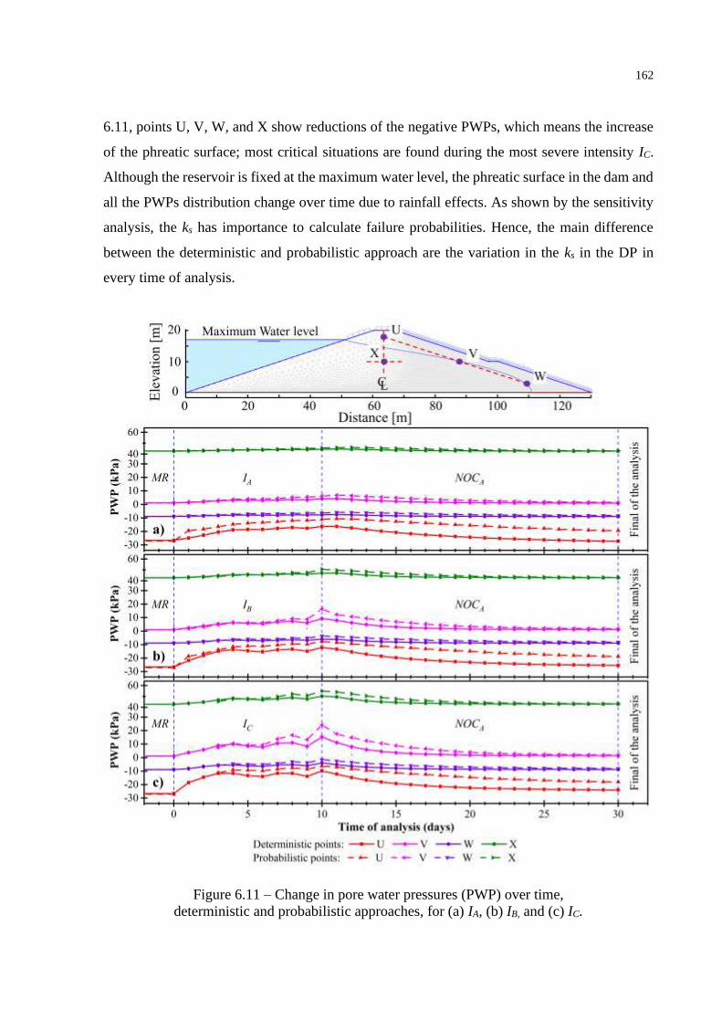
162

6.11, points U, V, W, and X show reductions of the negative PWPs, which means the increase

of the phreatic surface; most critical situations are found during the most severe intensity IC.

Although the reservoir is fixed at the maximum water level, the phreatic surface in the dam and

all the PWPs distribution change over time due to rainfall effects. As shown by the sensitivity

analysis, the ks has importance to calculate failure probabilities. Hence, the main difference

between the deterministic and probabilistic approach are the variation in the ks in the DP in

every time of analysis.

Figure 6.11 – Change in pore water pressures (PWP) over time,

deterministic and probabilistic approaches, for (a) IA, (b) IB, and (c) IC.

163

The time of PWPs dissipation depends on the ks of the dam. In earth dams structured

with low permeability soils, the dam has low dissipation of PWPs. However, or dams with high

permeability soils, the dam has a high dissipation.



normal operating case NOCA.

In a deterministic approach, the model can automatically locate the critical slip surface

of the dam according to the PWPs of each time step using the GeoStudio software. This is

reflected on a deterministic critical surface and deterministic phreatic surface, which are

represented by a deterministic value of FoS for every step of the time. The same scenario is

presented in a probabilistic approach. The DC software is used to find the DP in the last iteration

of the FORM, which means the determination of the probabilistic value of β for every step of

the time. Using the DP, a probabilistic critical surface, and the probabilistic phreatic surface is

represented. Figure 6.12 illustrates the deterministic and probabilistic slip (and phreatic)

surfaces, for transient analyses at time t=10 days, for IA, IB, and IC. Close results of critical

deterministic and probabilistic slip surfaces are found, but different FoS and β are reported.

These changes are basically by the variation in the deterministic and probabilistic phreatic

surfaces.

Some authors (Cheng et al., 2015; Low et al., 1998; Siacara et al., 2020b) report small

differences in stationary problems. However, other authors (Siacara et al., 2020a) reported large

differences in transient analysis in rapid drawdown and NOC conditions. For the study herein,

the deterministic and probabilistic critical slip surface has a very close configuration.

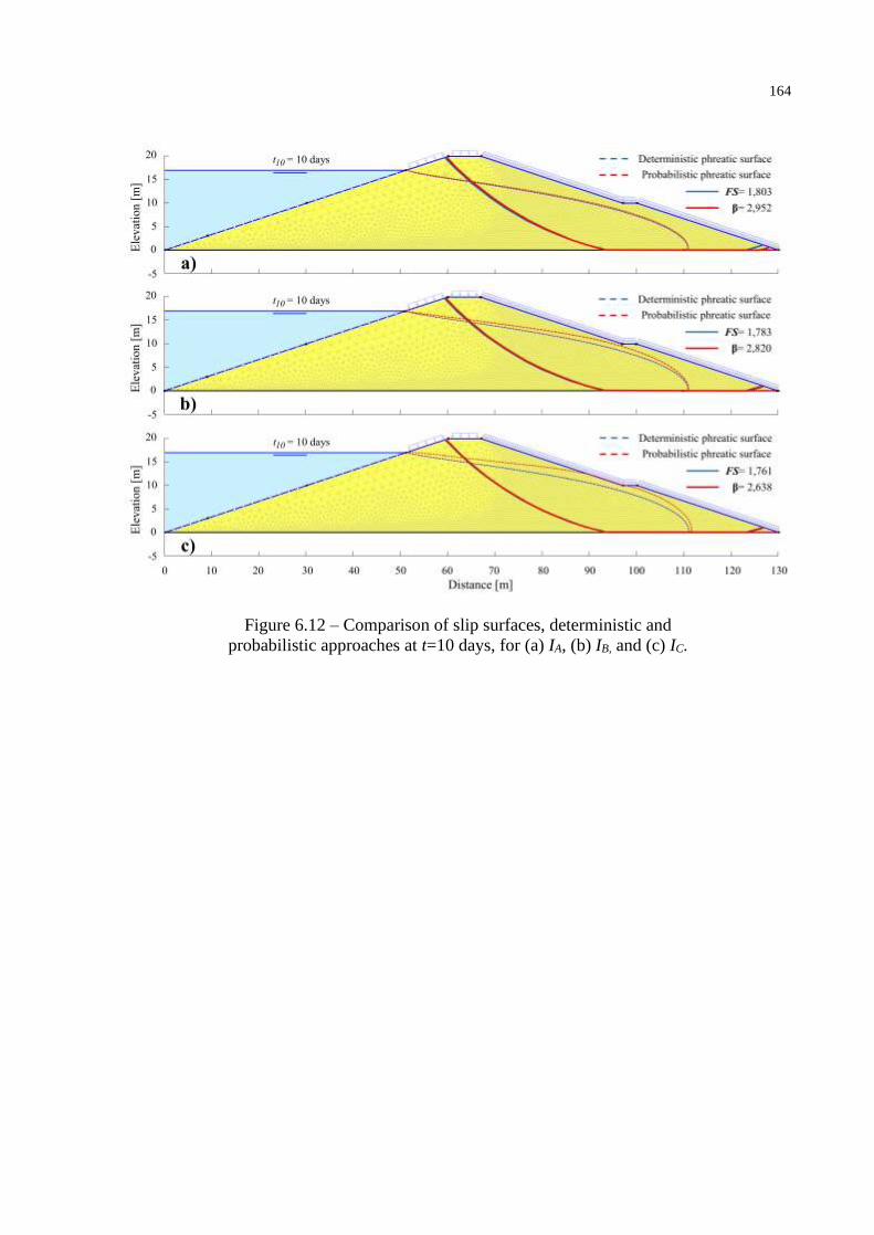
164


probabilistic approaches at t=10 days, for (a) IA, (b) IB, and (c) IC.

165

6.5 CONCLUSIONS

This Chapter addressed the transient reliability analysis of earth dams under rainfall and normal

operating conditions. In all of the probabilistic and deterministic analyses, the DC software was

employed, in which the probabilistic software calls the deterministic software as a black box.

The deterministic GeoStudio 2019 software was used to perform seepage and stability analysis.

The first-order reliability method was performed in the probabilistic StRAnD software to

perform reliability analyses. An earth dam was studied under three different initial conditions,

rainfall intensities, and normal operating conditions. The boundary conditions change at every

step of the time.

The major conclusions are:

• The initial PWP of the model defines the initial conditions of stability that define the

performance of the dam in the following days, and a large analysis shows the dissipation

of PWPs with the convergence of all the analyses in deterministic and probabilistic

terms. In a real problem, a short transient analysis can give a wrong overview by the

dependence on the initial PWPs.

• For an extreme rainfall IC, the reduction in FoS was 4 % and the reduction in β was

14.81 % for the dam studied herein. The critical deterministic and probabilistic time

depends on the rainfall intensity. For the study herein, the critical time is at the end of

the extreme rainfall or one day later.

• An advanced reliability analysis is presented taking into account rainfall effects during

a NOC. In the first ten days, when the boundary conditions are the same, close results

of reliability are found. This means a good performance of the iHLRF algorithm, and

convergence of the exact solution FORM method.

• The sensitivity analysis reveals that random equilibrium parameters of friction angle

(ϕ´) and cohesion (c´) have a greater impact, and the random seepage parameter of

saturated hydraulic conductivity (ks) has a greater impact on random pore water

pressures over time. The incidence of ks on the reliability analysis increase according to

the rainfall intensity and major changes in the reservoir level.

166

• The difference in pore water pressures between a deterministic and probabilistic

approach increase from the static long-term steady-state to transient analysis. The

changes are in function of the incidence of the behavior of the water in the dam, and a

large difference is found in more intense rainfalls.

• In the analysis herein for different rainfall intensities, the critical deterministic and

probabilistic slip surface presents close results, but different values of FoS and β.

Although there are cumulative effects of random ks over time, these differences in terms

of critical surfaces do not increase over time.

168

7 RELIABILITY ANALYSIS OF AN EARTH DAM IN

OPERATING CONDITIONS USING DIRECT COUPLING

ABSTRACT

Reliability analysis of geotechnical infrastructures has become very popular, due to the large

variability observed in soil properties. However, a comprehensive literature review shows that

the problem of normal operating conditions (NOC) of earth dams has not yet been studied from

a reliability perspective. This is a relevant problem, as studying normal operating conditions

helps to reduce the uncertainty related to dam performance, and provides another tool for

evaluating dam safety. This Chapter combines seepage analysis with limit equilibrium analysis

to investigate the safety of an existing old earth dam over time. One relevant feature of the study

is the use of realistic pore water pressures for each equilibrium analysis, accomplished by

considering a long-term steady-state analysis as an initial condition, followed by four years of

equilibrium analysis, before each transient seepage analysis. The numerical investigation is

accomplished by directly coupling the deterministic software packages Seepage/W and

Slope/W with the StRAnD reliability software. Direct coupling avoids errors associated to point

estimate methods and to using response surface surrogates. The first-order reliability method is

employed in reliability analysis. Sensitivity analyses reveal that four dam body parameters

(saturated hydraulic conductivity, ks; specific weight, γ; effective cohesion, c´; and friction

angle, ϕ´) and two filter parameters (ks and ϕ´) are the random parameters with the greatest

contribution to failure probabilities, for all the zones of analysis considered. A range of values

of the relationship between the reliability index (β) and the factor of safety (FS) was found for

all probabilistic and deterministic results. The differences in terms of pore water pressure

between deterministic and probabilistic approaches are presented. Finally, a critical slip surface,

identified in terms of minimum factor of safety, is shown here not to be the critical surface in

terms of the minimum reliability index.

Keywords: Earth dam reliability; reliability analysis; normal operating case; transient analysis;

equilibrium analysis.

169

7.1 INTRODUCTION

A country's economic growth is directly related to the construction of dams, and there are over

55,000 large dams throughout the world (those with a height of more than 15 m or a reservoir

larger than 3 million cubic meters) (ICOLD, 2021; Vallejo et al., 2002). The intended purposes

of large dams usually include providing water for irrigation, water supply to cities, improving

navigation, generating hydroelectric power (19 % of the world supply) and flood control

(Hartford et al., 2016). Few dams serve all these purposes, but some multi-purpose dams serve

more than one.

The failure of large dams is a concern in many countries due to the high economic and

social consequences associated with it. Zhang et al. (Zhang et al., 2016) present a study of

failures in dams from over 50 countries; additionally, 1443 cases of dam failures have been

collected from the literature and compiled into a database (ICOLD, 2021; Singh, 1996; Stanford

University, 1994; USCOLD, 1988, 1975; Vogel, 1980; Xu and Zhang, 2009). The work by

Menescal (Menescal, 2009) lists 166 cases of accidents and incidents that occurred in Brazil

from 1954 to 2009. Several methodologies and tools for estimating direct and indirect economic

impacts and related economic consequences of dam failure are found in the literature

(Ellingwood et al., 1993; Munger, 2009).

The geotechnical engineer responsible for designing a new dam must be able to make

reliable predictions about the behavior of the dam, under every anticipated operating condition

(e.g. end of construction, first filling of the reservoir, rapid drawdown and normal operating

conditions). The predictions usually involve both judgments and quantitative analyses, based

on data provided by the site investigation team (Cruz, 2004; Duncan et al., 2014; Fell et al.,

2015). All the information about the dam must be available, and additional laboratory or field

tests may be required to perform a complete study.

The safety evaluation of aging dams is an essential but complex undertaking, especially

when the original foundation investigation, dam design and construction details are not known

or are associated with significant uncertainty (Fenton and Griffiths, 2008; Zhang et al., 2016).

When information is limited, the real condition of the dam can often only be estimated.

Continuous monitoring of the dam by the variation in the water reservoir is an important activity

of dam safety management during normal operating conditions (NOC).

170

In a deterministic approach, the safety condition of a dam is usually verified by Factors

of Safety (FS) (Berilgen, 2007; Lane and Griffiths, 2000; Rahardjo et al., 2010). During the last

four decades, different authors (Duncan, 2000; Phoon, 2008) have worked to quantify the

variability in geotechnical materials and in developing methodologies to perform reliability

analysis of slopes and embankments in different conditions (Bhattacharya et al., 2003; Chen et

al., 2019; D.-Q. Li et al., 2019; Mouyeaux et al., 2018; Siacara et al., 2020b, 2020a).

In this Chapter, an existing old earth dam is used as study object in a reliability analysis

of NOC. A deterministic software (GeoStudio 2019, (GeoStudio, 2018a, 2018b)) and a

structural reliability software (StRAnD (Beck, 2008)) are combined to perform reliability

analysis of dams. This approach is known as Direct Coupling (DC) in the literature (Kroetz et

al., 2018; Napa-garcía, 2014; Siacara et al., 2020b, 2020a).

A relevant feature of the study is the use of realistic pore water pressures for each

equilibrium analysis, which is accomplished by considering a long-term steady-state analysis

as the initial condition, followed by four years of equilibrium analysis, before each transient

seepage analysis.

Recent dam failures in Brazil forced the government to change the laws and make them

stricter. Different laws were passed in the last 10 years to regulate different types of dams

(Paniago, 2018). These laws require dam owners to perform periodic evaluations of dam

stability to check the current general safety state of the dam. The aim here is to provide a tool

for monitoring old earth dams, considering deterministic and probabilistic approaches.

Dam safety management using a probabilistic approach represents an enhancement over

traditional dam safety practices, through an integrated process that involves quantifying the

uncertainties in geotechnical and operational parameters, and yielding a quantitative measure

of dam safety: the probability of failure, as a function of time. An existing old earth dam in

NOC is the object of study herein.

171

7.2 PROBLEM SETTING

7.2.1 Random seepage analysis and random transient pore water pressures

In transient problems, the equilibrium condition changes over time, due to the variation in the

water level and due to changes in pore water pressures (PWP). In the deterministic case, the

safety factor (FS) is understood to change over time, following the variation in the water

reservoir level. Similarly, the reliability index (β) evaluated over time is considered to describe

the instantaneous safety of the dam. However, it is not known in advance at which point in time

the minimal FS and β are reached. Hence, the reliability analysis has to be performed over time,

with a discretized time step (tk, k=0,1,…,K).

The reliability analysis for limit equilibrium at any time tk depends on the pore water

pressures at that time. However, because some seepage parameters are random, the PWPs at

time tk are random as well. Describing randomness in PWPs is difficult, because of their

distribution in space. Alternatively, the correct random PWPs at time tk can be found by running

the random seepage analyses since time zero (Siacara et al., 2020a). This also means running

the full random seepage analysis again, from time zero, for the PWPs at time tk+1. This has a

significant computational cost, when numerical solutions with many degrees of freedom are

computed.

In the Normal Operation Conditions (NOC) studied herein, the reservoir water level

changes constantly, going up and down, attenuating large deviations in PWPs, which could

result from extreme realizations of volumetric water content or hydraulic conductivity. A

practical consequence is that analyzing the whole seepage time-history is not necessary. This

is very relevant in the context of this study, as the finite element models employed are very

large, and the life of the studied dam is very long.

In this Chapter, the reliability analyses for limit equilibrium were performed considering

different time intervals for the random seepage analysis (sp=1, 5, 10 or 30 days). Hence, the

reliability analysis at time tk

starts at time tk-sp. In all the cases, the initial condition is the mean PWP curve found in the

deterministic (mean value) analysis. For sp=5 days or more, no differences were observed in

the calculated reliability indexes. Hence, sp=5 days was employed in all the reliability analyses

discussed herein.

172


As will be shown as follows, the relative importance of the problems random variables (factors

2

i ) changes during the transient analysis. The FORM solution depends on a design point (DP),

which, in turn depends on the cumulative effect of uncertain seepage variables up to analysis

time tk. As mentioned before, random seepage analyses were performed for sp=5 days, starting

at time tk-5.

In contrast, in the Monte Carlo Simulation (MCS) solution of transient problems, such as

normal operating conditions, each seepage sample produces a complete time history of pore

pressures, which is computed up to final time tK. The probabilistic limit equilibrium analysis at

time tk can be performed by sampling stability variables, and by sampling one of the PWPs

curves generated in the random seepage analysis at time tk. This is an advantage over FORM.

However, the FORM analysis is still competitive if the preceding seepage analysis is limited to

five days. FORM would lose competitiveness if the seepage analyses had to be performed from

time zero.

7.2.3 Review of target reliability index standards

The target reliability indices (βT) for different civil structures (building, bridges, etc.) are

defined in various structural design codes, but this is not the case for dams. As an example,

evaluation of dam safety in Brazil does not use target safety index by two major arguments: (i)

the safety format used is based on safety factors; (ii) authorities do not specify the required or

minimum safety levels.

Reliability indices provide a qualitative estimation of a dam performance taking into

account uncertainty in loads and materials. Dams are classified by the expected performance

level, where dams with relatively high reliability indices are expected to perform their function

well. In contrast, dams with low reliability indices are expected to perform poorly and present

rehabilitation problems (USACE, 1997). The target reliability values shown in Table 7.1 should

be used in general.

173

Table 7.1 – Target reliability indexes for dam stability analysis

(USACE, 1997).

Expected performance level Reliability index (β) Probability of failure (Pf)

High 5.0 3.0 x10-7

Good 4.0 3.0 x10-5

Above average 3.0 1.0 x10-3

Below average 2.5 6.0 x10-3

Poor 2.0 2.3 x10-2

Unsatisfactory 1.5 0.07

Hazardous 1.0 0.16

Comparisons between different countries about risk tolerability are not easy since

societal conflicts, national regulations, legal conflicts, owner and third-party values, and

judgements are involved. Nevertheless, due to the lack of specific orientation for Brazil, the

(ICOLD, 2005) criteria are used to evaluate the dam studied herein.

The βT for structural design is determined by calibrating to existing practice (Westberg,

2010). The target safety values of different structures cannot be used for dams. The reasons are

as follows: (i) the reliability index is nominal and comparison between other structures

(especially by the difference in failure modes and loading conditions) may not be correct; (ii)

consequences might not be comparative; (iii) Generally, dam safety risk management have

large scale consequences, and this affects societal judgment.

A dam is usually designed abiding to national or international norms. Generally, a

numerical model is used with information available from laboratory or field tests in critical and

normal conditions of load. Computational results prove whether the modeled structure meets

the safety requirements. The code requirement is:

Tprior (7.1)

For existing dams, the following requirement should be met:

Tposterior (7.2)

To validate these two statements, different actions may be applied in the existing dam.

Ditlevsen and Madsen (Ditlevsen and Madsen, 2007) define three different categories of

actions: (i) let the structure without changes; (ii) strengthen the structure; (iii) demolish the

structure.

174

7.2.4 Relationship between reliability index (β) and factor of safety (FS) for

specific dams

Usual safety analysis, monitoring and inspection of dams is based on safety factors. Structural

reliability analysis provides a more comprehensive quantitative estimate of dam safety, but it

is more complex to evaluate. Hence, it is helpful to have a measure of the relationship between

reliability index and safety factors, even if this measure is valid only for very specific

conditions. If such a measure can be found, the safety factor can be used as a substitute for the

reliability index to monitor the safety of a specific dam.

In this Chapter, we propose measuring the ratio R= β/FS for different operational

conditions over time, with all the other problem parameters remaining unchanged (such as

nominal values and probability distributions of geotechnical parameters). After ratio R is

computed at a minimum number of points in time, a confidence interval is evaluated for this

ratio:

( ) upperlower RRER (7.3)

where E( ) is the expected value operator. The lower and upper bounds are evaluated as:

( ) ( )

( ) ( )RVarkRER

RVarkRER

upper

lower

+=

−= (7.4)

where Var( ) is the variance operator, and parameter k yields the desired confidence interval.

For k= 2, for instance, one has a confidence of 95.5% that the actual ratio is contained within

the bounds. Now assume that the mean ratio E(R) and the bounds in Equation (7.4) have been

evaluated, for some normal operational conditions, and the safety factor FScurrent is evaluated

for another normal operational condition. The bounds on the estimated reliability index and the

mean estimated reliability index are obtained as:

( )

uppercurrentupper

currentmean

lowercurrentlower

RFSβ

REFSβ

RFSβ

=

=

=

(7.5)

Surely, the ratios and bounds in Equations (7.4) and (7.5) change for different dams, and for

different probabilistic characterization of the seepage and stability properties of the dam. The

relations above are assumed to be valid for a single dam in “stationary” normal operating

conditions (NOC). Surely, the relations above are not valid in the presence of extreme loading

events, such as rapid drawdown, extreme rainfall or earthquakes.

175

7.3 METHODOLOGY

7.3.1 Probabilistic modeling

The deterministic GeoStudio 2019 (GeoStudio, 2018a, 2018b) software and the probabilistic

StRAnD 1.07 (Beck, 2008) software were implemented using direct coupling to perform

deterministic and probabilistic calculations. An earth dam in long-term steady-state and during

a rapid drawdown was discussed by Siacara et al. (Siacara et al., 2020b, 2020a). In this research,

an earth dam in normal operating conditions (NOC) was evaluated. The deterministic limit

equilibrium method (LEM) (e.g. Morgenstern and Price) was used to find the factor of safety

(FS). The reliability index (β) is evaluated in a specific time or in a time frame using structural

reliability methods (e.g. FORM). This section presents an overview of the procedure

implemented. The procedure is illustrated by the flowchart shown by Siacara et al. (Siacara et

al., 2020b, 2020a), and the FORTRAN code was modified for this study as shown in Figure

7.1:

(1) Initial data of the problem: studies of topography, geology, geotechnical (laboratory and

field test), hydraulic and hydrological.

(2) Initial conditions of the model: choose and set up a two-dimensional (2D) model in

Seep/W of GeoStudio 2019 software. In the first step, the initial boundary conditions

(e.g., long term steady-state analysis with a specific water level of the reservoir) are

defining to perform seepage analysis. Then, the equilibrium and initial pore water

pressure (PWP) of the model are defined (Figure 7.2).

(3) Transient conditions of the model - Equilibrium time: in the second step in Seep/W, an

equilibrium time interval is defined to perform transient analysis. The boundary

conditions are in function of time (e.g. long time of the reservoir in normal operating

conditions). The main purpose of these steps is to find the correct PWP (equilibrium of

the PWP) by the transient analysis taking into account the variation in the reservoir

(measurements in the field). The equilibrium time of the analysis (tm) or the duration of

the analysis and number of steps (m) is defined, as well as time increment (Δt) (Figure

7.2).

(4) Transient conditions of the model – Analysis time: The third step in Seep/W is defining

an interval of time, which is a sequence of the last step. The boundary conditions are in

function of the time (e.g. normal operating conditions). The phreatic surface and PWP

of the model are found at every time of the analysis. The time of the analysis (tn) or the

duration of the analysis and number of steps (n), as well as time increment (Δt) is shown

in the Figure 7.2.

176

(5) Stability conditions of the model: choose and set up a 2D model in Slope/W of the

GeoStudio 2019 software. The last step in Slope/W is to perform the stability analysis

using LEM. The factor of safety (FS) is determined for every step of the seepage analysis

or at a specific time of the normal operating condition. The critical factor of safety (FScr)

is the smallest found during the analysis; it occurs at the critical time (tcr-d) (Figure 7.2).

(6) Define the probabilistic model: choose reliability methods in the StRAnD 2.00 software.

(7) Define deterministic (nominal) material properties for the seepage analysis and LEM.

(8) Define the probabilistic data for material properties.



procedure.

(10) GeoStudio 2019 file: File “.gsz” from GeoStudio is a ZIP file that contains different

files of the analysis. The definition file includes the input data and other configurations

in the form of an extension file “.xml” that has the same name as the “.gsz” file and is

the file used to change the input parameters. In the same folder, there is a file with the

output data and the file extension “.csv”, which is used as the input parameters for the

reliability analysis. The input parameters are varied at every iteration using the

GeoStudio file “.gsz” , which is decompressed and compressed, saving the FS to find

the DP.

(11) The results of the reliability analysis (number of evaluations, number of simulations,

reliability index, probability of failure, DP, etc.) are shown in the

STRAND_OUTPUT.txt file, whereas the critical surface is shown in the GeoStudio

software. The critical probabilistic time (tcr-p) is found, corresponding to the critical

reliability index (βcr) (Figure 7.2).

The FS is found from m to n steps of time or at a specific time of the transient analysis. From

the FS, the StRAnD software performs the reliability analysis in both options of time (Figure

7.2).

177


transient reliability analysis procedure by coupling GeoStudio and

StRAnD softwares packages (based on (Siacara et al., 2020b, 2020a)).

Figure 7.2 – Schematic procedure of the steady-state and transient

analysis to perform the limit equilibrium reliability analysis.

178


A) Earth dam of the study

The application of the probabilistic dam slope and flow analysis methodologies described

earlier in the Chapter are illustrated in the analysis of a well-documented Brazilian dam. The

dam is not identified due to privacy concerns. The dam main purpose is to generate 260.0 MW

(nominal power), with a tunnel work of 15.4 km, and a differential height of 770 m from the

reservoir to the power-house. The reservoir filling was started in July 1970, and the construction

of the dam was finished in August 1971. The dam has about 50 years of normal operation

conditions (NOC), and it is classified as an old earth dam. The following study is an academic

one; therefore, all the conclusions are only suggestions to the company in charge of the dam.

The dam was subject of extensive studies quantifying the soil properties from

instrumentation, field and laboratory tests. However, we were not given access to measured

data; hence, we could not evaluate the actual variability of the soil properties. These data were

taken from the literature, but adjusted to the actual mean values provided in previous studies of

the dam.

The earth dam was constructed from an embankment of 60 m in height and 1.3 million

cubic meters of earth, which resulted in a reservoir of 150 million cubic meters of water. It is a

dam of homogeneous type with different elements. The dam has a horizontal (approximately

1.8 m in height) and vertical filter (approximately 1.0 m in thickness) to reduce the pore water

pressure within the dam, conducting the water downstream.

The upstream rock mass at the feet of the embankment has the function of confining the

dam, and the downstream rock mass has the complementary function of drainage and increased

structural stability. The crest has 10 m in width and is used as a passage for the company´s

private vehicles. The dam is unsymmetrical; therefore, the berms and slopes are variable. For

protecting the slopes against erosion and other damaging effects (rainfall and reservoir waves),

the structure is lined with 1.0 m of rip-rap upstream and grass downstream of the dam.

As the foundations presented good quality and favorable conditions for implementing

the project, the concrete cut-off and the injection curtain initially foreseen in the project were

not executed. Nevertheless, the dam counts on a small trench positioned parallel to its axis,

excavated until the rock has some weathering to improve the waterproofing conditions of the

structure.

179

The dam foundation is of unweathered rock (granite and gneiss), and water level up to

4.0 m below the crest is the maximum water level. The saturated-unsaturated seepage and the

stability of the dam slopes, considering the variability of soil parameters, is analyzed.

The plan view and cross-section are shown in Figure 7.3 and critical cross-section A is

presented in Figure 7.4. Cross-section A is assumed to be the critical cross-section; it is used

throughout the analysis herein.

Different data and information on the earth dam studied are available (COPEL, 2016,

1998, 1987, 1986, 1971a, 1971b, 1963, 1958; Heuko, 2014; Seara, 2010; Sousa Pinto, 1972,

1971; Vargas, 1962; Vargas and Hsu, 1966). The data are divided into three categories,

according to type: field instrumentation, laboratory and field tests.

The case study advantage is that a reference system was installed during its construction,

which allowed localizing the tests in space (X, Y and Z according to the three axes). This system

consists of a grid formed by 24 profiles (A to Y) of 20 m in the longitudinal direction (Y axis),

22 profiles (13 upstream profiles from 0 to 26M and 9 downstream profiles from 0 to 18J) of

20 m in the transversal direction (X axis) and the elevation of the dam in axis Z (see Figures

7.3 and 7.4).

180

Figure 7.3 – The plan view and sections of the dam.

Figure 7.4 – Critical cross-section A of the dam.

181

B) Dam condition of analysis

In this study, deterministic and probabilistic analyses are performed on a critical cross-section

of the earth dam during NOC, where the embankment soil is saturated and unsaturated at

different times of analysis.

The deterministic parameters (nominal parameters) were quantified by field

instrumentation, laboratory and field tests from previous studies of the dam, and the uncertainty

in soil parameters was quantified from the literature (Siacara et al., 2020b).

The seepage analysis contains the representation of the SWCC and the hydraulic

conductivity function predicted by using the Van Genuchten equation (Van Genuchten, 1980),

and the Morgenstern and Price method (Morgenstern and Price, 1967, 1965) with the shear

strength criteria of unsaturated soils (Fredlund et al., 1978) is used as LEM. The Van Genuchten

fitting parameters (θs ,θr, a and n) were estimated using the Seep/W software database

(GeoStudio, 2015; van Genuchten et al., 1991) for every dam material.

The dam body consists of silty-clays, the filter of sands, and the rip-rap and rock mass

for protecting the fractured rock. For avoiding computational issues by differences in hydraulic

conductivity, a transitional material of 5 cm was used between the dam body and filter. The

random seepage analysis is characterized by the uncertainty of two SWCC fitting parameters

(a, n), the saturated and residual volumetric water contents (θs, θr), and the saturated hydraulic

conductivity parameter (ks). The random stability analysis is characterized by uncertain specific

weight (γ), effective cohesion (c´), effective friction angle (ϕ´) and the angle that increases shear

strength (ϕb). The uncertain parameters of the stability and seepage analyses are assumed to

have normal (N) or lognormal (LN) distributions. The mean (µ) and the coefficient of variation

(COV) of all parameters are shown in Table 7.2.

The SWCC and hydraulic conductivity curves corresponding to the mean values in

Table 7.2, are shown in Figures 7.5 (a) and (b), respectively.

182


Analysis

Materials Dam body Transition Filter Rock-Mass Probabilistic

distribution Observation

Parameters µ COV

(%) µ

COV

(%) µ

COV

(%) µ

COV

(%)

Seepage

Ks (m/seg) 1x10-6 80 1x10-5 80 1x10-4 80 1x10-2 80 LN [1]

θs (m3 m-3) 0.50 15 0.48 15 0.43 15 0.40 15 N [1]

θr (m3 m-3) 0.067 30 0.018 30 0.016 30 0.013 30 N [1]

a (kPa) 57.67 50 6.84 50 1.62 50 0.95 50 LN [1]

n 1.60 20 1.84 20 1.94 20 2.85 20 LN [1]

Stability

γ (kN/m3) 19.00 7 19.00 7 19.00 7 27.00 7 N [1]

c´ (kPa) 10.00 30 7.00 30 5.00 30 24.00 30 N [1]

ϕ´ (°) 28.00 20 29.00 20 30.00 20 35.00 20 LN [1]

ϕb (°) 17.00 20 15.00 20 0.00 - 0.00 - LN [1]

Anisotropy rk 5 - 5 - 1 - 1 - - [2]

183

The following remarks are made about the COV values and rk ratio in Table 7.2:

[1] The COV of ks , θs, θr, a, n, γ, c´, ϕ´ and ϕb for all the different soils variations was

compilation of Siacara et al. (Siacara et al., 2020b).

[2] The rk ratio for existing dams varies from 1 to 15 (Baligh and Levadoux, 1980; Kutzner,

1997; Mayne, 2007; Mouyeaux et al., 2019); Cruz (Cruz, 2004) suggests a value of 1

for non-cohesive soils and from 4 to 10 for cohesive soils. In compacted earth fills, the

rk ratio may exceed 20 (Novak et al., 2007). Fell et al. (Fell et al., 2015) and USACE

(USACE, 1994)give rk ratios in the order of 1 to 100, covering the possible range of

expected field conditions. A common value of 3 for rk ratio is suggested (Verbrugge and

Schroeder, 2018). For compacted soils, the rk ratio for non-cohesive soils varies from 1

to 40, and for cohesive soils from 0.4 to 4.1 (Chapuis et al., 1991). From laboratory

tests, the rk ratio varies from 1 to 4.1 (Chapuis et al., 1991). Leroueil et al. (Leroueil et

al., 2002) found rk ratios from 1 to 1.4 in compacted soils in laboratory, and Smith and

Konrad (Smith and Konrad, 2011) found an rk ratio of 5 using geostatistical analysis of

construction control data from the core of an earth dam.

Figure 7.5 – Mean value of hydraulic parameters (a) SWCC (b)

hydraulic conductivity curve.

Concerning anisotropy, the data available did not allow using a random characterization of

the anisotropy coefficients of the materials. The anisotropic coefficient (rk) was considered a

constant for the different materials. The rk ratio was assumed as 5 for dam body and transition,

and 1 for filter and rock-mass, according to the literature on cohesive and non-cohesive soils

(Table 7.2).

The USBR (USBR, 2011b) indicates that typical dams will have rk ratios ranging from 2 to

10, with higher values relating to higher water contents during placement. Older dams, such as

those constructed in the early 20th century or by hydraulic fill methods, may have anisotropy

as high as 50 due to stratification during placement and earlier compaction methods that did not

emphasize mixing and discing. However, coarse-grained materials, such as rockfill shells or

filter and drain materials, are typically placed in thicker lifts without as much compactive effort,

184

and they tend to have lower anisotropy. These types of soils are often assigned anisotropy

values of 1.


Seepage and stability analyses were performed in the GeoStudio software (Seep/W and

Slope/W), for normal operating conditions (NOC), to obtain deterministic (mean value) results

of pore water pressure (PWP) and factor of safety (FS) for the most critical slip surface. The

mean value (µ) of seepage properties (ks, θs, θr, a and n) and properties involved in stability

calculation (γ, c´, ϕ´ and ϕb), presented in Table 7.2, were used in this analysis. A two-

dimensional analysis is performed herein. Table 7.3 shows the duration in days of the different

analyses performed.

Table 7.3 – Duration of the different analyses performed herein.

N Step of analysis Type of analysis Initial time

(days)

Final time

(days) Duration

1 Initial condition Long term Steady-state

2 Equilibrium time Transient 0 1460 1460 (4 years)

3 Time of analysis Transient 1460 1825 365 (1 year)

Zone A Transient 1466 1481 15 days

B Transient 1600 1615 15 days

C Transient 1645 1660 15 days

D Transient 1810 1825 15 days

The initial PWP condition is the key input information for transient seepage analysis in

an earth dam, and it can be difficult to determine. The following methodology used herein will

help to define the correct initial conditions.

The first step (Table 7.3), an initial long-term steady-state analysis was performed to

determine the PWP for maximum water level conditions (845.0 m.a.s.l.), which is assumed at

initial time (t= 0 days). The events described in Table 7.3 correspond to the actual normal

operational conditions for the dam, following the official information available. The

nomenclature of events states event duration in days (e.g., t= 570 days represents 570 days of

analysis). This nomenclature corresponds to, but is independent of dam age.

The initial finite element seepage analysis also yields the position of the phreatic

surface. The PWP and total water head corresponding to the initial condition (t= 0 days) are

shown in Figure 7.6. The phreatic surface was assumed to be the line of zero pore water pressure

determined from the seepage analysis, as shown in Figure 7.6. The PWP values are negative in

185

the uppermost part of the flow region, above the phreatic surface. Negative PWPs have a minor

contribution to dam stability, but their effects are considered in the study.

The dam was modeled using triangular elements with of approximate absolute size of 5

meters. The discretization of the mesh was according to the size of the element and the

importance of the element in the analysis. A total of 33825 nodes and 67232 nodes were

automatically created by the mesh generator available in Seep/W.

Taking into account flow measurements during construction, the infiltration trough the

dam foundation was estimated at around 1.6 l/s, which, when increased by external

contribution, has led to values of the order of 3.6 l/s. However, the real value was about three

times higher than the one initially estimated. These differences eventually impacted the

performance of the horizontal filter. The water level was found to be above the horizontal filter,

and the downstream PWP was very different. This was verified with historical field

measurements (Sousa Pinto, 1972, 1971).

Figure 7.6 – Results of the seepage analysis for the initial condition

(t= 0 days) with pore water pressure (kPa) and total water head (m).

The second step (Table 7.3), the transient analysis (equilibrium time) is the variation of

the reservoir (oscillation between 845.0 and 827.0 m.a.s.l.) over four years (from t= 0 days to

t= 1460 days) to find the PWP equilibrium of the dam. The water level in the reservoir is

affected by hydrological events and by user demand. The partial or total emptying of the

reservoir is part of the dam operation procedures.

The behavior of the reservoir changes every day (there are always some water level

variations), and the dissipation time of PWP is insufficient; therefore, the stabilizing effect of

the water outside the dam is removed, and the shear stresses for equilibrium increase. The finite

element seepage analysis is performed at every time step (one day), to calculate the

186

corresponding PWP and to find the position of the phreatic surface (e.g., PWP and total water

head for t= 500 days are shown in Figure 7.7).

Figure 7.7 – Results of the seepage analysis for t= 500 days, with pore

water pressure (kPa) and total water head (m).

The third step (Table 7.3), the transient analysis is the variation in the reservoir

(oscillation between 844.0 and 831.0 m.a.s.l.) over one year (from t= 1460 days to t= 1825

days). During this step, the earth dam is considered to be in equilibrium, and PWP values are

more realistic. The finite element seepage analysis is performed at every time step (one day),

to calculate the corresponding PWP and to find the position of the phreatic surface (e.g., PWP

and total water head for t= 1600 days are shown in Figure 7.8).

Figure 7.8 – Results of the seepage analysis for t= 1600 days, with

pore water pressure (kPa) and total water head (m).

Dam stability calculations are performed in the downstream slope, using PWPs found

at every time step of the seepage analysis (initial long-term steady-state, equilibrium and last

transient analysis). Morgenstern and Price’s procedure is used for all LEM calculations. An

automatic search is conducted, by the entry and exit specification technique, to locate the most

critical circle for each representation of PWPs, for each time step. The entry and exit

187

specification technique consists of a variation in the grid-radius method. The entry and exit slip

surface discretization was performed at every 1.2 m, with circles defined by specifying the

radius tangent lines. The computational algorithm ensured that the entry and exit angle of each

slip surface did not exceed 90 degrees and that no straight line (infinite radius) was used as a

possible slip surface. The critical slip surface and the minimum factors of safety (FS) are

determined using Slope/W; results for times t= 0, t= 500 and t= 1600 days are shown in Figure

7.9 (a), (b) and (c), respectively. The figure also shows the finite element mesh used to

determine pore pressures in the seepage analysis.

Figure 7.9 – Critical slip surfaces for the dam: a) t= 0 days, b) t= 500

days and c) t= 1600 days.

The limit equilibrium analyses yielded different FS and different critical surfaces at

every time step due to varying reservoir water levels, as shown in Figure 7.10 (a) and (b). The

analyses were performed by applying a phreatic surface adjustment with the interpolated pore

pressures resulting from the seepage analysis. In SLOPE/W, all the slip surfaces must be

contained in the domain. If a trial slip surface intersects the lower boundary of the model, the

188

slip surface would follow the boundary. Once a slip surface is generated, the strength

parameters used in stability calculations are taken from the materials overlying the base of

individual slices. The stability analysis for the initial conditions (t0= 0 days) yielded the initial

safety factor as FS0= 2.13. During the equilibrium analysis (from t= 0 to t= 1460 days), the

oscillation of FS is between FSmax= 2.34 and FScr= 2.13. During transient analysis time (from

t= 1460 to t= 1825 days), the oscillation of FS is between FSmax= 2.30 and FScr= 2.18. Although

the maximum water level is reached several times, the critical FS is found for t= 0 days, because

the rise and fall velocity of the reservoir during NOC is not very large.

Figure 7.10 – Results of the limit equilibrium analysis for different

times of analysis: a) equilibrium + analysis time; b) zoom at analysis

time.

The mechanics behind the transient seepage analyses were developed more than 80

years ago. However, it is difficult to put the mechanics into immediate practical use owing to

the large number of numerical calculations required. In recent years, transient seepage analysis

programs, such as SEEP2D1, SEEP/W, and SLIDE, allowed these analyses to be conducted by

189

personal computers in relatively modest execution times (USACE, 2016b). However, these

transient analyses are uncommon in geotechnical engineering. In this study, we consider

unsaturated soils and employ long term steady-state analysis as an initial condition, followed

by four years of equilibrium analysis, to find more realistic PWP before the actual transient

analysis. This is a novelty of our analysis in comparison to standard practice.

The Bureau of Reclamation (USBR, 2011a, 1987), Bureau of Indian Standards (Bureau

of Indian Standards, 1975), U.S. Army Corps of Engineers Slope Stability Manual (USACE,

2003), Brazilian Power Plants – ELETROBRÁS (ELETROBRÁS, 2003) and others authors

(Cruz, 2004; Duncan et al., 2014; Fell et al., 2015) recommend a minimum factor of safety of

FS=1.5 for long-term steady-state conditions, and FS=1.1 to 1.3 for rapid drawdown analysis

of earth dams. All the factors of safety evaluated herein in the mean value (deterministic)

analysis satisfy this minimum stability criterion.

190


Reliability analyses for dam equilibrium were performed at the four time zones identified as A,

B, C and D Figure 7.10 and Table 7.3. (between t= 1460 and t= 1825 days). Reliability indexes

(β) and probabilities of failure (Pf) were evaluated by directly coupling GeoStudio and StRAnD

software packages, as described in Sections 7.2 and 7.3. The FORM method was performed.

The limit state gradients were estimated by finite differences. The search for the design point

was performed with the HLRF algorithm.

The reliability analysis considered five random seepage properties (Ks, θs, θr, a and n)

and four random stability calculation properties (γ, c´, ϕ´ and ϕb) for every material of the dam,

as shown in Table 7.2. The following reliability analyses results are presented as follows:

(1) Preliminary screening of random variable importance in NOC;

(2) Normal operating conditions at time zones A, B, C and D;

(3) Difference of critical PWP and phreatic surface in deterministic and probabilistic

analyses;

(4) Difference in critical surfaces in deterministic and probabilistic analyses.

(5) Sensitivity of the random variables w.r.t. seepage and equilibrium analyses;

7.4.1 Preliminary screening of random variable importance in NOC

An advantage of FORM is the possibility of carrying out a sensitivity analysis through the

direction cosines (α2) at the Design Point (DP). The α2 values show the relative contribution of

each random variable to calculated failure probabilities, with large α2 values revealing the most

important variables.

An initial reliability analysis was performed with 34 variables (Table 7.2) of the earth

dam, for four different times. These results (not shown here) reveal that, out of 34 initial random

variables, only four dam body parameters (ksat, γ, c´ and ϕ´) and two filter parameters (ksat and

ϕ´) are important, with individual contributions to reliability analysis greater than 0.1%. The

other 28 random variables resulted in nearly zero sensitivity coefficients (α2≈0); hence, these

random variables have negligible contributions to the computed failure probabilities and were

considered deterministic in the remaining analyses.

191

The numerical reliability analyses were performed by direct coupling, using a dual core

workstation computer, with processor speed of 2.1 GHz, and RAM memory of 64 GB. A

complete transient reliability analysis with 34 random variables took about 320 hours to

compute (with total analysis time of sixteen days and discretization of one day). Each day of

transient analysis took about 20 hours to compute. With the reduction to the six most important

random variables, the same transient reliability analysis was reduced to 96 hours, with each day

of transient analysis reduced to about 6 hours. This reveals the importance of pre-screening the

importance of random variables, and eliminating those of irrelevant contribution. Further

details on sensitivity coefficients of the remaining variables are presented in Section 7.4.5.

7.4.2 Analysis for Normal Operating Conditions (NOC)

During normal operating condition (NOC), we can obtain both deterministic FS and

probabilistic β of the unsaturated earth dam. Figure 7.10 shows the variation in water levels

over the analysis time, as well as the safety factors found in the deterministic (mean value)

analysis. The reliability analysis is performed assuming the reservoir water level known at the

end of each day; the end condition of one day is the starting condition for the next day. In dam

practice, water levels at the end of any day are well known, by the characteristics of the

hydraulic installations, such as the capacity of spillways. The reliability analysis is performed

using the FORM method in the zones A (from t=1466 to t=1481 days), B (from t=1600 to

t=1615 days), C (from t=1645 to t=1660 days) and D (from t=1810 to t=1825 days), as shown

in Figures 7.10 and 7.11.

In a deterministic solution using Seep/W software, one of the concerns is the

convergence criterion. The general techniques for verifying convergence include: (i) examining

the number of nodes that meet the convergence criteria in two successive iterations; (ii)

comparing iteration counts at each time step or reviewing the maximum allowable value; (iii)

examining the number of non-converged nodes at each iteration. These techniques are covered

in the material available in GeoStudio (GeoStudio, 2018a). Moreover, in the probabilistic

analyses, all the above convergence criteria were met.

The four zones of analysis (A to D) have lengths of 15 days (Table 7.3). As expected,

the reliability index and safety factors follow similar trends during the NOC analysis (Figure

7.11). Zones A, B and D show a negative tendency of the Pf curve, but zone C has a positive

tendency. The FS and β curves have an opposite behavior to the Pf curves for the four zones of

analysis, as expected. The determination of FS, β and Pf for every day of analysis reduces

192

uncertainty regarding the behavior of the dam (e.g. t= 1470, 1610, 1655 and 1820 days), as

shown in Figure 7.11.

Figure 7.11 (d) shows two results for specific times (t= 1820 and 1825 days) with a

difference of 5 days and a 0.66 m drop of the reservoir. The difference between results are these

two points in time, ΔFS= 4.3 x10-3, Δβ= 2.33 x10-2 and ΔPf= 4.17 x10-7. These variations are

important to prevent occasional unsafe behaviors.

Figure 7.11 – Safety factors, reliability index and failure probabilities

for zones: a) A, b) B, c) C and d) D.

Figure 7.11 shows how FS, β and Pf curves change during the normal operating

conditions. As stated in Section 7.2.9, it may be possible to estimate reliability index β from the

observed ratios R= β/FS of for this dam and for the random parameters considered in Table 7.2.

Based on the results in Figure 7.11, and using Equations (7.4) and (7.5), the ratios were found

as Rupper= 2.12, E(R)= 2.00 and Rlower= 1.88. Based on these ratios, and on the FS values

computed for the whole analysis period, the reliability index bounds were computed. The results

are first compared for the four zones (A, B, C and D) for which actual β values are known

(Figure 7.12). In Figure 7.12, actual β values are observed to indeed be within the bounds given

by Equations. (7.4) and (7.5). This could be expected, since the ratios above were computed in

the same zones (A, B, C and D).

193

The usefulness of the proposed bounds can be appreciated when observing the whole

(deterministic) analysis time, in Figure 7.13. In this figure, the bounds are employed to estimate

the maximum and minimum values of β for the whole interval, including the times between

zones A, B, C and D. From these bounds, it is estimated that the maximum and minimum

(critical) values of β are βmax=4.87 at t=1626 days, and βcr= 4.11 at t=1735 days. Hence, this

initial screening can be used to perform a reliability analysis at the most critical section, around

time t=1735 days. This was done herein, after identifying t=1735 as the critical time. The actual

reliability analysis at time t=1735 resulted in βreal= 4.07; a difference of only Δβ= 0.04 to the

estimated value. This confirms, by observation, that the bounds proposed in Equations (7.4)

and (7.5) can be used for screening the most critical section in NOC. Note that t=1735 is critical

because it is the end of a longer period for which the reservoir had been full or nearly full;

hence, pore water pressures were high in a significant part of the dam.

Considering the dam performance levels listed in Table 7.1 (USACE, 1997) and the

reliability index values computed herein, the analyzed dam is classified as between Good and

High. This includes the estimated critical value βcr.

Figure 7.12 – Estimation of reliability index (β) from FS and bounds

of ratio R= β/FS.

194

Figure 7.13 – Estimation of the reliability index (β) for the analysis

time.

Although reliability calculations have helpful results, the reliability theory has not been used

much in geotechnical engineer formation or practice because it involves new concepts that are

not familiar to many engineers. Other meaningful reasons are required computational time and

more data of the geomaterials, unavailable in most circumstances. Equation (7.4) and (7.5) are

alternatives to estimate β from the FS as is shown in Figure 7.13. Although this approach helps

geotechnical engineers to estimate reliability values from deterministic results, these equations

not avoid to perform reliability analysis. The observed ratios R= β/FS of every dam can be

improved in accuracy with more results from the reliability analysis, and a calibration with a

high number of results gives more reliability estimation. These ratios R can be defined during

the first years of NOC of the dam, and it can help during the safety monitoring of a dam. The

principal advantage of using these ratios R are performing deterministic transient analysis to

estimate the reliability results in function of time, avoiding more computational efforts. During

NOC, the estimation of β is helpful (e.g. a dam during large increases or decreases of the

reservoir; the state of the dam is known immediately). Factors of safety and reliability index

complement each other and hence both are more useful than knowing either one alone.

195


Differences between deterministic and probabilistic analyses in terms of seepage and stability

are further investigated. In every step of time tk, different PWPs, phreatic and failure surfaces

are illustrated over the dam. In the following figures, the results of the deterministic and

probabilistic analysis are illustrated using the GeoStudio software. Deterministic results are

represented by the mean values of random variables (Table 7.2) and probabilistic results are

illustrated using the DP values of the same random variables.

Figure 7.14 compares PWPs over the dam, in deterministic and probabilistic analyses,

for times t=1604 and t=1656 days. The critical equilibrium situation occurs for higher PWPs;

therefore, the most likely pore water pressures leading to equilibrium failure are significantly

higher than the mean pore pressures. The variation in PWPs depends on the zone of analysis,

and on the velocity of water level change. The differences between results in Figures 7.14 (a)

and (b) are mainly explained by use of mean value of ks (1.0 x 10-6 m/s) and the design point

value of ks (0.84 x 10-6 m/s for t= 1604 and 1.24 x 10-6 m/s for t= 1656 days). This difference

is estimated to be larger in zone C.

Figure 7.15 compares PWPs over dam height for the two cross-sections identified in

Figure 7.14 (A-A´ and B-B´), also for times t=1604 and t=1656 days. Figure 7.16 shows how

these PWP vary in time at points T and U in zones B and C, identified in Figure 7.14.

Differences in PWP between deterministic and probabilistic analyses are observed in zones B

and C over time. Hence, the differences between deterministic and probabilistic analyses can

be explained by the effects of seepage in the days preceding the equilibrium analysis, and

dissipation of PWPs in water level falls.

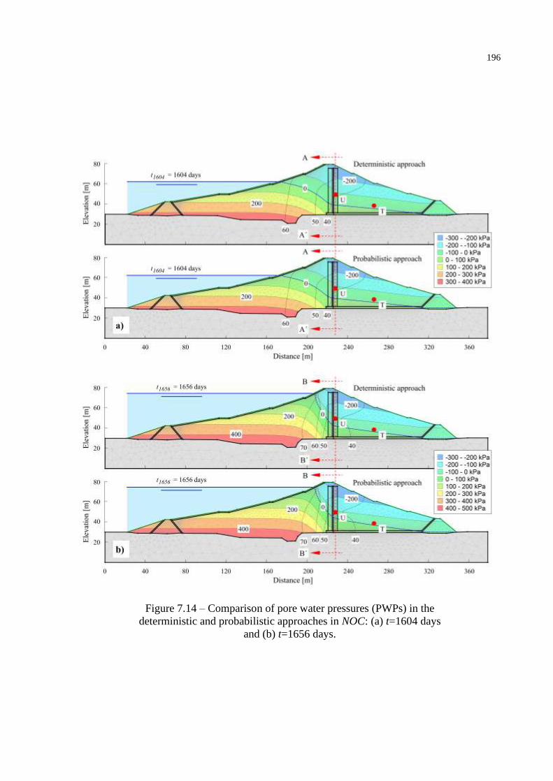
196

Figure 7.14 – Comparison of pore water pressures (PWPs) in the

deterministic and probabilistic approaches in NOC: (a) t=1604 days

and (b) t=1656 days.

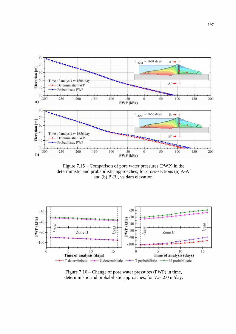
197

Figure 7.15 – Comparison of pore water pressures (PWP) in the

deterministic and probabilistic approaches, for cross-sections (a) A-A´

and (b) B-B´, vs dam elevation.

Figure 7.16 – Change of pore water pressures (PWP) in time,

deterministic and probabilistic approaches, for VA= 2.0 m/day.

198


A comparison of the corresponding critical deterministic and probabilistic slip surfaces, for

times t= 1604 and t=1656 days, is presented in Figures 7.17 (a) and (b), respectively. The

location of the critical slip surface does not change much over time in the deterministic (mean

value) analysis, as seen in Figure 7.9. The critical deterministic slip surface is located between

the rock foundation and the rock mass downstream.

The reliability analysis using FORM involves a search for the design point (DP). When

the random variables assume the values corresponding to the DP, the slip surface with the

highest probability of occurrence is obtained at every time step. This is called the probabilistic

slip surface.

As observed in Figures 7.14, 7.15 and 7.17, there are subtle differences between the

PWPs and phreatic surfaces observed in the deterministic and probabilistic analyses. As

discussed in the next session, this is a consequence of the small contribution of random seepage

parameters to the reliability problem. However, there are significant differences between

deterministic and probabilistic slip surfaces, as observed in Figure 7.17. The probabilistic slip

surface is located above the downstream rock mass, in contrast to the deterministic slip surface.

These results suggest that differences between deterministic and probabilistic slip surfaces, in

transient NOC analyses, are even larger than differences observed for stationary problems

(Cheng et al., 2015; Low et al., 1998; Siacara et al., 2020b, 2020a). Differences in critical slip

surfaces could be larger for zoned dams or for dams composed of different materials.

In normal operating conditions (NOC), safety factors and reliability indexes at a given

time depend on the history of the reservoir water level and PWP conditions. Finding the real

condition of earth dams is hard work in a deterministic approach, and using of probabilistic

approaches is a challenge for geotechnical engineers. This adds to the importance of performing

reliability analyses for assessing the safety of dams.

199


probabilistic approaches at times: a) t=1604 days and b) t=1656 days.

7.4.5 Sensitivity of random variables

Figure 7.18 illustrates sensitivity coefficients for the six most relevant random variables, under

NOC and for zones A, B, C and D. Firstly, the sensitivities are observed not to change

significantly in time, which is quite different from the case or rapid drawdown (Siacara et al,

2020a). This also adds to the argument that five days of previous seepage analysis is sufficient

for equilibrium analysis in NOC, whereas the whole time interval had to be considered in the

rapid drawdown analysis (Siacara et al, 2020a).

The results in Figure 7.18 also show that, of the six random variables with the greatest

contribution to failure probabilities, the dam body friction angle ϕ´ is the most important for all

the NOC zones considered herein. The second most important variable is dam body effective

cohesion c´. The other two parameters of the dam body (γ and ks) and two parameters of the

filter (ks and ϕ´) have smaller importance (α2≠ 0).

200

Figure 7.18 – Sensitivity coefficients of different random variables

over time for zones A, B, C and D.

Studies on stochastic pore pressure variability (Bergado and Anderson, 1985), transient

analysis of rapid drawdown (Siacara et al., 2020a) and stochastic hydraulic conductivity (Gui

et al., 2000b), as well as other studies (Srivastava et al., 2010; Yi et al., 2015), found seepage

properties to have great importance to reliability analyses. The reliability index decreases as the

COV of conductivity hydraulic increases. A comparison of our results with the references above

reveals that the importance of the seepage parameters (Ks, θs, θr, a and n) of the materials in our

study are smaller or nearly zero (α2≈0).

In deterministic analyses, it is well known that the increase of phreatic surfaces

downstream of the dam reduce safety factors. In the NOC reliability analysis, this results in

reduction of β´s and in a negative α2 value for dam body ks. Water flow through the lower part

of the critical deterministic and probabilistic surfaces (Figure 7.17 a and b) helps to explain the

smaller relevance of random seepage parameters in the reliability analysis.

201


This Chapter addressed transient reliability analysis of earth dams during normal operating

conditions (NOC). A direct coupling (DC) technique between the deterministic GeoStudio 2018

software and the structural reliability StRAnD software was employed. Numerical analysis of

seepage and stability were performed. The first-order reliability method (FORM) method was

used to find the design point in reliability analyses. An existing earth dam was studied, and four

time zones were considered.

The main conclusions are:

• A transient random seepage analysis needs to be performed before the equilibrium

analysis to determine realistic pore water pressures. Under normal operating conditions,

five days of previous seepage analysis were found to be sufficient, starting from the

mean value condition.

• Identifying the critical time corresponding to minimum reliability is very costly. A

simple empirical equation was proposed comparing safety factors (FS) and reliability

indexes (β) for a single dam in similar normal operating conditions. This equation yields

the expected (minimum and maximum) reliability indexes, based on FS calculations for

the whole life of the dam. Estimated minimum FS values can be used to find the

(approximated) critical time, at which the reliability analysis should be performed. Note

also that the critical time corresponding to minimum FS can be different from the critical

time corresponding to minimal β (Siacara et al., 2020a). The empirical relation is valid

for a single dam, and for the same description of random variables.

• The initial analysis listed 34 random geotechnical parameters: five seepage and four

equilibrium parameters for each material. Each day of random seepage analysis with 34

parameters took about 20 hours to compute. Sensitivity analyses revealed the six

parameters with the greatest impact on evaluated failure probabilities; a reduction in

random variable dimensionality reduced processing time for a daily transient analysis

to about 6 hours.

• Using deterministic (mean values) data of laboratory and field test, and statistical data

from the literature, our analysis reveals that four dam body parameters (ksat, γ, c´ and

ϕ´) and two filter parameters (ksat and ϕ´) presented the largest contribution to reliability

analysis. The friction angle (ϕ´) has the greatest impact on the reliability analysis for

equilibrium.

202

• Due to the cumulative effect of random saturated hydraulic conductivity (mainly) over

time, the time variations in pore water pressures, phreatic surfaces and critical slip

surfaces become much larger in probabilistic analysis than in deterministic (mean value)

analysis.

• The most probable slip surface, found in the reliability analysis, is not the same as the

critical slip surface found in a mean value analysis for the minimum factor of safety

(FS). The difference is due to seepage parameters and the geometry of the dam.

• Considering target reliability indexes suggested in ICOLD (ICOLD, 2005), the expected

performance level of the studied dam is Good.

In summary, the conclusions above point to the importance of employing structural

reliability techniques in the safety evaluation of geotechnical infrastructure.

204

8 RELIABILITY- BASED DESIGN OPTIMIZATION OF A

CONCRETE DAM

ABSTRACT

Performance and safety of geotechnical structures are affected by uncertainties. Yet, the design

of dams is nowadays still made using deterministic methods and design codes. Dam

optimization in a deterministic setting may lead to compromised safety margins. In this setting,

Reliability-Based Design Optimization (RBDO) appears as an alternative, allowing one to

optimize dam performance, but respecting specified reliability constraints. In this Chapter, we

employ an efficient and accurate Single-Loop Approach (SLA) in the RBDO of a concrete dam.

Considering dam equilibrium reliability constraints, we find the optimal dam base and optimal

placement of drainage galleries, for different dam heights and different target reliability index

(βT). We show how the governing failure mode changes for each optimal solution: for large βT,

sliding limit state is the active constraint; for smaller βT values, the eccentricity limit state

function is found to be the active constraint for the optimum dam. We also investigate how the

importance of random parameters change for each optimum solution: for large βT and failure

controlled by sliding, the cohesion and friction angle along dam base interface with foundation

rock are the most relevant uncertain parameters for dam equilibrium. For smaller βT with failure

controlled by eccentricity, the more relevant uncertain geotechnical parameters are the base

length of the dam, the specific weight of concrete, and the coefficient of drainage gallery

inefficiency.

Keywords: Reliability-based design optimization; Concrete dam; Reliability index; Dam

design; Single-Loop Approach.

205

8.1 INTRODUCTION

Geotechnical structures are designed under significant uncertainty in parameters. In concrete

dams, the traditional approach for verifying stability is based on deterministic methods that use

empirical safety factors (FS) or partial factors of safety for every failure mode. These empirical

FS allow us to design conservative dams, without explicitly considering the uncertainties in

geotechnical parameters. Different specialized standard agencies (CFBR, 2012; China Electric

Council, 2000; ELETROBRÁS, 2003; FERC, 2016; People’s Republic of China industry

standard, 2007; USACE, 2000, 1995; USBR, 1976) and some authors (Cruz, 2004; Fell et al.,

2015) give suggestions of minimum FS. These values determine if the structure has an

acceptable level of safety or not. If minimum values are not met, the existing structures need to

be strengthened and/or their use changed. In turn, the design procedure starts with an initial

definition of the cross-section geometry, which is progressively updated until the safety criteria

are met. However, these FS do not quantitatively measure the safety margin of the design and

do not account for the influence of different design variables and their uncertainties on the

overall system performance (Mahmood, 2020; Youn and Choi, 2004).

Probabilistic methods are a powerful tool to determine the probability of failure of a

structure in different loading conditions. Probabilistic methods consider geotechnical

parameters as random variables, which brings more confidence regarding the performance and

safety of structures (Baecher and Christian, 2003; Phoon and Ching, 2015). In large dams, the

development of national dam safety regulations was historically based on the classical approach

(deterministic analysis). The ICOLD bulletin (ICOLD, 1987) encouraged theoretical

investigations for the future adoption of a probabilistic approach to dam safety. This bulletin

states that the logical trend, in the design phase, goes from the predominantly deterministic

approach of global FS to the semi-probabilistic method of partial safety factors. For existing

dams, the standards-based approach is recognized to be increasingly inadequate (ICOLD,

2005). Due to their inherent conservatism, deterministic approaches may not be cost-effective

for design of new dams, or safety evaluation of existing dams (Bowles et al., 1998). In those

cases, the probabilistic approach has gained acceptance for the safety management of specific

dams, for which the economic resources are very important. Reliability methods have been

considered systematically to support decision-making regarding the operation or during the

design of a dam.

206

In the reliability theory, the first-order approximation to the probability of failure (Pf) is

obtained by approximating the limit state at the design point by a hyperplane, which leads to:

( )βPf − Φ (8.1)

Where Φ(.) is the standard Gaussian cumulative distribution function (CDF) and β is the

reliability index (Beck, 2019, 2017; Melchers and Beck, 2018). The minimum distance of the

limit state function to the origin is the so-called reliability index (β), and the point over the limit

state with minimum distance to the origin is called the “design point”. Defining a target

reliability index (βT) with a large distance away from the failure domain, the chance of

unsatisfactory performance can be reduced. In dam structures, βT should be a function of the

expected performance level (USACE, 1997). Increasing the safety of structural systems usually

implies additional costs, and sometimes cost savings can result in jeopardized safety (Melchers

and Beck, 2018). The optimum design mostly involves a tradeoff between safety and economy

(Zhao et al., 2015).

Deterministic Design Optimization (DDO) allows finding the shape or configuration of a

structure that is optimum in terms of mechanics, but the formulation grossly neglects parameter

uncertainty and its effects on structural safety (Beck and Gomes, 2012). Consequently, a

deterministic optimum design obtained without considering such uncertainties can result in an

unreliable design (Youn and Choi, 2004). Reliability-Based Design Optimization (RBDO) has

emerged as an alternative to properly model the safety-under-uncertainty part of the problem.

Uncertainties in geotechnical engineering come from loads, geotechnical properties, and

calculation models (Ang and Tang, 2007; Baecher and Christian, 2003; Phoon, 2008). The

purpose of RBDO is to find a balanced design that is not only economic but also reliable in the

presence of uncertainty (Yang and Hsieh, 2011). With RBDO, one can ensure that a minimum

(and measurable) level of safety is achieved by the optimum structure (Beck and Gomes, 2012).

Although the idea of RBDO is attractive, its implementation is generally not easy because

of the coupling between reliability assessment and cost minimization. Methods used to solve

RBDO problems are usually classified into three groups (Aoues and Chateauneuf, 2010; Beck,

2019):

(1) Bi-level RBDO approaches: reliability index approach (RIA) (Enevoldsen and

Sorensen, 1994; Tu et al., 1999; Yu et al., 1997) and performance measure approach

(PMA) (Tu et al., 1999; Youn et al., 2003);

207

(2) Mono-level RBDO approaches: Single Loop Single Variable (SLSV) (Chen et al.,

1997) , Single Loop approach (SLA) (Liang et al., 2007, 2004), Mono-Level RBDO

(Kaymaz and Marti, 2007), Reliable design space (Shan and Wang, 2008);

(3) Decoupled RBDO approaches: Traditional Approximation Method (TAM) (Torng and

Yang, 1993), Sequential Optimization and Reliability Assessment (SORA) (Du and

Chen, 2004), Sequential Approximate Programming (SAP) (Cheng et al., 2006; Yi et

al., 2008).

The above methods are very efficient for problems with linear and moderate nonlinear limit

state functions. Traditionally, an RBDO is conducted through a double-loop approach (also

known as a bi-level approach) in which the inner loop computes the reliability constraint, and

the outer loop conducts the optimization. For this reason, the double-loop RBDO method is

computationally expensive and, therefore, almost impractical for large-scale design problems.

Some studies have been carried out for the RBDO of geotechnical structures in recent

years. Chiti et al. (Chiti et al., 2016) used a subset simulation for RBDO of a concrete gravity

dam. Zhao et al. (Zhao et al., 2016) employed an Artificial Bee Colony (ABC) algorithm for

RBDO analysis of retaining walls and spread footings. Zevgolis et al. (Zevgolis et al., 2018)

proposed a probabilistic geotechnical design optimization framework for large open-pit

excavations. Zhao et al. (Zhao et al., 2017) employed least square support vector machine

(LSSVM) and artificial bee colony (ABC) algorithm for reliability-based support optimization

of rock bolt reinforcement around tunnels. Santos et al. (Santos et al., 2018) used the FORM-

based ant colony optimization (ACO) algorithm for reliability-based design optimization of

geosynthetic-reinforced soil walls. Ji et al. (Ji et al., 2019) used the inverse FORM approach

for reliability-based design in geotechnical engineering. Raviteja and Basha (Raviteja and

Basha, 2018) presented a target reliability-based design optimization (TRBDO) approach of V-

shaped anchor trenches for municipal solid waste landfills. Mahmood (Mahmood, 2020) used

the FORM method with a minimization algorithm to illustrate the optimization of a retaining

wall.

Using deterministic suggestions of specialized standard agencies and taking into account

uncertainties, this Chapter investigates the optimum location of gallery drainage and best

geometry of a concrete dam using a mono-level Single-Loop Approach (SLA). We exploit how

the governing failure mode changes as a function of the target reliability index (βT) employed

as design constraint, and as a function of dam height. We also investigate how the importance

of random parameters change for each optimum solution.

208

The remainder of this Chapter is organized as follows. The basic formulation of RBDO is

presented in Chapter 2. The application problem is described in Section 8.2. The detailed

reliability-based dam optimization problem is described in Section 8.3. The results of the

optimization analysis are presented and discussed in Section 8.4. Concluding remarks are

presented in Section 8.5.

209

8.2 THE APPLICATION PROBLEM

A concrete dam is adopted to illustrate the application of RBDO using the SLA algorithm. We

here adopt a section of a concrete dam that satisfies all the deterministic design requirements.

The concrete dam has a height of 50 m, and width of 7 m at the crest (a two-way highway exists

at the crest). The upstream face is vertical and the downstream face has an initial slope of

1V:0.733H. A drainage gallery with a square dimension of 2.0 m is located 5.0 m from the

upstream face to reduce uplift forces in the dam foundation and body of the dam. The spillway

gives a restriction of the maximum water level in the reservoir and this defines the freeboard,

which is considered to be 2.0 m under the crest of the dam. The bedrock, foundation of the dam,

is considered waterproof and impenetrable.

The downstream face slope is often considered the design variable. To meet stability

requirements, the slope is usually in the order of 1V:0.7H to 1V:0.8H, depending upon uplift

assumptions (Corns et al., 1988). However, for higher dams with low-density concrete or under

seismic loading, this relationship will be higher to meet stability requirements (ICOLD, 2000).

Some recommendations in the literature of minimal distances between the drainage

gallery and the upstream wall face of the dam were found. USACE (USACE, 1995) and USBR

(USBR, 1976) recommend a minimum distance of 1.524 m (5 ft.) for the placement of concrete

mass and to reduce stress concentrations. USACE (USACE, 2000) suggest a higher distance

than 5 % of the water reservoir height to have a reduction of the uplift pressure by the gallery

drainage. The upstream face of the gallery shall be located at a minimum distance of 5 % of the

maximum reservoir head or 3 m from the upstream face, whichever is greater (Bureau of Indian

Standards, 1985). The gallery drainage should be located between 3 m to 9 m away from the

upstream face to reduce uplift pressures (Hannah and Kennedy, 1938). To minimize the

possibility of cracking with serious leakage from the water reservoir, Jansen (Jansen, 1988)

states that the gallery must be at least 3 m away from the upstream face and at a distance of at

least 5 % of the water reservoir height. El-razek and Elela (El-razek and Elela, 2001)

experimentally found the optimum position of the drainage gallery, a relationship between the

horizontal distance of the gallery/Base of the dam gives 0.5. The research by Chawla et al.

(Chawla et al., 1990) showed that the size, location, and spacing of the drains impact the

distribution of internal uplift pressure by using an analytical solution based on the seepage

theory. Later, other authors (Chen et al., 2008; Daghestani et al., 2019; Nourani et al., 2017;

Zee et al., 2011) demonstrated it numerically with different computational models.

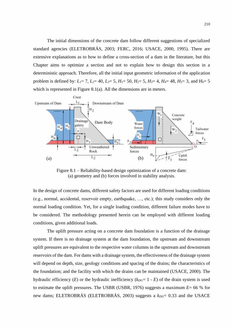
210

The initial dimensions of the concrete dam follow different suggestions of specialized

standard agencies (ELETROBRÁS, 2003; FERC, 2016; USACE, 2000, 1995). There are

extensive explanations as to how to define a cross-section of a dam in the literature, but this

Chapter aims to optimize a section and not to explain how to design this section in a

deterministic approach. Therefore, all the initial input geometric information of the application

problem is defined by: L1= 7, L2= 40, L3= 5, H1= 50, H2= 5, H3= 4, H4= 48, H5= 3, and H6= 5

which is represented in Figure 8.1(a). All the dimensions are in meters.

Figure 8.1 – Reliability-based design optimization of a concrete dam:

(a) geometry and (b) forces involved in stability analysis.

In the design of concrete dams, different safety factors are used for different loading conditions

(e.g., normal, accidental, reservoir empty, earthquake, …, etc.); this study considers only the

normal loading condition. Yet, for a single loading condition, different failure modes have to

be considered. The methodology presented herein can be employed with different loading

conditions, given additional loads.

The uplift pressure acting on a concrete dam foundation is a function of the drainage

system. If there is no drainage system at the dam foundation, the upstream and downstream

uplift pressures are equivalent to the respective water columns in the upstream and downstream

reservoirs of the dam. For dams with a drainage system, the effectiveness of the drainage system

will depend on depth, size, geology conditions and spacing of the drains; the characteristics of

the foundation; and the facility with which the drains can be maintained (USACE, 2000). The

hydraulic efficiency (E) or the hydraulic inefficiency (kDG= 1 - E) of the drain system is used

to estimate the uplift pressures. The USBR (USBR, 1976) suggests a maximum E= 66 % for

new dams; ELETROBRÁS (ELETROBRÁS, 2003) suggests a kDG= 0.33 and the USACE

(a) (b)

211

(USACE, 1995) limits a maximum of E= 50 %. French guidelines (CFBR, 2012) recommend

values of 𝐸 between 67 % to 50 % for regular geology and less for unfavorable geology. The

Chinese design guideline (Chinese Ministry of Hydroelectric Power, 2005) suggests an E

between 60 % to 80 %.

In this study, the theoretical approach of ELETROBRÁS (ELETROBRÁS, 2003) and

USBR (USBR, 1976) was taken into account to determine the uplift pressure in the drainage

line. The equivalent water column height is:

( ) 554DGe HHHkH +−= for H5 > H3 (8.2)

( ) 334DGe HHHkH +−= for H3 > H5 (8.3)

The forces and moment arms involved in the overturning limit state are listed in Table 8.1 and

shown in Figure 8.1(b).

Table 8.1 – Forces and moment arms for the rotational failure of the

concrete dam.

Force Moment arm

c1 HLW 11= 2

12

LLa1 −=

( )( )c2

HHLLW

2

2112 −−=

( )3

2 12 LLa2

−=

c3 aW 2= 32 LLa3 −=

w1

HF

2

2

4= 3

4HaF1 =

( )s

s2

HF

2

sin1 ´2

6 −=

3

6HaF2 =

we

3

LHLHLHLHF

2

3525234 −++=

( )325234

23

2

3

2

25

23

2

2

2

3234

36663622

LLHLHLH

LLLLH

LLLH

LLLH

ae

e

F3−++

−++

−+

−

=

( )( ) w4

HH

LLHF

21

12

2

5

2 −

−=

( )( )21

125

3 HH

LLHaF4

−

−=

w5

HF

2

2

5= 3

5HaF5 =

212

The mean value (µ) and coefficient of variation (COV) of the problems random variables are

obtained from related studies in the literature, as shown in Table 8.2. The uncertain parameters

involved in the analysis are the specific weight of the concrete (γc), the ultimate bearing capacity

of rock mass foundation (qu), the specific weight of the sedimentary material (γs), the friction

angle of the sedimentary material (ϕ´s), the cohesion along the interface between dam base and

foundation rock (c´rc), the friction angle along the interface between the dam base and

foundation rock (ϕ´rc) and the coefficient of drainage gallery inefficiency (kDG). Although the

specific weight of the water (γw) has a statistical variation as function of temperature, gravity

acceleration is employed as a constant value, equal to 9.81 kN/m3 (Das, 2014; USACE, 2000,

1995). The uncertain parameters are assumed to have normal (N) distributions, following Table

3. No correlation is considered between random parameters; hence, the correlation matrix is the

identity matrix.

Table 8.2 – Input parameters of the application problem.

Analysis Parameters µ COV (%) Observation

Concrete γc (kN/m3) 24 4 [1]

Rock qu (MPa) 15 50 [2]

Sedimentary material γs (kN/m3) 19 7 [3]

ϕ´s (º) 28 20 [4]

Interface Rock-Concrete c´rc (kPa) 250 40 [5]

ϕ´rc (º) 35 30 [6]

Drainage gallery inefficiency kDG 0.33 20 [7]

Observation:

[1]: The COV of γC is 4 % (JCSS, 2001) and other authors have related a COV about 3 % to

5 % (Pires et al., 2019). Nominal values were based on CFBR (CFBR, 2012) and JCSS

(JCSS, 2001).

[2]: The COV of qu for a rock foundation varies from 25.9 % to 44.5 % (Mao et al., 2012),

127 % (Alavi and Sadrossadat, 2016), and for soil foundations, 20 % (Mahmood, 2020).

Nominal values for a sandstone rock was taken from Duncan (Duncan, 1999).

[3]: The COV of γS for all the different soils varies from 3 % to 11 % (Siacara et al., 2020a,

2020b). Nominal values were based on Fredlund et al. (Fredlund et al., 2012) and USBR

(USBR, 1987).

[4]: The COV of ϕ´S for all the different soils varies from 10 % to 30 % in clays (Siacara et

al., 2020a, 2020b). Nominal values were taken from Fredlund et al. (Fredlund et al.,

2012) and USBR (USBR, 1987).

[5]: The COV of c´rc for all the different rocks varies from 36 % to 40 % (China Electric

Council, 2000), 64 % to 69 % (Lo and Grass, 1994), 65 % (Fishman, 2009) and 44 %

(Wilde and Johansson, 2013). Nominal values were based on Pires et al. (Pires et al.,

2019).

213

[6]: The COV of ϕ´RC for all the different rocks varies from 25 % to 30 % (China Electric

Council, 2000), 15 % (Wilde and Johansson, 2013), and 40 % (Fishman, 2009).

Nominal values were taken from NAVFAC (NAVFAC DM7-02, 1986).

[7]: The COV of k in a concrete dam varies from 15 % to 30 % (Pires et al., 2019). Nominal

values were based on FERC (FERC, 2016) and USACE (USACE, 2000).

The design of a concrete dam is based on the stability analysis of the cross-section,

considering all possible rigid body mechanisms. Although stresses shall not exceed some

admissible limits, the safety of concrete gravity dams is independent of the mechanical strength

of the concrete, since different mechanics of failures (e.g. sliding, overturning, …, etc.) occur

before a conditioning stress field is achieved (Chopra and Zhang, 1991).

The following five failure modes are determined for the present study: (a) overturning

failure, (b) sliding failure, (c) flotation failure, (d) eccentricity failure, and (e) bearing capacity

failure. For the initial design, recommended safety factors were taken from the Chinese

standards (China Electric Council, 2000; People’s Republic of China industry standard, 2007),

U.S. Army Corps of Engineers (USACE, 2000, 1995), Brazilian Power Plants –

ELETROBRÁS (ELETROBRÁS, 2003), Federal Energy Regulatory Commission (FERC,

2016), United States Bureau of Reclamation (USBR, 1976) and others (Cruz, 2004; Fell et al.,

2015).

In the sequence, these five failure modes (a to e) are described.

(a) The factor of safety for overturning failure (FSO) is given by a relationship between

resisting moment (MR) and overturning moment (MA):

0.2332211

5544332211 ++

++−+==

FFF

FF

A

R

OaFaFaF

aFaFawawaw

M

MFS (8.4)

(b) The factor of safety for sliding failure (𝐹𝑆𝑆) is given by a relationship between resisting

forces (FR) and resultant horizontal forces (FO):

( )0.2

tantan

521

2

´´

43321

´´

−+

++−−+=

+==

FFF

LcFFwww

F

AcN

F

FFS rcrc

O

rcrc

O

RS

(8.5)

where N is the sum of normal forces and A is the area of contact on the plane under

analysis.

(c) The factor of safety for flotation failure (FSF) is given by a relationship between

gravitational forces (FV) and resultant uplift pressure forces (FU):

3.13

4321 +−+

==F

Fwww

F

FFS

U

VF (8.6)

214

(d) The eccentricity factor of safety (FSE) is given by a relationship between the base of the

dam (L2) and six times its eccentricity (e):

0.1*6

2 =e

LFSE

(8.9)

(e) The factor of safety of bearing capacity failure (FSB) is given by a relationship between

the ultimate bearing capacity (qu) and maximum foundation pressure (qmax):

0.3*6

122

max

+

==

L

e

L

F

q

q

qFS

V

uuB (8.7)

where e is the eccentricity of the resultant forces, defined as:

V

AR

F

MMLX

Le

−−=−=

22

22 (8.8)

where X is the arm of the resultant net forces.

Using the initial geometry input, forces and arm moments involved in the safety analysis

(Figure 8.1 and Table 8.1), the following factors of safety are determined: (a) FSO= 2.15, (b)

FSS= 2.17, (c) FSF= 4.91, (d) FSE= 1.16 and (e) FSB= 8.20. All the factors of safety evaluated

herein in the mean value (deterministic) analysis satisfy the minimum stability criterion.

The downstream face slope defines the final volume of the concrete dam. If the base of

the dam is increased, the safety factors increase, but this also has an impact on construction

cost. The position of the drainage gallery defines the uplift forces, and it is an important part of

the determination of the FSs. The uplift forces increase about 5 % for every meter the drainage

gallery is moved away from the upstream face. It affects the determination of the FSs with a

reduction of about 4 % in flotation and eccentricity failure, 2 % in overturning and bearing

capacity failure, and 1 % in sliding failure. If the gallery drainage is defined away of the

upstream face, the base of the dam should be increased to meet all FSs.

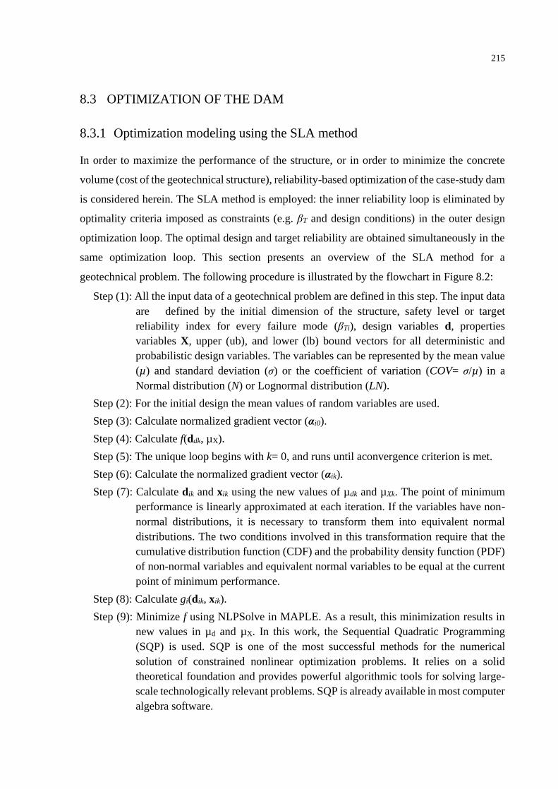
215

8.3 OPTIMIZATION OF THE DAM

8.3.1 Optimization modeling using the SLA method

In order to maximize the performance of the structure, or in order to minimize the concrete

volume (cost of the geotechnical structure), reliability-based optimization of the case-study dam

is considered herein. The SLA method is employed: the inner reliability loop is eliminated by

optimality criteria imposed as constraints (e.g. βT and design conditions) in the outer design

optimization loop. The optimal design and target reliability are obtained simultaneously in the

same optimization loop. This section presents an overview of the SLA method for a

geotechnical problem. The following procedure is illustrated by the flowchart in Figure 8.2:

Step (1): All the input data of a geotechnical problem are defined in this step. The input data

are defined by the initial dimension of the structure, safety level or target

reliability index for every failure mode (βTi), design variables d, properties

variables X, upper (ub), and lower (lb) bound vectors for all deterministic and

probabilistic design variables. The variables can be represented by the mean value

(µ) and standard deviation (σ) or the coefficient of variation (COV= σ/µ) in a

Normal distribution (N) or Lognormal distribution (LN).

Step (2): For the initial design the mean values of random variables are used.

Step (3): Calculate normalized gradient vector (αi0).

Step (4): Calculate f(ddk, µX).

Step (5): The unique loop begins with k= 0, and runs until aconvergence criterion is met.

Step (6): Calculate the normalized gradient vector (αik).

Step (7): Calculate dik and xik using the new values of µdk and µXk. The point of minimum

performance is linearly approximated at each iteration. If the variables have non-

normal distributions, it is necessary to transform them into equivalent normal

distributions. The two conditions involved in this transformation require that the

cumulative distribution function (CDF) and the probability density function (PDF)

of non-normal variables and equivalent normal variables to be equal at the current

point of minimum performance.

Step (8): Calculate gi(dik, xik).

Step (9): Minimize f using NLPSolve in MAPLE. As a result, this minimization results in

new values in µd and µX. In this work, the Sequential Quadratic Programming

(SQP) is used. SQP is one of the most successful methods for the numerical

solution of constrained nonlinear optimization problems. It relies on a solid

theoretical foundation and provides powerful algorithmic tools for solving large-

scale technologically relevant problems. SQP is already available in most computer

algebra software.

216

Step (10): An optimization condition is used to finish the optimization. The tolerance of the

analysis (TOL) is defined by the designer.

Step (11): The results of the optimization analysis (number of evaluations, sensitivity

coefficients at DP, optimized structure, reliability index, and the probability of

failure for every limit state function, evaluation time, DP, etc.) are shown in the

OUTPUT.txt file.

Figure 8.2 – Flowchart of SLA algorithm for a geotechnical problem

(based on (Liang et al., 2004)).

217

8.3.2 Definition of limit state functions and procedure for design optimization

The mean objective is to minimize the cross-section area of the dam, and to find the best

position of the gallery drainage by changing the design variables d= {L2, L3}. In this study,

initially the target reliability index is βT= 3.0 for all failure modes, which corresponds to a

probability of failure PfT≥ 1.0 x10-3. Considering target reliability indexes suggested in USACE

(USACE, 1997), the expected performance level of the design dam will be “above average”.

The design space to meet these objectives is considered to be 0.7*H1 ≤ L2 ≤ 2*H1 m; 0.05*H4

≤ L3 ≤ 15 m; or 3.0 ≤ L3 ≤ 15 m. The reliability-based design optimization (RBDO) problem

can be written as:

( ) ( )( )

( ) Si

aHHLLHLf

Ti =

−−−+=

dd

dd*

;4,3,2,1,:tosubject

5.0minimizeswichfind 2

211211

(8.10)

where f(d) is the cross-section area of the concrete dam and β1, β2, β3, and β4 are the reliability

constraints for the limit states of (a) overturning, (b) sliding, (c) flotation, and (d) eccentricity,

respectively. These reliability constraints are evaluated considering the following limit state

functions.

(a) The limit state function for overturning, with respect to the most extreme downstream point

of the surface under analysis, is defined as:

( ) −= ARO MMxg (8.11)

(b) The limit state function for sliding along the surface under analysis is defined by:

( ) ORS FFxg −= (8.12)

(c) The limit state function for flotation is defined by:

( ) UVF FFxg −= (8.13)

(d) The limit state function for eccentricity is defined as:

( )2

*61

L

exgE −= (8.14)

Limit state functions for overturning (Equation 8.11), sliding (Equation 8.12), flotation

(Equation 8.13), and eccentricity (Equation 8.14) are the geotechnical design requirements. The

limit state function for bearing capacity failure was not taken into account because of the high

value of the safety factor.

218

8.4 OPTIMIZATION ANALYSIS AND RESULTS

RBDO analyses were performed for the same scenario described in the mean value

(deterministic) analysis, including four different failure modes. A Single-Loop Approach

(SLA) was implemented in the MAPLE 2019 software, as described in Chapter 2 and Section

8.2. In this study, a common desktop computer was used, with a processor speed of 2.1 GHz (2

processors) and 64-GB RAM memory. The average computational time for each analysis is less

than 100 min.

The RBDO analysis considered 6 random variables of the problem (γc, γs, ϕ´s, c´rc, ϕ´rc, and

kDG), as shown in Table 8.2. The following optimization analysis results are presented:

(1) Initial results;

(2) RBDO for different target reliabilities (βT );

(3) Sensitivity of failure probabilities do random variables;

(4) RBDO for different dam heights;

(5) Comparison of RBDO with DDO.

8.4.1 Initial results

Starting from an initial design of d= {L2, L3}= {40, 5}, an initial optimum design is found by

solving the optimization problem in Equation (8.10). An optimal design of d= {L2, L3}= {77.4,

3.0} is found for βT= 3.0 and height of the dam H1= 50 m. In initial RBDO result with the SLA

method, the limit state function for sliding along the surface (gS(x)) controls the optimal

response, meaning that gS(x) is the active constraint at the optimal point. In this solution,

constraints gS, gF, and gE are not active.

The initial downstream face has a slope of 1V:0.733H, and the final slope optimized is

1V:1.56H for βT= 3.0. In terms of area, the areas of the initial design and global optimal design

are 1088.5 m2 and 1929.74 m2. The difference in areas between both approaches is 43.59 %

higher for the RBDO approach. The drainage system is moved from 5 m, in the deterministic

design, to 3 m in the RBDO design, with reference to dam upstream. It means less uplift

pressure acting on the concrete dam foundation.

All the design points in the above solutions were found using the SLA algorithm. None

of the limit state functions was excessively nonlinear; hence, no convergence problems were

observed in the analyses. In the case of nonlinear limit state functions, other algorithms based

on Monte Carlo simulation may be required (see, for instance, the discussion in Rashki et al.

219

(Rashki et al., 2014, 2012)). The algorithm was validated with earlier studies (Liang et al., 2007,

2004). The difference of results was less than 1 % between the results reported by Liang et al.

(Liang et al., 2007, 2004) and the present algorithm developed in MAPLE 2019 (Bernardin et

al., 2020; Maplesoft, 2020).

8.4.2 RBDO for different βT

In this section, the target reliability index (βT) is changed in order to analyze the variation in the

area between the original design and optimal design. From the results in Figure 8.3 and Table

8.3, we concluded that for the dam studied herein, the results are proportional, meaning smaller

reliability indices defined smaller areas. In the case of smaller areas, such as βT= 1.5 to 2.0, the

area is very similar to the deterministic analysis. In a conventional design, the deterministic

area is used, and it means an Unsatisfactory (βT= 1.5) to Poor (βT= 2.0) expected performance

level according to Table 2.1 (USACE, 1997). A considerable difference is found between βT=

1.5 to 3.0 with more than 43 % in terms of concrete area. Sometimes, this increase of concrete

area is deemed unnecessary by geotechnical engineers. Deterministic analyses are performed

with the optimized section where large FSs are found. In function of the deterministic and

RBDO results, the designer and owner or investor choose the final section assuming an

acceptable performance level of the dam.

Computationally, values of lengths of the dam for different βT can be obtained. Using

larger values of βT (2.5, 3.0, or more), the design of the dam will be unrealistic in terms of

benefit/cost, but it will have a guarantee performance level.

Figure 8.3 – Comparison of the initial design and the optimal designs

obtained with RBDO.

220

Table 8.3 – Results of the RBDO reliability analysis.

Description βT L2 L3 Area Difference (%)

Original design - 40.0 5.0 1088.50

Optimal design

1.5 40.3 3.0 1095.60 0.65

2 41.9 3.0 1131.16 3.77

2.5 50.9 3.0 1332.94 18.34

3 77.4 3.0 1929.74 43.59

In Table 8.4, values of the four limit state functions are presented at their design points

(gi(*

ix )), at the end of the optimization. A value close to zero indicates an active constraint,

meaning that the corresponding failure mode controlled the optimum design (i.e., halted the

objective function from being further minimized). As observed in Table 8.4, for the studied

dam the overturning (gO) and flotation (gF) failure modes never become active, for any of the

target reliabilities considered herein. The eccentricity (gE) failure mode is the active constraint

for the RBDO solution for smaller reliabilities (βT= 1.5 and 2.0), and the sliding failure mode

(gS) is the active constraint for large βT (βT= 2.5 and 3.0).

Table 8.4 – Limit state function values at the corresponding design

points for different target reliability index.

Failure mode Target reliability

βT= 1.5 βT= 2.0 βT= 2.5 βT= 3.0

Overturning (gO) 306752.73 313218.48 485929.04 1196889.79

Sliding (gS) 3842.72 1244.79 -5.97 x10-13 -8.53 x10-13

Flotation (gF) 19236.12 19121.93 21595.01 29776.17

Eccentricity (gE) -5.21 x10-13 5.55 x10-16 0.27 0.64


By using the SLA method, a sensitivity analysis through the direction cosines (α2) at the design

points is conducted, revealing the most significant variables for each failure mode. Figure 8.4

shows the sensitivity coefficients α2 of each random variable, for the four limit state functions

and for different target reliabilities βT. The sensitivity coefficients for the distance of drainage

gallery (L3), specific weight of the sedimentary material (γs) and friction angle of the

sedimentary material (ϕ´s) do not appear in Figure 8.4 because they are nearly zero (α2 ≈ 0) for

all failure modes; hence, these random variables have negligible contributions to the computed

failure probabilities and can be considered deterministic.

221

As observed in Figure 8.4, the cohesion and friction angle along dam base interface with

foundation rock (variables c´rc and ϕ´rc) have a considerable contribution for the sliding failure

mode, and variables L2, γc, and kDG are important in overturning, flotation, and eccentricity

failure modes. The drainage gallery inefficiency (kDG) increases in importance when βT

increases.

Since for large βT failure is controlled by sliding, it turns out that variables c´rc and ϕ´rc also

control design for large βT. In a similar way, variables L2, γc, and kDG control the optimal design

for small βT.

(a) βT= 1.5 (b) βT= 2.0

(c) βT= 2.5 (d) βT= 3.0

Figure 8.4 – Sensitivity coefficients for different failure modes and

target reliability indexes (βT).

222

8.4.4 RBDO for different dam heights

In this section, we address the optimization of dams of different heights, with same normal load

condition as defined in Section 8.2. Dam heights of H1= 30, 40, 50,60 and 70 m are considered

in this section.

Optimization results are shown in Figure 8.5, for different dam heights. As can be

observed in this figure, there is a range of βT values for which the objective function (dam cross-

section area) and optimum dam base L2 do not change much with the target reliability βT. Within

this “flat” region of the graphs in Figure 8.5, the change in area and in dam base is smaller than

10% (for same dam height H1), and the optimum design is controlled by the eccentricity failure

mode. Within the “non-flat” region, optimum dam design is controlled by the sliding failure

mode, and optimum area and dam base change more as a function of βT. For a dam with height

(𝐻1) of 70 m, for instance, optimum dam base 𝐿2 is almost the same for βT between 1.5 and 1.9;

but changes significantly as a function of βT for βT> 2.

As noted in Section 8.4.2, this relative importance of failure modes, changing with βT

and dam height, could be different in a deterministic optimization. In order to investigate this

claim, a comparative study is performed in the sequence, comparing results of RBDO and DDO.

(a) in terms of total area of concrete. (b) in terms of dam base (L2).

Figure 8.5 – Optimal RBDO solutions for different dam heights.

223

8.4.5 Comparison of RBDO with DDO

It is well reported in the literature on reliability of geotechnical soil structures (Cho, 2010;

Siacara et al., 2020b) that the most probable slip surface, or the slip surface corresponding to

the design point *

ix , is different than the slip surface corresponding to the minimum factor of

safety. This has been demonstrated, for instance, in a study addressing reliability of earth dams

(Siacara et al., 2020b). Similarly, in a study addressing rapid drawdown of earth dams (Siacara

et al., 2020a), it was shown that the critical time obtained in a probabilistic analysis is not the

same as that obtained in a deterministic design. Making a parallel of these results, with results

presented in this Chapter, it is perfectly plausible that a deterministic optimization could result

in different controlling failure modes, in comparison to those shown in Table 8.5.

It is clear that results of a deterministic design optimization (DDO) depend on the safety

factors employed as constraints, in the same way as results of Reliability-based Design

Optimization (RBDO) depend on the target reliabilities used as constraints in Equation (2.34).

In order to make a “fair” comparison between the approaches, it is reasonable to solve the

RBDO problem first, and use as constraint in DDO the minimum safety factor found in RBDO

(Beck and Gomes, 2012). Results are computed herein for dam heights H1= 70 and 30 m, and

different βT. The considered βT values target the boundary between governing failure constraints

(Figure 8.5). RBDO and DDO solutions are computed starting from initial designs d= {L2, L3}=

{60, 5} for H1= 70, and d= {L2, L3}= {25.3, 5} for 𝐻1 = 30.

Results are compared in Table 8.5, which shows that the optimum solutions are the

same, for all RBDO and DDO problems considered. This is a consequence of the small number

of design parameters considered herein (L2 and L3). As shown in Beck and Gomes (Beck and

Gomes, 2012), this is not to be expected in general, since different failure modes control de

optimum RBDO and DDO designs, as shown in the sequence.

Table 8.5 shows the values of the four limit state functions, evaluated at the

corresponding design points (gi(*

ix )), for the optimum RBDO designs. The minimum values of

gi(*

ix ), identified in bold face in Table 8.5, indicate the active reliability constraint for the

optimum RBDO design. As can be observed, for H1= 70 and βT= 1.8, eccentricity is the active

constraint in RBDO, and leads to the smallest FS. For all other H1= 70 cases, sliding failure is

the active reliability constraint. Yet, the minimum FS is obtained for the eccentricity failure

mode, for βT≤ 2.1, and for the sliding failure only for βT= 2.2. Something similar is noted for

H1= 30, where for βT= 2.5 eccentricity is the active reliability constraint and the minimum FS,

224

but for other βT values, differences are observed between active reliability constraint and

minimal safety factor.

The observation that the active reliability constraint is different to the minimum safety

factor constrain depending on problem parameters is evidence that the two formulations are not

equivalent. For instance, if the active reliability constrain is chosen as the reference for the

safety factor to be respected in DDO, like a design for minimum FS= 1.98 for H1= 70 and βT=

1.9, then the optimum solution is found as L2= 65.55 m, quite different to the RBDO optimum

of L2= 58.9 meters.

Table 8.5 – RBDO and DDO results for Limit state functions in the

design point for different target reliability index.

H1 βT Analysis L2 L3 Overturning

(gO)

Sliding

(gS)

Flotation

(gF)

Eccentricity

(gE)

70

1.8 RBDO

58.40 3.00 845917.08 869.37 37470.00 -5.10 x10-9

DDO 2.34 1.96 5.75 1.41

1.9 RBDO

58.90 3.00 851773.89 2.61 x10-12 37461.54 1.93 x10-3

DDO 2.37 1.98 5.75 1.44

2 RBDO

61.99 3.00 972406.90 -3.41 x10-12 38868.02 9.51 x10-2

DDO 2.50 2.07 5.74 1.67

2.1 RBDO

65.37 3.00 1109851.24 -8.53 x10-13 40404.58 0.18

DDO 2.65 2.18 5.74 1.96

2.2 RBDO

69.08 3.00 1267534.89 1.19 x10-12 42091.45 0.27

DDO 2.81 2.29 5.73 2.35

30

2.5 RBDO

25.42 3.00 70483.94 265.11 6955.87 -2.22 x10-16

DDO 2.44 3.15 4.71 1.51

2.6 RBDO

25.76 3.00 71804.29 -1.42 x10-13 6968.93 9.81 x10-3

DDO 2.47 3.18 4.71 1.56

2.7 RBDO

28.72 3.00 93075.74 4.55 x10-13 7456.92 0.17

DDO 2.70 3.50 4.66 2.03

2.8 RBDO

32.39 3.00 121861.48 8.53 x10-14 8063.73 0.32

DDO 2.95 3.89 4.60 2.78

2.9 RBDO

37.07 3.00 162410.96 -5.68 x10-14 8838.91 0.444

DDO 3.21 4.38 4.55 4.14

225

8.5 CONCLUSIONS

In this study, we addressed the reliability-based design optimization of a concrete dam. This

allowed us to find the minimal dam cross area, or minimum dam base, and the optimal location

of drainage gallery, by respecting reliability constraints with respect to four failure modes

related to overturning, sliding, flotation and eccentricity failure. An efficient mono-level single

loop approach was employed to keep the computational cost under control. In all solutions,

optimal placement of the drainage gallery changed from 5 m of the upstream to the minimum

of 3 m. The active reliability constraint at the end of the optimization reveals the failure mode

which controls optimum design. It was shown how the controlling failure mode changes as a

function of target reliability index βT and dam height, and how these do not correspond to the

minimum safety factors of deterministic design. For small target reliabilities and lower dam

heights, optimal design is controlled by the eccentricity failure mode, and does not change much

with βT. For larger target reliabilities and larger dam heights, optimum design is controlled by

sliding and changes significantly with βT. The analysis also reveals which random variables

have the greater contributions to failure probabilities, at the final (optimal) dam configurations.

For lower dams and smaller βT’s, optimal design is controlled by eccentricity, and the most

relevant uncertain geotechnical parameters are the base length of the dam, the specific weight

of concrete, and the coefficient of drainage gallery inefficiency. For higher dams and larger

target reliabilities, failure of optimal dams is controlled by sliding, and the most relevant

uncertain parameters for dam equilibrium are the cohesion and friction angle along dam base

interface with foundation rock.

227

9 FINAL REMARKS

9.1 SUMMARY AND MAIN CONCLUSIONS

The main objective of this thesis was to explore the applicability of probabilistic principles to

structural safety of earth and concrete dams. The intermediate tasks to perform a reliability-

based design of earth and concrete dams, based on direct coupling techniques and mono-level

RBDO approach, enabled the success of this work.

Firstly, introductory notes were presented. The role of dams in society, in general, and

in Brazil, in particular, was reviewed. The structural safety of dams was framed by a historical

perspective from a deterministic approach to the latest probabilistic approach evolution. After

the propagation of dam construction for hydropower generation, dam safety gained importance.

Since then, studies have been developed and probabilistic approaches to dam safety are already

implemented either in national regulations/technical rules or in guidelines for dam safety

management. In Brazil, the law of dam safety Nº 12,334 (Lei de Segurança de Barragens) of

2010, amended by Law Nº 14,066 of 2020, and ANEEL normative resolution Nº 696

(Resolução Normativa da Agência Nacional de Energia Elétrica) of 2015 obliges the periodic

evaluation of dam stability to check the current general safety state of the dam.

In the second chapter, the formulation of the soil conditions of the numerical model,

reliability formulation, optimization formulation and target reliability index in dams, was

presented. Again, a newest background on reliability-based design of earth and concrete dams

was mentioned. Themes such as the uncertainty modeling, the approaches for dam safety

analysis and reliability methods were detailed to frame the probabilistic approach. Procedures

for the reliability-based design and the RBDO, later applied, was also presented. Regarding the

code optimization, an alternative method was presented, reducing the computational cost.

In the third chapter, Equilibrium analysis of the earth dam was performed for three

different operating cases (OPCs). Long-term steady-state seepage and stability analyses were

performed. The results from FORM and SORM agreed with those from ISMC simulation. This

observation includes linearity of the limit state functions and of the transformation of lognormal

(LN) variables to standard normal space. Sensitivity analysis revealed that the four “stability

analysis” variables (c´, ϕ´, γ and ϕb) dominated failure probabilities, whereas the five “seepage

analysis” random variables (Ks, θs, θr, a and n) had little influence. In all the cases studied, the

friction angle (ϕ´) and the cohesion (c´) were found to be the most influential parameters in the

228

reliability analysis. The use of different probabilistic distributions for the geotechnical materials

showed higher values of reliability indexes using the lognormal (LN) distribution, and similar

values for normal (N) and truncated normal (TN) distributions. The coefficients of variation

(COVs) of random properties were shown to produce large impacts on dam reliability. Smaller

COVs lead to larger reliability indexes. Correlation between material properties was also

considered. Correlation between cohesion and friction angle (ρc´-ϕ´) was shown to have the

largest impact and to increase reliability indexes. Finally, it was shown that the most probable

slip surface, found in the reliability analysis, is not the same as the critical slip surface found in

a mean value analysis for the minimum factor of safety (FS).

In the fourth chapter, a comparison of DC software and commercial software was

analyzed using an earth dam as an example. The computational cost in SMC and MVFOSM

method for 100,000 simulations is 270 hours and 2 minutes for a FORM method. The

computational cost of the GeoStudio software packages is much higher than that of the DC

software. The use of ϕb affects β more in the LN distribution than in the N distribution.

Sensitivity analysis revealed that, for all the N distributions, the uncertainty in friction angle ϕ´

of the dam body has the greatest contribution to failure probabilities for all the operational cases

(OPCs). The second most important random variable is effective cohesion c´ and changes in

the angle that increase shear strength ϕb in low water levels. For all LN distributions, the

uncertainty in ϕ´ of the dam body and filter has the greatest contribution to failure probabilities

for all the OPCs. Finally, the probabilistic critical slip surface showed not to be the same as the

deterministic critical slip surface.

In the fifth chapter, dam discharge is well known to produce (temporary) reduction in

safety factors (FoS). The reduction in reliability index (β) is not proportional to the reduction

in safety factors. For a discharge velocity of 2 m/day, the reduction in FoS was 30%, but the

reduction in β was 43 % for the dam studied herein. In our study, reducing the discharge velocity

by a factor of four resulted in a 10 % increase in the critical safety factor, and in a 28% increase

in the critical reliability index. Using statistical data from the literature, our analysis reveals that

saturated hydraulic conductivity (ks) has greater impact on random pore pressures over time,

and ks followed by friction angle (ϕ´) and cohesion (c´) have greater impact on the reliability

analysis for equilibrium. Due to the cumulative effect of random saturated hydraulic

conductivity (mainly) over time, the time variations in pore water pressures, phreatic surfaces

and critical slip surfaces become much larger in probabilistic analysis than in deterministic

(mean value) analysis. Critical failure times and critical slip surfaces are different in

229

deterministic and in probabilistic analyses. Also, due to the cumulative effect of random ks over

time, these differences increase over time in transient analysis. Limitations of the direct

coupling analysis presented herein are basically those of LEM and FORM methods. If the

problems limit state functions become excessively non-linear, convergence problems and

multiple design points can be encountered. In these cases, it may be necessary to use advanced

Monte Carlo simulation techniques, or brute Monte Carlo coupled with response surface

techniques.

In the sixth chapter, the dam is analyzed in rainfall conditions. In a real problem, a short

transient analysis can give a wrong overview by the dependence on the initial PWPs. For an

extreme rainfall, the reduction in FoS was 4 % and the reduction in β was 14.81 % for the dam

studied herein. The critical deterministic and probabilistic time depends on the rainfall intensity.

An advanced reliability analysis is presented taking into account rainfall effects during a NOC.

In the first ten days, when the boundary conditions are the same, close results of reliability are

found. This means a good performance of the iHLRF algorithm, and convergence of the exact

solution FORM method. The sensitivity analysis reveals that random equilibrium parameters

of friction angle (ϕ´) and cohesion (c´) have greater impact, and the random seepage parameter

of saturated hydraulic conductivity (ks) has a greater impact on random pore water pressures

over time. The incidence of ks on the reliability analysis increases according to the rainfall

intensity and major changes in the reservoir level. The difference in pore water pressures

between a deterministic and probabilistic approach increases from the static long-term steady-

state to transient analysis. The changes are in function of the incidence of the behavior of the

water in the dam, and a large difference is found in more intense rainfalls. In the analysis herein

for different rainfall intensities, the critical deterministic and probabilistic slip surface presents

close results, but different values of FoS and β. Although there are cumulative effects of random

ks over time, these differences in terms of critical surfaces do not increase over time.

In the seventh chapter, a real dam is analyzed in normal operating conditions. Under

normal operating conditions, five days of previous seepage analysis were found to be sufficient,

starting from the mean value condition. Identifying the critical time corresponding to minimum

reliability is very costly. A simple empirical equation was proposed comparing safety factors

(FS) and reliability indexes (β) for a single dam in similar normal operating conditions. This

equation yields the expected (minimum and maximum) reliability indexes, based on FS

calculations for the whole life of the dam. Estimated minimum FS values can be used to find

the (approximated) critical time, at which the reliability analysis should be performed. The

230

empirical relation is valid for a single dam, and for the same description of random variables.

Each day of random seepage analysis with 34 parameters took about 20 hours to compute.

Sensitivity analyses revealed the six parameters with the greatest impact on the failure

probabilities evaluated; a reduction in random variable dimensionality reduced processing time

for a daily transient analysis to about 6 hours. Due to the cumulative effect of random saturated

hydraulic conductivity (mainly) over time, the time variations in pore water pressures, phreatic

surfaces and critical slip surfaces become much larger in probabilistic analysis than in

deterministic (mean value) analysis. The most probable slip surface found in the reliability

analysis is not the same as the critical slip surface found in a mean value analysis for the

minimum factor of safety (FS). The difference is due to seepage parameters and the geometry

of the dam. Considering target reliability indexes suggested in ICOLD (ICOLD, 2005), the

expected performance level of the studied dam is Good.

In the eighth chapter, a concrete dam was optimized taking into account the uncertainties.

The slope downstream and gallery drainage of the dam was optimized from a βT. These RBDO

results are related with different deterministic analysis to define the final geometry of the dam.

For a βT= 3, the difference in areas between deterministic and RBDO approaches is 43.59 %

higher for the RBDO approach in a dam of H1= 50 m. For the dam studied herein, the results

are proportional, which means smaller reliability indices define smaller areas. Using larger

values of βT > 3.0, the design of the dam will be unrealistic in terms of benefit/cost. In terms of

sensitivity analysis, only five input parameters of the application problem (L2, γc, c´rc, ϕ´rc, and

kDG) have a considerable contribution to the RBDO analysis. Finally, for the lower βT values

considered herein, the eccentricity limit state function was found to be the active constraint at

the optimum solution. For larger βT values, sliding limit state is the active constraint.

231


We have long built stable civil structures (e.g. dams, foundations, slopes, buildings, tunnels,

bridges, roads, …, etc.) by empirical experience. The desired level of safety is defined by a

deterministic factor of safety (FS), where the FS is defined classically as the ratio of the strength

(capacity) to the solicitation. The structures increasing the section or the surface of the elements

constituting these constructions by the desired FS and the importance of the structure.

Consequently, oversize constructions are often obtained with a high-performance uncertainty.

The natural resources are limited and the increasing demand for economically safe structures

led to improve civil structures design. In the function of these requirements, a new concept of

safety based on the theory of probability, called reliability analysis, was developed. This

method takes into account uncertainties (e.g. properties of materials, geometry, loads, natural

disasters, …, etc.) embedded in the analysis. In this case, safety is expressed by the probability

of failure (Pf) or the reliability index (β). Yet the probabilistic methods are little used in practice.

The normal practice in geotechnical engineering is around the deterministic analysis.

Different factors help to this fact:

(1) The essence of engineering is believe in accurate and precise calculations, with many

complex numerical simulations of supports;

(2) The belief that civil structures no chances for errors and failures, safety is insured;

(3) The society wants to believe in safe structures without chances of failures;

(4) Lack of specialized engineers into the university to introducing more the concept of the

probabilistic approach;

(5) Additional academic capacitation and effort is needed to perform and understand

probabilistic analysis.

Although the deterministic approach considers input parameters (e.g. material

properties, loadings, …, etc.) of the analysis by a unique specific value, it is evident that are

variables. These variations represent uncertainties and should not be defined as a unique value.

Reliability analysis emerges to be a response to these issues.

232

Reliability analyses of geotechnical structures can be performed using different

approaches. Monte Carlo simulation (MCS) is by far the most intuitive and well-known

probabilistic method; however, it usually implies a very large computational burden. Point

estimate methods (PEMs) are popular in geotechnical engineering, but they are inaccurate for

a number of problems. Both methods are used in different commercial software to perform

reliability analysis of geotechnical structures (e.g. slopes, tunnels, foundations, excavations,

anchors, retaining walls, …,etc.), but the computational cost and inaccurate results discourages

its application. In the normal practice in geotechnical engineering, the simplicity and smaller

computational cost of the PEM method produce its wide use without critical analysis of the

method and results. Although the use of whatever reliability method in a geotechnical study is

an initial step to improve the geotechnical practice, this method needs to be tested and compared

with exact solutions for avoiding large errors.

This doctoral thesis motivates geotechnical engineers to perform reliability analysis

using advanced methods of design. Different reliability analyses were performed demonstrating

the efficiency in terms of computational cost and accuracy of first-order reliability method

(FORM) and improving sampling Monte Carlo simulation (ISMC). A direct coupling (DC)

technique was developed as an efficient method to combine reliability and geotechnical

software. Reliability analysis in function of time was demonstrated as a powerful tool. In

addition, an advanced method of Reliability-Based Design Optimization (RBDO) was used to

optimize a concrete dam using an efficient Single-Loop Approach (SLA) method. Several

interesting results were found during this process, which will serve as the basis for subsequent

studies.

The reliability and RBDO analysis can be very useful decision-making tools in

geotechnical problems. A combination of deterministic and probabilistic approaches helps to

have a broad view of the problem. The probabilistic analysis is not an approach to replace

deterministic analysis. The author encourages geotechnical engineers to further study the

probabilistic approach in different geotechnical structures with different methods of reliability

and RBDO.

233

9.3 FUTURE WORKS

Many issues could be recommended, based on the outcomes of this research, and considering

the stage of development of dam stability analysis research. In this section, a number of the

main recommendations are presented.

(1) Kriging or Gaussian process regression in reliability analysis.

(2) RBDO with direct coupling method.

(3) Application of spatial variability using direct coupling in reliability and RBDO analysis.

(4) Determination of a dam system using direct coupling technique.

(5) Analyzing earthquake effects on a dam.

9.4 PUBLICATIONS FROM THIS RESEARCH

The work carried out in this research has been published in the following journal articles:

(1) Siacara, A.T., Beck, A.T., Futai, M.M., 2020a. Reliability analysis of rapid drawdown

of an earth dam using direct coupling. Comput. Geotech. 118, 103336. DOI:

https://doi.org/10.1016/j.compgeo.2019.103336

(2) Siacara, A.T., Napa-García, G.F., Beck, A.T., Futai, M.M., 2020b. Reliability analysis

of earth dams using direct coupling. J. Rock Mech. Geotech. Eng. 12, 366–380. DOI:

https://doi.org/10.1016/j.jrmge.2019.07.012

The following papers are in preparation to be submitted:

(3) Siacara, A.T., Napa-García, G.F., Beck, A.T., Futai, M.M., 2021. Reliability analysis of

an earth dam comparing results and efficiency of a commercial and direct coupling

software. Under review.


an earth dam under rainfall effects. Under review.


an earth dam in operating conditions using direct coupling. Under review.

(6) Siacara, A.T., G.P. Pellizzer, Beck, A.T., Futai, M.M., 2021. Reliability-Based Design

optimization of a concrete dam. Under review.

234

Moreover, the work in reliability analysis and dams has been presented and published in the

proceedings of the following conferences:

(1) Siacara, A.T., Pecapedra, L.L., Futai, M.M., 2018. Initial Steps to Design a Zoned Dam.

In: Third International Dam World Conference (DamWorld 2018), 2018, Foz do Iguaçu.

Methods of Analysis and Design of Dams, 2018. p. 1-10.

(2) Siacara, A.T., Beck, A.T., Futai, M.M.,2018. Confiabilidade de uma barragem de terra

antiga. In: VIII Congresso Luso-Brasileiro de Geotecnia (8CLBG), 2018, Salvador,

Bahia, Brazil. Reliability, safety and risk of dams, 2018. p. 1-10.

(3) Siacara, A.T., Pereira, M.S., Futai, M.M.,2018. Determination of the ultimate bearing

capacity at the Misicuni Dam, Bolivia. In: Eurock - Europian Rock Mechanics

Simposium (EuRock 2018), 2018, São Petersburgo, Russia. Reliability, safety and risk

of dams, 2018. v. 2. p. 1-8.

(4) Siacara, A.T., Pereira, M.S., Futai, M.M.,2018. Foundation on rock of Misicuni Dam.

In: 16 Congresso Nacional de Geotecnia (16CNG), 2018, Açores, Portugal.

Geotechnics, natural and geotechnical risks and sustainability, 2018. p. 1-9.

(5) Siacara, A.T., Beck, A.T., Futai, M.M.,2019. Reliability analysis of an infinite slope. In:

7th International Symposium on Geotechnical Safety and Risk (ISGSR 2019), 2019,

Taipei, Taiwan. Geotechnical reliability, safety and risk, 2019. p. 1-10. DOI:

10.3850/978-981-11-2725-0-IS1-17-cd


earth slopes using direct coupling. In: 16th International Conference of the International

Association for Computer Methods and Advances in Geomechanics (IACMAG 2020),

2021, Torino, Italy. Reliability and risk analysis, 2021. p. 1-8. DOI: 10.1007/978-3-030-

64514-4_110

(7) Siacara, A.T., Beck, A.T., Futai, M.M., 2021. Reliability analysis of an earth dam under

rapid drawdown conditions. In: Fourth International Dam World Conference, 2021,

Lisbon, Portugal. Stability of Dams and Slopes, 2021. p. 1-16.

(8) Siacara, A.T., Napa-García, G.F., Beck, A.T., Futai, M.M., 2021. Análise de

confiabilidade de primeira ordem (FORM) aplicada à engenharia de barragens. In: XX

Congresso Brasileiro de Mecânica dos Solos e Engenharia Geotécnica (COBRAMSEG

2021), 2021, Campinas, São Paulo, Brazil. Reliability analysis, 2021. p. 1-9.

235

(9) Siacara, A.T., Napa-García, G.F., Beck, A.T., Futai, M.M., 2021. Método do

acoplamento direto nas análises de confiabilidade de uma barragem de terra. In: XX

Congresso Brasileiro de Mecânica dos Solos e Engenharia Geotécnica (COBRAMSEG

2021), 2021, Campinas, São Paulo, Brazil. Reliability analysis, 2021. p. 1-9.

(10) Siacara, A.T., Beck, A.T., Futai, M.M., 2022. Reliability analysis of a shallow

foundation. In: 20th International Conference on Soil Mechanics and Geotechnical

Engineering (ICSMGE 2022), 2022, Sydney, Australia. Geotechnical reliability, safety

and risk, 2022. p. 1-5.

(11) Siacara, A.T., Beck, A.T., Futai, M.M., 2022. Incerteza na profundidade do leito

rochoso: Analise de confiabilidade de um talude infinito. In: VIII Conferência

Brasileira sobre Estabilidade de Encostas (COBRAE 2021), 2021, Porto de Galinhas,

Pernambuco, Brazil. Slope and embankments behavior, 2021. p. 1-7.

237

REFERENCES

Agarwal, H., Renaud, J., Lee, J., Watson, L., 2004. A Unilevel Method for Reliability Based Design

Optimization, in: 45th AIAA/ASME/ASCE/AHS/ASC Structures, Structural Dynamics &

Materials Conference. American Institute of Aeronautics and Astronautics, Reston, Virigina, pp.

5374–5392. https://doi.org/10.2514/6.2004-2029

Alavi, A.H., Sadrossadat, E., 2016. New design equations for estimation of ultimate bearing capacity of

shallow foundations resting on rock masses. Geosci. Front. 7, 91–99.

https://doi.org/10.1016/j.gsf.2014.12.005

Alonso, E., Pinyol, N., 2009. Slope stability under rapid drawdown conditions. First Ital. Work.

Landslides 11–27.

Alonso, E.E., 1976. Risk analysis of slopes and its application to slopes in Canadian sensitive clays.

Géotechnique 26, 453–472. https://doi.org/10.1680/geot.1976.26.3.453

Ang, A., Tang, W., 2007. Probability Concepts in Engineering: Emphasis on Applications to Civil and

Environmental Engineering, 2nd Editio. ed. John Wiley & Sons Ltd.

Ang, A., Tang, W., 1984. Probability Concepts in Engineering Planning and Design: Volume II –

Decision, Risk, and Reliability. John Wiley and Sons, New York.

Ang, A., Tang, W., 1975. Probability Concepts in Engineering Planning and Design: Volume I - Basic

Principles. John Wiley and Sons, New York.

Aoues, Y., Chateauneuf, A., 2010. Benchmark study of numerical methods for reliability-based design

optimization. Struct. Multidiscip. Optim. 41, 277–294. https://doi.org/10.1007/s00158-009-0412-

2

Babbit, H., Mraz, M., 1999. Emergency drawdown capability, in: 19th USCOLD Annual Lecture Series.

U.S. Committe on Large Dams, Atlanta, Georgia, pp. 277–292.

Baecher, G.B., Christian, J.T., 2003. Reliability and Statistics in Geotechnical Engineering. University

of Michigan: John Wiley & Sons Ltd.

Baligh, M.M., Levadoux, J.N., 1980. Research Report R80-11: Pore pressure dissipation after cone

penetration. Cambridge, Mass.

Beck, A.T., 2019. Reliability and safety of structures (in portuguese). Elsevier Editora Ltda, Sao Paulo,

Brazil.

Beck, A.T., 2017. Structural Reliability (in portuguese). Department of Structural Engineering,

University of São Paulo, Sao Paulo, Brazil.

Beck, A.T., 2015. Structural Reliability (in portuguese). Department of Structural Engineering,

University of São Paulo, Sao Paulo, Brazil.

Beck, A.T., 2013. Structural Optimization under Uncertainties: Understanding the Role of Expected

Consequences of Failure, in: Tsompanakis, Y., Topping, B. (Eds.), Soft Computing Methods for

Civil and Structural Engineering. Eds. Saxe-Coburg Publications, p. Chapter 5.

Beck, A.T., 2008. Structural Risk Analysis and Design - StRAnD, Release 1. ed. Department of

Structural Engineering, University of Sao Paulo (in portuguese), Sao Paulo, Brazil.

Beck, A.T., Ávila da S., C.R., 2016. Strategies for finding the design point under bounded random

variables. Struct. Saf. 58, 79–93. https://doi.org/10.1016/j.strusafe.2015.08.006

Beck, A.T., Gomes, W.J.D.S., 2012. A comparison of deterministic, reliability-based and risk-based

structural optimization under uncertainty. Probabilistic Eng. Mech. 28, 18–29.

https://doi.org/10.1016/j.probengmech.2011.08.007

238

Benjamin, J.R., Cornell, C.A., 1970. Probability, Statistics, and Decisions for Civil Engineering.

McGraw-Hill, New York.

Bergado, D.T., Anderson, L.R., 1985. Stochastic analysis of pore pressure uncertainty for the

probabilistic assessment of the safety of earth slopes. SOILS Found. 25, 87–105.

https://doi.org/10.3208/sandf1972.25.2_87

Berilgen, M.M., 2007. Investigation of stability of slopes under drawdown conditions. Comput.

Geotech. 34, 81–91. https://doi.org/10.1016/j.compgeo.2006.10.004

Bernardin, L., Chin, P., Demarco, P., Geddes, K.O., Hare, D.E.G., Heal, K.M., Labahn, G., May, J.P.,

Mccarron, J., Monagan, M.B., Ohashi, D., Vorkoetter, S.M., 2020. Maple Programming Guide,

Maplesoft,. ed. Waterloo Maple Inc.

Berveiller, M., Sudret, B. and Lemaire, M., 2004. Presentation of two methods for computing the

response coefficients in stochastic finite element analysis, in: 9th ASCE Specialty Conference on

Probabilistic Mechanics and Structural Reliability. Albuquerque, USA.

Berveiller, M., Sudret, B., Lemaire, M., 2006. Stochastic finite element: a non intrusive approach by

regression. Eur. J. Comput. Mech. 15, 81–92. https://doi.org/10.3166/remn.15.81-92

Bhattacharya, G., Jana, D., Ojha, S., Chakraborty, S., 2003. Direct search for minimum reliability index

of earth slopes. Comput. Geotech. 30, 455–462. https://doi.org/10.1016/S0266-352X(03)00059-4

Biernatowski, K., 1985. Statistical Characteristic of subsoil, in: Proceedings of the Eleventh

International Conference on Soil Mechanics and Foundation Engineering (ICSMFE). San

Francisco, pp. 799–802.

Bishop, A.W., 1955. The use of the Slip Circle in the Stability Analysis of Slopes. Géotechnique 5, 7–

17. https://doi.org/10.1680/geot.1955.5.1.7

Botros, F.E., Harter, T., Onsoy, Y.S., Tuli, A., Hopmans, J.W., 2009. Spatial Variability of Hydraulic

Properties and Sediment Characteristics in a Deep Alluvial Unsaturated Zone. Vadose Zo. J. 8,

276. https://doi.org/10.2136/vzj2008.0087

Bowles, D., Anderson, L., Glover, T., 1998. The practice of dam safety risk assessment and

management: Its roots, its branches and its fruit, in: Eighteenth USCOLD Annual Meeting and

Lecture. Buffalo, New York, USA, pp. 233–238.

Brand, E.W., 1984. Landslides in south Asia: A state-of-art report, in: Proceedings of the 4th

International Symposium on Landslides. Toronto, Canada, pp. 17–59.

Breitung, K., 1984. Asymptotic Approximations for Multinormal Integrals. J. Eng. Mech. 110, 357–

366. https://doi.org/10.1061/(ASCE)0733-9399(1984)110:3(357)

Brooks, R., Corey, A., 1964. Hydraulic properties of porous media. Hydrol. Pap. Color. State Univ. 3,

37 pp. https://doi.org/10.13031/2013.40684

Brown, A., 2009. Low level outlets 2: risk assessment. Dams Reserv. 19, 11–14.

https://doi.org/10.1680/dare.2009.19.1.11

Brown, A.J., Gosden, J.D., 2004. Interim guide to quantitative risk assessment for UK reservoirs.

Thomas Telford Ltd, London, UK.

Brown, D.H., 2009. Low level outlets 3: British Waterways’ approach. Dams Reserv. 19, 15–19.


Bureau of Indian Standards, 2004. Guidelines for planning and design of low level outlets for evacuating

storage reservoirs. New Delhi.

Bureau of Indian Standards, 1985. Code of practice for drainage system for gravity dams, their

foundations and abutments. New Delhi.

Bureau of Indian Standards, 1975. Code of practice for stability analysis of earth dams. New Delhi.

239

Calamak, M., Yanmaz, A.M., 2014. Probabilistic Assessment of Slope Stability for Earth-fill Dams

Having Random Soil Parameters. Hydraul. Struct. Soc. - Eng. challenges Extrem. 1–9.

https://doi.org/10.14264/uql.2014.16

Carsel, R.F., Parrish, R.S., 1988. Developing joint probability distributions of soil water retention

characteristics. Water Resour. Res. 24, 755–769. https://doi.org/10.1029/WR024i005p00755

CFBR, 2012. Recommendations for Justification of Stability of Gravity Dams. Comité Français des

Barrages et Réservoirs (CFBR).

Chapuis, R.P., Gill, D.E., Baass, K., 1991. Laboratory permeability tests on sand: influence of the

compaction method on anisotropy. Can. Geotech. J. 28, 172–173. https://doi.org/10.1139/t91-022

Chatra, A.S., Dodagoudar, G.R., Maji, V.B., 2017. Numerical modelling of rainfall effects on the

stability of soil slopes. Int. J. Geotech. Eng. 6362, 1–13.

https://doi.org/10.1080/19386362.2017.1359912

Chawla, A.S., Thakur, R.K., Kumar, A., 1990. Optimum Location of Drains in Concrete Dams. J.

Hydraul. Eng. 116, 930–943. https://doi.org/10.1061/(ASCE)0733-9429(1990)116:7(930)

Chen, R.H., Chen, H.P., Chen, K.S., Zhung, H.B., 2009. Simulation of a slope failure induced by rainfall

infiltration. Environ. Geol. 58, 943–952. https://doi.org/10.1007/s00254-008-1574-8

Chen, X., Hasselman, T., Neill, D., Chen, X., Hasselman, T., Neill, D., 1997. Reliability based structural

design optimization for practical applications, in: 38th Structures, Structural Dynamics, and

Materials Conference. American Institute of Aeronautics and Astronautics, Reston, Virigina, pp.

2724–2732. https://doi.org/10.2514/6.1997-1403

Chen, Y., Zhou, C., Zheng, H., 2008. A numerical solution to seepage problems with complex drainage

systems. Comput. Geotech. 35, 383–393. https://doi.org/10.1016/j.compgeo.2007.08.005

Chen, Z., Du, J., Yan, J., Sun, P., Li, K., Li, Y., 2019. Point estimation method: Validation, efficiency

improvement, and application to embankment slope stability reliability analysis. Eng. Geol.

105232. https://doi.org/10.1016/j.enggeo.2019.105232

Cheng, G., Xu, L., Jiang, L., 2006. A sequential approximate programming strategy for reliability-based

structural optimization. Comput. Struct. 84, 1353–1367.

https://doi.org/10.1016/j.compstruc.2006.03.006

Cheng, Y.M., 2003. Location of critical failure surface and some further studies on slope stability

analysis. Comput. Geotech. 30, 255–267. https://doi.org/10.1016/S0266-352X(03)00012-0

Cheng, Y.M., Li, L., Liu, L.L., 2015. Simplified approach for locating the critical probabilistic slip

surface in limit equilibrium analysis. Nat. Hazards Earth Syst. Sci. 15, 2241–2256.

https://doi.org/10.5194/nhess-15-2241-2015

China Electric Council, 2000. The Standards Compilation of Water Power in China. China Electric

Power Press, Beijing, China.

Chinese Ministry of Hydroelectric Power, 2005. Guideline for design of concrete gravity dams. Bejing,

China.

Ching, J.Y., Phoon, K.K., Hu, Y.G., 2009. Efficient Evaluation of Reliability for Slopes with Circular

Slip Surfaces Using Importance Sampling. J. Geotech. Geoenvironmental Eng. 135, 768–777.

https://doi.org/10.1061/(ASCE)GT.1943-5606.0000035

Chiti, H., Khatibinia, M., Akbarpour, A., Naseri, H.R., 2016. Reliability-Based Design optimization of

concrete gravity dams using subset simulation. Int. J. Optim. Civ. Eng. 6, 329–348.

Cho, S.E., 2010. Probabilistic Assessment of Slope Stability That Considers the Spatial Variability of

Soil Properties. J. Geotech. Geoenvironmental Eng. 136, 975–984.


240

Chopra, A.K., Zhang, L., 1991. Earthquake‐Induced Base Sliding of Concrete Gravity Dams. J. Struct.

Eng. 117, 3698–3719. https://doi.org/10.1061/(ASCE)0733-9445(1991)117:12(3698)

Christian, J.T., Ladd, C.C., Baecher, G.B., 1994. Reliability Applied to Slope Stability Analysis. J.

Geotech. Eng. 120, 2180–2207. https://doi.org/10.1061/(ASCE)0733-9410(1994)120:12(2180)

Chung, C., 2001. Stochastic analysis of infiltration and slope stability considering uncertainties in soil-

water retention and shear strength parameters. The Hong Kong University of Science and

Technology.

Combelles, J., Goube, A., Llopis, N., Paccard, M., 1985. Measures to improve the safety of hydraulic

structures in dams (in French), in: Transactions of the 15th International Congress on Large Dams.

Q59 R46, Lausanne.

COPEL, 2020. Photograph: Dam of concrete Mauá and earth Capivari-Cachoeira [WWW Document].

COPEL dams. URL https://www.copel.com/hpcweb/ (accessed 12.8.20).

COPEL, 2016. Execution of the water level meter, geotechnical field and laboratory tests (in

portuguese). Curitiba, Brazil.

COPEL, 1998. Inspection of the civil works of the hydroelectric plants Foz do Areia, secret, Jordan

derivation and Capivari-Cachoeira - Report No. 01 of the board of consultants and photographic

Report (in portuguese). Curitiba, Brazil.

COPEL, 1987. Capivari-Cachoeira hydroelectric power plant (in Portuguese). Curitiba, Brazil.

COPEL, 1986. Governador Parigot de Souza plant - Geotechnical inspection and instrumentation report

(in portuguese). Curitiba, Brazil.

COPEL, 1971a. Earth dam - Cut-off injection holes next to wall A-F (in portuguese). Curitiba, Brazil.

COPEL, 1971b. Earth Dam - Location of Casagrande and Maihak water level meters, settlement meters

and piezometers (in portuguese). Curitiba, Brazil.

COPEL, 1963. Earth dam - Location of drilling holes and profiles of natural terrain and probable rock


COPEL, 1958. Capivari-Cachoeira use - Situation Plan (in portuguese). Curitiba, Brazil.

Corns, C., Glenn, S., Ernest, K., 1988. Gravity dam design and analysis, in: R. B. Jansen. Van Nostrand

Reinhold (Ed.), Gravity Dam Design and Analysis. Springer, Boston, MA., pp. 466–492.

Cruz, P.T., 2004. 100 Brazilian dams (in portuguese), 2 Ed. ed. Oficina de textos, São Paulo.

Cuceoglu, F., 2016. An Experimental Study on Soil Water Characteristics and Hydraulic Conductivity

of Compacted Soils. Virginia Polytechnic Institute and State University.

Daghestani, T., Calamak, M., Yanmaz, A.M., 2019. On the Optimum Layout of a Drainage Gallery in

Concrete Gravity Dams On Isotropic Foundation. Environ. Eng. Geosci. 25, 345–358.

https://doi.org/10.2113/EEG-2206

Das, B.M., 2014. Principles of Geotechnical Engineering, 8th Editio. ed. Christopher M. Shortt, United

States of America.

DEFRA, 2006. Engineering guide to emergency planning for UK reservoirs, Volume 1 of 3: Main guide.

British Dam Society website. https://doi.org/10.1680/ersitf.35225.0032

Der Kiureghian, A., Lin, H., Hwang, S., 1987. Second‐Order Reliability Approximations. J. Eng. Mech.

113, 1208–1225. https://doi.org/10.1061/(ASCE)0733-9399(1987)113:8(1208)

Der Kiureghian, A., Liu, P., 1986. Structural Reliability under Incomplete Probability Information. J.

Eng. Mech. 112, 85–104. https://doi.org/10.1061/(ASCE)0733-9399(1986)112:1(85)

Ditlevsen, O., 1981. Principle of normal tail approximation. J. Eng. Mech. ASCE 107, 1191–1208.

241

Ditlevsen, O., Madsen, H.O., 2007. Structural Reliability Methods, Mechanical Engineering. Technical

University of Denmark.

Dou, H., Han, T., Gong, X., Zhang, J., 2014. Probabilistic slope stability analysis considering the

variability of hydraulic conductivity under rainfall infiltration–redistribution conditions. Eng.

Geol. 183, 1–13. https://doi.org/10.1016/j.enggeo.2014.09.005

Du, X., Chen, W., 2004. Sequential Optimization and Reliability Assessment Method for Efficient

Probabilistic Design. J. Mech. Des. 126, 225–233. https://doi.org/10.1115/1.1649968

Duncan, C.W., 1999. Foundations on Rock, Second Edi. ed. E & FN SPON, London and New York.

Duncan, J.M., 2000. Factors of Safety and Reliability in Geotechnical Engineering. J. Geotech.

Geoenvironmental Eng. 126, 307–316. https://doi.org/10.1061/(ASCE)1090-

0241(2000)126:4(307)

Duncan, J.M., Wright, S.G., Brandon, T.L., 2014. Soil Strength and Slope Stability, 2nd Editio. ed. John

Wiley & Sons Ltd, New Jersey.

El-Ramly, H., Morgenstern, N.R., Cruden, D.M., 2002. Probabilistic slope stability analysis for practice.

Can. Geotech. J. 39, 665–683. https://doi.org/10.1139/t02-034

El-razek, M.A., Elela, M.M.A., 2001. Optimal Position of Drainage Gallery underneath Gravity Dam,

in: Sixth International Water Technology Conference (IWTC). Alexandria, Egypt, pp. 181–192.

ELETROBRÁS, 2003. Civil project criteria for hydroelectric plants (in portuguese), Brazilian Power

Plants S.A. - ELETROBRÁS.

Ellingwood, B., Corotis, R.B., Boland, J., Jones, N.P., 1993. Assessing Cost of Dam Failure. J. Water

Resour. Plan. Manag. 119, 64–82. https://doi.org/10.1061/(ASCE)0733-9496(1993)119:1(64)

Enevoldsen, I., Sorensen, J.D., 1994. Reliability-based optimization in structural engineering. Struct.

Saf. 15, 169–196. https://doi.org/10.1016/0167-4730(94)90039-6

Environment Agency, 2017a. Guide to drawdown capacity for reservoir safety and emergency planning,

Dams and Reservoirs. Environment Agency, Horizon House, Deanery Road, Bristol, BS1 9AH.

Environment Agency, 2017b. Guide to drawdown capacity for reservoir safety and emergency planning.

Environment Agency, Horizon House, Deanery Road, Bristol, BS1 9AH.

FAO, 2009. Regulation No. 1600 on Dam Safety Regulation. Norway.

Fell, R., MacGregor, P., Stapledon, D., Bell, G., Foster, M., 2015. Geotechnical Engineering of Dams,

2nd Edition, 2nd Editio. ed. CRC Press, London. https://doi.org/10.1201/b17800

Feng, J., Zhang, L., Gao, L., Feng, S., 2018. Stability of railway embankment of China under extreme

storms. Environ. Geotech. 6, 1–15. https://doi.org/10.1680/jenge.17.00043

Fenton, G. a., Griffiths, D. V., 2008. Risk Assessment in Geotechnical Engineering. John Wiley & Sons,

Inc., Hoboken, NJ, USA. https://doi.org/10.1002/9780470284704

FERC, 2016. Engineering guidelines for evaluation of hydropower projects - Chapter III Gravity Dams.

Federal Energy Regulatory Commission, Office of Hydropower Licensing, Report No. FERC

0119-2, Washington DC, USA.

Fiessler, B., Neumann, H., Rackwitz, R., 1979. Quadratic limit states in structural reliability. J. Eng.

Mech. 105, 661–679.

Filz, G.M., Navin, M.P., 2006. Stability of column-supported embankments.

Fishman, Y.A., 2009. Stability of concrete retaining structures and their interface with rock foundations.

Int. J. Rock Mech. Min. Sci. 46, 957–966. https://doi.org/10.1016/j.ijrmms.2009.05.006

Flores Peñalba, R., Luo, Z., Juang, C.H., 2009. Framework for probabilistic assessment of landslide: a

case study of El Berrinche. Environ. Earth Sci. 59, 489–499. https://doi.org/10.1007/s12665-009-

242

0046-0

Fourie, A.B., 1996. Predicting rainfall-induced slope instability, in: Proceedings of the Institution of

Civil Engineers Geotechnical Engineering. London, United Kingdom, pp. 119(4), 211–218.

Fredlund, D.G., Dahlman, A.E., 1971. Statistical geotechnical properties of glacial lake Edmonton

sediments, in: Proc. 1st International Conference on Applications of Statistics and Probability to

Soil and Structural Engineering. Hong Kong, pp. 204–228.

Fredlund, D.G., Houston, S.L., 2009. Protocol for the assessment of unsaturated soil properties in

geotechnical engineering practice. Can. Geotech. J. 46, 694–707. https://doi.org/10.1139/T09-010

Fredlund, D.G., Krahn, J., 1977. Comparison of slope stability methods of analysis. Can. Geotech. J.

14, 429–439. https://doi.org/10.1139/t77-045

Fredlund, D.G., Morgenstern, N.R., Widger, R. a, 1978. The shear strength of unsaturated soils. Can.

Geotech. J. 15, 313–321. https://doi.org/10.1139/t78-029

Fredlund, D.G., Rahardjo, H., Fredlund, M.D., 2012. Unsaturated Soil Mechanics in Engineering

Practice. John Wiley & Sons, Inc., Hoboken, NJ, USA. https://doi.org/10.1002/9781118280492

Fredlund, D.G., Xing, A., 1994. Equations for the soil-water characteristic curve. Can. Geotech. J. 31,

521–532. https://doi.org/10.1139/t94-061

Freeman, H., 1963. An Introduction to Statistical Inference. Addison-Wesley, Reading, MA.

Gao, X., Liu, H., Zhang, W., Wang, W., Wang, Z., 2018. Influences of reservoir water level drawdown

on slope stability and reliability analysis. Georisk Assess. Manag. Risk Eng. Syst. Geohazards 0,

1–9. https://doi.org/10.1080/17499518.2018.1516293

Gasmo, J.M., Rahardjo, H., Leong, E.C., 2000. Infiltration effects on stability of a residual soil slope.

Comput. Geotech. 26, 145–165. https://doi.org/10.1016/S0266-352X(99)00035-X

GeoStudio, 2018a. Heat and Mass Transfer Modeling with GeoStudio, GEO-SLOPE. ed. GEO-SLOPE

International Ltd, Calgary, AB, Canada T2P.

GeoStudio, 2018b. Stability Modeling with GeoStudio, GEO-SLOPE. ed. GEO-SLOPE International

Ltd, Calgary, AB, Canada T2P 0T8.

GeoStudio, 2015. Seepage Modeling with SEEP / W, GEO-SLOPE. ed. GEO-SLOPE International Ltd,

Calgary, Alberta, Canada T2P 2Y5.

Gill, P.E., Murray, W., WrightRIGHT, M.., 1981. Practical optimization. London and New York:

Academic Press.

Gitirana Jr., G., Fredlund, D.G., 2005. Evaluation of the variability of unsaturated soil properties. Proc.

58th Can. Geotech. Conf.

Glade, T., Anderson, M., Crozier, M.J., 2005. Landslide Hazard and Risk.

Gosden, J., Hart, D., Dutton, T., 2014. Guide to drawdown capacity for reservoir safety and emergency

planning. Dams Reserv. 24, 134–135. https://doi.org/10.1680/dare.15.00001

Griffiths, D.V. V, Lane, P. a. A., 1999. Slope stability analysis by finite elements. Géotechnique 49,

387–403. https://doi.org/10.1680/geot.1999.49.3.387

Gui, S., Zhang, R., Turner, J.P., Xue, X., 2000a. Probabilistic Slope Stability Analysis with Stochastic

Soil Hydraulic Conductivity. J. Geotech. Geoenvironmental Eng. 126, 1–9.

https://doi.org/10.1061/(ASCE)1090-0241(2000)126:1(1)

Gui, S., Zhang, R., Turner, J.P., Xue, X., 2000b. Probabilistic Slope Stability Analysis with Stochastic

Soil Hydraulic Conductivity. J. Geotech. Geoenvironmental Eng. 126, 1–9.


Guo, X., Dias, D., Carvajal, C., Peyras, L., Breul, P., 2018. Reliability analysis of embankment dam

243

sliding stability using the sparse polynomial chaos expansion. Eng. Struct. 174, 295–307.

https://doi.org/10.1016/j.engstruct.2018.07.053

Hammitt, G.M., 1966. Statistical analysis of data from a comparative laboratory test program sponsored

by ACIL. U.S. Army Eng. Waterw. Exp. Station. Corps Eng. Miscellaneous Paper 4-785.

Hannah, F.W., Kennedy, R.C., 1938. The Design of Dams (2d ed.). London: McGraw-Hill book

company, inc., London and New York.

Harr, M.E., 2013. Accounting for certainty, in: Foundation Eng. in the Face of Uncertainty, Geo-

Congress. pp. 225–231. https://doi.org/10.1061/9780784412763

Harr, M.E., 1989. Probabilistic estimates for multivariate analyses. Appl. Math. Model. 13, 313–318.

https://doi.org/10.1016/0307-904X(89)90075-9

Harr, M.E., 1987. Reliability based design in civil engineering. McGraw Hill, London, New York, USA.

Harr, M.E., 1984. Reliability-based design in civil engineering, in: 1984 Henry M. Shaw Lecture. Dept.

of Civil Engineering, North Carolina State University, Raleigh, N.C.

Hartford, D.N., Baecher, G.B., Zielinski, P.A., Patev, R.C., Ascila, R., Rytters, K., 2016. Operational

Safety of Dams and Reservoirs Understanding the reliability of flow-control systems.

Hartford, D.N.D., Baecher, G.B., 2004. Risk and uncertainty in dam safety. Thomas Telford Publishing,

Hoboken, NJ USA. https://doi.org/10.1680/rauids.32705

Hasofer, A. M., Lind, N.C., 1974. Exact and invariant second-moment code format. J. Eng. Mech. Div.

100, 111–121.

Hasofer, Abraham M., Lind, N.C., 1974. Exact and Invariant Second-Moment Code Format. J. Eng.

Mech. Div. 100, 111–121. https://doi.org/10.1061/JMCEA3.0001848

Hassan, A.M., Wolff, T.F., 1999. Search Algorithm for Minimum Reliability Index of Earth Slopes. J.

Geotech. Geoenvironmental Eng. 125, 301–308. https://doi.org/10.1061/(ASCE)1090-

0241(1999)125:4(301)

Heuko, L.E., 2014. Definition of control parameters of an earth dam through statistical analysis and

performance evacuation: case study of Capivari-Cahoeira hydroelectric power plant (in

portuguese). Federal University of Paraná.

Hilton, H.H., Feigen, M., 1960. Minimum Weight Analysis Based on Structural Reliability. J. Aerosp.

Sci. 27, 641–652. https://doi.org/10.2514/8.8702

Hinks, J., 2009. Low level outlets 1: formula for target capacity. Dams Reserv. 19, 7–10.


Hoeg, K., Murarka, R.P., 1974. Probabilistic analysis of a retaining wall. J. Geotech. Eng. Div. ASCE

100(GT3):, 349–370.

Hong, H.P., 1998. An efficient point estimate method for probabilistic analysis. Reliab. Eng. Syst. Saf.

59, 261–267. https://doi.org/10.1016/S0951-8320(97)00071-9

Hu, Z., Du, X., 2014. Lifetime cost optimization with time-dependent reliability. Eng. Optim. 46, 1389–

1410. https://doi.org/10.1080/0305215X.2013.841905

ICOLD, 2021. Register of large dams [WWW Document]. URL https://www.icold-cigb.org/

ICOLD, 2019. B188: Statistical analysis of dam failures. Paris, France.

ICOLD, 2005. Bulletin 130: Risk Assessment in Dam Safety Management. Paris, France.

ICOLD, 2000. Bulletin 117: The gravity dam : a dam for the future - review and recommendations.

Paris, France.

ICOLD, 1987. Bulletin 59: Dam safety. Paris, France.

244

INMET - National Institute of Meteorology, 2019. Rainfall measurements of Brazil [WWW Document].

Minist. Agric. Livest. Supply. URL www.inmet.gov.br (accessed 10.23.19).

ISSMGE, 2004. Risk assessment – glossary of terms, ISSMGE TC32 – Technical Committee on Risk

Assessment and Management Glossary of Risk Assessment Terms. Paris, France.

Janbu, N., 1973. Slope Stability Computations, in: Embankment- Dam Engineering: Casagrande

Volume. John Wiley & Sons Ltd, New York, pp. 44–86.

Jansen, R.B., 1988. Advanced Dam Engineering for Design, Construction, and Rehabilitation. New

York: Van Nostrand Reinhold. https://doi.org/https://doi.org/10.1007/978-1-4613-0857-7

Javankhoshdel, S., Bathurst, R., 2015. Influence of cross-correlation between soil parameters on

probability of failure of simple cohesive and c- φ slopes. Can. Geotech. J. 6000, 1–44.

https://doi.org/10.1139/cgj-2015-0109

JCSS, 2001. Probabilistic Model Code, Part I - Basis of design. https://www.jcss.byg.dtu.dk.

Ji, J., Zhang, C., Gao, Y., Kodikara, J., 2019. Reliability-based design for geotechnical engineering: An

inverse FORM approach for practice. Comput. Geotech. 111, 22–29.

https://doi.org/10.1016/j.compgeo.2019.02.027

Ji, J., Zhang, C., Gao, Y., Kodikara, J., 2017. Effect of 2D spatial variability on slope reliability: A

simplified FORM analysis. Geosci. Front. 1–9. https://doi.org/10.1016/j.gsf.2017.08.004

Kaymaz, I., Marti, K., 2007. Reliability-based design optimization for elastoplastic mechanical

structures. Comput. Struct. 85, 615–625. https://doi.org/10.1016/j.compstruc.2006.08.076

Kristo, C., Rahardjo, H., Satyanaga, A., 2017. Effect of variations in rainfall intensity on slope stability

in Singapore. Int. Soil Water Conserv. Res. 1–7. https://doi.org/10.1016/j.iswcr.2017.07.001

Kroetz, H.M., Do, N., Dias, D., Beck, A.T., 2018. Reliability of tunnel lining design using the

Hyperstatic Reaction Method. Tunn. Undergr. Sp. Technol. 77, 59–67.

https://doi.org/10.1016/j.tust.2018.03.028

Kroetz, H.M., Moustapha, M., Beck, A.T., Sudret, B., 2020. A Two-Level Kriging-Based Approach

with Active Learning for Solving Time-Variant Risk Optimization Problems. Reliab. Eng. Syst.

Saf. 203, 107033. https://doi.org/10.1016/j.ress.2020.107033

Kulhawy, F.H., 1992. On the evaluation of soil properties. ASCE Geotech Spec. Publ, 95–115.

Kuschel, N., Rackwitz, R., 2000. Optimal design under time-variant reliability constraints. Struct. Saf.

22, 113–127. https://doi.org/10.1016/S0167-4730(99)00043-0

Kutzner, C., 1997. Earth and Rockfill Dams: Principles for Design and Construction, First edit. ed. CRC

Press.

Lacasse, S., Nadim, F., 1997. Uncertainties in characterizing soil properties, in: Norwegian

Geotechnical Institute. Olso, Norway, p. Publication No. 201, ASCE: 49–75.

Lacasse, S., Nadim, F., Liu, Z.Q., Eidsvig, U.K., Lin, C.G., 2019. Risk assessment and dams - Recent

developments and applications, in: XVII ECSMGE, Geotechnical Engineering Foundation of the

Future. pp. 1–26. https://doi.org/10.32075/17ECSMGE-2019-1110

Lane, P. a, Griffiths, D. V, 2000. Assessment of Stability of Slopes under Drawdown Conditions. J.

Geotech. Geoenvironmental Eng. 126, 443–450. https://doi.org/10.1061/(ASCE)1090-

0241(2000)126:5(443)

Lee, I.K., White, W., Ingles, O.G., 1983. Geotechnical Engineering, Boston, Pi. ed.

Lemaire, M., Chateauneuf, A., Mitteau, J.-C., 2009. Structural Reliability. John Wiley & Sons Ltd,

London, UK.

Leonel, E.D., Beck, A.T., Venturini, W.S., 2011. On the performance of response surface and direct

245

coupling approaches in solution of random crack propagation problems. Struct. Saf. 33, 261–274.

https://doi.org/10.1016/j.strusafe.2011.04.001

Leroueil, S., Le Bihan, J.-P., Sebaihi, S., Alicescu, V., 2002. Hydraulic conductivity of compacted tills

from northern Quebec. Can. Geotech. J. 39, 1039–1049. https://doi.org/10.1139/t02-062

Li, D.-Q., Wang, L., Cao, Z.-J., Qi, X.-H., 2019. Reliability analysis of unsaturated slope stability

considering SWCC model selection and parameter uncertainties. Eng. Geol. 260, 105207.

https://doi.org/10.1016/j.enggeo.2019.105207

Li, K.S., Cheung, R.W.M., 2001. Discussion of “Search algorithm for minimum reliability index of

earth slopes” by Hassan and Wolff. J. Geotech. GEOENVIRONMENTAL Eng. 110, 548.

https://doi.org/10.1016/S0161-6420(02)01759-1

Li, K.S., Lumb, P., 1987. Probabilistic design of slopes. Can. Geotech. J. 24, 520–535.

https://doi.org/10.1139/t87-068

Li, Y., Xu, W., Wang, S., Wang, H., Dai, Y., 2019. Slope stability analysis with reference to rainfall

infiltration in the Yongping Copper Mine, China. Curr. Sci. 116, 536–543.

https://doi.org/10.18520/cs/v116/i4/536-543

Li, Z., Ye, W., Marence, M., Bricker, J., 2018. Unsteady Seepage Behavior of an Earthfill Dam During

Drought-Flood Cycles. Geosciences 9, 17. https://doi.org/10.3390/geosciences9010017

Liang, J., Mourelatos, Z.P., Nikolaidis, E., 2007. A Single-Loop Approach for System Reliability-Based

Design Optimization. J. Mech. Des. 129, 1215. https://doi.org/10.1115/1.2779884

Liang, J., Mourelatos, Z.P., Tu, J., 2004. A Single-Loop Method for Reliability-Based Design

Optimization, in: Volume 1: 30th Design Automation Conference. ASMEDC, pp. 419–430.

https://doi.org/10.1115/DETC2004-57255

Liang, R.Y., Nusier, O.K., Malkawi, a. H., 1999. A reliability based approach for evaluating the slope

stability of embankment dams. Eng. Geol. 54, 271–285. https://doi.org/10.1016/S0013-

7952(99)00017-4

Liu, P.-L., Der Kiureghian, A., 1991. Optimization algorithms for structural reliability. Struct. Saf. 9,

161–177. https://doi.org/10.1016/0167-4730(91)90041-7

Lo, K.Y., Grass, J.D., 1994. Recent experience with safety assessment of concrete dams on rock

foundations, in: Canadian Dam Safety Conference. Winnipeg, Canada, pp. 231–250.

Lopez, R.H., Beck, A.T., 2012. Reliability-based design optimization strategies based on FORM: a

review. J. Brazilian Soc. Mech. Sci. Eng. 34, 506–514. https://doi.org/10.1590/S1678-

58782012000400012

Low, B.K., Gilbert, R.B., Wright, S.G., 1998. Slope Reliability Analysis Using Generalized Method of

Slices. J. Geotech. Geoenvironmental Eng. 124, 350–362. https://doi.org/10.1061/(ASCE)1090-

0241(1998)124:4(350)

Low, B.K., Tang, W.H., 2007. Efficient Spreadsheet Algorithm for First-Order Reliability Method. J.

Eng. Mech. 133, 1378–1387. https://doi.org/10.1061/(ASCE)0733-9399(2007)133:12(1378)

Low, B.K., Tang, W.H., 2004. Reliability analysis using object-oriented constrained optimization.

Struct. Saf. 26, 69–89. https://doi.org/10.1016/S0167-4730(03)00023-7

Low, B.K., Tang, W.H., 1997. Efficient Reliability Evaluation Using Spreadsheet. J. Eng. Mech. 123,

749–752. https://doi.org/10.1061/(ASCE)0733-9399(1997)123:7(749)

Lu, N., Likos, W.J., 2004. Unsaturated Soil Mechanics. John Wiley & Sons, Inc., Hoboken, NJ, USA.

https://doi.org/10.1051/lait

Luenberger, D., Ye, Y., 1984. Linear and nonlinear programming, 2nd ed. ed. Addison-Wesley.

Lumb, P., 1974. Application of statistics in soil mechanics, Soil Mechanics: New Horizons. Lee, I. K.

246

London, Newnes-Butterworth.

Lumb, P., 1962. Effect of rain storms on slope stability, in: Proceedings of the Symposium on Hong

Kong Soils. Hong Kong, pp. 73–87.

Luo, H.M., 2008. Study on the Stability and Unsaturated Seepage Characteristics of Landslide under

Rainfall Infiltration Condition. China University of Geosciences (WuHan).

Mahmood, K., Kim, J.M., Ashraf, M., Ziaurrehman, 2016. The effect of soil type on matric suction and

stability of unsaturated slope under uniform rainfall. KSCE J. Civ. Eng. 20, 1294–1299.

https://doi.org/10.1007/s12205-015-0796-z

Mahmood, K., Ryu, J.H., Kim, J.M., 2013. Effect of anisotropic conductivity on suction and reliability

index of unsaturated slope exposed to uniform antecedent rainfall. Landslides 10, 15–22.

https://doi.org/10.1007/s10346-012-0325-9

Mahmood, Z., 2020. Reliability-based optimization of geotechnical design using a constrained

optimization technique. SN Appl. Sci. 2. https://doi.org/10.1007/s42452-020-1948-4

Mao, N., Al-Bittar, T., Soubra, A.-H., 2012. Probabilistic analysis and design of strip foundations resting

on rocks obeying Hoek–Brown failure criterion. Int. J. Rock Mech. Min. Sci. 49, 45–58.

https://doi.org/10.1016/j.ijrmms.2011.11.005

Maplesoft, 2020. Maple User Manual, Maplesoft,. ed. Waterloo Maple Inc.

Mayne, P.W., 2007. NCHRP Synthesis 368: Cone Penetration Testing a Synthesis of Highway Practice,

Nchrp. Transportation Research Board, National Academic Press, Washington DC, USA.

Melchers, E.M., Beck, A.T., 2018. Structural Reliability Analysis and Prediction, 3er Editio. ed. John

Wiley & Sons Ltd, Chichester, UK. https://doi.org/10.1002/9781119266105

Menescal, R.A., 2009. Dam safety management in Brazil - Proposal for an integrated, decentralized,

transparent and participatory system (in portuguese). Federal University of Ceara.

Meyer, P.D., Rockhold, M.L., Gee, G.W., 1997. Uncertainty analyses of infiltration and subsurface flow

and transport for SDMP sites. Richland, WA. https://doi.org/10.2172/541818

Morgenstern, N.R., Price, V.E., 1967. A numerical method for solving the equations of stability of

general slip surfaces. Comput. J. 9, 388–393. https://doi.org/10.1093/comjnl/9.4.388

Morgenstern, N.R., Price, V.E., 1965. The Analysis of The Stability of General Slip Surfaces.

Géotechnique 18, 393–394. https://doi.org/10.1680/geot.1968.18.3.393

Mouyeaux, A., Carvajal, C., Bressolette, P., Peyras, L., Breul, P., Bacconnet, C., 2019. Probabilistic

analysis of pore water pressures of an earth dam using a random finite element approach based on

field data. Eng. Geol. 259, 105190. https://doi.org/10.1016/j.enggeo.2019.105190

Mouyeaux, A., Carvajal, C., Bressolette, P., Peyras, L., Breul, P., Bacconnet, C., 2018. Probabilistic

stability analysis of an earth dam by Stochastic Finite Element Method based on field data.

Comput. Geotech. 101, 34–47. https://doi.org/10.1016/j.compgeo.2018.04.017

Mualem, Y., 1976. A new model for predicting the hydraulic conductivity of unsaturated porous media.

Water Resour. Res. 12, 513–522. https://doi.org/10.1029/WR012i003p00513

Munger, D., 2009. Economic Consequences Methodology for Dam Failure Scenarios. United States of

America.

Napa-garcía, G.F., 2014. Reliability Analysis of Rock Slope with Planar Failure Using the Direct

Coupling Approach, in: ISRM Conference on Rock Mechanics for Natural Resources and

Infrastructure-SBMR 2014. International Society for Rock Mechanics, Goiania, Brazil.

Napa-García, G.F., Beck, A.T., Celestino, T.B., 2017. Reliability analyses of underground openings

with the point estimate method. Tunn. Undergr. Sp. Technol. 64, 154–163.

https://doi.org/10.1016/j.tust.2016.12.010

247

Nataf, A., 1962. Détermination des distributions de probabilités dont les marges sont données. C R Hebd

SeÂances Acad Sci 255, 42–43.

NAVFAC DM7-02, 1986. Foundations and earth structures. Washington DC, USA.

https://doi.org/10.20759/elsjp.47.2_351_1

Nielsen, D.R., Biggar, J.W., Erh, K.T., 1973. Spatial variability of field-measured soil-water properties.

Hilgardia 42, 215–259. https://doi.org/10.3733/hilg.v42n07p215

Nourani, B., Salmasi, F., Abbaspour, A., Oghati Bakhshayesh, B., 2017. Numerical Investigation of the

Optimum Location for Vertical Drains in Gravity Dams. Geotech. Geol. Eng. 35, 799–808.

https://doi.org/10.1007/s10706-016-0144-1

Novak, P., Moffat, A.I.B., Nalluri, C., Narayanan, R., 2007. Hydraulic Structures, Fourth Edition,

Fourth edi. ed. tay. https://doi.org/10.4324/9780203964637

Oliveira, O.M. de, 2004. Estudo sobre a resistência ao cisalhamento de um solo residual compactado

não saturado. Dep. Eng. Estruturas e Fundações. Escola Politécnica da Universidade de São Paulo.

Panchalingam, G., Harr, M.E., 1994. Modelling of many correlated and skewed random variables. Appl.

Math. Model. 18, 635–640. https://doi.org/10.1016/0307-904X(94)90322-0

Paniago, L.N., 2018. Dam Safety - Brazilian federal dam safety legislation commented (in portuguese),

E-book. ed. E-book, Brasília, Brazil.

People’s Republic of China industry standard, 2007. Design specification for earth-rock fill dams,

DL5395-2007. China Railway Publishing House, Beijing, China.

Peters, A., Doyle, T., Carter, I., Coombs, R., Brown, A.J., 2016. Building on RARS : development of

key themes, in: Proceedings of the 19th Biennial BDS Conference. Lancaster, UK, pp. 42–53.

Pham, H.Q., Fredlund, D.G., 2005. A volume-mass constitutive model for unsaturated soils, in:

Proceedings of the Fifty-Eighth Canadian Geotechnical Conference. Saskatoon, pp. 173–181.

Philpott, B., Oyeyemi, Y., Sawyer, J., 2008. Queen Mary and King George V emergency draw down

schemes, in: 15th Biennial BDS Conference. Warwick, UK, pp. 379–391.

Phoon, K.-K., 2008. Reliability-Based Design in Geotechnical Engineering: Computations and

Applications, Taylor & Francis Group. Taylor & Francis Group, London and New York.

Phoon, K.-K., Ching, J., 2015. Risk and reliability in geotechnical engineering. Taylor and Francis, CRC

Press. https://doi.org/10.1080/17499518.2015.1070784

Phoon, K.-K., Kulhawy, F.H., 1999a. Characterization of geotechnical variability. Can. Geotech. J. 36,

612–624. https://doi.org/10.1139/t99-038

Phoon, K.-K., Kulhawy, F.H., 1999b. Evaluation of geotechnical property variability. Can. Geotech. J.

36, 625–639. https://doi.org/10.1139/t99-039

Phoon, K., Nadim, F., Uzielli, M., Lacasse, S., 2006. Soil variability analysis for geotechnical practice.

Characterisation Eng. Prop. Nat. Soils 1–103. https://doi.org/10.1201/NOE0415426916.ch3

Pinyol, N.M., Alonso, E.E., Olivella, S., 2008. Rapid drawdown in slopes and embankments. Water

Resour. Res. 44, 1–22. https://doi.org/10.1029/2007WR006525

Pires, K.O., Beck, A.T., Bittencourt, T.N., Futai, M.M., 2019. Reliability analysis of built concrete dam.

Rev. IBRACON Estruturas e Mater. 12, 551–579. https://doi.org/10.1590/s1983-

41952019000300007

Poddar, N., Metya, S., Barman, A.K., Bhattacharya, G., 2016. Deterministic and probabilistic stability

analysis of earth slopes during rapid drawdown, in: 50th Indian Geotechnical Conference. College

of Engineering, Pune, India.

Prentice, J., 2005. Minimum discharge capacity of impounding reservoirs - Northumbria Water’s

248

experience and results capital spend. Dams Reserv. 15, 17–18.

Rackwitz, R., Fiessler, B., 1978. Structural reliability under combined random load sequences. Comput.

Struct. 9, 489–494. https://doi.org/10.1016/0045-7949(78)90046-9

Rahardjo, H., Nio, A.S., Leong, E.C., Song, N.Y., 2010. Effects of Groundwater Table Position and Soil

Properties on Stability of Slope during Rainfall. J. Geotech. Geoenvironmental Eng. 136, 1555–

1564. https://doi.org/10.1061/(ASCE)GT.1943-5606.0000385

Rahardjo, H., Ong, T.H., Rezaur, R.B., Leong, E.C., 2007a. Factors Controlling Instability of

Homogeneous Soil Slopes under Rainfall. J. Geotech. Geoenvironmental Eng. 133, 1532–1543.


Rahardjo, H., Ong, T.H., Rezaur, R.B., Leong, E.C., 2007b. Factors Controlling Instability of

Homogeneous Soil Slopes under Rainfall. J. Geotech. Geoenvironmental Eng. 133, 1532–1543.


Rahimi, A., Rahardjo, H., Leong, E.-C., 2011. Effect of Antecedent Rainfall Patterns on Rainfall-

Induced Slope Failure. J. Geotech. Geoenvironmental Eng. 137, 483–491.


Rajesh, S., Roy, S., Madhav, S., 2017. Study of measured and fitted SWCC accounting the irregularity

in the measured dataset. Int. J. Geotech. Eng. 11, 321–331.

https://doi.org/10.1080/19386362.2016.1219541

Rashki, M., Miri, M., Azhdary Moghaddam, M., 2012. A new efficient simulation method to

approximate the probability of failure and most probable point. Struct. Saf. 39, 22–29.


Rashki, M., Miri, M., Moghaddam, M.A., 2014. A simulation-based method for reliability based design

optimization problems with highly nonlinear constraints. Autom. Constr. 47, 24–36.

https://doi.org/10.1016/j.autcon.2014.07.004

Raviteja, K.V.N.S., Basha, B.M., 2018. Reliability Based LRFD of Geomembrane Liners for V-Shaped

Anchor Trenches of MSW Landfills. Int. J. Geosynth. Gr. Eng. 4, 5.

https://doi.org/10.1007/s40891-017-0123-5

Reale, C., Xue, J., Gavin, K., 2016. System reliability of slopes using multimodal optimisation.

Géotechnique 1–11. https://doi.org/10.1680/jgeot.15.P.142

Richards, L. a, 1931. Capillary conduction of Liquids through porous mediums. Physics (College. Park.

Md). 1, 318–333. https://doi.org/10.1063/1.1745010

Robinson, J.D., Vahedifard, F., AghaKouchak, A., 2016. Rainfall-triggered slope instabilities under a

changing climate: comparative study using historical and projected precipitation extremes. Can.

Geotech. J. 0, 1–11. https://doi.org/10.1139/cgj-2015-0602

Rodríguez, C.L., 2016. Reliability-based design and topology optimization of aerospace components

and structures. University of Coruña.

Rosenblueth, E., 1975. Point estimates for probability moments. Proc. Natl. Acad. Sci. 72, 3812–3814.

https://doi.org/10.1073/pnas.72.10.3812

Rotili, F., Sica, S., Pagano, L., 2017. Rapid drawdown on earth dam stability after a strong earthquake,

in: IARG 2017. Matera, Italy, pp. 1–6. https://doi.org/10.1016/j.compgeo.2019.103187

Salgado, R., Kim, D., 2014. Reliability Analysis of Load and Resistance Factor Design of Slopes. J.

Geotech. Geoenvironmental Eng. 140, 57–73. https://doi.org/10.1061/(ASCE)GT.1943-

5606.0000978

Santos, M.G.C., Silva, J.L., Beck, A.T., 2018. Reliability-based design optimization of geosynthetic-

reinforced soil walls. Geosynth. Int. 25, 442–455. https://doi.org/10.1680/jgein.18.00028

249

Sarma, S.K., 1973. Stability analysis of embankments and slopes. Géotechnique 23, 423–433.

https://doi.org/10.1680/geot.1973.23.3.423

Sarma, S.K., Tan, D., 2006. Determination of critical slip surface in slope analysis. Géotechnique 56,

539–550. https://doi.org/10.1680/geot.2006.56.8.539

Schultze, E., 1975. Some aspects concerning the application of statistics and probability to foundation

structures, in: Second International Conference on Applications of Statistics and Probability in

Soil and Structural Engineering. p. Aachen: 457–494.

Scolnik, H.D., Gambini, M.J., 2001. A new method to compute second derivatives. J. Comput. Sci.

Technol. 1, 6.

Seara, R.W., 2010. Dam performance evaluation of Governador Parigot de Souza hydroelectric power

plant (Capivari-Cachoeira) (in portuguese). Federal University of Ouro Preto.

Shan, S., Wang, G.G., 2008. Reliable design space and complete single-loop reliability-based design

optimization. Reliab. Eng. Syst. Saf. 93, 1218–1230. https://doi.org/10.1016/j.ress.2007.07.006

Sherwood, P.T., 1970. An examination of the reproducibility of soil classification and compaction tests,

in: Symposium on Quality Control of Road Works. Centre d’Etudes Techniques de l’Equipement.

Siacara, A.T., Beck, A.T., Futai, M.M., 2020a. Reliability analysis of rapid drawdown of an earth dam

using direct coupling. Comput. Geotech. 118, 103336.

https://doi.org/10.1016/j.compgeo.2019.103336

Siacara, A.T., Napa-García, G.F., Beck, A.T., Futai, M.M., 2020b. Reliability analysis of earth dams

using direct coupling. J. Rock Mech. Geotech. Eng. 12, 366–380.

https://doi.org/10.1016/j.jrmge.2019.07.012

Singh, A., 1971. How reliable is the factor of safety in foundation engineering?, in: First International

Conference on Applications of Statistics and Probability in Soil and Structural Engineering. Hong

Kong University, Hong Kong, p. Press: 389–424.

Singh, V.P., 1996. Dam Breach Modeling Technology, Water Science and Technology Library.

Springer Netherlands, Dordrecht. https://doi.org/10.1007/978-94-015-8747-1

Sivakumar Babu, G.L., Srivastava, A., 2010. Reliability Analysis of Earth Dams. J. Geotech.

Geoenvironmental Eng. 136, 995–998. https://doi.org/10.1061/(ASCE)GT.1943-5606.0000313

Sivakumar Babu, G.L., Srivastava, A., 2007. Reliability analysis of allowable pressure on shallow

foundation using response surface method. Comput. Geotech. 34, 187–194.


Sleep, M.D., 2011. Analysis of transient seepage through levees. Virginia Polytechnic Institute.

Sleep, M.D., Duncan, J.M., 2013. Effects of Initial Conditions on the Results of Transient Seepage

Analyses, in: Geo-Congress 2013. American Society of Civil Engineers, Reston, VA, pp. 1081–

1090. https://doi.org/10.1061/9780784412787.109

Smith, M., Konrad, J.-M., 2011. Assessing hydraulic conductivities of a compacted dam core using

geostatistical analysis of construction control data. Can. Geotech. J. 48, 1314–1327.

https://doi.org/10.1139/t11-038

Song, K., Yan, E., Zhang, G., Lu, S., Yi, Q., 2015. Effect of hydraulic properties of soil and fluctuation

velocity of reservoir water on landslide stability. Environ. Earth Sci. 74, 5319–5329.

https://doi.org/10.1007/s12665-015-4541-1

Sousa Pinto, N., 1972. Evolution of interstitial pressures at Capivari-Cachoeira Dam (in portuguese), in:

VIII National Seminar of Large Dams. Sao Paulo, Brazil.

Sousa Pinto, N., 1971. Capivari-Cachoeira Dam - Project and construction (in portuguese). Electr. J.

n.71, 162–172.

250

Spencer, E., 1973. Thrust line criterion in embankment stability analysis. Géotechnique 23, 85–100.

https://doi.org/10.1680/geot.1973.23.1.85

Spencer, E., 1967. A Method of analysis of the Stability of Embankments Assuming Parallel Inter-Slice

Forces. Géotechnique 17, 11–26. https://doi.org/10.1680/geot.1967.17.1.11

Srivastava, A., Babu, G.L.S., Haldar, S., 2010. Influence of spatial variability of permeability property

on steady state seepage flow and slope stability analysis. Eng. Geol. 110, 93–101.

https://doi.org/10.1016/j.enggeo.2009.11.006

Stamatopoulos, A.C., Kotzias, P.C., 1975. The relative value of increasing number of observations, in:

Second International Conference on Applications of Statistics and Probability in Soil and

Structural Engineering. Aachen, pp. 495–510.

Stanford University, 1994. National Performance of Dams Program [WWW Document]. URL

http://npdp.stanford.edu/ (accessed 10.14.19).

Stark, T.D., Jafari, N.H., Leopold, A.L., Brandon, T.L., 2014. Soil compressibility in transient

unsaturated seepage analyses. Can. Geotech. J. 51, 858–868. https://doi.org/10.1139/cgj-2013-

0255

Stark, T.D., Jafari, N.H., Zhindon, J.S.L., Baghdady, A., 2017. Unsaturated and Transient Seepage

Analysis of San Luis Dam. J. Geotech. Geoenvironmental Eng. 143, 04016093.


Streicher, H., Rackwitz, R., 2004. Time-variant reliability-oriented structural optimization and a renewal

model for life-cycle costing. Probabilistic Eng. Mech. 19, 171–183.

https://doi.org/10.1016/j.probengmech.2003.11.014

Sudret, B., Der Kiureghian, A., 2002. Comparison of finite element reliability methods. Probabilistic

Eng. Mech. 17, 337–348. https://doi.org/10.1016/S0266-8920(02)00031-0

Sudret, B., Der Kiureghian, A., 2000. Stochastic finite element methods and reliability. A state-of-the-

art-report, Technical Rep. UCB/SEMM-2000/08, Univ. of California, Berkeley, CA.

Sudret, B., Kiureghian, a Der, 2000. Stochastic Finite Element Methods and Reliability: A State-of-the-

Art Report. Univ. Calif. Berkeley 189.

Tam, M., Humphrey, M., 2012. Improving Anglian Water’s emergency response for reservoir safety,

in: Dams: Engineering in a Social and Environmental Context. ICE Publishing, London, pp. 474–

485. https://doi.org/10.1680/DAMS2012.57999.0041

Tan, C.P., Donald, I.B., Melchers, R.E., 1993. Probabilistic slip circle analysis of earth and rockfill

dams, in: Proc. Conference on Probabilistic Methods in Geotechnical Engineering. Camberra, pp.

281–288.

Tan, X., Hu, N., Li, D., Shen, M., Hou, X., 2013. Time-Variant Reliability Analysis of Unsaturated Soil

Slopes Under Rainfall. Geotech. Geol. Eng. 31, 319–327. https://doi.org/10.1007/s10706-012-

9565-7

Tan, X.H., Xu, Q., Xin, Z.Y., Xie, Y., Shen, M.F., 2014. Reliability analysis and sensitivity analysis of

unsaturated soil slopes under rainfall infiltration. Electron. J. Geotech. Eng. 19, 1635–1646.

Tang, D., Li, D.-Q., Cao, Z.-J., 2017. Slope stability analysis in the Three Gorges Reservoir Area

considering effect of antecedent rainfall. Georisk Assess. Manag. Risk Eng. Syst. Geohazards 11,

161–172. https://doi.org/10.1080/17499518.2016.1193205

Tang, W.H., Yucemen, M.S., Ang, a. H.-S., 1976. Probability-based short term design of soil slopes.

Can. Geotech. J. 13, 201–215. https://doi.org/10.1139/t76-024

Torii, A.J., Lopez, R.H., Beck, A.T., Miguel, L.F.F., 2019. A performance measure approach for risk

optimization. Struct. Multidiscip. Optim. 60, 927–947. https://doi.org/10.1007/s00158-019-

02243-5

251

Torng, T., Yang, R., 1993. An advanced reliability based optimization method for robust structural

system design, in: 34th Structures, Structural Dynamics and Materials Conference. American

Institute of Aeronautics and Astronautics, Reston, Virigina, pp. 1198–1206.

https://doi.org/10.2514/6.1993-1443

Tsaparas, I., Rahardjo, H., Toll, D.., Leong, E.., 2002. Controlling parameters for rainfall-induced

landslides. Comput. Geotech. 29, 1–27. https://doi.org/10.1016/S0266-352X(01)00019-2

Tu, J., Choi, K.K., Park, Y.H., 1999. A New Study on Reliability-Based Design Optimization. J. Mech.

Des. 121, 557–564. https://doi.org/10.1115/1.2829499

Tvedt, L., 1990. Distribution of Quadratic Forms in Normal Space—Application to Structural

Reliability. J. Eng. Mech. 116, 1183–1197. https://doi.org/10.1061/(ASCE)0733-

9399(1990)116:6(1183)

USACE, 2016a. PART 220 — Design criteria for dam and lake projects, in: U.S. Corps of Engineers –

Department of the Army (Ed.), Title 33 - Navigation and Navigable Waters. United States Corps

of Engineers - USACE, Washington, DC, pp. 220–221.

USACE, 2016b. Transient Seepage Analyses in Levee Engineering Practice. Washington, DC.

USACE, 2003. Slope Stability. United States Corps of Engineers - USACE, Washington, DC.

USACE, 2000. Evaluation and Comparison of Stability Analysis and Uplift Criteria for Concrete

Gravity Dams by Three Federal Agencies. USACE Engineer Manual, Washington DC, USA.

USACE, 1997. Introduction to probability and reliability methods for use in geotechnical engineering.

Washington, DC 20314-1000.

USACE, 1995. Gravity Dam Design. USACE Engineer Manual, Washington DC, USA.

USACE, 1994. Seepage Analysis and Control for Dams, EM-1110-2-1901, U.S. Army Corps of

Engineers.

USBR, 2011a. Embankment Dams. Chapter 4 : Static Stability Analysis, Design Standards No. 13.

Embankment Dams.

USBR, 2011b. Embankment Dams. Chapter 8 : Seepage, Design Standards No. 13: Embankment

DamsEmbankment Dams.

USBR, 1990. Criteria and guidelines for evacuating storage reservoirs and sizing of low-level outlet

works.

USBR, 1987. Bureau of Reclamation - Design of Small Dams, Third Edit. ed. US Government printing

Office.

USBR, 1976. Design of Gravity Dams. US Government printing Office.

USCOLD, 1988. Lessons from Dam Incidents. New York, USA.

USCOLD, 1975. Lessons from Dam Incidents. New York, USA.

Val, D., Bljuger, F., Yankelevsky, D., 1996. Optimization problem solution in reliability analysis of

reinforced concrete structures. Comput. Struct. 60, 351–355. https://doi.org/10.1016/0045-

7949(95)00390-8

Vallejo, L.I.G. de, Ferrer, M., Ortuño, L., Oteo, C., 2002. Ingeniería Geológica. Pearson Educación,

Madrid.

Van Genuchten, M.T., 1980. A Closed-form Equation for Predicting the Hydraulic Conductivity of

Unsaturated Soils. Soil Sci. Soc. Am. J. 44, 892.

https://doi.org/10.2136/sssaj1980.03615995004400050002x

van Genuchten, M.T., Leij, F.J., Yates, S.R., 1991. The RETC Code for Quantifying the Hydraulic

Functions of Unsaturated Soils. United States Environ. Reseach Lab. 93.

252

https://doi.org/10.1002/9781118616871

Vandenberge, D.R., 2014. Total stress rapid drawdown analysis of the Pilarcitos Dam failure using the

finite element method. Front. Struct. Civ. Eng. 8, 115–123. https://doi.org/10.1007/s11709-014-

0249-7

Vanderplaats, G., 1984. Numerical Optimization Techniques for Engineering Design: With

Applications. New York: McGraw-Hill.

Vargas, M., 1962. Capivari-Cachoeira Use - Study report of procedures for the implementation of the

concrete dam and possibility of construction of an earth dam (in portuguese). São Paulo, Brazil.

Vargas, M., Hsu, S.J.., 1966. Earth dam executive project over the Capivari river (Paraná) - Memorial


Verbrugge, J.-C., Schroeder, C., 2018. Geotechnical Correlations for Soils and Rocks. John Wiley &

Sons, Inc., Hoboken, NJ, USA. https://doi.org/10.1002/9781119482819

Viratjandr, C., Michalowski, R.L., 2006. Limit analysis of submerged slopes subjected to water

drawdown. Can. Geotech. J. 43, 802–814. https://doi.org/10.1139/t06-042

Vogel, A., 1980. Bibliography of the History of Dam Failures, Risk Assessment International. Vienna,

Austrua.

Wang, Y., Cao, Z., Au, S.-K., 2011. Practical reliability analysis of slope stability by advanced Monte

Carlo simulations in a spreadsheet. Can. Geotech. J. 48, 162–172. https://doi.org/10.1139/T10-044

Wang, Y., Shao, M., Han, X., Liu, Z., 2015. Spatial Variability of Soil Parameters of the van Genuchten

Model at a Regional Scale. CLEAN - Soil, Air, Water 43, 271–278.

https://doi.org/10.1002/clen.201300903

Westberg, M., 2010. Reliability-based assessment of concrete dam stability. Lund University.

Wilde, M.W., Johansson, F., 2013. System reliability of concrete dams with respect to foundation

stability: Application to a spillway. J. Geotech. Geoenvironmental Eng. 139, 308–319.


Wu, T.H., Kraft, L.M., 1970. Safety analysis of slopes. Soil Mech. Found. Div. ASCE 96, 609–630.

Wu, X.Z., 2013. Trivariate analysis of soil ranking-correlated characteristics and its application to

probabilistic stability assessments in geotechnical engineering problems. Soils Found. 53, 540–

556. https://doi.org/10.1016/j.sandf.2013.06.006

Wu, Z.Y., Li, Y.L., Chen, J.K., Zhang, H., Pei, L., 2013. A reliability-based approach to evaluating the

stability of high rockfill dams using a nonlinear shear strength criterion. Comput. Geotech. 51, 42–

49. https://doi.org/10.1016/j.compgeo.2013.01.005

Wyllie, D.C., Mah, C., 2014. Rock fall Engineering. https://doi.org/10.1201/b17470

Xu, Y., Zhang, L.M., 2009. Breaching Parameters for Earth and Rockfill Dams. J. Geotech.

Geoenvironmental Eng. 135, 1957–1970. https://doi.org/10.1061/(asce)gt.1943-5606.0000162

Xue, J.-F., Gavin, K., 2007. Simultaneous Determination of Critical Slip Surface and Reliability Index

for Slopes. J. Geotech. Geoenvironmental Eng. 133, 878–886.


Yan, D., Werners, S.E., Ludwig, F., Huang, H.Q., 2015. Hydrological response to climate change: The

Pearl River, China under different RCP scenarios. J. Hydrol. Reg. Stud. 4, 228–245.

https://doi.org/10.1016/j.ejrh.2015.06.006

Yang, I.-T., Hsieh, Y.-H., 2011. Reliability-based design optimization with discrete design variables

and non-smooth performance functions: AB-PSO algorithm. Autom. Constr. 20, 610–619.

https://doi.org/10.1016/j.autcon.2010.12.003

253

Yanmaz, A.M., Re, M., East, M., 2005. On the Reliability – Based Safety Analysis of the Porsuk Dam

29, 309–320.

Yi, P., Cheng, G., Jiang, L., 2008. A sequential approximate programming strategy for performance-

measure-based probabilistic structural design optimization. Struct. Saf. 30, 91–109.


Yi, P., Liu, J., Xu, C., 2015. Reliability Analysis of High Rockfill Dam Stability. Math. Probl. Eng.

2015, 1–8. https://doi.org/10.1155/2015/512648

Youn, B.D., Choi, K.K., 2004. A new response surface methodology for reliability-based design

optimization. Comput. Struct. 82, 241–256. https://doi.org/10.1016/j.compstruc.2003.09.002

Youn, B.D., Choi, K.K., Park, Y.H., 2003. Hybrid Analysis Method for Reliability-Based Design

Optimization. J. Mech. Des. 125, 221–232. https://doi.org/10.1115/1.1561042

Yu, X., Choi, K.K., Chang, K.H., 1997. A mixed design approach for probabilistic structural durability.

Struct. Optim. 14, 81–90. https://doi.org/10.1007/BF01812509

Zee, C.-H., Zee, Raymond, Zee, Roger, 2011. Pore Pressures in Concrete Dams. J. Geotech.

Geoenvironmental Eng. 137, 1254–1264. https://doi.org/10.1061/(ASCE)GT.1943-5606.0000536

Zevgolis, I.E., Deliveris, A. V., Koukouzas, N.C., 2018. Probabilistic design optimization and simplified

geotechnical risk analysis for large open pit excavations. Comput. Geotech. 103, 153–164.


Zhan, L., Chen, Y., Fredlund, D.G., 2012. Parametric analyses of intensity-duration curve for predicting

rainfall-induced landslides in residual soil slope in Southeastern coastal areas of China (in

Chinese). Rock Soil Mech. 33, 872–880.

Zhang, L., Li, J., Li, X., Zhang, J., Zhu, H., 2018. Rainfall-Induced Soil Slope Failure, Rainfall-Induced

Soil Slope Failure. https://doi.org/10.1201/b20116

Zhang, L., Peng, M., Chang, D., Xu, Y., 2016. Dam Failure Mechanisms and Risk Assessment, This

editi. ed. 2016 John Wiley & Sons Singapore Pte. Ltd. Registered.

https://doi.org/10.1002/9781118558522

Zhang, L.L., Zhang, J., Zhang, L.M., Tang, W.H., 2011. Stability analysis of rainfall-induced slope

failure: a review. Proc. Inst. Civ. Eng. - Geotech. Eng. 164, 299–316.

https://doi.org/10.1680/geng.2011.164.5.299

Zhang, Y., Der Kiureghian, A., 1997. Finite flement reliability methods for inelastic structures. Rep.

No. UCB/SEMM - 97/05, Dep. Civ. Environ. Eng. Univ. California, Berkeley.

Zhao, H., Ru, Z., Zhu, C., 2017. Reliability-based Support Optimization of Rockbolt Reinforcement

around Tunnels in Rock Masses. Period. Polytech. Civ. Eng. 62, 250–258.

https://doi.org/10.3311/PPci.10420

Zhao, H., Zhao, M., Zhu, C., 2016. Reliability-based optimization of geotechnical engineering using the

artificial bee colony algorithm. KSCE J. Civ. Eng. 20, 1728–1736. https://doi.org/10.1007/s12205-

015-0117-6

Zhao, L., Yang, F., Zhang, Y., Dan, H., Liu, W., 2015. Effects of shear strength reduction strategies on

safety factor of homogeneous slope based on a general nonlinear failure criterion. Comput.

Geotech. 63, 215–228. https://doi.org/10.1016/j.compgeo.2014.08.015

Zhao, Y.-G., Ono, T., 2000. New Point Estimates for Probability Moments. J. Eng. Mech. 126, 433–

436. https://doi.org/10.1061/(ASCE)0733-9399(2000)126:4(433)

Zhou, A., Huang, R., Sheng, D., 2016. Capillary water retention curve and shear strength of unsaturated

soils. Can. Geotech. J. 53, 974–987. https://doi.org/10.1139/cgj-2015-0322

255

APPENDIX A

MOMENTS OF RANDOM VARIABLES

256

APPENDIX A – MOMENTS OF RANDOM VARIABLES

More explanation of the following theory is found in Beck (Beck, 2019, 2017, 2015) and

Melchers and Beck (Melchers and Beck, 2018).

A.1 Mean or Expected Value (First Moment)

This is a ‘weighted average’ of all the values that a random variable may take:

( ) ( ) ( ) −

=

oc

oc i

iXiXX xpxdxxxfXE (A.1)

The integral expression is for continuous variables and the last expression is its discrete

approximation or is the expression for a discrete random variable. In both cases, the result is

called the ‘first moment’ since it is the first moment of ‘area’ of the probability density function

about the origin. (The mean µX is analogous to the centroidal distance of the cross-section for a

beam).

Other central tendency measures are the mode, which is the most probable value, i.e., the value

of x for which pX or fX is the greater and the median, which is the value of x for which FX(x)=

0.5, i.e., values above and below the mean are equally likely.

A.2 Variance and Standard Deviation (Second Moment)

The variance of a random variable is a measure of the degree of randomness about the mean:

( ) ( ) ( ) ( )−

−==−

oc

oc

XXX dxxfxXXE22

var (A.2)

Or

( ) ( ) ( ) ( )222

X

i

iXXi XExpx −=−= (A.3)

where the alternative expression is for discrete random variables. The last expression is exact

for both types of the random variable and is a useful result. The standard deviation is defined

as

( ) 2/1var XX =

(A.4)

and the coefficient of variation is defined as

X

XXCOV

=

(A.5)

257

A.3 Skewness γ1 (Third Moment)

A measure of skewness or lack of symmetry of distribution is given by the third central moment

about the mean:

( ) ( ) ( )−

−=−

oc

oc

X

3

X

3

X dxxfxXE (A.6)

Or

( ) ( ) −=i

iX

3

Xi xpx (A.7)

E(X − μX)3 will be positive if there is greater dispersion of values of X ≥ μX than for values of

X < μX; the sign and magnitude of E(X − μX)3 governs the sign and degree of ‘skewness’

( )3

X

3

X1

XE

−=

(A.8)

Positive skewness is indicated by the longer ‘tail’ of the distribution in the positive direction.

A.4 Skewness γ2 of Kurtosis (Fourth Moment)

A measure of the ‘flatness’ of distribution is given by the fourth central moment.

( ) ( ) ( )−

−=−

oc

oc

X

4

X

4

X dxxfxXE (A.9)

Or

( ) ( ) −=i

iX

4

Xi xpx (A.10)

The greater the moment, the ‘flatter’ (less peaked) the distribution is. Kurtosis is defined as

( )4

X

4

X2

XE

−=

(A.11)

with γ2 = 3.0 for a standard Normal distribution. The measure is used in statistics only for large

samples.

258

APPENDIX B

COMMON UNIVARIATE PROBABILITY DISTRIBUTIONS

259

APPENDIX B – COMMON UNIVARIATE PROBABILITY DISTRIBUTIONS



B.1 Normal distribution (Gaussian) N (µ, σ)

The Normal distribution is one that arises frequently in practice as a limiting case of other

probability distributions. It is also a reasonable model for observing different physical processes

or properties.

Its probability density function and its cumulative distribution functions are given by

( )( )

−−=

2

2/1 2

1exp

2

1

X

X

X

X

xxf

-∞ ≤ x ≤ ∞ (B.1)

( ) ( )( )

dvexFxXP

s

oc

v

X −

−

==2

2

1

2/12

1

-∞ ≤ x ≤ ∞ (B.2)

where

X

Xxs

−=

(B.3)

There is no simple expression for FX(x). However, there are many approximations. The

parameters of the distribution are the mean value (µX) and the standard deviation (σX). The

standard Normal Distribution N (0,1) is usually tabulated for both fX(x) and FX(x).

B.2 Lognormal distribution LN (λ, ε)

In the Lognormal distribution, the natural logarithm of the random variable X, rather than X

itself, has a Normal distribution. The probability density function and the cumulative

distribution functions are:

( )( )

−−=

2

2/1

ln

2

1exp

2

1

x

xxf X 0 ≤ x < ∞ (B.4)

( ) ( )

−==

−

xduufxF

x

oc

XX

ln

(No explicit form) (B.5)

The parameters are

( ) xXE lnln == (B.6)

260

( ) 2

ln

2 lnvar XX == (B.7)

Expression (B.6 and B.7) allows probabilities to be evaluated using standard Normal tables

when X is Lognormal. Further, the probability over an interval may be evaluated from

( )

−−

−=

alnblnbxaP

(B.8)

B.3 Truncated normal distribution TN (λ, ε)

The probability density function for a ≤ x ≤ b is:

( )( )

( ) ( )ab

X

Xzz

z1

xf−

=

(B.9)

Otherwise

( ) 0xfX = (B.10)

The cumulative density function for x < a

( ) 0xFX =

(B.11)

For a≤ x ≤ b

( )( ) ( )( ) ( )ab

aXX

ZZ

ZZxF

−

−=

(B.12)

The cumulative density function for x > b

( ) 0xFX =

(B.13)

( ) 1xFX = (B.14)

where ϕ is the standard normal PDF with μ=0 and σ2=1, and Φ is the standard normal CDF with

μ=0 and σ2=1. The zi is defined as:

−=

izi (B.15)

261

APPENDIX C

MOMENTS OF JOINTLY DISTRIBUTED VARIABLES

262

APPENDIX C – MOMENTS OF JOINTLY DISTRIBUTED VARIABLES



The concept of moments may be extended to an event that depends on two (or more)

random variables. Let the variables be the jointly distributed random variables X1 and X2.

C.1 Covariance and correlation

A further elementary moment exists involving both X1 and X2; this is the covariance. It has the

same dimension as variance:

( ) ( )( ) 21 2121 ,cov XX XXEXX −−

( )( ) ( )

− −

−−=

oc

oc

XX

oc

oc

XX dxdxxxfxx 212122 ,2122

C.1

Further, the correlation coefficient, defined as:

( )

( ) ( ) ( ) ( )

21

21

21

2/1

21

21 cov

varvar

cov,

XX

XX

XX

XX

XX

=

+=

-1 ≤ ρ < +1 C.2

is a measure of linear dependence between two random variables; if ρX1X2 = 0, it follows only

that (X1, X2) are not linearly related, but they may be related in some other (non-linear) way.

The correlation makes no statement about cause and effect (Benjamin and Cornell, 1970;

Freeman, 1963).

263

APPENDIX D

COMPLEMENTARY STANDARD NORMAL TABLE

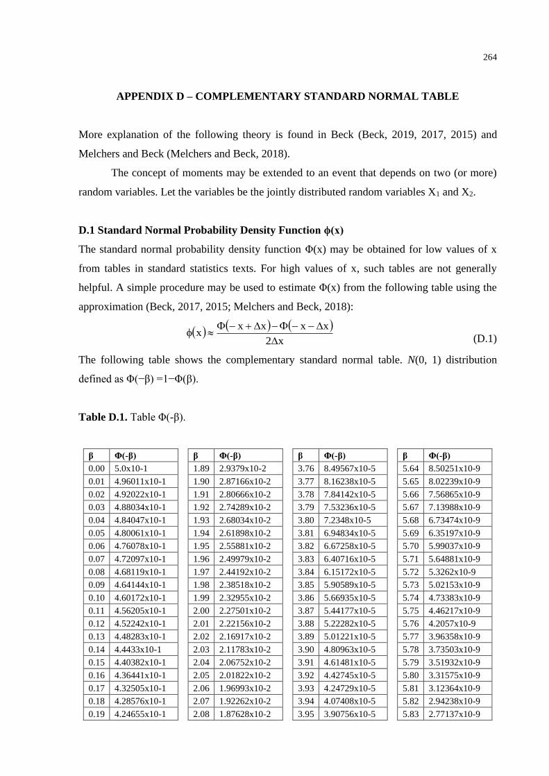
264

APPENDIX D – COMPLEMENTARY STANDARD NORMAL TABLE



The concept of moments may be extended to an event that depends on two (or more)

random variables. Let the variables be the jointly distributed random variables X1 and X2.

D.1 Standard Normal Probability Density Function ϕ(x)

The standard normal probability density function Φ(x) may be obtained for low values of x

from tables in standard statistics texts. For high values of x, such tables are not generally

helpful. A simple procedure may be used to estimate Φ(x) from the following table using the

approximation (Beck, 2017, 2015; Melchers and Beck, 2018):

( )( ) ( )

x2

xxxxx

−−−+−

(D.1)

The following table shows the complementary standard normal table. N(0, 1) distribution

defined as Φ(−β) =1−Φ(β).

Table D.1. Table Φ(-β).

β Φ(-β) β Φ(-β) β Φ(-β) β Φ(-β)

0.00 5.0x10-1 1.89 2.9379x10-2 3.76 8.49567x10-5 5.64 8.50251x10-9

0.01 4.96011x10-1 1.90 2.87166x10-2 3.77 8.16238x10-5 5.65 8.02239x10-9

0.02 4.92022x10-1 1.91 2.80666x10-2 3.78 7.84142x10-5 5.66 7.56865x10-9

0.03 4.88034x10-1 1.92 2.74289x10-2 3.79 7.53236x10-5 5.67 7.13988x10-9

0.04 4.84047x10-1 1.93 2.68034x10-2 3.80 7.2348x10-5 5.68 6.73474x10-9

0.05 4.80061x10-1 1.94 2.61898x10-2 3.81 6.94834x10-5 5.69 6.35197x10-9

0.06 4.76078x10-1 1.95 2.55881x10-2 3.82 6.67258x10-5 5.70 5.99037x10-9

0.07 4.72097x10-1 1.96 2.49979x10-2 3.83 6.40716x10-5 5.71 5.64881x10-9

0.08 4.68119x10-1 1.97 2.44192x10-2 3.84 6.15172x10-5 5.72 5.3262x10-9

0.09 4.64144x10-1 1.98 2.38518x10-2 3.85 5.90589x10-5 5.73 5.02153x10-9

0.10 4.60172x10-1 1.99 2.32955x10-2 3.86 5.66935x10-5 5.74 4.73383x10-9

0.11 4.56205x10-1 2.00 2.27501x10-2 3.87 5.44177x10-5 5.75 4.46217x10-9

0.12 4.52242x10-1 2.01 2.22156x10-2 3.88 5.22282x10-5 5.76 4.2057x10-9

0.13 4.48283x10-1 2.02 2.16917x10-2 3.89 5.01221x10-5 5.77 3.96358x10-9

0.14 4.4433x10-1 2.03 2.11783x10-2 3.90 4.80963x10-5 5.78 3.73503x10-9

0.15 4.40382x10-1 2.04 2.06752x10-2 3.91 4.61481x10-5 5.79 3.51932x10-9

0.16 4.36441x10-1 2.05 2.01822x10-2 3.92 4.42745x10-5 5.80 3.31575x10-9

0.17 4.32505x10-1 2.06 1.96993x10-2 3.93 4.24729x10-5 5.81 3.12364x10-9

0.18 4.28576x10-1 2.07 1.92262x10-2 3.94 4.07408x10-5 5.82 2.94238x10-9

0.19 4.24655x10-1 2.08 1.87628x10-2 3.95 3.90756x10-5 5.83 2.77137x10-9

265

β Φ(-β) β Φ(-β) β Φ(-β) β Φ(-β)

0.20 4.2074x10-1 2.09 1.83089x10-2 3.96 3.74749x10-5 5.84 2.61004x10-9

0.21 4.16834x10-1 2.10 1.78644x10-2 3.97 3.59363x10-5 5.85 2.45787x10-9

0.22 4.12936x10-1 2.11 1.74292x10-2 3.98 3.44576x10-5 5.86 2.31434x10-9

0.23 4.09046x10-1 2.12 1.7003x10-2 3.99 3.30366x10-5 5.87 2.17898x10-9

0.24 4.05165x10-1 2.13 1.65858x10-2 4.00 3.16712x10-5 5.88 2.05133x10-9

0.25 4.01294x10-1 2.14 1.61774x10-2 4.01 3.03594x10-5 5.89 1.93098x10-9

0.26 3.97432x10-1 2.15 1.57776x10-2 4.02 2.90991x10-5 5.90 1.81751x10-9

0.27 3.9358x10-1 2.16 1.53863x10-2 4.03 2.78884x10-5 5.91 1.71054x10-9

0.28 3.89739x10-1 2.17 1.50034x10-2 4.04 2.67256x10-5 5.92 1.60971x10-9

0.29 3.85908x10-1 2.18 1.46287x10-2 4.05 2.56088x10-5 5.93 1.51467x10-9

0.30 3.82089x10-1 2.19 1.42621x10-2 4.06 2.45364x10-5 5.94 1.42511x10-9

0.31 3.7828x10-1 2.20 1.39034x10-2 4.07 2.35066x10-5 5.95 1.34071x10-9

0.32 3.74484x10-1 2.21 1.35526x10-2 4.08 2.25179x10-5 5.96 1.26119x10-9

0.33 3.707x10-1 2.22 1.32094x10-2 4.09 2.15687x10-5 5.97 1.18627x10-9

0.34 3.66928x10-1 2.23 1.28737x10-2 4.10 2.06575x10-5 5.98 1.11569x10-9

0.35 3.63169x10-1 2.24 1.25455x10-2 4.11 1.9783x10-5 5.99 1.04921x10-9

0.36 3.59424x10-1 1.88 3.0054x10-2 4.12 1.89436x10-5 6.00 9.86588x10-10

0.37 3.55691x10-1 2.25 1.22245x10-2 4.13 1.81382x10-5 6.01 9.27617x10-10

0.38 3.51973x10-1 2.26 1.19106x10-2 4.14 1.73653x10-5 6.02 8.72085x10-10

0.39 3.48268x10-1 2.27 1.16038x10-2 4.15 1.66238x10-5 6.03 8.19798x10-10

0.40 3.44578x10-1 2.28 1.13038x10-2 4.16 1.59124x10-5 6.04 7.70571x10-10

0.41 3.40903x10-1 2.29 1.10107x10-2 4.17 1.523x10-5 6.05 7.24229x10-10

0.42 3.37243x10-1 2.30 1.07241x10-2 4.18 1.45755x10-5 6.06 6.80608x10-10

0.43 3.33598x10-1 2.31 1.04441x10-2 4.19 1.39477x10-5 6.07 6.39551x10-10

0.44 3.29969x10-1 2.32 1.01704x10-2 4.20 1.33457x10-5 6.08 6.00913x10-10

0.45 3.26355x10-1 2.33 9.90308x10-3 4.21 1.27685x10-5 6.09 5.64553x10-10

0.46 3.22758x10-1 2.34 9.64187x10-3 4.22 1.22151x10-5 6.10 5.30342x10-10

0.47 3.19178x10-1 2.35 9.38671x10-3 4.23 1.16846x10-5 6.11 4.98156x10-10

0.48 3.15614x10-1 2.36 9.13747x10-3 4.24 1.1176x10-5 6.12 4.67877x10-10

0.49 3.12067x10-1 2.37 8.89404x10-3 4.25 1.06885x10-5 6.13 4.39395x10-10

0.50 3.08538x10-1 2.38 8.65632x10-3 4.26 1.02213x10-5 6.14 4.12607x10-10

0.51 3.05026x10-1 2.39 8.42419x10-3 4.27 9.77365x10-6 6.15 3.87415x10-10

0.52 3.01532x10-1 2.40 8.19754x10-3 4.28 9.34467x10-6 6.16 3.63725x10-10

0.53 2.98056x10-1 2.41 7.97626x10-3 4.29 8.93366x10-6 6.17 3.4145x10-10

0.54 2.94599x10-1 2.42 7.76025x10-3 4.30 8.53991x10-6 6.18 3.20508x10-10

0.55 2.9116x10-1 2.43 7.54941x10-3 4.31 8.16273x10-6 6.19 3.00821x10-10

0.56 2.8774x10-1 2.44 7.34363x10-3 4.32 7.80146x10-6 6.20 2.82316x10-10

0.57 2.84339x10-1 2.45 7.14281x10-3 4.33 7.45547x10-6 6.21 2.64923x10-10

0.58 2.80957x10-1 2.46 6.94685x10-3 4.34 7.12414x10-6 6.22 2.48577x10-10

0.59 2.77595x10-1 2.47 6.75565x10-3 4.35 6.80688x10-6 6.23 2.33218x10-10

0.60 2.74253x10-1 2.48 6.56912x10-3 4.36 6.50312x10-6 6.24 2.18785x10-10

0.61 2.70931x10-1 2.49 6.38715x10-3 4.37 6.21233x10-6 6.25 2.05226x10-10

0.62 2.67629x10-1 2.50 6.20967x10-3 4.38 5.93397x10-6 6.26 1.92489x10-10

0.63 2.64347x10-1 2.51 6.03656x10-3 4.39 5.66753x10-6 6.27 1.80524x10-10

0.64 2.61086x10-1 2.52 5.86774x10-3 4.40 5.41254x10-6 6.28 1.69287x10-10

0.65 2.57846x10-1 2.53 5.70313x10-3 4.41 5.16853x10-6 6.29 1.58733x10-10

0.66 2.54627x10-1 2.54 5.54262x10-3 4.42 4.93505x10-6 6.30 1.48823x10-10

266

β Φ(-β) β Φ(-β) β Φ(-β) β Φ(-β)

0.67 2.51429x10-1 2.55 5.38615x10-3 4.43 4.71165x10-6 6.31 1.39518x10-10

0.68 2.48252x10-1 2.56 5.23361x10-3 4.44 4.49794x10-6 6.32 1.30782x10-10

0.69 2.45097x10-1 2.57 5.08493x10-3 4.45 4.29351x10-6 6.33 1.22581x10-10

0.70 2.41964x10-1 2.58 4.94002x10-3 4.46 4.09798x10-6 6.34 1.14883x10-10

0.71 2.38852x10-1 2.59 4.7988x10-3 4.47 3.91098x10-6 6.35 1.07657x10-10

0.72 2.35762x10-1 2.60 4.66119x10-3 4.48 3.73215x10-6 6.36 1.00877x10-10

0.73 2.32695x10-1 2.61 4.52711x10-3 4.49 3.56116x10-6 6.37 9.45141x10-11

0.74 2.2965x10-1 2.62 4.39649x10-3 4.50 3.39767x10-6 6.38 8.8544x10-11

0.75 2.26627x10-1 2.63 4.26924x10-3 4.51 3.24138x10-6 6.39 8.29429x10-11

0.76 2.23627x10-1 2.64 4.1453x10-3 4.52 3.09198x10-6 6.40 7.76885x10-11

0.77 2.2065x10-1 2.65 4.02459x10-3 4.53 2.94918x10-6 6.41 7.27598x10-11

0.78 2.17695x10-1 2.66 3.90703x10-3 4.54 2.81271x10-6 6.42 6.81372x10-11

0.79 2.14764x10-1 2.67 3.79256x10-3 4.55 2.6823x10-6 6.43 6.3802x10-11

0.80 2.11855x10-1 2.68 3.68111x10-3 4.56 2.55768x10-6 6.44 5.97368x10-11

0.81 2.0897x10-1 2.69 3.5726x10-3 4.57 2.43862x10-6 6.45 5.59251x10-11

0.82 2.06108x10-1 2.70 3.46697x10-3 4.58 2.32488x10-6 6.46 5.23515x10-11

0.83 2.03269x10-1 2.71 3.36416x10-3 4.59 2.21623x10-6 6.47 4.90015x10-11

0.84 2.00454x10-1 2.72 3.2641x10-3 4.60 2.11245x10-6 6.48 4.58613x10-11

0.85 1.97663x10-1 2.73 3.16672x10-3 4.61 2.01334x10-6 6.49 4.29182x10-11

0.86 1.94895x10-1 2.74 3.07196x10-3 4.62 1.9187x10-6 6.50 4.016x10-11

0.87 1.9215x10-1 2.75 2.97976x10-3 4.63 1.82833x10-6 6.51 3.75754x10-11

0.88 1.8943x10-1 2.76 2.89007x10-3 4.64 1.74205x10-6 6.52 3.51537x10-11

0.89 1.86733x10-1 2.77 2.80281x10-3 4.65 1.65968x10-6 6.53 3.28849x10-11

0.90 1.8406x10-1 2.78 2.71794x10-3 4.66 1.58105x10-6 6.54 3.07594x10-11

0.91 1.81411x10-1 2.79 2.6354x10-3 4.67 1.506x10-6 6.55 2.87685x10-11

0.92 1.78786x10-1 2.80 2.55513x10-3 4.68 1.43437x10-6 6.56 2.69039x10-11

0.93 1.76186x10-1 2.81 2.47707x10-3 4.69 1.36603x10-6 6.57 2.51577x10-11

0.94 1.73609x10-1 2.82 2.40118x10-3 4.70 1.30081x10-6 6.58 2.35224x10-11

0.95 1.71056x10-1 2.83 2.3274x10-3 4.71 1.23858x10-6 6.59 2.19914x10-11

0.96 1.68528x10-1 2.84 2.25568x10-3 4.72 1.17922x10-6 6.60 2.05579x10-11

0.97 1.66023x10-1 2.85 2.18596x10-3 4.73 1.1226x10-6 6.61 1.9216x10-11

0.98 1.63543x10-1 2.86 2.11821x10-3 4.74 1.06859x10-6 6.62 1.796x10-11

0.99 1.61087x10-1 2.87 2.05236x10-3 4.75 1.01708x10-6 6.63 1.67844x10-11

1.00 1.58655x10-1 2.88 1.98838x10-3 4.76 9.67965x10-7 6.64 1.56842x10-11

1.01 1.56248x10-1 2.89 1.92621x10-3 4.77 9.2113x10-7 6.65 1.46547x10-11

1.02 1.53864x10-1 2.90 1.86581x10-3 4.78 8.76476x10-7 6.66 1.36914x10-11

1.03 1.51505x10-1 2.91 1.80714x10-3 4.79 8.33907x10-7 6.67 1.27902x10-11

1.04 1.4917x10-1 2.92 1.75016x10-3 4.80 7.93328x10-7 6.68 1.19471x10-11

1.05 1.46859x10-1 2.93 1.69481x10-3 4.81 7.54651x10-7 6.69 1.11585x10-11

1.06 1.44572x10-1 2.94 1.64106x10-3 4.82 7.17791x10-7 6.70 1.0421x10-11

1.07 1.4231x10-1 2.95 1.58887x10-3 4.83 6.82665x10-7 6.71 9.73122x10-12

1.08 1.40071x10-1 2.96 1.5382x10-3 4.84 6.49196x10-7 6.72 9.08623x10-12

1.09 1.37857x10-1 2.97 1.489x10-3 4.85 6.17307x10-7 6.73 8.48316x10-12

1.10 1.35666x10-1 2.98 1.44124x10-3 4.86 5.86929x10-7 6.74 7.91933x10-12

1.11 1.335x10-1 2.99 1.39489x10- 4.87 5.57991x10-7 6.75 7.39225x10-12

1.12 1.31357x10-1 3.00 1.3499x10-3 4.88 5.30429x10-7 6.76 6.89959x10-12

1.13 1.29238x10-1 3.01 1.30624x10-3 4.89 5.0418x10-7 6.77 6.43913x10-12

267

β Φ(-β) β Φ(-β) β Φ(-β) β Φ(-β)

1.14 1.27143x10-1 3.02 1.26387x10-3 4.90 4.79183x10-7 6.78 6.0088x10-12

1.15 1.25072x10-1 3.03 1.22277x10-3 4.91 4.55382x10-7 6.79 5.60668x10-12

1.16 1.23024x10-1 3.04 1.18289x10-3 4.92 4.32721x10-7 6.80 5.23098x10-12

1.17 1.21x10-1 3.05 1.14421x10-3 4.93 4.11148x10-7 6.81 4.87993x10-12

1.18 1.19x10-1 3.06 1.10668x10-3 4.94 3.90613x10-7 6.82 4.55203x10-12

1.19 1.17023x10-1 3.07 1.07029x10-3 4.95 3.71067x10-7 6.83 4.24571x10-12

1.20 1.1507x10-1 3.08 1.035x10-3 4.96 3.52466x10-7 6.84 3.95967x10-12

1.21 1.13139x10-1 3.09 1.00078x10-3 4.97 3.34765x10-7 6.85 3.69249x10-12

1.22 1.11232x10-1 3.10 9.67603x10-4 4.98 3.17921x10-7 6.86 3.44302x10-12

1.23 1.09349x10-1 3.11 9.35437x10-4 4.99 3.01896x10-7 6.87 3.2101x10-12

1.24 1.07488x10-1 3.12 9.04255x10-4 5.00 2.86652x10-7 6.88 2.99261x10-12

1.25 1.0565x10-1 3.13 8.74032x10-4 5.01 2.7215x10-7 6.89 2.7896x10-12

1.26 1.03835x10-1 3.14 8.44739x10-4 5.02 2.58357x10-7 6.90 2.60014x10-12

1.27 1.02042x10-1 3.15 8.16352x10-4 5.03 2.4524x10-7 6.91 2.42328x10-12

1.28 1.00273x10-1 3.16 7.88846x10-4 5.04 2.32766x10-7 6.92 2.25819x10-12

1.29 9.85253x10-2 3.17 7.62195x10-4 5.05 2.20905x10-7 6.93 2.10421x10-12

1.30 9.68005x10-2 3.18 7.36375x10-4 5.06 2.09628x10-7 6.94 1.96049x10-12

1.31 9.50979x10-2 3.19 7.11364x10-4 5.07 1.98908x10-7 6.95 1.82643x10-12

1.32 9.34175x10-2 3.20 6.87138x10-4 5.08 1.88717x10-7 6.96 1.70136x10-12

1.33 9.17591x10-2 3.21 6.63675x10-4 5.09 1.79032x10-7 6.97 1.58473x10-12

1.34 9.01227x10-2 3.22 6.40953x10-4 5.10 1.69827x10-7 6.98 1.47587x10-12

1.35 8.8508x10-2 3.23 6.18951x10-4 5.11 1.61079x10-7 6.99 1.37446x10-12

1.36 8.6915x10-2 3.24 5.97648x10-4 5.12 1.52768x10-7 7.00 1.27981x10-12

1.37 8.53435x10-2 3.25 5.77025x10-4 5.13 1.44871x10-7 7.01 1.1916x10-12

1.38 8.37933x10-2 3.26 5.57061x10-4 5.14 1.37369x10-7 7.02 1.10933x10-12

1.39 8.22644x10-2 3.27 5.37737x10-4 5.15 1.30243x10-7 7.03 1.03267x10-12

1.40 8.07567x10-2 3.28 5.19035x10-4 5.16 1.23475x10-7 7.04 9.61176x10-13

1.41 7.92698x10-2 3.29 5.00937x10-4 5.17 1.17047x10-7 7.05 8.94562x10-13

1.42 7.78038x10-2 3.30 4.83424x10-4 5.18 1.10943x10-7 7.06 8.32501x10-13

1.43 7.63585x10-2 3.31 4.6648x10-4 5.19 1.05147x10-7 7.07 7.74658x10-13

1.44 7.49337x10-2 3.32 4.50087x10-4 5.20 9.96443x10-8 7.08 7.20757x10-13

1.45 7.35293x10-2 3.33 4.3423x10-4 5.21 9.44203x10-8 7.09 6.70575x10-13

1.46 7.2145x10-2 3.34 4.18892x10-4 5.22 8.94616x10-8 7.10 6.23779x10-13

1.47 7.07809x10-2 3.35 4.04058x10-4 5.23 8.4755x10-8 7.11 5.80203x10-13

1.48 6.94366x10-2 3.36 3.89712x10-4 5.24 8.02883x10-8 7.12 5.39624x10-13

1.49 6.81121x10-2 3.37 3.75841x10-4 5.25 7.60496x10-8 7.13 5.01821x10-13

1.50 6.68072x10-2 3.38 3.62429x10-4 5.26 7.20277x10-8 7.14 4.66682x10-13

1.51 6.55217x10-2 3.39 3.49463x10-4 5.27 6.82119x10-8 7.15 4.33875x10-13

1.52 6.42555x10-2 3.40 3.36929x10-4 5.28 6.45919x10-8 7.16 4.034x10-13

1.53 6.30084x10-2 3.41 3.24814x10-4 5.29 6.11582x10-8 7.17 3.74978x10-13

1.54 6.17802x10-2 3.42 3.13106x10-4 5.30 5.79013x10-8 7.18 3.48555x10-13

1.55 6.05708x10-2 3.43 3.01791x10-4 5.31 5.48126x10-8 7.19 3.23963x10-13

1.56 5.93799x10-2 3.44 2.90857x10-4 5.32 5.18836x10-8 7.20 3.01037x10-13

1.57 5.82076x10-2 3.45 2.80293x10-4 5.33 4.91064x10-8 7.21 2.79776x10-13

1.58 5.70534x10-2 3.46 2.70088x10-4 5.34 4.64733x10-8 7.22 2.59959x10-13

1.59 5.59174x10-2 3.47 2.60229x10-4 5.35 4.39771x10-8 7.23 2.41474x10-13

1.60 5.47993x10-2 3.48 2.50707x10-4 5.36 4.1611x10-8 7.24 2.24321x10-13

268

β Φ(-β) β Φ(-β) β Φ(-β) β Φ(-β)

1.61 5.36989x10-2 3.49 2.4151x10-4 5.37 3.93683x10-8 7.25 2.08389x10-13

1.62 5.26161x10-2 3.50 2.32629x10-4 5.38 3.72429x10-8 7.26 1.93567x10-13

1.63 5.15507x10-2 3.51 2.24053x10-4 5.39 3.52288x10-8 7.27 1.79745x10-13

1.64 5.05026x10-2 3.52 2.15773x10-4 5.40 3.33204x10-8 7.28 1.66922x10-13

1.65 4.94715x10-2 3.53 2.0778x10-4 5.41 3.15124x10-8 7.29 1.54987x10-13

1.66 4.84572x10-2 3.54 2.00064x10-4 5.42 2.97995x10-8 7.30 1.43885x10-13

1.67 4.74597x10-2 3.55 1.92616x10-4 5.43 2.8177x10-8 7.31 1.3356x10-13

1.68 4.64787x10-2 3.56 1.85427x10-4 5.44 2.66403x10-8 7.32 1.24012x10-13

1.69 4.5514x10-2 3.57 1.78491x10-4 5.45 2.51849x10-8 7.33 1.15075x10-13

1.70 4.45655x10-2 3.58 1.71797x10-4 5.46 2.38067x10-8 7.34 1.06803x10-13

1.71 4.36329x10-2 3.59 1.65339x10-4 5.47 2.25018x10-8 7.35 9.90874x10-14

1.72 4.27162x10-2 3.60 1.59109x10-4 5.48 2.12663x10-8 7.36 9.1982x10-14

1.73 4.18151x10-2 3.61 1.53099x10-4 5.49 2.00967x10-8 7.37 8.53206x10-14

1.74 4.09295x10-2 3.62 1.47302x10-4 5.50 1.89896x10-8 7.38 7.91589x10-14

1.75 4.00592x10-2 3.63 1.41711x10-4 5.51 1.79417x10-8 7.39 7.34413x10-14

1.76 3.92039x10-2 3.64 1.36319x10-4 5.52 1.695x10-8 7.40 6.81122x10-14

1.77 3.83636x10-2 3.65 1.3112x10-4 5.53 1.60115x10-8 7.41 6.31717x10-14

1.78 3.7538x10-2 3.66 1.26108x10-4 5.54 1.51236x10-8 7.42 5.85643x10-14

1.79 3.6727x10-2 3.67 1.21275x10-4 5.55 1.42835x10-8 7.43 5.42899x10-14

1.80 3.59303x10-2 3.68 1.16617x10-4 5.56 1.34887x10-8 7.44 5.03486x10-14

1.81 3.51479x10-2 3.69 1.12127x10-4 5.57 1.2737x10-8 7.45 4.66849x10-14

1.82 3.43795x10-2 3.70 1.078x10-4 5.58 1.20259x10-8 7.46 4.32432x10-14

1.83 3.3625x10-2 3.71 1.0363x10-4 5.59 1.13535x10-8 7.47 4.00791x10-14

1.84 3.28841x10-2 3.72 9.96114x10-5 5.60 1.07176x10-8 7.48 3.7137x10-14

1.85 3.21568x10-2 3.73 9.57399x10-5 5.61 1.01163x10-8 7.49 3.44169x10-14

1.86 3.14428x10-2 3.74 9.20101x10-5 5.62 9.54787x10-9

1.87 3.07419x10-2 3.75 8.84173x10-5 5.63 9.01048x10-9

269

APPENDIX E

RELATIONSHIP OF RELIABILITY RESULTS

270

APPENDIX E – RELATIONSHIP OF RELIABILITY RESULTS

More explanation of the following theory is found in Duncan et al. (Duncan et al., 2014) and

GeoStudio (GeoStudio, 2018b).

When the shape of the probability distribution is known, the reliability index can be related

directly to the probability of failure. Figure E.1 illustrates the relationship of the reliability index

to the probability of failure for a normally distributed factor of safety. The probability of failure

(Pf) can be determined using Table E.1 and E.2.

Figure E.1. Relationship between reliability index and the probability of failure for a normal

distribution.

271

Table E.1. Probabilities that Factor of Safety (normal distribution) is smaller than 1.0.

Coefficient of Variation of Factor of Safety (COVF in %)

FMLV 2 4 6 8 10 12 14 16 20 25 30 40 50 60 80

1.05 0.9 11.7 21.4 27.6 31.7 34.6 36.7 38.3 40.6 42.4 43.7 45.3 46.2 46.8 47.6

1.10 0.0 1.2 6.5 12.8 18.2 22.4 25.8 28.5 32.5 35.8 38.1 41.0 42.8 44.0 45.5

1.15 0.0 0.1 1.5 5.2 9.6 13.9 17.6 20.7 25.7 30.1 33.2 37.2 39.7 41.4 43.5

1.16 0.0 0.0 1.1 4.2 8.4 12.5 16.2 19.4 24.5 29.1 32.3 36.5 39.1 40.9 43.2

1.18 0.0 0.0 0.6 2.8 6.4 10.2 13.8 17.0 22.3 27.1 30.6 35.1 38.0 40.0 42.4

1.20 0.0 0.0 0.3 1.9 4.8 8.2 11.7 14.9 20.2 25.2 28.9 33.8 36.9 39.1 41.7

1.25 0.0 0.0 0.0 0.6 2.3 4.8 7.7 10.6 15.9 21.2 25.2 30.9 34.5 36.9 40.1

1.30 0.0 0.0 0.0 0.2 1.1 2.7 5.0 7.5 12.4 17.8 22.1 28.2 32.2 35.0 38.6

1.35 0.0 0.0 0.0 0.1 0.5 1.5 3.2 5.3 9.7 15.0 19.4 25.8 30.2 33.3 37.3

1.40 0.0 0.0 0.0 0.0 0.2 0.9 2.1 3.7 7.7 12.7 17.0 23.8 28.4 31.7 36.0

1.50 0.0 0.0 0.0 0.0 0.0 0.3 0.9 1.9 4.8 9.1 13.3 20.2 25.2 28.9 33.8

1.60 0.0 0.0 0.0 0.0 0.0 0.1 0.4 1.0 3.0 6.7 10.6 17.4 22.7 26.6 32.0

1.70 0.0 0.0 0.0 0.0 0.0 0.0 0.2 0.5 2.0 5.0 8.5 15.2 20.5 24.6 30.3

1.80 0.0 0.0 0.0 0.0 0.0 0.0 0.1 0.3 1.3 3.8 6.9 13.3 18.7 22.9 28.9

1.90 0.0 0.0 0.0 0.0 0.0 0.0 0.0 0.2 0.9 2.9 5.7 11.8 17.2 21.5 27.7

2.00 0.0 0.0 0.0 0.0 0.0 0.0 0.0 0.1 0.6 2.3 4.8 10.6 15.9 20.2 26.6

2.20 0.0 0.0 0.0 0.0 0.0 0.0 0.0 0.0 0.3 1.5 3.5 8.6 13.8 18.2 24.8

2.40 0.0 0.0 0.0 0.0 0.0 0.0 0.0 0.0 0.2 1.0 2.6 7.2 12.2 16.5 23.3

2.60 0.0 0.0 0.0 0.0 0.0 0.0 0.0 0.0 0.1 0.7 2.0 6.2 10.9 15.3 22.1

2.80 0.0 0.0 0.0 0.0 0.0 0.0 0.0 0.0 0.1 0.5 1.6 5.4 9.9 14.2 21.1

3.00 0.0 0.0 0.0 0.0 0.0 0.0 0.0 0.0 0.0 0.4 1.3 4.8 9.1 13.3 20.2

Table E.2. Probabilities that Factor of Safety (lognormal distribution) is smaller than 1.0.

Coefficient of Variation of Factor of Safety (COVF in %)

FMLV 2 4 6 8 10 12 14 16 20 25 30 40 50 60 80

1.05 0.8 12.0 22.0 28.0 33.0 36.0 39.0 41.0 44.0 47.0 49.0 53.0 55.0 58.0 61.0

1.10 0.0 0.9 6.0 12.0 18.0 23.0 27.0 30.0 35.0 40.0 43.0 48.0 51.0 54.0 59.0

1.15 0.0 0.0 1.1 4.0 9.0 13.0 18.0 21.0 27.0 33.0 37.0 43.0 48.0 51.0 56.0

1.16 0.0 0.0 0.7 3.0 8.0 12.0 16.0 20.0 26.0 32.0 36.0 42.0 47.0 50.0 56.0

1.18 0.0 0.0 0.3 2.0 5.0 9.0 13.0 17.0 23.0 29.0 34.0 41.0 45.0 49.0 55.0

1.20 0.0 0.0 0.1 1.2 4.0 7.0 11.0 14.0 21.0 27.0 32.0 39.0 44.0 48.0 54.0

1.25 0.0 0.0 0.0 0.3 1.4 4.0 6.0 9.0 15.0 22.0 27.0 35.0 41.0 45.0 51.0

1.30 0.0 0.0 0.0 0.1 0.5 1.6 3.0 6.0 11.0 17.0 23.0 31.0 37.0 42.0 49.0

1.35 0.0 0.0 0.0 0.0 0.2 0.7 1.9 4.0 8.0 14.0 19.0 28.0 34.0 40.0 47.0

1.40 0.0 0.0 0.0 0.0 0.0 0.3 1.0 2.0 5.0 11.0 16.0 25.0 32.0 37.0 45.0

1.50 0.0 0.0 0.0 0.0 0.0 0.0 0.2 0.7 3.0 6.0 11.0 19.0 27.0 32.0 41.0

1.60 0.0 0.0 0.0 0.0 0.0 0.0 0.1 0.2 1.1 4.0 7.0 15.0 22.0 28.0 38.0

1.70 0.0 0.0 0.0 0.0 0.0 0.0 0.0 0.1 0.5 2.0 5.0 12.0 19.0 25.0 34.0

1.80 0.0 0.0 0.0 0.0 0.0 0.0 0.0 0.0 0.2 1.2 3.0 9.0 16.0 22.0 31.0

1.90 0.0 0.0 0.0 0.0 0.0 0.0 0.0 0.0 0.1 0.7 2.0 7.0 13.0 19.0 29.0

2.00 0.0 0.0 0.0 0.0 0.0 0.0 0.0 0.0 0.0 0.4 1.3 5.0 11.0 17.0 26.0

2.20 0.0 0.0 0.0 0.0 0.0 0.0 0.0 0.0 0.0 0.1 0.6 3.0 8.0 13.0 22.0

2.40 0.0 0.0 0.0 0.0 0.0 0.0 0.0 0.0 0.0 0.0 0.2 1.9 5.0 10.0 19.0

2.60 0.0 0.0 0.0 0.0 0.0 0.0 0.0 0.0 0.0 0.0 0.1 1.1 4.0 7.0 16.0

2.80 0.0 0.0 0.0 0.0 0.0 0.0 0.0 0.0 0.0 0.0 0.0 0.7 3.0 6.0 13.0

3.00 0.0 0.0 0.0 0.0 0.0 0.0 0.0 0.0 0.0 0.0 0.0 0.4 1.8 4.0 11.0

RELIABILITY-BASED DESIGN OF AN EARTH AND ...

Documents

Transcript of RELIABILITY-BASED DESIGN OF AN EARTH AND ...