" -- 92-7 ,1 5

.... . "PREPRINT

-V - - - N

DDAMD EARTH<MODELS-": GOD':D :"/ /. N N I'

-'I"N '-./ 3 'N.-

\6);(NAS A-TM-X 708681 GODDARD ERTH MODELS (5 75-21920

AND 6) (NASA) 238 p HC $7.50- CSCL 08E

- J,~ N

Unclas

F " .LE R C

-- ; - _ - ' - - .I ~ I X IN

N~ N

. " . "(5-A- -D< )r >-\. -

G3/5 18816

' -,,A WAGNER"/. . I . . J. .LE R C H-

-.A 'R I C'HA RDSO

S- - - -,J. E BRO-WNDI. .,. , .

N , - , y.. , . . 1N< ; , - --.

• .N' - -N- ; . ,,I N . *-. - ) (.'. -- -, .

N ' /

, ' ,- -

-1 . :-, DECEMBER 197 -4, --)., - , ", N- iN

Ij.

" I -- - 6 . . .. _-

2 -

-/ \ " " , - " j

GODDARD SPACE FLIGHT CENTER-GREENBELTr MARYLAND,

S .. , - . .V

>.- -. '" • - ., -

I / ''

N~ -'

N.-_' \- 'N,

'N / I ~N

-For information concerning availabilityof this document contact:

Technical Information Division, Code 250Goddard Space Flight CenterGreenbelt, Maryland 20771

(Telephone 301-982-4488)

"This paper presents the views of the author(s), and does not necessarilyreflect the views of the Goddard Space Flight Center, or NASA."

N N

X-921-74-145

GODDARD EARTH MODELS (5 AND 6)

Francis J. Lerch

Carl A. Wagner

Geodynamics Branch. GSFC

James A. RichardsonJoseph E. Brownd

Computer Sciences Corp. , Silver Spring, Md.

December 1974

SResults presented at the 55th Annual Meeting of tllheArnerican Gcophysical Union, April 8-12. 1974, Washington, D.C.

GODDARD SPACE FLIGHT CENTER

Greenbelt, Maryland

GODDARD EARTH MODELS 5 AND 6

ABSTRACT

A comprehensive earth model has been developed at the Goddard Space Flight

Center to satisfy requirements of the National Geodetic Satellite Program. The

model consists of two complementary gravitational fields (in spherical harmon-

ics) and center-of-mass locations for 134 tracking stations on the earth's sur-

face. One gravitational field (Goddard Earth Model 5) is derived solely from

satellite tracking data. This data on 27 satellite orbits is the most extensive

used for such a solution. It includes 120,000 precisely reduced optical obser-

vations on 23 satellites, 160,000 one way doppler observations on 5 satellites.

10,000 laser ranges to 6 satellites, 100,000 S-band range and range-rate meas-

urements to 1 satellite, 4, 000 C-band ranges to 1 satellite and 3. 000 radio in-

terferometric (Minitrack) measurements on 4 satellite orbits. A second (com-

bination) solution (GEM 6) uses this data with 13,400 simultaneous events from

satellite camera observations, and 1654 50 x 50 surface gravimetric anomalies.

This solution consists of 134 geocentric station locations, 328 spherical harmon-

ics of gravity, the radius of the earth and the equatorial constant of gravity. The

derived gravitational field is complete to (16, 16) with resonant and zonal terms

to 22nd degree. The derived mean equatorial radius of the earth is 6378144 me-

ters. The satellite-only solution as a whole is accurate to about 4.5 milligals

as judged by the surface gravity data. The majority of the station coordinates

are accurate to better than 10 meters as judged by independent results from geo-

detic surveys and by doppler tracking of both distant space probes and near earth

orbits. Both of these figures serve to meet requirements of the national

program.

PRECEDING PAGE BLANK NOT FILMED

iii

PREFACE

Over the period of the National Geodetic Satellite Programnumerous people have contributed to the development of theprogram systems which led ultimately to the models forGEM 5 and 6. A list of these people and their areas of con-tribution is presented in a section under acknowledgments.For the current report, special acknowledgment is given toThomas V. Martin, of Wolf Research and Development Cor-poration and to Barbara H. Putney, of GSFC, for the prepa-ration of written material in Appendix A on the orbital theoryemployed in the GEODYN (Geodynamics) program. Specialacknowledgment is given to James S. Reece, of ComputerSciences Corporation, for his contributions to the geometrictheory and related program for the adjustment of station co-ordinates from simultaneous observations. Wayne A. Taylor,of Computer Sciences Corporation, was instrumental for thedata processing and Barbara H. Putney for the managementand integrity of the computer program system. Finally, weextend appreciation to Professor R. H. Rapp, of The OhioState University for his work in the preparation of thesurface gravity data employed and related techniques forapplications.

iv

ACKNOWLEDGMENT

The following contributors and their contributions to the development of theGoddard Earth Models have been recognized and are gratefully acknowledged.There are five periods for this development leading to the GEM 5 and 6 NGSPsolutions:

1. 1965-1966; the development of the GEOS-A flash schedule using data typesfor all major geodetic systems.

2. 1966-1968; GEOS A and B Tracking system intercomparisons: the initiation

of the NONAME orbit determination system.

3. 1967-1969; multi-satellite operations: the development of NONAME to han-

dle all satellites and tracking formats.

4. 1968-1971; GEOSTAR development and preliminary solutions: geodetic pa-rameter and station recovery capability from satellite tracking achievedfrom extended NONAME with MERGE and SOLVE programs.

5. 1971-1974; Goddard Earth Models solutions (1-6) from satellite and surfacegravity data.

The period of the contribution is indicated by a superscript on the contributor'sname. Four types of contributions are recognized: P-programming, develop-ment, and computer operations; RW-report writing; I-significant ideas; M-management operations (including project and data supply). These codes followthe contributor's name.

The following list is by no means exhaustive, and is broken down by organizationfor convenience.

Goddard Space Flight Center

F. Vonbun 2 -5(M), J. Siryl- 4 (I,P,M), D. Smith 4 , 5 (I), F. Lerchl- 5 (I,RW,P,M),

E. Dolll-3(I,M,RW), J. Marshl-3,5(I,RW,M,P), M. Velez 3 ,4(I,P,RW), G.

Brodsky3, 4 (P, RW), V. Laczo 3 , 4 (I,P), W. Kahn 3 , 4(I,M), B. Putney 3 - 5 (I,RW,

P,M), C. Wagner 4 , 5 (I,P,M,RW), T. Felsentreger 3 , 4 (I), J. Murphy3 , 4 (I),

J. Berbertl-3(I,RW), C. Looneyl(I,M), J. Zegalial, 2 (M), R. Mather 5 (I,P),

M. Khan 5 (I,P), E. Watkins2-5(M), D. Rose2-5(M).

v

Wolf Research and Development Corporation

R. Sandiferl, 2 (l,RW,P), S. Mossl- 3 (I,M), W. Wellsl- 3 (I), C. Martin2 , 3 (I,P,

RW), T. Martin 2 ,3, 5 (I,P), H. Kahlerl, 2 (I,P,M), E. Mullins 5 (RW), C. Goad2 , 3

(P,I), J. Serelis 5 (P), R. Williamsonl-3,5(P,i), V. Der 5 (I,P), J. Diamante 5

(I,P), J. Vetterl- 3 (P,I), S. Klosko 5 (), P. Dunn2 ' 3 (I,P,RW), B. Brown 2 , 3 (P,

I). M. Willoughbyl, 2 (P), N. Royl1 2 (I,RW), M. D'Arial,2(I,RW), B. O'Neilll, 2

(1,RW), Ms. Willoughbyl, 2 (P), B. Douglas 5 (I), M. Kaiserl(P,I.RW), R. Gotz 2 , 3

(1,RW,P), R. Brooks 1 '.2(I, RW).

Computer Sciences Corporation

K. Nickerson 4 ' 5 (I,P,M,RW), W. Taylor 4 , 5 (I,P,RW), D. McGraw 4 (P) , H.

Dennis4(P), H. Rainey 4 (P), D. Weiss 4 (P), C. Engrum4(P), L. Williams4(p),

C. Kenworthy 4 (P), K. Tasaki 4 (P), K. Lamars 4 (I), R. Grant 4 , 5 (I,P), M. Sand-

son 5 (I,RW,M), R. Brown 5 (I,P), J. Brownd 5 (I,P,RW,M), W. Strange 4 , 5 (I,M),

J. Richardson 5 (I,P,RW,M), J. Reece 5 (I,P,RW), R. Taylor 4 , 5 (M), M. Harri-

son 5 (P), A. Euler 5 (p).

IBM

F. Green 4 (I,M), R. Greene 4 (I,M), G. Finley3 , 4 (P), Y. Sawanobori 4 (p)

Computer Usage Corporation

C. Sheffield 4 (I), R. Hamblen 4 (P), J. Morris 4 (P).

Computer and Software, Inc. (and CSTA)

P. Gibbs 5 (P), D. Miller 5 (P), D. Mentges 4 , 5 (P), D. Mathews 4 (P), H. Huston 5 (P).

NASA Headquarters and Contracts through Headquarters

J. Rosenberg 1 , 2 (I, M ), W. Kaula 4 , 5 (I) , R. Rapp 5 (I,M), I. Mueller 2 (I), H.

Schmid 5 (M).

Smithsonian Astrophysical Observatory

B. Miller 4 , 5 (M).

vi

CONTENTS

Page

ABSTRACT . . ... .............. ... . . . . iii

PREFACE . . . . . . . . . . . . . . . . . . . . . . . . . . . . iv

ACKNOWLEDGMENTS ....................... v

1. INTRODUCTION . . . . . . . . . . . . . . . . .. . . . . 1

2. DATA EMPLOYED . ................ ..... 9

2.1 GEM 5 Data, Satellite Dynamic Solution . ......... 9

2.2 GEM 6 Data, Combination Solution . .......... . 9

3. MODELING AND ANALYSIS ................. 19

3.1 Geopotential . . . .... . . . . . . . . . . . . ...... 19

3.2 Techniques in Modeling the Data . ............ 20

3.3 Satellite Sensitivity to the Potential ..... . ... .... 22

3.4 Error Estimates for Geopotential Coefficients (GEM 5) . . . 28

3.4.1 Formulation of Error Estimates for GeoidHeight and Gravity Anomaly . ........... 28

3.4.2 Adjusted Error Estimates of PotentialCoefficients . . . . . . . . . . . . . . . . . .. 31

3.5 Relative Weighting and Error Estimates forCombined Solution (GEM 6).............. .. 33

3.6 Verification of Error Estimates . ............ 34

4. RESULTS . . . . . . . . . . . . . . . . . . . . . . . .. . 43

4.1 Gravitational Potential for GEM 5 and 6 . ......... 43

vii

CONTENTS (continued)

Page

4.1.1 ZonalHarmonics ................. 43

4.1.2 Comparison with Gravity Anomalies . ....... 43

4.1.3 Comparison with Satellite Data. . .......... 52

4.1.4 Geoid Height . . . . . . . . . . . . . . . . . .. 62

4.2 Station Coordinates for GEM 6 . ............. 65

4.2.1 Comparison with Other Solutions . ......... 72

4.2.2 Comparison with Mean Sea Level Heights . ..... 77

4.2.3 Comparison with Positions onNational Datums ................. 80

4.2.4 Displacements in Mean Pole andGreenwich Meridian . .............. 83

4.2.5 Summary of Results for Station Coordinates ..... 83

4.3 Geodetic Parameters . ................. 89

5. SUMMARY AND CONCLUSIONS ................ 93

REFERENCES ........... .. ... . . . ........ . 97

APPENDIX A-METHODS EMPLOYED . .............. A-1

Al. Orbit Theory for GEODYN . ............... Al-i

A2. Geometric Method for Simultaneous ObservationsIncluding Constraints from Datum Survey . ........ A2-1

A3. Gravimetric Method for Mean Anomaly Data . ....... A3-1

A4. Method of Combined Solution. .......... .... A4-1

APPENDIX B-SATELLITE AND GRAVITY DATA DISTRIBUTIONS B-1

viii1

LIST OF ILLUSTRATIONS

Figure Page

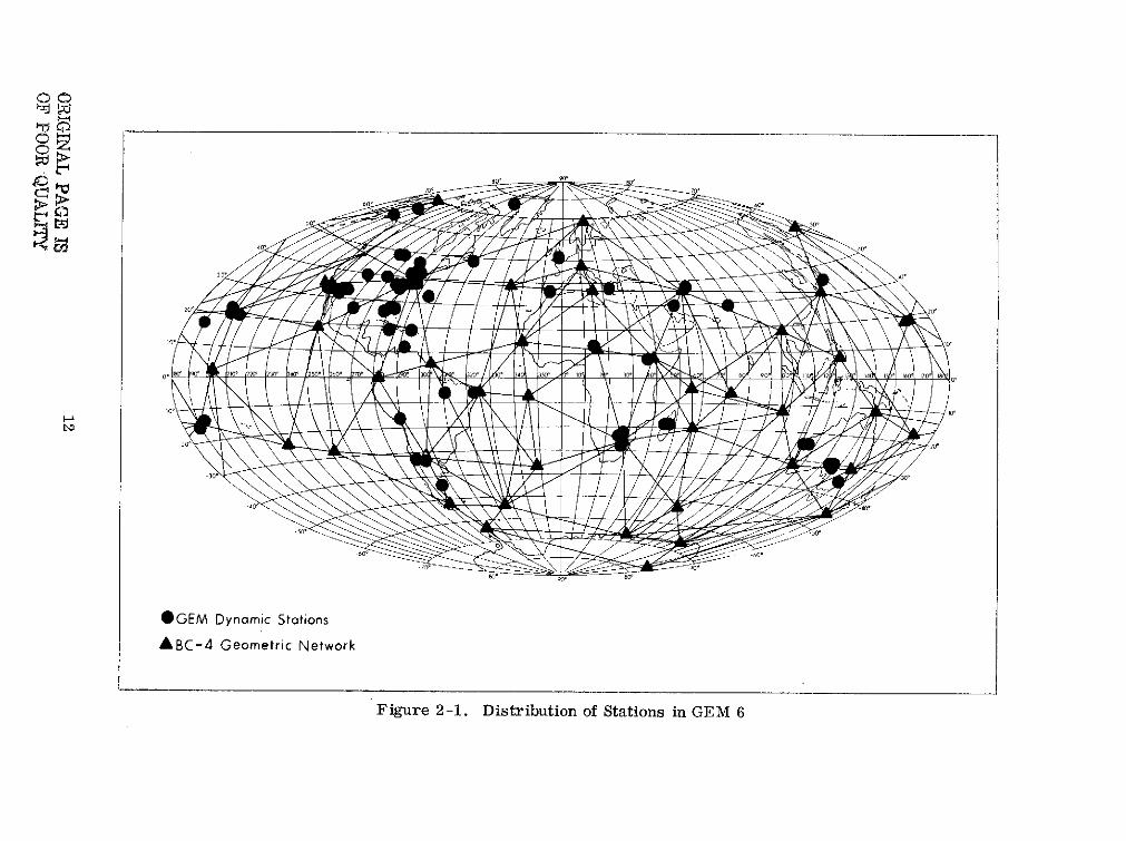
2-1 Distribution of Stations in GEM 6 . ....... . . . . . 12

2-2 BC-4 Baselines and Ties. . .... . . . . . . . . . . . 14

3-1 Average (rms) Coefficient Value by Degree . ....... 23

3-2 Satellite Sensitivity to Potential Terms (30 x 30) . ..... 26

3-3 Stochastic Satellite Sensitivity . ..... . . . . . . . ... 27

3-4 Average (rms) Standard Deviation Per Degree n

for GEM 5 and Gravimetry Solutions . ....... . . . 29

3-5 Percent Accuracy of GEM 5 Coefficients by Degree .... . 33

3-6 Percent Reduction in Error Variances of GEM 5 Due

to the Effect of Combining Gravimetry Data in GEM 6 . . . . 35

3-7 Comparison of Geoid Profile Derived from Altimetryand GEM 6 ...... ................ .... 38

3-8 Comparison of Error Estimates for Coefficients

of Degree n . . . . . . . . . . . . . . . . . . . . . . 39

4-1 GEM 5 Gravity Anomaly Contours . .......... . . 53

4-2 GEM 6 Gravity Anomaly Contours . .......... . . 54

4-3 GEM 5 Geoidal Heights ................. 55

4-4 GEM 6 Geoidal Heights ................. 56

4-5 Geoid Height Zonal Profile . ............... 63

4-6 Station Height above Geoid Computed by GEM 6

vs Surveyed Height . . . . . . . . . . . . . . . . . . . 79

4-7 Displacement of the Greenwich Meridian and Pole as

Shown through Comparisons with GEM 6 . .. . ..... . 87

ix

LIST OF TABLES

Table Page

1-1 Description of Goddard Earth Models . ....... . . . 5

2-1 Orbital Parameters on 27 Satellites and Distribution ofData for Satellite Arcs Using Optical Data Only ...... . 10

2-2 Distribution of Data for Satellite Arcs Using a Varietyof Tracking Systems ................. .. . 11

2-3 Simultaneous Observations Used for GeometricalStation Adjustment ................ .. 15

2-4 Baseline Constraints from Survey (BC-4 Stations) . .... . 15

2-5 Basic Geodetic Reference Parameters. . ......... . 16

2-6 Standard Deviations of Tracking Observations . ...... 16

3-1 Satellite Data and Sensitivity Level . ........... 24

3-2 Average (rms) Error Estimates for PotentialCoefficients of Degree n for GEM 6 ........... . . 35

3-3 Station Coordinate Error Estimates for TrackingSystems in GEM 6 ................... 36

4-1 GEM 5 Normalized Coefficients . ............ . 44

4-2 GEM 6 Normalized Coefficients ............ . . . 45

4-3 Comparison of Zonal Coefficients . ........ . . . . 46

4-4 Comparison of Terrestrial 50 Anomalies with AnomaliesComputed from Various Models . ............. 48

4-5 Statistical Error Estimates for Gravity Models Basedupon 50 Terrestrial Anomalies . ....... . . . . . . 49

4-6 Gravity Anomaly Degree Variances . ........... 51

4-7 RMS Value of Residuals of Two-Way Doppler for USBTracking on Daily Arcs of ERTS-1 . ........... 57

x

LIST OF TABLES (continued)

Table Page

4-8 Weighted RMS of Observation Residuals in Camera

Observations for a Weekly Arc on Each of 23 Satellites . . . 58

4-9 RMS of Residuals from Laser System Measurements

of Short Arcs of BE-C .................. 60

4-10 Comparison of Models for Long-Term Zonal

Perturbations....................... 60

4-11 Summary of Gravity Model Comparisons with

Satellite and Gravimetry Data . .. . ........... 61

4-12 Major Geoid Features . ................. 62

4-13 Global RMS of Geoid Height Differences with the

GEM 6 Model . . . . . . . . . . . . . . . . . . . . . . 64

4-14 Constraints on Relative Position (Survey Ties) . ...... 66

4-15 Constraints on Baseline Distance . ............ 68

4-16 GEM 6 Station Coordinates . ............... 69

4-17 Comparison with JPL's DSS (Deep Space Stations). . ... . 73

4-18 Direct Comparison of Spin Axis Distance andLongitude (GEM 6-JPL) ................. 73

4-19 Comparisons of GEM 6 with GEM 4 Station Positions . . .. 75

4-20 GEM 6-GSFC 73 Station Coordinates . ........ . . 76

4-21 Station Comparisons of GEM 6-SAO SE III .......... 76

4-22 Station Comparisons of GEM 6-NWL 9D . ......... 78

4-23 GEM 6-OSU WN4 Station Comparisons . ......... 78

4-24 Comparisons of Ay (coordinate differences) for

Selected BC-4 Stations. . ..... . . ......... 78

xi

LIST OF TABLES (continued)

Table Page

4-25 Station Comparisons of GEM 6-Mean Sea Level Height . . . 82

4-26 Adopted Origins Used for Solutions of Seven Parameterson Survey Datum . . . .. . .. . . . .. . . .. . .. 82

4-27 Solutions for Relation of GEM 6 to Major Datums . ..... 84

4-28 Differences between Coordinates of Stations in GEM 6and other Major Datums .................. 85

4-29 Datum Shifts to GEM 6 System .............. 88

xii

SECTION I. . . . . . .... INTRODUCTION

SECTION I . . . . . . . . . . INTRODUCTION

GODDARD EARTH MODELS 5 AND 6

1. INTRODUCTION

The 10 year National Geodetic Satellite Program (NGSP) had its start in 1964.

A principal goal was to determine a gravitational field for the earth complete to

(15,15) in spherical harmonics and with an overall accuracy of about 4 milligals

for this field. A complementary goal was to develop a worldwide geodetic sys-

tem. The geocentric position of a large number of surface stations on continents

and islands were to be found to within 10 meters.

At that time the long wavelength components of the field were virtually unknown,apart from the earth's oblateness and a few other low degree zonal terms. Until

these could be found, the bulk of the last 100 meters of the earth's shape would

remain unknown. Prior to the satellite era the positions of continents and ocean

islands themselves were not known to better than a kilometer with respect to

each other. These goals, while stated in terms of classical geodesy (the mea-

sure of the earth), were of equal utility to the space program.

Roughly speaking, the uncertainties of the earth's shape (the geoid) map with a

magnification of about ten to one into the periodic deviations of a close satellite's

orbit in a day's time. Similarly, the uncertainties in tracking station positions

map roughly one to one into periodic orbit errors. Thus, in the early 1960's the

tracking error within a well-observed one day arc, just from the uncertainties in

the gravity field and surface locations, was of the order of a kilometer. This

was an intolerable situation when the trackers available at the time had accura-

cies as much as two orders of magnitude better than this. But even before the

national program began Izsak (1963) at the Smithsonian Astrophysical Observa-

tory, Anderle (1965) at the Naval Weapons Laboratory, Guier (1963) at the Ap-

plied Physics Laboratory, and Kaula (1963) at Goddard Space Flight Center had

used camera and radio doppler tracking data to derive complex fields and begin

the reduction of these orbit errors. The methods available for orbit computation

in this early work were analytic and numeric; not essentially different from those

used now. Where only sparse camera data was used (and ultimate accuracy was

not required) Kaula and Izsak showed that simple linear perturbation theory for

the geopotential, lunar-solar gravity and radiation pressure, augmented by em-

pirical terms to account for atmospheric drag, could achieve acceptable results.

They demonstrated the importance of solving for the tracking station positions in

conjunction with the gravitational field and orbit parameters. Anderle and Guier,using dense doppler data in short arcs, computed their orbits numerically to high

precision (but with long computer times). Guier saved some computation time by

computing the gravitational field "partial derivatives" analytically. But he did

not work with as high a tracking density as Anderle.

1

Two other features of this early phase of the national program should be noted.All solutions for the zonal harmonics came from independent long arc analysesusing the well known secular and long period orbit perturbations of these terms.Secondly, even by the mid 1960's, combination solutions for the geopotentialwere attempted with more than one data type, from both satellites and surfacegravity [Kaula (1966a,b), Kohnlein (1967), Bjerhammar (1967), and Rapp (1968)].Formally, these gave the first complete (15, 15) fields, but the data coverage,both at the surface and on the satellites, was not yet sufficient to give accurateresults. Nevertheless, the computer techniques for large scale combination-data solutions (using the least squares adjustment process) were established by1968. At this time Goddard Space Flight Center undertook the task of producingan earth model to the full specifications of the program with use of all availabledata (Lerch and Kahn, 1968).

Goddard's approach, similar to Anderle's (1965), was touse numerical integra-tion for all orbit and "partials" computation, irrespective of satellite data type.In this way formal orbit computation accuracies of better than one meter (forextended arcs) could be achieved, looking forward to the 1970's when the morestringent requirements of the earth and ocean physics program would have to bemet [Kaula (1969)] . The unique feature of Goddard's approach (besides the com-prehensive data use) was to allow as free and simultaneous an adjustment aspossible for all the orbit, station, tracking and field parameters. In particular,the zonal geopotential was to be adjusted from the data simultaneously with theother field coefficients. It was expected that such an unconstrained and fullycorrelated solution, employing a large data base and accurate orbit perturba-tions, would find the most accurate values for the earth model parameters.

In support of this approach there is available at Goddard the computing capabilityof the IBM 360/95 data processor with approximately 5 megabytes of core stor-age. As an example of its speed, a weekly orbital ephemeris is generated inless than one minute with accuracy better than a meter for a complete 15 x 15geopotential field. Also an orbital data processing system was already availableas a result of intercomparison studies, performed for NGSP, of major geodetictracking systems observing the GEOS-I and II satellites (Lerch et al., 1967;Lerch and Kahn, 1968). This system formed the basis for the results obtainedhere, and its present development is described in the appendix of this report.

In 1971, a preliminary satellite field to (8,8) was derived at Goddard (Lerch,et al., 1971) from camera observations on 12 satellite orbits by numerical inte-gration. Tests indicated that this model was not as accurate as the first Smith-sonian Standard Earth (SE 1) (Lundquist and Veis, 1966) which used almost thesame data. Modeling for atmospheric drag perturbations, particularly for thelow altitude satellites, needed improvement. In 1972, the first of the GoddardEarth Models (GEM 1 and 2) was produced; GEM 1 (complete to (12,12)) using

2

only camera observations on 21 orbits (none of low inclination), and GEM 2(complete to (16,16)) combining this data with surface gravity information(anomalies). The locations of 46 tracking stations (world-wide) was an adjunctof these first models. These models proved fully competitive with the secondSmithsonian Standard Earth (SE 2) (Gaposchkin and Lambeck, 1970). They werefound to be surprisingly better in tests with (1 meter) laser data on certain wellknown orbits. Most remarkably, the zonals (of GEM 2) were accurate enoughto give significantly improved results over the Smithsonian SE 2 on two new or-bits of low inclination.

In 1972 (also), GEM 3 and 4 were derived from an extended data base using elec-tronic observations (doppler, S-band range and range-rate, Minitrack and laserrange measurements). Again GEM 3 (odd numbered) was a satellite-only field(complete to (12,12)). GEM 4 was a combination solution (complete to (16,16))with data from GEM 3 and surface gravity, and it included the geocentric loca-tions of 61 tracking stations. Satellite data on 27 orbits (including 2 of low in-clination) were included in these solutions. Tests with surface gravity datashowed improved results for GEM 3 over GEM 1 and SE 2. Models of GEM 1through 4 are referenced in Lei'ch et al., 1972a,b.

In 1973, simultaneous observations on the high altitude PAGEOS satellite becameavailable from the BC-4 cameras of the NOS network (Schmid, 1974). Additionallaser and simultaneous MOTS* camera observations on the GEOS I and II satel-lites (Reece and Marsh, 1973) were also utilized for an extended solution. Thesimultaneous observations provided the first opportunity for purely geometricstation recovery similar to the solutions pioneered by Veis (1963). In all, 134tracking stations could be colocated with the earth's center using survey ties be-tween some of the BC-4 sites and the previous satellite trackers on the close or-bits. New surface gravity data, in the form of world-wide 300 x 300 mile equalarea mean anomalies, were obtained from Rapp (1972). These proved muchsmoother than the data in GEM 2 and 4, and used geophysical model anomaliesas well as statistical prediction for the data in the world's unsurveyed areas (66percent of the total). All this new data was combined with the data previouslyprocessed for GEM 3 to produce the satellite-only field (GEM 5) and the newcombination model (GEM 6), as the Goddard Space Flight Center's final contri-bution to the NGSP. These final solutions are fully described in this report.

An overall summary of the contents of the GEM solutions is presented in Table1-1. The subsequent sections of the report are organized as follows:

2. Description of Data

3. Modeling and Analysis

*Minitrack Optical Tracking System

3

4. Results

5. Summary and Conclusions

Important aspects of the modeling are described and analyzed in Section 3. Adetailed account of the mathematical equations and methods for processing thedata is organized in Appendix A as follows:

Al - satellite dynamic (orbital) dataA2 - satellite geometric (simultaneous) dataA3 - gravimetric (surface) dataA4 - combination of above data

Finally, a detailed set of tabulations describing satellite and gravimetric data ispresented in Appendix B.

4

Table 1-1

Description of Goddard Earth Models (GEM)

Spherical* Stations'Solution Harmonics Coordinates Tracking Data Gravimetric Data

GEM 1 12 x 12 120,000 Camera Obs. on 23Satellites, MINITRACK Obs.on 2 Satellites

GEM 2 16 x 16 46 Stations GEM 1 Data 1707 50 x 50 Mean Gravity-Anomalies Based on 21, 00010 x 1' Values

GEM 3 12 x 12 400,000 Camera, Laser DMEand Electronic Obs. on 27Satellites Including Data fromSAS and PEOLE at LowInclination

GEM 4 16 x 16 61 Stations GEM 3 Data 1707 50 x 50 Mean Gravity-Anomalies Based on 21,00010 x 10 Values

GEM 5 12 x 12 GEM 3 Data with DifferentWeighting

GEM 6 16 x 16 134 Stations GEM 5 Data Plus Geometric Rapp's 50 Equal Area Mean Gravity-Data from BC-4 Camera, Anomalies Based on 23, 000 10 x 10Laser and MOTS Camera ValuesSystems

*Harmonics include zonal and satellite resonant coefficients to degree 22.

SECTION II ......... . DATA EMPLOYED

SECTION II . ... . .... DATA EMPLOYED

2. DATA EMPLOYED

2.1 GEM 5 Data, Satellite Dynamic Solution

Goddard Earth Model 5 has been computed from observations taken by camera,

electronic and laser systems on 27 close-earth satellites. The tracking systems

providing observational data included: Baker-Nunn cameras, Minitrack Inter-ferometer, Minitrack Optical Tracking System (MOTS) cameras, laser DME,Goddard Range and Range-Rate (GRARR) systems, C-band radar systems, andTranet Doppler systems. The satellite orbital geometry and data are presentedin Tables 2-1 and 2-2.

In brief, the data processed in the orbit computations of GEM 5 is as follows:

* 294 7-day-long optical data arcs consisting of approximately 120,000 ob-servations on 23 satellites (See Table 2-1),

* 68 7-day long arcs with electronic, laser, and additional optical dataconsisting of approximately 294,000 observations among 10 satellites(Minitrack data was employed to support analysis for zonal and satelliteresonant terms.),

* 100 one- and two-day arcs of GEOS data employed for improvement ofstations' coordinates.

A more complete description of the data distribution, summarized by station andby satellite arc in chronological order, is presented in Appendix B, Tables B-1to B-5.

2.2 GEM 6 Data, Combination Solution

GEM 6 has been computed from a combination of GEM 5 with surface gravimetricdata and BC-4, laser DME, and MOTS simultaneous observations. In addition,terrestrial baselines and local survey ties between stations were employed in theform of statistical constraints. In all, data was processed for a worldwide net-work of 134 tracking stations. A map illustrating the distribution of trackingstations is presented in Figure 2-1. Stations and/or observations employed inthe orbit mode of computation are referred to as a dynamic set and those em-ployed in the simultaneous mode, as with the BC-4 network, are referred to asa geometric set. Lines connecting the BC-4 stations in Figure 2-1 correspondto simultaneous observations and show how the BC-4 network is connected geo-metrically throughout the world. Geometric data for the MOTS and laser sys-tems was employed principally in the area of the U.S., and this is not illustratedin the above figure since these stations are also a part of the dynamic system.Geometric data for the BC-4 stations was observed on the PAGEOS satellite and

that for the MOTS and laser systems was observed on the GEOS-I and II satellites.

9

PRECEDING PAGE BLANK NOT FILMED

Table 2-1

Orbit Parameters on 27 Satellites and Distribution of Datafor Satellite Arcs Using Optical Data Only

294 Weekly Opt. Arcs (Primarily SAO Baker-Nunn)

A Perigee Mean Motion No. No.Satellite Name E Height(Meters) (Deg) (ki) (RevDay) Arcs Obs.

(ki )

TELSTAR-1 620291 9669530.1 0.2421 44.79 951.3 9.13 16 1946

GEOS-1 650891 8067353.6 0.0725 59.37 1107.5 11.98 35 45555*

SECOR-5 650631 8154869.9 0.0801 69.23 1140.1 11.79 4 290

OVI-2 650781 8314700.2 0.1835 144.27 414.8 11.45 4 910

ECHO-IRB 600092 7968879.1 0.0121 47.22 1501.0 12.20 18 2240

DI-D 670141 7641681.9 0.0842 39.45 589.0 13.07 9 6386

BE-C 650321 7503563.5 0.0252 41.17 941.9 13.36 22 4947

DI-C 670111 7344163.4 0.0526 40.00 586.6 13.79 4 902

ANNA-l B 620601 7504950.8 0.0070 50.13 1075.8 13.35 40 4183

GEOS-II 680021 7710806.6 0.0308 105.79 1114.2 12.82 24 25315*

OSCAR-7 660051 7404041.3 0.0242 89.70 847.7 13.63 4 1780

5BN-2 630492 7463226.9 0.0058 89.95 1062.5 13.47 5 355

COURIER-lB 600131 7473289.0 0.0174 28.34 988.5 13.44 12 3375

GRS 630261 7228289.3 0.0604 49.72 421.3 14.13 5 369

TRANSIT-4A 610151 7321521.7 0.0079 66.83 806.0 13.86 14 1316

BE-B 640841 7364785.0 0.0143 79.70 901.8 13.74 4 469OGO-2 650811 7345633.6 0.0739 87.37 424.8 13.79 7 461INJUN-1 610162 7312542.4 0.0076 66.81 895.0 13.88 9 768

AGENA-RB 640011 7297251.5 0.0010 69.91 920.2 13.93 7 1005

MIDAS-4 610281 9995760.5 0.0121 95.84 1504.8 8.69 20 14879

VAN-2RB 590012 8496759.8 0.1832 32.89 562.0 11.09 1 379

VAN-2 590011 8309120.5 0.1648 32.87 562.2 11.46 5 615VAN-3 590071 8511504.6 0.1906 33.35 517.9 11.06 15 990

SAS 701071 6922505.3 0.0030 3.03 523.5 15.07

PEOLE 701091 7006154.9 0.0162 15.01 515.4 14.80

TIROS-9 650041 8020761.2 0.1167 96.42 706.7 12.09

ALOU-2 650981 8097474.4 0.1508 79.83 502.0 11.91

Totals 294 119441*MOTS OBS.: GEOS-I-34000, GEOS-II-22000.

10

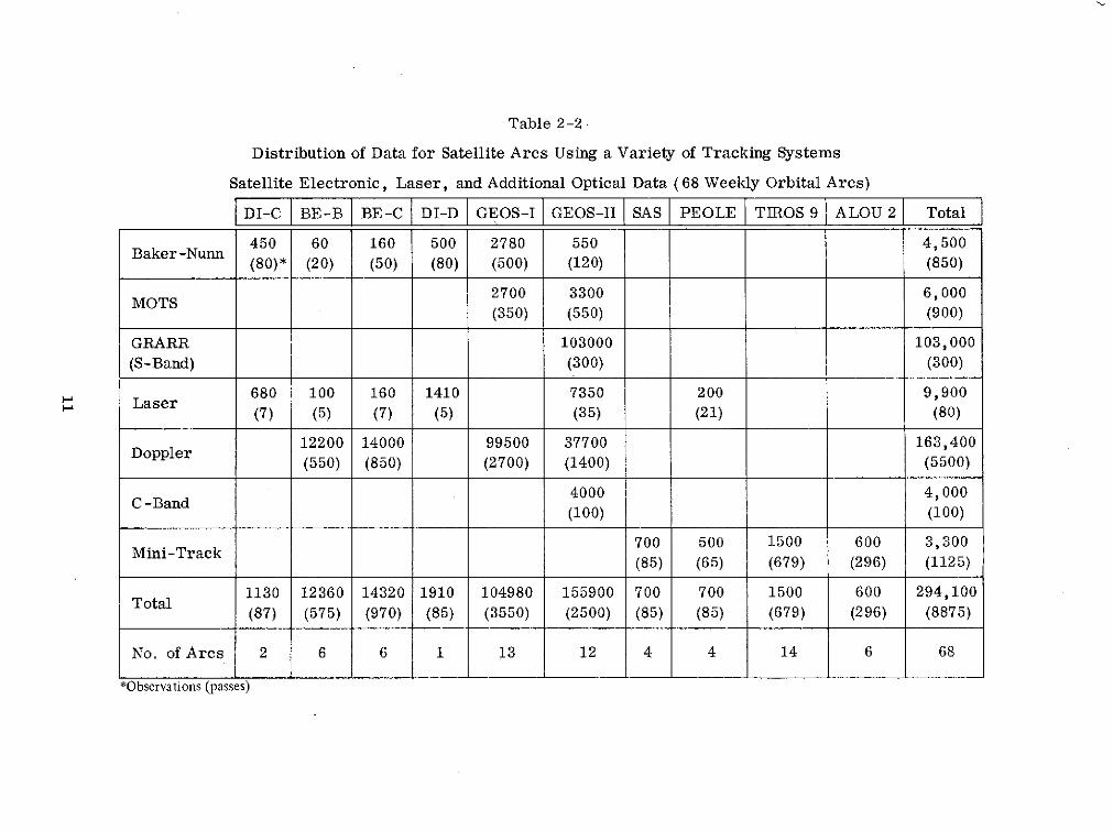
Table 2-2.

Distribution of Data for Satellite Arcs Using a Variety of Tracking Systems

Satellite Electronic, Laser, and Additional Optical Data (68 Weekly Orbital Arcs)

DI-C BE-B BE-C I DI-D GEOS-I GEOS-II SAS I PEOLE TIROS 9ALOU 2 Total

450 60 160 500 2780 550 4,500Baker-Nunn

(80)* (20) (50) (80) (500) (120) (850)

2700 3300 6,000

(350) (550) (900)

GRARR 103000 103,000

(S-Band) (300) (300)

680 100 160 1410 7350 200 9,900Laser (7) (5) (7) (5) (35) (21) (80)

12200 14000 99500 37700 163,400Doppler (550) (850) (2700) (1400) (5500)

C -Band 4000 4,000(100) (100)

Mini-Track 700 500 1500 600 3,300

(85) (65) (679) (296) (1125)

1130 12360 14320 1910 104980 155900 700 700 1500 600 294,100Total

(87) (575) (970) (85) (3550) (2500) (85) (85) (679) (296) (8875)

No. of Arcs 2 6 6 1 13 12 4 4 14 6 68

*Observations (passes)

00

"5° "50

20o

20

190. 1020 230ure 2-1. Distribution o Stations in GEM 6

20*

Data used in GEM 6 in addition to GE1V 5 data are listed with associated tables

and figures for reference as follows:

* Global surface gravity data in the form of 50 equal area (300n.m. sq.)

anomalies computed by Rapp (1972). Table B-10 of Appendix B.

* Geometric data of two-, three-, four-camera, and laser/two-camera

events from the MOTS-SPEOPT-Laser Network (primarily in the U.S.).

Table 2-3.

* 48 relative position constraints computed from local datum surveys.

(These constraints are used in order to combine the dynamic and geo-

metrically determined networks, and to cause closely situated stations

to adjust in a statistically constrained manner.) Figure 2-2.

* Eight baseline distance constraints, employed with the BC-4 data (2 in

U.S., 3 in Europe, 2 in Australia, and 1 in Africa). Figure 2-2 and

Table 2-4.

A complete listing, identifying the participating stations of some 13,000 simul-

taneous events in Table 2-3, is presented in Tables B-6 to B-8 of Appendix B.

A listing of 48 survey ties employed for stations is presented in Table B-9.

The gravimetry data included 1654 values of mean gravity anomalies for 50 equal

area blocks covering the whole earth. Of these, 1283 were predicted anomalies

based upon observed gravity measurements and 371 were modeled anomalies as

described by Rapp (1972). The predicted anomalies ranged from 1 to 15 mgal in

accuracy and modeled anomalies were estimated with an accuracy of 20 mgal.

This data is listed in Table B-10 along with the number of 10 equal area blocks

of observed anomalies that were used to predict the 50 mean anomaly. An over-

all view of coverage of the gravity data may be seen by Figure B-1, where the

distribution of the 50 equal area blocks is illustrated.

The accuracy estimate of the predicted anomaly is assigned to each block in Fig-

ure B-1. Generally small values of this quantity correspond to strong coverage

of observed gravity data and larger values to poor coverage. Blocks with blank

entries correspond to the modeled anomalies, and these are seen to be quite prev-

alent in the southern hemisphere.

Basic geodetic constants describing the reference ellipsoid of the earth and itsgravity are given in Table 2-5. Table 2-6 shows the standard deviations assign-

ed the various observations among the tracking systems. The inverse square

of the standard deviations were used as weights for the observations in the leastsquares normal equations.

13

4],6006 0

5o* - so

30' ,942 7 30'

210 9012 6134 611 6002 601 6015 2817

0601

6009 6064 6042o

I3 00 20' 2 0' 20 ' 250- 200 0 o' 300 31 320 330 3 0 0 0 0 0 00 - 120' 13 40 0' bO' 1 o0 ISO

*1025 283 6067 722

627e040n 6023

6019 \032 606030' -1038 -30*

80. ,9oo

BO 2

M BC-4 Baselines

A* BC-4 and Dynamic Station Ties

Figure 2-2. BC-4 Baselines and Ties

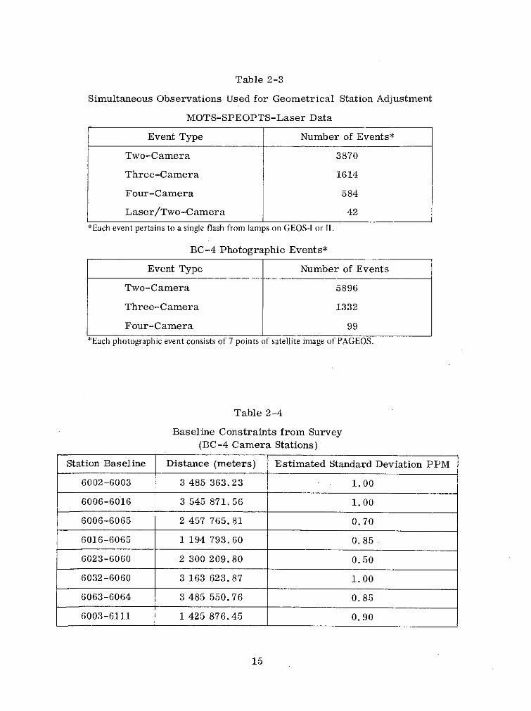
Table 2-3

Simultaneous Observations Used for Geometrical Station Adjustment

MOTS-SPEOPTS-Laser Data

Event Type Number of Events*

Two-Camera 3870

Three-Camera 1614

Four-Camera 584

Laser/Two-Camera 42

*Each event pertains to a single flash from lamps on GEOS-! or I1.

BC-4 Photographic Events*

Event Type Number of Events

Two-Camera 5896

Three-Camera 1332

Four-Camera 99

*Each photographic event consists of 7 points of satellite image of PAGEOS.

Table 2-4

Baseline Constraints from Survey(BC-4 Camera Stations)

Station Baseline Distance (meters) Estimated Standard Deviation PPM

6002-6003 3 485 363.23 1.00

6006-6016 3 545 871.56 1.00

6006-6065 2 457 765.81 0.70

6016-6065 1 194 793.60 0.85

6023-6060 2 300 209.80 0.50

6032-6060 3 163 623.87 1.00

6063-6064 3 485 550.76 0.85

6003-6111 1 425 876.45 0.90

15

Table 2-5

Basic Geodetic Reference Parameters

Mean equatorial radius, ae = 6378155 meters

Flattening, f = 1/298.255

Rotation rate, w = .7292115146 x 10 - 4 radians/second

Geocentric gravitational constant, GM = 3.986013 x 1014 meters 3 /second 2

Mean equatorial gravity ge = 978029.1 milligals

Table 2-6

Standard Deviations of Tracking Observations

Observation Standard Deviation

GRARR: range 10 meters

: range-rate 3 cm/sec

Laser: range 1 meter

Camera: declination (5) 2 seconds of arc

: right ascension (a cos6) 2 seconds of arc

MINITRACK: direction cosines 3 x 10 - 4

NWL Doppler: range-rate 4 cm/sec

C-Band radar: range 8 meters

16

SECTION III . ........ MODELING AND ANALYSIS -

3. MODELING AND ANALYSIS

The gravity potential of the earth (geopotential) is given as the sum of a centrif-

ugal potential and the gravitational potential expressed in an infinite series of

spherical harmonics. The gravitational potential is truncated and this effect

will be analyzed in terms of the geoid, orbits and data sensitivity. The spheri-

cal coordinates of the potential and the station coordinates are given in a center

of mass reference system which is oriented to the mean pole (CIO) of 1900-1905,

Bomford (1971). Satellite orbital motion provides the basis of a center of mass

origin. Orientation to the CIO pole is provided through use of polar motion data

distributed by the Bureau of International de l'Heure (BIH). Station observations

are processed in two modes: geometrically with only simultaneous events used,as with the BC-4 world triangulation network, and dynamically using the com-

puted orbits. Stations processed geometrically are tied to those processed dy-

namically through the use of local datum coordinates as shown in Figure 2-2.

Scale for the station coordinates is principally determined from the referencevalue of GM, Table 2-5, which provides scale for the satellite orbits throughthe gravitational potential. However the 8 baseline distances in Table 2-4 for

the BC-4 network contribute somewhat to this scale in the combination solution,GEM 6.

3.1 Geopotential

The gravity potential of the earth or geopotential is

W = V+4 (3.1)

where V is the gravitational potential, and 4) the centrifugal potential, and where

V =GM 1 + -- Pm (sin p) (Cnm os mX + S nm sin mX) ,

n=2 m=0

S= (rw cos p)2 , (3-2)

for which r, tp , X are spherical coordinates of radial distance, latitude, andlongitude, pm (sin p) is the associated normalized Legendre polynomial of

degree n, order m with argument sin t , Cnm, Snm are normalized sphericalharmonic coefficients, and w is the rotational velocity of the earth. The coef-ficients are termed zonals (Cno, Sno = 0), tesserals (Cnm , Snm, n # m), andsectorials (Cnn, Snn, n = m). C 10 , C, and S1, are equal to zero for a center ofmass reference system, and the coefficients C 2 1 and S21 correspond to a shift inposition of the mean pole. For an offset of 5 meters these coefficients (C 21 , S21)would be of the order of 10 -9 , and cannot be reliably determined. However,

19PR.CET)TN0. PAGE BLANK NOT FILMED

values for these coefficients are estimated in the solution to serve as a measureof the accuracy for the low degree and order coefficients.

The gravitational potential V is employed in computing satellite motion, and thepotential W, set equal to a constant Wo on the geoid, is employed for processingthe gravimetric data. The constant Wo is a function of the reference parametersGM, ae, f and w whose initial values are presented in Table 2-5. An adjustmentto the mean earth ellipsoidal parameters, ae and f, are made through use ofvalues of C20 , the leading oblateness coefficient, and ge, a value of equatorialgravity, both of which are derived in GEM 6. Formulation for this adjustmentof ge, ae and f is given in Section A3 of Appendix A on gravimetric methods. Analternate adjustment of ae through use of mean sea level height from station sur-vey data is presented in Section 4 on results. Results for geodetic parametersare summarized in Section 4.3.

The coefficients determined in the satellite solution for the GEM 5 model are asfollows: Cno for degrees 2 through 22, Cnm and Snm complete to degree andorder 12, and for satellite resonant coefficients of order 12, 13, and 14 n is com-plete to 22, and of resonant order 9 n extends to 15. The number of satellitesresonant for a given order m may be seen from the orbital mean motions listedin Table 2-1. Analysis for this particular truncation of the harmonics, includingterms to degree and order 30, is given in Section 3.3. In the GEM 6 solutionadditional coefficients are determined by combining surface gravity data with thesatellite tracking data. GEM 6 is complete to degree and order 16. The rela-tive effects of these two sources of data in estimating the coefficients will be de-scribed later where a solution based upon surface gravity data only is employed.

3.2 Techniques in Modeling the Data

The mathematical modeling for processing the satellite orbital data, the geomet-ric and gravimetric data, including the weighted least squares normal equations,and the method of combining the data for solution of the geodetic parameters arepresented in Appendix A. The material presented there for the satellite dynam-ics is quite extensive, and a brief account of it is described here since the orbi-tal data provides the main contribution to the geodetic model. Further the ma-terial covered in the appendix in this area is more general than our application,whereas the description given here is restricted to our geodetic problem.

The orbital force equations are integrated numerically in an inertial referencesystem with a uniform time (Al). The reference system is oriented in the celes-tial frame of the true equator and equinox of date, at the beginning of a weeklyarc of satellite data. An 11th order Cowell type of numerical integration is em-ployed with a stepsize to provide for better than one meter of accuracy in satel-lite position on the modeled forces. These forces include the effects of the

20

gravitational potential of the earth, sun and moon, solar radiation pressure, and

atmospheric drag based upon the Jacchia-Nicholet model (Jacchia, 1965).

Certain coordinate transformations and time conversions are employed to

process the forces, the observations, and station positions. Luni-solar pre-

cession and nutation of the earth, the rotation of the earth (UT-1 time), and po-

lar motion transformations are applied. Time system conversions between Al,UT-1, and UTC (transmitted time) are provided in BIH circulars along with po-

lar motion data in x, y angles. Polar motion data is applied to station coordi-

nates referenced to the mean CIO pole. Observation data are preprocessed,corrected, and transformed to Al time at the satellite for the observation equa-

tions. Data types are generally time tagged in UTC but will vary in the time

system and with the corrections to be applied. For instance, MOTS optical data

for right ascension and declination are in a true of date celestial system and time

tagged with UTC. On the other hand, Baker-Nunn optical data are received from

SAO in a reference system of the mean equator and equinox of 1950.0 and time

tagged in SAO atomic time at the station. The SAO observations are transformed

to the true equator and equinox of date, corrected for diurnal aberration and

parallactic refraction, and adjusted to Al time at the satellite by accounting for

the travel time of light to the station. The various processing for the different

data types may be seen in the appendix.

The variational equations for the orbital state parameters, drag force param-

eters, and potential coefficients are integrated numerically along with the force

equations for a weekly arc span of satellite data. The orbits are initially con-

verged to the observations through the process of differential corrections for the

satellite state and drag force parameters. This process is based upon a weighted

least squares adjustment, where the weights are the inverse of the variances of

the observation errors (Table 2-6). For certain electronic tracking systems, a

bias parameter is modeled for the data in a given satellite tracking pass at a

station. Since the number of modeled bias parameters may become large in a

weekly arc of data, each bias parameter is eliminated from the least squares

normal equations at the end of each tracking pass of data through the back sub-

stitution process. After convergence of the orbit a final iteration is made to

produce the normal equations for all parameters including the geodetic param-

eters for adjustments of the potential coefficients and station coordinates from

initial values.

All non-geodetic parameters are eliminated from the normal equations through

the technique of back substitution. The reduced normal equations are then com-

bined for all of the orbital arcs on the 27 satellites. The combined set of normal

equations are then solved separately for the satellite only (GEM 5) solution. They

are also reserved for combination with the normal equations for the geometric

and gravimetric data to provide the solution for GEM 6. The GEM 6 solution

21

contains 730 geodetic parameters, consisting of 134 station positions and 328potential coefficients.

In order to effect some control on the distribution of satellite data in GEM 5certain groups of satellite data arcs were proportionately downweighted. Ex-cluding GEOS-I and II which contain 60% of the optical data in Table 2-1, an av-erage of 2500 observations per satellite exist on the remaining 21 satellites.GEOS-I and II optical data arcs were downweighted to give an effective averageof about 10,000 observations per satellite. Similarly the 40 data arcs (princi-pally electronic data) on the first six satellites in Table 2-2 were downweightedto give an effective average of about 4000 observations per satellite. In additionto this consideration a standard error of unit weight was applied for each dataarc based upon the weighted observation residuals. The latter consideration wasemployed to account principally for degradation in orbital accuracy, particularlyfor effects of atmospheric drag on low altitude satellites.

3.3 Satellite Sensitivity to the Potential

The coefficients of the gravitational potential, excluding C 20 which is of order10 - 3 , gradually decrease in size with degree n. A rule given by Kaula for theaverage (rms) size coefficient (Cnm, Snm) for a given degree is

Sn - a{Cnm, Snm = 10-5/n 2 , form = 0 ton,

which may be seen from Figure 3-1 to compare reasonably with the GEM 5 co-efficients. This rule, with the use of orbital perturbation theory, from Kaula(1966 b), was employed in a harmonic analysis program to estimate the potentialperturbation of the satellite for individual terms in the gravitation potential.The 27 satellite orbits employed in GEM 5 were evaluated for the effects ofterms to degree and order 30. The number of different satellites that have sen-sitivity to a given potential term gives a qualitative measure of resolution forthat term. The result provides information to estimate where the satellite po-tential should be truncated.

This technique was employed by Strange (1968), and it requires a measure ofsatellite orbital sensitivity representative of the accuracy in the satellite ob-servational data. The satellites and associated data are listed in Tables 2-1and 2-2 including their orbital parameters, and the accuracy of the data is listedin Table 2-6. A fixed sensitivity level per satellite was used in this analysis asan along-track threshold, representative of the accuracy in the observation data.Although the radial and cross track perturbations are also significant, the pre-dominant component is generally the along-track one. Each potential term in Vgives rise to a spectrum of harmonics in orbital perturbations (Kaula, 1966 b,

22

44

40

36

32

28

0o 24

20

16

s n KAULA'S RULE

12 10-5/n 2

sn, GEM 510

8

6

4

2

00 4 6 8 10 12 14 16 18 20 22 24 26

DEGREE (n)

Figure 3-1. Average (rms) Coefficient Value by Degree

pg. 40). These were transformed to the along-track position component andthen summed (rss) for a net effect.

The satellite sensitivity levels and pertinent information are listed in Table 3-1.For the satellites containing just optical data in the solution the sensitivity levelvaries from 8 to 35 meters. Only two (high altitude) satellites have valuesgreater than 19 meters. Three satellites with only Minitrack data have sensi-tivity levels of over 100 meters; two of these contribute principally to the reso-lution of satellite resonant terms and the third, SAS (30 inclination), contributesmainly to the zonal terms. Seven satellites (affected by drag) have range and/orrange-rate data in the solution. Six of these with laser range data were assignedsensitivity levels of 5 meters, even though the data is accurate to one meter,whereas the seventh one was assigned 10 meters.

23

Table 3-1

Satellite Data and Sensitivity Level

Sensi- PrimarySatellite Data tivity (Kilo- E I Resonant

Name Type* Level (Degrees) Motion Period(Meters) meters) (Rev/Day) (Days)(Meters) (Days)

AGENA O 8.9 7297. 0.0010 69.91 13.92 5.0

ALOU-2 M 517.0 8100. 0.1505 79.82 11.90 6.2

ANNA-1B 0 10.9 7501. 0.0082 50.12 13.37 4.8

BE-B L, RR, O 5.0 7354. 0.0135 79.69 13.76 3.0

BE-C L, RR, O 5.0 7507. 0. 0257 41.19 13.35 5.6

COURIER O 10.6 7469. 0.0161 28.31 13.46 3.8

DI-C L, O 5.0 7341. 0.0532 39.97 13.81 2.5

DI-D L,O 5.0 7622. 0.0848 39.46 13.05 8.4

ECHO-1RB O 16.4 7966. 0.0118 47.21 12.21 11.9

GEOS-A RR, O 16.4 8075. 0.0719 59.39 11.96 7.0

GEOS-B L,R, RR,O 5.0 7711. 0.0330 105.79 12.82 5.7

GRS O 8.3 7239. 0.0598 49.76 14.10 10.7

INJUN O 9.1 7316. 0.0079 66.82 13.87 3.8

MIDAS-4 O 35.1 9995. 0.0112 95.83 8.69 3.0

OGO-2 O 9.3 7341. 0.0752 87.37 13.79 3.8

OSCAR-7 0 10.0 7411. 0.0224 89.70 13.60 2.2

OVI-2 O 18.8 8317. 0.0184 144.27 11.45 2.2

PEOLE L,M 5.0 7006. 0.0164 15.01 14.82 2.1

SAS M 163.0 6923. 0.0035 3.04 15.09 4.6

SECOR-5 O 17.2 8151. 0.0793 69.22 11.79 3.4

TELSTAR O 31.9 9669. 0.2429 44.79 9.13 14.9

TIROS-9 M 494.0 8024. 0.1173 96.41 12.07 19.5

TRANSIT-4A 0 9.2 7322. 0.0076 66.82 13.85 3.5

VAN2ROC O 20.5 8496. 0.1832 32.92 11.09 294.3

VAN2SAT O 18.6 8298. 0.1641 32.89 11.49 2.7

VAN3SAT O 20.7 8508. 0.1901 33.34 11.07 187.6

5BN-2 O 10.5 7462. 0.0058 89.95 13.46 2.4

*L - Laser Range, R - Range, RR - Range Rate, 0 - Optical, M - Minitrack

24

Two figures are presented to summarize the results. Figure 3-2 displays thenumber of satellites (satellite count) for each harmonic coefficient out to degreeand order 30 that have perturbations larger than the sensitivity level listed in

Table 3-1. Figure 3-3 is similar, except that the sensitivity level is reducedby one-fifth of the above size. The latter figure is used as a measure of sto-

chastic sensitivity, that is, resolution statistically. The solution passing throughthe mean of the observations is more accurate than any given observation.

In each of the two (sensitivity) figures the distribution pattern in the satellite

count is quite large for the low degree and order terms. Beyond a certain de-gree there is only good observability for the zonal terms, satellite resonant

terms, and low order terms. The satellites that are resonant of order m(m = 9, 11 through 14) can be seen from their mean motion in Table 3-1 by takingthe nearest integer value in revolutions per day. Also a satellite count is seenfor certain orders m of twice the above values. These correspond to secondaryresonance effects. Formulation for resonant analysis is given by Kaula (1966 b,pp. 49-56). The primary beat periods associated with the satellite resonant ef-fects are listed in Table 3-1.

Satellite perturbations for some of the potential terms are in the region of kilo-meters, particularly for long period zonal terms with periods of several monthsand for some satellite resonant terms. Because weekly satellite arcs are em-ployed in the solution, each harmonic perturbation in the analysis whose periodexceeded one week was proportionately reduced as the harmonic amplitude isproportional to its period. Similarly secular perturbations of the even zonalterms were computed for a weekly time span and these contribute principally tothe large satellite count for the even zonals.

In Figure 3-2 the satellite count for the bulk of the coefficients, excluding thezonal and resonant terms, is associated principally with the m-daily terms (ofm cycles per day). However, in Figure 3-3 for the lower sensitivity level,short period terms (less than one satellite revolution) also contribute to the sat-ellite sensitivity. Orbital perturbation formulas including the m-daily and shortperiod terms may be found on page 40 of Kaula (1966).

Based upon the above results the truncation for the low order terms (m = 0, 1and 2) could be extended beyond the point employed in GEM 5. Coefficients forsatellite resonant order 15 could be included. The general point of truncation atdegree 12 is probably satisfactory. The stochastic sensitivity level indicatesgood resolution in harmonics of degree 12. However, since a number of the 12thdegree terms are void in Figure 3-2, the recovery of these terms are basedupon small perturbations. It is shown later that, with use of error estimatesfor the potential coefficients, the 12th degree terms have about 40% accuracy.Thus, in all, it does not appear very beneficial to extend the general truncationof the harmonics beyond degree 12 for the satellite solution.

25

2 27 273 26 26 25 26S27 27 26 25 23 NUMBER OF SATELLITES OBSERVING A PERTURBATION(10 4 27 27 26 25 23

!1" 5 25 23 18 19 16 15 LARGER THAN THE MINIMUM OBSERVATION ERROR6 27 20 22 20 16 14 13 (TOTAL OF 27 SATELLITES)7 23 13 15 7 6 6 10 II

02 8 27 21 15 9 13 8 8 5 59 21 10 5 4 3 2 3 I 1 410 25 13 10 7 I 4 2 211 15 8 3 I I I 412 26 12 4 2 2 I 2 613 15 5 I 2 6 13

w 14 23 5 2 I I I 2 5 8 5w 15 8 5 I I 2 4 9 8 7" 16 25 6 I I I I 2 5 4 6w 17 6 I I 2 4 5 10 5a

18 22 2 I I I 2 4 5 719 4 I 2 4 5 9 I20 16 I 2 2 3 4 I21 4 2 2 4 8 I22 17 I 2 3 423 I 2 4 624 15 2 2 325 2 3 526 10 2 I 327 2 2 2 I28 9 2 I I 3 I29 I 2 I 3 I I30 4 2 I I I 2 I

0 I 2 3 4 5 6 7 8 9 10 11 12 13 14 15 16 17 18 19 20 21 22 23 24 25 26 27 28 29 30

ORDER

Figure 3-2. Satellite Sensitivity to Potential Terms (30 x 30)

2 27 273 26 27 26 274 27 27 27 26 27 NUMBER OF SATELLITES OBSERVING A5 26 25 24 23 23 23 PERTURBATION LARGER THAN 1/5 OF6 27 27 23 24 23 22 21 THE MINIMUM OBSERVATION ERROR7 24 25 23 22 22 21 19 198 27 24 22 21 22 21 17 17 179 24 22 20 18 18 18 19 15 15 17

10 26 22 20 15 18 16 18 14 14 15 14II 23 18 12 15 II 14 12 13 13 14 13 1512 26 16 19 II 12 12 12 9 13 II 12 15 1613 22 16 14 7 6 7 7 8 6 12 9 12 12 1614 25 18 15 II II 8 3 6 4 7 6 9 16 14 7

W 15 18 12 8 4 4 2 4 I 4 5 5 10 9 15 10 9l 16 25 14 10 8 2 4 3 I 3 3 I 5 14 10 13 6 2w 17 15 10 6 3 2 I 2 3 3 6 8 14 13 9 6 50 18 23 10 7 I 5 1 I I 1 2 6 10 1I 10 3 2 I

19 11 6 I 2 1 I I 1 5 8 9 13 9 3 4 220 22 10 2 3 I I 1 3 8 8 10 5 I21 13 3 3 I I I 1 3 7 7 13 8 222 19 6 2 I I I I 2 3 7 6 3 2 1 I23 8 5 I 2 3 6 12 8 2 I24 21 4 I I I I I 3 2 4 6 4 I25 7 3 3 2 5 9 5 I I26 18 2 I I 2 I 4 7 2 I I I27 3 I 2 I 5 7 I I I I 328 18 2 I 2 3 3 I I 2 I 7 429 3 I 2 4 6 I 2 I 2 2 I30 16 I I 2 3 3 2 6 5

0 I 2 3 4 5 6 7 8 9 10 11 12 13 14 15 16 17 18 19 20 21 22 23 24 25 26 27 28 29 30

ORDER

Figure 3-3. Stochastic Satellite Sensitivity

3.4 Error Estimates for Geopotential Coefficients of GEM 5

The average standard deviation (on) per degree n for the potential coefficientsare plotted in Figure 3-4 for both the satellite solution, GEM 5, and a gravimet-ric solution derived from the 50 mean gravity anomalies. Judging from theseformal error estimates the strength of the combination solution will predomi-nantly depend upon GEM 5. Analysis is presented to calibrate this informationin GEM 5 according to outside data sources.

The formal standard deviations are obtained from the inverse matrix of the nor-mal equations with observation weighting of 1/u2BS. Such results generally pro-vide optimistic error estimates without some upward adjustment. Relative val-ues of the standard deviations are generally considered meaningful, and hencethe adjusted values may be derived through a calibration factor. This factor isusually applied as a standard error of unit weight based upon the observationsemployed in the solution. This factor has already been included in a priori formfor each data arc of GEM 5. A calibration factor for GEM 5 will be derived be-low based upon gravimetry data not employed in the solution. It is expected thatthis will provide realistic error estimates for the GEM 5 coefficients. Use willbe made of the calibration factor for GEM 5 in the error estimates for GEM 6.

3.4.1 Formulation of Error Estimates for Geoid Height and Gravity Anomaly-The gravity anomaly Ag and geoid height hg may be represented, from Heiskanenand Moritz (1967), for a point (r, O , X) on the geoid as follows:

N n

Ag = (n - 1) Hnm (3.3)n=2 m=0

N n

hg = GM Hnm (3.4)

n=2 m=O

where

Hnm Pnm (sin ¢) ( cos mX + nm sin mX)(C 28

28

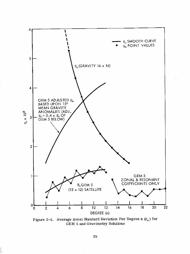
6

- an SMOOTH CURVE

* un POINT VALUES

5

un(GRAVITY 16 x 16)

4

GEM 5 ADJUSTED unBASED UPON 150MEAN GRAVITY

0o ANOMALIES (ADJ.3 a = 3.4x a, OF

GEM 5 BELOW)

2

1 GEM 5ZONAL & RESONANT

nGEM 5 COEFFICIENTS ONLY

(12 x 12) SATELLITE

0 1 1 1 1 1 - I I- I0 2 4 6 8 10 12 14 16 18 20 22

DEGREE (n)

Figure 3-4. Average (rms) Standard Deviation Per Degree n (an) forGEM 5 and Gravimetry Solutions

29

and Cnm = Cnm except for even zonals for which To = Cno - Cno and Cno are theoblate zonal coefficients for the reference ellipsoid. A mean square error esti-mate of Ag and hg over the geoid, due to the uncertainty onm (C,S) in the coeffi-cients, may be estimated from equations (3.3) and (3.4) with use of a sphericalapproximation r = R, where R is the mean radius of the earth. These resultsare

N

S= 2 (n-1)2 02 (T) (3.5)A2g = n

o2 = R2 U 2 (T) (3.6)n=2

a2 (T) 02~ (C) + a2 (3.7)m=0

where y is a mean value of gravity.

The average standard deviation per degree n ( n) plotted in Figure 3-4 was com-puted from (3.7) as follows:

2 (T)-2 n (3.8)

for harmonic terms complete to degree and order n, and for terms not completein degree n

a2 (T L)-2 - L

n L (3.9)

where L is the number of coefficients determined in the solution for thatdegree. With use of the standard deviations for GEM 5, the error committedin the gravity anomaly from (3.5) due to the modeled coefficients is, withS~ 10 6 mgal,

OAg = 1.3 mgal. (3.10)

30

Similarly the formal uncertainty estimate of the average global geoid height is,from (3.6),

Uh = .8 m (3.11)

3.4.2 Adjusted Error Estimates of Potential Coefficients-Comparisons of meangravity anomaly computed from GEM 5 (Gc ) with that computed (GT) directlyfrom terrestrial gravity data was made. The mean (free-air) gravity anomaliesare values averaged over equal area blocks (s x s square) on the geoid, and theblock size is given in terms of the geocentric angle 0 subtended by the length s.A commensurate block size 0 for mean gravity anomaly corresponding to a har-monic solution complete to degree and order N may be obtained from the halfwavelength resolution of the harmonics, namely

1800 (degrees)

Thus for N = 12, as in GEM 5, 150(0) equal area blocks of mean gravity anomalywere employed for a commensurate comparison.

A global set of such terrestrial anomalies were obtained from Hajela (1973) witherror estimates for each 15' anomaly. A global error between GT and Gc ac-counting for the errors in the gravimetry data gave

o (GT - Ge) = 4.4 mgal (3.12)

where a standard error (of unit weight) in the gravimetry data was 1.9 mgal.Note the discrepancy between (3.12) and that derived in (3.10) from the formalerror estimates in the coefficients. Equating these results in the form

o (GT - Ge) = KaAg (3.13)

gives 4.4 = 1.3K

or K = 3.4 (3.14)

as a calibration factor for on of GEM 5. An equivalent result to (3.12) is de-rived more indirectly in Section 4. with use of 50 mean anomalies, where thestatistical techniques of Kaula are employed.

Thus K an represents satellite coefficient errors that are more realistic asjudged by the gravimetric data. Furthermore K n may be used to check theaverage uncertainty in geoid height, oh in (3.11), with differences seen in com-parisons between geoid heights derived from GEM 5 and those derived from

31

detailed gravity data and astrogeodetic deflections in major areas of survey.These comparisons yield an rms difference of approximately 5 meters. Thisresult may be equated to a total predicted error as follows:

5 (K2 , +)2 (3.15)

oh : error in geoid height of .8 meter due to formalstandard errors in GEM 5 coefficients

K : scale factor of 3.4 obtained from (3.14)

h : error in geoid height due to coefficients notincluded in GEM 5.

The mean square error of omission, 6h 2 due to coefficients not included in GEM5, was estimated from (3.6) by using Kaula's value of 10-5 /n 2 for the uncertaintyin the omitted (unmodeled) coefficients. This result gave

5h2 = 22.6m 2 , (3.16)

and since oh = .8 m,

K2 Gh 2 = 7.4 m 2 . (3.17)

Then the total predicted error for geoid height is

(K 2 h2 + 5h2) = 5.5 m. (3.18)

The latter result is fairly consistent with the 5 meters in (3.15) which was ob-tained from the direct comparisons. It is noted that (3.18) does not provide astrong source of calibration since the omission error (3.16) is much largerthan the commission error (3.17).

From the above results, principally (3.13), it would seem that a better error es-timate for the standard deviations oi of the geopotential parameters of GEM 5 is

ai (error) = K oi (computed)

K = 3.4. (3.19)

The adjusted errors (K Un) by degree n are plotted in Figure 3-4. Based uponthese adjusted errors the percent accuracy for coefficients of degree n for GEM5 are plotted in Figure 3-5, where Kaula's rule (Figure 3-1) was used for theaverage size coefficient of degree n. In the combination solution (GEM 6) thegravimetry data should improve the relatively low accuracy in the high degreecoefficients.

32

PERCENT ACCURACY FOR COEFFICIENTS

Pn = (1 - Kn/s*) x 100

100 100

90 - - 90

' 80 - - 80- \GEM 5

70 - - 70

- 60 - - 60

50 - - 50

40 402 4 6 8 10 12 14 16

DEGREE (n)

s* : 10 5/n 2

K n: AVERAGE (rms) ERROR ESTIMATEFOR COEFFICIENTS OF DEGREE n(Calibration Factor K = 3.4)

Figure 3-5. Percent Accuracy of GEM 5 Coefficients by Degree

3.5 Relative Weighting and Error Estimates for Combined Solution GEM 6

A relative weighting factor w was applied in the combination solution for GEM 6

as follows:

S+ + w G = 0 (3.20)

where S, M, and G denote the normal matrix equations respectively for the sat-

ellite dynamic system (GEM 5), the geometric system, and the gravimetric sys-

tem. G contains just geopotential parameters, M station coordinate parameters

only, and S both station and geopotential parameters. Based upon the calibration

results of the satellite solution, as in 3.19, it was decided that some additional

weighting (w) for the gravimetry system G should be applied. Assuming the

standard deviations from G are correct, w should be 11.4 (K 2 ) based upon the

GEM 5 calibration.

A precise value for w, however, cannot be determined since the gravimetry so-

lution has not been calibrated against an external reference as has GEM 5. In a

previous combination solution for GEM 4 a relative weighting factor of w = 5 was

33

applied, and this value resulted in relatively poor comparisons for GEM 4 withsatellite data as shown in Table 4-11 of Section 4. A conservative value of w = 2was applied for GEM 6 and provided greatly improved results as shown in thesame table.

The inverse matrix of the normal equations for each system, G and S, has beenemployed to obtain the formal standard deviations for these systems. Similarly,the inverse matrix for the combined system (3.20), was used to provide thosefor GEM 6. Average (rms) error values for coefficients of degree n, U,, , wereobtained for GEM 6. As with GEM 5 these were likewise scaled by 3.4 (K) andare presented in Table 3-2. A relationship between the two solutions GEM 5 and6, showing the effect of combining the gravimetry data in GEM 6, is presented inFigure 3-6. The relationship gives the percent reduction of the coefficient errors(variances) of GEM 6 with respect to those of GEM 5, namely for each degree n

Pn = 1 - Un2 (GEM 6) / Un2 (GEM 5) (3.21)

Since Un is scaled by K in each solution the result for Pn does not depend upon Kbut it does depend upon the relative weighting factor w. The result for Pn showsthat the gravimetry data in GEM 6 has progressively greater effect as n increases,with relatively little effect on the low degree coefficients, and reduces the vari-ance of GEM 5 to 50% at about degree ten. Results are listed for n to degree 12,since GEM 5 contains just satellite resonant and zonal coefficients beyond thispoint.

Formal standard deviations for the station coordinates for GEM 6 also gave op-timistic results. This was seen from numerous comparisons with station coor-dinates, including datum survey, which are given in Section 4.2. Again, as withthe potential coefficients, relative values of the formal standard deviations forthe station coordinates were considered generally meaningful. These valueswere scaled by a factor of three to provide a more realistic error estimate, con-sistent with the above comparisons. Error estimates are given in Table 4-16of Section 4.2 for 134 tracking stations. A summary of the results is given inTable 3-3. These results show an average (rms) error of 6.6 meters for stationcoordinates. The BC-4 geometric system has the largest error among the track-ing systems with a value of 8.5 m. The errors refer to the dispersion or noisein the coordinates and do not represent an overall scale error or orientationerrors.

3.6 Verification of Error Estimates

The adjusted standard deviations of GEM 6 for geopotential and station coordi-nate parameters are used below to predict an error estimate for the averageuncertainty in the computed height of station above mean sea level (geoid). The

34

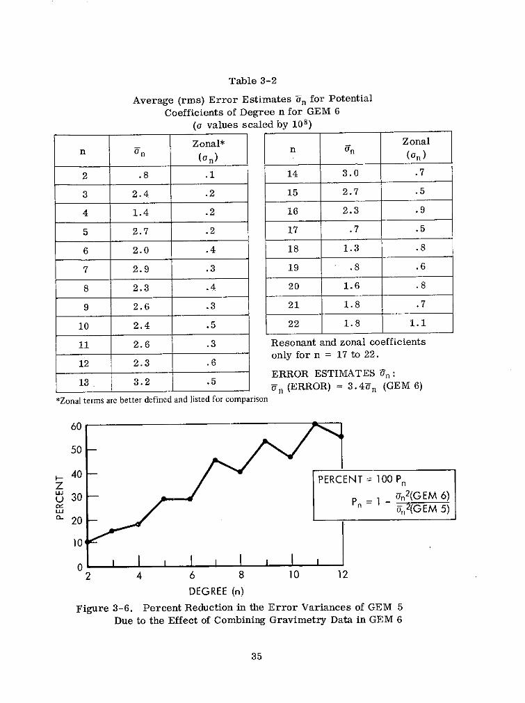
Table 3-2

Average (rms) Error Estimates on for Potential

Coefficients of Degree n for GEM 6

(a values scaled by 108)

Zonal* Zonaln ( n nn)

2 .8 .1 14 3.0 .7

3 2.4 .2 15 2.7 .5

4 1.4 .2 16 2.3 .9

5 2.7 .2 17 .7 .5

6 2.0 .4 18 1.3 .8

7 2.9 .3 19 .8 .6

8 2.3 .4 20 1.6 .8

9 2.6 .3 21 1.8 .7

10 2.4 .5 22 1.8 1.1

11 2.6 .3 Resonant and zonal coefficients

12 2.3 .6 only for n = 17 to 22.

ERROR ESTIMATES Un:13 3.2 .5 Un (ERROR) = 3.4Un (GEM 6)

*Zonal terms are better defined and listed for comparison

60

50

40 PERCENT = 100 PnZ n

U30 P 1 2(GEM 6)un 6n2(GEM 5)S20

104

2 4 6 8 10 12

DEGREE (n)

Figure 3-6. Percent Reduction in the Error Variances of GEM 5

Due to the Effect of Combining Gravimetry Data in GEM 6

35

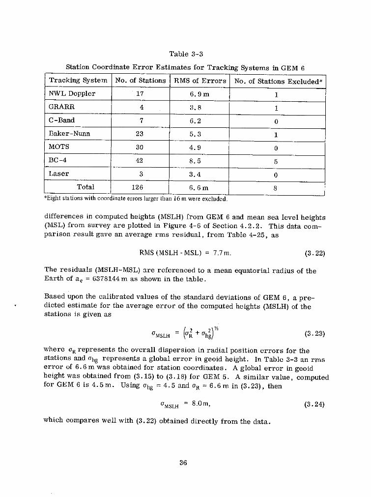
Table 3-3

Station Coordinate Error Estimates for Tracking Systems in GEM 6

Tracking System No. of Stations RMS of Errors No. of Stations Excluded*

NWL Doppler 17 6.9m 1

GRARR 4 3.8 1

C-Band 7 6.2 0

Baker-Nunn 23 5.3 1

MOTS 30 4.9 0

BC-4 42 8.5 5

Laser 3 3.4 0

Total 126 6.6 m 8

*Eight stations with coordinate errors larger than 16 m were excluded.

differences in computed heights (MSLH) from GEM 6 and mean sea level heights(MSL) from survey are plotted in Figure 4-6 of Section 4.2.2. This data com-parison result gave an average rms residual, from Table 4-25, as

RMS (MSLH - MSL) = 7.7m. (3.22)

The residuals (MSLH-MSL) are referenced to a mean equatorial radius of theEarth of ae = 6378144m as shown in the table.

Based upon the calibrated values of the standard deviations of GEM 6, a pre-dicted estimate for the average error of the computed heights (MSLH) of thestations is given as

aMSLH =j + hg) (3.23)

where aR represents the overall dispersion in radial position errors for thestations and ohg represents a global error in geoid height. In Table 3-3 an rmserror of 6.6 m was obtained for station coordinates. A global error in geoidheight was obtained from (3.15) to (3.18) for GEM 5. A similar value, computedfor GEM 6 is 4.5m. Using ohg = 4 .5 and oR = 6.6m in (3.23), then

UMSLH = 8.0m, (3.24)

which compares well with (3.22) obtained directly from the data.

36

An additional estimate for the average uncertainty in geoid height for GEM 6 has

recently been obtained from experimental altimeter data taken on SKYLAB IV

during one revolution of the earth. The ground track passed over nearly all

ocean surface. Geoid heights derived from the altimetry data are plotted in

Figure 3-7 along with those computed from GEM 6. These results were pre-

sented by C. Leitao of NASA (Wallops) at the International Symposium on Appli-

cations of Marine Geodesy, June 5, 1974, Columbus, Ohio. The reference for

this presentation is listed under McGoogan (1974), principal investigator for the

SKYLAB S-193 altimeter experiment. The rms of geoid height residuals in the

figure is approximately 7.3 meters, for which variations as large as 15 meters

may be seen in the southern area of the Atlantic Ocean. However, the orbital

position error may account for part of the 15 meters since S-band tracking data

coverage is lacking in this region.

A final comparison is made to check the estimated errors for the GEM 5 coeffi-

cients. The root mean square values for the differences in coefficients of de-

gree n (RMSn) between GEM 5 and a solution, SAT 16 x 16, are plotted in Figure

3-8. SAT 16 x 16 has been recently derived and is based upon satellite optical

and ISAGEX laser data, and it is complete to degree and order 16 in harmonics.

It contains the same satellites as in GEM 5 but does not include some 270,000

electronic observations contained in GEM 5. Values of bn, average (rms) stand-

are deviations for coefficients of degree n, have been calibrated for GEM 5 as

previously discussed to represent realistic error estimates, and these are plot-

ted in the figure for comparison. These error estimates compare favorably

with the coefficient differences, including the oscillations seen between even and

odd degree harmonics. For consecutive harmonics even degree terms have rel-

atively larger orbital perturbations and hence these have smaller errors as

shown in the figure.

37

100.0 1-0 TSKYLAB IV

80.0' 211 "ROUND THE WORLD:'DATA TAKE

SI 212 31 JAN 1974

60.0-, o

40.0 202 --. 20 10S 201 213

' 20.0 - 21 4-.-- ' iS1 215 216 2

S. ATLANTIC 215 216

209 223

Di GEM 6 GEOID

-. 40.0 207.-- - -S j 208 ALTIMETER GEOID 226

USING S-BAND ORBIT i225-60.0 ___'- -

S.-8 0 .0 -. .-- . .- -- .- --

-100.0 -- --- -- -i

15h00 0 s 15 30m00s 16h00 m00 s 16h20m00sGMT-TIME-SEC

Figure 3-7. Comparison of GEOID Profile Derived from Altimetry and GEM 6

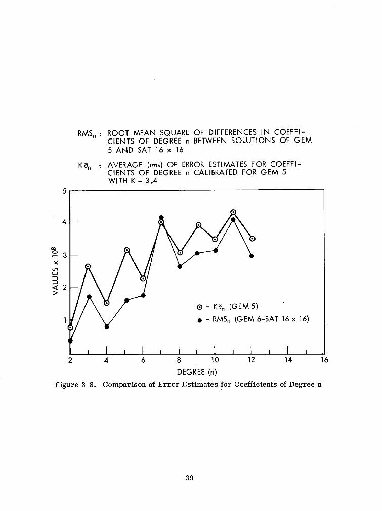
RMSn: ROOT MEAN SQUARE OF DIFFERENCES IN COEFFI-CIENTS OF DEGREE n BETWEEN SOLUTIONS OF GEM5 AND SAT 16 x 16

K-n : AVERAGE (rms) OF ERROR ESTIMATES FOR COEFFI-CIENTS OF DEGREE n CALIBRATED FOR GEM 5WITH K =3.4

5

x

42

E - Kn (GEM 5)

1 * - RMSn (GEM 6-SAT 16 x 16)

2 4 6 8 10 12 14 16

DEGREE (n)

Figure 3-8. Comparison of Error Estimates for Coefficients of Degree n

39

SECTION IV ...... ...... . .RESULTS (GEOPOTENTIAL AND STATIONS)

4. RESULTS

4.1 Gravitational Potential for GEM 5 and 6

Spherical harmonic coefficients, in terms of normalized values, are given in

Table 4-1 for GEM 5 and Table 4-2 for GEM 6.

4.1.1 Zonal Harmonics-Coefficients of the zonal harmonics have been deter-

mined by Cazenave et al. (1971) and by Kozai (1969) by analyses of orbital per-

turbations of long periods, while GSFC, in its work on GEM, determines them

by analysis of orbital perturbations on weekly arcs. The solution of Cazenave

et al. (French 71) resulted by a combination of Kozai's normal equations with

corresponding equations for three low-inclination satellites (SAS, PEOLE, DIAL).

Kozai's solution was used in the Smithsonian Standard Earth II (SAO SE 2).

Table 4-3 compares the zonal coefficients in GEM, the SAO SE 2, and the French

71. The rms differences from the coefficients of the French 71 are:

Solutions with Data on Satellites Solutions without Data fromof Low Inclination Satellites of Low-Inclination*

Solutions GEM 3 GEM 4 GEM 5 GEM 6 SAO SE 2 GEM 1 GEM 2

rms x 10 9 9.5 7.6 8.9 7.4 16.3 22.5 9.1

*Solutions without low inclination satellite data employ satellites whose inclinations are greater than 280.

The rms agreement with the French values is much better for the solutions thatcontain the data on low-inclination satellites than for the solutions that lack this

data. The comparisons of the French coefficients with the GEM 1, 3, and 5 co-efficients show progressively better agreement as do the comparisons with theGEM 2, 4, and 6 coefficients. The rms difference of 7.4 x 10 - 9 between GEM 6and the French values is approaching the error estimates given for the zonals byeach of the solutions. The rms of these error estimates is 4.5 x 10 - 9 for theFrench 71 and 5.7 x 10 - 9 for GEM 6, as obtained from Table 3-2. Hence these

results serve to confirm the error estimates derived in GEM 6, for which the

zonals are the best determined set. (From the values in Table 3-2 the average(rms) coefficient error is 27 x 10 -9 , significantly larger than the zonal errors.)

Secular and long period zonal perturbations on 21 satellites are analyzed for theabove models and presented in Section 4.1.3. In this analysis improved results

are obtained for those solutions which include low inclination satellite data.

4.1.2 Comparison with Gravity Anomalies-Data on surface gravity were em-

ployed for testing models derived only from satellite tracking data and models

PRECEDING PAGE BLANK NOT FILMED 43

Table 4-1

Normalized Coefficients in GEM 5 (x 106)

ZONAL S

INDEX VALLE INDEX VALUF INDEX VALUE INDEX VALUE INDEX VALUENM N N NM NM NM

2 0 -4e4.1662 3 C 0.9605 4 0 0.5363 5 0 0.0659 6 0 -0.14577 0 0.0956 8 0 0.0430 9 0 0.0272 to10 0 0.0587 1I 0 -0.0547

12 0 0.0338 13 C 0.0498 14 0 -0.0260 15 0 -0.0081 16 0 -0.004617 0 0.0215 18 C 0.0052 19 0 0.0031 20 0 0.0152 21 0 -0.010122 1 -C.0121

SECTORIALS AND TESF RALS

TNDEX VALUE IVDEX VALUE INDEX VALUEN M C S NM C S NM C S

2 1 -C.0012 -0.3 87 2 2 2.4282 --13802 3 .1 2.C055 0.24493 2 0.9296 -0.t26 3 3 0.7285 1.4052 4 1 -0.5396 -0.45254 2 0.3495 0.5719 4 3 0.9794 -3.2201 4 4 --0. 691 0.30265 1 -C.0579 -0.0993 5 2 0.6533 -0.3110 5 3 -0.4403 -0.24405 4 -C.2996 0.0261 5 5 0.1373 -0.6577 6 I -0.C756 -0.0145

6 2 C.C595 -C.3560 6 3 3.0784 -0.0095 e 4 -0C1018 -0.45376 9 -0.2858 -005174 6 6 0.03c7 -0.2265 7 1 0.2535 0.12447 2 C03409 %el149 7 3 0,2740 -0.2104 7 4 -0.3044 -0.10717 5 0.0028 0.0708 7 6 -0.3299 0.1584 7 7 0.0275 3.06618 1 0.0099 0.1836 8 2 0.0469 0.0719 8 3 -0.0289 -0.0721

8 4 --02410 3.0562 8 5 -0.0914 0.0773 8 6 -0.C545 0.31728 7 0.0685 C.0604 8 8 -0.0976 .( 826 9 1 0.1598 0.00635 2 0.0170 0.0023 9 3 -0.1269 -0.1234 9 4 0.0056 0.03479 5 -C.0250 -0.0839 9 6 0.0630 0.2220 9 7 -0.0711 -0.03879 8 0.1595 -0.0350 9 9 -0.,389 0.0884 10 1 0.C883 -0.1740

10 2 -C 0434 -C.3330 10 3 -0.0503 -0.1219 IC 4 -0.C740 -0.101510 5 -0.1183 -0.0480 10 6 -0.0096 -0*0795 10 7 -0.0135 -0.024710 8 0.0304 -0.1288 1) 9 0.1117 -0.0542 10 10 0.0696 -0.0405II I -Ce0203 0.1225 11 2 0.0326 -0.0883 II 3 0.0052 -0.1343II 4 0.0390 -0.0657 11 5 0. 181 0.0310 I1 6 0.0003 0.0478

11 7 Ce0125 -0.1186 11 8 -0.0246 0.0534 11 9 0.0195 0.063011 10 -0.0972 0.0036 I1 I1 0.0632 -0.0245 12 1 - .C831 -0.030212 2 -0.0280 C.3225 12 3 0.0842 0.0576 12 4 0.0033 -0.020112 5 0e0100 0.0146 12 6 0.0681 0.0404 12 7 -0.0149 0.016012 8 -0.0230 -0.160 12 9 0.0289 0.0426 12 10 -0.0071 0.0359

12 11 0.0036 0.0389 12 12 -0.0125 -0.0090 13 9 0.0952 0.085113 12 -C.0282 C.1002 13 13 -0.0598 0.0689 14 1 -0.0150 0.005314 9 C.0378 0.0644 14 II 0.0002 -0.0001 14 12 0.0070 -0.036614 13 0.0145 0.0264 14 14 -0.0455 -0.0045 1S 9 0.0643 0.058815 12 -0.0348 0.0154 15 13 -0.0?26 -0.0022 15 14 0.0037 -0.0191

16 12 0.0269 -0.3088 16 13 0.0009 -0.0132 16 14 -0C0217 -0.340617 12 0.0167 -0.0009 17 13 0.0104 0.0188 17 14 -0.0133 -0.002218 12 -0.0599 -0. 212 18 13 -0.0225 -0.0619 18 14 -0.0109 -0.003319 12 -0*0290 -0.0289 19 13 -0.0244 -0.0200 19 14 0.0002 0.000720 12 C.0073 -0.0000 20 13 -0.0020 -0.*017 20 14 .0C078 -0.0087

21 12 -0.0217 -0.0226 21 13 -0.0270 0.0108 21 14 0.0096 0.007322 12 -0.0399 -C.0053 22 13 --. 0412 -0.0159 22 14 -0.0080 0.0024

eTIGINAL PAGE IB

O POR1 QUALITY44

Table 4-2

Normalized Coefficients in GEM 6 (x 106)ZONAL$

INDEX VALLE INDEX VALUE INDEX VALUE INDEX VALUE INDEX VALUE

N M N M N M N M N N

2 0 -484.1661 3 0 0.9607 A 0 0.5362 5 0 0.0661 6 0 -401451

7 C 0.0961 8 0 0.0426 9 0 0.0264 10 0 0.0606 11 0 -0.0528

12 0 0.0306 13 0 0.0470 14 0 -0.0206 15 C --00045 16 0 -0.0077

17 0 0.0192 18 0 0.0091 19 0 0.0044 20 0 0.0143 21 0 -0.0098

22 C -0.0128

SECTCRIALS AND TESSERALS

INDEX VALLE I~DX VALUE INDEX VALUEND C 5 NM C S NM C S

2 1 -0.00C9 -0.0032 2 2 2.4251 -1.3ee3 3 1 2.0021 0.2482

3 2 0.9332 -0.6311 3 3 0.6969 1.4260 4 1 -0.5403 -0.4648

4 2 0.1461 0.6695 4 3 0.9655 -0.2073 4 4 -0.1636 0.3051

5 1 -0.06e4 -0.0842 5 2 0.6651 -0.3112 5 3 -0.4656 --01947

E 4 -0.2485 0.0360 5 5 0.1a45 -0.7119 6 1 -0.0734 0.0150

6 i 0.C643 -0.3740 6 3 0.0115 0.009 6 4 -0.0867 -0.4455

e 5 -0.274' -0.5464 6 6 0.0173 -0.2027 7 1 C.2501 0.1385

7 2 0.34E3 0.0875 7 3 0.1988 -0.1844 7 4 -C.28C7 -0.1408

7 5 0.0265 0.0228 7 6 -0.3074 0.1213 7 7 0.0424 0.0048

e 1 0.0102 0.0579 8 2 0.0o10 0.08te 8 3 -0.0378 -0.0667

8 4 -0.2!11 0.0284 8 5 -0*0570 0.0622 8 6 -0.0947 0.2528E 7 0.08ee 0.0819 e 8 -0.0832 0.0701 9 1 0.1426 0.01379 2 0.0552 -0.0216 9 3 -0.1299 -0.0727 9 4 -0.0125 -- 001475 5 -0.0036 -0.0686 r 6 0.0163 0.1267 9 7 -00oS66 -0.0037

e 0.2519 -0.0101 9 9 -0.0275 0.0873 10 1 0.0927 -0.1343

10 2 -0.0419 -0.0703 10 3 -0.0383 -0.0998 10 4 -0.0699 -0.1247

10 5 -0.0!25 -0.0377 10 6 -0.0550 -0.1342 10 7 0.0174 -0.023710 8 0*0473 -0.1213 10 9 0.0960 -0.0749 10 10 0.1365 -0.039111 1 -0.00e7 0.0431 11 2 -0.0123 -0.1176 11 3 -0.0334 -0.0841

11 4 -0.0263 -0.1033 11 5 0.0842 0.0406 11 t -0.0421 -0.0353

11 7 0.0041 -0.1123 11 8 -0.0204 0.0714 11 9 -0.0349 0.0393

i1 10 . -0.0464 -0.0333 11 11 0.0696 -0.0356 12 1 -0o0717 -00477

12 2 -0*0!30 0.0621 12 3 0.0694 0.0371 12 4 -0.0468 -0.0158

12 5 0.0124 0.0230 12 6 0.0531 0.0280 12 7 -0.0261 0.0127

12 e -0.01oe7 -0.0031 12 9 -0.0002 0.0251 12 10 0.0231 -0.0012

12 1 0.0066 0.0359 12 12 -0.0123 -0.0103 13 1 -0.0157 -0.0210

13 2 -0.04E4 -0.C867 13 3 -0.0460 0.0454 13 4 0.0298 -0.0670

13 5 0.05e6 0.0469 13 6 -0.0848 0.0577 13 7 -0.0414 0.0482

13 e -0.0055 -0.0347 13 9 0.0271 0.0588 13 10 -0.0240 -0.0044

13 11 -0.0576 -0.0830 13 12 -0.0261 0r0991 13 13 -0.4543 0.07

14 1 -0.0038 0.0480 14 2 -0.0150 0.0429 14 3 0.0653 0.003214 4 0.0019 0.0010 14 5 -0.0144 -0.0216 14 6 0.0166 --00442

14 7 0.0426 0.0030 14 8 -0.0007 -0.0414 14 9 0.0140 0.055214 10 -0.0380 -3.C797 14 11 0.0614 -0.0313 14 12 0.0047 -0.0413

14 13 0.0211 0.0281 14 14 -0.0448 -0.0016 15 1 0.0333 -0.0024

15 2 0.0370 -0.0641 15 3 -0.0457 0.0279 15 4 -0.0070 0.016315 5 0.0136 0.0358 15 6 -0.0130 -0.1076 15 7 0.0751 0.0668

15 8 -0.0251 -0.0242 15 9 0.0116 0.0385 15 10 0.0351 -0.0480

15 11 -0.0090 -0.0106 15 12 M0.0338 0.0145 15 13 -0.0191 -0.0400

1E 14 0.0036 -0.0189 15 15 -0.0444 0.0316 16 1 0.0321 -0.0091

1i P -0.0200 0.0639 16 3 -0.0083 -0.0205 16 4 0.0252 0.0306i6 5 0.0120 0.0173 16 6 0.0321 0.0136 16 7 -C.0003 -0.028616 a -0.0456 -0.0046 16 9 -0.0652 -0.0676 16 IC -0.0115 0.038616 i1 0.0189 -0.0076 16 12 0.0197 -0.0195 16 13 0.0034 -0.0139

16 14 -0.0172 -0.0430 16 15 -0.0475 -0.0378 16 16 -0.0376 -0.0119

17 12 0.0137 -0.0012 17 13 0.0145 0.0204 17 14 -0.0111 -0.001318 12 -0.0616 -0.0269 18 13 -0.0137 -0.0550 18 14 -0.0127 -0.0006

19 12 -0.0309 -0.0300 19 13 -0.0205 -0.0291 19 14 -0.0006 0.001120 12 -0.00!6 -0.0154 20 13 0.0114 -0.0282 20 14 0.0055 -0.0098

21 12 -0.0324 -0.0175 21 13 -0.0241 0.0108 21 14 0.0004 0.0078

22 12 -0.0435 -0.0065 22 13 -0.0324 -0.0151 22 14 -0.0077 -0.0007

C .!GTNAL PAGE IS

J..... QUJALITY 45

Table 4-3

Comparison of Zonal Coefficients (Normalized Coefficients x 106)

Cazenave et al KozaiDegree French 1971 GEM- GEM-2 GEM 3 GEM-4 GEM-5 GEM-6 SAO SE 2

2 -484.170 -484.177 -484.167 -484.171 -484.169 -484.166 -484.166 -484.166

3 .961 .962 .955 .958 .957 .961 .961 .959

4 .540 .557 .537 .547 .541 .536 .536 .531

5 .068 .062 .073 .068 .069 .066 .066 .0696 -. 155 -. 178 -. 145 -. 162 -. 153 -. 146 -. 145 -. 139

7 .094 .105 .087 .092 .091 .096 .096 .094

8 .051 .080 .040 .062 .051 .043 .043 .029

9 .027 .008 .033 .030 .031 .027 .026 .023

10 .051 .021 .065 .040 .050 .059 .061 .077

11 -. 049 -. 020 -. 055 -. 056 -. 056 -. 055 -. 053 -. 042

12 .038 .059 .021 .046 .039 .034 .031 .008

13 .039 .002 .043 .049 .048 .050 .047 .024

14 -. 016 -. 037 -. 009 -. 030 -. 027 -. 026 -. 021 .014

15 .015 .047 .004 -. 007 -. 005 -. 008 -. 005 .03116 -. 008 -. 013 -. 026 -. 012 -. 009 -. 005 -. 008 -. 033

17 .005 -. 035 .007 .020 .017 .022 .019 .014

18 .023 .018 .023 .016 .011 .005 .009 .038

19 .018 .045 .015 .008 .009 .003 .004 .035

20 .014 -. 002 -. 001 .003 .009 .015 .014 .001

21 -. 016 -. 031 -. 012 -. 008 -. 008 -. 010 -. 010 -. 022

22 -. 001 -. 004 -. 012 -. 014

Table 4-4

Comparisons of Terrestrial 50 Anomalies (GT) with

Anomalies (Gs) Computed from Various Models

E (GT - Gs)2] mgal 2

1281 1042 562 211

Model (Harmonics) Blocks Blocks Blocks Blocks

n>1 n> 5 n>15 n= 25

GEM 1 (12 x 12) 157 161 166 173

SE 2 (16 x 16) 164 168 167 172

GEM 3 (12 x 12) 152 155 161 170

GEM 5 (12 x 12) 151 155 160 171

GEM 4 (16 x 16) 149 136 127 127

GEM 6 (16 x 16) 134 129 126 116

EXP (20 x 20) 125 117 96 83

Satellite-Derived Solutions-GEM 1, 3, 5.Combined Solutions (satellite/gravimetry)-SE 2, GEM 4, 6, EXP.All solutions contained higher degree zonal and selected resonance terms extending to degree 21 or 22,

which were excluded from the computation of GS.

Kaula (1966) provided a statistical technique for estimating the mean square of

the errors (ET, ES, 5g) in E(GT - Gs) 2 for a given solution and a given set of

gravity anomaly data. The derivation assumes independence in the solution and

the data. The following quantities are defined for the statistical error estimates:

E((GT - GS) 2 ) = mean square difference between the terrestrial anomaly

GT and the anomaly G s computed from the solution

E(GT2 ) = mean square of the terrestrial anomalies

E(Gs2) = mean square of anomaly computed from the solution

E(GTGs) = estimate of the variance of G H , the true contribution to Gs

E(eT2 ) = mean square value of error in terrestrial anomaly

E(6g 2) = mean square value of neglected higher degree terms in

the Gs set (omission error)

E(ES2 ) = mean square error in the solution Gs (commission error).

48

derived by adding gravimetric data. Rapp's 50 equal-area (300n.m. squares)(555km) gravity anomalies are employed in the comparisons. These consist ofthe 1654 blocks of anomalies (Table B-10) of which 1283 of the 50 blocks werebased upon actual measurements of gravity in a form of 1" equal-area anomalies.For these 1283 blocks, mean square differences, E [(GT - Gs )2] , between the 5'gravity anomaly (GT) and the value (Gs) computed from the potential coefficientsof various models, form the basis of comparison for results presented in Table4-4. Values of G s were computed for the harmonics that are complete throughdegree and order N as indicated in the table for the different models. Twoblocks with values of GT greater than 70 mgals were excluded from the compari-sons, leaving a total of 1281 blocks.

Results for four subsets of the 1281 blocks are included in the table. These sub-sets are based upon the number (n) of 10 observed anomalies which were used toform the 50 mean terrestrial anomaly (GT). The four samples selected for thecomparisons consist of the 1281 blocks where n > 1, 1042 blocks for n > 5, 562blocks for n> 15, and 211 blocks for n = 25.

Models are listed in the table in the order of increasing agreement with the dataon surface gravity. The average reduction in E [(GT - Gs) 2] between GEM 1 andGEM 5 is about 5 mgal 2 for the four samples. This improvement is significantfor satellite models considering that the total reduction for this quantity is about33 mgal 2 when surface gravity data are included, as in the case of GEM 6.

GEM 6 was computed including the gravity data of Rapp in its solution. For thisreason GEM 6 is in better agreement with the test data than GEM 4, which useda similar but different set than Rapp's data in its solution. The improvement inGEM 3 and GEM 5 relative to GEM 1 is attributed to the inclusion of electronicand laser DME data. The result in Table 4-4 for the SAO Standard Earth II(SAO SE 2) is somewhat unexpected since it used a set of surface gravity data inits solution. However these data were based upon an earlier collection and werefewer than Rapp's data.

The value E(GT - Gs) 2 for the mean square gravity anomaly differences is dueto: (1) errors (Es ) of commission caused by errors in the potential coefficientsin the solution, (2) errors (eT) in the data, and (3) errors ( 6g) of omissioncaused by excluding higher-degree coefficients from the solution. The solution(EXP in Table 4-4) is derived in a manner similar to GEM 6 except that theEXP solution is complete to degree and order 20 in spherical harmonics. Thisextension is obtained from the contributions of the surface-gravity data. Since50 mean gravity anomalies correspond ideally to a model complete to degree andorder 36 in harmonics, the primary source of the value for the total error isdue to the omission errors 6g. The EXP model shows a considerable reductionin E(G, - G) 2 relative to GEM 6.

47

Table 4-5

Statistical Error Estimates for Gravity Models Based Upon 50 Terrestrial Anomalies GT andAnomalies Gs Obtained from Potential Coefficients

(mgal 2 )

E(GT-Gs) 2 E(GT GS) E(GS2 ) E(GT 2 ) E(ES2 ) E(eT 2 ) E(6 2)

GEM 5 (12 x 12)

n > (blocks)

10 (770) 156 183 207 315 24 19 113

15 (563) 160 188 209 326 21 16 123

20 (400) 151 181 198 315 17 14 120

GEM 6 (16 x 16)

n > (blocks)

10 (771) 126 213 237 315 24 19 83

15 (563) 126 218 235 326 17 16 93

20 (401) 115 210 219 315 10 14 91

EXP (20 x 20)

n >(blocks)

10 (771) 102 237 260 315 23 19 60

15 (563) 96 256 252 326 11 16 69

20 (401) 84 235 239 315 4 14 66

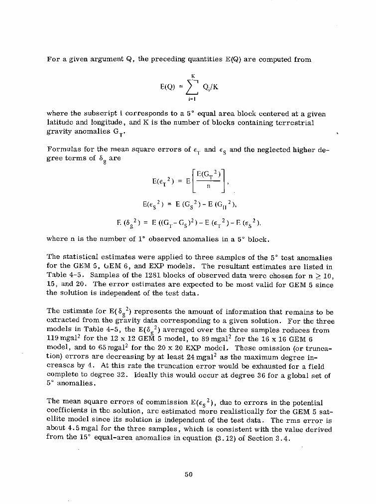
For a given argument Q, the preceding quantities E(Q) are computed from

K

E(Q) = Qj/K

where the subscript i corresponds to a 5' equal area block centered at a givenlatitude and longitude, and K is the number of blocks containing terrestrialgravity anomalies GT.

Formulas for the mean square errors of ET and es and the neglected higher de-gree terms of 6g are

SE(GT 2)-

E(eT2 ) = E ,

E(ES 2 ) = E (Gs 2 ) - E (GH 2) ,

E(6 2 ) = E((GT -GS) 2)-E(eT 2 ) - E(e 2)

where n is the number of 10 observed anomalies in a 5' block.

The statistical estimates were applied to three samples of the 50 test anomaliesfor the GEM 5, GEM 6, and EXP models. The resultant estimates are listed inTable 4-5. Samples of the 1281 blocks of observed data were chosen for n > 10,15, and 20. The error estimates are expected to be most valid for GEM 5 sincethe solution is independent of the test data.

The estimate for E( 6g2) represents the amount of information that remains to beextracted from the gravity data corresponding to a given solution. For the threemodels in Table 4-5, the E(6g2 ) averaged over the three samples reduces from119 mgal 2 for the 12 x 12 GEM 5 model, to 89mgal2 for the 16 x 16 GEM 6model, and to 65 mgal 2 for the 20 x 20 EXP model. These omission (or trunca-tion) errors are decreasing by at least 24 mgal 2 as the maximum degree in-creases by 4. At this rate the truncation error would be exhausted for a fieldcomplete to degree 32. Ideally this would occur at degree 36 for a global set of50 anomalies.

The mean square errors of commission E(es 2 ), due to errors in the potentialcoefficients in the solution, are estimated more realistically for the GEM 5 sat-ellite model since its solution is independent of the test data. The rms error isabout 4.5 mgal for the three samples, which is consistent with the value derivedfrom the 150 equal-area anomalies in equation (3.12) of Section 3.4.

50

Degree variances of gravity anomaly give a measure of the power spectrum cor-

responding to harmonic wavelengths of degree n. Gravity anomaly degree vari-

ances for the GEM 5, GEM 6, and EXP models are listed in Table 4-6. Values

are quite consistent from degree 2 to 12 for the three solutions. For these co-

efficients, a maximum difference of 3 mgal 2 is seen at degree 7 between GEM 5

and each of the combination solutions. Degree variances are listed beyond de-

gree 12 for the GEM 5 satellite model but these include only the effects of the

zonal and selected satellite resonant terms. Similarly the results agree very

well between the GEM 6 and the EXP model through degree 16. The sharp rise

in the EXP (20 x 20) result for degrees 19 and 20 is probably related to the so-

called "aliasing" effect. This effect is due to the truncation of the spherical

harmonics. Some of the remaining information in the gravity anomaly (6 g) for

higher degree (>20) terms is absorbed into adjacent degree terms in the solution.

Table 4-6

Gravity Anomaly Degree Variances (mgals2 )

Degree n GEM 5 GEM 6 EXP

0 - 9.0 9.02 7.3 7.3 7.3

3 33.5 33.6 33.54 19.5 19.3 19.3

5 20.4 21.6 21.1

6 18.6 20.0 19.77 20.1 17.4 17.1

8 10.5 8.4 8.49 10.0 8.8 8.5

10 10.8 11.4 10.711 7.1 7.7 7.512 4.0 4.1 4.213 5.2 10.6 9.314 1.7 5.9 6.215 1.9 8.5 6.7

16 0.7 6.8 7.517 0.3 0.3 5.5

18 2.4 2.4 7.719 1.0 1.0 12.520 0.5 0.5 10.921 0.8 0.9 0.8

22 1.6 1.5 1.5

51

Table 4-6 includes a value corresponding to the harmonic of degree zero,namely Ago, which was derived in the combination solutions as an adjustmentfor the reference value of equatorial gravity ge. Since A go = 3 mgal, the ref-erence value of ge given in Table 2-5 is adjusted to 978032.1 mgal (ge) so as tocorrespond to the observed gravity data. The observed and computed gravityanomalies used in the comparisons above referred to normal gravity with theadjusted ge'.

Maps of gravity anomaly contours are presented in Figures 4-1 for GEM 5 and4-2 for GEM 6. The differences in results are primarily due to the truncationat degree 12 in the GEM 5 model. The global RMS of the anomaly differencesfor the terms through degree 12 between the two models is 3 mgal and for termsbeyond degree 12 it is 5.5 mgal. Maps of geoid height are given in Figure 4-3for GEM 5 and 4-4 for GEM 6 and these are subsequently discussed in Section4.1.4. The maps are based upon a reference ellipsoid with parameters listedin Table 2-5. *

4.1.3 Comparison with Satellite Data (Analysis of the Effects of Different Mod-els of the Gravitation Potential on Satellite-Observation Residuals)-Orbits havebeen derived from several sets of tracking observations with use of variousmodels of the gravitational field. The rms of the observation residuals found byuse of the different models is used as a measure for comparing them. Resultsare presented in the following Tables:

Table 4-7 - USB tracking data on 11 daily arcs of the ERTS-1 satellite

Table 4-8 - 7-day arcs of camera data on 23 satellites

Table 4-9 - BE-C laser DME data on 22 short arcs

Table 4-10 - Long-term zonal perturbations on 21 satellites

The unified S-band (USB) tracking data were processed for 11 stations usingeach of the GEM models and SAO SE 2. The results are listed in Table 4-7.These data provided global coverage for the orbit on 11 daily arcs of the ERTS-1satellite. For each daily arc the number of two-way Doppler range-rate obser-vations and station passes are listed. The rms of the residuals are given foreach arc along with the average for the 11 arcs corresponding to each of the

*A map of geoid height of GEM 6 referenced to an earth in hydrostatic equilibrium is given by Khan andO'Keefe, "Recommended Reference Figures for Geophysics and Geodesy," GSFC X-592-73-318(Figure 2), October 1973.

52

-0 60o

40' AO'

20- 20'

Figure 4-1. GEM 5 Gravity Anomaly Contours(10mgal Interval)

Lnn

-30 -0'30

5-70

Figure 4-1. GEM 5 Gravity Anomaly Contours(10mgal Interval)

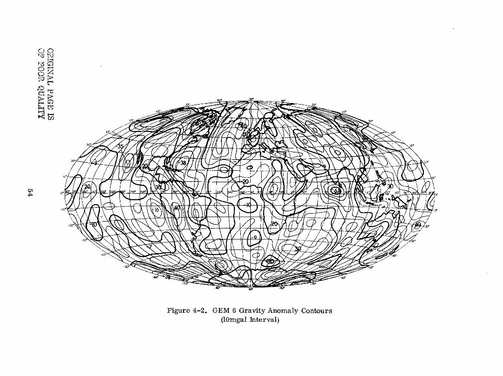
so-70.

5o* so.

30*30

20* 38 .,

10V

-To, 16

-30*

-2

-40'

--760

-o* -8T

Figure 4-2. GEM 6 Gravity Anomaly Contours(10mgal Interval)

55

60. 4

-- 70* -70*

Figu' 4-.G305Godl egt

1 30

'-40

-60

Fiue -. GE eodlHegt

(1m ntrvl

k70-

60'

-40

-°5

!01i

" 1 0D 25 0 32S 33 0 50 0 30' 40' 5 60' -ei 'A

10o 100

Figure 4-4. GEM 6 Geoidal Heights(lOm Interval)

Table 4-7

RMS (cm/sec) Value of Residuals of Two-Way Doppler forUSB Tracking on Daily Arcs of ERTS-1

Daily Arc No. of Obs. GEM 1 GEM 3 GEM 4 GEM 5 GEM 6 SE 2(1972) (passes)

7/23 2610 (27) 4.9 6.2 10.3 5.6 6.4 9.1

7/28 1924 (19) 4.9 5.5 4.7 5.5 4.0 9.4

7/29 1183 (18) 5.3 5.3 4.8 5.5 4.3 11.2

7/30 1167 (17) 5.4 6.2 5.6 6.1 3.7 8.7

7/31 989 (15) 5.9 5.7 5.4 5.7 6.2 9.8

8/1 1280 (19) 6.8 5.9 6.0 6.0 6.1 10.4

8/2 1239 (20) 6.4 5.3 6.1 5.2 4.9 11.7

8/4 1176 (18) 7.4 6.0 6.3 6.4 5.5 13.0

8/8 1026 (17) 6.1 6.0 9.1 6.4 6.3 9.1

8/9 1309 (20) 6.2 7.0 10.5 6.8 6.3 10.4

8/10 1686 (20) 5.8 6.1 9.9 6.1 6.9 10.1

Average rms 5.9 5.9 7.2 5.9 5.5 10.3

Orbital elements: a = 7283207m.,e = .0001,i = 99.120.11 USB Stations: ACN3, BDA3, CR03, CYI3, GDS8, GDSA, GWM3, HAW3, HSK8, MAD8, MIL3.Average of 7 stations participated per arc.

gravity models. The average rms shows the best result for GEM 6. The SE 2is significantly poorer than the GEM's in this comparison with data not includedin either solution.

Table 4-8 presents the weighted rms of observation residuals for a weekly arcon each of the 23 satellites that contain data from cameras (see Table 2-1). Therms values are weighted corresponding to the 2 arc second standard deviationrepresenting the accuracy of the cameras' data. Ideally then the rms valuesshould be close to unity (they may be scaled by a factor of 2 for conversion toare seconds). The average rms value per satellite is listed at the bottom of thetable for each of the gravity models in units of seconds of arc. The two solutionsGEM 1 and 3 and the GEM 6 combination solution all agree to within 0.37 arcseconds of the GEM 5 value of 2.37 arc seconds (in the average rms value persatellite). The GEM 4 and SE 2 are 0. 63 arc seconds and 1. 07 arc seconds lar-gerthanthe GEM 5 value, respectively. Again the GEM models give significantlybetter results than the SE 2.

57

Table 4-8

Weighted RMS of Observation Residuals in Camera Observations for aWeekly Arc on Each of 23 Satellites (Weight Based on 2 Seconds of Arc)

Satellite GEM 1 GEM 2 GEM 3 GEM 4 GEM 5 GEM 6 SAO SE 2

TELSTAR 0.9 0.9 0.9 0.9 0.9 1.0 2.5

GEOS-A 0.8 1.0 0.9 0.8 0.8 0.8 1.0

SECOR 1.3 1.2 1.3 1.2 1.3 1.2 1.3

OVI-2 2.0 2.3 2.0 2.3 2.0 2.2 2.1

ECHO 1.1 1.1 1.1 1.3 1.1 1.1 1.3

DI-D 1.5 1.7 1.5 1.7 1.4 1.7 2.5

BE-C 0.9 1.0 0.9 1.0 0.9 1.0 1.1

DI-C 1.1 1.5 1.2 1.8 1.0 1.3 1.9

ANNA-1B 1.1 1.3 1.3 1.5 1.1 1.3 1.3

GEOS-B 0.9 0.9 0.8 0.9 0.9 0.9 1.2

OSCAR 1.0 1.2 1.4 1.6 1.0 1.1 1.2

5BN-2 2.5 1.6 4.1 3.3 1.4 1.8 2.7

COURIER 1.2 1.4 1.3 1.3 1.2 1.2 1.1

GRS 1.9 2.3 2.0 2.6 1.8 2.0 4.3

TRANSIT 1.0 1.0 1.0 1.1 1.0 1.1 1.1

BE-B 1.2 1.3 1.4 1.6 1.3 1.6 1.4

OGO-2 1.6 2.9 1.3 2.9 1.4 2.6 2.9

INJUN 1.1 1.3 1.1 1.6 1.0 1.3 1.5

AGENA 1.7 1.6 1.6 1.8 1.6 1.5 2.4

MIDAS 0.8 0.8 0.8 0.8 0.8 0.8 0.8

VANG-2R 0.8 0.8 0.8 0.8 0.8 0.9 0.8

VANG-2S 1.5 1.7 1.4 1.6 1.4 1.7 1.5

VANG-3S 1.3 1.3 1.2 1.3 1.2 1.4 1.7

Average rms Average rms 2'54 2V79 2"t 71 3'10 2'37 2 1 74 3"'44(arc seconds)

58

Twenty-two short arcs on BE-C have been derived from laser data, which are

independent of the GEM solutions. The BE-C arcs are 3 revolutions in length;

each consists of four consecutive passes of data which were collected by the

GSFC laser system (GODLAS) at Greenbelt during a 5-month period starting in

July 1970. The rms of the residuals are listed in Table 4-9 for the individual

arcs, along with an average rms per arc. The results agree to within .3 meter

for the GEM 1, GEM 5, and GEM 6 models. These average rms values range

from 1. 33 to 1. 65 meters. As shown in the table somewhat larger average rms

values for GEM 3 (2.0 meters) and for the SE 2 model (2.51 meters) have been

obtained and a value as large as 4.05 meters has been obtained for GEM 4. For

short arcs derived from laser data on a single pass, all the above models gen-

erally give rms values of about 50 centimeters, corresponding closely to the es-

timate of the accuracy of GODLAS. A preliminary solution for the gravitational

potential (PGS 2), which was based upon camera data as in the case of GEM 1

but which is complete to degree and order 16 in harmonics and includes a num-

ber of selected higher degree terms, gave an average rms value of 1.06 meters

for the 22 four-pass arcs. Results for individual arcs for PGS 2 are listed in

Table 4-9 along with the results for the other models.

Zonal solutions were tested on the orbits of 21 satellites, most of which were

not used in the models being tested (e.g. Wagner, 1972). They include the low

inclination satellites of SAS and PEOLE. Tests were for the long-term zonal

effects on mean elements. Wagner uses as criteria the weighted rms of the

mean element residuals of each solution, which represents a relative measure

of accuracy. Results are listed in Table 4-10.

The solutions that contain the low inclination satellites, GEM 3 through 6 and

French 71, compare favorably in this test. Considering that the GEM satellite

solutions were based upon week-long orbital arcs and the French 71 solution was

based upon satellite long-term zonal effects, it verifies that good zonal recovery

may be achieved from short-term zonal effects. The SAO SE 2, GEM 1, and

GEM 2 solutions do not compare as well in these tests because they do not con-

tain the effects of low inclination satellites. Wagner's solution is expected to

have the lowest rms since it was based entirely upon the test data.

Summary results of Tables 4-7 through 4-10 of this section and Table 4-4 of the

previous section are presented in Table 4-11. The rms values of observation

residuals for the different data categories show, on the average, better results

for the GEM 5 and GEM 6 models. For purposes of ordering the models for

evaluation a simplified ranking scheme was used, as described in the table, and

was based upon the relative order of the rms values from the different compari-

sons. Using this method, GEM 5 and 6 rank highest while GEM 4 and the SE 2

model rank least.

59

Table 4-9

Rms(m) of Residuals from Laser System Measurements of Short Arcs of BE-C

DATE TIME NO.YYMMDD HHMMSS PTS. GEM 1 GEM 3 GEM 4 GEM 5 GEM 6 SAO SE 2 PGS 2

700706 205829 493 1.2 3.4 3.9 2.0 1.4 1.4 0.9

700818 040000 1712 2.1 1.4 1.3 1.8 2.1 1.4 1.2

700822 040435 1777 1.7 2.3 5.2 2.2 1.2 3.7 0.8

700824 024423 1338 1.5 1.2 1.8 1.2 1.8 0.9 1. 1

700825 035555 1197 1.2 2.4 5.5 1.3 3.0 1.4 1.3

700826 031510 1072 0.9 2.3 6.0 1.3 2.2 2.5 0.9

700827 023425 1498 1.3 2.7 5.3 2.0 1.3 3.1 0.8

700828 015324 1269 1.3 1.5 3.3 1.6 1.0 2.7 0.7

700829 011340 1579 1.3 0.9 0.8 1.1 1.2 1.1 i.0700831 014527 1008 0.7 2.0 5.1 1.0 2.5 1.6 1. 0

700901 010340 2001 1.2 3.3 7.5 2.0 2.4 3.6 1.0

700902 002214 1875 1.4 2.4 5.3 2.0 1.1 3.5 0.8

700902 230000 1567 1.2 1.1 2.1 1.4 0.7 1.9 0.8

700907 221312 1349 1.5 2.0 4.0 1.4 1.1 3.6 1.0

700911 193306 775 1. 1 2.8 5.4 1.7 1.9 2.7 0.9

700929 140000 615 1.0 1. 1 1.9 1.0 1.0 2.5 1. 1

701001 130000 690 1.9 0.8 1.7 1.4 1.7 1.7 1.7

701003 135548 818 0.9 2.0 7.3 1.0 2.6 3.0 2.2

701017 080000 568 2.2 1.9 3.2 2.2 1.3 4.0 1.1

701116 222815 506 1.1 2.9 5.1 1.7 2.3 2.1 1.2

701117 214802 723 1.1 1.9 5.0 1.3 1.6 3.4 1.0

701124 185600 1285 1.5 1.6 2.5 1.6 0.9 3.4 0.9

Average rms 1.33 2.00 4.05 1.54 1.65 2.51 1.06

Table 4-10

Comparison of Models for Long-Term (Orbital) Zonal Perturbations

Solution rms Solution rms Solution rms

SAO SE 2* 5.49 French 71 3.28 GEM 5 3.13

GEM 2* 4.80 GEM 3 2.92 GEM 6 2.97

GEM 1* 3.62 GEM 4 2.89 Wagner 1.50***These models did not include low inclination satellite in their solutions.

**This result was derived from direct use of the data.

60

Table 4-11

Summary of Gravity Model Comparisons with Satellite and Gravimetry Data(RMS of Observation Residuals)

Optical Data Doppler* Long-Term

on Weekly USB Doppler* Laser Data* Zonal 50 TerrestrialData on 11

Arcs for on 22 BE-C Perturbations Gravity Average**Models 23 Satellites Daily ERTS- Short Arcs on 21 Satellites Anomalies Rank

(seconds Arcs (meters) (relative (mgal)

of arc) measure)

GEM 1 2.54 5.9 1.33 3.62 13.3 2.3 (4)

GEM 3 2.71 5.9 2.00 2.92 13.0 2.2 (3)

GEM 4 3.10 7.2 4.05 2.89 12.1 2.8 (5)

GEM 5 2.37 5.9 1.54 3.13 13.0 1.6 (2)

GEM 6 2.74 5.5 1.65 2.97 11.7 1.4 (1)

SAO SE 2 3.44 10.3 2.51 5.49 13.3 4.6 (6)

*Data for these two categories were independent of the solutions for all models.

**Models were ranked in each category with a serial number (0, 1, 2, 3, 4, 5) corresponding respectively to increasing RMS values. The average

rank for a given model was obtained as the mean of the individual rankings, and the mean was used to rank the models from 1 to 6 as shown

in parentheses.

4.1.4 Geoid Height-Contour maps of geoidal heights relative to the referenceellipsoid are presented in Figures 4-3 and 4-4 for the GEM 5 and GEM 6 models,respectively. The major features of relative highs and lows are exhibited belowfor eight main features.

Table 4-12

Major Features of the Geoid

Approximate HeightNumber Geographic Name Approximate Height

Latitude Longitude GEM 5 GEM 6

1 Solomon Island High -100 1500 73 77

2 Indian Low 00 800 -110 -110

3 British Isle High 500 3500 64 70

4 Bahama Low 300 2900 -53 -55

5 Antartica High -550 500 46 50

6 North East Pacific Low 200 2400 -47 -55

7 Antartica Low -700 2000 -60 -57

8 South America High -200 2900 32 35

There is a good agreement between the two models in the major features. Thelargest difference is 8 meters and occurs at the North East Pacific Low.

Some comparisons are made between the GEM 6 and other geoids. A zonal pro-file of geoidal height from GEM 6 is given in Figure 4-5. An rms of differencesbetween geoidal heights computed from the zonal harmonic coefficients of Caze-nave et al. (1971) and from those of GEM 6 is 0.2 meters; the maximum differ-ence is less than a meter. In general a global rms of differences (Ah) in geoidalheight between two models may be estimated using Bruns formula (Heiskanenand Moritz, 1967) and it is given as follows:

rmsAh = (Anm + nm (4.1)

n=2 m=O

62

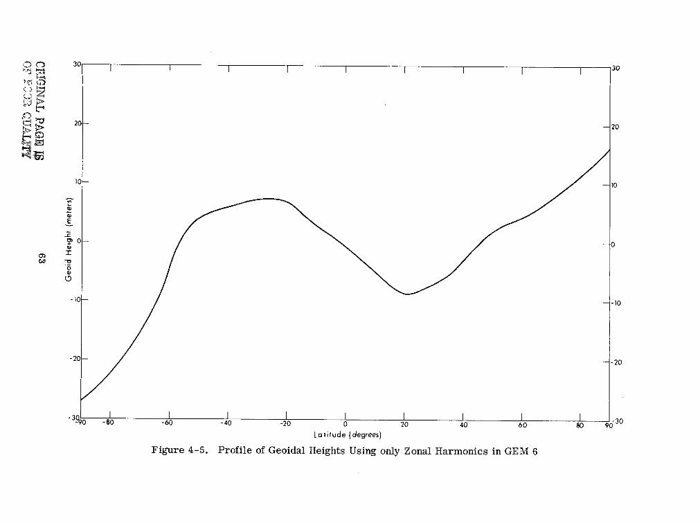
I- Ca 303 IoI I I 30

20 -20

10 - -10

E

-- 0

O

0

-10- - -10

-20 - -20

-I I I I I I I I -3 0-90 -80 -60 -40 -20 0 20 40 60 80 90

Lo atitude (degrees)

Figure 4-5. Profile of Geoidal Heights Using only Zonal Harmonics in GEM 6

where AC, AS are normalized coefficient differences of degree n and order mbetween the two models, Re is the mean radius for the earth, and N correspondsto the largest degree term in the models.

Using equation (4.1), comparisons between the GEM 6 solution and various mod-els are listed as follows:

Table 4-13

Global RMS of Geoid Height Differences with the GEM 6 Model

GEM 2 GEM 4 GEM 5 EXP (20 x20)

rms (meters) 3 3 4 4

The effect of truncation on geoid height for coefficients beyond degree N may beestimated from use of Kaula's values (10-5/n 2) for these coefficients. By ex-tending (4.1) and replacing the differences with Kaula's values we obtainapproximately

64rmsAh (n> N) = N (meters). (4.2)

Using the above result of 4 m for EXP (20 x 20) and a value of 3 m, obtainedfrom (4.2) with N = 20, for the effect of truncation, a global (rms) error ingeoid height for GEM 6 is estimated as

OAh (GEM 6 ) = (42 + 32)/2 = 5 m (4.3)

Errors in geoid height for GEM 6 may be expected to be smaller in areas of ma-jor survey where gravimetric data is more complete. For example, tests weremade for GEM 6 with the use of a detailed geoid in North America, Eurasia, andAustralia (Vincent et al., 1972) where 1°-by-l1 gravity anomaly data were used.An rms of geoid height differences for these areas was about 3.5 meters. How-ever large variations in geoid height exist in certain areas. For example, a dif-ference of 12 meters exists in the vicinity of the Puerto Rican Trench.

The result in Table 4-13 of 4m for the rms of geoid height differences betweenGEM 5 and 6 considers terms from degrees 12 to 16 that have not been includedin the solution for GEM 5. For terms that are common to the two models therms value for geoid height differences is 3 meters. This value compares closelyto the value obtained from the error estimates of the coefficients in GEM 5, asmay be seen from (3.17) of Section 3.

64

4.2 Station Coordinates for GEM 6

In conjunction with the derivation of the GEM 6 gravitational field, positions

were derived for some 134 tracking stations. Positions for all stations except

the BC-4 camera stations were derived dynamically. The positions of the BC-4

stations were derived by using the geometric theory of simultaneous observa-

tions between BC-4 cameras and using constraints on relative positions from

ground surveys to tie a subset of BC-4 stations to other camera and Doppler

stations. Also certain positions for MOTS and GSFC laser sites were derived

using both the geometric and dynamic process.

In addition, constraints from geodetic networks were applied to the relative po-

sitions of certain pairs of stations. These relative position constraints, based

on local datum survey coordinates, were applied to 47 pairs of stations, where

in our judgment such ground survey ties would strengthen the solution. Table

4-14 lists the ties, the A x, Ay, A z survey differences, an estimated uncertainty

used for weighting, and the residuals from the solution. Except for Doppler sta-

tions, uncertainties were estimated in a formal way from Simmons' Rule* as

a = .029 D21 3 (meters)

where D is the distance between the stations in kilometers. The Doppler sta-

tions are uncertain by an additional 3 meters due to a lack of information con-

cerning the relationship of the surveyed point to the electrical (phase) center of

the Doppler antennae. This weighting is not critical. A reasonable variation in

weights results in nearly the same solution.

In arriving at the station positions, a set of chord distances between BC-4 sta-

tions, with associated error estimates, were also enforced. These chord dis-

tances, taken from Mueller (1973), together with the error estimates assigned

in this solution are presented in Table 4-15. The observations used in the solu-

tion are described in Section 2 and the theory used in Appendix A.

The station coordinates were derived as part of the GEM 6 solution along with

the geopotential, amounting to 729 unknown parameters. The solution of this

large a set of normal equations required some attention to numerical accuracy.It was obtained by the Cholesky method with use of an iterative improvement

process. A computed condition number indicated that the corrections to initial

values were accurate to six digits. The average correction for station coordi-

nates was of the order of 10 meters, except for a few Doppler stations where the

corrections were of the order of 100 meters. Of the unknowns, 328 were cor-

rections to coefficients of the Earth's gravitational potential, and 402 were cor-

rections to assumed coordinates of 134 stations.

*Simmons, L. G., "How Accurate is First-Order Triangulation?", Journal of U.S. Coast and Geodetic Sur-

vey, April 1950.

65

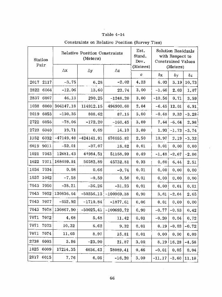
Table 4-14

Constraints on Relative Position (Survey Ties)

Est. Solution ResidualsRelative Position ConstraintsStation (Meters) Stand. with Respect to

Dev. Constrained ValuesPair (Meters) (Meters)

Ax Ay Azo bx 5y z

2017 2117 -3.75 6.28 -2.02 4.23 6.03 3.19 10.73

2822 6064 -12.06 13.60 23.74 3.00 -1.66 2.03 1.07

2837 6067 46.13 290.25 -1248.20 3.00 -10.56 0.71 3.59

1038 6060 304147.18 114912.15 494900.60 2.04 -6.45 12.01 6.91

2019 6053 -130.35 808.62 87.15 3.00 -0.48 9.33 -3.28

2722 6055 -78.06 -172.20 -160.45 3.00 7.44 -6.64 2.98

2723 6040 19.71 0.69 14.10 3.00 1.93 -1.73 -3.74

1152 6032 -47149.40 -424141.91 676055.82 2.50 10.97 2.19 -3.32

6019 9011 -52.01 -37.07 18.82 0.01 0.01 0.00 0.00

1021 7043 12681.43 44984.51 51158.99 0.49 -1.48 -2.67 -2.86

1022 7071 168409.91 50582.89 45732.81 0.93 0.60 6.44 2.51

1034 7034 0.08 0.66 -0.74 0.01 0.00 0.00 0.00

1037 1042 -7.58 -0.59 0.50 0.01 0.00 0.00 0.00

7043 7050 -38.21 -36.26 -31.23 0.01 0.00 0.01 0.01

7043 7052 130836.64 -50256.13 -100969.38 0.90 3.61 -2.64 2.65

7043 7077 -652.92 -1710.84 -1877.61 0.06 0.01 0.00 0.00

7043 7078 130867.90 -50025.41 -100693.72 0.90 -0.77 -0.53 0.42

7071 7072 4.08 5.48 11.42 0.01 -0.20 0.04 0.72

7071 7073 10.32 6.62 9.32 0.01 0.19 -0.03 -0.72

7071 7074 11.03 8.97 15.81 0.01 0.00 0.00 0.00

2738 6003 3.96 -23.90 21.87 3.00 8.19 16.28 -4.58

1025 6009 17214.35 4034.43 58089.41 0.46 -0.01 0.05 0.04

2817 6015 7.76 4.05 -16.20 3.00 -11.17 -3.60 11.18

66

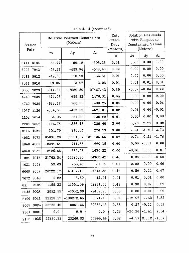
Table 4-14 (continued)

Est. Solution ResidualsRelative Position Constraints

Stand. with Respect to

Station (Meters) Dev. Constrained Values

Pair (Meters) (Meters)Ax Ay Az

o 6x 6y 5z

6111 6134 -53.77 -90.12 -305.26 0.01 0.00 0.00 0.00

6002 7043 -56.27 -499.54 -568.43 0.02 0.00 0.00 0.00

6011 9012 -49.58 118.93 -35.81 0.01 0.00 0.00 0.00

7071 9010 19.05 3.07 3.92 0.01 0.01 0.01 0.01

9003 9023 6011.64 -17986.56 -27467.42 0.30 -0.02 -0.04 0.42

4740 7039 -674.06 699.92 1476.31 0.04 0.00 0.00 0.00

4760 7039 -683.27 706.55 1488.25 0.04 0.00 0.00 0.01

1037 1126 -334.06 -403.53 -571.31 0.02 0.01 0.00 -0.01

1152 7054 54.96 -51.86 -135.62 0.01 0.00 0.00 0.00

2203 7052 -116.78 -336.48 -389.60 3.00 5.76 2.27 0.02

2115 4050 354.70 970.65 296.73 3.00 1.51 -3.76 3.73

4082 7071 65691.26 62291.57 137 735.55 0.87 -0.74 -0.31 -1.78

4840 4860 -2384.64 711.85 1660.19 0.06 0.00 -0.01 0.00

4840 7052 -2425.68 685.03 1630.22 0.06 -0.01 0.00 0.01

1024 4946 -21762.84 24680.80 54300.42 0.46 0.28 -0.20 -0.60

1031 6068 59.69 -55.46 51.19 0.01 0.00 0.00 0.00

6068 9002 28722.17 46167.12 -7673.38 0.42 0.50 -0.44 0.47

7072 9049 4.82 -3.60 -12.97 0.01 0.01 0.01 0.00

6111 9425 -1159.33 43554.59 52281.60 0.48 0.38 0.07 0.09

6042 9028 2992.55 -3032.66 -2462.26 0.08 0.00 0.01 0.00

2100 6011 32128.97 -180272.68 -83071.46 3.04 -12.07 1.62 5.85

9005 9025 36256.49 10061.56 30386.63 0.38 0.27 -0.11 0.52

7901 9001 0.0 0.0 0.0 4.23 -20.28 -1.41 7.34

2106 1035 -22330.33 23266.93 17999.44 3.02 -4.97 21.12 -1.57

67

Table 4-15

Constraints on Baseline Distance (BC-4 Stations)

Distance Estimated Standard Residual(meters) Deviation PPM, (m) (meters)

6002-6003 3 485 363.23 1.00 (3.49) 6.58

6006-6016 3 545 871.56 1.00 (3.55) 1.68

6006-6065 2 457 765.81 0.70 (1.72) -1.04

6016-6065 1 194 793.60 0.85 (1.02) 2.92

6023-6060 2 300 209.80 0.50 (1.15) -1.72

6032-6060 3 163 623.87 1.00 (3.16) -5.54

6063-6064 3 485 550.76 0.85 (2.96) -2.32

6003-6111 1 425 876.45 0.90 (1.29) -2.03

The station coordinate results are presented in Table 4-16 in the form of lati-tude, longitude, and geodetic height with respect to an ellipsoid having a semi-major axis of 6378155 meters and a flattening of 1/298.255.

Before discussing these results, the consequences of the applied constraintsshould be examined. First, comparisons of GEM 6 station coordinates withGEM 4 station coordinates, as well as with other solutions not involving theBC-4 stations, indicate that most positions derived dynamically are essentiallyunaffected by inclusion of the BC-4 network. The only exceptions are Dopplerstations 2019, 2722, 2723, and 2738. Only a small amount of Doppler data wasavailable for determination of the positions of these stations, and they are veryweakly determined from calculations using dynamics. These stations were es-sentially determined from the BC-4 and baseline data used in the solution.

Secondly, the baseline constraints and the ties to the dynamic system both pro-vide scale to the BC-4 network. The scale inferred by using the baselines onlyis approximately 2 ppm smaller than the dynamical results as discussed in Sec-tion 4.2.2. A comparison of combination solutions (BC-4 geometric and dynam-ical) with and without baselines shows essentially no change in scale for the BC-4 network, except for 8 of the 47 BC-4 stations that were tied in directly or

68

Table 4-16

GEM 6 Station Coordinates

STATION POSITIONS FOR BAKER-NUNN

STATION LATITUDE LONGITUDE HEIGHT SIGMA*

NAME NUMBER DEG MN SECOND DEG MN SECOND METERS METERS

1ORGAN 9001 32 25 25.079 253 26 48.996 1619.1 4.

LOLFAN 9002 -25 57 35.837 28 14 52.459 1559.0 3.

WOOMER 9003 -31 6 2.124 136 47 3.319 155.5 4.

1SPAIN 9004 36 27 46.818 353 47 36.958 60.0 3.

1TOKYO 9005 35 40 22.968 139 32 16.563 84.9 5.

INATAL 9006 29 21 34.781 79 27 27.517 1871.0 4.

1IUIPA 9007 -16 27 56.628 288 30 24.604 2484.7 4.

1CURAC 9008 29 38 13.839 52 31 11.372 1580.3 5.

ISHRAZ 9009 12 5 25.186 291 9 44.532 -23.2 5.

1JUPTR 9010 27 1 14.120 279 53 13.357 -24.8 3.

IVILDO 9011 -31 56 34.597 294 53 36.609 625.1 4.

1MAUIO 9012 20 42 26.175 203 44 33.983 3042.8 4.

HOPKIN 9021 31 41 3.302 249 7 18.599 2341.0 6.

AUSBAK 9023 -31 23 25.694 136 52 43.649 134.0 4.

DODAIR 9025 36 0 20.304 139 11 31.565 883.7 5.

DEZEIT 9028 8 44 51.242 38 57 33.407 1904.1 5.

COMRIV 9031 -45 53 12.290 292 23 9.413 192.5 5.

JUPGEO 9049 27 1 13.948 279 53 12.993 -28.1 3.

AGASSI 9050 42 30 21.542 288 26 30.583 129.9 17.

GREECE 9091 38 4 44.849 23 55 58.658 487.2 5.

COLDLK 9424 54 44 34.634 249 57 23.125 669.4 12.

EDWAFB 9425 34 57 50.677 242 5 8.030 748.9 6.

OSLONR 9426 60 12 39.200 10 45 2.938 617.0 13.

JOHNST 9427 16 44 38.879 190 29 9.343 18.8 7.

STATION POSITIONS FOR GRARR

STATION LATITUDE LUNGITUDE HEIGHT

NAME NUMBER DEG MN SECOND DEG MN SECOND METERS SIGMA

MADGAR 1122 -19 1 16.314 47 18 15.185 1349.6 38.

MADGAS 1123 -19 1 14.392 47 18 11.335 1387.6 5.

ROSRAN 1126 35 11 45.528 277 7 26.240 828.1 3.

ULASKR 1128 64 58 18.964 212 29 12.728 338.8 3.

CARVON 1152 -24 54 11.015 113 42 59.302 2.5 4.

STATION POSITIONS FOR C-BAND

STATION LATITUDE LONGITUDE HEIGHT

NAME NUMBER DEG MN SECOND DEG MN SECOND METERS SIGMA

ETRPRE 4050 -25 56 37.592 28 21 28.937 1588.6 12.

ETRMRT 4082 28 25 28.943 279 20 7.649 -30.7 5.

NBER34 4740 32 20 53.337 295 20 46.909 -26.9 4.

NWALI8 4840 37 50 29.160 284 30 53.007 -39.4 4.

NWALI3 4860 37 51 37.279 284 29 25.864 -36.4 4.

NBER05 4760 32 20 52.837 295 20 47.119 -24.9 4.

WOOR38 4946 -30 49 5.877 136 50 17.532 124.3 6.

*Error estimate for Cartesian coordinates.

ae = 6378155 mf = 1/298.255

OrIGINAL PAGE IS 69OP POORJ QUALITY

Table 4-16 (continued)

STATION POSITIONS FOR DOPPLER

STATION LATITUDE LONGITUDE HEIGHT SIGMANAME NUMBER DEG MN SECOND DEG MN SECOND METERS METERS

ANCHOR 2014 61 17 0.168 210 10 29.035 63.9 5.TAFUNA 2017 -14 19 49.937 189 17 3.046 27.4 5.THOLEG 2018 76 32 19.344 291 13 54.033 51.9 8.MCMRDO 2019 -77 50 52.257 166 40 25.770 -33.1 8.WAHIWA 2100 21 31 15.531 202 0 10.436 395.6 4.LACRES 2103 32 16 44.522 253 14 45.428 1150.7 5.LASHM2 2106 51 11 9.367 358 58 25.532 217.8 4.APLMND 2111 39 9 48.588 283 6 11.907 96.0 4.PRETOR 2115 -25 56 48.272 28 20 52.046 1582.6 5.ASAMDA 2117 -14 19 50.265 189 17 2.891 39.5 5.WALUDOP 2203 37 51 52.094 284 29 32.286 -38.0 9.ASCION 2722 - 7 58 9.757 345 35 40.701 88.6 8.COCOSL 2723 -12 11 44.560 96 50 3.054 -44.3 12.MOSLAK 2738 47 11 7.247 240 39 43.766 338.3 12.STNVIL 2745 33 25 32.087 269 5 9.799 -2.5 35.MESHED 2817 36 14 26.485 59 37 44.239 950.8 5.FRTLMY 2822 12 7 53.927 15 2 6.787 298.5 6.NATLDP 2837 - 5 54 57.998 324 49 55.950 3.9 5.

STATION POSITIONS FOR MOTS

STATION LATITUDE LONGITUDE HEIGHTNAME NUMBER DEG MN SECOND OEG MN SECOND METERS SIGMA

1BPOIN 1021 38 25 50.253 282 54 48.699 -38.2 3.IFTMYR 1022 26 32 53.359 278 8 4.161 -35.9 3.10OOMER 1024 -31 23 24.970 136 52 15.455 128.6 5.IOUITO 1025 - 0 37 21.567 281 25 16.401 3571.8 15.ISATAG 1028 -33 8 58.448 289 19 53.576 709.3 5.1MOJAV 1030 35 19 47.931 243 5 59.055 886.2 3.1JORUR 1031 -25 53 0.843 27 42 26.404 1537.2 3.1NEWFL 1032 47 44 29.838 307 16 46.121 64.2 7.1GFORK 1034 48 1 21.344 262 59 19.513 216.4 3.1WNKFL 1035 51 26 46.148 359 18 8.330 97.3 51ULASK 1036 64 58 37.046 212 28 31.715 284.1 7.1ROSMN 1037 35 12 7.388 277 7 41.321 864.1 3.InRORL 1038 -35 37 32.106 148 57 14.825 943.5 4.1ROSMA 1042 35 12 7.408 277 7 41.021 864.1 3.1TANAN 1043 -19 0 31.860 47 17 59.360 1362.2 6.1UNOAK 7034 48 1 21.344 262 59 19.513 215.4 3.1EDINB 7036 26 22 46.743 261 40 7.459 20.9 3.1COLBA 7037 38 53 36.207 267 47 40.940 227.4 3.IBERID 7039 32 21 49.826 295 20 35.069 -14.9 4.1PURIO 7040 18 15 28.817 294 0 23.584 -10.4 3.IGFSCP 7043 39 1 15.716 283 10 20.528 10.1 3.1DENVR 7045 39 38 48.056 255 23 38.640 1757.8 3.1JUM24 7071 27 1 14.010 . 279 53 12.657 -26.9 3.1JUM40 7072 27 1- 14.388 279 53 12.844 -26.1 3.1JUPCI 7073 27 1 14.372 279 53 13.060 -26.6 3.1JUBC4 7074 27 1 14.570 279 53 13.107 -25.9 3.ISUOBR 7075 46 27 21.306 279 3 10.514 235.5 5.IJAMAC 7076 18 4 34.700 283 11 27.038 417.9 5.1GFSCN 7077 3H 59 57.438 283 9 37.906 7.1 3.WALMOT 7078 37 51 47.543 2i4 29 27.717 -39.6 5.

70

Table 4-16 (continued)

STATION POSITIONS FOR BC-4

STATION LATITUDE LONGITUDE HEIGHT SIGMANAME NUMBER DEG MN SECOND DEG MN SECOND METERS METERS

BELTSV 6002 39 1 39.706 283 10 27.538 0.1 3.MOSELK 6003 47 11 6.660 240 39 43.768 331.6 7.SHEMYA 6004 52 42 48.985 174 07 26.363 38.3 17.TROMSO 6006 69 39 44.108 18 56 29.299 109.3 12.TRCERA 6007 38 45 36.426 332 54 25.707 99.9 8.PARMBO 6008 5 26 53.866 304 47 40.707 -30.2 12.OUITO 6009 - 0 5 51.408 281 34 47.674 2685.5 13.MAUIO 6011 20 42 27.235 203 44 38.433 3057.8 4.WAKEIS 6012 19 17 28.643 166 36 39.443 -15.6 9.KANOYA 6013 31 23 42.733 130 52 16.579 76.1 13.CATNIA 6016 37 26 38.374 15 2 45.352 38.6 7.MASHAD 6015 36 14 25.459 59 37 43.740 947.7 7.VILDOL 6019 -31 56 35.317 294 53 38.999 625.1 4.EASTER 6020 -27 10 36.330 250 34 22.636 199.6 17.TUTILA 6022 -14 19 54.394 189 17 8.692 15.5 8.THRUSD 6023 -10 35 3.276 142 12 39.420 107.9 8.INVERC 6031 -46 24 58.309 168 19 31.502 -11.5 7.CAVERS 6032 -31 50 25.036 115 58 31.671 -18.1 6.SOCORO 6038 18 43 58.568 249 2 41.347 -23.0 8.PITCRN 6039 -25 4 6.765 229 53 12.572 295.2 19.COCOSI 6040 -12 11 43.990 96 50 2.460 -47.8 8.ADISRA 6042 8 46 12.504 38 59 52.089 1865.2 5.CERROS 6043 -52 46 52.600 290 46 34.090 78.3 8.HEARDI 6044 -53 1 9.425 73 23 34.212 34.8 12.MAURIT 6045 -20 13 52.901 57 25 31.944 133.1 8.ZAMHGA 6047 6 55 20.395 122 4 8.907 59.3 11.PALMER 6050 -64 46 26.371 295 56 53.697 23.1 12.MAWSON 6051 -67 36 4.268 62 52 22.242 28.8 8.WILKES 6052 -66 16 44.937 110 32 7.169 -5.5 8.MCMRDO 6053 -77 50 41.846 166 38 31.279 -56.0 8.ASCENS 6055 - 7 58 15.213 345 35 34.770 70.1 7.XMASIL 6059 2 0 18.617 202 35 16.306 2.3 8.CULGDA 6060 -30 18 34.411 149 33 40.993 226.2 5.SGAISL 6061 -54 17 0.709 323 30 21.877 2.0 9.DAKAR 6063 14 44 42.292 342 31 0.697 44.3 7.FORTLY 6064 12 7 54.697 15 2 7.246 296.4 5.HOHNBG 6065 47 48 3.758 11 1 25.916 970.1 9.NATALR 6067 - 5 55 38.935 324 50 4.707 13.2 8.JOBIJRG 6068 -25 52 58.963 27 42 23.644 1539.2 3.TRSUNA 6069 -37 3 53.227 347 41 5.670 25.3 15.CHIMAI 6072 18 46 10.593 98 58 2.372 245.9 11.DGOGRA 6073 - 7 21 6.513 72 28 20.592 -77.9 9.MAHE 6075 - 4 40 14.620 55 28 47.950 534.4 9.PRTVLA 6078 -17 41 31.834 168 18 24.472 54.4 28.WRIGHT 6111 34 22 54.548 242 19 5.990 2247.7 5.PRRARW 6123 71 18 48.393 203 21 8.504 -34.0 18.WRIGHT 6134 34 22 44.455 242 19 5.765 2161.8 5.

STATION POSITIONS FOR LASER

STATION LATITUDE LONGITUDE HEIGHTNAME NUMBER DEG MN SECOND DEG MN SECOND METERS SIGMA

GODLAS 7050 39 1 14.387 283 10 18.638 11.1 3.WALLAS 7052 37 51 36.199 284 29 23.965 -42.4 3.CRMLAS 7054 -24 54 15.965 113 42 58.252 -3.5 4.

71

adjacent to the baselines (Table 4-15). Since the baselines are considered ac-curate to at least lppm, this solution (GEM 6, with baselines) was retained asbeing better for the eight stations 6003, 6004, 6006, 6007, 6008, 6063, 6065,and 6111.

From the above considerations the overall scale for the GEM 6 stations includingthe BC-4 geometric network is essentially derived through the dynamic system.This means that scale is determined by the reference value of GM (398601.3 km3/sec 2 ) employed inthe satellite dynamics. Here, an adjustment (s) in scale forcoordinates is related to GM as follows:

Ar _ AGM

r 3GM '

where r is the radial distance to the station. A current value of GM = 398600.8km 3/sec 2 (+0.4) has been obtained from analysis of Mariner 9 tracking data byEsposito and Wong (1972). Allowing for the new value of GM and its uncertainty,the scale would be reduced by 0.4ppm (±0.3). Hence, the above reduction inscale of 2ppm (Ar = -13 m), inferred by the 8 baselines from the geometric onlysolution, is not consistent with that inferred by recent estimates of GM.

4.2.1 Comparison with Other Solutions-Other solutions for station coordinatesare compared with GEM 6 to assess the random and systematic differences be-tween solutions. Coordinates of JPL's Deep Space Stations provide an indepen-dent source of comparison with GEM 6.

JPL's DSS solution (Mottinger, 1969) does not yield a station's complete position.The better determined parameters are distances from the spin-axis and differ-ences between the longitudes of the stations. In order to compare GEM 6 withJPL's solution, only the x, y coordinates were used (Table 4-17). GEM 6's co-ordinates for the DSS sites were obtained by using the local datum connectionsbetween the camera stations and the DSS stations. In Table 4-18 direct compar-isons are given with spin-axis distance (D) and longitude (X). JPL employs adifferent reference for longitude than GEM 6 which accounts for the large offsetof AX = 0.51". Removing this effect in longitude and an effect for scale on spinaxis distance, the resulting residuals (reflecting random errors) agree verywell as shown in Table 4-18. The scale difference of 1.4ppm is not explained.However, removal of just one station (Woomera) from this small sample wouldreduce the scale to 0.9ppm. The 3m rms (Table 4-17) is within the estimateof random error given for both GEM 6 and the JPL DSS solutions.

In Tables 4-19 through 4-23, GEM 6 is compared with five other solutions. Thefive solutions are (1) GEM 4, (2) GSFC 73 (Marsh et al., 1973), (3) SAO SE III(Gaposchkin 1973), (4) NWL 9D (Anderle 1973), and (5) the Ohio State University

72

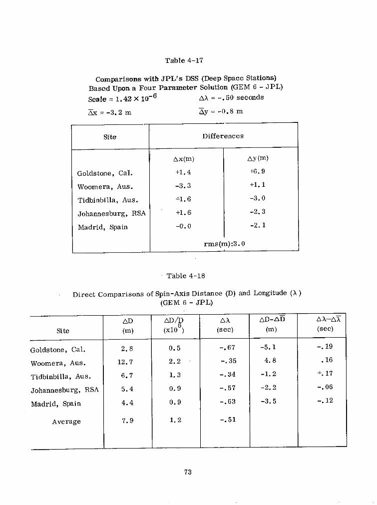
Table 4-17

Comparisons with JPL's DSS (Deep Space Stations)

Based Upon a Four Parameter Solution (GEM 6 - JPL)

Scale = 1.42 X 10 - 6 AX = -. 50 seconds

2x = -3.2 m 2y = -0.8 m

Site Differences

Ax(m) Ay(m)

Goldstone, Cal. +1.4 +6.9

Woomera, Aus. -3.3 +1.1

Tidbinbilla, Aus. +1.6 -3.0

Johannesburg, RSA +1. 6; -2. 3

Madrid, Spain -0'.0 -2. 1

rms (m):3. 0

Table 4-18

Direct Comparisons of Spin-Axis Distance (D) and Longitude (X)

(GEM 6 - JPL)

AD AD/D AX AD-AD AX-AX

Site (m) (x10 6) (sec) (m) (sec)

Goldstone, Cal. 2.8 0.5 -. 67 -5.1 -. 19

Woomera, Aus. 12.7 2.2 -. 35 4.8 .16

Tidbinbilla, Aus. 6.7 1.3 -. 34 -1.2 +. 17

Johannesburg, RSA 5.4 0.9 -.57 -2.2 -.06

Madrid, Spain 4.4 0.9 -.63 -3.5 -. 12

Average 7.9 1. 2 -. 51

73

WN 4 (Mueller 1973). Systematic differences between the solutions were esti-mated using station positions common to both solutions by solving for a transla-tion in space to make the origins coincide, three rotations about coordinate axesto orient the coordinate systems, and a scale difference. The systematic quan-tities are indicated in the tables together with the rms of the random differencesafter removal of the seven systematic parameters. The 7 parameter adjustmentand related symbols are defined in Section 4.2.3, equation (4.4).

The comparison with GEM 4 shown in Table 4-19 was carried out by solving forseven parameters using 62 common stations of GEM 6 and GEM 4. Three addi-tional seven-parameter solutions were made using subsets of the 62 stationscommon to the solutions, namely (1) 23 MOTS-SPEOPTS camera stations, (2)13 Doppler stations, and (3) 19 Baker-Nunn cameras. The comparison indicatesthe coordinate system of GEM 6 and GEM 4 are referred to the same center ofmass for all practical purposes, and that negligible differences of scale and ro-tation are involved. Hence, the coordinate systems of GEM 6 and GEM 4 arenearly identical, verifying that the addition of BC-4 geometric data has not sig-nificantly changed results from the dynamic system (GEM 4).

Table 4-20 presents results from seven-parameter solutions comparing GEM 6with GSFC 73. This result using 43 stations shows that a significant differenceoccurs in rotation (w) about the z-axis of 0.35" arc sec. The translation oforigin, scale difference, and other rotation parameters are negligible. AlthoughGSFC 73 is a solution based upon two day orbital arcs using optical data on twosatellites only, the above discrepancy in the longitude origin is not expected.

Differences in orientation among the models are discussed in Section 4.2.4,where polar and longitude displacements are plotted in Figure 4-7. Models areseen to vary from one another in longitudinal reference by as much as one sec-ond of arc.

Although good agreement exists in orientation between GEM 6 and OSU WN4,Table 4-23, large scale (1. 9 ppm) and translation (20 m) differences are seen inthis comparison of BC-4 camera stations. The large systematic differencescan be explained since WN-4 is a geometric only solution, which employs anarbitrary origin and derives scale from the eight baselines in Table 4-15. Theselarge differences do not exist in the BC-4 station comparison in Table 4-22 be-tween GEM 6 and NWL 9D, a solution whose results are derived dynamicallyfrom satellite doppler data. (The BC-4 station coordinates for NWL 9D wereinferred from adjacent doppler stations through use of survey ties.)

Since SE III and GEM 6 employ similar data, the comparisons in Table 4-21 be-tween these solutions should be closer. But the large systematic difference of15 m in the z-coordinate of the Baker-Nunn stations between GEM 6 and SE III

74

Table 4-19

Station Comparisons of GEM 6 with GEM 4

62 23 MOTS-SPEOPTS 19 BN 13 DopplerStations Camera Stations Camera Stations Stations

ax (m) .54±1.4 -. 58±2.7 .30±2. 4 .85±3.1

Ay (m) -. 44±1.4 -. 13±2.7 .03±2.4 -. 50±3.3

Sz (m) .22±1.4 -. 56±2. 8 3. 8±2. 4 -1.5±3.1

s (x106 ) -. 02± .22 -. 01± .42 .07± .37 -. 01± .48

E(sec) .00± .05 .02± .10 .02± .09 -. 10± .14

4(sec) -. 02± .05 -. 08± .13 .02± .10 -. 07± .11

w(sec) .04± .05 +.04± .12 .00± .86 +.06± .12

rms (m) ±3. 3 ±2.8 . 12 3. 7

Table 4-20

GEM 6 - GSFC 73 Station Coordinates

43 Stations

Ax (m) 0.5+ .7

AY (m) 0.6+ .6

Az (m) 2.1+ . 7

s (x106) .44+ .1

E (sec) .00+ .03

0 (sec) .04+ .03

w (sec) .35+ .03

rms (m) + 4.6

Table 4-21

Station Comparisons of GEM 6 - SAO Standard Earth III

68 Stations 17 BN Stations 47 BC-4 Stations

Ax (m) +4.2+1.22 1.9+2.4 +4.8+1.46

Ay (m) -5.3+1.22 -3.5+2.4 -6.2+1.46

Az (m) +9.5+1.22 15.0+2.4 +7.4+1.46

s (x 106) .49 + .05 .84+ .38 +.23 + .05

E (sec) +.19 + .05 -. 01+ .09 +.23 + .05

(sec) -. 08 + .05 -. 10+ .11 -. 09 + .06

w (sec) -. 46 + .05 -. 51+ .09 -. 47 + .06

rms (m) + 10 + 8 + 10

76

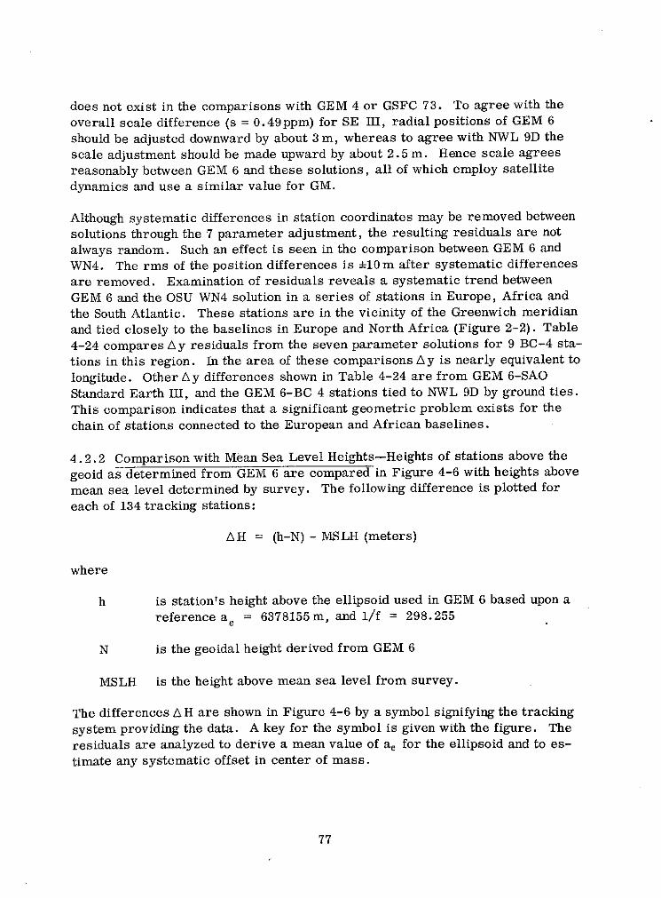
does not exist in the comparisons with GEM 4 or GSFC 73. To agree with the

overall scale difference (s = 0.49ppm) for SE III, radial positions of GEM 6

should be adjusted downward by about 3 m, whereas to agree with NWL 9D the

scale adjustment should be made upward by about 2.5 m. Hence scale agrees

reasonably between GEM 6 and these solutions, all of which employ satellite

dynamics and use a similar value for GM.

Although systematic differences in station coordinates may be removed between

solutions through the 7 parameter adjustment, the resulting residuals are not

always random. Such an effect is seen in the comparison between GEM 6 and

WN4. The rms of the position differences is ±10 m after systematic differences

are removed. Examination of residuals reveals a systematic trend between

GEM 6 and the OSU WN4 solution in a series of stations in Europe, Africa and

the South Atlantic. These stations are in the vicinity of the Greenwich meridian

and tied closely to the baselines in Europe and North Africa (Figure 2-2). Table

4-24 compares A y residuals from the seven parameter solutions for 9 BC-4 sta-

tions in this region. In the area of these comparisons Ay is nearly equivalent to

longitude. Other A y differences shown in Table 4-24 are from GEM 6-SAO

Standard Earth III, and the GEM 6-BC 4 stations tied to NWL 9D by ground ties.

This comparison indicates that a significant geometric problem exists for the

chain of stations connected to the European and African baselines.

4.2.2 Comparison with Mean Sea Level Heights-Heights of stations above the

geoid as determined from GEM 6 are compared in Figure 4-6 with heights above

mean sea level determined by survey. The following difference is plotted for

each of 134 tracking stations:

AH = (h-N) - MSLH (meters)

where

h is station's height above the ellipsoid used in GEM 6 based upon a

reference ae = 6378155m, and 1/f = 298.255

N is the geoidal height derived from GEM 6

MSLH is the height above mean sea level from survey.

The differences A H are shown in Figure 4-6 by a symbol signifying the tracking

system providing the data. A key for the symbol is given with the figure. The

residuals are analyzed to derive a mean value of ae for the ellipsoid and to es-

timate any systematic offset in center of mass.

77

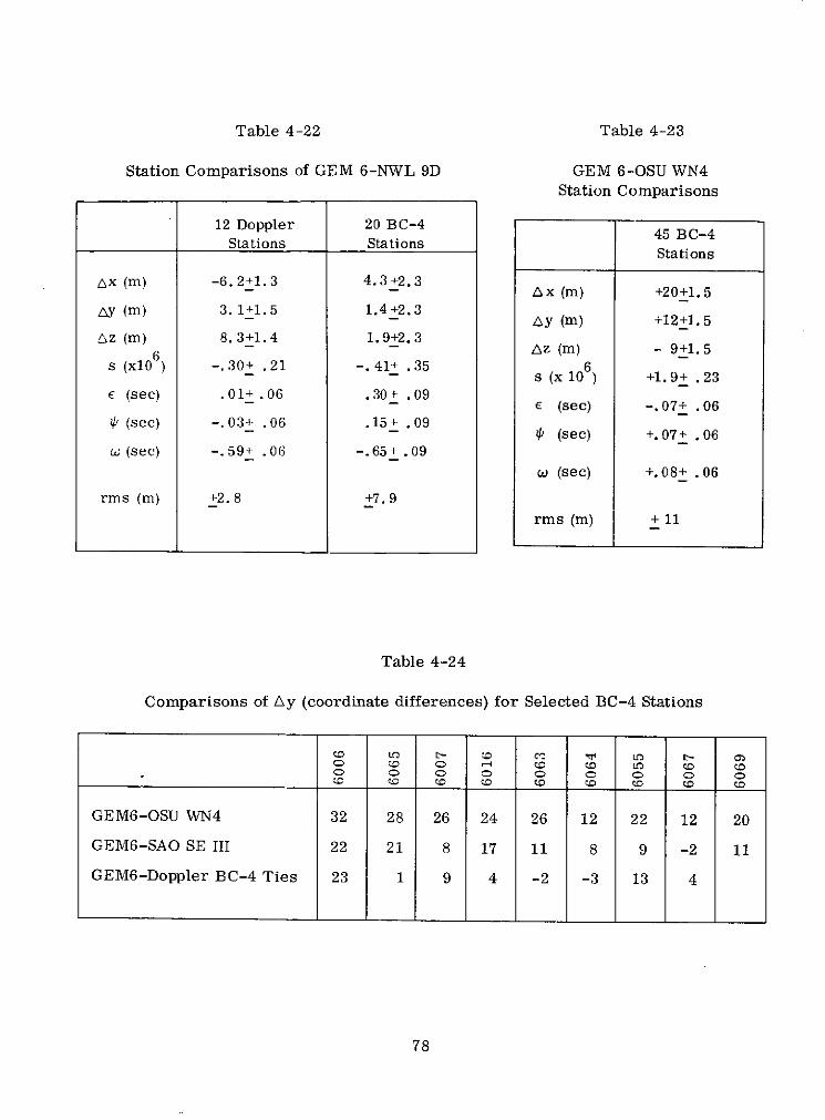
Table 4-22 Table 4-23

Station Comparisons of GEM 6-NWL 9D GEM 6-OSU WN4Station Comparisons

12 Doppler 20 BC-4 45 BC-4Stations Stations

Stations

Ax (m) -6.2+1.3 4.3 +2.3- ax (m) +20+1.5

AY (m) 3. 1+1.5 1.4+2.3- Ay (mn) +12+1.5

Az (m) 8.3+1.4 1.9+2.3- Az (m) - 9+1.5

s (x10 ) -. 30+ .21 -. 41+ .35 106)9 .23s (x 10 ) +1.9+ .23

E (sec) .01+ .06 .30+ .09- E (sec) -. 07+ .06

P (sec) -. 03+ .06 .15+ .09- -- (sec) +.07+ .06

w (sec) -. 59+ .06 -. 65+ .09w (sec) +.08+ .06

rms (m) +2.8 +7.9

rms (m) + 11

Table 4-24

Comparisons of Ay (coordinate differences) for Selected BC-4 Stations

LO L- CO ,:v U, L- M

GEM6-OSU WN4 32 28 26 24 26 12 22 12 20

GEM6-SAO SE III 22 21 8 17 11 8 9 -2 11

GEM6-Doppler BC-4 Ties 23 1 9 4 -2 -3 13 4

78

10 1010

05 - *05

0 o a = 6378155 o000, 0

-05 A -- 05

- ---10- - O ae = 63781441-20 0 a o o -

,0 0 0 0, 15 A Ao 80 -- 15 :.

o 0 C

-20 A o- 0 0-20

-25 0 - -25A A

-30 - - -30

-90 -80 -70 -60 -50 -40 -30 -20 -10 0 10 20 30 40 50 60 70 80 90LATITUDE OF STATION (DEGREES)

KEY TO STATIONS

* BAKER-NUNN MSLH = HEIGHT OF STATION ABOVE MEAN SEA LEVEL (SURVEY)0 NWL TRANET DOPPLER h = ELLIPSOIDAL HEIGHT OF STATION FROM DYNAMIC SOLUTIONv GRARR (ae = 6378155, 1/f = 298.255)o LASER N = GEOID HEIGHT DYNAMIC SOLUTION GRAVITY FIELDo MOTS AH = h-N-MSLHA BC-4

Figure 4-6. Station Height Above Geoid Computed by GEM 6 vs Surveyed Height

Table 4-25 shows solutions which estimate four systematic differences in the

coordinate system based upon the comparison of MSL heights. Three of the pa-rameters constitute a translation of the origin and the fourth is a change to the

semi-major axis, ae. Five solutions are presented in the table. Results are

given first for 114 stations representing a combination of the various tracking

systems used in GEM 6, followed by results from subsets of stations by datatype as follows: 29 MOTS-SPEOPTS camera stations, 40 BC-4 camera stations,19 Baker-Nunn camera (BN) stations, and 18 Doppler stations. The geoidal

heights used in the solution were computed from GEM 6 as were the ellipsoidal

heights.

The first solution (114 stations) shows a displacement of the origin of nearly 2.3

m and a best fitting equatorial radius ae of 6378144 m. The next four solutions

use subsets of stations to estimate the systematic differences. The derived

semi-major axis ranges from 6378141m to 6378149.3 m or a total excursion of

nearly 8 m. The solutions using MOTS-SPEOPTS cameras and the BN cameras

give the largest semi-major axes and the BC-4 network resulted in the smallest

semi-major axis, with the Doppler station solution occupying a central position.

Recall from Table 4-23 that the GEM 6-OSU WN4 gave a scale difference of 1.9

ppm, which when applied results in a derived semi-major axis for OSU WN4 by

this method of 6378129 m. This agrees with an independent geometric adjust-ment which we have made using only the BC-4 camera and baseline data. Ap-

parently the ties made between the BC-4 cameras and other tracking stations

(dynamic system) dominated the terrestrial baselines in the solutions for the

stations more removed from the baselines. The range of 8 m in determinations

of ae reflect systematic differences between the data from the tracking systems

for which the comparisons were made. No significant effect in center of mass

displacement (Ax, A y, A z) exists in the solution for the 114 stations. Some ef-fect is seen in the subset solutions where the station distribution is not as well

defined. These differences in the subset results reflect errors in the geoid

computed from GEM 6 and the selection process due to spacing of the stationsas well as the error in station height.

4.2.3 Comparison with Positions on National Datums-Stations' coordinates inGEM 6 are compared to coordinates in national or international datums by first

computing the datum shifts involved and using these to transform the coordi-nates. We refer to coordinates in the national or international datums as sur-veyed coordinates.

Let Xs rs hs be the geodetic coordinates of a particular station as determined by

survey on the ground. These are converted to rectangular coordinates xs, Ys,z s using the datum's specifications. xs, ys, zs will be referred to as "surveyed"

coordinates. The surveyed coordinates are transformed to the system of GEM 6

by the equation

80

s) x + Yo + (1 + s) -C C e Ys - Yo (4.4)

zs I \Az + zo -e s - zowhere

,s are surveyed coordinates transformed to GEM 6's system,

xsYs ) are surveyed coordinates in the original datum,

zs

Yo are the coordinates of the adopted datum origin,

s is the scale difference,

w is the rotation about the z-axis,

is the rotation about the y-axis,

is the rotation about the x-axis.

Table 4-26 shows the adopted origins Xo, , ho, transformed to xo, Yo, Zo forthe calculations outlined above. With the exception of the NAD 1927 the adoptedorigin for our calculations do not agree with the origins of the 4 datums whosesolutions are derived.

By including the coordinates of the datums' origin, the translation parameters(Ax, Ay, Az) are then exactly equal to the shift of the local datum at the datumorigin. Also the correlations between translational and rotational parametersare minimized.

*When used to compare GEM 6 with another geocentric solution the coordinates (xo, Yo, zo) are zero andthe survey coordinates are replaced by those for the geocentric solution.

81

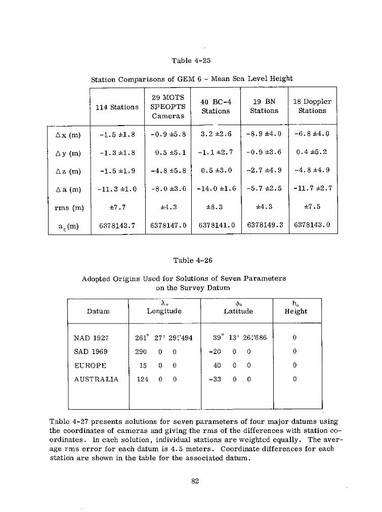
Table 4-25

Station Comparisons of GEM 6 - Mean Sea Level Height

29 MOTS 40 BC-4 19 BN 18 Doppler114 Stations SPEOPTS Stations Stations Stations

Cameras

Ax(m) -1.5 ±1.8 -0.9 ±5.8 3.2 ±2.6 -8.9 ±4.0 -6.8 ±4.0

Ay (m) -1.3 1.8 0.5 ±5.1 -1. 112.7 -0.9 ±3.6 0.4 ±5.2

Az (m) -1.5 ±1.9 -4.8 ±5.8 0.5 ±3.0 -2.7 ±4.9 -4.8 ±4.9

Aa (m) -11.3 ±1.0 -8.0 ±t3.0 -14.0 ±1.6 -5.7 :2.5 -11.7 ±2.7

rms (m) ±7.7 +4.3 ±8.3 ±4.3 ±7.5

a,(m) 6378143.7 6378147.0 6378141.0 6378149.3 6378143.0

Table 4-26

Adopted Origins Used for Solutions of Seven Parameters

on the Survey Datum

Xo o hoDatum Longitude Latitude Height

NAD 1927 2610 27' 291'494 390 13' 261'686 0

SAD 1969 290 0 0 -20 0 0 0

EUROPE 15 0 0 40 0 0 0

AUSTRALIA 124 0 0 -33 0 0 0

Table 4-27 presents solutions for seven parameters of four major datums usingthe coordinates of cameras and giving the rms of the differences with station co-ordinates. In each solution, individual stations are weighted equally. The aver-age rms error for each datum is 4.5 meters. Coordinate differences for eachstation are shown in the table for the associated datum.

82

A special comment is needed for the European Datum (ED 50) solution. The so-

lution is presented using only 5 stations for its determination. A number of other

stations connected to the ED 50 were rejected because they did not fit with anyreasonable hypothesis concerning the accuracy of the triangulation on ED 50.

4.2.4 Displacements in Mean Pole and Greenwich Meridian--In Figure 4-7 rel-

ative displacements of the Greenwich Meridian (the angle w converted to meters)

and the mean pole (the angles e and i converted to meters at the pole) are plotted

with GEM 6 referenced at the origin. The comparisons are made two ways, first

by differencing the solutions with GEM 6 for stations derived from dynamic data

and second, by differencing solutions for BC-4 stations with the GEM 6 BC-4 re-

sults. The NWL 9D solution is compared both ways, one by differencing twelve

doppler stations directly with GEM 6 doppler stations and secondly, by convert-ing the NWL 9D solution to coordinates of 30 BC-4 sites through local surveyties and differencing with GEM 6 BC-4 coordinates. An independent BC-4 geo-

metric only solution, GEM 61, was also compared with GEM 6 BC-4 results.

The comparisons for the stations derived from dynamic data tend to give moreconsistent results for the mean pole displacements than the comparisons for theBC-4 stations.

The diagram comparing displacements of the Greenwich Meridian shows closeagreement between GEM 4, GEM 6, OSU WN-4 and the GEM 6 independent geo-metric solution. Two of the other solutions plotted, the JPL and NWL 9D solu-tions, use different longitude references, since Doppler and distance measure-ments contain no directional references.

4.2.5 Summary of Results for Station Coordinates-Coordinates of the 134tracking stations computed in GEM 6 provide datum shifts for establishing a uni-fied world geodetic system for 11 different datums. GEM 6 station position re-sults are presented in Table 4-16 of Section 4.2, with respect to an ellipsoidhaving a semi-major axis of 6378155 m and a flattening of 1/298.255. Table 4-29shows the datum translations for transforming 11 local datums to the GEM 6system, and Table 4-27 gives the translation, scale difference, and 3 rotationsto transform 4 major datums to the GEM 6 system.

Radial positions of GEM 6 station coordinates and mean sea level heights fromsurvey indicate a mean radius ae for the Earth of 6378143.7 meters. Resultsfrom this analysis have been presented in Table 4-25 and Figure 4-6 where var-iations ranging from 6378141.0 meters to 6378149.3 meters can be seen for sub-sets of the tracking systems. An independent geometric solution of the BC-4data gives an ae of 6378129.0 meters based upon DME baselines. However, itwas shown that the latter result is inconsistent with recent estimates for GM.Further results in Table 4-25 for the total set of stations show that the center ofmass is determined to within 2 meters for the GEM 6 system.

83

Table 4-27

Solutions for Relation of GEM 6 to Major Datums*

GEM 6 - NAD GEM 6 - AUS GEM 6 - SAD GEM 6 - ED 1950

No. Stations 33 10 9 5

ax (m) -24 +2.1 -135 +4.0 -63 +3.7 -83 +5.1

Ay (m) 151 +2.3 -39 +4.0 0 +3.6 -116 +5.1

AZ (m) 187 .+2.1 133 +3.9 -32 +3.5 -120 +5.7

s (x 10 6) 1.7+1.2 2. 4+2.2 -1.3+1.2 -. 3+1.6

E (sec) -. 2+ .5 -1.0+ .7 .6+ .3 .6+ .6

0 (sec) .1+ .3 -1.2+ .6 -. 2+ .3 .4+1.0

w (sec) -. 8+ .3 .4+ .5 -. 0+ .4 -. 6+ .4

rms (m) ±4.0 +4.9 +6.0 +2.6

*The signs of Ax, Ay, Az should be reversed to find the displacement of the coordinate origin.

Table 4-28

Differences Between Coordinates of Stations in GEM 6 Datumand Other Major Datums

NAD 1927 - GEM 6

Meters

Station x Ay Az

1021 4 0 -5

1022 -1 -2 3

1030 1 -4 3

1034 -2 1 3

1037 -1 0 7

1042 -1 0 7

1126 -1 0 7

2203 0 7 -5

4082 0 5 7

4840 6 -4 -5

4860 6 -4 -5

6002 2 -2 -7

6111 -2 2 -4

6134 -2 2 -4

7034 -2 1 3

7036 2 0 1

7037 0 1 5

7043 2 -2 -7

7045 -3 -5 2

7050 2 -2 -7

7052 6 -4 -5

7071 -1 5 5

7072 -1 5 6

7073 -0 5 5

7074 -1 5 5

7075 -2 -2 -1

7077 2 -2 -7

7078 2 -2 -7

9001 -8 2 -2

9010 -1 5 5

9021 -5 -5 -4

9049 -1 5 6

9425 -1 2 4

rms 4.0

85

Table 4-28 (continued)

SAD 1969 - GEM 6

Meters

Station Ax Ay Az

1025 -8 -8 -31028 13 -9 -42837 17 4 -56008 0 3 -16009 -7 -8 -36019 -3 3 86067 6 4 -29009 -9 8 -109011 -3 3 89031 -7 0 12

rms 7.3

AUS 1965 - GEM 6Meters

Station Ax AY Az

1024 3 -7 -3

1038 -3 0 -51152 -6 -1 44946 4 -7 -36023 3 5 9

6032 0 4 -36060 -7 10 67054 -6 -1 49003 6 -2 -59023 6 -2 -5

rms 4. 9

ED 1950 - GEM 6Meters

Station Ax Ay Az

1035 -6 -4 -86015 10 2 119004 6 1 109008 -8 -1 -99091 -1 1 -5

rms 2.6

86

Displacement of Greenwich Meridianas compared to GEM 6

-i I uJ J 4

* AAe 0 0

-20 -10 0 10 20Displacement Positive East (meters)

Displacement of the pole ascompared to GEM 6.

A NWL 9D10--

AE SAO SE II

5-

GEM 4

GEM 6 *NWL 9D X-Axis (meters)A GEM 6I 0 0 NWL 9D

-10 5 GSFC '73 5 10

SAO SE Ilr

OSU WN-4A

*GEM 6 1 is on independentBC-4 solution. -5-

* Comparisons of solutions usingstations derived dynamically

A Comparisons of solutions, usingBC-4 stations -10

-10-

Figure 4-7. Displacement of the Greenwich Meridian and Pole as ShownThrough Comparisons with GEM 6

87

Table 4-29

Datum Shifts to GEM 6 System*

No. of MetersDatum Sites Ax Ay Az

NAD 1927 33 -22 155 187

SAD 1969 10 -66 3 -33

EUROPE 19501 4 -81 -115 -122

AUSTRALIA 1965 10 -130 -41 134

ADIND 5 -147 -3 211

OLD HAWAIIAN 4 61 -284 -182

ARC 5 -126 -110 -296

TOKYO 3 -147 509 686

SAMOA 1 -114 124 426

MADAGASCAR 2 -172 -237 -119

JOHNSTON IS. 1 177 -80 -209

*The signs of Ax, Ay, Az should be reversed to find the displacement of the coordinate origin.

Systematic differences of coordinates in dynamical solutions such as GEM 6,GSFC 73, the NWL 9D solution, and classical geodetic triangulation may be re-moved by estimating seven parameters. Three parameters are translations, threeare rotations and one is a scale change. After removing systematic differences,coordinates of major tracking systems in GEM 6 such as MOTS-SPEOPTS cam-eras, Baker-Nunn cameras and laser DME stations agree with the GSFC 73 so-lution and with classical geodetic triangulations so well that these coordinatesare believed to be known with an rms accuracy of about 5 m in each coordinate.Coordinates of Doppler stations are known in the GEM 6 system to an rms ofabout 7 m and BC-4 cameras are known to an rms of about 9 m in each coordinate.

Coordinates of BC-4 cameras derived through geometric theory by different in-vestigators give relatively large dispersions in the magnitudes of the seven pa-rameters used to estimate systematic differences in the solutions, comparedwith corresponding results from dynamic solutions. In addition relatively largedispersion exists after systematic differences are removed. The BC-4 cameranetwork has relatively fewer observations per station on the average comparedwith stations in dynamical solutions. Stations derived through dynamical proc-essing of observations are connected through orbital constraints with many otherstations, providing a stronger set of global connections for stations than the si-multaneous observations in the BC-4 network.

88

4.3 Geodetic Parameters

The reference values of the earth's ellipsoid and normal gravity are listed alongwith the corresponding adjusted values based upon the GEM solution as follows:

Reference Value Adjusted Value

ae (equatorial radius) 6378155 m 6378144 m

f (flattening) 1/298.255 1/298.257

ge (equatorial gravity) 97 8029. 1 mgal 978032. 1 mgal

The adjusted value for ge was derived from the surface gravity data. The ad-justed value of ae was derived in Section 4.2.2 from analysis of the GEM 6 sta-tion coordinates and MSL heights of stations. Another estimate of ae may bederived from the reference value of GM = 398601.3 km 3/sec 2 and the adjustedvalue of ge (Lerch et al., 1972). This value for ae is 6378142 m and it is wellwithin the range of values of ae associated with the results from subsets of sta-tions as given in Table 4-25. Since scale for the station positions is enforcedthrough GM, both estimates of ae are referenced to the above value of GM.

The adjusted value for flattening is based principally on the leading oblatenesscoefficient C 20 , and the maximum effect of the adjustment (Af) on ellipsoidal po-sition is less than 0.2 m. Hence flattening f essentially remains the same.

89

SECTION V. . ......... SUMMARY AND CONCLUSIONS

5. SUMMARY AND CONCLUSIONS

The Goddard Earth Model (GEM 6) has been developed to satisfy requirements

in the National Geodetic Satellite Program (NGSP) and to serve as a preliminary

model for investigations in the Earth and Ocean Physics Applications Program

(EOPAP). GEM 6 was derived from a comprehensive set of satellite tracking

and surface gravity data. Its solution consists of a gravitational potential in

spherical harmonics and a worldwide system of 134 tracking station locations.

Harmonic terms of the potential are complete for coefficients through degree

and order 16 and include some selected zonal and satellite resonant terms to

degree 22. Terms through degree 16 represent broad features of the gravity

field and provide resolution in wavelengths down to 2600 km on the geoid. These

broad features are estimated to have a worldwide average accuracy of 4. 5 mgal

in gravity anomaly and 3 m in geoid height.

Tracking station coordinates in the model are referenced to a center of mass

system, which is determined to better than 2 m. Transformations to this com-

mon reference system are given for 11 local datums throughout the world, thus

providing for a unified geodetic system of stations. Coordinates in GEM 6 are

estimated to have an average accuracy of 6.5 m, excluding possible rotation,

translation, and scale errors. Of these only a scale error would affect the rel-

ative position of stations. Scale for the stations depends upon the value of GM

employed. Current estimates of GM are consistent with a contraction of the

GEM 6 earth of only about 3m. Such an effect does not significantly increase

the above error estimate for station coordinates. These accuracy figures speci-

fied for the stations and the geoid serve to meet the goals of the national pro-

gram (NGSP).

In addition to the potential coefficients and station coordinates of GEM 6, certain

basic parameters associated with the mean earth ellipsoid were derived. These

are: ae = 6378144m for the semimajor axis, flattening f = 1/298.257, and

ge = 978032 mgal for equatorial gravity. The value of ae was derived from

analysis of radial coordinates of the tracking stations and their mean sea level

heights from survey. The value of flattening is essentially unchanged from the

initial reference value and the value of ge was derived from the gravimetry

data.

Along with GEM 6, a separate model of the gravitational potential (GEM 5) was

derived based upon only the data processed dynamically among 27 satellites.

Harmonics in GEM 5 are complete to degree and order 12, and include the se-

lected zonal and satellite resonant terms to degree 22. Satellite data of GEM 5

formed the m4jor contribution to the potential of GEM 6, controlling almost en-

tirely the long wavelength terms of low degree and accounting for about 30% of

the adjustment on the average for terms of degree 12 in GEM 6. The average

PRECEDING PAGE BLANK NOT FILMED

accuracy for the GEM 5 coefficients are shown to vary from better than 75%through degree 8 to 40% at degree 12. The accuracy of the high degree termsof GEM 6 is improved over GEM 5.

Error estimates for the GEM 6 coefficients show that the zonals are the best de-termined. Comparisons of zonal coefficients and their long-term perturbationson different satellite orbits verify the high accuracy of these terms in the GEMsolutions.

The error of 3 m for geoid height given above for GEM 6 corresponds to the longwavelength terms for the coefficients through degree 16. The zonal contributionis less than 1/3 meter. Considering coefficients beyond degree 16 a total (rms)error in geoid heights is estimated as 5 m. A single global track of SKYLABaltimetry has shown a 7.3m deviation (rms) from the GEM 6 geoid. Therefore,considerable improvement remains to be made to reduce the total error in thegeoid to 1/2 meter for application in the EOPAP program.

94

I REFERENCES

REFERENCES

1. Anderle, R. J., "Geodetic Parameter Set NWL-5-E-6 Based on Doppler

Satellite Observations," NWL Report 1978, 1965.

2. Anderle, R. J., "Transformation of Terrestrial Survey Data to Doppler

Satellite Datum, " presented at the IAG Symposium on Computational

Methods in Geometrical Geodesy, Oxford, England, September 1973.

3. Bjerhammar, A., "On a Coalescent World Geodetic System," Research

Institute for Geodetic Sciences (GIMRADA), 1967.

4. Bomford, G., Geodesy, Oxford University Press, 1971.

5. Cazenave, A., F. Forestier, F. Novel, and J. Pieplu, "Improvement of

Zonal Harmonics Using Observations of Low Inclination Satellites, DIAL

SAS, and PEOLE," paper presented at AGH Meeting, Wash. D.C., April

1971.

6. Esposito, P. B., and S. K. Wong, "Geocentric Gravitational Constant

Determined from Mariner 9 Radio Tracking Data," paper presented at the

International Symposium on Earth Gravity Models and Related Problems,

St. Louis, Missouri, 1972.

7. Gaposchkin, E. and K. Lambeck, "1969 Smithsonian Standard Earth (II),"SAO Special Report 315, 1970.

8. Gaposchkin, E. M., "Smithsonian Institution Standard Earth III," pre-

sented at American Geophysical Union Meeting, Washington, D.C.,

April 1973.

9. Guier, W. H., "Determination of the Nonzonal Harmonic of the Geopoten-

tial from Satellite Doppler Data," NATURE 200, 124-125, Oct. 12, 1963.

10. Hajela, D. P., "The Computation of 150 and 100 Equal Area Block Ter-

restrial Free Air Gravity Anomalies," Dept. of Geodetic Science, Report

No. 178, Ohio State University, June 1972.

11. Heiskanen, W., and H. Moritz, Physical Geodesy, W. H. Freeman and

Company, 1967.

12. Izsak, I. G., "Tesseral Harmonics in the Geopotential," NATURE 199,137-139, July 13, 1963.

97

PRECEDING PAGE BLANK NOT FILMED

13. Kaula, W. M., "Improved Geodetic Results from Camera Observations ofSatellites," J. Geophys. Res. 68, 5183-5189, Sept. 15, 1963.

14. Kaula, W. M., "Tests and Combinations of Satellite Determinations of theGravity Field," J. Geophys. Res. 71, 5303-5314, 1966a.

15. Kaula, W. M., Theory of Satellite Geodesy, Blaisdell Press, Waltham,Mass., 1966b.

16. Kaula, W. M., (Chairman), "The Terrestrial Environment Solid Earthand Ocean Physics Applications of Space and Astronomic Techniques. "Report of a Study at Williamstown, Mass. to the National Aeronautics andSpace Administration, NASA CR-1579, August 1969.

17. Kohnlein, W., "The Earth's Gravitational Field as Derived from a Com-bination of Satellite Data with Gravity Anomalies," In: Smithsonian Astro-physical Observatory Special Report 264, 57-72, 1967.

18. Kozai, Y., "Revised Zonal Harmonics in the Geopotential, " SAO SpecialReport 295, 1969.

19. Lerch, F., J. Marsh, and B. O'Neill, "Gravity Model Comparisons UsingGEOS-1 Long Arc Orbital Solutions," GSFC X-552-68-71, December 1967.

20. Lerch, F., and W. Kahn, "Geodetic Parameter and Station Recovery(GEOSTAR) Plan," Goddard Space Flight Center, Greenbelt, Md., 1968.

21. Lerch, F. J., C. A. Wagner, B. H. Putney, and K. G. Nickerson, "Pre-liminary Goddard Geopotential Using Optical Tracking Data and a Compar-ison with SAO Models," GSFC X-552-71-143, October 1971.

22. Lerch, F., C. Wagner, D. Smith, M. Sandson, J. Brownd, and J. Rich-ardson, "Gravitational Field Models for the Earth (GEM 1 and 2)," NASATMIX 65970, NTIS, Springfield, Va., May 1972a.

23. Lerch, F., C. Wagner, B. Putney, M. Sandson, J. Brownd, J. Richard-son, and W. Taylor, "Gravitational Field Models GEM 3 and 4," NASATMX 66207, NTIS, Springfield, Va., November 1972b.

24. Lerch, F. J., "Geometrical Geodesy Techniques in Goddard EarthModels," GSFC X-592-73-339, January 1974.

98

25. Lundquist, C. A., and G. Veis, "Geodetic Parameters for a 1966 Smith-

sonian Institution Standard Earth, " Smithsonian Astrophysical Observatory

Special Report 200, 1966.

26. Marsh, J., B. Douglas, and S. Klosko, "A Unified Set of Tracking Station

Coordinates Derived from Geodetic Satellite Tracking Data, " GSFC X-553-

71-370, July 1971.

27. McGoogan, J., C. Leitao, L. Miller, and W. Wells, "Skylab S-193 Al-

timeter Experiment Performance, Results and Applications," Paper pre-

sented at the International Symposium on Applications of Marine Geodesy,

Columbus, Ohio, June 1974.

28. Mottinger, N. A., "Status of DSS Location Solutions for Deep Space Probe

Missions: Third Generation Orbit Determination Program Solutions for

Mariner Mars 1969 Mission," JPL Space Program Summary 37-60, vol.

II, November 30, 1969.

29. Mueller, Ivan I., "Free Geometric Adjustment of the OSU/NGSP Global

Network (Solution WN-4)," presented at the First International Symposium

of the Use of Artificial Satellites for Geodesy and Geodynamics in Athens,

Greece, May 1973.

30. Rapp, R. H., "Further Studies in the Combination of Gravimetric and

Satellite Data, " Department of Geodetic Science Report No. 119, The Ohio

State University, December 1968.

31. Rapp, R. H., "The Formation and Analysis of a 50 Equal Area Block Ter-

restrial Gravity Field," Reports of the Department of Geodetic Science

No. 178, The Ohio State University Research Foundation, Columbus, Ohio,June 1972.

32. Rapp, R. H., "Current Estimates of Mean Earth Ellipsoid Parameters,"Geophysical Research Letters, Vol. 1, No. 1, AGU, May 1974.

33. Reece, J., and J. Marsh, "Simultaneous Observation Solutions for NASA-

MOTS and SPEOPT Station Positions on the North American Datum,"GSFC X-592-73-170, June 1973.

34. Schmid, H. H., '"Worldwide Satellite Triangulation Results and Analysis,"Journal of Geophysical Research, Vol. 79, 5349, December 1974.

35. Smith, D. E., F. J. Lerch, and C. A. Wagner, "A Gravitational Field

Model for the Earth," In: Space Research XIII, 11-20, Akademie-Verlag,Berlin, 1973.

99

36. Strange, W., F. Calabria, H. Rainey, and L. Gunshol, "Requirementsfor Resonant Satellites for Gravimetric Satellite Geodesy," Report pre-pared by Geonautics, Inc., for NASA under Contract NASW-1594, Janu-ary 1968.

37. Veis, G., "The Determination of Absolute Directions in Space with Arti-ficial Satellites," SAO Special Report 133, 1963.

38. Vincent, S., W. Strange, and J. Marsh, "A Detailed Gravimetric Geoidof North America, the North Atlantic, Eurasia, and Australia, " NASATMIX 66238, NTIS, Springfield, Va., September 1972.

39. Wagner, C. A., "Earth Zonal Harmonics from Rapid Numerical Analysisof Long Satellite Arcs," NASA TMX 66039, Nat. Technical InformationService, Springfield, Va. , 1972.

100

APPENDICES

APPENDIX A

METHODS EMPLOYED FOR DATA PROCESSING IN GEM 5 AND 6

CONTENTS

Appendix Page

Al ORBIT THEORY FOR GEODYN . ........... . Al-I

A2 GEOMETRIC METHODS FOR SIMULTANEOUSOBSERVATIONS INCLUDING CONSTRAINTS

FROM DATUM SURVEY. ................. A2-1

A3 GRAVIMETRIC METHOD FOR MEAN ANOMALYDATA . . . . . . . . . . . . . . . . . . . . . . . ... A3-1

A4 TECHNIQUES IN COMBINED SOLUTION . ........ A4-1

Al

APPENDIX Al . ....... ORBIT THEORY FOR GEODYN -

APPENDIX Al

ORBIT THEORY FOR GEODYN

CONTENTS

Page

AI-1.0 INTRODUCTION ..................... Al-1

A1-2.0 COORDINATE SYSTEMS . ............... . A1-2

A1-2.1 Definition . . . . . . . . . . . . . .. . . . . A1-2

A1-2.2 Topocentric .................. A1-2

A1-2.3 Time Systems ................. A1-3

A1-2.4 Polar Motion ................... A1-4

A1-2.5 Coordinate Systems for Motions of the Earth . . .. Al-6

A1-2. 6 True of Date Coordinate System . ........ A1-6

A1-2.7 Inertial Coordinate System . ........... A1-6

A1-2.8 Earth-Fixed Coordinate System . ....... . A1-7

A1-2.9 Greenwich Hour Angle . ........... A1-7

A1-2.10 Precession and Nutation . ........... . A1-7

A1-3.0 MEASUREMENT MODELING AND RELATEDDERIVATIVES ..................... A1-9

A1-3.1 Measurements ................. A1-9

A1-3.2 Variational Partials of the Measurements . ... . Al-12

A1-3.3 Corrections to Measurements . ......... Al-15

Al-iii

Page

A1-4.0 FORCE MODELS AND VARIATIONAL EQUATIONS . .... A1-20

A1-4.1 The Geopotential Field of the Earth . ....... A1-22

A1-4.1.1 Solid Earth Tides . ............... A1-28

A1-4.2 Luni-Solar-Planetary Ephemeris . ....... . A1-28

A1-4.3 Third-Body Gravitational Forces . ....... . A1-29

A1-4.4 Solar Radiation Pressure . ........... A1-30

A1-4.5 Atmospheric Drag. . . .... . ........... A1-30

A1-4.5.1 Atmospheric Density . ............. A1-32

A1-5.0 ADJUSTMENT PROCEDURES . ....... . . ...... A1-34

A1-5.1 Bayesian Least Squares Method . . .......... A1-34

A1-5.2 Measurement Bias Separation(Electronic Instruments) . ........... . A1-35

A1-6.0 NUMERICAL INTEGRATION PROCEDURE . ....... . A1-37

A1-6.1 Integration for Position and VelocityComponents .................. A1-37

A1-6.2 Integration for the Variational Equations ...... A1-38

A1-6.3 Interpolation . ................. A1-39

REFERENCES .............. . . . . . . . . . . . A1-40

Al-iv

APPENDIX Al

ORBIT THEORY FOR GEODYN

Al-1. 0 INTRODUCTION

Presented in this area are the procedures and mathematics used in process-

ing satellite tracking observations for orbit determination and geodetic param-

eter estimation. The methods in the GEODYN (geodynamics) system have been

chosen to give accurate results with a reasonable amount of computer time and

memory requirements. There has been a continuous upgrading of modeling,

satellite data type handling and computer application over the years. This Ap-

pendix represents the information as it was being applied at the end of 1972.

For GEM 5 the output of this system is a set of least squares normal equa-

tions for adjustments of geodetic parameters of station coordinates and potential

coefficients and for the satellite orbital parameters. These normal equations

are processed and combined as in A4 of the appendix.

Al-I

A1-2.0 GEODETIC COORDINATE SYSTEMS

A1-2.1 Definition

The GEODYN program involves the use of several coordinate systems. Itis convenient to define the station positions in a spherical coordinate system.This system uses an oblate spheroid or an ellipsoid of revolution as a model forthe geometric shape of the earth. The earth is flattened slightly at the poles andbulges a little at the equator; thus, a cross section of the earth through the polesis approximately an ellipse. Rotating an ellipse about its shorter axis forms anoblate spheroid.

An oblate spheroid is uniquely defined by specifying two dimensions, con-ventionally, the semi-major axis a and the flattening f, where f = (a-b)/a, andb is the semi-minor axis.

The coordinates utilized in GEODYN are termed geodetic coordinates andare defined as follows: 4 is the geodetic latitude, the acute angle between thesemi-major axis and a line through the observer perpendicular to the spheroid,X is the east longitude, the angle measured eastward in the equatorial plane be-tween the Greenwich meridian and the observer's meridian, and h is the sphe-roid height, the perpendicular height of the observer above the referencespheroid.

Methods exist for the conversion from 4, X, and h to Xe, Ye, and Ze , theearth-fixed cartesian coordinates, and for the inverse conversion.

A1-2.2 Topocentric

The observations of a spacecraft are usually referenced to the observer,and therefore an additional set of reference systems is used for this purpose.The origin of these systems, referred to as topocentric coordinate systems, isthe observer on the surface of the earth.

Topocentric right ascension and declination are measured in an inertial sys-tem whose Z-axis and X-Y plane are parallel to those of the geocentric inertialsystem defined by the true of date coordinate system. The X-axis in this casealso points toward the vernal equinox.

The other major topocentric system is the earth-fixed system determinedby the zenith and the observer's horizon plane. This is an orthonormal systemdefined by N, E and Z, which are unit vectors which point in the same direc-tions as vectors from the observer pointing north, east and toward the zenith.

A1-2

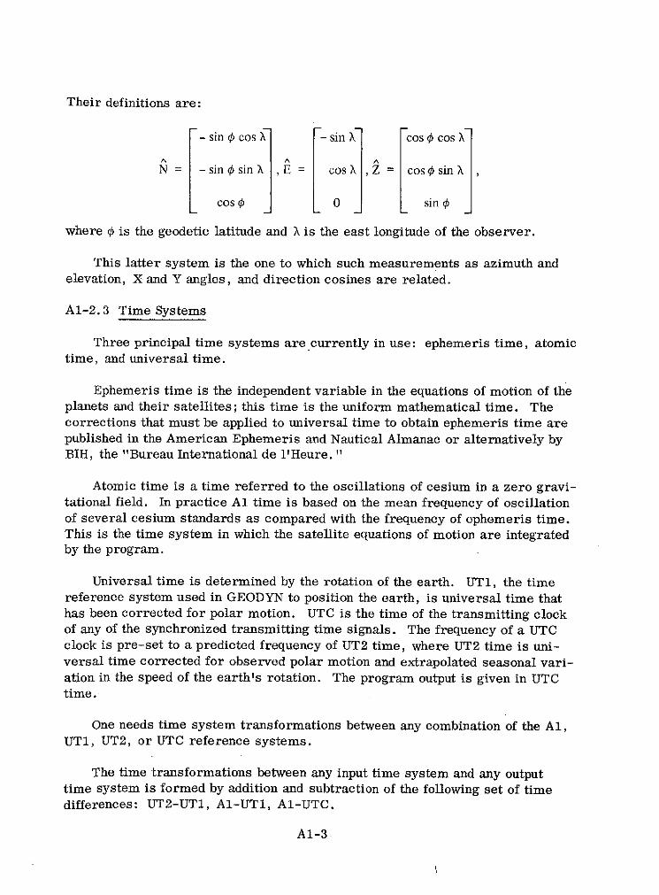
Their definitions are:

- sin ¢ cos sin cos cos X

A A AN = - sin sinX ,E = cos ,Z = cos sin X

cos 0 0 sin 0

where 0 is the geodetic latitude and X is the east longitude of the observer.

This latter system is the one to which such measurements as azimuth andelevation, X and Y angles, and direction cosines are related.

A1-2.3 Time Systems

Three principal time systems are currently in use: ephemeris time, atomictime, and universal time.

Ephemeris time is the independent variable in the equations of motion of theplanets and their satellites; this time is the uniform mathematical time. Thecorrections that must be applied to universal time to obtain ephemeris time arepublished in the American Ephemeris and Nautical Almanac or alternatively byBIH, the "Bureau International de 1'Heure. "

Atomic time is a time referred to the oscillations of cesium in a zero gravi-tational field. In practice Al time is based on the mean frequency of oscillationof several cesium standards as compared with the frequency of ephemeris time.This is the time system in which the satellite equations of motion are integratedby the program.

Universal time is determined by the rotation of the earth. UT1, the timereference system used in GEODYN to position the earth, is universal time thathas been corrected for polar motion. UTC is the time of the transmitting clockof any of the synchronized transmitting time signals. The frequency of a UTCclock is pre-set to a predicted frequency of UT2 time, where UT2 time is uni-versal time corrected for observed polar motion and extrapolated seasonal vari-ation in the speed of the earth's rotation. The program output is given in UTCtime.

One needs time system transformations between any combination of the Al,UT1, UT2, or UTC reference systems.

The time transformations between any input time system and any outputtime system is formed by addition and subtraction of the following set of timedifferences: UT2-UT1, Al-UT1, Al-UTC.

A1-3

The following equation is used to calculate (UT2-UT1) for any year:

(UT2-UT1) = +s 022 sin 2 nt - 012 cos 2rt -s006 sin 4rt +s007 cos 47rt

t = fraction of the tropical year elapsed from the beginning of the

Besselian year for which the calculation is made. (1 tropical year= 365.2422 days.)

This difference, (UT2-UT1) is known by the name "seasonal variation. " The

time difference (Al-UT1) is computed by lirear interpolation from a table ofvalues. The spacing for the table is every 10 days, which matches the incre-ment for the "final time of emission" data published by the U.S. Naval Observa-tory in the bulletin, "Time Signals." The differences for this table are deter-

mined by: (Al-UT1) = (A1-UTC) - (UT1-UTC). The values for (UT1-UTC) areobtained from "Circular D", BIH. The differences (A1-UTC) are determinedaccording to the following procedure.

UTC contains discontinuities both in epoch and in frequency because an at-tempt is made to keep the difference between a UTC clock and a UT2 clock lessthan s 1. When adjustments are made, by international agreement they are madein steps of S 1 and only at the beginning of the month, i.e., at 0hO UT of the firstday of the month. The general formula which is used to compute (A1-UTC) is(A1-UTC) = ao + a I (t-to). Both ao and a, are recovered from tables. The val-ues in the table for a o are the values of (A1-UTC) at the time of each particularstep adjustment. The values in the table for al are the values for the new ratesof change between the two systems after each step adjustment. Values for aoand a, are published both by the U.S. Naval Observatory and BIH.

A1-2.4 Polar Motion

Consider the point P which is defined by the intersection of the earth's axisof rotation at some time t with the surface of the earth. At some time t+At, theintersection will be at some point P' which is different than P. Thus the axis ofrotation appears to be moving relative to a fixed position on the earth; hence theterm "motion of the pole."

A rectangular coordinate system has been established with its center at apoint F fixed on the surface of the earth with F near the point P around 1900,and measurements have been taken of the rectangular coordinates of the point Pduring the period 1900. 0 - 1906. 0. It was observed that the point P moves inroughly circular motion in this coordinate system with two distinct periods, oneperiod of approximately 12 months and one period of 14 months. The mean po-sition of P during this period is defined to be the point Po, the mean pole of1900.0 - 1906.0.

A1-4

The mean is taken over a six year period in order to average out both the12 month term (6 periods) and the 14 month term (5 periods) simultaneously.The radius of this observed circle varies between 15 and 35 feet.

In addition to the periodic motion of P about Po, by taking six year meansof P in the years after 1900 - 1906, called Pin, there is seen to be secular mo-tion of the mean position of the pole away from its original mean position P 0 inthe years 1900 - 1906 at the rate of approximately 0'.'0032/year in the directionof the meridian 60°W, and a libration motion of a period approximately 24 yearswith a coefficient of about 0"'022. The short periodic motions over a period ofsix years average about 0'.'2 to 0'.'3.

This motion of the pole means that the observing stations are moving withrespect to the "earth-fixed" coordinate system used in GEODYN. The stationpositions must be corrected for this effect.

The position of the instantaneous or true pole is computed by linear inter-polation in a BIH table of observed values for the true pole relative to the meanpole of 1900 - 1906. The table increment is 10 days. The data in the table is inthe form of the coordinates of the true pole relative to the mean pole measuredin seconds of are. This data was obtained from "Circular D" which is publishedby BIH.

Consider the station vector X in a system attached to the earth of the meanpole and the same vector Y in the "earth-fixed" system of GEODYN referred tothe true pole of date. The transformation between Y and X consists of a rota-tion of x about the X, axis and a rotation of y about the X, axis; that is

1 0 0 cos x 0 -sin x

Y = R (y) R2 (x) X = 0 cosy sin y 0 1 0

0 -sin y cosy sin x 0 cos x

Because x and y are small angles, their cosines are set to 1 and their sinesequal to their values in radians. Consequently,

1 0 -x

Y= xy 1 y X

x -y 1

A1-5

A1-2. 5 Coordinate Systems for Motion of the Earth

The choice of appropriate coordinate systems for the orbit prediction prob-lem is controlled by several factors.

Firstly, in the case of a satellite moving in the earth's gravitational field,the most suitable reference system for orbit computation is a system with itsorigin at the earth's center of mass, referred to as a geocentric referencesystem.

Secondly, the satellite equations of motion are integrated in an inertial co-ordinate system.

Also, the earth is rotating at a rate 0 g, which is the time rate of change ofthe Greenwich hour angle. This angle is the hour angle of the true equinox ofdate with respect to the Greenwich meridian as measured in the equatorial plane.

Finally, the earth both precesses and nutates, thus changing the directionsof both the earth's spin axis and the true equinox of date in inertial space.

A1-2.6 True of Date Coordinate System

At any given time, the spin axis of the Earth (+Z) and the direction of thetrue equinox of date (+X) may be used to define a right-handed geocentric co-ordinate system. This system is known as the true of date coordinate system.The other coordinate systems of the program will be defined in terms of thissystem.

A1-2.7 Inertial Coordinate System

The inertial coordinate system is the true of date coordinate system definedat Oh0 of the reference day for each satellite. This is the system in which thesatellite equations of motion are integrated. This is a right-handed, Cartesian,geocentric coordinate system with the X-axis directed toward the true equinoxof 00 of the reference day and with the Z-axis directed parallel to the earth'sspin axis toward north at the same time. The Y-axis is defined so that the co-ordinate system is orthogonal.

It should be noted that the inertial system differs from the true of date sys-tem by the variation in time of the directions of the earth's spin axis and thetrue equinox of date. This variation is described by the effects of precessionand nutation.

A1-6

A1-2.8 Earth-Fixed Coordinate System

The earth-fixed coordinate system is geocentric, with the Z-axis pointingnorth parallel to the axis of rotation and with the X-axis parallel to the equato-rial plane, pointing toward the Greenwich meridian. The system is orthogonaland right-handed; thus the Y-axis is automatically defined. This system is ro-tating with respect to the true of date coordinate system. The Z-axis, the spinaxis of the earth, is common to both systems. The rotation rate is equal to theearth's angular velocity. Consequently, the hour angle 0 g of the true equinox ofdate with respect to the Greenwich meridian (measured westward in the equato-rial plane) is changing at a rate of 6g equal to the angular velocity of the earth.

A1-2. 9 Greenwich Hour Angle 0 g

The computation of the Greenwich hour angle is quite important because itprovides the orientation of the earth relative to the true of data system. Thisangle is the major variable in relating the earth-fixed system to the inertial ref-erence frame in which the satellite equations of motion are integrated.

The evaluation of 0g is discussed in detail in the Explanatory Supplement,

0 = 0go + Ati 6 + At +

where At, is the integer number of days since January 0.0 UT of the referenceyear, At 2 is the fractional UT part of a day for the time of interest, Ogo is theGreenwich hour angle on January 0. O0 UT of the reference year, 01 is the meanadvance of the Greenwich hour angle per mean solar day, 0, is the mean dailyrate of advance of Greenwich hour angle (27 + 01) , and AO is the equation ofequinoxes (nutation in right ascension).

The initial Ogo is obtained from the proper table in the Nautical Almanac ofvalues containing the Greenwich hour angle on January 0. O0 for each year.

A1-2. 10 Precession and Nutation

The inertial coordinate system of GEODYN, in which the equations of motionare integrated, is defined by-the true equator and equinox of date for 000 of thereference day. However, the earth-fixed coordinate system is related to thetrue equator and equinox of date at any given instant. Thus, it is necessary toconsider the effects which change the orientation in space of the equatorial planeand the ecliptic plane. These phenomena are the combined gravitational effectof the moon and the sun on the earth's equatorial bulge, and the effect of thegravitational pulls of the various planets on the earth's orbit. The first of theseaffects the orientation of the equatorial plane; the second affects the orientation

A1-7

of the ecliptic plane. Both affect the relationship between the inertial and earthfixed reference systems.

The effect of these phenomena is to cause precession and nutation, both forthe spin axis of the earth and for the ecliptic pole. This precession and nutationprovides the relationship between the inertial system defined by the true equatorand equinox of the reference date and the "instantaneous" system defined by thetrue equator and equinox of date at any given instant.

The luni-solar effects cause the earth's axis of rotation to precess and nu-tate about the ecliptic pole. This precession will not affect the angle betweenthe equatorial plane and the ecliptic (the "obliquity of the ecliptic") but will affectthe position of the equinox in the ecliptic plane. Thus the effect of luni-solarprecession is entirely in celestial longitude. The nutation will affect both, con-sequently we have nutation in longitude and nutation in obliquity.

The effect of the planets on the earth's orbit will cause both secular andperiodic deviations. However, the ecliptic is defined to be the mean plane of theearth's orbit. Periodic effects are not considered to be a change in the orienta-tion of the ecliptic; they are considered to be a perturbation of the earth's celes-tial latitude.

The secular effect of the planets on the ecliptic plane is separated into twoparts: planetary precession and a secular change in obliquity. The effect ofplanetary precession is entirely in right ascension. As is the convention, allof these secular effects are considered under the heading, "precession." Theperiodic effects are, nutation in longitude, and nutation in obliquity.

A1-8

A1-3.0 MEASUREMENT MODELING AND RELATED DERIVATIVES

A1-3.1 Measurements

It is necessary to provide the proper interaction between the observationsand the needed computed values of the observations.

The observations are geometric in nature. The computed values for the ob-servations are obtained by applying these geometric relationships to the com-puted values for the relative positions and velocities of the satellite and the ob-server at the desired time.

In addition to the geometric relationships, GEODYN allows for a timingbiasand for a constant bias to be associated with a measurement type from a givenstation. Adjustment of these biases is optional.

The measurement model is therefore

Ct+At t= ft ( ' r, -ob) + b + ft (?, rob) " At

where Ct+At, is the computed equivalent of the observation.taken at time t + At,F, is the earth-fixed position vector of the satellite, Fob, is the earth-fixed po-sition vector of the station, ft (r, r, rob), is the geometric relationship definedby the particular observation type at time t with the shortened notation f t, b, isa constant bias on the measurement, and At, is the timing bias associated withthe measurement. The functional dependence of ft was explicitly stated for thegeneral case. Many of the measurements are functions only of the position vec-tors and are hence not functions of the satellite velocity vector r.

One requires the partial derivatives of the computed values for the measure-ments with respect to the parameters being determined. These parameters are:the true of date position and velocity of the satellite epoch, the force modelparameters, the earth-fixed station positions, and the measurement biases.

These parameters are implicitly divided into a set a which are not con-cerned with the dynamics of satellite motion, and a set J which are.

The partial derivatives associated with the parameters a; i.e., station po-sitions and measurement biases are computed directly at the given observationtimes. The partial derivatives with respect to the parameters ; i.e., theepoch position and velocity and the force model parameters, must be determinedaccording to a chain rule:

aCt+At aCt+At a t

A1-9

where xt is the vector which describes the satellite position and velocity in trueof date coordinates. The partial derivatives a Ct+At/ax t are computed directlyat the given observation times, but the partial derivatives a t/ a may not be soobtained. These latter relate the true of date position and velocity of the satel-lite at the given time to the parameters at epoch through the satellite dynamics.The specific parameters are described in 4. 0.

The partial derivatives aRt/a are called the variational partials and areobtained by direct numerical integration of the variational equations. Theseequations are analogous to the equations of motion.

First consider the partial derivatives of the computed values associated withthe parameters in j. We have

aCt+At aft Rt

a a x t "

Note that we have dropped the partial derivative with respect to 3 of the differ-ential product ftAt. This is because we use first order Taylor series approxi-mation in our error model and hence higher order terms are assumed negligible.This linearization is also completely consistent with the linearization assump-tions made in the solution to the estimation equations.

The partial derivatives a ft /at are computed by transforming the partialderivatives aft/a and aft/a- from the earth-fixed system to the true of datesystem.

In summary, the partial derivatives required for computing the aCt+At'/a,the partial derivatives of the computed value for a given measurement, are thevariational partials and the earth-fixed geometric partial derivatives.

The partial derivatives of the computed values with respect to the stationpositions are simply related to the partial derivatives with respect to the satel-lite position at time t:

act+At aft aftai ob arhob ar

where i is the satellite position vector in earth-fixed coordinates. This simplerelationship is a direct result of the symmetry in position coordinates.

The partial derivatives with respect to the biases are,

_Ct+At aCt+Atab a (At) t

Al-10

Let us consider the calculation of the geometric function ft and its deriva-tives. These derivatives have been shown above to be the partial derivativeswith respect to satellite position and velocity at time t and the time rate of changeof the function ft"

The basic types of observation are right ascension and declination, range,range-rate, direction cosines, 1 and m, angles x and y, and azimuth and eleva-tion. The geometric relationship which corresponds to each of these observa-tions follow. It should be noted that in addition to the earth-fixed or inertialcoordinate systems, some of these use topocentric coordinate systems.

Range: Consider the station-satellite vector: p = r - rob, where F is thesatellite position vector (x, y, z) in the geocentric earth-fixed system, and robis the station vector in the same system.

The (slant) range, p is then the magnitude of the p vector, which is one ofthe measurements.

Range-rate: The time rate of change of this vector p is p = r, since rob0. Let us consider that.p = pu, where ^ is the unit vector in the direction of p.Thus we have p = + pi. The quantity p in the above equations is the value forthe range-rate and is determined by = * • r.

Right ascension and declination: The topocentric right ascension a and de-clination 6 are inertial coordinate system measurements. GEODYN computesthese angles from the components of the earth-fixed station-satellite vector andthe Greenwich hour angle 0g.

a = tan - 1 + O, = sin - 1

where pl, p2 , P3 are the geocentric coordinates of the p vector.

The remaining measurements are in the topocentric horizon coordinate sys-AA A

tem. These all require the N, Z, and E (north, zenith and east baseline) unitvectors which describe the coordinate system.

Direction cosines: There are three direction cosines associated with thestation-satellite vector in the topocentric system. These are

A A A A A

S= uE,m = u N, and n = -Z

Al-ll

X and Y angles: The X and Y angles are computed by

Xa = tan- 1 (),Ya = sin-i (m)

Azimuth and elevation are computed by:

Az = tan- (-) , E = sin - ' (n)

A1-3.2 Variational Partials of the Measurements

The partial derivatives for each of the calculated geometric equivalents withrespect to the satellite positions and velocity are given here. All are in the geo-centric, earth-fixed system. (The r i refer to the earth-fixed components of r.)

Range:

ap Pi

ar i P

Range-rate:

p 1 a4 Piarrar i P p

Right ascension:

u -P2 aut P1

arl p 2 p2 2 r2 pl 2 22 'Tr 3

Declination:

P -P- P3 -P 2 P3 } 1/l2 +P2 2

rl p2 12 + 2 pp2 2 22 p22

Direction cosines:

82 1 m inr - I [E i-ui], = [Ni - mui], = [Zi - nui]

3ri p i ari p Ari -

Al-12

X and Y angles:

aXa nEi -Z i YO N i - mu i

ari p(1-m 2 ) ' ar p - 2

Azimuth and elevation:

aA z mEi-QNi aEV Zi- nui

ari p -n 2 r p(1 -n 2 )

The derivatives of each measurement type with respect to time are pre-sented below. All are in the geocentric earth-fixed system.

Range:

A-p = ur.

Range-rate: The range rate derivative deserves special attention. Remem-bering that p.= r, we write p =ii - p. Thus = . p +u. p.. Because p =d/dt(pQ) = pu + f, we may substitute above for a: i = 1/p (. p - pu . p) +AAAu or, as p = u* p, we may write = l/p( - p2 + p . f). In order toobtain Pi, we use the limited gravitational potential

GM (I C 20 ae2

-= r P0 (sin ')r r2 2

The gradient of this potential with respect to the earth-fixed position coordinatesof the satellite is the part of ,p due to the potential

U GM 3 ae C20 2ZS 3 1 (5 sin 2 '- 1 - 2 - ri

ri r 2 r2 ri )

We must add to this the effect of the rotation of the coordinate system. (Theearth-fixed coordinate system rotates with respect to the true coordinates ofdate with a rate 0g, the time rate of change of the Greenwich hour angle.)

The components of p are then

pi = ar + [i coso + ~sinO ] 0 +ir2 0

A1-13

p,2 = a + [- X sin + y cos O] Og - ii0

au auP3 3 a

these transforms are used on the satellite velocity components k and y in thetrue coordinates of date.

It should be noted that all quantities in this formula, with the exception ofthose quantities in brackets, are earth-fixed values. (The magnitude r is invari-ant with respect to the coordinate system transformations.)

The remaining time derivatives are tabulated here:

Right ascension:

uI i2 - U2 i1I

Declination:

r3 - P U3

Direct cosines:

P . E-2~p . ~N-mpp p

X and Y angles:

X f(nE-Z) - N-mpa (1 - m2 ) p V

Azimuth:

p * (mE - 2N)

p (1 - m2 )

Elevation:

A

A pZ-m1

A1-14

A1-3.3 Corrections to Measurements

The function of data preprocessing is to convert and correct the data. These

corrections and conversions relate the data to the physical model and to the co-

ordinate and time reference systems used in GEODYN. The data corrections

and conversions implemented in GEODYN are to: transform all observation times

to Al time at the satellite, refer right ascension and declination observations to

the true equator and equinox of date, correct range measurements for trans-

ponder delay and gating effects, correct SAO right ascension and declination ob-

servations for diurnal aberration, correct for refraction, and convert TRANET

Doppler observations into range-rate measurements. These conversions and

corrections are applied to the data on the first iteration of each arc.

Al-3.3.1 Time Preprocessing-The time reference system used to specify

the time of each observation is determined by a time identifier on the data rec-

ord. This identifier also specifies whether the time recorded was the time at

the satellite or at the observing station.

The preprocessing in GEODYN transforms all observations to Al time. If

the time recorded is the time at the station, it is converted to time at the satel-

lite, by computing the propagation time between the spacecraft and the observing

station. The station-satellite distance used for this correction is computed from

the initial estimate of the trajectory.

There is special preprocessing for right ascension and declination measure-

ments for the GEOS satellites when input in National Space Science Data Center

format. If the observation is passive, the image recorded is an observation of

light reflected from the satellite and the times are adjusted for propagation de-

lay as above. If the observation is active, the image recorded is an observation

of light transmitted from the optical beacon on the satellite. The beacons on the

GEOS satellites are programmed to produce a sequence of seven flashes at four

second intervals starting on an even minute. For the active observations, the

times are set equal to the programmed flash time with a correction applied for

known clock errors, plus half a millisecond, the time allowed for flash buildup.

A1-3.3.2 Reference System Conversion to True of Date-The camera ob-

servations, right ascension and declination, may be input referred to the mean

equator and equinox of date, to the true equator and equinox of date, or to the

mean equator and equinox of some standard epoch.

A1-3.3.3 Transponder Delay and Gating Effects-The range observations

may be corrected on option for transponder delay or gating errors.

A1-15

The transponder delay correction is computed as a polynomial in the rangerate:

Ap = a0 + a + a2 (5)2

where a 0 , a1 , and a 2 depend on the characteristics of the particular satellite.

A gating error is due to the fact that actual range measurements are eithertime delays between transmitted and received radar pulses or the phase shiftsin the modulation of a received signal with respect to a coherent transmittedsignal. Thus there is the possibility of incorrectly identifying the returned pulseor the number of integral phase shifts. The difference between the observedrange and the computed range on the first iteration of the arc is used to deter-mine the appropriate correction. The correction is such that there is less thanhalf a gate, where the gate is the range equivalent of the pulse spacing or phaseshift. The appropriate gate depends on the particular station.

A1-3.3.4 Aberration-Optical measurements may require corrections forthe effects of annual aberration and diurnal aberration.

Annual Aberration-The corrections to right ascension and declination meas-urements for annual aberration effects are given by

20'.'5 (cos a' cos 0 cos eT + sin a' sin 0)

cos 6'

5 = 8' - 20''5 [cos 0 cos ET (tan ET cos 6'- sin a' sin 6')

+ cos a' sin 6' sin 0]

where: a is the true right ascension of the satellite, a' is the observed rightascension of the satellite, 6 is the true declination of the satellite, 6' is theobserved declination of the satellite, ET is the true obliquity of date, and 0 isthe geocentric longitude of the sun in the ecliptic plane.

Diurnal Aberration-The corrections to right ascension and declinationmeasurements for diurnal aberration effects are given by

a = a' + 0'.'320 cos ¢' cos hs sec 6'

6 = 5' + 0"'320 cos ' sin hs sin 6'

where: 0' is the geocentric latitude of the station, hs is the local hour anglemeasured in the westward direction from the station to the satellite, a is the

A1-16

true right ascension of the satellite, a' is the observed right ascension of the

satellite, 6 is the true declination of the satellite, and 6' is the observed decli-

nation of the satellite.

A1-3.3.5 Refraction Corrections-The GEODYN system can apply correc-

tions to all of the observational types significantly affected by refraction.

Right Ascension and Declination-Optical measurements may require cor-

rections for the effects of parallactic refraction. These corrections are given

by

a = a' - AR sin q/cos 6

6 = 6' - AR cos q

where the change in the zenith angle, AR, in radians is given by

AR - 0.435 (4.84813) tan Zo [1_e(-1.385) 10- 4 p cos Zp cos Zo

and a is the true right ascension of the satellite, a' is the observed right ascen-

sion of the satellite, 5 is the true declination of the satellite, 5' is the observed

declination of the satellite, Zo is the observed zenith angle in radians, p is the

range from the station to the satellite in meters, and q is the parallactic angle

in radians.

The parallactic angle q is defined by the intersection of two planes repre-

sented by their normal vectors P, and P 2 .

- A A

P= C, X u

P2 = u

where Cp = (0,0, 1), V is the unit local vertical at the station, and fi is the unit

vector pointing from the station to the satellite in inertial space.

Therefore, the sine and cosine of the parallactic angle are given by

A A

cos q = P1 P2

A A

sin q = P3 P2

A A

where P is the unit vector in the P direction, P 2 is the unit vector in the P1 A - A

1 2 2direction, and P 3 = x u/ 1 X U .

Al-17

The parallactic angle, q, is measured in the clockwise direction about thestation-satellite vector (i.e., a left-handed system is used to define this angle).All vectors and vector cross products used in this formulation conform to aright-handed system.

Range:

The refraction correction applied to CNES laser range data is

Apn

sin E2 + (cot ER) 10-3

and the correction applied to range data from all other tracking systems is

2.77 ns

328.5 (0.026 + sin E2 )

where Apn is that correction associated with a range observation measured alongthe direction of the satellite zenith, and is provided along with each observationon the data tape, E2 is the elevation angle computed from the initial estimate ofthe trajectory and ns is the PPM deviation from unity of the surface index ofrefraction (default value equals 328. 5).

Range Rate:

For range-rate, the correction Ai is derived from the range correction:

2.77 ns cos E2

328.5 (0.026 + sin Ek)2

where E2 is the computed rate of change of elevation.

Elevation:

For elevation observations the correction AE 2 is computed as follows:

ns 103

AE 2 = 16.44 + 930 tan E

Azimuth is not affected by refraction.

Al-18

Direction Cosines:

The corrections Ak and Am are derived from the elevation correction:

AQ = - sin Az sin (E) AE9

Am = - cos A z sin (E2) AEV

where A z is the azimuth angle computed from the intitial estimate of the

trajectory.

X and Y Angles:

For X and Y angles the corrections AX and AY are computed as follows:

sin Az AEVa (sin 2 E + sin 2 Az Cos 2 EQ)

cos Az sin Ek AEAYa

V1 - cos 2 Az cos2 Ek

Note that these are also derived from the elevation correction.

A1-3.3.6 TRANET Doppler Observations-TRANET Doppler observationsare received as a series of measured frequencies with an associated base fre-quency for each station pass. Using the following relationship, the GEODYN

system converts these observations to range-rate measurements.

c (FB - FM)

FM

where FM is the measured frequency, FB is the base frequency, and c is the

velocity of light.

A1-19

A1-4.0 FORCE MODEL AND VARIATIONAL EQUATIONS

The system requires computing positions and velocities of the spacecraft ateach observation time and therefore requires a force model. The dynamics ofthe situation are expressed by the equations of motion, which provide a relation-ship between the orbital elements at any given instant and the initial conditionsof epoch. There is an additional requirement for variational partials, which arethe partial derivatives of the instantaneous orbital elements with respect to theparameters at epoch and other parameters defined below. These partials aregenerated using the variational equations, which are analogous to the equationsof motion.

In a geocentric inertial rectangular coordinate system, the equations ofmotion for a spacecraft are of the form

rr = -

where r is the position vector of the satellite, p is GM, where G is the gravi-tational constant and M is the mass of the earth, and A is the acceleration causedby the asphericity of the earth, extraterrestrial gravitational forces, atmos-pheric drag and solar radiation.

This provides a system of second order equations which, given the epochposition and velocity components, may be integrated to obtain the position andvelocity at any other time. The direct integration of these accelerations inCartesian coordinates is known as Cowell's method and is the technique used inthe orbit generator.

There is an alternative way of expressing the above equations of motion:

r = VU+AD + AR

where U is the potential field due to gravity, AD contains the accelerations dueto drag, and, AR contains the accelerations due to solar radiation pressure.This is just a regrouping of terms coupled with a recognition of the existence ofa potential field. This is the form used in the program.

The inertial coordinate system in which these equations of motion are inte-grated is that system corresponding to the true of date system of Oh0 of the ref-erence day.

The evaluation of the accelerations for r is performed in the true of date sys-tem. Thus there is a requirement that the inertial position and velocity output

A1-20

from the integrator be transformed to the true of date system for the evaluationof the accelerations, and a requirement to transform the computed accelerationsfrom the true of date system to the inertial system.

The variational equations have the same relationship to the variational par-tials as the satellite position vector does to the equations of motion. The varia-

tional partials are defined as the M3t/a where Rt spans the true of date position

and velocity of the satellite at a given time, and spans the epoch parameters,geopotential coefficients, drag parameters, and solar radiation parameters.

The variational partials may be partitioned according to the satellite posi-tion and velocity vectors at the given time. Thus the required partials are aF-/a , a /a(, where r is the satellite position vector (x, y, z) in the true of date

system, and r is the satellite velocity vector (k, ~r, z) in the same system. Thefirst of these, ar/a, can be obtained by the double integration of

d2 af

dt 2 a/

or rather, since the order of differentiation may be exchanged, a r/8g. Notethat the second set of partials, ar/a , may be obtained by the first order inte-

gration of ar/a. Hence we recognize that the quantity to be integrated is ar/a3. Using the second form given for the equations of motion in the previous sub-section, the variational equations are given by

or ap ap (VU + D R )

where U is the potential field due to gravitational effects, AR is the accelerationdue to radiation pressure, and AD is the acceleration due to drag. At this pointwe must consider a few items:

1. The potential field is a function only of position. Thus we have

2. The partials of solar radiation pressure with respect to the geopotentialcoefficients, the drag coefficient, and the satellite velocity are zero,and the partials, with respect to satellite position, are negligible.

A1-21

3. Drag is a function of position, velocity, and the drag coefficients. Thepartials, with respect to the geopotential coefficients and satellite emis-sivity, are zero, but we have

aA D aA ax aAD acD aAD acDagD aAD t AD CD D AD a D--- = c -- + + - -

Let us write our variational equations in matrix notation. We define

n to be the number of epoch parameters in 0

F is a 3 x n matrix whose jth column vectors are a r/aj

U is a 3 x 6 matrix whose last 3 columns are zero and whose first 3columns are such that the i, jth element is given by a2 U/ari rj

D r is a 3 x 6 matrix whose j th column is defined by aAD/aXtj

X m is a 6 x n matrix whose i throw is given by a t/af j . Note that X mcontains the variational partials.

f is a 3 x n matrix whose first six columns are zero and whose last n-6columns are such that the i, jth element is given by a/ag* (VU + AD +AR). Note that the first six columns correspond to the first six ele-ments of p which are the epoch position and velocity. (This matrixcontains the direct partials of xt with respect to p.) We may now writeF = [U2c + Dr] Xm + f. This is a matrix form of the variationalequations.

Note that U2c' Dr, and f are evaluated at the current time, whereas Xm isthe output of the integration. Initially, the first six columns of Xm plus the sixrows form an identity matrix; the rest of the matrix is zero (for i = j, Xm =1; for i / j, Xm = 0).

A1-4.1 The Geopotential Field of the Earth

In GEODYN the earth's potential is described by a spherical harmonic ex-pansion and it is most conveniently expressed in a spherical coordinate systemwhere 0' is the satellite's geocentric latitude, X is the satellite's east longitude,and r is the geocentric range of the satellite.

The earth's gravity field is represented by the normal potential of anellipsoid of revolution and small irregular variations, expressed by a sum

A1-22

of spherical harmonics. This formulation, used in the GEODYN system, is

U = + nmax a )n pm (sin 0) [Cnm cos mX + Snm sin mX]

n=2 m=0

where G is the universal gravitational constant, M is the mass of the earth, r isthe geocentric satellite distance, nmax is the upper limit for the summation

(highest degree), ae is the earth's mean equatorial radius, P m (sin 0') indicate

the associated Legendre functions, and Cnm and Snm are the unnormalized

coefficients.

The relationships between the normalized coefficients (Cnm, Snm) and the

unnormalized coefficients are as follows:

n -m) ! (2n + 1) (2 - 56om) %nm

Cnm (n + m) ! nm

where 65o is the Kronecker delta, and 5om = 1 for m = 0 and 5om = 0 for m # 0.A similar expression is valid for the relationship between Snm and Snm"

The gravitational accelerations in true of date coordinates (R, i, 2) arecomputed from the geopotential, U (r, 0', X), by the chain rule; e.g.,

aU ar +au ao' au axar ax a0' ax ax ax

The accelerations j and 2 are determined likewise. The partial derivatives of

U with respect to r, ¢' , and X are given by

a = 1 + (C cos mX + Snm sin mX) (n + 1) p (sin

n=2 m=0

nmax an .3a= GMr nmax (Snm cos mX - Cnm sin mX) m Pm (sin ¢')

n=2 m=0

nmax n n

U M 'T (Cnm cos mX + S sin mX)

n=2 m=0

Pmn+1 (sin 0) - m tan O' Pm (sin 0')

Al-23

The partials derivatives of r, ¢', and X with respect to the true of date satelliteposition components are

ar riar i r

a'__ 1 F zri z+ arar i V2 +2 r2 r

ax 1 I ay ax

ri 2 + y2 ri x ari

The Legendre functions are computed via recursion formulae:

Zonals: m = 0

PO (sin ') 1 [(2n - 1) sin ' Po 1 (sin 0') - (n - 1) Pn- 2 (sinPP, (sin ')n

Po (sin ¢') = sin ¢'

Tesserals: m / 0 and m < n.

P" (sin ') = P 2 (sin 0') + (2n - 1) cos 0' Pm-' (sin ')

P1 (sin ¢') = cos ¢'

Sectorials: m = n

Pn= (2n - 1) cos' P (sin )

The relationship for the derivatives is given by

d (Pm (sin ) m (sin ')- m tan 0' P" (sin ')

It should also be noted that multiple-angle formulas are used for evaluatingthe sine and cosine of mX.

The variational equations require the computation of the matrix U2c, whoseelements are given by

(U 2 U(U2 c)i,j r

A1-24

where ri = {x, y, z} , the true of date satellite position, and U is the geopotential.

Because the Earth's field is in terms of r, sin 0', and X, we write

3

U2 c = CT U 2 C 1 ae C2 kk=1

where ek ranges over the elements r, sin 0', and X, U2 is the matrix whose i,jth element is given by a2 U/ae. ae , C1 is the matrix whose i, jth element isgiven by aei /arj , and C2k is a set of three matrices whose i, jth elements aregiven by a2 eka ri 3 rj.

We compute the second partial derivatives of the potential U with respect tor, ¢', and X:

a 2 U 2GM GM nmax (e n- + 21(n+ 1)(n + 2)ar2 ,3 r3

n=2 m=0

(Cnm cos mX + Snm sin mX) Pm (sin ¢')

GM nmax a n

U GM2 (n+ ) L (C cos mXar' r2 r nm

n=2 m=0

+Snm sin mX) , (Pm (sin #'))

a 2 U GM aenmax ( n n- - ,(n + 1) mr I r2 T

n=2 m=O

(- Cnm sin mX + Snm cos mX) P n (sin ¢')

32 U GM aeS2 r (Cnm cos mX + Snm sin mX)

n=2 m=0

2 Pnm (sin ,))

A1-25

nmax n na2u GM 7 (a

a m (- Cnm sin mXn=2 m=0

+ S cos mX) (M(sin&)

nmax na 2 U GM ( m2 (Cnmcos mX

ax2 rZn=2 m=0

+ Snm sin mX) Pm (sin ¢')

where

a (Pm(sin ')) = Pn+ 1 (sin ¢') - m tan 0' Pm (sin ¢')

a&2 P (sin = Pn+ 2 (sin ') -(m + 1) tan ' Pm+l (sin ')

- m tan 0' [Pm +I (sin 0')- m tan ' Pnm (sin ')]

- m sec 2 ¢' pm (sin 0')

The elements of U 2 have almost been computed. What remains is to trans-form from (r, 0', X) to (r, sin 0', X). This affects only the partials involving

au au a,'a sin 0' a¢' a sin 0'

a2 U ao' (2U a au a2 ,

Ssin 2 a sin ' a, a sin' o' a sin ,2

where

_ ' , _2_

a - sec ¢', = sin 0' sec 3 'a sin 0' a sin 0,2

For the C1 and C2k matrices, the partials of r, sin 0', and X are obtainedfrom the formulas

r = 2 +y2 + 2 sin' = X = tan- 1 -0.r A 26

Al-26

We have for C1:

ar ri

Dri r

a sin' -z ri 1 zari r3 r ar i

ax 1 ay axar i x2 + y2 L ar y r

The C2k are symmetric. The necessary elements are given by

2,r ri rj 1 ar i-+ -ar i arj r3 r 3rj

a2 sin ' 3z ri rj 1 z + ri z riari arj r5 r 3 ri rj

_2_ - 2rj x Y x+ 1 Fax ay y -x

a 1X - - 2 r x [ 1 a ay ax]ari arj ( 2 + y2 )2 ri ari X2 +2 rt ar a

If the gravitational constants, Cnm or Sn are being estimated, we requiretheir partials in the f matrix for the variational equations computations. Thesepartials are

a _U GM ae (inn,

nm = (n + 1) cos (mX) Pm (sinCnm r r2 nnm ( = m - sin (mX) Pm (sin ')

am - ) = - M ) cos (mX) Pml (sin ') - m tan ' Pn (sin ')

The partials for Snm are identical with Cnm when cos (mX) replaced by sin (mX)and when sin (mX) replaced by -cos (m ).

These partials are converted to inertial true of date coordinates using thechain rule; e.g.,

A1-27

S aU a aU ar a -aU aXCn ax aCm ar x aCnm ax

C (a) x+ acnm ax

A1-4.1.1 Solid Earth Tides-The gravitational potential originating fromsolid earth tides caused by a single disturbing body is given by

k2 GMd R5

UD (r) 2 RP r

k2 GMe Re 3SGMe Md(Re 3 (Rd )2_ 1

2 R e \ Rd)

and the resultant accelerations on a satellite due to this potential are

VUD =k GMd R [3-15 (Rd )2] r + 6 (Rd ) RdVUD 2 r4

where k, is the tidal coefficient of degree 2 called the "Love Number," G is theuniversal gravitational constant, Me is the mass of the Earth, Re is the meanearth radius, Md is the mass of the disturbing body, Rd is the distance from thecenter of mass of the earth to the center of mass of the disturbing body, r is thedistance from the center of mass of the earth to the satellite, Rd is the unit vec-tor and P is the unit vector from the center of mass of the earth to the satellite.

A1-4.2 Luni-Solar-Planetary Ephemeris

Precomputed equi-spaced ephemeris data in true of date coordinates for theMoon, the Sun, Venus, Mars, Jupiter and Saturn is used. The actual ephemer-ides are computed using Everett's fifth-order interpolation formula. The inter-val between ephemerides; i.e., the tabular interval, h, is 0.5 days for the Moonand the equation of the equinoxes and 4.0 days for the other bodies.

The GEODYN ephemeris tape contains all coordinates in true of date. Thequantities on the tape are, the geocentric lunar positions and the corresponding2nd and 4th differences, the solar positions relative to the Earth-Moon barycen-ter and the corresponding 2nd and 4th differences, the helicentric positions ofVenus, Mars, Jupiter and Saturn and the corresponding 2nd and 4th differences,and the equation of the equinoxes and its 2nd and 4th differences. This ephemeristape was prepared from a JPL planetary ephemeris tape corresponding to "JPLDevelopment Ephemeris Number 69." (Devine, 1957.)

A1-28

The formulation for Everett's fifth-order interpolation is:

y(t +sh) = yj F (1-s)+d F2 (1 -s)+ d F4 (1 - S)

+ Yj+ Fo (s)+ d?+1 F2 (s)+ d4 F4 (S)

where

Fo (s) = s; F2 (S) = [(s - 1) (s) (s +. 1)]/6; F4 (S) = [(S -2) (S -1) (s) (s + 1) (s + 2)] /120.

The quantity s is the fractional interval for the interpolation. The quantities djare obtained from the ephemeris tape.

A1-4.3 Third Body Gravitational Perturbations (Luni-Solar Forces)

The gravitational perturbations caused by a third body on a satellite orbitare treated by defining a function, Rd, which is the third-body disturbing po-tential. This potential takes on the following form:

GMmd 2r r2 2 r

rd d rd rd2 rd

where md is the mass of the disturbing body, rd is the geocentric true of dateposition vector to the disturbing body, S is equal to the cosine of the angle be-tween r and rd, r is the geocentric true of date position vector of the satellite,G is the universal gravitational constant, and M is the mass of the earth. Allperturbations are computed by,

ad = -GMmd Dd d/

where

d = r-rd, Dd = [rd 2 - 2r rd S + r2] 3/2

Then compute the matrix U2c whose i, j ' element is given by

a2 Rd GMmd [ri 3di djl

ari rj D d Lr + D/3

This matrix is a fundamental part of the variational equations.

A1-29

A1-4.4 Solar Radiation Pressure

The force due to solar radiation can have a significant effect on the orbitsof satellites with a large area to mass ratio. The accelerations due to solarradiation pressure are

A8

m s

S A

where v is the eclipse factor, such that v = 0 when the satellite is in the earth'sshadow and v = 1 when the satellite is illuminated by the Sun. CR is a factor de-pending on the reflectivity of the satellite, As is the cross sectional area of thesatellite, ms is the mass of the satellite, Ps is the solar radiation pressure inthe vicinity of the earth, and rs is the (geocentric) true of date unit vector point-ing to the Sun.

The unit vector rs is determined as part of the luni-solar-planetary ephem-eris computations (see A1-4.2).

The eclipse factor, v, is determined as follows: Compute D = r - .s wheref is the true of date position vector of the satellite. If D is positive, the satel-lite is always in sunlight. If D is negative, compute the vector PR P= r -D rs . This vector is perpendicular to Ps . If its magnitude is less than an earthradius, or if PR P < a2 , the satellite is in shadow.

The satellite is assumed to be specularly reflecting with reflectivity Ps; thusCR = 1+ Ps

When a radiation pressure coefficient CR is being determined the partialsfor the f matrix (see A1-4. 0) in the variational equations computations must becomputed. The i th element of this column matrix is given by

As

fi - Ps 's

A1-4.5 Atmospheric Drag

A satellite moving through an atmosphere experiences an atmospheric dragforce. The acceleration due to this force is given by

1 AsA D 2 C D - PD VrVr

A1-30

where CD is the satellite drag coefficient, As is the cross-sectional area of thesatellite, ms is the mass of the satellite, pD is the density of the atmosphereat the satellite position, and Vr is the velocity vector of the satellite relative tothe atmosphere.

Both As and CD are treated as constants in GEODYN. Although As dependssomewhat on satellite attitude, the use of a mean cross-sectional area does not

lead to significant errors at this time. The factor CD varies slightly with satel-

lite shape and atmospheric composition. However, it has been treated as a

satellite dependent constant.

The relative velocity vector, Vr , is computed assuming that the atmosphererotates with the Earth. The true of date components of this vector are then

x= X yr = yr g X Zr = Z

The quantities x, y, and i are the components of r, the satellite velocity intrue of date coordinates.

The direct partials for the f matrix of the variational equations when thedrag coefficient CD is being determined are given by

1 Asf 2 m PD VVr

The direct partials for the f matrix of the variational equations when thedrag rate CD is being determined are given by:

1 As= - 2 m D At Vr'r

where At is the time from epoch.

When drag is present the Dr matrix in the variational equations must alsobe computed. This matrix, which contains the partial derivatives of the dragacceleration with respect to the Cartesian orbital elements, is

1 As [ r av r _ apDDr 2 CD m D Vr + PD Vr + Vr=- Dm-ns V t D a-xt v r

where "xt is (x, y, z, x, r, i);

A1-31

0 -0 o0og o o

0 008vr

8a t 1 0 0

0 10

0 0 1

- r g xr r g r r 0g zr

xr Og xr xr Og Yr xr 6g ir8Vr _ 1

t Vr 0 0 0xt r r

xr x xr Xrr r Zr

Yr r r r Yr Zr

Zr xr ir r Zr ir

and apD /a Xt is the matrix containing the partial derivatives of the atmosphericdensity with respect to Rxt. Because the density is not a function of the satellitevelocity, the required partials are 3pD/a .

A1-4. 5. 1 Atmospheric Density-The atmospheric density is the factor whichis least well known in the computation of drag. The program uses the Jacchia-Nicolet model. This model gives densities between 120km and 1000km with anextrapolation formula for higher altitudes. (Jacchia, 1965.)

The formulae for computing the exospheric temperature have been modifiedaccording to Jacchia's later papers. The density computed from the exospherictemperature is based on density data provided in that report which presents den-sity distribution versus altitude and exospheric temperature.

The model of the atmosphere proposed by Nicolet considers that the funda-mental parameter is the temperature. Other physical parameters such as thepressure and density were derived from the temperature.

To calculate the fundamental parameter, the exospheric temperature,Jacchia considered the four factors of solar activity variation, semi-annual vari-ation, diurnal variation, and geomagnetic activity variation.

A1-32

In addition to the density, the partial derivatives of the density with respect

to the Cartesian position coordinates are required. These partials are used in

computing the drag contribution to the variational equations. The density is

given by

pD = exp (CO + C1 h + C2 h2 + C3 h3)

where h is the spheroid height, and the Ci are coefficients which are polynomials

in temperature as determined by the model. We then have

aPD aha = P (C1 +2C 2 h+3C3 h2)D 2

where Y is the true of date position vector of the satellite (x, y, z).

A1-33

A1-5.0 ADJUSTMENT PROCEDURES

A1-5.1 Bayesian Least Squares Method

It should be noted that the functional relationships between the observationsand parameters being solved for are in general non-linear; thus an iterativeprocedure is necessary to solve the resultant non-linear normal equations. TheNewton-Raphson iteration formula is used to solve these equations.

In a multi-satellite, multi-arc estimation program, it is necessary to for-mulate the estimation scheme in a manner such that the information for all satel-lite arcs are not in core simultaneously. The procedure used is a partitionedBayesian Estimation Scheme which requires only common parameter informationand the information for a single arc to be in machine memory at any given time.The development of the solution is given here.

The Bayesian estimation formula is

dx(n+1) = (BT WB + VA -1) -1 [BT Wdm + VA 1 (x(n) xA)

where xA is the a priori estimate of x; VA is the a priori covariance matrixassociated with XA; W is the weighting matrix associated with the observations;x(n) is the nth approximation to x; dm is the vector of residuals (O-C) from thenth approximation; dx(n+1) is the vector of corrections to the parameters; i.e.,

xn+ = xn + dx(n+l )

B is the matrix of partial derivatives of the observations with respect to theparameters where the i, jth element is given by am i /ax j .

The iteration formula given by this equation solves the non-linear normalequations formed by minimizing the sum of squares of the weighted residuals.

In the application for GEM models no a priori information is employed, thusVA1 and xA vanishes from the above Bayesian formula which then describes theusual least squares process. After convergence of the above orbital parametersthe normal equations, M, are formed for all parameters including the geodeticparameters as a contributory set to GEM 5. Therefore the normal equations forthe given arc of satellite data are

M = BT WB dx - BTWdm

where dx refers to adjustments for all parameters.

A1-34

For certain types of satellite tracking data for which a bias parameter isadjusted in the data, a reduced form of the above'normal equations is obtainedas described in the next section.

A1-5.2 Measurement Bias Separation (Electronic Instruments)

For certain types of electronic tracking data (e.g., Doppler data), biasesexist which are different from one pass to the next. In many cases, these biasesare of no interest per se, although their existence must be appropriately accountedfor if the data is to be used in an orbit or geodetic estimation. In addition, adesired arc of data involving hundreds of passes of the satellite over variousstations of such electronic data, and the complete solution for each bias wouldrequire the use of an excessively large amount of computer core for storing thenormal matrix for the complete set of adjusted parameters.

The effects of electronic biases can be removed, with the use of only a smallamount of additional core, by partitioning of the biases from the other param-eters being adjusted in the Bayesian least squares estimation. The forms whichthis partitioning takes can be seen from the solution of the basic measurementequation 8m = BeAb + BAx + e where 5m = the vector of residuals (O-C), Ab =the set of corrections that should be made to the electronic biases, Be = thematrix of partial derivatives of the measurements with respect to the biases (theelements of this matrix are either i's or O's), Ax = the set of corrections to bemade to all the other adjustable parameters, B = the matrix of partial deriva-tives of the measurements with respect to the x parameters, and e = the meas-urement noise vector.

The least squares solution of the above equation is

i BeT WBe Be -BeT W m

] BTWBe BTWB ,T WS m

with W the weight matrix (W- ' = E (eeT)), taken to be completely diagonal inGEODYN. The Ax part can be shown to be

S= [BT WB - BT WBe (Be WBe)-1 BeT WB] -1

[BT W6 m - BT WB (BeT WBe)_ Be' W6 m

To effectively remove the electronic bias effects, the last equation states thatthe normal matrix BTWB must have BT WBe (BeT WB )- Be T WSm subtractedfrom it. Due to the assumed independence of different measurements, it fol-lows that these quantities which must be subtracted are a sum of contributions

Al-35

for different satellite passes over various stations

nb

BT WBe (Be' WBe) 1 Be' WB = 2 B T WpBe (Be 'T W Bep) B-1 T W BPp=l

nb

BT WBe (Be' WBe) -I BeT W6m = BT WBe (Be WBep) Bep Wp mp

p=l

where nb is the total number of passes with electronic biases in the equipmentand the subscript p denotes an array for measurements of pass p. The compu-tation of the equational right hand sides requires the arrays Bp TWpBp = na x 1array, Be T WpBep = 1 x 1 array, Bep T Wpmp = 1 x 1 array where na is thenumber of adjusted parameters other than biases affecting the arc in which thebiases occur. Thus, na + 2 storage locations must be assigned for every biaswhich exists at any one time.

The individual biases may be adjusted, based on the previous iteration or-bital elements and force model parameters. This bias can then be used, alongwith the above accumulated arrays to properly correct the sum of weightedsquared residuals upon which the program does dynamic editing. Otherwise,however, it will not be possible for the statistical summaries to incorporate theadjusted values of the electronic biases unless substantial additional core isallocated.

A1-36

A1-6.0 NUMERICAL INTEGRATION PROCEDURE

Cowell's Sum method is used for direct numerical integration of both theequations of motion and the variational equations to obtain the position andvelocity and the attendant variational partials at each observation time. Valuesat the actual observation time are obtained by interpolation between values at even-numbered steps in the integration.

Let us first consider the integration of the equations of motion. These equa-tions are three second order differential equations in position, and would beformulated as six first order equations in position and velocity if a first orderintegration scheme were used for their solution. For reasons of increased ac-curacy and stability, the position vector i is obtained by a second order inte-gration of the accelerations r, where as the velocity vector t is obtained as thesolution of a first order system. These are both multi-step methods requiringat least one derivative evaluation on each step.

A1-6.1 Integration for Position and Velocity Components

To integrate the position components, the predictor formula

rn+l 2 rp n h2

is applied, followed by a Cowell corrector formula

n+1 = 2 + Yp rn-p+1 h2

The velocity components are obtained using the predictor formula

S q+1n+1 = 1 + p rn- h

p=0

followed by an Adams-Moulton corrector formula

q+1rn+ 1 = S 1 + p rn-p+) h,

p=0

where S 1 and S 2 are the first and second sums of the accelerations.

A1-37

In these integration formulae, h is the integration step size, q is the orderof the integration less 2, and rp, 7 'pY, fp and * are coefficients of integration.

A1-6.2 Integration of the Variational Equations

Let us next consider the integration of the variational equations (see A1-4. 0).These equations may be written as

Y = [AB] + f

where

[Y]= Xm

and, partitioning according to position and velocity partials,

[A B] = [U2c + Dr].

See A1-4. 0 for definitions of matrices involved.

Because A, B, and f are functions only of the orbital parameters, the inte-gration can be and is performed using only corrector formulae. (Note that A,B and f must be evaluated with the final correction values of rn+1 and rn+1-)

In the above corrector formulae, we substitute the equation for Y and solveexplicitly for Y and Y:

n+l [Xn'F = (I - H) 1 [n]

n+ LVn

Under certain conditions, a reduced form of this solution is used. It can besee from the variational and observation equations that if drag is not a factorand there are no range-rate or doppler measurements, the velocity variationalpartials are not used. There is then no need to integrate the velocity variationalequations. In the integration algorithm, the B matrix is zero and (I-H) is re-duced to a three-by-three matrix.

Backwards integration involves only a few simple modifications to thesenormal or forward integration procedures. The step size is made negative and

Al-38

the time completion test needs to be rephrased. The step size for these integra-tion procedures can be selected on the basis of perigee height and the eccentric-ity of the orbit if it is desired.

For a starting scheme, a Taylor series approximation is used to predict ini-tial values of position and velocity. With these starting values, the Sum array(Si and S2 variables) is evaluated. The loop is closed by interpolating for thepositions and velocities not at epoch and their accelerations evaluated. The sumsare now again evaluated.

A1-6.3 Interpolation

In this procedure interpolation is used for two functions. The first is theinterpolation of the orbit elements and variational partials to the observationtimes; the second is the interpolation for mid-points when the integrator is de-creasing the step size in the varistep mode of integration.

The formulas used are:

X (t + At) = 2 (t)+ - 1 S (0 + C i (At) f n i h2

i=0

for positions and

X (t+At) (t + C( (At) fn-) h

i=0

for velocities.

S 1 and S 2 are the first and second sums carried along by the integration, f'sare the back values of acceleration, h the step size, and Ci , C' are the interpo-lation coefficients. See Velez and Brodsky, 1969, for more complete information.

A1-39

REFERENCES TO APPENDIX Al.

1. Devine, C. J., JPL Development Ephemeris Number 19, JPL TechnicalReport 32-1181, Pasadena, California, 1967.

2. Explanatory Supplement to the Astronomical Ephemeris and the AmericanEphemeris and Nautical Almanac, H. M. Nautical Almanac Office, 1961.

3. Jacchia, L. G., Static Diffusion Models of the Upper Atmosphere with Em-pirical Temperatures Profiles, Special Report 170, Smithsonian InstitutionAstrophysical Observatory, Cambridge, Massachusetts, 1965.

4. Martin, T. V., C. C. Goad, M. M. Chin and N. C. Mullins, GEODYN,Vol. I, II, III and IV, Wolf Research and Development Corporation, River-dale, Maryland, 1972.

5. Maury, Jr., J. L. and G. D. Brodsky, Cowell Type Numerical Integrationas Applied to Satellite Orbit Computations, Goddard Space Flight Center,X-553-69-46, 1969.

6. Velez, C. E. and G. P. Brodsky, Geostar-1, A Geopotential and StationPosition Recovery System, Goddard Space Flight Center, X-553-69-544,1969.

7. Wolf Research and Development Corporation, Error Models for Solid Earthand Ocean Tidal Effects in Satellite Systems Analysis, Riverdale, Maryland,1972.

A1-40

APPENDIX A2 . ....... GEOMETRIC METHOD

APPENDIX A2

GEOMETRIC METHODS FOR SIMULTANEOUS OBSERVATIONSINCLUDING CONSTRAINTS FROM DATUM SURVEY

CONTENTS

Page

A2-1.0 TECHNIQUE FOR THE NORMAL EQUATIONS . ..... A2-3

A2-2.0 COORDINATE SYSTEM. . .............. . . . A2-6

A2-3.0 COPLANARITY EQUATION . .............. A2-6

A2-4.0 LENGTH EQUATION .................. A2-8

A2-5.0 CONDITION EQUATIONS FOR CONSTRAINTS . . ....... A2-13

A2-6. 0 CORRELATED OBSERVATIONS . ............ . A2-15

A2-1

APPENDIX A2

Geometric Methods for Simultaneous ObservationsIncluding Constraints from Datum Survey

Least squares normal equations are derived for the adjustment of stationcoordinates. The method is based upon the technique of formulating reducedcondition equations where the satellite parameters have been eliminated. Thedata considered consists of simultaneous events from MOTS (Minitrack OpticalTracking System) and laser systems on GEOS-I and II, the BC-4 worldwidecamera network on PAGEOS, and local datum survey ties and baselines. Thereduced condition equations are developed in this appendix and a case is consid-ered for the treatment of correlated observations.

A2-1.0 TECHNIQUE FOR THE NORMAL EQUATIONS

The mathematical analysis leading to the formation of normal equations forthe geometric adjustment of coordinates of tracking stations is based on the fol-lowing type of events:

1. Two cameras observe the satellite simultaneously2. Three cameras observe the satellite simultaneously3. Four cameras observe the satellite simultaneously4. Two cameras and one laser observe the satellite simultaneously.

Condition equations resulting from a given set of simultaneous observationsare of two types:

* Coplanarity equation, which requires that two observing stations andtheir directions to the satellite lie in the same plane.

* Length equation, which requires that the satellite position satisfying thetwo-station coplanarity relationship also agrees with the range from athird station.

Corresponding to each event condition equations of the following form areused:

m n

aiv i + bj x + c = 0 (1)

1 j

PRECEDING PAGE BLANK NOT FILMED A2-3

where a i , bj, and c are known constants derived in the subsequent sections,c is the discrepancy in the condition equation

vi are the unknown residuals (adjusted minus observed values)

xj are the unknown corrections to stations' Cartesian coordinates(adjusted minus initial values)

m is the number of observed quantities

n is the number of unknown coordinates.

The number and types of condition equations for events 1 through 4 aboveare as follows:

* For a two-camera event, one coplanarity equation is used.

* For a three-camera event, three coplanarity equations are used.

* For a four-camera event, five coplanarity equations are used.

* For a two-camera, single-laser event, one coplanarity equation and onelength equation are used.

The number of condition equations for each event corresponds to the number ofobservations less three, since the observation equations are reduced to a formwhere the three satellite position coordinates are eliminated. Each observingcamera contributes two observations in an event and an observing laser contrib-utes one observation. Each of the coplanarity equations for an event involvesdistinct pairs of observing stations.

Additional condition (constraint) equations specify coordinate differencesand also take the form of equation (1). Constraints are treated statistically,similar to observation equations, where values and accuracies are obtained froma priori information based on datum survey. Two types of constraint equationsare applied:

* Distance equations (baselines), which require the distance between twostations to remain near a given value

* Coordinate-shift equations, which require the differences between co-ordinates of two nearby stations to remain near a given value. Thisconstraint is used to connect the stations in the geometric geodesy withthose in the dynamic satellite geodesy.

For a geometric only solution a third type of statistical constraint may beapplied on individual station coordinates in order to fix the origin of the system.A priori values for these constraints should be taken from a different sourcethan datum survey such as from a previously determined geocentric solution in

A2-4

a center of mass reference frame. This constraint is not used in the combina-

tion solution with dynamic satellite geodesy.

For each event (or constraint) t, denote the associated condition equations

of the form (1) in matrix notation as

AVk + B&X + Ce = 0, (2)

for which an example of the dimensions and elements of the matrices are given

below. Minimizing Q below w.r.t. the unknown station coordinates in X and

residuals in VA will lead to the formation of the normal matrix equation. The

form Q is

K

Q (V 2(A + B X + Ck)) (3)

A=1

where MW is the diagonal weight matrix for the observations in VA and each

A is a column vector of Lagrangian multipliers corresponding to the number

of condition equations in event A. The resulting normal matrix equation to be

combined with the gravimetric and dynamic satellite geodesy systems is

K

JX + B BM 1C = N, (4)

=1

where

K

L (BIM A'BA), (5)A=1

M = (A W_' A ) (6)

The largest dimension of Mh is 5 x 5 corresponding to event of type 3 where

there are 5 coplanarity equations of condition. This case has 8 observations and

the dimensions of Ah, V{, B, and Ck are respectively 5 x 8, 8 x 1, 5 x Nx, and

5 x 1. Nx is the total number of all station coordinates and Bh (5 x Nx) would

contain for each of the 5 rows only 6 non-zero elements, corresponding to the

b. coefficients in (1) for each distinct coplanarity equation involving two observ-

ing stations. Each row of Ag has 4 non-zero elements corresponding to the ai

coefficients in (1), associated with the two observing stations in each coplanarity

equation.

A2-5

By employing a suitable set of constraints including those that fix the origin,N may be set equal to zero and a geometric only solution for X can be derivedfrom (4).

Condition equations for coplanarity, length, and constraints are developedin sections 2 through 5 and section 6 treats a case for correlated observations.

A2-2.0 COORDINATE SYSTEM

Camera observations in a and 8 are transformed from right ascension aand declination 8 to earth-fixed angles / and y. The conversion of a and 8,as corrected for precession, nutation, and polar motion, to the angles /3 and yis straightforward. The topocentric angle y is measured with respect to theequatorial plane and is equivalent to 8, i.e., y = 8. The angle 8 is measuredfrom the Greenwich meridian in a plane parallel to the equator and is

8= a - GHA (7)

where GHA is the Greenwich Hour Angle at the epoch of the observation.

A2-3.0 COPLANARITY EQUATION

The coplanarity equation requires that the volume of the parallelepipeddefined by the two station-to-satellite vectors and the station-to-station vectorand their respective errors be zero. The two station-to-satellite vectors aredefined in the local terrestrial coordinates as

. (8)Pi = U I + v i j wi K

where

u. = cos y. cos / i

vi = cos yi sin /i (i = 1, 2)

w. = sin y

The station-to-station direction vector is similarly defined in sphericalcoordinates by use of

/3 = tan-1 1Y2 1 0 27 (9)

A2-6

7= tan 1 [ 2 - ZY3 = t an- 1 7F 3 (10)

((X2- x1)2 (2 - y)2)

1/ 2 2 3 2

where x, y, z are the Cartesian coordinates and the range between the station

is

r3 = ((X2 - Xl)2 (Y2 2 ( 2 - Z1)2)1/2

The volume of the parallelepiped defined by these vectors (P, i, , 3 ) is givenby their triple scalar product, which is the determinant

cos y7 cos81 cos 72 os 2 COS os73 COS /33

Fo = Cos sin os 2 in COS 73 Sin 83 (12)

sin 7 1 sin 72 sin 7 3

and the adjusted volume through linear expansion is

F=F 0 +AF=0

The coefficients of the expansion are then given by

-= cos ya sin 72 Cos 73 cos(/ 3 -,81) - Cos 71 cos 72 sin 73 coS( 2 -,81) (13)

31F

a 2 -- = OS 1 COS 2 COS 7 3 sin(/33 - /32 )- siny 1 Cos7 2 Sin 73 sin(/32 -81)

+ sin yI sin 72 cos 73 sin(/3 - /1) (14)

a 3 - F- cos 2 [Cos 71 sin 73 cos( / 2 - 1 - sin COS 73 cos(3 - 82) ] (15)

A2-7

00a4'- - COS 1 COs 72 COS '3 si n(3 3 - 1) - Sin y1 sin 72 Cos 73 sin(/33 -

2

- cos yl sin '>2 sin 3 sin(32 1-/3) (16)

b = cos 73 [sin y7 cos 72 cos(,33 - /2) - cos y, sin Y2 cos(/33 - 11) ] (17)

b 2 = COS 71' COS 72 COS 73 sin(/32 -/31) - sin y 2 cos y sin y3 sin(/3 -3 2)3

+ cos Y'1 sin y2 sin y3 sin( 3 -/31) (18)

Since i1, ,'/32 , and 7,2 are observations, 831 , 'y7 , A2, and Ay2 are residualsand are designated v1 , v ,v3, and v4 , respectively. A/3 3 and A/ 3 are the inter-station direction adjustments. The variables to be solved for are corrections tothe stations Cartesian coordinates. The transformation of unknowns from inter-station direction to Cartesian coordinate corrections are given by equation 26.Then there results an equation of the form of (1).

A2-4.0 LENGTH EQUATION

The length equation is developed for two cameras and a laser DME observ-ing the satellite simultaneously. Assume the existence of two cameras (A andB), the laser DME (L), and the satellite (S), where directions from the camerasto the satellite are observed simultaneously (A to S and B to S) and a range isobserved at the same time from L to S. These quantities and auxiliary vectorsand angles are shown in Figure A-1. Assumed values of coordinates of thecameras and the laser system are used to calculate initial estimates of thedirections and distances between the cameras and the laser. By taking scalarproducts of the station-to-station and station-to-satellite vectors the cosinesof the angles, & , p, and are obtained as follows:

cos = i2 = sin 71 Sin y2 + COS 71 COS y2 cos(/32 - /3) (19)

cos 7 -- PP3 = sin 7 sin y3 + cos 7y cos 73 cos(/33 - P1) (20)

A2-8

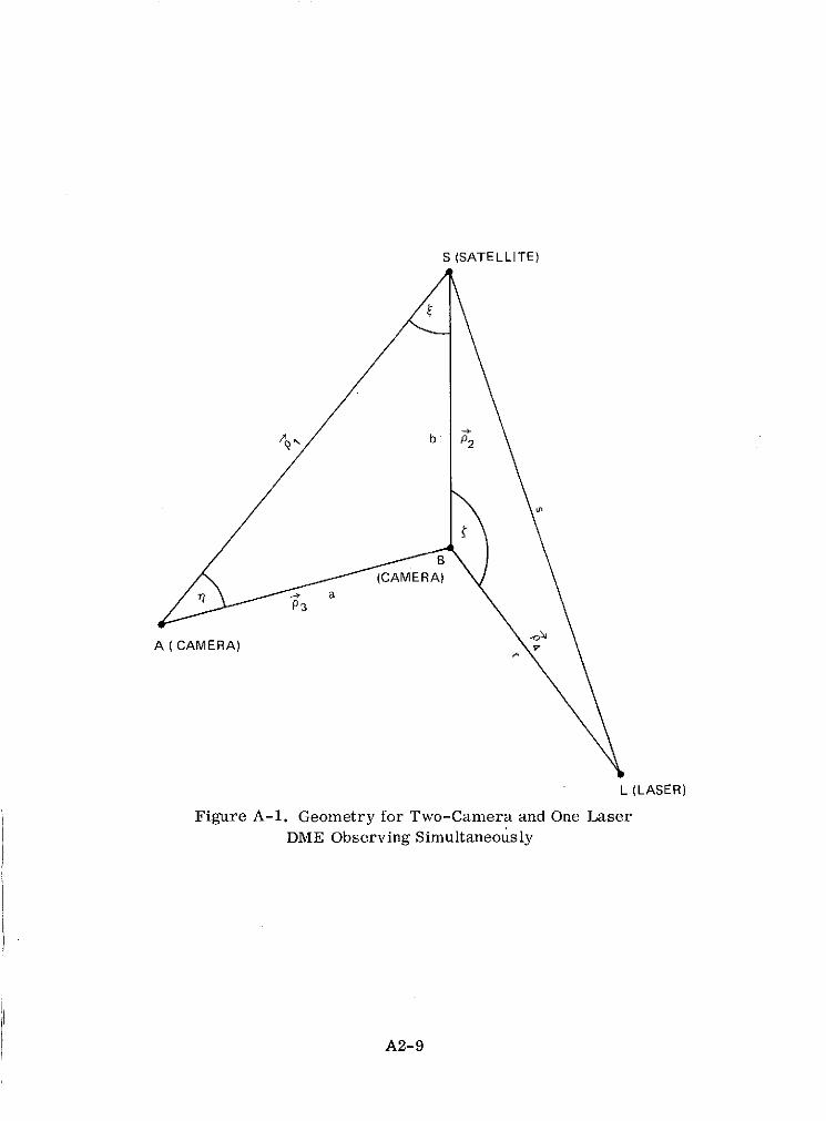
S (SATELLITE)

B

(CAMERA)

A(CAMERA) v

L (LASER)

Figure A-i. Geometry for Two-Camera and One Laser

DME Observing Simultaneously

A2-9

cos = pp 4 si 2 sin -y4 + COS Y2 Cos / 4 Cos(/34 - 2) (2'1)

where /3 , 11, 32, and /2 are directions to the satellite,

13 ' /3 are the inter-station angles for the two cameras, and

14 ' /4 are the inter-station angles for one camera and the lasersystem.

From Figure A-i the law of cosines will give, corresponding to the laserlength s

F = r 2 + b2 - 2br cos 5- s 2 = 0, (22)

and the law of sines will give for b above

sin 7b = a sl .

sin

Through the use of (19) through (21) we expand F linearly about the values ofa, r, /33 , 3, /84, 74, obtained from the initial station coordinates, and the values of

,81 , 7,/, '2 , and s o from the observations. Then we have using differentialsas adjustments (d = A)

aF aF aF aFF Fo +-da + dr + d3 + ... + -ds = 0-aa r a833

Divide F through by q = 2(b - r cos ) and denote the result by

ald,81 + a dy d + a3d/2 + a4 dy,2 + asds + bld/33 + b2 d-/3 + b3 da + b4d34 + bsd} 4

+ b6dr + C = 0 (23)

where C = F0 /q, and the differentials on the a i coefficients are the observationresiduals vi for i = 1 to 5. This represents the laser length equation. The co-efficients and C are evaluated from the initial values, where Fo is obtained fromthe misclosure of (22) and the coefficients in (23) are as follows:

A2-10

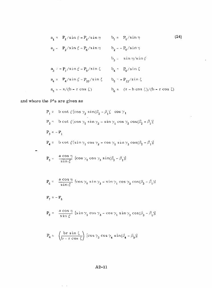
a, = P/sin e-P/sin b P= Ps/sin n (24)

a2 /sin- P6/sin - b = - P/sin 7

b3 sin -/sin

a3 = - P1 /sin - P/sin b4 = P/sin

a4 P4 /sin - P10/sin bs =-P12/sin

as = - s/(b - r cos b) b6 = (r - b cos )/(b - r cos 5)

and where the P's are given as

P 1 = b cot 5[cos y 2 sin( 2 - 13)] Cos 1

P2 = b cot C[cos sin sin - Sin yl cos -2 cos( 2 - 1)]

P3 = P1

P 4 = b cot f[sin9 1 cos -2 - Cos "1 sin 2 Cos(/32 - 31)]

a cos [cos -y/ cos Y3 sin('3 - ,8)]

5 sin ~

a cos cos siny-sinycos cos(3 -/1)6 sin1

P7 = - Ps

a cos FP8 a os [sin y/1 cos os - cosin cos( 3 - /31)]8s= sin1

P, = b r cos [cos /2 COS 74 sin( 4 -2

A2-11

P1 b - r cos [cos Y2 sin 74 - sin 72 COS 74 co(P 4 -2) ]

Pll = -P911 9

( br sin cos( - 8)]P12 b - r cos 2 O 4 - os 72 4 CO 42

In order to obtain the desired form (1) for Cartesian station coordinates, thecoplanarity and length equations are transformed from 7, /, r variables to x,y, z variables by using the relationships

x2 -x 1 = r Cosy cos8

y2 - Y1 = r cos / Sin 8

z 2 - 1 = r sin y (25)

Differentiating these expressions yields

dx2 - dxI -r cosy sin3 - r sin y cos 8 cosy cos8 d,8

dy2 - dy 1 = r cos y cos / - r sin - sin , cosy sin/3 d7T (26)

dz 2 - dz 1 0 r cosy sin y dr

Inverting Equation 26 produces the transformation

d,8 -sin/3 cos 8 0 dx 2 - dxr cos y r cosy

cdi) -sin-ycos/p -sinysinp cosy (27)r r r 2 - d

1

dr cosy cos p cos y sin/ sin dz 2 - dz

A2-12

A2-5.0 CONDITION EQUATIONS FOR CONSTRAINTS

The three types of condition equations are: (1) coordinate equations,(2) distance equations, and (3) coordinate-shift equations. As indicated pre-

viously constraints for station coordinates, distances (baselines), and coordinate

shifts (local datum ties) are based upon a priori information. Such information

is treated statistically as in the case of satellite observations, and hence weights

are applied corresponding to a priori errors.

A2-5.1 Coordinate Equation

Assume the input coordinates of the ith station are coordinates for which

a priori information is available. Let the input values of X i Yi, Z i be XioYo Zio , and denote the adjusted coordinates as

dxi = X1 - X io xi- 2

dyi = Yi - Yio 1 (28)

dz. Z - Z. io x

then the constraint equations in the form of equation (1) are simply

V. - X. = 01-2 1-2

.2 - xi = 0 (29)

V. - X. -O 0

A2-5.2 Distance Equations (Baselines)

The condition equation for the baseline distance q between the rth and sth

ground stations is

- dq + cos y cos 8(dxs - dxr) + cos y sin f(dys - dyr) + sin y(dz s - dZr) = 0 (30)

where Y and /3 are used as in (9) and (10) and the differentials are the unknown

station adjustments. The adjustment

dq = q - q, (q - 9) - (qc - q)

Sv - C (31)

A2-13

where q is the solution value, q, is the computed value based upon the initialstation coordinates, and qo is the a priori value for the constraint.

In conformity with the previous notation the terms dxs, dys, dz s , dx r, dYr,and dzr are replaced by xs_2, Xs, xs , xr_,2 , X1 , Sr , and dq by (31) to obtain

-v - cos Ycos /3(xs_2 - Xr-2) + COS' sin3,8(Xs_ 1 -X) + siny(XsXr)+ C = 0 (32)

A2-5.3 Coordinate-Shift Equations

For two nearby stations denote the difference in coordinates as

D = X2 - X 1

D = y - yl (33)

Dz z 2 z1

Since the results are similar for the three equations we will treat just one equa-tion of condition. For the x component the differential is

- dD + dx2 - dx, = 0, (34)

and as in the case of the distance equation (31)

dD = vx - C, vx = Dx - D , C =Dx - Dx (35)

where Dx is the unknown difference, Dxo is obtained from local survey stationcoordinates, and Dx, is computed from the initial input of the station coordinates.For the ith and jth stations, using the notation of the form (1) where differentialsare replaced by corrections xq and xp, the condition equations for (33) are

- Vx Xj-2 - Xi-2 + C x = 0

- v + Xj_ - Xi- 1 + C = 0 (36)

-v +x. -x. +C =0

A2-14

A2-6.0 COORELATED OBSERVATIONS

The model described above was developed for camera systems that observedsimultaneously the flashing lamps on GEOS-I and II, and then the model wasemployed to include the BC-4 camera network that observed the PAGEOS satel-lite. A BC-4 photograph taken on PAGEOS by an observing station, s, was re-duced to 7 time points (b = 1 to 7) of satellite observation angles (- , 38). Thereduced observations y~ and are correlated separately* in each type amongthe points 4 = 1 to 7. The modeling for the. correlated observations is presented.

Consider 7 events of the type (1), (2), or (3) described in section 1, whererespectively 2, 3, or 4 stations (S = 2, 3, or 4) observe the satellite simultaneouslyat each of the 7 reduced photographic points A = 1 to 7. Thus for each eventthere are 2S simultaneous observations, namely (k, i) for s = 1 to S. Let pdenote this configuration of S stations and 7 events, then for each p there are7 sets of matrix condition equations of the form (2). Denote these as

AVp +BpX + Cp = 0 (37)

where by row partitioning for k = 1 to 7

V = V

C = [C ] (38)

and AV lies along the diagonal submatrix path of A (with zero submatricesPfor off diagonal blocks)

Ap = [DIAG AV] (39)

The submatrices V4, B , and A are given as before in (2) for a particularevent, but here the event type for S = 2, 3, or 4 stations is fixed for the 7 eventsfor a given configuration p.

Denote the variance-covariance matrix of the observation errors as

SE(VpV T (40)

where V, corresponds to the observation errors (noise) in V,.

*Cross correlations between -y and 0 are assumed negligible in this analysis.

A2-15

The normal equations for the BC-4 observations is obtained by minimizing

Q = Q (41)

P

for the unknowns Vp and X, where

Q= Vpl- V - 2(AV + VpX + Cp) T p (42)

and

for which k is a vector of Lagrangian multipliers defined as in (3) for a givenevent. Hence the normal equations will have the form given in (4) through (6).Thus for each p the normal equations are

JpX+ BTMC= N (43)

where

]p= B Mpl

A. = ( PpAT), (44)

and the total set of normal equations for all p are then

N' = N.

It is of interest to compare the matrix M derived from 7 events to that of1M, given in (6) for a single event k. Take the case of S = 4 for which the dimen-sions A, Vk, and WA were given under (6) respectively as 5 x 8, 8 xl, and8 x 8, and for which there were 8 observations and 5 coplanarity equations ofcondition from the 4 observing stations in a given event. Consider 7 events ofthe same type as in the configuration p for S = 4, denote IV as M for k = 1to 7, and assume correlations are absent as in the previous modeling. Then

A2-16

MP

MP= [DIAG M] (45)

0 MP- - 35

x 35

where

=[A() ( 5x (46)

and since correlations are assumed absent here

P = FDIAG(W~])- ]

With correlations the same diagonal blocks in (45) arise for M in (44) sincein each event 4 all observations are uncorrelated, but similar off cdagonal blocks

also exist which is now shown. Using the submatrices V for V in (38) anddropping the superscript p on the submatrices, then the variance-covariance

matrix in (40) becomes

Pp =E(ViT) = [E(VfN)] for k= 1 to 7 and {= 1 to 7, (47)

which corresponds to 49 sublocks or submatrices in P . For a given event A

and t the only covariances occur when the station s and the angle yk or 81are the same. Denote the observation errors for a given 4 as (where T true,o observed)

yT1 1

(T) - 'y(0)

(48)

=- i = 1 to 2S,

T(T) - yT(O)

/ (T) - /(0) 2S 12S 1A2-17

then for a given k and {

E(VAVT) [E(iKv )] 2 2s i = 1 to 2S, j = 1 to 2S. (49)

and from the definition of the correlations

E(ik J) = ( )= for i j for all and

= -2 i (, ') for covariances ( , (50)

= 2 (4, 4) for variances = .

Thus, in each sublock of a given R and t, the off diagonal elements are zero and

E(Y ) = [DIAG i ) 2Sx 2s (51)

-D?/

and

p = [D ] (, = 1 to 7), (52)

Denote

Mp = [M] (" , j = 1 to 7), (53)

and with use of (38), (39), and (52) in (44) then by (53)

Mk= [ADA ](-3(2 ) (54)Now

MA = AADA A (55)

= AW 1 A = Mg,

which is the same as in (46) for the uncorrelated case.

The block form [M ,] for Mp, where Mk4 is given in (54), provides a con-venient method for the computations of M . However in the present case of cor-related observations there are 49 such blocks, whereas only the 7 diagonal blocksM ~R are computed for uncorrelated observations as in (45) or (55). The largestinverse matrix Mp to be inverted occurs for the case of S = 4 and which hasdimension 35 x 35, whereas previously for the case of uncorrelated observationsthe largest matrix was 5 x 5. Correlations are generally large among the

A2-18

reduced observations of a photograph. Thus the geometric normal equationsshould be analyzed further to investigate the overall effect of the correlation on

the final combination solution.

NASA-GSFC

A2-19

APPENDIX A3 . ....... GRAVIMETRIC METHOD m

APPENDIX A3

GRAVIMETRIC METHOD FOR MEAN ANOMALY DATA

CONTENTS

Page

A3-1.0 INTRODUCTION TO TECHNIQUE . ........... A3-3

A3-1.1 Synopsis of the Method and Procedure . ..... A3-3

A3-2.0 GRAVITY FUNCTIONS FOR THE EARTH. . ....... . A3-5

A3-2.1 Gravity Potential for the Geoid . ........ A3-5A3-2.2 Reference Potential and Earth Ellipsoid . .... A3-6

A3-3.0 GRAVITY FUNCTIONS BASED UPON INITIALCONDITIONS .............. ... ..... A3-7

A3-3.1 Initial Potential and Gravity Systemfor GEM 6 .................. A3-7

A3-3.2 Geometry of the Gravity System ... . .... .. A3-7A3-3.3 Initial Constants and Reference

Parameters .................. A3-8

A3-4.0 EXPANSION OF THE GRAVITY FUNCTION FORTHE GEOID ...................... A3-10

A3-4.1 Computations for Gravity and Geoid Height . . . . A3-12

A3-5.0 OBSERVATION EQUATION AND NORMALEQUATIONS ...................... A3-15

A3-5.1 Data Point of Gravity Anomaly . ........ A3-15A3-5.2 Conversion of Rapp's Gravity Formula. . ... . A3-15A3-5. 3 Observation Equation for Mean

Gravity Anomaly ............... A3-16A3-5.3.1 Truncation, Modeling, and Data Errors

in the Observation Equation. . .......... A3-17A3-5.4 Normal Equations for Gravity Data . ...... A3-18

A3-6.0 ADJUSTMENT OF REFERENCE PARAMETERS .... . . A3-20

A3-1

CONTENTS (Continued)

Page

A3-7.0 FORMULAE EMPLOYED FOR ANALYSIS OFMODELS WITH USE OF MEAN GRAVITYANOMALY DATA ................... A3-23

A3-7.1 Derivation of Gravity Anomaly Formula . .... A3-23A3-7.2 Mean Gravity Anomaly Residual and

Errors . ... .............. .. . A3-25A3-7.3 Degree Variances of Gravity Anomaly and

Error of Commission in Anomaly . ....... A3-26REFERENCES ................... ....... . A3-27

A3-2

APPENDIX A3

GRAVIMETRIC METHOD FOR MEAN ANOMALY DATA

A3-1.0 INTRODUCTION TO TECHNIQUE

A global set of 50 equal-area (300 n. m. sq.) mean gravity anomalies, formedby Rapp (1972), are modeled to provide for adjustment cf potential coefficientsthrough degree and order 16 and a mean value of gravity. Normal equations areprepared in a form to be combined with those obtained from the satellite data.For compatibility and subsequent adjustment of basic earth parameters, the grav-ity data is modeled with respect to the same initial parameters of the earth andinitial values of potential coefficients as used in the satellite normal equations.

Along with the mean gravity anomaly, the data of Rapp includes an errorestimate for the anomalyand acenter point in terms of geodetic latitude (0')andlongitude (X). The error estimates are employed for weighting the data in thenormal equations. The data was based principally upon 1' x 10 mean free-airanomalies, which approximate the undulation of gravity at mean sea level (geoid).In the modeling the gravitational potential for the geoid is expressed in sphericalharmonics with coefficients compatible with the gravitational potential of thesatellite model.

A3-1.1 Synopsis of the Method and Procedure

The anomaly of gravity for a point p on the geoid is defined as follows:

Ag E = g(p)- E(q) (1)

where q is the normal projection of the point p onto the ellipsoid of the earth andwhere

g(p) = IV W(p)I, yE(q) = IV U(q)l

for which W(p) is the gravity potential for the geoid and U(q) is a reference po-tential for the earth's ellipsoid of revolution, based upon a set of earth param-eters E = (GM, ae, f, w). Functions for the above quantities and their relationto the reference parameters are to be defined, including a gravitational potentialwhich is expressed in spherical harmonics with coefficients (Cm,, Snmi) for de-gree n and order m.

Similar functions to the above are to be established based upon initial condi-tions. Initial potential coefficients (Cm, S, n) and reference parameters E' are

A3-3

employed which are the same as used with the satellite data, providing for asimultaneous solution of gravity and satellite data for GEM 6. A computed anom-aly Ag c (P), analogous to (1), is formulated based upon the initial conditions.

Mean gravity anomaly data, A-OB(p), is referred to the reference systemof GEM 6 and an observation equation is established in the form of the followinglinear expansion:

AgOBS(p)- gc(P) = 6go +6g 1 (p)+ TN (p) + e(p)

6g, (p) = M2 (n-1)( n P(sin ) .n=2 m=0

(6Cnm cos (mX) + 6Snm sin (mX),) (2)

where the spherical coordinates (r, 0 , X) refer to the point P, 6go is an adjust-ment to a mean value of gravity and (6 Cnm, 6Sn ) are adjustments to potentialcoefficients from initial values. The truncation error TN (p) and errors 6(p),due to the data and the technique, are discussed.

Least squares normal equations are formed with the gravity data for coef-ficient adjustments complete through degree and order 16 (N = 16). Thesenormal equations are then to be combined with those from the satellite data togive the solution for GEM 6. Adjustments to certain basic earth constants arethen formulated from the solution parameters of GEM 6.

The derivation of the method, the gravity functions employed including re-lated constants, and the computational process are presented. Additional gravityformulae, which were used in the report for comparing different potential solu-tions with use of mean gravity anomaly data, are also derived herein.

A3-4

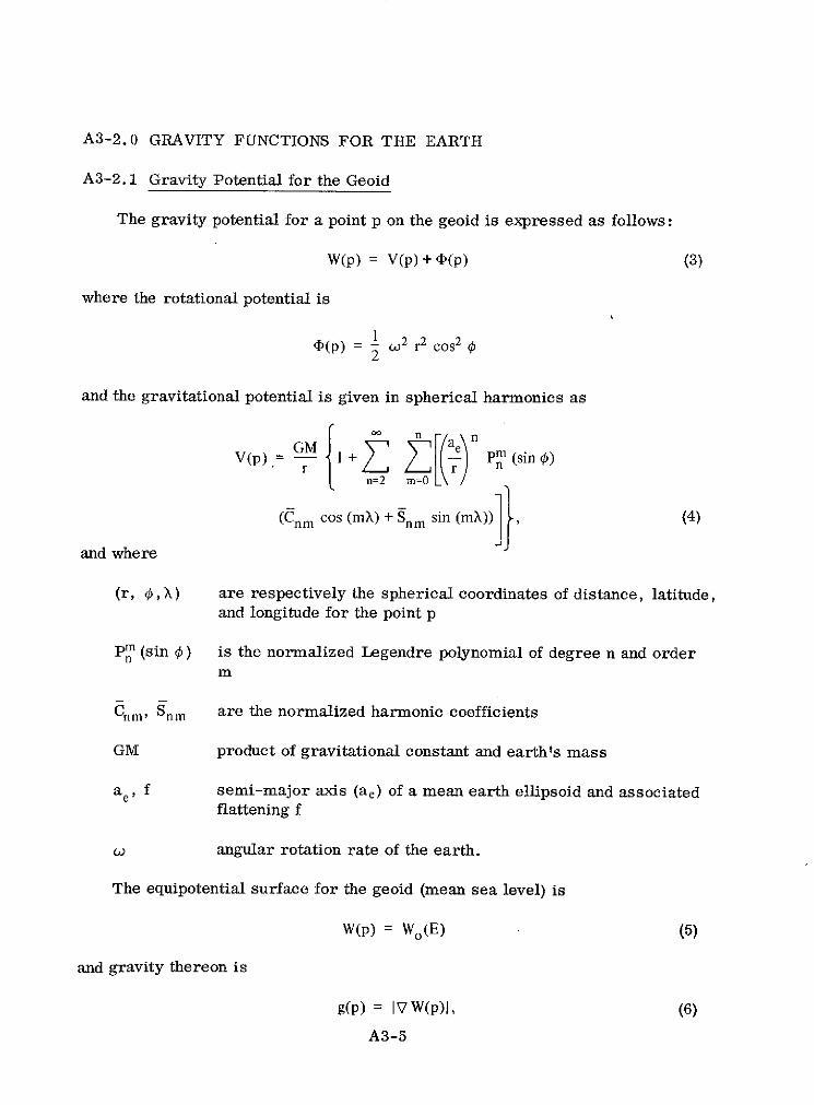
A3-2.0 GRAVITY FUNCTIONS FOR THE EARTH

A3-2.1 Gravity Potential for the Geoid

The gravity potential for a point p on the geoid is expressed as follows:

W(p) = V(p) + 4 (p) (3)

where the rotational potential is

D(p) = 2 r2 cos2 22

and the gravitational potential is given in spherical harmonics as0 n nV GM + 1+ Pm (s in )

V(n=2 m=0

(Cnm cos (mX) + Snm sin (mX))], (4)

and where

(r, 4,K) are respectively the spherical coordinates of distance, latitude,and longitude for the point p

Pnm (sin ¢) is the normalized Legendre polynomial of degree n and orderm

Cnm, Snm are the normalized harmonic coefficients

GM product of gravitational constant and earth's mass

ae, f semi-major axis (ae) of a mean earth ellipsoid and associatedflattening f

c angular rotation rate of the earth.

The equipotential surface for the geoid (mean sea level) is

W(p) = Wo(E) (5)

and gravity thereon is

g(p) = IVW(p)i, (6)

A3-5

where E denotes the basic set of earth constants

E = (GM, ae , f, c). (7)

The constant Wo is related functionally to the set of constants E and is consideredto be determined by them.

A3-2.2 Reference Potential and Earth Ellipsoid

A reference potential for the geoid is 3mployed to define gravity on the

earth's ellipsoid, which in turn will be needed to formulate gravity anomaly.The potential is similar in form to W(p) in (3) and is given simply by

U(p) =- GM + C20 P (sin 4)+C 0 P (sin0)] + 4(p),r 2(8)

where C2o and C* are determined by the basic constants, E = (GM, ae, f, W).

For a point q on the earth's ellipsoid, gravity thereon is defined by

7E ( q) = IV U(q)I (9)

and the ellipsoid has equipotential surface

U(q) = Uo(E) = Wo(E). (10)

The latter relation Uo(E) = Wo(E), for which Wo(E) = W(p) for mean sealevel as in (5), provides for a mean earth ellipsoid with mean equatorial radiusa e . Formulae for the above constants C,0' C*0, and Wo, as a function of the setE = (GM, ae, f, o), are given in Heiskanen and Moritz (1967).

A gravity formula for 7E (q), in (9), is given as a function of geodetic lati-tude 0' as follows:

YE(q) = YE(e) = ge(l + fl sin 2 0' + f2 sin 2 20') (11)

where ge, f 1 and f 2 are constants. The quantity ge is equitorial gravity on theellipsoid with an approximate value of 978 cm/sec 2 . The constants fl and f 2 arein magnitude respectively of the order of flattening f and f 2 .

Similar functions as described above are employed based upon initial valuesfor the set E.

A3-6

A3-3.0 GRAVITY FUNCTIONS BASED UPON INITIAL CONDITIONS

A3-3.1 Initial Potential and Gravity System for GEM 6

Variation of the gravity potential W(p) in (3) will be derived with respect toa computed potential Wc (P). Wc (P) has the same form as W(p) in (3) and isbased upon initial potential coefficients and reference parameters E' correspond-ingto the set E = (GM, ae, f, w). Analogous to the gravity system for the geoidand the earth's ellipsoid as described in A3-2.0, a computed system for gravitybased upon the initial conditions for GEM 6 is defined as follows:

Reference System of Gravity for GEM 6

approximate geoid

Wc(P) = U0 (E'), gc(P)= IVWc(P)I (12)

approximate reference potential

Uc (P) = U (P, C C40 , E') (13)

Uc(Q) = Uo(E'), yc(Q) = IVUc(Q)I (14)

where the point P lies on the approximate geoid and the point Q lies on thereference ellipsoid for GEM 6 with parameters E'. The reference potentialUc(P) is given by the form (8) with coefficients (C*' , C) and parameters E'.A formula for yc (Q) is given in the form (11) as 20

7c(') = g' (1 + f' sin 2 0' + f',sin2 20'). (15)

The geometry relating a point P on the equipotential surface (12) to a pointQ on the reference ellipsoid is presently described for the GEM 6 system.

A3-3.2 Geometry of the Gravity Systems

The geometry relating a point p on the geoid with a point q on the ellipsoidfor the earth is shown in Figure A3-1. The point p has geodetic coordinates (hg,0' , X) relative to the earth's ellipsoid at_the point q (0', X). The gravity systemis based uponthe potential coefficients(C, S) for the geoid and the constants E =(GM, ae, f, w). A similar geometry exists for the points P and Q for the gravitysystem of GEM 6, which is based upon initial potential coefficients (C', S') andinitial parameters E'. The potential Wc (P) is an initial approximation to thegeoid and its reference potential Uc (Q) is an initial approximation for that in (8)of the earth. The two systems will be related through a linear expansion ofgravity g(p) for the geoid about gc(P) in terms of adjustments (6C, 6S) and thereference parameters 6E = E - E'.

A3-7

GEOID: W(p) = Uo(E)

h g(p) = IVW(p)I

g(p)

ELLIPSOID: U(q) = Uo(E)

E (q) (q) = IVU(q)

A = g(p) - E (q)

hg = W(p) - U(p)

'E (q)

Figure A3-1. Geometry of the Geoid and Earth's Ellipsoid

The gravity anomaly for the earth is defined by (1) as

AgE = g(p) - 'E (q)

and that for GEM 6, based upon initial conditions, is

Age = g(P) - c (Q)

A3-3.3 Initial Constants and Reference Parameters

Initial reference parameters employed for the gravity data are the same setas employed with the satellite data, since both the satellite and gravity data areto be combined simultaneously in GEM 6.

The basic reference constants for GEM 6 are as follows:

GM' = 398601.3km 3 /sec 2

ae' = 6378155 m

f = 1/298.255

w = 0. 7292115146 x 10-4 rad/sec (16)

A3-8

Initial constants, derived from the set E' and used for the computed functionsdescribed under (13) and (15), are as follows:

C*' = - 484.17104 x 10 - 620

C*' = 0.7903 x 10 - 6

40

g' = 978029.1mgal

f' = .0053025

f2 =- .00000585 (17)

The above value of flattening f and rotation rate w are sufficiently accuratefor modeling the gravity data. Hence only GM' and a'e differ from the set E.

The reference value of GM' was derived from analysis of satellite data ondeep space probes and contains the mass of the atmosphere and earth. Thisvalue as indicated was employed for the satellite data on the close earth satel-lites in GEM 6, but it requires a nominal adjustment to remove the mass of theatmosphere for use with surface gravity data. The adjustment is given by

6GM 6MGM- - .87 x 10-6

GM M (18)

Essentially the value of GM' is accepted except for the nominal adjustment of theatmosphere.

The remaining parameter a'e is to be adjusted by 5 a'e. Its adjustment willbe related with use of (18) to an adjustment 6 go of a mean value of gravity,which is directly related to the gravity data. Since the computed functions andassociated constants refer to the set E' = (GM', a'e, f, w), GM and a e are re-garded as parameters in the variation of W(p).

A3-9

A3-4. 0 EXPANSION OF THE GRAVITY FUNCTION FOR THE GEOID

Denote the functional form for W(p) in (3) as

W(p) = W (p, C, S, E) = U0 (E)

and its gravity as

g(p) = IV W (p, C, S, E)I = g (p, C, S, E) (19)

where (C, S) denotes the potential coefficients and E = (GM, a e , f, W) the ref-

erence constants. For the system of gravity (12) based upon initial conditions,

denote from (19) above

WC(P) = W (P, C, S, E') = Uo(E'), gc(P) = IV Wc(P)I = g (P, C' S, E') (20)

where (C', S') denote initial potential coefficients and constants E' = (GM', ae,f, o). We wish to expand g(p) about gc(P) in terms of adjustments (6C, 6S) for

the potential coefficients from initial values and an adjustment 6g o of a mean

value of gravity in terms of 6GM and 5 a e from initial values. The expansion is

given under (35) and it is derived in the remainder of this section.

Since flattening f is the same in each system, the points, p and P, differ

only in geoid height relative to their respective ellipsoids. In geodetic coordinates

denote

p = (hg, 0', X), P = (hg, ', X) (21)

and to a sufficient approximation denote their radial coordinates respectively as

r = ae [I - fsin2 '+ 0 (f2)] +hg, r' = ae [1 -f sin 2 ' + 0 (f2)] + hg: (22)

In the expansion for g(p) the partial derivatives will be obtained to withinterms of the order of flattening relative to their magnitudes. The expansion is

made from the functional forms (19) and (20) as follows:

g(p) = g(P) + + (, (6C, S)3)

where for the central term of gravity and by use of (22)

GM 6GM GM 6ae GM hg - hg'6 2 - -2

r2 r2 r2 r r (24)

A3-10

To within terms of the order of flattening the first two terms in (24) become

6GM GM 6 ae GM 6GM 6 ae- 2 - --- 2- e 6g(

r2 2 r a 2 GM ae o (25)

From the relationship in (19), namely

W(p, C, S, E) = Uo(E) ,

we have by holding the parameters E fixed, 6 Uo(E) = 0 and in terms of the vary-ing quantities (hg, C, S)

6 Uo(E) = 0 = 6W (p, C, S, E) = W (p, C,S,E) -W(P, C:SE)

or

GM __W

0 - (hg - hg') + W (6 C, 6S)r 2 8(C, S) (26)

where from (22) use is made of 6 r = hg - hg' for ae fixed. Equation (26) estab-lishes the last term in (24) and with use of (25) then (24) becomes

6GM 2 aW= 6go - (6 C, 6 S),

r2 r a(C, S) (27)

and substituting this result into (23) then

2 aW agg(p) = go(P) + 6g (6C, 6S)+ (6C, 6S)r 3(C, S) a(C, S) (28)

For the harmonic terms of W(p) in (3) denote

W(p)= -GM + Wnm ( P, Cnm, Snm) + F(P),n, m (29)

where

Wnm CmSnm (sin ) [nm cos mX + m sin mX],Wnm P(PCnn ', nm r (30)

then(p) 6 (Cnm, Snm) = Wnm (P, 6 Cnm, 6Snm)

a(Cnm, Snm) (31)

A3-11

Denoting the direction of the local vertical by n' for a point p on the geoid,then since n' has small deviations from the normal to the ellipsoid we have

8W(p) W(p)g(p) = IV W(p)I = W) - p(32)

an' ahg (32)

For the last term in (28), with use of (32)

ag(p) _a(C, S) a(C, S) L ahg J a(C, S) Lha (33)

where the spherical approxmation in brackets gives terms to within anorder of flattening by (22). With use of the results from (29) through (33)we have

ag(p) (n + 1)

a(m, nm) nm r Wnm (p Cnm' nm) (34)

Substituting (31) and (34) into (28) and with use of (30) we have the followingresult for the expansion:

g(p) - g (P) = 6g(p) = 6go + 6g (p)

GM .)

6g 1 (p) = (n-1)

n=2 m=0

PM (sin ¢) (SCnm cos mX + 6Snm sin mX) (35)

and from (25)

GM 6GM 6 aego ae2 GM ae

For use in the normal equations for mean gravity anomaly, a value of N = 16 isemployed in (35) for the adjustments of spherical harmonic coefficients (6 C, S).

A3-4.1 Computations for Gravity and Geoid Height

In the expansion of g(p) in (35), the computed value gc(P) and the partial de-rivatives of g(p) with respect to the coefficients require the point P to be

A3-12

determined. Initial values of GM and ae, including the radial coordinate r = rfor P, are used in the expression for 6g(p) under (35) for computations. Co-ordinates of (0', X), as defined in (21) for the points p and P, are given with thegravity anomaly data. Hence only geoid height (hg') for P needs to be obtainedto establish the point P. The result for the computation of hg' is given below in(40) where Brun's formula is applied and the computation for gravity gc(P) isgiven in (41). The description and derivation for the computation of geoid heightis given in the remainder of this section.

Geoid height for the point P is derived from the condition (12) with use ofthe reference potential Uc(P) as defined under (13). By expansion

Uc(P) = Uo(E') - c hg' (36)

where y is defined in (14) and a gravity formula for yc(O ') is given in (15). Re-lated constants (ge, f', f) for yc (4') and those (C*, C*') for Uc(P) are given

numerically in (17).

With use of (12) there results from (36)

Wc(P) - Uc(P) Tc (P)

h-(, ) /c (37)

Tc(P) = Wc(P ) - Uc(P),

which is an application of Brun's formula.

Tc(P) is the disturbance potential for the gravity system under (12) and isgiven as follows through use of the forms of W(p) in (3) and U(p) in (8):

T, (P) =Tc G Mr Pm (sin ¢)

Sn=2 m=0

[C cos mX + msint mX) (38)

Co = C2' - C = 4.2 x 10 - 9

C = C40 - C40 = -0.2593 x 10-6 (39)

and for all other coefficients C*= Cm. The coefficient C0 is quite small andall other coefficients are approximately 10 - 5 /n 2 in magnitude using Kaula's ruleof thumb. Since geoid height hardly exceeds 100 meters and N = 16, T c (P) is

A3-13

evaluated by replacing the point P with its subnormal point Q on the referenceellipsoid of GEM 6. Geoid height is computed with use of (38) by

Tc(Q)hg' - hg' = ') (40)

The point P in spherical coordinates (r', 0, X) is obtained from customaryformula for transforming geodetic coordinates to spherical coordinates.

With the point P in spherical coordinates gc(P) is computed to sufficientaccuracy from

g,(P) -C- + (ar r2 (41)

where r = r', and the term for aWc/aX is negligible.

A3-14

A3-5.0 OBSERVATION EQUATION AND NORMAL EQUATIONS

A3-5.1 Data Point of Gravity Anomaly

Gravity anomaly is defined theoretically in (1). With use of (11) it may be

expressed as

AgE = g(p)- yE ( ' )

where E( ') depends upon the constants E = (GM, ae, f, w), g(p) is gravity at

a point p on the geoid, and (hg, 0', X) are the geodetic coordinates of the point

p relative to the earth's ellipsoid. In practice a data point of gravity anomaly

AgR(W', X) is referred to a gravity formula yR (l') based upon a known set of

constants E R, and the anomaly is expressed by

Ag R (0R X) = g(p) - ( ') (42)

where (0', X) refer to the point p as defined above.

For the system of constants E' as in GEM 6, let the data point of gravity

anomaly be designated as

Ag D (' X) = g(p)- c(¢'), (43)

then from (42)

Ag D (0 ") = AgR (0 X) + YR ( ' ) - 7c(')" (44)

Hence by (44), given the constants E R, a data point of gravity anomaly may be

converted to the system of GEM 6 and referred to the gravity formula for y7 (')

as designated in (43).

From (15), the difference in the gravity formulae, based upon the constants

E' and E R , is expressed by

fR () - YC( ') = Age + A ge sin 2 0' + Af2 g sin 2 20'. (45)

Numerical results are given in the next section for two gravity formulae

employed for use with Rapp's gravity data.

A3-5.2 Conversion of Rapp's Gravity Formula

The data of Rapp refers to a gravity formula 'yR consistent with the follow-

ing constants:

A3-15

ae = 6378137.8 meters

f = 1/298.258

GM = 398601.3 km 3 /sec 2 (46)

The gravity formula given by Rapp (1972) consistent with these constants and in-cluding a term of -0. 87 mgal for eliminating the mass of the atmosphere in GMis

TR = 978033.5 (1 + .00530243 sin 2 ' - .00000587 sin 2 20') (mgal) (47)

From (15) and the constants in (17), the gravity formula in the GEM 6 sys-tem is

'c = 978029.1 (1 + .0053025 sin 2 ' - .00000585 sin 2 20') (mgal), (48)

and from (47) and (48)

'R - C = Age = 4.4 mgal (49)

to within one-tenth of a milligal.

The difference of YR- 7c given in (49) may be explained by the following re-lationship among the parameters, namely

GM (5GM AaeGM e - 2 -a 4.4 mgal (50)

ae eGM awhere Rapp applied the nominal atmospheric correction 6GM/GM, given in (18),for his derived value of ge

It is noted that in the computation of y from the reference formula of gravity,such as in (47), the value for 0' need not be precisely known. A lateral displace-ment of 100 meters, corresponding to an error in ' , produces a maximum effectof 0.1 mgal on y. Such an effect is not greatly significant in the modeling for thegravity data which is at best accurate to about 1 mgal.

A3-5.3 Observation Equation for Mean Gravity Anomaly

From (35)

g(p) - gc(P) = Sg(p), (51)

A3-16

where 8 g(p) is given in terms of adjustments of the potential coefficients (8C,

S8) and an adjustment Ag o of a mean value of gravity. The relation (51) may be

written as

[g(p)- c Wc-) [gc(P) - (')= 8g(p), (52)

and with use of (43) for a data point of gravity anomaly, Ag D (4, X), this relation

(52) becomes

AgD 0 X)-Agc(P) = 8g(p) (53)

where

Agc(P) = g(P)- yc(0')- (54)

Mean gravity anomaly over a given area on a reference ellipsoid is an aver-

age point anomaly, as defined in (42), for a region of the geoid. In practice the

mean anomaly is centered in geodetic coordinates (0', X). Let the mean gravity

anomaly data of Rapp for 5' equal area blocks be designated as AgR (', h).

Then similar to (44) the data is referred to the GEM 6 system as

AgD ( X) = R g(: X) + yR (0')- yc (0') (55)

where yR - 70 is given in (45) and numerically in (49).

A3-5.3. 1 Truncation, Modeling, and Data Errors in Observation Equation

In Equation (53) we replace the point anomaly A gD (0 ', X ) by the mean anomaly

Sg D (4', X ) from (55) and form the observation equation as follows:

AgD (': X) -Agc(P) = 5g(p) + TN (p) + e(p) + eD (56)

where:

8 g(p) is given in (35) as an harmonic expansion expressed in terms of ad-

justments Ago and (8C, 5S) for coefficients complete through degree and order

N, TN(p) denotes the error due to truncation, e(p) denotes the error induced by

approximating a mean anomaly centered at (0', X) by a point anomaly evaluated

at the center point (4', X), and eD denotes errors in the data which vary from 1

to 20 mgal.

The modeling error for e(p) would certainly be significant for harmonic

terms of degree n which experience a complete cycle in a 5' block, namely

360n > - = 72.

5

A3-17

This error would vanish by averaging the computed anomaly Agc(P) and the vari-ation 6 g(p) over the 50 block, and the averaging is recommended for terms withuse of the present data where

n = 18. (57)

Effects of the error e(p) are discussed in A3-7. 1 where some numerical resultsare given, which show a small effect for a test case with truncation of N = 20.

Since N = 16 is employed for the trancation, the error e(p) is not significant.However the truncation error TN (p) is large. The effect of TN (p) on the modeledcoefficients is not significant in the normal equations because of the orthogon-ality property of the spherical harmonics. Nevertheless, some aliasing effectis experienced particularly on coefficients of degree 15 and 16, which haveneighboring frequencies to those just beyond the point of truncation. The alias-ing effect results because of the inhomogeneous set of gravity data with variableaccuracy, from 1 to 20mgals of error, which is applied in the weighting for thenormal equations. The weighting is necessary so that solution conforms appro-priately to the better data, but it tends to degrade the orthogonality conditionbetween distinct pairs of harmonics.

A3-5.4 Normal Equations for Gravity Data

Denote from (56), for the global set of anomaly data at each point i, theresidual

Vi = AgD (0i' X) - Agc (Pi) (58)

From the form of 6 g(p) given under (35), let the point pi correspond to thecomputed point Pi above, xj correspond to an adjustment parameter for the set(6 C, 6 S) and Ag o and Aij the corresponding spherical harmonic factor for theparameter xj, then

sg(Pi) = A xj

(59)

and with use of (58) the residual for the observation equation becomes

S = Aij xj. (60)

A3-18

For all observation data, namely Ag D (0i', ) for all i, (60) becomes in matrix

form

v = A x, V = [vi], A = [Ai], x = [xj]. (61)

The computations for the point Pi , and its gravity gc (Pi) are discussed in

A3-4.1, including the elements A ij *

The normal equations are formed with use of a diagonal weight matrix,

namely

W = [wi] (62)

where w i = 1/oi2 (OBS) and aoi (OBS) are given with the data AgR (i', Xi). The

normal equations for the gravity data, which are to be combined with the satel-

lite data in GEM 6, are given in matrix form from (60), (61), and (62) as

AT WV = AT WA x. (62)

A3-19

A3-6.0 ADJUSTMENT OF REFERENCE PARAMETERS

Based upon the adjustments 6g o and 6C20 from the combined solution ofGEM 6, an adjustment for equitorial gravity ge, and adjustments for the semi-major axis a. and flattening f are derived. The variational equations are givenbelow for the adjustment and numerical results are provided for the adjustedquantities. It is shown that ae depends upon the reference value of GM, whilege is independent of this value to within first order, and that the new value offlattening is essentially the same as that of the reference value employed. Initialvalues of parameters are given under (16) and (17).

A complete set of formulae relating the above quantities may be obtainedfrom Heiskanen and Moritz (1967). Their variational relationships result in aset of simultaneous equations of first order. Results are derived below whichare accurate to within the numerical values listed.

From (25) and the solution value of 6g o from GEM 6

6g = -GM = 3.0 mgal,0 ae2 GM ae (63)

where, with use of the nominal correction for the atmosphere in (18) for which6 GM/GM = -. 87 x 10-6 and use of the constants in (16),

5 ae = - 12.5 (64)

From the relationship

6go 6GM 6a,-- 2

ge GM ae (65)

and (63)

6g e - 6g o = 3.0 mgal. (66)

The adjustment for flattening f is obtained from the relation

3 16f = 6J 2 + - 6m,

2 2 ' (67)

where

6J 2 2 20

0 - C20 = - 4 8 4 . 16608 x 10- 6

A3-20

C' = -484.17104 x 10-

J 2 = - 11.1 x 10 - 9

and where

m - 2 a/g, (68)

6m = m - g - 17.3 x 10- 9 (69)

and thus

6f = - 25 x 10- 9 (70)

The new value for flattening, namely

fNEW = f+A5

will give

fNEW = 1/298.257 (71)

where for the reference value

f = 1/298.255.

Adjusted values for ae and ge, based upon the adjustments obtained above,

are

ae = 6378142.5 m

ge = 978032.1 mgal. (72)

-Rapp (1974) has provided new estimates for all the above basic parameters.

Of principal concern here are his new values for ge and f, since our value for

ge is derived directly from the gravity data as indicated by (66) and our refer-

ence value for flattening was assumed sufficiently accurate for modeling the

gravity data. His new values for these two parameters are given as

ge = 978031.7 +.77 mgal

A3-21

1/f = 298.2564 ±.0015

af = ±17 x 10- 9

which agree well with our results.

A3-22

A3-7.0 FORMULAE EMPLOYED FOR ANALYSIS OF MODELS WITH USE

OF MEAN GRAVITY ANOMALY DATA

Certain formulae were employed for the analysis of potential solutions,

among different models, with use of mean gravity anomaly data for which results

are given in the report. Let the potential coefficients of the models be designated

as (C, S) for coefficients complete through degree and order N, for N = 12, 16,

or 20. The models were based upon the same initial parameters as in GEM 6,

E'= (GM', a'e, f, c), hence the gravity anomaly data is referred to the GEM 6

gravity formula -c (0') as in (43), namely

Ag D (,,) = g(p)-yc() (73)

where g(p) as before is gravity on the geoid.

A3-7.1 Derivation of Gravity Anomaly Formula

Let the normalized potential coefficients for the geoid be designated as (C,

S), and its reference parameters by E = (GM, a e , f, w) as before. Hence the

functional form, given in (19) for g(p), is now designated as

g(p) = g (p, C, S, E),

and from the expansion in (35) g(p) may be represented in terms of parameters

E' by

g(p) = g (p, C, S, E') + 6g o , (74)

since the only difference is given by 6g o in (25) due to the two sets of param-

eters E and E'.

Let gravity g(P) for a solution with coefficients (C, S) be similarly designated

as in g(p) above, for parameters E and E', as follows:

g(P) = g (P, C, S, E) = gc (P, C, S, E') + 6g o . (75)

We may write an identity relation for (74) as

g(p) = gc (P, C, S, E') + 5g 2 (p)+ go,

5g 2 (p) = g (p, C, S, E') - g (P, C, S, E'), (76)

and again with use of the form of the expansion in (35)

5g 2 (p) = 6g, (p)+ TN (77)

A3-23

where 5g (p) now represents the effect of the errors (6C, 6S) committed in thecoefficients (C, S) through degree N, and where TN designates the effect of theerrors of omission for the coefficients (C, S) in g(p) beyond degree N. In thenew context it is more appropriate to designate 6g I (p) as eN, hence (77)becomes

6g 2 () = eN + TN (78)

where EN represents the errors in gravity committed by the errors in the solu-tion parameters (C, S) through degree N.

Substituting the result for 6g 2(p) from (78) into (76) for g(p), then (73) maybe expressed as

Ag D (0" k) = gc (P, C, S, E') - yc(O' ) + 5go + e + TN (79)

The quantity gc (P, C, S, E') may be computed analogous to gc(P) as describedin A3-4. 1. It is convenient in the remaining analysis to use an alternativemethod, which is more customary, for computing the gravity anomaly

Agc (P, C, S, E') = gc (P, C, S, E') - yc(¢') (80)

corresponding to these two terms in (79).

The result for Agc (P, C, S, E') is given in (85) below and it is establishedfrom use of the expansion given in (35), where gc (P, C, S, E') replaces g(p)and yc(P) replaces gc(P). The expressions for the gravity quantities are ob-tained from their respective potentials as follows:

gc (P, C, S, E') = Iv We (P, C,S, E')I (81)

-7 (P) = IV Uc (P)I, (82)

where, analogous to the reference system of GEM 6 in (12) through (14), Wc(P,C, S, E') is given by the form for W(p) in (3) and Uc(P) is given by the form (8)with use of the constants (C02 , C ) in (17). As in (37), geoid height hg for Pis related as

Wc (P, C, S, E') - Uc (P)

7c(¢') (83)

and is computed as in (40). With use of the approximation

GM' hgr 2 r

(84)

A3-24

and the above relations (81) through (83), we obtain from the technique given forthe expansion in (35) the following result for (80):

GM' aeAgc (P, C, S, E') = (n-) r

n=2 m=0

Pfl.(sin 4) (C* cos mX + Snm sin mX) (85)

where C* is defined by

C* = C2-C' C* = C40 -C*20 20 20' 40 40 40

and for all other (nm), C* = Cnm. The spherical coordinates (r, , X) for the

point P are obtained from its geodetic coordinates (hg, 0', X) relative to thereference ellipsoid for GEM 6 with parameters E' = (GM', a', f, w).

A3-7.2 Mean Gravity Anomaly Residual and Errors

As in the observation equation (56) for mean gravity anomaly, we replacethe point anomaly AgD(¢', X) in (79) by the mean anomaly A D( ', X). We then

obtain from (79) and (80) the residual us for a given solution of potential coeffi-cients, namely

Ag D (0 X) - Age (P, C, S, E') - 6g o =

s (86)

where in terms of the errors in (79) and (56)

Vs = eN + T N + e(p) + eD. (87)

In the report the mean square of the residuals, M(v2), was compared amongdifferent models, which are truncated at degrees N = 12, 16, and 20.

The errors eD for the data, TN for the truncation of the solution, and e(p)were discussed previously. Gravity anomaly Ag c in (85) is computed at thecenter point (0', X) of the data A9D ( ', X), as opposed to averaging the anomalyAgc over the 50 equal-area block of data, resulting formally in an error e(p) aspreviously described. Gravity anomaly Ag c was computed by both averagingand employing the center point only, for cases of N = 12, 16, and 20. Only aslight difference of less than one mgal 2 was seen in M(V2) for the case of N =20. Also Ag c , as computed directly by. (80) or by (85), gives no essentialdifference.

A3-25

The value of 6 go = 3. O0 mgals was used in (86) which best fits the data rel-ative to the reference constants E' of GEM 6. Hence, for a given potentialmodel, all quantities in (86) are computed w. r. t. the set E'.

The principal source of error of interest in (87) is EN , which is the effectof the errors (6C, 6 S) in the potential coefficients of a given solution. For twomodels with solutions sl and s2, truncated at degree N, the only difference inthe residuals from (87) is

VsI - s2 = eN(S)- EN (s2) (88)

since the other errors are the same. By the orthogonality property of the spher-ical harmonics and by the assumption of randomness of data errors (eD),then for a solution independent of the data we have from (87)

M(v s ) = M(2 ) + M(T ) + M(e2D) (89)

For two solutions independent of the data, such as different satellite solutions,

M(v2) 2) = Me (S1)] - M [E (s2)]. (90)

Hence the difference in the mean square residuals give a direct measure of theerrors in gravity as committed by the coefficient errors in the two models.

A3-7.3 Degree Variances of Gravity Anomaly and Error of Commission inAnomaly

Solutions were compared in the report based upon degree variances ofgravity anomaly. -n2 (Ag), which are derived directly from the coefficients ofdegree n, (Cnm, Snm). They are particularly of interest for high degree n, wheregreater variability is seen among different models. These irregularities occurin u2 for values of n bordering near the truncation point at degree N, and theseare usually due to the aliasing effect in the solution arising from the truncationerror TN.

By setting r = a. in (85) for gravity anomaly and taking the mean squarevalue over the earth, we have

N

02 (Ag) =Y an2 (Ag),

n=2 (91)

A3-26

for all n (# 2 or 4)

2 (Ag) = 1)2 (Cm + Sn)

m=0

and for n = (2, 4), Cnm is replaced by C* and C40 as given under (85).

Cross term effects from (85) vanish in (91) due to the orthogonality of theharmonics. Similarly to (91) we have for the errors in gravity anomaly (e), dueto the commision errors in the coefficients a2 ( 6Cnm ) and a 2 (6 Snm ), the followingresult:

N

2 [E(Ag)] n= o2 [E(Ag)

n=2

n

n2 [(Ag)] = g2 Z (n - 1)2 [ 2 (6Cnm) + 2(Snm). (92)

m=0

REFERENCES

Heiskanen, W. A., and H. Moritz, Physical Geodesy, W. H. Freeman, SanFrancisco, 1967.

Rapp, R. H., "The Formation and Analysis of a 50 Equal Area Block TerrestialGravity Field," Dept. of Geodetic Science Report No. 178, Ohio State Uni-versity Research Foundation, Columbus, Ohio, June 1972.

Rapp, R. H., "Current Estimates of Mean Earth Ellipsoid Parameters," Geo-physical Research Letters, Vol. 1, No. 1, AGU, May 1974.

A3-27

- APPENDIX A4 ... . . . . . TECHNIQUES IN COMBINED SOLUTION

APPENDIX A4

METHOD OF COMBINED SOLUTION

CONTENTS

Page

A4-1. 0 COMBINATION OF DIFFERENT SETS OF

DATA . . . . . . . . . . . . . . . . . . . . . . . . . A4-3

A4-1.1 Combined Set of Normal Equations

for GEM 5 ................ ... .. A4-3

A4-1.2 Combined System of Normal Equations

for GEM 6 ................. .. A4-5

A4-2.0 NUMERICAL TECHNIQUES . ............. . A4-6

A4-3.0 STATISTICS OF SOLUTION FOR THE

GEODETIC PARAMETERS . . . . . . . . . . . . ... A4-9

A4-1

APPENDIX A4

METHOD OF COMBINED SOLUTION

Described herein are, (1) the techniques employed for combining the nor-

mal equations for GEM 5 and GEM 6, (2) the numerical techniques for the solu-

tion of the geodetic parameters, and (3) the variance-covariance matrix for the

solution parameters.

A4-1.0 COMBINATION OF DIFFERENT SETS OF DATA

For GEM 5, the gravitational potential and stations' coordinates are com-

puted using only orbital (dynamical) theory. For GEM 6, the orbital theory is

combined with geometric theory and gravimetric theory.

A4-1.1 Combined Set of Normal Equations for GEM 5

The dynamical theory is used to generate systems of arc-specific normal

equations, i.e., the system of normal equations is generated for a given orbit.

These systems of normal equations are written in terms of arc-dependent (or-

bital elements) and are-independent variables (gravitational potential and station

parameters). Processing continues by reducing these systems of normal equa-

tions to systems written in arc-independent variables only. Once this is done,

normal equations using any number of arcs and/or surface and geometric data

are combined. The elimination of orbital elements from satellite-specific sys-

tems of normal equations is described herein.

The normal equations formed for individual arcs are of the form

B3 B2J (1)

where

B1 is the k-by-k matrix of coefficients involving partial derivatives with

respect to arc-independent variables only

B 2 is the (n-k)-by-(n-k) matrix of coefficients involving arc-dependent

partial derivatives only

B 3 is the (n-k)-by-k matrix of coefficients involving product-term partial

derivatives of arc-independent and arc-dependent variables

A4-3

PRECEDING PAGE BLANK NOT FILMED

X 1 is the k-dimensional vector X1, ... , Xk involving arc-independent vari-ables (gravitational parameters and tracking station coordinates)

X2 is the (n-k)-dimensional vector Xk+l, ... , Xn involving arc-dependentvariables (satellite vectors, tracking system biases, and drag and radi-ation pressure coefficients)

bi is the k-dimensional portion of the right-hand side vector associatedwith the are-independent and product term partial derivatives (B1 andBT)

b 2 is the (n-k)-dimensional portion of the right-hand side vector associatedwith the arc-dependent and product term partial derivatives (B2 andB3).

The back substitution solution for X2 gives

X 2 = B2 1 (b 2 - B 3 X 1 ) (2)

Using this result to find X 1 produces the expression

B1 X, + BT [B1 (b 2 -B 3X 1 ) = b (3)

which yields the equation

(1 -B B1 B3) X, = b1 - BTBg b 2 (4)

Equation 4 is the reduced system of normal equations in arc-independent vari-ables only. A reduced set of normal equations is formed for each arc prior toits aggregation to form a multi-arc solution for the arc-independent variables.Once equation 4 is solved, the result is substituted into equation 2 to produce anestimate of X2 , the arc-dependent variables.

A notational simplification is obtained by

B* = B - B TB 2 B3'

b* = b1 - BTB1 b2

x* = X1, (5)

which produces a reduced set of normal equations of the form

B*x* = b* (6)

A4-4

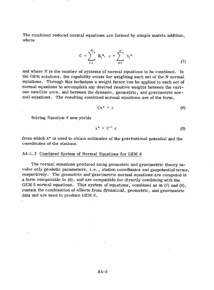
The combined reduced normal equations are formed by simple matrix addition,where

N N

C = Bi*, c = bi*

i=l i=1 (7)

and where N is the number of systems of normal equations to be combined. Inthe GEM solutions, the capability exists for weighting each set of the N normalequations. Through this technique a weight factor -can be applied to each set ofnormal equations to accomplish any desired relative weights between the vari-ous satellite arcs, and between the dynamic, geometric, and gravimetric nor-mal equations. The resulting combined normal equations are of the form,

Cx* = c (8)

Solving Equation 8 now yields

x* = C- 1 c (9)

from which x* is used to obtain estimates of the gravitational potential and thecoordinates of the stations.

A4-1.2 Combined System of Normal Equations for GEM 6

The normal equations produced using geometric and gravimetric theory in-volve only geodetic parameters, i.e., station coordinates and geopotentialterms,respectively. The geometric and gravimetric normal equations are computed ina form comparable to (6), and are compatible for directly combining with theGEM 5 normal equations. This system of equations, combined as in (7) and (8),contain the combination of effects from dynamical, geometric, and gravimetricdata and are used to produce GEM 6.

A4-5

A4-2.0 NUMERICAL TECHNIQUES

The numerical method employed for solving the system (8),

Cx* = c,

is discussed.

The approach described here uses single-precision arithmetic to estimatethe x* vector iteratively without first finding the C-1 matrix. Single-precision

arithmetic permits substantial reductions of core storage and does not increasecomputer utilization time. Test cases have shown that the single-precision iter-ative improvement yields solutions that agree to within 4 to 5 significant places

with double-precision inversion schemes when as many as 400 parameters wereestimated simultaneously.

A decomposition of the matrix C is computed by the Cholesky method suchthat

C = LLT (10)

where L is a lower triangular matrix (all elements of L above the diagonal areequal to zero). This decomposition is unique because C is symmetric and posi-tive definite.

Let the elements of the matrices above be denoted for row i and column jas

L = [Qij],C = [cij],c = [ci]l

The matrix L has ij = 0 for i < j, and remaining elements defined by

i-I

(11)j=1

j-1

cij- T im Qjm

i m=1 j (12)

for i = 1 to N where N is the order of the matrix.

A4-6

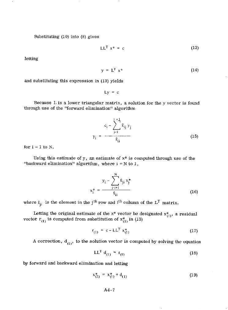
Substituting (10) into (8) gives

LLT x* = c (13)

letting

y = LT X* (14)

and substituting this expression in (13) yields

Ly = c

Because L is a lower triangular matrix, a solution for the y vector is foundthrough use of the "forward elimination" algorithm

i-1

ci - ' ij Yjj=

Yi= (15)

for i = 1 to N.

Using this estimate of y, an estimate of x* is computed through use of the"backward elimination" algorithm, where i = N to 1,

N

Yi- 1i X*

j=i+lx = (16)

where ji is the element in the jth row and ith column of the LT matrix.

Letting the original estimate of the x* vector be designated x* ), a residualvector r( 1) is computed from substitution of x*1 ) in (13)

r(1) = c - LLT x* (17)

A correction, d(, to the solution vector is computed by solving the equation

LLT d(1 ) = r(1) (18)

by forward and backward elimination and letting

X*) = x 0* + d (19)

A4-7

A new residual vector r( 2) is computed from (17) and (19) and the solutionimprovement vector is computed by forward and backward elimination until the

process converges. Usually 3 iterations are required for a system such as GEM 6.

A4-8

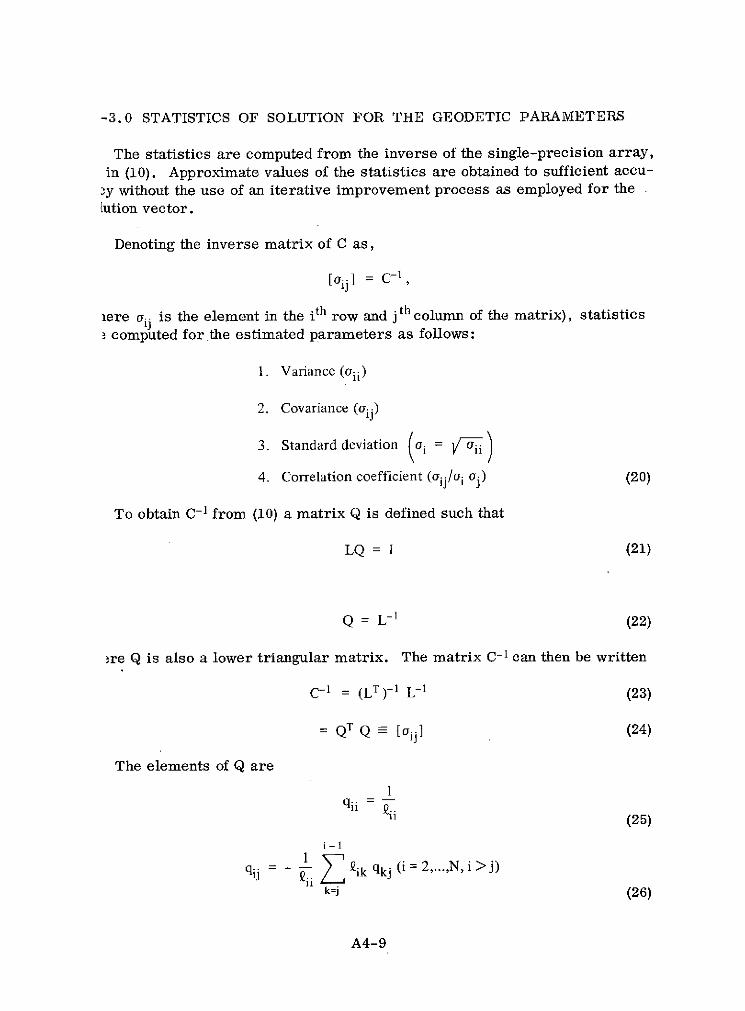
-3.0 STATISTICS OF SOLUTION FOR THE GEODETIC PARAMETERS

The statistics are computed from the inverse of the single-precision array,in (10). Approximate values of the statistics are obtained to sufficient accu-

,y without the use of an iterative improvement process as employed for theution vector.

Denoting the inverse matrix of C as,

[aij] = C- 1 ,

lere a is the element in the i th row and j th column of the matrix), statisticscomputed for the estimated parameters as follows:

1. Variance (Oii)

2. Covariance (aij)

3. Standard deviation (oi = )

4. Correlation coefficient (oij/ i aoj) (20)

To obtain C- 1 from (10) a matrix Q is defined such that

LQ = I (21)

Q = L- 1 (22)

re Q is also a lower triangular matrix. The matrix C- 1 can then be written

C-1 = (LT)-1 L-1 (23)

QT Q = [aij ] (24)

The elements of Q are

1

i = i (25)

qij ik qkj (i = 2,...,N, i > j)

k=j (26)

A4-9

where ij and qij are the elements of the ith row and jth column of the matricesL and Q, respectively. The elements of the inverse matrix C- 1, which is sym-metric, are given by the lower triangular elements

N

S qk iqkj,(i>j = 1,2,...,N)k=i (27)

A4-10

APPENDIX B. . . . .... . . SATELLITE AND GRAVITY DATA DISTRIBUTIONS

APPENDIX B

SATELLITE AND GRAVITY DATA DISTRIBUTIONS

This appendix presents detailed tabulations of the data employed in GEM 5and 6. A summary of this data was presented in Section 2.

CONTENTS

Table Page

B-1 Baker-Nunn Observations by Station and Satellitein 7-Day Arcs . .. . . .. . . .. . . . .... . .. . B-3

B-2 7-Day Electronic-Optical Arcs . ............... B-4

B-3 Satellite Time Periods of Baker-Nunn Arcs . ........ B-6

B-4 Station Passes in 2-Day Arcs. .......... ... . B-9

B-5 MOTS and SPEOPTS Camera Observations in7-Day Arcs . . .. . . . . .. . .. . .. . .... .. . B-11

B-6 BC-4 Simultaneous Photographic Events . ......... B-12

B-7 MOTS Geometric Events . ................ B-16

B-8 MOTS & Laser Geometric Events . . . . ......... . B-20

B-9 Survey Ties Employed . ................. B-21

B-10 50 Equal Area Surface Gravimetric Dataof Rapp (1972) . . . . . . . . . . . . . . . . . . . . . . B-23

Figure B-1. Distribution and Errors (mgal) of 5' MeanGravity Anomalies, Rapp (1972) . . . ..... ... . B-28

B-1

Table B-iBaker-Nunn Observations by Station and Satellite in 7-Day Arcs

SATELLITE SAO BAKER-NUNN STATIONS

9001 9002 9003 9004 9005 9006 9007 9008 9009 9010 9011 9012 9021 9023 9025 9028 9031 9050 9091 9424 9425 9426 9427

TELSTAR-1 135 117 101 57 55 73 65 71 71 44 78 103

GEOS-I 996 658 779 66 138 429 107 307 1127 424 255 809 96 108 15 13

SECOR-5 11 22 9 2 11 7 10 11 6 23 10 23

OVI-2 57 35 35 16 63 43 48 2 30 69 66

rz ECHO-1RB 68 121 202 97 59 51 63 112 56 83 158 50

0 DID 789 73 603 67 534 53 :27 245 134 139 85 6 69 65

BE-C 170 340 179 10 434 73 60 47 148 145 171 503 37 95 27 10

DIC 42 44 40 21 70 5 55 43 95 7 15 15

ANNA-1B 350 143 150 168 51 88 238 109 210

GEOS-II 572 843 80 321 68 371 331 370 66 204 438 894 14 183 34

OSCAR-7 28 59 34 176 97 49 47 17 93 207 123

5BN-2 27 24 3 5 19 9 11 16 8 18 18 21

tCOURIER-1B 52 168 106 36 154 176 125 132 243 218 47

CS GRS 30 6 34 12 31 7 9 13 18 15

TRANSIT-4A 93 82 142 64 31 10 26 16 21 33 64 59

BE-B 11 26 26 1 1 5 25 10 57 12 60

OGO-2 37 7 30 7 21 13 27 12 15 9 43 4 3 3

INJUN-1 33 62 36 18 54 3 15 41 22 21 75

AGENA-R 90 46 33 51 5 36 47 16 16 47 51 51 21

MIDAS-4 1180 74 675 530 820 212 595 573 631 169 650 118 323 255 576C0

'tt VANG-2-ROC 19 21 18 1 5 17 18 8 11 24 27 20

VANG-2-SAT 72 16 13 101 10 30 17 6 12 14 6 8

VANG-3-SAT 16 51 120 51 25 4 17 9 48 30 63 36

TOTAL 4306 2767 665 3986 1005 2910 1711 1194 1381 2882 1599 2721 331 2835 66 683 725 96 894 454 294 270 716

Each count refers to obs. pairs (right ascension and declination).

Table B-2

7-Day Electronic-Optical Arcs (by Satellite and Time Period)

Number of Stations (1) & Station Passes M UsedSatellite Time Period GRARR Doppler Laser Camera

DIC 4/22/67 - 4/28/67 2 6 6 25DIC 4/30/67 - 5/ 8/67 2 12 8 68DID 5/ 9/67 - 5/17/67 2 27 7 98BE-B 12/23/64 - 12/29/64 4 113BE-B 1/ 2/65 - 1/ 8/65 4 122BE-B 1/25/65 - 1/31/65 4 124BE-B 2/24/65 - 3/ 3/65 4 85BE-B 3/21/65 - 3/28/65 3 108BE-B 5/12/67 - 5/19/67 1 2 1 5 4 18BE-C 6/29/65 - 7/ 6/65 6 203BE-C 7/ 9/65 - 7/15/65 6 216BE-C 7/25/65 - 7/31/65 6 221BE-C 8/29/65 - 9/ 5/65 6 200BE-C 4/ 2/67 - 4/10/67 2 6 5 30BE-C 4/20/67 - 4/27/67 2 7 6 23GEOS-I 11/17/65 - 11/24/65 8 271 10 39GEOS-I 11/25/65 - 12/ 1/65 8 237 16 70GEOS-I 1/21/66 - 1/27/66 8 311 16 59GEOS-I 1/28/66 - 2/ 5/66 8 213 22 68GEOS-I 4/17/66 - 4/24/66 7 284 27 133GEOS-I 5/11/66 - 5/18/66 6 243 13 67GEOS-I 6/16/66 - 6/23/66 6 234 6 6GEOS-I 7/ 2/66 - 7/ 9/66 7 258 7 16GEOS-I 7/23/66 - 7/30/66 7 185 15 94GEOS-I 8/13/66 - 8/21/66 6 217 17 68GEOS-I 10/29/66 - 11/ 5/66 6 208 3 7GEOS-I 11/15/66 - 11/22/66 6 142 12 55GEOS-II 2/25/68 - 3/ 1/68 3 12 4 47 1 1 23 81GEOS-II 3/16/68 - 3/24/68 4 29 3 50 23 82GEOS-II 3/28/68 - 4/ 4/68 4 23 4 40 1 2 24 92GEOS-II 4/22/68 - 4/29/68 4 25 3 116 1 3 27 82GEOS-II 6/ 3/68 - 6/10/68 3 29 5 110 1 4 22 73GEOS-II 6/13/68 - 6/19/68 1 2 6 141 1 3 27 132GEOS-II 6/21/68 - 6/28/68 3 33 5 136 1 3 28 140GEOS-II 7/12/68 - 7/18/68 3 45 4 107 1 2GEOS-II 7/25/68 - 8/ 1/68 4 30 4 92 15 41GEOS-II 8/ 9/68 - 8/16/68 3 18 4 131 8 15•GEOS-II 8/31/68 - 9/ 7/68 3 20 3 31 1 5 22 67

B-4

Table B-2 (Continued)

Satellite Time Period GRARR Doppler Laser Camera

GEOS-II 10/19/68 - 10/26/68 3 20 2 51 1 4 22 73GEOS-II* 2/ 5/69 - 2/12/69 2 10PEOLE** 6/ 3/71 - 6/ 5/71 4 13PEOLE 6/ 6/71 - 6/10/71 1 9PEOLE 6/11/71 - 6/15/71 2 41PEOLE 6/16/71 - 6/19/71 2 13*C-Band tracking data from 8 stations with 105 station passes are also included.

**MINITRACK data were also used with each PEOLE arc.In addition to the above arcs, 4 SAS-A arcs, 14 TIROS arcs, and 6 ALOUETTE arcs with MINITRACK data onlywere used in the GEM solutions.

B-5

Table B-3

Satellite Time Periods of Baker-Nunn Arcs

TELSTAR ECHO BE-C OSCAR-7

8/10 - 8/17/62 9/13 - 9/20/60 3/ 2 - 3/ 7/66 4/ 1 - 4/ 7/6610/ 7 - 10/14 9/20 - 9/27 3/14 - 3/19 4/ 8 - 4/1410/24 - 10/31 9/27 - 10/ 4 3/25 - 3/31 4/15 - 4/2211/ 7 - 11/15 10/ 4 - 10/11 3/31 - 4/ 5 4/22 - 4/28/6611/15 - 11/23 10/11 - 10/18 4/ 5 - 4/1111/23 - 12/ 1 10/18 - 10/24 4/11 - 4/17 5BN-212/ 1 - 12/ 9 11/30 - 12/ 6 4/17 - 4/23 2/26 - 3/ 5/6512/ 9 - 12/17 12/13 - 12/20/60 4/23 - 4/29 3/ 4 - 3/1112/17 - 12/25/62 4/10 - 4/17/61 4/29 - 5/ 4 3/11 - 3/1812/25 - 1/ 1/63 4/17 - 4/24 5/ 4 - 5/10 4/19 - 4/261/ 1 - 1/ 9 4/24 - 4/30 5/10 - 5/16 4/26 - 5/21/ 9 - 1/17 5/11 - 5/18 5/16 - 5/21 5/25 - 5/31/651/26 - 2/ 2 6/19 - 6/26 5/22 - 5/275/23 - 5/30 8/ 8 - 8/15 5/27 - 6/ 2/66 COURIER6/ 9 - 6/16 8/15 - 8/22 3/12 - 3/17/67 12/23 - 12/29/666/23 - 6/30/63 8/22 - 8/29 3/17 - 3/23 12/31 - 1/ 6/67

SECOR 9/ 8 - 9/15 3/23 - 3/29 1/ 8 - 1/159/15 - 9/22/61 3/29 - 4/ 4 1/15 - 1/20

3/ 1 - 3/ 8/65 DID 4/ 4- 4/ 9 1/27- 2/ 23/15- 3/22 4/ 9 - 4/15 6/ 2- 6/ 9

12/ 1 - 12/ 8 2/19 - 2/26/67 4/15 - 4/20 6/ 9 - 6/1512/15 - 12/22/65 2/26 - 3/ 4 4/20 - 4/25/67 6/16 - 6/22

3/ 5 - 3/12 6/23 - 6/293/19 - 3/25 6/30 - 7/ 6

10/28 - 11/ 3/66 4/30 - 5/ 7 2/26 - 3/ 3/67 7/ 7 - 7/1311/ 4- 11/10 5/ 7- 5/13 3/ 4- 3/ 9 7/14- 7/2011/11 - 11/17 5/14 - 5/21 3/10 - 3/15 7/21 - 7/27/6711/18 - 11/24/66 5/21 - 5/28 3/16 - 3/21/67

GRS 5/28 - 6/ 3/67 DIC OGO- 25/15 - 5/21/66

6/16 - 6/23/65 VANGUARD-2 (Sat.) 2/24 - 3/ 3/67 5/21 - 5/276/23 - 6/30 4/ 7 - 4/14/60 3/ 3 - 3/11 5/27 - 6/ 26/30 - 7/ 7 4/14- 4/21 3/10 - 3/17 6/ 3 - 6/ 87/ 7 - 7/13 4/21 - 4/28 3/17 - 3/25/67 6/ 9 - 6/157/14 - 7/21/65 4/28 - 5/ 5 6/15 - 6/21

5/ 5 - 5/12/60 6/23 - 6/29/66

B-6

Table B-3 (Continued)

ANNA-1B GEOS-I GEOS-II TRANSIT

11/ 5 - 11/10/63 11/ 8 - 11/15/65 3/31 - 4/ 7/68 9/ 2 - 9/10/61

11/16 - 11/21 11/16 - 11/23 4/ 7 - 4/14 9/10 - 9/18

11/21 - 11/27 11/23 - 12/ 1 4/14 - 4/21 9/19 - 9/27

11/27 - 12/ 2 12/ 1 - 12/ 8 5/11 - 5/18 11/17 - 11/25

12/ 2 - 12/ 8 12/ 9 - 12/16 5/25 - 5/31 11/26 - 12/ 3

12/ 8 - 12/13 12/16 - 12/24 6/ 8 - 6/14 12/ 4 - 12/11

12/19 - 12/25/63 12/31 - 1/ 8/66 6/24 - 7/ 2 12/13 - 12/19

2/29 - 3/ 5/64 1/ 8 - 1/15 7/18 - 7/26 12/21 - 12/29/61

3/ 5 - 3/11 1/16 - 1/23 9/ 1 - 9/ 7 7/16 - 7/23/62

3/11 - 3/16 1/23 - 1/31 9/15 - 9/22 8/ 1 - 8/ 9

3/16- 3/22 1/31- 2/ 7 9/30- 10/ 6 8/ 7- 8/16

3/22- 3/27 2/ 8 - 2/16 10/ 6- 10/13 11/ 1- 11/ 8

4/ 2 - 4/ 7 2/16 - 2/23 10/13 - 10/20 11/ 9 - 11/16

4/13 - 4/17 2/24 - 3/ 3 10/20 - 10/27 11/17 - 11/24/62

4/19 - 4/24 3/ 3 - 3/11 11/ 3 - 11/10/68 AGENA

5/31 - 6/ 5 3/11 - 3/18 1/31 - 2/ 6/69

6/ 5 - 6/11 3/19 - 3/26 MIDAS 6/ 1 - 6/ 8/64

6/11 - 6/16 3/26 - 4/ 3 6/ 8 - 6/15

6/16 - 6/21 4/ 3 - 4/10 11/ 3 - 11/10/64 6/15 - 6/22

6/22 - 6/25 4/26 - 5/ 3 11/10 - 11/17 6/22 - 6/29

7/31 - 8/ 6 5/ 4 - 5/11 11/17 - 11/24 7/16 - 7/23

8/ 6 - 8/11 5/11 - 5/19 11/24 - 12/ 1 7/30 - 8/ 7

8/11 - 8/15 5/19 - 5/27 12/ 1 - 12/ 8 11/18 - 11/25/64

8/15 - 8/21 6/16 - 6/23 12/ 8 - 12/15 INJUN8/21 - 8/25 7/ 9 - 7/16 12/15 - 12/23/64

11/ 1- 11/ 5 8/ 1- 8/ 9 1/21 - 1/28/65 9/ 3 - 9/11/61

11/ 5 - 11/11 8/ 7 - 8/14 1/28- 2/ 4 9/ 9- 9/16

11/11 - 11/16 8/21 - 8/28 2/ 4- 2/11 9/16 - 9/22

11/16 - 11/22 8/28 - 9/ 4 2/11 - 2/18 12/21 - 12/28

11/22 - 11/27 9/ 4 - 9/11 2/25 - 3/ 4 12/28 - 1/ 3/62

11/27- 12/ 3 9/25- 10/ 2 3/ 4- 3/11 2/ 4- 2/11

12/ 3 - 12/ 7 10/18 - 10/25 3/11 - 3/18 2/11 - 2/18

12/ 7 - 12/14 11/ 1 - li/ 8 3/19 - 3/26 2/21 - 2/28

12/14 - 12/19/64 11/ 8 - 11/15 3/26 - 4/ 2 5/16 - 5/23

11/30 - 12/ 6/65 11/15 - 11/22/66 4/ 2 - 4/ 9 5/23 - 5/30/62

12/11 - 12/17 4/ 9 - 4/16

12/22 - 12/27/65 4/16 - 4/23

1/ 2- 1/ 7/66 4/23 - 5/ 1/65

1/13 - 1/17/66

B-7

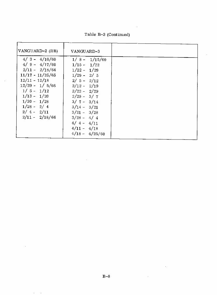
Table B-3 (Continued)

VANGUARD-2 (RB) VANGUARD-3

4/ 3 - 4/10/60 1/ 8 - 1/15/604/ 9 - 4/17/60 1/15 - 1/222/11 - 2/18/64 1/22 - 1/29

11/17 - 11/25/65 1/29 - 2/ 512/11 - 12/18 2/ 5 - 2/1212/29 - 1/ 5/66 2/12 - 2/19

1/ 5 - 1/12 2/22 - 2/291/13 - 1/20 2/29 - 3/ 71/20 - 1/28 3/ 7 - 3/141/28 - 2/ 4 3/14 - 3/212/ 4 - 2/11 3/21 - 3/282/11 - 2/18/66 3/28 - 4/ 4

4/ 4- 4/114/11 - 4/184/18 - 4/25/60

B-8

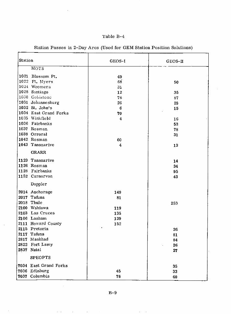
Table B-4

Station Passes in 2-Day Arcs (Used for GEM Station Position Solutions)

Station GEOS-I GEOS-II

MOTS

1021 Blossom Pt. 491022 Ft. Myers 68 501024 Woomnera 311028 Santiago 12 351030 Goldstone 76 871031 Johannesburg 26 281032 St. John's 6 151034 East Grand Forks 701035 Winkfield 4 161036 Fairbanks 531037 Rosman 781038 Orroral 311042 Rosman 601043 Tananarive 4 13

GRARR

1123 Tananarive 141126 Rosman 341128 Fairbanks 951152 Carnarvon 43

Doppler

2014 Anchorage 1492017 Tafuna 812018 Thule 2532100 Wahiawa 1192103 Las Cruces 1352106 Lasham 1392111 Howard County 1522115 Pretoria 262117 Tafuna 812817 Mashhad 842822 Fort Lamy 262837 Natal 27

SPEOPTS

7034 East Grand Forks 357036 Edinburg 45 337037 Columbia 78 40

B-9

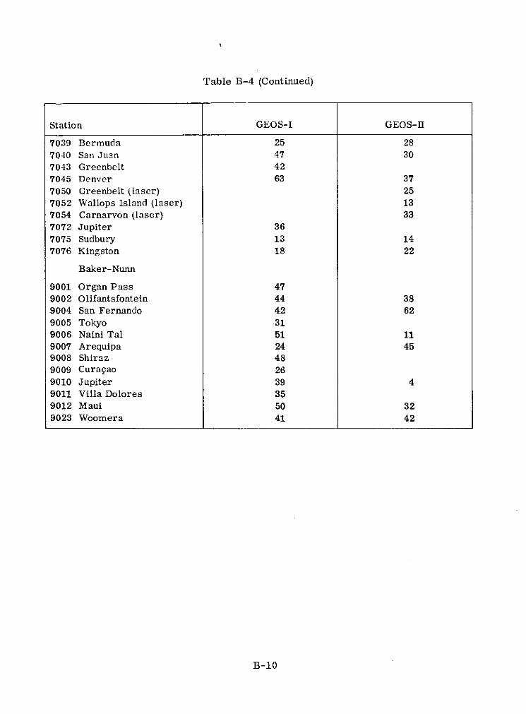
Table B-4 (Continued)

Station GEOS-I GEOS-II

7039 Bermuda 25 287040 San Juan 47 307043 Greenbelt 427045 Denver 63 377050 Greenbelt (laser) 257052 Wallops Island (laser) 137054 Carnarvon (laser) 33

7072 Jupiter 367075 Sudbury 13 14

7076 Kingston 18 22

Baker-Nunn

9001 Organ Pass 479002 Olifantsfontein 44 389004 San Fernando 42 62

9005 Tokyo 319006 Naini Tal 51 119007 Arequipa 24 459008 Shiraz 489009 Curagao 269010 Jupiter 39 49011 Villa Dolores 35

9012 Maui 50 329023 Woomera 41 42

B-10

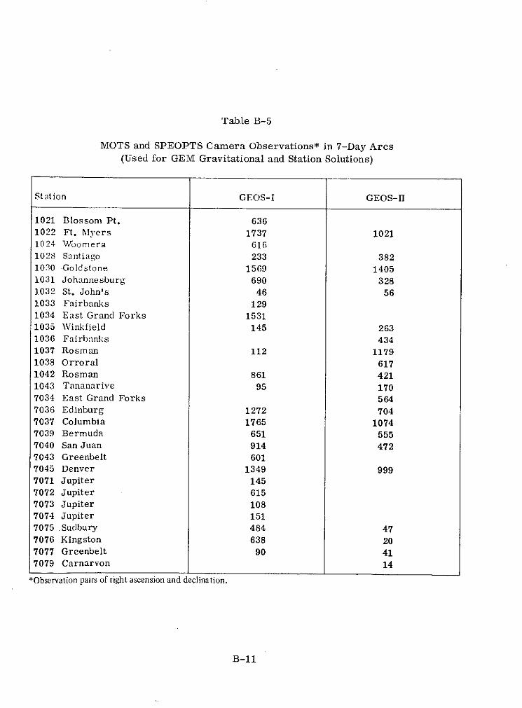
Table B-5

MOTS and SPEOPTS Camera Observations* in 7-Day Arcs(Used for GEM Gravitational and Station Solutions)

Station GEOS-I GEOS-II

1021 Blossom Pt. 6361022 Ft. Nlyers 1737 10211024 Voomera 6161028 Santiago 233 3821030 -Goldstone 1569 14051031 Johannesburg 690 3281.032 St. John's 46 561033 Fairbanks 1291034 East Grand Forks 15311035 Winkfield 145 2631036 Fairbanks 4341037 Rosman 112 11791038 Orroral 6171042 Rosman 861 4211043 Tananarive 95 1707034 East Grand Forks 5647036 Edinburg 1272 7047037 Columbia 1765 10747039 Bermuda 651 5557040 San Juan 914 4727043 Greenbelt 6017045 Denver 1349 9997071 Jupiter 1457072 Jupiter 6157073 Jupiter 1087074 Jupiter 1517075 Sudbury 484 477076 Kingston 638 207077 Greenbelt 90 417079 Carnarvon 14

*Observation pairs of right ascension and declination.

B-11

Table B-6

BC-4 Simultaneous Photographic Events

Two Station Events

No. of No. of No. ofStations Stations StationsEvents Events Events

6002 - 6003 6* 6009 - 6019 8 6019 - 6020 46002 - 6006 1 6009 - 6020 3 6019 - 6043 116002 - 6007 8 6009 - 6038 7 6019 - 6061 96002 - 6008 14 6009 - 6043 1 6019 - 6067 126002 - 6009 4 6019 - 6069 26002 - 6038 4 6011 - 6012 96002 - 6111 4 6011 - 6022 1 6020 - 6038 86002 - 6134 3 6011 - 6038 5 6020 - 6039 3

6011 - 6059 13 6020 - 6043 76003 - 6004 6 6011 - 6134 46003 - 6011 2 6022 - 6023 16003 - 6012 1 6012 - 6013 5 6022 - 6031 76003 - 6038 8 6012 - 6022 6 6022 - 6039 26003 - 6111 1 6012 - 6023 8 6022 - 6059 106003 - 6123 5 6012 - 6059 8 6022 - 6060 5

6022 - 6078 26004 - 6011 1 6013 - 6015 26004 - 6012 3 6013 - 6040 1 6023 - 6031 26004 - 6013 5 6013 - 6047 6 6023 - 6047 46004 - 6123 6 6013 - 6072 4 6023 - 6060 18

6013 - 6078 1 6023 - 6072 26006 - 6007 2 6023 - 6078 36006 - 6015 8 6015 - 6016 116006 - 6016 11 6015 - 6040 2 6031 - 6032 36006 - 6065 5 6015 - 6042 8 6031 - 6039 3

6015 - 6064 2 6031 - 6052 56007 - 6016 12 6015 - 6065 6 6031 - 6053 86007 - 6063 10 6015 - 6072 8 6031 - 6060 136007 - 6065 3 6015 - 6073 4 6031 - 6078 46007 - 6067 2 6015 - 6075 3

6032 - 6040 86008 - 6009 6 6016 - 6042 3 6032 - 6044 46008 - 6019 11 6016 - 6063 3 6032 - 6045 36008 - 6063 1 6016 - 6064 6 6032 - 6047 86008 - 6067 3 6016 - 6065 4 6032 - 6051 3

*Each photographic event consists of 7 points of satellite position observed simultaneously by thestations designated.

B-12

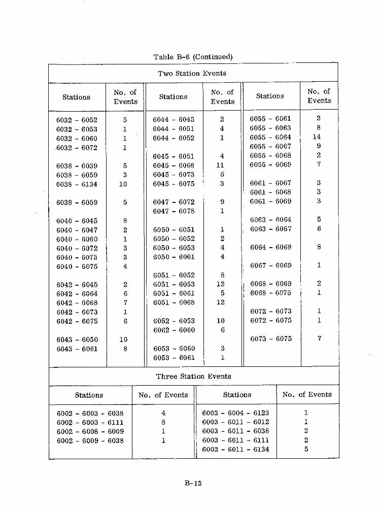
Table B-6 (Continued)

Two Station Events

No. of No. of No. ofStations Stations Stations

Events Events Events

6032 - 6052 5 6044 - 6045 2 6055 - 6061 2

6032 - 6053 1 6044 - 6051 4 6055 - 6063 8

6032 - 6060 1 6044 - 6052 1 6055 - 6064 14

6032 - 6072 1 6055 - 6067 9

6045 - 6051 4 6055 - 6068 2

6038 - 6039 5 6045 - 6068 11 6055 - 6069 7

6038 - 6059 3 6045 - 6073 5

6038 - 6134 10 6045 - 6075 3 6061 - 6067 36061 - 6068 3

6039 - 6059 5 6047 - 6072 9 6061 - 6069 3

6047 - 6078 1

6040 - 6045 8 6063 - 6064 5

6040 - 6047 2 6050 - 6051 1 6063 - 6067 6

6040 - 6060 1 6050 - 6052 2

6040 - 6072 3 6050 - 6053 4 6064 - 6068 8

6040 - 6073 3 6050 - 6061 4

6040 - 6075 4 6067 - 6069 1

6051 - 6052 8

6042 - 6045 2 6051 - 6053 12 6068 - 6069 2

6042 - 6064 6 6051 - 6061 5 6068 - 6075 1

6042 - 6068 7 6051 - 6068 12

6042 - 6073 1 6072 - 6073 1

6042 - 6075 6 6052 - 6053 10 6072 - 6075 1

6062 - 6060 6

6043 - 6050 10 6073 - 6075 7

6043 - 6061 8 6053 - 6060 3

6053 - 6061 1

Three Station Events

Stations No. of Events Stations No. of Events

6002 - 6003 - 6038 4 6003 - 6004 - 6123 1

6002 - 6003 - 6111 8 6003 - 6011 - 6012 1

6002 - 6008 - 6009 1 6003 - 6011 - 6038 2

6002 - 6009 - 6038 1 6003 - 6011 - 6111 26003 - 6011 - 6134 5

B-13

Table B-6 (Continued)

Three Station Events

Stations No. of Events Stations No. of Events

6004 - 6012 - 6013 3 6019 - 6020 - 6043 36019 - 6043 - 6061 4

6006 - 6015 - 6016 2

6006 - 6015 - 6065 3 6022 - 6023 - 6060 26022 - 6023 - 6078 1

6007 - 6016 - 6063 3 6022 - 6031 - 6059 1

6007 - 6016 - 6064 1 6022 - 6039 - 6059 2

6007 - 6016 - 6065 2

6007 - 6055 - 6067 2 6023 - 6031 - 6032 2

6007 - 6063 - 6064 2 6023 - 6031 - 6060 2

6007 - 6064 - 6065 1 6023 - 6032 - 6060 12

6007 - 6064 - 6067 1 6023 - 6040 - 6047 1

6008 - 6009 - 6019 1 6031 - 6032 - 6060 9

6008 - 6019 - 6061 1 6031 - 6051 - 6053 16008 - 6019 - 6067 2 6031 - 6052 - 6053 1

6031 - 6053 - 6060 36009 - 6019 - 6043 36009 - 6020 - 6038 2 6032 - 6040 - 6044 2

6032 - 6040 - 6045 1

6011 - 6012 - 6059 1 6032 - 6040 - 6047 16011 - 6022 - 6059 2 6032 - 6051 - 6052 3

6011 - 6038 - 6059 3 6032 - 6052 - 6053 1

6013 - 6040 - 6072 1 6040 - 6045 - 6073 4

6013 - 6047 - 6072 2 6040 - 6045 - 6075 1

6015 - 6016 - 6042 1 6042 - 6045 - 6068 2

6015 - 6016 - 6064 8 6042 - 6045 - 6075 4

6015 - 6016 - 6065 3 6042 - 6064 - 6068 9

6015 - 6040 - 6045 1 6042 - 6068 - 6075 16015 - 6040 - 6075 1

6015 - 6042 - 6045 4 6043 - 6050 - 6061 1

6015 - 6045 - 6073 16015 - 6072 - 6073 2 6044 - 6051 - 6068 16015 - 6072 - 6075 2

6045 - 6051 - 6068 2

6016 - 6063 - 6064 2 6045 - 6068 - 6075 1

6045 - 6073 - 6075 5

B-14

Table B-6 (Continued)

Three Station Events

Stations No. of Events Stations No. of Events

6051 - 6052 - 6053 3 6055 - 6063 - 6064 36055 - 6063 - 6067 4

6052 - 6053 - 6060 2 6055 - 6063 - 6069 2

Four Station Events

Stations No. of Events

6007 - 6016 - 6063 - 6064 1

6012 - 6022 - 6023 - 6060 1

6015 - 6016 - 6042 - 6064 16015 - 6042 - 6045 - 6073 26015 - 6042 - 6045 - 6075 16015 - 6045 - 6073 - 6075 1

6023 - 6031 - 6032 - 6060 36023 - 6032 - 6047 - 6060 2

6040 - 6045 - 6073 - 6075 1

B-15

Table B-7

MOTS Geometric Events

Two-Station Simultaneous Optical Observations

Two Stations Number of Two Stations Number ofObserving Flashes'Observed Observing Flashes Observed

1021-1022 20 1030-7075 8

1021-1034 16 1034-1042 41

1021-1042 10 1034-7036 33

1021-7036 5 1034-7037 220

1021-7037 29 1034-7045 100

1021-7039 21 1034-7075 60

1021-7040 16 1042-7036 34

1021-7045 1 1042-7037 25

1021-7075 81 1042-7039 9

1022-1030 58 1042-7040 13

1022-1034 16 1042-7045 24

1022-1042 64 1042-7075 19

1022-7036 109 7036-7037 92

1022-7037 124 7036-7045 94

1022-7039 48 7036-7076 50

1022-7040 106 7037-7039 35

1022-7045 44 7037-7045 168

1022-7076 151 7037-7075 91

1030-1034 134 7037-7076 16

1030-1042 6 7039-7040 95

1030-7036 254 7039-7075 25

1030-7037 114 7045-7075 14

1030-7045 358

B-16

Table B-7 (Continued)

Three-Station Simultaneous Optical Observations

Three Stations Number ofObserving Flashes Observed

1021-1034-7037 12

1021-1034-7075 12

1021-1042-7037 14

1022-1034-1042 39

1022-1034-7045 10

1022-1034-7075 14

1022-1042-7037 35

1022-7037-7039 21

1022-7039-7040 26

1022-7040-7076 47

1022-7045-7076 13

1030-1034-7036 10

1030-1034-7037 39

1030-1034-7045 14

1030-7036-7037 43

1030-7036-7045 45

1030-7037-7045 76

1034-1042-7037 17

1034-1042-7045 13

1034-7037-7045 44

1034-7037-7075 40

7036-7037-7045 30

B-17

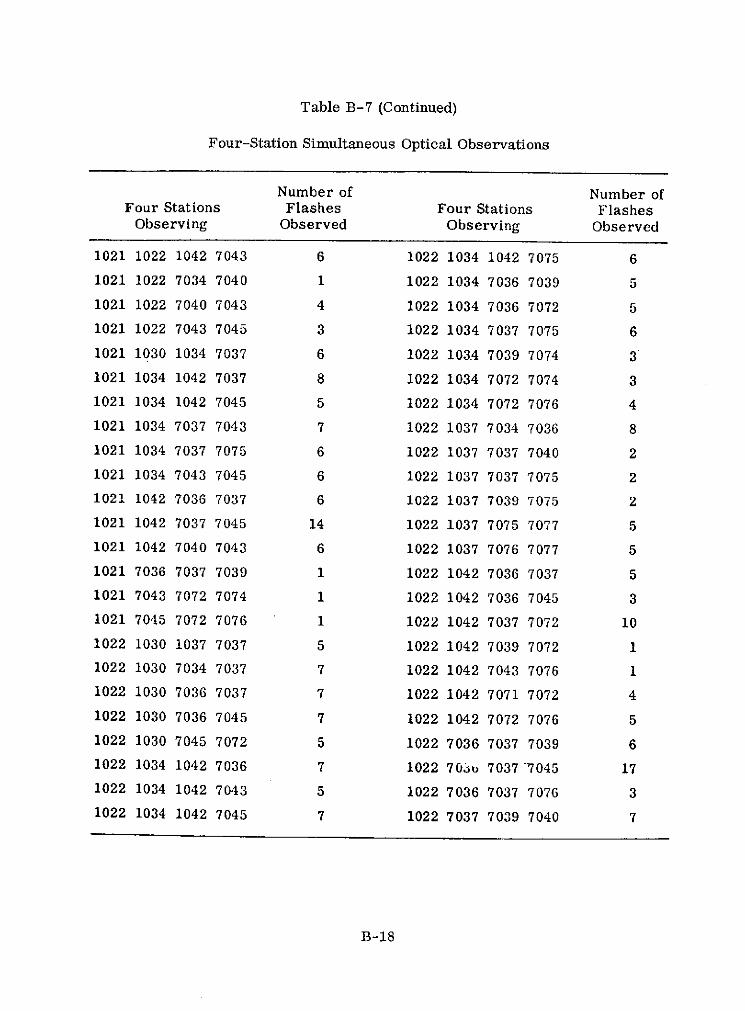
Table B-7 (Continued)

Four-Station Simultaneous Optical Observations

Number of Number ofFour Stations Flashes Four Stations Flashes

Observing Observed Observing Observed

1021 1022 1042 7043 6 1022 1034 1042 7075 6

1021 1022 7034 7040 1 1022 1034 7036 7039 5

1021 1022 7040 7043 4 1022 1034 7036 7072 5

1021 1022 7043 7045 3 1022 1034 7037 7075 6

1021 1030 1034 7037 6 1022 103.4 7039 7074 3

1021 1034 1042 7037 8 1022 1034 7072 7074 3

1021 1034 1042 7045 5 1022 1034 7072 7076 4

1021 1034 7037 7043 7 1022 1037 7034 7036 8

1021 1034 7037 7075 6 1022 1037 7037 7040 2

1021 1034 7043 7045 6 1022 1037 7037 7075 2

1021 1042 7036 7037 6 1022 1037 7039 7075 2

1021 1042 7037 7045 14 1022 1037 7075 7077 5

1021 1042 7040 7043 6 1022 1037 7076 7077 5

1021 7036 7037 7039 1 1022 1042 7036 7037 5

1021 7043 7072 7074 1 1022 1042 7036 7045 3

1021 7045 7072 7076 1 1022 1042 7037 7072 10

1022 1030 1037 7037 5 1022 1042 7039 7072 1

1022 1030 7034 7037 7 1022 1042 7043 7076 1

1022 1030 7036 7037 7 1022 1042 7071 7072 4

1022 1030 7036 7045 7 1022 1042 7072 7076 5

1022 1030 7045 7072 5 1022 7036 7037 7039 6

1022 1034 1042 7036 7 1022 703u 7037 7045 17

1022 1034 1042 7043 5 1022 7036 7037 7076 3

1022 1034 1042 7045 7 1022 7037 7039 7040 7

B-18

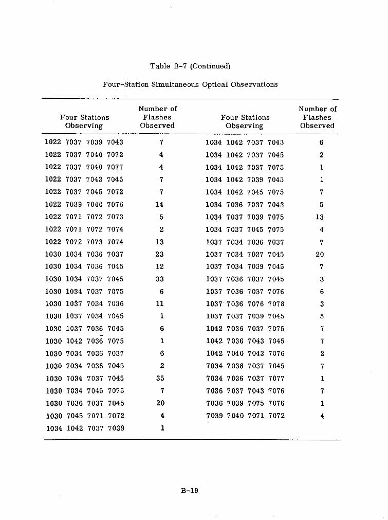
Table B-7 (Continued)

Four-Station Simultaneous Optical Observations

Number of Number ofFour Stations Flashes Four Stations Flashes

Observing Observed Observing Observed

1022 7037 7039 7043 7 1034 1042 7037 7043 6

1022 7037 7040 7072 4 1034 1042 7037 7045 2

1022 7037 7040 7077 4 1034 1042 7037 7075 1

1022 7037 7043 7045 7 1034 1042 7039 7045 1

1022 7037 7045 7072 7 1034 1042 7045 7075 7

1022 7039 7040 7076 14 1034 7036 7037 7043 5

1022 7071 7072 7073 5 1034 7037 7039 7075 13

1022 7071 7072 7074 2 1034 7037 7045 7075 4

1022 7072 7073 7074 13 1037 7034 7036 7037 7

1030 1034 7036 7037 23 1037 7034 7037 7045 20

1030 1034 7036 7045 12 1037 7034 7039 7045 7

1030 1034 7037 7045 33 1037 7036 7037 7045 3

1030 1034 7037 7075 6 1037 7036 7037 7076 6

1030 1037 7034 7036 11 1037' 7036 7076 7078 3

1030 1037 7034 7045 1 1037 7037 7039 7045 5

1030 1037 7036 7045 6 1042 7036 7037 7075 7

1030 1042 7036 7075 1 1042 7036 7043 7045 7

1030 7034 7036 7037 6 1042 7040 7043 7076 2

1030 7034 7036 7045 2 7034 7036 7037 7045 7

1030 7034 7037 7045 35 7034 7036 7037 7077 1

1030 7034 7045 7075 7 7036 7037 7043 7076 7

1030 7036 7037 7045 20 7036 7039 7075 7076 1

1030 7045 7071 7072 4 7039 7040 7071 7072 4

1034 1042 7037 7039 1

B-19

Table B-8

MOTS & LASER Geometric Events

Three-Station Simultaneous Optical-LASER Observations

Three Stations Observing Number of Flashes Observed

7040-7077-7050 1

7075-7077-7050 2

1037-7077-7050 19

1037-7075-7050 7

1022-7034-7052 4

1037-7034-7052 6

1037-7078-7052 1

B-20

Table B-9

Survey Ties Employed

Est.Relative Position Constraints Stand.

Station (Meters) Dev.

Pair (Meters)Ax Ay Az

2017 2117 -3.75 6.28 -2.02 4.23

2822 6064 -12.06 13.60 23.74 3.00

2837 6067 46.13 290.25 -1248.20 3.00

1038 6060 304147.18 114912.15 494900.60 2.04

2019 6053 -130.35 808.62 87.15 3.00

2722 6055 -78.06 -172.20 -160.45 3.00

2723 6040 19.71 0.69 14.10 3.00

1152 6032 -47149.40 -424141.91 676055.82 2.50

6019 9011 -52.01 -37.07 18.82 0.01

1021 7043 12681.43 44984.51 51158.99 0.49

1022 7071 168409.91 50582.89 45732.81 0.93

1034 7034 0.08 0.66 -0.74 0.01

1037 1042 -7.58 -0.59 0.50 0.01

7043 7050 -38.21 -36.26 -31.23 0.01

7043 7052 130836.64 -50256.13 -100969.38 0.90

7043 7077 -652.92 -1710.84 -1877.61 0.06

7043 7078 130867.90 -50025.41 -100693.72 0.90

7071 7072 4.08 5.48 11.42 0.01

7071 7073 10.32 6.62 9.32 0.01

7071 7074 11.03 8.97 15.81 0.01

2738 6003 3.96 -23.90 21.87 3.00

1025 6009 17214.35 4034.43 58089.41 0.46

2817 6015 7.76 4.05 -16.20 3.00

B-21

Table B-9 (Continued)

Relative Position Constraints Est.Stand.

Station (Meters) Dev.Station Dev.Pair Ay Az (Meters)

6111 6134 -53.77 -90.12 -305.26 0.01

6002 7043 -56.27 -499.54 -586.43 0.02

6011 9012 -49.58 118.93 -35.81 0.01

7071 9010 19.05 3.07 3.92 0.01

9003 9023 6011.64 -17986.56 -27467.42 0.30

4740 7039 -674.06 699.92 1476.31 0.04

4760 7039 -683.27 706.55 1488.25 0.04

1037 1126 -334.06 -403.53 -571.31 0.02

1152 7054 54.96 -51.86 -135.62 0.01

2203 7052 -116.78 -336.48 -389.60 3.00

2115 4050 354.70 970.65 296.73 3.00

4082 7071 65691.26 62291.57 137735.55 0.87

4840 4860 -2384.64 711.85 1660.19 0.06

4840 7052 -2425.68 685.03 1630.22 0.06

1024 4946 -21762.84 24680.80 54300.42 0.46

1031 6068 59.69 -55.46 51.19 0.01

6068 9002 28722.17 46167.12 -7673.38 0.42

7072 9049 4.82 -3.60 -12.97 0.01

6111 9425 -1159.33 43554.59 52281.60 0.48

6042 9028 2992.55 -3032.66 -2462.26 0.08

2100 6011 32128.97 -180272.68 -83071.46 3.04

9005 9025 36256.49 10061.56 30386.63 0.38

7901 9001 0.00 0.00 0.00 4.23

2106 1035 -22330.33 23266.93 17999.44 3.02

B-22

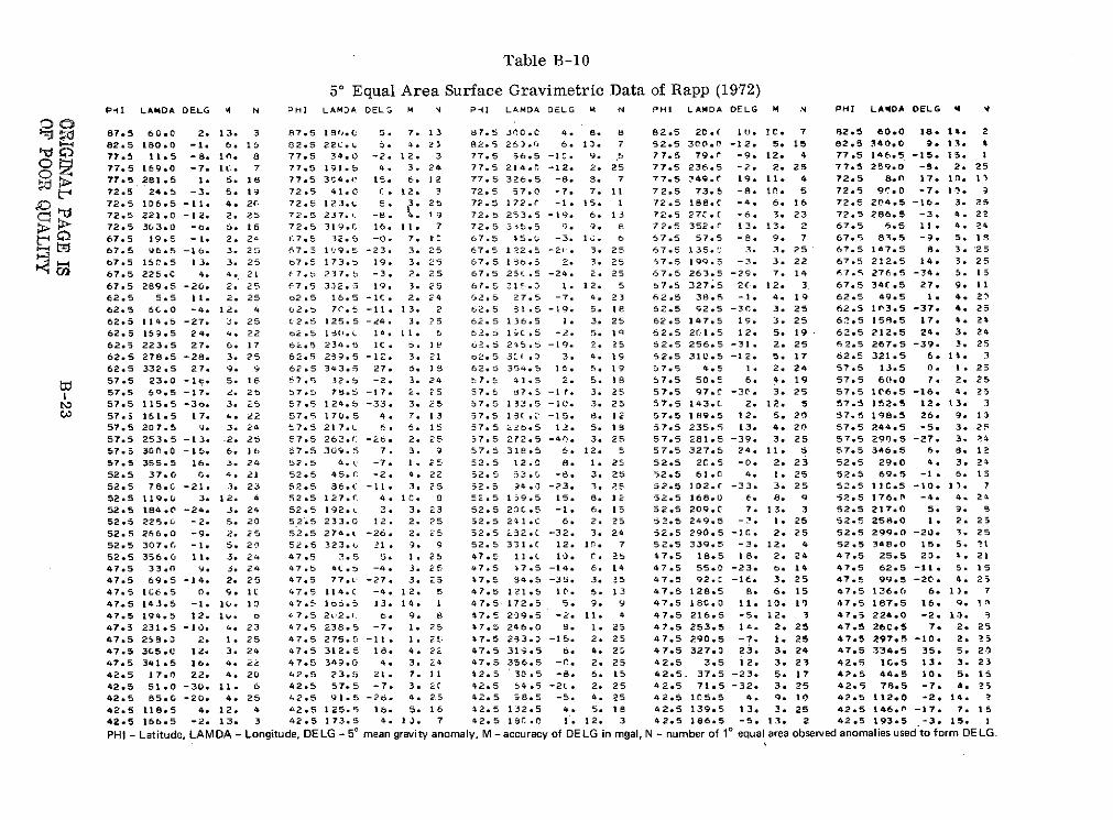
Table B-10

50 Equal Area Surface Gravimetric Data of Rapp (1972)PHI LAMDA DELG A N PHI LAMDA DELG M ' PlI LAMDA DELG M N DHI LAMDA DELG M N PHI LA4DA DELG 4 '

87.5 60.0 2. 13. 3 87.5 180.C 5. 7. 13 87.5 300.C 4. 8. 8 82.5 2C.C 10. 10. 7 82.5 60.0 18. 14. 2

82.5 180.0 -1. 6. 15 02.5 22C., 5. 4. 2) 82.5 25).f 6. 13. 7 82.5 300.0 -12. 5. 15 82.5 340.0 9. 13. 4

77.5 11.5 -8. In. 8 77.5 34.0 -2. 12. 3 77.5 56.5 -IC. 9. .5 77.5 79.P -9. 12. 4 77.5 146.5 -15. 15. 1

? 77.5 169.0 -7. 1C. 7 77.5 191.5 4. 3. 24 77.5 214.0 -12. 2. 25 77.5 236.5 -2. 2. 25 77.5 259.0 -9. 2. 25

t 77.5 281.5 1. 5. 18 77.5 354.0 15. 6. 12 77.5 326.5 -8. 8. 7 77.5 349.C 19. 11. 4 72.5 8.0 17. 1n. 1I

72.5 24.5 -3. 5. 19 72.5 41.0 0. 12. 3 72.5 57.0 -7. 7. 11 72.5 73.5 -8. 10. 5 72.5 9(.0 -7. 10. 3

72.5 106.5 -11. 4. 20 72.5 123. 5. 3. 25 72.5 172.r -1. 15. 1 72.5 188.C -4. 6. 16 72.5 204.5 -16. 3. 25

72.5 221.0 -12. 2. 25 72.5 237. -8. 4. 19 72.5 253.5 -19. 6. 13 72.5 27C.C -6. 3. 23 72.5 286.5 -3. 44 22

72.5 303.0 -o. 5. 16 72.5 319.C 16. 11. 7 72.5 335.5 9. 9. 8 72.5 352.r 13. 13. 2 67.5 6.5 11. 4. 24

67.5 19.5 -1. 2. 24 67.5 32.5 -0. 7. 1 67.5 45.u -3. 1 . 6 57.5 57.5 -8. 9. 7 67.5 83.5 -9. 5. 18

67.5 96.5 -16. 3. 25 67.3 1 :9.5 -23. 3. 25 67.5 122.5 -2c. 3. 25 67.5 135o. 3. 3. 25 67.5 147.5 8. 3. 25

S 7.5 150.5 13. 3. 25 67.5 173.b 19. 3. 25 67.5 166.5 2. 3. 25 57.5 199.5 -3. 3. 22 67.5 212.5 14. 3. 25

67.5 225.C 4. 4. 21 67.o 237.5 -3. 2. 25 67.5 250.5 -24. 2. 25 67.5 263.5 -29. 7. 14 67.5 276.5 -34. 5. 15

67.5 289.5 -20. 2. 25 f7.5 332.5 19. 3. 25 67.5 215.3 1. 12. 5 57.5 327.5 2C. 12. 3 67.5 34r.5 27. 9. 11

62.5 5.5 11. 2. 25 62.5 16.5 -IC. 2. 24 62.5 27.5 -7. 4. 23 62.5 38.5 -1. 4. 19 62.5 49.5 1. 4. 2?

62.5 60.0 -4. 12. 4 62.5 70.5 -11. 13. 2 62.5 31.5 -19. 5. 18 62.5 92.5 -30. 3. 25 62.5 103.5 -37. 4. 25

62.5 114.5 -27. 3. 25 02.5 125.5 -24. 3. ?5 62.5 136.5 1. 3. 25 62.5 147.5 19. 3. 25 62.5 158.5 17. 4. 2462.5 15~.5 24. 4. 22 2.5 13).. 16. 11. 62.5 1C.5 -2. 5. 1q 62.5 2C1.5 12. 5. 19 62.5 212.5 24. 3. 24

62.5 223.5 27. 6. 17 62.5 234.5 1(. 5. 1e 62.5 245.5 -19. 2. 25 62.5 256.5 -31. 2. 25 62.5 267.5 -39. 3. 25

62.5 278.5 -28. 3. 25 62.5 239.5 -12. 3. 21 o2.5 3MA.3 3. 4. 19 52.5 310.5 -12. 5. 17 62.5 321.5 6. 14. 3

62.5 332.5 27. 9. 9 62.5 343.5 27. 5. 18 62.5 354.5 15. 5. 19 57.5 4.5 1. 2. 24 57.5 13.5 0. 1. 25

t 57.5 23.0 -16. 5. 18 57.5 32.5 -2. 3. 24 57.5 41.5 2. 5. 18 57.5 50.5 6. 4. 19 57.5 60.0 7. 2. 25

57.5 5065 -17. 2. 25 57.5 7U.5 -17. 2. 25 57.5 87.5 -17. 3. 25 57.5 97.C -30. 3. 25 57.5 106.5 -16. 4. 25

b3 57.5 115.5 -36. 3. 25 57.5 124.5 -33. 3. 25 57.5 133.5 -1C. 3. 25 57.5 143.(. 2. 12. 5 57.5 152.5 12. 13. 3WC 57.5 161.5 17. 4. 22 57.5 170.5 4. 7. 13 57.5 13(., -15. 8. 12 57.5 189.5 12. 5. 20 57.5 198.5 25. 9. 13

57.5 207.5 9. 3. 24 57.5 217L 6. 5. 15 57.5 Z26.5 12. 5. 18 57.5 235.5 13. 4. 20 57.5 244.5 -5. 3. 2557.5 253.5 -13. .2. 25 57.5 263.( -26. 2. 25 57.5 272.5 -40. 3. 25 57.5 281.5 -39. 3. 25 57.5 290.5 -27. 3. 14

57.5 300.0 -15. 6. lb 57.5 309.5 7. 3. 9 57.5 318.5 5. 12. 5 57.5 327.5 24. 11. 5 57.5 346.5 5. 8. 12

57.5 355.5 16. 3. 24 52.5 4.1. -7. 1. 25 52.5 12.0 8. 1. 25 52.5 2C.5 -0. 2. 23 52.5 29.0 4. 3. 24

52.5 37.0 G. 4. 21 52.5 45.C -2. 4. 22 52.5 53.G -8. 3. 25 52.5 61.0 4. 1. 25 52.5 69.5 -1. 6. 1552.5 78.C -21. 3. 23 52.5 36.0 -11. 3. 25 52.5 94.0 -23. 3. 25 52.5 102.( -33. 3. 25 52.5 1IC.5 -10. 11. 7

52.5 119.0 3. 12. 4 52.5 127.C 4. IC. 8 52.5 159.5 15. 8. 12 52.5 168.0 6. 8. 9 52.5 176.0 -4. 4. 24

52.5 184.0 -24. 3. 24 52.5 192.. 3. 3. 23 52.5 23C 5 -1. 6. 15 52.5 209.C 7. 13. 3 52.5 217.0 5. 9. S

52.5 225.0 -2. 5. 20 52.5 233.0 12. 2. 25 52.5 241.0 6. 2. 25 52.5 249.5 - . 1. 25 52.5 258.0 1. 2. 2552.5 266.0 -9. 2. 25 52.5 274.k -26. 2. 25 52.5 232.C -32. 3. 24 52.5 290.5 -C1. 2. 25 52.5 299.0 -20. 3. 25

52.5 307.0 -1. 5. 23 52.5 323., 21. 9. 9 52.5 331.( 12. 10. 7 52.5 339.5 -3. 12. 4 52.5 348.0 15. 5. i1

52.5 356.0 11. 3. 24 47.5 3.5 5. 1. 25 47.5 11.C 1). C. 25 47.5 18.5 18. 2. 24 47.5 25.5 20. 4. 21

47.5 33.0 9. J. 24 47.5 40.5 -4. 3. 25 47.5 47.5 -14. 6. 14 47.5 55.0 -23. 6. 14 47.5 62.5 -11. 5. 15

47.5 69.5 -14. 2. 25 47.5 77.' -27. 3. 25 47.5 54.5 -36. 3. 25 47.5 92.: -16. 3. 25 47.5 99.5 -20. 4. 25

47.5 106.5 0. 9. 1C 47.5 114.7 -4. 12. 5 47.5 121.5 IC. 5. 13 47.5 128.5 8. 6. 15 47.5 136.0 6. 1). 7

47.5 143.5 -1. 1. 1 47.5 1o5.5 13. 14. 1 47.5 172.5 5. 9. 9 47.5 180.0 11. 10. 19 47.5 187.5 16. 9. In

47.5 194.5 12. 1, 6 17.5 2:2.4 6. 9. 8 47.5 209.5 -2. 11. 4 47.5 216.5 -5. 12. 3 47.5 224.0 -2. 10. 9

47.5 231.5 -10. 4. 23 67.5 238.5 -7. 1. 25 47.5 246.0 8. 1. 25 47.5 253.5 14. 2. 25 47.5 26C.5 7. 2. 25

47.5 258.0 2. 1. 25 47.5 275.5 -11. 1. 25 47.5 233.3 -15. 2. 25 47.5 290.5 -7. 1. 25 47.5 297.5 -10. 2. 2547.5 305.0 12. 3. 24 47.5 312.5 18. 4. 22 47.5 319.5 6. 4. 2G 47.5 327.0 23. 3. 24 47.5 334.5 35. 5. 20

47.5 341.5 16. 4. 2? 47.5 349.0 4. 3. 24 47.5 356.5 -0. 2. 25 42.5 3.5 12. 3. 23 42.5 10,5 13. 3. 23

42.5 17.0 22. 4. 20 42.5 23.5 21. 7. 11 42.5 30.5 -8. 6. 15 42.5. 37.5 -23. 5. 17 42.5 44.5 10. 5. 15

42.5 51.0 -30. 11. 6 42.5 57.5 -7. 3. 2C 42.5 54.5 -21. 2. 25 42.5 71.5 -32. 3. 25 42.5 78.5 -7. 4. 25

42.5 85.0 -20. 4. 25 42.5 91.5 -26. 4. 25 42.5 98.5 -5. 4. 25 42.5 105.5 4. 9. 10 42.5 112.0 -2. 14. ?

42.5 118.5 4. 12. 4 L2.5 125.5 16. 5. 16 42.5 132.5 4. 5. 18 42.5 139.5 13. 3. 25 42.5 146.0 -17. 7. 15

42.5 166.5 -2. 13. 3 42.5 173.5 4. 13. 7 42.5 15C.0 1. 12. 3 42.5 186.5 -5. 13. 2 42.5 193.5 -3. 15. 1

PHI - Latitude, LAMDA - Longitude, DELG - 5' mean gravity anomaly, M -accuracy of DELG in mgal, N - number of 10 equal area observed anomalies used to form DELG.

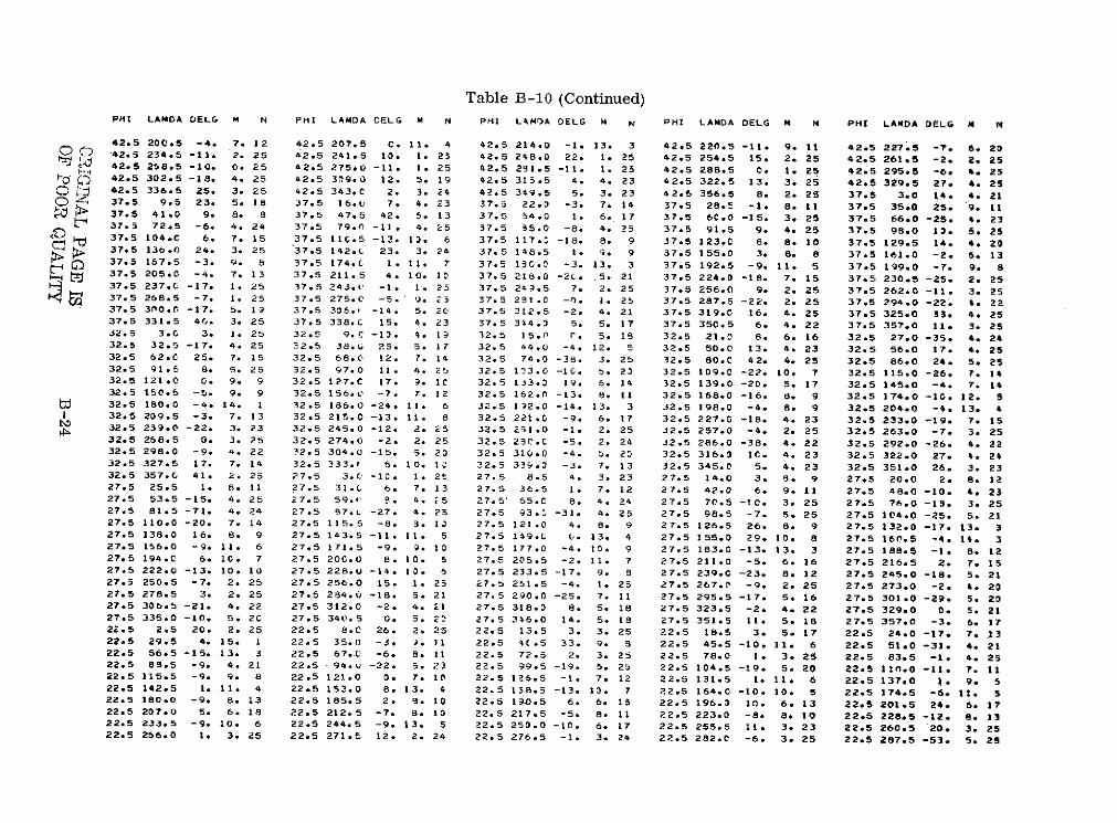
Table B-10 (Continued)PHI LAMDA DELG M N PHI LAMDA DELG M N PHI L4MA DELG M N PHI LAMDA DELG M N PHI LANDA DELG M N

42.5 200.5 -4. 7. 12 42.5 207.5 C. 11. 4 42.5 214.0 -1. 13. 3 42.5 220.5 -11. 9. 11 42.5 227.5 -7. 6. 23S 42.5 234.5 -11. 2. 25 42.5 241.5 10. 1. 25 42.5 248.0 22. 1. 25 42.5 254.5 15. 2. 25 42.5 261.5 -2. 2. 2542.5 258.5 -10. 0. 25 42.5 275.0 -11. 1. 25 42.5 291.5 -11. 1. 25 42.5 288.5 C. 1. 25 42.5 295.5 -6. 4. 25

10 0 42.5 302.5 -18. 4. 25 42.5 309.0 12. 5. 19 42.5 315.5 4. 4. 23 42.5 322.5 13. 3. 25 42.5 329.5 27. 4. 25Q 42.5 336.5 25. 3. 25 42.5 343.C 2. 3. 24 42.5 349.5 5. 3. 23 42.5 356.5 8. 2. 25 37.5 3.0 14. 4. 21C) 37.5 9.5 23. 5. 18 37.5 16.L 7. 4. 23 37.5 22.0 -3. 7. 14 37.5 28.5 -1. 8. 11 37.5 35.0 25. 9. It

37.5 41.0 9. 8. 8 37.5 47.5 42. 5. 13 37.5 54.0 1. 6. 17 37.5 6C.0 -15. 3. 25 37.5 66.0 -25. 4. 2337.5 72.5 -6. 4. 24 37.5 79.0 -11. 4. 25 37.5 35.0 -8. 4. 25 37.5 91.5 9. 4. 25 37.5 98.0 13. 5. 2537.5 104.C 6. 7. 15 37.5 ll0.5 -13. 10. 6 37.5 117.0 -18. 8. 9 37.5 123.C 8. 8. 10 37.5 129.5 14. 4. 2037.5 136.0 24. 3. 25 37.5 142.1 23. 3. 24 37.5 148.5 1. 9. 9 37.5 155.0 3. 8. 8 37.5 161.0 -2. 5. 13

p. 37.5 167.5 -3. 9. 8 37.5 174.0 1. 11. 7 37.5 13C.0 -3. 13. 3 37.5 192.5 -9. 11. 5 37.5 199.0 -7. 9. 8__ 37.5 205.0 -4. 7. 13 37.5 211.5 4. 10. 10 37.5 218.0 -2L. 5. 21 37.5 224.0 -18. 7. 15 37.5 230.5 -25. 2. 25

37.5 237.0 -17. 1. 25 37.5 243.( -1. 1. 25 37.5 243.5 7. 2. 25 37.5 256.0 9. 2. 25 37.5 262.0 -11. 3. 2537.5 268.5 -7. 1. 25 37.5 275.C -5. 0. 25 37.5 291.0 -0. 1. 25 37.5 287.5 -22. 2. 25 37.5 294.0 -22. 4. 2237.5 3n00o -17. 5. 1? 37.5 306., -14. 5. 20 37.5 312.5 -2. 4. 21 37.5 319.0 16. 4. 25 37.5 325.0 33. 4. 2537.5 331.5 40. 3. 25 37.5 338.C 15. 4. 23 37.5 344.0 5. 5. 17 37.5 350.5 6. 4. 22 37.5 357.0 11. 3. 2532.5 3.G 3. 1. 25 32.5 9.C -13. 4. 19 32.5 15,0 r. 5. 18 32.5 21.0 8. 6. 16 32.5 27.0 -35. 4. 2432.5 32.5 -17. 4. 25 32.5 38.0 25. 5. 17 32.5 44.0 -4. 12. 5 32.5 50.0 13. 4. 23 32.5 56.0 17. 4. 2532.5 62.0 25. 7. 15 32.5 68.0 12. 7. 14 32.5 74.0 -38. 3. 25 32.5 80.0 42. 4. 25 32.5 86.0 24. 5. 2532.5 91.5 8. 5. 25 32.5 97.0 11. 4. 25 32.5 133.0 -10. 5. 23 32.5 109.0 -22. 10. 7 32.5 115.0 -26. 7. 1432.5 121.0 0. 9. 9 32.5 127.C 17. 9. 10 32.5 133.3 19. 6. 14 32.5 139.0 -20. 5. 17 32.5 145.0 -4. 7. 1432.5 150.5 -5. 9. 9 32.5 156.0 -7. 7. 12 32.5 162.0 -13. 8. 11 32.5 168.0 -16. 8. 9 32.5 174.0 -10. 12. 5

t 32.5 180.0 -4. 14. 1 32.5 186.0 -24. 11. 6 32.5 132.0 -14. 13. 3 32.5 198.0 -4. 8. 9 32.5 204.0 -4. 13. 432.5 209.5 -3. 7. 13 32.5 215.0 -13. 11. 8 32.5 221.0 -9. 6. 17 32.5 227.0 -18. 4. 23 32.5 233.0 -19. 7. 1532.5 239.0 -22. 3. 23 32.5 245.0 -12. 2. 25 32.5 251.0 -1. 2. 25 32.5 257.0 -4. 2. 25 32.5 263.0 -7. 3. 2532.5 268.5 0. 3. 25 32.5 274.0 -2. 2. 25 32.5 20.0C -5. 2. 24 32.5 286.0 -38. 4. 22 32.5 292.0 -26. 4. 2232.5 298.0 -9. 4. 22 32.5 304.0 -15. 5. 20 32.5 310.0 -4. 5. 20 32.5 316.0 10. 4. 23 32.5 322.0 27. 4. 2432.5 327.5 17. 7. 14 32.5 333.( 5. 10. 10 32.5 339.3 -3. 7. 13 32.5 345.0 5. 4. 23 32.5 351.0 26. 3. 2332.5 357.0 41. 2. 25 27.5 3.( -10. 1. 25 27.5 8.5 4. 3. 23 27.5 14.0 3. 89 9 27.5 20.0 2. 8. 1227.5 25.5 1. 8. 11 27.5 31.0 6. 7. 13 27.5 36.5 1. 7. 12 27.5 42.0 6. 9. 11 27.5 A8.0 -10. 4. 2327.5 53.5 -15. 4. 25 27.5 59. 89. 4. '5 27.5" 65.C 8. 4. 24 27.5 70.5 -10. 3. 25 27.5 76.0 -19. 3. 2527.5 81.5 -71. 4. 24 27.5 87.. -27. 4. 25 27.5 93.0 -31. 4. 25 27.5 98.5 -7. 5. 25 27.5 104.0 -25. 5. 2127.5 110.0 -20. 7. 14 27.5 115.5 -8. 3. 10 27.5 121.0 4. 8. 9 27.5 126.5 26. 8. 9 27.5 132.0 -17. 13. 327.5 138.0 16. 8. 9 27.5 143.5 -11. 11. 5 27.5 149.U (. 13. 4 27.5 155.0 29. 10. 8 27.5 160.5 -4. 14. 327.5 156.0 -9. 11. 6 27.5 171.5 -9. 9. 10 27.5 177.0 -4. 10. 9 27.5 183.0 -13. 13. 3 27.5 188.5 -1. 8. 1227.5 194.0 6. 10. 7 27.5 20C.0 8. 10. 5 27.5 205.5 -2. 11. 7 27.5 211.0 -5. 6. 16 27.5 216.5 2. 7. 1527.5 222.0 -13. 10. 10 27.5 228.U -14. 10o 5 27.5 233.5 -17. 9. 8 27.5 239.0C -23. 8. 12 27.5 245.0 -18. 5. 2127.5 250.5 -7. 2. 25 27.5 256.0 15. 1. 25 27.5 251.5 -4. 1. 25 27.5 267.0 -9. 2. 25 27.5 273.0 -2. 4. 2027.5 278.5 3. 2. 25 27.5 284.0 -18. 5. 21 27.5 290.0 -25. 7. 11 27.5 295.5 -17. 5. 16 27.5 301.0 -29. 5. 2027.5 306.5 -21. 4. 22 27.5 312.0 -2. 4. 21 27.5 318.0 8. 5. 18 27.5 323.5 -2. 4. 22 27.5 329.0 0. 5. 2127.5 335.0 -10. 5. 20 27.5 340.5 0. 5. 23 27.5 346.0 14. 5. 18 27.5 351.5 11. 5. 18 27.5 357.0 -3. 6. 1722.5 2.5 20. 2. 25 22.5 8.0 26. 2. 25 22.5 13.5 3. 3. 25 22.5 18.5 3. 5 17 22.5 24.0 -17. 7T 1322.5 29.5 4. 15. 1 22.5 35.0 -3. ?. 31 22.5 40.5 33. 9. 8 22.5 45.5 -10. 11. 6 22.5 51.0 -31. 4. 2122.5 56.5 -15. 13. 3 22.5 67.0 -6. 8. 11 22.5 72.5 2. 3. 25 22.5 78.0 1. 3. 25 22.5 83.5 -1. 4. 2522.5 88.5 -9. 4. 21 22.5 94.u -22. 5. 23 22.5 99.5 -19. 5. 25 22.5 104.5 -19. 5. 20 22.5 110.0 -11. 7. 1122.5 115.5 -9. 9. 8 22.5 121.0 0. 7. 10 22.5 126.5 -1. 7. 12 22.5 131.5 1. 11. 6 22.5 137.0 1. 9. 522.5 142.5 1. 11. 4 22.5 153.0 8. 13. 4 22.5 158.5 -13. 13. 7 22.5 164.0 -10. 10. 5 22.5 174.5 -6. 11. 522.5 180.0 -9. 8. 13 22.5 185.5 2. 8. 10 22.5 190.5 6. 6. 15 22.5 196.0 10. 6. 13 22.5 201.5 24. 6. 1722.5 207.0 5. 6. 18 22.5 212.5 -7. 8. 10 22.5 217.5 -5. 8. 11 22.5 223.0 -8. 8. 10 22.5 228.5 -12. .S 1322.5 233.5 -9. 10. 6 22.5 244.5 -9. 13. 5 22.5 250.0 -10. 6. 17 22.5 255.5 11. 3. 23 22.5 260.5 20. 3. 2522.5 256.0 1. 3. 25 22.5 271.5 12. 2. 24 22.5 276.5 -1. 3. 24 22.5 282.0 -6. 3. 25 22.5 287.5 -53. 5. 25

Table B-10 (Continued)

PHI LANDA DELG M N PHI LAMDA DELG h 1 PHI LAMDA DLG M N PHI LAMDA DELG M N PHI LAMDA .3ELG M 4

22.5 293.0 -35. 4. 24 22.5 298.5 -28. 5. 21 22.5 303.5 -22. 4. 24 22.5 309.0 -23. 4. 23 22.5 314.5 5. 6. 18

0 22.5 319.5 0. 5. 18 22.5 325.( (. 5. 1s 22.5 33(.5 8. 5. 20 22.5 336.3 -3. 4. 21 22.5 341.5 4. 5. 21

1jJ 22.5 346.5 -3. 4. 21 22.5 352.0 -14. 5. 16 22.5 357.5' -5. 5. 15 17.5 2.5 7. 1. 25 17.5 7.5 6. 2. 25

17.5 13.0 -3. 2. 24 17.5 18.5.-11. 5. 11 17.5 23.5 5. 7. 12 17.5 34.0 10. 10. 6 17.5 39.5 4. 8. 13

17.5 44.5 8. 8. 11 17.5 49.5 -20. 3. 12 17.5 54.5 3. 11. 6 17.5 60.C 2. 15. 1 17.5 65.5 -11. 8. 9

0 - 17.5 70.5 -19. 8. IC 17.5 75.5 -23. 4. 24 17.5 30.5 -10. 3. 24 17.5 86.0 -13. 7. 14 17.5 91.5 -20. 8. 11

17.5 96.5 -9. 5. 20 17.5 101.5 -17. 2. 24 17.5 107.0 -10. 6. 14 17.5 112.5 -2. 14. 2 17.5 117.5 15. 14. 2

17.5 122.5 34. 8. 11 17.5 127.5 5. 12. 4 17.5 133.3 3. 11. 6 17.5 138.5 1. 8. 9 17.5 143.5 24. 9. 10

' ( 17.5 148.5 17. 10. 8 17.5 154.0 -7. 15. 1 17.5 159.5 -9. 12. 5 17.5 164.5 -8. 11. 6 17.5 169.5 -6. 9. 11

c 17.5 174.5 -9. 8. 10 17.5 18C.0 -2. 7. 12 17.5 185.5 0. 12. 5 17.5 190.5 -11. 8. 11 17.5 195.5 1. 12. 4

0 17.5 2D0.5 8. 8. 11 17.5 206.i 22. 8. 5 17.5 211.5 1. 11. 5 17.5 216.5 2. 13. 3 17.5 221.5 -11. 9. 9

17.5 227.C -8. 13. 3 17.5 232.5 -10. 13. 4 17.5 237.5 -12. 12. 3 17.5 242.5 -15. 8. 8 17.5 247.5 -13. 11. 5

17.5 253.0 -12. 4. 23 17.5 258,5 -7, 4. 23 17.5 253.5 30. 4. 22 17.5 268.5 14. 3. 24 17.5 274.0 21. 4. 23

J 17.5 279.5 4. 4. 25 17.5 284.5 -2. 4. 25 17.5 2S9.5 16. 4. 24 17.5 294.5 -45. 3. 25 17.5 300.0 -36. 4. 25

17.5 3C5.5 -17. 10. 7 17.5 310.5 -12. 11. 6 17.5 315.5 -12. 13. 6 17.5 320.5 -16. 11. 4 17.5 326.0 -5. 14. 2

17.5 331.5 2. 15. 1 17.5 336.5 24. 8. 8 17.5 341.5 1. 9. 10 17.5 347.3 12. 3. 22 17.5 352.5 1. 9. 11

17.5 357.5 6. 4. 21 12.5 2.5 1. 3. 22 12.5 7.5 8. 7. 15 12.5 12.5 8. 4. 18 12.5 18.0 2. 11. 4

12.5 23.5 -4. 12. 3 12.5 28.5 5. 10. 5 12.5 33.5 -4. 15. 1 12.5 38.5 22. 5. 16 12.5 43.5 4. 6. 17

12.5 48.5 3. 5. 15 12.5 54.0 -4. 4. 21 12.5 59.5 -9. 5. 17 12.5 64.5 -5. 13. 3 12.5 69.5 -35. 6. 16

12.5 74.5 -3u. 6. 16 12.5 79.5 -24. 6. 17 12.5 90.3 -6. 9. 7 12.5 95.5 -10. 5. 20 12.5 IC0.5 -6. 5. 19

12.5105.5 -6. 3. 25 12.5 110.5 1. 8. 13 12.5 115.5 8. 7. 14 12.5 120.5 29. 5. 17 12.5 126.0 36. 7. 14

12.5 131.5 8. 13. 3 12.5 136.5 1. 13. 7 12.5 141.5 25. 10. 5 12.5 146.5 -22. 5. 16 12.5 151.5 -3. 8. 13

S12.5 156.5 11. 8. 9 12.5 152.0 -6. 1D. 5 12.5 157.5 -5. 13. 3 12.5 177.5 17. 12. 5 12.5 182.5 13. 14. 2

I 12.5 187.5 -9. 13. 4 12.5 192.5 -6. 9. 5 12.5 198.0 6. 6. 14 12.5 213.5 2. 11. 6 12.5 218.5 0. 13. 4

12.5 244.5 -Y. 12. 5 12.5 254.5 -3. 13. 4 12.5 259.5 2. 11. 6 12.5 264.5 5. 9. 10 12.5 270.0 7. 5. 18

12.5 275.5 33. 5. 2C 12.5 250.5 -8. 7. 14 12.5 235.5 -17. 4. 23 12.5 290.5 -33. 6. 19 12.5 295.5 -25. 5. 21

12.5 30.5 -36. 4. 24 12.5 306.0 -34. 5. 2 12.5 311.5 -23. 7. 12 12.5 316.5 -11. 5. 19 12.5 321.5 -16. 12. 5

12.5 326.5 -9. 12. 3 12.5 331.5 -4. 9. 5 12.5 336.5 -9. 7. 13 12.5 342.0 11. 6. 14 12.5 347.5 10. 7. 15

12.5 352.5 11. 3. 23 12.5 357.5 3. 2. 25 7.5 2.5 17. 6. 15 7.5 7.5 23. 6. 12 7.5 12.5 19. 3. 11

7.5 17.5 2. 12. 2 7.5 22.5 -5. 12. 3 7.5 38.C 25. 6. 12 7.5 43.5 5. 13. 3 7.5 48.5 -IC. 15. 1

7.5 53.5 -36. 5. 19 7.5 58.5 -13. 5. 15 7.5 63.5 -24. 6. 13 7.5 68.5 -41. 5. 18 7.5 73.5 -43. 5. 18

7.5 78.5 -29. 5. 21 7.5 83.5 -35. 5. 17 7.5 88.5 -14. 7. 14 7.5 93.5 -23. 4. 23 7.5 98.5 8. 3. 25

7.5 103.5 5. 12. 4 7.5 109.0' 0. 7. 12 7.5 114.5 7. 6. 16 7.5 119.5 42. 11. 6 7.5 124.5 54. 7. 12

7.5 129.5 4. 10. 7 7.5 134.5 23. 3. 11 7.5 139.5 5. 8. 10 7.5 144.5 7. 8. 11 7.5 149.5 -5. 7. 13

7.5 .154.5 -59. 7. 10 7.5 159.5 5. 15. 1 7.5 159.5 .37. 15. 1 7.5 180.0 5. 9. 5 7.5 185.5 -9. 14. 3

7.5 190.5 -0. 6. 1 7.5 195.5 -1. 13. 3 7.5 23C.5 22. 9. 7 7.5 241.5 -6. 13. 4 7.5 245.5 -4. 13. 5

7.5 251.0 -4. 12. 5 7.5 256.5 3. 11. 6 7.5 251.5 2. 12. 5 7.5 266.5 3. 12. 6 7.5 271.5 10. 8. 12

7.5 276.5 25. 4. 23 7.5 281.5 21. 5. 19 7.5 250.5 27. 3. 22 7.5 291.5 3. 8. 11 7.5 296.5 -2. 11. 5

7.5 301.5 -12. 11. 4 7.5 3 6.5 -23. 9. 9 7.5 311.5 -34. 7. 15 7.5 316.5 -23. 7. 14 7.5 322.0 -12. 9. 11

7.5 327.5 7. d. 11 7.5 332.5 -1'. 6. 13 7.5 342.5 7. 8. 9 7.5 347.5 29. 6. 13 7.5 352.5 27. 3. 25

7.5 357.5 15. 2. 25 2.5 7.5 17. 10. 8 2.5 12.5 10. 12. 4 2.5 17.5 -11. 9. 8 2.5 22.5 -29. 7. 13

2.5 27.5 -4. d. 1Q 2.5 32.5 2. 4. 23 2.5 37.5 -2. 12. 4 2.5 42.5 -11. 13. 2 2.5 47.5 -30. 7. 14

2.5 52.5 -29. 5. 17 2.5 57.5 -19. 4. 23 2.5 52.5 -21. 4. 20 2.5 67.5 -24. 13. 9 2.5 72.5 -42. 5.'17

2.5 77.5 -43. 9. 10 2.5 82.5 -50. 3. 12 2.5 57.5 -16. 8. 10 2.5 92.5 -12. 5. 19 2.5 97.5 -13. 6. 18

2.5 102.5 14. 8. 9 2.5 107.5 16. 6. 14 2.5 112.5 13. 11. 6 2.5 117.5 1. 15. 1 2.5 122.5 24. S. 11

2.5 127.5 9. 8. 11 2.5 132.5 23. 13. 3 2.5 137.5 -1. 14. 2 2.5 142.5 4. 7. 15 2.5 147.5 11. 7. 13

2.5 152.5 11. 8. 11 2.5 157.5 2. 11. 5 2.5 177.5 6. 12. 5 2.5 182.5 3. 8. 12 2.5 187.5 -1. 8. 13

2.5 192.5 3. 14. 2 2.5 197.5 14. 12. 5 2.5 257.5 2. 15. 1 2.5 272.5 0. 14. 2 2.5 277.5 8. 7. 13

2.5 282.5 24. 3. 25 2.5 287.5 26. 2. 25 2.5 292.5 3. 15. 1 2.5 302.5 -11. 14. 2 2.5 307.5 -4. 12. 5

2.5 312.5 -2. 15. 1 2.5 317.5 -11. 11. 6 2.5 322.5 -5. 8. 13 2.5 327.5 10. 6. 18 2.5 332.5 5. 9. 13

2.5 342.5 -7. 9. 5 2.5 347.5 -8. 10. 6 2.5 352.5 5. 12. 4 2.5 357.5 2. 15. 1 -2.5 7.5 14. 15. 1

Table B-10 (Continued)PHI LAMDA DELG M N PHI LAMDA DELG N1 PHI LAMDA DELG M N PHI LAMDA DELG N PHI LAMDA DELG M N

-2.5 12.5 -9. 11. 6 -2.5 17.5 -21. 5. 18 -2.5 22.5 -37. 2. 25 -2.5 27.5 1. 5. 20 -2.5 32.5 -7. 4. 23-2.5 37.5 13. 7. 16 -2.5 42.5 -31. 5. 19 -2.5 47.5 -19. 6. 12 -2.5 52.5 -13. 4. 20 -2.5 57.5 -IS. 4. 23-2.5 62.5 -20. 6. 17 -2.5 67.5 -24. 10. 8 -2.5 72.5 -39. 6. 14 -2.5 77.5 -37. 9. 9 -2.5 82.5 -54. 5. 20-2.5 87.5 -32. 6. 15 -2.5 92.5 719. 8. 11 -2.5 97.5 4. 6. 15 -2.5 102.5 9. 9. 11 -2.5 107.5 30. 6. 17-2.5 112.5 12. 13. 3 -2.5 117.5. 8. 7. 13 -2.5 122.5 -3. 7. 16 -2.5 127.5 9. 5. 21 -2.5 132.5 24. 7. 17-2.5 137.5 2. 7. 11 -2.5 142.5 28. 3. 23 -2.5 147.5 37. 3. 25 -2.5 152.5 17. 6. 16 -2.5 157.5 18. 10.. 7-2.5 177.5 -6. 8. 11 -2.5 182.5 4. 13. 3 -2.5 157.5 -1. 9. 8 -2.5 197.5 .15. 12. 5 -2.5 202.5 6. 15. 1-2.5 277.5 0. 9. 7 -2.5 282.5 8. S. 11 -2.5 237.5 25. 11. 5 -2.5 292.5 15. 13. 3 -2.5 297.5 -2. 15. 1-2.5 302.5 -8. 13. 2 -2.5 307.5 -0. 12. 4 -2.5 312.5 -30. 5. 22 -2.5 317.5 -29. 6. 19 -2.5 322.5 -1. 9. 10-2.5 327.5 -7. 6. 16 -2.5 332.5 -5. 6. 19 -2.5 337.5 -10. 8. 14 -2.5 342.5 -12. 10. 7 -2.5 347.5 6. 10. 8-2.5 352.5 3. 12. 3 -7.5 7.5 -7. 12. 4. -7.5 12.5 10. 11. 3 -7.5 17.5 -4. 14. 2 -7.5 22.5 -11. 9. 12-7.5 27.5 -9. b. 21 -7.5 32.5 5. 4. 23 -7.5 38.3 -1. 5. 20 -7.5 43.5 -35. 5. 19 -7.5 48.5 -18. 6. 14-7.5 53.5 -2. 8. 9 -7.5 58.5 -6. 13. 8 -7.5 53.5 -8. 12. 5 -7.5 68.5 -5. 7. 12 -7.5 73.5 -4. 11. 6-7.5 78.5 -15. 13. 3 -7.5 83.5 -13. 13. 4 -7.5 38.5 -6. 13. 2 -7.5 93.5 -11. 11. 5 -7.5 98.5 8. 10. 10-7.5 1L3.5 -15. 4. 23 -7.5 109.( 18. -4. 21 -7.5 114.5 17. 5. 20 -7.5 119.5 -4. 5. 21 -7.5 124.5 -5. 5. 24-7.5 129.5 -20. 3. 25 -7.5 134.5 8. 5. 15 -7.5 139.5 16. 4. 21 -7.5 144.5 25. 3. 25 -7.5 149.5 20. 3. 25-7.5 154.5 36. 3. 25 -7.5 159.5 23. 3. 25 -7.5 154.5 -36. 4. 25 -7.5 169.5 -23. 13. 9 -7.5 174.5 3. 9. 9-7.5 18C. 1. 8. 6 -7.5 155.5 -5. 14. 2 -7.5 19L.5 -2. 9. 5 -7.5 200.5 22. 10. 6 -7.5 220.5 13. 14. 1-7.5 275.5 -d. 12. 3 -7.5 281.5 -8. 12. 4 -7.5 236.5 -13. 9. 8 -7.5 291.5 5. 13. 3 -7.5 296.5 2. 14. 1-7.5 311.5 -26. 7. 17 -7.5 316.5 -2A. 4. 25 -7.5 322.0 -4. 4. 25 -7.5 327.5 -17. 6. 15 -7.5 332.5 -6. 14. 3-7.5 337.5 -4. 1.1. o -7.5 342.5 -4. 6. 18 -7.5 347.5 3. 6. 19 -7.5 352.5 -4. 13. 2 -7.5 357.5 -3. 12. 3

-12.5 12.5 6. 13. 2 -12.5 18.L 4. 14. 1 -12.5 23.5 2. 11. 4 -12.5 28.5 -15. 7. 13 -12.5 33.5 -6. 9. 12W -12.5 38.5 -13. 11. 7 -12.5 43.5 -26. 5. 13 -12.5 46.5 11. 8. 13 -12.5 54.0 -5. 6. 14 -12.5 59.5 -27. 11. 4-12.5 64.5 4. 8. 10 -12.5 59.5 2. 11. 4 -12.5 79.5 -12. 13. 3 -12.5 84.5 -9. 13. 3 -12.5 90.0 -17. 12. 4-12.5 95.5 -1.. 5. 15 -12.5 ItC(;.5 -8. 5. 17 -12.5 1I5.5 3. 7. 12 -12.5 110.5 -8. 4. 20 -12.5 1155 -26. 5. 21-12.5 120.5 2. 3. 23 -12.5 120.u 23. 2. 25 -12.5 131.5 27. 2. 24 -12.5 136.5 19. 4. 21 -12.5 141.5 15. 3. 25-12.5 146.5 11. 3. 25 -12.5 151.5 19. 4. 25 -12.5 156.5 25. 4. 23 -12.5 162.C 11. 4. 25 -12.5 167.5 16. 6. 18-12.5 172.5 -5. 15. 1 -12.5 177.5 -2. 11. 5 -12.5 152.5 17. 9. 7 -12.5 187.5 14. 8. 11 -12.5 192.5 17. 9. 10-12.5 198.C 9. 12. 5 -12.5 260.5 -10. 1). 5 -12.5 235.5 -2. 10. 6 -12.5 290.5 13. 11. 6 -12.5 295.5 33. II. 6-12.5 306.0 -16. 15. 1 -12.5 311.5 5. 3. 15 -12.5 316.5 -8. 4. 25 -12.5 321.5 -3. 5. 20 -12.5 326.5 -15. 7. 14-12.5 342.0 -4. 11. 5 -12.5 347.5 -5. 8. 12 -12.5 352.5 -3. 12. 3 -12.5 357.5 -2. 13. 2 -17.5 7.5 2. 14. 2-17.5 13.0 5. 12. 2 -17.5 18.5 4. 15. 1 -17.5 23.5 -0. 11. 6 -17.5 28.5 IC. 7. 14 -17.5 34.0 -1. 7. 13-17.5 39.5 -15. d. 10 -17.5 44.5 4. 6. 17 -17.5 t;.5 18. 8. 12 -17.5 54.5 -8. 6. 14 -17.5 60.0 21. 6. 15-17.5 55.5 -4. 9. 7 -17.5 7(.5 1. 14. 2 -17.5 75.5 8. 13. 4 -17.5 80.5 -8. 7. 12 -17.5 86.0 -15. 9. 10-17.5 91.5 -29. 0. 15 -17.5 96.5 -2(. 7. 12 -17.5 131.5 -22. 8. 1' -17.5 107.0 -12. 9. 6 -17.5 112.5 -21. 7. 15-17.5 117.5 -b. 4. 20 -17.5 122.5 11. ?. 25 -17.5 127.5 13. 1. 25 -17.5 133.0 4. 1. 25 -17.5 138.5 9. 2. 25-17.5 143.5 20. 1. 25 -17.5 148.5 15. 3. 25 -17.5 154.0 11. 4. 25 -17.5 159.5 1. 5. 20 -17.5 164.5 18. 9. 1)-17.5 159.5 24. 10. 8 -17.5 174.5 20. 13. 5 -17.5 15C.D 18. 5. 11 -17.5 190.5 6. 9. 7 -17.5 200.5 9. 15. 1-17.5 206.0 16. IS. 1 -17.5 211.5 22. 13. 1 -17.5 216.5 1. 14. 1 -17.5 268.5 1. 15. 1 -17.5 279.5 -11. 14. 1-17.5 284.5 4. 13. 3 -17.5 239.5 57. 5. 11 -17.5 294.5 33. 6. 17 -17.5 300.0 19. 9. 7 -17.5 305.5 1. 13. 4-17.5 310.5 -21. 8. 13 -17.5 315.5 -23. 4. 25 -17.5 320.5 -14. 4. 23 -17.5 326.0 -16. 6. 13 -17.5 357.5 0. 11. 5-22.5 2.5 4. 9. 8 -22.5 8.0 -4. 12. 3 -22.5 13.5 4. 12. 3 -22.5 18.5 10. 10. 6 -22.5 24.0 2. 1). 7-22.5 29.5 8. 4. 20 -22.5 35.. -14. 10. 8 -22.5 4C.5 -14. 5. 18 -22.5 45.5 22. 5. 21 -22.5 51.0 9. 8. 10-22.5 56.5 7. 5. 21 -22.5 61.5 19. 6. 15 -22.5 57.0 3^. 5. 16 -22.5 72.5 16. 6. 15 -22.5 78.0 -3. 11. 8-22.5 83.5 -8. 13. 3 -22.5 E8.5 -11. 12. 5 -22.5 94.0 -14. 12. 5 -22.5 99.5 -28. 8. 10 -22.5 104.5 -7. 14. 3-22.5 110.0 5. 11. 6 -22.5 1.15.5 5. 3. 21 -22.5 121.0 -1. 4. 21 -22.5 126.5 -11. 1. 25 -22.5 131.5 -9. 2. 25-22.5 137.0 8. 2. 25 -22.5 142.5 5. 2. 25 -22.5 147.5 22. 2. 25 -22.5 153.0 8. 10. 8 -22.5 158.5 7. 12. 6-22.5 164.0 34. 6. 15 -22.5 169.5 23. 13. 6 -22.5 174.5 24. 11. 5 -22.5 180.C 4. 15. 1 -22.5 185.5 -20. 7. 15-22.5 190.5 -19. 6. 7 -22.5 239.0 3. 13. 3 -22.5 244.5 4. 12. 5 -22.5 287.5 -1. 9. 8 -22.5 293.0 61. 5. 18-22.5 298.5 -1. 1(. 9 -22.5 303.5 C. 12. 4 -22.5 3)9.0 -19. 4. 22 -22.5 314.5 -4. 5. 19 -22.5 319.5 -12. 7. 15-22.5 325.0 -14. 10. 6 -22.5 357.5 2. 15. 1 -27.5 3.0 3. 13. 3 -27.5 8.5 -2. 10. 7 -27.5 14.0 23. 7. 13

Table B-10 (Continued)PHI LAMDA DLLG M N PHI L4MDA DEL5 4 N OHI LANDA DELG M N PHI LAMDA DELG M N PHI LAMDA DELG M N

-27.5 20.0 15. 3. 23 -27.5 25.5 17. 2. 25 -27.5 31.3 35. 4. 20 -27.5 36.5 -10. 8. 10 -27.5 42.0 3. 7. 13-27.5 48.1 15. 6. 15 -27.5 53.5 5. 11. 7 -27.5 59.0 3. 7. 10 -27.5 65.0 10. 12. 4 -27.5 70.5 21. 12. 4-27.5 76.0 2U. 11. 7 -27.5 81.5 -5. 13. 4 -27.5 97.0 -3. 12. 5 -27.5 93.3 -6. 12. 5 -27.5 98.5 -5. 13. 5-27.5 104.0 -12. 10. 9 -27.5 110.0.-20. 8. 9 -27.5 115.5 -0. 3. 22 -27.5 121.0 -8. 5. 19 -27.5 126.5 -16. 4. 23

-27.5 132.0 -7. 4. 21 -27.5 138.- -10. 1. 25 -27.5 143.5 -5. 1. 25 -27.5 149.0 12. 1. 25 -27.5 155.0 4. 5. 18

-27.5 160.5 4. 9. 8 -27.5 166.C 13. 13. 3 -27.5 171.5 5. 13. 2 -27.5 177.0 0. 13. 3 -27.5 183.0 30. 11. 6

-27.5 188.5 -11. 9. 9 -27.5 245.d 0. 13. 3 -27.5 250.5 -2. 9. 9 -27.5 256.0 2. 15. 1 -27.5 261.5 -2. 14. 2

-27.5 290.0 55. 5. 18 -27.5 295.5 8. 2. 25 -27.5 331.0 12. 5. 17 -27.5 3C6.5 -7. 6. 16 -27.5 312.0 -10. 5. 19

-27.5 318.0 -12. 13. 2 -27.5 323.5 -7. 13. 6 -27.5 351.5 -3. 15. 1 -32.5 3.0, 4. 14. 1 -32.5 9.0 5. 10. 9-32.5 15.L 2. 6. 15 -32.5 21.' 20. 2. 25 -32.5 27.G 12. 3. 23 -32.5 32.5 17. 8. 11 -32.5 38.0 -2. 9. 8

-32.5 44.0 35. 1,. o -32.5 51..1 9. 12. 4 -32.5 52.0 -6. 1. 4 -32.5 74. 20. 9. 5 -32.5 91.5 12. 15. 1-32.5 97.0 -19. 8. 5 -32.5 113.C -24. 9. 7 -32.5 109.0 -26. 8. 13 -32.5 115.0 -15. 4. 21 -32.5 121.0 -15. 3. 24-32.3 127. -15. 6. 16 -32.5 132.(C -17. 5. 17 -32.5 139.0 -0. 2. 25 -32.5 145.0 -C. 3. 23 -32.5 150.5 21. 3. 25-32.5 156.' -10. 8. 11 -32.5 152.v -1. 15. 1 -32.5 174.C 25. 13. 2 -32.5 180.r -6. 13. 2 -32.5 186.0 -2. 13. 4-32.5 192.0 -15. 1L. 7 -32.5 215.r 1. 13. 3 -32.5 221.0 7. 12. 4 -32.5 227.0 2. 12. 5 -32.5 233.0 5. 13. 3

SlW -32.5 239.0 3. 12. 5 -32.5 245.'0 -1. 12. 5 -32.5 251.L -3. 11. 0 -32.5 257.0 -4. '. 12 -32.5 263.0 -10. 9. 6-32.5 268.5 -3. 9. 5 -32.5 274.' ,.. 9. 5 -32.5 28C.f -0. R. 5 -32.5 286.3 -6. 7. 11 -32.5 292.0 30. 3. 23

-32.5 298.0 11. 1. 25 -32.5 3n4.u 19. 3. 24 -32.5 310.C 5. 9. 3 -32.5 316.0 C. 12. 4 -32.5 322.0 4. 10. 5-32.5 327.5 -12. 12. 2 -32.5 333.C 4. 12. 3 -32.5 339.C 4. 15. 1 -32.5 351.0 -3. 12. 3 -32.5 357.0 11. 13. 3-37.5 9.5 -3. 13. 3 -37.5 22.: -3. 9. 1" -37.5 28.5 5. 7. 12 -37.5 35.0 5. 8. 7 -37.5 41.0 13. 13. 5

-37.5 55.C -1. 12. 4 -37.5 72.5 -2. 12. 4 -37.5 79.0 -6. 7. 13 -37.5 85.0 -5. 8. 7. -37.5 91.5 -3. 9. 7-37.5 98.0 -11. 10. 5 -37.5 104.( -21. 12. 5 -37.5 136.0 3. 9. 5 -37.5 142.0 2. 4. 19 -37.5 148.5 18. 6. 15-37.5 155.0 -10. 8. 8 -37.5 161.r -7. 13. 5 -37.5 157.5 4. 11. 5 -37.5 174.0 28. 7. 14 -37.5 180.0 -16. 5. 18

t -37.5 192.5 -24. 11. S -37.5 218..: -3. 13. 3 -37.5 224.3 -2. 13. 3 -37.5 23C.5 3. 12. 3 -37.5 237.0 4. 13. 3-37.5 243.C -3. 13. 2 -37.5 249.5 -4. 13. 2 -37.5 252.0 -7. 8. 9 -37.5 268.5 -1. 15. 1 -37.5 281.0 1. 15. 1-37.5 237.5 22. 6. 17 -37.5 294.. 0. 2. 25 -37.5 33tJ.r 11. 3. 22 -37.5 306.0 6. 7. 14 -37.5 312.5 -10. 11. 5

-37.5 319.0 -2. 15. 1 -37.5 338.( 6. 14. 2 -37.5 350.5 5. 13. 3 -42.5 30.5 70. 9. 5 -42.5 71.5 -4. 11. 4-42.5 146.0 18. 8. d -42.5 152.5 -7. 12. 5 -42.5 155.5 3. 13. 3 -42.5 173.5 10. 5. 18 -42.5 180.0 12. 9. 10-42.5 180.5 -20. 10. 7 -42.5 193.5 -14. 13. 3 -42.5 258.5 -5. S. * -42.5 281.5 -0. 12. 3 -42.5 288.5 35. 6. 15

-42.5 295.5 n. 7. 13 -42.5 3C2.5 -9. 7. 14 -42.5 339.0 -10. 9. 8 -42.5 315.5 -4. 14. 2 -42.5 356.5 -7. 15. 1-47.5 40.5 11. 15. 1 -47.5 69.5 15. 10. 5 -47.5 158.0 -9. 12. 5 -47.5 165.5 34. 11. 5 -47.5 172.5 17. 13. 4-47.5 180.0 -1. 15. 1 -47.5 187.5 -19. 7. 14 -47.5 194.5 C. 15. 1 -47.5 253.5 2. 14. 2 -47.5 268.0 1. 15. 1-47.5 275.5 10. 9. 9 -47.5 253.0 -19. 13. 2 -47.5 290.5 -6. 7. 13 -47.5 297.5 -9. 10. 7 -47.5 305.0 -12. 6. 16-52.5 69.5 13. 12. 4 -52.5 159.5 -1. 12. 5 -52.5 158.0 12. 12. 4 -52.5 192.0 -6. 10. 6 -52.5 249.5 7. 13. 2-52.5 282.0 4. 9. 8 -52.5 29C.5 4. 3. 8 -52.5 299.0 1. 5. 18 -52.5 307.3 -3. 12. 5 -52.5 323.0 26. 14. 3-57.5 50.5 7. 14. 1 -57.5 152.5 -1. 12. 5 -57.5 199.5 -23. 8. 1C -57.5 198.5 -11. 12. 2 -57.5 253.5 -4. 14. 2-57.5 290.5 15. 11. 7 -57.5 300.0 15. 5. 7 -57.5 3(9.5 9. 6. 13 -57.5 318.5 9. 13. 3 -57.5 327.5 13. 14. 2-57.5 337.0 14. 13. 3 -62.5 5.5 4. 14. 2 -62.5 16.5 15. 8. 8 -62.5 27.5 -0. 14. 1 -62.5 49.5 6. 15. 1-62.5 70.5 30. 10. 4 -62.5 81.5 12. 9. 1. -62.5 92.5 -17. 11. 7 -52.5 1C3.5 19. 13. 3 -62.5 114.5 -28. 13. 2-62.5 125.5 -18. 12. 3 -62.5 136.5 -5. 12. 3 -62.5 147.5 -11. 14. I -62.5 158.5 -3. 9. 9 -62.5 169.5 -1. 14. 1-62.5 190.5 -10. 9. 5 -62.5 201.5 -4. 12. 2 -52.5 245.5 3. 13. 2 -52.5 256.5 -2. 15. 1 -62.5 289.5 0. 12. 3

-62.5 300.0 38. 6. 15 -62.5 310.5 28. 11. 7 -67.5 6.5 2. 12. 5 -67.5 19.5 -9. 6. 14 -67.5 32.5 26. 7. 13

-67.5 46.0 4. 6. 13 -67.5 57.5 35. 7. 13 -57.5 70.5 17. 6. 13 -57.5 83.5 14. 6. 16 -67.5 96.5 20. 5. 18-67.5 109.5 15. 7. 15 -67.5 122.5 -15. 5. 10 -67.5 135.0 4. 13. 6 -67.5 147.5 -15. 8. 9 -67.5 160.5 -12. 5. 15-67.5 173.5 -8. b. 8 -67.5 186.5 -10. 6. 15 -67.5 199.5 -16. 10. 5 -67.5 212.5 2. 13. 1 -67.5 225.0 -15. 12. 3-67.5 237.5 -16. 11. 6 -67.5 250.5 -4. 12. 2 -67.5 253.5 15. 12. 2 -67.5 276.5 -5. 10. 5 -67.5 289.5 14. 12. 5-67.5 302.5 7. 15. 1 -72.5 8.0 10. 14. 2 -72.5 24.5 7. 10. 6 -72.5 90.) 10. 7. 12 -72.5 106.5 -31. 11. 7-72.5 139.C -17. 9. 8 -72.5 155.5 -23. 8. 5 -72.5 172.3 -16. 13. 2 -72.5 2C4.5 -17. 11. 3 -72.5 237.0 -14. 15. 2-72.5 253.5 -2. 15. 1 -72.5 270.u 9. 11. 5 -72.5 256.5 22. 10. 5 -77.5 79.0 16. 11. 5 -77.5 101.5 -14. 8. 12-77.5 124.0 -2. 14. 1 -77.5 146.5 -36. 6. 13 -77.5 159.3 -7. 8. 11 -77.5 191.5 -17. 9. 11 -77.5 214.0 -16. 9. 9-77.5 236.5 -6. 4. 20 -77.5 259.0 -14. 4. 22 -77.5 291.5 5. 9. 9 -77.5 304.C -3. 13. 3 -77.5 326.5 -15. 10. 9-82.5 60.0 28. 9. 7 -82.5 140.C -32. 7. 11 -82.5 180.0 -30. 5. 17 -82.5 220.0 -13. 10. 9 -82.5 260.0 -6. 3. 24-82.5 300.0 -16. 6. 14 -87.5 190.0 -19. 5. 14 -87.5 330.0 -12. 8. Ic

a 2 8 7 3 5 6

7 t 5 5 3 8 1 S 2

11 5 5 4 4 14 3 4 1 5

LI 1 T7 0 6 1 7 0 U 5 5 1

1 3 4 ' 2a 14 3 5 7

13 2 3 3 3 7

12 11 9 8 ~ a~x

3 2

1 3 1i G IP 3 6 4 1R Ef 3 9 -7 4

1 n q 3 152

1 3 a 1 1 132 5

72 12

115 1 U

1B-28

7 2I 1 1 2

9 3 L

S3 1 2 to4 2 3 1 1 \

12 1 111 9 7 _41114 1 2 12 8 3 2 1

15 14

MenGrvtyAomles ap 192(Nortern emishere

ORGINA PGE1,OF Poc)! QUALIT

7 11B-28

9 a12 2 1 7

1 1 10

12 1 9 9 1 1

1 12 13 a IS I 10 1 15

13 1 a 213 is 9

U2 1 2 10 g1 13 12 10 12 6 1j

1 1 0 19 1

a/ 11 9 6 1 1291 1

1 3 8 09 1 6 6

I 11 1 2 141

1 ~ ~ ~ 1 1 1 0 126 1 92 311 5 5 13

6 3 6 9 1 12 12 19 14 4 9 6 71 8 7 1 12 13 11 7

2 5 5 11 13 12 11 6

2 10 1 14 12 1

4 1 10 1 3 11 6 1

4 6 11 1

a I I 1 13 L 9

.6 8 6 5 5

Figure B-1 (continued). Distribution and Errors (mgal) of 50

Mean Gravity Anomalies, Rapp (1972)

(Southern Hemisphere)

E1 A 1 1LPAGE IS

OF 202 QULITYB-29

LLI.

CD

.. .. 4- .4- 44 4- ;.

-i4,, /

4 " ." " '/ "

SECTION I- .'. . .-. 9 ION

E I - . " N - 4 . INT-I -. 44 . . .-

SECTION-II DA-T-A" EMP, ', "

/ " -, - 4-44S. . I. ..

)SCINIIMODELING" AND ANALYSS/ """ "

.4 ' - • - .

SECTION I . : . , . . INTROD CNISNS• -- 4 -, - - , . ,.

441' ' 4r,

\APNDXA'l .OBTTERYFR.OY

op)NI" B, 'ST REJT AND O GOTENTY DAADSTIBUTION

SECTI IV. .. . . . . EMLOYEjD

-N / ,. :

- 1/

i ' 44

SETI ": / ......I- 44

T ON III-. .,.( MOELING AD

. . , ' . "- '4A, 44ENDC.ES ,- . . 44 /-

4,.-. 44 : 44444 44. ' -'44 4 / 4-

SPENCION I.. .... R E TS G ENAA ST S -. -

,~~~ .' ;. .. - - . .,> ..

ilIIII APPENDI~ A3 . .:. GAVMTRC EHD "

4 4 . N -

4,4 .._4,. • -4 , .! : j

-4, -44 -- 4 4 - 4 4 ', "" ,1

SECTION V. . . . ." "- , SUMMARY.-AND 4 CONCLUI N S SO UT ON

AP4PENDIXA

"p-~ : ._

'4 44- 44-4 \4,4 4-4-.

/\

IPEDT~A GAiIEo. /1'~

,/_ . ' , ", 7 " )4- "

44 4 4

444' -- 4-4-444