Intersecting Invariant Manifolds in Spatial RestrictedThree-Body Problems: Design and Optimization of

Earth-to-Halo Transfers in the Sun–Earth–Moon Scenario

R. Castellia,c, G. Mingottia, A. Zanzotteraa,b,∗, M. Dellnitza

aInstitut fur Industriemathematik, Universitat PaderbornWarburger Str. 100, 33098 Paderborn, Germany.

bDipartimento di Matematica ,Politecnico di MilanoPiazza L. da Vinci, 20133 Milano, Italy.

cBCAM - Basque Center for Applied MathematicsBizkaia Technology Park, 48160 Derio, Bizkaia, Spain.

Abstract

This work deals with the design of transfers connecting LEOs with halo orbits around

libration points of the Earth–Moon CRTBP using impulsive maneuvers. Exploit-

ing the coupled circular restricted three-body problem approximation, suitable first

guess trajectories are derived detecting intersections between stable manifolds re-

lated to halo orbits of EM spatial CRTBP and Earth-escaping trajectories integrated

in planar Sun-Earth CRTBP. The accuracy of the intersections in configuration space

and the discontinuities in terms of ∆v are controlled through the box covering struc-

ture implemented in the software GAIO. Finally first guess solutions are optimized

in the bicircular four-body problem and single-impulse and two-impulse transfers

are presented.

Keywords: Three-body problems, Halo orbits, Invariant manifolds, Box covering,

Bicircular model, Trajectory optimization.

1. Introduction

Halo orbits are well known three-dimensional periodic solutions around the collinear

libration points of the Circular Restricted Three Body Problem (CRTBP)[38].

R.W. Farquhar was one of the firsts to recognize the applicative importance of

these orbits either in Earth-Moon and Sun-Earth system [17]. Due to their location,

halo orbits are useful to perform experiments and observations concerning the solar

and space structure (L1-L2 libration point orbits in Sun–Earth system), to provide

continuous communication between Earth and the far-side of the Moon (L2 libration

point orbits in Earth-Moon system)[16] or as parking orbits in lunar exploration

missions [30]. Since 1978, when NASA launched the first halo orbit mission (ISEE-

3) [18], many other missions have taken advantage of the observational benefits

∗Corresponding authorEmail addresses: robertoc@math.upb.de (R. Castelli), mingotti@math.upb.de (G. Mingotti),

annazanz@math.upb.de (A. Zanzottera), dellnitz@math.upb.de (M. Dellnitz)

associated with these libration point orbits; among them there are the SOHO [21]

mission, the Genesis [29] mission, ACE 1 and the upcoming LISA Pathfinder 2.

In the last decades different techniques have been developed for the design of low

energy transfers in the Earth-Moon system. Some of them consider the low thrust

propulsion, see for instance [33, 32, 36, 25, 23] while concerning impulsive maneouvre

trajectories, two are the main approaches based respectively on the CRTBP and on

the Weak Stability Boundary (WSB) concept. The first one exploits the dynamics

of the Earth-Moon CRTBP and in this framework different transfer from Earth to

three-dimensional periodic or quasi periodic orbits have been proposed [1, 31, 34, 41].

In particular in [31] transfers with three impulsive maneuvers are presented taking

full advantage of lunar flyby.

In the second approach, the Earth-Moon restricted model is augmented with

the perturbation of the Sun yielding a relevant reduction of the energy required

for the transfer. The WSB concept was first introduced by Belbruno [3] in 1987 to

design low energy, ballistic transfers to the Moon and it was applied for the rescue of

the Hiten mission [8]. Since that time, the WSB theory has been deeply analyzed,

see for instance [6, 19], and successfully applied in the design of several efficient

trajectories,[11, 7, 9, 39, 12, 35].

From the perspective of the invariant manifold dynamics, a first analysis of ballis-

tic capture transfer is done in [5] and a systematic exploration of the Tube dynamics

was considered in [28, 27] yielding to the coupled CRTBP approximation. Basi-

cally the invariant manifolds of the periodic orbits in different circular restricted

three body problems provide dynamical channels in the phase space that can be

profitably exploited to accomplish various mission requirements, [22, 40, 26, 24, 13].

In this paper the coupled CRTBP approximation [28] is considered to design first

guesses of low energy ballistic trajectories from a Low-Earth-Orbit (LEO) to halo

orbits located around L2 libration point in Earth-Moon system. The trajectory

results from two stages: first the planar Sun-Earth CRTBP is adopted and the

spacecraft is moved away from the LEO orbit as in the Exterior WSB transfers,

then the stable invariant manifold of the target orbit in the spatial Earth-Moon

CRTBP is considered for the spacecraft to be ballistically captured to the Halo

orbit .

Possible connections between the two legs of the trajectory are detected on a

suitable Poincare section. Emphasis is given to the box covering technique imple-

mented to identify in a systematic way connecting points in the phase space. The

box covering, based on the software package GAIO, allows to deal easily with flows

of different dimensions as well as to control the accuracy of the intersections in the

configuration space.

Then, the first guess solutions obtained are optimized in the framework of the

Sun-perturbed Earth–Moon bicircular four-body problem, through a direct method

1http://www.srl.caltech.edu/ACE/2http://sci.esa.int/science-e/www/area/index.cfm?fareaid=40

2

approach and a multiple shooting technique [10], [37]. Finally, trajectories with

single-impulse and two-impulse maneuvers are presented and compared with results

already known in literature [35].

2. Dynamical Models

This section outlines the dynamical systems used to study the motion of a space-

craft under the gravitational effect of three massive bodies.

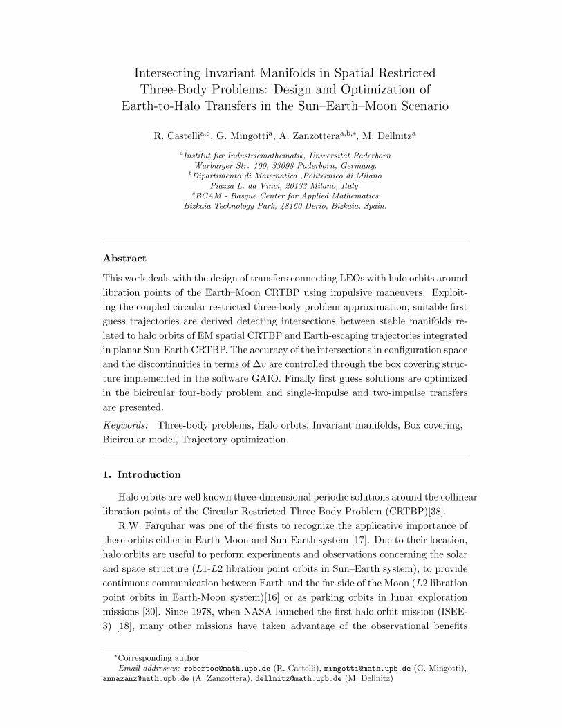
2.1. Circular Restricted Three-Body Problem

The circular restricted three-body problem (CRTBP) [38] studies the motion

of a massless particle m3 under the gravitational influence of two main primaries,

moving in circular orbits, as shown in Fig. 1(a).

In a rotating reference frame where the units of measure are normalized so that

the distance between the primaries, the modulus of their angular velocity and the

total mass are equal to 1, the motion of the third body is governed by the system

of equations x− 2y = Ωx

y + 2x = Ωy

z = Ωz

(1)

where Ω(x, y, z) = 12(x2 + y2) + 1−µ

r1+ µ

r2+ 1

2µ(1−µ) is the effective potential of the

system and the subscripts denote partial derivatives. Here µ = m2/(m1 +m2) is the

mass ratio of the primaries, while r21 = (x+µ)2+y2+z2 and r22 = (x−1+µ)2+y2+z2

are the distances from the spacecraft respectively to the larger and the smaller

primary. Let φ be the flow associated to the system (1), so that φ(ξ, ti; tf ) is the

solution at time tf leading from the initial data ξ = (x, y, z, x, y, z)(ti).

System (1) admits a first integral of motion, the Jacobi integral, defined as:

C(x, y, z, x, y, z) = 2Ω(x, y, z)− (x2 + y2 + z2) (2)

then, as C∗ varies, the family of 5-dimensional energy manifolds

M(C∗) = (x, y, z, x, y, z) : C(x, y, z, x, y, z) = C∗

is a foliation of the 6-dimensional phase space. For every C∗ the solution in the

configuration space of the equation C∗ = 2Ω(x, y, z) detects the zero-velocity surface,

which bounds the Hill’s region where the motion is possible and where it is forbidden.

The system (1) admits five equilibrium points, referred to as Lagrange points and

denoted with Li, i : 1 . . . 5: three of them L1, L2, L3 lie on the x-axis and represent

collinear configurations, while L4, L5 correspond to equilateral configurations of the

masses.

The topology of the Hill’s region changes in correspondence to the values Ci of

the Jacobi constant relative to the libration points, allowing to open necks between

different regions on the configuration space. The collinear libration points, as well as

the continuous families of planar and spatial periodic orbits, respectively Lyapunov

3

(a) Classic circular planar restricted three-

body problem.

(b) Sun-perturbed Earth–Moon RTBP.

Figure 1: Mathematical models to described the physics of the problem.

and Halo orbits, exhibit a saddle×center type stability character. The invariant

manifold structures related to these orbits act as separatrices in the energy surface

and provide dynamical channels in the phase space useful to the design of energy

efficient spacecraft trajectories [27].

In the following, to avoid any ambiguity between the two restricted models used

in the design process, the Jacobi constant C, its value Ci in correspondence of

the libration points and the flow φ will be labelled with the subscripts (·)SE and

(·)EM when they refers respectively to the planar Sun-Earth CRTBP and the spatial

Earth-Moon CRTBP.

2.2. Bicircular Restricted Four-Body Problem

The bicircular four-body model (BCRFBP) is a restricted four-body problem

where two of the primaries (the Earth and the Moon) are moving in circular orbit

around their center of mass B that is at the same time orbiting, together with

the last mass (the Sun), around the barycenter of the system. The motion of the

primaries is supposed to be co-planar and with constant angular velocity. Aiming to

write the equations of motion of the BCRFBP in the EM synodical reference frame,

with units of measure normalized as in the EM CRTBP, denote with θ(t) the phase

of the Sun, with ρs the distance between the Sun and the EM barycenter and with

rs the Sun-spacecraft distance (see Fig. 1(b)):

r2s = (x− ρs cos θ)2 + (y − ρs sin θ)2 + z2. (3)

Then the motion of the massless particle is governed by the following system of

differential equations, known also as Sun-perturbed Earth-Moon CRTBPx− 2y = ΩBx

y + 2x = ΩBy

z = ΩBz

(4)

where ΩB = Ω + msrs− ms

ρ2s(x cos θ + y sin θ).

This model can be considered a good approximation of the real Sun–Earth–Moon–

spacecraft four-body dynamics being the eccentricities of both Earth’s and Moon’s

4

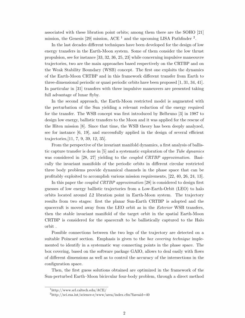
(a) Earth escape trajectory. (b) Halo arrival trajectory.

Figure 2: The two stages of the Earth-to-halo trajectory design.

orbits very small (respectively 0.016 and 0.054) and the Moon’s orbit inclined respect

to the ecliptic by only 5 deg. On the other hand, it’s worth noting that in the

bicircular model the motion of the primaries does not solve the three-body problem.

A more coherent model is the Quasi-Bicircular Problem proposed in [2].

3. Trajectory Design

The aim of this paper is to construct trajectories in the bicircular model, starting

from a LEO and targeting a halo orbit around L2 in the EM system. The design is

first performed in the CRTBP and then the initial guess trajectories are optimized

to be solution of the bicircular model.

The model adopted as approximation of the Sun–Earth–Moon–spacecraft re-

stricted four-body problem is the so called Coupled CRTBP [28]. It consists in the

superposition of SE and EM CRTBP: the former is used to model the motion in

the first part of the mission, then when the spacecraft is enough close to Moon to

benefit of its gravitational attraction, the EM CRTBP is introduced and the dy-

namical properties of the invariant manifold structures are exploited to fulfill the

requirements of the mission.

The intersection of the two flows is analyzed on a Poincare section allowing to

detect connections between two legs of trajectory, eventually applying an impulsive

maneuver, such as an out-of-plane contribution, required to obtain continuity in

velocity space.

In this work different Poincare sections will be introduced, each one defined as an

hyperplane in the phase space, whose projections on the configuration space reduces

to a line passing through the Earth.

3.1. Earth Escape Stage

The departure leg of the transfer consists in a trajectory leaving a LEO of hE =

167 km of altitude and integrated in planar SE CRTBP until the Poincare section

is reached. Any initial state yE is identified by the angle ϕE , that parametrizes the

5

position on the LEO with respect to a fixed direction, and the tangential impulsive

maneuver ∆vE provided by the launch vehicle and applied to insert the spacecraft

into a translunar trajectory (see Fig. 2(a)). Denote with

I = yE(ϕE ,∆vE) : 0 ≤ ϕE ≤ 2π , ∆vE ∈ Iv

the initial domain, where the magnitude of the initial maneuver is properly chosen

in order to decrease CSE of the spacecraft from the initial value evaluated on the

Earth parking orbit to a value in the interval IC = [3.000154, 3.0024] .

The upper bound of the interval IC has been chosen as the maximum value of

CSE that allows the Moon orbit to belong to the Hill’s region.

The variation of the Jacobi constant produced by a maneuver v applied in the

same direction of the motion is given by the formula

∆CSE = |v|2 + 2∣∣∣vtr− 1∣∣∣|v|r

where vt is the velocity of a probe orbiting on a LEO and r the geocentric distance,

both quantities, as well as v, expressed in SE dimensionless units.

Therefore, being CSE = 3.07051021± 3 · 10−9 the Jacobi constant associated to

a body orbiting on a LEO of 167km of altitude, the ∆vE maneuver has to be chosen

in the range Iv = [3210, 3300]m/s.

Once the angle ϕSE between the Poincare section and the x-axis is fixed, the

initial states yE ∈ I are forward integrated. Let be denoted with

PSE(ϕSE) = φSE(yE , 0; t) ∩ SSE(ϕSE) ,yE ∈ I , t ∈ [0, 1]

the set of all the possible intersections with the Poincare section. Note that the

cut of φSE(yE , 0; t) with the Poincare section is not guaranteed for all the yE ∈ I.

Indeed for large enough initial maneuver, ∆vE > 3260m/s, the lobe of the Hill’s

region containing the Earth joins the internal and external regions, thus some of the

trajectories may escape the Earth lobe before intersecting the section. This occurs

in particular for ∆vE > 3270m/s, when the stable manifold emanating from the two

Lyapunov orbits invest the Earth. In that case a small change in the initial position

on the Earth parking orbit produces very different results: some trajectories will

transit through the Lyapunov orbits, others will match the Poincare section in far

away points, being the amount of the twist produced on the trajectory very sensitive

with respect the initial position, [27].

3.2. Halo Capture Stage

In the second phase of the design the spatial EM CRTBP is considered to govern

the motion of the spacecraft and the invariant manifold structure associated to the

periodic orbits is exploited to fulfill the mission requirements. Indeed, concerning the

problem to target a halo orbit, once the spacecraft is placed on the stable manifold

it will fly for free along the manifold until, theoretically after an infinite time, it will

be inserted into the periodic orbit.

6

Let λ2 be used to denote the target halo orbit and yh its inner x-axis crossing.

To every point yins on the halo, in the following referred as insertion point, is

associated the time τh ∈ [0, T ] solution of yins = φEM (yh, 0; τh), being T the period

of the halo. As depicted in Fig. 2(b), any point yins is then slightly perturbed into

yins = yins + εvs, where the stable direction vs is provided by the monodromy

matrix, and each state yins is backwards integrated. The stable manifold W s(λ2) is

defined as

W s(λ2) =⋃yins

ysm = φ(yins, 0; τsm),∀τsm < 0

and it consists in a two-dimensional cylinder parametrized by τh ∈ [0, T ] and τsm ∈(−∞, 0). By construction, once the spacecraft is placed onto any point of the stable

manifold, the couple (τh, τsm) univocally determine how long the probe needs to fly

to reach the target orbit and which is the particular location of the insertion point.

In analogy with the notation adopted in the previous section, for a choice of the

angle ϕEM between the Poincare section SEM (ϕEM ) and the x-axis, define

PEM (ϕEM ) = W s(λ2) ∩ SEM (ϕEM ),

in the following denoted as Poincare map, the first intersection of the invariant tube

with the section. Since only the first intersection is taken into account, the Poincare

map is topologically equivalent to a circle, still parametrized by τh.

3.3. Trajectory connection

The last stage of the design process consists in gluing together, with the aid

of a impulsive maneuver, a Earth escaping orbit and a halo captured trajectory

yielding a complete Earth-to-halo transfer. The design of the whole Earth-to-halo

trajectory restricts to the selection of pairs of points ySE ∈ PSE and yEM ∈ PEM .

The necessary condition to identify feasible trajectories is the coincidence, at least

in configuration space, of the points ySE and yEM . That first requires the two

surfaces of section SSE and SEM to project on the same line in the (x, y) plane. In

terms of mutual position of the primaries, it means that the Earth–Moon line must

be tilted on the angle β = ϕSE − ϕEM respect to the Sun–Earth line at the instant

the spacecraft is on the section. Moreover, since the Poincare map PSE lives in the

z = 0 plane, the search of possible intersections is restricted to those points in

PEM with zero z-coordinate. Concerning the ∆V maneuver, since the spatial flow

is never tangential to the z = 0 plane (or it restricts to the planar motion), even if

it is possible to achieve satisfying intersections in configuration space between PSE

and PEM ∩z = 0, the out-of-plane component of the velocity maneuver can never

be avoided.

Candidate transfer point pairs are sought by varying the design parameters ϕSE ,

ϕEM , ∆vE , ϕE , yins, CEM in their range of definition and an efficient and systematic

search is numerically performed by means of a covering algorithm based on the box

structures implemented within the software package GAIO (see the next subsection).

7

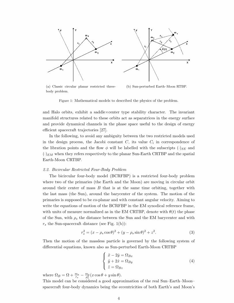
(a) PSE ∩ PEM in the r1, z coordinates. (b) PSE ∩ PEM in the r1, r1 coordinates.

(c) PSE ∩ PEM in the r1, r1θ coordinates. (d) PSE ∩ PEM in the r1, z coordinates.

Figure 3: Transfer point definition on suitable Poincare maps.

In the numerical simulations presented, in order to have a better visualization

of the selection of the transfer points, taking full advantage of the the geometry of

the maps, a system of cylindrical coordinates (r1, θ, z, r1, r1θ, z) is adopted. Here

(r1, θ) denotes the polar coordinates in the plane of the primaries with the Earth

as center and θ = 0 the Earth-Moon line, while z the out-of-plane component.

Fig. 3 depicts the Poincare maps PEM , PSE for a choice of ϕSE = 34π, ϕEM = π

4 ,

∆vE = 3280 m/s, CEM = 3.1495576 , while ϕE varies in [0, 2π] and yins along the

whole halo. In particular the subfigure Fig. 3(a) shows the projection into the (r1, z)

plane, while the remaining subfigures concern the velocity components. The grey

ring and black line stand respectively for PEM and PSE and the black dots and the

circles represents the intersections of the two maps in configuration space.

3.4. Box Covering Technique

GAIO (Global Analysis of Invariant Objects) is a set oriented software package

based on subdivision methods, with a searchable tree structured architecture, de-

8

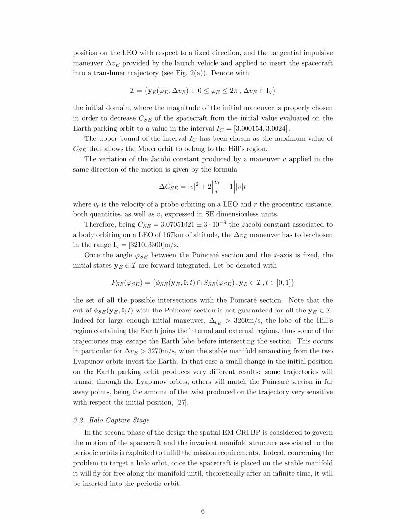
(a) Box covering of PEM (b) PSE and the covering of PEM

Figure 4: Left: the black dots are the points of PEM covered by the box collection F . Right:

F and PSE plotted in (r1, r1, z) cylindrical coordinates.

signed to study the global structure of a given dynamical system [14]. Although

the numerical methods provided by GAIO could be adopted in all the stages of the

mission design, showing versatility and efficiency [13], in this work only the basic

box structures and the routines for their management have been exploited.

A box B(C,R) is a N-dimensional rectangle, univocally identified by a center

C = (C1, · · · , CN ) ∈ RN and a vector of radii R = (r1, · · · , rn) ∈ RN , defined as

B(C,R) =N⋂i=1

(x1, x2, ....xN ) ∈ RN : |xi − Ci| < ri.

Starting from an initial box B0 containing PEM , a multiple subdivision process is

carried out to create families Fk of smaller boxes Bk with the property to cover B0,i.e.

⋃Bk = B0. In the k-th subdivision step each rectangle B(C,R) of the existing

collection Fk is subdivided with respect to the j-th coordinate, where j can vary

cyclically or can be chosen by the user. That means that passing from Fk−1 to Fk the

radius rj is halved, keeping ri, i 6= j unchanged, and the number of boxes increases

twofold. Once the radii of the boxes in Fk reach a prescribed size, the Poincare

map is inserted: only those boxes in Fk with non empty intersection with PEM are

stored, otherwise removed. Denote with box covering of the map PEM the collection

F of the remaining boxes, see Fig. 4(a). Note that the freedom of choosing the radii

along which to perform the subdivision, implies that the accuracy of the covering

could be set independently in each dimension. Then possible connections are sought

looking at the set E = F∩PSE , see Fig. 4(b). Since PSE lies on the z = 0 plane at

most two boxes of F , say B1, B2, are involved in the above intersection. Denoting

with Ei the subset of E whose elements are in Bi and with Mi the subset of PEM

covered by Bi (i = 1, 2), the preliminary set of transfer point pairs is defined as

T =⋃i=1,2

(ySE ,yEM ) : ySE ∈Mi ,yEM ∈ Ei.

9

Finally, in T the pair which minimizes the distance in velocity space is selected as

candidate transfer point pair. In this work, the necessary feasibility condition is

considered satisfied once the covering F is at least 10−4 (in EM units) accurate in

configuration space.

4. Trajectory Optimization

This section gives firstly a brief introduction of the trajectory optimization ap-

proach used in this work, then formulates in details the minimization problems later

solved.

Once feasible and efficient first guess solutions are achieved, combining the two

legs of the transfer, an optimization problem is stated. A given objective function

is minimized taking into account the dynamic of the process.

The dynamical model used to consider the gravitational attractions of all the

celestial bodies involved in the design process (i.e. the Sun, the Earth, and the

Moon) is the spatial BCRFBP described by (4) (written in an autonomous fashion)

with the adding of the term that corresponds to the rotation of the Sun:x− 2y = ΩBx

y + 2x = ΩBy

z = ΩBz

θ = ωs

(5)

According to the formalism proposed by Betts [10], the BCRFBP described by

(5) is written in the first-order form

x = vx

y = vy

z = vz

vx = 2vy + ΩBx

vy = −2vx + ΩBy

vz = ΩBz

θ = ωs

(6)

with vx = x, vy = y and vz = z. In a compact explicit form, system (6) reads

y = f [y(t),p, t], (7)

where f stands for the vector field and y = x, y, z, x, y, z, θ> is the state vec-

tor. The aim is finding y = y(t), t ∈ [ti, tf ], that minimizes a prescribed scalar

performance index or objective function

J = J(y,p, t), (8)

while satisfying certain mission constraints. These constraints are represented by

the two boundary conditions, defined at the end points of the optimization problem,

and by the inequality conditions, defined along the whole arc. These last quantities

10

are derived specifically for the mission investigated. Moreover, p stands for a vector

which brings together some parameters useful for the optimization process.

The optimization problem, OP, is then transcribed into a nonlinear program-

ming problem, NLP, using a direct approach. This method, although suboptimal,

generally shows robustness and versatility, and does not require explicit derivation

of the necessary conditions of optimality. Moreover, direct approaches offer higher

computational efficiency and are less sensitive to variation of the first guess solutions

[10]. Furthermore, a multiple shooting scheme is implemented. With this strategy,

the BCRFBP dynamics presented by (5) is forward integrated within N − 1 inter-

vals (in which [ti, tf ] is uniformly split), i.e. the time domain is divided in the form

ti = t1 < · · · < tN = tf , and the solution is discretized over the N grid nodes.

The continuity of position and velocity is imposed at their ends [15], in the form of

defects ηj = yj − yj+1 = 0, for j = 1, . . . , N − 1. The quantity yj stands for the

result of the integration, i.e. yj = φ(yj , t), tj ≤ tj+1. The algorithm computes the

value of the states at mesh points, satisfying both boundary and path constraints,

and minimizing the performance index.

Dynamics described by (5) are highly nonlinear and, in general, lead to chaotic

orbits. In order to find accurate optimal solutions without excessively increasing the

computational burden, an adaptive nonuniform time grid has been implemented.

Thus, when the trajectory is close to either the Earth or the Moon the grid is off-

line refined, whereas in the intermediate phase, where a weak vector field governs

the motion of the spacecraft, a coarse grid is used. The optimal solution found

is assessed a posteriori by forward integrating the optimal initial condition with a

Runge-Kutta 8th order scheme.

As far as it concerns the optimization algorithms, the Fortran package for large-

scale NLP, called SNOPT, has been used [20]. SNOPT is a general-purpose system

for solving optimization problems involving many variables and constraints. It min-

imizes a linear or nonlinear function subject to bounds on the variables and sparse

linear or nonlinear constraints. It is suitable for large-scale linear and quadratic

programming and for linearly constrained optimization, as well as for general non-

linear programs. Moreover, the solutions found are locally optimal, and ideally any

nonlinear functions should be smooth. Unknown gradients are estimated by finite

differences. SNOPT uses a sequential quadratic programming (SQP) algorithm that

obtains search directions from a sequence of quadratic programming subproblems.

Each QP subproblem minimizes a quadratic model of a certain Lagrangian function

subject to a linearization of the constraints. An augmented Lagrangian merit func-

tion is reduced along each search direction to ensure convergence from any starting

point.

4.1. Two-Impulse Problem Statement

In this section, the approach previously described is exploited to obtain optimal

transfers with two-impulsive maneuvers. According to the NLP formalism recalled,

the variable vector is

x = y1, . . . ,yN , t1, tN>, (9)

11

The initial conditions read:

ψi(y1, t1) :=(x1 + µ)2 + y21 + z21 − r2i = 0

(x1 + µ)(x1 − y1) + y1(y1 + x1 + µ) + z1z1 = 0,

(10)

which force the first y1 state of the transfer to belong to a circular orbit of radius

ri = RE+hE , where RE and hE stand for the Earth radius and the orbit altitude on

the Earth, respectively. The transfer ends when the spacecraft flies on the halo orbits

stable manifold, which is defined thanks to two parameters, as shown in Fig. 1(b).

In details, only the continuity in terms of position is imposed (and not velocity), so

that the final condition reads

ψf = yN − ysm = 0, (11)

where it is worth noting that yN = xN , yN , zN> and ysm = xsm, ysm, zsm>.

This means that, after the initial impulsive maneuver, a second one is required to

inject the spacecraft onto the stable manifold that takes it ballistically to the final

halo orbit associated.

The nonlinear equality constraint vector, made up of the boundary conditions

and the ones representing the dynamics, is therefore written as follows:

c(x) = ψi,η1, . . . ,ηN−1,ψf>. (12)

Moreover, aiming at avoiding the collision with the two primaries, the following

inequality constraints are imposed:

Ψcj(yj) :=

R2E − (xj + µ)2 − y2j − z2j ≤ 0

R2M − (xj − 1 + µ)2 − y2j − z2j ≤ 0,

j = 2, . . . , N − 1.

(13)

Finally, the flight time is searched to be positive, i.e.

Ψt = t1 − tN ≤ 0. (14)

The complete inequality constraint vector therefore reads:

g(x) = Ψc2, . . . ,Ψ

cN−1,Ψ

t>. (15)

As for the performance index to minimize, this is a scalar that represents the

two velocity variations at the beginning and at the final node of the transfer, i.e.

J(x) = ∆v1 + ∆vN . In details,

∆v1 =√

(x1 − y1)2 + (y1 + x1 + µ)2 + (z1)2 − vi, (16)

assuming vi =√

(1− µ)/ri as the velocity along the initial circular parking orbit,

and

∆vN =√

(xN − xsm)2 + (yN − ysm)2 + (zN − zsm)2, (17)

12

which represents the discontinuity in terms of velocity between the translunar tra-

jectory and the stable manifold related to the final halo.

In summary, the NLP problem for the two-impulse transfers is formulated as

follows:min J(x)

x

subject to c(x) = 0,

g(x) ≤ 0.(18)

4.2. Single-Impulse Problem Statement

As for the single-impulse trajectories, the variable vector is stated as follows:

x = y1, . . . ,yN ,p, t1, tN>, (19)

where p = τh, τsm, which is made up of two optimization parameters useful to

describe the final condition of the transfer (see Fig. 1(b)).

The equality constraint vector is defined, as in the previous paragraph, by (12)

with the exception of the final condition: in this case, at the final point of trajectory

optimization, the whole dynamical state is forced to be equal to the one associated

to the stable manifold (position and velocity):

ψf = yN − ysm = 0, (20)

where yN = xN , yN , zN , xN , yN , zN> and ysm = xsm, ysm, zsm, xsm, ysm, zsm>.

This means that, after the initial impulsive maneuver, the spacecraft flies ballistically

(with the dynamics described by the BCRFBP of (5)) to the final selected halo orbit,

with no other corrections.

In details, a generic point ysm on the stable manifold is defined as described in

section 3.2. Moreover, also the inequality constraint vector is defined in the same

way as in the two-impulse scenario.

Dealing with the objective index to minimize, this is made up of only the initial

velocity variation, i.e. the magnitude of the translunar insertion maneuver, i.e.

J(x) = ∆v1, where

∆v1 =√

(x1 − y1)2 + (y1 + x1 + µ)2 + (z1)2 − vi, (21)

assuming once again vi =√

(1− µ)/ri as the velocity of the initial circular orbit.

Finally, the NLP problem for the low-energy transfers is formulated in the same

fashion as proposed by (18) at the end of the previous section.

5. Optimized Transfer Solutions

In this section the transfers to halos obtained solving the optimization process

are presented. In the previous two sections, two families of trajectories are discussed,

according to the number of impulsive maneuvers that are allowed. In the follow-

ing, the optimized solutions are proposed in terms of some relevant performance

parameters.

13

5.1. Trajectories to Halos

Optimal two-impulse and single-impulse solutions are presented. These transfers

start from a circular parking orbit at an altitude of hE = 167 km around the Earth,

and reach a halo orbit around L2, with an out-of-plane amplitude of Az = 8000 km.

The results are shown in Tab. 1 as follows: sol.1.1 and sol.1.2 correspond to two-

impulse low energy transfers, while solutions sol.2.1 and sol.2.2 represent single-

impulse low energy transfers. Then, solutions below the line are some reference

impulsive transfers found in literature.

More in details, Table 1 is so structured: the second column ∆vi stands for the

initial impulsive maneuver that inserts the spacecraft onto the translunar trajectory.

The third column ∆vf represents the final impulsive maneuver that permits the

insertion of the spacecraft onto the stable manifold related to the target halo. This

latter maneuver is present only for the two-impulse trajectories. The fourth column

∆vt represents the overall amount of impulsive maneuvers necessary to complete the

Earth-to-halo transfers. Finally, the last column on the right stands for the whole

transfer time.

An analysis of the table shows that the single-impulse sol.2.1 (see Fig. 5(a))

offers the lowest value of the overall impulsive maneuvers (see ∆vt). This happens

because the first guess solution exploits deeply the dynamics of the RTBPs where it

is designed, and later of the Earth–Moon BCRFBP where it is optimized. Moreover,

this trajectory takes explicitly advantage of the initial lunar flyby. The latter can be

seen as a kind of aid in the translunar orbit insertion, as it reduces the ∆vi required

for that maneuver. The lunar flyby performs a change of plane of the translunar

trajectory that allows the insertion of the spacecraft onto the three-dimensional

halo stable manifold without any other maneuver. Summarizing, the single-impulse

trajectory corresponding to sol.2.1, acknowledges these remarks, as it shows the

lowest global ∆vt = 3161 m/s (with travel time ∆t = 98 days).

Table 1: Two-impulse and single-impulse low energy transfers to halos around L2. Comparison we

a set of impulsive reference solutions found in literature is also reported ([35, 31]).

Type ∆vi [m/s] ∆vf [m/s] ∆vt [m/s] ∆t [days]

sol.1.1 3110 214 3324 97

sol.1.2 3150 228 3378 120

sol.2.1 3161 0 3161 98

sol.2.2 3201 0 3201 126

Park. 3132 618 3750 –

Park. 3235 0 3235 –

Mingtao – – 3480 17

14

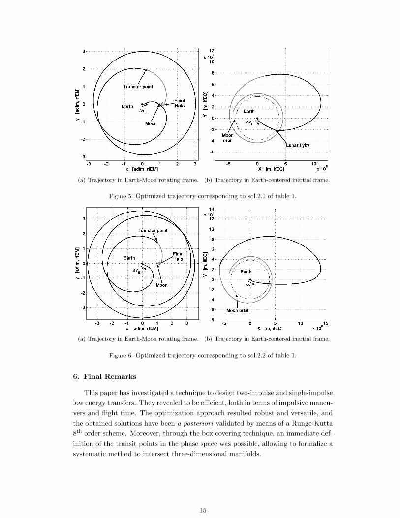
(a) Trajectory in Earth-Moon rotating frame. (b) Trajectory in Earth-centered inertial frame.

Figure 5: Optimized trajectory corresponding to sol.2.1 of table 1.

(a) Trajectory in Earth-Moon rotating frame. (b) Trajectory in Earth-centered inertial frame.

Figure 6: Optimized trajectory corresponding to sol.2.2 of table 1.

6. Final Remarks

This paper has investigated a technique to design two-impulse and single-impulse

low energy transfers. They revealed to be efficient, both in terms of impulsive maneu-

vers and flight time. The optimization approach resulted robust and versatile, and

the obtained solutions have been a posteriori validated by means of a Runge-Kutta

8th order scheme. Moreover, through the box covering technique, an immediate def-

inition of the transit points in the phase space was possible, allowing to formalize a

systematic method to intersect three-dimensional manifolds.

15

Acknowledgements

This work has been supported by the Marie Curie Actions Research and Training

Network AstroNet, Contract Grant No. MCRTN-CT-2006-035151.

References

[1] E.M. Alessi, G. Gomez and J. Masdemont. Two-manoeuvres transfers between

LEOs and Lissajous orbits in the Earth-Moon system. Advances in Space

Research, 45(10): 1276–1291, 2010.

[2] M.A. Andreu. The quasi-bicircular problem. Phd Thesis, Departament de

Matematica Aplicada i Analisi, Universitat de Barcelona, 1998.

[3] E. Belbruno. Lunar capture orbits, a method for constructing EarthMoon tra-

jectories and the lunar GAS mission. In: Proceedings of AIAA/DGLR/JSASS

Inter. Propl. Conf. AIAA Paper No. 87-1054, 1987

[4] E.A. Belbruno and J.K. Miller. A ballistic lunar capture trajectory for

Japanese spacecraft Hiten. JPL IOM, 312: 90–94, 1990.

[5] E.A. Belbruno. The Dynamical Mechanism of Ballistic Lunar Capture Trans-

fers in the Four-Body Problem from the Perspective of Invariant Manifolds and

Hill’S Regions. Technical Report, Centre de Recerca Matematica, Barcelona,

Spain, 1994.

[6] E.A. Belbruno. Capture Dynamics and Chaotic Motions in Celestial Mechan-

ics. Princeton University Press, Princeton 2004.

[7] E.A. Belbruno and J.P. Carrico. Calculation of weak stability boundary bal-

listic lunar transfer trajectories. In AIAA/AAS Conference, 2000.

[8] E.A. Belbruno and J.K. Miller, Sun-Perturbed Earth-to-Moon Transfers with

Ballistic Capture. Journal of Guidance Control and Dynamics, 16: 770–775,

1993.

[9] M. Bello, F. Graziani, P. Teofilato, C. Circi, M. Portfilio and M. Hechler, A

systematic analysis on weak stability boundary transfers to the moon. 51st

International Astronautical Congress, 2000.

[10] J.T. Betts. Survey of Numerical Methods for Trajectory Optimization. Journal

of Guidance control and dynamics, 21(2): 193–207, 1998.

[11] C. Circi, P. Teofilato. On the dynamics of weak stability boundary lunar

transfers. Celestial Mechanics and Dynamical Astronomy, 79: 41–72, 2001..

[12] C. Circi and P. Teofilatto. Weak stability boundary trajectories for the deploy-

ment of lunar spacecraft constellations. Celestial Mechanics and Dynamical

Astronomy, 95: 371–390, 2006.

16

[13] M. Dellnitz, O. Junge, M. Post, and B. Thiere. On Target for Venus: Set

Oriented Computation of Energy Efficient Low Thrust Trajectories. Celestial

Mechanics and Dynamical Astronomy, 95: 357–370, 2006.

[14] M. Dellnitz and O. Junge. Set Oriented Numerical Methods for Dynamical

Systems. Handbook of dynamical systems, 2(1): 900, 2002.

[15] P.J. Enright and B.A. Conway. Discrete Approximations to Optimal Trajec-

tories Using Direct Transcription and Nonlinear Programming. Journal of

Guidance Control and Dynamics, 15: 94–1002, 1992.

[16] R.W. Farquhar. Future Missions for Libration-Point Satellites. Astronautics

and Aeronautics, 7: 52–56, 1969.

[17] R.W. Farquhar. The control and use of Libration-Point Satellites. Astronautics

and Aeronautics, 1968.

[18] R.W. Farquhar, D.P. Muhonen, C. Newman, and H. Heuberger. The First

Libration Point Satellite, Mission Overview and Flight History. In AIAA/AAS

Conference, 1979.

[19] F. Garcia and G. Gomez. A note on weak stability boundaries. Celestial

Mechanics and Dynamical Astronomy, 97(2): 87–100, 2007.

[20] P.E. Gill, W. Murray and M.A. Saunders. Users Guide for SNOPT 5.3: A

Fortran Package for Large-Scale Nonlinear Programming. Boeing Information

and Support Services, 1998.

[21] G. Gomez, J. Masdemont, and J.M. Mondelo. A Dynamical System Approach

for the Analysis of the SOHO Mission. In Third International Symposium on

Spacecraft Flight Dynamics, European Space Agency, Darmstadt, Germany,

449–454, 1991.

[22] G. Gomez, W. S. Koon, M. W. Lo, J. E. Marsden, J. Masdemont and S.

D. Ross Connecting orbits and invariant manifolds in the spatial restricted

three-body problem Nonlinearity, 17(5): 1571–1606, 2004

[23] A.L. Herman and B.A. Conway. Optimal, Low-Thrust, EarthMoon Orbit

Transfer. Journal of Guidance, Control, and Dynamics, 21(1): 141–147, 1998.

[24] K.C. Howell, B.T. Barden, and M.W. Lo. Application of Dynamical Systems

Theory to Trajectory Design for a Libration Point Mission. Journal of Astro-

nautical Sciences, 45(2): 161–178, 1997.

[25] C.A. Kluever and B.L Pierson. Optimal low-thrust three-dimensional Earth-

moon trajectories. Journal of Guidance Control Dynamics, 18(4): 830–837,

1995.

17

[26] W.S. Koon, M.W. Lo, J.E. Marsden, and S.D. Ross. Constructing a Low

Energy Transfer Between Jovian Moons. Contemporary Mathematics, 292:

129–146, 2002.

[27] W.S. Koon, M.W. Lo, J.E. Marsden, and S.D. Ross. Heteroclinic Connections

Between Periodic Orbits and Resonance Transitions in Celestial Mechanics.

Chaos: An Interdisciplinary Journal of Nonlinear Science, 10: 427, 2000.

[28] W. Koon, M. Lo, J. Marsden, and S. Ross. Low Energy Transfer to the Moon.

Celestial Mechanics and Dynamical Astronomy, 81: 63–73, 2001.

[29] M. Lo, B. Williams, W. Bollman, D. Han, Y. Hahn, J. Bell, E. Hirst, R. Cor-

win, P. Hong, K. Howell, B. Barden, and R. Wilson. Genesis mission design.

J. Astron. Sci., 49: 169–184, 2001.

[30] M.W. Lo and M.J. Chung. Lunar Sample Return via the Interplanetary Su-

perhighway. In AIAA/AAS Conference, 886: 100–110, 2002.

[31] L. Mingtao and Z. Jianhua. Impulsive Lunar Halo Transfers Using the Stable

Manifolds and Lunar Flybys. Acta Astronautica, 66: 1481–1492, 2010.

[32] G. Mingotti, F. Topputo, and F. Bernelli-Zazzera. Combined Optimal Low-

Thrust and Stable-Manifold Trajectories to the Earth-Moon Halo Orbits. In

AIP Conference Proceedings, 886: 100–112, 2007.

[33] M.T. Ozimek and K.C. Howell. Low-thrust transfers in the earth-moon system,

including applications to libration point orbits. Journal of Guidance, Control,

and Dynamics, 33, 2010.

[34] J.S. Parker and G.H. Born. Direct luna Halo orbit transfers. In AAS/AIAA

Spaceflight Dynamics Conference, 2007.

[35] J.S. Parker. Families of Low-Energy Lunar Halo Transfers. In AAS/AIAA

Spaceflight Dynamics Conference, 90: 1–20, 2006.

[36] P. Pergola. Low Thrust Transfer to Backflip Orbits. Advances in Space Re-

search, 2010.

[37] C. Simo, G. Gomez, A. Jorba, and J. Masdemont. The Bicircular Model near

the Triangular Libration Points of the RTBP. In From Newton to Chaos,

343–370, 1995.

[38] V. Szebehely. Theory of Orbits: the Restricted Problem of Three Bodies. Aca-

demic Press New York, 1967.

[39] F. Topputo and E. Belbruno. Computation of the Weak Stability Boundaries:

Sun-Jupiter System. Celestial Mechanics and Dynamical Astronomy, 105(1):

3–17, 2009.

18

[40] K. Yagasaki. Sun-Perturbed Earth to Moon transfer with low energy and

moderate flight time. Celestial Mechanics and Dynamical Astronomy, 90: 197–

212, 2004.

[41] K. Yagasaki. Computation of low energy Earth-to-Moon transfers with mod-

erate flight time. Physica, 197: 313–331, 2004.

19