
Fault Tolerance for Large Scale Protein 3D Reconstruction from Contact Maps
Upload
khangminh22Category
view
2download
0
RELIABILITY AND FAULT-TOLERANCE ISSUES
IN REAL-TIME SYSTEMS
Edited by N VISWANADHAM
INDIAN ACADEMY OF SCIENCES Bangalore 560 080

Digitized by the Internet Archive in 2018 with funding from
Public.Resource.Org
https://archive.org/details/reliabilityfaultOOunse

RELIABILITY AND FAULT-TOLERANCE ISSUES
IN REAL-TIME SYSTEMS

/

RELIABILITY AND FAULT-TOLERANCE ISSUES
IN REAL-TIME SYSTEMS
Edited by N VISWANADHAM
19 8 7
INDIAN ACADEMY OF SCIENCES
BANGALORE 560 080

The cover shows the construction of a generalised Indra network from the paper by Raghavendra & Varma
© 1987 by the Indian Academy of Sciences
Reprinted from Sadhana-Academy Proceedings in Engineering Sciences Volume 11, pp. 1-272, 1987
Edited by N Viswanadham and printed for the Indian Academy of Sciences by Phoenix Printing Co.
Attibele Industrial Area, Bangalore-562 107, India

CONTENTS
Foreword 1
Fault-tolerant software
S K SRIVASTAVA: A tutorial on the principles of fault tolerance 7
V V S SARMA: A survey of software dependability 23
BHARAT BHARGAVA and LESZEK LILIEN: Enforcement of data consistency in database systems 49
L M PATNAIK and S BALAJI: Byzantine-resilient distributed computing systems 81
Fault-tolerant architectures
N N BISWAS and S SRINIVAS: Fault tolerance in multiprocessor systems 93
C S RAGHAVENDRA and ANUJAN VARMA: Reliability and fault- tolerance in multistage interconnection networks 111
C R DAS and L N BHUYAN: Reliability and fault-tolerance issues of multiprocessor and multicomputer systems 129
K K AGGARWAL: Fast approximate methods for the reliability analysis of computer networks 155
Performance modelling
U NARAYANA BHAT and KRISHNA M KAVI: Reliability models for computer systems: An overview including dataflow graphs 167
Y NARAHARI and N VISWANADHAM: Performance modelling of a fault-tolerant real-time multiprocessor using stochastic Petri nets 187
K S TRIVEDI and J B DUGAN: Computer-aided reliability analysis of fault-tolerant systems 209
Applications
D BASU, K V S S PRASAD RAO, S V L A VARAPRASAD, X KURIEN, R JAYASRI and M BHARATHI: A fault-tolerant computer
system for India’s satellite launch vehicle programmes 221
STVIURUGESAN and P S GOEL: Fault-tolerant spacecraft attitude control system 223

263
273
276
K SRI RAM and K IYER: Safety of nuclear power plants
Subject Index
Author Index

Foreword
The importance of fault-tolerance and reliability issues in real-time computer control systems might easily be appreciated in the context of the ever increasing use of computers in application areas such as control of hazardous chemical plants and nuclear reactors in process industry, battle management and weapon delivery in defence, intensive care and diagnostic systems in health care and control systems for air and high-speed ground transportation. The use of computers in such systems, for fault-detection and diagnosis, and system reconfiguration, has the potential of dramatically improving the operational effectiveness of real-time systems. The computer system being the principal component of monitoring and control equipment, its failure could result in disastrous consequences, and hence, such a system should be installed only after adequate demonstration of its required level of reliability.
Real-time computer control systems have three major constituents: the physical plant, the computer system and the instrumentation system that interfaces the plant with the computer. The human operator also plays a crucial role especially in emergencies. Equipment failures, malfunctions of sensors, actuators, computer hardware and software, and operator lapses may cause major damage to the system, endanger human life and may turn the environment toxic. Systematic design of reliable computer control systems is therefore an important and a very challenging task. The system has to maintain optimal performance during normal operation, and must also cope with randomly occurring emergencies during which the plant conditions are hostile, by taking corrective actions with strict real-time deadlines.
A preliminary failure cause-consequence analysis should be performed for the computer controlled system to identify the potential hazards associated with failures in each of the subsystems and the human operator. Such an analysis would reveal the criticality of each of the faults. Hazard analysis techniques based on Failure modes and effects analysis, Event trees, Fault trees. Digraphs, and Cause-consequence diagrams are useful for this purpose. A fault-diagnostic system is then designed to detect, diagnose and compensate for these failures and is implemented via software along with other monitoring and control functions. Expert systems, Kalman filters, observers, parity space techniques, fault trees, detection filters etc. are used in the design of the fault diagnostic system. These algorithms are implemented using fault-tolerant hardware and software. The design of fault-tolerant systems is thus a complex problem requiring expertise from a variety of disciplines.
In this special issue, we concentrate on the reliability and fault-tolerance issues in real-time computer systems. We organise the papers in four sections:
(i) Fault-tolerant Software (ii) Fault-tolerant Computer Architectures
(iii) Performance Modelling of Fault-tolerant Systems (iv) Applications
1

2 Foreword
1. Fault-tolerant software
In real-time systems, software is the key to the performance and error-free
operation of the system. Real-time software is a special class of software with
certain unique characteristics, such as operation in unpredictable and asynchronous
environments and response generation according to strict deadline schedules.
Reliability, safety and fault-tolerance are desirable features of real-time
software. Reliability is the probability that the system will perform its intended
function for a specified period of time under a set of specified environmental
conditions. Safety is the probability that conditions leading to an accident do not
occur whether or not the intended function is performed. In general, reliability
requirements are concerned with making the system failure-free whereas safety
requirements are concerned with making it accident-free. Fault-tolerance is the
survival attribute of the real-time software system. The software should provide
correct results in the face of various failures. A major technological concern for the
coming years is the ever widening gap between the demand for high quality, robust
software and its supply. This is of utmost relevance in the Indian context since there
are concerted efforts underway to produce control software for life critical systems
including satellite launch vehicles, high-tech combat aircraft, C3 systems, nuclear
power plants and hazardous chemical processes.
There are four papers in this issue which focus on reliable and fault-tolerant
software. The first paper by Shrivastava is a didactic exposition on the various
issues in the design and implementation of fault-tolerant software. He presents a
methodology for constructing software modules that can tolerate both expected
and unexpected faults including design faults. Following this, the design of
fault-tolerant algorithms - algorithms that incorporate software techniques for
tolerating hardware faults - is discussed. The use of these techniques is illustrated
in replicated distributed processing and for constructing robust distributed
programs.
The survey paper on software dependability by Sarma presents a case for
developing a unified framework for dependability. Dependability is a generic
concept that has attracted wide attention recently and subsumes various quality
factors such as reliability, availability, maintainability, complexity and safety. The
paper also surveys the models and methods for software reliability which is the
best-known dependability measure and discusses the important notion of software
fault-tolerance.
Database consistency is a fundamental requirement of a database system. The
paper by Bhargava & Lilien brings out comprehensively the role of fault-tolerant
software in maintaining database consistency in the presence of faults and restoring
consistency after site crashes and network partitionings. Besides, the paper also
discusses the verification of integrity assertions which is fundamental for ensuring
the semantic integrity of a database.
The fourth paper in this section, by Patnaik & Balaji, is a survey paper on an
important class of fault-tolerant distributed computing systems. These systems are
designed to tolerate Byzantine faults which could correspond to any arbitrary
behaviour on the part of hardware or software components of the system. The
authors discuss agreement problems, agreement protocols, and their applications,
in the context of Byzantine-resilient systems.

Foreword 3
2. Fault-tolerant computer architectures
Fault-tolerance is achieved in computer systems by introducing redundant or spare
processors and mempry elements, and capabilities for automatic fault-diagnosis
recovery and reconfiguration. With the rapid progress made in VLSI technology
and in semiconductor memories, high performance processor and memory units
are available at low cost. Distributed computer systems which are interconnections
of high performance processors, memory elements and I/O units by means of a
communication network have natural fault-tolerance attributes and, by adding
capabilities of fault-diagnosis and reconfiguration, they can be made ultra-reliable.
Distributed computing systems are broadly divided into multiprocessor and
multicomputer systems. A multiprocessor system consists of a number of proces¬
sing elements connected to a number of memory modules through an interconnec¬
tion network. Three types of interconnection topologies have been proposed in the
literature. They include crossbar, multistage interconnection networks and multi¬
ple bus organizations. In multicomputer systems, each processor has its own
memory and inter-processor communication is achieved by a message/packet
switching protocol. Several structures including loops, trees, full connections and
hypercubes have been proposed. Studies relating to performance and reliability
computations are needed to evaluate these distributed computer architectures. In this volume, we have four papers dealing with fault-tolerant computer
architectures. Biswas & Srinivas present a review of various approaches toward
tolerating hardware faults in multiprocessor systems. A survey of various models,
techniques and methods for fault diagnosis is provided in this paper. Reconfigur-
able architectures and fault-tolerant VLSI processor arrays are also considered.
Raghavendra & Anujan Varma consider reliability and fault-tolerance issues in
the design and analysis of multistage interconnection networks (min) for multi¬
processors. They consider multistage networks which are typically built for N inputs
and N outputs using 2x2 switching elements and log2/V stages. Further, several
approaches for achieving fault-tolerance in MIN are discussed and methods for
reliability analysis of min are explained.
Reliability and fault-tolerance evaluation of multiprocessor and multicomputer
architectures with emphasis on graceful degradation is considered by Das &
Bhuyan. They define two measures, reliability and performance availability, to
characterize and evaluate multiprocessor and multicomputer architectures. Band¬
width availability and computation communication availability are used to quantify
performance availability of multiprocessors and multicomputers. To evaluate the
reliability and performance availability, they describe two models: a bus-oriented
model and a switch-oriented model. The former is useful for crossbar and multiple
bus multiprocessors and the latter for all types of multiprocessors.
Reliability calculation in large computer networks is an issue that abounds in
computational problems and, in general, the problem complexity is exponential.
Aggarwal presents a high-speed approximate method for reliability analysis of
computer communication networks using clustering methods. Fie also defines a
reliability index, an approximate measure of the overall reliability of the system,
that can be easily incorporated into reliable system design.

4 Foreword
3. Performance modelling of fault-tolerant systems
One of the very important questions that arises when considering fault-tolerant systems is whether the system would perform the intended function at the specified levels of performance. Such a quantitative performance evaluation is required at each stage of the system life cycle: while evaluating alternative designs, while verifying a particular prototype, while guiding redesign and when the system is in operation.
Three methods are available for fault-tolerant system performance: measure¬ ment, simulation performance modelling and analytic performance modelling. Performance measurement is possible once a system is built, has been instrumented and is in operation. There are three major drawbacks of this method: first, performance figures relate to the specific system architecture under its current work load, second, measurement is not feasible during the design and development stages of the system, and third, measuring performance in a complex system environment is tedious and costly.
The most attractive approach to fault-tolerant system performance evaluation is through modelling. Fault-tolerant systems consist of a set of redundant resources: data, hardware and software elements and a set of randomly arriving tasks compete for these resources. The resources are prone to random errors and failures. Thus fault-tolerant systems are discrete-event dynamical systems where events occur at random time instants and the performance measures of interest include: resource utilization, contention for resources, response times, performance degradation, degree of fault-tolerance etc.
The tools of discrete-event simulation could be employed for simulation performance modelling of discrete-event dynamical systems. Here simulation models are driven by random input sequences and produce random output sequences. Statistical output analysis is required to interpret results of simulation models. Analytical models of discrete-event dynamical systems include Markov chains, queueing networks and stochastic Petri nets. All the analytical techniques lead to large-size models and their solution requires computer-aided analysis. User friendly computer-aided simulation and analytical performance modelling techni¬ ques would help the designer to concentrate on higher level decision-making rather than get bogged down with myriad computational issues.
In this special issue, we have three papers on performance modelling of fault-tolerant computer systems. Narayan Bhat & Kavi provide a critical overview of the approaches to reliability modelling. They show that Petri nets and dataflow graphs facilitate reliability analysis of complex systems. Narahari & Viswanadham present the performance evaluation of a fault-tolerant real-time multiprocessor (ftmp) using stochastic Petri nets. They develop four such models featuring various degrees of FTMP details and compute various performance measures including bus contention, processor utilization and waiting times. Trivedi & Dugan discuss the seven major issues in computer-aided reliability modelling and analysis of complex fault-tolerant systems and discuss the recent progress made in each of these seven areas.

Foreword 5
4. Applications
We have three application-oriented papers in this issue, the first two dealing with spacecraft on-board fault-tolerant computers and spacecraft fault-tolerant control systems and the third one with nuclear reactor safety issues. The first paper in this section, by Basu et al, describes the on-board fault-tolerant computer system for ISRO’s Augmented Satellite Launch Vehicle. They describe the architectural attributes of the on-board computer and the details of software testing carried out in order to ensure reliable operation.
The second paper in this section deals with another important application area-spacecraft control systems. Spacecraft have to function continuously without interruptions and without maintenance for periods of 7-15 years. The spacecraft control system has to detect, diagnose and estimate failures in various components and reconfigure the control system. This fault-tolerance feature has to be incorporated keeping in view the limitations on weight, power and computational facilities. Murugesan & Goel present a brief description of the attitude control system and highlight essential features of the fault-tolerant control system. They also present algorithms for fault detection, identification and reconfiguration for various elements of the spacecraft control system.
Safety in nuclear power plants is an important and widely discussed issue. The Three-mile Island and Chernobyl accidents and their consequences have brought to focus the deficiencies in the current safety control systems. Sri Ram & Iyer discuss safety issues in the CANDU type of nuclear reactors. They review the recent work on station blackout, operational transients, and small and large break loss of coolant accidents. They also stress on the nuclear safety culture to be practised by the operators in all operating nuclear power plants.
Taken together, the fourteen representative papers of the issue help the reader to obtain a global view of the design of real-time systems with specifications on reliability and fault-tolerance. I hope that this special issue will stimulate further interest in this area leading to more reliable and safer real-time systems.
I would like to express my sincere thanks to — the authors for their enthusiastic response to my invitation, — the reviewers for their help in providing me with prompt and critical reviews, — Mr Y Narahari, for his invaluable and cheerful help in a variety of ways, — Prof. R Narasimha, Chairman, Editorial Board, Sadhana for his constant help
and encouragement. — Ms K Shashikala, for editorial help.
October 1987 N VISWANADHAM Guest Editor

A tutorial on the principles of fault tolerance
S K SHRIVASTAVA
Computing Laboratory, University of Newcastle upon Tyne NE1 7RU,
UK
Abstract. The paper begins by examining the four aspects of fault
tolerance - error detection, damage assessment, error recovery and
fault treatment - and describes how these aspects can be incorporated
in systems. Following this, a methodology for the construction of robust
software systems is presented, covering the topics of design fault
tolerance and software implemented fault tolerance. Some aspects of
modelling faulty behaviour of components is presented and the notion
of a family of fault-tolerant algorithms is introduced.
Keywords. Error recovery; fault tolerance; reliability; exception
handling; fault classification; atomic actions; replicated processing; real
time systems.
1. Introduction
A reliable computing system must be capable of providing normal services in the
presence of a finite number of component failures. Faults within a system cause its
failure. These faults could be present in either the components of the system or in its
design. The paper examines in §2 the nature of systems and their failures and
presents a methodology for the construction of robust software modules - modules
capable of tolerating both expected and unexpected faults. The next section
discusses design fault tolerance and the subsequent section discusses software
implemented fault tolerance, describing the principles of constructing algorithms
capable of tolerating component failures of specified types. Conclusions from our
study are presented in the last section.
2. Systems and their failures
Following Anderson & Lee (1981, 1982), a system is defined to consist of a set of
components which interact under the control of an algorithm (or design). The
components of a system are themselves systems as is the algorithm (design). The
phrase ‘algorithm of a system’ is used here to refer to that part of the system which
actually supports the interactions of the components.
The internal state of a system is the aggregation of the external states of all its
components. The external state of a system is an abstraction of its internal state.
7

8 S K Shrivastava
During a transition from one external state to another, the system may pass through a number of internal states for which the abstraction, and hence the external state is not defined. We assume the existence of an authoritative
specification of behaviour for a system which defines the external states of the system, the operations that can be applied to the system, the results of these operations and the transitions between external states caused by these operations.
In our everyday conversations we tend to use the terms ‘fault’, ‘failure’ and ‘error’ (often interchangeably) to indicate the fact that something is ‘wrong’ with a system. However, in any discussion on reliability and fault tolerance, a little more precision is called for to avoid any confusion. Failure of a system is said to occur when the behaviour of the system first deviates from that required by the, specification. The reliability of the system can then be characterized by a function R(t) which expresses the probability that no failure of the system will have occurred by time t. We term an internal state of a system an erroneous state when that state is such that there exist circumstances (within the specification of the use of the system) in which further processing by the normal part of the system will lead to failure. The phrase ‘normal part of a system’ is used here to admit the possibility of introducing in the system extra components and algorithms to specifically prevent failures. Such additions are referred to as the redundant (exceptional or abnormal)
part of the system. The term ‘error’ is used to designate that part of the internal state that is ‘incorrect’. The terms ‘error’, ‘error detection’ and ‘error recovery’ are used as casual equivalents for ‘erroneous state’, ‘erroneous state detection’ and ‘erroneous state recovery’.
Next we might ask why a system enters an erroneous state (one that leads to a failure). The reason for this could be either the failure of a component or the design (or both). Naturally, a component (or design) being a system, may itself fail because of its internal state being erroneous. It is often convenient to be able to talk about causes of system failure without actually referring to internal states of the system's components and design. We achieve this by referring to the erroneous state of a component or design as a fault in the system. A fault could either be a component fault or a design fault; so a component fault can result in an eventual component failure and similarly a design fault can lead to a design failure. Either of these internal (to a system) failures will cause the system to go from a valid state to an erroneous state; the transition from a valid to an erroneous state is referred to as the manifestation of a fault.
To summarize: a system fails because it contains faults; during the operation of a system a fault manifests itself in the form of the system state going into an erroneous state such that - unless corrective actions by the redundant part of the system are undertaken - a system failure will eventually occur.
3. Principles of fault tolerance
Two complementary approaches have been noted for the construction of reliable systems (Avizienis 1976). The first approach, which may be termed fault
prevention, tries to ensure that the implemented system does not and will not contain any faults. Fault prevention has two aspects: (i) fault avoidance techniques are employed to avoid introducing faults into the

Principles of fault tolerance 9
system (e.g. system design methodologies, quality control); (ii) fault removal techniques are used to find and remove faults which were inadvertently introduced into the system (e.g. testing and validation).
The second approach, which has been termed fault tolerance, is of special significance to us because of the impracticality of ensuring the complete absence of faults in a system containing a large number of components. Four constituent phases of the fault-tolerance approach have been identified: (i) error detection; (ii) damage assessment; (iii) error recovery; and (iv) fault treatment and continued system service.
3.1 Error detection
In order to tolerate a fault, it must first be detected. Since internal states of components are not usually accessible, a fault cannot be detected directly, and hence, its manifestations, which cause the system to go into an erroneous state, must be detected. Thus the usual starting point for fault-tolerance techniques is the detection of errors.
3.2 Damage assessment
Before any attempt can be made to deal with the detected error, it is usually necessary to assess the extent to which the system state has been damaged or corrupted. If the delay, identified as the latency interval of that fault, between the manifestation of a fault and the detection of its erroneous consequences is large, it is likely that the damage to the system state will be more extensive than if the latency interval were shorter.
3.3 Error recovery
Following error detection and damage assessment, techniques for error recovery must be utilized in an attempt to obtain a normal error-free system state. In the absence of such an attempt (or if the attempt is not successful) a failure is likely to ensue. There are two fundamentally different kinds of recovery techniques. The backward recovery technique consists of discarding the current (corrupted) state in favour of an earlier state (naturally, mechanisms are needed to record and store system states). If the prior state recovered to, preceded the manifestation of the fault, then an error free state will have been obtained. In contrast a forward
recovery technique involves making use of the current (corrupted) state to construct an error free state.
3.4 Fault treatment and continued service
Once recovery has been undertaken, it is essential to ensure that the normal operation of the system will continue without the fault immediately manifesting itself once more. If the fault is believed to be transient, no special actions are necessary, otherwise, the fault must be removed from the system. The first aspect of fault treatment is to attempt to locate the fault; following this, steps can be taken to either repair the fault or to reconfigure the rest of the system to avoid the fault.
To illustrate the ideas presented so far, let us examine the recovery block mechanism (Horning et al 1974; Randell 1975), a well-known method of constructing fault-tolerant software. The syntax of a recovery block construct is,

10 S K Shrivastava
ensure ( acceptance test ) by P0 else-by Px else fail;
which depicts a software system with four components, the two procedures F() (the primary) Px (the alternative), the acceptance test and the set of global variables accessible to the procedures (not shown above). The algorithm of the system is the control structure implied by the syntax. If we assume that the acceptance test is ‘perfect’ (i.e. detects all violations of the specification) then the recovery block shown can tolerate faults within procedure P0 (if any) that could lead to its failure, provided of course, that Pj passes the test. Regarding P0 as a system, its faults are essentially design faults. So, when it is said that ‘a recovery block can tolerate design faults’, what is really meant is that it can tolerate faults in some of its components (P0 in our case) which could fail due to design faults in them. We shall next see how the four aspects of fault tolerance are embodied in a recovery block. The acceptance test (a boolean expression) is used for detecting errors. Damage assessment is particularly simple: only the component in execution is assumed to be affected. (We are assuming the simple case of a single sequential process; when interacting processes are involved, damage assessment can be quite difficult, Randell 1975.) Error recovery - backward in this case - consists of recovering the state of the executing program to that at the beginning of the recovery block. Finally, the program in execution (primary or alternative) is assumed to be faulty, so its faults are avoided by executing the next alternative (if any).
The four aspects of fault tolerance form the basis for all fault-tolerance techniques and provide a sound foundation for design and implementation of reliable systems (Anderson & Lee 1981).
4. Software design methodology
In this section we will present a methodology for the construction of robust software systems based on the treatment presented in Anderson & Lee (1981) and Cristian (1982). Following generally accepted software engineering concepts, we shall assume the use of data abstractions (abstract data types) in program development. This leads to software systems that are structured into a hierarchy of modules (or components). Such a hierarchy may be represented by an acyclic graph (figure 1) where modules are represented by nodes and an arrow from a node A to a node B means that A is a user of B; that is, there are one or more operations in A
such that a successful completion of one such operation depends on the successful
Figure 1. Hierarchy of modules.

Principles of fault tolerance 11
completion of some operation provided by B - in other words, B provides certain services to A.
4.1 Expected events
The specified services provided by a given module can be classified into normal
services (expected and desired) and abnormal or exceptional services (expected but undesired). In programming language terms, when a user module calls a procedure exported by a lower level module, then either the call terminates normally (expected desired service is obtained) or an exceptional return is obtained. Let us now consider the design of an intermediate module such as B (see figures 1 & 2).
A normal chain of events might consist of some procedure of A making a call on B, as a result of which B calls a lower level module (say E), this call returns normally, and subsequently A’s call returns normally. We examine now the two cases that could lead to A’s call returning exceptionally.
(i) A call to a lower level module (such as E) by B returns exceptionally. In such a case we say that an exception is detected in B (this is synor ymous to saying that an error is detected in B\ we will use the term ‘exception’ here because it is more commonly used when talking about software). If this exception is not ‘handled’, then module B would certainly fail to provide the specified service to A. To cope with the detected exceptions, module B therefore contains exception handlers (the handlers thus represent the ‘abnormal’ part of a system mentioned earlier). If, des¬ pite the occurrence of a lower level exceptional return, module B provides a nor¬ mal service to A, we say that the lower level exception has been masked by the handler in B. On the other hand, if B is unable to mask a lower level exception and provides an exceptional return to A, we say that the lower level exception has been propagated to a higher level.
(ii) A boolean expression in B - inserted specifically for detecting an error (ex¬ ception) - evaluates to false. The treatment of this exception by its handler is similar to the previous case: either that exception is masked, in which case (provided no further exceptions are encountered) B will return normally to A, otherwise an exceptional return is obtained by A.
We thus see that the construction of a robust module requires the provision of (a) exception handlers for coping with exceptions propagated from lower levels; and (b) boolean expressions for detecting exceptions arising in the module itself,
module 'B'
normal exceptional return returns
i t t.u normal exceptional part part
r~f t n call normal exceptional
return returns
fail exception
fail exception
Figure 2. Structure of a module.

12 S K Shrivastava
and their exception handlers. Note that it is possible (and often desirable for the sake of simplicity) to map several exceptions onto a single handler.
The need for exception handling facilities in programming languages has now been recognised and many modern languages such as CLU (Liskov & Snyder 1979) and ADA (Luckham & Polak 1980) contain specific features for exception handling. We shall use here some simple notations which will enable us to illustrate these ideas with the help of a few examples. The following notation will be used to indicate that a procedure P, in addition to the normal return, also provides an
exceptional return E:
procedure P(- -) signals E;.
The invoker of P can define the exceptional continuation to be some operation H
which will be termed the handler of E:
P(- -) [£=>#];.
In the body of P, the designer of P can insert the following syntactic constructs (where the braces indicate that the signal operation is optional):
(a) [P=> ....; {signal E}];
(b) <2[D=s>....; {signal £}];.
Construct (a) represents the case whereby an exception is detected by a run time test; whilst the second construct represents the case when invocation of an operation Q results in an exceptional return D which in turn could lead to the signalling of exception E. When an exception is signalled using construct (a) or (b), the control passes to the handler of that exception (H in this case).
Example: We consider the design of a procedure P which adds three positive integers. The procedure uses the operation ‘ + ’ (typically provided by the hardware interpreter) which can signal an overflow exception OV.
procedure P(var i: integer; j, k\ integer) signals OW;
begin
. i := i+ j[OV==^> signal OW];
i : = i + k[OV=z>i := i—j\ signal OW];
end;.
It is assumed above that no assignment is performed if an exception is detected during the execution of the operation ‘ + \
The above example also illustrates an important aspect of exception handling, which is that before signalling an exception it is often necessary to perform a ‘clean up’ operation. The most sensible strategy is to ‘undo’ any side effects produced by the procedure. If all the procedures of a module follow this strategy, we get a module with the following highly desirable property: either the module produces results that reflect the desired normal service to the caller, or no results are produced and an exceptional return is obtained by the caller.
Example: A file manager module exports a procedure CREATE whose function is to create a file containing n blocks. Assume that the file manager employs two discs

Principles of fault tolerance 13
for block allocation such that a given file has its blocks on either disc d\ or d2, and that Mi and M2 are the disc manager modules for dx and d2 respectively.
procedure CREATE (n: integer) signals NS;
begin
Mi • AL(n)[DO==>M2- AL(n)[DO ==> restore; signal NS]];
end;.
The above procedure illustrates how an exception may be masked. The AL procedure of a disc manager allocates n blocks, but if the number of free blocks is less than requested, a disc overflow exception (DO) is signalled. The first handler of this exception tries to get space from the second disc manager. If a second DO exception is detected then the procedure is exited with a ‘no space’ exception NS. The procedure ‘restore’ recovers the state of global variables accessible to CREATE to that at the beginning of the call (this follows from our philosophy of undoing any side effects before signalling an exception).
4.2 Unexpected events
So far we have considered the treatment of ‘expected events’ (desired or undesired); we turn our attention to the treatment of unexpected (and therefore undesired) events. Let us assume that the hardware interpreter over which the software under consideration is executing is behaving according to the specifica¬ tion. Then, any unexpected behaviour from a software module must be attributed to the existence of one or more design faults in that module or any of its lower level modules. In general, during the execution of a procedure P of a module, a design fault can manifest itself in any of the following ways: 1) the execution of P does not terminate; 2) a lower level exception is detected for which there is no exception handler in P;
3) the execution of P terminates normally (the invoker obtains a normal return) but the results produced by P are not in accord with the specification.
It is clear that situations (1) and (2) will eventually cause a failure of the module; situation (3) represents the case where the module has failed but this event has not yet been detected by the system. To cope with such cases, we can employ a default exception handler:
procedure P(- -) signals E ;
begin
end [=> “default handler”];.
The control goes to this handler during the execution of P whenever an exception is detected for which there is no handler. Thus, to cope with situation (1) it is possible to start a ‘timer’ concurrently with the invocation of P ; the ‘time out' exception will then be handled by the default handler. All the lower level exceptions with no programmed handlers will similarly be handled by the default handler. Finally we

14 S K Shrivastava
make use of run time checks (assertions) to detect possible violations of specifications to minimise the danger of undetected failures (case 3).
What should be the strategy adopted by a default handler? The simplest thing to do is to undo any side effects produced by the procedure and to signal a fail
exception (see figure 2). When the invoker receives a fail exception, it means that the called module has failed to provide the specified service. Nevertheless, the called module hasiailed ‘cleanly’ since no side effects have been produced. It is also possible for the default handler to mask the (unanticipated) exception by calling an alternative procedure in the hope of circumventing the design fault(s). The similarity with the recovery block approach is not accidental, as the example below shows how a recovery block can be modelled by making use of default exception
handlers: ensure ( acceptance test ) by P0 else-by Pi else fail;.
The "above construct is equivalent to the following one:
Po [-> restore; P [ [ — > restore; signal fail]];
where, P-, i = 0, 1, is given by:
procedure P[
begin
body of Pt\
assert ( acceptance test );
end [ — => signal fail];.
The following design methodology has then emerged. During the design of a given module, we carefully analyse the cases that could prevent the module from providing the desired normal services. We make use of specific exception handlers to either mask the effects of such undesired but expected exceptions or to signal an appropriate exception to the caller of the module; the purpose of signalling an exception is to indicate to the caller that the normal service cannot be provided and also to give an indication of the reason (e.g. arithmetic overflow, disc full, fail etc.). We make use of default exception handlers or recovery blocks to obtain a measure of tolerance against design faults. The capability of tolerating design faults rests largely on the ‘coverage’ of run time checks (such as acceptance tests) for detecting errors. Often, for reasons of efficiency, it is not possible to check completely within a procedure that the results produced have been according to the specification (e.g. for a routine that sorts its input, the check that the output has been sorted would be almost as complex as the routine itself); hence run time checks are often limited to checking certain critical aspects of the specification (hence the name ‘acceptance test’). This means that the possibility of undetected failures cannot be ruled out entirely.
5. Tolerance for design faults
The difficulty in providing tolerance for design faults is that their consequences are unpredictable. As such, tolerance can only be achieved if design diversity has been

Principles of fault tolerance 15
built into the system (figure 3). In the last section, recovery blocks (or default exception handlers) were mentioned as a mechanism for introducing design diversity. In this section the concept of design diversity is explored further. One more proposal, in addition to recovery blocks, has been made for tolerating design faults in software, and is known as N-version programming (Avizienis 1985). Both the approaches can be described uniformly using the diagram given below (Lee & Anderson 1985; pp. 64-77).
Each redundant module has been designed to produce results acceptable to the adjudicator. Each module is independently designed and may utilize different algorithms as chosen by its designer. In the yV-version approach-, the adjudicator is essentially a majority voter (the scheme is analogous to the hardware approach known as the /V-modular redundant technique). The recovery block scheme has an adjudicator which applies an acceptance test to each of the outputs from the modules in turn, in a fixed sequence.
The operational principles of the N-version approach are straightforward: all of the N modules are executed in parallel and their results are compared by a voting mechanism provided by the adjudicator. The implementation of this scheme requires a driver program which is necessary for: (i) invoking each of the modules; (ii) waiting for the modules to complete their execution; and (iii) performing the voting function. Each module must be executed without interference from other modules. One way of achieving this goal is to physically separate the modules - each module is run on a separate processor.
A special case of ^-version programming is when the degree of replication is just two. In this case the adjudicator provides a comparison check. The Airbus A310 slat and flap control system (Martin 1982) uses this approach, for driving stepping motors via a comparator. In the event of a discrepancy, the motors are halted, the control surfaces locked and the flight crew alerted.
Experiments conducted at UCLA and elsewhere on N-version programming (Avizienis 1985; Knight & Leveson 1986) and at Newcastle on recovery blocks (Anderson et al 1985) have produced encouraging results indicating that tolerance to design faults is certainly possible.
Figure 3 Design diversity.

16 S K Shrivastava
6. Software implemented fault tolerance
6.1 Tolerance to hardware faults
The techniques presented in §4 can be applied to the case when lower level modules have been implemented in hardware (e.g. disc units, processors). If these modules also provide normal and exceptional services (which is usually the case) then higher level software modules which use them can employ the fault-tolerance techniques discussed previously to either mask a lower level hardware exception or to propagate it as a higher level exception. The term software implemented fault
tolerance is often used to refer to software techniques for tolerating hardware faults. The resulting algorithms will be termed fault-tolerant algorithms. When dealing with hardware the following points must be borne in mind: (i) An exceptional response is often obtained due to a transient fault in the hardware; thus simply retrying the operation may prove to be sufficient. (ii) All hardware components eventually fail (due to ageing and wearout); so when a failure of a hardware module is suspected, steps might be required to permanently remove the module from the system (reconfigure the system). (iii) Diagnostic techniques can be used in an operational system to detect possible failures of components and to repair (replace) them before these components are utilised for services.
The function of a fault-tolerant algorithm of a system is to detect failures of the system’s components and to attempt to tolerate these failures so as to provide specified services.
Example. Construction of reliable disc storage out of unreliable discs. A disc can fail (permanently) due to defective disc surface conditions, failure of the disc drive
system or failure of the read-write electronics. In addition, various other accidents can occur which can cause data stored in one or more pages of a disc to be cor¬ rupted. Here we will briefly discuss tolerance to these latter kind of failures.
We assume the existence of the following two hardware procedures for accessing a disc:
procedure write (at: address; data: page);
procedure read (at: address; var data: page) signals looksbad;.
The exception iooksbad’ indicates that the data read could be corrupted. This could either be because the page is really corrupted or some transient failure has occurred - in which case a bounded number of retries should eventually result in good data being read. The effect of a write operation is that either (i) the addressed page gets the data; or (ii) the addressed page remains unchanged or gets corrupted data.
We next construct fault-tolerant read and write operations using the unreliable operations mentioned above:
procedure careful-read (at: address; var data: page) signals bad-page;
begin
use read operation at most n number of times to obtain good data (i.e. not looksbad) else signal bad-page;
end;

Principles of fault tolerance 17
procedure careful-write (at: address; data: page) signals bad-page
begin
perform ‘write’ and then ‘careful-read’ on the same page to check written data = read data; if the check fails even after n retries then signal bad-page
end;.
One way we can guard against accidental corruption of a page is by making sure that an uncorrupted copy of the page is available somewhere. This can be achieved by employing two discs (with independent failure modes) and by maintaining pairs of pages on these discs. It is then necessary to check at regular intervals that the pairs of pages have identical uncorrupted data stored in them; if not, the corrupted page of a pair is updated by performing a careful read on the paired page followed by a careful write on the corrupted page. The interval of running this checking process is chosen so as to reduce the probability of both the pages of a pair becoming corrupted to an acceptably small quantity (Lampson & Sturgis 1981).
6.2 Modelling faulty behaviour of components
The simple example of the previous sub-section illustrates how, given a specification of abnormal behaviour of components, specific measures can be employed in fault-tolerant algorithms. The fault-tolerance measure employed by ‘careful-read’ (namely, repeated retries) will only be effective, when a read opera¬ tion fails by reading the addressed page in a detectably incorrect manner (excep¬ tion looksbad is signalled). Clearly, the employed measure will not be effective if a disc fails, say, by correctly reading a page other than the intended one. Thus, design of a fault-tolerant algorithm of a system entails making assumptions about the behaviour of faulty components of the system. A given faulty component can behave in many different ways, some of which will be easier to tolerate than others; furthermore, certain patterns of faulty behaviour are likely to be more probable than others.
Suppose we can classify faulty behaviour of a component starting from those that are relatively restricted breaches of the specification (caused by simple faults) to those that are increasingly more general breaches of the specification (caused by complex faults). Then we can design a family of fault-tolerant algorithms - from simple ones tolerating simple faults to increasingly more complex ones tolerating larger classes of more general faults. Given such a family of algorithms, one can select a particular one depending upon the stated reliability requirements - choosing an algorithm tolerating larger classes of faults (or in the extreme, all
types of faults) for a system requiring a very high degree of reliability. In this section, such a fault classification is presented. The treatment presented here is based on that by Ezhilchelvan & Shrivastava (1986) where more details can be
found. Following Kopetz (1985, pp. 91-101), the response of a component for a given
input will be said to be correct if the output value is not only as expected, but also produced on time. Formally, the correct response of a component is defined as
follows.

18 S K Shrivastava
Correct response of a component: Let a component receive at time tt an input requiring a non-null response from the component and as a result produce an output value vy at time tj. For that input, the response vy at time tj is correct iff: (i) the value is correct: vy = wj, where Wj is the expected value consistent with the specification; and, (ii) the response is correct: tj = f; + L/+ 8t, where td is the minimum delay time of the component, and 8t is the unpredictable delay such that 0 < 8t < tmax, and /max is the maximum unpredictable delay time of the component.
The values td and tmax are constants for a given component. First of all, we note that the response of a component cannot be instantaneous to a given input but must experience a finite minimum amount of delay which is specified by the parameter td. Secondly, it is usual in engineering specifications to indicate a time interval during which a response is required; according to our definition, this interval is from ti + td to ti + td + tmax.
A correctly functioning component does not arbitrarily produce responses. In particular, when there is no input (null input) or when no response is expected for an input, there is naturally no output value produced (output is null). The values td and tmax are meaningful only when non-null output values are produced.
If vy Wj, then the output value will be termed incorrect; similarly, if tj < ti + td (output produced too early) or tj > ti + td + tmax (output produced too late), then the response time will also be termed* incorrect.
Given the above definitions of correct and incorrect responses, there can be at most three possible ways by which a response can deviate from that specified. This leads to the following three types of faults.
(/) Timing fault: A fault that causes a component to produce the expected value for a given input either too early or too late will be termed a timing fault and the corresponding failure a timing failure. Using our notation:
(i) vy- = Wj, and (ii) either tj < tt + td or tj > tj + td + tmax.
(ii) Value fault: A fault that causes a component to respond, for a given input, within the specified time interval, but with a wrong value will be termed a value fault and the corresponding failure a value failure:
(i) vy Wj, and (ii) tj = tl-^tdJt8t.
(iii) Commission fault: A fault of commission is responsible for a commission failure with the following property:
vy # Wj, and/or tj ^ tt + td + 8t.
A commission failure is any violation from the specified behaviour. In particular, it includes the possibility of a component producing a response when no input was supplied.
(iv) Omission fault: Many fault-tolerant algorithms are designed under a particularly simple failure mode assumption, which is that a component can fail only by producing no response. A fault which causes a component, for a given input requiring a non-null response, not to produce any response will be termed an omission fault and the corresponding failure an omission failure.

Principles of fault tolerance 19
We could regard ‘not producing a response’ as equivalent to ‘producing a null value on time’, thereby treating an omission fault as a special case of a value fault. We can also treat an omission fault as a special case of a timing fault by regarding ‘not producing a response' as equivalent to ‘producing a correct value at infinite time’.
Fault!failure lattice: A commission fault (failure) subsumes all the other three types of faults (failures). The relationships among these four types of faults (failures) can be expressed by the following fault (failure) lattice (figure 4), where an arrow from A to B, indicates that fault (failure) type A is a special case of fault (failure) type B.
(The relation *->’ is transitive.) An important observation can now be made which is that a fault-tolerant algorithm designed to tolerate ra, m > 0, timing failures (value failures) can also tolerate m omission failures and further that an algorithm designed to tolerate m commission failures can tolerate m failures of any type. The top of the lattice represents the simplest and the bottom, the most general fault (failure).
Examples: We will next give some examples of various types of failures. A self-checking component (e.g. a processor) that stops functioning as soon as an error is detected within itself can be regarded as suffering from omission failures. On the other hand, a self-checking component, which upon detecting an error, responds within time by producing a ‘fail signal’ can be said to fail due to a value fault. If the signal is produced too late or too early, then the failure would be classed as a commission failure. A software module that produces correct output values but too late (perhaps because the processor executing the program was overloaded) will fail in a timing manner. Similarly, late delivery of an uncorrupted message will be termed a timing failure, while a late delivery of a corrupted message will be a failure of commission. Delivery of a corrupted message within time will be a value failure. A component that produces values arbitrarily will have a commission fault.
The above classification is based on the behaviour of a component with respect to an individual response. Each type of fault (and failure) can be further subclassified when a sequence of responses is considered. If a particular faulty behaviour persists for a ‘sufficiently lengthy’ response sequence, then that failure type can be classified as permanent (as against transient). The ideas presented here are discussed at length by Ezhilchelvan & Shrivastava (1986) where a family of agreement protocols has also been developed.
omission
commission Figure 4. Fault/failure lattice.

20 S K Shrivastava
7. Concluding remarks
We began by examining the nature of systems and their faults and developed basic concepts of fault tolerance. These concepts were utilized in a methodology for the
development of robust software modules - the building blocks of any software system. The concepts presented here can be applied to the design of a wide variety of computing systems. We present two examples from distributed systems composed of a number of nodes (computer systems) connected by a communica¬ tions system (e.g. a local area network).
(1) Robust distributed programs: Let us consider the reliability aspects of distributed programs: programs that have been composed out of modules residing on different nodes of a distributed system. We will consider a specific class of applications such as banking and office information systems, where maintaining the integrity of stored data is of considerable importance. Imagine that the nodes of the system provide various services which can be invoked from any node. A typical distributed program might be thought of as composed out of a ‘root’ program (running at a user’s node) that contains service calls to some remote services and routines at nodes that provide the services. The execution of such a program will involve a group of cooperating processes distributed over the system. When a program running at some node makes a legitimate service call to some other node, there can be many reasons why that service might not be available; for example, the communication link between the nodes might be faulty or the server node may have ‘crashed’ and so on. For these, and many other reasons, it is quite possible for the computation of a distributed program to arrive at a state from which further meaningful progress is not possible. Under such circumstances it is preferable that the computation be terminated without producing any results (side effects). Various reliability mechanisms are necessary for supporting such ‘cleanly’ terminating programs that maintain the integrity of stored data. In addition to the integrity requirement, we also require the property of durability of results: once results have been produced by a terminated program, the results should survive system failures with a high probability of success. Finally, it is required that the stored data be made available despite system failures.
It is well-known that the above reliability requirements can be tackled within the framework of atomic actions (atomic transactions) (Lampson & Sturgis 1981; Gray 1986) . The methodology presented here provides an ideal set of structuring concepts (Randell 1985). System design will require making fault models of components such as communication media, nodes and storage media. Specific fault-tolerant algorithms are then constructed for reliable interprocess communica¬ tions (e.g. remote procedure calls, Lin & Gannon 1985; Panzieri & Shrivastava 1987) , reliable storage, maintenance of replicated data, concurrency control and so forth. The most convenient way of introducing design diversity in such a system is at the level of atomic actions; for example, by executing each primary or alternative of recovery blocks as an atomic action.
There is a large body of literature on the topic of atomic actions in distributed systems. The interested reader may find the tutorial presented in Shrivastava (1985a, pp. 102-121) a useful starting point.

Principles of fault tolerance 21
(ii) Replicated distributed processing: Many real-time systems require a very high degree of reliability, for which utilization of modular redundancy in the form of replication of processing modules with majority voting provides a very attractive possibility. An added advantage of replicated processing for real-time systems is that the time critical nature of processing often means that masking of failures by majority voting is the most appropriate fault treatment strategy. We will consider our system to be composed of a number of nodes fully connected by means of redundant communication channels. A node will represent a functional processing module, constructed as a number of processors and voters in a classical NMR
(TV-modular redundant) configuration. Fault-tolerant scheduling algorithms are required for properly executing real-time tasks in a replicated manner (Shrivastava 1987). In particular it is necessary to ensure that all the non-faulty processors of a node execute incoming tasks in an identical order. An interesting aspect of the work reported by Shrivastava (1987) is that the exception‘handling framework reported here can be applied to the development of voting algorithms for detecting certain types of component failures (see Mancini & Shrivastava 1986 for more details). Thus, voters enhanced in this manner can be exploited for passing on component failure information to the reconfiguration sub-system.
The replicated distributed processing architecture, briefly mentioned here, provides a suitable framework for executing TV-version programs. The system developed at UCLA (Avizienis 1985) has many similarities to the architecture described here.
Many of the ideas presented in this paper have been developed over the years by a well-established research group at the author’s institution. Some of the work of this group is available in book form (Shrivastava 1985b) and may be of interest to readers wishing to delve further into the exciting subject of fault-tolerant computing.
The work reported here has been supported in part by research grants from the Science and Engineering Research Council and the Ministry of Defence. Comments from Tom Anderson on a previous version of the paper are gratefully acknowledged.
References
Anderson T, Barrett P A, Halliwell D N, Moulding M R 1985 IEEE Trans. Software Eng. SE-11:
1502-1510 Anderson T, Lee P A 1981 Fault tolerance: Principles and practice (Englewood Cliffs, NJ: Prentice Hall)
Anderson T, Lee P A 1982 Proc. of 12th Fault-tolerant Computing Symposium, Santa Monica (Silver
Spring, MD: IEEE Comput. Soc. Press) pp. 29-33 Avizienis A 1976 IEEE Trans. Comput. C-25: 1304-1312
Avizienis A 1985 IEEE Trans. Software Eng. SE-11: 1491-1501
Cristian F 1982 IEEE Trans. Comput. C-31: 531-540 Ezhilchelvan P, Shrivastava S K 1986 Proc. 5th Symp. on reliability in distributed software and database
systems, Los Angeles (Silver Spring, MD: IEEE Comput. Soc. Press) pp. 215-222
Gray J N 1986 IEEE Trans. Software Eng. SE-12: 684-689 Horning J J, Lauer H C, Melliar-Smith P M, Randell B 1974 Lect. Notes Comput. Sci. 16: 177-193

22 S K Shrivastava
Knight J C, Leveson N G 1986 Proc. of 16th Int. Symp. on Fault Tolerant Computing, Vienna (Silver
Spring, MD: IEEE Comput. Soc. Press) pp. 165-170
Kopetz H 1985 in Resilient computing systems (London: Collins)
Lampson B, Sturgis H 1981 Lect. Notes Comput. Sci. 105: 246-265
Lee P A, Anderson T 1985 in Resilient computing systems (London: Collins)
Lin K J, Gannon J D 1985 IEEE Trans. Software Eng. SE-11: 1126-1135
Liskov H, Snyder A 1979 IEEE Trans. Software Eng. SE-5: 546-558
Luckham D C, Polak W 1980 ACM Trans. Program. Lang. Syst. 2: 225-233
Mancini L, Shrivastava S K 1986 Proc. of 16th Int. Symp. on fault-tolerant Computing, Vienna (Silver
Spring, MD: IEEE Comput. Soc. Press) pp. 384-389
Martin D J 1982 AFARD Symp. on software for Avionics, the Hague, 36: 1
Panzieri F, Shrivastava S K 1987 IEEE Trans. Software Eng. (to appear)
Randell B 1975 IEEE Trans. Software Eng. SE-1: 220-232
Randell B 1985 in Reliable computer systems (ed.) S K Shrivastava (Berlin: Springer-Verlag) chap. 7
Shrivastava S K 1985a in Resilient computing systems (London: Collins)
Shrivastava S K (ed.) 1985b Reliable computer systems. Texts and monographs in computer scienct
(Berlin: Springer-Verlag)
Shrivastava S K 1987 Lecture Notes Comput. Sci. 248: 325-337

A survey of software dependability
V V S SARMA
Department of Computer Science and Automation, Indian Institute of Science, Bangalore 560 012, India
Abstract. This paper presents on overview of the issues in precisely defining, specifying and evaluating the dependability of software, particularly in the context of computer controlled process systems. Dependability is intended to be a generic term embodying various quality factors and is useful for both software and hardware. While the developments in quality assurance and reliability theories have pro¬ ceeded mostly in independent directions for hardware and software systems, we present here the case for developing a unified framework of dependability-a facet of operational effectiveness of modern technolo¬ gical systems, and develop a hierarchical systems model helpful in clarifying this view.
In the second half of the paper, we survey the models and methods available for measuring and improving software reliability. The nature of software “bugs”, the failure history of the software system in the various phases of its lifecycle, the reliability growth in the development phase, estimation of the number of errors remaining in the operational phase, and the complexity of the debugging process have all been considered to varying degrees of detail. We also discuss the notion of software fault-tolerance, methods of achieving the same, and the status of other measures of software dependability such as maintainability, availability and safety.
Keywords. Software dependability; software reliability; software fault-tolerance; computer controlled process systems; software quality assurance.
1. Introduction
A major technological concern for the next decade is the serious and widening gap between the demand for high quality software and its supply. Examples of such systems in the Indian context are the flight control software for the light combat aircraft designed to go into production in the 1990s and the software for the command-control-communication systems of national defence. Process control software for the control and management of nuclear power plants and hazardous chemical processes is also required to be error-free and fault-tolerant.
23

24 V V S Sarma
Computer software refers to computer programs, procedures, rules and possibly associated documentation and data pertaining to the operation of a computer
system. System-software pertains to the software designed for a specific computer system or family of systems to facilitate the operation of the computer system and associated programs such as the operating systems, compilers and utilities. Application software is specifically produced for the functional use of a computer, for example, the software for navigation of an aircraft.
Software may conveniently be viewed as an instrument (or a function or a black box) for transforming a discrete set of inputs into a discrete set of outputs. For example, a program contains a set of coded statements which evaluate a mathematical expression or solve a set of equations and store the set of results in a temporary or permanent location, decide which group of statements to execute next or to perform appropriate I/O operations. With a large number of programmers carrying out this task of generating a program, discrepancies arise between what the finished software product does and what the user wants it to do as specified in the original requirement specification. In addition, further problems arise on account of the computing environment in which the software is used. These discrepancies lead to faulty software. Faults in software arise due to a wide variety of causes such as the programmer’s misunderstanding of requirements, ignorance of the rules of the computing environment and poor documentation.
Large software systems often involve millions of lines of code, often developed by the cooperative efforts of hundreds of programmers. Enhancing the productivity of software development teams, while assuring the dependability of software, is the challenging goal of software engineering. Problems that come in the way of development of dependable software are: fuzzy and incomplete formulation of system specifications in the initial stages of a software development project, changes in requirement specifications during system development, and imperfect prediction of needed resources and time targets.
A large scale system is often evaluated in terms of its operational effectiveness. The latter is an elusive concept that encompasses technical, economic and behavioural considerations (Bouthonnier & Levis 1984). System dependability is a facet of effectiveness. Dependability is “the quality of service delivered by a computer system, such that reliance can justifiably be placed on this service” (Laprie 1984, 1985). The quality of service denotes its aggregate behaviour characterizing the system’s trustworthiness, continuity of operation and its contribution to the plant’s trouble-free operation. The behaviour is simply what it does in the course of its normal operation or in the presence of unanticipated undesirable events. In the context of process control, an example of a large scale system is a process controlled by a distributed computer system (DCS). A DCS is defined as a collection of processor-memory pairs connected by a communication subnet and logically integrated in various degrees by a distributed operating system and/or a distributed database. In such a process, the DCS should provide, in real-time, information regarding the plant state variables and structure to the various control agents. The control software must react adequately to the chance occurrences of undesirable events such as physical failures, design faults or environmental conditions. The overall dependability evaluation of the system depends upon the designer’s ability to define compatible dependability metrics for the software, hardware and human operator components of a large system.

A survey of software dependability 25
The paper is organized as follows. Section 2 contains the development of a hierarchical model useful for understanding the effectiveness and the dependability of a complex system in terms of the three basic notions of a system, a mission and a context. Section 3 specializes these definitions to software systems and identifies a set of useful dependability factors. Section 4 presents a detailed study of the software reliability models. Section 5 introduces the notion of software fault- tolerance and describes the means of achieving it. Section 6 briefly reviews the status of other dependability metrics such as availability and maintainability. Section 7 discusses some implications of dependability in the context of process control.
2. A hierarchical model for system evaluation
Figure 1 shows a hierarchical model for defining the effectiveness of a complex system. The operational effectiveness is an elusive concept that encompasses technical, economic and behavioural considerations. Dependability is one facet of a
system context mission
Figure 1. (a) Hierarchical system model for dependability definitions.

26 V V S Sarma
System
Mission
Context
Primitives
Attributes
Measures of effective¬ ness
The whole of the process control system including all of its components (e.g. the plant, the sensors, the actuators, the control computer, including the hardware and the software), the operators, the set of operating procedures and their interactions.
The set of objectives and tasks that an organization hopes to accomplish with the help of the system over a prescribed time period. The objectives are global accomplishments stated at a hiher level in the hierarchical model. They are achieved by satisfactory completion of lower level functional tasks. If a DCS is a system, transmission of a message between two specified nodes is a particular mission.
The environment in which the mission takes place and the system operates.
The parameters that describe the system and the mission. For example, the primitives of a DCS are the numbers of nodes and links, the node reliabilities and the link capacities. The mission primitives are the origin-destination pairs and the message size.
Higher level system properties and mission requirements. An example in the DCS context is the maximum delay allowed for communication between a source-destination pair.
Quantities that result from a comparison of the system and the mission attributes. They reflect the extent to which the mission requirements and the system capabilities match.
Figure l.(b) Definitions of system effectiveness terms.
system’s effectiveness while performance and cost are other important dimensions. Figure la Refines several of the terms of figure 1 (Bouthonnier & Levis 1984). Example 1 clarifies these terms in the context of a transoceanic flight (a mission) performed by a modern commercial aircraft (a system). Dependability denotes the quality of service delivered by a system as it accomplishes a prescribed mission. By observing this behaviour or the data characterizing it, it is possible to label it as “success” or “failure”. There is no need to restrict to binary or dichotomous descriptions. Several levels and combinations of system accomplishments as perceived by interacting systems can be used.
Example 1: (Dependability evaluation of an aircraft flight) In this example, we consider the effectiveness of an aircraft mission (say, a trans-oceanic flight of a modern transport aircraft) and its relationship to the dependability of its control computers. It is assumed that the computer system is ultra-reliable (with reliability of the order of 1-10-9 for a 10-hour mission). This level of reliability is achievable in computers such as SIFT (software implemented fault-tolerance) and FTMP (fault-tolerant multi-processor) developed under NASA
sponsorship (Siewiorek & Swarz 1982: Viswanadham et al 1987). The aircraft mission may be a trans-Atlantic flight from Paris to Houston. Note that the dependability of this particular flight differs for a flight from Paris to New Delhi, which is mostly on land with additional navigational aids and airports for emergency landing. The environment in which the mission takes place determines the context (see figure 1). The system primitives are the aircraft computer components and their reliabilities while the mission primitives are the various

A survey of software dependability 27
phases of the flight and their durations (Pedar & Sarma 1981). The survivability of the autoland function at the end of a 10-hour flight is a mission attribute while a system attribute is the probability of the loss of a control task due to software errors. Whether we can accomplish the mission on hand with the system may be determined via the system and mission loci which are determined from the corresponding attributes. Using this hierarchical model, it is possible to compute the probabilities of several accomplishment levels achievable by the mission as shown by Pedar & Sarma (1981) (see example 3 below, § 6.3). This also provides a basis for comparing the various fault-tolerant computer architectures for flight control computers.
Example 2 considers the dependability modelling of a complex system consisting
of hardware, software and humans.
Example 2: (Overall system reliability assessment) Let us assume that a good-sized computer system is needed in a critical control application. The first step in system design is to apportion the specified overall system reliability between the hardware, the software and the human operators. An expression for the computer system reliability is given by
R = P (S.H.O) = P(S) P(H\S) P(0\H.S). (1)
In (1), S, H, and O stand for the events in which the software, the hardware and the operator perform without failure and (.) denotes set intersection. Assuming independence (Shooman 1983),
P(H\S) = P(H), and P(0\S.H) = P(O), (2)
giving
R = P(S) P(H) P(O) = Rs-Rh-Po- (3)
This procedure can be used to set the reliability goals initially. The software, the hardware and the operator can be assumed to be in series. While this example does not throw light on the special characteristics of software reliability, it shows the use of having common dependability measures. A unified framework is thus essential in estimating quantitatively the operational effectiveness and dependability of a large system.
3. Software dependability factors
At present, software dependability is the limiting factor in achieving a high operational effectiveness of complex computer-based systems. Quality assurance has different implications in software and hardware systems. While the emphasis in hardware quality control is on controlling the quality of fabrication of an accepted design, the nature of the design process itself is to be properly understood and controlled for obtaining high quality software. Currently, there is no widely accepted set of factors, definitions or metrics for describing the dependability of software across its lifecycle. Software products and processes may be characterized across many dimensions and levels. At the topmost level, we may specify what are called software dependability factors. This refers to the management-oriented view

28 V V S Sarma
of software dependability. Some examples of these factors are: correctness, efficiency, integrity, reliability, maintainability, safety etc. At the middle level, quality attributes from the programmer’s viewpoint such as complexity, modularity, security, traceability etc. may also be used to define software dependability. At the lowest level we may consider various metrics and measures which are numbers calculated based on appropriate models of software. These metrics may be related either to the dependability factors at the top level or to the quality attributes at the second level.
In spite of the considerable work in the area of software quality assurance, several questions remain unanswered because of the lack of proper definitions and quantitative information obtained from appropriate data analysis. Some of the questions are (Cavano 1985): 1. How does the software acquisition manager go about establishing meaningful measures for software dependability factors? 2. What tradeoffs need be considered in terms of dependability, cost, schedule and performance? 3. How can future values of factors such as software reliability be predicted and evaluated at key milestones in the development life cycle? 4. What development techniques are required to improve confidence in the project? 5. How much testing should be performed and what testing techniques are required to achieve specified reliability levels? 6. How can the user assess how well dependability goals were met during deployment of the software?
The US Department of Defense (dod) has sponsored considerable work in the area of software quality and reliability at the RADC (Rome Air Development Centre). What are available today are a large collection of seemingly important software attributes and factors. In the last decade several models have been developed to evaluate the attributes and factors. In this section, we shall briefly review the definitions of some of the factors and survey the state-of-the-art with respect to the extent to which the questions raised above may be answered.
At the first step, we give the preliminary definitions of some software dependability terms as given by the IEEE glossary of Software Engineering Terminology (IEEE 1979).
Software quality
1. The totality of features and characteristics of a software product that bears on its ability to satisfy given needs e.g. to confirm to specifications. 2. The degree to which software possesses a desired combination of attributes. 3. The degree to which a customer or user perceives that software meets his composite expectations.
Quality metric
A quantitative measure of the degree to which the software possesses a given attribute which affects its quality.

A survey of software dependability 29
Software reliability
1. The ability of a program to perform a required function under stated conditions for a stated period of time. 2. The probability that the software will not cause the failure of a system for a specified time under specified conditions. This probability is a function of the inputs to and the use of a program as well as a function of the faults existing in the software. The inputs determine whether the faults in a program are encountered in an execution of the program.
Software maintenance
Modification of a software product after delivery to correct latent faults, to improve performance or other attributes or to adapt the product to a changed environment.
Software maintainability
1. A measure of the time required to restore a program to operational state after a failure occurs. Note that in the case of software, service reaccomplishment only requires an execution restart with an input pattern different from the one which led to failure. This measure also depends on whether the software is critical or noncritical (Laprie 1984). 2. The ease with which software can be maintained. 3. Ability to restore the software to a specified state.
Software availability
The probability that the software will be able to perform its designated function when required for use.
Software life cycle
The period of time commencing from the point when a software product is conceived and ending when the product is no longer in use.
The definitions of the terms as presented in the IEEE glossary of terms only indicate the broad sense in which the terms are being used by the software engineering community. The definitions are to be refined considerably, if they are to be of any use in providing quantitative understanding of the field of software dependability. In table 1, we provide a list of dependability factors with their brief descriptions and the phase of the software life cycle in which they can be used.
4. Software reliability
The most widely studied among software dependability factors is software reliability. Definitions 1 and 2 in § 3 characterize the two senses in which the term is used. When used as a metric as per definition 2, the definition should include an appropriate definition of system success or failure, the operational conditions of the software use and the specification of the random variable in question.
Note: At this point, it is helpful to clarify the notions of fault, error and failure. A programmer’s mistake is a fault in the system. This leads to an error in the

30 V V S Sarma
Table 1. Software dependability factors
Operational phase
Correctness Extent to which specifications are met
Reliability Period in which intended function is met
Efficiency Amount of computer resources and code needed
Integrity Extent to which unauthorized access is limited
Usability Ease of learning and operation
Availability Fraction of time in which the intended
function is met
Safety Period in which the system does not go
to unsafe states
Maintenance phase
Maintainability Period in which faults can be located
and fixed
Testability Ease of testing to insure correctness
Flexibility Ease of modification
Transition phase
Portability Transferability from one hardware or
software environment to another
written software (e.g. an erroneous instruction or data). The error is latent until activation and becomes effective when an appropriate input pattern activates the erroneous module. This causes deviation in the delivered service (resulting in an unacceptable discrepancy in the output) when a failure is said to occur. Program faults are also called bugs.
The specification of the computing environment must include precise statements regarding the host machine, the operating system and support software, complete ranges of input and output data and the operational procedures. While the conceptual definition is generally accepted, the method of estimating and measuring this quantity is riddled with many questions.
4.1 Issues in software reliability modelling
While the definition of software reliability appears similar to its hardware counterpart, several distinguishing features must be carefully considered.
(i) Phases of software life cycle: It is convenient to quantify software reliability based on the phase of the software life cycle in which the analysis is conducted (Shooman 1983; Goel 1985). The following phases may be distinguished:
— Development phase — Requirements phase — Design and programming phase
— Testing phase — Module test phase -Integration and functional test phase

A survey of software dependability 31
— Validation phase — Operational phase — Maintenance phase — Retirement/transition phase
Different models and measures of software reliability may be appropriate in different phases of the life cycle.
(ii) Nature of software development. The process of software development has considerable effect on the evolution of software reliability notions. Software generation grows through a sequence of less reliable steps. User needs are translated into formal or informal requirements. The requirements are then transformed into formal specifications. These may vary during the development phase resulting in inconsistencies. Further, some of the requirements may involve solutions that are not known or concepts that are not formalizable. In view of these, software dependability depends critically on the reliability of the development process, which cannot be quantified easily.
(iii) Failure severity classification: All failures are not identical nor are the bugs causing them. It is convenient to classify software failures as critical, major and minor on the basis of the consequences associated with the failures. An example of a minor failure is a misspelled or badly aligned output and it may just cause annoyance to the user. A major failure may be an irrevocably damaged data base and a critical one is the failure of a control task designed to prevent an accident in a nuclear plant. It may be appropriate to define several software reliability measures such as
R\(t) = P{no critical failure in interval [0, £]}, (4)
R2(t) — P{no critical or major failure in [0, /]}, (5a)
R3(/) = P{no critical, major or minor failure in [0, /]}. (5b)
The reliability measure R\(t) is easily seen to be a safety measure.
(iv) Exposure period: It is often understood that reliability is a perception of the change of a system’s quality with time. Hardware reliability is adequately characterized by the random life time (or time-to-failure) of an item. rlhe choice of a suitable random variable is complicated in software reliability. There are many time variables of interest in the software life cycle such as operating time, calendar time during operation, calendar time during development, working time (man¬ hours) during coding, development, testing and debugging phases and the computer test times throughout the various stages of the program. A possible unit of time in case of an application program is a “run”, corresponding to the selection of a point from the input domain (see § 4.2) of the program. The reliability over / runs, R(i), is given by
Rif) — P{no failure over i runs}. (6)
Assuming that inputs are selected according to some probability distribution
function, we have
R( 0 = [«(!)]' = R‘, (7)

32 V V S Sarma
where R = R( 1). We may define the reliability as follows:
R = 1 —lim (riJn), (8) n —> sc
where, n = number of runs and rif = number of failures in n runs. Several questions arise in using (8) for reliability estimation. In the testing phase, successive runs are to be selected with distinct inputs suitable for exposing certain types of faults as part of a testing strategy. Assumptions are to be made regarding whether modifications are allowed between successive tests after an error is exposed. For some programs (e.g. operating systems), it is difficult to determine what constitutes a run. In such cases, the unit of exposure period is either the calendar time or the CPU time.
R(t) = Reliability over t seconds
= P{no failure in interval [0, r]}. (9)
(v) Structure of software: A great achievement of the hardware reliability theory is that the system reliability measure incorporates both the stochastic information about component failure behaviour and the deterministic structural information which relates the status of the components and the system in the form of reliability block diagrams, structure functions and fault trees. In contrast, it is more difficult to visualize the components of a program and the structural relationships between the components and the system from a reliability point of view. While the instruction may be viewed as a basic component of a software system, it is more appropriate to think of large programs as composed of separately compilable subprograms called “modules”. The complex structure of software does not permit simple relationships between the system reliability, the module reliability and the instruction reliability as in the case of hardware. It is easy to visualize some structural relationships, in case of such constructs as recovery blocks or Ar-version programming. Additional modelling studies are needed to relate the complexity measures of software with software system reliability. A class of models called micro-models have been proposed to take into account the program path structure in the execution.
(vi) What leads to a software failure and what are the quantities to be measured?: These are the fundamental questions to be answered in order to arrive at acceptable software reliability models
A. Failure modes: Hardware components normally fail due to the following causes-poor quality of materials and fabrication, overload of components and wear due to old age or wearout. It may be argued that all but the wearout mode apply equally well to hardware and software. The analog of poor quality fabrication is either a typographical error eluding a compiler check or inclusion of the wrong version of a subroutine. Overload occurs because of faster inputting of data at terminals or because of the number of terminals approaching the maximum limit in a time-shared environment. However, most frequently, the software failures are due to man-made design faults unlike hardware systems where such faults are rare.
Is the reliability of a program determined by the number of bugs (faults) in it? The early bug counting models of software reliability are based on this view.

A survey of software dependability 33
B. Fault seeding: Estimating the number of remaining faults in a program on the basis of the number of already observed and corrected faults is often not a straightforward proposition. An empirical approach proposed was to seed the program with a number of known faults. The program is tested and the observed number of exposed seeded and indigenous faults are counted. From these an estimate of the fault content of the program prior to seeding is obtained and this is used to estimate the software reliability. The basic assumptions are that seeded faults are distributed uniformly in the program and that both seeded and indigenous faults are equally likely to be detected.
C. Times between failures: An alternative to bug count or failure count is to measure the sequence of failure times (or failure intervals). We may assume that the time between successive failures obeys a distribution whose parameters depend upon the number of remaining faults in the program. This provides an alternative framework for model development.
D. Test inputs: It is easy to see that a program with two bugs in a little exercised portion of a code is more reliable than a program with only one more frequently encountered bug. In other words, the perceived software reliability depends upon a subset of inputs representative of the operational usage of the program. In § 4.2, we describe a conceptual model of software failures which leads to another class of models (called the input domain based models) for software reliability assessment.
(vii) Meeting software dependability specifications: Given that dependability criteria are to be imposed on software systems, there are three main ways which when used together ensure that the required standards are met: (1) fault avoidance-development of design methodologies and environments in which the design faults are eliminated or reduced significantly; (2) fault detection and correction-management of development, testing and validation phases with design reviews, code inspection, program analysis and testing, debugging, verification and data analysis and modelling for dependability prediction; and (3) fault tolerance- employment of defensive programming techniques based on redundancy such as design diversity and multiversion programming.
4.2 Behaviour characterization of a software system
The most widely used conceptual model of software is the input-program-output model (Littlewood 1980, see figure 2a). The program P is a mapping from an input space, /, to an output space, 0, i.e. P:I —» 0. Let O' be the subspace of erroneous outputs, defined with respect to the specification of P, and let T be the subspace of erroneous inputs such that O' is its image through P. For a (hypothetical) error- free program, the subspace /' will be empty. A failure occurs when the program receives an input from /', which is selected by some (possibly random) mechanism. The situation models the “input uncertainty” leading to system failure (Laprie 1984).
Let us now consider two versions P(l) and P(2) of the same program, written from the same specifications. They have the same input space, /, the same output space, O, and the same subspace of erroneous outputs O'. The two programs differ in the way they partition the input space into a subset /', which will lead to failure and its complement (see figure 2b). The situation shows up the “program uncertainty” component of software unreliability. A sequence of programs P( 1),

34 V V S Sarma
b)
Figure 2. (a) Failure behaviour of a program, (b) Failure behaviour of two versions of
the same program.
P(2), . . . , P(m), . . . , each of them differing from its predecessors by the corrections which have been performed, may now be considered. The result of this
debugging process itself is unpredictable and the sequence /'(l), /'(2), . . . , /'(m), . . . , corresponds to the above sequence of programs. The programmer's intention is to obtain /'(i) C /'(/— 1) for all / > 1, but this cannot be guaranteed. This characterization of the software failure process shows up the clear distinction between (i) the behaviour of the program to failure and (ii) the failure restoration behaviour. This is used in § 4.3d to evaluate the dependability of software in the operational phase. Dependable programs can be defined in this framework. A program may be designed to give specified service in a portion of the input domain and indicate the user when an input from an exceptional domain is encountered.
4.3 Software reliability models
The assessment of software reliability is important right from the development phase of the software life cycle. It has to be demonstrated to the user at the time of delivery that the software has the fewest number of faults. Also the cost of detecting and correcting faults via testing increases rapidly with the time to their discovery. A number of models have been proposed in the literature for characterizing (measuring, estimating and predicting) software reliability. The basis of many of these models has often been viewed with considerable skepticism and it has been argued that it is more important to prove that the software meets (or does not meet) its requirements specification. The first difficulty with this latter

35 A survey of software dependability
approach is that the requirements specification itself may be unreliable, incomplete and may change with time. Secondly, current program verification techniques cannot cope with the size and complexity of software for real-time applications. Exhaustive testing is also ruled out given the larg number of possible inputs, limited resources (time and money) allowed for testing, and also because of lack of realistic inputs (e.g. as in a missile defence system). The only feasible approach for assessing software reliability, at present, would appear to be using the existing models.
It is worthwhile to remember that the main aim of modelling is to obtain an abstraction of the behaviour or structure of a real system or a process. There are conflicting requirements such as accuracy, simplicity, ease of validation and ease of data collection in choosing a model and it is also true that any one model is not equally applicable in all conceivable situations. We shall describe several representative models for software reliability in the context of a particular phase of the software life cycle, where they can be most useful (Goel 1983, 1985; Troy & Moawad 1985).
4.3a Development phase: In this phase, the software system is designed as per requirement specification. The program is debugged and tested. Software reliability may be quantified by modelling the process by which the program errors are corrected in the debugging phase. The reliability is related to the number of remaining errors in the program. The early models of Jelinski-Moranda and Shooman belong to this class of error counting models (Shooman 1983). If we assume a perfect debugging process, a previously fixed error does not surface again and a corrective action does not introduce new errors. In such a case, the reliability of a program increases in the development phase, and these models are commonly called reliability growth models. These are used to predict the reliability of the software system on the basis of the error history in the development phase in the form of error count or failure interval data.
Model A. Shooman model of error removal: This models the dynamics of the debugging process. It is assumed that all software errors lead to system failure. No differentiation is made between errors on the basis of their severity or the amount of redesign effort needed to rectify these errors. Data is collected regarding the
number of errors removed in the interval [0,r], £,.(r), where ris the debugging time in months, and the error removal rate is given by,
r(r) = d Er{T)ldT
Let I = total number of machine language instructions, then p(r) = r(r)l I = normalized error removal rate, and e(r) = fr0p(x)dx = normalized total number of errors removed. Figure 3 shows the cumulative normalized error curve. We observe that the number of remaining errors is given by
£j(t) = Et-Ec(t). (10)
Normalizing this by dividing throughout by I, we obtain
£i(t) = (Erll) - (Ec(r)lf) = (Et/I) e,(r). (11)
A tempting hypothesis at this stage is to assume that the rate of error detection (and correction) is proportional to the number of errors remaining in the program.

36 V V S Sarma
6(j(t) = 6c(X) = number of detected and corrected errors
Figure 3. Error removal in the development phase.
d£d(T)/dr = dec(r)dr = k[(ET/I) - ec(r)],
where A: is a constant of proportionality. Hence
[dec(r)/dr] + K[ec(r)\ = k[Er/I] and ec(0) = 0. (12)
The solution of this equation is
sc(t) = (Et/I)[ \-e-kr). (13)
This is called the exponential error removal model. Several such models can be formulated based on different assumptions of error generation and correction.
We assume that software errors in operation occur because of the occasional traversing of a portion of a program containing a hitherto undetected bug. The hazard rate h(t) is related to the number of remaining bugs in the program, £\{t) in (ii).
MO = = y, (14)
where y is a constant for a given r. The corresponding software reliability is
R = exp[- yt\. (15)
Model B. The general Poisson model: This is also a bug counting model in which it is assumed that all errors have the same failure rate </>. If Ay is the failure rate of the program after the yth failure, N is the number of bugs originally present, My is the number of bugs corrected before the yth failure, and after the (/- l)th failure, the failure rate Ay is given by (Goel 1983).
Ay = (N- Mj)(f). (16)
The software reliability is given by the formula
R,(t) = e^p[— <t>(N — (17)

A survey of software dependability 37
In (17), a is a constant. In this model, the assumption that all errors have the same failure rate is hard to justify. In fact, earlier errors have a greater failure rate and are detected more easily.
4.3b Testing phase: It may be argued that in the final testing and validation phases, the performance of a program as measured by the times between successive failures is more important than its state as measured by the number of residual bugs. Littlewood (1980) proposes a model in which each bug is assumed to cause software failures randomly in a Poisson manner, independent of other bugs in the program..
Model C. Time between failures model: Consider a typical history of software failures as shown in figure 4. 7, is the execution time of the program between the (/— l)th and the ith failures and A, is the failure rate of the program when (/— 1) failures have occurred [i.e. (/— 1) bugs removed, leaving (N— /+ 1) bugs]. If the rate of occurrence of the failures for the yth bug is a random variable vr having the same distribution for all y, the failure rate A, of the program is the random variable given by
A,- = v{ + v2 + . . . + vN_i+ ,. (18)
{vj} is assumed to be a sequence of gamma random variables. The first parameter of the distribution records the way in which bugs in a program are eliminated with certainty when they produce failures. The parameter is of the form (N — i+ lL*. The second parameter is of the form, fi + ti+t2 + • • T,_i, which represents the belief that the bugs which have survived for a long time are, possibly, ones with a small occurrence rate. The distribution of a single bug is gamma with parameters a
and (3.
The hazard rate, /?(f), of the program at the instant marked NOW in figure 4 [i.e. between (/ — 1 )th and ith failure] is given by
h{t) = [(N — / + l)o;]/(/3 4-1\ + t2T . . .+^/_i). (19)
Littlewood also suggests estimation of these model parameters using a Bayesian approach.
Model D. Littlewood-Verral model: Successive execution times between failures (see figure 4) are assumed to be exponential random variables, T,, 73, 73. 7/, .... The density function of 7, is of the form
fr,U,\K) = Ajexp(A,f)- (20)
The parameters A, of the densities are assumed to be independent Gamma random variables, with their density functions defined by
Ti
now
N bugs + +
N-l bugs
i time ——
:|failure 2nd|failure (i-i)stj
N j+i bugs
l ith failure
Figure 4. A typical history of failure.

38 V V S Sarma
/t,0;|A,) = [ifc]“A,“ ‘exp[-i/j(/)A,]/r(tt). (21)
The function ip(i) is an increasing function of i and it describes the quality of the programmer and the “difficulty” of the programming task. Using (20) and (21), the PDF for Tt which is not directly conditional upon i can be shown to be a Pareto distribution of the form
= a[<K0]"/[f/+ (22>
The reliability growth arising from the debugging process is represented by the growth function, <//(/). Some method of statistical inference is used to estimate this function <//(/) and also the parameter a. We may, for example, assume ijj(i) of the form (Littlewood 1980):
«K0 = iSi + fci. (23)
Thus all the parameters of the models can be estimated from data and the various reliability measures can be derived in a straightforward manner. The Littlewood- Verral model can easily represent reliability decay caused by imperfect debugging as well.
4.3c Validation phase: Software used for highly critical real-time control applica¬ tions must have high reliability. Ideally, we would like to prove that the software meets the specifications. In the validation phase, the software is thoroughly tested by determining the response of a program (success/failure) to a random sample of test cases, specifically for estimating the reliability. The modelling process is used to develop a stopping rule for determining when to discontinue testing and to declare that the software is ready for use at a prescribed reliability level. Any errors discovered in this phase are not corrected. In fact, the software may be rejected if even a single “critical” error is discovered.
Model E. Nelson model'. The reliability of software may be estimated by this model in the testing phase (Ramamoorthy & Bastani 1982).
R = 1 - (nf/n), (24)
where n is the total number of test cases and nt denotes the number of failures out of these n runs. The estimate converges to the true value of reliability in the limit as n approaches infinity. Such a simple-minded model suffers from several drawbacks, such as (i) a large number of test cases must be used for having a high confidence in reliability estimation, (ii) the approach does not consider any complexity measure of the program such as the number of paths, and (iii) it does not take into account the specific nature of the input domain of the program.
4.3d Operational phase: The dependability measures of software systems in the operational phase may be evaluated by using Markov models.
Model F. Behaviour of an atomic system (Laprie-Markov model): Laprie (1984) assumes that an error due to a design fault in an atomic software system produces a failure only if the software system is being executed. He accounts for two types of

A survey of software dependability 39
processes: (1) the solicitation process, in which the system is alternatively idle and under execution, and (2) the failure process.
Figure 5 shows the Markov model for the atomic software system. In this model, r] is the solicitation rate; I/17 is the mean duration of the idle period. 8 is the end-of-solicitation rate; 1/5 is the mean duration of the execution period. A is the failure rate; 1/A is the mean latency of the system. The system reliability R(t) = Pi(t) + P2(t), where Pft) = P {system is in state i at time t}. R(t) is easily calculated by solving the Markovian state differential equations obtained from figure 5. By assuming that the duration of the execution period is negligible in comparison with error latency, i.e. 8> A, and (17 + 5) A, it may be shown that
R(t) = exp [17/(5+ v)] = exp[—7rAf],
where tt = (l/5)/[(l/5) + (I/17)] and MTTF = 1/ttA.
Model G. Markov model of a complex software system: A complex software system is assumed to be made up of n software components, of failure rates A,, i = 1, 2, . . . , n. The transfer of control between components is assumed to be a Markov process, whose parameters are: 1/5,, mean execution time of component i,
i = 1,2, . . . , n and q,y = P {component j is executed after component /|no failure occurred while executing component /}. The Markov model of the system is an n +1 state model, where the system is UP in the first n states (component i executed without failure in state i) and the (« + l)th state is an absorbing state, the down
state. The Markov chain model could be a starting point for reliability modelling of complex software systems (Laprie 1984).
4.3e Maintenance phase: In this phase, addition of new features to the software and improvements in the algorithms can be considered. These activities can perturb the reliability of software. Most software reliability models assume that the efficiency of debugging is independent of the system’s reliability. Not only is debugging imperfect, but the imperfection increases with time. The longer the system is in operation, the subtler the remaining bugs are and these cannot easily be fixed by a less insightful debugger. Both these things lead to a constant number of bugs in the system after some time. In the maintenance phase, if we combine the continual modification of the program to accommodate new requirements with the subtlety of the remaining bugs and the decreased efficiency of the available debuggers, we can see that the number of bugs increases eventually to a point where the program must be scrapped. With maintenance included in the theory of software reliability, the theory should, therefore, predict that the software does wear out, in the sense that it is no longer economically modifiable.
idle software executed software
tailed state
Figure 5. Markov model of the failure behaviour
of an atomic software system.

40 V V S Sarma
4.3f Criteria for model comparisons: The proliferation of software reliability models has caused considerable confusion to software engineers and managers. A decision to choose a particular model in a given context should be based on the following criteria. (i) Predictive validity. The model should be capable of predicting future failure behaviour during either the development phase or the operational phase from the present and the past failure behaviour in the respective phase. The random processes underlying software failures can be described either in terms of the failure intervals (measured in calendar time or execution time) or in terms of counting the errors causing failures. The most general description concerning these processes is given by the probability distribution functions of the several random variables (joint and marginals). Appropriate dependability measures may be obtained from these. At the present time, it appears that error counting approaches are more practical for use (Troy & Moawad 1985). (ii) Capability or utility: The capability or the utility of a model should be judged on the basis of its ability to give sufficiently accurate estimates of quantities such as the present reliability, the MTTF, the number of residual faults, the expected date of reaching a specified reliability goal, the expected cost for reaching a dependability goal and the estimates of human and computer resources needed to achieve this goal.
(iii) Quality and modelling assumptions: Modelling involves many simplifying assumptions as it attempts an abstraction of a real process. These assumptions need to be validated based on the data available. While the axiomatic theories adopt the Leibnizian philosophy “truth is in the model”, statisticians take a Lockean approach “truth is in the data”. We believe that the Kantian statement, “truth is not entirely in a model or in data but emerges from the interaction of model and data”, should be the natural choice of the software engineer in selecting a software reliability model. The process of enquiry gets into a cycle of hypothesize-measure- analyse-predict steps (Churchman 1971). Troy & Moawad (1985) recommend the validation of modelling assumptions at conceptual, structural and operational levels and compare the models on the basis of the components of inputs, outputs, estimators of parameters, hypotheses involved and mathematical formulation. (iv) Applicability. A model should be judged on the basis of the degree of applicability across different software products (size, structure, function), different operational environments, different life cycle phases and different types of reliability behaviour (reliability growth and decay). (v) Simplicity. The model should be conceptually simple and should permit inexpensive data collection. (vi) Program complexity and structure: It is reasonable to assume that the software cannot be treated as “atomic”, meaning that it is an indivisible unit. The structure of the software system, composed of separate units or modules, is to be taken into account in a more meaningful way than is being done presently. The system structure changes during the development phase, and dependability modelling should take into account the evolution of the system structure.
The study of Troy & Moawad (1985) represents a step in the direction of a systematic comparison of the well-known Musa (1984) and Littlewood-Verrall models on the basis of the criteria listed above using RADC/DAC database. Goel
(1985) recommends a step-by-step procedure for developing and choosing

A survey of software dependability 41
Table 2. Steps in software reliability assessment
Step Activity
1 Study software failure data
2 Choose a reliability model based on the life cycle phase
3 Estimate model parameters using a method such as maximum likelihood estimation 4 Obtain the fitted model
5 Perform goodness-of-fit test
6 - Go to step 2 if the test rejects the model and repeat through step 6 with another model or after collecting additional data
Decision making regarding the release of the software product or continuation of the testing process
appropriate models for software reliability assessment. Table 2 summarizes these steps.
5. Software fault-tolerance
The tolerance of design faults, especially in software, is a more recent addition to the objectives of fault-tolerant system design. The two currently identified strategies of achieving fault-tolerance in software systems are recovery blocks and design diversity.
5.1 Recovery blocks
A block of a program is any segment of a large program (e.g. a module, a subroutine, a procedure or a paragraph) which performs some conceptual operation. Such blocks also provide natural units for error-checking and recovery. By adding extra information for this purpose they become recovery blocks. The basic structure of a recovery block is shown in figure 6. A recovery block consists of an ordinary block in the programming language (the primary alternate), plus an acceptance test and a sequence of alternate blocks. The acceptance test is just a logical expression that is to be evaluated upon completion of any alternate to determine whether it has performed acceptably. If an alternate fails to complete (e.g. because of an error or exceeding of a time limit) or fails the acceptance test, the next alternate (if any) is entered. However, before a further alternate is tried, the state is restored to what it was just prior to entering the primary alternate.
A: ensure T by P : begin
< program text > end
else by Q : begin < program text > end
Figure 6. Recovery block struc¬
ture (72 acceptance test, P: prim¬
ary alternate and Q: secondary
alternate). else error

42 V V S Sarma
When no further alternates remain after a failure, the recovery block itself is deemed to have failed (Randell 1975).
Laprie (1984) models the design process of a recovery block, and evaluates its reliability in a Markovian framework. He notes the important role played by the acceptance test in the failure process of a recovery block. It is not hard to give a structural reliability interpretation for this. A recovery block with three alternates is analogous to a system with triple modular redundancy (tmr). The acceptance test is a critical component of the structure similar to that of a voter in a TMR
system.
5.2 Multiple computations
The use of redundant copies of hardware, data and programs has proven to be quite effective in the detection of physical faults and subsequent recovery. This approach is not appropriate for tolerance of design faults that are due to human mistakes or defective design tools. The faults are reproduced when redundant copies are made.
A. Design diversity: Design diversity is the approach in which the hardware and software elements that are due to be used for multiple computations are not copies, but are independently designed to meet the given requirements. Different designers and tools are employed in each effort and commonalities are systemati¬ cally avoided. The obvious advantage of design diversity is that reliable computing does not require the complete absence of design faults, but that designers should not produce similar errors in the majority of designs.
A very effective approach to the implementation of fault-tolerance has been the execution of multiple (TV-fold with TV^2) computations that have the same objective: a set of results derived from a given set of initial conditions and inputs. Two fundamental requirements apply to such multiple computations: 1) The consistency of initial conditions and inputs for all TV instances of computation must be assured, and 2) A reliable decision algorithm that determines a single decision result from the multiple results must be provided.
The decision algorithm may utilize a subset of all TV results for a decision; e.g., the first result that passes an acceptance test may be chosen. The decision may also be that a decision rule cannot be determined, in which case a higher level recovery procedure may be invoked. The decision algorithm itself is often implemented N times - once for each instance of computation that uses the decision result. Only one computation is then affected by the failure of one decision element (e.g., a majority vote). Multiple computations may be implemented by TV-fold replications in three domains: time (repetition), space (hardware) and program (software). Notation: The reference or simplex case is that of one execution (simplex time IT), of one program (simplex software IS) on one hardware channel (simplex hardware 1H), described by the notation: 1T/1S/1H. Concurrent execution of TV copies of program on TV hardware channels is 177NS/NH. Examples of such systems are the space-shuttle computer (TV = 4), sift (TV^3), FTMP (N = 3) and No. 1 ESS
(Electronic Switching System - AT & T Bell Laboratories) (TV = 2) (Siewiorek & Swarz 1982). The TV-fold time cases employ the sequential execution of more than one computation. Some transient faults are detected by the repeated execution of the same copy of the program on the same machine (2T/IS/IH).
Faults that affect only one in a set of TV computations are called “simplex” faults.

A survey of software dependability 43
A simplex fault does not affect other computations although it may be a single or a multiple fault within one channel. Simplex faults are effectively tolerated by the multiple computation approach as long as input consistency and an adequate decision algorithm are provided. The M-plex faults (2<M<N) that affect M out of the N computations form a set for the purpose of fault-tolerance. Related M-plex faults are those for which a common cause that affects M computations exists or is hypothesized.
B. N-version programming: An effective method to avoid identical errors that are due to design faults in /V-fold implementations is to use independently designed software and/or hardware elements instead of identical copies. This approach directly applies to parallel systems 177/VD57AT7, which can be converted to 177NDS/NH for /V-fold diverse software or 1T/NS/NDH for yV-fold diverse hardware of 1T/NDS/NDH for diversity in both hardware and software. The sequential systems (/V-fold time) have been implemented as recovery blocks with N sequentially applicable alternate programs (NT/NDS/IH) that use the same hardware. An acceptance test is performed for fault detection and the decision algorithm selects the first set of results that pass the test.
/V-version programming is the independent generation of N> 2 software modules called “versions”, from the initial specification. “Independent generation” here means programming efforts carried out by individuals or groups which do not interact with respect to the programming process. Wherever possible, different algorithms and programming languages or translators are used in each effort. The goal of the initial specification is to state the functional requirements completely, while leaving the widest choice of implementations to the N programming efforts. An initial specification defines: (1) the function to be implemented by an /V-version software unit, (2) data formats for the special mechanisms: decision vectors (d-vectors), decision status indicators (^-indicators), and synchronization mechanisms, (3) the cross-check points (cc-points) for d-vector generation, (4) the decision algorithm, and (5) the responses to the possible outcomes of decisions. The term decision is used here as a general term, while comparison refers to the N = 2 case and the term voting to a majority decision with N > 2. The decision algorithm explicitly states the allowable range of discrepancy in the numerical results.
It is the fundamental conjecture of the vV-version approach that the independ¬ ence of programming efforts will greatly reduce the probability that software design faults will cause similar errors in two or more versions. Together with a reasonable choice of d-vectors and cc-points, the independence of design faults is expected to turn /V-version programming into an effective method to achieve design fault- tolerance. The effectiveness of the entire approach depends on the validity of this conjecture. Experimental investigations are necessary to demonstrate this validity. The following questions remain to be answered: (1) Which requirements (e.g., need for formal specifications, choice of suitable type of problems, nature of algorithms, timing constraints, decision algorithms etc.) have to be met for the /V-version programming to be feasible at all, regardless of its cost? (2) What methods should be used to compare the cost and the effectiveness of this approach to the two alternatives: single version programming and the recovery block
approach? Avizienis (1985) discusses these issues and the experiments at UCLA. McHugh

44 V V S Sarma
(1984) describes a large scale experiment conducted by several universities (North Carolina State University, University of California at Los Angeles, University of Illinois, and University of Virginia) to determine the effect of fault-tolerant software techniques under carefully controlled conditions. Graduate students from these four places produced multiple versions of the same function and the resulting code was combined in a variety of fault-tolerant configurations such as recovery blocks and ^/-version schemes. The idea is to avoid correlated errors in the codes produced. A surprising outcome was that programmers at two universities generated identical faults. Multiversion software has been proposed for use in the safety control system of nuclear reactors. The outputs of these multiple versions are operationally subjected to a majority voter and the system gives incorrect outputs whenever a majority of its component versions fail. An unexpected outcome from recent experimental studies is that totally uncorrelated design faults in the software appeared as coincident failures in the application environment with two or more versions failing when operating on the same input. It is therefore necessary to study conditions under which employment of multiversion software is a better strategy than use of a single version (Eckhardt & Lee 1985).
C, Consensus protocols: Voting is used by a wide variety of algorithms in distributed systems to achieve mutual exclusion. For example, consider a restricted operation like updating a database. Each computer or node participating in the algorithm is given a number of votes out of a total of T votes. Only a group of nodes with a majority of votes performs the updating. Similarly in commit protocols, voting ensures that a transaction is not committed by one group and aborted by another. It is possible to optimize the reliability of critical operations provided by voting mechanisms in DCS by using consensus protocols. These involve optimal vote assignment after efficiently partitioning the network into groups of nodes (Garcia-Molina & Barbara 1984).
6. Other dependability factors
6.1 Software maintainability
A question often asked in software engineering is “How is a software system modularized so that the resulting modules are both testable and maintainable?” The issues of testability and maintainability are important dimensions of dependability if we recognize the fact that half of development time is spent in testing while maintainance has the potential of absorbing a considerable portion of the budget. Thus testability is important in the design and testing phases while maintainability is important in the operational and maintainance phases of the software life cycle.
A hardware system is usually visualized as performing an alternating movement between two states, UP and DOWN, separated by the events of failure and representation. While reliability is the measure of the random time duration during
which the system is continuously in the UP state, maintainability refers to the time spent in DOWN state. MTTR (mean time to repair) characterizes maintainability for software systems. Laprie (1984) recommends a similar model for software (valid, at least, for critical software). Characterizing the maintainability of a general software

A survey of software dependability 45
system is complex. One approach suggested in the literature is based on using the complexity metrics of a program. The complexity is a measure of the effort required to understand the program and is usually based on the control or data flow of the program (McCabe 1976). The self-descriptiveness of a program is a measure of how clear the program is, i.e., how easy it is to read, understand and use. Other measures such as extensibility (a measure of the extent to which the program can support the extension of critical functions), stability (resistance to amplification of changes), accessibility (ease of access of a program module) and testability (effort required for testing) have also been used to assess a program’s maintainability. Many of these measures can be defined using the representation of the program as a directed graph (Mohanty 1979). An alternative approach which shows promise is to arrive at a measure of program difficulty as a function (e.g. a simple sum) of the difficulties of its constitutent elements. Berns uses this approach to arrive at the difficulty measure of a fortran program by assigning weights to its elements (e.g. statement types, operators, symbols etc.) (Berns 1984).
6.2 Software availability
While the definition of availability as given in § 3 appears satisfactory, its evaluation poses some problems for software. The failure-restoration model suggested by Laprie (1984) appears justifiable only in the case of critical software. In case of noncritical software, correction of errors can be performed on a different copy of the software. The classical availability expression
A = MTTF/(MTTF + MTTR)
is therefore applicable in the case of either critical software or in the early development phase.
6.3 Software safety
The increased use of computers in life critical applications has brought importance to a relatively unexplored facet of software development-software safety (Leveson 1984). We may define safety as follows.
Definition: Software safety is the probability that a given software system operates for some time period without an accident resulting in injury or death to humans interacting with the system or unintentional damage to the equipment or data stored, caused by a software error on the machine or the distributed environment for which it is designed.
The system safety is a global dependability measure (figure 1). To determine safety formally, appropriate mission accomplishments are to be defined. We may note that every failure is not safety-related. Only a subset of failure states are of interest as seen from the following example.
Example 3 (Safety of an aircraft flight): While evaluating the performability of an aircraft, it is usual to consider the following accomplishment set (Pedar & Sarma 1981):
A = {at\i = 1,2,3,4,5}.

46 V V S Sarma
Each cii denotes a distinguishable level of accomplishment, given by
ax — a fuel-efficient and safe mission from the source to a destination
airport,
a2 = a safe mission from source to destination but the fuel management task has failed,
a2 ~ a fuel-efficient flight but the flight is diverted to a different airport because the autolanding failed,
a4 = a safe mission with diversion and with failures of fuel management function,
as = a fatal crash.
The performability is a combined measure incorporating performance and reliability and is used for degradable computer systems. In this example, only the accomplishment level denoting fatal crash is related to the safety of the mission.
In the absence of adequate safety specifications, even with the system operating satisfactorily with respect to availability and performance specifications, the system might be operating in accident-prone conditions. Safety is of prime concern both during the normal operation of the system and in the presence of undesirable events such as module failures and environmental causes.
7. Dependability issues in real-time process control
A control system, or process, can be divided into the controller and the controlled plant. A control design job can be broadly defined as specifying and implementing the functions that drive the inputs so that a plant performs a specified process (or completes a prescribed mission). Design may be broken into two successive tasks, control engineering and software engineering.
The dynamics of the plant are described by the state equations, relating the inputs, the outputs and the internal state variables of the plant. The controller often includes a model of the plant (either an observer or a Kalman filter necessary for implementing optimal and adaptive control functions). The determination of the control law is in the domain of control engineering. Software engineering implements the specified control law as an executable computer program, accommodating such criteria as dependability and flexibility.
The control theory component refers to the feedback control action of moderate complexity and high reliability. The needed response times are from seconds to minutes in the process control context. In contrast, the man/machine system is of the open loop control variety and deals with process variable display systems and alarm systems. The possible states and transitions are shown in figure 7. The
required response times are tens of minutes. The fault-tolerant trip systems are ultra-reliable, closed-loop control systems which initiate drastic actions such as the fail-safe plant shut down. The ability of the process to either survive in the face of
failures, errors, and design flaws or to be safely shut down is to be evaluated.
Appropriate measures for dependability specification and evaluation of process

A survey of software dependability 47
major plant or
1- normal running
4 - safe shut-down
2 - minor upset 3-major upset Figure 7. State transitions in
5-accident process control systems.
control systems and associated control software can be defined only by complete mathematical modelling of the process, including the plant, and the controller, including the implementation of the control law (Viswanadham et al 1987).
All the control functions are to be taken into account in the evaluation of software dependability measures in the process control context. It is assumed in the subsequent analysis that all these are implemented in software. The basic control software tasks involve the continuous time process control algorithms. An additional set of software tasks include the open-loop functions of data instru¬ mentation, data logging and alarm systems for the man-machine subsystem. The critical set of software tasks involve software-based safety (trip) procedures involving safe shut down of the process. Software safety study essentially involves reliability evaluation, verification, and validation of this particular software task.
The main issue in the design of software is to establish the safety boundary between the control in the normal or minor upset operating region and the automated protection system. This decision regarding the operating region is based on multi-sensor data evolving in time. The decision procedures invariably involve some type of sequential probability tests (SPRT). As in any hypothesis testing situation, there are chances of two types of errors (the miss and the false alarm) with different costs of consequences. The miss may mean an increased risk of a potential disaster while a false alarm might mean economic penalty due to unwarranted plant shut down. In some cases, it may be worthwhile to delay the decision by a small amount of time so that further data may be accumulated. System level safety measures include the reliability of this decision making capability.
References
Avizienis A 1985 IEEE Trans. Software Eng. SE-11: 1491-1501
Berns G M 1984 Common. ACM 27: 14-23 Bouthonnier V, Levis A H 1984 IEEE Trans. Syst. Man Cybern. SMC-14: 48-53
Cavano J P 1985 IEEE Trans. Software Eng. SE-11: 1449-1455 Churchman C W 1971 The design of enquiring systems (New York: Basic Books)
Eckhardt D E, Lee L D 1985 IEEE Trans. Software Eng. SE-11: 1511-1517

48 V V S Sarma
Garcia-Molina H, Barbara D 1984 Proc. 4th Int. Conf. on Distributed Computing Systems (Silver
Spring, MD: IEEE Comput. Soc. Press) pp. 340-346
Goel A 1983 A Guidebook for Software Reliability Assessment, Tech. Rept. 83-11 (New York,
Syracuse Univ. Dept. Ind. Eng. & OR)
Goel A 1985 IEEE Trans. Software Eng. SE-11: 1411-1423
IEEE 1979 Software engineering terminology (New York: IEEE Press)
Laprie J C 1984 IEEE Trans. Software Eng. SE-10: 701-714
Laprie J C 1985 Digest Fault-tolerant Comput. Symp. (Silver Spring, MD: IEEE Comput. Soc. Press) 15:
pp. 2-11
Liveson N G 1984 Computer 17: 48-55
Littlewood B 1980 IEEE Trans. Software Eng. SE-6: 480-500
McCabe T J 1976 IEEE Trans. Software Eng. SE-2: 308-320
McHugh J 1984 Proc. Seventh Minnowbrook Workshop on Software Performance Evaluation, Syracuse University, New York, pp. 73-74
Mohanty S N 1979 ACM Comput. Surv. 11: 251-275
Musa J 1984 in Handbook of software engineering (eds) C R Vick, C V Ramamoorthy (New York: Van
Nostrand) chap. 18, pp. 392-412
Pedar A, Sarma V V S 1981 IEEE Trans. Reliab. R-30: 429-437
Ramamoorthy C V, Bastani F B 1982 IEEE Trans. Software Eng. SE-8: 354-371 Randell B 1975 IEEE Trans. Software Eng. SE-1: 220-232
Shooman M L 1983 Software engineering (New York: McGraw-Hill)
Siewiorek D P, Swarz S 1982 The theory and practice of reliable system design (Bedford, Mass: Digital
Press) Troy R, Moawad R 1985 IEEE Trans. Software Eng. SE-11: 839-849
Viswanadham N, Sarma V V S, Singh M G 1987 Reliability of computer and control systems
(Amsterdam: North Holland)

Enforcement of data consistency in database systems
BHARAT BHARGAVA1 and LESZEK LILIEN2
'Department of Computer Sciences, Purdue University, West Lafayette, IN 47907, USA “Department of Electrical Engineering and Computer Science, Univer¬ sity of Illinois at Chicago, Chicago, IL 60680, USA
Abstract. The absolute correctness of a database is an ideal goal and can not be guaranteed. Only a lower level of database consistency can be enforced in practice. We discuss the issue of database consistency beginning with identification of correctness criteria for database systems. A taxonomy of methods for verification and restoration of database consistency is used to identify classes of methods with a practical significance. We discuss how fault tolerance (using both general and application-specific system properties) allows us to maintain database consistency in the presence of faults and errors in a database system and how database consistency can be restored after site crashes and network partitionings. A database system can ensure the semantic integrity of a database via verification of a set of integrity assertions. We show how to efficiently verify the integrity of a database state. Finally, batch verification of integrity assertions is presented as one of the promising approaches that use parallelism to speed up the verification.
Keywords. Database crash and recovery; database systems; software fault tolerance; semantic integrity.
1. Introduction
1.1 Motivation and goal of this paper
High quality data and continuous access to them are the essential elements of a reliable database system. There are many techniques and tools to increase system reliability. In the context of a database system they all serve one purpose: preservation of consistency of data stored in a database.
We quote significant results in the area of system reliability, and interpret these results from the point of view of their contribution to database consistency. There is no attempt to derive the results or explain their derivation.
One of the tools used to guard data consistency are integrity assertions maintained by an integrity subsystem. An analogy to the role of an integrity subsystem in a database system is the function of a chartered accountant (or an auditor). We show why an integrity subsystem is used as the last resort, called for when all other means of guarding database consistency fail.
49

50 Bharat Bhargava and Leszek Lilien
1.2 Basic notions
Given an initial database state S{), a database state S is transaction-consistent
(Eswaran et al 1976) if and only if there exists a sequence of transactions executed
serially (one at a time) which transforms S0 into S.
A database state is integral if all integrity assertions defined for the database
evaluate to TRUE for this state (some of the synonyms of “integral” are “whole; entire; intact,” AHD 1978). An integrity assertion (Fernandez & Summers 1976) is, basically, a predicate on database values that prohibits some incorrect combina¬ tions of the database values. There are two types of integrity assertions (Ullman 1980). One type is structural, concerning only equalities among values in the database (e.g., functional dependencies) and the second type deals with the actual values stored in the database.
We need to define a number of notions used later in this paper. A fault is defined as a malfunction in a hardware, software or human component of the system (e.g., design faults) that may cause failures or introduce errors to the system. Errors are incorrect entities or pieces of program stored or transmitted within the system, or lost entities or pieces of program. A fault causes, directly or through the errors it introduces, a failure (crash). A failure (crash) is cessation of a normal (prescribed by the specification), timely operation by all or a part of the system, or delivery to the outside world of incorrect data (Gibbons 1976; Anderson & Knight 1983; Avizienis & Kelly 1984).
We interpret a detection of a fault or an error at instant t as a failure at instant t: the moment it is detected, the system must take some special action and its normal operation is disrupted. Note that some failures will become manifest directly through detection of faults and not through detection of errors introduced by these faults. For example, in the case of a major hardware fault, the fault detection and the failure are simultaneous.
There are two modes of operation after a failure occurs in the system: adaptation and recovery (Bhargava & Filien 1987). During adaptation the system attempts to remove the errors but ignores the sources of errors, while during recovery it deals with the sources of errors. Adaptation contains bypass, when the system removes the errors, and restart when the system resumes its (maybe degraded) service. Recovery contains repair of the faulty system elements and their reintegration into the system to upgrade its level of performance.
1.3 Paper outline
The paper is organized as follows. Section 2 presents criteria used to maintain database consistency (correctness). Section 3 presents a taxonomy of methods for verification and restoration of database consistency and identifies these classes of the taxonomy that are practically useful. These “useful” classes are discussed in the subsequent sections. Since it is impossible to avoid all failures in a database system, we need (a) fault-tolerant techniques to maintain data consistency in spite of imperfect system components that generate data errors, (b) techniques to detect data inconsistency, and (c) methods to restore data consistency once it is damaged or lost. These are the topics of §§4 and 5. Section 6 presents batch integrity verification as one of three approaches for verification of data consistency that speed up verification by the use of parallelism. Section 7 concludes the paper.

Enforcement of data consistency in database systems 51
2, Correctness criteria for database systems
In this section we first identify failures that can introduce inconsistencies into a database and then consider different criteria used to define consistency of a database.
2.1 Possible failures in database systems
There are many types of failures that can affect a database system. We classify these failures as follows:
(a) data failure: (i) inconsistent writeset, when the values of a transaction writeset (i.e., the set of items updated by the transaction) of a correct transaction is incorrect; special cases of this class of failures are system input failures, when a transaction “transfers’’ incorrect data from system environment to its own output, (ii) database failure, when faults or errors of unknown origin are detected in the database, (b) transaction failure: (i) internal transaction failure, when, due to faulty transaction code, there is a contradiction between the planned and the performed activities of a transaction, (ii) external transaction failure, caused by mishandling of a correct transaction by the database management system; for example, mishandling of a transaction by a concurrency controller, a commitment mechanism (an atomicity controller), or a transaction abort due to a deadlock, (c) configuration failure: (i) host crash (system failure), when the volatile database, that is database buffer, is lost (e.g., due to power failure^ memory failure, processor failure, software fault), (ii) network partitioning, when communication line failures break all connections between two or more subsets of system sites; communication line failures that do not cause partitionings are ignored, (iii) media failure (storage crash), when the stable database, that is database resi¬ dent on the secondary storage, or its part is lost due to media malfunction (e.g., disk head crash).
We are interested in the correctness of a database maintained by a database system. Correctness of such a database may be damaged in one of the following ways: (a) incorrect data are introduced into the database directly from the environment (via human user, sensors, etc.), (b) a faulty transaction performs incorrect updates on a database, (c) a transaction is not executed atomically, that is, only some but not all of its actions are performed (e.g., in a money transfer transaction only the withdrawal ph ase but not the deposit phase in executed), (d) incorrect concurrent execution of transactions is allowed, (e) host crashes, network partitionings, and media failures affect transaction
results.
2.2 Correctness criteria for a database system
To guard against the damage of database correctness, we need correctness criteria for different elements of a database system. First of all we must make the notion of

52 Bharat Bhargava and Leszek Li lien
“correctness” more precise. In fact, an absolute correctness of a database or of a transaction is an ideal and unobtainable goal, since there are no means of ensuring that the whole database and all transactions are perfect (faultless). As a consequence, only acceptability (Randell et al 1978), enforcing some lower, imperfect standard of behaviour, is a practical notion. We will use the notion of data consistency (or, consistency in a broad sense) as a synonym for acceptability of
data. We can discriminate different classes of consistency. The following criteria are
used in centralized database systems:
• transaction correctness - ensuring that transactions themselves are acceptable, • atomicity - ensuring that a transaction completes all or none of its updates before termination; if a transaction is interrupted during its execution, the atomicity controller must clean up its updates in one of two ways: (1) either undo all the updates that the transaction managed to perform before the interruption, or (2) redo all the updates that the transaction did not complete due to the interruption, • transaction-consistency - ensuring that concurrently executing transactions pro¬ duce only transaction-consistent states, • integrity - ensuring that a database may assume only such states as correspond to possible real-world states.
AH of the criteria used in centralized database systems apply to distributed database systems as well (even if, due to increased system complexity, fulfilling them is more difficult). The additional criterion of mutual consistency of multiple copies of data requires that in a quiescent database state eventually all copies of a given data item reach the same value.
Many of the correctness criteria are interrelated. For example there is a clear connection between concurrency control and integrity, atomicity and mutual consistency etc.
The above criteria are used to maintain database consistency. Sometimes, due to a failure, these criteria can be violated (e.g., faulty concurrency controller does not respect transaction-consistency) and, as a result, the database may become inconsistent. In such a case, database consistency must be restored via recovery; after recovery all the consistency criteria are again satisfied.
3. Complexity analysis results of methods for verification and restoration of
database consistency
In the previous section we have seen a range of criteria used for defining consistency of a database. This section proposes a taxonomy of different approaches to verification and restoration of database consistency, investigates the time complexity of the identified classes of the taxonomy, and identifies the classes that can include feasible verification or restoration methods.
3.1 Illustration of state and history restoration
To illustrate updates and transactions, we use a graphical representation. Figure 1 shows a sequence of transactions updating a database with two entities, E\ and E2.

Enforcement of data consistency in database systems 53
Figure 1. An illustration of transaction and
database model.
We assume that initially both entities have value 0 (point O). The first update changes database state from O to A, the next update from A to B etc. For example, the first transaction consisting of two updates changes the database state from O to B. The trajectory OABCDEFG represents an actual history of transaction executions. The conventions introduced in figure 1 are used in the subsequent figures.
During the processing of transactions in a database system, the system uses two types of storage media: volatile (e.g., primary memory) and stable (e.g., secondary storage) (Lampson & Sturgis 1976). When a system crash occurs, the volatile storage may be lost and the state of the stable storage corrupted. The state of the system just before (after) the crash is called a before-crasli state (an after-crash
state). To continue the processing, the system must restore a consistent database state.
State restoration recreates an integral or a transaction-consistent database state, in figure 2 these states are donated by o or • (the need for two distinct symbols will be revealed later). These states either actually existed in the past (states R, T, G), or would actually exist in the future (state A), or are other states that are consistent (states P, Q, S, V, W). Among the categories of state restoration are optimal state
restoration and approximate state restoration. The goal of the former is recreation of the consistent database state which is closest to a given after-crash state and the goal of the latter is recreation of a state within a specified distance from a given after-crash state. In figure 2, for example, optimal state restoration would recreate state W. Approximate state restoration could restore any of the states within the acceptability limit defined by LFand L2, that is, any of the states T, U, V, W, X.
Approximate state restoration can be assisted by a log of the actions (in this case, updates) performed on the database. We say that the database system has the log
up to the state S, if the sequence of actions transforming an initial database state S{)
into a database state S can be recreated by the system on demand.

54 Bharat Bhargava and Leszek Li lien
O 0 acceptable database states
history-preserving database states created by histories thatcontain no incomplete transactions
Let LI and L2 be coordinates of the acceptability limit for an approximate restoration and D1 denote the distance from the after-crash state AS to the most recent consistent database state recorded on the log (figure 3). (Note that only actual past database states are recorded on the log.) A log-assisted approximate state restoration is called a backward approximate state restoration if D1 is within the limit given by LI and L2 (cf. Randell et al 1978). For example, if 51 is recorded on the log, recreation of this state is a backward approximate state restoration.
We call a state history-preserving if it can be reached from the before-crash state BS by undoing or completing some of the transactions contained in the actual history that created the state BS; this guarantees transaction atomicity. (Whenever a transaction is undone, all its dependent transactions, that is transactions that rely on data produced by this transaction, are undone as well.) History restoration is restoration of a history-preserving state created by a history that contains no incomplete transactions.
Serializability allows for only those interleaving of actions of different transac¬ tions that result in the same effects on the database as a serial, that is one-at-a-time, execution of transactions. Assuming that the concurrency control mechanism allows only for serializable histories (Eswaran et al 1976) (which is most often the case), history restoration recreates a history which is serializable. In addition, this history contains only completed transactions (atomicity is guaranteed by the

Enforcement of data consistency in database systems 55
database system). Hence, history restoration results in restoring a transaction- consistent database state.
Figure 2 indicates possible goals of history restoration with •. As illustrated, history restoration recreates either a state that actually existed in the past (states R,
T, U) 01 a state that would actually exist in the future (state X). Optimal history
restoration restores the state U. Approximate history restoration could restore any of the states T, U, X.
Approximate history restoration can be facilitated by a log. Let D2 be the distance from the after-crash state AS to the most recent transaction-consistent and history-preserving state recorded on the log. A log-assisted restoration is called a backward approximate history restoration if D2 is within the limits given by LI and L2. For example (figure 3), if the state S2 is recorded on the log, restoration of this state is a backward approximate history restoration.
For most database applications history restoration is the prevailing practice. However, state restoration might be sufficient in some systems. A notable example is the broad class of real-time systems, including many control systems, exhibiting a cyclic nature. For these systems, the state of a process at the beginning of each cycle is very similar (Anderson & Knight 1983). Furthermore, missing a few cycles of system history is frequently admissible. Therefore, recovery after a crash can be implemented by state restoration.
For some classes there is no difference between state and history restoration. For example, since each state recorded on the log is history-preserving, backward approximate transaction-consistent state restoration recreating a state S is equivalent to backward approximate history restoration recreating the same state
5.

56 Bharat Bhargava and Leszek Lilien
3.2 Assumptions of the analysis
The complexity analysis uses the following assumptions: (a) For a database containing m entities, each database state is represented by an
ra-dimensional vector of the values of these entities. The initial database state S{) is the vector of zeroes, i.e., 50 = 0m. (b) For any two database states their distance can be determined. (The distance measure can be defined by the database administrator.) (c) Integrity of a single writeset of each transaction in verified before this writeset is posted to the database and to the log (if the log is used). If a writeset violates database integrity, it is rejected (that is, the transaction is rejected). As a consequence, each transaction-consistent history-preserving state is integral as well. (d) Concurrency control mechanism maintains transaction-consistency and mutual consistency, and atomicity control mechanism commits fully completed transac¬ tions only. (e) Each integrity assertion can be efficiently evaluated. (f) The system log records the order and identifiers of executed programs. System
log up to state LS is represented as a sequence of transaction identifiers, such that the serial execution of this transaction sequence transforms the initial database state into the database state LS. We can say that state LS is recorded on the log.
None of these assumptions is overly restrictive. Specifically, assumption (e) must be honoured if integrity assertions are to be of practical value.
3.3 Database state verification
The verification of a database state and restoration of a database state or restoration of database history are not trivial tasks. Time complexities for these tasks are studied in this and the following subsections.
The two-dimensional taxonomy of different classes of methods for database state verification can be expressed as:
{NO LOG, LOG} x {INCONSISTENT, INTEGRAL}
This taxonomy produces four different classes. NO LOG and LOG differentiate between verification without and with the assistance of the log. T CONSISTENT and INTEGRAL tell whether a given state is to be verified as transaction-consistent or integral. For example, the decision problem for the class NO LOG INTEGRAL deals in a formal way with the question: “Given an arbitrary database state, is verification of its integrity without the assistance of the system log practically feasible?”
Considering these four classes we have shown (Lilien & Bhargava 1985) that: (1.) the verification without log whether a database state is transaction-consistent is NP-complete; (2) the verification without log whether a database state is integral can be decided in a polynomial time;
(3) the log-assisted verification whether a database state is transaction-consistent is NP-complete;
(4) the log-assisted verification whether a database state is integral can be decided in a polynomial time.

Enforcement of data consistency in database systems 57
3.4 Database state restoration
The three-dimensional taxonomy of methods for state restoration can be expressed as:
{NO LOG, LOG} x {OPTIMAL, APPROXIMATE} x {TCONSISTENT, INTEGRAL}
This taxonomy produces eight different classes. As defined, OPTIMAL and APPROXIMATE denote the search for the state which is closest to a given after-crash state and a state within a specified distance from a given after-crash state, respectively. For example, the class NO LOG OPTIMAL T CONSISTENT deals in a formal way with the question “Is restoration of the transaction-consistent state closest to a given after-crash state practically feasible if the system log is not used?’* Considering these eight classes we have shown (Lilien & Bhargava 1985) that: (1) the restoration without a log of the optimal transaction-consistent state is NP-hard; (2) the restoration without a log of the optimal integral state is NP-hard; (3) the restoration without a log of an approximate transaction-consistent state is NP-hard; (4) the restoration without a log of an approximate integral state is NP-complete; (5) the log-assisted restoration of the optimal transaction-consistent state is an NP-hard problem; (6) the log-assisted restoration of the optimal integral state is an NP-hard problem; (7) the Jog-assisted restoration of an approximate transaction-consistent state is an NP-hard problem; (8) the log-assisted restoration of an approximate integral state is an NP-complete problem.
Among different subclasses of the log-assisted restoration of an approximate transaction-consistent or integral state are backward approximate transaction-
consistent/ integral state restorations (Randell etal 1978). The following results hold: (7a) the time complexity of backward approximate transaction-consistent state restoration is linear in the number of update records on the log; (8a) the time complexity of backward approximate integral state restoration is linear in the number of update records on the log.
3.5 Database history restoration
The two-dimensional taxonomy of classes of history restoration can be expressed
as:
{NO LOG, LOG} x {OPTIMAL, APPROXIMATE}
Since by assumptions (c) and (e) every state constructed by history restoration is transaction-consistent and integral, “T CONSISTENT” and “integral” are omitted in the class specification. This taxonomy produces, therefore, four classes.
Considering these four classes we have shown (Lilien & Bhargava 1985) that: (1) the restoration without a log of the optimal history-preserving state is NP-hard; (2) the restoration without a log of an approximate history-preserving state is NP-hard; (3) the log-assisted restoration of the optimal history-preserving state is NP-hard;

58 Bharat Bhargava and Leszek Lilien
(4) the log-assisted restoration of an approximate history-preserving state is
NP-hard. The following result holds for a subclass of the log-assisted approximate history restoration: (4a) the time complexity of backward approximate history restoration is linear in
the number of update records on the log. There is more than just a formal similarity between backward approximate transaction-consistent state restoration (see §3.4) and backward approximate history restoration, because backward approximate transaction-consistent state restoration recreating a state S is equivalent to backward approximate history restoration recreating the same state S.
3.6 Discussion of the results
The above analysis justifies in a formal way the use of integrity assertions. As shown, integrity, in contrast to transaction-consistency, is a practical criterion for verification of acceptability of a database state. Of course, the notion of transaction-consistency is important as the criterion for concurrency control. Its use allows for creation of transaction-consistent database states. Subsequently, these states can be recorded on the system log and, when necessary, restored after a crash.
Note that in case of transaction-consistent state verification we mention explicitly transaction-consistency but not transaction correctness or atomicity. The reason is that we assume that both are ensured by the database system. Similarly, in case of integral state verification we mention explicitly integrity but not transaction correctness, atomicity, or transaction-consistency. Again, we assume that all three are ensured by the database system. Furthermore, we omit here the criterion of mutual consistency that must be considered in a distributed database system.
The analysis also formally justifies the common practice of pre-recording database states for their possible restoration in case of a crash If an adequate consistent database state is pre-recorded, backward approximate transaction- consistent state restoration, backward approximate integral state restoration, and backward approximate history restoration all have fast algorithms. Otherwise, none of the identified state or history restoration classes has an efficient algorithm.
4. Maintaining data consistency via fault tolerance
Since it is impossible to avoid all possible failures in a database system, we need solutions that preserve data consistency in spite of failures. To that end, the database system should be (a) fault-tolerant: able to adapt to failures and to work in a degraded state (that is, with some of its components failed), and (b) able to restore a consistent database state through recovery.
Fault-tolerant system capabilities must be carefully designed and built into the
system. The two types of fault-tolerance solutions general and application-specific, are discussed in §§4.1 and 4.2, respectively.
Enforcement of data consistency in database systems 59
4.1 General solutions to system fault tolerance
We discuss the fault-tolerant solutions in the context of the correctness criteria enumerated in §2 (with the exception of the integrity criterion to which §5.2 is devoted).
4.1a The criterion of transaction correctness: Transaction checks - The criterion of transaction correctness ensures consistency of intentions of a transaction (a process) with the actions that the transaction actually performs. The intention of a transaction is expressed within the program for the transaction by checks or tests (Randell et al 1978). Checks (tests) are predicates on the old/new values of the local program variables and database entities, which should return the Boolean value “TRUE” (indicating error-free condition) when evaluated. For example, a check for a sorting transaction may verify whether on the output list some next value is larger than or equal to the preceding value.
A transaction may also faii due not to its intent violation but to faults that produce failures indirectly. One example is “cheating” transaction atomicity control, for instance, when the “TRANSACTION END” declaration, to be used for a proper transaction termination, is misplaced. Checks used for monitoring against these indirect faults have to be derived not only from transaction specifications but also from requirements for other transaction management subsystems, such as concurrency control or atomicity control.
Paradigm for bypass of transaction failures - Transaction (process) failures can be classified into (i) expected, (ii) unexpected but manageable, and (iii) unexpected and unmanageable (Gray 1978).
(i) Forward bypass of expected transaction failures - Bypass in case of expected transaction failures takes on a form of exception handling (Randell et al 1978; Yemini 1982). A transaction can contain statements which cause particular exceptions - such as arithmetic overflow, end of tape, array bound checks - to “hold”, and statements indicating what is to be done when each of these exceptions occurs. Exceptions can be organized into hierarchies (Gray 1978), so that if a lower level of the hierarchy fails to handle a failure, it is passed to a higher levei of the hierarchy.
(ii) Backward bypass of unexpected but manageable transaction failures - A method based on the principle of retry can be used to bypass unexpected transient faults. Within a transaction a number of save points (Gray et al 1981) (called also backup
points (Davies 1978) is specified. A save point stores information necessary for transaction restart from this point. In case of a transaction failure, restart from its last save point is performed.
A more general adaptation method for unexpected transaction failures relies on implementing transactions as recovery blocks. Each recovery block (Randell 1975) comprises a check, called an acceptance test, and a collection of alternative procedures, called alternates. The procedures are functionally identical but independently implemented; for instance, they can use different algorithms or merely be written by different programmers. However, in some cases the primary procedure could realize a given function exactly, while each alternate could produce only approximate, but still acceptable results.

60 Bharat Bhargava and Leszek Lilien
On an entry to a recovery block the primary alternate is tried. If it succeeds, that is, passes the acceptance test, a normal block exit follows. If it fails, all variables are restored to their values as of entry to the recovery block, then the second alternate is tried etc. In general, an acceptance test has a limited ability to detect errors, so it is possible that erroneous results pass the test.
Modification of the recovery block concept for real-time adds to it a watchdog
timer that monitors availability of an output within a specified time interval (Hecht 1976). A further modification leads to the construction of the deadline mechanism
(Wei & Campbell 1980). If a transaction implemented as a recovery block uses values updated by
uncommitted transactions, an adaptation mechanism for interacting recovery blocks (“conversation”) has to be used (Randell 1975; Kim 1982; Shin & Lee 1984) to prevent cascading aborts (“domino effect”) when abort of a given transaction causes aborts of all transactions that used its results.
Save points and recovery blocks are mechanisms internal to a transaction. Other adaptation techniques for unexpected failures could involve mechanisms external to transactions. An example is the majority voting scheme (N-version programming, Avizienis & Kelly 1984), selecting a consistent output produced by a majority of concurrently run transactions, while ignoring an inconsistent minority.
(iii) Bypass of a priori suspected transactions - A transaction can be suspected as faulty by a past history of its executions. A recently modified or added transaction is more likely to be faulty than an “old” one. If the suspicion is sufficiently strong, the transaction should be eliminated from the system.
4.1b The criterion of atomicity: Commitment, undoing, and redoing - Even with the assumption that a system is failure-free, transaction atomicity must be controlled. For example, when a transaction might be aborted (even if it is correct) for a reason such as deadlock resolution, its atomicity must be controlled.
Each transaction consists of a number of actions some of which can be cancelled (iundone) without difficulty. The first action of a transaction which cannot be easily cancelled is called a commit action. A transaction can be easily stopped and aborted at any time before but not after its commitment (Gray 1980).
Actions that can be easily cancelled are called undoable (Gray 1980). Once the consequences of an action have filtered to the environment, the action might be difficult or impossible to undo (Randell 1978) and, at best, can be compensated. For example, a compensation for an erroneous payment may require legal action. For implementing undoability of transactions a log [also called journal (Rosenk- rantz 1978) or audit trail (Chandy 1975)] of important system events is kept. Specifically, ail system updates are recorded on the undo log (Gray 1980) - for example as a pair: old value/new value for each updated entity. Now, an uncommitted transaction can be undone by setting entities to their old values.
All actions following transaction commitment must be durable (redoable): once a transaction commits, all its effects must persist even in the presence of crashes. If lost due to a crash, committed transactions can be redone (Gray 1980; Gray et al 1981) using new values recorded on the REDO log (which is a part of the system
log)- Commitment is an impediment to transaction abort. A widely used solution is
deferring the commit action of a transaction (cf. Davies 1978, Gray 1978). One

Enforcement of data consistency in database systems 61
popular implementation of commit deferment uses a private working space for each updating transaction. All updated data are kept in this space during transaction execution. At the end of the transaction all updates kept in the working space are either made visible in the database (commitment) or backed out (abort). Backing out is done simply by erasing the working space (Munz 1980).
Commit protocols: Protocols used for commitment of a transaction are called commit protocols. There are protocols which give participating sites of a distributed system autonomy; that is, allow participating hosts to abandon a transaction at any time up to the moment when the host starts to participate in the making of the abort-or-comrnit decision. The best known and simplest representative of these protocols is the two-phase commit (2PC) protocol (Lampson & Sturgis 1976; Skeen and Stonebraker 1983): During phase 1 all hosts are queried whether they can commit a transaction. All hosts agreeing to commit are equally prepared either to commit or to abort the transaction. All disagreeing hosts send abort messages. Using these votes, a decision to commit or to abort the transaction is reached. There are different versions of the protocol depending on how this decision is made. In phase 2 the decision is communicated to all other hosts, which uniformly abort or commit the transaction.
The 2PC protocol is a paradigm and in its pure form can be used only in systems without host crashes or partitionings. For example, the 2PC protocol can be blocked and thus prevented from termination in the case when not all hosts of a system are operational. This happens because the protocol requires the answers of all hosts to terminate. A three-phase commit (3pc) protocol assures nonblocking of the commitment process in case of host crashes (Skeen 1981). There exist even more robust commit protocols (Dolev & Strong 1982) based on the Byzantine Agreement
(that is, based on the solution to the Byzantine Generals Problem, Lamport et a'l
1982).
4.1c The criteria of transaction-consistency and mutual consistency: Concurrency
control - The goal of concurrency control is ensuring a correct concurrent execution of transactions, that is, such execution as maintains transaction- consistency for each data item and mutual consistency among multiple physical copies of the same logical data item. The common operational criterion for ensuring transaction-consistency is serializability. However, weaker operational criteria, allowing for a higher degree of concurrency, can be used to improve system performance (Garcia-Moiina 1983; Lynch 1983). The most promising of these approaches use semantic information.
Concurrency control in a fault-tolerant system must allow for both adaptation to host crashes and adaptation to network partitionings (when subsets of system sites cannot communicate with each other). Both these issues are discussed below.
Adaptation of concurrency control to host crashes - There are a number of strategies for adaptation of concurrency control to host crashes. In the simplest strategy the possibility of host crashes is ignored; if such a crash occurs, it causes host crash catastrophe - which destroys database consistency. On the other extreme, a strategy may allow continuation of updates without restrictions; in this case the database system should be able to restore transaction-consistency and mutual consistency or the concurrency control algorithm itself should be inherently robust

62 Bharat Bhargava and Leszek Lilien
(e.g., majority consensus algorithm, Thomas 1979, works correctly as long as a majority of hosts are operational).
Adaptation of concurrency control to partitionings - The protocols for this adaptation are, in general, more difficult and expensive than protocols for adaptation to host crashes (since a crashed site stops working and therefore cannot violate mutual consistency). After partitioning splits the system, each partition can be kept internally consistent by using the regular concurrency control techniques. However, as the following example illustrates, internal consistency does not imply mutual consistency (that is, transactions allowed in separate partitions can be incorrect in the context of a fully connected system) (Alsberg & Day 1976).
Example. In a fully connected naive automated banking system nobody can overdraw an account. Suppose that the system is split into two partitions and each partition allows withdrawal of no more than the full account balance. As a result, double the amount of the balance can be withdrawn by withdrawing the full balance in both partitions, u
For a majority of applications, operation in a partitioned state consists of providing a very degraded service. The service in this case depends heavily on the application semantics as well as the frequency and duration of partitionings and can easily span the entire spectrum from doing nothing - which is a complete degradation - to only slightly impaired operation (Alsberg & Day 1976).
Protocols for adaptation of concurrency control to partitionings must be complemented by recovery protocols. The selection of a given adaptation strategy for concurrency control depends on the ability of its complementary recovery protocol to reach a consistent state once partitions are reconnected. (Recovery to a consistent database state after reconnection - that is the resumption of com¬ munication among partitions - is discussed in §5.lb.)
Extending the classifications available in the literature (Shipman 1979; Davidson 1984), we classify (Bhargava & Lilien 1987) the adaptation protocols as shown in figure 4. We will discuss here only two example classes.
A. Partitioning avoidance. B. Update avoidance.
B.l. Update prohibition. B. 2. Update retraction.
C. Update permissiveness. C. l. Update conflict prevention.
C.1.1. Permit updates if only one partition exists. C.l.2. Permit updates in one partition only. C.l.3. Permit updates of different entities in more than one partition. C.l.4. Permit updates of some entities in more than one partition.
C.2. Update conflict reconciliation. C.2.1. Limited conflict reconciliation. C.2.2. Unlimited conflict reconciliation.
D. Hybrid solutions.
Figure 4. A classification of protocols for adaptation of concurrency control to partitionings.

Enforcement of data consistency in database systems 63
(i) Adaptation protocol that preserves mutual consistency but still permits updates of
some entities in more than one partition - In this case, adaptation requires knowledge of semantics of both the transaction set and of the database, that is, solutions are application-dependent, and hence difficult to generalize. The following example illustrates this case (Shipman 1979).
Example. The copies of seat assignment information are kept at several sites within a ten-site airline reservation system. Suppose, that the system is partitioned into seven-site and three-site partitions when X seats are still available. The protocol could state that the larger partition is allowed to allocate up to 7/10 * X seats on any flight, while the smaller partition is allowed to allocate up to 3/10* X seats. For a requirement stated simply as “No flight is overbooked” the mutual consistency is preserved. H
(ii) Adaptation protocols based on the update conflict reconciliation approach - In this case some conflicting updates (that is, updates which may violate mutual consistency among sites in different partitions) are allowed in a partitioned system. We have identified two methods of conflict reconciliation: (a) a limited conflict reconciliation, (b) an unlimited conflict reconciliation.
(a) Eimited conflict reconciliation - In this case the basis for the discussion is the paradigm of mutually reconcilable transactions. We distinguish an application- dependent subset of transactions - called a reconcilable transaction subset (.RTS) - such that all transactions from the subset can be processed in the partitioned system with the guarantee that the merge of the partitions incurs constant costs, independently of the number of reconcilable transactions executed in a partitioned system. Let us consider an example.
Example. We assume a two-site database system, with a single logical entity Xfully replicated (XI at site 1 and X2 at site 2). Suppose, that all transactions update entities irrespective of their old values by a constant, and that a partitioning occurs at instant tp when XI(tp) — X2(tp) = 125. Suppose further that in a partitioned system transactions arrive at both sites: Site 1 processes four transactions which add 10, add 80, subtract 15, and add 25 respectively; site 2 processes five transactions which subtract 10, add 25, add 15, add 30, and subtract 10, respectively. At the instant tr when partitions are reconnected Xl(tr) = 125 + 10 + 80— 15 + 25 = 225 and X2(tr) = 125 — 10 + 25 + 15 + 30— 10 = 175. To find a mutually consistent database state of the reconnected system, the following application-dependent “reconciliation formula” is used:
X = Xl(tr) + [X2(tr) - X2(tp)} = 225 + (175 -125) = 275.
This value of X is given to both physical copies of X. 0 The example shows the semantically simplest case: transactions perform “blind”
additions and subtractions, updating old values by a constant. As a consequence, the reconciliation formula is simple. But the example illustrates the basic idea well.
The choice of the reconcilable transaction subset has obviously an effect on system performance measures such as throughput, response time etc. Hence, the set could be optimized with the goal of improving some of these measures.

64 Bharat Bhargava and Leszek Li lien
(b) Unlimited update conflict reconciliation - The adaptation protocols based on this approach are the most general and optimistic protocols for adaptation of concurrency control to partitionings (Alsberg & Day 1976). The approach allows execution of all transactions in all partitions. Of course, some transactions are blocked if data they need is not in the partition in which they run. Optimistic protocols maintain the highest possible operational power during partitioning. The costs of eliminating inconsistencies are paid during recovery from the partitioning (Davidson 1984).
This approach is more useful if fewer conflicts occur. If only syntactic information is used, in the worst case all transactions executed in all but one partition have to be backed out and then reexecuted (or redone) after system reconnection. In the best case, it is possible that for a relatively large database and a relatively short-lived partitioning no conflicts whatsoever occur or conflicts are only “syntactic” and are easily resolved by using semantic properties of transactions and of the database.
For a fixed transaction set, the decision to allow optimistic approach may be based on the analysis of the transaction and database semantics and the frequency of conflicts. For an arbitrary transaction set such optimism is completely blind.
4.2 Application-specific fault-tolerant solutions
In this subsection we discuss a few database applications that have semantic features useful for the application-specific solutions for increasing system fault- tolerance.
4.2a En route air traffic control: In en route air traffic control, every site controls an area of the airspace, with some overlap between neighbouring sites, in which controlled planes are handed over from one to the other area. This domain- dependent property shows that the sites are strongly autonomous. As a consequence, only communication between sites controlling geographically neigh¬ bouring airspace areas is critical. Furthermore, the primary function of each site, which is preventing collisions of the planes within its area, can be performed even if communication with neighbouring sites is lost. Both these properties allow significant reduction of problems associated with network partitioning, by using custom-made network partitioning protocols. Also adaptation to site crashes can be custom-made. If neighbouring sites can extend their area of control to cover the area of the failed site, a site crash can be very conveniently and easily masked. In case of heavy loads on a site or in case of system malfunctions (caused, e.g., by a failure of primary procedures within recovery blocks), the resulting processing delays may be compensated for by delaying entry of planes from the neighbouring airspace areas.
4.2b Airline reservation system :An important integrity constraint in an airline reservation system is “Do not overbook the plane.” Of course, 100% utilization of seats on each flight is the ultimate goal of each airline. The reservation system can be easily prepared to handle network partitionings as follows. Suppose that the system has two sites only, in Chicago and in West Lafayette, and that the following agreement between the sites is in effect. If at the moment of partitioning a number

Enforcement of data consistency in database systems 65
of seats are available on a flight, 65% of these seats are assigned to the Chicago site and the remaining ones to the West Lafayette site. Please note that partitioning is detected immediately if in a normal operation every seat reservation must be agreed upon with the other site, and therefore there is no danger of overbooking.
If no partitioning strategy is worked out ahead of time, overbooking can occur. In that case, the inconsistencies are treated by compensation: some passengers are requested to take other flights (even with other carriers). In case there are no convenient flights, the volunteering passengers may agree to wait overnight in return for accommodation and allowances.
4.2c Automatic banking: Banks provide automatic banking service to their customers, via a network of automatic banking machines under control of a database system managing checking and saving accounts. Suppose, there is a $200 per day limit on the amount of withdrawal per checking account. In a normally operating system, it is impossible to exceed this limit. The situation changes in a partitioned system. The individual banking machines can communicate only with the machines in the same partition. Then, it is conceivable that a customer can withdraw $200 from one machine in each partition and hence exceed the daily limit. The trivial solution to this problem is to stop withdrawals in all but one partition as soon as a partitioning occurs. Of course the privileged partition must be identified before the moment of partitioning, for example, as the one that contains a popular location. This solution severely reduces availability of withdrawals; deposits can proceed in all partitions with no restrictions.
A better solution might allow withdrawals in all partitions, and call for compensating actions in case a customer exceeds the daily limit. Compensation could be in a form of (a) automatic transfer of an appropriate amount from the saving account to the checking account of the customer, or (b) automatic deduction of penalty fees from the checking or the saving account of the customer. In extreme cases, such as an overdraft, compensation may require legal actions against the guilty customer. However, the benefits of assuming full system availability, even during system partitioning, may outweigh the risks.
Partitionings or site crashes may also make obtaining the exact account balance information impossible. In this case a backup (for example, the archive log) can be used to give the customer an outdated balance of his account with an appropriate warning, such as:
“The balance as of 8 a.m. this morning was $1563.86. More recent information temporarily unavailable.”
4.2d Medical diagnosis: In medical databases storing patient records there is inherently a certain amount of redundancy. For example, heart size has an effect on the curvature of ribs, which in turn has an effect on the functioning of lungs. Whenever an enlarged heart is observed, the adverse effect of this condition on breathing should be expected. Such interrelationships between data values should be used to enforce data integrity.
Some of these interdependencies may also be useful if some parts of the medical database become unavailable, due to failures such as site crashes or network partitionings. To use an earlier example, from the data indicating an enlarged heart

66 Bharat Bhargava and Leszek Lilien
the system should be able to infer breathing problems and warn the doctor, even if the data on the patient’s breathing condition is temporarily unavailable.
4.2e Strategic defence :A strategic defence system, such as the Stategic Defense Initiative (SDl), has to work in an extremely hostile environment. In addition to high reliability requirements for systems expected to work for long periods of time in challenging space conditions, multiple site crashes are to be expected due to not only natural causes but also due to enemy attacks. Therefore, this application requires very quick system reconfiguration (that is, changing system configuration to eliminate failed elements or to activate spares). Reconfiguration can be facili¬ tated by the requirements of high autonomy of sites and flexibility of the commu¬ nication system.
Some application-dependent information can help in this case also. The system has to maintain a database of potential targets. Each site might have a local database with a subset of this global database. Ideally, all sites together must cover every target. The situation when a target is covered by many sites causes no problems as long as no target is overlooked. This means that full mutual consistency of the local databases is too strong a requirement and not only can but should be relaxed in order to improve system performance (by simplifying data synchronization actions).
The weak criterion of mutual consistency of local databases, and the necessity to continue system operation with system sites being destroyed, introduce uncertainty and approximation as the normal modes of system operation. This creates both challenges and opportunities for the system designer, especially with respect to fault tolerance functions of the system.
5. Verification and restoration of data consistency
In the previous section we have discussed the means of maintaining database consistency via the use of fault-tolerant techniques and methods. Ideally, these mechanisms would be so perfect that no inconsistent data would ever be allowed into the database. Realistically, the effort to maintain consistency is only half the job of a database system, since some errors get into the database and cause inconsistency. The other half of the job is detecting these errors and restoring database consistency.
This section concentrates on the issues of verification of database consistency (to detect the inconsistencies) and restoration of database consistency once its violation is detected. In §5.1 we consider only the crashes that are relatively easy to detect, since they produce many visible symptoms (these are “clean" failures; no crashes that can go undetected are considered). Therefore, the issue of detection is not discussed: as soon as a crash occurs it is detected, and proper measures are taken to restore the consistency of the possibly damaged database. For that case, we consider only restoration of database integrity.
In §5.2 we consider damage to database consistency that is difficult to detect and may be detected after delay. The issue of verification of database consistency in order to detect so-called “hidden errors" that somehow found their way into the database is absolutely critical in this case. We might not be able to find out how
these errors got into the database but we must at least have some way of detecting

Enforcement of data consistency in database systems 67
(even if with considerable delay) the existence of these errors. It is a much tougher problem than restoration of database consistency once a proper error diagnosis has been made. Both verification and restoration of database consistency are discussed in this case.
5.1 Restoration of data consistency after site crashes and network partitionings
In this subsection we consider only recovery from site crashes and network partitionings. As mentioned, detection of these crashes is assumed to be straightforward.
5.1a Recovery from host crashes’ The operation of a distributed system can continue even with some of its hosts crashed. Adaptive action (see §4) can eliminate unoperational hosts from the system. Performance will be degraded, and the degree of degradation will depend on the number of hosts in the system and on the ways data are replicated (Bhargava 1984). If any of the system functions uses a centralized control algorithm and if a crashed host acted as the central controller for this function, the database system is burdened with the election of a new central controller (Gardarin & Chu 1980; Garcia-Moiina 1982).
For simplicity, usually it is assumed that the effects of a host crash are limited to a single site; this assumption is realized in practice through the use of commit protocols, which assures that local copies of the results of the committed transactions can be restored after a site crash. In such a situation, host recovery can be achieved without compensation of committed transactions at other sites, because transactions that are not committed can be easily aborted (compensation
requires running transactions that make up for undesirable updates performed by committed transactions that must be rolled back).
Host recovery from a crash typically includes (a) restoration of a transaction- consistent database state at the recovering site, and (b) performing on the local database the updates missed while the host was down (this step restores mutual consistency of the recovering site with the other sites).
(a) Restoration of a consistent database state - Since we have assumed that the effects of a crash are limited to a single site, only local information available at the recovering host is used in the restoration of database consistency. The basic techniques for restoration of a consistent database state can be classified as follows (Bhargava & Lilien 1987): (i) log-only restoration, (ii) snapshot and log restoration, (iii) simple checkpoints and log restoration, (iv) time-stamped checkpoints and log restoration. The most efficient of these techniques is the time-stamped checkpoint and log restoration technique. Techniques using semantic information can be expected to
be more efficient.
(b) Updating database to current system-wide state - Updating a database to the current system-wide state can be based on obtaining lost information, such as update and synchronization data, from other hosts of a (partially) replicated database system (Champine 1979; Bhargava 1987). Sometimes a host under reinte¬ gration cannot - because of failures of other hosts - obtain information necessary

68 Bharat Bhargava and Leszek Lilien
for the update. In this case it can allow only read operations on its database, with a warning that data might be obsolete (Munz 1980). Updates under these conditions could lead to inconsistencies; after other hosts recover, two different versions of the same data exist, violating mutual consistency.
If the host crash did not last for a long time, the most efficient update procedure is to obtain lost updates from another host. Otherwise, the best approach is to acquire the entire database from a nearby site. The latter alternative is not viable if the database is very large compared to the spare communications bandwidth available (Champine 1979). An implementation for the former alternative is given in Attar et al (1984). The basic idea is that special copier transactions read data values at remote sites and write them into the database controlled by the recovering host. Copiers must be synchronized by the concurrency control protocol exactly like other transactions. Note that only those entities that were updated while the recovering host was unoperational need to be read by copiers. In Bhargava (1987), fail locks have been used to identify these entities.
5.1b Recovery from network partitionings: As long as message re-routing (Alsberg & Day 1976; Morgan et al 1977) can guarantee communication between any pair of sites, communication line failures remain transparent. Re-routing can be done by the underlying network (in which case it is transparent to the database system) or, if the network is dumb, by the database system itself. A proper network topology aids this task.
Repair of a partitioning ends with the resumption of communication among partitions, that is, reconnection. Mutual reintegration of reconnected partitions,
called a merge, has as its goal the reconciliation of all mutual inconsistencies among reconnected partitions. Correct merge actions may depend on the topology of partitioning, and the semantics of the database and transactions that run during partitioning (Rothnie & Goodman 1977).
Merge protocols and techniques for adaptation to a partitioning used by concurrency control protocols are interdependent. In general, the smaller the degradation in the operation of concurrency control in a partitioned system, the higher the complexity of the corresponding merge protocol used during system recovery. Merge protocols can be classified as shown in figure 5 (Bhargava & Lilien 1987). In parentheses we specify for which category of concurrency control adaptation protocols a given merge protocol applies. Below we discuss briefly only the most interesting merge class.
Merge by partition reconciliation - Since no reconciliation is necessary for entities that have preserved their mutual consistency, an efficient merge process requires
A. “Empty" merge (for update prohibition protocols of cc). B. Merge by update retraction (for update retraction protocols). C. Merge by compensation of lost updates (for update conflict prevention
protocols). D. Merge by partition reconciliation (for update conflict reconciliation
protocols). E. Hybrid techniques (for hybrid solutions).
Figure 5. A classification of merge protocols.

Enforcement of data consistency in database systems 69
detecting these entities of different partitions that are (or, pessimistically, could be) mutually inconsistent. A detection method for the case when entities are files is given in Parker et al (1983).
For the limited update conflict reconciliation approach, the technique using the reconcilable transaction subsets (see §4.1c) and reconciliation formulas or other semantic-dependent methods (see, e.g., Garcia-Molina 1983) can be used.
For the unlimited update conflict reconciliation, reconfiguration control must be able to reconcile any detected update conflicts. If it is impossible to predict which transactions will have to be undone, each transaction executed while the system is partitioned must be either uncommitted or compensable (Davidson 1984; Bhargava & Lilien 1987).
5.2 Restoration of data consistency after detection of hidden errors in the database
In spite of all fault-tolerance measures, errors find their way into the database. The ultimate means of detection and elimination of these “hidden” errors from the database is the use of integrity verification and enforcement tools. This is the topic discussed in this section.
5.2a Verification of data consistency: Integrity assertions and database integrity - Integrity verification fulfills a need for database validation as the means of main¬ taining data reliability at some required level (Florentin 1974). Database integrity is specified by a set of integrity assertions, which are, basically of the form:
IF trigger THEN constraint ELSE violation action,
where “constraint” is a predicate prohibiting some incorrect combinations of database values, and “trigger” specifies when the constraint should be evaluated. In case a triggered constraint evaluates to “FALSE,” a special “violation action” is performed by the system.
We consider only semantic integrity assertions that deal with the actual values stored in the database and ignore structural constraints, such as functional dependencies, among attributes in the database.
Mechanisms for database integrity validation - Mechanisms for validation of integrity of database-resident data, are primarily implemented by a semantic integrity subsystem (Eswaran & Chamberlin 1975; Stonebraker 1975; Lilien & Bhargava 1985). A semantic integrity subsystem could consist of five principal components (Hammer & McLeod 1975): (a) High-level nonprocedural languages to express a set of integrity assertions. (b) Processors for the nonprocedural languages, which translate high level integrity assertions into an internal form. (c) Integrity assertion enforcer (checker) to determine which integrity assertions need to be checked after one or more database changes occur and to perform that
checking. (d) Violation-action processor, which takes appropriate action when an integrity assertion violation is detected by the enforcer. (e) Integrity assertion compatibility checker, which is responsible for ensuring that the current set of integrity assertions for a database is free from conflicts and other
undesirable properties.

70 Bharat Bhargava and Leszek Lilien
The integrity subsystem invokes execution of the appropriate constraint predicate whenever an event specified by a trigger condition takes place. A trigger may be activated: (a) before or after execution of a transaction, (b) after an occurrence of a specific database state, (c) after an occurrence of a specific transaction between states, (d) periodically, or (e) upon user or system demand
(Hammer & McLeod 1975).
Integrity assertion activation - An integrity assertion can be enforced after a primitive database change, after some logical group of changes, or upon user or system demand (Hammer & McLeod 1975). We can specify types of database access - such as insertion, modification, deletion - for which an assertion is to be invoked (Fernandez & Summers 1976) and classify the assertions as insertion rules, change rules, and deletion rules, respectively (Fong & Kimbleton 1980).
A trigger subsystem (Eswaran et al 1976), used for implementation of integrity assertions, invokes execution of the body of a trigger (a program) whenever an event specified by a trigger condition takes place. A trigger may be activated: (a) before or after the execution of a statement expressed in a data sublanguage, or (b) after an occurrence of a specific database state, or (c) after an occurrence of a specific transition between states.
For special types of databases - large design databases - the maintenance is delayed until strictly necessary and integrity violations are temporarily tolerated. Integrity assertions are pre-compiled procedures included in entity definitions and automatically activated by the system. Temporary existence of simultaneous alternative values for entities, which is important in systems for decision making, is allowed (Lafue 1979).
Subsets of integrity assertions to be activated for a given database state can be specified by the condition of applicability given in the definition of each assertion.
Costs of integrity enforcement - Note that the cost of verification of a single integrity assertion is high, comparable to the cost of running a single retrieval query. Therefore, although the importance of semantic integrity control in database systems is well-known, only limited forms of integrity verification, involving only simplest forms of integrity assertions, have been incorporated into existing database systems. The costs of achieving a high degree of database consistency may be prohibitive (Fong & Kimbleton 1980). Hence efficiency/ effectiveness compromise is critical. Numerous query optimization techniques (see, e.g., Jarke & Koch 1984, Yu & Chang 1984) can be applied to integrity verification. Additionally, other improvements discussed below are available.
Specifically for the verification of transaction writeset, the approach called query modification is applicable. Query modification requires that each interaction with the database is immediately modified by appending to it integrity assertions (at the query language level) to one guaranteed to have no database integrity violations. It is argued that appending integrity assertions at this high level increases update efficiency and allows for enforcing complex integrity checking that is difficult to enforce at lower levels. The scheme also allows the user to demand the enforcement of integrity assertions (using the retrieve command), instead of checking them at each update.
For many updates only partial evaluation of integrity assertions is necessary. For example, an integrity assertion verifying that maximum allowed plane altitude is

Enforcement of data consistency in database systems 71
not exceeded cannot change its value from TRUE to FALSE if the plane is descending. Lengthy recomputation of assertions should not be required to determine that the update could not violate database integrity. There is a method (Buneman & Clemons 1979) - working not only for trivial cases as the one described - that reduces the work necessary for determining that an update could not falsify an integrity assertion. For a certain class of updates, no database accesses are necessary to determine that an integrity assertion could not change its value. For other classes of updates, a partial evaluation of assertions is required to determine this fact.
Statistical methods for integrity analysis (Svanks 1981) drastically reduce verification costs at the price of lower effectiveness of error detection. These methods can be used (a) for estimating the reliability of data if the exact verification of database contents is not required, or (b) between regular, exact verifications of database contents.
Another efficient strategy for integrity verification - ordered batch verification
(Lilien & Bhargava 1984) - is particularly attractive for delayed integrity assertions when integrity assertions are verified in batches. Proposed heuristics define a proper order of verification of the integrity assertions that result in a substantial decrease of the I/O costs as compared to an arbitrary order of verification. More details of this method are given in §6.
Specialized hardware allows for further efficiency improvements. For example, in a cellular-logic device with an array of cells, each containing rotating memory and a special-purpose processor, verification can be performed independently of the host at the place where data are stored (Hong & Su 1981).
Input data integrity - Input errors are a special case of data errors since system data
input is just a transmission of data from the environment to the system. Protection against input errors is a distinctly different issue since the input steps over the barrier between the system and its environment. In such a case, it is no longer adequate to consider only the system factors; the environmental ones should also be investigated. In particular, those factors that define kinds and frequency of the probable input errors require special attention. Prevention of certain erroneous inputs in the environment may be more efficient than their detection by input checking.
5.2b Restoration of data consistency. The goal of database recovery, that is, recovery from errors found in the database, is to restore the semantic integrity of the database with the minimal loss of work already performed by the system. As shown in §3, recreating a consistent (“integral”) database state “closest” to a given inconsistent (“nonintegral”) database state, if based on syntactic information only, is practically infeasible. This explains why the syntactic solutions proposed in the literature use the simpler paradigm of backward recovery that relies on the restoration of a pre-recorded integral database state.
Integrity control must block access to erroneous database entities; it may also be able to make some data errors transparent. For example, for transactions accepting highly correlated numerical data as input, detection of a data error can be followed by the generation of estimated data to replace the wrong or unexpected data (cf.
Yee & Su 1978).

72 Bharat Bhargava and Leszek Lilien
Database recovery attempts to remove database errors that were caused by faults undetected by all other mechanisms within the database system. Attempts to locate the original undiagnosable faults could be futile; in such a case we must treat the database itself as the source of errors. The aim is to repair the database
automatically, by restoring its integrity. Database recovery may require removing the effects of committed transactions.
The only way of cancelling the effects of a committed transaction is compensation - a new transaction is run to offset these effects (Gray et al 1981). Compensation of a transaction is possible if reverse operation for each of its actions exists (cf. Archer et al 1984). Many real life actions seem naturally to come in pairs with reverse actions, e.g., deposits and withdrawals, credits and debits, issues and receipts, which makes compensation of these actions easy. But in many other real-time systems, such as nuclear power plant control, monitoring intensive-care patients etc., there are also actions which are difficult to compensate or - even worse - are irreversible (Hebalkar 1978; Leveson & Harvey 1983).
A classification of database repair procedures is shown in figure 6 (Bhargava & Lilien 1987). Here we briefly discuss only two of them.
(i) Database repair after limited and diagnosable errors - If error propagation is limited and can be traced, a method called database patching here, can be used. Database patching (Davies 1978) (cf. backtracking algorithm in Wiederhold 1977) consists of three steps following detection of an error. First, the original erroneous data are diagnosed and corrected and the transaction that has written these data is. determined. Next, the extent of the exposure resulting from the original error is determined. Third, for each transaction that had a different input, it must be decided whether the difference affected the outcome of that transaction. If so, then it must be decided whether to undo the old transaction and rerun it to generate differences, or to compensate by means of another transaction. The results of the third step are examined to see which output data would have been different. The second and third steps are repeated until no more transactions are affected.
(ii) Database repair after an extensive damage or undiagnosable errors - Database patching is possible only if erroneous data can be identified and requires that database update history be recorded by the system (on the log) in sufficient detail. Also, if errors propagate widely throughout the database before they can be detected, database patching is impossible, and local database repair (involving onl> the crashed site) or global database repair (involving other sites also) must be performed.
If errors are confined to a single site, then local database repair is done in a way identical to recovery from a host crash (see §5.la). If errors have propagated over two or more sites, or when local restoration of an integral state at a site does not guarantee mutual consistency of all database sites, local repair is impossible. In thi
A. Database repair after limited and diagnosable errors. B. Database repair after an extensive damage or undiagnosable errors.
B.l. Local database repair. B.2. Global database repair.
Figure 6. A classification of database repair procedures.

Enforcement of data consistency in database systems 73
case, the mutual consistency of all sites can be ensured only by restoring synchronized checkpoints of “correct” local states. This solution is much more expensive (Bhargava & Lilien 1987).
6. Batch verification of integrity assertions
As mentioned in §5.2a, the cost of verification of database integrity (particularly its long duration) is a critical factor in achieving a high degree of data correctness in a database. The most promising approaches to verification of integrity assertions are, in our opinion, the ones that try to make use of different forms of parallelism in this verification.
We see at least three forms of parallelism useful for integrity verification: (i) batch integrity verification: trying to utilize the fact that verification of two or more different integrity assertions may require access to the same subset of database pages; (ii) inter-assertion parallelism: using parallel processing (a multiprocessor or a distributed system) to verify different assertions in parallel, (iii) intra-assertion parallelism: using parallel processing to verify different parts of the same or different integrity assertions in parallel.
Each of these approaches can further benefit from a specialized hardware such as custom-made VLSI chips (see analogous solutions for relational database opera¬ tions, Kung & Lehman 1980, Lehman 1982). In this section we present the batch integrity verification problem and review proposed solutions to this problem.
6.1 Optimal batch lA verification problem
Optimization of the IA verification process can be achieved through proper scheduling of the integrity assertions (ia) (for details see Lilien & Bhargava 1984). We use the fact that at least some of the IA can be verified with a delay. After a database is updated by a number of transactions, all the “delayed” IA are verified. For the evaluation of an assertion a number of database pages need to be transferred from the secondary storage to the fast memory. Since certain pages may be required for evaluation of different integrity assertions, the order of the evaluation of the integrity assertions determines the total number of pages fetched from the secondary storage. Hence, the schedule for the evaluation determines the costs of the database verification process (measured in terms of the number of page fetches). Finding a minimum-cost schedule for the verification of a batch of IA is an optimization problem, called the optimal batch IA verification (OBIAV) problem.
Example. Integrity assertions IA1? IA2, and IA3 are to be verified. IA! needs pages 1, 5, 7, IA2 needs pages 2, 4, 8, and ia3 needs pages 1,3,5 (see figure 7). Assume that the memory buffer can hold three pages and assume that initially none of the needed pages is in the buffer. If the ia are verified in the order IAi-ia2-ia3,
3 + 3 + 3 = 9 pages have to be transferred to the memory from the secondary storage. If the IA are checked in the order iArlA3-lA2, only 3+1 + 3 = 7 page transfers are required (lA3 uses pages 1 and 5 already in the buffer after the verification of IA!). ■

74 Bharat Bhargava and Leszek Lilien
pages required for verification
IAy.1,5,7 IA2: 2,4,8 IA3:1,3, 5
natural order (1-2-3) an optimal order (1 -3~2)
101 102 103
1 5 7
2 4 8
1 3 5
c = o
C= 3
C = 6
Cs 9
101 102 103
1 5 7
+1 + 5 3
2 4 8
c = o
C= 3
0 4
0 7
C-cumulative verification cost Figure 7. An illustration of the optimal batch IA verification ((OBIAV) problem.
Determining a schedule for an IA verification cannot be performed a priori. A verification process involves only a subset (defined at the run-time) of the whole set of IA defined on the database. The optimal subset order is, in general, different from the subset order derived by the projection of the optimal set order (cf. Lilien & Bhargava). We call this property a dynamic character of the optimal batch IA
verification.
6.2 Identification of integrity assertions and pages required for the I A verification
process
Before the optimal batch IA verification (obiav) problem can be solved, we need to know: (a) the batch of the IA to be verified;
(b) the set of pages required for the verification of every IA of the batch. The subset of the IA to be verified by an IA Verifier is determined by the updates made since the previous database verification. The verification of an IA involves, in general, not only the updated pages but also the semantically interdependent (via IA) pages.
Example’. Suppose that the following set of integrity assertions is defined on a database (figure 8):
IAS = {IA,,IA2}
IA] = “employee’s salary < his manager’s salary” . ia2 = “employee’s age > 16”
and the only updates performed since the previous database verification raise an
employee’s salary. Then, the database must be verified by the assertion ia1? but
there is no need to check IA2.
Suppose that Adams’s record is on page X (figure 8). If Adams’s salary was raised, not only page X (with Adams’s salary) but also page Y (with Smith’s salary) must be fetched from the secondary storage to verify the assertion lAt. H

75 Enforcement of data consistency in database systems
salary < his manager's salary"
mployee's age>16 "
Figure 8. An example for identification of IA and pages required for IA verification.
employee salary manager Smith 20,000 Jones
page Y
IA, =Memployee's
I A? =“e
employee salary manager
Adams 15,000 Smith
page X
The algorithm for identification of the IA and the pages required for the IA
verification is given and discussed in Lilien & Bhargava (1984).
6.3 Approximate solutions to the OBIAV problem
Once the batch of IA to be verified and pages required for the verification of every IA of the batch are identified, the optimal batch IA verification (OBIAV) problem is defined. We have shown (Lilien & Bhargava 1984) that this problem is NP-hard. As a consequence, no practical optimization algorithm exists for the OBIAV problem, and we look for the approximation algorithms. After the selection/definition of the approximation algorithms, we analyse their worst case behaviour theoretically and their average behaviour experimentally.
6.3a Approximation algorithms: Recall that the OBIAV problem has a dynamic character. As a consequence, the ordering of the IA cannot be done a priori and has to be done in the real time. Hence, very fast approximation algorithms are needed.
In Lilien & Bhargava (1984) four approximation algorithms are compared with the RANDOM ORDER algorithm, representing a naive approach to the IA
verification and used as a benchmark for the comparison. The algorithms searching for the approximate solutions are: NEAREST NEIGHBOR, NEAREST INSERTION,
FARTHEST INSERTION, and MAXIMAL UTILIZATION.
Let us consider the general principles of operation of these algorithms. RANDOM
ORDER, NEAREST NEIGHBOR, and MAXIMAL UTILIZATION are the path-building
algorithms. At each step one more IA is selected, and added tc the end of the path constructed so far (figure 9). NEAREST INSERTION, and FARTHEST INSERTION are the cycle-building algorithms. At each step one more IA is selected, and inserted at a minimal cost into the cycle constructed so far. For example, in figure 10, lAm is selected and inserted between IA, and IA* (i.e., the arc lA;-> IA* is replaced by the sequence of arcs lA;-»lAm and IAW--»IA*).

76 Bharat Bhargava and Leszek Lilien
step 0: initial buffer state
step V
• • • «
step 2 (T)— Figure 9. The principle of opera¬
tion for the path-building sched¬
uling algorithms.
6.3b Worst case behaviours of the approximation algorithms: In the study of the worst case behaviours of the approximation algorithms we have analysed the theoretical worst case performance of NEAREST NEIGHBOR, NEAREST INSERTION,
FARTHEST INSERTION, and MAXIMAL utilization (Lilien & Bhargava 1985) and have shown that for a given n-node hibiav digraph none of these approximation algorithms can produce a Hamiltonian circuit more than n-1 times worse than an optimal Hamiltonian circuit.
6.3c Experimental comparison of the average behaviours of the approximation
algorithms: The experimental average behaviours of the approximation algor¬ ithms were analysed by simulation (Lilien & Bhargava 1984). We present the assumptions and results of the analysis below.
Assumptions for the analysis - The following assumptions were used: (Al) The memory buffer size is limited. (A2) At most a single secondary storage access (a page fetch) is required to bring any database entity to the fast memory. (A3) The number of pages needed for the verification of a single integrity assertion does not exceed the capacity of the memory buffer reserved for the verification. (A4) An IA being added to the path may require accessing a page not available in the buffer. If the buffer is full, a path-building scheduling algorithm must remove a page from the buffer to make room for the required page. It removes the page
step 0: - initial buffer state
Figure 10. The principle of operation for
the cycle-building scheduling algorithms.

Enforcement of data consistency in database systems 77
which (1) is not used by this IA, and (2) is least often used by the IA still to be added to the path.
(A5) Transactions processed at the instant when an IA verification starts are interrupted (they are resumed after the IA verification is successfully completed). (A6) The costs for a scheduling algorithm for a given IA verification are measured in terms of the number of page fetches required for this verification. (A7) During computation of the costs for an IA verification schedule, an IA under evaluation may require accessing a page not available in the buffer. If the buffer is full, a page must be removed from the buffer to make room for the required page. We remove the page which (1) is not used by the IA under evaluation, and (2) is least often used by the IA still to be evaluated.
Results of the average behaviour comparison - Three simulation experiments were carried out to study the relative costs of the approximation algorithms as a function of the size of the database, the size (the cardinal number) of the set of integrity assertions, and the size of the memory buffer (Lilien & Bhargava 1984).
The intuitive notions defined informally below are useful in the discussion of the simulation results. The semantic complexity of a database is directly proportional to the number of integrity assertions defined on the database and inversely propor¬ tional to the size of the database. The density of a batch of IA is directly propor¬ tional to the number of integrity assertions in the batch to be verified and inversely proportional to the size of the buffer used for the verification.
We have found that (at least within the range of parameter values used in the simulation) the average relative costs of the non-random approximation algorithms decrease when the semantic complexity of the database increases. Similarly, we have found that (at least within the range of parameter values used in the simulation) the average relative costs of the non-random approximation algorithms decrease when the density of the batch of IA increases. (We assume here that the number of the assertions checked during each IA verification is directly proportion¬ al to the number of the assertions defined on the database.)
High semantic complexity of the database and high density of the batch of IA are precisely the cases in which optimization of the IA verification is critical. In other words, the simulation strongly suggests that the average behaviours of the non-random approximation algorithms are better in the environments in which the cost savings are more critical.
7. Conclusions
There would be no need for the data integrity control if ideal input integrity control, concurrency control, and transaction atomicity control could be im¬ plemented, together with a faultless transaction set. However, only a part of system input errors are detected by input data control before they penetrate the system. Similarly, faults in transactions happen and only some of them are detected by the transaction correctness control. The remaining, unrecognized faulty transactions can update the database or compromise the concurrency control and the transaction atomicity control, which results in database contamination (Edelberg
1974; Bellon & Saucier 1982).

78 Bharat Bhargava and Leszek Lilien
Detection of an error or fault by input data control or by transaction correctness control is an immediate detection; assuming that only verified system input and transaction output data are made visible to other transactions, such a detection prevents the contamination of the database. However contamination occurs in reality - erroneous data pass input data control and transaction correctness control checks and find their way into the database, where they remain undetected for a
time. Detection of such hidden errors (called also latent errors, Shin & Lee 1984) constitutes delayed detection and is the domain of the data integrity control.
Hidden errors have a tendency to propagate causing data deterioration (Adiba et
al 1978; Schlageter & Dadam 1980). For example, erroneous input to a transaction gives an avalanche of incorrect output data. It is the role of the data integrity control to reduce error propagation to manageable proportions by error confine¬ ment (Denning 1976) and to detect errors before database deterioration exceeds the critical point of no return.
The above discussion fully justifies calling integrity control a last resort in the effort to maintain database consistency. Unfortunately, in practice, the integrity control is performed, at best, in a rudimentary way and without automatization to the desirable degree, comparable to the degree of automatization of concurrency control or transaction commitment mechanisms. For example, out of 14 systems investigated in Schmidt & Brodie (1983), only two (Ingres and Query-by-Example) have some form of integrity mechanism.
We believe that the major reasons for this neglect of integrity enforcement are as follows. First, a psychological factor plays an important role. Since errors are statistically rare, there is a strong temptation not to verify integrity at all necessary times. The attitude does not take into account longevity of databases (error accumulation over time!) and inability (yet) of database systems to tolerate incomplete/faulty data. Second, verification of a single assertion can be as expensive as execution of a single query. With significant number of assertions required for adequate data integrity control, a naive approach may make the costs of integrity verifications prohibitively high. Third, there is a lack of general integrity enforcement mechanisms: it is unclear how to restore database integrity if a violation is .detected with a delay. This problem is also related to the issue of error confinement in databases.
Although some important results of investigations on reduction of costs of integrity enforcement are available in the literature, there is much to be done in this area. For some time, all the gains in efficiency of integrity verification are likely to be consumed by increased precision and power of the augmented set of integrity assertions. This is clear evidence of the need for further research effort in this direction. In most applications, it is desirable to limit the cost of verifying integrity assertions to about 15% of the cost of normal processing. Research is needed to decrease such costs. We may have to look into hardware solutions rather than purely software ones to achieve this goal.
Even though the research on efficient integrity enforcement as presented here benefits database consistency, it could bring an important side benefit: Integrity assertions can be used as an alternative method to enrich database semantics. Instead of specifying a new data model for each application or for each group of similar applications, database semantics can be enriched by definition of a set of explicit integrity assertions (cf. Fernandez & Summers 1976).

Enforcement of data consistency in database systems 79
Other applications of this research could be found in software validation and verification, where acceptance tests, acceptance checks, and integrity assertions would play the role of the dynamic analysis techniques (Adrion et al 1982).
References
Adiba M, Chupin J C, Demolombe R, Gardarin G, LeBihan J 1978 Proceedings of the 4th International
Conference on Very Large Data Bases, West Berlin (Silver Spring, MD: IEEE Comput. Soc. Press) pp. 89-105
Adrion W R, Branstad M A, Chcrniavsky J C 1982 ACM Comput. Surv. 14: 159-192
Alsberg P A, Day J D 1976 Proceedings of the 2nd International Conference on Software Engineering,
San Francisco, California (Silver Spring, MD: IEEE Comput. Soc. Press) pp. 562-570 AHD 1978 The American heritage dictionary of the English language (Boston: Houghton- Mifflin) Anderson T, Knight J C 1983 IEEE Trans. Software Eng. SE-9: 355-364
Archer J E Jr, Conway R, Schneider F B 1984 ACM Trans. Program. Lang. Syst. 6: 1-19
Attar R, Bernstein P A, Goodman N 1984 IEEE Trans. Software Eng. SE-10: 645-650 Avizienis A, Kelly J P J 1984 IEEE Comput. 17: 67-80
Bellon C, Saucier A G 1982 IEEE Trans. Comput. C-31: 311-317 Bhargava B 1984 J. Syst. Software 4: 239-264
Bhargava B 1987 J. Manage. Inf. Syst. 4: 93-112
Bhargava B, Lilien L 1987 Concurrency control and reliability in distributed systems (ed.) B Bhargava (New York: Van Nostrand Reinhold) pp.1-84
Buneman O P, Clemons E K 1979 ACM Trans. Database Syst. 4: 368-382
Champine G A 1979 IEEE Comput. 12: 27-41 Chandy K M 1975 IEEE Comput. 8: 40-47
Davies C T 1978 IBM Syst. J. 17: 179-198
Davidson S B 1984 ACM Trans. Database Syst. 9: 456-481
Denning P J 1976 ACM Comput. Surv. 8: 359-389
Dolev D, Strong H R 1982 Proceedings of the Second Symposium on Reliability in Distributed Software
and Database Systems, Pittsburgh, Pennsylvania (Silver Spring, MD: IEEE Comput. Soc. Press) pp.
53-60
Edelberg M 1974 Proceedings of the ACM SIGMOD Workshop on Data Description, Access and
Control, Ann Arbor, Michigan (New York: ACM Press) pp. 419-430
Eswaran K P, May D D, Chamberlin 1975 Functional specifications of a Subsystem for Data Base
Integrity, IBM Report RJ 1601, IBM Research Laboratory, San Jose, California, June
Eswaran K P, Gray J N, Lorie R, Traiger A 1976 Commun. ACM 19: 624—633 Fernandez E B, Summers R C 1976 Proceedings of the AFIPS National Computer Conference, New
York (Montvale, NJ: AFIPS Press) pp. 819-827
Florentin J J 1974 Comput. J. 17: 52-58 Fong E, Kimbleton S R 1980 Proceedings of the AFIPS National Computer Conference, Anaheim,
California (Montvale, NJ: AFIPS Press) pp. 261-268
Garcia-Molina H 1982 IEEE Trans. Comput. C-31: 48-59 Garcia-Molina H 1983 ACM Trans. Database Syst. 8: 186-213 Gardarin G, Chu W W 1980 IEEE Trans. Comput. C-29: 1060-1068
Gibbons T 1976 Integrity and recovery (Rochelle Park, NJ: Hayden) Gray J 1978 Lecture notes in computer science # 60. Operating systems and advanced course (eds) R
Bayer, R M Graham, G Seegmuller (New York: Spnnger-Verlag) pp. 393-481 Gray J N 1980 A transaction model, IBM Research Report RJ2895, IBM Research Division, San Jose
Laboratory, San Jose, California, February Gray J N, McJones P, Blasgen M, Lindsay B, Lorie R, Price T, Putzolu F, Traiger 11981 ACM Comput.
Surv. 13: 223-242 Hammer M M, McLeod D J 1975 Proceedings of the International Conference on Very Large Data
Bases, Framingham, Massachusetts (Silver Spring, MD: IEEE Comput. Soc. Press) pp. 25-42
Hebalkar P G 1978 Proceedings of the Fourth International Conference on Very Large Data Bases, West
Berlin (Silver Spring, MD: IEEE Comput. Soc. Press) pp. 442-449
Hecht H 1976 ACM Comput. Surv. 8: 391-407
Hong Y C, Su S Y W 1981 ACM Trans. Database Syst. 6: 416-440
Jarke M, Koch J 1984 ACM Comput. Surv. 16: 11-152

80 Bharat Bhargava and Leszek Lilien
Kim K H 1982 IEEE Trans. Software Eng. SE-8: 189-197
Kung H T, Lehman P L 1980 Proc. ACM-SIGMOD International Conference on Management of Data
(New York: ACM Press) pp. 105-116
Lafue G M E 1979 Proceedings of the AFIPS National Computer Conference, New York (Montvale, NJ:
AFIPS Press) pp. 713-715
Lampson B, Sturgis H 1976 Crash Recovery in a Distributed Data Storage System, Technical Report,
Xerox Palo Alto Research Center, Palo Alto, California
Lamport L, Shostak R, Pease M 1982 ACM Trans. Program. Lang. Syst, 4: 382-401
Lehman P L 1982 Proc. CMC VLSI Conference, Pittsburgh, Pennsylvania (Rockville: Computer
Science Press)
Leveson N G, Harvey P R 1983 IEEE Trans. Software Eng. SE-9: 569-579
Lilien L, Bhargava B 1984 IEEE Trans. Software Eng. SE-10: 664-680
Lilien L, Bhargava B 1985 IEEE Trans. Software Eng. SE-11: 865-885
Lynch N A 1983 ACM Trans. Database Syst. 8: 484-502
Morgan D E, Taylor D J, Custeau G 1977 IEEE Comput. 10: 42-50
Munz R 1980 Distributed data bases (ed.) C Delobel, W Litwin (Amsterdam: North-Holland) pp.
173-182
Parker D S, Popek G J, Rudisin G, Stoughton A, Walker B J, Walton W, Chow J M, Edwards D, Kiser
S, Kline C 1983 IEEE Trans. Software Eng. SE-9: 240-247
Randell B 1975 IEEE Trans. Software Eng. SE-1: 220-232
Randell B, Lee P A, Treleaven P C 1978 ACM Comput. Surv. 10: 123-165
Rosenkrantz D J 1978 Proceedings of the ACM SIGMOD International Conference on Management of
Data, Austin, Texas (New York: ACM Press) pp. 3-8
Rothnie J B, Goodman N 1977 Proceedings of the Third International Conference on Very Large Data
Bases, Tokyo, Japan (Silver Spring, MD: IEEE Comput. Soc. Press) pp. 48-62
Schlageter G, Dadam P 1980 Distributed data bases (ed) C Delobel, W Litwin (Amsterdam:
North-Holland) pp. 191-200
Schmidt J W, Brodie M L (eds) 1983 Relational database systems. Analysis and comparison (New York:
Springer-Verlag)
Shin K G, Lee Y H 1984 IEEE Trans. Software Eng. SE-10: 692-700
Shipman D 1979 IEEE Database Eng. 3: 3-8
Skeen D 1981 Proceedings of the ACM SIGMOD International Conference on Management of Data,
Ann Arbor, Michigan (New York: ACM Press) pp. 133-142
Skeen D, Stonebraker M 1983 IEEE Trans. Software Eng. SE-9: 219-228
Stonebraker M 1975 Proceedings of the ACM SIGMOD Conference, San Jose, California (New York:
ACM Press) pp. 188-194
Svanks M I 1981 Integrity Analysis: A Methodology for EDP Audit and Data Quality Control,
Technical Report #131 (Ph.D. thesis). Department of Computer Science, University of Toronto,
Toronto
Thomas R H 1979 ACM Trans. Database Syst. 4: 180-209
Ullman J D 1980 Principles of database systems (Rockville, MD: Computer Science Press)
Wei A Y, Campbell R H 1980 Construction of a Fault-Tolerant Real-Time Software System, Technical
Report UIUCDCS-R-80-1042, Department of Computer Science, University of Illinois at Urbana,
Champaign, December
Wiederhold G 1977 Database design (New York: McGraw-Hill)
Yee J G, Su S Y H 1978 Proceedings of the 2nd International Computer Software and Application
Conference COMPSAC, Chicago, Illinois (Silver Spring, MD: IEEE Comput. Soc. Press)
Yemini S 1982 Proceedings of the 7th symposium on Principles of Programming Languages(New York:
ACM Press)
Yu C T, Chang C C 1984 ACM Comput. Surv. 16: 399-433

Byzantine-resilient distributed computing systems
L M PATNAIK1 and S BALAJI2
department of Computer Science & Automation, Indian Institute of Science, Bangalore 560 012, India 2Control Systems Division, ISRO Satellite Centre, Vimanapura P.O., Bangalore 560 017, India
Abstract. This paper is aimed at reviewing the notion of Byzantine- resilient distributed computing systems, the relevant protocols and their possible applications as reported in the literature. The three agreement problems, namely, the consensus problem, the interactive consistency problem, and the generals problem have been discussed. Various agreement protocols for the Byzantine generals problem have been summarized in terms of their performance and level of fault-tolerance. The three classes of Byzantine agreement protocols discussed are the deterministic, randomized, and approximate agreement protocols. Finally, application of the Byzantine agreement protocols to clock synchronization is highlighted.
Keywords. Byzantine generals problem; agreement protocols; distri¬ buted computing; fault-tolerance.
1. Introduction
Very high reliability and uninterrupted operation of the computing system are vital in certain applications like on-board spacecraft systems and nuclear power plants. Malfunction of such critical systems causes severe penalties. This calls for the desigii of highly reliable and available computing systems. There are two approaches for achieving higher reliability, namely fault-avoidance and fault- tolerance. Fault-avoidance results from conservative design principles, such as, the use of high-reliability components, component burn-in, and careful signal-path routing with the goal of reducing the possibility of a failure. The fault-tolerance approach, on the other hand, accepts the inevitability of failures and overcomes the effects of defects through functional redundancy, thereby achieving a higher reliability than that is achievable by fault-avoidance techniques.
Fault-tolerance concepts have been extensively used during the past 15-20 years. The SIFT (software implemented fault-tolerance) computer is an example of a computer that is built using fault-tolerance concepts (Wensley et al 1978). The four
81

82 L M Patnaik and S Balaji
classes of faults studied in the literature are ‘fail-stop’, ‘omission faults’, ‘timing faults’ and ‘Byzantine faults’ (Cristian et al 1984; Ezhilchelvan & Shrivastava 1986). Because of the complexity of ‘Byzantine faults’, the Byzantine fault-tolerance concepts have gained the significant attention of researchers in the recent past. Developing techniques to tolerate ‘Byzantine faults’ in a distributed computing system (DCS) is gaining significance due to the inherent advantages of reliability, load balancing, high throughput, and modular expansion of such systems. This paper is an attempt at reviewing the work done in the area of ‘Byzantine-resilient distributed computing systems’. The rest of the paper is organized as follows. Section 2 presents some of the conceptual preliminaries required to study the Byzantine-resilient DCS. In §3, we discuss the three classes of agreement problems. Some of the deterministic, randomized and approximate Byzantine agreement protocols reported in the literature with their merits and demerits are highlighted in §4. A few typical examples found in the literature concerning the use of Byzantine agreement protocols are highlighted in §5. Section 6 concludes the paper.
2. Conceptual preliminaries
In this section, we present some of the conceptual preliminaries required to study Byzantine-resilient DCS. We classify the faults into four types (Cristian et al 1984; Strong 1985; Ezhilchelvan & Shrivastava 1986). The simplest kind of fault is the ‘fail-stop’ type. In this type, a component (a processor or a link) may fail at any time, but once it fails, it immediately ceases to operate. A similar but more encompassing fault is the ‘omission fault’. In this case, the component may fail to provide some specified function but otherwise it continues to operate normally. Both these classes of faults cannot alter and/or introduce spurious messages. Another class of faults is the ‘timing faults’. In this case, a correct message or response comes from the faulty component earlier or later than the time specified for the arrival of the message. It may be noted that the ‘omission faults’ can be viewed as a special case of ‘late timing faults’ with an infinite delay. The ‘early timing faults’ and iate timing faults’ are also referred respectively as ‘race faults’ and ‘performance faults’ (Cristian et al 1984). Finally, the class of the most complex faults is the ‘Byzantine faults’ or the ‘arbitrary faults’. A ‘Byzantine fault’ is an instance of arbitrary behaviour on the part of a device, a processor, or a program. It can exhibit malicious behaviour. It can send messages when it is not supposed to, make conflicting claims with other processes, act dead for a while and then revive itself.
A ‘process’ is an isolated agent of a DCS, having only a partial view of the global state of the DCS. The ‘processes’ involve themselves in cooperatively performing a
joint task under the influence of a distributed algorithm. A fault-tolerant DCS
concerns itself with the problems related to performing a cooperative task with potentially non-cooperative processes (a fault-tolerant system continues to perform its intended task despite failures in the underlying hardware/software). A DCS that can tolerate ‘Byzantine faults’ is termed as ‘Byzantine-resilient DCS’. The degree of fault-tolerance of a DCS is equal to the maximum number of faults that can be tolerated without affecting the overall system performance. The two classes of processes considered in the design of a fault-tolerant DCS are ‘synchronous’ and

Byzantine-resilient DCS 83
‘asynchronous’ (Perry 1985). Systems in which there is a finite bounded delay on the operations of the processes and on their intercommunication time are said to be ‘synchronous’. In such systems, ‘unannounced process deaths’, as well as long delays in the response from the processes, are considered to be faults. The processes execute the assigned tasks in lock step in ‘synchronous’ systems. In an ‘asynchronous’ system, finite differences in the process speeds and message delivery time are allowed. In such a system, a very slow process cannot be distinguished from a ‘dead’ process.
The interval of time during which each non-faulty process is able to exchange a message with all other non-faulty processes is called a ‘phase’. An ‘oral message’ is one whose contents are completely under the control of the sender (Pease et al
1980; Lamport et al 1982), so a traitorous sender transmits any possible message. An ’authenticated message’ contains a portion of the message encoded in such a way that any receiver can verify that the message is authentic and the receiver can identify the sender, but no process can forge the signature of another (Pease et al
1980; Lamport et al 1982; Dolev & Strong 1983). Thus no process can change the contents of a message. The definition of ‘oral message’ is embodied in the following:
(a) every message that is sent is delivered correctly; (b) the receiver of a message knows who has sent it; (c) the absence of a message can be detected.
3. The agreement problems
One of the most important issues in a fault-tolerant DCS is that of reaching an agreement. In most applications, it is necessary for all processes to agree on the value broadcast by some process. Reaching an agreement is complicated by the presence of potentially faulty processes among the ‘participants’. The key point is not what the processes agree on but the fact that they must all come to the same conclusion. Though voting seems to be an obvious solution, since distinct reliable processes might receive conflicting votes from a faulty process, the processes might also reach conflicting conclusions about the outcome of the election and hence fail to reach an agreement. Moreover, voting demands substantial hardware thereby having a detrimental effect on the cost and reliability. Reaching agreement has been extensively studied in the literature (Pease et al 1980; Lamport et al 1982; Fischer 1983; Attiya et al 1984; Toueg 1984; Turpin & Coan 1984; Lamport 1984; Mahaney & Schneider 1985; Perry 1985). In particular, reaching agreement in the presence of ‘Byzantine faults’ has gained significant attention of the researchers.
Three closely related agreement problems that have been extensively studied in the literature (Fischer 1983) are (i) the consensus problem, (ii) the interactive consistency problem, and (iii) the generals problem. The consensus problem is for the non-faulty processes to agree on a bit y, called the consensus value. A protocol for the consensus problem has to ensure that each reliable process i eventually terminates with a bit yt, and y, = y for all i. The bit y, in general, will depend on the initial bits xt for all 1 «£ i ^ n, where n is the number of processes participating. The protocol to solve this ‘consensus problem’ must satisfy the following
conditions:

84 L M Patnaik and S Balaji
Agreement: All non-faulty processes agree on a common value.
Validity: If all non-faulty processes choose the same initial value, then all non-faulty processes agree on this value.
The next in the class of agreement problems is the interactive consistency’ problem. The interactive consistency’ problem is similar to the ‘consensus problem’ except that the goal of the protocol is for the non-faulty processes to agree on a vector Y, called the ‘consensus vector’. The last in the class of agreement problems is the ‘generals problem’ (Lamport et al 1982). The ‘generals problem’ is defined as follows: Given is a collection of n distributed, potentially faulty processes able to communicate only by means of messages. Assume that a distinguished process called the ‘general’ or ‘transmitter’ is trying to send its initial bit x to all other processes. The protocol for the ‘generals problem’ has to ensure that all the processes in the collection agree on the value x. The desired protocol is said to solve the ‘generals problem’ if it satisfies the following constraints:
Agreement: All non-faulty processes agree on a common value.
Validity: If the general does not fail, then all non-faulty processes agree on x.
The ‘generals problems’ is referred to as ‘Byzantine generals problem’ in the literature. The name ‘Byzantine’ refers to a military scenario that was initially used to describe the problem (Lamport et al 1982). The version of the Byzantine generals problem is ‘synchronous’ or ‘asynchronous’ depending on the underlying collection of processes operating synchronously or asynchronously.
Given a protocol for the ‘consensus problem’, the Byzantine generals problem may be solved by having each process choose the value broadcast by the general as its initial value. On the other hand, given a protocol for the Byzantine generals problem, the consensus problem may be solved allowing each process to execute a copy of the ‘Byzantine agreement protocol’. In view of this, in this paper, we will concentrate only on the ‘Byzantine agreement protocol’.
A ‘Byzantine agreement’ is said to be ‘immediate Byzantine agreement’ (iba), if all non-faulty processes also agree during the phase at which they reach agreement. IBA is essential in cases where the processes are required to perform some synchronous action immediately after reaching agreement. Otherwise, we say that the agreement is ‘eventual Byzantine agreement’ (eba) in the sense that each process decides on its value y but cannot synchronize its decision with that of the others until some later phase. One example where it is enough to ensure EBA is while guaranteeing the consistency of a distributed database. In a distributed database, one must operate on the most recently updated version of the database. All that is necessary to be ensured is that the version chosen by all other parties to the agreement is one and the same. It may be noted that IBA implies EBA. It is possible that EBA can often be reached earlier than IBA (Dolev et al 1982).
4. The Byzantine agreement protocols
The motivation behind the development of Byzantine agreement protocols (bap)
has been the realization, during the development of SIFT (Wensley et al 1978), that simple majority voting is not sufficient for obtaining ‘interactive consistency’ which arises in the synchronization of clocks, stabilization of inputs from sensors and

Byzantine-resilient DCS 85
agreement on the results of diagnostic systems. It is shown by Pease etal (1980) that there exist protocols to guarantee ‘interactive consistency'. The three classes of bap
studied in the literature are (i) deterministic BAP, (ii) randomized BAP, and (iii) approximate BAP. The deterministic BAP are capable of solving only the synchronous version of the Byzantine generals problem (bgp). Some of the randomized BAP that are reported in the literature are capable of solving both asynchronous and synchronous versions of the BGP. Approximate BAP help in situations wherein it is not possible to reach exact agreement. BAP are reported for both the cases of systems of processes that comftiunicate with one another through (i) ‘oral messages’ and (ii) ‘authenticated messages’. If a system can tolerate upto t failures and if / < t is the actual number of failures in the system, then it is sometimes possible to stop the execution of the protocol in fewer phases than the BAP takes when t failures occur. Protocols with this property are referred to in the literature as ‘early stopping protocols’. We will review the work done in the areas of ‘synchronous’ and ‘asynchronous’ systems of processes using both ‘oral messages’ and ‘authenticated messages’.
4.1 Deterministic Byzantine agreement protocols
In this subsection, we consider algorithms for achieving Byzantine agreement among multiple processes. The context for this BAP is a network of unreliable processes that have a means of conducting several synchronized phases of information exchange, after which they must all agree on some set of information. Considerable work has been done in this area of ‘deterministic-’ Byzantine agreement. Tables 1 and 2 summarize, respectively, some of the unauthenticated and authenticated BAP in terms of their performance (number of phases of
Table 1. Summary of unauthenticated BAP.
Serial
Number Reference
Performance
Number Number of
of.phases messages IBA/EBA Remarks
1 Lamport et al
(1982) / + 1 0(n,+ ') IBA n>3t
2 Dolev &
Reischuk (1982) / + 1 il(n +12) IBA
3 Dolev et al
(1982a) 2/ + 3 0(nt+ t3) IBA
4 Reischuk (1985) 2/+3 Polynomial in n and t
IBA n >20/
5 Fischer &
Lynch (1982)
t-f 1 — IBA
6 Dolev et al
(1982b)
t+ 1 Polynomial in n and t
IBA n>2t2 +
3/ + 4
7 Dolev et al
(1982b)
min(2/+ 5,
2/+ 3)
0(dnt2 V) EBA n close to
3/ + 1
8 Dolev et al
(1982b) It + 3 Polynomial
in n and t
IBA n close to
3/ + 1 9 Dolev et al
(1982b)
min(/+ 2,
/+!)
Q(dnt2 V) EBA n>2t2 + 3/+ 4

86 L M Patnaik and S Balaji
Table 2. Summary of authenticated BAP.
Performance
Serial Number Number of Number of
Number Reference of phases messages signatures IBA/EBA Remarks
1 Lamport et al
(1982)
t +1 0(nt+1)
0(nt2 + t3)
IBA n>3t
2 Dolev &
Strong (1982)
t 4-1 0{nt + t2)
Cl(n-ht2)
IBA
3 Dolev &
Reischuk (1982)
t+ 1 CL(nt) IBA
information exchange and number of messages) and nature of BAP(lBA or EBA). In the tables, the symbols/, t and n denote the actual number of failures in the system, the upper bound on the number of potentially undetected faulty processes, and the total number of processes participating, respectively. The symbol d denotes the phase number at which the protocol terminates and V is the consensus vector.
4.1a Two simple deterministic agreement protocols :We present below Pascal-like procedures for two simple deterministic Byzantine agreement protocols developed by Lamport et al (1982). The first algorithm uses oral messages and the second uses digital signatures (to avoid forgery of messages) for reaching agreement. These algorithms are used with suitable modification by Lamport & Melliar-Smith (1984) for achieving fault-tolerant clock synchronization. The procedures are self- explanatory.
4.1b Unauthenticated protocol:
PROCEDURE OraLMessage_Protocol (m); BEGIN
Send_Message_to_All; (*to all processes which have not acted as sender so far*)
FOR consensus := 1 TO n DO BEGIN FOR process := 1 TO n DO
BEGIN Receive_Message (vprocess); (* process receives the message from the sender
and adds it to the set vprocess*) (*Vprocess i= default if not received in time*)
m := m — 1;
IF m > = 0 THEN OraLMessage_Protocol (m); (* process recursively sends messages to all other
processes which have not yet acted as sender*) Find_Majority (vprocess, ^consensus ) >
(* return the majority of vprocess in vconsensus*) END;
END; END;

Byzantine-resilient DCS 87
4.1c Authenticated protocol:
PROCEDURE Signed_Message_Protocol; BEGIN
Sign_the_Message; (*sender signs the message for authentication*) Send_to_All; (*and sends the signed message to every other process*) FOR process := 1 TO n—1 DO (*repeat the following for every other
process*) BEGIN
Vprocess := [ ] (*empty set*) FOR round := 1 TO m + 1 DO (*ra is the degree of fault- tolerance*)
BEGIN Receive_Message (msg, modified); IF NOT modified THEN (*if the msg is not modified*)
BEGIN
^process • ^process + msg; (*add the message msg to the set vproCess*)
Append_Sign (msg); (*process appends its signature to the message msg*)
Relay_to_Others_Yet_to_Sign (msg); END;
END; Compute_Agreed_upon_ Value; (* decode the set vprocess using a predetermined
deterministic function to get the consistency vector*) END;
END;
4.2 Randomized Byzantine agreement protocols
The randomizing BAP employ randomly chosen numbers in the execution of protocols to reach an agreement. Two possible notions of randomized BAP are discussed in the literature (Rabin 1983). One notion is concerned with the protocols which achieve Byzantine agreement with a small probability of error (in consensus value). Given e > 0, we say that randomizing protocols, P,, 1 i ^ n, are 1 — e
reliable BAP in the presence of upto t faulty processes, if for every fixed or randomized behaviour of upto t faulty processes, the non-faulty processes reach Byzantine agreement with a probability of at least 1 — e. We call this randomized BAP of type 1. The other notion of ‘randomizing protocols’ demands that for some constant c, the non-faulty processes achieve Byzantirj agreement within an expected number c of phases and without any error. We call this randomized BAP
of type 2. Randomizing protocols have been studied in the literature for both ‘synchronous’
and ‘asynchronous’ versions of the Byzantine generals problem. Unlike the deterministic BAP the randomizing BAP circumvent the impossibility of Byzantine agreement for an ‘asynchronous’ system of processes. The notion of ‘randomizing protocols’ for the solution of BGP was first introduced by Rabin (1983).

88 L M Patnaik and S Balaji
Randomized bap of types 1 and 2 are discussed by Rabin (1983). Perry (1985) considers randomization as a means of achieving early stopping of the execution of the agreement protocols. Table 3 gives a summary of some of the randomized BAP
reported in the literature in terms of their performance.
4.3 Approximate Byzantine agreement protocols
Clock synchronization and stabilization of inputs from sensors in a process control system are two examples where approximate agreement of messages is desired (Wensley et al 1978). Dolev et al (1983) consider a variant of the traditional Byzantine generals problem, in which processes start with arbitrary real values rather than with boolean values, and in which approximate rather than exact agreement is the desired goal. Dolev et al (1983) present algorithms to reach approximate agreement in both ‘asynchronous’ and ‘synchronous’ systems, under the assumption of a computation model in which processes can send messages containing arbitrary real values which the processes can as well store. For any preassigned e > 0, as small as desired, an approximate agreement algorithm must satisfy the following two conditions:
Agreement: All non-faulty processes eventually halt with output values that are within e of one another.
Validity: The value output by each non-faulty process must be in the range of the initial values of the non-faulty processes.
Dolev et al (1983) assume the lower bounds on the number of processes for reaching approximate agreement to be 31 in the ‘synchronous’ case and 51 in the ‘asynchronous’ case. Two agreement protocols to achieve approximate agreement are presented by Mahaney & Schneider (1985), which exhibit graceful degradation when as many as 2/3 of the processes are faulty.
Table 3. Summary of randomized BAP.
Serial
Number Reference
Authenticated/
unauthenticated
Performance
Number of Number of
phases messages Remarks
1 Rabin (1983) Authenticated 4 — t<n/10 (synchronous &
asynchronous) 2 Perry (1984) Unauthenticated
(synchronous) 3 — n>3t (asynchronous) 3 — n>6t
3 Chor & Coan Unauthenticated 0(t/log n) 0(n2t/\ogn) n>3t (1984) (synchronous)
4 Feldman & Micali Authenticated <7 (log n) t<n/3 (1985) (synchronous)
5 Broder & Dolev Authenticated 3/ + 3 t<n/2 (1984) (synchronous)

Byzantine-resilient DCS 89
5. Applications of Byzantine agreement protocols
Though considerabie amount of work has been done in the area of Byzantine agreement, there has been a controversy among the research community with regard to the applicability of Byzantine agreement protocols, mainly because of high message overhead of these protocols. Some of the applications of Byzantine agreement protocols reported in the literature are (i) clock synchronization (Wensley et al 1978; Pease et al 1980; Lamport & Melliar-Smith 1984, 1985; Mahaney & Schneider 1985; Shin & Ramanathan 1987) (ii) fault-tolerant computer for nuclear power plant operations (Lala 1986; Lala et al 1986) (iii) real-time computing environment (Smith 1986) and (iv) distributed database management (Garcia-Molina et al 1986). In this section, we consider the specific case of clock synchronization and discuss the application of Byzantine agreement protocols to this significant problem of a DCS in the presence of malicious faults.
For clarity of discussion, we begin with definitions of a few necessary terms. A ‘clock’ is a device that periodically makes a transition between two successive clock states. The clock states can be conceived as being numbered consecutively. The time (T) that is directly observable in a particular clock is called its ‘clock time’. The ‘real time (7)’ is the time that is measured in the Newtonian time frame which is not directly observable. The clock can be defined as a mapping C from real time t to a clock time T such that C(t) = T. The inverse clock function is defined as r(T) = C_1(T) = t. The concept of clock synchronization is defined as follows (Johnson & Butler 1984): Two clocks rt and are synchronized within 8 of each other at time T if
\rl(T)-ri(T)\ < S.
Since the clocks can drift with respect to one another, it is necessary to synchronize the clocks periodically. A clock synchronization algorithm periodically resynchronizes the clocks in the system. Such an algorithm requires that each processor exchanges clock values with every other processor and processes these values to maintain sychronism. A fault-tolerant system needs a clock synchroniza¬ tion algorithm that works despite faulty behaviour by some processors and/or clocks. Construction of clock synchronization algorithms becomes difficult when the DCS is assumed to contain potentially malicious processors and clocks. Since the problem of clock synchronization is similar to that of agreement, a Byzantine agreement protocol with suitable modifications can solve the clock synchronization problem in the presence of malicious faults. Lamport & Melliar-Smith (1984, 1985) propose two algorithms known as ‘interactive consistency’ algorithms that are derived from Byzantine agreement protocols presented by Lamport et al (1982). The Pascal-like procedures presented in §4.1 hold good for the clock synchroniza¬ tion problem with the messages exchanged being the clock values. The first algorithm requires at least 3m + 1 non-faulty clocks to handle upto m faulty clocks. The second algorithm uses digital signatures for authentication and requires at least m +1 non-faulty clocks to tolerate upto m faulty clocks. Mahaney & Schneider (1985) present an ‘inexact agreement algorithm’ and discuss the applicability of this approximate Byzantine agreement algorithm to the clock synchronization problem. The Byzantine agreement protocol presented by Pease etal (1980) is made use of in the design of SIFT (Wensley et al 1978) computer for devising a clock synchroniza-

90 L M Patnaik and S Balaji
tion algorithm in the presence of Byzantine faults. All these algorithms assume a fully connected clocking system; that is, each and every clock in the network of clocks receives clock values from every other clock in the network. This assumption makes the design of the fault-tolerant clock synchronization mechanism complex because of the large number of interconnections required among the clocks. In a recent paper, Shin & Ramanathan (1987) propose a method that uses only 20-30% of the total number of interconnections required by the other methods that have been discussed above. The network of clocks/processors is assumed to exhibit the following properties: (i) the network of processors executes a number of jobs in parallel, (ii) each of these jobs is decomposed into a set of cooperating tasks that communicate closely with one another during the course of execution of the job, (iii) each job is assigned to a group of processors which are tightly synchronized, (iv) each group of processors is decomposed into redundant clusters, (v) each of the clusters in a group executes the same task for redundancy purposes. In view of these properties of the network, it is necessary to have intragroup and intergroup clock synchronization. The proposed method for clock synchronization makes use of the phase-locked algorithm (Krishna et al 1985) at two different levels. The phase-locked algorithm requires a fully connected network of 3m -I-1 clocks to tolerate upto rn malicious faults. By using the phase-locked algorithm, each clock synchronizes itself with respect to (i) all the clocks in its own group, and (ii) one clock from each of the other groups. This method greatly reduces the number of interconnections required for clock synchronization and seems to be promising in the context of a large network of processors.
6. Conclusions
The problem of obtaining ‘interactive consistency’ is one of the fundamental issues in the design of fault-tolerant distributed computing systems. It is realized by researchers that simple majority voting does not solve this problem, especially when the distributed computing system comprises potentially malicious compo¬ nents. When the problem of achieving extremely high reliability of the distributed computing system is faced, the Byzantine agreement protocols provide a solution to this problem. However, the solution seems to be inherently expensive. It is felt that the ongoing research in the areas of randomized Byzantine agreement protocols and the early stopping protocols will provide less expensive Byzantine agreement protocols.
The encouragement extended by Mr P S Goel, Indian Space Research Organisa¬ tion Satellite Centre, Bangalore, during the course of this work, is gratefully acknowledged.

Byzantine-resilient DCS 91
References
Attiya C, Dolev D, Gil J 1984 Proc. ACM Symp. Principles of Distributed Computing (New York: ACM
Press)
Broder A Z, Dolev D 1984 Proc. IEEE Symp. Foundations of Computer Science (Silver Spring, MD:
IEEE Comput. Soc. Press)
Chor B, Coan B A 1984 Proc. IEEE Symp. Reliability in Distributed Software and Database Systems
(Silver Spring, MD: IEEE Comput. Soc. Press)
Cristian F, Aghili H, Strong R 1984 Atomic Broadcast from Simple Message Diffusion to Byzantine
Agreement, IBM Res. Rep. RJ4540(48668) Dolev D, Fischer M J, Fowler R, Lynch N A, Strong H R 1982a Inf. Control 52: 257-274
Dolev D, Lynch N A, Pinter S S, Stark E W, Weihl W E 1983 Proc. IEEE Symp. Reliablity in
Distributed Software and Database Systems (Silver Spring, MD; IEEE Comput. Soc. Press)
Dolev D, Reischuk R 1982 Bounds on Information Exchange for Byzantine Agreement, IBM Res. Rep. RJ3587(42133)
Dolev D, Ruediger R, Strong H R 1982b Proc. IEEE Symp. Foundations of Computer Science (Silver
Spring, MD: IEEE Comput. Soc. Press)
Dolev D, Strong FI R 1982 Proc. IEEE Symp. Reliability in Distributed Software and Database Systems
(Silver Spring, MD: IEEE Comput. Soc. Press) Dolev D, Strong H R 1983 SIAM J. Comput. 12: 656-666
Ezhilchelvan P D, Shrivastava S K 1986 Proc. IEEE Symp. Reliability in Distributed Software and Database Systems (Silver Spring, MD: IEEE Comput. Soc. Press)
Feldman P, Micali S 1985 Proc. IEEE Symp. Foundations of Computer Science (Silver Spring, MD:
IEEE Comput. Soc. Press) Fischer M J 1983 Proc. Int. Conf. Foundations of Computing Theory (New York: ACM Press)
Fischer M J, Lynch N A 1982 Inf. Process. Eett. 14: 183-186 Garcia-Molina H, Pittelli F, Davidson S 1986 ACM Trans. Database Syst. 11: 27-47
Johnson S C, Butler R W 1984 AIAAUEEE 6th Digital Avionics Systems Conference (New York: IEEE
Press) Krishna C M, Shin K G, Butler R W 1985 IEEE Trans. Comput. C-34: 752-756
Lala J H 1986 Fault-tolerant Comput. Symp.-16 (Silver Spring, MD: IEEE Comput. Soc. Press)
Lala J H, Alger L S, Gauthier R J, Dzwonezyk M J 1986 AIAAUEEE 7th Digital Avionics Systems Conference (New York: IEEE Press)
Lamport L 1984 ACM Trans. Program. Lang. Syst. 6: 254-280
Lamport L, Melliar-Smith P M 1984 Proc. ACM Symp. Principles of Distributed Computing (New York:
ACM Press) Lamport L, Melliar-Smith P M 1985 J. ACM 32: 52—78
Lamport L, Shostak R, Pease M 1982 ACM Trans. Program. Lang. Syst. 4: 382-401
Mahaney S R, Schneider F B 1985 Proc. ACM Symp. Principles of Distributed Computing (New York:
ACM Press) Pease M, Shostak R, Lamport L 1980 J. ACM 27: 228-234
Perry K J 1984 Proc. IEEE Symp. Reliability in Distributed Software and Database Systems (Silver Spring, MD: IEEE Comput. Soc. Press)
Perry K J 1985 Early Stopping Protocols for Fault-Tolerant Distributed Agreement, TR 85-662, Dept, of Computer Science, Cornell University
Rabin M O 1983 Proc. IEEE Symp. Foundations of Computer Science (Silver Spring, MD: IEEE
Comput. Soc. Press)
Reischuk R 1985 Inf. Control 64: 23-42
Shin K G, Ramanathan P 1987 IEEE Trans. Comput. C-36: 2-12 Smith T B Fault-tolerant Comput. Symp.-16 (Silver Spring, MD: IEEE Comput. Soc. Press)
Strong R 1985 IEEE COMPCON (Silver Spring, MD: IEEE Comput. Soc. Press)
Toueg S 1984 Proc. ACM Symp. Principles of Distributed Computing (New York: ACM Press) Turpin R, Coan B A 1984 Inf. Process. Lett. Hs: 73-76
Wensley J H, Lamport L, Goldberg J, Green M W, Levitt K N, Melliar-Smith P M, Shostak R E, Weinstock C B 1978 Proc. IEEE 66: 1240-1255


Fault tolerance in multiprocessor systems
NRIPENDRA N BISWAS and S SRINIVAS
Department of Electrical Communication Engineering, Indian Institute of Science, Bangalore 560 012, India
Abstract. Multiprocessor systems which afford a high degree of parallelism are used in a variety of applications. The extremely stringent reliability requirement has made the provision of fault-tolerance an important aspect in the design of such systems. This paper presents a review of the various approaches towards tolerating hardware faults in multiprocessor systems. It emphasizes the basic concepts of fault tolerant design and the various problems to be taken care of by the designer. An indepth survey of the various models, techniques and methods for fault diagnosis is given. Further, we consider the strategies for fault-tolerance in specialized multiprocessor architectures which have the ability of dynamic reconfiguration and are suited to VLSI
implementation. An analysis of the state-of-the-art is given which points out the major aspects of fault-tolerance in such architectures.
Keywords. Dynamic architecture; fault-tolerance;, fault-tolerant com¬ puter architecture; multiprocessor systems; reconfiguration; system- level diagnosis; VLSI processor arrays.
1. Introduction
Fault-tolerant computing can be defined as the ability to execute specified algorithms correctly inspite of the presence of faults. The complexity of supersystems and the increasing use of such computer systems for critical applications have called for the consideration of fault-tolerance as one of the most important issues in the design of such systems.
Real-time computer systems impose the most stringent fault-tolerant require¬ ments. A single faulty computation in such systems employed for computation- critical applications may result in the loss of human life or costly equipment. Moreover, the delay associated with fault recovery should be extremely small. Examples of real-time critical applications where fault-tolerant systems have to be utilized are in avionics computers for dynamically unstable aircraft, in spacecraft, traffic control, patient monitoring in hospitals and in anti-ballistic missile (ABM)
defence applications. Other applications where fault-tolerant computers play a major role include long-life applications (e.g. unmanned spacecraft), applications requiring high availability (e.g. commercial services and telephone switching) and real-time signal processing.
93

94 Nripendra N Biswas and S Srinivas
From 1970 onwards, attention has been paid towards the technology of fault-tolerant computing. New theory and techniques for fault detection and error correction, fault modelling, analysis, synthesis, and architectures for fault-tolerant systems and their reliability evaluation are being developed; the ultimate aim is to design robust computers to meet the ever increasing fault-tolerance requirements in present day systems. One of the first operational computer with self-repair provisions was the JPL-STAR (Avizienis et al 1971). On the other side, the electronic switching system (ESS) was developed for high availability (Bell Labs 1977; Toy 1978). Two very advanced research machines were developed for commercial aircraft control under the sponsorship of NASA-the FTMP (fault-tolerant multi¬ processor) (Hopkins et al 1978) and SIFT (software implemented fault-tolerance) (Wensley et al 1978). PLURIBUS (Katuski et al 1978), MICRONET (Wittie 1978) and tandem (Katzman 1978) are examples of other fault-tolerant computer systems developed for different applications.
The advent of VLSI (very large scale integration) technology has resulted in the development of multiprocessor systems consisting of an interconnection of autonomous processing elements. Such multiprocessor systems are superior to uniprocessor architectures for a variety of real-time applications since they support highly parallel computations. But at the same time, multiprocessor systems have added new dimensions to the problem of providing fault-tolerance. The large
number of processors in the system increase the system’s probability of failure. Correspondingly, complex mechanisms have to be incorporated for dealing with the effects of failures and providing greater system reliability. Further, the complexity of large multiprocessor systems dictate the need to develop complex fault models and methodologies for achieving the required level of fault-tolerance.
Two approaches for hardware fault-tolerance in multiprocessor systems can be outlined: (1) static redundancy techniques; (2) diagnosis techniques. Fault- tolerance through static redundancy is achieved by replicating the processors. Each processor takes the same input and feeds a voter, which votes the majority of the outputs as the output of the processors. Thus faults occurring in a certain number of processors are, in effect, masked by this method. The latter approach involves a systematic sequence in which tests are applied to locate the faulty processors with consequent isolation of the faulty processors and recovery of the processes. Depending upon the diagnosis method, the faulty processors may be replaced by spares in which case the system’s throughput remains the same as before. On the other hand, spares may not be used and the system continues execution with performance degradation. These principles have been established by research over the past decade and several survey papers have appeared (Avizienis 1978; Rennels 1980, 1984; Friedman & Simoncini 1980; Avizienis & Kelly 1984; Siewiorek 1984; Kuhl & Reddy 1986) which either examine a specific aspect of fault-tolerance or give an overview of fault-tolerance techniques in a restricted class of systems. In this paper, we present a survey of the methods for obtaining fault-tolerance in multiprocessor systems. Fault-tolerance through diagnosis of faults has been an active area of research and new models, techniques and methods for diagnosis are being reported. We present a fairly in-depth and state-of-the-art survey of system-level diagnosis. Further, we also consider the various strategies for fault-tolerance in specialized multiprocessor architectures which have the ability of dynamic reconfiguration and also those which are suited for VLSI implementation.

Fault tolerance in multiprocessor systems 95
The multiprocessor system under consideration consists of autonomous proces¬ sor modules connected by an interconnection system (bus, direct links or switching
networks). Each processor is equipped with a local memory which it can access by a local bus. The local memory of one processor module is accessible by other processor modules. A fault is assumed to manifest as a failure of the processors, while a fault in an interconnection facility is attributed to the failure of one or more processors which make use of that facility. Both distributed and centralized architectures are considered.
2. Static redundancy techniques
As mentioned earlier, in the context of multiprocessor systems, the utilization of extra hardware in a static redundancy scheme is at the processor level, with fault-tolerance being achieved by the replication of processors. A popular scheme used is the Triple Modular Redundancy (tmr) shown in figure 1. Here three identical processors take the same input and feed a common voter. The voter takes a majority vote to provide the correct output when a major number of processors are fault-free. It is seen that the tmr scheme can mask faults in any one of the processors.
The TMR scheme can be extended to the NMR (u-modular redundancy) scheme, where n identical processors feed a common voter. Since the voter has to take a majority decision, the number of processors n should be odd. In this case, faults in upto {n— l)/2 processors can be tolerated.
The main advantage of the TMR/NMR scheme is that it can mask errors instantaneously allowing programs to execute without interruption since there is no need for an error detection and fault recovery procedure. Hence it is used in systems employed for computation critical applications where even a small delay due to the occurrence of a fault can jeopardize the entire operation.
However, the scheme can be viewed as a rigid and expensive way of achieving fault-tolerance. The power consumption is considerable since all the redundant processors need to be powered. Further, the voter has to be designed to provide very high reliability, since the failure of the voter can cause system failure. To overcome this problem, a redundant voter scheme is sometimes adopted (Su & Hsieh 1982) where the voter is also replicated.
Many variations to the TMR/NMR scheme have been suggested to suit specific fault-tolerant requirements. One such scheme (Losq 1976) makes use of the

96 Nripendra N Biswas and S Srinivas
threshold voter in place of the majority voter. The voter output is 1 only if the
weighted sum of its inputs is equal to or greater than its threshold M. Thus upto M faulty processors can be tolerated. The C.vmp (Siewiorek et al 1978) utilizes the TMR scheme with bidirectional voters. Su & DuCasse (1980) present a scheme for tolerating multiple faults. In this method, a 5mr system will automatically reconfigure into a TMR system when two modules fail simultaneously, and thus it is more efficient than the ordinary 5mr scheme.
Another new technique is the (N, K) concept fault-tolerance (Krol 1986) which makes it possible to choose the ratio between memory and processor redundancy so as to minimize the total amount of hardware.
3. Diagnosis techniques
In contrast to the replication in hardware with consequent masking of faulty processors, another method of obtaining fault-tolerance in multiprocessor systems is by the automatic diagnosis of faulty units followed by system reconfiguration and a recovery of the processes, thus providing safe operation. This scheme removes the inflexibility of the static redundancy scheme inasmuch as it makes possible the repair or replacement of the faulty units or allows the system to work in a gracefully degraded fashion. But the trade-off for this advantage is the requirement of a technique for rapidly detecting and locating the faults. Almost all techniques for fault diagnosis consider the system to be partitioned into a number of subsystems, or units, and aim at unambiguously identifying malfunctioning subsystems upto a given multiplicity. What follows here is a brief survey of the theories, models and algorithms for system-level fault diagnosis. The techniques are presented with the view of any computer system in general and are applicable to multiprocessor systems, where our notion of each subsystem or unit refers to an autonomous processing element.
3.1 System-level diagnosis
Preparata et al (1967, PMC hereafter) proposed one of the first models for system diagnosis. The system is partitioned into a number of disjoint subsystems under the assumption that each subsystem or unit can be completely tested by some combination of other units. Each test so defined involves the controlled application of stimuli to the unit under test and the analysis of the ensuing responses resulting in the evaluation of the tested unit as being fault-free or faulty. The PMC model utilises a diagnostic graph in which the n units (uuu2,. . . ,un) of the system S are represented as nodes and the edges of the graph represent the connection assignment that assigns each unit to test a subset of other units. The outcome of a test in which w, tests Uj is denoted by at,, where a^ = 1 if unit ut finds unit Uj faulty and atj = 0 otherwise. If itself is faulty, a,y is unreliable. Given the set of test outcomes {«,,}, known as the syndrome, the problem is to identify all the faulty units in S. The PMC model gives the condition under which this is possible assuming that the system has atmost t faulty units. This has led to a measure called f-diagnosability. Further, all the t faulty units may be located under the application
of a test set only once or under the application of the test set in a sequence of k steps, with some of the faulty modules being located and repaired at each step.

Fault tolerance in multiprocessor systems 97
More specifically, a system is /-fault diagnosable without (with) repair if one test routine is sufficient to identify all (at least one) faulty units provided the number of such units does not exceed t. The /-fault diagnosability without repair (with repair) is also referred to as one-step diagnosability (sequential diagnosability). Preparata et al (1967) showed that if a system of n units is one-step /-fault diagnosable, then n 2= 2/ + 1, and each unit must be tested by at least / other units. For example, figure 2a shows a 1-fault diagnosable system. It can be verified that any single faulty unit can be located from the syndrome, but the presence of two faulty units makes the syndrome unreliable. The optimal connection assignment for a 2-fault diagnosable system is given in figure 2b. PMC also gave optimal assignments for sequential diagnosis procedures. Hakimi & Amin (1974) showed that the conditions of PMC
are sufficient if no two units test each other in the system. They also give a necessary and sufficient condition for a general system (which does not have the above restriction) to be /-diagnosable. Based on the PMC model, researchers laid emphasis on three main problems of system diagnosis: (a) determination of necessary and sufficient conditions under which a system is /-fault diagnosable. In other words, this is the problem of synthesis-to determine the set of tests given a predetermined value of diagnosability; (b) determination of the diagnosability of the system given the set of tests-the problem of analysis, and (c) development of efficient algorithms for diagnosis.
In order to overcome the shortcomings of the PMC model and also to suit different environments, many generalizations were made in the graph model. Russell & Kime (1975a, b) formalize the model in terms of faults, tests and the relationships between them and represent the system of n units as S= {3%2r,F, G} where ^ = {/i,/2,... is the set of n possible faults, 9" = {/i, t2, • • •, tp} is the set of p tests, F = {F1, F2,..., Fr) is the set of all fault patterns and G is a 2n *p array called the Generalized fault table having Gf =0,1 or X, if for fault pattern FK present, test /; is known to always pass, always fail or has an unknown result. In contrast to the PMC model where each test completely checks exactly one unit [single unit per test (supt)] and is invalidated by exactly
Ui X 0 0 0 1
UI U 2 X X 0 0 1
(a)
Figure 2. Optimal connection assignment for (a) 1-fault diagnosable system (X represents
unreliable output) and (b) 2-fault diagnosable system.

98 Nripendra N Biswas and S Srinivas
one unit [single invalidation per test (sipt)], the Russell-Kime model relaxes these assumptions and allows for multiple units per test (mupt) and multiple invalida¬ tions per test (mipt). This removes the restriction placed by the PMC model on the communication paths being fault-free. (The abbreviations SUPT, SIPT etc. were introduced by Holt & Smith 1981.)
A simpler version of the PMC model, claimed to be more realistic, was introduced by Barsi et al (1976). The PMC model assumes that the test outcome is not predictable whenever the testing unit is faulty. This implies that if a faulty unit performs a test, a fault-free unit could be judged faulty or a faulty unit could be judged fault-free. This type of test invalidation is called symmetric invalidation. Barsi et al (1976) assumed that all invalidation takes the form of a correct unit being judged faulty, that is, if both the testing and the tested units are faulty, the test outcome is necessarily T\ This is called asymmetric invalidation. In this model, the tested unit is unambiguously fault-free whenever the outcome is 0, and this leads to simpler diagnosis algorithms. The following table gives the test outcomes for both types of invalidations.
Hi uj
Test outcome
Symmetric
invalidation
Asymmetric
invalidation
Fault-free Fault-free 0 0
Fault-free Faulty 1 1
Faulty Fault-free 0 or 1 0 or 1
Faulty Faulty 0 or 1 1
Holt & Smith (1981) give the conditions for /-diagnosability with and without repair for systems with asymmetric invalidation. The other models for system diagnosis include the two-level model (McPherson & Kime 1979) which disting¬ uishes the fault level at which testing is performed and the part level at which diagnosability is defined. Thus it removes the restriction that the level of replacable units be the same as the level of functional units. Kime (1979) defines a model which gives a mathematical interpretation and encompasses the previous models. A model in which propagation of faults is considered for diagnosis has been proposed recently (Huang & Chen 1986). McPherson & Kime (1984) analyse a model for fault diagnosis where immediate repair of faulty units is not assumed and thus diagnosis is performed in the presence of faults which have already been determined by previous tests. Maheshwari & Hakimi (1976) take into account the probabilistic nature of the occurrence of faults, thereby removing the assumption that all faults are equiprobable. They present necessary and sufficient conditions for a system to be probabilistically /-diagnosable.
For fault diagnosis with repair, Friedman (1975) proposes a new measure called /-out-of-s (t/s) diagnosability which assumes that some good units are also replaced. A system is t/s diagnosable if a set of/< / faulty units can be located and repaired by replacing atmost s units. Chwa & Hakimi (1981) give a characterization of t/t diagnosable systems.
A number of efficient algorithms based on the above models and measures have been given: Meyer & Masson (1978) (one-step /-fault diagnosability with symmetric

Fault tolerance in multiprocessor systems 99
invalidation); Smith (1979) and Butler (1981) (algorithms for t/s diagnosabihty); Ciompi & Simoncini (1979) (algorithm for /-fault diagnosabihty with repair) Meyer (1981) (algorithm for asymmetric invalidation) and Hayes (1976). Dahbura & Masson (1984) have exploited the graph theoretic properties of the graph model and have given an 0(n2 5) algorithm, which is the least complex as compared to other algorithms, for identifying faults in a /-diagnosable system. In an improve¬ ment of this work, they have identified a new class of systems, called self-implicating systems (Dahbura et al 1985). If a system is identified to be self-implicating, the diagnosis algorithm can be greatly simplified. Narasimhan & Nakajima (1986) give an algorithm for analysing the diagnosabihty of a system with asymmetric invalidation.
So far, the faults in the system were considered to be of the permanent type. Mallela & Masson (1978) studied the diagnosis capabilities of systems with intermittent faults. They show that in contrast to a permanent fault diagnosable system, there exists only a single type of intermittent fault diagnosable system-a /-intermittent fault diagnosable system both with and without repair must satisfy the same necessary and sufficient conditions. They have extended this work to in¬ clude hybrid fault situations (Mallela & Masson 1980) which specifies bounded combinations of permanently faulty and intermittently faulty units in the system. Dahbura & Masson (1983) tackle the problem of intermittent faults and hybrid fault situations by a procedure called ‘greedy diagnosis’. Intermittent faults are diagnosed by a comparison syndrome, which is obtained by assigning each job to two units and comparing the outcomes of the two units. For hybrid fault situations, the procedure aims at diagnosing units as faulty as soon as they satisfy certain conditions. But the diagnosis procedure may become complicated in certain cases.
3.1a Adaptive diagnosis: Nakajima (1981) proposed a new approach to system diagnosis called adaptive diagnosis. Instead of the normal procedure in which the test results are used to identify all the faulty units, this approach aims at identifying a fault-free unit first and then using this unit as a tester to identify all faulty units. Hakimi & Nakajima (1984) show that for systems with symmetric invalidation, a fault-free unit can be identified after the application of at the most (2/—1) tests. This implies that at the most (n — 1) H- (2/ — 1) tests are sufficient to identify all faulty units. An optimum adaptive algorithm has been presented for asymmetric invalidation also. The major limitation of adaptive system diagnosis is that every unit must be capable of testing every other unit. However, the number of tests required is reduced compared to conventional methods.
3.1b Distributed diagnosis: In most of the above methods, it was assumed that a central unit which forms the hardcore of the system executes the fault diagnosis algorithm and determines the faulty units from the set of test outcomes obtained from other units. But in large multiprocessor systems, a central unit may not be available for coordinating the fault diagnosing procedures. Even if a central facility is possible, this unit could pose a reliability bottleneck. This has led to the development of distributed diagnosis algorithms for such systems by which all the fault-free nodes can independently produce correct diagnoses of the condition of all the other units. Typically in such systems, diagnostic messages which contain information concerning test results are allowed to flow between nodes and such messages may reach non-neighbouring nodes by passing through one or more

100 Nripendra N Biswas and S Srinivas
intermediate nodes. A message passing through a faulty node may be altered or destroyed. This makes the diagnosis problem more complicated in distributed systems. Once all the fault-free nodes of the system produce correct diagnoses, they can stop interacting with the faulty nodes and thus such units are logically isolated from the system. This concept of distributed fault-tolerance was introduced by Kuhl & Reddy (1980). Diagnosis algorithms for distributed systems are given in Kuhl & Reddy (1981) and Hosseini et al (1984). The main feature of the algorithms is that a diagnostic message is passed in such a way as to ensure its reliability. Specifically, a node «z will accept a diagnostic message from a neighbour Uj only if u( is a tester of Uj and is certain that Uj is fault-free. In this way, valid diagnostic information flows backward along paths of the diagnostic graph. A diagnosability measure for distributed diagnosis is given (Hosseini et al 1984) and using this measure, sufficient conditions are given for a system employing the algorithm to achieve a given level of diagnosability.
Holt & Smith (1985) follow a different approach by relaxing the requirement that all good units be able to determine the location of all faults. Methods for diagnosis for repair and diagnosis for graceful degradation are considered. In the former case, identification of one faulty unit is sufficient and the diagnosis-repair cycle is repeated until the entire system is working. In the latter case, the goal is to identify some good sets of units that can remain in operation. The ‘roving diagnosis’ concept of Nair (1978) is useful for distributed diagnosis in which one portion of the system not performing computations at that time is utilised to diagnose another portion, while the remainder of the system continues normal operation. The processors which are diagnosed as fault-free in turn diagnose the other processors. Thus algorithm execution and system diagnosis can take place simultaneously.
3.2 Recovery
Following fault detection and diagnosis, the system undergoes a reconfiguration so that faulty processor nodes are purged out and replaced by spare nodes or the system continues to operate in a degraded mode. Recovery is the scheme for dealing with the damage caused by a fault (Kim 1979). All affected processes must be backed up or rolled back to a state which is fault-free. This scheme, known as backward error recovery, provides for recovery points (rp) for each process in the system. At each recovery point, all the necessary information about the current state of the process is saved. When applied to multiprocessor systems with many intercommunicating processes, the setting-up of proper recovery points poses a problem. To visualize this, consider the following example.
Figure 3 shows three communicating processes in a system. The dashed lines between processes indicate points of interprocess communication. The left brackets
([) represent the recovery points. If a fault was detected at point x in process A, only one recovery action needs to be done to back up to rA3. If an error was detected at point y in process B, then process B has to backup to rB3 and process A has to backup to rA2, and not rA3, since A communicates with B between rA2 and rA3. If an error at point z in process C is detected, then process C has to backup to rC3 and process B to rB2. This causes process A to backup to rAu and then process Chas to backup to rCx. Eventually, all three processes A, B and Chave rolled back to their starting point. This phenomenon is called the domino effect of recovery.

Fault tolerance in multiprocessor systems 101
The amount of roll-back for each of the situations depicted above is shown by the curved lines, called recovery lines. To prevent the domino effect, proper recovery points should be established. For example, if we had a recovery point at 2' (before process B communicates with process C) then we can form a recovery line from rA2 to rB2' to rC3. The selection of appropriate recovery points forms an important problem in multiprocessor systems with a large number of communicating processes.
A roll-back recovery mechanism using hardware recovery blocks has been given by Lee & Shin (1984). Each processor module consists of a number of state-save units controlled by a monitor switch. At regular intervals, each module saves its state and executes a diagnostic test. If the processor is fault-free, then the current state is considered as the recovery point for the next interval. Otherwise, the faulty processor is purged out and the associated process will roil back to one of the previously saved states. Analytical results indicate that proper partitioning and allocation of tasks are necessary to reduce the probability of multistep roll-back and the domino effect.
4. Reconfigurable architectures
The ability of a multiprocessor system to reconfigure dynamically in order to purge out the faulty nodes is one of the aspects to be considered while designing the system. In addition to enhancing fault-tolerance capabilities, reconfiguration can also be used to restructure the system to suit the specific task being executed. This type of functional reconfiguration can increase the throughput of the system by matching the architecture to the algorithm. Many reconfigurable multiprocessor/ multicomputer architectures have been proposed and implemented, some of which have both functional and fault-tolerant reconfiguration capabilities (Kartashev & Kartashev 1980; Snyder 1982; Pradhan 1985b; Rucinski & Pokoski 1986), while some architectures are designed mainly to handle fault-tolerant reconfiguration (Negrini et al 1986; Raghavendra et al 1984; Pradhan & Reddy 1982; Pradhan 1985a; Clarke & Nikolaou 1982). We discuss important methods adopted to obtain reconfiguration in some of the proposed architectures. Reconfiguration aspects pertaining to VLSI array architectures will be discussed in §5.
The reconfiguration methodology adopted for fault-tolerance may serve two purposes. In one case, the reconfiguration may be able to disconnect the faulty

102 Nripendra N Biswas and S Srinivas
processors and simultaneously bring in spare processors so that the system will continue to work with the same throughput. In the other case, spares may not be used and the system may be reconfigured so that faulty nodes are effectively removed and the connectivity of the system is not lost. Here the system will continue to work with a degraded performance. Certain reconfiguration strategies may adopt a combination of the above two types, with spares being used to replace critical processors (which have a high probability of failure), the remaining processors being designed for graceful degradation.
Two types of reconfiguration may be outlined: one is the logical reconfiguration, where no switching mechanism is employed and the processors are connected by direct links. The internode communication is established by logically routing the information so that the faulty processors are avoided. The second type is the hardware or physical reconfiguration, which makes use of a switching network to establish different connections.
Any reconfiguration method should satisfy the following requirements. First, the time for reconfiguration should be minimal. Second, the bit size of the routing code required to route the information to various nodes under faulty conditions should also be minimal. Third, fast internode communication should be possible. This implies that the switching network used for reconfiguration should not introduce a large delay. Another important measure of the effectiveness of the methodology is the number of faulty nodes that can be reconfigured out of the system without losing the system’s connectivity.
Pradhan & Reddy (1982) and Pradhan (1985a) propose reconfigurable fault- tolerant multiprocessor network architectures. The context of fault-tolerance considered here is that of direct link networks designed for performance degradation with logical reconfiguration. The networks are established by algebraic properties and exploiting the algebraic structure of the network yields optimality in terms of routing distance with faults, number of connections per node and the number of faulty nodes that could be tolerated. For example (Pradhan & Reddy 1982), for a network with n = rm nodes, any two nodes i and j are connected
if = jcj—i, 1 ^ w ^ ra-1,
or iM = j^+u 0 ^ w ^ m-2,
where (im-i... Mo) and (jm-i • • -jijo) are the radix-r representations of i and j respectively. This network has nr - (r2 + r)/2 data links and can tolerate upto (r— 1) faulty nodes. The architectures adopt self-diagnosis for use in a distributed environment. Pradhan (1985b) has proposed a similar architecture but with the added advantage of supporting functional reconfiguration.
Raghavendra et al (1984) consider fault-tolerant reconfigurations in binary tree architectures. The scheme utilises one spare node per tree level and a number of redundant links which are connected by means of decoupling networks. Hardware reconfiguration is performed by setting switches in the decoupling networks by a host computer. One faulty node per level can be tolerated by this method. Another scheme for fault-tolerance with performance degradation is also given. In this case, the neighbour of a faulty node acts as a spare and makes use of redundant links for communication with the children of the faulty node. Hassan & Agarwal (1986) suggest a modular approach for fault-tolerant binary trees which uses redundant blocks. Each block consists of four nodes connected in such a manner that if any

Fault tolerance in multiprocessor systems 103
one node goes faulty, the remaining three nodes can be restructured to form the binary subtree. This scheme removes some of the drawbacks of the method of Raghavendra et al (1984) by having localized switching control, less redundant links and higher reliability.
4.1 Dynamic architectures
An interesting class of reconfigurable multiprocessor/multicomputer parallel architectures, called dynamic computer architectures (Kartashev & Kartashev 1980), is now under development. These architectures can be reconfigured to give variable width computers so that dynamic adaptation to varying degrees of instruction and data parallelism can be achieved. Another attribute of the dynamic architecture is its capability to function as a multicomputer/multiprocessor network characterized by different topological configurations among its computers. The high degree of parallelism and adaptability afforded by the dynamic architectures makes it suitable for real-time applications, like radar signal processing (Davis et al 1982).
One of the widely used computing structures of the dynamic architecture class is the reconfigurable binary tree. Kartashev & Kartashev (1981) have developed an efficient reconfiguration technique for a binary tree structure organized using the Dynamic Computer Group where each tree node is an autonomous computer element (CE) consisting of a processor element (PE), memory element (me) and I/O
element (GE). With this technique, a binary tree structure with K nodes is established by providing an n-bit reconfiguration constant (n = log2K) called bias to all the tree nodes. For this purpose, each tree node is provided with an n-bit shift register called shift register with variable bias (srvb) (see figure 4) which stores the position code of the node. When a bias B is given, each node N generates the position code of its successor node N* by the following operation:
TV* = 1[/V] © B, (1)
where 1 [N] represents a one-bit noncircular left shift of N and © represents mod 2 (EX-OR) addition. Thus N establishes connection with N*. For example, figure 5a shows a configuration of a binary tree of eight nodes (0,1,..., 7) when it receives bias B = 001. By changing the bias to B = 010, we get a new tree configuration as shown in figure 5b. With an zz-bit bias, it is possible to generate 2n different trees by this method.
The fast reconfiguration technique and the availability of 2" configurations can serve as a powerful tool for enhancing the fault-tolerance of a binary tree with
0
A 2 Ai A0
Figure 4. A 3-bit shift register with variable bias.
a2a\a{) is the position code of the node. A2A ,/4() is
the position code of the successor node obtained
by application of bias b2bxb().

104 Nripendra N Biswas and S Srinivas
Figure 5. Two configurations of a 8-node reconfigurable
binary tree structure; (a) for bias B = 001, and (b) for
bias B = 010
multiple faults. Kartashev & Kartashev (1983) have suggested fast reconfiguration techniques by which all the faulty nodes in the tree can be purged out and the binary tree continues to work in a gracefully degraded fashion. Consider the 4-level binary tree with bias 14 and root 10 as shown in figure 6a. Suppose, during the course of the system operation, nodes 0,2,4,6 and 8 are found faulty. Then, by applying bias 3, the tree can be configured as shown in figure 6b, in which all the faulty nodes have been purged into the leaves positions. Now the binary tree can continue to work as a 3-level tree so that the connectivity of the fault free nodes is not lost. This type of gracefully degraded tree (gdt) is called 1-truncated GDT.
Consider a second example (figure 7a) in which we have faulty nodes in both the leaf and nonleaf positions. Now the tree can be configured as shown in figure 7b, in which all the faulty nodes have been purged out into a 2-level end subtree. This type of GDT in which the faulty nodes form an /-level end subtree is called an /-truncated GDT. Kartashev & Kartashev (1983) have shown that finding the bias for a 1-truncated GDT can be done by a single mod-2 addition (one clock period). For the case of the /-truncated GDT, the bias can be found by a sequence of (/— 1) mod 2 additions. Once the bias has been found, reconfiguration can be performed by (1) during the time of a single clock period.
Figure 6. (a) A 4-level binary tree with faulty nodes, (b) 1-truncated GDT.

Fault tolerance in multiprocessor systems 105
Figure 7. (a) A 4-level tree with faulty leaves and non-leaves, (b) 2-truncated GDT with a
2-level end subtree.
5. Fault-tolerant VLSI processor arrays
Fault-tolerance considerations in VLSl/wsi multiprocessor systems have received a lot of attention lately. Processor arrays which afford high parallelism are well-suited to VLSI or WSI implementation because of the regularity of their architecture and the locality of their interconnection structure. When a processor array is implemented on a single chip or wafer, the provision of fault-tolerance poses many extra problems not encountered in multichip or non wafer-scale architectures. First, the chip area should be utilised very efficiently. It has been shown (Mead & Conway 1980) that the probability of finding a fault-free circuit on chip decreases exponentially with the chip area. Hence excessive increase in chip area due to the introduction of fault-tolerance circuits may actually decrease the reliability of the system rather than enhancing it. Another consequence of an increase in area is a possible reduction in wafer yield (Koren & Breuer 1984). Hence the fault-tolerance circuits should be simple and regular and should occupy less area but, at the same time, should support a variety of fault-tolerance algorithms. The importance of maintaining a small chip area is evidenced by the fact that many fault-tolerance models (for e.g., Rosenberg 1985) measure the suitability of the design in terms of the area occupied. Second, ordinary fault models do not suffice in the VLSI environment. A physical defect, which may have occurred at production time, may render a large block of logic as faulty. Hence the fault model should be able to take care of such cluster distribution of faults also. Third, faulty processors on chip cannot be repaired or replaced. The alternative is to utilise spare processors and dynamically reconfigure the array to bring in the spares and purge out the faulty modules or allow for graceful degradation of the system. In the case of reconfiguration, the locality of the interconnections should be maintained and simple routing techniques should be adopted. Further, each processor should have self-testing circuits and it should be able to transmit its state (as faulty or fault-free) to its neighbouring processors by a single bit code.
Negrini et al (1986) propose a number of reconfiguration algorithms for two-dimensional VLSI processor arrays which vary in terms of the probability of

106 Nripendra N Biswas and S Srinivas
survival to a given number of processor faults and the complexity of the reconfiguration-controlling circuits. To understand the basic principles involved in
such algorithms, consider the 5*5 VLSI processor array shown in figure 8a. In addition to the 16 processors active under fault-free conditions, it has an extra row and an extra column of processors. In the event of multiple faults occurring in the array (figure 8b), the reconfiguration algorithm restructures the array into the fault-free array with the faulty cells by-passed. Variations to the straightforward restructuring in the above example include the “fixed fault stealing” and “variable fault stealing” algorithms (Sami & Stefanelli 1986) which are more complex but show an increased probability of tolerance to faults. Algorithms to deal with cluster distribution of faults is given in Negrini & Stefanelli (1985). Rucinski & Pokoski (1986) propose a reconfigurable architecture for executing systolic algorithms. The grid of processors is restructured to tailor the architecture to the algorithm being executed. The upper layer of processors monitors the structure and enables the system to reorganize itself in case of faults.
Koren (1981) gives distributed algorithms for structuring arrays and trees on a grid of processors in the presence of faults. In particular, he addresses the problem of embedding a binary tree on the grid under faulty conditions. In this method, all processors in the row and the column of a faulty processor are configured as connecting elements thus isolating the faulty processor. Though the structuring algorithm is relatively simple, the technique results in many fault-free processors acting as connecting elements, and thus they are underutilized.
Many fault-tolerant array architectures (Manning 1977; Fussell & Varman 1982), in addition to the one discussed above, have internal switching mechanisms inside each processor and the processors perform all the switching necessary to establish connections. Snyder (1982) suggested the CHip (Configurable, Highly Parallel) computer in which the switches are segregated from the PE. The CHiP architecture consists of a collection of PE, a switching lattice and a controller. Each switch contains memory which stores several configuration settings which enable it to
Figure 8. (a) A VLSI array with faulty processors (shaded cells are faulty), (b)
Reconfiguration of (a) to the fault-free array by utilization of spare processors.

Fault tolerance in multiprocessor systems 107
establish connections among its incident data paths. The controller loads the switch memory with the configuration codes. In the event of a faulty processor being detected, a configuration code is broadcast to route around the faulty processor. This scheme utilises the fault-free processors adequately but the reconfiguration algorithms are complex.
The Diogenes strategy (Rosenberg 1983) is a new approach for realizing testable fault-tolerant arrays with 100% utilization of fault-free processors. In this method, the processors are laid out in a line, with global busses running above the line. The connection of each processor to the bus is through switches which are controlled by control lines. For example, in the case of a linear array, only one control line (GOOD/) is sufficient (see figure 9) for each processor. GOOD/ = 1 if the processor is fault-free, and 0 otherwise. Thus, when the array of processors is scanned, only those processors with GOOD/ = 1 get connected while others are just by-passed. Thus it combines the advantages of having external switches and also simple and fast dynamic reconfiguration. But the global busses have to be fault-free and may thus pose a reliability bottleneck. Rosenberg (1983) also gives layouts for a binary tree, a pyramid and a rectangular grid. All these layouts aim at linearizing the topology to utilize the principle of the Diogenes strategy.
So far, fault-tolerance with the utilization of spares has been considered. An alternative scheme is to allow for graceful degradation. Fortes & Raghavendra (1985) suggest schemes for graceful degradation of processor arrays wherein both the processor array and the algorithm in execution are simultaneously reconfi¬ gured. They have shown that any algorithm executable in a processor array can be reorganized to suit the reconfiguration properties and executed in the degraded array.
A new method for fault-tolerance in a mesh-connected processor array is the algorithm-based fault-tolerance (Huang & Abraham 1984; Bannerjee & Abraham 1986). In contrast to the reconfiguration techniques, this method aims at obtaining reliable results from computations by on-line detection and correction of faults. The algorithm is redesigned to execute encoded data and produce encoded results which can be used for fault detection. Both permanent and transient faults can be tolerated but the method is not applicable to a general computational environment. To visualize the basic principles involved in such a scheme, consider a matrix multiplication operation performed on a multiple processor system. Suppose
GOODj
"-O— GLOBAL BUS
PROCESSOR; Figure 9. The processor layout in the Diogenes
approach.

108 Nripendra N Biswap and S Srinivas
A = flu fln
B = ^11 bi2 1 1 and C = A*B =
"C\\ Ci2
^21 a22 7 b 21 b22 C21 c22
We form augmented matrices
a 11 <?i2
a21 a22
a3\ a32
and B' = bn b\i b\3
b2\ ^22 ^23
A' has an additional row which contains the column checksum (that is,
a3i = an + a2u a32 ~ ^12 + ^22) and B' has an additional column which contains the row checksum (that is, b13 = hn + b12; b23 = b2i~\-b22). Now
A'*B' = C' = C11 c\2 C13
C21 c22 c23
c3l c32 c33
It can be verified that c13 = cn+cl2;c23 = c21 + c22; c31 = cn + c2l;c32 = c12 + c22 and c33 = c]3 + c23. In other words, the matrix multiplication operation has preserved the checksum property. The multiplication is executed on a processor array as shown in figure 10 and the results of the computation are stored in the corresponding processors (processor P,j stores the result c,y). Now the row checksum and column checksum are calculated and compared with the result obtained in the checksum row and the checksum column. If any single processor Ptj is faulty and has given an erroneous result, it will result in the checksum in the ith row and the yth column disagreeing with the calculated value. Thus the faulty processor can be located at the intersection of the ith row and the yth column and the result can be corrected (by adding the difference of the correct checksum and the obtained checksum to q,). It has been shown that the checksum property is preserved for other matrix operations like scalar product, addition, LU decomposi¬ tion and transpose. Algorithm-based fault-tolerance is also being investigated for other applications like the solution of Laplace equations. The overhead required in terms of the hardware redundancy and time for checking consistency is small compared to other schemes.
b2j b22 b23
bn b 12 bn » w
Q\2 On
022 021
032 O31 Figure 10. Checksum matrix multiplication in a
mesh-connected processor array.

Fault tolerance in multiprocessor systems 109
6. Conclusions
Though a number of techniques for achieving fault-tolerance have been and are being developed, fault-tolerant technology has continued to pose many challenges to researchers. The increasing complexity of present day computer systems and the very high reliability requirements of the applications for which they are employed have resulted in a diversified approach towards fault-tolerance. There is as yet no comprehensive and universal method for fault-tolerance in multiprocessor systems. Future research should aim at designing a multiprocessor architecture which adapts to computational and reliability requirements by exercising both functional and fault-tolerant reconfiguration. In addition, the architecture should be suitable to VLSI implementation.
References
Avizienis A 1978 Proc. IEEE 66: 1109-1125 Avizienis A, Gilley G C, Mathur F P, Rennels D A, Rohr J A, Rubin D K 1971 IEEE Trans. Comput.
C-20: 1312-1321 Avizienis A, Kelly J P J 1984 Computer 17: 67-80
Banerjee P, Abraham J A 1986 IEEE Trans. Comput. C-35: 296-306
Barsi F, Grandoni F, Maestrini P 1976 IEEE Trans. Comput. C-25: 585-593 Bell Labs 1977 Bell Syst. Tech. J. 56: 1015-1331
Butler J T 1981 IEEE Trans. Comput. C-130: 590-596 Chwa K, Hakimi S L 1981 IEEE Trans. Comput. C-30: 414-422
Ciompi P, Simoncini L 1979 IEEE Trans. Comput. C-28: 362-365 Clarke E M, Nikolaou C N 1982 IEEE Trans. Comput. C-31: 771-784 Dahbura A T, Masson G M 1983a IEEE Trans. Comput. C-32: 777-782
Dahbura A T, Masson G M 1983b IEEE Trans. Comput. C-32: 953-957 Dahbura A T, Masson G M 1984 IEEE Trans. Comput. C-33: 486-492
Dahbura A T, Masson G M, Yang C 1985 IEEE Trans. Comput. C-34: 718-723
Davis C, Kartashev S P, Kartashev S I 1982 Proc. 1982 AF1PS Conf. (Montvale, NJ: AFIPS Press) 51:
167-185 Fortes JAB, Raghavendra C S 1985 IEEE Trans. Comput. C-34: 1033-1044
Friedman A D 1975 Proc. 1975 Int. Symp. Fault-tolerant Computing (Silver Spring, MD: IEEE Comput.
Soc. Press) pp. 167-169 Friedman A D, Simoncini L 1980 IEEE Comput. 13: 47-53 Fussell D, Varman P 1982 Proc. 9th Int. Symp. Comput. Architecture (Silver Spring, MD: IEEE Comput.
Soc. Press) Hakimi S L, Amin A T 1974 IEEE Trans. Comput. C-23: 86-88
Hakimi S L, Nakajima K 1984 IEEE Trans. Comput. C-33: 234-240 Hassan ASM, Agarwal V K 1986 IEEE Trans. Comput. C-35: 356-361
Hayes J P 1976 IEEE Trans. Comput. C-25: 875-884 Holt C S, Smith J E 1981 IEEE Trans. Comput. C-30: 679-690
Holt C S, Smith J E 1985 IEEE Trans. Comput. C-34: 19-32
Hopkins A L, Smith T B, Lala J H 1978 Proc. IEEE 66: 1221-1239
Hossieni S H, Kuhl J G, Reddy S M 1984 IEEE Trans. Comput. C-33: 223-233
Huang K H, Abraham J A 1984 IEEE Trans. Comput. C-33: 518-528
Huang K H, Chen T 1986 IEEE Trans. Comput. C-35: 1082-1086 Kartashev S I, Kartashev S P 1980 IEEE Trans. Comput. C-29: 1114-1132
Kartashev S P, Kartashev S I 1981 Proc. 1981 Int. Conf. on parallel processing (Silver Spring, MD: IEEE
Press) pp. 131-141 Kartashev S P, Kartashev S I 1983 Proc. 1983 AFIPS Conf. (Montvale, NJ.: AFIPS Press) 53: 595-610
Katuski D, Elsam E S, Mann W F, Roberts E S, Robinson J G, Skowrolski F S, Wolf E W 1978 Proc.
IEEE 66: 1146-1159

110 Nripendra N Biswas and S Srinivas
Katzman J A 1982 in Computer structures: principles and examples (eds) D P Siewiorek, C G Bell, A
Newell (New York: McGraw Hill) Kim K H 1979 Proc. 1st Int. Conf. on Distributed Computer Systems (Silver Spring, MD: IEEE Comput.
Soc. Press) pp. 284-295
Kime C R 1979 IEEE Trans. Comput. C-28: 754-767
Krol T 1986 IEEE Trans. Comput. C-35: 339-349 Koren I 1981 Proc. 8th Annual Symp. on Computer Architecture (Silver Spring, MD: IEEE Comput. Soc.
Press) pp. 425-442
Koren I, Breuer M A 1984 IEEE Trans. Comput. C-33: 21-27 Kuhl J G, Reddy S M 1980 Proc. Seventh Annual Symp. on Computer Architecture (Silver Spring, MD:
IEEE Comput. Soc. Press) pp. 23-30
Kuhl J G, Reddy S M 1981 Proc. 11th Int. Symp. on Fault-Tolerant Computing (Silver Spring, MD: IEEE
Comput. Soc. Press) pp. 100-105
Kuhl J G, Reddy S M 1986 Computer 19: 56-67
Lee Y, Shin K G 1984 IEEE Trans. Comput. C-33: 113-124
Losq T 1976 IEEE Trans. Comput. C-25: 569-578 Maheshwari S N, Hakimi S L 1976 IEEE Trans. Comput. C-25: 228-236
Mallela S, Masson G M 1978 IEEE Trans. Comput. C-27: 560-566
Mallela S, Masson G M 1980 IEEE Trans. Comput. C-29: 461-470
Manning F B 1977 IEEE Trans. Comput. C-26: 536-552
McPherson J A, Kime C R 1979 IEEE Trans. Comput. C-27: 16-27
McPherson J A, Kime C R 1984 IEEE Trans. Comput. C-33: 943-947
Mead C, Conway L 1980 Introduction to VLSI systems (Reading, MA: Addison-Wesley)
Meyer G G L 1981 IEEE Trans. Comput. C-30: 81-83
Meyer G G L, Masson G M 1978 IEEE Trans. Comput. C-27: 1059-1063
Nair R 1978 Diagnosis, self-diagnosis and roving diagnosis in distributed digital systems, TR-823,
Coord. Sci. Lab. Univ. Illinois, Urbana
Nakajima K 1981 Proc. 19th Annu. Allerton Conf. Commun. Contrib. and Comput. (New York: IEEE
Press) pp. 697-706
Narasimhan J, Nakajima K 1986 IEEE Trans. Comput. C-35: 1004-1008
Negrini R, Sami M, Stefanelli R 1986 Computer 19: 78-87
Negrini R, Stefanelli R 1985 Proc. Int. Conf. Circuits and Systems (New York: IEEE Press) pp. 190-196 Pradhan D K 1985a IEEE Trans. Comput. C-34: 33-45
Pradhan D K 1985b IEEE Trans. Comput. C-34: 437-447
Pradhan D K, Reddy S M 1982 IEEE Trans. Comput. C-31: 863-870
Preparata F, Metze G, Chien R 1967 IEEE Trans. Electron. Comput. EC-16: 848-854
Raghavendra C S, Avizienis A, Ercegovac M D 1984 IEEE Trans. Comput. C-33: 568-572 Rennels D A 1980 IEEE Comput. 13: 55-65
Rennels D A 1984 IEEE Trans. Comput. C-33: 1116-1129
Rosenberg A L 1983 IEEE Trans. Comput. C-32: 902-910
Rosenberg A L 1985 IEEE Trans. Comput. C-34: 578-584
Rucinski A, Pokoski J L 1986 Proc. 1986 Int. Conf. Distributed Comput. Systems (Silver Spring, MD:
IEEE Comput. Soc. Press) pp. 175-182
Russell J, Kime C R 1975a IEEE Trans. Comput. C-24: 1078-1089
Russell J, Kime C R 1975b IEEE Trans. Comput. C-24: 1155-1161
Sami M, Stefanelli R 1986 Proc. IEEE 74: 712-722
Siewiorek D P 1984 Computer 17: 9-18
Siewiorek D P, Kini V, Mashburn H, McConnel S, Tsao M 1978 Proc. IEEE 66: 1178-1220 Smith J E 1979 IEEE Trans. Comput. C-28: 374-378
Snyder L 1982 IEEE Comput. 15: 47-56
Su S Y H, Du Casse E 1980 IEEE Trans. Comput. C-29: 254-257
Su S Y H, Hsieh Yu-I 1982 in Designing and programming modern computers and systems (eds)
Kartashev S P, Kartashev S I (Englewood Cliffs, NJ: Prentice Hall) vol. 1 Toy W N 1978 Proc. IEEE 66: 1221-1239
Wensley J H, Lamport L, Goldberg J, Green M W, Levitt K H, Smith P M M, Shostak R E, Weinstock C B 1978 Proc. IEEE 66: 1240-1255
Wittie L 1978 Simulation 31(11): 145-153

Reliability and fault-tolerance in multistage inter¬ connection networks
C S RAGHAVENDRA* and ANUJAN VARMAf
* Electrical Engineering-Systems Department, University of Southern California, Los Angeles, CA 90089-0781, USA
IBM Thomas J Watson Research Center, Yorktown Heights, NY 10598, USA
Abstract. Reliability and fault-tolerance issues are important in the study of interconnection networks used in large multiprocessor systems because of the large number of components involved. In this paper we study these issues with respect to multistage networks which are typi¬ cally built for N inputs and N outputs using 2x2 switching elements and \og2N stages. In such networks, the failure of a switching element or connecting link destroys the communication capability between one or more pair(s) of source and destination terminals. Many techniques exist for designing multistage networks that tolerate switch and/or link failures without losing connectivity. Several approaches for achieving fault-tolerance in multistage interconnection networks are described in this paper. The techniques vary from providing redundant components in the network to making multiple passes through the faulty network. Quantitative measures are introduced for analysis of the reliability of these networks in terms of the component reliabilities. Several examples are given to illustrate the techniques.
Keywords. Multistage interconnection networks; parallel processing; fault-tolerance; reliability analysis; shuffle/exchange networks.
1. Introduction
With the present state of technology, building multiprocessors with hundreds of processors is feasible; several such projects are currently in various stages of development (Computer 1985; Hwang 1984; Pfister et al 1985). Many of these multiprocessors are designed and built for use in real-time applications. Fault- tolerance aspects play an important role in the reliability, availability, and safety of these systems. Communication networks used for processor-processor and proces¬ sor-memory information exchanges in such multiprocessor systems contribute significantly to the performance as well as reliability of the overall system. Design techniques to increase the reliability and fault-tolerance of interconnection networks are the subject of this paper.
Ill

112 C S Raghavendra and Anujan Varma
There are two models of multiprocessor systems which use an interconnection network. In the first model a number of processors share a set of memory units and the interconnection network is introduced between them. For parallel access of the memory modules, the network should be able to perform many permutation functions. In the second model, the network interconnects a set of processor- memory pairs and is used for exchanging results during execution of programs. For both the models, it is possible to study the desirable properties of the network without losing generality. The interconnection of N processors to N memory modules is a difficult problem when N is large (typically N ^ 210). A crossbar network is ideal for both types of systems, as it would perform all the needed mappings. Flowever, the cost of a crossbar network grows very rapidly with the size of the system. Further, the cost of increasing reliability and fault-tolerance of crossbars is relatively high and thus is not cost effective for large systems.
Several network topologies have been designed which require much less hardware than crossbars and they can be broadly categorized into static and dynamic topologies (Anderson & Jensen 1975). In a static scheme, each processor is connected by dedicated links to a subset of processors. Several static structures with regular topology have been proposed - these include ring (Liu 1978), tree (Harris & Smith 1977), near-neighbour mesh (Barnes et al 1968), hypercubes (Seitz 1985), systolic arrays (Kung 1982), and pyramids (Tanimoto 1983). A comparative study of these static networks can be found in Wittie (1981). In these networks, each processor can directly communicate only with a small number of processors, and communication with others involves the transfer of information through one or more intermediate processors.
Dynamic networks allow different connections to be set up between processing elements by changing their internal states. Multistage switching networks, which consist of cascaded stages of switching elements, are networks with a dynamic topology. Several multistage networks with N = 2" inputs and outputs and log2/V stages of 2x2 switching elements have been studied in the literature (Feng 1981). These networks contain 0(N \og2N) gates which can be significantly less than the 0(N2) required by a crossbar network. For example, figure 1 shows a multi¬ processor system with 16 processors interconnected through an omega network. In this paper we study the reliability and fault-tolerance aspects of such multistage networks.
At the other end of the spectrum, the linear bus offers a simple and inexpensive means of communication for a system with a small number of processors. Bus-based architectures have been used successfully in many commercial multi¬ processor systems and several standards for such buses have evolved; their advantages include simplicity, low cost, availability of standard hardware, and ease of expansion. However, the communication bandwidth of such systems is limited; moreover, the architecture is susceptible to single-point failures, resulting in low reliability. Also, the number of elements that can be connected to the bus is limited by the fan-in/fan-out constraints of the bus-interface elements, and the operational speed is limited by the physical capacitances associated with the bus. The communication bandwidth and reliability can be improved by the use of multiple buses (Lang et al 1982).
In large interconnection networks the reliability and fault-tolerance issues become important. As the number of switching elements and links increases, the

Reliability and fault-tolerance in multistage networks 113
Figure 1. A multiprocessor system with 16 processors interconnected through an omega network.
chance of one or more failures becomes higher. Multistage networks with log2N stages of 2 x 2 switching elements provide a unique path between every pair of source and destination terminals. Therefore, the failure of a single switching element or connecting element destroys the paths between several input-output pairs. Several approaches have been investigated to improve the reliability and fault-tolerance of multistage networks. These include providing redundant copies of the network to create multiple disjoint paths between terminal-pairs (Reddy &

114 C S Raghavendra and Anujan Varma
Kumar 1984; Raghavendra & Varma 1984), adding one or more extra stages (Adams & Siegel 1982) and adding extra switching elements and links to introduce redundant paths between source and destination terminals (Ciminiera & Serra 1982; Padmanabhan & Lawrie 1983; Parker & Raghavendra 1984). Path redundancy can be introduced in an existing network, or a new network can be
designed with redundant connections. This paper is organized as follows: In the next section some basic principles of
design and operation of multistage networks are presented. In §3, various techniques for designing fault-tolerant interconnection networks are discussed. Reliability measures and evaluation methods are presented in §4. Finally, summary and conclusions are given in §5.
2. Multistage interconnection networks
Multistage networks are typically designed using log2/V stages of 2 x 2 switching elements to connect N = 2n inputs to N outputs; each stage has N/2 switching elements. They can also be built using larger switches and a correspondingly less number of stages, with similar properties. There exist many different topologies for multistage interconnection networks which are characterized by the pattern of the connecting links between stages. The omega network shown in figure 1 maintains a uniform connection pattern between stages, known as the perfect shuffle (Stone 1971; Lawrie 1975), many other multistage networks have non-uniform connection patterns between stages. The minimum requirement of any of these networks is to provide full access capability, which means that any input terminal of the network should be able to access any output terminal in one pass through the network.
Multistage networks differ in the interconnection pattern between stages, the type and operation of individual switching elements, and the control scheme for setting up the switching elements. Examples include the baseline (Wu & Feng 1980), omega (Lawrie 1975), banyan (Goke & Lipovski 1973), the indirect binary /7-cube (Pease 1977), flip (Batcher 1976), and delta (Patel 1981) networks. The topological equivalence of several of these networks has been established (Agrawal 1983; Parker 1980; Wu & Feng 1980). In multistage networks, data must flow through several switching stages; hence, these networks may have a longer internal delay as compared to a crossbar.
An important characteristic of these multistage interconnection networks is the unique-path property. This means that each source has exactly one path through the network to reach any particular destination. Moreover, the routing of data from source to destination can be performed in a distributed manner using the destination address as routing tag. For example, the route taken by a source with binary address s„ _ i sn _2 ... s0 to destination dn _ i dn _2 . .. d0 in an omega network
will be uniquely specified by the path code as sn-iSn-2- . . s0 dn~ldn_2 • • • d0. The position of the path in any intermediate stage of the network can be found by observing a log2V-bit long window in the path code. Conflicts can arise while routing multiple connections (or permutations) through such networks when two inputs request the same output link of a switch in some intermediate stage.
This class of networks does not realize all the possible permutations of data between inputs and outputs. Networks capable of realizing all the N\ permutations

Reliability and fault-tolerance in multistage networks 115
between the N inputs and outputs are known as rearrangeable networks. The
omega network shown in figure 1 does not possess this property since many
permutations cause conflicts in one or more of the switching stages. The number of
passable permutations can be increased by increasing the number of stages. This
also introduces multiple paths between source and destination terminals. However,
the control algorithm to find non-conflicting paths for arbitrary permutations in
such networks can be quite complex. A well-studied multistage rearrangeable
network is the Benes network (Benes 1965) which consists of 2 log2/V— 1 stages of
2x2 switching elements. A serial cascade of the ojnega network with its inverse
network also displays this property.
Only a limited set of permutations is required in some computational
environments, and multistage unique-path networks will be adequate in such cases.
A control algorithm is required to set up the switching elements for performing
various permutations. It is necessary to have small setup times in an environment
where the switching permutations change rapidly. While the control of a crossbar is
relatively straightforward, the algorithm for finding the switch-settings in some
multistage networks is more complex.
Although the unique-path property facilitates simple routing, it has a negative
effect on the reliability of the network. If a switch fails, no paths can be routed
through that switch, and therefore several source-destination pairs will not be able
to communicate. Clearly, the full access capability is lost when there is a fault in the
network. Some form of redundancy is necessary to maintain full access capability in
the presence of faults. Several approaches to increase reliability and fault-tolerance
have been studied by researchers. These include providing multiple layers of
subnetworks, adding extra switching stages, employing larger-size switches and
extra links, and making multiple passes through the network. Some of these
techniques are discussed in the next section.
3. Fault-tolerance techniques
In this section we study some of the fault-tolerance techniques for multistage
networks. In a unique-path non-redundant network, such as the omega network,
any single failure will destroy the full access property of the network. Most of the
fault-tolerance schemes are aimed at maintaining full access in the presence of one
or more component failures. Many methods of designing fault-tolerant multistage
networks by incorporating redundant switching elements and links have been
explored in the literature. It should be noted that switch-failures in the first and last
stages of the network can be tolerated only by connecting each source and
destination to multiple switching elements in the first and last stages of the
network, respectively. Many fault-tolerant networks do not provide such redun¬
dancy and hence the fault-tolerance in such networks is restricted to faults in
switching elements and links in the intermediate stages of the network.
3.1 Redundancy at the network level
An approach to design fault-tolerant networks is to use multiple copies of a basic
network such as the omega network. A class of fault-tolerant networks of this type

116 C S Raghavendra and Anujan Varma
is the generalized Indra networks (GIN) (Varma & Raghavendra 1985) which can
be viewed as the union of L parallel layers (or copies) of a basic network with an
initial distribution stage; each basic network is a delta network constructed from
R x R switches. The switch-size R and the redundancy L determine the
fault-tolerance capability of the network. This network is shown in figure 2. The
interconnection pattern between stages of each subnetwork is the generalized
shuffle (Patel 1981). The initial distribution stage consists of N switches, each a
crossbar of size Rx L. On the input side, each source terminal is connected to R
different switches as shown in figure 2. On the output side, the output terminals of
the L subnetworks converge on the N destination terminals.
In the GIN, there exist R. L paths between any source and destination and the
route can be specified by a (2m + l)-digit path, where m — log/^/V. The first m digits
in the path code specify the source address and the last m digits specify the
destination address in the radix-/? number system; the intermediate digit is a
radix-/, digit that can be selected arbitrarily. The GIN maintains the simple
Source Stage 0 RxL
Destination
Figure 2. Construction of a generalized Indra network (GIN).

Reliability and fault-tolerance in multistage networks 117
tag-based routing of connections; the last (m+ 1) digits of the path code are used as
the routing tag. Further, there are multiple ways of realizing permutations in the
GIN. Since each of the subnetworks is a delta network, any permutation passable by
the delta network can be realized even when there are many faults in the network.
Moreover, many permutations which produce conflicts in the delta network can be
routed on the GIN by partitioning the connections into non-conflicting sets and
passing each set through a different layer of the network. This routing problem can
be formulated as a vertex-colouring problem in graph theory (Varma &
Raghavendra 1985).
The Merged Delta Networks (mdn) (Reddy & Kumar 1984) are constructed by
combining d identical layers (copies) of N/d x N/d delta networks to form a network
with N inputs and outputs. The basic difference between an MDN and a GIN is that
the MDN allows connections to cross layers between stages of the network, whereas
a connection is confined to a single layer in the GIN. Given d copies of delta
networks, each with N/d inputs and outputs and consisting of R x R switching
elements, an MDN is constructed as follows:
1. Increase the size of all switching elements to R. d x R. d.
2. If an input(output) terminal / of the network was originally connected to switch j
in the input(output) stage of one of the delta networks, connect it to switch j in the
input(output) stage of all the delta networks.
3. If a switch j in some stage / of the delta network was originally connected to
switch k of the stage (/+ 1), connect it to switch k in stage (/+ 1) of all the delta
networks.
An MDN constructed from d copies of delta networks is referred to as a d-MDN.
Figure 3 shows a 2-MDN consisting of 8 inputs and outputs constructed from two
identical copies of delta networks of size 4.
Figure 3. A 2-MDN with 8 inputs and outputs.

118 C S Raghavendra and Anujan Varma
Another example of combining multiple layers of networks to obtain fault-
tolerance is the class of Augmented C-Networks (ACN). The omega network has
the property that for each switching element in every stage, except the last, another
switching element exists in the same stage such that they are connected to a
common pair of switches in the next stage. Such a pair of switches is called
“conjugates" (Reddy & Kumar 1984) or “output buddies" (Agrawal 1983).
Networks satisfying this property are called C-networks and can be used to
construct Augmented C-Networks (acn) (Reddy & Kumar 1984). An ACN with
N = 2" inputs and outputs is constructed from an omega network of the same size
as follows:
1. Replace each 2x2 switch by a 4x4 switch.
2. If an input terminal in the original network is connected to a switch j in the input
stage of the network, connect the input terminal to the conjugate of j also.
3. If an output terminal of the network was initially connected to switch j of the
network, connect it also to the switch (/ + /V/4) mod M2.
4. For every stage / except the last, if a switch j is connected to switches k, k' of
stage (/ + 1), connect its two new outputs to the conjugates of k and k' in stage
(/ + 1). Figure 4 shows an ACN with N = 8 inputs and outputs constructed from an
omega network of the same size. The added links are shown by broken lines.
3.2 Redundant stages in the network
Adding redundant copies of networks is an expensive solution, but allows routing
of classes of permutations even when there are multiple switch-failures. If only the
Figure 4. An ACN with N — 8.

Reliability and fault-tolerance in multistage networks 119
full access capability is required, then extra switching stages can be used to provide
multiple disjoint paths between source and destination pairs. This technique
provides fault-tolerance at a modest overhead. Examples include the Extra-stage
cube network (Adams & Siegel 1982) and banyan networks with redundant stages
(Cherkassky et al 1984).
Figure 5 shows an extra-stage omega network obtained by adding a redundant
switching stage at the input of the network. The extra stage allows the network to
retain its full-access capability in the presence of single switch-failures in any stage
except the first and the last. For all single failures in the intermediate stages, the
network can also route permutations by performing multiple passes, each pass
realizing a submap of the permutation (Varma & Raghavendra 1986a).
3.3 Other fault-tolerant designs for full access
Multistage networks designed to. provide full access in the presence of faults include
the Augmented Data Manipulator (ADM) networks (McMillen & Siegel 1982), the gamma network (Parker & Raghavendra 1984), the F-network (Ciminiera & Serra
1982), and the modified omega networks (Padmanabhan & Lawrie 1983). These net¬
works use enhanced switching elements and/or additional links between stages to
provide multiple paths between input/output pairs, thereby achieving fault-tolerance.
The ADM and Inverse ADM (iADM) networks as well as the gamma network are
based on ±2' interconnection between stages. They use switching elements with
three inputs and outputs except in the input and output stages, where the switches
are 1 x 3 and 3x1, respectively. Each of these networks has {n + 1) switching stages
Figure 5. The extra-stage omega network.

120 C S Raghavendra and Anujan Varma
for N = 2" inputs and outputs. At stage i of the IADM, the outputs of a switch j are connected to the switches /, (/ + 2') mod A, and (j — 2‘) mod A, of the (z + l)th stage. The gamma network uses the same interconnection patterns as the IADM. The difference between the adm/iadm networks and the gamma network is that
the switching elements in the former networks allow only one connection to be
routed at a time, whereas the switching elements in the latter are 3x3 crossbars.
Figure 6 shows the gamma network for A = 8. The set of paths between a
source-destination pair in the gamma network can be specified using the binary
fully-redundant number system. Under this system, a digit can take one of the three
values - 0, 1, and I (T stands for —1). An input-output connection can be routed by means of a /7-digit routing tag which is the modulo-A difference between the
destination and the source expressed in binary redundant number system. The
value of the routing tag can be used in a straightforward manner to set up the path
in the network. A switch in stage / needs to examine only the zth digit of the tag: if
this digit is 0, the straight connection is used, if 1 then the downward ( + 2') link is
used, and if I then the upward ( — 2') link is used. When the source and destination
are distinct, there are multiple representations for the routing tag; hence there are
multiple paths for routing the connection in the network.
3.4 Time-redundancy for dynamic full access
The techniques discussed above achieve their fault-tolerance by means of
redundant hardware. An alternate approach to fault-tolerance is obtained by
means of redundancy in time. Thus, data may be routed in a unique-path network
in the presence of faults by performing multiple passes through the network. When
a fault-free path is not available, it may still be possible to route data from the input
terminal to the output terminal in multiple passes by routing through intermediate
destinations if the input and output terminals of the network are connected to the
same set of nodes. This approach is useful when a unique-path network is used for
processor-processor connection. The network is said to possess dynamic full access
(dfa) capability if every processor in the system can communicate with every other
processor in a finite number of passes through the network, routing the data
through intermediate PE if necessary (Shen & Hayes 1984). Even though the failure
of a single component destroys the full access capability of the omega network, a
large number of faults do not destroy the DFA capability. Thus, by devising a
routing procedure that allows routing through intermediate processors, connectiv¬
ity of the system can be maintained.
It has been shown that the DFA capability is maintained under a large number of
faults. A maximum of (log2A — 2) passes through the network are shown to be
sufficient for the communication between any two processors in the system for a
network of size A ^ 32 if the faults satisfy certain conditions (Varma &
Raghavendra 1986b). The reconfigured system operates in a degraded mode owing
to the increased latency and the additional blocking and congestion introduced by
the loss of paths. However, a large waste of computational effort and resources
associated with the reassignment of processors is prevented under this scheme.
3.5 Discussion
Of the various techniques described in this section, schemes incorporating
network-level redundancy are the most general; such schemes are capable of

Reliability and fault-tolerance in multistage networks 121
e a
0
1
2
3
4
5
6
7
Figure 6. The gamma network for N = 8.

122 C S Raghavendra and Anujan Varma
tolerating a certain minimum number of faults occurring anywhere in the network without affecting performance significantly. However, these networks are expen¬ sive to build, particularly when the network size is large. Time redundancy is the least expensive technique to implement since it requires no extra hardware in the network. However, the technique is also the least powerful since not all single faults in the network are tolerated and faults cause a significant degradation in
performance. Most of the techniques proposed in the literature fall somewhere between these
two extremes, that is, between zero and 100% redundancy. A majority of these schemes do not tolerate faults in the input and output stages of the network. It should be noted that the only way of tolerating faults in the input and output stages is by providing redundant links from processors and by increasing the size and/or number of switching elements in these stages. Alternately one could treat the first and last stages as the hard core of the system or regard them as part of the processors. Faults can occur in the first or last stages, but these are treated as processor faults.
4. Reliability analysis
Fault-tolerant interconnection networks are capable of retaining the full access capability in the presence of one or more faulty components. One way to quantify the capability of networks in sustaining failures is by evaluation of the terminal reliability between individual input and output terminals. Terminal reliability, generally used as a measure of the robustness of a communication network, is the probability of the existence of at least one fault-free path between a designated pair of input and output terminals. The terminal reliability is usually expressed as a symbolic expression in terms of the individual reliabilities of the switching elements and the connecting links of the network. Most of the multistage interconnection networks have a uniform topology and the terminal reliability in such networks is independent of the relative position of the input and output terminals considered. The gamma network, however, has a terminal reliability that is a function of the relative position of the input and output terminals.
For the evaluation of the terminal reliability of a redundant-path interconnection network, the set of paths in the network between the given pair of terminals is represented as a directed graph, sometimes referred to as the redundancy graph
(Padmanabhan & Lawrie 1983a), with its vertices representing the switching elements and edges representing the connecting links. The vertices and edges are then weighted with the reliabilities of the components they represent. This graph can then be used to formulate the terminal reliability expression between the source and destination nodes. Several algorithms exist for the efficient computation of terminal reliability expressions of computer communication networks (Abraham 1979; Grnarov et al 1980; Hariri & Raghavendra 1986) which can be applied to interconnection networks as well. However, such algorithms do not explicitly make use of the structure of the paths and result in wasteful computation when the network has a regular topology. In many cases, the regular structure of the redundancy graph of an interconnection network can be used to derive reliability expressions in an iterative or recursive manner.

Reliability and fault-tolerance in multistage networks 123
Another useful measure of the reliability of an interconnection network is the probability of full access from a given input terminal of the network; under this criterion, the network is considered failed when a connection cannot be made from the given input terminal to one or more of the output terminals. This reliability measure is sometimes referred to as the Source-to-Multiple Terminal Reliability or SMT reliability (Satyanarayana & Hagstrom 1981). A stricter measure of reliability is the network reliability, which is the probability that every input terminal of the network has full access.
For the reliability analysis, we assume that all the switches have identical and constant failure-rates A, and that the switch failures are statistically independent. The failures are assumed to follow a general Poisson distribution. With these assumptions, the reliability function for a single switching element in the network is given by
pit)
where p(t) represents the probability of the element being operational during the interval (0, /). For convenience, we will refer to p(t) simply as p. Without loss of generality, we consider only switch-failures and assume that links do not fail. Failures of links can be accounted for in this model in a straightforward manner by considering them as part of the switching elements.
Another useful measure of network reliability is its mean time to failure (MTTF).
The mttf of a system is defined as the expected time of the first system failure, given the successful startup at time zero. For a system with reliability function R(t),
the MTTF is given by
MTTF
p GO
R(t)dt.
In a unique-path multistage network like the omega network, the terminal reliability is simply pn, the series-combination of the reliabilities of the n switching elements in the path. For full access from an input terminal, every switch in the tree from this terminal to the output of the network should be fault-free; there are N — 1 switching elements in this tree which gives the full access reliability as pN~x.
Finally, full access from all the input terminals requires all the switching elements to be fault-free, so that the network reliability is pNn'2. These expressions serve as lower bounds for the reliability of fault-tolerant multistage networks.
The computation of reliability expressions for a fault-tolerant network, in general, is more complex because of the multiplicity of paths involved and the interaction between them. In this section, we show the computation of the expressions for the ACN for illustration.
Figure 7 shows the redundancy graph of the ACN with N = 2n inputs and outputs between an input terminal 5 and output terminal d. Because of the uniformity of the network, the redundancy graph is identical for all input-output connections. The graph has four nodes in every stage except the first and the last. The graph in figure 7 can be reduced to that in figure 8 by combining pairs of nodes into composite nodes. Each of the composite nodes in figure 8 has reliability px = 1 — (1 — p)2. The terminal reliability of the ACN is hence given by
TRACN = p2i[i-(i-pr2)2]. (3)

124 C S Raghavendra and Anujan Varma
stage 0 ► • •
n —2 n— 1
Figure 7. Redundancy graph of the ACN between input terminal s and output terminal d.
Figure 9 shows the redundancy graph of an ACN with N = 32 between an input terminal 5 and the 32 output terminals. Each node in figure 9 is a composite node with reliability px. For an ACN with N = 2" inputs and outputs, the reliability for full access from an input terminal is given by
FRacn = P\-Rain), (4)
where Ra(n) is given by the recurrence equation
Ra(n) = 2px{\-px)p^2" ~-V) + p]Rl(n-\), (5)
for n ^ 3 with R(,{2) = px. This recurrence equation is obtained by considering the redundancy graph as two
tree-shaped graphs, each rooted on one of the nodes in the second stage and with common leaf nodes. The first term is obtained by considering one of the root nodes as faulty, and the second occurs when both are fault-free.
Figure 10 shows the redundancy graph of a 2-mdn with N = 2" inputs and outputs between input terminal s and output terminal d\ figure 11 shows the same graph for a generalized Indra network with switch-size R and number of layers L. The terminal reliability of these networks can be evaluated using similar techniques. A comparison of the MTTF for a single input-output connection of the three networks is shown in table 1. The MTTF was obtained by integrating the terminal reliability function numerically. A switch failure rate of 1 per million hours was assumed for every 4x4 switch. The GIN of redundancy 2 uses 2x2 switches, and the failure rate of the individual switches in this network was taken as 0-25 per million hours. The ACN and 2-mdn use 4x4 switches.
So far our criterion for reliability was the capability of the interconnection network to provide connections from input terminals to output terminals. When a
Stage 0 1 2 n-3 n-2 n— 1
Figure 8. Reduced redundancy graph.

Reliability and fault-tolerance in multistage networks 125
Figure 9. Redundancy graph of the ACN with N = 32 between input terminal s and the
32 output terminals.
stage 0 1 n—3 n-2
Figure 10. Redundancy graph of a 2-MDN between input terminal s and output terminal d.
Table 1. Comparison of MTTF of some fault-tolerant networks for one-to-one connections.
MTTF (million hours)
Network size (N)
GIN
(R = 2)
GIN (R = 4) ACN 2-MDN
16 1-6028 1-0435 0-7115 0-6999
32 1-3453 — 0-6319 0-5821 64 1-1588 0-8028 0-5717 0-5063
128 1-0177 — 0-5246 0-4527 256 0-9071 0-6506 0-4868 0-4124
512 0-8181 — 0-4556 0-3807 1024 0-7451 0-5463 0-4294 0-3551

126 C S Raghavendra and Anujan Varma
stage 0 l m
Ux Vx
Figure 11. Redundancy graph of a GIN.
redundant-path interconnection network is used to connect processing elements
(PE) among themselves, the reliability of the system depends on the reliability of
the PE as well as that of the network. In practice, the PE are more complex than the
switching elements in the network, and are more prone to failures, unless some
mechanisms for fault-tolerance are provided. Instead of making the PE and the
interconnection network fault-tolerant individually, an alternate technique is to
construct the system with a larger number of processors than is necessary and
connect them through a larger-size network. Thus, a multiprocessor system with N
active PE can be designed with M > N PE connected through an Mx M
interconnection network; the availability of a subset of N fault-free PE with
communication capability among themselves is sufficient for the operation of the
system. Faults in PE are sustained by switching in one of the unused PE. Faults in
the interconnection network are tolerated either by selecting alternate paths, if
available, or by choosing a subset of N active PE such that the faulty paths are not
used. The system is considered to have failed when it becomes impossible to find a
subset of N fault-free processors with the desired level of communication capability
among themselves. This technique also provides tolerance to switch-failures in the
first and last stages of the network.
5. Conclusion
In this paper, we examined some of the fault-tolerance and reliability issues in the
design and analysis of multistage interconnection networks for multiprocessors.
Some of the commonly-used techniques for providing fault-tolerance in these
networks were reviewed. Useful measures for evaluation of the reliability of the
networks were presented. These techniques are valuable in the design and analysis
of reliable multistage interconnection networks.

Reliability and fault-tolerance in multistage networks 127
This research is supported by the NSF Presidential Young Investigator Award No.
DCI-8452003, a grant from AT&T Information Systems, and a grant from TRW.
References
Abraham J A 1979 IEEE Trans. Reliab. R-23: 58-61
Adams G B III, Siegel H J 1982 IEEE Trans. Comput. C-31: 443-454
Agrawal D P 1983 IEEE Trans. Comput. C-32: 637-648
Anderson G A, Jensen E D 1975 ACM Comput. Surv. 7: 197-213
Barnes G H, Brown R M, Kato M, Kuck D J, Slotnik D L, Stokes R A 1968 IEEE Trans. Comput.
C-17: 746-757
Batcher K E 1976 Proceedings of the 1976 International Conference on Parallel Processing (Silver Spring,
MD: IEEE Comput. Soc. Press) pp. 65-71
Benes V E 1965 Mathematical theory of connecting networks and telephone traffic (New York: Academic
Press)
Cherkassky V, Opper E, Malek M 1984 Proceedings of the 14th Annual International Symposium of
Fault-Tolerant Computing (Silver Spring, MD: IEEE Comput. Soc. Press)
Ciminiera L, Serra A 1982 Proceedings of the International Conference in Parallel Processing (Silver
Spring, MD: IEEE Comput. Soc. Press)
Computer 1985 18 (no. 6)
Feng T Y 1981 Computer 14: 12-27
Goke L R, Lipovski G J 1973 Proceedings of the First Annual Symposium on Computer Architecture
(Silver Spring, MD: IEEE Comput. Soc. Press) pp. 21-28
Grnarov A, Kleinrock L, Gerla M 1980 A New Algorithm for Symbolic Reliability Analysis of Computer
Communication Networks, Proceedings of the Pacific Telecommunications Conference
Harris J A, Smith D R 1977 Proceedings of the Fourth Symposium on Computer Architecture (Silver
Spring, MD: IEEE Comput. Soc. Press) pp. 41-48
Hariri S, Raghavendra C S 1986 Proceedings of the IEEE INEOCOM 86 (Silver Spring, MD: IEEE
Comput. Soc. Press)
Hwang K 1984 Supercomputers: Design and applications, Tutorial (Silver Spring, MD: IEEE Comput.
Soc. Press)
Kung H T 1982 Computer 15: 37-46
Lang T, Valero M, Alegre I 1982 IEEE Trans. Comput. C-31: 1227-1234
Lawrie D H 1975 IEEE Trans. Comput. C-24: 1145-1155
Liu M T 1978 in Advances in computers (New York: Academic Press) 17: 163-221
McMillen R J, Siegel H J 1982 IEEE Trans. Comput. C-31: 1202-1214
Padmanabhan K, Lawrie D H 1983a Proceedings of the International Conference on Parallel Processing
(Silver Spring, MD: IEEE Comput. Soc. Press) pp. 71-75
Padmanabhan K, Lawrie D H 1983b IEEE Trans. Comput. C-32: 1099-1108
Parker D S 1980 IEEE Trans. Comput. C-29: 213-222
Parker D S, Raghavendra C S 1984 IEEE Trans. Comput. C-33: pp. 367-373
Patel J H 1981 IEEE Trans. Comput. C-30: 771-780
Pease M C 1977 IEEE Trans. Comput. C-26: 458-473
Pfister G F, Brantley W C, George D A, Harvey S L, Kleinfelder W J, McAuliffe K P, Melton E A,
Norton V A, Weiss J 1985 Proceedings of the International Conference on Parallel Processing (Silver
Spring, MD: IEEE Comput. Soc. Press) pp. 764-771
Raghavendra C S, Varma A 1984 Proceedings of the Real-Time Systems Symposium, Austin, Texas
(Silver Spring, MD: IEEE Comput. Soc. Press) pp. 153-164
Reddy S M, Kumar V P 1984 Proceedings of the International Conference on Parallel Processing (Silver
Spring, MD: IEEE Comput. Soc. Press) pp. 155-164
Satyanarayana A, Hagstrom J N 1981 IEEE Trans. Reliab. R-30: 325-334
Seitz C L 1985 Commun. ACM 28: 22-33
Shen J P, Hayes J P 1984 IEEE Trans. Comput. C-33: 241-248
Stone H S 1971 IEEE Trans. Comput. C-20: 153-161
Tanimoto S L 1983 Proceedings of the 10th Annual International Symposium on-Cotnputer Architecture
(Silver Spring, MD: IEEE Comput. Soc. Press) pp. 372-378

128 C S Raghavendra and Anujan Varma
Varma A, Raghavendra C S 1985 Proceedings of the International Conference on Parallel Processing
(Silver Spring, MD: IEEE Comput. Soc. Press) pp. 328-333
Varma A, Raghavendra C S 1986a Proceedings of the 6th International Conference on Distributed
Computing Systems, Cambridge, Massachusetts (Silver Spring, MD: IEEE Comput. Soc. Press) pp.
54-61
Varma A, Raghavendra C S 1986b Digest of Papers, the 16th Annual Symposium on Fault-Tolerant
Computing, Vienna, Austria (Silver Spring, MD: IEEE Comput. Soc. Press) pp. 104-109
Wittie L D 1981 IEEE Trans. Comput. C-30: 264-273
Wu C L, Feng T-Y 1980 IEEE Trans. Comput. C-29: 694-702

Reliability and fault-tolerant issues of multiprocessor and multicomputer systems
C R DAS and L N BHUYAN
Department of Electrical Engineering, The Pennsylvania State University, University Park, PA 16802, USA
The Center for Advanced Computer Studies, University of Southwestern Louisiana, P.O. Box 44330, Lafayette, LA 70504, USA
Abstract. This paper deals with the reliability and fault-tolerance evaluation of multiprocessor and multicomputer architectures consider¬ ing the degradation of both computation and communication capabili¬ ties. Reliability and performance availability (pa) are used to charac¬ terize and evaluate the dependability of these architectures. Bandwidth availability (BA) and computation-communication availability (CCA) are used to quantify the PA of multiprocessors and multicomputers, respectively. These measures are based on the system requirements for the parallel execution of a task (job) that consists of a few subtasks. We present two different dependability models for multiprocessors, namely: a bus-oriented model (bom) and a switch-oriented model (SOM). The BOM is an analytical model and is used to evaluate multiprocessors with crossbar and multiple-bus interconnections. The SOM uses simulation to analyze all types of multiprocessors. A simulation technique is also presented to compute the reliability and CCA of various types of multicomputer networks suggested in the literature.
Keywords. Reliability modelling; multiprocessors; multicomputer; bandwidth availability; computation-communication availability; cross¬ bar; graceful degradation; multistage interconnection network; multiple bus.
1. Introduction
In recent years, parallel/distributed computing is becoming increasingly popular because of its application in diverse areas such as weather forecasting, image processing, space flight control, and industrial process control. Parallel/distributed computers are broadly divided into two categories depending on the type of interconnection topology. These are called multiprocessor systems and multi¬ computer systems.
A list of symbols is given at the end of the paper. 129

130 C R Das and L N Bhuyan
A multiprocessor system consists of a number of processing elements (PE)
connected to a number of memory modules (mm) through an interconnection network. Three types of interconnection topologies, namely: crossbar (Wulf & Bell 1972), multistage interconnection networks (min) (Feng 1981), and multiple-bus (Lang et al 1982; Marsan & Gerla 1982) have been proposed in the literature for multiprocessor organizations. Performance evaluations of these interconnection networks (in) have been reported extensively using analytic and simulation models (Bhandarkar 1975; Kruskal & Snir 1983; Mudge et al 1984). Most of the models use bandwidth (bw) as a performance metric, where BW is defined as the average number of MM remaining busy in a cycle. The BW of a multiprocessor depends on the type of the in.
In contrast to multiprocessor organizations, each processing node in a multicomputer system has its own local memory. The inter-processor communica¬ tion in these systems is achieved by a message/packet switching protocol. Several structures such as loops, trees, full connection, and hypercube have been proposed (Anderson & Jenson 1975; Bhuyan & Agrawal 1984; Reed & Schwetman 1983;
Wittie 1981) to interconnect a network of computers. The performance of a multicomputer is usually defined in terms of the average distance between the nodes and the average traffic density on a link.
The performance accomplishments expected from these parallel machines are two-fold. First, high computing power should be provided by exploiting parallel¬ ism. Second, these architectures should be highly reliable because of the critical applications in which they are used. Failures of these machines will not only result in financial loss but can also affect life and society depending on the application. Therefore, these systems should be designed to provide a high degree of fault-tolerance. These two requirements are contradictory in a sense that high computing power is achieved by designing increasingly complex systems which in turn reduce system reliability.
The performance analyses of the parallel systems outlined above, implicitly assume that the components of a system are fault-free. For example, the BW of an MIN or the average distance of a ring network is computed assuming that all the elements of the system are working perfectly. These results give the so called “ideal" performance of a system. However, in a real situation the components of a system fail at random depending on their failure rates. At the system level, a multiprocessor or multicomputer consists of two subsystems. One subsystem is the computation facility which is provided by processors (nodes) and memories. The second subsystem is the communication network, used to support interprocessor communication. The failure of a processor (node), or a memory unit reduces the hardware resources available on the system. The failure of the interconnection switches or links degrades the communication capability of the network. All these faults affect the dependability (Laprie & Costes 1982) and the performance of the system to varying degrees. The need for high reliability enforces design of a system that does not fail due to the failure of a single component. Rather, the system should be able to detect any faulty element and should have the ability to reconfigure and operate in a degraded mode. Hence, graceful degradation should be an inherent attribute of a system to improve fault-tolerance.
Since the early days of fault-tolerant computing, reliability modelling has been used as a major tool to study the effectiveness of fault-tolerant computers. In

Multiprocessor & multicomputer systems 131
particular, system reliability is of primary concern for many critical applications.
But, reliability is a probabilistic estimate and only gives the operational status of
the system at any time t. Reliability does not give any idea about the available
computing power of a system at that instant. Higher performance being the basic
objective of the parallel architectures, a combination of performance and reliability
measure is more appropriate for these systems. Therefore, a performance-related
reliability attribute is also required in addition to the reliability assessment to
properly evaluate different multiprocessor and multicomputer systems.
This paper deals with the reliability and fault-tolerance evaluation of multi¬
processor and multicomputer architectures in reference to their behaviour with
graceful degradation. It differs from most of the work in this area in that here we
have modelled the degradation of the communication network and have
incorporated it in the overall system dependability. Two dependability measures,
known as reliability and performance availability (pa), are used to characterize and
evaluate these architectures. Reliability of a system at time t is defined as the
probability that the system is operational during the interval (0, t), provided it was
up at time t = 0 (Trivedi 1982). We define performance availability, PA, as a
generic performance related reliability measure for both multiprocessors and
multicomputers. It is the expected amount of performance available on the system
at time t.
The above two measures are based on the system requirements for the
concurrent execution of a task (job) that consists of a few subtasks. Hence, we use “task based reliability” (Ingle & Siewiorek 1977), which is defined as the probability
that the system has at least the minimum number of resources working at time t for
the execution of a task (job) and there exists a valid interconnection between the
resources. The justification for using task based reliability in the distributed
computing domain is that because these systems are meant for the parallel
execution of the subtasks, there should be at least the minimum number of
resources available in the system as required by the task. Using task requirement as
the basic measure to define the working state of a system, we write PA of a system at time t, PAs(t), as
PAv(0 = X P,(0-CA,(0. (1) /•= 1
where P,(/) is the probability that the system is in an operating state /, CA,(r) is the
computation availability of the system in state /, and x is the number of maximum
possible working states. An appropriate value for the term CA(r) again depends on
the type of the parallel system. We defer the quantification of PAs(t) to later
sections, where we discuss multiprocessors and multicomputers separately.
The paper is organized as follows. In §2, a brief introduction to various multiprocessors and multicomputers is presented. Section 3 summarizes most of the
research efforts related to this work. In §4, we present two different models for the
reliability and PA^(r) evaluation of multiprocessors. These are called bus-oriented
model (BOM) and switch-oriented model (SOM). In §5, reliability and PA of
multicomputer networks are discussed. Section 6 summarizes the various results of
this paper.

132 C R Das and L N Bhuyan
2. Parallel system representation
In this section, an outline of various multiprocessor and multicomputer
architectures is presented.
2.1 Multiprocessor systems
As mentioned in the introduction, multiprocessor architectures can be divided into
three categories based on the type of the IN.
Figure 1 shows M * N crossbar architecture with M PE and N MM. There are M * N cross point switches providing a unique path from each processor to each memory. This architecture allows all possible one-to-one and simultaneous mappings between the PE and the MM provided the requests are distinct. The only possible interference in this architecture is the memory access conflicts, i.e., when more than one processor requests service from the same memory unit. Because the connection cost of a network is proportional to the number of switching elements (se), the crossbar interconnection is not suitable for implementing large systems.
MIN is a cost-effective communication structure to interconnect a large number of PE and MM. A number of MIN have been proposed to design the multiprocessors (Wu & Feng 1984). Most of the MIN use 2*2 switching elements (SE). The min are functionally equivalent but they differ in permutation capabilities depending on the type of interconnection used between two stages of switches. An N * N multi¬ processor system using MIN is connected through (Af/2). log2yV SE. There are log2Ar stages of (N/2) SE per stage in the network, thereby justifying the name multistage. The MIN are generally blocking networks which do not allow all possible permutations. Both link conflicts and memory access conflicts are possible in these networks. However, the cost of the MIN being 0(N. log2Ar), it is attractive for large systems. A specific type of MIN, called Omega network (Lawrie 1975) is shown in figure 2 for N = 16.
Figure 3 shows an M * N * B multiple-bus architecture having M processors, N
MM, and B buses, where B < min (A/, N). A bus is connected to all the PE and to
Figure 1. An M*N multiprocessor with
crossbar interconnection.

Multiprocessor & multicomputer systems 133
Figure 3. An M*N*B multiple-bus multi¬ processor.

134 C R Das and L N Bhuyan
all the MM. The arbiter cyclically allocates a bus to a memory that has an outstanding request. Thus, B PE can be connected to B MM at a time. The cost of this structure is 0[Z?(M + yV)]. This architecture has the simplicity of a shared bus, but it can give better performance and fault-tolerance with increase in the number of buses.
2.2 Multicomputer systems
Several structures such as loops, trees, mesh, and hypercube have been proposed in the literature (Anderson & Jenson 1975; Bhuyan & Agrawal 1984; Reed & Schwetman 1983; Wittie 1981) to interconnect a large network of computers. Some of the architectures are shown in figure 4. Each processing node in a multicomputer system has its own local memory. Degree and diameter are the two common terms used to describe multicomputer networks. The degree of a node is the number of links per node in the network. The diameter d of a network is defined as d = max (dj j \ 1 < /, j < N), where dt j is the distance between node / and node j along the shortest path and N is the total number of nodes in the structure. The performance of the multicomputer is usually defined in terms of the average distance between the nodes and the average traffic density on a link. These measures depend on the diameter and the degree of a node. The diameter of a network is usually inversely proportional to the degree of a node. The basic motivation in the study of the multicomputer network has been to design a cost effective network that has a low degree as well as a small diameter. The cost of various multicomputers with the same number of nodes is defined in terms of the number of links in the network.
completely connected(FC)
CKHJ
0—0—0
Q-(>A) mesh
Figure 4. Some multicomputer
organizations.

Multiprocessor & multicomputer systems 135
3. Related work
3.1 Reliability/availability models
Although there has been ongoing research on the fault-tolerant aspects of computing systems, most of the work is confined to uniprocessor systems or to multiprocessor systems where the IN is assumed perfect (Beaudry 1978; Meyer 1980; Ng & Avizienis 1977). The reliability of the communication network is difficult to model and can lead to NP-complete problems (Ball 1980). As a result, the IN reliability has usually been avoided while computing the system reliability. Nevertheless, the reliability of the parallel systems has been studied under two different approaches, namely: terminal reliability, and task based reliability.
Terminal reliability is defined as the probability that at least one communication path exists between a pair of nodes. Raghavendra has analyzed the terminal reliability of a type of MIN that provides alternate paths between each input and output pair (Raghavendra & Parker 1984). Grnarov et al (1979) have presented an efficient algorithm for computing the terminal reliability of computer communica¬ tion networks. The algorithm is based on symbolic reliability analysis. Two good tutorial examples on the multicomputer reliability are by Wilkov (1972) and Frank & Frisch (1970). These authors have applied a graph theoretic approach to estimate terminal reliability. The calculation of the terminal reliability is confined only between the source and sink nodes. Therefore, we feel that this measure is an oversimplified estimate for parallel systems. Terminal reliability is more appropri¬ ate for communication networks but not for computationally intensive systems. Grnarov & Gerla (1981) have proposed multiterminal reliability as another parameter for distributed computer systems. They compute the probability of successful communication between a set of known nodes for the execution of a task.
Reliability models based on task requirements are more general than the previous models because the source and destination nodes are not explicitly specified in this case. The system remains operational as long as a task can be executed with the available resources. This allows incorporation of graceful degradation into the system to improve fault-tolerance. Task based reliability evaluation of C. mmp and Cm* architectures were presented by Ingle & Siewiorek (1977) by considering processor and memory failures. The degradation of the IN
was not modelled in this analysis. Hwang & Chang (1982) have analysed the reliability of crossbar, shared bus and multiport memory structures using a graph model. Closed form reliability expressions were derived via combinatorial path enumeration on the probabilistic graph representation of a multiprocessor system. Two other reliability models that can fit into task based reliability analysis of multicomputer networks are known as the survivability index (Merwin & Mirhakak 1980) and the team approach (Hilborn 1980). Survivability is measured as the probability of finding a connected network with all nodes or a percentage of nodes after random node and link failures. The survivability index is defined as the average number of programs that remain operational after these failures. The team approach (Hilborn 1980) depends both on the existence and communication connectivity between the team members for full performance. Recently, a probabilistic model for the availability analysis of distributed systems was given by

136 C R Das and L N Bhuyan
Tsuchiya (1985), where the failure of the communication network is avoided for
simplicity. Research efforts to compute the system reliability with automated program
packages have also achieved much attention in recent years. Two of these programs that use Markov models are ARIES (Ng & Avizienis 1980) and CARE III (Stiffler et al
1979). ARIES (Automated Reliability Interactive Estimation System) can compute transient and steady state reliabilities for both repairable and non-repairable systems. CARE III, on the other hand, uses a time-varying Markov model for non-repairable ultrareliable systems with a short mission time. Here, the failure distribution is assumed to be Weighbull. These packages do not compute performance-related reliability attributes.
3.2 Performance-related dependability models
Performance-related dependability measures are relatively new compared to classical reliability theory. A major contribution in this area is by Beaudry (1978). She has defined a few performance-related measures like computation reliability, computation availability, applicable to degradable multiprocessor systems. These measures can be applied to both repairable and non-repairable systems. Meyer (1980) has introduced a unified parameter, known as performability, to deal with both continuous and discrete performance variables. The model finds the probability of successful operation over a specified time T at various accomplish¬ ment levels. Gay & Ketelson (1979) have used a Markov model to find the variation in system workload and capacity for degradable multiprocessors. An interactive graphic program package, called PEREL, has been developed by Huslende (1981) to evaluate the performance and reliability of multiprocessor systems. The model accepts the performance and reliability requirements specified by the user. A few other models have been suggested by different authors to capture the dependability of degradable systems (Chou & Abraham 1980; Losq 1977). But, as mentioned above, the degradation in the IN has been neglected so that closed form solutions can be obtained. Recently, Arlat & Laprie (1983) have presented a Markov model for performance-related dependability evaluation of repairable multiprocessor architectures using an Omega interconnection. How¬ ever, they use a number of simplifying assumptions so that a Markovian analysis can be done. Another difficulty with this model is that the state transition diagram becomes unmanageable for non-repairable systems.
4. Multiprocessor fault-tolerance
We present in this section, two different models for computing reliability and performance availability (pa) of multiprocessor architectures using crossbar, MIN
and multiple-bus interconnections. The first model, known as the bus-oriented model (bom), is applicable to systems where the IN can be represented by a set of buses. The novelty of this model is that because the bus connections are symmetrical, closed-form analytical expressions can be derived. However, this mode’ cannot accommodate MIN because the connecting elements in the MIN are

Multiprocessor & multicomputer systems 137
SE, not buses. Therefore, a second model, known as switch-oriented model (SOM),
of the multiprocessors is also developed. The SOM represents the IN more accurately compared to the BOM. Moreover, the SOM will enable us to compare the fault-tolerance characteristics of the three types of architectures on a uniform basis.
At this point we quantify the (pa) attribute of the multiprocessors used in this paper. Bandwidth (bw) has been used as a common measure for all types of IN. For a synchronous system, BW is defined as the average number of processors or memory modules (mm) remaining busy in a cycle. We combine reliability and BW to define “bandwidth availability” (ba) as the PA measure for all multiprocessor networks. BAs(t) of a system at time t is defined as the expected amount of BW
available on the system at that time.
4.1 Bus-oriented model {BOM)
This model is applicable to crossbar and multiple-bus systems. Here, we consider the PE, MM, and buses as the basic components of a multiprocessor. This model does not include the failure of the interface switches assuming that these failures are included in the bus failure rate. Effect of the failures of the PE, MM and buses on overall system reliability and BA is captured by this model.
The multiple-bus architecture is depicted in figure 3. The crossbar system, of figure 1, is modelled as a bus oriented network as shown in figure 5. These are N
buses; a bus is connected to all the processors, but to only one memory. The cost of an N *N *B multiple-bus connection with N/2 buses is approximately the same as that of an N *N crossbar (Lang et al 1982).
4.1a Reliability analysis: The multiple-bus structure of figure 3 is divided into three independent submodules; processors, buses and memories (Das & Bhuyan 1985a). The system reliability is obtained by considering the series reliability of these submodules. We assume that the elements of a submodule are all independent, identical, and have the same failure rate. The failures are assumed to be exponentially distributed for simplicity. Thus, we define Ap, Am, and \b as the failure rate of a processor, a memory and a bus, respectively. Then, Rp(t) = e~xp',
Rm(t) = e~xmr, Rb(t) = e~xbr give the corresponding reliabilities. If a task needs at least I processors, J memories for execution and a bus for communication, the reliability of the multiple-bus system Rsm(t) is given by
1
2
N
Figure 5. An M * N crossbar multiprocessor.

138 C R Das and L N Bhuyan
RsJt) = RJt) £ c"-' (£) [^W]' [1 -RP(t)]M-‘
x X ^ J [/?m(0]' [1 - Rm(t)]N-!
x I ^"‘(*) [**«]*[!-**«]*-*, (2)
where C^, Cm, Q, are the coverage factors for the processor, memory, and bus, respectively, and Ra(t) is the reliability of the arbiter. Coverage (Arnold 1973) is defined as the probability that the system recovers successfully given that there was a failure.
In case of the crossbar architecture, shown in figure 5, as a bus is connected to only one memory, the failure of a bus or a memory reduces the size of the crossbar to Hence, the reliability of a memory module is expressed as: Re(t) = Rm(t) • Rb(t) = e~ V, with an equivalent failure rate, \e = (Am 4- Xb). The reliability of the crossbar system Rsc{t) with minimum I processors and J memories active is then
Rscit) = RJt) X cy-‘ [/?„(/)]' [1 -Rpit)]"-1
X £ C?~i (N. ) [/?e(0]; [1 - (3)
where Ce is the coverage of a memory-bus combination. Figure 6 shows the comparison of reliability between a multiple-bus and a
crossbar system for the same processor and memory requirements. The reliability of the arbiter and the coverage parameters are all assumed to be unity in this figure. The original configurations are a 16*16*8 multiple-bus system, both having approximately the same cost. The multiple-bus has a better reliability than the
Figure 6. Reliability of a 16 * 16 * 8
multiple-bus and a 16 * 16 crossbar
for a task requiring / processors
and I memories. (-multiple-bus;
- crossbar; \p = \m = 0-0001; = 0-00005; Ra(t) = Cp = Cm = Cb= 1.)

Multiprocessor & multicompui systems 139
crossbar because the buses are independent in the former and only one bus may be sufficient for keeping the system operational. However, in a crossbar the stipulation of the memory-bus configuration is quite rigid. Also, it may be observed in figure 6 that the reliability of the multiprocessors increases dramatically if a task can be executed with fewer processors and memory units allowing graceful degradation.
4.1b Bandwidth availability (BA) analysis: BAs(t), as defined earlier, gives the expected amount of BW available on the system at time t. Hence, to compute the BAs(t) of a reconfigured system having i processors, j memories and an interconnection between them, we need the BW of this /*/ system, for i < M,
j < N, employing either a multiple-bus or a crossbar connection. BW analysis of synchronous multiple-bus and crossbar networks are generally
based on two types of memory reference principles. The first one is called the uniform memory reference (umr), where a processor requests any one of the common MM with equal probability. The second one is called the favourite memory analysis (FMR) where a processor requests a particular memory more frequently than other processors. UMR and FMR can be combined and represented by a single parameter m. For m — l/N, the analysis reduces to UMR and for m > 1/A, the analysis for FMR is obtained. BW analysis using this parameter m for crossbar and multiple-bus interconnections are reported in Bhuyan (1985) and Das & Bhuyan (1985). For simplicity, we will use the BW expressions for UMR in this paper. The expressions are based on synchronous operation, independent request generation, and request rejection assumptions.
Let us assume that a system has i PE and j MM at any time t. Defining p as the probability with which a processor generates a request in a cycle and m = l/N, the BW of the crossbar is (Bhuyan 1985)
BW,, =/'{l-(l-/>//)'}. (4)
We can write the probability of referencing exactly y memories as
P(y) = (L{i-(i-MTF-{(i-p//)i}/-r- (5)
As an i *j * k multiple-bus can have at best k connections per cycle, the BW of the architecture is given by (Das & Bhuyan 1985a)
Bw,y* = j. (l — (l — p/y)'} — X (y-k)-p(y). (6) y — k + 1
The first term in (6) is the BW of an i * j crossbar and the second term gives the degradation in performance due to bus insufficiency.
Now the BA of the multiple-bus system, BA5W(^) at time t is expressed as
m n B
BA sm(t)= III BW,j*, (7) / = / j = J k= 1
where Pijk(t) is the probability that the system has i PE, j MM and k buses at time t

140 C R Das and L N Bhuyan
for I < i < M, J < j < TV, and 1 < k < BW^ is the BW of the system at that instant and is given by (6). The probability of a working state (/, j, k) at any time t is given by (Das & Bhuyan 1985a)
P»jk(t) = (f) Cp~‘(Rp(t)y (1 - Rp(t))M~'
x (Nj) C%-P(Rm(t)y (1 -Rm(t))N~J
x [Bk)cBb-k {R„{t))k (\-Rb{t))B~k- (8)
It should be observed that we add the expected BW of all the working states to get BA. The BA of the crossbar architecture BAsc(t), is similarly given by
M N
BAsc(f) = I X Py(0-BW,y(0, (9) i = I j=J
where Pyit) is the probability that the system has i processors and j memories working at time t. Mathematically, Pij(t) is expressed as
pm = M
cy-'[RP(t)Y [1 -A(0] M-i
4
In figure 7, we present the variation of the BA with time for different processor and memory requirements of a task. We use B = N/2 for the multiple-bus because
Figure 7.' Bandwidth availability
of a 16* 16*8 multiple-bus and a
16* 16 crossbar for a task requir¬
ing / processors and I memories.
(-multiple-bus;-crossbar;
A p = km = 0-0001; A* = 0-00005;
Raif) = Cp = Cm = Cb = 1; p =
1-0, m = \/N).

Multiprocessor & multicomputer systems 141
the initial performance of the multiple-bus is then close to that of a crossbar. The BW is calculated for a probability of request equal to 1. It is seen that even though the crossbar has a better BA at the beginning, mainly due to its better performance, the BA of the multiple-bus exceeds that of the crossbar after a certain time. This time can be reduced if we use more buses.
4.2 Switch-oriented model (SOM)
In this model we shall consider the PE, MM and switching elements (SE) as the basic components of a multiprocessor. The SE are connected in a specific pattern to form the IN. Under fault-free condition the IN allows a rich subset of one-to-one and simultaneous mappings of the PE to MM and the system satisfies the dynamic full accessibility (dfa) property (Agrawal & Leu 1985; Shen & Hayes 1980). DFA
means that any input port can be connected to any output port. The multiprocessors, using SE for crossbar, MIN and multiple-bus IN, are shown
in figures 1, 2, and 8, respectively. Again, we are using a specific type of MIN, called Omega network (Lawrie 1975) in this work. However, the same model can also be applied to other types of MIN. The stage number and position of the switch in that stage are shown within bracket for each switch in figure 2. Each processor or' memory of the multiple-bus interconnection, depicted in figure 8, is connected through B interface switches to the global buses. The total number of interface switches is B(M + N). The failure of an interface switch destroys only one of the B alternate paths from a PE to any MM. A processor or memory is completely isolated from the system only when all its B switches are faulty.
The connecting capacity of the switches being very unsymmetrical, an analytical modelling for SOM seems extremely difficult. We, therefore, use simulation techniques to evaluate the reliability and PA of the three types of architectures (Das & Bhuyan 1985b). The bandwidth availability (ba) analysis needs the BW of the degraded system at any time t. Analytical solutions for the BW of a randomly truncated multiprocessor using MIN or multiple-bus structure are extremely difficult. We determine the BW of the two systems by simulation and use these results to find the BA of the corresponding multiprocessors. The analytical solution for the BW of the truncated crossbar connection is fairly straightforward.
Figure 8. An M * N * B multiple-bus
multiprocessor.

142 C R Das and L N Bhuyan
4.2a Reliability modelling: The task-based reliability simulation is based on the
following assumptions: (1) We assume that all the PE, MM and SE are homogeneous and have identical exponential failure distributions. Thus, we define Xp, Am, Xs as the failure rate of a
PE, MM and SE, respectively. (2) The probability of a bus failure in case of a multiple-bus arphitecture and the probability of a link failure for crossbar or MIN are negligible compared to the
probability of a switch failure. (3) The central controllers of the multiprocessor systems are highly fault-tolerant and do not fail. However, this assumption can be relaxed by taking an appropriate failure rate for the controller and by switching off the system whenever the
controller fails. All the three architectures initially possess full connectivity which is represented
by a reachability matrix R (Agrawal & Leu 1985). All the elements of the matrix are T indicating that there is a path from any input to any output. A ‘O’ in any position R(i, j) represents that there is no path from processor i to memory j. Whenever a processor i fails, all the entries in the ith row become ‘OVand none of the memories is accessed by that processor. The system in fact reddces from an M * N to an (M— 1) * N structure. Similarly, failure of an MM j reduces an M * N structure to an M *(A— 1) and the y’th column entries become 0. The failure of an SE destroys the connection between a few input and output ports, thereby making the corresponding elements of the reachability matrix ‘O’.
We use multiple independent repetition techniques to determine the reliability of a system at time t. It is evident that the initial R matrix, providing full connectivity among M PE and N MM, has a random number of ‘O’ entries due to the failure of processors, MM and SE with progress of time. Given such a matrix with 1 and 0 as elements, the aim is to find out whether the system is operational at that time. The next part of the program determines whether there exists a fully connected submatrix R' such that the number of PE and MM satisfy the minimum resource requirements.
This can be obtained by keeping a count of the number of active memories connected to each PE and a group (set) representing those memories. The following two examples give an elaborate explanation of different situations.
Example 1 - Let us assume that PE 15 and SE 8 have failed at any time in figure 2. The R matrix is then given in figure 9. We can get two subsystems (11 * 16) and (15 * 8) from this matrix. If the minimum resource requirements are satisfied by any of the two subsystems, then the multiprocessor remains operational and is reliable.
The necessity of using memory groups to represent the MM connected to each PE
will be evident from the next example.
Example 2 - Let us assume that switches 8, 11, 12 and 15 have failed in the multiprocessor, represented by figure 2. The R matrix for the system is shown in figure 10. If we keep an account of only the number of MM connected to each PE,
we will get a (16 * 8) subsystem since each processor has access to 8 memories. But actually there are two disjoint (8 * 8) groups embedded in the R matrix of figure 10. The PE {0, 2, 4, 6, 8, 10, 12, 14} have access to MM {8. .15} and PE (1, 3, 5, 7, 9, 11, 13, 15} have memory connections to {0. .7}. Two PE belong to the same group only

Multiprocessor & multicomputer systems 143
PS
+
0 15
0 0 0 0 0 0 0 0 1 1 1 ] 1 1 1 1 1 1 1 1 1 1 1 1 1 1 1 1 1 1 1 1
1 1 1 1 1 1 1 1 1 1 1 1 1 1 1 1 1 1 1 1 1 1 1 1 1 1 1 1 1 1 1 1
0 0 0 0 0 0 0 0 1 1 1 1 1 1 1 1
1 1 1 1 1 1 1 1 1 1 1 1 1 1 1 1
1 1 1 1 1 1 1 1 1 1 1 1 1 1 1 1
1 1 1 1 1 1 1 1 1 1 1 1 1 1 1 1 0 0 0 0 0 0 0 0 1 1 1 1 1 1 1 1
1 1 1 1 1 1 1 1 1 1 1 1 1 1 1 1
1 1 1 1 1 1 1 1 1 1 1 1 1 1 1 1
1 1 1 1 1 1 1 1 1 1 1 1 1 1 1 1
0 0 0 0 0 0 0 0 1 1 1 1 1 1 1 1
1 1 1 1 1 1 r 1 1 1 1 1 1 1 1 1
1 1 1 1 1 1 1 1 1 1 1 1 1 1 1 1
0 0 0 0 0 0 0 0 0 0 0 0 0 0 0 0
Figure 9. Reachability matrix after processor 15 and SE 8 have
failed.
if their memory connections are the same. This information helps us to derive two (8 * 8) subsystems from figure 10.
4.2b Bandwidth availability computation: The analytical models proposed in the literature for the BW calculation of MIN and multiple-bus interconnections are not valid for randomly truncated networks. The simulation technique used here is based on the fact that only the subset of processors and memories that represent a valid multiprocessor (satisfying the DFA property) after failures, contributes to the
performance at time t. Even if some other PE have access to the selected memory group they should not generate requests for those memories. It is assumed that the
NT! -> PE
0 15
0 0 0 0 0 0 0 0 1 1 1 1 1 1 1 1
1 1 1 1 1 1 1 1 0 0 0 0 0 0 0 0
0 0 0 0 0 0 0 0 1 1 1 1 1 1 1 1
1 1 1 1 1 1 1 1 0 0 0 0 0 0 0 0
0 0 0 0 0 0 0 0 1 1 1 1 1 1 1 1
1 1 1 1 1 1 1 1 0 0 0 0 0 0 0 0
0 0 0 0 0 0 0 0 1 1 1 1 1 1 1 1
1 1 1 1 1 1 1 1 0 0 0 0 0 0 0 0
0 0 0 0 0 0 0 0 1 1 1 1 1 1 1 1
1 1 1 1 1 1 1 1 0 0 0 0 0 0 0 0
0 0 0 0 0 0 0 0 1 1 1 1 1 1 1 1
1 1 1 1 1 1 1 1 0 0 0 0 0 0 0 0
0 0 0 0 0 0 0 0 1 1 1 1 1 1 1 1
1 1 1 1 1 1 1 1 0 0 0 0 0 0 0 0 Figure 10. Reacha
0 0 0 0 0 0 0 0 1 1 1 1 1 1 1 1 after switches 8, 11,
1 1 1 1 1 1 1 1 0 0 0 0 0 0 0 0 have failed.

144 C R Das and L N Bhuyan
central controller decides about the configuration of a valid multiprocessor and disconnects the rest of the processors and memories from the system. We have not considered multiprogramming in this model. However, if we allow multiple jobs of the same type to run, we can compute the BA by adding the BA of all the subsets that satisfy the task requirement.
We have again assumed a synchronous multiprocessor environment with independent request generation and rejection of unsuccessful requests. Also, we have used a uniform memory reference for computing the BW. Any general reference can be incorporated in the simulation without difficulty. We use a parameter p as the probability with which a processor generates a request in every cycle.
The BW of a crossbar for any arbitrary number of PE and MM can be obtained from (4).
The BW model for the Omega network generates the address bits of the destination memory for a valid processor and the routing is done through log2A^ switches. The selection process of a valid multiprocessor assures that the set of switches that are necessary for routing the request in the system are perfect. Therefore, the BW of the selected system is computed without checking the individual switch conditions in the IN.
The situation for the multiple-bus is different in the sense that even if we have selected a valid multiprocessor, the number of paths available for different processor-memory pairs can vary from 1 to B. So, the central controller after receiving a request for an idle memory from a processor, checks for common interface switches on the corresponding process-memory pair and grants a bus accordingly. That means if processor interface switch i and memory interface switch i are perfect, then bus i is selected.
4.2c Simulation results: The reliabilities of a 16 * 16 multiprocessor with crossbar, Omega and multiple-bus interconnections were simulated for various task requirements. Figure 11 shows the variation of reliability with time for the three
Figure 11. Reliability of a
16*16*8 multiple-bus and a
16*16 crossbar and Omega
systems for a task requiring I pro¬
cessors and I memories and with¬
out repair. (—- multiple-bus;
-crossbar;-Omega;
—x—x—x 2-replicated Omega;
A,, = 0-000202, A,„ = 0-000224;
Av (crossbar, multiple-bus) =
0-00000067; A^ (Omega) =
0-0000019; coverage = 1-0.)

Multiprocessor & multicomputer systems 145
types of architectures without repair. The failure rates of a PE and an MM with associated circuitry are taken as 202 and 224 per 106 hours, respectively. These failure rates are the same as those considered for C.mmp (Ingle & Siewiorek 1977). Any change of these values will affect all the systems equally. The SE failure rates are Xs = 0-67 for crossbar or multiple-bus and \s = 1-9 for MIN (Das 1986). These switch failures are determined from the MIL-HDBK-217B reliability model for MOS IC (Siewiorek & Swartz 1982) after some preliminary designs of the switches. However, these failure rates are input to the simulator, so that results can be obtained for other designs. Based on these switch failure rates the total IN failure rate for the crossbar and multiple-bus is 17T5 in 106 hours and for the Omega connection is 60-8 in 106 hours. It is observed that the crossbar and Omega structure reliabilities are very close for I = / = 8 and 12. Even though the failure rate of the Omega interconnection is about one-third of that of the crossbar, the latter has a slightly better reliability. This is because the failure of an SE in an MIN disconnects a group of PE and MM, whereas for the crossbar an SE failure disconnects only one PE and MM. For the case when all the 16 PE and MM are necessary, the reliability of the Omega structure is slightly better than that of the crossbar. In this case both the crossbar and Omega architectures need all the elements to work perfectly and the system reliability becomes a series reliability of the PE, MM and the IN. The total IN failure rate of the MIN being less than that of the crossbar, the reliability of a multiprocessor with MIN is better. However, this improvement is very small since the total failure rate of the PE and MM is very high compared to the IN failure rate and the system fails mostly due to PE or MM faults. So, we have shown the curve only for the Omega architecture for I = J = 16. The reliability of the multiple-bus in this case is slightly better than the Omega. With degradation, the reliability of the multiple-bus is much better because of the available alternate paths.
Figure 12 shows the variation of BA with time for the multiprocessors without repair. The failure rates are the same, as used in the reliability comparison in figure
Figure 12. Bandwidth availability
of a 16* 16*8 multiple-bus and a 16* 16 crossbar and Omega struc¬
tures for a task requiring / proces¬
sors and / memories and without
repair. (- multiple-bus;-
crossbar;-Omega;
—x—x—x 2-replicated Omega;
\p — 0-000202, A, „ = 0-000224;
A„ (crossbar, multiple-bus) =
0-00000067; A, (Omega) =
0-0000019; coverage = 1-0.)

146 C R Das and L N Bhuyan
11. The BW is computed for a probability of request equal to 1. We have used B - N/2 for the multiple-bus to keep its cost and performance close to that of the
crossbar. The initial BW of the crossbar being the highest among the three archi¬ tectures, it has a better BA in the beginning. However, after some time the BA of the multiple-bus exceeds that of the crossbar. The BA of the Omega structure is the minimum.
All the above results show that MIN structure has the lowest reliability and BA.
On the other hand, it has the minimum cost because of only (N/2) \og2N SE used for the IN. If the performance and fault-tolerance issues are critical, then we can use replica led MIN (Kruskal 1983) to provide alternate paths between a PE and an MM.
Here, we study a 2-replicated Omega interconnection that consists of two copies of the Omega IN in parallel. We assume that a PE sends its requests randomly to one of the two copies when there are two alternate paths. The reliability and BA curves for the 2-Omega without repair are also plotted in figure 11 and figure 12 for I = 8. It can be observed that, if required, the Omega connection has the potential for providing better dependability at a lower cost compared to the other two architectures.
5. Multicomputer fault-tolerance
A few multicomputer networks were described earlier with examples given in figure 4. Each structure possesses some unique advantages and disadvantages compared to another. For example, a bi-directional single loop (ring) structure has only two I/O ports per node, but the diameter (maximum number of hops between any two nodes along the shortest path) is N/2 in a system with N nodes. Any two non-adjacent faulty nodes or links disconnect the loop. On the other hand, a completely connected structure has (N- 1) I/O ports per node, and the distance between any two nodes is unity. The structure is highly fault-tolerant, but due to its high cost the structure is unsuitable for systems with a large number of nodes. The cost and performance of other structures such as the chordal ring, mesh, and hypercube, lie between these two extremes (Wittie 1981; Bhuyan & Agrawal 1984). We develop a simulation model to compute the task-based reliability and computation and communication availability (CCA) of a multicomputer structure for multiple node and link failures. The model can be used to compare different multicomputer graphs. The CCA is used to quantify the performance availability, PAs(t), of a multicomputer system.
5.1 Computation-communication availability (CCA)
The computation capacity of a network is directly proportional to the number of operational nodes. The communication capacity of a network is usually measured in terms of the average delay of a message between a source and a destination. Under the usual assumption of uniform traffic generation, fixed routing etc. (Wittie 1981;_Bhuyan Agrawal 1984), the delay of a multicomputer is proportional to 1 - pd, where d is the average number of hops a message passes through in its route and p is the utilization factor. Here, p = y/pc, where y is throughput in messages/second, 1/ p is the average message length in bits/message and c is the

Multiprocessor & multicomputer systems 147
total capacity of the network in bits/second. When p approaches l/d, the delay approaches infinity corresponding to a saturation of ysat. Then ysat = puc/d truly represents the communication capacity of a network. Here /z being a constant and c being directly proportional to the number of links L, ysat = kx L/d for some constant kx. Although this is a good measure for the communication capability of the links, the number of nodes may be insufficient to handle that amount of traffic. In a network with N nodes, k2N messages can be generated or processed in unit time for some constant k2. Hence, the actual communication capability is min [kx(L/d), k2N]. With unit constants, we can safely assume min (L/d, N) as a figure of merit. A similar measure was considered for the performance comparison of various multicomputers (Reed & Schwetman 1983).
The computation capability being proportional to N, we can define the computation communication capability of a network as N. min (N, L/d). The cost of a multicomputer system includes the cost of processors (nodes), links and I/O
ports. If we start with the same number of nodes for all the structures, we can assume that the cost is proportional to the number of links L. Taking performance and cost into account, we define the computation-communication availability of the
system [cca5(0] as
CCA,(0 4l V - min (N„ L,ld,), (11) L i= 1
where at time t, the network contains x disjoint segments with the ith segment having A, nodes, L, links and average distance dt. We will consider disjoint segments that have more than two connected nodes. Hence,
* X
Y Nj < N and T L, < L 1=1 1=1
for Nj > 2. Note from the above CCAs(t) expression that a completely connected structure will be node deficient whereas a loop structure will be link deficient.
Computation-communication availability, as defined above, can be interpreted differently for different applications. If the multicomputer only executes tasks that need a minimum of I nodes, the CCA is obtained by summing over the disjoint sets that satisfy this minimum requirement. When 1 = 2, the availability is the same as that denoted by the equation above. On the other hand, for batch processing environments, where the multicomputer executes one task at a time, the CCA of the system will be the maximum of the available computation-communications over all the disjoint multicomputer sets. The task can then be executed on any set that has at least / connected nodes. If none of the disjoint sets has I nodes the CCA of the system is assumed to be zero. These availability models are called “task based CCA”
models in this work in order to distinguish them from the absolute CCA whose equation was derived earlier. The model is capable of computing both the absolute and task based CCA of any multicomputer network.
5.2 Simulation techniques
We represent a multicomputer topology by an adjacency matrix A using graph theoretic notations. The matrix elements A [/,/] and A [/, /] are T if there is a link

148 C R Das and L N Bhuyan
between node i and node j. Otherwise A[i,j] = A [/, i] = 0. A nonfailed node i, 1 < i < N, is represented by making the diagonal element A[i,j] = 1.
We use a reachability matrix R to show the graph connectivity. The matrix specifies whether or not there exists a path between two nodes which are not necessarily adjacent. The connectivity of any arbitrary graph can be obtained from its adjacency matrix using any standard algorithm (Tanenbaum 1981). It is evident that the initial reachability matrix R of any connected network has all its elements as T, indicating that there is a path from any node to any other node in the network.
It is assumed that the failure of the nodes and the links are exponentially distributed over time. We assume homogeneity of all the nodes as well as of all the links to consider identical failure characteristics. Thus, we define A„ and A7 as the failure rates of a node and a link respectively. The node and link failure rates of a system are given by a A„ and b A7, where a and b are the number of active nodes and links taking part in computation/communication at any time t. A node is considered active if it is a member of a set of connected nodes and a link is active if it is used for communication between two active nodes.
Whenever a node i fails, all the entries of the /th row as well as of the ith column of the A matrix are made ‘O’. Similarly, if the random failure of a link destroys the connection between nodes i and j, then the A [/,/] and A [/, /] elements of the A matrix are made ‘O’. The A matrix is thus modified depending on these two types of faults. This modification of the A matrix is reflected in the reachability matrix /?, which can be divided into various disjoint matrices having all the elements as T\ For example, the R matrix for the ring network of figure 13 is given in figure 14. It can be observed that the failure of node 4 and link 11 has resulted in two disjoint sets. In one of the sets the connected nodes are {1, 2, 3, 12, 13, 14, 15. 16} and the second connected set is (5, 6, 7, 8, 9, 10, 11}. These two sets are obtained from the R matrix of figure 14.
The R matrix, obtained above, is searched exhaustively to obtain all the available submatrices. A submatrix is valid if it has all l’s so that it can represent a set of connected nodes (subgraph). The communication performance of a subgraph is

Multiprocessor & multicomputer systems 149
1 l ll 0 0 0 0 0 0 0 0 11 1 1 1 1 I l ll 0 0 0 0 0 0 0 0 1 1 1 1
1 l ll 0 n 0 0 0 0 0 0 ll 1 1 1 1
0 0 0 0 0 0 0 0 0 0 0 0 0 0 0 n
n 0 0 0 ri 1 1 1 1 1 i; 0 0 0 0 0
0 0 0 0 'i 1 1 1 1 1 1 0 0 0 0 0
n 0 0 0 1 1 1 1 1 1 0 0 0 0 0
0 0 0 0 i ,i 1 1 1 1 1 1( 0 0 0 0 0
0 0 0 0 ii 1 1 1 1 1 1 0 0 0 0 n
0 0 0 0 ii 1 1 1 1 1 1 0 0 0 0 0
0 0 0 0 ii 1 1 1 1 1 l! 0 0 0 0 0
l 1 T) 0 0 0 0 0 0 0 0 'l 1 1 1 1
i 1 0 0 0 0 0 0 0 0 1 1 1 1 1
l 1 l! 0 0 0 0 0 0 0 0 1 1 1 1 1
i 1 I, n 0 0 0 0 0 0 0 ,1 1 1 1 1
i 1 ll 0 0 0 0 0 0 0 0 ,1 1 1 1 1 Figure 14. Reachability matrix for figure 13
then obtained from min (Nh Li/dj), where N) is the number of active nodes in subgraph i, Lt is the number of links that are used for communication and dt is the average distance a message has to travel in the zth subgraph. L, is obtained by counting all A [/, k] such that /, k e {subgraph /} and k >/+l. The average distance for arbitrary network is defined as
Ni Ni
I I 7=1 k=1
[Ni(N,- 1)], (12)
where djk is the shortest distance from node j to node k. We use a shortest path algorithm to find d]k from any node to any other node in the subgraph and finally compute d. The adjacency matrix A is used to find the shortest path between nodes of a subgraph. We use multiple independent repetition techniques to determine the Rs(t) and CCAs(t).
5.3 Simulation results
The simulation model, discussed in §5.2, can be used to analyse any arbitrary network topology. It accepts the initial A matrix and the task requirement / as the input parameters and gives the reliability Rs(t) and computation-communication availability CCA^(/) variation with time. We present here the fault-tolerant capability of five types of multicomputer networks. These are: Full connection (FC), mesh, Hypercube (HC), binary tree and ring networks. The topologies are shown in figure 4.
We have taken an initial configuration of 16 nodes (TV = 16) for all the networks. Most of our results are based on a node failure rate = 100 in 106 hours and link failure rate A7 = 20 in 106 hours. The link failure rate is taken as one-fifth of the processor failure rate and does include the interfaces at both ends of the link. We would like to emphasize that the model accepts these failure rates as inputs and hence is suitable for any other failure rates that can be determined for another implementation based on a component count and technology.
Figure 15 shows the variation of reliability with time for all the above networks

150 C R Das and L N Bhuyan
0 600 1200 1800 2400 3000 hr
time
Figure 15. Reliability variation with time for a rask requiring 12 processors and without
repair. (A/; = 0-0001; X, - 0-00002; coverage = 1-0.)
when a task needs a minimum of 12 processors and with no repair facility. The results indicate that the FC has the maximum reliability as expected. The reliability of the HC is very close to that of the FC even though it has only 32 links
compared to 120 in the FC. This suggests that with a typical link failure rate of 20 in 106 hours four alternate paths from each node are sufficient to provide reliability close to that of the complete connection. The (N— 1) links from each node in an FC
are mostly required for better communication capability and do not increase the reliability linearly. The mesh connection is in the middle range of the reliability bounds. The tree and ring connections have almost similar poor reliability properties.
Figure 16 shows the variation of CCAv(r) with time for the five topologies and with no repair. We use / = 2 to compute the absolute CCA. It is seen that the FC
behaves worst in this case. Even though the FC has the maximum communication
Figure 16. Absolute CCAS (/) variation
with time and without repair. (A„ =
0-0001; A/ = 0-00002; coverage = 1-0.)

Multiprocessor & multicomputer systems 151
performance (d = 1), its large number of links brings the performance/cost ratio down. The tree and the ring connections lie in the middle of the graph suggesting that they have a fair performance and low cost. They are suitable for applications where communication requirements are not stringent. The HC connection gives the best performance/cost behaviour. This is because it has an optimum number of links to provide reliability and CCA close to those of the FC.
Table 1 shows the task based CCA comparison of five topologies. It can be observed that the CCAs(t) of the FC shows the least degradation with time. This is because of good fault-tolerance and communication attributes. The mesh connec¬ tion has the second-best CCA after FIC. Comparing the results of figure 16 with those of table 1 for I = 8, we observe that the CCA of the ring and tree structures increases dramatically for 1 = 2. Also, the CCA of the FC is almost the same for both 1 = 2 and 1 = 8. This implies that the FC has a low probability of having a subgraph with less than 8 nodes in 3000 hours.
The effect of node failure rate and repair interval on system reliability has also been reported using this simulator (Bhuyan & Das 1986).
Table 1. Task based CCA,.(r) without repair, A„ — 0-0001. — 0-00002, cove¬ rage = 1-0.
Time FC HC Mesh Tree Ring
0 2-13 7-50 6-00 4-36 ' 3-75 300 2-02 6-85 5-43 3-70 3-09 600 1 -90 6-17 4-87 3-16 2-58 900 1-81 5-62 4-36 2-68 2-09
1200 1-71 5-06 3-90 2-24 1-71 1500 1-62 4-56 3-49 1-88 1-42 1800 1-52 4-14 3-08 1-52 1 -14 2100 1-43 3-76 2-74 1-26 0-93 2400 l-35 3-40 2-44 1-05 0-77 2700 1-28 3-07 2-16 0-86 0-61 3000 1-20 2-75 1-89 0-70 0-48
0 2-13 7-50 6-00 4-36 3-75 300 2-00 6-85 5-39 3-58 2-99 600 1*91 6-17 4-79 2-84 2-32 900 1-80 5-67 4-30 2-23 1-72
1200 1-68 5-09 3-74 1-72 1-30 1500 1-57 4-54 3-30 1-34 0-96 1800 1-41 4-03 2-83 1-01 0-69 2100 1-30 3-50 2-40 0-79 0-48 2400 1-18 3-00 2-01 0-58 0-35 2700 1-04 2-54 1-66 0-43 0-24 3000 0-88 2-19 1-35 0-31 0-17
0 2-13 7-50 6-00 4-36 3-75 300 1-29 4-60 3-69 2-49 2-31 600 0-77 3-00 2-25 1-50 1-33 900 0-50 1-75 1-39 0-89 0-79
1200 0-31 1-21 0-96 0-46 0-46 1500 0-18 0-70 0-52 0-28 0-27 1800 0-11 0-48 0-35 0-18 0-18 2100 0-06 0-28 0-19 0-11 0-10 24(H) 0-04 0-14 0-10 0-05 0-06 2700 002 0-09 0-06 0-04 0-04 3(H)0 0-02 0-07 0-04 0-03 0-02

152 C R Das and L N Bhuyan
6. Conclusions
In this paper we have developed various methodologies for reliability and PA evaluation of multiprocessor and multicomputer systems. Degradation of both
computation and communication subsystems are modelled in this study. Two different models are presented for the multiprocessor systems. The
bus-oriented model (bom) considers processors, memories and bus failures in crossbar and multiple-bus systems. Analytical expressions for computing reliability and BA are derived. The results indicate that the reliability of the multiple-bus is better than that of the crossbar. The BA of the multiple-bus also exceeds that of the crossbar after some time, depending on the number of buses and reference probabilities p and m.
The second model, known as the switch-oriented model (SOM), is a more practical model as compared to the BOM. The model can be used to study the reliability and BA behavior of all types of multiprocessors. Typical results indicate that the multiple-bus structure performs the best because of the large number of alternate paths between the processors and memories. The MIN with a unique path between a source and destination has the minimum dependability. However, it has the potential to provide better fault-tolerance by using parallel MIN, while keeping the cost at a minimum relative to other configurations.
Reliability and computation-communication availability (CCA) evaluation of multicomputer networks are presented using a simulation technique. Simulation is adopted because of the analytical intractability of the problem. The model is quite general and is applicable to all multicomputer graphs. The model accepts the adjacency matrix and task requirement as the inputs and produces Rs(t) and
CCAv(r) as outputs. Typical results indicate that the hypercube structure performs the best from the reliability and availability standpoints. Its cost and performance were shown earlier (Bhuyan & Agrawal 1984) to be a reasonable balance between loop and completely connected structures.
We have attempted to present some fault-tolerant attributes of parallel computers on a unified basis in this paper. We hope to extend these models to include transient and software failures and also to analyse the effect of all these failures on potential users of parallel/distributed systems.
This research was conducted when Das was with the University of Southwestern Louisiana. It was supported in part by the NSF Grant No. DMC-8513041.
List of symbols
A adjacency matrix; B number of buses in a multiple-bus architecture; BAs(t) bandwidth availability of a multiprocessor at time t; BW bandwidth; C coverage;
CCAs(t) computation-communication availability of a multicomputer at time t\ d average message distance;

Multiprocessor & multicomputer systems 153
/ minimum number of processors required to keep the system operational; J minimum number of memory units required to keep the system operational; L number of links in a multicomputer graph; m probability with which processor /(/>■) requests to memory module / (MM,); M number of processors; N number of MM in a multiprocessor/number of nodes in a multicomputer; p probability with which a processor generates a request in every cycle; Pij(t) probability that the system has / processors and j memories at time t\ Pjjk(t) probability that the system has i processors,j memories, and k buses at time /; R reachability matrix;
R(t) reliability at time f; A failure rate; p utilization factor; y throughput.
References
Agrawal D P, Leu Ja-Song 1985 IEEE Trans Comput. C-34: 255-266
Anderson G A, Jenson E D 1975 ACM Comput. Surv. 197-213
Arlat J, Laprie J C 1983 Proc. 13th Eault-tolerant Comput. Symp. (Silver Spring, MD: IEEE Comput.
Soc. Press) pp. 276-283 Arnold T F 1973 IEEE Trans Comput. C-22: 251-254
Ball M O 1980 Networks 10: 153-165 Beaudry M D 1978 IEEE Trans Comput. C-27: 540-547
Bhandarkar D P 1975 IEEE Trans Comput. C-24: 897-908 Bhuyan L N 1985 IEEE Trans Comput. C-34: 279-283
Bhuyan L N, Agrawal D P 1984 IEEE Trans Comput. C-33: 323-333
Bhuyan L N, Das C R 1986 Ini. Conf. on Parallel Processing (Silver Spring, MD: IEEE Comput. Soc. Press) pp. 576-583
Chou T C K, Abraham J A 1980 IEEE Trans. Reliab. R-29: 70-74
Das C R 1986 Dependability evaluation of parallel!distributed computer networks, Ph.D dissertation. University of Southwestern Louisiana
Das C R, Bhuyan L N 1985a IEEE Trans. Comput. (Special issue on Parallel Processing): 918-926 Das C R, Bhuyan L N 1985b Int. Conf. on Parallel Processing (Silver Spring, MD: IEEE Comput. Soc.
Press) pp. 591-598 Feng T Y 1981 IEEE Comput. 14: 12-27 Frank H, Frisch I T 1970 IEEE Trans. Commun. Technol. Com-18: 501-519
Gay F A, Ketelsen M L 1979 Proc. Eault-tolerant Comput. Symp.-9, Madison (Silver Spring, MD: IEEE Comput. Soc. Press) pp. 51-57
Grnarov A, Kleinrock L, Gerla M 1979 Proceedings Computer Networking Symposium (Gaithersbergs:
Natl. Bur. Stand.) pp. 17-20
Grnarov A, Gerla M 1981 Proc. Int. Conf. on Parallel Processing (Silver Spring, MD: IEEE Comput.
Soc. Press) pp. 76-89
Hilborn G 1980 Proc. National Computer Conference (Montvale, NJ: AFIPS Press) pp. 157-163 Huslende R 1981 Proc. ACM/SIGMATRICS -Conf. on Measurement and Modelling of Computer
Systems (New York: ACM Press) pp. 157-164
Hwang K, Chang T P 1982 IEEE Trans. Reliab. R-31: 469-473
Ingle A D, Siewiorek D P 1977 Proc. Fault-tolerant Comput. Symp.-7, Los Angeles, California (Silver Spring, MD: IEEE Comput. Soc. Press) pp. 3-9
Kruskal C P, Snir M 1983 IEEE Trans. Comput. C-32: 1091-1098
Lang T, Valero M, Alegre I 1982 IEEE Trans. Comput. C-31: 1227-1234
Laprie J C, Costes A 1982 Proc. Fault-tolerant Comput. Symp.-12 (Silver Spring, MD: IEEE Comput.
Soc. Press) pp. 18-21

154 C R Das and L N Bhuyan
Lawrie D 1975 IEEE Trans. Comput. C-24: 1145-1155
Losq J 1977 Proc. Fault-tolerant Comput. Symp.-7 (Silver Spring, MD: IEEE Comput. Soc. Press) pp.
29-34
Marsan A M, Gerla M 1982 IEEE Trans. Comput. C-31: 239-248
Merwin R E, Mirhakak M 1980 Proc. National Computer Conference (Montvale, NJ: AFIPS Press)
pp. 139-146
Meyer J F 1980 IEEE Trans. Comput: C-29: 720-731
Mudge T, Hayes J P, Buzzard G D, Winsor D C 1984 Proc. Int. Conf. on Parallel Processing (Silver
Spring, MD: IEEE Comput. Soc. Press) pp. 228-232
Ng Y W, Avizienis A 1977 Proc. Fault-tolerant Comput. Symp.-7 (Silver Spring, MD: IEEE Comput.
Soc. Press) pp. 22-28
Ng Y W, Avizienis A 1980 IEEE Trans. Comput. C-29: 1002-1011
Raghavendra C S, Parker D S 1984 Proc. 4th Int. Conf. on Distributed Computing Systems (Silver
Spring, MD: IEEE Comput. Soc. Press) pp. 461-471
Reed D A, Schwetman H D 1983 IEEE Trans. Comput. C-32: 83-95
Shen J P, Hayes J P 1980 Proc. 7th Symposium on Comput. Architecture, La Baule, France (Silver
Spring, MD: IEEE Comput. Soc. Press) pp. 61-71
Siewiorek D P, Swartz R S 1982 The theory and practice of reliable system design (Bedford, Mass: Digital
Press)
Stiffler J J, Bryant L A, Guccione L 1979 CARE III Final Report: Phase one, NASA Langley Research
Center, NASA Contractor Report -159122, Langley, VI
Tanenbaum A S 1981 Computer networks (Englewood Cliffs, NJ: Prentice-Hall)
Trivedi K 1982 Probability and statistics with reliability, queueing and computer science (Englewood
Cliffs, NJ: Prentice-Hall)
Tsuchiya M 1985 J. Syst. Software 5: 221-227
Wilkov R 1972 IEEE Trans. Commun. Com-20: 660-678
Wittie L D 1981 IEEE Trans. Comput. C-30: 264-273
Wu C L, Feng T Y 1984 A tutorial on interconnection networks for parallel and distributed processing
(Silver Spring, MD: IEEE Comput. Soc. Press)
Wulf W A, Bell C G 1972 Proc. AFIPS, Fall Joint Computer Conference (Montvale, NJ: AFIPS Press)
pp. 765-777

Fast approximate methods for the reliability analysis of computer networks
K K AGGARWAL
Department of Electronics and Communication Engineering, Regional Engineering College, Kurukshetra 132 119, India
Abstract. The complexity of computer communication networks has taken a dramatic upswing, following significant developments in electronic technology such as medium and large scale integrated circuits and microprocessors. Although components of a computer communica¬ tion network are broadly classified into software, hardware and communications, the most important problem is that of ensuring the reliable flow of information from source to destination.
An important parameter in the analysis of these networks is to find the probability of obtaining a situation in which each node in the network communicates with all other remaining communication centres (nodes). This probability, termed as overall reliability, can be deter¬ mined using the concept of spanning trees.
As the exact reliability evaluation becomes unmanageable even for a reasonable sized system, we present an approximate technique using clustering methods. It has been shown that when component reliability $2 0.9, the suggested technique gives results quite close to those obtained by exact methods with an enormous saving in computation time and memory usage.
For still quicker reliability analysis while designing the topological configuration of real-time computer systems, an emph ’ :al form of the reliability index is proposed which serves as a fairly good indicator of overall reliability and can be easily incorporated in a design procedure, such as local search, to design maximally reliable computer communica¬ tion network.
Keywords. Computer communications; overall reliability; clustering approach; reliability index.
1. Introduction
Computer networks are used, for the most part, in one of three ways: by people who require computational resources from a distance, by computers interacting
155

156 K K Aggarwal
with one another, or by people interacting with one another. The complexity of computer communication networks has taken a dramatic upswing, following significant developments in electronic technology such as medium and large-scale integrated circuits and microprocessors (Frank & Frisch 1979). As computer networks are increasingly being put into use, the organizations they serve are becoming increasingly concerned about network reliability and availability as they realize the advantages of systems which seldom crash because of malfunctions over systems which run very rapidly between frequent crashes (Morgan et al 1977).
Components of a computer-communication network are broadly classified into software, hardware and communications. The term, computer communications, implies a variety of user-to-computer or computer-to-computer interfaces realized by communication links. These range from various forms of teleprocessing (as in today’s data processing industry) and time-sharing systems (between collections of terminals and central computers) to the burgeoning computer-to-computer communication networks typified by the Advanced Research Projects Agency Network (ARPANET).
The major problems (Kimbleton & Schneider 1975) in computer communica¬ tions include topological network optimization for cost, delay and throughput, routing techniques, flow control, queueing problems and the design of efficient protocols, and also to establish that they are effective, interfacing the network with a variety of terminals, computers, and other networks. Frequently these problems may transcend the pure communications problem i.e. that of ensuring the flow of information from source to destination. Indeed, people working in computer networking frequently distinguish between the ‘computer-communications net¬ work’ and the ‘communications subnet’ (Soi & Aggarwal 1981). The former includes the latter plus the terminals, devices, and computer intercommunication via the subnet. This logically includes the resident processes that control or interface with the subnet.
One of the fundamental considerations in the design of a communication subnet is the reliability and availability of the communication paths between all pairs of nodes. These characteristics strongly depend on the topological layout of the communication links, in addition to the reliability and availability of the individual computer systems (nodes) and communication facilities. Links and nodes in real networks can fail' with non-zero probability, resulting in interruption of some communication paths. It is most important (Locks 1985) to evaluate the network overall reliability in order to know the probability of successful communication between any pair of nodes.
The overall reliability is defined as the probability of obtaining a situation in which each node in the network communicates with all other remaining nodes. If this probability is to be calculated using the concepts of terminal reliability only, one can proceed by finding all possible paths between each of the n(n-1)/2 node pairs (Hansler et al 1972). Since this is impractical for graphs with a large number of nodes, an alternative exact procedure (Aggarwal & Rai 1981) is to use the concept of spanning trees. Even this being computationally intractable, fast approximate methods are discussed in the following sections for the reliability analysis of computer networks.

Reliability analysis of computer networks 157
Table 1. Number of spanning trees
Figure Network size Number
number bee) of spanning trees
1 (6. 9) 55
2 (8.12) 207
2. Clustering method
The most efficient exact technique for the reliability analysis of computer networks, also becomes impractical even for moderate size networks because the number of spanning trees grows very fast with a slight increase in the network size. Table 1 depicts our experience with the spanning tree approach for two different topologies.
It is obvious that for networks with about one hundred nodes, the procedure suggested will fail because of the enormous amount of computer time and storage needed for reliability evaluation. An intuitive idea for solving the overall network reliability problem seems to be in imposing a decomposable structure (Nakazawa 1976, 1985; Aggarwal & Soi 1982; Gadani & Misra 1982) on the network which will result in a set of smaller networks. In this section, we propose an m-level hierarchical clustering (mhc) of the set of nodes to realize such decompositions of the network (Soi & Aggarwal 1985). The method, though approximate only, yields results quite comparable with exact techniques. No significant error in the value of overall reliability results when practical values of link reliability (0.9 or above) are considered. The quantitative investigation of the proposed method indicates that the exactness of the results depends heavily on the clustering structure chosen and, thus, there is a strong need to obtain optimal clustering structures which will lead to best results (Anderberg 1973).
Basically, an m-level hierarchical clustering (mhc) of a set of nodes consists of grouping the network nodes (which we shall define as 0th level clusters) into 1st
Figure 1. Topology of example 1 - different levels of clustering, (a) 2 level clustering, (b) 3 level clustering.

158 K K Aggarwal
Figure 2. Topology of example 2 - different
clustering arrangements, (a) good clustering,
(b) poor clustering.
level clusters, which in turn are grouped into 2nd level clusters, etc. This operation continues in a bottom-up fashion, finally grouping the (ra-2) level clusters into (ra-i) level clusters, whose union constitutes the rath level cluster. The rath level cluster is the highest level cluster and as such it includes all the nodes of the network. The structure of MHC can best be understood by an example. Figure 3 shows a 3-level hierarchical clustering imposed on a 24-node network, where nodes are identified using the Dewey notation (Knuth 1969).
The overall reliability evaluation after imposing MHC proceeds as below.
Step 1\ As 1st level clusters are composed of Oth level clusters, i.e. network nodes, overall reliability of each 1st level cluster can be calculated using the spanning tree approach. Since each 1st level cluster contains only a small number of nodes (Oth level clusters), this step will not involve much labour. Step 2: Each 1st level cluster is treated as a new node (super-cluster) with its reliability as calculated in step 1. Overall reliability of each 2nd level cluster is again obtained by using a spanning tree on the new connected graph formed by the new “nodes” (1st level clusters). Step 3: Repeat step (2) until the reliability of the rath level cluster is calculated, which is the overall reliability of the network.
1.1.3 Figure 3. Clustering levels.

Reliability analysis of computer networks 159
2.1 Numerical examples
For illustration, we assume below that network nodes are perfectly reliable and all links have the same reliability, p (or unreliability, q). These assumptions are made for the sake of mathematical simplicity only and the observations made by us as well as the MHC approach hold good even when nodes are not perfect as also when links have different reliabilities.
Example l \ The network topology for this example is shown in figure 1. It has 6 nodes and 9 branches. In (a), we impose 2-level clustering while in (b), we impose 3-level clustering to illustrate the effect of clustering levels on the results obtained.
Using the spanning tree approach, exact overall reliability expression for this network is
rfa = 55p5-l55p6 + 16V-84p8+ 16p9. (1)
Using 2-level hierarchical clustering (figure la) reliability can be evaluated as below: 1. Evaluate the overall reliability of 1st level clusters. In this case, there are two 1st level clusters, 1 and 2. Reliability of each 1st level cluster which consists of 0 level clusters (i.e. network nodes) is evaluated using the spanning tree approach. Considering 1st level cluster number 1,
R\ = p~ + 2p~q — 3p~—2p~.
Similarly, /?2, reliability of second 1st level cluster, is
R2 = 3/r-2p3.
2. The 2nd level cluster can be shown graphically as having two nodes with reliabilities R} and R2, respectively, interconnected by three branches X4, X5 and X6 in parallel. Therefore,
/?al = /?,(l-<73)/?2 = 27/rs-63/?6 + 57/?7-24/?8 + 4p9. (2)
Proceeding in a similar way, we evaluate the overall reliability when 3-level clustering, as shown in figure lb, is imposed on the network,
Rht = I2p5-24p('+\9p1-7p*+p9. (3)
Example 2: The network topology for this example is shown in figure 2. It has 8 nodes and 12 branches. In this case, we impose two forms of clustering structures, both 2-level, to quantitatively illustrate the effect on overall reliability of poor and good clustering. The exact reliability, using spanning trees, is given in (4) for this topology. The overall reliability evaluated using clustering imposed in figures 2 a and b, respectively, is given in (5) and (6),
Ri2 = 208p7-752p's + 1110/?y—835/710 + 320/?11 — 50/712,
R,i2 = 72/r7-210/?x + 249//'-151/?lo + 47/V'-6p12,
Rh2 = 54p7- 153//s + 177//'-105/?"' + 32/; "-4/;'2
(4)
(5)
(6)

160 K K Aggarwal
Table 2. Solution of example 1.
p ^£1 Ra\ Relative error Rbl Relative error
0-90 0-9753 0-9438 0-0323 0-7940 0-1859 0-91 0-9804 0-9541 0-0268 0-8142 0-1695 0-92 0-9847 0-9635 0-02115 0-8352 0-1518 * 0-93 0-9885 0-9718 0-0169 0-8562 0-1339 0-94 0-9918 0-9792 0-0127 0-8771 0-1157 0-95 0-9944 0-9854 0-0091 0-8979 0-0971 0-96 0-9965 0-9906 0-0059 0-9186 0-0782 0-97 0-9981 0-9947 0-0034 0-9392 0-0590 0-98 0-9992 0-9976 0-0016 0-9596 0-0396 0-99 0-9998 0-9994 0-0004 0-9799 0-0199 1-00 1-0000 1-0000 0 1-0000 0
2.2 Discussion of results
Tables 2 and 3 depict the numerical value of overall reliability by evaluating the reliability expressions for different values of p (i.e. p varying from 0.9 to 1.0). We have taken this range of p because in practical r£al networks the communication link is invariably expected to have a value of reliability higher than 0.9. The following observations are now made. (1) The MHC technique presented yields results quite close to the result obtained by the exact techniques. There is very little error, which is almost insignificant. Figure 4 depicts plot of error as a function of link reliability value (only better clustering is considered in this figure). (2) MHC techniques behave better and give results closer to those obtained by exact techniques when the number of levels used in clustering is less. Thus, when a designer is increasing the number of levels to produce a more cost-effective hierarchical structure, the accuracy in the evaluation of overall reliability has to be traded-off with the cost of obtaining the same. (3) Results obtained using the MHC technique depend heavily on the choice of the clustering structures. Better results are obtained with clusters chosen to give
Table 3. Solution of example 2
P Re2 Ral Relative error Rbl Relative error
0-90 0 9622 0-9110 0-0532 0-8409 0-1261 0-91 0-9702 0-9269 0-0446 0-8612 0-1123 0-92 0-9769 0-9415 0-0362 0-8807 0-0985 0-93 0-9827 0-9546 0-0286 0-8995 0-0848 0-94 0-9876 0-9662 0-Q216 0-9171 0-0714 0-95 0-9915 0-9763 0-0153 0-9338 0-0582 0-96 0-9947 0-9846 0-0102 0-9495 0-0454 0-97 0-9971 0-9913 0-0058 0-9640 0-0322 0-98 0-9987 0-9961 0-0026 0-9773 0-0214 0-99 0-9997 0-9990 0-0007 0-9893 0-0104 1-00 1-0000 1-0000 0 1-0000 0

Reliability analysis of computer networks 161
Figure 4. Relative error.
maximally connected subgraphs, while poor results are obtained when chain clusters are used. (4) The errors in the results obtained by the MHC technique and those obtained by the exact technique go on decreasing as the value of p increases and in the limit when p becomes unity, error is zero. MHC thus gives almost the same results as exact techniques in most of the range of interest, with the additional advantage of enormous saving in computation time as well as storage (due to the reduced number of spanning trees to be handled and the simpler reliability expression involved). (5) Exact techniques work ideally only if one can assume availability of practically infinite storage and computer time, but in realistic situations this assumption is obviously not valid. Thus, with a reasonable limit on the availability of storage and computer time, MHC techniques may rather prove to be a necessity for large networks.

162 K K Aggarwal
3. Reliability index
In this section, we discuss a still faster method which does not give the reliability value but rather gives a reliability index, proportional to the reliability value, based on network topological parameters. A network can be described topologically by its parameters such as: number of nodes, number of links, ratio of number of links to number of nodes in the network, minimum node connectivity, network radius, network diameter, network girth, and network articulation level.
3.1 Existing reliability measures
Several existing reliability criteria based on network topology are briefly discussed in this section.
1. Connectivity, the simplest reliability criterion, is the minimum number of edges or nodes which must be removed from a network in order to break all paths between any pair of nodes. It is equal to the lower bound on the maximum number of edge or node disjoint paths between any pair of nodes (Wilkov 1972). 2. Cohesion, a more general reliability criterion, is defined (Boesch & Thomas 1970) as the minimum number of edges or nodes which must be removed from a graph in order to isolate any subgraph of m nodes from the rest of the graph.
3. Diameter is the maximum length of any shortest path in a graph (in terms of links traversed). If d(i,j) denotes the distance between nodes n, and nj in a graph G, then the maximum length of any shortest path in G represents the diameter as:
K(G) = max {d(i, j)}. (7) ij
The realization of graphs with minimal diameter as maximally reliable networks is discussed (Toueg & Steiglitz 1970).
4. Girth is the minimum length of any circuit in a graph. A simple heuristic method for generating graphs of given girth having a specified number of edges and a minimal number of nodes is suggested (Wilkov 1972). 5. Network articulation level is a measure of network vulnerability and considers both nodes and edges for defining network topology. Node (edge) articulation of level m is that minimal set of m nodes (edges) which, if deleted, would break the network into at least two non-communicating subnets. As a measure of network articulation level, prime node (edge) cutsets of size m with respect to any pair of nodes is defined in (8) and (9).
Xn(m) = max {X"j(m)}, (8) ij
Xe(m) = max {X*(9) ij
3.2 Suggested reliability index
The previous section briefly described the existing reliability measures based on the network topology. None of these criteria is an adequate measure for designing computer networks (CN) with maximal overall reliability. The failure to meet the design requirements probably results from very high interdependence among these

Reliability analysis of computer networks 163
*3
8
(g) 1 • X7 5 Xs 3
Figure 5. Network configuration: (a) 9 nodes, 12 edges; ;b) 8 nodes, 12 edges; (c) 7 nodes, 10 edges; (d) 6 nodes* 9 edges; (e) 8 nodes, 12 edges; (f) 7 nodes, 11 edges; (g) 8 nodes, 12 edges; (h) 6 nodes, 9 edges.
topological parameters. We have investigated this problem by experimenting on several ARPANET-like networks a-nd summarize the effect of topological parameters on overall reliability as follows: 1. Reliability increases with an increase in connectivity. 2. Reliability decreases with an increase in the diameter of the network. 3. Reliability increases with an increase in the girth of the network. 4. Reliability decreases with a decrease in the cohesion of the network. 5. Reliability increases with a decrease in the node (edge) articulation level of the network. Based on the above observations, we assert that a maximally reliable network should have maximum connectivity, minimal diameter, maximum girth, large value

164 K K Aggarwal
Table 4. Reliability index.
Network Reliability description Overall reliability (p) Topology parameters index
Figure (n,e) 0-6 0-7 0-8 0-9 d 'K m t 8 X"(m) P
a (9,12) 0-349 0-551 0-801 0-958 2 3 3 2 3 4 3-37 b (8,12) 0-381 0-618 0-831 0-962 2 4 3 2 2 9 3-47 c (7,10) 0-449 0-677 0-866 0-972 2 3 3 3 2 4 3:75 d (6, 9) 0-476 0-729 0-887 0-975 2 3 3 3 2 3 4-00 e (8,13) 0-485 0-731 0-896 0-982 2 3 3 3 1 4 4-25 f (7,11) 0-525 0-745 0-904 0-983 2 3 3 3 1 3 4-28
g (8,12) 0-528 0-753 0-922 0-991 3 2 4 4 0 0 8-50 h (6, 9) 0-626 0-821 0-944 0-993 3 2 4 4 0 0 -8-50
of cohesion, and a minimum level of articulation for both nodes and edges. But in the design of computer networks, it is impossible to meet all these requirements simultaneously. Hence, we realized the need for developing a reliability index, based on a combination of these topological parameters, which is a suitable index of overall reliability. With a view to having a single reliability index (Soi & Aggarwal 1981) which can be incorporated in the design of maximally reliable networks, we suggest
/ + 8 + d 2 c P =- + — ,
K + Xe(m) + X"{m) n (10)
where e = number of edges, n = number of nodes, d = connectivity, t = girth, K — diameter, Xe{m) = network edge articulation level, X\m) = network node articulation level, 8 = cohesion and P = reliability index.
For the purpose of verification, eight different ARPANET-like topologies were chosen (figures 5a-h).
We also calculated the topology parameters which form the basis of the existing reliability measures and the reliability index. Table 4 summarizes the important results. Results confirm that none of the reliability measures based on a single network topology paramefer is suitable for designing networks with maximum overall reliability. The reliability index which has been formulated by taking into account all the topological parameters bear testimony that overall reliability increases with-an increase in the index. In on-line performance modelling and analysis of CN it is customary to measure the parameters describing the network
topology and to have a qualitative idea of the overall reliability of the network. The evaluation of reliability index from the topological parameters is quite simple and does not require too much computation. Thus, determining this index to get a qualitative idea of network overall reliability is far more economical and simple from the computational point of view as compared to evaluating the overall reliability of a network. These reliability indices can also compare the overall reliability of different network topologies without actually solving for the overall reliability.

Reliability analysis of computer networks 165
References
Aggarwal K K, Rai S 1981 IEEE Trans. Rehab. R-30: 32-35
Aggarwal K K, Soi I M 1982 Proceedings of Annual Reliability Symposium, Los Angeles
Anderberg M R 1973 Cluster analysis for applications (New York: Academic Press)
Boesch F T, Thomas R E 1970 IEEE Trans. Commun. CM-18: 484-489
Frank H, Frisch I T 1979 Communication, transmission, and transportation networks (Reading, Mass.:
Addrson-Wesley)
Gadani J P, Misra K B 1982 IEEE Trans. Rehab. R-31: 49-50
Hansler E, McAbliffe G K, Wilkov R S 1972 IEEE Trans. Commun. CM-20: 640-644 Kimbleton S R, Schneider G M 1975 ACM Comput. Surv. 7: 129-172
Knuth D E 1969 The art of computer programming (Reading, Mass.: Addison-Wesley)
Locks M O 1985 IEEE Trans. Rehab. R-34: 425-436
Morgan D E, Taylor D J, Custeau G 1977 IEEE Comput. 10: 42-51
Nakazawa H 1976 IEEE Trans. Rehab. R-25: 77-80
Nakazawa H 1985 IEEE Trans. Rehab. R-34: 131-135
Soi I M, Aggarwal K K 1981 IEEE Trans. Rehab. R-30: 438-443
Soi I M, Aggarwal K K 1985 Microelectron. Rehab. 25: 215-222
Toueg S, Steiglitz K 1970 IEEE Trans. Comput. C-19: 537-542
Wilkov R S 1972 Proc. on computer communication networks and tele-traffic (New York: Polytechnic Institute of Brooklyn)


Reliability models for computer systems: An overview including dataflow graphs
U NARAYAN BHAT1 and KRISHNA M KAVI2
'Department of Statistics, Southern Methodist University, Dallas,
Texas 75275, USA
department of Computer Science and Engineering, University of
Texas at Arlington, Arlington, Texas 76019, USA
Abstract. The reliability of a system is the probability that the system
will perform its intended mission under given conditions. This paper
provides an overview of the approaches to reliability modelling and
identifies their strengths and weaknesses. The models discussed include
structure models, simple stochastic models and decomposable stochastic
models. Ignoring time-dependence, structure models give reliability as a
function of the topological structure of the system. Simple stochastic
models make direct use of the properties of underlying stochastic
processes, while decomposable models consider more complex systems
and analyse them through subsystems. Petri nets and dataflow graphs
facilitate the analysis of complex systems by providing a convenient
framework for reliability analysis.
Keywords. Reliability; stochastic models; decomposition-aggregation
method; stochastic Petri nets; dataflow graphs.
1. Introduction
In the pursuit of maximum efficiency in the operation of computer systems, the
complexity of equipment and configurations has been an ever-increasing phe¬
nomenon. One of the measures of system effectiveness is reliability defined as the
probability that the system will adequately perform its intended mission for a given
period of time under stated environmental conditions. If an adequate mathematical
model can be developed for the system, reliability can be determined from that
model. The intention of this paper is to discuss some of the significant approaches
to modelling available in the literature and to introduce dataflow graphs as a
possible modelling technique.
The literature on reliability models is vast and it is not the intention of this paper
to provide an extensive overview of different types of available models even though
such a survey could prove to be quite beneficial for a reliability scientist. Here we
wish to concentrate on the approaches to modelling and the general classes of
167

168 U Narayan Bhat and Krishna M Kavi
models such approaches cover. For specific models, the readers may be referred to the bibliographies appearing in Agrawal & Barlow (1984), Kumar & Agarwal (1980), Lie et al (1977), Osaki & Nakagawa (1976) and Tillman et al (1980).
Weiss (1963) has classified reliability models as being either topological or time-dependent. A topological reliability model considers reliability as a function of system structure at a fixed moment of time. On the other hand a time-dependent reliability model considers the state of the system as a stochastic process and reliability is determined as a performance measure of the underlying process. In the following sections we shall discuss some specific illustrative models which are either structural or stochastic or a combination of both.
2. Structure models
In considering complex systems, it is common to use stochastic networks in which components of the system correspond to the arcs of the network. Thus the probability that a component functions is identified as the probability that the corresponding arc of the network functions. The reliability of the network can be defined as the probability that a path consisting of only functioning arcs exists from the originating node to the exit node. With this network model, the problem of reliability determination is transformed into a problem of identifying the paths through the network and the resulting probability.
The structure of a reliability network is described using structure functions. Consider a system consisting of r components Alf A2y . . . , Ar. Associate a state variable xt such that
1 if A, is working,
0 if A, has failed.
Similarly, define the state variable y such that
if the system is working,
if the system has failed.
Now, one can define a function <f) such that
y = 4>{x 1, x2, . . . , xr); (1)
such functions are known as structure functions. Monotone (also known as coherent) structure functions can be used to represent reliability networks. For example a series network of r components has the structure function
r 4
y = II • (2) i=l
and a parallel network of r components, where at least one component should be working for system success, has the structure function,
y = i - fl (i-*,)- /=1
(3)

Reliability models for computer systems 169
Noting that the reliability of a unit is the probability that the corresponding state
variable jc assumes the value 1, when all components in the network perform
independently of each other, the reliability of the network is determined by
replacing the Us by the corresponding reliabilities in the structure function. For
example, let p{ be the reliability of the component Aj(i = 1, 2, . . . , r). Then, the
reliabilities of the series (ser) and parallel (paral) structures are obtained as
Rscr = II Ph i= 1
(4)
FI 0 ~Pi), ,= 1
respectively.
For a given reliability network, structure functions can be established using
minimal paths or minimal cuts of the underlying graph. For a comprehensive
discussion of the properties of structure functions and their role in the
determination of the reliability of complex structures reference can be made to
Barlow & Proschan (1975) and Kaufmann et al (1977).
Algorithms for the computation of reliability using stochastic networks generally
use graph theoretic concepts such as path, state and cutset enumerations. A major
drawback of these enumeration techniques is that the number of operations grows
exponentially with the size of the network. If there are n nodes in the network, 2"
states should be considered. Using path enumeration algorithms, the determination
of probabilities from the identified paths is made with the application of the
inclusion-exclusion theorem for probabilities. If there are n paths A ,, A2, . . . , An
linking the input node i with the output node /, let Sr be the probability that exactly
r of these paths function. Now the probability that at least one of the paths function
is given by
Rx = 5,-52T53- . . . ±Sn. (5)
Also, the probability that at least m of the n paths function is given by
I (-ir r- 1
m — 1
(Feller 1968, pp. 99, 109).
The inclusion-exclusion principle results in the cancellation of many terms in (5)
and their inclusion initially increases the size of the problem. An algorithm to use
only the noncancelling terms of (5) has been given by Satyanarayana & Prabhakar
(1978) based on the concept of domination in the underlying graph of the network.
For extensions of this technique and related results, reference can be made to
Satyanarayana & Hagstrom (1981), Satyanarayana (1982), Satyanarayana & Chang
(1983) and Agrawal & Satyanarayana (1984). For an excellent survey of network
reliability including the use of domination theory and special structures see
Agrawal & Barlow (1984) and for efficient algorithms using the inclusion-exclusion
principle see Abraham (1979), Aggarwal et al (1975), Fratta & Montanari (1973)
and Lee (1980).

170 U Narayan Bhat and Krishna M Kavi
Other efforts in simplifying the problem have led to the decomposition approach as given by Rosenthal (1977) and the use of upper and lower bounds as given by Shogan (1976). Various other algorithms have been discussed by Grnarov et al (1979) and Grnarov & Gerla (1981).
A specific problem that is very characteristic of computer networks and has attracted considerable attention is parallel computation. This procedure is based on the simultaneous execution of several computational steps. Several graph theoretic algorithms have tried to address this problem without much success. The most effective solution so far has been the use of reduction in which essential parallel arcs are considered as arcs in series. If only some of the parallel arcs are needed, the set of parallel arcs are replaced by a single arc with reliability corresponding to the parallel set. We shall discuss this problem later in more detail. For general properties of models for parallel computation the readers are referred to Karp & Miller (1966) and Miller (1973).
3. Simple Markovian models
An overwhelming majority of time-dependent reliability models use a Markov process to represent the system. Even when they depart from strictly Markovian models, either quasi-Markovian properties are assumed or state space is sufficiently expanded to make the system Markovian. We identify below some of the representative techniques used in some simple models.
Consider a two-component system, with one component in operation and the second on standby. Let \x be the (constant) failure rate of the active component and A2(A2 ^A}) be the failure rate of the standby component. With this assumption (constant failure rate meaning that the life times are exponential) the reliability can be obtained in two ways. First let us use the simpler approach of identifying events that contribute to the successful operation of the system during (0,t]. Let Pn(t) be the probability that the number of failed components during (0, /] is n (n = 0,1,2). Clearly we have
P0(t) = exp(- Ap) exp(-A2r) = exp[-(A, + A2)f]. (7)
When one component has failed, it could be either the standby component or the one in operation. In the latter case, the standby component takes the place of the failed component immediately. Thus we get
Px(t) = exp(-A^) [l-exp(-A2/)] + r *
+ Aj exp(-Ajr)exp(-A2r)exp[-Ax(r— t)] dT
= [(A, + A2)/A2]{exp(-A,0 exp[-(A, + A2)r]}. (8)
The reliability R(t) is now obtained as
m = p0(t)+pm
= [(A| + A2)/A2] exp(—A,/) —(A,/A2) exp[—(A, + A2)f]. (9)

Reliability models for computer systems 171
Equation (9) can also be obtained using the following argument (Trivedi 1982). The
system life is composed of two components, (i) time until the first failure, which has
an exponential distribution with failure rate (At + A2); and (ii) after the first failure
the time until the second failure, which has an exponential distribution with failure
rate Aj. Thus the life distribution of the system has the probability density
(A1 + A2) exp[—(Aj + A2)t]A1 exp[—Aj(/- t)] dr Jo
= (Al/A2) (Al + A2){exP(-V)-exP[-(Al + A2)f]}> (10)
which also leads to (9). In fact Trivedi (1982, p. 167) has shown that this argument
can be extended to a system with hybrid vV-tuple modular redundancy (hybrid NMR,
for short) which was originally analysed by Mathur & Avizienis (1970). A hybrid
NMR system consists of N+ S independent components, N of which are in operation
and the remaining S are in a standby mode. A minimum of, say, m components are
needed for the successful operation of the system. System modules such as the
hybrid NMR are integral parts of fault-tolerant computer systems.
3.1 Fault coverage
In the design of fault-tolerant computer systems a feature that has been introduced
to bring more realism to the model is the coverage parameter. For instance in a
hybrid NMR system on the failure of an on-line component, it may be impossible to
switch-in a standby component soon enough to recover from failure. If that
happens the fault is said to be uncovered. The probability that a fault can be
covered is known as the coverage parameter.
Suppose we incorporate the coverage feature in the one unit standby system
considered above. Let A2 and A2 be the constant failure rates of the on-line and the
standby components, respectively. Also let cl and c2 be the probabilities that the
system will recover from a failure of the on-line and the standby unit respectively.
A direct Markov process approach would seem to be appropriate in this case. (For
the extension of the previous approach, see Trivedi 1982, p. 254.)
For the probabilities Pn(t) (n = 0,1, 2) that there are n failed units in the system
at time t, we have the difference-differential equations
Po(!) ~ ~ (A1 A2)^o(0>
Pi(0 ~ ~ Ai Pi (0 T (Aici A2c2)P0(0>
^2(0 = [(1 “ cl)Al + (1 — c2)^2]^0'(0 + AlA (0> (11)
with the initial condition P„(0) = 1 for n = 0, and = 0 otherwise. Using Laplace
transforms the set of equations (11) can be solved to give
p<M = exp[-(Ai + A2)'L
PM = [(AiC1 + A2c2)/A2]{expt-A1/]-exp[-(Al + A2)/]},
pi0) = [(l-.cl)A, + (l — c2)A2]exp[ — (A1 + A2)/] +
+ (A i/a2 ) (A iC, + A2c2) {exp( - A ,0 — exp[ — (A, + A2)r]}. (12)
and

172 U Narayan Bhat and Krishna M Kavi
It should be noted that P2(t) is also the probability density of system life. Using the so-called “equivalent” coverage parameter
c = + A2c2)/(A1 + A2),
and noting that the reliability R(t) is given by P0(t) + Px(t), we get
R(t) = exp[-(A, + A2)f] + [c(A, + A2)/A2]x
x {exp(—Aj?) - exp[-(A, + A2)t]}. (13)
If we are interested only in the mean time to failure, it can be determined directly from the Laplace transforms (lt) of P0(t) and Px(t). Let </>„(#) be the LT of Pn(t) and p(6) = <£o(0) + 4>i(0); then the expected length of system life E[L] follows as
E[L] =
r oo
R(t)dt = lim p(6) o 0
- [1/(^1 +A2)][l + (Ai + A2)c/Ai].
(14)
(15)
A similar method can be employed to get the reliability characteristics of a hybrid NMR system introduced earlier, but now with a coverage parameter. For the expression for E[L] in this case see Trivedi (1982, p. 259) where it is derived by the conditional distribution arguments illustrated earlier.
In the example discussed above we have assumed that the coverage probability is known. In practice, it is not easy to estimate. Given below is an indirect approach to its estimation, which also provides a better insight into the coverage phenomenon. (See Stiffler 1980 and Trivedi & Geist 1981, 1983.)
A Markov model for fault detection can be given as follows. The model has five states. An active state A, a benign state B, an error state E, a detection state D and a fail state F. Let A be the rate at which A produces errors and 8 be the rate at which the errors are detected. Assuming the faults to be of intermittent type, the process switches back and forth between the active state A and the benign state B (where no errors are produced) with rates a (for A —» B) and (3 (for B —» A). The error can also be detected from the error state E. Hence let qy and py(p = 1 — q) be the rates for the transitions E —» D and E —» F, respectively. With constant transition rates we have exponential residence times and a Markov model. The process is governed by the differential equations
PA(t) = -(a + \ + 8)PA(t) + pPB(t),
PB (0 = — (3Pb (t) + aPA (t),
Pe(0 ~ — ^
Pd(0 = (0 + y^E (0 >
Pf(0 = (16) with the initial condition PA{0) = 1. Taking Laplace transforms in the usual manner and simplifying we get
4>d(0) = (l/e)l8 + qyA/(8+y)]{(0 + l3)/[(d + P)(d+a + \ + 8)-aP]}.
(17)

Reliability models for computer systems 173
Clearly lim PD(t) gives the probability that the fault will be eventually detec- f_»oc
ted before the system fails. Thus this probability can be used as the coverage probability for the process. Using properties of Laplace transforms, we get for the estimate of the coverage probability
c = lim PD{t) = lim dcf)D(0) = (5 + q\)/(8+ a). (18) t—* 6 —> 0
3.2 Systems with repair
In the examples above we have considered only non-maintained systems in which a failed component is only replaced, but not repaired. Therefore the appropriate Markov process model has the characteristics of a pure death process which can be analysed as a Markov process as well as through simple conditional probability arguments. However, if the component maintenance feature is incorporated, simple arguments fail and only Markov process techniques are effective except for some simple system configurations. We give below some examples of such problems.
Consider the one unit standby system considered above with a maintenance feature. Let Xx and A2 be the constant failure rates of the on-line and the standby component, respectively. Also let the repair time of a failed unit be exponentially distributed with mean l/p regardless of the on-line or standby nature of usage. Now for the probabilities Pn(t) (n = 0, 1, 2), that therd are n failed units in the system at time /, we have the difference-differential equations
P0(*) = — (Ai + A2)P0(0 mA(0,
P\(t) = ~ (Aj + p,)Px(t) + (Ai + \2)P0(t),
Piit) = A Ait), (19)
with the initial condition Pn(0) = 1 if n = 0, and = 0, otherwise. These equations can be solved taking LT and inverting them. If we introduce an imperfect coverage feature into the model with coverage probabilities cx and c2, we get the differential equations
Po(0 = ~ (Ai T A2)/>q(0 + pPx(t),
PM — — (Aj + /x) Pj (t) + (AjCj + A2c2) Pq(0,
P'(t) = [(1 —Cj)Aj +.(1 — c2)\2]P0(t) + \xPx(t). (20)
The extension of this analysis to the hybrid NMR system follows on similar lines. For an example with three active units, a spare and imperfect coverage, the readers are referred to Trivedi (1982, p. 404).
3.3 Availability
Availability is another reliability characteristic which gives the long run probability that the system will be available for use. For instance, consider the one unit standby system with maintenance whose behaviour is described through (16), As represented, the system fails when both units fail. Suppose the system is brought back to operation through repair on the failed units. Then state 2 (with two failed units) will no longer be an absorbing state. Assuming that when there are two failed

174 U Narayan Bhat and Krishna M Kavi
units repair on both of them occurs simultaneously and the repair times are exponential with rate /x, the long term probability pn (n = 0, 1, 2) that the number of failed units at the time of observation is n is given by the steady state equations
(A,+A2)p0 = ppt,
(A, + p)P\ = (A, + A 2)p0 + 2pp2,
^■PPi ~ ^\Pi-
Solving these equations with the help of the additional condition
we get
Pn = 2p2/D, p, = 2/a(A,+A2)/D, p2 = A,(A|+A2)/D, where
D = 2/x" + (2/x + A j) (A j + A2).
The availability of the system
A = Pq -\- p j — 2 /x()U + Aj-I-A2)/Z). (22)
As illustrated above, the analysis of maintained systems is very much similar to the analysis of queueing systems. The occurrence of failures is the customer arrival and the repair time is the service time. A large number of papers have appeared in the literature which exploit this similarity. In many of these papers component failure distributions or the repair time distributions have been assumed to be non-exponential. Several of the papers listed in the two bibliographies cited above
(Osaki & Nakagawa 1976, and Kumar & Agarwal 1980) provide excellent examples of such investigations.
3.4 NMR systems with voting
The NMR systems described above come with “voters” which match the signals coming from the parallel components to make sure that the required number of them are functioning. Consider a triple modular redundant (tmr) system with a majority voter. The three parallel .components have a constant failure rate of A, and a constant repair rate of px. Let A2 be the failure rate of the voter when all three components are working and A3, when one of the three has failed. Now the state space needs to be specified by a vector (n, m) where n is the number of failed components and m is the state of the voter (0 if functioning and 1 if it has failed). The probabilities Pnm (n = 0, 1, 2; m = 0, 1) satisfy the equations
pm(0 = — (3Aj + A2) P(x)(0 + P\Pw(t),
Ao(0 = — (2^i T A3 + /Xj) P\o{t) + 3A1F00(r),
^20 (0 = 2A1P10(/l),
pn0) ~ ^3^io(0’ (23)
with the initial condition P/;w(0) = 1 Only if n = 0 and m = 0, and = 0, otherwise. As described above the performance of the voter is dependent on the
performance of the parallel components. This dependence forced us to use an enlarged state space. If the two subsystems - the 3 parallel components and the

Reliability models for computer systems 175
voter - are independent they can be decomposed into two systems which can be
analysed separately. In larger networks with dependent subsystems, the state space
requires expansion to provide information on every subsystem. Consequently, the
extension of a Markov process model to a large network has to confront the
problem of an expanding state space as well. A method intended to overcome this
problem uses a decomposition-aggregation approach, in which the subsystems are
analysed first, the results of which are then aggregated to provide the analysis of the
entire network (see Rosenthal 1977). This method is the subject of the next section.
We close this section by directing the attention of the reader to three reliability
prediction models for large fault-tolerant computer systems. (1) ARIES-an
automated reliability estimation system model by Ng & Avizienis (1977) which
determines reliability in terms of the solutions for the forward Kolmogorov
equations of the underlying Markov process where the states are the working'and
failed components of the network. (2) SURF - a reliability model by Landrault &
LaPrie (1978), which is similar to ARIES except that it allows for non-exponential
life distributions using the method of stages. (3) CAST - a complementary analytic
simulative technique developed by Conn et al (1977) which is a special case of the
ARIES model, but with the introduction of aspects such as coverage and transient
faults. For an excellent review of these models reference can be made to Geist &
Tnvedi (1983).
4. Decomposable stochastic models
The decomposition-aggregation solution technique has been successfully used in
the analysis of queueing networks. An illustration of this technique in the queue
context is given by Chandy et al (1975). Also see Brandwajn (1974) and Chandy &
Sauer (1978). The major thrust of the method lies in decomposing the network into
sub-networks, which can be relatively easily analysed, and in aggregating the
results as a network of sub-networks. Unless the sub-networks are independent
(that is, made up of irreducible sets of states in the terminology of a Markov
process) the results so derived can only be approximate, as the interactions
between the states in different subnetworks will have to be ignored while
aggregating the results. Nevertheless, the method has proved quite successful in
queueing networks when the sub-networks are only mildly dependent. We give
below a simple illustration of this technique in reliability analysis based on an
example given by Trivedi & Geist (1981, 1983) (also see Geist & Trivedi 1983 for a
discussion on the merits of the CARE III approach to reliability modelling). Consider the example we used earlier to get an estimate of the coverage
probability. In that example we considered a five-state model with an active state
A, benign state B, error state E, detection state D and fail state F. Then we had
only one unit in consideration. Suppose now, there are two units and at least one of
them should be functioning for system success. With two units, we may think of two
types of failures, one due to an undetected fault and hence an uncovered failure, and
the second due to the lack of functioning units even though the failures have been
covered. Thus, the various states of the model are: 0 - both units are functioning,
1A - only one unit is functioning, IB - the unit is in a benign state, ID - fault
detection state, IE - error state, IF - fail state due to the uncovered failure of one

176 U Narayan Bhat and Krishna M Kavi
I-1
Figure 1. An 8-state Markov
model of a two-component sys¬
tem.
unit, 2F - fail state due to the uncovered failure of both units and 2G - fail state due to the lack of functioning units. A Markov model similar to the one whose transitions are governed by (18) can be developed under the assumptions that the transition rates are constant. For explicit expressions for the probabilities Pn(t)
(n = 0, 1A, 1E, 1D, IF, 2F and 2G) the readers are referred to Trivedi & Geist (1981, p. 21) who do not include the benign state IB for the sake of simplicity.
An approximation to the above system is obtained by lumping states 1 A, IB, IE,
and ID into a single state, say 1G and considering a 5-state process instead of the original 8-state process. This is illustrated in the figures 1 and 2.
It may be noted that the subsystem inside the square box in figure 1 is similar to the fault detection system considered in (18). If the system given by figure 2 is to represent the system given by figure 1, the rates of transition from 1G to 2G and 2F
in figure 2 should be the same as those in figure 1. It is easy to see that these are not the same; in fact, one can show that these need not even be constants, which is a necessary condition to make the reduced system a time-homogeneous Markov process. Nevertheless, as an approximation one could analyse the subsystem 1G separately as is done in the fault detection model and get a rate of transition from subsystem 1G to state IF such that the mean residence time of the system in 1G is the same as the total mean residence time in states 1 A, 1B, ID and IF. For instance, ignoring state IB (i.e., setting a = f3 = 0) for simplicity, noting that the mean residence time in state n is given by
* oo
lim exp (- 6t) Pn (r) dt, J o
Figure 2. A 5-state lumped
Maikov model of the system
shown in figure 1.

Reliability models for computer systems 111
the total mean residence time 77 in states 1A, ID and IE is obtained as
17 = [A(y+A + p + S) + y(S + (7p)]/[A(y + A)(S + p + A)]. (24)
Let a (assumed constant) be the rate of transition between 1G and IF. Then, the mean residence time of the process in state 1G, denoted by v, is obtained as
v = 1/(a + A). (25)
Equating (24) and (25) we get
a = py{Ap/[A(y + A + p + 5) + y(8 +qp)]}. (26)
Now using a as the constant transition rate between 1G and IF the system can be analysed as a simple time-homogeneous Markov process.
Alternatively, one could define a time dependent transition rate a\t) between 1G and IF and determine a'(t) using the relation
[^(O + AbM + AdM + AeCOKM = pyf\EU)- (27)
Clearly this leads to a non-homogeneous Markov process whose analysis is by no means simple and requires either explicit solutions for the probabilities in (27), in which case, the approximation is unnecessary, or another set of approximations to determine them indirectly. For details see Trivedi & Geist (1981). Also see Stiffler et al (1979) for the CARE III Final Report where non-homogeneous process approximations are extensively proposed.
One of the advantages of the decomposition-aggregation approach is the facility it provides for the use of appropriate solution techniques for sub-networks. The Hybrid Automated Reliability Predictor (harp, for short) model designed by Geist et al (1983) (also see Geist & Trivedi 1983) combines both analytical and simulation models using subsystems. This hybrid model is used to overcome some of the major limitations posed by the ultrahigh reliability predictor models such as CARE III (also, ARIES, SURF and CAST mentioned in the last section). In an illustration of this approach, a fault-tolerant computer system similar to the one described earlier, is decomposed into fault-occurrence and fault-handling submodels. Justification of this decomposition is based on the observation that the fault occurrence behaviour of a system is composed of relatively infrequent events while fault-handling behaviour is composed of relatively frequent events.
As reported in Trivedi et al (1984), the fault-occurrence model uses systems of differential equations for the underlying (possibly non-homogeneous) Markov process. Such equations involve coverage distributions reflecting the capability of the system to recover from faults. We illustrate this procedure using the time-homogeneous case (Trivedi 1984).
Let Pft) denote the probability of being in an operational state j representing the number of covered faults at time t. Let Ar r+1 be the transition rate from state r to r + 1 (rate of occurrence of fault where the system is in state r). Also let pD(x) be the probability density of the time needed for fault detection. We now have
rt
Pj(t-x)Aw+ xpD(x)exp(- AJ+, j+2x) dx. J 0
Equation (19) gives the LT of pD(x) in a simple fault handling model. As discussed in Trivedi et al (1984) an Extended Stochastic Petri Net (ESPN) simulation model is

178 U Narayan Bhat and Krishna M Kavi
used in more complex examples. Petri net models are described in the next subsection. Equation (28) can be evaluated by numerical integration.
To determine the reliability R(t) of the system, define Qj(t) as the probability that by time t exactly j faults have occurred, either all of them have been covered or the last one is being handled, and the system has not failed. Using P^t) we get
G/+i(0
"t
pj(x) A/.,+iP/'MexP(“ Vu+2*) d*. . 0
where pF(x) gives the probability that a single fault will not cause system failure in time x (i.e. complement of the c.d.f. for system failure). The reliability of the system now follows by noting
m = l Qji o. (30)
where S is the set of operational states. The ESPN model can be used to determine pF(x) as well.
4.1 Petri net models
Petri nets have been used to model systems which exhibit concurrent, asynchronous or nondeterministic behaviour. A Petri net is a bipartite directed graph with a set of places P (shown as circles) and a set of transitions T (shown as bars) as the two classes of nodes; a set of edges E connects places and transitions. Places can contain tokens to enable transitions; a transition is enabled when each of its input places contains at least one token. An enabled transition fires consuming one token from each of its input places and creating a token at each of its output places. The tokens at places can be used to define the state (or marking) of a Petri net and the firing of transitions to define state changes. For a more detailed introduction, the readers are referred to Peterson (1977, 1981).
Several extensions have been proposed to the basic Petri net model described above. They include the OR-logic (not all input places need contain tokens to enable a transition), inhibitor-arc (transition is enabled only when the input place does not contain a token), probability-arc (to introduce non-determinism in enabling transitions) and counter-arc (transition enabled only when the input arc contains at least k tokens). ESPN models include inhibitor, probability and counter arcs.
Timing information can also be associated with Petri nets to facilitate reliability and performance analysis of computer systems using these models. Sifakis and
others (see Coolahan & Roussopoulos 1983, and Sifakis 1980) associate a non¬ negative constant b with each place having the semantics that an arriving token is “unavailable” until it has been at the place for a time interval of length b. Time can be associated also with transitions. In timed transition Petri nets (Magott 1984; Ramamoorthy & Ho 1980; Zuberek 1980) a non-negative constant is associated with a transition, similar to associating time with places. In stochastic Petri nets (Beyaert et al 1981; Dugan et al 1984; Molloy 1981, 1982, 1985), a probability distribution is associated with the transitions. Here, once a transition is enabled, an amount of time with a specified probability distribution elapses. If the transition is still enabled, it will then fire. Zero firing time is allowed by some researchers

Reliability models for computer systems 179
(Marsan et al 1984). Molloy establishes an isomorphism between the markings in a Petri net and a Markov process enabling the application of either time- homogeneous or semi-Markov analysis techniques to Petri net models.
One of the problems with both timed transition and stochastic Petri nets is when to begin the firing epoch - upon arrival of the first token or the instant a transition is enabled. One need also consider whether a second or subsequent epoch can begin while one is still in progress. A second problem to resolve is firing conflicts. Those models that depend on fixed firing time generally assign a probability over the marking space from the current to the next marking. Stochastic Petri net models generally use the firing rate (based on random firing times) to determine the next marking from the current one. A difficulty arises if one allows zero firing time with some transitions. The probability that such transitions will fire once enabled approaches one. The solution is to augment the firing rates with transition probabilities as is done in timed place Petri nets. This is achieved by the introduction of inhibitor, probability and counter arcs as in ESPN.
4.2 Dataflow graph models
In recent years the dataflow concept of computation has attracted considerable attention among computer architects and programming language designers. Dataflow graph models have been successfully employed to simulate computer systems (Gaudiot & Ercegovac 1984; Kavi 1983; Srini & Asenjo 1983). The dataflow model can also be used to represent concurrent, asynchronous or nondeterministic behaviour of computer systems. A formal definition of dataflow graph models is presented in Kavi et al (1986). The chief advantage of dataflow graphs over other models is their compactness and general amenability to direct interpretation.
Dataflow graphs are bipartite directed graphs where the two types of nodes are called actors and links. The nodes are interconnected by edges which can be considered as channels of communication. Actors represent functions performed (similar to transitions in Petri nets) and links are considered as place holders of tokens (similar to places in Petri nets). For the purpose of studying the reliability of a dataflow graph model, the actual meaning of the functions performed by actors and the type of data tokens are not relevant. The presence of tokens at links act as triggering signals to enable actors to perform. Such dataflow graphs are known as uninterpreted dataflow graphs.
In its basic form, actors are cleared for execution only when all the input links to the actors contain tokens and no output links contain tokens (Dennis 1974). When the actor executes (fires), tokens from the input links are consumed and new tokens are generated on the output links. This mode of sequencing has been extended to permit the execution of actors when only a subset of input links (called input firing semantic set, F,) contain tokens and only a subset of output links (called output firing semantic set, F2) is empty; tokens on the input set are consumed and new tokens are generated on the output set. For different instances of the execution of an actor the firing semantic sets may be different, thus introducing nondetermina- cy. Probability distributions can be associated with the input and output firing semantic sets to represent the nondeterministic nature of execution.
Five different actor types can be identified based on the firing sets. Conjunctive actor: All input links must contain tokens for the actor to fire.

180 U Narayan Bhat and Krishna M Kavi
Disjunctive actor: Only one of the input links must contain a token for the actor to
fire.
Collective actor: One or more of the input links may contain tokens for the actor to
fire. Collective actors are not considered in this paper.
Selective actor: When the actor fires, only one of the output links receives a token.
Distributive actor: When the actor fires, all output links receive tokens.
The graphical representation of these actor types is shown in figure 3. The
reliability of an actor at is denoted by Rah the reliability of the path from to
including the reliability of ai but excluding the reliability of af by Rtj, while the
reliability of link j (or that of the communication path) is denoted by C}.
The reliability of a dataflow graph can be defined as the probability of successful
completion of a sequence of operations to be performed by the actors of the graph.
Thus, if this sequence is identified as the path of a particle traversing the graph,
then the reliability is the probability of occurrence of a successful path.
Because of the hierarchical nature of dataflow graphs, the reliability of a
dataflow graph can be determined in two stages. At the first stage, reliabilities of
subgraphs are calculated. At the second stage, the reliabilities of the subgraphs are
combined appropriately based on the topological structure of the graph. This
decomposition-aggregation approach is similar to that of HARP (Dugan et al 1984).
However both structural and behavioural decomposition are possible with dataflow
graph models. In addition, dataflow graph models can be functionally interpreted
while Petri nets can only be used in an uninterpreted manner.
In combining subgraph reliabilities the expressions shown in figure 3 should be
used to account for the dataflow actor types. Collective actors are not considered in
this paper. The following observations distinguish paths in dataflow graphs from
the series and parallel paths in reliability networks, (a) Conjunctive and distribu¬
tive actors are indicative of parallel paths all of which are needed for successful
operation. When the paths are independent of each other, the reliability of the
graph consisting of parallel paths is obtained as the product of reliabilities of
individual paths, (b) Disjunctive and selective actors result in more than one path,
only one of which is needed. The reliability of the graph with such paths is obtained
by combining the reliabilities of individual paths using the path probabilities as
weights, (c) When the paths are not independent, the dependent structure
determines how the reliabilities of individual actors (or subgraphs) are combined to
get the reliability of the graph.
The following steps can be used to determine the reliability of a dataflow graph.
(1) Identify subgraphs.
(2) Obtain reliabilities of subgraphs by either using other methods such as Markov
chains, HARP, CARE III, or using this algorithm recursively.
(3) Replace subgraphs by single actors producing a reduced graph.
(4) Identify distinct paths.
(5) Combine actor (subgraph) reliabilities using actor types to determine the
reliability of each path.
(6) Combine path reliabilities giving the reliability of the entire graph.
Example 1. Baer (1980) used Petri nets to model the control flow in the execution
of an instruction in a single accumulator arithmetic and logic unit. Figure 4 shows a
dataflow equivalent of the Petri net given by Baer (also see Kavi and Bhat 1986).

Reliability models for computer systems 181
Rjj = Rj Cj for is 1,2.k
n,T2 v Pi1 pi2 p-,k
_jU.. 1 (disjunctive laj
Rjj =Pjj Rj Cj for i*1.2
c selective
P; il -V Pi2
3 k pj
r
ak
'ik R|j = P jj R j C j for j =1,2
R jj = R j C j for j =1,2 . . . .k
Figure 3. Reliability expressions for dataflow actors.
The actors are intentionally named by the events in order to facilitate interpreta¬ tion.
Three distinct paths P,, P2 and P3 can be identified in figure 4.
a j / j a9 l2a3/^a^
Pi
P2
Pi
Pt
Pi
Pi
~ Ua5 —
^8a15^21
fasl\3al0 P 4 ^\5a 13^19"
Ps l {6a
17/23
—'^28^24 ’

182 U Naravan Bhat and Krishna M Kavi
P2 ~ ha6 —
l\Qa\\l\la\^2\
Ua\A^2<da\6^22a\1^27>
- flio/ 18*24 >
^3 — hal -
h\a\^2Qa\J'22a\1^22
l\2a 9^Ua 12^18^15^21
— a18^24 •
The probabilities /?,, p2, p3 indicate the frequency of Conditional, Store and Arithmetic instructions, respectively (in a typical program), while pA, p5 are the probabilities that a condition will or will not be satisfied. Note that these are the probabilities defined with the output firing semantic sets. The probabilities with
start
Figure 4. Dataflow graph of a simple computer system.

Reliability models for eomputer systems 183
input firing semantic sets are significant for collective actors only. The reliability of path P, is given by
= C4R5C hR|SC21C -jRflC 13R^RtfC )9 + p^C U,Rl4C20^10^22) x
X R l7C 2}R in^24-
The reliabilities R{2) and R{}) of paths f\ and !\ can be determined .in a similar manner. Then the system reliability is given by
R(G) = RlClR2C2RliC^(<plR^)+p2R{2)^p?R^)).
Example 2. Here, the reliability of a bridge network is calculated using dataflow models. Figure 5a shows a bridge network and figure 5b shows the dataflow graph model of the bridge network. For representational convenience the bidirectional nature of the unit E is shown by using two separate actors (a5, a(f). Four distinct paths can be identified in the dataflow graph of figure 5b.
P\: /()tf (/1 a 117a 31$a 7/ |, a^l ^a, | / \ ?
P2! /(/^(/1 a | lya3fyi5/9a$1 \2a \(J\$a \f \$
{J 2a 2^4a J Ha ^\2a uJ\4a 11^15
P<\' l ()U(J 2^2^ 4^ 4^ 7^ (J 10^7^ 13^ 11^15
However, the four paths are not independent. The following dependency structure is assumed.
Path P3 is used when all units are working; P{ is used only when unit C is not working or C is working but D is not working; P4 is used when units A and D are not working; P2 is used when units C and B are not working. For the purpose of
Figure 5. (a) A bridge network, (b) Dataflow graph of bridge network.

184 U Narayan Bhat and Krishna M Kavi
convenience, the reliabilities of all actors except ax (unit A), a9 (unit B), a2 (unit C), aU) (unit D), a5, a(l (unit E), are set to 1. The reliabilities of all links are also set to 1. The reliability of the dataflow graph representing the bridge network can then
be calculated as
/^(Bridge Network) = R^ + R^[(l-Rc) + Rc(l ~RD)] +
+ R^(\-RB)(l-Rc) +
+ R^(1-Ra)(\-Rd)
= RcRd + RaRb[(1-Rc) + Rc(1-Rd)] +
+ RaReRd(1-Rb){1-Rc) +
+ RcReRb( 1 — Ra) (1 — Rd)
where R(l) is the reliability of path Pt. RA, RB, Rc, RD, RE are the reliabilities of units A, B, C, D, E, respectively.
5. Concluding remarks
The objective of this overview has been to identify various modelling techniques available to a reliability scientist working on computer systems. Since the time factor is a crucial element in the consideration of reliability, structure models alone are not adequate. The best approach seems to be the one in which the distinct characteristics of the structure are combined with a stochastic process model. Several models based on this approach have been introduced (e.g. CARE III, HARP,
Dataflow). These techniques are quite recent and further investigations are in progress at various academic, industrial and government institutions. The dataflow models presented here do not incorporate time as a continuous parameter.
The state of an uninterpreted dataflow graph can be defined by using markings similar to those in Petri nets. The markings can then be used to define Markov processes enabling the application of both discrete and continuous Markov analysis techniques to dataflow graph models. This is the subject of the authors’ current research.
Mathematical modelling is a process of approximating the behaviour of a real system and therefore the ultimate choice of this model will evidently be in the trade-off between the realism brought to the model and its tractability.
References
Abraham J A 1979 IEEE Trans. Reliab. R-28: 58-61
Aggarwal K K, Misra K B, Gupta J S 1975 IEEE Trans. Reliab. R-24: 83-85
Agrawal A, Barlow R E 1984 Oper. Res. 32: 478-492
Agrawal A, Satyanarayana A 1984 Oper. Res. 32: 492-515
Baer J L 1980 Computer systems architecture (Rockville, MD: Computer Science Press)
Barlow R E, Proschan F 1975 Statistical theory of reliability and life testing'{New York: Holt, Rinehart and Winston)

Reliability models for computer systems 185
Beyaert B, Florin G, Lone P, Natkin S 1981 Proc. Symp. on Fault Tolerant Computing (Silver Spring,
MD: IEEE Comput. Soc. Press) pp. 79-81
Brandwajn A 1974 Acta Inf. 4: 11-47
Chandy K M, Herzog U. Woo L 1975 IBM J. Res. Dev. 19: 43-49
Chandy K M. Sauer C H 1978 ACM Comput. Surv. 10: 281-317
Conn R, Merryman P, Whitelaw K 1977 Proc. AIAA Comput. Aerospace Conf. Los Angeles, California
(New York: AIAA Press)
Coolahan J E, Roussopoulos N 1983 IEEE Trans. Software Eng. SE-9: 603-616
Dennis J B 1974 First version of dataflow procedural language. Lecture notes in Computer Science
(Berlin: Springer-Verlag) vol. 19
Dugan J B, Trivedi K S, Geist R M, Nicola V F 1984 Performance '84 (ed.) E Gelenbe (Amsterdam:
Elsevier Science) pp. 507-519 Feller W 1968 An introduction to probability theory and its applications 3rd edn (New York: John Wiley)
vol. 1 Fratta L, Montanari U G 1973 IEEE Trans. Circuit Theory CT-20: 203-211
Gaudiot J E, Ercegovac M D 1984 Proc. Fourth Int. Conf. Distributed Comput. Syst., San Francisco
(Silver Spring, MD: IEEE Comput. Soc. Press) pp. 2-9
Geist R M, Trivedi K S 1983 IEEE Trans. Comput. C-32: 1118—1127
Geist R M, Trivedi K S. Dugan J B, Smothermann M 1983 Proc. IEEE/AIAA 5th Digital Avionics
Systems Conf. (New York: IEEE Press) 16.5.1-16.5.9 Grnarov A, Gerla M 1981 Proc. Int. Conf. on Parallel Processing (Silver Spring, MD: IEEE Comput.
Soc. Press) pp. 79-86 Grnarov A, Kleinrock L, Gerla M 1979 Proc. Computer Networking Symposium (Silver Spring, MD:
IEEE Comput. Soc. Press) pp. 17-20
Karp R M, Miller R E 1966 SIAM J. Appl. Math. 14: 1390-1411
Kaufmann A, Grouchko D, Cruon R 1977 Mathematical models for the study of the reliability of systems
(New York: Academic Press)
Kavi K M 1983 Proc. IASTD Int. Symp. Simulation and Modeling, Orlando (Calgary: ACTA Press)
pp. 1-4
Kavi K M, Bhat U N 1986 IEEE Trans. Reliab. R-35: 529-531
Kavi K M, Buckles B P, Bhat U N 1986 IEEE Trans. Comput. C-35: 940-948
Kumar A, Agarwal M 1980 IEEE Trans. Reliab. R-29: 290-294
Landrault C, LaPrie J C 1978 Information technology (ed.) J Moneta (Amsterdam: North Holland)
Lee S H 1980 IEEE Trans. Reliab. R-29: 24-26
Lie C H, Hwang C L, Tillman F A 1977 AIIE Trans. 9: 247-259
Magott J 1984 Inf. Process. Lett. 18: 7-13
Marsan M A, Balbo G. Conte G 1984 ACM Trans. Comput. Syst. 2: 93-122
Mathur F P, Avizienis A 1970 A FIPS Con f. Proc. SJCC (Montvale. NJ: AFIPS Press) 36: 375-383
Miller R E 1973 IEEE Trans. Comput. C-22: 710-717
Molloy M K 1981 On the integration of delay and throughput measure in distributed processing models,
Ph.D. dissertation. University of California, Los Angeles
Molloy M K 1982 IEEE Trans. Comput. C-31: 913-917
Molloy M K 1985 IEEE Trans. Software Eng. SE-11: 417-423
Ng Y W, Avizienis A 1977 Proc. 1977 Annual Reliability, Maintainability Symp. (New York: IEEE Press)
Osaki S, Nakagawa T 1976 IEEE Trans. Reliab. R-25: 284-286
Peterson J L 1977 A CM Comput. Surv. 19: 233-252
Peterson J L 1981 Petri net theory and the modeling of systems (Englewood Cliffs, NJ: Prentice-Hall)
Ramamoorthy C V, Ho G S 1980 IEEE Trans. Software Eng. SE-6: 440-449
Rosenthal A 1977 SIAM J. Appl. Math. 32: 384-393
Satyanarayana A 1982 IEEE Trans. Reliab. R-31: 23-32
Satyanarayana A, Chang M K 1983 Networks 13: 107-120
Satyanarayana A, Hagstrom J N 1981 IEEE Trans. Reliab. R-30: 325-334
Satyanarayana A, Prabhakar A 1978 IEEE Trans. Reliab. R-27: 82-100
Shogan A W 1976 Oper. Res. 34: 1027-1044

186 U Narayan Bhat and Krishna M Kavi
Sifakis J 1980 Network theory and applications (ed.) W Brower (Berlin: Springer-Verlag) pp. 307-319
Srini V P, Asenjo J F 1983 Proc. of the Tenth Int. Symp. Comput. Arch. Stockholm (Silver Spring, MD: IEEE Comput. Soc. Press) pp. 194-206
Stiffler J J, Bryant L A, Guccione L 1979 Care III final report. Phase I, Volume II, NASA Langley
Research Centre, Hampton, Virginia
Stiffler J J 1980 Proc. Tenth Int. Symp. on Fault Tolerant Computing, Kyoto, Japan (Silver Spring, MD: IEEE Comput. Soc. Press) pp. 216-218
Tillman F A, Hwang C L, Kuo W 1980 IEEE Trans. Rehab. R-29: 295-304
Trivedi K S 1982 Probability and statistics with reliability, queueing and computer science applications
(Englewood Cliffs, NJ: Prentice Hall)
Trivedi K S 1984 Mathematical computer performance and reliability (eds) G Iazeolla, P J Courtois and
A Hoadijk (Amsterdam: North Holland)
Trivedi K S, Dugan J B, Geist R M, Smotherman T 1984 IEEE: Fourteenth Int. Symp. Fault Tolerant
Computing (Silver Spring, MD: IEEE Comput. Soc. Press) pp. 77-82
Trivedi K S, Geist R M 1981 A tutorial in the CARE III approach to reliability modelling, NASA
Contractor Report 3488
Trivedi K S, Geist R M 1983 IEEE Trans. Reliab. R-32: 463-468
Weiss G H 1963 Statistical theory of reliability (ed.) M Zelen (Madison, Wis: University of Wisconsin
Press) pp. 3-51
Zuberek W M 1980 Proc. Seventh Int. Symp. Comput. Architecture (Silver Spring, MD: IEEE Comput.
Soc. Press) pp. 88-96

Performance modelling of a fault-tolerant real-time multi¬ processor using stochastic Petri nets
Y NARAHARI and N VISWANADHAM
Department of Computer Science & Automation, Indian Institute of Science, Bangalore 560 012, India
Abstract. The fault-tolerant multiprocessor (ftmp) is a bus-based multiprocessor architecture with real-time and fault-tolerance features and is used in critical aerospace applications. A preliminary perform¬ ance evaluation is of crucial importance in the design of such systems. In this paper, we review stochastic Petri nets (spn) and develop SPN-based performance models for FTMP. These performance models enable efficient computation of important performance measures such as processing power, bus contention, bus utilization, and waiting times.
Keywords. Real-time control; fault-tolerant multiprocessors; perform¬ ance modelling; queueing networks; stochastic Petri nets.
1. Introduction
The principal contribution of this paper is in conducting the performance evaluation of FTMP, a fault-tolerant real-time multiprocessor for air traffic control, by constructing stochastic Petri net (spn) based performance models. This paper also purports to be a survey on the SPN modelling technique for performance evaluation.
Performance evaluation is an indispensable part of the design of computer systems. There are mainly three techniques which have been extensively used in performance evaluation: simulation, queueing networks, and stochastic Petri nets. Simulation is a powerful tool but requires enormous computation to yield accurate performance estimates. Queueing networks and SPN are analytical modelling tools and are much more efficient than simulation for approximate performance prediction. Efficient computational methods are available for a class of queueing networks called product form queueing networks (pfqn) but the use of pfqn
entails several restrictive assumptions to be made on the system being modelled. SPN are in this sense more versatile than pfqn. The focus in this paper is on SPN
based performance evaluation of multiprocessors, which is now an important topic of research (Marsan et al 1986). In particular, we consider the ftmp system.
FTMP (fault-tolerant multiprocessor) (Hopkins et al 1978) is a highly reliable, fault-tolerant, real-time multiprocessor which embodies many innovations of the current research in fault-tolerant computing and distributed computing. FTMP is a
187

188 Y Narahari and N Viswanadham
bus-based architecture and has been proposed as the central computer for civil transport aircraft applications. An engineering prototype of FTMP was developed by the Charles Stark Draper laboratory and installed at the NASA Langley Research Center. It is designed to have a failure rate of the order of 10“10 failures per hour on ten-hour flights where no airborne maintenance is available. In view of the critical applications for which FTMP is used, a preliminary evaluation of its performance and reliability assumes tremendous importance. Shin et al (1985) have addressed some vital performance issues of FTMP using a closed queueing network (cqn) model and have derived useful performance measures such as processing power, bus utilization, bus contention, and waiting times, under specified work load conditions. In this paper, we develop performance models of FTMP based on generalized stochastic Petri nets (gspn). We show how the GSPN models overcome some of the inadequacies of the CQN model and lead to a more realistic and accurate description of the FTMP architecture.
We first present in § 2, a comprehensive survey of stochastic Petri nets to make the paper self-contained. In § 3, we briefly review the FTMP architecture and the CQN model of FTMP. In § 4, we present several GSPN models for FTMP. We also suggest many improvements over these models and raise some theoretical questions for future investigation. The GSPN models presented in this paper have been analysed using a software package developed by us at the Indian Institute of Science. This package is coded in Pascal and runs on a DEC-1090 system.
2. Stochastic Petri nets
Stochastic Petri nets (spn) have recently emerged as a powerful modelling and performance evaluation tool for concurrent systems. SPN are an outgrowth of timed Petri nets (tpn) which in turn have evolved from the classical Petri nets. In this section, we present an introduction to the performance evaluation methodology based on SPN. We first present essential details of classical Petri nets. Petri nets were first proposed by Carl Adam Petri (Petri 1966).
2.1 Petri nets
Definition 1: Petri net. A Petri net is a quadruple (P, 7, A,M0) where
P = {puP2, • • • • ,Pn) is a set of places, T = {t\,t2,.. •. ,tm} is a set of transitions, A C (PxT) U (PxP) is a set of arcs, M0 : P —> X is a mapping called initial marking that associates zero or
more tokens to each place. Ji is the set of all non-negative integers. Further, m ^ 0, n 2= 0, m + n ^ 1, and P Pi T = 0.
In a Petri net model of a given system, places represent conditions, resources or buffers, while transitions represent events (activities) or event epochs. Tokens signify the truth value of conditions or individual resources or individual buffers. Arcs indicate the various types of dependencies between places and transitions. Initial marking represents the initial state of the system.
Generally, places are represented by circles, transitions by bars, and tokens by black dots or integer labels. Arcs are shown by directed arcs.

Multiprocessor performance modelling 189
Definition 2: Input places and output places. If t is any transition of a Petri net (P, P, A, A/,,), we define the set of input places of t by
IP(t) = {peP: (pj)eA}
and the set of output places of t by OP(t) = {peP: (t,p) eA}.
Definition 3: Enabling and firing of transitions. Let M: P —* X be a marking of a Petri net (P, P, A, M{)). A transition t e T is said to be enabled in marking M iff
Af(P) 2* 1 Vpe /P(f).
A transition t enabled in a marking M can ‘fire1. When t fires, the marking of the Petri net changes to M' where M' is given by
M'(p) = M(p)- 1, p e /P(f), = M(/;)+l, p e OP(r), = M(j?), otherwise.
We say in this case that M' is immediately reachable from M and we write M—UM'.
We assume in this paper that the firing of two different transitions in a given marking cannot lead to the same marking. That is,
M -iU AT and M M' => /, = h.
Definition 4: Reachability set. Let (P, P, A,A7()) be a Petri net. A marking M' is said to be reachable from M if there exists a sequence of transitions by firing which we can obtain M' from M. Reachability of markings is a reflexive and transitive relation and the transitive closure of this relation is called the reachability set of the Petri net.
The reachability set is denoted by R[M()\ and comprises all markings reachable from M() in zero or more steps.
Definition 5: Reachability graph. Let P[M()] be the reachability set of a Petri net (P, P,A,Mo). The reachability graph is a directed graph (L,E) where V = R[M0]
is the set of vertices and E is the set of directed arcs defined by
(M\,Mf) e E iff there exists a transition T such that ——>M2.
Definition 6: Conflicting and concurrent transitions. In a Petri net (P, P,A,A/0), given any two transitions tx and t2, we say f, and t2 are conflicting if IP(t\) n lP{t2) 0. Otherwise, they are said to be concurrent.
The above definition can be generalized to more than two transitions in the natural way. Petri nets capture non-determinism through conflicting transitions and concurrency through concurrent transitions and can also represent elegantly the co-existence of non-determinism and concurrency.
2.2 Stochastic Petri nets
Classical Petri nets are useful in investigating qualitative properties of concurrent systems such as boundedness, existence/absence of deadlocks, and mutual exclusion. However they cannot be used for quantitative performance evaluation. By introducing time into the definition of a Petri net, several researchers have proposed timed Petri nets (tpn) for performance evaluation of concurrent systems (see Ramchandani 1973, Sifakis 1977, and Ramamoorthy & Ho 1980). Stochastic

190 Y Narahari and N Viswanadham
Petri nets (spn) are a recently proposed special class of timed Petri nets in which transitions or places are associated with stochastic time durations. SPN with timed places are equivalent to SPN with timed transitions and in this paper, we shall consider the latter class of SPN.
Definition 7: Stochastic Petri net. An SPN is a quintuple (P,T,A,M0,F) where (P, T,A,M()) is a Petri net and F is a mapping with domain R[M0] x T. In each MeP[M0], F associates with each transition reP, a firing time which is a continuous random variable. The firing times are all independently distributed.
Note from the above definition that the random variable associated with a transition is in general marking-dependent. In an SPN, when a transition r is enabled in a marking A7, the tokens remain in the input places of t during the firing time of t. At the end of the firing time, a token is removed from each input place of t and a token is deposited in each output place of t. When a transition t gets enabled, we say 7 starts firing’ and when the firing time has elapsed, we say 7 finishes firing’ or just say 7 fires’. It is however possible that t gets disabled sometime before finishing firing due to the firing of a conflicting transition. Also, no two concurrently enabled transitions of an SPN can finish firing simultaneously.
SPN were first proposed by Natkin (1980) and Molloy (1981) in independent proposals. SPN and their extensions have been used in the performance study of multiprocessors (Marsan et al 1984; Holliday & Vernon 1985; Marsan et al 1986), priority queueing disciplines in time-shared computer systems (Balbo et al 1986; Zuberek 1985), fault-tolerant computer systems (Meyer et al 1985; Dugan et al 1984, pp. 507-519), and several other concurrent systems.
Definition 8: Marking process of SPN. Let (P, T,A,MQ) be an SPN. Let Xft) represent the marking of the SPN at time t ^ 0 and let A(0) = M{). Then {X(t),t ^ 0}, is a stochastic process called the marking process of the SPN.
The basic philosophy underlying the use of various classes of SPN in performance evaluation is the equivalence of their marking process to a Markov or semi-Markov process with discrete state space. The typical steps in SPN-based performance evaluation include: (1) modelling the given system by an SPN (2) deriving the stochastic process underlying the SPN model and computing steady-state distribu¬ tion of the stochastic process, and (3) obtaining the required performance measures from the solution of the stochastic process. All steps in the SPN based performance evaluation can be automated and this factor is one of the key advantages of the SPN. Also, SPN are graphical models of concurrency, randomness, and synchronization and SPN models can be constructed in a natural way from a description of the system components and interactions. Moreover, there are certain features called non-product form features which are captured nicely by SPN but cannot be represented by efficiently solvable queueing networks (Balbo et al 1986). These advantages have established SPN as a principal, modelling tool for performance evaluation. Several software packages have been developed for performance evaluation using SPN (IEEE 1985).
In this paper, we survey two widely used classes of SPN-Exponential timed Petri nets (ETPN) proposed by Natkin (1980) and Molloy (1981) and Generalized stochastic Petri nets (GSPN) developed by Marsan et al (1984). In the sequel, the definitions and results presented are taken from the key papers of Natkin (1980),

191 Multiprocessor performance modelling
\
Molloy (1981), and Marsan et al (1984, 1985). We have made some minor changes in notation to suit the style of the paper. Also, we use the title ‘Exponential timed Petri nets' because it is more suggestive.
2.3 Exponential timed Petri nets
Definition 9: Exponential timed Petri nets (ETPN). An ETPN is an SPN in which the firing time of each transition in every marking is an exponential random variable. Formally, an ETPN is a quintuple (P, P,A,M0,F) where (P, P,A,M()) is a Petri net and F: R[M()\ x T —> *31 is a function that associates with each (Mj) e F[M()] x P, a real number {fh is the set of all real numbers). F(M, t) for each M e R [M0] and t e T
is to be interpreted as the rate of exponential random variable associated with transition t.
The reachability set of an ETPN is the same as that of the corresponding Petri net. However the reachability graphs of the two are different in one respect: if Mx and M2 are two markings such that M2 is reached by the concurrent firing of two transitions tx and t2, then in the case of a classical Petri net, there will be an arc from M\ to M2 in the reachability graph while such an arc will not exist in the case of an ETPN.
2.3a Analysis of an ETPN: Let (A"(/), t^ 0} be the marking process of the ETPN
(P, P,A,M0,F). The marking process of an ETPN is a continuous time Markov chain (CTMC). Hence the theory of Markov chains can be used to analyse an ETPN.
The CTMC associated with an ETPN has the following characteristics. (1) The state space of the CTMC is precisely the reachability set of the ETPN.
(2) The state transition probability matrix (TPM) of the embedded Markov chain (EMC) of the CTMC is computed as follows.
Let Mh Mj e R [M()] and suppose p,-j is the element of TPM corresponding to Mt and Mj. If Mj is not immediately reachable from A/,, then pq = 0. Otherwise, let /v
t: be the transitions enabled in Mt and let
Mj lk > Mj for some ke {1,2
Then
Pa = Kj I A,., 7=1
where A, is the firing rate of the transition p in the marking Mt.
(3) The sojourn time of each marking M (amount of time the marking process stays in M) is an exponentially distributed random variable with rate equal to the sum of the rates of those of the enabled transitions in M which lead to a marking other than M on firing.
By solving the above CTMC using standard techniques (Ross 1983), one can obtain the steady state probability distribution of the marking process. These steady state probabilities can be used in the computation of generic performance measures such as (1) probability that a given place has a token, (2) mean number of tokens in a given place, and (3) mean number of firings of a transition in unit
time.

192 Y Narahari and N Viswanadham
2.4 Generalized stochastic Petri nets
Definition 10: Generalized stochastic Petri nets (GSPN). A GSPN is a quintuple (P, P,A,M0,F) where (P, P,v4,M0) is a Petri net, P is partitioned into two sets P7 and Te, and P is a firing time function which gives the rate of the exponential random variable associated with each t e TE in each reachable marking of the GSPN.
The elements of Tj are called immediate transitions and they have a firing time equal to zero in all markings. The elements of TE, which we call exponential transitions, have an exponentially distributed firing time in each marking of the GSPN. In the graphical representation of a GSPN, a horizontal line represents an immediate transition and a rectangular bar represents an exponential transition.
2.4a Firing rules for a GSPN: GSPN markings are of two types: those in which at least one immediate transition is enabled are called vanishing markings (so called because immediate transitions fire in zero time) and those in which only exponential transitions are enabled are called tangible markings. The firing of transitions in a tangible marking is on the same lines as in etpn. In a vanishing marking, the following firing rules are followed. 1. The enabled exponential transitions are not fired and only the enabled immediate transitions are allowed to fire. 2. If two or more concurrent immediate transitions are enabled, all of them fire simultaneously. 3. If some of the enabled immediate transitions are conflicting, only one of them is allowed to fire at a time, according to predefined probability distribution. Such distributions are called random switches and they contribute significantly to the modelling power of GSPN (Marsan et al 1984).
2.4b Reachability graph of a GSPN: The reachability set of a GSPN (P, P, A, Af0, F) is a subset of that of the underlying Petri net. This is because of the following reasons. (!) Immediate transitions are given priority over exponential transitions. (2) Concurrently enabled immediate transitions fire simultaneously and this eliminates several intermediate states. The reachability graph of a GSPN can be constructed from its reachability set in the usual way.
2.4c Analysis of a GSPN: Marsan et al (1984) have shown that the marking process of a GSPN is a stochastic point process with discrete state space. The marking process of the GSPN is assured of having a steady state probability distribution under the following conditions. 1. The underlying Petri net is bounded (i.e., the number of reachable markings is finite). 2. The underlying Petri net is proper (i.e., the initial marking is reachable from all reachable markings).
3. The firing rates of the exponential transitions do not depend on the time of observation.
Marsan et al (1984) have presented an efficient solution technique for GSPN
satisfying the above conditions. We outline the various steps in this procedure. The GSPN models presented in this paper satisfy all these conditions and can be analysed using the following steps.

Multiprocessor performance modelling 193
1. The reachability set of the GSPN is determined. 2. The embedded Markov chain (EMC) of the GSPN has precisely the same states as in the reachability set. The transition probability matrix (tpm) of the EMC is computed. The entries in the TPM corresponding to vanishing states are computed using the predefined random switches and the entries corresponding to tangible
states are obtained as in the case of ETPN. 3. The EMC comprises both vanishing and tangible states. Since the marking process stays for zero time in each vanishing marking, we do not require any information about the vanishing states. A reduced embedded Markov chain (remc) that comprises only tangible states is derived from the EMC. The TPM of the REMC can be efficiently computed using a technique developed in Marsan et al (1984). Let {M0,Mi,... ,Mt} be the set of all tangible states. The TPM of the REMC will then be of order-(/+!). Let P denote this TPM. 4. The mean sojourn times ra0, mi,..., mt of the tangible states M0, Mi,..., Mt, respectively, are computed as in the case of ETPN. 5. If II = (tt0, tti, ..., nr), then the solution of the equations
7T0 + IT i + . . . + 77, = 1,
up = n,
yields the stationary probability distribution of the REMC. 6. If p0,pi,... ,pt are the steady state probabilities of the tangible states of the marking process of the GSPN, then
t
Pi — iTimi/ X ,mj, i — 0,1,2, — ,t. y=o
7. Various performance measures of the system modelled by the GSPN are deter¬ mined using the above probabilities.
2.5 A GSPN example
To illustrate the various steps in the analysis of a GSPN, we present the GSPN model of a simple two-processor system where each processor acts as a standby for the other. In this system, there are two processors Px and P2. When a job is waiting in the system and both the processors are up, the job is assigned to Px. If Px fails while processing the job, P2 takes up the processing of the job and simultaneously, Px gets repaired. When P2 is processing, it may break down at which time Px may be down or in working condition. In the latter case, Px will process the job. A GSPN model that represents the interactions in this system is shown in figure 1. For this
GSPN,
P = {PuP2,P3,P4,P5,P6,Pl}
T = {h,t2,t2,t4,t5,t6,t7,t8}; Pi ~ {hd
Pe = {hdtdsdcdids)
M0 = (0011000)
F(M, ti+2) = r, V M e /?[M0], and i = 1,2,3,4,5,6,
where each r, is a real number that represents the exponential firing rate of tran¬
sition tj.

194 Y Narahari and N Viswanadham
\
Figure 1. GSPN model of a two-processor system
in which each processor acts as the standby for
the other.
The function A is represented in the diagram by the directed arcs. There is a special arc between px and t2, called the inhibitor arc. The effect of this arc is that t2 will fire only if there is a token each in p2 and p3 and no token in px. This effectively gives a way of giving priority to t\ over t2. It is clear that t2 can fire only if tx is not enabled. The physical interpretation of the places and transitions of this GSPN model is shown in table 1.
We now explain the various steps in the analysis of the GSPN model.
Step 1. By tracing the evolution of this GSPN from the initial marking, we can generate the reachability set. There are five tangible states and three vanishing states M5,M6,M7. The reachability graph is shown in figure 2. The markings are described therein. Single circles represent vanishing states and double circles represent tangible states.
Step 2. The EMC of the marking process of the GSPN is also shown in figure 2. The transition probabilities are labelled on the directed arcs. If there is no directed arc between two states, say from M, to Mr the meaning is the (/,/)th entry in the TPM is zero.
Table 1. Interpretation of the places and transitions of the GSPN model of figure 1.
Pi : P| available /,
p2 : Job ready t2
p2 : P2 available g
Pa : P| executing the job t4
/G : P2 executing the job t5
Po : Pi undergoing repair /6
Pi '■ P2 undergoing repair t7
Pi starts executing the job
P2 starts executing the job
Pi finishes executing the job
Pi fails while executing the job
P2 fails while executing the job
P2 finishes executing the job Repair of P,
Repair of P,

Multiprocessor performance modelling 195
Figure 2. Embedded Markov chain and the transition probabilities for the GSPN model of
the two-processor system. The states with double circles are tangible states and the rest are
vanishing states.
Step 3. The REMC which comprises only the tangible states is shown in figure 3. By careful observation of figures 2 and 3,, how the REMC is obtained from the EMC
becomes clear. The non-zero entries of the TPM of the REMC are shown as labels on the directed arcs of figure 3.
Step 4. The mean sojourn times of the tangible states are given by
m() = l/(r,+r2); mx = l/(r3 + r4 + r5);
m2 = l/(r3 + r4); m3 = l/(r5 + r6);
m4 = l/(ri + r2 + r6).
Steps 5, 6, and 7 are now easy to work out and this completes the analysis of this GSPN model.

196 Y Narahari and N Viswanadham
3. Queueing network model of ftmp
In the case of ftmp, the performance measures of interest would be: real-time performance of the system, degree of fault-tolerance attained by the system, processing power, utilization of the system bus and the processors, and contention for various resources. Shin et al (1985) have constructed a closed queueing network (CQN) model for the FTMP and have obtained several of these performance measures by solving the CQN model. In this section, we give essential details of the FTMP and review the CQN model.
3.1 FTMP architecture
There are four major components in FTMP hardware: processing clusters (PC),
input/output (i/o) links, system bus, and system memory. A block diagram of the FTMP hardware is shown in figure 4. There are mPC. Each PC consists of one or more pairs of a processor and a local (cache) memory. Each PC is identical in the sense of having the same number of processor/memory pairs. All pairs in a cluster work independently on a single task at any given time to improve the reliability of the system. The system bus is a time-shared bus which is redundant for the sake of reliability. Only one cluster transmits and receives data over all copies of the bus at a time. The system memory is a collection of dynamic RAM. These are redundant with the restriction that only one system memory location may be addressed at a given time. I/O links are components that enable data to be transmitted to or from external devices such as sensors, actuators, and displays.
1 * 2 * 6
Figure 3. Reduced embedded Markov
chain and the transition probabilities for
the CiSPN model of the two-processor system.

Multiprocessor performance modelling 197
PC = processing cluster
LM = local memory Figure 4. FMTP system architecture
I/O = input / output (figure taken from Shin et al 1985).
3.2 FTMP workload
It is the workload which decides the performance of a computer system and it is no
different in the case of FTMP. Since FTMP is used in a real-time environment for air
traffic control, the workload it handles comprises a fixed set of tasks that belong to several job classes. The tasks in each job class have the same frequency of initiation and are despatched at regular intervals to handle repetitive functions such as flight control, configuration control, fault detection, fault recovery, and system displays.
Different job-classes are assigned different priorities based on their frequency of initiation. A job-class gets priority over another if it has greater frequency of initiation than the latter. Consequently, a cluster working on or about to work on a task gets priority for using system resources over a cluster working on or about to work on a task that is initiated less frequently compared to the first.
3.3 Operating rules
All tasks to be executed by the system are stored in the system memory. An idle cluster wishing to process a task, say of class /, has to first gain control of the system bus. The idle cluster waits until the bus is free and proceeds to participate in a polling sequence, which is a decision process to determine the cluster with highest priority. For this, each cluster transmits its priority number over the system bus and a voting mechanism decides the cluster which will gain control of the system bus. If a cluster fails in a polling sequence, it waits until the bus is free again and initiates another polling sequence.
A cluster that succeeds in a polling sequence reads the task queue for a specific job class from system memory and determines the next task to be executed, based on a FCFS policy. The cluster then reads in the selected task and all data required for processing the task. This data may be obtained from I/O link reads or more system memory reads. After obtaining all information necessary for internally executing the task, the cluster updates the task queue in the system memory and releases the bus. When a cluster completes a task, it will again request bus control and transmit its results to relevant addresses. It then determines which job class to process next and then proceeds as before. At any given time, all the clusters could be processing tasks simultaneously, resulting in peak performance. There is

198 Y Narahari and N Viswanadham
degradation in performance when a cluster becomes idle, waiting for control of the
system bus.
3.4 Engineering prototype of FTMP
The performance evaluation studies carried out in Shin et al (1985) and in this paper are on an engineering prototype of FTMP built by the Charles Stark Draper Laboratory and installed at the NASA AIRLAB at the Langley research centre. A block diagram of the hardware architecture of the prototype is shown in figure 5. The prototype comprises ten identical line replaceable units (lru). Each LRU
contains a processor/cache memory module, a shared 16 K word memory, an I/O
port, a clock generator, and related peripheral support and control circuitry. A processing cluster is a processor triad and triple modular redundancy is used. Upto three processor triads can be in operation simultaneously, utilizing nine of the ten processor/cache modules. The tenth module serves as a spare. With three triads operating simultaneously, the system functions as a 3-processor multiprocessor.
Upto three memory triads can be formed from nine memory modules, with the tenth module used as a spare. Each memory triad corresponds to a single 16 K work region of the system memory and thus we have 48 K words of contiguous shared memory when three memory triads are operating simultaneously.
Communications between the processors and the shared memory are through three serial system buses: a data transmit bus, a data receive bus, and a polling bus for resolving bus contention. The bus system has redundancy, but from the programmer’s viewpoint, there is only one system bus. All information processing and transmission is conducted in triplicate so that local voters in each module can correct errors.
The software is divided into five groups-executive software, facilities software, acceptance test/diagnostic software, applications software, and support software. Depending on the frequency of initiation, these various tasks fall into three job classes with the nominal frequencies 25 Hz (job class 1), 12-5 Hz (job class 2) and 3T25 Hz (job class 3). There is a dispatch algorithm (which is part of the executive software) which initiates these tasks at the corresponding frequencies. For using system resources, tasks of job class 1 get priority over those of job class 2 and job class 3 and tasks of job class 2 get priority over those of job class 3.
3.5 Queueing network model of FTMP
The model proposed by Shin et al (1985) for FTMP is a closed queueing network (cqn). In figure 6, we show the CQN model for the FTMP prototype. This model has
Figure 5. Architecture of the
engineering prototype of FTMP
(from Shin et al 1985).

Multiprocessor performance modelling 199
node 3
Figure 6. Closed queueing network model of FTMP, developed by Shin el al (1985).
five nodes and each node represents a customer that needs service. The tokens that move about the CQN model are the exponential servers moving from customer to customer. Various tasks are the customers while the processing clusters and the system bus are the servers. Since the number of servers remains the same between any two successive server failures, this queueing network becomes a CON.
3.5a Assumptions in the CQN model: 1) Processing clusters and the system bus do not fail. This assumption effectively means that failures and reconfigurations in the system will result in a change in the number of tokens in the CQN.
2) Processing time of each task is an exponentially distributed random variable. The processing rate of a task of job class i (i = 1,2,3) is /x;. 3) Idle time of each cluster is exponentially distributed with rate /x7. 4) Bus transmission time of all tasks is exponentially distributed with rate ps.
5) Number of tasks in each |ob class is at least one.
3.5b Nodes of the CQN model: Node 1 represents transmission activity over the system bus. It consists of a non-preemptive priority queue and an exponential transmission server. A token at this node represents a cluster that is either waiting to transmit on the system bus or currently transmitting. A non-preemptive priority queue is used to enforce the priorities among clusters based on the job classes they are processing. Clusters processing tasks of the same job class transmit on a FCFS
basis. Node 2 represents idle clusters. This is a multiserver node with three servers
(same as the number of clusters). A node of this type indicates that all the clusters may be served at this node without a queue forming. The sojourn time in this idle

200 Y Narahari and N Viswanadham
state is exponentially distributed with rate /x7. The rate at which clusters leave this node is k-pj where k is the number of tokens being served by the node.
Nodes 3, 4, and 5 represent the processing of the job classes 1, 2, and 3 respectively. Each of these nodes, like node 2, is a multiserver node with three servers. The rate at which clusters leave the node / + 2 (/ = 1,2,3) is k-pj where k is the number of
tokens being served by the node.
3.5c Branch probabilities: When a cluster completes transmission on the system, it either drops into the idle state or continues processing. The probability of the former event is P7 and that of the latter is Pp, with Pf + Pp = 1. When a cluster is to enter a processing state, there is a probability P, of its getting assigned to a task of
class i where i = 1,2,3. Also, JP1 + P2 + ^>3 = 1- Typically, P,>P; when i<j. Typical values for these branch probabilities as well as the exponential service rates are given in the NASA report of Shin et al (1985). These parameters were obtained through analysing experimental data of the FTMP prototype and also by making reasonable assumptions.
3.5d Analysis of the CQN model: The system state is a 5-tuple (a1,a2,a3,a4,a5)
where at e {0,1,2,3} is the total number of tokens representing clusters at node i, i = 1,2,3,4,5. In the CQN model of the ftmp prototype, there are 35 system states [Shin et al 1985]. These 35 states are shown in table 2. These states constitute those of a continuous time Markov chain. Since it is possible for a token in this model to move from one node to any other node, the Markov chain is irreducible. Also, since there is a non-zero probability that a token leaving a node will return to that node, the Markov chain is recurrent. Thus we have a finite, irreducible, recurrent Markov chain and we can therefore compute the steady state probability distribution using classical techniques (Ross 1983).
The following performance measures have been obtained, using the steady state probabilities.
Table 2. System states of the CQN model of FTMP.
State ax a2 03 @4 05 State a\ 02 03 04 05
0 3 0 0 0 0 18 0 2 0 0 1 1 2 1 0 0 0 19 0 1 2 0 0 2 2 0 1 0 0 20 0 1 1 1 0 3 2 0 0 1 0 21 0 1 1 0 1 4 2 0 0 0 1 22 0 1 0 2 0 5 1 2 0 0 0 23 0 1 0 1 1 6 1 1 1 0 0 24 0 1 0 0 2 7 1 1 0 1 0 25 0 0 3 0 0 8 1 1 0 0 1 26 0 0 2 1 0 9 1 0 2 0 0 27 0 0 2 0 1
10 1 0 1 1 0 28 0 0 1 2 0 11 1 0 1 0 1 29 0 0 1 1 1 12 1 0 0 2 0 30 0 0 1 0 2 13 1 0 0 1 1 31 0 0 0 3 0 14 1 0 0 1 1 32 0 0 0 2 1 15 0 3 0 0 0 33 0 0 0 1 2 16 0 2 1 0 0 34 0 0 0 0 3 17 0 2 0 1 0

Multiprocessor performance modelling 201
1. Probability that a duster is idle. 2. Probability that there is bus contention. 3. Average queueing time of a customer of class i (i = 1,2,3). 4. Mean queueing time for a typical customer. Also, variations of these measures due to change in system parameters such as the exponential service rates and branch probabilities have also been investigated.
4. Stochastic Petri net models of FTMP
The CQN model of FTMP, reviewed in the previous section is not adequate for the following reasons. 1. The bus transmission time for all tasks is assumed to be identically distributed. A more realistic assumption would be to consider different exponential distribu¬ tions for the bus transmission times of different job classes. 2. The CQN model does not capture the exact sequence of operations in the FTMP since idle clusters are shown in the model to start processing a task straightaway. In the actual system, an idle cluster first obtains all the programs and data corresponding to the next task from the system memory and I/O links and then only starts processing the task. 3. The CQN model is valid only when there are no processor and bus failures. In the event of a failure of a processing cluster or bus, the number of tokens in the CQN model comes down by one and we have to solve this new CQN separately. Further, reconfiguration activity is not represented in the model. 4. After finishing the processing of a task, a cluster goes through an exponentially distributed idle period. In the actual system, however, the idle time of a cluster is decided by various factors such as the rate at which jobs are initiated, the number of resources in the system, etc.
In this section, we show how compact performance models can be built for FTMP using GSPN. In the report of Shin et al (1985), a GSPN model has been presented for FTMP, which is very huge, cumbersome, and intractable. The GSPN models that we present in this paper are however easy to understand and solve. We first develop a GSPN model which is an exact replica of the CQN model.
4.1 GSPN model 1
Figure 7 shows a GSPN model of FTMP, whose layout follows closely that of the CQN model of figure 6. The interpretation of the places and transitions of this model, the firing rates of the exponentially timed transitions, and the specifications of the random switches in this model are all given in table 3. Note that several of the firing rates are marking dependent, as in case of the CQN model. The random switches aid us in making decisions at various points and use the branch probabilities of the CQN model. The place pi of the model represents node 2 of the CQN model; places P3,p4,p5 represent nodes 3,4,5 respectively; and, places p7 and p8 represent node 1. The initial marking of this model is (300001000) which corresponds to the state when all three clusters are idle and the system bus is free.
The reachability set consists of 35 tangible states and 40 vanishing states. The former states correspond precisely to the 35 system states of the CQN model. Also, the performance results obtained from these two models are identical.

202 Y Narahari and N Viswanadham
Figure 7. A GSPN model of FTMP, modelling exactly the
same features as the closed queueing network model of
Shin et al (1985).
Table 3. Description of GSPN model 1.
P\ Idle clusters b Idling phase of clusters; rate =
Pi Clusters ready to process tasks ^2 Cluster chooses to process a task of class 1
Pi Clusters processing tasks of class 1 h Cluster chooses to process a task of class 2
P4 Clusters processing tasks of class 2 U Cluster chooses to process a task of class 3
Ps Clusters processing tasks of class 3 h Processing of tasks of class 1; rate = m{p?,)-iJLl
Pc Bus idle Processing of tasks of class 2; rate = m{p4)-ix2
Pi Clusters waiting to transmit on the bus h Processing of tasks of class 3; rate = m{p5)-/x2
Px Bus transmission in progress h Cluster starts bus transmission
Pm Cluster that has just finished a bus h Bus transmission activity; rate = fxs transmission bo : Cluster becomes idle after bus transmission
bi : Cluster resumes processing after bus transmission
Random switches
1) Transitions t2j2jA with probabilities P,, P2, and P3 respectively.
2) Transitions /,,, and tu with corresponding probabilities P, and Pp.

Multiprocessor performance modelling 203
4.2 GSPN model 2
In the GSPN model 1, we did not explicitly represent the priorities assigned to the clusters based on the job classes they are working on nor did we model the polling sequence. In GSPN model 2, which is pictured in figure 8, we capture the above features. The place p7 of GSPN model 1 is now replaced by three places p7ips,p9, to model explicitly clusters working on three different job classes. Also we have used inhibitor arcs to give priority to transition t8 over t9 and r10 and to transition t9 over t10. The places p\-pe and the transitions t\-t7 in the two GSPN models have the same significance. The interpretation of the remaining places and transitions is given in table 4. The reachability set of GSPN model 2 comprises 48 tangible states and 75 vanishing states. Owing to space constraints, we are not giving a list of these states. We can however find a mapping (that is not one-to-one) which associates these 48 states to the 35 states obtained in the case of the previous model. By analysing this GSPN model and computing its steady state distribution, we can directly obtain performance measures such as mean bus waiting times of clusters processing different job classes. This is in addition to the performance measures that can be computed using the earlier models.
Figure 8. A GSPN model of FTMP, showing explicitly
the priorities enforced in the polling mechanism.

204 Y Narahari and N VLwanadham
Table 4. Description of GSPN model 2. The placesPi~Pe and transitions t\-t7 have the same description as in table 3. The phrase ‘cluster of type
/’ means a cluster working on or about to work on a task of class i(i — 1,2,3).
p7 : Clusters of type 1 waiting to access the bus
pH : Clusters of type 2 waiting to access the bus
p9 : Clusters of type 3 waiting to access the bus
pl0 : Bus transmission in progress
pn : Cluster, just after finishing a bus transmission
ts : Cluster of type 1 starts using the bus
t9 : Cluster of type 2 starts using the bus
tw : Cluster of type 3 starts using the bus
tu : Bus transmission activity; rate = ps t12 : Cluster becomes idle after finishing a bus
transmission tl3 : Cluster resumes processing after finishing a
bus transmission.
Random switches 1) Transitions t2, t3 and t4 with corresponding probabilities P\,P2 and P3. 2) Transitions ti2 and tl3 with probabilities P7 and Pp respectively.
4.3 GSPN model 3
This GSPN model overcomes two shortcomings of the previous models. The first one is in representing the exact sequence of operations a processing cluster undergoes. In the previous models, a cluster, after the idling phase, started processing a selected task straightaway, instead of first acquiring ail the programs and data required for executing the task. Secondly, the previous models did not consider the individual characteristics of tasks of different job classes with the result that their identity is not maintained throughout the model. The present model overcomes these two difficulties by including a small number of additional places and transitions. The model is shown in figure 9, and the description of the elements of the model is given in table 5. It may be noted that the processing of each job class is now separately modelled and there is no loss of identity of job classes anywhere. There are now 15 places and 19 transitions and the reachability set comprises 104 tangible states and 145 vanishing states. Using this model, we can get more detailed and accurate information about the FTMP system. For instance, in addition to all the previously mentioned performance measures, we can now compute the fraction oi time the bus is used by each job class and the total processing time for each job class.
4.4 GSPN model 4
We now show how failures and the subsequent reconfiguration/repair activities in FTMP can be modelled using GSPN. In the FTMP, there can be failure of processors, memories, or the system bus. We shall only consider processor failures. When a processor fails, its triad will attempt to complete its current job step, which it will be able to do unless a second failure prevents it. When the job step is complete, one of the other processor triads is assigned the task of reconfiguring the injured triad. If a spare processor is available, the injured triad is connected to the appropriate bus and if no spares are available, it is retired. In the latter case, the resources of the multiprocessor are diminished by one processing unit and the two unfailed members of the retired triad are now available as spares. More details about reconfiguration and repair can be found in Hopkins et al (1978).

Multiprocessor performance modelling 205
Figure 9. A GSPN model of FfMP,
taking care of priorities and individual
characteristics of job classes.
Figure 10 shows a GSPN that models reconfiguration and repair in the event of processor failures. The overall GSPN model of FTMP can be easily constructed from this GSPN. Table 6 gives the interpretation of the places and transitions of this GSPN.
It is to be noted that multiple failures are not taken care of by this model. By solving the overall GSPN model, we can now obtain the performance measures in the presence of failures.
In respect of modelling failures, GSPN models have one definite advantage over the CON model. The closed nature of the CON model depends crucially on the fact that there are no failures in the system. To obtain the performance of the system in the presence of failures using CON models, one has to obtain the performance contribution from each of the configurations and weight it by the relative time of operation. The GSPN model on the other hand, gives a direct and more accurate method of computing system performance in the presence of failures.

206 Y Narahari and N Viswanadham
Table 5. Description of GSPN model 3. The phrase ‘cluster of type /’ refers to a cluster that is working on or about to work on a task of class i.
In this table, the index i takes the values 1,2,3 wherever mentioned.
Pi Idle clusters h
Pi Clusters ready to process ti+l
Pi+2 Clusters of type i waiting to access the bus
Pe Bus available ti+ 4
Pi+6 Clusters of type i using the system bus ti+7
Pi+9 A cluster of type i that has just finished
using the bus ti+10
Pi+12 Clusters processing tasks of job class i
ti+13
^+16
Random switches
t2,h,t4 with probabilities PUP2,P2, respectively
tu and tl4 with probabilities PI and Pp, respectively
tl2 and f15 with probabilities Pf and Pp, respectively
r13 and t16 with probabilities P, and Pp, respectively
Idle phase of clusters; rate = m(/71)-/a,/
A cluster chooses to process a task of
class i
A cluster of type i starts using system bus
Bus transmission activity of cluster of
type i\ rate = fis.
A cluster of type i becomes idle after
using the system bus
A cluster of type i resumes processing
its task after using the system bus
Processing activity by clusters of type
i; rate = m{pi+l2)-Pi
4.5 Other refinements
Here, we outline how we can construct more realistic models for FTMP. We consider not only GSPN but also other recent variants of SPN proposed in the literature.
4.5a FTMP dispatching: In the FTMP, there is a dispatching program, part of the executive software, which schedules various tasks at regular intervals to handle repetitive applications. In the models discussed so far, processing clusters are assumed to have exponentially distributed idle times. This is not a reasonable assumption because the idle time of a cluster is decided by the arrival pattern of the incoming jobs as scheduled by the dispatching algorithm and by random
i i i
Figure 10. A GSPN representation of
reconfiguration and repair in FTMP in
the event of a processor failure. Note
that the arcs from p4 to t5 and from t6 to
p4 have multiple arcs with weights 3
and 2, respectively.

Multiprocessor performance modelling 207
Table 6. Interpretation of the places and transitions of the GSPN model of figure 10.
Pi : Clusters processing tasks of a given job class
p2 : Bus available Pi : Failed clusters
p4 : Spare processors available
p5 : Reconfiguration in progress ph : Idle clusters
p-, : Repair of a processor in progress
11 : A cluster finishes processing a task
t2 : A processor fails during execution of a task G : Reconfiguration starts
tA : Reconfiguration activity
t5 : A processor triad is formed from three spare
processors
tb : Spares not available and hence the two
unfailed processors become spares
t7 : Repair activity of a processor
phenomena such as process/cluster/memory/bus failures. Therefore by representing the actions of the dispatcher explicitly in the model, we obtain a more realistic model.
4.5b Non-exponential distributions: In a GSPN, all the timed transitions have exponential distributions associated with them. It is often more realistic and more accurate to assume non-exponential distributions. However the analysis of such an SPN becomes complex since the memoryless property of the exponential distribu¬ tion cannot be used any more. In the literature, Molloy (1981), Dugan et al (1984), Marsan et al (1985), Meyer et al (1985), and Haas & Shedler (1986) represent the major efforts in incorporating general distributions in SPN. The FTMP performance models using non-exponential distributions can be analysed through the results of these researches.
4.5c Deterministic and stochastic firing times: Some work has been carried cut recently in the analysis of stochastic Petri nets with three types of transitions: those which fire in zero time, those which fire in deterministic time and those which fire in an exponentially distributed time. Marsan & Chiola (1986) have presented a technique by which such an SPN can be analysed, when in each reachable marking of the SPN, at most one concurrent deterministic transition is enabled.
In a real-time environment such as the one in which FTMP is used, normally there is a fixed set of jobs executed at regular intervals. Hence the program size and the I/O data will be almost the same for a given task. It is therefore more realistic to assume deterministic durations for processing times and bus transmission times. The technique devised by Marsan & Chiola (1986) can be used for analysing the GSPN models 1, 2, and 3 by assuming deterministic bus transmission times and keeping the rest of the models unchanged. However their technique cannot be used if we assume deterministic processing times. This suggests an interesting future direction for research jiamely the theoretical investigation of solutions of FTMP
models when deterministic and stochastic firing times coexist.
4.5d Integrated models using queueing networks and GSPN: In this paper, we have looked at both CON and GSPN models of FTMP. A class of queueing networks called product from queueing networks (pfqn) is efficiently solvable but entails several restrictive assumptions to be made on the modelled system. These restrictive assumptions such as absence of blocking, absence of synchronization, and absence of priorities can be overcome by GSPN models. An interesting technique has been developed by Balbo et al (1986), which combines the best features of PFQN and

208 Y Narahari and N Viswanadham
GSPN and obtains integrated models for the given system. Such an integrated model for FTMP is worth investigation and will lead to a model more efficient than that
based on PFQN alone or GSPN alone.
5. Conclusions
Stochastic Petri nets represent a recent modelling technique for performance evaluation of computer systems. In this paper, we have presented an overview of SPN and developed elegant GSPN models for FTMP, a bus-based, real-time, fault-tolerant multiprocessor used as the central computer in air-traffic control applications. We have also brought out several advantages of the GSPN models over a queueing network based model proposed earlier by Shin et al (1985). The GSPN
models presented have been used for computing vital performance measures of
FTMP, using an analysis package developed by us.
References
Balbo G, Bruell S C, Ghanta S 1986 IEEE Trans. Software Eng. SE-12: 561-576
Dugan J B, Trivedi K S, Geist R M, Nicola V F 1984 in Performance ’84 (ed.) E Gelenbe (Elsewier:
North-Holland)
Haas P J, Shedler G S 1986 Performance Evaluation 6: 189-204
Holliday M A, Vernon M K 1985 Proc. Int. Workshop on timed Petri nets, Torino, Italy (Silver Spring,
MD: IEEE Comput. Soc. Press) Hopkins A L Jr, Smith T B, Lala J H 1978 Proc. IEEE 66: 1221-1239
IEEE 1985 Proc. of the Int. Workshop on timed Petri nets, Torino, Italy (Silver Spring, MD: IEEE
Comput. Soc. Press) Marsan M A, Balbo G, Bobbio A, Chiola G, Conte G, Cumani A 1985 Proc. Int. Workshop on timed
Petri nets, Torino, Italy (Silver Spring, MD: IEEE Comput. Soc. Press) pp. 80-87
Marsan M A, Balbo G, Conte G 1984 ACM Trans. Comput. Syst. 2: 93-122
Marsan M A, Balbo G, Conte G 1986 Performance models of multiprocessor systems (Boston: The MIT
Press)
Marsan M A, Chiola G 1986 Proc. 7th European workshop on applications and theory of Petri nets,
Oxford, England pp. 151-165
Meyer J F, Movaghar A, Sanders W H 1985 Proc. Int. Workshop on timed Petri nets, Torino, Italy
(Silver Spring, MD: IEEE Comput. Soc. Press) pp. 106-115
Molloy M K 1981 On the integration of delay and throughput measures in distributed processing models,
Ph D thesis, University of California, Los Angeles
Natkin S 1980 Reseaux de Petri Stochastiques, These de Docteur-Ingegneur, CNAM-Paris
Petri C A 1966 Communication with automata, Ph D thesis', Technical Report RADC-TR-65-377, New
York, January 1966
Ramamoorthy C V, Ho G S 1980 IEEE Trans. Software Eng. SE-6: 440-449
Ramchandani C 1973 Analysis of asynchronous concurrent systems by timed Petri nets, Ph D thesis,
Massachusetts Institute of Technology
Ross S M 1983 Stochastic processes (New York: John Wiley and Sons)
Shin K G, Woodbury M H, Lee Y H 1985 Modelling and measurement of fault-tolerant
multiprocessors, NASA Contractor Report CR-3920, August
Sifakis J 1977 Third Int. Workshop on modelling and performance evaluation of computer systems,
Amsterdam (Amsterdam: North-Holland)
Zuberek W M 1985 Int. Workshop on timed Petri nets, Torino, haly (Silver Spring, MD: IEEE Comput. Soc. Press)

Computer-aided reliability analysis of fault-tolerant systems
KISHOR S TRIVEDI and JOANNE BECHTA DUGAN
Department of Computer Science, Duke University, Durham, NC, USA 27706
Abstract. We present an overview of the major problems inherent in
reliability modelling of fault-tolerant systems. The problems faced while
modelling such systems include the need to consider a very large state
space, non-exponential distributions, error analysis, the need to
perform a combined evaluation of performance and reliability, and the
need to include the details of fault/error handling behaviour. Some of
the proposed solutions are discussed and current tools (HARP, SAVE,
DEEP and SHARPE) to facilitate evaluation of such systems are
described. References are provided to many of the important techni¬
ques utilized in reliability, availability, and performance modelling of
such systems.
Keywords. Fault-tolerant systems; hierarchical modelling; Markov
chains; performability modelling; reliability modelling; sensitivity
analysis.
1. Introduction
In recent years, the demand for computing capacity has sustained a tremendously
high rate of growth. Coupled with technological advances, this demand has spurred
an increased interest in multiple processor and distributed computing systems.
However, many interesting problems in the analysis of such systems must yet be
solved in order to provide the designers and users with cost-effective tools for
system evaluation. In addition to the need to derive measures of system
effectiveness for a given system and its associated parameters, there is a need to
provide techniques for selecting that set of parameter values which would optimize
system effectiveness in a given setting. The criteria for selection may be based on
reliability, availability, performance, cost, or a combination of these measures. We
will use the term dependability (Laprie 1985) to mean reliability, availability or a
combined measure of performance and reliability or availability. Many of the tools
necessary for these analyses have their foundations in probability theory and
statistics. 209

210 Kishor S Trivedi and Joanne Bechta Dugan
There are three general techniques for system evaluation: testing, simulation, and analytical modelling. Exhaustive testing is likely to produce the most accurate results, but will tend to be extremely expensive. Further, the selection among a set of architectural alternatives during system design precludes the use of testing. In any case, the use of testing techniques implies the need for experimental
design and statistical analysis of observed data. When the testing approach is not feasible, the system must be hierarchically
decomposed until a level is reached where testing is feasible. Component test data must then be combined into a system evaluation using a simulation model, an analytical model, or a hybrid model. Simulation models can be more realistic than analytical models, but are likely to produce less realistic results than testing. Like testing, simulation models also require careful design of (simulation) experiments and statistical analysis of output data. Simulation models can be driven by either an event trace or by distributions of random times to the occurrence of events, in which case procedures to generate random variates are needed (Trivedi 1982). Development of simulation models can be simplified by using modelling languages such as Extended Stochastic Petri Nets (Dugan et al 1984, 1985) or RESO (Sauer et al 1982). Running time of simulation models may be reduced by using variance reduction techniques.
Testing and simulation models can be expensive both to develop and to run (to obtain statistically significant results), and thus the alternative of analytic modelling can appear quite attractive, particularly if a variety of systems needs to be evaluated. A large number of “standard” analytic models for computer system evaluation are available (Siewiorek & Swarz 1982; Trivedi 1982).
Analytic model types include combinatorial (e.g., Trivedi 1982, chapters 1-5), Markov (Siewiorek & Swarz 1982; Trivedi 1982), semi-Markov (Feller 1964), renewal (Trivedi 1982), and regression models (Trivedi 1982). Solution techniques include transform methods (Kulkarni et al 1986, 1987), recursive techniques, and numerical solution of differential (Reibman & Trivedi 1987), integral (Stiffler & Bryant 1982), or algebraic (Goyal et al 1986, 1987; Trivedi 1982) equations.
Combinatorial models such as fault-trees and reliability block diagrams are efficient for model specification and are often efficient for model evaluation. But the use of these simple models may overlook important system dependencies. Markov models can capture such important system behaviour, but the size of a Markov model may grow exponentially with the number of components in the system. Analytic models of computer systems have traditionally incorporated simplifying assumptions, so the models are solvable for the desired system measures. The modeller has assumed that the system under study would be sufficiently robust such that the extracted measures would give at least order-of- magnitude information.
In summary then, simulation models, combinatorial models and Markov models,
each have their positive and negative aspects. Alone, each is inadequate for the modelling task of complex fault-tolerant systems. Defining and solving models for complex systems, in a cost-effective and accurate manner, requires the use of hybrid models that retain the advantages and avoid the disadvantages of each of the above modelling techniques. Indeed, HARP (the Hybrid Automated Reliability Predictor) effectively combines simulation and Markov models (Dugan et al 1986; Trivedi et al 1985) and SHARPE (Symbolic Hierarchical Availability, Reliability

Computer-aided reliability analysis 211
and Performance Evaluator) combines the power of Markov models with the efficiency and parsimony of combinatorial models (Sahner & Trivedi 1986, 1987).
The major issues in reliability modelling of complex fault-tolerant systems can be divided into the following categories: (1) Construction and solution of large models. (2) The need to allow for non-exponential distributions. (3) The need to accurately model fault coverage. (4) Model validation or verification (Sargent 1982) and the need to provide automated sensitivity of model results with respect to significant model parameters. (5) Efficient and accurate numerical solution methods. (6) Hierarchical modelling. (7) Combined evaluation of performance and reliability. In the next few sections, we will discuss recent progress made in each of these seven areas of research. The related and important issue of software reliability modelling is not discussed in this paper; interested readers may consult Goel (1983).
2. Large model construction and solution
Combinatorial models such as reliability block diagrams and fault-trees are parsimonious and can be valuable for simplifying the arduous and error-prone task of model construction. However, these combinatorial models are restrictive in their expressive power. In particular, various kinds of dependencies that exist in real systems are difficult, if not impossible, to express using these methods. Some examples of system dependencies are repair dependency (Goyal et al 1986), near-coincident-fault dependency (Trivedi et al 1985; Dugan et al 1986), transient and intermittent faults (Dugan et al 1986; Sahner & Trivedi 1986) and so forth. On the other hand, Markov and semi-Markov models can express complex system dependencies, but they are large and difficult to construct. As a simple example, a system model using a fault-tree with twenty basic events corresponded to a Markov chain with nearly 25,000 states and 350,000 transitions (Dugan et al 1986).
One approach to large model construction exploits the parsimony of combinato¬ rial models for initial system specification, and later introduces interdependencies into an automatically generated Markov model. For example, the system model can be specified as a fault-tree to HARP which then automatically generates a Markov model that allows for near-coincident fault dependencies. SAVE (System Availability Estimator) allows a block-diagram-like specification and a specifica¬ tion of repair and other dependencies, and then automatically generates a Markov chain (Goyal et al 1986).
A related approach is to specify the system model using a stochastic Petri net which can be automatically converted into a Markov chain under certain conditions (Dugan et al 1984). Petri nets appear to be gaining considerable support in this context. A Petri net is a directed bipartite graph whose two vertex sets are called places and transitions. Places contain 0 or more tokens, and the state of the net is represented by the number of such tokens in each place. Should all arcs into a transition emanate from places which contain 1 or more tokens, the transition is said to be enabled. Enabled transitions may fire, that is, remove 1 token from each input place and add 1 token to each output place. Extensions include firing time

212 Kishor S Trivedi and Joanne Bechta Dugan
distributions, probabilistic arcs, inhibitor arcs, and logic gates (Meyer et al 1984; Dugan et al 1985). The major advantage of such nets is the facility for the concise
specification of concurrent behaviour. Yet another approach is to allow hybrid and hierarchical combinations of
submodel types expressed in the language most appropriate for the subsystem being modelled. This is the approach chosen in SHARPE (Sahner & Trivedi 1986).
The methods for solving large models can be classified into those that avoid the generation of large state space and those that tolerate a large state space. Two methods of avoiding a large state space include the exclusive use of combinatorial models and the specification of the model as a stochastic Petri net and then simulation of the net. The latter approach is used as one of the solution methods in DEEP (the Duke ESPN Evaluation Package) (Dugan et al 1984, 1985). A more interesting way of avoiding large state space is model-level decomposition. This is used in both HARP and SHARPE. In HARP, the coverage (or fault/error-handling) submodel is solved separately and the results are combined with the fault- occurrence model. This method has been named behavioural decomposition (Trivedi & Geist 1983; Trivedi et al 1985). The SHARPE approach will be described later in § 7.
A large state space can be tolerated by either using sparse matrix methods so as to be able to store and solve large matrix problems, or by using matrix-level decomposition. Sparse matrix methods are used in SAVE, HARP and DEEP. Matrix- level decomposition has been recently studied for transient analysis of stiff Markov chains (Bobbio & Trivedi 1986). Yet another popular approach in connection with reliability/availability models is state truncation used in SAVE.
3. Non-exponential distributions
The use of homogeneous Markov chains implies that the holding time in a given state of the Markov chain is exponentially distributed. For a more accurate model of the system, it may be necessary to allow for non-exponential holding (sojourn) times.
Non-homogeneous Markov models remove the exponential holding time assumption without increasing the size of the state space. But parameter specification for such models can be extremely difficult. The state transition rates are functions of global time (time from entry into the initial state), not time from entry into the given state. In many cases, it is only the latter information which is available to the modeller. Though global time dependence may be available in certain instances and may be entirely appropriate for some processes (e.g., failure
processes in a non-repairable flight control system), it is rarely appropriate and available for an entire system (Trivedi & Geist 1983). HARP and CARE III allow the fault-occurrence model to be a non-homogeneous Markov chain.
Semi-Markov models provide locally time-dependent transition rates that are useful for accurate specification of the system behaviour. Transient analysis of acyclic semi-Markov chains can be done efficiently using the convolution integration method. Such models can be specified and solved in SHARPE.
Steady-state analysis of finite irreducible semi-Markov chains can be performed
using the method of imbedded Markov chains; this has been recently implemented

Computer-aided reliability analysis 213
by Phil Chimento in SHARPE. Nevertheless, transient analysis of cyclic semi- Markov models of sufficient complexity to capture the essential details of the system (e.g., 100,000 states) is difficult to solve for the desired information.
One attractive method of Markovizing non-Markovian models is the Coxian method of stages (Cox 1955). Although this method tends to increase the size of the state space, it has been used effectively by many researchers (Costes et al 1981; Sahner & Trivedi 1986, 1987). Another method for handling non-exponential distributions is Monte-Carlo simulation, as is used in DEEP.
4. Modelling coverage
After a fault has occurred, the system may eventually detect it, at which time the system may try to recover or reconfigure itself. If successful, the system will continue to function in a (possibly) degraded state. The system may fail subsequent to the detection of a fault if the spares are exhausted. If the fault is not detected or if the recovery is unsuccessful then a coverage failure occurs. A coverage factor is used to capture this latter event (Bouricius et al 1969). It has been recognized for some time that the coverage probability is extremely important in determining system reliability/availability.
The modelling of coverage deserves particular attention. As shown in Bouricius et al (1969), small variations in the coverage may contribute to large variations in the reliability. The estimation of the coverage (as a parameter), or the evaluation of the model used to describe the fault/error handling behaviour (and the insertion of its results into the fault occurrence model), are then critical. Coverage (after a failure of component j in state /) may be specified at various levels of abstraction. The simplest specification is a single value (may be even independent of the particular state /). Or a distribution of detection latency times and a probability of detection may be given (Wensley et al 1978). A more elaborate method allows the specification of a Markov or semi-Markov process [CARE II (Stiffler et al 1975) and CARE III (Stiffler & Bryant 1982)], or even a model of the fault/error handling subsystem to be simulated (as in Trivedi et al 1985, Dugan et al 1986). Other possibilities are the use of experimental data (Lala 1983), or of a catalogue of predefined fault/error handling models (Dugan et al 1986).
When a coverage model is integrated with a fault-occurrence model, the resulting overall model not only becomes large but also becomes stiff in the numerical sense. Apart from the use of methods specially tailored for solving stiff differential equations (Shampine & Gear 1979; Reibman & Trivedi 1987) several approxima¬ tion methods have been devised. All these methods assume that actions in the coverage models are relatively rapid with respect to fault-occurrences, and hence, states of the coverage model can be replaced by a branch point. This is the method used in CARE II (Stiffler et al 1975) and HARP (Trivedi et al 1985) and has been called behavioural decomposition. A semi-Markov version of this method is described in McGough et al (1985), and a Markov version in a general setting is
described in Bobbio & Trivedi (1986). Furthermore, it is possible to consider the time spent in the coverage model while still replacing the coverage model by a branch point (Dugan et al 1986). Thus, we can predict the probability of a near-coincident fault, or the probability that the time to recover exceeds some

214 Kishor S Trivedi and Joanne Bechta Dugan
deadline. Furthermore, this method of dealing with near-coincident faults has proven to be conservative (McGough et al 1985). For a detailed exposition of
coverage models see (Dugan & Trivedi 1986).
5. Model validation and verification
When models are used for system evaluation, the analyst may decide to ignore certain features of the system, such as structure, workload, fault-occurrence behaviour, or its fault/error-handling behaviour. This is often done to simplify the model and to make it analytically tractable. The modeller assumes that the ignored features do not have a significant influence on system effectiveness. It is then important to validate the model against data collected by testing on the system itself, or, if such is not possible, to analyse the effects of the ignored features on the output of the model. Ignoring important aspects of system behaviour can result in significant errors in model construction and can cause model predictions to deviate substantially from real system performance. While it may be possible to resort to proof procedures to show that the model is a proper abstraction of the modelled system (Wensley et al 1978), normally we resort to face validity (Sargent 1982) or depend upon operational (input-output) validation. As part of model validation, it is necessary to determine if the underlying assumptions are correct by means of mathematical analysis or by the statistical analysis of experimental data. If the assumptions cannot be supported by such analyses, then either the model must be changed or the effect of the erroneous assumptions on the model solution must be bounded.
Typical examples include distributional assumptions and independence assump¬ tions, whose effects may be benign, but certainly must be addressed (Osaki &
Nishio 1980; Trivedi et al 1985). Further, it is possible for systems to start operation in a state other than that which is defined by the model. Some reliability prediction packages include the analysis of such uncertainty (Trivedi et al 1985). Another class of modelling errors arises from model sensitivity to variations in the input parameters. It is often possible to analyse the effect of such parametric errors in reliability prediction models (Smotherman et al 1986) and in availability models (Goyal et
al 1986, 1987). Two distinct approaches are used in harp and SAVE. In HARP each parameter can be specified as a nominal value and a variation. The output of HARP
includes a guaranteed bound on system unreliability as input parameters vary over their specified ranges. In SAVE, on the other hand, derivatives of the measures of interest (such as steady-state availability) with respect to chosen parameters (such as a failure rate or repair rate) are computed.
Errors in the model solution process (as contrasted with those from model construction) represent another major difficulty in system evaluation. These errors can be classified into approximation errors and numerical errors. Approximation techniques are often used because an exact solution is either impossible or computationally expensive. Errors arise while solving complex models through approximation techniques. McGough et al (1985) have analysed and bounded
approximation errors in certain reliability models. Finally, truncation and roundoff are two types of numerical errors, and must always be given careful consideration.

Computer-aided reliability analysis 215
6. Solution methods
Relevant measures for reliability analysis are the reliability, as a function of the mission time, and the MTTF (mean-time-to-failure). Since there is an eventual system failure, a transient analysis must be performed, until an absorbing (failed) state is reached. Relevant measures when studying availability are A(t) (instan¬ taneous availability at time t), Ass (steady-state availability), U(t) [uptime in a given interval (0,/)], D(t) (downtime), the MTTF, the MTTR (mean-time-to-repair), or Af(t) (interval availability). The model can be solved in the transient or in the steady-state, depending on which measures are of interest (Goyal et al 1987).
Depending on the characteristics of the model and of the distributions, the model may correspond to a simple combinatorial situation (Mathur 1972; Sahner & Trivedi 1987), to a homogeneous Markov chain, or to a non-homogeneous Markov chain. We assume that the model being solved is an w-state Markov chain with transition rate matrix Q = [q,y] where q,j is the transition rate from state / to state /, qu = —'Lj^jqij and the state probability vector is P(t) = [Pt(/),...,/*„(/)].
First consider the steady-state solution for computing steady-state availability and related measures. Let it = lim P(t), assuming that the limit exists. Then
r—> sc
= 0, Ass = Z Ki, (i) i i^G
where G is the set of states in which the system is up. For small to medium-sized matrices, a direct method such as Gaussian elimination is adequate; but for large sparse matrices, iterative methods such as Gauss-Seidel or optimal SOR (Successive Over Relaxation) are preferred (Goyal et al 1986, 1987). For large stiff matrices, decomposition methods may be utilized (Bobbio & Trivedi 1986).
In case we are interested in the sensitivity of Ass with respect to some parameter, say A, we can solve the equation:
SQ= -irV, £S, = 0, (2)
where
d7r/dA = S, dQ/dA = V, dAss/dX = Z *S/. ieG
Methods of solving (1) are also applicable for solving (2) (Goyal et al 1986, 1987). For transient analysis, we are interested in solving the following system of linear
ordinary differential equations with constant coefficients:
P'U) = P(t)Q, P(0) = P„. (3)
Transient analysis of acyclic models is possible in time O (n2) where n is the number of states (Marie et al 1987; Sahner & Trivedi 1986). Furthermore, it is often possible to reduce a cyclic reliability model into an acyclic one using the instantaneous coverage approximation (McGough et al 1985; Trivedi et al 1985).
For cyclic Markov chains, eigenvector methods (ARIES) (Makam et al 1982) or Laplace transform methods (SURF) (Costes et al 1981) are relatively slbw. Recommended methods are high-order explicit methods for solving a system of ordinary differential equations such as Runpe-Kutta-Fehlbere. as used in HARP, or

216 Kishor S Trivedi and Joanne Bechta Dugan
Uniformization (also called randomization), as used in SAVE. For stiff systems, implicit methods such as TR-BDF2 are preferable (Reibman & Trivedi 1987). Alternatively, matrix-level decomposition methods can also be used (Bobbio & Trivedi 1986) for stiff systems. If the transition rates are not constant (i.e., if the Markov chain is non-homogeneous), either a numerical solution of ordinary differential equations (Trivedi et al 1985; Reibman & Trivedi 1987) or the convolution-integration technique may be used (CARE III) (Stiffler & Bryant 1982).
In order to solve for the mttf, we solve the linear system of equations:
tQ = -P(h MTTF = X Ti- (4) ieG
We can use the same methods as used in the solution of (1).
7. Hierarchical modelling
We have developed a hierarchical modelling technique that makes it possible to use mixtures of different kinds of models at different levels in order to avoid a state space explosion (Sahner & Trivedi 1986, 1987). This technique differs from models such as HARP (Dugan etal 1986) and CARE III (Stiffler & Bryant 1982) in several ways. HARP
and CARE III assume a specific fixed hierarchy of models geared toward modelling a chosen class of systems. The SHARPE technique allows complete freedom in the number of levels in the hierarchy, which kinds of models to use at each level, and how to combine the models. The basic building blocks in SHARPE are chosen from seven model types. These building blocks can be combined hierarchically in a very flexible manner, with the number and types of models at each level, and the particular infor¬ mation carried between the models left up to the modeller. Components in each model type are assigned cumulative distribution functions (CDF) that are symbolic in the time variable t. The analysis of each model type is carried out symbolically, resulting in another CDF that is symbolic in t. The interpretation of the component and result CDF is left up to the modeller.
The following seven model types are allowed in SHARPE:
(1) series-parallel reliability block diagrams; (2) fault-trees without repeated nodes; (3) acyclic Markov chains; (4) irreducible cyclic Markov chains; (5) cyclic Markov chains with absorbing states; (6) acyclic semi-Markov chains; (7) series-parallel directed (acyclic) graphs. Block-diagram and fault-tree models are specialized for modelling reliability and availability. Each component is assigned a cumulative distribution function for the time-to-failure of the component. The system is then analysed'to obtain the CDF of the time-to-failure of the system as a whole. The other model types can be used to model performance as well as reliability.
Markov and semi-Markov chains that have absorbing states are analysed for the CDF of the time-to-absorption. If such a chain is acyclic, the analysis also produces the probability of ever visiting each state. Irreducible cyclic Markov chains are analysed for the steady-state probabilities of being in each state.

Computer-aided reliability analysis 217
The series-parallel graph submodel is the most general model. In this model, the nodes represent activities and the arcs represent precedence constraints placed on the activities. Each node in the graph is assigned a CDF, and the graph submodel is analysed for the CDF of the time-to-completion for the appropriate events in the graph.
The different types of submodels can be combined hierarchically by using all or part of the solution to one submodel as part of the specification of another submodel. One method for combining submodels is to assign the CDF from the result of a submodel as the CDF for a basic event in some other model. This method of combining submodels allows us to efficiently analyse large systems whose “badness” (non-series-parallel structure) is contained in a subsystem * or a set of subsystems, with the remaining portions of the system being “well-behaved”. We can extract the non-series-parallel portions of the overall structure and pay the price of 2" states to analyse them exactly using Markov chains. Then, we use the results from those portions as the CDF of basic components in the remaining graph and use a combinatorial solution method to analyse the system. This decomposi¬ tion/aggregation results in an exact solution.
A second way to combine submodels is to pass information from one submodel to another by means of one or more of the various scalar (as opposed to CDF)
quantities produced during the analysis of a submodel. SHARPE makes available the mean and variance of each CDF produced by the analysis of a system and the value of each CDF at specified values of t (including t = 0 and t = °°). SHARPE also makes available the probability of visiting a state in a Markov or semi-Markov chain. These scalars can be used in another model as elements in the expressions that specify probability values, transition rates, and the parameters of distribution functions. This mechanism allows for the expression of aggregation/approximation within the SHARPE framework.
8. Combined evaluation of performance and reliability
The separation of reliability and performance evaluation of a computer system is no longer appropriate for systems with graceful degradation capabilities. Combined evaluation of performance and reliability of such systems is an active area of research.
Most current models for the combined evaluation of performance and reliability can be classified as either combinatorial, semi-Markov reward processes, or queueing systems subject to failure. These models often differ in the intended measure of system performance. Measures derived using combinatorial methods include the probability of catastrophic failure during the execution of a program and the distribution of elapsed time of a program (Castillo & Siewiorek 1980; Duda 1983; Krishna & Shin 1983; Kulkarni et al 1986, 1987; Sahner & Trivedi 1987).
For example in SHARPE, a precedence graph model of program can be specified in which each module can be assigned a possibly defective distribution function. This allows us to model the possibility that the module will not complete due to a software/hardware failure. SHARPE then computes the probability that the program (precedence graph) as a whole does not complete and the distribution function of the time-to-complete in case it does (Sahner & Trivedi 1986, 1987).

218 Kishor S Trivedi and Joanne Bechta Dugan
In Markov and semi-Markov models, we may attach a reward rate to each state obtaining a (semi)Markov reward model. Thus if r, is the reward rate in state /, then for a stochastic process {X(t)\t\ >0}, we define the accumulated reward Y(t) in the interval (0,t) as Y(t) = fbrx(T)dr. Measures considered by the semi-Markov reward models are moments and the distribution of the accumulated reward Y(t),
until time t; and reward until system failure, Y(°°). We have recently shown that task-oriented models (the former) and resource-oriented models (the latter) are duals of each other (Kulkarni et al 1986, 1987). The measures evaluated by queueing models include the program response times, queue lengths, and utilizations of various servers (Baccelli & Trivedi 1983, 1985; Gaver 1962; Mitrani & King 1983 ; Nicola et al 1986).
Existing models can also be divided along the lines of approximate versus exact, capacity-based versus throughput-based versus response-time based, no resource contention versus resource'contention, and transient versus steady-state. Early models for the evaluation of fault-tolerant systems were capacity-based. For instance, Beaudry (1978) and Osaki & Nishio (1980) assumed that the system performance was proportional to the number of available processors. Beaudry considered a Markov reward model, while Osaki and Nishio allowed general distribution of times-to-failure using a semi-Markov reward process. Both these efforts considered the accumulated reward until failure.
Other models have allowed for nonlinearities inherent in system performance measures due to queueing effects. Many of these efforts have taken advantage of the fact that the times-to-failure and times-to-repair are usually several orders of magnitude larger than the time to complete the execution of a program. Therefore, the model can be solved by decomposing system behaviour into submodels and later combining the results of the submodels. These models can be considered to be Markov reward processes. For instance, Meyer (1982) considered an Ml Min queue with finite buffer as a performance submodel to compute the steady-state throughputs (or reward rates) in different structure-states. He then combined these with exponential times-to-failure distributions for the processors and buffers to compute the distribution of the accumulated reward (or the number of unit-time jobs completed) in the bounded utilization period [0, t]. Such models are further discussed in Kulkarni et al (1986, 1987) and computational techniques based on double transform inversion which are applicable to repairable, as well as non-repairable systems, are described.
Several authors have considered exact models which include resource-contention (queueing), program characteristics, and failure and repair processes. Gaver (1962) considered a single server M/G/l queue with constant failure rate and generally distributed repair times. He derived an expression for steady-state average response time allowing for different types of failure interruptions. Mitrani & King (1983) studied M/M/n degradable systems with constant failure and repair rates. Assuming perfect coverage, they provided a numerical procedure for computing the steady-state average response time. In Baccelli & Trivedi (1983), we considered a two-processor standby-redundant system with a Poisson arrival stream of jobs and a general service-time distribution. We also provided a numerical procedure to compute the average response time.. In Nicola et al (1986) we carried out queueing analysis of an M/G/l system in which the server was subject to failures and repairs
and the job in service could experience a loss of work. In Baccelli & Trivedi (1985),

Computer-aided reliability analysis 219
we carried out the transient analysis of an M/Gl 1 queue in which there is a hard deadline on job response times.
9. Conclusion
We have presented a brief overview of probabilistic models used in the analysis of fault-tolerant multiple processor systems. For a more detailed study, the reader is referred to several books (Osaki & Nishio 1980; Siewiorek & Swarz 1982; Trivedi 1982) and survey papers (Barlow & Lambert 1975, pp. 7-35; Geist & Trivedi 1983; Goel 1983; Goyal et al 1987; Laprie 1984; Trivedi et al 1980; Mulazzani & Trivedi 1986).
This research was supported in part by the Air Force Office of Scientific Research under grant AFOSR-84-0132, by the Army Research Office under contract DAAG29-84-0045 and by the National Aeronautics and Space Administration under grant NAG 1-70.
References
Baccelli F, Trivedi K 1983 Proceedings IF1P Symposium, PERFORMANCE '83 (Amsterdam: North
Holland).
Baccelli F, Trivedi K 1985 Oper. Res. Lett. 4(4): 161-168
Barlow R, Lambert H 1975 Reliability and fault-tree analysis (SIAM: Philadelphia) pp. 7-35
Beaudry M D 1978 IEEE Trans. Comput.C-27: 540-547
Bobbio A, Trivedi K 1986 IEEE Trans. Comput. C-35: 803-814
Bouricius W, Carter W, Schneider P 1969 Proceedings 24th Annual ACM National Conference (New
York: ACM Press) pp. 295-309
Castillo X, Siewiorek D P 1980 Proceedings 1980 Int. Symposium on Fault-Tolerant Computing,
Portland ME (Silver Spring, MD: IEEE Comput. Soc. Press) pp. 187-192
Costes A, Doucet J, Landrault C, Laprie J 1981 Proceedings IEEE Eault-tolerani Comput. 5y.s'/.-ll,
(Silver Spring, MD: IEEE Comput. Soc. Press) pp. 72-78
Cox D 1955 Proc. Camb. Philos. Soc. 51: 313-319
Duda A 1983 Inf. Process. Lett. 16: 221-229
Dugan J B, Bobbio A, Ciardo G, Trivedi K 1985 Proceedings International workshop on timedpetri nets,
Torino, Italy (Silver Spring, MD: IEEE Comput. Soc. Press)
Dugan J B, Trivedi K 1986 Coverage modelling for dependability analysis of fault-tolerant systems IEEE Trans.
Comput. (submitted)
Dugan J B, Trivedi K, Geist R, Nicola V 1984 PERFORMANCE '84 (ed.) E Gelenbe (Amsterdam:
Elsevier Science Publishers)
Dugan J B, Trivedi K, Smotherman M, Geist R 1986 AIAA J. Guidance, Control. Dvn. 9: 319-331
Feller E 1964 Proc. Natl. Acad. Sci. 51: 653-659
Gaver D P 1962 J. R. Stat. Soc. B24: 73-90
Geist R, Trivedi K 1983 IEEE Trans. Comput.C-32: 1118-1127
Goel A 1983 A Guidebook for Software Reliability Assessment, Syracuse University, Tech. Report
Goyal A, Lavenberg S, Trivedi K 1987 Anti. Oper. Res. 8: 285-306
Goyal A, Carter W, de Souza e Silva E, Lavenberg S, Trivedi K 1986 Proceedings 16th Int. Symposium
on Fault-Tolerant Computing, Vienna (Silver Spring, MD: IEEE Comput. Soc. Press)
Krishna C M, Shin K G 1983 in performance '83 (Amsterdam: North Holland)

220 Kishor S Trivedi and Joanne Bechta Dugan
Kulkarni V, Nicola V, Smith R, Trivedi K 1986 Proceedings 16th lnt. Symposium on Fault-Tolerant
Computing, Vienna (Silver Spring, MD: IEEE Comput. Soc. Press)
Kulkarni V, Nicola V, Trivedi K 1987 The Completion Time of a Job on Multi-mode Systems, Adv.
Appl. Probab. December (to appear)
Lala J H 1983 Proceedings 5th IEEEIAIAA Digital Avionics Systems Conference (New York: IEEE Press)
Laprie J 1984 in Mathematical computer performance and reliability (eds) G Lazeolla, P J Courtois, A
Hordijk (Amsterdam: Elsevier Science Publishers)
Laprie J 1985 Proceedings IEEE 15th Fault-Tolerant Computing Symposium (Silver Spring, MD: IEEE
Comput. Soc. Press) pp. 2-7
Makam S, Avizienis A, Grusas G 1982 UCLA ARIES ’82 User’s Guide, Computer Science Department,
Report No. CSD-820830, August
Marie R A, Reibman A L, Trivedi K S 1986 Transient solution of acyclic Markov chains Performance
Evaluation (Amsterdam: North Holland) (to appear)
Mathur F P 1972 Proceedings A FI PS Fall Joint Computer Conference (Montvale NJ: AFIPS Press) 41: 65-82
McGough J, Smotherman M, Trivedi K 1985 IEEE Trans. Comput. C-34: 602-609
Meyer J 1982 IEEE Trans. Comput. C-31: 648-657
Meyer J, Movagher A, Sanders W 1984 Stochastic Activity Networks: Structure, Behaviour and Application,
Tech. Report, Industrial Technology Institute, Univ. of Michigan, December
Mitrani I, King P J B 1983 IEEE Trans. Comput. C-32: 96-98
Mulazzani M, Trivedi K S 1986 Dependability prediction: Comparison of Tools and Techniques, Proc. IFAC
SAFECOMP ’86, Sarlat, France
Nicola V, Kulkarni V G, Trivedi K S 1984 IEEE Trans. Software Eng. SE-13: 363-375
Osaki S, Nishio T 1980 Lect. Notes Comput. Sci.
Reibman A L, Trivedi K S 1987 Comput. Oper. Res. (submitted)
Sahner R, Trivedi K 1987 IEEE Trans. Software Eng.
Sahner R, Trivedi K 1986 A hierarchical combinatorial-Markov method of solving complex reliability models,
Proceedings ACM/IEEE Fall Joint Computer Conference, November, Dallas, Texas Sargent R 1982 in Progress in modeling and simulation (ed.) F E Celliar (London: Academic Press)
Sauer C, NacNair E, Kurose J 1982 Proceedings 1982 National Computer Conference (Montvale, NJ:
AFIPS Press) Shampine L F, Gear C W 1979 SIAM Rev. 21: 1-17
Siewiorek D, Swarz R 1982 The theory and practice of reliable system design (Bedford, Mass: Digital
Press) Smotherman M, Geist R, Trivedi K 1986 IEEE Trans. Comput. C-35: 333-338
Stiffler J et al 1975 An Engineering Treatise of the CARE II Dual Mode and Coverage models. Final
Report, NASA Contract L-18084A, November
Stiffler J, Bryant L 1982 CARE III Phase III Report - Mathematical Description, NASA Contract Report 3566,
November Trivedi K 1982 Probability and statistics with reliability, queuing and computer science applications
(Englewood Cliffs, NJ: Prentice Hall)
Trivedi K, Gault J, Clary J 1980 in Proceedings, Pathways to System Integrity Symposium (Washington:
Natl. Bur. Stan.)
Trivedi K, Geist R 1983 IEEE Trans. Reliab. R-32: 463-468
Trivedi K, Geist R, Smotherman M, Dugan J 1985 lnt. /, Comput. Elec. Eng. 11: 87-108
Wensley J, Lamport L, Goldberg J, Green M W, Levitt K N, Melliar-Smith P M, Shostak R E, Weinstock C B
1978 Proc. IEEE 66: 1240-1255

A fault-tolerant computer system for India’s satellite launch vehicle programmes
D BASU, K V S S PRASAD RAO, S V L A VARAPRASAD, T KURIAN, T JAYASRI and M BHARATHI
Electronics Systems Division, Vikram Sarabhai Space Centre, Trivan¬ drum 695 022, India
Abstract. The on-board computer (OBC) systems that are planned to be used in India’s forthcoming launch vehicle programmes, viz, the Augmented Satellite Launch Vehicle (aslv) and Polar Satellite Launch Vehicle (PSLV) exercise total control over the vehicle during its flight, carrying out complex real-time computations related to vehicle naviga¬ tion, guidance, autopilot and the generation of mission critical event commands. The success of the country’s launch vehicle missions, therefore, depends to a very large extent on the reliable operation of the OBC. To enhance the reliability of such a computer system, fault- tolerant design techniques have been resorted to and the system after thorough testing is now ready to be flown on the ASLV. This paper highlights the design of such an OBC mainly from the points of view of the fault-tolerant methods incorporated. The relevance of fault- tolerance to critical flight computers is first discussed. This is followed by a presentation of possible fault-tolerant configurations and the considerations that led to the choice of the present system. A brief description of the OBC system architecture and the methods of testing that ensure its reliable operation follow. The paper concludes with an assessment of the present system and possible future improvements.
Keywords. Satellite launch vehicles; on-board computer; fault-toler¬ ant system; closed loop guidance; redundancy; microprocessor.
1. Introduction
India’s Augmented Satellite Launch Vehicle (ASLV) aims at enhancing the
performance of the earlier Satellite Launch Vehicle (SLV) series of launchers by improving its specifications in two distinct but significant areas. Payload capability is sought to be increased from 40 kg in the SLV case to 150 kg for the ASLV by using two solid-propellant based strap-on boosters. Another very important technologic¬
al innovation that is planned to be introduced in the ASLV is the use of a closed loop
221

222 D Basil et al
guidance system upto the third stage. This will lead to a more predictable orbital specification of the satellite as follows:
altitude 400 km ±50 km, inclination 136° ±0-5°.
The fourth stage of the ASLV will be unguided but spin stabilized. The orbital specifications laid down for the next generation Polar Satellite Launch Vehicle (PSLV) is as follows:
altitude 900 km ±15 km, inclination error less than 0-1°.
This would be achieved among other things by extending the closed loop guidance to the point of injection of the satellite. Thus it can be appreciated that the use of a closed loop guidance scheme results in a more accurate orbit for the satellite. It may be noted that the SLV had a much simpler open loop guidance scheme in which no attempt was made to correct for the deviations from the nominal trajectory of the rocket due to various disturbances both internal and external to the rocket’s propulsion system. In such a scheme, the vehicle’s pitching schedule is predeter¬ mined and stored on board the rocket. However, the desired orbit can be achieved in such a case if all subsystems such as propulsion, control etc. perform as per their nominal specifications and the external forces due to aerodynamics and wind are as per prediction. The actual subsystem performances achieved in flight may deviate from the nominal specifications and this will result in a substantial deviation of the orbit. Such a situation is clearly not acceptable for the ASLV and PSLV missions. A closed loop guidance scheme which can modify the existing pitch programme and generate a new steering schedule during flight becomes necessary. This must take care of performance dispersions in flight and use navigation information to correct the pitching sequences in order to obtain the specified orbit. The successful implementation of a closed loop guidance scheme hinges to a very large extent on the reliable operation of the on-board computer (OBC) system. The OBC commands total control over the vehicle during its flight, cafrying out complex real-time computations related to vehicle navigation, guidance, autopilot and the generation of mission critical event commands. In addition, the OBC is required to participate in the prelaunch operations of on-board sensors calibration, count down operations, alignment of the inertial reference frame etc. (Basu et al 1985). As has been witnessed in the major launch vehicles abroad, the flight management role of the OBC is steadily growing both in sophistication and complexity (Cooper & Chow 1976). The present trend is to delegate more and more functions to the computer. It is well-established that many system level problems that appear late in the development cycle resort to software solutions and hence increase the load on the OBC. Our experience at the Vikram Sarabhai Space Centre (VSSC) is in line with the above observation.
2. Choice of the OBC configuration for ASLV
The considerations which guided the choice of a suitable OBC configuration for the ASLV can be broadly classified into two major types and are discussed below.

Fault-tolerant computer system for SLV programmes 223
2.1 Choice of the devices
The primary constraints on any OBC system are low power, weight and volume, and high reliability. Weight and volume of the hardware should not exceed the limits beyond which it becomes difficult to integrate the computer into the launch vehicle’s equipment bay. Reliability is perhaps the single most important factor which affects the computer architecture in several ways. In most cases only proven (5-10 years old) technology can be used to reduce the chance of unexpected failure modes. Parts are extensively screened and tested, driving their cost to four or five times those on the commercial market. The idea is to prevent any defective or weak components from breaking down and causing mission failure. This is the traditional fault intolerant approach (Avizienis 1978). In the case of the OBC designed at VSSC, it was decided to use components which can be screened in-house. This is also consistent with the overall policy of using parts which are not necessarily the latest available on the commercial market. Components to be used for critical on-board applications must conform to stringent military standards, must have a good record of use in similar applications and must pass through the rigorous screening tests that they would be subjected to at the components screening laboratory of VSSC. It is important to appreciate that the components chosen for any on-board application at a given point in time would always be inferior in their functional capabilities to devices which have been introduced more recently. This is perhaps the most important and cardinal principle which overrides any other conflicting design requirement. One of the Consequences of this consideration was the choice of the microprocessor and memory devices. Motorola’s 6800 micro¬ processor may seem to be too primitive a choice today. However, at the time of finalizing the ASLV-OBC configuration in the early eighties, this was the only device that could satisfy all the above criteria. Similarly, the 2114, a 1 Kx4 static RAM
was chosen as the memory device because of its long and successful record of use.
2.2 Choice of a suitable redundancy management scheme
When the above well-known methods are feared to be inadequate, fault-tolerant system design is an effective method of improving system reliability. However, designing a practical system is an involved task and often implementation and validation difficulties may defeat its very purpose. Though reliability prediction studies are often resorted to as a means of arriving at ballpark figures of Mean Time Between Failures (mtbf) of OBC systems, such studies are seldom used as a yardstick of choice. This is because for launch vehicles, the number of computers made and used are so small that statistics is not of very great relevance. In the case of a practical time bound project such as the ASLV, it is important to define clearly the goals of fault-tolerance and the methods of validation. Such decisions are at best subjective but are arrived at through an intensive review process within the VSSC in which the views of the various multidisciplinary research groups involved in the project are sought and debated by a peer group of experts including the designers. In our case, the main design objective set was that redundancy must be built into the system such that all single point failures are tolerated. Given the single point fault-tolerant requirement of the system, there remain a number of possible options for implementing fault-tolerance through the use of various redundancy management schemes.

224 D Basu et al
2.2a Triple modular redundancy : In this scheme computers or computer modules are run in triplets and their corresponding outputs voted for error correction. This is a form of masking redundancy used in the Saturn V guidance computer. The masking function employs redundancy to ensure that the effect of a fault is completely contained within a system module. The size of a module is selected to optimize its failure rate. As long as the redundancy is not exhausted, the fault is concealed within the module and no symptoms whatsoever appear on the outputs. The use of this form of redundancy is based on the assumption that failures of the redundant modules are independent - an assumption that is difficult to justify when the hardware circuits are packaged within the same mechanical enclosure and share the same power supply and voter circuits. Additionally, triple modular redundancy (tmr) architectures are awkward owing to their high cost in terms of both weight and volume which would lie between 3 and 4 times the cost of a simplex non-redundant system. The testability of a TMR system is poor owing to the masking of all single faults during even the testing phase. This absence of an indication when a redundant module finally fails coupled with the complexity of the hardware and the tight synchronization requirements of the different modules made it imperative for us to drop this scheme and look for a simpler alternative.
2.2b Duplex with comparison : Here the computers are run in pairs comparing their outputs for fault detection. If a disagreement occurs, software diagnostic routines identify the faulty unit and it is either replaced or disabled. Even though the complexity of this type of system is significantly less than that of the TMR type, it still calls for synchronous operation of the two systems on whose outputs the comparison is to be made. The main limitation of this approach is the need for recovery software to remain operational even in the presence of faults since the software controlled recovery can be initiated only upon the detection of a fault. A simpler and more implementable choice is discussed next.
2.2c Dual processor with hot standby : In this scheme two independent and identical computing systems with concurrent internal fault detection hardware perform identical functions. If one of the computing systems fails, its checking hardware disables it and the other system continues the computations. The system degrades from a dual to a single one. It can be appreciated that with the single point failure goal set for our system, this scheme is the most easily realizable scheme and was hence chosen as the basis on which the OBC configuration for ASLV was frozen.
It may be noted that a variation of this scheme in which one of the computing systems remains unpowered or in a cold standby mode until the i lain computer fails seems to be attractive from the point of view of power consumption. However, such a system calls for initializing and restarting of the program on the cold standby hardware within an identifiable and measurable period of time. As launch vehicle navigation and guidance require continuous and uninterruptible service in a very stringent real-time environment, this alternative was dropped in favour of the hot standby mode in which no such break of computations becomes necessary.
3. Architectural attributes of the OBC
Having decided on the dual processor with hot standby as the basic method of :ating all single point faults, it is worthwhile examining the other architectural L ^ sy

Fault-tolerant computer system for SLV programmes 225
attributes of the OBC which make it suitable for the given application. Since the dominant natural frequencies of the stabilization and control system of a launch vehicle are considerably higher than those of a guidance and navigation system, a higher computing speed is required of the OBC for the autopilot algorithms. Typically two to four computing cycles per second are sufficient for the ascent navigation of a launch vehicle, while 50 computing cycles per second may be required for flight control. Furthermore, the provision of digital flight control by the OBC makes possible the use of digital filtering techniques to enhance the vehicle’s stability. With the above considerations in mind, the main computing cycles for the OBC have been split into two and are known as:
Major cycle - every 500 ms. The functions of navigation and guidance are carried out once every major cycle. Minor cycle - every 20 ms. The functions of vehicle control, digital filtering and self-check are implemented every minor cycle.
The architecture which supports this type of cyclic, iterative computations is based on a distributed and multiprocessing system. It consists of the following attributes:
• a few basic building blocks or modules; • a parallel bus for intraprocessor data flow; • a serial bus for interprocessor data flow; • a set of standard software modules.
The computational load on the OBC in terms of execution time, memory requirements and periodicity of computations has been estimated and is presented in table 1.
From these estimates, it was realized that the major number crunching operations should be carried out in a central processing system known as the Navigation, Guidance and Control Processor (ngc). Since the NGCP contains vital state information, viz, flight time, velocity, position etc., loss of which would lead to mission failure, it is essential that the NGCP be isolated electrically from its environment to as large an extent as is possible. Thus, it was decided that the basic
Table 1. Computational load on OBP.
Function
Execution
time
(ms)
Periodicity
(ms)
Memory
(K byte)
Navigation 52-0 500 4-5
Guidance 20-0 500 5-0
Digital autopilot 9-5 20 2-5
(includes 3 sixth order filters)
Vehicle sequencing 0-5 20 0-5
Telemetry 2-0 20 0-5
Serial input/output 4-0 20 —
(maximum) Self-check 1-5 20 0-8
Operating system 0-1 20 5-0

226 D Basil et al
tasks of data acquisition and distribution i.e. input/output would be carried out by separate stage processor modules (spm) located close to the sensors and actuators in the various stages of the rocket. The transmission of data between the NGCP and SPM would be via optically isolated serial data links. This eliminates the necessity of running sensitive analog signal lines over large distances and the serial data links lend themselves to error detection and retry procedures. The use of optical isolators results in the elimination of ground current loops and the consequent improvement in reliability. The overall architecture of the OBC system for ASLV is shown in figure 1. The NGCP receives its input sensor data via an optically isolated serial link from the Navigation Electronics Module Processor (NEMP). The NEMP is essentially another SPM and derives its name from the fact that it is located close to the navigation system sensors. The real-time computations of navigation, guidance and digital autopilot which require extensive mathematical operations are programmed into the NGCP. The outputs of the NGCP are passed on to the SPM
again via a serial data link. Both the NGCP-NEMP and NGCP-SPM links operate at 500 KBPS and as already stated use a protocol that supports error detection and retry procedures. The function of the SPM is to receive the attitude error commands and vehicle sequencing event commands from the NGCP, decode these commands and then distribute them to the appropriate sequencing relays and stage control plant interfaces (CPIF) via the selection logic (SL). The entire computing chain consisting of NEMP, NGCP and SPM is duplicated as one main and one hot standby. A hardcore circuit in the NGCP of the main chain in conjunction with the self-check software and the serial link protocol continuously monitors the health of the entire chain and in the event of a detectable malfunction anywhere in the chain, alerts the SL. Under
Figure 1. On-board computer configuration for ASLV.

Fault-tolerant computer system for SLV programmes 227
normal fault-free operations of the OBC, the inputs of the SL are connected to the outputs of the main chain. When any malfunction is detected, the SL inputs switch to the outputs of the hot standby chain thus ensuring continued correct operation of the system. The operation of the hardcore is analogous to the working of a watchdog timer (Torin 1976). The hardcore receives a synthesized alive message from the NGCP self-check software every 20 ms. If the hardcore misses an alive message, then the NGCP has either detected a permanent failure in the main chain (viz, the failure of the NGCP-NEMP link) or the NGCP has developed an internal failure which prevents it from sending an alive message. The hardware faults covered by the self-check software include failures in both the NGCP-NEMP and NGCP-SPM links, memory faults and faults in the multiply/divide circuit. Apart from these, the various application software modules carry out data consistency checks at various points in the algorithms (Dasgupta & Ghose 1986).
If these checks indicate erroneous execution of the programs either due to bad data getting into the system via the sensors or due to wrong flow of control which has remained latent in the software and which has not been uncovered in any previous simulation test, an indication is given to self-check software. The self-check software in turn refrains from sending an alive message to the hardcore, initiating a switchover to the hot standby chain. A detailed tabulation of the different fault types covered by the system, i.e. fault types which cause switchover to the hot standby chain, is given in appendix A.
There are two more serial links connected to each NGCP. One of them is connected to the checkout (C/o) computer, and is used for all preflight operations like automatic checkout, flight initialization, alignment of inertial platform etc. under command from a ground-based checkout computer. The other serial link is a unidirectional one and is used for telemetering flight data. It may be noted that for the ASLV mission the NGCP, SPM and SL are all located in the equipment bay (eb) on top of the third stage (S3) of the rocket. To meet the real-time computational load presented in table 1, the NGCP uses two M6800 microprocessors working in parallel in a multiprocessing mode. A global memory of 1 K byte capacity is used for synchronization and data flow. Figure 2 shows the block diagram of the NGCP. Each
Figure 2. Block diagram of NGCP.

228 D Basil et al
processor has in addition to the common global RAM, its own local memory, serial
I/O ports and a micro-programmed 16-bit hardware multiply/divide unit. The latter performs a 16-bit multiply/divide operation including operand fetches from the
local memory in 50 microseconds.
3.1 System software
The primary aim of the OBC system software is to manage and coordinate the different processors/tasks and system resources in real time. The real-time executive (rex) is designed to incorporate the following features.
• Schedule execution of different programs/tasks in real time; ® maintain the real-time clock to synchronize different functions/tasks;
® handle all I/O operations;
® keep a watch on the system health by means of a self-check routine; • receive and execute commands from C/O computer during preflight operations.
To handle the above mentioned functions, REX has the following modules.
• COP - command processor and communication handler;
• TASH - task scheduler and handler; ® SCRD - self-check routines and diagnostics.
The OBC-REX has 3 basic modes of operation viz. monitor mode, preflight mode and flight mode. The monitor mode which is a non-real-time mode is used for loading data from the C/O computer and for testing the different hardware modules of the OBC under command from the C/O computer. The preflight mode and the flight mode denote that the OBC system’s operating environment is real-time and that the OBC is executing tasks in the preflight and flight phases of the mission respectively.
The COP accepts commands and associated data through the serial links and manages the serial bus protocol. The TASH is the overall supervisor that maintains the real-time, keeps track of the tasks, gets them executed in the correct sequence and maintains the required task synchronization. The SCRD is used to check the health of all the hardware elements of the system in real-time. This package in conjunction with the hardcore circuit is responsible for alerting the SL to carry out a switchover from the main to the standby chain in the event of any failure in the main chain.
4. Methods of validation
The successful deployment of the OBC in a launch vehicle calls for satisfying stringent functional test requirements coupled with the need for simulation of its intended flight functions in a closed loop guidance environment (Basu et al 1986). Thus the tests on the OBC can be classified into two broad types.
4.1 Static tests
The static tests help in checking each functional module of the OBC like memory, multiply/divide and input/output ports.

Fault-tolerant computer system for SLV programmes 229
4.2 Dynamic tests
The dynamic tests call for initiating the simulated flight mode operation of the OBC.
Under this mode, the inputs to the NGCP corresponding to the nominal flight trajectory of the ASLV mission are simulated in real-time from a ground-based computer controlled test bed. The outputs of the NGCP flowing out of the digital telemetry data link are stored in the disk memory of the test bed for further analysis. In addition, the analog outputs of the SPM are recorded on an ultraviolet recorder.
While the static tests fulfil the objective of checking the proper functioning of each hardware module of the OBC, the dynamic tests help in establishing the validity of the total flight software and evaluating it against mission requirements. The dynamic test bed for the OBC also provides a very powerful tool for evaluating the fault-handling capabilities of the system in the following manner. (a) It is possible to perturb the nominal simulated input profile in various ways so as to create different error conditions which the application software modules can detect and then initiate a switchover through the self-check software.
(b) It is possible to simulate hardware failures like power supply failure, serial link faults between NGCP-NEMP and NGCP-SPM during a nominal simulation run and monitor its effect on the hardcore circuit.
5. Conclusions
In this paper, an attempt has been made to establish the importance of the reliable operation of the OBC so that it is possible to attain the accurate orbital specifications that India’s satellite launchers ASLV and PSLV aim for. The choice of a suitable redundancy management scheme that can be implemented and tested within a given time frame has been presented, followed by a brief description of the architecture that has been realized for the ASLV mission. As has been explained, the choice of components, which has a direct bearing on the architecture, was made in the early eighties. Consequently there exists a technological hiatus between the present day state-of-the-art and the OBC for ASLV. This is sought to be reduced for the PSLV launch, scheduled in a few years from now in the following manner. • Use of 16-bit microprocessor M68000 and higher density memory chips which are now available to military standards. This would not only increase the computation¬ al capability of the OBC but also its reliability due to the elimination of about 30% of the hardware which the multiply/dividp circuits presently occupy. • Use of application-specific integrated circuits based on C MOS gate arrays.
• Use of high density packaging techniques which are now being qualified for launch vehicle environment.
The basic architectural attributes would remain the same in that the processing power would be distributed among various functionally autonomous computing modules, physically separated from each other but communicating through optically isolated serial links. There would be two computing chains, one main and one hot standby. However, provision is being made in the design for cross¬ strapping between the two chains so that any computing module of each chain could receive inputs from its preceding computing modules of both the chains.

230 D Basil et al
While this would increase the fault-handling capability of the overall system, it would call for a tighter Synchronization between the two chains. This would increase the complexity considerably, which may not be justified but for the enhanced fault-tolerant capability of the system. The pros and cons of the cross-strapping concept are now being debated at the various technical review fora of VSSC and it may take some more time before a final view emerges. However, these relate to finer system refinements. The basic method of providing fault
tolerance for the ASLV-OBC configuration, viz. dual processor with hot standby, would continue to hold good for the PSLV-OBC also.
Appendix A. Fault types covered directly or indirectly by the self-check software.
Fault type Comments
Serial links NGCP-NEMP
NGCP-SPM
Local bus of NGCP - 2 numbers
Global bus of NGCP
Multiply/divide circuit
RAM
Clock
Power supply
NGCP self-check software monitors the proper functioning of both these links every minor cycle. Thus any failure in either of these two links can be easily detected to cause a switchover.
Any fault in the local bus would cause the pro¬ cessor to “hang”, a situation which would prevent the ^elf-check software from being invoked peri¬ odically. The absence of the periodic generation of the “alive” signal generated by the self-check software will cause a switchover.
The self-check software reads and writes two fixed and complementary patterns in a known location of the global memory every minor cycle and checks for correct execution.
Certain fixed worst case patterns are tested for correct execution by the self-check software every minor cycle. This is a direct check. Data consistency checks carried out at various points in the different application software modules would detect faults not covered by the fixed patterns.
Two fixed and complementary patterns are writ¬ ten and read for correct execution every minor cycle by the self-check software. RAM faults not covered by the above direct checks would be detected by the data consistency checks in the application software modules.
Any fault in the clock would prevent the pro¬ cessor from running correctly. This condition results in the stoppage of the periodic generation of the “alive” signal to the hardcore.
Any power supply fault is detected in the same manner as in the clock above.

Fault-tolerant computer system for SLV programmes 231
NEMP failure
SPM failure
NGCP self-check software interrogates the NEMP
every 20 ms. If the NEMP is healthy it responds to this interrogation from the NGCP by carrying out its own self-check and transmitting back an ap¬ propriate acknowledge-code. The absence of this acknowledge-code indicates to the NGCP self¬ check software that the NEMP is faulty.
Same as in the NEMP failure above
References
Avizienis A 1978 Proc. IEEE 66: 1109-1125
Basu D, Kulkarni A D, Omana. Mammen 1985 Comput. Age April: 49-54
Basu D, Liginlal D, Omana Mammen, Vijayan Nair V 1986 12th Annual IEEE Industrial Electronics Society Conference, Milwaukee, October
Cooper A E, Chow W T 1976 IBM J. Res. Dev. 5-19
Dasgupta S, Ghose M K 1986 National Systems Conference NSC, NSC-86, New Delhi, December
Torin J M 1976 J. Brit. Interplanet. Soc. 29: 219-231


Fault-tolerant spacecraft attitude control system
S MURUGESAN and P S GOEL
Control Systems Division, ISRO Satellite Centre, Bangalore 560 017, India
Abstract. Spacecraft perform a variety of useful tasks in our day-to- day life. These are such that spacecraft need to function properly without interruptions for 7 to 15 years in space without any mainte¬ nance. Though most spacecraft have redundant systems to serve as back-ups in case of failures, they greatly depend on human assistance through ground stations for failure analysis, remedial actions and redundancy management, resulting in interruption in services rendered. There is, therefore, need for a fault-tolerant system that functions despite failures and takes remedial action, without human assistance/ intervention, autonomously on board the spacecraft.
Commonly used techniques for fault-tolerance in computers cannot be directly used for fault-tolerance in sensors and actuators of a closed loop control system. Further, for space applications fault-tolerance needs to be achieved without much penalty in weight and computational requirements.
This paper describes briefly the attitude control system (ACS) of a spacecraft and highlights the essential features of a fault-tolerant control system. Schemes for fault tolerance in sensors and actuators are presented with an analysis on various failure modes and their effects. Newly developed fault-detection, identification and reconfiguration (fdir) algorithms for various elements of ACS are described in detail. Also an optimum symmetrically skewed configuration for the attitude reference system using dynamically tuned gyros is developed.
Some of the schemes have already been used in Indian Spacecraft. As future Indian space missions will directly cater to various applications on an operational basis, the ultimate objective is to have a totally fault-tolerant ‘intelligent’ autonomous spacecraft.
Keywords. Spacecraft; fault-tolerant control; autonomous recon¬ figuration; fault tolerance; attitude control; gyros; attitude reference
system.

234 S Murugesan and P S Goel
1. Introduction
“It is a feature of most, if not all, control systems that they are only really noticed
when they go wrong” — A J Sarnecki
“Be prepared for the unexpected”
“Better put a strong fence round the top
valley”
— Motto of US Scout
of the cliff than an ambulance down the
— Unknown
Attitude control of spacecraft is the process of orienting and maintaining the spacecraft and/or the application payloads - such as cameras, antennae, and radiometers - in a desired direction. The satellite’s axes inclination with respect to a reference is called the satellite’s attitude or orientation. Attitude control is also required to orient solar panels for maximum power generation, to maintain the desired thermal conditions within the spacecraft and to cater to any other specific requirements like having the very high resolution radiometer (vhrr) cooler looking away from the sun.
The attitude control system (acs), the heart of a spacecraft, consists of various types of sensors and actuators, and control electronics (on-board computer). The control electronics process attitude information from sensors according to given control strategies and generate control signals for actuators to correct attitude errors, if any. Modern spacecraft that render a variety of sophisticated services impose stringent requirements on attitude accuracy and jitter (attitude rate) and consequently the ACS becomes very complex. Also, the long life of space missions (10 to 15 years) significantly influence the system design and operation.
In our modern society, spacecraft play many important roles, domestic and international telecommunication and broadcasting, weather forecasting ^meteoro- logy), remote sensing, reconnaissance (military applications) etc. and their services have become essential in our day-to-day life. Hence, there is a growing need to provide uninterrupted operation of spacecraft over very long periods of 10 to 15 years. Therefore, ACS need to be highly reliable and provide uninterrupted operation, in addition to meeting other stringent performance requirements.
However, despite various efforts to improve reliability of a system through ‘fault-avoidance’ techniques such as improvements in design and fabrication, use of high reliability and burnt-in or screened components and elaborate and intensive testing, failures do occur in various subsystems during their long operational life. Failure of even one of the components/subsystems might lead to malfunction of the entire control system which, in turn, might result in aborting the mission. Effects of failures may range from an interruption in service for a few days and degraded performance to catastrophic ending of the mission.
1.1 Need for an autonomous fault-tolerant system
Most of the earlier and current spacecraft control systems generally have redundant units/subsystems to achieve required reliability and to mitigate mission critical ‘single-point-failures’. They are, however, greatly dependent on ground support for

Fault-tolerant spacecraft attitude control system 235
decision making and management of redundant units. Diagnosis and adaption to faults is carried out by mission/subsystem specialists on ground through careful analysis of various performance and status information telemetered (transmitted) to the ground. Depending on the nature of fault(s) remedial actions are taken through telecommands to effect recovery and to bring the spacecraft back to normal operations. But this approach is not suitable for complex spacecraft and invariably leads to attitude loss and interruption in service which is not tolerable in many applications. Also, there are attendant risks of attitude reacquisition and fuel penalty. Further, this approach suffers from the following limitations:
(1) Due to inherent delays in taking corrective actions from ground, failures such as free flow of fuel through thrusters and the speed of reaction/momentum wheel going beyond its absolute maximum limits, might lead to catastrophic effects.
(2) As in low earth remote sensing satellites, spacecraft may not be ‘visible’ from ground station(s) all the time to take corrective measures. For deep space missions, interactive control is not possible because of the very long time (about 30 minutes) taken for information travel. (3) Also, before corrective action is taken the attitude might have been lost necessitating ‘reacquisition’ of the attitude. Reacquisition attitude is not an easy exercise, especially in the absence of a global network of ground stations, and might take a few hours to a couple of days interrupting the utility of the mission. (4) In a crisis like a natural calamity, or an external threat, when continued spacecraft operational support would be required more than ever, ground contact and control could be interrupted for long periods.
Thus, there is need to design and incorporate a fault-tolerant control system that performs its functions autonomously despite failures. This can be achieved using redundant subsystems and detecting behaviour of subsystems on board the spacecraft, with full autonomy to switch automatically to redundant units in case of failures. This approach also simplifies ground station operations significantly.
1.2 Fault-tolerance in the control system
The fault-tolerance approach accepts the inevitability of failures and counteracts the effect of failures through functional redundancy. It is a “fault-management” technique. Functional redundancy may be achieved either by repeated execution (temporal) or replicated hardware and software (physical). Fault-tolerant systems automatically maintain correct operation of the system despite failures without human intervention. They also have better reliability and system integrity than is achievable by fault avoidance.
The concept of fault-tolerance is not new and a lot of techniques have been developed for fault-tolerance in computer hardware and software (Avizienis 1976; Rennels 1978; Bennets 1979; Siewiorek & Swaz 1981). Since failure modes and redundancy management of sensors and actuators are quite different from that of the computer/control electronics systems, widely used fault-tolerant computing techniques are not directly applicable to sensors and actuators. For instance, actuators that failed in a continuous actuating mode cannot be left as such by substituting a redundant actuator, as is usually done in computers/control

236 S Murugesan and P S Goel
electronics. The popular triple modular redundancy (tmr) with majority-voting is
also not applicable to actuators like reaction/momentum wheels. Also, space applications impose severe constraints on weight, volume, power
consumption and location for mounting sensors/actuators. Hence, the number of redundant units - degree of redundancy - have to be kept to a minimum. On-board fault detection and identification algorithms for actuators and sensors should be simple for implementation without much increase in hardware, software and run-time overheads. In addition, it is desirable that these algorithms are based on existing performance measurements, without need for additional monitors/
transducers. The basic principle of an autonomous fault-tolerant control system is to prevent a
faulty unit from having any further effect and to automatically substitute a redundant subsystem in place of the failed unit before failure results in unacceptable performance. Thus, this strategy enables the system to continue to s perform its function without interruption even in case of failures. An autonomous fault-tolerant attitude control system besides performing the normal attitude control functions does the following on board the spacecraft: i) monitors performance of its various subsystems, ii) detects and identifies failures, if any, and iii) reconfigures the subsystem (substitutes a redundant module) automatically on board the spacecraft.
A fault-tolerant attitude control system by tolerating failures in sensors, actuators and control electronics, ensures correct operation inspite of failures; it gives un¬ interrupted performance and enhances the reliability, the life of the spacecraft and the probability of mission success.
But, as yet, not many spacecraft have autonomous fault-tolerance features. This perhaps may be due to the complexity of fault-detection and identification algorithms proposed earlier and the feasibility of only limited on-board computa¬ tions. Now, however, with the availability of high performance microprocessors and reasonably simple algorithms it is possible to have an autonomous fault-tolerant spacecraft attitude control system. In the following, with a brief discussion on various subsystems of ACS, we highlight essential requirements of a fault-tolerant control system and discuss some simple schemes for fault-tolerance in attitude sensors and actuators. Fault-tolerant computers/electronics have been discussed quite extensively elsewhere (Avizienis 1976; Rennels 1978; Bennets 1979; Siewiorek & Swaz 1981).
2. Basics of spacecraft attitude control
The attitude control systems orients and maintains the spacecraft at the desired state in spite of disturbance torques and other perturbations on the spacecraft. The life of the attitude control components/elements essentially decides the operational life of a spacecraft. Attitude control of a spacecraft is a classical closed-loop control problem and figure 1 gives the functional relationship between the various elements of ACS and their inputs/outputs. The input reference gives the desired state of the system; the actual state of the system measured by attitude sensors forms the feedback signal. The difference between the reference and the feedback signal is the error signal indicating deviation between the desired and the actual state.

Fault-tolerant spacecraft attitude control system 237
• i
Figure 1. Block schematic of spacecraft attitude control systems.
Generally, attitude measurement is related directly to desired orientation, and hence attitude sensors’ outputs directly give the error signal.
The controller generates actuating signals to torquing devices/actuators, based on the error signal and according to ‘control laws’ that give the desired overall system-performance. Actuators generate torque/force in the desired direction under command from the controller. The spacecraft dynamics gives the rela¬ tionship between the motion of the spacecraft and the torque/forces (either intentionally generated or disturbance) affecting the motion; it forms a part of the control system. The dynamic behaviour of the spacecraft is generally determined by its physical characteristics like moment of inertia, static/dynamic unbalance etc.
One would expect little disturbance to a spacecraft once the spacecraft is in orbit. However, there are several sources of disturbance torques/forces: aerodynamic pressure, solar radiation, magnetic effects, gravity gradience and internal disturb¬ ances, which tend to turn the spacecraft away from its nominal attitude. The attitude control system counteracts these disturbances and maintains the desired attitude. Disturbance torques are either cyclic or secular. Cyclic disturbances do not cause net change in attitude after one complete orbit. Secular torques operate more or less constantly in the same direction; they, therefore, eventually require the operation of thrusters to remove their cumulative effects.
The motion of the spacecraft is measured by attitude sensors and feedback to the controller. There are various types of attitude sensors and actuators (figure 2) and their choice depends on the required attitude accuracy/stability, type of stabilisa¬ tion used, mission application, reliability and life of the spacecraft.
Attitude control requirements for a given mission depend on application. Important attitude control parameters are: pointing direction, manoeuvres (change in pointing direction), pointing accuracy and stability (maximum attitude rate). Also, it has to meet other mission requirements, such as minimum on-orbit life, reliability, weight and cost.
2.1 Stabilisation techniques
A spacecraft that is not stabilised in some way will tumble in orbit due to forces of disturbance present in the space environment. Consequently, payloads, sensors,

238 S Murugesan and P S Goel
• sun sensor • earth sensor • gyros
• analog system • hard wired
digital system
• gas jets(RCS) • momentum wheels • reaction wheels
• star sensors • RF sensors
• microprocessor based system
• magnetic torquers • electric/ ion
propulsion
Figure 2. Elements of attitude control systems.
antennae and solar arrays will be pointing in random directions. Spacecraft, therefore, have to be stabilised in orbit to maintain desired orientation.
Spacecraft may be stabilised by passively controlling the axes using environmental torques or by actively controlling the axes using hardware such as gas jets, momentum/ reaction wheels and electro-magnetic torquers. Passive stabilisation makes use of either gravity gradient, solar radiation or aerodynamic environmental torques and does not consume the spacecraft’s electrical power and propellants. Also, there is no need for attitude sensors, actuators and on-board controllers. But these techniques have severe limitation on the pointing accuracy and direction of orienta¬ tion. Further, they depend on the altitude and the shape of spacecraft and are very slow in response. Passive stabilisation techniques are, therefore, not generally used as a primary mode of control. Active stabilisation, on the other hand, is more accurate, flexible and faster; it can be adjusted to meet the mission requirements. In the “zero-g" space environment a small force is sufficient to turn the spacecraft. Spacecraft could be spin stabilised or three-axis stabilised.
2.1a Spin stabilisation: The simplest means of controlling the attitude of a spacecraft is to spin the spacecraft about its axis of maximum moment of inertia; the momentum imparted by spin keeps the spin axis fixed in inertial space. Orientation of the spin axis assists the satellite mission to varying degrees. Body-fixed solar arrays in a spinning spacecraft give relatively low solar power - 25 to 30% of sun-oriented solar panel of the same area - since at a time not all the solar cells will be facing the sun. Further, spin stabilisation results in wobble (nutation) and is limited to a single axis.
2.1b Three-axis stabilisation: In ‘three-axis-stabilisation’, also known as body stabilisation, all the three axes, pitch, roll and yaw, are actively controlled using
intentionally generated torques to counteract disturbances. In a spacecraft that maintains its orientation relative to earth, i) the yaw axis is directed towards the nadir (i.e. towards the earth centre), ii) the pitch axis is directed towards the negative orbit normal, and iii) the roll axis is perpendicular to the other two such

Fault-tolerant spacecraft attitude control system 239
that the unit vectors along the three axes have the relation R = Px Y. The pitch, roll and yaw angles, 6, </> and i//, are defined as right-handed rotations about their axes (Wertz 1978; Thomson 1963).
Stabilisation can be achieved using momentum/reaction wheels, which absorb disturbance torques and mass expulsion devices (such as gas or ion thrusters), and electromagnetic coils, which generate torque* by interacting with the earth’s magnetic field. A mass expulsion system refers to a reaction control system (rcs)
consisting of gas thrusters; it generates force/torque by expelling cold or hot gas under pressure. A very low torque is sufficient to change the orientation of a spacecraft. One pair of thrusters pointing in the opposite directions is provided for each of the three axes and attitude is maintained or altered by ‘firing’ both the thrusters simultaneously. The thrusters generate short and matched torque pulses. RCS is efficient in execution of a manoeuvre, simple to operate and not limited to a particular altitude/environment. But, they require complex hardware/plumbing and limit the life of the control system by the amount of fuefstored. RCS, however, is essential for recovery from large initial attitude error/rate (attitude acquisition) and for orbit control.
(i) Momentum biased system: An internal momentum wheel, a rotating flywheel with a large inertia, is spun up to maintain a large momentum about its spin axis; it keeps that axis stabilised in two coordinates in inertial space. A momentum wheel that is mounted along the pitch axis of a spacecraft actively controls the pitch axis by modulating the wheel speed around a bias speed. Momentum due to disturbance torques are absorbed by momentum wheels. When secular disturbance torques force the wheel speed to go beyond the operating limits, external torquing by a magnetic torquer or by a reaction control system (rcs) is used to bring the wheel speed within limits. This is known as ‘momentum dumping’.
Only roll error needs to be corrected, when it exceeds a limit, by external torquing. Roll-yaw coupling, over a quarter of an orbit due to gyroscopic stiffness, automatically limits the yaw error. Pitch and roll errors are sensed by earth sensors. The controller generates control signals for momentum wheels and magnetic torquer/thrusters.
(ii) Zero momentum (reaction wheel) system: In a zero-momentum system, spacecraft is stabilized in all the three axes by reaction wheels mounted along each axis. Rotation about any axis is accomplished by changing the speed of the corresponding reaction wheel; no thruster firing is needed until the wheel speed reaches its limits. The nominal speed of a reaction wheel is zero; the wheel can be rotated in either direction to absorb disturbance torques or to reorient the spacecraft. Pitch and roll errors are measured by earth sensors, while the gyro gives the yaw error. An attitude reference system (ARS) using gyros also gives attitude
error about all the three axes.
(\\\) Hybrid system: Stabilisation using the momentum wheels for pitch control and the reaction wheel for roll/yaw control is also feasible. Also two momentum wheels in V-configuration can be used for both pitch and roll/yaw control. Such schemes give continuous pitch and roll control.
(iv) Magnetic control: A magnetic field produced by ihe on-board magnetic coil/torquer interacts with earth’s magnetic field and generates torque to orient the

240 S Murugesan and P S Go el
spacecraft and to counteract disturbance forces. By controlling magnitude and direction of the current through magnetic torquer, in relation with the earth’s magnetic field, the required control torque is obtained.
2.2 Modes of operation
Primary modes of operation are: attitude acquisition, attitude maintenance and orbit control. An initial mode of operation, which controls the attitude rates and provides proper orientation after separation from the launcher/booster, is known as attitude acquisition. Attitude maintenance (also known as normal mode) covers operations required to maintain proper attitude/orientation. During this phase, a spacecraft renders the designated services. The other mode-of control ensures proper orientation of the spacecraft during velocity corrections required for orbit control.
The amount of propellant that can be carried becomes the ultimate life-limiting factor of a spacecraft. Lifetimes of upto 10 to 15 years are required in many spacecraft. The possibility of replenishing the propellant while the spacecraft is in orbit by means of excursions by the Space Shuttle promises to remove this limitation; but this is feasible only for low earth-orbiting spacecraft since the Space Shuttle does not reach geosynchronous altitudes.
Also the electromechanical systems that are continuously in rotation, such as momentum/reaction wheels and gyros, must have very long operational life. The reliability, life and criticality of failures determine the number of redundant units and their configuration.
%
3. Fault-tolerant attitude control system
Fault-tolerant attitude control systems (FACS) consist of a fault-tolerant attitude control electronics and a set of redundant attitude sensors and actuators. The attitude control electronics, besides performing the attitude control function, does the following automatically on board the spacecraft: i) monitors performance of various sensors and actuators, ii) detects and identifies failures, if any, and iii) reconfigures the faulty subsystem. A fault-tolerant attitude control system by tolerating failures in sensors, actuators and control electronics ensures correct operation despite failures; it gives uninterrupted performance and enhances the reliability and probability of mission success.
3.1 Requirements of FACS
Essential requirements of a fault-tolerant attitude control system are;
1. Despite single failure in any one or more of the critical subsystems, the attitude control system (ACS) must perform all its functions autonomously and without any interruption. Also, depletion of fuel due to failure should be avoided.
2. The number of redundant units (the degree of redundancy) is to be minimum as there are severe constraints on power consumption, weight, volume and locations used for mounting sensors and actuators.
3. Fault detection, identification and reconfiguration schemes/algorithms should be fairly simple and realisable using a microcomputer.

Fault-tolerant spacecraft attitude control system 241
4. Fault detection and identification schemes, to the extent possible, should be
based on the already available performance measures/monitors and other
house-keeping information; additional transducers/monitors should be avoided.
5. Transient failures present for relatively short duration and disappearing later,
should not result in reconfiguration.
6. FACS should protect against 'hard-over' failures that result in attitude loss,
interruption in service and catastrophic effects like depletion of propellant. 'Soft
failures' result in marginal degradation in performance and do not cause any
catastrophic effects. Soft failures, if any, can therefore be identified by analysing
the telemetered data on ground and necessary remedial actions can be taken
through telecommand.
7. FACS should store the history of events and information about sequence of
actions taken to mask failures and sent them through telemetry.
8. Provision should exist to enable or disable the autonomous reconfiguration,
either through telecommand or by signals generated on board.
9. Despite various measures taken if the spacecraft attitude is lost, the
fault-tolerance scheme should generate a signal to keep the spacecraft in a 'safe
mode’, which ensures generation of adequate solar power and healthy, safe and
commandable state of the spacecraft. After detailed analysis remedial action can be
taken from the ground to resume normal operations, if possible.
10. Add-on approach: Fault-tolerant techniques/schemes should be general in
nature so that they are applicable to most spacecraft. Further, fault-tolerance
should be achieved with existing and proven subsystems (sensors and actuators)
without need for changes/modifications in the sensors and actuators.
3.2 Fault-tolerance in control electronics
A fault-tolerant attitude control system requires fault-tolerant control electronics, attitude sensors and actuators (Murugesan 1985). The microprocessor based
spacecraft attitude control electronics (microcomputer) and its software can be
made fault-tolerant by adopting the well-known hardware and software fault
tolerance techniques used for general purpose computers (Avizienis 1976;
Anderson & Lee 1981; Flecht 1979; Siewiorek & Swaz 1981; Johnson 1984; Lala
1985). The control electronics, besides performing the functions needed for
attitude control, carries out the processing and take decisions necessary for
fault-tolerance in sensors and actuators (figure 3).
3.3 Fault-tolerance in sensors
A traditional scheme for protecting against failures in a sensor is to have three (dr
more) sensors for measuring the same parameter, with some form of voting on their
output. The well-known majority voting, however, is not suited for triplicated
sensors since output of different sensors measuring the same parameter may not be
exactly equal due to several factors including noise, drift and lack of precision.
Therefore, a different selection procedure - such as weighted nonlinear averaging
(Brown 1975) and median selection (McConnel & Siewiorek 1981; Ammons 1979),
which mask the output that is significantly different from others that are 'nearly
alike’ - has to be used. This type of voting is known as 'inexact voting’. Weighted
non-linear averaging, however, is complex to implement. A simple feedback type

242 S Murugesan and P S Go el
signals for autonomous reconfiguration of sensors /actuators
- signals for attitude control functions z::: signals for achieving fault-tolerance
Figure 3. Basic scheme of fault-tolerance in attitude control systems.
median selector for analog signals is given in figure 4. A novel and simple cascadable median selector for /7-bit digital data using \n!2\ IK byte PROM
(Programmable Read Only Memories) is described by Murugesan (1985). A static redundant system automatically and instantaneously protects against
failures without any need for explicit fault detection and identification of faulty sensor. But this scheme requires three (or more) sensors, imposes a heavy burden on power consumption since all the sensors and its processing electronics are to be powered, and increases the weight, volume, cost and constraints on mounting space/locations for sensors.
In many applications, therefore, a fault-tolerant scheme based on two redundant sensors (dynamic redundancy) is desired. As both the sensors in a dual-redundant system are powered and measure the same parameter, detection of failure, if any, is quite simple. However, there is no direct way of identifying which of the two
Figure 4. Median selector for analog signals.

Fault-tolerant spacecraft attitude control system 243
sensors is faulty. Many indirect approaches have been proposed for fault detection and identification: Multiple model methQd (Wilsky 1976), generalised likelihood ratio test (GLRT) (Wilsky 1980), failure detection filters (Wilsky 1976), multiple Luenberger observer (Clark 1975) etc. But these schemes are complex and require a lot of real-time on-board computations. Further, they are sensitive to model errors, system non-linearity and parameter variations. Hence, these techniques are not suitable for on-board implementation in most spacecraft.
Simple fault-tolerance schemes based on the sensor’s output and the general behaviour of the spacecraft’s attitude are, therefore, developed for earth sensors and given in the next section. Also, a new skewed configuration for a fault-tolerant attitude reference system using three dynamically tuned gyros (dtg) is described in §5. It is an optimum configuration in terms of error in the attitude estimate, computational requirements/complexity and fault coverage. This configuration is better than the other configurations proposed so far.
3.4 Fault-tolerance in actuators
The nature of failures in actuators and their effects is different from that of sensors and computers. Fault-tolerance schemes suitable for sensors/computers, therefore, may not be directly suitable for actuators,. For instance, an actuator that failed in a continuous actuating mode can not be simply substituted by a redundant actuator, leaving the faulty actuator as such, as is usually done in sensor/computers. The failed actuator is to be prevented from having any further effects on the overall system performance, and leaky or fully open flow control valves/pipe lines have to be inhibited before an alternate valve/path is chosen and depletion of propellant/ fuel has to be stopped. The fault-tolerance approach differs depending on the type of actuator.
Failure modes and fault detection and identification (fdi) algorithms for reaction/momentum wheels and reaction control systems (RCS) are described in the subsequent sections. The control electronics monitor the performance of actuators, detect and identify the failure based on the FDI algorithms (developed in this work) and reconfigure the actuators accordingly.
4. Fault-tolerant dual-redundant earth sensor
Earth sensors measure both pitch and roll errors of a three-axis stabilised satellite. They basically detect the infrared radiation from earth and compute pitch and roll errors, 6 and </>, respectively. The outputs of earth sensors (es) are fed to controllers; the controllers drive the actuators so as to correct the attitude errors, if any, and maintain the spacecraft in the desired orientation. Two earth sensors ES1
and es2 are used, as shown in figure 5, which are redundant to each other. Outputs of either of the sensors can be selected for closed-loop attitude control. The two earth sensors may be identical or of different types, thereby providing ‘design
diversity’. Earth sensor failures can broadly be classified as soft and hard failures. Bias
errors, excessive random noise on output and scale factor errors are considered as soft failures. Under hard failures, however, outputs may be stuck-at-a-low value,

244 S Murugesan and P S Goel
reconfiguration enable/disable
earth sensor
ES, 1
earth sensor ES2 2
e
ground override ESt/ESj select
earth sensor Hfailure monitor
and selector
ES1/ES2 select
T_L 9 attitude controller
i i_i
02
spacecraft dynamics
control signal
Figure 5. Fault-tolerant dual-redundant earth sensors.
including zero, or stuck-at-a-higher value (relative to normal attitude error), including saturated levels. While soft failures result in poor measurement accuracy and hence degraded performance of the attitude control system, hard failures lead to attitude loss and might jeopardize the whole mission. Thus, hard failures are more critical than soft failures.
4.1 Detection and identification of failures
When both the sensors ESj and ES2 measure attitude of the spacecraft, performance of a sensor can be compared with respect to the other, facilitating easy detection and identification of certain sensor failures. For instance, if only one sensor is working and measured attitude error shows an unusually high value, we cannot conclude that error is high because of failure of the sensor, since failure of the controller and/or actuators also could result in higher attitude errors. Thus, it is very difficult to identify the exact source of failure in a closed-loop control system without additional information.
In an ideal situation, outputs of both the sensors would be exactly equal and hence their difference would be zero. However, because of non-identical sensing, misalignment, unequal bias, minor variations in scale factors and random noise, a non-zero difference is normally obtained even if both the sensors are working properly.
Either ES1 or ES2 can be selected for closed-loop attitude control; the sensor in the loop is designated as ESA, while the other that is not used for closed-loop control is designated as ESB. Considering the possibility of hard failures in one of the sensors of a dual-redundant sensor system, the five operating conditions are as in table 1.
An algorithm for detection and identification of hard failures of earth sensors is given in figure 6. When an output of the sensor ESA, which in the closed-loop, fails at high, controllers would be continuously torquing the reaction/momentum wheels and/or thrusters in the same direction resulting in continuous increase in attitude errors in the opposite direction. The attitude errors, however, would be properly sensed by the redundant sensor ESB, which is not in the loop. If the difference in

Fault-tolerant spacecraft attitude control system 245
Table 1. The five possible operating conditions of a
dual-redundant sensor system
Sensor in the loop
ESa
Sensor not in the loop
ESb
Ok Ok
Stuck-at-high Ok
Stuck-at-low Ok
Ok Stuck-at-high
Ok Stuck-at-low
pitch or roll outputs of two sensors ESA and ESB, (0A~6B) or (</>A—</>B),exceeds the
threshold ed indicating failure of one of the sensors, and if the outputs 0A or (fA are
greater than the upper limit eL! for at least three consecutive samples, then ESA is
considered faulty.
( return ^ Figure 6. FDI algorithm for dual- redundant earth sensor.

246 S Murugesan and P S Goel
On the other hand, if the sensor ESA is stuck at zero (or low), the controller output will be near zero and hence the actuators will not impart significant torque to the spacecraft. Since attitude is not controlled under this failure mode, attitude error would gradually build up depending on residual rate and disturbance on the spacecraft. But the attitude error will be properly measured by ESR. Thus, when the difference in the outputs of the sensors ESA and ESB exceeds the threshold, ed,
failure will be detected. If the attitude error as measured by ESB still continues to increase in the same direction, the sensor ESA is considered stuck-at-low.
If the failure of earth sensor is detected and the above checks do not indicate failure in ESA, even after an elapse of sufficiently large time (about 100s or so), then ESRis considered faulty. Stuck-at-zero (low) failures in ESR, do not have any impact on the spacecraft performance or on the other sensors, and hence, it can not be identified by the above methods. If a sensor is functioning normally, there would be small variations (noise) in the output. However, if an output is stuck-at-zero or any other value, there wodld not be any change/variations. Thus, if the output dB or </>R remain constant without any changes for a large duration (100s) then ESR is considered faulty.
Excessive random noise in sensor outputs is detected using the statistical technique ‘hypothesis testing’ Variance of a set of samples of an output is a measure of scatter of the output about the mean value; if it exceeds an upper limit that output is excessively noisy, and hence, the sensor is considered faulty. ‘Trend’ in output has, however, to be removed before computation of sample variance
Although bias errors are less troublesome, if its magnitude is high it will shift the
orientation of the spacecraft, and hence the payload, resulting in performance
degradation and/or interruption in service. Let us assume that sensor ESA which is
in the closed-loop has developed a bias error of +0h. Because of closed-loop
control action, the output ESa will be maintained near zero by orienting the
spacecraft towards the opposite direction, resulting in attitude error of —0b\ As the
redundant sensor ESB (which is not in the loop) is functioning properly, its output
will correctly measure the attitude error of —6h. On the other hand, if ESA is
functioning properly and ESB has a bias of — 0h, then also the output of ESAwould be
near zero, while that of ESB would be —6h. Bias errors of sensors used for
closed-loop control, therefore, cannot be directly detected and identified from the
sensor outputs alone and an indirect approach using other factors which depend on
the type of attitude stabilisation and controller used is required. As the scheme is
not general and is mission-specific, it is not described further here. Further details are given elsewhere (Murugesan 1985).
4.2 Autonomous reconfiguration of earth sensors
The reconfiguration scheme for earth sensors is as follows:
(i) If ES, outputs are being used for closed-loop control and the sensor is found faulty, the outputs of the redundant sensor ES2 are selected for closed-loop control; on the other hand, if ES2 has failed, ES, outputs continue to be used for control. (ii) If ES2 outputs are being used for closed-loop control and ES2 is found faulty, the outputs of ES, are selected for closed-loop control; on the other hand, if ES, is faulty, ES2 outputs continue to be used for closed-loop control.

Fault-tolerant spacecraft attitude control system 247
The above scheme for sensor failure detection is insensitive to failures in other subsystems. For instance, if attitude errors become large due to improper functioning of attitude control electronics or actuators, the earth sensor will not be identified as faulty since outputs from both the sensors would still be nearly equal, indicating proper operation of both the sensors. Further, although fault detection time is high under certain failure modes, it does not significantly affect the performance of a spacecraft, as the time constant of a spacecraft attitude control system is high.
5. Fault-tolerant attitude reference system using dynamically tuned gyros
Attitude reference systems (ars) using gyros give the attitude of a spacecraft about the three orthogonal reference axes X{, X2 and X3; they are preferred for spacecraft control applications since they have better (short-term) accuracy than earth sensors. For achieving very high reliability over a long period and for fault-tolerance, attitude reference systems use more gyros than the minimum required for basic measurement along the three principal axes. Fault-tolerance is achieved by autonomous failure detection and identification (FDI) and isolation of a faulty gyro, with subsequent modification in attitude estimation schemes. Also, redundant information improves accuracy of the derived attitude estimate by reducing uncertainties.
A dynamically tuned gyro (DTG) measures angular information along two perpendicular directions and two DTG are sufficient to provide attitude information about all the three axes. But, an ARS using more than two DTG provides attitude information about all the three principle axes despite failure of one or more DTG.
An attitude reference system with three DTG can tolerate failure of any one DTG.
DTG can be arranged in various geometrical configurations. The basic considera¬ tions involved in selecting a particular configuration are: (1) effectiveness of fault detection, identification and reconfiguration, (2) simplicity of computations and processing, and (3) error in estimated attitude for a given error in gyro output.
The orthogonal configuration (Flarrison & Chen 1975) has the measurement axes of DTG along the reference axes. It is simple and gives minimum error in the estimated attitude, for a given error in gyro output. Though the orthogonal configuration is claimed to be the optimum configuration, identification of faulty DTG is based on the hypothesis that if a DTG fails then its outputs from both the axes will be erroneous. However, when failure is not common to both the axes, a particular output alone would be erroneous, while the other output is correct. For instance, if final output-buffer, parallel-to-serial shift register or a logic gate of an output is faulty, then that output alone would be erroneous. Hence, in the orthogonal configuration one cannot identify and tolerate a faulty DTG under all types of failure.
Though orthogonal-cum-skewed (Engelder 1980) and coplanar (Harrison & Gai 1977) configurations tolerate all modes of failure of DTG, they give more error in the attitude estimate than the orthogonal scheme. Further, processing and FDI
schemes for these configurations involve more computations. We, therefore, have developed a new symmetrically-skewed optimum configura¬
tion for an attitude reference system using three DTG (figure 7). Three DTG D,, D2, and D2 are arranged such that.

248 S Murugesan and P S Goel
X,
Di
d2
d3
in Xr-X2
in X2-X3
in X3“-Xj
plane
plane
plane
Figure 7. A new symmetrically skewed configuration for the attitude reference system using DTG.
(i) the measurement axes Yxx and Yn of DTG D} lie in the Xx-X2 plane and make an angle of 45° with respect to the reference axis Xx.
(ii) the measurement axes Y21 and Y22 of DTG D2 lie in the X2-X3 plane and make
an angle of 45° with respect to the reference axes X2, and
(iii) the measurement axes Y31 and Y32 of DTG D3 lie in the X3-Xx plane and make an angle of 45° with respect to the reference axis X3.
The outputs ytj, i— 1 to 3 and j= 1 to 2 from the DTG are related to the attitude xx,
x2 and x3 along the three principal axes as follows:
yn c -c o" yn c c 0 y 21 0 c -c *1 y 22 = 0 c c • *2 y 31 -c 0 c *3
y 32 c 0 c
+ L
where C = 0-7072 and f is the measurement noise.
Attitude estimates xx, x2 and i3 are obtained from the output of DTG , i — 1 to 3, j = 1 to 2, using the least square estimation technique. The attitude estimate when all DTG are functioning properly is given by
i, = A:,(^n+>>i2->-3,+>32),
*2 = KAyu+yn-yu+yn)’

249 Fault-tolerant spacecraft attitude control system
X3 ~ ^3(^31 JV32 — ^21 Fy'22)^ (2)
where K3 = 0-3536.
5.1 Failure detection, identification and reconfiguration
For detection and identification of faulty DTG, however, a set of parity equations {/?i, p2- ■ ■Pk} is required. A parity equation is a linear combination of the DTG
output, and is independent of the attitude X\, x2 andjc3 along the three reference axes. The parity equation is defined as
p ~ f Obi? yi2> ^21^ ••• ym9 ym),
and by definition,
P *f(x 1, x2, x3). (3)
Thus, parity equations expose only the combined measurement error, if any, and not attitude information.
The set of parity equations, however, must satisfy the following conditions: (1) each measurement is incorporated in at least one parity equation, and (2) the pattern of parity equations should provide the information necessary for fault identification. The parity equations are given by
Pi = Cyn+yD + Cysi-yaz).
P2 ~ (yn ^yn)+ (fti — yn)’ (4)
ft = Gai +^32) + G21 —^22)-
Under failure-free’operation of the DTG, the three parity equation residuals pv,
p2 and p3 would be very low. But, if a DTG is faulty, and hence any one or both of its outputs are erroneous, then those parity equation residuals involving the erroneous output will have a large value. To detect failure in a system, therefore, the parity equation residuals are compared with a failure threshold, /th, selected in consistency with normal measurement errors, uncertainties and noise.
The Boolean variable Ft is set to ONE if the parity equation residual p] is greater than /th; and reset to ZERO otherwise; i.e.,
F, = 1, if Pj > /lh,
= 0, otherwise, for i = 1 to 3. (5)
In case of failure of a DTG, two of the three Boolean variables F1, F2 and F3 would be ONE, thereby detecting a failure in the attitude reference system.
The value of the Boolean variable Ft can also be decided based on current and the last few observations using statistical techniques such as the Generalised Likelihood Ratio Test (glrt) (Daly et al 1979) and modified sequential probability ratio test (Chin & Adams 1976). The advantage of these techniques is that even the smallest failure magnitudes falling within the range of measurement uncertainties and noise can be detected with low probabilities of false and miss alarm. But these schemes require additional computations/processing.
A faulty gyro can easily be identified from the Boolean variables Fu F2 and F3.
For instance, if the DTG Dx is faulty, and either one or both of its outputs yn and y12 are erroneous, then the parity equation residuals px and p2 will exceed the

250 S Murugesan and P S Goel
failure threshold/th setting Fx and F2 to ONE. Since the outputs of the other DTG are correct, the parity equation residual p3 will be less than the threshold and, hence, F3 will be ZERO. Thus, if Fx and F2 are ONE and F3 is ZERO, DTG Dx is faulty. Similarly, other faulty DTG can be identified from Fx, F2 and F3.
The DTG Dj is faulty if the Boolean variable L, as given below in (6), is ONE;
otherwise the DTG Z), is faulty-free.
Li = Fj F2 F3,
L2 = F, Fj F3, (6)
L3 = F\ F2 f3.
As seen from parity (4) and the Boolean equations (6) for fault identification, this FDI scheme detects and identifies a faulty gyro irrespective of whether one or both the outputs of the DTG are erroneous.
When a DTG is faulty, the attitude along the three principle axes is estimated from the outputs of the other two DTG, based on the least square estimation technique, ignoring both the outputs of the faulty DTG. The attitude estimates for various cases of failure of DTG are given in figure 8.
The proposed configuration is better than the other configurations and requires only simple computations for estimation of attitude and fault detection and identification (FDI). It tolerates failure in one or both the outputs of a DTG and gives the same accuracy in the attitude estimate as that of the orthogonal configuration. Comparison of various configurations is given in Murugesan (1985).
6. Fault-tolerant reaction/momentum wheel system
A reaction wheel basically consists of a flywheel (disc-shaped rotating mass of required inertia) driven by an electric motor and the associated bearings and drive electronics. The reaction wheel rotates in either direction from zero to a maximum permissible speed of about 6000 rpm. For long-life operation iq space, conven¬ tional brushed d.c. motors are not suitable as drives for reaction/momentum wheels due to severe catastrophic wear of brushes and commutator segments,
possibility of ‘cold welding’ between contacting surfaces under hard vacuum and arcing across brushes and commutating segments. Iron-less brushless d.c. motors are, therefore, generally used for reaction/momentum wheels.
Another critical component in the reaction/momentum wheel is the bearing; it should withstand over ten years of continuous operation. Further, conventional lubrication is not adequate for space applications. Hence, specially designed and lubricated ball-bearings with better finish of balls and races are used. With advances in magnetic materials and microelectronics, magnetic bearings that do not have physical contact between rotor and stator are being increasingly used in reaction/momentum wheels. Magnetic bearings facilitate higher wheel speeds and enhance operation life of reaction/momentum wheels.
Reaction torque: The change in wheel speed gives rise to reaction torque, and hence, counters disturbance torques about the axis of angular momentum vector. The reaction torque, TR, is given by

Fault-tolerant spacecraft attitude control system 251
(Veturn^
Figure 8. FDI algorithm for attitude reference systems.

252 S Murugesan and P S Goel
TR=/(dS/df), (7)
where S = wheel speed, rad/s; and / = moment of inertia of the wheel, kg.m . Depending on the control signal from attitude control electronics, the reaction/ momentum wheel varies its speed, thereby generating the required reaction torque.
The reaction wheel operates over a nominal speed of zero. When the wheel speed reaches its maximum limit in either direction due to accumulated corrections of secular disturbance torques, the wheel speed is brought within the limits by imparting external torque using thrusters or a magnetic torquer.
Momentum wheels are similar to reaction wheels in principle of operation except that a momentum wheel operates only in one direction over a large bias speed (also known as nominal speed) of about 3000 to 6000 rpm.
6.1 Failure modes and their effects
Reaction/momentum wheels might fail in one or more of the following modes.
1. Failure to respond to control signals: This type of failure causes the wheel to decelerate slowly or hold its speed, without any response to control signals. Faulty commutation/drive electronics, drive motor and power supply, break in the interconnecting wires and grounding of the electrical inputs/outputs might result in this type of failures.
2. Decreased reaction torque: Due to increased friction between stator and rotor, inadequate lubrication and marginal failures in 'bearings and its races, and decreased motor torque and current drive, for a given torque control signal, the rate of change of speed, and hence, generated reaction torque, might be less than the nominal value.
3. Increased bias torque: When the torque control signal (TCS) is zero the wheel should hold its speed thereby generating no reaction torque. But, because of changes in the friction due to aging, temperature etc., the wheel may not be able to hold its speed. The speed may either increase or decrease gradually, thereby generating a low reaction torque, known as bias torque, even when the TCS is zero.
4. Continuous generation of reaction torque: Stuck-up failures in commutation/ drive electronics might result in continuous increase or decrease in speed, thereby generating reaction torque, independent of the torque control signal.
5. Excessive, noise torque: A major source of torque noise is bearings. Wear or deformation of certain balls in the bearings, increased gap between the bearing and its races, or cage instability give rise to non-uniform movement of the rotor/wheel at certaindocations during a revolution. As reaction torque is proportional to instantaneous rate of change of the speed, any non-uniformity in the movement results in torque noise. It is generally random in nature. Also, due to commutation at low speeds, the torque generated by d.c. motors might have some torque ripple/noise.
All these failures except excessive torque noise might result in large attitude errors and/or attitude loss. The consequences of these failures range from interruption in service for a few days and difficult reacquisition of attitude to catastrophic ending of the mission.

Fault-tolerant spacecraft attitude control system 253
Excessive torque noise from a reaction/momentum wheel results in increased jitter, without significantly affecting attitude error. Attitude errors remain within the normal limits even with excessive torque noise. While increased jitter does not affect the services rendered by geostationary communication satellites, it might result in poor quality of pictures and/or data obtained from remote sensing and meteorological satellites. Jitter cannot easily be measured on board a spacecraft. In view of the noncritical nature of this failure and the complexity in measurement of jitter/torque noise, it is not necessary to protect automatically the reaction/ ■momentum wheel system against excessive torque noise. Corrective actions, if necessary, could be taken from the ground itself without major shortcomings, by switching over to redundant wheels through telecommands.
6.2 Fault detection and identification
The fault detection and identification algorithm for reaction/momentum wheels should detect and identify the wheel failures alone; faults in other subsystems should not be misinterpreted as faults in reaction/momentum wheels. Further, it is desirable that the algorithm is based on the already existing measurements/ parameters.
The ‘failure sensitive filter’ proposed by Marie (1982) is complex and can detect only abrupt and hard failures of the wheels. We, therefore, develop here a simple FDI algorithm (Murugesan 1981, 1984a to detect all types of wheel failures except the excessive torque noise which anyway does not result in catastrophic effect or interruption in service.
All types of failures of a reaction/momentum wheel directly affect change in wheel speed and hence the reaction torque. For instance, in the case of no'response to the torque control signal (tcs), the wheel speed might remain the same or decelerate slowly due to natural run-down independent of the TCS; reduced reaction torque is due to reduced rate of change of wheel speed; bias torque results in continuous change in wheel speed even when the TCS is zero. Change in wheel speed is, therefore, taken as the basis for detection and identification of a faulty wheel.
The FDI algorithm (figure 9) is based on comparison of actual and expected changes in wheel speed during a given duration for a given torque control signal.
The expected change in wheel speed of an ideal failure-free wheel, Se, over an interval tm is computed by integrating the torque control signal as given below:
ASe = (G!l)
h + lm
Tsdt
h
where, I = moment of inertia of the wheel, kg.m2; Ts = torque control signal, volts; G = gain factor. Newton-metre/volt. Actual change in wheel speed, over the same interval,
A Sa = S(tl + tm)-S(tl), (9)
where, S(tl + tm) is wheel speed at t = tx + tm; S(tx) is the wheel speed at t = tx.
For a properly functioning and fault-free wheel, actual and expected changes in wheel speed dqring a given interval would nearly be the same; there may, however, be some difference between these two changes in speed because of non-zero bias torque, variations in gain factor due to aging, temperature etc., and uncertainties

254 S Murugesan and P S Goel
and errors in speed measurement. A certain number of these variations/ imperfections are acceptable as they do not significantly affect spacecraft attitude. A faulty wheel, however, will result in a large difference between these two changes in speed. Therefore, for detection and identification of a faulty wheel, the magnitude of the difference between the actual and expected changes in speed of a wheel is compared with a threshold.
If the difference between the actual and expected change in wheel speed of a reaction/momentum wheel is more than the threshold for at least three or more consecutive measurements, then that particular wheel is considered faulty. Check for consistency in fault identification for three consecutive measurements gives protection against transient malfunction of the wheel and spurious speed information.
6.3 Reconfiguration and recovery
If a reaction/momentum wheel is identified as faulty, then that particular wheel is switched off and a redundant wheel is enabled automatically to perform the function of the faulty wheel, with necessary modifications/changes in the controllers. Recovery from failures and resumption of normal performance is accomplished by the redundant wheel.

Fault-tolerant spacecraft attitude control system 255
The faulty wheel that is switched off will decelerate very slowly because of its friction (natural run-down) giving very small disturbance torque to the spacecraft. The run-down may even continue for one or two hours if the wheel has been running near the maximum operating speed. However, this disturbance torque will be absorbed by the redundant wheel since its torquing capability is much higher than the disturbance torque generated during natural run-down.
Although the fault detection and identification algorithm remains the same for various geometric arrangements of reaction/momentum wheels, the exact recon¬ figuration scheme varies depending on the physical arrangement and number of wheels. Further details are given in Murugesan (1981, 1985).
7. Fault tolerance in the reaction control system
A reaction control system (rcs) basically consists of a propellant tank, to store required propellant at high pressure, an electrically operated isolation valve and a set of thrusters in different physical locations on the spacecraft to generate required thrust and/or torque about a desired axis. Isolation valves are used to either block or allow the flow of propellant from storage tank to thrusters, by energising appropriate electromagnetic coils of the isolation valves. A thruster consists of a flow control valve (fcv) and a combustion chamber. When propellant passes through the combustion chamber, chemical reaction takes place generating a thrust through the nozzle. However, when FCV is not energised, the propellant flow to the combustion chamber is inhibited and hence, thrust is not developed.
A reaction control system is used during various phases of a mission for attitude control during transfer orbit, spacecraft attitude acquisition, orbit correction (station-keeping) and momentum dumping operations. It uses stored propellant (fuel) for generation of thrust/torque, unlike the other actuators like reaction/ momentum wheels and magnetic torquers which make use of on-board generated solar power. Operation of RCS consumes propellants, thereby depleting the propellant available for further use. When propellant is completely depleted, RCS
cannot generate any thrust eventually ending the useful life of the mission. Proper operation of RCS, without any additional depletion of propellant due to faults in the system is, therefore, essential for the success of a spacecraft mission.
To avoid single point failures, generally, RCS has two sets of functionally redundant thrusters, a set of isolation valves and two propellant tanks (figure 10). Upon actuating signal from the attitude controller, thrusters develop the needed thrust/torque. Any one or both the blocks (block 1 and 2) can be enabled or disabled through ground commands.
7.1 Failures in RCS and their effects
In a reaction control system the critical and most probable source of failure is the thruster (flow control valve). Certain types of failures in RCS, apart from resulting in loss of spacecraft attitude, might completely deplete the propellant before any corrective action could be taken from the ground through telecommands.
The large thrust developed by faulty thrusters, that are stuck-at-open or have a large leakage, cannot be compensated by reaction/momentum wheels used for attitude control during the normal phase of a mission. Eventually, these types of

256 S Murugesan and P S Goel
propellant propellant tank 1 tank 2
block 1 block 2
thrusters thrusters
IV : isolation valves
Figure 10. Schematic of a typical reaction control system.
failures, if not corrected, result in rapid attitude error build-up and hence lead to loss of attitude, and more importantly, deplete the propellant, reducing the mission life and/or terminating the mission.
Failures resulting in low leakage give continuous low-level thrust or torque, which can be compensated by reaction/momentum wheels used for the normal phase of operation. But, there would be more frequent momentum dumpings, due to excessive wheel speed build-up. Though small leakages may not result in appreciable attitude error, considerable amount of propellant may be depleted reducing the life of the mission.
A stuck-at-close mode failure, however, does not generate disturbance torques, deplete the propellant or directly result in catastrophic effects. But, such a faulty thruster does not generate thrust/torque when required, and hence, ceases to perform its function of effectively correcting attitude errors and reducing the wheel speed when momentum dumping is carried out.
7.2 Fault detection
Detection and identification of a faulty thruster would have been quite simple if the actual thrust developed by each thruster is directly measured. Incorporation of transducers for thrust measurement is complex and adds to failure modes and

Fault-tolerant spacecraft attitude control system 257
unreliability. Detection and identification of faulty thrusters has, therefore, to be based on indirect information such as overall attitude performance of the spacecraft.
Stuck-at-open and large leakage failures result in rapid attitude error build-up and large attitude errors, and finally lead to loss of attitude. Fault detection based on attitude error rate alone, however, could be misleading and result in wrong interpretation, since attitude error rates could vary considerably during normal operation itself; for instance, between zero crossing and peak of the attitude errors that vary between positive and negative values in a limit cycle, and sudden external disturbances. On the other hand, a decision based on absolute error alone also could mislead, since excessive bias torque in reaction/momentum wheel results in large attitude error. These types of failures are, therefore, detected by comparing the rate of attitude error build-up and the absolute value of the attitude error with their upper limits.
Low-level leakage of propellant gives a low bias thrust/torque. These disturb¬ ances can be counteracted by reaction/momentum wheels and/or thrusters and the controllers used for normal phase operations. Therefore, there may not be appreciable increase in attitude errors and their rate. Hence, these failures are detected based on on-board comparison of the ‘behaviour’ of controllers with the ‘behaviour during failure-free operation.
In a reaction-wheel-based control system, wherein reaction wheels are used for attitude control along all the three axes of a spacecraft, the disturbances due to low-level leakage lead to excessive wheel speed build-up since the wheels counteract these additional disturbances also. Hence, more frequent momentum dumpings than is needed during the normal failure-free operation would take place. Therefore, fault detection is based on the number of momentum dumping operations performed during a given duration. Though the detection time may be relatively large, it does not significantly affect the system performance and propellant depleted due to low-level leakage might not be much.
In a momentum wheel system, by monitoring excessive momentum dumpings and roll corrections by thrusters over a given duration, low-level leakages in RCS
are detected. In a hybrid system also low-level leakages in thrusters are detected by comparing the number of momentum dumping operations about pitch and roll axes for a given duration, with a threshold.
Thrusters failing at the stuck-at-closed mode do not generate torque/thrust when required and hence controllers will not be able to effectively correct the attitude errors and reduce the wheel speed when the momentum dumping operation is carried out. Consequently attitude errors and wheel speed will exceed the normal limits. Thus, when sensors and control electronics are working properly, but attitude error and/or wheel speed corresponding to that function go beyond the normal limits, the reaction control system is considered faulty.
7.3 Fault identification and reconfiguration
When the isolation valves of block 1 are kept open and that of block 2 are closed, if the RCS is found faulty, then block 1 is faulty since the thrusters of block 2 cannot generate any thrust/torque when its isolation valves are closed. Hence, the isolation valves of block 1 are closed and an isolation valve of block 2 is opened,

258 S Murugesan and P S Goel
thereby enabling the working of thrusters of block 2. Similar operations are carried out when isolation valves of block 2 are open, while that of block 1 are closed, and the RCS is found faulty.
However, when isolation valves of both the thruster blocks 1 and 2 are open, it is not possible straightaway to identify the faulty thruster block and, therefore, a ‘trial-and-error’ method is adopted. After failure detection, isolation valves of block 1 are closed, while that of block 2 remain open. If block 1 was faulty, there would not be any further increase in attitude rate and error, since the faulty thruster block 1 is disabled. On the other hand, if thruster block 2 is faulty, attitude error and/or wheel speed will further increase indicating that the fault still exists and the thruster block 2 is faulty. Then, the isolation valves of block 2 are closed and that of block 1 are opened, thereby enabling working of the failure-free thruster block and disabling the faulty one.
Since momentum/reaction wheels and normal mode controllers might not be able to correct fairly large attitude errors and/or rates caused by faulty thrusters, attitude is controlled using thrusters for some time immediately after the autonomous reconfiguration of thrusters, then the normal mode is revived.
8. Simulation results
The proposed fault-tolerance schemes were validated through computer simula¬ tions. Attitude dynamics, sensors, controllers, reaction/momentum wheels and
degree
i | | i-1
o 100 200 300 S time
Figure 11. Autoreconfiguration of the pitch wheel.

Fault-tolerant spacecraft attitude control system 259
Table 2. Maximum attitude error before reconfiguration due to stuck-up
failure in earth sensor ES.
ESA stuck-up value
(degree)
A
^max
(degree)
Detection time
(5)
0-0 0-50 20-0
0-1 0-40 35-0
0-2 0-30 37-5
0-3 0-15 7-5
0-5 0-15 7-5
NOTE: (i) 0max is the absolute maximum attitude error before re¬
configuration;
(ii) attitude error and rate when fault occurred were 0-1° and 0-01°/s,
respectively.
reaction control system were modelled on a digital computer, with provision to simulate different modes of failure of various subsystems. Performance of the fault-detection, identification and reconfiguration (fdir) algorithms and fault- tolerant system were studied under different failure modes and the performance is satisfactory. Some typical results are given in table 2 and figure 11.
9. Conclusions
With a discussion on the impact of failure of the attitude control system on services rendered by a spacecraft and on mission life, limitations of the existing systems that have redundancy, but need ground-station support for analyses of failures and subsequent remedial actions, are highlighted. The need for autonomous spacecraft attitude control system is emphasized and its essential features are formulated.
Limitations of commonly used schemes for fault tolerance in computers for a real-time control system that consists of dual-redundant attitude sensors and actuators are presented. Though some isolated attempts, like schemes for fault tolerance in attitude reference system using gyros and some theoretical studies on fault detection in a system, were made, there was no comprehensive study to make the entire attitude control system fault-tolerant as yet. A comprehensive study on ‘autonomous spacecraft attitude control system through reconfiguration’, covering various aspects of the system, is made.
Newly developed autonomous FDIR schemes for dual-redundant earth sensors, attitude reference systems using gyros, reaction/momentum wheel systems and reaction control systems are presented. Also proposed is a new symmetrically- skewed configuration for an attitude reference system using three dynamically tuned-gyros; it has better features than the other configurations.
The proposed schemes are general (or universal) in nature and could be applied to any spacecraft; further, they are relatively simple and hence, do not increase the hardware and software overhead on control electronics much. Also, they do not call for any modification in the already existing and space-proven sensors and actuators. Some of the schemes have already been used in Indian spacecraft. These schemes could be adopted for other applications also with minor modifications.

260 S Murugesan and P S Goel
9.1 Further challenges
Though this study covers all major failures in the various elements of attitude control systems that are very critical to a mission, aspects like excessive bias and scale factor errors, and rtpple/noise reaction torque from reaction/momentum wheels are not studied in detail; they could be taken up for detailed study. Also, the proposed scheme could be further studied with reference^to a specific mission for further refinement and extensive simulations could be carried out.
In addition, the concept of artificial intelligence (Al) and ‘learning/expert systems’ could be exploited for autonomous on-board evaluation of system performance, decision-making and failure management. Systems that use Al
concepts can observe and understand the ‘behaviour’ of the system, draw ‘reasoned conclusions’ from the observations and take appropriate decisions like human experts.
As future space missions will directly cater to various applications on an operational basis, the ultimate objective is to have a totally fault-tolerant ‘intelligent’ autonomous spacecraft.
The authors thank Professor U R Rao, Shri N Pant, Dr K Kasturirangan, and Professor E V Krishnamurthy for motivating them, and for suggestions and guidance. They are also grateful to Professor N Viswanadham, Indian Institute of Science, for inviting them to contribute this paper and for his suggestions. The authors also acknowledge the assistance and cooperation of their colleagues in the Control Systems Division.
List of symbols
Di, D2, D3 ed
C/ F,
fth G
I
U P
Pi R
S
Tr
Ts
xux2,x3
X / , X 2 •> X 21
XU X2, X3
Yo
dynamically tuned gyros: threshold for error difference; upper limit for absolute error; Boolean variable; failure threshold; gain factor, Nm/s; moment of inertia of wheel; Boolean variable; pitch axis; parity equation residual; roll axis; wheel speed, rad/s; reaction torque; torque control signal; orthogonal reference axes; attitude along three reference axes; estimates of attitude along Xu X2 and X3, respectively;
measurement axis of a DTG;

Fault-tolerant spacecraft attitude control system 261
ya sa Se
<f>
0
m
output of a DTG;
actual change in wheel speed;
expected change in wheel speed;
measurement noise;
roll error;
pitch error;
yaw* error;
smallest integer not less than x.
References
Anderson T, Lee P A 1981 Fault-tolerance: principle and practice (Englewood Cliffs, NJ: Prentice Hall)
Ammons E E 1979 AIAA paper no. 79 - 17771
Avizienis A 1976 IEEE Trans. Comput. C-28: 1304-1312
Bennets R G 1978 Electron. Power 24: 845—851
Bennets R G 1979 Electron. Power 25: 51-56
Brown R B 1975 J. Dynamics Syst., Measurement Control 41-45
Clark R N 1975 IEEE Trans. Aerosp. Electron. Syst. AES-11: 465-473
Chen T T, Adams M B 1976 IEEE Trans Autom. Control AC-21: 750-757
Daly R C, Gai E, Harrison J V 1979 J. Guidance Control 2: 9-17
Engelder P D 1980 Proc. IEEE Natl. Aerosp. Conf. (New York: IEEE Press) pp. 330-337
Harrison T, Chen T T 1975 IEEE Trans. Aerosp. Electron. Syst. AES-11: 349-357
Harrison J V, Gai E 1977 IEEE Trans. Aerosp. Electron. Syst. AES-13: 631-643
Hecht A 1979 IEEE Trans. Reliab. R-28: 227-232
Iserman R 1981 Automatica 4(6): 17: 387-404
Johnson B W 1984 IEEE Micro 4(6): 6-21
Lala P K 1985 Fault-tolerant and fault testable hardware design (London: Prentice Hall)
Marie J L 1982 IFAC Conf. automatic control in space, pp. 575-582
McConnel Siewiorek, S R D P 1981 IEEE Trans. Comput. C-30: 161-164
Murugesan S 1981 Proc. AIAA Computers in aerospace conference, AIAA paper No. 81-2171, AIAA,
San Diego, CA.
Murugesan S 1984a Simulation results on autonomous reconfiguration of reaction wheel system,
ISAC/ISRO, Bangalore
Murugesan S 1984b IEEE Int. Conf. Computers, Systems and Signal Processing, 2: 712-716
Murugesan S 1985 Autonomous fault-tolerant spacecraft control system through reconfiguration, Ph.D
thesis, Indian Institute of Science, Bangalore
Rennels D A 1978 Proc. IEEE 60: 1255-1286 Siewiorek D P, Swaz R S 1981 Theory and practice of reliable system design (Mass: Digital Press)
Thomson W H 1963 Introduction to space dynamics (New York: John Wiley)
Wertz J R 1978 Spacecraft attitude determination and control (Dordrecht: Reidel)
Wilsky A S 1976 Automatica 12: 601-611
Wilsky A S 1980 IEEE Trans. Autom. Control AC-21: 347-360

*
'

Safety of nuclear power plants
K S RAM*+ and K IYER
Department of Mechanical Engineering, Indian Institute of Technolo¬ gy, Powai, Bombay 400 076, India + On deputation from: Department of Mechanical Engineering, Indian Institute of Technology, Kanpur 208 016, India
Abstract. The safety of operating nuclear power plants of the CANDU
type is described in this paper. The need for a systematic study on these types of heavy water reactors similar to the safety studies done on light water reactors is brought out in this paper. Some of the work done on station blackout, operational transients, small and large break loss of coolant accidents is reviewed. Recent nuclear power plant accidents, namely Three-Mile Island-2 and Chernobyl, seem to indicate that an understanding of man-machine interaction and human behaviour under stress is important for the safety aspects and more work needs to be done in these areas.
Keywords. Nuclear power plant; safety; reliability; probabilistic risk assessment; loss of coolant accident.
1. Introduction
This paper deals with some of the safety issues related to the pressure tube heavy-water-cooled, heavy-water-moderated and natural uranium fueled CANDU
type reactors. This class of reactors is called Pressurised Heavy Water Reactors (phwr). Measures must be taken to ensure nuclear power plant safety during the various phases starting with ’site selection and design4, during ’construction4, and ’commissioning4, and finally during the ’operation4 of the plant. Aspects of safety during operation is the topic of this paper. Power plant safety is aimed at protecting the workers, the public and the environment from potential adverse effects of radiation release resulting from failure of safety systems during operation.
Nuclear power plants are safe as long as the energy release from fission reactors is controllable. For achieving this, the integrity of the fuel element, a reliable control system and the primary heat removal system are essential. The integrity of fuel elements is essential as 98% of the radioactive fission products are contained
*To whom correspondence should be addressed. 263

264 K S Ram and K Iyer
power transients reactor physics
coolant density—
neutronic trips power transients — core and hot element power
— decay power
hermal-hydraulics break discharge
coolant temperature - pressure
sheath/coolant HTC-
i
metal /water reaction heat
Ho
fuel
■ coolant temperature pressure
PT/ coolant HTC
-channel geometry
fuel/sheath — temperature radiant heat
metal/water — reaction/heat bund le/element behaviour
-fission product release/ behaviour
-H-,
PT sag. strain
post contact — behaviour >T/CT
moderator
local moderator temperature
containment
pressure - activity release long-term releases—
— high building pressure trip
ECC conditioning signal
atmospheric dispersion
weather scenario release height/location
Figure !.
hydraulics
Interaction between thermal
and neutronics.
by the cladding of the fuel element. The second and third lines of defence in preventing the release of radiation are the primary heat transport system and the containment building. Release of radioactive fission products poses a grave threat to public safety due to the biological effects of radiation exposure. The fuel element integrity is affected by radiation damage, thermal cycling, fission gas pressure build-up etc. Thus a study of the interactions between reactor physics (neutronics) and thermal hydraulics is quite important. A typical interaction is shown in figure 1.
The various sources of energy in a nuclear power plant are the stored energy of the fuel, latent heat/sensible heat of the coolant, moderator and structures; decay heat, even after shutdown, due to fission products (nearly 7% of steady state immediately after shutdown); and chemical reactions of clad materials (zirconium, graphite and stainless steel) with water and steam at elevated temperatures releasing hydrogen. Besides these, the nuclear transients depending on the amplitude and rate of reactivity insertions release uncontrolled energy leading to fuel and clad melting or bursting, and fuel pin slumping. Such an event releases large quantities of fission gases as in the case of the Chernobyl, USSR, accident in 1986.

Safety of nuclear power plants 265
2. Sources of radiation
The concern in reactor accidents is regarding gaseous or volatile fission product radionuclides. Noble gases xenon and krypton do not pose a serious biological threat as they are inert. Volatile nuclides include iodine, bromine, cesium, rubidium, tellurium, serium and antimony. Only on vaporization of the fuel are significant amounts of Te, Se, Sb released. Their release due to fuel melt is small compared to the other volatile species. The so-called ’source ternT calculations are primarily concerned with isotopes of iodine 135I, 134I, 133I, 132I and 131I. Of these 131I is important from the biological aspect. The maximum permissible concentrations of this iodine isotope are 0.3 picocuries/cc in water and 0T x 10~3 picocuries/cc of air. 131I emits beta rays, 90% of the time with 0.606 MeV energy and also gamma rays, 82% of the time with 0.364 MeV energy. Lead of 3 mm thickness is required to reduce the radiation intensity by fifty percent. Typical inventories of fission product radionuclides in a thermal reactor are given in table 1.
It can be seen from the table that iodine isotope inventories are several megacuries in a reactor. The potential release of iodine in an accident and the amount of dilution and diffusion required to bring the concentrations to 10“16 curies/cc pose challenging problems in reactor safety. Release to the environment can be calculated by using the following expression.
Release to environment = inventory in core x release fraction from fuel x release fraction from primary system x release fraction from containment.
Thus the safety study involves the estimation of the fractional release due to failure of the engineered safety systems. It is estimated that in the Three-Mile Island-2 (tmi-2) accident an equivalent of 0.001% of 131I and in Chernobyl, inspite of a severe fire, only about 20% of 131I was released from the core inventory. Because of the primary system and containment integrity in tmi-2 only a very small
fraction of this was released to the environment as borne out by field survey studies.
Table 1. Fission products of significance in reactor accidents after one year of opera¬
tion at 3000 MW (Th).
Inventory (MCi)
At 1 day after
Isotope Half-life shut-down shut-down Comment
K9Sr 58 days 117 117 Hazard to bone and lung
9,lSr 28 years 3-6 3-6
1311 8-1 days 75 69 132J 2-3 hr 114 0 High volatility, hazard 1331 21 hr 165 78 to the thyroid due to 134 J 52 min 189 0 ingestion and inhalation
1351 . 6-7 hr 165 13
137Cs 26-6 yr 3-8 3-8 Ingestion hazard to
muscle (whole body)
103 Ru 41 years. 77 77 Hazard to kidney
l,)6Ru 1 year 4-6 3-6

266 K S Ram and K Iyer
3. phwr systems safety
Before issuing an operating license for CANDU reactors, two categories of failures are analysed from the safety point of view (Yaremy 1986a).
The single failure category - analyses total failure of process systems, inspite of redundancy included in the design, leading to release of radioactivity. Safety systems are available. The dual failure category - analyses release of activity under total failure of process system and the safety systems.
Some of the process systems may be broadly classified as: fuel and fuel handling; electrical system; reactor control; reactor components; coolant systems.
The safety systems, often called engineered safety features (ESF), of a nuclear plant are: mechanical and liquid poison shut-down/moderator dumping; emer¬ gency core cooling; containment.
It is customary to indicate process system and safety system failures in a tabular
form to indicate the ’safety assessment matrix4 as shown in table 2. Some of the disadvantages of the single and dual failure approach are:
(1) Difficulty in dealing with safety support system failures, such as electrical supply, instrument air, or service water, whose failure could result in common failure of a process system as well as a safety system. (2) Analysis of potential common-mode events such as earthquakes and aircraft crashes, which could affect both the systems. (3) The need to establish dependence on human involvement in accident management.
Single and dual failure approach methods are supplemented by the safety design matrix approach wherein the initiating event is analysed in terms of the reliability of the individual components or components as building blocks.
Because of the limitations mentioned of the single and dual failure approaches, probabilistic risk assessment (pra) or probabilistic safety analysis (PSA) methods are being applied to the PHWR systems. The application of PRA and the develop¬ ment of an appropriate database have not yet reached the state where individual licensing of PHWR is purely based on these statistical evaluations.
4. Safety analysis
Historically, safety issues were studied as early as 1957, when the theoretical possibilities and consequences of major accidents in large nuclear power plants were analysed in the WASH-740 (1957) report. Subsequently the BMI-1910 (1971) report for core melt-down evaluation was published. According to Yaremy (1986b) the Canadian authorities in 1975 used the safety design matrix approach to familiarise designers with the safety problems. Most of- these above studies are deterministic in nature and are based on classical approaches. When the WASH-1400 (1975) report on reactor safety study was published, it opened avenues for estimating the probability through the Bayesian approach. Whether it is a classical approach or the Bayesian approach, the steps involved in evaluating the occurrence probability of a top event by the probabilistic risk assessment (pra) or probabilistic safety analysis (PSA) are shown in figure 2.

Safety of nuclear power plants
Table 2. Safety assessment matrix (Yaremy 1986b).
267
Special safety systems
Process failures
Shut-down Emergency
1 or 2 core cooling Containment
Fuel and fuel handling
Fuel failure in the core
Fuel failures during fuel
handling
x x X X
Electrical system
Complete and partial loss
of off-site and main
generator power supplies
x x x x
Reactor control X X X X
Reactivity disturbances
from wrongful use of
reactivity devices at
both full and low power
Foss of primary pressure
control
Foss of secondary
pressure control
Reactor components x x x x
Flow blockage in a fuel
channel
Failure of primary heat
transport system pump
circulation
Foss of shield cooling
Foss of shut-down
cooling
Foss of service water
Coolant systems xxx x
Failure in the major
pipes of the primary
heat transport system
Feeder failure
End fitting failure
Steam main failure
Foss of feedwater supply
etc.
One of the significant conclusions of the WASH-1400 (1975) reactor safety study is that the risk to the public from nuclear power reactors arise primarily from core melt-down accidents. A committee was appointed to estimate the conservative or nonconservative nature of the results of the reactor safety study (Lewis 1978). Subsequent to the TMI-2 accident, there are several studies reevaluating the ‘source terms’ i.e. the inventory of radioactive sources which could be potentially released in an accident and it is believed that earlier calculations overestimated the release of the 131I isotope.

268 K S Ram and K Iyer
Figure 2. Event tree models, either classical or Bayesian.
Quantifying the uncertainties based on ‘engineering judgement’ was suggested by Erdmann et al (1981). Engineering judgement is a rational way to quantify the knowledge accumulated by a specialist, and means exist to remove or minimize bias. When an expert uses engineering judgement to reach a quantified value for a parameter of interest, how for off is he and how wide is his range of uncertainty? Capen (1976) states that single judgements are less valuable than group averages, but he also states that the more expert the judges, the larger is the band of uncertainty they will assign. Recently mathematical models have benn developed (N D Singpurwala, private communication, 1986) for decision-making under uncertainty. These models include a correlation parameter (negative or positive) between two expert opinions, to help the analyst in making decisions. The proceedings of the international seminar on the role of data and judgement in probabilistic risk and safety analysis, published in Nuclear Engineering and Design
(May 1986, Vol. 92, no. 2) contain several articles on this subject.
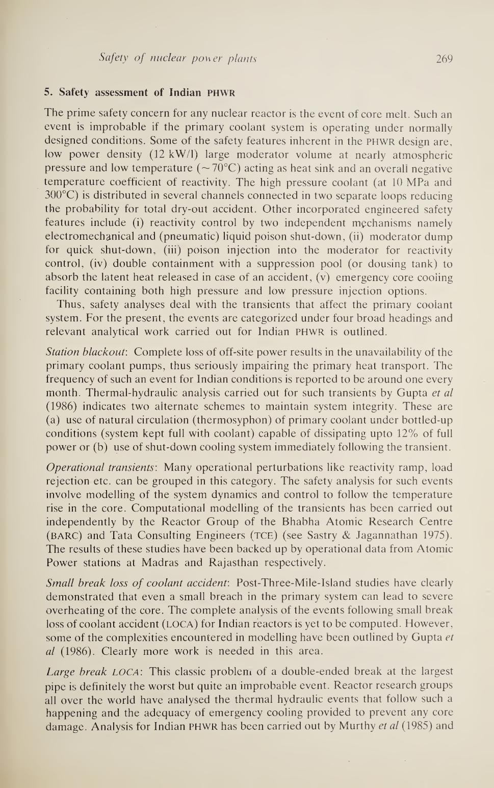
Safety of nuclear power plants 269
5. Safety assessment of Indian phwr
The prime safety concern for any nuclear reactor is the event of core melt. Such an event is improbable if the primary coolant system is operating under normally designed conditions. Some of the safety features inherent in the phwr design are, low power density (12 kW/1) large moderator volume at nearly atmospheric pressure and low temperature (~70°C) acting as heat sink and an overall negative temperature coefficient of reactivity. The high pressure coolant (at 10 MPa and 300°C) is distributed in several channels connected in two separate loops reducing the probability for total dry-out accident. Other incorporated engineered safety features include (i) reactivity control by two independent mechanisms namely electromechanical and (pneumatic) liquid poison shut-down, (ii) moderator dump for quick shut-down, (iii) poison injection into the moderator for reactivity control, (iv) double containment with a suppression pool (or dousing tank) to absorb the latent heat released in case of an accident, (v) emergency core cooiing facility containing both high pressure and low pressure injection options.
Thus, safety analyses deal with the transients that affect the primary coolant system. For the present, the events are categorized under four broad headings and relevant analytical work carried out for Indian PHWR is outlined.
Station blackout: Complete loss of off-site power results in the unavailability of the primary coolant pumps, thus seriously impairing the primary heat transport. The frequency of such an event for Indian conditions is reported to be around one every month. Thermal-hydraulic analysis carried out for such transients by Gupta et al
(1986) indicates two alternate schemes to maintain system integrity. These are (a) use of natural circulation (thermosyphon) of primary coolant under bottled-up conditions (system kept full with coolant) capable of dissipating upto 12% of full power or (b) use of shut-down cooling system immediately following the transient.
Operational transients: Many operational perturbations like reactivity ramp, load rejection etc. can be grouped in this category. The safety analysis for such events involve modelling of the system dynamics and control to follow the temperature rise in the core. Computational modelling of the transients has been carried out independently by the Reactor Group of the Bhabha Atomic Research Centre (BARC) and Tata Consulting Engineers (tce) (see Sastry & Jagannathan 1975). The results of these studies have been backed up by operational data from Atomic Power stations at Madras and Rajasthan respectively.
Small break loss of coolant accident'. Post-Three-Mile-Island studies have clearly demonstrated that even a small breach in the primary system can lead to severe overheating of the core. The complete analysis of the events following small break loss of coolant accident (loca) for Indian reactors is yet to be computed. However, some of the complexities encountered in modelling have been outlined by Gupta et
al (1986). Clearly more work is needed in this area.
Large break LOCA: This classic problem of a double-ended break at the largest
pipe is definitely the worst but quite an improbable event. Reactor research groups all over the world have analysed the thermal hydraulic events that follow such a happening and the adequacy of emergency cooling provided to prevent any core damage. Analysis for Indian PHWR has been carried out by Murthy et al (1985) and

270 K S Ram and. K Iyer
MPa
Figure 3. Pressure transient due to cold leg rupture for a 200 MW reactor.
Bajaj & Malhotra (1985). A typical pressure response computed by Gupta et al
(1986) is shown in figure 3. Some of the correlations used in modelling appear to have been developed for vertical geometries and are yet to be established for horizontal geometries encountered in Indian PHWR. Experimental efforts to generate data is under way (Venkatraj & Saha 1985) and one has to wait for the verification of computer codes. However, computation has also been extended to quantifying the containment loading and subsequent release of radioactivity following a large break LOCA (Bajaj 1986).
These preliminary accident studies leading to core melt-down are essential to establish the probability of the top event. Besides the initiating events mentioned above, leading to the core melt-down, other initiating events of lesser consequences also need to be studied. The reliability of PHWR control by Electro Mechanical Shut-down Rods (EMSR) as well as Liquid Poison Rod (lpr) systems was studied by Sharma & Ram (1980) and the time-dependent unavailability results are given in table 3.

Safety of nuclear power plants 271
Table 3. Time-dependent unavailability, Q
Target
reliability
R(t = 8760 hr)
Weibull
distribution
scale parameter
EMSR system
Q(t = 720 hr)
LPR system
Q(t = 720 hr)
Combined
Q(t = 720 hr)
0-90 26987-6 0-0324 0-0271 8-78 x 10~4
0-99 87380-6 2-47 x 10~2 1-88 x HE2 4-17 x 1()-4
0-999 276947-9 2-398 x 10“2 i-59i x ur2 3-815 x 10“4
0-9999 876000-0 2-39 x H)-2 0-0158 3-766x 10“4
R(t) = target reliability at the end of a year (t = 8760 hr) of a basic component under
aging alone.
Weibull distribution shape parameter = 2.
Number of basic components 12 in EMSR: 16 in LPR affected by aging.
A case study for the reliability of electric service supply system for the Madras Atomic Power Plant was carried out by Bhattacharya et al (1984, p. 316). The assessed unavailabilities and frequencies of failure of emergencv electric supplv are found to be within target values of 3 x 10⁻⁵ yrs/yr. Emergency electric supply is
different from other safety systems as it is normally in the standby mode and comes in only when the emergency supply is called for. A beginning is made with systematic probabilistic safety assessment of the Indian PHWR (Babar & Kakodkar 1986).
6. Conclusions
Both the TMI-2 and the Chernobyl accidents seem to indicate that operator error contributed to the serious consequences. The overall reliability of a system is affected because the men involved have some probability of performing their normal tasks incorrectly. Thus human reliability should form an integral part of reliability studies. Dhillon (1984, p. 188) has reviewed the work on human errors in engineering systems. Human-error probability is defined as the ratio of total amount of known errors of a given type to the total amount of opportunities for the error. This probability can vary from 0.003 to 0.5. Some of the human error prevention methods are man-machine system analysis, error cause removal program and quality circle formation. These studies are essential for safe and reliable operation of nuclear power plants.
In a recent report (IAEA 1986) published on the Chernobyl accident, the need for a ‘nuclear safety culture’ in all operating nuclear power plants is stressed. The lessons learned from the accident imply three lines of action:
(1) Training, with special emphasis on the need to acquire good understanding of the reactor- and its operation, and with the use of simulators giving a realistic representation of severe accident sequence. (2) Auditing, both internal and external to the utility, in particular to prevent complacency arising from routine operations. (3) Permanent awareness by all personnel of the safety implications of any deviation from the procedures.

272 K S Ram and K Iyer
This report also emphasizes the importance of a satisfactory man-machine interface. The Chernobyl and TMI accidents identify two lines of action:
(1) The clear display to the operator of data vital to safety should be tailored to ensure optimum use. For a system as complex as a nuclear power plant, real-time data display and interpretation are important. Built-in diagnostic capability should be included. (2) Although ultimate reliance must rest on the operating staff and their comprehension of the system safety, the complexity of the nuclear power plant always requires that there be reliable safety back-up by way of automatic devices that ensure that the plant remains in safe operating territory in all respects. This back-up must be rapid by way of its logical structure and speed of response. It must be so designed as to be difficult to bypass, and so that normal or planned operation raises no temptation to bypass it.
It is envisaged that application of Artificial Intelligence or expert systems will lead tq safer operation of nuclear power plants.
References
Babar A K, Kakodkar A 1986 Status of probabilistic safety assessment in India, IAE-AERB workshop on safety, Bombay
Bajaj S S 1986 Safety analysis for PHWRS in India, IAEA-AERB Workshop on safety, Bombay
Bajaj S S, Malhotra P K 1985 LOCA Blowdown analysis code THYNAC, Indo-German Workshop on
transient analysis and ECCS, Bombay j Bhattacharyya D, Bajaj S S, Babar A K, Rao V V S 1984 Proc. national conference on quality and
reliability (Bombay: Indian Inst. Technol.)
BMI-1910 1971 Core melt-down evaluation (Columbus, USA: Batelle Memorial Institute)
Capen C 1976 J. Pet. Technol. 28: 8-12
Dhillon B S 1984 Proc. national conference on quality and reliability (Bombay: Indian Inst. Technol.)
Erdmann R C, Leverenj F L Jr, Lellouche G S 1981 Nucl. Technol. 53: 374-379
Gupta S K, Ghosh A K, Murthy L G K 1986 Computer codes for thermal hydraulic analysis of Indian PHWR safety. IAEA-AERB workshop on safety, Bombay
IAEA 1986 IAEA safety series no. 75-INSAG-l, Summary report on the post-accident review meeting on the Chernobyl accident, IAEA-Vienna
Lewis H W 1978 Risk assessment review group report to US NRC, NUREG-CR-0400, Washington, DC
Murthy LG K, Gupta S K, Lele H G 1985 Development of Computer Codes for Loss of Coolant
Accident Analysis for PHWR, Indo-German workshop on transient analysis and ECCS, Bombay
Sastry V A, Jagannathan P 1975 Digital simulation of CANDIJ reactors (Bombay: Tata Consulting Engineers)
Sharma D D, Ram K S 1980 Nucl. Eng. Design 61: 265-276
Venkatraj V, Saha D 1985 Separate Effect Tests on LOCA, Indo-German workshop on transient analysis and ECCS, Bombay
WASH-740 1957 Theoretical possibilities and consequences of major accidents in large nuclear power plants, US-AEC report
WASH-1400 1975 Reactor Safety Study, US NRC report, Washington, DC
Yaremy E M 1986a Licensing requirements for PHNR safety analysis, IAEA-AERB workshop on safety analysis, Bombay
Yaremy E M 1986b'Application of PSA in licensing of PHWR, IAEA-AERB workshop on safety analysis, Bombay

Subject Index
Agreement protocols
Byzantine-resilient distributed computing sys¬
tems 81
Atomic actions A tutorial on the principles of fault tolerance 7
Attitude control Fault-tolerant spacecraft attitude control sys¬
tem 233
Attitude reference system Fault-tolerant spacecraft attitude control sys¬
tem 233 Autonomous reconfiguration
Fault-tolerant spacecraft attitude control sys¬
tem 233
Bandwidth availability Reliability and fault-tolerant issues of multi¬ processor and multicomputer systems 129
Byzantine generals problem Byzantine-resilient distributed computing sys¬
tems 81
Close loop guidance A fault-tolerant computer system for India’s
satellite launch vehicle programmes 221
Clustering approach Fast approximate methods for the reliability
analysis of computer networks 155 Computation-communication availability
Reliability and fault-tolerant issues of multi¬
processor and multicomputer systems 129
Computer communications Fast approximate methods for the reliability
analysis of computer networks 155
Computer controlled process
A survey of software dependability 23
Crossbar Reliability and fault-tolerant issues of multi¬
processor and multicomputer systems 129
Database crash and recovery Enforcement of data consistency in database
systems 49
Database systems Enforcement of data consistency in database
systems 49
Dataflow graphs Reliability models for computer systems: An
overview including dataflow graphs 167
Decomposition-aggregation method
Reliability models for computer systems: An overview including dataflow graphs 167
Distributed computing Byzantine-resilient distributed computing sys¬
tems 81 Dynamic architecture
Fault tolerance in multiprocessor systems 93
Error recovery A tutorial on the principles of fault tolerance 7
Exception handling A tutorial on the principles of fault tolerance 7
Fault classification
A tutorial on the principles of fault tolerance 7
Fault tolerance
A tutorial on the principles of fault tolerance 7 Byzantine-resilient distributed computing sys¬
tems 81 Fault tolerance in multiprocessor systems 93
Reliability and fault-tolerance in multistage interconnection networks 111
Fault-tolerant spacecraft attitude control sys¬ tem 233
Fault-tolerant computer architecture Fault tolerance in multiprocessor systems 93
Fault-tolerant control Fault-tolerant spacecraft attitude control sys¬
tem 233
Fault-tolerant multiprocessors Performance modelling of a fault-tolerant real¬
time multiprocessor using stochastic Petri nets 187
Fault-tolerant systems Computer-aided reliability analysis of fault-
tolerant systems 209 A fault-tolerant computer system for India’s
satellite launch vehicle programmes 221
Graceful degradation
Reliability and fault-tolerant issues of multi¬
processor and multicomputer systems 129 Gyros
Fault-tolerant spacecraft attitude control sys¬
tem . 233
273

274 Subject Index
Hierarchical modelling
Computer-aided reliability analysis of fault-
tolerant systems 209
Loss of coolant accident
Safety of nuclear power plants 263
Markov chains
Computer-aided reliability analysis of fault-
tolerant systems 209
Microprocessor
A fault-tolerant computer system for India’s
satellite launch vehicle programmes 221
Multicomputer
Reliability and fault-tolerant issues of multi¬
processor and multicomputer systems 129
Multiple bus Reliability and fault-tolerant issues of multi¬
processor and multicomputer systems 129
Multiprocessor systems
Fault tolerance in multiprocessor systems 93
Multiprocessors Reliability and fault-tolerant issues of multi¬
processor and multicomputer systems 129
Multistage interconnection networks
Reliability and fault-tolerance in multistage
interconnection networks 111 Reliability and fault-tolerant issues of multi¬
processor and multicomputer systems 129
Nuclear power plant
Safety of nuclear power plants 263
On-board computer
A fault-tolerant computer system for India’s
satellite launch vehicle programmes 221
Overall reliability
Fast approximate methods for the reliability
analysis of computer networks 155
Parallel processing
Reliability and fault-tolerance in multistage
interconnection networks 111
Performability modelling
Computer-aided reliability analysis of fault-
tolerant systems 209
Performance modelling
Performance modelling of a fault-tolerant real¬
time multiprocessor using stochastic Petri nets
187 Probabilistic risk assessment
Safety of nuclear power plants 263
Queueing networks
Performance modelling of a fault-tolerant real¬ time multiprocessor using stochastic Petri nets
187
Real-time control
Performance modelling of a fault-tolerant real¬
time multiprocessor using stochastic Petri nets 187
Real-time systems
A tutorial on the principles of fault tolerance 7
Reconfiguration
Fault tolerance in multiprocessor systems 93
Redundancy A fault-tolerant computer system for India’s
satellite launch vehicle programmes 221
Reliability
A tutorial on the principles of fault tolerance 7
Reliability models for computer systems: An
overview including dataflow graphs 167
Safety of nuclear power plants 263
Reliability analysis
Reliability and fault-tolerance in multistage
interconnection networks 111
Reliability index
Fast approximate methods for the reliability
analysis of computer networks 155
Reliability modelling
Reliability and fault-tolerant issues of multi¬
processor and multicomputer systems 129
Computer-aided reliability analysis of fault- tolerant systems 209
Replicated processing
A tutorial on the principles of fault tolerance 7
Safety
Safety of nuclear power plants 263
Satellite launch vehicles A fault-tolerant computer system for India's
satellite launch vehicle programmes 221
Semantic integrity
Enforcement of data consistency in database
systems 49
Sensitivity analysis
Computer-aided reliability analysis of fault-
tolerant systems 209
Shuffle/exchange networks
Reliability and fault-tolerance in multistage
interconnection networks 111
Software dependability
A survey of software dependability 23
Software fault tolerance
Enforcement of data consistency in database
systems 49
A survey of software dependability 23
Software quality assurance
A survey of software dependability 23
Software reliability
A survey of software dependability 23
Spacecraft
Fault-tolerant spacecraft attitude control sys¬
tem 233

Subject Index
Stochastic Petri nets
Reliability models for computer systems: An
overview including dataflow graphs 167
Performance modelling of a fault-tolerant real¬
time multiprocessor using stochastic Petri nets 187
Stochastic models Reliability models for computer systems: An overview including dataflow graphs 167
System-level diagnosis Fault tolerance in multiprocessor systems
VL SI processor arrays
Fault tolerance in multiprocessor systems

Author Index
AHD
Abraham J A
Adams G B
Adams M B
Adiba M
Adrion W R
Agarwal M
Agarwal V K
Aggarwal K K
Aghili H
see Cristian F
Agrawal A
Agrawal D P
Alegre I
see Lang T
Alger L S
see Lala J H
Alsberg P A
Amin AT
Ammons E E
Anderberg M R
Anderson G A
Anderson T
Archer J E Jr
Arlat J
Arnold T F
Asenjo J F,
Attar R
Attiya C
Avizienis A
see Makam S
see Raghavendra C S
Babar A K
see Bhattacharyya D
Baccelli F
Baer J L
Bajaj S S
see Bhattacharyya D Balaji S
Balbo G
see Marsan M A
Ball M O
Bannerjee P
Barbara D
Barlow R E
50
107,122,136,169
114,119
249
78
79
168,174
102 155,156,158,164,169
82
168,169
114,118,130,134,141,146,152
112,130,137
89
62, 64, 68
97
241
158
112,130,134
7,10,15,50,55,241
72
136
138
179
68 83
8, 15, 21, 50, 60, 94, 135, 136,
171, 175, 223, 235, 236, 241
215 101-103
271
271
218
180
270
271
81
190, 207
179, 187, 190-193, 207
135
107
44
168,169,219
Barnes G H
Barrett P A
see Anderson T
Barsi F
Bastani F B
Basu D
Batcher K E
Beaudry M D
Bell C G
Bell Labs
Bellon C
Benes V E
Bennets R G
Berns G M
Bernstein P A
see Attar R
Beyaert B
Bhandarkar D P
Bharathi M
Bhargava B 49, 50,
Bhat U N
see Kavi K M
Bhattacharyya D
Bhuyan L N 129,
Biswas N N
Blasgen M
see Gray J N
Bobbio A
see Dugan J B
see Marsan M A
Boesch F T
Bouricius W
Bouthonnier V
Brandwajn A
Branstad M A
see Adrion W R
Brantley W C
Breuer M A
Broder A Z
Brodie M L
Brown R B
Brown R M
see Barnes G H
Bruell S C
see Balbo G
Bryant L
see Stiffler J J
112
15
98
38
221,222,228
114
135,218
130
94
77
115
235,236
.45
68 178
130
221 57,62,67-69,71-73,75-77
167,180
179
271
130,134,137,139-141,146,
151, 152
93
59, 60, 72
212.215.216
210,212
191,207
162
213
24,26
175
79
111 105
88 78
241
112
190, 207
210.213.216
136,177
276

Author Index 277
Buckles B P Conway R
see Kavi K M 179 see Archer J E Jr 72 Buneman O P 71 Coolahan J E 178 Butler J T 99 Cooper A E 222 Butler R W 89 Costes A 130,213,215
see Krishna C M 90 Cox D 213 Buzzard G D Cristian F 10,82
see Mudge T 130 Cruon R
see Kaufmann A Cumani A
169
Campbell R H 60 see Marsan M A 191,207 Capen C 268 Custeau G Carter W
see Bouricius W 213
see Morgan D E 68,156
see Goyal A 210,211,214,215 Dadam P 78 Castillo X 217 Dahbura A T 99 Cavano J P 28 Daly R C 249
Chamberlin 69 Das C R 129,137,139-141,145,151
Champine G A 67,68 Dasgupta S 227
Chandy K M 60,175 Davidson F
Chang C C 70 see Garcia-Molina H 89
Chang M K 169 Davidson S B 62, 64, 69
Chang T P 135 Davies C T 59, 60, 72,103
ChenTT 98, 247 Day J D 62, 64, 68
Cherkassky V 119 Demolombe R Cherniavsky J C see Adiba M 78
see Adrion W R 79 Denning P J 78 Chien R Dennis J B 179
see Preparata F 96,97 de Souza e Silva E
ChinTT 249 see Goyal A 210,211,214,215
Chiola G 207 Dhillon B S 271
see Marsan M A 191,207 Dolev D 61,83,84,86,88
Chor B 88 see Attiya C 83
Chou T C K 136 Doucet J
Chow J M see Costes A 213,215
see Parker D S 69 DuCasse E 96
Chow W T 222 Duda A 217
ChuWW 67 Dugan J B 178,180,190, 207, 209-214 Chupin J C see Geist R M 177
see Adiba M 78 see Trivedi K S 177,210-216
Churchman C W 40 Dzwonezyk M J
Chwa K Ciardo G
98 see Lala J H 89
see Dugan J B 210,212 Eckhardt D E 44
Ciminiera L 114,119 Edelberg M 77
Ciompi P 99 Edwards D
Clark R N 243 see Parker D S 69
Clarke E M 101 Elsam E S
Clary J see Katuski D 94
see Trivedi K S 219 Engelder P D 247
Clemons E K 71 Ercegovac M D 179
Coan B A 83,88 see Raghavendra C S 101-103
Computer 111 Erdmann R C 268
Conn R 175 Eswaran K P 50, 54, 69, 70
Conte G see Marsan M A 179, 187, 190-193,207
Ezhilchelvan P 17, 19,82
Conway L 105 Feldman P 88

278 Author Index
Feller E 210
Feller W 169
Feng T Y 112,114,132
Fernandez E B 50,70,78
Fischer M J 83
see Dolev D 84
Florentin J J 69
Florin G
see Beyaert V 178
Fong E 70
Fortes JAB 107
Fowler R
see Dolev D 84
Frank H 135,156
Fratta L 169
Friedman A D 94,98
Frisch IT 135,156
Fussel D 106
Gadani J P 158
Gai E 247
see Daly R C 249
Garcia-Molina H 44,61,67,69,89
Gardarin G 67
see Adiba M 78
Gaudiot J E 179
Gault J
see Trivedi K S 219
Gauthier R J
see Lala J H 89
Gaver D P 218
Gay F A 136
Gear C W 213
Geist R 172,175-177,212, 219
see Dugan J B 178,180,190,207, 210-213
see Trivedi K S 177,210-216
George D A 111
Gerla M 130,135,170
see Grnarov A 122,135,170
Ghanta S
see Balbo G 190, 207
Ghose M K 227
Ghosh A K
see Gupta S K 269,270
Gibbons T 50
Gil J
see Attiya C 83
Gilley G C
see Avizienis A 94 Goel A 30,35,36,40,211,219 Goel P S 233 Goke L R 114 Goldberg J
see Wensley J H 81,84,88,89,94,213,214 Goodman N 68
see Attar R 68
Goyal A 210,211,214,215,219
Graham R M
see Gray J N 59, 60, 72
Grandoni F
see Barsi F 98
Gray J N 20, 59,60, 72
see Eswaran K P 50,54, 70
Green M W
see Wensley J H 81,84,88,89,94,213,214
Grnarov A 122,135,170
Grouchko D
see Kaufmann A 169
Grusas G
see Makam S 215
Guccione L
see Stiffler J J 136,177
Gupta J S
see Aggarwal K K 169
Gupta S K 269,270
see Murthy L G K 269
Haas P J 207
Hagstorm J N 123,169
Hakimi S L 97-99
Halliwell D N
see Anderson T 15
Hammer M M 69,70
Hansler E 156 Hariri S 122
Harris J A 112 Harrison J V 247
see Daly R C 249 Harvey P R 72 Harvey S L 111 Hassan ASM 102 Hayes J P 99,120,141
see Mudge T 130 Hebalkar P G 72 Hecht A 241 Hecht H 60 Herzog U
see Chandy K M 175 Hilborn G 135 HoGS 178,189 Holliday M A 190 Holt C S 98,100 Hong Y C 71 Hopkins A L Jr 94,187, 204 Horning J J 9 Hosseini S H 100 Hsieh Yu-I 95 Huang KH 98,107 Huslende R 136 Hwang C L
see Lie C H 168

Author Index 279
see Tillman F A 168 Kumar A 168,174 Hwang K 111, 135 Kumar V P 114,117,118
Kung H T 73,112 IAEA 271 Kuo W IEEE 28 see Tillman F A 168 Ingle A D 131,135,145 Kurian T 221 Iyer K 263 Kurose J
Jagannathan P 269 see Sauer C 210
Jarke M 70 Jayasri T 221
LaPrie J C 175
Jensen E D 112,130,134 Lafue G M E 70
Johnson B W 241 Lala J H 89,213
Johnson S C 89 see Hopkins A L 94,187, 204
Lala P K 241 Kakodkar A 271 Lambert H 219 Karp R M 170 Lamport L 61,83,84,86, 89 Kartashev S I 101,103,104 see Pease M 83,85,89
see Davis C 103 see Wensley J'H 81,84,88,89,94,213,214 Kartashev S P 101,103,104 Lampson B 17, 20, 53, 61
see Davis C 103 Landrault C 175 Kato M see Costes A 213,215
see Barnes G H 112 Lang T 112,130,137 Katuski D 94 Laprie J C 24, 29, 33, 38,42, 45,130,136, 209, 219 Katzman J A 94 see Costes A 213,215 Kaufmann A 169 Lauer H C Kavi K M 167,179,180 see Horning J J 9 Kelly JPJ 50, 60,94 Lavenberg S
Ketelson M L 136 see Goyal A 210,211,214,215,219 Kim K H 60,100 Lawrie D H 114,119,122,132,141 Kimbleton S R 70,156 LeBihan J
Kime C R 97 see Adiba M 78 King P J B 218 Lee L D 44 Kini V Lee PA 7,10,15,241
see Siewiorek D P 96 see Randell B 52, 54,57,59 Kiser S LeeSH 169
see Parker D S 69 Lee YH 60,78,101 Kleinfelder W J 111 see Shin K G 188,196,198,201,208 Kleinrock L 1 Lehman P L 73
see Grnarov A 122,135,170 Lele H G
Kline C see Murthy L G K 269 see Parker D S 69 Lellouche G S
Knight J C 15,50,55 see Erdmann R C 268 Knuth D E 158 Leu Ja-Song 141 Koch J 70 Leverenj F L Jr
Kopetz H 17 see Erdmann R C 268 Koren I 105,106 Leveson N G 15,45,72
Krishna C M 90, 270 Levis A H 24,26 KrolT 96 Levitt K H
Kruskal C P 130,146 see Wensley J H 81,84,88,89,94,213,214 Kuck D J Lewis H W 267
see Barnes G H 112 LieCH 168 KuhlJG 94,100 Liginlal D
see Hossieni S H 100 see Basu D 228 Kulkarni A D Lilien L 49, 50, 57, 62, 67-69, 71-73, 75-77
see Basu D 222 Lipovski G J 114 Kulkarni V 210,217,218 Liskov H 12
see Nicola V 218 Littlewood B 33,38

280 Author Index
Liu MT
Lone P
see Beyaert B
Lone R
see Eswaran K P
Losq J
Losq T
Luckham D C
Lynch N A
see Dolev D
MacNair E
see Sauer C
Maestrini P
see Barsi F
Magott J
Mahaney S R Maheshwari S N
Makam S
Malek M
see Cherkassky V
Malhotra P K
Mallela S
Mancini L
Mann W F
see Katuski D
Manning F B
Marie J L
Marie R A
Marsan M A
Martin D J
Mashburn H
see Siewiorek D P
Masson G M
see Dahbura A T
Mathur F P
see Avizienis A
McAbliffe G K
see Hansler E
McAuliffe K P
McCabe T J
McConnel S R
see Siewiorek D P McGough J
McHugh J
McJones P
see Gray J N
McLeod D J
McMillen R J
McPherson J A Mead C
Melliar-Smith P M
see Horning J J
see Wensley J H Melton E A
Merryman P
see Conn R
112 Merwin R E
Metze G
135
178 see Preparata F 96,97
Meyer G G L 98,99
50,54,70 Meyer J F 135,136,190,207,212,218
136 Micali S 88
95 Miller R E 170
12 Mirhakak M 135
61 Misra K B 158
84,88 see Aggarwal K K 169 . Mitrani I 218
Moawad R 35,40
210 Mohanty S N 45
Molloy M K 178,190,191,207
98 Montanari U G 169
178 Morgan D E 68,156
83,88,89 Moulding M R
98 see Anderson T 15
215 Movaghar A
see Meyer J F 190, 207
119 Movagher A
270 see Meyer J 212
99 Mudge T 130
21 Mulazzani M 219 Munz R 61,68
94 Murthy L G K 269
106 see Gupta S K 269,270
253 Murugesan S 233,241,242,246, 250,253,255
215 Musa J 40 130,179,187,190-193,207
15 Nair R 100 Nakagawa T 168,174
96 Nakajima K 99 98,99 Nakazawa H 158
99 Narahari Y 187 171,215 Narasimhan J 99
94 Natkin S 190 see Beyaert B 178
156 Negrini R 101,105,106 111 NgYW 135,136,175 45 Nicola V F 218
241 see Dugan J B 178, 180, 190,207,210-212 96 see Kulkarni V 210,217,218
213-215 Nikolaou C N 101 44 Nishio T 214,218,219
Norton V A 111 59, 60, 72
69,70 Omana Mammen 119 see Basu D 222,228 98 Opper E
105 see Cherkassky V 119 86,89
q Osaki S 168,174,214,218,219
7
81,84,88,89,213,214 Padmanabhan K 114,119,122 111 Panzieri F 20
Parker D S 69,114,135 175 Patel J H 114,116

Author Index 281
Patnaik L M 81 Pease M 83,85,89,114
see Lamport L 61,83,84,86,89
Pedar A 27,46 Perry K J 83,88
Peterson J L 178 Petri C A 188
Pfister G F 111
Pinter S S see Dolev D 88
Pittelli F
see Garcia-Molina H 89 Pokoshi J L 101,106 Polak W 12 Popek G J
see Parker D S 69 Prabhakar A 169 Pradhan D K 101,102 Preparata F 96,97 Proschan F 169
Rabin M O 87,88 Raghavendra C S 101-103,111,114,116,
Rai S 117, 119, 120, 122, 135
156 Ram K S 263,270 Ramamoorthy C V 38,178,189 Ramanathan 89,90 Ramchandani C 189
Randell B 9,10, 20, 42, 52, 54, 57, 59, 60 see Horning J J 9
Rao K V S S Prasad 221
Rao V V S see Bhattacharyya D 271
Reddy S M 94,100-102,113,117,118
see Hossieni S H 100
Reed D A 130,134,147
Reibman A L 210,213,216
see Marie R A 215
Reischuk R 86
Rennels D A 94, 235, 236
see Avizienis A 94
Roberts E S
see Katuski D 94
Robinson J G
see Katuski D 94
Rohr J A see Avizienis A 94
Rosenberg A L 105,107
Rosenkrantz D J 60
Rosenthal A 170,175
Ross S M 191,200
Rothnie J B 68
Roussopoulos N 178
Rubin D K see Avizienis A 94
Rucinski A 101,106
Rudisin G
see Parker D S Ruediger R
see Dolev D
Russel J
69
84
97
Saha D
Sahner R
Sami M
see Negrini R
Sanders W H
see Meyer J F Sargent R
Sarma V V S
see Viswanadham Sastry V A
Satyanarayana A Saucier A G
Sauer C H
Schlageter G
Schmidt J W Schneider F B
see Archer J E Jr Schneider G M
Schneider P
see Bouricius W Schwetman H D Seegmuller G
see Gray J N Seitz C L
Serra A
Shampine L P' Sharma D D
Shedler G S Shen J P
Shin KG 60,
see Krishna C M Shipman D
Shogan A W
Shooman M L
Shostalk R E see Lamport L
see Pease M
see Wensley J H
Shrivastava S K
Siegel H J Siewiorek D P 26,
Sifakis J Simoncini L
Singh M G see Viswanadham
Skeen D
Skowrolski F S
see Katuski D
Slotnik D L
see Barnes‘G H
270 211-213,215-217
106 101.105
190,207, 212 211,214
23,27,46 N 26,47
269 123,169
77 175,210
78
78 83, 88, 89
72
156
213 130,134,147
59, 60,62 112
114,119
213 270 207
120,141 78,89,90,101,188,196,198,
201, 208, 217 90
62,63 170
27, 30,35
61,83,84,86,89
83,85,89 81,84,88,89,94,213,214
7,17,19-21,82
114,119
42,94,96,131,135,145,210,
217, 219, 235, 236, 241
178,189
94,99
N 26,47
61
94
112

282 Author Index
Smith D R
Smith J E
Smith P M M
see Wensley J H
Smith R
see Kulkarni V
Smith T B
see Hopkins A L
Smothermann M
see Dugan J B
see Geist R M
see McGough J
see Trivedi K S
Snir M
Snyder A
Snyder L
Soi IM
Srini V P
Srinivas S
Stark E W
see Dolev D
Stefanelli R
see Negrini R
Steiglitz K
Stiffler J J
Stokes R A
see Barnes G H
Stone H S
Stonebraker M
Stoughton A
see Parker D S
Strong H R
see Cristian F
see Dolev D
Sturgis H
Su S Y H
Summers R C
Svanks MI
Swartz R S
Swarz R
Swarz S
Swaz R S
Tanenbaum A S
Tanimoto S L
Taylor D J
see Morgan D E
Thomas R E
Thomas R H
Thomson W H
Tillman F A
see Lie C H
Torin J M
Toueg S
Toy WN
Traiger A
see Eswaran K P
112 Treleaven P C
98, 99,100 see Randell B 52,54,57,59
Trivedi KS 131,171,172,175-177,209-219
94 see Dugan J B 178,180,190,207, 210-213
see Geist R M 111
217,218 see Goyal A 210,211,214,215,219
89 see Kulkarni V 210,217,218
94,187,204 see Marie R A 215
see McGough J 213,214,215
210,211,213 see Nicola V 218
177 Troy R 35,40
213-215 Tsao M 177,210-216 see Siewiorek D P 96
130 Tsuchiya M 136
12 Turpin R 83
101,106
156,158,164 Ullman J D 50
179
93 Valero M
see Lang T 112,130,137 88 Varaprasad S V L A 221
106 Varma A 111,114,116,117,119,120 101,105 Varman P 106
162 Venkatraj V 270 136,172,177,210,213,216 Vernon M K 190
112 Vijayan Nair V
see Basu D 228 114 Viswanadham N 26,47,187
61,69
69
61,82,83,86
Walker B J
see Parker D S 69
82 84
Walton W
see Parker D S 69
17,20, 53,61 Wei AY 60
71,95,96 Weihl W E
50,70,78 see Dolev D 88
71 Weinstock C B
145 see Wensley J H 81,84,88,89,94,213,214
210, 219 Weiss G H 168
26, 43 Weiss J 111
235,236,241 Wensley J H 81,84,88,89,94,213,214 Wertz J R 239
148 Whitelaw K
see Conn R 175 112 Wiederhold G 72
Wilkov R S 135,162 68,156 see Hansler E 156
162 Wilsky A S 243 62 Winsor D C
239 see Mudge T 130 168 Wittie L D 94,112,130,134,146 168 Wolf E W 227 see Katuski D 94
83,162 Woo L 94 see Chandy K M 175
50, 54, 70 Woodbury M H
see Shin K G 188,196,198,201,208

Author Index
WuCL 114,132
WulfWA 130
Yang C
see Dahbura A T 99
Yaremy EM 266, 267
283
YeeJG 71
Yemini S 59
YuCT 70
Zuberek W M 178,190


ACADEMY PUBLICATIONS IN
ENGINEERING SCIENCES
General Editor: R Narasimha
Volume 1. The Aryabhata Project (eds U R Rao, K Kasturirangan)
Volume 2. Computer Simulation (eds N Seshagiri, R Narasimha)
Volume 3. Rural Technology (ed. A K N Reddy)
Volume 4. Alloy Design (eds S Ranganathan, V S Arunachalam, R W Cahn) ...attempt in bringing together a series of articles, written by eminent scientists of India and abroad...Academy deserves all praise in bringing out these two timely issues.
Powder Metall. Assoc. India, Newslett.
Volume 5. Surveys in Fluid Mechanics (eds R Narasimha, S M Deshpande)
An informal and stimulating publication...(provides) a survey of many important topics in Fluid Mechanics...All the papers are of excellent technical content and most are very well written. Many include lengthy reference lists, which are as useful as the body of the paper...The publishing quality is very good...
IEEE Journal of Ocean Engineering
...The general level (of papers) is high...Several are likely to have wide appeal... Judging by the invited lectures, the Asian Congresses of Fluid Mechanics are off to a good start.
Journal of Fluid Mechanics
Volume 6. Wood Heat for Cooking (eds K Krishna Prasad, P Verhaart)
...interesting and stimulating account of technical thinking on the wood stove problem up to date...excellent collection of valuable and thought-provoking investigations on the subject.
Rev. Projector (India)
Volume 7. Remote Sensing (eds B L Deekshatulu, Y S Rajan)
...Several contributions are specifically addressing topics of national interest, however, the majority of the papers is of general interest for a wide community. The book can serve not only as an inventory of the Indian activities, but also as a textbook on techniques and applications of remote sensing.
Photogrammetria ...particularly refreshing...
Int. J. Remote Sensing
Volume 8. Water Resources Systems Planning (eds M C Chaturvedi, P Rogers)
...It is well got up and very well printed and forms a valuable addition to our limited literature on Water Resources of India.
Curr. Sci.
Volume 9. Reactions and Reaction Engineering (eds R A Mashelkar, R Kumar)
Copyright © 2022 FDOKUMEN